MRI Phase Mismapping Image Artifact correction - SUST ...

1

بسم ميحرلا نمحرلا هللا

Sudan University of Science &Technology

College of Graduate Studies

Biomedical Engineering

Department

MRI Phase Mismapping

Image Artifact correction في صور الرنين المغنطيسي فقدان الطورتصحيح التشوهات الناتجه عن

A Thesis Submitted in partial Fulfillment of the Requirements for the M.Sc. degree

in Biomedical Engineering

Presented By:

Ashraf Abrahim Abdallah ahmed

Supervised By:

Dr. Mawia Ahmed Hassan

JUNE 2016

I

ACKNOWLEDGEMENT

Praise be to Allah, Lord of Universe.

My deepest gratitude are due to all who have contributed to this humble work,

without their assistance the task would be impossible.

In particular I would like to acknowledge a deep gratitude to my supervisor Dr.

Mawia Ahmed Hassan for his non ending assistance and patience. I am also

grateful to him for helping me with his unlimited experience and orientation for

further knowledge and publication and good would communication.

I express my appreciation of the support of Dr. Omer E. H. Hamid always

supporting me and push me towards the knowledge and development.

Special thanks are extended to all the staff of the Department of medical

engineering for their understanding and support.

Grateful thanks are due to all who helped me in the tedious work of analysis,

printing and arrangement of this text.

Last but not least, a very special thanks for my big family father and mother they

are every time pushing my dreams towards, and I would like to acknowledge the

assistance of my wife sulima, she is the real MSc maker by supporting and offering

the chance for reading and researching and special thanks to my kids smiles.

II

TABLE OF CONTENTS

ACKNOWLEDMENT........................................................................................ I

Table of Contents .............................................................................................. II

LIST of FIGURES ........................................................................................... .V

LIST of TABELS ......................................................................................... ....IX

Abstract ............................................................................................................ .X

XI ..… ................................................................................................... اطتخص

CHAPTER ONE ………………………………………………………………..1

1. INTRODUCTION ………………………………………………….…………1

1.1 General overview………………………………………………….…………1

1.2 The Problem Statement ………………………………………………….…..2

1.3 Thesis Objectives ……………………………………………………….……2

1.4 Thesis Organization ………………………………………………….………3

CHAPTER TWO ………………………………………………………………..4

2. THEORETICAL BACKGROUND……………………………………….…...4

2.1 Introduction ……………………………………………………………….….4

2.2 The working principle of MRI ……………………………………………….4

2.3 Applications of MRI Techniques…………………………………………….6

2.4 Hardware of MRI……………………………………………………….….....6

2.4.1 Magnets of MRI……………………………………………………….…….7

2.4.1.1 Permanent magnets………………………………………………….…….7

2.4.1.2 Resistive magnets…………………………………………………….……7

2.4.1.3 Superconducting magnets………………………………………………...8

2.4.2 Radio-frequency coils……………………………………………………....8

2.4.3 Gradients coils…………………………………………………………….....8

2.4.4 Shimming coil……………………..……………………………………..….9

III

2.4.5 Computer system in MRI………………………………………………..….9

2.5 Artifacts of MRI………..……………………………………………….….....9

2.5.1 Chemical shift………………………………………………………..……..10

2.5.2 Chemical misregistration……………………………………………..…….10

2.5.3 Magnetic susceptibility……………………...………………………..…….10

2.5.4 Aliasing…………………………………………………………………..….11

2.5.5 Phase mismapping……………………………………………………….….11

2.6 K-space‖ data acquisition and image reconstruction …………………….…11

2.6.1 K-space matrix……………………………………………………………...11

2.6.2 Two-dimensional data acquisition…………………………………………13

2.7 Classification of Motion in MRI according to the acquisition blocks……...15

2.7.1 intrashot-motion……………………………………………………………..15

2.7.2 intershot-motion…………………………………………………………….15

2.8 classification of motion according to the human body …………………….16

2.8.1 rigid-motion…………………………………………………………………16

2.8.2 non-rigid-motion……………………………………………………………16

2.9 Correction Approaches………………………………………………………16

2.9.1 Prospective Motion Correction……………………………………………16

2.9.2 Retrospective Motion Correction………………………………………….16

2.9.3 Data Acquisition Strategies………………………………………………...16

2.10 Image restoration……………………………………………………………16

CHAPTER THREE ………………………………………………………...….18

3. LITERATURE REVIEW ………………………………………………….… 18

3.1 Prospective Motion Correction……………………………………..….….18

3.2 Retrospective Motion………………………………………………….…...22

3.3 Data Acquisition Strategies…………………………………………….……27

CHAPTER FOUR …………………………………………………………...….33

IV

4. METHODOLOGY……………………………………………………………33

4.1 The methodology proceeds as follows ……………………………………...33

4.2 Motion Blur Angle Estimation Algorithm……………………………….…35

4.3 Motion Blur Length Estimation Algorithm………………………………...35

4.4 Hough Transform Method………………………………………………….38

4.5 Cepstral Method …………………………………………………………….39

4.6 Wiener Filtering………………………………………………………….….40

CHAPTER FIVE ……………………………………………..………………...41

5. RESULTS AND DISCUSSION …………………………..…………….……41

CHAPTER SIX ………………………………………………………..…...…..64

6. CONCLUSION AND RECOMMENDATIONS ……………….....…….…..64

6.1 Conclusion …………………………………………………………..…..…..64

6.2 Recommendations and Future Work……………………………...…….….65

REFERENCES…………………………………………………………..…….…66

V

LIST OF FIGURES

Figure 2.1 principle of MRI……………………………………………………...5

Figure 2.2 Hardware components of MRI……………………………………….7

Figure 2.3 matrix of MRI………………………………………………………..12

Figure 2.4 k-space distance, location, grayscale………………………………...12

Figure 2.5 MRI pulse sequence………………………………………………….13

Figure 4.1 hough transform……………………………………………………..38

Figure 4.2 cepstral transform method…………………………………………………………..39

Figure 5.1 Comparison between the original coronal MRI image (L) and the

corrected image R with angle 112 and length 11……………………………..42


corrected image R with angle 99 and length 11………………………………42




corrected image R with angle 179 and length 13……………………………...43


corrected image R with angle 2 and length 7…………………………………44


corrected image R with angle 16 and length 7………………………………..44

VI






corrected image R with angle 145 and length 7……………………………….46



Figure 5.11 Comparison between the original sagittal MRI image (L) and the





corrected image(R) with angle 179 and length 4……………………………….50








corrected image R with angle 110 and length 8………………………………...52

VII







Figure 5.21 Comparison between the original axial MRI image (L) and the




Figure 5.23Comparison between the original axial MRI image (L) and the

corrected image R with angle 4 and length 6…………………………………..57


corrected image R with angle 4 and length 6………………………………….57


corrected image R with angle 110 and length 7………………………………...58


corrected image(R) with angle 162 and length 4……………………………….58





VIII





IX

LIST OF TABLES

Table 5.1 comparison between SNR of motion image and corrected image (coronal

image ………………………………………………...…………………………..47

Table 5.2 comparison between SNR of motion image and corrected image (sagittal

image ……………………………………………………..………………………54

Table 5.3 comparison between SNR of motion image and corrected image (axial

image ……………………………………………………………………………..60

X

ABSTRACT

MRI machine one of the most significant diagnostic modalities. The only

restriction that affects the MRI image is that imaging procedure take very long

time comparing with CT scan and other diagnostic modalities, thus old patient,

children and the illness people cannot stay without movement inside the magnet

therefore artifact will affect the MRI image and several miss analysis may occur

especially in the neuroanatomical measurements. Many procedure has been use to

solve this problem for example before during and after the MRI image

reconstruction. in this study the effectiveness of a new retrospective motion

correction technique has been applied and tested. Three different section MRI

image ( coronal, sagittal and axial ) were used and given different correction

results. That was by develop algorithm to correct the motion blur in the MRI image

that corrupted by patient rigid motion. Wiener filter was used as the main

restoration procedure by means of angle and length estimation of the motion blur.

Motion blur angle and length were estimated using Hough transformer. The

technique was applied and tested several time, it gave acceptable correction result

in the sagittal image compare with the coronal one but the technique was result in

the least motion blur correction in the axial image. Signal to noise ratio was

calculated for every image to figure out the degree of the correction technique

according to the different estimated angle and length. Signal to noise ratio values

were to be through with correction result.

XI

المستخلص

ا االجس اتشخيصي غير ا عيب احيذ يى في طي فتر افحص مار يعتبر اري اغطيطي

بجاز االشع امطعي بعض االجس االخري جذ ا غابي ارضي وبار اط االطفاي ارضي

صر في اضاع احرج اليطيم اىث فتر طي داخ اغطيص . ا يؤثر ضبا عي جد ا

باتاي تحياتشخيصا تشخيصا خاطا . تت اعذيذ احاالت تصحيح اتشات ااتج حرو

اريض داخ اغطيص ا طرق تطتخذ لب تىي اصر بعضا اثاء تىي اصر االخر يم

بتصحيح اتشات في اصر بعذ تىيا.

ك طريم جذيذ تصحيح اتشات في صر اري ااتج حرو اريض في اذراض اتاي ت تطبي

اثاء اتصير داخ اغطيص ره بعذ تىي اصر . ت اختيار ثالث صر ري غطيطي ماطع

ختف في اراش ريض تحرن اثاء اتصير. ت اضتخذا رشح ار في ااتالب ورشح اضاضي عي

صحيح اتشات باالضاف رشحات اخري . ت احصي عي تائج تاز في مطعي ) اجابيت

االاي (تائج تضط في حا امطع االخير اعرضي

1

CHAPTER ONE

1. INTRODUCTION

1.1 General overview

Magnetic resonance imaging (MRI) is an imaging technique used primarily in

medical settings to produce high quality images of the inside of the human body.

MRI is based on the principles of nuclear magnetic resonance (NMR), a

spectroscopic technique used by scientists to obtain microscopic chemical and

physical information about molecules .The technique was called magnetic

resonance imaging rather than nuclear magnetic resonance imaging (NMRI)

because of the negative connotations associated with the word nuclear. [1]

MRI scanning is always kept at a high standard quality by taking firm unshaken

pictures of appointed body areas of patients. This brings up the problem of patient

motion which interferes with the accuracy and precision of the scanning process,

leading to improper analysis and misinterpretation of findings, thus misguiding

important decisions based on MRI scan results. Also, running an MRI demands

high operating expenses to be approved, taking into consideration the electrical

supply to the scan, maintenance costs and valued time consumption. Therefore, it

is mandatory to detect patient motion which is one of the main causes of MRI

artifact. From this point, the idea of this project was born, to create algorithm that

detects patient motion values (length and angle of the blur motion) and determines

the direction and level of the motion. This would help to reduce cost and time, and

help in achieving a higher quality image.

2

1.2 The Problem Statement

Artifacts caused by head and body motion pose a significant problem for the in

vivo magnetic resonance imaging (MRI) of the human brain. Motion artifacts

adversely affect the ability to accurately characterize the size, shape, and tissue

properties of brain structures in both research subjects and clinical patients. In

cognitive neuroscience applications, cross-sectional and longitudinal effects in

neuroanatomical measurements are relatively small, making them easily obscured

by distortions arising from patient and subject movement. Image quality is often

degraded by motion artifacts, including image blurring and ghosting [1]. A number

of techniques are employed to help in get rid of these problems: one is to prevent

the motion occurring using sedation or physical restraints. Sedation involves risk

[2] and also adds complication to the scan. Physically restraining patients is only

partially effective.

1.3 Thesis Objectives

The objectives of this Thesis are:

1. The main objective at this work is to develop algorithm to correct the motion

blur in the MRI image that corrupted by patient rigid motion. depend on the

estimated angle and length of the blur

2. Develop an algorithm which can be estimate the angle and the length of motion

blur MRI image.

3- Determine the suitable angle and length which result in the maximum

correction.

3

1.4 Thesis Organization

This Thesis consist of six chapters, first chapter is an introduction, second chapter

will provide the theoretical background, third chapter which introduce the

previous studies and the literature reviews, forth chapter will describe the

research methodology, the result obtained and discussion of these results given in

the fifth chapter and in the last chapter will contain conclusion and

recommendations future work should be considered.

4

CHAPTER TWO

2. THEORETICAL BACKGROUN

2.1 Introduction:

This chapter describes the working principle of MRI, applications of MRI

techniques, as well as hardware of MRI. Several artifacts related to MRI are also

discussed in this chapter plus the K-space‖ data acquisition and image

reconstruction.

The description of MRI image motion classification according to two different

approach are shown as well as the proposed MRI image motion correction. Finally

wiener filter and Hough transform also describe in this chapter.

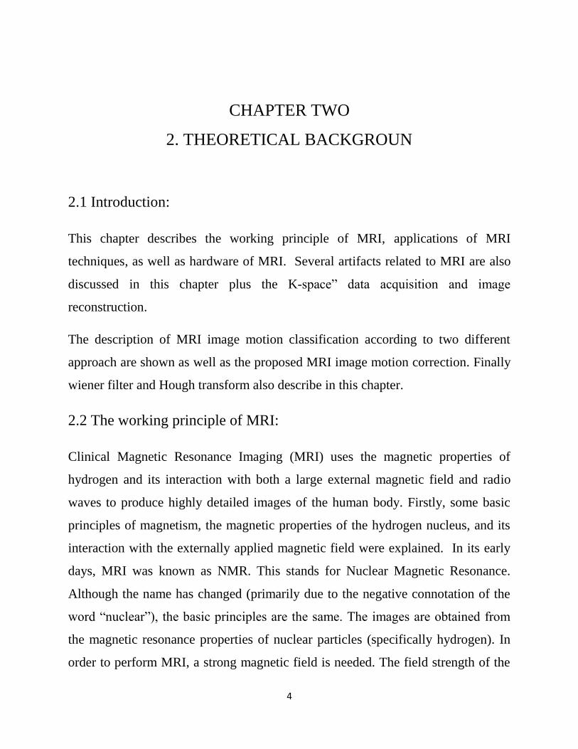
2.2 The working principle of MRI:

Clinical Magnetic Resonance Imaging (MRI) uses the magnetic properties of

hydrogen and its interaction with both a large external magnetic field and radio

waves to produce highly detailed images of the human body. Firstly, some basic

principles of magnetism, the magnetic properties of the hydrogen nucleus, and its

interaction with the externally applied magnetic field were explained. In its early

days, MRI was known as NMR. This stands for Nuclear Magnetic Resonance.

Although the name has changed (primarily due to the negative connotation of the

word ―nuclear‖ , the basic principles are the same. The images are obtained from

the magnetic resonance properties of nuclear particles (specifically hydrogen). In

order to perform MRI, a strong magnetic field is needed. The field strength of the

5

magnets used for MR is measured in units of Tesla. One Tesla is equal to 10,000

Gauss. The magnetic field of the earth is approximately 0.5 Gauss. Given that

relationship, a 1.0 T magnet has a magnetic field approximately 20,000 times

stronger than that of the earth. The type of magnets used for MR imaging usually

belongs to one of three types; permanent, resistive, and superconductive. A

permanent magnet is sometimes referred to as a vertical field magnet. These

magnets are constructed of two magnets (one at each pole). The patient lies on a

scanning table between these two plates. Advantages of these systems are:

Relatively low cost, No electricity or cryogenic liquids are needed to maintain the

magnetic field, their more open design may help alleviate some patient anxiety,

nearly nonexistent fringe field. It should be noted that not all vertical field magnets

are permanent magnets. Resistive magnets are constructed from a coil of wire. The

more turns to the coil, and the more current in the coil, the higher the magnetic

field. These types of magnets are most often designed to produce a horizontal field

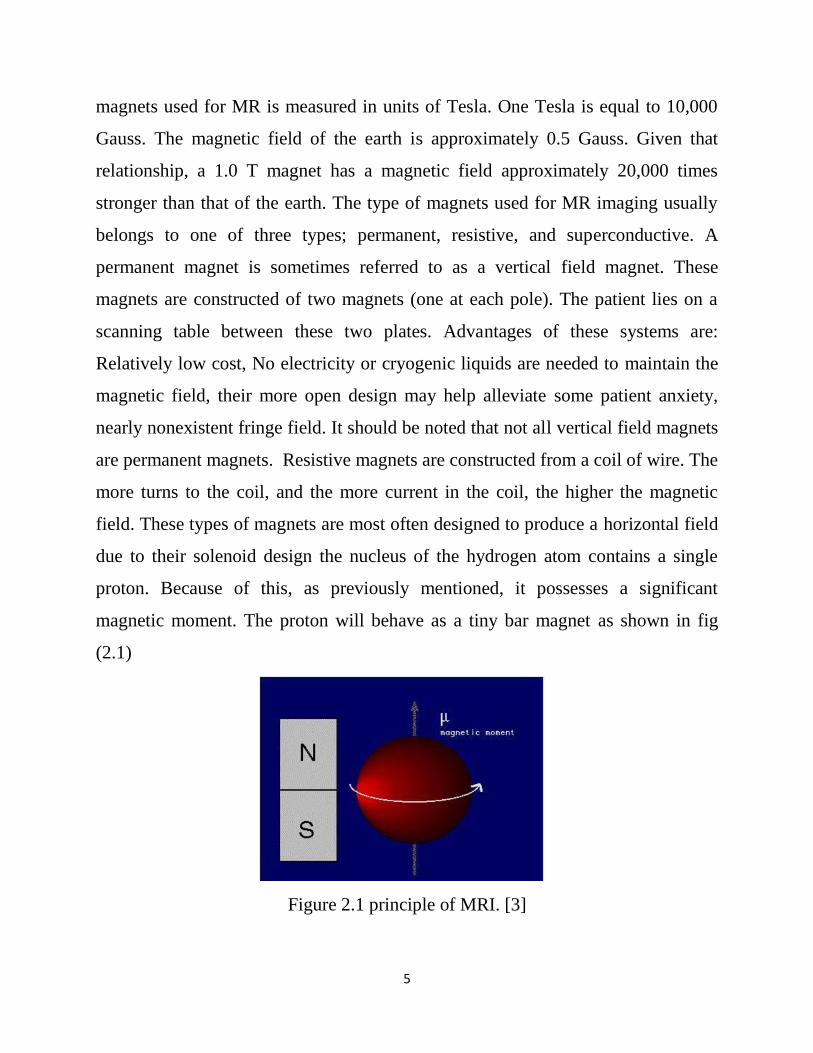
due to their solenoid design the nucleus of the hydrogen atom contains a single

proton. Because of this, as previously mentioned, it possesses a significant

magnetic moment. The proton will behave as a tiny bar magnet as shown in fig

(2.1)

Figure 2.1 principle of MRI. [3]

6

Because of the spin characteristics of the proton, if it is placed in a large external

magnetic field, it will assume one of two possible positions. It will align (at a slight

angle) in either a parallel or anti-parallel with the direction of the magnetic field.

[3]

2.3 Applications of MRI Techniques:

MRI is used as a diagnostic tool for identification of medical conditions and for

monitoring their treatment courses, such as:

Tumors of the chest, abdomen or pelvis.

Coronary artery disease and heart problems including the aorta,

coronary arteries and blood vessels, by examining the size and

thickness of the chambers of the heart and the extent of damage

caused by a heart attack or progressive heart disease.

Tumors and other abnormalities of the reproductive organs (e.g.,

uterus, ovaries, testicles, prostate).

Causes of pelvic pain in women, such as endometriosis.[3]

2.4 Hardware of MRI:

The basic components of an NMR imaging system [4] as shown in fig (2.2)

Magnets.

Radio-frequency coils.

Gradients.

Shimming

Computer

http://www.radiologyinfo.org/en/glossary/glossary1.cfm?gid=722

7

Figure 2.2 Hardware components of MRI. [5]

2.4.1 Magnets of MRI:

There are three several different types of magnets that can be used to produce the

magnetic field [6]

Permanent magnets.

Resistive magnets.

Superconducting magnets.

2.4.1.1 Permanent magnets:

A permanent magnet consists of a material, which has been magnetized such that it

won‘t lose its magnetic field, like the ones you put on your refrigerator). The field

strength is usually very low and ranges between 0.064T ~ 0.3T. Permanent

magnets have usually an open design, which is more comfortable for the patient.

[7]

2.4.1.2 Resistive magnets:

8

Resistive magnets are very large electro magnets. The magnetic field is generated

by a current, which runs through loops of wire. Resistive magnets come in two

flavors: air-core and iron-core. The field strength can be up to 0.3 Tesla. They

produce a lot of heat, which requires water-cooling. They need a lot of power to

run, and are usually switched off when not in use to conserve power [7]

2.4.1.3 Superconducting magnets:

Today‘s most commonly used magnets are superconducting magnets. The

magnetic field is generated by a current, which runs through a loop of wire. The

wire is surrounded with a coolant, such as liquid helium, to reduce the electric

resistance of the wire. Once a system is energized, it won‘t lose its magnetic field.

Superconductivity allows for systems with very high field strengths up to 12 Tesla.

The ones that are most used in clinical environments run at 1.5 Tesla. Most

superconducting magnets are bore type magnets. [7]

2.4.2 Radio-frequency coils:

RF coils are needed to transmit and receive radio-frequency waves used in MRI

scanners. RF coils are one of the most important components that affect image

quality. Current MRI scanners have a range of RF coils suitable to acquire images

of all body parts. There are two types of RF coils, volume coils and surface coils.

[7]

2.4.3 Gradients coils:

Gradient coils provide a linear gradation or slope of the magnetic field strength

from one end of the magnet to the other. This is achieved by passing current

through the gradient coils .The direction of the current through the coil determines

whether the magnetic field strength is increased or decreased relative to isocentre.

The polarity of the current flowing through the coil determines which end of the

9

gradient is higher than isocentre (positive) and which end is lower (negative).

Gradient coils are powered by gradient amplifiers. There are two gradient

amplifiers for each gradient, one affixed to the high end of the gradient, the other

to the low. [7]

2.4.4 Shimming coil:

Shimming coil is used in the process of balancing the main magnetic field.

Shimming coil is critical to the maintenance of homogeneity. It reduces residual

inhomogeneity as well as patient induced inhomogeneity. [7]

2.4.5 Computer system in MRI:

Currently, every MRI system has a minimum of two computers. The main or host

computer controls the user interface software. Software enables the operator to

control all functions of the scanner either directly or indirectly. The second

computer system is a dedicated image processor used for performing the Fourier

transformations or other processing of the detected data. [7]

2.5 Artifacts of MRI:

An artifact is something that appears in an image and is not a true representation of

an object or structure within the body [8]

Artifacts are misrepresentations of tissue structures seen in images produced by

MRI. Examples are:

Chemical shift.

Chemical misregistration.

Magnetic susceptibility.

Aliasing.

Phase mismapping .[9]

10

2.5.1 Chemical shift:

Chemical shift artifact is a displacement of signal between fat and water along the

frequency axis of the image. An example is around the kidneys where the water-

filled kidneys are surrounded by peri-renal fat. To avoid this artifact MRI operator

has to:

Scan with a low field strength magnet.

Broaden the receive bandwidth. [9]

2.5.2 Chemical misregistration:

Chemical misregistration is caused by the difference in precessional frequency

between fat and water that results in their magnetic moments being in phase with

each other at certain times and out of phase at others.

This artifact mainly occurs along the phase axis and causes a dark ring around

structures that contain both fat and water. To reduce this artifact MRI operator has

to Use Spin Echo (SE) or Fast Spin Echo (FSE) pulse sequences (which use RF,

re-phasing pulses). [9]

2.5.3 Magnetic susceptibility:

The magnetic susceptibility of a substance is the ability of external magnetic fields

to affect the nuclei of a particular atom, and is related to the electron configurations

of that atom. Magnetic susceptibility artifact occurs because all tissues magnetize

to a different degree depending on their magnetic characteristics. To eliminate this

artifact MRI operator has to:

Use Spin Echo or Fast Spin Echo pulse sequences (which use RF

rephasing pulses).

Removing all metal items from the patient before the examination. [9]

11

2.5.4 Aliasing:

This occurs when anatomy that is producing signal exists outside Field of View

(FOV) in the phase direction. Anatomy from one side of the image overlaps the

other. To eliminate or reduce the aliasing, one has to increase the FOV to the

boundaries of the coil. [9]

2.5.5 Phase mismapping:

Phase artifact results from anatomy moving between the application of the phase

encoding gradient and the frequency encoding gradient (intra-view) and motion

between each application of the phase gradient (view to view). If anatomy moves

during these periods it is assigned the wrong phase value and is mismapped onto

the image. It causes an artifact called phase mismapping and always occurs along

the phase axis of the image. This artifact appears as blurring or ghosting across the

image. This artifact is eliminated by:

Changing the phase and frequency direction removes the artifact from

the area of interest.

Designing a system to detect the patient motion, and this is the

objective of the project. [9]

2.6 K-space‖ data acquisition and image reconstruction

2.6.1 K-space matrix

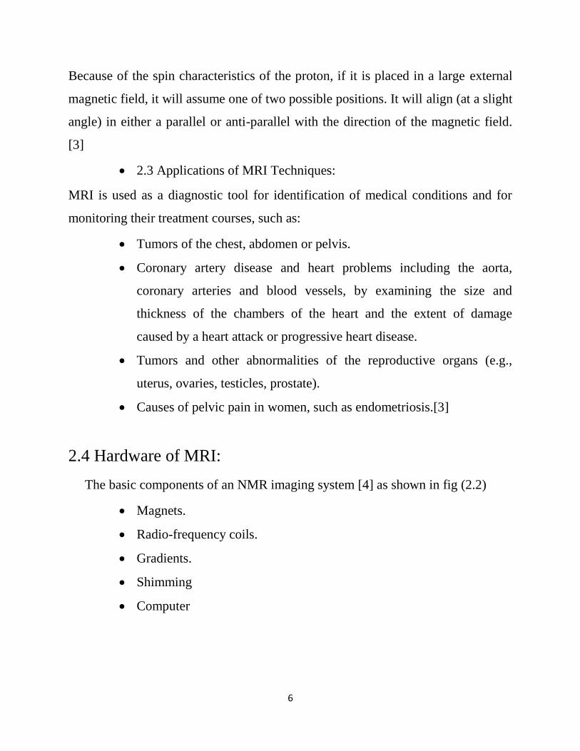
MR data are initially stored in the k-space matrix fig (2.3), the

―frequency domain‖ repository [10]

The axes have units of cycles/unit distance

Each axis is symmetric about the center of k-space, ranging from –

fmax to +fmax

12

Low-frequency signals are mapped around the origin of k-space and high

frequency signals are mapped further from the origin in the periphery

Figure 2.3 matrix of MRI.

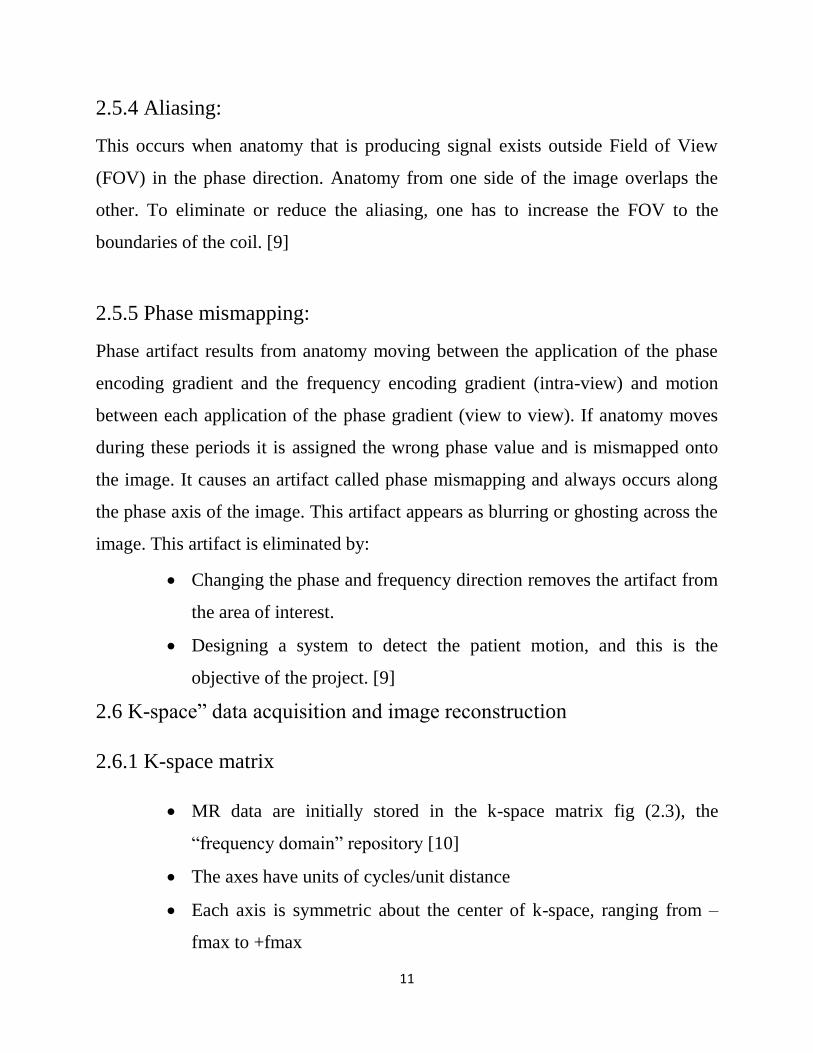
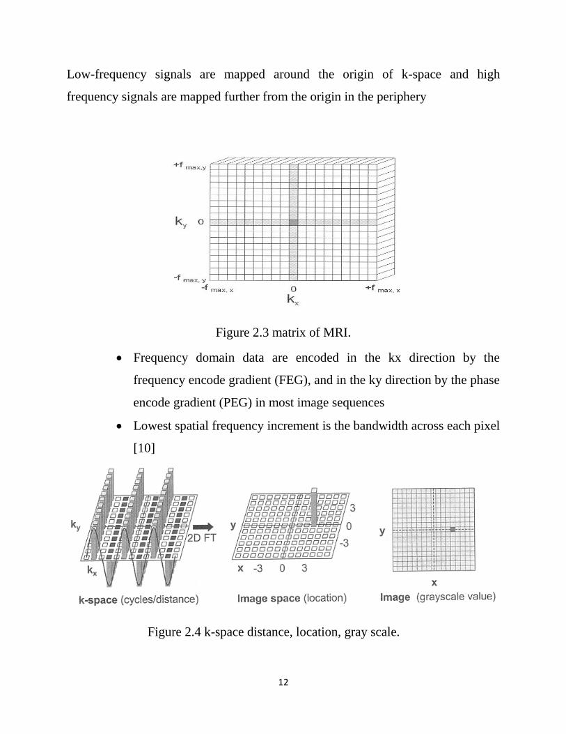
Frequency domain data are encoded in the kx direction by the

frequency encode gradient (FEG), and in the ky direction by the phase

encode gradient (PEG) in most image sequences

Lowest spatial frequency increment is the bandwidth across each pixel

[10]

Figure 2.4 k-space distance, location, gray scale.

13

2.6.2 Two-dimensional data acquisition:-

MR data acquired as a complex, composite frequency waveform

With methodical variations of the PEG during each acquisition fig

(2.5), the k-space matrix is filled to produce the desired variations

across the frequency and phase encode directions [10]

Figure 2.5 MRI pulse sequence.

1. Narrow band RF excitation pulse applied simultaneously with the slice

select gradient (SSG)

Energy absorption dependent on amplitude and duration of the RF

pulse at resonance

Longitudinal magnetization converted to transverse magnetization,

extent of which depends on saturation of spins and angle of excitation

14

90-degree flip angle produces maximal transverse magnetization

2. Phase encode gradient (PEG) applied for a brief duration to create phase

difference among spins along the phase encode direction

Produces several ―views‖ of the data along the ky axis, corresponding

to the strength of the PEG

3. Refocusing 180-degree pulse delivered after selectable delay time, TE/2

Inverts direction of individual spins and reestablishes phase coherence of

transverse magnetization with formation of echo at time TE

4. During echo formation and subsequent decay, frequency encode gradient

(FEG) applied orthogonal to both slice select and phase encode gradient

directions

Encodes precessional frequencies spatially along the readout gradient

5. Simultaneous to application of FEG and echo formation, computer acquires

the time-domain signal using an analog-to-digital converter (ADC)

Sampling rate determined by excitation bandwidth

One-dimensional Fourier transform converts the digital data into

discrete frequency values and corresponding amplitudes

Proton precessional frequencies determine position along the kx (readout) direction

6. Data deposited in k-space matrix in a row, specifically determined by the

PEG strength applied during excitation

Incremental variation of the PEG throughout the acquisition fills the

matrix one row at a time

15

Possible to acquire the phase encode data in nonsequential order to fill

portions of k-space more pertinent to the requirements of the exam

(e.g., in low-frequency, central area of k-space)

After matrix is filled, columns contain positionally dependent phase

change variations along the KY (phase encode) direction

7. Two-dimensional inverse Fourier transform decodes the frequency domain

information piecewise along the rows and then along the columns of k-space

8. Final image is a spatial representation of the proton density, T1, T2, and flow

characteristics of the tissue using a gray-scale range

Each pixel represents a voxel; thickness determined by slice select

gradient strength and RF frequency bandwidth [10]

2.7 Classification of Motion in MRI according to the acquisition blocks

2.7.1 intrashot-motion

Motion present during acquisition blocks

Effects: determined by presence of field gradients! Additional signal

Phase; corrupted excitation profile. [11]

2.7.2 intershot-motion

Motion present between acquisition blocks

Approximation: motion state changes only with the phase encoding

(Cartesian sampling) [11]

16

2.8 classification of motion according to the human body Rigid/non-

rigid motion

2.8.1 rigid-motion

Translation: Fourier-shift-theorem

Rotation: Fourier-rotation theorem

Rigid motion manifests itself in blurring and ghosting

Head-motion, arm-motion, leg-motion

2.8.2 non-rigid-motion

Hard to determine, cardiac-motion, respiration, gastrointestinal

Peristalsis, pulsatile brain-motion

2.9 Correction Approaches

2.9.1 Prospective Motion Correction:

E.g. PROMO, real-time gradient adjustment, gating, triggering

2.9.2 Retrospective Motion Correction:

Mathematical approaches focusing on data consistency

2.9.3 Data Acquisition Strategies:

E.g. PROPELLER sequence, radial/spiral sampling, fast-imaging techniques

[11]

2.10 Image restoration

Image restoration is one of the fundamental problems in image processing. It

aims at reconstruction of true image from the degraded image. There are two main

kinds of blurring: one is motion blur, which is caused by the relative motion

17

between the camera and object during image capturing; the other is defocus blur,

which is due to the inaccurate focal length adjustment at the time of image

capturing. Blurring induces the degradation of image quality, specifically for sharp

images where the high frequency information can be easily lost due to blur. An

image restoration technique refers as non-blind restoration, if blur kernel

information is available. In case of blind restoration, blur kernel information is not

known. Blind image restoration problem has been categorized into two groups. In

the first group, we can put those methods in which the point spread function (PSF)

of blur is estimated in first step and then degraded image is restored using any of

the classical deconvolution methods such as wiener or inverse filtering in

subsequent step. In the methods of second group, PSF estimation and image

restoration are achieved simultaneously [12].

18

CHAPTER THREE

3. LITERATURE REVIEW

The MRI image motion correction goes through three main methods this chapter

will discuss some papers were published during the last fifteen years.

3.1 Prospective Motion Correction real time motion correction.

―A paper describes Prospective Acquisition Correction for Head Motion with

Image-based Tracking for Real-Time fMRI 0222, [13]‖

A prospective Acquisition Correction for Head Motion with Image-based Tracking

for Real-Time fMRI. Scanning and processing of data were performed on a

standard MAGNETOM Symphony 1.5T MR system (Siemens, Erlangen,

Germany). For image acquisition a 2D single shot EPI and a fast RF-spoiled

gradient echo sequence (FLASH) were programmed with full oblique and off-

center functionality for all axes. Calculation of complete sequence timing including

the physical gradient pulses is performed on the fly within 3 milliseconds prior to

each scanned volume. So real-time adjustment of position and orientation of the

slice stack is possible. The system allows real-time reconstruction of the data using

the imaging computer. For further evaluation of the images, the data are transferred

to the host computer. Here a motion detection algorithm related to the method

introduced by Friston et al. (4,5) is applied, estimating a three dimensional rigid

body transformation against a reference volume. The new positional information is

passed to the measurement computer, which adjusts the parameters for slice

orientation and position for the next acquisition. In this implementation the

positional information is fed back with a temporal delay of one acquisition cycle,

which is about 4 seconds in usual 2D multi-slice EPI based MRI measurements.

19

Clinical datasets show that the residual scan to scan motion is commonly smaller

than 50mm and so almost negligible in the most cases. Thus fine adjustment of the

residual motion is performed by the real-time application of additional

retrospective correction of the volumes with Fourier interpolation.

Contributions of this work has a high stability and accuracy involving real-time

motion correction. An unmodified commercial MRI scanner was used, so the

clinical use of PACE is possible. Benefits of the PACE technique can be visualized

by examination of difference images. Significant decrease of variance when the

PACE method was used in comparison to retrospective techniques.

This technique has a clear draw back because of using again the retrospective

method to correct the residual motion which some data may loss. And this adds

some complexity in procedure.

―A paper introduces - Prospective motion correction of high-resolution magnetic

resonance imaging data in children 2010, [14]‖

This method attempts to address the problem of motion at its source by keeping the

measurement coordinate system fixed with respect to the subject throughout image

acquisition. The technique also performs automatic rescanning of images that were

acquired during intervals of particularly severe motion. Unlike many previous

techniques, this approach adjusts for both in-plane and through-plane movement,

greatly. Imaging data were obtained at the UCSD Radiology Imaging Laboratory

on a 1.5 Tesla GE Signa HDx 14.0M5 Twin Speed system (GE Healthcare,

Waukesha, WI) using an eight-channel phased array head coil. Acquisitions

included a conventional three-plane scout and a set of four 3D inversion recovery

spoiled gradient echo (IR-SPGR) T1-weighted volumes with pulse sequence

parameters optimized for maximum gray/white matter contrast (TE=3.9 ms,

20

TR=8.7 ms, TI=270 ms, flip angle=8°, TD=750 ms, bandwidth=±15.63 kHz,

FOV=24 cm, matrix=192×192, voxel size=1.25×1.25×1.2 mm). The sequences

used for the four T1 images were identical except that PROMO motion tracking

and correction was turned off for two scans and on for the other two, in alternating

fashion. The order of scanning for the four T1 scans was counterbalanced across

subjects, with four participants undergoing a sequence of on–off–on–off and five

undergoing off–on–off–on.

Real-time motion tracking and correction with spiral navigator (SNAV) sequences

was performed using the extended Kalman filter (EKF) algorithm (Gelb, 1974)

applied to MRI as reported by Dale and colleagues (White et al., 2007, 2010) and

as described previously for prospective motion correction in S-NAV 3D pulse

sequences (Roddey et al., 2008;Shankaranarayanan et al., 2007). Five sets of three

orthogonal low flip, single shot S-NAVs were interspersed within the dead time of

all four 3D IR-SPGR T1 scans in order to measure and adjust for head movement

while scanning (White et al., 2010). Of note, the placement of the S-NAV scans

can vary according to the specific pulse sequence being used. Online navigator-

derived motion measures were used to adjust the image coordinate system with

respect to brain position and to automatically rescan images that were acquired

during intervals with particularly high motion, as determined by the position

difference between the two navigator scans that ―sandwich‖ each partition. For this

study, a rescan threshold was determined based on the noise level characteristics of

a sample of ―cooperative‖ adult subjects i.e., who showed a relative absence of

motion). Rescans were set to be triggered by a norm of 1 or greater in the motion

measures during an acquisition (i.e., a norm of 1 mm of total translation or a norm

of 1° of total rotation by any combination of the head position values. A rescan of

the entire volume was allowed, if necessary according to subject movement. For

images acquired without PROMO, scan duration was 8 min, 40 s per T1 volume.

21

The S-NAV/EKF framework offers the advantage of image based tracking within

regions of interest that are specific to each subject, masking out motion from non-

brain locations such as the neck and jaw, which can corrupt the motion estimates.

Motion estimates for the PROMO-enabled volumes were computed from navigator

scans, tracking position as a six-element vector. As an index of each individual's

magnitude of head motion, the norm of the range of motion measures (minimum to

maximum) was computed across both PROMO-on scans for each subject for

translation and rotation. This ―Euclidean‖ or L2 norm is a normalized measure of

the magnitude of variability in motion—in this case the square root of the sum of

squares of the range of motion—that has the advantage of being independent of

relative position in the x, y, z coordinate space. Motion estimates were not

calculated for the two PROMO-off scans, since tracking and correction was

disabled.

The contributions In addition to improvements in quantitative measures, PROMO

corrected volumes also were consistently rated subjectively as superior to

uncorrected images for both overall clarity and reduced motion-specific artifacts.

As with quantitative measures, qualitative ratings were better in all cases when

PROMO was enabled. Although this particular study did not focus on clinical

pulse sequences, our findings suggest that prospective motion correction would

also be useful in standard clinical neuroradiological assessment and diagnosis.

Main drawbacks the number of rescans required because of subject movement,

and therefore the additional time required for acquisition with PROMO enabled,

also varied considerably among subjects. The additional acquisition time required

for PROMO-on scans was on average 34.3 s per volume, but this varied widely

and was heavily affected by one outlying individual; the median additional scan

time was 7.5 s, the standard deviation was 69.4 s, and the duration ranged from 0

to 292.5 s (4 min, 52.5 s). The correlation coefficient (Pearson, one-tailed) between

22

the total number of rescans and head translation was r=0.72 (p=0.01) and between

rescans and rotation was r=0.61 (p=0.04).

3.2 Retrospective Motion Correction mathematical approaches focusing on data

consistency.

―A paper describe Image-Based Method for Retrospective Correction of

Physiological Motion Effects in fMRI: RETROICOR 2000, [15]”

Simple MRI image-based motion correction method that does not have the

limitations of k-space methods that preclude high spatial frequency correction.

Low-order Fourier series are fit to the image data based on time of each image

acquisition relative to the phase of the cardiac and respiratory cycles, monitored

using a photo plethysmograph and pneumatic belt, respectively. The RETROICOR

method is demonstrated using resting-state experiments on three subjects and

compared with the k-space method. The method is found to perform well for both

respiration- and cardiac-induced noise without imposing spatial filtering on the

correction.

The correction method assumes that the time series of intensities y (t) in a pixel is

corrupted by additive noise resulting from cardiac and respiratory functions. The

cardiac and respiratory states are monitored during the scan using a photo

plethysmograph and a pneumatic belt placed around the subject‘s abdomen,

respectively. It is assumed that the physiological processes are quasi-periodic so

that cardiac and respiratory phases can be uniquely assigned for each image in the

time series. All experimental imaging data were obtained with a 3 T scanner

equipped with high-performance gradients and receiver (GE Signa, rev 8.2.5,

Milwaukee, WI). T1weighted FSE scans were acquired for anatomic reference

23

(TR/ spin-echo time (TE)/ETL 5 68 msec/4000 msec/12). An automated high-order

shimming method based on spiral acquisitions was employed to reduce B0

heterogeneity. Resting-state ―functional‖ acquisitions used a 2D spiral gradient-

recalled echo sequence with TE 30 msec, field of view (FOV) 22 cm, and scan

duration of 200 sec (8). The in-plane trajectory was a single-shot uniform-density

spiral providing resolution of 2.3 mm (matrix 96 3 96). Either three or twelve 5

mm slices (depending on TR; see below) were acquired with axial scan plane. In

Subject 3, oblique coronal planes nominally perpendicular to the calcarine fissure

(often used when studying visual cortex) were also obtained. A homemade head

coil was used for all scans and subjects were stabilized with foam padding packed

tightly in the coil. Images were reconstructed into a 128 3128 matrix with an off-

line computer (Sun Microsystems, Mountain View, CA) using gridding and fast-

Fourier transforms (FFTs). Linear shim corrections for each slice were applied

during reconstruction using individual field maps obtained during the scan. Two

scans were obtained for each of three subjects at TRs of 250 msec (3 slices, 800

time frames each) and 1000 msec (12 slices, 200 frames). The shorter TR ensured

that cardiac fluctuations in the images were resolved without temporal aliasing,

whereas the longer TR provided more typical scan conditions in which cardiac

pulsation could alias into spectral regions that overlap with those of the stimulus

and respiration. The resting-state data were acquired with no intentional task, for

which the subjects were instructed to keep their eyes closed.

The contributions of this work are: first, The RETROICOR method, in contrast

with RETROKCOR, treats each pixel separately and therefore does not introduce

artificial coupling of noise corrections across spatial regions. As a result, the RMS

noise from cardiac and localized respiratory pulsatility was found to be reduced to

a greater extent by the new method than by the k-space method. Second, that real-

24

image data rather than complex raw data are corrected, which reduces the

computational burden by half. Furthermore, because it is a post processing method

operating on images, it may be easier to apply in practice than the k-space method

because it is not necessary to invoke an off-line reconstruction after the corrections

are made. Main drawbacks an assumption of the image-based correction is that

each image is collected at a discrete time for which unique cardiac and respiratory

phases can be assigned. This is a good assumption for single-shot imaging, but

may not hold for multishot acquisitions, because the multiple-TR periods needed

for all segments may span several cardiac or respiratory cycles

―A paper propose Retrospective Motion Correction Protocol for High-Resolution

Anatomical MRI 2006, [16]‖

In this study a retrospective motion correction (RMC) were tested, common for

functional MRI (fMRI) image motion correction, as a means to improve the quality

of high-resolution 3-D anatomical MR images. RMC methods are known to be

effective for correcting interscan retrospective motion correction algorithm is

proposed, which significantly reduces ghosting and blurring artifacts due to subject

motion. The technique of the raw data of standard imaging sequences was used; no

sequence modifications or additional equipment such as tracking devices are

required. Similar to other approaches, we assume that the motion time-scale is

longer than the repetition time TR, i.e. we model the motion trajectory as a

piecewise constant function. We neglect second order effects such as the influence

of motion on the magnetic field. Like all other reference-free (no external

information on motion) methods we assume that the imaged object behaves as a

rigid body. Under these assumptions we can correct for arbitrary motion

trajectories in 6 degrees of freedom for both 2D and 3D acquisitions. We provide a

Matlab implementation of GradMC along with 4 examples.

25

First the motion corrupted k-space data was modeled. Next, the cost function based

on the image gradient entropy metric was constructed. We then describe how

translational and rotational motion was implemented, and deal with non-linearities

and local minima in our objective using multiscale optimization. Finally, we

demonstrate that our method can be extended to multiple coils.

The contributions the obvious and very strong advantage of our method (and

retrospective methods in general) is that it can be applied to any already acquired

dataset (subject to our model assumptions), and does not require the use of any

tracking equipment, or special imaging sequences. By applying additional

constraints, it may also be extendable to handle non-rigid body motion, for which

prospective correction is highly challenging.

Main drawbacks the current major limitation of the method was the inability to

correct for motion involving strong rotations (angles larger than 3°). The visual

quality of a reconstructed image never gets worse than that of a degraded image,

however, the stronger the rotation, the less improvement can be achieved. For

rotation angles larger than 10°, the corrected image looks essentially the same as

the degraded one. A strong assumption we make is that the imaged object behaves

as a rigid body. Indeed, this is what allows us to carry out fast multiplications with

the matrix A_ in the Fourier domain. Slight deviations from non-rigidity are well

tolerated, however gross effects (e.g. due to movement of the tongue during the

acquisition) make an artifact-free correction difficult. We also assume that the

input to Grad MC is the raw k-space data along with the order in which the k-space

was sampled. In a clinical setting, such data is not always available, because often

only magnitude images are preserved. Since real data from the scanner often has

non-uniform spatial phase

26

―A paper propose Blind Retrospective Motion Correction of MR Images 2007.

[17]‖

Another retrospective motion correction algorithm is proposed, which significantly

reduces ghosting and blurring artifacts due to subject motion. The technique uses

the raw data of standard imaging sequences; no sequence modifications or

additional equipment such as tracking devices are required. Similar to other

approaches, we assume that the motion time-scale is longer than the repetition time

TR, i.e. we model the motion trajectory as a piecewise constant function. We

neglect second order effects such as the influence of motion on the magnetic field.

Like all other reference-free (no external information on motion) methods we

assume that the imaged object behaves as a rigid body. Under these assumptions

we can correct for arbitrary motion trajectories in 6 degrees of freedom for both 2D

and 3D acquisitions. We provide a Matlab implementation of GradMC along with

4 examples. first the motion corrupted k-space data was modeled. Next, we

construct the cost function based on the image gradient entropy metric. We then

describe how translational and rotational motion is implemented, and deal with

non-linearities and local minima in our objective using multiscale optimization.

Finally, we demonstrate that our method can be extended to multiple coils.

The contributions the obvious and very strong advantage of our method (and

retrospective methods in general) was that it can be applied to any already acquired

dataset (subject to our model assumptions), and does not require the use of any

tracking equipment, or special imaging sequences. By applying additional

constraints, it may also be extendable to handle non-rigid body motion, for which

prospective correction is highly challenging.

The major limitation of our method is the inability to correct for motion involving

strong rotations (angles larger than 3°). The visual quality of a reconstructed image

27

never gets worse than that of a degraded image, however, the stronger the rotation,

the less improvement can be achieved. For rotation angles larger than 10°, the

corrected image looks essentially the same as the degraded one. A strong

assumption we make is that the imaged object behaves as a rigid body. Indeed, this

is what allows us to carry out fast multiplications with the matrix A_ in the Fourier

domain. Slight deviations from non-rigidity are well tolerated, however gross

effects (e.g. due to movement of the tongue during the acquisition) make an

artifact-free correction difficult. We also assume that the input to Grad MC is the

raw k-space data along with the order in which the k-space was sampled. In a

clinical setting, such data is not always available, because often only magnitude

images are preserved. Since real data from the scanner often has non-uniform

spatial phase

3.3 Data Acquisition Strategies: e.g. PROPELLER sequence, radial/spiral

sampling, fast-imaging techniques

―A paper describe Periodically Rotated Overlapping Parallel Lines with Enhanced

Reconstruction 0211, [18]‖

A PROPELLER MRI data was collected in such a way that can mitigate the (in-

plane motion, phase inconsistencies, and through-plane motion). This approach can

be blended with many techniques, and has been successfully implemented with

gradient echo and turbo spin echo sequences. Data are collected in k-space in N

strips, each consisting of L parallel lines, corresponding to the L lowest phase

encoded lines in any Cartesian-based data collection.

Each strip is rotated in k-space by an angle , so that the total Rotated,

overlapping strips in k-space. Data set spans a circle in k-space. If a matrix

28

diameter of M is desired, then Land N are chosen so that . The

central circle in k-space with diameter L is collected for each of the N strips; these

are used to form N low-resolution images, which are compared to each other to

remove in-plane displacement and phase errors that are slowly varying spatially.

These factors are corrected for each strip.

Cross-correlation measures between the low resolution images are used to

determine which strips were collected with significant through-plane displacement.

As the data are combined in k-space, the data from strips with the least amount of

through-plane motion are preferentially used in regions of strip overlap, thus

reducing artifacts from through-plane motion.

The contributions of this work are: removal of respiratory motion from ECG gated

cardiac MRI, allowing breath hold-quality images without breath holding Motion

correction was performed using only a limited FOV around the heart in the low-

resolution images.

Main drawbacks successfully only with gradient echo and turbo spin echo

sequences. Increase in overall imaging time (due to strip overlap) and a loss of

information at the corners of k-space.

―A paper describe Motion Correction with Propeller MRI: Application to Head

Motion 2010, [19]‖

The PROPELLER MRI (Periodically Rotated Overlapping Parallel Lines with

Enhanced Reconstruction) was implemented as a new technique in data collection

and reconstruction. The data is collected in concentric rectangular strips that rotate

around the k space. The central portion is contained in each strip and therefore can

be used to obtain a low frequency average image It can compensate for the phase

and bulk translation, rotation and scaling in the image. Moreover it can further

29

reject data which has significant motion based on a correlation measure. Methods

which collect data from center to outwards of k space such as projection

reconstruction and spiral MRI reduce these motion artifacts by oversampling the

central k-space which can be thought as an analogy of averaging the data in

conventional imaging. Other methods try to estimate the motion or motion related

phase from extra collected data which are referred as navigator echoes. They

generally compute the bulk transformation in the data and correct for these artifacts

in the image.

Phase Correction: In this step, we correct the small displacement in the k-space due

to the imperfect gradient of MRI machine. The basic idea is to remove the low

frequency part of the reconstructed image phase by a pyramid triangle window.

Bulk Transformation Correction: After doing the phase correction of the data we

estimated the bulk transformation of the object between each strip and corrected

for these artifacts. If we restrict our model to affine case the bulk transformation

are caused by rotation, translation and scaling. These transformations have nice

one to one Fourier transform correspondences. In our approach we estimated each

transformation separately.

Bulk Translation Correction: From the Fourier Transform theory we know that

translation in image space causes some linear phase shifts in its Fourier transform.

Therefore, the linear phase shift can be corrected by estimating the translation in

image space.

Bulk Scaling Correction:

As rotation and translation in image space have corresponding properties in Fourier

space, a similar relation is also observed with the scaling in the image space.

Scaling in image space also causes scaling in Fourier space. However this scaling

30

is inversely proportional such that contraction in one domain produces

corresponding expansion in the other domain. (Equation 3). Therefore, the scaling

factor in image space can be directly computed using the k-space data as done in

rotation case. Correlation Weighting: some strips will still have factors that will

produce artifacts because of the significant inter-plane motion after doing all the

previous corrections. We can calculate a weight of each strip based on the

correlation, and then multiply the data of each strip by this weight to compensate

for these artifacts.

The contributions of this work that the registration correction works very well.

Looking at the original images that were reconstructed from each strip we do not

see much registration errors. Therefore there have been little changes after rotation,

translation and scaling corrections

Main drawbacks the excessive oversampling of the center of k-space and neglect

the hall. K-space is one of the main dis advantages which affect the producing

image. Second the assumption that motion is rigid since we use head data, the

movements are restricted only to rigid case

―A paper propose different method MRI with TRELLIS: which is a novel

approach to motion correction 2012, [20]‖

This was provide a full description of the TRELLIS k-space trajectory and

reconstruction algorithm. Results from computer simulations, a physical ‗moving

phantom‘ and a human subject are presented. Through comparison with existing

methods. K-Space is filled using orthogonal overlapping strips and the directions

for phase- and frequency-encoding are alternated such that the frequency-encode

direction always runs lengthwise along each strip. The overlap between strips is

used both for signal averaging and to produce a system of equations that, when

31

solved, quantifies the rotational and translational motion of the object- an acronym

for Translation and Rotation Estimation using Linear Least-squares and Interleaved

Strips and so named because its sampling pattern looks like a trellis. Results

obtained from simulations with computer-generated phantoms, a purpose-built

moving phantom, and in human subjects show the method is effective. TRELLIS

offers some advantages over existing techniques in that k-space is sampled

uniformly and all acquired data are used for both motion detection and image

reconstruction. This technique has some similarities to PROPELLER: it does not

require extra hardware; it samples k-space more than once in order to obtain

information about patient motion; and the final reconstruction requires some form

of gridding.

The contributions of TRELLIS may offer significant advantages because the whole

of k-space is uniformly sampled instead of concentrating sampling in the center of

k-space as in PROPELLER. Therefore all collected data are used for both motion

detection and image reconstruction and excessive oversampling of the center of k-

space is avoided. It is likely, however, that this advantage is gained at a cost of

decreased motion detection accuracy compared to PROPELLER. It is interesting to

note that the TRELLIS sequence is relatively robust to motion even without the

application of motion correction performed in post-processing.

Main drawbacks. TRELLIS may have some problem multishot diffusion-weighted

sequences. Strip in H and V lies directly over the center of k-space (Fig. 10B). The

advantage is that the center of k-space will always be kept intact, no matter what

motion occurred during imaging. Currently, ‗holes‘ in k-space near the origin

caused by a gap between strips after rotation correction can occasionally cause

artifacts. The optimum width of each strip has also yet to be found. No

assumptions are made about the nature of the motion as a function of time.

32

Incorporating prior knowledge of the maximum possible values of velocity or

acceleration.

33

CHAPTER FOUR

4. METHODOLOGY

This chapter introduces the research methods that were used for this thesis

including the main algorithm and the motion blur angle estimation algorithm and

motion blur length estimation, were discussed in details, then Hough transform,

cepstral method and wiener filter theories were demonstrating.

4.1 The methodology proceeds as follows:

first Appling Hough transformer function to the motion blurred image (Ifbl), to

prepare motion angle estimation by building up the accumulator array.

Second Estimate the motion blur angle (THETA) using function that takes image

as input and returns a collection of possible blur angles using step2 and other

functions.

Third Estimate the length of the motion blur (LEN) which is the number of pixels

by which the image is blurred the estimation depend on step2 beside other

functions

Forth Prepare the wiener filter algorithm using the estimation of angle and length

of the motion blur and SNR as parameters.

Fifth Starting motion blur correction by calling THETA value and LEN value and

wiener filter function

Sixth The resulted corrected images according to different THETA and LEN

estimation was displayed with better appearance in the blurred pixels.

Seventh the corrected image suffering some blur in the whole image sharping

process are applied for better appearance

Eighth SNR calculated for the input images and the output image in order to verify

which estimate THETA and LEN are result in better motion blur correction and to

verify wiener filter validation in motion blur correction.

34

Block diagram 4.1 illustrate the main methodology process

Appling Hough transformer function

to the motion blurred image

Estimate the motion blur angle

(THETA)

Estimate the length of the motion

blur (LEN)

Prepare the wiener filter algorithm

using the estimation of angle and length

Starting motion blur correction by

calling THETA value and LEN

value and wiener filter function

Sharping process was applied to the

resulted image for better appearance

SNR calculated for the input

images and the output image

35

4.2 Motion Blur Angle Estimation Algorithm

a) Performing Median Filter before restoring the blurred image and Display the

input image.

b) Converting image from spatial domain to frequency domain.

c) Compute the log spectrum of F (u, v).

d) Convert the image to Cestrum (spectrum (IFT)) domain Compute the inverse

Fourier transform of log spectrum.

e) Finding the edge map of the image in cepstral domain of step d.

f) Let theta min and the theta max be the minimum and maximum values of the

motion blur angle.

g) Calling Hough transform to initialized the accumulator array.

h) Finding first maximum in the accumulator.

i) Storing first maximum in the array.

j) Saving the original accumulator array.

k) . Find the peak in Hough transform (the maximum value in accumulator

array) which is perpendicular to the motion blur angle.

l) Iterating 10 times to find 10 highest angle values.

m) Calculate the possible values of THETA

4.3 Motion Blur Length Estimation Algorithm

a) Performing Median Filter before restoring the blurred image and Display

the input image.

b) Converting image from spatial domain to frequency domain.

c) Compute the log spectrum of F (u, v).

d) Convert the image to Cepstrum (spectrum (IFT)) domain Compute the

inverse Fourier transform of log spectrum.

36

e) Rotate the cepstral by the estimated angle in the inverse direction.

f) Convert the 2-D matrix of step e to 1-D by taking the averages of columns.

g) Find the distance of first negative peak from the origin which is

corresponding to motion length.

h) If Zero Crossing found then return it as the blur length

i) If Zero Crossing not found then find the lowest peak Calculating the blur

length using Lowest Peak

Block diagram 4.2 illustrate motion Blur Angle Estimation Algorith

Performing Median Filter to the input

image

Converting image from spatial domain

to frequency domain

Compute the log spectrum

Convert the image to Cepstrum

domain

Finding the edge map of the image in

cepstral domain

Calling Hough transform to initialized

the accumulator array

Finding first maximum in the

accumulator.

Storing first maximum in

the array

Saving the original

accumulator array

Find the peak in Hough

transform

Iterating 10 times to find 10

highest angle values

Calculate the possible

values of THETA

37

Block diagram 4.3 illustrate motion Blur length Estimation Algorithm

Rotate the cepstral by the estimated

angle in the inverse direction

Convert the 2-D matrix of previous step

to 1-D by taking the averages of

columns

Find the distance of first

negative peak from the origin

If Zero Crossing found then return it as

the blur length

Performing Median Filter to the input

image

Converting image from spatial

domain to frequency domain

Compute the log spectrum

Convert the image to Cepstrum domain

If Zero Crossing not found then find the lowest peak

calculating the blur length using Lowest Peak

38

4.4 Hough Transform Method

The Hough transform [21] can be applied to find global patterns such as lines,

circles, and ellipses in an image in a parameter space. It is especially useful in line

detection because lines can be easily detected as points in Hough transform space,

based on the polar representation of line given by (Equ. 4.1):

Where (X, Y are Cartesian coordinates of a point on the line; θ is the angle

between the perpendicular from the origin to the given line and the x-axis and ρ is

the length of the perpendicular. Thus, a pair of coordinates ρ, θ can describe a

line in polar domain. Fig. 4.1 shows transformation of line parameters from image

domain to polar domain.

Figure 4.1 hough transform

The blur direction is obtained by locating the maximum value of this accumulator

array. The ϴ value corresponding to the maximum value of the accumulator array

is the angle perpendicular to the blur direction. True blur direction is given by 900

- 0.

39

4.5 Cepstral Method Cepstrum transform [21] can be used for separation of blur components and image

components. Cepstrum transform of an image f(x, y) is defined in Equ(4.2) as

follows: C {f(x,y)} = F-1 Log │F(f(x,y))│ 4.2

Uniform motion blur in Frequency domain has periodic patterns by zero crossing

of sinc function. Periodic patterns make negative peaks in cepstrum domain. Fig

4.2 shows cepstrum of blurred image has the negative peaks that are arisen by

motion blur. For an estimated angle, we can estimate the blur length in an image.

With the image in the cepstrum domain, first rotate the image by the expected blur

angle and then take the average of each column to collapse 2-D cepstral into 1-D.

By finding the number of columns between origin and first negative peak, we are

able to find the periodicity and estimate the blur length for a given angle.

Figure 4.2 cepstral transform method

4.6 Wiener Filtering

Wiener filtering (after N. Wiener, who first proposed the method in 1 942) is

One of the earliest and best known approaches to linear image restoration. A

40

Wiener filter seeks an estimate that minimizes the statistical error function

Equ(4.3)

=E {( - 4.3

Where E is the expected value operator and f is the undegraded image [22].

Description

J = deconvwnr(I,PSF,NSR) deconvolves image I using the Wiener filter algorithm,

returning deblurred image J. Image I can be an N-dimensional array. PSF is the

point-spread function with which I was convolved. NSR is the noise-to-signal

power ratio of the additive noise. NSR can be a scalar or a spectral-domain array of

the same size as I. Specifying 0 for the NSR is equivalent to creating an ideal

inverse filter.

The algorithm is optimal in a sense of least mean square error between the

estimated and the true images.

J = deconvwnr (I, PSF, NCORR, ICORR) deconvolves image I, where NCORR is

the autocorrelation function of the noise and ICORR is the autocorrelation function

of the original image. NCORR and ICORR can be of any size or dimension, not

exceeding the original image. If NCORR or ICORR are N-dimensional arrays, the

values correspond to the autocorrelation within each dimension.

If NCORR or ICORR are vectors, and PSF is also a vector, the values represent the

autocorrelation function in the first dimension. If PSF is an array, the 1-D

autocorrelation function is extrapolated by symmetry to all non-singleton

dimensions of PSF. If NCORR or ICORR is a scalar, this value represents the

power of the noise of the image [23].

41

CHAPTER FIVE

5. RESULTS AND DISCUSSION

A new method for MRI motion blur correction on the personal computer (PC) side

using MATLAB program had been developed, the resulted images and the

measured values will be discus in this chapter

To assess the overall impact of the using wiener filter in MRI image motion blur,

the expected motion blur angle and motion blur length were estimated for more

details Hough transform was used in line detection, ten different expected angles

and length of motion blur were estimated.

According to the different measured angles and lengths motion correction was

applied by wiener filter ten times, the resulted images were treated by sharpening

filters and SNR were measured for all corrected image in order to compare which

estimated angle and length were result a better a pperance.

For the ten different motion blur angles and lengths in coronal brain MRI image,

the correction method results illustrated in the following figures, every one figure

include the original image beside the corrected image in order to compare the

different angles and length values restoration and their effect in the original

corrupted image.

Then the same algorithm has been used for another sagittal and axial MRI motion

blur image and the resulted corrected image has been illustrated following the

coronal image figures, different angle and length for motion blur images has been

estimated and accordingly different result was observed.

42


corrected image R with angle 112 and length 11.



43


corrected image(R with angle 173 and length 5.



44





45





46





47

The following table include the estimated SNR for coronal corrected image in

different angles and lengths comparing with the motion blurred image.

Table 5.1 comparison between SNR of motion image and corrected image (coronal

image).

Estimated angle &length Motion blurred

image SNR

corrected image SNR

Figure 5.1, length: 11, angle: 112 -2.4619 -0.81093








Figure 5.9 length: 7, angle: 145 -2.4619 -1.8852


48

By the visual inspection and consultation of radiologist and senior technologist

comparing the original motion blurred image and motion corrected image. There is

some anatomical structure were going to be diagnosable and clear more than

before correction specially in angle 99 fig (5.2) and angle 112 fig (5.1)with the

same length 11.

The table above (5.1) contains the ten corrected image with their angles, lengths

and SNR. Angle 99 fig (5.2) had the maximum SNR value in the table which

determines that it has the better motion blur correction even by the visual

inspection the correction was clear and given clear result in the coronal brain MRI

image.

Figure 5.3 with angle 173 and length 5 had the minimum SNR value hence lowest

degree of motion blur correction.

For the remaining corrected image they gave some degrees of correction but

different values of motion distortion was remained in the image and that is why the

correction algorithm take different value of expected angles and lengths.

By the visual inspection comparing the original motion blurred image and motion

corrected image. There is some anatomical structure was going to be diagnosable

and clear more than before correction specially in angle 99 and angle 112 with the

same length 11.

49





50


corrected image(R) with angle 179 and length 4.



51


corrected image R with angle 21 and length 11



52





53





54

The following table include the estimated SNR for sagittal corrected image in


Table 5.2 comparison between SNR of motion image and corrected image (sagittal

image) .

Estimated angle &length Motion

blurred

image SNR

Corrected image

SNR











55

Also in the sagittal image the visual inspection and consultation of radiologist and

senior technologist comparing the original motion blurred image and motion

corrected image. There is some anatomical structure were going to be diagnosable

and clear more than before correction specially in fig(5.12) angle 173 ,and

fig(5.14)with angle2 , fig(5.15) with angle 21 and fig(5.17) with angle 110 .

The table above (5.2) contain the ten corrected image with their angles, lengths and

SNR. Angle 21 fig (5.15) and angle 110 fig 5.17 had the maximum SNR value in

the table which determine that it has the better motion blur correction even by the

visual inspection the correction was clear and given clear result in the sagittal brain

MRI image.




56


corrected image(R) with angle 172 and length 10



57

Figure 5.23Comparison between the original axial MRI image (L) and the




58





59





60





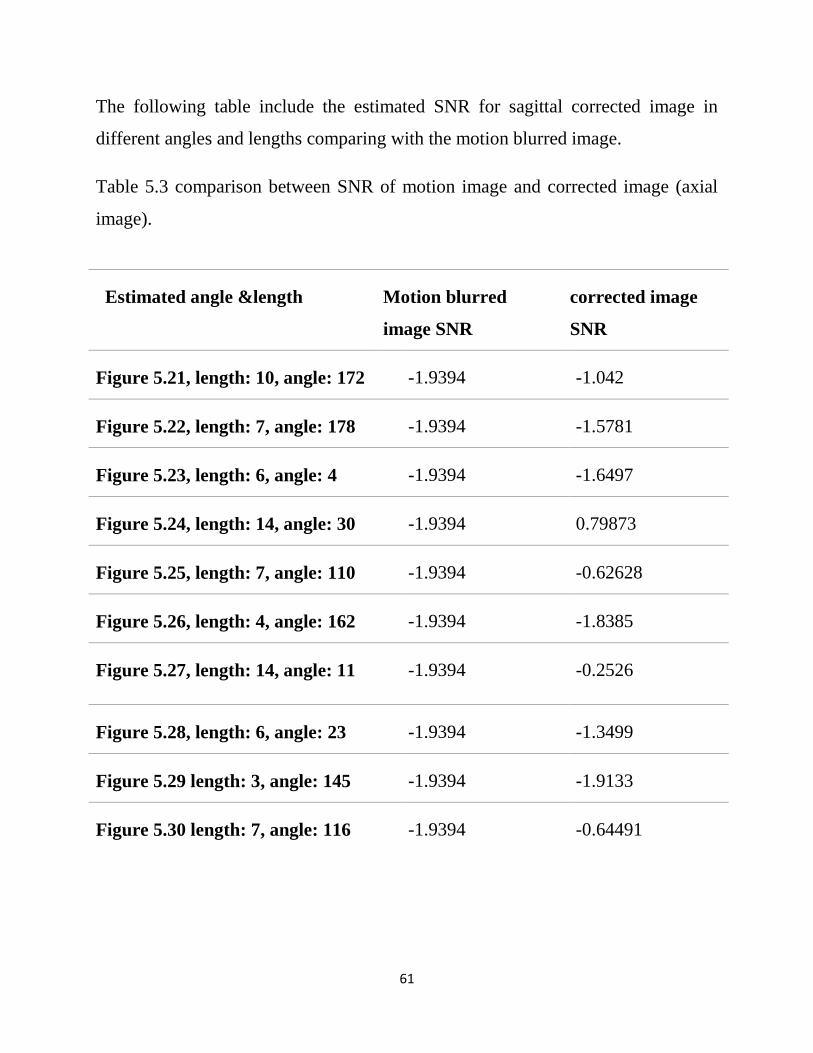
61

The following table include the estimated SNR for sagittal corrected image in


Table 5.3 comparison between SNR of motion image and corrected image (axial

image).

Estimated angle &length Motion blurred

image SNR

corrected image

SNR




Figure 5.24, length: 14, angle: 30 -1.9394 0.79873







62

Finally in the axial corrupted image also by visual inspection and consultation of

radiologist and senior technologist comparing the original motion blurred image

and motion corrected image. There is some anatomical structure were going to be

diagnosable and clear more than before correction specially in fig 5.21 angle

172 ,and fig 5.22 with angle 178 , fig 5.15 .

The table above (5.3) contain the ten corrected image with their angles, lengths and

SNR. Although fig 5.21 angle 172 , and fig (5.22) with angle 178 , fig 5.15 .

Had not the maximum SNR value in the table, they had the better motion blur

correction even by the visual inspection the correction was clear and given clear

result in the axial brain MRI image.




63

CHAPTER Six

6. CONCLUSION AND RECOMMENDATIONS

6.1 Conclusion

In this study, a motion blur correction algorithm, used to assess coronal, sagittal

and axial image for the MRI brain corrupted with rigid motion.

Wiener filter was taken as the main algorithm in the correction procedure.

According to ten different angles and lengths estimated before starting the

correcting procedure.

The correction algorithm achieved the best results which lead to clear appearance

in anatomical brain feature and remove the motion blur which can obscure very

important details.

Although the corrected image by wiener filter gave a best result, it suffering some

degree of unsharpeness, application of sharpening filter was needed and it gave

better results.

Motion blur in sagittal image result in highly degree of correction by the algorithm

in the research. Since more than five images according to the different degree of

angle and length estimation was totally corrected.

64

6.2 Recommendations and Future Work

Following the algorithm described in this thesis and the other methods of MRI

image motion correction in the literature review chapter three indicate that the

problem was still remain this is as general.

For developing the results in this research:-

1. Develop more different algorithm.

2. Use different method for sharpening following the corrected image by

wiener filter (this is can improve the final result).

3. Using more than ten motion blur angle and length to increase the probability

of achieving the maximum motion blur correction.

65

REFERENCES

[1] Google Internet, ―General views‖, Copy right J.P-Horn.

[2] Liang Z-P, Lauterbur PC,‖ Principles of magnetic resonance imaging: a signal

processing perspective‖, New York, Vol.4, No.16, 2000.

[3] Mohamed Abdullah, A., ―the working principle of MRI lecture/Class‖,

University of medical science and technology, Vol.3, NO.6, 2008.

[4] Rskhandpur, ―Hand book of bio medical instrumentation‖, second edition,

http://books.google.com/books.

[5]Wikipedia, ―Hardware of MRI‖, http://en.wikipedia.org/wiki/mri.

[6] Perry sprawls, Jr, Ph.D., FACR, ―Physical principles of medical Imaging‖,

printed in United State of America, Vol.54, No.5, 2008.

[7] Mohamed Abdullah, A, ―Hardware of MRI‖, University of medical science and

technology, Vol.12, No.3, 2008.

[8] Perry sprawls, Ph.D., FACR, FAAPM, ―Magnetic resonance imaging‖,

Department of radiology mory university, Vol.23, No.7, 2009.

[9] Mohamed Abdullah, A, ―Artifact of MRI‖, University of medical science and

technology, Vol.55, No.11, 2008.

[10] Atkinson D,‖ Magnetic Resonance Imaging II‖, Magnetic Resonance in

Medicine, Vol.44, No.9, 2012.

[11] Matthias Schlogl,‖ Motion Correction in MRI‖, Magnetic Resonance in

Medicine, Vol.13, NO.5, 2013.

http://books.google.com/books

66

[12] Mark Jenkinson, Peter Bannister, “Improved Optimization for the Robust and

Accurate Linear Registration and Motion Correction of Brain Images”, Elsevier

Science (USA), Vol.17, No.10, 2002.

[13]Stefan Thesen, Oliver Heid,‖ Prospective Acquisition Correction for Head

Motion with Image-based Tracking for Real-Time fMRI‖, Computer methods in

Biomechanics and Biomedical engineering,Vol.30,No.11,2009.

[14] Timothy T. Brown, Joshua M. Kuperman,‖ Prospective motion correction of

high-resolution magnetic resonance imaging data in children‖, journal homepage:

www.elsevier.com/locate/ynimg,Vol.53,No.2,2010.

[15] Gary H. Glover, Tie-Qiang Li, ―Image-Based Method for Retrospective

Correction of Physiological Motion Effects in fMRI: RETROICOR‖, Magnetic

Resonance in Medicine, Vol.44, No.8, 2000.

[16] Peter Kochunov, Jack L. Lancaster, ―Retrospective Motion Correction

Protocol for High-Resolution Anatomical MRI‖, Human Brain Mapping, Vol.27,

No.11, 2006.

[17] Alexander Loktyushin, Hannes Nickisch, ―Blind Retrospective Motion

Correction of MR Images‖, Medical Imaging, Vol.55, No.7, 2007.

[18] James G. Pipe, ―Periodically Rotated Overlapping ParallEL Lines with

Enhanced Reconstruction (PROPELLER) MRI; Application to Motion

Correction‖, Proceedings of the International Society for Magnetic Resonance in

Medicine Sixth Scientific Meeting and Exhibition Sydney, V0l.22, NO.5, 2011.

[19] Belma Dogdas, Quanzheng Li, ―Motion Correction with Propeller MRI:

Application to Head Motion‖, International Journal of Electrical, Electronics and

Computer Systems, Vol.26, No.12, 2010.

http://www.elsevier.com/locate/ynimg,Vol.53,No.2,2010

67

[20] Julian Maclaren, Michael Herbst, ―Prospective Motion Correction in Brain

Imaging: A Review‖, Suffix Indicating a Corporation, Vol.23, No.6, 2012.

[21] Shamik Tiwari, V. P. Shukla,‖ Review of Motion Blur Estimation

Techniques‖, Image and Graphics,Vol.1,No.4,2013.

[22] R. C. Gonzalez and R. E. Woods, ―Digital Image Processing”, Prentice Hall,

Vol.33, No.4, 2007.

[23] MATLAB tool books, www.mathwork.com.

MRI Phase Mismapping Image Artifact correction - SUST ...

Documents

Transcript of MRI Phase Mismapping Image Artifact correction - SUST ...