Titulación: Grado en Ingeniería Biomédica

Autor: Alba Pedrero Pérez

Tutor: Mónica Abella García

Co-Tutor: Claudia de Molina Gómez

Leganés, 9 de julio de 2014

Trabajo de Fin de Grado

Truncation Artifact Correction for Micro-CT

Scanners

ii

Truncation Artifact Correction for Micro-CT Scanners

Laboratorio de Imagen Médica (LIM) Unidad de Medicina y Cirugía Experimental (UMCE) Hospital General Universitario Gregorio Marañón

Departamento de Bioingeniería e Ingeniería Aeroespacial

Universidad Carlos III de Madrid

iii

Título: Truncation Artifact Correction for Micro-CT Scanners

Autor: Alba Mª Pedrero Pérez

Tutor: Mónica Abella García

Co-Tutor: Claudia de Molina Gómez

EL TRIBUNAL

Presidente: Jorge Ripoll Lorenzo

Vocal: Ricardo Domínguez Reyes

Secretario: Sara Guerrero Aspizua

Realizado el acto de defensa y lectura del Trabajo de Fin de Grado el día 9 de

Julio de 2014 en Leganés, en la Escuela Politécnica Superior de la Universidad

Carlos III de Madrid, acuerda otorgarle la CALIFICACIÓN de

VOCAL

SECRETARIO PRESIDENTE

iv

v

Abstract

The work included in this project is framed on one of the lines of research carried out at the

Laboratorio de Imagen Médica de la Unidad de Medicina y Cirugía Experimental (UMCE) of Hospital

General Universitario Gregorio Marañón and the Bioengineering and Aerospace Department of

Universidad Carlos III de Madrid. Its goal is to design, develop and evaluate new data acquisition

systems, processing and reconstruction of multimodal images for application in preclinical research.

Inside this research line, an x-ray computed tomography (micro-CT add on) system of high resolution

has been designed for small animal. Nowadays, computed tomography (CT) is one of the techniques

most widely used to obtain anatomical information from living subjects. Different artifacts from

different nature usually degrade the qualitative and quantitative analysis of these images. This

creates the urgent need of developing algorithms to compensate and/or reduce these artifacts.

The general objective of the present thesis is to implement a method for compensating

truncation artifact in the micro-CT add-on scanner for small animal developed at Hospital

Universitario Gregorio Marañón. This artifact appears due to the acquisition of incomplete x-ray

projections when part of the sample, especially obese rats, lies outside the field of view. As a result

of these data inconsistencies, bright shading artifacts and quantification errors in the images may

appear after the reconstruction process.

First of all, truncation artifact in the high resolution micro-CT add-on scanner was studied. Then,

after a review of the proposed methods in the literature, the optimal approach for the micro-CT add-

on was selected, based on a sinogram extrapolation technique developed by Ohnesorge et al [1].

This method consists on a symmetric mirroring extrapolation of the truncated projections that

guarantees continuity at the truncation point. It includes a sine shaping effect that ensures a smooth

attenuation signal drop. Truncation artifact correction method has been validated in simulated and

real studies. Results show an overall significant reduction of truncation artifact. This algorithm has

been adapted and implemented in the reconstruction interface of the preclinical high-resolution

micro-CT scanner, which is manufactured by SEDECAL S.L. and commercialized worldwide.

Key words:

X-ray, CT, micro-CT, artifact, truncation

vi

Resumen

El trabajo de este proyecto se encuadra dentro de una línea de investigación que se desarrolla

en el Laboratorio de Imagen Médica de la Unidad de Medicina y Cirugía Experimental (UMCE) del

Hospital General Universitario Gregorio Marañón y el Departamento de Bioingeniería e Ingeniería

Aeroespacial de la Universidad Carlos III de Madrid. Su objetivo es diseñar, desarrollar y evaluar

nuevos sistemas de adquisición de datos, procesamiento y reconstrucción de imágenes multi-

modales para aplicaciones en investigación preclínica. Dentro de esta línea de investigación se ha

desarrollado un tomógrafo de rayos X de alta resolución para pequeños animales (micro-TAC add-

on). Actualmente, la tomografía axial computarizada es una de las técnicas más ampliamente

utilizadas para la obtención de información anatómica in vivo. Existe una serie de artefactos de

distinta naturaleza en este tipo de imágenes que generalmente degradan y dificultan el análisis

cualitativo y cuantitativo de las imágenes, dando lugar a una necesidad imperante de desarrollar

algoritmos de corrección y/o reducción de estos artefactos.

El objetivo general del presente proyecto es la implementación de un algoritmo para la

corrección del artefacto de truncamiento en el escáner micro-TAC add-on desarrollado en el Hospital

Universitario Gregorio Marañón. Este artefacto aparece debido a la adquisición de proyecciones

incompletas cuando parte de la muestra, especialmente ratas obesas, se extiende fuera del campo

de visión. Estas inconsistencias en los datos obtenidos pueden dar lugar a la aparición de bandas

brillantes y errores en la cuantificación de las imágenes después del proceso de reconstrucción.

En primer lugar, se ha estudiado el artefacto de truncamiento en el escáner micro-TAC add-on

de alta resolución. Seguidamente, se ha llevado a cabo una revisión de los métodos propuestos en la

bibliografía, seleccionando una estrategia óptima para el micro-TAC add-on bajo estudio: una técnica

de extrapolación del sinograma publicado por Ohnesorge et al [1]. Este método consiste en una

extrapolación de espejo simétrico de las proyecciones truncadas que garantiza la continuidad en el

punto de truncamiento. Incluye el modelado de una sinusoide que asegura una caída de señal en los

valores de atenuación suave. Este método ha sido validado en estudios simulados y reales. Los

resultados muestran una clara reducción del artefacto de truncamiento. El resultado de este

proyecto ha sido incorporado en la interfaz de reconstrucción del escáner pre-clínico micro-TAC add-

on de alta resolución fabricado por SEDECAL S.A. y comercializado por todo el mundo.

Palabras clave:

Rayos x, TAC, micro-TAC, artefacto, truncamiento

vii

Agradecimientos

En primer lugar, me gustaría dar las gracias a todas aquellas personas que han contribuido a

sacar el Grado en Ingeniería Biomédica adelante y a todos los que nos han acompañado en estos

cuatro años: Manolo, Juanjo, Javier, Jose Luis, Marcela, Marta.

Me gustaría agradecer especialmente a mi tutora, Mónica, todo su apoyo y paciencia, tanto en

este proyecto como de cara al próximo año. Y a mi co-tutora, Claudia por sus consejos y ánimos.

Al hospital y a los compañeros del LIM, por recibirnos con los brazos abiertos y hacer la cuesta

arriba un poco más fácil. A todos los proyectandos que tanto a las 9 de la mañana como a las 9 de la

noche llenan el buffer.

A Carmen, Cris y Laura, porque sois las mejores. Carmen y su eterna ilusión. Cris y su gran

fortaleza. Laura y su adorable tranquilidad. Por vuestro apoyo. Por acogerme en vuestra ciudad, en

vuestras vidas, en vuestras casas. El próximo año estaremos repartidas por Europa. No sabemos lo

que nos deparará el destino, pero lo que sí sé es que seguiréis siendo mi familia físicamente más

cercana. Os deseo lo mejor.

A Miguel, Celia, Gema, Nuria y todos los que han vivido estos cuatro años conmigo, día a día, en

la resi. A Pepi, por cuidar de todos nosotros.

A Fernan, por hacerme feliz y arrancarme sonrisas en los buenos y malos momentos. Por

demostrarme día tras día, año tras año, que vale la pena luchar por lo que quieres.

Finalmente, a mi familia, por estar siempre ahí, por apoyarme, mimarme y haberme dado los

medios para llegar hasta aquí. A mi padre y su eterno apoyo. A mi madre y sus mimos. A mi hermana

viajera por ser un modelo a seguir. A mi abuela, por ser la persona más buena que hay.

viii

Content

1. Introduction to Medical Imaging ........................................................................................... 1

1. 1. Fundaments of X-ray Imaging ................................................................................................. 2

1. 2. Image Reconstruction ............................................................................................................. 5

1. 3. Artifacts in CT .......................................................................................................................... 8

2. Motivation, Context and Objectives .................................................................................... 17

2. 1. Context .................................................................................................................................. 18

2. 2. Objectives and Key Milestones ............................................................................................. 25

2. 3. Outline of the Document ...................................................................................................... 25

3. Study of Truncation Artifact ................................................................................................ 27

4. Correction of Truncation Artifact ......................................................................................... 31

4. 1. Bibliography Review of Truncation Correction Methods ...................................................... 31

4. 2. Selected Correction Method ................................................................................................. 33

5. Results ............................................................................................................................... 45

5. 1. Quantitative Analysis ............................................................................................................ 45

5. 2. Real Truncated Rat Acquisitions ........................................................................................... 48

5. 3. Implementation .................................................................................................................... 49

6. Discussion and Conclusions ................................................................................................. 52

Annex A - FBP ......................................................................................................................... 55

Annex B - ACT ......................................................................................................................... 57

Annex C - HDR ........................................................................................................................ 59

Annex D - Macro ..................................................................................................................... 61

References .............................................................................................................................. 63

Glossary ................................................................................................................................... 65

ix

Image Index Figure 1 – (a) Medical imaging techniques according to their energy. Two different scales are shown, from top

to bottom: according to wavelength (m) and photon energy; (b) Comparison between radiation type, its

corresponding wavelength and an approximate scale of wavelength with objects (Suetens, 2008). .................... 1

Figure 2 - Scheme representing the different components of an x-ray scanner (Jan, 2006)................................... 2

Figure 3 – (left) X-ray chest projection with overlaying information; (b) vertebral column and head x-ray

projection. ............................................................................................................................................................... 2

Figure 4 – (left) Three orthogonal directions of the medical imaging of the human body; (right) A, B and C axial,

sagittal and coronal views respectively of a CT study (Fuji Synapse). .................................................................... 3

Figure 5– (a) parallel beam geometry; (b) fan beam geometry; (c) cone beam geometry. (Hsieh, 2009) ............. 4

Figure 6 – Basic example illustrates the concept of projection. .............................................................................. 5

Figure 7 – Basic example illustrates the concept of backprojection. Upper image corresponds to the original

image. Image on the left is obtained by backprojecting for ϴ=0 . Image on the right is the added sum of the

backprojected images obtained for ϴ=0 and ϴ=90 . Resulting image is not exactly the same as the original

one. However, pixel value distribution is maintained. ............................................................................................ 6

Figure 8 – Original image (top) consists of a single point. In the bottom part, images resulting from

backprojection of 3, 6 and 360 degrees respectively are shown. In the last case, image on the right, it can be

observed how the point edges are smoother than in the other ones. .................................................................... 6

Figure 9– Scheme of the different steps in the FBP and the filter effect ................................................................. 7

Figure 10 – (a) CT Axial section of a homogeneous cylinder without beam hardening in which the yellow line

represents the profile across the red line, (b) same axial section with beam hardening, in which the cupping

artifact can be observed; (c) axial section of brain CT without beam hardening, (d) same axial section of brain

CT with beam hardening artifact; difference between these two images is highlight with the red arrow (Barret

et al, 2004). ............................................................................................................................................................. 9

Figure 11 - Axial (left) and coronal (right) images showing streaking artifact due to photon starvation (Barret et

al, 2004). ............................................................................................................................................................... 10

Figure 12 – a) Sagittal section of a chest CT showing motion artifact due to cardiac motion (Department of

Radiology, Vancouver General Hospital, University of British Columbia/Canada; b) and c) Pediatric phantom,

simulating a non-sedated baby. b) Shows poor image quality due to motion while in c) motion artifacts have

been significantly reduced by the use of rapid scanning. (Siemens AG) ............................................................... 10

Figure 13 – CT image showing the appearance of artifact caused by metallic artifacts (Barret et al, 2004). ...... 11

Figure 14 – Scheme showing different detector misalignments (Abella et al, 2012). .......................................... 12

Figure 15 – (left) Reconstructed image without geometric misalignment; (right) reconstructed image with

horizontal detector displacement (Sun et al, 2006). ............................................................................................. 12

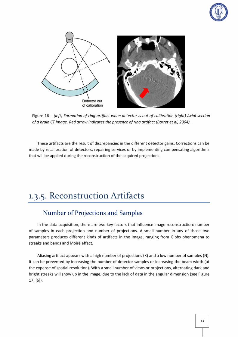
Figure 16 – (left) Formation of ring artifact when detector is out of calibration (right) Axial section of a brain CT

image. Red arrow indicates the presence of ring artifact (Barret et al, 2004). .................................................... 13

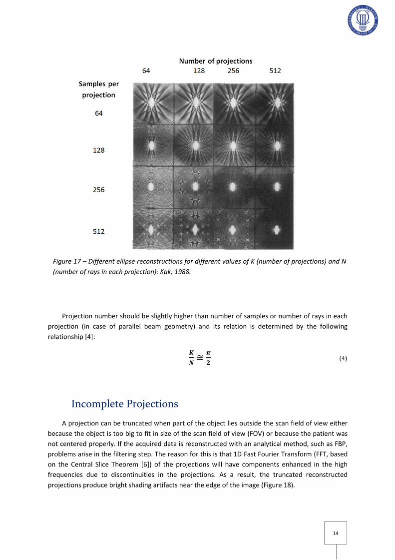
Figure 17 – Different ellipse reconstructions for different values of K (number of projections) and N (number of

rays in each projection): Kak, 1988. ...................................................................................................................... 14

x

Figure 18 – CT image showing truncation artifact (bright shading) because of patient diameter (70 cm) was

bigger than field of view (50 cm of diameter). ..................................................................................................... 15

Figure 19 – Sagittal, coronal and axial sections (left, middle and right, respectively) of a PET/CT rat study. Red

arrow points out a myocardial infarction. ............................................................................................................ 17

Figure 20 – Axial view of a CT study of a rat where the arrows indicate the truncation artifact. ........................ 18

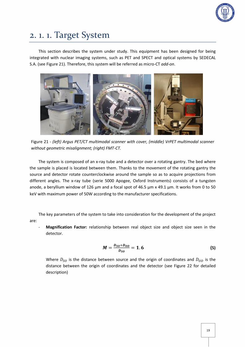
Figure 21 - (left) Argus PET/CT multimodal scanner with cover, (middle) VrPET multimodal scanner without

geometric misalignment; (right) FMT-CT.............................................................................................................. 19

Figure 22 – Illustration of the cone beam geometry formed by the x- ray source and the detector .................... 20

Figure 23 – Scheme showing how certain thickness of different attenuation coefficients influences the x-ray

beam (Hsieh, 2009). .............................................................................................................................................. 21

Figure 24 – (a) Raw data; (b) Flood image without object placed in the field of view; (c) Dark image; (d) Raw

data after undergoing aforementioned corrections of gain and dead pixels; (e) Attenuation image after

applying the logarithm to (d). ............................................................................................................................... 22

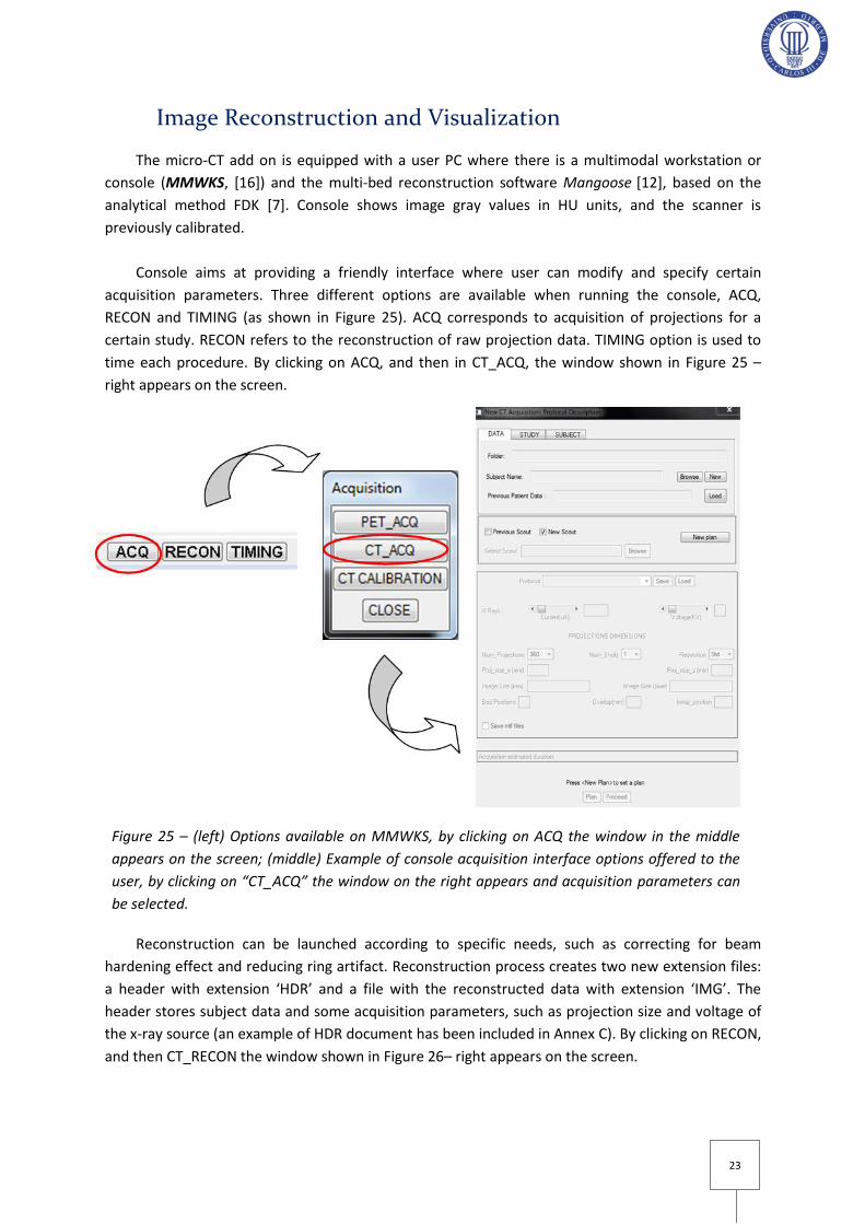
Figure 25 – (left) Options available on MMWKS, by clicking on ACQ the window in the middle appears on the

screen; (middle) Example of console acquisition interface options offered to the user, by clicking on “CT_ACQ”

the window on the right appears and acquisition parameters can be selected. .................................................. 23

Figure 26 – (left) Options available on MMWKS, by clicking on RECON the window in the middle appears on the

screen; (middle) Example of Console Reconstruction interface options, by clicling on CT RECON the image on the

right opens. With BROWSE option a certain study can be selected, in this example a rat CT, and corrections can

be applied before reconstruction. ......................................................................................................................... 24

Figure 27 – Example of MMWKS interface showing a mouse CT after reconstruction ........................................ 24

Figure 28 – (left) CT scheme showing an object (red cube) that lies outside the FOV; (right) A, complete

projection of a mouse CT study. B, truncated projection of a rat CT study. ......................................................... 27

Figure 29 – (left) Complete projection of a mouse CT study, (right) complete profile along yellow line plotted in

the projection on the left. ..................................................................................................................................... 27

Figure 30 – (left) Truncated projection of a mouse CT study, (right) truncated profile along yellow line plotted in

the projection on the left. ..................................................................................................................................... 28

Figure 31 – Effect of the filtering step: (left) homogeneous frequency distribution at the edges, (right) high

frequencies have been enhanced in the truncated image. ................................................................................... 28

Figure 32 – Reconstructed CT image showing truncation artifact (bright circular shading) combined with

streaking (Mawlawi et al, 2006). .......................................................................................................................... 29

Figure 33 – Illustration of projection truncation in a phantom. (a) Original projection without truncation. (b)

Simulated moderate level of projection truncation. (c) Simulated severe level of projection truncation (Hsieh,

2009). .................................................................................................................................................................... 29

Figure 34 – Top row shows the different fields of view, second row shows the corresponding sinograms, third

row shows filtered sonograms and bottom row shows FBP reconstructions. Fist column (A) corresponds to a

complete FOV acquisition, second column (B) Corresponds to a limited FOV in which the sinogram outside the

FOV is set to zero, resulting in bright shading artifact. Finally, third column (C) presents a limited FOV, with the

sinogram outside the field of view set to the end values. In this way, discontinuities are prevented, avoiding the

bright rim (Boas 2012). ......................................................................................................................................... 31

Figure 35 – Top image shows a truncated sinogram, bottom image shows the correcting sinogram form by sine

completing curves (Ohnesorge et al, 2000). ......................................................................................................... 32

xi

Figure 36 – Top image shows a truncated sinogram, bottom image shows the correcting sinogram form by sine

completing curves (Chityala et al, 2005). ............................................................................................................. 32

Figure 37 – Profile showing an original truncated projection profile with extension according to value at

the sides pre-set to zero. ....................................................................................................................................... 33

Figure 38 – (left) “symmetric mirroring” extrapolation (back dashed line) at the left side is performed around

point (red dashed line) and (right) symmetric mirroring extrapolation (back dashed line) at the right side is

performed around point (red dashed line). Back dashed lines denoted by and indicate the sine

shaping effect (Ohnesorge et al, 2000)................................................................................................................. 35

Figure 39 – Comparison of profiles without truncated correction (top), with extrapolation without sine shaping,

where the effect of low could not be overcome (middle) and with extrapolation with sine (bottom) using

the implemented code. ......................................................................................................................................... 36

Figure 40 – (left) Extrapolated projection profile with smooth transition to zero values; (right) Effect of the

filtering step showing a homogeneous distribution. ............................................................................................ 36

Figure 41– Flow chart of the simplified algorithm. Circles correspond to functions and squares to Boolean

operators. ............................................................................................................................................................. 37

Figure 42 – Truncated projections of a rat CT which have been extrapolated with extensions of 20, 30 and 40

pixels at each side, from left to right, respectively. Profiles plot along the yellow lines are shown in Figure 43. 39

Figure 43 – Comparison performed in ImageJ between extrapolated profiles drawn in Figure 42 with different

extension values at the sides (in pixels). From top to bottom Next=20, Next=30 and Next=40, respectively. Red

and blue circles indicate the extrapolation performed at the left and right edges, respectively. ........................ 39

Figure 44 – (left) complete original projection of a cylinder phantom CT, yellow lines indicate the boundaries for

truncation; (right) truncated projection after cropping the original projection 90 pixels at each side. ............... 41

Figure 45 – Axial sections of a cylinder phantom CT (left) Original projection without truncation, the image has

been manually cropped after reconstruction (90 pixels at each side); (middle) Reconstructed data without

truncation correction. ........................................................................................................................................... 41

Figure 46 – (left) Original mouse projection data; (middle) Mouse projection data with induced truncation of

140 pixels at each side; (left) mouse projection data with induced truncation of 160 pixels at each side. It can be

observe how the loss of signal with 160 pixels is much more aggressive in the protruded mass than with 140. 42

Figure 47 – Axial sections of mouse CT (left) Original projection without truncation, the image has been

manually cropped after reconstruction (160 pixels at each side); (right) Reconstructed data without truncation

correction. ............................................................................................................................................................. 42

Figure 48 – Axial sections of mouse CT showing the line across which profiles have been drawn. (left) Original

image; (right) Image with artifact. ....................................................................................................................... 43

Figure 49 –Axial sections of a rat CT extending outside the Field Of View without algorithm correction. ........... 43

Figure 50 – Axial sections of a cylinder phantom CT (left) Original projection without truncation, (middle)

Reconstructed data without truncation correction; (right) Reconstructed data with truncation correction. ...... 45

Figure 51 – Axial sections of mouse CT (left) Original projection without truncation, the image has been

manually cropped after reconstruction (160 pixels at each side); (middle) Reconstructed data without

truncation correction; (right) Reconstructed data with truncation correction. .................................................... 46

Figure 52 – Axial sections of mouse CT showing the line across which profiles have been drawn. (left) Original

image; (middle) Image with artifact; (right) Corrected Image. ............................................................................ 47

Figure 53 – Comparison of profiles drawn along the yellow lines. ....................................................................... 47

xii

Figure 54 – Axial sections of a rat CT extending outside the Field Of View: (left) Reconstructed data without

truncation correction; (right) Reconstructed data with truncation correction. .................................................... 48

Figure 55 – (left) Console interface options offered to the user, by clicking on “RECON” reconstruction options

appear on the screen (middle); by clicking on CT_RECON Console Reconstruction window appears, offering the

user the choice to select different correction methods. Truncation option appears highlighted in a red circle. Rat

Projections from two different angles are shown. ................................................................................................ 49

Figure 56 – Upper row: sagittal, coronal and axial views respectively of a truncated CT image with truncation

correction. Lower row: truncated CT image without truncation correction. ........................................................ 50

xiii

Table Index

Table 1– Available CTF files features according to binning value ......................................................................... 22

Table 2 – Scheme showing the correspondence between binning value, projection size and Next value needed to

extrapolate and correct truncated projections. .................................................................................................... 39

Table 3 – Analysis of the Region of Interest (ROI) of the cylinder Recovery of mean CT value in % has been done

by comparing the corrected image with the image with artifact. ........................................................................ 45

Table 4 – Analysis of the Regions of Interest (ROI) of mouse acquisitions. ROI 1 has an area equal to 396 pixels

while ROI 2 has an area of 568 pixels. Blue numbers are key indicators of the correction algorithm performance.

.............................................................................................................................................................................. 46

Table 5 – Analysis of the Regions of Interest (ROI) drawn in rat acquisitions. ROI 1 has area equal to 1444 pixels

while ROI 2 has an area of 1008 pixels. Red numbers are key indicators of the correction algorithm. ................ 48

xiv

Introduction

1

1. Introduction to Medical Imaging

Medical image is the representation of the spatial distribution of one or more chemical or

physical properties of the organism, which are the origin of contrast. Medical image acquisition

involves the irradiation of the sample with certain energy. Depending on the type of energy

involved, different acquisition techniques are classified into modalities [2]. X rays and γ rays are

forms of electromagnetic radiation. The former is the incident radiation corresponding to

radiography and Computed Tomography (CT) images, while the latter gives rise to nuclear imaging

(Scintigraphy, Positron Emission Tomography, PET, and Single Photon Emission Computed

Tomography, SPECT). In Magnetic Resonance Imaging (MRI) the incident energy are radio frequency

waves. Ultrasound Imaging (US) uses mechanical energy, in form of ultrasound waves. Figure 1

shows a scheme of the different energies.

X-rays are forms of ionizing radiation. Because of its high energy they are able to eject an

electron from an atom, leading to chemical reaction in an organism. High ionization dose may induce

damage to the patient. Therefore, carefully planning of the radiation needed for the study is needed.

Figure 1 – (a) Medical imaging techniques according to their energy. Two different scales

are shown, from top to bottom: according to wavelength (m) and photon energy; (b)

Comparison between radiation type, its corresponding wavelength and an approximate

scale of wavelength with objects (Suetens, 2008).

2

1. 1. Fundaments of X-ray Imaging

The basic principle behind x-ray image formation in radiography (2D) is that the x-ray beam

goes through the sample, suffer different attenuation according to the traversed tissues and finally

reach the detector, where the information about the accumulated attenuation is recorded in a

projection [3].

Figure 2 illustrates the different components of an x ray scanner. Diffuse radiation is emitted

from the x-ray tube. A primary collimator focuses the beam ensuring the rays follow the desired

trajectory. Pre-patient filter cancels out low radiation dose that will otherwise remain in the patient

body (blue Region of Interest) without reaching the detector. As some scattered radiation (deviated

rays) may occur, an anti-scatter grid is placed before the detector so as to limit the incoming x-ray

direction. Finally, the attenuated x-ray beam lands on the detector and is recorded in a projection, as

illustrated in Figure 3, [3]. From thorax image superposition of ribs, lungs and heart is quite evident.

Figure 3 – (left) X-ray chest projection with overlaying information; (b) vertebral column and

head x-ray projection.

Figure 2 - Scheme representing the different components of an x-ray scanner (Jan, 2006).

3

However, the problem with this technique is that all the anatomical information in 3D is

collapsed into a projection (2D). Depth information is lost as there is no way of knowing the

attenuation coefficient of a certain structure located above or below in space. It was latent the need

of finding a new geometric configuration for the acquisition: rotating the source from different

angles around the sample, so that information is obtained from every angle. In such a way, a 3D

image (Tomography) was generated from 2D (Radiography) projection data, getting rid of overlaying

object information. Tomography is derived from the Greek word tomos (to cut) and graphos (image).

Figure 4 shows the three orthogonal directions, in which “cuts” are performed. Different gray

levels in each projection are related to the x ray attenuating properties of the tissues, which directly

depend on mass density and atomic number [4]. Gray levels close to white color correspond to high

density areas, that is, places where there is higher x-ray photons absorption, gray areas with soft

tissues, medium density, and dark areas with the lowest possible density (air). As such, the

differences in density between soft tissues are not remarkable and maximum contrast differences

are achieved with bone and air [4].

The mathematical foundation of computed tomography (CT) was first derived by Radon in 1917.

However, it was not until the development of modern computers that the technique became at all

viable. The original breakthrough was made by G. N. Hounsfield of EMI Laboratories in 1972,

showing a practical method for generating cross-sectional images of the head [5]. Since then, CT has

experienced tremendous growth in recent years, in terms both of basic technology and new clinical

applications [4]. This technique provide with valuable 3D information for diagnosis, having both an

excellent spatial resolution and, in the most recent scanners, a fast acquisition.

Figure 4 – (left) Three orthogonal directions of the medical imaging of the human body; (right)

A, B and C axial, sagittal and coronal views respectively of a CT study (Fuji Synapse).

4

According to the detector shape, there are three possible configurations: parallel beam, fan

beam and cone beam geometry (Figure 5, [4]). Parallel beam refers to a punctual source that moves

in small increments parallel to the detector elements. In fan beam geometry the x-rays are equally

spaced (landing on a detector line) or equiangular spaced (landing on a circular line detector).

Finally, in cone beam geometry, the detector is flat and the x-rays describe a cone shape.

The most common units for CT data representation are Hounsfield Units (HU) or CT number. It

consists on a re-scaling of gray values according to two known tissue values: air (-1000 HU) and

water (- 1000). Soft tissues (including fat, muscle, and other body tissues) have CT numbers range

from -100 HU to 60HU. Bones are more attenuated and have CT numbers from 250 HU to over 1000

HU. In such a way, impact of non-idealities of the acquisition process is reduced and small

differences between tissue types are enhanced [4].

CT number or HU is defined by:

(1)

1. 1. 1. Projection

Data recorded on the detector is known as projection. A simple example is presented here so as

to illustrate the concept of projection.

Figure 6 shows how a projection is obtained, according to different attenuation coefficients ( )

in a parallel beam geometry configuration. Projection for projection angle ϴ=0 would be the sum of

the attenuation coefficients along the different horizontal ray trajectories. Each projection recorded

data represents the total attenuation traversed by an x-ray and t axis represents the distance of

from the x-ray to the object center of coordinates. Information from a single projection angle is not

enough to know the exact distribution of the four different attenuation values in the image. If a

projection is performed at angle ϴ=90 , additional attenuation information along the vertical axis

will be obtained. For solving this simple example only two rays for two different projection angles

are needed: they form a system of four equations with four unknowns. However, in a real case,

number of unknowns is higher and a lot of projections (recorded data) are needed to as to

accurately reconstruct an object.

Figure 5– (a) parallel beam geometry; (b) fan beam geometry; (c) cone beam geometry.

(Hsieh, 2009)

5

1. 2. Image Reconstruction

The central idea of tomography is the reconstruction of a volume from raw projection data (line

integrals) of the volume itself. There are different reconstruction methods that can be grouped into

two categories, analytical or iterative, according to the mathematical base they use for going from

projections to the original data set.

Analytical techniques are based on the Central Slice Theorem [6] and are divided into two

categories, direct methods: Fourier based or Filtered Backprojection (FBP) based. Iterative

techniques solve systems of equations until convergence to the solution and allow including more

exhaustive models of the acquisition process. The reason for this is that, in contrast to analytical

techniques, iterative methods are not restricted to the system geometry. FBP method is explained

here, due to its relevance for the present project. A brief description of FDK reconstruction (named

after Feldkamp, David and Kreis), similar to FBP, is also included.

1. 2. 1. Filtered Backprojection (FBP)

Filtered Backprojection method is based on the Central Slice Theorem [6] and it is divided into

two steps: filtration and backprojection. Figure 7 clarifies the concept of backprojection, following

with the example presented in Figure 6. Backprojected image for angle ϴ=0 degrees is obtained

replicating attenuation values recorded by the horizontal rays. In the same way, backprojected

image is obtained for ϴ=90 . Final backprojected image will be the sum of backprojected images for

each angle.

Figure 6 – Basic example illustrates the concept of projection.

6

As stated before, in a real case (with more pixels), more projections are needed to recover the

original object. Figure 8 illustrates resulting images from different backprojection angles. They are a

blurred version of the original image, due to the high low frequency component present in the

backprojected image. Therefore, in order to completely recover the original image, the filtering step

is needed in the reconstruction process.

Figure 7 – Basic example illustrates the concept of backprojection. Upper image corresponds to

the original image. Image on the left is obtained by backprojecting for ϴ=0 . Image on the right is

the added sum of the backprojected images obtained for ϴ=0 and ϴ=90 . Resulting image is not

exactly the same as the original one. However, pixel value distribution is maintained.

Figure 8 – Original image (top) consists of a single point. In the bottom part, images resulting

from backprojection of 3, 6 and 360 degrees respectively are shown. In the last case, image on

the right, it can be observed how the point edges are smoother than in the other ones.

7

Projections can be measured for ϴ ranging from 0 to . Stacking all these projections results

in a 2D data set called sinogram.

Filter influence on the final image is illustrated in Figure 9. Starting from the sinogram , a direct

backprojection without filtering will result on a blurred image, in which the low frequency

component in the image is really high. However, if a ramp filter is applied to the initial sinogram,

high frequencies are enhanced, while keeping low frequencies. This yields better reconstruction

results, in which the low sampling densities in high components have been compensated.

Formal Definition of FBP

Given the sinogram , the question is how to reconstruct the distribution of attenuation

coefficients , or generically, the function . Intuitively, one could think of the following

procedure. For a particular line , assign the value to all points (x,y) along that line.

Repeat this (i.e. integrate) for ranging from 0 to [2]. This procedure is defined by:

(2)

Derivation of this equation is included in Annex A.

1. 2. 2. FDK Reconstruction

FDK is a reconstruction algorithm designed for cone beam geometry scanners. It was proposed

by Feldkamp, David and Kreis in 1984 [7].

Figure 9– Scheme of the different steps in the FBP and the filter effect

8

In this method, reconstruction problem is studied as a FBP, but introducing a third (axial)

coordinate in such a way that all rays can be considered starting from transformations in the system

of reference.

Complete mathematical derivation that can be seen in [6], yields the following equation:

–

(3)

It represents the convolution of the projections and the spatial version of the ramp filter

previously mentioned for FBP. In addition, projections are weighted twice. First weighting,

, appears because of the coordinate change. It compensates the oblique path rays

describe in cone beam geometry. The second weighting,

, depends on the distance of the

point to be reconstructed to the source.

In cone beam with circular trajectory, projections from every angle have information coming

from different planes. In fact, only in the central slice correct data are obtained and FBP can be

applied. Therefore, this is the only slice that can be reconstructed without uncertainty. Uncertainties

are bigger as we go farther away from the center, which is known as cone beam artifact.

1. 3. Artifacts in CT

1.3.1. Introduction

The systematic discrepancy between real attenuation coefficients and the reconstructed values

in the CT image is known as CT artifact and can be recognized in the reconstructed image in the

form of undesirable lines, shadows, rings or other effects [4]. CT images are inherently more prone

to artifacts than conventional radiographs because the image is reconstructed from approximately a

million independent detector measurements [8]. Moreover, the reconstruction technique assumes

the consistency of all acquired values, reflecting every acquisition error in the reconstructed image.

The sources of artifacts can be classified in four categories [8]: (1) physics-based artifacts, which

result from the physical processes involved in the acquisition of CT data; (2) patient-based artifacts,

which are caused by such factors as patient movement or the presence of metallic materials in or on

the patient; (3) scanner- based artifacts, which result from imperfections in scanner function; and (4)

artifacts produced by the image reconstruction process.

9

1.3.2. Physics-Based Artifacts

Beam Hardening

There are two factors that intervene in beam hardening origin: attenuation coefficients

dependency on energy and the polyenergetic nature of the x-ray source beam. Beam Hardening is

the process whereby the average energy of the x-ray beam increases when traversing an increasing

thickness of material (the beam “hardens”), because less energy photons are preferentially absorbed

(x-ray photons are attenuated more per unit thickness than higher energy photons. This is a direct

consequence of the energy-dependence of attenuation coefficients, which are higher at lower

energies. Because of this, x-ray travelling in different trajectories across an object, will emerge with

different spectra, giving rise to data inconsistencies that result in reconstruction artifacts [9].

There are two common types of artifact can result from beam hardening effect: so-called

cupping artifacts and the appearance of dark bands or streaks between dense objects of an image

with heterogeneous volumes. These effects are illustrated on Figure 10, [8].

Photon Starvation

Photon starvation occurs when too few photons reach the detector. As a result, strong streaks

appear through paths of high x-ray attenuation, where a lot of photons have been absorbed, and

there is a decrease in the Signal to Noise Ratio (SNR), Figure 11. The reconstruction process has the

effect of greatly magnifying the noise, resulting in horizontal streaks in the image [8]. This photon

starvation artifact phenomenon occurs frequently when a pelvis or shoulder is scanned with thin

slices [10].

Figure 10 – (a) CT Axial section of a homogeneous cylinder without beam hardening in which

the yellow line represents the profile across the red line, (b) same axial section with beam

hardening, in which the cupping artifact can be observed; (c) axial section of brain CT

without beam hardening, (d) same axial section of brain CT with beam hardening artifact;

difference between these two images is highlight with the red arrow (Barret et al, 2004).

10

There are two approaches aiming at reducing this artifact: Tube Current Modulation and

Adaptive Filtration. The former implies the application of a higher x-ray tube current, so as to

increase the probability that photons can traverse through the body and reach the detector, while

the latter is based on the use of an adaptive filtration algorithm that will smooth the attenuation in

the damaged areas before reconstruction.

1.3.3. Patient-based Artifacts

Patient Motion

Data inconsistencies appear when the patient moves during the scan, either voluntarily or

involuntary. The first one refers usually to respiratory motion, while the latter comprises peristalsis

and cardiac motion (as can be seen in Figure 12 - left). Various methods can be used to reduce

patient motion, such as instructing a patient to hold his or her breath or by means of sedation (eg,

pediatric patients, Figure 12 – middle and right).

Figure 11 - Axial (left) and coronal (right) images showing streaking artifact due to photon

starvation (Barret et al, 2004).

Figure 12 – a) Sagittal section of a chest CT showing motion artifact due to cardiac motion

(Department of Radiology, Vancouver General Hospital, University of British Columbia/Canada; b)

and c) Pediatric phantom, simulating a non-sedated baby. b) Shows poor image quality due to

motion while in c) motion artifacts have been significantly reduced by the use of rapid scanning.

(Siemens AG)

11

However, there are some preventive measures the operator can take into account to minimize

this kind of artifact during the acquisition: the use of positioning aids to avoid voluntary movement

or setting a scan time as short as possible to decrease discrepancies between different projections.

Additionally, there are special built-in features on some scanners that use software correction by

automatically applying reduced weighting to the beginning and end views, reducing their

contribution to the final image [8].

Metallic Materials

Depending on the shape and density of the metal objects, such as dental prosthesis or hip

implant, the appearance of this type of artifact can vary significantly (see Figure 13). They occur

because the density of the metal is beyond the normal range that can be handled by the computer,

resulting in incomplete attenuation profiles [8]. Nowadays there are post-processing methods for

correcting the images although details in the tissue that surrounds the implant are not completely

recovered [11].

1.3.4. Scanner-Based Artifacts

Mechanical Artifacts

The following geometric misalignments can appear in the detector because of variations with

respect to its ideal position in the scanner, giving rise to mechanical artifacts, as is shown in Figure

14, [12]: (a) Vertical and horizontal displacement of the detector; (b) rotation of the detector with

respect to the z axis, parallel to detector plane columns; (c) detector tilt towards the x ray source

around u axis; (d) skew of the detector in its plane, being coincident to the primary beam.

Figure 13 – CT image showing the appearance of artifact caused by metallic artifacts (Barret et al,

2004).

12

Depending on the geometric misalignment, different artifacts appear in the reconstructed

image. Figure 15 illustrates the artifact formed in a CT image acquisition by a detector whose plane

is horizontally shifted.

Ring Artifacts

If one of the detectors is out of calibarion on a third generation (rotating x-ray tube and

detector assembly) scanner, the detector will give a consistenly erroneous reading at each angular

view (see Figure 16 – left, [8]), resulting in a circular artifact after reconstruction process, as can be

observed in Figure 16-right, [8], [12]. This artifact can impair the diagnostic value of an image, and

this is particularly likely when central detectors are affected, creating a dark smudge at the center of

the image.

Figure 14 – Scheme showing different detector misalignments (Abella et al, 2012).

Figure 15 – (left) Reconstructed image without geometric misalignment; (right) reconstructed

image with horizontal detector displacement (Sun et al, 2006).

13

These artifacts are the result of discrepancies in the different detector gains. Corrections can be

made by recalibration of detectors, repairing services or by implementing compensating algorithms

that will be applied during the reconstruction of the acquired projections.

1.3.5. Reconstruction Artifacts

Number of Projections and Samples

In the data acquisition, there are two key factors that influence image reconstruction: number

of samples in each projection and number of projections. A small number in any of those two

parameters produces different kinds of artifacts in the image, ranging from Gibbs phenomena to

streaks and bands and Moiré effect.

Aliasing artifact appears with a high number of projections (K) and a low number of samples (N).

It can be prevented by increasing the number of detector samples or increasing the beam width (at

the expense of spatial resolution). With a small number of views or projections, alternating dark and

bright streaks will show up in the image, due to the lack of data in the angular dimension (see Figure

17, [6]).

Figure 16 – (left) Formation of ring artifact when detector is out of calibration (right) Axial section

of a brain CT image. Red arrow indicates the presence of ring artifact (Barret et al, 2004).

14

Projection number should be slightly higher than number of samples or number of rays in each

projection (in case of parallel beam geometry) and its relation is determined by the following

relationship [4]:

(4)

Incomplete Projections

A projection can be truncated when part of the object lies outside the scan field of view either

because the object is too big to fit in size of the scan field of view (FOV) or because the patient was

not centered properly. If the acquired data is reconstructed with an analytical method, such as FBP,

problems arise in the filtering step. The reason for this is that 1D Fast Fourier Transform (FFT, based

on the Central Slice Theorem [6]) of the projections will have components enhanced in the high

frequencies due to discontinuities in the projections. As a result, the truncated reconstructed

projections produce bright shading artifacts near the edge of the image (Figure 18).

Figure 17 – Different ellipse reconstructions for different values of K (number of projections) and N

(number of rays in each projection): Kak, 1988.

15

One approach to combating projection truncation is prevention by carefully center the patient

in the scan FOV. However there are some cases in which this is unavoidable, especially in obese

patients. Currently, different methods that try to correct the discrepancies caused by this artifacts

are being implementing.

Figure 18 – CT image showing truncation artifact (bright shading) because of patient diameter (70

cm) was bigger than field of view (50 cm of diameter).

16

Motivation, Context and Objectives

17

2. Motivation, Context and Objectives During the last decades, the numbers of animal models of human disease have largely

increased. For the development of a drug or a medical procedure to treat a certain disease, there are

some steps that must be followed: experimental design, in vitro testing and in vivo experimentation

[13]. The last step in a drug commercialization implies the use of individuals to test the systemic

effect of the drug, that is, the whole body’s response to it. As the use of humans for the first testing

of the medicament is not safe enough to guarantee the integrity of the patients, animals must be

used until it is guaranteed that the drug is ready to be tried in humans. The main consideration to

have in mind when drugs have to be tested is to have an organism as similar as possible to a human.

Vertebrate animals are the best option because of their proximity in the evolutionary tree. Rats and

mice are the most used animals for in vivo tests because they share most of the anatomy and its

physiological functions. As both animals and humans share pathological features, the diseases that

these organisms suffer are also similar.

Furthermore, use of small animals in preclinical imaging has become pivotal. Preclinical imaging

for small animal refers to the in vivo visualization for research purposes. It embraces four common

imaging modalities: Computed Tomography (CT), Nuclear Imaging (PET and SPECT), Magnetic

Resonance Imaging (MRI) and Optical Imaging [14]. Different anatomical or functional information is

obtained according to the modality selected.

Micro-CT is the most widely used anatomical imaging for small animal because of its high

resolution and ease of integration in combined designs, especially in nuclear medicine scanners (PET

and SPECT) [15]. This allows performing combined studies that are inherently registered (with

aligned features of interest). In Figure 19 shows coronal, sagittal and axial sections of a combined

PET/CT study. It can be observed how the functional image makes use of the anatomical image for

having a reliable location reference.

Figure 19 – Sagittal, coronal and axial sections (left, middle and right, respectively) of a PET/CT

rat study. Red arrow points out a myocardial infarction.

18

Most of the micro-CT scanners available for small animal provide a limited field of view (FOV)

required for the acquisition of certain samples. Some of the samples that are usually compromised

include big rats (such as obese rats or rats in which a tumor growth has been induced) that extend

outside the FOV, resulting in incomplete projections.

As a result of these data inconsistencies, bright shading artifacts may appear after the

reconstruction process (see Figure 20). Therefore, truncated projections degrade the quantitative

analysis of CT data. On account of this, it is necessary to correct truncation artifacts so as to obtain

good image quality for diagnosis and research.

2. 1. Context

The work of this project is framed on one of the lines of research carried out at the Laboratorio

de Imagen Médica de la Unidad de Medicina y Cirugía Experimental (UMCE) of Hospital General

Universitario Gregorio Marañón and the Departamento de Bioingeniería e Ingeniería Aeroespacial of

Universidad Carlos III de Madrid. Its objective is to design, develop and evaluate new data

acquisition systems, processing and reconstruction of multimodal images for application in

preclinical research. According to this research stream, an x-ray tomography system (micro-CT add-

on) of high resolution has been designed for small animal [15]. Given the aforementioned problems

with limited FOV in micro-CT scanners, a correction algorithm for truncation artifact has been

developed. It will be integrated into the preclinical high-resolution micro-CT add-on scanner

manufactured and distributed worldwide by the Sociedad Española de Electromedicina y Calidad S.A.

(SEDECAL, Madrid, Spain).

Figure 20 – Axial view of a CT study of a rat where the arrows indicate the truncation

artifact.

19

2. 1. 1. Target System

This section describes the system under study. This equipment has been designed for being

integrated with nuclear imaging systems, such as PET and SPECT and optical systems by SEDECAL

S.A. (see Figure 21). Therefore, this system will be referred as micro-CT add-on.

The system is composed of an x-ray tube and a detector over a rotating gantry. The bed where

the sample is placed is located between them. Thanks to the movement of the rotating gantry the

source and detector rotate counterclockwise around the sample so as to acquire projections from

different angles. The x-ray tube (serie 5000 Apogee, Oxford Instruments) consists of a tungsten

anode, a beryllium window of 126 μm and a focal spot of 46.5 μm x 49.1 μm. It works from 0 to 50

keV with maximum power of 50W according to the manufacturer specifications.

The key parameters of the system to take into consideration for the development of the project

are:

- Magnification Factor: relationship between real object size and object size seen in the

detector.

(5)

Where is the distance between source and the origin of coordinates and is the

distance between the origin of coordinates and the detector (see Figure 22 for detailed

description)

Figure 21 - (left) Argus PET/CT multimodal scanner with cover, (middle) VrPET multimodal scanner

without geometric misalignment; (right) FMT-CT.

20

- Spatial Resolution: it depends on two different components, one due to the intrinsic

resolution of the detector and another one due to x-ray source focal size. Magnification

factor influences over both of them, changing their relative weighting when calculating

resolution. The higher resolution that can be achieved in this micro-CT add-on is 50 μm on

the detector [15].

- Field of View (FOV): it defines the diameter of the object volume that can be reconstructed.

It will be limited by detector size and distance from the origin of coordinates to source and

detector. It is calculated as follows:

(6)

Where refers to detector height

Figure 22 – Illustration of the cone beam geometry formed by the x- ray source and the

detector

21

X-Ray Image Generation in the Detector

X-ray photons are emitted from a source, traverse the sample suffering different attenuation

(as illustrated in Figure 23, [4]) and finally reach the detector, obtaining a projection.

The number of photons that reach the detector ( after traversing the sample is registered in

the detector and related to the number of incident photons through the following expression:

(7)

Where corresponds to the lineal attenuation coefficient at a certain point and to

the intensity that is detected when the x-ray source is switched off, also known as “dark current”.

(8)

will be obtained by performing an acquisition without the sample but with the x-ray source

on. The same parameters as in the previous acquisition should be maintained. This acquisition is

usually known as flood image ( and is described in the following equation:

(9)

Substituting from equation (9) into (8) yields the value of the linear attenuation integral (10),

where different detector gains ( and dark current have been adjusted:

(10)

Detector may have pixels that are not working properly and not receiving the incoming signal.

As such, they are usually called “dead pixels”. Before acquisition, calibration is needed to correct

their effect. For this, it is necessary to find the exact position of those pixels and to interpolate them

with the neighboring pixels.

Figure 23 – Scheme showing how certain thickness of different attenuation coefficients

influences the x-ray beam (Hsieh, 2009).

22

Figure 24 shows the different intermediate images generated in the acquisition process.

Each acquisition consist of a header document with ‘ACT’ extension (an example of ACT

document has been included in Annex B) and several files with projection data with extension ‘CTF’.

The former contains the necessary information concerning the parameters that were used to

perform the study, such as size and number of projections. The latter, projection data, is stored in

files and codified with 16 bits unsigned (unsigned integer or uint) in the corresponding ‘CTF’. The

total number of ‘CTF’ files created depends on two parameters: binning and number of projections

(angular positions) that were used for the acquisition. Binning value can be modified by the user and

is related with the pixel size in the detector (50x50µm) and the pixel size in the projection, that is,

50·binning x 50·binning µm. Table 1 summarizes how different binning values are related to changes

in pixel size, projection size and number of projections.

Binning Pixel size (µm) Projection size (pixels)

Number of projections per ‘CTF’ file

1 50 2400x2400 30

2 100 1200x1200 90

4 200 600x600 180

Table 1– Available CTF files features according to binning value

Figure 24 – (a) Raw data; (b) Flood image without object placed in the field of view; (c) Dark

image; (d) Raw data after undergoing aforementioned corrections of gain and dead pixels; (e)

Attenuation image after applying the logarithm to (d).

23

Image Reconstruction and Visualization

The micro-CT add on is equipped with a user PC where there is a multimodal workstation or

console (MMWKS, [16]) and the multi-bed reconstruction software Mangoose [12], based on the

analytical method FDK [7]. Console shows image gray values in HU units, and the scanner is

previously calibrated.

Console aims at providing a friendly interface where user can modify and specify certain

acquisition parameters. Three different options are available when running the console, ACQ,

RECON and TIMING (as shown in Figure 25). ACQ corresponds to acquisition of projections for a

certain study. RECON refers to the reconstruction of raw projection data. TIMING option is used to

time each procedure. By clicking on ACQ, and then in CT_ACQ, the window shown in Figure 25 –

right appears on the screen.

Reconstruction can be launched according to specific needs, such as correcting for beam

hardening effect and reducing ring artifact. Reconstruction process creates two new extension files:

a header with extension ‘HDR’ and a file with the reconstructed data with extension ‘IMG’. The

header stores subject data and some acquisition parameters, such as projection size and voltage of

the x-ray source (an example of HDR document has been included in Annex C). By clicking on RECON,

and then CT_RECON the window shown in Figure 26– right appears on the screen.

Figure 25 – (left) Options available on MMWKS, by clicking on ACQ the window in the middle

appears on the screen; (middle) Example of console acquisition interface options offered to the

user, by clicking on “CT_ACQ” the window on the right appears and acquisition parameters can

be selected.

24

Furthermore, additional features of the console include, apart from visualization and

handling, segmentation, registration and analysis of the reconstructed images (Figure 27).

Figure 27 – Example of MMWKS interface showing a mouse CT after reconstruction

Figure 26 – (left) Options available on MMWKS, by clicking on RECON the window in the middle

appears on the screen; (middle) Example of Console Reconstruction interface options, by clicling on

CT RECON the image on the right opens. With BROWSE option a certain study can be selected, in

this example a rat CT, and corrections can be applied before reconstruction.

25

2. 2. Objectives and Key Milestones

The goal of this project is to develop a truncation artifact correction algorithm and to integrate

it into the micro-CT add-on scanner available at Hospital Universitario Gregorio Marañón.

This project has a clear task division, including the following milestones:

1. Study of the target system: micro-CT add-on scanner for small animal imaging.

2. Study of truncation artifact in the aforementioned scanner.

3. Bibliography review of methods for truncation artifact correction. Implementation of the

selected algorithm for truncation artifact correction according to the scanner needs.

4. Method evaluation and results.

5. Implementation of the correction method into the reconstruction interface of the target

system and assessment of the complete software.

2. 3. Outline of the Document

The present document is organized in 6 sections. Section 1 presents an introduction to x-ray

imaging in general and in CT in particular, including a brief section for image reconstruction. It also

presents a detailed description of the different CT artifacts that degrade image quality.

In Section 2 relevancy of CT scanners in preclinical application is described. Motivation and

context justify the need of developing an algorithm for truncation correction in the micro-CT add-on.

A detailed description of the target system is made. Key milestones of the project and outline of the

document are listed.

In Section 3, Truncation artifact is studied, explaining the relevance of correcting these data

inconsistencies.

In section 4, proposed methods in the literature are reviewed and the selected correction

method is presented. Methodology for algorithm efficacy evaluation is explained.

In section 5, performance of the algorithm is evaluated through simulations and real raw

truncated projections from the scanner.

In section 6, overall conclusions and limitations of the project are presented and future work

lines are proposed.

26

Study of Truncation Artifact

27

3. Study of Truncation Artifact

Truncation artifact appears due to the acquisition of incomplete projections when part of the

sample lies outside the field of view (FOV). This effect is illustrated in Figure 28 - left, where the blue

cube fits inside the x-ray beam (grey area) while the red cube is bigger and the cone beam rays are

unable to cover its whole surface. Therefore, the complete projection defining red cube shape will

not be recorded by the detector, as part of it lies outside the scan FOV. Acquired data are thus

abruptly discontinuous at the projection boundaries. Incomplete projections are likely to occur in

the target system when working with obese rats, too big to fit inside the scanner, and even some

studies that require positioning the bed in such a way that part of it lies outside the field of view.

Figure 28 – right shows in (A) a complete projection of a mouse that perfectly fits inside the FOV and

(B) a truncated projection of a rat body that extends beyond the scanner FOV.

Figure 29 – left shows a complete mouse projection. Profile showed in Figure 29 – right was

drawn along the yellow line in Figure 29 – left.

Figure 28 – (left) CT scheme showing an object (red cube) that lies outside the FOV; (right) A,

complete projection of a mouse CT study. B, truncated projection of a rat CT study.

Figure 29 – (left) Complete projection of a mouse CT study, (right) complete profile along yellow line

plotted in the projection on the left.

28

Figure 30 - left illustrates a truncated projection. Figure 30 – right shows the sudden loss of

signal at both projection boundaries in the truncated profile drawn along the yellow line in Figure 30

– left.

If the truncated data is reconstructed with an analytical method, such as (FBP), problems arise

in the filtering step. The reason for this is that 1D FFT of the projections will have components

enhanced in the high frequency components due to discontinuities in the projections. This creates

sharp edges, and their effect will be amplified by the ramp filter in FBP (as shown in Figure 31 -

right).

Figure 31 – Effect of the filtering step: (left) homogeneous frequency distribution at the edges, (right)

high frequencies have been enhanced in the truncated image.

Figure 30 – (left) Truncated projection of a mouse CT study, (right) truncated profile along yellow

line plotted in the projection on the left.

29

As a result of the high frequency component increment , reconstructed truncated projections

may produce bright shading artifacts near the edge of the reconstructed image (Figure 32, [17]). In

some cases, bright rim can be combined with characteristic streaking.

Truncation artifact degrades the qualitative and quantitative analysis of the images. Figure 33

illustrates how the more an area (phantom portion) is truncated, the higher the artifact influences

the resulting image, [4]. On account of this, correction algorithms are necessary to visualize the

peripheral structures within the scan FOV [1]. In this way, misleading information and consequent

misdiagnose of a CT study could be prevented.

One approach to reduce truncation artifact is by adequately positioning the sample in the scan

FOV. However, as stated above, there are some cases in which this is unavoidable. It creates the

need of developing algorithms for correcting the acquired data.

Figure 33 – Illustration of projection truncation in a phantom. (a) Original projection without

truncation. (b) Simulated moderate level of projection truncation. (c) Simulated severe level of

projection truncation (Hsieh, 2009).

Figure 32 – Reconstructed CT image showing truncation artifact (bright circular shading) combined

with streaking (Mawlawi et al, 2006).

30

Correction of Truncation Artifact

31

4. Correction of Truncation Artifact

4. 1. Bibliography Review of Truncation

Correction Methods

Various approaches have been proposed to reduce truncation artifact in cases where patients

are too big to fit in the scanner FOV. Furthermore, special interest is placed in limited field of view

CT (also known as interior CT), in which only a small region of interest inside the body (such as spine

or tumors) is acquired, reducing patient dose. One way of doing this is by performing a complete low

dose acquisition to complement the high dose Region of Interest (ROI) acquisition [18]. This option is

not suitable for the problem in the micro-CT add-on when rats extend outside the field of view,

making acquisition of complete low dose image impossible.

The proposed approaches to correct the truncation artifact are based on completing the

projections, following different strategies. Figure 34, column C, shows a simple solution by setting

the sinogram outside FOV to the end projection values and reconstruct the image using FBP,

proposed by Boas et al in 2012 [19].

Figure 34 – Top row shows the different fields of view, second row shows the corresponding sinograms, third row shows filtered sonograms and bottom row shows FBP reconstructions. Fist column (A) corresponds to a complete FOV acquisition, second column (B) Corresponds to a limited FOV in which the sinogram outside the FOV is set to zero, resulting in bright shading artifact. Finally, third column (C) presents a limited FOV, with the sinogram outside the field of view set to the end values. In this way, discontinuities are prevented, avoiding the bright rim (Boas 2012).

32

Even though the aforementioned approach reduces to a high extend the bright rim of

truncation, a small error still appears at the edge [19]. In order to minimize this uncertainty, Hsieh

proposed in 2004 [20] an approach that makes use of the fact that the total attenuation of each

ideal projection remains constant over the views. They use the magnitudes and slopes of the

projection samples at the location of truncation to estimate water cylinders that can best fit to the

projection data outside the FOV. The difficulty is how to estimate water cylinders to complete

projection data. Ohnesorge et al 2000 [1] developed an extrapolation method that solves the

problem of estimating the data outside the FOV: data outside projection boundaries is simulated

with a symmetric mirroring extrapolation with respect to the truncated profile. Extrapolated pixels

at projection sides define continuous intensity decay (see Figure 35).

A different approach is that presented by Chityala et al [21], who proposed an extrapolation

technique that takes advantage of the fact that every feature in the object traces a sine curve in the

sinogram. By completing the sine curves in a truncated sinogram, it is possible to obtain

reconstruction comparable to full Field Of View. This effect is illustrated in Figure 36, [21]. However,

this approach implies certain complexity for modeling sonogram curves.

Figure 36 – Top image shows a truncated sinogram, bottom image shows the correcting sinogram form by sine completing curves (Chityala et al, 2005).

Figure 35 – Top image shows a truncated sinogram, bottom image shows the correcting sinogram

form by sine completing curves (Ohnesorge et al, 2000).

33

Finally, Wiegert et al presented in 2005 another technique for completing the sinogram, based

on a priori knowledge. This is done by selecting a CT scan of a different patient/sample showing the

same body region. 3D image registration is done so as to match both acquisitions. Then, reference

data is used to complete the projections [22]. Although this approach is very attractive, it was not

selected because of the problems common to registration of rats that would be in different positions

and probably with different induced tumors.

Ohnesorge et al algorithm [1] has been selected as the optimal one for the micro-CT add-on

because of its ease of implementation and efficiency in modeling smooth extrapolated profiles.

4. 2. Selected Correction Method

Method proposed by Ohnesorge et al aims at extrapolating the truncated projections at the

edges with a smooth transition of the projection data to the baseline [1]. This extrapolation is

performed before image reconstruction. Truncated projections are extended at the sides and values

are assigned based on a “symmetric mirroring” extrapolation that is performed perpendicularly to

the decaying profile. After the extrapolation procedure an appropriate weighting is applied to

ensure a smooth transition to zero values. Moreover, noise properties are maintained in the

extrapolated region [1].

To guarantee low computational effort, the first algorithm step identifies those projection lines

where the scanned object extends beyond the field of view. If the values at the projection line edges

are above a predefined threshold, ., that line will be extended at both edges (by a certain pixel

distance, in the radial direction, with the added pixels pre-set to zero, as shown in Figure 37.

However, if the values at the edges do not exceed this threshold, projection will be extended at the

sides, but data remain unaltered, as no extrapolation is performed [1].

Figure 37 – Profile showing an original truncated projection profile with extension according to

value at the sides pre-set to zero.

34

Let’s consider a truncated projection where:

Let be the extended truncated projection, filled by zeroes at the sides, allocating in

its center the original truncated projection; mathematically:

(11)

(see Figure 38) denote the non-zero attenuation values at the projection edges,

and . These are the central points around which the “symmetric mirroring”

extrapolation will be performed (as illustrated in the profiles of Figure 38 with the red dashed line)

[1]. Small differences in profile value are calculated starting from to the previous pixel position

and subtracting to those differences in the next pixel position (as illustrated in Equations 14 and

15) are extrapolation is perform. The process is repeated for .

The extrapolation is done in the interval between the projection edges ) and the

first value that exceeds the double edge value ( ). The equations

14 and 15 yield the black dashed line that continues the black solid line profile in Figure 38, [1]. Also,

the mirroring operation should not exceed the extrapolation range (fixed parameter, ).

Therefore, the indices and must be limited with:

(12)

(13)

Having these boundaries in mind, the extrapolation is calculated as follows:

For the left extended side:

) (14)

For the right extended side:

(15)

35

Finally, the extrapolated projection is generated by multiplying by a sine

going from

for the left edge and to

for the right edge. This weighting (denoted by

and

) is especially needed if the extrapolated data does not hit the base line after

the mirroring operation, with occurs for low values of . Even more, the sine will be elevated to

=0.75 so smooth its shape, as proposed by Ohnesorge et al, [1]. This effect is illustrated in Figure 38

by the dashed line and

. Therefore, mathematically:

For the left extended side:

(16)

For the right extended side:

(17)

Figure 39 shows the effect of the sine shaping effect. The upper profile corresponds to a

truncated projection that has been extended at the sides. The profile in the middle has been

extrapolated without applying the sine. As a result, on the right side there is a sharp decrease in gray

values (red circle, right) and on the left side extrapolation values do not reach zero value. Finally, the

bottom profile corresponds to an extrapolation with the sine shaping effect: a smooth transition can

be clearly observed at both sides (blue circles).

Figure 38 – (left) “symmetric mirroring” extrapolation (back dashed line) at the left side is performed

around point (red dashed line) and (right) symmetric mirroring extrapolation (back dashed line) at

the right side is performed around point (red dashed line). Back dashed lines denoted by and

indicate the sine shaping effect (Ohnesorge et al, 2000).

36

Figure 40 shows how projection profile and filtering effect should be after applying a truncation

artifact correction algorithm. On the left, an extrapolated projection with smooth transition to zero

values is shown. On the right, the filtered profile shows a homogeneous distribution.

Figure 39 – Comparison of profiles without truncated correction (top), with extrapolation without sine

shaping, where the effect of low could not be overcome (middle) and with extrapolation with sine

(bottom) using the implemented code.

Figure 40 – (left) Extrapolated projection profile with smooth transition to zero values; (right) Effect of

the filtering step showing a homogeneous distribution.

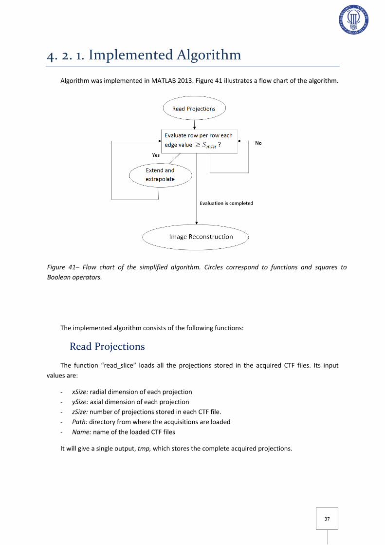
37

4. 2. 1. Implemented Algorithm

Algorithm was implemented in MATLAB 2013. Figure 41 illustrates a flow chart of the algorithm.

The implemented algorithm consists of the following functions:

Read Projections

The function “read_slice” loads all the projections stored in the acquired CTF files. Its input

values are:

- xSize: radial dimension of each projection

- ySize: axial dimension of each projection

- zSize: number of projections stored in each CTF file.

- Path: directory from where the acquisitions are loaded

- Name: name of the loaded CTF files

It will give a single output, tmp, which stores the complete acquired projections.

Figure 41– Flow chart of the simplified algorithm. Circles correspond to functions and squares to

Boolean operators.

38

Ohnesorge Extrapolation

The function “Ohnesorge_extrap” extends and extrapolates the projections whose edge values

are above the minimum gray value defined by . Its input values are the following:

- tmp: Acquired projections

- binning: according to projection binning value, parameter will be set.

- : minimum value above which a projection is considered to be truncated. And

therefore will be extended and extrapolated.

it gives as output the extrapolated (corrected) projections, p_ext. Finally, extrapolated

projections are temporarily stored, so as to evaluate and quantify algorithm performance.

A careful study of two key parameters, and , was made for algorithm

implementation,:

-

is the minimum threshold that the edge attenuation values should have in a truncated

projection so as to be considered for extension and further extrapolation . In case of severe

truncation, can be increased up to 1000 and still the algorithm will extrapolate every projection

line. was set to 50 (gray pixel value) for the target system. 50 is a number low enough to ensure

every little sample (in the case of mouse usually starting at 500) and bed discontinuity (200) is

modeled.

For each projection view, the algorithm will analyze line by line (row by row of the 2D projection

data) whether both edges have suffered truncation or not. In the case that only one side has been

truncated, the extrapolation will be performed just on that edge.

-

is the size (length) of the added pixels, pre-set to zero. The extension number corresponds

to just one side; therefore, the total added pixels are . Ohnesorge et al [1] proposes a value

of close to

. Most of the studies in the target system are made using binning 4, which have an

(total number of projection samples) around 512. Different values have been tested in rat

and mice acquisitions: 20, 30 and 40 for projections obtained with binning 4. Figure 42 shows three

different projections that have been extrapolated with , and ,

respectively. Figure 43 presents their corresponding profiles plotted along the yellow line. It can be

observed how the signal drop is smoother with Moreover; difference in computational

time was not significant. Therefore, for the implementation in the micro-CT scanner an extension

value of 40 has been applied. This selected value (40 for binning 4) also matches with the reference

one, proposed by Ohnesorge et al (

, [1]

39

It should be noted that selected depends directly on binning value;Table 2 shows the

values for all the binning configurations available in the scanner.

Binning Pixel size (µm) Projection size (pixels)

Next value (one projection side)

1 50 2400x2400 160

2 100 1200x1200 80

4 200 600x600 40

Figure 42 – Truncated projections of a rat CT which have been extrapolated with extensions of 20, 30

and 40 pixels at each side, from left to right, respectively. Profiles plot along the yellow lines are shown

in Figure 43.

Figure 43 – Comparison performed in ImageJ between extrapolated profiles drawn in Figure 42 with

different extension values at the sides (in pixels). From top to bottom Next=20, Next=30 and Next=40,

respectively. Red and blue circles indicate the extrapolation performed at the left and right edges,

respectively.

Table 2 – Scheme showing the correspondence between binning value, projection size and Next

value needed to extrapolate and correct truncated projections.

40

4. 2. 2. Evaluation

Algorithm performance was evaluated through the following steps:

- Quantitative analysis of CT studies from the micro-CT scanner in which different amounts of

truncation at the sides were induced.

- Analysis with real truncated data from the micro-CT scanner.

Quantitative Analysis

In order to assess the ability of the algorithm to reduce the truncation artifact, induced

truncations were simulated in complete projections from the scanner (as can be seen in Figure 44

and Figure 46) and reconstruction was performed. This enabled the quantitative comparison of

original complete data with truncated projections with and without the algorithm correction. Two

different set of projections are used to illustrate the process: from a cylinder phantom study and

from a mouse study.

So as to compare the different images, reconstructed images from no-truncated projections

were crop in ImageJ after reconstruction. In such a way, they matched in size with the reconstructed

images from truncated projections that, because of the missing information at the sides, were

smaller in size.

Moreover, In order to do a quantitative analysis, using ImageJ, same Regions of Interest (ROI)

with circular shapes were drawn in homogeneous regions and analyzed in every image. To do so,

straightforward macros were created [23]. A macro is a simple program that performs a series of

ImageJ commands. One of them is included in Annex D for additional information: it opens the

images, crops the original one, delineates the same Regions of Interest in the three different images

and measures their areas and mean values. In such a way, it is ensured that the same regions are

analyzed in every image.

Percentage of recovery from truncation artifact in mean CT values is calculated as follows:

(18)

- PHANTOM CYLINDER:

Phantom cylinder data consisted on 360 projections taken around 360 degrees, binning 4, radial

size of 512 pixels and axial size of 512 pixels. Truncation width of 90 pixels at each side has been

induced in the original complete projections from a phantom cylinder, as illustrated in Figure 44 by

the yellow lines.

41

The main point to bear in mind with this phantom is that when inducing truncation at both

edges through all the projections we would be creating a cylinder with smaller diameter.

The objective of this section is to evaluate how the algorithm behaves when working with a

homogeneous media and how values of regions not too close to the edges vary with and without the

algorithm with the presence of truncated data. Figure 45 shows the images to be analyzed with the

reconstructed images corresponding ROI delineated by a yellow circle. Same ROI will be drawn after

algorithm correction.

- MICE ACQUISITIONS FROM THE SCANNER:

Mice data consisted on 360 projections taken around 360 degrees, binning 4, radial size of 516

pixels and axial size of 570 pixels. Different scenarios were analyzed so as to see how the algorithm

Figure 45 – Axial sections of a cylinder phantom CT (left) Original projection without truncation, the

image has been manually cropped after reconstruction (90 pixels at each side); (middle)

Reconstructed data without truncation correction.

Figure 44 – (left) complete original projection of a cylinder phantom CT, yellow lines indicate the

boundaries for truncation; (right) truncated projection after cropping the original projection 90 pixels

at each side.

42

overcomes different amounts of truncation and subsequent loss of information: truncation of 140

pixels and of 160 pixels in the case of mice acquisitions. Figure 46 illustrates how truncation has

been performed at the sides of each projection.

The exact ROIs corresponding to soft tissue are drawn in every image so as to ensure accuracy

in the comparison (Figure 47 shows the ROIs in the image with induced truncation 140, but the same

ROIs have been drawn for truncation value 160). One of them has been placed closer to the area

where bright rim has been corrected. The other one has been placed in a farther region of

homogeneous soft tissue.

Figure 46 – (left) Original mouse projection data; (middle) Mouse projection data with induced

truncation of 140 pixels at each side; (left) mouse projection data with induced truncation of 160

pixels at each side. It can be observe how the loss of signal with 160 pixels is much more

aggressive in the protruded mass than with 140.

Figure 47 – Axial sections of mouse CT (left) Original projection without truncation, the image

has been manually cropped after reconstruction (160 pixels at each side); (right) Reconstructed

data without truncation correction.

43

Furthermore, a profile has been drawn across the bright rim so as to evaluate algorithm

behavior when reducing the sharp transition, as indicated in Figure 48.

Real Truncated Data from the Scanner

The final step in the algorithm evaluation consists on an evaluation of real truncated

acquisitions from the micro-CT, as their body extended beyond the scan field of view. Comparison is

done between the corrected Image (reconstructed image from truncated projections that have been

corrected with the algorithm) and the image with artifact, which comes from the reconstruction of

the truncated projections obtained during a real acquisition. As a result, it is not possible to obtain a

quantitative comparison of how the image would have behaved without the artifact.

Two ROIs have been drawn: the first one (ROI 1) is located closed to the truncation edge, the

second one (ROI 2) is placed a little more inward but still close to the image boundary. Rat body lying

outside the field of view and with the ROIs already drawn can be observed in Figure 49.

Figure 49 –Axial sections of a rat CT extending outside the Field Of View without algorithm

correction.

Figure 48 – Axial sections of mouse CT showing the line across which profiles have been drawn. (left)

Original image; (right) Image with artifact.

44

Results

45

5. Results

5. 1. Quantitative Analysis

5. 1. 1. Cylinder Phantom – Induced Truncation

Figure 50 shows the results of the simulation, where corrected image appears on the right.

Table 3 presents the results of the analysis of the ROI shown in Figure 50.

BH_cylinder - Induced truncation of 90 pixels at projection boundaries

Mean Value Original image Image with artifact Corrected Image Recovery%

ROI 1 -326,504 300,453 127,041 57,71

Table 3 – Analysis of the Region of Interest (ROI) of the cylinder Recovery of mean CT value in %

has been done by comparing the corrected image with the image with artifact.

Figure 50 – Axial sections of a cylinder phantom CT (left) Original projection without truncation,

(middle) Reconstructed data without truncation correction; (right) Reconstructed data with

truncation correction.

46

5. 1. 2. Mice Acquisitions – Induced Truncation

Figure 51 shows the results of the simulation, where corrected image appears on the right.

Table 4 presents the results of the analysis of the ROI shown in Figure 51.

Mouse_19_basal - Induced truncation of 140 pixels at projection boundaries

Mean ROI values

Original Image Image with Artifact Corrected Image Recovery%

ROI 1 (farther) 128,722 598,73 543,828 9,17

ROI 2 (closer) 92,451 587,537 499,507 14,98

Mouse_19_basal - Induced truncation of 160 pixels at projection boundaries

ROI 1 (farther) 128,722 690,402 574,005 16,86

ROI 2 (closer) 92,451 941,644 537,486 42,92

Table 4 – Analysis of the Regions of Interest (ROI) of mouse acquisitions. ROI 1 has an area equal

to 396 pixels while ROI 2 has an area of 568 pixels. Blue numbers are key indicators of the

correction algorithm performance.

Figure 51 – Axial sections of mouse CT (left) Original projection without truncation, the image

has been manually cropped after reconstruction (160 pixels at each side); (middle) Reconstructed

data without truncation correction; (right) Reconstructed data with truncation correction.

47

-2000

-1000

0

1000

2000

3000

4000

5000

0 10 20 30 40 50

Gra

y va

lue

s

Distance (pixels)

Profiles across bright rim

Original Image Image with Artifact Corrected Image

Comparison between profiles (drawn in Figure 52) is shown in Figure 53. The smooth transition

performed by the correction algorithm is observed.

Figure 52 – Axial sections of mouse CT showing the line across which profiles have been drawn.

(left) Original image; (middle) Image with artifact; (right) Corrected Image.

Figure 53 – Comparison of profiles drawn along the yellow lines.

48

5. 2. Real Truncated Rat Acquisitions

Figure 54 shows the results of the simulation, where corrected image appears on the right.

Table 5 presents the results of the analysis of the ROIs shown in Figure 54.

Rata_ZDF

Mean ROI values

Image with Artifact Corrected Image Recovery %

ROI 1 -181,87 -219,383 20,63

ROI 2 106,025 76,495 27,85

Table 5 – Analysis of the Regions of Interest (ROI) drawn in rat acquisitions. ROI 1 has area equal

to 1444 pixels while ROI 2 has an area of 1008 pixels. Red numbers are key indicators of the

correction algorithm.

Figure 54 – Axial sections of a rat CT extending outside the Field Of View: (left) Reconstructed

data without truncation correction; (right) Reconstructed data with truncation correction.

49

5. 3. Implementation

Compete truncation correction algorithm was adapted from MATLAB 2013 to IDL 8.3 and

integrated inside the complete software of console MMWKS [16]. Before implementing the

algorithm in IDL, reconstruction of the extrapolated (corrected) projections was made in MATLAB,

using an Image Reconstruction Toolbox (IRT). The “Image Reconstruction Toolbox” is a collection of

open source algorithms for imaging reconstruction. This software has been developed at the

University of Michigan by Jeff Fessler and his students. Within this Toolbox, the analytical

reconstruction method FDK (named after Feldkamp, Davis and Kress) has been used. A careful

evaluation of CT reconstruction (CT_recointerface.pro) work flow was made, so as to properly fit

truncation artifact correction in the MMWKS library.

In addition to this, an interface is needed, so as to offer truncation correction option to

laboratory technicians. Truncation artifact correction algorithm is designed to be applied just before

undergoing reconstruction, as the extended projections will be the input to Mangoose [12]

reconstruction software.

By clicking on RECON and CT_RECON the window shown in Figure 55 – right appears on the

screen. It can be seen how inside “Corrections” section a specific option for Truncation has been

implemented (bottom red oval). By clicking on “BROWSE” in the reconstruction interface, the user

can select the file with extension “.ACT” of the acquired study to be reconstructed. Furthermore, as

indicated by the upper red oval shown in Figure 55, every time that truncation correction is selected

the HDR and IMG file names created after reconstruction are named with the suffix “_truncation”.

Figure 55 – (left) Console interface options offered to the user, by clicking on “RECON”

reconstruction options appear on the screen (middle); by clicking on CT_RECON Console

Reconstruction window appears, offering the user the choice to select different correction methods.

Truncation option appears highlighted in a red circle. Rat Projections from two different angles are

shown.

50

If the MMWKS [16] detects truncation option has been activated, the raw projections stored in

CTF files are extended and extrapolated. Then, extrapolated projections are stored in temporal CTF

files. When truncated option is activated, MMWKS calls Mangoose reconstruction software [12]

with option –d modified so as to extend the radial dimension of the projections. Finally, when

reconstruction process is completed, temporal files are deleted.

Figure 56 shows two reconstruction results with truncation correction and without truncation

correction in the console.

Figure 56 – Upper row: sagittal, coronal and axial views respectively of a truncated CT image

with truncation correction. Lower row: truncated CT image without truncation correction.

51

Discussion and Conclusions

52

6. Discussion and Conclusions The present Bachelor Thesis has been developed inside a line of research of high resolution

scanners for preclinical application at the Hospital Universitario Gregorio Marañón. It has been

focused in the development of an algorithm for correcting micro-CT artifacts produced by truncated

or incomplete projections. These artifacts are usually characterized by bright shading and

quantification errors.

After a review of the proposed methods in the literature, an optimal approach for the micro-CT

add-on under study was selected, based on a sinogram extrapolation method published by

Ohnesorge et al [1]. This method consists on a symmetric mirroring extrapolation of the truncated

projections that guarantees continuity at the truncation point. It includes a sine shaping effect that

ensures a smooth attenuation signal drop. Furthermore, noise properties in the extrapolated region

are preserved.

Algorithm performance was assessed using real CT studies. Data of complete cylinder phantom

and mice projections from the scanner was modified by simulating different amounts of induced

truncation at the projection sides. In this way, original image from complete projections and

truncated images with and without correction algorithm were compared. Cylinder results show

overall significant recovery from truncation artifact: recovery of 58% in mean CT values. In mice

results three different tendencies were observed. First, algorithm shows higher recovery in areas

closer to the image boundaries (from 15% to 43% in images with induced truncation of 140 and 160

pixels, respectively) in contrast to farther areas (from 9% to 17% in images with induced truncation

of 140 and 160 pixels, respectively). Second, the higher the induced truncation in the original image

is, the more the algorithm recovers from the truncation artifact: from 15% in an image with induced

truncation of 140 pixels to 43% in an image with induced truncation of 160 pixels (both of these

values are obtained from a ROI closer to the image boundaries). Third, a profile drawn across the

bright rim shows the smooth transition created by the algorithm; it tries to lower gray values down

to the reference of the original image.

Finally, real truncated rat projections from the scanner were also analyzed. However, in this

case there was no reference from complete projection data to compare with. Results show a

recovery of 21 to 28%.

Therefore, the algorithm eliminates the characteristic bright rim and reduces, to some extent

although not completely, the increment suffered by CT values in the presence of the artifact.

Algorithm showed a problem when bones were truncated: their gray values were so high that there

was not a significant smooth transition at the edges.

Future work lines will focus on overcoming the problems found in the developed method,

especially to have a complete recovery of CT values. Implementation of some of the truncation

correction methods proposed in the bibliography review will be done to study if they are able to

overcome these algorithm limitations. Approach proposed by Wiegert et al (2004) is particularly

attractive. It uses reference data previously obtained in the scanner so as to complete the missing

parts in the projections [24].

53

Also, given that the micro-CT add-on is designed to be integrated with a PET scanner, it would

be interesting to evaluate the impact of the truncation artifact on the PET values when using the CT

image to correct for attenuation.

54

55

Annex A - FBP According to the Central Slice Theorem, projection Fourier transforms fill points in space with a

polar sampling. From the Central Slice Theorem, backprojection can be done with a polar coordinate

system in the frequency domain. Starting from the equation analysis that relates the Radon

Transform with the object Fourier transform, it can be observed that the inverse of the Radon

transform can be converted into a backprojection of the previously filtered projections in the image

space domain, which defines its name, Filtered Backprojection.

The equation that relates the distribution f(x,y) with its 2D Fourier Transform F(u,v) is the

following:

For going from this coordinate system (u,v) to the polar coordinate system, the following

change of variation is needed:

Therefore, applying this change of variables , yields:

Dividing this integral for in two parts:

Yields:

From Fourier Transform property:

56

Finally:

Taking into account that the Central Slice theorem can be substituted by the 2D transform of

the distribution for a projection angle given by the 1D transform of the corresponding projection,

yields:

Which can be simplified to:

This equation is the inverse Fourier transform of the product of two transforms. This product

corresponds in the projection space with the convolution of the projection, , with a function

whose Fourier transform is igual to a ramp function, . Therefore, it is a filtered projection.

Rearranging the terms yields:

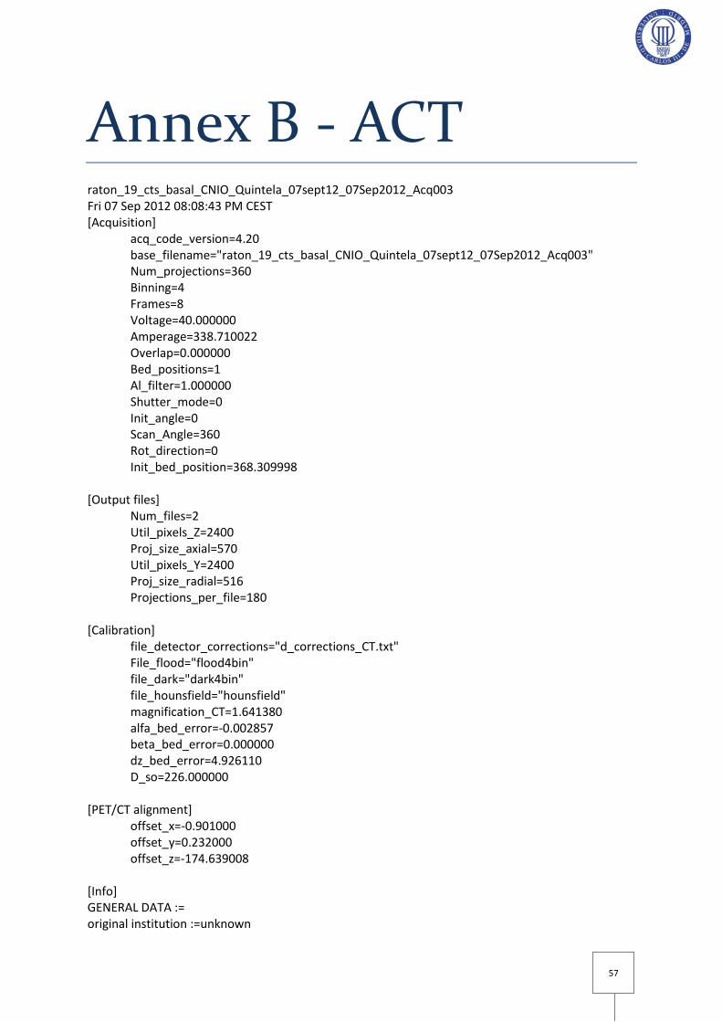
57

Annex B - ACT raton_19_cts_basal_CNIO_Quintela_07sept12_07Sep2012_Acq003 Fri 07 Sep 2012 08:08:43 PM CEST [Acquisition] acq_code_version=4.20 base_filename="raton_19_cts_basal_CNIO_Quintela_07sept12_07Sep2012_Acq003" Num_projections=360 Binning=4 Frames=8 Voltage=40.000000 Amperage=338.710022 Overlap=0.000000 Bed_positions=1 Al_filter=1.000000 Shutter_mode=0 Init_angle=0 Scan_Angle=360 Rot_direction=0 Init_bed_position=368.309998 [Output files] Num_files=2 Util_pixels_Z=2400 Proj_size_axial=570 Util_pixels_Y=2400 Proj_size_radial=516 Projections_per_file=180 [Calibration] file_detector_corrections="d_corrections_CT.txt" File_flood="flood4bin" file_dark="dark4bin" file_hounsfield="hounsfield" magnification_CT=1.641380 alfa_bed_error=-0.002857 beta_bed_error=0.000000 dz_bed_error=4.926110 D_so=226.000000 [PET/CT alignment] offset_x=-0.901000 offset_y=0.232000 offset_z=-174.639008 [Info] GENERAL DATA := original institution :=unknown

58

originating system :=unknown contact person :=unknown patient name :=raton_19_cts_basal_CNIO_Quintela_07sept12 patient ID := patient breed:= patient dob:= patient age:= patient sex:=Other patient weight (gr):= patient size (cm):= patient orientation :=Head_in patient rotation :=Prone study ID := study date :=7/9/2012 study time :=20:00:33 data description := process description:= user comment=

59

Annex C - HDR ;INTERFILE -Grupo Imagen UMCE HGGMFri Sep 07 20:11:43 2012 INTERFILE := imaging modality:=ct version of keys := 5.4 date of keys := 2006:22:10 acq code version:=4.20 reconstruction code version:=version: 3.2.0 GENERAL DATA := original institution:=unknown originating system:=unknown contact person := www.hggm.es/image patient name:=raton_19_cts_basal_CNIO_Quintela_07sept12 patient id:=none patient breed:=unknown patient dob:=none patient age:=unknown patient sex:=Other patient weight (gr):=0 patient size (cm):=unknown patient orientation:=head_in patient rotation:=prone study id:=none study date:=7/9/2012 study time:=20:00:33 data description:=none process description:=Reconstructed CT user comment:=none name of data file:=raton_19_cts_basal_CNIO_Quintela_07sept12_07Sep2012_Acq003.img IMAGE DATA := imagedata byte order:=littleendian slice orientation:= number format:=signed integer number of bytes per pixel:=2 number of dimensions:=1 matrix size [1]:=516 matrix size [2]:=516 matrix size [3]:=570 scaling factor (mm/pixel) [1]:=0.121849 scaling factor (mm/pixel) [2]:=0.121849 scaling factor (mm/pixel) [3]:=0.121849 data compression := none number of time frames:=1 offset [1]:=-0.901000 offset [2]:=0.232000 offset [3]:=193.671 gated data:=no

60

average cycle length (msec):=NA cyclelength deviation (%):=NA accepted deviation (%):=NA CT IMAGE DATA:= number of projections:=360 projection binning:=4 voltage (kv):=40.0000 amperage (ua):=338.710 start horizontal bed position (mm):=368.310 overlap (mm):=0.0 magnification factor:=1.64138 number of bed positions:=1 alum filter thickness (mm):=1.00000 projection size [1]:=516.000 projection size [2]:=516.000 projection size [3]:=570.000 number of shots:=8 beam hardening:=None reconstruction binning:=1 method of reconstruction:=FeldKamp type of interpolation:=Lineal method of scatter correction:=NONE axial correction:=Yes vertical smooth:=NO axial smooth:=NO ring reduction:=NO TEMPORAL STUDY := index nesting level := (time frame) image duration (sec) [1] :=0.000000 image relative start time (sec) [1] :=0.000000 END OF INTERFILE :=

61

Annex D - Macro // Open the reconstructed images in ImageJ // Open Original Image run("Raw...", "open=[E:\\Trabajo de Fin de Grado\\Rata micro-CT\\raton_19_cts_basal_CNIO_Quintela_07sept12\\Acq003\\raton_19_cts_basal_CNIO_Quintela_07sept12_07Sep2012_Acq003.img] image=[16-bit Signed] width=516 height=516 offset=0 number=300 gap=0 little-endian"); // Crop manually the original image so that it matches in size with the truncated ones for the ROI analysis makeRectangle(161, 161, 196, 196); run("Crop"); //Open the Truncated Image without Algorithm Correction run("Raw...", "open=[E:\\Trabajo de Fin de Grado\\Rata micro-CT\\raton_19_cts_basal_CNIO_Quintela_07sept12\\Acq003\\modif\\raton_19_cts_basal_CNIO_Quintela_07sept12_07Sep2012_Acq003_ring.img] image=[16-bit Signed] width=196 height=196 offset=0 number=300 gap=0 little-endian"); //Open the Truncated Image with Algorithm Correction run("Raw...", "open=[E:\\Trabajo de Fin de Grado\\Rata micro-CT\\raton_19_cts_basal_CNIO_Quintela_07sept12\\Acq003\\modif\\raton_19_cts_basal_CNIO_Quintela_07sept12_07Sep2012_Acq003_truncation.img] image=[16-bit Signed] width=196 height=196 offset=0 number=300 gap=0 little-endian"); // ROI Analysis: //mouse reconstrcuted image with induced truncation of 160 pixels at each side: //original Image: selectWindow("raton_19_cts_basal_CNIO_Quintela_07sept12_07Sep2012_Acq003.img"); makeOval(140, 62, 25, 20); run("Measure"); run("Add Selection..."); makeOval(51, 12, 40, 18); run("Measure"); //Truncated Image without Algorithm Correction: selectWindow("raton_19_cts_basal_CNIO_Quintela_07sept12_07Sep2012_Acq003_ring.img"); makeOval(140, 62, 25, 20); run("Measure"); run("Add Selection..."); makeOval(51, 12, 40, 18); run("Measure");

62

//Truncated Image with Algorithm Correction: selectWindow("raton_19_cts_basal_CNIO_Quintela_07sept12_07Sep2012_Acq003_truncation.img"); makeOval(140, 62, 25, 20); run("Measure"); run("Add Selection..."); makeOval(51, 12, 40, 18); run("Measure");

63

References 1. Ohnesorge, B., et al., Efficient correction for CT image artifacts caused by objects extending

outside the scan field of view. Medical physics, 2000. 27(1): p. 39-46. 2. Suetens, P., Fundamentals of medical imaging. 2009: Cambridge University Press. 3. Jan, J., Medical image processing, reconstruction and restoration: concepts and methods.

2010: CRC Press. 4. Hsieh, J. Computed tomography: principles, design, artifacts, and recent advances. 2009.

SPIE Bellingham, WA. 5. Farrell, D., Investigation and demonstration of a technique in CT image reconstruction for use

with truncated data. 2006, University of Dublin, Trinity College. 6. Kak, A.C. and M. Slaney, Principles of computerized tomographic imaging. 2001: Society for

Industrial and Applied Mathematics. 7. Feldkamp, L., L. Davis, and J. Kress, Practical cone-beam algorithm. JOSA A, 1984. 1(6): p.

612-619. 8. Barrett, J.F. and N. Keat, Artifacts in CT: Recognition and Avoidance. RadioGraphics, 2004.

24(6): p. 1679-1691. 9. Beutel, J., et al., Handbook of Medical Imaging, Volume 3. Display and PACS. 2002:

Washington, DC: SPIE Press. 10. Mori, I., et al., Photon starvation artifacts of X-ray CT: their true cause and a solution.

Radiological Physics and Technology, 2013. 6(1): p. 130-141. 11. Yazdi, M., et al., An opposite view data replacement approach for reducing artifacts due to

metallic dental objects. Medical physics, 2011. 38(4): p. 2275-2281. 12. Abella, M., et al., Software architecture for multi-bed FDK-based reconstruction in X-ray CT

scanners. Computer methods and programs in biomedicine, 2012. 107(2): p. 218-232. 13. Senn, S.S., Statistical issues in drug development. Vol. 69. 2008: John Wiley & Sons. 14. Hildebrandt, I.J., H. Su, and W.A. Weber, Anesthesia and Other Considerations for in Vivo

Imaging of Small Animals. ILAR Journal, 2008. 49(1): p. 17-26. 15. Vaquero, J.J., et al., Assessment of a New High-Performance Small-Animal X-Ray Tomograph.

Nuclear Science, IEEE Transactions on, 2008. 55(3): p. 898-905. 16. Pascau, J., et al., Multimodality workstation for small animal image visualization and

analysis. 2006. 17. Mawlawi, O., et al., Truncation Artifact on PET/CT: Impact on Measurements of Activity

Concentration and Assessment of a Correction Algorithm. American Journal of Roentgenology, 2006. 186(5): p. 1458-1467.

18. Chityala, R., et al. Region of interest (ROI) computed tomography (CT): Comparison with full field of view (FFOV) and truncated CT for a human head phantom. in Medical Imaging. 2005. International Society for Optics and Photonics.

19. Boas, F.E. and D. Fleischmann, CT artifacts: causes and reduction techniques. Imaging in Medicine, 2012. 4(2): p. 229-240.

20. Hsieh J, C.E., Thibault J, Grekowicz B, Horst A, McOlash S, Myers TJ., A novel reconstruction algorithm to extend the CT scan field-of-view. Med Phys., 2004.

21. Chityala, R., et al. Artifact reduction in truncated CT using sinogram completion. in Medical Imaging. 2005. International Society for Optics and Photonics.

22. Wiegert, J., et al. 3D ROI imaging for cone-beam computed tomography. in International Congress Series. 2004. Elsevier.

23. Pérez, J.M.M. and J. Pascau, Image Processing with ImageJ. 2013: Packt Publishing Ltd.

64

24. Wiegert, J., et al., Projection Extension for Region Of Interest Imaging in Cone-Beam CT1. Academic Radiology, 2005. 12(8): p. 1010-1023.

65

Glossary CT: Computed Tomography

FBP: Filtered Backprojection

FDK: Feldkamp, David y Kreis

FFT: Fast Fourier Transform

FOV: Field of view

HU: Hounsfield Units

IDL: Interactive Data Language

LIM: Laboratorio de Imagen Médica

MATLAB: Matrix Laboratory

MMWKS: Multimodality workstation

MRI: Magnetic Resonance Imaging

PET: Positron Emission Tomography

ROI: Region of Interest

SEDECAL: Sociedad Española de Electromedicina y Calidad

SNR: Signal to Noise Ratio

SPECT: Single Photon Emission Tomography

TAC: Tomografía Axial Computarizada

UMCE: Unidad de Medicina y Cirugía Experimental.

US: Ultrasound

66

67