Nagib Yassin ESTATÍSTICA EXPERIMENTAL ESTATÍSTICA EXPERIMENTAL
Upload
khangminh22Category
view
0download
0
Modelling and Experimental Characterization of
Nanoindentation Responses of Various Biocomposite
Materials
Pengfei Duan
School of Engineering
Newcastle University
A thesis submitted for the degree of
Doctor of Philosophy
February 2018

i
Abstract
In the past decades, composite materials (which are usually classified into
fibre-reinforced composites and particle-reinforced composites, depending on the
geometry of the reinforcements) have been widely applied in tissue engineering
as implant scaffolds. A lot of work has been done on the bulk mechanical
properties of these composites. However, there is lack of nanomechanical
characterization of such composites, which is crucial for understanding the cell-
material interactions at small scale, and further optimizing the design of scaffold
materials to promote the formation of new viable tissue.
Nanoindentation has been used for nanomechanical characterization of a
wide range of composite materials, but there is lack of comprehensive modelling
of these composites. Therefore, this thesis begins with the modelling of the
nanomechanics of inclusion-reinforced composite materials. In this part, finite
element analysis (FEA) is adopted to study the spatial-dependent mechanical
response of fibre/matrix and particle/matrix composites. The effects of various
factors (such as inclusion geometry, indenter geometry, inclusion orientation and
relative indentation location) on the nanomechanical response are studied.
Various indentation-based empirical or semi-analytical models have been
examined and novel analytical models are proposed to describe the
nanomechanical behaviour of these inclusion-reinforced composites.
Towards the end of this thesis, the nanoindentation characterization of typical
biocomposite materials is presented, namely extracellular matrix. For these
complex composites, the existing analytical models may not be directly applied.
However, with the aid of a statistical model and FEA, it has been demonstrated
that mechanical properties of each individual component can be determined.

ii
Acknowledgements
I would like to express my deeply thanks to all the people I came across
during this four years. Among these, I would like to especially express my deep
gratitude to the following people and organisation:
My supervisors, Dr Jinju Chen and Prof Steve Bull, for sharing their
invaluable and vast knowledge. Without their enlightening guidance and
encouragement, I could not have finished this thesis. Their
conscientiousness and carefulness inspire me not only in this project but
also in my future study.
Newcastle University for providing the Teaching Scholarship.
All the colleagues and staff in School of Chemical Engineering and
Advanced materials and School of Mechanical and System Engineering
for their friendliness and support. Dr Jose Portoles, Dr Zhongxu Hu, Dr
Oana Bretcanu, Prof Peter Cumpson and Prof Yanping Cao for their
technical support. Dr David Swailes, Dr Francis Franklin, Dr Piergiorgio
Gentile and Mr Robert Davidson for their kindness and friendship. Special
thanks to Dr Mohammed Al-Washahi, Dr Ana Ferreira-Duarte and Mr
Murhamdilah Morni who helped me a lot, especially in the beginning.
Dr Ria Toumpaniari and Dr Simon Partridge for providing the mineralized
matrix samples. Dr Saikat Jana for providing the inclusion/matrix samples.
All my friends for their encouragement, support and friendship.
My girlfriend Boru for her understanding, encouragement and support. My
family for their spiritual and financial support without any expectation of
return.
iii
List of Publications
1. Duan, P., Kandemir, N., Wang, J. and Chen, J. (2017) 'Rheological
Characterization of Alginate Based Hydrogels for Tissue Engineering', MRS
Advances, 2(24), pp. 1309-1314.
2. Duan, P. and Chen, J. (2015) 'Nanomechanical and microstructure analysis
of extracellular matrix layer of immortalized cell line Y201 from human
mesenchymal stem cells', Surface and Coatings Technology, 284, pp. 417-
421.
3. Duan, P., Bull, S. and Chen, J. (2015) 'Modeling the nanomechanical
responses of biopolymer composites during the nanoindentation', Thin Solid
Films, 596, pp. 277-281.
4. Kandemir, N., Xia, Y., Duan, P., Yang, W. and Chen, J. (2018) 'Rheological
Characterization of Agarose and Poloxamer 407 (P407) Based Hydrogels',
MRS Advances, pp.1-6.
5. Cao, Y., Su, B., Chinnaraj, S., Jana, S., Bowen, L., Charlton, S., Duan, P.,
Jakubovics, N.S. and Chen, J. (2018) 'Nanostructured titanium surfaces
exhibit recalcitrance towards Staphylococcus epidermidis biofilm formation',
Scientific Reports, 8(1), p. 1071.
6. Cao, Y., Duan, P. and Chen, J. (2016) 'Modelling the nanomechanical
response of a micro particle-matrix system for nanoindentation tests',
Nanotechnology, 27(19), p. 195703.
7. Wang, W.B., Fu, Y.Q., Chen, J.J., Xuan, W.P., Chen, J.K., Wang, X.Z.,
Mayrhofer, P., Duan, P.F., Bittner, A. and Schmid, U. (2016) 'AlScN thin film
based surface acoustic wave devices with enhanced microfluidic
performance', Journal of Micromechanics and Microengineering, 26(7),
p.075006
iv
8. Chen, J. and Duan, P. (2014) 'Nanomechanical responses of biopolymer
composites determined by nanoindentation with a conical tip', European Cells
and Materials, Vol. 28. Suppl. 4, p.65, ISSN 1473-2262,
http://www.ecmjournal.org
v
Table of Contents
Abstract .............................................................................................................. i
Acknowledgements .......................................................................................... ii
List of Publications .......................................................................................... iii
List of Figures ................................................................................................... x
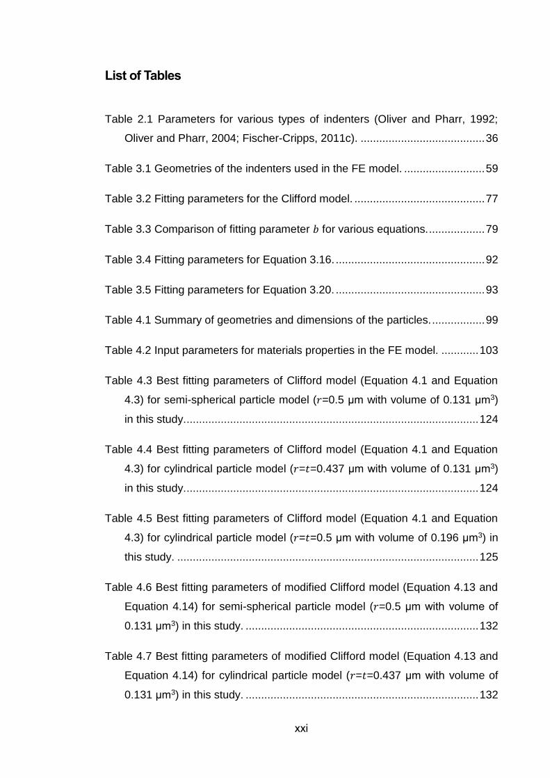
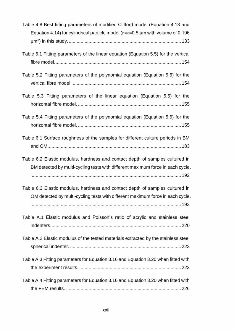
List of Tables .................................................................................................. xxi
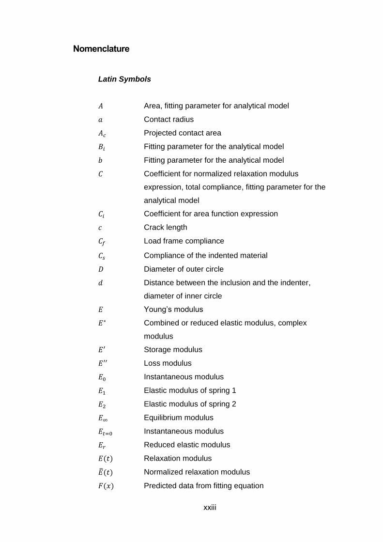
Nomenclature ............................................................................................... xxiii
Chapter 1. Introduction .................................................................................... 1
1.1 Introduction ............................................................................................ 2
1.2 Aim and objectives ................................................................................. 3
1.3 Thesis outline ......................................................................................... 3
Chapter 2. Nanoindentation Techniques ........................................................ 7
2.1 Introduction to nanoindentation .............................................................. 8
2.2 Force-displacement curves .................................................................... 9
2.2.1 General parameters in a P-δ curve .................................................. 9
2.2.2 Extraction of elastic modulus and hardness from the P-δ curves ... 12
2.2.2.1 Unloading curve method ............................................................ 12
2.2.2.2 Loading curve method ............................................................... 16
2.2.2.3 Energy-based method ................................................................ 20
2.2.2.4 Slope-based method .................................................................. 24
2.2.3 Extraction of time-dependent properties from the P-δ curves ........ 25
2.2.3.1 Dynamic nanoindentation test .................................................... 25
2.2.3.2 Quasi-static nanoindentation test ............................................... 27
2.2.4 Extraction of other mechanical properties from the P-δ curves ...... 32
vi
2.3 Indenter geometry and selection .......................................................... 33
2.4 Factors affecting the nanoindentation results ...................................... 37
2.4.1 Load frame compliance.................................................................. 38
2.4.2 Tip geometry .................................................................................. 39
2.4.3 Surface roughness ......................................................................... 41
2.4.4 Initial penetration depth.................................................................. 42
2.4.5 Thermal drift and creep .................................................................. 43
2.4.6 Piling-up and sinking-in .................................................................. 45
2.4.7 Indentation size effect .................................................................... 46
2.5 Application of nanoindentation in biomaterials ..................................... 47
2.5.1 Mineralized tissues ........................................................................ 47
2.5.2 Soft tissues .................................................................................... 50
2.5.3 Acellular biomaterials (Inclusion-reinforced composites) ............... 51
2.6 Summary ............................................................................................. 54
Chapter 3. Nanomechanical Modelling of Viscoelastic Fibre in
Viscoelastic Matrix ...................................................................... 55
3.1 Introduction .......................................................................................... 56
3.2 Finite element method ......................................................................... 59
3.3 Results and discussion ........................................................................ 64
3.3.1 Model validation ............................................................................. 64
3.3.2 The Young’s modulus determined by FEA ..................................... 67
3.3.3 Comparison of the various empirical models ................................. 72
3.3.4 Alternative models ......................................................................... 78
3.3.5 A new linear-based model ............................................................. 92
3.4 Summary ............................................................................................. 94
vii
Chapter 4. Nanomechanical Modelling of Elastic-Plastic Particles in
Elastic-Plastic Matrix ................................................................... 95
4.1 Introduction .......................................................................................... 96
4.2 Analytical method ................................................................................ 97
4.3 Methodology ........................................................................................ 98
4.3.1 Finite element modelling setting up ................................................ 98
4.3.2 Model calibration .......................................................................... 103
4.3.3 Elastic-plastic material model....................................................... 103
4.3.4 Curve fitting .................................................................................. 106
4.4 Results and discussion ...................................................................... 106
4.4.1 Model validation ........................................................................... 106
4.4.2 Typical load-displacement curves ................................................ 110
4.4.3 Model elastic-plastic response of the composites during
nanoindentation ........................................................................... 117
4.5 Summary ........................................................................................... 134
Chapter 5. Nanomechanical Modelling of Elastic Fibre with Different
Orientations in Elastic Matrix .................................................... 135
5.1 Introduction ........................................................................................ 136
5.2 Methodology ...................................................................................... 137
5.2.1 Analytical method ......................................................................... 137
5.2.2 Finite element method ................................................................. 138
5.2.3 Model calibration and curve fitting ................................................ 143
5.3 Results and discussion ...................................................................... 144
5.3.1 The apparent Young’s modulus determined by FEA .................... 144
5.3.2 Extraction of the elastic modulus of the inclusion and the
matrix ........................................................................................... 152
5.3.3 Effect of indenter geometry .......................................................... 156
5.4 Summary ........................................................................................... 162
viii
Chapter 6. Nanomechanical Case Study on Mineralized Matrix:
Experimental Characterization and Finite Element
Modelling .................................................................................... 163
6.1 Introduction ........................................................................................ 164
6.2 Materials and experimental methods ................................................. 165
6.2.1 Sample preparation ..................................................................... 165
6.2.2 Thickness measurement .............................................................. 166
6.2.3 Surface analysis .......................................................................... 167
6.2.3.1 Optical microscope .................................................................. 168
6.2.3.2 Profilometer ............................................................................. 168
6.2.3.3 Scanning electron microscope and energy-dispersive X-ray
spectroscopy ........................................................................... 169
6.2.3.4 Atomic-force microscope ......................................................... 171
6.2.4 Nanoindentation ........................................................................... 174
6.2.4.1 Hysitron Triboindenter .............................................................. 174
6.2.4.2 Different test modes ................................................................. 176
6.2.5 Statistical analysis ....................................................................... 179
6.2.6 Finite element modelling .............................................................. 180
6.3 Results and discussion ...................................................................... 182
6.3.1 Surface analysis .......................................................................... 182
6.3.2 Nanoindentation results ............................................................... 191
6.3.2.1 The apparent elastic modulus and hardness ........................... 191
6.3.2.2 Data analysis by the Gaussian mixture model ......................... 200
6.3.3 Finite element simulations ........................................................... 210
6.4 Summary ........................................................................................... 212
Chapter 7. Conclusions and Further Work ................................................. 215
7.1 Conclusions ....................................................................................... 216
7.2 Further follow up ................................................................................ 217
ix
Appendix A. Experimental Tests of a Viscoelastic Fibre in a Viscoelastic
Matrix .......................................................................................... 219
A.1 Introduction ........................................................................................ 219
A.2 Description of the samples and the instrument .................................. 219
A.3 Experiment results ............................................................................. 221
A.4 Finite element modelling results ........................................................ 223
Appendix B. Nanomechanical Modelling of a Porous Structure .............. 227
B.1 Modelling of a porous structure .......................................................... 227
B.2 Finite element modelling results ........................................................ 227
References..................................................................................................... 229
x
List of Figures
Figure 1.1 A flow chart of the structure of this thesis .......................................... 5
Figure 2.1 Schematic of a typical force and displacement curve of an elastic-
plastic material indented by a pyramidal indenter. ..................................... 11
Figure 2.2 Schematic of a cross section of an indentation with the assumption
that piling-up and sinking-in are negligible. Various dimensions that used in
the analysis are indicated (Oliver and Pharr, 1992). .................................. 13
Figure 2.3 Schematic of the radial displacement of the deformed surface after
load removal (Hay et al., 1999). ................................................................. 16
Figure 2.4 Schematic of a non-perfect indenter with a rounded tip (Sun et al.,
1999). ......................................................................................................... 20
Figure 2.5 Dynamic mechanical model of a nanoindentation instrument. 𝒎 is the
mass of the indenter and shaft, 𝑪𝒇 is the load frame compliance, 𝑺 is the
contact stiffness, 𝝀𝑺 is a damping coefficient of the contact, 𝒌𝑺 is the stiffness
of the mounting spring, and 𝝀 is a damping coefficient related to the
instrument (Fischer-Cripps, 2011e). ........................................................... 27
Figure 2.6 Mechanical models of a viscoelastic material. (a) A two-element
Maxwell model. (b) A three-element Voigt model. (c) Combined Maxwell-
Voigt model. 𝜼 is the coefficient of viscosity, 𝑬𝟏 and 𝑬𝟐 are elastic modulus
related to the relaxation modulus (Fischer-Cripps, 2011e). ........................ 28
Figure 2.7 Schematic of cracks introduced by (a) Vickers indenter and (b)
Berkovich indenter. Crack length 𝒄 is the distance between the centre of the
impression and the crack tip, and crack length 𝒍 is the distance between the
corner of the impression and the crack tip (Fischer-Cripps, 2007). ............ 32
Figure 2.8 A representative uniaxial stress-strain response for an ideal elastic-
plastic material. 𝒙 is the strain hardening index, 𝒀 is the yield stress, and the
proportionality constant 𝑲 = 𝒀(𝑬/𝒀)𝒙 . For 𝒙 = 𝟎 , the material is elastic
perfectly-plastic. ......................................................................................... 33
xi
Figure 2.9 Schematic of indenting a tissue sample with various indenters, (a) a
spherical tip with a large diameter, (b) a spherical tip with a small diameter,
(c) a sharp indenter, and (d) a cylindrical flat punch with a large diameter
(Ebenstein and Pruitt, 2006). ...................................................................... 37
Figure 2.10 Schematic of the comparison of contact area between an ideal
conical tip and a non-ideal conical tip (Fischer-Cripps, 2011b). ................. 40
Figure 2.11 Illustration of the contact of a conical indenter with a fractal surface
(Bobji and Biswas, 1999). ........................................................................... 41
Figure 2.12 Schematic of the existence of initial penetration depth (Fischer-
Cripps, 2011b). ........................................................................................... 43
Figure 2.13 Schematic of the nose phenomenon on the P-δ curve indented from
a viscoelastic material (Ebenstein and Pruitt, 2006). .................................. 44
Figure 2.14 Illustration of sinking-in and piling-up during nanoindentation
(Fischer-Cripps, 2011b). ............................................................................. 45
Figure 2.15 Schematic of mechanical transition between dentin and enamel. The
plot showed the corresponding mechanical properties determined from
indentations. It showed that both hardness and elastic modulus rapidly
decreased from enamel region to dentin region (Marshall et al., 2001a) .... 49
Figure 2.16 Hierarchical structure of the FE model of lobster cuticle: (I) N-acetyl-
glucosamine molecules, (II) α-chitin chains, (III) representative volume
element (RVE) of a chitin fibre, (IVa) RVE of chitin fibres arranged in twisted
plywood without canals, (IVb) RVE of mineral-protein matrix, (V) transversely
isotropic cuticle without canals, (VI) cuticle with a hexagonal array of canals,
and (VII) composite cuticle (Nikolov et al., 2010). ...................................... 50
Figure 2.17 Schematic of nanocomposites reinforced by (a) aligned fibres, (b)
randomly oriented fibres, (c) aligned platelets, and (d) particles (Liu and
Brinson, 2008). ........................................................................................... 52
xii
Figure 2.18 Computational model of (a) a cylindrical indenter indenting into a
composite with uniform distribution of fibres, (b) a cylindrical indenter
indenting into a composite with random distribution of fibres, and (c) a
cylindrical indenter with irregular profile indenting into a composite with
random distribution of elliptical fibres (Cao and Chen, 2012). .................... 53
Figure 2.19 Schematic of the grid indentation for a composite material. Small
displacement enables the mechanical characterization of each individual
constituent, while large displacement leads to the properties of the
homogenized medium (Constantinides et al., 2006). .................................. 53
Figure 3.1 Schematic of the indentation of a two-phase biopolymer
composite. .................................................................................................. 60
Figure 3.2 Finite element mesh for the inclusion/matrix system, (a) the overview
of the inclusion/matrix system, (b) enlarged details of inclusion elements
underneath the tip. ..................................................................................... 61
Figure 3.3 Ramping-holding procedure............................................................. 61
Figure 3.4 Absolute deviation (|𝑭𝟎 − 𝑭𝒊|/𝑭𝟎) between the force from the models
with different mesh density, indented by the indenters with (a) 𝜽 = 𝟕𝟎. 𝟑°, 𝒓 =
𝟎. 𝟏 𝝁𝒎, (b) 𝜽 = 𝟔𝟎°, 𝒓 = 𝟎. 𝟏 𝝁𝒎, and (c) 𝜽 = 𝟕𝟎. 𝟑°, 𝒓 = 𝟎. 𝟎𝟏 𝝁𝒎 .......... 65
Figure 3.5 Absolute deviation ( |𝑭𝑯𝒆𝒓𝒕𝒛 − 𝑭𝑺𝒊𝒎𝒖𝒍𝒂𝒕𝒆𝒅|/𝑭𝑯𝒆𝒓𝒕𝒛 ) between the
theoretical data and the simulated data indented by a spherical indenter. . 67
Figure 3.6 Force-displacement curves of the 10 MPa inclusion surrounding by
matrix with increasing elastic modulus from 2 to 50 MPa, indented by the
indenters with (a) 𝜽 = 𝟕𝟎. 𝟑°, 𝒓 = 𝟎. 𝟏 𝝁𝒎, (b) 𝜽 = 𝟔𝟎°, 𝒓 = 𝟎. 𝟏 𝝁𝒎, and (c)
𝜽 = 𝟕𝟎. 𝟑°, 𝒓 = 𝟎. 𝟎𝟏 𝝁𝒎. ........................................................................... 68
Figure 3.7 The Young’s modulus of the inclusion/matrix system, 𝑬(𝒄𝒐𝒎𝒑𝒐𝒔𝒊𝒕𝒆),
measured by the indenters with (a) 𝜽 = 𝟕𝟎. 𝟑°, 𝒓 = 𝟎. 𝟏 𝝁𝒎, (b) 𝜽 = 𝟔𝟎°, 𝒓 =
𝟎. 𝟏 𝝁𝒎, and (c) 𝜽 = 𝟕𝟎. 𝟑°, 𝒓 = 𝟎. 𝟎𝟏 𝝁𝒎. ................................................ 70
xiii
Figure 3.8 Fit the 𝑬(𝒄𝒐𝒎𝒑𝒐𝒔𝒊𝒕𝒆) by (a) Equation 3.1, (b) Equation 3.4, (c)
Equation 3.5, and (d) Equation 3.6, when the half-included angle of the
indenter equals 70.3˚, and the tip radius of the indenter equals 0.1 μm. .... 72
Figure 3.9 Fit the 𝑬(𝒄𝒐𝒎𝒑𝒐𝒔𝒊𝒕𝒆) by Clifford model, (a) 𝜽 = 𝟕𝟎. 𝟑°, 𝒓 = 𝟎. 𝟏 𝝁𝒎,
𝑬𝑴 < 𝑬𝑰 , (b) 𝜽 = 𝟕𝟎. 𝟑° , 𝒓 = 𝟎. 𝟏 𝝁𝒎 , 𝑬𝑴 > 𝑬𝑰 , (c) 𝜽 = 𝟔𝟎° , 𝒓 = 𝟎. 𝟏 𝝁𝒎 ,
𝑬𝑴 < 𝑬𝑰 , (d) 𝜽 = 𝟔𝟎°, 𝒓 = 𝟎. 𝟏 𝝁𝒎, 𝑬𝑴 > 𝑬𝑰 , (e) 𝜽 = 𝟕𝟎. 𝟑°, 𝒓 = 𝟎. 𝟎𝟏 𝝁𝒎,
𝑬𝑴 < 𝑬𝑰, and (f) 𝜽 = 𝟕𝟎. 𝟑°, 𝒓 = 𝟎. 𝟎𝟏 𝝁𝒎, 𝑬𝑴 > 𝑬𝑰. .................................. 74
Figure 3.10 Plot the 𝑬(𝒄𝒐𝒎𝒑𝒐𝒔𝒊𝒕𝒆) using modified Equation 3.16, (a) 𝜽 = 𝟕𝟎. 𝟑°,
𝒓 = 𝟎. 𝟏 𝝁𝒎 , 𝑬𝑴 < 𝑬𝑰 , (b) 𝜽 = 𝟕𝟎. 𝟑° , 𝒓 = 𝟎. 𝟏 𝝁𝒎 , 𝑬𝑴 > 𝑬𝑰 , (c) 𝜽 = 𝟔𝟎° ,
𝒓 = 𝟎. 𝟏 𝝁𝒎, 𝑬𝑴 < 𝑬𝑰, (d) 𝜽 = 𝟔𝟎°, 𝒓 = 𝟎. 𝟏 𝝁𝒎, 𝑬𝑴 > 𝑬𝑰, (e) 𝜽 = 𝟕𝟎. 𝟑°, 𝒓 =
𝟎. 𝟎𝟏 𝝁𝒎, 𝑬𝑴 < 𝑬𝑰, and (f) 𝜽 = 𝟕𝟎. 𝟑°, 𝒓 = 𝟎. 𝟎𝟏 𝝁𝒎, 𝑬𝑴 > 𝑬𝑰. ................ 80
Figure 3.11 Plot the 𝑬(𝒄𝒐𝒎𝒑𝒐𝒔𝒊𝒕𝒆) using modified Equation 3.17, (a) 𝜽 = 𝟕𝟎. 𝟑°,
𝒓 = 𝟎. 𝟏 𝝁𝒎 , 𝑬𝑴 < 𝑬𝑰 , (b) 𝜽 = 𝟕𝟎. 𝟑° , 𝒓 = 𝟎. 𝟏 𝝁𝒎 , 𝑬𝑴 > 𝑬𝑰 , (c) 𝜽 = 𝟔𝟎° ,
𝒓 = 𝟎. 𝟏 𝝁𝒎, 𝑬𝑴 < 𝑬𝑰, (d) 𝜽 = 𝟔𝟎°, 𝒓 = 𝟎. 𝟏 𝝁𝒎, 𝑬𝑴 > 𝑬𝑰, (e) 𝜽 = 𝟕𝟎. 𝟑°, 𝒓 =
𝟎. 𝟎𝟏 𝝁𝒎, 𝑬𝑴 < 𝑬𝑰, and (f) 𝜽 = 𝟕𝟎. 𝟑°, 𝒓 = 𝟎. 𝟎𝟏 𝝁𝒎, 𝑬𝑴 > 𝑬𝑰. ................ 83
Figure 3.12 Plot the 𝑬(𝒄𝒐𝒎𝒑𝒐𝒔𝒊𝒕𝒆) using modified Equation 3.18 and Equation
3.20, (a) 𝜽 = 𝟕𝟎. 𝟑° , 𝒓 = 𝟎. 𝟏 𝝁𝒎 , 𝑬𝑴 < 𝑬𝑰 , (b) 𝜽 = 𝟕𝟎. 𝟑° , 𝒓 = 𝟎. 𝟏 𝝁𝒎 ,
𝑬𝑴 > 𝑬𝑰, (c) 𝜽 = 𝟔𝟎°, 𝒓 = 𝟎. 𝟏 𝝁𝒎, 𝑬𝑴 < 𝑬𝑰, (d) 𝜽 = 𝟔𝟎°, 𝒓 = 𝟎. 𝟏 𝝁𝒎, 𝑬𝑴 >
𝑬𝑰, (e) 𝜽 = 𝟕𝟎. 𝟑°, 𝒓 = 𝟎. 𝟎𝟏 𝝁𝒎, 𝑬𝑴 < 𝑬𝑰, and (f) 𝜽 = 𝟕𝟎. 𝟑°, 𝒓 = 𝟎. 𝟎𝟏 𝝁𝒎,
𝑬𝑴 > 𝑬𝑰. ..................................................................................................... 86
Figure 3.13 Plot the 𝑬(𝒄𝒐𝒎𝒑𝒐𝒔𝒊𝒕𝒆) using modified Equation 3.19, (a) 𝜽 = 𝟕𝟎. 𝟑°,
𝒓 = 𝟎. 𝟏 𝝁𝒎 , 𝑬𝑴 < 𝑬𝑰 , (b) 𝜽 = 𝟕𝟎. 𝟑° , 𝒓 = 𝟎. 𝟏 𝝁𝒎 , 𝑬𝑴 > 𝑬𝑰 , (c) 𝜽 = 𝟔𝟎° ,
𝒓 = 𝟎. 𝟏 𝝁𝒎, 𝑬𝑴 < 𝑬𝑰, (d) 𝜽 = 𝟔𝟎°, 𝒓 = 𝟎. 𝟏 𝝁𝒎, 𝑬𝑴 > 𝑬𝑰, (e) 𝜽 = 𝟕𝟎. 𝟑°, 𝒓 =
𝟎. 𝟎𝟏 𝝁𝒎, 𝑬𝑴 < 𝑬𝑰, and (f) 𝜽 = 𝟕𝟎. 𝟑°, 𝒓 = 𝟎. 𝟎𝟏 𝝁𝒎, 𝑬𝑴 > 𝑬𝑰. ................ 89
Figure 4.1 Schematic of the indentation of (a) the spherical particle embedded in
the matrix and (b) the cylindrical particle embedded in the matrix. ............. 99
Figure 4.2 Overview of the finite element mesh and the enlarged details of
elements underneath the tip for (a) the spherical particle embedded in the
matrix and (b) the cylindrical particle embedded in the matrix. ................. 101
xiv
Figure 4.3 Schematic of the loading-unloading indentation protocol which has a
maximum displacement of 0.1 μm. ........................................................... 102
Figure 4.4 Rheological model of an elastic-plastic material by arranging the spring
and the friction element in series. The spring represents the elastic behaviour
and the friction element represents the plastic behaviour. ....................... 105
Figure 4.5 Uniaxial elastic-plastic stress-strain curve. 𝒙 is the strain hardening
index, and the proportionality constant 𝑲 = 𝒀(𝑬/𝒀)𝒙. For 𝒙 = 𝟎, the material
is elastic perfectly-plastic (Yu, 2006). ....................................................... 105
Figure 4.6 Absolute deviation (|𝑭𝟎 − 𝑭𝒊|/𝑭𝟎) between the force from the models
with different mesh density for (a) semi-spherical particle (0.5 μm) embedded
in the matrix, (b) cylindrical particle (0.437 μm) embedded in the matrix and
(c) cylindrical particle (0.5 μm) embedded in the matrix. .......................... 108
Figure 4.7 Absolute deviation ( |𝑭𝑯𝒆𝒓𝒕𝒛 − 𝑭𝑺𝒊𝒎𝒖𝒍𝒂𝒕𝒆𝒅|/𝑭𝑯𝒆𝒓𝒕𝒛 ) between the
theoretical data and the simulated data for each particle/matrix system when
indented by a spherical indenter. ............................................................. 110
Figure 4.8 The load-displacement curves for the indentation test upon a semi-
spherical particle within the matrix, (a) HA particle embedded in polymer 1,
(b) HA particle embedded in polymer 2, (c) HA particle embedded in polymer
3, (d) polymer 1 embedded in the HA matrix, (e) polymer 2 embedded in the
HA matrix and (f) polymer 3 embedded in the HA matrix. .................... 111
Figure 4.9 Composite elastic modulus (𝑬𝑪) against RID for (a) three different HA
particles embedded in polymer 1 and (b) three different particles of polymer
1 embedded in the HA matrix. .................................................................. 115
Figure 4.10 Composite hardness (𝑯𝑪) against RID for (a) three different HA
particles embedded in polymer 1 and (b) three different particles of polymer
1 embedded in the HA matrix. .................................................................. 116
xv
Figure 4.11 Plots of 𝑬𝑪
∗ −𝑬𝑷∗
𝑬𝑴∗ −𝑬𝑷
∗ against 𝒛 using Equation 4.1 for, (a) semi-spherical HA
particles (0.5 μm) in polymers, (b) semi-spherical polymers (0.5 μm) in HA
matrix, (c) cylindrical HA particles (0.437 μm) in polymers, (d) cylindrical
polymers (0.437 μm) in HA matrix, (e) cylindrical HA particles (0.5 μm) in
polymers and (f) cylindrical polymers (0.5 μm) in HA matrix. ................... 118
Figure 4.12 Plots of 𝑯𝑪−𝑯𝑷
𝑯𝑴−𝑯𝑷 against 𝒛 using Equation 4.3 for, (a) semi-spherical
HA particles (0.5 μm) in polymers, (b) semi-spherical polymers (0.5 μm) in
HA matrix, (c) cylindrical HA particles (0.437 μm) in polymers, (d) cylindrical
polymers (0.437 μm) in HA matrix, (e) cylindrical HA particles (0.5 μm) in
polymers and (f) cylindrical polymers (0.5 μm) in HA matrix. ................... 121
Figure 4.13 Plots of 𝑬𝑪
∗ −𝑬𝑷∗
𝑬𝑴∗ −𝑬𝑪
∗ against 𝒛 using Equation 4.13 for, (a) semi-spherical
HA particles (0.5 μm) in polymers, (b) semi-spherical polymers (0.5 μm) in
HA matrix, (c) cylindrical HA particles (0.437 μm) in polymers, (d) cylindrical
polymers (0.437 μm) in HA matrix, (e) cylindrical HA particles (0.5 μm) in
polymers and (f) cylindrical polymers (0.5 μm) in HA matrix. ................... 126
Figure 4.14 Plots of 𝑯𝑪−𝑯𝑷
𝑯𝑴−𝑯𝑪 against 𝒛 using Equation 4.14 for, (a) semi-spherical
HA particles (0.5 μm) in polymers, (b) semi-spherical polymers (0.5 μm) in
HA matrix, (c) cylindrical HA particles (0.437 μm) in polymers, (d) cylindrical
polymers (0.437 μm) in HA matrix, (e) cylindrical HA particles (0.5 μm) in
polymers and (f) cylindrical polymers (0.5 μm) in HA matrix. ................... 129
Figure 5.1 Schematic of the indentation of reinforced fibre with different
orientations in matrix. (a) A vertical fibre embedded in the matrix and (b) a
horizontal fibre embedded in the matrix, with the indenter just above the
centre of the inclusion. ............................................................................. 139
Figure 5.2 Finite element mesh for (a) the vertical fibre model and (b) the
horizontal fibre model in the case of 𝒅/𝒓 = 𝟐, indented by the conical indenter.
................................................................................................................. 141
xvi
Figure 5.3 Finite element mesh for the vertical fibre model in the case of 𝒅/𝒓 = 𝟐,
indented by the Berkovich indenter with two different orientations. That is, (a)
the pyramid flat faces toward the fibre and (b) the pyramid edge faces toward
the fibre. ................................................................................................... 142
Figure 5.4 Loading-unloading procedure. ....................................................... 143
Figure 5.5 The F-δ curves for the indentation test on (a) vertical fibre model and
(b) horizontal fibre model, with the conical indenter. ................................ 145
Figure 5.6 The composite elastic modulus for (a) the vertical fibre model and (b)
the horizontal fibre model, with different distances between the conical
indenter and the inclusion. ....................................................................... 146
Figure 5.7 Von Mises stress contours for the vertical fibre model with a
displacement of 0.5 μm, when (a) 𝒅/𝒓 = 𝟎, (b) 𝒅/𝒓 = 𝟏, (c) 𝒅/𝒓 = 𝟐, (d)
𝒅/𝒓 = 𝟑 and (e) 𝒅/𝒓 = 𝟓. For standardization, all the figures share the same
stress scale. ............................................................................................. 147
Figure 5.8 Von Mises stress contours for the horizontal fibre model from two
orthogonal cross-sections with a displacement of 0.5 μm, when (a) 𝒅/𝒓 = 𝟎,
(b) 𝒅/𝒓 = 𝟎. 𝟓, (c) 𝒅/𝒓 = 𝟐, (d) 𝒅/𝒓 = 𝟑, (e) 𝒅/𝒓 = 𝟒 and (f) 𝒅/𝒓 = 𝟓. For
standardization, all the figures share the same stress scale. ................... 150
Figure 5.9 Comparison of the von Mises stress contours for the vertical fibre
model with 𝒅/𝒓 = 𝟐, indented by (a) the Berkovich indenter with the pyramid
flat facing toward the fibre, (b) the Berkovich indenter with the pyramid edge
facing toward the fibre and (c) the conical indenter. For standardization, the
maximum stress limit was set to 1.2 MPa and the minimum stress limit was
set to 0 MPa in all the figures. .................................................................. 157
Figure 5.10 The apparent elastic modulus for the vertical fibre model in the case
of 𝒅/𝒓 = 𝟐, indented by different indenters and orientations. ................... 160
xvii
Figure 5.11 The quantification of 0.2 MPa contour line of von Mises stress
contours shown in Figure 5.9. That is, the contour lines of the vertical fibre
model with 𝒅/𝒓 = 𝟐, when indented by (a) the Berkovich indenter with the
pyramid flat facing toward the fibre, (b) the Berkovich indenter with the
pyramid edge facing toward the fibre and (c) the conical indenter. The origin
of each coordinate system represents the indentation point. ................... 160
Figure 6.1 Schematic of the crater within the sample produced by a ball crater
tester. In practice, the outer circle will be irregular for a coating layer with non-
uniform thickness. .................................................................................... 167
Figure 6.2 Representative surface profile of a mineralized matrix sample. ..... 168
Figure 6.3 Illustration of the main components of a typical SEM (Mintz,
2015). ....................................................................................................... 169
Figure 6.4 Schematic diagram of various signals emitted from the interaction
volume when the electron beam hits the sample surface (Claudionico, 2015).
................................................................................................................. 170
Figure 6.5 Schematic of an AFM using beam deflection detection (Nobelium,
2015). ....................................................................................................... 172
Figure 6.6 Relation between interatomic force and tip-to-sample distance, when
the van der Waals force is dominated (Howland and Benatar, 1996; Maver et
al., 2013). ................................................................................................. 172
Figure 6.7 Schematic of AFM image artefacts due to (a) the bluntness of the tip,
(b) a faster scanning speed, and (c) a steep sample topography. ............ 173
Figure 6.8 Pictures of Hysitron Triboindenter, (a) granite base, X-Y positioning
stage, top-down optical microscope, TriboScanner and transducer, (b)
schematic of the three-plate capacitive transducer, and (c) vibration isolation
platform and acoustic enclosure (Wang et al., 2009). .............................. 175
xviii
Figure 6.9 Schematic of various load functions, (a) a typical loading-unloading
function, (b) a loading-unloading function with holding period at maximum
load, (c) multi-cycling load function for constant repetition mode with holding
period in each cycle, (d) multi-cycling load function for ramping mode, (e)
multi-cycling load function for constant repetition mode, and (f) multi-cycling
load function for ramping mode with holding period in each cycle (Nowicki et
al., 2003; Chen and Bull, 2008; Bull et al., 2012). .................................... 176
Figure 6.10 Schematic of the multi-cycling loading function ........................... 179
Figure 6.11 Schematic of (a) the model with distribution of different indented
locations, (b) vertical distance of each indentation points away from the
interface, and (c) the meshes for the model. ............................................ 181
Figure 6.12 Typical SEM images of cells cultured at different conditions (A: day
7, BM; B: day 14, BM; C: day 21, BM; D: day 7, OM; E: day 14, OM), an
enlargement of the marked area in figure C is shown in Figure 6.13. ...... 184
Figure 6.13 Minerals observed on samples cultured in BM for 21 days. ......... 186
Figure 6.14 EDS spectrum for the minerals observed on the sample cultured in
BM for 21 days. ........................................................................................ 186
Figure 6.15 Representative intensity profile of calcium and phosphorus for the
minerals detected in the line scan mode and the corresponding percentage
of calcium and phosphorus. ..................................................................... 187
Figure 6.16 Representative AFM images of samples cultured at different
conditions (A: day 7, BM; B: day 14, BM; C: day 21, BM; D: day 7, OM; E:
day 14, OM). ............................................................................................ 188
Figure 6.17 Representative polarized light images of samples harvested from (a,
b) day 14, BM, (c, d) day 14, OM. Among them, image (a, c) are samples
viewed with parallel polars, and image (b, d) are the same field viewed with
crossed polars. ......................................................................................... 190
Figure 6.18 Representative force-displacement curve from multi-cycling tests for
sample cultured in BM for 21 days. .......................................................... 191
xix
Figure 6.19 Young’s modulus (± SD) of samples cultured in (a) BM and (b) OM
(P<0.001), as a function of average contact depth for nanoindentation tests
in the peak load range 1~9 mN. ............................................................... 194
Figure 6.20 Hardness (± SD) of samples cultured in (a) BM and (b) OM (P<0.001),
as a function of average contact depth for nanoindentation tests in the peak
load range 1~9 mN. .................................................................................. 195
Figure 6.21 Histograms of elastic modulus for reported engineered bone
produced by C3H10T1/2 MSC line grown in vivo for 28 days (Pelled et al.,
2007a). ..................................................................................................... 197
Figure 6.22 Histograms of elastic modulus for mineralized matrix samples
cultured from (a) day 7, (b) day 14 and (c) day 21, tested at two different peak
loads (1000 µN and 7000 µN). ................................................................. 198
Figure 6.23 Representative distributions of Young’s modulus for the matrix
harvested from (a) day 14, BM, (b) day 14, OM, tested at a peak load of 1000
µN. ............................................................................................................ 202
Figure 6.24 Young’s modulus of two different components in the matrix cultured
in different media for (a) 7 days, (b) 14 days and (c) 21 days, determined by
the Gaussian mixture model for nanoindentation tests in the peak load range
1~9 mN. .................................................................................................... 203
Figure 6.25 Hardness of two different components in the matrix cultured in
different media for (a) 7 days, (b) 14 days and (c) 21 days, determined by the
Gaussian mixture model for nanoindentation tests in the peak load range 1~9
mN. ........................................................................................................... 204
Figure 6.26 The (a) Young’s modulus and (b) hardness of each component in the
matrix cultured in different media as a function of culture period. ............. 206
Figure 6.27 Elastic anisotropy ratio for samples cultured in (a) BM and (b) OM,
and hardness anisotropic ratio for samples cultured in (c) BM and (d) OM, as
a function of average contact depth for nanoindentation tests in the peak load
range 1~9 mN. ......................................................................................... 208
xx
Figure 6.28 The elastic modulus of the numerical model indented at different
locations (as illustrated in Figure 6.11) around the interface between (a) two
orthogonal fibres, and (b) mature and immature bone nodules. ............... 211
Figure A.1 Schematic of a fibre/matrix cube, with an 8mm diameter through-hole
in the centre. ............................................................................................ 220
Figure A.2 Microscope image for the conical tip, which has the tip radius of 43
μm. ........................................................................................................... 221
Figure A.3 Fit the experiment results with (a) Equation 3.16 and (b) Equation 3.20.
................................................................................................................. 222
Figure A.4 Overview of the finite element mesh for the inclusion/matrix composite,
and the enlarged details of elements underneath the tip. ......................... 224
Figure A.5 Fit the FEM results with (a) Equation 3.16 and (b) Equation 3.20.
................................................................................................................. 225
Figure B.1 Finite element meshes for the porous model. The diameter of the hole
was set as 3.78 µm, symmetric boundary conditions were applied to the sides
to simulate a periodically porous structure, and the distance between the
centre of the hole and indented surface varied between 4 µm and 6 µm.
................................................................................................................. 228
Figure B.2 The elastic modulus of the porous model with hole arranged to a lower,
middle or upper position. .......................................................................... 228
xxi
List of Tables
Table 2.1 Parameters for various types of indenters (Oliver and Pharr, 1992;
Oliver and Pharr, 2004; Fischer-Cripps, 2011c). ........................................ 36
Table 3.1 Geometries of the indenters used in the FE model. .......................... 59
Table 3.2 Fitting parameters for the Clifford model. .......................................... 77
Table 3.3 Comparison of fitting parameter 𝑏 for various equations. .................. 79
Table 3.4 Fitting parameters for Equation 3.16. ................................................ 92
Table 3.5 Fitting parameters for Equation 3.20. ................................................ 93
Table 4.1 Summary of geometries and dimensions of the particles. ................. 99
Table 4.2 Input parameters for materials properties in the FE model. ............ 103
Table 4.3 Best fitting parameters of Clifford model (Equation 4.1 and Equation
4.3) for semi-spherical particle model (𝑟=0.5 μm with volume of 0.131 μm3)
in this study. .............................................................................................. 124
Table 4.4 Best fitting parameters of Clifford model (Equation 4.1 and Equation
4.3) for cylindrical particle model (𝑟=𝑡=0.437 μm with volume of 0.131 μm3)
in this study. .............................................................................................. 124
Table 4.5 Best fitting parameters of Clifford model (Equation 4.1 and Equation
4.3) for cylindrical particle model (𝑟=𝑡=0.5 μm with volume of 0.196 μm3) in
this study. ................................................................................................. 125
Table 4.6 Best fitting parameters of modified Clifford model (Equation 4.13 and
Equation 4.14) for semi-spherical particle model (𝑟=0.5 μm with volume of
0.131 μm3) in this study. ........................................................................... 132
Table 4.7 Best fitting parameters of modified Clifford model (Equation 4.13 and
Equation 4.14) for cylindrical particle model (𝑟=𝑡=0.437 μm with volume of
0.131 μm3) in this study. ........................................................................... 132
xxii
Table 4.8 Best fitting parameters of modified Clifford model (Equation 4.13 and
Equation 4.14) for cylindrical particle model (𝑟=𝑡=0.5 μm with volume of 0.196
μm3) in this study. ..................................................................................... 133
Table 5.1 Fitting parameters of the linear equation (Equation 5.5) for the vertical
fibre model. ............................................................................................... 154
Table 5.2 Fitting parameters of the polynomial equation (Equation 5.6) for the
vertical fibre model. .................................................................................. 154
Table 5.3 Fitting parameters of the linear equation (Equation 5.5) for the
horizontal fibre model. .............................................................................. 155
Table 5.4 Fitting parameters of the polynomial equation (Equation 5.6) for the
horizontal fibre model. .............................................................................. 155
Table 6.1 Surface roughness of the samples for different culture periods in BM
and OM. .................................................................................................... 183
Table 6.2 Elastic modulus, hardness and contact depth of samples cultured in
BM detected by multi-cycling tests with different maximum force in each cycle.
................................................................................................................. 192
Table 6.3 Elastic modulus, hardness and contact depth of samples cultured in
OM detected by multi-cycling tests with different maximum force in each cycle.
................................................................................................................. 193
Table A.1 Elastic modulus and Poisson’s ratio of acrylic and stainless steel
indenters. .................................................................................................. 220
Table A.2 Elastic modulus of the tested materials extracted by the stainless steel
spherical indenter. .................................................................................... 223
Table A.3 Fitting parameters for Equation 3.16 and Equation 3.20 when fitted with
the experiment results. ............................................................................. 223
Table A.4 Fitting parameters for Equation 3.16 and Equation 3.20 when fitted with
the FEM results. ....................................................................................... 226
xxiii
Nomenclature
Latin Symbols
𝐴 Area, fitting parameter for analytical model
𝑎 Contact radius
𝐴𝑐 Projected contact area
𝐵𝑖 Fitting parameter for the analytical model
𝑏 Fitting parameter for the analytical model
𝐶 Coefficient for normalized relaxation modulus
expression, total compliance, fitting parameter for the
analytical model
𝐶𝑖 Coefficient for area function expression
𝑐 Crack length
𝐶𝑓 Load frame compliance
𝐶𝑠 Compliance of the indented material
𝐷 Diameter of outer circle
𝑑 Distance between the inclusion and the indenter,
diameter of inner circle
𝐸 Young’s modulus
𝐸∗ Combined or reduced elastic modulus, complex
modulus
𝐸′ Storage modulus
𝐸′′ Loss modulus
𝐸0 Instantaneous modulus
𝐸1 Elastic modulus of spring 1
𝐸2 Elastic modulus of spring 2
𝐸∞ Equilibrium modulus
𝐸𝑡=0 Instantaneous modulus
𝐸𝑟 Reduced elastic modulus
𝐸(𝑡) Relaxation modulus
��(𝑡) Normalized relaxation modulus
𝐹(𝑥) Predicted data from fitting equation
xxiv
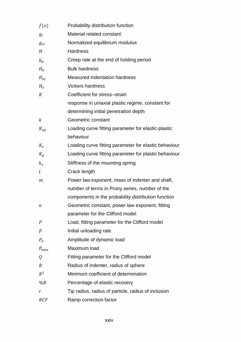
𝑓(𝑥) Probability distribution function
𝑔𝑖 Material related constant
𝑔∞ Normalized equilibrium modulus
𝐻 Hardness
ℎℎ Creep rate at the end of holding period
𝐻0 Bulk hardness
𝐻𝑚 Measured indentation hardness
𝐻𝑣 Vickers hardness
𝐾 Coefficient for stress–strain
response in uniaxial plastic regime, constant for
determining initial penetration depth
𝑘 Geometric constant
𝐾𝑒𝑝 Loading curve fitting parameter for elastic-plastic
behaviour
𝐾𝑒 Loading curve fitting parameter for elastic behaviour
𝐾𝑝 Loading curve fitting parameter for plastic behaviour
𝑘𝑠 Stiffness of the mounting spring
𝑙 Crack length
𝑚 Power law exponent, mass of indenter and shaft,
number of terms in Prony series, number of the
components in the probability distribution function
𝑛 Geometric constant, power law exponent, fitting
parameter for the Clifford model
𝑃 Load, fitting parameter for the Clifford model
�� Initial unloading rate
𝑃0 Amplitude of dynamic load
𝑃𝑚𝑎𝑥 Maximum load
𝑄 Fitting parameter for the Clifford model
𝑅 Radius of indenter, radius of sphere
𝑅2 Minimum coefficient of determination
%𝑅 Percentage of elastic recovery
𝑟 Tip radius, radius of particle, radius of inclusion
𝑅𝐶𝐹 Ramp correction factor
xxv
𝑟𝑒𝑠𝑛𝑜𝑟𝑚 Fitting parameter that represents the goodness of the
fitting
𝑆 Contact stiffness
𝑡 Time, coating thickness, thickness of particle
𝑡𝑅 Rise time of loading period
𝑉𝑝 Volume of the residual impression
𝑤 Radius of inclusion, volume fraction in probability
distribution function
𝑊𝑒 Elastic work of indentation
𝑊𝑝 Plastic work of indentation
𝑊𝑡 Total work of indentation
𝑥 Work hardening exponent
𝑌 Yield stress
𝑦 Observed data from simulation
�� Mean of the observed data
𝑧 Relative contact radius
Greek Symbols
𝛼 Effective cone angle, roughness parameter
𝛽 Geometry correction factor
𝛾 Geometry correction factor, strain
𝛿 Displacement, phase difference
𝛿𝑐 Contact depth
𝛿𝑚𝑎𝑥 Maximum depth
𝛿𝑟𝑒𝑠 Residual depth
𝛿𝑠 Elastic depth
휀 Tip-dependent intercept factor, strain
휀 Strain increment
𝜂 Viscosity coefficient
𝜃 Half included indenter angle
𝜅 Tip-dependent constant
𝜆 Damping coefficient related to the instrument
xxvi
𝜆𝑠 Damping coefficient of the contact
𝜈 Poisson’s ratio
𝜉 Correction factor
𝜎 Stress
𝜎𝑠 Material constant related to surface roughness
𝜎𝑌 Yield stress
𝜏 Material time constant
𝜓 Empirical constant
𝜔 Frequency of dynamic load
𝜙 Empirical constant, phase difference
Acronyms
AFM Atomic force microscope
BM Basal medium
BSE Back-scattered electrons
CSM Continuous stiffness method
EDS Energy-dispersive X-ray spectroscopy
EDTA Ethylenediaminetetraacetic acid
FEA Finite element analysis
FEM Finite element modelling
HA Hydroxyapatite
hMSCs Human mesenchymal stem cells
hTERT Human telomerase reverse transcriptase
ISE Indentation size effect
Nylon 6 Polyamide 6
OM Osteogenic medium
PDLLA Poly-DL-lactic acid
PDMS Polydimethylsiloxane
PE Polyethylene
PGA Polyglycolic acid
PLA Polylactic acid
PLLA Poly-L-lactic acid

xxvii
PP Polypropylene
RID Relative indentation depth
RVE Representative volume element
SD Standard deviation
SE Secondary electrons
SEM Scanning electron microscope


Chapter 1
Introduction
2
Chapter 1. Introduction
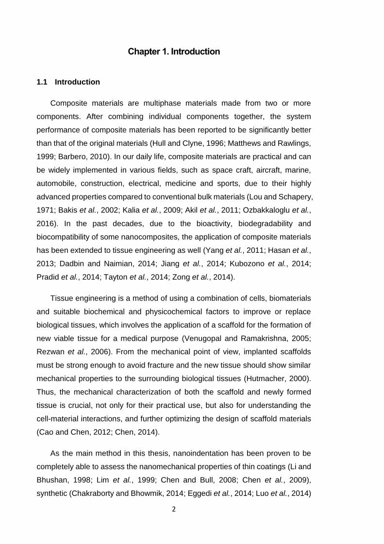
1.1 Introduction
Composite materials are multiphase materials made from two or more
components. After combining individual components together, the system
performance of composite materials has been reported to be significantly better
than that of the original materials (Hull and Clyne, 1996; Matthews and Rawlings,
1999; Barbero, 2010). In our daily life, composite materials are practical and can
be widely implemented in various fields, such as space craft, aircraft, marine,
automobile, construction, electrical, medicine and sports, due to their highly
advanced properties compared to conventional bulk materials (Lou and Schapery,
1971; Bakis et al., 2002; Kalia et al., 2009; Akil et al., 2011; Ozbakkaloglu et al.,
2016). In the past decades, due to the bioactivity, biodegradability and
biocompatibility of some nanocomposites, the application of composite materials
has been extended to tissue engineering as well (Yang et al., 2011; Hasan et al.,
2013; Dadbin and Naimian, 2014; Jiang et al., 2014; Kubozono et al., 2014;
Pradid et al., 2014; Tayton et al., 2014; Zong et al., 2014).
Tissue engineering is a method of using a combination of cells, biomaterials
and suitable biochemical and physicochemical factors to improve or replace
biological tissues, which involves the application of a scaffold for the formation of
new viable tissue for a medical purpose (Venugopal and Ramakrishna, 2005;
Rezwan et al., 2006). From the mechanical point of view, implanted scaffolds
must be strong enough to avoid fracture and the new tissue should show similar
mechanical properties to the surrounding biological tissues (Hutmacher, 2000).
Thus, the mechanical characterization of both the scaffold and newly formed
tissue is crucial, not only for their practical use, but also for understanding the
cell-material interactions, and further optimizing the design of scaffold materials
(Cao and Chen, 2012; Chen, 2014).
As the main method in this thesis, nanoindentation has been proven to be
completely able to assess the nanomechanical properties of thin coatings (Li and
Bhushan, 1998; Lim et al., 1999; Chen and Bull, 2008; Chen et al., 2009),
synthetic (Chakraborty and Bhowmik, 2014; Eggedi et al., 2014; Luo et al., 2014)
3
and natural tissues (Chen et al., 2010a; Oyen, 2013; Chen et al., 2014; Cyganik
et al., 2014; De Silva et al., 2014; Jaramillo-Isaza et al., 2014; Sun et al., 2014),
which are also composite materials in nature. Thus, the motivation of this thesis
is that by using nanoindentation techniques the spatial-dependent mechanical
properties of synthesized composite materials and newly formed tissues can be
understood, so that how mechanical response will be affected by various practical
indentation protocols, indenter geometry, chemical composition of each
constituent, and microstructure must also be understood.
1.2 Aim and objectives
This study aims to employ a nanomechanical approach to understand the
mechanical response of typical biocomposites (fibre-reinforced composites,
particle-reinforced composites and complex mineralized matrix). The specific
objectives that this thesis intends to address are as follows:
To understand the spatial-dependent mechanical properties of fibre-
reinforced composite materials by empirical analytical models, and
propose novel analytical models if necessary.
To analyse the effects of particle size and shape on the nanomechanical
response of particle-reinforced composite materials.
To investigate the effects of fibre orientation and indentation location on
the nanomechanical response of fibre-reinforced composite materials.
To study the nanomechanics, microstructure and chemical composition
of complex mineralized matrix (newly formed tissues synthesized by
immortalized cell line Y201), and then further establish the correlations
between them.
1.3 Thesis outline
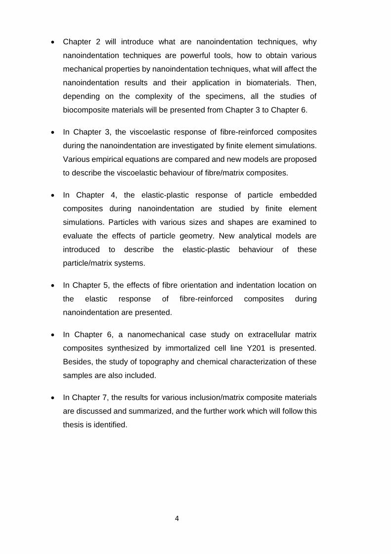
This thesis contains seven chapters (as illustrated in Figure 1.1), which are
organised as follows:
4
Chapter 2 will introduce what are nanoindentation techniques, why
nanoindentation techniques are powerful tools, how to obtain various
mechanical properties by nanoindentation techniques, what will affect the
nanoindentation results and their application in biomaterials. Then,
depending on the complexity of the specimens, all the studies of
biocomposite materials will be presented from Chapter 3 to Chapter 6.
In Chapter 3, the viscoelastic response of fibre-reinforced composites
during the nanoindentation are investigated by finite element simulations.
Various empirical equations are compared and new models are proposed
to describe the viscoelastic behaviour of fibre/matrix composites.
In Chapter 4, the elastic-plastic response of particle embedded
composites during nanoindentation are studied by finite element
simulations. Particles with various sizes and shapes are examined to
evaluate the effects of particle geometry. New analytical models are
introduced to describe the elastic-plastic behaviour of these
particle/matrix systems.
In Chapter 5, the effects of fibre orientation and indentation location on
the elastic response of fibre-reinforced composites during
nanoindentation are presented.
In Chapter 6, a nanomechanical case study on extracellular matrix
composites synthesized by immortalized cell line Y201 is presented.
Besides, the study of topography and chemical characterization of these
samples are also included.
In Chapter 7, the results for various inclusion/matrix composite materials
are discussed and summarized, and the further work which will follow this
thesis is identified.
5
Figure 1.1 A flow chart of the structure of this thesis.
Chapter 1
• Introduction
Chapter 2
• Introduction to nanoindentation techniques
• Literature review
Chapter 3-5
• Nanomechanical modelling of inclusion/matrix systems
Chapter 6
• Nanomechanical case study on extracellular matrix
composites
Chapter 7
• Conclusion and further work
Chapter 3
Chapter 4
Chapter 5
Chapter 6
Viscoelastic fibre in
viscoelastic matrix
Elastic-plastic particles in
elastic-plastic matrix
Elastic fibre in elastic matrix
Extracellular matrix synthesized
by immortalized cell line Y201


Chapter 2
Nanoindentation Techniques
8
Chapter 2. Nanoindentation Techniques
2.1 Introduction to nanoindentation
The origins of the indentation technique can be traced back to the Mohs
hardness in 1824 (Tabor, 1954), in which a qualitative hardness scale of various
minerals was given by the ability of harder mineral to leave a scratch in a softer
one. Thereafter, various quantitative hardness tests were established by
indenting a material whose mechanical properties were unknown with another
material whose geometry and mechanical properties were known. Among which,
nanoindentation techniques were developed in the early seventies of last century
(Bulychev et al., 1975; Newey et al., 1982; Pethica et al., 1983; Georges and
Meille, 1984; Wierenga and Franken, 1984; Doerner and Nix, 1986), to meet the
growing requirements of knowing the mechanical properties of thin films, coatings
and samples with small volumes.
Nanoindentation is a technique with the same principle as macroindentation
and microindentation (i.e. conventional indentation tests), while measuring the
properties of materials at the length scale of nanometres. This difference also
gives the nanoindentation tests a distinctive feature, that is, an indirect
measurement of contact area between the sample and the indenter. In
conventional indentation tests, the projected area of residual impression left on
the sample surface after indenter removal is usually measured by light
microscopy. The hardness is then determined by the peak load divided by the
projection of the residual area (or surface area in the case of Vickers hardness).
Whereas in nanoindentation tests, the size of residual impression can be less
than 1 micrometre which is difficult to be accurately measured by the conventional
optical methods (Doerner and Nix, 1986). For this reason, an alternative method
is to analyse the continuously recorded force-displacement curve and correlate it
to the hardness and elastic modulus for a given indenter geometry. The contact
area can then be indirectly determined from the contact depth with the known
geometry of the indenter (Doerner and Nix, 1986; Oliver and Pharr, 1992;
Hainsworth and Page, 1994; Oliver and Pharr, 2004). In other words, this leads
to different definitions between the hardness measured from conventional
indentation tests and the hardness measured from nanoindentation tests. In the
9
former case, hardness is defined as the ratio of maximum force over the residual
area, in which case the elastic recovery of the contact area will not be considered.
While in the latter case, hardness is determined by maximum force over contact
area under load, having corrected for the elastic deflection of the sample surface.
It is not only the hardness (𝐻) that nanoindentation can provide. By carefully
selecting the indenter, designing the loading protocol and choosing the
appropriate analysis model, various properties can be extracted from the
recorded force-displacement curves, such as elastic modulus ( 𝐸 ), fracture
toughness, viscoelastic properties, film adhesion and strain-hardening exponent
(Ebenstein and Pruitt, 2006; Yang et al., 2006; Chen and Bull, 2010). Nowadays,
nanoindentation techniques have not only been widely used for the study of
coatings (Oliver and Pharr, 1992; Bull, 2001; Berasategui and Page, 2003; G-
Berasategui et al., 2004), but also gained the popularity in the study of
biomaterials (Hasler et al., 1998; Haque, 2003; Kinney et al., 2003; Aryaei and
Jayasuriya, 2013; Chen, 2014), nanocomposites (Gao and Mäder, 2002; Lee et
al., 2007) and specimens in high temperature environments (Beake and Smith,
2002; Schuh et al., 2005).
2.2 Force-displacement curves
2.2.1 General parameters in a P-δ curve
During the nanoindentation test, the applied force (𝑃) and displacement (𝛿)
of the indenter are continuously recorded as force-displacement curves. This
force-displacement curve has been considered as the mechanical ‘‘fingerprint’’ of
a material (Page and Hainsworth, 1993), in which a number of basic parameters
can be quantified and used to assess the mechanical properties of the specimen.
Figure 2.1 shows a typical P-δ curve from the nanoindentation test. According to
Page and Hainsworth, the basic parameters that can be quantified are listed
below (Page and Hainsworth, 1993):
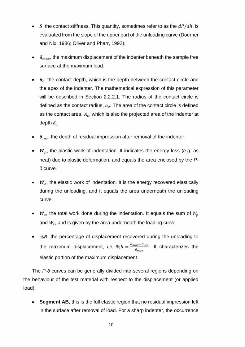
𝑷𝒎𝒂𝒙, the maximum applied load.
10
𝑺, the contact stiffness. This quantity, sometimes refer to as the 𝑑𝑃/𝑑ℎ, is
evaluated from the slope of the upper part of the unloading curve (Doerner
and Nix, 1986; Oliver and Pharr, 1992).
𝜹𝒎𝒂𝒙, the maximum displacement of the indenter beneath the sample free
surface at the maximum load.
𝜹𝒄, the contact depth, which is the depth between the contact circle and
the apex of the indenter. The mathematical expression of this parameter
will be described in Section 2.2.2.1. The radius of the contact circle is
defined as the contact radius, 𝑎𝑐. The area of the contact circle is defined
as the contact area, 𝐴𝑐, which is also the projected area of the indenter at
depth 𝛿𝑐.
𝜹𝒓𝒆𝒔, the depth of residual impression after removal of the indenter.
𝑾𝒑, the plastic work of indentation. It indicates the energy loss (e.g. as
heat) due to plastic deformation, and equals the area enclosed by the P-
δ curve.
𝑾𝒆, the elastic work of indentation. It is the energy recovered elastically
during the unloading, and it equals the area underneath the unloading
curve.
𝑾𝒕, the total work done during the indentation. It equals the sum of 𝑊𝑝
and 𝑊𝑒, and is given by the area underneath the loading curve.
%𝑹, the percentage of displacement recovered during the unloading to
the maximum displacement, i.e. %𝑅 =𝛿𝑚𝑎𝑥−𝛿𝑟𝑒𝑠
𝛿𝑚𝑎𝑥. It characterizes the
elastic portion of the maximum displacement.
The P-δ curves can be generally divided into several regions depending on
the behaviour of the test material with respect to the displacement (or applied
load):
Segment AB, this is the full elastic region that no residual impression left
in the surface after removal of load. For a sharp indenter, the occurrence
11
of this elastic region results from the tip blunting, which will be described
in Section 2.4.2.
Segment BC, this is the region that behaviour transits from elastic
behaviour to elastic-plastic behaviour.
Segment CD, this is a plastic-dominated region where a fully developed
plastic zone obtained.
Segment DE, this is the initial part of the unloading curve. It is assumed
that, within this region, the contact area keeps constant with the
decreasing displacement.
Segment EF, this is the region in which elastic recovery occurs and the
shape of impression changes with the decreasing displacement.
Figure 2.1 Schematic of a typical force and displacement curve of an elastic-plastic material indented by a pyramidal indenter.
Based on the information shown in Figure 2.1, various analytical methods
have been developed to obtain the basic mechanical properties such as the
hardness and elastic modulus, which will be described in Section 2.2.2. In
practice, several other features may occur in the P-δ curves depending on the
12
nature of the material or the structure of the material. Features such as creep,
cracks, adhesion, piling-up and sinking-in will also be discussed in the following
section.
2.2.2 Extraction of elastic modulus and hardness from the P-δ curves
Various methods have been developed to extract 𝐸 and 𝐻 from the P-δ
curves. These methods include but are not limited to: unloading curve method,
loading curve method, energy-based method, slope-based method, and dynamic
method. Among them, Oliver and Pharr method (Oliver and Pharr, 1992) is the
most popular one, and it has been used to investigate the materials with a wide
range of elastic modulus and hardness.
2.2.2.1 Unloading curve method
Modelling the material response of a loading curve is much more complex,
as it may consist of both plastic and elastic behaviours. Therefore, the unloading
curve is normally used to obtain elastic modulus and hardness by assuming there
is only elastic behaviour involved in the unloading. Based on the analysis for the
elastic unloading curve with a flat punch indenter (Sneddon, 1965), Doerner and
Nix proposed a linear relationship in the first one third of the unloading curve for
nanoindentation by a flat punch indenter (Doerner and Nix, 1986). Soon, Oliver
and Pharr extended this method to the cases of various indenters by proposing
a power law relationship in the initial part of the unloading curve. The validity of
Sneddon analysis for various indenters was verified by them as well (Oliver and
Pharr, 1992). In the Sneddon analysis, the elastic modulus is given by (Sneddon,
1965),
𝑆 =𝑑𝑃
𝑑ℎ=
2
√𝜋𝐸𝑟√𝐴𝑐 (2.1)
where 𝐸𝑟 is the reduced modulus that combines the modulus of the indenter and
the test specimen, which can be described as,
1
𝐸𝑟=
1 − 𝑣𝑠2
𝐸𝑠+
1 − 𝑣𝑖2
𝐸𝑖 (2.2)
13
where 𝐸𝑠 and 𝑣𝑠 are the Young’s modulus and the Poisson’s ratio for the
specimen, respectively. 𝐸𝑖 and 𝑣𝑖 are the Young’s modulus and the Poisson’s
ratio for the indenter, respectively. For a commercially used diamond tip, the
Young’s modulus is 1141 GPa and the Poisson’s ratio is 0.07.
In order to obtain the contact stiffness from the P-δ curve, Oliver and Pharr
proposed a power law relationship for the initial part of the unloading curve, which
is expressed as,
𝑃 = 𝐵(𝛿 − 𝛿𝑟𝑒𝑠)𝑚 (2.3)
where 𝐵, 𝑚 and 𝛿𝑟𝑒𝑠 are the fitting constants determined by the least squares
fitting procedure. By differentiating Equation 2.3 with respect to the depth, the
unloading slope at the peak depth can be mathematically expressed as,
𝑆 =𝑑𝑃
𝑑𝛿|
𝛿=𝛿𝑚𝑎𝑥
= 𝑚𝐵(𝛿𝑚𝑎𝑥 − 𝛿𝑟𝑒𝑠)𝑚−1 (2.4)
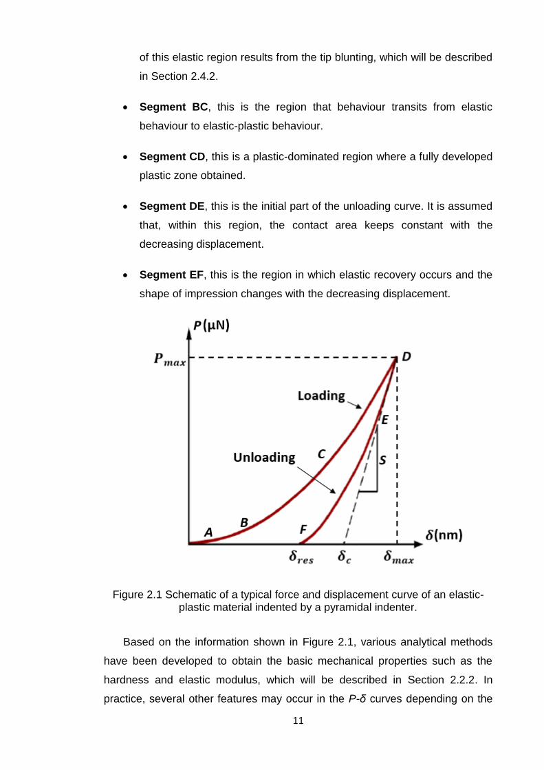
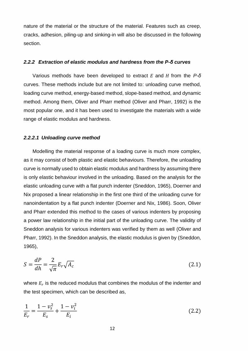
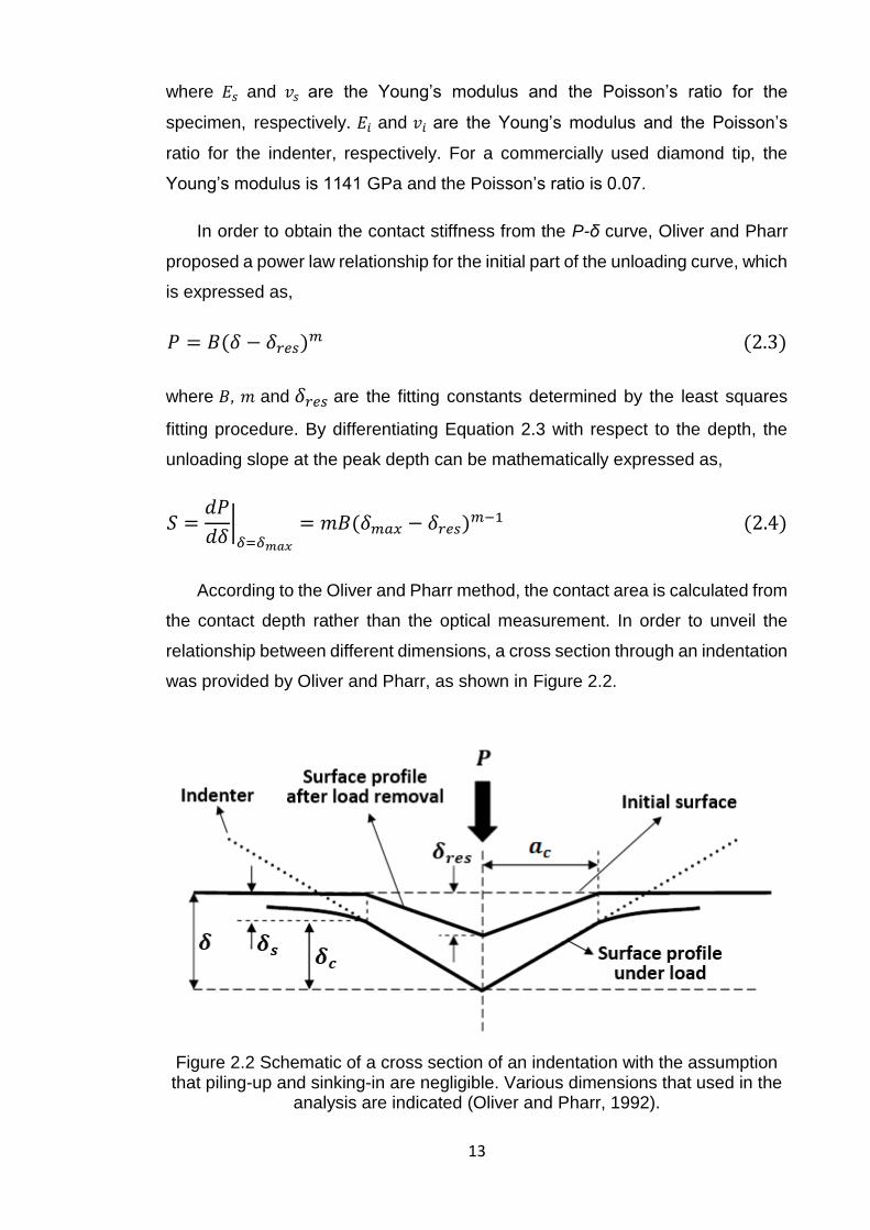
According to the Oliver and Pharr method, the contact area is calculated from
the contact depth rather than the optical measurement. In order to unveil the
relationship between different dimensions, a cross section through an indentation
was provided by Oliver and Pharr, as shown in Figure 2.2.
Figure 2.2 Schematic of a cross section of an indentation with the assumption that piling-up and sinking-in are negligible. Various dimensions that used in the
analysis are indicated (Oliver and Pharr, 1992).
14
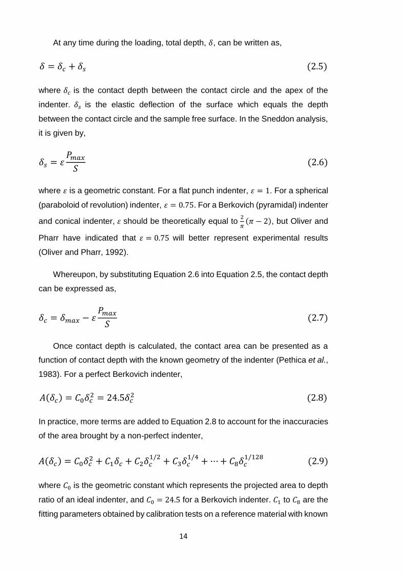
At any time during the loading, total depth, 𝛿, can be written as,
𝛿 = 𝛿𝑐 + 𝛿𝑠 (2.5)
where 𝛿𝑐 is the contact depth between the contact circle and the apex of the
indenter. 𝛿𝑠 is the elastic deflection of the surface which equals the depth
between the contact circle and the sample free surface. In the Sneddon analysis,
it is given by,
𝛿𝑠 = 휀𝑃𝑚𝑎𝑥
𝑆 (2.6)
where 휀 is a geometric constant. For a flat punch indenter, 휀 = 1. For a spherical
(paraboloid of revolution) indenter, 휀 = 0.75. For a Berkovich (pyramidal) indenter
and conical indenter, 휀 should be theoretically equal to 2
𝜋(𝜋 − 2), but Oliver and
Pharr have indicated that 휀 = 0.75 will better represent experimental results
(Oliver and Pharr, 1992).
Whereupon, by substituting Equation 2.6 into Equation 2.5, the contact depth
can be expressed as,
𝛿𝑐 = 𝛿𝑚𝑎𝑥 − 휀𝑃𝑚𝑎𝑥
𝑆 (2.7)
Once contact depth is calculated, the contact area can be presented as a
function of contact depth with the known geometry of the indenter (Pethica et al.,
1983). For a perfect Berkovich indenter,
𝐴(𝛿𝑐) = 𝐶0𝛿𝑐2 = 24.5𝛿𝑐
2 (2.8)
In practice, more terms are added to Equation 2.8 to account for the inaccuracies
of the area brought by a non-perfect indenter,
𝐴(𝛿𝑐) = 𝐶0𝛿𝑐2 + 𝐶1𝛿𝑐 + 𝐶2𝛿𝑐
1/2+ 𝐶3𝛿𝑐
1/4+ ⋯ + 𝐶8𝛿𝑐
1/128 (2.9)
where 𝐶0 is the geometric constant which represents the projected area to depth
ratio of an ideal indenter, and 𝐶0 = 24.5 for a Berkovich indenter. 𝐶1 to 𝐶8 are the
fitting parameters obtained by calibration tests on a reference material with known
15
mechanical properties. Actually, elastically isotropic materials, such as fused
quartz and aluminium, are widely used as the reference materials due to their
elastic moduli are independent of displacement (Oliver and Pharr, 1992). Besides,
the surface quality of the reference material should be carefully controlled, as this
may affect the independency of its elastic modulus (Zheng et al., 2007).
The hardness of test sample is given by,
𝐻 =𝑃
𝐴(𝛿𝑐) (2.10)
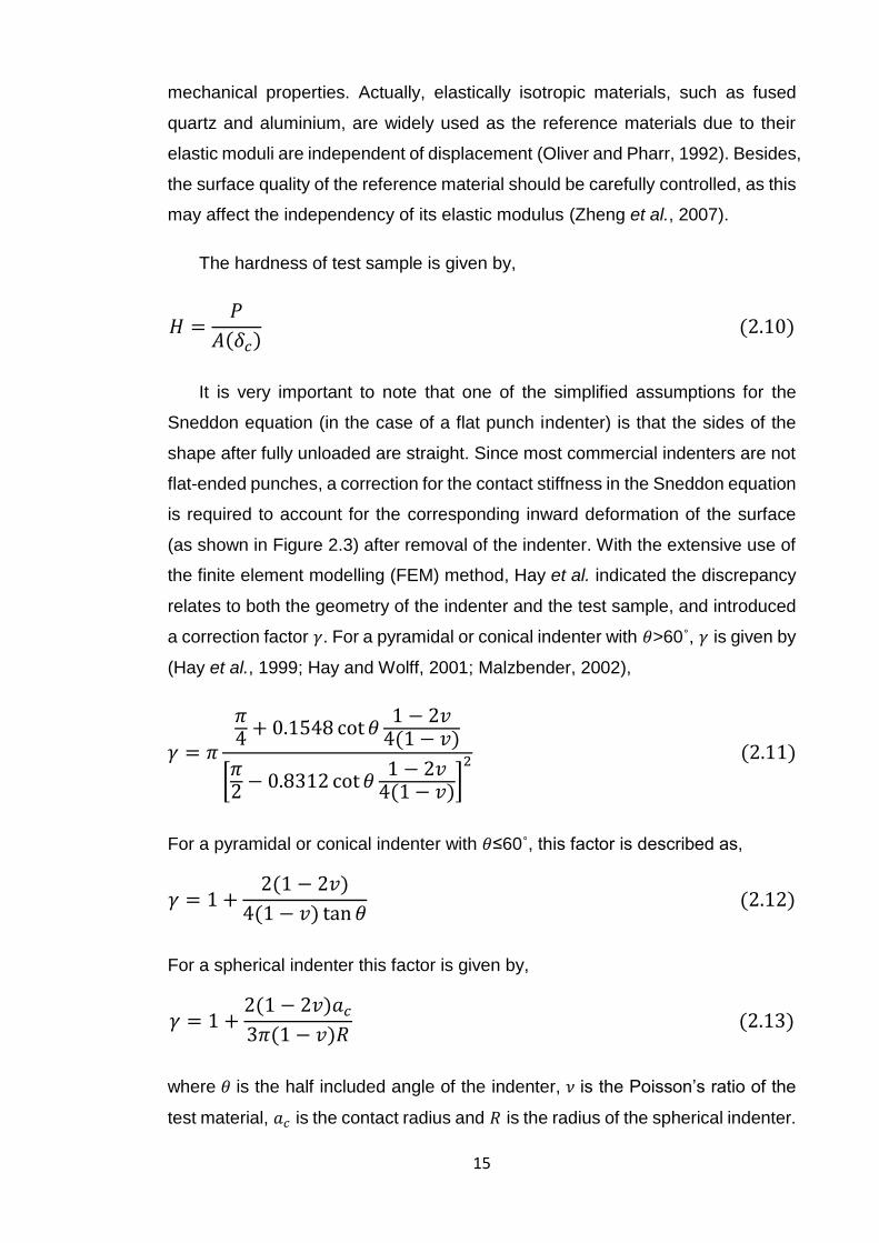
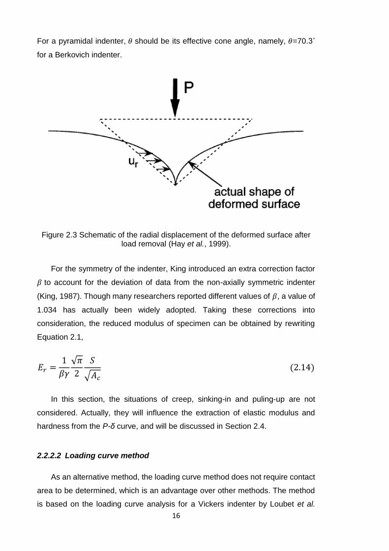
It is very important to note that one of the simplified assumptions for the
Sneddon equation (in the case of a flat punch indenter) is that the sides of the
shape after fully unloaded are straight. Since most commercial indenters are not
flat-ended punches, a correction for the contact stiffness in the Sneddon equation
is required to account for the corresponding inward deformation of the surface
(as shown in Figure 2.3) after removal of the indenter. With the extensive use of
the finite element modelling (FEM) method, Hay et al. indicated the discrepancy
relates to both the geometry of the indenter and the test sample, and introduced
a correction factor 𝛾. For a pyramidal or conical indenter with 𝜃>60˚, 𝛾 is given by
(Hay et al., 1999; Hay and Wolff, 2001; Malzbender, 2002),
𝛾 = 𝜋
𝜋4
+ 0.1548 cot 𝜃1 − 2𝑣
4(1 − 𝑣)
[𝜋2
− 0.8312 cot 𝜃1 − 2𝑣
4(1 − 𝑣)]
2 (2.11)
For a pyramidal or conical indenter with 𝜃≤60˚, this factor is described as,
𝛾 = 1 +2(1 − 2𝑣)
4(1 − 𝑣) tan 𝜃 (2.12)
For a spherical indenter this factor is given by,
𝛾 = 1 +2(1 − 2𝑣)𝑎𝑐
3𝜋(1 − 𝑣)𝑅 (2.13)
where 𝜃 is the half included angle of the indenter, 𝜈 is the Poisson’s ratio of the
test material, 𝑎𝑐 is the contact radius and 𝑅 is the radius of the spherical indenter.
16
For a pyramidal indenter, 𝜃 should be its effective cone angle, namely, 𝜃=70.3˚
for a Berkovich indenter.
Figure 2.3 Schematic of the radial displacement of the deformed surface after load removal (Hay et al., 1999).
For the symmetry of the indenter, King introduced an extra correction factor
𝛽 to account for the deviation of data from the non-axially symmetric indenter
(King, 1987). Though many researchers reported different values of 𝛽, a value of
1.034 has actually been widely adopted. Taking these corrections into
consideration, the reduced modulus of specimen can be obtained by rewriting
Equation 2.1,
𝐸𝑟 =1
𝛽𝛾
√𝜋
2
𝑆
√𝐴𝑐
(2.14)
In this section, the situations of creep, sinking-in and puling-up are not
considered. Actually, they will influence the extraction of elastic modulus and
hardness from the P-δ curve, and will be discussed in Section 2.4.
2.2.2.2 Loading curve method
As an alternative method, the loading curve method does not require contact
area to be determined, which is an advantage over other methods. The method
is based on the loading curve analysis for a Vickers indenter by Loubet et al.
17
(Loubet et al., 1986), starting from the P-δ relationship previously developed by
Sneddon (Sneddon, 1965). During loading, for the case of a non-adhesive conical
indenter with half included angle of 𝜃 in contact with the surface of a smooth
elastic body, the P-δ relationship can be expressed as (Sneddon, 1965),
𝑃 =2𝐸 tan 𝜃
(1 − 𝑣2)𝜋𝛿2 (2.15)
Based on the analysis of experimental loading curves, a general relation
between force and displacement for an elastic-plastic loading is found and given
by (Loubet et al., 1986),
𝑃 = 𝐾𝑒𝑝𝛿𝑛 (2.16)
where 𝐾𝑒𝑝 is a constant depending on the nature of contact, namely: elastic,
elastic-plastic, or purely plastic. 𝑛 is a geometric constant depending on the
geometric of the indenter. For Berkovich (pyramidal) and conical indenters, 𝑛=2.
By assuming the total displacement can be disassociated into a plastic part and
an elastic part, Equation 2.16 can be rewritten as,
𝑃𝑝 = 𝐾𝑝𝛿𝑝2 (2.17)
𝑃𝑒 = 𝐾𝑒𝛿𝑒2 (2.18)
where 𝐾𝑝 and 𝐾𝑒 are the proportionality factors of plastic behaviour and elastic
behaviour, respectively. 𝛿𝑝 and 𝛿𝑒 are the plastic contributed displacement and
the elastic contributed displacement, respectively. Finally, by assuming that
Equation 2.17 and Equation 2.18 are used for two springs in series and 𝛿 = 𝛿𝑝 +
𝛿𝑒, therefore,
(𝐾𝑒𝑝)−
12 = (𝐾𝑝)
−12 + (𝐾𝑒)−
12 (2.19)
By carefully selecting the plastic and elastic proportionality factors, Loubet et al.
expressed Equation 2.16 in terms of the Vickers hardness (𝐻𝑣) as (Loubet et al.,
1986),
18
𝐾𝑒𝑝 = [0.92 (1 − 𝑣2
𝐸) √𝐻𝑣 +
0.194
√𝐻𝑣
]
−2
(2.20)
In 1996, a further development on loading curve analysis was given by
Hainsworth et al. (Hainsworth et al., 1996). In their method, 𝛿𝑝 and 𝛿𝑒 were
related to 𝛿𝑐 and 𝛿𝑠 in Equation 2.5, respectively. For Berkovich (pyramidal) and
conical indenters, by rearranging Equation 2.8 and Equation 2.10, the plastic
depth is given by,
𝛿𝑝 =1
√𝐶0
√𝑃
𝐻= 𝜙√
𝑃
𝐻 (2.21)
where 𝐶0 is the geometric constant shown in Equation 2.8. 𝜙 is an empirical
constant proposed by Hainsworth et al., which is mathematically equal to 1/√𝐶0.
Substituting Equation 2.1 into Equation 2.6, and assuming that the indenter is
much stiffer than the specimen, the elastic depth is given by,
𝛿𝑒 =휀√𝜋(1 − 𝑣2)
2
𝑃
𝐸√
𝐻
𝑃= 𝜓
𝑃
𝐸√
𝐻
𝑃 (2.22)
where 𝑣 is the Poisson’s ratio of test specimen and 휀 is the geometric constant
shown in Equation 2.6. 𝜓 is another empirical constant proposed by Hainsworth
et al., which is mathematically equal to 휀√𝜋(1 − 𝑣2)/2. Therefore, the total depth
can be expressed as,
𝛿 = 𝛿𝑝 + 𝛿𝑒 = 𝜙√𝑃
𝐻+ 𝜓
𝑃
𝐸√
𝐻
𝑃 (2.23)
Substituting Equation 2.23 into Equation 2.16 (in the case of 𝑛=2) gives,
𝐾𝑒𝑝 = (𝜙1
√𝐻+ 𝜓
√𝐻
𝐸)
−2
(2.24)
19
𝑃 = (𝜙1
√𝐻+ 𝜓
√𝐻
𝐸)
−2
𝛿2 (2.25)
By best-fitting the experimental data, Hainsworth et al. expressed Equation
2.25 in terms of a used Berkovich indenter as,
𝑃 = (0.194
√𝐻+ 0.930
√𝐻
𝐸)
−2
𝛿2 (2.26)
which is identical to the expression of a Vickers indenter (Equation 2.20). This is
not surprising due to the fact that Berkovich indenter has the same projected area
to depth ratio as a Vickers indenter, which theoretically makes these two
indenters have the same values of 𝜙 and 𝜓.
Based on Equation 2.25, Malzbender et al. took the indenter deformation into
consideration and rewrote the equation with the reduced modulus instead of the
Young’s modulus. In the case of a perfect Berkovich (pyramidal) or conical
indenter, the P-δ relationship is then given by (Malzbender and den Toonder,
2000),
𝑃 = (1
√𝐶0√𝐻+ 휀
√𝜋𝐻
2𝐸𝑟)
−2
𝛿2 (2.27)
For a non-perfect indenter, an alternative relationship is given by,
𝑃 = (1
√𝐶0√𝐻+ 휀
√𝜋𝐻
2𝐸𝑟)
−2
(𝛿 + 𝜉)2 (2.28)
where 𝜉 accounts for the tip rounding for a non-perfect indenter, as shown in
Figure 2.4.
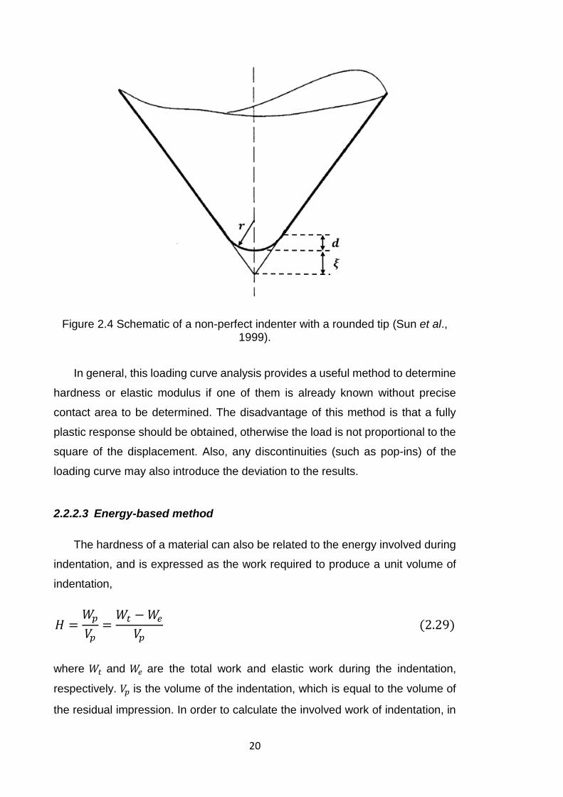
20
Figure 2.4 Schematic of a non-perfect indenter with a rounded tip (Sun et al., 1999).
In general, this loading curve analysis provides a useful method to determine
hardness or elastic modulus if one of them is already known without precise
contact area to be determined. The disadvantage of this method is that a fully
plastic response should be obtained, otherwise the load is not proportional to the
square of the displacement. Also, any discontinuities (such as pop-ins) of the
loading curve may also introduce the deviation to the results.
2.2.2.3 Energy-based method
The hardness of a material can also be related to the energy involved during
indentation, and is expressed as the work required to produce a unit volume of
indentation,
𝐻 =𝑊𝑝
𝑉𝑝=
𝑊𝑡 − 𝑊𝑒
𝑉𝑝 (2.29)
where 𝑊𝑡 and 𝑊𝑒 are the total work and elastic work during the indentation,
respectively. 𝑉𝑝 is the volume of the indentation, which is equal to the volume of
the residual impression. In order to calculate the involved work of indentation, in
21
the case of a Berkovich indenter, Equation 2.16 is rewritten as (Fischer-Cripps,
2011a),
𝑃𝑙𝑜𝑎𝑑𝑖𝑛𝑔 = 𝐾𝑒𝑝𝛿2 (2.30)
𝑃𝑢𝑛𝑙𝑜𝑎𝑑𝑖𝑛𝑔 = 𝐾𝑒(𝛿 − 𝛿𝑟𝑒𝑠)𝑚 (2.31)
At the maximum load, the boundary condition is given by,
𝑃 = 𝐾𝑒𝑝𝛿𝑚𝑎𝑥2 = 𝐾𝑒(𝛿𝑚𝑎𝑥 − 𝛿𝑟𝑒𝑠)𝑚 (2.32)
where 𝐾𝑒𝑝 and 𝐾𝑒 are the constants depending on the nature of contact, namely:
elastic, elastic-plastic, or purely plastic. 𝑚 is the power law index proposed in
Equation 2.3, and 𝑚 should be smaller than two due to the fact that the sides of
the residual impression are curved during the unloading. In practice, these
parameters can be extracted by a least squares fitting procedure. Then, the
involved work of the indentation is calculated by integrating the force with respect
to the displacement,
𝑊𝑡 = ∫ 𝐾𝑒𝑝𝛿2𝛿𝑚𝑎𝑥
0
=𝐾𝑒𝑝𝛿𝑚𝑎𝑥
3
3 (2.33)
𝑊𝑒 = ∫ 𝐾𝑒𝛿𝑚𝛿𝑚𝑎𝑥
0
=𝐾𝑒(𝛿𝑚𝑎𝑥 − 𝛿𝑟𝑒𝑠)𝑚+1
𝑚 + 1 (2.34)
By dividing Equation 2.34 by Equation 2.33 and expressing the ratio 𝐾𝑒/𝐾𝑒𝑝 in
terms of Equation 2.32, a linear relationship between the ratio of elastic work to
the total work and the ratio of residual depth to maximum can be obtained,
𝑊𝑒
𝑊𝑡=
3
𝑚 + 1(1 −
𝛿𝑟𝑒𝑠
𝛿𝑚𝑎𝑥) (2.35)
By assuming the radius of the contact circle is the same at maximum load and
full unload, the volume of the indentation is given by,
𝑉𝑝 =𝜋
3𝑎𝑐
2𝛿𝑟𝑒𝑠 (2.36)
22
In this mathematical method, the evaluation of contact area (or contact radius)
is required, which will be influenced by the unnoticed sinking-in or piling-up.
Alternatively, Tuck et al. proposed a method without calculation of the contact
area (Tuck et al., 2001). By rewriting Equation 2.10 and Equation 2.16 at the
maximum load, a linear relationship between the contact depth and the maximum
depth can be obtained,
𝑃𝑚𝑎𝑥 = 𝐻𝐶0𝛿𝑐2 (2.37)
𝑃𝑚𝑎𝑥 = 𝐾𝑒𝑝𝛿𝑚𝑎𝑥2 (2.38)
where 𝐾𝑒𝑝 can be extracted by the least squares fitting procedure, and the
contact depth is proportional to the maximum depth. Then, Tuck et al. proposed
that 𝐴𝑐 = 𝑘𝛿𝑚2 , where 𝑘 is a geometric constant, and the total work of indentation
is given by,
𝑃𝑚𝑎𝑥 = 𝐻𝑘𝛿𝑚𝑎𝑥2 (2.39)
𝑊𝑡 = ∫ 𝑃𝑑𝛿𝛿𝑚𝑎𝑥
0
=𝑘𝐻𝛿𝑚𝑎𝑥
3
3 (2.40)
Substituting Equation 2.39 into Equation 2.40, the hardness is given by,
𝐻 =3𝑊𝑡
𝑘𝛿𝑚𝑎𝑥3 =
𝑃𝑚𝑎𝑥3
9𝑘𝑊𝑡2 (2.41)
It can be observed that, in these equations, the calculation of the contact area
is not required. Thus, this method avoids the problems associated with the
contact area. It was reported that the hardness obtained by this method agrees
well with the values obtained by Oliver and Pharr method at big loads (Tuck et
al., 2001; Bull, 2002). However, it was also reported that there are big errors for
the hardness extraction from highly elastic materials by this method, which can
be up to 70% when the 𝐻/𝐸 ratio is higher than 0.025.
In 2002, based on FEM for a conical indenter, Cheng et al. observed the
linear relationship described in Equation 2.35 and then proposed a linear
relationship between the ratio of elastic work to the total work and the ratio of
23
hardness to reduced modulus for pyramidal indenters with 60˚<𝜃<80˚ (Cheng et
al., 2002),
𝑊𝑒
𝑊𝑡= 𝜅−1
𝐻
𝐸𝑟 (2.42)
where 𝜅 is a constant depending on the indenter half included angle, and is
approximately equal to 5.3 when 𝜃=70.3˚. Substituting Equation 2.1 and Equation
2.10 into Equation 2.42, the hardness and the reduced modulus are expressed
as,
𝐻 = 𝜅2𝜋
4𝑆2 (
𝑊𝑒
𝑊𝑡)
2 1
𝑃𝑚𝑎𝑥 (2.43)
𝐸𝑟 = 𝜅𝜋
4𝑆2
𝑊𝑒
𝑊𝑡
1
𝑃𝑚𝑎𝑥 (2.44)
For spherical indenters, Ni et al. observed similar relation between 𝑊𝑒/𝑊𝑡
and 𝐻/𝐸𝑟, which is expressed as (Ni et al., 2004),
𝑊𝑒
𝑊𝑡= 1.6869(
𝑅
𝛿𝑚𝑎𝑥)0.62
𝐻
𝐸𝑟 (2.45)
Although the linear equations between the ratio of 𝑊𝑒/𝑊𝑡 and 𝐻/𝐸𝑟 were
commonly accepted, it has been found that non-linear relationship will be more
accurate to describe this ratio (Malzbender, 2002; Chen and Bull, 2009c). The
expressions are given by,
𝑊𝑒
𝑊𝑡= (
휀
2+
𝛾
𝜋 tan 𝜃
𝐸𝑟
𝐻)
−1
(2.46)
𝑊𝑒
𝑊𝑡=
1.5(1.24 + 0.2𝑥)𝜋
(0.24 + 0.2𝑥)𝛾
𝐻
𝐸𝑟tan 𝜃 (
1
1 +𝜋휀2𝛽
𝐻𝐸𝑟
tan 𝜃) (2.47)
where 𝑥 is the work hardening exponent, which will be further described in
Section 2.2.4.
24
2.2.2.4 Slope-based method
By rearranging Equation 2.10 and Equation 2.14, Joslin and Oliver
demonstrated that the parameter given by the load divided by the square of the
unloading contact stiffness (𝑆𝑢) was independent of the displacement or the
contact area, which is given by (Joslin and Oliver, 1990),
𝑃
𝑆𝑢2
=𝜋𝐻
4𝛽2𝐸𝑟2
(2.48)
This equation shows the advantage that it is more sensitive to changes in elastic
modulus of the specimen than the changes of the hardness, and the contact area
is not involved.
Based on the relation between the force and the square of the displacement
presented in Equation 2.27, the expression of the loading contact stiffness (𝑆𝑙) is
given by differentiating the equation with respect to the displacement
(Malzbender and den Toonder, 2000; Oliver, 2001),
𝑆𝑙 = 2 (1
√𝐶0√𝐻+
휀
𝛽
√𝜋𝐻
2𝐸𝑟)
−2
𝛿 (2.49)
Then, the ratio between loading slope and unloading slope is given by (Oliver,
2001),
𝑆𝑢
𝑆𝑙=
𝐸𝑟
𝐻√𝜋𝐶0
+휀
2 (2.50)
Substituting Equation 2.10 and Equation 2.14 into Equation 2.50, the expressions
for the hardness and elastic modulus can be described as,
𝐸𝑟 = √𝜋
𝐶0
1
2𝑃𝑚𝑎𝑥𝛽(
𝑆𝑢2𝑆𝑙
2𝑆𝑢 − 휀𝑆𝑙) (2.51)
𝐻 =1
𝐶0𝑃𝑚𝑎𝑥(
2𝑆𝑢 − 휀𝑆𝑙
𝑆𝑢𝑆𝑙)
−2
(2.52)
25
As this method is based on the assumption that the load is proportional to the
square of the displacement. This method is supposed to show the same limitation
as the loading curve method, namely, a fully plastic response should be obtained.
Creep would also affect the loading slope and unloading slope. In an extreme
case, a negative unloading slope will be obtained.
2.2.3 Extraction of time-dependent properties from the P-δ curves
Solid-like materials store energy when undergoing deformation and quickly
return to their original state following removal of stress. Viscous materials
dissipate energy when undergoing deformation and present a time-dependent
deformed state after the removal of stress. A material that undergoes elastic
deformation, but exhibits time-dependent behaviour is called viscoelastic.
Nanoindentation also offers the quantitative measurement of such viscoelastic
properties. In one way, a small sinusoidal force is integrated to the main load.
The resulting oscillatory displacement signal is used to provide the elastic and
viscous properties of the specimen in the frequency domain. In the other way, the
force or displacement is held at a specified value for a certain period. The
resulting creep or relaxation data, associated with an appropriate mechanical
model, is used to characterize the elastic and viscous properties of the specimen
in the time domain.
2.2.3.1 Dynamic nanoindentation test
In 1988, Pethica and Oliver introduced a continuous stiffness method (CSM),
which enables the measurement of the contact stiffness continuously, by
superimposing a small sinusoidal oscillatory force to the main load (Pethica and
Oliver, 1988). This small alternating current force is modulated with a frequency
𝜔 and amplitude 𝑃0, and is given by (Lucas et al., 1998),
𝑃 = 𝑃0𝑒𝑖𝜔𝑡 (2.53)
The resulting oscillatory displacement will have the same oscillatory frequency,
but with a phase difference 𝛷 (0<𝛷<90˚),
𝛿 = 𝛿0𝑒𝑖(𝜔𝑡+𝛷) (2.54)

26
Therefore, the velocity and acceleration of the mass is given by taking the first
and second differentiations with respect to time,
𝑑𝛿
𝑑𝑡= 𝑖𝜔𝛿 (2.55)
𝑑2𝛿
𝑑𝑡2= −𝜔2𝛿 (2.56)
Here, for the model shown in Figure 2.5, the force is expressed as,
𝑃 = [(1
𝑆+ 𝐶𝑓)
−1
+ 𝑘𝑠 − 𝑚𝜔2 + 𝑖𝜔(𝜆 + 𝜆𝑠)] 𝛿 (2.57)
The magnitude of the stiffness of the contact can be calculated from the amplitude
of the displacement to force ratio,
|𝑃0
𝛿0| = √[(
1
𝑆+ 𝐶𝑓)
−1
+ 𝑘𝑠 − 𝑚𝜔2]
2
+ 𝜔2(𝜆 + 𝜆𝑠)2 (2.58)
Or from the phase difference 𝛷 between the load and displacement,
tan 𝛷 =𝜔(𝜆 + 𝜆𝑠)
(1𝑆
+ 𝐶𝑓)−1
+ 𝑘𝑠 − 𝑚𝜔2
(2.59)
Within these unknown parameters, the calibration of 𝐶𝑓 will be discussed in
Section 2.4.1. 𝑘𝑠 , 𝑚 and 𝜆 can be obtained by oscillating the indenter in air.
Therefore, the storage modulus (𝐸′), loss modulus (𝐸′′), complex modulus (𝐸∗)
and the phase difference (𝛿) between the stress (𝜎) and strain (𝛾) in the test
material are given by,
𝐸′ =𝜎0 cos 𝛿
𝛾0=
𝑆√𝜋
2√𝐴𝑐
(2.60)
𝐸′′ =𝜎0 sin 𝛿
𝛾0=
𝜔𝜆𝑠√𝜋
2√𝐴𝑐
(2.61)
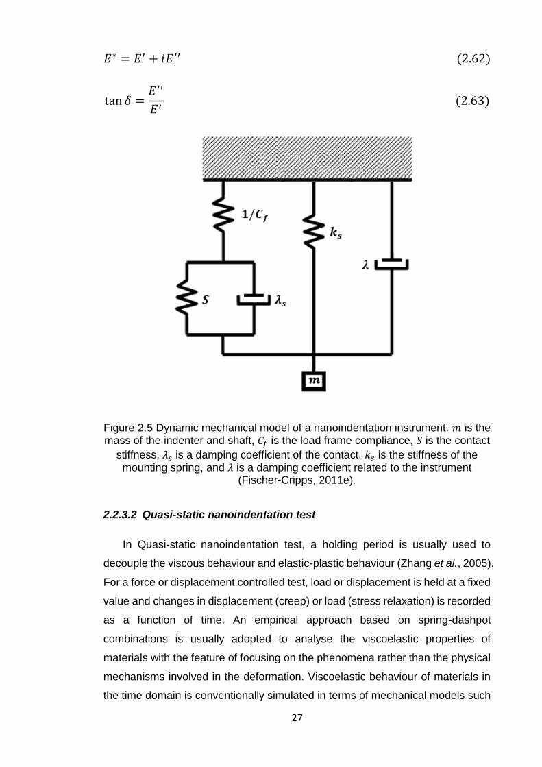
27
𝐸∗ = 𝐸′ + 𝑖𝐸′′ (2.62)
tan 𝛿 =𝐸′′
𝐸′ (2.63)
Figure 2.5 Dynamic mechanical model of a nanoindentation instrument. 𝑚 is the mass of the indenter and shaft, 𝐶𝑓 is the load frame compliance, 𝑆 is the contact
stiffness, 𝜆𝑠 is a damping coefficient of the contact, 𝑘𝑠 is the stiffness of the mounting spring, and 𝜆 is a damping coefficient related to the instrument
(Fischer-Cripps, 2011e).
2.2.3.2 Quasi-static nanoindentation test
In Quasi-static nanoindentation test, a holding period is usually used to
decouple the viscous behaviour and elastic-plastic behaviour (Zhang et al., 2005).
For a force or displacement controlled test, load or displacement is held at a fixed
value and changes in displacement (creep) or load (stress relaxation) is recorded
as a function of time. An empirical approach based on spring-dashpot
combinations is usually adopted to analyse the viscoelastic properties of
materials with the feature of focusing on the phenomena rather than the physical
mechanisms involved in the deformation. Viscoelastic behaviour of materials in
the time domain is conventionally simulated in terms of mechanical models such
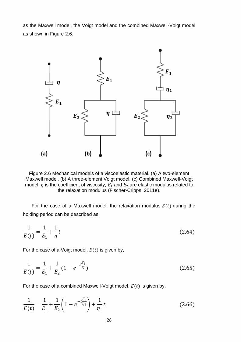
28
as the Maxwell model, the Voigt model and the combined Maxwell-Voigt model
as shown in Figure 2.6.
Figure 2.6 Mechanical models of a viscoelastic material. (a) A two-element Maxwell model. (b) A three-element Voigt model. (c) Combined Maxwell-Voigt
model. 𝜂 is the coefficient of viscosity, 𝐸1 and 𝐸2 are elastic modulus related to the relaxation modulus (Fischer-Cripps, 2011e).
For the case of a Maxwell model, the relaxation modulus 𝐸(𝑡) during the
holding period can be described as,
1
𝐸(𝑡)=
1
𝐸1+
1
𝜂𝑡 (2.64)
For the case of a Voigt model, 𝐸(𝑡) is given by,
1
𝐸(𝑡)=
1
𝐸1+
1
𝐸2(1 − 𝑒
−𝑡𝐸2𝜂 ) (2.65)
For the case of a combined Maxwell-Voigt model, 𝐸(𝑡) is given by,
1
𝐸(𝑡)=
1
𝐸1+
1
𝐸2(1 − 𝑒
−𝑡𝐸2𝜂2) +
1
𝜂1𝑡 (2.66)
29
In practice, these fundamental models are combined with additional elements
to describe different time-dependent behaviours. For example, for the case of a
Prony series model which is widely used in practice, 𝐸(𝑡) is given by (Cao et al.,
2010; Chen and Lu, 2012),
𝐸(𝑡) = 𝐸0 [1 − ∑ 𝑔𝑖 (1 − 𝑒−
𝑡𝜏𝑖)
𝑚
𝑖=1
] = 𝐸∞ + 𝐸0 ∑ 𝑔𝑖𝑒−
𝑡𝜏𝑖
𝑚
𝑖=1
(2.67)
where 𝐸0 = 𝐸(𝑡 = 0) is the instantaneous modulus, 𝐸∞is the equilibrium modulus
once the material is totally relaxed, 𝑔𝑖 is the material related constant, 𝜏𝑖 is the
material time constant, and 𝑚 is the number of terms in the series.
Whereupon, for the case of a constant load 𝑃0 with a pyramidal indenter or
spherical indenter, the depth creep of penetration is expressed as,
𝛿2(𝑡) =𝜋(1 − 𝑣2)
2 tan 𝜃
𝑃0
𝐸(𝑡) pyramidal or conical indenter (2.68)
𝛿3/2(𝑡) =3(1 − 𝑣2)
4√𝑅
𝑃0
𝐸(𝑡) spherical indenter (2.69)
Or in the case of a constant displacement 𝛿0 with a pyramidal indenter or
spherical indenter, the relaxation load is given by,
𝑃(𝑡) =2 tan 𝜃 𝛿0
2
𝜋(1 − 𝑣2)𝐸(𝑡) pyramidal or conical indenter (2.70)
𝑃(𝑡) =4√𝑅𝛿0
3/2
3(1 − 𝑣2)𝐸(𝑡) spherical indenter (2.71)
By applying the Buckingham Pi theorem in dimensional analysis, Cao et al.
proposed that the normalized relaxation modulus ��(𝑡) (the ratio of relaxation
modulus to instantaneous modulus) is independent of the geometry of the
indenter and sample surface, but depends only on the load history (Cao et al.,
2009; Cao et al., 2010). The relationship between the normalized relaxation
modulus and the load history is given by,
30
��(𝑡) =𝐸(𝑡)
𝐸0=
𝑃(𝑡)
𝑃0= 𝐶
𝑃(𝑡)
𝛿0 (2.72)
where 𝑃0 and 𝛿0 are the applied load and resultant displacement at the starting
point of relaxation, respectively. 𝐶 is the ratio between 𝛿0 and 𝑃0 . The
significance of this work is that it is independent of displacement and geometry
of the indenter, and it can be used to porous materials as well.
After fitting creep or relaxation curves to the selected model, the time-
dependent properties can be extracted in terms of relaxation modulus. While it is
very important to note that Equations 2.64-2.72 assume a Heaviside unit step
increase in load or displacement. In practice, a step increase in load or
displacement is not experimentally feasible, and a finite time period is required
for the load or displacement increases from zero to the set value. If the loading
time is comparable to the material time constant, the resulting instantaneous
modulus can be very much less than the nominal value of the material.
In consequence, the accuracy of results fitted from these equations is highly
dependent on the loading rate and the time-dependent nature of the material. To
account for the influence from the loading period, many sophisticated models
have been developed. In 2005, Oyen analysed the difference between creep
functions of the ramp loading and step loading in the case of indenting a spherical
indenter into viscoelastic polymers, and proposed a dimensionless ramp
correction factor (Oyen, 2005),
𝑅𝐶𝐹𝑖 =𝜏𝑖
𝑡𝑅(𝑒
𝑡𝑅𝜏𝑖 − 1) (2.73)
where 𝑡𝑅 is the rise time of loading period. It indicates that, once the loading time
is in an order less than the material time constant, the effect from the loading time
can be ignored and the numerical errors from fitting the creep or relaxation data
by Equations 2.68-2.72 will be negligible. In contrast, once the loading time is
comparable to the material time constant, the effect from the loading time should
be considered and Equations 2.68-2.72 should be modified by the ramp
correction factor. In the case of indenting a spherical indenter into a viscoelastic
material, when a Prony series model is adopted, the modified relaxation force
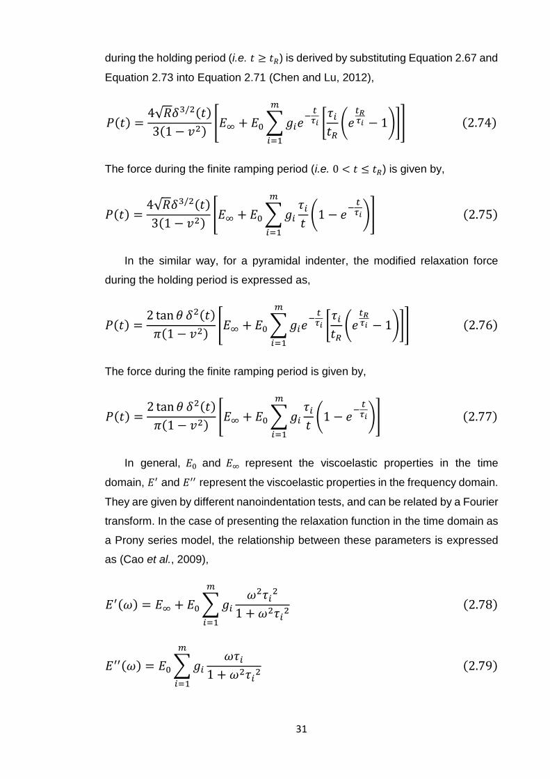
31
during the holding period (i.e. 𝑡 ≥ 𝑡𝑅) is derived by substituting Equation 2.67 and
Equation 2.73 into Equation 2.71 (Chen and Lu, 2012),
𝑃(𝑡) =4√𝑅𝛿3/2(𝑡)
3(1 − 𝑣2)[𝐸∞ + 𝐸0 ∑ 𝑔𝑖𝑒
−𝑡𝜏𝑖 [
𝜏𝑖
𝑡𝑅(𝑒
𝑡𝑅𝜏𝑖 − 1)]
𝑚
𝑖=1
] (2.74)
The force during the finite ramping period (i.e. 0 < 𝑡 ≤ 𝑡𝑅) is given by,
𝑃(𝑡) =4√𝑅𝛿3/2(𝑡)
3(1 − 𝑣2)[𝐸∞ + 𝐸0 ∑ 𝑔𝑖
𝜏𝑖
𝑡(1 − 𝑒
−𝑡𝜏𝑖)
𝑚
𝑖=1
] (2.75)
In the similar way, for a pyramidal indenter, the modified relaxation force
during the holding period is expressed as,
𝑃(𝑡) =2 tan 𝜃 𝛿2(𝑡)
𝜋(1 − 𝑣2)[𝐸∞ + 𝐸0 ∑ 𝑔𝑖𝑒
−𝑡𝜏𝑖 [
𝜏𝑖
𝑡𝑅(𝑒
𝑡𝑅𝜏𝑖 − 1)]
𝑚
𝑖=1
] (2.76)
The force during the finite ramping period is given by,
𝑃(𝑡) =2 tan 𝜃 𝛿2(𝑡)
𝜋(1 − 𝑣2)[𝐸∞ + 𝐸0 ∑ 𝑔𝑖
𝜏𝑖
𝑡(1 − 𝑒
−𝑡𝜏𝑖)
𝑚
𝑖=1
] (2.77)
In general, 𝐸0 and 𝐸∞ represent the viscoelastic properties in the time
domain, 𝐸′ and 𝐸′′ represent the viscoelastic properties in the frequency domain.
They are given by different nanoindentation tests, and can be related by a Fourier
transform. In the case of presenting the relaxation function in the time domain as
a Prony series model, the relationship between these parameters is expressed
as (Cao et al., 2009),
𝐸′(𝜔) = 𝐸∞ + 𝐸0 ∑ 𝑔𝑖
𝜔2𝜏𝑖2
1 + 𝜔2𝜏𝑖2
𝑚
𝑖=1
(2.78)
𝐸′′(𝜔) = 𝐸0 ∑ 𝑔𝑖
𝜔𝜏𝑖
1 + 𝜔2𝜏𝑖2
𝑚
𝑖=1
(2.79)
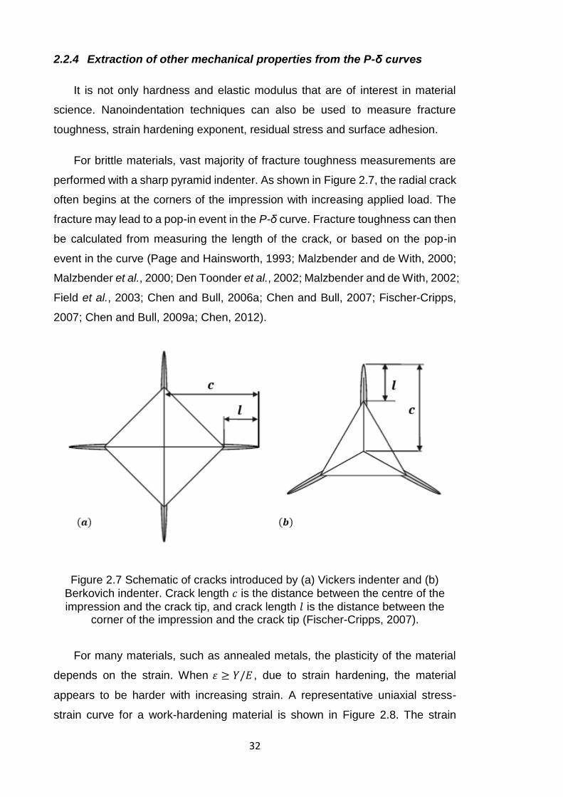
32
2.2.4 Extraction of other mechanical properties from the P-δ curves
It is not only hardness and elastic modulus that are of interest in material
science. Nanoindentation techniques can also be used to measure fracture
toughness, strain hardening exponent, residual stress and surface adhesion.
For brittle materials, vast majority of fracture toughness measurements are
performed with a sharp pyramid indenter. As shown in Figure 2.7, the radial crack
often begins at the corners of the impression with increasing applied load. The
fracture may lead to a pop-in event in the P-δ curve. Fracture toughness can then
be calculated from measuring the length of the crack, or based on the pop-in
event in the curve (Page and Hainsworth, 1993; Malzbender and de With, 2000;
Malzbender et al., 2000; Den Toonder et al., 2002; Malzbender and de With, 2002;
Field et al., 2003; Chen and Bull, 2006a; Chen and Bull, 2007; Fischer-Cripps,
2007; Chen and Bull, 2009a; Chen, 2012).
Figure 2.7 Schematic of cracks introduced by (a) Vickers indenter and (b)
Berkovich indenter. Crack length 𝑐 is the distance between the centre of the
impression and the crack tip, and crack length 𝑙 is the distance between the corner of the impression and the crack tip (Fischer-Cripps, 2007).
For many materials, such as annealed metals, the plasticity of the material
depends on the strain. When 휀 ≥ 𝑌/𝐸 , due to strain hardening, the material
appears to be harder with increasing strain. A representative uniaxial stress-
strain curve for a work-hardening material is shown in Figure 2.8. The strain
33
hardening exponent 𝑥 is usually calculated from the uniaxial stress strain curve
given by a traditional tensile test. Indeed, it can also be extracted from the P-δ
curve generated by the nanoindentation test (Shinohara et al., 1994; Ahn and
Kwon, 2001; Pelletier, 2006).
Figure 2.8 A representative uniaxial stress-strain response for an ideal elastic-
plastic material. 𝑥 is the strain hardening index, 𝑌 is the yield stress, and the proportionality constant 𝐾 = 𝑌(𝐸/𝑌)𝑥. For 𝑥 = 0, the material is elastic perfectly-
plastic.
In addition, the possible residual stress and surface adhesion can also affect
the determination of hardness and Young’s modulus extracted from the P-δ
curves. By employing appropriate advanced methods, these residual stress and
surface adhesion can be quantified (Johnson et al., 1971; Underwood, 1973;
Roberts et al., 1999; Taljat and Pharr, 1999).
2.3 Indenter geometry and selection
The tip end of the indenter is typically made from very stiff material, such as
diamond or sapphire, thereby it is much stiffer than most of the tested materials.
From the view of the indenter shape, there are various types of indenters can be
chosen for a specific task, such as flat, pyramidal, spherical or conical shape. The
parameters of the commonly used indenters are summarized in Table 2.1, and
these indenters include:
34
Cylindrical flat punch indenter
This type of indenter has the advantage of a constant contact
geometry. The contact area is independent of the depth and is less likely
to be influenced by creep or thermal drift. Therefore, it is relatively
straightforward to interpret the data. The drawback is high stress
concentration around edge (Chen, 2014). It is usually used in the study of
soft solids or viscoelastic materials (Cheng et al., 2000).
Spherical indenter
For a spherical indenter, the indentation strain (which represents the
ratio of contact radius to effective indenter radius) is initially small and
produces only elastic deformation. With the increase of strain, such an
indenter provides a smooth transition from elastic to plastic deformation.
Thus, it is usually used in the study of elastic to plastic transition, or in the
case that only elastic deformation is desired (Bell et al., 1992; Field and
Swain, 1995). This type of indenter is difficult to be manufactured from
hard materials with high quality and typically made as a sphero-conical
shape.
Conical indenter
A conical indenter has a much smaller contact area compared with
flat punch indenter and spherical indenter. Due to its axial symmetry, it is
convenient to treat the nanoindentation data from a pyramidal indenter as
the data taken with an equivalent conical indenter with an effective cone
angle 𝛼 (Fischer-Cripps, 2011c). On the other hand, its axial symmetry
avoids the stress concentration at the sharp edges which are involved in
a pyramidal indenter. However, very few nanoindentation tests have been
performed with conical indenter, as it is challenging to manufacture a
sharp diamond conical tip at small scale (Chen, 2014).
For an ideal sharp conical indenter (or equivalent conical indenter) a
condition of fully plastic deformation from the moment that indenter
contacts with the specimen is expected. However, during the manufacture
or the use of indenter in practice, tip blunting is inevitable that would lead
35
to an elastic response during the initial contact (Chen and Bull, 2006c;
Chen and Bull, 2009b; Fischer-Cripps, 2011d).
Berkovich indenter
The Berkovich indenter is the most frequently used indenter in
nanoindentation. It is a three-sided pyramid with the advantage that three
planes are more readily machined to meet at a single point thus ensuring
a more precise indentation process, compared to a Vickers indenter
(Bhushan and Li, 2003). It has a half included angle of 65.27˚ and a total
included angle (edge to plane) of 142.3˚. The tip radius for a brand new
Berkovich indenter is usual around 50-100nm, and typically rises to about
200nm with use. Therefore, the primary applications of Berkovich indenter
are bulk materials, thin films greater than 100nm, scratch testing and in-
situ imaging.
Vickers indenter
The Vickers indenter is a square pyramid and similar to Berkovich
indenter due to the same area to depth ratio. However, it is less commonly
used in the nano range than the Berkovich indenter, because it is difficult
to machine the four planes to a single point at such small scale and the
resulting line of conjunction at the tip is inevitable (Tsui et al., 1996;
Bhushan and Li, 2003).
Cube corner indenter
The Cube corner indenter is similar to the Berkovich indenter except
it has a half included angle of 35.26˚ and a total included angle of 90˚.
Because of the sharpness of the tip, this type of indenter produces much
higher stress and strain on the contact area, and a much more confined
plastic deformation zone. Therefore, this type of indenter is commonly
used in the study of the fracture toughness, where small cracks will be
intentionally produced in brittle materials, or in the case of thin coatings
where the effect from the substrate can be minimized (Pharr, 1998;
Fischer-Cripps, 2011c).
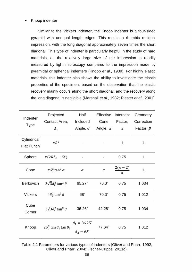
36
Knoop indenter
Similar to the Vickers indenter, the Knoop indenter is a four-sided
pyramid with unequal length edges. This results a rhombic residual
impression, with the long diagonal approximately seven times the short
diagonal. This type of indenter is particularly helpful in the study of hard
materials, as the relatively large size of the impression is readily
measured by light microscopy compared to the impression made by
pyramidal or spherical indenters (Knoop et al., 1939). For highly elastic
materials, this indenter also shows the ability to investigate the elastic
properties of the specimen, based on the observation that the elastic
recovery mainly occurs along the short diagonal, and the recovery along
the long diagonal is negligible (Marshall et al., 1982; Riester et al., 2001).
Indenter
Type
Projected
Contact Area,
𝑨𝒄
Half
Included
Angle, 𝜽
Effective
Cone
Angle, 𝜶
Intercept
Factor,
𝜺
Geometry
Correction
Factor, 𝜷
Cylindrical
Flat Punch 𝜋𝑅2 - - 1 1
Sphere 𝜋(2𝑅𝛿𝑐 − 𝛿𝑐2) - - 0.75 1
Cone 𝜋𝛿𝑐2 tan2 𝛼 𝛼 𝛼
2(𝜋 − 2)
𝜋 1
Berkovich 3√3𝛿𝑐2 tan2 𝜃 65.27˚ 70.3˚ 0.75 1.034
Vickers 4𝛿𝑐2 tan2 𝜃 68˚ 70.3˚ 0.75 1.012
Cube
Corner 3√3𝛿𝑐
2 tan2 𝜃 35.26˚ 42.28˚ 0.75 1.034
Knoop 2𝛿𝑐2 tan 𝜃1 tan 𝜃2
𝜃1 = 86.25˚
𝜃2 = 65˚ 77.64˚ 0.75 1.012
Table 2.1 Parameters for various types of indenters (Oliver and Pharr, 1992; Oliver and Pharr, 2004; Fischer-Cripps, 2011c).
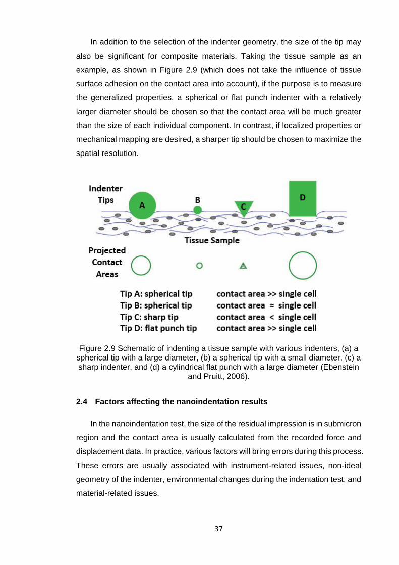
37
In addition to the selection of the indenter geometry, the size of the tip may
also be significant for composite materials. Taking the tissue sample as an
example, as shown in Figure 2.9 (which does not take the influence of tissue
surface adhesion on the contact area into account), if the purpose is to measure
the generalized properties, a spherical or flat punch indenter with a relatively
larger diameter should be chosen so that the contact area will be much greater
than the size of each individual component. In contrast, if localized properties or
mechanical mapping are desired, a sharper tip should be chosen to maximize the
spatial resolution.
Figure 2.9 Schematic of indenting a tissue sample with various indenters, (a) a spherical tip with a large diameter, (b) a spherical tip with a small diameter, (c) a sharp indenter, and (d) a cylindrical flat punch with a large diameter (Ebenstein
and Pruitt, 2006).
2.4 Factors affecting the nanoindentation results
In the nanoindentation test, the size of the residual impression is in submicron
region and the contact area is usually calculated from the recorded force and
displacement data. In practice, various factors will bring errors during this process.
These errors are usually associated with instrument-related issues, non-ideal
geometry of the indenter, environmental changes during the indentation test, and
material-related issues.
38
2.4.1 Load frame compliance
Both the displacement and applied force will be recorded during the
nanoindentation test. However, this recorded displacement data is the sum of the
depth of penetration within the specimen and the deflection of the load frame
arising from the reaction force. Oliver and Pharr considered the load frame
compliance and sample compliance as two springs in series, therefore the total
compliance is given by (Oliver and Pharr, 1992),
𝐶 = 𝐶𝑓 + 𝐶𝑠 (2.80)
where 𝐶 is the total compliance, and it equals 𝑑ℎ/𝑑𝑃 . 𝐶𝑓 is the load frame
compliance. 𝐶𝑠 is the compliance of the indented material, and it equals the
inverse of the stiffness, 𝑆, which is given by Equation 2.1. Then, Equation 2.80
can be rewritten as,
𝑑ℎ
𝑑𝑃= 𝐶𝑓 +
√𝜋
2𝛽𝐸𝑟√𝐴𝑐
(2.81)
It shows that, by making various indents on a reference material with known
elastic modulus, the plot of 𝑑ℎ/𝑑𝑃 versus 𝐴𝑐−1/2 should be linear and the
intercept would give the load frame compliance directly. The disadvantage of this
method is that the data obtained at large forces is preferred, as it results a more
obvious observation of load frame compliance effects and a less influence from
tip defects (such as tip blunting). On the other hand, since this method depends
upon an accurate indenter area function, an iterative process is required to reach
a convergent value. However, it was reported that, in the case of a very high load
frame compliance or a quite blunt indenter, this iterative process is time-
consuming or even fails to obtain a convergent value (Oliver and Pharr, 2004).
Alternately, to avoid the contact area involved in the expression, Equation
2.48 is substituted into Equation 2.80, then yields,
𝑑ℎ
𝑑𝑃= 𝐶𝑓 +
√𝜋𝐻
2𝛽𝐸𝑟√𝑃 (2.82)
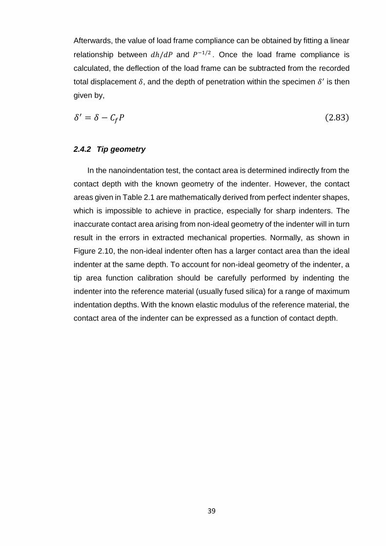
39
Afterwards, the value of load frame compliance can be obtained by fitting a linear
relationship between 𝑑ℎ/𝑑𝑃 and 𝑃−1/2 . Once the load frame compliance is
calculated, the deflection of the load frame can be subtracted from the recorded
total displacement 𝛿, and the depth of penetration within the specimen 𝛿′ is then
given by,
𝛿′ = 𝛿 − 𝐶𝑓𝑃 (2.83)
2.4.2 Tip geometry
In the nanoindentation test, the contact area is determined indirectly from the
contact depth with the known geometry of the indenter. However, the contact
areas given in Table 2.1 are mathematically derived from perfect indenter shapes,
which is impossible to achieve in practice, especially for sharp indenters. The
inaccurate contact area arising from non-ideal geometry of the indenter will in turn
result in the errors in extracted mechanical properties. Normally, as shown in
Figure 2.10, the non-ideal indenter often has a larger contact area than the ideal
indenter at the same depth. To account for non-ideal geometry of the indenter, a
tip area function calibration should be carefully performed by indenting the
indenter into the reference material (usually fused silica) for a range of maximum
indentation depths. With the known elastic modulus of the reference material, the
contact area of the indenter can be expressed as a function of contact depth.
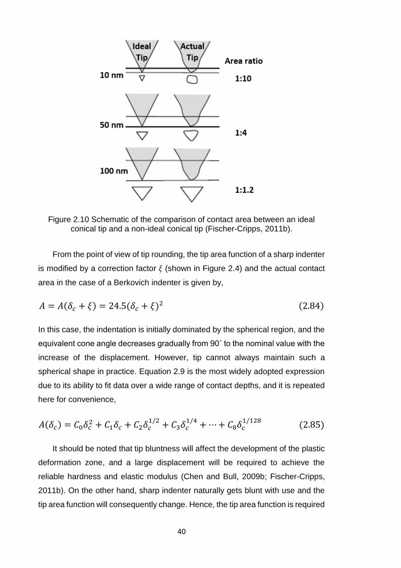
40
Figure 2.10 Schematic of the comparison of contact area between an ideal conical tip and a non-ideal conical tip (Fischer-Cripps, 2011b).
From the point of view of tip rounding, the tip area function of a sharp indenter
is modified by a correction factor 𝜉 (shown in Figure 2.4) and the actual contact
area in the case of a Berkovich indenter is given by,
𝐴 = 𝐴(𝛿𝑐 + 𝜉) = 24.5(𝛿𝑐 + 𝜉)2 (2.84)
In this case, the indentation is initially dominated by the spherical region, and the
equivalent cone angle decreases gradually from 90˚ to the nominal value with the
increase of the displacement. However, tip cannot always maintain such a
spherical shape in practice. Equation 2.9 is the most widely adopted expression
due to its ability to fit data over a wide range of contact depths, and it is repeated
here for convenience,
𝐴(𝛿𝑐) = 𝐶0𝛿𝑐2 + 𝐶1𝛿𝑐 + 𝐶2𝛿𝑐
1/2+ 𝐶3𝛿𝑐
1/4+ ⋯ + 𝐶8𝛿𝑐
1/128 (2.85)
It should be noted that tip bluntness will affect the development of the plastic
deformation zone, and a large displacement will be required to achieve the
reliable hardness and elastic modulus (Chen and Bull, 2009b; Fischer-Cripps,
2011b). On the other hand, sharp indenter naturally gets blunt with use and the
tip area function will consequently change. Hence, the tip area function is required
41
to be updated at intervals, according to the number of indents and types of
indented material (Chen and Bull, 2009b).
2.4.3 Surface roughness
Since the contact area is calculated indirectly, the existence of surface
roughness may contribute to the errors in the measurement of contact area
between the sample and the indenter. For the contact of a conical indenter with
a nominally flat surface shown in Figure 2.11, surface roughness leads to a
smaller actual contact area than the calculated contact area, and thus results in
the underestimation of hardness and elastic modulus.
Figure 2.11 Illustration of the contact of a conical indenter with a fractal surface (Bobji and Biswas, 1999).
To account for the effect of surface roughness, Johnson introduced a
roughness parameter 𝛼 and proposed that effect of surface roughness is
significant when 𝛼 > 0.05 (Johnson, 1987). This parameter 𝛼 is given by,
𝛼 =𝜎𝑠𝑅
𝑎02 (2.86)
where 𝜎𝑠 is a material constant related to surface roughness, 𝑅 is the radius of
the indenter and 𝑎0 is the contact radius obtained under the same applied load
for the flat surface.
42
In 1996, Bobji et al. proposed a relationship between bulk hardness and
measured indentation hardness (Bobji et al., 1996). For a large spherical indenter,
it is given by,
𝐻𝑚 = 𝐻0 (1 +𝛿𝑒
𝛿) (2.87)
For a conical or pyramidal indenter, it is given by,
𝐻𝑚 = 𝐻0 (1 +𝛿𝑒
𝛿)
2
(2.88)
where 𝛿e is a material constant related to indenter geometry and surface
roughness, 𝐻𝑚 is the measured indentation hardness and 𝐻0 is the bulk
hardness.
Although there are more complicated expressions existed to account for a
more accurate effect of surface roughens on mechanical properties estimation
(Johnson, 1987; Bobji and Biswas, 1999; Jiang et al., 2008), they all
demonstrated that the effect of roughness is significant when the displacement is
comparable to the surface roughness, but negligible when the displacement is
much greater than the surface roughness. Therefore, to minimize the effect of
roughness, it is useful to indent the sample at a large penetration. Alternatively,
sample can be carefully polished to reduce the roughness. However, the
polishing procedure may affect the surface properties, especially for some metals.
2.4.4 Initial penetration depth
During a nanoindentation test, the displacement data is ideally recorded from
the free surface of the sample. While in practice, the tip must first make contact
with the indented surface with an initial penetration depth ( 𝛿𝑖 ) before the
displacement data being recorded. Thus this initial penetration depth is made as
small as possible to minimize the errors due to this depth. Although this
unrecorded initial penetration depth is minimal, as shown in Figure 2.12, it may
still result in errors in all subsequent displacement measurements and errors in
the corresponding estimation of hardness and elastic modulus.
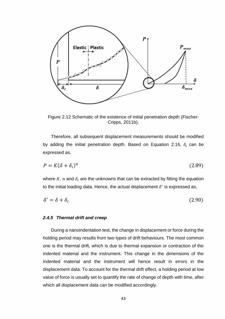
43
Figure 2.12 Schematic of the existence of initial penetration depth (Fischer-Cripps, 2011b).
Therefore, all subsequent displacement measurements should be modified
by adding the initial penetration depth. Based on Equation 2.16, 𝛿𝑖 can be
expressed as,
𝑃 = 𝐾(𝛿 + 𝛿𝑖)𝑛 (2.89)
where 𝐾, 𝑛 and 𝛿𝑖 are the unknowns that can be extracted by fitting the equation
to the initial loading data. Hence, the actual displacement 𝛿′ is expressed as,
𝛿′ = 𝛿 + 𝛿𝑖 (2.90)
2.4.5 Thermal drift and creep
During a nanoindentation test, the change in displacement or force during the
holding period may results from two types of drift behaviours. The most common
one is the thermal drift, which is due to thermal expansion or contraction of the
indented material and the instrument. This change in the dimensions of the
indented material and the instrument will hence result in errors in the
displacement data. To account for the thermal drift effect, a holding period at low
value of force is usually set to quantify the rate of change of depth with time, after
which all displacement data can be modified accordingly.
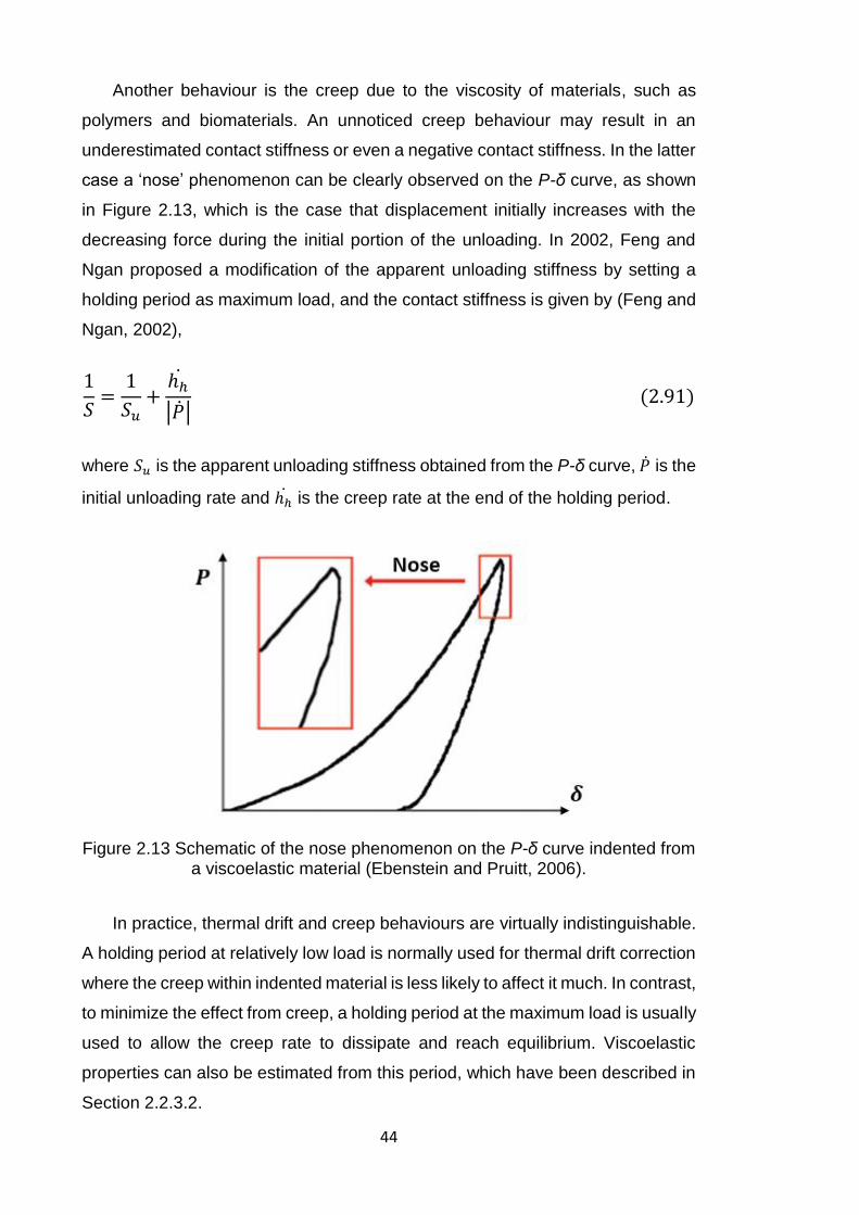
44
Another behaviour is the creep due to the viscosity of materials, such as
polymers and biomaterials. An unnoticed creep behaviour may result in an
underestimated contact stiffness or even a negative contact stiffness. In the latter
case a ‘nose’ phenomenon can be clearly observed on the P-δ curve, as shown
in Figure 2.13, which is the case that displacement initially increases with the
decreasing force during the initial portion of the unloading. In 2002, Feng and
Ngan proposed a modification of the apparent unloading stiffness by setting a
holding period as maximum load, and the contact stiffness is given by (Feng and
Ngan, 2002),
1
𝑆=
1
𝑆𝑢+
ℎℎ
|��| (2.91)
where 𝑆𝑢 is the apparent unloading stiffness obtained from the P-δ curve, �� is the
initial unloading rate and ℎℎ is the creep rate at the end of the holding period.
Figure 2.13 Schematic of the nose phenomenon on the P-δ curve indented from a viscoelastic material (Ebenstein and Pruitt, 2006).
In practice, thermal drift and creep behaviours are virtually indistinguishable.
A holding period at relatively low load is normally used for thermal drift correction
where the creep within indented material is less likely to affect it much. In contrast,
to minimize the effect from creep, a holding period at the maximum load is usually
used to allow the creep rate to dissipate and reach equilibrium. Viscoelastic
properties can also be estimated from this period, which have been described in
Section 2.2.3.2.
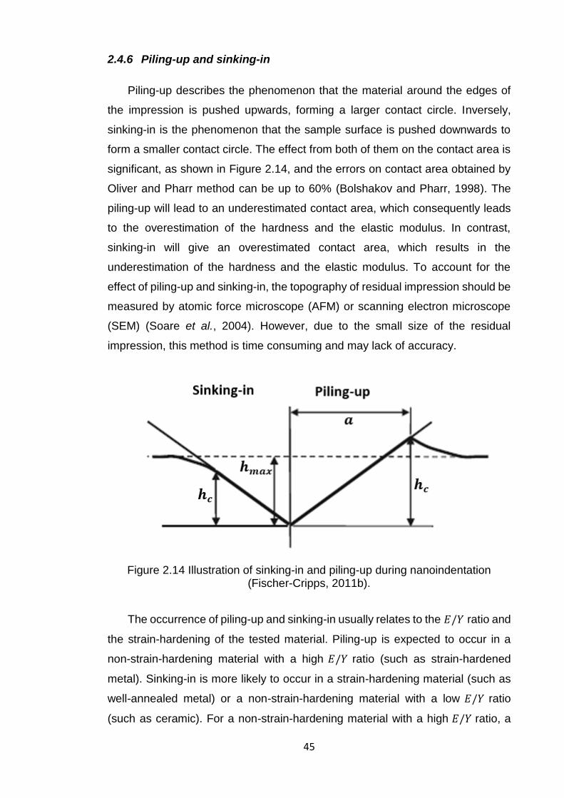
45
2.4.6 Piling-up and sinking-in
Piling-up describes the phenomenon that the material around the edges of
the impression is pushed upwards, forming a larger contact circle. Inversely,
sinking-in is the phenomenon that the sample surface is pushed downwards to
form a smaller contact circle. The effect from both of them on the contact area is
significant, as shown in Figure 2.14, and the errors on contact area obtained by
Oliver and Pharr method can be up to 60% (Bolshakov and Pharr, 1998). The
piling-up will lead to an underestimated contact area, which consequently leads
to the overestimation of the hardness and the elastic modulus. In contrast,
sinking-in will give an overestimated contact area, which results in the
underestimation of the hardness and the elastic modulus. To account for the
effect of piling-up and sinking-in, the topography of residual impression should be
measured by atomic force microscope (AFM) or scanning electron microscope
(SEM) (Soare et al., 2004). However, due to the small size of the residual
impression, this method is time consuming and may lack of accuracy.
Figure 2.14 Illustration of sinking-in and piling-up during nanoindentation (Fischer-Cripps, 2011b).
The occurrence of piling-up and sinking-in usually relates to the 𝐸/𝑌 ratio and
the strain-hardening of the tested material. Piling-up is expected to occur in a
non-strain-hardening material with a high 𝐸/𝑌 ratio (such as strain-hardened
metal). Sinking-in is more likely to occur in a strain-hardening material (such as
well-annealed metal) or a non-strain-hardening material with a low 𝐸/𝑌 ratio
(such as ceramic). For a non-strain-hardening material with a high 𝐸/𝑌 ratio, a
46
well-developed plastic deformation zone presents a hemispherical shape
meeting the sample surface outside the contact circle, in which case most of the
plastic deformation occurs in the area around the tip. For a strain-hardening
material, during the nanoindentation test, the material within the plastic
deformation zone becomes harder with increasing displacement. Therefore, the
material outside the plastic deformation zone tends to be elastically deformed.
Since the material within the plastic deformation zone actually acts as an effective
indenter and indents downwards, sinking-in occurs. For a non-strain-hardening
material with a low 𝐸/𝑌 ratio, the plastic deformation is typically confined and the
elastic deformation is spread to a larger area to accommodate the indented
volume. Thus, sinking-in is to be expected in this case.
2.4.7 Indentation size effect
Indentation size effect (ISE) is the phenomenon that the hardness of a
material changes with the decreasing displacement, which is expected to be
independent of scale, at very small indentation depth. This phenomenon exists in
the nanoindentation of nearly all materials at sufficiently small displacement. In
2003, Bull summarized the various mechanisms of ISE and classified them as
the extrinsic causes and the intrinsic causes (Bull, 2003).
Extrinsic causes are the effects related to the sample surface conditions or
the tip area function calibration. They can be removed or minimized with careful
sample preparation and careful tip area function calibration. These extrinsic
causes include:
The presence of very thin oxide layers arising from environmental
exposure. Due to the different mechanical properties of the thin oxide
layer, the observed ISE indeed reflects the sample behaviour.
Errors arising from sample preparation. For some metals, ISE is observed
due to work hardening and residual stresses induced by polishing
procedure. For ceramics, ISE arises due to cracks at shallow depth and
residual stresses induced by polishing procedure.
The presence of interfacial friction between the tip and indented material
(Li et al., 1993).
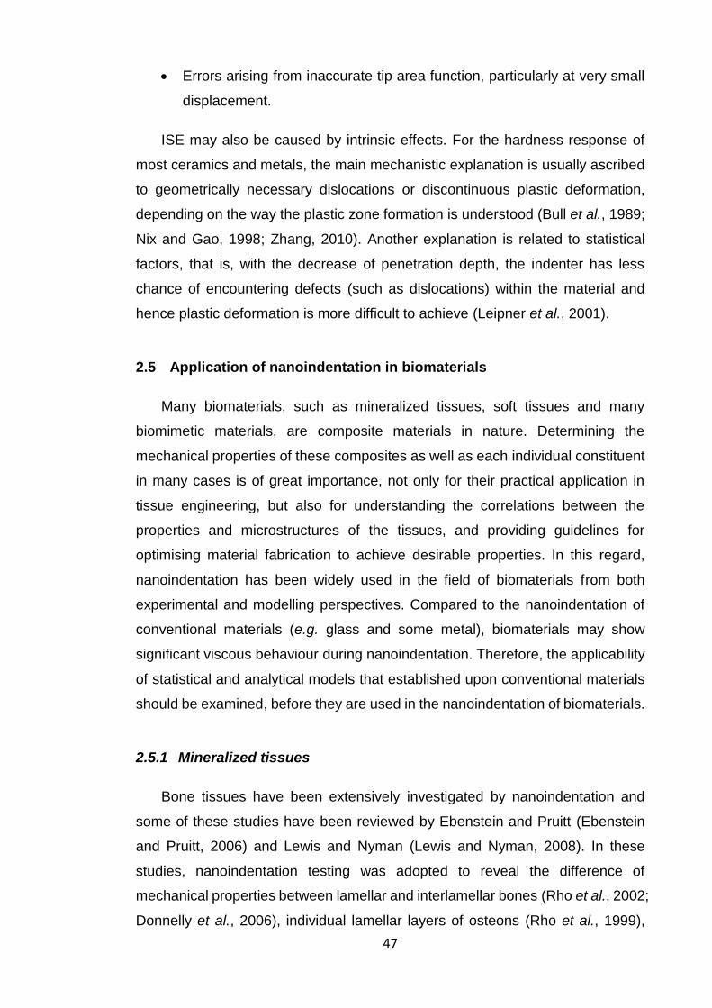
47
Errors arising from inaccurate tip area function, particularly at very small
displacement.
ISE may also be caused by intrinsic effects. For the hardness response of
most ceramics and metals, the main mechanistic explanation is usually ascribed
to geometrically necessary dislocations or discontinuous plastic deformation,
depending on the way the plastic zone formation is understood (Bull et al., 1989;
Nix and Gao, 1998; Zhang, 2010). Another explanation is related to statistical
factors, that is, with the decrease of penetration depth, the indenter has less
chance of encountering defects (such as dislocations) within the material and
hence plastic deformation is more difficult to achieve (Leipner et al., 2001).
2.5 Application of nanoindentation in biomaterials
Many biomaterials, such as mineralized tissues, soft tissues and many
biomimetic materials, are composite materials in nature. Determining the
mechanical properties of these composites as well as each individual constituent
in many cases is of great importance, not only for their practical application in
tissue engineering, but also for understanding the correlations between the
properties and microstructures of the tissues, and providing guidelines for
optimising material fabrication to achieve desirable properties. In this regard,
nanoindentation has been widely used in the field of biomaterials from both
experimental and modelling perspectives. Compared to the nanoindentation of
conventional materials (e.g. glass and some metal), biomaterials may show
significant viscous behaviour during nanoindentation. Therefore, the applicability
of statistical and analytical models that established upon conventional materials
should be examined, before they are used in the nanoindentation of biomaterials.
2.5.1 Mineralized tissues
Bone tissues have been extensively investigated by nanoindentation and
some of these studies have been reviewed by Ebenstein and Pruitt (Ebenstein
and Pruitt, 2006) and Lewis and Nyman (Lewis and Nyman, 2008). In these
studies, nanoindentation testing was adopted to reveal the difference of
mechanical properties between lamellar and interlamellar bones (Rho et al., 2002;
Donnelly et al., 2006), individual lamellar layers of osteons (Rho et al., 1999),
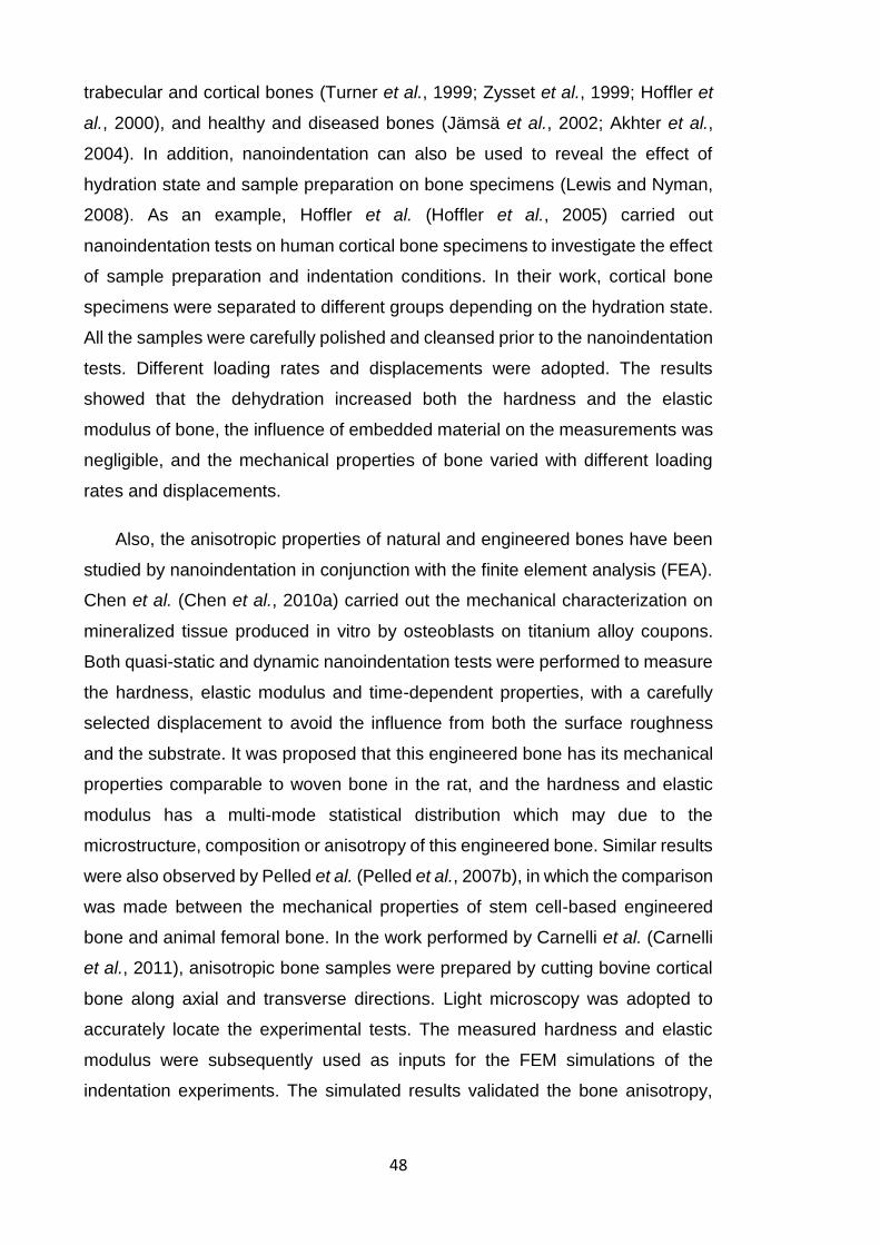
48
trabecular and cortical bones (Turner et al., 1999; Zysset et al., 1999; Hoffler et
al., 2000), and healthy and diseased bones (Jämsä et al., 2002; Akhter et al.,
2004). In addition, nanoindentation can also be used to reveal the effect of
hydration state and sample preparation on bone specimens (Lewis and Nyman,
2008). As an example, Hoffler et al. (Hoffler et al., 2005) carried out
nanoindentation tests on human cortical bone specimens to investigate the effect
of sample preparation and indentation conditions. In their work, cortical bone
specimens were separated to different groups depending on the hydration state.
All the samples were carefully polished and cleansed prior to the nanoindentation
tests. Different loading rates and displacements were adopted. The results
showed that the dehydration increased both the hardness and the elastic
modulus of bone, the influence of embedded material on the measurements was
negligible, and the mechanical properties of bone varied with different loading
rates and displacements.
Also, the anisotropic properties of natural and engineered bones have been
studied by nanoindentation in conjunction with the finite element analysis (FEA).
Chen et al. (Chen et al., 2010a) carried out the mechanical characterization on
mineralized tissue produced in vitro by osteoblasts on titanium alloy coupons.
Both quasi-static and dynamic nanoindentation tests were performed to measure
the hardness, elastic modulus and time-dependent properties, with a carefully
selected displacement to avoid the influence from both the surface roughness
and the substrate. It was proposed that this engineered bone has its mechanical
properties comparable to woven bone in the rat, and the hardness and elastic
modulus has a multi-mode statistical distribution which may due to the
microstructure, composition or anisotropy of this engineered bone. Similar results
were also observed by Pelled et al. (Pelled et al., 2007b), in which the comparison
was made between the mechanical properties of stem cell-based engineered
bone and animal femoral bone. In the work performed by Carnelli et al. (Carnelli
et al., 2011), anisotropic bone samples were prepared by cutting bovine cortical
bone along axial and transverse directions. Light microscopy was adopted to
accurately locate the experimental tests. The measured hardness and elastic
modulus were subsequently used as inputs for the FEM simulations of the
indentation experiments. The simulated results validated the bone anisotropy,
49
and proved that FEA is a useful tool to enable us to get a deeper understanding
of the mechanical properties of mineralized tissues.
In teeth, nanoindentation testing has been primarily used to obtain the
nanomechanical mapping around the dentin-enamel interface to investigate the
transition between the less mineralized dentin and the more mineralized enamel
(Fong et al., 1999; Urabe et al., 2000; Marshall et al., 2001a), with an example
shown in Figure 2.15. In conjunction with the chemical mapping, the changes of
hardness, elastic modulus and mineral content around the dentin-enamel
interface were extensively studied by nanoindentation (Tesch et al., 2001; Cuy et
al., 2002). In addition, nanoindentation testing integrated with other methods was
also adopted to reveal the mechanical, chemical and structural difference
between the enamel prisms and sheaths (Ge et al., 2005), peritubular and
intertubular dentin (Kinney et al., 1996a; Kinney et al., 1996b), cementum and
dentin (Ho et al., 2004; Ho et al., 2005), and healthy dentin and carious dentin
(Marshall et al., 2001b; Angker et al., 2005).
Figure 2.15 Schematic of mechanical transition between dentin and enamel. The plot showed the corresponding mechanical properties determined from
indentations. It showed that both hardness and elastic modulus rapidly decreased from enamel region to dentin region (Marshall et al., 2001a).
Another interesting case study of mineralized tissues is the modelling of
arthropod exoskeleton carried out by Nikolov et al. (Nikolov et al., 2010).
Arthropod exoskeleton, such as the lobster cuticle, usually has a hierarchical
biological structure with chitin protein fibres. In this study, the lobster exoskeleton
was modelled in a multiscale FE model to study the correlation between the
50
hierarchical structure and the anisotropic properties of the chitin fibre. Figure 2.16
shows the key microstructures of lobster cuticle at various length scales. These
simulation results showed that the cholesteric plywood superstructure allowed
the reinforcement of the cuticle by chitin-protein fibres, provided the transverse
isotropic properties to resist the macroscopic force, prevented microcrack
propagation, and enabled energy dissipation during impact loading.
Figure 2.16 Hierarchical structure of the FE model of lobster cuticle: (I) N-acetyl-glucosamine molecules, (II) α-chitin chains, (III) representative volume element
(RVE) of a chitin fibre, (IVa) RVE of chitin fibres arranged in twisted plywood without canals, (IVb) RVE of mineral-protein matrix, (V) transversely isotropic cuticle without canals, (VI) cuticle with a hexagonal array of canals, and (VII)
composite cuticle (Nikolov et al., 2010).
2.5.2 Soft tissues
For soft tissues, nanoindentation has also proven itself to be a valuable tool
for the measurement of mechanical properties of cartilage (Ebenstein et al., 2004;
Simha et al., 2004), demineralized dentin (Balooch et al., 1998), the stratum
corneum layer of skin (Yuan and Verma, 2006), diseased artery tissue (Ebenstein
and Pruitt, 2004) and healthy arteries (Lundkvist et al., 1996). As an example,
Lundkvist et al. (Lundkvist et al., 1996) carried out AFM-based indentation tests
on healthy human artery to investigate the viscoelastic properties. The samples
were prepared by cutting the vessel longitudinally into squares and placing in
saline solution. Indents were performed in liquid with a spherical indenter. The
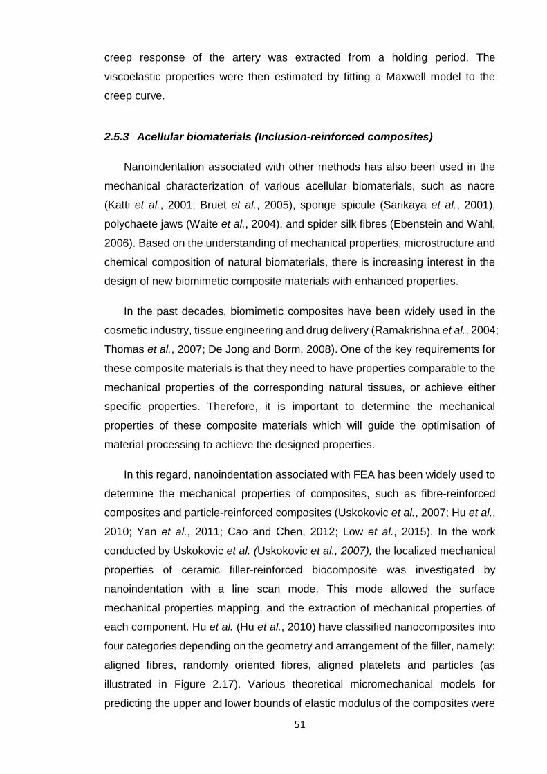
51
creep response of the artery was extracted from a holding period. The
viscoelastic properties were then estimated by fitting a Maxwell model to the
creep curve.
2.5.3 Acellular biomaterials (Inclusion-reinforced composites)
Nanoindentation associated with other methods has also been used in the
mechanical characterization of various acellular biomaterials, such as nacre
(Katti et al., 2001; Bruet et al., 2005), sponge spicule (Sarikaya et al., 2001),
polychaete jaws (Waite et al., 2004), and spider silk fibres (Ebenstein and Wahl,
2006). Based on the understanding of mechanical properties, microstructure and
chemical composition of natural biomaterials, there is increasing interest in the
design of new biomimetic composite materials with enhanced properties.
In the past decades, biomimetic composites have been widely used in the
cosmetic industry, tissue engineering and drug delivery (Ramakrishna et al., 2004;
Thomas et al., 2007; De Jong and Borm, 2008). One of the key requirements for
these composite materials is that they need to have properties comparable to the
mechanical properties of the corresponding natural tissues, or achieve either
specific properties. Therefore, it is important to determine the mechanical
properties of these composite materials which will guide the optimisation of
material processing to achieve the designed properties.
In this regard, nanoindentation associated with FEA has been widely used to
determine the mechanical properties of composites, such as fibre-reinforced
composites and particle-reinforced composites (Uskokovic et al., 2007; Hu et al.,
2010; Yan et al., 2011; Cao and Chen, 2012; Low et al., 2015). In the work
conducted by Uskokovic et al. (Uskokovic et al., 2007), the localized mechanical
properties of ceramic filler-reinforced biocomposite was investigated by
nanoindentation with a line scan mode. This mode allowed the surface
mechanical properties mapping, and the extraction of mechanical properties of
each component. Hu et al. (Hu et al., 2010) have classified nanocomposites into
four categories depending on the geometry and arrangement of the filler, namely:
aligned fibres, randomly oriented fibres, aligned platelets and particles (as
illustrated in Figure 2.17). Various theoretical micromechanical models for
predicting the upper and lower bounds of elastic modulus of the composites were
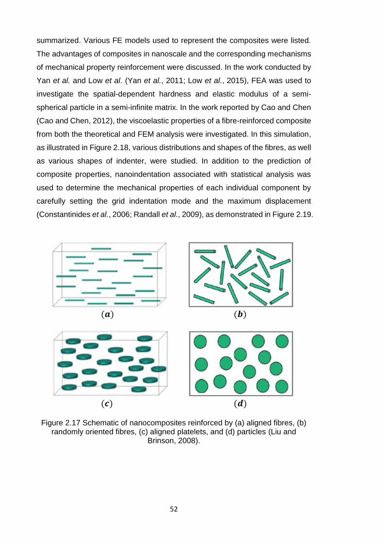
52
summarized. Various FE models used to represent the composites were listed.
The advantages of composites in nanoscale and the corresponding mechanisms
of mechanical property reinforcement were discussed. In the work conducted by
Yan et al. and Low et al. (Yan et al., 2011; Low et al., 2015), FEA was used to
investigate the spatial-dependent hardness and elastic modulus of a semi-
spherical particle in a semi-infinite matrix. In the work reported by Cao and Chen
(Cao and Chen, 2012), the viscoelastic properties of a fibre-reinforced composite
from both the theoretical and FEM analysis were investigated. In this simulation,
as illustrated in Figure 2.18, various distributions and shapes of the fibres, as well
as various shapes of indenter, were studied. In addition to the prediction of
composite properties, nanoindentation associated with statistical analysis was
used to determine the mechanical properties of each individual component by
carefully setting the grid indentation mode and the maximum displacement
(Constantinides et al., 2006; Randall et al., 2009), as demonstrated in Figure 2.19.
Figure 2.17 Schematic of nanocomposites reinforced by (a) aligned fibres, (b) randomly oriented fibres, (c) aligned platelets, and (d) particles (Liu and
Brinson, 2008).
(𝒂) (𝒃)
(𝒄) (𝒅)
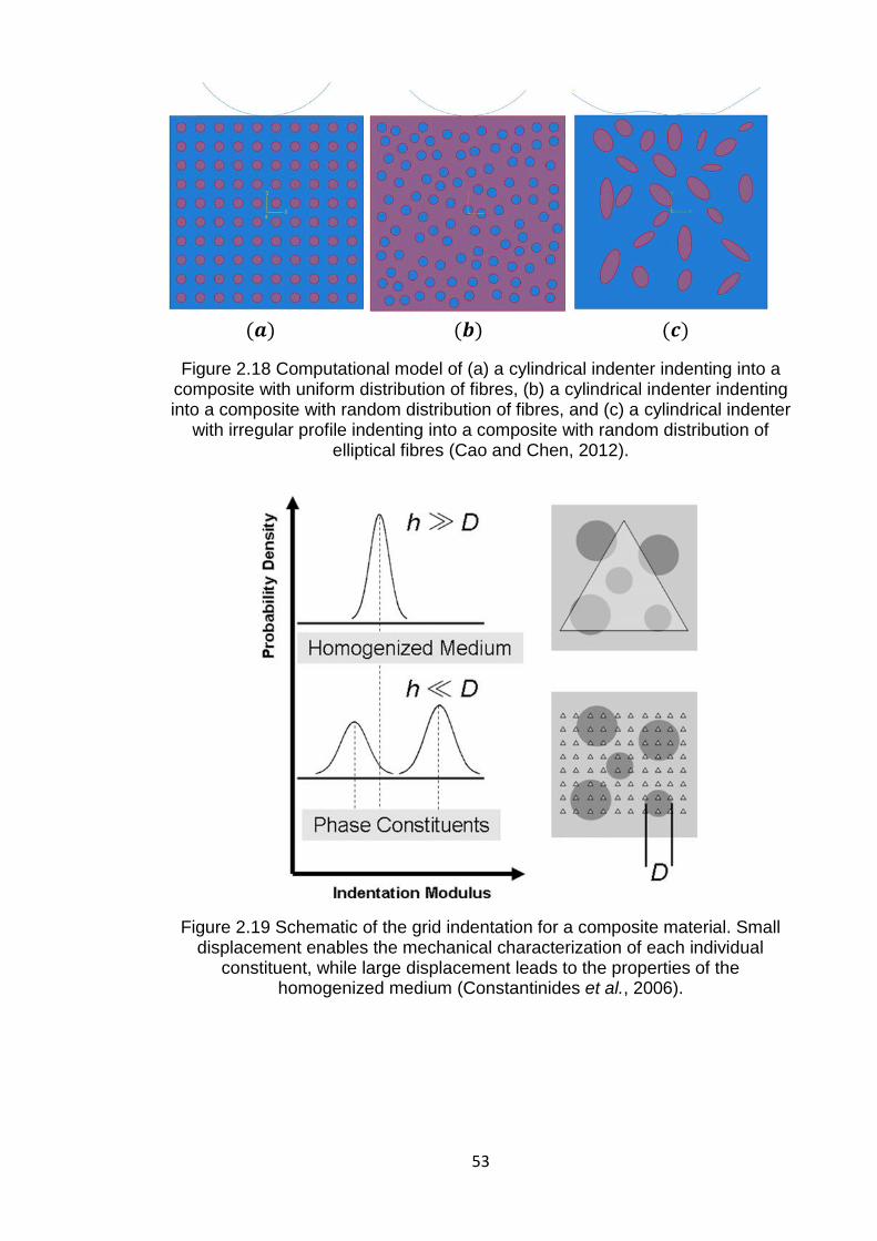
53
Figure 2.18 Computational model of (a) a cylindrical indenter indenting into a composite with uniform distribution of fibres, (b) a cylindrical indenter indenting into a composite with random distribution of fibres, and (c) a cylindrical indenter
with irregular profile indenting into a composite with random distribution of elliptical fibres (Cao and Chen, 2012).
Figure 2.19 Schematic of the grid indentation for a composite material. Small displacement enables the mechanical characterization of each individual
constituent, while large displacement leads to the properties of the homogenized medium (Constantinides et al., 2006).
(𝒂) (𝒃) (𝒄)

54
2.6 Summary
In this chapter, a variety of nanoindentation methods were introduced, which
were used to estimate mechanical properties of the indented material (hardness,
elastic modulus and time-dependent properties). Indenter selection, factors that
affect the results, and the application of nanoindentation in biomaterials from both
experimental and modelling perspectives were discussed. In the next chapter,
based on the computational modelling, a fibre/matrix composite model will be
presented to assess its viscoelastic response during nanoindentation.
Chapter 3
Nanomechanical Modelling of
Viscoelastic Fibre in
Viscoelastic Matrix
56
Chapter 3. Nanomechanical Modelling of Viscoelastic Fibre in
Viscoelastic Matrix
3.1 Introduction
In the past decades, fibre-reinforced polymer composite materials have been
widely applied in many fields, such as aerospace, military equipment, automobile,
construction and tissue engineering, due to their highly advanced performance
over conventional materials (Lou and Schapery, 1971; Bakis et al., 2002; Kalia et
al., 2009; Akil et al., 2011; Ozbakkaloglu et al., 2016). For some composite
materials, such as glass fibre-reinforced plastic, solid propellant, and some
biomimetic materials, they may exhibit significant viscoelastic behaviour (Hashin,
1966; Lou and Schapery, 1971; Calvert, 1992).
Nanoindentation is particularly useful to determine the elastic moduli of
individual phases in composite materials such as biopolymer composites for
tissue engineering (Herruzo et al., 2014). When performing nanoindentation on
these fibre-reinforced composite materials, it is essential to define the influence
of the surrounding second phase. Thus, this chapter is focused on the
investigation of the viscoelastic response of the unidirectional fibre/matrix
composite under nanoindentation test by FEA. FEA of nanoindentation has been
widely used to better understand experimental results and guide the design of
experimental protocols. This numerical method is based on the assumption that
an approximate solution of any indentation problem can be reached by
subdividing the tested material, which may have complex structure or properties,
into smaller and simpler parts. FEA is a powerful tool to simulate the
nanoindentation processes in ideal conditions, which may be limited in an
experimental approach. In addition, it can also help extract more information from
the experimental results and enable us to get a deeper understanding of the
tested material. The disadvantage of the FEA is that the accuracy of the
simulations and convergence are dependent on the design of mesh. It is also a
continuum solution which is no longer valid at small scale, where individual atomic
processes are dominated. The reliability of the model also depends on the careful
selection of constitutive models for materials properties.
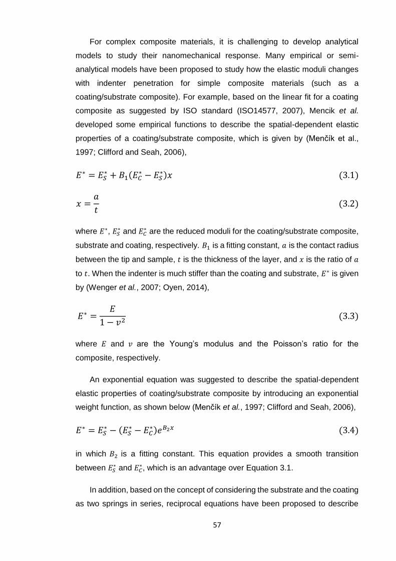
57
For complex composite materials, it is challenging to develop analytical
models to study their nanomechanical response. Many empirical or semi-
analytical models have been proposed to study how the elastic moduli changes
with indenter penetration for simple composite materials (such as a
coating/substrate composite). For example, based on the linear fit for a coating
composite as suggested by ISO standard (ISO14577, 2007), Mencik et al.
developed some empirical functions to describe the spatial-dependent elastic
properties of a coating/substrate composite, which is given by (Menčík et al.,
1997; Clifford and Seah, 2006),
𝐸∗ = 𝐸𝑆∗ + 𝐵1(𝐸𝐶
∗ − 𝐸𝑆∗)𝑥 (3.1)
𝑥 =𝑎
𝑡 (3.2)
where 𝐸∗, 𝐸𝑆∗ and 𝐸𝐶
∗ are the reduced moduli for the coating/substrate composite,
substrate and coating, respectively. 𝐵1 is a fitting constant, 𝑎 is the contact radius
between the tip and sample, 𝑡 is the thickness of the layer, and 𝑥 is the ratio of 𝑎
to 𝑡. When the indenter is much stiffer than the coating and substrate, 𝐸∗ is given
by (Wenger et al., 2007; Oyen, 2014),
𝐸∗ =𝐸
1 − 𝑣2 (3.3)
where 𝐸 and 𝑣 are the Young’s modulus and the Poisson’s ratio for the
composite, respectively.
An exponential equation was suggested to describe the spatial-dependent
elastic properties of coating/substrate composite by introducing an exponential
weight function, as shown below (Menčík et al., 1997; Clifford and Seah, 2006),
𝐸∗ = 𝐸𝑆∗ − (𝐸𝑆
∗ − 𝐸𝐶∗)𝑒𝐵2𝑥 (3.4)
in which 𝐵2 is a fitting constant. This equation provides a smooth transition
between 𝐸𝑆∗ and 𝐸𝐶
∗, which is an advantage over Equation 3.1.
In addition, based on the concept of considering the substrate and the coating
as two springs in series, reciprocal equations have been proposed to describe
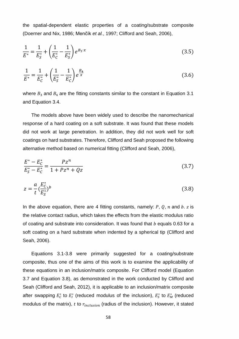
58
the spatial-dependent elastic properties of a coating/substrate composite
(Doerner and Nix, 1986; Menčík et al., 1997; Clifford and Seah, 2006),
1
𝐸∗=
1
𝐸𝑆∗ + (
1
𝐸𝐶∗ −
1
𝐸𝑆∗) 𝑒𝐵3∙𝑥 (3.5)
1
𝐸∗=
1
𝐸𝐶∗ + (
1
𝐸𝑆∗ −
1
𝐸𝐶∗) 𝑒
𝐵4𝑥 (3.6)
where 𝐵3 and 𝐵4 are the fitting constants similar to the constant in Equation 3.1
and Equation 3.4.
The models above have been widely used to describe the nanomechanical
response of a hard coating on a soft substrate. It was found that these models
did not work at large penetration. In addition, they did not work well for soft
coatings on hard substrates. Therefore, Clifford and Seah proposed the following
alternative method based on numerical fitting (Clifford and Seah, 2006),
𝐸∗ − 𝐸𝐶∗
𝐸𝑆∗ − 𝐸𝐶
∗ =𝑃𝑧𝑛
1 + 𝑃𝑧𝑛 + 𝑄𝑧 (3.7)
𝑧 =𝑎
𝑡(𝐸𝐶
∗
𝐸𝑆∗)𝑏 (3.8)
In the above equation, there are 4 fitting constants, namely: 𝑃, 𝑄, 𝑛 and 𝑏. 𝑧 is
the relative contact radius, which takes the effects from the elastic modulus ratio
of coating and substrate into consideration. It was found that 𝑏 equals 0.63 for a
soft coating on a hard substrate when indented by a spherical tip (Clifford and
Seah, 2006).
Equations 3.1-3.8 were primarily suggested for a coating/substrate
composite, thus one of the aims of this work is to examine the applicability of
these equations in an inclusion/matrix composite. For Clifford model (Equation
3.7 and Equation 3.8), as demonstrated in the work conducted by Clifford and
Seah (Clifford and Seah, 2012), it is applicable to an inclusion/matrix composite
after swapping 𝐸𝐶∗ to 𝐸𝐼
∗ (reduced modulus of the inclusion), 𝐸𝑆∗ to 𝐸𝑀
∗ (reduced
modulus of the matrix), 𝑡 to 𝑟𝑖𝑛𝑐𝑙𝑢𝑠𝑖𝑜𝑛 (radius of the inclusion). However, it stated
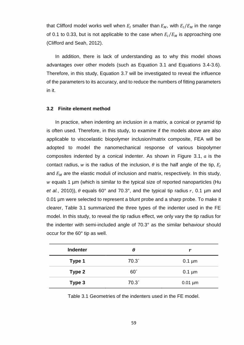
59
that Clifford model works well when 𝐸𝐼 smaller than 𝐸𝑀, with 𝐸𝐼/𝐸𝑀 in the range
of 0.1 to 0.33, but is not applicable to the case when 𝐸𝐼 𝐸𝑀⁄ is approaching one
(Clifford and Seah, 2012).
In addition, there is lack of understanding as to why this model shows
advantages over other models (such as Equation 3.1 and Equations 3.4-3.6).
Therefore, in this study, Equation 3.7 will be investigated to reveal the influence
of the parameters to its accuracy, and to reduce the numbers of fitting parameters
in it.
3.2 Finite element method
In practice, when indenting an inclusion in a matrix, a conical or pyramid tip
is often used. Therefore, in this study, to examine if the models above are also
applicable to viscoelastic biopolymer inclusion/matrix composite, FEA will be
adopted to model the nanomechanical response of various biopolymer
composites indented by a conical indenter. As shown in Figure 3.1, 𝑎 is the
contact radius, 𝑤 is the radius of the inclusion, 𝜃 is the half angle of the tip, 𝐸𝐼
and 𝐸𝑀 are the elastic moduli of inclusion and matrix, respectively. In this study,
𝑤 equals 1 µm (which is similar to the typical size of reported nanoparticles (Hu
et al., 2010)), 𝜃 equals 60° and 70.3°, and the typical tip radius 𝑟, 0.1 µm and
0.01 µm were selected to represent a blunt probe and a sharp probe. To make it
clearer, Table 3.1 summarized the three types of the indenter used in the FE
model. In this study, to reveal the tip radius effect, we only vary the tip radius for
the indenter with semi-included angle of 70.3° as the similar behaviour should
occur for the 60° tip as well.
Indenter 𝜽 𝒓
Type 1 70.3˚ 0.1 µm
Type 2 60˚ 0.1 µm
Type 3 70.3˚ 0.01 µm
Table 3.1 Geometries of the indenters used in the FE model.
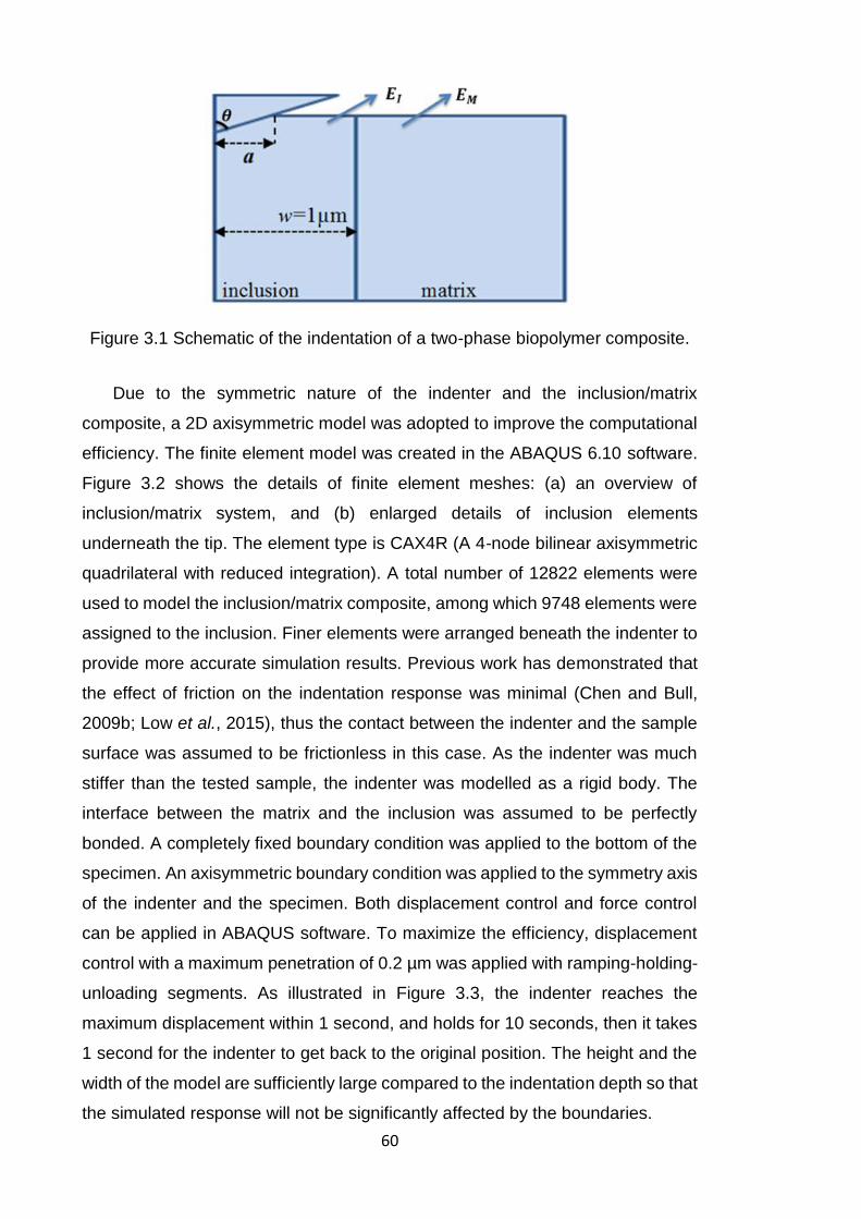
60
Figure 3.1 Schematic of the indentation of a two-phase biopolymer composite.
Due to the symmetric nature of the indenter and the inclusion/matrix
composite, a 2D axisymmetric model was adopted to improve the computational
efficiency. The finite element model was created in the ABAQUS 6.10 software.
Figure 3.2 shows the details of finite element meshes: (a) an overview of
inclusion/matrix system, and (b) enlarged details of inclusion elements
underneath the tip. The element type is CAX4R (A 4-node bilinear axisymmetric
quadrilateral with reduced integration). A total number of 12822 elements were
used to model the inclusion/matrix composite, among which 9748 elements were
assigned to the inclusion. Finer elements were arranged beneath the indenter to
provide more accurate simulation results. Previous work has demonstrated that
the effect of friction on the indentation response was minimal (Chen and Bull,
2009b; Low et al., 2015), thus the contact between the indenter and the sample
surface was assumed to be frictionless in this case. As the indenter was much
stiffer than the tested sample, the indenter was modelled as a rigid body. The
interface between the matrix and the inclusion was assumed to be perfectly
bonded. A completely fixed boundary condition was applied to the bottom of the
specimen. An axisymmetric boundary condition was applied to the symmetry axis
of the indenter and the specimen. Both displacement control and force control
can be applied in ABAQUS software. To maximize the efficiency, displacement
control with a maximum penetration of 0.2 µm was applied with ramping-holding-
unloading segments. As illustrated in Figure 3.3, the indenter reaches the
maximum displacement within 1 second, and holds for 10 seconds, then it takes
1 second for the indenter to get back to the original position. The height and the
width of the model are sufficiently large compared to the indentation depth so that
the simulated response will not be significantly affected by the boundaries.
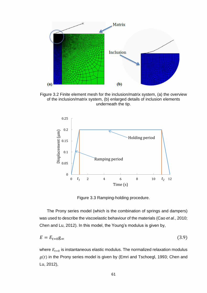
61
Figure 3.2 Finite element mesh for the inclusion/matrix system, (a) the overview of the inclusion/matrix system, (b) enlarged details of inclusion elements
underneath the tip.
Figure 3.3 Ramping-holding procedure.
The Prony series model (which is the combination of springs and dampers)
was used to describe the viscoelastic behaviour of the materials (Cao et al., 2010;
Chen and Lu, 2012). In this model, the Young’s modulus is given by,
𝐸 = 𝐸𝑡=0g∞ (3.9)
where 𝐸𝑡=0 is instantaneous elastic modulus. The normalized relaxation modulus
𝑔(𝑡) in the Prony series model is given by (Emri and Tschoegl, 1993; Chen and
Lu, 2012),
0
0.05
0.1
0.15
0.2
0.25
0 2 4 6 8 10 12
Dis
pla
cem
ent
(µm
)
Time (s)
t1 t2
Ramping period
Holding period
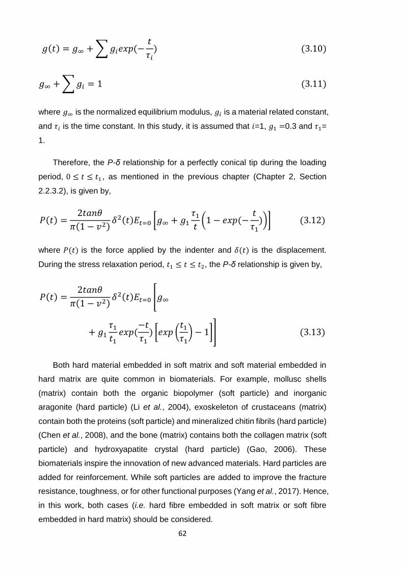
62
𝑔(𝑡) = 𝑔∞ + ∑ 𝑔𝑖𝑒𝑥𝑝 (−𝑡
𝜏𝑖) (3.10)
𝑔∞ + ∑ 𝑔𝑖 = 1 (3.11)
where 𝑔∞ is the normalized equilibrium modulus, 𝑔𝑖 is a material related constant,
and 𝜏𝑖 is the time constant. In this study, it is assumed that 𝑖=1, 𝑔1 =0.3 and 𝜏1=
1.
Therefore, the P-δ relationship for a perfectly conical tip during the loading
period, 0 ≤ 𝑡 ≤ 𝑡1 , as mentioned in the previous chapter (Chapter 2, Section
2.2.3.2), is given by,
𝑃(𝑡) =2𝑡𝑎𝑛𝜃
𝜋(1 − 𝑣2)𝛿2(𝑡)𝐸𝑡=0 [𝑔∞ + 𝑔1
𝜏1
𝑡(1 − 𝑒𝑥𝑝 (−
𝑡
𝜏1))] (3.12)
where 𝑃(𝑡) is the force applied by the indenter and 𝛿(𝑡) is the displacement.
During the stress relaxation period, 𝑡1 ≤ 𝑡 ≤ 𝑡2, the P-δ relationship is given by,
𝑃(𝑡) =2𝑡𝑎𝑛𝜃
𝜋(1 − 𝑣2)𝛿2(𝑡)𝐸𝑡=0 [𝑔∞
+ 𝑔1
𝜏1
𝑡1𝑒𝑥𝑝 (
−𝑡
𝜏1) [𝑒𝑥𝑝 (
𝑡1
𝜏1) − 1]] (3.13)
Both hard material embedded in soft matrix and soft material embedded in
hard matrix are quite common in biomaterials. For example, mollusc shells
(matrix) contain both the organic biopolymer (soft particle) and inorganic
aragonite (hard particle) (Li et al., 2004), exoskeleton of crustaceans (matrix)
contain both the proteins (soft particle) and mineralized chitin fibrils (hard particle)
(Chen et al., 2008), and the bone (matrix) contains both the collagen matrix (soft
particle) and hydroxyapatite crystal (hard particle) (Gao, 2006). These
biomaterials inspire the innovation of new advanced materials. Hard particles are
added for reinforcement. While soft particles are added to improve the fracture
resistance, toughness, or for other functional purposes (Yang et al., 2017). Hence,
in this work, both cases (i.e. hard fibre embedded in soft matrix or soft fibre
embedded in hard matrix) should be considered.
63
In this study, the Poisson’s ratios of the inclusion and matrix were fixed at 0.3.
According to the elastic modulus of typical biopolymers reported in literature, the
equilibrium elastic modulus of inclusion, 𝐸𝐼, was set to 10 MPa (similar to the
elastic modulus of 50/50 poly-L-lactic acid (PLLA)/poly-DL-lactic acid (PDLLA)
blends (Chen et al., 2003)). While the equilibrium elastic modulus of the matrix,
𝐸𝑀, varied from 2 MPa (similar to the elastic modulus of PDLLA (Chen et al.,
2003)) to 50 MPa (similar to the elastic modulus of 50/50 polyglycolic acid
(PGA)/gelatin blends (Hajiali et al., 2011)) to define the influence of surrounding
second phase, which covers a wide range of typical biopolymers (Chen et al.,
2003; Balakrishnan and Banerjee, 2011; Mukherjee and Kao, 2011). Additional
simulation was done by assuming 𝐸𝑀 = 𝐸𝐼 =10 MPa for calibration.
Matlab code was written to perform the curve fitting and extract the fitting
parameters in different models. The quality of the fitting was estimated by
calculating the minimum ‘𝑟𝑒𝑠𝑛𝑜𝑟𝑚’ value, which is given by,
𝑟𝑒𝑠𝑛𝑜𝑟𝑚 = ∑(𝐹(𝑥𝑖) − 𝑦𝑖)2
𝑖
(3.14)
where 𝑟𝑒𝑠𝑛𝑜𝑟𝑚 presents the quality of a fitting. This parameter can be
automatically obtained from Matlab software and it varies from zero to infinity.
Within this range, a smaller value indicates a better fitting and zero means a
perfect fitting. 𝐹(𝑥) is the predicted data from fitting equation, and 𝑦 is the
observed data from simulation. During the curve fitting, in order to improve the
computational efficiency, the fitting parameter 𝑏 in Clifford model was predefined
and manually adjusted until achieving a minimum 𝑟𝑒𝑠𝑛𝑜𝑟𝑚 value. Besides, the
influence of fitting parameters with different decimal places (i.e. 1, 2, 3…) on the
𝑟𝑒𝑠𝑛𝑜𝑟𝑚 value were investigated. Then, as a trade-off between efficiency and
accuracy, fitting parameters were rounded to 3 decimal places.
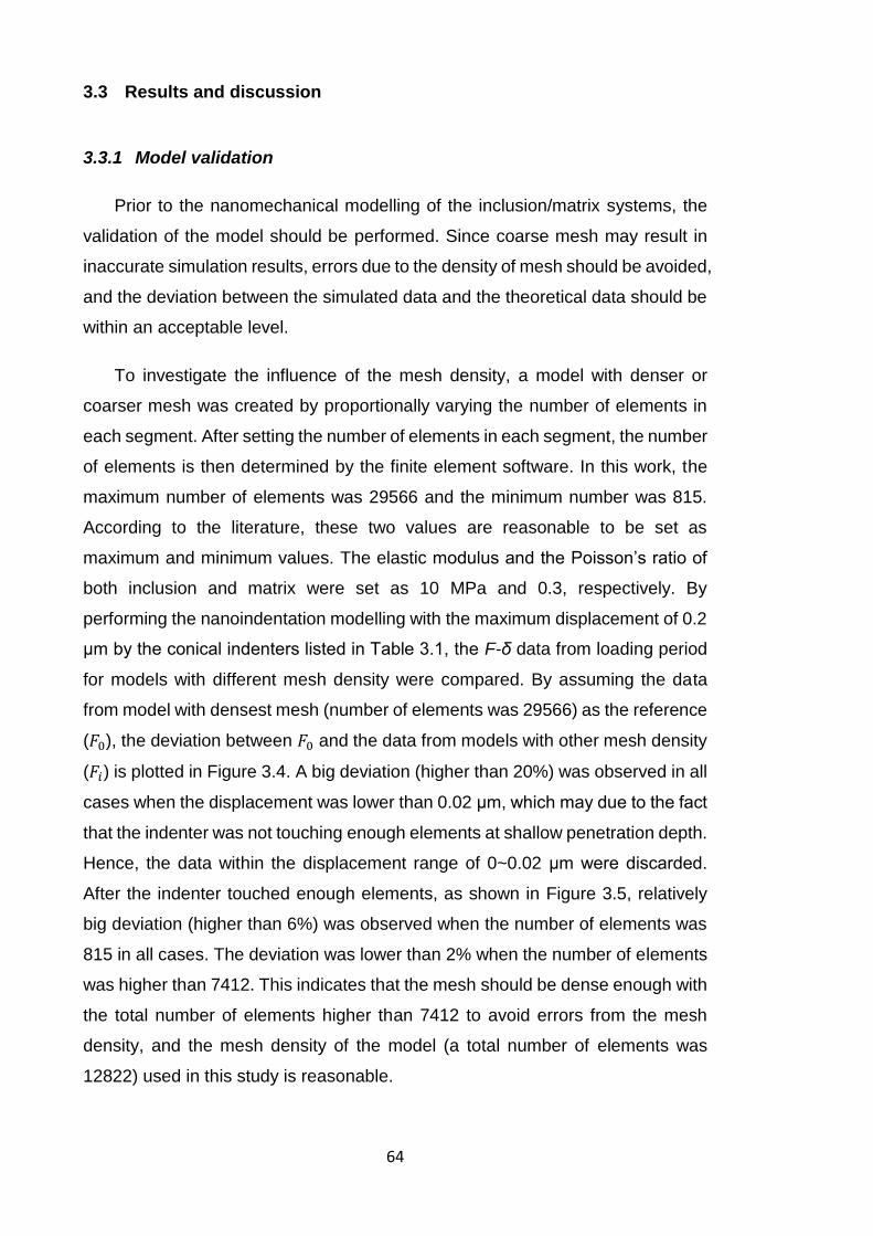
64
3.3 Results and discussion
3.3.1 Model validation
Prior to the nanomechanical modelling of the inclusion/matrix systems, the
validation of the model should be performed. Since coarse mesh may result in
inaccurate simulation results, errors due to the density of mesh should be avoided,
and the deviation between the simulated data and the theoretical data should be
within an acceptable level.
To investigate the influence of the mesh density, a model with denser or
coarser mesh was created by proportionally varying the number of elements in
each segment. After setting the number of elements in each segment, the number
of elements is then determined by the finite element software. In this work, the
maximum number of elements was 29566 and the minimum number was 815.
According to the literature, these two values are reasonable to be set as
maximum and minimum values. The elastic modulus and the Poisson’s ratio of
both inclusion and matrix were set as 10 MPa and 0.3, respectively. By
performing the nanoindentation modelling with the maximum displacement of 0.2
μm by the conical indenters listed in Table 3.1, the F-δ data from loading period
for models with different mesh density were compared. By assuming the data
from model with densest mesh (number of elements was 29566) as the reference
(𝐹0), the deviation between 𝐹0 and the data from models with other mesh density
(𝐹𝑖) is plotted in Figure 3.4. A big deviation (higher than 20%) was observed in all
cases when the displacement was lower than 0.02 μm, which may due to the fact
that the indenter was not touching enough elements at shallow penetration depth.
Hence, the data within the displacement range of 0~0.02 μm were discarded.
After the indenter touched enough elements, as shown in Figure 3.5, relatively
big deviation (higher than 6%) was observed when the number of elements was
815 in all cases. The deviation was lower than 2% when the number of elements
was higher than 7412. This indicates that the mesh should be dense enough with
the total number of elements higher than 7412 to avoid errors from the mesh
density, and the mesh density of the model (a total number of elements was
12822) used in this study is reasonable.
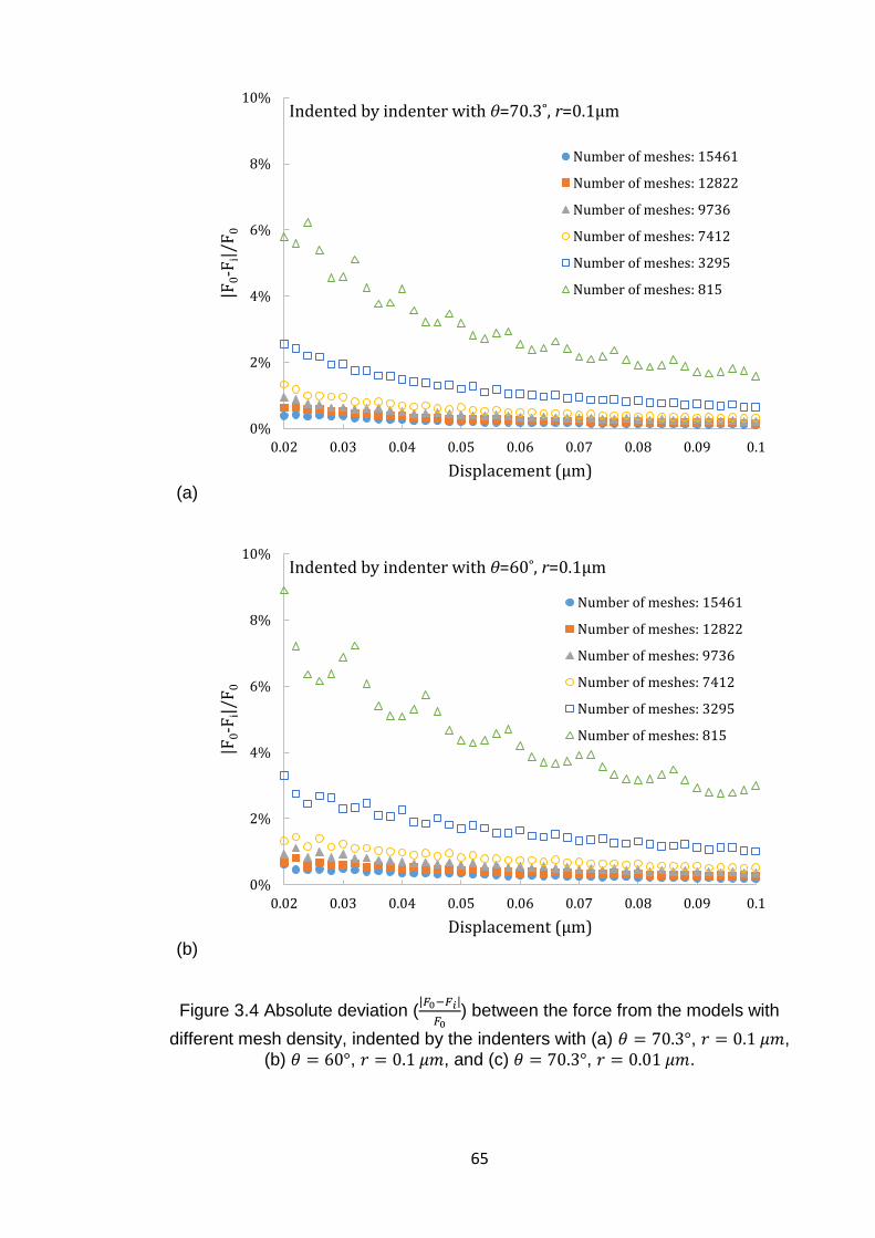
65
(a)
(b)
Figure 3.4 Absolute deviation (|𝐹0−𝐹𝑖|
𝐹0) between the force from the models with
different mesh density, indented by the indenters with (a) 𝜃 = 70.3°, 𝑟 = 0.1 𝜇𝑚, (b) 𝜃 = 60°, 𝑟 = 0.1 𝜇𝑚, and (c) 𝜃 = 70.3°, 𝑟 = 0.01 𝜇𝑚.
0%
2%
4%
6%
8%
10%
0.02 0.03 0.04 0.05 0.06 0.07 0.08 0.09 0.1
|F0-F
i|/F
0
Displacement (µm)
Indented by indenter with θ=70.3˚, r=0.1μm
Number of meshes: 15461
Number of meshes: 12822
Number of meshes: 9736
Number of meshes: 7412
Number of meshes: 3295
Number of meshes: 815
0%
2%
4%
6%
8%
10%
0.02 0.03 0.04 0.05 0.06 0.07 0.08 0.09 0.1
|F0-F
i|/F
0
Displacement (µm)
Indented by indenter with θ=60˚, r=0.1μm
Number of meshes: 15461
Number of meshes: 12822
Number of meshes: 9736
Number of meshes: 7412
Number of meshes: 3295
Number of meshes: 815
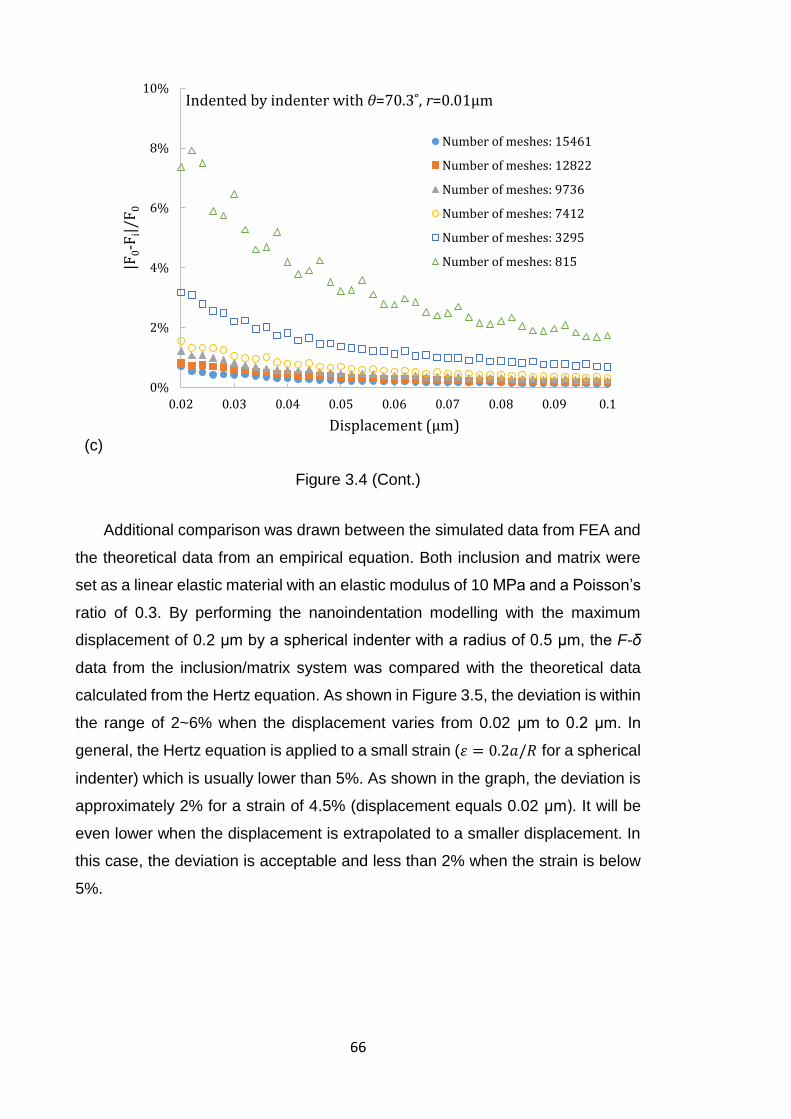
66
(c)
Figure 3.4 (Cont.)
Additional comparison was drawn between the simulated data from FEA and
the theoretical data from an empirical equation. Both inclusion and matrix were
set as a linear elastic material with an elastic modulus of 10 MPa and a Poisson’s
ratio of 0.3. By performing the nanoindentation modelling with the maximum
displacement of 0.2 μm by a spherical indenter with a radius of 0.5 μm, the F-δ
data from the inclusion/matrix system was compared with the theoretical data
calculated from the Hertz equation. As shown in Figure 3.5, the deviation is within
the range of 2~6% when the displacement varies from 0.02 μm to 0.2 μm. In
general, the Hertz equation is applied to a small strain (휀 = 0.2𝑎/𝑅 for a spherical
indenter) which is usually lower than 5%. As shown in the graph, the deviation is
approximately 2% for a strain of 4.5% (displacement equals 0.02 μm). It will be
even lower when the displacement is extrapolated to a smaller displacement. In
this case, the deviation is acceptable and less than 2% when the strain is below
5%.
0%
2%
4%
6%
8%
10%
0.02 0.03 0.04 0.05 0.06 0.07 0.08 0.09 0.1
|F0-F
i|/F
0
Displacement (µm)
Indented by indenter with θ=70.3˚, r=0.01μm
Number of meshes: 15461
Number of meshes: 12822
Number of meshes: 9736
Number of meshes: 7412
Number of meshes: 3295
Number of meshes: 815
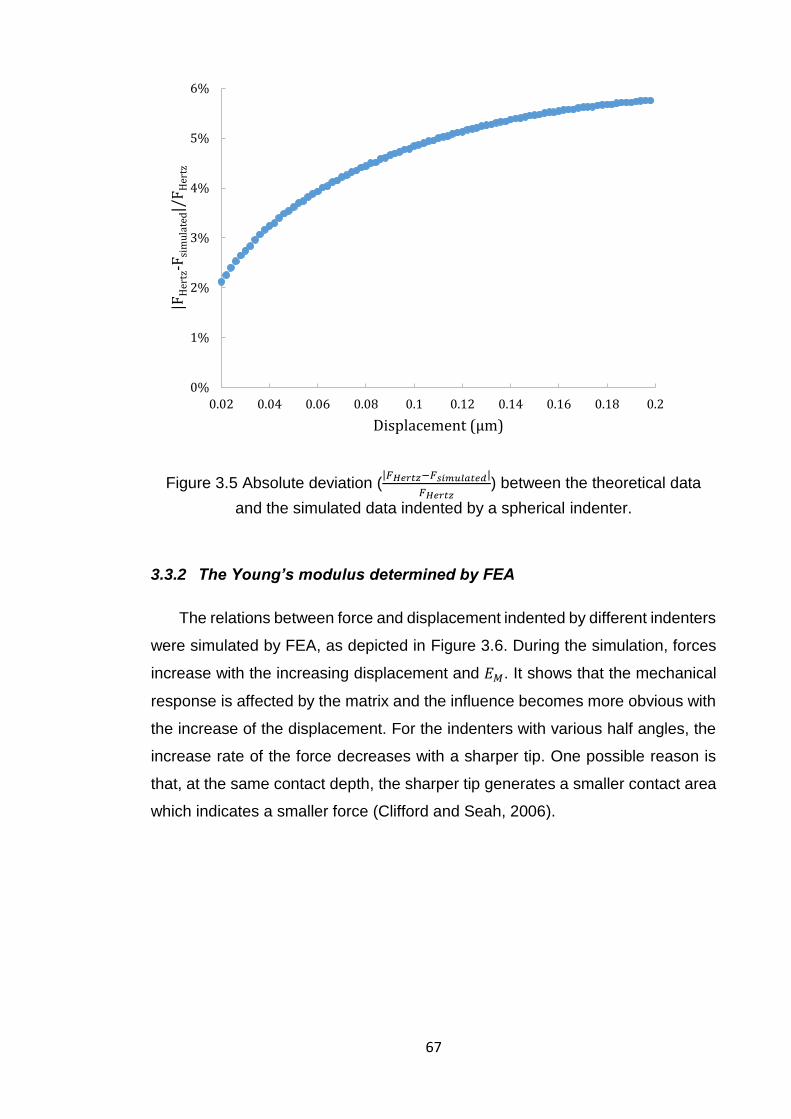
67
Figure 3.5 Absolute deviation (|𝐹𝐻𝑒𝑟𝑡𝑧−𝐹𝑠𝑖𝑚𝑢𝑙𝑎𝑡𝑒𝑑|
𝐹𝐻𝑒𝑟𝑡𝑧) between the theoretical data
and the simulated data indented by a spherical indenter.
3.3.2 The Young’s modulus determined by FEA
The relations between force and displacement indented by different indenters
were simulated by FEA, as depicted in Figure 3.6. During the simulation, forces
increase with the increasing displacement and 𝐸𝑀. It shows that the mechanical
response is affected by the matrix and the influence becomes more obvious with
the increase of the displacement. For the indenters with various half angles, the
increase rate of the force decreases with a sharper tip. One possible reason is
that, at the same contact depth, the sharper tip generates a smaller contact area
which indicates a smaller force (Clifford and Seah, 2006).
0%
1%
2%
3%
4%
5%
6%
0.02 0.04 0.06 0.08 0.1 0.12 0.14 0.16 0.18 0.2
|FH
ertz
-Fsi
mu
late
d|/
FH
ertz
Displacement (µm)
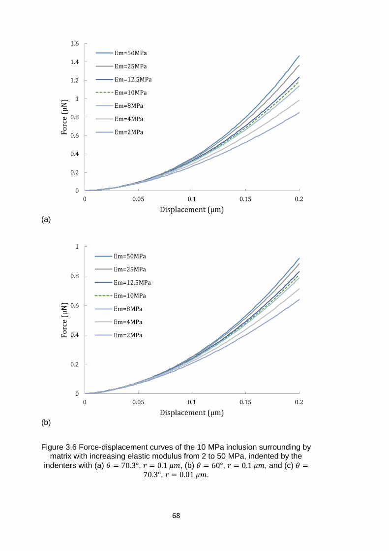
68
(a)
(b)
Figure 3.6 Force-displacement curves of the 10 MPa inclusion surrounding by matrix with increasing elastic modulus from 2 to 50 MPa, indented by the
indenters with (a) 𝜃 = 70.3°, 𝑟 = 0.1 𝜇𝑚, (b) 𝜃 = 60°, 𝑟 = 0.1 𝜇𝑚, and (c) 𝜃 =70.3°, 𝑟 = 0.01 𝜇𝑚.
0
0.2
0.4
0.6
0.8
1
1.2
1.4
1.6
0 0.05 0.1 0.15 0.2
Fo
rce
(µN
)
Displacement (µm)
Em=50MPa
Em=25MPa
Em=12.5MPa
Em=10MPa
Em=8MPa
Em=4MPa
Em=2MPa
0
0.2
0.4
0.6
0.8
1
0 0.05 0.1 0.15 0.2
Forc
e (µ
N)
Displacement (µm)
Em=50MPa
Em=25MPa
Em=12.5MPa
Em=10MPa
Em=8MPa
Em=4MPa
Em=2MPa
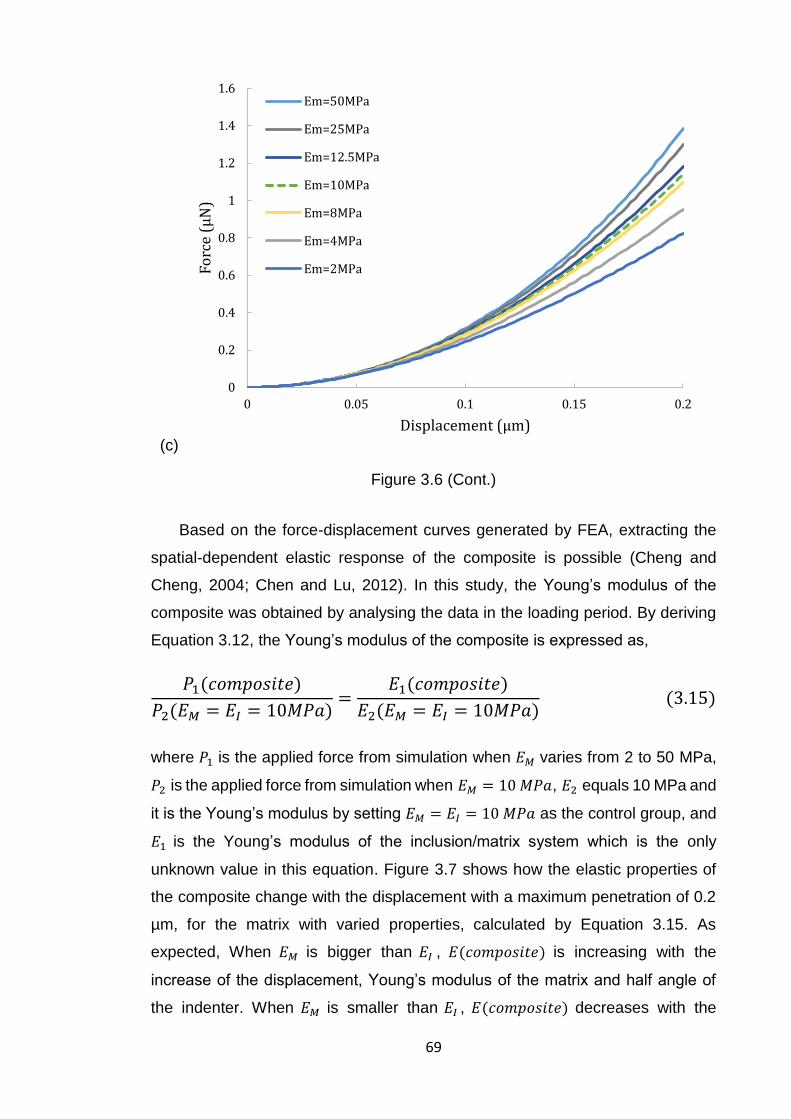
69
(c)
Figure 3.6 (Cont.)
Based on the force-displacement curves generated by FEA, extracting the
spatial-dependent elastic response of the composite is possible (Cheng and
Cheng, 2004; Chen and Lu, 2012). In this study, the Young’s modulus of the
composite was obtained by analysing the data in the loading period. By deriving
Equation 3.12, the Young’s modulus of the composite is expressed as,
𝑃1(𝑐𝑜𝑚𝑝𝑜𝑠𝑖𝑡𝑒)
𝑃2(𝐸𝑀 = 𝐸𝐼 = 10𝑀𝑃𝑎)=
𝐸1(𝑐𝑜𝑚𝑝𝑜𝑠𝑖𝑡𝑒)
𝐸2(𝐸𝑀 = 𝐸𝐼 = 10𝑀𝑃𝑎) (3.15)
where 𝑃1 is the applied force from simulation when 𝐸𝑀 varies from 2 to 50 MPa,
𝑃2 is the applied force from simulation when 𝐸𝑀 = 10 𝑀𝑃𝑎, 𝐸2 equals 10 MPa and
it is the Young’s modulus by setting 𝐸𝑀 = 𝐸𝐼 = 10 𝑀𝑃𝑎 as the control group, and
𝐸1 is the Young’s modulus of the inclusion/matrix system which is the only
unknown value in this equation. Figure 3.7 shows how the elastic properties of
the composite change with the displacement with a maximum penetration of 0.2
µm, for the matrix with varied properties, calculated by Equation 3.15. As
expected, When 𝐸𝑀 is bigger than 𝐸𝐼 , 𝐸(𝑐𝑜𝑚𝑝𝑜𝑠𝑖𝑡𝑒) is increasing with the
increase of the displacement, Young’s modulus of the matrix and half angle of
the indenter. When 𝐸𝑀 is smaller than 𝐸𝐼 , 𝐸(𝑐𝑜𝑚𝑝𝑜𝑠𝑖𝑡𝑒) decreases with the
0
0.2
0.4
0.6
0.8
1
1.2
1.4
1.6
0 0.05 0.1 0.15 0.2
Fo
rce
(µN
)
Displacement (µm)
Em=50MPa
Em=25MPa
Em=12.5MPa
Em=10MPa
Em=8MPa
Em=4MPa
Em=2MPa
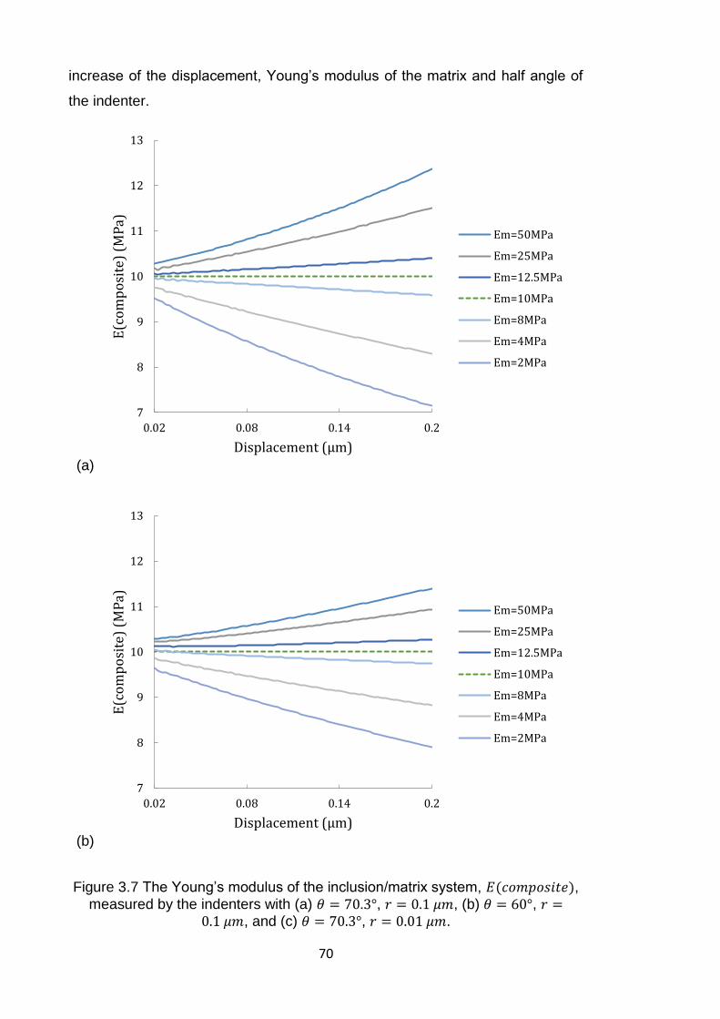
70
increase of the displacement, Young’s modulus of the matrix and half angle of
the indenter.
(a)
(b)
Figure 3.7 The Young’s modulus of the inclusion/matrix system, 𝐸(𝑐𝑜𝑚𝑝𝑜𝑠𝑖𝑡𝑒),
measured by the indenters with (a) 𝜃 = 70.3°, 𝑟 = 0.1 𝜇𝑚, (b) 𝜃 = 60°, 𝑟 =0.1 𝜇𝑚, and (c) 𝜃 = 70.3°, 𝑟 = 0.01 𝜇𝑚.
7
8
9
10
11
12
13
0.02 0.08 0.14 0.2
E(c
om
po
site
) (M
Pa)
Displacement (µm)
Em=50MPa
Em=25MPa
Em=12.5MPa
Em=10MPa
Em=8MPa
Em=4MPa
Em=2MPa
7
8
9
10
11
12
13
0.02 0.08 0.14 0.2
E(c
om
po
site
) (M
Pa)
Displacement (µm)
Em=50MPa
Em=25MPa
Em=12.5MPa
Em=10MPa
Em=8MPa
Em=4MPa
Em=2MPa
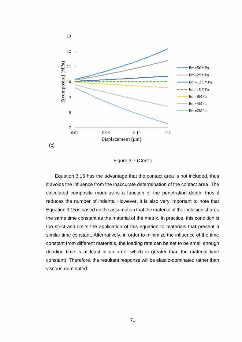
71
(c)
Figure 3.7 (Cont.)
Equation 3.15 has the advantage that the contact area is not included, thus
it avoids the influence from the inaccurate determination of the contact area. The
calculated composite modulus is a function of the penetration depth, thus it
reduces the number of indents. However, it is also very important to note that
Equation 3.15 is based on the assumption that the material of the inclusion shares
the same time constant as the material of the matrix. In practice, this condition is
too strict and limits the application of this equation to materials that present a
similar time constant. Alternatively, in order to minimize the influence of the time
constant from different materials, the loading rate can be set to be small enough
(loading time is at least in an order which is greater than the material time
constant). Therefore, the resultant response will be elastic-dominated rather than
viscous-dominated.
7
8
9
10
11
12
13
0.02 0.08 0.14 0.2
E(c
om
po
site
) (M
Pa)
Displacement (µm)
Em=50MPa
Em=25MPa
Em=12.5MPa
Em=10MPa
Em=8MPa
Em=4MPa
Em=2MPa
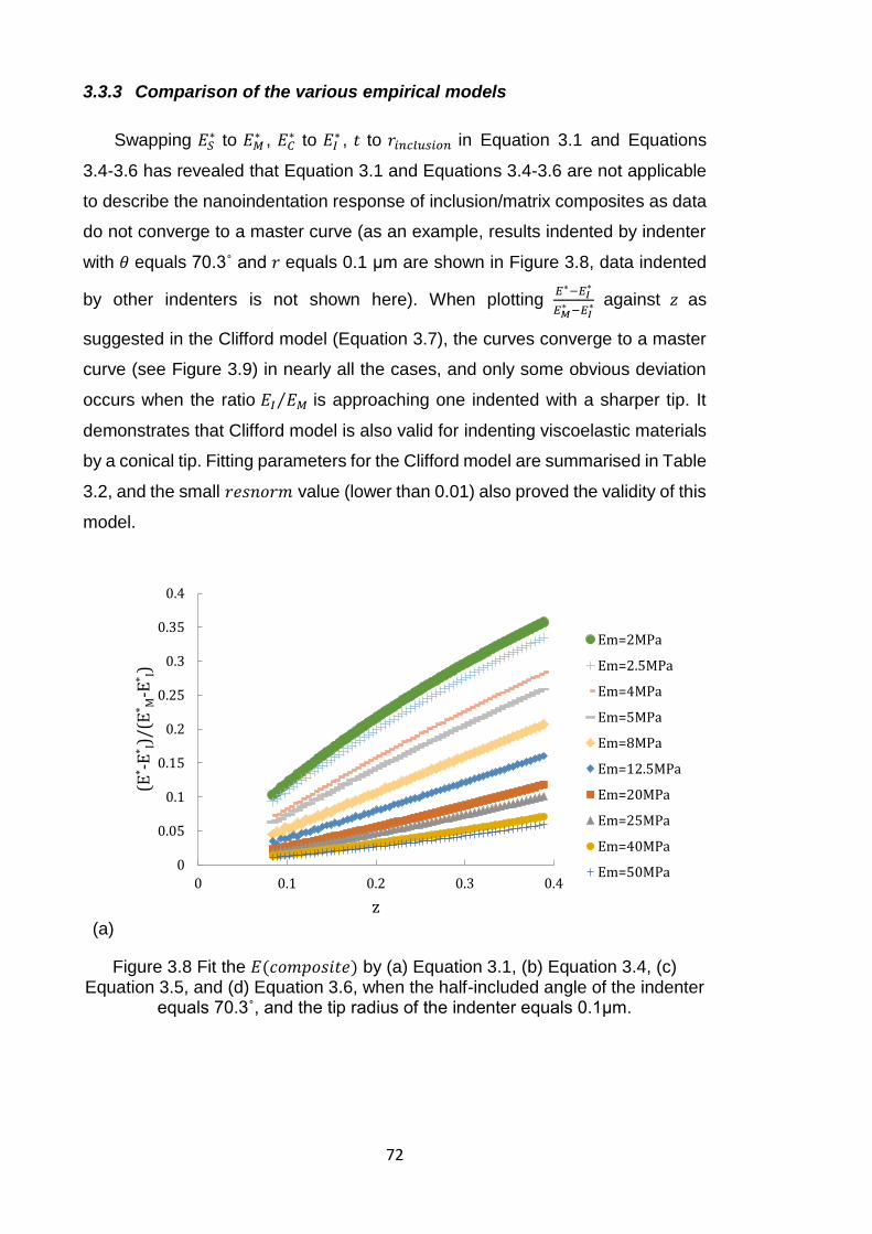
72
3.3.3 Comparison of the various empirical models
Swapping 𝐸𝑆∗ to 𝐸𝑀
∗ , 𝐸𝐶∗ to 𝐸𝐼
∗ , 𝑡 to 𝑟𝑖𝑛𝑐𝑙𝑢𝑠𝑖𝑜𝑛 in Equation 3.1 and Equations
3.4-3.6 has revealed that Equation 3.1 and Equations 3.4-3.6 are not applicable
to describe the nanoindentation response of inclusion/matrix composites as data
do not converge to a master curve (as an example, results indented by indenter
with 𝜃 equals 70.3˚ and 𝑟 equals 0.1 μm are shown in Figure 3.8, data indented
by other indenters is not shown here). When plotting 𝐸∗−𝐸𝐼
∗
𝐸𝑀∗ −𝐸𝐼
∗ against 𝑧 as
suggested in the Clifford model (Equation 3.7), the curves converge to a master
curve (see Figure 3.9) in nearly all the cases, and only some obvious deviation
occurs when the ratio 𝐸𝐼 𝐸𝑀⁄ is approaching one indented with a sharper tip. It
demonstrates that Clifford model is also valid for indenting viscoelastic materials
by a conical tip. Fitting parameters for the Clifford model are summarised in Table
3.2, and the small 𝑟𝑒𝑠𝑛𝑜𝑟𝑚 value (lower than 0.01) also proved the validity of this
model.
(a)
Figure 3.8 Fit the 𝐸(𝑐𝑜𝑚𝑝𝑜𝑠𝑖𝑡𝑒) by (a) Equation 3.1, (b) Equation 3.4, (c) Equation 3.5, and (d) Equation 3.6, when the half-included angle of the indenter
equals 70.3˚, and the tip radius of the indenter equals 0.1μm.
0
0.05
0.1
0.15
0.2
0.25
0.3
0.35
0.4
0 0.1 0.2 0.3 0.4
(E* -
E* I)
/(E
* M-E
* I)
z
Em=2MPa
Em=2.5MPa
Em=4MPa
Em=5MPa
Em=8MPa
Em=12.5MPa
Em=20MPa
Em=25MPa
Em=40MPa
Em=50MPa
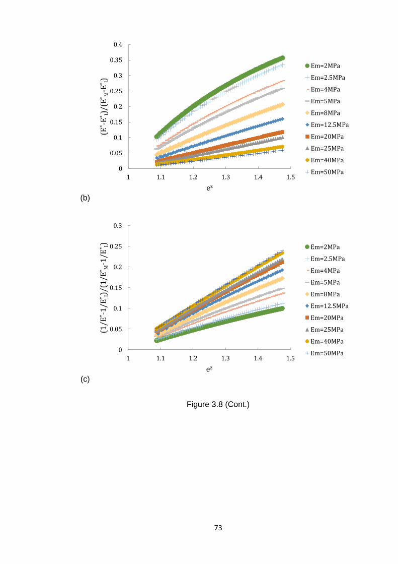
73
(b)
(c)
Figure 3.8 (Cont.)
0
0.05
0.1
0.15
0.2
0.25
0.3
0.35
0.4
1 1.1 1.2 1.3 1.4 1.5
(E* -
E* I)
/(E
* M-E
* I)
ez
Em=2MPa
Em=2.5MPa
Em=4MPa
Em=5MPa
Em=8MPa
Em=12.5MPa
Em=20MPa
Em=25MPa
Em=40MPa
Em=50MPa
0
0.05
0.1
0.15
0.2
0.25
0.3
1 1.1 1.2 1.3 1.4 1.5
(1/E
* -1
/E* I)
/(1
/E* M
-1/E
* I)
ez
Em=2MPa
Em=2.5MPa
Em=4MPa
Em=5MPa
Em=8MPa
Em=12.5MPa
Em=20MPa
Em=25MPa
Em=40MPa
Em=50MPa
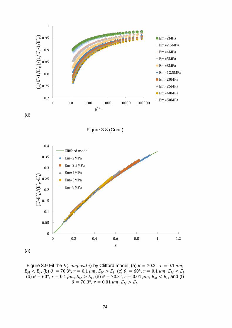
74
(d)
Figure 3.8 (Cont.)
(a)
Figure 3.9 Fit the 𝐸(𝑐𝑜𝑚𝑝𝑜𝑠𝑖𝑡𝑒) by Clifford model, (a) 𝜃 = 70.3°, 𝑟 = 0.1 𝜇𝑚, 𝐸𝑀 < 𝐸𝐼, (b) 𝜃 = 70.3°, 𝑟 = 0.1 𝜇𝑚, 𝐸𝑀 > 𝐸𝐼, (c) 𝜃 = 60°, 𝑟 = 0.1 𝜇𝑚, 𝐸𝑀 < 𝐸𝐼, (d) 𝜃 = 60°, 𝑟 = 0.1 𝜇𝑚, 𝐸𝑀 > 𝐸𝐼, (e) 𝜃 = 70.3°, 𝑟 = 0.01 𝜇𝑚, 𝐸𝑀 < 𝐸𝐼, and (f)
𝜃 = 70.3°, 𝑟 = 0.01 𝜇𝑚, 𝐸𝑀 > 𝐸𝐼.
0.7
0.75
0.8
0.85
0.9
0.95
1
1 10 100 1000 10000 100000
(1/E
* -1
/E* M
)/(1
/E* I-
1/E
* M)
e1/z
Em=2MPa
Em=2.5MPa
Em=4MPa
Em=5MPa
Em=8MPa
Em=12.5MPa
Em=20MPa
Em=25MPa
Em=40MPa
Em=50MPa
0
0.05
0.1
0.15
0.2
0.25
0.3
0.35
0.4
0 0.2 0.4 0.6 0.8 1 1.2
(E* -
E* I)
/(E
* M-E
* I)
z
Clifford model
Em=2MPa
Em=2.5MPa
Em=4MPa
Em=5MPa
Em=8MPa
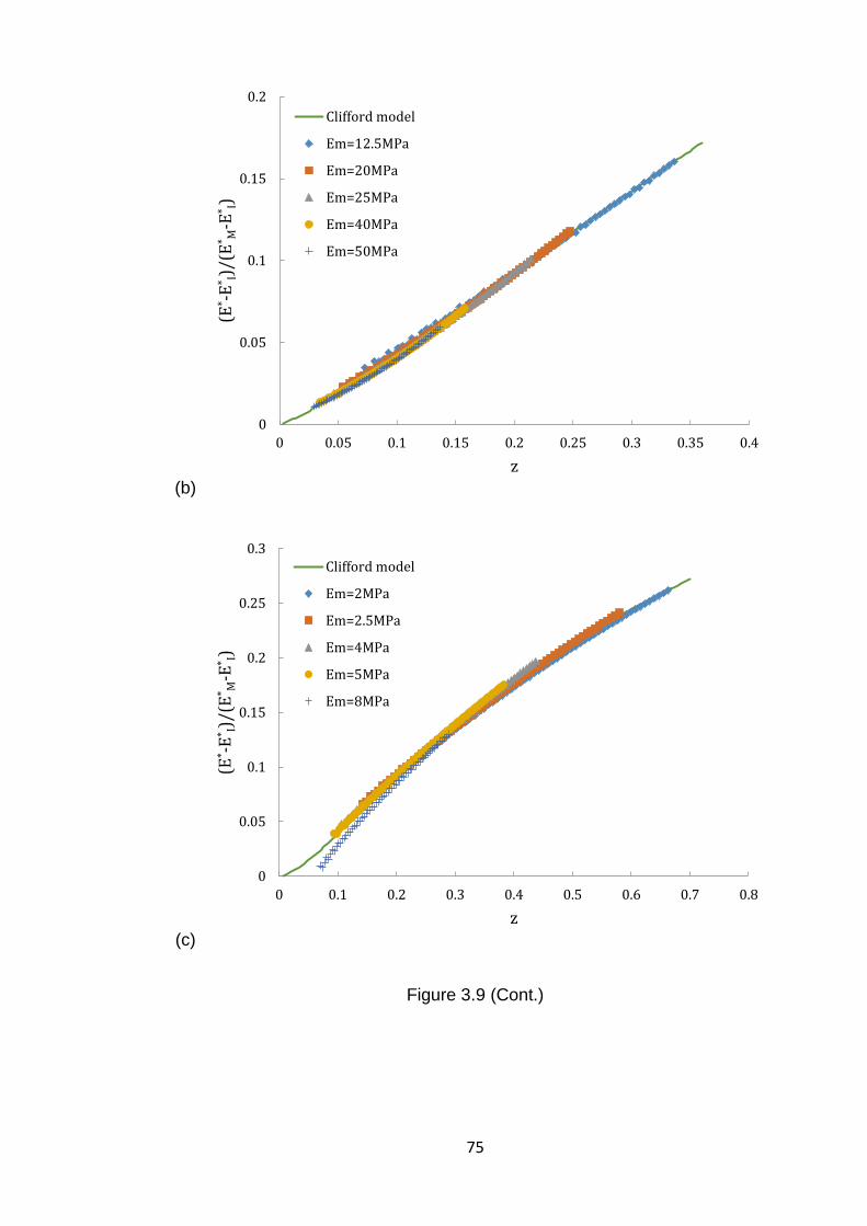
75
(b)
(c)
Figure 3.9 (Cont.)
0
0.05
0.1
0.15
0.2
0 0.05 0.1 0.15 0.2 0.25 0.3 0.35 0.4
(E* -
E* I)
/(E
* M-E
* I)
z
Clifford model
Em=12.5MPa
Em=20MPa
Em=25MPa
Em=40MPa
Em=50MPa
0
0.05
0.1
0.15
0.2
0.25
0.3
0 0.1 0.2 0.3 0.4 0.5 0.6 0.7 0.8
(E* -
E* I)
/(E
* M-E
* I)
z
Clifford model
Em=2MPa
Em=2.5MPa
Em=4MPa
Em=5MPa
Em=8MPa
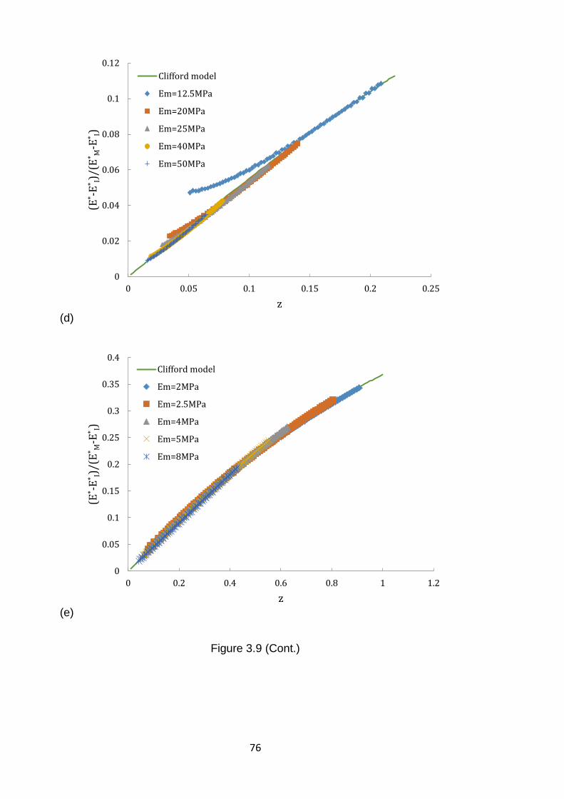
76
(d)
(e)
Figure 3.9 (Cont.)
0
0.02
0.04
0.06
0.08
0.1
0.12
0 0.05 0.1 0.15 0.2 0.25
(E* -
E* I)
/(E
* M-E
* I)
z
Clifford model
Em=12.5MPa
Em=20MPa
Em=25MPa
Em=40MPa
Em=50MPa
0
0.05
0.1
0.15
0.2
0.25
0.3
0.35
0.4
0 0.2 0.4 0.6 0.8 1 1.2
(E* -
E* I)
/(E
* M-E
* I)
z
Clifford model
Em=2MPa
Em=2.5MPa
Em=4MPa
Em=5MPa
Em=8MPa
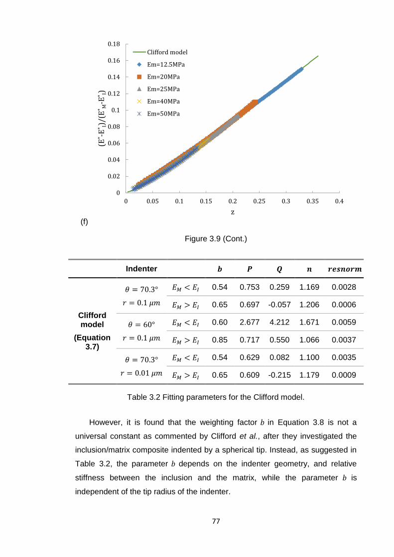
77
(f)
Figure 3.9 (Cont.)
Indenter 𝒃 𝑷 𝑸 𝒏 𝒓𝒆𝒔𝒏𝒐𝒓𝒎
Clifford model
(Equation 3.7)
𝜃 = 70.3°
𝑟 = 0.1 𝜇𝑚
𝐸𝑀 < 𝐸𝐼 0.54 0.753 0.259 1.169 0.0028
𝐸𝑀 > 𝐸𝐼 0.65 0.697 -0.057 1.206 0.0006
𝜃 = 60°
𝑟 = 0.1 𝜇𝑚
𝐸𝑀 < 𝐸𝐼 0.60 2.677 4.212 1.671 0.0059
𝐸𝑀 > 𝐸𝐼 0.85 0.717 0.550 1.066 0.0037
𝜃 = 70.3°
𝑟 = 0.01 𝜇𝑚
𝐸𝑀 < 𝐸𝐼 0.54 0.629 0.082 1.100 0.0035
𝐸𝑀 > 𝐸𝐼 0.65 0.609 -0.215 1.179 0.0009
Table 3.2 Fitting parameters for the Clifford model.
However, it is found that the weighting factor 𝑏 in Equation 3.8 is not a
universal constant as commented by Clifford et al., after they investigated the
inclusion/matrix composite indented by a spherical tip. Instead, as suggested in
Table 3.2, the parameter 𝑏 depends on the indenter geometry, and relative
stiffness between the inclusion and the matrix, while the parameter 𝑏 is
independent of the tip radius of the indenter.
0
0.02
0.04
0.06
0.08
0.1
0.12
0.14
0.16
0.18
0 0.05 0.1 0.15 0.2 0.25 0.3 0.35 0.4
(E* -
E* I)
/(E
* M-E
* I)
z
Clifford model
Em=12.5MPa
Em=20MPa
Em=25MPa
Em=40MPa
Em=50MPa
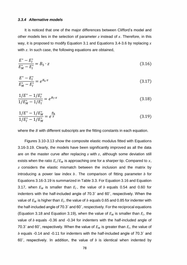
78
3.3.4 Alternative models
It is noticed that one of the major differences between Clifford’s model and
other models lies in the selection of parameter 𝑧 instead of 𝑥. Therefore, in this
way, it is proposed to modify Equation 3.1 and Equations 3.4-3.6 by replacing 𝑥
with 𝑧. In such case, the following equations are obtained,
𝐸∗ − 𝐸𝐼∗
𝐸𝑀∗ − 𝐸𝐼
∗ = 𝐵5 ∙ 𝑧 (3.16)
𝐸∗ − 𝐸𝐼∗
𝐸𝑀∗ − 𝐸𝐼
∗ = 𝑒𝐵6∙𝑧 (3.17)
1/𝐸∗ − 1/𝐸𝐼∗
1/𝐸𝑀∗ − 1/𝐸𝐼
∗ = 𝑒𝐵7∙𝑧 (3.18)
1/𝐸∗ − 1/𝐸𝑀∗
1/𝐸𝐼∗ − 1/𝐸𝑀
∗ = 𝑒𝐵8𝑧 (3.19)
where the 𝐵 with different subscripts are the fitting constants in each equation.
Figures 3.10-3.13 show the composite elastic modulus fitted with Equations
3.16-3.19. Clearly, the models have been significantly improved as all the data
are on the master curve after replacing 𝑥 with 𝑧, although some deviation still
exists when the ratio 𝐸𝐼 𝐸𝑀⁄ is approaching one for a sharper tip. Compared to 𝑥,
𝑧 considers the elastic mismatch between the inclusion and the matrix by
introducing a power law index 𝑏 . The comparison of fitting parameter 𝑏 for
Equations 3.16-3.19 is summarized in Table 3.3. For Equation 3.16 and Equation
3.17, when 𝐸𝑀 is smaller than 𝐸𝐼 , the value of 𝑏 equals 0.54 and 0.60 for
indenters with the half-included angle of 70.3˚ and 60˚, respectively. When the
value of 𝐸𝑀 is higher than 𝐸𝐼, the value of 𝑏 equals 0.65 and 0.85 for indenter with
the half-included angle of 70.3˚ and 60˚, respectively. For the reciprocal equations
(Equation 3.18 and Equation 3.19), when the value of 𝐸𝑀 is smaller than 𝐸𝐼, the
value of 𝑏 equals -0.36 and -0.34 for indenters with the half-included angle of
70.3˚ and 60˚, respectively. When the value of 𝐸𝑀 is greater than 𝐸𝐼, the value of
𝑏 equals -0.14 and -0.11 for indenters with the half-included angle of 70.3˚ and
60˚, respectively. In addition, the value of 𝑏 is identical when indented by
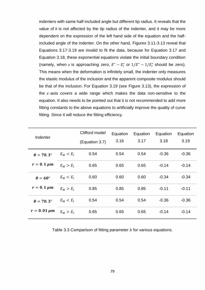
79
indenters with same half-included angle but different tip radius. It reveals that the
value of 𝑏 is not affected by the tip radius of the indenter, and it may be more
dependent on the expression of the left hand side of the equation and the half-
included angle of the indenter. On the other hand, Figures 3.11-3.13 reveal that
Equations 3.17-3.19 are invalid to fit the data, because for Equation 3.17 and
Equation 3.18, these exponential equations violate the initial boundary condition
(namely, when 𝑧 is approaching zero, 𝐸∗ − 𝐸𝐼∗ or 1/𝐸∗ − 1/𝐸𝐼
∗ should be zero).
This means when the deformation is infinitely small, the indenter only measures
the elastic modulus of the inclusion and the apparent composite modulus should
be that of the inclusion. For Equation 3.19 (see Figure 3.13), the expression of
the 𝑥 -axis covers a wide range which makes the data non-sensitive to the
equation. It also needs to be pointed out that it is not recommended to add more
fitting constants to the above equations to artificially improve the quality of curve
fitting. Since it will reduce the fitting efficiency.
Indenter Clifford model
(Equation 3.7)
Equation
3.16
Equation
3.17
Equation
3.18
Equation
3.19
𝜽 = 𝟕𝟎. 𝟑°
𝒓 = 𝟎. 𝟏 𝝁𝒎
𝐸𝑀 < 𝐸𝐼 0.54 0.54 0.54 -0.36 -0.36
𝐸𝑀 > 𝐸𝐼 0.65 0.65 0.65 -0.14 -0.14
𝜽 = 𝟔𝟎°
𝒓 = 𝟎. 𝟏 𝝁𝒎
𝐸𝑀 < 𝐸𝐼 0.60 0.60 0.60 -0.34 -0.34
𝐸𝑀 > 𝐸𝐼 0.85 0.85 0.85 -0.11 -0.11
𝜽 = 𝟕𝟎. 𝟑°
𝒓 = 𝟎. 𝟎𝟏 𝝁𝒎
𝐸𝑀 < 𝐸𝐼 0.54 0.54 0.54 -0.36 -0.36
𝐸𝑀 > 𝐸𝐼 0.65 0.65 0.65 -0.14 -0.14
Table 3.3 Comparison of fitting parameter 𝑏 for various equations.
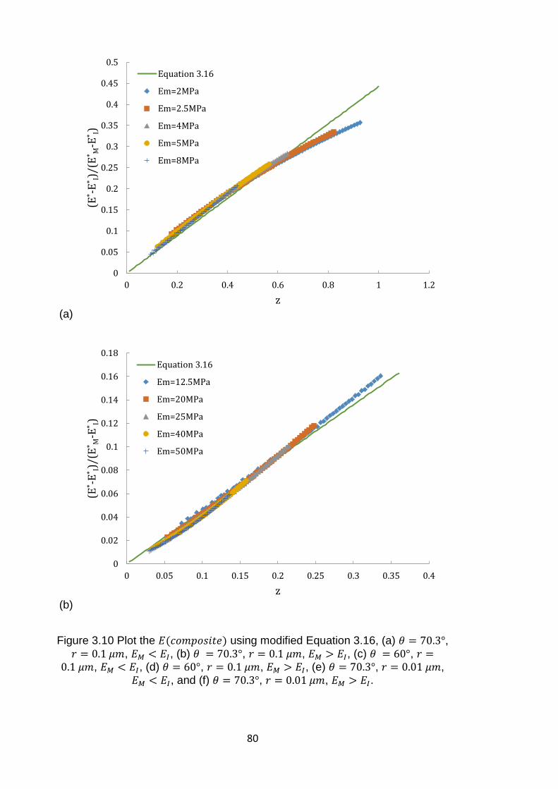
80
(a)
(b)
Figure 3.10 Plot the 𝐸(𝑐𝑜𝑚𝑝𝑜𝑠𝑖𝑡𝑒) using modified Equation 3.16, (a) 𝜃 = 70.3°, 𝑟 = 0.1 𝜇𝑚, 𝐸𝑀 < 𝐸𝐼, (b) 𝜃 = 70.3°, 𝑟 = 0.1 𝜇𝑚, 𝐸𝑀 > 𝐸𝐼, (c) 𝜃 = 60°, 𝑟 =
0.1 𝜇𝑚, 𝐸𝑀 < 𝐸𝐼, (d) 𝜃 = 60°, 𝑟 = 0.1 𝜇𝑚, 𝐸𝑀 > 𝐸𝐼, (e) 𝜃 = 70.3°, 𝑟 = 0.01 𝜇𝑚,
𝐸𝑀 < 𝐸𝐼, and (f) 𝜃 = 70.3°, 𝑟 = 0.01 𝜇𝑚, 𝐸𝑀 > 𝐸𝐼.
0
0.05
0.1
0.15
0.2
0.25
0.3
0.35
0.4
0.45
0.5
0 0.2 0.4 0.6 0.8 1 1.2
(E* -
E* I)
/(E
* M-E
* I)
z
Equation 3.16
Em=2MPa
Em=2.5MPa
Em=4MPa
Em=5MPa
Em=8MPa
0
0.02
0.04
0.06
0.08
0.1
0.12
0.14
0.16
0.18
0 0.05 0.1 0.15 0.2 0.25 0.3 0.35 0.4
(E* -
E* I)
/(E
* M-E
* I)
z
Equation 3.16
Em=12.5MPa
Em=20MPa
Em=25MPa
Em=40MPa
Em=50MPa
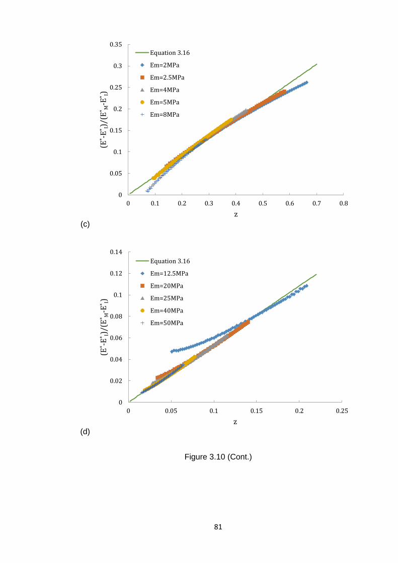
81
(c)
(d)
Figure 3.10 (Cont.)
0
0.05
0.1
0.15
0.2
0.25
0.3
0.35
0 0.1 0.2 0.3 0.4 0.5 0.6 0.7 0.8
(E* -
E* I)
/(E
* M-E
* I)
z
Equation 3.16
Em=2MPa
Em=2.5MPa
Em=4MPa
Em=5MPa
Em=8MPa
0
0.02
0.04
0.06
0.08
0.1
0.12
0.14
0 0.05 0.1 0.15 0.2 0.25
(E* -
E* I)
/(E
* M-E
* I)
z
Equation 3.16
Em=12.5MPa
Em=20MPa
Em=25MPa
Em=40MPa
Em=50MPa
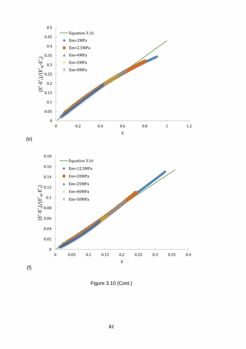
82
(e)
(f)
Figure 3.10 (Cont.)
0
0.05
0.1
0.15
0.2
0.25
0.3
0.35
0.4
0.45
0.5
0 0.2 0.4 0.6 0.8 1 1.2
(E* -
E* I)
/(E
* M-E
* I)
z
Equation 3.16
Em=2MPa
Em=2.5MPa
Em=4MPa
Em=5MPa
Em=8MPa
0
0.02
0.04
0.06
0.08
0.1
0.12
0.14
0.16
0.18
0 0.05 0.1 0.15 0.2 0.25 0.3 0.35 0.4
(E* -
E* I)
/(E
* M-E
* I)
z
Equation 3.16
Em=12.5MPa
Em=20MPa
Em=25MPa
Em=40MPa
Em=50MPa
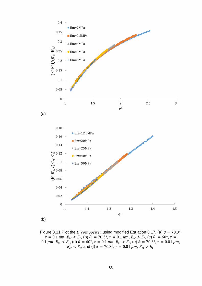
83
(a)
(b)
Figure 3.11 Plot the 𝐸(𝑐𝑜𝑚𝑝𝑜𝑠𝑖𝑡𝑒) using modified Equation 3.17, (a) 𝜃 = 70.3°, 𝑟 = 0.1 𝜇𝑚, 𝐸𝑀 < 𝐸𝐼, (b) 𝜃 = 70.3°, 𝑟 = 0.1 𝜇𝑚, 𝐸𝑀 > 𝐸𝐼, (c) 𝜃 = 60°, 𝑟 =
0.1 𝜇𝑚, 𝐸𝑀 < 𝐸𝐼, (d) 𝜃 = 60°, 𝑟 = 0.1 𝜇𝑚, 𝐸𝑀 > 𝐸𝐼, (e) 𝜃 = 70.3°, 𝑟 = 0.01 𝜇𝑚,
𝐸𝑀 < 𝐸𝐼, and (f) 𝜃 = 70.3°, 𝑟 = 0.01 𝜇𝑚, 𝐸𝑀 > 𝐸𝐼.
0
0.05
0.1
0.15
0.2
0.25
0.3
0.35
0.4
1 1.5 2 2.5 3
(E* -
E* I)
/(E
* M-E
* I)
ez
Em=2MPa
Em=2.5MPa
Em=4MPa
Em=5MPa
Em=8MPa
0
0.02
0.04
0.06
0.08
0.1
0.12
0.14
0.16
0.18
1 1.1 1.2 1.3 1.4 1.5
(E* -
E* I)
/(E
* M-E
* I)
ez
Em=12.5MPa
Em=20MPa
Em=25MPa
Em=40MPa
Em=50MPa
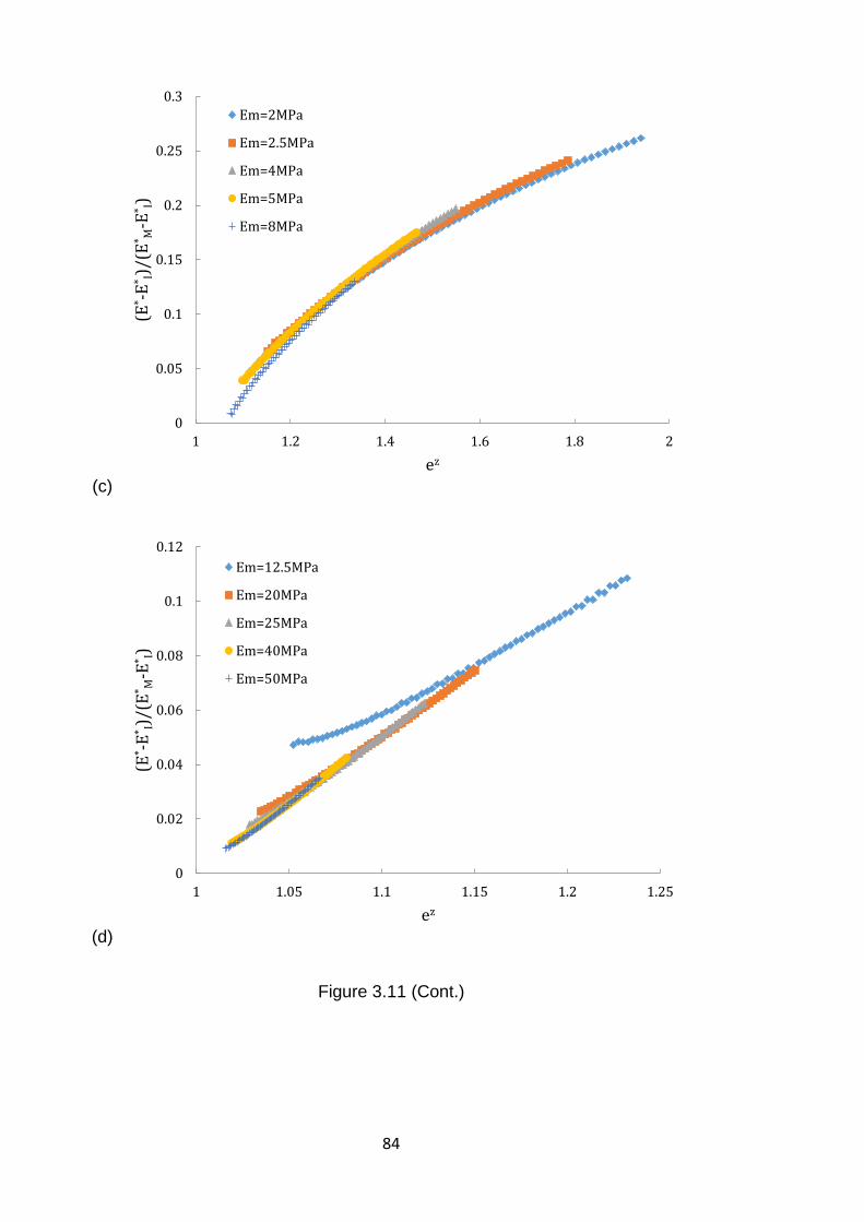
84
(c)
(d)
Figure 3.11 (Cont.)
0
0.05
0.1
0.15
0.2
0.25
0.3
1 1.2 1.4 1.6 1.8 2
(E* -
E* I)
/(E
* M-E
* I)
ez
Em=2MPa
Em=2.5MPa
Em=4MPa
Em=5MPa
Em=8MPa
0
0.02
0.04
0.06
0.08
0.1
0.12
1 1.05 1.1 1.15 1.2 1.25
(E* -
E* I)
/(E
* M-E
* I)
ez
Em=12.5MPa
Em=20MPa
Em=25MPa
Em=40MPa
Em=50MPa
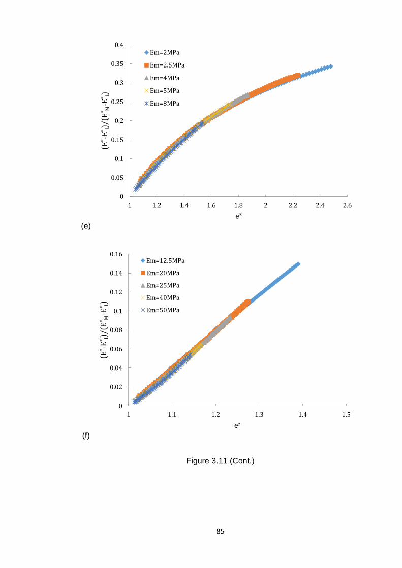
85
(e)
(f)
Figure 3.11 (Cont.)
0
0.05
0.1
0.15
0.2
0.25
0.3
0.35
0.4
1 1.2 1.4 1.6 1.8 2 2.2 2.4 2.6
(E* -
E* I)
/(E
* M-E
* I)
ez
Em=2MPa
Em=2.5MPa
Em=4MPa
Em=5MPa
Em=8MPa
0
0.02
0.04
0.06
0.08
0.1
0.12
0.14
0.16
1 1.1 1.2 1.3 1.4 1.5
(E* -
E* I)
/(E
* M-E
* I)
ez
Em=12.5MPa
Em=20MPa
Em=25MPa
Em=40MPa
Em=50MPa
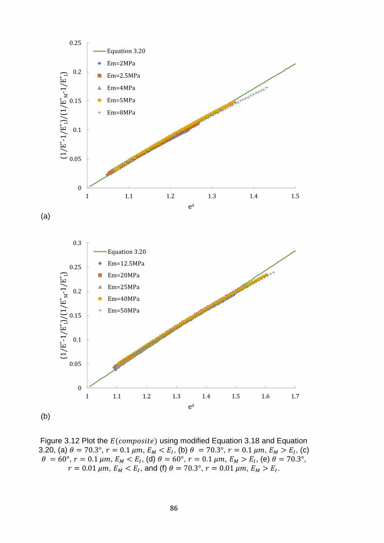
86
(a)
(b)
Figure 3.12 Plot the 𝐸(𝑐𝑜𝑚𝑝𝑜𝑠𝑖𝑡𝑒) using modified Equation 3.18 and Equation
3.20, (a) 𝜃 = 70.3°, 𝑟 = 0.1 𝜇𝑚, 𝐸𝑀 < 𝐸𝐼, (b) 𝜃 = 70.3°, 𝑟 = 0.1 𝜇𝑚, 𝐸𝑀 > 𝐸𝐼, (c) 𝜃 = 60°, 𝑟 = 0.1 𝜇𝑚, 𝐸𝑀 < 𝐸𝐼, (d) 𝜃 = 60°, 𝑟 = 0.1 𝜇𝑚, 𝐸𝑀 > 𝐸𝐼, (e) 𝜃 = 70.3°,
𝑟 = 0.01 𝜇𝑚, 𝐸𝑀 < 𝐸𝐼, and (f) 𝜃 = 70.3°, 𝑟 = 0.01 𝜇𝑚, 𝐸𝑀 > 𝐸𝐼.
0
0.05
0.1
0.15
0.2
0.25
1 1.1 1.2 1.3 1.4 1.5
(1/E
* -1
/E* I)
/(1
/E* M
-1/E
* I)
ez
Equation 3.20
Em=2MPa
Em=2.5MPa
Em=4MPa
Em=5MPa
Em=8MPa
0
0.05
0.1
0.15
0.2
0.25
0.3
1 1.1 1.2 1.3 1.4 1.5 1.6 1.7
(1/E
* -1
/E* I)
/(1
/E* M
-1/E
* I)
ez
Equation 3.20
Em=12.5MPa
Em=20MPa
Em=25MPa
Em=40MPa
Em=50MPa
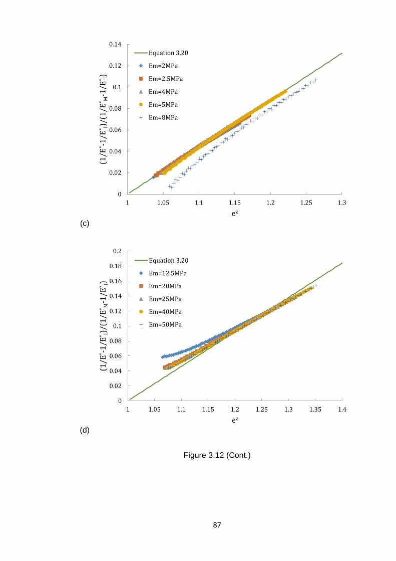
87
(c)
(d)
Figure 3.12 (Cont.)
0
0.02
0.04
0.06
0.08
0.1
0.12
0.14
1 1.05 1.1 1.15 1.2 1.25 1.3
(1/E
* -1
/E* I)
/(1
/E* M
-1/E
* I)
ez
Equation 3.20
Em=2MPa
Em=2.5MPa
Em=4MPa
Em=5MPa
Em=8MPa
0
0.02
0.04
0.06
0.08
0.1
0.12
0.14
0.16
0.18
0.2
1 1.05 1.1 1.15 1.2 1.25 1.3 1.35 1.4
(1/E
* -1
/E* I)
/(1
/E* M
-1/E
* I)
ez
Equation 3.20
Em=12.5MPa
Em=20MPa
Em=25MPa
Em=40MPa
Em=50MPa
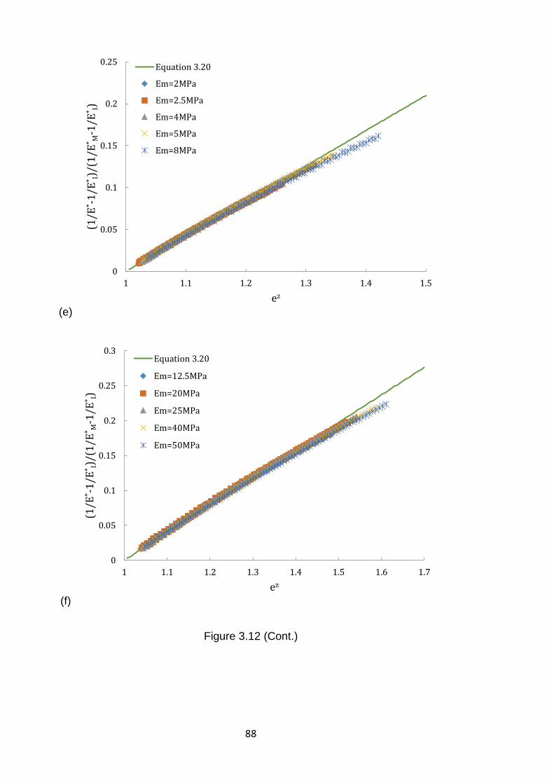
88
(e)
(f)
Figure 3.12 (Cont.)
0
0.05
0.1
0.15
0.2
0.25
1 1.1 1.2 1.3 1.4 1.5
(1/E
* -1
/E* I)
/(1
/E* M
-1/E
* I)
ez
Equation 3.20
Em=2MPa
Em=2.5MPa
Em=4MPa
Em=5MPa
Em=8MPa
0
0.05
0.1
0.15
0.2
0.25
0.3
1 1.1 1.2 1.3 1.4 1.5 1.6 1.7
(1/E
* -1
/E* I)
/(1
/E* M
-1/E
* I)
ez
Equation 3.20
Em=12.5MPa
Em=20MPa
Em=25MPa
Em=40MPa
Em=50MPa
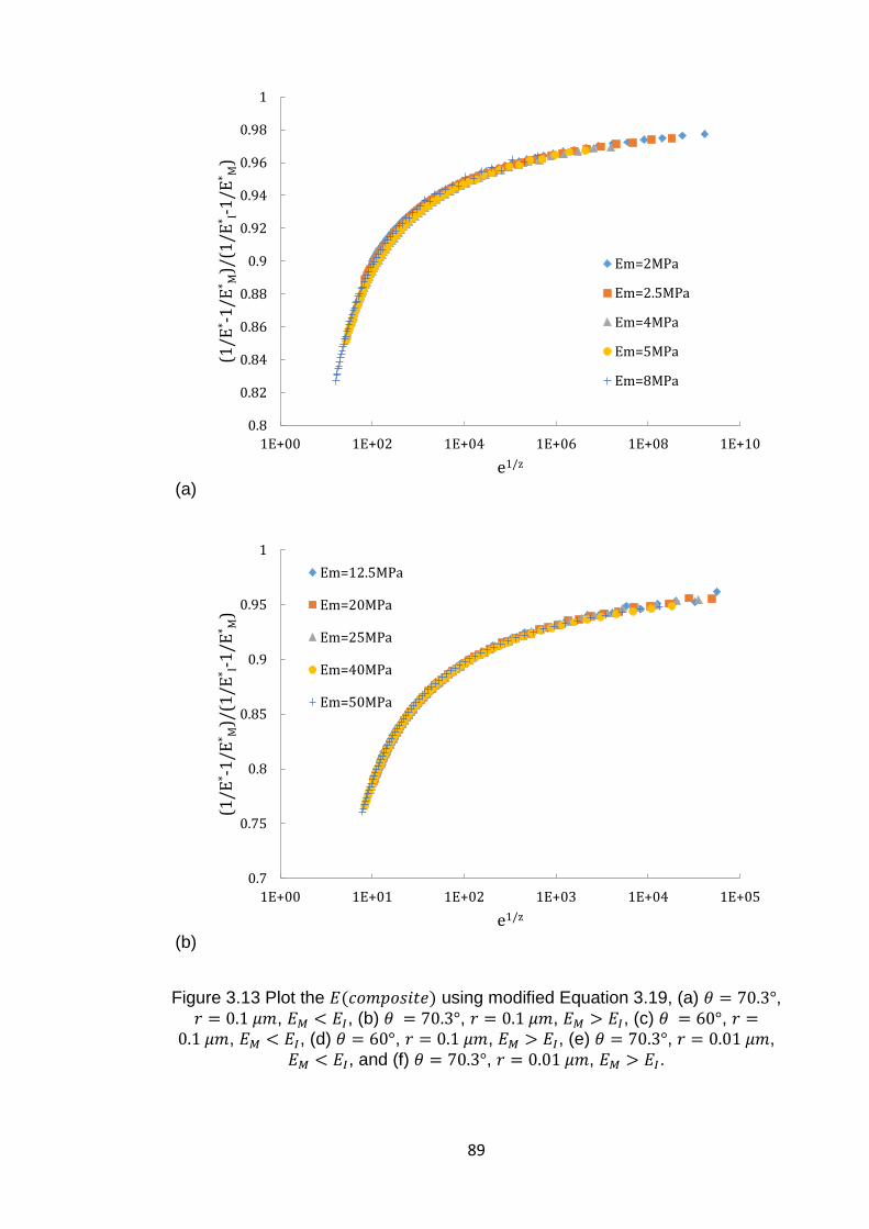
89
(a)
(b)
Figure 3.13 Plot the 𝐸(𝑐𝑜𝑚𝑝𝑜𝑠𝑖𝑡𝑒) using modified Equation 3.19, (a) 𝜃 = 70.3°, 𝑟 = 0.1 𝜇𝑚, 𝐸𝑀 < 𝐸𝐼, (b) 𝜃 = 70.3°, 𝑟 = 0.1 𝜇𝑚, 𝐸𝑀 > 𝐸𝐼, (c) 𝜃 = 60°, 𝑟 =
0.1 𝜇𝑚, 𝐸𝑀 < 𝐸𝐼, (d) 𝜃 = 60°, 𝑟 = 0.1 𝜇𝑚, 𝐸𝑀 > 𝐸𝐼, (e) 𝜃 = 70.3°, 𝑟 = 0.01 𝜇𝑚,
𝐸𝑀 < 𝐸𝐼, and (f) 𝜃 = 70.3°, 𝑟 = 0.01 𝜇𝑚, 𝐸𝑀 > 𝐸𝐼.
0.8
0.82
0.84
0.86
0.88
0.9
0.92
0.94
0.96
0.98
1
1E+00 1E+02 1E+04 1E+06 1E+08 1E+10
(1/E
* -1
/E* M
)/(1
/E* I-
1/E
* M)
e1/z
Em=2MPa
Em=2.5MPa
Em=4MPa
Em=5MPa
Em=8MPa
0.7
0.75
0.8
0.85
0.9
0.95
1
1E+00 1E+01 1E+02 1E+03 1E+04 1E+05
(1/E
* -1
/E* M
)/(1
/E* I-
1/E
* M)
e1/z
Em=12.5MPa
Em=20MPa
Em=25MPa
Em=40MPa
Em=50MPa
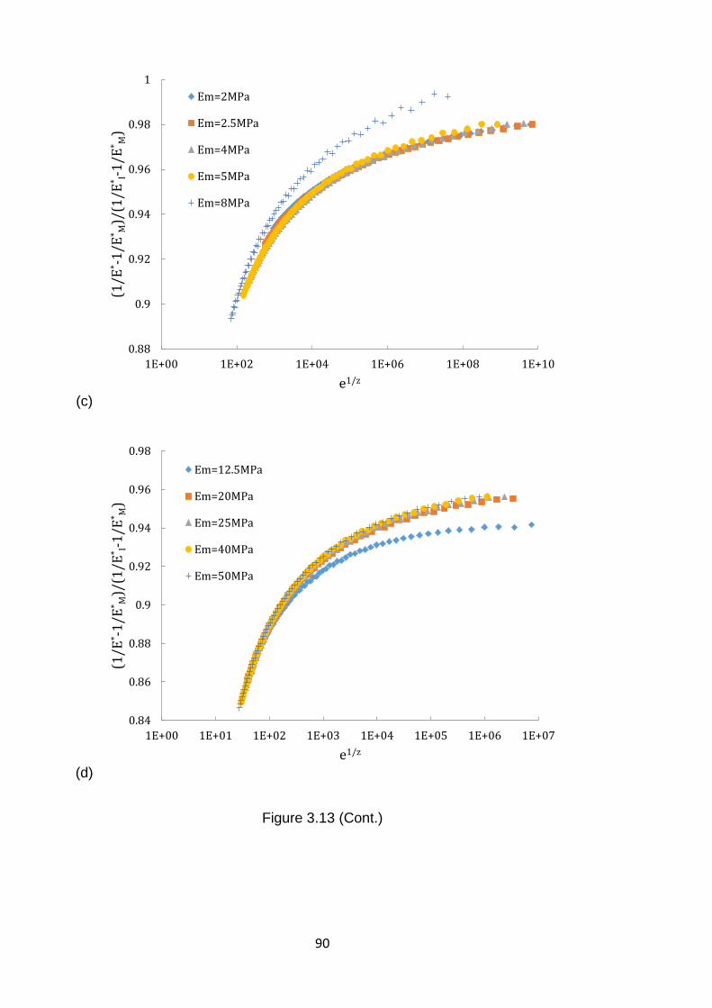
90
(c)
(d)
Figure 3.13 (Cont.)
0.88
0.9
0.92
0.94
0.96
0.98
1
1E+00 1E+02 1E+04 1E+06 1E+08 1E+10
(1/E
* -1
/E* M
)/(1
/E* I-
1/E
* M)
e1/z
Em=2MPa
Em=2.5MPa
Em=4MPa
Em=5MPa
Em=8MPa
0.84
0.86
0.88
0.9
0.92
0.94
0.96
0.98
1E+00 1E+01 1E+02 1E+03 1E+04 1E+05 1E+06 1E+07
(1/E
* -1
/E* M
)/(1
/E* I-
1/E
* M)
e1/z
Em=12.5MPa
Em=20MPa
Em=25MPa
Em=40MPa
Em=50MPa
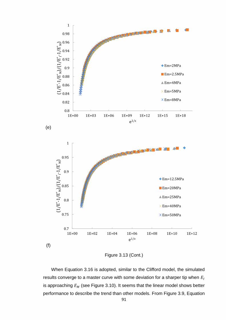
91
(e)
(f)
Figure 3.13 (Cont.)
When Equation 3.16 is adopted, similar to the Clifford model, the simulated
results converge to a master curve with some deviation for a sharper tip when 𝐸𝐼
is approaching 𝐸𝑀 (see Figure 3.10). It seems that the linear model shows better
performance to describe the trend than other models. From Figure 3.9, Equation
0.8
0.82
0.84
0.86
0.88
0.9
0.92
0.94
0.96
0.98
1
1E+00 1E+03 1E+06 1E+09 1E+12 1E+15 1E+18
(1/E
* -1
/E* M
)/(1
/E* I-
1/E
* M)
e1/z
Em=2MPa
Em=2.5MPa
Em=4MPa
Em=5MPa
Em=8MPa
0.7
0.75
0.8
0.85
0.9
0.95
1
1E+00 1E+02 1E+04 1E+06 1E+08 1E+10 1E+12
(1/E
* -1
/E* M
)/(1
/E* I-
1/E
* M)
e1/z
Em=12.5MPa
Em=20MPa
Em=25MPa
Em=40MPa
Em=50MPa
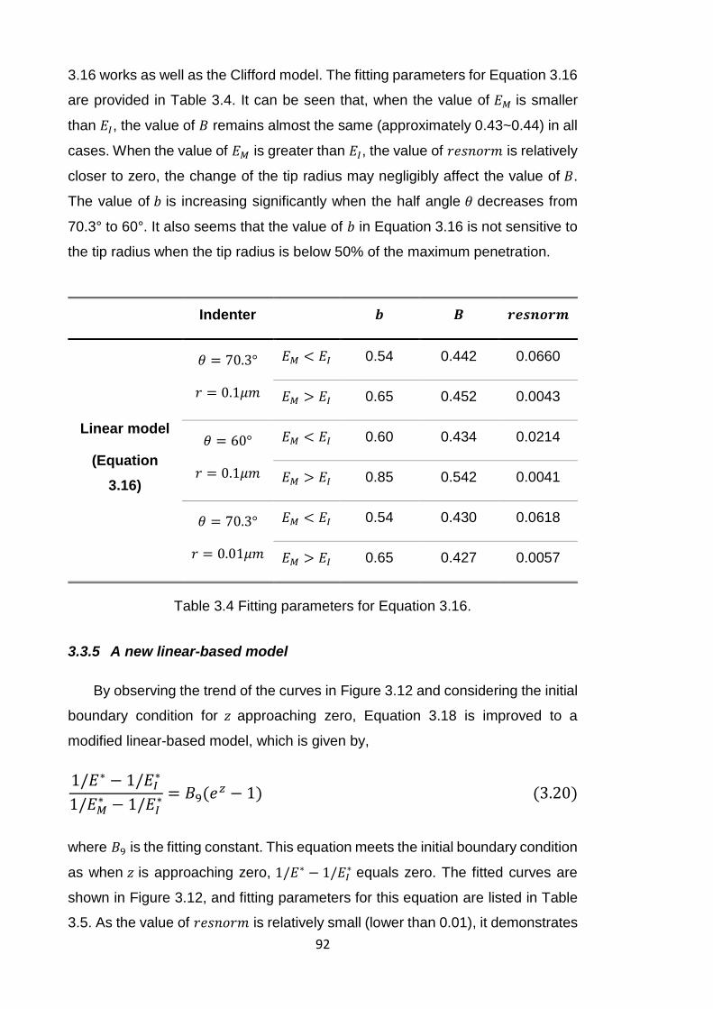
92
3.16 works as well as the Clifford model. The fitting parameters for Equation 3.16
are provided in Table 3.4. It can be seen that, when the value of 𝐸𝑀 is smaller
than 𝐸𝐼, the value of 𝐵 remains almost the same (approximately 0.43~0.44) in all
cases. When the value of 𝐸𝑀 is greater than 𝐸𝐼, the value of 𝑟𝑒𝑠𝑛𝑜𝑟𝑚 is relatively
closer to zero, the change of the tip radius may negligibly affect the value of 𝐵.
The value of 𝑏 is increasing significantly when the half angle 𝜃 decreases from
70.3° to 60°. It also seems that the value of 𝑏 in Equation 3.16 is not sensitive to
the tip radius when the tip radius is below 50% of the maximum penetration.
Indenter 𝒃 𝑩 𝒓𝒆𝒔𝒏𝒐𝒓𝒎
Linear model
(Equation
3.16)
𝜃 = 70.3°
𝑟 = 0.1𝜇𝑚
𝐸𝑀 < 𝐸𝐼 0.54 0.442 0.0660
𝐸𝑀 > 𝐸𝐼 0.65 0.452 0.0043
𝜃 = 60°
𝑟 = 0.1𝜇𝑚
𝐸𝑀 < 𝐸𝐼 0.60 0.434 0.0214
𝐸𝑀 > 𝐸𝐼 0.85 0.542 0.0041
𝜃 = 70.3°
𝑟 = 0.01𝜇𝑚
𝐸𝑀 < 𝐸𝐼 0.54 0.430 0.0618
𝐸𝑀 > 𝐸𝐼 0.65 0.427 0.0057
Table 3.4 Fitting parameters for Equation 3.16.
3.3.5 A new linear-based model
By observing the trend of the curves in Figure 3.12 and considering the initial
boundary condition for 𝑧 approaching zero, Equation 3.18 is improved to a
modified linear-based model, which is given by,
1/𝐸∗ − 1/𝐸𝐼∗
1/𝐸𝑀∗ − 1/𝐸𝐼
∗ = 𝐵9(𝑒𝑧 − 1) (3.20)
where 𝐵9 is the fitting constant. This equation meets the initial boundary condition
as when 𝑧 is approaching zero, 1/𝐸∗ − 1/𝐸𝐼∗ equals zero. The fitted curves are
shown in Figure 3.12, and fitting parameters for this equation are listed in Table
3.5. As the value of 𝑟𝑒𝑠𝑛𝑜𝑟𝑚 is relatively small (lower than 0.01), it demonstrates
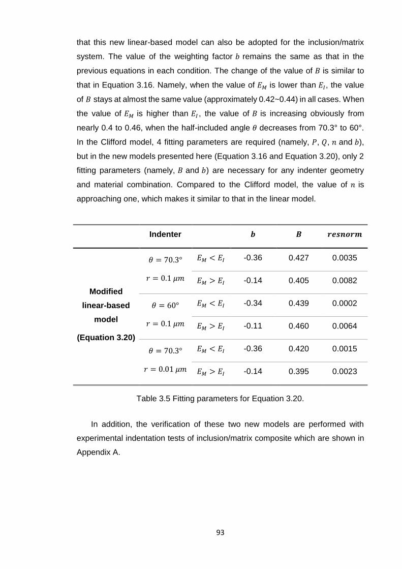
93
that this new linear-based model can also be adopted for the inclusion/matrix
system. The value of the weighting factor 𝑏 remains the same as that in the
previous equations in each condition. The change of the value of 𝐵 is similar to
that in Equation 3.16. Namely, when the value of 𝐸𝑀 is lower than 𝐸𝐼, the value
of 𝐵 stays at almost the same value (approximately 0.42~0.44) in all cases. When
the value of 𝐸𝑀 is higher than 𝐸𝐼 , the value of 𝐵 is increasing obviously from
nearly 0.4 to 0.46, when the half-included angle 𝜃 decreases from 70.3° to 60°.
In the Clifford model, 4 fitting parameters are required (namely, 𝑃, 𝑄, 𝑛 and 𝑏),
but in the new models presented here (Equation 3.16 and Equation 3.20), only 2
fitting parameters (namely, 𝐵 and 𝑏) are necessary for any indenter geometry
and material combination. Compared to the Clifford model, the value of 𝑛 is
approaching one, which makes it similar to that in the linear model.
Indenter 𝒃 𝑩 𝒓𝒆𝒔𝒏𝒐𝒓𝒎
Modified
linear-based
model
(Equation 3.20)
𝜃 = 70.3°
𝑟 = 0.1 𝜇𝑚
𝐸𝑀 < 𝐸𝐼 -0.36 0.427 0.0035
𝐸𝑀 > 𝐸𝐼 -0.14 0.405 0.0082
𝜃 = 60°
𝑟 = 0.1 𝜇𝑚
𝐸𝑀 < 𝐸𝐼 -0.34 0.439 0.0002
𝐸𝑀 > 𝐸𝐼 -0.11 0.460 0.0064
𝜃 = 70.3°
𝑟 = 0.01 𝜇𝑚
𝐸𝑀 < 𝐸𝐼 -0.36 0.420 0.0015
𝐸𝑀 > 𝐸𝐼 -0.14 0.395 0.0023
Table 3.5 Fitting parameters for Equation 3.20.
In addition, the verification of these two new models are performed with
experimental indentation tests of inclusion/matrix composite which are shown in
Appendix A.
94
3.4 Summary
FE simulations were used to investigate the nanomechanical response of
inclusion/matrix polymer composite indented by conical tip with different half-
included angle and different tip radius. The ratio of elastic modulus of inclusion
over matrix (𝐸𝐼 𝐸𝑀⁄ ) varies from 0.2 to 5, which covers a wide range of polymer
composite materials. The FE results have revealed that the measured elastic
modulus of the inclusion can be significantly affected by the surrounding matrix
well before the indenter touches the matrix. Various indentation-based models
have been examined. It is revealed that the Clifford model can be extended to
the conical tip, but the constant 𝑏 will change with the tip geometry. Inspired by
the Clifford model, a power law index 𝑏 was introduced to consider the elastic
mismatch between the inclusion and the matrix, which makes the data converge
to the same master curve in almost all cases. The fitting results show that a
simpler linear model (Equation 3.16) is available for the conical indenter.
Moreover, a new linear-based model has been presented here (Equation 3.20),
which shows good performance as well. But in these two simpler equations, only
two fitting parameters are necessary to describe the nanoindentation response
for composites with any material combination, rather than the four fitting
parameters in the Clifford model.
In the next chapter, finite element modelling for particle-reinforced
composites will be presented to assess their elastic-plastic response during
nanoindentation.
Chapter 4
Nanomechanical Modelling of
Elastic-Plastic Particles in
Elastic-Plastic Matrix
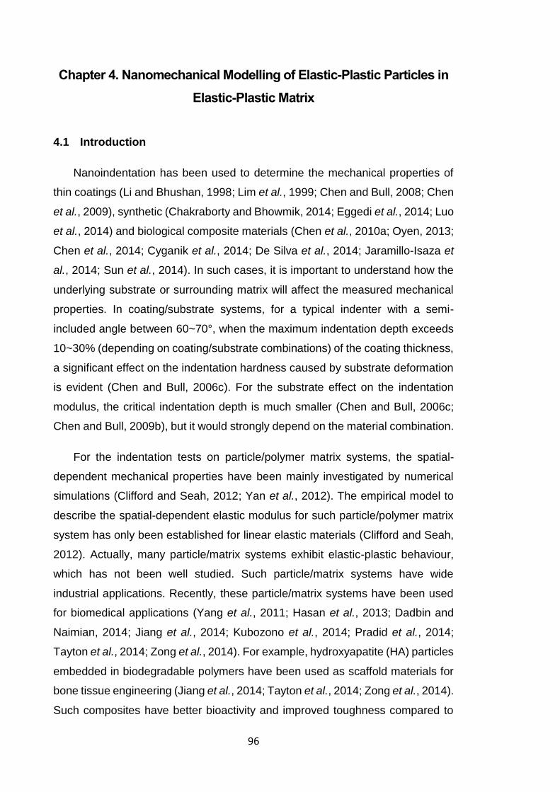
96
Chapter 4. Nanomechanical Modelling of Elastic-Plastic Particles in
Elastic-Plastic Matrix
4.1 Introduction
Nanoindentation has been used to determine the mechanical properties of
thin coatings (Li and Bhushan, 1998; Lim et al., 1999; Chen and Bull, 2008; Chen
et al., 2009), synthetic (Chakraborty and Bhowmik, 2014; Eggedi et al., 2014; Luo
et al., 2014) and biological composite materials (Chen et al., 2010a; Oyen, 2013;
Chen et al., 2014; Cyganik et al., 2014; De Silva et al., 2014; Jaramillo-Isaza et
al., 2014; Sun et al., 2014). In such cases, it is important to understand how the
underlying substrate or surrounding matrix will affect the measured mechanical
properties. In coating/substrate systems, for a typical indenter with a semi-
included angle between 60~70°, when the maximum indentation depth exceeds
10~30% (depending on coating/substrate combinations) of the coating thickness,
a significant effect on the indentation hardness caused by substrate deformation
is evident (Chen and Bull, 2006c). For the substrate effect on the indentation
modulus, the critical indentation depth is much smaller (Chen and Bull, 2006c;
Chen and Bull, 2009b), but it would strongly depend on the material combination.
For the indentation tests on particle/polymer matrix systems, the spatial-
dependent mechanical properties have been mainly investigated by numerical
simulations (Clifford and Seah, 2012; Yan et al., 2012). The empirical model to
describe the spatial-dependent elastic modulus for such particle/polymer matrix
system has only been established for linear elastic materials (Clifford and Seah,
2012). Actually, many particle/matrix systems exhibit elastic-plastic behaviour,
which has not been well studied. Such particle/matrix systems have wide
industrial applications. Recently, these particle/matrix systems have been used
for biomedical applications (Yang et al., 2011; Hasan et al., 2013; Dadbin and
Naimian, 2014; Jiang et al., 2014; Kubozono et al., 2014; Pradid et al., 2014;
Tayton et al., 2014; Zong et al., 2014). For example, hydroxyapatite (HA) particles
embedded in biodegradable polymers have been used as scaffold materials for
bone tissue engineering (Jiang et al., 2014; Tayton et al., 2014; Zong et al., 2014).
Such composites have better bioactivity and improved toughness compared to
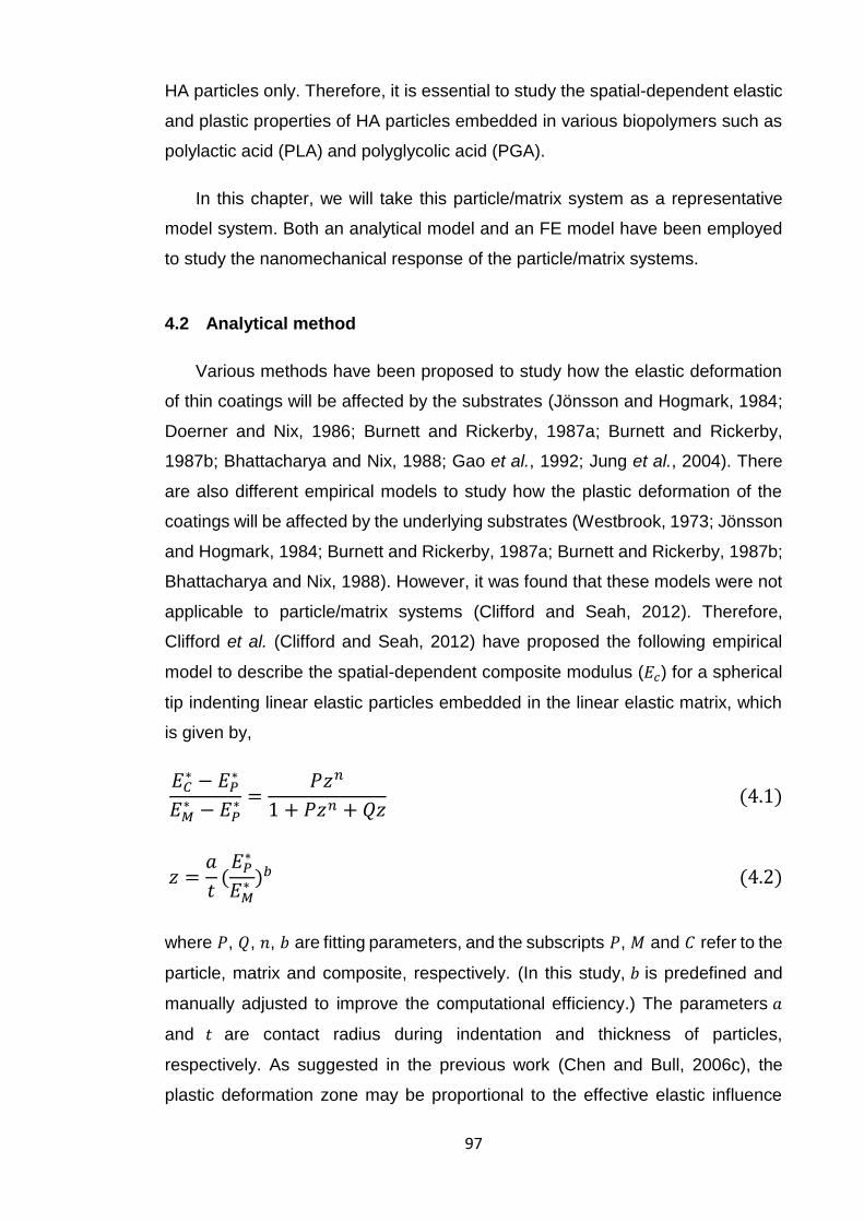
97
HA particles only. Therefore, it is essential to study the spatial-dependent elastic
and plastic properties of HA particles embedded in various biopolymers such as
polylactic acid (PLA) and polyglycolic acid (PGA).
In this chapter, we will take this particle/matrix system as a representative
model system. Both an analytical model and an FE model have been employed
to study the nanomechanical response of the particle/matrix systems.
4.2 Analytical method
Various methods have been proposed to study how the elastic deformation
of thin coatings will be affected by the substrates (Jönsson and Hogmark, 1984;
Doerner and Nix, 1986; Burnett and Rickerby, 1987a; Burnett and Rickerby,
1987b; Bhattacharya and Nix, 1988; Gao et al., 1992; Jung et al., 2004). There
are also different empirical models to study how the plastic deformation of the
coatings will be affected by the underlying substrates (Westbrook, 1973; Jönsson
and Hogmark, 1984; Burnett and Rickerby, 1987a; Burnett and Rickerby, 1987b;
Bhattacharya and Nix, 1988). However, it was found that these models were not
applicable to particle/matrix systems (Clifford and Seah, 2012). Therefore,
Clifford et al. (Clifford and Seah, 2012) have proposed the following empirical
model to describe the spatial-dependent composite modulus (𝐸𝑐) for a spherical
tip indenting linear elastic particles embedded in the linear elastic matrix, which
is given by,
𝐸𝐶∗ − 𝐸𝑃
∗
𝐸𝑀∗ − 𝐸𝑃
∗ =𝑃𝑧𝑛
1 + 𝑃𝑧𝑛 + 𝑄𝑧 (4.1)
𝑧 =𝑎
𝑡(
𝐸𝑃∗
𝐸𝑀∗ )𝑏 (4.2)
where 𝑃, 𝑄, 𝑛, 𝑏 are fitting parameters, and the subscripts 𝑃, 𝑀 and 𝐶 refer to the
particle, matrix and composite, respectively. (In this study, 𝑏 is predefined and
manually adjusted to improve the computational efficiency.) The parameters 𝑎
and 𝑡 are contact radius during indentation and thickness of particles,
respectively. As suggested in the previous work (Chen and Bull, 2006c), the
plastic deformation zone may be proportional to the effective elastic influence
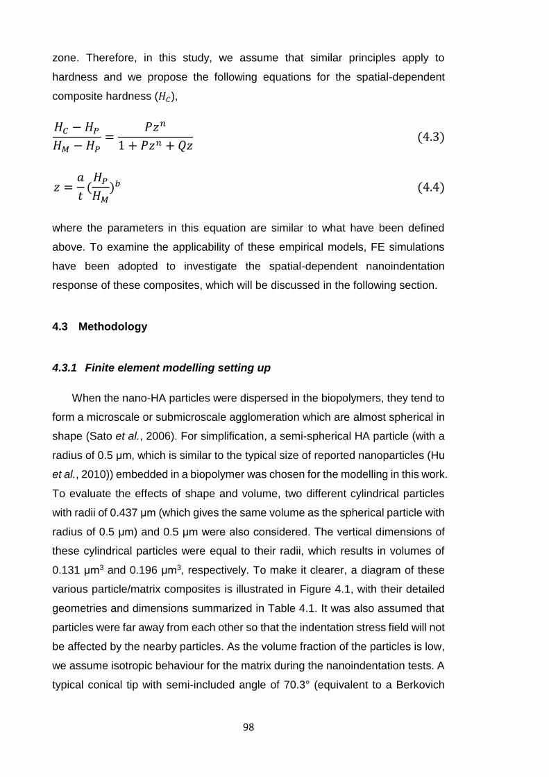
98
zone. Therefore, in this study, we assume that similar principles apply to
hardness and we propose the following equations for the spatial-dependent
composite hardness (𝐻𝐶),
𝐻𝐶 − 𝐻𝑃
𝐻𝑀 − 𝐻𝑃=
𝑃𝑧𝑛
1 + 𝑃𝑧𝑛 + 𝑄𝑧 (4.3)
𝑧 =𝑎
𝑡(
𝐻𝑃
𝐻𝑀)𝑏 (4.4)
where the parameters in this equation are similar to what have been defined
above. To examine the applicability of these empirical models, FE simulations
have been adopted to investigate the spatial-dependent nanoindentation
response of these composites, which will be discussed in the following section.
4.3 Methodology
4.3.1 Finite element modelling setting up
When the nano-HA particles were dispersed in the biopolymers, they tend to
form a microscale or submicroscale agglomeration which are almost spherical in
shape (Sato et al., 2006). For simplification, a semi-spherical HA particle (with a
radius of 0.5 μm, which is similar to the typical size of reported nanoparticles (Hu
et al., 2010)) embedded in a biopolymer was chosen for the modelling in this work.
To evaluate the effects of shape and volume, two different cylindrical particles
with radii of 0.437 μm (which gives the same volume as the spherical particle with
radius of 0.5 μm) and 0.5 μm were also considered. The vertical dimensions of
these cylindrical particles were equal to their radii, which results in volumes of
0.131 μm3 and 0.196 μm3, respectively. To make it clearer, a diagram of these
various particle/matrix composites is illustrated in Figure 4.1, with their detailed
geometries and dimensions summarized in Table 4.1. It was also assumed that
particles were far away from each other so that the indentation stress field will not
be affected by the nearby particles. As the volume fraction of the particles is low,
we assume isotropic behaviour for the matrix during the nanoindentation tests. A
typical conical tip with semi-included angle of 70.3° (equivalent to a Berkovich
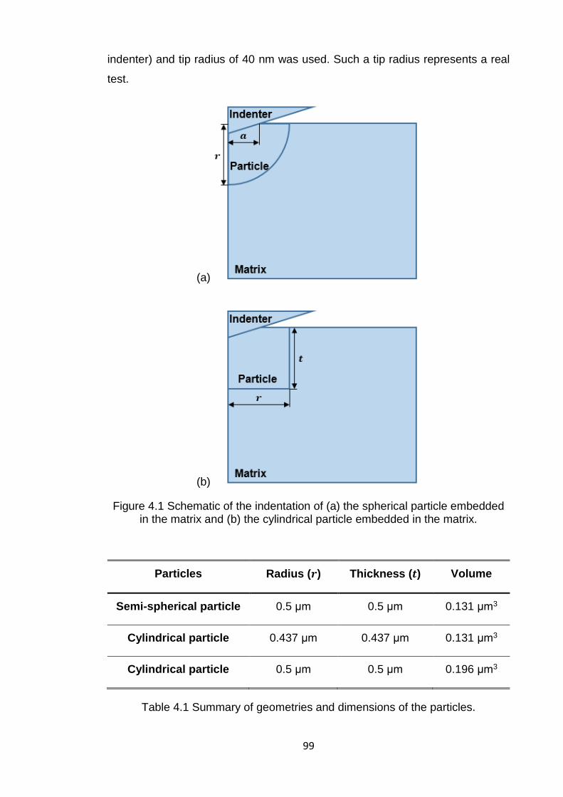
99
indenter) and tip radius of 40 nm was used. Such a tip radius represents a real
test.
(a)
(b)
Figure 4.1 Schematic of the indentation of (a) the spherical particle embedded in the matrix and (b) the cylindrical particle embedded in the matrix.
Particles Radius (𝒓) Thickness (𝒕) Volume
Semi-spherical particle 0.5 μm 0.5 μm 0.131 μm3
Cylindrical particle 0.437 μm 0.437 μm 0.131 μm3
Cylindrical particle 0.5 μm 0.5 μm 0.196 μm3
Table 4.1 Summary of geometries and dimensions of the particles.
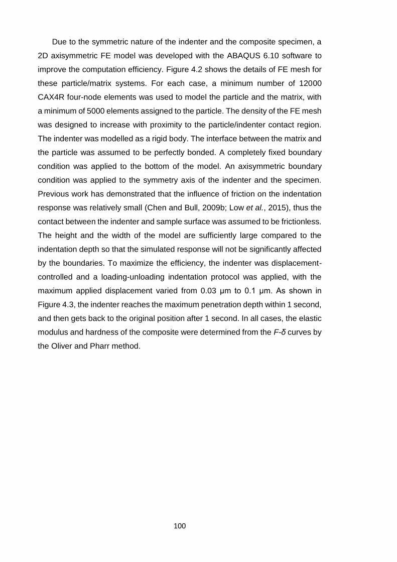
100
Due to the symmetric nature of the indenter and the composite specimen, a
2D axisymmetric FE model was developed with the ABAQUS 6.10 software to
improve the computation efficiency. Figure 4.2 shows the details of FE mesh for
these particle/matrix systems. For each case, a minimum number of 12000
CAX4R four-node elements was used to model the particle and the matrix, with
a minimum of 5000 elements assigned to the particle. The density of the FE mesh
was designed to increase with proximity to the particle/indenter contact region.
The indenter was modelled as a rigid body. The interface between the matrix and
the particle was assumed to be perfectly bonded. A completely fixed boundary
condition was applied to the bottom of the model. An axisymmetric boundary
condition was applied to the symmetry axis of the indenter and the specimen.
Previous work has demonstrated that the influence of friction on the indentation
response was relatively small (Chen and Bull, 2009b; Low et al., 2015), thus the
contact between the indenter and sample surface was assumed to be frictionless.
The height and the width of the model are sufficiently large compared to the
indentation depth so that the simulated response will not be significantly affected
by the boundaries. To maximize the efficiency, the indenter was displacement-
controlled and a loading-unloading indentation protocol was applied, with the
maximum applied displacement varied from 0.03 μm to 0.1 μm. As shown in
Figure 4.3, the indenter reaches the maximum penetration depth within 1 second,
and then gets back to the original position after 1 second. In all cases, the elastic
modulus and hardness of the composite were determined from the F-δ curves by
the Oliver and Pharr method.
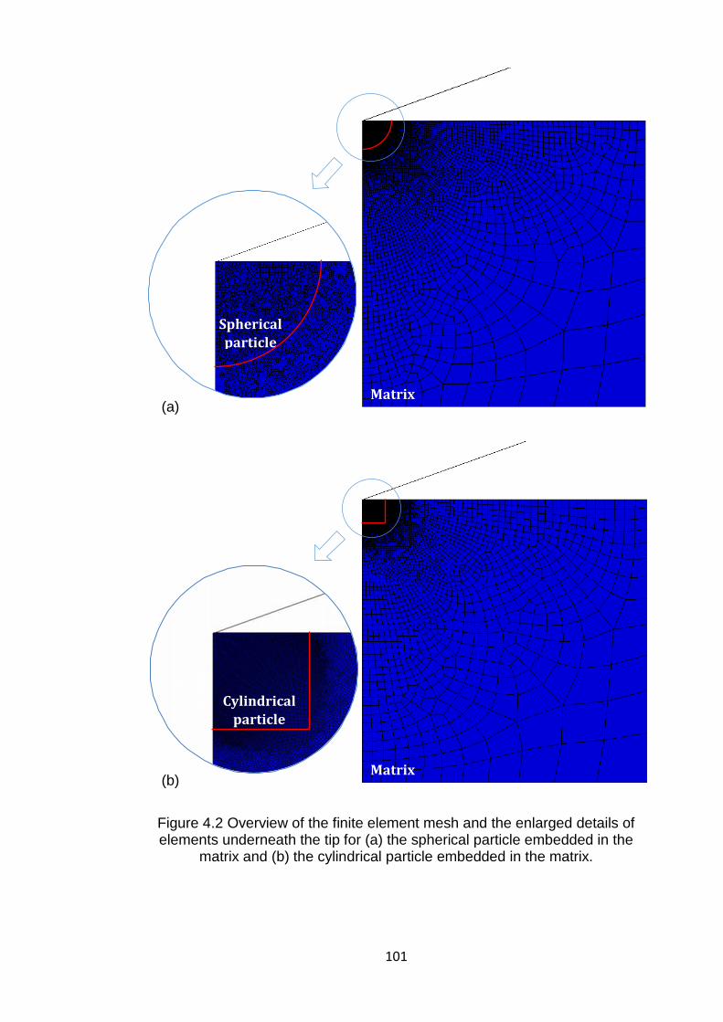
101
(a)
(b)
Figure 4.2 Overview of the finite element mesh and the enlarged details of elements underneath the tip for (a) the spherical particle embedded in the
matrix and (b) the cylindrical particle embedded in the matrix.
Matrix
Matrix
Cylindrical
particle
Spherical
particle
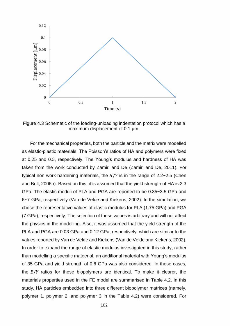
102
Figure 4.3 Schematic of the loading-unloading indentation protocol which has a maximum displacement of 0.1 μm.
For the mechanical properties, both the particle and the matrix were modelled
as elastic-plastic materials. The Poisson’s ratios of HA and polymers were fixed
at 0.25 and 0.3, respectively. The Young’s modulus and hardness of HA was
taken from the work conducted by Zamiri and De (Zamiri and De, 2011). For
typical non work-hardening materials, the 𝐻/𝑌 is in the range of 2.2~2.5 (Chen
and Bull, 2006b). Based on this, it is assumed that the yield strength of HA is 2.3
GPa. The elastic moduli of PLA and PGA are reported to be 0.35~3.5 GPa and
6~7 GPa, respectively (Van de Velde and Kiekens, 2002). In the simulation, we
chose the representative values of elastic modulus for PLA (1.75 GPa) and PGA
(7 GPa), respectively. The selection of these values is arbitrary and will not affect
the physics in the modelling. Also, it was assumed that the yield strength of the
PLA and PGA are 0.03 GPa and 0.12 GPa, respectively, which are similar to the
values reported by Van de Velde and Kiekens (Van de Velde and Kiekens, 2002).
In order to expand the range of elastic modulus investigated in this study, rather
than modelling a specific mateerial, an additional material with Young’s modulus
of 35 GPa and yield strength of 0.6 GPa was also considered. In these cases,
the 𝐸/𝑌 ratios for these biopolymers are identical. To make it clearer, the
materials properties used in the FE model are summarised in Table 4.2. In this
study, HA particles embedded into three different biopolymer matrices (namely,
polymer 1, polymer 2, and polymer 3 in the Table 4.2) were considered. For
0
0.02
0.04
0.06
0.08
0.1
0.12
0 0.5 1 1.5 2
Dis
pla
cem
ent
(μm
)
Time (s)
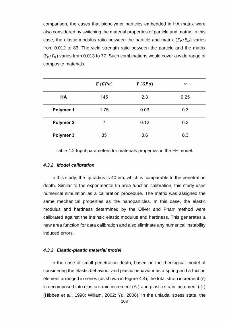
103
comparison, the cases that biopolymer particles embedded in HA matrix were
also considered by switching the material properties of particle and matrix. In this
case, the elastic modulus ratio between the particle and matrix (𝐸𝑃/𝐸𝑀) varies
from 0.012 to 83. The yield strength ratio between the particle and the matrix
(𝑌𝑃/𝑌𝑀) varies from 0.013 to 77. Such combinations would cover a wide range of
composite materials.
𝑬 (𝑮𝑷𝒂) 𝒀 (𝑮𝑷𝒂) 𝝂
HA 145 2.3 0.25
Polymer 1 1.75 0.03 0.3
Polymer 2 7 0.12 0.3
Polymer 3 35 0.6 0.3
Table 4.2 Input parameters for materials properties in the FE model.
4.3.2 Model calibration
In this study, the tip radius is 40 nm, which is comparable to the penetration
depth. Similar to the experimental tip area function calibration, this study uses
numerical simulation as a calibration procedure. The matrix was assigned the
same mechanical properties as the nanoparticles. In this case, the elastic
modulus and hardness determined by the Oliver and Pharr method were
calibrated against the intrinsic elastic modulus and hardness. This generates a
new area function for data calibration and also eliminate any numerical instability
induced errors.
4.3.3 Elastic-plastic material model
In the case of small penetration depth, based on the rheological model of
considering the elastic behaviour and plastic behaviour as a spring and a friction
element arranged in series (as shown in Figure 4.4), the total strain increment (휀)
is decomposed into elastic strain increment (휀��) and plastic strain increment (휀��)
(Hibbett et al., 1998; Willam, 2002; Yu, 2006). In the uniaxial stress state, the
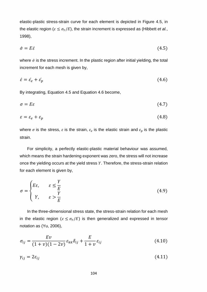
104
elastic-plastic stress-strain curve for each element is depicted in Figure 4.5, in
the elastic region (휀 ≤ 𝜎𝑌/𝐸), the strain increment is expressed as (Hibbett et al.,
1998),
�� = 𝐸휀 (4.5)
where �� is the stress increment. In the plastic region after initial yielding, the total
increment for each mesh is given by,
휀 = 휀�� + 휀�� (4.6)
By integrating, Equation 4.5 and Equation 4.6 become,
𝜎 = 𝐸휀 (4.7)
휀 = 휀𝑒 + 휀𝑝 (4.8)
where 𝜎 is the stress, 휀 is the strain, 휀𝑒 is the elastic strain and 휀𝑝 is the plastic
strain.
For simplicity, a perfectly elastic-plastic material behaviour was assumed,
which means the strain hardening exponent was zero, the stress will not increase
once the yielding occurs at the yield stress 𝑌. Therefore, the stress-strain relation
for each element is given by,
𝜎 = {𝐸휀, 휀 ≤
𝑌
𝐸
𝑌, 휀 >𝑌
𝐸
(4.9)
In the three-dimensional stress state, the stress-strain relation for each mesh
in the elastic region (휀 ≤ 𝜎𝑌/𝐸 ) is then generalized and expressed in tensor
notation as (Yu, 2006),
𝜎𝑖𝑗 =𝐸𝑣
(1 + 𝑣)(1 − 2𝑣)휀𝑘𝑘𝛿𝑖𝑗 +
𝐸
1 + 𝑣휀𝑖𝑗 (4.10)
𝛾𝑖𝑗 = 2휀𝑖𝑗 (4.11)
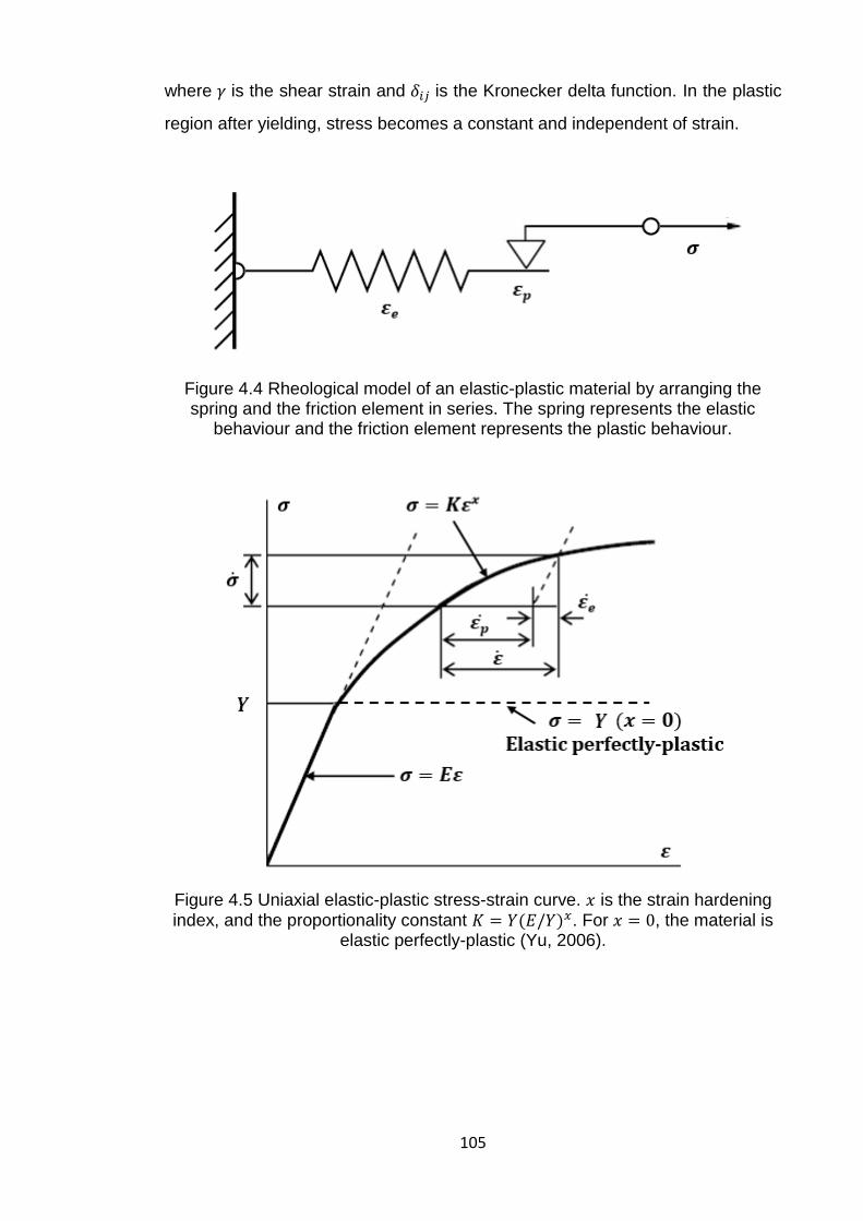
105
where 𝛾 is the shear strain and 𝛿𝑖𝑗 is the Kronecker delta function. In the plastic
region after yielding, stress becomes a constant and independent of strain.
Figure 4.4 Rheological model of an elastic-plastic material by arranging the spring and the friction element in series. The spring represents the elastic
behaviour and the friction element represents the plastic behaviour.
Figure 4.5 Uniaxial elastic-plastic stress-strain curve. 𝑥 is the strain hardening index, and the proportionality constant 𝐾 = 𝑌(𝐸/𝑌)𝑥. For 𝑥 = 0, the material is
elastic perfectly-plastic (Yu, 2006).
106
4.3.4 Curve fitting
Matlab code was written to perform the curve fitting and extract the fitting
parameters. In this chapter, the goodness of the fitting was determined by
calculating the coefficient of determination (𝑅2) value, which is given by,
𝑅2 = 1 −∑ (𝑦𝑖 − 𝐹(𝑥𝑖))
2𝑖
∑ (𝑦𝑖 − ��)2𝑖
(4.12)
where 𝑅2 is a statistical parameter, which varies between 0 and 1. Within this
range, a larger value means a better fitting and one represents a perfect fitting.
𝐹(𝑥) is the predicted data from the fitting equation, 𝑦 is the observed data from
simulation, and �� is the mean of the observed data. During the curve fitting, in
order to improve the computational efficiency, the fitting parameter 𝑏 in Clifford
model was predefined and manually adjusted until achieving a minimum 𝑟𝑒𝑠𝑛𝑜𝑟𝑚
value. Besides, the influence of fitting parameters with different decimal places
(i.e. 1, 2, 3…) on the 𝑅2 value were investigated. Then, as a trade-off between
efficiency and accuracy, all the fitting parameters were rounded to 3 decimal
places.
In the previous chapter, the 𝑟𝑒𝑠𝑛𝑜𝑟𝑚 value was used to present the quality
of a fitting instead of 𝑅2, which has the limitation of depending on the magnitudes
of the data. Therefore, to avoid the confusion due to the magnitudes of the data,
the 𝑅2 value was used to indicate the fitting quality in this chapter.
4.4 Results and discussion
4.4.1 Model validation
Prior to the nanomechanical modelling of the particle/matrix systems, these
models should be validated. Since coarse mesh may result in inaccurate
simulation results, errors due to the density of mesh should be avoided, and the
deviation between the simulated data and the theoretical data should be within
an acceptable level.
107
To investigate the influence from the mesh density, a model with denser or
coarser mesh was created by proportionally varying the number of elements in
each segment. For each particle/matrix system (namely, different particle
geometry), the maximum number of elements was approximately 30000 and the
minimum number was approximately 760. According to the literature, these
values are reasonable to be set as maximum and minimum values. (After setting
the number of elements in each segment, the number of elements is then
determined by the finite element software. However, due to different particle
geometry in each particle/matrix system, the number of elements for each system
with a similar mesh density will be slightly different.) Both particle and matrix were
defined as HA material. By performing the nanoindentation modelling with the
maximum displacement of 0.1 μm by the defined conical indenter, the F-δ data
from loading period for models with different mesh density were compared. By
assuming the data from model with densest mesh (number of elements was
approximately 30000) as the reference (𝐹0), the deviation between 𝐹0 and the
data from models with other mesh density (𝐹𝑖 ) is plotted in Figure 4.6. A big
deviation (higher than 20%) was observed in all cases when the displacement
was lower than 0.02 μm, which may due to the fact that the indenter was not
touching enough elements at shallow penetration depth. Therefore, the data
within the displacement range of 0~0.02 μm were discarded. After the indenter
touched enough elements, as shown in Figure 4.6, big deviation (higher than 10%)
was observed when the number of elements was lower than approximately
9000~10000 in all cases. The deviation was approximately 2~3% when the
number of elements was higher than approximately 10000. It indicates that the
mesh should be dense enough with the total number of elements higher than
10000 to avoid errors from the mesh density, and the mesh density of models
(with a minimum of 12000 elements) used in this study is reasonable.
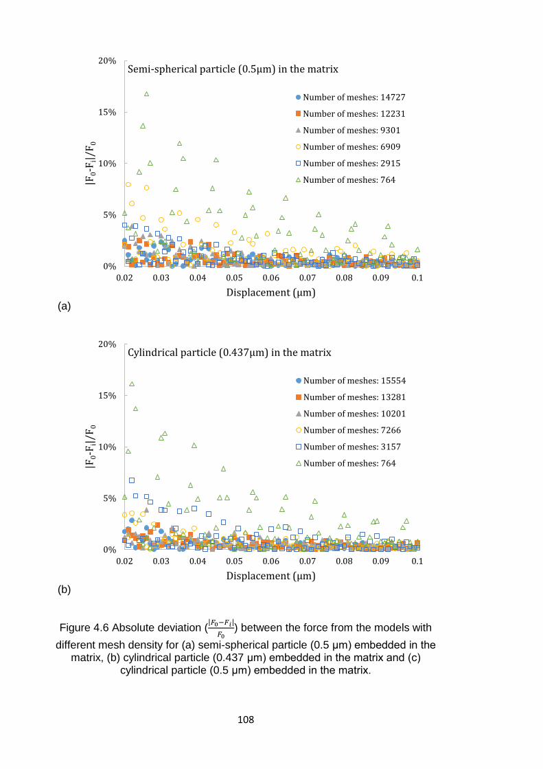
108
(a)
(b)
Figure 4.6 Absolute deviation (|𝐹0−𝐹𝑖|
𝐹0) between the force from the models with
different mesh density for (a) semi-spherical particle (0.5 μm) embedded in the matrix, (b) cylindrical particle (0.437 μm) embedded in the matrix and (c)
cylindrical particle (0.5 μm) embedded in the matrix.
0%
5%
10%
15%
20%
0.02 0.03 0.04 0.05 0.06 0.07 0.08 0.09 0.1
|F0-F
i|/F
0
Displacement (µm)
Semi-spherical particle (0.5μm) in the matrix
Number of meshes: 14727
Number of meshes: 12231
Number of meshes: 9301
Number of meshes: 6909
Number of meshes: 2915
Number of meshes: 764
0%
5%
10%
15%
20%
0.02 0.03 0.04 0.05 0.06 0.07 0.08 0.09 0.1
|F0-F
i|/F
0
Displacement (µm)
Cylindrical particle (0.437μm) in the matrix
Number of meshes: 15554
Number of meshes: 13281
Number of meshes: 10201
Number of meshes: 7266
Number of meshes: 3157
Number of meshes: 764
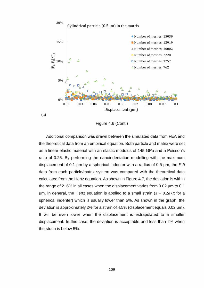
109
(c)
Figure 4.6 (Cont.)
Additional comparison was drawn between the simulated data from FEA and
the theoretical data from an empirical equation. Both particle and matrix were set
as a linear elastic material with an elastic modulus of 145 GPa and a Poisson’s
ratio of 0.25. By performing the nanoindentation modelling with the maximum
displacement of 0.1 μm by a spherical indenter with a radius of 0.5 μm, the F-δ
data from each particle/matrix system was compared with the theoretical data
calculated from the Hertz equation. As shown in Figure 4.7, the deviation is within
the range of 2~6% in all cases when the displacement varies from 0.02 μm to 0.1
μm. In general, the Hertz equation is applied to a small strain (휀 = 0.2𝑎/𝑅 for a
spherical indenter) which is usually lower than 5%. As shown in the graph, the
deviation is approximately 2% for a strain of 4.5% (displacement equals 0.02 μm).
It will be even lower when the displacement is extrapolated to a smaller
displacement. In this case, the deviation is acceptable and less than 2% when
the strain is below 5%.
0%
5%
10%
15%
20%
0.02 0.03 0.04 0.05 0.06 0.07 0.08 0.09 0.1
|F0-F
i|/F
0
Displacement (µm)
Cylindrical particle (0.5μm) in the matrix
Number of meshes: 15039
Number of meshes: 12919
Number of meshes: 10002
Number of meshes: 7228
Number of meshes: 3257
Number of meshes: 762
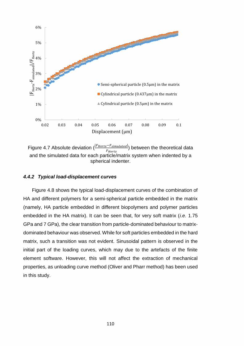
110
Figure 4.7 Absolute deviation (|𝐹𝐻𝑒𝑟𝑡𝑧−𝐹𝑠𝑖𝑚𝑢𝑙𝑎𝑡𝑒𝑑|
𝐹𝐻𝑒𝑟𝑡𝑧) between the theoretical data
and the simulated data for each particle/matrix system when indented by a spherical indenter.
4.4.2 Typical load-displacement curves
Figure 4.8 shows the typical load-displacement curves of the combination of
HA and different polymers for a semi-spherical particle embedded in the matrix
(namely, HA particle embedded in different biopolymers and polymer particles
embedded in the HA matrix). It can be seen that, for very soft matrix (i.e. 1.75
GPa and 7 GPa), the clear transition from particle-dominated behaviour to matrix-
dominated behaviour was observed. While for soft particles embedded in the hard
matrix, such a transition was not evident. Sinusoidal pattern is observed in the
initial part of the loading curves, which may due to the artefacts of the finite
element software. However, this will not affect the extraction of mechanical
properties, as unloading curve method (Oliver and Pharr method) has been used
in this study.
0%
1%
2%
3%
4%
5%
6%
0.02 0.03 0.04 0.05 0.06 0.07 0.08 0.09 0.1
|FH
ertz
-Fsi
mu
late
d|/
FH
ertz
Displacement (µm)
Semi-spherical particle (0.5μm) in the matrix
Cylindrical particle (0.437μm) in the matrix
Cylindrical particle (0.5μm) in the matrix
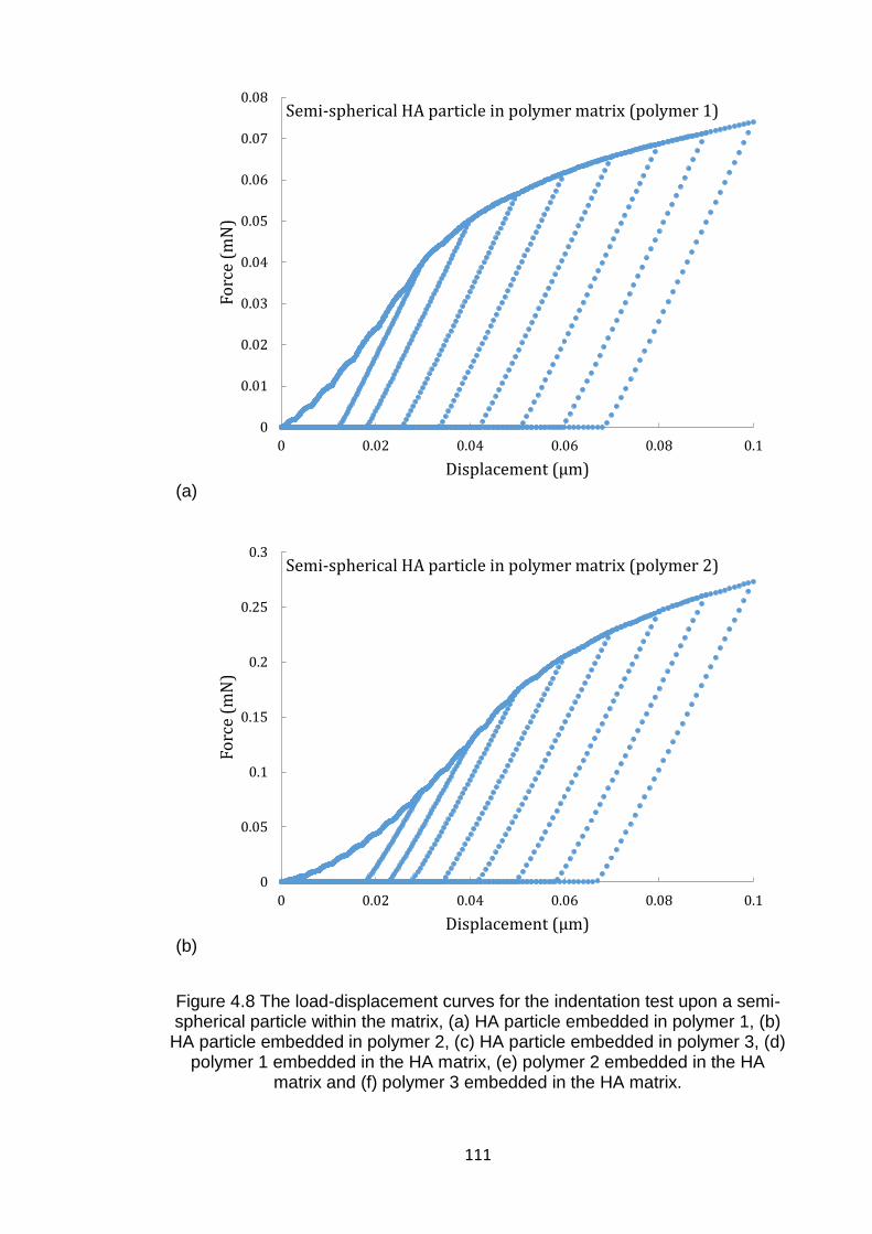
111
(a)
(b)
Figure 4.8 The load-displacement curves for the indentation test upon a semi-spherical particle within the matrix, (a) HA particle embedded in polymer 1, (b)
HA particle embedded in polymer 2, (c) HA particle embedded in polymer 3, (d) polymer 1 embedded in the HA matrix, (e) polymer 2 embedded in the HA
matrix and (f) polymer 3 embedded in the HA matrix.
0
0.01
0.02
0.03
0.04
0.05
0.06
0.07
0.08
0 0.02 0.04 0.06 0.08 0.1
Forc
e (m
N)
Displacement (µm)
Semi-spherical HA particle in polymer matrix (polymer 1)
0
0.05
0.1
0.15
0.2
0.25
0.3
0 0.02 0.04 0.06 0.08 0.1
Forc
e (m
N)
Displacement (µm)
Semi-spherical HA particle in polymer matrix (polymer 2)
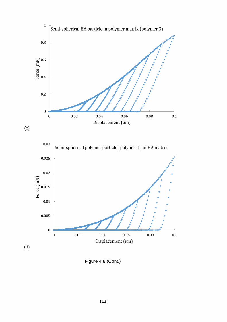
112
(c)
(d)
Figure 4.8 (Cont.)
0
0.2
0.4
0.6
0.8
1
0 0.02 0.04 0.06 0.08 0.1
Forc
e (m
N)
Displacement (µm)
Semi-spherical HA particle in polymer matrix (polymer 3)
0
0.005
0.01
0.015
0.02
0.025
0.03
0 0.02 0.04 0.06 0.08 0.1
Forc
e (m
N)
Displacement (µm)
Semi-spherical polymer particle (polymer 1) in HA matrix
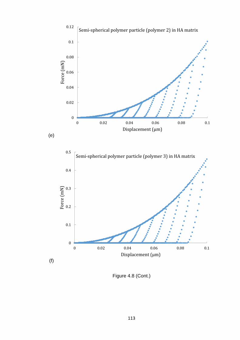
113
(e)
(f)
Figure 4.8 (Cont.)
0
0.02
0.04
0.06
0.08
0.1
0.12
0 0.02 0.04 0.06 0.08 0.1
Forc
e (m
N)
Displacement (µm)
Semi-spherical polymer particle (polymer 2) in HA matrix
0
0.1
0.2
0.3
0.4
0.5
0 0.02 0.04 0.06 0.08 0.1
Forc
e (m
N)
Displacement (µm)
Semi-spherical polymer particle (polymer 3) in HA matrix
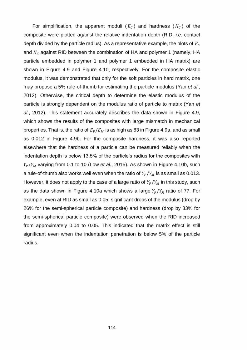
114
For simplification, the apparent moduli ( 𝐸𝐶 ) and hardness ( 𝐻𝐶 ) of the
composite were plotted against the relative indentation depth (RID, i.e. contact
depth divided by the particle radius). As a representative example, the plots of 𝐸𝐶
and 𝐻𝐶 against RID between the combination of HA and polymer 1 (namely, HA
particle embedded in polymer 1 and polymer 1 embedded in HA matrix) are
shown in Figure 4.9 and Figure 4.10, respectively. For the composite elastic
modulus, it was demonstrated that only for the soft particles in hard matrix, one
may propose a 5% rule-of-thumb for estimating the particle modulus (Yan et al.,
2012). Otherwise, the critical depth to determine the elastic modulus of the
particle is strongly dependent on the modulus ratio of particle to matrix (Yan et
al., 2012). This statement accurately describes the data shown in Figure 4.9,
which shows the results of the composites with large mismatch in mechanical
properties. That is, the ratio of 𝐸𝑃/𝐸𝑀 is as high as 83 in Figure 4.9a, and as small
as 0.012 in Figure 4.9b. For the composite hardness, it was also reported
elsewhere that the hardness of a particle can be measured reliably when the
indentation depth is below 13.5% of the particle’s radius for the composites with
𝑌𝑃/𝑌𝑀 varying from 0.1 to 10 (Low et al., 2015). As shown in Figure 4.10b, such
a rule-of-thumb also works well even when the ratio of 𝑌𝑃/𝑌𝑀 is as small as 0.013.
However, it does not apply to the case of a large ratio of 𝑌𝑃/𝑌𝑀 in this study, such
as the data shown in Figure 4.10a which shows a large 𝑌𝑃/𝑌𝑀 ratio of 77. For
example, even at RID as small as 0.05, significant drops of the modulus (drop by
26% for the semi-spherical particle composite) and hardness (drop by 33% for
the semi-spherical particle composite) were observed when the RID increased
from approximately 0.04 to 0.05. This indicated that the matrix effect is still
significant even when the indentation penetration is below 5% of the particle
radius.
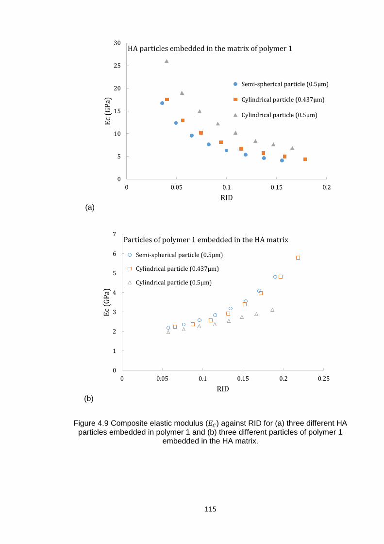
115
(a)
(b)
Figure 4.9 Composite elastic modulus (𝐸𝐶) against RID for (a) three different HA particles embedded in polymer 1 and (b) three different particles of polymer 1
embedded in the HA matrix.
0
5
10
15
20
25
30
0 0.05 0.1 0.15 0.2
Ec
(GP
a)
RID
HA particles embedded in the matrix of polymer 1
Semi-spherical particle (0.5μm)
Cylindrical particle (0.437μm)
Cylindrical particle (0.5μm)
0
1
2
3
4
5
6
7
0 0.05 0.1 0.15 0.2 0.25
Ec
(GP
a)
RID
Particles of polymer 1 embedded in the HA matrix
Semi-spherical particle (0.5μm)
Cylindrical particle (0.437μm)
Cylindrical particle (0.5μm)
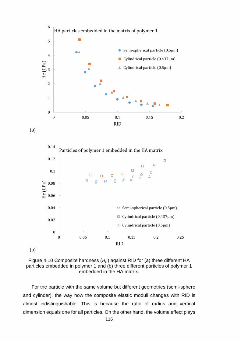
116
(a)
(b)
Figure 4.10 Composite hardness (𝐻𝐶) against RID for (a) three different HA particles embedded in polymer 1 and (b) three different particles of polymer 1
embedded in the HA matrix.
For the particle with the same volume but different geometries (semi-sphere
and cylinder), the way how the composite elastic moduli changes with RID is
almost indistinguishable. This is because the ratio of radius and vertical
dimension equals one for all particles. On the other hand, the volume effect plays
0
1
2
3
4
5
6
0 0.05 0.1 0.15 0.2
Hc
(GP
a)
RID
HA particles embedded in the matrix of polymer 1
Semi-spherical particle (0.5μm)
Cylindrical particle (0.437μm)
Cylindrical particle (0.5μm)
0
0.02
0.04
0.06
0.08
0.1
0.12
0.14
0 0.05 0.1 0.15 0.2 0.25
Hc
(GP
a)
RID
Particles of polymer 1 embedded in the HA matrix
Semi-spherical particle (0.5μm)
Cylindrical particle (0.437μm)
Cylindrical particle (0.5μm)
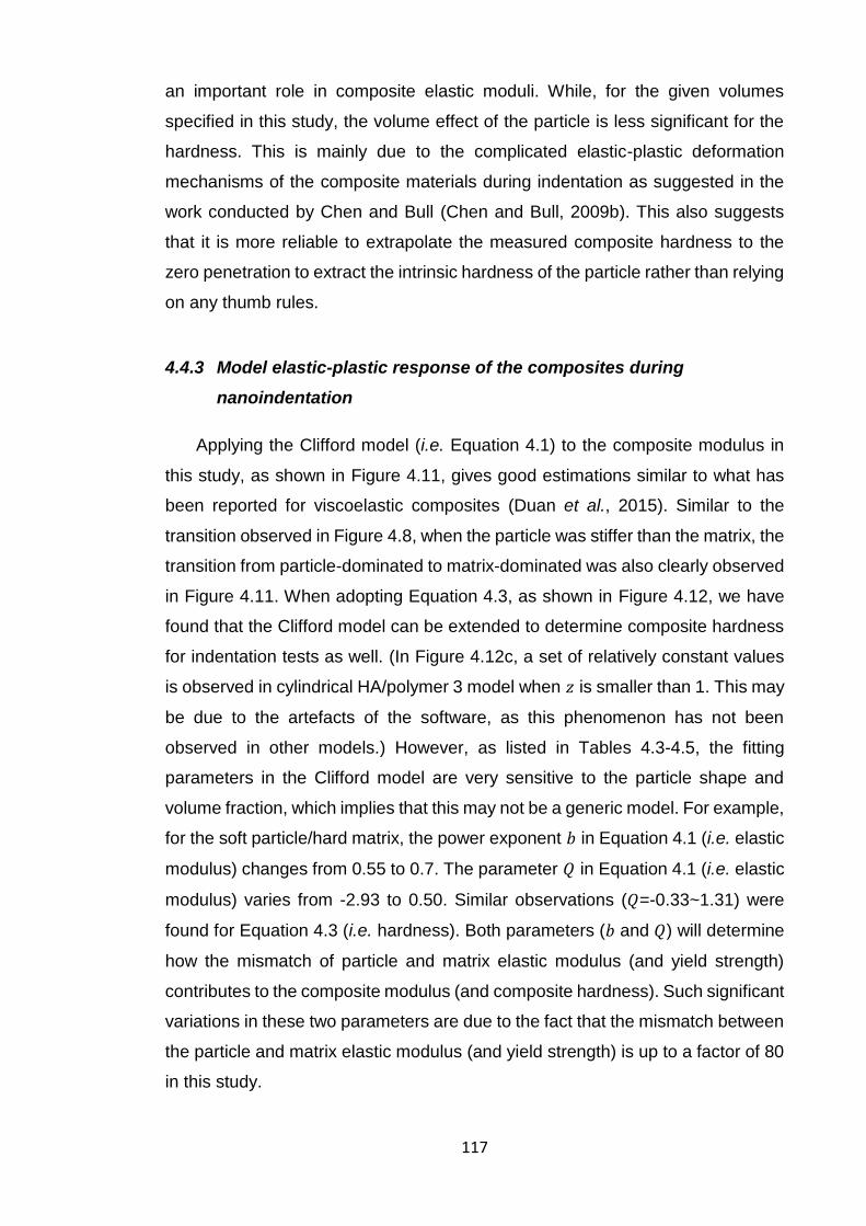
117
an important role in composite elastic moduli. While, for the given volumes
specified in this study, the volume effect of the particle is less significant for the
hardness. This is mainly due to the complicated elastic-plastic deformation
mechanisms of the composite materials during indentation as suggested in the
work conducted by Chen and Bull (Chen and Bull, 2009b). This also suggests
that it is more reliable to extrapolate the measured composite hardness to the
zero penetration to extract the intrinsic hardness of the particle rather than relying
on any thumb rules.
4.4.3 Model elastic-plastic response of the composites during
nanoindentation
Applying the Clifford model (i.e. Equation 4.1) to the composite modulus in
this study, as shown in Figure 4.11, gives good estimations similar to what has
been reported for viscoelastic composites (Duan et al., 2015). Similar to the
transition observed in Figure 4.8, when the particle was stiffer than the matrix, the
transition from particle-dominated to matrix-dominated was also clearly observed
in Figure 4.11. When adopting Equation 4.3, as shown in Figure 4.12, we have
found that the Clifford model can be extended to determine composite hardness
for indentation tests as well. (In Figure 4.12c, a set of relatively constant values
is observed in cylindrical HA/polymer 3 model when 𝑧 is smaller than 1. This may
be due to the artefacts of the software, as this phenomenon has not been
observed in other models.) However, as listed in Tables 4.3-4.5, the fitting
parameters in the Clifford model are very sensitive to the particle shape and
volume fraction, which implies that this may not be a generic model. For example,
for the soft particle/hard matrix, the power exponent 𝑏 in Equation 4.1 (i.e. elastic
modulus) changes from 0.55 to 0.7. The parameter 𝑄 in Equation 4.1 (i.e. elastic
modulus) varies from -2.93 to 0.50. Similar observations (𝑄=-0.33~1.31) were
found for Equation 4.3 (i.e. hardness). Both parameters (𝑏 and 𝑄) will determine
how the mismatch of particle and matrix elastic modulus (and yield strength)
contributes to the composite modulus (and composite hardness). Such significant
variations in these two parameters are due to the fact that the mismatch between
the particle and matrix elastic modulus (and yield strength) is up to a factor of 80
in this study.
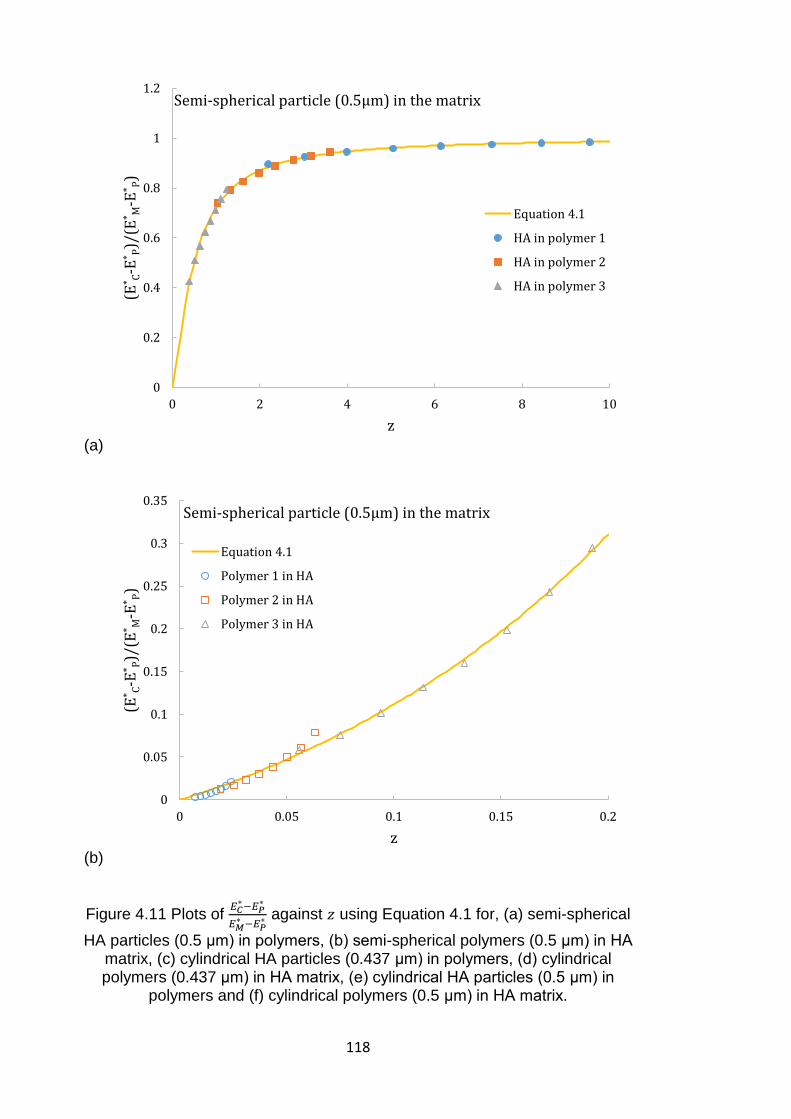
118
(a)
(b)
Figure 4.11 Plots of 𝐸𝐶
∗−𝐸𝑃∗
𝐸𝑀∗ −𝐸𝑃
∗ against 𝑧 using Equation 4.1 for, (a) semi-spherical
HA particles (0.5 μm) in polymers, (b) semi-spherical polymers (0.5 μm) in HA matrix, (c) cylindrical HA particles (0.437 μm) in polymers, (d) cylindrical polymers (0.437 μm) in HA matrix, (e) cylindrical HA particles (0.5 μm) in
polymers and (f) cylindrical polymers (0.5 μm) in HA matrix.
0
0.2
0.4
0.6
0.8
1
1.2
0 2 4 6 8 10
(E* C
-E* P
)/(E
* M-E
* P)
z
Semi-spherical particle (0.5μm) in the matrix
Equation 4.1
HA in polymer 1
HA in polymer 2
HA in polymer 3
0
0.05
0.1
0.15
0.2
0.25
0.3
0.35
0 0.05 0.1 0.15 0.2
(E* C
-E* P
)/(E
* M-E
* P)
z
Semi-spherical particle (0.5μm) in the matrix
Equation 4.1
Polymer 1 in HA
Polymer 2 in HA
Polymer 3 in HA
119
(c)
(d)
Figure 4.11 (Cont.)
0
0.2
0.4
0.6
0.8
1
1.2
0 2 4 6 8 10 12
(E* C
-E* P
)/(E
* M-E
* P)
z
Cylindrical particle (0.437μm) in the matrix
Equation 4.1
HA in polymer 1
HA in polymer 2
HA in polymer 3
0
0.05
0.1
0.15
0.2
0.25
0.3
0.35
0.4
0.45
0 0.05 0.1 0.15 0.2 0.25
(E* C
-E* P
)/(E
* M-E
* P)
z
Cylindrical particle (0.437μm) in the matrix
Equation 4.1
Polymer 1 in HA
Polymer 2 in HA
Polymer 3 in HA
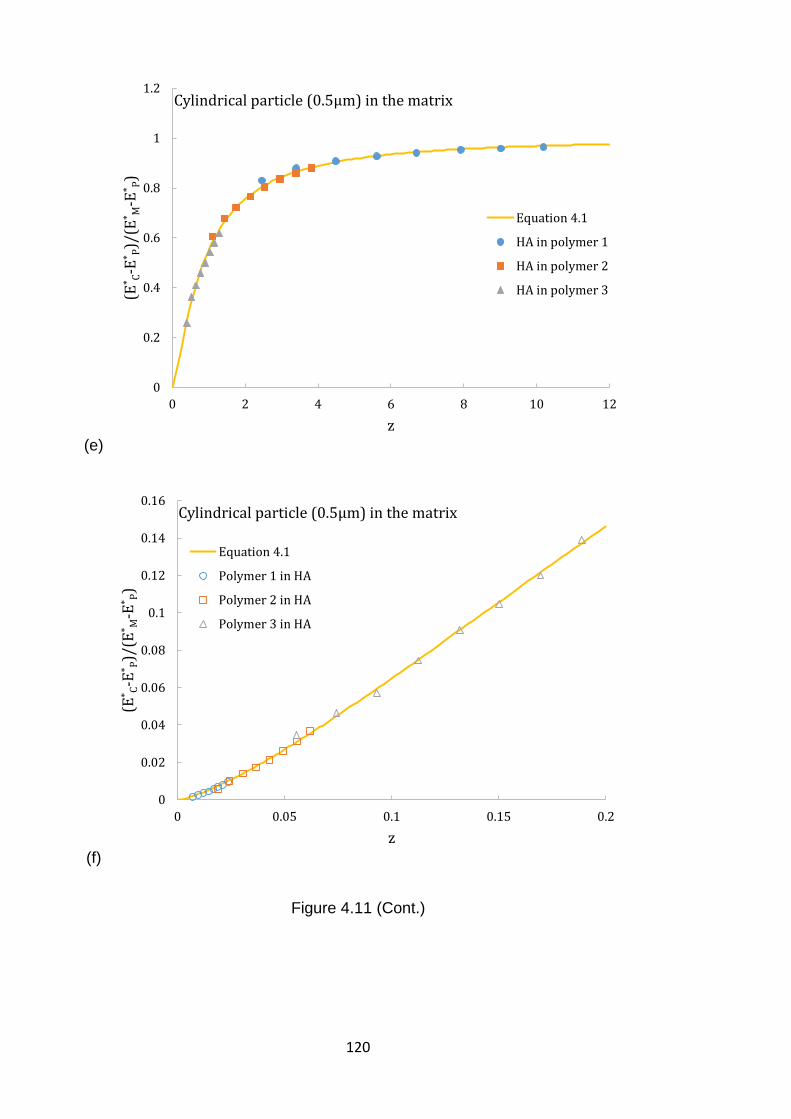
120
(e)
(f)
Figure 4.11 (Cont.)
0
0.2
0.4
0.6
0.8
1
1.2
0 2 4 6 8 10 12
(E* C
-E* P
)/(E
* M-E
* P)
z
Cylindrical particle (0.5μm) in the matrix
Equation 4.1
HA in polymer 1
HA in polymer 2
HA in polymer 3
0
0.02
0.04
0.06
0.08
0.1
0.12
0.14
0.16
0 0.05 0.1 0.15 0.2
(E* C
-E* P
)/(E
* M-E
* P)
z
Cylindrical particle (0.5μm) in the matrix
Equation 4.1
Polymer 1 in HA
Polymer 2 in HA
Polymer 3 in HA
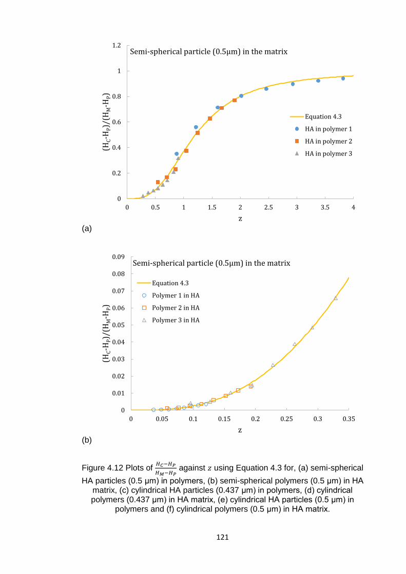
121
(a)
(b)
Figure 4.12 Plots of 𝐻𝐶−𝐻𝑃
𝐻𝑀−𝐻𝑃 against 𝑧 using Equation 4.3 for, (a) semi-spherical
HA particles (0.5 μm) in polymers, (b) semi-spherical polymers (0.5 μm) in HA matrix, (c) cylindrical HA particles (0.437 μm) in polymers, (d) cylindrical polymers (0.437 μm) in HA matrix, (e) cylindrical HA particles (0.5 μm) in
polymers and (f) cylindrical polymers (0.5 μm) in HA matrix.
0
0.2
0.4
0.6
0.8
1
1.2
0 0.5 1 1.5 2 2.5 3 3.5 4
(HC-H
P)/
(HM
-HP)
z
Semi-spherical particle (0.5μm) in the matrix
Equation 4.3
HA in polymer 1
HA in polymer 2
HA in polymer 3
0
0.01
0.02
0.03
0.04
0.05
0.06
0.07
0.08
0.09
0 0.05 0.1 0.15 0.2 0.25 0.3 0.35
(HC-H
P)/
(HM
-HP)
z
Semi-spherical particle (0.5μm) in the matrix
Equation 4.3
Polymer 1 in HA
Polymer 2 in HA
Polymer 3 in HA
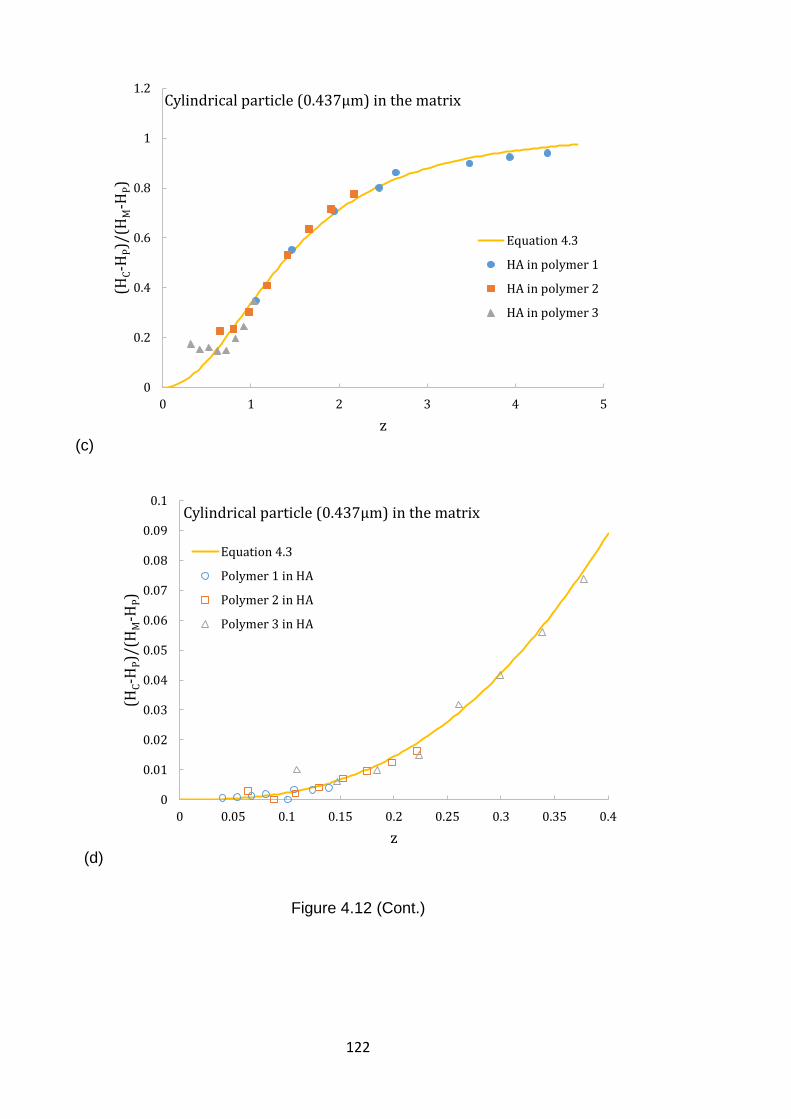
122
(c)
(d)
Figure 4.12 (Cont.)
0
0.2
0.4
0.6
0.8
1
1.2
0 1 2 3 4 5
(HC-H
P)/
(HM
-HP)
z
Cylindrical particle (0.437μm) in the matrix
Equation 4.3
HA in polymer 1
HA in polymer 2
HA in polymer 3
0
0.01
0.02
0.03
0.04
0.05
0.06
0.07
0.08
0.09
0.1
0 0.05 0.1 0.15 0.2 0.25 0.3 0.35 0.4
(HC-H
P)/
(HM
-HP)
z
Cylindrical particle (0.437μm) in the matrix
Equation 4.3
Polymer 1 in HA
Polymer 2 in HA
Polymer 3 in HA
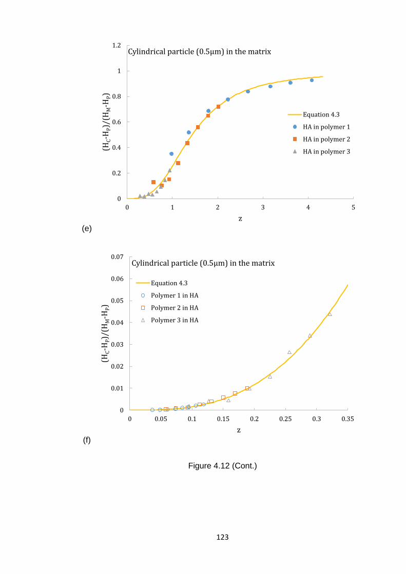
123
(e)
(f)
Figure 4.12 (Cont.)
0
0.2
0.4
0.6
0.8
1
1.2
0 1 2 3 4 5
(HC-H
P)/
(HM
-HP)
z
Cylindrical particle (0.5μm) in the matrix
Equation 4.3
HA in polymer 1
HA in polymer 2
HA in polymer 3
0
0.01
0.02
0.03
0.04
0.05
0.06
0.07
0 0.05 0.1 0.15 0.2 0.25 0.3 0.35
(HC-H
P)/
(HM
-HP)
z
Cylindrical particle (0.5μm) in the matrix
Equation 4.3
Polymer 1 in HA
Polymer 2 in HA
Polymer 3 in HA
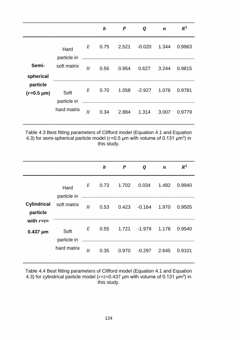
124
𝒃 𝑷 𝑸 𝒏 𝑹𝟐
Semi-
spherical
particle
(𝒓=0.5 μm)
Hard
particle in
soft matrix
𝐸 0.75 2.521 -0.020 1.344 0.9963
𝐻 0.56 0.954 0.627 3.244 0.9815
Soft
particle in
hard matrix
𝐸 0.70 1.058 -2.927 1.076 0.9781
𝐻 0.34 2.884 1.314 3.007 0.9779
Table 4.3 Best fitting parameters of Clifford model (Equation 4.1 and Equation
4.3) for semi-spherical particle model (𝑟=0.5 μm with volume of 0.131 μm3) in this study.
𝒃 𝑷 𝑸 𝒏 𝑹𝟐
Cylindrical
particle
with 𝒓=𝒕=
0.437 μm
Hard
particle in
soft matrix
𝐸 0.73 1.702 0.034 1.482 0.9940
𝐻 0.53 0.423 -0.164 1.970 0.9505
Soft
particle in
hard matrix
𝐸 0.55 1.721 -1.979 1.178 0.9540
𝐻 0.35 0.970 -0.297 2.645 0.9101
Table 4.4 Best fitting parameters of Clifford model (Equation 4.1 and Equation
4.3) for cylindrical particle model (𝑟=𝑡=0.437 μm with volume of 0.131 μm3) in this study.
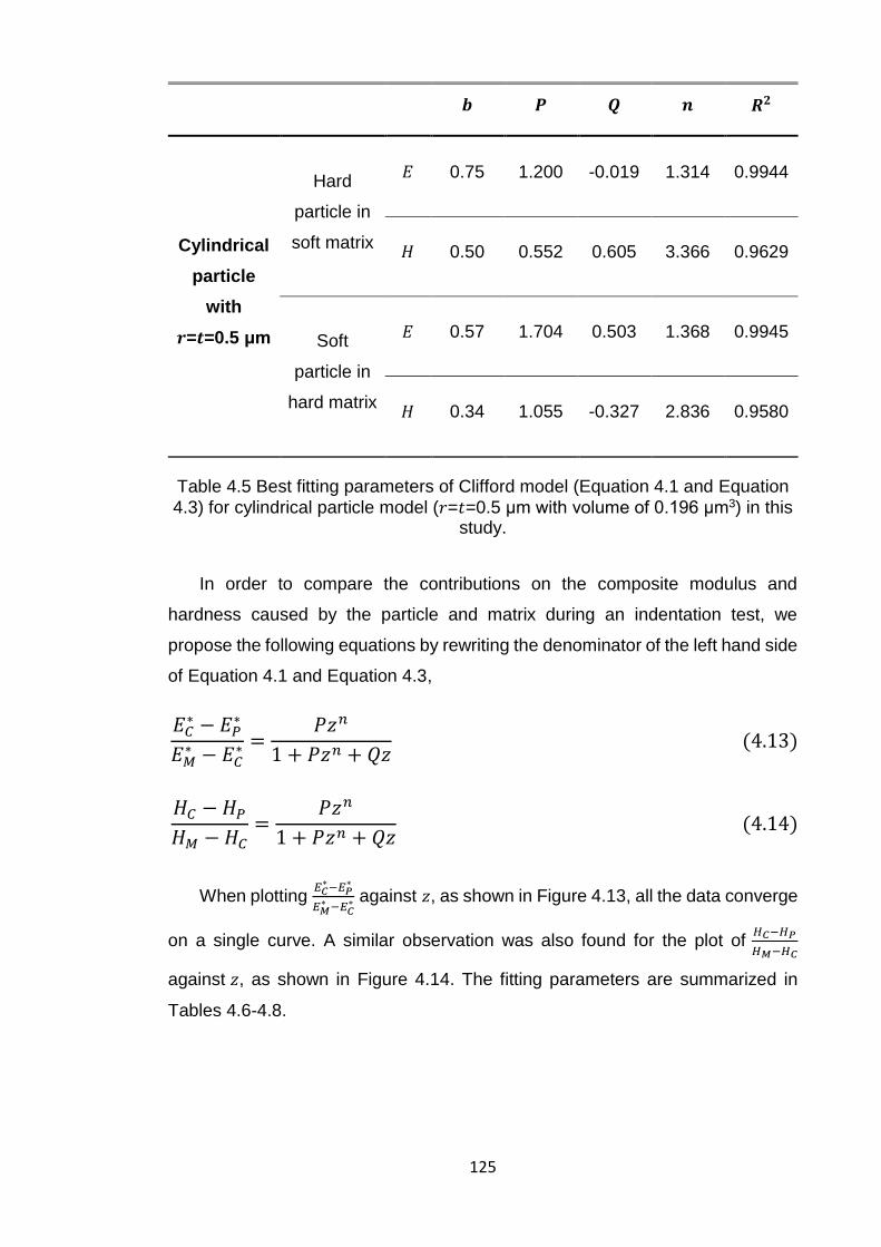
125
𝒃 𝑷 𝑸 𝒏 𝑹𝟐
Cylindrical
particle
with
𝒓=𝒕=0.5 μm
Hard
particle in
soft matrix
𝐸 0.75 1.200 -0.019 1.314 0.9944
𝐻 0.50 0.552 0.605 3.366 0.9629
Soft
particle in
hard matrix
𝐸 0.57 1.704 0.503 1.368 0.9945
𝐻 0.34 1.055 -0.327 2.836 0.9580
Table 4.5 Best fitting parameters of Clifford model (Equation 4.1 and Equation
4.3) for cylindrical particle model (𝑟=𝑡=0.5 μm with volume of 0.196 μm3) in this study.
In order to compare the contributions on the composite modulus and
hardness caused by the particle and matrix during an indentation test, we
propose the following equations by rewriting the denominator of the left hand side
of Equation 4.1 and Equation 4.3,
𝐸𝐶∗ − 𝐸𝑃
∗
𝐸𝑀∗ − 𝐸𝐶
∗ =𝑃𝑧𝑛
1 + 𝑃𝑧𝑛 + 𝑄𝑧 (4.13)
𝐻𝐶 − 𝐻𝑃
𝐻𝑀 − 𝐻𝐶=
𝑃𝑧𝑛
1 + 𝑃𝑧𝑛 + 𝑄𝑧 (4.14)
When plotting 𝐸𝐶
∗−𝐸𝑃∗
𝐸𝑀∗ −𝐸𝐶
∗ against 𝑧, as shown in Figure 4.13, all the data converge
on a single curve. A similar observation was also found for the plot of 𝐻𝐶−𝐻𝑃
𝐻𝑀−𝐻𝐶
against 𝑧, as shown in Figure 4.14. The fitting parameters are summarized in
Tables 4.6-4.8.
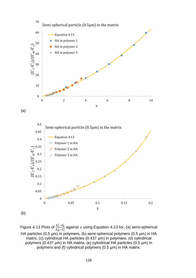
126
(a)
(b)
Figure 4.13 Plots of 𝐸𝐶
∗−𝐸𝑃∗
𝐸𝑀∗ −𝐸𝐶
∗ against 𝑧 using Equation 4.13 for, (a) semi-spherical
HA particles (0.5 μm) in polymers, (b) semi-spherical polymers (0.5 μm) in HA matrix, (c) cylindrical HA particles (0.437 μm) in polymers, (d) cylindrical polymers (0.437 μm) in HA matrix, (e) cylindrical HA particles (0.5 μm) in
polymers and (f) cylindrical polymers (0.5 μm) in HA matrix.
0
10
20
30
40
50
60
70
0 2 4 6 8 10
(E* C
-E* P
)/(E
* M-E
* C)
z
Semi-spherical particle (0.5μm) in the matrix
Equation 4.13
HA in polymer 1
HA in polymer 2
HA in polymer 3
0
0.05
0.1
0.15
0.2
0.25
0.3
0.35
0.4
0.45
0.5
0 0.05 0.1 0.15 0.2
(E* C
-E* P
)/(E
* M-E
* C)
z
Semi-spherical particle (0.5μm) in the matrix
Equation 4.13
Polymer 1 in HA
Polymer 2 in HA
Polymer 3 in HA
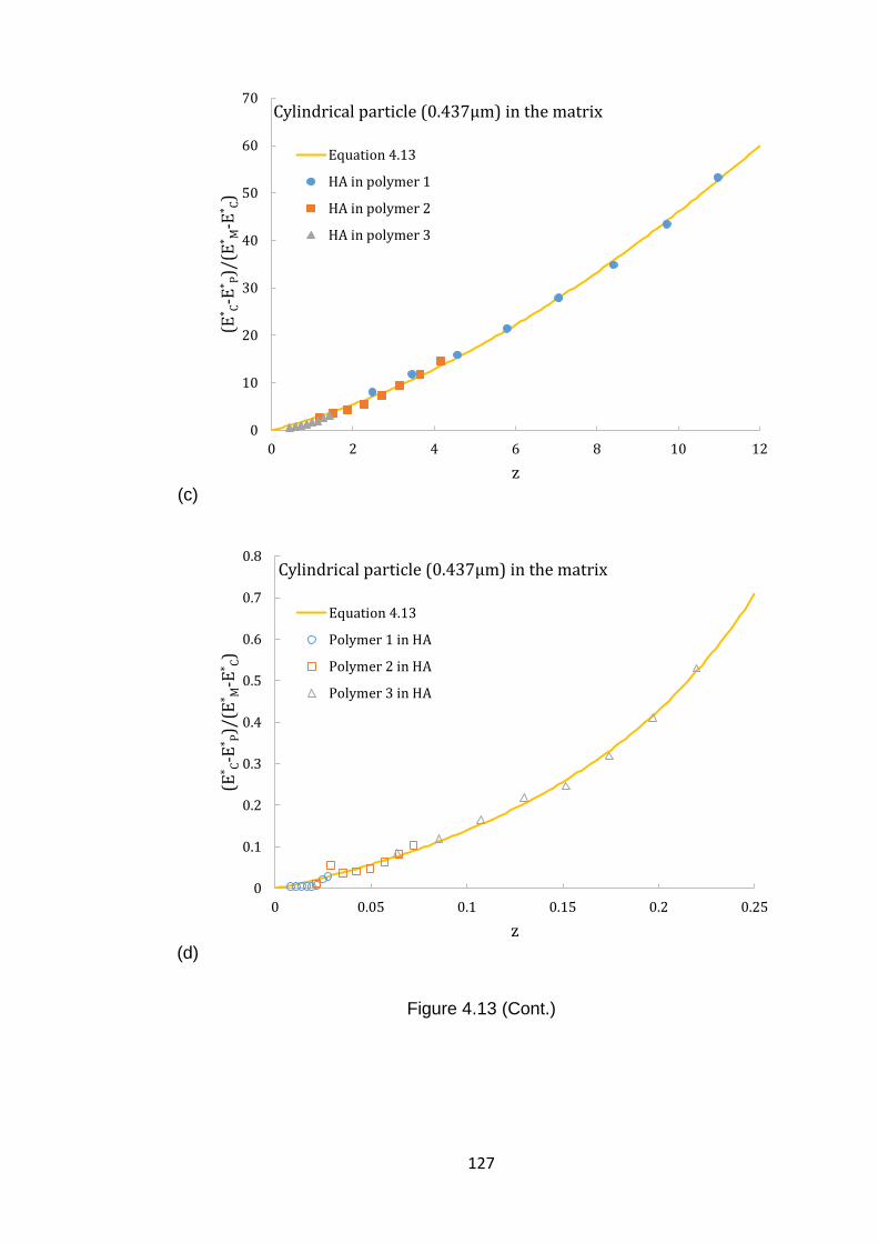
127
(c)
(d)
Figure 4.13 (Cont.)
0
10
20
30
40
50
60
70
0 2 4 6 8 10 12
(E* C
-E* P
)/(E
* M-E
* C)
z
Cylindrical particle (0.437μm) in the matrix
Equation 4.13
HA in polymer 1
HA in polymer 2
HA in polymer 3
0
0.1
0.2
0.3
0.4
0.5
0.6
0.7
0.8
0 0.05 0.1 0.15 0.2 0.25
(E* C
-E* P
)/(E
* M-E
* C)
z
Cylindrical particle (0.437μm) in the matrix
Equation 4.13
Polymer 1 in HA
Polymer 2 in HA
Polymer 3 in HA
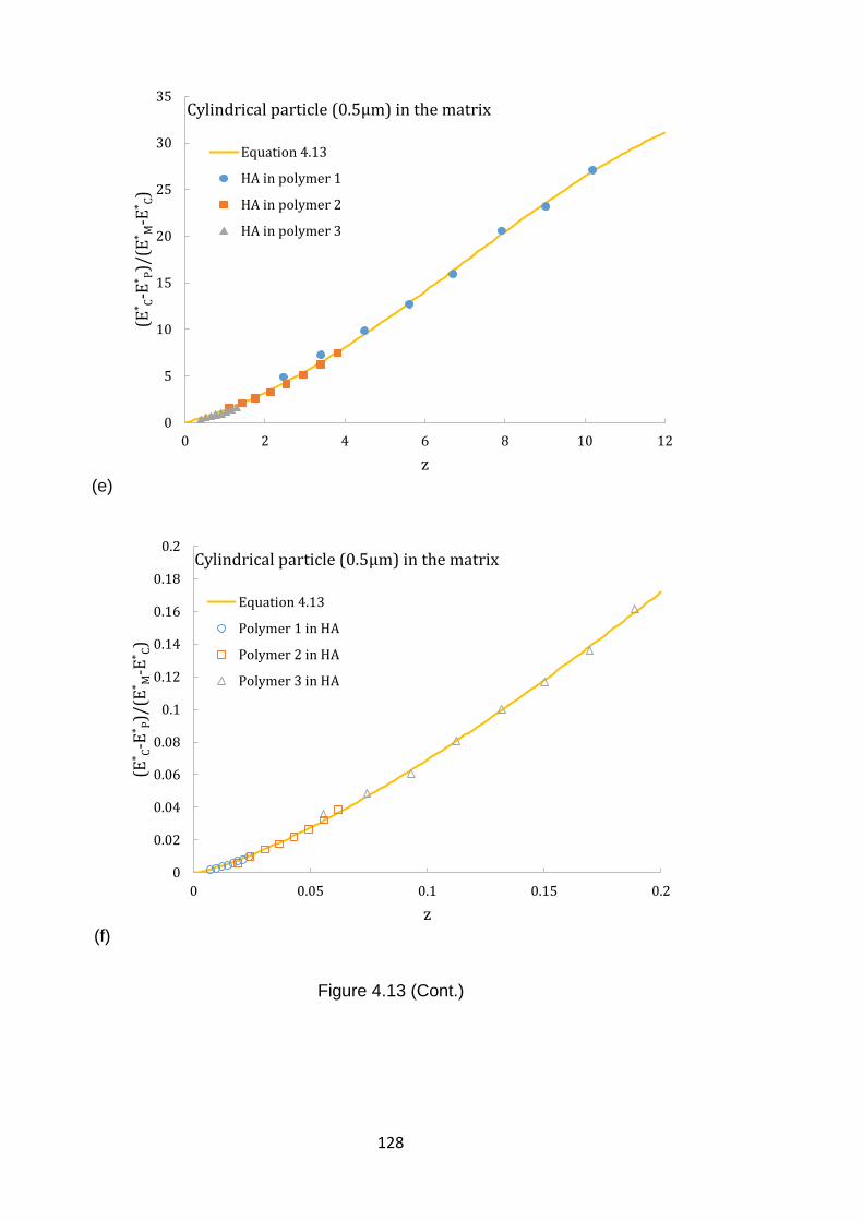
128
(e)
(f)
Figure 4.13 (Cont.)
0
5
10
15
20
25
30
35
0 2 4 6 8 10 12
(E* C
-E* P
)/(E
* M-E
* C)
z
Cylindrical particle (0.5μm) in the matrix
Equation 4.13
HA in polymer 1
HA in polymer 2
HA in polymer 3
0
0.02
0.04
0.06
0.08
0.1
0.12
0.14
0.16
0.18
0.2
0 0.05 0.1 0.15 0.2
(E* C
-E* P
)/(E
* M-E
* C)
z
Cylindrical particle (0.5μm) in the matrix
Equation 4.13
Polymer 1 in HA
Polymer 2 in HA
Polymer 3 in HA
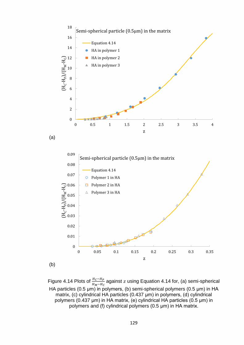
129
(a)
(b)
Figure 4.14 Plots of 𝐻𝐶−𝐻𝑃
𝐻𝑀−𝐻𝐶 against 𝑧 using Equation 4.14 for, (a) semi-spherical
HA particles (0.5 μm) in polymers, (b) semi-spherical polymers (0.5 μm) in HA matrix, (c) cylindrical HA particles (0.437 μm) in polymers, (d) cylindrical polymers (0.437 μm) in HA matrix, (e) cylindrical HA particles (0.5 μm) in
polymers and (f) cylindrical polymers (0.5 μm) in HA matrix.
0
2
4
6
8
10
12
14
16
18
0 0.5 1 1.5 2 2.5 3 3.5 4
(HC-H
P)/
(HM
-HC)
z
Semi-spherical particle (0.5μm) in the matrix
Equation 4.14
HA in polymer 1
HA in polymer 2
HA in polymer 3
0
0.01
0.02
0.03
0.04
0.05
0.06
0.07
0.08
0.09
0 0.05 0.1 0.15 0.2 0.25 0.3 0.35
(HC-H
P)/
(HM
-HC)
z
Semi-spherical particle (0.5μm) in the matrix
Equation 4.14
Polymer 1 in HA
Polymer 2 in HA
Polymer 3 in HA
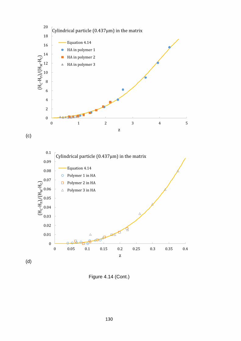
130
(c)
(d)
Figure 4.14 (Cont.)
0
2
4
6
8
10
12
14
16
18
20
0 1 2 3 4 5
(HC-H
P)/
(HM
-HC)
z
Cylindrical particle (0.437μm) in the matrix
Equation 4.14
HA in polymer 1
HA in polymer 2
HA in polymer 3
0
0.01
0.02
0.03
0.04
0.05
0.06
0.07
0.08
0.09
0.1
0 0.05 0.1 0.15 0.2 0.25 0.3 0.35 0.4
(HC-H
P)/
(HM
-HC)
z
Cylindrical particle (0.437μm) in the matrix
Equation 4.14
Polymer 1 in HA
Polymer 2 in HA
Polymer 3 in HA
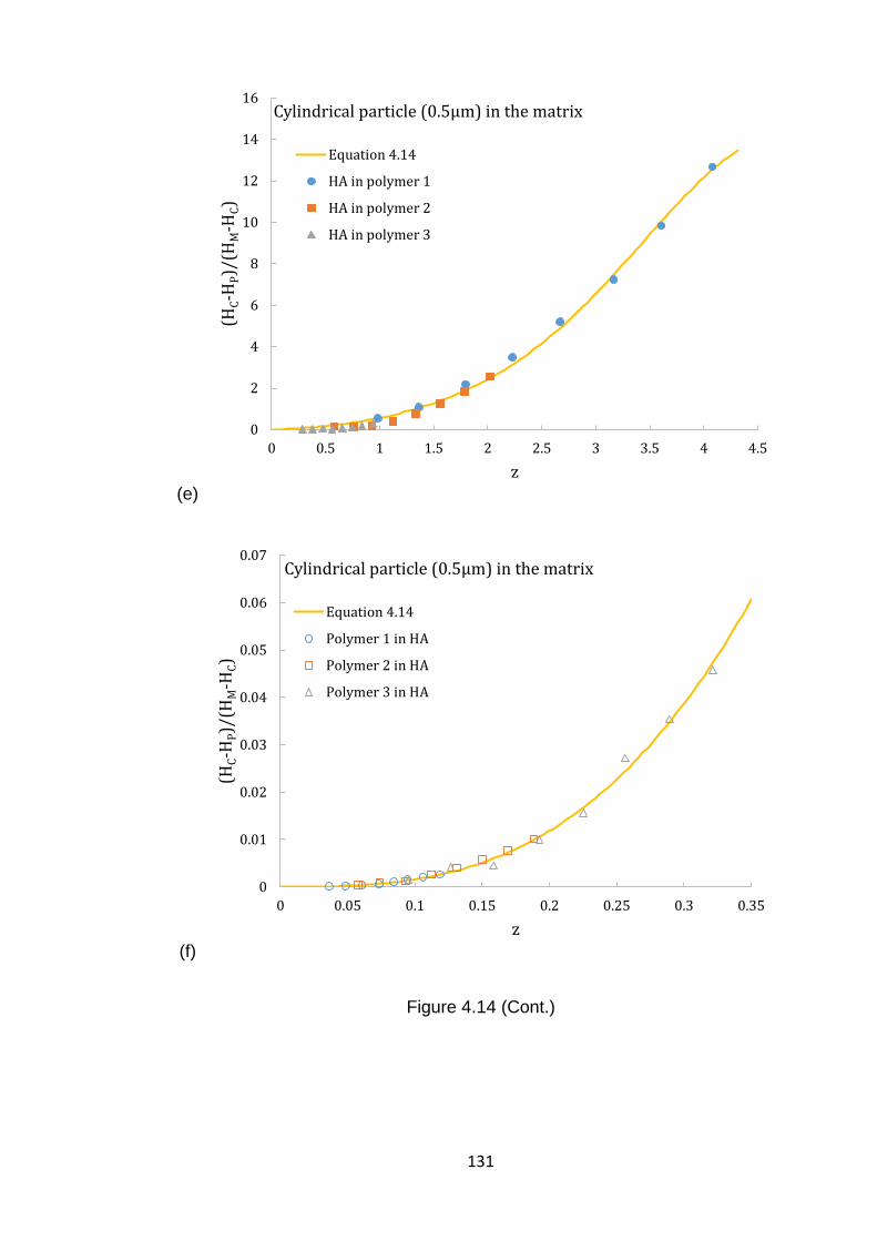
131
(e)
(f)
Figure 4.14 (Cont.)
0
2
4
6
8
10
12
14
16
0 0.5 1 1.5 2 2.5 3 3.5 4 4.5
(HC-H
P)/
(HM
-HC)
z
Cylindrical particle (0.5μm) in the matrix
Equation 4.14
HA in polymer 1
HA in polymer 2
HA in polymer 3
0
0.01
0.02
0.03
0.04
0.05
0.06
0.07
0 0.05 0.1 0.15 0.2 0.25 0.3 0.35
(HC-H
P)/
(HM
-HC)
z
Cylindrical particle (0.5μm) in the matrix
Equation 4.14
Polymer 1 in HA
Polymer 2 in HA
Polymer 3 in HA
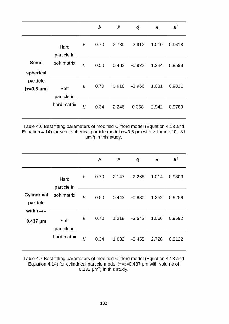
132
𝒃 𝑷 𝑸 𝒏 𝑹𝟐
Semi-
spherical
particle
(𝒓=0.5 μm)
Hard
particle in
soft matrix
𝐸 0.70 2.789 -2.912 1.010 0.9618
𝐻 0.50 0.482 -0.922 1.284 0.9598
Soft
particle in
hard matrix
𝐸 0.70 0.918 -3.966 1.031 0.9811
𝐻 0.34 2.246 0.358 2.942 0.9789
Table 4.6 Best fitting parameters of modified Clifford model (Equation 4.13 and
Equation 4.14) for semi-spherical particle model (𝑟=0.5 μm with volume of 0.131 μm3) in this study.
𝒃 𝑷 𝑸 𝒏 𝑹𝟐
Cylindrical
particle
with 𝒓=𝒕=
0.437 μm
Hard
particle in
soft matrix
𝐸 0.70 2.147 -2.268 1.014 0.9803
𝐻 0.50 0.443 -0.830 1.252 0.9259
Soft
particle in
hard matrix
𝐸 0.70 1.218 -3.542 1.066 0.9592
𝐻 0.34 1.032 -0.455 2.728 0.9122
Table 4.7 Best fitting parameters of modified Clifford model (Equation 4.13 and
Equation 4.14) for cylindrical particle model (𝑟=𝑡=0.437 μm with volume of 0.131 μm3) in this study.
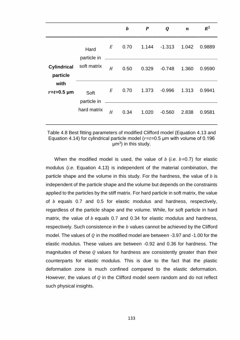
133
𝒃 𝑷 𝑸 𝒏 𝑹𝟐
Cylindrical
particle
with
𝒓=𝒕=0.5 μm
Hard
particle in
soft matrix
𝐸 0.70 1.144 -1.313 1.042 0.9889
𝐻 0.50 0.329 -0.748 1.360 0.9590
Soft
particle in
hard matrix
𝐸 0.70 1.373 -0.996 1.313 0.9941
𝐻 0.34 1.020 -0.560 2.838 0.9581
Table 4.8 Best fitting parameters of modified Clifford model (Equation 4.13 and
Equation 4.14) for cylindrical particle model (𝑟=𝑡=0.5 μm with volume of 0.196 μm3) in this study.
When the modified model is used, the value of 𝑏 (i.e. 𝑏=0.7) for elastic
modulus (i.e. Equation 4.13) is independent of the material combination, the
particle shape and the volume in this study. For the hardness, the value of 𝑏 is
independent of the particle shape and the volume but depends on the constraints
applied to the particles by the stiff matrix. For hard particle in soft matrix, the value
of 𝑏 equals 0.7 and 0.5 for elastic modulus and hardness, respectively,
regardless of the particle shape and the volume. While, for soft particle in hard
matrix, the value of 𝑏 equals 0.7 and 0.34 for elastic modulus and hardness,
respectively. Such consistence in the 𝑏 values cannot be achieved by the Clifford
model. The values of 𝑄 in the modified model are between -3.97 and -1.00 for the
elastic modulus. These values are between -0.92 and 0.36 for hardness. The
magnitudes of these 𝑄 values for hardness are consistently greater than their
counterparts for elastic modulus. This is due to the fact that the plastic
deformation zone is much confined compared to the elastic deformation.
However, the values of 𝑄 in the Clifford model seem random and do not reflect
such physical insights.
134
4.5 Summary
FEM was done to study the spatial-dependent composite modulus and
hardness during nanoindentation tests. The reported rule-of-thumb to determine
the modulus and hardness of particles at a penetration below 5% and 13.5% are
reasonable approximations for composites with relatively small mismatch in
elastic modulus and hardness between particle and matrix. But they do not apply
to the composites with large mismatch in elastic modulus and hardness between
particle and matrix. Therefore, new models have been developed based on the
original Clifford model, which enables us to determine elastic modulus and
hardness for such composite materials. These models have been successfully
applied to various composites regardless of particle geometry, volume and
material combination. In principle, such models can also be extended to biological
composites such as biofilms which can be treated as hard particles (bacteria)
embedded in soft matrix (extracellular polymeric substance).
In the next chapter, finite element modelling for the nanoindentation of
inclusion/matrix composite with varying indentation locations and fibre
orientations will be presented to assess the elastic response of this
inclusion/matrix composite.
Chapter 5
Nanomechanical Modelling of
Elastic Fibre with Different
Orientations in Elastic Matrix
136
Chapter 5. Nanomechanical Modelling of Elastic Fibre with Different
Orientations in Elastic Matrix
5.1 Introduction
During the past decades, biocomposites (such as bioceramics and
biopolymers) have been widely used as artificial scaffold materials in tissue
engineering (Venugopal and Ramakrishna, 2005; Rezwan et al., 2006; Soloviev,
2012). As one of the key requirements, implanted scaffolds must be strong
enough to avoid the fracture during the patient’s normal activities (Hu et al., 2010).
Thus, it is of great importance to understand how the surrounding matrix will affect
the measured mechanical properties, which will provide a guidance for the
optimisation of material processing to achieve the target design properties.
Numerous studies have proved that nanoindentation is a powerful tool to
determine the mechanical properties of composite materials (Li and Bhushan,
1998; Lim et al., 1999; Chen et al., 2010a; Chakraborty and Bhowmik, 2014; De
Silva et al., 2014; Herruzo et al., 2014). However, when performing
nanoindentation on inclusions or the matrix, it is challenging to define the
inevitable influence of the surrounding second phase. There is a lack of
sophisticated studies on how the indentation location and the inclusion orientation
would affect the mechanical behaviours of the composites. Therefore, in this
chapter, FEA is adopted to investigate the elastic response of fibre-reinforced
composite under nanoindentation test. By varying the indentation location and
the fibre orientation, this work reveals the correlation between the elastic
properties of fibre-reinforced composite and the elastic properties of each
individual constituent. In practice, this work can be used to predict the elastic
response of fibre periodically reinforced composites, or extract the properties of
the matrix and the fibre.
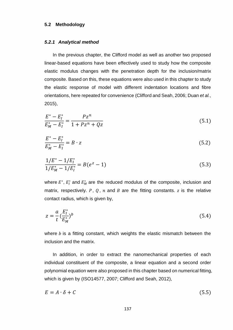
137
5.2 Methodology
5.2.1 Analytical method
In the previous chapter, the Clifford model as well as another two proposed
linear-based equations have been effectively used to study how the composite
elastic modulus changes with the penetration depth for the inclusion/matrix
composite. Based on this, these equations were also used in this chapter to study
the elastic response of model with different indentation locations and fibre
orientations, here repeated for convenience (Clifford and Seah, 2006; Duan et al.,
2015),
𝐸∗ − 𝐸𝐼∗
𝐸𝑀∗ − 𝐸𝐼
∗ =𝑃𝑧𝑛
1 + 𝑃𝑧𝑛 + 𝑄𝑧 (5.1)
𝐸∗ − 𝐸𝐼∗
𝐸𝑀∗ − 𝐸𝐼
∗ = 𝐵 ∙ 𝑧 (5.2)
1/𝐸∗ − 1/𝐸𝐼∗
1/𝐸𝑀∗ − 1/𝐸𝐼
∗ = 𝐵(𝑒𝑧 − 1) (5.3)
where 𝐸∗, 𝐸𝐼∗ and 𝐸𝑀
∗ are the reduced modulus of the composite, inclusion and
matrix, respectively. 𝑃 , 𝑄 , 𝑛 and 𝐵 are the fitting constants. 𝑧 is the relative
contact radius, which is given by,
𝑧 =𝑎
𝑡(
𝐸𝐼∗
𝐸𝑀∗ )𝑏 (5.4)
where 𝑏 is a fitting constant, which weights the elastic mismatch between the
inclusion and the matrix.
In addition, in order to extract the nanomechanical properties of each
individual constituent of the composite, a linear equation and a second order
polynomial equation were also proposed in this chapter based on numerical fitting,
which is given by (ISO14577, 2007; Clifford and Seah, 2012),
𝐸 = 𝐴 ∙ 𝛿 + 𝐶 (5.5)
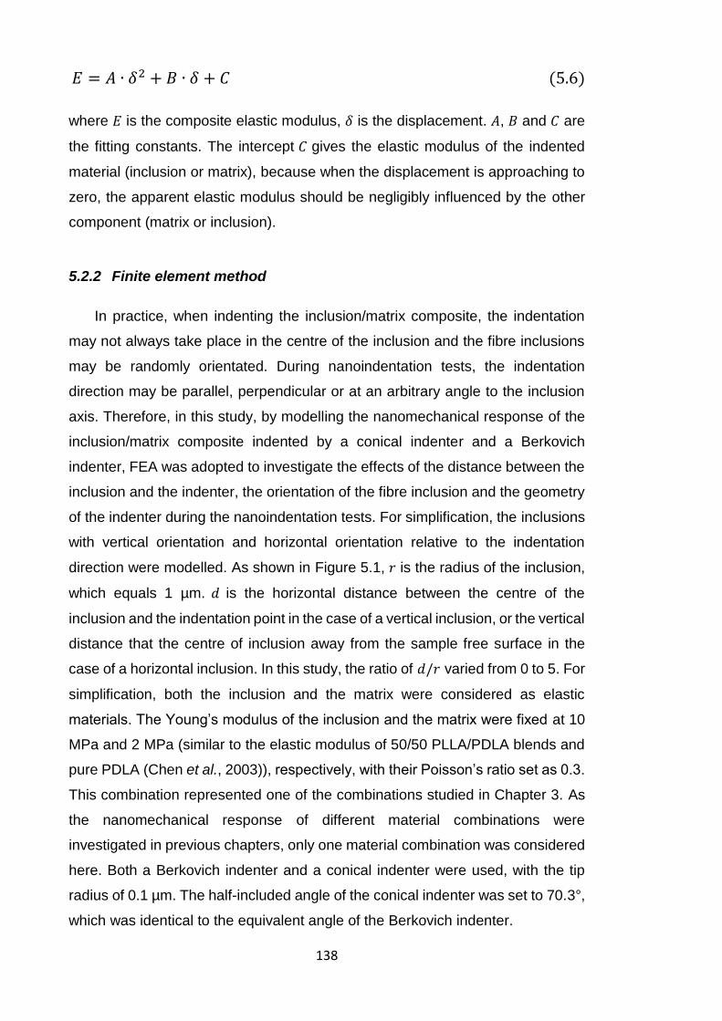
138
𝐸 = 𝐴 ∙ 𝛿2 + 𝐵 ∙ 𝛿 + 𝐶 (5.6)
where 𝐸 is the composite elastic modulus, 𝛿 is the displacement. 𝐴, 𝐵 and 𝐶 are
the fitting constants. The intercept 𝐶 gives the elastic modulus of the indented
material (inclusion or matrix), because when the displacement is approaching to
zero, the apparent elastic modulus should be negligibly influenced by the other
component (matrix or inclusion).
5.2.2 Finite element method
In practice, when indenting the inclusion/matrix composite, the indentation
may not always take place in the centre of the inclusion and the fibre inclusions
may be randomly orientated. During nanoindentation tests, the indentation
direction may be parallel, perpendicular or at an arbitrary angle to the inclusion
axis. Therefore, in this study, by modelling the nanomechanical response of the
inclusion/matrix composite indented by a conical indenter and a Berkovich
indenter, FEA was adopted to investigate the effects of the distance between the
inclusion and the indenter, the orientation of the fibre inclusion and the geometry
of the indenter during the nanoindentation tests. For simplification, the inclusions
with vertical orientation and horizontal orientation relative to the indentation
direction were modelled. As shown in Figure 5.1, 𝑟 is the radius of the inclusion,
which equals 1 µm. 𝑑 is the horizontal distance between the centre of the
inclusion and the indentation point in the case of a vertical inclusion, or the vertical
distance that the centre of inclusion away from the sample free surface in the
case of a horizontal inclusion. In this study, the ratio of 𝑑/𝑟 varied from 0 to 5. For
simplification, both the inclusion and the matrix were considered as elastic
materials. The Young’s modulus of the inclusion and the matrix were fixed at 10
MPa and 2 MPa (similar to the elastic modulus of 50/50 PLLA/PDLA blends and
pure PDLA (Chen et al., 2003)), respectively, with their Poisson’s ratio set as 0.3.
This combination represented one of the combinations studied in Chapter 3. As
the nanomechanical response of different material combinations were
investigated in previous chapters, only one material combination was considered
here. Both a Berkovich indenter and a conical indenter were used, with the tip
radius of 0.1 µm. The half-included angle of the conical indenter was set to 70.3°,
which was identical to the equivalent angle of the Berkovich indenter.
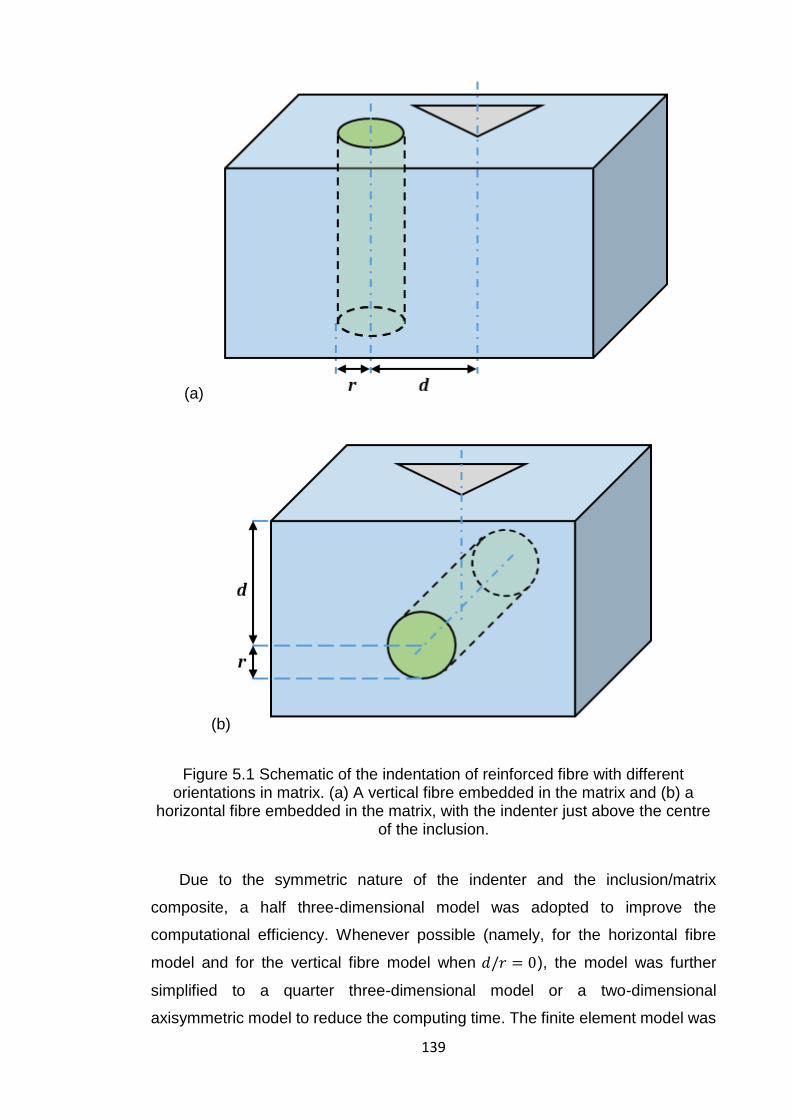
139
(a)
(b)
Figure 5.1 Schematic of the indentation of reinforced fibre with different orientations in matrix. (a) A vertical fibre embedded in the matrix and (b) a
horizontal fibre embedded in the matrix, with the indenter just above the centre of the inclusion.
Due to the symmetric nature of the indenter and the inclusion/matrix
composite, a half three-dimensional model was adopted to improve the
computational efficiency. Whenever possible (namely, for the horizontal fibre
model and for the vertical fibre model when 𝑑/𝑟 = 0), the model was further
simplified to a quarter three-dimensional model or a two-dimensional
axisymmetric model to reduce the computing time. The finite element model was
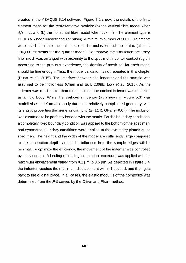
140
created in the ABAQUS 6.14 software. Figure 5.2 shows the details of the finite
element mesh for the representative models: (a) the vertical fibre model when
𝑑/𝑟 = 2, and (b) the horizontal fibre model when 𝑑/𝑟 = 2. The element type is
C3D6 (A 6-node linear triangular prism). A minimum number of 200,000 elements
were used to create the half model of the inclusion and the matrix (at least
100,000 elements for the quarter model). To improve the simulation accuracy,
finer mesh was arranged with proximity to the specimen/indenter contact region.
According to the previous experience, the density of mesh set for each model
should be fine enough. Thus, the model validation is not repeated in this chapter
(Duan et al., 2015). The interface between the indenter and the sample was
assumed to be frictionless (Chen and Bull, 2009b; Low et al., 2015). As the
indenter was much stiffer than the specimen, the conical indenter was modelled
as a rigid body. While the Berkovich indenter (as shown in Figure 5.3) was
modelled as a deformable body due to its relatively complicated geometry, with
its elastic properties the same as diamond (𝐸=1141 GPa, 𝑣=0.07). The inclusion
was assumed to be perfectly bonded with the matrix. For the boundary conditions,
a completely fixed boundary condition was applied to the bottom of the specimen,
and symmetric boundary conditions were applied to the symmetry planes of the
specimen. The height and the width of the model are sufficiently large compared
to the penetration depth so that the influence from the sample edges will be
minimal. To optimize the efficiency, the movement of the indenter was controlled
by displacement. A loading-unloading indentation procedure was applied with the
maximum displacement varied from 0.2 µm to 0.5 µm. As depicted in Figure 5.4,
the indenter reaches the maximum displacement within 1 second, and then gets
back to the original place. In all cases, the elastic modulus of the composite was
determined from the F-δ curves by the Oliver and Pharr method.
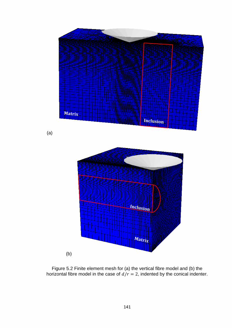
141
(a)
(b)
Figure 5.2 Finite element mesh for (a) the vertical fibre model and (b) the
horizontal fibre model in the case of 𝑑/𝑟 = 2, indented by the conical indenter.
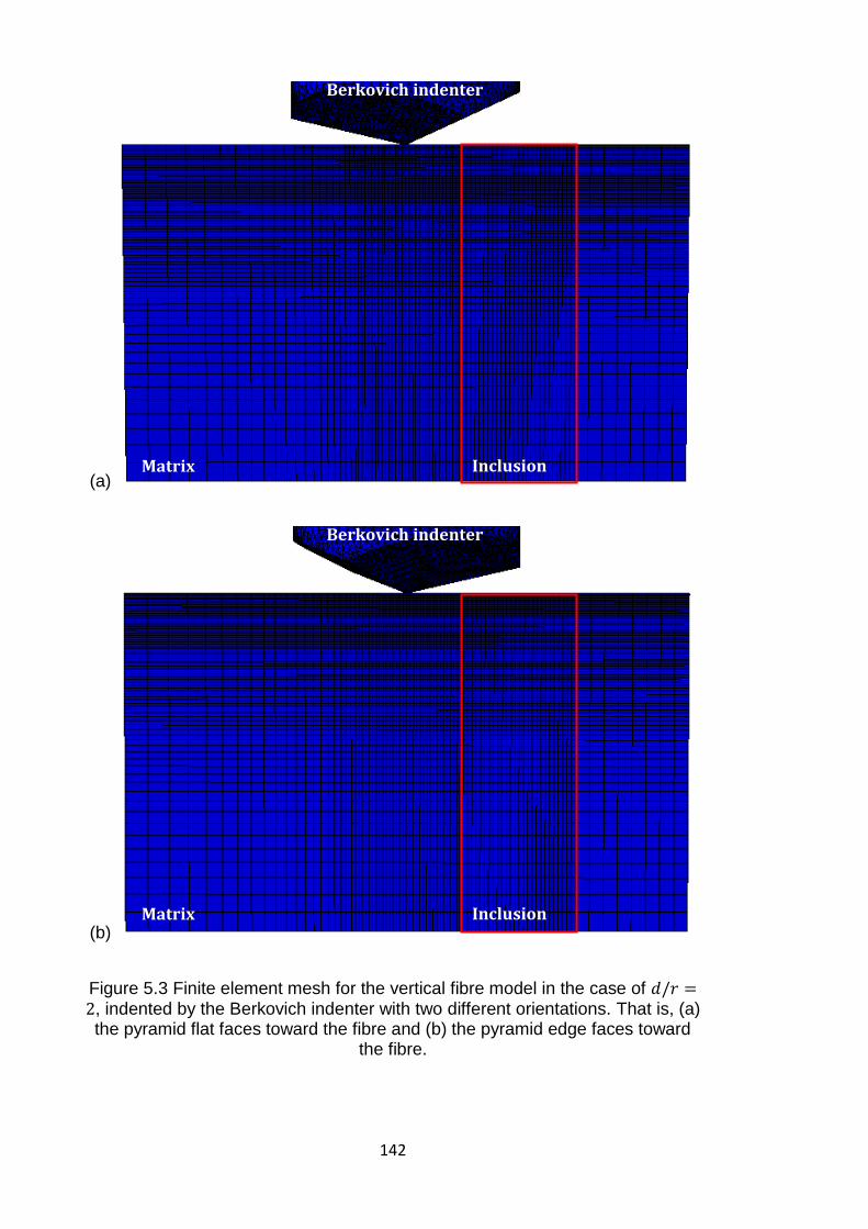
142
(a)
(b)
Figure 5.3 Finite element mesh for the vertical fibre model in the case of 𝑑/𝑟 =2, indented by the Berkovich indenter with two different orientations. That is, (a) the pyramid flat faces toward the fibre and (b) the pyramid edge faces toward
the fibre.
Berkovich indenter
Berkovich indenter
Inclusion Matrix
Inclusion Matrix
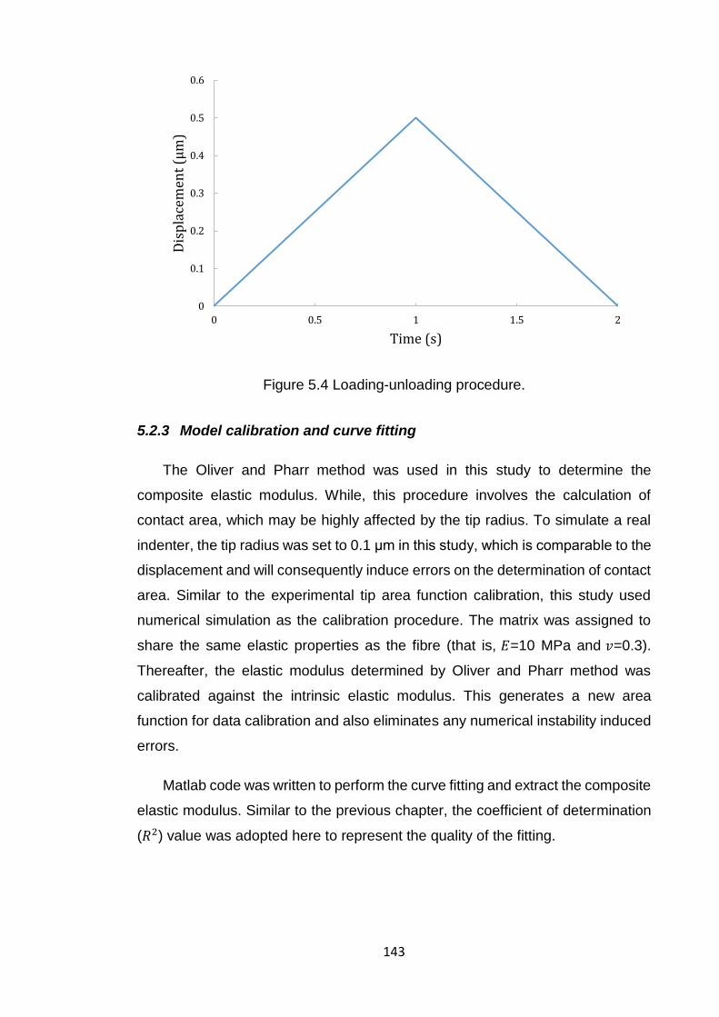
143
Figure 5.4 Loading-unloading procedure.
5.2.3 Model calibration and curve fitting
The Oliver and Pharr method was used in this study to determine the
composite elastic modulus. While, this procedure involves the calculation of
contact area, which may be highly affected by the tip radius. To simulate a real
indenter, the tip radius was set to 0.1 μm in this study, which is comparable to the
displacement and will consequently induce errors on the determination of contact
area. Similar to the experimental tip area function calibration, this study used
numerical simulation as the calibration procedure. The matrix was assigned to
share the same elastic properties as the fibre (that is, 𝐸=10 MPa and 𝑣=0.3).
Thereafter, the elastic modulus determined by Oliver and Pharr method was
calibrated against the intrinsic elastic modulus. This generates a new area
function for data calibration and also eliminates any numerical instability induced
errors.
Matlab code was written to perform the curve fitting and extract the composite
elastic modulus. Similar to the previous chapter, the coefficient of determination
(𝑅2) value was adopted here to represent the quality of the fitting.
0
0.1
0.2
0.3
0.4
0.5
0.6
0 0.5 1 1.5 2
Dis
pla
cem
ent
(µm
)
Time (s)
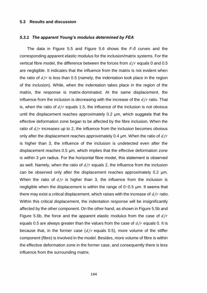
144
5.3 Results and discussion
5.3.1 The apparent Young’s modulus determined by FEA
The data in Figure 5.5 and Figure 5.6 shows the F-δ curves and the
corresponding apparent elastic modulus for the inclusion/matrix systems. For the
vertical fibre model, the difference between the forces from 𝑑/𝑟 equals 0 and 0.5
are negligible. It indicates that the influence from the matrix is not evident when
the ratio of 𝑑/𝑟 is less than 0.5 (namely, the indentation took place in the region
of the inclusion). While, when the indentation takes place in the region of the
matrix, the response is matrix-dominated. At the same displacement, the
influence from the inclusion is decreasing with the increase of the 𝑑/𝑟 ratio. That
is, when the ratio of 𝑑/𝑟 equals 1.5, the influence of the inclusion is not obvious
until the displacement reaches approximately 0.2 μm, which suggests that the
effective deformation zone began to be affected by the fibre inclusion. When the
ratio of 𝑑/𝑟 increases up to 2, the influence from the inclusion becomes obvious
only after the displacement reaches approximately 0.4 μm. When the ratio of 𝑑/𝑟
is higher than 3, the influence of the inclusion is undetected even after the
displacement reaches 0.5 μm, which implies that the effective deformation zone
is within 3 μm radius. For the horizontal fibre model, this statement is observed
as well. Namely, when the ratio of 𝑑/𝑟 equals 2, the influence from the inclusion
can be observed only after the displacement reaches approximately 0.2 μm.
When the ratio of 𝑑/𝑟 is higher than 3, the influence from the inclusion is
negligible when the displacement is within the range of 0~0.5 μm. It seems that
there may exist a critical displacement, which raises with the increase of 𝑑/𝑟 ratio.
Within this critical displacement, the indentation response will be insignificantly
affected by the other component. On the other hand, as shown in Figure 5.5b and
Figure 5.6b, the force and the apparent elastic modulus from the case of 𝑑/𝑟
equals 0.5 are always greater than the values from the case of 𝑑/𝑟 equals 0. It is
because that, in the former case (𝑑/𝑟 equals 0.5), more volume of the stiffer
component (fibre) is involved in the model. Besides, more volume of fibre is within
the effective deformation zone in the former case, and consequently there is less
influence from the surrounding matrix.
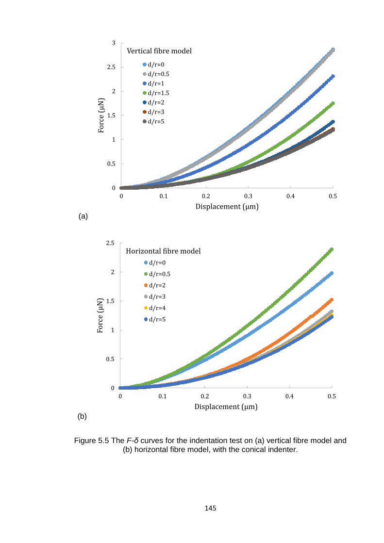
145
(a)
(b)
Figure 5.5 The F-δ curves for the indentation test on (a) vertical fibre model and (b) horizontal fibre model, with the conical indenter.
0
0.5
1
1.5
2
2.5
3
0 0.1 0.2 0.3 0.4 0.5
Fo
rce
(µN
)
Displacement (µm)
Vertical fibre model
d/r=0
d/r=0.5
d/r=1
d/r=1.5
d/r=2
d/r=3
d/r=5
0
0.5
1
1.5
2
2.5
0 0.1 0.2 0.3 0.4 0.5
Forc
e (µ
N)
Displacement (µm)
Horizontal fibre model
d/r=0
d/r=0.5
d/r=2
d/r=3
d/r=4
d/r=5
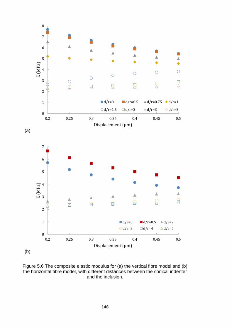
146
(a)
(b)
Figure 5.6 The composite elastic modulus for (a) the vertical fibre model and (b) the horizontal fibre model, with different distances between the conical indenter
and the inclusion.
0
1
2
3
4
5
6
7
8
0.2 0.25 0.3 0.35 0.4 0.45 0.5
E (
MP
a)
Displacement (µm)
d/r=0 d/r=0.5 d/r=0.75 d/r=1
d/r=1.5 d/r=2 d/r=3 d/r=5
0
1
2
3
4
5
6
7
0.2 0.25 0.3 0.35 0.4 0.45 0.5
E (
MP
a)
Displacement (µm)
d/r=0 d/r=0.5 d/r=2
d/r=3 d/r=4 d/r=5
147
In order to further analyse the relation between the ratio of 𝑑/𝑟 and the
corresponding nanomechanical response for the inclusion/matrix system, von
Mises stress contours are plotted to represent the stress distribution (Guo and
Yen, 2004; Walter et al., 2007). As illustrated in Figure 5.7, stress contours for
the vertical fibre model indented by the conical indenter are plotted with the
displacement equal to 0.5 μm. For standardization, the maximum stress limit was
set to 1.2 MPa and the minimum stress limit was set to 0 MPa in all cases. It
shows that, for the vertical fibre model, the response is mainly fibre-dominated
when the indentation takes place in the region of the fibre (𝑑/𝑟 < 1, Figure 5.7a).
When the interface between the fibre and the matrix is indented (𝑑/𝑟 = 1, Figure
5.7b), both of them will contribute to the resulting response. Even at a small
displacement, it is still difficult to extract the individual properties from the
corresponding F-δ curve. When the indentation occurs in the region of the matrix
(𝑑/𝑟 > 1, Figure 5.7c-e), the response will be matrix-dominated. In this case, the
influence from the inclusion can be negligible (Figure 5.7d-e) until the indenter
directly touches the inclusion (Figure 5.7c). It indicates that, once the
displacement is small enough, the properties for each individual phase can be
extracted from the corresponding F-δ curve.
(a)
Figure 5.7 Von Mises stress contours for the vertical fibre model with a
displacement of 0.5 μm, when (a) 𝑑/𝑟 = 0, (b) 𝑑/𝑟 = 1, (c) 𝑑/𝑟 = 2, (d) 𝑑/𝑟 = 3 and (e) 𝑑/𝑟 = 5. For standardization, all the figures share the same stress
scale.
Inclusion Matrix
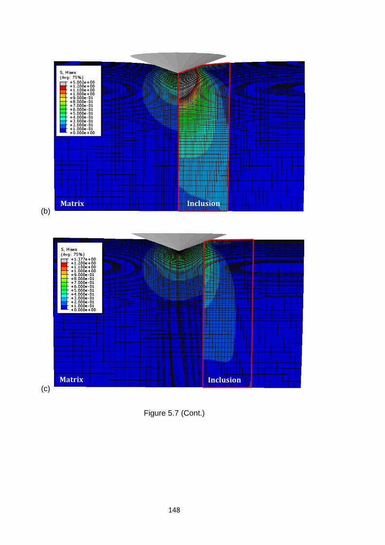
148
(b)
(c)
Figure 5.7 (Cont.)
Inclusion Matrix
Inclusion Matrix
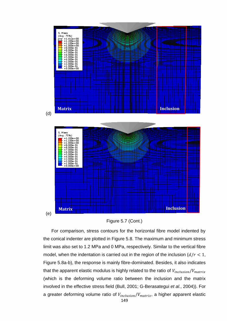
149
(d)
(e)
Figure 5.7 (Cont.)
For comparison, stress contours for the horizontal fibre model indented by
the conical indenter are plotted in Figure 5.8. The maximum and minimum stress
limit was also set to 1.2 MPa and 0 MPa, respectively. Similar to the vertical fibre
model, when the indentation is carried out in the region of the inclusion (𝑑/𝑟 < 1,
Figure 5.8a-b), the response is mainly fibre-dominated. Besides, it also indicates
that the apparent elastic modulus is highly related to the ratio of 𝑉𝑖𝑛𝑐𝑙𝑢𝑠𝑖𝑜𝑛/𝑉𝑚𝑎𝑡𝑟𝑖𝑥
(which is the deforming volume ratio between the inclusion and the matrix
involved in the effective stress field (Bull, 2001; G-Berasategui et al., 2004)). For
a greater deforming volume ratio of 𝑉𝑖𝑛𝑐𝑙𝑢𝑠𝑖𝑜𝑛/𝑉𝑚𝑎𝑡𝑟𝑖𝑥, a higher apparent elastic
Inclusion Matrix
Inclusion Matrix
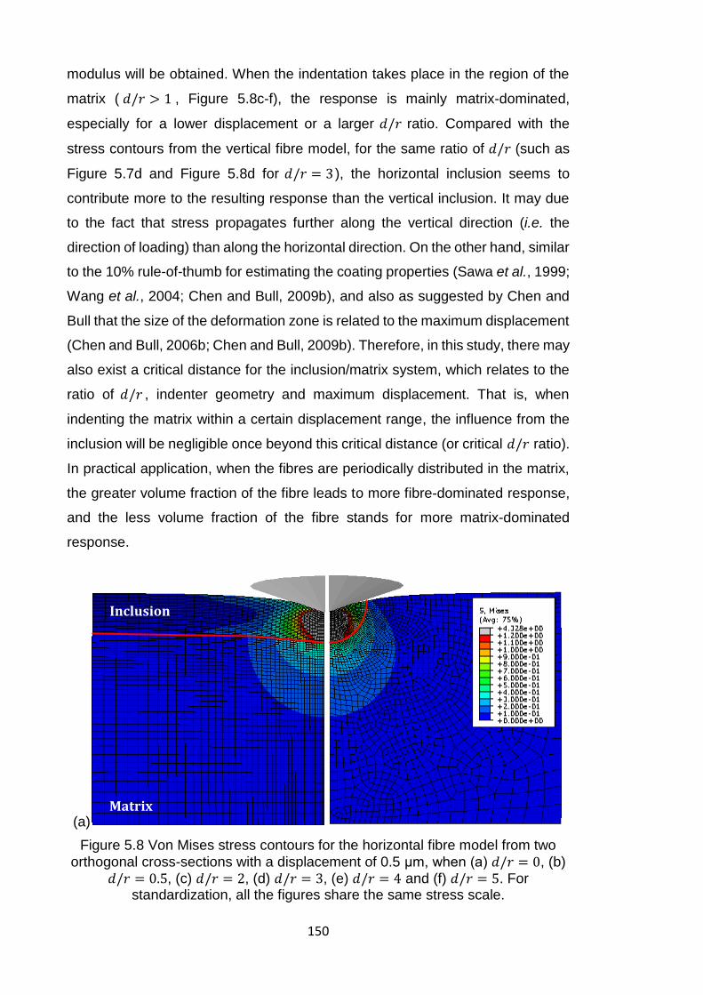
150
modulus will be obtained. When the indentation takes place in the region of the
matrix ( 𝑑/𝑟 > 1 , Figure 5.8c-f), the response is mainly matrix-dominated,
especially for a lower displacement or a larger 𝑑/𝑟 ratio. Compared with the
stress contours from the vertical fibre model, for the same ratio of 𝑑/𝑟 (such as
Figure 5.7d and Figure 5.8d for 𝑑/𝑟 = 3 ), the horizontal inclusion seems to
contribute more to the resulting response than the vertical inclusion. It may due
to the fact that stress propagates further along the vertical direction (i.e. the
direction of loading) than along the horizontal direction. On the other hand, similar
to the 10% rule-of-thumb for estimating the coating properties (Sawa et al., 1999;
Wang et al., 2004; Chen and Bull, 2009b), and also as suggested by Chen and
Bull that the size of the deformation zone is related to the maximum displacement
(Chen and Bull, 2006b; Chen and Bull, 2009b). Therefore, in this study, there may
also exist a critical distance for the inclusion/matrix system, which relates to the
ratio of 𝑑/𝑟 , indenter geometry and maximum displacement. That is, when
indenting the matrix within a certain displacement range, the influence from the
inclusion will be negligible once beyond this critical distance (or critical 𝑑/𝑟 ratio).
In practical application, when the fibres are periodically distributed in the matrix,
the greater volume fraction of the fibre leads to more fibre-dominated response,
and the less volume fraction of the fibre stands for more matrix-dominated
response.
(a)
Figure 5.8 Von Mises stress contours for the horizontal fibre model from two
orthogonal cross-sections with a displacement of 0.5 μm, when (a) 𝑑/𝑟 = 0, (b) 𝑑/𝑟 = 0.5, (c) 𝑑/𝑟 = 2, (d) 𝑑/𝑟 = 3, (e) 𝑑/𝑟 = 4 and (f) 𝑑/𝑟 = 5. For
standardization, all the figures share the same stress scale.
Inclusion
Matrix
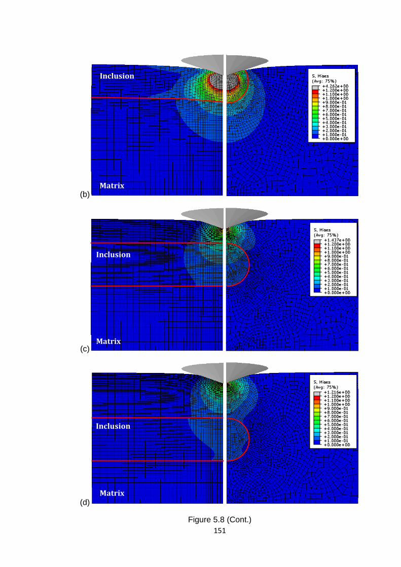
151
(b)
(c)
(d)
Figure 5.8 (Cont.)
Inclusion
Matrix
Inclusion
Matrix
Inclusion
Matrix
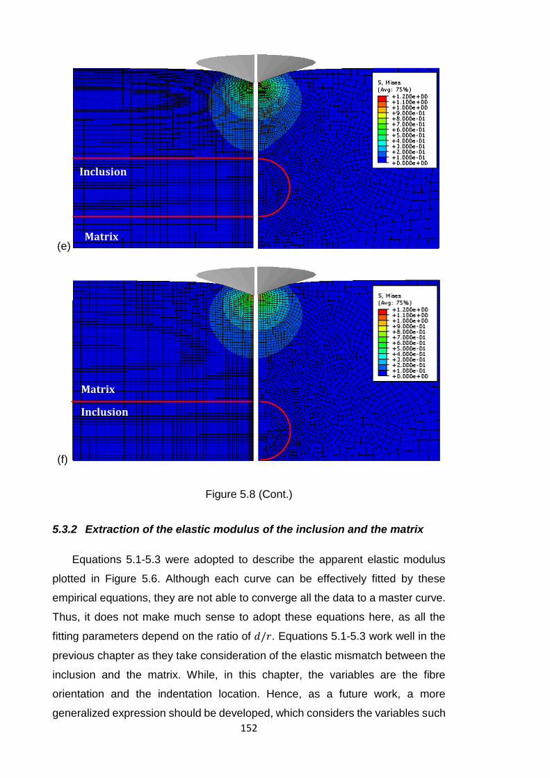
152
(e)
(f)
Figure 5.8 (Cont.)
5.3.2 Extraction of the elastic modulus of the inclusion and the matrix
Equations 5.1-5.3 were adopted to describe the apparent elastic modulus
plotted in Figure 5.6. Although each curve can be effectively fitted by these
empirical equations, they are not able to converge all the data to a master curve.
Thus, it does not make much sense to adopt these equations here, as all the
fitting parameters depend on the ratio of 𝑑/𝑟. Equations 5.1-5.3 work well in the
previous chapter as they take consideration of the elastic mismatch between the
inclusion and the matrix. While, in this chapter, the variables are the fibre
orientation and the indentation location. Hence, as a future work, a more
generalized expression should be developed, which considers the variables such
Matrix
Inclusion
Matrix
Inclusion
153
as indentation location, fibre orientation, indenter geometry and even the
inclusion geometry.
On the other hand, Equation 5.5 and Equation 5.6 were adopted to extract
the elastic modulus of each individual component. By fitting these equations to
the curves plotted in Figure 5.6, the relevant fitting parameters are shown in
Tables 5.1-5.4. The 𝑅2 value is higher than 0.95 in each case, which shows the
good qualify of the fitting. For the linear equation, the parameter 𝐴 reflects the
changing trend of the apparent elastic modulus with respect to the displacement.
A higher value of 𝐴 leads to greater increment of the apparent elastic modulus.
As listed in Table 5.1 and Table 5.3, when the ratio of 𝑑/𝑟 is greater than 1, the
value of 𝐴 is decreasing with the increase of 𝑑/𝑟. It indicates that, when indenting
the matrix, the influence from the fibre will decrease with the increase of 𝑑/𝑟 ratio.
The parameter 𝐶 represents the modulus of the indented bulk material, which is
the intercept of extrapolating the fitting equation to zero contact depth. In both the
vertical and horizontal fibre cases, when indenting the matrix, the value of 𝐶 from
the linear equation will be closer to the exact elastic modulus of the matrix (2 MPa)
rather than the value from the polynomial equation. In contrast, when indenting
the inclusion, the value of 𝐶 from the polynomial equation will be closer to the
exact elastic modulus of the inclusion (10 MPa) rather than the value from the
linear equation. While, when indenting the interface between the inclusion and
the matrix (as shown in Figure 5.7b), both of these two equations are invalid to
extract the elastic modulus of either individual component, because even when
extrapolating the displacement to zero, the influence from both the fibre and the
matrix still cannot be ignored.
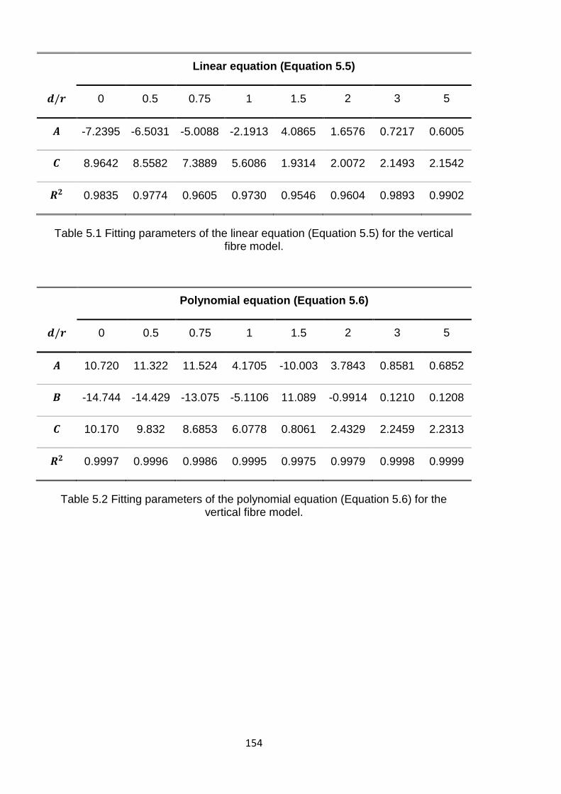
154
Linear equation (Equation 5.5)
𝒅/𝒓 0 0.5 0.75 1 1.5 2 3 5
𝑨 -7.2395 -6.5031 -5.0088 -2.1913 4.0865 1.6576 0.7217 0.6005
𝑪 8.9642 8.5582 7.3889 5.6086 1.9314 2.0072 2.1493 2.1542
𝑹𝟐 0.9835 0.9774 0.9605 0.9730 0.9546 0.9604 0.9893 0.9902
Table 5.1 Fitting parameters of the linear equation (Equation 5.5) for the vertical fibre model.
Polynomial equation (Equation 5.6)
𝒅/𝒓 0 0.5 0.75 1 1.5 2 3 5
𝑨 10.720 11.322 11.524 4.1705 -10.003 3.7843 0.8581 0.6852
𝑩 -14.744 -14.429 -13.075 -5.1106 11.089 -0.9914 0.1210 0.1208
𝑪 10.170 9.832 8.6853 6.0778 0.8061 2.4329 2.2459 2.2313
𝑹𝟐 0.9997 0.9996 0.9986 0.9995 0.9975 0.9979 0.9998 0.9999
Table 5.2 Fitting parameters of the polynomial equation (Equation 5.6) for the vertical fibre model.
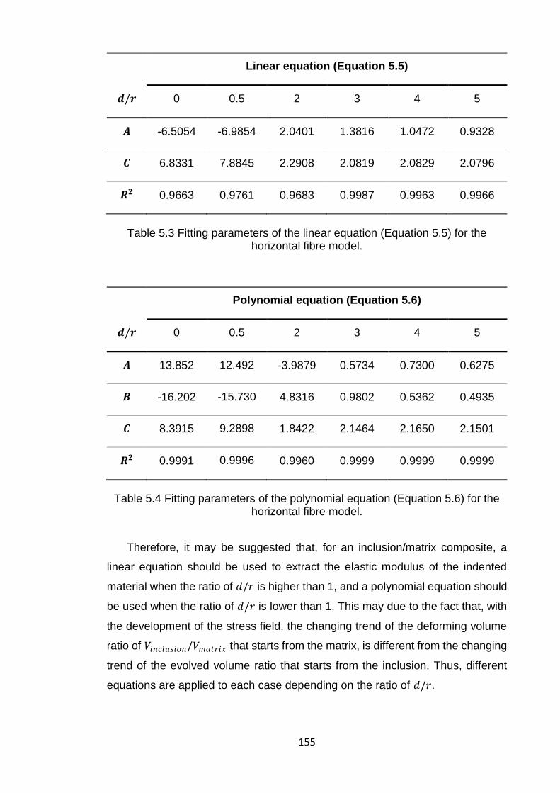
155
Linear equation (Equation 5.5)
𝒅/𝒓 0 0.5 2 3 4 5
𝑨 -6.5054 -6.9854 2.0401 1.3816 1.0472 0.9328
𝑪 6.8331 7.8845 2.2908 2.0819 2.0829 2.0796
𝑹𝟐 0.9663 0.9761 0.9683 0.9987 0.9963 0.9966
Table 5.3 Fitting parameters of the linear equation (Equation 5.5) for the horizontal fibre model.
Polynomial equation (Equation 5.6)
𝒅/𝒓 0 0.5 2 3 4 5
𝑨 13.852 12.492 -3.9879 0.5734 0.7300 0.6275
𝑩 -16.202 -15.730 4.8316 0.9802 0.5362 0.4935
𝑪 8.3915 9.2898 1.8422 2.1464 2.1650 2.1501
𝑹𝟐 0.9991 0.9996 0.9960 0.9999 0.9999 0.9999
Table 5.4 Fitting parameters of the polynomial equation (Equation 5.6) for the horizontal fibre model.
Therefore, it may be suggested that, for an inclusion/matrix composite, a
linear equation should be used to extract the elastic modulus of the indented
material when the ratio of 𝑑/𝑟 is higher than 1, and a polynomial equation should
be used when the ratio of 𝑑/𝑟 is lower than 1. This may due to the fact that, with
the development of the stress field, the changing trend of the deforming volume
ratio of 𝑉𝑖𝑛𝑐𝑙𝑢𝑠𝑖𝑜𝑛/𝑉𝑚𝑎𝑡𝑟𝑖𝑥 that starts from the matrix, is different from the changing
trend of the evolved volume ratio that starts from the inclusion. Thus, different
equations are applied to each case depending on the ratio of 𝑑/𝑟.
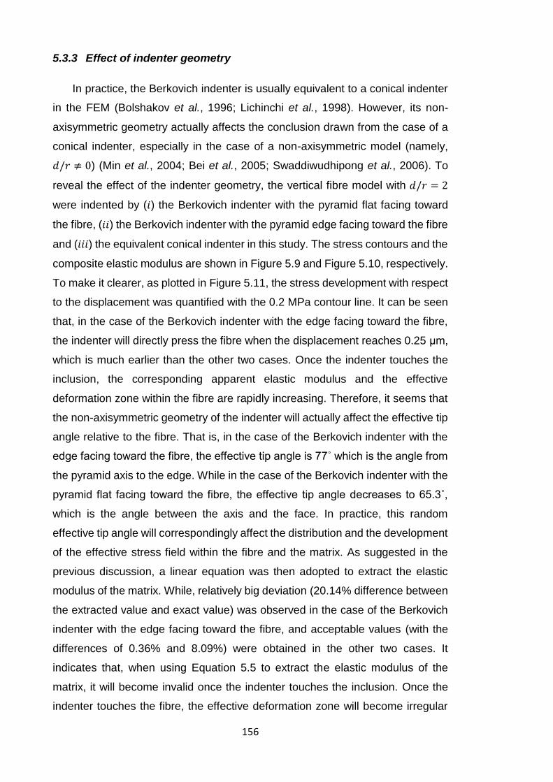
156
5.3.3 Effect of indenter geometry
In practice, the Berkovich indenter is usually equivalent to a conical indenter
in the FEM (Bolshakov et al., 1996; Lichinchi et al., 1998). However, its non-
axisymmetric geometry actually affects the conclusion drawn from the case of a
conical indenter, especially in the case of a non-axisymmetric model (namely,
𝑑/𝑟 ≠ 0) (Min et al., 2004; Bei et al., 2005; Swaddiwudhipong et al., 2006). To
reveal the effect of the indenter geometry, the vertical fibre model with 𝑑/𝑟 = 2
were indented by (𝑖) the Berkovich indenter with the pyramid flat facing toward
the fibre, (𝑖𝑖) the Berkovich indenter with the pyramid edge facing toward the fibre
and (𝑖𝑖𝑖) the equivalent conical indenter in this study. The stress contours and the
composite elastic modulus are shown in Figure 5.9 and Figure 5.10, respectively.
To make it clearer, as plotted in Figure 5.11, the stress development with respect
to the displacement was quantified with the 0.2 MPa contour line. It can be seen
that, in the case of the Berkovich indenter with the edge facing toward the fibre,
the indenter will directly press the fibre when the displacement reaches 0.25 μm,
which is much earlier than the other two cases. Once the indenter touches the
inclusion, the corresponding apparent elastic modulus and the effective
deformation zone within the fibre are rapidly increasing. Therefore, it seems that
the non-axisymmetric geometry of the indenter will actually affect the effective tip
angle relative to the fibre. That is, in the case of the Berkovich indenter with the
edge facing toward the fibre, the effective tip angle is 77˚ which is the angle from
the pyramid axis to the edge. While in the case of the Berkovich indenter with the
pyramid flat facing toward the fibre, the effective tip angle decreases to 65.3˚,
which is the angle between the axis and the face. In practice, this random
effective tip angle will correspondingly affect the distribution and the development
of the effective stress field within the fibre and the matrix. As suggested in the
previous discussion, a linear equation was then adopted to extract the elastic
modulus of the matrix. While, relatively big deviation (20.14% difference between
the extracted value and exact value) was observed in the case of the Berkovich
indenter with the edge facing toward the fibre, and acceptable values (with the
differences of 0.36% and 8.09%) were obtained in the other two cases. It
indicates that, when using Equation 5.5 to extract the elastic modulus of the
matrix, it will become invalid once the indenter touches the inclusion. Once the
indenter touches the fibre, the effective deformation zone will become irregular
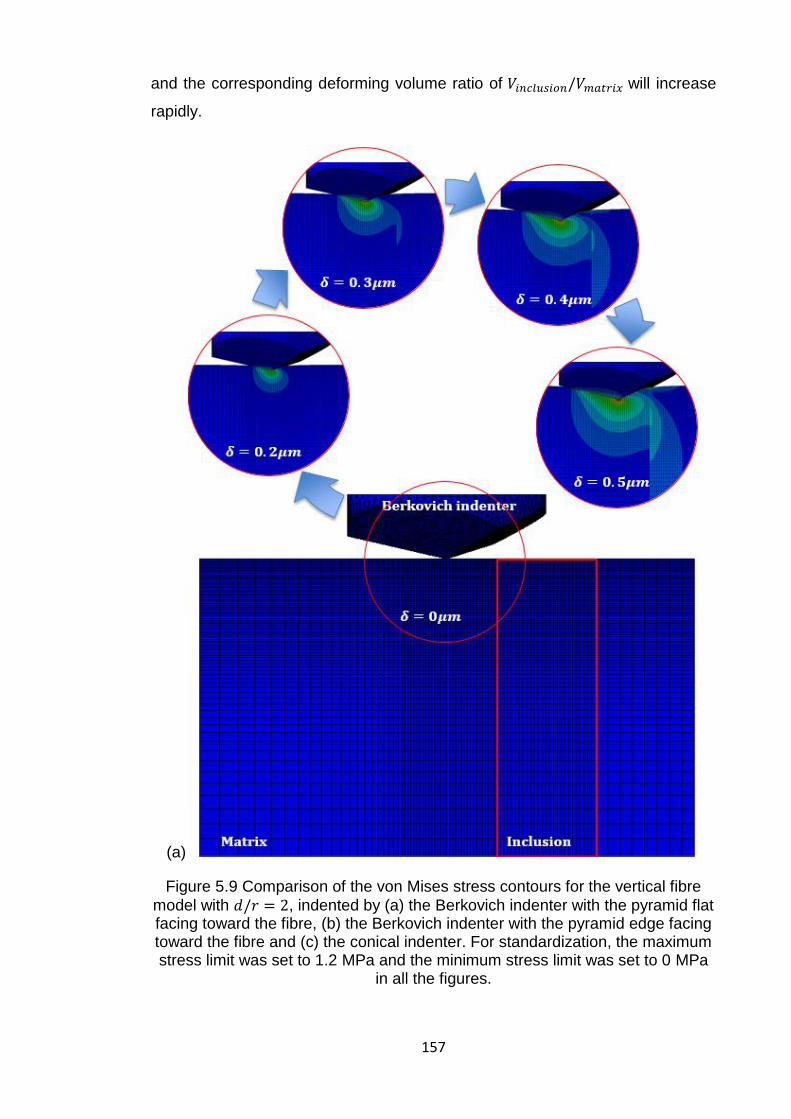
157
and the corresponding deforming volume ratio of 𝑉𝑖𝑛𝑐𝑙𝑢𝑠𝑖𝑜𝑛/𝑉𝑚𝑎𝑡𝑟𝑖𝑥 will increase
rapidly.
(a)
Figure 5.9 Comparison of the von Mises stress contours for the vertical fibre
model with 𝑑/𝑟 = 2, indented by (a) the Berkovich indenter with the pyramid flat facing toward the fibre, (b) the Berkovich indenter with the pyramid edge facing toward the fibre and (c) the conical indenter. For standardization, the maximum stress limit was set to 1.2 MPa and the minimum stress limit was set to 0 MPa
in all the figures.
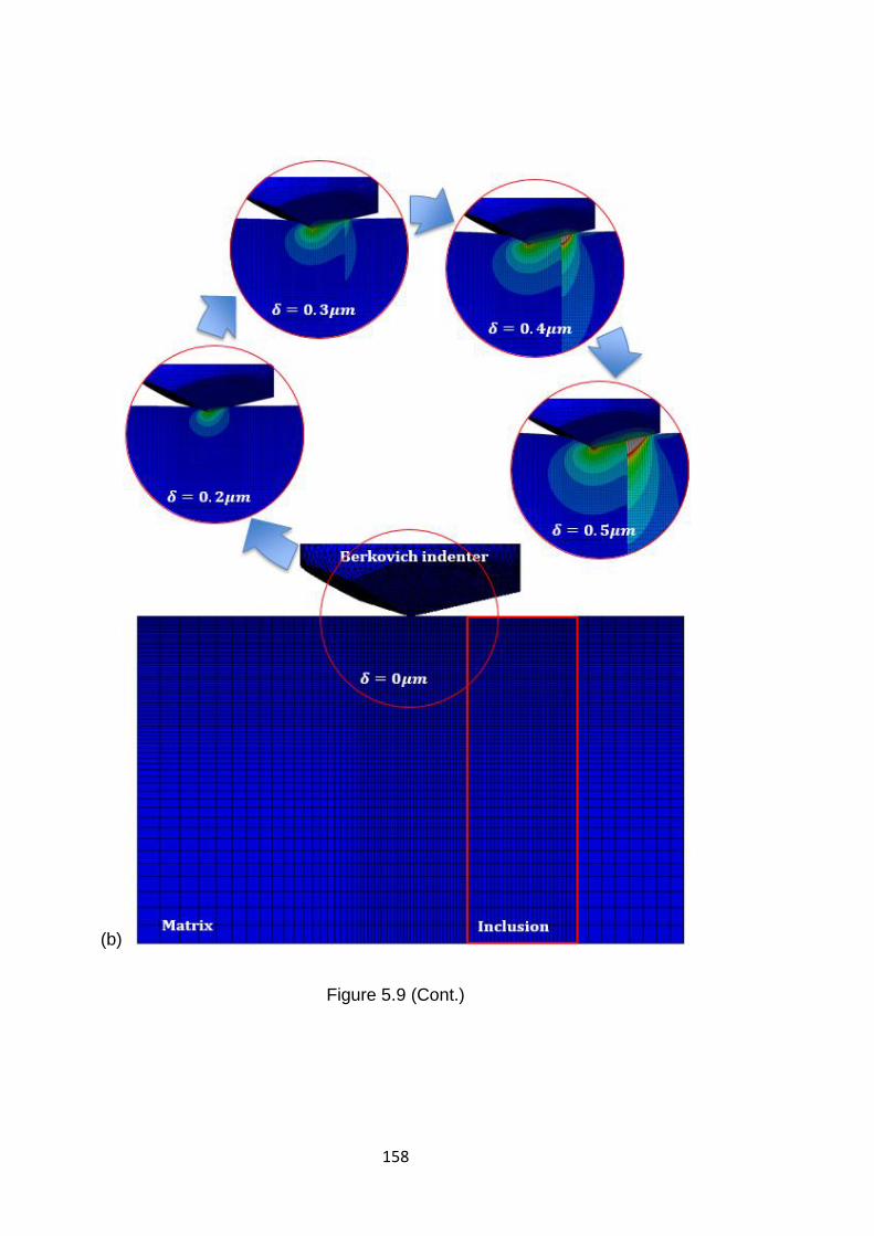
158
(b)
Figure 5.9 (Cont.)
159
(c)
Figure 5.9 (Cont.)
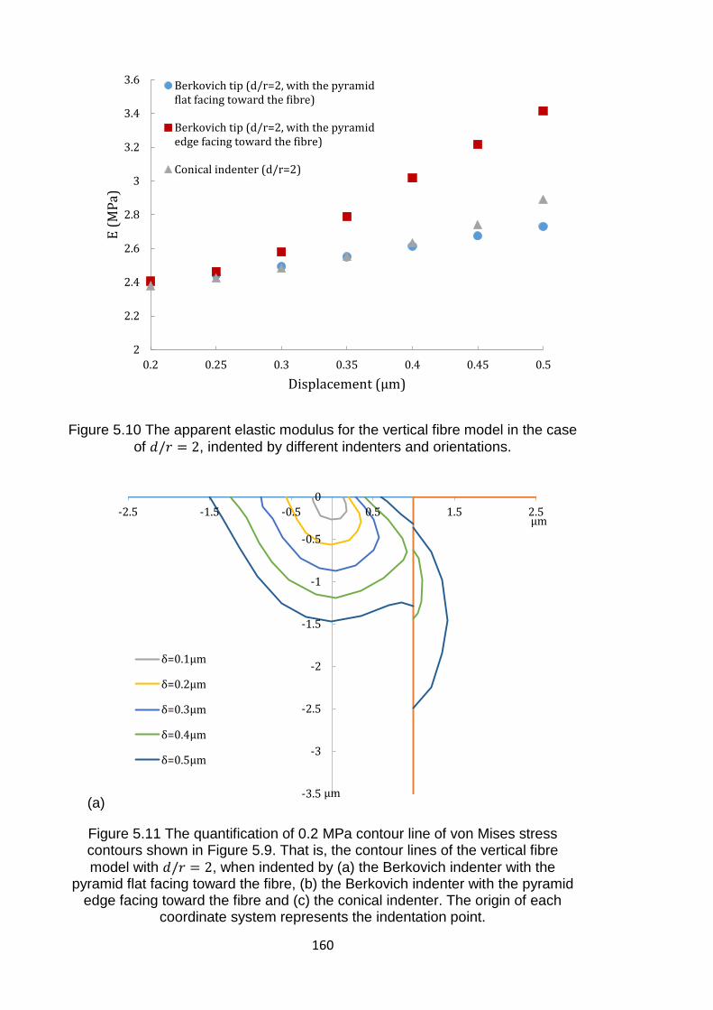
160
Figure 5.10 The apparent elastic modulus for the vertical fibre model in the case
of 𝑑/𝑟 = 2, indented by different indenters and orientations.
(a)
Figure 5.11 The quantification of 0.2 MPa contour line of von Mises stress contours shown in Figure 5.9. That is, the contour lines of the vertical fibre
model with 𝑑/𝑟 = 2, when indented by (a) the Berkovich indenter with the pyramid flat facing toward the fibre, (b) the Berkovich indenter with the pyramid
edge facing toward the fibre and (c) the conical indenter. The origin of each coordinate system represents the indentation point.
2
2.2
2.4
2.6
2.8
3
3.2
3.4
3.6
0.2 0.25 0.3 0.35 0.4 0.45 0.5
E (
MP
a)
Displacement (µm)
Berkovich tip (d/r=2, with the pyramidflat facing toward the fibre)
Berkovich tip (d/r=2, with the pyramidedge facing toward the fibre)
Conical indenter (d/r=2)
-3.5
-3
-2.5
-2
-1.5
-1
-0.5
0
-2.5 -1.5 -0.5 0.5 1.5 2.5
δ=0.1μm
δ=0.2μm
δ=0.3μm
δ=0.4μm
δ=0.5μm
µm
µm
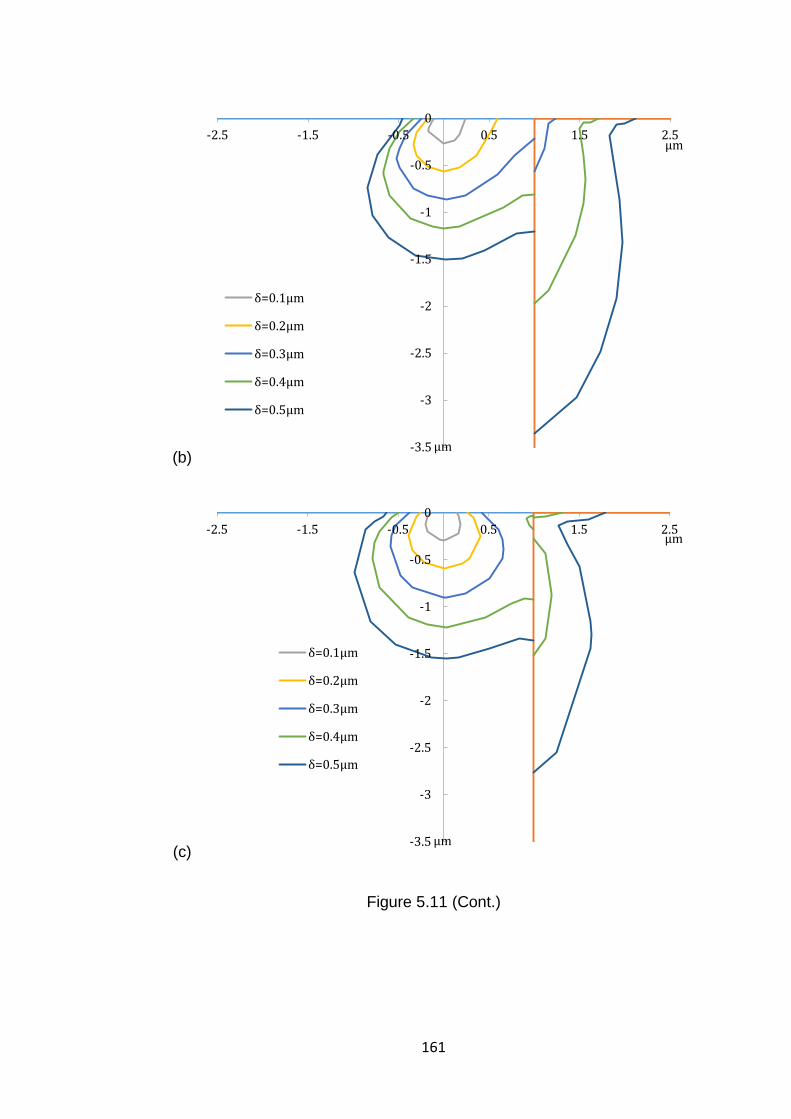
161
(b)
(c)
Figure 5.11 (Cont.)
-3.5
-3
-2.5
-2
-1.5
-1
-0.5
0
-2.5 -1.5 -0.5 0.5 1.5 2.5
δ=0.1μm
δ=0.2μm
δ=0.3μm
δ=0.4μm
δ=0.5μm
µm
µm
-3.5
-3
-2.5
-2
-1.5
-1
-0.5
0
-2.5 -1.5 -0.5 0.5 1.5 2.5
δ=0.1μm
δ=0.2μm
δ=0.3μm
δ=0.4μm
δ=0.5μm
µm
µm
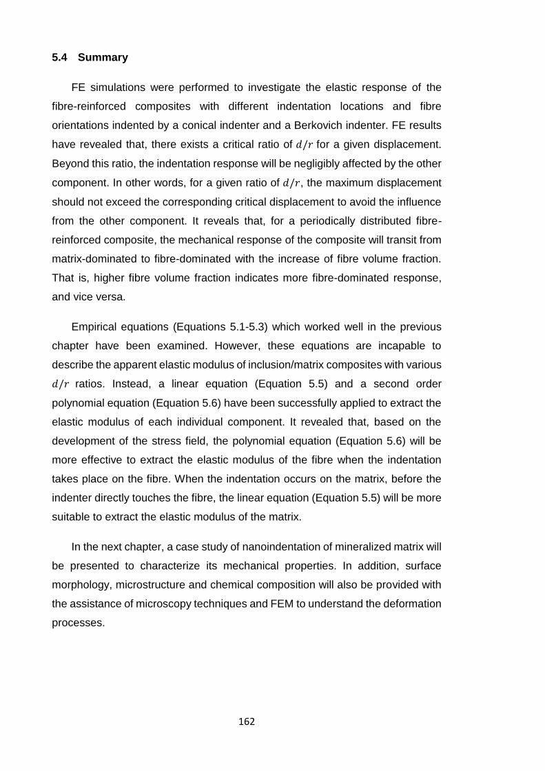
162
5.4 Summary
FE simulations were performed to investigate the elastic response of the
fibre-reinforced composites with different indentation locations and fibre
orientations indented by a conical indenter and a Berkovich indenter. FE results
have revealed that, there exists a critical ratio of 𝑑/𝑟 for a given displacement.
Beyond this ratio, the indentation response will be negligibly affected by the other
component. In other words, for a given ratio of 𝑑/𝑟, the maximum displacement
should not exceed the corresponding critical displacement to avoid the influence
from the other component. It reveals that, for a periodically distributed fibre-
reinforced composite, the mechanical response of the composite will transit from
matrix-dominated to fibre-dominated with the increase of fibre volume fraction.
That is, higher fibre volume fraction indicates more fibre-dominated response,
and vice versa.
Empirical equations (Equations 5.1-5.3) which worked well in the previous
chapter have been examined. However, these equations are incapable to
describe the apparent elastic modulus of inclusion/matrix composites with various
𝑑/𝑟 ratios. Instead, a linear equation (Equation 5.5) and a second order
polynomial equation (Equation 5.6) have been successfully applied to extract the
elastic modulus of each individual component. It revealed that, based on the
development of the stress field, the polynomial equation (Equation 5.6) will be
more effective to extract the elastic modulus of the fibre when the indentation
takes place on the fibre. When the indentation occurs on the matrix, before the
indenter directly touches the fibre, the linear equation (Equation 5.5) will be more
suitable to extract the elastic modulus of the matrix.
In the next chapter, a case study of nanoindentation of mineralized matrix will
be presented to characterize its mechanical properties. In addition, surface
morphology, microstructure and chemical composition will also be provided with
the assistance of microscopy techniques and FEM to understand the deformation
processes.

Chapter 6
Nanomechanical Case Study on
Mineralized Matrix:
Experimental Characterization
and Finite Element Modelling
164
Chapter 6. Nanomechanical Case Study on Mineralized Matrix:
Experimental Characterization and Finite Element Modelling
6.1 Introduction
Tissue engineering is the use of a combination of cells, biomaterials and
suitable biochemical and physicochemical factors to improve or replace biological
tissues. In the last decades, biomaterial scaffolds have been widely used in bone
tissue engineering (Stevens, 2008; Zhang et al., 2009; Deb et al., 2010; Baino et
al., 2011; Ferreira et al., 2012). Scaffolds with various combinations of
constituents are designed to achieve a better biofunctionality and mechanical
strength. Of these, cell-based materials have shown promising prospects for
future exploitation (Bianco and Robey, 2001; Tuan et al., 2003; Gamie et al.,
2012). Very recently, genetic modified cells have been adopted (James et al.,
2015). The immortalized cell line Y201 derived from human mesenchymal stem
cells (hMSCs) circumvents the issues of limited life-span and high variability of
hMSCs (Gong et al., 2011; Liu et al., 2012). However, whether these cells may
proliferate in suitable manner and produce appropriate mineralized matrix for
given cell culture conditions remains elusive, which is essential for bone
regeneration.
To achieve this, it is essential to understand the properties of the mineralized
matrix synthesized by these cells (Gough et al., 2004; Jell et al., 2008;
Bandyopadhyay-Ghosh et al., 2010; Baino et al., 2011). Due to its inhomogeneity
in both chemistry and microstructure, the nanomechanical properties of such
inhomogeneous materials are difficult to be reliably measured, especially for a
thin layer of mineralized matrix.
Nanoindentation has proven an effective technique to assess the
nanomechanical properties of natural tissues such as bone and biological cells
(Kavukcuoglu et al., 2007; Pelled et al., 2007a; Tai et al., 2008; Kavukcuoglu et
al., 2009; Chen et al., 2010b; Jang et al., 2014; Oyen, 2015). Our previous work
has demonstrated that the measured apparent elastic modulus generally has a
bimodal distribution and the Gaussian mixture model enabled us to extract
properties for two components in the matrix (Duan and Chen, 2015). However,
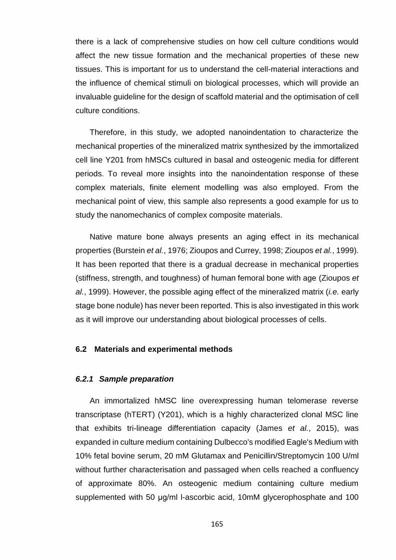
165
there is a lack of comprehensive studies on how cell culture conditions would
affect the new tissue formation and the mechanical properties of these new
tissues. This is important for us to understand the cell-material interactions and
the influence of chemical stimuli on biological processes, which will provide an
invaluable guideline for the design of scaffold material and the optimisation of cell
culture conditions.
Therefore, in this study, we adopted nanoindentation to characterize the
mechanical properties of the mineralized matrix synthesized by the immortalized
cell line Y201 from hMSCs cultured in basal and osteogenic media for different
periods. To reveal more insights into the nanoindentation response of these
complex materials, finite element modelling was also employed. From the
mechanical point of view, this sample also represents a good example for us to
study the nanomechanics of complex composite materials.
Native mature bone always presents an aging effect in its mechanical
properties (Burstein et al., 1976; Zioupos and Currey, 1998; Zioupos et al., 1999).
It has been reported that there is a gradual decrease in mechanical properties
(stiffness, strength, and toughness) of human femoral bone with age (Zioupos et
al., 1999). However, the possible aging effect of the mineralized matrix (i.e. early
stage bone nodule) has never been reported. This is also investigated in this work
as it will improve our understanding about biological processes of cells.
6.2 Materials and experimental methods
6.2.1 Sample preparation
An immortalized hMSC line overexpressing human telomerase reverse
transcriptase (hTERT) (Y201), which is a highly characterized clonal MSC line
that exhibits tri-lineage differentiation capacity (James et al., 2015), was
expanded in culture medium containing Dulbecco's modified Eagle's Medium with
10% fetal bovine serum, 20 mM Glutamax and Penicillin/Streptomycin 100 U/ml
without further characterisation and passaged when cells reached a confluency
of approximate 80%. An osteogenic medium containing culture medium
supplemented with 50 μg/ml l-ascorbic acid, 10mM glycerophosphate and 100
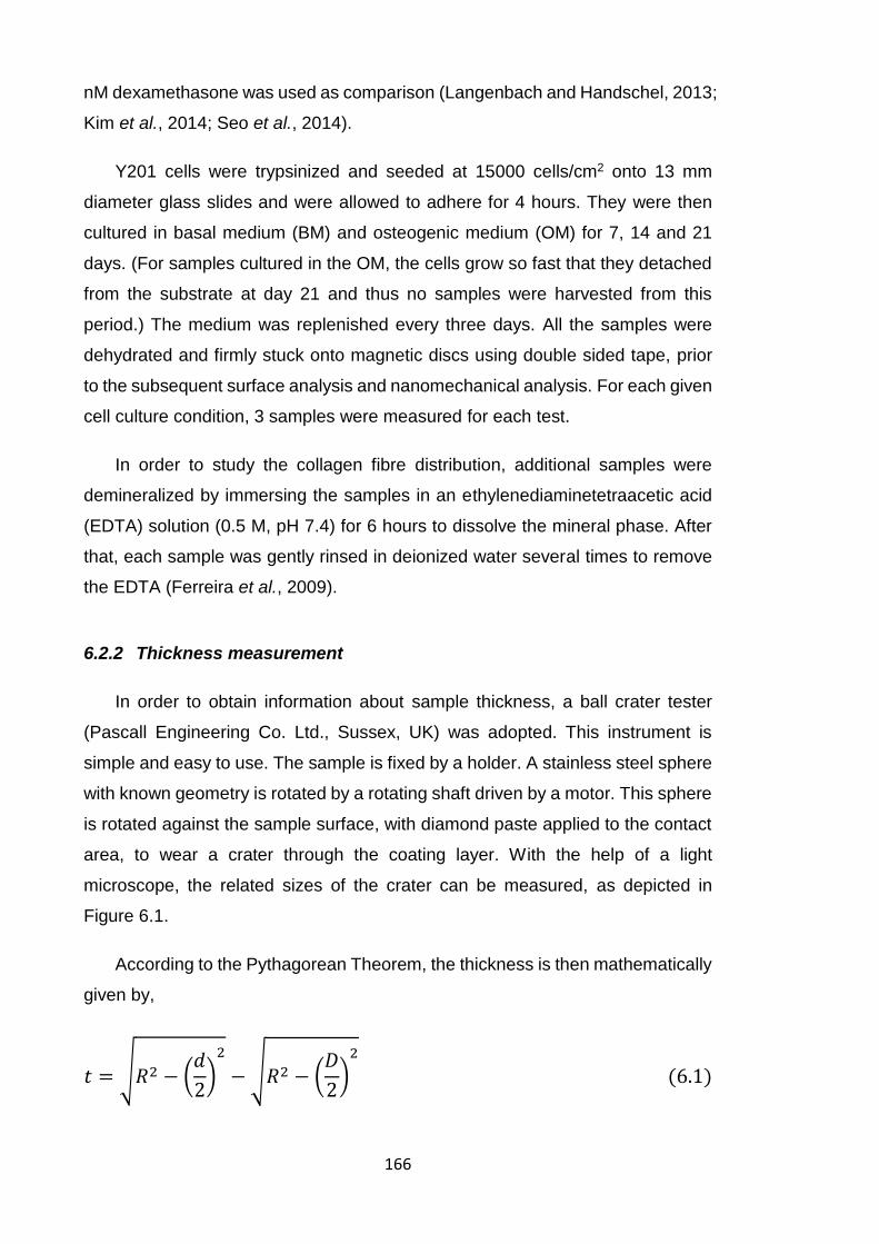
166
nM dexamethasone was used as comparison (Langenbach and Handschel, 2013;
Kim et al., 2014; Seo et al., 2014).
Y201 cells were trypsinized and seeded at 15000 cells/cm2 onto 13 mm
diameter glass slides and were allowed to adhere for 4 hours. They were then
cultured in basal medium (BM) and osteogenic medium (OM) for 7, 14 and 21
days. (For samples cultured in the OM, the cells grow so fast that they detached
from the substrate at day 21 and thus no samples were harvested from this
period.) The medium was replenished every three days. All the samples were
dehydrated and firmly stuck onto magnetic discs using double sided tape, prior
to the subsequent surface analysis and nanomechanical analysis. For each given
cell culture condition, 3 samples were measured for each test.
In order to study the collagen fibre distribution, additional samples were
demineralized by immersing the samples in an ethylenediaminetetraacetic acid
(EDTA) solution (0.5 M, pH 7.4) for 6 hours to dissolve the mineral phase. After
that, each sample was gently rinsed in deionized water several times to remove
the EDTA (Ferreira et al., 2009).
6.2.2 Thickness measurement
In order to obtain information about sample thickness, a ball crater tester
(Pascall Engineering Co. Ltd., Sussex, UK) was adopted. This instrument is
simple and easy to use. The sample is fixed by a holder. A stainless steel sphere
with known geometry is rotated by a rotating shaft driven by a motor. This sphere
is rotated against the sample surface, with diamond paste applied to the contact
area, to wear a crater through the coating layer. With the help of a light
microscope, the related sizes of the crater can be measured, as depicted in
Figure 6.1.
According to the Pythagorean Theorem, the thickness is then mathematically
given by,
𝑡 = √𝑅2 − (𝑑
2)
2
− √𝑅2 − (𝐷
2)
2
(6.1)
167
where 𝑡 is the thickness of the coating layer, 𝑅 is the radius of the stainless steel
sphere (𝑅 equals 12.7 mm in this study), 𝑑 and 𝐷 are the diameter of the inner
and outer circles, respectively. In this study, the thickness of these matrix layers
is 18.5±8.4 μm at the centre of the sample.
Figure 6.1 Schematic of the crater within the sample produced by a ball crater tester. In practice, the outer circle will be irregular for a coating layer with non-
uniform thickness.
6.2.3 Surface analysis
Although nanoindentation techniques are powerful tools, their applications
are limited to the mechanical characterization of materials. In order to obtain a
further understanding of deformation mechanisms, microstructure, surface
morphology or chemical composition of tested materials, the assistance of
microscopy techniques is necessary (Pharr, 1998; Goodhew et al., 2000; Wei et
al., 2005). In this study, prior to nanomechanical tests, microscopy techniques
have been extensively used with the aim of understanding the topography and
chemical characterization of the mineralized matrix samples.
168
6.2.3.1 Optical microscope
The collagen fibre analysis of samples was performed with an Olympus BH2-
UMA polarizing microscope (Olympus Europa GmbH, Hamburg, Germany) with
a magnification 500X. This instrument adopts a polarized light illumination system
with a pair of polarizing plates, which allows the birefringent samples to be
observed, such as some crystals, plastics and collagen (Sano, 1988).
6.2.3.2 Profilometer
In this study, the surface roughness measurement was conducted by a ZYGO
5000 profilometer (ZYGO Corporation, Middlefield, CT, USA). This instrument is
based on the white light interferometry method, with a fast and non-contact
operation, and excellent vertical resolution (up to 0.1 nm). Figure 6.2 shows the
representative roughness image of a sample surface, with a view area of 1.58
mm × 1.19 mm.
Figure 6.2 Representative surface profile of a mineralized matrix sample.
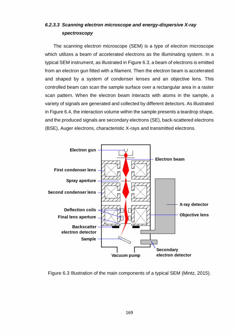
169
6.2.3.3 Scanning electron microscope and energy-dispersive X-ray
spectroscopy
The scanning electron microscope (SEM) is a type of electron microscope
which utilizes a beam of accelerated electrons as the illuminating system. In a
typical SEM instrument, as illustrated in Figure 6.3, a beam of electrons is emitted
from an electron gun fitted with a filament. Then the electron beam is accelerated
and shaped by a system of condenser lenses and an objective lens. This
controlled beam can scan the sample surface over a rectangular area in a raster
scan pattern. When the electron beam interacts with atoms in the sample, a
variety of signals are generated and collected by different detectors. As illustrated
in Figure 6.4, the interaction volume within the sample presents a teardrop shape,
and the produced signals are secondary electrons (SE), back-scattered electrons
(BSE), Auger electrons, characteristic X-rays and transmitted electrons.
Figure 6.3 Illustration of the main components of a typical SEM (Mintz, 2015).
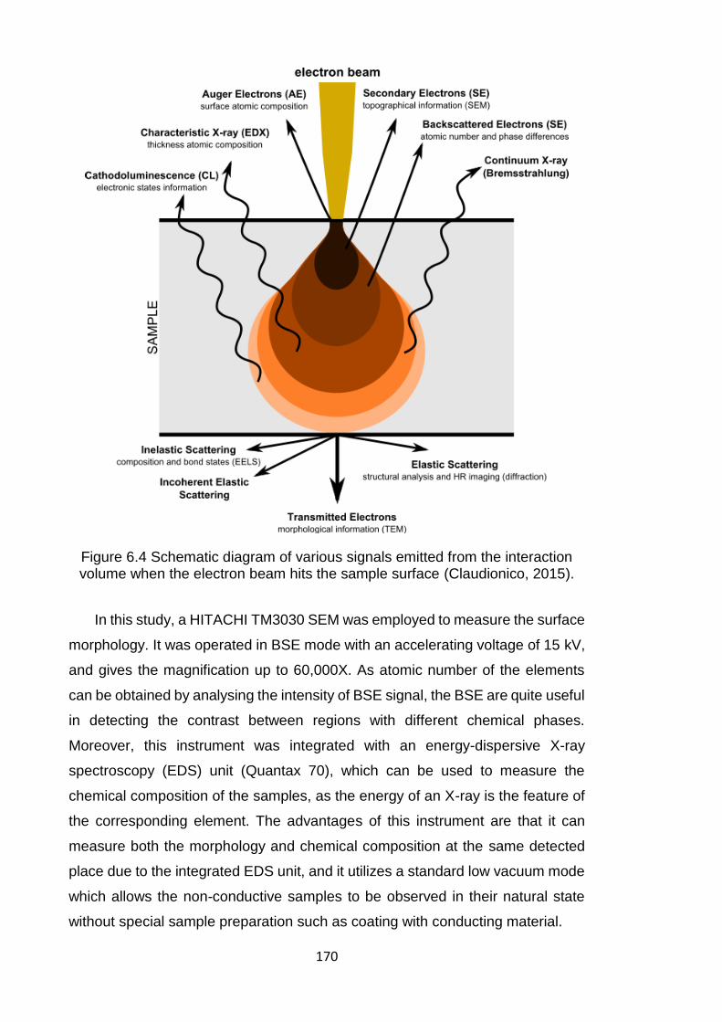
170
Figure 6.4 Schematic diagram of various signals emitted from the interaction volume when the electron beam hits the sample surface (Claudionico, 2015).
In this study, a HITACHI TM3030 SEM was employed to measure the surface
morphology. It was operated in BSE mode with an accelerating voltage of 15 kV,
and gives the magnification up to 60,000X. As atomic number of the elements
can be obtained by analysing the intensity of BSE signal, the BSE are quite useful
in detecting the contrast between regions with different chemical phases.
Moreover, this instrument was integrated with an energy-dispersive X-ray
spectroscopy (EDS) unit (Quantax 70), which can be used to measure the
chemical composition of the samples, as the energy of an X-ray is the feature of
the corresponding element. The advantages of this instrument are that it can
measure both the morphology and chemical composition at the same detected
place due to the integrated EDS unit, and it utilizes a standard low vacuum mode
which allows the non-conductive samples to be observed in their natural state
without special sample preparation such as coating with conducting material.
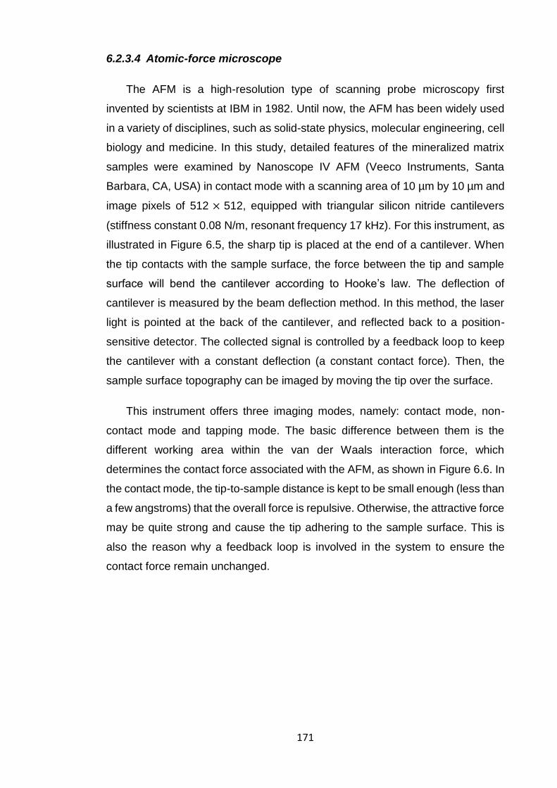
171
6.2.3.4 Atomic-force microscope
The AFM is a high-resolution type of scanning probe microscopy first
invented by scientists at IBM in 1982. Until now, the AFM has been widely used
in a variety of disciplines, such as solid-state physics, molecular engineering, cell
biology and medicine. In this study, detailed features of the mineralized matrix
samples were examined by Nanoscope IV AFM (Veeco Instruments, Santa
Barbara, CA, USA) in contact mode with a scanning area of 10 µm by 10 µm and
image pixels of 512 × 512, equipped with triangular silicon nitride cantilevers
(stiffness constant 0.08 N/m, resonant frequency 17 kHz). For this instrument, as
illustrated in Figure 6.5, the sharp tip is placed at the end of a cantilever. When
the tip contacts with the sample surface, the force between the tip and sample
surface will bend the cantilever according to Hooke’s law. The deflection of
cantilever is measured by the beam deflection method. In this method, the laser
light is pointed at the back of the cantilever, and reflected back to a position-
sensitive detector. The collected signal is controlled by a feedback loop to keep
the cantilever with a constant deflection (a constant contact force). Then, the
sample surface topography can be imaged by moving the tip over the surface.
This instrument offers three imaging modes, namely: contact mode, non-
contact mode and tapping mode. The basic difference between them is the
different working area within the van der Waals interaction force, which
determines the contact force associated with the AFM, as shown in Figure 6.6. In
the contact mode, the tip-to-sample distance is kept to be small enough (less than
a few angstroms) that the overall force is repulsive. Otherwise, the attractive force
may be quite strong and cause the tip adhering to the sample surface. This is
also the reason why a feedback loop is involved in the system to ensure the
contact force remain unchanged.
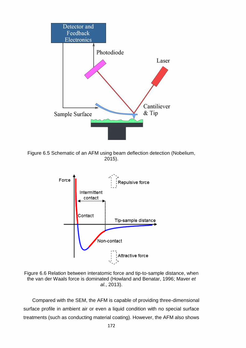
172
Figure 6.5 Schematic of an AFM using beam deflection detection (Nobelium, 2015).
Figure 6.6 Relation between interatomic force and tip-to-sample distance, when the van der Waals force is dominated (Howland and Benatar, 1996; Maver et
al., 2013).
Compared with the SEM, the AFM is capable of providing three-dimensional
surface profile in ambient air or even a liquid condition with no special surface
treatments (such as conducting material coating). However, the AFM also shows
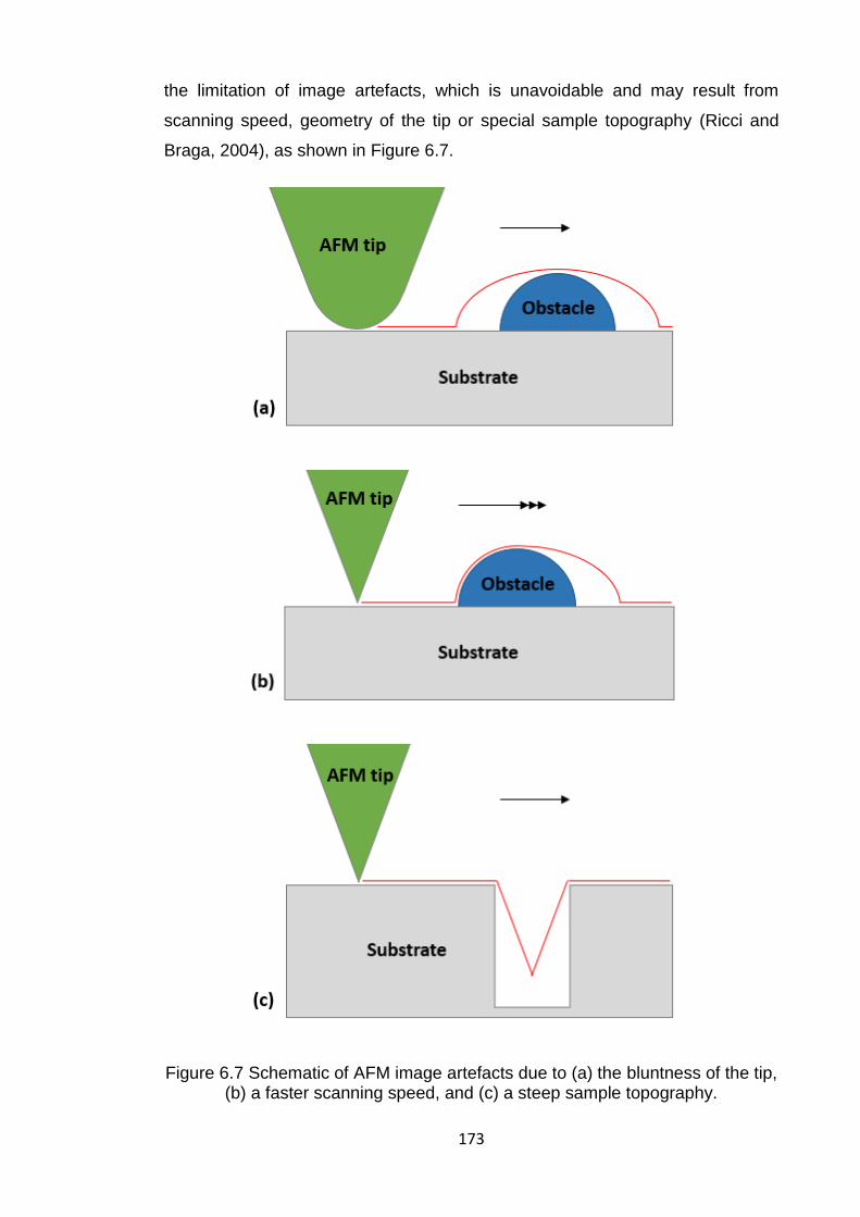
173
the limitation of image artefacts, which is unavoidable and may result from
scanning speed, geometry of the tip or special sample topography (Ricci and
Braga, 2004), as shown in Figure 6.7.
Figure 6.7 Schematic of AFM image artefacts due to (a) the bluntness of the tip, (b) a faster scanning speed, and (c) a steep sample topography.
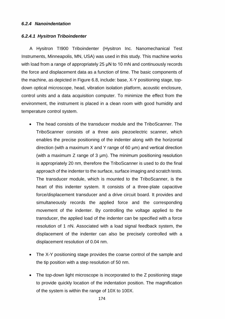
174
6.2.4 Nanoindentation
6.2.4.1 Hysitron Triboindenter
A Hysitron TI900 Triboindenter (Hysitron Inc. Nanomechanical Test
Instruments, Minneapolis, MN, USA) was used in this study. This machine works
with load from a range of appropriately 25 μN to 10 mN and continuously records
the force and displacement data as a function of time. The basic components of
the machine, as depicted in Figure 6.8, include: base, X-Y positioning stage, top-
down optical microscope, head, vibration isolation platform, acoustic enclosure,
control units and a data acquisition computer. To minimize the effect from the
environment, the instrument is placed in a clean room with good humidity and
temperature control system.
The head consists of the transducer module and the TriboScanner. The
TriboScanner consists of a three axis piezoelectric scanner, which
enables the precise positioning of the indenter along with the horizontal
direction (with a maximum X and Y range of 60 μm) and vertical direction
(with a maximum Z range of 3 μm). The minimum positioning resolution
is appropriately 20 nm, therefore the TriboScanner is used to do the final
approach of the indenter to the surface, surface imaging and scratch tests.
The transducer module, which is mounted to the TriboScanner, is the
heart of this indenter system. It consists of a three-plate capacitive
force/displacement transducer and a drive circuit board. It provides and
simultaneously records the applied force and the corresponding
movement of the indenter. By controlling the voltage applied to the
transducer, the applied load of the indenter can be specified with a force
resolution of 1 nN. Associated with a load signal feedback system, the
displacement of the indenter can also be precisely controlled with a
displacement resolution of 0.04 nm.
The X-Y positioning stage provides the coarse control of the sample and
the tip position with a step resolution of 50 nm.
The top-down light microscope is incorporated to the Z positioning stage
to provide quickly location of the indentation position. The magnification
of the system is within the range of 10X to 100X.
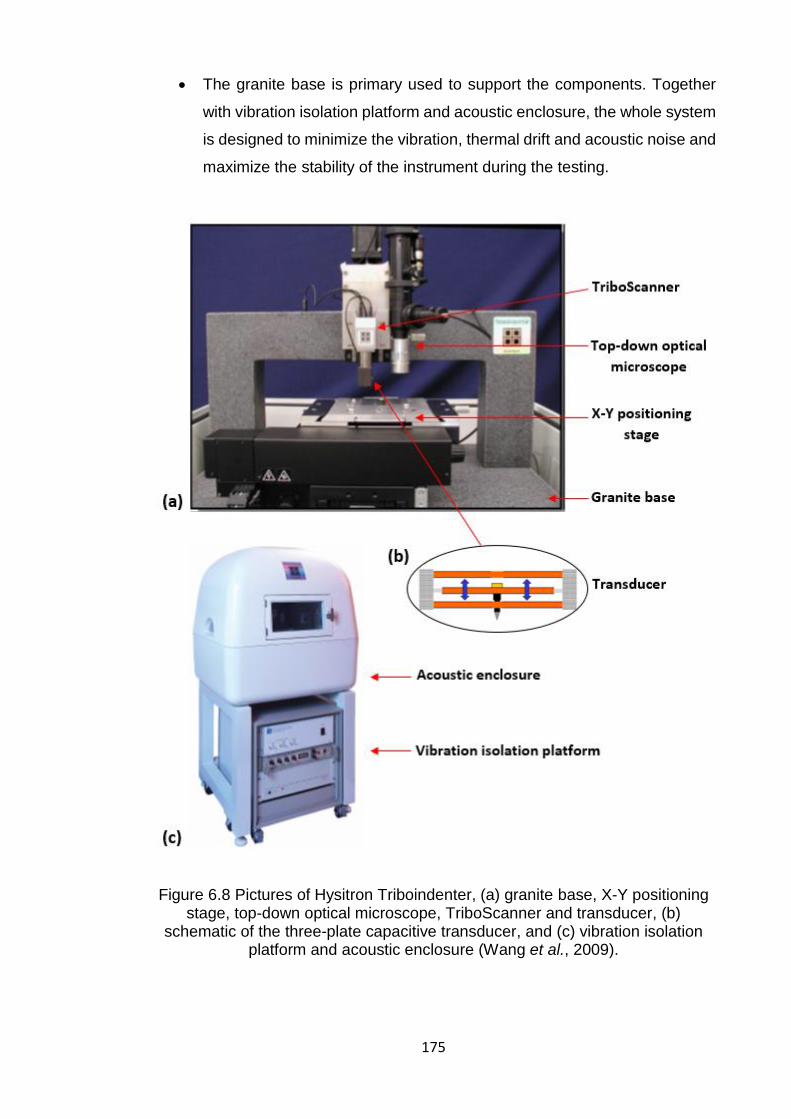
175
The granite base is primary used to support the components. Together
with vibration isolation platform and acoustic enclosure, the whole system
is designed to minimize the vibration, thermal drift and acoustic noise and
maximize the stability of the instrument during the testing.
Figure 6.8 Pictures of Hysitron Triboindenter, (a) granite base, X-Y positioning stage, top-down optical microscope, TriboScanner and transducer, (b)
schematic of the three-plate capacitive transducer, and (c) vibration isolation platform and acoustic enclosure (Wang et al., 2009).
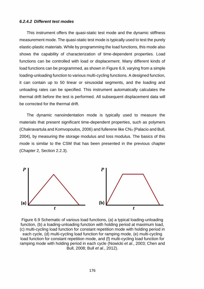
176
6.2.4.2 Different test modes
This instrument offers the quasi-static test mode and the dynamic stiffness
measurement mode. The quasi-static test mode is typically used to test the purely
elastic-plastic materials. While by programming the load functions, this mode also
shows the capability of characterization of time-dependent properties. Load
functions can be controlled with load or displacement. Many different kinds of
load functions can be programmed, as shown in Figure 6.9, varying from a simple
loading-unloading function to various multi-cycling functions. A designed function,
it can contain up to 50 linear or sinusoidal segments, and the loading and
unloading rates can be specified. This instrument automatically calculates the
thermal drift before the test is performed. All subsequent displacement data will
be corrected for the thermal drift.
The dynamic nanoindentation mode is typically used to measure the
materials that present significant time-dependent properties, such as polymers
(Chakravartula and Komvopoulos, 2006) and fullerene like CNX (Palacio and Bull,
2004), by measuring the storage modulus and loss modulus. The basics of this
mode is similar to the CSM that has been presented in the previous chapter
(Chapter 2, Section 2.2.3).
Figure 6.9 Schematic of various load functions, (a) a typical loading-unloading function, (b) a loading-unloading function with holding period at maximum load, (c) multi-cycling load function for constant repetition mode with holding period in
each cycle, (d) multi-cycling load function for ramping mode, (e) multi-cycling load function for constant repetition mode, and (f) multi-cycling load function for ramping mode with holding period in each cycle (Nowicki et al., 2003; Chen and
Bull, 2008; Bull et al., 2012).
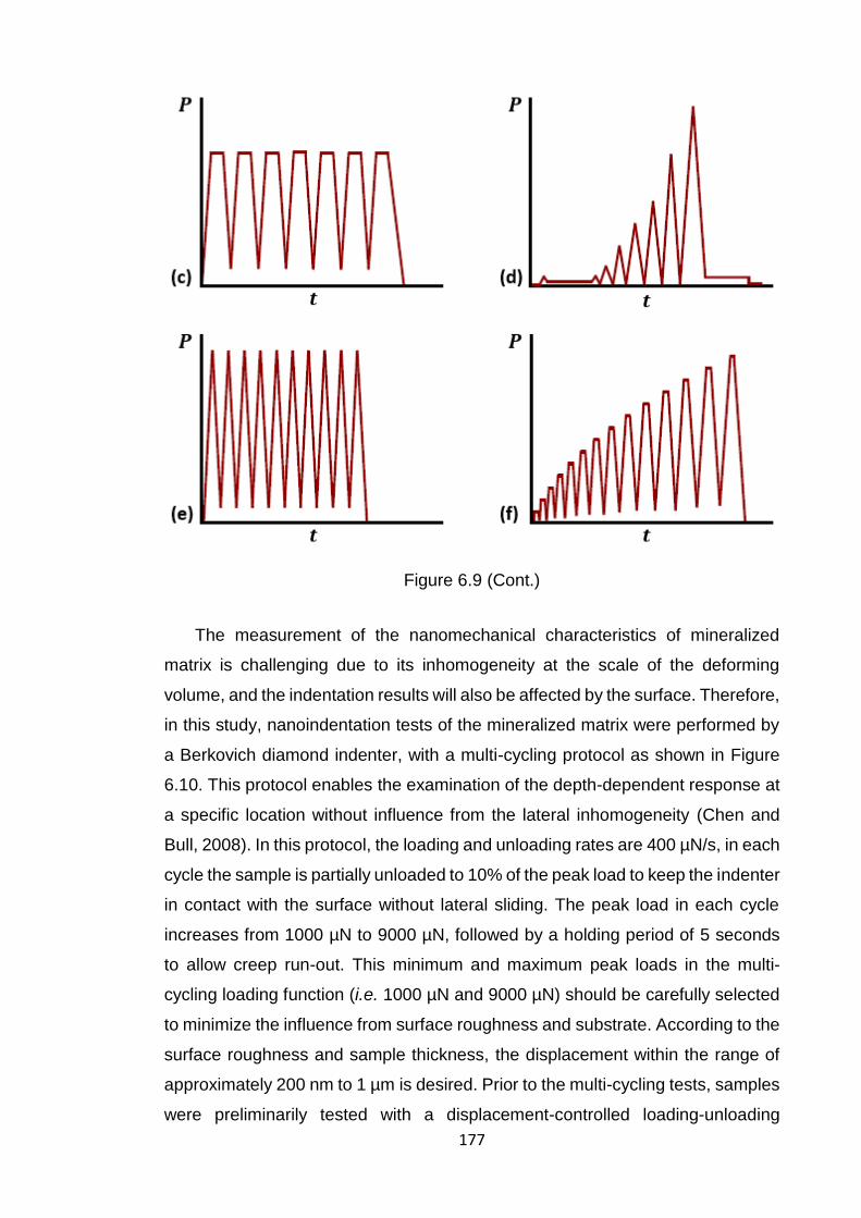
177
Figure 6.9 (Cont.)
The measurement of the nanomechanical characteristics of mineralized
matrix is challenging due to its inhomogeneity at the scale of the deforming
volume, and the indentation results will also be affected by the surface. Therefore,
in this study, nanoindentation tests of the mineralized matrix were performed by
a Berkovich diamond indenter, with a multi-cycling protocol as shown in Figure
6.10. This protocol enables the examination of the depth-dependent response at
a specific location without influence from the lateral inhomogeneity (Chen and
Bull, 2008). In this protocol, the loading and unloading rates are 400 µN/s, in each
cycle the sample is partially unloaded to 10% of the peak load to keep the indenter
in contact with the surface without lateral sliding. The peak load in each cycle
increases from 1000 µN to 9000 µN, followed by a holding period of 5 seconds
to allow creep run-out. This minimum and maximum peak loads in the multi-
cycling loading function (i.e. 1000 µN and 9000 µN) should be carefully selected
to minimize the influence from surface roughness and substrate. According to the
surface roughness and sample thickness, the displacement within the range of
approximately 200 nm to 1 µm is desired. Prior to the multi-cycling tests, samples
were preliminarily tested with a displacement-controlled loading-unloading
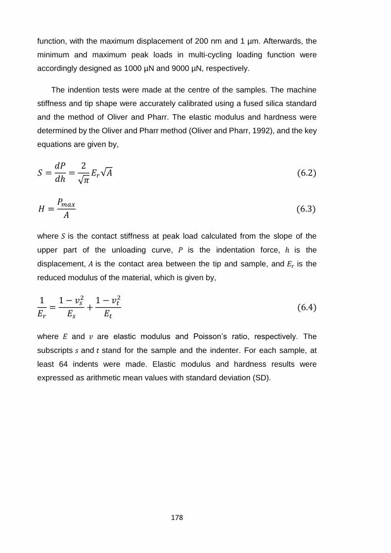
178
function, with the maximum displacement of 200 nm and 1 µm. Afterwards, the
minimum and maximum peak loads in multi-cycling loading function were
accordingly designed as 1000 µN and 9000 µN, respectively.
The indention tests were made at the centre of the samples. The machine
stiffness and tip shape were accurately calibrated using a fused silica standard
and the method of Oliver and Pharr. The elastic modulus and hardness were
determined by the Oliver and Pharr method (Oliver and Pharr, 1992), and the key
equations are given by,
𝑆 =𝑑𝑃
𝑑ℎ=
2
√𝜋𝐸𝑟√𝐴 (6.2)
𝐻 =𝑃𝑚𝑎𝑥
𝐴 (6.3)
where 𝑆 is the contact stiffness at peak load calculated from the slope of the
upper part of the unloading curve, 𝑃 is the indentation force, ℎ is the
displacement, 𝐴 is the contact area between the tip and sample, and 𝐸𝑟 is the
reduced modulus of the material, which is given by,
1
𝐸𝑟=
1 − 𝑣𝑠2
𝐸𝑠+
1 − 𝑣𝑡2
𝐸𝑡 (6.4)
where 𝐸 and 𝑣 are elastic modulus and Poisson’s ratio, respectively. The
subscripts 𝑠 and 𝑡 stand for the sample and the indenter. For each sample, at
least 64 indents were made. Elastic modulus and hardness results were
expressed as arithmetic mean values with standard deviation (SD).
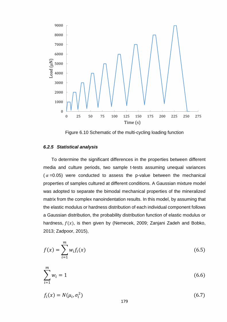
179
Figure 6.10 Schematic of the multi-cycling loading function
6.2.5 Statistical analysis
To determine the significant differences in the properties between different
media and culture periods, two sample t-tests assuming unequal variances
( 𝛼 =0.05) were conducted to assess the p-value between the mechanical
properties of samples cultured at different conditions. A Gaussian mixture model
was adopted to separate the bimodal mechanical properties of the mineralized
matrix from the complex nanoindentation results. In this model, by assuming that
the elastic modulus or hardness distribution of each individual component follows
a Gaussian distribution, the probability distribution function of elastic modulus or
hardness, 𝑓(𝑥), is then given by (Nemecek, 2009; Zanjani Zadeh and Bobko,
2013; Zadpoor, 2015),
𝑓(𝑥) = ∑ 𝑤𝑖𝑓𝑖(𝑥)
𝑚
𝑖=1
(6.5)
∑ 𝑤𝑖 = 1
𝑚
𝑖=1
(6.6)
𝑓𝑖(𝑥) = 𝑁(𝜇𝑖 , 𝜎𝑖2) (6.7)
0
1000
2000
3000
4000
5000
6000
7000
8000
9000
0 25 50 75 100 125 150 175 200 225 250 275
Lo
ad (
µN
)
Time (s)
180
where 𝑚 is the number of the components, 𝑤𝑖 and 𝑓𝑖(𝑥) are volume fraction and
Gaussian distribution for component 𝑖 , respectively. Moreover, 𝜇𝑖 and 𝜎𝑖
represent the mean and standard deviation of the mechanical properties for
component 𝑖, respectively. A Matlab code was written to complete this statistical
analysis. Different 𝑚 values have been assumed (i.e. 1, 2, 3…), but only 𝑚=2
gives the best fitting results. It indicates that there are possibly two major
components in the mixture model.
6.2.6 Finite element modelling
To further understand the nanoindentation response of the mineralized matrix,
FEM was employed (Fan et al., 2004; Carnelli et al., 2011). As found in our
previous study (Duan and Chen, 2015), the distribution of apparent elastic
modulus generally appeared to be bimodal (more details will be presented in the
following section). This may be attributed to transversely isotropic properties or
two components with different mechanical properties. Therefore, in this study we
examined these two cases by assuming a transversely isotropic material or the
matrix composed of two components in the FE model. A conical tip with
equivalent semi-apical angle to a Berkovich indenter was used. This is a
reasonable assumption for investigating the elastic response.
As illustrated in Figure 6.11a, part 1 and part 2 present (𝑖) the transversely
isotropic properties of the matrix in two perpendicular directions, or ( 𝑖𝑖 ) the
isotropic properties of mature and immature matrix, respectively. In the former
case, the elastic modulus of the transversely isotropic fibre was set as 15 GPa in
the transverse direction, and 28 GPa in the longitudinal direction. In the latter
case, the elastic modulus of mature and immature bone nodules was set to be
28 GPa and 15 GPa, respectively. The selected elastic moduli are within the
range of our experimental measurements. The Poisson’s ratio in both cases was
assumed to be 0.3. As illustrated in Figure 6.11b, different locations were
indented by a conical tip with tip radius of 0.01 µm: indented on each individual
part (point A, I), indented at their interface (point E), and indented at points that
are 0.25 µm (point D, F), 0.5 µm (point C, G), and 1 µm (point B, H) away from
the interface. For the case of indentation on each individual part, the properties
of the two parts were set to be the same and the indentation occurred at the
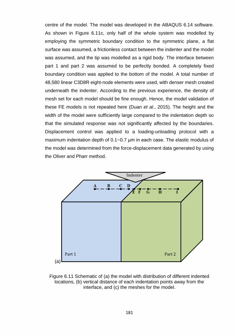
181
centre of the model. The model was developed in the ABAQUS 6.14 software.
As shown in Figure 6.11c, only half of the whole system was modelled by
employing the symmetric boundary condition to the symmetric plane, a flat
surface was assumed, a frictionless contact between the indenter and the model
was assumed, and the tip was modelled as a rigid body. The interface between
part 1 and part 2 was assumed to be perfectly bonded. A completely fixed
boundary condition was applied to the bottom of the model. A total number of
48,580 linear C3D8R eight-node elements were used, with denser mesh created
underneath the indenter. According to the previous experience, the density of
mesh set for each model should be fine enough. Hence, the model validation of
these FE models is not repeated here (Duan et al., 2015). The height and the
width of the model were sufficiently large compared to the indentation depth so
that the simulated response was not significantly affected by the boundaries.
Displacement control was applied to a loading-unloading protocol with a
maximum indentation depth of 0.1~0.7 μm in each case. The elastic modulus of
the model was determined from the force-displacement data generated by using
the Oliver and Pharr method.
(a)
Figure 6.11 Schematic of (a) the model with distribution of different indented locations, (b) vertical distance of each indentation points away from the
interface, and (c) the meshes for the model.
Part 1 Part 2
Indenter
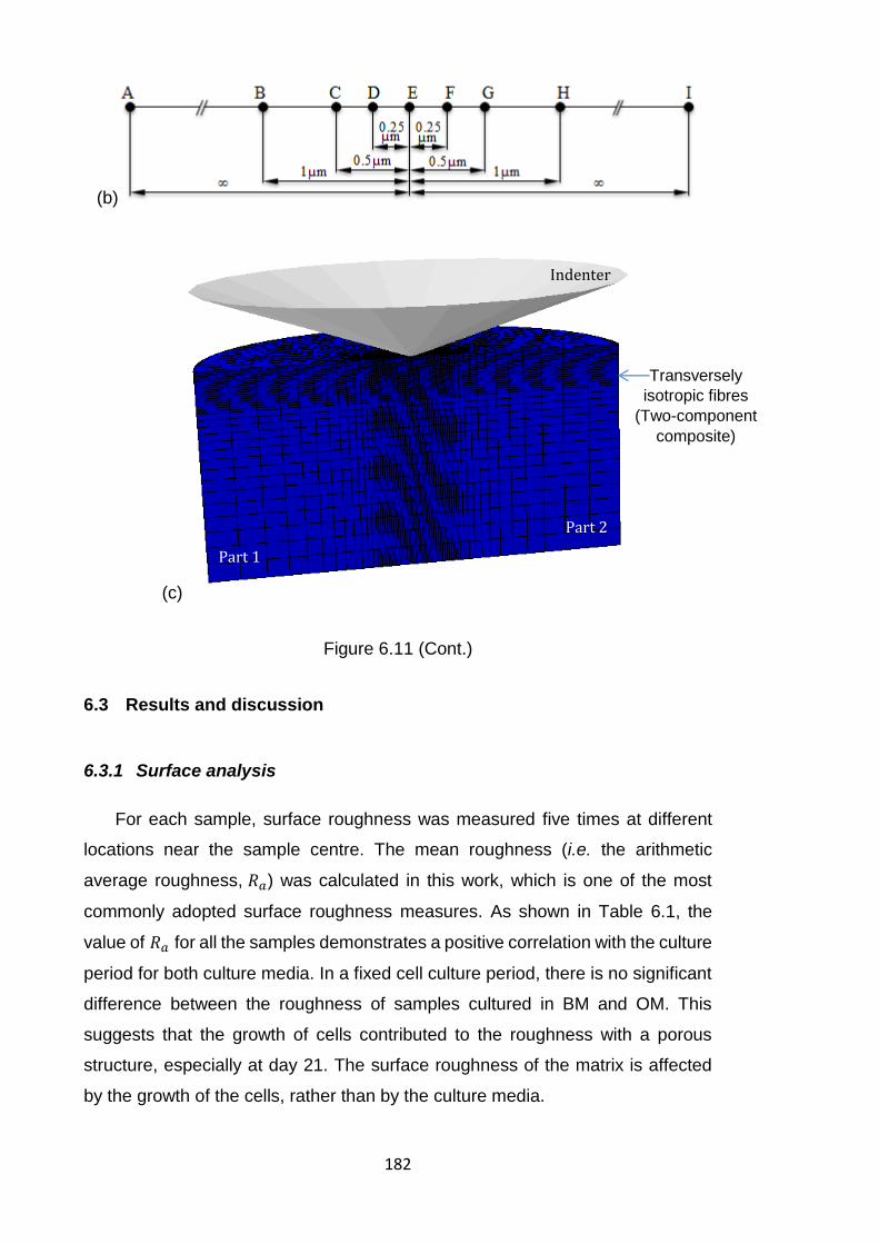
182
(b)
(c)
Figure 6.11 (Cont.)
6.3 Results and discussion
6.3.1 Surface analysis
For each sample, surface roughness was measured five times at different
locations near the sample centre. The mean roughness (i.e. the arithmetic
average roughness, 𝑅𝑎) was calculated in this work, which is one of the most
commonly adopted surface roughness measures. As shown in Table 6.1, the
value of 𝑅𝑎 for all the samples demonstrates a positive correlation with the culture
period for both culture media. In a fixed cell culture period, there is no significant
difference between the roughness of samples cultured in BM and OM. This
suggests that the growth of cells contributed to the roughness with a porous
structure, especially at day 21. The surface roughness of the matrix is affected
by the growth of the cells, rather than by the culture media.
Part 1
Part 2
Indenter
Transversely
isotropic fibres
(Two-component
composite)
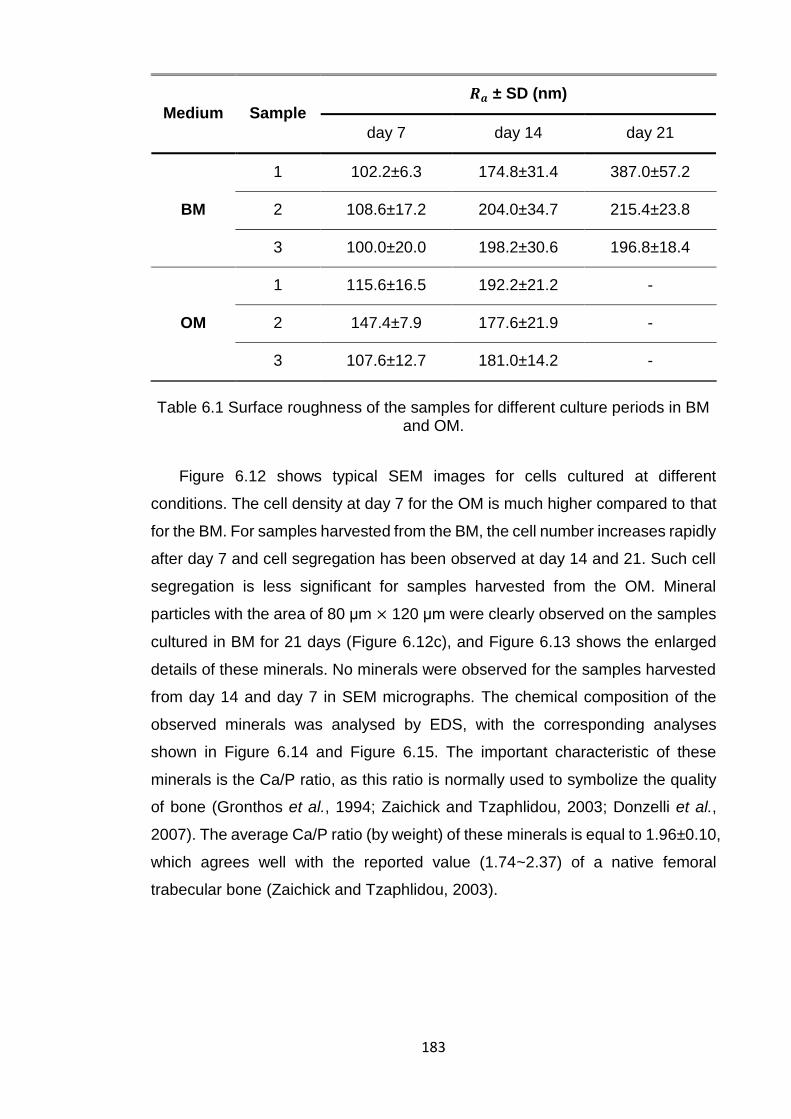
183
Medium Sample
𝑹𝒂 ± SD (nm)
day 7 day 14 day 21
BM
1 102.2±6.3 174.8±31.4 387.0±57.2
2 108.6±17.2 204.0±34.7 215.4±23.8
3 100.0±20.0 198.2±30.6 196.8±18.4
OM
1 115.6±16.5 192.2±21.2 -
2 147.4±7.9 177.6±21.9 -
3 107.6±12.7 181.0±14.2 -
Table 6.1 Surface roughness of the samples for different culture periods in BM and OM.
Figure 6.12 shows typical SEM images for cells cultured at different
conditions. The cell density at day 7 for the OM is much higher compared to that
for the BM. For samples harvested from the BM, the cell number increases rapidly
after day 7 and cell segregation has been observed at day 14 and 21. Such cell
segregation is less significant for samples harvested from the OM. Mineral
particles with the area of 80 μm × 120 μm were clearly observed on the samples
cultured in BM for 21 days (Figure 6.12c), and Figure 6.13 shows the enlarged
details of these minerals. No minerals were observed for the samples harvested
from day 14 and day 7 in SEM micrographs. The chemical composition of the
observed minerals was analysed by EDS, with the corresponding analyses
shown in Figure 6.14 and Figure 6.15. The important characteristic of these
minerals is the Ca/P ratio, as this ratio is normally used to symbolize the quality
of bone (Gronthos et al., 1994; Zaichick and Tzaphlidou, 2003; Donzelli et al.,
2007). The average Ca/P ratio (by weight) of these minerals is equal to 1.96±0.10,
which agrees well with the reported value (1.74~2.37) of a native femoral
trabecular bone (Zaichick and Tzaphlidou, 2003).
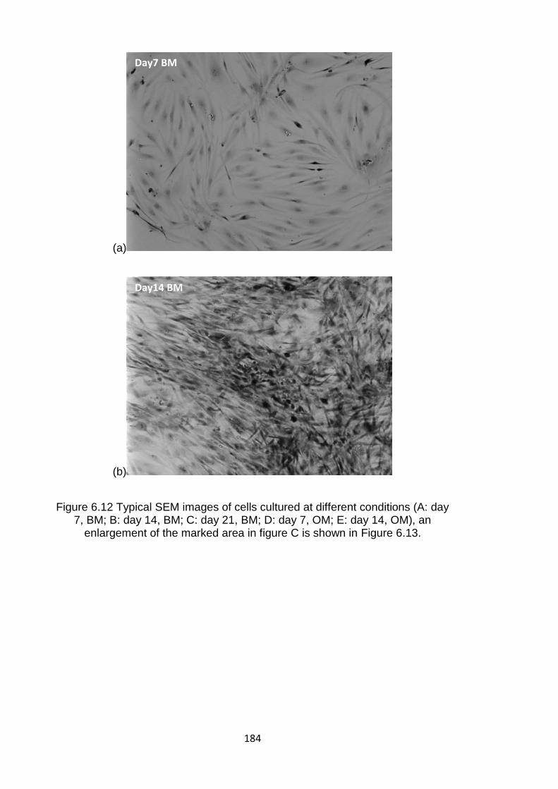
184
(a)
(b)
Figure 6.12 Typical SEM images of cells cultured at different conditions (A: day 7, BM; B: day 14, BM; C: day 21, BM; D: day 7, OM; E: day 14, OM), an
enlargement of the marked area in figure C is shown in Figure 6.13.
Day7 BM
Day14 BM
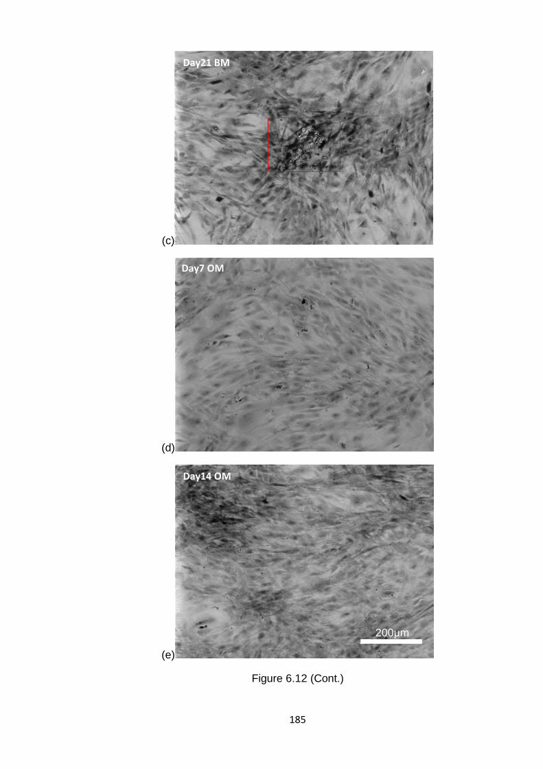
185
(c)
(d)
(e)
Figure 6.12 (Cont.)
Day21 BM
Day7 OM
Day14 OM
200μm
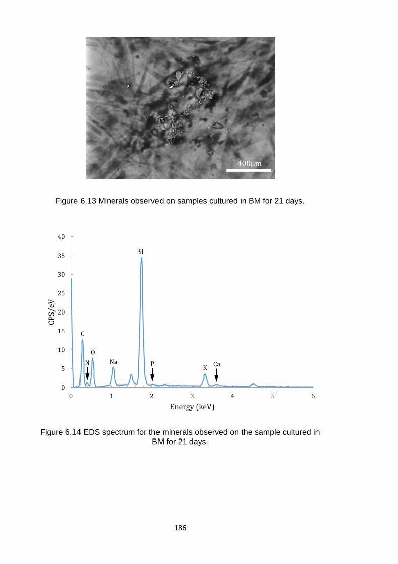
186
Figure 6.13 Minerals observed on samples cultured in BM for 21 days.
Figure 6.14 EDS spectrum for the minerals observed on the sample cultured in BM for 21 days.
0
5
10
15
20
25
30
35
40
0 1 2 3 4 5 6
CP
S/e
V
Energy (keV)
Ca
Si
PK
O
N
C
Na
400μm
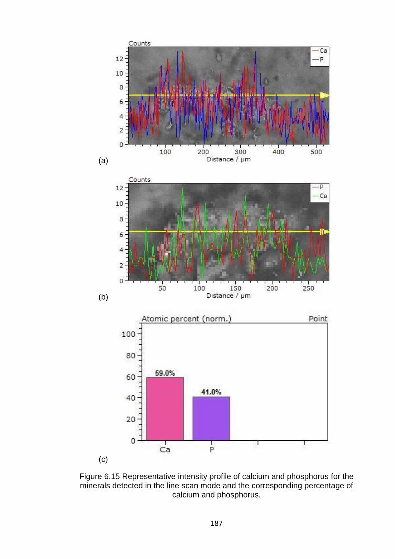
187
(a)
(b)
(c)
Figure 6.15 Representative intensity profile of calcium and phosphorus for the minerals detected in the line scan mode and the corresponding percentage of
calcium and phosphorus.
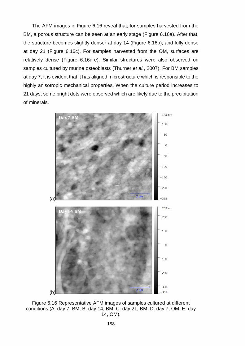
188
The AFM images in Figure 6.16 reveal that, for samples harvested from the
BM, a porous structure can be seen at an early stage (Figure 6.16a). After that,
the structure becomes slightly denser at day 14 (Figure 6.16b), and fully dense
at day 21 (Figure 6.16c). For samples harvested from the OM, surfaces are
relatively dense (Figure 6.16d-e). Similar structures were also observed on
samples cultured by murine osteoblasts (Thurner et al., 2007). For BM samples
at day 7, it is evident that it has aligned microstructure which is responsible to the
highly anisotropic mechanical properties. When the culture period increases to
21 days, some bright dots were observed which are likely due to the precipitation
of minerals.
(a)
(b)
Figure 6.16 Representative AFM images of samples cultured at different conditions (A: day 7, BM; B: day 14, BM; C: day 21, BM; D: day 7, OM; E: day
14, OM).
Day14 BM
Day7 BM
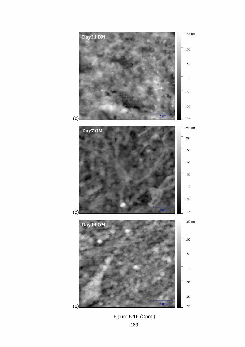
189
(c)
(d)
(e)
Figure 6.16 (Cont.)
Day21 BM
Day7 OM
Day14 OM
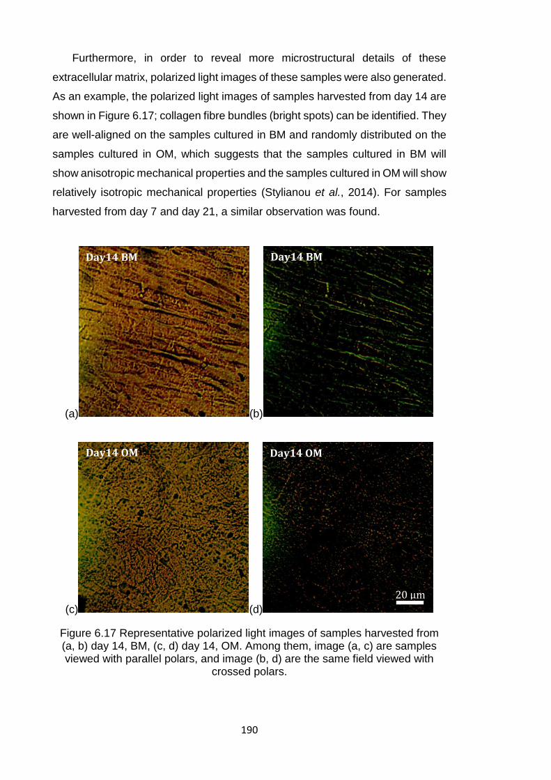
190
Furthermore, in order to reveal more microstructural details of these
extracellular matrix, polarized light images of these samples were also generated.
As an example, the polarized light images of samples harvested from day 14 are
shown in Figure 6.17; collagen fibre bundles (bright spots) can be identified. They
are well-aligned on the samples cultured in BM and randomly distributed on the
samples cultured in OM, which suggests that the samples cultured in BM will
show anisotropic mechanical properties and the samples cultured in OM will show
relatively isotropic mechanical properties (Stylianou et al., 2014). For samples
harvested from day 7 and day 21, a similar observation was found.
(a) (b)
(c) (d)
Figure 6.17 Representative polarized light images of samples harvested from (a, b) day 14, BM, (c, d) day 14, OM. Among them, image (a, c) are samples viewed with parallel polars, and image (b, d) are the same field viewed with
crossed polars.
20 μm
Day14 BM Day14 BM
Day14 OM Day14 OM
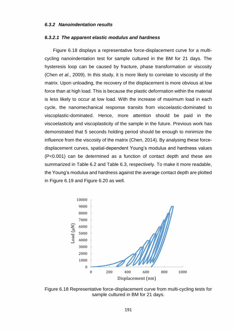
191
6.3.2 Nanoindentation results
6.3.2.1 The apparent elastic modulus and hardness
Figure 6.18 displays a representative force-displacement curve for a multi-
cycling nanoindentation test for sample cultured in the BM for 21 days. The
hysteresis loop can be caused by fracture, phase transformation or viscosity
(Chen et al., 2009). In this study, it is more likely to correlate to viscosity of the
matrix. Upon unloading, the recovery of the displacement is more obvious at low
force than at high load. This is because the plastic deformation within the material
is less likely to occur at low load. With the increase of maximum load in each
cycle, the nanomechanical response transits from viscoelastic-dominated to
viscoplastic-dominated. Hence, more attention should be paid in the
viscoelasticity and viscoplasticity of the sample in the future. Previous work has
demonstrated that 5 seconds holding period should be enough to minimize the
influence from the viscosity of the matrix (Chen, 2014). By analysing these force-
displacement curves, spatial-dependent Young’s modulus and hardness values
(P<0.001) can be determined as a function of contact depth and these are
summarized in Table 6.2 and Table 6.3, respectively. To make it more readable,
the Young’s modulus and hardness against the average contact depth are plotted
in Figure 6.19 and Figure 6.20 as well.
Figure 6.18 Representative force-displacement curve from multi-cycling tests for
sample cultured in BM for 21 days.
0
1000
2000
3000
4000
5000
6000
7000
8000
9000
10000
0 200 400 600 800 1000
Lo
ad (
µN
)
Displacement (nm)
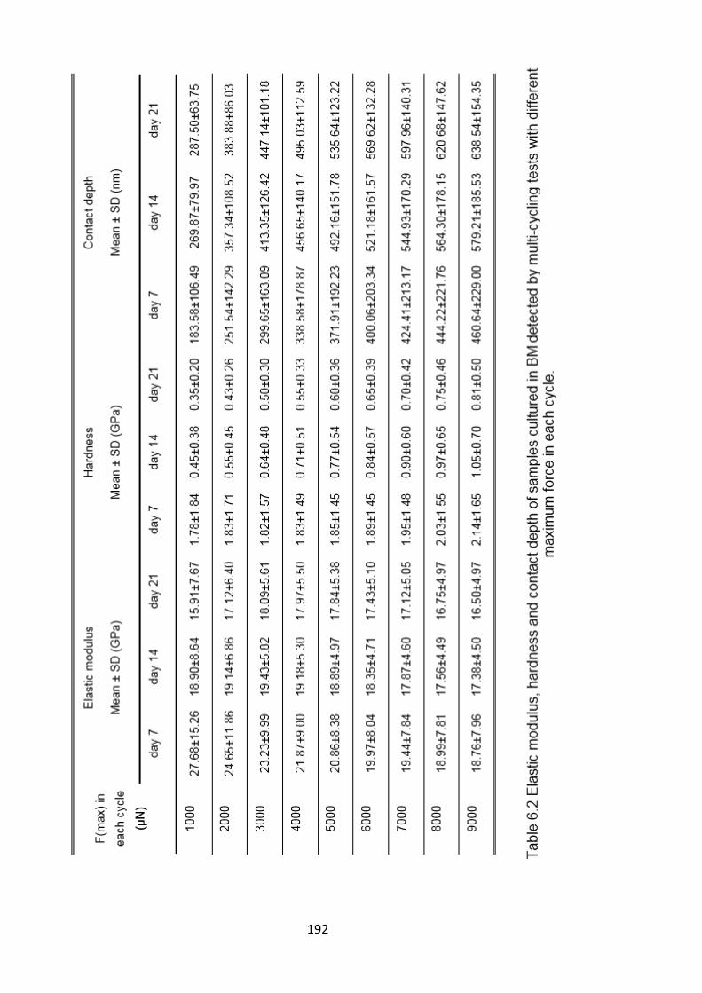
192
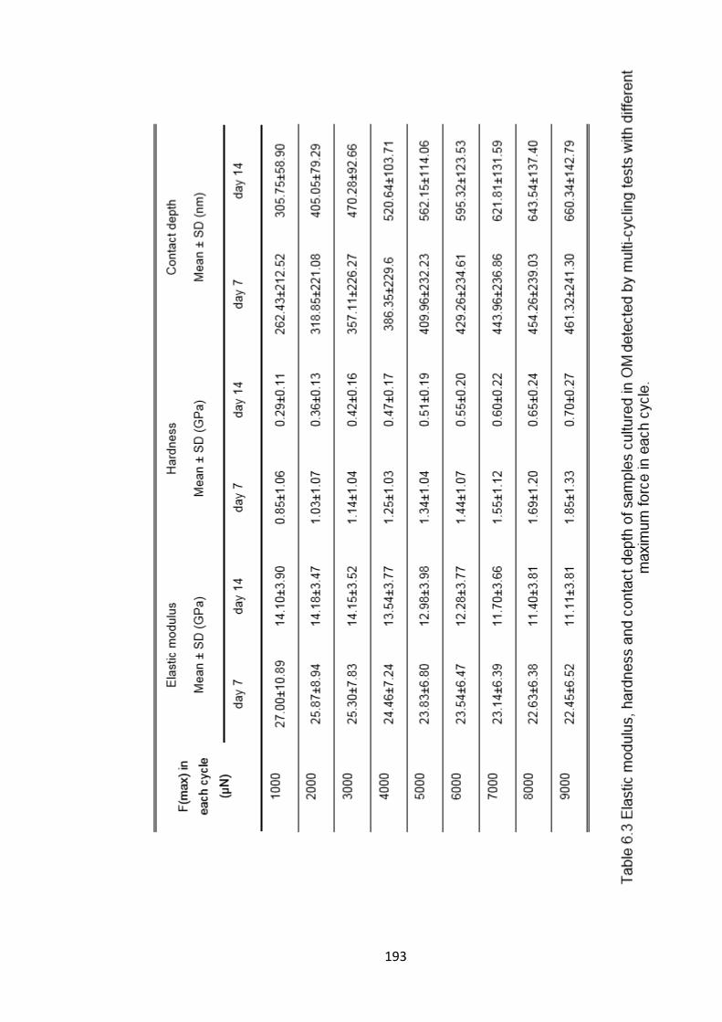
193
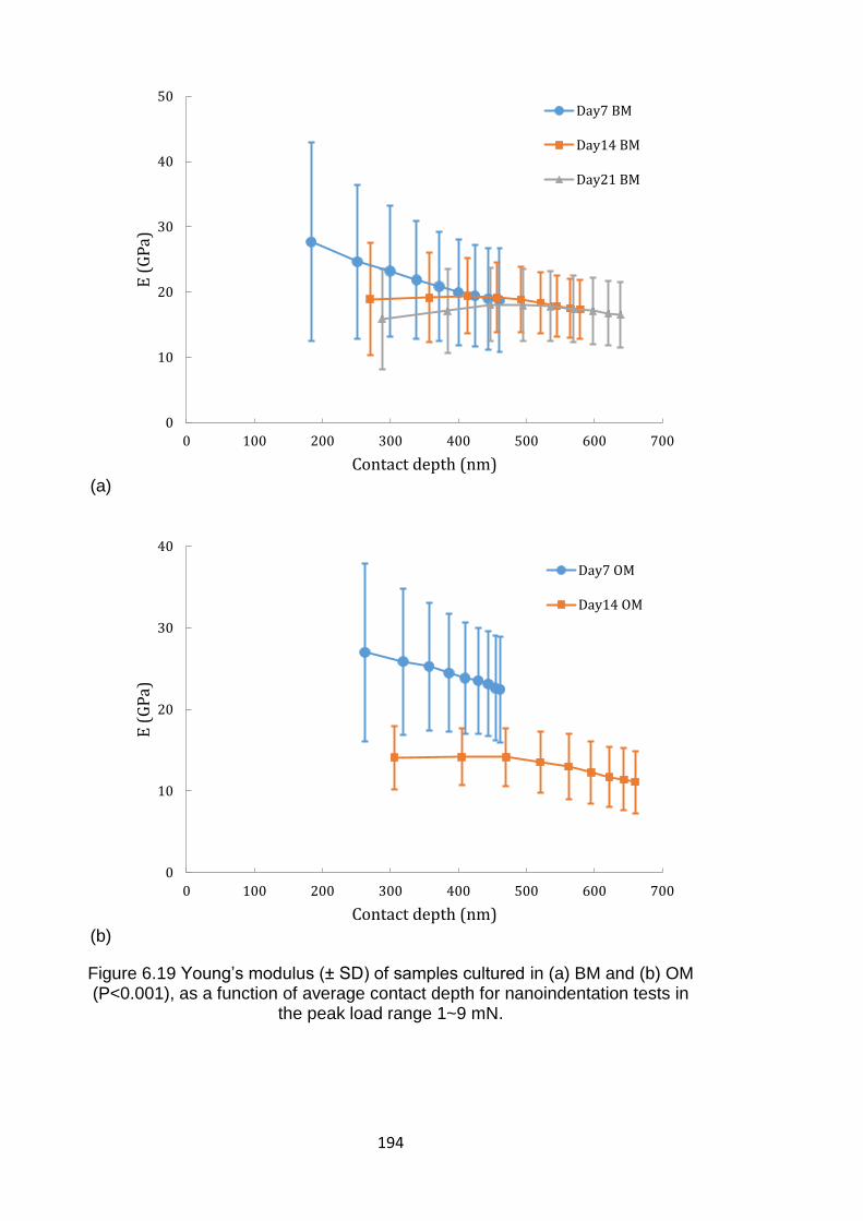
194
(a)
(b)
Figure 6.19 Young’s modulus (± SD) of samples cultured in (a) BM and (b) OM (P<0.001), as a function of average contact depth for nanoindentation tests in
the peak load range 1~9 mN.
0
10
20
30
40
50
0 100 200 300 400 500 600 700
E (
GP
a)
Contact depth (nm)
Day7 BM
Day14 BM
Day21 BM
0
10
20
30
40
0 100 200 300 400 500 600 700
E (
GP
a)
Contact depth (nm)
Day7 OM
Day14 OM
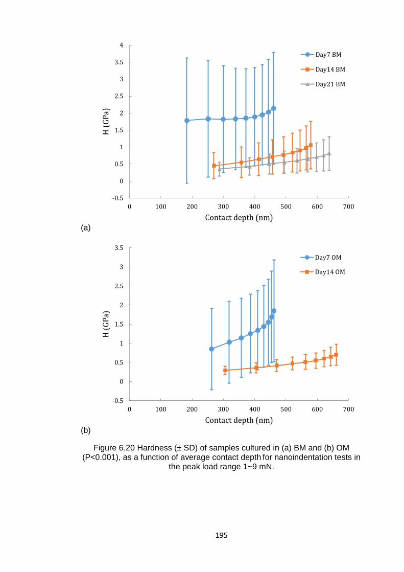
195
(a)
(b)
Figure 6.20 Hardness (± SD) of samples cultured in (a) BM and (b) OM (P<0.001), as a function of average contact depth for nanoindentation tests in
the peak load range 1~9 mN.
-0.5
0
0.5
1
1.5
2
2.5
3
3.5
4
0 100 200 300 400 500 600 700
H (
GP
a)
Contact depth (nm)
Day7 BM
Day14 BM
Day21 BM
-0.5
0
0.5
1
1.5
2
2.5
3
3.5
0 100 200 300 400 500 600 700
H (
GP
a)
Contact depth (nm)
Day7 OM
Day14 OM
196
In the given load range (1~9 mN), the average Young’s modulus of samples
cultured in the BM changes in the range of 18.8~27.7 GPa at day 7. These values
decrease to 17.4~18.9 GPa at day 14 and 15.9~18.1 GPa at day 21. In the same
load range, the average Young’s modulus of samples cultured in the OM is in the
range of 22.5~27.0 GPa at day 7. These values decrease to 11.1~14.2 GPa at
day 14. In general, for all the samples, the measured Young’s moduli decrease
with the contact depth across the entire load range. Similar to the Young’s moduli,
the measured hardness values also decrease with the cell culture period.
For elastic modulus, it has been reported that the modulus of collagen in
nanoindentation ranges from 1.71 GPa to 3.31 GPa (Chaudhry et al., 2009), and
modulus of human vertebral trabeculae is from 11.3 GPa to 15.8 GPa (Wolfram
et al., 2010). Thus, the elastic modulus of the matrix is similar to native bone after
7 to 14 days, and the relatively high Young’s modulus of mineralized matrix in
contrast to the collagen fibres indicates that the matrix is highly mineralized
(Wenger et al., 2007; Chaudhry et al., 2009). The minerals are likely to be
nanocrystals, as a very limited amount of crystals were observed at the micro
scale or above by SEM. This may suggest the matrix has a highly
inhomogeneous structure near the surface and the effect from the substrate is
negligible. When the contact depth is below 450 nm, there is strong depth
dependent behaviour for day 7 samples (both BM and OM). It has been reported
in the previous AFM results (Figure 6.16) that the sample structure changes from
porous to dense with the increasing culture period. Thus, it indicates the elastic
modulus will be highly affected by the porous surface structure at shallow contact
depth, especially at day 7. With an increase of contact depth, the porous structure
underneath the indenter is compressed, pores are closed up and then the
corresponding elastic modulus becomes more stable.
It is also interesting to investigate the distribution of the measured apparent
elastic modulus. It was reported elsewhere that the engineered bone can have a
wide distribution of nanoindentation modulus (Pelled et al., 2007a; Chen et al.,
2010b). For example, Figure 6.21 shows the distribution of the nanoindentation
modulus for an engineered bone produced by the C3H10T1/2 MSC line grown in
vivo for 28 days (Pelled et al., 2007a). For comparison, Figure 6.22 displays
histograms of the elastic modulus for mineralized matrix samples at the same
peak loads (i.e. 1000µN and 7000 µN). Similar to the data shown in Figure 6.21,
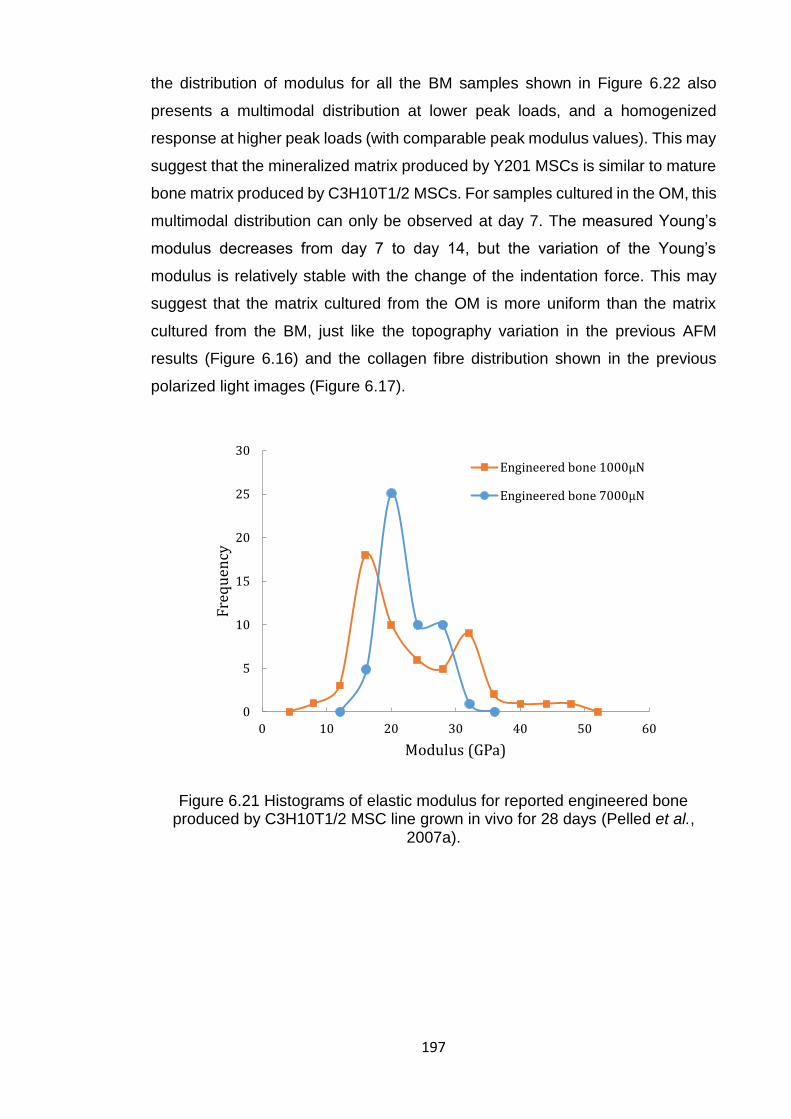
197
the distribution of modulus for all the BM samples shown in Figure 6.22 also
presents a multimodal distribution at lower peak loads, and a homogenized
response at higher peak loads (with comparable peak modulus values). This may
suggest that the mineralized matrix produced by Y201 MSCs is similar to mature
bone matrix produced by C3H10T1/2 MSCs. For samples cultured in the OM, this
multimodal distribution can only be observed at day 7. The measured Young’s
modulus decreases from day 7 to day 14, but the variation of the Young’s
modulus is relatively stable with the change of the indentation force. This may
suggest that the matrix cultured from the OM is more uniform than the matrix
cultured from the BM, just like the topography variation in the previous AFM
results (Figure 6.16) and the collagen fibre distribution shown in the previous
polarized light images (Figure 6.17).
Figure 6.21 Histograms of elastic modulus for reported engineered bone produced by C3H10T1/2 MSC line grown in vivo for 28 days (Pelled et al.,
2007a).
0
5
10
15
20
25
30
0 10 20 30 40 50 60
Fre
qu
ency
Modulus (GPa)
Engineered bone 1000µN
Engineered bone 7000µN
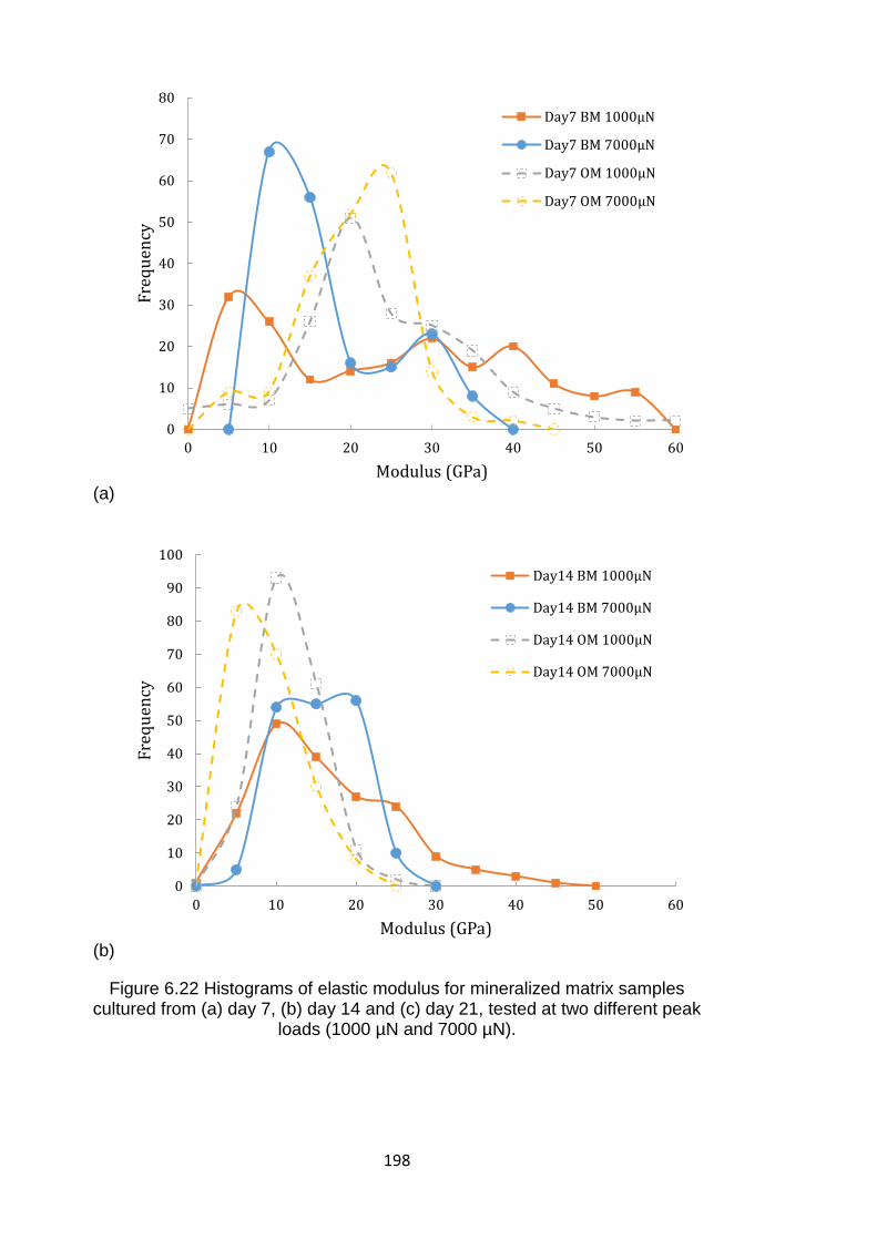
198
(a)
(b)
Figure 6.22 Histograms of elastic modulus for mineralized matrix samples cultured from (a) day 7, (b) day 14 and (c) day 21, tested at two different peak
loads (1000 µN and 7000 µN).
0
10
20
30
40
50
60
70
80
0 10 20 30 40 50 60
Fre
qu
ency
Modulus (GPa)
Day7 BM 1000µN
Day7 BM 7000µN
Day7 OM 1000µN
Day7 OM 7000µN
0
10
20
30
40
50
60
70
80
90
100
0 10 20 30 40 50 60
Fre
qu
ency
Modulus (GPa)
Day14 BM 1000µN
Day14 BM 7000µN
Day14 OM 1000µN
Day14 OM 7000µN
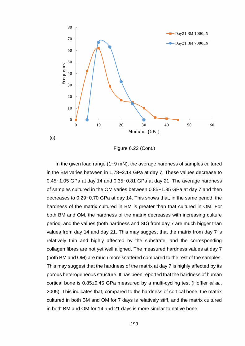
199
(c)
Figure 6.22 (Cont.)
In the given load range (1~9 mN), the average hardness of samples cultured
in the BM varies between in 1.78~2.14 GPa at day 7. These values decrease to
0.45~1.05 GPa at day 14 and 0.35~0.81 GPa at day 21. The average hardness
of samples cultured in the OM varies between 0.85~1.85 GPa at day 7 and then
decreases to 0.29~0.70 GPa at day 14. This shows that, in the same period, the
hardness of the matrix cultured in BM is greater than that cultured in OM. For
both BM and OM, the hardness of the matrix decreases with increasing culture
period, and the values (both hardness and SD) from day 7 are much bigger than
values from day 14 and day 21. This may suggest that the matrix from day 7 is
relatively thin and highly affected by the substrate, and the corresponding
collagen fibres are not yet well aligned. The measured hardness values at day 7
(both BM and OM) are much more scattered compared to the rest of the samples.
This may suggest that the hardness of the matrix at day 7 is highly affected by its
porous heterogeneous structure. It has been reported that the hardness of human
cortical bone is 0.85±0.45 GPa measured by a multi-cycling test (Hoffler et al.,
2005). This indicates that, compared to the hardness of cortical bone, the matrix
cultured in both BM and OM for 7 days is relatively stiff, and the matrix cultured
in both BM and OM for 14 and 21 days is more similar to native bone.
0
10
20
30
40
50
60
70
80
0 10 20 30 40 50 60
Fre
qu
ency
Modulus (GPa)
Day21 BM 1000µN
Day21 BM 7000µN
200
6.3.2.2 Data analysis by the Gaussian mixture model
The structure and composition of biological tissues are often complex, which
leads to a complicated mechanical response in a nanoindentation test (Gupta et
al., 2005; Gupta et al., 2006; Shahar et al., 2007; Zebaze et al., 2011). It has been
reported that the Young’s modulus of cortical bone is anisotropic (Dong and Guo,
2004; Wenger et al., 2007). For dehydrated human tibial cortical bone, the elastic
modulus of osteogenic lamellae measured by nanoindentation is 14~19 GPa in
the transverse direction, and 23~27 GPa in the longitudinal direction. The elastic
modulus of interstitial lamellae is 17~21 GPa in the transverse direction, and
25~29 GPa in the longitudinal direction (Fan et al., 2002). Thus, the mineralized
matrix may also be anisotropic like the bone tissue.
Figure 6.23 depicts the representative distributions of Young’s modulus for
the matrix harvested from BM and OM after 14 days, tested at a peak load of
1000 µN. Therefore, it is essential to do statistical analysis by the Gaussian
mixture model (Equations 6.5-6.7). In this model, it assumes that the measured
probability distribution of elastic modulus or hardness of each sample is a
weighted combination of a finite number of components. For each individual
component, its elastic modulus or hardness distribution follows Gaussian
distribution. The deconvolution is performed by fitting Equations 6.5-6.7 (the
weighted combination of a finite number of components) to the measured
probability distribution curve. A Matlab code was written to complete this curve
fitting procedure. Different number of components have been assumed (i.e. 1, 2,
3…), from the mathematical point of view, only when there are 2 components it
gives the best fitting results. It indicates that there are possibly two major
components in the mixture model. (There may exist more than 2 components, but
some of them may share the similar properties or have a negligible volume friction.
Hence, the number of components is mathematically chosen as 2.) The extracted
elastic modulus and hardness of each component are shown in Figure 6.24 and
Figure 6.25. For samples cultured in BM, the Young’s modulus of component 1
is approximately 10~17 GPa, which seems almost independent of cell culture
period. The Young’s modulus of component 2 is approximately 28~34 GPa at day
7. After day 7, this value decreases to 20~25 GPa. The hardness of component
1 is about 0.3~0.7 GPa, and is almost independent of culture period as well. The
hardness of component 2 is 2.52~2.84 GPa at day 7, this value decreases to
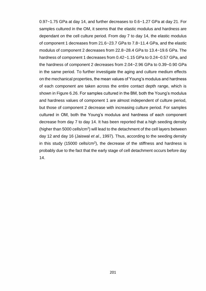
201
0.97~1.75 GPa at day 14, and further decreases to 0.6~1.27 GPa at day 21. For
samples cultured in the OM, it seems that the elastic modulus and hardness are
dependant on the cell culture period. From day 7 to day 14, the elastic modulus
of component 1 decreases from 21.6~23.7 GPa to 7.8~11.4 GPa, and the elastic
modulus of component 2 decreases from 22.8~28.4 GPa to 13.4~19.6 GPa. The
hardness of component 1 decreases from 0.42~1.15 GPa to 0.24~0.57 GPa, and
the hardness of component 2 decreases from 2.04~2.96 GPa to 0.39~0.90 GPa
in the same period. To further investigate the aging and culture medium effects
on the mechanical properties, the mean values of Young’s modulus and hardness
of each component are taken across the entire contact depth range, which is
shown in Figure 6.26. For samples cultured in the BM, both the Young’s modulus
and hardness values of component 1 are almost independent of culture period,
but those of component 2 decrease with increasing culture period. For samples
cultured in OM, both the Young’s modulus and hardness of each component
decrease from day 7 to day 14. It has been reported that a high seeding density
(higher than 5000 cells/cm2) will lead to the detachment of the cell layers between
day 12 and day 16 (Jaiswal et al., 1997). Thus, according to the seeding density
in this study (15000 cells/cm2), the decrease of the stiffness and hardness is
probably due to the fact that the early stage of cell detachment occurs before day
14.
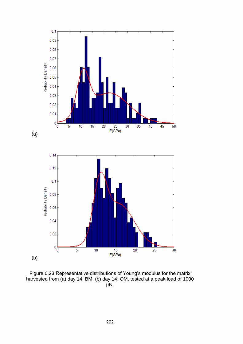
202
(a)
(b)
Figure 6.23 Representative distributions of Young’s modulus for the matrix harvested from (a) day 14, BM, (b) day 14, OM, tested at a peak load of 1000
µN.
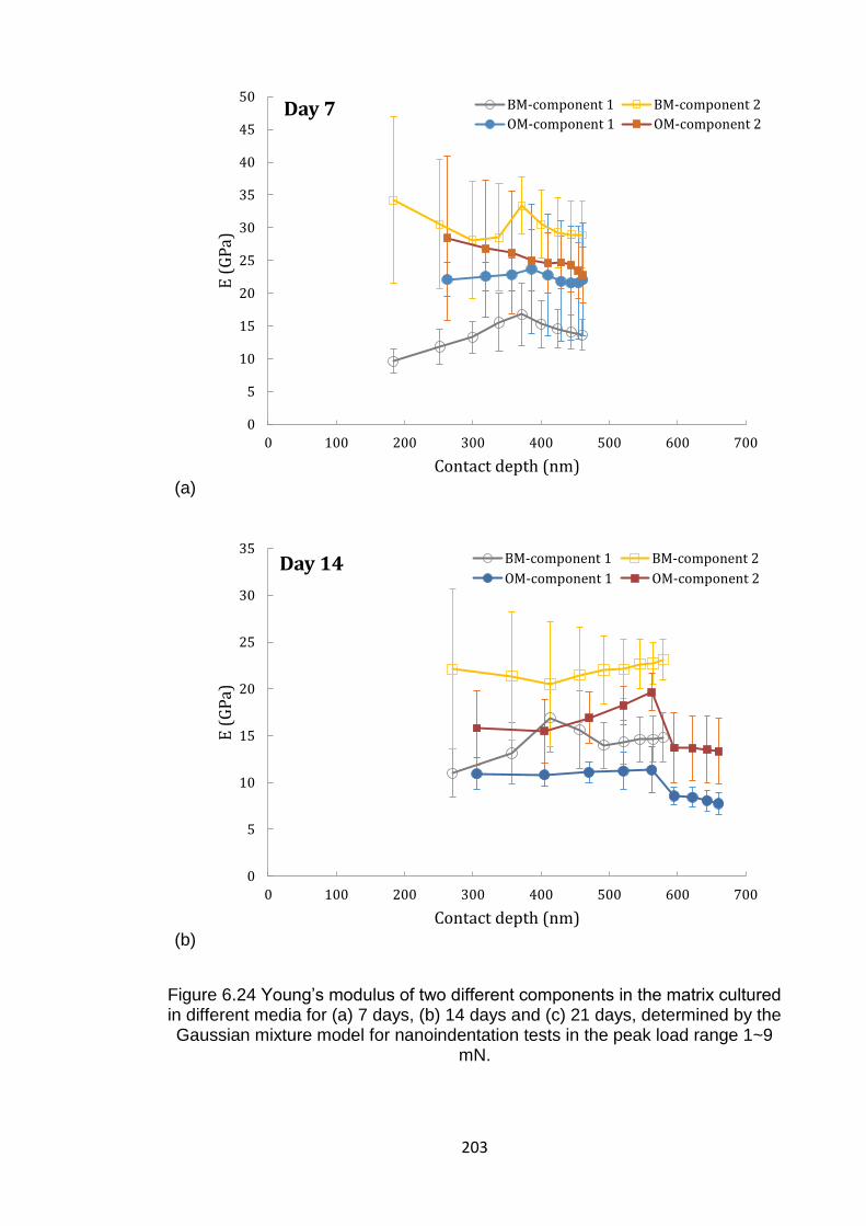
203
(a)
(b)
Figure 6.24 Young’s modulus of two different components in the matrix cultured in different media for (a) 7 days, (b) 14 days and (c) 21 days, determined by the Gaussian mixture model for nanoindentation tests in the peak load range 1~9
mN.
0
5
10
15
20
25
30
35
40
45
50
0 100 200 300 400 500 600 700
E (
GP
a)
Contact depth (nm)
Day 7 BM-component 1 BM-component 2
OM-component 1 OM-component 2
0
5
10
15
20
25
30
35
0 100 200 300 400 500 600 700
E (
GP
a)
Contact depth (nm)
Day 14 BM-component 1 BM-component 2
OM-component 1 OM-component 2
204
(c)
Figure 6.24 (Cont.)
(a)
Figure 6.25 Hardness of two different components in the matrix cultured in different media for (a) 7 days, (b) 14 days and (c) 21 days, determined by the Gaussian mixture model for nanoindentation tests in the peak load range 1~9
mN.
0
5
10
15
20
25
30
35
0 100 200 300 400 500 600 700
E (
GP
a)
Contact depth (nm)
Day 21 BM-component 1
BM-component 2
0
0.5
1
1.5
2
2.5
3
3.5
4
4.5
5
0 100 200 300 400 500 600 700
H (
GP
a)
Contact depth (nm)
Day 7BM-component 1 BM-component 2
OM-component 1 OM-component 2
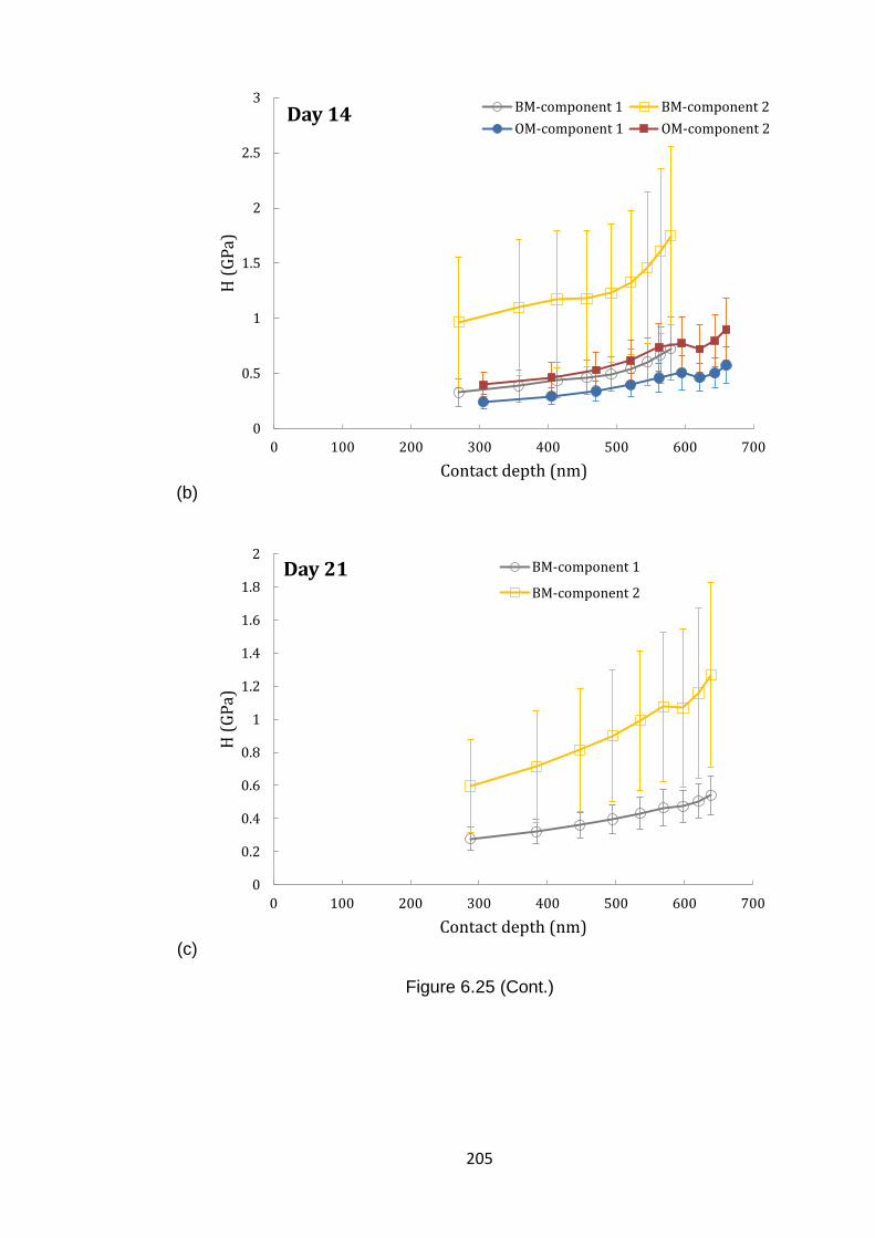
205
(b)
(c)
Figure 6.25 (Cont.)
0
0.5
1
1.5
2
2.5
3
0 100 200 300 400 500 600 700
H (
GP
a)
Contact depth (nm)
Day 14 BM-component 1 BM-component 2
OM-component 1 OM-component 2
0
0.2
0.4
0.6
0.8
1
1.2
1.4
1.6
1.8
2
0 100 200 300 400 500 600 700
H (
GP
a)
Contact depth (nm)
Day 21 BM-component 1
BM-component 2
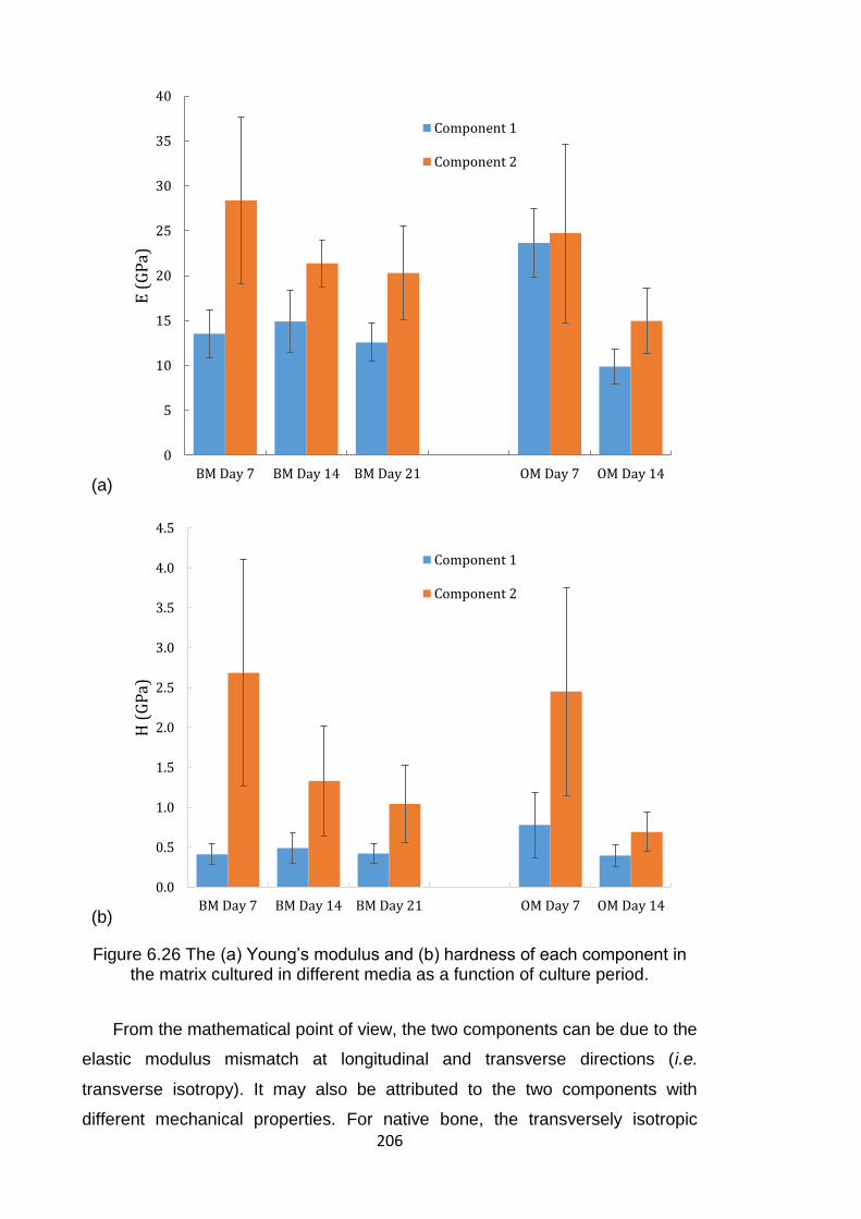
206
(a)
(b)
Figure 6.26 The (a) Young’s modulus and (b) hardness of each component in the matrix cultured in different media as a function of culture period.
From the mathematical point of view, the two components can be due to the
elastic modulus mismatch at longitudinal and transverse directions (i.e.
transverse isotropy). It may also be attributed to the two components with
different mechanical properties. For native bone, the transversely isotropic
0
5
10
15
20
25
30
35
40
BM Day 7 BM Day 14 BM Day 21 OM Day 7 OM Day 14
E (
GP
a)Component 1
Component 2
0.0
0.5
1.0
1.5
2.0
2.5
3.0
3.5
4.0
4.5
BM Day 7 BM Day 14 BM Day 21 OM Day 7 OM Day 14
H (
GP
a)
Component 1
Component 2
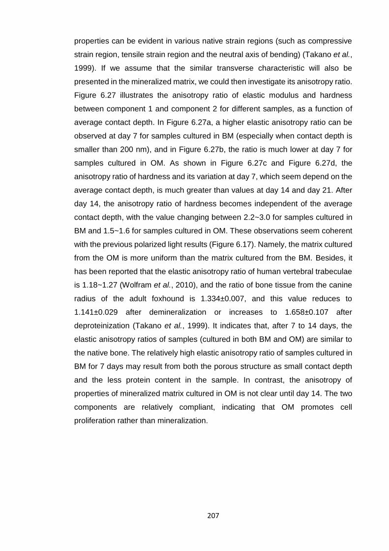
207
properties can be evident in various native strain regions (such as compressive
strain region, tensile strain region and the neutral axis of bending) (Takano et al.,
1999). If we assume that the similar transverse characteristic will also be
presented in the mineralized matrix, we could then investigate its anisotropy ratio.
Figure 6.27 illustrates the anisotropy ratio of elastic modulus and hardness
between component 1 and component 2 for different samples, as a function of
average contact depth. In Figure 6.27a, a higher elastic anisotropy ratio can be
observed at day 7 for samples cultured in BM (especially when contact depth is
smaller than 200 nm), and in Figure 6.27b, the ratio is much lower at day 7 for
samples cultured in OM. As shown in Figure 6.27c and Figure 6.27d, the
anisotropy ratio of hardness and its variation at day 7, which seem depend on the
average contact depth, is much greater than values at day 14 and day 21. After
day 14, the anisotropy ratio of hardness becomes independent of the average
contact depth, with the value changing between 2.2~3.0 for samples cultured in
BM and 1.5~1.6 for samples cultured in OM. These observations seem coherent
with the previous polarized light results (Figure 6.17). Namely, the matrix cultured
from the OM is more uniform than the matrix cultured from the BM. Besides, it
has been reported that the elastic anisotropy ratio of human vertebral trabeculae
is 1.18~1.27 (Wolfram et al., 2010), and the ratio of bone tissue from the canine
radius of the adult foxhound is 1.334±0.007, and this value reduces to
1.141±0.029 after demineralization or increases to 1.658±0.107 after
deproteinization (Takano et al., 1999). It indicates that, after 7 to 14 days, the
elastic anisotropy ratios of samples (cultured in both BM and OM) are similar to
the native bone. The relatively high elastic anisotropy ratio of samples cultured in
BM for 7 days may result from both the porous structure as small contact depth
and the less protein content in the sample. In contrast, the anisotropy of
properties of mineralized matrix cultured in OM is not clear until day 14. The two
components are relatively compliant, indicating that OM promotes cell
proliferation rather than mineralization.
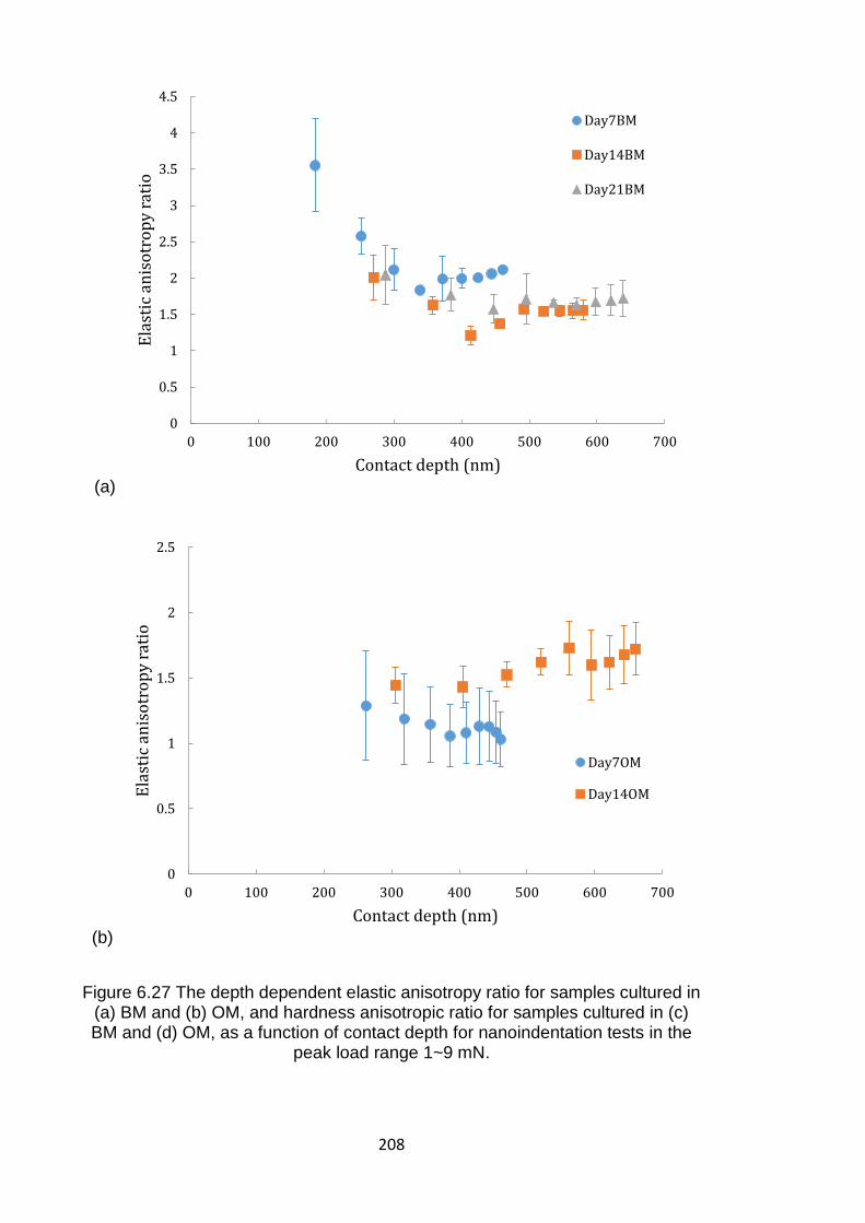
208
(a)
(b)
Figure 6.27 The depth dependent elastic anisotropy ratio for samples cultured in (a) BM and (b) OM, and hardness anisotropic ratio for samples cultured in (c) BM and (d) OM, as a function of contact depth for nanoindentation tests in the
peak load range 1~9 mN.
0
0.5
1
1.5
2
2.5
3
3.5
4
4.5
0 100 200 300 400 500 600 700
Ela
stic
an
iso
tro
py
rati
o
Contact depth (nm)
Day7BM
Day14BM
Day21BM
0
0.5
1
1.5
2
2.5
0 100 200 300 400 500 600 700
Ela
stic
an
iso
tro
py
rati
o
Contact depth (nm)
Day7OM
Day14OM
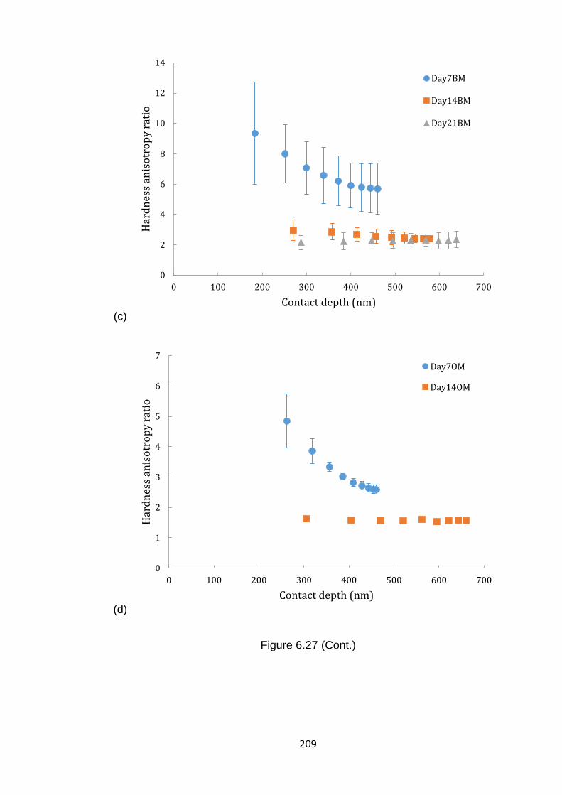
209
(c)
(d)
Figure 6.27 (Cont.)
0
2
4
6
8
10
12
14
0 100 200 300 400 500 600 700
Har
dn
ess
anis
otr
op
y ra
tio
Contact depth (nm)
Day7BM
Day14BM
Day21BM
0
1
2
3
4
5
6
7
0 100 200 300 400 500 600 700
Har
dn
ess
anis
otr
op
y ra
tio
Contact depth (nm)
Day7OM
Day14OM
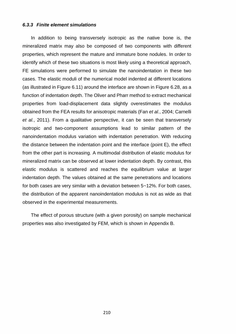
210
6.3.3 Finite element simulations
In addition to being transversely isotropic as the native bone is, the
mineralized matrix may also be composed of two components with different
properties, which represent the mature and immature bone nodules. In order to
identify which of these two situations is most likely using a theoretical approach,
FE simulations were performed to simulate the nanoindentation in these two
cases. The elastic moduli of the numerical model indented at different locations
(as illustrated in Figure 6.11) around the interface are shown in Figure 6.28, as a
function of indentation depth. The Oliver and Pharr method to extract mechanical
properties from load-displacement data slightly overestimates the modulus
obtained from the FEA results for anisotropic materials (Fan et al., 2004; Carnelli
et al., 2011). From a qualitative perspective, it can be seen that transversely
isotropic and two-component assumptions lead to similar pattern of the
nanoindentation modulus variation with indentation penetration. With reducing
the distance between the indentation point and the interface (point E), the effect
from the other part is increasing. A multimodal distribution of elastic modulus for
mineralized matrix can be observed at lower indentation depth. By contrast, this
elastic modulus is scattered and reaches the equilibrium value at larger
indentation depth. The values obtained at the same penetrations and locations
for both cases are very similar with a deviation between 5~12%. For both cases,
the distribution of the apparent nanoindentation modulus is not as wide as that
observed in the experimental measurements.
The effect of porous structure (with a given porosity) on sample mechanical
properties was also investigated by FEM, which is shown in Appendix B.
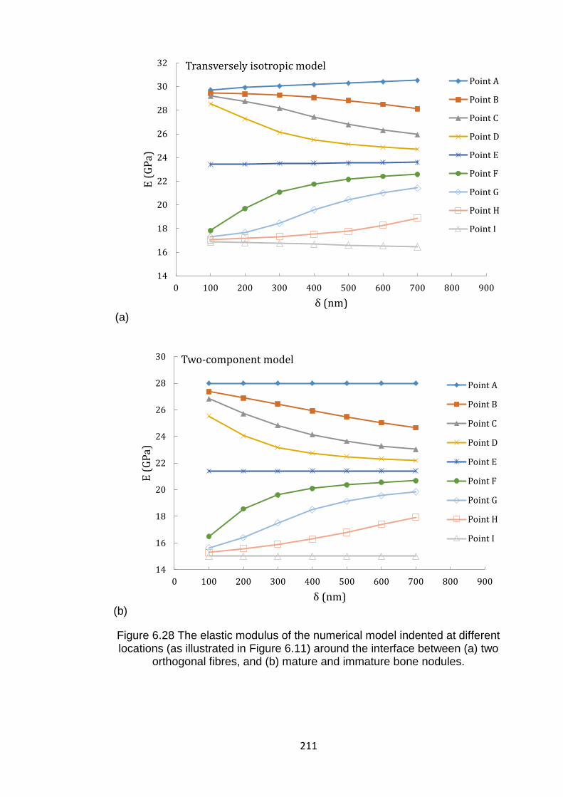
211
(a)
(b)
Figure 6.28 The elastic modulus of the numerical model indented at different locations (as illustrated in Figure 6.11) around the interface between (a) two
orthogonal fibres, and (b) mature and immature bone nodules.
14
16
18
20
22
24
26
28
30
32
0 100 200 300 400 500 600 700 800 900
E (
GP
a)
δ (nm)
Transversely isotropic model
Point A
Point B
Point C
Point D
Point E
Point F
Point G
Point H
Point I
14
16
18
20
22
24
26
28
30
0 100 200 300 400 500 600 700 800 900
E (
GP
a)
δ (nm)
Two-component model
Point A
Point B
Point C
Point D
Point E
Point F
Point G
Point H
Point I
212
6.4 Summary
In this study, the nanoindentation with multi-cycling protocol proved to be
effective to study how the nanomechanical properties of the matrix synthesized
by the cell would be affected by cell culture media and culture duration. Together
with surface analysis and FEA, the correlation between the sample
microstructure and nanomechanics has been studied.
Nanoindentation tests have revealed that the stiffness and hardness of bone
nodules (i.e. mineralized matrix) produced by Y201 cell line are comparable to
native bone, and present a multimodal distribution. As an explanation, these bone
nodules may present both mature (stiff phase) and immature (compliant phase)
state. However, there is no direct evidence to support this assumption. As another
explanation, similar to native bone, the multimodal distribution is more likely due
to the anisotropic behaviour of these bone nodules, which has been revealed in
the polarized light images. The ratio of elastic modulus and hardness at these
two orthogonal directions (or between stiffer and softer phases) can be up to 2
and 5, respectively. The bone nodules produced by cells in basal medium appear
to be stiffer and more anisotropic compared to that in osteogenic medium, as
confirmed in both nanoindentation tests and polarized light images. In the
polarized light images, an anisotropic collagen fibre distribution has been
observed on BM samples and a relatively uniform collagen fibre distribution has
been observed on their counterparts from OM. This anisotropic collagen fibre
distribution explains the multimodal distribution of the mechanical properties, as
confirmed in the FE simulations.
From the point of culture period, it has also been shown that the cell culture
duration does not affect the elastic modulus and hardness in the transverse
direction but it significantly affects the elastic modulus and hardness at
longitudinal direction after day 7. When cell culture period reaches 14 days, the
matrix becomes stabilized in the longitudinal direction and there is no further
change with the cell culture period. In addition, mineralized matrix has revealed
a more porous structure at day 7, compared to that at day 14 and 21, which
explains the wider span of the distribution of measured mechanical properties at
day 7. For both basal and osteogenic media, the bone nodules have exhibited
reverse aging behaviour compared to native bone despite the fact that their

213
microstructure becomes denser with the increase of cell culture period. This is
possibly due to the fact that cell proliferation outcompetes the mineralization
processes.


Chapter 7
Conclusions and Further Work
216
Chapter 7. Conclusions and Further Work
7.1 Conclusions
Firstly, some empirical equations have been modified and two new equations
have been proposed to describe the nanoindentation response of inclusion/matrix
composite materials. For an indentation test, many empirical or semi-analytical
models have been proposed to study how the elastic modulus of the coated
systems changes with the penetration. However, little work has been done for the
inclusion/matrix composite materials. In this work, those indentation-based
empirical or semi-analytical models have been examined. The analysis has
shown that those semi-analytical models need to be modified before they can be
extended to the inclusion/matrix systems, by considering the elastic mismatch
between the fibre and the matrix. In addition, two simpler models have been
proposed, which show good performance but with less fitting parameters
compared to other empirical models.
In practice, according to different applications, the reinforcement of
composite materials may have different geometries. Therefore, it is necessary to
investigate the effect of inclusion geometry on the nanomechanical behaviour of
composite materials, which has not been well studied. On the other hand, many
particle/matrix systems may also exhibit elastic-plastic behaviour. Some
empirical models have been developed to describe the spatial-dependent
composite modulus during nanoindentation tests for linear elastic particles
embedded in a linear elastic matrix. No such models have been developed for
elastic-plastic composites. Based on the original Clifford model, extended Clifford
models have been proposed in this study, which enable us to determine the
elastic modulus and the hardness of composites with large mismatch in elastic
modulus and hardness. These models have been successfully applied to various
composites regardless of particle shape, volume and material combination.
During nanoindentation tests of composite materials, the relative indentation
location will also affect their nanomechanical response. Analysis has shown that,
the empirical equations, which work well in the previous chapters, failed to
describe the composite elastic modulus of an inclusion/matrix system with various
217
𝑑/𝑟 ratios. Hence, as a future work, those existing models should be further
developed to specify the effects of indentation location and indenter geometry.
On the other hand, a linear equation and a polynomial equation have been
adopted to extract the elastic modulus of each individual component by
extrapolating the equation to zero displacement. It has revealed that the second
order polynomial equation can effectively extract the elastic modulus of the fibre
in the case of indenting the fibre. In the case of indenting the matrix, before the
indenter touches the fibre, a linear equation can effectively extract the elastic
modulus of the matrix.
Finally, in addition to the theoretical analyses, a nanomechanical case study
of a typical biocomposite materials (namely extracellular mineralized matrix) was
performed. For these complex composites, the existing analytical models may
not be directly applied. However, with the assistance of microscopy techniques,
a statistical model and FEA, the anisotropic behaviour of the mineralized matrix
has been revealed and the corresponding mechanical properties of each
individual component have been determined. Moreover, the effects of both cell
culture medium and culture duration on the nanomechanical properties and
microstructure of the mineralized matrix have also been successfully
demonstrated.
7.2 Further follow up
In the nanomechanical modelling part, some analytical models have been
proposed and successfully applied to the system with different composite
material combinations, and the system with different inclusion geometries.
However, these equations have not been expanded to the case of different
inclusion alignments and indentation locations. Thus, to further complete the
description of the nanomechanical response of the inclusion/matrix composite, a
more generalized equation should be developed in a future study, which
considers the change of the material properties, inclusion geometries, inclusion
alignments and indentation locations.
In the nanomechanical case study part, the viscosity of the sample has been
avoided by adding a holding period in each loading cycle. Hence, as a future work,

218
a comprehensive study of the visco-elastic-plastic behaviour of the sample
should be undertaken.
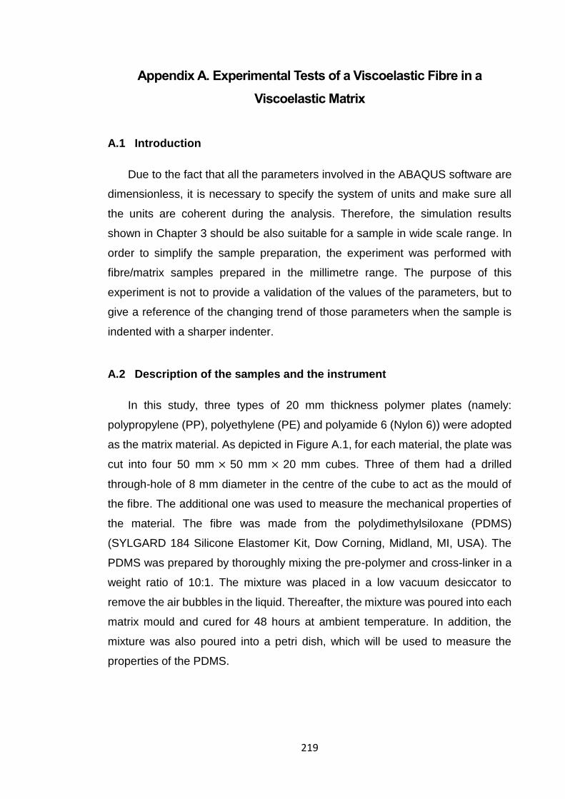
219
Appendix A. Experimental Tests of a Viscoelastic Fibre in a
Viscoelastic Matrix
A.1 Introduction
Due to the fact that all the parameters involved in the ABAQUS software are
dimensionless, it is necessary to specify the system of units and make sure all
the units are coherent during the analysis. Therefore, the simulation results
shown in Chapter 3 should be also suitable for a sample in wide scale range. In
order to simplify the sample preparation, the experiment was performed with
fibre/matrix samples prepared in the millimetre range. The purpose of this
experiment is not to provide a validation of the values of the parameters, but to
give a reference of the changing trend of those parameters when the sample is
indented with a sharper indenter.
A.2 Description of the samples and the instrument
In this study, three types of 20 mm thickness polymer plates (namely:
polypropylene (PP), polyethylene (PE) and polyamide 6 (Nylon 6)) were adopted
as the matrix material. As depicted in Figure A.1, for each material, the plate was
cut into four 50 mm × 50 mm × 20 mm cubes. Three of them had a drilled
through-hole of 8 mm diameter in the centre of the cube to act as the mould of
the fibre. The additional one was used to measure the mechanical properties of
the material. The fibre was made from the polydimethylsiloxane (PDMS)
(SYLGARD 184 Silicone Elastomer Kit, Dow Corning, Midland, MI, USA). The
PDMS was prepared by thoroughly mixing the pre-polymer and cross-linker in a
weight ratio of 10:1. The mixture was placed in a low vacuum desiccator to
remove the air bubbles in the liquid. Thereafter, the mixture was poured into each
matrix mould and cured for 48 hours at ambient temperature. In addition, the
mixture was also poured into a petri dish, which will be used to measure the
properties of the PDMS.
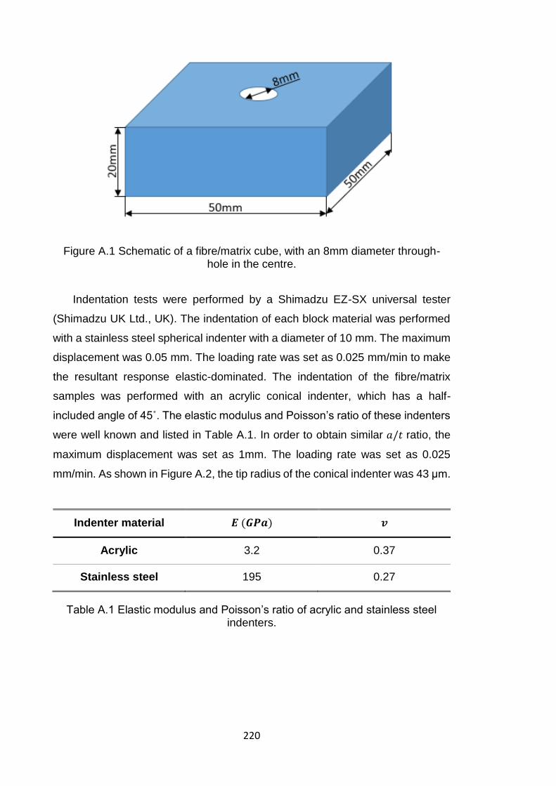
220
Figure A.1 Schematic of a fibre/matrix cube, with an 8mm diameter through-hole in the centre.
Indentation tests were performed by a Shimadzu EZ-SX universal tester
(Shimadzu UK Ltd., UK). The indentation of each block material was performed
with a stainless steel spherical indenter with a diameter of 10 mm. The maximum
displacement was 0.05 mm. The loading rate was set as 0.025 mm/min to make
the resultant response elastic-dominated. The indentation of the fibre/matrix
samples was performed with an acrylic conical indenter, which has a half-
included angle of 45˚. The elastic modulus and Poisson’s ratio of these indenters
were well known and listed in Table A.1. In order to obtain similar 𝑎/𝑡 ratio, the
maximum displacement was set as 1mm. The loading rate was set as 0.025
mm/min. As shown in Figure A.2, the tip radius of the conical indenter was 43 μm.
Indenter material 𝑬 (𝑮𝑷𝒂) 𝒗
Acrylic 3.2 0.37
Stainless steel 195 0.27
Table A.1 Elastic modulus and Poisson’s ratio of acrylic and stainless steel indenters.
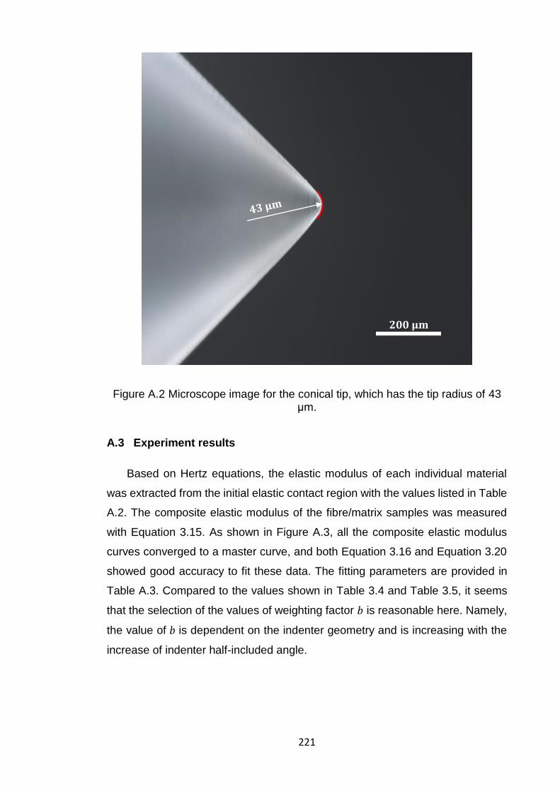
221
Figure A.2 Microscope image for the conical tip, which has the tip radius of 43 μm.
A.3 Experiment results
Based on Hertz equations, the elastic modulus of each individual material
was extracted from the initial elastic contact region with the values listed in Table
A.2. The composite elastic modulus of the fibre/matrix samples was measured
with Equation 3.15. As shown in Figure A.3, all the composite elastic modulus
curves converged to a master curve, and both Equation 3.16 and Equation 3.20
showed good accuracy to fit these data. The fitting parameters are provided in
Table A.3. Compared to the values shown in Table 3.4 and Table 3.5, it seems
that the selection of the values of weighting factor 𝑏 is reasonable here. Namely,
the value of 𝑏 is dependent on the indenter geometry and is increasing with the
increase of indenter half-included angle.
200 μm
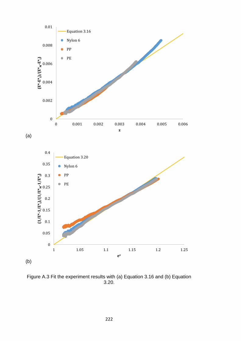
222
(a)
(b)
Figure A.3 Fit the experiment results with (a) Equation 3.16 and (b) Equation 3.20.
0
0.002
0.004
0.006
0.008
0.01
0 0.001 0.002 0.003 0.004 0.005 0.006
(E*-
E* I)
/(E
* M-E
* I)
z
Equation 3.16
Nylon 6
PP
PE
0
0.05
0.1
0.15
0.2
0.25
0.3
0.35
0.4
1 1.05 1.1 1.15 1.2 1.25
(1/
E*-
1/
E* I)
/(1
/E
* M-1
/E
* I)
ez
Equation 3.20
Nylon 6
PP
PE
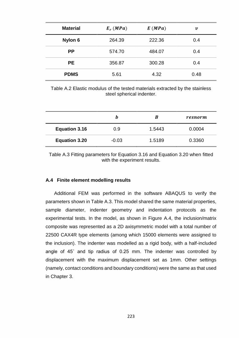
223
Material 𝑬𝒓 (𝑴𝑷𝒂) 𝑬 (𝑴𝑷𝒂) 𝒗
Nylon 6 264.39 222.36 0.4
PP 574.70 484.07 0.4
PE 356.87 300.28 0.4
PDMS 5.61 4.32 0.48
Table A.2 Elastic modulus of the tested materials extracted by the stainless steel spherical indenter.
𝒃 𝑩 𝒓𝒆𝒔𝒏𝒐𝒓𝒎
Equation 3.16 0.9 1.5443 0.0004
Equation 3.20 -0.03 1.5189 0.3360
Table A.3 Fitting parameters for Equation 3.16 and Equation 3.20 when fitted with the experiment results.
A.4 Finite element modelling results
Additional FEM was performed in the software ABAQUS to verify the
parameters shown in Table A.3. This model shared the same material properties,
sample diameter, indenter geometry and indentation protocols as the
experimental tests. In the model, as shown in Figure A.4, the inclusion/matrix
composite was represented as a 2D axisymmetric model with a total number of
22500 CAX4R type elements (among which 15000 elements were assigned to
the inclusion). The indenter was modelled as a rigid body, with a half-included
angle of 45˚ and tip radius of 0.25 mm. The indenter was controlled by
displacement with the maximum displacement set as 1mm. Other settings
(namely, contact conditions and boundary conditions) were the same as that used
in Chapter 3.
224
Figure A.4 Overview of the finite element mesh for the inclusion/matrix composite, and the enlarged details of elements underneath the tip.
The composite elastic modulus that was extracted from the simulated results
was also fitted by Equation 3.16 and Equation 3.20. As shown in Figure A.5, both
of these equations showed good accuracy to fit these data, which agrees well
with the previous observation. The fitting parameters are listed in Table A.4. The
value of 𝑏 was almost identical (namely, approximately 0.9 for Equation 3.16 and
-0.03 for Equation 3.20) with the values shown in Table A.3, which demonstrates
the accuracy of Equation 3.16 and Equation 3.20. However, the difference
between the value of fitting parameter 𝐵 shown in Table A.3 and Table A.4 is not
negligible (namely, approximately 1.52~1.54 for the experimental results and
approximately 0.79~0.81 for the FEM results). It could be argued that the
experimental indents may not ideally take place at the centre of the inclusion or
the displacement data may be affected by the initial penetration depth. In either
case, the composite elastic modulus will be overestimated and correspondingly
lead to a higher value of 𝐵.
Inclusion
Matrix
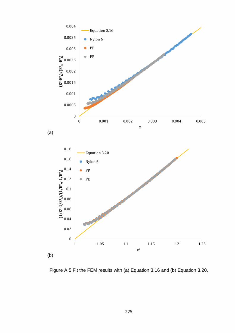
225
(a)
(b)
Figure A.5 Fit the FEM results with (a) Equation 3.16 and (b) Equation 3.20.
0
0.0005
0.001
0.0015
0.002
0.0025
0.003
0.0035
0.004
0 0.001 0.002 0.003 0.004 0.005
(E*-
E* I)
/(E
* M-E
* I)
z
Equation 3.16
Nylon 6
PP
PE
0
0.02
0.04
0.06
0.08
0.1
0.12
0.14
0.16
0.18
1 1.05 1.1 1.15 1.2 1.25
(1/
E*-
1/
E* I)
/(1
/E
* M-1
/E
* I)
ez
Equation 3.20
Nylon 6
PP
PE
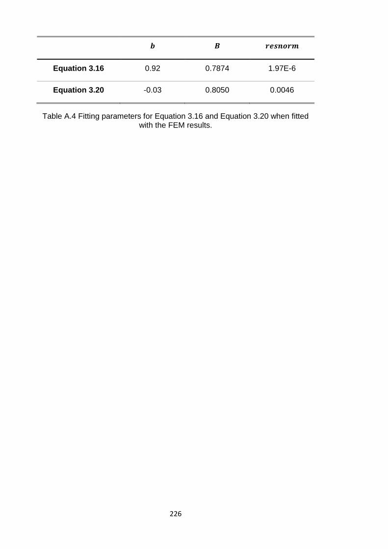
226
𝒃 𝑩 𝒓𝒆𝒔𝒏𝒐𝒓𝒎
Equation 3.16 0.92 0.7874 1.97E-6
Equation 3.20 -0.03 0.8050 0.0046
Table A.4 Fitting parameters for Equation 3.16 and Equation 3.20 when fitted with the FEM results.
227
Appendix B. Nanomechanical Modelling of a Porous Structure
B.1 Modelling of a porous structure
As the native bone and engineered bone appeared to be porous, additional
simulations were done by assuming a porous structure of the matrix, where the
elastic modulus was set as 28 GPa and the Poisson’s ratio was set as 0.3. For
simplicity, as shown in Figure B.1, the pores were assumed to be spherical and
underneath the point of indentation. The porosity was assumed to be 7.2% similar
to that of cortical bone (Martin and Boardman, 1993; Roschger et al., 2001; Wang
and Ni, 2003), with the distance between the centre of the hole and indented
surface varied between 4 µm and 6 µm. In each case, approximately 60,000
linear C3D8R eight-node elements were used, with denser mesh created
underneath the indenter. Similar to the previous model, a symmetric boundary
condition and a completely fixed boundary condition were applied to the
symmetric plane and the bottom, respectively. In addition, to achieve the 7.2%
porosity, symmetric boundary conditions were also applied to the sides of this
representative volume to simulate a periodically porous structure. The surface
was assumed to be flat, and has a frictionless contact with the rigid indenter. The
same lateral dimensions were adopted to minimize edge effects on the simulated
response. Displacement control with the same loading protocol was applied.
B.2 Finite element modelling results
As a porous structure was observed on mineralized matrix at early stage (i.e.
day 7) by AFM, additional simulations of porous model were done by FEM. The
corresponding simulation results are plotted in Figure B.2. It can be seen that the
indenter position relative to the pore would lead to a significantly large span of
peak values of nanoindentation modulus. This is particularly significant for the
low indentation penetration. Such an observation agrees with experimental
observations (see Figure 6.19 and Figure 6.20). For relatively short cell culture
period, the mineralized matrix is usually very porous which will result in large span
of peak values of nanoindentation modulus. With the increase of cell culture
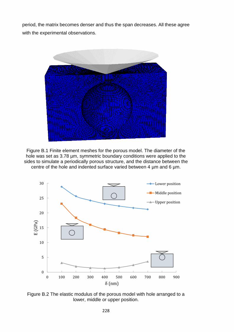
228
period, the matrix becomes denser and thus the span decreases. All these agree
with the experimental observations.
Figure B.1 Finite element meshes for the porous model. The diameter of the hole was set as 3.78 µm, symmetric boundary conditions were applied to the
sides to simulate a periodically porous structure, and the distance between the centre of the hole and indented surface varied between 4 µm and 6 µm.
Figure B.2 The elastic modulus of the porous model with hole arranged to a
lower, middle or upper position.
0
5
10
15
20
25
30
0 100 200 300 400 500 600 700 800 900
E (
GP
a)
δ (nm)
Lower position
Middle position
Upper position
229
References
Ahn, J.-H. and Kwon, D. (2001) 'Derivation of plastic stress–strain relationship
from ball indentations: examination of strain definition and pileup effect',
Journal of Materials Research, 16(11), pp. 3170-3178.
Akhter, M.P., Fan, Z. and Rho, J.Y. (2004) 'Bone intrinsic material properties in
three inbred mouse strains', Calcified Tissue International, 75(5), pp. 416-
420.
Akil, H., Omar, M.F., Mazuki, A.A.M., Safiee, S., Ishak, Z.A.M. and Bakar, A.A.
(2011) 'Kenaf fiber reinforced composites: A review', Materials & Design,
32(8), pp. 4107-4121.
Angker, L., Swain, M.V. and Kilpatrick, N. (2005) 'Characterising the micro-
mechanical behaviour of the carious dentine of primary teeth using nano-
indentation', Journal of Biomechanics, 38(7), pp. 1535-1542.
Aryaei, A. and Jayasuriya, A.C. (2013) 'Mechanical properties of human
amniotic fluid stem cells using nanoindentation', Journal of Biomechanics,
46(9), pp. 1524-1530.
Baino, F., Ferraris, M., Bretcanu, O., Verné, E. and Vitale-Brovarone, C. (2011)
'Optimization of composition, structure and mechanical strength of bioactive
3-D glass-ceramic scaffolds for bone substitution', Journal of Biomaterials
Applications, p. 0885328211429193.
Bakis, C.E., Bank, L.C., Brown, V., Cosenza, E., Davalos, J.F., Lesko, J.J.,
Machida, A., Rizkalla, S.H. and Triantafillou, T.C. (2002) 'Fiber-reinforced
polymer composites for construction—state-of-the-art review', Journal of
Composites for Construction, 6(2), pp. 73-87.
Balakrishnan, B. and Banerjee, R. (2011) 'Biopolymer-based hydrogels for
cartilage tissue engineering', Chemical reviews, 111(8), pp. 4453-4474.
230
Balooch, M., Wu-Magidi, I.C., Balazs, A., Lundkvist, A.S., Marshall, S.J.,
Marshall, G.W., Siekhaus, W.J. and Kinney, J.H. (1998) 'Viscoelastic
properties of demineralized human dentin measured in water with atomic
force microscope (AFM)-based indentation', Journal of Biomedical Materials
Research, 40(4), pp. 539-544.
Bandyopadhyay-Ghosh, S., Faria, P.E.P., Johnson, A., Felipucci, D.N.B.,
Reaney, I.M., Salata, L.A., Brook, I.M. and Hatton, P.V. (2010)
'Osteoconductivity of modified fluorcanasite glass-ceramics for bone tissue
augmentation and repair', Journal of Biomedical Materials Research Part A,
94(3), pp. 760-768.
Barbero, E.J. (2010) Introduction to composite materials design. CRC press.
Beake, B.D. and Smith, J.F. (2002) 'High-temperature nanoindentation testing
of fused silica and other materials', Philosophical Magazine A, 82(10), pp.
2179-2186.
Bei, H., George, E.P., Hay, J.L. and Pharr, G.M. (2005) 'Influence of indenter tip
geometry on elastic deformation during nanoindentation', Physical Review
Letters, 95(4), p. 045501.
Bell, T.J., Field, J.S. and Swain, M.V. (1992) 'Elastic-plastic characterization of
thin films with spherical indentation', Thin Solid Films, 220(1-2), pp. 289-
294.
Berasategui, E.G. and Page, T.F. (2003) 'The contact response of thin SiC-
coated silicon systems—Characterisation by nanoindentation', Surface and
Coatings Technology, 163, pp. 491-498.
Bhattacharya, A.K. and Nix, W.D. (1988) 'Finite element simulation of
indentation experiments', International Journal of Solids and Structures,
24(9), pp. 881-891.
Bhushan, B. and Li, X. (2003) 'Nanomechanical characterisation of solid
surfaces and thin films', International Materials Reviews, 48(3), pp. 125-164.
Bianco, P. and Robey, P.G. (2001) 'Stem cells in tissue engineering', Nature,
414(6859), pp. 118-121.
231
Bobji, M.S. and Biswas, S.K. (1999) 'Deconvolution of hardness from data
obtained from nanoindentation of rough surfaces', Journal of Materials
Research, 14(6), pp. 2259-2268.
Bobji, M.S., Fahim, M. and Biswas, S.K. (1996) 'Hardness estimated from the
indentation of a spherical body. Some implications for nanoindentation test
results', Tribology Letters, 2(4), pp. 381-391.
Bolshakov, A., Oliver, W.C. and Pharr, G.M. (1996) 'Influences of stress on the
measurement of mechanical properties using nanoindentation: Part II. Finite
element simulations', Journal of Materials Research, 11(03), pp. 760-768.
Bolshakov, A. and Pharr, G.M. (1998) 'Influences of pileup on the measurement
of mechanical properties by load and depth sensing indentation techniques',
Journal of Materials Research, 13(04), pp. 1049-1058.
Bruet, B.J.F., Qi, H.J., Boyce, M.C., Panas, R., Tai, K., Frick, L. and Ortiz, C.
(2005) 'Nanoscale morphology and indentation of individual nacre tablets
from the gastropod mollusc Trochus niloticus', Journal of Materials
Research, 20(09), pp. 2400-2419.
Bull, S.J. (2001) 'Modelling the hardness response of bulk materials, single and
multilayer coatings', Thin Solid Films, 398, pp. 291-298.
Bull, S.J. (2002) 'Extracting hardness and Young's modulus from load–
displacement curves', Zeitschrift für Metallkunde, 93(9), pp. 870-874.
Bull, S.J. (2003) 'On the origins and mechanisms of the indentation size effect',
Zeitschrift für Metallkunde, 94(7), pp. 787-792.
Bull, S.J., Page, T.F. and Yoffe, E.H. (1989) 'An explanation of the indentation
size effect in ceramics', Philosophical Magazine Letters, 59(6), pp. 281-288.
Bull, S.J., Sanderson, L., Moharrami, N. and Oila, A. (2012) 'Effect of
microstructure on hardness of submicrometre thin films and nanostructured
devices', Materials Science and Technology, 28(9-10), pp. 1177-1185.
232
Bulychev, S.I., Alekhin, V.P., Shorshorov, M.H., Ternovskii, A.P. and Shnyrev,
G.D. (1975) 'Determining Young's modulus from the indentor penetration
diagram', Ind. Lab., 41(9), pp. 1409-1412.
Burnett, P.J. and Rickerby, D.S. (1987a) 'The mechanical properties of wear-
resistant coatings: I: Modelling of hardness behaviour', Thin Solid Films,
148(1), pp. 41-50.
Burnett, P.J. and Rickerby, D.S. (1987b) 'The mechanical properties of wear-
resistant coatings: II: Experimental studies and interpretation of hardness',
Thin Solid Films, 148(1), pp. 51-65.
Burstein, A.H., Reilly, D.T. and Martens, M. (1976) 'Aging of bone tissue:
mechanical properties', J Bone Joint Surg Am, 58(1), pp. 82-86.
Calvert, P. (1992) 'Biomimetic ceramics and composites', Mrs Bulletin, 17(10),
pp. 37-40.
Cao, Y.-P. and Chen, K.-L. (2012) 'Theoretical and computational modelling of
instrumented indentation of viscoelastic composites', Mechanics of Time-
Dependent Materials, 16(1), pp. 1-18.
Cao, Y.-P., Ji, X.-Y. and Feng, X.-Q. (2010) 'Geometry independence of the
normalized relaxation functions of viscoelastic materials in indentation',
Philosophical Magazine, 90(12), pp. 1639-1655.
Cao, Y., Ma, D. and Raabe, D. (2009) 'The use of flat punch indentation to
determine the viscoelastic properties in the time and frequency domains of
a soft layer bonded to a rigid substrate', Acta Biomaterialia, 5(1), pp. 240-
248.
Carnelli, D., Lucchini, R., Ponzoni, M., Contro, R. and Vena, P. (2011)
'Nanoindentation testing and finite element simulations of cortical bone
allowing for anisotropic elastic and inelastic mechanical response', Journal
of Biomechanics, 44(10), pp. 1852-1858.
Chakraborty, H. and Bhowmik, N. (2014) 'Quasi‐static and dynamic
nanoindentation and scratch behavior of multifunctional titania/poly (methyl
methacrylate) composite', Polymer Composites, 35(7), pp. 1372-1376.
233
Chakravartula, A. and Komvopoulos, K. (2006) 'Viscoelastic properties of
polymer surfaces investigated by nanoscale dynamic mechanical analysis',
Applied Physics Letters, 88(13), p. 131901.
Chaudhry, B., Ashton, H., Muhamed, A., Yost, M., Bull, S. and Frankel, D.
(2009) 'Nanoscale viscoelastic properties of an aligned collagen scaffold',
Journal of Materials Science: Materials in Medicine, 20(1), pp. 257-263.
Chen, C.-C., Chueh, J.-Y., Tseng, H., Huang, H.-M. and Lee, S.-Y. (2003)
'Preparation and characterization of biodegradable PLA polymeric blends',
Biomaterials, 24(7), pp. 1167-1173.
Chen, J. (2012) 'Indentation-based methods to assess fracture toughness for
thin coatings', Journal of Physics D: Applied Physics, 45(20), p. 203001.
Chen, J. (2014) 'Nanobiomechanics of living cells: a review', Interface Focus,
4(2), p. 20130055.
Chen, J., Birch, M.A. and Bull, S.J. (2010a) 'Nanomechanical characterization of
tissue engineered bone grown on titanium alloy in vitro', Journal of Materials
Science: Materials in Medicine, 21(1), pp. 277-282.
Chen, J., Birch, M.A. and Bull, S.J. (2010b) 'Nanomechanical characterization of
tissue engineered bone grown on titanium alloy in vitro', J Mater Sci Mater
Med, 21(1), pp. 277-82.
Chen, J. and Bull, S.J. (2006a) 'Assessment of the toughness of thin coatings
using nanoindentation under displacement control', Thin Solid Films, 494(1),
pp. 1-7.
Chen, J. and Bull, S.J. (2006b) 'A critical examination of the relationship
between plastic deformation zone size and Young's modulus to hardness
ratio in indentation testing', Journal of Materials Research, 21(10), pp. 2617-
2627.
Chen, J. and Bull, S.J. (2006c) 'On the relationship between plastic zone radius
and maximum depth during nanoindentation', Surface and Coatings
Technology, 201(7), pp. 4289-4293.
234
Chen, J. and Bull, S.J. (2007) 'Indentation fracture and toughness assessment
for thin optical coatings on glass', Journal of Physics D: Applied Physics,
40(18), p. 5401.
Chen, J. and Bull, S.J. (2008) 'Multi-cycling nanoindentation study on thin
optical coatings on glass', Journal of Physics D: Applied Physics, 41(7), p.
074009.
Chen, J. and Bull, S.J. (2009a) 'Modelling the limits of coating toughness in
brittle coated systems', Thin Solid Films, 517(9), pp. 2945-2952.
Chen, J. and Bull, S.J. (2009b) 'On the factors affecting the critical indenter
penetration for measurement of coating hardness', Vacuum, 83(6), pp. 911-
920.
Chen, J. and Bull, S.J. (2009c) 'Relation between the ratio of elastic work to the
total work of indentation and the ratio of hardness to Young's modulus for a
perfect conical tip', Journal of Materials Research, 24(03), pp. 590-598.
Chen, J. and Bull, S.J. (2010) 'Approaches to investigate delamination and
interfacial toughness in coated systems: an overview', Journal of Physics D:
Applied Physics, 44(3), p. 034001.
Chen, J., Bull, S.J., Roy, S., Kapoor, A., Mukaibo, H., Nara, H., Momma, T.,
Osaka, T. and Shacham-Diamand, Y. (2009) 'Nanoindentation and
nanowear study of Sn and Ni–Sn coatings', Tribology international, 42(6),
pp. 779-791.
Chen, J. and Lu, G. (2012) 'Finite element modelling of nanoindentation based
methods for mechanical properties of cells', Journal of Biomechanics,
45(16), pp. 2810-2816.
Chen, J., Wright, K.E. and Birch, M.A. (2014) 'Nanoscale viscoelastic properties
and adhesion of polydimethylsiloxane for tissue engineering', Acta
Mechanica Sinica, 30(1), pp. 2-6.
Chen, P.-Y., Lin, A.Y.-M., McKittrick, J. and Meyers, M.A. (2008) 'Structure and
mechanical properties of crab exoskeletons', Acta Biomaterialia, 4(3), pp.
587-596.
235
Cheng, L., Xia, X., Yu, W., Scriven, L.E. and Gerberich, W.W. (2000) 'Flat‐
punch indentation of viscoelastic material', Journal of Polymer Science Part
B: Polymer Physics, 38(1), pp. 10-22.
Cheng, Y.-T. and Cheng, C.-M. (2004) 'Scaling, dimensional analysis, and
indentation measurements', Materials Science and Engineering: R: Reports,
44(4–5), pp. 91-149.
Cheng, Y.-T., Li, Z. and Cheng, C.-M. (2002) 'Scaling relationships for
indentation measurements', Philosophical Magazine A, 82(10), pp. 1821-
1829.
Claudionico (2015) File:Electron Interaction with Matter.svg. Available at:
https://commons.wikimedia.org/wiki/File:Electron_Interaction_with_Matter.s
vg#metadata (Accessed: 05 April 2017).
Clifford, C.A. and Seah, M.P. (2006) 'Modelling of nanomechanical
nanoindentation measurements using an AFM or nanoindenter for
compliant layers on stiffer substrates', Nanotechnology, 17(21), p. 5283.
Clifford, C.A. and Seah, M.P. (2012) 'Modelling of surface nanoparticle
inclusions for nanomechanical measurements by an AFM or nanoindenter:
spatial issues', Nanotechnology, 23(16), p. 165704.
Constantinides, G., Chandran, K.S.R., Ulm, F.J. and Van Vliet, K.J. (2006) 'Grid
indentation analysis of composite microstructure and mechanics: Principles
and validation', Materials Science and Engineering: A, 430(1-2), pp. 189-
202.
Cuy, J.L., Mann, A.B., Livi, K.J., Teaford, M.F. and Weihs, T.P. (2002)
'Nanoindentation mapping of the mechanical properties of human molar
tooth enamel', Archives of Oral Biology, 47(4), pp. 281-291.
Cyganik, Ł., Binkowski, M., Kokot, G., Rusin, T., Popik, P., Bolechała, F.,
Nowak, R., Wrobel, Z. and John, A. (2014) 'Prediction of Young׳ s modulus
of trabeculae in microscale using macro-scale׳ s relationships between
bone density and mechanical properties', Journal of the Mechanical
Behavior of Biomedical Materials, 36, pp. 120-134.
236
Dadbin, S. and Naimian, F. (2014) 'Gamma radiation induced property
modification of poly (lactic acid)/hydroxyapatite bio‐nanocomposites',
Polymer International, 63(6), pp. 1063-1069.
De Jong, W.H. and Borm, P.J.A. (2008) 'Drug delivery and nanoparticles:
applications and hazards', International Journal of Nanomedicine, 3(2), p.
133.
De Silva, R.T., Pasbakhsh, P., Goh, K.L., Chai, S.P. and Chen, J. (2014)
'Synthesis and characterisation of poly (lactic acid)/halloysite
bionanocomposite films', Journal of Composite Materials, 48(30), pp. 3705-
3717.
Deb, S., Mandegaran, R. and Di Silvio, L. (2010) 'A porous scaffold for bone
tissue engineering/45S5 Bioglass® derived porous scaffolds for co-culturing
osteoblasts and endothelial cells', Journal of Materials Science: Materials in
Medicine, 21(3), pp. 893-905.
Den Toonder, J., Malzbender, J. and Balkenende, R. (2002) 'Fracture
toughness and adhesion energy of sol-gel coatings on glass', Journal of
Materials Research, 17(1), pp. 224-233.
Doerner, M.F. and Nix, W.D. (1986) 'A method for interpreting the data from
depth-sensing indentation instruments', Journal of Materials Research,
1(04), pp. 601-609.
Dong, X.N. and Guo, X.E. (2004) 'The dependence of transversely isotropic
elasticity of human femoral cortical bone on porosity', Journal of
biomechanics, 37(8), pp. 1281-1287.
Donnelly, E., Baker, S.P., Boskey, A.L. and van der Meulen, M.C.H. (2006)
'Effects of surface roughness and maximum load on the mechanical
properties of cancellous bone measured by nanoindentation', Journal of
Biomedical Materials Research Part A, 77(2), pp. 426-435.
237
Donzelli, E., Salvadè, A., Mimo, P., Viganò, M., Morrone, M., Papagna, R.,
Carini, F., Zaopo, A., Miloso, M., Baldoni, M. and Tredici, G. (2007)
'Mesenchymal stem cells cultured on a collagen scaffold: In vitro osteogenic
differentiation', Archives of Oral Biology, 52(1), pp. 64-73.
Duan, P., Bull, S. and Chen, J. (2015) 'Modeling the nanomechanical responses
of biopolymer composites during the nanoindentation', Thin Solid Films,
596, pp. 277-281.
Duan, P. and Chen, J. (2015) 'Nanomechanical and microstructure analysis of
extracellular matrix layer of immortalized cell line Y201 from human
mesenchymal stem cells', Surface and Coatings Technology, 284, pp. 417-
421.
Ebenstein, D.M., Kuo, A., Rodrigo, J.J., Reddi, A.H., Ries, M. and Pruitt, L.
(2004) 'A nanoindentation technique for functional evaluation of cartilage
repair tissue', Journal of Materials Research, 19(01), pp. 273-281.
Ebenstein, D.M. and Pruitt, L.A. (2004) 'Nanoindentation of soft hydrated
materials for application to vascular tissues', Journal of Biomedical
Materials Research Part A, 69(2), pp. 222-232.
Ebenstein, D.M. and Pruitt, L.A. (2006) 'Nanoindentation of biological materials',
Nano Today, 1(3), pp. 26-33.
Ebenstein, D.M. and Wahl, K.J. (2006) 'Anisotropic nanomechanical properties
of Nephila clavipes dragline silk', Journal of Materials Research, 21(08), pp.
2035-2044.
Eggedi, O., Valiyaneerilakkal, U., Darla, M.R. and Varghese, S. (2014)
'Nanoindentation and thermal characterization of poly
(vinylidenefluoride)/MWCNT nanocomposites', AIP Advances, 4(4), p.
047102.
Emri, I. and Tschoegl, N.W. (1993) 'Generating line spectra from experimental
responses. Part I: Relaxation modulus and creep compliance', Rheologica
Acta, 32(3), pp. 311-322.
238
Fan, Z., Rho, J.Y. and Swadener, J.G. (2004) 'Three-dimensional finite element
analysis of the effects of anisotropy on bone mechanical properties
measured by nanoindentation', Journal of materials research, 19(01), pp.
114-123.
Fan, Z., Swadener, J.G., Rho, J.Y., Roy, M.E. and Pharr, G.M. (2002)
'Anisotropic properties of human tibial cortical bone as measured by
nanoindentation', Journal of orthopaedic research, 20(4), pp. 806-810.
Feng, G. and Ngan, A.H.W. (2002) 'Effects of creep and thermal drift on
modulus measurement using depth-sensing indentation', Journal of
Materials Research, 17(03), pp. 660-668.
Ferreira, A.M., Gentile, P., Chiono, V. and Ciardelli, G. (2012) 'Collagen for
bone tissue regeneration', Acta biomaterialia, 8(9), pp. 3191-3200.
Ferreira, A.M., González, G., González-Paz, R.J., Feijoo, J.L., Lira-Olivares, J.
and Noris-Suárez, K. (2009) 'Bone Collagen Role in Piezoelectric Mediated
Remineralization', Acta Microscopica, 18(3).
Field, J.S. and Swain, M.V. (1995) 'Determining the mechanical properties of
small volumes of material from submicrometer spherical indentations',
Journal of Materials Research, 10(01), pp. 101-112.
Field, J.S., Swain, M.V. and Dukino, R.D. (2003) 'Determination of fracture
toughness from the extra penetration produced by indentation-induced pop-
in', Journal of Materials Research, 18(06), pp. 1412-1419.
Fischer-Cripps, A.C. (2007) 'Elastic-plastic indentation stress fields',
Introduction to Contact Mechanics, pp. 137-150.
Fischer-Cripps, A.C. (2011a) 'Analysis of nanoindentation test data', in
Nanoindentation. Springer, pp. 39-75.
Fischer-Cripps, A.C. (2011b) 'Factors affecting nanoindentation test data', in
Nanoindentation. Springer, pp. 77-104.
Fischer-Cripps, A.C. (2011c) 'Nanoindentation testing', in Nanoindentation.
Springer, pp. 21-37.
239
Fischer-Cripps, A.C. (2011d) 'Simulation of Nanoindentation Test Data', in
Nanoindentation. Springer, pp. 105-117.
Fischer-Cripps, A.C. (2011e) 'Time-dependent Nanoindentation', in
Nanoindentation. Springer, pp. 125-145.
Fong, H., Sarikaya, M., White, S.N. and Snead, M.L. (1999) 'Nano-mechanical
properties profiles across dentin–enamel junction of human incisor teeth',
Materials Science and Engineering: C, 7(2), pp. 119-128.
G-Berasategui, E., Bull, S.J. and Page, T.F. (2004) 'Mechanical modelling of
multilayer optical coatings', Thin Solid Films, 447, pp. 26-32.
Gamie, Z., Tran, G.T., Vyzas, G., Korres, N., Heliotis, M., Mantalaris, A. and
Tsiridis, E. (2012) 'Stem cells combined with bone graft substitutes in
skeletal tissue engineering', Expert opinion on biological therapy, 12(6), pp.
713-729.
Gao, H. (2006) 'Application of fracture mechanics concepts to hierarchical
biomechanics of bone and bone-like materials', Advances in Fracture
Research, pp. 101-137.
Gao, H., Chiu, C.-H. and Lee, J. (1992) 'Elastic contact versus indentation
modeling of multi-layered materials', International Journal of Solids and
Structures, 29(20), pp. 2471-2492.
Gao, S.-L. and Mäder, E. (2002) 'Characterisation of interphase nanoscale
property variations in glass fibre reinforced polypropylene and epoxy resin
composites', Composites Part A: Applied Science and Manufacturing, 33(4),
pp. 559-576.
Ge, J., Cui, F.Z., Wang, X.M. and Feng, H.L. (2005) 'Property variations in the
prism and the organic sheath within enamel by nanoindentation',
Biomaterials, 26(16), pp. 3333-3339.
Georges, J.M. and Meille, G. (1984) 'Vickers indentation curves of magnesium
oxide (MgO)', Journal of Tribology 106(1), pp. 43-48.
240
Gong, M., Bi, Y., Jiang, W., Zhang, Y., Chen, L., Hou, N., Liu, Y., Wei, X., Chen,
J. and Li, T. (2011) 'Immortalized mesenchymal stem cells: an alternative to
primary mesenchymal stem cells in neuronal differentiation and
neuroregeneration associated studies', Journal of biomedical science,
18(1), p. 1.
Goodhew, P.J., Humphreys, J. and Beanland, R. (2000) Electron microscopy
and analysis. CRC Press.
Gough, J.E., Jones, J.R. and Hench, L.L. (2004) 'Nodule formation and
mineralisation of human primary osteoblasts cultured on a porous bioactive
glass scaffold', Biomaterials, 25(11), pp. 2039-2046.
Gronthos, S., Graves, S.E., Ohta, S. and Simmons, P.J. (1994) 'The STRO-1+
fraction of adult human bone marrow contains the', Blood, 84(12), pp. 4164-
4173.
Guo, Y.B. and Yen, D.W. (2004) 'A FEM study on mechanisms of discontinuous
chip formation in hard machining', Journal of Materials Processing
Technology, 155, pp. 1350-1356.
Gupta, H.S., Seto, J., Wagermaier, W., Zaslansky, P., Boesecke, P. and Fratzl,
P. (2006) 'Cooperative deformation of mineral and collagen in bone at the
nanoscale', Proceedings of the National Academy of Sciences, 103(47), pp.
17741-17746.
Gupta, H.S., Wagermaier, W., Zickler, G.A., Raz-Ben Aroush, D., Funari, S.S.,
Roschger, P., Wagner, H.D. and Fratzl, P. (2005) 'Nanoscale deformation
mechanisms in bone', Nano Letters, 5(10), pp. 2108-2111.
Hainsworth, S.V., Chandler, H.W. and Page, T.F. (1996) 'Analysis of
nanoindentation load-displacement loading curves', Journal of Materials
Research, 11(08), pp. 1987-1995.
Hainsworth, S.V. and Page, T.F. (1994) 'Nanoindentation studies of
chemomechanical effects in thin film coated systems', Surface and Coatings
Technology, 68, pp. 571-575.
241
Hajiali, H., Shahgasempour, S., Naimi-Jamal, M.R. and Peirovi, H. (2011)
'Electrospun PGA/gelatin nanofibrous scaffolds and their potential
application in vascular tissue engineering', International Journal of
Nanomedicine, 6, p. 2133.
Haque, F. (2003) 'Application of nanoindentation development of biomedical to
materials', Surface Engineering, 19(4), pp. 255-268.
Hasan, M.S., Ahmed, I., Parsons, A.J., Walker, G.S. and Scotchford, C.A.
(2013) 'The influence of coupling agents on mechanical property retention
and long-term cytocompatibility of phosphate glass fibre reinforced PLA
composites', Journal of the Mechanical Behavior of Biomedical Materials,
28, pp. 1-14.
Hashin, Z. (1966) 'Viscoelastic fiber reinforced materials', AIAA Journal, 4(8),
pp. 1411-1417.
Hasler, E.M., Herzog, W., Wu, J.Z., Müller, W. and Wyss, U. (1998) 'Articular
cartilage biomechanics: theoretical models, material properties, and
biosynthetic response', Critical Reviews in Biomedical Engineering, 27(6),
pp. 415-488.
Hay, J.C., Bolshakov, A. and Pharr, G.M. (1999) 'A critical examination of the
fundamental relations used in the analysis of nanoindentation data', Journal
of Materials Research, 14(06), pp. 2296-2305.
Hay, J.L. and Wolff, P.J. (2001) 'Small correction required when applying the
Hertzian contact model to instrumented indentation data', Journal of
Materials Research, 16(05), pp. 1280-1286.
Herruzo, E.T., Perrino, A.P. and Garcia, R. (2014) 'Fast nanomechanical
spectroscopy of soft matter', Nature Communications, 5.
Hibbett, Karlsson and Sorensen (1998) ABAQUS/standard: User's Manual.
Hibbitt, Karlsson & Sorensen.
242
Ho, S.P., Balooch, M., Goodis, H.E., Marshall, G.W. and Marshall, S.J. (2004)
'Ultrastructure and nanomechanical properties of cementum dentin
junction', Journal of Biomedical Materials Research Part A, 68(2), pp. 343-
351.
Ho, S.P., Sulyanto, R.M., Marshall, S.J. and Marshall, G.W. (2005) 'The
cementum–dentin junction also contains glycosaminoglycans and collagen
fibrils', Journal of Structural Biology, 151(1), pp. 69-78.
Hoffler, C.E., Guo, X.E., Zysset, P.K. and Goldstein, S.A. (2005) 'An application
of nanoindentation technique to measure bone tissue lamellae properties',
Journal of Biomechanical Engineering, 127(7), pp. 1046-1053.
Hoffler, C.E., Moore, K.E., Kozloff, K., Zysset, P.K., Brown, M.B. and Goldstein,
S.A. (2000) 'Heterogeneity of bone lamellar-level elastic moduli', Bone,
26(6), pp. 603-609.
Howland, R. and Benatar, L. (1996) A Practical Guide: To Scanning Probe
Microscopy. Park scientific instruments.
Hu, H., Onyebueke, L. and Abatan, A. (2010) 'Characterizing and modeling
mechanical properties of nanocomposites-review and evaluation', Journal of
Minerals and Materials Characterization and Engineering, 9(04), p. 275.
Hull, D. and Clyne, T.W. (1996) An introduction to composite materials.
Cambridge university press.
Hutmacher, D.W. (2000) 'Scaffolds in tissue engineering bone and cartilage',
Biomaterials, 21(24), pp. 2529-2543.
ISO14577 (2007) 'Metallic materials—Instrumented indentation test for
hardness and materials parameters—Part 4. Test method for metallic and
non-metallic coatings', International Standards Organisation, Geneva,
Switzerland.
Jaiswal, N., Haynesworth, S.E., Caplan, A.I. and Bruder, S.P. (1997)
'Osteogenic differentiation of purified, culture‐expanded human
mesenchymal stem cells in vitro', Journal of Cellular Biochemistry, 64(2),
pp. 295-312.
243
James, S., Fox, J., Afsari, F., Lee, J., Clough, S., Knight, C., Ashmore, J.,
Ashton, P., Preham, O. and Hoogduijn, M. (2015) 'Multiparameter analysis
of human bone marrow stromal cells identifies distinct immunomodulatory
and differentiation-competent subtypes', Stem cell reports, 4(6), pp. 1004-
1015.
Jämsä, T., Rho, J.-Y., Fan, Z., MacKay, C.A., Marks, S.C. and Tuukkanen, J.
(2002) 'Mechanical properties in long bones of rat osteopetrotic mutations',
Journal of Biomechanics, 35(2), pp. 161-165.
Jang, I.K., Tanaka, R., Wurihan, Suzuki, D., Shibata, Y., Fujisawa, N.,
Tanimoto, Y., Ogura, K., Kamijo, R. and Miyazaki, T. (2014)
'Nanomechanical properties and molecular structures of in vitro mineralized
tissues on anodically-oxidized titanium surfaces', Nanomedicine, 10(3), pp.
629-37.
Jaramillo-Isaza, S., Mazeran, P.E., El-Kirat, K. and Ho Ba Tho, M.C. (2014)
'Effects of bone density in the time-dependent mechanical properties of
human cortical bone by nanoindentation', Computer Methods in
Biomechanics and Biomedical Engineering, 17(sup1), pp. 34-35.
Jell, G., Notingher, I., Tsigkou, O., Notingher, P., Polak, J.M., Hench, L.L. and
Stevens, M.M. (2008) 'Bioactive glass‐induced osteoblast differentiation: A
noninvasive spectroscopic study', Journal of Biomedical Materials Research
Part A, 86(1), pp. 31-40.
Jiang, L., Xiong, C., Jiang, L. and Xu, L. (2014) 'Effect of hydroxyapatite with
different morphology on the crystallization behavior, mechanical property
and in vitro degradation of hydroxyapatite/poly (lactic-co-glycolic)
composite', Composites Science and Technology, 93, pp. 61-67.
Jiang, W.-G., Su, J.-J. and Feng, X.-Q. (2008) 'Effect of surface roughness on
nanoindentation test of thin films', Engineering Fracture Mechanics, 75(17),
pp. 4965-4972.
Johnson, K.L. (1987) Contact mechanics. Cambridge university press.
244
Johnson, K.L., Kendall, K. and Roberts, A.D. (1971) 'Surface energy and the
contact of elastic solids', Proceedings of the Royal Society of London A:
Mathematical, Physical and Engineering Sciences, 324, pp. 301-313.
Jönsson, B. and Hogmark, S. (1984) 'Hardness measurements of thin films',
Thin Solid Films, 114(3), pp. 257-269.
Joslin, D.L. and Oliver, W.C. (1990) 'A new method for analyzing data from
continuous depth-sensing microindentation tests', Journal of Materials
Research, 5(01), pp. 123-126.
Jung, Y.-G., Lawn, B.R., Martyniuk, M., Huang, H. and Hu, X.Z. (2004)
'Evaluation of elastic modulus and hardness of thin films by
nanoindentation', Journal of Materials Research, 19(10), pp. 3076-3080.
Kalia, S., Kaith, B.S. and Kaur, I. (2009) 'Pretreatments of natural fibers and
their application as reinforcing material in polymer composites—a review',
Polymer Engineering & Science, 49(7), pp. 1253-1272.
Katti, D.R., Katti, K.S., Sopp, J.M. and Sarikaya, M. (2001) '3D finite element
modeling of mechanical response in nacre-based hybrid nanocomposites',
Computational and Theoretical Polymer Science, 11(5), pp. 397-404.
Kavukcuoglu, N.B., Denhardt, D.T., Guzelsu, N. and Mann, A.B. (2007)
'Osteopontin deficiency and aging on nanomechanics of mouse bone', J
Biomed Mater Res A, 83(1), pp. 136-44.
Kavukcuoglu, N.B., Patterson-Buckendahl, P. and Mann, A.B. (2009) 'Effect of
osteocalcin deficiency on the nanomechanics and chemistry of mouse
bones', J Mech Behav Biomed Mater, 2(4), pp. 348-54.
Kim, K.-I., Park, S. and Im, G.-I. (2014) 'Osteogenic differentiation and
angiogenesis with cocultured adipose-derived stromal cells and bone
marrow stromal cells', Biomaterials, 35(17), pp. 4792-4804.
King, R.B. (1987) 'Elastic analysis of some punch problems for a layered
medium', International Journal of Solids and Structures, 23(12), pp. 1657-
1664.
245
Kinney, J.H., Balooch, M., Marshall, S.J., Marshall, G.W. and Weihs, T.P.
(1996a) 'Atomic force microscope measurements of the hardness and
elasticity of peritubular and intertubular human dentin', Journal of
Biomechanical Engineering, 118, pp. 133-135.
Kinney, J.H., Balooch, M., Marshall, S.J., Marshall, G.W. and Weihs, T.P.
(1996b) 'Hardness and Young's modulus of human peritubular and
intertubular dentine', Archives of Oral Biology, 41(1), pp. 9-13.
Kinney, J.H., Marshall, S.J. and Marshall, G.W. (2003) 'The mechanical
properties of human dentin: a critical review and re-evaluation of the dental
literature', Critical Reviews in Oral Biology & Medicine, 14(1), pp. 13-29.
Knoop, F., Peters, C.G. and Emerson, W.B. (1939) 'A sensitive pyramidal-
diamond tool for indentation measurements', Journal of Research of the
National Bureau of standards, 23(1), pp. 39-61.
Kubozono, K., Takechi, M., Ohta, K., Ono, S., Nakagawa, T., Fujimoto, S. and
Kamata, N. (2014) 'Aesthetic recovery of alveolar atrophy following
autogenous onlay bone grafting using interconnected porous hydroxyapatite
ceramics (IP-CHA) and resorbable poly-L-lactic/polyglycolic acid screws:
case report', BMC Oral Health, 14(1), p. 60.
Langenbach, F. and Handschel, J. (2013) 'Effects of dexamethasone, ascorbic
acid and β-glycerophosphate on the osteogenic differentiation of stem cells
in vitro', Stem Cell Res Ther, 4(5), p. 117.
Lee, S.-H., Wang, S., Pharr, G.M. and Xu, H. (2007) 'Evaluation of interphase
properties in a cellulose fiber-reinforced polypropylene composite by
nanoindentation and finite element analysis', Composites Part A: Applied
Science and Manufacturing, 38(6), pp. 1517-1524.
Leipner, H.S., Lorenz, D., Zeckzer, A., Lei, H. and Grau, P. (2001)
'Nanoindentation pop-in effect in semiconductors', Physica B: Condensed
Matter, 308, pp. 446-449.
246
Lewis, G. and Nyman, J.S. (2008) 'The use of nanoindentation for
characterizing the properties of mineralized hard tissues: State‐of‐the art
review', Journal of Biomedical Materials Research Part B: Applied
Biomaterials, 87(1), pp. 286-301.
Li, H., Ghosh, A., Han, Y.H. and Bradt, R.C. (1993) 'The frictional component of
the indentation size effect in low load microhardness testing', Journal of
Materials Research, 8(5), pp. 1028-1032.
Li, X. and Bhushan, B. (1998) 'Measurement of fracture toughness of ultra-thin
amorphous carbon films', Thin Solid Films, 315(1), pp. 214-221.
Li, X., Chang, W.-C., Chao, Y.J., Wang, R. and Chang, M. (2004) 'Nanoscale
structural and mechanical characterization of a natural nanocomposite
material: the shell of red abalone', Nano Letters, 4(4), pp. 613-617.
Lichinchi, M., Lenardi, C., Haupt, J. and Vitali, R. (1998) 'Simulation of
Berkovich nanoindentation experiments on thin films using finite element
method', Thin Solid Films, 312(1-2), pp. 240-248.
Lim, Y.Y., Chaudhri, M.M. and Enomoto, Y. (1999) 'Accurate determination of
the mechanical properties of thin aluminum films deposited on sapphire flats
using nanoindentations', Journal of Materials Research, 14(06), pp. 2314-
2327.
Liu, H. and Brinson, L.C. (2008) 'Reinforcing efficiency of nanoparticles: A
simple comparison for polymer nanocomposites', Composites Science and
Technology, 68(6), pp. 1502-1512.
Liu, T.M., Ng, W.M., Tan, H.S., Vinitha, D., Yang, Z., Fan, J.B., Zou, Y., Hui,
J.H., Lee, E.H. and Lim, B. (2012) 'Molecular basis of immortalization of
human mesenchymal stem cells by combination of p53 knockdown and
human telomerase reverse transcriptase overexpression', Stem cells and
development, 22(2), pp. 268-278.
Lou, Y.C. and Schapery, R.A. (1971) 'Viscoelastic characterization of a
nonlinear fiber-reinforced plastic', Journal of Composite Materials, 5(2), pp.
208-234.
247
Loubet, J.L., Georges, J.M. and Meille, G. (1986) 'Vickers indentation curves of
elastoplastic materials', in Microindentation Techniques in Materials
Science and Engineering. ASTM International.
Low, T.F., Pun, C.L. and Yan, W. (2015) 'Theoretical study on nanoindentation
hardness measurement of a particle embedded in a matrix', Philosophical
Magazine, 95(14), pp. 1573-1586.
Lucas, B.N., Oliver, W.C. and Swindeman, J.E. (1998) 'The dynamics of
frequency-specific, depth-sensing indentation testing', MRS Online
Proceedings Library Archive, 522.
Lundkvist, A., Lilleodden, E., Siekhaus, W., Kinney, J., Pruitt, L. and Balooch,
M. (1996) 'Viscoelastic properties of healthy human artery measured in
saline solution by AFM-based indentation technique', MRS Proceedings,
436, p. 353.
Luo, J., Zhao, Z., Shen, J. and Zhang, C. (2014) 'Elastic–plastic analysis of
ultrafine-grained Si2N2O–Si3N4 composites by nanoindentation and finite
element simulation', Ceramics International, 40(5), pp. 7073-7080.
Malzbender, J. (2002) 'Indentation load–displacement curve, plastic
deformation, and energy', Journal of Materials Research, 17(02), pp. 502-
511.
Malzbender, J. and de With, G. (2000) 'Energy dissipation, fracture toughness
and the indentation load–displacement curve of coated materials', Surface
and Coatings Technology, 135(1), pp. 60-68.
Malzbender, J. and de With, G. (2002) 'A model to determine the interfacial
fracture toughness for chipped coatings', Surface and Coatings Technology,
154(1), pp. 21-26.
Malzbender, J., de With, G. and Den Toonder, J.M.J. (2000) 'Elastic modulus,
indentation pressure and fracture toughness of hybrid coatings on glass',
Thin Solid Films, 366(1), pp. 139-149.
Malzbender, J. and den Toonder, J. (2000) 'The P–h^2 relationship in
indentation', Journal of Materials Research, 15(05), pp. 1209-1212.
248
Marshall, D.B., Noma, T. and Evans, A.G. (1982) 'A Simple Method for
Determining Elastic‐Modulus–to‐Hardness Ratios using Knoop Indentation
Measurements', Journal of the American Ceramic Society, 65(10).
Marshall, G.W., Balooch, M., Gallagher, R.R., Gansky, S.A. and Marshall, S.J.
(2001a) 'Mechanical properties of the dentinoenamel junction: AFM studies
of nanohardness, elastic modulus, and fracture', Journal of Biomedical
Materials Research, 54(1), pp. 87-95.
Marshall, G.W., Habelitz, S., Gallagher, R., Balooch, M., Balooch, G. and
Marshall, S.J. (2001b) 'Nanomechanical properties of hydrated carious
human dentin', Journal of Dental Research, 80(8), pp. 1768-1771.
Martin, R.B. and Boardman, D.L. (1993) 'The effects of collagen fiber
orientation, porosity, density, and mineralization on bovine cortical bone
bending properties', Journal of biomechanics, 26(9), pp. 1047-1054.
Matthews, F.L. and Rawlings, R.D. (1999) Composite materials: engineering
and science. Elsevier.
Maver, U., Maver, T., Persin, Z., Mozetic, M., Vesel, A., Gabersček, M. and
Stana-Kleinschek, K. (2013) 'Polymer characterization with the atomic force
microscope', in Polymer Science. InTech.
Menčík, J., Munz, D., Quandt, E., Weppelmann, E.R. and Swain, M.V. (1997)
'Determination of elastic modulus of thin layers using nanoindentation',
Journal of Materials Research, 12(09), pp. 2475-2484.
Min, L., Wei-Min, C., Nai-Gang, L. and Ling-Dong, W. (2004) 'A numerical study
of indentation using indenters of different geometry', Journal of Materials
Research, 19(01), pp. 73-78.
Mintz (2015) File:Schema MEB (en).svg. Available at:
https://commons.wikimedia.org/wiki/File:Schema_MEB_(en).svg (Accessed:
06 April 2017).
Mukherjee, T. and Kao, N. (2011) 'PLA based biopolymer reinforced with
natural fibre: a review', Journal of Polymers and the Environment, 19(3), pp.
714-725.
249
Nemecek, I.J. (2009) Nanoindentation of heterogeneous structural materials.
PhD thesis, Czech Technical University, Prague, Czech Republic.
Newey, D., Wilkins, M.A. and Pollock, H.M. (1982) 'An ultra-low-load
penetration hardness tester', Journal of Physics E: Scientific Instruments,
15(1), p. 119.
Ni, W., Cheng, Y.-T., Cheng, C.-M. and Grummon, D.S. (2004) 'An energy-
based method for analyzing instrumented spherical indentation
experiments', Journal of Materials Research, 19(01), pp. 149-157.
Nikolov, S., Petrov, M., Lymperakis, L., Friák, M., Sachs, C., Fabritius, H.O.,
Raabe, D. and Neugebauer, J. (2010) 'Revealing the Design Principles of
High‐Performance Biological Composites Using Ab Initio and Multiscale
Simulations: The Example of Lobster Cuticle', Advanced Materials, 22(4),
pp. 519-526.
Nix, W.D. and Gao, H. (1998) 'Indentation size effects in crystalline materials: a
law for strain gradient plasticity', Journal of the Mechanics and Physics of
Solids, 46(3), pp. 411-425.
Nobelium (2015) File:Atomic force microscope block diagram.svg. Available at:
https://commons.wikimedia.org/wiki/File:Atomic_force_microscope_block_di
agram.svg (Accessed: 06 April 2017).
Nowicki, M., Richter, A., Wolf, B. and Kaczmarek, H. (2003) 'Nanoscale
mechanical properties of polymers irradiated by UV', Polymer, 44(21), pp.
6599-6606.
Oliver, W.C. (2001) 'Alternative technique for analyzing instrumented
indentation data', Journal of Materials Research, 16(11), pp. 3202-3206.
Oliver, W.C. and Pharr, G.M. (1992) 'An improved technique for determining
hardness and elastic modulus using load and displacement sensing
indentation experiments', Journal of Materials Research, 7(06), pp. 1564-
1583.

250
Oliver, W.C. and Pharr, G.M. (2004) 'Measurement of hardness and elastic
modulus by instrumented indentation: Advances in understanding and
refinements to methodology', Journal of Materials Research, 19(01), pp. 3-
20.
Oyen, M.L. (2005) 'Spherical indentation creep following ramp loading', Journal
of Materials Research, 20(08), pp. 2094-2100.
Oyen, M.L. (2013) 'Nanoindentation of biological and biomimetic materials',
Experimental Techniques, 37(1), pp. 73-87.
Oyen, M.L. (2014) 'Mechanical characterisation of hydrogel materials',
International Materials Reviews, 59(1), pp. 44-59.
Oyen, M.L. (2015) 'Nanoindentation of hydrated materials and tissues', Current
Opinion in Solid State and Materials Science, 19(6), pp. 317-323.
Ozbakkaloglu, T., Chen, J.-F., Smith, S.T. and Dai, J.-G. (2016) 'Applications of
Fiber Reinforced Polymer Composites', International Journal of Polymer
Science, 2016, p. 1.
Page, T.F. and Hainsworth, S.V. (1993) 'Using nanoindentation techniques for
the characterization of coated systems: a critique', Surface and Coatings
Technology, 61(1-3), pp. 201-208.
Palacio, J.F. and Bull, S.J. (2004) 'Dynamic indentation measurements on
amorphous materials', Zeitschrift für Metallkunde, 95(5), pp. 335-339.
Pelled, G., Tai, K., Sheyn, D., Zilberman, Y., Kumbar, S., Nair, L.S., Laurencin,
C.T., Gazit, D. and Ortiz, C. (2007a) 'Structural and nanoindentation studies
of stem cell-based tissue-engineered bone', J Biomech, 40(2), pp. 399-411.
Pelled, G., Tai, K., Sheyn, D., Zilberman, Y., Kumbar, S., Nair, L.S., Laurencin,
C.T., Gazit, D. and Ortiz, C. (2007b) 'Structural and nanoindentation studies
of stem cell-based tissue-engineered bone', Journal of Biomechanics, 40(2),
pp. 399-411.
Pelletier, H. (2006) 'Predictive model to estimate the stress–strain curves of bulk
metals using nanoindentation', Tribology International, 39(7), pp. 593-606.
251
Pethica, J.B., Hutchings, R. and Oliver, W.C. (1983) 'Hardness measurement at
penetration depths as small as 20 nm', Philosophical Magazine A, 48(4), pp.
593-606.
Pethica, J.B. and Oliver, W.C. (1988) 'Mechanical properties of nanometre
volumes of material: use of the elastic response of small area indentations',
MRS Proceedings, 130, p. 13.
Pharr, G.M. (1998) 'Measurement of mechanical properties by ultra-low load
indentation', Materials Science and Engineering: A, 253(1), pp. 151-159.
Pradid, J., Keawwattana, W. and Tangbunsuk, S. (2014) 'Study the effect of
HAp content in PLA/HAp microsphere on the efficiency of drug
(Clindamycin) loading process', Advanced Materials Research, 834, pp.
559-562.
Ramakrishna, S., Huang, Z.-M., Kumar, G.V., Batchelor, A.W. and Mayer, J.
(2004) An introduction to biocomposites. World Scientific.
Randall, N.X., Vandamme, M. and Ulm, F.-J. (2009) 'Nanoindentation analysis
as a two-dimensional tool for mapping the mechanical properties of
complex surfaces', Journal of Materials Research, 24(03), pp. 679-690.
Rezwan, K., Chen, Q.Z., Blaker, J.J. and Boccaccini, A.R. (2006)
'Biodegradable and bioactive porous polymer/inorganic composite scaffolds
for bone tissue engineering', Biomaterials, 27(18), pp. 3413-3431.
Rho, J.Y., Zioupos, P., Currey, J.D. and Pharr, G.M. (1999) 'Variations in the
individual thick lamellar properties within osteons by nanoindentation',
Bone, 25(3), pp. 295-300.
Rho, J.Y., Zioupos, P., Currey, J.D. and Pharr, G.M. (2002) 'Microstructural
elasticity and regional heterogeneity in human femoral bone of various ages
examined by nano-indentation', Journal of Biomechanics, 35(2), pp. 189-
198.
Ricci, D. and Braga, P.C. (2004) 'Recognizing and avoiding artifacts in AFM
imaging', Atomic Force Microscopy: Biomedical Methods and Applications,
pp. 25-37.
252
Riester, L., Bell, T.J. and Fischer-Cripps, A.C. (2001) 'Analysis of depth-sensing
indentation tests with a Knoop indenter', Journal of Materials Research,
16(06), pp. 1660-1667.
Roberts, S.G., Lawrence, C.W., Bisrat, Y., Warren, P.D. and Hills, D.A. (1999)
'Determination of surface residual stresses in brittle materials by Hertzian
indentation: Theory and experiment', Journal of the American Ceramic
Society, 82(7), pp. 1809-1816.
Roschger, P., Rinnerthaler, S., Yates, J., Rodan, G.A., Fratzl, P. and
Klaushofer, K. (2001) 'Alendronate increases degree and uniformity of
mineralization in cancellous bone and decreases the porosity in cortical
bone of osteoporotic women', Bone, 29(2), pp. 185-191.
Sano, Y. (1988) 'Optical anisotropy of bovine serum albumin', Journal of Colloid
and Interface Science, 124(2), pp. 403-406.
Sarikaya, M., Fong, H., Sunderland, N., Flinn, B.D., Mayer, G., Mescher, A. and
Gaino, E. (2001) 'Biomimetic model of a sponge-spicular optical fiber—
mechanical properties and structure', Journal of Materials Research, 16(05),
pp. 1420-1428.
Sato, K., Hotta, Y., Nagaoka, T., Yasuoka, M. and Watari, K. (2006)
'Agglomeration control of hydroxyapatite nano-crystals grown in phase-
separated microenvironments', Journal of Materials Science, 41(17), pp.
5424-5428.
Sawa, T., Akiyama, Y., Shimamoto, A. and Tanaka, K. (1999) 'Nanoindentation
of a 10 nm thick thin film', Journal of Materials Research, 14(06), pp. 2228-
2232.
Schuh, C.A., Mason, J.K. and Lund, A.C. (2005) 'Quantitative insight into
dislocation nucleation from high-temperature nanoindentation experiments',
Nature Materials, 4(8), pp. 617-621.
253
Seo, C.H., Jeong, H., Feng, Y., Montagne, K., Ushida, T., Suzuki, Y. and
Furukawa, K.S. (2014) 'Micropit surfaces designed for accelerating
osteogenic differentiation of murine mesenchymal stem cells via enhancing
focal adhesion and actin polymerization', Biomaterials, 35(7), pp. 2245-
2252.
Shahar, R., Zaslansky, P., Barak, M., Friesem, A.A., Currey, J.D. and Weiner,
S. (2007) 'Anisotropic Poisson's ratio and compression modulus of cortical
bone determined by speckle interferometry', Journal of Biomechanics,
40(2), pp. 252-264.
Shinohara, K., Yasuda, K., Yamada, M. and Kinoshita, C. (1994) 'Universal
method for evaluating work-hardening exponent of metals using ultra-
microhardness tests', Acta Metallurgica et Materialia, 42(11), pp. 3909-
3915.
Simha, N.K., Carlson, C.S. and Lewis, J.L. (2004) 'Evaluation of fracture
toughness of cartilage by micropenetration', Journal of Materials Science:
Materials in Medicine, 15(5), pp. 631-639.
Sneddon, I.N. (1965) 'The relation between load and penetration in the
axisymmetric Boussinesq problem for a punch of arbitrary profile',
International Journal of Engineering Science, 3(1), pp. 47-57.
Soare, S., Bull, S.J., O'Neil, A.G., Wright, N., Horsfall, A. and dos Santos,
J.M.M. (2004) 'Nanoindentation assessment of aluminium metallisation; the
effect of creep and pile-up', Surface and Coatings Technology, 177, pp.
497-503.
Soloviev, M. (2012) Nanoparticles in Biology and Medicine: Methods and
Protocols. Humana Press.
Stevens, M.M. (2008) 'Biomaterials for bone tissue engineering', Materials
today, 11(5), pp. 18-25.
254
Stylianou, A., Kontomaris, S.V., Yova, D. and Balogiannis, G. (2014) 'AFM
multimode imaging and nanoindetation method for assessing collagen
nanoscale thin films heterogeneity', XIII Mediterranean Conference on
Medical and Biological Engineering and Computing 2013, pp. 407-410.
Sun, J., Ling, M., Wang, Y., Chen, D., Zhang, S., Tong, J. and Wang, S. (2014)
'Quasi-static and dynamic nanoindentation of some selected biomaterials',
Journal of Bionic Engineering, 11(1), pp. 144-150.
Sun, Y., Zheng, S., Bell, T. and Smith, J. (1999) 'Indenter tip radius and load
frame compliance calibration using nanoindentation loading curves',
Philosophical Magazine Letters, 79(9), pp. 649-658.
Swaddiwudhipong, S., Hua, J., Tho, K.K. and Liu, Z.S. (2006) 'Equivalency of
Berkovich and conical load-indentation curves', Modelling and Simulation in
Materials Science and Engineering, 14(1), p. 71.
Tabor, D. (1954) 'Mohs's hardness scale-a physical interpretation', Proceedings
of the Physical Society. Section B, 67(3), p. 249.
Tai, K., Pelled, G., Sheyn, D., Bershteyn, A., Han, L., Kallai, I., Zilberman, Y.,
Ortiz, C. and Gazit, D. (2008) 'Nanobiomechanics of repair bone
regenerated by genetically modified mesenchymal stem cells', Tissue Eng
Part A, 14(10), pp. 1709-20.
Takano, Y., Turner, C.H., Owan, I., Martin, R.B., Lau, S.T., Forwood, M.R. and
Burr, D.B. (1999) 'Elastic anisotropy and collagen orientation of osteonal
bone are dependent on the mechanical strain distribution', Journal of
orthopaedic research, 17(1), pp. 59-66.
Taljat, B. and Pharr, G.M. (1999) 'Measurement of residual stresses by load and
depth sensing spherical indentation', MRS Proceedings, 594, p. 519.
255
Tayton, E., Purcell, M., Aarvold, A., Smith, J.O., Briscoe, A., Kanczler, J.M.,
Shakesheff, K.M., Howdle, S.M., Dunlop, D.G. and Oreffo, R.O.C. (2014) 'A
comparison of polymer and polymer–hydroxyapatite composite tissue
engineered scaffolds for use in bone regeneration. An in vitro and in vivo
study', Journal of Biomedical Materials Research Part A, 102(8), pp. 2613-
2624.
Tesch, W., Eidelman, N., Roschger, P., Goldenberg, F., Klaushofer, K. and
Fratzl, P. (2001) 'Graded microstructure and mechanical properties of
human crown dentin', Calcified Tissue International, 69(3), pp. 147-157.
Thomas, V., Dean, D.R., Jose, M.V., Mathew, B., Chowdhury, S. and Vohra,
Y.K. (2007) 'Nanostructured biocomposite scaffolds based on collagen
coelectrospun with nanohydroxyapatite', Biomacromolecules, 8(2), pp. 631-
637.
Thurner, P.J., Oroudjev, E., Jungmann, R., Kreutz, C., Kindt, J.H., Schitter, G.,
Okouneva, T.O., Lauer, M.E., Fantner, G.E. and Hansma, H.G. (2007)
'Imaging of bone ultrastructure using atomic force microscopy', Modern
Research and Educational Topics in Microscopy, pp. 37-48.
Tsui, T.Y., Oliver, W.C. and Pharr, G.M. (1996) 'Indenter geometry effects on
the measurement of mechanical properties by nanoindentation with sharp
indenters', MRS Proceedings, 436, p. 147.
Tuan, R.S., Boland, G. and Tuli, R. (2003) 'Adult mesenchymal stem cells and
cell-based tissue engineering', Arthritis Research and Therapy, 5(1), pp. 32-
45.
Tuck, J.R., Korsunsky, A.M., Bull, S.J. and Davidson, R.I. (2001) 'On the
application of the work-of-indentation approach to depth-sensing indentation
experiments in coated systems', Surface and Coatings Technology, 137(2),
pp. 217-224.
Turner, C.H., Rho, J., Takano, Y., Tsui, T.Y. and Pharr, G.M. (1999) 'The elastic
properties of trabecular and cortical bone tissues are similar: results from
two microscopic measurement techniques', Journal of Biomechanics, 32(4),
pp. 437-441.
256
Underwood, J.H. (1973) 'Residual-stress measurement using surface
displacements around an indentation', Experimental Mechanics, 13(9), pp.
373-380.
Urabe, I., Nakajima, S., Sano, H. and Tagami, J. (2000) 'Physical properties of
the dentin-enamel junction region', American Journal of Dentistry, 13(3), pp.
129-135.
Uskokovic, P.S., Tang, C.Y., Tsui, C.P., Ignjatovic, N. and Uskokovic, D.P.
(2007) 'Micromechanical properties of a hydroxyapatite/poly-L-lactide
biocomposite using nanoindentation and modulus mapping', Journal of the
European Ceramic Society, 27(2), pp. 1559-1564.
Van de Velde, K. and Kiekens, P. (2002) 'Biopolymers: overview of several
properties and consequences on their applications', Polymer Testing, 21(4),
pp. 433-442.
Venugopal, J. and Ramakrishna, S. (2005) 'Applications of polymer nanofibers
in biomedicine and biotechnology', Applied Biochemistry and Biotechnology,
125(3), pp. 147-157.
Waite, J.H., Lichtenegger, H.C., Stucky, G.D. and Hansma, P. (2004) 'Exploring
molecular and mechanical gradients in structural bioscaffolds',
Biochemistry, 43(24), p. 7653.
Walter, C., Antretter, T., Daniel, R. and Mitterer, C. (2007) 'Finite element
simulation of the effect of surface roughness on nanoindentation of thin
films with spherical indenters', Surface and Coatings Technology, 202(4),
pp. 1103-1107.
Wang, M., Liechti, K.M., White, J.M. and Winter, R.M. (2004) 'Nanoindentation
of polymeric thin films with an interfacial force microscope', Journal of the
Mechanics and Physics of Solids, 52(10), pp. 2329-2354.
Wang, X. and Ni, Q. (2003) 'Determination of cortical bone porosity and pore
size distribution using a low field pulsed NMR approach', Journal of
Orthopaedic Research, 21(2), pp. 312-319.
257
Wang, X.H., Jacobsen, S., He, J.Y., Zhang, Z.L., Lee, S.F. and Lein, H.L.
(2009) 'Application of nanoindentation testing to study of the interfacial
transition zone in steel fiber reinforced mortar', Cement and Concrete
Research, 39(8), pp. 701-715.
Wei, G., Bhushan, B. and Torgerson, P.M. (2005) 'Nanomechanical
characterization of human hair using nanoindentation and SEM',
Ultramicroscopy, 105(1), pp. 248-266.
Wenger, M.P.E., Bozec, L., Horton, M.A. and Mesquida, P. (2007) 'Mechanical
properties of collagen fibrils', Biophysical journal, 93(4), pp. 1255-1263.
Westbrook, J.H. (1973) 'The science of hardness testing and its research
applications'.
Wierenga, P.E. and Franken, A.J.J. (1984) 'Ultramicroindentation apparatus for
the mechanical characterization of thin films', Journal of Applied Physics,
55(12), pp. 4244-4247.
Willam, K. (2002) 'Constitutive models for engineering materials', Encyclopedia
of Physical Science and Technology, 3, pp. 603-633.
Wolfram, U., Wilke, H.-J. and Zysset, P.K. (2010) 'Transverse isotropic elastic
properties of vertebral trabecular bone matrix measured using
microindentation under dry conditions (effects of age, gender, and vertebral
level)', Journal of Mechanics in Medicine and Biology, 10(01), pp. 139-150.
Yan, W., Pun, C.L. and Simon, G.P. (2012) 'Conditions of applying Oliver–Pharr
method to the nanoindentation of particles in composites', Composites
Science and Technology, 72(10), pp. 1147-1152.
Yan, W., Pun, C.L., Wu, Z. and Simon, G.P. (2011) 'Some issues on
nanoindentation method to measure the elastic modulus of particles in
composites', Composites Part B: Engineering, 42(8), pp. 2093-2097.
Yang, B., Riester, L. and Nieh, T.G. (2006) 'Strain hardening and recovery in a
bulk metallic glass under nanoindentation', Scripta Materialia, 54(7), pp.
1277-1280.
258
Yang, H.S., Park, J., La, W.G., Jang, H.-k., Lee, M. and Kim, B.-S. (2011) '3, 4-
Dihydroxyphenylalanine-assisted hydroxyapatite nanoparticle coating on
polymer scaffolds for efficient osteoconduction', Tissue Engineering Part C:
Methods, 18(4), pp. 245-251.
Yang, W., Liu, Q., Yue, Z., Li, X. and Xu, B. (2017) 'Rotation of hard particles in
a soft matrix', Journal of the Mechanics and Physics of Solids, 101, pp. 285-
310.
Yu, M.-H. (2006) Generalized plasticity. Springer Science & Business Media.
Yuan, Y. and Verma, R. (2006) 'Measuring microelastic properties of stratum
corneum', Colloids and Surfaces B: Biointerfaces, 48(1), pp. 6-12.
Zadpoor, A.A. (2015) 'Nanomechanical characterization of heterogeneous and
hierarchical biomaterials and tissues using nanoindentation: The role of
finite mixture models', Materials Science and Engineering: C, 48(0), pp.
150-157.
Zaichick, V. and Tzaphlidou, M. (2003) 'Calcium and phosphorus concentrations
and the calcium/phosphorus ratio in trabecular bone from the femoral neck
of healthy humans as determined by neutron activation analysis', Applied
radiation and isotopes, 58(6), pp. 623-627.
Zamiri, A. and De, S. (2011) 'Mechanical properties of hydroxyapatite single
crystals from nanoindentation data', Journal of the Mechanical Behavior of
Biomedical Materials, 4(2), pp. 146-152.
Zanjani Zadeh, V. and Bobko, C.P. (2013) 'Nanoscale mechanical properties of
concrete containing blast furnace slag and fly ash before and after thermal
damage', Cement and Concrete Composites, 37(0), pp. 215-221.
Zebaze, R.M.D., Jones, A.C., Pandy, M.G., Knackstedt, M.A. and Seeman, E.
(2011) 'Differences in the degree of bone tissue mineralization account for
little of the differences in tissue elastic properties', Bone, 48(6), pp. 1246-
1251.
259
Zhang, C.Y., Zhang, Y.W., Zeng, K.Y. and Shen, L. (2005) 'Nanoindentation of
polymers with a sharp indenter', Journal of Materials Research, 20(06), pp.
1597-1605.
Zhang, H., Ye, X.-J. and Li, J.-S. (2009) 'Preparation and biocompatibility
evaluation of apatite/wollastonite-derived porous bioactive glass ceramic
scaffolds', Biomedical Materials, 4(4), p. 045007.
Zhang, S. (2010) Nanostructured thin films and coatings: mechanical properties.
CRC Press.
Zheng, L., Schmid, A.W. and Lambropoulos, J.C. (2007) 'Surface effects on
Young’s modulus and hardness of fused silica by nanoindentation study',
Journal of Materials Science, 42(1), pp. 191-198.
Zioupos, P. and Currey, J.D. (1998) 'Changes in the stiffness, strength, and
toughness of human cortical bone with age', Bone, 22(1), pp. 57-66.
Zioupos, P., Currey, J.D. and Hamer, A.J. (1999) 'The role of collagen in the
declining mechanical properties of aging human cortical bone', Journal of
biomedical materials research, 45(2), pp. 108-116.
Zong, C., Qian, X., Tang, Z., Hu, Q., Chen, J., Gao, C., Tang, R., Tong, X. and
Wang, J. (2014) 'Biocompatibility and bone-repairing effects: comparison
between porous poly-lactic-co-glycolic acid and nano-hydroxyapatite/poly
(lactic acid) scaffolds', Journal of Biomedical Nanotechnology, 10(6), pp.
1091-1104.
Zysset, P.K., Guo, X.E., Hoffler, C.E., Moore, K.E. and Goldstein, S.A. (1999)
'Elastic modulus and hardness of cortical and trabecular bone lamellae
measured by nanoindentation in the human femur', Journal of
Biomechanics, 32(10), pp. 1005-1012.

Copyright © 2022 FDOKUMEN