International Journal of Heat and Mass Transfer 48 (2005) 1–14

www.elsevier.com/locate/ijhmt

Experimental and numerical characterization of the transversedispersion at the exit of a short ceramic foam inside a pipe

J.C.F. Pereira a,*, I. Malico a,b, T.C. Hayashi a, J. Raposo a

a Department of Mechanical Engineering, Instituto Superior Tecnico, Av. Rovisco Pais, 1049-001 Lisbon, Portugalb Department of Physics, Universidade de Evora, Av. Romao Ramalho, 59, 7000-671 Evora, Portugal

Received 6 October 2003; received in revised form 17 August 2004

Abstract

The paper theoretically and numerically describes and experimentally studies transverse dispersion of a passive tra-

cer in highly porous ceramic foams of different pore sizes. The pore Reynolds numbers range from 10 to 300. Digital

images of the dispersion patterns were recorded and an approximate transverse dispersion coefficient was determined.

Numerical solutions of the steady fluid flow and scalar concentrations confirm that the transverse dispersion coefficient

models, based on the assumption of dominance of mechanical dispersion and on the linear dependence of the transverse

dispersion model on ud, are able to predict satisfactorily the dispersion of a tracer for the range of Reynolds numbers

considered. An alternative derivation of this linear dependence based on the closure of the volume averaged scalar

transport equation is also presented. The influence of the length of the porous media in the stream direction on trans-

versal and longitudinal dispersion is consistent with findings for packed beds at much lower Peclet and Reynolds

numbers.

� 2004 Elsevier Ltd. All rights reserved.

1. Introduction

Flow in porous media is of interdisciplinary interest

and traditionally of special relevance to hydrology,

petroleum and chemical engineering. Recently, porous

ceramic foams, with porosities greater than 85%, or

other highly porous materials, such as metal wires and

metal foils, have been incorporated in several energy

equipments, such as combustors, catalytic exhausters,

filters, heat-exchangers, see e.g. Howell et al. [1] and Tri-

mis and Durst [2]. Most of these applications use cera-

mic foams in the pore size range from 10 to 60ppi

(pores per inch). Consequently, there is research interest

0017-9310/$ - see front matter � 2004 Elsevier Ltd. All rights reserv

doi:10.1016/j.ijheatmasstransfer.2004.08.001

* Corresponding author. Fax: +351 21 849 52 41.

E-mail address: jose@navier.ist.utl.pt (J.C.F. Pereira).

in porous media flows at high pore Reynolds numbers,

Red = O(102), and high porosity media, as well as in

dodecahedron pore geometric structures typical of cera-

mic foams.

Scalar dispersion in porous media is assumed to be

Fickian at sufficiently large characteristic scales and

hence, the governing macroscopic equation has the same

form of the transport convection–diffusion equation in

which the dispersion coefficients are obtained from cor-

relations or models. There have been many experimental

measurements of scalar dispersion in packed beds, see

e.g. Pfannkuch [3], Harleman and Rumer [4], Fried

and Combarnous [5] and a review of longitudinal and

lateral dispersion measurements was presented by Han

et al. [6], showing that transverse dispersion grows line-

arly with Peclet number for Pe > 1. Common to the

majority of the experiments are the low Reynolds

ed.

Nomenclature

a particle radius [m]

asf area of interface between solid and fluid per

unit volume of porous medium [m�1]

c solute concentration [kg/m3]

c fluctuation of solute concentration [kg/m3]

Cij auto covariance matrix of solute particle

velocity [(m/s)2]

CD drag coefficient

CE Ergun coefficient

C1 coefficient, defined in Eq. (22)

C2 coefficient, defined in Eq. (16)

D effective dispersion coefficient [m2/s]

D hydrodynamic dispersion tensor [m2/s]

D* total dispersion tensor [m2/s]

Dm molecular diffusion coefficient of the solute

in the fluid [m2/s]

DL longitudinal component of the total disper-

sion tensor [m2/s]

DT transverse component of the total dispersion

tensor [m2/s]

d pore diameter [m]

df fiber diameter [m]

Fi convective flux at face i of a control volume

[(kg/m2s)(m/s)]

K permeability of porous medium [m2]

KM kinetic energy per unit mass due to average

motion [m2/s2]

kD kinetic energy per unit mass due to disper-

sion [m2/s2]

L sample length [m]

M mass of solute [kg]

_mi mass flux at a face i of a control volume

[kg/m2s]

P pressure [N/m2]

PD production rate of dispersion kinetic energy

[m2/s3]

Pe Peclet number based on pore diameter, ud/

Dm, or based on particle radius, ua/Dm

r body force term, in Eq. (5)

Ris radius of incense stick [m]

Red Reynolds number based on pore diameter,

ud/mft time [s]

u filtration velocity [m/s]

v velocity vector [m/s]

v fluctuation velocity vector [m/s]

vi component of velocity vector in direction i

[m/s]

x, horizontal (longitudinal) spatial coordinate

[m]

xi spatial coordinate in direction i [m]

y vertical spatial coordinate [m]

z horizontal (transverse) spatial coordinate

[m]

Greek symbols

U dissipation rate of dispersion kinetic energy

[m2/s3]

e porosity of porous medium

/ solid volume fraction (/ = 1 � e)c* longitudinal dispersivity [m]

lf dynamic viscosity of fluid [kg/ms]

mf kinematic viscosity of fluid [m2/s]

qf density of fluid [kg/m3]

r2ij covariance matrix of solute particles dis-

placements [m2]

s tortuosity tensor; stress tensor [N/m2]

f weighting factor used to avoid oscillation in

the numerical method

Subscripts

d pore diameter

T transverse

L longitudinal

DL computational domain length

x component in direction x

y component in direction y

z component in direction z

Superscripts

CDS central differences approximation

UDS upwind differences scheme

f fluid phase

s solid phase

Others

h i denotes the local volume average of a quan-

tity, see the Appendix for definition

h ia denotes the local intrinsic a-phase average

of a quantity, see the Appendix for

definition

2 J.C.F. Pereira et al. / International Journal of Heat and Mass Transfer 48 (2005) 1–14

numbers for which the flow is steady and well described

by Stokes theory.

Several models for dispersion in porous media have

been developed to express the dependency of the disper-

sion coefficients on the pore structure. Brenner [7] devel-

oped a theory for determining the transport properties

in spatially periodic porous media in the presence of

convection and showed that, for the long-time limit,

J.C.F. Pereira et al. / International Journal of Heat and Mass Transfer 48 (2005) 1–14 3

the mean-square displacement of particles grows linearly

with time. Carbonell and Whitaker [8] and Quintard and

Whitaker [9] developed a closure strategy for the volume

averaging form of the convection–diffusion equation in

which the macroscopic dispersion coefficient is calcu-

lated by solving a closure problem on a unit cell. Several

calculations were carried out for two-dimensional spa-

tially periodic porous media, see e.g. Kuwahara et al.

[10], Souto and Moyne [11] and Hsiao and Advani

[12]. The general theory formulated is based on volume

averaging and requires that the pore spatial structure

and periodicity be estimated by means of approximate

models in order to evaluate the elements of the disper-

sion and tortuosity tensors. At high Peclet numbers,

Koch et al. [13] showed that the mechanism of disper-

sion in ordered (periodic) and disordered porous media

differs qualitatively due to the stochastic fluid velocity

field in disordered media that is independent of the

molecular diffusivity. For Stokes flow through an array

of spheres, Koch and Brady [14] made a comprehensive

analysis of the dispersion long-time limit in disordered

porous media. It was shown that, for high Peclet num-

bers, the randomly distributed solid boundaries induce

a stochastic velocity field and the resulting mechanical

dispersion is proportional to ua and is independent of

molecular diffusion. When the solute is trapped in re-

gions from which it can escape only by molecular diffu-

sion the tracer holdup dispersion is proportional to u2a2/

Dm. Near the solid surfaces, convection and molecular

diffusion influence the solute transport and their type

of boundary-layer dispersion grows as ua ln(Pe). The

theoretical fundamentals of scalar dispersion in porous

media can be found in e.g. Bear [15], Nield and Bejan

[16] and Kaviany [17].

Experiments of transverse scalar dispersion in cera-

mic foams have been conducted only at very high Peclet

numbers and were reported by Benz et al. [18] for

Pe = O(104) and Hackert et al. [19] for Pe = O(108).

They concluded that the normalised transverse disper-

sion coefficient, DT/ud, depends on pore Reynolds num-

ber, Red, and on the number of pores per inch. The

normalised transverse dispersion coefficient increases

up to a pore Reynolds number of about 300 or 400

and assumes a constant value in the range of 0.11–0.16

for higher values of Red. Questions arise about the dom-

inant dispersion mechanisms at high pore Reynolds

numbers and if the dispersion becomes non-Fickian at

so high Peclet numbers, see e.g. Lowe and Frenkel

[20]. Several calculations of the dispersion in packed

beds of spheres have been performed with Lattice–Boltz-

man, see e.g. Hill and Koch [21], allowing for the iden-

tification of transitions from steady to periodic and

chaotic dynamics occurring at particle Reynolds number

approximately equal to 30. Although there are several

turbulence models proposed for calculating turbulent

flow in porous media, see e.g. Masuoka and Takatsu

[22] and Antohe and Lage [23], there is a lack of com-

plete understanding either about the time and length

scales involved and of the occurrence, in the pores, of

the ‘‘turbulent flow characteristics’’ or about the equa-

tions modeling closures, see e.g. Travkin and Catton

[24] and the review of Nield [25].

The main objective of the present work is twofold.

Firstly, experimental measurements of the transverse

dispersion coefficient, DT, are reported for flows through

short Al2O3 ceramic foams with 10, 20 and 60ppi placed

inside a pipe. The present experiments are compared

with measurements reported in the literature and with

theoretical expressions aiming to deepen the understand-

ing of scalar dispersion in ceramic foams in the range of

10 6 Red 6 300. Secondly, axisymmetric pipe flow cal-

culations are presented in a computational domain that

starts upstream of the foam and extends up to a half

pipe diameter downstream. The calculation of the trans-

verse dispersion coefficient follows the same procedure

used in the experimental procedure and aim to investi-

gate closure models for scalar dispersion coefficients. A

dispersion model is derived based on the volume averag-

ing closure of the scalar transport equation.

In the next section of this paper the experimental pro-

cedure is described and a comparison between the exper-

imental data obtained in this and other experiments is

made. This is followed by a description of the numerical

model as well as by a discussion on the predictions,

which are compared to the experimental results. The

paper ends with summary conclusions.

2. Test section and experimental technique

A schematic drawing of the experimental arrange-

ment is shown in Fig. 1. Air enters a Perspex pipe with

84mm diameter, which serves as a mount for the test

section pipe. It is then guided into the 200mm long test

section pipe through a 20ppi ceramic foam, which also

holds a smoke source incense stick. The porous sample,

with an 84mm diameter and 50mm long and, is placed

in the top of the test section pipe. A laser light sheet,

5W Ion-Ar, illuminates the exit smoke pattern.

Three ceramic foams made of Al2O3 with 10, 20 and

60ppi were used. The average pore diameters are esti-

mated according to Hackert et al. [19] as being equal

to twice the ppi fraction, which gives 5.1, 2.6 and

0.85mm pore diameters, respectively. The experimental

setup is similar to the one proposed by Hackert et al.

[19]. In both cases, the foam specimens used are 50mm

long. However, in the present work, the foam specimens

have a diameter equal to 84mm, while those described in

[19] had 49mm in diameter.

The dispersion coefficient, D, defined as the tracer

dispersion coefficient in a frame of reference moving

with the mean flow velocity, can be calculated from

Fig. 1. Schematic drawing of the experimental setup.

4 J.C.F. Pereira et al. / International Journal of Heat and Mass Transfer 48 (2005) 1–14

the time dependent behaviour of the dispersion tensor,

see e.g. Maier et al. [26]:

DijðtÞ ¼1

2

d

dt½r2

ijðtÞ� ¼Z t

0

Cijðt0Þdt0 ð1Þ

where the tensor r2ij ¼ h½xiðtÞ � hxiðtÞi�½xjðtÞ � hxjðtÞi�i is

the covariance matrix of solute particle displacements

and the tensor Cij(t) = h[vi(t) � hvii][vj(0) � hvji]i is the

auto covariance matrix of solute particle velocity in

the pores. If d½r2ijðtÞ�=dt is constant, then Fick�s law

is appropriate to describe dispersion and this deriva-

tive is equivalent to twice the dispersion tensor of

the advection–diffusion equation [15]. In the present

work, only the measurements of the dispersion rate

in the transverse direction were performed, by means

of the calculation of the variance (r2) of the solute

concentrations, following the procedure outlined in

[19].

Digital images of the resulting smoke distribution

profile at the outlet plane of the porous ceramic sample

were taken using a CCD camera linked to a frame

grabber video card with a 640 · 480 pixels resolution

that processes and stores in a computer the digitised

images with 256 grey levels. In Fig. 2(a) an example

of such images is presented. The approximate trans-

verse dispersion coefficient was evaluated from the dig-

ital images by assuming that the tracer intensity at each

pixel is correlated with the tracer concentration and

that the dispersion of individual tracer particles ap-

proaches a Gaussian distribution in the continuum

limit.

The analytical solution of the three-dimensional

transport of an amount of mass M injected at a point

source at time t = 0, is given by Eq. (2).

cðx; y; z; tÞ ¼ M

8eðptÞ1:5ffiffiffiffiffiffiffiffiffiffiffiffiffiffiffiffiDxDyDz

p� exp �ðx� utÞ2

4Dxt� y2

4Dyt� z2

4Dzt

" #ð2Þ

Assuming that the concentration profile is Gaussian,

the dispersion coefficient is given by 4tDT ¼ 2r2y . The

variation of the average transverse dispersion coefficient

between two moments in time t1 and t2 = t1 + Dt is

Dr2 ¼ r22 � r2

1 ¼ 2DTðt2 � t1Þ. For steady flow, time

can be replaced by downstream distance Dx = Dt Æ u, orL = u Æ Dt, yielding the transverse dispersion to be equal

to Eq. (3).

DT ¼ u2

Dr2

Lð3Þ

The procedure to calculate Dr2 ¼ r22 � r2

1 consists in

comparing the evolution of the variances of the images

intensity at the inlet and outlet planes of the ceramic

foam. The variance is calculated as the mean value of

the variances along the two orthogonal coordinate direc-

tions centered at the image mass centre and evaluated

from five stored images. Fig. 2(b) shows a typical image

intensity profile, whose similarity to the scalar con-

centration profile is used to calculate the dispersion

coefficient. Very near the foam outlet the flow is charac-

terised by pore-like discrete three-dimensional micro-jets

that are very stable in the range of Reynolds numbers

investigated. The peak values presented in Fig. 2(b) de-

note the signatures of those micro-jets. After perturbing

the outlet flow between two consecutive images there

was virtually no difference in the two images intensities.

This explains the very low scatter observed in the aver-

aged data from 5 or 10 images, which was less than

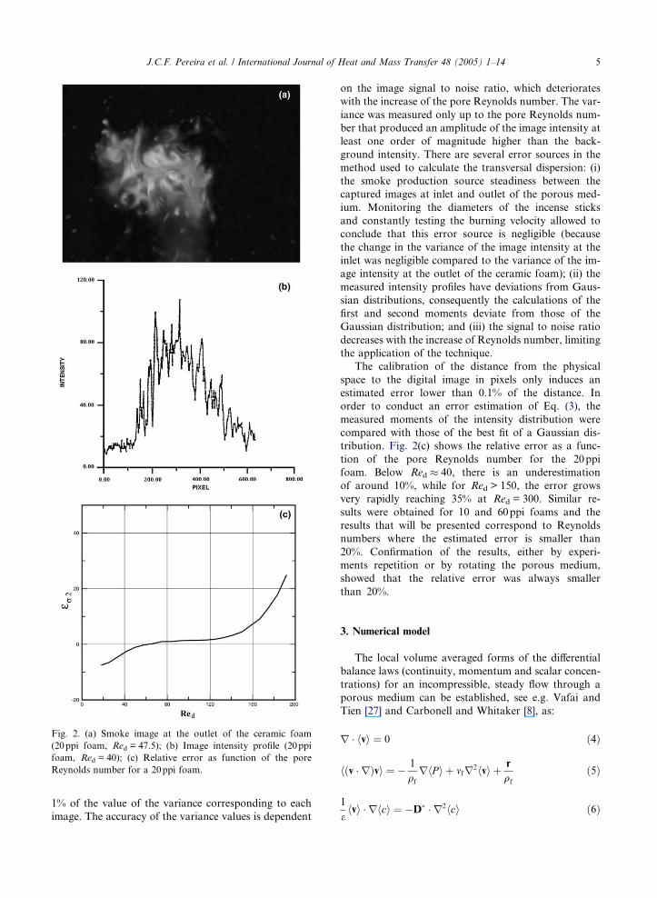
Fig. 2. (a) Smoke image at the outlet of the ceramic foam

(20ppi foam, Red = 47.5); (b) Image intensity profile (20ppi

foam, Red = 40); (c) Relative error as function of the pore

Reynolds number for a 20ppi foam.

J.C.F. Pereira et al. / International Journal of Heat and Mass Transfer 48 (2005) 1–14 5

1% of the value of the variance corresponding to each

image. The accuracy of the variance values is dependent

on the image signal to noise ratio, which deteriorates

with the increase of the pore Reynolds number. The var-

iance was measured only up to the pore Reynolds num-

ber that produced an amplitude of the image intensity at

least one order of magnitude higher than the back-

ground intensity. There are several error sources in the

method used to calculate the transversal dispersion: (i)

the smoke production source steadiness between the

captured images at inlet and outlet of the porous med-

ium. Monitoring the diameters of the incense sticks

and constantly testing the burning velocity allowed to

conclude that this error source is negligible (because

the change in the variance of the image intensity at the

inlet was negligible compared to the variance of the im-

age intensity at the outlet of the ceramic foam); (ii) the

measured intensity profiles have deviations from Gaus-

sian distributions, consequently the calculations of the

first and second moments deviate from those of the

Gaussian distribution; and (iii) the signal to noise ratio

decreases with the increase of Reynolds number, limiting

the application of the technique.

The calibration of the distance from the physical

space to the digital image in pixels only induces an

estimated error lower than 0.1% of the distance. In

order to conduct an error estimation of Eq. (3), the

measured moments of the intensity distribution were

compared with those of the best fit of a Gaussian dis-

tribution. Fig. 2(c) shows the relative error as a func-

tion of the pore Reynolds number for the 20ppi

foam. Below Red � 40, there is an underestimation

of around 10%, while for Red > 150, the error grows

very rapidly reaching 35% at Red = 300. Similar re-

sults were obtained for 10 and 60ppi foams and the

results that will be presented correspond to Reynolds

numbers where the estimated error is smaller than

20%. Confirmation of the results, either by experi-

ments repetition or by rotating the porous medium,

showed that the relative error was always smaller

than 20%.

3. Numerical model

The local volume averaged forms of the differential

balance laws (continuity, momentum and scalar concen-

trations) for an incompressible, steady flow through a

porous medium can be established, see e.g. Vafai and

Tien [27] and Carbonell and Whitaker [8], as:

r � hvi ¼ 0 ð4Þ

hðv � rÞvi ¼ � 1

qf

rhP i þ mfr2hvi þ r

qf

ð5Þ

1

ehvi � rhci ¼ �D� � r2hci ð6Þ

6 J.C.F. Pereira et al. / International Journal of Heat and Mass Transfer 48 (2005) 1–14

In Eq. (5), r stands for the body force term, which is

caused by the micropore structure and measures the

resistance imposed by the solid matrix to the fluid flow:

r ¼ � lf

Khvi � CE

K1=2qhviv ð7Þ

where CE stands for the Ergun coefficient.

The total dispersivity tensor D* = Dm[I + s] + D, in

Eq. (6), receives contribution from molecular diffusion,

DmI, from the tortuosity of the porous media, Dms,

and from the effect of the velocity field through the dis-

persion tensor D.

Since the scalar dispersion from a point source yields a

three-dimensional dispersion pattern, the calculations of

the flow upstream, through and downstream of the cera-

mic foam cylinder inserted in a pipe were axisymmetric.

The problem arises of how to model the longitudinal,

DL, and transversal, DT, components of the tensor D*.

For most cases, the transversal dispersion is at least one

order of magnitude smaller than the longitudinal disper-

sion, which is expressed by DL = c*u + Dm, the dispersiv-

ity, DL/u, being a characteristic property of the medium.

Problem dependent correlations for DL/u are available,

either at column scale or for field applications. The selec-

tion of DL and DT will be discussed in the next section.

Although the flow problem under consideration

could be calculated only by the scalar transport equation

with the prescribed velocity field, for generality reasons,

the continuity and two momentum equations for axi-

symmetric flow were solved with the finite volume SIM-

PLE algorithm [28]. To decrease false diffusion owing to

first order upwind schemes, the deferred correction

numerical treatment of convection [29] is used. The con-

vective fluxes are approximated by:

F i ¼ ½ _mivUDSi �m þ _mi½vCDS

i � vUDSi �m�1 ð8Þ

where m denotes the iteration level.

The second term on the right-hand side is evaluated

using values from the previous iteration, while the firs

one is computed using the UDS approximation. On con-

vergence, the UDS contribution cancels out leaving the

CDS solution that is free from dissipation errors, but

would require a factor f < 1 to avoid oscillatory solu-

tions. For the present case f = 0.85.

The computational domain consists of an axisym-

metric pipe with an 84mm diameter and a porous cylin-

der inside. The pipe inlet is located 5mm upstream of the

porous foam, which is 50mm long, and the outlet is lo-

cated one half-pipe diameter downstream of the foam.

Eqs. (4)–(6) are solved along with the proper boundary

condition, which are as follows:

At the inlet (x = 0),

vxð0; yÞ ¼ u; vyð0; yÞ ¼ 0; cð0; yÞ ¼1 for y 6 Ris

0 for y > Ris

�ð9Þ

At the outlet of the computational domain (x = xDL),

ocox

ðxDL; yÞ ¼ovxox

ðxDL; yÞ ¼ovyox

ðxDL; yÞ ¼ 0 ð10Þ

At the pipe wall, non-slipping condition and imper-

meability to the tracer are imposed. The interface condi-

tions between the porous medium and the clear fluid

were satisfied due to the use of the control volume face

fluxes equality. The normal and the tangential stresses

were made continuous through the interface.

4. Results

Effective transverse diffusivity, DT normalised effec-

tive transverse diffusivity, DT/ud, and transverse disper-

sivity, DT/u, are presented in Fig. 3(a), (b) and (c),

respectively, as functions of the pore Reynolds number

and for different pore sizes. The present experiments

are compared with data reported for ceramic foams by

other authors. Since the present experimental conditions

are similar to those reported by Hackert et al. [19], the

data compares satisfactorily and falls inside the maxi-

mum 20% relative error estimation that was also re-

ported in that work. The experimental results reported

by Benz et al. [18] were obtained at higher pore

Reynolds numbers and are consistent with the trend ob-

served in the present measurements. Fig. 3(a) and (b)

show a strong dependence of DT on the pore Reynolds

number. The increase in DT can be attributed to a pure

mechanical dispersion process in which the smoke

molecular diffusion is not relevant for each of the foams

considered.

The data corresponding to the upper limit of the

Reynolds number in Fig. 3(a)–(c) is subjected to some

controversial interpretation. Hackert et al. [19] as well

as Benz et al. [18] suggest that the normalised effective

transverse dispersion coefficient, DT/ud, increases with

Reynolds up to about 300 < Red < 400, see Fig. 3(b),

and then becomes approximately constant with Redowing to turbulent mixing within the pores. The critical

Reynolds number for transition to purely turbulent

flow in packed beds is in the range of Red � 150

according to Jolls and Hanratty [30] while, for Dybbs

and Edwards [31], this transition occurs for Red � 300.

For ceramic foams, according to Hall and Hiatt [32],

the critical Reynolds number is in the range of

300 6 Red 6 400.

For Stokes flow through a random packed bed of

spheres, Koch and Brady [14] derived analytical expres-

sions for the longitudinal and transverse dispersion coef-

ficients. Since the solid phase is not permeable to the

tracer, for Pe � 1, DL and DT are given by:

DL

Dm

¼ 1þ 3

4Peþ 1

6p2/Pe lnðPeÞ ð11Þ

0 100 200 3000

100

200

300

400

500

present work, 10 ppipresent work, 20 ppipresent work, 60 ppiHackert et al. [19], 10 ppiHackert et al. [19], 20 ppiHackert et al. [19], 30 ppiHackert et al. [19], 45 ppi

dRe

D× 1

06/(

m2 /s

)

10 100

10 10 10 10 10 10 10 1010

101

103

105

107

109

Pe d

DT

/Dm

(a)

10 10 100

0.1

0.2

0.3

0.4

0.5

0.6

0.7

present work, 10 ppipresent work, 20 ppipresent work, 60 ppiHackert et al. [19], 10 ppiHackert et al. [19], 20 ppiHackert et al. [19], 30 ppiHackert et al. [19], 45 ppiBenz et al. [18], 10 ppiBenz et al. [18], 20 ppiBenz et al. [18], 30 ppiBenz et al. [18], 50 ppi

dRe

DT

×10

3/m

/u×

(c)

10 10 10 100.00

0.02

0.04

0.06

0.08

0.10

0.12

0.14

0.16

0.18

present work,10 ppi

present work, 20 ppi

present work, 60 ppi

Hackert et al. [19], 10 ppi

Hackert et al. [19], 20 ppi

Hackert et al. [19], 30 ppi

Hackert et al. [19], 45 ppi

Benz et al. [18], 10 ppi

Benz et al. [18], 20 ppi

Benz et al. [18], 30 ppi

Benz et al. [18], 50 ppi

D/u

dT

Red(b)

(d)

10 ppi, present work20 ppi, present work60 ppi, present workHackert et al. [19]Han et al. [6]Benz et al. [18]Hassinger and von Rosenberg [33]Koch and Brady theory (low Ped) [14]Koch and Brady theory (high Ped) [14]

T

Fig. 3. (a) Effective transverse diffusivity as function of the pore Reynolds number for several ceramic foams; (b) Normalised effective

transverse diffusivity as function of the pore Reynolds number for several ceramic foams; (c) Transverse dispersivity as function of the

pore Reynolds number for several ceramic foams; (d) Comparison of effective transverse diffusivity measurements with theory.

J.C.F. Pereira et al. / International Journal of Heat and Mass Transfer 48 (2005) 1–14 7

DT

Dm

¼ 1þ 63

320

ffiffiffiffiffiffi2/

pPe ð12Þ

In the above equations, the length scale used in the

Peclet number is the sphere radius.

A plot of Eq. (12) is shown in Fig. 3(d) together with

the present measurements and including also data from

low Peclet number flows in fixed beds ([6] and [33], cit. in

[19]). The length scale used in Eq. (12) for the Peclet

number was the pore diameter. In the expressions of

Koch and Brady, the Peclet number is based on the

sphere radius [14]. They were modelling dispersion in

packed beds where the porous medium is composed of

particles. This paper reports the modelling of dispersion

in ceramic foams, consolidated media, where the charac-

teristic length is the pore diameter. One should note that

for ceramic or metal foams, the reported equivalent par-

ticle diameter, for a given ppi number, is smaller than

the pore diameter [1,34] and consequently Eq. (12),

based on an equivalent particle radius length scale,

would strongly underpredict the dispersion coefficient.

The logarithmic plot shows that the theoretical curve,

Eq. (12), is a satisfactory approximation of all the exper-

imental data. Two-dimensional calculations performed

using models or correlations of the dispersion coeffi-

cients in the scalar transport equation will be reported

in the next paragraphs.

According to Eq. (6), one needs to supply both trans-

verse and longitudinal dispersion coefficients to the gov-

erning equations. The present experimental method does

not allow measuring the longitudinal diffusion coeffi-

cient and, to the authors� knowledge, this coefficient is

not available for ceramic foams. Therefore, a numerical

study was conducted to find out the influence of this

8 J.C.F. Pereira et al. / International Journal of Heat and Mass Transfer 48 (2005) 1–14

coefficient. The study consisted in assigning the longitu-

dinal and transversal coefficients to the equations and

calculating, from the resulting concentration field solu-

tion, the transverse diffusivity. The calculation of the

transverse diffusivity followed the procedure used in

the experiments and expressed in Eq. (3), in which the

variance immediately downstream of the foam, r22, and

at the inlet, r21, were calculated from the predicted con-

centration profile in the same manner as in the experi-

mental procedure.

In order to assess the influence of the mesh refine-

ment on the predictions, a grid sensitivity study was

undertaken. The numerical grid used in the two-dimen-

sional, axisymmetric calculations expands in both axial

and radial directions in order to concentrate the grid

lines in the zone of main interest for the study of the dis-

persion of a scalar inside the foam. Three meshes were

considered: 53 · 40, 106 · 80 and 212 · 160. Fig. 4

shows the concentration of points in the dispersion re-

Fig. 4. Calculation domain and mesh used in the computational m

centreline, ranging from 1.0 to 0.1 with a 0.1 increment and from 0.09 t

gion close to the centreline, as well as a detail of the pre-

dicted isocontours of concentration of solute in that

region. The transverse dispersion coefficients calculated

with the finest grid are less than 0.1% smaller than the

ones obtained with the 106 · 80 grid, while the coarsest

mesh results are 1% higher, which denotes the independ-

ence of the solution on further grid refinement. There-

fore, the numerical results presented in this work were

obtained with the 106 · 80 grid.

Recalling from Fig. 3(d) that the theoretical DT re-

sults by Koch and Brady [14], Eq. (12), agree well with

the experimental data in the high Reynolds number re-

gion, Fig. 5(a) shows that if the scalar transport equa-

tion uses DL and DT given by Eqs. (11) and (12),

respectively, the predicted dispersion coefficients are

lower than the value used in the transport equation,

the differences being higher for the case of the 10ppi

foam and relatively lower for the 60ppi foam. These re-

sults indicate that, for the short lengths of the foam sam-

odel. Detail of solute mass fraction isocontours close to the

o 0.05 with a 0.01 increment (results for 10ppi foam, Red = 400).

Red

DT

016

(/m

2s /)

10 ppi, Hackert et al [19]10 ppi, present work20 ppi, Hackert et al [19]20 ppi, present work30 ppi, Hackert et al [19]45 ppi, Hackert et al [19]60 ppi, present workall foams (DL=DT, Eq.(12) )

×

Repore

DT

016

(/m

2s /)

10 ppi, Hackert et al [19]10 ppi, present work20 ppi, Hackert et al [19]20 ppi, present work20 ppi, predicted, L = 50 mm10 ppi, predicted, L = 100 mm

×

Repore

DT

106

/(m

2 /s)

0 100 200 300 400

0 100 200 300 400 0 100 200 300 400

0

100

200

300

400

500

600

0

100

200

300

400

500

600

0

100

200

300

400

500

600

10 ppi, Hackert et al [19]10 ppi, present work20 ppi, Hackert et al [19]20 ppi, present work30 ppi, Hackert et al [19]45 ppi, Hackert et al [19]60 ppi, present work10 ppi, predicted20 ppi, predicted60 ppi, predicted

×

c / c0

y

0.060.00 0.01 0.02 0.03 0.04 0.050

0.02

0.04

0.03

0.01

/m

DL calculated using Eq.(11)

DL calculated using Eq.(12)

(a) (b)

(c) (d)

Fig. 5. (a) Comparison of effective transverse diffusivity measurements (filled symbols) and predictions (lines) as function of pore

Reynolds number. In all predictions, DL and DT were calculated according to Eqs. (11) and (12), respectively, and L = 50mm; (b)

Ratio of predicted concentration at the porous sample outlet plane to the initial concentration of solute (10ppi foam, Red = 400,

c0 = 1.0kg/m3); (c) Comparison of effective transverse diffusivity measurements (filled symbols) and prediction (line) as function of pore

Reynolds number. In the calculation, DL = DT were calculated according to Eq. (12), and L = 50mm; (d) Comparison of effective

transverse diffusivity measurements (filled symbols) and prediction (line) as function of pore Reynolds number. In the predictions, DL

and DT were calculated according to Eqs. (11) and (12), respectively.

J.C.F. Pereira et al. / International Journal of Heat and Mass Transfer 48 (2005) 1–14 9

ples used in the present work, the longitudinal dispersion

coefficient influences the concentration profile and con-

sequently the prediction of DT.

In order to evaluate this influence, Fig. 5(b) shows

the concentration profile at the foam outlet, for 10ppi

and L = 50mm, obtained using DL given by Eq. (11)

or made equal to DT which means that the DL value

introduced in the scalar transport equation is of the or-

der of one-tenth of the theoretical value obtained with

Eq. (11). Fig. 5(c) shows the DT values predicted for

the decreased DL case when DL and DT used in the sca-

lar transport equation are both calculated with Eq. (12).

In this case, the influence of the pore sizes is not ob-

served, and the predicted DT values present a better

agreement with the experimental data.

The strong influence of the DL value in short foams is

in agreement with the study in fixed beds of Han et al.

[6], which demonstrates the need to observe a minimum

dispersion length to obtain measurements of the longitu-

dinal dispersion coefficients that are not dependent on

the position in the packed bed. In this paper, it is also

shown that the dispersion length constraint is dependent

on the value of the Peclet number. Additionally, Han

et al. [6] conclude that one should expect that the trans-

verse diffusivity measured in a transient experiment

would be subjected to the same long-time constraint as

10 J.C.F. Pereira et al. / International Journal of Heat and Mass Transfer 48 (2005) 1–14

the longitudinal diffusivities. Adapting the reasoning of

Han et al. [6] in their one-dimensional analysis to the

longitudinal direction in this problem, and adopting

the pore diameter as the characteristic length scale for

flow in ceramic foam, this constraint can be expressed as

Ld

ePe

� 1 ð13Þ

confirming that the larger the Peclet number, the larger

the required length for constant axial dispersion coeffi-

cients to be observed.

It is not possible to extrapolate directly the results

from packed beds to ceramic foams, but one should ex-

pect that the longitudinal diffusivity would be dependent

on L/d, up to the required ratio of foam length to parti-

cle or pore diameter in order to treat the longitudinal

diffusivity as constant. On the other hand, it was not

found that the column length affects the transverse dis-

persion coefficient. If the critical L/d value is not satis-

fied, one observes significantly lower values of the

coefficients. Han et al. [6] wrote ‘‘some of the previous

results in the literature indicate that the longitudinal dis-

persivity depends less strongly on the Peclet number at

very high values of Peclet, than at lower values. This

has been attributed to turbulence effects. However, a

similar phenomenon is observed in this work under

laminar flow conditions when the dispersion distances

are too short to satisfy the constraint’’, (Eq. (13)). Fig.

5(d) shows that if the length L of the 10ppi foam is

doubled, the predicted DT agrees with the predictions

obtained for the 20ppi foam with L = 50mm, because

the L/d ratio is the same. Many calculations were

performed and the final conclusion is that for foams

with L = 50mm one needs to reduce DL in order to pre-

dict a DT value closer to the one used in the scalar

transport equation. Numerical results obtained for dif-

ferent DL values and for 10, 20 and 60ppi foams with

50mm in length, show that to fulfil the requirement of

the predicted DT being equal to the one used in the

transport equation, the DL should be approximately

equal to DT.

5. Discussion

Fig. 5(c) shows predictions of DT in satisfactory

agreement with the experimental data, bearing in mind

the scatter in the data. One should take in consideration

that the theoretical model of Koch and Brady [14],

although for Pe � 1, was based in the Stokes flow

assumption. In addition, the literature reveals that even

for isotropic porous media the transverse and longitudi-

nal coefficients are not equal when the medium is so

long that constant axial dispersivities are reached.

Consequently the previous results, in the range 10 <

Red < 300, are also in agreement with the analysis pre-

sented by Han et al. [6] about the effect of the packed

bed length on the longitudinal dispersion coefficient.

When mechanical dispersion is the dominant mode,

the dispersion coefficients are proportional to ud, see

e.g. the analysis of five different models of transverse

thermal dispersion conducted by Alazmi and Vafai

[35]. The same is true for the effective diffusivity of fi-

brous media, approximated by cylinders, see Koch and

Brady [36]. There have been several assumptions to de-

rive this dependence and, in this paper, the authors pre-

sent one that will be obtained from closure modelling of

the volume averaged scalar transport equation.

One can define spatial deviations of the point concen-

tration and fluid velocity in terms of the intrinsic phase

average values [8,37] according to c ¼ hcif þ c and

v ¼ hvif þ v. It is admitted that, in the solid, c ¼ hcis ¼0 and v ¼ hvis ¼ 0. The scalar transport equation as de-

rived by Gray [37] is:

ohciot

þ 1

ehvi � rhci ¼ r � ðD� � rhciÞ ð14Þ

where

D� � rhci ¼ Dmðrhci þ sÞ � hcvi ð15Þ

Consequently, the dispersive scalar flux vector is

modelled according to gradient type, Fickian law with

an unknown dispersion coefficient D*.

The modelling assumption for the dispersion coeffi-

cient made in this study is generally based in dimen-

sional analysis. Since kD has units m2/s2 and D* units

are m2/s, one may express the dispersion coefficient as:

D� ¼ C2k2D=U ð16Þ

In Eq. (16), U stands for the dissipation rate of the

‘‘dispersion’’ kinetic energy and has units m2/s3. The

equation for kD is derived in the Appendix. Under equi-

librium assumptions, one may simplify the kD equation

by estimating that there is a dominant role of production

and dissipation in the energy budget relatively to other

transport terms. The production term may be modelled

by:

PD ¼ 1

2CDasfhui2hui ð17Þ

where asf denotes the area per unit volume of the porous

media, u stands for the filtration velocity and CD is the

drag coefficient.

Bhattacharya et al. [34] and Calmidi and Mahajan

[38] provide a model for the estimation of asf which is

based on a representation of the approximate foam

structure as an open cell shaped like a dodecahedron,

yielding:

asf ¼3p

ð0:59Þ2dGðeÞ d f

dð18Þ

J.C.F. Pereira et al. / International Journal of Heat and Mass Transfer 48 (2005) 1–14 11

where:

d f

d¼ 1:18

ffiffiffiffiffiffiffiffiffiffiffi1� e3p

r1

GðeÞ ð19Þ

In Eqs. (18) and (19), the shape function G(e) is includedto take into account the variation of the struts cross-

section with porosity:

G ¼ 1� e�ð1�eÞ=0:04 ð20Þ

Thus, Eq. (18) can be written as:

asf ¼HðeÞd

ð21Þ

Dimensional analysis shows that scalar dissipation

can be evaluated using a prescribed length scale equal

to the pore diameter:

U ¼ k3=2D

dC1 ð22Þ

Replacing the value of U in Eq. (16) yields:

DT ¼ C2 � k1=2D � d ð23Þ

The dispersive kinetic energy can be extracted by

equating PD = U,

1

2CDu3HðeÞ ¼ k3=2D � C1 ð24Þ

yielding:

DT ¼ C2

C1=31

1

2CD � 3p

0:5921:18

ffiffiffiffiffiffiffiffiffiffiffi1� e3p

r" #1=3

ud ð25Þ

The value of CD that stands for the bulk drag coeffi-

cient is a function of e [39], and a rough estimation is

CD � 0.5. For the case under consideration, in Eq.

(25) e = 0.87, which yields DT ¼ 0:91 C2

C1=3

1

ud. The deter-

mination of the constants is out of the scope of this

work, but taking into consideration that C1=31 should

be close to unity and under the assumption that

C2 � 0.1, the derivation of DT is very close to the Koch

and Brady�s result (DT = 0.1ud), and consequently with

the measurements. The important remark concerning

this discussion is that DT is a linear function of Peclet

for a prescribed e and as far as CD is constant in Eq.

(25).

The above procedure is not valid for turbulent flow

because time was not considered. So, the similarities

with turbulent flow analysis are only due to the

mathematical decomposition of the point values of the

quantities into a mean part and a fluctuation. The de-

scribed approach is valid as far as the modelling of the

production and dissipation of ‘‘dispersion’’ kinetic en-

ergy and the equilibrium assumption are physically

sound.

6. Conclusions

This paper reports experimental, numerical and theo-

retical results of transverse dispersion coefficients for

flow in the range 10 < Red < 300 within high porosity

ceramic foams with 10, 20 and 60 pores per inch. The

main results are summarized as follows.

Experiments show a dependence of DT on the pore

Reynolds number. The increase of DT with Red can be

attributed to a pure mechanical dispersion process.

Calculation of the transverse dispersion coefficient by

means of the theoretical expression by Koch and Brady

[14], using the pore diameter as a characteristic length,

agrees satisfactorily with the experiments, despite the

high Reynolds number considered.

Numerical predictions using DL and DT according to

Koch and Brady in the scalar transport equation were

performed with the aim of recovering the DT value from

the calculated concentration field following the

procedure used in the experiments. The predictions show

the strong dependence of DL on the foam length to pore

diameter ratio (L/d) and the influence of this dependence

in the recovered DT values. The DT value for 60ppi is

better predicted than for 10ppi, because the former

has a higher L/d value. For the 60ppi foam, this

value is approximately 60 while the 10ppi foam has

L/d ffi 10.

Owing to the short foam length considered, the DL

value introduced in the scalar transport equation was

decreased according to the theoretical findings for

packed beds, yielding excellent agreement of the DT val-

ues estimated using the expression by Koch and Brady

with the ones recovered from the predictions.

For the range of pore Reynolds number considered,

dispersion in porous media is mainly due to mechanical

dispersion, which results in the dispersion coefficient

being proportional to ud. The Koch and Brady�s theoret-ical relationship for DT is in agreement with the experi-

ments. A derivation for DT is presented, which is based

on the modelling closure of the volume average form of

the scalar transport equation. The dispersive scalar flux

vector in this equation is modelled from the dispersive

kinetic energy and a pore diameter prescribed length

scale.

Acknowledgments

This work was partially supported by Fundacao para

a Ciencia e a Tecnologia (Lisbon, Portugal, FCT project

number PRAXIS/3/3.1/CTAE/1915/95) and by EC pro-

ject ENK6-CT-2000-00317. T.C. Hayashi would like to

thank the Fundacao Coordenacao de Aperfeicoamento

de Pessoal de Nıvel Superior, CAPES (Brasilia, Brazil)

for the Ph.D. fellowship granted.

12 J.C.F. Pereira et al. / International Journal of Heat and Mass Transfer 48 (2005) 1–14

Appendix A. Derivation of the averaged form of balance

equations

The phase average of some quantity wa of the a-phase is defined as:

hwai ¼1

V¼

ZV¼V aþV b

wa dV ðA:1Þ

In this development, it is assumed that the value of

wa is zero in the b-phase. On the other hand, hwai is

an average associated with some point in the flow do-

main. This point is not necessarily in the a-phase, so that

hwai is defined for the whole space and may be non-zero

in the b-phase.A second average to consider is the intrinsic phase

average, which is computed by finding the integral only

over the volume Va of the a-phase contained in the rep-

resentative elementary volume V:

hwaia ¼ 1

V a

ZV a

wa dV ðA:2Þ

The two averages are related by

eahwaia ¼ hwai ðA:3Þ

where ea = Va/V. This variable is the porosity of the por-

ous medium if a is the fluid phase.

Another important relationship is the theorem that

relates the average of a derivative to the derivative of

an average [40]:

hrwai ¼ rhwai þ1

V

ZAab

wana dA ðA:4Þ

where Aab is the area of the a–b interface and na is the

outwardly oriented unit vector normal to Aab.

In what follows, all quantities are defined in the a-phase (fluid) and, for convenience, the subscript will

no be longer indicated with velocity, pressure and energy

contents. However, it will be indicated along with fluid

properties, meaning that these properties are evaluated

as intrinsic phase averages and admitted to be constant.

The phase averaged balance equation for kinetic

energy (mechanical energy for an isothermal flow) reads

[41]:

o

otvivi2

� �� �þ o

oxj

vivi2

vj� �� �

¼ � 1

qoðPvjÞoxj

� �þ m

o

oxj

o

oxj

vivi2

� �� �� �

� movioxj

ovioxj

� �ðA:5Þ

According to the general transport theorem [40],

o

ot1

2vivi

� �¼ o

ot1

2vivi

� �� 1

V

ZAab

1

2vivi

w � ndA

ðA:6Þ

where w is the velocity of the interface Aab, which is zero

in the present case. The averaging theorem Eq. (A.4) can

be applied to the other terms of the transport equation

(Eq. (A.5)). Since the velocity on the interface Afs is zero,

Eq. (A.5) reads:

o

otvivi2

D Eþ o

oxj

vivi2

vjD E

¼ � 1

qf

ohPvjioxj

þ mfo

oxj

o

oxj

vivi2

D E � mf

ovkoxj

ovkoxj

� �ðA:7Þ

Representing the point velocity values as vi ¼ hviifþvi, the mechanical energy is expressed as a sum of a

phase averaged contribution and a dispersive mechani-

cal energy term as:

vivi2

¼ hviifhviif

2þ vivi

2þ hviif vi ðA:8Þ

Evaluation of the different terms of Eq. (A.7) yields

an equation that represents the sum of the mechanical

energy of the phase averaged flow plus the dispersive

mechanical energy. Denoting KM = (hviifhviif)/2 and

kD ¼ ðviviÞ=2,

ohKMiot

þ o

oxjhKMhvjifi

� � 1

qf

oðhP ifhviifÞoxj

þ mfo

oxj

o

oxjhKMi

"

þmfohvkif

oxj

ohvkif

oxj

* +þ 1

qf

o

oxjh�qfhvii

f vivji

� 1

qf

h�qf vivjiohviif

oxj

#¼ �A� ðA:9Þ

in which A* is equal to:

A� ¼ o

othkDi þ

o

oxjhkDhvjifi

�"� 1

qf

o

oxjhP vji þ mf

o

oxj

o

oxjhkDi

�mfovkoxj

ovkoxj

� �� 1

qf

hqf vivjiohviif

oxj� o

oxj

vivi2

vj

� �#

ðA:10Þ

Obviously, the LHS of Eq. (A.9) is the phase aver-

aged transport equation for the kinetic energy of the

phase averaged velocity, while the RHS of Eq. (A.10)

represents the transport equation of the dispersion ki-

netic energy. The authors point out the analogy with

the Reynolds averaging, since all surface integrals vanish

because of no-slip conditions, that is familiar to turbu-

lence specialists.

J.C.F. Pereira et al. / International Journal of Heat and Mass Transfer 48 (2005) 1–14 13

The modelling of the diffusion-like terms may follow

the Fick�s law gradient type approach. For the diffusion

term,

� o

oxj

1

qf

hP vji �vivi2

vj

� �� �þ mf

o

oxj

o

oxjhkDi

’ Do

oxj

o

oxjhkDi

ðA:11Þ

A production term is written as:

1

qf

h�qf vivjiohviif

oxj¼ PD ðA:12Þ

and a dissipation term is as follows:

�mfovkoxj

ovkoxj

� �¼ U ðA:13Þ

For the present work, it is supposed that the disper-

sive energy budget is dominated by production and dis-

sipation. Consequently, the term enclosed in brackets in

Eq. (A.10) becomes

PD þ U ¼ 0 ðA:14Þ

One should take into consideration that no time aver-

age was considered. Consequently, the derivation of Eq.

(A.13) has nothing in common with turbulent kinetic

energy. However, both analyses share the concept of

averaged velocity (in space or time) that is a pure math-

ematical one.

References

[1] J.R. Howell, M.J. Hall, J.L. Ellzey, Combustion of

hydrocarbon fuels within porous inert media, Prog. Energy

Combust. Sci. 22 (1996) 121–145.

[2] D. Trimis, F. Durst, Combustion in a porous medium—

Advances and applications, Combust. Sci. Technol. 121

(1996) 153–168.

[3] H.O. Pfannkuch, Contribution a l�etude des deplacements

de fluids miscibles dans un milieu poreux, Rev. Inst.

Francais Petrole 18 (1963) 215–270.

[4] D.R.F. Harleman, R.R. Rumer, Longitudinal and lateral

dispersion in an isotropic porous medium, J. Fluid Mech.

16 (1963) 385–394.

[5] J.J. Fried, M.A. Combarnous, Dispersion in porous media,

Adv. Hydrosci. 7 (1971) 169–262.

[6] N.W. Han, J. Bhakia, R.G. Carbonell, Longitudinal and

lateral dispersion in packed beds: effect of column length

and particle size distribution, AIChE J. 31 (1985) 277–288.

[7] H. Brenner, Dispersion resulting from flow through

partially periodic porous media, Philos. Trans. Roy. Soc.,

London 297 (1980) 81–133.

[8] R.G. Carbonell, S. Whitaker, Dispersion in pulsed systems

II—Theoretical developments and passive dispersion in

porous media, Chem. Eng. Sci. 38 (1983) 1795–1802.

[9] M. Quintard, S. Whitaker, Transport in ordered and

disordered porous media: volume-averaged equations,

closure problems, and comparison with experiment, Chem.

Eng. Sci. 48 (1993) 2537–2564.

[10] F. Kuwahara, A. Nakayama, H. Koyama, A numerical

study of thermal dispersion in porous media, ASME J.

Heat Transfer 118 (1996) 756–761.

[11] H.P.A. Souto, C. Moyne, Dispersion in two-dimensional

periodic porous media. Part II: Diffusion tensor, Phys.

Fluids 9 (1997) 2253–2263.

[12] K.T. Hsiao, S.G. Advani, A theory to describe heat

transfer during laminar incompressible flow of a fluid in

periodic porous media, Phys. Fluids 11 (1999) 1738–1748.

[13] D.L. Koch, R.G. Cox, H. Brenner, J.F. Brady, The effect

of order on dispersion in porous media, J. Fluid Mech. 200

(1989) 173–188.

[14] D.L. Koch, J.F. Brady, Dispersion in fixed beds, J. Fluid

Mech. 154 (1985) 399–427.

[15] J. Bear, Dynamics of Fluid in Porous Media, American

Elsevier, New York, 1972, pp. 579–664.

[16] D.A. Nield, A. Bejan, Convection in porous media, second

ed., Springer-Verlag, New York, 1999, Chapters 2 and 4.

[17] M. Kaviany, Principles of Heat Transfer in Porous Media,

second ed., Springer-Verlag, New York, 1995, pp. 157–

258.

[18] P. Benz, P. Hutter, A. Schlegel, Radiale Stoffdispersions-

koeffizienten in durchstromten keramischen Schaumen,

Warme Stoffubertrag. 29 (1993) 125–127.

[19] C.L. Hackert, J.L. Ellzey, O.A. Ezekoye, M.J. Hall,

Transverse dispersion at high Peclet numbers in short

porous media, Exper. Fluids 21 (1996) 286–290.

[20] C.P. Lowe, D. Frenkel, Do hydrodynamic dispersion

coefficients exist? Phys. Rev. Lett. 77 (22) (1996) 4552–

4555.

[21] R.J. Hill, D.L. Koch, Moderate-Reynolds-number flow in

a wall-bounded porous medium, J. Fluid Mech. 453 (2002)

315–344.

[22] T. Masuoka, Y. Takatsu, Turbulence model for flow

through porous media, Int. J. Heat Mass Transfer 39

(1996) 2803–2809.

[23] B.V. Antohe, J.L. Lage, A general two-equation macro-

scopic turbulence model for incompressible flow in porous

media, Int. J. Heat Mass Transfer 40 (1997) 3013–3024.

[24] V.S. Travkin, L. Catton, Nonlinear effects in multiple

regime transport of momentum in longitudinal capillary

porous medium morphology, J. Por. Med. 2 (1999) 277–

294.

[25] D.A. Nield, Alternative models of turbulence in a porous

medium and related matters, ASME J. Fluids Eng. 123

(2001) 928–931.

[26] R.S. Maier, D.M. Kroll, R.S. Bernard, S.E. Howington,

J.F. Peters, H.T. Davis, Pore-scale simulation of disper-

sion, Phys. Fluids 12 (2000) 2065–2079.

[27] K. Vafai, L.C. Tien, Boundary and inertia effects on flow

and heat transfer in porous media, Int. J. Heat Mass

Transfer 24 (1981) 195–203.

[28] S.V. Patankar, D.B. Spalding, A calculation procedure for

heat, mass and momentum transfer in three-dimensional

parabolic flows, Int. J. Heat Mass Transfer 15 (1972) 1787–

1806.

[29] J.H. Ferziger, M. Peric, Computational Methods for

Fluid Dynamics, third rev. ed., Springer-Verlag, Berlin,

2002, pp. 148–151.

14 J.C.F. Pereira et al. / International Journal of Heat and Mass Transfer 48 (2005) 1–14

[30] K.R. Jolls, T.J. Hanratty, Transition to turbulence for flow

through a dumped bed of spheres, Chem. Eng. Sci. 21

(1966) 1185–1190.

[31] A. Dybbs, R.V. Edwards, R.V., A new look at porous

media fluid mechanics–Darcy to turbulent, in: J. Bear,

M.Y. Corapcioglu (Eds.), Fundamentals of Transport

Phenomena in Porous Media, Martinus-Nijhoff Publica-

tions, Netherlands, 1984, pp. 199–254.

[32] M.J. Hall, J.P. Hiatt, Measurements of pore scale flows

within and exiting ceramic foams, Exper. Fluids 20 (1996)

433–440.

[33] R.C. Hassinger, D.U. von Rosenberg, A mathematical and

experimental examination of transverse dispersion coeffi-

cients, Soc. Petrol. Eng. J. 243 (1968) 195–204.

[34] A. Bhattacharya, V.V. Calmidi, R.L. Mahajan, Thermo-

physical properties of high porosity metal foams, Int. J.

Heat Mass Transfer 45 (2002) 1017–1031.

[35] B. Alazmi, K. Vafai, Analysis of variants within the

porous media transport models, ASME J. Heat Transfer

122 (2000) 303–326.

[36] D.L. Koch, J.F. Brady, The effective diffusivity of fibrous

media, AIChE J. 32 (1986) 575–591.

[37] W.G. Gray, A derivation of the equations for multi-phase

transport, Chem. Eng. Sci. 30 (1975) 229–233.

[38] V.V. Calmidi, R.L. Mahajan, Forced convection in high

porosity metal foam, ASME J. Heat Transfer 122 (2000)

557–565.

[39] H.M. Nepf, Drag, turbulence and diffusion in flow through

emergent vegetation, Water Resour. Res. 35 (2) (1999)

479–489.

[40] S. Whitaker, Advances in theory of fluid motion in porous

media, Ind. Eng. Chem. 61 (12) (1969) 14–28.

[41] R.B. Bird, W.E. Stewart, E.N. Lightfoot, Transport Phe-

nomena, John Wiley & Sons, Inc., New York, 1960, p. 81.