
PAGOSA physics manual - Library Without Walls
249
LA-14425-M Manual Approved for public release; distribution is unlimited. PAGOSA Physics Manual
-
Upload
khangminh22 -
Category
Documents
-
view
0 -
download
0
Transcript of PAGOSA physics manual - Library Without Walls

LA-14425-MManualApproved for public release; distribution is unlimited.
PAGOSAPhysics Manual

This report was prepared as an account of work sponsored by an agency of the U.S. Government. Neither Los Alamos National Security, LLC, the U.S. Government nor any agency thereof, nor any of their employees make any warranty, express or implied, or assume any legal liability or responsibility for the accuracy, completeness, or usefulness of any information, apparatus, product, or process disclosed, or represent that its use would not infringe privately owned rights. Reference herein to any specific commercial product, process, or service by trade name, trademark, manufacturer, or otherwise does not necessarily constitute or imply its endorsement, recommendation, or favoring by Los Alamos National Security, LLC, the U.S. Government, or any agency thereof. The views and opinions of authors expressed herein do not necessarily state or reflect those of Los Alamos National Security, LLC, the U.S. Government, or any agency thereof. Los Alamos National Laboratory strongly supports academic freedom and a researcher’s right to publish; as an institution, however, the Laboratory does not endorse the viewpoint of a publication or guarantee its technical correctness.
Los Alamos National Laboratory, an Affirmative Action/Equal Opportunity Employer, is operated by Los Alamos National Security, LLC, for the National Nuclear Security Administration of the U.S. Department of Energy under contract DE-AC52-06NA25396.
Cover Art:The Eulerian three-dimensional compressible Navier Stokes equations are shown in their Cartesian component form under a PAGOSA simulation of a shaped charge at 27 µs after detonation.

LA-14425-MManualIssued: August 2010
PAGOSA Physics Manual
Wayne N. WeselohSean P. ClancyJames W. Painter
Group XTD-1 Silverton Code ProjectLos Alamos National Laboratory

This page intentionally left blank

v
Acknowledgments The authors wish to thank the many individuals who developed, documented, and commented on the original algorithms in PAGOSA. In particular, Rick Smith, Doug Kothe, Chuck Zemach, Ian Gray, Kathy Holian, Tom Bennion, Martin Torrey, and Tom Adams provided personal communications, notes, comments, and insights into the algorithmic construction of PAGOSA. The reviewers of this physics manual helped immeasurably in the quality and accuracy of the material presented. In many ways, this physics manual is the result of an archeological process. Many of the original algorithm authors have left Los Alamos National Laboratory or are now retired or deceased. Uncovering and deciphering the remaining artifacts from the original code development has been a painstaking endeavor filled with surprising moments. We thank Bob Webster, Bill Archer, and Ed Dendy for their help in the review process. Brendan Kullback and Mark Carrara assisted in verifying many of the equations and derivations presented. Thanks to the technical editor, Lisa Rothrock, for her valuable suggestions, comments, and contributions in making this document be good English.

vi
This page intentionally left blank.

vii
Contents
Acknowledgments................................................................................................................v Acronyms......................................................................................................................... xiii Nomenclature.....................................................................................................................xv 0 Introduction ................................................................................................................. 3
0.1 Algorithm ............................................................................................................. 4 1 Governing Equations................................................................................................. 11 2 The Eulerian Grid...................................................................................................... 17
2.1 Mixed Cells ........................................................................................................ 19 2.2 Finite Differences............................................................................................... 20 2.3 Momentum Control Volume .............................................................................. 21 2.4 Ghost Cells ......................................................................................................... 22 2.5 Grid Decomposition ........................................................................................... 22
3 Strain Rates................................................................................................................ 27 4 Operator Splitting ...................................................................................................... 33
4.1 Lagrangian Phase ............................................................................................... 34 4.2 X Advective Phase ............................................................................................. 35 4.3 Y Advective Phase ............................................................................................. 35 4.4 Z Advective Phase.............................................................................................. 35 4.5 Lagrangian Phase ............................................................................................... 37
4.5.1 Lagrangian Setup for Advection................................................................. 39 4.6 Advection Phases ............................................................................................... 42
4.6.1 Advection of Momentum............................................................................ 45 4.6.2 Energy Advection ....................................................................................... 47
5 Integration of the Hydrodynamic Variables .............................................................. 51 5.1 Predictor Stage ................................................................................................... 53 5.2 Lagrangian Velocity Update .............................................................................. 54 5.3 Corrector Stage................................................................................................... 55
6 Equation of State ....................................................................................................... 61 6.1 Ideal Gas EOS .................................................................................................... 61 6.2 Void EOS ........................................................................................................... 62 6.3 Polynomial EOS................................................................................................. 62 6.4 Modified Osborne (or Quadratic) EOS .............................................................. 63 6.5 Jones-Wilkins-Lee (or JWL) EOS ..................................................................... 64 6.6 Grüneisen (or Us-Up) EOS ................................................................................. 65 6.7 SESAME EOS.................................................................................................... 67
6.7.1 Ramp Treatment.......................................................................................... 68 6.7.2 SESAME Body Internal Energy Iteration .................................................. 69
6.8 Exponential EOS................................................................................................ 71 6.9 Becker-Kistiakowsky-Wilson High-Explosive (BKW-HE) EOS...................... 71
6.9.1 Solid Components....................................................................................... 71 6.9.2 Gaseous Components.................................................................................. 72 6.9.3 Mixed Components..................................................................................... 72
6.10 Pmin ................................................................................................................... 75 7 Sound Speed .............................................................................................................. 79

viii
7.1 Ideal Gas EOS Sound Speed .............................................................................. 81 7.2 Void EOS Sound Speed ..................................................................................... 81 7.3 Polynomial EOS Sound Speed........................................................................... 81 7.4 Modified Osborne (or Quadratic) EOS Sound Speed ........................................ 82 7.5 Jones-Wilkins-Lee (or JWL) EOS Sound Speed ............................................... 83 7.6 Grüneisen (or Us-Up) EOS Sound Speed ........................................................... 84 7.7 SESAME EOS Sound Speed.............................................................................. 85 7.8 Exponential EOS Sound Speed .......................................................................... 86 7.9 PAGOSA Sound Speed...................................................................................... 86
8 Artificial Viscosity .................................................................................................... 89 9 Computing A Timestep ............................................................................................. 95 10 Initial Conditions..................................................................................................... 101 11 Boundary Conditions............................................................................................... 105
11.1 Reflective Boundary Conditions .................................................................. 105 11.2 Transmissive Boundary Conditions ............................................................. 106 11.3 Other Boundary Conditions.......................................................................... 107
12 Programmed Burn ................................................................................................... 111 12.1 Simple Point ................................................................................................. 112 12.2 Simple Line................................................................................................... 112 12.3 Simple Plane ................................................................................................. 112 12.4 Simple Cylinder............................................................................................ 113 12.5 Simple Sphere............................................................................................... 113 12.6 Simple Ring .................................................................................................. 113 12.7 Limitations of Simple Detonators................................................................. 114 12.8 Other Detonation Models ............................................................................. 115
13 Divergence Options................................................................................................. 119 13.1 Uniform ........................................................................................................ 119 13.2 Void Closure................................................................................................. 119 13.3 Pressure Relaxation ..................................................................................... 122
14 Strength ................................................................................................................. 129 14.1 Cauchy Stress Tensor ................................................................................... 131 14.2 Strain Rate Splitting...................................................................................... 131 14.3 Yield Criterion.............................................................................................. 134 14.4 Flow-Stress Models ...................................................................................... 139
14.4.1 Elastic Perfectly Plastic......................................................................... 139 14.4.2 Modified Steinberg-Cochran-Guinan.................................................... 140 14.4.3 Steinberg-Cochran-Guinan.................................................................... 141 14.4.4 Johnson-Cook (JC)................................................................................ 142 14.4.5 Preston-Tonks-Wallace (PTW) ............................................................. 143 14.4.6 Mechanical Threshold Stress (MTS)..................................................... 145 14.4.7 Kospall .................................................................................................. 148 14.4.8 Thermal Softening................................................................................. 149 14.4.9 Work Hardening.................................................................................... 150
15 Fracture and Damage............................................................................................... 155 15.1 Johnson Spall ............................................................................................... 155 15.2 Johnson-Cook Damage ................................................................................ 157

ix
16 Crush ................................................................................................................. 161 Appendix A. The Constitutive Equations..................................................................... 167 Appendix B. Initial Volume Fraction Calculation ....................................................... 169 Appendix C. Youngs Interface Reconstruction............................................................ 173
C.1 Analytic Geometry ........................................................................................... 173 C.2 Distance Parameter ρ........................................................................................ 175 C.3 ρ Symmetry ...................................................................................................... 177 C.4 Volume v .......................................................................................................... 177 C.5 v Symmetry ...................................................................................................... 179
Appendix D. Lagrangian-Phase Equation .................................................................... 181 Appendix E. First-, Second-, and Third-Order Advection........................................... 183
E.1 First-Order Advection ...................................................................................... 184 E.2 Second-Order Advection.................................................................................. 184 E.3 Third-Order Advection..................................................................................... 185 E.4 Gradient Limiters and Monotonicity, ............................................................... 188 E.5 PAGOSA Advection ........................................................................................ 190 E.6 Advection Example: Advection of a Square Pulse .......................................... 193
Appendix F. Initial Timestep Calculation.................................................................... 195 Appendix G. Multi-Material Interface Reconstruction for Advection ........................ 197
G.1 Reconstruction.................................................................................................. 197 G.2 Volume Fraction Identifier............................................................................... 198
Appendix H. The Cauchy-Stokes Decomposition Theorem ........................................ 203 H.1 Translation........................................................................................................ 204 H.2 Rotation ............................................................................................................ 204 H.3 Dilatation.......................................................................................................... 205 H.4 Shear Deformation ........................................................................................... 205
Appendix I. Stress Rotation ........................................................................................ 207 Appendix J. Diagnostics.............................................................................................. 211
J.1 Volume............................................................................................................. 211 J.2 Mass ................................................................................................................. 211 J.3 Internal Energy................................................................................................. 211 J.4 Kinetic Energy.................................................................................................. 211 J.5 Elastic Distortional Energy ............................................................................. 212 J.6 Plastic Work ..................................................................................................... 212 J.7 Mass Melted ..................................................................................................... 212 J.8 Mass Burned..................................................................................................... 213 J.9 Mixed-Cell Statistics ........................................................................................ 213 J.10 Minimum and Maximum Statistics .................................................................. 213
Appendix K. Momentum UPDATE ............................................................................. 215 Appendix L. Pin Package............................................................................................. 217
L.1 Four Points ....................................................................................................... 218 L.2 Three Points...................................................................................................... 219 L.3 Two Points........................................................................................................ 219 L.4 One Point.......................................................................................................... 219 L.5 Zero Points ....................................................................................................... 219
Appendix M. Tracers..................................................................................................... 221

x
M.1 Interpolation ..................................................................................................... 221 M.2 Integration ........................................................................................................ 222 M.3 Comments......................................................................................................... 223
Index ................................................................................................................................225
Figures
Figure 0.1. Flowchart showing an overview of the PAGOSA algorithm.. ...................... 5 Figure 0.2. Flowchart showing the Lagrangian phase of the PAGOSA algorithm.......... 6 Figure 0.3. Flowchart showing the advection phase(s) of the PAGOSA algorithm.. ...... 7 Figure 2.1. A single Eulerian cell in the computational domain. ....................................17 Figure 2.2. The spatial centering of the PAGOSA state variables. .................................19 Figure 2.3. A cross section of the momentum control volume. ..................................... 21 Figure 2.4. Domain decomposition of an Eulerian grid. ................................................ 23 Figure 3.1. The gradient finite difference computation.................................................. 28 Figure 4.1. A typical sequence of Lagrangian and advection steps. .............................. 36 Figure 4.2. A cross section of an Eulerian cell............................................................... 39 Figure 4.3. An Eulerian cell containing four materials. ................................................. 41 Figure 4.4. The solution of the advection equation........................................................ 43 Figure 4.5. Diagram of the advection cells involved in Eq. (4.34). ............................... 44 Figure 5.1. The integration step begins with all the variables at a time (n). .................. 52 Figure 5.2. The predictor integration step advances the state variables to a time.......... 53 Figure 5.3. The Lagrangian velocity update first integrates the velocities .................... 54 Figure 5.4. The corrector integration step uses the time-centered velocity ................... 55 Figure 6.1. The SESAME ramp treatment. .................................................................... 68 Figure 6.2. Example of the use of Pmin in an EOS with a van der Waals loop............. 75 Figure 8.1. A typical pressure and artificial viscosity in the region of a shock. ............ 91 Figure 11.1. The reflective (symmetry) boundary conditions........................................ 105 Figure 11.2. The transmissive boundary condition. ....................................................... 106 Figure 12.1. An explosive is to be detonated at the point shown................................... 114 Figure 12.2. An explosive, shown in the previous figure............................................... 115 Figure 13.1. Schematic showing two different methods of contracting void................. 121 Figure 14.1. The elastic-plastic behavior of a typical ductile material .......................... 129 Figure 14.2. The elastic-plastic behavior of a PAGOSA material with strength. .......... 130 Figure 14.3. The two possible final states for a single timestep t . ............................. 136 Figure 14.4. The vector components of an elastic-plastic state...................................... 136 Figure 14.5. An elastic-perfectly plastic material. ......................................................... 139 Figure 14.6. The thermal softening function Fmelt .......................................................... 149 Figure B.1. Volume fractions of a mixed cell containing three materials ................... 169 Figure B.2. A pathological case where some materials can go missing from a cell..... 170 Figure B.3. Exact volume fractions and ideal interfaces. ............................................. 171 Figure B.4. Reconstructed interfaces and volume fractions ......................................... 171 Figure C.1. Tetrahedron bounded by the ( , ) plane. ............................................... 174 Figure D.1. Lagrangian expansion of a fluid. ............................................................... 182 Figure E.1. Cell advection diagram. ............................................................................. 183 Figure E.2. Upwind, downwind, and third-order gradients. ......................................... 188

xi
Figure E.3. The Youngs/van Leer gradient limiter. ...................................................... 189 Figure E.4. Advection of a square pulse....................................................................... 193 Figure G.1. The advection volume (shown in yellow) contains three materials........... 197 Figure G.2. A cross section of an Eulerian cell showing a material interface .............. 198 Figure G.3. The case of positive flux is simply the complement in Figure G.2. .......... 199 Figure G.4. If we are given the volume behind the plane ............................................. 200 Figure G.5. The advection volume in the new coordinate system ................................ 202 Figure H.1. The types of motion ................................................................................... 205 Figure L.1. The material surface, shown as a yellow triangle ...................................... 217 Figure L.2. A typical pin distance vs simulation time. ................................................. 218 Figure M.1. A tracer particle at (x,y,z) in an Eulerian cell............................................. 221
Tables
Table 5.1 A Schematic of the Hydrodynamic Variables ............................................ 57 Table 9.1. The Timestep Controls in PAGOSA Hydrodynamics ................................ 97 Table 14.1. The PAGOSA Elastic-Plastic Algorithm at a Glance............................... 133

xii
This page intentionally left blank.

xiii
Acronyms
AWRE Atomic Weapons Research Establishment
BKW Becker-Kistiakowsky-Wilson
CFL Courant-Friedrichs-Lewy
DT Deuterium and Tritium
EOS Equation of State
EOSPAC Equation-of-State Package
HE High Explosive
JC Johnson-Cook
JWL Jones-Wilkins-Lee
LANL Los Alamos National Laboratory
LASL Los Alamos Scientific Laboratory
MTS Mechanical Threshold Stress
OFHC Oxygen-Free High Conductivity
PIC Particle-in-Cell (Method)
PTW Preston-Tonks-Wallace

xiv
This page intentionally left blank.

xv
Nomenclature a characteristic speed (4.6) a bulk material sound speed (6.7.1)
na EOS constants (6.3) A JWL EOS constant (6.5) Aijkn fourth-order tensor (A) Areai face areas of an Eulerian cell (2.0) b EOS constants (6.3) B JWL EOS constant (6.5) Bf burn fraction (6.5, 12.0) Bt burn time (12.0) c isentropic sound speed (7.0) c0 Grüneisen EOS constant (6.6) c cell average sound speed (8.0) c constant vector (3.0) D discrete linear operator (4.0) D detonation velocity (12.0) Di density gradient (4.6, E.3, E.4)
ije strain tensor (1.0)
ije strain rate tensor for small strains, /ik ike e t (1.0, 3.0) eije elastic portion of the strain tensor (14.2) p
ije plastic portion of the strain tensor (14.2) E specific internal energy (per unit mass) (1.0, E.5) EH Hugoniot internal energy (6.6) ET tabular internal energy (SESAME) (6.7) ES energy shift (6.7) E* user-selected internal energy (6.7.2) F function (0.2, 2.0, 3.0)
iF body force vector, ( , , )x y zF F FF (1.0) Fmelt flow-stress melt factor (14.4.2, 14.4.3, 14.4.7, 14.4.8) G shear modulus (1.0, 7.9, 14.4) G0 elastic-perfectly plastic shear modulus (14.4.1) Gmax maximum shear (14.4) Hmelt flow-stress melt factor (14.4.7) i indices, x (2.0) I identity matrix/operator (5.0) j indices, y (2.0)
nJ invariants of the deviatoric stress tensor 1 2 3( , , )J J J (1.0, 14.3) k indices, z (2.0)

xvi
L continuous linear operator (4.0) L length scale (8.0) m mass of an Eulerian cell (2.0) Mass mass on a momentum control volume (vertex mass) (2.0) n unit normal (C, D) P pressure (1.0, 6.0) PH Hugoniot pressure (6.6) P average cell pressure (5.2, 6.0, K) Q artificial viscosity (8.0) Q1 linear artificial viscosity (8.0) Q2 quadratic (von Neumann) artificial viscosity (8.0) Qik orthogonal rotation tensor (I) R line-of-sight distance (12.0) R1 JWL EOS constant (6.5) R2 JWL EOS constant (6.5) Rij stress rotation tensor (I) s Grüneisen EOS constant (6.6) S entropy (8.0) S Youngs/van Leer advection gradient limiter (E) S deviatoric stress tensor (1.0, 14.3, A)
ijS deviatoric stress tensor (component form) (1.0, A) SR scaling ratio (6.7) t time (1.0, 4.0, 5.0, 9.0, 10.0) tn discrete time at interval (n) (2.2) T temperature (6.9, 7.0, 8.0) T solution time interval (2.2) T0 tetrahedron volume (A)
*T homologous temperature (14.4.4) u velocity vector ( , , )U V Wu (1.0, 13.0, D) U x velocity component (1.0) U face-averaged x velocity component (3.0)
sU shock velocity (6.6)
pU particle velocity (6.6) v truncation volume (A) V y velocity component (1.0) V face-averaged y velocity component (3.0) Vol cell volume (2.0) W z velocity component (1.0) We elastic distortional energy (J) Wp plastic work (J)

xvii
W face-averaged z velocity component (3.0) Wik spin tensor (I) x Cartesian coordinate x (1.0)
minx minimum extent of the Eulerian mesh (2.0)
maxx maximum extent of the Eulerian mesh (2.0) y Cartesian coordinate y (1.0)
miny minimum extent of the Eulerian mesh (2.0)
maxy maximum extent of the Eulerian mesh (2.0) Y yield modulus (14.4) Y0 elastic-perfectly-plastic yield modulus (14.4.1) Ymax maximum yield (14.4) z Cartesian coordinate z (1.0)
minz minimum extent of the Eulerian mesh (2.0)
maxz maximum extent of the Eulerian mesh (2.0) exponential EOS constant (6.8) EOS constants (6.9) EOS constants (6.1) flow-stress constants (14.4.3)
' flow-stress constants (14.4.3)
nk Kronecker delta (A, H, I) internal energy per original volume (6.0)
i advection coefficients (E.5)
Courant number (4.6, E) angle (A) material temperature (14.4.7) bulk modulus (6.3) proportionality function (14.2) compression factor (6.0) μ direction vector, 1 2 3( , , ) μ (C) nondimensional spatial variable (E)
imk Levi-Civita pseudotensor (A, H) mass density (1.0, 4.0, 5.0, D, E, F) distance parameter (C)
0 nominal mass density (6.0) average cell density (5.2, 7.9, 8.0) advection (cell boundary) density (4.6, E)
T tabular density (SESAME) (6.7)
ik Cauchy stress tensor (14.1, 14.3) PTW flow-stress (14.4.5) scalar function (3.0)

xviii
( )m volume fraction of material (m) (2.1, B) yield function argument (14.3) arbitrary hydrodynamic variable (2.0, 4.0) JWL EOS constant (6.5)
i axial rotation vector (1.0, H) Grüneisen parameter (6.6)
x cell width—x dimension (2.0) y cell width—y dimension (2.0) z cell width—z dimension (2.0)
ij rotation rate tensor (1.0, 14.3, I) In these equations, dots refer to the time derivative of the variable. The subscripts i, j, and k can assume the values x, y, or z. The equations are written in full three-dimensional (3D) Cartesian component form, which should give the reader a better understanding of the equations and techniques being used in PAGOSA. To make this document as widely accessible as possible, only a modest mathematical background is presumed—essentially, a thorough understanding of calculus and vector analysis. The equations are almost always written in their 3D Cartesian component form. More elaborate technical issues are reserved for the many appendices.

Chapter 0 Introduction
1
CHAPTER 0
Introduction In the beginning the Universe was created. This has made a lot of people very angry and
been widely regarded as a bad move.
-Douglas Adams, The Hitchhiker’s Guide to the Galaxy (1979)

Chapter 0 Introduction
2
This page intentionally left blank.

Chapter 0 Introduction
3
0 INTRODUCTION
PAGOSA is a computational fluid dynamics computer program developed at Los Alamos National Laboratory (LANL) for the study of high-speed compressible flow and high-rate material deformation. PAGOSA is a three-dimensional Eulerian finite difference code, solving problems with a wide variety of equations of state (EOSs), material strength, and explosive modeling options. This document presents the finite difference equations that are used in the PAGOSA continuum mechanics computer code. This program is especially intended to be used for the numerical simulation of the interactions of gases, fluids, and solids. PAGOSA is used to investigate high-pressure and high-strain-rate phenomena associated with explosive-driven systems, high-velocity impacts, etc., where material pressures range from kilobars to megabars. At these pressures all materials exhibit considerable volume changes so that incompressibility is not a valid assumption. These types of continuum mechanics computer codes are intended to resolve the behavior of compression and rarefaction waves generated within materials. In common parlance, PAGOSA often is called a hydrocode, wave code, or shock code. These synonyms deserve a small digression, and the following explanation is given by Zukas:1
What is a hydrocode and where did it get that ridiculous name? Hydrocodes fall into the very large category of computational continuum mechanics. They were born in the late 1950’s when, following the development of the particle-in-cell (PIC) method at Los Alamos National (then Scientific) Laboratory, Robert Bjork at the Rand Corporation applied PIC to the problem of steel impacting steel and aluminum impacting aluminum at velocities of 5.5, 20 and 72 km/s. This is cited in the literature as the first numerical investigation of an impact problem. Because such impact velocities produce pressures in the colliding materials exceeding their strength by several orders of magnitude, the calculations were performed assuming hydrodynamic behavior (material strength is not considered) in the materials. Hence, the origin of the term hydrocode—a computer program for the study of very fast, very intense loading on materials and structures. …Such calculations are no longer performed in hydrodynamic mode yet the old name has stuck.
1Jonas Zukas, Introduction to Hydrocodes (Studies in Applied Mechanics 49) (Elsevier Ltd., Kidlington, Oxford OX5, UK, 2004), Preface, page v.

Chapter 0 Introduction
4
0.1 Algorithm
The highlights of the PAGOSA continuum mechanics computer code are that
PAGOSA was created for simulations running on massively parallel supercomputers;
PAGOSA is a finite difference code with a Cartesian fixed orthogonal Eulerian mesh;
PAGOSA is a multi-material code—an arbitrary number of materials, per cell, can be easily computed and visualized;
time integration is fully explicit, with a timestep controlled by the Courant condition—the time integration is second-order accurate;
the Eulerian mesh is staggered, with cell-centered quantities (e.g., density and internal energy) and vertex-centered quantities (e.g., velocity) to increase accuracy;
a standard von Neumann artificial viscosity may be used to spread hydrodynamic shocks over several cells;
the upstream weighted, monotonicity-preserving advection scheme is conservative (total energy is not necessarily conserved during advection)—the donor cell (first-order), van Leer (second-order), and Youngs/van Leer (third-order) methods are automatically selected, depending on the local conditions; and
PAGOSA uses an efficient material interface reconstruction algorithm so that all the interfaces within a cell can be easily represented.
Figure 0.1 shows a simplified schematic of the computational cycle. First, the strain rates, EOS, artificial viscosity, and sound speeds are computed. On the first cycle, these computations are based on the initial conditions. The Courant condition (i.e., a stable timestep) for the cycle is next computed. The Lagrangian phase integrates the equation for a single timestep. A flowchart showing the details of the integration process is shown in Figure 0.2. The equations of motion are solved explicitly in time. The advection phases remap the Lagrangian variables back onto the original Eulerian mesh. A flowchart of the remap process is shown in Figure 0.3.

Chapter 0 Introduction
5
Figure 0.1. Flowchart showing an overview of the PAGOSA algorithm. The numbers in
parentheses are the chapters and sections corresponding to the relevant physics.
If trouble is encountered during a computational cycle, the cycle is completed, during which print and restart files are written. The error handling occurs inside the diagnostics computational block shown in Figure 0.1. Chapter 5 presents the predictor-corrector integration scheme used for the hydrodynamics variables in the Lagrangian phase. The integration scheme consists of two parts—the predictor and the corrector. Consider the differential equation
( , )d y
f x yd x
, 0 0( )y x y .
The numerical solution of this equation is divided into intervals, or steps ix . Given a timestep h, the predictor step creates an approximation 1/2iy at the halfway point
/ 2ix h ; the corrector step then is applied:

Chapter 0 Introduction
6
Figure 0.2. Flowchart showing the Lagrangian phase of the PAGOSA algorithm. The numbers
in parentheses are the chapters and sections corresponding to the relevant physics.
11/2 2 ( , )i i i iy y h f x y predictor and
11 1/22( , )i i i iy y h f x h y corrector .
This sequence completes one timestep in the PAGOSA simulation. Conceptually, the Lagrangian phase creates a distorted mesh, which is remapped onto the original Eulerian mesh. This remap results in a transport of mass, energy, and momentum through each face of each cell of the Eulerian mesh. After the transport is complete in all three directions, new material mass densities, energies, and pressures are computed. A new velocity field is computed for the entire mesh. Next, the boundary conditions are applied to the exterior surface of the Eulerian mesh. Symmetries in the simulation can be exploited by using reflective (symmetry) boundary conditions. In this way the computational cost of a problem can be reduced. At the end of the Lagrangian and advection phases, all of the materials with strength are subjected to the yield criteria. Materials that have deformed beyond their elastic regime have “yielded” and flow plastically. The elastic-plastic von Mises yield criteria are described in Chapter 14.

Chapter 0 Introduction
7
Figure 0.3. Flowchart showing the advection phase(s) of the PAGOSA algorithm. The numbers
in parentheses are the chapters and sections corresponding to the relevant physics.
The governing equations representing the well-known conservation laws of mass, momentum, and energy are given in Chapter 1. The complete sets of equations solved by PAGOSA are presented there. The Navier-Stokes equations are written, and no derivation of those equations is presented. The user may consult any number of textbooks for the derivation.2 The construction of the Eulerian grid is presented in Chapter 2. The Eulerian mesh is the computational domain of the simulation. Chapter 3 introduces the concept of strain rates and the numerical discretization of those rates. The basic numerical differencing techniques used in PAGOSA are detailed here. In Chapter 4 the Strang operator-splitting technique is applied to the governing equations of Chapter 1. The resulting Lagrangian- and advection-phase equations are numerically solved by the methods developed in Chapter 3. The integration of the basic hydrodynamic variables is presented in Chapter 5. The predictor-corrector technique used in PAGOSA is second-order accurate in time.
2L.D. Landau and E.M. Lifshitz, Fluid Mechanics (Pergamon Press, Addison-Wesley Publishing Company, Inc., 1959), Chapter II, pp. 47–54.

Chapter 0 Introduction
8
Chapters 6, 7, and 8 are concerned with the thermodynamics of the simulation. The EOS provides a closure to the fundamental equations by connecting the density, energy, and pressure. A stable timestep must be computed for every step of the simulation. The Courant timestep controls are described in Chapter 9. The initial and boundary conditions for the governing equations are presented in Chapters 10 and 11. The initial conditions apply to all of the fundamental variables in the simulation in the interior of the Eulerian mesh. The boundary conditions apply to the exterior surface of the Eulerian mesh. For high-explosive materials, a common method of releasing the chemical energy into the simulation is “programmed burn.” These algorithms are described in Chapter 12. The various divergence options are described in Chapter 13. Because PAGOSA has only one velocity field, choices exist regarding how that velocity field is applied in every cell of the simulation. Chapter 14 describes the algorithms for materials possessing strength, including the algorithm for elastic-plastic yield, as well as the various models for shear and yield moduli available in PAGOSA. Chapter 15 describes the algorithms for materials possessing damage or fracture models. Chapter 16 describes the algorithms for materials possessing a crush model. Appendices A–M contain detailed information on the derivations, as well as other additional information that supplements the development of the PAGOSA algorithms. The information in these appendices is not crucial to the understanding of the main points in the presentation; however, a more complete view of PAGOSA can be had by a careful reading of them. Note that acronyms are defined at the first instance in each chapter.

Chapter 1 Governing Equations
9
CHAPTER 1
Governing Equations
Great laws are not divined by flashes of inspiration, whatever you may think. It usually takes the combined work of a world of scientists over a period of centuries.
-Isaac Asimov, Nightfall (1941)

Chapter 1 Governing Equations
10
This page intentionally left blank.

Chapter 1 Governing Equations
11
1 GOVERNING EQUATIONS
The partial differential equations solved in PAGOSA are presented. Many equivalent forms of the system of differential equations characterize the flow of inviscid3 fluids and solid materials in Eulerian coordinates, but certain formulations lead to considerably more accurate difference approximations than do others. These equations express the laws of conservation of mass, momentum, and energy locally. When these equations are combined with a material model relating stress to deformation, an equation of state (EOS), and a set of initial and boundary conditions, they give a complete description of the motion of a continuum. The difference approximations have proven (empirically) to be quite accurate and generally most satisfactory for a wide range of three-dimensional problems. In the current formulation, density and the three components of velocity are considered to be fundamental variables; it is quite important to carry this notion over to the difference equations. The first condition, the equation of continuity, expresses the conservation of mass as4
U V Wt x y z
u , (1.1)
where u is the velocity vector, ( , , )U V Wu . This equation defines the time evolution of density. The Navier-Stokes equations5 express the conservation of linear momentum as
1 1 xyx xx xz
SF S SU U U U PU V W
t x y z x x y z
, (1.2a)
1 1y yx yy yzF S S SV V V V P
U V Wt x y z y x y z
, and (1.2b)
1 1 zyzxz zz
SSF SW W W W PU V W
t x y z z x y z
, (1.2c)
where S is the symmetric and traceless deviatoric stress tensor and is the difference between the total stress tensor and the isotropic pressure6 P. The total stress tensor is
3Inviscid is defined as having no viscosity. 4G.K. Batchelor, An Introduction to Fluid Dynamics (Cambridge University Press, New York, New York, 2000), p. 74.
5Ibid., p. 147. 6It should be mentioned that the mechanical pressure cannot always be identified with the thermodynamic pressure, but the difference is usually of little consequence from an engineering point of view.

Chapter 1 Governing Equations
12
never computed in PAGOSA and therefore is omitted in this overview. These three equations define the time evolution of the velocity field. The deviatoric stress tensor,7 a symmetric tensor,8 expresses the relationship between stress and strain as
132 ( )xx xxS G e u , 2 ( )xy xyS G e , (1.3a,b)
132 ( )yy yyS G e u , 2 ( )xz xzS G e , and (1.3c,d)
132 ( )zz zzS G e u , 2 ( )yz yzS G e . (1.3e,f)
The shear modulus, G, is evaluated using one of several available flow-stress models (e.g., Elastic-Perfectly-Plastic, Steinberg-Cochran-Guinan, Kospall, and Johnson-Cook). The shear modulus, G, contains the material information about melting, pressure, and density dependencies and the material-specific constants. These flow-stress models are described in Section 14.4. The terms in the brackets in Eqs. (1.2a–c) are computed only for materials with strength. Equations (1.3a–f) are not computed for purely hydrodynamic materials. This concept applies to all the optional physics (e.g., burn, fracture, and crush). The physics is computed only for a material when appropriate. In this way, the computational overhead is reduced to what is necessary to satisfy the physics. The stress deviators are further adjusted for material rotation, plasticity, fracture, damage, and spall and are described in Chapter 14. This second-order tensor S has three invariants:9 1 ( ) 0xx yy zzJ trace S S S S , (1.4a)
2 2 2 2 2 2 21 12 2 2( ) ( )xx yy zz xy xz yzJ trace S S S S S S S , and (1.4b)
3 ( )J det S . (1.4c)
The invariants of tensors is an important concept in continuum mechanics. The second invariant J2 will become important when we consider the yield stress of a material. The spatial velocity gradient tensor can be decomposed into a symmetrical part and an antisymmetrical (also called skew-symmetric) part. The symmetrical part of this tensor can be identified with the strain rate tensor e in the limit of small strains.10 In this limit, the strain rate tensor can be written as
7This constitutive relation has many names: Hooke’s law, the linear stress-strain equations, etc. A simple derivation is given in Appendix A.
8The symmetry of the tensor is a consequence of the conservation of angular momentum. 9The values of
1 2 3, ,J J J are the same (invariant), regardless of the orientation of the coordinate system. 10 I.S. Sokolnikoff, Mathematical Theory of Elasticity (McGraw-Hill, New York, 1956), pp.29-33.

Chapter 1 Governing Equations
13
xx
Ue
x
, 1
2xy
U Ve
y x
, (1.5a,b)
yy
Ve
y
, 1
2xz
U We
z x
, and (1.5c,d)
zz
We
z
, 1
2yz
V We
z y
. (1.5e,f)
The trace of the strain rate tensor is the divergence of the velocity vector, given as
xx yy zz
U V We e e
x y z
u . (1.6)
The trace of the strain tensor (without the time derivative) is called the dilatation. The dilatation represents the contraction or expansion of a material element. Mathematically, it is simply xx yy zzdilatation e e e . (1.7)
In fluid mechanics, a flow is called incompressible if the divergence of the velocity field is identically zero. This flow corresponds to a material element having no change in volume (contraction or expansion). In PAGOSA, which solves the equations for compressible flow, a material cannot be truly incompressible. However, a material can have a very large value for a bulk compression modulus.11 The excursions from incompressible flow can be made arbitrarily small from an engineering point of view. The antisymmetrical (skew-symmetric) part of the spatial velocity gradient tensor is the vorticity tensor, the components of which are
12
1
2xy yx z
U V
y x
, (1.8a)
12
1
2xz zx y
U W
z x
, and (1.8b)
12
1
2yz zy x
V W
z y
, (1.8c)
where is the axial vector12 associated with the vorticity tensor.
11See Section 6.3, Polynomial Equation of State, for an example. 12Mathematically the axial vorticity vector is the curl of the velocity vector. For example, if 0 u , the
flow is called irrotational.

Chapter 1 Governing Equations
14
In matrix form,
0 01
0 02
0 0
xy xz z y
xy yz z x
xz yz y x
Ω .
The pressure is assumed to be related to the density and internal energy by the equation ( , )P P E EOS. (1.9) The EOS can be analytic or tabular and includes phase transitions for each material. The EOS must be solved in conjunction with the equation for specific internal energy as
2
2( )
( xx xx yy yy zz zz
xy xy xz xz yz yz
E E E EU V W P
t x y zS e S e S e
S e S e S e
u
. (1.10)
The internal energy is further divided into an elastic distortional energy and plastic work. The difference is that the plastic work results in raising the internal energy of the material, whereas the elastic distortional energy is recoverable by the system. These details will be discussed in Chapter 14. The above development is for a single material. The above equations are applied to every material in PAGOSA. In the following algorithm descriptions, the fundamental variables are scaled by a volume fraction representing the amount of each material in a particular region of space. The material interface treatment is a unique and powerful feature in PAGOSA. Remarkably, these equations capture the flow and deformation of gases, fluids, and solids and the interactions between them, when formulated for multifield13 flow. The history of these equations is a fascinating story in its own right. The history of modern physics is intimately tied to these equations because originally the luminiferous aether was believed to behave as an elastic solid.14 The first step in numerically solving the above equations is to create a computational grid. The creation of the Eulerian grid is discussed in the next chapter.
13D.A. Drew and S.L. Passman, Theory of Multicomponent Fluids (Applied Mathematical Sciences 135)
(Springer Publishing Company, New York, 1998). 14Sir E. Whittaker, A History of the Theories of Aether and Electricity (Dover Publications, Inc., Mineola,
New York, 1989), Chapter V: “The Aether as an Elastic Solid,” pp. 128–169.

Chapter 2 The Eulerian Grid
15
CHAPTER 2
The Eulerian Grid
Every cubic inch of space is a miracle.
-Walt Whitman, Miracles (1871)

Chapter 2 The Eulerian Grid
16
This page intentionally left blank.

Chapter 2 The Eulerian Grid
17
2 THE EULERIAN GRID
The computational domain is a box (mathematically it is a cuboid15 or rectangular parallelepiped). The user chooses the computational range of interest by choosing the coordinate ranges min max min max min max[ : ] [ : ] [ : ]x x y y z z Eulerian computational domain .
The governing equations are solved numerically with the appropriate initial and boundary conditions. The computational domain is divided into cells16 bounded by the surfaces min ( 1)ix x i x max1, 2,...,i i ,
min ( 1)jy y j y max1, 2,...,j j , and
min ( 1)kz z k z max1, 2,...,k k ,
where , ,x y z are the grid spacings and the dimensions of a single Eulerian cell. The cell dimensions are shown in Figure 2.1. The coordinates of the lower left corner of the
cell with the indices (i,j,k) correspond to (xi,yj,zk). The cell is the basic spatial discretization in the solution of the partial differential equations. The cell and the entire mesh are fixed in space. Materials move through the grid (also referred to as a mesh) subject to the governing equations and initial and boundary conditions. As time progresses, the variables are computed at fixed points of the grid. In the Eulerian formulation, the volume of the cell is invariant, and changes in density are due to changes in the mass of a material in a particular cell.
The important geometric properties of the Eulerian cell include Cell widths , ,x y z , Cell volume Vol x y z , and
Face areas xArea y z x component
yArea x z y component
zArea x y z component .
15A cuboid is defined as a closed box with three pairs of rectangular faces. The black monolith with side
lengths of 1, 4, and 9 in the book and film version of 2001: A Space Odyssey is an example of a cuboid. 16The terms “cell” and “zone” are used interchangeably in the text.
Figure 2.1. A single Eulerian cell in the computational domain.

Chapter 2 The Eulerian Grid
18
The numerical solution of partial differential equations17 involves a two-step process:
1. Create a finite difference scheme (a difference approximation to the partial differential equations on a grid).
2. Solve the difference equations; the solution is written in the form of a high-order system of linear and/or nonlinear algebraic equations.
The numerical treatment of the original partial differential equations requires that the variables be discretized temporally and spatially. In PAGOSA, a staggered grid is used, where some variables are centered on the cell vertices, whereas others are cell centered. The discretization begins with the basic cell-centered hydrodynamic variables, as shown in Figure 2.2:
Density ( ; , , )t x y z 1/2, 1/2, 1/2ni j k
Internal energy ( ; , , )E t x y z 1/2, 1/2, 1/2ni j kE Cell Centered
Pressure ( ; , , )P t x y z 1/2, 1/2, 1/2n
i j kP
The superscript refers to a discrete time (n), and the subscripts refer to a discrete position in space (in this case, the center of the cell). Note: The superscript (n) is not an exponent or a power-law index, but simply a time index. The cell centers are located at the geometric center of the cell; the center coordinates are
11/2 12 ( )i i ix x x , much as for the other coordinates.
The velocity vector is defined at the cell vertices: X velocity ( ; , , )U t x y z 1/2
, ,ni j kU
Y velocity ( ; , , )V t x y z 1/2, ,n
i j kV Vertex Centered
Z velocity ( ; , , )W t x y z 1/2, ,n
i j kW
The superscript in this case refers to a half-timestep (n + ½), and the subscript refers to a vertex located at (i,j,k). The time centering of the above equations is only an example. The exact time centering [i.e., (n), (n + ½), or (n + 1) as superscripts] will be deferred until the discussion in Chapter 5, Integration of the Hydrodynamic Variables. The variables from the original partial differential equations (e.g., U, ) are continuous functions of space and time. This statement is not true of the finite difference
17William H. Press, Brian P. Flannery, Saul A. Teukolsky, and William T. Vetterling, Numerical Recipes in
Fortran: The Art of Scientific Computing, second edition (Cambridge University Press, New York, New York, 1992), pp. 818–849.
Chapter 2 The Eulerian Grid
19
representation described above. In the literature of finite difference equations, the two functions are often denoted differently to distinguish between the continuous and discrete functions.18 For example, the discrete functions and their solutions will depend on the choice of grid spacing (zone size). In this text, the same symbols will be used for both
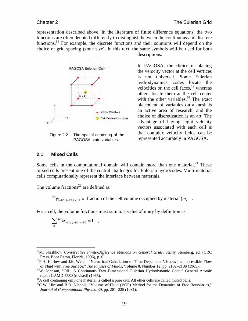
descriptions. In PAGOSA, the choice of placing the velocity vector at the cell vertices is not universal. Some Eulerian hydrodynamics codes locate the velocities on the cell faces,19 whereas others locate them at the cell center with the other variables.20 The exact placement of variables on a mesh is an active area of research, and the choice of discretization is an art. The advantage of having eight velocity vectors associated with each cell is that complex velocity fields can be represented accurately in PAGOSA.
2.1 Mixed Cells
Some cells in the computational domain will contain more than one material.21 These mixed cells present one of the central challenges for Eulerian hydrocodes. Multi-material cells computationally represent the interface between materials. The volume fractions22 are defined as
( )1/2, 1/2, 1/2 fraction of the cell volume occupied by material ( )m
i j k m .
For a cell, the volume fractions must sum to a value of unity by definition as
( )1/2, 1/2, 1/2 1m
i j km
,
18M. Shashkov, Conservative Finite-Difference Methods on General Grids, Stanly Steinberg, ed. (CRC
Press, Boca Raton, Florida, 1996), p. 6. 19F.H. Harlow and J.E. Welch, “Numerical Calculation of Time-Dependent Viscous Incompressible Flow
of Fluid with Free Surface,” The Physics of Fluids, Volume 8, Number 12, pp. 2182–2189 (1965). 20W. Johnson, “OIL, A Continuous Two Dimensional Eulerian Hydrodynamic Code,” General Atomic
report GAMD-5580 (revised) (1965). 21A cell containing only one material is called a pure cell. All other cells are called mixed cells. 22C.W. Hirt and B.D. Nichols, “Volume of Fluid (VOF) Method for the Dynamics of Free Boundaries,”
Journal of Computational Physics, 39, pp. 201–225 (1981).
Figure 2.2. The spatial centering of the PAGOSA state variables.

Chapter 2 The Eulerian Grid
20
where the summation is over all the materials defined in the simulation. As the simulation progresses, the volume fractions are recomputed for each new timestep. The question is how to compute the initial volume fractions. These fractions are computed using a variation of a Monte-Carlo technique.23 Each cell is sampled with a regular array of “particles,” and the resulting statistics are used to compute the initial volume fractions. A more detailed discussion is given in Appendix B. Most cells in a simulation are pure cells. The single-material-governing equations shown in Chapter 1 apply directly in this case. For example, cell average pressures are identical to the material pressures. No interfaces exist in these cells.24 On the other hand, mixed cells provide a richness and complexity to the solution of the governing equations. In a mixed cell, each material possesses its own density, internal energy, and pressure. In general, no attempt is made to force a pressure or temperature equilibrium between the individual materials (see Chapter 13 for a more complete explanation). The cell average pressure is the volume fraction average of each material pressure. Each material in a mixed cell has its own interface represented by a plane; in this way, the materials can be localized within the cell.
2.2 Finite Differences
It is natural to divide the simulation time interval [0,T] into short subintervals, with a step denoted t . In general, the time intervals will change as the simulation progresses [i.e., the time interval (also called the timestep) will change, depending on the exact physical state at that time]. The simulation time after N steps is
01
NN n
n
t t t
, the simulation time at cycle N .
The finite difference method is a numerical technique for approximating the solution of partial differential equations. A partial derivative is replaced with a finite difference as, for example, the partial time derivative of an arbitrary function
11/2, 1/2, 1/2 1/2, 1/2, 1/2
n ni j k i j k
nt t
, (2.1)
where we have used the standard notation 1 1
1/2 1/2 1/2 1/2, 1/2, 1/2( , , , )n ni j k i j kt x y z .
Now suppose we wish to create a finite difference approximation for the equation
23William H. Press, Brian P. Flannery, Saul A. Teukolsky, and William T. Vetterling, Numerical Recipes in
Fortran: The Art of Scientific Computing, second edition (Cambridge University Press, New York, New York, 1992), pp. 155–158.
24The only pathological exception is when two adjacent pure cells have different materials. The material interface coincides with the cell face.

Chapter 2 The Eulerian Grid
21
( , )F t xt
, and (2.2a)
1
1/2, 1/2, 1/2 1/2, 1/2, 1/21/2, 1/2, 1/2
n ni j k i j k n
i j knF
t
, 1n n nt t t . (2.2b)
Solving this equation yields the following algebraic equation: 1
1/2, 1/2, 1/2 1/2, 1/2, 1/2 1/2, 1/2, 1/2n n n ni j k i j k i j kt F . (2.3)
This technique will be used repetitively in the following chapters. The finite difference approximations25 to the governing equations will be developed in the following chapters.
2.3 Momentum Control Volume
The momentum control volume, or dual mesh, surrounds the vertex. This volume is staggered with respect to the original Eulerian mesh, which is created by connecting the centroids of the Eulerian cells and therefore is identical to the Eulerian mesh, but translated by half a cell in each dimension, as shown in Figure 2.3. In three dimensions, each vertex is surrounded by eight Eulerian cells.
Figure 2.3. A cross section of the momentum control volume. The two-dimensional cut of this
control volume passes through the vertex (i,j,k).
The mass of a single Eulerian cell is computed by 1 1 1 1 1 1 1 1 1 1 1 1
2 2 2 2 2 2 2 2 2 2 2 2
( ) ( ), , , , , , , ,
j ji j k i j k i j k i j k
j
m Vol , (2.4)
25R.D. Richtmyer and K.W. Morton, Difference Methods for Initial-Value Problems, second edition
(reprinted) (Krieger Publishing Company, Malabar Florida, 1994).

Chapter 2 The Eulerian Grid
22
where the summation is over all materials (j). The mass associated with the vertex is computed by
1 1 1 1 1 1 1 1 1 1 1 12 2 2 2 2 2 2 2 2 2 2 2
1 1 1 1 1 1 1 1 1 1 1 12 2 2 2 2 2 2 2 2 2 2 2
1, , 8 , , , , , , , ,
, , , , , , , ,
(
)
i j k i j k i j k i j k i j k
i j k i j k i j k i j k
Mass m m m m
m m m m
, (2.5)
and the x component of momentum associated with the vertex is
, , , , , ,i j k i j k i j kMomentum Mass U . (2.6)
The momentum control volume becomes important in the discussion of solving the momentum equations (1.2abc).
2.4 Ghost Cells
An extra layer of cells is added to the outside of the computational grid to aid in the construction and implementation of the boundary conditions. In the literature on Eulerian hydrodynamics codes, these “extra” cells are called ghost cells or guard cells. The addition of the external cells is used to extend the grid so that the solver need not be directly aware of its computational boundary. Two types of boundary conditions are implemented in PAGOSA—reflective and transmissive boundaries. These conditions are discussed in Chapter 11. The boundary conditions are applied to all six exterior faces of the computational grid. Each face of the Eulerian mesh can have a different boundary condition. Other boundary conditions may be added in the future.
2.5 Grid Decomposition
The solution of three-dimensional problems requires large amounts of memory and processing power to produce mesh-converged results in a reasonable time. The orthogonality of the grid allows for a straightforward spatial decomposition, as illustrated in Figure 2.4.

Chapter 2 The Eulerian Grid
23
Figure 2.4. Domain decomposition of an Eulerian grid. The example shows the grid being
decomposed onto eight processors. The size and shape of the decomposed grid are the same on each processor.

Chapter 2 The Eulerian Grid
24
This page intentionally left blank.

Chapter 3 Strain Rates
25
CHAPTER 3
Strain Rates
I have no satisfaction in formulas unless I feel their numerical magnitude.
-Lord Kelvin, Life of Sylvanus Thompson

Chapter 3 Strain Rates
26
This page intentionally left blank.
Chapter 3 Strain Rates
27
3 STRAIN RATES
The strain rate calculation in PAGOSA requires the evaluation of all the derivates of the velocity vector u = (U,V,W). Specifically, the derivatives that need to be evaluated are
, , , , , , and , ,U U U V V V W W W
x y z x y z x y z
.
Before we can construct a numerical approximation to the above partial derivatives, we need to take a mathematical detour. Start with the divergence theorem26
3 2nV S
d x d x F F . (3.1)
Let F c , where c is a constant vector 0 and is a scalar that is a function only of position. Then we have
3 2nV S
d x d x F c . (3.2)
However, the divergence produces
( ) F c c c c (3.3) because c is a constant vector. In this case, the divergence theorem reduces to
3 2ˆ 0nV S
d x d x c . (3.4)
Because c is nonzero and arbitrary, the dot product cannot be zero unless the quantity inside the brackets is zero.
Next, take the limit of the volume as it approaches zero. In this limit, we assume that the gradient is uniform and constant over the volume or has a mean value27 of
3 3 2
0 0 0ˆlim lim lim n
Vol Vol VolV V S
d x d x d x
, (3.5)
where 3
V
d x Vol .
26P. Morse and H. Feshbach, Methods of Theoretical Physics, Part I (McGraw Hill, New York, 1953), pp.
37–39. 27In the sense of given by the mean value theorem for integration.

Chapter 3 Strain Rates
28
Then under these circumstances,
2
0
1ˆlim n
VolS
d xVol
. (3.6)
Apply this new definition of the gradient to a single cell in the Eulerian mesh. The volume element is Vol x y z , the unit normals n are the Cartesian unit vectors, and the surface areas are those of the cell.
The gradient of a scalar field, in this case the x component of the velocity U , can be computed from the surface integral of the velocity field
1
0
1lim i i
Vol
U d y d z U d y d z U UU
x x y z x y z x
. (3.7)
The term in the square brackets is the integral average of the velocity over the relevant surface area. Evaluating the integrals at the limits of the integration produces the final result28 in Eq. (3.7). iU is the area-averaged velocity on the x face of the cell. The value of iU is computed as the arithmetic average of the corner vertex velocities:29 1
, , , 1, , , 1 , 1, 14 ( )i i j k i j k i j k i j kU U U U U . (3.8)
The scheme is shown in Figure 3.1. The other gradients are handled similarly.
Figure 3.1. The gradient finite difference computation.
28The difference scheme presented is spatially second-order accurate. 29The integral average is approximated by the arithmetic average of the four corner velocities. However, the
same answer is arrived at if it is assumed that the velocity is a bilinear function of position on the face.

Chapter 3 Strain Rates
29
The strain rates are defined as
1
,2x x x y
U U Ve e
x y x
, (3.9a,b)
1
,2y y x z
V U We e
y z x
, and (3.9c,d)
1
,2z z y z
W V We e
z z y
, (3.9e,f)
and the finite difference approximations are
1 1 12 2 2
1, ,
i ix x i j k
U Ue
x
, (3.10a)
1 1 12 2 2
1 1, ,
1
2j j i i
x y i j k
U U V Ve
y x
, (3.10b)
1 1 12 2 2
1 1, ,
1
2k k i i
x z i j k
U U W We
z x
, (3.10c)
1 1 12 2 2
1
, ,
j jyy i j k
V Ve
y
, (3.10d)
1 1 12 2 2
11, ,
1
2j jk k
y z i j k
W WV Ve
z y
, and (3.10e)
1 1 12 2 2
1, ,
k kz z i j k
W We
z
. (3.10f)
Note that the strain rates are cell-centered quantities, whereas the velocities are vertex centered. In mathematical terms, the difference operator maps vertex quantities to cell-centered quantities.
Finally, the divergence is computed as x x y y z ze e e u , (3.11)
and the finite difference approximation is
1 1 12 2 2
11 1, ,
j ji i k ki j k
V VU U W W
x y z
u . (3.12)

Chapter 3 Strain Rates
30
This page intentionally left blank.

Chapter 4 Operator Splitting
31
CHAPTER 4
Operator Splitting
No need to ask. He’s a smooth operator.
-Sade, Diamond Life (1984)

Chapter 4 Operator Splitting
32
This page intentionally left blank.

Chapter 4 Operator Splitting
33
4 OPERATOR SPLITTING
Operator-splitting methods are mathematical techniques used for solving partial differential equations. These methods are commonly used to reduce the computational effort required to solve the complex governing equations into a simpler set of equations. We begin with the three-dimensional (3D) Euler equations:30 Conservation Law
0 U V Wt x y z
u Mass , (4.1)
1
0 U U U U P
U V Wt x y z x
Momentum (X) , (4.2)
1
0 V V V V P
U V Wt x y z y
Momentum (Y) , (4.3)
1
0 W W W W P
U V Wt x y z z
Momentum (Z) , and (4.4)
0 E E E E P
U V Wt x y z
u Internal energy , (4.5)
where the velocity vector is defined as ( , , )U V Wu . A variety of approaches exists for the differencing of the equations. The method used in PAGOSA is based on the “Strang operator-splitting” technique.31 The above equations all have the form
1 2 3( ) 0L L Lt
, (4.6)
where is any of the variables (i.e., , , , , U V W E ). The operators L1, L2, and L3 are linear (spatial) partial differential operators. If 1D is a finite-difference approximation to 1L , then the finite-difference equivalent32 of the above operator equation is simply
11 2 3(1 )n nD t D t D t . (4.7)
This equation can be rewritten to within a second-order approximation as
1 21 2 3(1 ) (1 ) (1 ) ( )n nD t D t D t O t . (4.8)
30The body forces and stress deviators are unnecessary for this discussion. 31Gilbert Strang, “On the Construction and Comparison of Difference Schemes,” SIAM Journal of
Numerical Analysis, Volume 5, Issue 3, pp. 506–517 (September 1968). 32A variation of Eq. (2.3).

Chapter 4 Operator Splitting
34
The time operator is “split” in the specific sequence:
1 2 3, , , and
,
L L Lt t t
t t t t
(4.9)
or, in the finite-difference form,
1
2
13
(1 )
(1 )
(1 )
n
n
D t
D t
D t
, (4.10)
which will provide a second-order accurate solution of the original equations.33 The attraction of operator splitting is clear.34 The operator splitting replaces a complex set of equations with three much simpler equations.35 The PAGOSA version of this operator-splitting technique results in the following equations.
4.1 Lagrangian Phase
Conservation Law
0t
u Mass , (4.11)
10
U P
t x
Momentum (X) , (4.12)
10
V P
t y
Momentum (Y) , (4.13)
10
W P
t z
Momentum (Z) , and (4.14)
0E P
t
u Internal energy . (4.15)
The equations in the Lagrangian phase are simply the 3D Lagrangian hydrodynamic equations, the difference properties and behaviors of which are well understood from decades of experiences with Lagrangian hydrocodes. The remainder of the technique results in three additional sets of equations associated with the three Cartesian axes.
33The second-order accuracy is described in Chapter 5 (Integration of the Hydrodynamic Variables). 34G.I. Marchuk, Methods of Numerical Mathematics, Second Edition, translated by A.A. Brown (Springer-
Verlag, New York, 1982), Section 9.4, pp. 421-439. 35D. Gottlieb, “Strang-Type Difference Schemes for Multi-Dimensional Problems,” SIAM Journal of
Numerical Analysis, Volume 9, Issue 4, 650–661 (September 1972).

Chapter 4 Operator Splitting
35
4.2 X Advective Phase Conservation Law
0Ut x
Mass , (4.16)
0U U
Ut x
Momentum (X) , (4.17)
0V V
Ut x
Momentum (Y) , (4.18)
0W W
Ut x
Momentum (Z) , and (4.19)
0E E
Ut x
Internal energy. (4.20)
4.3 Y Advective Phase Conservation Law
0Vt y
Mass , (4.21)
0U U
Vt y
Momentum (X) , (4.22)
0V V
Vt y
Momentum (Y) , (4.23)
0W W
Vt y
Momentum (Z) , and (4.24)
0E E
Vt y
Internal energy. (4.25)
4.4 Z Advective Phase Conservation Law
0Wt z
Mass , (4.26)
0U U
Wt z
Momentum (X) , (4.27)
0V V
Wt z
Momentum (Y) , (4.28)
0W W
Wt z
Momentum (Z) , and (4.29)
0E E
Wt z
Internal energy . (4.30)
These equations are the Eulerian-, remap-, or advection-phase equations.

Chapter 4 Operator Splitting
36
The advection phase essentially forms a three-stage remapping procedure from the distorted Lagrangian grid (produced by the Lagrangian phase) back to the original Eulerian grid.36 The Lagrangian phase may be regarded as a sequence of computations based on the (fictitious) Lagrangian grid, which coincides with the Eulerian mesh at the beginning of the phase. The advection phases conduct the transport of mass and material quantities between cells and may be viewed as a remapping of the distorted Lagrangian grid back onto the fixed Eulerian grid. In the Lagrangian phase, the density has a constant value and is adjusted at each new timestep by the mass transport of the advection phases. Figure 4.1 illustrates the situation where the x-advection remap is executed first. However, the three 1D advection phases in the orthogonal coordinate directions should alternate (permute) in sequence in successive timesteps to achieve overall second-order accuracy in time. The advection remap permutation tends to mitigate any directional bias in each computational cycle. The choices of how to start the permutation cycle and which permutations to use are outstanding research issues. In PAGOSA, all six spatial permutations are used, beginning with the x direction.
Figure 4.1. A typical sequence of Lagrangian and advection steps.
36Methods that perform the advection in a single conservative step are collectively called unsplit advection
methods. Although unsplit methods have a theoretical advantage over operator-splitting methods, the advantage remains largely theoretical.

Chapter 4 Operator Splitting
37
In PAGOSA, the advection order is permuted as
Timestep Advection Order
1 X-Y-Z 2 Z-X-Y 3 Y-Z-X 4 X-Z-Y 5 Y-X-Z 6 Z-Y-X 7 X-Y-Z (permutations repeat every six timesteps)
etc. Next, we examine the procedures that PAGOSA uses to solve the individual phases—the Lagrangian phase and the three advection phases. Notice that the variables , , , ,U V W E have been split into two. For example, a density is associated with the Lagrangian phase, and another is associated with the Eulerian (remap) phase. During a computational timestep, both sets of variables are computed and used.
4.5 Lagrangian Phase
The solution of the Lagrangian mass conservation, Eq. (4.11) in our finite-difference form, is37
1 [1 ( ) ]n nVol Vol t u , and 1 1( / )n n n nVol Vol . (4.31a,b) If all of the materials within the zone are assumed to undergo uniform compression (or expansion) during the timestep, then all of the individual volume fractions remain unchanged. This assumption is clearly poor for cells containing mixtures of solids and liquids or gases. The actual integration of the Lagrangian phase, Eq. (4.31), is discussed in Chapter 5, Integration of the Hydrodynamic Variables. The time centering of the divergence and timestep is also discussed in this chapter.38 Finally, notice that the product of the divergence and the timestep is a dimensionless quantity that “controls” the fractional change in volume for that single timestep. This observation implies that the timestep should be limited by the inverse of the divergence of the velocity: one of several limits placed on the timestep. These timestep controls are discussed in Chapter 9.
37See Appendix D for the complete derivation of this expression. 38The complete spatial and time indices have been omitted in Eq. (4.31) for clarity.

Chapter 4 Operator Splitting
38
The Lagrangian momentum equations [Eqs. (4.12), (4.13), and (4.14)] are the next to be solved. The components of the pressure gradient can be put in a finite-difference form using the same methodology developed in Chapter 3. However, because the velocity is spatially vertex centered, the relevant volume is the momentum control volume surrounding the vertex.39 The gradient40 is
1/2 1/2
0
( )lim i i i
Vol
P dy dz P P AreaP
x x y z x y z
, (4.32)
where the Areai is the relevant surface area of the momentum control volume and the volume in the denominator is the momentum control volume associated with the vertex located at ( , , )i j k . The average cell-centered pressure P is used to compute the gradient. The finite-difference form of Eq. (4.12) is
11/2 1/2( )
n nn ni ii i i
n
i
U U P P Area
t x y z
. (4.33)
Notice that the denominator on the right-hand side of the equation is simply the mass of the momentum control volume. One modification is necessary for this equation. The artificial viscosity is an additional “pressure” that can contribute to the acceleration. With the artificial viscosity term, Q, added, the equation is
1/2 1/21 1/2 1/2( ) ( )n nn ni in n ni i i i
i i ni
P Q Area P Q AreaU U t
Mass
. (4.34)
The term inside the brackets is the x component of the acceleration. All components of accelerations are limited so that “numerical” noise is suppressed in the simulation. A user cutoff parameter is used to suppress small accelerations. The Q term will contribute only in a few cells around shock locations. Otherwise, it has a value of zero away from shocks.41 The artificial viscosity is added for purposes of numerical stability, entropy production at shocks, and energy conservation. Equation (4.34) is the x-momentum finite-difference solution of the Lagrangian-phase equations.42
39See Section 2.3 for a description of the momentum control volume. 40The gradient is computed as in Eq. (3.6); however, in this case, the areas and volumes are computed with
respect to the vertex-centered momentum control volume. 41See Chapter 8 for details. 42The gravitational body forces are included by simply adding
xg t to the right-hand side of Eq. (4.34).

Chapter 4 Operator Splitting
39
For vertices surrounded by cells of void, the velocities are zero. The vertex mass (Massi) is computed from the eight surrounding Eulerian cells as
18
nnniiMass Vol , (4.35)
where the mass is computed from the average cell density and the Eulerian cell volumes. This velocity equation is used in the predictor-corrector integration of the Lagrangian equations [Eqs. (4.11)–(4.15)]. The integration algorithm is discussed in Chapter 5. The Lagrangian energy equation (4.15) is solved in the same manner as (4.11).
4.5.1 Lagrangian Setup for Advection The last step in the Lagrangian phase is to compute the volume fractions that will be advected in the advection phases. The idea is to compute the volume fraction of the advected portion of a material on one side of a plane that passes through the Eulerian cell, as shown in Figure 4.2.
Figure 4.2. A cross section of an Eulerian cell showing a material interface with a direction vector µ, a volume fraction to be advected ε (relative to the full cell volume Vol), and the volume fraction of the advected portion of the material Vp.
In this case, we know the volume of the cell (Vol), we know the direction vector associated with the interface (µ), and we know that this vector points out of the material

Chapter 4 Operator Splitting
40
that lies “behind” the plane. The volume fraction of the advected portion of the material is what is to be computed. The derivation of the algorithm used to calculate the advection volumes is given in Appendix G.43 The advected portion of material (m) is given by pv v ( , ) μ , (4.36)
where
11 12 (1 ) μ (4.37)
and v is the volume fraction of material within a unit cube, which is behind the interface plane. Note that if 0 , then the plane lies entirely outside the advection volume and
pv 0 . Conversely, if max , then v 1 and pv . The algorithm described above is based on the Los Alamos National Laboratory publication LA-UR-07-2274.44 The complete derivation is presented in that document. The interface reconstruction is an integral part of the advection process. An example is shown in Figure 4.3. Four materials exist in a single Eulerian cell at a moment in time. A priority number is associated with each material. The priority number provides an ordering to the material advection sequence. This “onion skin” method45 is used in PAGOSA to provide a systematic reconstruction for the multi-material, multiple interface cells (mixed cells). The last material is computed separately so that material masses and volume fractions are conserved. The order of material advection has not been addressed. PAGOSA uses a scheme whereby each material is given a priority. The advection order starts with priority 1 through the maximum number of materials. There are several potential problems with this algorithm. The priorities for each material are in general spatially and temporally dependent, but are instead arbitrarily specified as constants by the user.46 Nothing precludes the intersection of interfaces within a cell (resulting in negative volume fluxes).47 Intersections of material (T and Y junctions) cannot be properly 43 The definitions of the variables in Eqs. (4.36) and (4.37) are detailed in Appendix G. 44Chuck Zemach, “Notes on Calculation of the Volume of a Stretched Cube behind a Truncating Volume,”
Wayne Weseloh, editor, Los Alamos National Laboratory report LA-UR-07-2274 (March 1, 2007). 45David L. Youngs, “Time-Dependent Multi-Material Flow with Large Fluid Distortion,” Numerical
Methods for Fluid Dynamics, K.W. Morton and M.J. Baines, editors, (Academic Press, London England, 1982), pp. 273–285.
46Wayne Weseloh, “PAGOSA Input Reference Manual,” Version 17.0, Los Alamos National Laboratory report LA-CP-10-00113, p. 64 (January 2010).
47The probability of this occurrence increases with the number of materials in a cell.

Chapter 4 Operator Splitting
41
represented.48 In addition, a poor normal (μ ) estimation can lead to misrepresentations in the interface topology.
Figure 4.3. An Eulerian cell containing four materials separated by three distinct interfaces (left)
is simplified into a sequence of three separate two-material (one-interface) representations (right) by accumulating materials at each step in the sequence. The accumulation order depends on the specific material priorities [e.g., the priority 1 material is treated first (second left); the priority 2 material is accumulated next (third left), followed by the priority 3 material]. The numbers refer to the priority number.
An excellent review article on the volume of fluid interface treatments is given by Pilliod and Puckett.49
48A. Caboussat, M. Francois, R. Glowinski, D. Kothe, and J. Sicilian, “A Numerical Method for Interface
Reconstruction of Triple Points within a Volume Tracking Algorithm,” Mathematical and Computer Modelling, Volume 48, pp. 1957–1971 (2008).
49James E. Pilliod Jr. and Elbridge G. Puckett, “Second-Order Accurate Volume-of-Fluid Algorithms for Tracking Material Interfaces,” Journal of Computational Physics, Volume 199, pp. 465–502 (2004).

Chapter 4 Operator Splitting
42
4.6 Advection Phases
In the advection phase (also called the remap phase), the hyperbolic advection equation
0at x
(4.38)
is integrated forward in time, where the variable represents any advected (usually conserved) quantity, such as the mass, momentum, specific internal energy, and stress deviator. The characteristic speed a is the local time-centered fluid velocity in that cell. A variant of van Leer’s50 monotonic upwind scheme proposed by Youngs51 is currently used in PAGOSA.
Advection: The horizontal flow of water or air. Webster’s College Dictionary, 1991 Consider the 1D x-advection equation for the conservation of mass [as shown in Eq. (4.16) repeated below]. The partial differential equation is
0Ut x
.
The general solution of this equation is
( , ) F( )x t x U t , (4.39)
where F is an arbitrary differentiable function. In this case, the function represents a density wave traveling to the right with speed U , which has a shape that does not change as it moves. The initial wave profile is given by ( ,0) F( )x x , which is d’Alembert’s solution to the advection equation. An example of the solution is shown in Figure 4.4 for a Gaussian pulse as an initial condition.
50B. van Leer, “Towards the Ultimate Conservative Difference Scheme IV. A New Approach to Numerical
Convection,” Journal of Computational Physics, Volume 23, Issue 3, pp. 276–299 (March 1977). 51David L. Youngs, “Time Dependent Multi-Material Flow with Large Fluid Distortion,” Numerical
Methods for Fluid Dynamics, K.W. Morton and M.J. Baines, editors (Academic Press, London, England, 1982), pp. 273–285.

Chapter 4 Operator Splitting
43
Figure 4.4. The solution of the advection equation.
The precise finite-difference form of Eq. (4.16) depends on the sign of the velocity U. The differences are always on the “upwind” (or upstream) side of the cell at which the gradient is being evaluated. Mathematicians often refer to difference equations just with positive coefficients52 and therefore obscure the issue. In PAGOSA, the finite-difference equation is most generally written as
1 12 2
11
0n n n n
i ii iU
t x
, if 0U , and (4.40a)
1 12 2
11
0n n n n
i ii iU
t x
, if 0U , (4.40b)
where i is the density at the i cell boundary. The cells used in constructing the gradient depend on the sign of the velocity, as shown in Figure 4.5. Rewriting Eq. (4.34a) for the case 0U , we have
1 12 2
11( )n n n n
i ii i
, (4.41)
where is the Courant number. Mathematically, it is defined as
( / )U t x definition of the Courant number.53
52G.E. Forsythe and W. Wasow, Finite Difference Methods for Partial Differential Equations (Wiley,
Hoboken, New Jersey, 1960). 53The term is named after Richard Courant (1888–1972), a mathematician whose work in the analysis of
numerical methods laid much of the groundwork for modern computational fluid dynamics.
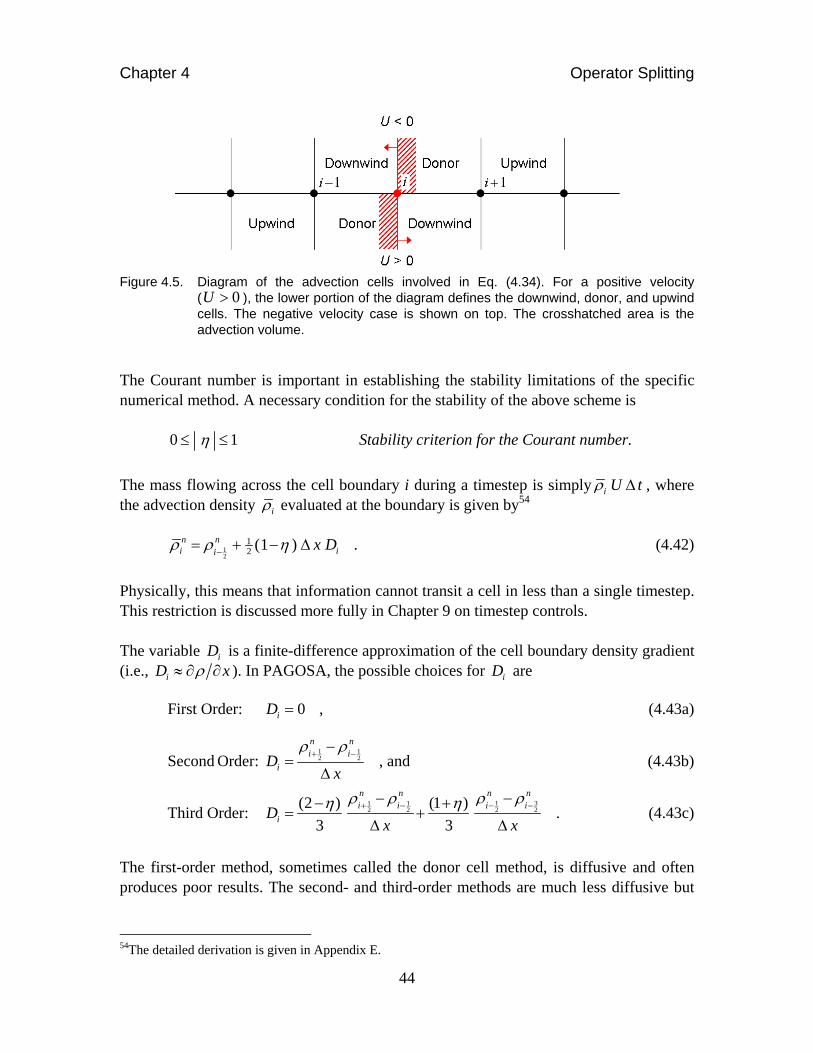
Chapter 4 Operator Splitting
44
Figure 4.5. Diagram of the advection cells involved in Eq. (4.34). For a positive velocity
( 0U ), the lower portion of the diagram defines the downwind, donor, and upwind cells. The negative velocity case is shown on top. The crosshatched area is the advection volume.
The Courant number is important in establishing the stability limitations of the specific numerical method. A necessary condition for the stability of the above scheme is 0 1 Stability criterion for the Courant number.
The mass flowing across the cell boundary i during a timestep is simply i U t , where the advection density i evaluated at the boundary is given by54
12
12 (1 )n n
i iix D . (4.42)
Physically, this means that information cannot transit a cell in less than a single timestep. This restriction is discussed more fully in Chapter 9 on timestep controls. The variable iD is a finite-difference approximation of the cell boundary density gradient (i.e., iD x ). In PAGOSA, the possible choices for iD are First Order: 0iD , (4.43a)
Second Order: 1 12 2
n ni i
iDx
, and (4.43b)
Third Order: 1 31 122 2 2
(2 ) (1 )
3 3
n nn nii i i
iDx x
. (4.43c)
The first-order method, sometimes called the donor cell method, is diffusive and often produces poor results. The second- and third-order methods are much less diffusive but
54The detailed derivation is given in Appendix E.

Chapter 4 Operator Splitting
45
suffer from nonphysical oscillations and occasionally negative densities. These deficiencies are corrected by limiting the density gradients in the following manner:
1 31 122 2 2min , 2 , 2
n nn nii i i
i iD S Dx x
, (4.44)
where
1 12 2
1 1 1 32 2 2 2
1 12 2
1
0 sign ( ) sign ( )
1
n ni i
n n n ni i i i
n ni i
S
, (4.45)
which is the Youngs/van Leer gradient limiter method.55 Details of the methodology are given in Appendix E. The above discussion applies to the density equations [Eqs. (4.16), (4.21), and (4.26)] and the internal energy equations [Eqs. (4.20), (4.25), and (4.30)]. The actual integration of the advection phase equations is discussed in Chapter 5, Integration of the Hydrodynamic Variables.
4.6.1 Advection of Momentum The final equations to be solved [Eqs. (4.17)–(4.19), (4.22)–(4.24), and (4.27–4.29)] describe the evolution of the velocity field. For example [as shown in Eq. (4.17) repeated below],
0U U
Ut x
is the x-momentum update for the x-advection phase. The momentum advection proceeds in exactly the same way as that previously described in Appendix E, with two important differences. The control volume of interest in this case is the momentum control volume centered on the cell vertex. The fundamental variable in this case is momentum instead of velocity. From the cell-centered advection described previously, we know the mass in the advection control volume before and after the three advection phases. Upwind,
55David L. Youngs, “Time-Dependent Multi-Material Flow with Large Fluid Distortions,” Numerical
Methods for Fluid Dynamics, K.W. Morton and M.J. Baines, editors (Academic Press, London, England, 1982), pp. 273–285.

Chapter 4 Operator Splitting
46
downwind, and donor cells are identified by the amount of mass crossing the surface of the control volume. Downwind is assumed to be a positive mass flux in the positive coordinate direction. Imagine the indices in Figure 4.5 shifted half a cell to the right:
11
n nn i i in outi n
i
Mass U Flux FluxU
Mass
, (4.46)
where the Flux is the momentum flux at the surface of the momentum control volume. It is simply a statement of the conservation of linear momentum.56 In this way, the linear momentum is conserved by construction. The momentum flux is computed as
1 12 2
12 (1 )n n n
i ii iFlux Mass U D
, (4.47)
where the mass increment is computed in the direction of the advection [W in the case of Eq. (4.27) shown above]. Just as with the cell-centered advection, three advection sweeps are performed after the Lagrangian phase occurs. All of the advection sweeps happen in concert, as shown in Figure 0.3. The fluxes are computed at cell centers using the variable iD , which in this case is a finite-difference approximation of the vertex velocity gradient (i.e., iD U x ). In PAGOSA, the possible choices for iD are First Order: 0iD , (4.48a)
Second Order: 1n ni i
i
U UD
x
, and (4.48b)
Third Order: 1 1(2 ) (1 )
3 3
n n n ni i i i
i
U U U UD
x x
. (4.48c)
These gradient limiters are again used to suppress oscillations and enforce a consistency with the cell-centered advection:
1 1
min , 2 , 2n n n ni i i i
i i
U U U UD S D
x x
, (4.49)
56David J. Benson, “Momentum Advection on a Staggered Mesh,” Journal of Computational Physics,
Volume 100, pp. 143–162 (1992).

Chapter 4 Operator Splitting
47
where
1
1 1
1
1
0 sign ( ) sign ( )
1
n ni i
n n n ni i i i
n ni i
U U
S U U U U
U U
(4.50)
and 1
2( / ) /n n n
i iiW t x Mass Mass . (4.51)
See Section 5 in Appendix E for the motivation of this expression.
4.6.2 Energy Advection The internal energy advection equations [Eqs. (4.20), (4.25), and (4.30)] are solved in a slightly different manner from that shown for the densities. Start with the internal energy equation [as shown in Eq. (4.20), which is repeated below]:
0E E
Ut x
.
Then apply the substitution E E in the above equation. The result is
( ) ( )
0 0 0
E E E EU U E U
t x t x t x
E
. (4.52)
Thus, the conservation law applies equally well to the product of density and internal energy. The finite-difference equation of this new equation is
1 1 1 12 2 2 2
1 11 1
0n n n n
i i i ii i i iE E E E
Ut x
. (4.53)
Rewritten in the same style as Eq. (4.41), we have
1 1 1 12 2 2 2
1 11 1
n n n ni i i ii i i i
tE EE E U
x
. (4.54)
Now the mass associated with the advection volume is
i i im U A t . (4.55)

Chapter 4 Operator Splitting
48
The first term in the square brackets of Eq. (4.54) can be manipulated in the following way:
12
1 1 12 2 2
12
12
1 12 2
( ) iiii i ii i ii ii
i i i i
iii iii
i i
EmE EU A t mtEU
x x A V V
Em mE
m m
. (4.56)
Thus, the internal energy update now appears as
11 1 1 1 322 2 2 2 2
1 11
n n n n n ni iii i i i i
E EE E
, (4.57)
where57 1
2/i i
m m . (4.58)
The densities at all of the necessary spatial and temporal positions are known, so the internal energy then may be computed with the same advection scheme presented earlier. Multiplying by the updated advection volume, we finally have 1 1 1 1 1
2 2 2 2 2
1 11 1( ) /n n n n n
i i i ii i i i iE E Vol m E m E mass
. (4.59)
Solving this last equation completes all of the advection of all hydrodynamic variables.
57See Appendix E, Section 5 for details.

Chapter 5 Integration of the Hydrodynamic Variables
49
CHAPTER 5
Integration of the Hydrodynamic Variables
Nature laughs at the difficulties of integration.
-Pierre-Simon Laplace, The Armchair Science Reader (1959)

Chapter 5 Integration of the Hydrodynamic Variables
50
This page intentionally left blank.

Chapter 5 Integration of the Hydrodynamic Variables
51
5 INTEGRATION OF THE HYDRODYNAMIC VARIABLES
The integration of the Lagrangian- and Eulerian-phase equations [Eqs. (4.11)–(4.30)] is described in this chapter. The equations follow the form
( , )F tt
, (5.1)
where F is a source term in the Lagrangian and Eulerian equations. For simplicity, we consider a scalar variable , which may be any of the hydrodynamic state variables. Various methods for solving the above equation are possible. The clear candidates for the time discretization are
the explicit Euler method (forward scheme): 1 ( , )n n n nt F t , (5.2)
the implicit Euler method (backward scheme): 1 1 1( , )n n n nt F t , and (5.3)
the semi-implicit Euler method (trapezoidal scheme): 1 1 11
2 [ ( , ) ( , ) ]n n n n n nt F t F t . (5.4)
Note that these schemes may be interpreted either as finite-difference approximations of the time derivative or as finite-difference approximations of the time integration of the source term. Indeed,
1
1( ) ( )n
n
tn n
tt t F dt
, (5.5)
and the various schemes can be viewed as different ways of approximating the integral. The explicit and implicit Euler methods are first-order accurate, whereas the trapezoidal scheme is second-order accurate. However, before proceeding, a serious handicap should be noted. The source term F depends on the unknown variable , and we face the problem of not being able to calculate 1 1 1( , )n n nF F t before we know 1n , which is to be computed from 1nF . A vicious circle is created here. We need to circumvent the exact calculation by searching for a good approximation.

Chapter 5 Integration of the Hydrodynamic Variables
52
Such an approximation is possible by using a guess * in the F term at time 12nt :
1 12 2 *( , )n nF F t , (5.6)
as long as the variable * is a sufficiently good estimate of 1n . The closer * is to 1n , the more faithful the scheme is to the ideal implicit value. If this estimate * is
provided by a preliminary explicit (forward) step, according to
12 1
2 ( , )n n n nt F t predictor, (5.7)
1 12 21 11 1
2 2( ) [ ( , ) ( , )]n nn n n n nF F F F t F t evaluation, and (5.8)
121 nn n t F corrector, (5.9)
then we obtain a two-step algorithm that is second-order accurate in time.58 This second-order method is a particular member of a family of so-called predictor-corrector methods, in which a guess * is used as a proxy for 1n in the computation of the complicated source terms. The integration process begins at time level nt , as shown in Figure 5.1. Figure 5.1. The integration step begins with all the variables at a time (n). The velocities are
shown as triangles and the state variables as circles. The velocities are spatially centered on vertices, whereas the other state variables are cell centered.
58William H. Press, Saul A. Teukolsky, William T. Vetterling, and Brian P. Flannery, Numerical Recipes in
Fortran: The Art of Scientific Computing, second edition (Cambridge University Press, New York, New York, 1992), Section 16.7, pp. 740–744.

Chapter 5 Integration of the Hydrodynamic Variables
53
5.1 Predictor Stage
The predictor stage of the integration (see Figure 5.2) starts with the following steps:
1/2 121 ( )n n n nVol Vol t u , (5.10a)
1/2 1/2( / )n n n nVol Vol , (5.10b)
1/2 12( )
n nn n n n
nn
P QE E t
u , and (5.10c)
1/2 1/2 1/2( , )n n nP P E . (5.10d) The internal state cell-centered variables are advanced to half-timestep values. The basic hydrodynamic variables are shown above; however, if the material has strength, then the stress deviators, plastic work, and the other strength-related variables are also advanced. This procedure also applies to the various fracture and crush variables that are chosen and initialized in a simulation. The spatial indexing has been omitted for clarity.
Figure 5.2. The predictor integration step advances the state variables to a time (n+1/2). The
velocities are advanced to a time (n+1) using the state variables, which are evaluated at a time (n+1/2).
Before the corrector stage can be applied, the velocity at the half-timestep must be computed. The velocities are vertex-centered quantities, so the appropriate volume is the momentum control volume, as described in Section 2.3. The mass associated with this control volume is the vertex mass.

Chapter 5 Integration of the Hydrodynamic Variables
54
5.2 Lagrangian Velocity Update
The Lagrangian velocity update (see Figure 5.3) begins with computing the vertex masses59:
18
n nniMass Vol and (5.11a)
1/2 1/2 1/2 1/2
1 1/2 1/2 1/2 1/2 1/2 1/2( ) ( )n n n nn n ni i i i i ii i n
i
P Q Area P Q AreaU U t
Mass
(5.11b)
and similarly for the other components of the velocity vector.60 The volume in Eq. (5.11a) is the original Eulerian cell volume and not the distorted Lagrangian volume. Equation (5.11b) is the finite-difference solution to Eq. (4.12). The spatial derivative has been discretized over the momentum control volume in the manner described in Section 4.5. The resulting velocity vector is 1 1 1 1( , , )n n n nU V W u .
Figure 5.3. The Lagrangian velocity update first integrates the velocities to the time (n+1). It
then averages the two velocities to create a temporally centered velocity un+1/2.
The half-timestep velocities and divergences are then computed as
1/2 11
2
1/2 112
( )
( ) (( ) ( ) )
n n n
n n n
u u u
u u u . (5.11c)
59 For the Lagrangian phase, remember that 1/2 1n n nMass Mass Mass . 60The term inside the brackets of Eq. (5.11b) is the acceleration. Acceleration cutoffs are applied to each
component of the acceleration terms to suppress numerical “noise” in the simulation.

Chapter 5 Integration of the Hydrodynamic Variables
55
An interesting validation for the choice of the time-centered velocity is given in Douglass and Stagg’s Los Alamos National Laboratory 2007 report.61 Energy conservation for the Lagrangian predictor-corrector integration timestep can be achieved only by the above choice of velocities.
5.3 Corrector Stage
The corrector stage (see Figure 5.4) of the integration uses the updated velocity information to construct the (n+1) values of the hydrodynamic variables for each material:
1 1/21 ( )n n n nVol Vol t u , (5.12a)
1 1( / )n n n nVol Vol , (5.12b)
1/2 1/21 1/2( )
n nn n n n
nn
P QE E t
u , and (5.12c)
1 1 1( , )n n nP P e . (5.12d)
Figure 5.4. The corrector integration step uses the time-centered velocity un+1/2 to update the state variables from time (n) to time (n+1).
61Rod Douglass and Alan Stagg, “A Vertex-Staggered Hydrodynamics Model for Compressible Flows,”
Los Alamos National Laboratory report LA-UR-07-6986 (2007). Section 4.1.5 gives the detailed derivation.

Chapter 5 Integration of the Hydrodynamic Variables
56
The corrector completes the integration for a timestep. The procedure is carried out for each material in a cell. Thus, each material in a cell has its own density, internal energy, pressure, etc. No pressure or temperature equilibrium is enforced in this methodology. In the above discussion, it has been assumed that the divergence of the velocity is applied uniformly to all materials in a cell. Uniform compression for all materials in a mixed cell is only one of the divergence methods available in PAGOSA. The divergence is related to the compression of the material [see Eqs. (1.6) and (1.7) and Appendix D]. The solution to the basic Navier-Stokes hydrodynamic equations is now complete. Each of the governing equations has been solved. An outline of the equations and solutions is given in Table 5.1. The mass, momentum, and energy conservation laws are completely represented. The derivations and solutions presented thus far have omitted the stress deviators for brevity. The development of the algorithms dealing with strength is delayed until Chapter 14. The equations and solutions for the various flow-stress models available in PAGOSA are presented in Section 14.4. Each component of a multi-material cell carries a complete set of computational variables, including the stress deviators, elastic distortional energy, and plastic strain. Following the current PAGOSA philosophy, each material suffers the same “cell” strain rate, but the constitutive relations are applied to each material independently of the others.

Chapter 5 Integration of the Hydrodynamic Variables
57
Table 5.1 A Schematic of the Hydrodynamic Variables, Their Conservation Equations, and Their Finite-Difference Solutions
Variable Governing Operator Finite-Difference Equation Splita Solution (1.1) (4.11) Lag (5.12b) (4.16) Eul (4.34) U (4.21) Eul (4.34) V (4.26) Eul (4.34) W U (1.2a) (4.12) Lag (5.11b) U (4.17) Eul (4.46) (4.22) Eul (4.46) (4.27) Eul (4.46) V (1.2b) (4.13) Lag (5.11b) V (4.18) Eul (4.46) (4.23) Eul (4.46) (4.28) Eul (4.46) W (1.2c) (4.14) Lag (5.11b) W (4.19) Eul (4.46) (4.24) Eul (4.46) (4.29) Eul (4.46) E (1.10) (4.15) Lag (5.12c) E (4.20) Eul (4.59, Appendix E.5) (4.25) Eul (4.59, Appendix E.5) (4.30) Eul (4.59, Appendix E.5) P (1.9) N/A (Chapter 6) aThe operator-splitting equations are represented by the one Lagrangian-phase equation (Lag) and three orthogonal
Eulerian-phase equations (Eul).

Chapter 5 Integration of the Hydrodynamic Variables
58
This page intentionally left blank.

Chapter 6 Equation of State
59
CHAPTER 6
Equation of State
The ideal gas law is the equation of state of a hypothetical ideal gas. It is a good approximation (…) although it has severe limitations.
-Max Planck, Treatise on Thermodynamics (1903)

Chapter 6 Equation of State
60
This page intentionally left blank.

Chapter 6 Equation of State
61
6 EQUATION OF STATE
The set of conservation equations solved in PAGOSA contains six dependent variables: velocity (three components), pressure, mass density, and specific internal energy. This system of equations is closed mathematically by specifying an equation of state (EOS) for each material. The EOS specifies the pressure for a given material as a function of the density and specific internal energy62 as
( , )P P E (6.1) for each material (m) in the cell. A few of the forms of this equation are described in the following pages. The average pressure in a cell is simply the volume-fraction-weighted average of all the material pressures in a cell, as defined by
( ) ( )m m
m
P P , (6.2)
where ( )m is the volume fraction for material (m). The following notation is used in describing the various EOSs: E0 internal energy per original volume,
10
compression / expansion factor, and
0 01
1
V
V
specific volumes.
6.1 Ideal Gas EOS
One of the simplest forms of an EOS is the ideal gas law63
EOS Gas Ideal)1( EP , (6.3) where is ratio of specific heats at constant pressure and constant volume. The ideal gas law is favored for monatomic gases at high temperatures and low pressures. This law does not factor in the size of the molecules or intermolecular attractions. However, it is often used in limited regimes, with the value of adjusted to fit some data, but only to get a qualitative understanding of how the system will behave using an easily manipulated EOS.
62This type of EOS is denoted “incomplete” because the temperature cannot be calculated unless the
specific heat is known. 63It is a simply derived alternative to the well-known equation PV = nRT.

Chapter 6 Equation of State
62
6.2 Void EOS
Another commonly used EOS is void. For this EOS, the density, specific internal energy, and pressure are all set to zero:
0EOS Void0
0
PE
. (6.4)
This form has the advantage that no sound speed is computed, and therefore, the material cannot control the timestep in a simulation. The other advantage is void closure. Imagine two materials that are about to collide. The interface reconstruction within a cell allows the three materials to be represented by two planes. If the intervening material is a void, then the void closure model can be invoked. This option allows the two materials to come smoothly into contact without creating bubbles or small densities that are often problematic for any other EOS.
6.3 Polynomial EOS
A common analytic EOS is the polynomial EOS, which is often used in fitting experimental EOS data. This EOS has the form
* 2 3 * 2 30 1 2 3 0 1 2 3( ) Polynomial EOSP a a a a b b b b . (6.5)
The constants *
2a and *2b can assume different values in expansion and compression:
* 22
2
0 compression
0 expansion
c
e
aa
a
and similar expressions for *
2b . One clear simple case of the polynomial EOS is a constant pressure. In this case,
0 0 constant,a P and the other constants have the value zero. Another special case of the polynomial EOS can be demonstrated by considering the bulk modulus for adiabatic compression, which is defined as
SS
PP
)1( .
Integrating the expression, the pressure is (for moderate compression/expansion)
2 3 41 1 12 3 4
log (1 )
-1 1
eP
.

Chapter 6 Equation of State
63
Thus, to first order, the EOS is
10 P .
In terms of the polynomial EOS, 1a , and all the other constants have a value of zero.
6.4 Modified Osborne (or Quadratic) EOS
This form was originally derived by Group T-5 at Los Alamos Scientific Laboratory in the 1950s as a fit between low-pressure Hugoniot data and the high-pressure Thomas-Fermi-Dirac theory.64 One of the reasons for the particular form of the equation, sometimes called the quadratic EOS,65,66 was the small amount of memory of the computers then in use.
* 2 * 2 * 2 21 2 0 1 2 0 1 2
0
( ) ( )Osborne
a a b b b c c cP
EOS. (6.6)
Many of the original constants found by R. K. Osborne are still in use today. The constants *
2a , *2b , and *
2c assume different values in expansion and compression:
expansion
ncompressio
0
0
2
2*2
e
c
a
aa
and similar expressions for *
2b and *2c . The traditional Osborne EOS is recovered by
setting 2 2 2 2 2 2 , , and 0e c e c e ca a b b c c .
The constants of the Osborne EOS need to be scaled in the case of an alloy or isotope where the constants are not known. A suggested scaling is given by Lambourn:67
1 2,a a should be scaled with 20 ,
0 1 2 0, , ,b b b should be scaled with 0 , and
0 1,c c should not be scaled (should remain at their original values).
64R.P. Feynman, N. Metropolis, and E. Teller, “Equations of State of Elements Based on the Generalized
Fermi-Thomas Theory,” Physical Review, Volume 75, Issue 10, p. 1561 (January 1949). 65F.H. Harlow and W.E. Pracht, “Formation and Penetration of High-Speed Collapse Jets,” The Physics of
Fluids, Volume 9, Number 10, pp. 1951–1959 (October 1966). 66T.D. Riney, “Numerical Evaluation of Hypervelocity Impact Phenomena,” in High Velocity Impact
Phenomena, edited by R. Kinslow (Academic Press, New York/London, 1970), pp. 157–212. 67B.D. Lambourn, “Density Scaling for the Osborne Equation of State,” Atomic Weapons Research
Establishment (AWRE) HWH Note No. 3/80, Aldermaston, Berkshire, UK (October 1980).

Chapter 6 Equation of State
64
6.5 Jones-Wilkins-Lee (or JWL) EOS
The JWL EOS68 is often used for computing the EOS of high-explosive detonation products. Its development began with an equation proposed by Jones and Miller69 and extended by Wilkins.70 It is therefore now referred to as the JWL EOS. The EOS is written as
1 0 2 0/ /
1 0 2 0
1 1 JWL EOSR RP A e B e ER R
, (6.7)
where the five constants ( ,,, 21 RRBA, ) are experimentally determined. Note that the constants A and B have the units of pressure, whereas the other constants are dimensionless. If the high explosive (HE) is detonated by the program burn algorithm, the pressure and energy are gradually deposited into a cell over several timesteps. The pressure is scaled by a factor called the burn fraction Bf . The burn fraction values range between zero and one. A value of zero indicates that the detonation wave has not yet reached the cell, and a value of one indicates a completely burned cell. The program burn algorithm defines a “burn time” for each cell vertex in the simulation.71 Of the eight cell vertices, the difference between the minimum and maximum burn times is referred to as the burn interval for a cell. Mathematically, we have
min 1 2 3 4 5 6 7 8
max 1 2 3 4 5 6 7 8
interval max min
min
min interval min max
max
min ( , , , , , , , )
max ( , , , , , , , )
0 if
( ) / if
1 if
t t t t t t t t t
t t t t t t t t t
t t t
t t
Bf t t t t t t
t t
.
68E.L. Lee, H.C. Hornig, and J.W. Kury, “Adiabatic Expansion of High Explosive Detonation Products,”
Lawrence Radiation Laboratory, University of California report UCRL-50422 (May 2, 1968). 69H. Jones and A. Miller, “The Detonation of Solid Explosives: The Equilibrium Conditions in the
Detonation Wave-Front and the Adiabatic Expansion of the Products of Detonation,” Proceedings of the Royal Society of London. Series A, Mathematical and Physical Sciences, Volume 194, No. 1039 (November 9, 1948), pp. 480–507.
70M. Wilkins, “The Equation of State of PBX 9404 and LX04-01,” Lawrence Radiation Laboratory, University of California report UCRL-7797 (1964).
71In reactive burn models, the burn fraction is evolves according to the physics of the reaction progress.

Chapter 6 Equation of State
65
This procedure usually results in the cell pressure developing over four or five timesteps. The maximum timestep is adjusted so that a cell cannot burn in fewer steps. Tables of constants for many explosives have been compiled by Brigitta Dobratz.72 The constants used in the PAGOSA code have a slightly different form from the original JWL form. The translation between the two forms is PAGOSA Dobratz Handbooks W
B1 A
C1 0 1R 1R
B2 B
C2 0 2R 2R
e0 0 0/E E0 The main advantage of the JWL EOS lies in its ability to describe the Chapman-Jouget adiabat accurately. The above parameters have been chosen to satisfy the measured Chapman-Jouget state, the measured expansion of a cylinder test, some asymptotic thermodynamics limitations, and hydrodynamic continuity equations.
6.6 Grüneisen (or Us-Up) EOS
The most common description of solids uses the measured Hugoniot curve as a reference and uses the Grüneisen relationship to extrapolate off the reference curve. It is often the case that the Hugoniot curve can be represented over a large range of pressures as a simple linear expression73,74 in the -S PU U plane:
0S PU c s U Grüneisen EOS , (6.8a)
( / ) ( )H HP P V E E , (6.8b) 2 2
0 0 0 0 0( ) [ ( ) ]HP P c V V V s V V , (6.8c) 1
0 0 02 ( ) ( )H HE E P P V V , and (6.8d)
0 1 0( / )V V , (6.8e)
where HP is the pressure on the Hugoniot, HE is the energy on the Hugoniot, 0V is the initial specific volume ( 1
0 ), and V is the state-specific volume ( 1 ). In the above
72Brigitta M. Dobratz, “Properties of Chemical Explosives and Explosive Simulants,” Lawrence Livermore
Laboratory, University of California report UCRL-14592 (July 31, 1974). 73M. van Thiel, A.S. Kusubov, and A.C. Mitchell, “Compendium of Shock Wave Data,” Lawrence
Radiation Laboratory, University of California report UCRL-50108, Volume 1, Supplement 1 (October 1967).
74Stanley P. Marsh, LASL Shock Hugoniot Data (University of California Press, Berkeley, California, 1980).

Chapter 6 Equation of State
66
expressions, 0c and s are constants obtained from the relationship between shock speed
SU and particle speed PU . The Hugoniot pressure relation contains a simple pole at 0 0/ ( )s V V V . This relation puts a limit on the allowable density for this EOS. If a maximum density is not specified, then a maximum is imposed by
max 0 0max 99% , 21
s
s
,
where 0 is the nominal mass density. This particular EOS is sufficiently different from the others described that a short description of the derivation is warranted. The thermodynamic states off of the Hugoniot curve can be obtained by constructing a Taylor expansion, at constant density, about the reference Hugoniot curve. Mathematically, it is
2
2
2
1( , ) ( ) ( ) ( )
2H H H
P PP E P E E E E
E E
,
where ( )HE E is the displacement from the Hugoniot curve. The values denoted with the subscript H are points on the reference Hugoniot curve. The definition of the Grüneisen parameter is
/P
VE
Grüneisen relation .
It is usually assumed that the parameter is a linear function of the compression/expansion, i.e., 0 1 0( / ) , so that the higher-order terms in the Taylor expansion vanish. The EOS becomes
( , ) ( ) ( / ) [ ( ) ]H HP E P V E E .
Experimentally, it has been found that for many solids, the Hugoniot curve can be represented as a simple linear curve in the -S PU U plane. Contrary to what is usually found in the literature, 0c is not the bulk sound speed in the ambient state. Rather, it is the value of the intercept of the -S PU U line.75
75Ya Zel’dovich and Yu Raizer, Physics of Shock Waves and High Temperature Hydrodynamic Phenomena
(Dover Publications, Mineola, New York, 2002). See footnote, p. 710.
Chapter 6 Equation of State
67
6.7 SESAME EOS
A tabular EOS that represents hundreds of materials and experiments is available using the Los Alamos National Laboratory (LANL) SESAME database.76,77 The database contains EOS tables for pressure and internal energy as a function of temperature. The database library has several advantages: it can accurately represent phase transitions, it represents a wide range of temperatures and densities, and it represents the best experimental and theoretical data available at LANL. The data are inverted before they are used in PAGOSA so that the pressure is solely a function of density and internal energy. The SESAME EOS is
),( TTSESAME EPP , SESAME EOS (6.9)
where SESAMEP is the tabular EOS. The tabular database is read using the EOS package (EOSPAC) software library.78 The library software allows for various ways of interpolating and scaling the tabular data. The relation of “code” input to the tabular EOS is given by
(SR)
( ES) / SR ,T
TE E
where SR = density scaling ratio and ES = energy shift. The scaling ratio parameter SR is often useful in modeling isotopic mixtures. For example, if AT is the atomic mass for a particular SESAME EOS, an EOS for an atomic mass A is obtained by setting the scaling ratio SR = AT / A . Suppose we wish to model a gas of hydrogen (H2). The SESAME identification number for deuterium is 5263. A scaling ratio of SR = 2 scales the SESAME tabular deuterium EOS to hydrogen. Similarly, a scaling ratio of SR = 0.8 scales the SESAME tabular deuterium EOS to a 50%:50% mixture of deuterium and tritium (DT).
76S.P. Lyon and J.D. Johnson, “SESAME: The Los Alamos National Laboratory Equation of State
Database,” Los Alamos National Laboratory report LA-UR-92-3407 (October 1992). 77K.S. Holian, “T-4 Handbook of Material Properties Data Bases, Volume Ic: Equations of State,” Los
Alamos National Laboratory report LA-10160-MS (November 1984). 78David A. Pimentel, “EOSPAC 5 User Manual,” Los Alamos National Laboratory report LA-UR-03-4510,
Version 5.35, Revision 0 (August 2003).

Chapter 6 Equation of State
68
The energy shift is defined by ES = -∆E (initial → final) , where ∆E is the energy required to transform the low-density phase to the high-density phase. There are two cases. If the initial phase is stable, then the value of ES is negative. If the initial phase is metastable, then the value of ES is positive. The pressure-density curve at T = 0 K is commonly called the “cold curve” and was traditionally modeled by empirical formulas (e.g., analytic potentials combined with the Thomas-Fermi-Dirac theory). The modern theory uses relativistic electronic band structure methods to compute the cold curve. The total pressure can be thought of as being the sum of the cold-curve pressure and the thermal pressure (i.e., the pressure due to positive internal energies).
6.7.1 Ramp Treatment For the treatment of foams and certain types of phase transitions, it is possible to modify the SESAME EOS by adding a ramp (see Figure 6.1) that describes the behavior of the material under low stress. The material begins in a porous or low-density state. The EOS in this regime is
)1( 01 AP ,
where 0 is the initial density and 1A is the bulk modulus. The bulk modulus can be computed from the sound speed as
21 0A a ,
where a is the bulk sound speed. If 01A , then no ramp calculation is done. At some value of pressure
1P , the material begins to crush, or transform, to a SESAME EOS. The EOS of the “crush curve” is given by
2 0 3( 1 )P A A .
Figure 6.1. The SESAME ramp treatment.

Chapter 6 Equation of State
69
If 02A , then no crush regime exists and the equation represented by the first line is continued until it crosses the SESAME curve. The value of 2A can be computed from the crossing at the transition pressure 1P , or it can be guessed at if no other information is available:
1 12
1 1 3
P AA
P A A
if 1P is known.
2 1 /10A A if 1P cannot be measured.
The transition pressure for foams is often small (< 1 kbar). On the other hand, for a phase transition, the value of 1P must be determined from experiments. The value of 3A can be adjusted to give the appropriate slope for the crush curve. In the absence of any data, the default value ( 03 A ) should give acceptable results. However, a better value might be 79
3 1 1 2[1 / 1 / ]A P A A .
At some pressure 2P , the crush curve crosses the SESAME curve. At that point the material is “crushed.” Subsequently, the material may behave either reversibly (follow the ramp on expansion) or irreversibly (remain on the high-density phase on expansion). Foams are normally reversible; however, phase transitions may exhibit either behavior. Materials may also behave irreversibly if they melt (i.e., if the melt energy or melt temperature is exceeded).
6.7.2 SESAME Body Internal Energy Iteration 80 In some cases the initial conditions for a particular SESAME material are not completely known. For example, the user may know the initial density and a desired initial pressure but not know the corresponding initial internal energy. PAGOSA provides a solution to this dilemma by providing a mechanism for setting the initial density and pressure within a body specification. PAGOSA and EOSPAC together then iterate until the appropriate initial internal energy is found. Given the density and the desired initial pressure, the EOS is
( , )P P E .
79The value of 1P should be measured in this case. B.I. Bennett, Los Alamos National Laboratory, private
communication, October 22, 1984. 80Never use the SESAME body iteration option with the ramp treatment. The results are often wrong.

Chapter 6 Equation of State
70
If the desired initial pressure is 0P and the desired initial density is 0 , then the EOS can be written as
*0 0( , )P P E .
The problem is finding the value of internal energy *E that satisfies this relation. The algorithm for finding *E starts with the Newton-Raphson method.81 The method is often written as
1
( )
( )n
n nn
f xx x
f x
1, 2,3,..., .n max iteration .
To apply this method to our problem, we first start with an approximation for the derivative:
0
0
P PP
E E E
.
The EOSPAC derivatives are with respect to the logarithm of density and energy, so
log
P PE
E E
.
The equation now can be cast in the Newton-Raphson form
1 0( ) / /n n nE E P P P E and
1
1 01 ( ) / logn n nE E P P P E
1, 2,3,..., .n max iteration .
The iteration process completes when the pressure is within an acceptable range of 0P . The convergence criterion used in PAGOSA is
01 nP P tolerance .
Occasionally, the resulting initial internal energy has a small negative value. Some of the SESAME tables have “poor” data in particular regions or the interpolation scheme is not sufficient for the data provided. The user is always responsible for checking the results of the PAGOSA-generated initial conditions. 81William H. Press, Brian P. Flannery, Saul A. Teukolsky, and William T. Vetterling, Numerical Recipes in
Fortran: The Art of Scientific Computing (Cambridge University Press, New York, New York, 1986), pp. 254–259.

Chapter 6 Equation of State
71
6.8 Exponential EOS
The exponential EOS is unique in PAGOSA in that it specifies a pressure as a function of time. Mathematically, the form is 0( ) tP t P e , Exponential EOS
where 0P is the pressure at 0t and is the decay constant (with units of time-1). This analytic form of the EOS provides a simple time-dependent pressure that can be used in certain test problems for validation and verification.82
6.9 Becker-Kistiakowsky-Wilson High-Explosive (BKW-HE) EOS
The BKW-HE EOS combines the solid Grüneisen form and a BKW gaseous form to model a shock-initiated HE. This form is usually used to model a shock-initiated explosive as it transitions from an undetonated solid to a fully burned detonation product. The discussion follows the one given in Mader.83 The EOS computes the pressure, internal energy, specific volume, temperature, and burn fraction for solids, gases, and mixtures of the two. The following subscripts are used in this discussion: g gaseous component, H Hugoniot, i isentrope, and S solid component.
6.9.1 Solid Components The solid, undetonated HE begins with a solid Mie-Grüneisen EOS with a Walsh-Christian temperature84 fit to a fourth-degree polynomial. The solid component uses the Grüneisen form described above: 0s pU c s U ,
20 0
0 2
0 0
( )
( )s
H
s
c V VP P
V s V V
,
10 02 ( ) ( )H H sE P P V V , and
82Wayne Weseloh, “The Response of a Spherical Shell to an Impulsive Pressure,” Los Alamos National
Laboratory report LA-UR-04-1683 (March 2004). 83Charles Mader, Numerical Modeling of Explosives and Propellants, Second Edition (CRC Press, Boca
Raton, Florida, 1998), pp. 308–311. Mader calls this his Hell Of a Mess (HOM) EOS. 84John Walsh and Russell Christian, “Equation of State for Metals from Shock Wave Measurements,”
Physical Review, Volume 97, pp. 1544–1556 (1955).

Chapter 6 Equation of State
72
( )S H S HS
P P E EV
,
where
0 1 0( / )SV V ,
2 3 4( ) ( ) ( ) ( )e H e S e S e S e Slog T F G log V H log V I log V J log V , and
23890( )
( )S H S HV
T T E EC solid
.
The constant in the last equation is a conversion factor involving the mechanical equivalent of heat. The units of heat capacity Cv are (cal g-1 deg-1), and the units of internal energy are (Mbar cm3 g-1). Constants for various explosives are given in Mader’s book85 and the accompanying data CD-ROM.
6.9.2 Gaseous Components The detonation products are computed using the BKW EOS.85 2 3 4( ) ( ) ( ) ( )e i e g e g e g e glog P A B log V C log V D log V E log V ,
2 3 4( ) ( ) ( ) ( ) ( )e i e i e i e i e ilog E Z K L log P M log P N log P O log P ,
2 3 4( ) ( ) ( ) ( )e i e g e g e g e glog T Q R log V S log V T log V U log V ,
1 2 32 ( ) 3 ( ) 4 ( )e g e g e gR S log V T log V U log V ,
1( )g i g i
g
P P E EV
, and
'
23890( )
( )g i g iV
T T E EC gas
.
The parameter Z is a constant used to change the gas standard state to be consistent with the solid explosive standard state (which in PAGOSA requires the value 0Z ). The final case is when a material is a combination of the solid and gaseous states. The burn fraction Bf controls the mixture. For mixed components, we have 0 1Bf .
6.9.3 Mixed Components The specific volumes and internal energies are partitioned as a linear combination of the solid and gaseous components. The “burning” cells are assumed to be in pressure and temperature equilibrium: 85Charles Mader, Numerical Modeling of Explosives and Propellants, Second Edition (CRC Press, Boca
Raton, 1998), pp. 377–408 (Appendix E).

Chapter 6 Equation of State
73
(1 )g SV Bf V Bf V ,
(1 )g SE Bf E Bf E ,
g SP P P , and
g ST T T .
Substituting these equations into the ones above results in an equation representing the temperature difference between the solid and gas. The Secant Method86 is used to solve the resulting nonlinear algebraic equation. Limits are set at every cycle of the iteration to prevent the solution from becoming unbounded or unphysical. Convergence is achieved when the temperature difference between the solid and gaseous components is less than tdel (usually ~10 K). The solid component BKW-HE parameters are 0c intercept of the Us/Up line,
s slope of the Us/Up line, 0 the first Grüneisen ratio,
1 the second Grüneisen ratio,
0P initial pressure,
maxd maximum allowable density (solid),
F polynomial temperature coefficient, G polynomial temperature coefficient, H polynomial temperature coefficient, I polynomial temperature coefficient, J polynomial temperature coefficient, VC heat capacity (solid), and
linear coefficient of thermal expansion.
86William H. Press, Brian P. Flannery, Saul T. Teukolsky, and William T. Vetterling, Numerical Recipes in
Fortran: The Art of Scientific Computing (Cambridge University Press, New York, New York, 1986), pp. 248–251.

Chapter 6 Equation of State
74
The gaseous state parameters are A HOM polynomial coefficient for the isentropic pressure, B HOM polynomial coefficient for the isentropic pressure, C HOM polynomial coefficient for the isentropic pressure, D HOM polynomial coefficient for the isentropic pressure, E HOM polynomial coefficient for the isentropic pressure, K HOM polynomial coefficient for the isentropic internal energy, L HOM polynomial coefficient for the isentropic internal energy, M HOM polynomial coefficient for the isentropic internal energy, N HOM polynomial coefficient for the isentropic internal energy, O HOM polynomial coefficient for the isentropic internal energy, Q HOM polynomial coefficient for the isentropic temperature, R HOM polynomial coefficient for the isentropic temperature, S HOM polynomial coefficient for the isentropic temperature, T HOM polynomial coefficient for the isentropic temperature, U HOM polynomial coefficient for the isentropic temperature, '
VC heat capacity (gas),
Z a constant used to offset (shift) the gas standard state ( 0Z ), max maximum allowable density (gas), and
min minimum allowable density (gas).
The mixed state uses both the solid and gaseous parameters and the following conver-gence criteria:
maxit maximum number of iterations for the mixed component solver, and tdel temperature difference convergence value.

Chapter 6 Equation of State
75
6.10 Pmin
It is often necessary to limit the pressures resulting from the EOS evaluation. Regions of the EOS are suppressed for many reasons, which fall into three major categories. The first category is demonstrated in Figure 6.2. The plot illustrates a van der Waals loop in the EOS at room temperature. Problems arise when the material density falls below some critical value. Material sound speeds become unphysical.87 A value of Pmin is chosen to suppress the offending portion of the EOS.
Figure 6.2. Example of the use of Pmin in an EOS with a van der Waals loop.
A second way that Pmin often is used is as a simple-minded spall model. When the material pressure drops below Pmin, the pressure is held at Pmin, regardless of the density and internal energy. This application of Pmin is an awkward attempt to approximate the physics of the material in a state exceeding its dynamic tensile strength. No change is made to the stress deviators S while the material is this state.88 The third way that Pmin is used in PAGOSA is as a floor or cutoff to the EOS. For example, if it is desired that a material never go into tension during the simulation, then setting Pmin to a value of zero will allow the material to experience only compression.
87The sound speed is related to the slope of the adiabat at a given point. 88Every hydrocode implements Pmin in a different and unique manner. Reducing complicated physics to a
single parameter is at best a poor scheme.

Chapter 6 Equation of State
76
This page intentionally left blank.

Chapter 7 Sound Speed
77
CHAPTER 7
Sound Speed
There is more to life than increasing its speed.
-Mohatma Gandhi (1869–1948)

Chapter 7 Sound Speed
78
This page intentionally left blank.

Chapter 7 Sound Speed
79
7 SOUND SPEED
When a material is perturbed, the net result is a wave propagating away from the disturbed region into the undisturbed region. The speed at which the wave travels in a given medium under specified conditions is known as the speed of sound. The speed of sound does not explicitly appear in the hydrodynamics equations. However, it is used to calculate the Courant timestep (see Chapter 9). It also can be used to check the thermodynamics properties of materials in a cell. The isentropic sound speed is defined as89,90
2
S
Pc
(7.1)
at constant entropy S. This form is not convenient for computation, so it is necessary to recast the expression in terms of partial derivatives at constant density and constant internal energy. The pressure is a function of density and internal energy
( , )P P E . (7.2) The differential is
E
P PdP d dE
E
. (7.3)
The pressure also can be written as a function of density and entropy
( , )P P S . (7.4)
The differential is
S
P PdP d dS
S
. (7.5)
89L.D. Landau and E.M. Lifshitz, Fluid Mechanics (Pergamon Press, Addison-Wesley Publishing Company
Inc. Reading Massachusetts, 1959), p. 246. 90Ya. B. Zeldovich and Yu. P. Raizer, Physics of Shock Waves and High-Temperature Hydrodynamic
Phenomena (Dover Publications Inc. Mineola, New York, 2002), p. 7.

Chapter 7 Sound Speed
80
For an isentropic process, these two forms reduce to
E S
P P Pd dE d
E
. (7.6)
The internal energy is a function of density and entropy
( , )E E S . (7.7) The differential is
S
E EdE d dS
S
. (7.8)
Combining Eqs. (7.6) and (7.8) yields
E S S
P P E P
E
. (7.9)
Thus, given the definition of sound speed [Eq. (7.1)], we have
2
S E S
P P P Ec
E
. (7.10)
Using the first law of thermodynamics, for a single component system with one reversible work mode, we have
2
dE Q W
T d S p dV
PT d S d
. (7.11)
The coefficient of the second differential (density) now can be identified with the corresponding differential in Eq. (7.8). If we substitute into Eq. (7.10), the sound speed is computed for each material as
22
E
P P Pc
E
. (7.12)

Chapter 7 Sound Speed
81
The sound speed is used in various other parts of the computation cycle. For example, the sound speed is used to establish the proper timestep for each computational step.91
7.1 Ideal Gas EOS Sound Speed
For the ideal gas equation of state (EOS), the pressure and sound speed are simply
( 1)P E and
22
2( 1) ( 1)
( 1)
E
P P Pc
E
PE
PE
. (7.13)
7.2 Void EOS Sound Speed
A void material has no sound speed, so the value is deliberately set to zero:
0P , and
2 0c . (7.14)
7.3 Polynomial EOS Sound Speed
The polynomial EOS is written as
* 2 3 * 2 30 1 2 3 0 1 2 3( )P a a a a E b b b b ,
where
0
1
.
91See Chapter 9 for more details.

Chapter 7 Sound Speed
82
The partial derivatives for the sound speed calculation are
* 2 * 21 2 3 1 2 3
0 0
* 2 30 1 2 32 2
12 3 2 3
E E E
P P
Ea a a b b b
P P Pb b b b
E
such that the sound speed is
2 * 21 2 3
0
* 21 2 3
0
* 2 30 1 2 32
12 3
2 3
c a a a
Eb b b
Pb b b b
. (7.15)
7.4 Modified Osborne (or Quadratic) EOS Sound Speed
The Osborne EOS is written as
* 2 * 2 * 2 21 2 0 1 2 0 1 2
0
( ) ( )a a b b b c c cP
.
The partial derivatives for the sound speed calculation are
* * 2 *1 2 1 2 1 2
0 0
* 2 * 20 1 2 0 1 2
2 20
2 2 2 1
2( )
E E E
P P
a a b b c c
b b b c c c PP P P
E
.

Chapter 7 Sound Speed
83
Accordingly,
* * 2 *1 2 1 2 1 22
0
* 2 * 20 1 2 0 1 2
20
2 2 2 1
2( )
a a b b c cc
b b b c c c PP
. (7.16)
7.5 Jones-Wilkins-Lee (or JWL) EOS Sound Speed
The JWL EOS,
1 0 2 0/ /
1 0 2 0
1 1R RP A e B e ER R
,
is similarly evaluated in Eq. (7.12). The corresponding terms are
1 0 1 0
2 0 2 0
/ /1 02
1 0 1 0
/ /2 02
2 0 2 0
11
11
R R
E
R R
ARP Ae e
R R
BRBe e E
R R
and
2
P PP
E
.
Therefore,
1 0 1 0
2 0 2 0
/ /2 1 02
1 0 1 0
/ /2 02
2 0 2 0
11
11
R R
R R
ARAc e e
R R
BRBe e
R R
E P
. (7.17)
The above sound speed is for the detonation products of the explosive. Before and during the detonation, the pressure in the undetonated explosive is zero and the sound speed is set as follows:

Chapter 7 Sound Speed
84
2
2 2
2
0
9 0 1
1JWL
D Bf
c D Bf
c Bf
, (7.18)
where D is the detonation velocity and Bf is the burn fraction.
7.6 Grüneisen (or Us-Up) EOS Sound Speed
The Grüneisen EOS is
( / ) ( )H HP P V E E .
Differentiation according to Eq. (7.12) is provided with added complexity, where
2 20 0 0 0 0
10 0 02
0 1 0
( ) [ ( ) ]
( ) ( )
( / )
H
H H
P P c V V V s V V
E E P P V V
V V
and
where the specific volume is defined as
1/V
such that
2
2 300 0 0 0 02
12
0
12
( ) 2 ( ) ( )
( / ) ( / )
1 1
( ) ( )
H H
E E E
E E E
H H
E E E
H
P P V
V
cV s V V s V V V s V V
VV V
V V
VE E E E
V
P
00 2
( ) H
E
P PV V
.

Chapter 7 Sound Speed
85
Thus,
( / ) ( ) ( / ) ( )HH H
E E E E
PPV E E V E E
and
2 2( / )
P P PV
E
, and
2
2
( / ) ( )
( / ) ( ) ( / )
HH
E E
H
E
Pc V E E
PV E E V
. (7.19)
7.7 SESAME EOS Sound Speed
The EOS package (EOSPAC) utility software package92 extracts the pressure from the Los Alamos National Laboratory (LANL) SESAME database. The EOSPAC software also supplies the partial derivatives of pressure with respect to density and internal energy. The sound speed is computed directly from these numerical derivatives. The EOSPAC derivatives are with respect to the logarithm of density and energy, so93
1
logE E SESAME
P P
1
logSESAME
P P
E E E
,
and the appropriate substitutions then are made into Eq. (7.12). The EOSPAC software allows the tabular data to be interpolated in various ways [e.g., biquadratic (six-point) interpolation]. The choice of interpolation method will influence the results of the partial derivatives and therefore the sound speed. An additional point, not referred to earlier, concerns SESAME materials that melt during the simulation. Two SESAME tables can be loaded by PAGOSA—one for the unmelted state and one for the melted state. Certainly, the sound speeds are very different for these two states of the material. However, not every SESAME material has a corresponding SESAME melt table. Compromises and engineering approximations immediately become
92David A. Pimentel, “EOSPAC 5 User Manual,” Los Alamos National Laboratory report LA-UR-03-4510,
Version 5.35, Revision 0 (August 2003). 93The logarithms are natural logarithms (logarithms to the base e).

Chapter 7 Sound Speed
86
significant considerations. It is always important to understand and investigate the assumptions and limitations in any EOS, including the SESAME EOS.
7.8 Exponential EOS Sound Speed
The exponential EOS is
0( ) tP t P e .
In this case, the pressure is not a function of either density or internal energy, so
2 0c . (7.20) The exponential EOS is intended to be a pressure (normal stress boundary condition) for particular simulations. As a consequence, the thermodynamics of this material should play little or no role in the simulation.
7.9 PAGOSA Sound Speed
The internal sound speed computed by PAGOSA is altered in an attempt to find the largest possible “wave” velocity. The goal is to eventually compute a stable timestep for the simulation. The total sound speed,
2 2 4 2
3EOS
G Qc c
, (7.21)
is composed of three parts. The first term is the sound speed corresponding to the EOS
( , )P P E , the second term converts the sound speed to a longitudinal elastic wave speed for elastic-plastic materials, and the third term ensures the stability in the presence of shocks (Q terms) . The diagnostic information in PAGOSA returns only the isentropic sound speed. However, it is important to understand that internal to PAGOSA, the sound speed has additional terms. It is hoped that in the future, these terms can be computed individually and their influence on the timestep can be evaluated individually.

Chapter 8 Artificial Viscosity
87
CHAPTER 8
Artificial Viscosity The equations of hydrodynamics are modified by the inclusion of additional terms which greatly simplify the procedures needed for stepwise numerical solution of the equations
in problems involving shocks.
-J. von Neumann and R.D. Richtmyer (1950)

Chapter 8 Artificial Viscosity
88
This page intentionally left blank.
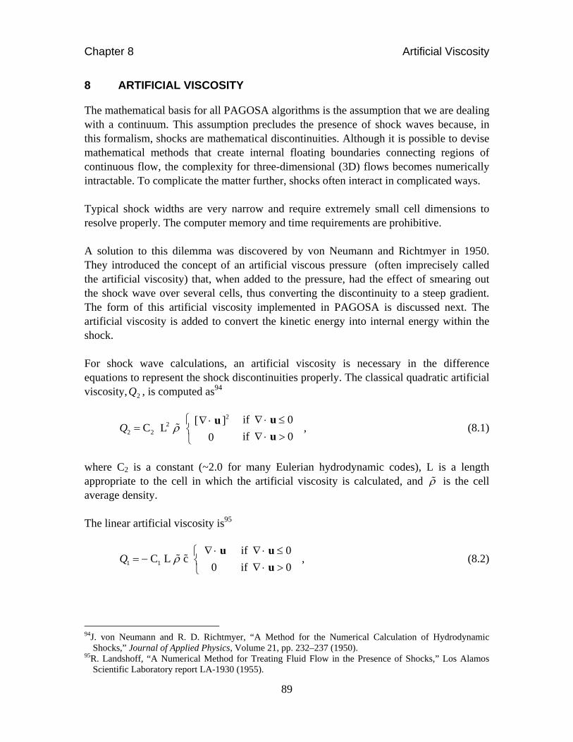
Chapter 8 Artificial Viscosity
89
8 ARTIFICIAL VISCOSITY
The mathematical basis for all PAGOSA algorithms is the assumption that we are dealing with a continuum. This assumption precludes the presence of shock waves because, in this formalism, shocks are mathematical discontinuities. Although it is possible to devise mathematical methods that create internal floating boundaries connecting regions of continuous flow, the complexity for three-dimensional (3D) flows becomes numerically intractable. To complicate the matter further, shocks often interact in complicated ways. Typical shock widths are very narrow and require extremely small cell dimensions to resolve properly. The computer memory and time requirements are prohibitive. A solution to this dilemma was discovered by von Neumann and Richtmyer in 1950. They introduced the concept of an artificial viscous pressure (often imprecisely called the artificial viscosity) that, when added to the pressure, had the effect of smearing out the shock wave over several cells, thus converting the discontinuity to a steep gradient. The form of this artificial viscosity implemented in PAGOSA is discussed next. The artificial viscosity is added to convert the kinetic energy into internal energy within the shock. For shock wave calculations, an artificial viscosity is necessary in the difference equations to represent the shock discontinuities properly. The classical quadratic artificial viscosity, 2Q , is computed as94
22
2 2
if 0[ ]C L
if 00Q
uu
u , (8.1)
where C2 is a constant (~2.0 for many Eulerian hydrodynamic codes), L is a length appropriate to the cell in which the artificial viscosity is calculated, and is the cell average density. The linear artificial viscosity is95
1 1
if 0C L c
0 if 0Q
u u
u , (8.2)
94J. von Neumann and R. D. Richtmyer, “A Method for the Numerical Calculation of Hydrodynamic
Shocks,” Journal of Applied Physics, Volume 21, pp. 232–237 (1950). 95R. Landshoff, “A Numerical Method for Treating Fluid Flow in the Presence of Shocks,” Los Alamos
Scientific Laboratory report LA-1930 (1955).

Chapter 8 Artificial Viscosity
90
where C1 is a constant and c is the cell-average sound speed. The linear artificial viscosity is used to damp out oscillations behind the shock waves.96 Both coefficients (C1 and C2) and the length scale L are user selectable. These equations incorporate a suggestion by Rosenbluth97 that the artificial viscosity should have a value of zero when the fluid is undergoing an expansion (the divergence of the velocity field is positive). The total artificial viscosity,Q , is
21 QQQ . (8.3) The artificial viscosity acts to spread the shock over a few cells in such a way that the variables vary continuously through the region of the shock and satisfy the Rankine-Hugoniot conservation relations. The shock will be spread over several zones, regardless of the cell size. A few cells away from the shock, the artificial viscosity is zero. The effect of artificial viscosity is very much cell size dependent. Simulations at very fine mesh resolutions may not need any artificial viscosity. Further, in simulations where extreme gradients do not exist, the artificial viscosity may need to be suppressed entirely. The excessive use of artificial viscosity often damps out the solution. It is said that experience is the key to success. Shock artificial viscosities introduce problems and errors of their own. In strong shocks, “wall heating” and “shock-less heating” can occur, leading to errors in the internal energy surrounding the shock.98 Errors in internal energy lead to errors in density and the shock speed. Many of these effects are seen in the so-called Noh problem.99 The densities at symmetry boundaries are usually severely reduced, and the internal energies are significantly overpredicted. All of these anomalies are sensitive to mesh resolution. Treating the artificial viscosity as a pressure term in the momentum and energy finite-difference equations allows the work done by the viscosity to be identified with the thermodynamic irreversibility of the shock. When we compare the energy equation with the first law of thermodynamics:
96The coefficients used in Lagrangian hydrodynamics codes are different from the ones listed above. 97R.D. Richtmyer and K.W. Morton, Difference Methods for Initial Value Problems, second edition
(Interscience Publishers, New York, New York, 1967), p. 313, footnote 11. 98W.F. Noh, “Errors for Calculations of Strong Shocks Using an Artificial Viscosity and an Artificial Heat
Flux,” Lawrence Livermore National Laboratory report UCRL-53669 (1985). 99W.F. Noh, “Errors for Calculations of Strong Shocks Using an Artificial Viscosity and an Artificial Heat
Flux,” Journal of Computational Physics, Volume 72, pp. 78–120 (1987).

Chapter 8 Artificial Viscosity
91
( )dE P Q dV
TdS d E P dV
and
TdS Q dV .
The entropy increase dS is being generated by the artificial viscosity. The entropy is not computed in PAGOSA; however, it is a useful conceptual explanation of the physical and numerical processes involved in the solution of the Navier-Stokes equations. An interesting problem is in the choice of the length parameter L. The Wilkin’s form100 of the artificial viscosity, the default for PAGOSA, uses a length calculated across the cell in the direction of the maximum pressure gradient. The length scale adapts in each zone, depending on the local pressure gradients. On the other hand, in 2D problems, the length scale could be computed in several different ways. The appropriate length scale might be the diagonal distance across the cell. The length scale computation is selected by the user. In 1D problems, only x would be an appropriate length scale choice. For an ideal shock, the pressure is a square wave. When the artificial viscosity is computed and added to the pressure, the result is shown in Figure 8.1. The shock is spread out over several cells, and the artificial viscosity is a fraction of the amplitude of the pressure in the region of the shock and is nonexistent away from the shock.
Figure 8.1. A typical pressure and artificial viscosity in the region of a shock.
100M.L. Wilkins, “Use of Artificial Viscosity in Multidimensional Fluid Dynamic Calculations,” Journal of
Computational Physics, Volume 36, pp. 281–303 (1980).

Chapter 8 Artificial Viscosity
92
This page intentionally left blank.

Chapter 9 Computing a Timestep
93
CHAPTER 9
Computing a Timestep
I am not discouraged, because every wrong attempt discarded is another step forward.
-Thomas A. Edison (1847–1931)

Chapter 9 Computing a Timestep
94
This page intentionally left blank.

Chapter 9 Computing a Timestep
95
9 COMPUTING A TIMESTEP
The timestep in any simulation must be smaller than that given by the Courant-Friedrichs-Lewy (CFL) condition.101 This condition is necessary for the stability of the numerical solution of the partial differential equations. Physically, the timestep restriction102 prevents information from moving beyond a cell in a single step. A timestep for each component of the velocity is computed as follows.
U mint safeu x U , (9.1)
V mint safeu y V , (9.2)
W mint safeu z W , (9.3)
UC min [| | ]t safec x cU , (9.4)
VC min [| | ]t safec y cV , and (9.5)
WC min [| | ]t safec z cW , (9.6)
where safeu and safec are safety factors (between 0 and 1) used to reduce the timestep further and ensure numerical stability. The velocity components , , and U V W are evaluated at the cell centers.103 The location of the controlling timestep is also computed and displayed for each cycle of the integration. This information is useful in understanding what is controlling the timestep and where that control is specifically located. Occasionally, a material can move into an equation-of-state (EOS) regime where the calculated sound speed can be quite large. If the sound speed is large enough, it will control the simulation with very small timesteps. In these cases, knowing the location and state of the material can aid the user in setting appropriate density and pressure cutoffs. The question reduces to knowing if the timestep control falls within a region of interest. In addition, the divergence also has an associated timestep given by
DIV min 1t safed u . (9.7)
The safety factor safed is related to the amount that the cell can expand (or contract) during the Lagrangian phase. This timestep condition helps keep distortions small during a single timestep.
101R. Courant, K. Friedrichs, and H. Lewy, “Über die Partiellen Differenzengleichungen der
Mathematischen Physik,” Mathematische Annalen, Volume 100, Number 1, pp. 32–74 (1928). An English language translation of the original German paper appears in “On the Partial Difference Equations of Mathematical Physics,” IBM Journal, pp. 215–234 (March 1967).
102R.D. Richtmyer and K.W. Morton, Difference Methods for Initial Value Problems, second edition (reprinted) (Krieger Publishing Company, Malabar, Florida, 1994), pp. 9–16, 45–48, and 83–90.
103Ensuring that the sound speed and velocities are spatially centered in the same manner.

Chapter 9 Computing a Timestep
96
In simulations involving the detonation of explosives with the programmed burn algorithm, the timestep is limited so that the detonation wave traverses a cell in a few steps (approximately four by default104). In the timestep computation, to ensure the stability during the high-explosive burn, a value of three times the detonation velocity is used in place of the sound speed for cells containing undetonated or partially detonated explosive. This restriction allows the pressure in the cell to build slowly as the energy is deposited into the cell:
D
min , ,
3 D
x y zt safec
, (9.8)
where D is the detonation velocity of the explosive. The calculation timestep is the minimum of all the various controls, as shown in Table 9.1:
U V W UC VC WC DIV D MAXmin ( , , , , , , , , )t t t t t t t t t t , (9.9)
where MAXt is a user-specified maximum timestep for the simulation. The timesteps can be adjusted in other ways. The timestep can grow under certain circumstances and is allowed to grow by a small factor for each new step. Typically this increase is 5% to 10% in step size from cycle to cycle. However, the timestep can shrink dramatically at any point in the simulation. For example, if a detonation begins or if two shocks collide, then the timestep will adjust to reflect the new physics in the simulation. The timestep will be computed subject to the restrictions described above and subject to the minimum and maximum timestep values. The timestep is also limited by minimum value. If the value of the timestep drops below a specified minimum value ( MINt ), then the simulation is stopped. This situation can occur when a calculation has difficulty with an EOS with unrealistic densities or internal energies. If the timestep becomes too small, it is usually indicative of some problem in the simulation. In certain simulations, when an exact final simulation time is wanted, the timestep is adjusted for the last integration step. If the normally computed timestep would overshoot the desired time, a fraction of the timestep is used. This option is useful when simulations are to be compared with experiments, for example.
104The default user parameter is safec = ¾, so the detonation requires a minimum of four steps to traverse a
cell.

Chapter 9 Computing a Timestep
97
Table 9.1. The Timestep Controls in PAGOSA Hydrodynamics (the Controls Include the Standard CFL Stability Restrictions, as Well as Controls Set at the User’s Discretion)
CODE CONTROL EQUATION
Div DIVt (9.7)
Fin nt ( finalt t )
G - t growth t
I 0t Initial timestep
Max MAXt User selectable
Min MINt User selectable
U Ut (9.1)
V Vt (9.2)
W Wt (9.3)
U+c UCt (9.4)
V+c VCt (9.5)
W+c WCt (9.6)
The initial timestep, 0t , is either set by the user or computed by trial and error from the initial conditions. The user is encouraged to compute the initial timestep manually. Appendix F provides a few important ideas for computing an initial timestep ( 0t ). In cases where the timestep is too large for the Lagrangian or advection phases,105 the PAGOSA algorithm “backs up” to the last simulation time and attempts a smaller timestep. This backup capability is an important feature in PAGOSA and provides a robust method of continuing a simulation when the CFL conditions vary significantly over the course of the complete simulation. The safety factors, growth factors, minimum timesteps, and maximum timesteps all have default values in PAGOSA. These factors have been fine tuned and adjusted over many years for typical problems of interest.
105For example, if the Lagrangian-phase volume consumes the entire Eulerian cell volume. Another
common occurrence is when the Lagrangian-phase volume is negative.

Chapter 9 Computing a Timestep
98
This page intentionally left blank.

Chapter 10 Initial Conditions
99
CHAPTER 10
Initial Conditions
These mysteries are heightened when we reflect how surprising it is that the laws of nature and the initial conditions of the universe should allow for the existence of beings
who could observe it.
-Steven Weinberg, Scientific American (October 1994)

Chapter 10 Initial Conditions
100
This page intentionally left blank.

Chapter 10 Initial Conditions
101
10 INITIAL CONDITIONS
The solution of the partial differential equations presented in Chapter 1 requires a set of initial conditions for the fundamental variables at the beginning of the simulation ( 0t t ). For every material and every cell, the following initial conditions are needed:
0
0
0
0
0
( ; , , ) initial density,
( ; , , ) initial volume fraction,
( ; , , ) initial x velocity,
( ; , , ) initial y velocity,
( ; , , ) initial z velocity,
t t x y z
t t x y z
U t t x y z
V t t x y z
W t t x y z
0
and
( ; , , ) initial internal energyE t t x y z
The pressures can be derived from the densities and internal energies. Similarly, the cell masses can be derived from the densities, volume fractions, and cell sizes. On the other hand, the stress deviators are initially zero.
0
0
0
0
0
0
( ; , , ) = 0
( ; , , ) = 0
( ; , , ) = 0
( ; , , ) = 0
( ; , , ) = 0
( ; , , ) = 0 .
xx
xy
xz
yy
yz
zz
S t t x y z
S t t x y z
S t t x y z
S t t x y z
S t t x y z
S t t x y z
There are no initial material stresses; this fact may be incompatible with the other initial conditions specified by the user. It is important to ensure that all initial conditions are consistent and compatible. In the case of programmed burn explosives, the vertex-centered burn times are required initial conditions. The “simple” programmed burn algorithms are detailed in Chapter 12. The general three-dimensional programmed burn algorithm106 allows for more complicated geometries, shadow regions, and multiple high-explosive materials. ( , , ) programmed burn times (vertex centered)Bt x y z .
106Tom Bennion, Sean Clancy, and Wayne Weseloh (editors), “The PAGOSA 3D Programmed Burn
Algorithm,” Los Alamos National Laboratory report LA-UR-09-04016, Revision 1 (May 2009).

Chapter 10 Initial Conditions
102
This page intentionally left blank.

Chapter 11 Boundary Conditions
103
CHAPTER 11
Boundary Conditions
The cube which you will generate will be bounded by six sides, that is to say, six of your insides.
-Edwin A. Abbott, Flatland (1884)

Chapter 11 Boundary Conditions
104
This page intentionally left blank.

Chapter 11 Boundary Conditions
105
11 BOUNDARY CONDITIONS
Boundaries on which the boundary conditions are set form the exterior surface of the Eulerian computational domain. The two types of boundary conditions available in PAGOSA are reflective (symmetry) and transmissive.
11.1 Reflective Boundary Conditions
The reflective boundary conditions, sometimes called the symmetry boundary conditions, represent a boundary of the Eulerian mesh where the interior is a mirror image of the other side. No motion is possible normal to the boundary; only motion tangential to the boundary is allowed. In the current implementation of PAGOSA, materials contacting a reflective (symmetry) boundary cannot subsequently pull away from it. At a reflective (symmetry) boundary, the ghost cells are the mirror image of their “real” neighbors. For example, on the xmin boundary surface, the boundary conditions would be
0, , 2, ,
1, ,
0, , 2, ,
0
n nj k j k
nj k
n nj k j k
U U
V
W W
and
1 1 1 3 1 12 2 2 2 2 2
1 1 1 3 1 12 2 2 2 2 2
1 1 1 3 1 12 2 2 2 2 2
1 1 1 3 1 12 2 2 2 2 2
, , , ,
, , , ,
, , , ,
, , , ,
n nj k j k
n nj k j k
n nj k j k
n nj k j k
E E
P P
.
The general prescription is shown in Figure 11.1. The cell-centered portion of the ghost cells is simply copied from the adjacent Eulerian cells. However, the velocities at handled differently. The normal component of the velocity is zero at the reflective (symmetry) boundary, whereas the tangential component is computed in the same manner as every “interior” cell.
Figure 11.1. The reflective (symmetry) boundary conditions.

Chapter 11 Boundary Conditions
106
The above situation is complicated at the intersection of two or three reflecting boundaries. The row of ghost cells must be set appropriately in these cases.
11.2 Transmissive Boundary Conditions
The transmissive boundary conditions allow material to flow out of the computational domain by absorbing all incident waves without generating any signals back into the Eulerian mesh that might perturb the solution. Achieving this boundary condition is very difficult, and implementations are generally poor in most Eulerian hydrocodes. The transmissive boundary conditions (see example in Figure 11.2) provide a way to anticipate the flow behavior at the very limit of the computational domain. The flow properties at the boundary must derive from the knowledge of the flow inside the computational domain, coupled with some approximations of the outside flow:
0, , 1, , 2, ,
0, , 1, ,
0, , 1, ,
n n nj k j k j k
n nj k j k
n nj k j k
U U U
V V
W W
and
1 1 1 3 1 12 2 2 2 2 2
1 1 1 3 1 12 2 2 2 2 2
1 1 1 3 1 12 2 2 2 2 2
1 1 1 3 1 12 2 2 2 2 2
, , , ,
, , , ,
, , , ,
, , , ,
n nj k j k
n nj k j k
n nj k j k
n nj k j k
E E
P P
Some small amount of information is reflected off of the transmissive boundary back into the simulation. It is always important to choose the position of a transmissive boundary so that it has only a minimal effect on the results of the simulation.
Figure 11.2. The transmissive boundary.

Chapter 11 Boundary Conditions
107
11.3 Other Boundary Conditions
Other types of boundary conditions are possible and under consideration:
inflow, periodic, and pinned, no slip, or no velocity.

Chapter 11 Boundary Conditions
108
This page intentionally left blank.

Chapter 12 Programmed Burn
109
CHAPTER 12
Programmed Burn
Double, double toil and trouble, fire burn, and caldron bubble.
-William Shakespeare, Macbeth (1603–1607)

Chapter 12 Programmed Burn
110
This page intentionally left blank.

Chapter 12 Programmed Burn
111
12 PROGRAMMED BURN
The programmed burn technique107 is used in PAGOSA to simulate the detonation of explosives when the properties of that particular explosive are well known and its behavior is not the focus of the study. The basic assumption is that the detonation wave front travels in all directions at the Chapman-Jouget detonation108 velocity. The position of the detonation front is predicted based on the initial configuration of the explosive. The detonation burn times, Bt, are defined at the cell vertices. For simulations using the programmed burn technique, the burn times are computed as part of the initial conditions. The burn times are computed from a user-selected detonator type and the explosive detonation velocity D. For vertices in no way connected to the explosive, the burn times are set to a large value, btlim. For cells that contain any explosive, the burn time is computed for every vertex. The propagation of the detonation is modeled by a simple line-of-sight approximation to a complicated Huygen’s construction. The detonation wave is regarded as a propagating energy deposition front in the explosive. The difference between the minimum and maximum burn times of the eight cell vertices is referred to as the burn interval for a cell. Mathematically, we have
min 1 2 3 4 5 6 7 8
max 1 2 3 4 5 6 7 8
interval max min
min
min interval min max
max
min ( , , , , , , , )
max ( , , , , , , , )
0 if
( ) / if
1 if
t t t t t t t t t
t t t t t t t t t
t t t
t t
Bf t t t t t t
t t
.
The burn fraction, Bf, is used in the Jones-Wilkins-Lee (JWL) equation of state (EOS) (Section 6.5) to allow a gradual deposition of pressure/energy into a cell. The energy starts to deposit proportionally from the time when the detonation front first arrives at the cell. This energy deposition, combined with the EOS of the explosive material, produces a finite pressure in the cell, which then begins to affect other portions of the problem. Detonation points normally occur on the surface of explosive regions. The available simple (i.e., line-of-sight) detonator types are Point, Line, Plane, Cylinder, Sphere, and Ring. These types are described in the following sections.
107Programmed burn is not the only technique for handling explosives in PAGOSA. Several reactive burn
models are available for a more detailed study of explosive behavior. 108J.A. Zukas and W.P. Walters, Explosive Effects and Applications (Springer-Verlag Inc., New York, New
York, 1998), pp. 116–121, 127.
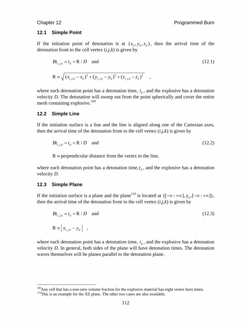
Chapter 12 Programmed Burn
112
12.1 Simple Point
If the initiation point of detonation is at ( , , )d d dx y z , then the arrival time of the detonation front to the cell vertex (i,j,k) is given by , , R /i j k dBt t D and (12.1)
2 2 2, , , , , ,R ( ) ( ) ( )i j k d i j k d i j k dx x y y z z ,
where each detonation point has a detonation time, dt , and the explosive has a detonation velocity D. The detonation will sweep out from the point spherically and cover the entire mesh containing explosive.109
12.2 Simple Line
If the initiation surface is a line and the line is aligned along one of the Cartesian axes, then the arrival time of the detonation front to the cell vertex (i,j,k) is given by , , R /i j k dBt t D and (12.2)
R perpendicular distance from the vertex to the line, where each detonation point has a detonation time, dt , and the explosive has a detonation velocity D.
12.3 Simple Plane
If the initiation surface is a plane and the plane110 is located at ([ : ], ,[ : ])dy , then the arrival time of the detonation front to the cell vertex (i,j,k) is given by , , R /i j k dBt t D and (12.3)
, ,R i j k dy y ,
where each detonation point has a detonation time, dt , and the explosive has a detonation velocity D. In general, both sides of the plane will have detonation times. The detonation waves themselves will be planes parallel to the detonation plane.
109Any cell that has a non-zero volume fraction for the explosive material has eight vertex burn times. 110This is an example for the XZ plane. The other two cases are also available.

Chapter 12 Programmed Burn
113
12.4 Simple Cylinder
If the initiation surface is a cylinder and the cylinder axis is aligned along one of the Cartesian axes, then the arrival time of the detonation front to the cell vertex (i,j,k) is given by , , R /i j k dBt t D and (12.4)
R radial distance from the vertex to the cylindrical surface, where each detonation point has a detonation time, dt , and the explosive has a detonation velocity D. In general, both sides of the cylindrical surface will have detonation times. The detonation waves themselves will be cylinders concentric to the cylindrical detonation surface.
12.5 Simple Sphere
If the initiation surface is a sphere, then the arrival time of the detonation front to the cell vertex (i,j,k) is given by , , R /i j k dBt t D and (12.5)
R radial distance from the vertex to the spherical surface, where each detonation point has a detonation time, dt , and the explosive has a detonation velocity D. In general, both sides of the spherical surface will have detonation times. The center coordinates and radius of the detonation surface must be specified by the user. The detonation waves themselves will be spheres concentric to the spherical detonation surface.
12.6 Simple Ring
If the initiation surface is a ring, then the arrival time of the detonation front to the cell vertex (i,j,k) is given by , , R /i j k dBt t D and (12.6)
R minimum distance from the vertex to the ring surface, where each detonation point has a detonation time, dt , and the explosive has a detonation velocity D. If the inner radius of the ring detonator is zero, then the surface is a circle. In addition, if the outer radius is larger than the computational mesh, this case reduces to a simple plane detonator.

Chapter 12 Programmed Burn
114
12.7 Limitations of Simple Detonators
In some cases, the line-of-sight approach is a poor approximation to the physics in the simulation. Situations exist where portions of the material are not within the line of sight. These shadow regions can be important in a simulation. In these cases, other detonation methods should be used. Consider the complicated explosive geometry in Figure 12.1. The detonation point, located on the left, has a limited line of sight to most of the explosive material. The demarcation between the line-of-sight regions and the shadow regions is shown by the red dotted lines. The distance calculations for the lines and will clearly be in error. A contour plot of the burn times is one of the best methods of checking the computation.
Figure 12.1. An explosive is to be detonated at the point shown. The lines and point to
regions that are directly within the line of sight of the detonator. The lines and point to the shadow regions. The distance calculation assumptions are violated because the line-of-sight path crosses another material.
The programmed burn methodology is most often used in conjunction with the JWL EOS (Section 6.5). The combination ignores many physical properties that could be important in a simulation. For example, the detonation front contains a reaction zone111 of a finite width. In the simple model of detonation, we treat the reaction zone as if it had zero width. The detonation velocity varies as a function of the local shock curvature.112,113
The detonation velocity D in the line-of-sight programmed burn method is a constant.
111P.W. Cooper, Explosives Engineering, (Wiley-VCH, New York, New York, 1996), pp. 275–298. 112J.B. Bdzil, D.S. Stewart, and T.L. Jackson, “Program Burn Algorithms Based on Detonation Shock
Dynamics: Discrete Approximations of Detonation Flows with Discontinuous Front Models,” Journal of Computational Physics, Volume 174, pp. 870–902 (2001).
113D.E. Lambert, D.S. Scott, S. Yoo, and B.D. Wescott, “Experimental Validation of Detonation Shock Dynamics in Condensed Explosives,” Journal of Fluid Mechanics, volume 546, pp. 227–253 (2006).

Chapter 12 Programmed Burn
115
The programmed burn algorithm is a geometric construction approximating many complicated nonlinear processes. This algorithm can be a very good approximation to reality if the questions driving the simulation are not about details of the high-explosive detonation.114 One way of avoiding the difficulties with shadow regions is for the user to construct a series of connected regions, each with a single individual detonator. In the case shown in Figure 12.2, the explosive has been divided into four regions. The first region, A, is the line-of-sight region. The original detonation point is now designated as detonator 1 and corresponds to region A. Regions B, C and D are shadow regions.
Figure 12.2. An explosive, shown in the previous figure, is to be detonated with four distinct
detonation points. Region A is the line-of-sight region, which will be detonated with detonator 1 (the original detonator). Region B is a shadow region, detonated by detonator 2. Region C is the second shadow region, detonated by detonator 3. The remaining explosive material, D, will be detonated by detonator 4. The four regions A, B, C, and D have the same material properties.
The detonation times for the four detonation points are
1 dt t material A, 2 1 12 /t t R D material B, 3 1 13 /t t R D material C, and 4 3 34 /t t R D material D, where ikR is defined as the minimum distance between points i and k. Each region would need to have a unique material number for this method to work properly.
12.8 Other Detonation Models
Several other options exist in PAGOSA for the release of energy from an explosive, including reactive burn models (CJ Volume, DynaBurn, Forest Fire, and Multi-Shock 114Tom Bennion, Sean Clancy, and Wayne Weseloh (editors), “The PAGOSA 3D Programmed Burn
Algorithm,” Los Alamos National Laboratory report LA-UR-09-04016, Revision 1 (May 2009).

Chapter 12 Programmed Burn
116
Forest Fire). The description of these models is beyond the scope of this work and therefore is not discussed here.

Chapter 13 Divergence Options
117
CHAPTER 13
Divergence Options
One cannot escape the feeling that these mathematical formulas have an independent existence and an intelligence of their own, that they are wiser than we are, wiser even
than their discoverers.
-Heinrich Hertz (1857–1894)

Chapter 13 Divergence Options
118
This page intentionally left blank.

Chapter 13 Divergence Options
119
13 DIVERGENCE OPTIONS
The implementation of material models in PAGOSA is made somewhat difficult because of the use of a single velocity field for all materials. Under certain circumstances, mixed cell components can behave nonphysically if they possess very different compressibilities or shear moduli. Various divergence models have been developed to handle these situations. To understand why divergence is central to this issue, consider the Lagrangian equation [Eq. 4.11)] developed in Chapter 4:
0t
u .
Rewriting Eq. (4.15) with the reference density explicitly included, we find
10 0( / ) ( / )
t
u . (13.1)
If the compression and the rate of compression are increasing, then the divergence is negative.
13.1 Uniform
All materials in a mixed cell are uniformly compressed (or expanded) at the same rate using the same value of divergence. No distinction is made between gases, liquids, metals, or voids within a single Eulerian cell. The differences in compressibility between materials are ignored, and all materials are treated with the same value. Consider the right-hand side of Eq. (13.1). Using this uniform compression model, all materials in a mixed cell would be subject to the same divergence.
13.2 Void Closure
Void closure is a phenomenon that occurs when a void material is sandwiched between two nonvoid materials. For the uniform case described above, all the materials in mixed cells under compression will be squeezed in proportion to their material volume fraction. This squeezing leads to over-compression of the nonvoid materials, which is clearly nonphysical. In reality, the voids would be squeezed out before any compression of the materials occurred. In practice, the void closure model in PAGOSA allows the void to be squeezed out between two objects that are colliding. Without the model, a small amount of void would remain forever sandwiched between the two objects.

Chapter 13 Divergence Options
120
The details of the void closure model are as follows.115 During both the predictor and corrector steps of the Lagrangian phase in PAGOSA, the velocity divergence is examined in each mixed cell. If the divergence is negative (i.e., the cell is contracting), the cell is inspected for the presence of void materials. If void material is found, then the minimum and maximum priorities of all materials present in the surrounding 26 neighboring cells are determined. If the priority of the void to be closed is between the minimum and maximum priorities of the neighboring cells, then that void will be contracted preferentially. That is, the void will take up any contraction of the cell before any other materials are allowed to compress. If the volume of the void is insufficient to use the contraction entirely, then the other materials in the cell will share the remaining contraction according to their individual volume fractions. If the priority of a closeable void does not occur between the minimum and maximum priorities of the neighboring nonvoid materials, it may still be allowed to close if no neighboring cells are pure void cells. In PAGOSA, when a void is preferentially contracted in a mixed cell, the contributions to the energy change from the nonvoid materials are multiplied by a scalar factor. Figure 13.1 shows a diagram of the derivation of this factor for a mixed cell containing one solid material and a void. At the start of the Lagrangian phase, we have 0
mat = the volume fraction of the material and
0void = the volume fraction of the void.
After the contraction occurs during the predictor portion of the Lagrangian phase, we have 1
mat = the volume fraction of the material and
1void = the volume fraction of the void.
Figure 13.1(a) shows the partitioning of material and void in the cell before contraction. The whole cell will contract by V (which has a negative value) during the predictor portion of the Lagrangian phase. Figure 13.1(b) illustrates the case where the contraction is apportioned between material and void according to their individual volume fractions. In this case, the volume change of the solid material after the predictor phase is given by
115K.S. Holian [Los Alamos National Laboratory (LANL)], D.J. Cagliostro (LANL), T.F. Adams (LANL),
and B. Parker [Atomic Weapons Research Establishment (AWRE), United Kingdom], private communication, November 9, 1990.

Chapter 13 Divergence Options
121
/0
w o matmatV V . (13.2)
Figure 13.1(c) illustrates the case in which void closure occurs, and the void contracts before the solid material is allowed to contract. In this case, the volume change of the material is given by 1 0( )w mat mat
matV V V V . (13.3) The factor that multiplies the contribution to the energy change by the contraction of the material then is the change in volume of the material with void closure divided by the change in volume of the material without void closure, as
1 0
0
( )mat mat
mat
V V Vf
V
. (13.4)
The densities of the nonvoid material components of the mixed cell are clearly modified by this preferential contraction of the void.
Figure 13.1. Schematic showing two different methods of contracting void in a mixed cell. At the
beginning of the Lagrangian phase (a), the mixed cell contains solid material and void. If the contraction is apportioned between solid and void according to volume fractions, then the solid is preferentially compressed (b). If the void contracts before the solid is allowed to contract, then the result is (c).
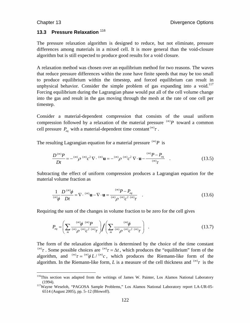
Chapter 13 Divergence Options
122
13.3 Pressure Relaxation 116
The pressure relaxation algorithm is designed to reduce, but not eliminate, pressure differences among materials in a mixed cell. It is more general than the void-closure algorithm but is still expected to produce good results for a void closure. A relaxation method was chosen over an equilibrium method for two reasons. The waves that reduce pressure differences within the zone have finite speeds that may be too small to produce equilibrium within the timestep, and forced equilibrium can result in unphysical behavior. Consider the simple problem of gas expanding into a void.117 Forcing equilibrium during the Lagrangian phase would put all of the cell volume change into the gas and result in the gas moving through the mesh at the rate of one cell per timestep. Consider a material-dependent compression that consists of the usual uniform compression followed by a relaxation of the material pressure ( )m P toward a common cell pressure eqP with a material-dependent time constant ( )m .
The resulting Lagrangian equation for a material pressure ( )m P is
( )( )
( ) ( ) 2 ( ) ( ) ( ) 2( )
mmeqm m m m m
m
P PD Pc c
Dt
u u . (13.5)
Subtracting the effect of uniform compression produces a Lagrangian equation for the material volume fraction as
( )( )
( )( ) ( ) ( ) 2 ( )
1mm
eqmm m m m
P PD
Dt c
u u . (13.6)
Requiring the sum of the changes in volume fraction to be zero for the cell gives
( ) ( ) ( )
( ) ( ) 2 ( ) ( ) ( ) 2 ( )/m m m
eq m m m m m mm m
PP
c c
. (13.7)
The form of the relaxation algorithm is determined by the choice of the time constant ( )m . Some possible choices are ( )m t , which produces the “equilibrium” form of the algorithm, and ( ) ( ) ( )/m m mL c , which produces the Riemann-like form of the algorithm. In the Riemann-like form, L is a measure of the cell thickness and ( )m is the
116This section was adapted from the writings of James W. Painter, Los Alamos National Laboratory
(1994). 117Wayne Weseloh, “PAGOSA Sample Problems,” Los Alamos National Laboratory report LA-UR-05-
6514 (August 2005), pp. 5–12 (Blowoff).

Chapter 13 Divergence Options
123
estimated time for the wave to traverse material (m) and change the material pressure from ( )m P to eqP .
In the equilibrium form, eqP takes on the well-known form
( ) ( ) ( )
( ) ( ) 2 ( ) ( ) 2/m m m
eq m m m mm m
PP
c c
(13.8)
and the volume fraction equation becomes
( )( )
( ) ( ) ( ) 2
1mm
eq
m m m
P PD
Dt c t
. (13.9)
When the left-hand side of Eq. (13.9) is differenced, t cancels from the equation. To first approximation, the changes in volume fractions will tend to equilibrate the material pressures within a timestep t . In the Riemann-like form, eqP takes on the form
( )
( ) ( ) ( ) ( )
1/m
eq m m m mm m
PP
c c
, (13.10)
and the volume fraction equation becomes
( )( )
( ) ( )
mmeq
m m
P PD
Dt c L
. (13.11)
For a two-material cell, this form is similar to the methods developed by David Youngs118 and Ransom and Hicks.119 For PAGOSA, a variation of the Riemann-like method was chosen. Modifications were required to handle some of the difficulties with the basic method, such as ( )m t and a potential instability associated with the artificial pressure Q .
118David L. Youngs (AWRE, United Kingdom), private communication, January 15, 1992. 119V.H. Ransom and D.L. Hicks, “Hyperbolic Two-Pressure Models for Two-Phase Flow,” Journal of
Computational Physics, Volume 53, pp. 124–151 (1984).

Chapter 13 Divergence Options
124
The differenced equation for ( )m ,
( )
( ) * ( )( ) ( ) 2 ( )
1m
eqm mm m m
P P t
c
, (13.12)
requires a stability and accuracy condition on the integration timestep t , where t t .
t must be ( )m to prevent overshoots of eqP , and it must be small enough to produce a good approximation to the exponential correction of . If t t , relaxation subcycling is required. For stability, the definition of ( )m is replaced with ( ) ( )max[ / ,1.1 / (1 )]m mL c t f , where max( , )f safeu safec is a safety factor between 0 and 1. This definition guarantees that ( )mt . For accuracy and stability, the fractional change in ( )m for any single material in a cell is allowed to be no larger than the maximum allowable fractional change in the cell volume. For the case ( )m
eqP P , the singularity at ( ) 0m c is mitigated by replacing ( )m c with ( ) ( )m m
pc U , where ( )mpU is estimated from
2 ( )( ) ( )
( ) ( )( )2 2
mm meqm m
p m
P Pc cc U
. (13.13)
Equation (13.13) is obtained by applying a linear -s pU U approximation120 with 1s to a two-material, one-dimensional planar boundary. When ( ) *m has been evaluated, the density and internal energy are updated according to
( )
( ) * ( )( ) *
mm m
m
, (13.14)
and
( ) * ( )( )
( ) * ( ) ( ) * ( )( ) ( )
0 0 0
(1 ) ( )m mm
m m m mm m
P QE E t F F t
u u ,(13.15)
where
( ) ( )
( ) 0( )
0
10 1 1
m mm
m
tF
t
u
u . (13.16)
120See Chapter 6.6, Grüneisen EOS.

Chapter 13 Divergence Options
125
In the above equations, the subscript 0 indicates a value at the beginning of the hydrodynamic timestep. ( ) *m and ( )m are the values of the volume fraction for successive relaxation subcycles. The last term in Eq. (13.15) is required to partially correct the defect in the relaxation process related to the artificial pressure Q. Without it, the relaxation process tends to overexpand materials significantly to compensate for the introduction of internal energy by Q. The current limits on F are imposed for stability and may be relaxed in the future. The introduction of the last term in Eq. (13.15) requires that the cell-averaged Q in the momentum equation be replaced with
( ) * ( ) ( )0
m m m
m
QF
. (13.17)
The approach described above works reasonably well if material strength effects are insignificant compared with the basic hydrodynamics. However, if strength effects are significant, the algorithm must be properly adjusted to avoid anomalous results. In particular, instead of relaxing just the pressure ( )m P toward equilibrium, it is necessary to relax ( ) ( )m mP n S n , where ( )m S is the material-dependent, deviatoric stress tensor and n is the average unit interface normal vector for the mixed cell. The algorithm obtains the average value for n by volume averaging the individual surface normals obtained by interface reconstruction in the mixed cell.121 We therefore make the replacements ( ) ( ) ( )m m mP P n S n (13.18) and
( )
( ) 2 ( ) 2( )
4
3
mm m
m
Gc c
, (13.19)
where ( )m G is the material-dependent shear modulus. In addition, the zone strain-rate
tensor e used to update ( )m S is replaced with the material-dependent, strain-rate tensor ( )m e , which is approximated by
( )
( )( )
1 mm
m
D
Dt
e e nn . (13.20)
121Chapter 4.5.1 and Appendix C.

Chapter 13 Divergence Options
126
This page intentionally left blank.

Chapter 14 Strength
127
CHAPTER 14
Strength
People do not lack strength, they lack will.
-Victor Hugo (1802–1885)

Chapter 14 Strength
128
This page intentionally left blank.

Chapter 14 Strength
129
14 STRENGTH
This chapter is concerned with materials that can support a shear without continuous deformation. These elastic (and plastic) materials are different from the hydrodynamic materials studied up to this point.122 The stress deviators S will be fully described. Consider the stress-vs-strain curve of a typical solid material. During the first portion of the curve (up to a strain of less than ~1%), the stress and strain are proportional. This proportionality holds until point a in Figure 14.1, the proportional limit, is reached. We know that stress and strain are proportional because this segment of the line is straight. Hooke’s Law, named after physicist Robert Hooke (1635–1703), is applicable in the region in which stress and strain are proportional. Every material has a unique elastic modulus value (the slope of the line segment 0a in Figure 14.1). That is, the stress required to produce a given strain depends on the nature of the material under stress. Figure 14.1. The elastic-plastic behavior of a typical ductile material (e.g., copper). Point a is the
proportional limit, point b is the yield point, point c is a state in the plastic regime, point d is the ultimate tensile strength of the material, and point e is the fracture point.
From points a to b on the figure, stress and strain are not proportional; nevertheless, if the stress is removed at any point between 0 and b, the curve will be retraced in the opposite direction and the material will return to its original shape and length. In other words, the
122R.P. Feynman, R.B. Leighton, and M. Sands, The Feynman Lectures on Physics: Commemorative Issue,
Three Volume Set (Addison Wesley, Reading, Massachusetts, 1989). See Volume II, Chapters 38 and 39 on elasticity.
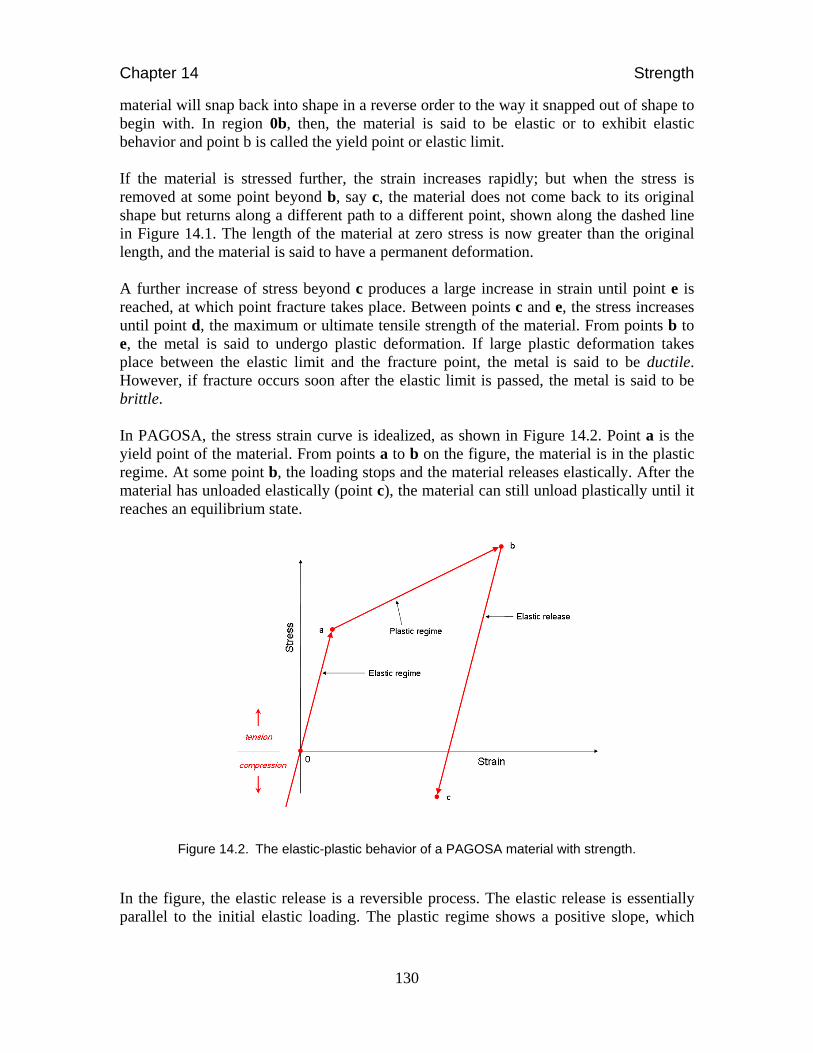
Chapter 14 Strength
130
material will snap back into shape in a reverse order to the way it snapped out of shape to begin with. In region 0b, then, the material is said to be elastic or to exhibit elastic behavior and point b is called the yield point or elastic limit. If the material is stressed further, the strain increases rapidly; but when the stress is removed at some point beyond b, say c, the material does not come back to its original shape but returns along a different path to a different point, shown along the dashed line in Figure 14.1. The length of the material at zero stress is now greater than the original length, and the material is said to have a permanent deformation. A further increase of stress beyond c produces a large increase in strain until point e is reached, at which point fracture takes place. Between points c and e, the stress increases until point d, the maximum or ultimate tensile strength of the material. From points b to e, the metal is said to undergo plastic deformation. If large plastic deformation takes place between the elastic limit and the fracture point, the metal is said to be ductile. However, if fracture occurs soon after the elastic limit is passed, the metal is said to be brittle. In PAGOSA, the stress strain curve is idealized, as shown in Figure 14.2. Point a is the yield point of the material. From points a to b on the figure, the material is in the plastic regime. At some point b, the loading stops and the material releases elastically. After the material has unloaded elastically (point c), the material can still unload plastically until it reaches an equilibrium state.
Figure 14.2. The elastic-plastic behavior of a PAGOSA material with strength.
In the figure, the elastic release is a reversible process. The elastic release is essentially parallel to the initial elastic loading. The plastic regime shows a positive slope, which

Chapter 14 Strength
131
represents work hardening in the material during plastic deformation. The empirical formula used to model this process is described in Section 14.4.9.
14.1 Cauchy Stress Tensor
A second-order tensor, the Cauchy stress tensor, completely describes the state of stress of a material body. In previous chapters, the stress tensor had been decomposed into its spherical and deviatoric parts:123 ij ij ijP S . (14.1)
The Cauchy stress tensor is symmetric in its indices. If the stress deviator 0ijS , then the stress has the form ij ijP . This form is called a pure hydrostatic state of stress, and P is the hydrostatic pressure. The negative sign arises because, by convention, we regard pressure, which causes compression, as positive, but we define compressive stress as negative. The stress deviator S in PAGOSA is associated with materials with a shear modulus G. The constitutive relations are given in Chapter 1, Eqs. (1.3a)–(1.3f). These constitutive relations connect the stress deviator and the material strain rates. The strain rates act differently, depending on the state of the material: elastic regime or plastic regime. The next section describes the decomposition of the strains into their elastic and plastic parts. Unlike finite elasticity, this model of elastic response does not carry the initial unstressed state as a reference state and thus is more suited to elastic-plastic modeling, where the plastic deformation continuously changes the zero-stress reference state.
14.2 Strain Rate Splitting
To separate the elastic and plastic flow behavior, the total linear strain is assumed to be linearly separable into an elastic component and a plastic component:
e pij ij ije e e . (14.2)
It is found experimentally that, to a good approximation, the purely plastic component of the deformation of most materials124 under hydrostatic loading should involve no volume
123It is a physically convenient decomposition for materials that exhibit plastic incompressibility. See P.J.
Maudlin, “Constitutive Behavior of Model FCC, BCC, and HCP Metals: Experiments, Modeling and Validation,” Los Alamos National Laboratory report LA-UR-98-4891 (January 1999).
Up to this point, the stress tensor and tensor notation have been avoided. However, to progress forward, explicit use of the Cauchy stress tensor and tensor notation is necessary and essential.

Chapter 14 Strength
132
change (dilatation). In other words, the plastic state of the material is incompressible. Therefore, 0p p p p
kk xx yy zze e e e , (14.3)
which expresses the property for the plastic strain. It follows that the divergence is e p e
kk kk kk kke e e e u . (14.4)
For plastic behavior, the elastic component e
ije does not vanish in general. It is assumed that any changes in the stress state in the plastic regime are an elastic response to the elastic strain rates. The details of the elastic-plastic response flow follow the Prandtl-Reuss treatment for fully compact ductile metals as presented in Freudenthal and Geiringer.125 The second assumption in the Prandtl-Reuss treatment is that the plastic strain is proportional to the current stress deviator: p
ij ije S 0 , (14.5)
where is the proportionality function between the plastic strain and the elastic-plastic response flow rule. The changes in the deviatoric stress tensor are given by 2 ( )p
ij ij ijS G e e . (14.6)
A derivation of this constitutive relation is given in Appendix A. In PAGOSA the elastic response of the material is decoupled from its thermodynamics. Thus, for the elastic regime in the absence of shocks, the material response should be isentropic. In particular, the isentropic part of the response should follow an adiabat of the equation of state (EOS). The basic elastic-plastic algorithm is shown in Table 14.1.
124J.J. Gilman, Micromechanics of Flow in Solids (McGraw-Hill, New York, New York, 1969). 125A.M. Freudenthal and M. W. Geiringer, “The Mathematical Theories of the Inelastic Continuum,” in
Handbuch der Phsyik (Springer-Verlag, New York, New York), Volume VI (1958).

Chapter 14 Strength
133
Table 14.1. The PAGOSA Elastic-Plastic Algorithm at a Glance
1) 1
2ji
ijj i
uue
x x
12
if predcitor,
if corrector,
n
n
u u
u u
linear strain rate tensor
2) 13ij ij ij kke e linear deviatoric strain rate tensor
3) 1
2ji
ijj i
uu
x x
linear spin (or rotation) tensor
4) Y and G flow-stress and shear modulus
5) old oldij im mj im mjR S S rotation term
6) * 2oldij ij ij ijS S G t R t elastic prediction (trial stress)
7)
* *
2
3( ) 1
2
( ) 1 1
ij ijS Sf plastic for f
Y
f elastic for f
radial return correction
8) fSS ijnewij /* new stress deviator
9) 12 [ ( ) ( ) ]old new old new
ij im mj mj im im mjR S S S S rotation update
10) 1
2p new old
ij ij ij ij ije t S S R tG
linear plastic strain tensor
11) 23
p p peq ij ije e e change in equivalent plastic strain
12) 23 ij ij deviatoric strain rate
13) p old pij ijW S e change in plastic work
14) peq
pold
pnew eee equivalent plastic strain
15) /poldnew WEE specific internal energy

Chapter 14 Strength
134
14.3 Yield Criterion
The plastic behavior of a metal is a reflection of modifications of the internal material structure. At the macroscopic level, this behavior produces a material flow. This flow results in permanent local deformations and energy dissipation, which contributes to the local specific internal energy of the material. The basic assumption is that there exists a scalar function of stress and strain, ( , )F σ ε , that characterizes the elastic and plastic states of the material.126 When the scalar function is negative, the state is elastic. When the scalar function is zero, the state is plastic; that is, when ( , ) 0F σ ε is reached, plastic deformations will develop. The case for which the scalar function is positive is physically unreachable. Any tendency in the state variables toward a positive scalar value is compensated by the plastic deformation such that the zero scalar function value is maintained. The scalar value of zero is called the “yield criterion.” For isotropic materials, the yield criterion should be independent of the coordinate system. In PAGOSA, this yield criterion is a function of the stress deviator invariants. In particular, the second invariant is chosen.127 It is customary to relate the yield criterion to the yield stress 0Y for the material in a simple tension test. In the one-dimensional uniaxial stress configuration (simple tension), yield occurs when 0xx Y and all other components 0ij
so that 1
03P Y ,
the stress deviators are 2 1 1
0 0 03 3 3, ,xx yy zzS Y S Y S Y ,
and all the other stress deviators are zero. The second invariant of the stress deviator tensor is related to the yield criterion by the classic von Mises yield criterion128
126The functional form of ( , )F σ ε is termed the yield surface. 127See Eq. (1.4) in Chapter 1 for the three tensor invariants. 128Richard von Mises, “Mechanik der Festen Korper im Plastisch Deformablen Zustand,” Göttingen
Nachrichten Mathematische Physik., Volume 1, pp. 582–592 (1913).

Chapter 14 Strength
135
2 2 2 2 2 21
2 2
2 2 2 21 4 1 1 10 0 0 02 9 9 9 3
( )
( ) 0 0 0
xx yy zz xy xz yzJ S S S S S S
Y Y Y Y
.
This equation is the relation between the second deviatoric stress invariant and the yield stress: the classical von Mises yield criterion. This form is generalized in PAGOSA by replacing 0Y by the yield function 21 1
1 22 2 3 [ ( , ,...) ]ij jiJ S S Y . (14.7)
The forms of the yield function Y available in PAGOSA are given in Sections 14.4.1 to 14.4.7. The arbitrary arguments n are the dependencies of the yield function. The yield limiting algorithm in PAGOSA can be understood best in a nine-dimensional stress deviator space.129 In this space, a stress deviator is represented by a vector S , where its elements are the tensor components of S . The Euclidian norm of the vector S is given as 1 1
2 2 2ij ijJ S S S . (14.8)
The classical von Mises yield criterion is
32 ij ijY S S , (14.9)
which represents a hyper-sphere with a radius of 2 / 3 Y , where the specific value depends on the current state variables influencing the yield function Y. States inside the hyper-sphere are elastic, and states on the surface of the hyper-sphere are plastic:
Elastic : 23 YS and (14.10a)
Plastic: 23 YS . (14.10b)
If components of the S vector are referred to the material (co-rotational) frame, the strain rate deviator e can be represented in this space by a vector 2G e , where the elements are scaled by 2G , whereG is the current shear modulus. The elastic-plastic distortions are shown in Figures 14.3 and 14.4. 129The style and mathematical structure of this exposition is primarily credited to Ian N. Gray, Atomic
Weapons Research Establishment (AWRE), Aldermaston, Berkshire, UK.

Chapter 14 Strength
136
Suppose the stress deviator vector at time t is 0S and the vector at time t t is 1S . The yield criterion are shown as
Figure 14.3. The two possible final states for a single timestep t . In the case where the
transition to a final state is elastic, the strain rate deviator is all elastic. On the other hand, if the transition is to a final plastic state, the strain rate deviator splits into two parts: elastic and plastic. The plastic contribution must lie on the yield surface. The elastic part cannot exceed the yield surface under these circumstances. The vector
*S is called the elastic predictor and has the value of the stress deviator if the total strain rate deviator was all elastic. The conditions do not uniquely determine 1S when the final state is plastic. The condition used in PAGOSA that provides a unique solution is given by the mathematical expression
1pij ije t S .
Figure 14.4. The vector components of an elastic-plastic state.

Chapter 14 Strength
137
Now with the above condition, the values of 1S and pije can be determined by (not
including the rotation terms) ( I ) Elastic Prediction * 0 2G t S S ε , (14.11) ( II ) Yield Limiting
** 23
1
* *2 23 3/
Y
Y Y
SSS
S S , and (14.12)
( III ) Strain Rate Deviator Splitting
1 0( )
2p
G t
S S
e ε . (14.13)
The above algorithm provides a first-order (backward) difference approximation to 1S and pe . It also has the virtue of automatically handling the elastic-plastic transitions, as shown in Figures 14.3 and 14.4. The stress deviator is updated so that the elastic predictor contains the rotation correction terms * 0 2 ( )ij ij ij ik kj ik kjS S G t S S t , (14.14)
where all variables are appropriately time centered. The plastic strain is computed as
1 0( ) ( )
2 2ij ij ik kj ik kjp
ij ij
S S S Se
G t G
. (14.15)
Remember that in general, G and Y are functions of density, pressure, and internal energy. The specific forms are described in Section 14.4.1 through 14.4.7. The velocity field at the start of a timestep (time nt ) is used to evaluate the divergence,
ike , mn . Using these values, a forward differencing of the stress deviator equations, together with the yield-limiting algorithm, gives a first-order prediction of the stress deviator at a half timestep 1/2nt ( 1
2nt t ). For multi-material cells, the cell strain rate is

Chapter 14 Strength
138
applied to each material component separately, regardless of its compressibility,130 and no attempt is made to force any equilibrium between the various components. Using the velocity divergence to update the specific volume (and density) and forward differencing the internal energy equation, using plastic strain rates from the yield-limiting algorithm, allows a first-order EOS prediction of pressure at time 1/2nt ( 1
2nt t ). Again, a uniform
cell value of velocity divergence is applied to components of multi-material cells. Straightforward spatial differencing of pressures and stress deviators at 1/2nt ( 1
2nt t )
allows the acceleration equations to give a second-order update of the velocity field from time nt to t t . From the velocity fields at times nt and nt t , the divergence, ike , and mn are evaluated at the half timestep 1/2nt ( 1
2nt t ) and used in a second-order differencing of
the stress deviator and energy equations to update the remaining quantities at time nt t . See Chapter 5 on Integration for more details.
The Lagrangian phase passes cell velocities at half timesteps to the advection phases. To avoid problems in consistency with the yield surface following advection, the last Lagrangian step passes its elastic prediction (not yield-limited) value of the stress deviator to the advection phases. The post-advection deviators are considered to be elastic predictions and are yield limited according to the post-advection values of plastic strain, pressure, and internal energy.
130As in the case of the “uniform” divergence option (Chapter 13.1).

Chapter 14 Strength
139
14.4 Flow-Stress Models
The flow-stress models give specific functional forms to the shear and yield moduli. In situations where very high hydrodynamic pressures or large strains are created, the constitutive relations may generate unrealistically large values for G and Y. To avoid this problem, the user can supply a maximum permitted shear modulus maxG and a maximum permitted yield modulus maxY . In PAGOSA these limits are implemented as
maxmin ( , )G G G and (14.16)
maxmin ( , )Y Y Y . (14.17)
If the yield modulus is set to a large value, then the material behavior is completely elastic and no plastic deformation occurs. This flow-stress model can be useful in some test problems and cases where the deformation is expected to be purely elastic.
14.4.1 Elastic Perfectly Plastic The elastic-perfectly plastic model is an idealized material and the easiest to understand. The shear and yield moduli are simply constants. The shear and yield moduli are 0G G , and 0Y Y . (14.18)
In this case, the plastic regime, shown in Figure 14.5, is a horizontal line. The stress in the plastic regime would be independent of the strain. The effects of thermal softening and work hardening are absent from this model. The class of elastic-perfectly plastic materials is an idealization to keep the constitutive equations simple. The idealization is reasonable for materials that do not show significant work hardening. The adequacy of this idealization depends on the purpose and requirement of the specific application.
Figure 14.5. An elastic-perfectly plastic material.

Chapter 14 Strength
140
14.4.2 Modified Steinberg-Cochran-Guinan The Modified Steinberg-Cochran-Guinan model131 is applicable for high-strain-rate materials (usually metals). The shear modulus and yield strength are functions of equivalent plastic strain, pressure, and internal energy. The shear modulus is '
0 cor meltG G P F , (14.19)
1
3' '01 ( / )corP P , and (14.20)
/( )
0m
mmelt E E E
m
E EF
E Ee
. (14.21)
Equation (14.20) is a pressure correction term, and Eq. (14.21) is a thermal softening term. The yield strength is given by
0 01 ( )p pcor meltY Y e e P F
, and (14.22)
1
301 ( / )corP P . (14.23)
The pressure correction terms are different for shear and yield; however, the thermal softening term is the same for Eqs. (14.19) and (14.22). The time-integrated equivalent plastic strain is denoted pe . This model requires seven user-supplied inputs: '
0, , , , , , and Pme E .
A single melt energy mE is specified for the material. If the internal energy is greater than this value, then both G and Y are set to a value of zero. The thermal softening is discussed in Section 14.4.8.
131D.J. Steinberg, S.G. Cochran, and M.W. Guinan, “A Constitutive Model for Metals Applicable at High-
Strain Rate,” Journal of Applied Physics, Volume 51, Issue 3, pp. 1498–1504 (1980).

Chapter 14 Strength
141
14.4.3 Steinberg-Cochran-Guinan The Steinberg-Cochran-Guinan model is a full-temperature version of the Modified Steinberg-Cochran-Guinan model. The material temperatures ( ) are obtained from the SESAME database via the EOSPAC library (see Chapter 6, Section 6.7). The shear modulus is ' '
0 ( )cor meltG G P F , (14.24)
1
3' '01 ( / )corP P , and (14.25)
' ' ( )melt T roomF . (14.26)
The yield strength is given by
0 01 ( ) ( )p pcor meltY Y e e P F
, (14.27)
1
301 ( / )corP P , and (14.28)
( )melt T roomF . (14.29)
The pressure and thermal softening terms are different for the shear and yield equations. The time-integrated equivalent plastic strain is denoted P . It is computed simply as
23
0
tp p p
ik ike e e dt . (14.30)
This model requires nine user-supplied inputs: ' '
0, , , , , , , , and pT T room melte .
The pressure correction terms [Eqs. (14.24) and (14.27)] are set to a value of one in the case where 0P (i.e., tension). In the case where the material temperature exceeds the melt temperature ( melt ), both G and Y are set to a value of zero.

Chapter 14 Strength
142
14.4.4 Johnson-Cook (JC) The Johnson-Cook (JC) model132 is an empirical flow-stress model. The shear modulus and yield strength are functions of equivalent plastic strain, pressure, and internal energy. The shear modulus is
*0 [1 max (0, ) ]m
corG G P T and (14.31)
1corP P . (14.32)
The yield strength is given by * *
0( ) (1 log )[1 max (0, ) ]mp e pY Y Be C e T , (14.33)
where the homologous temperature *T is given by
* room
melt roo
mel
m
tE ET
E E
(14.34)
and the dimensionless plastic strain rate is *
0/e e e , and -10 1.0 se . (14.35)
This model requires seven user-supplied inputs: , , , , , , and melt roomB C n m E E .
132G.R. Johnson and W.H. Cook, “A Constitutive Model and Data for Metals Subjected to Large Strains,
High Strain Rates, and High Temperatures,” Proceedings of Seventh International Symposium on Ballistics, The Hague, The Netherlands, pp. 541–548 (April 1983).

Chapter 14 Strength
143
14.4.5 Preston-Tonks-Wallace (PTW) The Preston-Tonks-Wallace (PTW) yield model is a physically based constitutive model. The following have been taken from several sources: a published paper by PTW133 and a memorandum by Zocher and Flower-Maudlin.134 The shear modulus is
TGG o 1 , (14.36)
where Go is the initial shear modulus at 0 K and is a user-defined parameter and is also a user-defined dimensionless material constant. The normalized temperature in the above equation is defined to be
meltTTT /
, (14.37)
where Tmelt is either a user-defined melt temperature from data or the melt temperature field generated by a SESAME melt model. The flow-stress (also known as yield strength Y) for PTW is, as a function of the stress tensor 2 , (14.38) or, in terms of normalized stress,
G
2 . (14.39) The normalized stress is defined to be
1
log 1 exp
exp 1
os yo e
s yyo
yo
pS W
pS p
S
, (14.40)
where the equivalent plastic strain is calculated from the code. The parameter W is defined as
133D.L. Preston, D.L. Tonks, and D.C. Wallace, “Model of Plastic Deformation for Extreme Loading
Conditions,” Journal of Applied Physics, Volume 93, Issue 1, pp. 211–223 (January 2003). 134M.A. Zocher and E.C. Flower-Maudlin, “The Implementation of Plasticity into CHAD,” Los Alamos
National Laboratory, X-4 memorandum to L.S. Bennett, M.B. Prime, M.W. Burkett, and R. Mason (January 29, 1999).

Chapter 14 Strength
144
1 exps y
yo
W pS
. (14.41)
The user-defined dimensionless parameters in the above and following equations are p, So, and o.
The yield stress y
and saturation stress s
equations are defined at follows. The yield stress is
2
1max ln , min ,y
y o o oy y y erf T y S
, (14.42)
and the saturation stress is
max ln ,s o o oS S S erf T S
. (14.43)
The “ erf “ in the yield stress and saturation stress equations is the error function. The equivalent plastic strain and equivalent plastic strain rate are used in the above equations. The strain-rate scaling factor used in the equations above is defined to be
1/3
1 4
2 3
G
M
, (14.44)
where M (≡1.x 10-24 A is the atomic mass of an atom. Clearly, is the material mass density. This strain-rate scaling factor is the reciprocal of the time required for a shear wave to traverse a unit cell (atomic vibration frequency). The flow-stress and the shear modulus G are set to zero when the temperature is greater than the melt temperature. The form requires both the maximum yield strength and initial and maximum shear modulus. A von Mises yield criterion is used that results in a “radial return” to the yield surface. This model requires 14 user-supplied inputs: , p, So, S∞, , , yo, y∞, y1, y2, , , Tmelt, and A.

Chapter 14 Strength
145
14.4.6 Mechanical Threshold Stress (MTS) The mechanical threshold stress (MTS) yield model is a physically based constitutive model founded on dislocation mechanics.135 The accumulative flow-stress, also known as yield strength Y, is calculated as
1
( / )N
a io ii
S
, (14.45)
where a
, o, and N are user-defined parameters. Currently, three terms are used in the
above equation. The summed product in the above equation separates the contribution
from interaction i into a structure evolution term i
modified with a constant-structure
deformation Si that is mainly a function of temperature and strain rate. The index i can
assume the values 1, 2, or 3, where they represent dislocation, interstitial atomic, and
solute atomic terms, respectively. The athermal threshold stress a
represents dislocation
interactions with long-range barriers, such as boundaries, and is assumed to be constant.
The shear modulus is
3
21 1
1 hardb T
bG b p P
e
, (14.46)
where b1, b2, b3, and phard are user-defined parameters. The pressure and temperature, P and T, are calculated from the EOS. Generally, phard has a value of 0.7 for copper and 0.0 (zero) for most other materials.
The, i
described above is obtained from the structure evolution equation, which is a
differential hardening law:
ioi
XF
1
, (14.47)
where the expression is just t , with and being the total strain and total strain rate, respectively. The equation for the dislocation rate o varies according to the material.
135P.J. Maudlin, R.F. Davidson, and R.J. Henninger, “Implementation and Assessment of the Mechanical-
Threshold-Stress Model Using EPIC2 and PINON Computer Codes,” Los Alamos National Laboratory report LA-11895-MS (September 1990).

Chapter 14 Strength
146
The five different possibilities are idmts Theta equation
3
31 2 0
1 2 3
1 2 3
1 2
/0
1) ( / ) ln( / ) , or
2) ln , or
3) ln , or
4) , or
5) ( / ) ,
o s
o
o
o
kT A bo os s
a a kT b
a a a
a a a
a a T
(14.48)
where a1, a2, and a3, are the three user-defined parameters. The F(Xi) and Xi are defined as
tanh
tanh ii
XXF , (14.49)
and
s
i
iX
, (14.50)
respectively. The saturation threshold stress at 0 K is
3( )
0
kT A b
ss so a
. (14.51)
In this equation, so
, so , b3, and A are user-defined parameters, and k is the Boltzmann
constant. The last term in the above equation, a
, is usually nonzero for copper and zero
for all other materials. It should be noted that the relationships for o , F(Xi), so
, and
are material specific. A constant-structure deformation term Si, which is a function of
temperature and strain rate, is defined to be
ip
iq
i
ii gb
kTS
11
3
ln1
, (14.52)
where b is the magnitude of Burgers Vector (the inter-atomic distance in the slip direction) and gi is a normalized activation energy for a given dislocation/obstacle interaction.

Chapter 14 Strength
147
The flow-stress and the shear modulus G are set to zero when the temperature is greater than the melt temperature. If the SESAME melt model is specified for the associated material, MTS uses the melt temperature field generated by the SESAME melt model instead of the user-defined Tmelt. Currently, the SESAME EOS database must be used with this yield model. The form requires both the maximum yield strength and the maximum shear modulus. A von Mises yield criterion is used, which results in a “radial return” to the yield surface. The dislocation rate equation must be chosen by specifying idmts = 1, 2, 3, 4, or 5. This constant specifies which dislocation rate equation o is used in the model.
This model requires 35 user-supplied inputs: b1, b2, b3, phard, od , god, oi , goi, os , gos,
1/pd, 1/qd, 1/pi, 1/qi, 1/ps, 1/qs, a
, d
, i
, s
, b, boltz, Tmelt, Troom, Gmin, min,, A, a
,
o
, a1, a2, a3, 0s , and idmts.

Chapter 14 Strength
148
14.4.7 Kospall The Kospall model136 is closely related to the Steinberg-Cochran-Guinan model. The shear modulus contains two thermal softening terms and a pressure correction term: ' ' '
0 ( )cor melt meltG G P F H , (14.53)
1
3'01 ( / )corP b P , (14.54)
' ( )melt roomF h , and (14.55)
'/( )
0m
mmelt g E E E
m
E EH
E Ee
. (14.56)
Note that the input parameter h is taken as an absolute value to avoid confusion with other hydrodynamics codes using the Kospall model. Similarly, the yield modulus has two thermal softening terms:
0 1 ( )pcor melt meltY Y e P F H
, (14.57)
1
301 ( / )corP b q P , (14.58)
( )melt roomF h , and (14.59)
/( )
0m
mmelt f E E E
m
E EH
E Ee
. (14.60)
The first thermal softening term is based on temperature, and the second is based on internal energy. The temperatures are found from the SESAME database for the material of interest. This model requires eight user-supplied inputs: , , , , , , , and roomb f g h q .
136D.J. Steinberg and M.W. Guinan, “Constitutive Relations for the KOSPALL code,” Lawrence
Livermore National Laboratory report UCID-16326 (December 1973).

Chapter 14 Strength
149
14.4.8 Thermal Softening The shear and yield moduli degrade (soften) as a function of the degree of melt. The term
exp ( )meltm
EF
E E
(14.61)
is used in many of the flow-stress models to approximate this melt behavior. The expression provides a crude model for the diminishing strength upon melting. The parameter mE specifies the specific internal energy for melting. In some strength forms, it is a user-specified input; in others, it is obtained from the SESAME EOS database. If mE E , then the term is evaluated. If mE E , the term and thus the yield strength are set to zero. The melt term has no physical significance; it is simply a convenient functional expression that provides a smooth transition to zero strength at melting. The thermal softening coefficient controls the shape of the melt function. Typical values for are in the range of 10-2 to 10-3 dimensionless units. A value of zero results in a step function, as illustrated in Figure 14.6.
Figure 14.6. The thermal softening function Fmelt as a function of the specific internal energy. In the limit 0 , the term becomes a step function.

Chapter 14 Strength
150
14.4.9 Work Hardening Work hardening, also known as strain hardening, is the strengthening of a material by plastic deformation. Work hardening is a consequence of plastic deformation—a permanent change in shape. The associated elastic deformation is reversible. Most materials do not exhibit only one or the other, but rather a combination of the two deformations. Work hardening is most common in ductile materials such as metals. If the material is work hardened, then some initial hypersurface represents the primary
yield. Further plastic straining alters the shape of the current yield surface. For example,
if 0Y is the primary yield surface, then the distance to the von Mises yield surface is
0 2 / 3Y . Suppose that the straining continues beyond 0Y to 1Y and that the material is
then completely unloaded. The material now possesses a yield surface at a distance
1 2 / 3Y . The new surface surrounds and is “concentric” with the primary yield surface.
The implication here is that the material has been isotropically work hardened. This result
can be represented by a yield surface, which expands with stress and strain history,
retaining the same shape throughout. Several empirical mathematical descriptions of the work-hardening phenomenon exist. Holloman’s equation137 is a power law relationship between the stress and the plastic strain: ( )p nA e , (14.62)
where is the stress, A is the strength hardening coefficient, pe is the plastic strain, and n is the strain hardening index.138 Ludwik’s equation139 is similar but includes the yield stress ( )p nY A e . (14.63)
If the material has a history of deformation, then the yield stress will be increased by a
term, which depends on the initial plastic strain 0pe as
0( )p p nijY A e e . (14.64)
137J.H. Holloman and J.D. Lubahn, “Plastic Flow of Metals,” Physical Review, Volume 70, Issue 9-10, p.
775 (October 1946). 138A.W. Bowen and P.G. Partridge, “Limitations of the Hollomon Strain-Hardening Equation,” Journal of
Physics D, Applied Physics, Volume 7, pp. 969–978 (1974). 139P. Ludwik, Elemente der Technologischen Mechanik (Springer, Berlin, Germany, 1909).

Chapter 14 Strength
151
The strain-hardening index can be evaluated by
log ( )
log ( )e
e
de dn
de d e
. (14.65)
The index can be evaluated by examining the slope on a log-log plot of the data. Work hardening is an important feature in correctly modeling the deformation of materials in the plastic regime. The work-hardening term in many of the flow-stress models has the form
0 01 ( )p pY e e
, (14.66)
which is a generalization of Eq. (14.63). The material-specific inputs are 0, , and pe .

Chapter 14 Strength
152
This page intentionally left blank.

Chapter 15 Fracture and Damage
153
CHAPTER 15
Fracture and Damage
“I lose my temper, but it's all over in a minute," said the student. "So is the hydrogen bomb," I replied. "But think of the damage it produces!”
-Spencer Tracy (1900–1967)

Chapter 15 Fracture and Damage
154
This page intentionally left blank.

Chapter 15 Fracture and Damage
155
15 FRACTURE AND DAMAGE
The main objectives when modeling fracture/damage are to predict where the fracture/damage will occur (see Rinehart and Pearson140 for an introduction of fracture under impulsive loading). The fracture and damage models are able to describe the initiation and propagation of these properties. PAGOSA possesses two models for fracture and damage: (1) the Johnson spall model for investigating the ductile hole growth for materials under tensile stresses and (2) The Johnson-Cook (J-C) damage model for investigating the fracture characteristics of metals under impulsive loads. The J-C damage model predicts fracture from dynamic loading conditions. The formulation is similar in form to the flow-stress model described in Section 14.4.4. The Johnson spall model predicts the growth of porosity (distension) in a material. One of the simplest forms of mechanical spalling is the plate impact: two waves of compression are reflected on the free-surfaces of the plates; they then interact to generate a region of high-tension stress inside one of the plates. Voids are not created by PAGOSA. However, the region of spallation and its volume can be estimated.
15.1 Johnson Spall 141
The amount of spall with this model is described by a distention ratio . If the solid volume of a material (with all the pores removed) is defined as 0V and the actual volume of the material (with pores) is V , then the distention ratio is defined as 0/V V distention ratio. (15.1)
In terms of porosity, we have
1
porosity. (15.2)
The ductile void growth can be described by a model that relates the pressure P and the distention ratio . The equilibrium P- curve is given by
2
log3 1eq e
YP
. (15.3)
140John S. Rinehart and John Pearson, Behavior of Metals under Impulsive Load (Dover Publications Inc.,
New York, New York, 1954), pp. 124–145. 141J.N. Johnson, “Dynamic Fracture and Spallation in Ductile Solids,” Journal of Applied Physics, Volume
52, Issue 4, pp. 2812–2825 (1981).

Chapter 15 Fracture and Damage
156
If the pressure is negative and below the pressure determined from the equilibrium curve for a given , then voids will grow. Otherwise, the distention ratio will not be allowed to increase any further. It is important to note that the value of the distention ratio must be greater than or equal to one. Also, for void growth to begin, the initial distention ratio of a material must be slightly greater than one. For example, the initial distention ratio for oxygen-free, high-conductivity (OFHC) copper142 has a value of 1.0003. The time evolution of the distention ratio is given by integrating the rate143 equation as
2/3 1/30
0 0
(1/ ) ( 1) ( 1) 0
p
p
and (15.4)
log1
sep P
, (15.5)
where the constant s has replaced 2
3 Y , P is the material pressure, is a coefficient relating to the resistance to plastic flow void growth, and 0 is the initial distention ratio. The yield and shear moduli are modified to reflect the evolving porosity in the material. The moduli are modified above the threshold stress value of 0p . Then /Y Y and (15.6)
4 5
(1 ) 1 27 5
G G
, (15.7)
where is the Poisson ratio of the fracture material. The form of the shear modulus is attributed to Mackenzie.144 The Johnson spall model may be used with any flow-stress model described in Chapter 14 (Sections 14.4.1 through 14.4.7). The Johnson spall model requires four inputs: 0 , , , and s .
The formulation restricts the Poisson ratio to values of 1 1
5 2 .
142Ibid., p. 2821. 143Ibid., p 2817, Eq. (32). 144J.K. Mackenzie, “The Elastic Constants of a Solid Containing Spherical Holes,” Proceeding of the
Physical Society, Section B, Volume 63, Number 1, pp. 2–11 (January 1950).

Chapter 15 Fracture and Damage
157
15.2 Johnson-Cook Damage 145
The damage in the cell is defined as
0
0
t n nN
f fnt
D dt
, (15.8)
where is the increment of equivalent plastic strain that occurs in one integration step and f is the equivalent strain at fracture. Fracture occurs when 1.0D . The general expression for the strain rate at fracture is given by Johnson and Cook146 as
* * *
1 2 3 4 5[D D exp(D σ )] [1 D log (ε )] [1 D T ]fe , (15.9)
where * the dimensionless stress ratio, /*
m , for 1.5* ;
m the average of the normal stresses;
the von Mises equivalent stress; * the dimensionless strain rate, 0
* / with 10 1.0 s ; and
*T the homologous temperature, )TT(/)TT(T roommeltroom* .
The J-C damage model can be used with any flow-stress model described in Chapter 14 (Sections 14.4.1 through 14.4.7). The J-C damage model requires 10 material inputs: 1 2 3 4 5D , D , D , D , D ,
room melt fail min levele , e , p , , and damagef .
The spall stress failp is an experimentally determined value for this model. The strain
makes a transition ( minf ) from Eq. (15.9) to a linear expression before spalling occurs.147
The damage threshold ( level damage ) is the value of D at the onset of damage (usually set
to a value of 1.0, as stated above).
145G.R. Johnson and W.H. Cook, “Fracture Characteristics of Three Metals Subjected to Various Strain
Rates, Temperatures, and Pressures,” Engineering Fracture Mechanics, Volume 21, Number 1, pp. 31–48 (1985).
146Ibid., p. 40, Eq. (3). 147Ibid., p. 46, Figure 15.

Chapter 15 Fracture and Damage
158
This page intentionally left blank.

Chapter 16 Crush Models
159
CHAPTER 16
Crush Model
Obstacles cannot crush me. Every obstacle yields to stern resolve.
-Leonardo da Vinci (1452–1519)

Chapter 16 Crush Models
160
This page intentionally left blank.
Chapter 16 Crush Models
161
16 CRUSH
The P-α crush model is based on the published version in the CTH Eulerian code used at Sandia National Laboratories.148 The model originally was proposed by Hermann149 as a simple way to describe the compaction of pores in a material. The model uses a distention ratio variable, defined as /s , (16.1)
where s is the density of the solid material and is the macroscopic material density. The equation of state (EOS) of the porous material is determined from the EOS of the regular solid material as
P(, E,) 1
Ps(s, E)
1
Ps(, E ) . (16.2)
The 1/factor ensures thermodynamic consistency for the EOS. This improvement in the crushing model was originally suggested by Carroll and Holt.150 The crushing behavior (that is, the evolution of the distention ratio in time) is dependent on the pressure. It is assumed that the material starts out at an initial distention ratio 0: 0 0 0/s , (16.3)
where s0 is the reference density of the solid matrix and 0 is the initial density of the porous material. An initial elastic region exists up to a pressure Pe, in which if the pressure is relieved, the distention ratio will return to its initial value. The actual compaction region starts at the pressure Pe, and all voids are crushed out (that is numerically, = 1) when the pressure reaches Ps. The maximum allowed distention ratio for a given value of pressure between those two pressures is given by
2
max ( ) 1 ( 1) se
s e
P PP
P P
for Pe < P < Ps . (16.4)
148G.I. Kerley, CTH Equation of State Package: Porosity and Reactive Burn Models, Sandia National
Laboratories report SAND92-0553 (April 1992). 149W. Hermann, “Constitutive Equation for the Dynamic Compaction of Ductile Porous Materials,” Journal
of Applied Physics, Volume 40, pp. 2490–2499 (1969). 150M.M. Carroll and A.C. Holt, “Static and Dynamic Pore-Collapse Relations for Ductile Porous
Materials,” Journal of Applied Physics, Volume 43, pp. 1626–1636 (1972).

Chapter 16 Crush Models
162
Crushing as a function of time follows the pressure history according to
P
d d d PP
dt d P dt
. (16.5)
As the material compacts, if the pressure is suddenly decreased at any point, the material will behave elastically (reversibly) until the pressure again increases to the maximum pressure for a given distention ratio. Release and recompression behaviors are reversible until all pores are crushed out. (The term “reversible” in this case has nothing to do with the strength model; it is only relevant to the behavior of the P- model. However, as an aside, a P-material may also have strength.) When material is compacting, the change in distention ratio with respect to pressure is given by
0max
2
( 1)( )2 s
P
s e
P Pd P
d P P P
for max and 0P . (16.6)
In the elastic region, the change in distention ratio with respect to pressure is given by
22
11P h
for max and / or 0P , (16.7)
where
0
11
1e s
s
c ch
c
. (16.8)
The sound speed for the fully dense solid is given by cs, and that for the elastic region of the porous material is ce. These values are input constants for the material and model in the code and are generally obtained from experimental data. The distention ratio parameter must be advanced in time in the Lagrangian phase of the code and must be advected in the advection phase. However, in the advection phase, the distention ratio is converted to porosity, which is then advected and subsequently converted into a distention ratio. The model is fairly sensitive to the timestep. In fact, an internal subcycling occurs to advance the distention ratio in time in the Lagrangian phase in smaller steps. This subcycling can be controlled by the user. However, even the overall timestep may need to be reduced to ensure that a simulation does not go unstable. In addition, to be even more conservative, the user should specify that there be only one Lagrangian cycle per advection step.

Chapter 16 Crush Models
163
A P- model requires six material inputs: 0 , , , , , and e s e sP P c c ,
where 0 the initial distention ratio,
eP the pressure at end of the elastic region,
sP the pressure at which all pores are crushed out,
ec the sound speed in the elastic region,
sc the sound speed of the fully dense solid, and
Poisson’s ratio. The shear modulus G and yield modulus Y can be modified by the distention ratio. This option modifies the moduli by /Y Y and (16.9)
4 5
(1 ) 1 27 5
G G
, (16.10)
where the porosity is computed from the distention ratio [i.e., ( 1) / ].
The SESAME EOS ramp treatment (see Section 6.7.1) cannot be used simultaneously with the crush model. The two forms of handling porosity are inconsistent with one another.

Chapter 16 Crush Models
164
This page intentionally left blank.

Appendices
165
APPENDICES

Appendices
166
This page intentionally left blank.

Appendix A The Constitutive Equations
167
APPENDIX A. THE CONSTITUTIVE EQUATIONS
We assume that the deviatoric stress rates are a linear function of the velocity gradients.151,152 In tensor notation,
kij ijkn
n
uS A
x
, and , , , , ,i j k n x y z , (A.1)
where ijknA is an arbitrary fourth-order tensor. First decompose the gradient into its symmetrical and antisymmetrical parts:
12
kk n k n k n k nm m
n
ue e
x
, (A.2)
where k nm is the Levi-Civita pseudotensor.153 Assume that the ijknA tensor is isotropic:154
ijkn ik jn in jk ij knA G G G , (A.3) where , , and G G G are scalar coefficients. The tensor ijknA is symmetrical in the indices i and j because the stress deviator is symmetrical in these indices. This symmetry implies that G G . The tensor is also symmetrical in the indices k and n. This symmetry results in the antisymmetrical portion of Eq. (A.2) vanishing155 (i.e., k nm 0 ):
2ij i j j i i j k k i j i j k kS G e G e G e G e G e . (A.4) The stress deviator tensor is traceless, and its derivative is also traceless. Thus,
2 3 (2 3 ) 0ii ii ii iiS G e G e G G e . (A.5)
Therefore, the isotropic constitutive relation for deviatoric stress and the linearly elastic small strains are
1 13 32 ( ) 2 ( )ij ij ij k k ij ijS G e e G e u . (A.6)
Equation (A.6) can be integrated in time, and the constant of integration is zero. Assume the physical argument that no strains implies no stress.
151B. de Saint-Venant, “Note à Joindre au Mémoire sur la Dynamique des Fluids,” Comptes Rendus,
Volume 17, pp. 1240–1244 (1843), originally presented on April 14, 1834. 152G.G. Stokes, Transactions of the Cambridge Philosophical Society, Volume 8, pp. 287 (1845) (also
appears in the collected works G.G. Stokes, Mathematical and Physical Papers, Volume I, p. 75). 153G. Arfken, Mathematical Methods for Physicists (Academic Press, Inc., Harcourt Brace Jovanovich
Publishers, Orlando, Florida, 1970), p. 132. It is sometimes called the permutation symbol. 154H. Jeffreys, Cartesian Tensors (Cambridge University Press, New York, New York, 1979), pp. 66–70. 155It is assumed that a deviatoric stress cannot be created by a pure rotation.

Appendix A The Constitutive Equations
168
This page intentionally left blank.
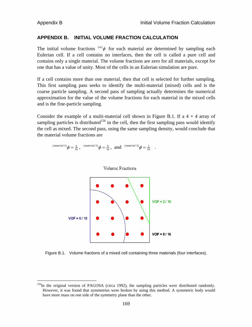
Appendix B Initial Volume Fraction Calculation
169
APPENDIX B. INITIAL VOLUME FRACTION CALCULATION
The initial volume fractions ( )m for each material are determined by sampling each Eulerian cell. If a cell contains no interfaces, then the cell is called a pure cell and contains only a single material. The volume fractions are zero for all materials, except for one that has a value of unity. Most of the cells in an Eulerian simulation are pure. If a cell contains more than one material, then that cell is selected for further sampling. This first sampling pass seeks to identify the multi-material (mixed) cells and is the coarse particle sampling. A second pass of sampling actually determines the numerical approximation for the value of the volume fractions for each material in the mixed cells and is the fine-particle sampling. Consider the example of a multi-material cell shown in Figure B.1. If a 4 × 4 array of sampling particles is distributed156 in the cell, then the first sampling pass would identify the cell as mixed. The second pass, using the same sampling density, would conclude that the material volume fractions are
( 1) 616
material , ( 2) 816
material , and ( 3) 216
material .
Figure B.1. Volume fractions of a mixed cell containing three materials (four interfaces).
156In the original version of PAGOSA (circa 1992), the sampling particles were distributed randomly.
However, it was found that symmetries were broken by using this method. A symmetric body would have more mass on one side of the symmetry plane than the other.

Appendix B Initial Volume Fraction Calculation
170
A different sampling density would result in different initial volume fractions. The user is responsible for deciding the cell size, coarse- and fine-sampling densities, and what features are important to capture in the initial geometry of the simulation. Each material in the cell possesses an interface. For example, in Figure B.1, the first material has an interface represented by the blue line. The second material has two interfaces: the green line and the blue curve. The third material has a single interface represented by the green curve. In total, four interfaces are shown in Figure B.1. The curved surfaces of the input body definitions will be represented by planes in each cell. Each material interface in a cell is represented by a plane (see Appendix C). Therefore, a part of the geometry information is lost in the surface reconstruction algorithm. Small features less than a cell thick can be represented using this technique. However, some pathological cases are of note. Consider the case shown in Figure B.2, with four materials. In this case, one of the materials has an orientation and a thickness that escape detection by our sampling process. The cell would be identified as mixed during the coarse-particle sampling. How-ever, only three of the four materials would be identified, which requires that the sampling density be chosen with some care and a detailed knowledge of the parts in the simulation.157 The volume fractions for this sampling density are
( 1) 10
16
( 2) 216
( 3)
( 4) 416
016 0
material
material
material
material
.
Figure B.2. A pathological case where some materials can go missing from a cell.
157The total mass could be numerically correct. However, the mass distribution could be wrong.

Appendix B Initial Volume Fraction Calculation
171
The thin layer of material (material 3) is missing, and the volume fraction for material 4 is also incorrect. Doubling the fine-particle density (8 × 8 instead of 4 × 4) would capture part of the missing material and result in a better balance between the representations of materials 3 and 4. Clearly, a tradeoff between computation and simulation fidelity is evident. A higher density of sampling particles means a longer computation. Eventually, the user is faced with the situation of diminishing returns. The extra accuracy is not worth the computational effort. This Monte Carlo technique is used to compute the initial volume fraction for a simulation. As the simulation proceeds, the volume fractions for each cell are recomputed based on the advection volumes (see Chapter 4 and Appendix E for details about the advection algorithm). Finally, a numerical example of the particle sampling technique is shown in Figures B.3 and B.4. An offset circle is placed in a uniform 4 × 4 Eulerian mesh. The exact volume fractions and ideal interfaces are shown in Figure B.3.
Figure B.3. Exact volume fractions and ideal interfaces. The ideal values for the volume fractions are 0.0% ,
1 1 112 4 43 31.51467 % ,
1 13 2 3 1 91.322295 % , and
100.0%
Figure B.4. Reconstructed interfaces and volume fractions based on the PAGOSA initial volume fraction algorithm with a small sampling density.

Appendix B Initial Volume Fraction Calculation
172
This page intentionally left blank.

Appendix C Youngs Interface Reconstruction
173
APPENDIX C. YOUNGS INTERFACE RECONSTRUCTION
The following is based on publication LA-UR-07-2274.158 The complete derivation is presented in that document.
C.1 Analytic Geometry
Consider the equation of a plane in Cartesian 3 space:
1 2 3 0x y z . (C.1)
Define the following quantities:
direction vector 1 2 3( , , ) , and
distance parameter . The sense of and the sign of are not defined by the equation. For example, we could say that
1 2 3 ( ) 0x y z ,
so that the direction of and the sign of are reversed.
The direction cosines of the normal to the plane are
31 2
2 2 2 2 2 2 2 2 21 2 3 1 2 3 1 2 3
, ,
, (C.2)
and the distance from the coordinates’ “origin” to the plane is
2 2 21 2 3
. (C.3)
Equation (C.1) divides all space into two regions. The direction vector points into the region “in front of the plane” and away from the region “in back of the plane.” Given a point 0 0 0 0( , , )x x y z , then
158Chuck Zemach, “Notes on Calculation of the Volume of a Stretched Cube behind a Truncating Volume,”
Wayne Weseloh, editor, Los Alamos National Laboratory report LA-UR-07-2274 (March 1, 2007).

Appendix C Youngs Interface Reconstruction
174
0x lies behind the plane if 1 0 2 0 3 0 0x y z and
0x lies in front of the plane if 1 0 2 0 3 0 0x y z .
Suppose that 0 0 0 0( , , )x x y z is a point and ( , ) is a plane. Define a right tetrahedron with vertices 0 , , ,X Y ZP P P P as follows (see Figure C.1):
Set 0 0 0 0( , , )P x y z .
Draw lines through 0P parallel to the x, y, and z axes.
Define ZP intersection of the z line with the plane.
If ( , , )ZP x y z , then 0x x , 0y y , and 1 0 2 0 3 0x y z , so
1 0 2 0 3[ ] /z x y
and
0 0 1 0 2 0 3( , ,[ ] / )ZP x y x y .
Figure C.1. Tetrahedron bounded by the ( , ) plane.
Similarly, ,X YP P are the intersections of the x line and y lines into the plane, respectively, and
2 0 3 0 1 0 0([ ] / , , )XP y z y z and
0 1 0 3 0 2 0( ,[ ] / , )YP x x z z .
Define
0 0T , if 0x is in front of the plane,

Appendix C Youngs Interface Reconstruction
175
0T volume of the tetrahedron if 0x is in back of the plane.
Then for 0x in back of the plane, the volume of the tetrahedron is159
0 0 0 0
1
3! X Y ZT P P P P P P , or
3
1 0 2 0 3 00
1 2 3
( )
6
x y zT
. (C.4)
In this definition,
0T is always 0 .
0T if any one of 1 2 3, , 0 , which corresponds to the ( , ) plane being parallel to one or more of the x, y, and z axes.
1 2 3, , , can have any sign, but 1 2 3 0 .
The expression for 0T is unchanged under a (positive)
scaling 2i i , 2 .
C.2 Distance Parameter ρ
Consider a volume fraction v containing the origin and satisfying the relation 1
20 v .
The case where 1
2 v 1 is obtained by symmetry (discussed below). The plane is described by the direction cosines 1 2 3( , , ) , which satisfy
1 2 30 and 2 2 21 2 3 1 .
The equation for the plane is 1 2 3x y z and has five different solutions for
( , v) , which correspond to the five ways of slicing a cube with a plane. The variable mask is logically true when a particular following case applies.
159L.E. Dickson, “Note on the Volume of a Tetrahedron in Terms of the Coordinates of the Vertices,” The
American Mathematical Monthly, Volume 14, Number 6/7 (June–July, 1907), pp. 117–118.

Appendix C Youngs Interface Reconstruction
176
Case 1. Triangular Section Mask: 10< v v , where 2
1 1 2 3v / 6 with 2 0 .
Solution: 1/3
1 2 36 v (C.5)
If 1 0 , then v = 0 .
Case 2. Quadrilateral Section, Type A Mask: 1 2v < v v , where
2
2 1 2 2 1 2 3v 3 ( ) / 6 with 2 0 .
Solution: 21 11 2 3 12 38 v (C.6)
There is no solution if 2 0 . And 1 0 is acceptable.
Case 3. Pentagonal Section
Mask: 2 3v < v v if 1 2 3 ( 1 0 )
2 4v < v v if 1 2 3 .
In this last mask, if 1 0 , then 2 4v v , where
3 3 33 3 1 3 2
31 2 3
( ) ( )v
6
, and
4 1 2 3v ( ) / 2 .
Solution: 1 2 1 22 2 cos ( 2 ) / 3 , and (C.7)
1 1 2 3
1 2
3( 2 v )cos
4 2
.

Appendix C Youngs Interface Reconstruction
177
Case 4. Hexagonal Section
Mask: 13 2v < v if 1 2 3 ( 1 0 ) .
Solution: 2 10 0 22 cos ( 2 ) / 3 , and
1 1
0 1 2 32 2( ) (v ) , and (C.8)
1 1 2 32 3/ 210 2
3 (1 2 v )cos
4( )
.
Case 5. Quadrilateral Section, Type B
Mask: 1
4 2v < v if 1 2 3 .
Both 1 0 and 2 0 are acceptable.
Solution: 1
3 1 22v ( ) . (C.9)
C.3 ρ Symmetry
For the case of 12 < v 1 , the solution is obtained by
max( v ) (1 v ) , (C.10)
where
max 1 2 3 .
C.4 Volume v
Given a vector normal to a plane passing through a unit cube and which need not be normalized but which satisfies
1 2 30 ,
and given , where / | | is the distance from the origin to the plane and which satisfies

Appendix C Youngs Interface Reconstruction
178
1max20< ,
where
max 1 2 3 ,
the case of 1
max max2 < is obtained by symmetry (discussed below).
The volume fraction behind the plane that contains the origin has five different solutions corresponding to the five ways of a plane slicing a cube. Case 1. Triangular Section
Mask: 10< , ,
where 1 0 .
Solution: 3
1 2 3
v ( )6
. (C.11)
Case 2. Quadrilateral Section, Type A
Mask: 1 2< , ,
where 2 0
Solution: 2 2
1 1
2 3
(3 3 )v ( )
6
(C.12)
Case 3. Pentagonal Section
Mask: 2 1 2 3< min( , ) with 1 0 .
Solution: 3 3 3
1 2
1 2 3
( ) ( )v ( )
6
(C.13)

Appendix C Youngs Interface Reconstruction
179
Case 4. Hexagonal Section
Mask: 13 max2< , 1 2 3 , and 1 0 .
Solution:
3 3 3 31 2 3
1 2 3
( ) ( ) ( )v ( )
6
(C.14)
Case 5. Quadrilateral Section, Type B Mask: 1
1 2 max2< with 1 2 3 .
Solution: 1 2
3
2 ( )v ( )
2
(C.15)
C.5 v Symmetry
For the case of 1max max2 < , the solution is obtained by
maxv ( ) 1 v ( ) , (C.16)
where
max 1 2 3 .

Appendix C Youngs Interface Reconstruction
180
This page intentionally left blank.

Appendix D Lagrangian-Phase Equation
181
APPENDIX D. LAGRANGIAN-PHASE EQUATION
Consider the expansion of a fluid. Let V be the volume of the fluid element, bounded by a surface S . Let S move with the fluid so that it always contains the same particles (i.e., a Lagrangian surface). Let u be the velocity. Then ˆu n is the component of the velocity along the outward normal vector n . As the fluid moves, a point on the surface is displaced. The Lagrangian equation for mass continuity160 is given by
0t
u .
The mass within the bounded surface S is m . The mass density of the material within the surface S is simply
/m Vol . Substituting the expression for density into the continuity equation, we find that
10
Vol
Vol t
u . (D.1)
This expression in a finite difference form is
12
11( )
n nn
n
Vol Vol
Vol t
u , or (D.2)
1 [1 ( ) ]n nVol Vol t u , (D.3) where the superscripts refer to the (n) and (n+1) timesteps. The cell may contain multiple materials, each with their own individual volumes. The Lagrangian volume is the sum of all those individual volumes. The entire cell volume evolves subject to the expression in Eq. (D.3). An alternate way of understanding Eq. (D.3) is by a first-principles derivation. Consider the expansion of a fluid element. Let V be the volume of the fluid bounded by a surface S. Let S move with the fluid so that it always contains the same material. Let iu
160 See Eq. (4.11) in Chapter 4 (Operator Splitting).

Appendix D Lagrangian-Phase Equation
182
be the local fluid velocity. Then ˆi iu n u n is the component of velocity in the direction
of the outward normal. As the fluid moves, a fluid element on the surface is displaced, as shown in Figure D.1. The normal displacement in an infinitesimal time dt is i iu n dt . Thus, the volume of the thin shell between the surface S at time t and the surface formed later at time t + dt is
2Volume i idt u n d x . (D.4)
Figure D.1. Lagrangian expansion of a fluid.
However, this volume is an increase in the volume V, and so we have
2 2 3ˆi i
Volu n d x d x d x
t
u n u (D.5)
by Green’s theorem. Partition the volume Vol, and consider a sequence of volumes, all enclosing point P. Let the volumes shrink to point P. Then we have
3
0 0
1 1lim lim
Vol Vol
Vold x
Vol t Vol
u u (D.6)
evaluated at point P, exactly as was previously found in Eq. (D.1). The divergence of the velocity at point P is the expansion of the fluid at point P.

Appendix E First-, Second-, and Third-Order Advection
183
APPENDIX E. FIRST-, SECOND-, AND THIRD-ORDER ADVECTION
Figure E.1. Cell advection diagram.
Consider the x-advection-phase conservation of mass equation. The one-dimensional equation is
0Ut x
. (E.1)
If we assume that the velocity U is a constant, the finite difference form can be written as
1 12 2
11
0n n n n
i ii iU
t x
,
where the i densities are evaluated at the cell boundaries, as shown in Figure E.1. Solving for the density at the new time, we have
1 1 12 2 2
11 1( ) ( )n n n n n n n
i i i ii i i
tU
x
tU
x
. (E.2)
The problem is to find the cell boundary densities in terms of the surrounding cell-centered densities. The mass flow through the cell boundary located at index i is equal to
i iU A t , where iA is the cell boundary surface area. First we choose a nondimensional spatial variable161
xxxi /)( . (E.3)
The velocity at 0 is assumed to be positive.162 The time indices will be dropped for the remaining portion of the derivation. The density is assumed to be a polynomial function163 of the dimensionless spatial variable (i.e., 2a b c ). The increasing orders of advection correspond to the increasing degrees of the density polynomial. Note that the degree of the polynomial does not necessarily correspond to a formal order of accuracy.
161For simplicity, assume a constant cell size. Variable zoning requires slight modifications to the
equations. 162This is only one case of the trichotomy. A negative velocity represents another case and is not derived
here. The zero velocity case is trivial. 163Richard L. Bowers and James R. Wilson, Numerical Modeling in Applied Physics and Astrophysics
(Jones and Bartlett Publishers, Boston, Massachusetts, 1991), pp. 238–243 and Appendix C.

Appendix E First-, Second-, and Third-Order Advection
184
E.1 First-Order Advection
The density is assumed to be a constant function over the range [0,1] as
a . (E.4) The average density of the advection volume ( [0, ] ) is assumed to be the density at the cell boundary. The cell boundary average density is
adi
0
1 . (E.5)
The cell centered density is
12
1
0i
d a . (E.6)
The coefficient a is thus known. First-order advection, also called upwind advection or the donor cell method, is164
12
i i First Order . (E.7)
Upwind differencing is simple but known to be diffusive. The first-order method often gives poor results.
E.2 Second-Order Advection
In this case, the density is assumed to be a linear function over the range [ 1,1] . The polynomial is
ba . (E.8) The average density of the advection volume is assumed to be the density at the cell boundary. The advection density is assumed to be constant in the range [0, ] . The cell boundary average density is
12
0
1i d a b
. (E.9)
164Bram van Leer, “Upwind and High-Resolution Methods for Compressible Flow: From Donor Cell to
Residual-Distribution Schemes,” Communications in Computational Physics, Volume 1, Number 2 pp. 192–206 (April 2006).

Appendix E First-, Second-, and Third-Order Advection
185
The cell-centered densities are
12
12
012
1
112
0
, andi
i
d a b
d a b
. (E.10)
The coefficients a and b are easily evaluated. They are
1 12 2
1 12 2
12 ( ) , and
i i
i i
a
b
. (E.11)
The cell boundary density is
1 1 1 12 2 2 2
1 12 2( ) ( )i i i i i
,
which can be written as
1 1 12 2 2
12 (1 ) ( )i i i i
Second Order. (E.12)
Equation (E.12) is second-order advection. This method is less diffusive than the first-order method, but nonphysical oscillations and negative densities often occur. It is interesting to note that in the limit as 0 , the second-order method results in the cell boundary average density being just the average of the densities on either side of the boundary.
E.3 Third-Order Advection
In this case, the density is assumed to be of the form of a quadratic function over the range of [ 1, 2] . The polynomial is
2a b c . (E.13) The cell boundary average density is
231
21
0
1
cbadi . (E.14)
The cell-centered densities are

Appendix E First-, Second-, and Third-Order Advection
186
12
12
32
01 12 3
1
11 12 3
0
23 72 3
1
,
, and
.
i
i
i
d a b c
d a b c
d a b c
(E.15)
We have three simultaneous equations with three unknowns. In matrix form, we have
1/2
11/26
3/2
6 3 2
6 3 2
6 9 14
i
i
i
a
b
c
. (E.16)
The solution of this 3 × 3 matrix equation is
1/2
11/26
3/2
2 5 1
6 6 0
3 6 3
i
i
i
a
b
c
, (E.17)
or
1 1 1 32 2 2 2
16 (2 )
i i i ia ,
1 12 2i i
b , and
1 1 32 2 2
12 ( 2 )
i i ic .
The cell boundary density is
1 1 1 3 1 1 1 1 32 2 2 2 2 2 22 2
1 1 1 1 32 2 2 2 2
1 1 1 1 32 2 2 2 2
21 1 16 2 6
2 21 1 1 1 13 2 6 6 6
1 1 12 3 3
(2 ) ( ) ( 2 )
( ) ( ) ( ) ( )
(1 )[ (2 ) ( ) (1 ) ( ) ]
i i i i i i i ii i
i i i i i
i i i i i
. (E.18)
The third-order method yields a cell boundary density of
1 1 1 1 32 2 2 2 2
16 (1 )[ (2 ) ( ) (1 ) ( ) ]i i i i i i
Third Order .

Appendix E First-, Second-, and Third-Order Advection
187
The third-order method is less diffusive than the second-order method but still exhibits some minor problems with negative densities and nonphysical oscillations. These problems can be eliminated by using the gradient limiters discussed next. The methodology presented here presumably can be extended indefinitely. However, the higher-order advection schemes require increasingly more complexity and more distant cell information. For all the possible advection methods discussed, the density at the cell boundary can be written following the style of Youngs:165
12
12 (1 )i ii
x D , (E.19)
where /iD x has the role of the density gradient. This formalism provides a concise way of understanding the various methods. The gradients are
First Order: 0iD , (E.20a)
Second Order: 1 12 2i i
iDx
, and (E.20b)
Third Order: 1 31 122 2 2
(2 ) (1 )
3 3ii i i
iDx x
. (E.20c)
The higher-order methods require more information to construct an approximation to the density gradient at the cell boundary. A physical interpretation of the above equations can be gained by considering a simple example. A material of uniform density is moving with a positive velocity through the 1D Eulerian mesh. In this case, all the gradients are zero. First, second, and third orders give the same answer—simple downwind advection (donor cell advection). However, this advection is only first order! First-order advection gives the correct answer in this simple example. The cell boundary densities are the same as the cell-centered densities. Next consider a square pulse with a uniform density moving with a positive velocity in a 1D Eulerian mesh. The top of the pulse exhibits the same behavior as described in the previous example. Locally, the density gradients are all zero. Again, the result is first-order advection. The gradients will be nonzero only near the edge of the pulse. The finite difference gradients can capture the infinite slope at the edge of the pulse only partially.
165David L. Youngs, “Time-Dependent Multi-Material Flow with Large Fluid Distortions,” Numerical
Methods for Fluid Dynamics, K.W. Morton and M.J. Baines, editors (Academic Press, London England, 1982), pp. 273–285.

Appendix E First-, Second-, and Third-Order Advection
188
The square pulse will smooth out over many advection steps. The higher-order advection methods become important when the density gradients are large. The numerical advection of a square pulse is shown at the end of this appendix.
E.4 Gradient Limiters and Monotonicity166,167
The choice of advection order depends on the local density gradients. The third-order method is clearly the best choice in most situations. In fact, it is the default advection method used in PAGOSA. However, the third-order method is occasionally nonphysical.
Figure E.2. Upwind, downwind, and third-order gradients.
The nonphysical behaviors can be eliminated by choosing iD such that 168
1 1 1 32 2 2 2
1 1 1 32 2 2 2
, ,2 2min (
2 1) /
3 3
i i i ii
i i i i
D
x
. (E.21)
The result is that in some cases the density gradient can be first, second, or third order, depending on the exact local density distribution. Figure E.2 shows this option
166Bram van Leer, “Towards the Ultimate Conservative Difference Scheme IV. A New Approach to
Numerical Convection,” Journal of Computational Physics, Volume 23, pp. 276–299 (March 1977). 167Bram van Leer, “Towards the Ultimate Conservative Difference Scheme V. A Second-Order Sequel to
Godunov’s Method,” Journal of Computational Physics, Volume 32, pp. 101–136 (July 1979). 168 David L. Youngs, “Time-Dependent Multi-Material Flow with Large Fluid Distortions,” Numerical
Methods for Fluid Dynamics, K.W. Morton and M.J. Baines, editors (Academic Press, London England, 1982), pp. 277-285.

Appendix E First-, Second-, and Third-Order Advection
189
graphically.169 It is a powerful and convenient way of understanding the various limiters and monotonicity conditions that are needed to realize fully the third-order advection method. It is important to note that the gradients are limited and not the densities themselves. This gradient limiting ensures that the conservation law is not violated. In general, the van Leer limiter allows for the largest possible gradient without oscillations and therefore the least amount of diffusion. This choice of nonlinear cutoff of the density gradient also ensures that the new density gradient (at the next timestep,
1n ) will have the following property:
1 1 1 1 12 2 2 2 2
1min ( , ) max ( , )n n n n ni i i i i
. (E.22)
This condition guarantees that when a monotonic initial value distribution is advected, the resulting distribution is also monotonic.170 In highly discontinuous flows, the value of iD is modified to prevent undershoots and overshoots. A multiplicative factor is constructed such that, as shown in Figure E.3,
1 1 1 32 2 2 2
1 12 2
1 1 1 32 2 2 2
( ) ( ) 00( )
( ) ( ) 01
i i i i
i ii i i i
S sign
. (E.23)
If the upwind and downwind gradients differ in sign, the factor S is set to zero.
Figure E.3. The Youngs/van Leer gradient limiter. When (a), the gradients are monotonic, or
when (b), the gradients indicate that the density has reached a local maximum (minimum).
169 Sean Clancy, Los Alamos National Laboratory, personal communication (June 5, 2008). 170Randall J. LeVeque, Numerical Methods for Conservation Laws, Second Edition (Birkhäuser Verlag,
New York, New York, 1992), pp. 183–187.
(a) (b)

Appendix E First-, Second-, and Third-Order Advection
190
The sign factor for the value of S establishes the local sign of the gradient. The Youngs/ van Leer gradient limiter suppresses negative densities or reduces the density gradient to zero if an extremum is reached or if the slope does not agree with the trend in density averages. An example of the effect of the gradient limiter is shown in the last section of this appendix. The negative densities and other nonphysical behaviors readily apparent in the third-order method are suppressed using the Youngs/van Leer gradient limiter.
E.5 PAGOSA Advection
All of these pieces are brought together in PAGOSA. Start with the following definitions:
12
ni
Don donor cell,
1 32 2
n ni i
Upw upwind gradient, and
1 12 2
n ni i
Dnw downwind gradient,
and we define the following coefficients
1 12 2
1 12 2
1
2
3 1
4 1
/
/
(1 ) /6
(2 ) / 6
n ni i
i i
Vol Vol
m m
.
The value , defined in Eq. (E.2), sometimes called the Courant number, can be related to the fractional advection volume. The Courant number is less than unity because the advection volume must be less than the original cell volume. The Courant number, at index i, is
12
12
1
advection volume
cell volumeii i
i ii i
VolU t AtU
x x A Vol
.
The cell boundary density, with all factors included, is
1 3 4(1 ) min( , , )i Don S Upw Dnw Upw Dnw .
The interface (cell boundary) mass flux is 1
2i ii
m Vol .

Appendix E First-, Second-, and Third-Order Advection
191
The updated cell mass is
1 12 2
11
n ni ii i
mass mass m m .
The new cell mass is the old cell mass plus the mass entering from the left boundary minus the mass leaving through the right boundary. Remember that we have assumed that
0iU ; therefore, in every cell we have mass entering from the left and leaving to the right. The updated cell density is171
1 1 1 1 12 2 2 2 2
1 1 / ( )n n n n ni i i i i
mass Vol Vol Vol .
The new cell density is the new cell mass divided by the new associated cell volume. Next, the specific internal energy is advected. The process is basically the same as that described above, with a few exceptions. The specific internal energy is advected by mass and not by volume, as was done previously.172 Start with the following definitions:
12
ni
Don E donor cell,
1 32 2
n ni i
Upw E E upwind gradient, and
1 12 2
n ni i
Dnw E E downwind gradient.
The cell boundary specific internal energy is
2 3 4(1 ) min( , , )iE Don S Upw Dnw Upw Dnw ,
where S has the same form as before, except that specific internal energy functionally replaces density in that equation [Eq. (E.23)]. The updated cell specific internal energy is
1 1 1 1 12 2 2 2 2
1 11 1( ) /n n n n n
i i i ii i i i iE E Vol m E m E mass
.
This equation completes the advection-phase of the basic hydrodynamic variables.
171 The temporal indices (n) and (n+1) refer to before and after the advection sweep. 172Roger B. DeBar, “Fundamentals of the KRAKEN Code,” Lawrence Livermore Laboratory report UCIR-
760, pp. 13–14 (March 1974).
Appendix E First-, Second-, and Third-Order Advection
192
Each of the finite difference equations has stability173 and convergence considerations, dissipation,174 dispersion,175 and phase errors.176 These analyses and considerations are beyond the scope of this work. Please consult the literature. The cell-centered quantities (e.g., strain rates, stress deviators, and elastic distortional energy) are advected by mass in the same way that the specific internal energy is advected. To prevent small values from being advected through the Eulerian mesh, various cutoffs are imposed on the advection algorithm. If the advection volume is too small, then it is set to zero. The final section of this appendix gives a numerical example of advecting a square pulse.
173Robert D. Richtmeyer and K.W. Morton, Difference Methods for Initial Value Problems, Second Edition
(Interscience Publishers, Malden, Massachusetts, 1967), pp. 320–330. 174Dale R. Durran, Numerical Methods for Wave Equations in Geophysical Fluid Dynamics (Springer-
Verlag, New York, New York, 1999), pp. 72–86. 175Lawrence L. Tackas, “A Two-Step Scheme for the Advection Equation with Minimized Dissipation and
Dispersion Errors,” Monthly Weather Review, Volume 113, pp. 1050–1065 (June 1985). 176W.P. Crowley, “Numerical Advection Experiments,” Monthly Weather Review, Volume 96, pp. 1–11
(January 1968).

Appendix E First-, Second-, and Third-Order Advection
193
E.6 Advection Example: Advection of a Square Pulse An example of the advection of a square pulse is provided in Figure E.4.
Figure E.4. Advection of a square pulse.
The results of a test problem using the advection equations are shown in Figure E.4. A square pulse with a uniform constant velocity is propagated through 300 cells. The exact solution is shown in black in each case. The initial square pulse is 20 cells wide, with a density of unity. The Courant number 0.100 .

Appendix E First-, Second-, and Third-Order Advection
194
This page intentionally left blank.

Appendix F Initial Timestep Calculation
195
APPENDIX F. INITIAL TIMESTEP CALCULATION
The timestep used for each cycle must be less than the maximum stable timestep for each cell in the simulation. The initial timestep can be specified by the user for the simulation and must satisfy the following conditions:
0 min , ,max( ) max( ) max( )
x y zt
U c V c W c
. (F.1)
Two equations that are useful for estimating the initial timestep are the equations for the sound speed of an elastic solid:
1c
, equivoluminal wave propagation speed and (F.2)
43
2
Gc
, irrotational (shear) wave propagation speed , (F.3)
where is the bulk modulus, G is the shear modulus, and is the mass density. In the case of solid materials, the initial timestep can often be computed by
0
1 2
min , ,
max ,
x y zt
c c
. (F.4)
When the simulation involves HE, the sound speed for the undetonated explosive is set to 3D, where D is the explosive detonation velocity. The timestep for the explosive is then given by
0 min , ,
3
x y zt safec
D
, (F.5)
where safec is the Courant safety factor described in Chapter 9. The initial condition should be chosen by the user to be much smaller than any of the above criteria. The timestep should “creep up” to a stable timestep determined from the most restrictive criterion.

Appendix F Initial Timestep Calculation
196
This page intentionally left blank.

Appendix G Multi-Material Interface Reconstruction for Advection
197
APPENDIX G. MULTI-MATERIAL INTERFACE RECONSTRUCTION FOR ADVECTION 177
G.1 Reconstruction
For each sweep of the advection phase, it is necessary to compute the volume fractions that will be advected in that sweep. The advection volume may contain several materials, as shown in Figure G.1. Figure G.1. The advection volume (shown in yellow) contains three materials to be advected.
The flux direction in this case is negative.
The main object of this process is to find the advection volume for each material in a cell given the advection volume and the volume fraction of each material in the donor cell and its 26 neighbors. The notation for this appendix is v = donor cell volume,
v = advection volume, vm = advection volume for the material (m),
= v / v advection volume fraction,
vm = donor cell volume fraction of material (m),
vm
= total volume fraction up to the mth interface,
v p m = portion of v
m contained in the advection volume,
mμ = vector normal to the mth interface, pointing out of the volume vm
, and
vm
= v vp m total advection volume up to the mth interface.
177Rick Smith, Los Alamos National Laboratory, personal communication, March 15, 1991.

Appendix G Multi-Material Interface Reconstruction for Advection
198
The procedure for calculating the individual material advection volumes is to
calculate , initialize all v 0
m ,
sum over the number of materials (m) (except for the last material): o increment the sum and obtain v
m ,
o calculate mμ from the gradients of vm
(26 neighbors + donor) ,
o calculate v p m (depends on , mμ , and v
m) ,
o calculate 1
v v v vm p mm , and
o determine a new value of v v vpm m .
end of material loop (m) , and calculate the last material ( ) ( ) 1
v v vlast m last m .
For the v 0 cases (i.e., flux through the right face of the cell), we must ensure that the donor cell quantities (in the cell to the left) are used. Also, it is necessary to replace
1 and substitute the advection volume fraction with its complement.
G.2 Volume Fraction Identifier
The idea is to compute the volume fraction of the advected portion of a material on one side of a plane that passes through the Eulerian cell, as shown in figure G.2.
Figure G.2. A cross section of an Eulerian cell showing a material interface with a direction
vector µ, a volume fraction to be advected ε (relative to the full cell volume Vol), and the volume fraction of the advected portion of the material Vp.

Appendix G Multi-Material Interface Reconstruction for Advection
199
In this case we know the volume of the cell (Vol), the volume fraction of the materials behind the plane (<v>), and the direction vector associated with the interface (µ) and which points out of the material that lies “behind” the plane.178 The volume fraction of the advected portion of the material is what is to be computed (<vp>) and is defined relative to the full cell volume. In the derivation, if we assume that the flux direction is for the positive flux, the solution can be obtained by treating the nonadvected portion as the advection volume (see Figures G.2 and G.3). The coordinate system used here has X0 at the origin (where X0 is the vertex with the same indices as the cell). In this derivation, it is assumed that the flux direction is negative (through the face containing X0). For the case of positive flux, the solution can be obtained by treating the nonadvected portion as the advection volume, as shown in Figure G.3. Figure G.3. The case of positive flux is simply the complement of the previous case shown in
Figure G.2.
If we denote the solution for positive and negative flux as ( )
pV and ( )pV , respectively,
then ( )pV is given in terms of ( )
pV by
( ) ( )
p pV ( ) V (1 )Vol , (G.1)
where Vol is the full cell volume.
178The direction vector for the interface is computed by a simple finite difference formula using the volume
fractions of the surrounding 26 cells.

Appendix G Multi-Material Interface Reconstruction for Advection
200
The algorithm for the solution of ( )
pV is obtained in two steps (see Figure G.4):
Step 1. Find the equation of the plane d μ x . Step 2. Transform the advection volume into a unit cube, and using the equation for the plane in the transformed frame, find the volume fraction V of the material within this cube that is behind the plane (see Appendix C for details). The solution for pV is then given by
pV V .
Figure G.4. If we are given the volume behind the plane (v) and the unit normal µ, the algorithm
will find the distance parameter d.
We begin with the detailed procedures for Step 1. Step 1. Find the equation of the plane d μ x in the coordinate frame x , with 0x at
the origin. Let mx be the coordinate of the vertex toward which μ most closely points (i.e., kμ x is a minimum for the vertex k m ). Now translate to a frame x with mx at the origin as m x x x , (G.2)
md d μ x , and (G.3) 1
1 1 2 2 3 32 ( ) ( ) ( )m md μ x . (G.4)

Appendix G Multi-Material Interface Reconstruction for Advection
201
Now normalize μ to unity - a unit normal vector. Then ˆ μ x , (G.5) ( ) /md d μ , and (G.6) ˆ /μ μ μ . (G.7) By symmetry, the solution ( , )V μ will not change if we replace 1 2 3ˆ ˆ ˆ ˆ( , , ) μ c (G.8) and reorder the components of c such that 1 2 30 c c c . (G.9) The solution then is ˆ( , ) ( , )V V μ c , which is derived in Appendix C and report LA-UR-07-2274179. The solution is then md d μ . (G.10) Note that /d μ is the distance from the origin 0x to the plane. If 0d , then 0x is behind the plane and thus inside the material; however, if 0d , we have the situation where
0x is in front of the plane and outside the material. The algorithm proceeds with Step 2. Step 2. Next, transform to a coordinate system x in which the advection volume is
stretched to a unit cube (see Figure G.5): 1 2 3( / , , )x x xx and (G.11)
2 3( , , )x xg . (G.12) Now translate these equations to a new frame x with mx at the origin, where mx is the vertex in the new unit cube representing the advection volume toward which g most closely points (i.e., kg x is a minimum for the vertex k m ):
179Chuck Zemach and Wayne Weseloh (editor), “Notes on Calculation of the Volume of a Stretched Cube
behind a Truncating Volume,” Los Alamos National Laboratory report LA-UR-07-2274 (March 1, 2007).

Appendix G Multi-Material Interface Reconstruction for Advection
202
Figure G.5. The advection volume in the new coordinate system stretched to a unit cube.
m x x x , (G.13)
md d g x , and (G.14)
11 1 2 2 3 32 ( ) ( ) ( )m md g g g g g g g x . (G.15)
Now we need to determine the fraction v of the advection volume that lies behind the plane. By symmetry, the solution v ( , )g will not change if we permute the components of 1 2 30 g g g . (G.16)
We can again use the results in Appendix C, which derive v( , )g . The solution for pv is
then finally given by pV V ( , ) g and (G.17)
11 12 (1 )md d g g g . (G.18)
Note that if 0 , then the plane lies entirely outside the advection volume and pV 0 .
Conversely, if max , then V 1 and pV .
This algorithm is applied over all materials in the mixed cell, as described in Figure 4.3 and the associated text. A flowchart of that algorithm is shown at the beginning of this appendix.

Appendix H The Cauchy-Stokes Decomposition Theorem
203
APPENDIX H. THE CAUCHY-STOKES DECOMPOSITION THEOREM
The decomposition theorem developed by Cauchy180 and Stokes181 states that
An arbitrary instantaneous state of a fluid particle moving along its path may be resolved at each position ( , )ix P t as a superposition of (1) a translation, (2) a rigid rotation, (3) a dilatation along three mutually perpendicular axes, and (4) a shear motion.
Consider a velocity field ( , )i ku x t of a moving fluid particle in a neighborhood of its
position kx at a time t . When the velocity field is continuous and differentiable, a Taylor
expansion of the velocity function near a point P exists and takes the form
( , ) ( , ) ( )ii k i k
j
uu x t u P t x P
x
. (H.1)
The gradient can be decomposed into its symmetrical and antisymmetrical parts as
12
iij ij ij ij m m
j
ue e
x
, (H.2)
where the symmetrical tensor e is called the strain rate tensor, the antisymmetrical tensor is called the vorticity tensor, and is the axial vector associated with the vorticity tensor. The permutation symbol i j m is the Levi-Civita pseudotensor,182 where
12( , ) ( , )i k i ij j ij m j mu x t u P t e x x . (H.3)
The second term can be written as
12( )i j j ij j k
k
e x e x xx
. (H.4)
180D’Augustin Cauchy, “Mémoire sur les Dilatations, les Condensations et les Rotations Produites par un
Changement de Forme dans un Système de Points Matériels,” in Oeuvres Complètes D’Augustin Cauchy (Series 2) (Gauthier-Villars et Fils, Imprimeurs-Libraires du Bureau des Longitudes, de L’école Polytechnique, Paris, 1841), Volume 12, pp. 343–367.
181George Gabriel Stokes, “On the Theories of Internal Friction of Fluids in Motion, and of the Equilibrium and Motion of Elastic Solids,” in Mathematical and Physical Papers (Cambridge University Press, London, 1845), Volume I, pp. 75–129 (1845).
182G. Arfken, Mathematical Methods for Physicists (Academic Press, Inc., Harcourt Brace Jovanovich Publishers, London, England, 1970), p. 132. It is sometimes called the permutation symbol.

Appendix H The Cauchy-Stokes Decomposition Theorem
204
This term represents a velocity field normal at each point to the quadratic surface
i j j ke x x constant , which contains the point P. Because the symmetric tensor possesses three mutually perpendicular eigenvectors, the eigenvalues of the deformation tensor e measure the rates of extension per unit length of the fluid particle at ( , )kx P t in the directions of the eigenvectors, which can always be taken as the three basis vectors of the velocity field. Therefore, Eq. (H.1) becomes
21( , ) ( , ) ( ) ( / 2) ( )
2i k i ij j k ij m j mk
u x t u P t e x x x O xx
. (H.5)
Thus, the first term represents a translation. Simple integration of the velocity field gives the three translations. The second term determines the distortion of the fluid element. The distortion consists of a dilatation (the diagonal terms of the tensor ike ) and a superposition of shear motions (the off-diagonal terms of the tensor ike ). The vorticity tensor (or vorticity vector) determines the rigid rotation of a fluid particle that keeps its volume and shape the same. The rotation axis is defined by the direction of the vorticity vector and an angular velocity of / 2m . This result is profound. Each piece of the deformation can be computed independently, and the results can be combined by linear superposition. Consider the motion of a small mass of an arbitrary shape, such as a cube. The motion of the cube may be divided into two types: a rigid body motion and a deformation motion. The rigid body motion may be divided further into a translation and a rotation. As the mass undergoes its rigid body motion, it can also deform. The deformation of the mass can be completely specified by describing the dilatation (volumetric expansion or contraction) and the shear strains of the mass, as shown in Figure H.1.
H.1 Translation
The translation is given by integrating the velocity vector u , which is closely related to the advection (remap) phase.
H.2 Rotation
The rotation rate is the angular velocity vector ω and is related to the vorticity183 tensor Ω . Rotation may or may not occur in a particular flow/deformation. A flow where the vorticity is zero is known as irrotational flow.
183See Eq. (1.8).

Appendix H The Cauchy-Stokes Decomposition Theorem
205
Figure H.1. The types of motion that, when superimposed, completely describes the kinematics
of a small elemental mass. The cubical shape is arbitrary.
H.3 Dilatation
The dilatation represents the contraction or expansion of an elemental mass. The rate of dilatation is related to the velocity divergence.184 The numerical value of the dilatation is independent of the coordinate system because it is the first invariant of the strain rate tensor [Eq. (1.5)].
H.4 Shear Deformation
A shear strain deformation is a strain that acts parallel to the surface of the material upon which it is acting. Thus, in our cubic example, the 90° angles between faces diverge from that value. The strain rate tensor [Eq. (1.5)] gives the rate at which the sides close toward each other.
184See Eqs. (1.6) and (1.7).

Appendix H The Cauchy-Stokes Decomposition Theorem
206
This page intentionally left blank.

Appendix I Stress Rotation
207
APPENDIX I. STRESS ROTATION
An important concept in the formulation of constitutive theories in deformations is that of frame indifference, or objectivity.185 The basic idea is that the constitutive relation between stress and strain should be unaffected by any rigid body rotations the material may undergoing at a particular instant of time. Mathematically we describe this situation by defining an alternative reference frame that is rotating and translating with respect to the original Eulerian coordinate system. For the constitutive relations to be meaningful, the tensor quantities we use (stress, stress rate, strain, and strain rate) should transform according to the laws of tensor calculus. If a given quantity does this transformation, we say it is material frame indifferent; if it does not, we say it is not properly invariant or not objective. The deviatoric stress in the Eulerian (laboratory) frame is S* and is denoted S in the material (rotated) frame of reference.186 The deviatoric stress tensor transforms as187
*ij ik km mjS Q S Q , (I.1)
where Q is a proper orthogonal (rotation) tensor that transforms the tensor S. Because Q is an orthogonal tensor, the transpose is the inverse. Thus,
ij jk ikQ Q . (I.2)
If we take the time derivative of the above equation,
ij jk ij jkQ Q Q Q 0 ij jk ij jkQ Q Q Q . (I.3)
Then we right-and-left multiply both sides of Eq. (I.1) by orthogonal tensors. Thus,
*ij ik km mjS Q S Q . (I.4)
The time derivative of the deviatoric stress tensor, Eq. (I.1), produces
*ij ik km mj ik km mj ik km mjS Q S Q Q S Q Q S Q . (I.5)
185 J.K. Dienes, “Analysis of Rotation and Stress Rate in Deforming Bodies,” Acta Mechanica, Volume 32, Issue 4, pp. 217-232 (1979). 186G.A. Holzapfel, Nonlinear Solid Mechanics (John Wiley and Sons, Weinheim, Germany), pp. 192–196
(2001). 187J.L. Synge and A. Schild, Tensor Calculus (Dover Publications Inc., Mineola, New York), p. 13 (1978).

Appendix I Stress Rotation
208
If we substitute Eq. (I.4) into the above equation,
* * *( ) ( )ij ik kn nl lm mj ik km mj ik kn nl lm mjS Q Q S Q Q Q S Q Q Q S Q Q , * **
ik kn nl lj ik km mj in nl lm mjij Q Q S Q S QS S Q Q , and * **
ik kn nj iki km mj il lj m mjQ Q S Q S Q S Q QS . (I.6)
If we apply Eq. (I.3),
* * *ij ik kn nj ik kn nj ik kn njS Q Q S Q S Q S Q Q . (I.7)
If we introduce a new variable,
ij ik kjW Q Q . (I.8)
We will find that this rotation is actually related to the vorticity tensor, but for now it is simply a mathematical convenience. Equation (I.7) is now written as
* * *ij ik kn nj in nj ik kjS Q S Q W S S W . (I.9)
Equation (I.9) is known as the Jaumann derivative,188 or the Jaumann-Zaremba rate.189 These objective rates are simply an application of the Lie derivative.190 What is not generally known or conceded is that Zaremba essentially introduced what is now known as the Jaumann derivative [but commonly referred to as the corotational (sometimes spelled “co-rotational”) derivative]. The rotational portion of Eq. (I.9) is computed separately as
* *ij ik kj ik kjR W S S W . (I.10)
188G. Jaumann, “Geschlossenes System Physikalischer und Chemischer Diffcrentialgesefze,”
Sitzungsberichte Akademie Wissenschaften Wien, IIa, p. 120 (1911). 189S. Zaremba, “Sur une Forme Perfectionnée de la théorie de la Relaxation,” Bulletin International de
l’Academie des Sciences de Cracovie, pp. 592–614 (1903). 190J.E. Marsden and T.J.R. Hughes, Mathematical Foundations of Elasticity (Prentice-Hall, Inc.,
Englewood Cliffs, New Jersey, 1983), pp. 99–102 (box 6.1).
Laboratory Frame
Material Frame
Rotation
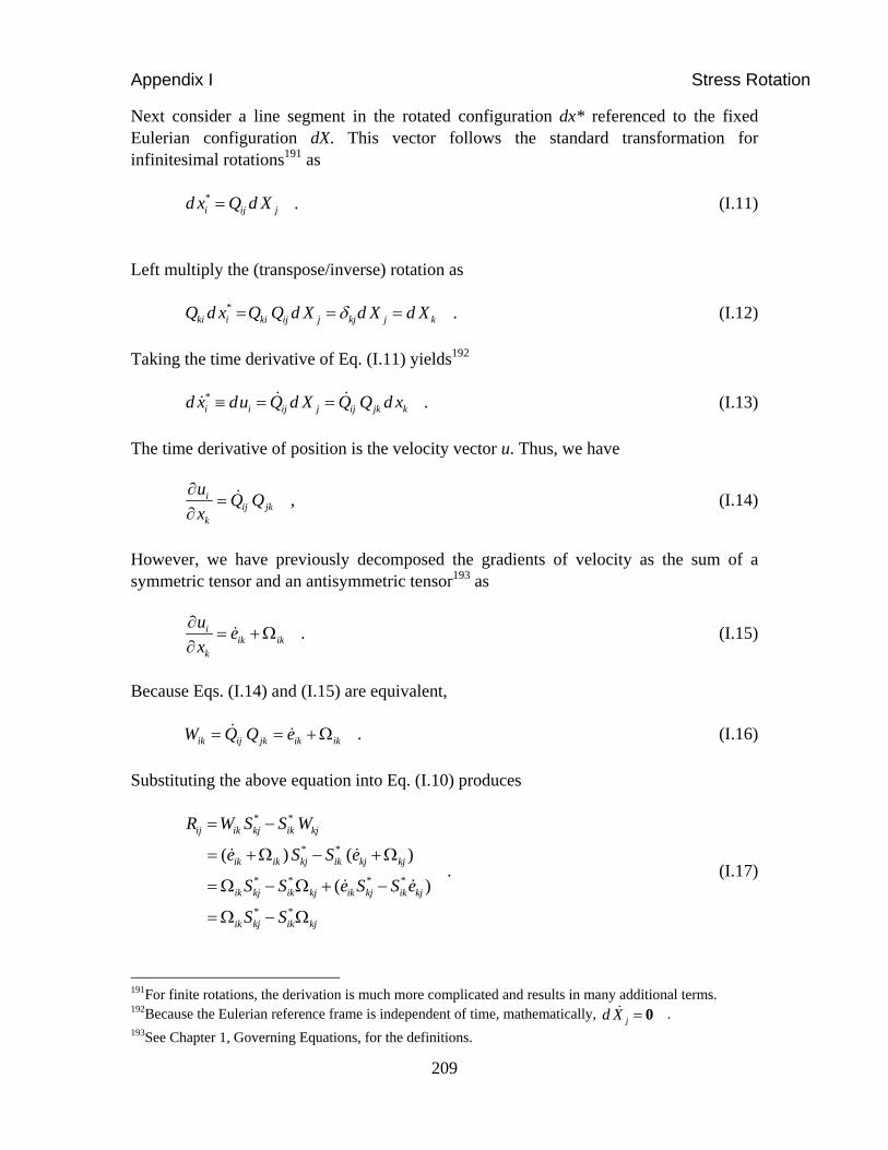
Appendix I Stress Rotation
209
Next consider a line segment in the rotated configuration dx* referenced to the fixed Eulerian configuration dX. This vector follows the standard transformation for infinitesimal rotations191 as
*i ij jd x Q d X . (I.11)
Left multiply the (transpose/inverse) rotation as
*ki i ki ij j kj j kQ d x Q Q d X d X d X . (I.12)
Taking the time derivative of Eq. (I.11) yields192 *
i i ij j ij jk kd x du Q d X Q Q d x . (I.13)
The time derivative of position is the velocity vector u. Thus, we have
iij jk
k
uQ Q
x
, (I.14)
However, we have previously decomposed the gradients of velocity as the sum of a symmetric tensor and an antisymmetric tensor193 as
iik ik
k
ue
x
. (I.15)
Because Eqs. (I.14) and (I.15) are equivalent,
ik ij jk ik ikW Q Q e . (I.16)
Substituting the above equation into Eq. (I.10) produces
* *
* *
* * * *
* *
( ) ( )
( )
ij ik kj ik kj
ik ik kj ik kj kj
ik kj ik kj ik kj ik kj
ik kj ik kj
ij
ij
ij
R W S S W
e S S e
S S e S S e
S
R
R
SR
. (I.17)
191For finite rotations, the derivation is much more complicated and results in many additional terms. 192Because the Eulerian reference frame is independent of time, mathematically,
jd X 0 . 193See Chapter 1, Governing Equations, for the definitions.

Appendix I Stress Rotation
210
The strain rate tensor e and the deviatoric stress tensor S are both symmetric in their indices; therefore, the term in the parentheses is zero. The rigid body rotation must be subtracted out of the deviatoric stress tensor before we can compute the deformation of the material in the cell. The velocity field applies to all materials in a cell; therefore, the rotation also applies to all materials in a given cell. The complete rotation terms194 in Eq. (I.10) are
2 2 ,
2 2 ,
( ) ,
(2 ) , an
0 0
0 d
( ) .0 2
xx xy xy xz xz
yy xy xy yz yz
xy xy xx yy xz yz yz xz
xz xz xx yy xy yz yz xy
yz yz xx yy xy xz xz xy
R S S
R S S
R S S S S
R S S S S
R S S S S
(I.18)
These rotation terms are used in PAGOSA.
194The
zzR is not needed becausezzS is not directly computed. Remember that S is traceless:
( )zz xx yyS S S .

Appendix J Diagnostics
211
APPENDIX J. DIAGNOSTICS
The diagnostics in PAGOSA allow the user to confirm the conservation laws for mass and energy. The following sections detail the calculation of the various diagnostics available.
J.1 Volume
The total volume of material (m) in the simulation is 1 1 1 1 1 1
2 2 2 2 2 2
( ) ( ), , , ,
Volume m mi j k i j k
cells
Vol , (J.1)
where Vol is the Eulerian cell volume. The summation is over every cell in the Eulerian mesh, excluding the ghost cells.
J.2 Mass
The total mass of material (m) in the simulation is 1 1 1 1 1 1 1 1 1
2 2 2 2 2 2 2 2 2
( ) ( ) ( ), , , , , ,
Mass m m mi j k i j k i j k
cells
Vol . (J.2)
As before, the summation is over the entire Eulerian mesh.
J.3 Internal Energy
The internal energy of material (m) in the simulation is 1 1 1 1 1 1 1 1 1 1 1 1
2 2 2 2 2 2 2 2 2 2 2 2
( ) ( ) ( ) ( ), , , , , , , ,
IE m m m mi j k i j k i j k i j k
cells
E Vol . (J.3)
As before, the summation is over the entire Eulerian mesh.
J.4 Kinetic Energy
The kinetic energy poses a problem in computation. The mass is a cell-centered variable, whereas the velocities are vertex centered. In PAGOSA, the square of the velocities is averaged at the cell centers. First, the value of u u is computed for each vertex. Next, the cell-centered velocity is obtained by arithmetically averaging the eight vertex quantities. This average magnitude is used to compute the kinetic energy. The kinetic energy of material (m) in the simulation is
1 1 1 1 1 1 1 1 1 1 1 12 2 2 2 2 2 2 2 2 2 2 2
( ) ( ) ( ) 2 2 212 , , , , , , , ,
KE m m mi j k i j k i j k i j k
cells
Vol U V W (J.4)
over the entire Eulerian mesh.

Appendix J Diagnostics
212
J.5 Elastic Distortional Energy 195
The elastic distortional energy is the energy in the material due to elastic distortions. The elastic distortional energy eW is computed from the rate equation 2 ( )e e e e e e e
xx xx yy yy zz zz xy xy xz xz yz yzW S e S e S e S e S e S e . (J.5)
The elastic energy can be recovered in the form of kinetic energy. Think of a spring storing and releasing energy. This energy is computed for each material in the simulation that possesses a deviatoric stress.
J.6 Plastic Work
The plastic work is the energy in the material due to plastic distortions. The plastic work pW is computed from the rate equation
2 ( )p p p p p p p
xx xx yy yy zz zz xy xy xz xz yz yzW S e S e S e S e S e S e . (J.6)
The plastic work is part of the internal energy of the material and is computed separately for the convenience of the user. The plastic work represents an irreversible process.
J.7 Mass Melted
Only materials with a flow-stress model have a melt mass computed. First, determine that the material exceeds the melt energy or temperature. The melt factor for material (m) is computed as
( ) ( )
( ) 1 or
0
m mm melt meltE E
fotherwise
. (J.7)
Then 1 1 1 1 1 1 1 1 1 1 1 1
2 2 2 2 2 2 2 2 2 2 2 2
( ) ( ) ( ) ( ), , , , , , , ,
Mass(melt) m m m mi j k i j k i j k i j k
cells
f Vol . (J.8)
The total mass was melted for material (m). If the factor f has a value of one everywhere, then the entire mass is melted and reduces to Eq. (J.2). The diagnostic holds for a particular moment in time. The mass can melt, freeze, and melt again during the course of the simulation.
195In PAGOSA the elastic distortional energy is computed separately and is not included in the total internal
energy. This point has been and continues to be controversial in hydrocode forums.

Appendix J Diagnostics
213
J.8 Mass Burned
Only materials with a detonation model have a burn mass computed. The burn fraction196 Bf ranges from zero to one, as 1 1 1 1 1 1 1 1 1 1 1 1
2 2 2 2 2 2 2 2 2 2 2 2
( ) ( ) ( ) ( ), , , , , , , ,
Mass(burn) m m m mi j k i j k i j k i j k
cells
Bf Vol . (J.9)
The total mass was burned (detonated) for material (m). If the factor Bf has a value of one everywhere, then the entire mass is burned and reduces to Eq. (J.2)
J.9 Mixed-Cell Statistics
In normal circumstances, only a small percentage of the cells in a simulation is mixed. The vast majority of cells contain a single material (pure cells). The mixed-cell statistics can be useful to the user in several ways. First, the statistics reveal the cell with the maximum number of materials. For example, if the maximum is two, then at least one cell in the simulation contains two materials that share an interface. As this number increases, the ability for the algorithm to represent the geometry accurately is severely compromised. However, if this cell inhabits an unimportant region of the simulation, then the statistic may be safely ignored. The volume fraction determines the type: Mixed cells 0 1 . Pure cells 0 1 .
J.10 Minimum and Maximum Statistics
For each of the important simulation variables, the minimum and maximum values for pure and mixed cells are tabulated. These statistics can be useful in determining the extreme states of the materials in question. For example, an unphysical sound speed or temperature may indicate that the equation of state is in a dubious regime.
196See Chapter 12 for the definition of a burn fraction.

Appendix J Diagnostics
214
This page intentionally left blank.

Appendix K Momentum Advection
215
APPENDIX K. MOMENTUM UPDATE The stress deviators contribute to the velocity fields, as can be seen readily in Eqs. (1.2a), (1.2b), and (1.2c). The individual stress deviators contribute to the momentum in much the same way as the pressure. The x component of the Navier-Stokes equation (Eq. 1.2a) is
1 1 xyxx xz
SS SU P
t x x y z
. (K.1)
The complication arises when we address the question of mixed cells. A mixed cell contains materials of various densities, pressures, and stress deviators. Let us denote the density of material (m) by ( )m , the pressure of material (m) by ( )m P , etc. The equation for a particular material in a single Eulerian cell now can be written as
( )( ) ( )( )
( )mm mm
xym xx xzSS SU P
t x x y z
. (K.2)
Notice that the velocity U does not have a material index. The velocity field applies to all materials in a cell.197 Next, multiply both sides of the equation by the cell volume and the material volume fraction. Then
( )( ) ( ) ( )
( )( ) ( )( )
mm m m
mm mxym xx xz
U PVol Vol
t x
SS SVol
x y z
. (K.3)
When we sum over all materials in the momentum control volume and the
( ) ( )m m
m
Mass Vol , (K.4)
then Eq. (K.3) becomes
xyxx xz
SS SU PMass
t x x y z
, (K.5)
where the titles refer to the cell-averaged quantities.
197In theory, a velocity field could exist for each material in a cell.

Appendix K Momentum Advection
216
The partial derivatives are constructed in the same manner as described in Chapter 2. However, the momentum control volume covers the eight cells that surround the vertex. The differencing and integration are done in the same way as the other variables described in Chapters 4 and 5.

Appendix L Pin Package
217
APPENDIX L. PIN PACKAGE
The pin diagnostic is used to record arrival times at a particular point in space. The diagnostic is positioned near a material surface, and electrical connections carry the timing signal to a recording device. The pin package in PAGOSA allows the user to emulate this experimental diagnostic tool. Consider a point in space inside the Eulerian mesh, as shown in Figure L.1. The pin is located at
( , , )p p px y zx . (L.1)
As the simulation proceeds, the material surface of interest will move into the Eulerian cell containing the point x. The perpendicular distance of a point x to the material plane is given by
1 2 3
2 2 21 2 3
p p px y zd
, (L.2)
where is the distance parameter associated with the material plane. The material surface is characterized by a direction vector, as described in Appendix C. With each new timestep, a new distance is computed and stored for later use. Typically, the material passes through the cell in a few timesteps, as shown in Figure L.2.
Figure L.1. The material surface, shown as a yellow triangle, is represented as a plane possessing a unique direction vector 1 2 3, ,( ) that points to the pin location (shown as a blue dot). If the point x lies in front of the plane, the distances are positive. If the point x lies behind the plane, the distances are negative.

Appendix L Pin Package
218
The optimal situation is when four distance data points are recorded—two with positive distances and two with negative distances. Lagrange interpolation198 is used to find the zero crossing time, which occurs when the pin is on the material surface.
Figure L.2. A typical pin distance vs simulation time plot that points to the pin location (shown as
a blue dot). If the point x lies in front of the plane, the distances are positive. If the point x lies behind the plane, the distances are negative.
Pathological situations can results in fewer than four data pints being available. The crossing algorithm in PAGOSA changes, depending on the number of distance data points available from the simulation. The individual cases are detailed below.
L.1 Four Points
When four data points are available for computing a pin-crossing time, the Lagrange interpolation formula is
1 2 3 4 2 1 3 4
2 1 3 1 4 1 1 2 3 2 4 2
3 1 2 4 4 1 2 3
1 3 2 3 4 3 1 4 2 4 3 4
( ) ( ) ( ) ( ) ( ) ( )
( ) ( ) ( ) ( ) ( ) ( )
cross
t d d d t d d dt
d d d d d d d d d d d d
t d d d t d d d
d d d d d d d d d d d d
. (L.3)
Appropriate checks are made to ensure that the denominators are not too small and that the crossing time is within the proper range. These checks prevent extrapolation outside the physical range of interest.
198William H. Press, Saul A. Teukolsky, William T. Vetterling and Brian P. Flannery, Numerical Recipes in
Fortran The Art of Scientific Computing, second edition (Cambridge University Press, New York, New York, 1992), pp. 102–104.

Appendix L Pin Package
219
L.2 Three Points
Three data points allows for a second-order Lagrange interpolation to be used. The crossing time is then
1 2 3 2 1 3 3 1 2
2 1 3 1 1 2 3 2 1 3 2 3( ) ( ) ( ) ( ) ( ) ( )cross
t d d t d d t d dt
d d d d d d d d d d d d
. (L.4)
Appropriate checks are made to ensure that the denominators are not too small and that the crossing time is within the proper range. These checks prevent extrapolation outside the physical range of interest.
L.3 Two Points
When only two data points are available for a pin diagnostic, we resort to linear interpolation to find the crossing time as
2 1 1 2 2 1( ) / ( )crosst d t d t d d . (L.5)
Appropriate checks are made to ensure that the denominator is not too small and that the crossing time is within the proper range. These checks prevent extrapolation outside the physical range of interest.
L.4 One Point
On rare occasions, the material flow is so complicated that only one distance point is available for computing the pin-crossing time. The crossing time is estimated by linear interpolation based on the maximum velocity allowed by the Courant timestep safety factor safeu199 as
1 1( / )crosst t t d safeu , (L.6) where t is the current simulation time.
L.5 Zero Points
This pathological case is used when the material interface jumps over the cell containing the pin diagnostic without ever being in the cell at any time. The pin-crossing time is approximated by taking the average of the simulation times surrounding the event as 1
1 22 ( )crosst t t , (L.7) where 1t and 2t are current and previous simulation times, respectively.
199 See Chapter 9.

Appendix L Pin Package
220
This page intentionally left blank.

Appendix M Tracers
221
APPENDIX M. TRACERS
The tracer particle is an important diagnostic tool in PAGOSA. Massless tracer particles are placed in the computational domain, and information at the particle location is recorded for the benefit of the user. Two types of tracer particles are available—Eulerian and Lagrangian. The Eulerian tracer particle is fixed in space at its original coordinates. However, the Lagrangian tracer moves with the material following the velocity field. Each tracer type has its own unique uses and capabilities. For example, if the simulation is given of an experiment that has a probe (sensor) fixed at a particular location, the Eulerian tracer particle is the most appropriate choice to use for modeling this probe. In the Taylor Anvil sample problem,200 the shape and deformation of the projectile is one of the desired measurements. Placing Lagrangian tracer particles on the surface of the projectile allows the diagnostic to move with the material surface. Many other uses for the tracer diagnostic easily can be imagined.
M.1 Interpolation
The tracer particle begins its life at a point in space within the computational domain and in a single Eulerian cell, as shown in Figure M.1. The velocities are defined at cell vertices (Chapter 2), and some interpolation is necessary to estimate the velocity at the particle coordinates (x,y,z). A tri-linear interpolation formula is used to find the velocity
Figure M.1. A tracer particle at (x,y,z) in an Eulerian cell.
200Wayne Weseloh, “PAGOSA Sample Problems,” Los Alamos National Laboratory report LA-UR-05-
6514 (August 2005).

Appendix M Tracers
222
at the tracer location. For the U velocity, the interpolation appears as
0 1 2 3 4 5 6 7( , , )U x y z a a x a y a z a x y a xz a yz a x yz , (M.1)
where the coefficients 0 7a a are derived from the eight known velocities at the cell vertices. The other components of velocity are found in the same way. Once the velocity field is constructed at the point of interest, the Lagrangian tracer particles can be moved by integrating the equations of motion for these massless particles.
M.2 Integration
The integration applies only to the Lagrangian tracers because the Eulerian tracers are fixed in space and report the changes in quantities as materials sweep past them. The integration scheme follows the same predictor-corrector methodology presented in Chapter 5. The positions of the Lagrangian tracers after one timestep are
1/2 / 2n n n t x x u predictor and (M.2) 1 1/2n n n t x x u corrector . (M.3) Because the interpolation point wanders from cell to cell, the interpolated function values change continuously. However, the gradients (velocities and accelerations) of the interpolated function change discontinuously at the boundaries of each cell. The integration uses the velocity field generated by the Lagrangian-phase integration described in Sections 5.1, 5.2, and 5.3. In theory, it is possible to use the velocity field from the advection-phase solution (Section 4.6.1) instead of the Lagrangian-phase solution; some other hydrocodes have this option. PAGOSA uses only the Lagrangian-phase velocities. At the new tracer position, a new interpolation is used to construct the appropriate velocity field and prepare for the next integration step. This process is repeated for the duration of the simulation. Lagrangian tracer particles can fly off the mesh during an integration step. These particles are then lost to the simulation—no further information can be recorded for these particles. The same tri-linear interpolation is used for all variables of interest associated with the tracer particle. For variables located at cell vertices (e.g., U, W, and Bt), the interpolation

Appendix M Tracers
223
coefficients are obtained from the local vertices of the cell containing the tracer particle. For variables located at cell centers (e.g., P, Q, and Bf), the interpolation coefficients are obtained from the cell centers of the vertex volume containing the tracer particle.
M.3 Comments
The concept of a continuous variable field is useful in constructing a tracer particle diagnostic. However, previously (Chapter 3.0) we assumed that the gradients were uniform over the cell volume. No functional form was assumed for the fundamental variables. The tracer diagnostic operates under slightly different assumptions than did the fundamental hydrodynamics. This concept illustrates an important point. The tracer diagnostic is only a diagnostic tool. For example, a Lagrangian tracer particle placed on a material interface will not exactly follow the movements of that interface. The particle may be in a different cell from the interface. Or the particle may lead or lag the movement of the interface. The interface reconstruction (see Section 4.5.1, Appendix C, and Appendix G) is based on a set of algorithms that is different from the algorithms presented in this appendix. Note that when the material volume fractions in a multi-material cell are adjusted during the Lagrangian phase, a change is implied in the distribution of velocity field in the cell. The movement of the Lagrangian tracer particle depends critically on the sub-cell velocity distribution and needs to be adjusted if the pressure relaxation or void closure divergence options are invoked (Chapter 13). No adjustments are necessary with the uniform divergence option.

Appendix M Tracers
224
This page intentionally left blank.

Index
225
acceleration, 38, 54, 138, 222 adiabatic, 62, 65, 132 advection
definition, 42 example, 193 first order, 184, 187 gradient limiters, 188 internal energy, 47 mass, 33, 34, 35 momentum, 33, 34, 35, 45 monotonic, 189 phase, 35, 42 pseudocode, 190 second order, 184 square pulse, 193 third order, 185 van Leer limiter, 189
aether, 14 angular momentum, 12 artificial viscosity, 38, 86, 123, 125, 223
linear, 89 quadratic, 89 von Neumann, 89
boundary conditions reflective, 105 transmissive, 106
bulk modulus, 13, 62, 68, 195 Cartesian, 28, 34, 173 Cauchy stress tensor, 131 Cauchy-Stokes decomposition theorem
derivation, 203 dilatation, 205 rotation, 204 shear, 205 translation, 204
cell area, 17 boundary, 183 size, 17 vertex, 17, 18 volume, 17
CFL condition, 97 Chapman-Jouget, 65, 111 cold curve, 68
compression, 13, 37, 56, 61, 62, 63, 66, 75, 119, 122, 131, 155
computational grid, 14, 22, 113 conservation law, 7, 11, 33, 34, 35, 47,
56, 189, 211 angular momentum, 12 energy, 14 internal energy, 14 linear momentum, 11 mass, 11
constitutive equation, 167 constitutive relation, 12, 56, 131, 132,
139, 167, 207 coordinates
Eulerian, 17 corrector, 52, 53, 55, 222 Courant condition, 4, 95, 97 Courant number, 43, 44, 190, 193 crush, 8, 12, 53, 68, 161, 163 damage, 8, 12, 155, 157 deformation motion, 204 density
mass, 33, 34, 35 detonation, 64, 213 dilatation, 13, 132, 204, 205 direction vector, 39, 173, 198, 199, 217 distance parameter, 173, 200, 217 divergence theorem, 27 donor cell, 44, 184, 187, 190, 191, 197,
198 downwind, 46, 189, 190 dual mesh, 21 elastic
energy, 212 release, 162 work, 212
elastic distortional energy, 14, 56, 192, 212
elastic perfectly plastic, 139 elastic regime, 131, 132 energy
conservation, 34, 35 elastic distortional energy, 212 internal, 211 kinetic, 211

Index
226
plastic work, 212 specific internal energy, 14
energy shift, 67, 68 entropy, 38, 79, 80, 91 EOS
see equation of state, 11 EOSPAC, 67, 69, 70, 85, 141 equation of state, 11, 14, 57, 61, 111,
132, 161, 213 BKW-HE, 71, 73 exponential, 71 gas, 61 Grüneisen, 65 ideal gas, 61 JWL, 64, 65, 83, 111, 114 modified Osborne, 63 Osborne, 63 polynomial, 62 SESAME, 67, 68, 69, 70, 85, 141,
143, 147, 148, 149, 163 tabular, 67, 69 Us-Up, 65 void, 62, 119
Euler equations, 33 Eulerian
cell, 17, 183 cell area, 17 cell size, 17 cell vertex, 17 cell volume, 17 grid, 17, 22
Eulerian phase, 35, 36, 37, 42, 45, 47, 57 evolution equation
internal energy, 33, 34, 35, 47, 48, 191
mass, 33, 34, 35 momentum, 33, 34, 35, 215
expansion, 61, 66 exponential, 71, 86 finite difference approximation, 20, 29 finite difference equations, 20, 29, 181,
183, 192 advection, 183, 184, 185, 190 Lagrangian, 181
finite difference form, 181, 183 finite differences
stability, 44 first law of thermodynamics, 80, 90 flow-stress
elastic perfectly plastic, 139 Johnson-Cook, 12, 142 Kospall, 12, 148 mechanical threshold stress, 145 models, 139 modified Steinberg-Cochran-Guinan,
140 Preston-Tonks-Wallace, 143 Steinberg-Cochran-Guinan, 12, 141 thermal softening, 149 work hardening, 150, 151
flux, 46 fracture, 8, 12, 53, 130, 155, 156, 157
Johnson spall, 155 Johnson-Cook damage, 157
frame indifference, 207 functions, 137, 140, 142 ghost cells, 22, 105, 106, 211 governing equations, 17, 20, 21, 33, 56 gradient limiter, 188 Grüneisen, 65, 71, 84, 124 Grüneisen parameter, 66 Grüneisen relation, 66 hexagonal section, 177, 179 high explosive, 64, 71, 111, 115 Hooke’s Law, 129 Hugoniot, 65 hydrocodes, 19, 34, 106, 222 ideal gas, 61, 81 incompressible, 13, 132 initial conditions, 69, 70, 97, 101, 111 integration, 18, 45, 51, 138, 222 interface
hexagonal section, 177, 179 pentagonal section, 176, 178 quadrilateral section
type A, 176, 178 type B, 177, 179
reconstruction, 41, 197 triangular section, 176, 178
interface reconstruction, 40, 62, 125, 173, 223

Index
227
internal energy, 14, 33, 34, 35, 48, 75, 79, 80, 89, 101, 124, 134, 137, 138, 140, 142, 149, 191, 211
invariants, 12, 134 irrotational, 13, 195, 204 isotropic, 11, 134, 167 Jaumann derivative, 208 Johnson spall, 155 Johnson-Cook damage, 157 JWL EOS, 64 Lagrangian phase, 34, 37, 39, 46, 57,
120, 122, 138, 162, 181 Levi-Civita pseudotensor, 167, 203 linear momentum, 11, 46 mass, 33, 34, 35, 211 mass burned, 213 mass melted, 212 mechanical threshold stress, 145, 147 melt temperature, 69, 141, 143, 144, 147 mesh
Eulerian, 14, 17, 19, 36 mixed cells, 19, 20, 40, 56, 119, 120,
121, 122, 125, 169, 202, 213, 215 modified Steinberg-Cochran-Guinan,
140, 141 modulus
bulk, 13, 62, 68, 195 elastic, 129 shear, 12, 125, 131, 132, 135, 139,
140, 141, 142, 143, 144, 145, 147, 148, 149, 156, 163, 195
yield, 139, 140, 141, 142, 143, 148, 149, 156, 163
momentum conservation, 33, 34, 35 equations, 12
momentum control volume, 21, 22, 38, 45, 46, 53, 54, 215, 216
monotonic, 42, 189 Monte-Carlo technique, 20 MTS
see mechanical threshold stress, 145, 147
multi-material, 19 Navier-Stokes equations, 11, 91, 215 Newton-Raphson method, 70
Noh problem, 90 numerical approximation, 27, 169 operator splitting, 33, 34
stability, 44 PAGOSA, 3, 11, 12, 13, 14, 18, 19, 22,
27, 33, 34, 36, 37, 40, 42, 43, 44, 46, 56, 61, 65, 67, 69, 70, 71, 72, 75, 85, 86, 89, 91, 97, 105, 111, 115, 119, 120, 123, 130, 131, 132, 134, 135, 136, 139, 155, 171, 188, 190, 210, 211, 217, 218, 221, 222
particle speed, 66 pentagonal section, 176, 178 permutation, 36, 203 phase errors, 192 phase transition, 67, 68 plastic
strain, 131, 137 work, 212
plastic regime, 129, 130, 131, 132, 139, 151
plasticity, 12 pmin, 75 Prandtl-Reuss treatment, 132 predictor, 52, 53, 222 pressure, 11, 14, 20, 56, 61, 62, 63, 64,
65, 67, 68, 69, 70, 71, 73, 75, 79, 81, 85, 86, 89, 91, 95, 96, 101, 111, 122, 123, 131, 137, 138, 139, 140, 141, 145, 148, 156, 161, 162, 215
pressure gradient, 38, 91 pressure relaxation, 122 Preston-Tonks-Wallace, 143 priority, 40, 41, 120 programmed burn, 96, 101, 111, 114,
115 limitations, 114
PTW see Preston-Tonks-Wallace, 143
P-α crush model, 161 Q
see artificial viscosity, 38, 86, 123, 125, 223
quadrilateral section type A, 176, 178 type B, 177, 179

Index
228
ramp treatment, 68, 163 Rankine-Hugoniot, 90 reconstruction
see interface reconstruction, 41, 197 remap
see Eulerian phase, 35 safec, 95, 195 safed, 95 safety factors, 95, 97 safeu, 95, 219 sampling density, 169, 170, 171 scaling ratio, 67 secant method, 73 SESAME, 67, 68, 69, 70, 85, 141, 143,
147, 148, 149, 163 energy shift, 67 iteration, 69 ramp, 68 scaling ratio, 67
shock speed, 66, 90 shock waves, 89, 90 sound speed, 62, 66, 68, 79, 80, 81, 82,
83, 85, 86, 90, 95, 96, 162, 163, 195, 213 exponential, 86 gas, 81 Grüneisen, 84 ideal gas, 81 JWL, 83 modified Osborne, 82 Osborne, 82 polynomial, 81 SESAME, 85 tabular, 85 Us-Up, 84 void, 81
spatial centering density, 18 internal energy, 18 pressure, 18 velocity, 18
specific internal energy, 14, 42, 61, 62, 134, 149, 191, 192
square pulse, 187, 192, 193 staggered grid, 18 statistics, 213
Steinberg-Cochran-Guinan, 141, 148 strain, 131, 137 strain rate, 13, 27 Strang operator splitting, 7, 33, 34 stress tensor, 11, 12, 125, 131, 132, 143,
207, 210 T junctions, 40 tabular EOS
see SESAME, 67 Taylor expansion, 66, 203 tensor
antisymmetric, 12, 167, 203, 209 Cauchy, 131 spatial velocity gradient, 12 strain rate, 13, 27 stress tensor, 12 symmetric, 12, 167, 203, 204, 209 vorticity, 13
tetrahedron, 174 thermal softening, 139, 140, 141, 148,
149 Thomas-Fermi-Dirac theory, 68 timestep, 37, 97, 195 timestep controls
Courant, 43, 44, 79, 95, 190, 193, 195, 219
detonation, 96 divergence, 95 initial, 195 Lagrangian, 95, 181
tracers, 221 transport, 36 triangular section, 176, 178 uniform divergence, 223 upwind, 42, 189, 190 velocity divergence, 13, 120, 138, 205 vertex, 18 vertex mass, 39, 53 void closure, 119 volume, 177, 211 volume fraction, 14, 37, 39, 40, 61, 101,
119, 120, 121, 122, 123, 125, 169, 170, 171, 175, 178, 197, 198, 199, 213, 215, 223 defintion, 19 initial, 20, 169

Index
229
von Mises, 6, 134, 147 von Neumann, 89 vorticity tensor, 203 wall heating, 90 work hardening, 150 Y junctions, 40 yield criterion, 134, 135, 136, 144, 147
yield function, 135 yield modulus, 139, 148, 163 yield surface, 136, 138, 144, 147, 150 Youngs interface reconstruction, 173 Youngs/van Leer gradient limiter, 45,
189, 190 zone, 17, 19, 37, 91, 114, 122, 125

This report has been reproduced directly from the best available copy. It is available electronically on the Web (http://www.doe.gov/bridge).
Copies are available for sale to U.S. Departmentof Energy employees and contractors from: Office of Scientific and Technical Information P.O. Box 62 Oak Ridge, TN 37831 (865) 576-8401
Copies are available for sale to the public from: National Technical Information Service U.S. Department of Commerce 5285 Port Royal Road Springfield, VA 22161 (800) 553-6847