MODELING OF TUMOR GROWTH AND OPTIMIZATION OF ...
204
MODELING OF TUMOR GROWTH AND OPTIMIZATION OF THERAPEUTIC PROTOCOL DESIGN KANCHI LAKSHMI KIRAN B.E.(Hons), National Institute of Technology, Durgapur, India A THESIS SUBMITTED FOR THE DEGREE OF DOCTOR OF PHILOSOPHY DEPARTMENT OF CHEMICAL & BIOMOLECULAR ENGINEERING NATIONAL UNIVERSITY OF SINGAPORE 2011
-
Upload
khangminh22 -
Category
Documents
-
view
1 -
download
0
Transcript of MODELING OF TUMOR GROWTH AND OPTIMIZATION OF ...
MODELING OF TUMOR GROWTH AND
OPTIMIZATION OF THERAPEUTIC PROTOCOL
DESIGN
KANCHI LAKSHMI KIRAN
B.E.(Hons), National Institute of Technology, Durgapur, India
A THESIS SUBMITTED
FOR THE DEGREE OF DOCTOR OF PHILOSOPHY
DEPARTMENT OF CHEMICAL & BIOMOLECULAR ENGINEERING
NATIONAL UNIVERSITY OF SINGAPORE
2011
ACKNOWLEDGMENTS
Firstly, I would like to thank my parents for their love and affection, valuable
teachings and their perseverance in making me a responsible global citizen. My
parents have been the prime force behind my achievements. I want to dedicate this
work to my parents. I am thankful to my brothers, uncle and my late grandparents
for their love, concrete support and encouragement.
I am very lucky to be part of the group “Informatics Process Control Unit
(IPCU)” under the supervision of Dr. Lakshminarayanan Samavedham (Laksh). I
would like to thank Dr. Laksh not only for introducing me to an interesting research
discipline but also for his support, encouragement, and mentorship. During my PhD,
I was given complete freedom which provided me more opportunities to learn and
cherish various phases of my graduate student life. I was allowed to teach graduate
and undergraduate students, mentor final year projects of undergraduate students,
attend and organize conferences and meetings and lead the activities of Graduate
Students Association (GSA). My journey of PhD at NUS has been very adventurous
and I feel it is like swimming in an ocean rather than swimming in a pool. I have
got everlasting recipe from the thoughtful discussions with Dr. Laksh on several
topics for leading a fruitful life.
I would like to thank my senior IPCU members - Balaji, Raghu, Sreenu, Sundar
for sharing their invaluable experiences and for their motivation during the budding
stage of my PhD which accelerated my research progress. Also, I would like to
thank my contemporary IPCU members - Abhay, Naviyn, Logu, Karthik, May Su,
Prem, Manoj, Vaibhav, Krishna, Pavan, Kalyan for their professional comments and
critique. I carry with me a lot of happy memories of the IPCU lab.
ii

I would like to thank the department for giving me an opportunity to serve
as the President of GSA - ChBE. I also would like to extend my sincere thanks
to GSA committee members - Sudhir, Sundaramoorthy, Suresh, Abhay, Sadegh,
Naviyn, Logu, Hanifa, Vasanth, Niranjani, Shreenath, Anoop, Ajitha, Vamsi, Anji,
Srivatsan and Vignesh for their support, cooperation and hope on me as a leader.
Moreover, I want to thank all other friends from NUS for their help.
I would like to thank Prof. Farooq and Prof. Feng Si-Shen for their constructive
comments and suggestions on my PhD qualifying report and presentation. I also
want to thank Prof. Krantz, Dr. Rudiyanto Gunawan, Prof. Rangaiah at NUS,
Singapore and Prof. Sundarmoorthy at Pondicherry Engineering college, India for
their help and encouragement.
I wish to thank Prof. Vito Quaranta, Vanderbilt University for providing me
an opportunity to deliver an invited lecture at Vanderbilt Ingram Cancer Centre,
Vanderbilt University.
I would like to thank administrative staff and lab officers of the department for
their help during my PhD.
Last but not least, I am very grateful to NUS for providing me precious moments,
financial support and a platform for participating in various global programs which
led to my allround development.
iii
TABLE OF CONTENTS
Page
Summary . . . . . . . . . . . . . . . . . . . . . . . . . . . . . . . . . . . viii
List of Tables . . . . . . . . . . . . . . . . . . . . . . . . . . . . . . . . . x
List of Figures . . . . . . . . . . . . . . . . . . . . . . . . . . . . . . . . xi
Abbreviations . . . . . . . . . . . . . . . . . . . . . . . . . . . . . . . . . xiv
Nomenclature . . . . . . . . . . . . . . . . . . . . . . . . . . . . . . . . . xv
1 Introduction . . . . . . . . . . . . . . . . . . . . . . . . . . . . . . . . 1
1.1 Motivation . . . . . . . . . . . . . . . . . . . . . . . . . . . . . . . 1
1.1.1 Role of process systems engineering in cancer therapy . . . 3
1.2 Cancer statistics . . . . . . . . . . . . . . . . . . . . . . . . . . . 5
1.3 What is cancer ? . . . . . . . . . . . . . . . . . . . . . . . . . . . 6
1.3.1 Different stages of tumor growth . . . . . . . . . . . . . . . 8
1.4 Clinical phases . . . . . . . . . . . . . . . . . . . . . . . . . . . . 8
1.4.1 Cancer detection . . . . . . . . . . . . . . . . . . . . . . . 9
1.4.2 Cancer diagnosis . . . . . . . . . . . . . . . . . . . . . . . 9
1.4.3 Cancer therapy . . . . . . . . . . . . . . . . . . . . . . . . 10
1.4.4 Emerging and targeted therapies . . . . . . . . . . . . . . 11
1.5 Our focus - avascular tumor growth . . . . . . . . . . . . . . . . . 13
1.6 Contributions . . . . . . . . . . . . . . . . . . . . . . . . . . . . . 14
1.7 Thesis organization . . . . . . . . . . . . . . . . . . . . . . . . . . 15
2 Literature review . . . . . . . . . . . . . . . . . . . . . . . . . . . . . 17
2.1 Mathematical modeling of cancer growth . . . . . . . . . . . . . . 17
2.2 Continuum models . . . . . . . . . . . . . . . . . . . . . . . . . . 20
2.2.1 Homogenous models . . . . . . . . . . . . . . . . . . . . . 21
2.2.2 Heterogenous models . . . . . . . . . . . . . . . . . . . . . 23
2.2.3 Spatio-temporal models . . . . . . . . . . . . . . . . . . . 24
2.2.4 Discrete and hybrid models . . . . . . . . . . . . . . . . . 32
iv
Page
2.2.5 Model calibration . . . . . . . . . . . . . . . . . . . . . . . 33
2.3 Tumor and its interaction with immune system . . . . . . . . . . 34
2.3.1 Tumor-immune models . . . . . . . . . . . . . . . . . . . . 37
2.4 Model-based design of treatment protocols of cancer therapy . . . 38
2.4.1 Pharmacokinetic and pharmacodynamic modeling . . . . . 39
2.4.2 Optimal control theory (OCT) . . . . . . . . . . . . . . . . 40
2.4.3 Description of optimization problem formulation using cancertherapy models . . . . . . . . . . . . . . . . . . . . . . . . 42
2.5 Challenges in the model-based applications . . . . . . . . . . . . . 44
2.5.1 Description of the strategy implemented in this thesis work 45
3 Mathematical modeling of avascular tumor growth based on dif-fusion of nutrients and its validation . . . . . . . . . . . . . . . . . 47
3.1 Introduction . . . . . . . . . . . . . . . . . . . . . . . . . . . . . . 47
3.2 The proposed model . . . . . . . . . . . . . . . . . . . . . . . . . 48
3.2.1 Model equations . . . . . . . . . . . . . . . . . . . . . . . 50
3.3 Model solution . . . . . . . . . . . . . . . . . . . . . . . . . . . . 52
3.3.1 Non-dimensionalization of equations . . . . . . . . . . . . 52
3.3.2 Numerical procedure . . . . . . . . . . . . . . . . . . . . . 53
3.4 Model validation and discussion . . . . . . . . . . . . . . . . . . . 54
3.4.1 Validation with in vitro data (Freyer and Sutherland, 1986b) 54
3.4.2 Validation with in vitro data (Sutherland et al., 1986) . . . 59
3.4.3 Comparison with Casciari et al. (1992) model . . . . . . . 64
3.4.4 Comparison with parameters of Gompertzian relation basedon experimental data (Burton, 1966) . . . . . . . . . . . . 65
3.5 Conclusions . . . . . . . . . . . . . . . . . . . . . . . . . . . . . . 66
4 Sequential scheduling of cancer immunotherapy and chemother-apy using multi-objective optimization . . . . . . . . . . . . . . . 67
4.1 Introduction . . . . . . . . . . . . . . . . . . . . . . . . . . . . . . 67
4.2 Mathematical model . . . . . . . . . . . . . . . . . . . . . . . . . 68
4.3 Multi-objective optimization . . . . . . . . . . . . . . . . . . . . . 71
4.3.1 Non-domination set (Pareto set) . . . . . . . . . . . . . . . 72
4.3.2 NSGA-II . . . . . . . . . . . . . . . . . . . . . . . . . . . . 72
v

Page
4.3.3 Post-Pareto-optimality analysis . . . . . . . . . . . . . . . 74
4.4 Problem formulation . . . . . . . . . . . . . . . . . . . . . . . . . 75
4.4.1 Non-dimensionalization . . . . . . . . . . . . . . . . . . . . 78
4.5 Results and discussion . . . . . . . . . . . . . . . . . . . . . . . . 78
4.5.1 Case 1: Chemotherapy . . . . . . . . . . . . . . . . . . . . 78
4.5.2 Case 2: Immune-chemo combination therapy . . . . . . . . 83
4.6 Conclusions . . . . . . . . . . . . . . . . . . . . . . . . . . . . . . 87
5 Model-based sensitivity analysis and reactive scheduling of den-dritic cell therapy . . . . . . . . . . . . . . . . . . . . . . . . . . . . 89
5.1 Introduction . . . . . . . . . . . . . . . . . . . . . . . . . . . . . . 89
5.1.1 Dendritic cell therapy . . . . . . . . . . . . . . . . . . . . . 90
5.2 Scheduling under uncertainty . . . . . . . . . . . . . . . . . . . . 91
5.3 Mathematical model . . . . . . . . . . . . . . . . . . . . . . . . . 92
5.4 Global sensitivity analysis . . . . . . . . . . . . . . . . . . . . . . 94
5.4.1 Theoretical formulation of HDMR . . . . . . . . . . . . . . 96
5.4.2 RS-HDMR . . . . . . . . . . . . . . . . . . . . . . . . . . . 97
5.5 Results and discussion . . . . . . . . . . . . . . . . . . . . . . . . 99
5.5.1 Uncertainty and sensitivity analysis using HDMR . . . . . 99
5.5.2 Validation of HDMR results using reactive scheduling . . . 102
5.5.3 Comparison between nominal and reactive schedule for cases1-3 . . . . . . . . . . . . . . . . . . . . . . . . . . . . . . . 103
5.5.4 Reactive scheduling of combination therapy and dendritic celltherapy . . . . . . . . . . . . . . . . . . . . . . . . . . . . 106
5.6 Conclusions . . . . . . . . . . . . . . . . . . . . . . . . . . . . . . 110
6 Application of scaling and sensitivity analysis for tumor-immunemodel reduction . . . . . . . . . . . . . . . . . . . . . . . . . . . . . 112
6.1 Introduction . . . . . . . . . . . . . . . . . . . . . . . . . . . . . . 112
6.2 Mathematical model . . . . . . . . . . . . . . . . . . . . . . . . . 113
6.3 Scaling analysis . . . . . . . . . . . . . . . . . . . . . . . . . . . . 115
6.3.1 Algorithm . . . . . . . . . . . . . . . . . . . . . . . . . . . 116
6.3.2 Reduced model . . . . . . . . . . . . . . . . . . . . . . . . 117
6.4 Global sensitivity analysis for correlated inputs . . . . . . . . . . 120
vi

Page
6.5 Results and discussion . . . . . . . . . . . . . . . . . . . . . . . . 123
6.5.1 Comparison between original model and reduced model viatheoretical identifiability analysis . . . . . . . . . . . . . . 123
6.5.2 Sensitive parametric groups based on global sensitivity analysis 126
6.5.3 Comparison between original model and reduced model - Pa-rameter estimation . . . . . . . . . . . . . . . . . . . . . . 130
6.6 Conclusions . . . . . . . . . . . . . . . . . . . . . . . . . . . . . . 133
7 Population based optimal experimental design in cancer diagnosisand chemotherapy - in silico analysis . . . . . . . . . . . . . . . . 135
7.1 Introduction . . . . . . . . . . . . . . . . . . . . . . . . . . . . . . 135
7.2 Mathematical model . . . . . . . . . . . . . . . . . . . . . . . . . 138
7.3 Population-based studies . . . . . . . . . . . . . . . . . . . . . . . 139
7.3.1 Optimal design of experiments for cancer diagnosis . . . . 139
7.3.2 Optimal design of chemotherapeutic protocol and post-therapyanalysis . . . . . . . . . . . . . . . . . . . . . . . . . . . . 144
7.4 Conclusions . . . . . . . . . . . . . . . . . . . . . . . . . . . . . . 150
8 Conclusions and recommendations for future work . . . . . . . . 152
8.1 Conclusions . . . . . . . . . . . . . . . . . . . . . . . . . . . . . . 152
8.2 Recommendations for future work . . . . . . . . . . . . . . . . . . 157
8.2.1 Validation of the tumor growth models . . . . . . . . . . . 157
8.2.2 Model-based therapeutic design . . . . . . . . . . . . . . . 157
8.2.3 Multiscale modeling . . . . . . . . . . . . . . . . . . . . . 158
8.2.4 Statistical analysis using clinical data of cancer . . . . . . 162
References . . . . . . . . . . . . . . . . . . . . . . . . . . . . . . . . . . . 164
Appendix . . . . . . . . . . . . . . . . . . . . . . . . . . . . . . . . . . . 180
Publications & Presentations . . . . . . . . . . . . . . . . . . . . . . . 181
Curriculum Vitae . . . . . . . . . . . . . . . . . . . . . . . . . . . . . . 183
vii

SUMMARY
Cancer is a leading fatal disease with millions of people falling victim to it every
year. Indeed, the figures are alarming and increasing significantly with each passing
year. Cancer is a complex disease characterized by uncontrolled and unregulated
growth of cells in the body. Cancer growth can be broadly classified into three stages
namely, avascular, angiogenesis and metastasis based on their location and extent
of spread in the body. Mechanisms of cancer growth have been poorly understood
thus far and considerable resources have been committed to elucidate these mech-
anisms and arrive at effective therapeutic strategies that have minimal side effects.
Mathematical modeling can help in the modeling of cancer mechanisms, to propose
and validate hypothesis and to develop therapeutic protocols. This research intends
to contribute to this important area of cancer modeling and treatment.
Among these stages, study of avascular stage is quite relevant to the present
trend of technology development. Many mathematical models have been developed
to comprehend the avascular tumor growth, but the availability of a compendious
model is still elusive. This thesis proposes a simple mechanistic model to explain
the phenomenon of tumor growth observed from the multicellular tumor spheroid
experiments. The main processes incorporated in the mechanistic model for the
avascular tumor growth are diffusion of nutrients through the tumor from the mi-
croenvironment, consumption rate of the nutrients by the cells in the tumor and cell
death by apoptosis and necrosis.
Chemotherapy and immunotherapy are the main focus of this thesis - tumor
growth models are integrated with the pharmacokinetic and pharmacodynamic mod-
els of therapeutic drugs. The integrated model is used to optimize the therapeutic
interventions in order to kill the tumor cells and avert the catastrophic side effects
viii

by effectively leveraging multi-objective optimization and control methods. Further-
more, scaling and sensitivity analysis are applied on the tumor-immune models to
screen the dominating mechanisms affecting the tumor growth. Then, the dominant
mechanisms are used to test out the aspects of intrapatient and interpatient variabil-
ity. Application of reactive scheduling approach is addressed to nullify the effects
of intrapatient variability on the therapeutic outcome. Similarly, population-based
simulation studies are carried out to design diagnostic and therapeutic protocols
and to find the parametric combinations that determine the treatment outcome.
Overall, this thesis showcases the utility and ability of process systems engineering
approaches in improving the cancer diagnosis and treatment.
ix
LIST OF TABLES
Table Page
1.1 Differences between benign and malignant tumors . . . . . . . . . . . 7
3.1 Parameter values . . . . . . . . . . . . . . . . . . . . . . . . . . . . . 55
3.2 Maximum volume of multicellular tumor spheroids at different concen-trations . . . . . . . . . . . . . . . . . . . . . . . . . . . . . . . . . . 58
3.3 Values of the parameter k1 of Gompertzian empirical relation . . . . 65
4.1 Parameter values (Kuznetsov et al., 1994; Martin, 1992) . . . . . . . 70
5.1 Parameter values (Piccoli and Castiglione, 2006) . . . . . . . . . . . . 95
5.2 Parameter bounds . . . . . . . . . . . . . . . . . . . . . . . . . . . . 99
5.3 Variation of accuracy with sample size and relative error . . . . . . . 101
5.4 Parameter ranking (R) . . . . . . . . . . . . . . . . . . . . . . . . . . 101
5.5 Variation of key parameters . . . . . . . . . . . . . . . . . . . . . . . 107
6.1 Parameter values . . . . . . . . . . . . . . . . . . . . . . . . . . . . . 116
6.2 Parametric groups . . . . . . . . . . . . . . . . . . . . . . . . . . . . 118
6.3 Values of dimensionless coefficients . . . . . . . . . . . . . . . . . . . 119
6.4 Scale factors of rate of change of the scaled states . . . . . . . . . . . 119
6.5 Relative importance of parameter groups (Πi) based on Spjusing HDMR
model . . . . . . . . . . . . . . . . . . . . . . . . . . . . . . . . . . . 128
6.6 Structural sensitivity indices (Sapj) for the key parameters . . . . . . 128
6.7 Comparison of confidence regions between original and reduced models 132
6.8 Closeness between parameter estimates and “true” values . . . . . . . 132
x
LIST OF FIGURES
Figure Page
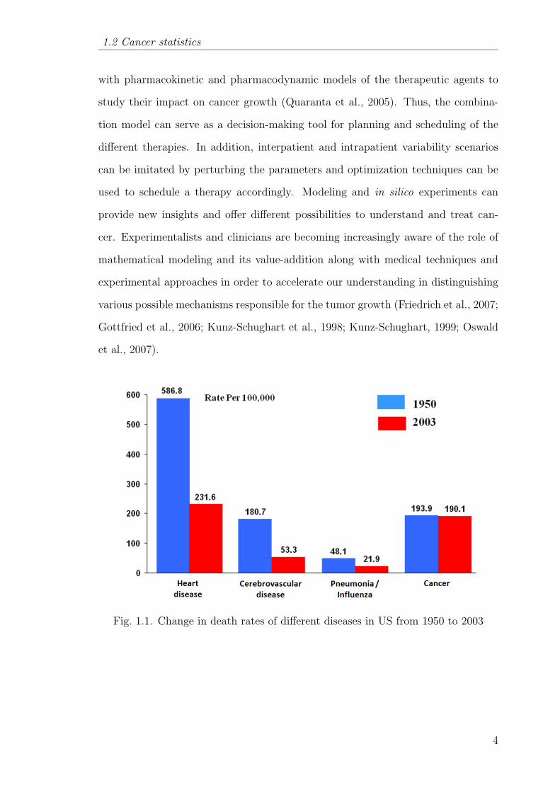
1.1 Change in death rates of different diseases in US from 1950 to 2003 4
1.2 Clinical phases of cancer treatment . . . . . . . . . . . . . . . . . 9
2.1 Publications on tumor microenvironment during 1995-2008 . . . . 18
2.2 Different spatial scales in tumor growth studies . . . . . . . . . . 20
2.3 Classification of tumor growth models . . . . . . . . . . . . . . . . 21
2.4 Functional models . . . . . . . . . . . . . . . . . . . . . . . . . . . 24
2.5 Classification of immune actions . . . . . . . . . . . . . . . . . . . 35
2.6 Description of different immune actions . . . . . . . . . . . . . . . 37
2.7 Metrics of PK-PD modeling . . . . . . . . . . . . . . . . . . . . . 41
2.8 Strategy followed in this thesis . . . . . . . . . . . . . . . . . . . . 46
3.1 Different zones in avascular tumor growth . . . . . . . . . . . . . 48
3.2 Tumor growth curves of simulated and experimental data at 16.5mmol/L glucose and 0.28 mmol/L oxygen . . . . . . . . . . . . . 56
3.3 Quiescent and necrotic radius at different tumor radius during itsgrowth at 16.5 mmol/L glucose and 0.28 mmol/L oxygen . . . . . 56
3.4 Tumor growth curves of simulated and experimental data at 16.5mmol/L glucose and 0.07 mmol/L oxygen . . . . . . . . . . . . . 57
3.5 Quiescent and necrotic radius at different tumor radius during itsgrowth at 16.5 mmol/L glucose and 0.07 mmol/L oxygen . . . . . 57
3.6 Profile of partial pressure of oxygen (PO2) in the HT29 spheroidswhen its diameter is 1039 µm . . . . . . . . . . . . . . . . . . . . 60
3.7 Profile of partial pressure of oxygen (PO2) in the HT29 spheroidswhen its diameter is 1116 µm . . . . . . . . . . . . . . . . . . . . 60
3.8 Profile of partial pressure of oxygen (PO2) in the HT29 spheroidswhen its diameter is 1169 µm . . . . . . . . . . . . . . . . . . . . 61
3.9 Profile of partial pressure of oxygen (PO2) in the HT29 spheroidswhen its diameter is 1415 µm . . . . . . . . . . . . . . . . . . . . 61
3.10 Profile of partial pressure of oxygen (PO2) in the HT29 spheroidswhen its diameter is 2077µm . . . . . . . . . . . . . . . . . . . . . 62
xi

Figure Page
3.11 Profile of partial pressure of oxygen (PO2) in the HT29 spheroidswhen its diameter is 2156 µm . . . . . . . . . . . . . . . . . . . . 62
3.12 Profile of partial pressure of oxygen (PO2) in the HT29 spheroidswhen its diameter is 2314 µm . . . . . . . . . . . . . . . . . . . . 63
3.13 Variation of partial pressure of oxygen (PO2) at the centre of theHT29 spheroids with the increase in its diameter . . . . . . . . . . 63
3.14 Comparison between the proposed model and Casciari et al. (1992)model on the basis of variation of oxygen concentration at the centreof the EMT6/Ro spheroids with the increase in its diameter . . . 64
4.1 Schematic representation of NSGA-II . . . . . . . . . . . . . . . . 73
4.2 L2 norm method . . . . . . . . . . . . . . . . . . . . . . . . . . . 74
4.3 Schematic representation of the problem . . . . . . . . . . . . . . 75
4.4 Comparison between original and non-dimensionalized model . . 79
4.5 Algorithm to find the optimal compromise solution . . . . . . . . 79
4.6 Pareto solutions for the problem formulation for case 1 (i.e. onlychemotherapy) . . . . . . . . . . . . . . . . . . . . . . . . . . . . 80
4.7 Comparison of evolution of states between cluster 1 and cluster 2 81
4.8 Evolution of states corresponding to the proposed treatment protocolof doxorubicin . . . . . . . . . . . . . . . . . . . . . . . . . . . . 81
4.9 Reduced representation of Pareto solutions for the problem formula-tion for case 2 (i.e. combination therapy) . . . . . . . . . . . . . . 84
4.10 Treatment protocol corresponding to the proposed combination ther-apy . . . . . . . . . . . . . . . . . . . . . . . . . . . . . . . . . . 85
4.11 Evolution of states corresponding to the proposed combination ther-apy . . . . . . . . . . . . . . . . . . . . . . . . . . . . . . . . . . . 85
4.12 Comparison of tumor relapse time between the proposed chemother-apy and the proposed combination therapy . . . . . . . . . . . . . 86
5.1 Dendritic cell/Vaccine therapy . . . . . . . . . . . . . . . . . . . . 90
5.2 Comparison between nominal and reactive schedule when parametersare not varied . . . . . . . . . . . . . . . . . . . . . . . . . . . . . 104
5.3 Comparison between nominal and reactive schedule when key param-eters are varied . . . . . . . . . . . . . . . . . . . . . . . . . . . . 104
5.4 Comparison between nominal and reactive schedule when non-keyparameters are varied . . . . . . . . . . . . . . . . . . . . . . . . . 105
5.5 Comparison of α value for the three cases . . . . . . . . . . . . . . 105
xii
Figure Page
5.6 Evolution of tumor for different therapy cases . . . . . . . . . . . 109
5.7 Reactive schedule of dendritic cell therapy . . . . . . . . . . . . . 109
5.8 Comparison of total dosage between reactive scheduling and nominalscheduling . . . . . . . . . . . . . . . . . . . . . . . . . . . . . . . 110
6.1 Sequential methodology . . . . . . . . . . . . . . . . . . . . . . . 113
6.2 Comparison of evolution of states between original model and reducedmodel . . . . . . . . . . . . . . . . . . . . . . . . . . . . . . . . . 120
6.3 Sensitivity indices of the parametric groups . . . . . . . . . . . . . 126
6.4 Patterns of HDMR component functions with the variations in keyparameters. X-axis: Scaled key parameter values, Y-axis: Scaledvalues of the component functions . . . . . . . . . . . . . . . . . . 129
7.1 Determination of diagnostic protocol (Di) for a patient populationbased on information index (Ii) evaluated using the mathematicalmodel . . . . . . . . . . . . . . . . . . . . . . . . . . . . . . . . . 137
7.2 Post - therapy analysis using statistical modeling to find the rulesdetermining the therapeutic effect on a patient . . . . . . . . . . . 137
7.3 Pareto solution (problem formulation A) corresponding to populationbased design of diagnostic protocol . . . . . . . . . . . . . . . . . 143
7.4 Proposed sampling times of tumor, CD8+ T-cells and interleukinduring diagnosis . . . . . . . . . . . . . . . . . . . . . . . . . . . . 143
7.5 Pareto solution (problem formulation B) corresponding to populationbased design of treatment protocol . . . . . . . . . . . . . . . . . 146
7.6 Proposed treatment protocol for the considered patient cohort . . 148
7.7 Tumor evolution in different patients . . . . . . . . . . . . . . . . 148
7.8 Rules to determine the success of proposed treatment protocol on thepopulation . . . . . . . . . . . . . . . . . . . . . . . . . . . . . . . 149
8.1 Application of this thesis work in the clinical practice . . . . . . . 156
8.2 A multiscale framework for comprehending cancer using OMICS data 161
8.3 Identification of diagnostic features and the prediction of therapeuticdesign using clinical data . . . . . . . . . . . . . . . . . . . . . . . 162
xiii
ABBREVIATIONS
DZM Different zone model
MZM Mixed zone model
MCTS Multicellular tumor spheroids
MAT Monoclonal antibody therapy
ACT Adoptive-cell-transfer therapy
AUC Area under the curve
PK Pharmacokinetic
PD Pharmacodynamic
OMM Oxygen microelectrode measurements
MOO Multi-objective optimization
GA Genetic algorithm
NSGA Non-dominated sorting genetic algorithm
TRT Tumor relapse time
DC Dendritic cells
DCV Dendritic cell vaccine
GSA Global sensitivity analysis
VBM Variance based methods
HDMR High dimensional model reduction
EFAST Extended fourier amplitude sensitivity tests
RS-HDMR Random sampling - High dimensional model reduction
FIM Fisher information matrix
xiv
NOMENCLATURE
Chapter 2
N Tumor cells
N0 Initial number of tumor cells
k Proliferation rate constant
θ Carrying capacity of tumor size
α Parameter which determines whether the saturated tumor
size is attained quickly or slowly
P , Q, D Densities of proliferating cells, quiescent cells, dead cells
kpp Proliferation rate of proliferating cells
kpq, kqp, kpd, kqd Transformation rate constant
λ Decay rate of dead cells
Ci(r, t) Concentration distribution of the diffusible chemicals
R(t) The position of the outer tumor radius
Rq(t) The locus of the boundary separating proliferating and qui-
escent cells
Rn(t) The locus of the boundary separating quiescent and necrotic
cells
Di Diffusion coefficient
φi Volume fraction of cell type in a given phase
νi Velocity of cell type in a given phase
λi(φi, Ci) Chemical and phase dependent production
C(t) Therapeutic drug
X(t) State variables
U(t) input or control or manipulated variables
xv

Chapter 3
Ci(t) Concentration of nutrients (Oxygen or Glucose)
R(t) The position of the outer tumor radius
Rq(t) The locus of the boundary separating proliferating and qui-
escent cells
Rn(t) The locus of the boundary separating quiescent and necrotic
cells
A Proliferation rate constant
Ap Apoptosis rate constant
Ne Necrotic rate constant
Ci∞ Concentration of the nutrient at the tumor surface
D1 Diffusivity of glucose
C1c Critical concentration of glucose
µ1 Maximum consumption rate of glucose
K1 Michaelis-Menten constant for glucose
D2 Diffusivity of oxygen
C2c Critical concentration of oxygen
µ2 Maximum consumption rate of oxygen
K2 Michaelis-Menten constant for oxygen
ν Volume of the tumor
ν0 Initial volume of the tumor
k1, k2 Gompertzian parameters
Chapter 4
E(t) Effector cells
T (t) Tumor cells
M(t) Chemotherapeutic drug
N Number of therapeutic interventions
tf Stipulated course period
xvi

Ne Number of interventions of effector cells
Chapter 5
H(t) Helper T-cells
C(t) Cytotoxic T-cells
M(t) Tumor cells
D(t) Dendritic cells
I(t) Interleukin
Vf Variance of the model output
Vi,Vij Partial variances of the inputs
Si,Sij Sensitivity indices
G Model output
P Parameter set
u1 Input rate of dendritic cells
u2 Input rate of interleukin
Chapter 6 & 7
T Tumor cells
N Natural killer cells
L Cytotoxic T-cells
C Circulating lymphocytes
I Interleukin
M Doxorubicin
U Input rate of doxorubicin
O Model output
Gi Sensitivity matrix
Jc Joint confidence interval
ψ1 Significance level
Πi Parametric groups
αi time derivative scale factors
xvii

Ts, Ns, Ls, Cs, Ms Scale factors
nP1, nP2 population size
xviii

Chapter 1 Introduction
Chapter 1
INTRODUCTION
‘Growth for the sake of growth is the ideology of the cancer cell.’
- Edward Abbey
1.1 Motivation
The global challenge driving the oncology community is to understand and ex-
ploit the complex nature of cancer growth to discover specific diagnostic indices
and treatment protocols for anti-cancer drugs. This challenge demands conduct-
ing laboratory and clinical experiments for the collection of informative data. The
aggregated knowledge from the experiments and clinical experiences must then be
translated into promising therapies and used in P4 (preventive, proactive, partic-
ipatory and personalized) medicine. Presently, cancer diagnostic and treatment
protocols are suggested based on the knowledge generated from clinical trials in-
volving particular cohort of patients, but are applied on other patient groups as well
(Kleinsmith, 2005). Also, for a given treatment protocol only few patients may be
cured and others may not. Variability in patient outcomes is one of the practical
challenges of the existing and emerging therapeutic protocols. Variability can be
broadly classified as interpatient and intrapatient variability. Interpatient varibility
is the difference in effect of therapy (target or side effects) on different patients. On
the other hand, intrapatient variability is the variations that occur in a given patient
during the treatment course. In fact, it is necessary to know the reason behind the
variability of the effect of diagnostic and treatment protocols on the patients, so
that the protocols can be tailored appropriately to individual patients or patient
1
1.1 Motivation
groups. It is to be noted that experiments that can elucidate the reasons for inter-
and intrapatient variability are costly and time-consuming. The objectives of any
therapy are to minimize the total number of cancer cells by maintaining it below
the lethal level while minimizing the side effects. Keeping this in view, the main
challenge is to find a way for the clinical implementation of novel and combinatorial
therapies. FDA approval is needed before any clinical implementation - the whole
process of discovery, laboratory trials and approval can take several years. Accord-
ing to recent studies, the cost involved in the research and development of a new
drug for Food and Drug Administration (FDA) approval is between US $ 500 million
and US $ 800 million and the development time is around 10-12 years. For example,
Dendreon took around 18 years to get FDA’s approval and around US $ 750 million
was invested. A lot of in vitro/in vivo experiments should be performed to clear
the different phases of FDA approval and understand the side effects, efficacy and
the variability of the therapy (Lord and Ashworth, 2010). In this context, in silico
(computer) based tools may help to investigate the fundamentals of cancer growth
and unique features of a given therapy and its protocols. Even FDA has recognized
and encouraged the population based pharmacokinetic and pharmacodynamic mod-
eling studies to ease the approval of new drugs with lesser number of experiments.
In this regard, Gatenby (1998) states that ‘recent research in tumor biology, partic-
ularly that using new techniques from molecular biology, has produced information
at an explosive pace. Yet, a conceptual framework within which all these new (and
old data) can be fitted is lacking’. Gatenby and Gawlinski (2003) stress the point
that clinical oncologists and tumor biologists possess virtually no comprehensive
theoretical model to serve as a framework for understanding, organizing and apply-
ing the data and emphasize the need to develop mechanistic models that provide
real insights into critical parameters that control system dynamics. Murray (2002)
states that ‘the goal is to develop models which capture the essence of various in-
teractions allowing their outcome to be more fully understood’. Tiina et al. (2007)
presented the results of a search in the PubMed bibliographic database which shows
2

Chapter 1 Introduction
that, out of 1.5 million papers in the area of cancer research, approximately 5% are
related to mathematical modeling. According to Byrne (1999), effective and efficient
treatment modalities can be developed by identifying the mechanisms which control
the cancer growth. Thus, once we understand the mechanism, the key components
of it can be modified to eliminate (or reduce pain arising from) the disease. This
state of knowledge may be possibly reached through laboratory experiments alone,
but at the cost of infinite time and numerous (replicated) experiments. However,
the achievement of this goal can be speeded up through the application of process
systems engineering techniques (Mathematical modeling, Control theory and Op-
timization) to describe different aspects of solid tumor growth in the absence or
presence of anti-cancer agents. This implies that sound and robust tools are essen-
tial in order to investigate the fundamentals of cancer growth and unique features
of a given therapy and its protocols.
1.1.1 Role of process systems engineering in cancer therapy
Mathematical modeling and simulation is a versatile tool in comprehending the
system behavior and has been used for different applications in natural science and
engineering disciplines (Quarteroni, 2009). A mathematical model is an abstraction
of a process system. It is composed of model equations and parameters. Usually,
available experimental data is used for estimating the model parameters and for val-
idating its prognostic ability. Then, parametric analysis (sensitivity analysis with
respect to parameters) of the model is performed to understand the domain and
variations of the system behavior with the variation in the parameters (Rodrigues
and Minceva, 2005). With understanding of the system and a valid model, one can
pursue model based process control and optimization (Edgar et al., 2001). In a sim-
ilar fashion, the applications of the tumor growth modeling are many (Deisboeck
et al., 2009). Firstly, cancer growth can be predicted and the main parameters re-
sponsible for it can be better understood. Secondly, these models can be combined
3
1.2 Cancer statistics
with pharmacokinetic and pharmacodynamic models of the therapeutic agents to
study their impact on cancer growth (Quaranta et al., 2005). Thus, the combina-
tion model can serve as a decision-making tool for planning and scheduling of the
different therapies. In addition, interpatient and intrapatient variability scenarios
can be imitated by perturbing the parameters and optimization techniques can be
used to schedule a therapy accordingly. Modeling and in silico experiments can
provide new insights and offer different possibilities to understand and treat can-
cer. Experimentalists and clinicians are becoming increasingly aware of the role of
mathematical modeling and its value-addition along with medical techniques and
experimental approaches in order to accelerate our understanding in distinguishing
various possible mechanisms responsible for the tumor growth (Friedrich et al., 2007;
Gottfried et al., 2006; Kunz-Schughart et al., 1998; Kunz-Schughart, 1999; Oswald
et al., 2007).
Fig. 1.1. Change in death rates of different diseases in US from 1950 to 2003
4

Chapter 1 Introduction
1.2 Cancer statistics
The word Cancer (meaning “crab” in Latin) was introduced by Hippocrates in
the 5th century BC to explain a group of diseases resulting from the abnormal growth
and spread of tissues to the other parts of the body and ultimately proving fatal.
Even though cancer has subsisted for a very long time, its existence is noticeably
increasing during the last 50 years. As of now, the probability that a randomly
selected person will get cancer has almost doubled when compared to 1950s (Klein-
smith, 2005). Cancer stands next only to heart disease in the list of most fatal
diseases in the world. From Figure 1.1, it is obvious that the decrease in death rate
of cancer patients over the years 1950-2003 has been minimal as compared to other
major diseases. Cancer related deaths have been escalating meteorically - according
to the World Health Organization (WHO), 7.6 million people died of cancer (out of
58 million deaths overall) in 2008. They speculated that cancer deaths will increase
to 18% and 50% by 2015 and 2030 respectively. Recently, the American Cancer
Society (ACS) reported that around 1.6 million new cancer cases and 0.6 million
cancer death cases occured in the US in 2009. According to another report on
worldwide cancer rates by the WHO’s International Agency for Research on Cancer
(IARC), North America leads the world in the rate of cancers diagnosed in adults,
followed closely by Western Europe, Australia and New Zealand. In Britain, it was
estimated using 2008 data that more than one in three were expected to develop
the disease over their survival period 1. According to Cancer Council Australia,
around 114,000 new cases of cancer were diagnosed in Australia in 2010 and it was
estimated that one in two Australians will be diagnosed of cancer by the age of 85.
Cancer deaths in Singapore reflected the global trend (27.1% of total deaths) during
the period 1998-2002 and approximately 49,400 new cases of cancer were diagnosed
during the period 2005-2009 2. The reasons for such alarming trends include the
1http://info.cancerresearchuk.org/cancerstats/incidence/risk/2http://www.nrdo.gov.sg/uploadedFiles/NRDO/Cancer Trends Report%20 05-09.pdf
5

1.3 What is cancer ?
non-availability of definite therapy for all types of cancer and the indeterminate
nature of the existing therapies for patients with same type of cancer.
The above mentioned figures have drawn the attention of researchers to under-
stand the mechanism of cancer and come out with better therapies. In this effort,
remarkable progress has been made in the past few decades in uncovering some of
the cellular and molecular mechanisms leading to cancer and the cumulative infor-
mation reveal that around 100 types of cancer exist. Their names are distinguished
from one another on the basis of its location and the cell type involved. Based on
the gravity of the cancer problem, Perumpanani (1996) remarks that ‘the research
community has taken on the challenge posed by cancer on a war-footing and this
has in recent years resulted in an explosion in our understanding of cancer’. Some
researchers claim that the analysis of cancer mechanisms has enhanced our under-
standing of the normal cells (Alberts et al., 2002; Kleinsmith, 2005). This may
lead to many fundamental discoveries in cell biology and broadly benefit the vari-
ous fields of medicine. Despite the advances made in the understanding of cancer
and mechanisms, much remains to be done before the deaths of millions of people
due to cancer can be reduced. One main challenge is to be able to understand and
exploit the complex nature and multiple stages of tumor growth. Another challenge
is to conduct the right laboratory and bedside experiments to collect useful data to
extract information regarding the mechanisms of cancer cell behavior.
1.3 What is cancer ?
Cancer is the uncontrolled proliferation of abnormal cells of any tissue or organ
in the human body. An abnormal cancer cell evolves from the normal cell due to
accumulation of DNA damage - this DNA damage (i.e. genetic mutations in pieces of
DNA) makes the cell immortal. The genes transferred from the parents might carry
with them an inherent risk or susceptibility to cancer. When such a “normal” but
6

Chapter 1 Introduction
Table 1.1Differences between benign and malignant tumors
Trait Benign MalignantNuclear size Small LargeRatio of nuclear size to Low Highcytoplasmic volumeNuclear shape Regular Pleomorphic (irregular shape)Mitotic index Low HighTissue organization Normal DisorganizedDifferentiation Well differentiated Poorly differentiatedTumor boundary Well defined Poorly defined
“risk prone” cell is exposed to external factors such as UV radiation, carcinogenic
chemicals etc., it could undergo a series of genetic mutations and transform into a
cancerous cell. Mutations cause the cell to evade cell death and grow improperly
with or without growth signals from the environment (Hanahan and Weinberg, 2000;
Martins et al., 2007). Once the cancer cell is formed, it searches for nutrients from
the nearby tissues and proliferates rapidly compared to the adjacent normal cells
(Tiina et al., 2007). The induced mutation by the external factors not only enhances
the proliferation rate of the cells but also decreases its death rate by down-regulating
and up-regulating the tumor suppressor genes and oncogenes respectively (Hanahan
and Weinberg, 2000). Over time, this results in the formation of a clump of cells
known as neoplasm or tumor. Tumor growth is based upon conditions like tumor
location, cell type, and nutrient supply. On the basis of the growth pattern, tumors
are classified into two fundamental groups. One group is benign tumors whose
growth is narrowed to a local area and are composed of well-differentiated cells.
The other one is malignant tumors which can invade the nearby tissues, migrate to
other parts of the body and their cells are poorly differentiated. The differences in
the microscopic appearance of the benign and malignant tumors are tabulated in
Table 1.1.
7

1.4 Clinical phases
1.3.1 Different stages of tumor growth
Generally, the overall cancer growth is categorized into three stages namely avas-
cular, angiogenesis and metastasis (Tiina et al., 2007). In avascular stage, the tu-
mor growth is localized and nutrients are consumed from the nearby tissues. At
this stage, the tumor is known as benign tumor as it is not life-threatening and its
growth rate is usually slower than that in the other two later stages. Initially, avas-
cular tumors get adequate nutrients and the cells flourish. As time proceeds, the
avascular tumor growth rate reduces and reaches saturation size due to insufficient
nutrition supply to the innermost cells in the tumor. Then, the nutrient-deficient
tumor cells signal the nearby blood vessels about their nutrient requirement leading
to the second stage called angiogenesis. Consequently, the tumor develops associ-
ation with the blood vessels in its proximity. Subsequently, the tumor cells loosen
and the cell debris flows through the connected blood vessels. The tumor cells can
thus migrate from their origin to the other parts of the body resulting in the final
stage called metastasis. After metastasis, the patient will be left with multiple tu-
mors in the body (Kleinsmith, 2005), because the migrated cancer cells invade the
other parts of the body via repetition of the above mentioned growth phases. At
the angiogenesis and metastasis stage, the tumor grows very randomly as well as
rapidly and is quite malignant. Treatment, at this stage, becomes quite complicated
and often unfruitful. Hence, the early detection of tumor in avascular stage enables
cancer cure with higher probability.
1.4 Clinical phases
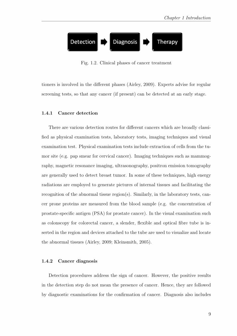
The common phases any cancer patient undergoes are detection, diagnosis and
administration of therapy (Figure 1.2). A multidisciplinary team comprising of
specialized clinicians, pathologists, radiologists, pharmacists, nurses, general practi-
8
Chapter 1 Introduction
Fig. 1.2. Clinical phases of cancer treatment
tioners is involved in the different phases (Airley, 2009). Experts advise for regular
screening tests, so that any cancer (if present) can be detected at an early stage.
1.4.1 Cancer detection
There are various detection routes for different cancers which are broadly classi-
fied as physical examination tests, laboratory tests, imaging techniques and visual
examination test. Physical examination tests include extraction of cells from the tu-
mor site (e.g. pap smear for cervical cancer). Imaging techniques such as mammog-
raphy, magnetic resonance imaging, ultrasonography, positron emission tomography
are generally used to detect breast tumor. In some of these techniques, high energy
radiations are employed to generate pictures of internal tissues and facilitating the
recognition of the abnormal tissue region(s). Similarly, in the laboratory tests, can-
cer prone proteins are measured from the blood sample (e.g. the concentration of
prostate-specific antigen (PSA) for prostate cancer). In the visual examination such
as colonscopy for colorectal cancer, a slender, flexible and optical fibre tube is in-
serted in the region and devices attached to the tube are used to visualize and locate
the abnormal tissues (Airley, 2009; Kleinsmith, 2005).
1.4.2 Cancer diagnosis
Detection procedures address the sign of cancer. However, the positive results
in the detection step do not mean the presence of cancer. Hence, they are followed
by diagnostic examinations for the confirmation of cancer. Diagnosis also includes
9
1.4 Clinical phases
quantification of cancer characteristics. In this regard, it requires the biopsy spec-
imen extracted from the tumor site. Microscopic and pathological studies are per-
formed to grade the tumor based on distinctive features such as cell morphology,
mitotic index and doubling time. Mitotic index indicates the percentage of dividing
cells where as doubling time implies the rate of division. Further, the tumor staging
is determined based on different criteria: (a) the size of the localized tumor and its
spread to the nearby tissues, (b) the extent of spread to the regional lymph nodes
and (c) the extent of spread to the distant parts (metastasis). This kind of staging
is known as TNM staging where T, N, M stands for tumor, lymph node and metas-
tasis respectively. Additionally, biochemical tests of the molecular components of
the cells may figure out gene or proteins expressed in the tumor which will serve as
biomarkers or prognostic indicators. For example, estrogen receptor is an indicator
of breast cancer prognosis. The information about tumor grading, staging concluded
from pathological and radiological data, patient’s blood cell count and his/her his-
torical health record, are referred for suggesting a particular therapy or combination
of therapies. Then, it is the role of oncology pharmacists to monitor and prepare
the therapy. Presently, they use their clinical and pharmaceutical expertise in de-
signing the treatment plan for an individual. The freedom of attempting intuitive
ideas regarding therapeutic inputs in designing cancer therapy is very less and it
demands foolproof evidence owing to ethical constraints.
1.4.3 Cancer therapy
Research efforts over the last hundred years has resulted in the development of
many treatment modalities. The most common of these are surgery, chemotherapy,
radiation therapy, and immunotherapy (Airley, 2009; Kleinsmith, 2005). However,
there is no specific therapy for treating all forms of cancer and each therapy has
its own advantages and deficiencies. As a rule, surgery is preferred to remove the
tumors provided its location permits surgical intervention. However, all cancer cells
10
Chapter 1 Introduction
cannot be removed by surgery and hence surgery is usually followed or substituted by
chemotherapy and/or radiation therapy. Among these two, chemotherapy is better
than radiation therapy because it is a systemic therapy. In systemic therapies, drug
circulates in the blood stream and not only kills the residual cancer cells at the
tumor site but also annihilates migrated cancer cells. On the contrary, radiation
therapy is a localized therapy which is a better option in the early stages of cancer
(Shepard et al., 1999). In general, most of the patients undergo chemotherapy at
some stage of their treatment. Chemotherapy is administered as a course in cycles
based on the health condition of the patient rather than as a one-shot treatment
(Airley, 2009). This serves to lessen its side effects and to accomplish the goal of
the chemotherapy. The principle of chemotherapy is to recognize and attack the
rapidly proliferating cells by restraining DNA replication and by rupturing their
DNA. Consequently, it may also damage normal cells that are fast proliferating by
nature (e.g. blood cells, cells lining the intestines, colon, cells inside the mouth
and throat, cells in hair follicles). Yet another problem is that some cancer cells
may acquire mutations which make them resistant to chemotherapy drugs. In this
case, even the few drug resistant cancer cells may lead to the invasive growth of the
tumor. The side effects of chemotherapy can sometimes be worse than the disease
itself. Thus, only chemotherapy as an adjuvant therapy after surgery or as a prime
therapy, may not eradicate the tumor completely and may lead to serious side effects.
One solution to this challenging issue is the application of combination therapy. In
this regard, combining chemotherapy with emerging and targeted therapies such
as immunotherapy can be a promising and synergistic option to treat many cancer
types (Gabrilovich, 2007; Lake and Robinson, 2005).
1.4.4 Emerging and targeted therapies
Surgery, radiation therapy and chemotherapy either alone or in various combi-
nations are successful only when the tumor is identified in the initial stages. But,
11
1.4 Clinical phases
still there are some cancers (pancreas, liver or lungs) which are detected only at
their aggressive stages. Now, cancer scientists are putting lot of efforts in develop-
ing novel and effective treatment strategies with higher selectivity such that only
cancer cells are targeted while sparing the normal cells. Thus, these therapies are
known as targeted therapies. These include immunotherapy, gene therapy, and vi-
ral therapy. In immunotherapy, the main idea is to identify and extract or engineer
the immune cells which are cytotoxic to tumor cells to improve the selectivity and
cytotoxicity. Some forms of immunotherapy are Bacillus Calmette-Guerin (BCG)
(Bunimovich-Mendrazitsky et al., 2007), cytokine therapy, adoptive cell transfer
therapy. In BCG therapy, bacteria are injected into the patients to provoke the
immune system and eliminate tumor cells. The success of BCG therapy has been
notable in the treatment of early stage bladder cancer. Similarly, in cytokine ther-
apy, cytokines (proteins) are used to stimulate the immune response. This will be
discussed elaboratively in the following chapter. Gene therapy exploits the role of
oncogenes and tumor suppressor genes in cancer development based on discoveries
over the past two decades. In gene therapy, the defective genes are replaced by the
normal genes (Mesri et al., 2001). In one form of gene therapy, viruses containing the
normal copy of p53 gene (tumor suppressor gene) in their DNA are used to replace
the defective p53 gene. Alternatively, in viral therapy, viruses are engineered to
recognize the cells with defective p53 gene and kill them. This process is known as
lysis. ONYX-015 is one such engineered advenovirus, which replicates swiftly in the
defective p53 gene cells and eventually activates the immune response (Zurakowski
and Wodarz, 2007). However, these emerging therapies are still in their early phases
and demand the computational modeling support to test different hypothesis and
expedite the clinical implementation procedures.
12
Chapter 1 Introduction
1.5 Our focus - avascular tumor growth
There are many reasons for concentrating on avascular tumor growth. The first
motivation is the increasing awareness of cancer among people. In the past, cancer
was often recognized only at the later stages. But nowadays, based on the health
history of their immediate family members, and due to better awareness programs,
people become cautious and undergo regular health checkups. Governments, in
developing countries, also organize mass health check and screening campaigns. If
anything, people will undergo more regular, frequent and possibly cheaper health
scans in the future. Thus, diseases such as cancer may be detected earlier rather than
later. The second motivation is provided by the advancements in the biomedical
field over the past 30 years (Preziosi, 2003), and sophistication of experimental
approaches such as imaging and gene sequencing. These advanced techniques can
locate tumors even when their size is very small (in the order of 100 µm). As a
result, data corresponding to avascular tumor growth should not be a constraining
factor in its modeling. Note, however, that it does not mean that avascular stage
is the most important. In fact, from a clinical point of view, angiogenesis and
metastasis are of equal (if not more) significance and modeling of these stages is
also important for designing cancer therapies. As a starting point to comprehend
the complexity of all stages of cancer, it will be better to start with a study of the
avascular tumor growth study. While avascular tumor growth is simple to model
mathematically, it also contains many of the phenomena that are similar to the case
of vascular models. Moreover, the reproducibility of experiments with avascular
tumor growth is better than with vascular tumors. The experiments of avascular
tumor growth can also be done in vitro in the form of multicellular tumor spheroids
(MCTS) which are quite cheap relative to animal experiments (Freyer, 1988; Freyer
and Sutherland, 1986b,a; Kunz-Schughart et al., 1998; Kunz-Schughart, 1999; Hlatky
et al., 1988a; Marusic et al., 1994; Maruic et al., 1994; Mueller-Klieser, 1997, 1987;
Oswald et al., 2007). Therefore, the modeling of avascular tumor can be helpful
13

1.6 Contributions
in making predictions and designing experiments on the advanced stages of cancer
as well (Tiina et al., 2007). Research in cancer biology related to avascular tumor
growth has provided a vast amount of data through in vitro (Freyer, 1988; Freyer
and Sutherland, 1986b,a) and in vivo experiments (Marusic et al., 1994) of different
cancer cell lines. Despite this, an appropriate mechanism-based mathematical model
for illustrating the tumor growth remains elusive. In the avascular stage, the tumor
growth involves the formation of three zones, namely proliferation zone, quiescent
zone and necrotic zone. Eventually, in the avascular stage, the tumor reaches a
steady size. The cause for the attainment of steady state by the tumor has been
hypothesized in different ways. The study of tumor growth and its use for the
development of cancer therapies is therefore an important area of research. Its
valuable outcomes can provide a helping hand in enhancing the quality of life and
increase life span of the cancer patients resulting in social and economic benefits to
the world.
1.6 Contributions
The thesis work seeks to address the following issues in the field of in silico
cancer research.
1. Mathematical Modeling: In this research, a mechanistic model is developed for
predicting the avascular tumor growth based on microenvironment conditions
(moving boundary problem). This work can be useful for tumor pathologists
who may wish to categorize the tumor cells into either benign or malignant
by estimating the model parameters using tumor growth data.
2. Optimization, Control: Tumor growth models are integrated with the phar-
macokinetic and pharmacodynamic models of cancer therapeutics and an op-
timization problem keeping in view the objectives of tumor reduction and
14
Chapter 1 Introduction
minimization of side effects is formulated. Then, multi-objective stochastic
optimization is applied to design an optimal treatment plan.
3. Model reduction, Sensitivity analysis: Many of the unresolved issues in the
medical field remain so because they are not data rich. This makes it very
difficult to estimate model parameters precisely. Hence, model simplification
is an important step in model-based practical applications. In this work, a
tumor-immune model is reduced and sensitivity analysis is performed to find
the influential parametric groups. This facilitates the use of model based ex-
perimental design to design experiments and help experimentalists to generate
informative data.
4. Data driven analysis: The main idea is to mimic a veteran oncologist in sug-
gesting standard treatment plan for the cancer patients by employing quanti-
tative approaches. “Patients” are generated by varying the sensitive parame-
ters of the model. The average therapeutic protocol for the generated patient
cohort for a given therapy is determined by framing an optimization prob-
lem with suitable objectives and constraints. The obtained optimal treatment
planning is applied on these patients to study its effect on the tumor evolu-
tion during the therapeutic horizon. Later, data driven techniques are used to
derive “rules” based on key parameter values that can help predicting success
of the therapy on future patients.
1.7 Thesis organization
The second chapter describes different categories of mathematical models used
for tumor growth analysis and emphasizes the utility of optimal control theory in
designing cancer therapy protocols. Also, the challenges that can be addressed us-
ing PSE methodologies and tools are highlighted. In Chapter 3, a new mechanistic
model for avascular tumor growth is proposed based on the hypothesis of diffusion
15

1.7 Thesis organization
and consumption of nutrients. The proposed model is also validated with data
from multicellular tumor spheroid experiments. The application of multi-objective
optimization in the sequential scheduling of chemotherapy and immunotherapy for
a given “patient” (a tumor-immune-chemo model with known parameters) is the
subject of Chapter 4. Chapter 5 is devoted to the issue of intrapatient variability
and its effect on the treatment outcomes. Particularly, it focuses on the schedul-
ing of dendritic cell therapy under uncertainty using reactive scheduling strategy.
The interesting question of quantification of variability using sensitivity analysis is
also visited. Chapter 6 projects the usefulness of model reduction in promoting
model-based approaches in clinical settings. Model reduction using scaling and sen-
sitivity analysis is exemplified with an example of tumor-immune model. Chapter 7
addresses population based studies (interpatient variability) using reduced tumor-
immune model (from Chapter 6) to design diagnostic and therapeutic protocols.
Parametric combinations that determine the treatment outcome are also uncovered
using a classification tool. In the final chapter (Chapter 8), the key conclusions of
the thesis are summarized along with recommendations for future work.
16

Chapter 2
LITERATURE REVIEW
‘Imagination is more important than knowledge.’
- Albert Einstein
In this chapter, the main focus is on the description of different classes and subclasses
of tumor growth models. Models depicting the interaction between tumor cells
and immune system are discussed by elaborating on the different mechanisms of
immune action. Development of treatment protocols using the combination of tumor
growth and pharmacokinetic-pharmacodynamic models is presented. The challenges
in deriving ideas from mathematical modeling techniques for clinical implementation
are briefly discussed.
2.1 Mathematical modeling of cancer growth
Cancer research is a very good example of multidisciplinary team that includes
biologists, clinicians, oncologists, pharmacists, general practitioners, radiologists,
mathematicians and engineers. The role of mathematicians and engineers in cancer
has been realized only in the recent years even though many mathematical models
were developed to expound tumor growth in the last few decades (Anderson and
Quaranta, 2008; Byrne, 2010). At the same time, Figure 2.1 shows the increasing
trend of number of research articles in the field of tumor microenvironment over
the 1995-2008 period (Witz, 2009). According to Anderson and Quaranta (2008),
the proposed models can be broadly classified as continuum, discrete and hybrid
models based on the scales of the mechanism of interest. Traditionally, tissue and
17

Chapter 2 Literature Review
Fig. 2.1. Publications on tumor microenvironment during 1995-2008
cell scale phenomena are studied using continuum and discrete models respectively.
Then, hybrid models are introduced in order to understand the effect of cell scale
phenomena on the tissue scale. Each type of model has its own advantages and
disadvantages.
There are many review articles which provide comprehensive details on the chrono-
logical development of mathematical models that deal with different stages of cancer
growth (Araujo and McElwain, 2004; Bellomo, Angelis and Preziosi, 2003; Byrne
et al., 2006; Lowengrub et al., 2010; Sanga et al., 2007, 2006; Tiina et al., 2007).
Araujo and McElwain (2004) presented a comprehensive discussion on the history of
studies related to solid tumor growth, illustrating the role of mathematical modeling
approaches from the early decades of twentieth century to the present time. This
review projected a proper balance between the mathematical models and experimen-
tal investigations which have been carried over these years. Such a comprehensive
review covering theoretical and experimental domain is indeed useful; otherwise, the
mathematical models have no utility by themselves. Overall, their work provided a
glimpse on the status and achievements of mathematical modeling of both avascular
and vascular tumor growth. It included the models of avascular tumors, multicellu-
18
2.1 Mathematical modeling of cancer growth
lar spheroids, models of tumor invasion and metastasis, as well as that of vascular
tumor. Thus, this review provides a general idea of models for tumor growth. The
review by Tiina et al. (2007) concentrated exclusively on the models of avascular
tumor growth. It discussed the broad classification of the avascular tumor growth
models into continuum mathematical models and discrete cell population models.
Tiina et al. (2007) pointed out the fact that the hitherto developed mathematical
models were very simple as they focused on certain general processes (diffusion of nu-
trients) that did not fully account for the complexity of the biology and biochemistry
of the avascular tumor growth. Another encouraging view from the authors is that
mathematical modeling has two-fold applications in cancer biology. On one hand,
they can be applied for the verification of hypotheses as suggested by the experimen-
talist and on the other hand, they provide a framework for predicting the outcomes
of other intuitive ideas. They highlighted the impact of mathematical modeling in
tumor biology by considering an example under the category of continuum model.
This review also included the theory of multiphase models, tissue mechanics models,
and discrete models. According to Tiina et al. (2007), the motivation for the dis-
crete models is the advances in biotechnology which makes it feasible to capture data
related to phenomena occurring at mesoscopic and microscopic levels (Figure 2.2).
This cellular level knowledge is used to obtain information about the macroscale
phenomena of tumor growth by using multiscale modeling. Similarly, Lowengrub
et al. (2010) have provided a broad classification of models. Specifically, this work
has focused on the continuum models, their analysis and model calibration using
clinical data to predict tumor morphology and growth. However, the complexity of
the models increases significantly by incorporating the updated knowledge of cancer
biology at different scales.
By raising this issue of model complexity, Tiina et al. (2007) introduced the
parameterization of the models as an important challenge. A well-parameterized
model implies that, only from the knowledge of parameter values, we should be able
to differentiate the variations in the system behavior. As a simple example, based
19

Chapter 2 Literature Review
Fig. 2.2. Different spatial scales in tumor growth studies
on the value of Reynolds number (Re), we are able to conclude the characteristics of
the flow of a Newtonian fluid through a circular pipe such as laminar (Re < 2100)
or turbulent (Re > 2100). Thus, better parameterized models are the models where
the parameters have physical meaning. The key message is that simpler and better
parameterized mechanistic models are required and are important as compared to
other models that just fit the data.
2.2 Continuum models
Continuum modeling approach is very convenient to study large scale systems.
Continuum models are useful once a cell is already transformed to a cancerous cell
after undergoing mutations in its genetic code. Tumors are considered as collection
of cells in continuum models in which they are described as density or volume frac-
tion of cells. Experimentally, it is observed that transformation in the tumor occur
as it progresses and results in the formation of different regions. In continuum mod-
els, the rules are framed for different regions of the tumor but not for each and every
cell. Thus, individual cells in the tumor cannot be tracked separately. They are usu-
ally, described using ordinary, partial differential and integro-differential equations
and detail explanation is provided in the later part. The main advantage is that
continuum models have fewer parameters and they can be easily estimated from the
20

2.2 Continuum models
Fig. 2.3. Classification of tumor growth models
available experimental model system like multicellular tumor spheroids. Continuum
models are quite relevant to quantify the macroscale tumor behaviour.
Another review chapter by Byrne in Preziosi (2003) is mainly based on earlier
valuable contributions (Byrne, 1999, 1997; Byrne and Chaplain, 1998, 1996, 1995;
Byrne and Gourley, 1997). This review further narrowed down to the continuum
models of the avascular tumor growth. Continuum models for avascular tumor
growth can be further classified into two categories: homogeneous and heterogeneous
models (see Figure 2.3). These are explained in the next section.
2.2.1 Homogenous models
Homogenous models are those in which all the tumor cells are assumed to be alike
and they ignore the spatial effects in explaining the growth dynamics of the tumor
growth. These are the earliest models and are formulated as system of differential
equations. All homogeneous models are empirical (e.g. exponential model, logistic
model, Gompertzian model). These models are data-specific and are unable to shed
21

Chapter 2 Literature Review
light on the inherent mechanisms governing the tumor cells because they are built
by data-fitting of in vitro and in vivo experimental results. Marusic et al. (1994)
used the in vitro data of multicellular tumor spheroids available for 15 different cell
lines (Freyer, 1988) to test several empirical models. In vivo tumor growth data
obtained by injecting tumor cells from two of the above mentioned cell lines into
athymic mice were used to test different empirical models (Marusic et al., 1994).
The exponential growth model is the simplest homogenous model in which the total
number of cells in the solid tumor increases exponentially with time. In this model,
all cells are assumed to receive the nutrients and other growth factors abundantly.
This model is quite precise in representing the very early growth of the tumor and
is given by Equations (2.1) and (2.2):
dN
dt= kN, with N(t = 0) = N0, (2.1)
N(t) = N0ekt (2.2)
where, k > 0 is the net rate at which the cells proliferate, and N0 represents
the initial number of the tumor cells. The exponential model does not capture the
decreased growth rate of tumor cells and their attainment of final saturation which
are obtained from the in vitro and in vivo experiments. The decrease in growth
rates and final saturation happen because, with the increase in the tumor size, all
cells will not have access to same amount of nutrients and growth factors. In order
to capture the saturation of tumor size a generalized empirical model is given by
Equations (2.3) and (2.4):
dN
dt=k
αN
[1−
(N
θ
)α], with N(t = 0) = N0, (2.3)
N(t) = θ
(Nα
0
Nα0 + (θα −Nα
0 )e−kt
)(2.4)
22
2.2 Continuum models
where, θ is the carrying capacity of tumor size and α is a parameter which
determines whether the saturated tumor size is attained quickly or slowly. When
α = 1, the model is called the logistic growth model and when α→0+, the model
is called the Gompertzian growth model. In this way many empirical models were
fitted to the experimental data, but the parameters of the models could always be
related to exact phenomenon of the tumor growth.
2.2.2 Heterogenous models
Functional models are also called as compartmental models or spatially averaged
models and they assume that different cell types are in different compartments based
on cell kinetics (Preziosi, 2003). Cell kinetics is the transformation of a cell from
one phase to another phase depending on the environmental conditions. Based on
the availability of nutrients and activity of the cells, there are three types of cells
namely proliferating cells, quiescent cells and necrotic cells. Usually, the outer layer
of tumor consists of proliferating cells, as they will be getting sufficient nutrients.
The cells in the inner layer next to proliferation zone are called the quiescent cells.
Quiescent cells do not proliferate but they are alive, because the quantum of nutrient
supply reaching them is just able to keep them alive. The innermost zone of the
tumor consists of necrotic cells which are dead due to the inadequacy of nutrients. In
Piantadosi (1985), the transition between the resting and growing cells is expressed
in terms of ordinary differential equations. Furthermore, the model assumes that
production of the growing fraction and loss fraction from the resting fraction of cell
population follows first order kinetics. Garner et al. (2006) analyzed a simple cell
population model to study the long-term behavior of quiescent and proliferating
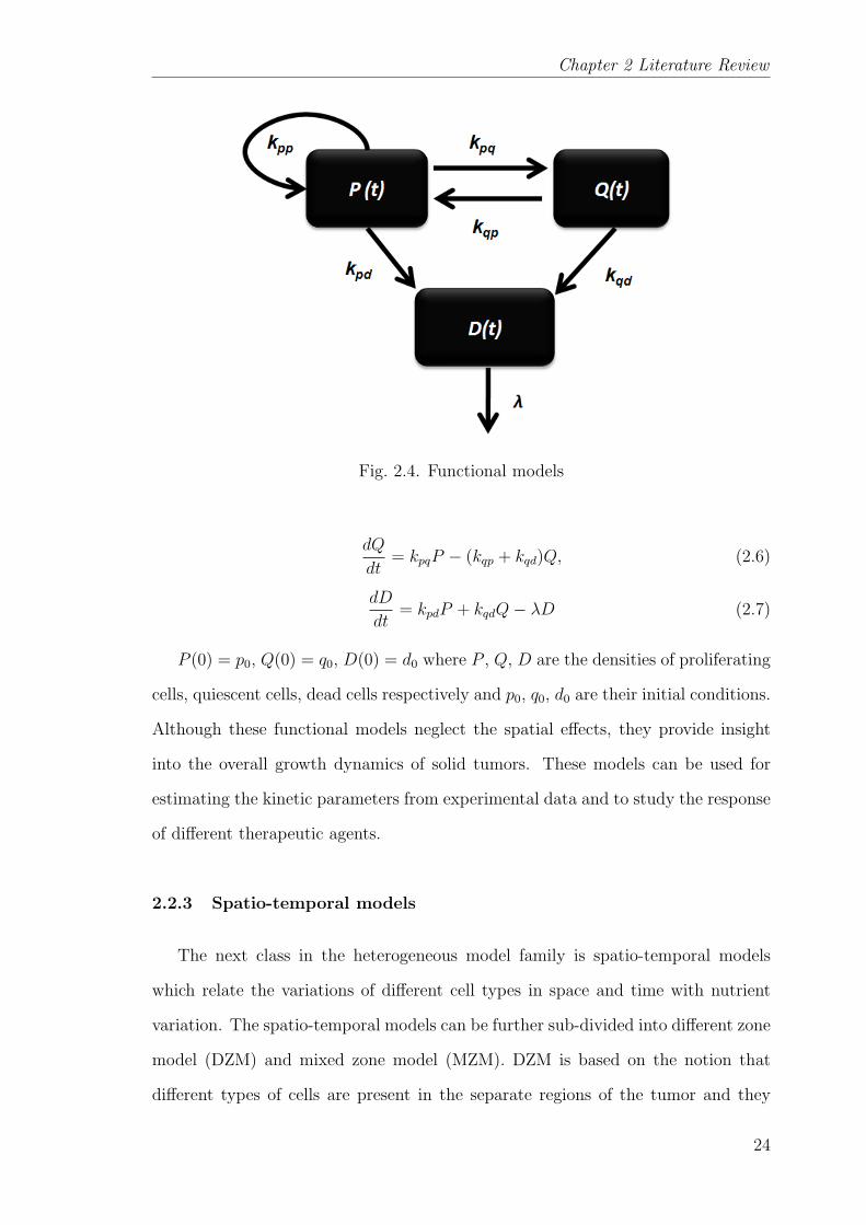
cells. An example of the functional model is shown below (Figure 2.4) for different
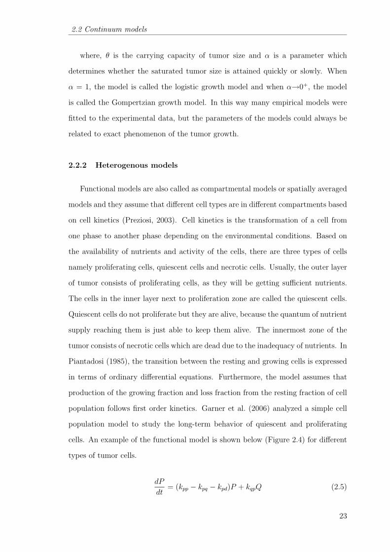
types of tumor cells.
dP
dt= (kpp − kpq − kpd)P + kqpQ (2.5)
23
Chapter 2 Literature Review
Fig. 2.4. Functional models
dQ
dt= kpqP − (kqp + kqd)Q, (2.6)
dD
dt= kpdP + kqdQ− λD (2.7)
P (0) = p0, Q(0) = q0, D(0) = d0 where P , Q, D are the densities of proliferating
cells, quiescent cells, dead cells respectively and p0, q0, d0 are their initial conditions.
Although these functional models neglect the spatial effects, they provide insight
into the overall growth dynamics of solid tumors. These models can be used for
estimating the kinetic parameters from experimental data and to study the response
of different therapeutic agents.
2.2.3 Spatio-temporal models
The next class in the heterogeneous model family is spatio-temporal models
which relate the variations of different cell types in space and time with nutrient
variation. The spatio-temporal models can be further sub-divided into different zone
model (DZM) and mixed zone model (MZM). DZM is based on the notion that
different types of cells are present in the separate regions of the tumor and they
24
2.2 Continuum models
are separated by boundaries. The goal, then, is to find the position of the interface
between the regions spatially and temporally on the basis of the nutrient levels. The
motivation for DZMs was from the idea of biologists which focused on the effect of
the tumor growth due to variations in the composition of the medium surrounding
the tumors. The main measurements made by the biologists in these experiments
are: radii of the tumors over time, nutrient distribution within the tumors and the
ratio of the radii of different zones in the tumor. Thus, the key variables in these
types of models are: R(t), the position of the outer tumor radius of the assumed
radially symmetric tumor; Ci(r, t), the concentration distribution of the diffusible
chemical (this may be nutrients, anti-cancer drugs, growth inhibitors); Rq(t), the
locus of the boundary separating proliferating and quiescent cells; and Rn(t), the
locus of the boundary separating the quiescent and necrotic cells. Since the tumor
size changes with time, the domains on which the model is formulated also changes
and this problem falls in the category of moving boundary problems. The simplest
DZM which explains the growth of a radially symmetric, avascular tumor include
equations governing the evolution of the important diffusible chemicals Ci(r, t), the
outer tumor radius R(t), and the quiescent and necrotic radii Rq(t) and Rn(t). The
principle of mass balance is used to derive equations for Ci(r, t) and R(t) where
as Rq(t) and Rn(t) are based on the assumption that quiescent and necrotic zone
formation is the result of concentration of chemicals (mainly the growth factors)
falling below their threshold values. The model equations are stated in both words
and in mathematics to clearly emphasize the connection between the underlying
physical assumptions and the mathematical formulation.
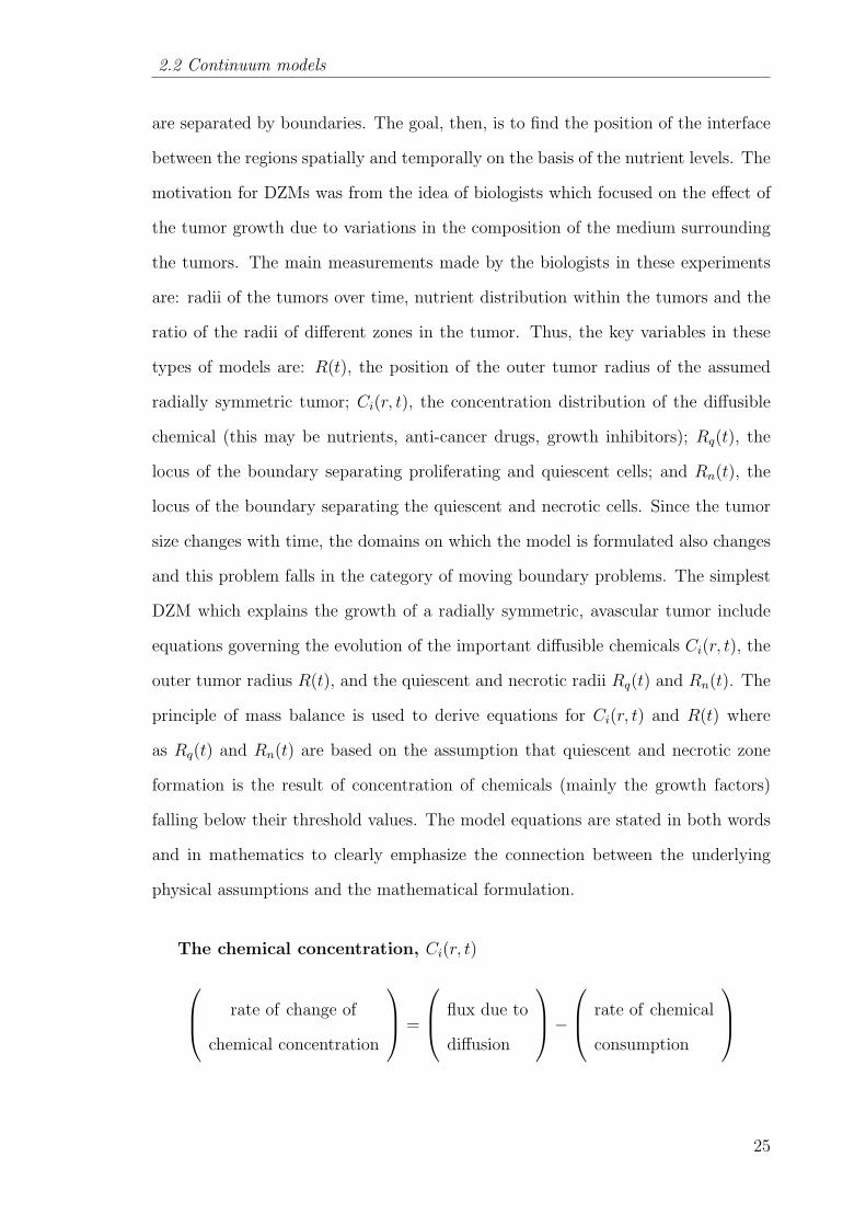
The chemical concentration, Ci(r, t)
rate of change of
chemical concentration
=
flux due to
diffusion
− rate of chemical
consumption
25

Chapter 2 Literature Review
∂Ci∂t
=Di
r2
∂
∂r
(r2∂Ci∂r
)− Γ(Ci, R,Rq, Rn) (2.8)
In Equation (2.8), Di denotes the assumed constant diffusion coefficient of the
chemical i and Γ(Ci, R,Rq, Rn) denotes its rate of consumption or production. In
reality, Γ(Ci, R,Rq, Rn) is a nonlinear function that depends on the type of cell
line and the chemical of interest. In order to observe the behavior of the model,
sometimes, only vital chemicals are considered and it is also assumed that their
consumption rate is constant or follows some typical trends (Michaelis - Menten).
The outer tumor radius, R (t)
rate of change of
tumor volume
=
total rate of cell
proliferation
− total rate of
cell death
1
3
d
dt
(R3)
= R2dR
dt=
R∫0
S (c, R,Rq, Rn)r2dr −R∫
0
N (c, R,Rq, Rn)r2dr (2.9)
In Equation (2.9), S (c, R,Rq, Rn) and N (c, R,Rq, Rn) denote respectively the rates
of cell proliferation and cell decay within the tumor. Cell proliferation rate is as-
sumed constant in many cases to make the model simpler, but in reality, it may
depend on the local concentration of the nutrients. The total death rate is assumed
to be the combination of apoptosis and necrosis. Apoptosis occurs in the quiescent
and proliferating zones and necrosis result from the deprivation of the nutrients in
the necrotic zone.
The contributions of Burton (1966) and Greenspan (1972) are deemed as pioneer-
ing studies in the development of heterogeneous models. These two seminal works
in the field of modeling of avascular tumor growth has been quoted extensively and
form the basis for most of the future works. According to Burton (1966), the tumor
growth decrease happens because of the formation of the necrotic region which is
26
2.2 Continuum models
based on the concentration of oxygen in the solid tumor. The model assumes that
the tumor is spherical in shape, and diffusion is the only mode for the transport of
oxygen to all cells in the tumor and the consumption rate of oxygen per unit volume
of the tumor tissue is constant. Then, this diffusion based model was solved and an
analytical relation between the critical radius, necrotic radius and tumor radius was
derived. Critical radius is the tumor radius at which the necrotic region begins to
form at its centre. An empirical fitting of the Gompertzian relation to this analyti-
cal equation was done. The author observed that the fit is good over a range of 100
fold increase in tumor size and matches closely with the experimental results based
on the 18 different types of the tumors. The best part of this work is the ability
of the model to predict without any reference to physiological parameters of the
tumor. However, there is a drawback in this work; the analytical relation was based
on the assumption that, the concentration gradient of oxygen is zero everywhere in
the necrotic zone which is not always the case (Casciari et al., 1992). In Greenspan
(1972), the author developed a model of tumor growth based on diffusion and in-
corporated different hypotheses to model the internal processes responsible for the
tumor growth. The main assumptions are:
1. Disintegration of necrotic cells into a number of chemical compounds and their
role in inhibiting the mitosis of cancer cells (transforming of proliferating cells
to quiescent cells).
2. Surface tension among living cancer cells maintain a compact and solid mass
and it is responsible for the inward motion of cells from the outer region to
compensate the loss due to the disintegration of necrotic cells.
3. The loss of necrotic core is proportional to its volume
4. All living cells are identical and are analogous to incompressible fluid as they
assumed that the density of cells is the same everywhere in the tumor.
27

Chapter 2 Literature Review
5. The proliferation rate of cell volume by mitosis is based on the concentration
of the nutrients and the chemicals produced by the necrotic region.
The theory of Greenspan (1972) considered two different possibilities responsible
for the introduction of inhibitory factors. The first one is a chemical inhibitor that
is the product of necrosis resulting from the insufficient nutrient supply. The second
possibility is purely based on the products of the metabolic processes of the living
cells. Based on these assumptions, the author has analyzed tumor growth retarda-
tion due to necrosis and waste products and finally concluded that these analyses
can be related to experimental observations based on the onset of necrosis. The
work of Greenspan (1972) proved to be the main impetus for the theory of growth
inhibitory factors in later works (Adam and Maggelakis, 1989; Adam, 1987a,b, 1986;
Glass, 1973; Shymko and Glass, 1976). But these models neglected the cell volume
loss due to necrosis. In Glass (1973), they considered the chalone mechanism to
illustrate the growth retardation of the tumor. Chalones are the mitotic inhibitors
which are partially responsible for the controlled replication of the cells. They fur-
ther assumed that the production of chalone was uniform throughout the tissue,
which then diffuse and decay. Shymko and Glass (1976) extended this hypothesis
to higher dimensions and endeavored to study the effect of different geometries on
the pattern and the stability of growth. Then, Adam (1989, 1988, 1987a,b, 1986)
improved the idea of Glass (1973) by regarding the spatially non-uniform inhibitor
production, different geometries and validating with experimental results of Folk-
man and Hochberg (1973). In addition to non-uniform inhibitor production, a new
model by Chaplain et al. (1994) introduced a nonlinear, spatially dependent diffu-
sion coefficient to explain the diffusion of a growth inhibitory factor. The results
from this model were shown to be compatible with the experimental findings over
the profiles of the growth inhibitory factors.
28
2.2 Continuum models
The extended work of Burton (1966) and Greenspan (1972) by Deakin (1975) ar-
gued that the rate of oxygen consumption cannot be uniform throughout the tumor.
This argument was based on the experimental evidence from Sutherland and Du-
rand (1973). Deakin (1975) considered that the oxygen consumption is proportional
to the oxygen concentration but considered the non-uniformity of oxygen only to the
viable rim thickness. Later McElwain and Ponzo (1977) investigated the effects of
this non-uniformity and produced three different phases in the tumor development.
Another important contribution of Sutherland and Durand (1973) is the obser-
vation of dormancy of multicellular spheroids without the formation of necrotic
region. This issue was further emphasized by the results of Durand (1976). The
additional cell loss mechanism is noticed as apoptosis (Kerr, 1971; Kerr et al., 1972)
and the model by McElwain and Morris (1978) was the first work to include it. A
blended model was introduced based on the propositions of these works (Deakin,
1975; Greenspan, 1972; McElwain and Ponzo, 1977). According to the review paper
Tiina et al. (2007), the model proposed by Casciari et al. (1992) is a “breakthrough”
example of mathematical modeling in tumor biology. This work provided the im-
petus to study the effect of concentration gradients of multiple nutrients such as
oxygen, glucose, lactate ions, carbon dioxide, bicarbonate ions, chlorine ions and
hydrogen ions and their varying consumption rates. It also included the effect of
the waste products of the metabolism. The main assumption of the model is that
cellular metabolism and cell growth rates are mainly dependent on the local con-
centration of oxygen, glucose concentration and extracellular pH. The authors have
used empirical expressions for the consumption rate of oxygen and glucose and the
cell proliferation rate based on the experimental data. Moreover, they assumed that
the necrotic zone formation is based on the critical concentration of glucose. This
model was validated with published data of EMT6/Ro spheroids in terms of oxygen
and glucose profiles at the centre of the tumor and their consumption rates. The
model showed a good fit when the spheroid growth data is below 700 µm. The
29
Chapter 2 Literature Review
model was quite successful in predicting the viable rim thickness at particular con-
ditions. The authors finally suggest that other factors like cell-cell contact effects
may be used to explain the tumor growth. Despite these improved aspects, their
model did not include apoptosis. In the paper Busini et al. (2007), a comprehen-
sive mechanistic model comprising the main processes related to tumor growth like
nutrient consumption, mitosis, apoptosis and necrosis was discussed. The model
was represented in population balance equations and was combined with the drug
models. Their solution was validated with both in vitro and in vivo results. The
shortcoming of this work is that it did not include the quiescent zone formation.
There are some works which have emphasized on the effect of acidosis on tumor
growth (Gatenby and Gawlinski, 2003, 1996; Gatenby et al., 2006; Smallbone et al.,
2005). The hypothesis in the literature is that the transformation of cells from pro-
liferating to quiescent or necrotic is attributed to the acidic environment (lower pH
value)(Vaupel et al., 1989). In the hypoxic conditions (oxygen deficient), glycolytic
phenotype is observed where glucose is metabolized via glycolysis or anaerobic res-
piration and produces lactic acid. There is also a theory known as Warburg effect
which states that the tumor cells adopt glycolysis pathway for glucose metabolism
even in the normoxic conditions. Based on these theories, acidosis is included in
the continuum models by the considering the variation of H+ ion concentration in
the tumor. Other modeling works found consistency with experimental observations
about the correlation of apoptotic pathways in the normal cells near the tumor with
the acidic environment (Gatenby and Gawlinski, 1996). In contrast, the MZMs
suggest that the regions of different types of cells are not separated sharply, but
gradually. Thus, MZM aims to find spatial and temporal variation of the number of
cells of different types per unit volume of the tumor. These models come under the
category of multiphase models (Ambrosi and Preziosi, 2002; Breward et al., 2003,
2002).
∂φi∂t
+∇ · (viφi) = ∇ · (Di∇φi) + λi(φi, Ci)− µi(φi, Ci) (2.10)
30
2.2 Continuum models
where, for different phase (cell type) ’i’, φi is the volume fraction (∑
i φi = 1), vi is
the velocity, Di is the random motility or diffusion, λi(φi, Ci) is the chemical and
phase dependent production, and µi(φi, Ci) is the chemical and phase dependent
degradation/death. The first MZM was probably suggested by Ward and King
(1997). Unlike DZMs, this model does not consider different layers for different
type of cells in the avascular tumor. Instead, it presumes a mixture of live and dead
cells and describes the variation of live cell density and dead cell density with the
variation of the nutrients. DZMs have considered the a priori knowledge of tumor
structure with three different regions. According to Ward and King (1997) the
structure of different regions of tumor growth should not be assumed but it should
be produced from the solutions of the models. In this paper, the authors proposed
a model without any such presumptions about the tumor structure in the form of
a system of partial differential equations to describe the growth of an avascular
tumor spheroid. Moreover, the authors also performed asymptotic analysis (effects
of limiting values of parameters) in order to distinguish the exponential growth phase
and retardation growth phase of the tumor. This model was then extended by the
inclusion of pharmacokinetics and pharmacodynamics of the diffusible drug and its
effects were compared between the multicellular spheroids and the monolayer cases.
Another example of MZM is the model by Sherratt and Chaplain (2001). According
to them, most of the previous models developed were based on in vitro experiments
on multicellular spheroids. Consequently, this model is inclined towards representing
in vivo phenomena rather than in vitro and considers the nutrient source as nearby
tissues. In addition, the model also included the concept of cell movement reflecting
the contact inhibition of migration. Similarly, the work by Breward et al. (2002)
considered two phase model to describe the avascular tumor growth which was
further advanced by accounting for ATP production from energy metabolism in the
models of multicellular tumor spheroids (Bertuzzi et al., 2007; Venkatasubramanian
et al., 2006). There are other good examples of MZM (Tindall and Please, 2007;
Tindall et al., 2008). In Tindall and Please (2007), effects of cell cycle dynamics
31
Chapter 2 Literature Review
was considered and their main focus was on two different conditions of chemotatic
responses of proliferating cells and quiescent cells to the external nutrient supply
and their effects on the tumor structure. They extended this work in Tindall et al.
(2008) to study the formation of necrotic region in avascular tumors and analytically
proved that necrotic core is correlated with low levels of nutrient concentration.
2.2.4 Discrete and hybrid models
Discrete modeling focuses on tracking and updating the state of individual cells
which are guided by specific biophysical rules. Framing of these rules is a challenging
task that demands a lot of experimental analyses related to inter and intracellular
events (e.g. biochemical pathways, cell cycle) controlling the cell survival and death.
However, discrete modeling will be very useful for studying the mechanisms such as
nutrient consumption, cell division, interaction with the microenvironment (growth
factors, extracellular matrix, and immune system) and the progressive steps of trans-
formation of a normal cell to a cancer cell. In short, discrete models characterize
the state of the cells based on the microenviroment conditions. Some of the review
works are given here (Abbott et al., 2006; Drasdo et al., 2007; Anderson and Quar-
anta, 2008; Araujo and McElwain, 2004; Byrne et al., 2006; Deisboeck et al., 2009;
Lowengrub et al., 2010; Moreira and Deutsch, 2002; Quaranta et al., 2008, 2005).
Hybrid modeling is also known as multiscale modeling. It is the combination of
both continuum and discrete models. These models attempt to provide comprehen-
sive explanation of the tumor growth on the basis of the mutual information transfer
between sub-cellular, cellular and tumor scales (Bellomo, Angelis and Preziosi, 2003;
Kim and Stolarska, 2007; Martins et al., 2007; Stolarska et al., 2009; Weinan et al.,
2007). Consequently, it helps to relate the mishappenings at the cell level to the
aggressiveness and morphology of the tumor. In the hybrid approaches of tumor
modeling, the diffusion of nutrients is explained by the continuum models and the
32
2.2 Continuum models
cell state is defined by the discrete model based on the local concentration of the
nutrients. As a result, the computational cost for both discrete model simulation
and hybrid model simulation increases significantly with the increase in number of
cells.
Some works have used continuum and discrete models to compare the tumor
evolution using multicellular tumor spheroids (Byrne and Drasdo, 2009; Schaller
and Meyer-Hermann, 2006). Eventually, they concluded that continuum models are
simple and suitable enough to use for predicting the tumor growth. However, the
discrete or hybrid models might be necessary to understand microscale mechanisms
taking place in the cells (Schaller and Meyer-Hermann, 2006).
2.2.5 Model calibration
The parameters of the model play a vital role in predicting the outputs of interest
through simulations. In the field of tumor growth modeling, the parameters are ob-
tained in different ways. The parameters are estimated from the tumor growth data
gathered from in vivo, in vitro experiments and magnetic resonance images (MRI).
In vivo studies are done using DNA transfection methods. In these methods, DNA
of the tumor cell is transfected into normal cells to transform them to tumor cells
followed by injecting them into laboratory mice (Kleinsmith, 2005). However, this is
an arduous procedure and requires the modification of the mice subjects by knock-
ing out some genes to nullify the effect of immune system on tumor growth. On
the other hand, conventional suspension and monolayer in vitro experiments do not
exactly represent the tumor growth. Therefore, alternatively, multicellular tumor
spheroid experiments (MCTS) are preferred as a model experimental system for
avascular tumor (LaRue et al., 1998; Kunz-Schughart, 1999; Kunz-Schughart et al.,
1998; Mueller-Klieser, 1997). MCTS replicates the three dimensional network of
cell-cell and cell-matrix interactions. This experimental methodology was adapted
33
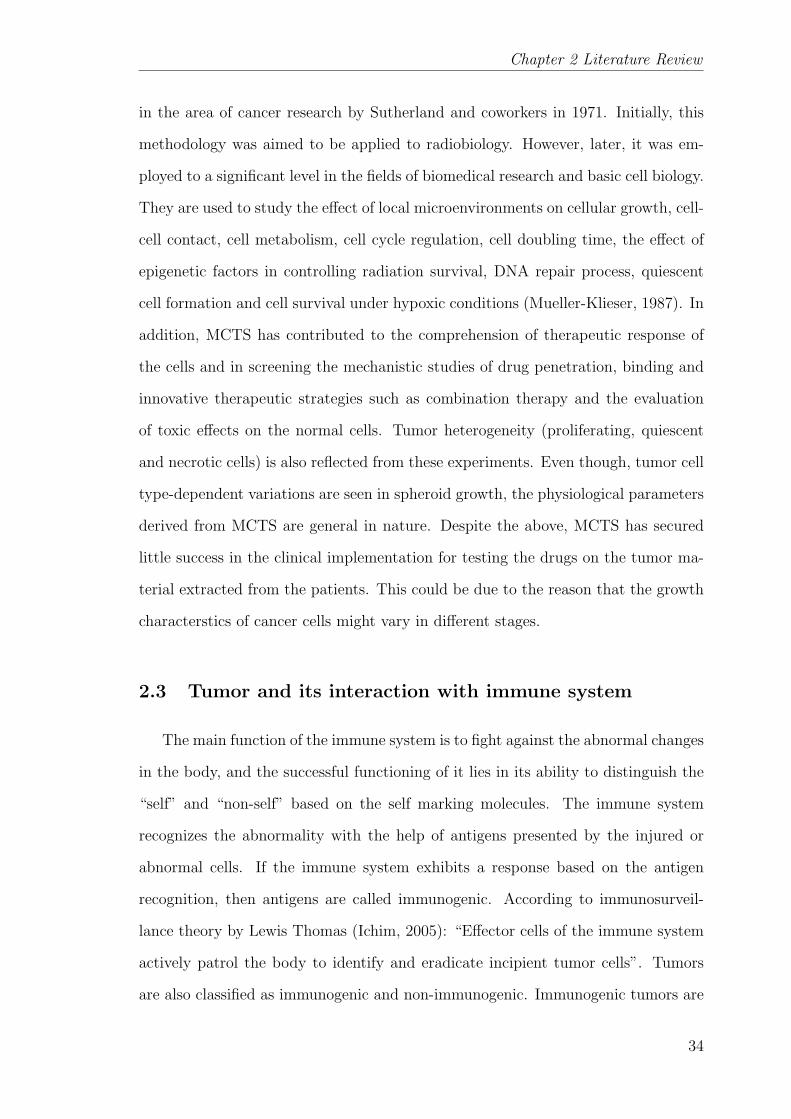
Chapter 2 Literature Review
in the area of cancer research by Sutherland and coworkers in 1971. Initially, this
methodology was aimed to be applied to radiobiology. However, later, it was em-
ployed to a significant level in the fields of biomedical research and basic cell biology.
They are used to study the effect of local microenvironments on cellular growth, cell-
cell contact, cell metabolism, cell cycle regulation, cell doubling time, the effect of
epigenetic factors in controlling radiation survival, DNA repair process, quiescent
cell formation and cell survival under hypoxic conditions (Mueller-Klieser, 1987). In
addition, MCTS has contributed to the comprehension of therapeutic response of
the cells and in screening the mechanistic studies of drug penetration, binding and
innovative therapeutic strategies such as combination therapy and the evaluation
of toxic effects on the normal cells. Tumor heterogeneity (proliferating, quiescent
and necrotic cells) is also reflected from these experiments. Even though, tumor cell
type-dependent variations are seen in spheroid growth, the physiological parameters
derived from MCTS are general in nature. Despite the above, MCTS has secured
little success in the clinical implementation for testing the drugs on the tumor ma-
terial extracted from the patients. This could be due to the reason that the growth
characterstics of cancer cells might vary in different stages.
2.3 Tumor and its interaction with immune system
The main function of the immune system is to fight against the abnormal changes
in the body, and the successful functioning of it lies in its ability to distinguish the
“self” and “non-self” based on the self marking molecules. The immune system
recognizes the abnormality with the help of antigens presented by the injured or
abnormal cells. If the immune system exhibits a response based on the antigen
recognition, then antigens are called immunogenic. According to immunosurveil-
lance theory by Lewis Thomas (Ichim, 2005): “Effector cells of the immune system
actively patrol the body to identify and eradicate incipient tumor cells”. Tumors
are also classified as immunogenic and non-immunogenic. Immunogenic tumors are
34
2.3 Tumor and its interaction with immune system
Fig. 2.5. Classification of immune actions
those which are recognized by the immune cells in the human body. But not all
antigens are immunogenic. Before studying the tumor-immune interactions, we can
take a brief look at the mechanisms of the immune system. In this regard, the review
paper by Adam et al. (2003) provides a comprehensive discussion on the immune
response in cancer.
In our body, the immune action is carried out by specialized cells called lym-
phocytes which are mostly present in the blood. The common lymphocytes are
macrophages, dendritic cells, natural killer (NK) cells, lymphokine activated killer
(LAK) cells, B-cells and T-cells. Immune response is categorized as natural immu-
nity, humoral immunity and cellular immunity based on the lymphocytes (Figure
2.5). Macrophages, dendritic cells, natural killer cells are responsible for natural im-
munity, in which these cells directly attack the infected cells (cancer cell) and act as
antigen presenting cells (APC). Antigen is an agent which can easily be recognized
by immune cells. Thus, APC highlights the infected cells and alerts the T-cells for
further action against the infected cells. In humoral immunity, antibodies produced
by B-cells encounters the infected cells. Each B-cell has a specific antibody of a
particular shape. The concept of antibody-antigen interaction resembles the mech-
anism of lock and key. When the shape of an antibody of a B-cell matches exactly
35
Chapter 2 Literature Review
with the shape of the antigen corresponding to the infected cells, B-cell proliferates
and produces plasma cells which actively secrete the antibodies. These antibodies
neutralize the activity of the infected cell by inhibiting their cell division process,
by producing a lethal group of enzymes called complement and by opsonization. In
opsonization, antibodies coat the infected cells in order to make them easily rec-
ognizable by the killer lymphocytes. This process is known as antibody dependent
cell-mediated cytotoxicity. In cellular immunity, the key players are T-cells which
are further classified as helper T-cells (CD4+) and cytotoxic T-cells (CD8+). Helper
T-cells gets activated by the natural immune cells and regulates the production of
the cytokines. Cytokines are the proteins which keep the momentum of all the im-
mune cells as per their requirement. Interleukins and interferons are regarded as the
important cytokines to fulfill the immune action. Cytotoxic T-cells directly attack
the infected cells after its activation by the cytokines.
Cancer immunotherapy is broadly classified into different schemes - monoclonal
antibody therapy (MAT), adoptive-cell-transfer therapy (ACT), vaccine therapy
and interleukin therapy (Figure 2.6). The common aspect of all schemes of im-
munotherapy is to enhance the immunogenicity of the individual. Immunogenicity
is the ability of the immune system to recognize tumor cells. MAT is based on
the mechanism of humoral immunity while others are based on cellular immunity.
In MAT, antibodies are produced in large quantities using hybridoma technology
and injected into the patient. In ACT, tumor infiltrating lymphocytes exhibiting
the anti-tumor activity are found. They are then isolated and cultured in larger
quantities in the presence of cytokines (interleukin) and injected back to the patient
(Dudley et al., 2002; Dudley and Rosenberg, 2003). In vaccine therapy, APCs are
engineered externally to recognize the tumor associated antigens and trigger the
cellular mediated immunity. At present, extensive clinical studies are being done
on dendritic cell therapy (Aarntzen et al., 2008; Ballestrero et al., 2008; Banchereau
36

2.3 Tumor and its interaction with immune system
Fig. 2.6. Description of different immune actions
et al., 2001; Dhodapkar et al., 1999; Jacobs et al., 2009; Svane et al., 2003; Vuylsteke
et al., 2006; Ludewig and Hoffman, 2005).
2.3.1 Tumor-immune models
Many tumor-immune interaction models have been developed and some of the
review works are Bellomo, Bellouquid and De Angelis (2003); Bellomo and Preziosi
(2000). They can be classified on the basis of immune cells interaction and model
type (e.g. functional and spatio-temporal) models). In the first type of classification
there are two categories of models. In the first category, all types of immune cells
are included as one ensemble called as effector cells (Joshi et al., 2009; Kirschner
and Panetta, 1998; Kuznetsov and Knott, 2001; Kuznetsov et al., 1994). Contrast-
ingly, in the second category of models, the kinetics and interaction of different
immune cells and their activation by cytokines is studied (Cappuccio et al., 2007;
Castiglione and Piccoli, 2007, 2006; De Boer and Hogeweg, 1986; Pappalardo et al.,
2005; de Pillis et al., 2009, 2006, 2005; Castiglione et al., 2004; Piccoli and Cas-
37

Chapter 2 Literature Review
tiglione, 2006; Szymanska, 2003). In some models, phenomena such as sneaking
through and tumor dormancy are introduced - these models account for situations
where the tumor camouflages the immune system. The only model in which the
parameters are estimated using experimental data is that of Kuznetsov et al. (1994)
and it was further extended by distinguishing the action of different immune cells.
The aforementioned tumour-immune models are functional type, where spatial vari-
ations of immune cells are neglected. There are some works which considered spatio-
temporal tumour-immune models and solved using lattice fixed discrete models such
as cellular automata (Mallet and De Pillis, 2006).
2.4 Model-based design of treatment protocols of cancer
therapy
The field of mathematical modeling of anticancer therapies has witnessed sev-
eral contributions over the past four decades (Eisen, 1979; Swan, 1990; Martin, 1992;
Swan, 1995; Swierniak et al., 2009). A recent review on modeling as a tool for plan-
ning cancer therapies by Swierniak et al. (2009) focuses majorly on optimization
of cell cycle phase-specific chemotherapy, anti-angiogenic therapy and the effect of
drug resistance. Cell cycle phase models are the compartmental models where the
compartments indicate different phases of the cell cycle (Agur et al., 1988; Panetta
and Adam, 1995; Gardner, 2000; Dua et al., 2008). The review also briefly addresses
the strategies of optimal control such as bang-bang control and singular control in
the model-based cancer therapy with age structured models accounting for kinetic
heterogeneity of cancer cells. Eventually, this work stresses on multiscale models
and its utility in realizing personalized therapy as a reality. Another mini-review
(Gardner and Fernandes, 2003) was on computational assistance as new tools for
chemotherapy. It discussed about the issues associated with the application of op-
timal control theory to cancer chemotherapy. This work also highlights examples
(Panetta and Fister, 2000; Swierniak et al., 1996) to depict the variations of the
38
2.4 Model-based design of treatment protocols of cancer therapy
sub-optimal or optimal solutions with different problem formulations and model
simplification strategies. Gardner and Fernandes (2003) also summarize the advan-
tages and disadvantages of computational tools such as OncoTCap developed by
Day and colleagues at the University of Pittsburgh Cancer Institute1 and KITT
- Kinetically tailored treatment (Gardner, 2002). These models include the com-
plex interactions involved in the tumor growth, the effect of cell cycle phase specific
drugs, effect of cell cycle phase non-specific cytostatic drugs and the phenomenon
of drug resistance. These simulators are used to analyze different phenomena and
therapy schedules of drugs with individual patient kinetic parameters as inputs (es-
timated from the tumor biopsy tests). Finally, Gardner and Fernandes (2003), also
emphasize on the need for validation of the simulators with individual patient data
so as to open avenues for promising and individual therapies.
2.4.1 Pharmacokinetic and pharmacodynamic modeling
Pharmacokinetics (PK) is the study of the flow of a drug in the body which
includes the mechanisms of absorption, distribution, metabolism, excretion and lib-
eration of the drug. Hence the pharmacokinetic models describe the relationship
between the dosage and the concentration of the drug in the blood after its admin-
istration (Swierniak et al., 2009). There are different routes of drug administration
(oral, intravenous, intramuscular, peritoneal) and the route employed decides the
structure of the PK models. The common parameters in these models are volume of
distribution, clearance rate, and biological half life. The PK models can be classified
as non-compartmental model (same as non-parametric models) and compartmental
models (functional models) (Holford et al., 2010). In non-compartmental analysis,
blood/plasma samples are collected at some regulated intervals to estimate the total
drug exposure by estimating the area under the curve of drug concentration-time
graph. Compartmental models are kinetic models which are used to predict the
1http:// www.oncotcap.pitt.edu/2000
39
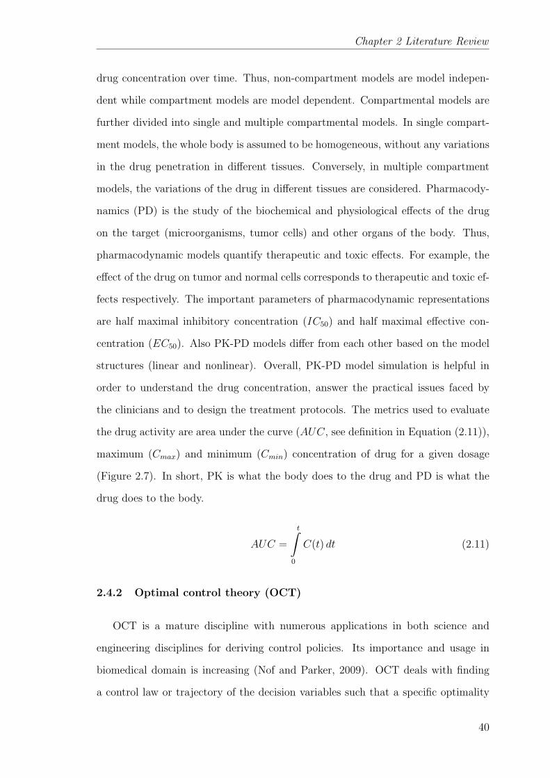
Chapter 2 Literature Review
drug concentration over time. Thus, non-compartment models are model indepen-
dent while compartment models are model dependent. Compartmental models are
further divided into single and multiple compartmental models. In single compart-
ment models, the whole body is assumed to be homogeneous, without any variations
in the drug penetration in different tissues. Conversely, in multiple compartment
models, the variations of the drug in different tissues are considered. Pharmacody-
namics (PD) is the study of the biochemical and physiological effects of the drug
on the target (microorganisms, tumor cells) and other organs of the body. Thus,
pharmacodynamic models quantify therapeutic and toxic effects. For example, the
effect of the drug on tumor and normal cells corresponds to therapeutic and toxic ef-
fects respectively. The important parameters of pharmacodynamic representations
are half maximal inhibitory concentration (IC50) and half maximal effective con-
centration (EC50). Also PK-PD models differ from each other based on the model
structures (linear and nonlinear). Overall, PK-PD model simulation is helpful in
order to understand the drug concentration, answer the practical issues faced by
the clinicians and to design the treatment protocols. The metrics used to evaluate
the drug activity are area under the curve (AUC, see definition in Equation (2.11)),
maximum (Cmax) and minimum (Cmin) concentration of drug for a given dosage
(Figure 2.7). In short, PK is what the body does to the drug and PD is what the
drug does to the body.
AUC =
t∫0
C(t) dt (2.11)
2.4.2 Optimal control theory (OCT)
OCT is a mature discipline with numerous applications in both science and
engineering disciplines for deriving control policies. Its importance and usage in
biomedical domain is increasing (Nof and Parker, 2009). OCT deals with finding
a control law or trajectory of the decision variables such that a specific optimality
40

2.4 Model-based design of treatment protocols of cancer therapy
Fig. 2.7. Metrics of PK-PD modeling
criterion is achieved. In terms of cancer therapy, the control law is related to the
intervention times and dosage of the drug such that tumor is completely eliminated
and side effects due to the drug is minimized. The control problem includes cost
function(s) (objective(s) (J)) which are a function of state variables (X(t)), input
or control or manipulated variables (U(t)) as shown in Equation (2.12). Thus, an
optimal control problem is a set of system equations describing the control actions
for minimizing or maximizing the cost functions. The independent variable is time
(t) , to is the initial time and tf is the final time. The terms Φ and L given in
Equation (2.12) represent the endpoint cost and Lagrangian respectively. Equation
(2.13) represents the dynamic model of the real system. And b in Equation (2.14)
corresponds to equality and inequality constraints on state variables, input variables
and time to be considered while proposing a control law.
Elements of the optimal control problem
Objectives:
J = Φ(x(t0), t0, x(tf ), tf ) +
tf∫t0
L(x(t), u(t), t)dt (2.12)
41
Chapter 2 Literature Review
Dynamic model:
•x(t) = f(x(t), u(t), t) (2.13)
Constraints:
b(x(t), u(t), t) ≤ 0 (2.14)
The state variables in the context of cancer therapy are the density of cells (cancer
cells, normal cells, immune cells) and the concentration of therapeutic agents. The
input variables denote the therapeutic dosages. The cost functions include mini-
mization of tumor burden (area under the curve of tumor evolution), final tumor
size, maximum tumor size and minimization of therapeutic burden (area under the
curve of concentration of therapeutic agent) and cumulative dosage rate of therapeu-
tic agent for a given time horizon. The usual decision variables are type of therapy,
time of intervention, dosage rate and duration of therapeutic intervention. The con-
straints are on the drug dosage rate, maximum and minimum concentration of the
drug in the body during the treatment course. Particularly, many domain problems
relevant to cancer therapy were formulated and solved using OCT. These include
Swan (1986, 1990, 1995), Murray (1990a,b), Martin (1992), Iliadis and Barbolosi
(2000), Barbolosi and Iliadis (2001), Parker and Doyle (2001), Matveev and Savkin
(2002), de Pillis and Radunskaya (2003), Piccoli and Castiglione (2006), Cappuc-
cio et al. (2007), Castiglione and Piccoli (2007), de Pillis et al. (2007), Ledzewicz
and Schttler (2007), Dua et al. (2008) and Chareyron and Alamir (2009). Often,
these optimal control problems are nonlinear and hence numerical techniques are
employed for solving them.
2.4.3 Description of optimization problem formulation using cancer ther-
apy models
Broadly, cancer therapy models are characterized based on tumor stage, type
of therapies (surgery, radiation therapy, chemotherapy, immunotherapy, viral ther-
42
2.4 Model-based design of treatment protocols of cancer therapy
apy), and models used for tumor growth and PK-PD of the drugs. In the model
based therapeutic design, until now, optimal control theory was fully exploited in
order to address the scheduling of therapies using a therapeutic agent (Barbolosi
and Iliadis, 2001; Cappuccio et al., 2007; Dua et al., 2008; Ghaffari and Naserifar,
2010; Harrold and Parker, 2009; Martin, 1992; Swan, 1995) and combination of ther-
apeutic agents (Chareyron and Alamir, 2009; de Pillis et al., 2006; Tse et al., 2007;
Kiran et al., 2009). In the above work, tumor growth, pharmacokinetic, pharma-
codynamic models were coupled and optimization of the therapy with objectives,
constraints and decision variables on tumor cells, normal cells and therapeutic agents
was demonstrated. The formulated optimization problem was solved using different
algorithms like gradient based methods, evolutionary methods (genetic algorithm,
particle swarm optimization, differential evolution, simulated annealing etc.).
One major focus of the above-mentioned work was on the formulation of ob-
jectives and constraints so as to achieve better solutions (Gardner and Fernandes,
2003). Depending on how one formulates the objectives, one may have a single
or multi-objective optimization problem. However, as mentioned before, scheduling
cancer therapy usually involves multiple objectives such as the need to shrink tumor
growth and avoidance of treatment side effects. In some of the previous work (Dua
et al., 2008), different objectives related to the tumor cells and therapeutics was com-
bined into a single objective. In such a strategy, the assignment of weights to the
different objectives is an intricate issue. Often, in such cases, the problem is solved
repeatedly by varying the weightage of objectives to find the best solution using
gradient based methods and evolutionary algorithms. Such a strategy can be time-
consuming. On the other hand, very little work has been done using multi-objective
optimization strategy where the problem is solved by considering all the objectives
for sets of solutions (Pareto set)(McCall et al., 2007; Kiran et al., 2009; Kiran and
Lakshminarayanan, 2009). Multi-objective optimization enables the understanding
of the therapeutic consequences and provides a chance to choose a solution from
the Pareto set as per the requirements of the decision maker. The selection of the
43
Chapter 2 Literature Review
solution from the Pareto set may not always be straightforward - a systematic post
analysis of the Pareto set is essential in order to choose an appropriate solution.
The chosen solution is called as optimal compromised solution, because the optimal
solution for one objective may not be the optimal solution for the other objective(s).
Thus, the post-Pareto-optimality analysis facilitates the decision making process.
2.5 Challenges in the model-based applications
There are some challenging aspects that need to be addressed before using tumor
growth models in actual practice. Mathematical models can become highly complex
by integrating all the knowledge on cell and tissue acquired by biologists relating to
the tumor growth phenomenon. In general, complexity can be related to the model
structure, the number of parameters in the model and their order of magnitude,
nonlinearity in parameters/states, practical constraints in measurement times and
in manipulating the input variables, magnitude and character of measurement errors
etc (Sun, 2006; Sun and Hahn, 2006). These reasons necessitate more tumor size
measurements to estimate parameters with acceptable precision. Often, however,
the availability of tumor size data for a given patient is quite limited. In such cases,
the precise estimation of all the patient parameters can become quite difficult. In
some of the earlier work, non-dimensionalization strategy was used to ease numer-
ical solution of the models (Kirschner and Panetta, 1998; Kuznetsov et al., 1994;
de Pillis et al., 2006; Ward and King, 1997). However, the theoretical implications of
parametric groups were not highlighted. Even the parametric sensitivity on the out-
put of interest is studied using one parameter at a time (OAT) method (Kirschner
and Panetta, 1998; Kuznetsov et al., 1994; de Pillis et al., 2009, 2006, 2005).
The main drawback of the existing tumor growth models is that some of them
are too simple while some are too complex to explain the mechanism of the nutri-
ents effect on tumor growth. Model validation, an important feature in the model
building process is found to be missing for some theoretical models in the literature.
44
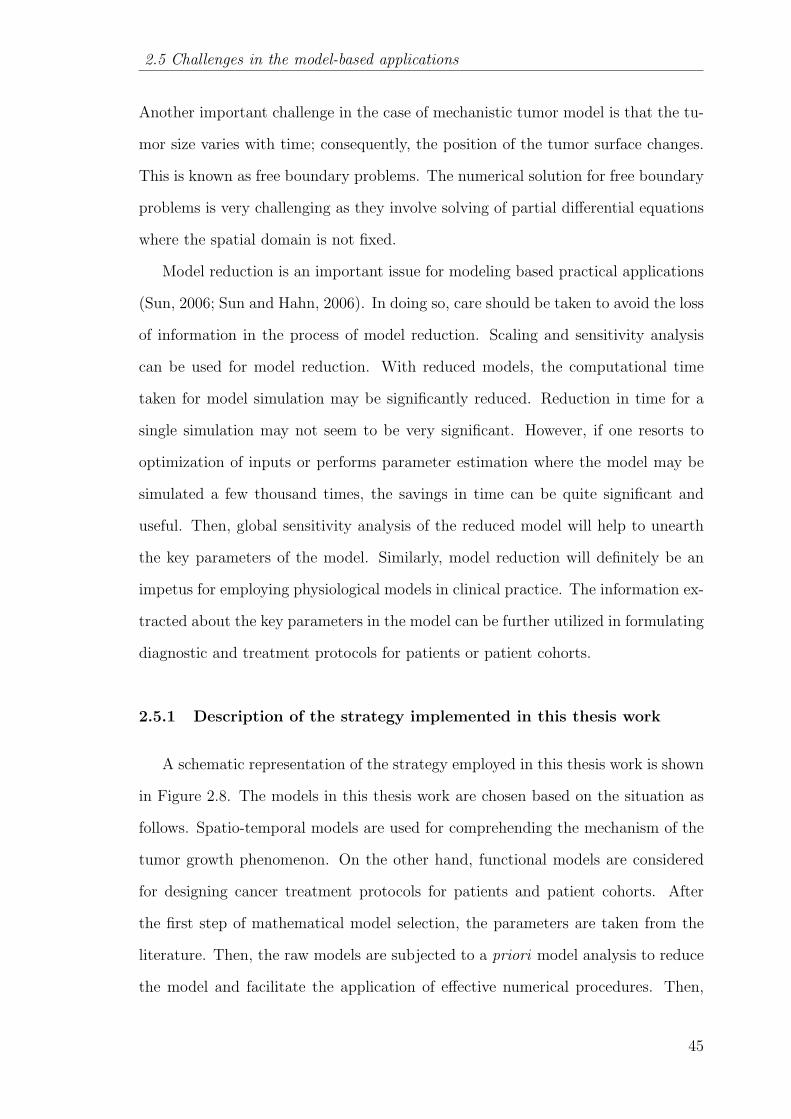
2.5 Challenges in the model-based applications
Another important challenge in the case of mechanistic tumor model is that the tu-
mor size varies with time; consequently, the position of the tumor surface changes.
This is known as free boundary problems. The numerical solution for free boundary
problems is very challenging as they involve solving of partial differential equations
where the spatial domain is not fixed.
Model reduction is an important issue for modeling based practical applications
(Sun, 2006; Sun and Hahn, 2006). In doing so, care should be taken to avoid the loss
of information in the process of model reduction. Scaling and sensitivity analysis
can be used for model reduction. With reduced models, the computational time
taken for model simulation may be significantly reduced. Reduction in time for a
single simulation may not seem to be very significant. However, if one resorts to
optimization of inputs or performs parameter estimation where the model may be
simulated a few thousand times, the savings in time can be quite significant and
useful. Then, global sensitivity analysis of the reduced model will help to unearth
the key parameters of the model. Similarly, model reduction will definitely be an
impetus for employing physiological models in clinical practice. The information ex-
tracted about the key parameters in the model can be further utilized in formulating
diagnostic and treatment protocols for patients or patient cohorts.
2.5.1 Description of the strategy implemented in this thesis work
A schematic representation of the strategy employed in this thesis work is shown
in Figure 2.8. The models in this thesis work are chosen based on the situation as
follows. Spatio-temporal models are used for comprehending the mechanism of the
tumor growth phenomenon. On the other hand, functional models are considered
for designing cancer treatment protocols for patients and patient cohorts. After
the first step of mathematical model selection, the parameters are taken from the
literature. Then, the raw models are subjected to a priori model analysis to reduce
the model and facilitate the application of effective numerical procedures. Then,
45
Chapter 2 Literature Review
Fig. 2.8. Strategy followed in this thesis
the reduced models are used to formulate optimization problems for realistically -
considered applications. The aim of the thesis is to develop simulation based tumor
growth studies that might be decision-support tools for the clinicians and oncological
pharmacists.
46
Chapter 3
MATHEMATICAL MODELING OF AVASCULAR
TUMOR GROWTH BASED ON DIFFUSION OF
NUTRIENTS AND ITS VALIDATION
‘All models are wrong, but some are useful.’
- George E P Box
3.1 Introduction
In this chapter, a mathematical model based on the diffusion of nutrients is
developed by considering the physiological changes accompanying the growth of
avascular tumor. Avascular tumor growth involves the formation of three different
zones namely proliferation, quiescent and necrotic zones. The main processes on
which avascular tumor growth depends are: (i) diffusion of nutrients through the
tumor from the contiguous tissues, (ii) consumption rate of the nutrients by the
cells in the tumor and (iii) cell death by apoptosis and necrosis. In the model, it
is assumed that the tumor is spherical and the principal nutrients responsible for
its growth are oxygen and glucose. By solving for the concentration profiles using
the proposed model which describes the above processes, the radii of the quiescent
and necrotic zones as well as that of the tumor are computed. The proposed model
is also validated using in vitro tumor growth data and Gompertzian empirical rela-
tionship parameters available in the literature. The model is shown to be successful
in capturing the saturated volume of the avascular tumor for different nutrient con-
47
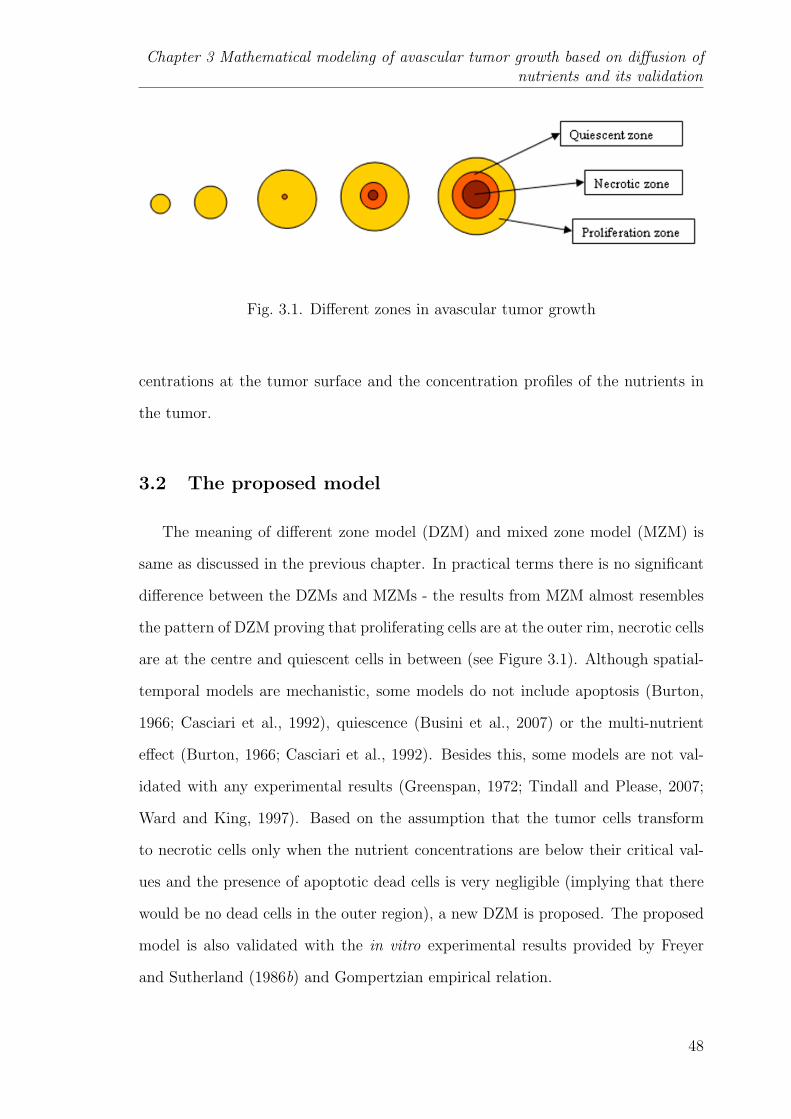
Chapter 3 Mathematical modeling of avascular tumor growth based on diffusion ofnutrients and its validation
Fig. 3.1. Different zones in avascular tumor growth
centrations at the tumor surface and the concentration profiles of the nutrients in
the tumor.
3.2 The proposed model
The meaning of different zone model (DZM) and mixed zone model (MZM) is
same as discussed in the previous chapter. In practical terms there is no significant
difference between the DZMs and MZMs - the results from MZM almost resembles
the pattern of DZM proving that proliferating cells are at the outer rim, necrotic cells
are at the centre and quiescent cells in between (see Figure 3.1). Although spatial-
temporal models are mechanistic, some models do not include apoptosis (Burton,
1966; Casciari et al., 1992), quiescence (Busini et al., 2007) or the multi-nutrient
effect (Burton, 1966; Casciari et al., 1992). Besides this, some models are not val-
idated with any experimental results (Greenspan, 1972; Tindall and Please, 2007;
Ward and King, 1997). Based on the assumption that the tumor cells transform
to necrotic cells only when the nutrient concentrations are below their critical val-
ues and the presence of apoptotic dead cells is very negligible (implying that there
would be no dead cells in the outer region), a new DZM is proposed. The proposed
model is also validated with the in vitro experimental results provided by Freyer
and Sutherland (1986b) and Gompertzian empirical relation.
48
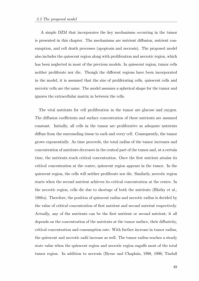
3.2 The proposed model
A simple DZM that incorporates the key mechanisms occurring in the tumor
is presented in this chapter. The mechanisms are nutrient diffusion, nutrient con-
sumption, and cell death processes (apoptosis and necrosis). The proposed model
also includes the quiescent region along with proliferation and necrotic region, which
has been neglected in most of the previous models. In quiescent region, tumor cells
neither proliferate nor die. Though the different regions have been incorporated
in the model, it is assumed that the size of proliferating cells, quiescent cells and
necrotic cells are the same. The model assumes a spherical shape for the tumor and
ignores the extracellular matrix in between the cells.
The vital nutrients for cell proliferation in the tumor are glucose and oxygen.
The diffusion coefficients and surface concentration of these nutrients are assumed
constant. Initially, all cells in the tumor are proliferative as adequate nutrients
diffuse from the surrounding tissue to each and every cell. Consequently, the tumor
grows exponentially. As time proceeds, the total radius of the tumor increases and
concentration of nutrients decreases in the central part of the tumor and, at a certain
time, the nutrients reach critical concentration. Once the first nutrient attains its
critical concentration at the centre, quiescent region appears in the tumor. In the
quiescent region, the cells will neither proliferate nor die. Similarly, necrotic region
starts when the second nutrient achieves its critical concentration at the centre. In
the necrotic region, cells die due to shortage of both the nutrients (Hlatky et al.,
1988a). Therefore, the position of quiescent radius and necrotic radius is decided by
the value of critical concentration of first nutrient and second nutrient respectively.
Actually, any of the nutrients can be the first nutrient or second nutrient; it all
depends on the concentration of the nutrients at the tumor surface, their diffusivity,
critical concentration and consumption rate. With further increase in tumor radius,
the quiescent and necrotic radii increase as well. The tumor radius reaches a steady
state value when the quiescent region and necrotic region engulfs most of the total
tumor region. In addition to necrosis (Byrne and Chaplain, 1998, 1996; Tindall
49
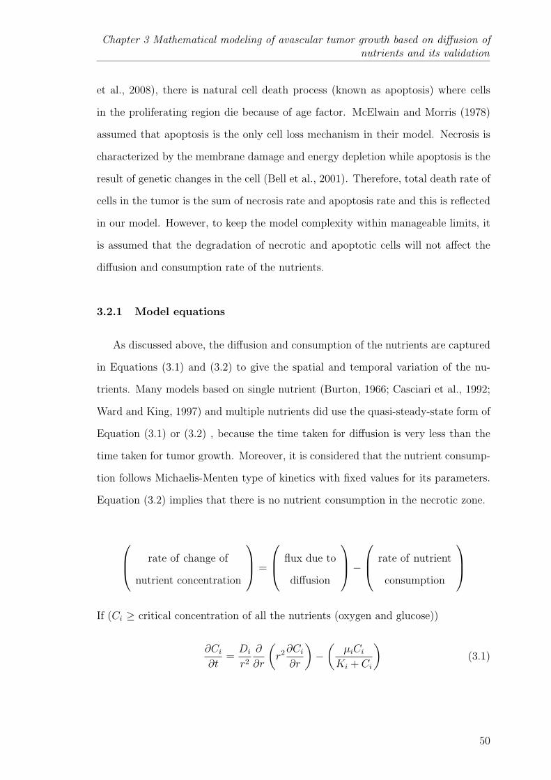
Chapter 3 Mathematical modeling of avascular tumor growth based on diffusion ofnutrients and its validation
et al., 2008), there is natural cell death process (known as apoptosis) where cells
in the proliferating region die because of age factor. McElwain and Morris (1978)
assumed that apoptosis is the only cell loss mechanism in their model. Necrosis is
characterized by the membrane damage and energy depletion while apoptosis is the
result of genetic changes in the cell (Bell et al., 2001). Therefore, total death rate of
cells in the tumor is the sum of necrosis rate and apoptosis rate and this is reflected
in our model. However, to keep the model complexity within manageable limits, it
is assumed that the degradation of necrotic and apoptotic cells will not affect the
diffusion and consumption rate of the nutrients.
3.2.1 Model equations
As discussed above, the diffusion and consumption of the nutrients are captured
in Equations (3.1) and (3.2) to give the spatial and temporal variation of the nu-
trients. Many models based on single nutrient (Burton, 1966; Casciari et al., 1992;
Ward and King, 1997) and multiple nutrients did use the quasi-steady-state form of
Equation (3.1) or (3.2) , because the time taken for diffusion is very less than the
time taken for tumor growth. Moreover, it is considered that the nutrient consump-
tion follows Michaelis-Menten type of kinetics with fixed values for its parameters.
Equation (3.2) implies that there is no nutrient consumption in the necrotic zone.
rate of change of
nutrient concentration
=
flux due to
diffusion
− rate of nutrient
consumption
If (Ci ≥ critical concentration of all the nutrients (oxygen and glucose))
∂Ci∂t
=Di
r2
∂
∂r
(r2∂Ci∂r
)−(
µiCiKi + Ci
)(3.1)
50

3.2 The proposed model
else
∂Ci∂t
=Di
r2
∂
∂r
(r2∂Ci∂r
)(3.2)
where, r is the radial position in the tumor; i = 1 and i = 2 represents glucose
and oxygen respectively. Equations (3.3) through (3.5) give the temporal variation
of the tumor radius at the different stages of tumor growth. These equations include
decay rate of dead cells based on apoptosis as well as necrosis. The apoptosis-based
dead cells decay at a rate proportional to the volume of the viable zone (proliferation
and quiescent), whereas necrosis based dead cells decay at a rate proportional to
the volume of the necrotic zone. As stated earlier, the model assumes that decayed
cells do not affect the diffusion and consumption of the nutrients.
The outer tumor radius, R(t)
rate of change of
volume of tumor
=
total rate of cell
proliferation
− total decay rate of
dead cells
First stage (all cells are in proliferation zone; Rq = 0, Rn = 0)
3R2dR
dt= A(R3)− Ap(R3) (3.3)
Second stage, (appearance of quiescent zone Rq > 0, Rn = 0)
3R2dR
dt= A(R3 −R3
q)− (ApR3) (3.4)
Third stage (appearance of necrotic zone appears Rq > Rn, Rn > 0)
3R2dR
dt= A(R3 −R3
q)− (Ap(R3 −R3
n))− (NeR3n) (3.5)
where, Rn(t) is the radial position of the outer radius of necrotic zone from the
tumor centre, Rq(t) is the radial position of the outer radius of quiescent zone from
51
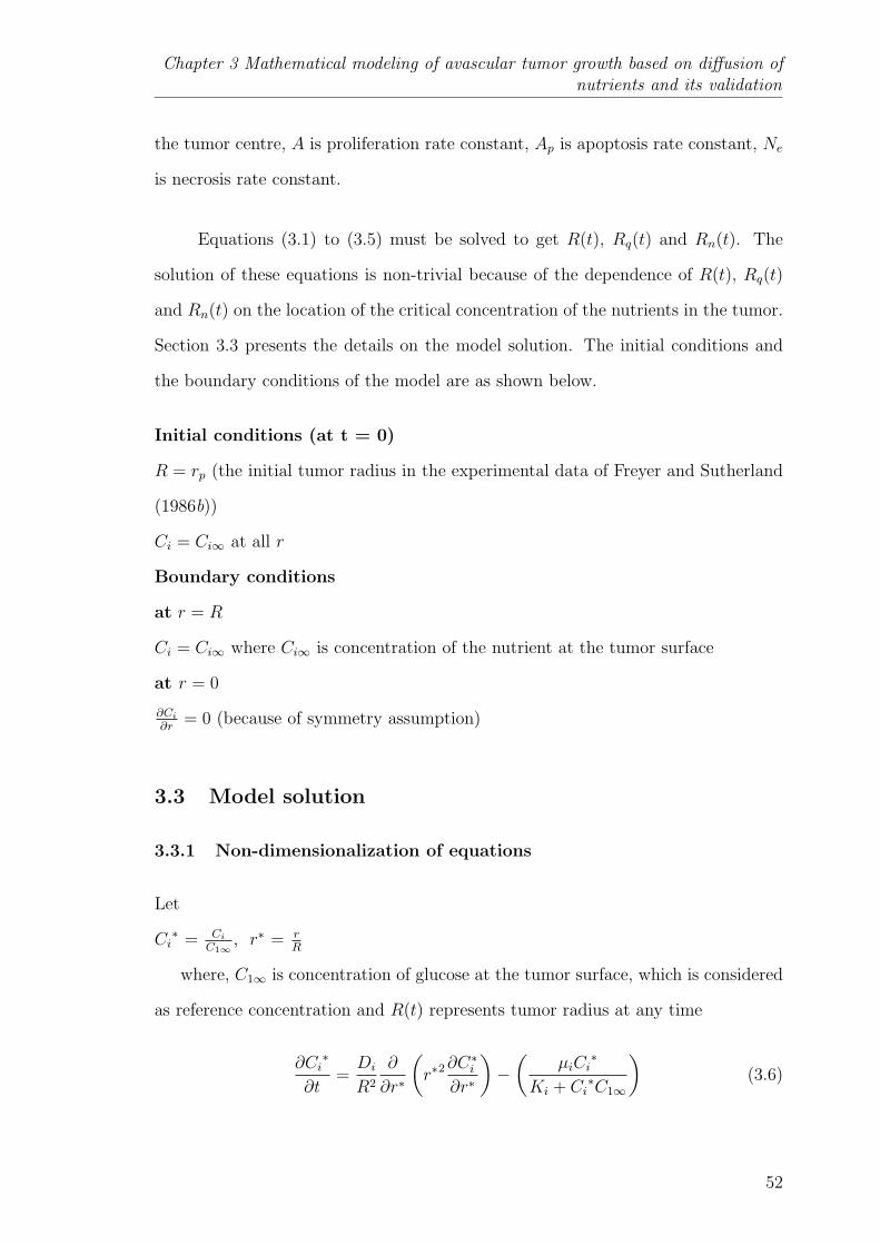
Chapter 3 Mathematical modeling of avascular tumor growth based on diffusion ofnutrients and its validation
the tumor centre, A is proliferation rate constant, Ap is apoptosis rate constant, Ne
is necrosis rate constant.
Equations (3.1) to (3.5) must be solved to get R(t), Rq(t) and Rn(t). The
solution of these equations is non-trivial because of the dependence of R(t), Rq(t)
and Rn(t) on the location of the critical concentration of the nutrients in the tumor.
Section 3.3 presents the details on the model solution. The initial conditions and
the boundary conditions of the model are as shown below.
Initial conditions (at t = 0)
R = rp (the initial tumor radius in the experimental data of Freyer and Sutherland
(1986b))
Ci = Ci∞ at all r
Boundary conditions
at r = R
Ci = Ci∞ where Ci∞ is concentration of the nutrient at the tumor surface
at r = 0
∂Ci
∂r= 0 (because of symmetry assumption)
3.3 Model solution
3.3.1 Non-dimensionalization of equations
Let
Ci∗ = Ci
C1∞, r∗ = r
R
where, C1∞ is concentration of glucose at the tumor surface, which is considered
as reference concentration and R(t) represents tumor radius at any time
∂Ci∗
∂t=Di
R2
∂
∂r∗
(r∗2
∂C∗i∂r∗
)−(
µiCi∗
Ki + Ci∗C1∞
)(3.6)
52

3.3 Model solution
3.3.2 Numerical procedure
For non-dimensionalization, one can choose either C1∞ or C2∞ as the reference
concentration. Here, C1∞ has been chosen as reference concentration, because C1∞
is greater than C2∞. Therefore, the solution of dimensionless concentrations of
oxygen and glucose is always bounded between 0 and 1. The non-dimensionalized
partial differential equation (3.6) and the outer tumor radius equations (Equation
(3.3) to (3.5) as appropriate) are solved to get the tumor radius at different times.
Equation (3.6) can be transformed to a set of ordinary differential equations and
solved using the “Method of lines” (Lee and Schiesser, 2003). In this method, the
spatial derivatives are transformed to algebraic form by using a finite difference
approximation of required accuracy. The set of ordinary differential equations can
be solved as initial value problems using MATLAB (Shampine, 1994). Note that
the number of finite difference points is fixed along the tumor radius.
Nutrient concentrations, tumor radius, necrotic zone radius and quiescent zone
radius are functions of time. However, there are no equations available for the
temporal variation of necrotic zone radius and quiescent zone radius. Therefore, the
number of unknowns (5) are more than the number of equations (3). In order to
deal with this scenario, the equations are solved for short time intervals by assuming
necrotic zone radius (Rn) and quiescent zone radius (Rq) as piecewise constant. The
question is: what would be the range of the time interval over which the radii of
the necrotic zone and quiescent zone may be considered as constant? It is known
that cells take a few hours to several days for completing a cell cycle (Kleinsmith,
2005). Therefore, it is logical to proceed with the proposition that time interval may
be based upon the duration of cell cycle. Thus, the cell cycle theory informs that
noticeable growth of tumor radius is seen after every few hours to days. Therefore,
the following solution strategy is devised. Initially, quiescent and necrotic zones do
not exist. Rq(0) and Rn(0) are therefore taken as zero. The equations are solved
53

Chapter 3 Mathematical modeling of avascular tumor growth based on diffusion ofnutrients and its validation
for a 3 hour horizon (say from t = 0 to t = 3 hours). At the end of 3 hours, the
concentration profile of glucose and oxygen are examined in order to locate Rq and
Rn corresponding to their critical concentrations. Then, the obtained values of Rq
and Rn are substituted in the appropriate outer tumor radius equations (one of
Equations (3.3) to (3.5)) based on the tumor stage and simulated for next 3 hours.
These solution steps are repeated for the next block of 3 hours using appropriate
initial conditions for the state variables until the tumor radius attains a steady state
value.
3.4 Model validation and discussion
Model validation is a very crucial and essential part of mathematical modeling.
In this work, the model is validated with the available in vitro results in the lit-
erature and with a well known empirical relation related to tumor growth called
Gompertzian relation (Burton, 1966). The values of the model parameters and
their references are presented in Table 3.1. These parameters are either measured
directly (diffusivities, critical concentration of the nutrients, maximum consump-
tion rates) or estimated (Michaelis-Menten constants, proliferation rate constant,
apoptosis rate constant, necrotic rate constant) by fitting to a model. Note that
the validation data sets are independent from data sets that were used to derive the
model parameters summarized in Table 3.1. Thus, the proposed model has been
subjected to stringent tests as reported below.
3.4.1 Validation with in vitro data (Freyer and Sutherland, 1986b)
In Freyer and Sutherland (1986b), EMT6/Ro mouse mammary carcinoma cell
spheroids were cultured in suspension in either 0.28 mmol/L or 0.07 mmol/L oxygen
and 16.5, 5.5, 1.7, 0.8 mmol/L glucose to study the effects of glucose and oxygen on
spheroid growth. They determined the value of mean size of a spheroid population
54

3.4 Model validation and discussion
Table 3.1Parameter values
Symbols Quantity Value UnitsD1 Diffusivity of glucose 1.1× 10⁻⁶ cm2/s
(Casciari et al., 1988)C1c Critical concentration of glucose 7.7× 10⁻⁶ mole/cm3
(Hlatky et al., 1988b)µ1 Maximum consumption rate of glucose 4× 10⁻⁸ mole/cm3.s
(Casciari et al., 1992)K1 Michaelis-Menten constant for glucose 4× 10⁻⁸ mole/cm3
(Casciari et al., 1992)D2 Diffusivity of oxygen 1.82× 10⁻⁵ cm2/s
(Mueller-Klieser and Sutherland, 1985)C2c Critical concentration of oxygen 2× 10⁻⁸ mole/cm3
(Jiang et al., 2005)µ2 Maximum consumption rate of oxygen 1.43916× 10⁻⁸ mole/cm3.s
(Casciari et al., 1992)K2 Michaelis-Menten constant for oxygen 4.640× 10⁻⁹ mole/cm3
(Casciari et al., 1992)A Proliferation rate constant 0.12− 5.2 1/day
Burton (1966)Ap Apoptosis rate constant 1.5× 10⁻⁶ 1/hour
(Busini et al., 2007)Ne Necrosis rate constant 1.36× 10⁻² 1/hour
(Busini et al., 2007)
by measuring the two orthogonal diameters on each of 50 spheroids using an inverted
microscope fitted with a calibrated eyepiece reticule. Using the above data, they
evaluated the total spheroid volume variation with time for 28 days, maximum
volume of the tumor, exponential doubling time and tumor diameter at the onset
of necrosis for different media conditions.
Simulated growth curve was obtained from the proposed model using the param-
eter values in Table 3.1. Figure 3.2 shows the simulated growth curve of the tumor
for 28 days in comparison with the experimental data when the glucose and oxy-
gen concentrations in the media are 16.5 mmol/L and 0.28 mmol/L respectively.
There is a high degree of agreement between the simulated growth curve and the
55

Chapter 3 Mathematical modeling of avascular tumor growth based on diffusion ofnutrients and its validation
Fig. 3.2. Tumor growth curves of simulated and experimental dataat 16.5 mmol/L glucose and 0.28 mmol/L oxygen
Fig. 3.3. Quiescent and necrotic radius at different tumor radiusduring its growth at 16.5 mmol/L glucose and 0.28 mmol/L oxygen
56
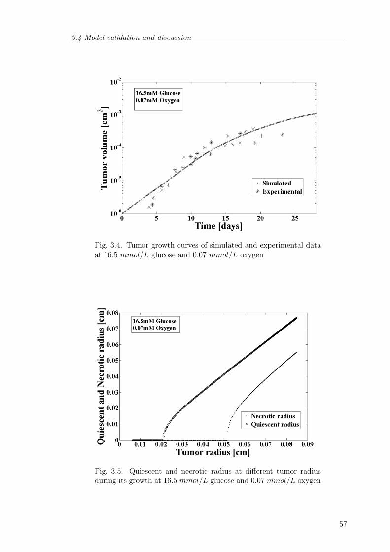
3.4 Model validation and discussion
Fig. 3.4. Tumor growth curves of simulated and experimental dataat 16.5 mmol/L glucose and 0.07 mmol/L oxygen
Fig. 3.5. Quiescent and necrotic radius at different tumor radiusduring its growth at 16.5 mmol/L glucose and 0.07 mmol/L oxygen
57

Chapter 3 Mathematical modeling of avascular tumor growth based on diffusion ofnutrients and its validation
Table 3.2Maximum volume of multicellular tumor spheroids at different con-centrations
External oxygen External glucose Maximum Maximumconcentration concentration volume volume
(mmol/L) a (mmol/L)a (cm3)a (cm3)b
0.28
16.5 4.4× 10⁻²c 9× 10⁻³
5.5 1.1× 10⁻²c 3.2× 10⁻³
1.7 8.3× 10⁻⁴ 1.1× 10⁻³
0.8 8.3× 10⁻⁴ 4.54× 10⁻⁴
0.07
16.5 7.7× 10⁻³ 2.6× 10⁻³
5.5 6.1× 10⁻⁴ 6.99× 10⁻⁴
1.7 1.5× 10⁻⁴ 1.56× 10⁻⁴
0.8 7.8× 10⁻⁵ 4.48× 10⁻⁵
a Freyer and Sutherland (1986)b Proposed modelc Extrapolated values (experimental)
experimental data. The simulated curve shows that once the quiescent and necrotic
zones are formed in the tumor, the tumor growth retards and reaches a final state
(see Figure 3.2 for t > 25 days). In addition, the proposed model was able to locate
the position of outer radius of the quiescent and necrotic zones as shown in Figure
3.3. The tumor diameter at the onset of necrosis is almost the same as that of the
estimated value (0.0516 cm) in Freyer and Sutherland (1986b). In order to test the
prognostic ability of the model, the simulated results are verified with the exper-
imental data, when the oxygen concentration is changed to 0.07 mmol/L. These
results are shown in Figures 3.4 and 3.5 respectively. It is seen that the tumor
diameter at the onset of necrosis (0.0510 cm) is in good agreement with the value
given in Freyer and Sutherland (1986b). Table 3.2 shows the comparison between
simulated values and the experimental values of the maximum volume of the tumor
for different combinations of glucose and oxygen concentrations. The experimental
values (3rd column) are from Freyer and Sutherland (1986b). The agreement be-
tween the experimental values and our model predictions (4th column) is very good.
Interestingly, it is observed from Table 3.2 that for a given concentration of oxygen,
58
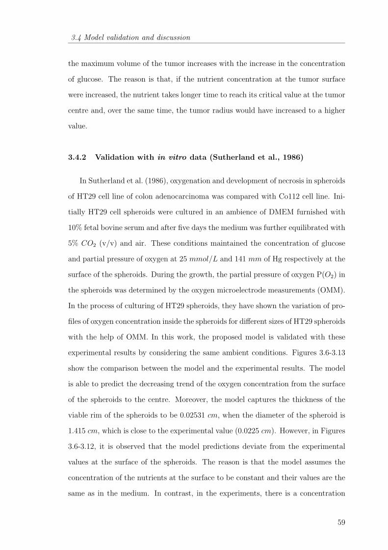
3.4 Model validation and discussion
the maximum volume of the tumor increases with the increase in the concentration
of glucose. The reason is that, if the nutrient concentration at the tumor surface
were increased, the nutrient takes longer time to reach its critical value at the tumor
centre and, over the same time, the tumor radius would have increased to a higher
value.
3.4.2 Validation with in vitro data (Sutherland et al., 1986)
In Sutherland et al. (1986), oxygenation and development of necrosis in spheroids
of HT29 cell line of colon adenocarcinoma was compared with Co112 cell line. Ini-
tially HT29 cell spheroids were cultured in an ambience of DMEM furnished with
10% fetal bovine serum and after five days the medium was further equilibrated with
5% CO2 (v/v) and air. These conditions maintained the concentration of glucose
and partial pressure of oxygen at 25 mmol/L and 141 mm of Hg respectively at the
surface of the spheroids. During the growth, the partial pressure of oxygen P(O2) in
the spheroids was determined by the oxygen microelectrode measurements (OMM).
In the process of culturing of HT29 spheroids, they have shown the variation of pro-
files of oxygen concentration inside the spheroids for different sizes of HT29 spheroids
with the help of OMM. In this work, the proposed model is validated with these
experimental results by considering the same ambient conditions. Figures 3.6-3.13
show the comparison between the model and the experimental results. The model
is able to predict the decreasing trend of the oxygen concentration from the surface
of the spheroids to the centre. Moreover, the model captures the thickness of the
viable rim of the spheroids to be 0.02531 cm, when the diameter of the spheroid is
1.415 cm, which is close to the experimental value (0.0225 cm). However, in Figures
3.6-3.12, it is observed that the model predictions deviate from the experimental
values at the surface of the spheroids. The reason is that the model assumes the
concentration of the nutrients at the surface to be constant and their values are the
same as in the medium. In contrast, in the experiments, there is a concentration
59

Chapter 3 Mathematical modeling of avascular tumor growth based on diffusion ofnutrients and its validation
Fig. 3.6. Profile of partial pressure of oxygen (PO2) in the HT29spheroids when its diameter is 1039 µm
Fig. 3.7. Profile of partial pressure of oxygen (PO2) in the HT29spheroids when its diameter is 1116 µm
gradient of the nutrients from the bulk medium to the surface. This also implies
that the deviation of the model will be more when the diameter of the spheroids is
very small and this is seen clearly in Figure 3.13.
60

3.4 Model validation and discussion
Fig. 3.8. Profile of partial pressure of oxygen (PO2) in the HT29spheroids when its diameter is 1169 µm
Fig. 3.9. Profile of partial pressure of oxygen (PO2) in the HT29spheroids when its diameter is 1415 µm
61
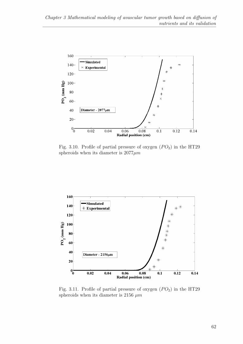
Chapter 3 Mathematical modeling of avascular tumor growth based on diffusion ofnutrients and its validation
Fig. 3.10. Profile of partial pressure of oxygen (PO2) in the HT29spheroids when its diameter is 2077µm
Fig. 3.11. Profile of partial pressure of oxygen (PO2) in the HT29spheroids when its diameter is 2156 µm
62
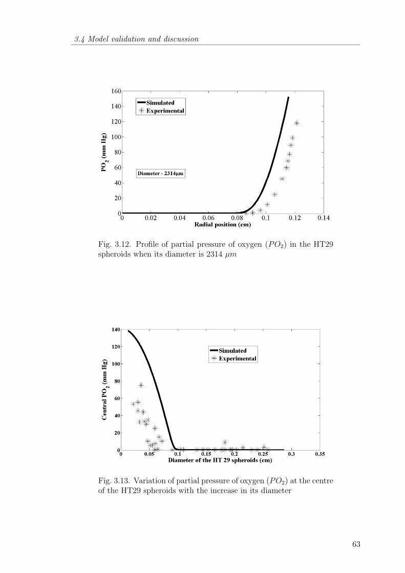
3.4 Model validation and discussion
Fig. 3.12. Profile of partial pressure of oxygen (PO2) in the HT29spheroids when its diameter is 2314 µm
Fig. 3.13. Variation of partial pressure of oxygen (PO2) at the centreof the HT29 spheroids with the increase in its diameter
63

Chapter 3 Mathematical modeling of avascular tumor growth based on diffusion ofnutrients and its validation
Fig. 3.14. Comparison between the proposed model and Casciariet al. (1992) model on the basis of variation of oxygen concentrationat the centre of the EMT6/Ro spheroids with the increase in itsdiameter
3.4.3 Comparison with Casciari et al. (1992) model
Casciari et al. (1992) validated their model with the experiment results of Mueller-
Klieser and Sutherland (1982), where EMT6/Ro spheroids were cultured in 500 ml
Bellco flasks containing 300 ml BME with 15% fetal bovine serum, 0.21 mmol/L
oxygen and 5.5 mmol/L glucose. The proposed model is now tested with the same
experimental results - the result is shown in Figure 3.14. The discrepancy between
the model and the experimental results at the lower spheroid diameter is due to
assumption that the concentration of nutrients at the surface is equal to that in the
bulk medium. However, the model is able to capture the decreasing nature of the
oxygen concentration at the centre even for spheroid diameter beyond 700 µm as in
the experimental results, which is not seen in the Casciari et al. (1992) model. Note
that the proposed model is simpler than the Casciari et al. (1992) model but can
provide better representation of the experimental data in some regions.
64
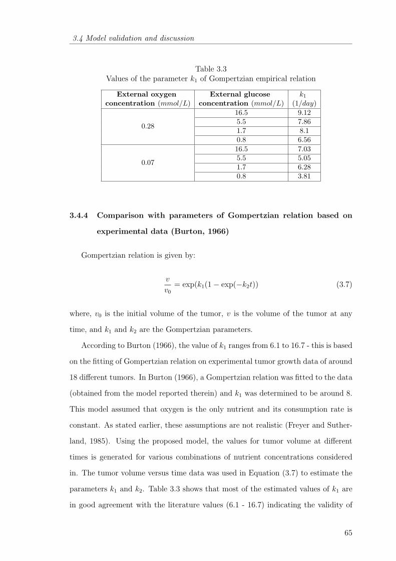
3.4 Model validation and discussion
Table 3.3Values of the parameter k1 of Gompertzian empirical relation
External oxygen External glucose k1
concentration (mmol/L) concentration (mmol/L) (1/day)
0.28
16.5 9.125.5 7.861.7 8.10.8 6.56
0.07
16.5 7.035.5 5.051.7 6.280.8 3.81
3.4.4 Comparison with parameters of Gompertzian relation based on
experimental data (Burton, 1966)
Gompertzian relation is given by:
v
v0
= exp(k1(1− exp(−k2t)) (3.7)
where, v0 is the initial volume of the tumor, v is the volume of the tumor at any
time, and k1 and k2 are the Gompertzian parameters.
According to Burton (1966), the value of k1 ranges from 6.1 to 16.7 - this is based
on the fitting of Gompertzian relation on experimental tumor growth data of around
18 different tumors. In Burton (1966), a Gompertzian relation was fitted to the data
(obtained from the model reported therein) and k1 was determined to be around 8.
This model assumed that oxygen is the only nutrient and its consumption rate is
constant. As stated earlier, these assumptions are not realistic (Freyer and Suther-
land, 1985). Using the proposed model, the values for tumor volume at different
times is generated for various combinations of nutrient concentrations considered
in. The tumor volume versus time data was used in Equation (3.7) to estimate the
parameters k1 and k2. Table 3.3 shows that most of the estimated values of k1 are
in good agreement with the literature values (6.1 - 16.7) indicating the validity of
65
Chapter 3 Mathematical modeling of avascular tumor growth based on diffusion ofnutrients and its validation
the proposed avascular tumor growth model. The exceptions occur at the lower
value of external oxygen concentration when the external glucose concentration is
5.5 mmol/L or 0.8mmol/L.
3.5 Conclusions
In this chapter, a new mathematical model for avascular tumor growth was intro-
duced. It is mechanistic and considers all the relevant cellular process (proliferation,
apoptosis and necrosis) and their dependency on the diffusion and consumption of
the nutrients. The model is simple yet powerful. It was successful in capturing the
tumor growth and the maximum volume achieved under different media conditions.
On the basis of the results of onset of necrosis, the proposition that necrotic zone
is observed when the concentrations of both vital nutrients are below their critical
values appears to be true. Moreover, the model is predictive in identifying the size
of proliferation zone, quiescent zone and necrotic zone and their effect on the overall
tumor growth. Therefore, the proposed model can be a supporting tool for tumor
pathologists in determining tumor growth relevant parameters corresponding to the
tumor sample extracted from the patients.
66
Chapter 4
SEQUENTIAL SCHEDULING OF CANCER
IMMUNOTHERAPY AND CHEMOTHERAPY USING
MULTI-OBJECTIVE OPTIMIZATION
‘We must develop knowledge optimization initiatives to leverage our key
learnings.’
- Scott Adams
4.1 Introduction
In the previous chapter, the utility of spatio-temporal models in diagnostic pro-
cedures were discussed, while from this chapter onwards, the focus is on using func-
tional models to develop therapeutic strategies. In general, the objectives of any
therapy or combination of therapies are to minimize the total number of cancer
cells by maintaining it below the lethal level while minimizing the side effects. In
this chapter, the main contribution is the therapeutic protocol analysis for a given
patient and given time horizon using multi-objective optimization.
Chemotherapy is one of the prominent treatment modalities of cancer and gen-
erally, all cancer patients undergo chemotherapy at some stage of their treatment.
However, it is not always a comprehensive solution as an adjuvant therapy or as a
prime therapy for tumor regression. Therefore, chemotherapy is administered to the
patient in synergistic combination with the other treatment modalities such as im-
munotherapy in order to eliminate the tumor. In the present chapter, chemotherapy
using doxorubicin and its combination with adoptive-cell-transfer therapy (ACT) is
67
Chapter 4 Sequential scheduling of cancer immunotherapy and chemotherapy usingmulti-objective optimization
considered. ACT is one immunotherapy scheme where the recognized anti-tumor
T-cells are cultured externally and administered to the patient (Ho et al., 2003; Dud-
ley and Rosenberg, 2003; Rosenberg et al., 2008). Practically, ACT has proved its
worth by causing tumor regression in patients with melanoma or lymphoma (Dudley
et al., 2002).
An in silico pharmacokinetic/pharmacodynamic model describing the interac-
tion between tumor cells, immune cells and doxorubicin is used to formulate a
multi-objective optimization problem by considering clinically relevant objectives
and constraints. Then, the multi-objective optimization problem is solved using a
Pareto based approach known as non-dominated sorting genetic algorithm (NSGA-
II) (Deb et al., 2000) for different cases in order to discover a therapeutically effi-
cacious treatment regimen. Then, a systematic post analysis is performed using L2
norm method (Kasprzak and Lewis, 2001) in order to choose and recommend an ap-
propriate solution from the Pareto set obtained from NSGA-II. The chosen solution
can be considered as the optimal compromise solution, because the optimal solution
for one objective may not be the optimal solution for the other objective(s). The
details about these methods are provided in the later part of this chapter. In this
chapter, the main focus is on the comparison of the efficacy of the chemotherapy
alone and and its combination with ACT.
4.2 Mathematical model
Tumor-immune interaction models explain interactions between different type of
immune cells and tumor cells. There are many tumor-immune interaction models
as discussed in chapter 2. The model employed in this chapter is taken from the
work of Kuznetsov et al. (1994) because it is the mother model for tumor-immune
interactions. It explains different phenomena of tumor-immune interactions like
sneak-through and tumor dormancy. “Sneak-through” is the phenomenon in which
immune system evades tumor. In tumor dormancy phase, tumor size remains con-
68
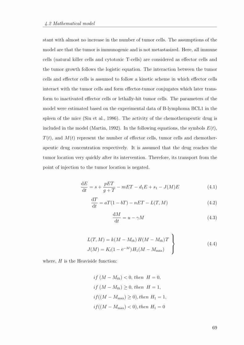
4.2 Mathematical model
stant with almost no increase in the number of tumor cells. The assumptions of the
model are that the tumor is immunogenic and is not metastasized. Here, all immune
cells (natural killer cells and cytotoxic T-cells) are considered as effector cells and
the tumor growth follows the logistic equation. The interaction between the tumor
cells and effector cells is assumed to follow a kinetic scheme in which effector cells
interact with the tumor cells and form effector-tumor conjugates which later trans-
form to inactivated effector cells or lethally-hit tumor cells. The parameters of the
model were estimated based on the experimental data of B-lymphoma BCL1 in the
spleen of the mice (Siu et al., 1986). The activity of the chemotherapeutic drug is
included in the model (Martin, 1992). In the following equations, the symbols E(t),
T (t), and M(t) represent the number of effector cells, tumor cells and chemother-
apeutic drug concentration respectively. It is assumed that the drug reaches the
tumor location very quickly after its intervention. Therefore, its transport from the
point of injection to the tumor location is negated.
dE
dt= s+
pET
g + T−mET − d1E + s1 − J(M)E (4.1)
dT
dt= aT (1− bT )− nET − L(T,M) (4.2)
dM
dt= u− γM (4.3)
L(T,M) = k(M −Mth)H(M −Mth)T
J(M) = Kl(1− e−M)H1(M −Mmax)
(4.4)
where, H is the Heaviside function:
if (M −Mth) < 0, then H = 0,
if (M −Mth) ≥ 0, then H = 1,
if((M −Mmax) ≥ 0), then H1 = 1,
if((M −Mmax) < 0), then H1 = 0
69
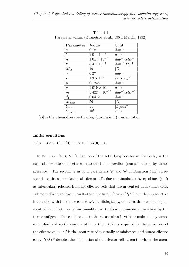
Chapter 4 Sequential scheduling of cancer immunotherapy and chemotherapy usingmulti-objective optimization
Table 4.1Parameter values (Kuznetsov et al., 1994; Martin, 1992)
Parameter Value Unita 0.18 day−1
b 2.0× 10⁻⁹ cells−1
n 1.01× 10⁻⁷ day−1cells−1
k 8.4× 10⁻³ day−1[D]−1
Mth 10 [D]γ 0.27 day−1
s 1.3× 10⁴ cellsday−1
p 0.1245 day−1
g 2.019× 10⁷ cellsm 3.422× 10⁻¹⁰ day−1cells−1
d1 0.0412 day−1
Mmax 50 [D]Umax 51 [D]day−1
S1max 107 cells
[D] is the Chemotherapeutic drug (doxorubicin) concentration
Initial conditions
E(0) = 3.2× 10⁵, T (0) = 1× 10¹⁰, M(0) = 0
In Equation (4.1), ‘s’ (a fraction of the total lymphocytes in the body) is the
natural flow rate of effector cells to the tumor location (non-stimulated by tumor
presence). The second term with parameters ‘p’ and ‘g’ in Equation (4.1) corre-
sponds to the accumulation of effector cells due to stimulation by cytokines (such
as interleukin) released from the effector cells that are in contact with tumor cells.
Effector cells degrade as a result of their natural life time (d1E ) and their exhaustive
interaction with the tumor cells (mET ). Biologically, this term denotes the impair-
ment of the effector cells functionality due to their continuous stimulation by the
tumor antigens. This could be due to the release of anti-cytokine molecules by tumor
cells which reduce the concentration of the cytokines required for the activation of
the effector cells. ‘s1’ is the input rate of externally administered anti-tumor effector
cells. J(M)E denotes the elimination of the effector cells when the chemotherapeu-
70

4.3 Multi-objective optimization
tic drug concentration exceeds the Mmax value (Equation (4.4)) where k is the rate
of elimination of the effector cells. In Equation (4.2), ‘a’ is the maximal growth
rate of the tumor cells and it incorporates both their proliferation and death rates
whereas ‘1/b’ is the carrying capacity of the tumor cells, where aT (1− bT ) signifies
tumor growth because of nutrients such as glucose and oxygen without the effect
of immune response. The tumor cells are killed by their interaction with effector
cells and chemotherapeutic intervention. The pharmacokinetics of the chemother-
apeutic drug is illustrated by Equation (4.3) where ‘u’ is its input rate and ‘γ’ is
its decay rate. The pharmacodynamics of the drug is indicated by L(T,M), where
it is clarified that the drug can have predominant effect on tumor cells only if its
concentration is more than the threshold concentration (Mth) (Equation (4.4)). Kl
is the rate of elimination of tumor cells due to the chemotherapeutic drug. The
parameter values are given in Table 4.1. Another assumption is that parameters
of the patient model do not change significantly during the treatment horizon. As
a result, the problem of treatment protocol design can be solved as an open loop
optimal control problem using the integrated model to explore the efficacious and
endurable possibility for tumor regression. The three basic assumptions regarding
the delivery of chemotherapeutic drug are:
(a) Intravenous injection of the drug
(b) Instantaneous mixing of the drug with the plasma
(c) the time taken by the drug to reach the tumor site is negligible.
4.3 Multi-objective optimization
Multi-objective optimization (MOO) is the optimization of two or more conflict-
ing objectives of a physical system represented in the form of a mathematical model
subjected to some known constraints. MOO is widely used in many fields such
as process design, aerospace, medical applications, and automobile design. Unlike
71
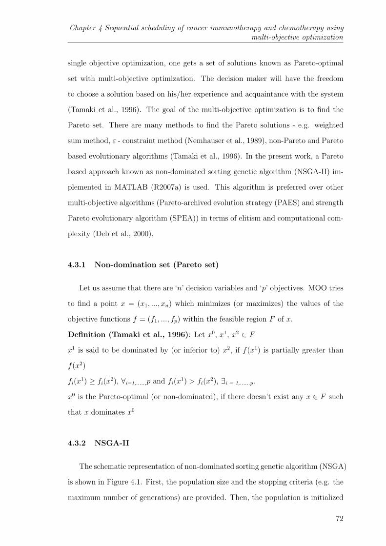
Chapter 4 Sequential scheduling of cancer immunotherapy and chemotherapy usingmulti-objective optimization
single objective optimization, one gets a set of solutions known as Pareto-optimal
set with multi-objective optimization. The decision maker will have the freedom
to choose a solution based on his/her experience and acquaintance with the system
(Tamaki et al., 1996). The goal of the multi-objective optimization is to find the
Pareto set. There are many methods to find the Pareto solutions - e.g. weighted
sum method, ε - constraint method (Nemhauser et al., 1989), non-Pareto and Pareto
based evolutionary algorithms (Tamaki et al., 1996). In the present work, a Pareto
based approach known as non-dominated sorting genetic algorithm (NSGA-II) im-
plemented in MATLAB (R2007a) is used. This algorithm is preferred over other
multi-objective algorithms (Pareto-archived evolution strategy (PAES) and strength
Pareto evolutionary algorithm (SPEA)) in terms of elitism and computational com-
plexity (Deb et al., 2000).
4.3.1 Non-domination set (Pareto set)
Let us assume that there are ‘n’ decision variables and ‘p’ objectives. MOO tries
to find a point x = (x1, ..., xn) which minimizes (or maximizes) the values of the
objective functions f = (f1, ..., fp) within the feasible region F of x.
Definition (Tamaki et al., 1996): Let x0, x1, x2 ∈ F
x1 is said to be dominated by (or inferior to) x2, if f(x1) is partially greater than
f(x2)
fi(x1) ≥ fi(x
2), ∀i=1,.....,p and fi(x1) > fi(x
2), ∃i = 1,......p.
x0 is the Pareto-optimal (or non-dominated), if there doesn’t exist any x ∈ F such
that x dominates x0
4.3.2 NSGA-II
The schematic representation of non-dominated sorting genetic algorithm (NSGA)
is shown in Figure 4.1. First, the population size and the stopping criteria (e.g. the
maximum number of generations) are provided. Then, the population is initialized
72
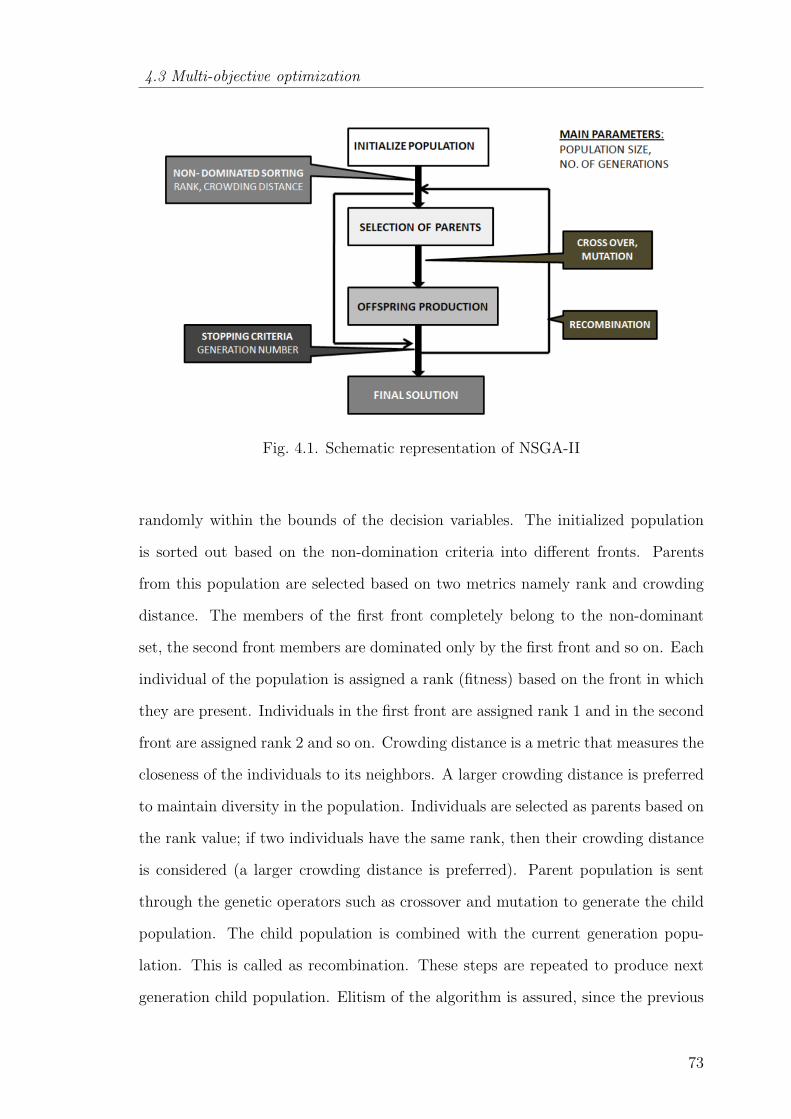
4.3 Multi-objective optimization
Fig. 4.1. Schematic representation of NSGA-II
randomly within the bounds of the decision variables. The initialized population
is sorted out based on the non-domination criteria into different fronts. Parents
from this population are selected based on two metrics namely rank and crowding
distance. The members of the first front completely belong to the non-dominant
set, the second front members are dominated only by the first front and so on. Each
individual of the population is assigned a rank (fitness) based on the front in which
they are present. Individuals in the first front are assigned rank 1 and in the second
front are assigned rank 2 and so on. Crowding distance is a metric that measures the
closeness of the individuals to its neighbors. A larger crowding distance is preferred
to maintain diversity in the population. Individuals are selected as parents based on
the rank value; if two individuals have the same rank, then their crowding distance
is considered (a larger crowding distance is preferred). Parent population is sent
through the genetic operators such as crossover and mutation to generate the child
population. The child population is combined with the current generation popu-
lation. This is called as recombination. These steps are repeated to produce next
generation child population. Elitism of the algorithm is assured, since the previous
73
Chapter 4 Sequential scheduling of cancer immunotherapy and chemotherapy usingmulti-objective optimization
Fig. 4.2. L2 norm method
and current best individuals are added in the population. The same procedure is
continued until the GA evolves to the maximum number of generations. Overall, the
prominent tuning parameters in this algorithm are the number of generations, prob-
abilities for crossover and mutation processes. Matlab implementation of NSGA-II
can be easily obtained in the internet. The main challenging task in this algorithm
is the choice of population size and maximum number of generations. Generally,
higher the population size and the number of generations are preferred. However,
it is computationally intensive. In this work, the population size and the number of
generations are chosen based on the iterative preliminary runs of the optimization
problem.
4.3.3 Post-Pareto-optimality analysis
In the literature, there are many methods for post-Pareto-optimality analysis
such as clustering techniques, ranking techniques and distance based methods such
as L2 norm. Here, L2 norm method involving the concept of utopia point is used
to find the optimal compromise solution (Kasprzak and Lewis, 2001). Utopia point
is the theoretically best performance point; in our case, the origin is assumed as
74
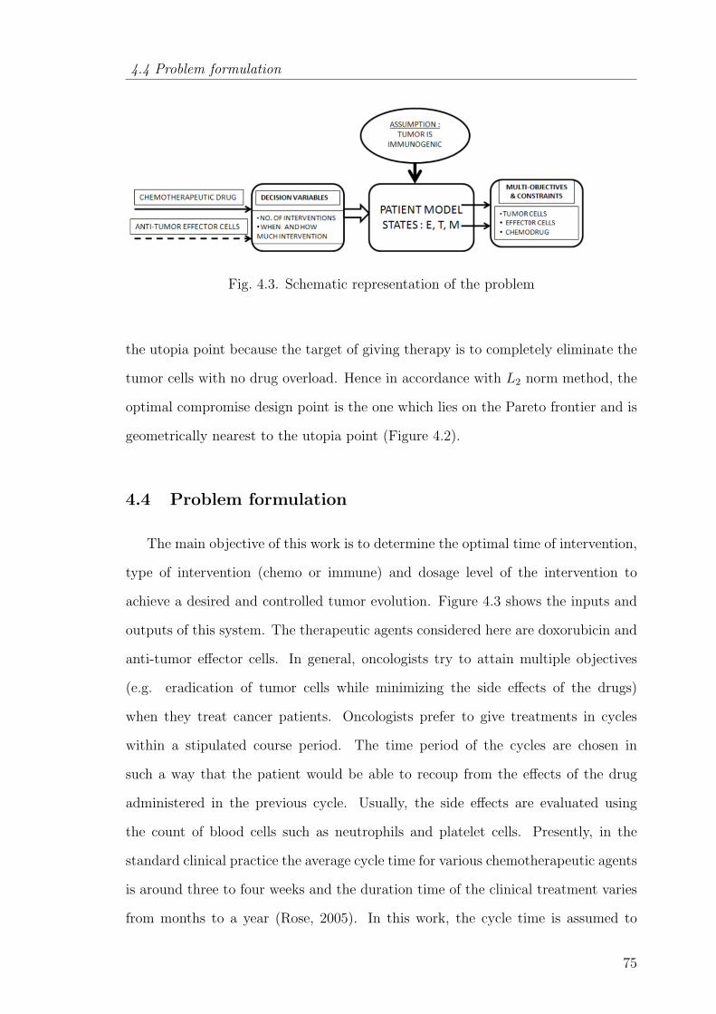
4.4 Problem formulation
Fig. 4.3. Schematic representation of the problem
the utopia point because the target of giving therapy is to completely eliminate the
tumor cells with no drug overload. Hence in accordance with L2 norm method, the
optimal compromise design point is the one which lies on the Pareto frontier and is
geometrically nearest to the utopia point (Figure 4.2).
4.4 Problem formulation
The main objective of this work is to determine the optimal time of intervention,
type of intervention (chemo or immune) and dosage level of the intervention to
achieve a desired and controlled tumor evolution. Figure 4.3 shows the inputs and
outputs of this system. The therapeutic agents considered here are doxorubicin and
anti-tumor effector cells. In general, oncologists try to attain multiple objectives
(e.g. eradication of tumor cells while minimizing the side effects of the drugs)
when they treat cancer patients. Oncologists prefer to give treatments in cycles
within a stipulated course period. The time period of the cycles are chosen in
such a way that the patient would be able to recoup from the effects of the drug
administered in the previous cycle. Usually, the side effects are evaluated using
the count of blood cells such as neutrophils and platelet cells. Presently, in the
standard clinical practice the average cycle time for various chemotherapeutic agents
is around three to four weeks and the duration time of the clinical treatment varies
from months to a year (Rose, 2005). In this work, the cycle time is assumed to
75
Chapter 4 Sequential scheduling of cancer immunotherapy and chemotherapy usingmulti-objective optimization
be four weeks and stipulated course period (tf ) as 1 year. Therefore, the total
number of therapeutic interventions (N) is taken as 12. Keeping in view the usual
objectives of the oncologists, multiple (three) objectives (McCall et al., 2007) and
the constraints to be satisfied for the therapeutic interventions are considered. The
objectives considered are listed and discussed next. Mathematically, objective 1
corresponds to minimizing the area under the tumor profile as shown in Figure 4.4.
However, with only objective 1, desired results may not be ensured because it may
so happen that the number of tumor cells may shoot up to a very high value at any
point of time, even while remaining at low values during the rest of the treatment
period. Such abrupt increases in the concentration of the tumor cells may lead to
further stages of cancer such as vascularization and metastasis. At these stages, the
disease is very difficult to treat. In order to handle this issue, the minimization of
objectives 2 and 3 are also considered. Objective 2 corresponds to the tumor size
on the final day of the stipulated course period which is practically expected to be
very low value. Objective 3 controls the maximum possible tumor size throughout
the stipulated course time. The incorporation of constraints (ii-iv) in the problem
formulation prevents the side effects due to doxorubicin. Constraints (ii) and (iii)
are related to input rate and maximum concentration of doxorubicin respectively.
High drug concentrations (beyond the safe limits, i.e., greater than Mmax), could
destroy neighboring normal tissues and the patients may experience undesirable side
effects. Practically, constraints (ii) and (iii) imply the instantaneous and short-term
effects of the drug. Constraint (iv) is a measure of drug clearance in the body. It
physically interprets the long-term effect of the drug on the organs such as the heart
or liver and the blood cell count. Constraint (vii) conveys that the minimum value
of tumor size should be more than or equal to 1 tumor cell. If this is not taken into
account, the tumor size will go to a negligibly low value ( 10−20) which is due to
the continuous nature of state variable. Mathematically, the lower value may sound
good; however, it has no medical significance.
76

4.4 Problem formulation
Objectives
Objective 1: mintf∫0
T (t) dt
Objective 2: min (T (tf ))
Objective 3: min (Tmax)
Constraints
(i) : Equations (4.1) through (4.4) i.e. the mathematical model
(ii) : 0 ≤ u(ti) ≤ umax
(iii): 0 ≤ M(t) ≤Mmax
(iv) :tf∫0
M(t) dt ≤ 4100
(v) : tf = 1 year
(vi) : N (no. of therapeutic interventions) = 12
(vii): min(T (t)) ≥ 1
where, ti is the intervention time and umax is the upper bound on the input rate
of doxorubicin
In this chapter, the comparison of the efficacies between chemotherapy and its
combination with ACT is particularly sought using the above problem formulation.
In the case of combination therapy, the number of immunotherapeutic interventions
are regarded as a decision variable as well and determined the optimum number
of immunotherapeutic interventions required to replace the chemotherapeutic inter-
ventions while satisfying all the constraints.
77
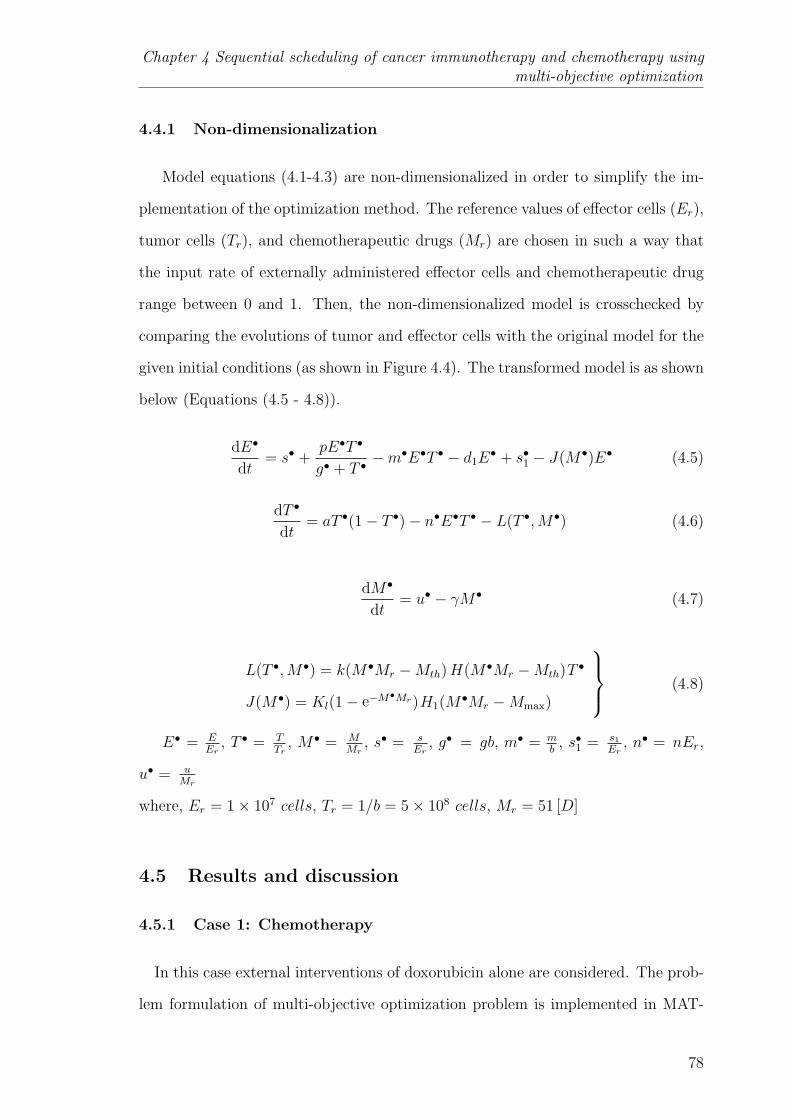
Chapter 4 Sequential scheduling of cancer immunotherapy and chemotherapy usingmulti-objective optimization
4.4.1 Non-dimensionalization
Model equations (4.1-4.3) are non-dimensionalized in order to simplify the im-
plementation of the optimization method. The reference values of effector cells (Er),
tumor cells (Tr), and chemotherapeutic drugs (Mr) are chosen in such a way that
the input rate of externally administered effector cells and chemotherapeutic drug
range between 0 and 1. Then, the non-dimensionalized model is crosschecked by
comparing the evolutions of tumor and effector cells with the original model for the
given initial conditions (as shown in Figure 4.4). The transformed model is as shown
below (Equations (4.5 - 4.8)).
dE•
dt= s• +
pE•T •
g• + T •−m•E•T • − d1E
• + s•1 − J(M•)E• (4.5)
dT •
dt= aT •(1− T •)− n•E•T • − L(T •,M•) (4.6)
dM•
dt= u• − γM• (4.7)
L(T •,M•) = k(M•Mr −Mth)H(M•Mr −Mth)T•
J(M•) = Kl(1− e−M•Mr)H1(M•Mr −Mmax)
(4.8)
E• = EEr
, T • = TTr
, M• = MMr
, s• = sEr
, g• = gb, m• = mb
, s•1 = s1Er
, n• = nEr,
u• = uMr
where, Er = 1× 10⁷ cells, Tr = 1/b = 5× 10⁸ cells, Mr = 51 [D]
4.5 Results and discussion
4.5.1 Case 1: Chemotherapy
In this case external interventions of doxorubicin alone are considered. The prob-
lem formulation of multi-objective optimization problem is implemented in MAT-
78

4.5 Results and discussion
Fig. 4.4. Comparison between original and non-dimensionalized model
Fig. 4.5. Algorithm to find the optimal compromise solution
LAB (R2007a) and solved to find the timing and dosage of 12 chemotherapeutic
interventions within the course time. The population size and number of gener-
79
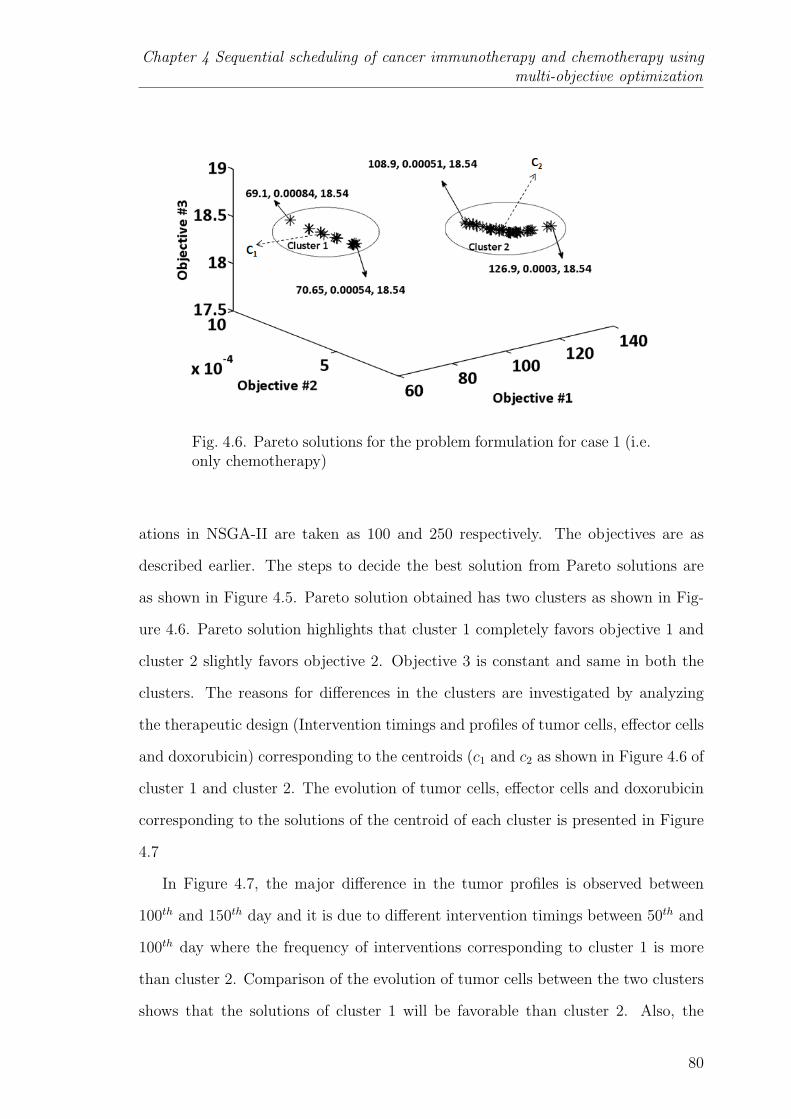
Chapter 4 Sequential scheduling of cancer immunotherapy and chemotherapy usingmulti-objective optimization
Fig. 4.6. Pareto solutions for the problem formulation for case 1 (i.e.only chemotherapy)
ations in NSGA-II are taken as 100 and 250 respectively. The objectives are as
described earlier. The steps to decide the best solution from Pareto solutions are
as shown in Figure 4.5. Pareto solution obtained has two clusters as shown in Fig-
ure 4.6. Pareto solution highlights that cluster 1 completely favors objective 1 and
cluster 2 slightly favors objective 2. Objective 3 is constant and same in both the
clusters. The reasons for differences in the clusters are investigated by analyzing
the therapeutic design (Intervention timings and profiles of tumor cells, effector cells
and doxorubicin) corresponding to the centroids (c1 and c2 as shown in Figure 4.6 of
cluster 1 and cluster 2. The evolution of tumor cells, effector cells and doxorubicin
corresponding to the solutions of the centroid of each cluster is presented in Figure
4.7
In Figure 4.7, the major difference in the tumor profiles is observed between
100th and 150th day and it is due to different intervention timings between 50th and
100th day where the frequency of interventions corresponding to cluster 1 is more
than cluster 2. Comparison of the evolution of tumor cells between the two clusters
shows that the solutions of cluster 1 will be favorable than cluster 2. Also, the
80
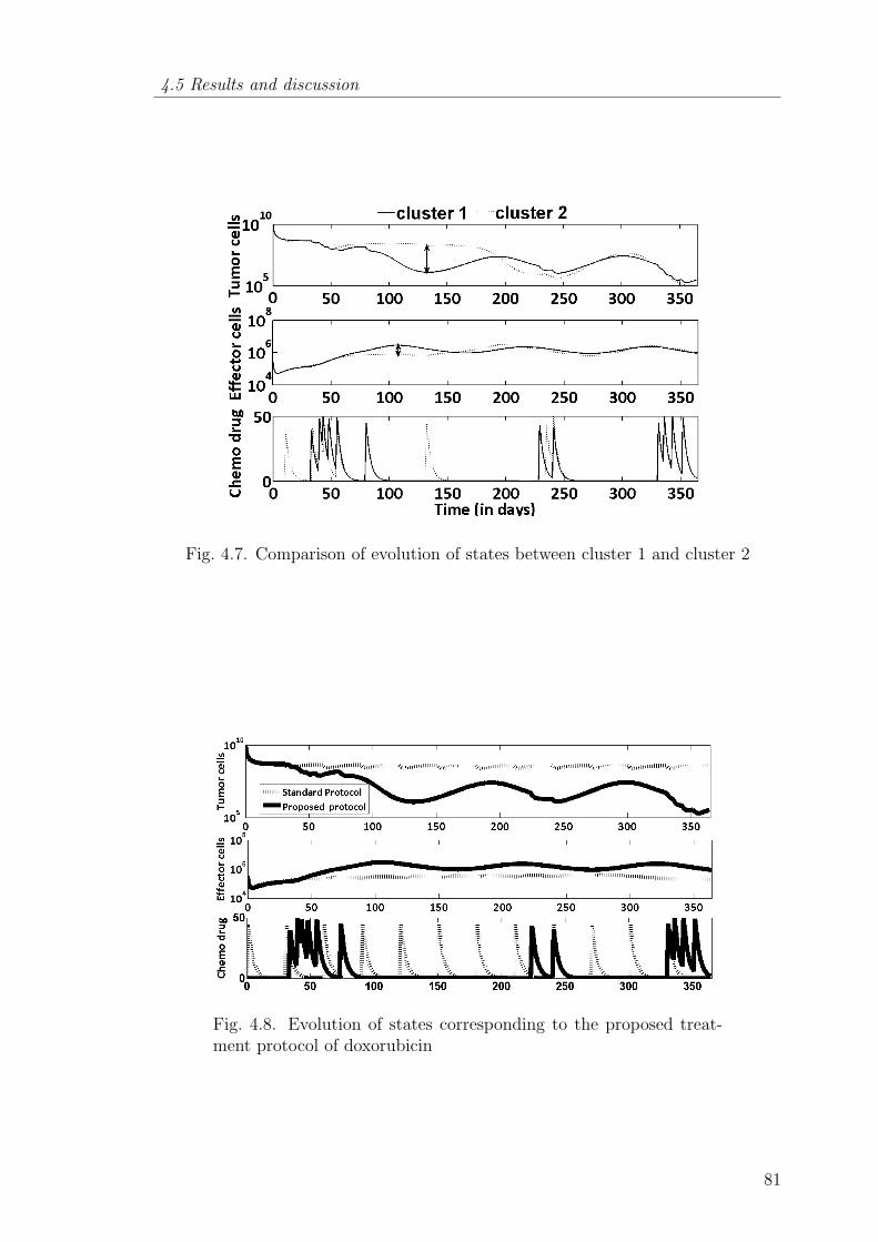
4.5 Results and discussion
Fig. 4.7. Comparison of evolution of states between cluster 1 and cluster 2
Fig. 4.8. Evolution of states corresponding to the proposed treat-ment protocol of doxorubicin
81
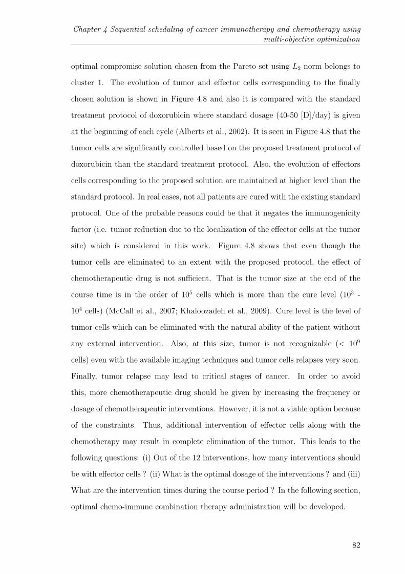
Chapter 4 Sequential scheduling of cancer immunotherapy and chemotherapy usingmulti-objective optimization
optimal compromise solution chosen from the Pareto set using L2 norm belongs to
cluster 1. The evolution of tumor and effector cells corresponding to the finally
chosen solution is shown in Figure 4.8 and also it is compared with the standard
treatment protocol of doxorubicin where standard dosage (40-50 [D]/day) is given
at the beginning of each cycle (Alberts et al., 2002). It is seen in Figure 4.8 that the
tumor cells are significantly controlled based on the proposed treatment protocol of
doxorubicin than the standard treatment protocol. Also, the evolution of effectors
cells corresponding to the proposed solution are maintained at higher level than the
standard protocol. In real cases, not all patients are cured with the existing standard
protocol. One of the probable reasons could be that it negates the immunogenicity
factor (i.e. tumor reduction due to the localization of the effector cells at the tumor
site) which is considered in this work. Figure 4.8 shows that even though the
tumor cells are eliminated to an extent with the proposed protocol, the effect of
chemotherapeutic drug is not sufficient. That is the tumor size at the end of the
course time is in the order of 105 cells which is more than the cure level (103 -
104 cells) (McCall et al., 2007; Khaloozadeh et al., 2009). Cure level is the level of
tumor cells which can be eliminated with the natural ability of the patient without
any external intervention. Also, at this size, tumor is not recognizable (< 109
cells) even with the available imaging techniques and tumor cells relapses very soon.
Finally, tumor relapse may lead to critical stages of cancer. In order to avoid
this, more chemotherapeutic drug should be given by increasing the frequency or
dosage of chemotherapeutic interventions. However, it is not a viable option because
of the constraints. Thus, additional intervention of effector cells along with the
chemotherapy may result in complete elimination of the tumor. This leads to the
following questions: (i) Out of the 12 interventions, how many interventions should
be with effector cells ? (ii) What is the optimal dosage of the interventions ? and (iii)
What are the intervention times during the course period ? In the following section,
optimal chemo-immune combination therapy administration will be developed.
82

4.5 Results and discussion
4.5.2 Case 2: Immune-chemo combination therapy
In this case, an additional objective (objective 4, F2) related to the number
of interventions of effector cells (Ne) is included (Equation (4.9)). However, other
objectives and constraints in the problem formulation are same as mentioned in
Section 4.4. The minimization of objective 4 is important. Biologically, it means,
excessive immune cells may lead to the heavy competition among themselves for the
cytokine (Ho et al., 2003). Cytokines are proteins that are the limiting and essential
constituents for the persistent activation of cytotoxic lymphocytes.
F2 = Ne (4.9)
Overall, in the combination therapy optimization problem, there are 4 objectives,
25 decision variables and 3 constraints. Among the 25 decision variables, there are
24 continuous variables and one integer variable. The integer variable corresponds
to the number of immunotherapeutic interventions (which could range from 1 to
12), and the 24 continuous variables relate to the timing (12) and amount (12) of
the interventions (either chemotherapy or immunotherapy). The multi-objective
optimization is now solved again using NSGA-II with population size and number
of generations being 100 and 250 respectively. Finally, a Pareto front comprising of
multiple solutions is obtained. As it is a 4-dimensional objective function space, the
solution cannot be readily visualized. To make visualization easier, the objectives
relevant to tumor cells and effector cells are summarized separately. F1 corresponds
to the distance between the tumor related objectives on the Pareto curve and their
values in utopia point. Then F1 is plotted against F2 (the number of effector cells
interventions) as shown in Figure 4.9 .
F1 =√
(objective 1)2 + (objective 2)2 + (objective 3)2 (4.10)
83
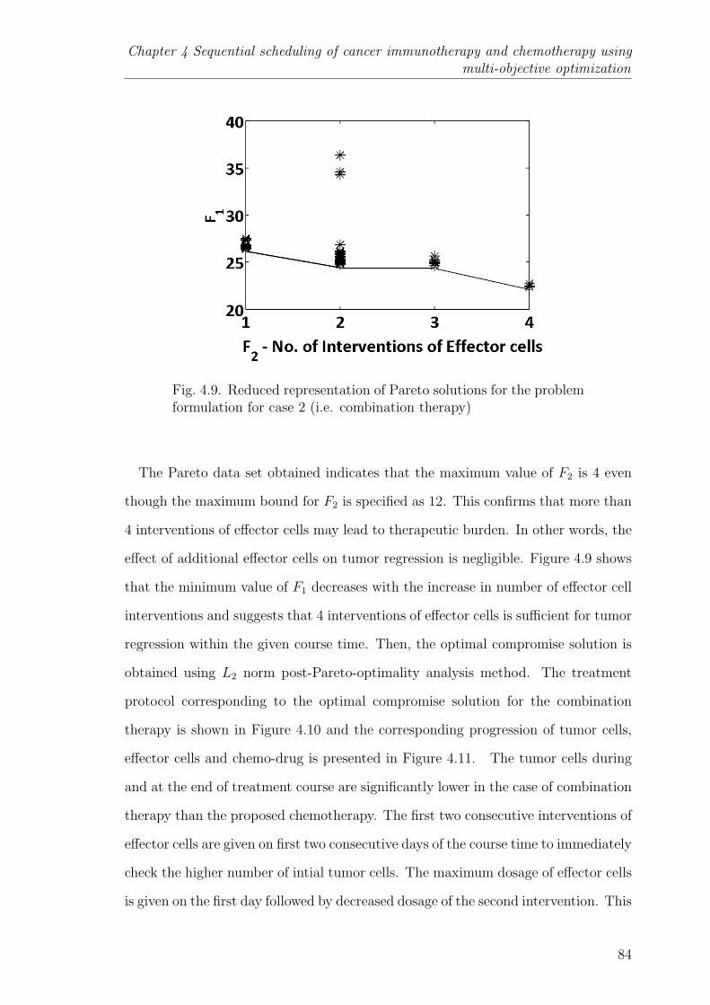
Chapter 4 Sequential scheduling of cancer immunotherapy and chemotherapy usingmulti-objective optimization
Fig. 4.9. Reduced representation of Pareto solutions for the problemformulation for case 2 (i.e. combination therapy)
The Pareto data set obtained indicates that the maximum value of F2 is 4 even
though the maximum bound for F2 is specified as 12. This confirms that more than
4 interventions of effector cells may lead to therapeutic burden. In other words, the
effect of additional effector cells on tumor regression is negligible. Figure 4.9 shows
that the minimum value of F1 decreases with the increase in number of effector cell
interventions and suggests that 4 interventions of effector cells is sufficient for tumor
regression within the given course time. Then, the optimal compromise solution is
obtained using L2 norm post-Pareto-optimality analysis method. The treatment
protocol corresponding to the optimal compromise solution for the combination
therapy is shown in Figure 4.10 and the corresponding progression of tumor cells,
effector cells and chemo-drug is presented in Figure 4.11. The tumor cells during
and at the end of treatment course are significantly lower in the case of combination
therapy than the proposed chemotherapy. The first two consecutive interventions of
effector cells are given on first two consecutive days of the course time to immediately
check the higher number of intial tumor cells. The maximum dosage of effector cells
is given on the first day followed by decreased dosage of the second intervention. This
84

4.5 Results and discussion
Fig. 4.10. Treatment protocol corresponding to the proposed com-bination therapy
Fig. 4.11. Evolution of states corresponding to the proposed combination therapy
85
Chapter 4 Sequential scheduling of cancer immunotherapy and chemotherapy usingmulti-objective optimization
Fig. 4.12. Comparison of tumor relapse time between the proposedchemotherapy and the proposed combination therapy
decrease could be to avoid overdosage and hence therapeutic burden. Instead, the
second intervention is accompanied by the maximum dose of doxorubicin to suppress
tumor growth. Another interesting observation is the decreasing trend of tumor size
until 70 days due to the early interventions and during this period no additional
therapeutic interventions are made. The remaining interventions of effector cell and
doxorubicin are fairly spread out in time. Moreover, the interventions are made only
when the growing phase of tumor cells is detected. Thus, the above features justify
the coherency in the proposed combination therapy protocol.
Tumor relapse time (TRT) is considered as another metric to evaluate the effect
of the proposed optimal therapeutic strategies in case 1 (chemotherapy only) and
case 2 (combination therapy). TRT is defined as the time taken by the tumor to
recur and reach peak from its size at the end of the course time. The increase in
tumor cells is dangerous and increases the probability of tumor transformation to
later stages which limits the efficacy of the therapy (Alberts et al., 2002). A larger
value of TRT is better and it indicates patient survival time without interventions.
86

4.6 Conclusions
It is observed in Figure 4.12 that the peak tumor size corresponding to the combi-
nation therapy is higher than chemotherapy. This is because of the different ratio of
effector cells and tumor cells (E:T) between proposed combination therapy (0.016)
and proposed chemotherapy (0.03) at their respective TRTs. Thus, higher ratio
(E:T) controls the peak values during tumor progression. Clinically, this suggests
that the measurement of the density of effector cells at the tumor location is essen-
tial along with blood cell count. Also, the steady state analysis in either case shows
no difference in tumor size and time taken to reach steady state after the treat-
ment course. However, TRT for the combination therapy is approximately 3 times
more than the chemotherapy (Figure 4.12). Moreover, after combination therapy,
it takes an extra 90 days for the tumor to reach the peak value attained with the
proposed chemotherapy. Overall, the in silico analysis supports that the proposed
combination strategy is pragmatic and appears to be effective than chemotherapy
alone.
4.6 Conclusions
In this chapter, the main idea was to use multi-objective optimization and
post-Pareto-optimality analysis to determine and compare therapeutic strategies
for treatment of tumor. Chemotherapy alone and a combination therapy that in-
cludes chemotherapy and immunotherapy are considered. The multi-objective func-
tions chosen for achieving the satisfactory tumor reduction and the total number
of therapeutic interventions are based on the accepted medical protocols and cur-
rent clinical practice. The simulation results indicate that the performance of the
proposed chemotherapy protocol is better than the standard protocol and suggests
taking into account the immunogenicity factor prior to every therapeutic interven-
tion. However, chemotherapy alone is not sufficient for eradicating the tumor in
the stipulated course time of one year. Additional intervention of effector cells (i.e.
immunotherapy) is required for satisfying all the objectives of the problem. Using
87
Chapter 4 Sequential scheduling of cancer immunotherapy and chemotherapy usingmulti-objective optimization
the L2 norm method to find the optimal compromise solution from the Pareto set,
it is seen that four immunotherapeutic interventions out of twelve interventions is a
better option for treating tumors. More than four immunotherapeutic interventions
lead to unnecessary therapeutic burden with negligible improvement in patient con-
dition. The results suggest that the first two interventions of effector cells should
be at the early phase of the course time in order to control the tumor cells. Then,
remaining interventions are suggested whenever there is a steep rise in the tumor
profile. Thus, the intervention timings seem rational. TRT value is also signifi-
cantly better for the combination therapy. In broader sense, this chapter highlights
that optimization techniques implemented in the treatment planning simulators can
support the oncology pharmacists in determining and analyzing the therapeutic
schedule of a given therapy. In this chapter, it was assumed that the variation of
the patient parameters is negligible. However, in the next chapter, intrapatient vari-
ability is accounted during the treatment and applied the optimization techniques
to guide immunotherapy.
88
Chapter 5
MODEL-BASED SENSITIVITY ANALYSIS AND
REACTIVE SCHEDULING OF DENDRITIC CELL
THERAPY
‘Sensitivity analysis for modellers? Would you go to an orthopaedist
who didn’t use X-ray?’
- Jean-Marie Furbringer
5.1 Introduction
Intrapatient variability is a key challenge in cancer treatment. This makes it nec-
essary to find the factors affecting tumor growth and accordingly schedule therapies
over the treatment horizon for a given patient. In this chapter, model-based studies
are performed to investigate these issues for optimal immunotherapeutic interven-
tion. Dendritic cell therapy is a targeted immunotherapy where the dendritic cells
and its activating agents such as interleukin are engineered, stimulated to recognize
and specifically to eradicate tumors. A mathematical model that integrates tumor
dynamics and dendritic cell therapy is used to perform the analysis. Unlike the
previous chapter, in this chapter different types of immune cells are explicitly con-
sidered instead of assuming all of them as effector cells. Global sensitivity analysis
of the model is done using high dimensional model reduction (HDMR) technique fol-
lowed by variance based analysis and the key parameters altering the tumor growth
are identified. The variations in these key parameters are deemed to result in in-
trapatient variability during the treatment phase. Then, reactive scheduling is used
89

Chapter 5 Model-based sensitivity analysis and reactive scheduling of dendritic celltherapy
Fig. 5.1. Dendritic cell/Vaccine therapy
to schedule dendritic cell interventions with and without interleukin interventions
under the varying conditions of the patient. Moreover, the key parameters obtained
from HDMR are verified using the reactive scheduling and nominal scheduling ap-
proaches. Besides saving costs, the in silico analysis done in this chapter may be
useful to the oncology community in designing experiments to clinically measure the
influential parameters.
5.1.1 Dendritic cell therapy
Dendritic cells (DC) are the professional antigen presenting cells which are
present in small amounts in the blood and almost every tissue. They work at the
interface between the peripheral tissues and lymphoid organs and induce the T-cell
mediated immune response. In dendritic cancer vaccine (DCV) therapy, dendritic
cells are fused with tumor associated antigens to mature and transform to antigen-
loaded dendritic cells (Ballestrero et al., 2008; Banchereau et al., 2001; Nencioni
et al., 2008). Then, these matured dendritic cells are injected back to the patient
(see Figure 5.1). Tumor associated antigens can be of different forms (DNA, RNA,
90
5.2 Scheduling under uncertainty
proteins, peptides, killed tumor cells and cell lysates). Overall, the main parameters
of DCV are type of DC subset and its maturation, dosage, frequency and route of
injection of DC. Like other therapies, higher frequency of DC dosage might lead
to activation-induced death of T-cells. Even the induced cytotoxic T-cells may kill
DCs. In either case, efficacy of the vaccine reduces. In order to overcome this,
oncologists are proposing combination therapies, presuming their synergistic action
on the tumor size. In such cases, adjuvant therapy such as interleukin therapy can
be given to maintain the prolonged activity of the T-cells (Banchereau et al., 2001).
5.2 Scheduling under uncertainty
In the domain of mathematical modeling, system uncertainty is a very impor-
tant issue. Here, one quantifies the uncertainty in the model output that is gen-
erated from the uncertainty in the parameters and input factors (Marino et al.,
2008; Saltelli et al., 2008). In model-based approaches, uncertainties of model pa-
rameters are considered using different methods such as bounded form, probability
description, and fuzzy description (Li and Ierapetritou, 2008a). Bounded form and
probability description methods are used when the historical data related to pa-
rameters are available. Else, fuzzy description is used. A probability description is
preferred when specific information about the distribution of parameters is known
whereas bounded form is considered only when we know the range of the parameters.
However, it is not often that parameter of a biological system has a detailed descrip-
tion. Theoretically, in this case, the problem is solved by assuming that parameters
follow a simple probabilistic distribution such as uniform distribution. Scheduling
under uncertainty is a challenging problem in technological and biomedical systems.
It is broadly classified as preventive scheduling (schedule generation) and reactive
scheduling (schedule revision) (Li and Ierapetritou, 2008a,b). Preventive scheduling
is used when the knowledge of the possible uncertain events are available based
on the historical experiences. Thus, in this case, rigorous analysis is made before
91
Chapter 5 Model-based sensitivity analysis and reactive scheduling of dendritic celltherapy
implementing the schedule. Different techniques for preventive scheduling include
stochastic scheduling, robust optimization, fuzzy programming, sensitivity analysis
and parametric programming. Contrastingly, in reactive scheduling or reschedul-
ing, the schedule is regularly updated or modified and adapted to the unexpected
disturbances of the system (Li and Ierapetritou, 2008b). It is considered that the
present problem of DCV therapy falls under the category of reactive scheduling.
This is because patients are regularly monitored by oncologists and the treatment
plan may be adjusted based on their condition at the time of their regular check up.
If there is any change in patient’s condition from what was expected, the treatment
schedule is suitably rescheduled. However, there are some shortcomings with reac-
tive scheduling. The prime concern is the reaction time available to make updated
decisions. The reaction time varies for different unexpected scenarios. Another
important point is that the reactive decisions can be taken only after identifying
the reasons for the unexpected scenario. In the language of mathematical model-
ing, this means unraveling the sensitive parameters responsible for uncertainty in
the measurable or observable variables. Taking into consideration the positive and
shortcomings discussed above, a hybrid approach that involves global sensitivity
analysis (Marino et al., 2008) followed by reactive scheduling is proposed in this
chapter. This approach involves the application of global sensitivity analysis of the
model to find the prominent parameters and considering uncertainty only in these
parameters to perform reactive scheduling. The main asssumptions in this study are
that the parameters follow uniform distribution and the uncertainty in the output
of interest (eg., tumor growth) is only because of variations in the parameters.
5.3 Mathematical model
Among all tumor-immune models, the only work which explicitly includes the
activity of dendritic cells is that of Piccoli and Castiglione (2006) and this work is
focused on the investigation of DCV therapy scheduling. The model explains the
92

5.3 Mathematical model
tumor evolution and its interaction with the helper T-cells (CD4+) and cytotoxic
T-cells (CD8+) due to the intervention of externally modified and antigen-loaded
dendritic cells. The model assumes that all tumor cells are immunogenic. In other
words, tumor cells are recognized by injected dendritic cells and are presented to
cytotoxic T-cells. The interactions between the cytotoxic T-lymphocytes and the
tumor cells are represented by a kinetic scheme and are presented in the form of
ordinary differential equations. The states in the model are denoted by
(a) H(t), helper T-cells (CD4+)
(b) C(t), cytotoxic T-cells (CD8+)
(c) M(t), tumor cells
(d) D(t), dendritic cells
(e) I(t), interleukin
dH
dt= a0 − b0H + c0Dd0γ(H, f0) (5.1)
dc
dt= a1 − b1C + c1I(M +D)d1γ(C, f1) (5.2)
dM
dt= d2γ(M, f2)− e2MC (5.3)
dD
dt= −e3DC + u1 (5.4)
dI
dt= a4HD − c4CI − e4I + u2 (5.5)
where
γ(x, θ) = x(1− x/θ)
The first two terms (a0 , b0H) in Equation (5.1) depict the natural flow of helper
T-cells to the tumor site (non-stimulated by tumor presence) and their natural decay
rate respectively. Similarly, the first two terms (a1, b1C) in Equation (5.2) repre-
sent the natural flow rate of cytotoxic T-cells to the tumor site (non-stimulated
by tumor presence) and their natural decay rate respectively. The model assumes
93
Chapter 5 Model-based sensitivity analysis and reactive scheduling of dendritic celltherapy
that tumor growth follows the logistic equation with the constants d2 and f2. d2
is the maximal growth rate of tumor cells and f2 is carrying capacity of tumor
cells. These parameters signify tumor growth because of nutrients such as glucose
and oxygen without the effect of immune response. The term e2MC in Equa-
tion (5.3) represents pharmacodynamics which means the elimination of tumor cells
due to CD8+ T-cells. Equation (5.4) explains the pharmacokinetics (e3DC) and
‘u1’ is the input rate of the matured and antigen-loaded dendritic cells. Once the
dendritic cells are injected, the CD4+ T-cells, CD8+ T-cells, and interleukins are
triggered as shown in Equations (5.1, 5.2 & 5.5) respectively by the following terms
(c0Dd0γ(H, f0), c1I(M + D)d1γ(C, f1), a4HD). In the same way, the second and
third terms in Equation (5.5) denote the loss of interleukin (IL-2) as a result of
its interactions with CD8+ T-cells and its natural decay respectively and ‘u2’ is
the input rate of externally administered interleukin. Another assumption in the
model is that externally administered DCV is the only source of dendritic cells. The
parameter values of the mathematical model are given in Table 5.1.
5.4 Global sensitivity analysis
Global sensitivity analysis (GSA) is an approach to identify and quantify the
factors (parameters) contributing to the variation in the objective of interest (tu-
mor size). Unlike local sensitivity analysis, the factors are varied simultaneously
over a wide range in GSA. Saltelli et al. (2008) describe the different methods that
are available to perform GSA based on the a priori knowledge of the relationship
between inputs and outputs. The measures used for linear relationship between the
parameters and the output are Pearson correlation coefficient, partial correlation
coefficient and regression coefficient. For monotonic nonlinear relationships, rank
based transforms such as Spearman rank coefficient, partial rank correlation coeffi-
cient and rank regression coefficient could be considered. Variance based methods
(VBM) such as Sobol method, extended Fourier amplitude sensitivity tests (EFAST)
94

5.4 Global sensitivity analysis
Table 5.1Parameter values (Piccoli and Castiglione, 2006)
Parameter Description Value Unitsc=cells, h=hours
a0 birth rate 10−4 ch−1mm−3
b0 death rate 0.005 h−1
c0 Maximum proliferation rate 10d0 1/2 saturation constant 10−2 c−1h−1mm3
f0 Carrying capacity 1 cmm−3
a1 birth rate 10−4 ch−1mm−3
b1 death rate 0.005 h−1
c1 Maximum proliferation rate 10d1 1/2 saturation constant 10−2 h−1(mm−3/c)2
f1 Carrying capacity 1 cmm−3
d2 1/2 saturation constant of tumor 0.02 h−1
e2 Killing of tumor cells by CD8+ T-cells 0.1 c−1h−1mm3
f2 Carrying capacity of tumor 1 cmm−3
e3 CD8+ T cells killing of DC 0.1 c−1h−1mm3
a4 IL-2 production 10−2 c−1h−1mm3
c4 IL-2 uptake 10−7 c−1h−1mm3
e4 IL-2 degradation rate 10−2 h−1
are preferred owing to their wider applicability (Marino et al., 2008; Saltelli et al.,
1999). In these approaches variance of the output is decomposed into contributions
from different factors. Sensitivity indices are calculated to rank the factors based
on their contributions. The main advantages of VBM are: (i) sensitivity measure
is model-free (ii) it is able to realize the impact of full range of variations of each
input factor and the interactions among the input factors and (iii) reliability. In
spite of these advantages, there is one major disadvantage. In most of the cases,
direct relationship between input and output factors is unknown. As a result, it
is computationally expensive to evaluate output by solving nonlinear differential
equations for different set of input factors. In that regard, metamodeling approach
is an alternative where the inputs and outputs are directly related and it is a com-
putationally cheaper approximation of the original model. Then, the philosophy of
variance based sensitivity analysis can be extended to these metamodels for identify-
95
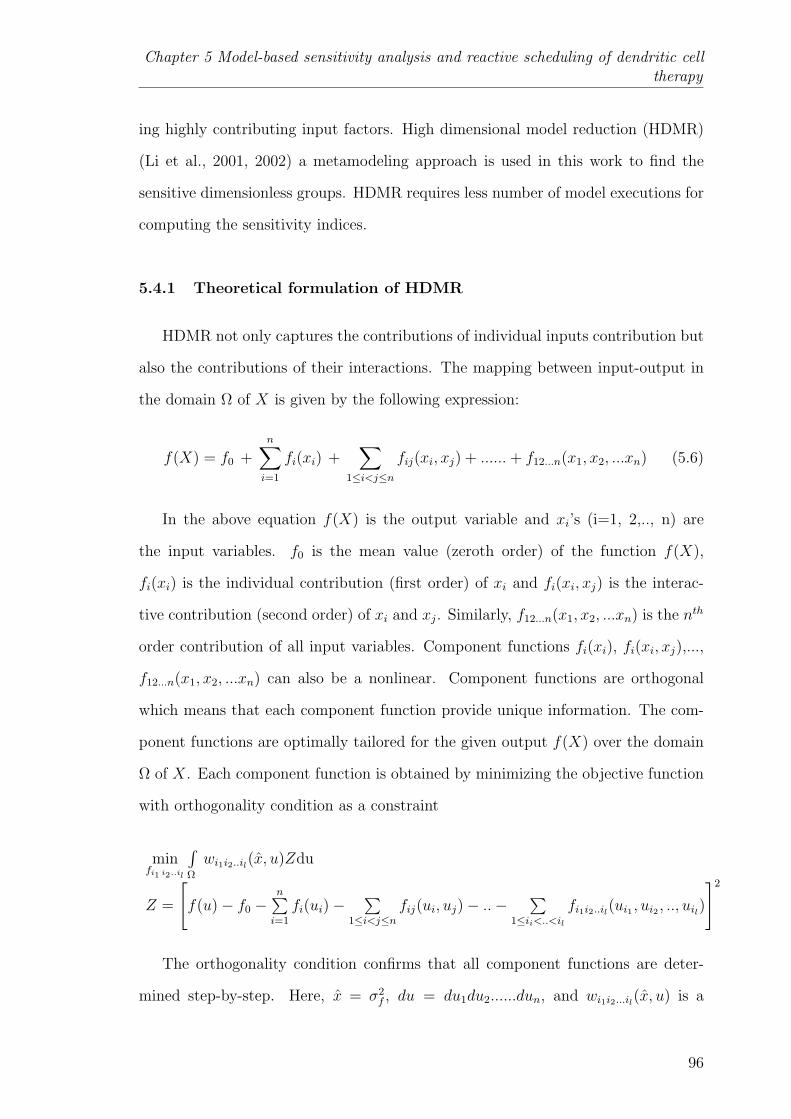
Chapter 5 Model-based sensitivity analysis and reactive scheduling of dendritic celltherapy
ing highly contributing input factors. High dimensional model reduction (HDMR)
(Li et al., 2001, 2002) a metamodeling approach is used in this work to find the
sensitive dimensionless groups. HDMR requires less number of model executions for
computing the sensitivity indices.
5.4.1 Theoretical formulation of HDMR
HDMR not only captures the contributions of individual inputs contribution but
also the contributions of their interactions. The mapping between input-output in
the domain Ω of X is given by the following expression:
f(X) = f0 +n∑i=1
fi(xi) +∑
1≤i<j≤n
fij(xi, xj) + ......+ f12...n(x1, x2, ...xn) (5.6)
In the above equation f(X) is the output variable and xi’s (i=1, 2,.., n) are
the input variables. f0 is the mean value (zeroth order) of the function f(X),
fi(xi) is the individual contribution (first order) of xi and fi(xi, xj) is the interac-
tive contribution (second order) of xi and xj. Similarly, f12...n(x1, x2, ...xn) is the nth
order contribution of all input variables. Component functions fi(xi), fi(xi, xj),...,
f12...n(x1, x2, ...xn) can also be a nonlinear. Component functions are orthogonal
which means that each component function provide unique information. The com-
ponent functions are optimally tailored for the given output f(X) over the domain
Ω of X. Each component function is obtained by minimizing the objective function
with orthogonality condition as a constraint
minfi1 i2..il
∫Ω
wi1i2..il(x, u)Zdu
Z =
[f(u)− f0 −
n∑i=1
fi(ui)−∑
1≤i<j≤nfij(ui, uj)− ..−
∑1≤ii<..<il
fi1i2..il(ui1 , ui2 , .., uil)
]2
The orthogonality condition confirms that all component functions are deter-
mined step-by-step. Here, x = σ2f , du = du1du2......dun, and wi1i2...il(x, u) is a
96
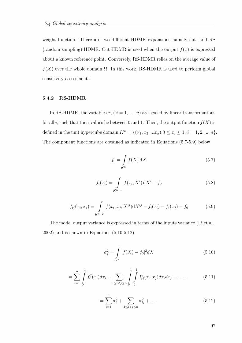
5.4 Global sensitivity analysis
weight function. There are two different HDMR expansions namely cut- and RS
(random sampling)-HDMR. Cut-HDMR is used when the output f(x) is expressed
about a known reference point. Conversely, RS-HDMR relies on the average value of
f(X) over the whole domain Ω. In this work, RS-HDMR is used to perform global
sensitivity assessments.
5.4.2 RS-HDMR
In RS-HDMR, the variables xi ( i = 1, ...., n) are scaled by linear transformations
for all i, such that their values lie between 0 and 1. Then, the output function f(X) is
defined in the unit hypercube domainKn = (x1, x2, ...xn)|0 ≤ xi ≤ 1, i = 1, 2, ..., n.
The component functions are obtained as indicated in Equations (5.7-5.9) below
f0 =
∫Kn
f(X) dX (5.7)
fi(xi) =
∫Kn−1
f(xi, Xi) dX i − f0 (5.8)
fij(xi, xj) =
∫Kn−2
f(xi, xj, Xij)dX ij − fi(xi)− fj(xj)− f0 (5.9)
The model output variance is expressed in terms of the inputs variance (Li et al.,
2002) and is shown in Equations (5.10-5.12)
σ2f =
∫Kn
[f(X)− f0]2dX (5.10)
=n∑i=1
1∫0
f 2i (xi)dxi +
∑1≤i<j≤n
1∫0
1∫0
f 2ij(xi, xj)dxidxj + ........ (5.11)
=n∑i=1
σ2i +
∑1≤i<j≤n
σ2ij + ..... (5.12)
97
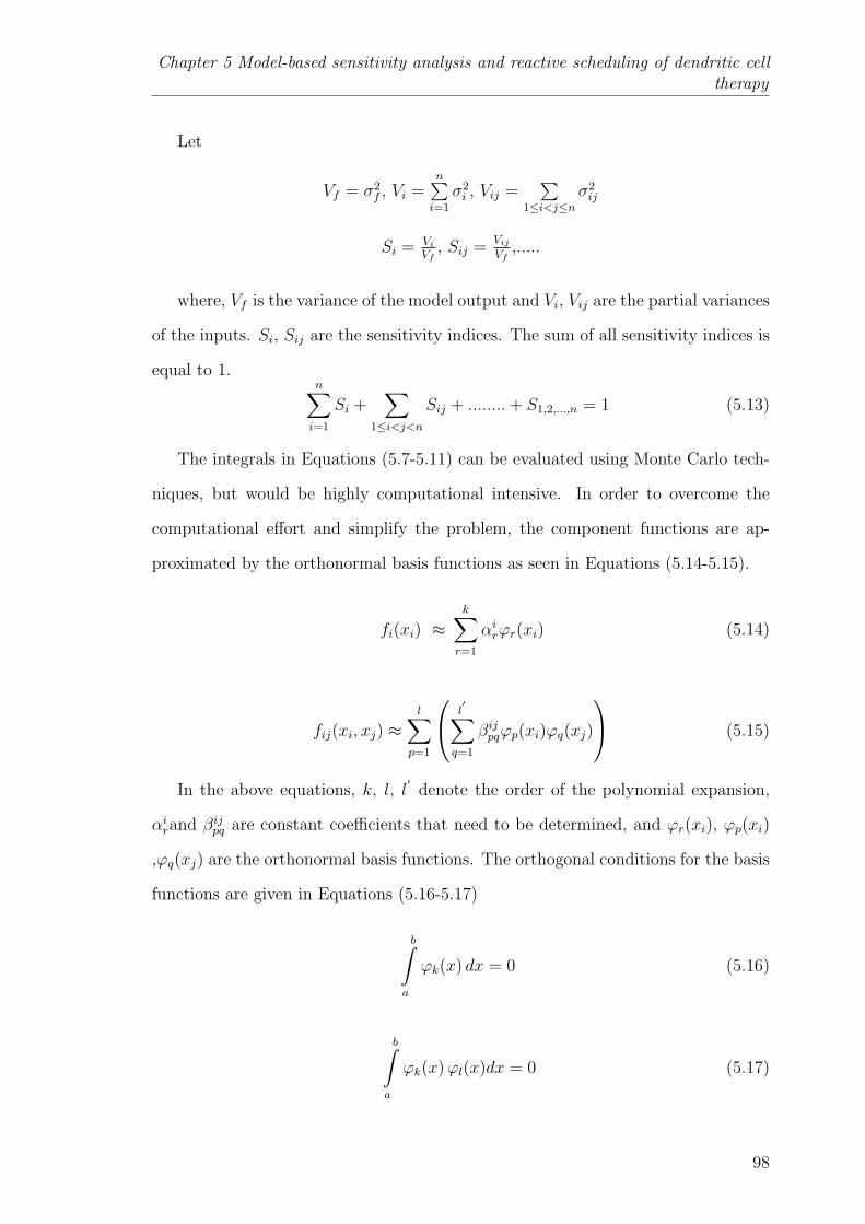
Chapter 5 Model-based sensitivity analysis and reactive scheduling of dendritic celltherapy
Let
Vf = σ2f , Vi =
n∑i=1
σ2i , Vij =
∑1≤i<j≤n
σ2ij
Si = Vi
Vf, Sij =
Vij
Vf,.....
where, Vf is the variance of the model output and Vi, Vij are the partial variances
of the inputs. Si, Sij are the sensitivity indices. The sum of all sensitivity indices is
equal to 1.n∑i=1
Si +∑
1≤i<j<n
Sij + ........+ S1,2,...,n = 1 (5.13)
The integrals in Equations (5.7-5.11) can be evaluated using Monte Carlo tech-
niques, but would be highly computational intensive. In order to overcome the
computational effort and simplify the problem, the component functions are ap-
proximated by the orthonormal basis functions as seen in Equations (5.14-5.15).
fi(xi) ≈k∑r=1
αirϕr(xi) (5.14)
fij(xi, xj) ≈l∑
p=1
l′∑
q=1
βijpqϕp(xi)ϕq(xj)
(5.15)
In the above equations, k, l, l′
denote the order of the polynomial expansion,
αirand βijpq are constant coefficients that need to be determined, and ϕr(xi), ϕp(xi)
,ϕq(xj) are the orthonormal basis functions. The orthogonal conditions for the basis
functions are given in Equations (5.16-5.17)
b∫a
ϕk(x) dx = 0 (5.16)
b∫a
ϕk(x)ϕl(x)dx = 0 (5.17)
98
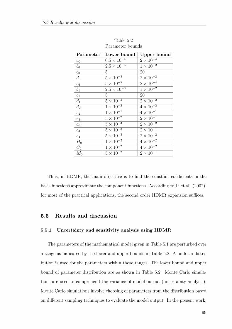
5.5 Results and discussion
Table 5.2Parameter bounds
Parameter Lower bound Upper bounda0 0.5× 10⁻⁴ 2× 10⁻⁴
b0 2.5× 10⁻³ 1× 10⁻²
c0 5 20d0 5× 10⁻³ 2× 10⁻²
a1 5× 10⁻⁵ 2× 10⁻⁴
b1 2.5× 10⁻³ 1× 10⁻²
c1 5 20d1 5× 10⁻³ 2× 10⁻²
d2 1× 10⁻² 4× 10⁻²
e2 1× 10⁻¹ 4× 10⁻¹
e3 5× 10⁻² 2× 10⁻¹
a4 5× 10⁻³ 2× 10⁻²
c4 5× 10⁻⁸ 2× 10⁻⁷
e4 5× 10⁻³ 2× 10⁻²
H0 1× 10⁻² 4× 10⁻²
C0 1× 10⁻² 4× 10⁻²
M0 5× 10⁻² 2× 10⁻¹
Thus, in HDMR, the main objective is to find the constant coefficients in the
basis functions approximate the component functions. According to Li et al. (2002),
for most of the practical applications, the second order HDMR expansion suffices.
5.5 Results and discussion
5.5.1 Uncertainty and sensitivity analysis using HDMR
The parameters of the mathematical model given in Table 5.1 are perturbed over
a range as indicated by the lower and upper bounds in Table 5.2. A uniform distri-
bution is used for the parameters within those ranges. The lower bound and upper
bound of parameter distribution are as shown in Table 5.2. Monte Carlo simula-
tions are used to comprehend the variance of model output (uncertainty analysis).
Monte Carlo simulations involve choosing of parameters from the distribution based
on different sampling techniques to evaluate the model output. In the present work,
99
Chapter 5 Model-based sensitivity analysis and reactive scheduling of dendritic celltherapy
Latin hypercube sampling is used, because, it requires lesser samples (compared to
other sampling strategies) to provide an unbiased estimate of the model output and
ensures the coverage of the entire domain of the parameter space. The model output
of interest, in this case, is related to the tumor cells and the expression is given by
Equation (5.18).
G =
tf∫0
M(t, P ) dt (5.18)
where, G is model output, P is the parameter set (inputs) and tf is the final time. It
is assumed that measurement error associated with G is negligible. It implies that
the variations in G is only because of variations in the parameters. Uncertainty
analysis of G is done for different sample sizes (N) and the HDMR model in combi-
nation with variance based method is then applied to uncover the key parameters.
The HDMR model is justified based on the accuracy value for first and second order
component functions and the average G values (f0). It is known that a good meta-
model (HDMR model) is possible if it is built using larger number of samples. Table
5.3 shows that with the increase in sample size from 1000 to 7000, ∆f0 is observed to
decrease drastically to a very low value. So, HDMR analysis is concluded with 7000
samples. Relative percentage error is the allowable percentage of error in predicting
the validation data set by the HDMR model. Accuracy value denotes the prognostic
ability of the HDMR model. If the accuracy value is 100%, it means that the model
is able to reproduce the results of the data used for validation. It is obvious that
accuracy value of a model always increases with the increase in relative percentage
error and for a given sample size, similar trend is observed for both first order and
second order component function HDMR models. Also, for a given sample size and
relative percentage error, the accuracy value increase appreciably from first order
to the second order component function. The accuracy values for 20% relative error
are more than 97% for all sample sizes and for both 1st and 2nd order component
functions. Overall, Table 5.3 conveys that a reasonable and simple metamodel can
represent the data generated by the parameter perturbations. Table 5.4 presents
100

5.5 Results and discussion
Table 5.3Variation of accuracy with sample size and relative error
AccuracySample Size (N) f0 ∆f0 1st order 2nd order
(average G value) = |(f0)j+1 − (f0)j | Relative error (%) Relative error (%)
5% 10% 20% 5% 10% 20%
1000 0.821 0.031 63.5 93.5 97.5 84 97 98.5
3000 0.852 0.01 72.5 93.7 98 82.7 97.5 99.2
5000 0.862 0.001 78.6 95.8 98.3 98.2 99.2 99.7
7000 0.863 80.4 95.3 97.5 93.7 97.8 98.9
Table 5.4Parameter ranking (R)
Sample Size (N) 1st order (Si)∑Si 2nd order (Sij)
∑Sij
R1 R2 R3 R4 R1 R2 R3 R4 R5
1000 9 6 10 5 0.812 (9,10) (6,9) (5,10) (5,9) (5,6) 0.102
3000 9 6 10 5 0.798 (6,9) (5,6) (9,10) (5,9) (6,10) 0.1477
5000 9 6 10 5 0.834 (6,9) (9,10) (6,10) (5,9) (5,6) 0.1375
7000 9 6 10 5 0.842 (6,9) (9,10) (5,9) (5,6) (5,10) 0.1096
ranking order of the individual and interactive contributions of the parameters to
the output G. The parameter numbers provided in Table 5.4 follows to the serial
number order mentioned in Table 5.2. Consistency in the ranking of the individual
contributions of the parameters is seen for all the sample sizes. The summation
of the sensitivity indices of individual contributions and interactive contributions
account for approximately 80% and 12% respectively for the total variance of G.
Although, there is disparity in the sequence of the interactive contributions, the
interactive parameter sets are almost the same for all sample sizes. Thus, the sen-
sitive parameters responsible for the tumor evolution are d2, b1, e2 and a1. The
overall contributions of the parameters are (evaluated using Equations (5.10-5.13)):
d2 (31%), e2 (21%), b1 (16%), a1 (15%), other first order interactions (12%) and
higher order interactions (5%).
101
Chapter 5 Model-based sensitivity analysis and reactive scheduling of dendritic celltherapy
5.5.2 Validation of HDMR results using reactive scheduling
The sensitive parameters obtained via HDMR analysis are verified by the applica-
tion of reactive scheduling approach on the dendritic cell therapy planning problem.
The physiological model described in section 5.3 will serve as the “patient”. In this
regard, three cases are considered. The first case is nominal scheduling, where the
schedule for the total time horizon is based on the initially observed parameter val-
ues and does not consider their variation. In the second and third cases, reactive
scheduling is considered by varying the sensitive parameters and insensitive param-
eters (as found from the HDMR analysis) respectively. Then, the results of all the
cases are compared. In this optimization problem, the objective is to minimize the
number of tumor cells by the end of time horizon using appropriate interventions
of dendritic cells. The interventions are assumed to be spaced evenly at two weeks.
The duration of each intervention is fixed to be 1 hour. Practically, this implies that
the patient’s condition is checked once every two weeks and appropriate dendritic
cell intervention is provided (Banchereau et al., 2001). Here, the time horizon to
eliminate the tumor is taken to be around 6 months (or 4500 hours). Thus, the pa-
tient undergoes 14 interventions over the treatment horizon. The nominal schedule
resembles the situation where the physician designs the treatment schedule based
on initial observation of the patient and proceeds to give corresponding dosage of
dendritic cells until the end of the time horizon. However, in reactive scheduling,
the treatment schedule is updated based on the patient’s condition at the time of
each intervention. As a result, the number of interventions for which the dosage of
dendritic cells to be planned will decrease everytime by 1 at each intervention point.
The dosage of dendritic cells is constrained between 0 and 2 units (Banchereau et al.,
2001). This optimization problem is solved using simulated annealing (Kirkpatrick
et al., 1983) algorithm implemented in MATLAB.
102

5.5 Results and discussion
Problem formulation
Objectives
• minu(tk)
M(tf )
where, k is the intervention number and k = 1, 2...., 14
Constraints
• Mathematical model
• tf = 6 months
• Intervention timings are fixed, tk = (k − 1)× 14× 24
•
if (tk < t < tk + 1)
0 ≤ u1 ≤ 2
else
u1 = 0
Decision Variables
• Dosage of dendritic cells at each intervention
5.5.3 Comparison between nominal and reactive schedule for cases 1-3
In cases 1 and 3, the dosages of dendritic cells are expected to be the same with
either nominal schedule or reactive schedule. This is because case 1 considers no
variation in parameters and case 3 considers variation only in the non-key parame-
ters. From Figure 5.2, it is seen that the dosage rates for case 1 in either schedules
are almost same. In case 2, the key parameters (d2, b1, e2 and a1 ) found from
HDMR analysis are varied randomly and Figure 5.3 shows that there is a signifi-
cant difference between dosage values of dendritic cells to achieve approximately the
same final tumor size. In Figure 5.4 which corresponds to case 3, the dosage rates
are observed to be practically the same except at the interventions 2 and 4.
103
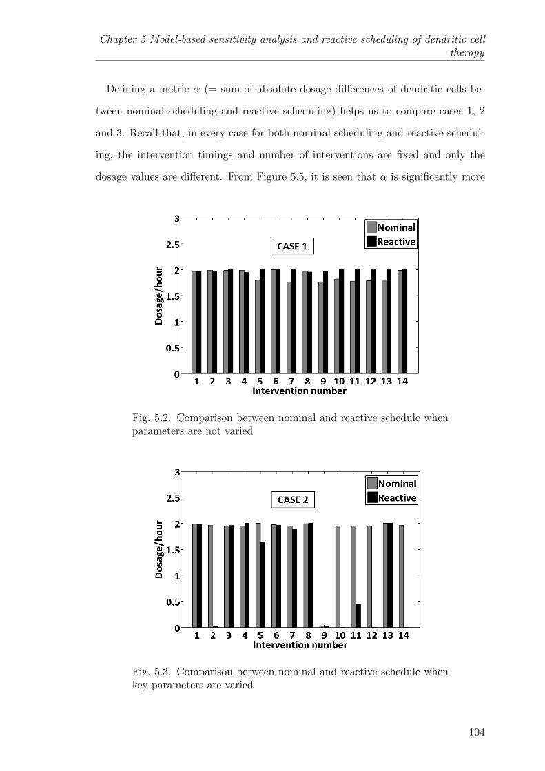
Chapter 5 Model-based sensitivity analysis and reactive scheduling of dendritic celltherapy
Defining a metric α (= sum of absolute dosage differences of dendritic cells be-
tween nominal scheduling and reactive scheduling) helps us to compare cases 1, 2
and 3. Recall that, in every case for both nominal scheduling and reactive schedul-
ing, the intervention timings and number of interventions are fixed and only the
dosage values are different. From Figure 5.5, it is seen that α is significantly more
Fig. 5.2. Comparison between nominal and reactive schedule whenparameters are not varied
Fig. 5.3. Comparison between nominal and reactive schedule whenkey parameters are varied
104
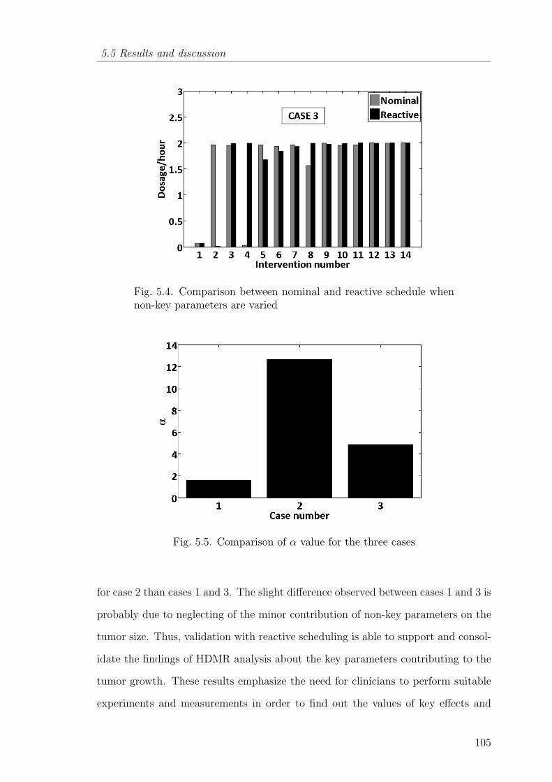
5.5 Results and discussion
Fig. 5.4. Comparison between nominal and reactive schedule whennon-key parameters are varied
Fig. 5.5. Comparison of α value for the three cases
for case 2 than cases 1 and 3. The slight difference observed between cases 1 and 3 is
probably due to neglecting of the minor contribution of non-key parameters on the
tumor size. Thus, validation with reactive scheduling is able to support and consol-
idate the findings of HDMR analysis about the key parameters contributing to the
tumor growth. These results emphasize the need for clinicians to perform suitable
experiments and measurements in order to find out the values of key effects and
105
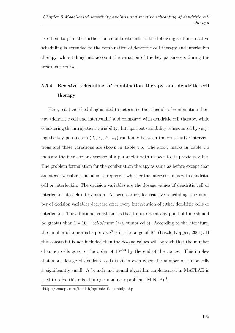
Chapter 5 Model-based sensitivity analysis and reactive scheduling of dendritic celltherapy
use them to plan the further course of treatment. In the following section, reactive
scheduling is extended to the combination of dendritic cell therapy and interleukin
therapy, while taking into account the variation of the key parameters during the
treatment course.
5.5.4 Reactive scheduling of combination therapy and dendritic cell
therapy
Here, reactive scheduling is used to determine the schedule of combination ther-
apy (dendritic cell and interleukin) and compared with dendritic cell therapy, while
considering the intrapatient variability. Intrapatient variability is accounted by vary-
ing the key parameters (d2, e2, b1, a1) randomly between the consecutive interven-
tions and these variations are shown in Table 5.5. The arrow marks in Table 5.5
indicate the increase or decrease of a parameter with respect to its previous value.
The problem formulation for the combination therapy is same as before except that
an integer variable is included to represent whether the intervention is with dendritic
cell or interleukin. The decision variables are the dosage values of dendritic cell or
interleukin at each intervention. As seen earlier, for reactive scheduling, the num-
ber of decision variables decrease after every intervention of either dendritic cells or
interleukin. The additional constraint is that tumor size at any point of time should
be greater than 1× 10⁻¹⁰cells/mm3 (≈ 0 tumor cells). According to the literature,
the number of tumor cells per mm3 is in the range of 106 (Laszlo Kopper, 2001). If
this constraint is not included then the dosage values will be such that the number
of tumor cells goes to the order of 10−20 by the end of the course. This implies
that more dosage of dendritic cells is given even when the number of tumor cells
is significantly small. A branch and bound algorithm implemented in MATLAB is
used to solve this mixed integer nonlinear problem (MINLP) 1.
1http://tomopt.com/tomlab/optimization/minlp.php
106
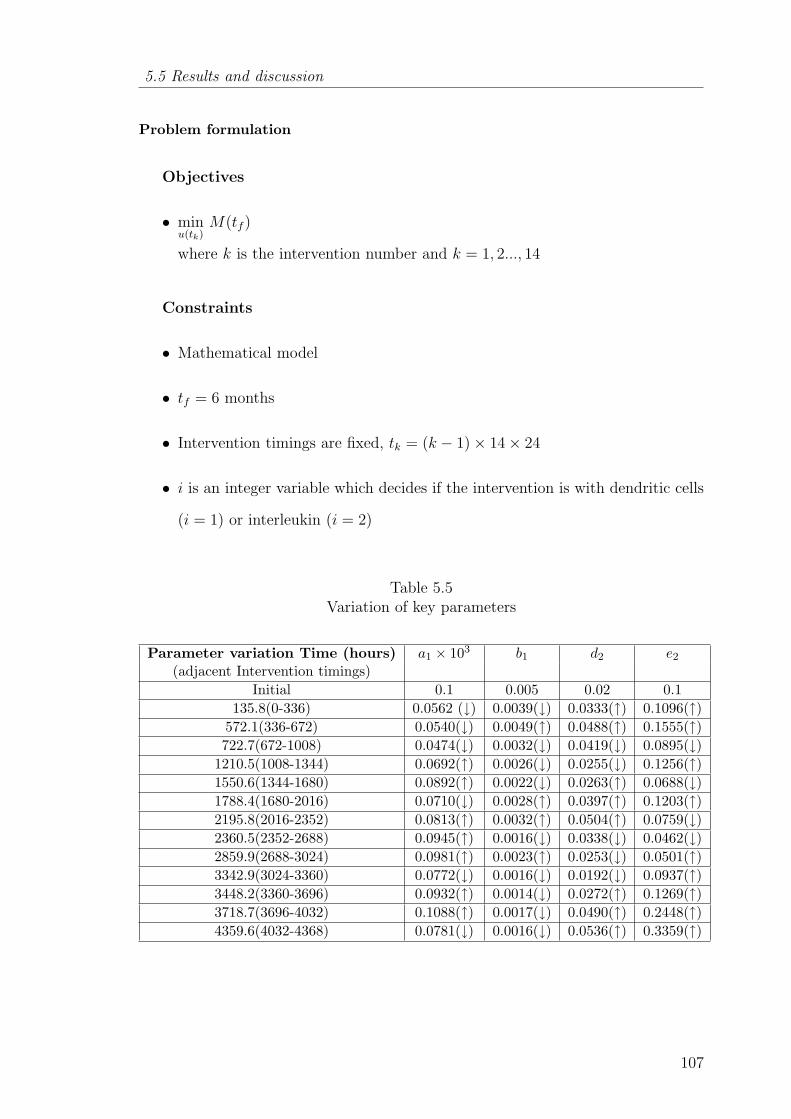
5.5 Results and discussion
Problem formulation
Objectives
• minu(tk)
M(tf )
where k is the intervention number and k = 1, 2..., 14
Constraints
• Mathematical model
• tf = 6 months
• Intervention timings are fixed, tk = (k − 1)× 14× 24
• i is an integer variable which decides if the intervention is with dendritic cells
(i = 1) or interleukin (i = 2)
Table 5.5Variation of key parameters
Parameter variation Time (hours) a1 × 103 b1 d2 e2
(adjacent Intervention timings)Initial 0.1 0.005 0.02 0.1
135.8(0-336) 0.0562 (↓) 0.0039(↓) 0.0333(↑) 0.1096(↑)572.1(336-672) 0.0540(↓) 0.0049(↑) 0.0488(↑) 0.1555(↑)722.7(672-1008) 0.0474(↓) 0.0032(↓) 0.0419(↓) 0.0895(↓)
1210.5(1008-1344) 0.0692(↑) 0.0026(↓) 0.0255(↓) 0.1256(↑)1550.6(1344-1680) 0.0892(↑) 0.0022(↓) 0.0263(↑) 0.0688(↓)1788.4(1680-2016) 0.0710(↓) 0.0028(↑) 0.0397(↑) 0.1203(↑)2195.8(2016-2352) 0.0813(↑) 0.0032(↑) 0.0504(↑) 0.0759(↓)2360.5(2352-2688) 0.0945(↑) 0.0016(↓) 0.0338(↓) 0.0462(↓)2859.9(2688-3024) 0.0981(↑) 0.0023(↑) 0.0253(↓) 0.0501(↑)3342.9(3024-3360) 0.0772(↓) 0.0016(↓) 0.0192(↓) 0.0937(↑)3448.2(3360-3696) 0.0932(↑) 0.0014(↓) 0.0272(↑) 0.1269(↑)3718.7(3696-4032) 0.1088(↑) 0.0017(↓) 0.0490(↑) 0.2448(↑)4359.6(4032-4368) 0.0781(↓) 0.0016(↓) 0.0536(↑) 0.3359(↑)
107
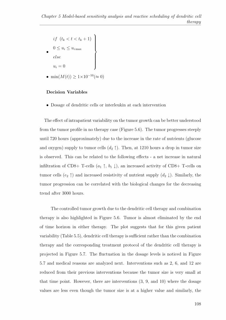
Chapter 5 Model-based sensitivity analysis and reactive scheduling of dendritic celltherapy
•
if (tk < t < tk + 1)
0 ≤ ui ≤ uimax
else
ui = 0
• min(M(t)) ≥ 1×10⁻¹⁰(≈ 0)
Decision Variables
• Dosage of dendritic cells or interleukin at each intervention
The effect of intrapatient variability on the tumor growth can be better understood
from the tumor profile in no therapy case (Figure 5.6). The tumor progresses steeply
until 720 hours (approximately) due to the increase in the rate of nutrients (glucose
and oxygen) supply to tumor cells (d2 ↑). Then, at 1210 hours a drop in tumor size
is observed. This can be related to the following effects - a net increase in natural
infiltration of CD8+ T-cells (a1 ↑, b1 ↓), an increased activity of CD8+ T-cells on
tumor cells (e2 ↑) and increased resistivity of nutrient supply (d2 ↓). Similarly, the
tumor progression can be correlated with the biological changes for the decreasing
trend after 3000 hours.
The controlled tumor growth due to the dendritic cell therapy and combination
therapy is also highlighted in Figure 5.6. Tumor is almost eliminated by the end
of time horizon in either therapy. The plot suggests that for this given patient
variability (Table 5.5), dendritic cell therapy is sufficient rather than the combination
therapy and the corresponding treatment protocol of the dendritic cell therapy is
projected in Figure 5.7. The fluctuation in the dosage levels is noticed in Figure
5.7 and medical reasons are analyzed next. Interventions such as 2, 6, and 12 are
reduced from their previous interventions because the tumor size is very small at
that time point. However, there are interventions (3, 9, and 10) where the dosage
values are less even though the tumor size is at a higher value and similarly, the
108

5.5 Results and discussion
Fig. 5.6. Evolution of tumor for different therapy cases
Fig. 5.7. Reactive schedule of dendritic cell therapy
109
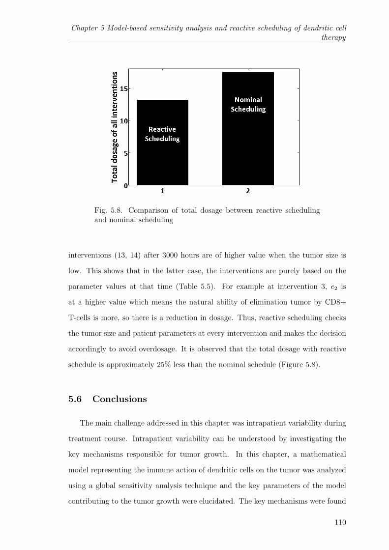
Chapter 5 Model-based sensitivity analysis and reactive scheduling of dendritic celltherapy
Fig. 5.8. Comparison of total dosage between reactive schedulingand nominal scheduling
interventions (13, 14) after 3000 hours are of higher value when the tumor size is
low. This shows that in the latter case, the interventions are purely based on the
parameter values at that time (Table 5.5). For example at intervention 3, e2 is
at a higher value which means the natural ability of elimination tumor by CD8+
T-cells is more, so there is a reduction in dosage. Thus, reactive scheduling checks
the tumor size and patient parameters at every intervention and makes the decision
accordingly to avoid overdosage. It is observed that the total dosage with reactive
schedule is approximately 25% less than the nominal schedule (Figure 5.8).
5.6 Conclusions
The main challenge addressed in this chapter was intrapatient variability during
treatment course. Intrapatient variability can be understood by investigating the
key mechanisms responsible for tumor growth. In this chapter, a mathematical
model representing the immune action of dendritic cells on the tumor was analyzed
using a global sensitivity analysis technique and the key parameters of the model
contributing to the tumor growth were elucidated. The key mechanisms were found
110

5.6 Conclusions
to be proliferation of tumor cells, its interaction with CD8+ T-cells and the source
and decay mechanisms of CD8+ T-cells. From a broader perspective, the biological
implication from the global sensitivity analysis is that development of drugs that
can activate and perpetuate CD8+ T-cells is important to eliminate tumors. The
results of HDMR were validated by formulating an optimization problem and by
comparing the outcomes of nominal and reactive scheduling. This work points to
the importance of using tumor size data to determine the key model parameters and
using the latest parameter estimates to schedule future therapeutic interventions on
the patient. Reactive scheduling was also applied to compare combination therapy
and dendritic cell therapy. In the case study, it was seen that dendritic cell therapy is
enough to eliminate tumor. Overall, reactive scheduling is very useful in the medical
field to plan therapies considering the intrapatient variability and avoid side effects.
111
Chapter 6 Application of scaling and sensitivity analysis for tumor-immune modelreduction
Chapter 6
APPLICATION OF SCALING AND SENSITIVITY
ANALYSIS FOR TUMOR-IMMUNE MODEL
REDUCTION
‘Although our intellect always longs for clarity and certainty, our
nature often finds uncertainty fascinating.’
- Karl Von Clausewitz
6.1 Introduction
In the previous chapters, it is seen that mathematical modeling plays a facil-
itating role in comprehending tumor growth and its interaction with the immune
system. However, there are some hindrances in modeling these phenomena. Firstly,
the complexity of the tumor-immune model increases with the inclusion of dynam-
ics of different types of immune cells. In this chapter, complexity is considered in
terms of number of parameters and differences in the order of magnitude of their
values. This may result in non-identifiability, imprecise measurement/ estimation
of the parameters. Secondly, very few parameters in the model will significantly
influence the evolution of state variables and it is important for us to know these
sensitive parameters.
In this chapter, a recent and elaborate tumor-immune model is considered and
its reduced parametric representation is obtained through a systematic approach
without any loss in its predictive ability. The schematic representation of the se-
quential methodology (scaling analysis followed by sensitivity analysis) adopted in
112

6.2 Mathematical model
Fig. 6.1. Sequential methodology
this chapter is shown in Figure 6.1. Scaling analysis is a systematic technique
which involves grouping of parameters in a model and representing it in a reduced
parametric form. Scaling approach also ensures that the coefficients in the model
(parametric groups) are approximately in the order-of-one. The advantage of scal-
ing approach is quantified using theoretical identifiability analysis and by evaluating
the condition number of the Fisher information matrix. With reduced models, the
computational time taken for model evaluation may be significantly reduced. Sub-
sequently, global sensitivity analysis of the reduced model is performed to unearth
the key parametric groups of the model. Such model reduction and parameter anal-
ysis may be necessary in order to increase the possibility of bringing model-based
approaches to standard medical practice and patient care.
6.2 Mathematical model
Tumor-immune model considered in this chapter is adapted from the work by
de Pillis et al. (2009). In the model, it is considered that, symbols, T , N , L, C, I
represent tumor cells, natural killer (NK) cells, cytotoxic (CD8+) T-cells, circulating
lymphocytes, and interleukin respectively. The units of immune cells (N , L, C) and
cytokines (I) are given in number of cells per litre of blood and international unit
113
Chapter 6 Application of scaling and sensitivity analysis for tumor-immune modelreduction
(IU) per litre of blood respectively, while the tumor (T ) is represented as total
number of cells. In Equation (6.1), the first term corresponds to the nutrients based
on tumor growth. The second and third terms explain the elimination of tumor
cells due to NK cells, CD8+ T-cells. The expression for D is given in Equation (6.2)
where d and l signify the immune strength (recognizing and attacking capacity)
known as immunogenicity against the tumor cells. In Equation (6.3), eC denotes
the localization of natural killer cells at the tumor site based on the number of
circulating lymphocytes. fN denotes the natural decay of NK cells. The loss of
natural killer cells due to its interaction with tumor cells is given by pNT . The
activation of NK cells by interleukin is given by pNNI/(gN + I). In Equation (6.4),
jTL/(k+T ) elucidates the stimulation of the CD8+ T-cells as a result of the presence
of lysed tumor cells debris. Similarly, r1NT represent the stimulation of cytotoxic
cells due to the presence of the NK-lysed tumor cells. The localization of activated
CD8+ T-cells at the tumor location is captured by r2CT term. The activation
of cytotoxic cells by interleukin is described by pILI/(gI + I). However, excessive
number of cytotoxic cells in the presence of interleukin leads to its deactivation and
is shown by the term uL2CI/(κ + I). In previous work (de Pillis et al., 2006),
the natural decay of cytotoxic T-cells was expressed as −mL. Later, in de Pillis
et al. (2009), it was modified to θmL/(θ + I) owing to the realization that the
cytotoxic T-cells decrease only due to the increased concentration of interleukin
above a threshold limit. In Equation (6.5), −µII, ϕC and ωLI/(ζ + I) quantify
the natural decay of interleukin, production of interleukin by the helper T-cells and
CD8+ T-cells respectively. In Equation (6.6), α is the natural ability of the bone
marrow to generate lymphocytes in any individual and β is the overall decay rate
of the circulating lymphocytes. The parameter values are given in Table 6.1.
dT
dt= aT (1− bT )− cNT −DT (6.1)
D = d(L/T )l
s+ (L/T )l(6.2)
114

6.3 Scaling analysis
dN
dt= eC − fN − pNT +
pNNI
gN + I(6.3)
dL
dt=θmL
θ + I+
jTL
k + T− qLT + (r1N + r2C)T − uL2CI
κ+ I+
pILI
gI + I(6.4)
dI
dt= −µII + ϕC +
ωLI
ζ + I(6.5)
dC
dt= α− βC (6.6)
Model reduction analysis is applied on the model and Equations (6.1-6.6) are
considered while applying scaling and sensitivity analysis. The above model has
29 parameters and this can pose significant challenges for parameter estimation
in the face of limited patient data. We might therefore benefit by obtaining a
minimal parametric model and determining the key parameter combinations with
high accuracy for enabling clinical applications.
6.3 Scaling analysis
Scaling analysis is a systematic procedure for non-dimensionalization of depen-
dent and independent variables as well as their derivatives in a mathematical model
representing a physical process. Non-dimensionalization is done such that the vari-
ables and their derivatives are bounded by order-of-one scale which is a unique aspect
of the scaling analysis proposed by Krantz (2007b,a). The order-of-one scaling en-
sures that the values of the dimensionless variables, their derivatives and coefficients
in the model lie between zero and more-or-less one. Order-of-one scaling not only fa-
cilitates minimum parametric representation but also supports model simplification
based on the magnitude of the dimensionless parameter groups. One key advantage
of the scaled model is that if the coefficient value of any term is very low, it can be
ignored. Similar conclusions cannot be made based on coefficient values in the case
of the original model.
115

Chapter 6 Application of scaling and sensitivity analysis for tumor-immune modelreduction
Table 6.1Parameter values
Parameter Value Unitsa 4.31× 10⁻¹ Day−1
b 1.02× 10⁻⁹ Cellsc 2.9077× 10⁻¹³ l/Cells−1perday−1
e 1.3875× 10⁻³ Day−1
f 1.25× 10⁻² Day−1
p 2.794× 10⁻¹³ Cells−1perday−1
pN 6.68× 10⁻² Day−1
gN 2.5036× 10⁵ IU/lm 9× 10⁻³ Day−1
θ 2.5036× 10⁻³ IU/lq 3.422× 10⁻¹⁰ Cells−1perday−1
r1 2.9077× 10⁻¹¹ Cells−1perday−1
r2 5.8467× 10⁻¹³ Cells−1perday−1
pI 2.971 Day−1
gI 2.5036× 10³ IU/lu 4.417× 10⁻¹⁴ l2/Cells−2perday−1
κ 2.5036× 10³ IU/lj 1.245× 10⁻² Day−1
k 2.019× 10⁷ cellsα 1.4175× 10⁷ Cells/lday−1
β 6.3× 10⁻³ Day−1
υ 5.199× 10⁻¹ Day−1
µI 11.7427 Day−1
ω 7.874× 10⁻² IU/Cells−1perday−1
ϕ 2.38405× 10⁻⁷ IU/Cells−1perday−1
ζ 2.5035× 10³ IU/ld 2.34 Day−1
l 2.09s 3.8× 10⁻³
6.3.1 Algorithm
1. Mathematical model representing the physical process (tumor-immune inter-
actions): model equations, initial, boundary and auxiliary conditions are as-
sumed to be available.
2. Introduce scale factors and reference factors for all dependent, independent
variables and their derivatives.
116

6.3 Scaling analysis
3. Form dimensionless variables in the model equations.
4. Use the coefficient of the dominating phenomenon and divide both sides of the
equations with it.
5. Determine the scale factors and reference factors.
6. Check if the magnitude of all the dimensionless coefficients in the model is of
the order-of-one. If not, the algorithm is repeated from step 4.
7. After successful implementation of steps 1 to 6, the minimum parametric rep-
resentation of the model is obtained.
In the equations below, subscripts ‘f ′ and ‘s′ refers to reference factors and scale
factors respectively. The reference values Tf , Nf , Lf , If , Cf are considered to be
zero because their minimum possible value is zero. 1/α1, 1/α2, 1/α3, 1/α4, 1/α5
refer to scaling factors for time derivatives of T , N , L, I and C respectively. The
transformed variables are as given below.
T ∗ =T−Tf
Ts, N∗ =
N−Nf
Ns, L∗ =
L−Lf
Ls, I∗ =
I−IfIs
, C∗ =C−Cf
Cs,(dTdt
)∗= α1
(dTdt
),(
dNdt
)∗= α2
(dNdt
),(dLdt
)∗= α3
(dLdt
),(dIdt
)∗= α4
(dIdt
),(dCdt
)∗= α5
(dCdt
)
6.3.2 Reduced model
The minimum parametric model is shown in Equations (6.7-6.11) and the scale
factors are given below.
Ts = 1b, Ns = eCs
f, Cs = α
β, Ls = 5.268 × 10⁵, Is = 1073, α1 = 1
abT 2s
, α2 = 1eCs
,
α3 = 1r1NsTs
, α4 = 1µIs
, α5 = 1α
(dT
dt
)∗= α1
(dT
dt
)= T ∗ − T ∗2 − Π1N
∗T ∗ − Π2T∗(L∗
T ∗
)Π3
(6.7)
(dN
dt
)∗= α2
(dN
dt
)= C∗ − Π4N
∗ − Π5N∗T ∗ +
Π6N∗(
Π7
I∗+ 1) (6.8)
117
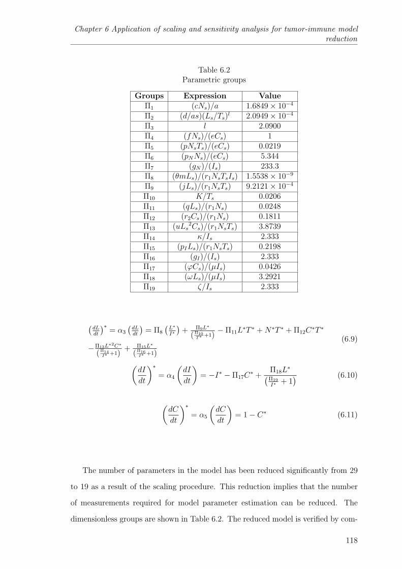
Chapter 6 Application of scaling and sensitivity analysis for tumor-immune modelreduction
Table 6.2Parametric groups
Groups Expression ValueΠ1 (cNs)/a 1.6849× 10⁻⁴
Π2 (d/as)(Ls/Ts)l 2.0949× 10⁻⁴
Π3 l 2.0900Π4 (fNs)/(eCs) 1Π5 (pNsTs)/(eCs) 0.0219Π6 (pNNs)/(eCs) 5.344Π7 (gN)/(Is) 233.3Π8 (θmLs)/(r1NsTsIs) 1.5538× 10⁻⁹
Π9 (jLs)/(r1NsTs) 9.2121× 10⁻⁴
Π10 K/Ts 0.0206Π11 (qLs)/(r1Ns) 0.0248Π12 (r2Cs)/(r1Ns) 0.1811Π13 (uLs
2Cs)/(r1NsTs) 3.8739Π14 κ/Is 2.333Π15 (pILs)/(r1NsTs) 0.2198Π16 (gI)/(Is) 2.333Π17 (ϕCs)/(µIs) 0.0426Π18 (ωLs)/(µIs) 3.2921Π19 ζ/Is 2.333
(dLdt
)∗= α3
(dLdt
)= Π8
(L∗
I∗
)+ Π9L∗
(Π10T∗ +1)
− Π11L∗T ∗ +N∗T ∗ + Π12C
∗T ∗
−Π13L∗2C∗
(Π14I∗ +1)
+ Π15L∗
(Π16I∗ +1)
(6.9)
(dI
dt
)∗= α4
(dI
dt
)= −I∗ − Π17C
∗ +Π18L
∗(Π19
I∗+ 1) (6.10)
(dC
dt
)∗= α5
(dC
dt
)= 1− C∗ (6.11)
The number of parameters in the model has been reduced significantly from 29
to 19 as a result of the scaling procedure. This reduction implies that the number
of measurements required for model parameter estimation can be reduced. The
dimensionless groups are shown in Table 6.2. The reduced model is verified by com-
118
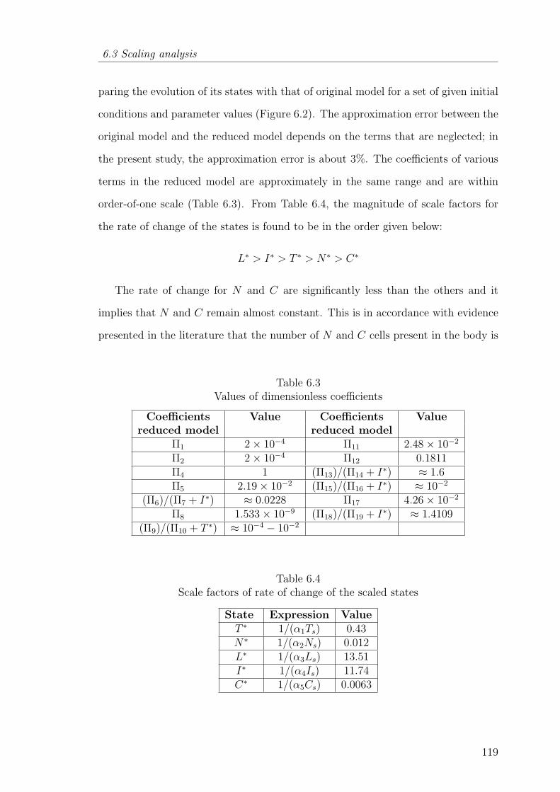
6.3 Scaling analysis
paring the evolution of its states with that of original model for a set of given initial
conditions and parameter values (Figure 6.2). The approximation error between the
original model and the reduced model depends on the terms that are neglected; in
the present study, the approximation error is about 3%. The coefficients of various
terms in the reduced model are approximately in the same range and are within
order-of-one scale (Table 6.3). From Table 6.4, the magnitude of scale factors for
the rate of change of the states is found to be in the order given below:
L∗ > I∗ > T ∗ > N∗ > C∗
The rate of change for N and C are significantly less than the others and it
implies that N and C remain almost constant. This is in accordance with evidence
presented in the literature that the number of N and C cells present in the body is
Table 6.3Values of dimensionless coefficients
Coefficients Value Coefficients Valuereduced model reduced model
Π1 2× 10⁻⁴ Π11 2.48× 10⁻²
Π2 2× 10⁻⁴ Π12 0.1811Π4 1 (Π13)/(Π14 + I∗) ≈ 1.6Π5 2.19× 10⁻² (Π15)/(Π16 + I∗) ≈ 10−2
(Π6)/(Π7 + I∗) ≈ 0.0228 Π17 4.26× 10⁻²
Π8 1.533× 10⁻⁹ (Π18)/(Π19 + I∗) ≈ 1.4109(Π9)/(Π10 + T ∗) ≈ 10−4 − 10−2
Table 6.4Scale factors of rate of change of the scaled states
State Expression ValueT ∗ 1/(α1Ts) 0.43N∗ 1/(α2Ns) 0.012L∗ 1/(α3Ls) 13.51I∗ 1/(α4Is) 11.74C∗ 1/(α5Cs) 0.0063
119
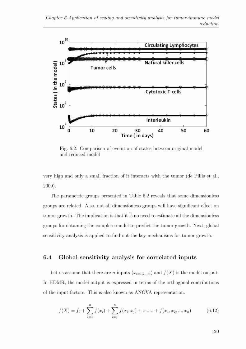
Chapter 6 Application of scaling and sensitivity analysis for tumor-immune modelreduction
Fig. 6.2. Comparison of evolution of states between original modeland reduced model
very high and only a small fraction of it interacts with the tumor (de Pillis et al.,
2009).
The parametric groups presented in Table 6.2 reveals that some dimensionless
groups are related. Also, not all dimensionless groups will have significant effect on
tumor growth. The implication is that it is no need to estimate all the dimensionless
groups for obtaining the complete model to predict the tumor growth. Next, global
sensitivity analysis is applied to find out the key mechanisms for tumor growth.
6.4 Global sensitivity analysis for correlated inputs
Let us assume that there are n inputs (xi=1,2,..,n) and f(X) is the model output.
In HDMR, the model output is expressed in terms of the orthogonal contributions
of the input factors. This is also known as ANOVA representation.
f(X) = f0 +n∑i=1
f(xi) +n∑i 6=j
f(xi, xj) + ........+ f(x1, x2, ..., xn) (6.12)
120
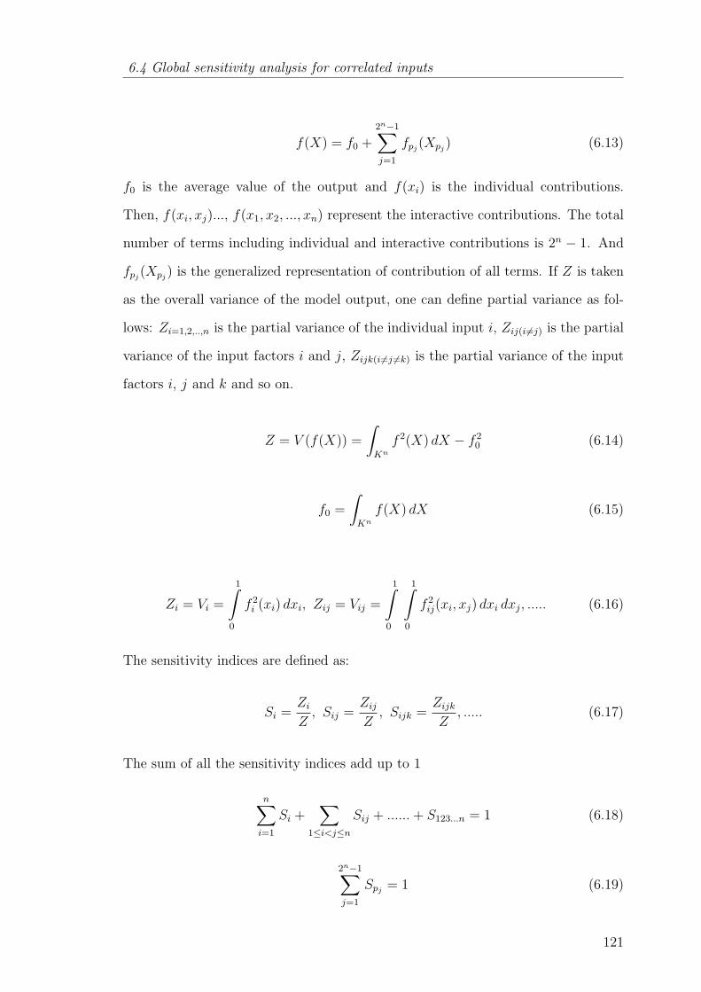
6.4 Global sensitivity analysis for correlated inputs
f(X) = f0 +2n−1∑j=1
fpj(Xpj
) (6.13)
f0 is the average value of the output and f(xi) is the individual contributions.
Then, f(xi, xj)..., f(x1, x2, ..., xn) represent the interactive contributions. The total
number of terms including individual and interactive contributions is 2n − 1. And
fpj(Xpj
) is the generalized representation of contribution of all terms. If Z is taken
as the overall variance of the model output, one can define partial variance as fol-
lows: Zi=1,2,..,n is the partial variance of the individual input i, Zij(i 6=j) is the partial
variance of the input factors i and j, Zijk(i 6=j 6=k) is the partial variance of the input
factors i, j and k and so on.
Z = V (f(X)) =
∫Kn
f 2(X) dX − f 20 (6.14)
f0 =
∫Kn
f(X) dX (6.15)
Zi = Vi =
1∫0
f 2i (xi) dxi, Zij = Vij =
1∫0
1∫0
f 2ij(xi, xj) dxi dxj, ..... (6.16)
The sensitivity indices are defined as:
Si =ZiZ, Sij =
ZijZ, Sijk =
ZijkZ
, ..... (6.17)
The sum of all the sensitivity indices add up to 1
n∑i=1
Si +∑
1≤i<j≤n
Sij + ......+ S123...n = 1 (6.18)
2n−1∑j=1
Spj= 1 (6.19)
121
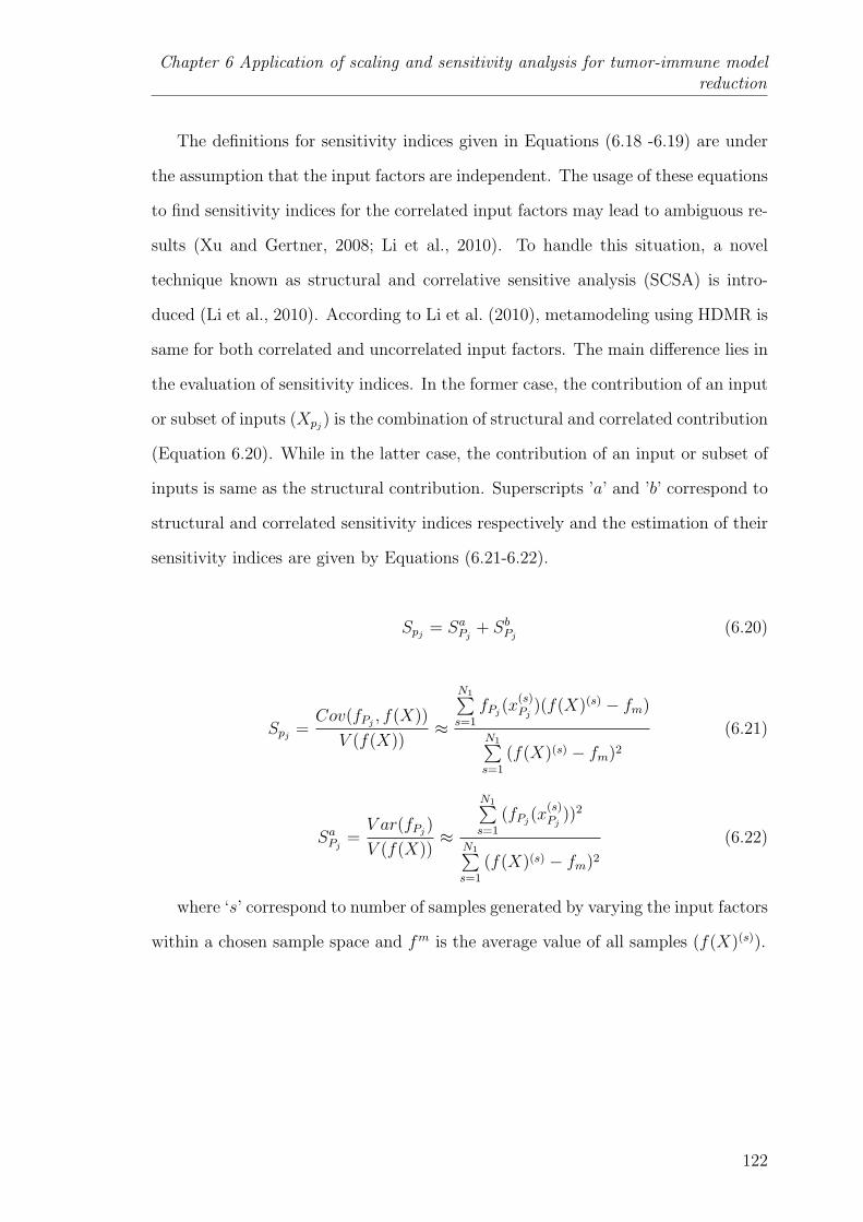
Chapter 6 Application of scaling and sensitivity analysis for tumor-immune modelreduction
The definitions for sensitivity indices given in Equations (6.18 -6.19) are under
the assumption that the input factors are independent. The usage of these equations
to find sensitivity indices for the correlated input factors may lead to ambiguous re-
sults (Xu and Gertner, 2008; Li et al., 2010). To handle this situation, a novel
technique known as structural and correlative sensitive analysis (SCSA) is intro-
duced (Li et al., 2010). According to Li et al. (2010), metamodeling using HDMR is
same for both correlated and uncorrelated input factors. The main difference lies in
the evaluation of sensitivity indices. In the former case, the contribution of an input
or subset of inputs (Xpj) is the combination of structural and correlated contribution
(Equation 6.20). While in the latter case, the contribution of an input or subset of
inputs is same as the structural contribution. Superscripts ’a’ and ’b’ correspond to
structural and correlated sensitivity indices respectively and the estimation of their
sensitivity indices are given by Equations (6.21-6.22).
Spj= SaPj
+ SbPj(6.20)
Spj=Cov(fPj
, f(X))
V (f(X))≈
N1∑s=1
fPj(x
(s)Pj
)(f(X)(s) − fm)
N1∑s=1
(f(X)(s) − fm)2
(6.21)
SaPj=V ar(fPj
)
V (f(X))≈
N1∑s=1
(fPj(x
(s)Pj
))2
N1∑s=1
(f(X)(s) − fm)2
(6.22)
where ‘s’ correspond to number of samples generated by varying the input factors
within a chosen sample space and fm is the average value of all samples (f(X)(s)).
122
6.5 Results and discussion
6.5 Results and discussion
6.5.1 Comparison between original model and reduced model via theo-
retical identifiability analysis
The main idea in this section is to quantify the advantage of scaling analysis via
theoretical identifiability analysis. Identifiability analysis is one of the key steps be-
fore parameter estimation in the model building process (Rodriguez-Fernandez and
Banga, 2010). It questions the existence of a unique solution of model parameters
for a given set of observations. Broadly, there are two main classes of identifiability
analysis, a priori and a posterior identifiability analysis. In a priori identifiability
analysis, the uniqueness is tested with the assumption that the real system and
model have identical structure; there are no experimental constraints for collect-
ing the output data. In addition, it is assumed that the measured output data is
perfect data, i.e., noise free data. Hence, it is also called as the theoretical identi-
fiability analysis. To the contrary, in a posterior identifiability analysis (practical
identifiability analysis), measured output data is noisy and it considers the practical
constraints such as variations of manipulated variables, cost involved in conducting
the experiments.
In the present work, the focus is on theoretical identifiability analysis using the
sensitivity matrix i.e., the Jacobian matrix of the model output at different times
for a parameter set of the considered model structure. Therefore, it is also called as
sensitivity identifiability (Cintron-Arias et al., 2009).
Let us assume a nonlinear dynamic system of the form
dYdt
= g(Y (t), U(t), t, P )
M(t) = h(Y (t), P )
Y (0) = Y0(P )
(6.23)
123

Chapter 6 Application of scaling and sensitivity analysis for tumor-immune modelreduction
where Y , U , P , t represent the states, inputs, parameters and time variable re-
spectively. Y0 is the initial condition of the state vector Y . g(.) and h(.) includes
the state equations and output equations respectively. In the tumor-immune model,
Y corresponds to tumor cells, natural killer (NK) cells, cytotoxic (CD8+) T-cells,
circulating lymphocytes, and interleukin respectively. M corresponds to the daily
measurement of tumor cells over the 1 month period. Tumor data is generated by
simulating the original model and subsequently used for performing the identifia-
bility analysis on original and reduced model. The information about the system
captured in the measurements is quantified by Fisher information matrix (FIM) as
given in Equation (6.24). The sufficient condition for theoretically identifiable is the
non-singularity (i.e. low condition number) of FIM.
FIM =v∑i=1
GTi Gi (6.24)
where
Gi =
∂y1
∂p1
∂y1
∂p2......∂y1
∂pj
∂y2
∂p1
∂y2
∂p2......∂y2
∂pj
.........................
∂ym
∂p1
∂ym
∂p2......∂ym
∂pj
i
(6.25)
is the sensitivity matrix and ν is the number of measurements (equal to 31 in this
case). The number of parameters is indicated by the variable j (j = 29 for the
original tumor-immune model and j = 19 for the reduced model). Let FIM1(29×
29) and FIM2(19 × 19) represent the Fisher information matrix for the assumed
measurement data for the original and reduced model respectively. Let CN1 and
CN2 refer to the condition numbers of FIM1 and FIM2 respectively. Rc is the
index which quantifies the effect of scaling analysis on the conditioning of FIM.
Rc =log(CN2)
log(CN1)(6.26)
124
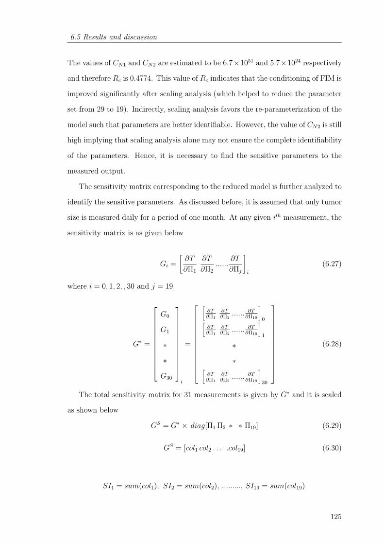
6.5 Results and discussion
The values of CN1 and CN2 are estimated to be 6.7×1051 and 5.7×1024 respectively
and therefore Rc is 0.4774. This value of Rc indicates that the conditioning of FIM is
improved significantly after scaling analysis (which helped to reduce the parameter
set from 29 to 19). Indirectly, scaling analysis favors the re-parameterization of the
model such that parameters are better identifiable. However, the value of CN2 is still
high implying that scaling analysis alone may not ensure the complete identifiability
of the parameters. Hence, it is necessary to find the sensitive parameters to the
measured output.
The sensitivity matrix corresponding to the reduced model is further analyzed to
identify the sensitive parameters. As discussed before, it is assumed that only tumor
size is measured daily for a period of one month. At any given ith measurement, the
sensitivity matrix is as given below
Gi =
[∂T
∂Π1
∂T
∂Π2
......∂T
∂Πj
]i
(6.27)
where i = 0, 1, 2, , 30 and j = 19.
G∗ =
G0
G1
∗
∗
G30
i
=
[∂T∂Π1
∂T∂Π2
...... ∂T∂Π19
]0[
∂T∂Π1
∂T∂Π2
...... ∂T∂Π19
]1
∗
∗[∂T∂Π1
∂T∂Π2
...... ∂T∂Π19
]30
(6.28)
The total sensitivity matrix for 31 measurements is given by G∗ and it is scaled
as shown below
GS = G∗ × diag[Π1 Π2 ∗ ∗ Π19] (6.29)
GS = [col1 col2 . . . . .col19] (6.30)
SI1 = sum(col1), SI2 = sum(col2), ........., SI19 = sum(col19)
125

Chapter 6 Application of scaling and sensitivity analysis for tumor-immune modelreduction
Fig. 6.3. Sensitivity indices of the parametric groups
“coli ” stands for columnwise elements of Gs sensitivity index and “SI” is an
index which implies the variation of tumor cells with respect to the parametric
groups (Πi). In Figure 6.3 the values of SI for all the parameters are projected in
the decreasing order of their contribution. It is observed that the parameters Π3,
Π18, Π2, Π19, and Π13 are the most sensitive parametric groups. The determination
of these sensitive parameters guides parameter estimation in deciding the parameters
to be estimated and the parameters to be fixed at their nominal values for a given
dataset of measured variables (discussed in Section 6.5.3). In the following section,
the sensitive parametric groups are further verified using global sensitivity analysis.
6.5.2 Sensitive parametric groups based on global sensitivity analysis
The parameters (i.e., dimensionless groups (Πi) of the reduced model are directly
varied by 25% of their nominal values. The nominal values of the dimensionless
groups are obtained by substituting the nominal values of the parameters of original
model (Table 6.1). The dimensionless groups (Πi) are assumed to follow a uniform
distribution within their sample space (Marino et al., 2008). The samples are chosen
from the sample space using experimental designs such as Latin hypercube sampling
126
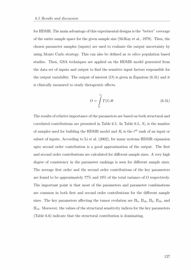
6.5 Results and discussion
for HDMR. The main advantage of this experimental designs is the “better” coverage
of the entire sample space for the given sample size (McKay et al., 1979). Then, the
chosen parameter samples (inputs) are used to evaluate the output uncertainty by
using Monte Carlo strategy. This can also be defined as in silico population based
studies. Then, GSA techniques are applied on the HDMR model generated from
the data set of inputs and output to find the sensitive input factors responsible for
the output variability. The output of interest (O) is given in Equation (6.31) and it
is clinically measured to study therapeutic effects.
O =
tf∫0
T (t) dt (6.31)
The results of relative importance of the parameters are based on both structural and
correlated contributions are presented in Table 6.5. In Table 6.5, N1 is the number
of samples used for building the HDMR model and Ri is the ith rank of an input or
subset of inputs. According to Li et al. (2002), for many systems HDMR expansion
upto second order contribution is a good approximation of the output. The first
and second order contributions are calculated for different sample sizes. A very high
degree of consistency in the parameter rankings is seen for different sample sizes.
The average first order and the second order contributions of the key parameters
are found to be approximately 77% and 19% of the total variance of O respectively.
The important point is that most of the parameters and parameter combinations
are common in both first and second order contributions for the different sample
sizes. The key parameters affecting the tumor evolution are Π3, Π18, Π2, Π19, and
Π13. Moreover, the values of the structural sensitivity indices for the key parameters
(Table 6.6) indicate that the structural contribution is dominating.
127
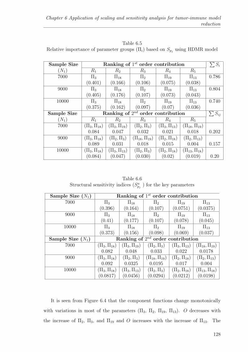
Chapter 6 Application of scaling and sensitivity analysis for tumor-immune modelreduction
Table 6.5Relative importance of parameter groups (Πi) based on Spj
using HDMR model
Sample Size Ranking of 1st order contribution∑Si
(N1) R1 R2 R3 R4 R5
7000 Π3 Π18 Π2 Π19 Π13 0.786(0.401) (0.166) (0.106) (0.075) (0.038)
9000 Π3 Π18 Π2 Π19 Π13 0.804(0.405) (0.176) (0.107) (0.073) (0.043)
10000 Π3 Π18 Π2 Π19 Π13 0.740(0.375) (0.162) (0.097) (0.07) (0.036)
Sample Size Ranking of 2nd order contribution∑Sij
(N1) R1 R2 R3 R4 R5
7000 (Π3,Π18) (Π3,Π19) (Π2,Π3) (Π3,Π13) (Π18,Π19)0.084 0.047 0.032 0.021 0.018 0.202
9000 (Π3,Π18) (Π2,Π3) (Π18,Π19) (Π2,Π18) (Π2,Π13)0.089 0.031 0.018 0.015 0.004 0.157
10000 (Π3,Π18) (Π3,Π13) (Π2,Π3) (Π2,Π18) (Π13,Π18)(0.084) (0.047) (0.030) (0.02) (0.019) 0.20
Table 6.6Structural sensitivity indices (Sapj
) for the key parameters
Sample Size (N1) Ranking of 1st order contribution7000 Π3 Π18 Π2 Π19 Π13
(0.396) (0.164) (0.107) (0.0751) (0.0375)9000 Π3 Π18 Π2 Π19 Π13
(0.41) (0.177) (0.107) (0.078) (0.045)10000 Π3 Π18 Π2 Π19 Π13
(0.373) (0.156) (0.098) (0.069) (0.037)Sample Size (N1) Ranking of 2nd order contribution
7000 (Π3,Π18) (Π3,Π19) (Π2,Π3) (Π3,Π13) (Π18,Π19)0.082 0.048 0.033 0.022 0.0178
9000 (Π3,Π18) (Π2,Π3) (Π18,Π19) (Π2,Π18) (Π2,Π13)0.092 0.0325 0.0195 0.017 0.004
10000 (Π3,Π18) (Π3,Π13) (Π2,Π3) (Π2,Π18) (Π13,Π18)(0.0817) (0.0456) (0.0294) (0.0212) (0.0198)
It is seen from Figure 6.4 that the component functions change monotonically
with variations in most of the parameters (Π3, Π2, Π19, Π13). O decreases with
the increase of Π2, Π3, and Π19 and O increases with the increase of Π13. The
128

6.5 Results and discussion
Fig. 6.4. Patterns of HDMR component functions with the variationsin key parameters. X-axis: Scaled key parameter values, Y-axis:Scaled values of the component functions
component function corresponding to the parameter Π18 increases at a decreasing
rate and reaches a maximum value very close to Π18 = 1. In addition, the sensitive
parameters obtained via global sensitivity analysis are the same sensitive parameters
obtained in the identifiability analysis step. Thus, the model analysis indicates
that the major mechanisms controlling tumor growth are the immunogenicity and
cytotoxicity of CD8+ T-cells over tumor cells; effect of tumor microenvironment
129
Chapter 6 Application of scaling and sensitivity analysis for tumor-immune modelreduction
such as nutrients (Π2, Π3, Π13) and the activation of cytokines (interleukin) in the
presence of CD8+ T-cells (Π18, Π19). This macroscale analysis suggests to tumor
pathologists that they could look at the gene networks related to these mechanisms
and locate the responsible genes.
Here, the analysis is done after the parameters are known. However, in reality, all
these 19 parameters of the reduced model are not known. In that case, patient spe-
cific tumor growth and immunological data could be used to estimate them. Then,
sensitivity analysis within a range of these parameter estimates might help tumor
pathologists in designing experiments for finding the key mechanism (Kontoravdi
et al., 2005). Appropriate therapies can then be developed to target the respective
genes and control the tumor growth. This emphasizes that experiments should be
designed in a way that the identified key parameters are precisely estimated.
6.5.3 Comparison between original model and reduced model - Param-
eter estimation
Parameter estimation is one of the prime steps in the model building process. It
is an optimization problem where the objective is to minimize the nonlinear least
squares measure i.e., the closeness of fit between the measurements (data) (yi) and
the model output (yiM) (as shown in Equation (6.32)). The values of yi
M is based
on the decision variables (model parameters (Pr)) guided by the optimizer (Englezos
and Kalogerakis, 2001). In this section, the confidence intervals of the parameter
estimates of the original and reduced models are compared. There are two types of
confidence intervals for parameters: individual confidence intervals and joint con-
fidence intervals. Former type assumes that the parameters are independent from
each other; as a result it may be misleading. The joint parameter regions can be
obtained from different methods such as linear approximation and F-test or log-
likelihood. In the present work, F-test method is used because it avoids the error
130
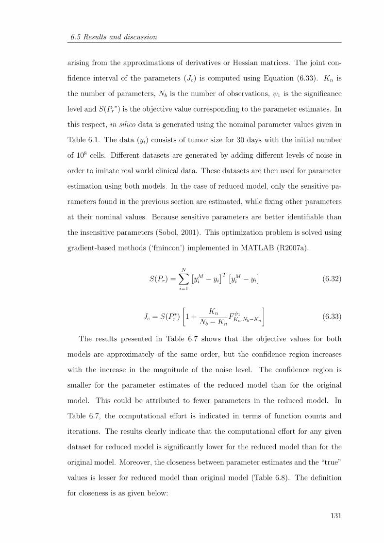
6.5 Results and discussion
arising from the approximations of derivatives or Hessian matrices. The joint con-
fidence interval of the parameters (Jc) is computed using Equation (6.33). Kn is
the number of parameters, Nb is the number of observations, ψ1 is the significance
level and S(Pr∗) is the objective value corresponding to the parameter estimates. In
this respect, in silico data is generated using the nominal parameter values given in
Table 6.1. The data (yi) consists of tumor size for 30 days with the initial number
of 108 cells. Different datasets are generated by adding different levels of noise in
order to imitate real world clinical data. These datasets are then used for parameter
estimation using both models. In the case of reduced model, only the sensitive pa-
rameters found in the previous section are estimated, while fixing other parameters
at their nominal values. Because sensitive parameters are better identifiable than
the insensitive parameters (Sobol, 2001). This optimization problem is solved using
gradient-based methods (‘fmincon’) implemented in MATLAB (R2007a).
S(Pr) =N∑i=1
[yMi − yi
]T [yMi − yi
](6.32)
Jc = S(P ∗r )
[1 +
Kn
Nb −Kn
Fψ1
Kn,Nb−Kn
](6.33)
The results presented in Table 6.7 shows that the objective values for both
models are approximately of the same order, but the confidence region increases
with the increase in the magnitude of the noise level. The confidence region is
smaller for the parameter estimates of the reduced model than for the original
model. This could be attributed to fewer parameters in the reduced model. In
Table 6.7, the computational effort is indicated in terms of function counts and
iterations. The results clearly indicate that the computational effort for any given
dataset for reduced model is significantly lower for the reduced model than for the
original model. Moreover, the closeness between parameter estimates and the “true”
values is lesser for reduced model than original model (Table 6.8). The definition
for closeness is as given below:
131

Chapter 6 Application of scaling and sensitivity analysis for tumor-immune modelreduction
Table 6.7Comparison of confidence regions between original and reduced models
Original model% Noise Objective function Jc Function countadded value S(pr
∗) (iterations)
0 4.75× 10⁻⁶ 0.0066 2828(51)
1 3.9× 10⁻⁴ 0.5434 2422(55)
5 1.3× 10⁻² 18.02 2812(37)
−1 5.2× 10⁻⁴ 0.725 2182(48)
−5 6.4× 10⁻³ 8.863 2511(50)Reduced model
% Noise Objective function Jc Function countadded value S(pr
∗) (iterations)
0 2.13× 10⁻⁵ 3.78× 10⁻⁵ 27(2)
1 5.35× 10⁻⁴ 9.47× 10⁻⁴ 18(2)
5 2.33× 10⁻² 4.12× 10⁻² 363(21)
−1 1.1× 10⁻³ 1.9× 10⁻³ 28(2)
−5 7.1× 10⁻³ 1.26× 10⁻² 80(10)
Table 6.8Closeness between parameter estimates and “true” values
% noise added Original model Reduced model0 15.01 1.33× 10⁻²
1 15.65 8.7× 10⁻⁵
5 16.85 2.7× 10⁻²
−1 14.06 0.76−5 6.08 2.04
132

6.6 Conclusions
Let us assume that “DF” represents the difference between parameter esti-
mates and “true values (TV )” and RF = DF/(TV ). Closeness measure (CM) is the
logarithm of sum of absolute values of “RF”.
CM = log10(sum(abs(RF ))) (6.34)
Overall, the reduced model performs better and can thus be used for practical ap-
plications such as designing model-based diagnostic and therapeutic protocols. In
spite of these advantages, scaling analysis can become very difficult for large and
complex systems, particularly if done manually. We are aware that some research
groups (apart from ours) are trying to develop computer codes to automate the scal-
ing analysis procedure. When these codes are available, scaling large scale models
in an error free manner can be easily accomplished.
6.6 Conclusions
This chapter exemplifies the significance of model reduction techniques in com-
prehending tumor-immune interactions. However, complexity of physiological mod-
els may hinder their clinical applications. Tumor-immune model elucidating the
immunogenic tumor growth was considered in this work. Scaling approach was used
to obtain a minimal tumor-immune model with significantly smaller number of pa-
rameters and without any loss in the predictive ability. The magnitude of coefficients
in the minimal model is in the order-of-one value unlike the original model. The
time derivative scale factors showed that rate of change of CD8+ T cells is very
high in comparison with natural killer cells and circulating lymphocytes. The ad-
vantage of scaling analysis is quantified and found the identifiable parameters using
theoretical identifiability analysis. It was observed that the scaling analysis helps
in conditioning the Fisher Information matrix. Further, global sensitivity analysis
was performed to identify the key parameters affecting the tumor growth. The re-
133
Chapter 6 Application of scaling and sensitivity analysis for tumor-immune modelreduction
sults obtained from global sensitivity analysis were in agreement with the results
of theoretical identifiability analysis. The mechanisms controlling the immunogenic
tumor growth were tumor microenvironment, immunogenicity and amplification of
cytokine production due to CD8+ T-cells. This suggests that the pathologists may
look into these relevant gene networks for discovering the genetic factors and facil-
itate personalized therapy. The results presented in this work computed that the
uncertainty of the parameter estimates of reduced model is smaller than that of
the original model. Also, the computational effort of reduced model for parameter
estimation is significantly less compared to the computational effort required for
the original model. In the next chapter, this reduced tumor-immune model is used
to conduct model-based population studies wherein the population is generated in
silico by varying the key parameters affecting the tumor growth. This may help us
to understand and address the effect of interpatient variability on protocol design.
134

Chapter 7
POPULATION BASED OPTIMAL EXPERIMENTAL
DESIGN IN CANCER DIAGNOSIS AND
CHEMOTHERAPY - IN SILICO ANALYSIS
‘In my opinion, no single design is apt to be optimal for everyone.’
- Donald Norman
7.1 Introduction
Interpatient variability is one of the critical issues in the clinical implementation
of cancer diagnostic and therapeutic protocols. Presently, cancer diagnostic and
therapeutic protocols are suggested based on clinical trials conducted on a particu-
lar cohort of patients. However, these developed protocols are used on other patient
groups as well (Kleinsmith, 2005). Also, for a given treatment protocol, only few
patients may be fully cured and others may not be. In fact, it is necessary to know
the reasons behind the observed variability in the effect of diagnostic and treatment
protocols on patients - this will help to tailor and improve the protocols to meet
the treatment objectives. These experiments will cost significant time and money.
According to recent studies, the cost involved in the research and development of a
new drug for Food and Drug Administration (FDA) approval is between US $ 500
million and US $ 800 million and the development time is around 10-12 years. It is
reported that 1 out of 1000 potential drugs reaches the clinical stage and around 90%
of the drugs fail during clinical trials (Holford et al., 2010).1 This means, failure of a
1http://www.news-medical.net/news/2004/12/07/6730.aspx
135

Chapter 7 Population based optimal experimental design in cancer diagnosis andchemotherapy - in silico analysis
drug can be quite frustrating in terms of wasted effort and expenditure. Currently,
big pharmaceutical companies are trying to minimize this loss by embracing the op-
tion of modeling and simulation (in silico experiments) based clinical trials (Holford
et al., 2010). In fact, FDA is recognizing and encouraging clinical trial simulations
using pharmacokinetic and pharmacodynamic models to ease the approval of new
drugs with lesser number of experiments (Hooker and Vicini, 2005).2 At the same
time, these in silico experiments might help in customizing optimal dosing regimens
of existing therapies for a specific population.
According to recent reviews on modeling of cancer growth (Lowengrub et al., 2010)
and optimization of anticancer therapies (Swierniak et al., 2009), little or no work
has been done on population based studies for designing diagnostic protocol and the
post-therapy analysis of therapeutic protocols. Consequently, the main questions
addressed in this chapter are: (i) how does one design diagnostic protocols such
that the patient specific parameters are better estimated and (ii) how to capitalize
on previous records of patient treatment to find patient specific parameters that
decide the outcome of the therapy. In order to address these issues, reduced tumor-
immune model from the previous chapter is used for performing population-scale
studies. In this chapter, a diagnostic protocol is proposed for the population using
the concept of optimal design of experiments. Figure 7.1 projects the idea of choosing
a diagnostic protocol based on information index for a given in silico patient cohort.
To do this, a multi-objective optimization problem is formulated with the objectives:
(i) maximization of information index and (ii) minimization of measurement effort
during the medical examinations.
Even though treatment protocol for a given drug or therapy is suggested based on
human trials, the application of the same treatment protocols might fail with some
patients (as shown in Figure 7.2). This is to be expected because the human trials
2http://www.fda.gov/downloads/Drugs/GuidanceComplianceRegulatoryInformation/Guidances/UCM072137.pdf
136
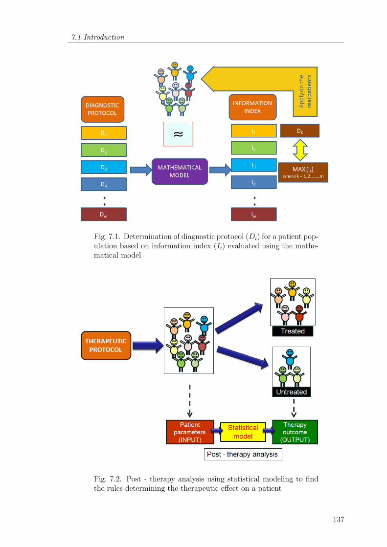
7.1 Introduction
Fig. 7.1. Determination of diagnostic protocol (Di) for a patient pop-ulation based on information index (Ii) evaluated using the mathe-matical model
Fig. 7.2. Post - therapy analysis using statistical modeling to findthe rules determining the therapeutic effect on a patient
137
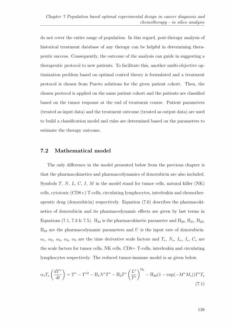
Chapter 7 Population based optimal experimental design in cancer diagnosis andchemotherapy - in silico analysis
do not cover the entire range of population. In this regard, post-therapy analysis of
historical treatment database of any therapy can be helpful in determining thera-
peutic success. Consequently, the outcome of the analysis can guide in suggesting a
therapeutic protocol to new patients. To facilitate this, another multi-objective op-
timization problem based on optimal control theory is formulated and a treatment
protocol is chosen from Pareto solutions for the given patient cohort. Then, the
chosen protocol is applied on the same patient cohort and the patients are classified
based on the tumor response at the end of treatment course. Patient parameters
(treated as input data) and the treatment outcome (treated as output data) are used
to build a classification model and rules are determined based on the parameters to
estimate the therapy outcome.
7.2 Mathematical model
The only difference in the model presented below from the previous chapter is
that the pharmacokinetics and pharmacodynamics of doxorubicin are also included.
Symbols T , N , L, C, I, M in the model stand for tumor cells, natural killer (NK)
cells, cytotoxic (CD8+) T-cells, circulating lymphocytes, interleukin and chemother-
apeutic drug (doxorubicin) respectively. Equation (7.6) describes the pharmacoki-
netics of doxorubicin and its pharmacodynamic effects are given by last terms in
Equations (7.1, 7.3 & 7.5). Π24 is the pharmacokinetic parameter and Π20, Π21, Π22,
Π23 are the pharmacodynamic parameters and U is the input rate of doxorubicin.
α1, α2, α3, α4, α5 are the time derivative scale factors and Ts, Ns, Ls, Is, Cs are
the scale factors for tumor cells, NK cells, CD8+ T-cells, interleukin and circulating
lymphocytes respectively. The reduced tumor-immune model is as given below.
α1Ts
(dT ∗
dt
)= T ∗ − T ∗2 −Π1N
∗T ∗ −Π2T∗(L∗
T ∗
)Π3
−Π20(1− exp(−M∗Ms))T∗Ts
(7.1)
138
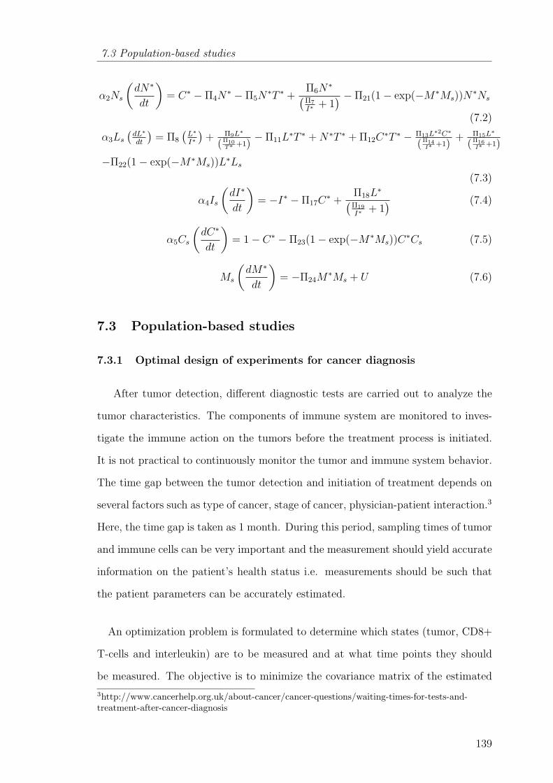
7.3 Population-based studies
α2Ns
(dN∗
dt
)= C∗ − Π4N
∗ − Π5N∗T ∗ +
Π6N∗(
Π7
I∗+ 1) − Π21(1− exp(−M∗Ms))N
∗Ns
(7.2)
α3Ls(dL∗
dt
)= Π8
(L∗
I∗
)+ Π9L∗
(Π10T∗ +1)
− Π11L∗T ∗ +N∗T ∗ + Π12C
∗T ∗ − Π13L∗2C∗
(Π14I∗ +1)
+ Π15L∗
(Π16I∗ +1)
−Π22(1− exp(−M∗Ms))L∗Ls
(7.3)
α4Is
(dI∗
dt
)= −I∗ − Π17C
∗ +Π18L
∗(Π19
I∗+ 1) (7.4)
α5Cs
(dC∗
dt
)= 1− C∗ − Π23(1− exp(−M∗Ms))C
∗Cs (7.5)
Ms
(dM∗
dt
)= −Π24M
∗Ms + U (7.6)
7.3 Population-based studies
7.3.1 Optimal design of experiments for cancer diagnosis
After tumor detection, different diagnostic tests are carried out to analyze the
tumor characteristics. The components of immune system are monitored to inves-
tigate the immune action on the tumors before the treatment process is initiated.
It is not practical to continuously monitor the tumor and immune system behavior.
The time gap between the tumor detection and initiation of treatment depends on
several factors such as type of cancer, stage of cancer, physician-patient interaction.3
Here, the time gap is taken as 1 month. During this period, sampling times of tumor
and immune cells can be very important and the measurement should yield accurate
information on the patient’s health status i.e. measurements should be such that
the patient parameters can be accurately estimated.
An optimization problem is formulated to determine which states (tumor, CD8+
T-cells and interleukin) are to be measured and at what time points they should
be measured. The objective is to minimize the covariance matrix of the estimated
3http://www.cancerhelp.org.uk/about-cancer/cancer-questions/waiting-times-for-tests-and-treatment-after-cancer-diagnosis
139

Chapter 7 Population based optimal experimental design in cancer diagnosis andchemotherapy - in silico analysis
parameters which is equivalent to maximization of Fisher information matrix (FIM)
(Englezos and Kalogerakis, 2001). The elements of FIM are the sensitivity indices of
the parameters. Generally, the maximization of FIM is done by reducing the matrix
to a scalar quantity. In this regard, there are different scalar criteria to maximize
FIM - these include D-optimality, A-optimality and E-optimality. D-optimality is
the most common approach (which uses the determinant value of FIM as the scalar
metric for optimization) and it gives equal weightage to all the parameters (k).
There are many biomedical applications based on D-optimality criterion, one such
example is the work by Hulting et al. (2006).
FIM =v∑i=1
GiTGi (7.7)
where
Gi =
∂z1∂k1
∂z1∂k2
...... ∂z1∂kp
∂z2∂k1
∂z2∂k2
...... ∂z2∂kp
.........................
∂zm
∂k1
∂zm
∂k2......∂zm
∂kp
i
(7.8)
Cov(∧k) ≥ FIM−1 (7.9)
In Equations (7.7) and (7.8), z represents states, k represents parameters, m
is the number of states, p is the number of parameters and ν is the number of
observations. According to Cramer-Rao inequality, the covariance matrix of the
parameters is greater than or equal to inverse of FIM (Equation 7.9).
One key focus of the present work is on optimal design of experiments for a given
population where the objective is to maximize population Fisher information ma-
trix (PFIM) (Aarons and Ogungbenro, 2010; Hooker and Vicini, 2005; Silber et al.,
2009). This is essential in order to take care of interpatient variability. In this work,
a patient is assumed to be represented by the reduced form of tumor-immune model
which was explained in Section 7.2. In the previous chapter, using the same model,
the key parameteric groups (Π3, Π18, Π2, Π19, Π13) affecting the tumor growth (no
140

7.3 Population-based studies
treatment case) were determined using global sensitivity analysis techniques. In the
present study, interpatient variability is simulated by varying the key parameteric
groups influencing the tumor growth while fixing the remaining insensitive parame-
teric groups at their nominal values. The parametric groups are assumed to follow
uniform distribution. And another assumption is that the measurement error asso-
ciated with state variables (tumor, immune cells and interleukin) is negligible. It
means the variation in the state variables is only because of the variations in the
parametric groups. Then, the key parametric groups are varied by ±25% of their
nominal values and the patient population is chosen from the parameter space using
Latin hypercube sampling. The above population selection is quite similar to later
phases of clinical trial where different individuals are randomly selected to test the
new protocols (Airley, 2009; Kleinsmith, 2005). Here, the population size (nP1) is
chosen as 300 which is equivalent to considering 300 patients for analyzing the fea-
tures of their tumors. In formulation A of the problem, objective 1a corresponds to
the determinant of the Fisher information matrix and objective 2a is the numbers of
states to be measured (y1). The practical implication of second objective is to reduce
the measurement effort. The decision variables included are the sampling timings
(xi) and two integer variables y1 and y2. y1 represents the number of states (CD8+
T-cells, interleukin) to be measured in addition to the measurement of tumor. If y1
turns out to be 1, then it means only tumor measurement is enough. If y1 turns out
to be 3, then it means all states need to be measured at the sampling times. For
y1 = 2 there are two possibilities (tumor and CD8+ T-cells (y2 = 1) or tumor and
interleukin (y2 = 2)). The choice of the possibility is based on the integer variable
y2.
Problem formulation A
Objectives
Objective 1a: minxi,y1,y2
− log10
(mean
(nP1∑j=1
|det(FIMj)|
))
141
Chapter 7 Population based optimal experimental design in cancer diagnosis andchemotherapy - in silico analysis
Objective 2a: min(y1)
Decision variables
xi (i = 1, 2, ., 5) are the sampling times
y1 - number of states to be measured in addition to state 1
y2 - combination of states to be measured if y1 = 2
Constraints
Constraint 1a: 0 ≤ xi ≤ 30 days (Continuous variable)
Constraint 2a: 1 ≤ y1 ≤ 3 (Integer variable)
Constraint 3a: 1 ≤ y2 ≤ 2 (Integer variable)
This mixed integer dynamic optimization problem is solved using non-dominated
sorted genetic algorithm (NSGA II) implemented in MATLAB (R2007a) (Deb et al.,
2000). The main advantages of NSGA II are that it is very easy to implement and
requires less computational effort than other genetic algorithms. The Pareto set
obtained is projected in Figure 7.3. Lesser value of objective 1a implies that more
information is captured. Figure 7.3 shows that the information content increases
by 133% when another state (CD8+ T-cells) is measured in addition to tumor size.
Adding the extra measurement of interleukin (to CD8+ T-cells & tumor size mea-
surement) increases the information content by an extra 20%. This makes sense
because most of the information about interleukin dynamics can be captured from
the dynamics of CD8+ T-cells. Overall, maximum information is captured by mea-
suring all the states. The best times for sampling the states are presented in Figure
7.4. Clearly, three groups of sampling times is observed from Figure 7.4. The fre-
quency of sampling is higher in the initial days after detection. The first two samples
must be collected on 2nd day and then the next two samples must be taken on the
142
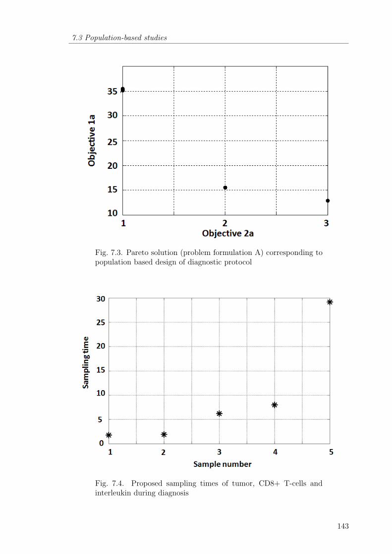
7.3 Population-based studies
Fig. 7.3. Pareto solution (problem formulation A) corresponding topopulation based design of diagnostic protocol
Fig. 7.4. Proposed sampling times of tumor, CD8+ T-cells andinterleukin during diagnosis
143
Chapter 7 Population based optimal experimental design in cancer diagnosis andchemotherapy - in silico analysis
7th and 8th days. The final sample must be taken close to the end of diagnostic time.
This is an acceptable and logical result because the system dynamics is significant
during the first 10 days after the tumor detection and, after that; the system has
almost reached a steady state.
7.3.2 Optimal design of chemotherapeutic protocol and post-therapy
analysis
Tumor diagnosis is followed by selection of the treatment modalities and dosage
planning. Usually, chemotherapy (being a systemic therapy) is preferred (Stuschke
and Pottgen, 2010; Kleinsmith, 2005) and is administered periodically over the treat-
ment course. For example, doxorubicin (60− 75 mg/m2) is given once every 3− 4
weeks (Airley, 2009). In this work, for simplicity, the intervention is assumed to be
given once every 3 weeks and the treatment horizon is considered as one year. The
approximate number of interventions (nI) per year is equal to 18. However, some-
times, the side effects of chemotherapy such as neutropenia (Rivera et al., 2003) and
cardiotoxicity (Swain et al., 2003) are more critical than the tumor growth itself.
Therefore, it is necessary to include relevant constraints on doxorubicin while de-
signing the treatment protocol. To understand the effect of doxorubicin, a patient
cohort is generated by changing the values for parametric groups in the model. The
parameters in this part of the study include not only those found to be important
from global sensitivity analysis but also the pharmacokinetic (Π24) and pharma-
codynamic (Π20, Π21, Π22, Π23) parameters. From Equation (7.6), lower value of
Π24 indicates the decrease in the decay of doxorubicin. As a result, the drug con-
centration in the body might increase. Similarly, lower value of pharmacodynamic
parameters signifies the phenomenon of drug resistance. Another important question
posed is whether the key parameters affecting the tumor remain the same or change
due to the inclusion of pharmacokinetics and pharmacodynamics of doxorubicin.
This question is answered in the later sections based on post-therapy analysis.
144

7.3 Population-based studies
A multi-objective optimization problem is formulated to find a compromise solu-
tion balancing the objectives: tumor elimination and reduction of side effects. In the
formulation below, objectives 1b-3b are related to tumor cells and they correspond
to overall tumor growth control, minimization of final tumor size at the end of treat-
ment course and the minimization of maximum possible tumor size respectively. The
remaining objectives 4b and 5b emphasize on the reduction of doxorubicin dosages
and controlled regulation of circulating lymphocytes respectively. Therefore, these
objectives serve to prevent infections due to the imbalance in immune cells (Rivera
et al., 2003). Constraint 1b is the time duration to achieve the targets of the treat-
ment. Constraint 2b relates to the total number of interventions (nI). C3 and C4
represents the constraint on the maximum drug concentration and drug concentra-
tion in the body during the treatment course respectively (Hon and Evans, 1998;
Laginha et al., 2005). Constraints 3b and 4b help to prevent immediate and long
term side effect on the patients respectively.
Problem formulation B
Objectives
Objective 1b: min
nP2∑j=1
(tf∫0
T dt
)j
nP2
Objective 2b: min
nP2∑j=1
(Tf)j
nP2
Objective 3b: min
nP2∑j=1
(max(T ))j
nP2
Objective 4b:
18∑i=1
qi
Objective 5b: max
nP2∑j=1
(min(C))j
nP2
145
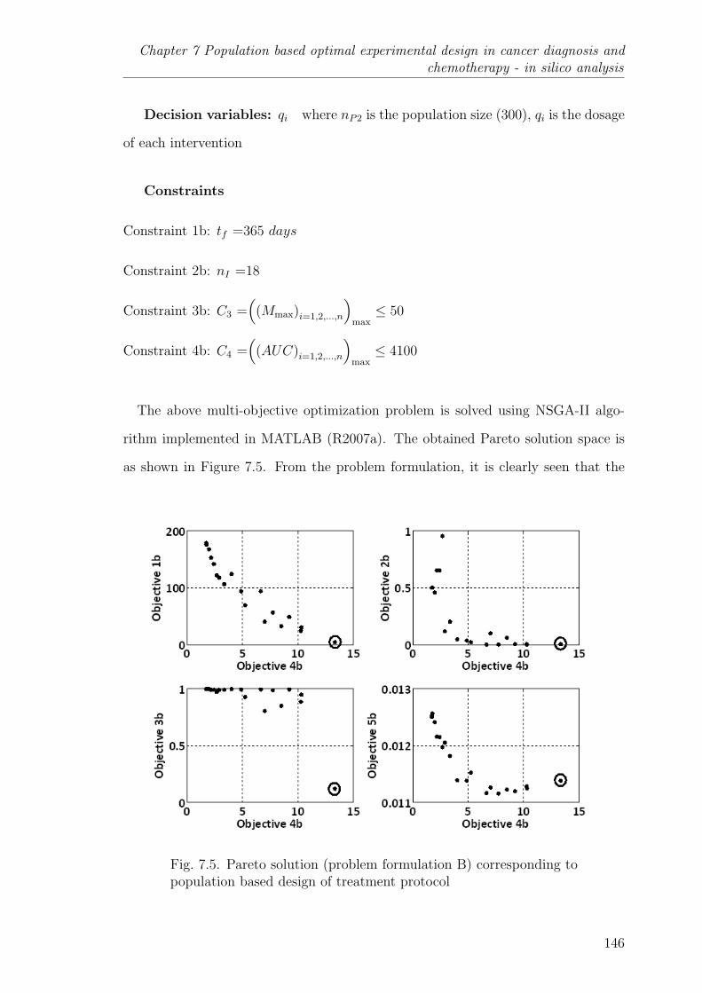
Chapter 7 Population based optimal experimental design in cancer diagnosis andchemotherapy - in silico analysis
Decision variables: qi where nP2 is the population size (300), qi is the dosage
of each intervention
Constraints
Constraint 1b: tf =365 days
Constraint 2b: nI =18
Constraint 3b: C3 =(
(Mmax)i=1,2,...,n
)max≤ 50
Constraint 4b: C4 =(
(AUC)i=1,2,...,n
)max≤ 4100
The above multi-objective optimization problem is solved using NSGA-II algo-
rithm implemented in MATLAB (R2007a). The obtained Pareto solution space is
as shown in Figure 7.5. From the problem formulation, it is clearly seen that the
Fig. 7.5. Pareto solution (problem formulation B) corresponding topopulation based design of treatment protocol
146
7.3 Population-based studies
main concern is to understand the effect of chemotherapy on tumor cells and cir-
culating lymphocytes. Thus, in Figure 7.5, the objectives related to tumor cells
(objectives 1b, 2b, and 3b) and circulating lymphocytes (objectives 5b) are plotted
against the objective 4b (total dosage of doxorubicin (given in scaled units))4. It is
observed that objectives 1b, 2b decreases with the increase in doxorubicin dosage.
Initially, the decrease of objective 2b is steep with the increase in objective 4b and
after that, it stays almost constant. It implies that the effect of doxorubicin dosage
becomes insignificant in decreasing the final tumor size when the total doxorubicin
dosage exceed 5 units. However, it is noticed that the decrease of objective 3b
(maximum possible tumor size) is significant only when the value of the total drug
dosage is greater than 10 units. Also, from the values of objective 5b in Figure 7.5,
it can be said that the variation of objective 5b with objective 4b is practically neg-
ligible. Overall, Pareto solution suggests that the total doxorubicin dosage should
be in between 10 units and 15 units in order to satisfy all the objectives related to
tumor growth. Thus, the therapeutic protocol corresponding to the encircled point
in Figure 7.5 is chosen and is presented in Figure 7.6.
The selected treatment protocol is then implemented on the patient cohort used
in the optimization problem and their corresponding tumor evolution is computed
(Figure 7.7). It is noticed that tumor regression is observed in 43% of the patients
while there is no effect of the therapy on the others. According to Khaloozadeh
et al. (2009), a patient is said to be in “safer zone” if the number of tumor cells is
less than 104. Thus, the treatment protocol applied on the patient cohort indicates
that only some patients are brought to a safe level. This resembles the real scenario
wherein due to interpatient variability only a portion of patients with same tumor
size are cured with the standard treatment protocols.
It is important to derive the “rules” which determine the success of the proposed
treatment protocol. In this regard, the patient cohort is divided into two groups viz.
cured and uncured at the end of the treatment period. A dataset which includes the
4One scaled unit is equivalent to 60 mg/m2
147

Chapter 7 Population based optimal experimental design in cancer diagnosis andchemotherapy - in silico analysis
Fig. 7.6. Proposed treatment protocol for the considered patient cohort
Fig. 7.7. Tumor evolution in different patients
patient parameters and their therapy outcome (after the execution of the proposed
treatment protocol) is created for this purpose. This dataset is used to develop a
148

7.3 Population-based studies
statistical model in the form of classification tree using the classification algorithm
“classregtree” command implemented in MATLAB (R2007a). This command gen-
erates a classification tree for the response variable as a function of the predictors
(patient parameters).
Initially, 100 model building runs are carried out on the dataset. In each run,
the dataset is randomly divided into training (70%) and testing (30%) sets and a
classification model is generated using training set. Each generated model is tested
with their respective testing set. Models with more than 90% correct classification
of test samples are selected from these 100 models and in our case, 2 such models
were found. In order to choose a model among these two selected models, further
testing is performed.
Each selected model is checked for its consistency in terms of correct classifica-
tion by carrying out 1000 runs where, in each run, the training and testing samples
are selected randomly. Finally, the best model is chosen and its decision tree is
Fig. 7.8. Rules to determine the success of proposed treatment pro-tocol on the population
149

Chapter 7 Population based optimal experimental design in cancer diagnosis andchemotherapy - in silico analysis
presented in Figure 7.8. It is observed that the average correct classification by the
decision tree is 90%. In Figure 7.8, ‘N’ and ‘Y’ means no and yes respectively, S1 and
S2 corresponds to the safe level and unsafe level of tumor size by final time respec-
tively. The prominent parameters influencing the treatment protocol and grouping
of patient cohort are found to be pharmacodynamic parameters (Π20, Π21), pharma-
cokinetic parameter (Π24) and the parameter related to the activation of interleukin
due to presence of CD8+ T-cells (Π18). Furthermore, the decision tree (given in
Figure 7.8) is cross validated with the decision tree obtained from the commercial
data mining software, CART5. The decision tree obtained from CART confirms that
pharmacokinetic (Π24) and pharmacodynamic parameters (Π20, Π21) determine the
treatment outcome which is also in agreement with the literature (Canal et al.,
1998). If the pharmacokinetic and pharmacodynamic parameters are low, then the
drug concentration in the patient remains at a high level leading to acute side effects.
This highlights that it is very important and informative to monitor the drug activity
in the patient to estimate the pharmacokinetic and pharmacodynamic parameters
during the initial interventions. Such early quantification of drug activity can help
to decide whether to increase the drug dosage (within the safer limits) or opt for
alternative drugs in the future interventions on this patients. Analysis of historical
record of the outcomes obtained by applying different therapies on different patient
cohorts may help to pave way for understanding the epidemiological differences and
personalizing therapy for the patients by making effective use of existing treatment
modalities.
7.4 Conclusions
This work exemplifies the significance of modeling and optimization techniques
in designing diagnostic and therapeutic protocols for cancer. Tumor-immune model
elucidating the immunogenic tumor growth was considered in this work. The sim-
5http://salford-systems.com/cart.php
150
7.4 Conclusions
plified model is used to imitate cohort based clinical trials to find optimal sampling
times of measurement of tumor, CD8+ T-cells and interleukin during diagnosis and
determine optimal doxorubicin dosage for the standard protocol. Multi-objective
optimization problems were formulated to study optimal design of diagnosis and
therapy. The results of diagnosis protocols reveal that more information can be
captured by measuring interleukin concentration and CD8+ T-cells along with the
tumor measurement. It was found that the frequency of sampling needs to be high
within first 10 days after tumor is detected which is in coherent with the dynamics of
the states. Similarly, “cohort based” studies were performed to determine a better
treatment protocol of doxorubicin. Then, statistical classification techniques helped
to identify that pharmacokinetic, pharmacodynamic and CD8+ T-cells activation
parameters determine the success of the proposed treatment protocol. Such in silico
analysis can be helpful in the eventual development of personalized therapy.
151
Conclusions and recommendations for future work
Chapter 8
CONCLUSIONS AND RECOMMENDATIONS FOR
FUTURE WORK
‘One ounce of practice is worth a thousand pounds of theory.’
- Swami Vivekananda
8.1 Conclusions
Cancer is a global issue and an important multidisciplinary field of research with
a lot of open ended and challenging problems. The main thrust of this thesis is
to highlight that application of process systems engineering techniques can play an
important role in addressing the problems related to cancer dynamics and its treat-
ment. The main focus of this thesis is to study the initial stages of cancer progression
- avascular tumor growth and its interaction with the therapeutic agents. In the
first two chapters, the role of modeling in cancer, broader review of works which
were done hitherto, challenges and contributions of this thesis were introduced.
The first objective of this work was to develop a mechanistic mathematical model
to describe the avascular tumor growth. The proposed model accounts for all the
pertinent cellular processes (proliferation, apoptosis and necrosis) and their depen-
dency on the diffusion and consumption of the nutrients. The model was able to syn-
chronize with the experimental results in terms of predicting tumor growth and max-
imum volume achieved under different microenvironment conditions. The results
of onset of necrosis clarifies the proposition that necrotic zone is the consequence
152
8.1 Conclusions
of the critical concentrations of both vital nutrients. The time at which necrotic
zone starts might indicate tumor vascularization (connection with the nearby blood
vessels). Additionally, the model is prognostic in distinguishing the size of prolifer-
ation zone, quiescent zone and necrotic zone and their effect on the overall tumor
growth. Practically, it is formidable to measure the diffusive and consumption rate
parameters of the nutrients. Therefore, the proposed model can be useful for tumor
pathologists in determining those parameters from the multicellular tumor spheroid
experimental data using the sample extracted from the patient.
The second objective was to propose a therapeutic protocol for a given patient
while considering practical multiple objectives associated with cancer therapies.
Chemotherapy is the common adjuvant therapy given to the patient at stage or
another during the course of cancer treatment and, nowadays, they are combined
with the targeted therapies to reduce the side effects. Thus, the multiple objectives
can be broadly related to tumor reduction and reduction of side effects. This sce-
nario is dealt in chapter 4 by formulating a multi-objective optimization problem
using a tumor-immuno-chemo model (patient representation) adapted from the lit-
erature. NSGA -II was used to find the solution set known as Pareto set and the
decision variables represented the timing and dosage of the interventions. Then,
post-Pareto-optimality analysis was done to choose a solution from Pareto set. The
results for the considered patient have shown that the performance of the proposed
chemotherapy protocol was better than the standard protocol employed in medi-
cal practice. However, at the end of the treatment course the number of tumor
cells were in the range of 105 cells. Alternatively, the combination of chemotherapy
and immunotherapy resulted in almost complete elimination of tumor cells. Also,
post-treatment analysis based on tumor relapse time has indicated that combina-
tion therapy is better than chemotherapy. As a whole, this work suggests that
the immunogenicity factor (intensity of tumor-immune interactions) must be taken
into account prior to every therapeutic intervention. The real outcome of this work
153
Conclusions and recommendations for future work
emphasizes on the utility of computer based pre-treatment analysis or treatment
planning decision-support system for oncologists in deciding a treatment protocol
for a patient.
Intrapatient variability is one of the major challenges in cancer therapy because
variability in patient dynamics (response to drugs) might result in overdosage or
underdosage of therapeutic agents. Thus, it is necessary to monitor the patient
regularly and look for tumor growth variations which can be attributed to different
factors. The questions addressed were related to the parameters which are to be
monitored when a patient visits the clinic and how to reschedule the interventions
based on those parameter values. In chapter 5, this challenge was investigated using
a mathematical model elucidating the interaction between tumor cell and different
types of immune cells. The key parameters affecting the tumor growth were found
out using global sensitivity analysis techniques. The key mechanisms were found
to be the proliferation of tumor cells due to nutritional effect, its interaction with
CD8+ T-cells and the availability of CD8+ T-cells. These key parameters are
further crosschecked by formulating an optimization problem and comparing the
nominal and reactive schedules of the dendritic cell interventions. The nominal and
reactive schedules for variation in non-key parameters were approximately the same,
while in the case of key parameter variations they were different. Similar results
were observed in these simulation studies. Further, for a given parametric variation,
reactive scheduling was applied to propose the dosage interventions of single therapy
of dendritic cells and the combination therapy of dendritic cells and interleukin. The
case study has shown that dendritic cells interventions alone were enough to control
and bring down the tumor size. Moreover, the cumulative dosage of dendritic cells
for the reactive scheduling was lesser than the nominal scheduling. The practical
implication is that combination therapy is not an absolute solution when the patient
variability is significant. So, it is important to re-estimate the patient parameters
154
8.1 Conclusions
regularly and this kind of treatment planning simulators/decision-support systems
will be useful in rescheduling the therapeutic interventions.
Another issue addressed in this thesis relates to the importance of simplification
of complex physiological models in order to facilitate its clinical applications. The
complexity of physiological models increases with the inclusion of updated knowl-
edge about them. In this regard, scaling and sensitivity analysis approaches were
utilized to obtain a reduced parametric model. As a case study, a comprehensive
and highly parameterized tumor-immune model was taken from literature. Scal-
ing analysis helped in obtaining a minimal model with lesser number of parameters
than the original model without any loss of information. That is, no reduction in the
predictive ability of the model. At the same time, the values of the coefficients in
the model equation were in the order-of-one. This implies that corresponding terms
in the equation with lowest coefficient values can be nullified. Also, the advantage
of scaling analysis is quantified using theoretical identifiability analysis. Further,
the application of global sensitivity analysis helped in finding the key parameters
affecting tumor growth. The key mechanisms were found to be the effect of nutri-
ents, intensity of interaction between tumor cells and CD8+ T-cells and they are
in agreement with the previous case study done in chapter 5. Another comparison
between reduced and original model was done on the basis of parameter estima-
tion. The results have shown that the uncertainty of the parameter estimates of
the reduced model is smaller than that of the original model (as expected). Also,
the computational effort is significantly less for the parameter estimation of reduced
model when compared to the original model.
The simplified model was used to imitate cohort-based clinical trials and ac-
counted for interpatient variability. Then, for a given patient cohort (generated
by varying key parameters), optimal sampling times for collecting tumor cells and
immune cells from patient during diagnosis (before treatment is commenced) and
155
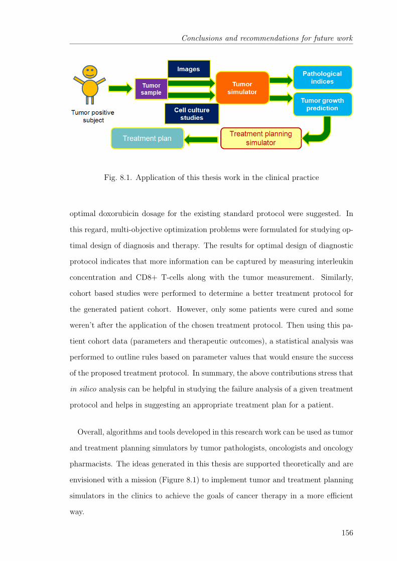
Conclusions and recommendations for future work
Fig. 8.1. Application of this thesis work in the clinical practice
optimal doxorubicin dosage for the existing standard protocol were suggested. In
this regard, multi-objective optimization problems were formulated for studying op-
timal design of diagnosis and therapy. The results for optimal design of diagnostic
protocol indicates that more information can be captured by measuring interleukin
concentration and CD8+ T-cells along with the tumor measurement. Similarly,
cohort based studies were performed to determine a better treatment protocol for
the generated patient cohort. However, only some patients were cured and some
weren’t after the application of the chosen treatment protocol. Then using this pa-
tient cohort data (parameters and therapeutic outcomes), a statistical analysis was
performed to outline rules based on parameter values that would ensure the success
of the proposed treatment protocol. In summary, the above contributions stress that
in silico analysis can be helpful in studying the failure analysis of a given treatment
protocol and helps in suggesting an appropriate treatment plan for a patient.
Overall, algorithms and tools developed in this research work can be used as tumor
and treatment planning simulators by tumor pathologists, oncologists and oncology
pharmacists. The ideas generated in this thesis are supported theoretically and are
envisioned with a mission (Figure 8.1) to implement tumor and treatment planning
simulators in the clinics to achieve the goals of cancer therapy in a more efficient
way.
156

8.2 Recommendations for future work
8.2 Recommendations for future work
8.2.1 Validation of the tumor growth models
The main limitation of mathematical modeling is that there is no perfect model
which can exactly replicate all the scenarios observed in a real system. Also, model
accuracy is dependent on the dataset used to build the model and numerical tech-
niques used to solve the model. Hence, a model should be thoroughly validated and
understand its range of predictive capability before using it for real time applica-
tions.
The mechanistic model developed in this work (Chapter 3) was validated with
some of the in vitro and in vivo tumor growth data. However, it needs to be val-
idated further with some more cell studies encompassing different types of cancer
in order to test its robustness. Moreover, the mechanistic avascular tumor growth
model developed in this work focused only on the diffusion of nutrients, but not on
the dynamics of the growth factors. It was assumed that the presence of growth
factors allows the tumor cells to uptake the nutrients and nurture. It is necessary to
understand the mechanism that underlies how the presence of growth factors regu-
lates the tumor growth. Another issue is the availability of wide range of models to
explain a given phenomenon, for example, tumor-immune interactions. The ques-
tion is which model is to be chosen for tumor growth predictions and therapeutic
analysis. One of the ways could be the approaches of model discrimination. Even-
tually, a model chosen from model discrimination procedure can be used to analyze
the clinical data on tumor growth which is available in the form of images. The
probable challenge is in using the image data to estimate model parameters.
8.2.2 Model-based therapeutic design
In the present thesis work, therapeutic analysis were done using doxorubicin,
immune cells and interleukin interventions by formulating optimization problems.
157
Conclusions and recommendations for future work
Similar analysis can be extended to other types of cancer drugs for improving their
protocol design and for proposing innovative combinatorial strategies. In addition,
even though the present work has focused on model simplification which helps in
reducing model simulation time, it did not address the issue of computational time
for optimization which is one of the important factors in order to promote in silico
analysis in the clinical applications. In this regard, a comparative study of dif-
ferent optimization algorithms can be done for solving a therapeutic design based
optimization problem and also novel algorithms can be proposed.
8.2.3 Multiscale modeling
Cancer diagnosis is a very crucial phase to reap the benefits of available treat-
ment modalities. Presently, tumor pathological studies based on multicellular tu-
mor spheroid (MCTS) experiments have made a great impact in grading the tumor
cells (Rodrguez-Enrquez et al., 2008; Mueller-Klieser, 1997). These experiments
closely resemble in vivo tumor growth experiments. The effect of microenviron-
ment, therapeutics and cell-cell interactions on tumor growth is better understood
and treatment regimens can be planned accordingly. Many mathematical model-
ing approaches have been suggested to extract the physiological reasons and to test
different hypotheses on MCTS growth. However, most of the mechanistic models
(replicating MCTS experiments) discussed so far capture the macroscopic level ob-
servations and ignore the microscopic level issues. Cancer cells are formed due to
genetic changes which eventually result in the distortion of the cell division process.
The prime objective of the work proposed here is to pinpoint the distortion. In
general, a cell divides by passing through different phases of the cell cycle. The
phases of the cell cycle are G1, S, G2 and M. G1 and G2 are the preparatory phases
for the DNA-duplication (S) and mitosis (M) respectively. In different phases differ-
ent activated proteins are needed to carry on the cell cycle events. These proteins
are activated via phosphorylation by phase-wise phosphorylated cyclin dependent
158
8.2 Recommendations for future work
kinases (cdk) complexes (Qu et al., 2003). Formation and phosphorylation of cdk
complexes initiate as soon as a cell is divided into two daughter cells. The source for
the activation of cdk complexes are phase dependent cyclins and adenosine triphos-
phate (ATP) produced from the glucose metabolism. Transfer from one phase of
the cell cycle to other phase indirectly depends on the concentration of ATP which
is the product of glycolysis and oxidative phosphorylation. According to the con-
troversial theory of Warburg effect, enhanced glycolysis is a feature of a cancer cell.
It means that the oxidative phosphorylation process is avoided in the cell and the
total ATP is produced only by the glycolytic pathway (Moreno-Snchez et al., 2007;
DeBerardinis et al., 2008). In addition to this, there are cell cycle checkpoints based
on the threshold concentration of the growth factors and proteins. Usually, if any
abnormality is observed, p53 pathway triggers the cell to commit suicide known
as apoptosis (Danilo and Jose, 2009). But, these controlling mechanisms are be-
lieved to be inactive in the cancer cells. Most of the previous works were focused
on particular individual pathways. So, the future work could focus to integrate the
aforementioned biochemical pathways of cell cycle progression and cell division with
the glucose metabolism and analyze the cancerous features by calculating the time
taken to complete a cell cycle.
The main steps include:
1. Acquisition and preprocessing of metabolome, proteome and genome data from
the available databases.
2. Application of data mining techniques to develop the network models eluci-
dating the causality and relationship among the metabolites, proteins, and
genes.
3. Parametric sensitivity analysis of the network models will be performed to
investigate the key parameters affecting the cell cycle progression and its di-
vision.
159
Conclusions and recommendations for future work
4. Application of multiscale modeling to predict the tumor growth and the vari-
ation in the tumor morphology over time.
The above four steps will be explained in detail below.
Building of network models
The goal of the proposed work is to develop a network model among the metabo-
lites, proteins and genes which quantify biochemical pathways from the omics data.
With the advent of whole genome sequence and other high-throughput experimen-
tal technologies, biological research has transformed from data poor to a data rich
discipline (Mosca et al., 2010; Joyce and Palsson, 2006). The large data sets being
interpreted to find the relationships and causalities. Relationship analysis is a subset
of causality, as causality not only checks the relationship between the components
but also highlights the direction of the relationship. The network model obtained
should be validated prior to its usage for further research and applications. In this
regard, the complete dataset should be preprocessed and can be divided into train-
ing and validation datasets. Preprocessing is necessary in order to reduce the effect
of noise in the data on the network model construction. Then network models can
be built using training sets and verified using validation sets. The topology of the
network models can be further consolidated by comparing with available pathways
from the literature. Particularly, available information on feedback loops (positive
or negative) can be checked. Alternatively, the developed network model can be
split into smaller networks and some networks with strong theoretical backup can
be selected for comparison.
Identification and ranking of the key mechanism of the network
Network models facilitate the comprehension of the integrated biochemical path-
ways driving the cell cycle. However, these models are complex with numerous
variables and parameters. Model complexity is one of the issues of multiscale net-
160
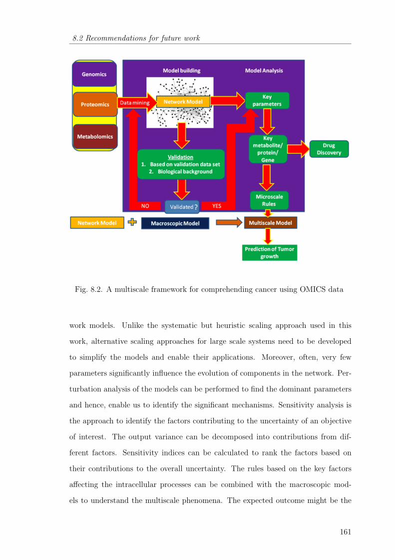
8.2 Recommendations for future work
Fig. 8.2. A multiscale framework for comprehending cancer using OMICS data
work models. Unlike the systematic but heuristic scaling approach used in this
work, alternative scaling approaches for large scale systems need to be developed
to simplify the models and enable their applications. Moreover, often, very few
parameters significantly influence the evolution of components in the network. Per-
turbation analysis of the models can be performed to find the dominant parameters
and hence, enable us to identify the significant mechanisms. Sensitivity analysis is
the approach to identify the factors contributing to the uncertainty of an objective
of interest. The output variance can be decomposed into contributions from dif-
ferent factors. Sensitivity indices can be calculated to rank the factors based on
their contributions to the overall uncertainty. The rules based on the key factors
affecting the intracellular processes can be combined with the macroscopic mod-
els to understand the multiscale phenomena. The expected outcome might be the
161
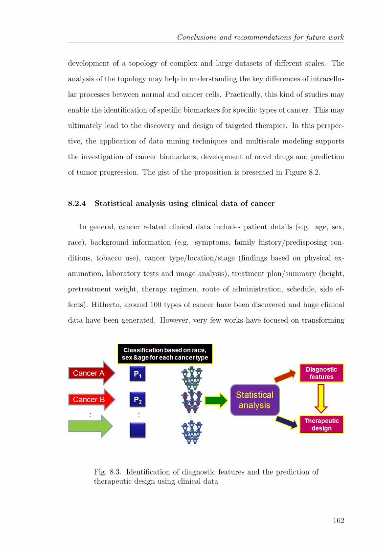
Conclusions and recommendations for future work
development of a topology of complex and large datasets of different scales. The
analysis of the topology may help in understanding the key differences of intracellu-
lar processes between normal and cancer cells. Practically, this kind of studies may
enable the identification of specific biomarkers for specific types of cancer. This may
ultimately lead to the discovery and design of targeted therapies. In this perspec-
tive, the application of data mining techniques and multiscale modeling supports
the investigation of cancer biomarkers, development of novel drugs and prediction
of tumor progression. The gist of the proposition is presented in Figure 8.2.
8.2.4 Statistical analysis using clinical data of cancer
In general, cancer related clinical data includes patient details (e.g. age, sex,
race), background information (e.g. symptoms, family history/predisposing con-
ditions, tobacco use), cancer type/location/stage (findings based on physical ex-
amination, laboratory tests and image analysis), treatment plan/summary (height,
pretreatment weight, therapy regimen, route of administration, schedule, side ef-
fects). Hitherto, around 100 types of cancer have been discovered and huge clinical
data have been generated. However, very few works have focused on transforming
Fig. 8.3. Identification of diagnostic features and the prediction oftherapeutic design using clinical data
162
8.2 Recommendations for future work
the available data to knowledge. In this regard, statistical analysis of clinical data
can be helpful. The first step could be to construct a database using data from
cancer clinics in a given geographical region. Then, the patients could be classified
according to sex, age, race, location for a given cancer type (Figure 8.3). After
classification, the data sets could be analyzed using statistical tools to find out can-
cer prone diagnostic features and relate them to the therapeutic design. Overall,
the above-mentioned approach might help in bringing the personalized therapy in
practice.
163
REFERENCES
REFERENCES
Aarntzen, E., Figdor, C., Adema, G., Punt, C. and de Vries, I. (2008), ‘Dendriticcell vaccination and immune monitoring’, Cancer Immunology, Immunotherapy57(10), 1559–1568.
Aarons, L. and Ogungbenro, K. (2010), ‘Optimal design of pharmacokinetic studies’,Basic Clinical Pharmacology and Toxicology 106(3), 250–255.
Abbott, R. G., Forrest, S. and Pienta, K. J. (2006), ‘Simulating the hallmarks ofcancer’, Artificial Life 12(4), 617–634.
Adam, J. A. (1986), ‘A simplified mathematical model of tumor growth’, Mathe-matical Biosciences 81(2), 229–244.
Adam, J. A. (1987a), ‘A mathematical model of tumor growth. ii. effects of geometryand spatial nonuniformity on stability’, Mathematical Biosciences 86(2), 183–211.
Adam, J. A. (1987b), ‘A mathematical model of tumor growth. iii. comparison withexperiment’, Mathematical Biosciences 86(2), 213 – 227.
Adam, J. A. (1988), ‘A mathematical model of tumor growth by diffusion’, Mathe-matical and Computer Modelling 11, 455–456.
Adam, J. A. (1989), ‘A mathematical model of tumor growth by diffusion’, Mathe-matical Biosciences 94(1), 155–155.
Adam, J. A. and Maggelakis, S. A. (1989), ‘Mathematical models of tumor growth.iv. effects of a necrotic core’, Mathematical Biosciences 97(1), 121–136.
Adam, J. K., Odhav, B. and Bhoola, K. (2003), ‘Immune responses in cancer’,Pharmacology and Therapeutics 99, 113–132.
Agur, Z., Arnon, R. and Schechter, B. (1988), ‘Reduction of cytotoxicity to normaltissues by new regimens of cell-cycle phase-specific drugs’, Mathematical Bio-sciences 92(1), 1–15.
Airley, R. (2009), Cancer chemotherapy, Wiley-Blackwell, Hoboken, NJ.
Alberts, B., Johnson, A., Lewis, J., Raff, M., Roberts, K. and Walter, P. (2002),Molecular biology of the cell, 4th edn, Garland Science., New York.
Ambrosi, D. and Preziosi, L. (2002), ‘On the closure of mass balance models fortumor growth’, Mathematical Models and Methods in Applied Sciences 12(5), 737–754.
Anderson, A. R. A. and Quaranta, V. (2008), ‘Integrative mathematical oncology’,Nat Rev Cancer 8(3), 227–234.
164
REFERENCES
Araujo, R. P. and McElwain, D. L. S. (2004), ‘A history of the study of solid tumourgrowth: the contribution of mathematical modelling’, Bulletin of MathematicalBiology 66(5), 1039–1091.
Ballestrero, A., Boy, D., Moran, E., Cirmena, G., Brossart, P. and Nencioni, A.(2008), ‘Immunotherapy with dendritic cells for cancer’, Advanced Drug DeliveryReviews 60(2), 173–183.
Banchereau, J., Schuler-Thurner, B., Palucka, A. K. and Schuler, G. (2001), ‘Den-dritic cells as vectors for therapy’, Cell 106(3), 271–274.
Barbolosi, D. and Iliadis, A. (2001), ‘Optimizing drug regimens in cancer chemother-apy: a simulation study using a pk-pd model’, Computers in Biology and Medicine31(3), 157–172.
Bell, H. S., Whittle, I. R., Walker, M., Leaver, H. A. and Wharton, S. B. (2001),‘The development of necrosis and apoptosis in glioma: experimental findings usingspheroid culture systems’, Neuropathology 38; Applied Neurobiology 27, 291–304.
Bellomo, N., Angelis, E. D. and Preziosi, L. (2003), ‘Review article: Multiscalemodeling and mathematical problems related to tumor evolution and medicaltherapy’, Journal of Theoretical Medicine 5(2), 111–136.
Bellomo, N., Bellouquid, A. and De Angelis, E. (2003), ‘The modelling of the im-mune competition by generalized kinetic (boltzmann) models: Review and re-search perspectives’, Mathematical and Computer Modelling 37(1-2), 65–86.
Bellomo, N. and Preziosi, L. (2000), ‘Modelling and mathematical problems relatedto tumor evolution and its interaction with the immune system’, Mathematicaland Computer Modelling 32(3-4), 413–452.
Bertuzzi, A., Fasano, A., Gandolfi, A. and Sinisgalli, C. (2007), ‘Atp productionand necrosis formation in a tumour spheroid model’, Math. Model. Nat. Phenom.2(3), 30–46.
Breward, C., Byrne, H. and Lewis, C. (2003), ‘A multiphase model describing vas-cular tumour growth’, Bulletin of Mathematical Biology 65(4), 609–640.
Breward, C. J. W., Byrne, H. M. and Lewis, C. E. (2002), ‘The role of cell-cellinteractions in a two-phase model for avascular tumour growth’, Journal of Math-ematical Biology 45(2), 125–152.
Bunimovich-Mendrazitsky, S., Shochat, E. and Stone, L. (2007), ‘Mathematicalmodel of bcg immunotherapy insuperficial bladder cancer’, Bulletin of Mathe-matical Biology 69(6), 1847–1870.
Burton, A. (1966), ‘Rate of growth of solid tumors as a problem of diffusion’, Growth30, 229–244.
Busini, V., Arosio, P. and Masi, M. (2007), ‘Mechanistic modelling of avascular tu-mor growth and pharmacokinetics influence–part i’, Chemical Engineering Science62(7), 1877–1886.
165
REFERENCES
Byrne, H., Alarcon, T., Owen, M., Webb, S. and Maini, P. (2006), ‘Modelling aspectsof cancer dynamics: a review’, Philosophical Transactions of the Royal Society A:Mathematical, Physical and Engineering Sciences 364(1843), 1563–1578.
Byrne, H. and Drasdo, D. (2009), ‘Individual-based and continuum models of grow-ing cell populations: a comparison’, Journal of Mathematical Biology 58(4), 657–687.
Byrne, H. M. (1997), ‘The effect of time delays on the dynamics of avascular tumorgrowth’, Mathematical Biosciences 144(2), 83–117.
Byrne, H. M. (1999), ‘A weakly nonlinear analysis of a model of avascular solidtumour growth’, Journal of Mathematical Biology 39(1), 59–89.
Byrne, H. M. (2010), ‘Dissecting cancer through mathematics: from the cell to theanimal model’, Nature Reviews Cancer 10(3), 221.
Byrne, H. M. and Chaplain, M. A. J. (1995), ‘Growth of nonnecrotic tumors in thepresence and absence of inhibitors’, Mathematical Biosciences 130(2), 151–181.
Byrne, H. M. and Chaplain, M. A. J. (1996), ‘Modelling the role of cell-cell adhe-sion in the growth and development of carcinoma’, Mathematical and ComputerModelling 24(12), 1–17.
Byrne, H. M. and Chaplain, M. A. J. (1998), ‘Necrosis and apoptosis: distinct cellloss mechanisms in a mathematical model of avascular tumour growth’, Compu-tational and Mathematical Methods in Medicine 1(3), 223 – 235.
Byrne, H. M. and Gourley, S. A. (1997), ‘The role of growth factors in avasculartumour growth’, Mathematical and Computer Modelling 26(4), 35–55.
Canal, P., Gamelin, E., Vassal, G. and Robert, J. (1998), ‘Benefits of pharmacolog-ical knowledge in the design and monitoring of cancer chemotherapy’, Pathologyand Oncology Research 4, 171–178.
Cappuccio, A., Castiglione, F. and Piccoli, B. (2007), ‘Determination of the opti-mal therapeutic protocols in cancer immunotherapy’, Mathematical Biosciences209(1), 1–13.
Casciari, J. J., Sotirchos, S. V. and Sutherland, R. M. (1988), ‘Glucose diffusivityin multicellular tumor spheroids’, Cancer Res 48(14), 3905–3909.
Casciari, J. J., Sotirchos, S. V. and Sutherland, R. M. (1992), ‘Mathematicalmodelling of microenvironment and growth in emt6/ro multicellular tumourspheroids’, Cell Proliferation 25(1), 1–22.
Castiglione, F. and Piccoli, B. (2006), ‘Optimal control in a model of dendritic celltransfection cancer immunotherapy’, Bulletin of Mathematical Biology 68(2), 255–274.
Castiglione, F. and Piccoli, B. (2007), ‘Cancer immunotherapy, mathematical mod-eling and optimal control’, Journal of Theoretical Biology 247(4), 723–732.
166
REFERENCES
Castiglione, F., Piccoli, B. and ieee (2004), Optimal control in a model of dendriticcell transfection cancer immunotherapy, in ‘43rd IEEE Conference on Decisionand Control’, San Diego, CA, pp. 585–590.
Chaplain, M. A. J., Benson, D. L. and Maini, P. K. (1994), ‘Nonlinear diffusionof a growth inhibitory factor in multicell spheroids’, Mathematical Biosciences121(1), 1–13.
Chareyron, S. and Alamir, M. (2009), ‘Mixed immunotherapy and chemotherapyof tumors: Feedback design and model updating schemes’, Journal of TheoreticalBiology 258(3), 444–454.
Cintron-Arias, A., Banks, H. T., Capaldi, A. and L., L. A. (2009), ‘A sensitivitymatrix based methodology for inverse problem formulation’, Journal of Inverseand Ill-Posed Problems 17, 545–564.
Danilo, R. and Jose, M. P. (2009), ‘An integrated network-based mechanistic modelfor tumor growth dynamics under drug administration’, Computers in Biologyand Medicine 39(4), 368–384.
De Boer, R. J. and Hogeweg, P. (1986), ‘Interactions between macrophages and t-lymphocytes: Tumor sneaking through intrinsic to helper t cell dynamics’, Journalof Theoretical Biology 120(3), 331–351.
de Pillis, L. G., Gu, W., Fister, K. R., Head, T., Maples, K., Murugan, A., Neal, T.and Yoshida, K. (2007), ‘Chemotherapy for tumors: An analysis of the dynamicsand a study of quadratic and linear optimal controls’, Mathematical Biosciences209(1), 292–315.
de Pillis, L. G., Gu, W. and Radunskaya, A. E. (2006), ‘Mixed immunotherapy andchemotherapy of tumors: modeling, applications and biological interpretations’,Journal of Theoretical Biology 238(4), 841–862.
de Pillis, L. G. and Radunskaya, A. (2003), ‘The dynamics of an optimally controlledtumor model: A case study’, Mathematical and Computer Modelling 37(11), 1221–1244.
de Pillis, L. G., Radunskaya, A. E. and Wiseman, C. L. (2005), ‘A validated math-ematical model of cell-mediated immune response to tumor growth’, Cancer Res65(17), 7950–7958.
de Pillis, L., Renee Fister, K., Gu, W., Collins, C., Daub, M., Gross, D., Moore,J. and Preskill, B. (2009), ‘Mathematical model creation for cancer chemo-immunotherapy’, Computational and Mathematical Methods in Medicine: AnInterdisciplinary Journal of Mathematical, Theoretical and Clinical Aspects ofMedicine 10(3), 165 – 184.
Deakin, A. (1975), ‘Model for the growth of a solid in vitro tumour’, Growth 39, 159–165.
167
REFERENCES
Deb, K., Agrawal, S., Pratap, A. and Meyarivan, T. (2000), A fast elitist non-dominated sorting genetic algorithm for multi-objective optimization: Nsga-ii,Parallel Problem Solving from Nature PPSN VI. 6th International Conference.Proceedings (Lecture Notes in Computer Science Vol.1917), Springer-Verlag,Paris, France, pp. 849–58.
DeBerardinis, R. J., Lum, J. J., Hatzivassiliou, G. and Thompson, C. B. (2008), ‘Thebiology of cancer: Metabolic reprogramming fuels cell growth and proliferation’,Cell Metabolism 7(1), 11–20.
Deisboeck, T. S., Zhang, L., Yoon, J. and Costa, J. (2009), ‘In silico cancer modeling:is it ready for prime time?’, Nat Clin Prac Oncol 6(1), 34–42.
Dhodapkar, M. V., Steinman, R. M., Sapp, M., Desai, H., Fossella, C., Krasovsky,J., Donahoe, S. M., Dunbar, P. R., Cerundolo, V., Nixon, D. F. and Bhard-waj, N. (1999), ‘Rapid generation of broad t-cell immunity in humans after asingle injection of mature dendritic cells’, The Journal of Clinical Investigation104(2), 173–180.
Drasdo, D., Hoehme, S. and Block, M. (2007), ‘On the role of physics in thegrowth and pattern formation of multi-cellular systems: What can we learn fromindividual-cell based models?’, Journal of Statistical Physics 128(1), 287–345.
Dua, P., Dua, V. and Pistikopoulos, E. N. (2008), ‘Optimal delivery of chemother-apeutic agents in cancer’, Computers and Chemical Engineering 32(1-2), 99–107.
Dudley, M. E. and Rosenberg, S. A. (2003), ‘Adoptive-cell-transfer therapy for thetreatment of patients with cancer’, Nat Rev Cancer 3(9), 666–675.
Dudley, M. E., Wunderlich, J. R., Robbins, P. F., Yang, J. C., Hwu, P., Schwartzen-truber, D. J., Topalian, S. L., Sherry, R., Restifo, N. P., Hubicki, A. M., Robinson,M. R., Raffeld, M., Duray, P., Seipp, C. A., Rogers-Freezer, L., Morton, K. E.,Mavroukakis, S. A., White, D. E. and Rosenberg, S. A. (2002), ‘Cancer regressionand autoimmunity in patients after clonal repopulation with antitumor lympho-cytes’, Science 298(5594), 850–854.
Durand, R. (1976), ‘Cell cycle kinetics in an in vitro tumor model’, Cell Proliferation9(5), 403–412.
Edgar, T., Himmelblau, D. and Lasdon, L. (2001), Optimization of chemical pro-cesses, McGraw-Hill Chemical engineering series.
Eisen, M. (1979), Mathematical models in cell biology and cancer chemotherapy /Martin Eisen, Lecture notes in biomathematics ; 30, Springer-Verlag, Berlin ;New York :.
Englezos, P. and Kalogerakis, N. (2001), Applied parameter estimation for chemicalengineers, Marcel Dekker, New York.
Folkman, J. and Hochberg, M. (1973), ‘Self-regulation of growth in three dimen-sions’, J. Exp. Med. 138(4), 745–753.
168

REFERENCES
Freyer, J. P. (1988), ‘Role of necrosis in regulating the growth saturation of multi-cellular spheroids’, Cancer Res 48(9), 2432–2439.
Freyer, J. P. and Sutherland, R. M. (1985), ‘A reduction in the in situ rates ofoxygen and glucose consumption of cells in emt6/ro spheroids during growth’,Journal of cellular physiology 124, 516–524.
Freyer, J. P. and Sutherland, R. M. (1986a), ‘Proliferative and clonogenic hetero-geneity of cells from emt6/ro multicellular spheroids induced by the glucose andoxygen supply’, Cancer Res 46(7), 3513–3520.
Freyer, J. P. and Sutherland, R. M. (1986b), ‘Regulation of growth saturation anddevelopment of necrosis in emt6/ro multicellular spheroids by the glucose andoxygen supply’, Cancer Res 46(7), 3504–3512.
Friedrich, J., Seidel, C. and Kunz-Schughart, L. A. (2007), Multicellular spheroids:An underestimated tool is catching up again, in ‘17th Annual Meeting of theGerman-Society-of-Cytometry (DGfZ)’, Regensburg, GERMANY, p. 2.
Gabrilovich, D. I. (2007), ‘Combination of chemotherapy and immunotherapy forcancer: a paradigm revisited’, The Lancet Oncology 8(1), 2–3.
Gardner, S. N. (2000), ‘A mechanistic, predictive model of dose-response curves forcell cycle phase-specific and nonspecific drugs’, Cancer Research 60(5), 1417–1425.
Gardner, S. N. (2002), ‘Modeling multi-drug chemotherapy: tailoring treatment toindividuals’, Journal of theoretical biology 214, 181–207.
Gardner, S. N. and Fernandes, M. (2003), ‘New tools for cancer chemotherapy:computational assistance for tailoring treatments’, Molecular Cancer Therapeutics2(10), 1079–1084.
Garner, A. L., Lau, Y. Y., Jordan, D. W., Uhler, M. D. and Gilgenbach, R. M.(2006), ‘Implications of a simple mathematical model to cancer cell populationdynamics’, Cell Proliferation 39(1), 15–28.
Gatenby, R. A. (1998), ‘Mathematical models of tumor-host interactions’, CancerJournal - France 11(6), 289–293.
Gatenby, R. A. and Gawlinski, E. T. (1996), ‘A reaction-diffusion model of cancerinvasion’, Cancer Research 56(24), 5745–5753.
Gatenby, R. A. and Gawlinski, E. T. (2003), ‘The glycolytic phenotype in carcino-genesis and tumor invasion’, Cancer Research 63(14), 3847–3854.
Gatenby, R. A., Gawlinski, E. T., Gmitro, A. F., Kaylor, B. and Gillies, R. J.(2006), ‘Acid-mediated tumor invasion: a multidisciplinary study’, Cancer Re-search 66(10), 5216–5223.
Ghaffari, A. and Naserifar, N. (2010), ‘Optimal therapeutic protocols in cancerimmunotherapy’, Computers in Biology and Medicine 40(3), 261–270.
169
REFERENCES
Glass, L. (1973), ‘Instability and mitotic patterns in tissue growth’, Transactionsof the ASME. Series G, Journal of Dynamic Systems, Measurement and Control95(3), 324–6.
Gottfried, E., Kunz-Schughart, L. A., Andreesen, R. and Kreutz, M. (2006), ‘Bravelittle world - spheroids as an in vitro model to study tumor-immune-cell interac-tions’, Cell Cycle 5(7), 691–695.
Greenspan, H. (1972), ‘Models for the growth of a solid tumor by diffusion’, Studiesin Applied Mathematics 52, 317–340.
Hanahan, D. and Weinberg, R. (2000), ‘The hallmarks of cancer’, Cell 100, 57 – 70.
Harrold, J. M. and Parker, R. S. (2009), ‘Clinically relevant cancer chemotherapydose scheduling via mixed-integer optimization’, Computers and Chemical Engi-neering 33(12), 2042–2054.
Hlatky, L., Sachs, R. and Alpen, E. (1988a), ‘Joint oxygen-glucose deprivation as thecause of necrosis in a tumor analog’, Journal of Cellular Physiology 134(2), 167–178.
Hlatky, L., Sachs, R. K. and Alpen, E. L. (1988b), ‘Joint oxygen-glucose depriva-tion as the cause of necrosis in a tumoranalog’, Journal of Cellular Physiology134, 167–168.
Ho, W. Y., Blattman, J. N., Dossett, M. L., Yee, C. and Greenberg, P. D. (2003),‘Adoptive immunotherapy: Engineering t cell responses as biologic weapons fortumor mass destruction’, Cancer Cell 3(5), 431–437.
Holford, N., Ma, S. C. and Ploeger, B. A. (2010), ‘Clinical trial simulation: Areview’, Clin Pharmacol Ther 88(2), 166–182.
Hon, Y. and Evans, W. (1998), ‘Making tdm work to optimize cancer chemotherapy:a multidisciplinary team approach’, Clinical Chemistry 44, 388–400.
Hooker, A. and Vicini, P. (2005), ‘Simultaneous population optimal design forpharmacokinetics-pharmacodynamic experiments’, AAPS Journal 7(4), E759–E785.
Hulting, S., Rollins, D. and Bhandari, N. (2006), ‘Optimal experimental design forhuman thermoregulatory system identification.’, Chemical Engineering Researchand Design 84.
Ichim, C. (2005), ‘Revisiting immunosurveillance and immunostimulation: Implica-tions for cancer immunotherapy’, Journal of Translational Medicine 3(1), 8.
Iliadis, A. and Barbolosi, D. (2000), ‘Optimizing drug regimens in cancer chemother-apy by an efficacy-toxicity mathematical model’, Computers and Biomedical Re-search 33(3), 211–226.
170
REFERENCES
Jacobs, J., Aarntzen, E., Sibelt, L., Blokx, W., Boullart, A., Gerritsen, M.-J.,Hoogerbrugge, P., Figdor, C., Adema, G., Punt, C. and de Vries, I. (2009),‘Vaccine-specific local t cell reactivity in immunotherapy-associated vitiligo inmelanoma patients’, Cancer Immunology, Immunotherapy 58(1), 145–151.
Jiang, Y., Pjesivac-Grbovic, J., Cantrell, C. and Freyer, J. P. (2005), ‘A multiscalemodel for avascular tumor growth’, Biophys. J. 89(6), 3884–3894.
Joshi, B., Wang, X., Banerjee, S., Tian, H., Matzavinos, A. and Chaplain, M. A. J.(2009), ‘On immunotherapies and cancer vaccination protocols: A mathematicalmodelling approach’, Journal of Theoretical Biology 259(4), 820–827.
Joyce, A. R. and Palsson, B. O. (2006), ‘The model organism as a system: integrat-ing ’omics’ data sets’, Nat Rev Mol Cell Biol 7(3), 198–210.
Kasprzak, E. M. and Lewis, K. E. (2001), ‘Pareto analysis in multiobjective op-timization using the collinearity theorem and scaling method’, Structural andMultidisciplinary Optimization 22(3), 208–218.
Kerr, J. (1971), ‘Shrinkage necrosis: a distinct mode of cellular death’, journal ofpathology 105, 13–20.
Kerr, J., A.H., W. and A.R., C. (1972), ‘Apoptosis: a basic biological phe-nomenon with wide-ranging implications in tissue kinetics’, British journal ofcancer 26, 239–257.
Khaloozadeh, H., Yazdani, S. and Kamyab, M. (2009), ‘Optimization ofbreast cancer chemotherapy regimens using a pharmacokinetic/pharmacodynamicmodel-based design’, Pharmaceutical Medicine 23(1), 11–18 10.2165/01317117–200923010–00004.
Kim, Y. and Stolarska, M. A. (2007), ‘A hybrid model for tumor spheroid growthin vitro i: Theoretical development and early results’, Mathematical models andmethods in applied sciences 17, 1173–1198.
Kiran, K. L., Jayachandran, D. and Lakshminarayanan, S. (2009), Multi-objectiveoptimization of cancer immuno-chemotherapy, in ‘13th International Conferenceon Biomedical Engineering’, pp. 1337–1340.
Kiran, K. L. and Lakshminarayanan, S. (2009), Treatment planning of cancer den-dritic cell therapy using multi-objective optimization, in ‘In proceedings of AD-CHEM 2009’, Istanbul, Turkey.
Kirkpatrick, S., Gelatt, C. D. and Vecchi, M. P. (1983), ‘Optimization by simulatedannealing’, Science 220(4598), 671–680.
Kirschner, D. and Panetta, J. C. (1998), ‘Modeling immunotherapy of the tumorimmune interaction’, Journal of Mathematical Biology 37(3), 235–252.
Kleinsmith, L. (2005), Principles of cancer biology, Addison-wesley.
171
REFERENCES
Kontoravdi, C., Asprey, S., Pistikopoulos, E. and Mantalaris, A. (2005), ‘Applica-tion of global sensitivity analysis to determine goals for design of experiments:An example study on antibody-producing cell cultures’, Biotechnology Progress21, 1128–1135.
Krantz, W. (2007a), Scaling analysis as a pedagogical tool in teaching transport andreaction processes, in ‘ASEE Annual Conference’.
Krantz, W. B. (2007b), Scaling Analysis in Modeling Transport and Reaction Pro-cesses: A Systematic Approach to Model Building and the Art of Approximation,John Wiley & Sons, Hoboken, New Jersey.
Kunz-Schughart, L. A. (1999), ‘Multicellular tumor spheroids: intermediatesbetween monolayer culture and in vivo tumor’, Cell Biology International23(3), 157–161.
Kunz-Schughart, L. A., Kreutz, M. and Knuechel, R. (1998), ‘Multicellularspheroids: a three-dimensional in vitro culture system to study tumour biology’,International Journal of Experimental Pathology 79(1), 1–23.
Kuznetsov, V. A. and Knott, G. D. (2001), ‘Modeling tumor regrowth and im-munotherapy’, Mathematical and Computer Modelling 33(12-13), 1275–1287.
Kuznetsov, V. A., Makalkin, I. A., Taylor, M. A. and Perelson, A. S. (1994), ‘Non-linear dynamics of immunogenic tumors: Parameter estimation and global bifur-cation analysis’, Bulletin of Mathematical Biology 56(2), 295–321.
Laginha, K., Verwoert, S., Charrois, G. and Allen, T. (2005), ‘Determination of dox-orubicin levels in whole tumor and tumor nuclei in murine breast cancer tumors’,Clinical Cancer Research 11, 6944–6949.
Lake, R. A. and Robinson, B. W. S. (2005), ‘Immunotherapy and chemotherapy - apractical partnership’, Nat Rev Cancer 5(5), 397–405.
LaRue, K. E. A., Bradbury, E. M. and Freyer, J. P. (1998), ‘Differential regula-tion of cyclin-dependent kinase inhibitors in monolayer and spheroid cultures oftumorigenic and nontumorigenic fibroblasts’, Cancer Research 58(6), 1305–1314.
Laszlo Kopper, M. (2001), ‘Tumor cell growth kinetics’, CME Journal of GynecologicOncology (6), 141–143.
Ledzewicz, U. and Schttler, H. (2007), ‘Optimal controls for a model with phar-macokinetics maximizing bone marrow in cancer chemotherapy’, MathematicalBiosciences 206(2), 320–342.
Lee, H. J. and Schiesser, W. E. (2003), Ordinary and partial differential equation rou-tines in C, C++, Fortran, Java, Maple, and MATLAB, Chapman & Hall/CRC.
Li, G., Rabitz, H., Yelvington, P. E., Oluwole, O. O., Bacon, F., Kolb, C. E. andSchoendorf, J. (2010), ‘Global sensitivity analysis for systems with independentand/or correlated inputs’, The Journal of Physical Chemistry A 114, 6022–6032.
172

REFERENCES
Li, G., Rosenthal, C. and Rabitz, H. (2001), ‘High dimensional model representa-tions’, The Journal of Physical Chemistry A 105(33), 7765–7777.
Li, G., Wang, S.-W., Rabitz, H., Wang, S. and Jaffc, P. (2002), ‘Global uncer-tainty assessments by high dimensional model representations (hdmr)’, ChemicalEngineering Science 57(21), 4445–4460.
Li, Z. and Ierapetritou, M. (2008a), ‘Process scheduling under uncertainty: Reviewand challenges’, Computers & Chemical Engineering 32(4-5), 715–727.
Li, Z. and Ierapetritou, M. G. (2008b), ‘Reactive scheduling using parametric pro-gramming’, AIChE Journal 54(10), 2610–2623.
Lord, C. and Ashworth, A. (2010), ‘Biology-driven cancer drug development: backto the future’, BMC Biology 8(1), 38.
Lowengrub, J. S., Frieboes, H. B., Jin, F., Chuang, Y.-L., Li, X., Macklin, P.,Wise, S. and Cristini, V. (2010), ‘Nonlinear modelling of cancer: bridging the gapbetween cells and tumours’, Nonlinearity 23(1), R1–R91.
Ludewig, B. and Hoffman, M. W., eds (2005), Adoptive immunotherapy: methodsand protocols, Humana press, Totowa, NJ.
Mallet, D. G. and De Pillis, L. G. (2006), ‘A cellular automata model of tumor-immune system interactions’, Journal of Theoretical Biology 239(3), 334–350.
Marino, S., Hogue, I., Ray, C. and Kirschner, D. (2008), ‘A methodology for per-forming global uncertainty and sensitivity analysis in systems biology’, Journalof Theoretical Biology 254(1), 178–196.
Martin, R. B. (1992), ‘Optimal control drug scheduling of cancer chemotherapy’,Automatica 28(6), 1113–1123.
Martins, M. L., Ferreira Jr, S. C. and Vilela, M. J. (2007), ‘Multiscale models forthe growth of avascular tumors’, Physics of Life Reviews 4(2), 128–156.
Maruic, M., Bajzer, e., Vuk-Pavlovic, S. and Freyer, J. (1994), ‘Tumor growth invivo and as multicellular spheroids compared by mathematical models’, Bulletinof Mathematical Biology 56(4), 617–631.
Marusic, M., Bajzer, Z., Freyer, J. P. and Vuk-Pavlovic, S. (1994), ‘Analysis ofgrowth of multicellular tumour spheroids by mathematical models’, Cell Prolifer-ation 27(2), 73–94.
Matveev, A. S. and Savkin, A. V. (2002), ‘Application of optimal control theory toanalysis of cancer chemotherapy regimens’, Systems & Control Letters 46(5), 311–321.
McCall, J., Petrovski, A. and Shakya, S. (2007), Evolutionary algorithms for can-cer chemotherapy optimization, in Y. P. Gary B. Fogel, David W. Corne, ed.,‘Computational Intelligence in Bioinformatics’, pp. 263–296.
173

REFERENCES
McElwain, D. L. S. and Morris, L. E. (1978), ‘Apoptosis as a volume loss mechanismin mathematical models of solid tumor growth’, Mathematical Biosciences 39(1-2), 147–157.
McElwain, D. L. S. and Ponzo, P. J. (1977), ‘A model for the growth of a solidtumor with non-uniform oxygen consumption’, Mathematical Biosciences 35(3-4), 267–279.
McKay, M., Beckman, R. and Conover, W. (1979), ‘A comparison of three methodsfor selecting values of input variables in the analysis of output from a computercode’, Technometrics 21, 239–245.
Mesri, M., Wall, N. R., Li, J., Kim, R. W. and Altieri, D. C. (2001), ‘Cancer genetherapy using a survivin mutant adenovirus’, The Journal of Clinical Investigation108(7), 981–990.
Moreira, J. and Deutsch, A. (2002), ‘Cellular automaton models of tumor develop-ment: A critical review’, Advances in Complex Systems 5(2), 247–267.
Moreno-Snchez, R., Rodrguez-Enrquez, S., Marn-Hernndez, A. and Saavedra, E.(2007), ‘Energy metabolism in tumor cells’, FEBS Journal 274(6), 1393–1418.
Mosca, E., Alfieri, R., Merelli, I., Viti, F., Calabria, A. and Milanesi, L. (2010),‘A multilevel data integration resource for breast cancer study’, BMC SystemsBiology 4(1), 76.
Mueller-Klieser, W. (1987), ‘Multicellular spheroids. a review on cellular aggregatesin cancer research.’, Journal of cancer research and clinical oncology 113, 101–122.
Mueller-Klieser, W. (1997), ‘Three-dimensional cell cultures: from molecular mech-anisms to clinical applications’, Am J Physiol Cell Physiol 273(4), C1109–1123.
Mueller-Klieser, W. and Sutherland, R. M. (1982), ‘Oxygen tensions in multicellspheroids of two cell lines’, British Journal of Cancer 45, 256–264.
Mueller-Klieser, W. and Sutherland, R. M. (1985), ‘Oxygen consumption and oxygendiffusion properties of multicellular spheroids from two cell lines’, Advances inexperimental medicine and biology 180, 311.
Murray, J. (2002), Mathematical Biology : An Introduction, Springer, Berlin.
Murray, J. M. (1990a), ‘Optimal control for a cancer chemotheraphy problem withgeneral growth and loss functions’, Mathematical Biosciences 98(2), 273–287.
Murray, J. M. (1990b), ‘Some optimal control problems in cancer chemotherapy witha toxicity limit’, Mathematical Biosciences 100(1), 49–67.
Nemhauser, G., Rinnooy Kan, A. H. and Todd, M. J. (1989), Optimization, North-Holland.
Nencioni, A., Grnebach, F., Schmidt, S. M., Mller, M. R., Boy, D., Patrone, F.,Ballestrero, A. and Brossart, P. (2008), ‘The use of dendritic cells in cancer im-munotherapy’, Critical Reviews in Oncology/Hematology 65(3), 191–199.
174

REFERENCES
Nof, S. Y. and Parker, R. S. (2009), Automation and control in biomedical systems,in ‘Springer Handbook of Automation’, Springer Berlin Heidelberg, pp. 1361–1378.
Oswald, J., Marschner, K., Kunz-Schughart, L. A., Schwenzer, B. and Pietzsch, J.(2007), Multicellular tumor spheroids as a model system for the evaluation ofpet radiotracer uptake, in ‘20th Annual Congress of the European-Association-of-Nuclear-Medicine’, Copenhagen, DENMARK, pp. S138–S138.
Panetta, J. C. and Adam, J. (1995), ‘A mathematical model of cycle-specificchemotherapy’, Mathematical and Computer Modelling 22(2), 67–82.
Panetta, J. C. and Fister, K. R. (2000), ‘Optimal control applied to cell-cycle-specificcancer chemotherapy’, SIAM Journal on Applied Mathematics 60(3), 1059–1072.
Pappalardo, F., Lollini, P.-L., Castiglione, F. and Motta, S. (2005), ‘Modeling andsimulation of cancer immunoprevention vaccine’, Bioinformatics 21(12), 2891–2897.
Parker, R. S. and Doyle, F. J. (2001), ‘Control-relevant modeling in drug delivery’,Advanced Drug Delivery Reviews 48(2-3), 211–228.
Perumpanani, A. J. (1996), Malignant and morphogenetic waves, Hilary term, Ox-ford University.
Piantadosi, S. (1985), ‘A model of growth with first-order birth and death rates’,Computers and Biomedical Research 18(3), 220–232.
Piccoli, B. and Castiglione, F. (2006), ‘Optimal vaccine scheduling in cancer im-munotherapy’, Physica A: Statistical Mechanics and its Applications 370(2), 672–680.
Preziosi, L. (2003), Cancer modelling and simulation, CRC press.
Qu, Z., MacLellan, W. and Weiss, J. (2003), ‘Dynamics of the cell cycle: checkpoints,sizers, and timers’, Biophys J 85(6), 3600 – 11.
Quaranta, V., Rejniak, K. A., Gerlee, P. and Anderson, A. R. A. (2008), ‘Invasionemerges from cancer cell adaptation to competitive microenvironments: Quan-titative predictions from multiscale mathematical models’, Seminars in CancerBiology 18(5), 338–348.
Quaranta, V., Weaver, A. M., Cummings, P. T. and Anderson, A. R. A. (2005),‘Mathematical modeling of cancer: The future of prognosis and treatment’, Clin-ica Chimica Acta 357(2), 173–179.
Quarteroni, A. (2009), ‘Mathematical models in science and engineering’, Noticesof the American Mathematical Society 56, 10–19.
Rivera, E., Haim Erder, M., Fridman, M., Frye, D. and Hortobagyi, G. (2003),‘First-cycle absolute neutrophil count can be used to improve chemotherapy-dosedelivery and reduce the risk of febrile neutropenia in patients receiving adjuvanttherapy: a validation study’, Breast Cancer Res 5, R114 – R120.
175
REFERENCES
Rodrguez-Enrquez, S., Gallardo-Prez, J. C., Avils-Salas, A., Marn-Hernndez, A.,Carreo-Fuentes, L., Maldonado-Lagunas, V. and Moreno-Snchez, R. (2008), ‘En-ergy metabolism transition in multi-cellular human tumor spheroids’, Journal ofCellular Physiology 216(1), 189–197.
Rodrigues, A. and Minceva, M. (2005), ‘Modelling and simulation in chemicalengineering: Tools for process innovation’, Computers & Chemical Engineering29, 1167–1183.
Rodriguez-Fernandez, M. and Banga, J. (2010), ‘Senssb: A software toolbox for thedevelopment and sensitivity analysis of systems biology models’, Bioinformatics26, 1675–1676.
Rose, P. G. (2005), ‘Pegylated liposomal doxorubicin: Optimizing the dosing sched-ule in ovarian cancer’, Oncologist 10(3), 205–214.
Rosenberg, S. A., Restifo, N. P., Yang, J. C., Morgan, R. A. and Dudley, M. E.(2008), ‘Adoptive cell transfer: a clinical path to effective cancer immunotherapy’,Nat Rev Cancer 8(4), 299–308.
Saltelli, A., Ratto, M., Andres, T., Campolongo, F., Cariboni, J., Gatelli, D.,Saisana, M. and Tarantola, S. (2008), Global sensitivity analysis. The primer,John Wiley & Sons Ltd.
Saltelli, A., Tarantola, S. and Chan, K. P. S. (1999), ‘A quantitative model-independent method for global sensitivity analysis of model output’, Technomet-rics 41(1), 39–56.
Sanga, S., Frieboes, H. B., Zheng, X., Gatenby, R., Bearer, E. L. and Cristini, V.(2007), ‘Predictive oncology: A review of multidisciplinary, multiscale in silicomodeling linking phenotype, morphology and growth’, NeuroImage 37(Supple-ment 1), S120–S134.
Sanga, S., Sinek, J. P., Frieboes, H. B., Ferrari, M., Fruehauf, J. P. and Cristini, V.(2006), ‘Mathematical modeling of cancer progression and response to chemother-apy’, Expert Review of Anticancer Therapy 6(10), 1361–1376.
Schaller, G. and Meyer-Hermann, M. (2006), ‘Continuum versus discrete model:a comparison for multicellular tumour spheroids’, Philosophical Transactionsof the Royal Society A: Mathematical, Physical and Engineering Sciences364(1843), 1443–1464.
Shampine, L. F. (1994), Numerical solution of Ordinary Differential Equations,Chapman & Hall.
Shepard, D. M., Ferris, M. C., Olivera, G. H. and Mackie, T. R. (1999), ‘Optimizingthe delivery of radiation therapy to cancer patients’, SIAM Review 41(4), 721–744.
Sherratt, J. A. and Chaplain, M. A. J. (2001), ‘A new mathematical model foravascular tumour growth’, Journal of Mathematical Biology 43(4), 291–312.
176

REFERENCES
Shymko, R. M. and Glass, L. (1976), ‘Cellular and geometric control of tissue growthand mitotic instability’, Journal of Theoretical Biology 63(2), 355–374.
Silber, H., Nyberg, J., Hooker, A. and Karlsson, M. (2009), ‘Optimization of theintravenous glucose tolerance test in t2dm patients using optimal experimentaldesign’, Journal of Pharmacokinetics and Pharmacodynamics 36(3), 281–295.
Siu, H., Vitetta, E., May, R. and Uhr, J. (1986), ‘Tumor dormancy. i. regression ofbcl1 tumor and induction of a dormant tumor state in mice chimeric at the majorhistocompatibility complex’, J Immunol 137(4), 1376–1382.
Smallbone, K., Gavaghan, D. J., Gatenby, R. A. and Maini, P. K. (2005), ‘The roleof acidity in solid tumour growth and invasion’, Journal of Theoretical Biology235(4), 476–484.
Sobol, I. (2001), ‘Global sensitivity indices for non-linear mathematical models andtheir monte carlo estimates’, Mathematics and computers in simulation 55, 271–280.
Stolarska, M. A., Kim, Y. and Othmer, H. G. (2009), ‘Multi-scale models of cell andtissue dynamics’, Philosophical Transactions of the Royal Society A: Mathemati-cal, Physical and Engineering Sciences 367(1902), 3525–3553.
Stuschke, M. and Pottgen, C. (2010), ‘Chemotherapy: Effectiveness of adjuvantchemotherapy for resected nsclc’, Nat Rev Clin Oncol 7, 613–614.
Sun, C. (2006), Model reduction of systems exhibiting two-time scale behaviour orparametric uncertainty, PhD thesis, Texas A&M University.
Sun, C. and Hahn, J. (2006), ‘Parameter reduction for stable dynamical systemsbased on hankel singular values and sensitivity analysis’, Chemical EngineeringScience 61(16), 5393–5403.
Sutherland, R. and Durand, R. (1973), ‘Hypoxic cells in an in vitro tumour model’,Internation journal of radiation biology 23, 235–246.
Sutherland, R. M., Sordat, B., Bamat, J., Gabbert, H., Bourrat, B. and Mueller-Klieser, W. (1986), ‘Oxygenation and differentiation in multicellular spheroids ofhuman colon carcinoma’, Cancer Res 46, 5320–5329.
Svane, I. M., Soot, M. L., Buus, S. and Johnsen, H. E. (2003), ‘Clinical applicationof dendritic cells in cancer vaccination therapy’, Apmis 111(7-8), 818–834.
Swain, S. M., Whaley, F. S. and Ewer, M. S. (2003), ‘Congestive heart failure inpatients treated with doxorubicin’, Cancer 97, 2869 – 2879.
Swan, G. W. (1986), ‘Cancer chemotherapy: Optimal control using the verhulst-pearl equation’, Bulletin of Mathematical Biology 48(3-4), 381–404.
Swan, G. W. (1990), ‘Role of optimal control theory in cancer chemotherapy’, Math-ematical Biosciences 101(2), 237–284.
177

REFERENCES
Swan, G. W. (1995), ‘Optimal control of drug administration in cancer chemother-apy’, Bulletin of Mathematical Biology 57(3), 503–504.
Swierniak, A., Kimmel, M. and Smieja, J. (2009), ‘Mathematical modeling as atool for planning anticancer therapy’, European Journal of Pharmacology 625(1-3), 108–121.
Swierniak, A., Polanski, A. and Kimmel, M. (1996), ‘Optimal control problemsarising in cell-cycle-specific cancer chemotherapy’, Cell Proliferation 29(3), 117–139.
Szymanska, Z. (2003), ‘Analysis of immunotherapy models in the context of cancerdynamics’, Int.J. Appl. Math. Comput. Sci. 13(3), 407– 418.
Tamaki, H., Kita, H. and Kobayashi, S. (1996), Multi-objective optimization bygenetic algorithms: a review, in ‘Proceedings of IEEE International Conferenceon Evolutionary Computation’, pp. 517–522.
Tiina, R., Chapman, S. J. and Philip, K. M. (2007), ‘Mathematical models of avas-cular tumor growth’, SIAM Rev. 49(2), 179–208.
Tindall, M. J., Please, C. P. and Peddie, M. J. (2008), ‘Modelling the formation ofnecrotic regions in avascular tumours’, Mathematical Biosciences 211(1), 34–55.
Tindall, M. and Please, C. (2007), ‘Modelling the cell cycle and cell movement inmulticellular tumour spheroids’, Bulletin of Mathematical Biology 69(4), 1147–1165.
Tse, S.-M., Liang, Y., Leung, K.-S., Lee, K.-H. and Mok, T. S.-K. (2007), ‘Amemetic algorithm for multiple-drug cancer chemotherapy schedule optimiza-tion’, IEEE Transactions on Systems, Man, and Cybernetics, Part B: Cybernetics37(1), 84–91.
Vaupel, P., Kallinowski, F. and Okunieff, P. (1989), ‘Blood flow, oxygen and nutrientsupply, and metabolic microenvironment of human tumors: A review’, CancerResearch 49(23), 6449–6465.
Venkatasubramanian, R., Henson, M. A. and Forbes, N. S. (2006), ‘Incorporatingenergy metabolism into a growth model of multicellular tumor spheroids’, Journalof Theoretical Biology 242(2), 440–453.
Vuylsteke, R. J., Molenkamp, B. G., van Leeuwen, P. A., Meijer, S., Wijnands, P. G.,Haanen, J. B., Scheper, R. J. and de Gruijl, T. D. (2006), ‘Tumor-specific cd8+t cell reactivity in the sentinel lymph node of gm-csf treated stage i melanomapatients is associated with high myeloid dendritic cell content’, Clinical CancerResearch 12(9), 2826–2833.
Ward, J. P. and King, J. R. (1997), ‘Mathematical modelling of avascular-tumourgrowth’, Math Med Biol 14(1), 39–69.
178
REFERENCES
Weinan, E., Engquist, B., Li, X., Ren, W. and Vanden-Eijnden, E. (2007), ‘Heteroge-neous multiscale methods: A review’, Communications in computational physics2(3), 367–450.
Witz, I. P. (2009), ‘The tumor microenvironment: The making of a paradigm’,Cancer Microenvironment 2 (Suppl 1), S9–S17.
Xu, C. and Gertner, G. Z. (2008), ‘Uncertainty and sensitivity analysis for modelswith correlated parameters’, Reliability Engineering & System Safety 93, 1563–1573.
Zurakowski, R. and Wodarz, D. (2007), ‘Model-driven approaches for in vitro combi-nation therapy using onyx-015 replicating oncolytic adenovirus’, Journal of The-oretical Biology 245(1), 1–8.
179
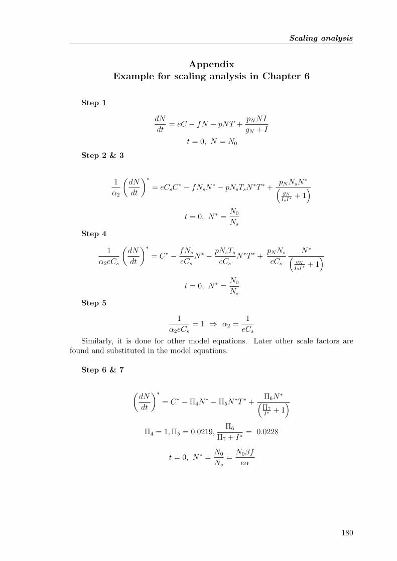
Scaling analysis
AppendixExample for scaling analysis in Chapter 6
Step 1
dN
dt= eC − fN − pNT +
pNNI
gN + I
t = 0, N = N0
Step 2 & 3
1
α2
(dN
dt
)∗= eCsC
∗ − fNsN∗ − pNsTsN
∗T ∗ +pNNsN
∗(gN
IsI∗+ 1)
t = 0, N∗ =N0
Ns
Step 4
1
α2eCs
(dN
dt
)∗= C∗ − fNs
eCsN∗ − pNsTs
eCsN∗T ∗ +
pNNs
eCs
N∗(gN
IsI∗+ 1)
t = 0, N∗ =N0
Ns
Step 5
1
α2eCs= 1 ⇒ α2 =
1
eCs
Similarly, it is done for other model equations. Later other scale factors arefound and substituted in the model equations.
Step 6 & 7
(dN
dt
)∗= C∗ − Π4N
∗ − Π5N∗T ∗ +
Π6N∗(∏
7
I∗+ 1)
Π4 = 1,Π5 = 0.0219,Π6
Π7 + I∗= 0.0228
t = 0, N∗ =N0
Ns
=N0βf
eα
180
Publications & Presentations
Publications & Presentations
Journal articles
1. Kiran, K.L., Jayachandran, D., and Lakshminarayanan, S. Mathematical mod-eling of avascular tumor growth based on diffusion of nutrients and its valida-tion, The Canadian Journal of Chemical Engineering, 2009, 87, 732-740.
2. Kiran, K.L., and Lakshminarayanan, S. Global sensitivity analysis and model-based reactive scheduling of targeted cancer immunotherapy, BioSystems,2010, 101, 117-26.
3. Kiran, K.L., Lakshminarayanan, S. Application of scaling and sensitivity anal-ysis for tumor-immune model reduction, Chemical Engineering Science,2011, 66, 5164-5172.
4. Kiran, K.L., Lakshminarayanan, S. Dosage optimization of chemotherapy andimmunotherapy: In silico analysis using pharmacokinetic-pharmacodynamicand tumor growth models, 2011 (Under review).
5. Kiran, K.L., Lakshminarayanan, S. Population based optimal experimentaldesign in cancer diagnosis and chemotherapy, 2011 (Under review).
Peer Reviewed Conference Papers
1. Kiran, K.L., Jayachandran, D., and Lakshminarayanan, S. Mechanistic mod-eling of avascular tumor growth, In proceedings of ADCONIP 2008, Jasper,Canada 2008.
2. Kiran, K.L., Jayachandran, D., and Lakshminarayanan, S. Multi-objectiveOptimization of Cancer Immuno-Chemotherapy, 13th International Confer-ence on Biomedical Engineering, 2009, pp. 1337-1340.
3. Kiran, K.L., and Lakshminarayanan, S. Treatment planning of cancer den-dritic cell therapy using multi-objective optimization, In proceedings of AD-CHEM 2009, Istanbul, Turkey 2009.(Keynote paper).
4. Kiran, K.L., Lakshminarayanan, S., Sundaramoorthy, S. Application of modelsimplification approaches for tumor-immune modeling, In proceedings of COSMA2009, India, 2009.
5. Kiran, K.L., Kandpal, M., and Lakshminarayanan, S. Characterization of fre-quently sampled intravenous glucose tolerance test using scaling and sensitiv-ity analysis of MINMOD, The 2010 International Conference on Modelling,Identification and Control (ICMIC), pp. 179-184.
6. Mai chan, L., Kiran, K. L., Lakshminarayanan, S. Data driven strategy forimmunotherapy treatment planning, In proceedings of PSE ASIA 2010, Sin-gapore, 2010 .
181
Publications & Presentations
7. Raghuraj Rao, Kiran, K.L. and Lakshminarayanan, S. PSE techniques in met-allurgical industry, In proceedings of PSE ASIA 2010, Singapore, 2010.
Conference - Oral Presentations
1. Kiran, K.L., Jayachandran, D. and Lakshminarayanan, S. Mechanistic mod-eling of avascular tumor growth, ADCONIP 2008, Jasper, Alberta, Canada.
2. Kiran, K.L., Jayachandran, D. and Lakshminarayanan, S. Multi-objective op-timization of cancer immuno-chemotherapy, ICBME 2008, Singapore.
3. Kiran, K.L., Lakshminarayanan, S. Treatment planning of cancer dendriticcell therapy using multi-objective optimization, ADCHEM 2009, Turkey.(Keynote paper).
4. Kiran, K.L., Mai Chan, L., Lakshminarayanan, S. Optimization and datadriven strategies for robust treatment planning of dendritic cell-interleukintherapy, AIChE Annual Meeting 2009, Nashville.
5. Kiran, K.L., Lakshminarayanan, S., Sundaramoorthy, S. Application of modelsimplification approaches for tumor-immune modeling, COSMA 2009, NITCalicut, India.
6. Kiran, K.L., Manoj, K, Lakshminarayanan, S. Characterization of frequentlysampled intravenous glucose tolerance test using scaling and sensitivity anal-ysis on MINMOD, ICMIC 2010, Okayama, Japan.
7. Mai chan, L., Kiran, K. L., Lakshminarayanan, S. Data driven strategy forimmunotherapy treatment planning, PSE ASIA 2010, Singapore.
8. Raghuraj Rao, Kiran, K.L. and Lakshminarayanan, S. PSE techniques in met-allurgical industry, PSE ASIA 2010, Singapore.
9. Kiran, K.L., Loganathan, P., Lakshminarayanan, S. Modeling and analysisof biochemical pathways of glucose metabolism and cell cycle progression,Satellite conference of ICM-2010, Hyderabad, India.
10. Kiran, K.L., Lakshminarayanan, S. Investigation of intracellular cancerousbiomarkers: In silico analysis, 27th HUGO-IABCR Congress 2010, Genomics,biology and breast cancer treatment, Singapore.
Conference - Poster Presentations
1. Kiran, K.L., Lakshminarayanan, S. Targeted immunotherapy for cancer andits treatment planning using multi-objective optimization, ISPE, Singapore,2009. (Award winning poster)
182

KIRAN CV
CURRICULUM VITAE
NAME: KANCHI LAKSHMI KIRAN Office Phone: (65) 65165802Graduate Research Scholar (PhD Student) Hand Phone: (65) 96372987E5-03-30, Dept. of Chemical & Biomolecular Engg. Fax: (65) 67791936National University of Singapore Email: [email protected],Singapore - 117576 [email protected]
Date of birth: 4th December, 1984
Educational qualifications:
• Doctor of Philosophy, 2007 – 2011Chemical & Biomolecular Engineering,National University of Singapore, Singapore
• Bachelor of Engineering, 2002 – 2006Chemical Engineering,National institute of technology, Durgapur, India
Technical skills:Domain: Modeling and simulation, Optimization, Data analysis, Control, Multi-variate statistics, Root cause analysis, Decision making.Programming Languages: MATLAB, COMSOL, FORTRAN, CData mining tools: ACE, MARS, TREENET, Genetic Programming, NetLogo, Any-logic
Current job:Research engineer, Energy Efficiency Research Center, Singapore Development Cen-ter, Yokogawa.
Project works:PhD Thesis (2007-2011): Modeling of tumor growth and optimization of therapeuticprotocol designIn this interdisciplinary research, the aim is to “develop supporting tools for oncolo-gists in the implementation of preventive and personalized cancer therapeutic strate-gies” via the application of Chemical Engineering Principles and Process SystemEngineering techniques.
183

KIRAN CV
Commercial project (2008): Optimal design of experiments for parameter estima-tionDevelopment of a MATLAB based tool “Model Based Experimental Design (MBOED)”a project sponsored by the Centre for Development of Teaching and Learning (CDTL),NUS. Mini projects
1. Model based studies of diagnostic protocols of diabetes (2010)
2. Process systems engineering in metallurgical process (2010) (in collabara-tion with Aqua Alloys Pvt. Ltd., India)
3. Optimization of radiation therapy for cancer treatment (2007)
B.E. final year project (2006): Pneumatic separation of coal particles
Industrial experience:
1. Vocational training in Vizag Steel Plant, India (2005)
2. Worked as Management Trainee in Associate Cement Companies, India (2006)
Major achievements:
1. Nominated by the Faculty at NUS to participate in the 7th Global StudentForum on Engineering Education, Singapore (2010)
2. Shortlisted for advanced professional degree (APD) event organized by McK-insey & company, Singapore (July, 2010)
3. Won 3rd Prize in International Society for Pharmaceutical Engineering’s stu-dent poster competition , Singapore (June, 2010)
4. Won the “Leadership Award” for organizing ChemBiotech’ 09-10 (An inter-national conference on Chemical and Biomolecular Engineering) , Singapore
5. Delivered an invited lecture on “Application of Modeling and OptimizationStrategies for Tumor Growth and Development of Therapeutic Interventions ”at Vanderbilt Ingram Cancer Centre, Vanderbilt University, Tennessee (Novem-ber, 2009)
6. Keynote paper presentation at ADCHEM 2009, Turkey
7. Graduate Research Scholarship from Singapore Government (2007-2011)
8. 96.26 percentile in GATE- Graduate Aptitude Test in Engineering (Top 5%),India (2005)
9. 2nd prize in paper presentation in National level tech festival, NIT, Durgapur(2006)
10. Ranked in the top 1% in the competitive exam (EAMCET) , India (2002)
11. Mathematics topper in 10th board exams, India (2000)
184
KIRAN CV
Responsible roles:
Teaching assistantship
1. Tutorship for Process modeling and numerical simulation (CN 3421) (2007)
2. Training students to learn MATLAB (CN 5010) (2008-2010)
3. Tutor and grader for Data based process characterization (CN 4245R) (2009)
Extra curricular activities
1. Student representative for Engineering Postgraduate Council (2010)
2. Student member of American Institute of Chemical Engineers (2008-2011)
3. International Society for Pharmaceutical Engineering (ISPE), Singapore (2010-2011)
4. President of Graduate Student’s Association (2009-10)
5. President, ChemBiotech’ 09-10, Singapore
6. Student organizer for the international conference, PSE ASIA, Singapore (2010)
7. ISTE - Indian Society for Technical Education (2002-2006), NIT, Durgapur
8. CHESS- Chemical Engineering Student’s Society (2002-2006), NIT, Durgapur
9. CCA- Centre for Cognitive Activities (2002-2006), NIT, Durgapur
10. Representative of Training and Placement Student’s Work (2002-2006)
References:Assoc. Prof. Lakshminarayanan SBlk E4, 4 Engineering Drive 4, #06-05, Singapore 117576Department of Chemical & Biomolecular EngineeringNational University of Singapore, SingaporeTel:(65) 65168484 Email: [email protected]
Prof. Farooq ShamsuzzamanBlk E5, 4 Engineering Drive 4, #02-26, Singapore 117576Department of Chemical & Biomolecular EngineeringNational University of Singapore, SingaporeTel: (65) 65166545 Email: [email protected]
Prof. Rangaiah Gade PanduBlk E5, 4 Engineering Drive 4, #02-25, Singapore 117576Department of Chemical & Biomolecular EngineeringNational University of Singapore, SingaporeTel: (65) 65162187 Email: [email protected]
185

KIRAN CV
Dr. Rao RaghurajVice President-operationsAqua Alloys Pvt. Ltd.Sanmati Bldg, Sadashiv Nagar, Belgaum, KarnatakaIndia - 590 009 Mobile: 9243209569Email: [email protected]
186