ww.sciencedirect.com

i n t e rn a t i o n a l j o u r n a l o f h y d r o g e n en e r g y 3 7 ( 2 0 1 2 ) 2 4 7 0e2 4 8 1

Available online at w

journal homepage: www.elsevier .com/locate/he

Modeling and optimization of a 1 kWe HT-PEMFC-basedmicro-CHP residential system

Alexandros Arsalis*, Mads P. Nielsen, Søren K. Kær

Department of Energy Technology, Aalborg University, Pontoppidanstræde 101, 9220 Aalborg Ø., Denmark

a r t i c l e i n f o

Article history:

Received 11 August 2011

Received in revised form

11 October 2011

Accepted 18 October 2011

Available online 16 November 2011

Keywords:

PBI

HT-PEMFC

Micro-CHP

Residential system

Optimization

Fuel cell system

* Corresponding author.E-mail address: aar@et.aau.dk (A. Arsalis

0360-3199/$ e see front matter Copyright ªdoi:10.1016/j.ijhydene.2011.10.081

a b s t r a c t

A high temperature-proton exchange membrane (HT-PEMFC)-based micro-combined-

heat-and-power (CHP) residential system is designed and optimized, using a genetic

algorithm (GA) optimization strategy. The proposed system consists of a fuel cell stack,

steam methane reformer (SMR) reactor, water gas shift (WGS) reactor, heat exchangers,

and other balance-of-plant (BOP) components. The objective function of the single-

objective optimization strategy is the net electrical efficiency of the micro-CHP system.

The implemented optimization procedure attempts to maximize the objective function by

variation of nine decision variables. The value of the objective function for the optimum

design configuration is significantly higher than the initial one, with a 20.7% increase.

Copyright ª 2011, Hydrogen Energy Publications, LLC. Published by Elsevier Ltd. All rights

reserved.

1. Introduction system to provide greater operational flexibility during

A residential application of combined-heat-and-power (CHP)

technology is a micro-CHP system, providing electricity and

heat (hot water and space heating) for a detached single-

family household. Such a system is designed to convert the

chemical energy in a fuel into both electrical power and

useful heat [1e5]. Micro-CHP systems operating on natural

gas must be coupled with a fuel processing unit, to allow

conversion of natural gas to hydrogen. Balance-of-plant (BOP)

components are also needed to perform various necessary

tasks, such as air compressing or water pumping, while heat

exchangers are necessary for the thermal management of

the system. The thermal management of the system includes

heating/cooling of components (e.g. steam reforming), and

also heat recovery to satisfy the residential load profile (e.g.

space heating). A thermal storage tank is coupled with the

).2011, Hydrogen Energy P

transient load demands.

Micro-CHP systems can be categorized into combustion-

and fuel cell-based. Although combustion-based technologies

are more mature and currently available in the market, fuel

cell-based systems are considered more promising for

a number of reasons. Combustion-based systems, such as the

internal combustion engine technology, are not suitable for

micro-CHP applications mainly due to their high thermal-to-

electric ratio (TER) [1], and also due to their low efficiencies

at part-load operation. Fuel cell-based stationary power

generation technology is capable of achieving high efficien-

cies, with lower emissions as compared to combustion-based

systems. Also these systems have simple routine mainte-

nance requirements and quiet operation [1,6,7].

The operating temperature in a fuel cell stack is an

important element for the efficiency and the degradation of

ublications, LLC. Published by Elsevier Ltd. All rights reserved.

i n t e r n a t i o n a l j o u r n a l o f h y d r o g e n en e r g y 3 7 ( 2 0 1 2 ) 2 4 7 0e2 4 8 1 2471

the membrane. Fuel cell technologies operating at high

temperatures can lessen the cooling requirements, simplify

water management and reduce contamination problems.

High temperature-proton exchange membrane fuel cells (HT-

PEMFC) utilize a Polybenzimidazole (PBI) membrane, which

operates at temperatures between 150 and 200 �C. It is there-

fore an ideal match for a micro-CHP system, because not only

the rates of electrochemical kinetics are enhanced and water

management and cooling is simplified, but also useful waste

heat can be recovered, and lower quality reformed hydrogen

may be used as fuel [8e11].

A global optimization strategy is usually desirable for

multi-component systems, such as the micro-CHP system

under study, because the global maximum is not just the best

solution to the optimization problem, but also because local

maxima can severely confound the interpretation of the

results of studies investigating the effects of model parame-

ters [12]. A stochastic method, such as genetic algorithms

(GA), can solve a problem with a systematic multi-start

approach with random sampling.

2. System layout

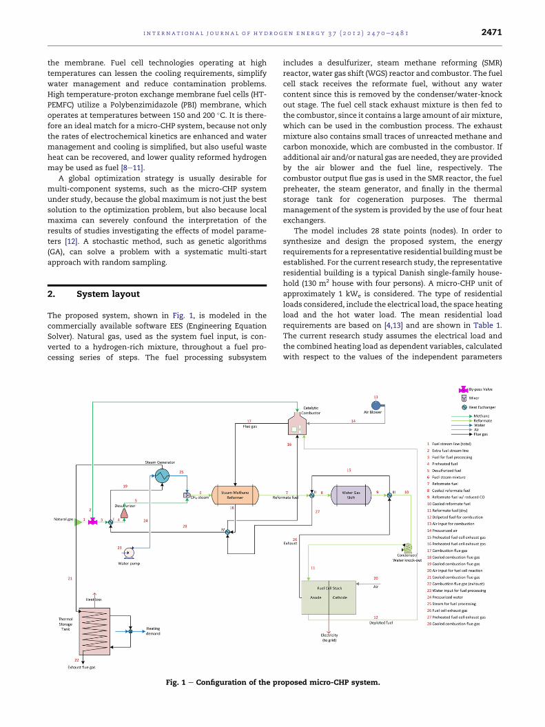
The proposed system, shown in Fig. 1, is modeled in the

commercially available software EES (Engineering Equation

Solver). Natural gas, used as the system fuel input, is con-

verted to a hydrogen-rich mixture, throughout a fuel pro-

cessing series of steps. The fuel processing subsystem

Fig. 1 e Configuration of the pr

includes a desulfurizer, steam methane reforming (SMR)

reactor, water gas shift (WGS) reactor and combustor. The fuel

cell stack receives the reformate fuel, without any water

content since this is removed by the condenser/water-knock

out stage. The fuel cell stack exhaust mixture is then fed to

the combustor, since it contains a large amount of airmixture,

which can be used in the combustion process. The exhaust

mixture also contains small traces of unreacted methane and

carbon monoxide, which are combusted in the combustor. If

additional air and/or natural gas are needed, they are provided

by the air blower and the fuel line, respectively. The

combustor output flue gas is used in the SMR reactor, the fuel

preheater, the steam generator, and finally in the thermal

storage tank for cogeneration purposes. The thermal

management of the system is provided by the use of four heat

exchangers.

The model includes 28 state points (nodes). In order to

synthesize and design the proposed system, the energy

requirements for a representative residential buildingmust be

established. For the current research study, the representative

residential building is a typical Danish single-family house-

hold (130 m2 house with four persons). A micro-CHP unit of

approximately 1 kWe is considered. The type of residential

loads considered, include the electrical load, the space heating

load and the hot water load. The mean residential load

requirements are based on [4,13] and are shown in Table 1.

The current research study assumes the electrical load and

the combined heating load as dependent variables, calculated

with respect to the values of the independent parameters

oposed micro-CHP system.

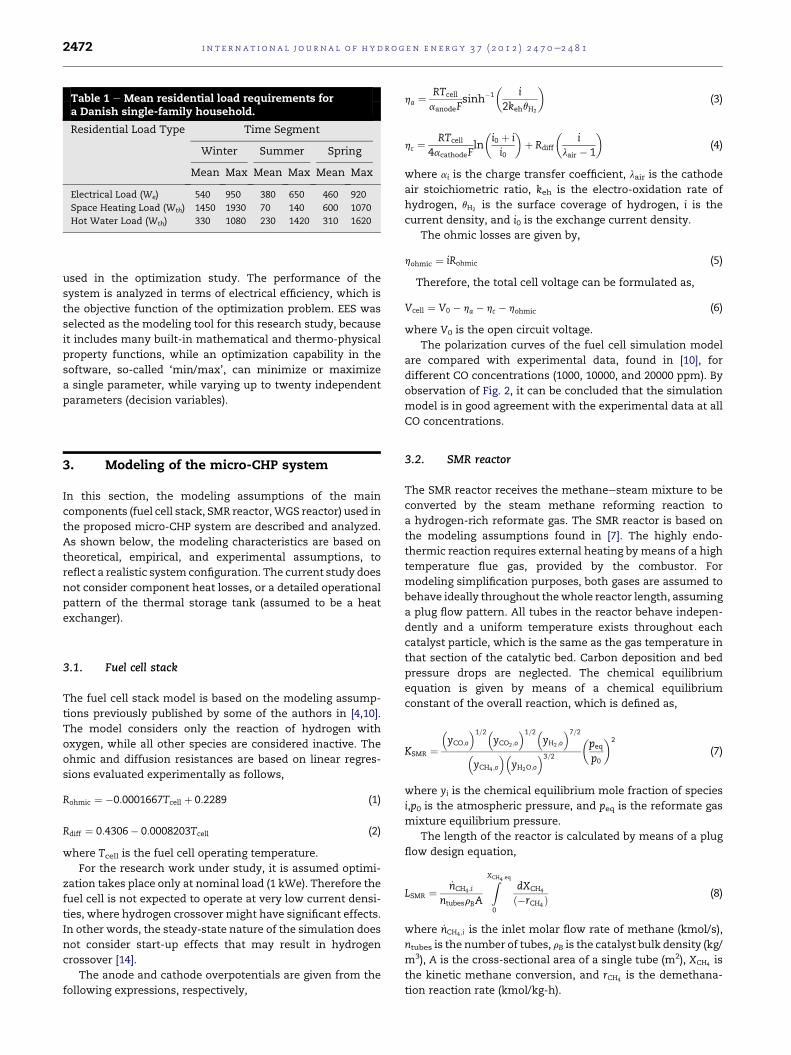
Table 1 e Mean residential load requirements fora Danish single-family household.

Residential Load Type Time Segment

Winter Summer Spring

Mean Max Mean Max Mean Max

Electrical Load (We) 540 950 380 650 460 920

Space Heating Load (Wth) 1450 1930 70 140 600 1070

Hot Water Load (Wth) 330 1080 230 1420 310 1620

i n t e rn a t i o n a l j o u r n a l o f h y d r o g e n en e r g y 3 7 ( 2 0 1 2 ) 2 4 7 0e2 4 8 12472

used in the optimization study. The performance of the

system is analyzed in terms of electrical efficiency, which is

the objective function of the optimization problem. EES was

selected as the modeling tool for this research study, because

it includes many built-in mathematical and thermo-physical

property functions, while an optimization capability in the

software, so-called ‘min/max’, can minimize or maximize

a single parameter, while varying up to twenty independent

parameters (decision variables).

3. Modeling of the micro-CHP system

In this section, the modeling assumptions of the main

components (fuel cell stack, SMR reactor,WGS reactor) used in

the proposed micro-CHP system are described and analyzed.

As shown below, the modeling characteristics are based on

theoretical, empirical, and experimental assumptions, to

reflect a realistic system configuration. The current study does

not consider component heat losses, or a detailed operational

pattern of the thermal storage tank (assumed to be a heat

exchanger).

3.1. Fuel cell stack

The fuel cell stack model is based on the modeling assump-

tions previously published by some of the authors in [4,10].

The model considers only the reaction of hydrogen with

oxygen, while all other species are considered inactive. The

ohmic and diffusion resistances are based on linear regres-

sions evaluated experimentally as follows,

Rohmic ¼ �0:0001667Tcell þ 0:2289 (1)

Rdiff ¼ 0:4306� 0:0008203Tcell (2)

where Tcell is the fuel cell operating temperature.

For the research work under study, it is assumed optimi-

zation takes place only at nominal load (1 kWe). Therefore the

fuel cell is not expected to operate at very low current densi-

ties, where hydrogen crossover might have significant effects.

In other words, the steady-state nature of the simulation does

not consider start-up effects that may result in hydrogen

crossover [14].

The anode and cathode overpotentials are given from the

following expressions, respectively,

ha ¼RTcell

a Fsinh�1

�i

2k q

�(3)

anode eh H2

hc ¼RTcell

4acathodeFln

�i0 þ ii0

�þ Rdiff

�i

lair � 1

�(4)

where ai is the charge transfer coefficient, lair is the cathode

air stoichiometric ratio, keh is the electro-oxidation rate of

hydrogen, qH2is the surface coverage of hydrogen, i is the

current density, and i0 is the exchange current density.

The ohmic losses are given by,

hohmic ¼ iRohmic (5)

Therefore, the total cell voltage can be formulated as,

Vcell ¼ V0 � ha � hc � hohmic (6)

where V0 is the open circuit voltage.

The polarization curves of the fuel cell simulation model

are compared with experimental data, found in [10], for

different CO concentrations (1000, 10000, and 20000 ppm). By

observation of Fig. 2, it can be concluded that the simulation

model is in good agreement with the experimental data at all

CO concentrations.

3.2. SMR reactor

The SMR reactor receives the methaneesteam mixture to be

converted by the steam methane reforming reaction to

a hydrogen-rich reformate gas. The SMR reactor is based on

the modeling assumptions found in [7]. The highly endo-

thermic reaction requires external heating by means of a high

temperature flue gas, provided by the combustor. For

modeling simplification purposes, both gases are assumed to

behave ideally throughout thewhole reactor length, assuming

a plug flow pattern. All tubes in the reactor behave indepen-

dently and a uniform temperature exists throughout each

catalyst particle, which is the same as the gas temperature in

that section of the catalytic bed. Carbon deposition and bed

pressure drops are neglected. The chemical equilibrium

equation is given by means of a chemical equilibrium

constant of the overall reaction, which is defined as,

KSMR ¼�yCO;o

�1=2�yCO2 ;o

�1=2�yH2 ;o

�7=2

�yCH4 ;o

��yH2O;o

�3=2

�peq

p0

�2

(7)

where yi is the chemical equilibrium mole fraction of species

i,p0 is the atmospheric pressure, and peq is the reformate gas

mixture equilibrium pressure.

The length of the reactor is calculated by means of a plug

flow design equation,

LSMR ¼ _nCH4 ;i

ntubesrBA

ZXCH4 ;eq

0

dXCH4

ð�rCH4 Þ(8)

where _nCH4 ;i is the inlet molar flow rate of methane (kmol/s),

ntubes is the number of tubes, rB is the catalyst bulk density (kg/

m3), A is the cross-sectional area of a single tube (m2), XCH4 is

the kinetic methane conversion, and rCH4 is the demethana-

tion reaction rate (kmol/kg-h).

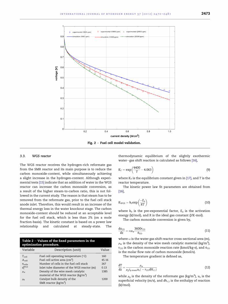
Fig. 2 e Fuel cell model validation.

i n t e r n a t i o n a l j o u r n a l o f h y d r o g e n en e r g y 3 7 ( 2 0 1 2 ) 2 4 7 0e2 4 8 1 2473

3.3. WGS reactor

The WGS reactor receives the hydrogen-rich reformate gas

from the SMR reactor and its main purpose is to reduce the

carbon monoxide-content, while simultaneously achieving

a slight increase in the hydrogen-content. Although experi-

mental tests [15] indicate that an addition of water in theWGS

reactor can increase the carbon monoxide conversion, as

a result of the higher steam-to-carbon ratio, this is not fol-

lowed in the current study. The reason is that steam has to be

removed from the reformate gas, prior to the fuel cell stack

anode inlet. Therefore, this would result in an increase of the

thermal energy loss in the water knockout stage. The carbon

monoxide-content should be reduced at an acceptable level

for the fuel cell stack, which is less than 2% (on a mole

fraction-basis). The kinetic constant is based on a power law

relationship and calculated at steady-state. The

Table 2 e Values of the fixed parameters in theoptimization procedure.

Variable Description (unit) Value

Tcell Fuel cell operating temperature (�C) 160

Acell Fuel cell active area (cm2) 45.16

ncells Number of cells in the fuel cell stack 267

dWGSi Inlet tube diameter of the WGS reactor (m) 0.13

rw Density of the wire mesh catalytic

material of the WGS reactor (kg/m3)

1385

rB Catalyst bulk density of the

SMR reactor (kg/m3)

1200

thermodynamic equilibrium of the slightly exothermic

wateregas shift reaction is calculated as follows [16],

KT ¼ exp

�4400T

� 4:063

�(9)

where KT is the equilibrium constant given in [17], and T is the

reactor temperature.

The kinetic power law fit parameters are obtained from

[16],

KWGS ¼ k0exp

��Ea

RT

�(10)

where k0 is the pre-exponential factor, Ea is the activation

energy (kJ/mol), and R is the ideal gas constant (J/K-mol).

The carbon monoxide conversion is given by,

dxCO

dz¼ urw

3600rCO_nCO

(11)

where u is the water gas shift reactor cross-sectional area (m),

rw is the density of the wire mesh catalytic material (kg/m3),

rCO is the carbon monoxide reaction rate (kmol/kg-s), and _nCO

is the molar flow rate of carbon monoxide (kmol/s).

The temperature gradient is defined as,

dTdz

¼ rw

rgcp;massusð � rCOdHr;1Þ (12)

while rg is the density of the reformate gas (kg/m3), us is the

superficial velocity (m/s), and dhr,1 is the enthalpy of reaction

(kJ/mol).

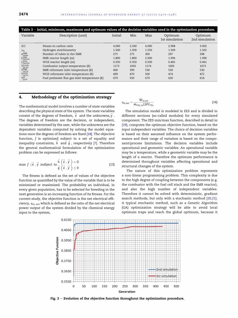
Table 3 e Initial, minimum, maximum and optimum values of the decision variables used in the optimization procedure.

Variable Description (unit) Initial Min Max Optimum1st simulation

Optimum2nd simulation

S/C Steam-to-carbon ratio 4.000 2.500 4.000 2.908 3.002

lH2 Hydrogen stoichiometry 1.500 1.500 1.550 1.509 1.502

nSMRtubes Number of tubes in the SMR 275 275 300 297 298

LSMRreactor SMR reactor length (m) 1.800 1.800 2.000 1.994 1.996

LWGSreactor WGS reactor length (m) 0.350 0.350 0.500 0.465 0.441

TCombfg;out Combustor output temperature (K) 1173 1050 1174 1095 1073

TSMRref;in SMR reformate inlet temperature (K) 400 399 530 530 530

TWGSref;in WGS reformate inlet temperature (K) 499 470 500 474 472

TFPfg;in Fuel preheater flue gas inlet temperature (K) 670 550 670 620 614

i n t e rn a t i o n a l j o u r n a l o f h y d r o g e n en e r g y 3 7 ( 2 0 1 2 ) 2 4 7 0e2 4 8 12474

4. Methodology of the optimization strategy

Themathematical model involves a number of state variables

describing the physical state of the system. The state variables

consist of the degrees of freedom, x/

and the unknowns,y/

.

The degrees of freedom are the decision, or independent,

variables determined by the user, while the unknowns are the

dependent variables computed by solving the model equa-

tions once the degrees of freedom are fixed [18]. The objective

function, f is optimized subject to a set of equality and

inequality constraints, h/

and g/

, respectively [7]. Therefore

the general mathematical formulation of the optimization

problem can be expressed as follows:

max f ðx/ ; y/ Þsubject to

h/ �

x/

; y/

�¼ 0

g/

�x/

; y/

�� 0

(13)

The fitness is defined as the set of values of the objective

function as quantified by the value of the variable that is to be

minimized or maximized. The probability an individual, in

every given population, has to be selected for breeding in the

next generation is an increasing function of its fitness. For the

current study, the objective function is the net electrical effi-

ciency, hel, net which is defined as the ratio of the net electrical

power output of the system divided by the chemical energy

input to the system,

Fig. 3 e Evolution of the objective function t

hel;net ¼_Wel;net

_mCH4 ;inLHVCH4

(14)

The simulation model is modeled in EES and is divided in

different sections (so-called modules) for every simulated

component. The EES min/max function, described in detail in

[19], computes the optimum objective function, based on the

input independent variables. The choice of decision variables

is based on their assumed influence on the system perfor-

mance and their range of variation is based on the compo-

nent/process limitations. The decision variables include

operational and geometric variables. An operational variable

may be a temperature, while a geometric variable may be the

length of a reactor. Therefore the optimum performance is

determined throughout variables affecting operational and

structural changes of the system.

The nature of this optimization problem represents

a non-linear programming problem. This complexity is due

to the high degree of coupling between the components (e.g.

the combustor with the fuel cell stack and the SMR reactor),

and also the high number of independent variables.

Therefore it cannot be solved with deterministic, gradient

search methods, but only with a stochastic method [20,21].

A typical stochastic method, such as a Genetic Algorithm

(GA) optimization strategy will be able to avoid local

optimum traps and reach the global optimum, because it

hroughout the optimization procedure.

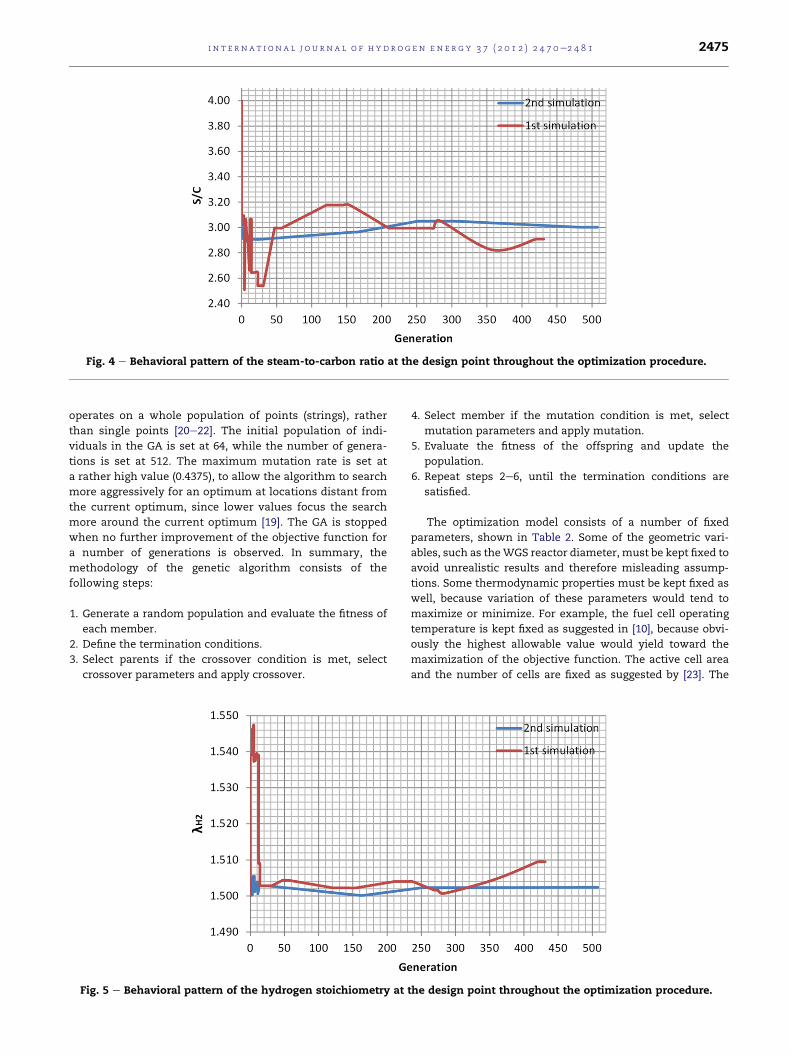
Fig. 4 e Behavioral pattern of the steam-to-carbon ratio at the design point throughout the optimization procedure.

i n t e r n a t i o n a l j o u r n a l o f h y d r o g e n en e r g y 3 7 ( 2 0 1 2 ) 2 4 7 0e2 4 8 1 2475

operates on a whole population of points (strings), rather

than single points [20e22]. The initial population of indi-

viduals in the GA is set at 64, while the number of genera-

tions is set at 512. The maximum mutation rate is set at

a rather high value (0.4375), to allow the algorithm to search

more aggressively for an optimum at locations distant from

the current optimum, since lower values focus the search

more around the current optimum [19]. The GA is stopped

when no further improvement of the objective function for

a number of generations is observed. In summary, the

methodology of the genetic algorithm consists of the

following steps:

1. Generate a random population and evaluate the fitness of

each member.

2. Define the termination conditions.

3. Select parents if the crossover condition is met, select

crossover parameters and apply crossover.

Fig. 5 e Behavioral pattern of the hydrogen stoichiometry at

4. Select member if the mutation condition is met, select

mutation parameters and apply mutation.

5. Evaluate the fitness of the offspring and update the

population.

6. Repeat steps 2e6, until the termination conditions are

satisfied.

The optimization model consists of a number of fixed

parameters, shown in Table 2. Some of the geometric vari-

ables, such as theWGS reactor diameter, must be kept fixed to

avoid unrealistic results and therefore misleading assump-

tions. Some thermodynamic properties must be kept fixed as

well, because variation of these parameters would tend to

maximize or minimize. For example, the fuel cell operating

temperature is kept fixed as suggested in [10], because obvi-

ously the highest allowable value would yield toward the

maximization of the objective function. The active cell area

and the number of cells are fixed as suggested by [23]. The

the design point throughout the optimization procedure.

Fig. 6 e Behavioral pattern of the number of tubes in the SMR reactor at the design point throughout the optimization

procedure.

i n t e rn a t i o n a l j o u r n a l o f h y d r o g e n en e r g y 3 7 ( 2 0 1 2 ) 2 4 7 0e2 4 8 12476

values for the SMR and WGS reactor parameters are selected

from [7] and [16], respectively.

5. Results and discussion

In this section the optimum configuration of the proposed

micro-CHP system is presented, and then compared to the

results obtained prior to the application of the optimization

strategy. In addition, the optimization process is analyzed to

indicate its main characteristics.

The decision variables, shown in Table 3, were chosenwith

an initial value as typically found in the literature for the kind

of system under study. Their allowable range of variation is

chosen on the basis of component/process operational and/or

structural limitations. Therefore these constraints are based

on knowledge of the solution space and on observation of the

Fig. 7 e Behavioral pattern of the SMR reactor length at the

behavioral pattern of the optimization algorithm. The

optimum values, shown in Table 3, are the ones used to

evaluate the global optimumobjective function. The optimum

values are evaluated after two sequential simulation runs;

after the first simulation run is completed a second run

repeats the optimization, using the optimum values of the

first optimization as the new initial values. The purpose of this

procedure is to ensure that the best possible value of the

objective function is reached. In addition, the variation of the

nine independent variables is more stable in the second

simulation, as compared to the first simulation, while the

optimization evolves toward the final generations.

The genetic algorithm required 508 generations until the

optimum value for the objective function was reached, while

the simulation for the optimization strategy was performed in

33,346 iterations. By comparison of the optimum and initial

design configurations, it can be concluded that the initial

design point throughout the optimization procedure.

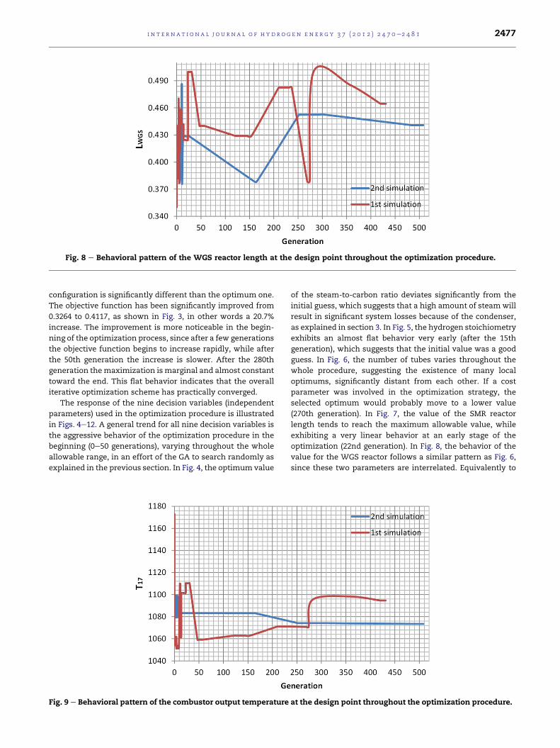
Fig. 8 e Behavioral pattern of the WGS reactor length at the design point throughout the optimization procedure.

i n t e r n a t i o n a l j o u r n a l o f h y d r o g e n en e r g y 3 7 ( 2 0 1 2 ) 2 4 7 0e2 4 8 1 2477

configuration is significantly different than the optimum one.

The objective function has been significantly improved from

0.3264 to 0.4117, as shown in Fig. 3, in other words a 20.7%

increase. The improvement is more noticeable in the begin-

ning of the optimization process, since after a few generations

the objective function begins to increase rapidly, while after

the 50th generation the increase is slower. After the 280th

generation themaximization ismarginal and almost constant

toward the end. This flat behavior indicates that the overall

iterative optimization scheme has practically converged.

The response of the nine decision variables (independent

parameters) used in the optimization procedure is illustrated

in Figs. 4e12. A general trend for all nine decision variables is

the aggressive behavior of the optimization procedure in the

beginning (0e50 generations), varying throughout the whole

allowable range, in an effort of the GA to search randomly as

explained in the previous section. In Fig. 4, the optimum value

Fig. 9 e Behavioral pattern of the combustor output temperature

of the steam-to-carbon ratio deviates significantly from the

initial guess, which suggests that a high amount of steamwill

result in significant system losses because of the condenser,

as explained in section 3. In Fig. 5, the hydrogen stoichiometry

exhibits an almost flat behavior very early (after the 15th

generation), which suggests that the initial value was a good

guess. In Fig. 6, the number of tubes varies throughout the

whole procedure, suggesting the existence of many local

optimums, significantly distant from each other. If a cost

parameter was involved in the optimization strategy, the

selected optimum would probably move to a lower value

(270th generation). In Fig. 7, the value of the SMR reactor

length tends to reach the maximum allowable value, while

exhibiting a very linear behavior at an early stage of the

optimization (22nd generation). In Fig. 8, the behavior of the

value for the WGS reactor follows a similar pattern as Fig. 6,

since these two parameters are interrelated. Equivalently to

at the design point throughout the optimization procedure.

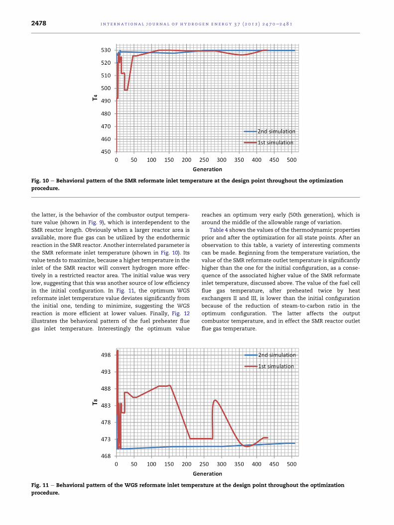
Fig. 10 e Behavioral pattern of the SMR reformate inlet temperature at the design point throughout the optimization

procedure.

i n t e rn a t i o n a l j o u r n a l o f h y d r o g e n en e r g y 3 7 ( 2 0 1 2 ) 2 4 7 0e2 4 8 12478

the latter, is the behavior of the combustor output tempera-

ture value (shown in Fig. 9), which is interdependent to the

SMR reactor length. Obviously when a larger reactor area is

available, more flue gas can be utilized by the endothermic

reaction in the SMR reactor. Another interrelated parameter is

the SMR reformate inlet temperature (shown in Fig. 10). Its

value tends to maximize, because a higher temperature in the

inlet of the SMR reactor will convert hydrogen more effec-

tively in a restricted reactor area. The initial value was very

low, suggesting that this was another source of low efficiency

in the initial configuration. In Fig. 11, the optimum WGS

reformate inlet temperature value deviates significantly from

the initial one, tending to minimize, suggesting the WGS

reaction is more efficient at lower values. Finally, Fig. 12

illustrates the behavioral pattern of the fuel preheater flue

gas inlet temperature. Interestingly the optimum value

Fig. 11 e Behavioral pattern of the WGS reformate inlet temper

procedure.

reaches an optimum very early (50th generation), which is

around the middle of the allowable range of variation.

Table 4 shows the values of the thermodynamic properties

prior and after the optimization for all state points. After an

observation to this table, a variety of interesting comments

can be made. Beginning from the temperature variation, the

value of the SMR reformate outlet temperature is significantly

higher than the one for the initial configuration, as a conse-

quence of the associated higher value of the SMR reformate

inlet temperature, discussed above. The value of the fuel cell

flue gas temperature, after preheated twice by heat

exchangers II and III, is lower than the initial configuration

because of the reduction of steam-to-carbon ratio in the

optimum configuration. The latter affects the output

combustor temperature, and in effect the SMR reactor outlet

flue gas temperature.

ature at the design point throughout the optimization

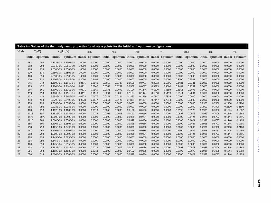
Table 4 e Values of the thermodynamic properties for all state points for the initial and optimum configurations.

Node Ti (K) _miðkg=sÞ yCH4 yCO yCO2 yH2 yH2O yN2 yO2

initial optimum initial optimum initial optimum initial optimum initial optimum initial optimum initial optimum initial optimum initial optimum

1 298 298 2.833E-05 2.550E-05 1.0000 1.0000 0.0000 0.0000 0.0000 0.0000 0.0000 0.0000 0.0000 0.0000 0.0000 0.0000 0.0000 0.0000

2 298 298 2.834E-06 9.501E-10 1.0000 1.0000 0.0000 0.0000 0.0000 0.0000 0.0000 0.0000 0.0000 0.0000 0.0000 0.0000 0.0000 0.0000

3 298 298 2.550E-05 2.550E-05 1.0000 1.0000 0.0000 0.0000 0.0000 0.0000 0.0000 0.0000 0.0000 0.0000 0.0000 0.0000 0.0000 0.0000

4 420 530 2.550E-05 2.550E-05 1.0000 1.0000 0.0000 0.0000 0.0000 0.0000 0.0000 0.0000 0.0000 0.0000 0.0000 0.0000 0.0000 0.0000

5 420 530 2.550E-05 2.550E-05 1.0000 1.0000 0.0000 0.0000 0.0000 0.0000 0.0000 0.0000 0.0000 0.0000 0.0000 0.0000 0.0000 0.0000

6 420 530 1.400E-04 1.114E-04 0.2000 0.2499 0.0000 0.0000 0.0000 0.0000 0.0000 0.0000 0.8000 0.7501 0.0000 0.0000 0.0000 0.0000

7 845 942 1.400E-04 1.114E-04 0.0411 0.0140 0.0568 0.0787 0.0568 0.0787 0.3973 0.5506 0.4481 0.2781 0.0000 0.0000 0.0000 0.0000

8 499 472 1.400E-04 1.114E-04 0.0411 0.0140 0.0568 0.0787 0.0568 0.0787 0.3973 0.5506 0.4481 0.2781 0.0000 0.0000 0.0000 0.0000

9 566 561 1.400E-04 1.114E-04 0.0411 0.0140 0.0031 0.0099 0.1104 0.1474 0.4510 0.6193 0.3944 0.2094 0.0000 0.0000 0.0000 0.0000

10 433 433 1.400E-04 1.114E-04 0.0411 0.0140 0.0031 0.0099 0.1104 0.1474 0.4510 0.6193 0.3944 0.2094 0.0000 0.0000 0.0000 0.0000

11 433 433 6.698E-05 7.644E-05 0.0678 0.0177 0.0051 0.0126 0.1823 0.1864 0.7447 0.7834 0.0000 0.0000 0.0000 0.0000 0.0000 0.0000

12 433 433 2.679E-05 3.840E-05 0.0678 0.0177 0.0051 0.0126 0.1823 0.1864 0.7447 0.7834 0.0000 0.0000 0.0000 0.0000 0.0000 0.0000

13 298 298 2.928E-04 1.038E-04 0.0000 0.0000 0.0000 0.0000 0.0000 0.0000 0.0000 0.0000 0.0000 0.0000 0.7900 0.7900 0.2100 0.2100

14 298 298 2.928E-04 1.038E-04 0.0000 0.0000 0.0000 0.0000 0.0000 0.0000 0.0000 0.0000 0.0000 0.0000 0.7900 0.7900 0.2100 0.2100

15 468 458 1.182E-03 1.408E-03 0.0060 0.0013 0.0005 0.0009 0.0162 0.0136 0.0000 0.0000 0.0995 0.0973 0.6935 0.7006 0.1844 0.1862

16 1014 890 1.182E-03 1.408E-03 0.0060 0.0013 0.0005 0.0009 0.0162 0.0136 0.0000 0.0000 0.0995 0.0973 0.6935 0.7006 0.1844 0.1862

17 1173 1073 1.500E-03 1.550E-03 0.0000 0.0000 0.0000 0.0000 0.0328 0.0284 0.0000 0.0000 0.1300 0.1424 0.6928 0.6797 0.1444 0.1495

18 1016 909 1.500E-03 1.550E-03 0.0000 0.0000 0.0000 0.0000 0.0328 0.0284 0.0000 0.0000 0.1300 0.1424 0.6928 0.6797 0.1444 0.1495

19 666 605 1.500E-03 1.550E-03 0.0000 0.0000 0.0000 0.0000 0.0328 0.0284 0.0000 0.0000 0.1300 0.1424 0.6928 0.6797 0.1444 0.1495

20 298 298 1.125E-03 1.349E-03 0.0000 0.0000 0.0000 0.0000 0.0000 0.0000 0.0000 0.0000 0.0000 0.0000 0.7900 0.7900 0.2100 0.2100

21 487 464 1.500E-03 1.550E-03 0.0000 0.0000 0.0000 0.0000 0.0328 0.0284 0.0000 0.0000 0.1300 0.1424 0.6928 0.6797 0.1444 0.1495

22 298 298 1.500E-03 1.550E-03 0.0000 0.0000 0.0000 0.0000 0.0328 0.0284 0.0000 0.0000 0.1300 0.1424 0.6928 0.6797 0.1444 0.1495

23 298 298 1.145E-04 8.595E-05 0.0000 0.0000 0.0000 0.0000 0.0000 0.0000 0.0000 0.0000 1.0000 1.0000 0.0000 0.0000 0.0000 0.0000

24 298 298 1.145E-04 8.595E-05 0.0000 0.0000 0.0000 0.0000 0.0000 0.0000 0.0000 0.0000 1.0000 1.0000 0.0000 0.0000 0.0000 0.0000

25 420 530 1.145E-04 8.595E-05 0.0000 0.0000 0.0000 0.0000 0.0000 0.0000 0.0000 0.0000 1.0000 1.0000 0.0000 0.0000 0.0000 0.0000

26 432 432 1.182E-03 1.408E-03 0.0060 0.0013 0.0005 0.0009 0.0162 0.0136 0.0000 0.0000 0.0995 0.0973 0.6935 0.7006 0.1844 0.1862

27 564 553 1.182E-03 1.408E-03 0.0060 0.0013 0.0005 0.0009 0.0162 0.0136 0.0000 0.0000 0.0995 0.0973 0.6935 0.7006 0.1844 0.1862

28 670 614 1.500E-03 1.550E-03 0.0000 0.0000 0.0000 0.0000 0.0328 0.0284 0.0000 0.0000 0.1300 0.1424 0.6928 0.6797 0.1444 0.1495

internatio

nal

journal

of

hydrogen

energy

37

(2012)2470e2481

2479

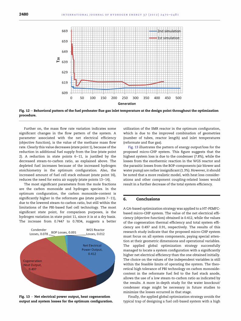
Fig. 12 e Behavioral pattern of the fuel preheater flue gas inlet temperature at the design point throughout the optimization

procedure.

i n t e rn a t i o n a l j o u r n a l o f h y d r o g e n en e r g y 3 7 ( 2 0 1 2 ) 2 4 7 0e2 4 8 12480

Further on, the mass flow rate variation indicates some

significant changes in the flow pattern of the system. A

parameter associated with the net electrical efficiency

(objective function), is the value of the methane mass flow

rate. Clearly this value decreases (state point 1), because of the

reduction in additional fuel supply from the line (state point

2). A reduction in state points 6e11, is justified by the

decreased steam-to-carbon ratio, as explained above. The

depleted fuel increases because of the increased hydrogen

stoichiometry in the optimum configuration. Also, the

increased amount of fuel cell stack exhaust (state point 16),

reduces the need for extra air supply (state points 13e14).

The most significant parameters from the mole fractions

are the carbon monoxide and hydrogen species. In the

optimum configuration, the carbon monoxide-content is

significantly higher in the reformate gas (state points 7e11),

due to the lowered steam-to-carbon ratio, but still within the

limitations of the PBI-based fuel cell technology. The most

significant state point, for comparison purposes, is the

hydrogen variation in state point 11, since it is at a dry basis.

The increase from 0.7447 to 0.7834, suggests a better

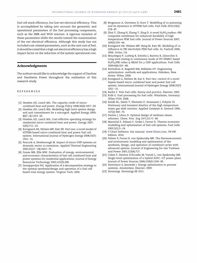
Fig. 13 e Net electrical power output, heat cogeneration

output and system losses for the optimum configuration.

utilization of the SMR reactor in the optimum configuration,

which is due to the improved combination of geometries

(number of tubes, reactor length) and inlet temperatures

(reformate and flue gas).

Fig. 13 illustrates the pattern of energy output/loss for the

proposed micro-CHP system. This figure suggests that the

highest system loss is due to the condenser (7.8%), while the

losses from the exothermic reaction in the WGS reactor and

the parasitic losses from the BOP-components (air blower and

water pump) are rather insignificant (1.3%). However, it should

be noted that a more realistic model, with heat loss consider-

ations and other component coupling-related losses would

result in a further decrease of the total system efficiency.

6. Conclusions

AGA-based optimization strategywas applied to a HT-PEMFC-

based micro-CHP system. The value of the net electrical effi-

ciency (objective function) obtained is 0.412, while the values

of the cogeneration thermal efficiency and total system effi-

ciency are 0.497 and 0.91, respectively. The results of this

research study indicate that the proposed micro-CHP system

must focus on all system components, paying special atten-

tion at their geometric dimensions and operational variables.

The applied global optimization strategy successfully

managed to locate a system configuration with a significantly

higher net electrical efficiency than the one obtained initially.

The choice on the values of the independent variables is still

within the feasible limits of operating the system. The theo-

retical high tolerance of PBI technology on carbon monoxide-

content in the reformate fuel fed to the fuel stack anode,

allows the use of a low steam-to-carbon ratio as indicated by

the results. A more in-depth study for the water knockout/

condenser stage might be necessary in future studies to

minimize the losses occurred in that stage.

Finally, the applied global optimization strategy avoids the

typical trap of designing a fuel cell-based system with a high

i n t e r n a t i o n a l j o u r n a l o f h y d r o g e n en e r g y 3 7 ( 2 0 1 2 ) 2 4 7 0e2 4 8 1 2481

fuel cell stack efficiency, but low net electrical efficiency. This

is accomplished by taking into account the geometric and

operational parameters of the fuel processing components,

such as the SMR and WGS reactors. A rigorous variation of

these parameters shifts the results toward the maximization

of the net electrical efficiency. Although this study has not

included cost-related parameters, such as the unit cost of fuel,

it shouldbenoted that ahighnet electrical efficiencyhas ahigh

impact factor on the reduction of the system operational cost.

Acknowledgments

The authorswould like to acknowledge the support of Danfoss

and Dantherm Power throughout the realization of this

research study.

r e f e r e n c e s

[1] Hawkes AD, Leach MA. The capacity credit of micro-combined heat and power. Energy Policy 2008;36(4):1457e69.

[2] Hawkes AD, Leach MA. Modelling high level system designand unit commitment for a microgrid. Applied Energy 2009;86(7e8):1253e65.

[3] Hawkes AD, Leach MA. Cost-effective operating strategy forresidential micro-combined heat and power. Energy 2007;32(5):711e23.

[4] Korsgaard AR, Nielsen MP, Kær SK. Part one: a novel model ofHTPEM-based micro-combined heat and power fuel cellsystem. International Journal of Hydrogen Energy 2008;33(7):1921e31.

[5] Peacock A, Newborough M. Impact of micro-CHP systems ondomestic sector co emissions. Applied Thermal Engineering2005;25(17e18):2653e76.

[6] Gunes MB, Ellis MW. Evaluation of energy, environmental,and economic characteristics of fuel cell combined heat andpower systems for residential applications. Journal of EnergyResources Technology 2003;125(3):208.

[7] Georgopoulos NG. Application of a decomposition strategy tothe optimal synthesis/design and operation of a fuel cellbased total energy system. Virginia Tech; 2002.

[8] Bergmann A, Gerteisen D, Kurz T. Modelling of co poisoningand its dynamics in HTPEM fuel cells. Fuel Cells 2010;10(2):278e87.

[9] Zhai Y, Zhang H, Zhang Y, Xing D. A novel H3PO4/nafionePBIcomposite membrane for enhanced durability of hightemperature PEM fuel cells. Journal of Power Sources 2007;169(2):259e64.

[10] Korsgaard AR, Nielsen MP, Bang M, Kær SK. Modeling of coinfluence in PBI electrolyte PEM fuel cells. In: Fuelcell 2006;2006. Irvine, CA.

[11] Mocoteguy P, Ludwig B, Scholta J, Barrera R, Ginocchio S.Long term testing in continuous mode of HT-PEMFC basedH3PO4/PBI celtec-p MEAS for m-CHP applications. Fuel Cells2009;9(4):325e48.

[12] Ravindran A, Ragsdell KM, Reklaitis GV. Engineeringoptimization: methods and applications. Hoboken, NewJersey: Wiley; 2006.

[13] Korsgaard a, Nielsen M, Kar S. Part two: control of a novelhtpem-based micro combined heat and power fuel cellsystem. International Journal of Hydrogen Energy 2008;33(7):1921e31.

[14] Barbir F. Pem fuel cells: theory and practice. Elsevier; 2005.[15] Kolb G. Fuel processing for fuel cells. Weinheim, Germany:

Wiley-VCH; 2008.[16] Keiski RL, Salmi T, Niemisto P, Ainassaari J, Pohjola VJ.

Stationary and transient kinetics of the high temperaturewater-gas shift reaction. Applied Catalysis A: General 1996;137(2):349e70.

[17] Davies J, Lihou D. Optimal design of methane steamreformer. Chem. Proc. Eng 1971;52:71e80.

[18] Marechal F, Palazzi F, Godat J, Favrat D. Thermo-economicmodelling and optimisation of fuel cell systems. Fuel Cells2005;5(1):5e24.

[19] F-Chart Software. Ees manual. www.fchart.com, V8.590Edition: 2010.

[20] Pelster S, Favrat D, von Spakovsky MR. The thermoeconomicand environomic modeling and optimization of thesynthesis, design, and operation of combined cycles withadvanced options. Journal of Engineering for Gas Turbinesand Power 2001;123(4):717.

[21] Calise F, Dentice d’Accadia M, Vanoli L, von Spakovsky MR.Single-level optimization of a hybrid SOFCeGT power plant.Journal of Power Sources 2006;159(2):1169e85.

[22] Sieniutycz S, Jezowski J. Energy optimization in processsystems. Amsterdam: Elsevier; 2009.

[23] Serenergy. Serenergy.dk 2011.