reliability modeling, testing and optimization of systems - RUcore

©2018

Yao Cheng

ALL RIGHTS RESERVED

RELIABILITY MODELING, TESTING AND OPTIMIZATION OF SYSTEMS

WITH MIXTURES OF ONE-SHOT UNITS

by

YAO CHENG

A dissertation submitted to the

School of Graduate Studies

Rutgers, The State University of New Jersey

In partial fulfillment of the requirements

For the degree of

Doctor of Philosophy

Graduate Program in Industrial and Systems Engineering

Written under the direction of

Elsayed A. Elsayed

And approved by

_______________________________

_______________________________

_______________________________

_______________________________

_______________________________

New Brunswick, New Jersey

JANUARY, 2018

ii

ABSTRACT OF THE DISSERTATION

RELIABILITY MODELING, TESTING AND OPTIMIZATION OF SYSTEMS WITH

MIXTURES OF ONE-SHOT UNITS

By YAO CHENG

Dissertation Director:

Elsayed A. Elsayed

One-shot units are usually produced and stored (or used as standby) in batches until

retrieved. These units can be defined as a system which may experience degradations or

sudden failures during its storage period. To assess the reliability performance of the units,

reliability tests are repeatedly (in non-identical pattern) and randomly conducted across the

lifetime of the units; where corresponding actions are taken afterwards. The continuous

arrival of batches and conduct of tests induce the system contains a mixture of

nonhomogeneous units, which is defined as a general “k-out-of-n: F system” with k and n

nonhomogeneous and time-dependent. In this dissertation, we propose models to

investigate the reliability metrics of the system under a variety of scenarios. Extensive

simulation studies are performed to validate the models.

Failure or degradation caused by thermal fatigue is a pervasive phenomenon during the

one-shot units’ storage period. The Birnbaum-Saunders (BS) distribution is specifically

developed for describing mechanical fatigue failures, but limited in describing a variety of

iii

hazard functions. Hence it is reasonable to investigate whether the generalized form of BS

(GBS) distribution can be extended for modeling the plastic deformation induced by

thermal cyclic stresses and providing reliability metrics of units subject to thermal fatigue.

In this dissertation, we investigate system reliability metrics when subjecting to thermal

fatigue failure by adopting the GBS accelerated model.

The one-shot units might experience competing failure modes during its storage period.

Specifically, repeated thermal cyclic tests (TCTs) are randomly conducted; at the end of

an arbitrary TCT, the unit’s failure is observed either when any of its failure modes occurs

suddenly or when any of its degradation modes reach its “failure threshold”. Under such

circumstances, unit’s failure data cannot be described by a single failure time distribution;

instead, a competing failure model which considers multiple failure modes is adopted to

assess unit’s reliability metrics. The units’ potential failure modes as well as the reliability

metrics of the system under competing failure modes are investigated in this dissertation.

Due to the characteristics of one-shot units and recent advances in technology and materials,

one-shot units are usually highly reliable and it is impractical to obtain one-shot units’

failure (degradation) data under operating conditions. Accelerated life testing (ALT) is an

efficient approach to obtain failure/degradation observations in a much shorter time period

and utilize the test data to predict reliability metrics under normal operating conditions. We

develop physics-statistics-based models and obtain optimal sequential accelerated non-

destructive test (NDT) plans under different scenarios. The efficiency of the NDT plans is

iv

validated by comparing the system reliability metrics obtained under accelerated and

normal conditions.

NDT assesses unit’s functionality without permanent damage in order to demonstrate the

unit’s reliability. However, one cannot make decisions regarding system reliability by only

depending on NDT results because NDT does not fully perform the unit’s functionality. In

contrast, destructive testing (DT) fully tests the unit’s functionality but destroys the units.

This intensifies the need to investigate hybrid reliability tests that include both NDT and

DT. In this dissertation, an optimal sequential hybrid reliability testing plan is designed and

the results of the tests are utilized to improve the accuracy of the system reliability metrics

estimation. We validate that by conducting hybrid reliability test, the unit’s lifetime

parameters approach their true values. As the reliability estimation converge, we decrease

the number of units tested in DTs and eventually perform NDT only.

There exists many situations that a specific number of one-units are used consecutively

when put into operational use. Therefore, it becomes interesting and challenging to

determine the characteristics and sequence of the one-shot units to be launched such that

the operational use of the launched units is optimized. Defining the launched one-shot units

as a system, we investigate the reliability metrics of the system to optimize the system’s

operational use at arbitrary time by formulating an optimization problem which is

applicable to a variety of objectives. We also provide the bounds of the system’s successful

operational probability estimation.

v

ACKNOWLEDGEMENT

I would like to express my deepest gratitude to my advisor Professor Elsayed A. Elsayed

for your guidance, patience, inspiration, encouragement and support though my MS and

Ph. D. study over the years. Your knowledge and personality have had a profound

influence on my academy career and life. You have set me an example of excellence as a

mentor, instructor, and role model.

My sincere thanks are extended to Professor Susan Albin, Professor Weihong Guo,

Professor Hoang Pham and Professor John Kolassa for serving on my committee and

providing me valuable suggestions that improve the quality of my dissertation. My

appreciation also goes to Ms Cindy Ielmini and Ms Helen Smith-Pirrello for their warm

help during these years.

I also take this opportunity to thank my fiancé, Dr. Yang Li. It is your academic

suggestion, mental support and love that encourages and accompanies me through the

challenging, interesting and unforgettable journey. I would also like to thank my parents

and grandparents for their understanding and selfless support on all my decisions.

vi

TABLE OF CONTENTS

ABSTRACT ........................................................................................................................ ii

ACKNOWLEDGEMENT .................................................................................................. v

LIST OF TABLES ............................................................................................................ xii

LIST OF FIGURES ......................................................................................................... xiv

CHAPTER 1 INTRODUCTION ....................................................................................... 1

1.1 Research Background .................................................................................................1

1.1.1 Reliability of One-shot Units and Systems Composed of One-shot Units ..........1

1.1.1.1 Reliability of One-shot Units .........................................................................1

1.1.1.2 Systems Composed of One-shot Units ...........................................................3

1.1.2 Reliability Testing ................................................................................................5

1.1.3 ALT (ADT) Models and Optimal Testing Plans ..................................................8

1.1.3.1 ALT (ADT) Models .........................................................................................8

1.1.3.2 Optimal Testing Plans..................................................................................11

1.1.4 One-shot Units Optimal Operational Use .........................................................12

1.2 Dissertation Organization .........................................................................................13

CHAPTER 2 LITERATURE REVIEW .......................................................................... 18

2.1 Literature Review.....................................................................................................19

2.2 Limitations of Literature ..........................................................................................29

CHAPTER 3 RELIABILTY MODELING AND PREDICTION OF SYSYTEMS WITH

MIXTURE OF UNITS ..................................................................................................... 31

3.1 Reliability Evaluation of Systems with Mixture of Units ........................................32

vii

3.1.1 Distribution of Failed Units under “No-Removal” Scenario .............................35

3.1.2 Distribution of Failed Units under “p-Consecutive-Failure-Removal”

Scenario......................................................................................................................38

3.1.3 Distribution of Failed Units under “p- Failure-Removal” Scenario ..................40

3.1.4 Distribution of Failed Units Considering Effect of Aging .................................41

3.2 System Reliability ....................................................................................................42

3.3 System Reliability by Sampling ...............................................................................44

3.4 Alternative System Reliability Evaluation Approaches ...........................................46

3.4.1 Approach 1 (A1) ................................................................................................46

3.4.2 Approach 2 (A2) ................................................................................................47

3.4.3 Approach 3 (A3) ................................................................................................49

3.5 Simulation Studies ....................................................................................................51

3.5.1 A Simulation Model ...........................................................................................51

3.5.2 Simulation Results and Validation.....................................................................56

3.6 Alternative System Reliability Evaluation Approaches ...........................................59

3.6.1 Distribution of Failures under Different Scenarios ............................................59

3.6.2 System Reliability Estimation for both testing the entire Population and by

Sampling ................................................................................................................... 61

3.6.3 An illustration of A1 ..........................................................................................62

3.7 Conclusions ..............................................................................................................64

CHAPTER 4 RELIABILTY MODELING OF SYSYTEMS WITH MIXTURE OF

UNITS: A STOCHASTIC APPROACH .......................................................................... 65

4.1 Failure Distribution of Systems with Mixture of Units Using SA ...........................66

viii

4.1.1 Reliability Metrics of the Systems Using the SA without Repairs ....................67

4.1.2 Failure Distribution and Reliability of Systems Using the SA with Repairs .....73

4.2 Reliability Metrics of Systems with Mixture of Units Using SA by Sampling. ......77

4.3 Numerical Comparisons ...........................................................................................80

4.3.1 System Reliability Metrics Estimation by Testing the Total Population ...........81

4.3.2 System Reliability Metrics Estimation by Sampling .........................................83

4.4 Conclusions ..............................................................................................................84

CHAPTER 5 RELIABILITY MODELING OF MIXTURES OF ONE-SHOT UNITS

UNDER THERMAL CYCLIC STRESSES ..................................................................... 86

5.1 Generalized Birnbaum-Saunders (GBS) Distribution ..............................................88

5.2 Reliability Prediction Models for Thermal Fatigue Data. ........................................90

5.2.1 The Coffin-Manson (CM) Model .....................................................................90

5.2.2 GBS Performance in Predicting Thermal Fatigue Life .....................................92

5.3 Reliability Metrics of Systems with Mixtures of One-Shot Units ...........................94

5.3.1 ATCT and Equivalent Test Duration .................................................................94

5.3.2 System Reliability Metrics under ATCTs ..........................................................96

5.4 Simulation Model ...................................................................................................106

5.5 Numerical Illustrations and Validation of the Proposed Models ...........................110

5.5.1 GBS Performance in Predicting Fatigue Life .................................................110

5.5.2 System Reliability ...........................................................................................111

5.5.3 Expected Number of Failures by the Proposed Model and the Simulation

Model ........................................................................................................................112

5.6 Conclusion .............................................................................................................114

ix

CHAPTER 6 RELIABILITY MODELING OF MIXTURES OF ONE-SHOT UNITS

UNDER COMPETING FAILURE MODES.................................................................. 115

6.1 Unit’s Reliability under Competing Failure Modes ...............................................116

6.2 System Reliability Metrics under Competing Failure Modes. ...............................121

6.2.1 System Failure Distribution and Reliability under Competing Failure

Modes. ......................................................................................................................122

6.2.2 System’s Time-to-kth-Failure ...........................................................................124

6.3 Generalization of System Reliability Metrics Modeling ........................................126

6.4 Simulation Model ...................................................................................................127

6.5 A Numerical Illustration .........................................................................................130

6.6 Conclusions ............................................................................................................134

CHAPTER 7 OPTIMAL SEQUENTIAL ALT PLANS ................................................ 135

7.1 Power-Law Humidity Model .................................................................................137

7.2 Optimal Sequential Accelerated NDTs Plans ........................................................139

7.2.1 Mean Residual Life (MRL), Scenarios and Notations.....................................140

7.2.2 Optimization of Sequential Accelerated NDTs under TS1 ..............................143

7.2.3 Optimization of Sequential Accelerated NDTs under TS2 ..............................152


7.4 Conclusions ............................................................................................................162

CHAPTER 8 OPTIMAL DESIGN OF HYBRID SEQUENTIAL TESTING PLANS . 163

8.1 Optimal Sequential Hybrid Reliability Testing Plans based on Two Separate

Samples ........................................................................................................................164

8.2 Optimal Sequential Hybrid Testing Plans based on One Sample ..........................173

x

8.2.1 Optimal Sequential Hybrid Testing Plans for the TSa .....................................174

8.2.2 Optimal Sequential Hybrid Testing Plans for the TSb ....................................180

8.2.3 Optimal Sequential Hybrid Testing Plans for the TSc .....................................184

8.3 Simulation Studies ..................................................................................................184


8.5 Conclusions ............................................................................................................196

CHAPTER 9 OPTIMAL SELECTION AND OPERATIONAL SEQUENCING OF

NONHOMOGENEOUS ONE-SHOT UNITS ............................................................... 197

9.1 One-shot Units’ Operational Use Reliability .........................................................198

9.2 Optimal Selection and Operational Sequencing of One-shot Units .......................200

9.2.1 Optimal Selection and Operational Sequencing ..............................................201

9.2.2 Time-to-kth-failure of a Population with Nonhomogeneous One-shot Units ...207

9.2.2.1 Probability Density Function (pdf) of System’s Time-to-kth-Failure .........207

9.2.2.2 Expected Sime-to-kth-Failure of the System ...............................................210

9.3 Bounds of System’s Successful Probability ...........................................................213

9.3.1 Bounds of System’s Successful Probability of Operation under Constant

Failure Rate ..............................................................................................................214

9.3.2 Bounds of System’s Successful Probability under Time-dependent Failure

Rate ...........................................................................................................................215

9.4 Simulation Model...................................................................................................218

9.5 Numerical Illustrations ...........................................................................................220

9.6 Conclusions ............................................................................................................225

CHAPTER 10 CONCLUSIONS .................................................................................... 227

xi

APPENDIX ..................................................................................................................... 231

REFERENCES ............................................................................................................... 235

xii

LIST OF TABLES

Table 3.1 Means of expected number of failures at the end of first 10 tests using exact

model, A2, A3, and simulation model ............................................................................... 57

Table 3.2 Standard deviations of expected number of failures at the end of first 10 tests

using exact model, A2, A3, and simulation model ........................................................... 58

Table 4.1 Probabilities of system’s numbers of arrived batches and performed test ........ 81

Table 5.1 Expected fatigue life predicted by the CM model and the GBS model .......... 110

Table 5.2 Expected number of failures at arbitrary time between the first three tests based

on proposed model and simulation model with batch sizes in a) ................................... 113


on proposed model and simulation model with batch sizes in b) ……………………...113


on proposed model and simulation model with batch sizes in c) ................................... 113

Table 7.1 Optimal testing plans for the first three accelerated NDTs under TS2………161

Table 7.2 Optimal testing plans for the first three accelerated NDTs under TS3 ........... 161

Table 7.3 Objective function values after the first three accelerated and normal NDTs under

TS2 and TS3 ................................................................................................................... 162

Table 8.1 First four optimal reliability tests based on the method proposed in section 6.1

for the testing scenario investigated in section 6.1 ......................................................... 193

Table 8.2 First four optimal reliability tests based on the simulation study for the testing

scenario investigated in section 6.1 ................................................................................ 194

xiii


for the TSa ....................................................................................................................... 194

Table 8.4 First four optimal reliability tests based on the simulation study for the TSa 194


for the TSb ...................................................................................................................... 195

Table 8.6 First four optimal reliability tests based on the simulation study for the TSb 195

Table 9.1 Reliabilities of the one-shot units (with different characteristics) at time t

......................................................................................................................................... 216

Table 9.2 One-shot units’ optimal selection and launching sequences with testing

parameters a) at time t ................................................................................................... 223


parameters a) at time 6500t ........................................................................................ 223


parameters b) at time 6500t ....................................................................................... 223

xiv

LIST OF FIGURES

Figure 3.1 Relationship between and ....................................................................... 34

Figure 3.2 Test procedure under “no-removal” scenario .................................................. 36

Figure 3.3 Test procedure under “2-consecutive-failure-removal” scenario .................... 56

Figure 3.4 Procedure of obtaining in one iteration in simulation model ................... 59

Figure 3.5 Procedure of obtaining in one iteration of the simulation ........................... 60

Figure 3.6 Procedure of the comparison among exact model, A2, A3, and simulation

model................................................................................................................................. 62

Figure 3.7 Expected probability of failure for one unit in the first 50 tests based on A2 . 63

Figure 3.8 Distribution of failed units under different scenarios ...................................... 63

Figure 4.1 System reliability using the OA and SA over time ......................................... 83

Figure 4.2 Expected numbers of failures with different sample sizes and total population

using the two approaches .................................................................................................. 84

Figure 5.1 System reliability until time t with .............................................. 111

Figure 5.2 System reliability until time t with .............................................. 112

Figure 6.1 Steps of simulating the number of failures in the 1st batch after the 1st TCT.128

Figure 6.2 Steps of simulating the number of failures in the 1st batch at the end of the 2nd

TCT……………………………………………………………………………………..130

Figure 6.3 System reliability until the 3rd TCT under different failure modes ............... 133

Figure 6.4 System reliability until the 3rd TCT under different failure modes ............... 133

ˆys

ys

mK

3K

% 50%p

% 90%p

1

CHAPTER 1

INTRODUCTION

1.1 Research Background

The development of new technologies and global competition emphasize the need for

accurate estimation or prediction of a unit’s quality. Reliability is one of the most important

quality characteristics of interest. Reliability is defined as the probability that a unit

operates for a given period of time (design lifetime) under the designed operating

conditions. Although modeling of systems reliability has been extensively investigated, the

reliability modeling of one-shot units is limited which motivates the research of this

dissertation.

1.1.1 Reliability of One-shot Units and Systems Composed of One-shot Units

1.1.1.1 Reliability of One-shot Units

There exist some types of units that can only perform its function once as its use is normally

accompanied by irreversible reactions, e.g. chemical reaction or physical destruction. After

the use, the units are destroyed or require extensive repair. Units with such a property are

referred to as one-shot units. Missiles, airbags and most of the military weapons are typical

examples of one-shot units. An important characteristic of one-shot units is its long-term

2

storage period or standby status before delivered to users or deployed. To illustrate, military

weapons are conventionally stored for long periods, often in excess of decades until there

is a need. The auto airbag is another example of one-shot units as an airbag stays in standby

status during a vehicle operating life and inflates rapidly (in millisecond) when an accident

or collision happens in order to provide the auto occupant(s) with protection. One-shot

unit’s storage life (or time in standby status) approximately equals to its operational life.

Generally, the reliability of one-shot units is defined as the probability that they

successfully perform required function when needed. Initially, reliability of one-shot units

is simply assigned a time-independent probability. However, reliability of one-shot units

needs to consider the effect of aging since the units experience a variety of potential failure

modes which are caused by different failure mechanisms and are dependent on the length

of the storage/standby periods. These failure modes may inhibit one-shot unit’s ability to

perform its function. For example, the integrated circuit (IC) board of the missile’s

electronic guidance system might no longer function properly as the temperature

fluctuation incudes the crack of the solder joints to an unacceptable level (thermal fatigue),

or as its resistance degrades and eventually reaches a critical point, or due to a failure

without indicator. Meanwhile, the IC board might fail suddenly with no indicator of failure.

Determining the status of one-shot units during the long storage/standby period under

different types of failure modes, evaluating the reliability of stored one-shot units and

ensuring the proper function of one-shot units when needed become an important issue.

3

1.1.1.2 Systems Composed of One-shot Units

Batches of one-shot units are produced and stored to form a system. Current research on

one-shot units’ reliability is sparse by addressing single (non-repeated) test and assuming

that all units are homogenous. In real life, the successive arrivals of batches and the

repeated reliability tests result in a mixture of nonhomogeneous units with different

characteristics at any point of time. Instead of the exact lifetime data, the testing results

only show the number and the characteristics of the testing units. Such data can be

addressed as generalized binary data. As reliability tests (non-destructive or other types)

are repeated during the life horizon of the units, appropriate decisions are made regarding

the failed units during the test. Specifically, there could be the following possible decisions

regarding the failed units:

1. Failed units are repaired and placed back into the system with a higher failure rate;

2. Failed units are discarded after certain consecutive number of failures;

3. Failed units are discarded after certain number of failures.

Consequently, the characteristics of the units in the system are continuously changing.

Specifically, the population size changes as the new batches arrive and failed units might

be discarded. In the system, some units are newly arrived whereas some units are aged;

some are repaired multiple times and might have high failure rates and some have never

failed.

4

The extensive experience with units’ reliability testing indicates that all tests require some

kind of combinatorial testing such as “k-out-of-n” system. In this dissertation, the system

with a mixture of different units can be defined as a generalized “k(t)-out-of-n(t): F system”.

Specifically, in this dissertation, the “k(t)-out-of-n(t): F system” is a generalization of

traditional “k-out-of-n: F system” as both k(t) and n(t) increase with time. Characteristic

of such a system is described in details and the reliability metrics evaluation under different

scenarios becomes challenging. Computationally efficient approximations that evaluate the

system reliability metrics over an extended time horizon as well as large batch sizes have

significant practical values and should be investigated. Additionally, not much attention

has been paid to investigate the effect of population’s non-homogeneity on reliability

prediction. This is addressed in details in this dissertation.

For the system described above, there could be many testing approaches and testing

scenarios to conduct the reliability tests during the storage period (under either normal or

accelerated conditions) such that the unit’s/system’s reliability metrics are assessed. The

reliability tests can be performed by testing the entire population; however, with the

continuous arrival of units, the cost of testing a large population becomes high and testing

samples which represent the population mixture proves to be a viable alternative. Different

types of reliability tests under different scenarios, as well as their advantages,

disadvantages, and applications, are discussed later in this dissertation.

5

In real life, times of arrivals of batches, times to perform the reliability tests, and the batch

sizes are not arbitrary. Instead, they could be described by specific probabilistic

distributions. To illustrate, the arrival of batches and the conduct of the reliability tests may

follow nonhomogeneous Poisson distributions and the batch size may follow a uniform or

normal distribution. Under such circumstances, the potential condition and reliability of

the system can be obtained by applying a stochastic approach (SA). The details are

investigated in the dissertation.

1.1.2 Reliability Testing

Performing reliability testing is an effective approach to demonstrate or predict the

reliability of the units or systems, which is a function of time. Specifically, to determine

the reliability of one-shot units, one can perform either DT or NDT under either normal or

accelerated conditions.

DT involves the actual use of the units and determines whether the units perform the

expected function or not. Its use is limited since performing such a test “destroys” the unit

or requires high repair cost, the units are discarded after the test. Accordingly, it is not

appropriate to conduct DT using large samples. Consequently, performing the test on a

limited number of one-shot units inevitably results in sampling errors.

6

Another type of reliability test, NDT, assesses the unit’s reliability without causing

permanent damage. The NDT is used to ensure that the testing units continue to perform

their functions after the test. The procedures during NDT incorporate inspecting, testing,

and evaluating individual units or assemblies. For example, the electronic guidance

subsystem of a missile may be subjected to a functional test or electric field test such as

thermal cyclic test (TCT) to determine its reliability. In a TCT, the testing systems are

heated at a temperature and kept for a certain dwell time, then cooled to a temperature to

complete a testing cycle. Obviously, there exists no limit on the number of testing units

except test time and cost. However, it is difficult to make decisions regarding system

reliability by completely relying on the results of NDT since it does not fully perform all

functions of the units.

Most of the research in the literature utilizes and analyzes the failure data obtained from

DTs, which destroys (consumes) the one-shot units. In this dissertation, we consider

repeated NDTs (under either normal or accelerated conditions) during the storage period

of the one-shot units which do not affect the units’ functionality. We also utilize the units’

lifetime models to predict the units’ reliability behavior, by assuming that test data only

show the number and combination of the failed units at the end of each test when repeated

NDTs are performed.

Besides performing NDT, it is also challenging but interesting to hybridize NDT and DT

to demonstrate and predict the reliability of the system, which has not been addressed and

investigated in previous research. To conclude, the reliability metrics of the system

7

composed of one-shot units can be assessed by considering a variety of combinations of

reliability tests. Specifically, we investigate the following testing scenarios in this

dissertation:

1. Conducting a sequence of normal NDTs on the entire population/selected samples;

2. Conducting a sequence of accelerated NDTs on the entire population/selected samples;

3. Conducting a sequence of normal hybrid reliability tests on the selected samples.

Specifically, when scenario 3 (conducting hybrid reliability tests that utilize NDTs and

DTs) is considered, the following two specific approaches are taken into consideration:

a. Each NDT and DT are performed on two different samples;

b. Each NDT and DT are performed using the same sample;

Units failed in the NDTs are either repaired and tested in DTs, or repaired and placed back

into the system, or discarded.

The above tests are repeatedly performed during the entire storage period of one-shot units

in order to determine the reliability metrics of the system regularly. Once the type of the

reliability test is determined (NDT, or hybrid reliability test), designing the optimal

sequential reliability testing plan based on sampling is necessary and challenging. To

8

illustrate, it is reasonable to minimize the number of units destroyed during the tests, i.e.,

the number of units assigned to the DTs, while obtaining accurate reliability metrics

estimation.

When designing the optimal sequential NDTs plans under accelerated conditions, the

difference between the reliability estimation obtained under accelerated and normal

conditions needs to be minimized, or/and the test durations need to be reduced.

Investigation of the above problems is unique and has significant contributions.

It is difficult to continuously monitor one-shot units’ status. In such a case, reliability tests

are performed at discrete time intervals and only the number of occurrences (say failures)

during an interval is known, i.e., no information between observation time points is

available. Panel count data which include the number of event occurrences between

observation time points are collected. In this dissertation, the collected panel count data

demonstrate the testing units’ nonhomogeneous characteristics, which are general.

Reliability estimation is then obtained by considering the general panel count data.

1.1.3 Accelerated Life Testing (ALT) Models and Optimal Testing Plans

1.1.3.1 ALT Models

9

There are many situations that neither exact nor binary failure/degradation data of highly-

reliable units under normal operating conditions are attainable during its expected life, e.g.,

the electronic units (transistors, resistors, integrated circuits, and capacitors, etc.) show low

failure rates during their lifetime and only a small number of failures occur if the reliability

tests are conducted at normal conditions. An effective approach to obtain failure data

within a reasonable period of time is to consider accelerated life testing, which induces

failures quickly by subjecting the units to severer stresses conditions than normal operating

conditions. The accelerated data are then used to estimate the unit’s reliability metrics

under normal stresses. In this dissertation, we intend to investigate the use of the ALT in

estimating the reliability of one-shot units.

The accuracy of reliability metrics estimation is highly dependent on: 1) a proper ALT

model that models the unit’s life characteristics, reflects the effect of applied stresses on

the units’ reliability metrics, and accurately relates the failure data under the severer

stresses and normal stresses, and 2) an optimal ALT plan that specifically determines the

details of implementing the ALT.

Elsayed (2012) classifies ALT models mainly into three categories: statistics-based models

(including parametric and non-parametric models), physics-statistics-based models, and

physics-experimental-based models.

10

Statistic-based models are generally used when the exact relationship between the applied

stresses and failure times of the units cannot be determined based on the physics or

chemistry principles of the units. Either parametric models (failure time distributions) or

non-parametric models (linear, proportional-hazards (PH), and proportional-odds (PO),

etc.) can be adopted. However, if only a small number of units are tested for a short time,

evaluation process will be biased since insufficient failure data are collected. Besides, only

analyzing the unit’s lifetime based on statistic-based models is insufficient since statistics-

based models fail to consider the unit’s failure mechanism.

The physics-based models are effective in estimating unit’s reliability metrics and

addressing subtle performance problems (e.g., when only very few units are tested) once

the unit’s specific failure mechanisms are known; especially when the changes in the unit’s

physics are closely related to the unit’s lifetime model parameters. However, the

uncertainty of modeling (caused by the variation of the unit’s material property, operating

conditions, and the variation during the unit’s manufacturing process) is not considered in

most of the physics-based models. This is addressed in the next models.

Physics-statistics-based models consider both the statistics-based models and physics-

based models by describing the physics of unit’s failure mechanisms and considering the

uncertainty during the modeling process. Arrhenius model, Eyring model, and inverse

power rule model, are typical examples of physics-statistics-based models. We intend to

investigate physics-statistics-based model to estimate the reliability of one-shot units.

11

In some cases, the unit exhibits degradation indicator before failure. In such cases, we

monitor the degradation indicator with time (under normal or accelerated conditions) and

utilize the degradation data to estimate the unit’s/system’s expected time to failure (time to

reach a threshold of the degradation level) and other reliability metrics. We refer to the test

where degradation data are collected at accelerated conditions as accelerated degradation

testing (ADT). Elsayed (2012) summarizes typical ADT models, similar to the ALT

models: the physics-based models such as resistor degradation mode, laser degradation

model and hot-carrier degradation model; the stochastic degradation models such

Brownian motion models, Inverse Gaussian models and Gamma models; and the physics-

statistics-based models which include the characteristics of the previous two models. In

this dissertation, we investigate the system reliability metrics under the scenario that the

units are subject to different types of failure modes.

1.1.3.2 Optimal Testing Plans

Once the ALT (ADT) models are determined, an optimal ALT (ADT) plan is designed.

The reliability metrics obtained via extrapolation in accelerated stresses levels and reduced

test duration are inevitably less accurate than those obtained under normal reliability tests.

The motivation of the optimal ALT (ADT) plan design is to obtain reliability metrics

estimates at normal operating conditions as accurate as possible. Specifically, an ALT

(ADT) plan needs to be designed to optimize a specific objective (usually minimizing the

12

error of certain reliability metrics estimates at normal operating conditions) while

satisfying given constraints.

Usually, some or all of the following decision variables need to be determined: the applied

stresses (temperature, electric field, radiation, etc.), the method of stress application

(constant stress, step stress, cyclic stress, ramp-step stress, and triangular-cyclic stress, etc.),

the applied stresses levels, the number of testing units to be allocated to each stress level,

the test duration, and the time to perform the test.

In this dissertation, different types of reliability tests are successively performed and

corresponding optimal sequential testing plans based on sampling need to be designed

(when the reliability tests are performed under accelerated stresses). Different from the

traditional ALT plan that considers the reliability metrics of individual units, we propose

sequential ALT plans by taking the system reliability metrics into account, which is

significantly different from existing ALT plans and is realistic. Moreover, the optimal ALT

plans are designed sequentially, i.e., the design of current testing plan is dependent on the

previous testing plans, which incorporates and generalizes the traditional design of single

ALT plan.

1.1.4 One-shot Units Optimal Operational Use

13

One-shot units such as missiles, airbags, and most of the military weapons are deployed

after long terms of storage (or standby). It is important to ensure the stored units operate

its function properly when needed. In this dissertation, we investigate the optimization of

one-shot units’ operational use at arbitrary time.

There exists many situations that the one-units are used consecutively when put into

operational use. To illustrate, a certain number of one-shot units are selected from the

stored population and launched in sequence. The population has a mixture of one-shot units

with nonhomogeneous characteristics due to the units’ different arrival times and the

conduct of the sequential reliability tests during its storage period. Therefore, it becomes

interesting and challenging to determine the characteristics and sequence of the one-shot

units to be launched such that the operational use of the launched units is optimized.

Defining the launched one-shot units as a system, the reliability metrics of the system (e.g.,

the probability that the system achieves the successful operation, the expected number of

successfully launched units) need to be investigated. In this dissertation, we optimize the

system’s operational use at arbitrary time by formulating an optimization problem which

is applicable to a variety of objectives. We also provide the bounds of the system’s

successful operational probability estimation and develop a simulation study to validate the

proposed approach.

1.2 Dissertation Organization

14

The dissertation is organized as follows: In chapter 2, we provide a detailed review of

related literature. We summarize the literature, analyze its contributions and limitations,

and highlight the motivation as well as the uniqueness of the problems investigated in the

dissertation.

In chapter 3, we propose the problem, describe the system in details, and develop effective

models to estimate the system reliability metrics under different scenarios by either testing

the population or testing the sample. The effect of aging on the system reliability is also

taken into consideration. Defining the system as a generalized “k(t)-out-of-n(t): F” system,

we develop analytical expressions of the system reliability metrics. We also propose

several computationally effective alternatives to investigate the system reliability metrics

when the batch size is large or when the reliability tests are performed extensively over the

time horizon. Extensive simulation studies are studied in chapter 3 to validate the proposed

models under different scenarios.

In chapter 4, the problem investigated in chapter 3 is solved by using a stochastic approach.

We assume that specific probabilistic distributions are used to describe the batches’ arrival

times, batches’ sizes, and the times to conduct the tests, then the system reliability metrics

are investigated. The potential characteristics of the system (the number of units in the

system, the ages of the units, the times to perform the reliability tests, and the times to

repair failed units, etc.) become complicated. The expected system reliability metrics are

15

then compared with those investigated in chapter 3. Reliability metrics based on sampling

is also discussed.

In chapter 5, we address the system reliability metrics under thermal fatigue. Modeling

units’ thermal fatigue life due to cyclic temperature fluctuation based on Coffin-Mason

(CM) principle has been extensively investigated. However, sparse research assesses the

thermal fatigue life by providing the reliability metrics of components/systems under

thermal fatigue. We investigate a GBS distribution and its performance in predicting

fatigue failure caused by thermal cyclic stresses. We then apply the GBS distribution to

model the reliability metrics of a system with mixtures of nonhomogeneous one-shot units

subject to thermal fatigue. An extensive simulation model is developed to validate the

system reliability metrics accuracy. Numerical examples are presented to illustrate the use

of the models.

In chapter 6, the reliability metrics of the system under competing failure modes are

investigated. The unit’s failure is observed either when any of its failure modes occurs

suddenly (failure modes without indicators of failure) or when any of its degradation modes

(which exhibit indicators that eventually lead to failure) reach its “failure threshold”.

Meanwhile, the unit is repaired either when it fails between two reliability tests or when

one of its degradation modes reaches the predetermined “repair threshold”, where the

“repair threshold” is lower than the “failure threshold”. We study the units’ potential failure

modes, its reliability at arbitrary time and the reliability metrics of the system under a

generalized competing failure modes.

16

In chapter 7, we address the design of optimal sequential accelerated NDTs plans. We first

study the individual unit’s reliability behavior under accelerated conditions by developing

a statistics-physics-based lifetime distribution, which directly relates the applied stresses

to the system reliability metrics. We then propose the optimal design of sequential

accelerated NDTs, taking system’s/sample’s reliability metrics under different testing

scenarios into account. Specifically, we determine the optimal times to perform the tests,

the applied stresses levels, and the test durations. The uncertainty during the sampling

procedure as well as the units’ characteristics are considered. We show that a well-designed

sequential accelerated NDT is an effective approach to reduce the test durations while

providing accurate reliability prediction with negligible consequences on the residual lives

of the units and other system reliability metrics. Moreover, we numerically illustrate that

the sample size has no effect on the accelerated NDTs plan design, in the long run.

In chapter 8, we consider the optimization of sequential hybrid reliability tests (including

DT and NDT) based on sampling with the objective of minimizing the number of units

used in the DT while obtaining accurate estimates of the reliability metrics. Specifically,

we determine the optimal times to perform the tests and the number of units assigned to

the two types of testing in each hybrid test. Consequently, after conducting a number of

hybrid tests, we decrease the sample size of the DT as the accuracy of reliability metrics

estimation improves and eventually we conduct NDT only. The optimization problem is

studied under several testing scenarios. The proposed methods are validated by numerical

illustrations and extensive simulation studies.

17

In chapter 9, we optimize the operational use of the one-shot units at arbitrary time during

its storage. Some units (with nonhomogeneous characteristics) are selected from storage

and launched or operationally used at arbitrary time as needed. Referring to the launched

units as a system, we optimize the system’s operational use by determining the selected

units’ characteristics (number of units selected from each batch) and its launching sequence.

The system reliability metrics such as the expected number of successfully launched units,

the average and variance of the probability that the system achieves a successful operation,

and the expected time of the system’s kth failure are considered in the optimum selection

procedure. Considering the units’ inhomogeneity, we provide the confidence bounds of the

probability that the system achieves a successful operation based on the units’ optimal

selection and launching sequence.

In chapter 10, we give conclusive remarks of our research.

18

CHAPTER 2

LITERATURE REVIEW

In this chapter, we present a detailed overview of research related to the problem being

investigated in this dissertation. We summarize the limitations of current research and

highlight the motivation and the uniqueness of the research in the dissertation. We first

review the research on the storage life and reliability metrics of one-shot units. There is

extensive work on thermal fatigue failure, however, limited research is done on the

reliability metrics of systems with mixtures of one-shot units when subjecting to thermal

fatigue. We review current study on thermal fatigue and summarize existing approaches

and models on thermal fatigue. We then review the research on the reliability evaluation

and optimization of different types of k-out-of-n systems. Most of the existing research is

based on the assumptions that units in the system are identical, which is limited. There is

few research on the reliability metrics of systems composed of one-shot units. Evaluation

of system’s reliability through the conduct of NDT is limited. There is no investigation on

hybridizing NDT and DT when conducting reliability tests. We then present a thorough

review of literature about the current ALT models and design of optimal ALT plans.

Limited research is carried on the design, analysis, and application of sequential ALT plans

when evaluating one-shot unit’s storage reliability during its lifetime. We also review units’

lifetime models under different failure modes related to the proposed research but not as

general as the lifetime models we investigate in the dissertation.

19

In section 2.1, we review all related literature in details. In section 2.2, we summarize the

limitations of the literature and highlight the importance and uniqueness of the research in

this dissertation.

2.1 Literature Review

Approaches to estimate the reliability of one-shot electro-explosive units are introduced

and current practices which can result in suspect data are discussed. Besides, remedial

action which leads to accurate and dependable methods of reliability estimation is

suggested (Peckham, 1965). Several priors in the Bayesian approach (with three different

prior settings) for the predictions of reliability metrics of electro-explosive units at

operating conditions under the exponential lifetime distribution are compared (Fan et al.,

2009). The deterioration of stored one-shot units is examined and the reliability levels of

individual units which together with the inspection regime give a particular reliability level

in the delivered units are established (Newby, 2008). Apparently, no research is carried on

the reliability metrics on systems that composed of nonhomogeneous one-shot units.

Approaches and difficulties of estimating the total life (which approximately equals to the

storage life) of one-shot unit are investigated as follows: prognostics and health monitoring

(PHM) systems are entirely applied in design and storage stages of tactical missile.

Engineering approaches to the life degradation factor analysis and life prediction process

are investigated (Li et al., 2014). The analysis results are used by U.S. Army personnel and

20

contractors in evaluating current missile programs, the results are also used in the design

of future missile systems. The storage-life modeling method of electric steering gear based

on competing failure modes is studied, including the function and structure principle, the

main performance parameters and failure thresholds of electric steering gear. The

sensitivity of the various components of the electric steering gear is also analyzed in order

to determine the degradation paths of the components (Deng et al., 2014). A case study of

condition-based remaining storage life prediction for gyros in the inertial navigation system

is presented (Wang et al., 2014) on the basis of the condition monitoring data by

considering the slow degradation that occurs when the system is in storage. The previously

mentioned literature only analyzes the storage lifetime of individual one-shot units rather

than the reliability metrics of systems that compose one-shot units. Moreover, the effect of

time on unit’s storage life and characteristics is not addressed during the analysis.

Failure or degradation caused by thermal fatigue is a pervasive phenomenon. Temperature

fluctuation in thermal fatigue can quickly lead to strains which are much higher than the

elastic limit thus cause plastic strains and deformation in each cycle. Therefore, most

mechanical stress fatigue models that deal with high-cycle failure (e.g., the S-N curve,

Miner’s law) are not readily applicable for modeling thermal fatigue failure. Instead,

Coffin-Manson (CM) model and its modified versions (e.g., Norris-Landzberg model,

Engelmaier’s model and Darveaux’s model) are widely adopted when assessing the unit’s

cycle-to-thermal-failure especially for low-cycle fatigue, where the CM model considers

the loads in terms of plastic strain rather than stress.

21

Darveaux’s model (McPherson, 2010) considers the strain rate effect under various ramp

rates for the prediction of thermal fatigue lifetime of the solder interconnections. The

derivation and application of the CM model to different types of materials (ductile, plastic,

and brittle) are discussed and illustrated in McPherson (McPherson, 2010). The parameters

of the CM model for solder fatigue life prediction are evaluated and different reference

temperatures are simulated to investigate the effect of temperature on solder fatigue life

prediction (Che and Pang, 2013)

The parameters of Engelmaier’s model are recalibrated (Salmela et al., 2005) to contrast

the fatigue data. A rapid life-prediction simulation approach for solder joints based on

Engelmaier’s model is developed (Qi et al., 2009) for combined temperature cycle and

vibration conditions. The life expectancy of solder interconnect under simple temperature

cycles using the Engelmaier model is predicted (Chai et al., 2014). The characteristic

lifetime data are contrasted with a recalibrated Engelmaier’s model (Putaala et al., 2012).

Norris-Landzberg’s model is recalibrated to provide an accurate estimation of units’

lifetime under mechanical fatigue (Pan et al., 2005). It is also indicated that Norris–

Landzberg’s model fits the experimental data accurately and the error is less than 6%

in the lead-free assemblies (Vasudevan and Fan, 2008). In this paper, the CM model is used

to validate the accelerated statistical model that we propose.

Thermal cyclic test (TCT) is performed to obtain the units’ fatigue life data which are then

used for units’ fatigue life modeling. When performing TCT, the testing units’ material

properties and the TCT plan (e.g., dwell time, heating and cooling rate and temperature

22

amplitude) have a direct impact on the units’ fatigue life. It shows that the damage per

thermal cycle increases with the temperature amplitude (Qi et al., 2006). It is also validated

that a faster ramp rate generates more fatigue failures per cycle and thus decreases the

testing units’ fatigue life (Zhai and Blish, 2003), (Qi et al., 2006), (Darveaux, 2002),

(Chaparala et al., 2005) and (Ghaffarian, 2000). However, the effect of the ramp rate and

the dwell time on testing units’ life are negligible due to the stress relaxation at maximum

cycle temperature (Schubert et al., 2002).

Accelerated thermal cyclic test (ATCT) is applied where the testing samples are subjected

to a larger temperature fluctuation than the actual situation in order to induce sufficient

failures. A comprehensive set of ATCTs are performed on vehicles (Ma et al., 2011) to

analyze the impact of solder alloy characteristics on ATCT acceleration factors. By

simulating ATCTs under different conditions, it is determined that the ATCT acceleration

factor is independent of sample composition (Bosco et al., 2016). An ATCT is introduced

(Yang et al., 2008) to approximate the operating conditions, showing that the low thermal

conductivity and high specific heat of lead-free solder cause a short thermal fatigue life.

Experimental and modeling results of surviving material combinations that occur at various

temperatures are described (Shapiro et al., 2010). Different plated through holes (PTH)

cycle-to-failure (CTF)-temperature models are evaluated for its effectiveness in

determining acceleration factors for PTH fatigue life prediction under different conditions

(Xie et al., 2008).

23

The Birnbaum-Saunders (BS) distribution is specifically developed for describing

mechanical fatigue failures. It is noted that the BS distribution can be applied even when

the assumption of the BS is relaxed (Desmond, 1985), i.e., the crack increment in a certain

cycle not only depends on the applied stresses but is also affected by the accumulated crack

size. It is stated that the BS distribution is more flexible than the Inverse Gaussian (IG)

distribution (Bhattacharyya and Fries, 1982). Owen proposes a generalized BS (GBS)

distribution by introducing a second shape parameter (Owen, 2006).

Reliability tests are performed during the storage period of one-shot units. Instead of

continuous monitoring of the units, reliability tests are carried out at discrete times;

correspondingly, the test data (panel count data) only show the status (fail, survive, or other

states) of testing units. The following literature covers recent studies on the analysis of

panel count data: the statistical analysis of interval-censored failure time data with

applications are explored, three different data sets (Breast Cancer, Hemophilia, and AIDS

data) are used to numerically illustrate both parametric and nonparametric methods of

analysis (Sun and Fang, 2003). A family of mixed Poisson likelihood regression method

for longitudinal interval count data is applied (Thall, 1988) to estimate and test the unit’s

failure rate over a time of a particular event. Meanwhile, a related empirical Bayesian

estimation of random-effect parameters is proposed. A method for fitting the proportional

hazards (PH) regression model when utilizing interval-censored observations is developed

(Finkelstein, 1986). The Poisson assumption of panel count data when the observation time

or process is related to the underlying recurrent event process is relaxed and a robust

method for regression analysis of panel count data is applied (Zhao et al., 2013).

24

Meanwhile, the asymptotic properties of the resulting estimates are discussed and

numerical illustrations are proposed to demonstrate the use of the approach in practical

situations. Nonparametric estimation procedures for the marginal mean function of a

counting process are developed based on periodic observations (Hu et al., 2009). Obviously,

most of the current research on panel count data emphasizes on the optimization of

parameter estimation. Little attention has been paid to the application of panel count data

to unit’s lifetime models and reliability prediction.

It is assumed that the system is good if and only if less (no less) than k out of the n units

fail (survive). There is an extensive work on the reliability of traditional k-out-of-n: F (G)

systems: The reliability of a k-out-of-n system based on expandable reliability block

diagram is calculated (Chang and Zhao, 2013), which is very efficient and convenient for

engineering application. A fast and robust reliability evaluation algorithm based on

conditional probabilities is developed (Amari et al., 2009), which is computationally

efficient and general for calculating the exact reliability of large multi-state-k-out-of-n

systems. An effective approach is proposed (Tian et al., 2008) for obtaining the “reliability

bounds” of complex k-out-of-n systems with a large number of components and possible

states by focusing on the probability of the system in certain states, which provides the

range of the system reliability in a much shorter computation time.

Consecutive-k-out-of-n: F (G) system is a special kind of k-out-of-n: F (G) system, where

the system works if and only if less (no less) than k consecutive units fail (survive). The

25

reliability evaluation and optimization of such a system have been investigated as follows:

Recent advances in methods of reliability evaluation, importance and optimal stochastic

orderings of the units in consecutive-k-out-of-n systems are reviewed comprehensively

(Eryilmaz, 2010). Optimal system reliability design of consecutive-k-out-of-n systems is

investigated, both invariant and variant optimal design under different circumstances are

proposed (Zuo, 1989). Zuo’s work is generalized and extended to multi-dimensional

consecutive-k-out-of-n systems (Kuo and Zuo, 2003); other types of k-out-of-n and

consecutive-k-out-of-n systems are meanwhile addressed, e.g., the s-stage-k-out-of-n

systems, linear and circular m-consecutive-k-out-of-n systems and the k-within-

consecutive-m-out-of-n systems. The optimal component arrangement for a multi-

state consecutive-k-out-of-n: F system with the objective of maximizing the expectation of

the system state is considered (Akiba et al., 2011) when the selected units are arranged to

the positions in the system. Graphical Evaluation and Review Technique (GERT) is applied

(Agarwal et al., 2007) to deal with the reliability of m-consecutive-k-out-of-n: F system

with (k-1)-step Markov dependence and m-consecutive-k-out-of-n: F system with Block-k

dependence. The time efficiency of GERT is validated by illustrative numerical examples.

The Stein-Chen method is employed (Godbole, 1993) to obtain the Poisson approximation

for a linear m-consecutive-k-out-of-n system, considering the units in the system are

stationary Markov dependent. The reliability and residual lifetime of linear and

circular consecutive-k-out-of-n systems with nonhomogeneous components lifetimes are

investigated (Salehi et al., 2011), i.e., the lifetimes of components are independent but

nonhomogeneous. However, the units in the system are non-repairable and investigation

of system’s current status relies on system’s previous status.

26

Performing reliability tests is an effective process to assess and predict the reliability of

various types of units. Reliability tests might either destroy the testing unit’s serviceability

(DT) or not (NDT). The optimization of the NDT program is studied (Hunt and Wester,

2013) for a missile inventory system. Specifically, the number of testing units in each NDT

is optimized with the constraint of frequency of NDTs. However, the reliability of

individual missile is considered to be independent of the time and age, which is unrealistic.

The test planning methods for designing accelerated destructive degradation tests is studied

from different aspects (Shi et al., 2009), including non-Bayesian and Bayesian methods.

The effect of sample size and test duration on the optimal plan is shown by conducting

sensitivity analysis. The reliability of NDT techniques for the inspection of pipeline welds

employed in the petroleum industry is evaluated (Carvalho et al., 2008). Tests on specimen

made from pipelines containing defects are carried out and artificial neural networks (ANN)

in the detection and automatic classification of the defects are used. To conclude, the use

of NDT for reliability estimation of one-shot units is limited and the hybrid reliability

testing that combines NDT and DT has not been addressed so far.

There are many situations when the failure data of the test units are lacking especially when

the reliability test is performed under normal operating conditions. In such cases, ALT is

applied by subjecting the units to severer-than-normal stresses, such that failures are

induced in a much shorter time and accelerated data are then utilized with appropriate ALT

model to estimate the units’ lifetime under normal conditions.

27

Statistics-based models, physics-statistics-based models, and physics-experimental-based

models are discussed (Elsayed, 2012). An overall review of ALT models that are widely

used in engineering practice is provided (Escobar and Meeker, 2006), including both

statistics-based models and physics-based models.

Several frequently used types of testing stresses and corresponding failure mechanisms that

the stresses might induce are introduced (Elsayed, 2012). The design of ALT plans under

different conditions and constrains are summarized; the concept and detailed application

of the equivalent ALT plans are explained (Elsayed, 2012). The methods and principles of

designing optimal ALT plans with two experimental factors without interactions are

investigated (Escobar and Meeker, 1995). Escobar and Meeker’s work is extended by

designing the optimal ALT plan with two types of stresses assuming possible interactions

between them (Park and Yum, 1996). It is widely accepted that if the ALT is performed

under multiple stresses levels, the number of testing units should be allocated inversely

proportional to the applied stresses levels.

An ALT plan needs to be designed to accurately estimate the unit’s (system’s) reliability

metrics while reducing the testing time. Extensive work can be found in designing ALT

plan on regular units (which is different from one-shot units) by assuming different types

of ALT models and different objective functions (see (Liao and Elsayed, 2010), (Zhu and

Elsayed, 2013), (Zhao and Elsayed, 2005), (Elsayed and Jiao, 2002), (Zhang, 2007),

(Nelson and Meeker, 1978) , etc.). The application of ALT on one-shot units is limited: an

28

optimal ALT plan is designed by assuming the testing unit’ lifetime follows a Weibull

distribution (Balakrishnan and Ling, 2013). However, the work assumes only a single

accelerated DT is conducted and the units are homogeneous. Moreover, the testing plan is

designed by considering the individual unit’s reliability, which is limited. There is no

research investigating the design of optimal accelerated NDT plan based on the system’s

reliability metrics with mixture of nonhomogeneous one-shot units.

The current research on ALT plan design only addresses the single optimal testing plan

without considering the possibility that a sequential ALTs are performed. Besides, the

testing scenario that failed units are repaired, placed back into the system, and are subjected

to the next ALT has not been addressed yet.

When evaluating the reliability of the system or units (under either normal or accelerated

stresses), the unit’s lifetime model (physics-based model, statistics-based model, or

physics-statistics-based model) is of great significance. A probabilistic physics of failure

approach for estimating tube rupture frequency in steam generator of water reactor is

presented (Chatterjee and Modarres, 2012). A methodology for the implementation of

physics-based models of unit lifetimes is described (Hall and Strutt, 2003), treating the

uncertain parameters as random variables which can be described by certain statistical

distribution and sampled using Monte Carlo methods. The application of physics-statistics-

based model to ALT, where the model parameter (usually scale parameter) is dependent

on the applied stresses has not been extensively investigated. Current work on physics

29

models or physics-statistics-based models does not pay attention to the lifetime of one-shot

units, which is limited.

2.2 Limitations of Literature

A thorough review of the literature shows that the research on storage life and storage

reliability of one-shot units is limited as current work only focuses on identical one-shot

units. Moreover, the investigation of one-shot unit’s reliability metrics is limited to the

individual units. The effect of successive reliability tests on the unit’s reliability has not

been investigated. In additional, most of the current work only assigns a constant value as

the reliability of the one-shot units, where the effect of time is not considered in the

reliability modeling of the one-shot units. There is also no investigation on the reliability

modeling of mixtures of nonhomogeneous one-shot units when subjecting to a variety

types of failure modes such as thermal fatigue, degradation, and/or competing failure

modes.

Although ALT models and optimization of ALT plan design have been widely and

extensively investigated, they are limited to testing the units as a onetime ALT and all

testing units are identical and non-repairable. Designing optimal sequential ALT plans for

the system which considers the one-shot units’ nonhomogeneous characteristics has not

been addressed. The consequence of applying accelerated NDT needs to be discussed.

30

Significant work has been done on the reliability modeling of different types of systems.

However, the characteristics of the units in the system are assumed to be identical,

stationary, and known beforehand. This dissertation investigates the generalized k(t)-out-

of-n(t) systems composed of units whose characteristics vary and are nonhomogeneous,

which is a generalization of previous work.

Although extensive research has been done on the reliability optimization of a variety of

k(t)-out-of-n(t) and consecutive-k(t)-out-of-n(t) systems, literature review indicates that

there is no research on nonhomogeneous one-shot units. Moreover, current research is

based on the assumptions that the characteristics of the units in the system are known and

the units are non-repairable, which fails to provide a generalized result.

The hybridization of NDT and DT when performing reliability tests has not been studied.

Moreover, the effect of sequential hybrid reliability tests on the estimates of system

reliability metrics has not be considered. We investigate hybrid reliability tests by

performing NDT and DT under different testing scenarios. By investigating the design of

optimal sequential hybrid tests, we increase the accuracy of system reliability estimation

and the unit’s lifetime parameter.

31

CHAPTER 3

RELIABILTY MODELING AND PREDICTION OF SYSYTEMS WITH

MIXTURES OF UNITS

One-shot units such as missiles, airbags, and most military weapons, are usually produced

in batches and then stored (or used as standby) for a long time before deployment. These

units can be defined as a system which may experience degradation or failure during its

storage period due to corrosion, thermal fatigue, or repeated shock loads. It is important to

ensure these units or systems perform its function when needed regardless of its storage

(standby) duration. Conducting NDTs during the storage period is an effective way to

assess their functionality. Moreover, these tests are repeated during the entire life horizon

of the unit (system). Corresponding actions (either repair or discard failed units) can be

taken. The testing is randomly performed over time, and the population becomes a mixture

because of the different ages of the units and the conduct of previous multiple test.

Specifically, the population might contain previously repaired units, recently arrived units,

or units that arrived at different time periods into the storage area).

Once all units in the storage are defined as a system, the reliability of the individual units

which can be either identical or nonhomogeneous with different characteristics (age,

number of repairs, failure rate, etc.) have a direct effect on the system’s reliability metrics.

A system with a mixture of different units can be defined as a general “k(t)-out-of-n(t): F

system”. Traditional k-out-of-n: F systems assume all units in the system are identical and

the system is good if and only if less than k out of the n units fail. However, when units

32

arrive at different times and NDTs are performed repeatedly, both k(t) and n(t) become

mixtures of nonhomogeneous units and increase with time. Details of such a system are

described in this chapter.

The remainder of the chapter is organized as follows: section 3.1 presents the problem and

proposes models for different scenarios. Predicting the distribution of failed units when

considering the effect of aging on the system is presented. We then develop general

expressions of the system reliability metrics in section 3.2. In section 3.3, predicting

distribution of failed units as well as the expected number of failures by sampling are

investigated. Three approaches are provided in section 3.4 to estimate system reliability

over an extended time horizon as well as large batch sizes, their limitations and applicable

conditions are discussed. A general simulation model is developed in section 3.5 to validate

the proposed models and approaches. Several examples are provided in section 3.6 to

numerically illustrate the use of the models.

3.1 Reliability Evaluation of Systems with Mixtures of Units

One-shot units are produced in batches and kept in storage until needed. Specifically, the

ith batch of units with size ni arrives into the storage at time iw immediately after

production. NDTs are conducted at arbitrary time during the entire life horizon of the units

by either testing all units in the storage area or by testing selected samples. The mth test is

performed at time mt , which is independent of the unit’s arrival time iw . The test is assumed

33

to be instantaneous (duration of the test is ignored). Failed units are either repaired and

placed back into the system, or removed after a predetermined number of repairs

(consecutive or not). The failure rates are increasing functions of the number of repairs,

and the effect of aging on the failure rate is also considered. All units in the storage are

defined as a system which is composed of nonhomogeneous units that arrived at different

times, subjected to different series of tests, and repaired at different times. In this chapter,

the system fails at time t, if k(t) or more units fail, which is referred to as “k(t)-out-of-n(t):

F” system. This criterion is commonly used in many reliability testing such as reliability

acceptance test and reliability demonstration test. Note that in this chapter, k(t) is not fixed

and increases as n(t) increases with the continuous arrival of batches.

We investigate the distribution of failed units at the end of an arbitrary test when all units

in the system are tested. The following are necessary notations:

:iw time when the ith batch arrives in storage;

:mt time when the mth test is performed, 1,2,3...m ;

:mK total number of failed units observed at mt ;

:in size of the ith batch;

iz : number of tests performed before arrival of the ith batch;

/ :x xF f cdf/pdf of unit lifetime after the xth repair;

34

, ,/ :m m

i j i jK R number of failed/survived units at mt , the , ,/m m

i j i jK R units are from the ith batch

and observed to fail at test sequence j ; note that j does not exist when 0j ;

j : the th NDT in test sequence j ;

# j : the number of tests in sequence j ;

ys : time when the yth failure of the unit is observed; and

ˆys : last test time before y

s , if y ys t

1, ˆ

y ys t

;

m

iN : a certain batch state, which is a combination of units with different characteristics in

the ith batch;

mN : a certain system state, which is a combination of units with different characteristics

(certain states for all batches).

Figure 3.1 illustrates the relationship between ˆys and ys , where ys could be the time of any

of the first (m-1) tests. Note that ˆys is uniquely determined by ys , while 1ys could be any

test time of the first (y-1) tests.

Figure 3.1 Relationship between andˆ y ys s

35

There could be numerous possible system states when the tests are performed depending

on the size and arrival time of the batches in the system. Generally, when the mth test is

performed, number of possible system states equals to the number of feasible solutions of

the following equation sets. Meanwhile, number of solutions of the ith row of the following

equation sets is the number of possible states of the ith batch:

1, 1, 1

, ,

Row 1

Row

m m

j j

j

m m

i j i j i

j

K R = n

K R = n i

We numerically show how the system states and batch states reflect by ,

m

i jK and ,

m

i jR ,i j

at time 2t (the end of the 2nd test), assuming there are two batches ( 1, 2i ) in the system by

2t , each batch has 5 units ( 1 2 5n n ). Specifically, the first batch arrives before the first

NDT and the second batch arrives between the first and second NDT (see Figure 3.2). The

system reliability metrics under different scenarios are analyzed in details from section

3.1.1, 3.1.2, and 3.1.3, respectively.

3.1.1 Distribution of Failed Units under “No-Removal” Scenario

In this section, we study the mixtures of units under the “no-removal” scenario, i.e., a failed

unit is repaired and placed back into the population which results in a higher failure rate of

36

the system. Figure 3.2 shows the failed and repaired units at the end of the first two NDTs

under “no-removal” scenario, where we simplify the scenario by assuming only one batch

arrives between two tests without loss of generality. It is assumed that1 2 1 2, , ,t t n n ,

1 2 and w w are arbitrary.

Figure 3.2 Test procedure under “no-removal” scenario

To obtain the probability of having exactly mk (

ranges from 0 tom

i

mii w t

k n ;

) failures

among all the units at test time ( m mP K k ), we analyze the system state at time mt , all

system states that yield mk failures (system state that satisfies ,

m m

i j

i j

k k ) are

considered and its probabilities are calculated and summed; consequently, the sum of the

probabilities is m mP K k (term A of Eq. (3.1)). Since all batches are independent, the

probability of certain system state (term B) equals to the product (term C) of the

probabilities of all possible states of all batches. The probability of a batch’s certain state

(term D) is obtained by using a multinomial distribution (term D), equaling to number of

trials/ways to generate the specific batch state (term E), times the probability of one “trail”

37

to generate the specific batch state (certain combination of units with different

characteristics (term F)):

,

, ,

, , , ,

, , ,

=

, ; ,

! ,

! !

m m m

i j

i

j

E

mi j

a

m mi j i j

m m m mi j i j i j i j

b

m m mi j i j i j

P K k P K k

P K k R r i j

nP K k R

k r

¯

, ;

C

i

F

A

D

mi j

a b

B

r j

(3.1)

where

,

mmi j

i j

k ka

, -

mmi j

i ji

i

n kb r

Term F is calculated in Eq. (2) as:

,1 ,0

, , , , -1

1 1 1

-1

, ; - - - 1- -

- - -

- - -

m mi ik rm m m m

i j i j i j i j m i m i m i

i ij j

j j

m m

P K k R r j F t w F t w F t w

F t w F t w L

F t j j F t j j

,

,

1 1 1- - -

1- -

mi j

mi j

k

rj

i ij j

j

m

F t w F t w L

F t j j

(3.2)

38

where

-1

1 1 1

1

- - -

j

a a

j j j j

a

L F t t F t t .

Note that 1s could be any test selected from 1,... 1iz m , and as could be any test

selected from 1 1,..., 1as m . Moreover, constraint (3.3) must be satisfied:

, ,

m m

i j i j i

j

k r = n i (3.3)

The expected number of failures at mt is calculated accordingly:

0

i

i

m

n

m m m m

k

E K k P K k (3.4)

3.1.2 Distribution of Failed Units under “p-Consecutive-Failure-Removal” Scenario

Now consider the same system discussed in the previous scenario with the exception that

when a unit experiences the pth consecutive failure, it is removed from the system without

repair. The following notations are necessary to obtain the distribution of failures:

'j : test sequence indicating the time when the failures are observed where # j p ;

39

:j'' test sequence indicating the time when the failures are observed, where # j p and

there are less than p consecutive tests in j'' ;

:j''' test sequence indicating the time when the j failures are observed, where # j p

and there are p or more consecutive tests in j''' ; and

:j union of j' , j'' and j''' .

Compared to Eq. (3.1), m mP K k changes since system states that include units with p

or more consecutive failures (combinations of ,

m

i jk and ,m

i jr units including '''j ) are not

counted. The term B remains unchanged as explained in section 3.1.1.

,=

! , ; ,

! !

m m m m m

i j i, j

i j' i j''

B

m m m mAi i, j i, j i, j i, j j

m ma b

i, j i, j

j

P K k = P K + I K k

n P K k R r j l

k r

i

(3.5)

where0 if 1

1 if 1

i

i

I z m p

I z m p ，and terms a and b are interpreted in section 3.1.1.

In additional, constraint (3.6) must be satisfied:

40

'''

m m m m m m

i, j' i, j' i, j'' i, j'' i, j''' i, j''' i

j' j'' j

k +r + I k +r + k +r = n i (3.6)

3.1.3 Distribution of Failed Units under “p-Failure-Removal” Scenario

If a unit is removed from the system when it experiences the pth failure (either consecutive

or not), system states including units with p or more failures ( ,

m

i jk and ,m

i jr units including

either j'' or j''' ) are not counted, the failure distribution of the system is obtained via Eq.

(3.7):

,

, , , ,

=

! , ;

! !

m m m m

i j

i j

i

m mi i, j i, j

j


a b

P K k = P K = k

n P K k R r j =

k r

(3.7)

where terms a and b are interpreted in section 3.1.1.

Comparing the system failure distributions under the above three scenarios, we expect most

failures when there is no removal (scenario 1). An intuitive explanation is that keeping

repaired units which have higher failure rates increases the expected number of failures. In

section 3.6, we provide a numerical comparison of system reliability metrics under the

three scenarios.

41

3.1.4 Distribution of Failed Units Considering Effect of Aging

Currently, units stored for long periods of time experience aging, which has a direct effect

on its failure rates. Assuming an one-shot unit has a Weibull storage lifetime in Eq.(3.8),

its failure rate increases due to change in the Weibull shape parameter. In other words, the

shape parameter is an increasing function of the unit’s age. Under such circumstance, term

B in Eq. (3.1) is obtained by Eq. (3.9) as:

1

γ tt

θF t;θ,γ t = - e

(3.8)

-1

1 1

1

,1 ,0

, , , ,

- - -

0 0 0

ˆ

, ;

; , - ; , 1- ; ,m i m i m i

i i

m m-

j j

m mi i

m m m m

i j i j i j i j

t w t w t w

s s

i i i i

w w

t t

j j

j i

s s

k r

P K k R r j

f d f d f d

f δ - w ; , δ - w dδ - f δ - w ; , δ - w dδ

L

f δ - s ; , δ - w dδ - f δ -

1 1,ˆ

i i

m

j

mi, j

mi j

j i

js s

j

i i i i

w w

t

j

j i

s

k

r

s ; , δ - w dδ

f δ - w ; , δ - w dδ - f δ - w ; , δ - w dδ

L 1- f δ - s ; , δ - w dδ

(3.9)

where

42

1 1ˆ

-a a

a a

a a

a i a i

s s

a s s

L = f δ - s ; , δ - w dδ f δ - s ; ,γ δ - w dδ

The above model assumes that a failed unit is repaired to as-good-as new condition.

However, the effect of aging and repairs on the failure rate is cumulative. Accordingly,

m mP K k under different scenarios can be obtained by applying the models in section

3.1.

3.2 System Reliability

Wide applications of fault-tolerant systems, e.g., k-out-of-n systems, are found in industrial

and military systems where it is not necessarily that all units are required to be operational.

In this chapter, the system is operational when less than %q of units of the system fail,

which can be defined as a generalized “k(t)-out-of-n(t)” system. Clearly, both k(t) and n(t)

are functions of time, i.e., they experience step increases when new batches arrive.

Specifically, we have: i

i

i w t

k t q n

,

% and , i

ii w t

n t n

. Eq. (3.10) calculates

the system reliability at arbitrary time:

,

0

%

m

m m

m

ii w ti

k

nq

R t P K k

(3.10)

43

where mR t is the reliability of the system at any time between 1,m mt t and 1 2m , , ....

Specifically, system reliability is a piecewise function as shown in Eq. (3.11). Expression

of system reliability changes according to the increasing number of tests since the potential

system states increase significantly with the performance of tests. The reliability is

expressed as

1 1

2 2

1

0

1

m m- m

R t t t

R t t < t t

R t = R t t < t t

(3.11)

Intuitively, the system reliability shows a small step increment when new units are

introduced, or when the system is tested and the failed units are repaired.

Reliability prediction models are proposed in this section to deal with systems experiencing

complex states, taking into account the age distribution of the units, repaired/unrepaired

units, removal of failing units, and the conduct of multiple tests. These models can be

applied to different cases, e.g., when the repair of the units results in as-good-as new units

(with unchanged failure rates), or when the repair only restores the units to as-good-as old.

Moreover, in reality, previous test results are known, i.e., 1 1

, , and m m

i j i jk r ,i j are known

when predicting system reliability metrics at mt ; under such circumstance, there is no need

to investigate potential system states in the previous tests, consequently,

1 1 1 1

, , , , , , , ,, ; , , ; , m m m m m m m m

i j i j i j i j i j i j i j i jP K k R r i j K k R r i j can be similarly obtained.

44

Theoretically, system reliability metrics can be obtained using the above models under any

scenarios. However, for large mt and/or, the extensive system states complicate the

analytical expression. Later, we present approaches for reliability estimation under such

circumstances.

3.3 System Reliability by Sampling

When the size of the total population in the system is large, it is impractical to test all units

in the system. A possible approach to estimate the reliability of the system is to perform

sampling. What fundamentally matters for the statistic from a random sample is that it

represents the population mixture. Selecting a sample size proportional to the batch size

and investigating effective relationship between the population and the samples become a

feasible approach to estimate the reliability of the system.

Additional notations:

,,

/ :m m

i ji jK R

S S number of failed/survived units that are selected from , , and m m

i j i jK R at mt ;

:mP N probability of being in system state mN , i.e., the term B in Eq. (3.1)

( , , , ,, ; ,m m m m

i j i j i j i jK k R r i j );

is : number of units selected from the ith batch; and

45

m

sK : number of selected units that fail at mt .

Assuming all failed units are repaired and placed back into the population, the failure

distribution of the sample is obtained by Eq. (3.12):

m

m m m m m m

s s s s

N

P K k P K k N P N

(3.12)

where

, , , ,

, ,

, ,

,

,

, ; ,


m mi j i j

m m m m

s s K k R r

m m

i j i j

i

i

mm ski ji j

mm ski ji j

i j k r

i

s k

s k

P K k N P S s S s N i j

k r

s s

n

s

(3.13)

Eq. (3.13) calculates the expected distribution of failures of a sample. Since repeated tests

are performed and repeated samples are selected, in the long run, the expectation of the

sample’s reliability metrics represents the population’s metrics without loss of generality,

as on average units with different characteristics are proportionally selected in the samples.

This is validated in section 3.5.

46

3.4 Alternative System Reliability Evaluation Approaches

A computationally efficient approach is required when m or in are large. We provide three

time-saving approaches, summarize the limitations and applicable conditions of the three

approaches in this section.

3.4.1 Approach 1 (A1)

This approach only considers the effects of some of the repairs or/and aggregates the arrival

times of different batches. Since the batch arrival time and the test time are independent, we

can use the exact arrival time of each batch while considering some of the repairs, or

aggregate the arrival times of different batches, but take all repairs into consideration.

Moreover, this approach obtains system reliability metrics conditional on the previous

system metrics, e.g., system’s reliability performances obtained in the mth test are utilized

to predict the system’s reliability in the following test. Intuitively, it provides accurate

estimation especially for early tests but underestimates the system reliability as m increases

because some repairs are overlooked. To conclude, it applies to the situation when 1t

θ or

when the time increment between two adjacent tests is small. A reasonable explanation is

when 1t

θ , the probability of failure is small and the effect of the repair is insignificant. We

numerically illustrate an application of A1 in section 3.6.

47


One of the most frequently investigated reliability metrics is the expected number of failures

during a specified time period. In this section, we apply the renewal process (RP) since the

observed time scale is discrete. We first investigate the scenario when the repair of the units

has no effect on units’ failure rates. The following additional notations are necessary:

m

iM : the number of expected failures of one unit from the ith batch by mt ; and

, mM t : the number of expected failures of one unit in the interval , mt t .

The number of expected failures until time mt for a unit from the ith batch is derived as:

1 11

+1, 1

10

1 1

i

ii

i

i

i iz + z +a+i

z +a

m-z -m

i z m z+a+ , m

α=

t -w t -w

t -w

M = + M t f t dt + I + M t f t dt (3.14)

where1 if 1 0 if 1

i

i

z < m -I =

z = m -

, and

1

+

1

1

0

+a

+a-

,m a,m

m, m

t -tm-

α= t -t

M t + M t f t dt

M t = i

48

The integral 1

i

i

i

iz +a+

z +a

t -w

t -w

f t dt is the probability that the first failure of the unit occurs in the

interval 1,i iz a z at t .

RP can be applied to the general case when the failure rate of the unit is an increasing

function of the number of repairs experienced by the unit. We define the following notations:

f t: pdf of unit lifetime after failures; and

,mM t

: the number of expected failures of a unit during interval , mt t with

failures.

The number of expected failures until mt for one unit in the ith batch is obtained recursively

by:

1 1

1 0 1 01

+1, 110

1 1

iz + ii z+a+i

i i

z+a i

m

i

t

t -w t -wm-z -

z m z +a+ ,mα= -w

M = +M t f t dt + I +M t f t dt (3.15)

where1 if 1 0 if 1

i

i

z < m -I =

z = m -

, and

-1

--1

, ,

1 -

1

a

a

t tm

m a m

t t

M t M t f t dt

, 0 m mM t

49

For the system, we have:

m m

i isystemi

E K = n M

(3.16)

1 1m- m

i isystemi

E K = n M

(3.17)

The total number of expected failures at mt equals to 1m m

system systemE K - E K . Applying

Eqs. (3.16) and (3.17), the distribution of failures in the mth test is obtained by first

calculating the average failure probability mp of a single unit:

1m m-

system system

m

i

i

E K - E Kp

n

.

Accordingly, m mP K k is calculated as:

1

mim m

m mm

mi

i

k -i

n kn

P K = k = p - p

k

(3.18)


The complexity of the models discussed in section 3.1 is caused by the investigation of the

system’s detailed conditions. Specifically, listing all feasible solutions to

, ,

m m

i j i j i

j

K R n and calculating corresponding probabilities become complex as in and

m increase. We derive a simplified model which yields accurate reliability prediction by

50

defining m

iK and m

iR as the number of failed and survived units at mt from the ith batch.

We only consider the effect of aging of the units on the failure distribution and

= ,m m m m

i i i iP K k R r and ( )m mP K k are respectively determined as:

! = ,( )

! !m m m mi i i

i i i

m m m m

i i i i im m

m mi i i

k k r n k

n P K k R rP K k

k r

(3.19)

where

1

1 1

1 1

1

1

1

1

2 1

ˆ

= ,ˆ

mi

i

k

m i m i

i i

m m m m

i i i i a a

a a a a

j j

m j m j

m i m i

m z j

j a a

F t w F t w

F s w F s w

P K k R rF s s F s s

F t s F t s

F t w F t w

F s

1

1 1

1

2 1

ˆ

ˆ

1

mi

i

r

i i

a a

a a a a

j

m j

m z j

j a a

w F s w

F s s F s s

F t s

In this section, we propose three computationally efficient approaches to estimate the

system reliability. A1 is limited as it only predicts the system reliability metrics accurately

at its early stages. A2 calculates the system failure distribution within short time under

arbitrary condition and provides results close to the exact solutions. A3 gives exact system

reliability metrics while masking detailed system conditions. A2 and A3 are compared with

51

a simulation model in section 3.5 to validate its feasibility.

3.5 Simulation Model

In this section, we develop a simulation model to validate the exact model, A2, and A3. We

introduce the objective and the procedure of the simulation study in section 3.5.1. In section

3.5.2, we numerically obtain the reliability metrics using the simulation model and compare

the results with those of three proposed approaches. We then predict the system reliability

metrics with large size batches and extensive testing over time, based on A2.

3.5.1 Simulation Model

The objective of this simulation model is to validate that:

a. The exact model and A3 obtain accurate and identical system reliability metrics prediction;

b. A2 provides accurate system reliability metrics prediction for large mt and in .

To validate the exact model, A2, and A3 comprehensively, we apply r (r is usually large)

replications of simulation, each replication with one set of randomly generated test

parameters (batch size in , batch arrival time iw , number of batches between two adjacent

tests y , test time yt , where 1,2,...,y m ). In each replication, we obtain the reliability

52

metrics ( mE K and m mP K k ) using the three approaches and the simulation model.

Afterwards, we obtain and compare the mean and standard deviation of the r replications.

The test parameters are randomly generated with:

, , 1,2,...,y L Uunidrnd y m ;

1( , ), 1,2,...,

y y L Ut t rand t t y m

;

,i L Un unidrnd n in ; and

1 1, , ,i y y i y yw rand t t w t t

The failure time of the units has the following Weibull parameters:

100; , 1 x

xt

F t e

(3.20)

where x represents the effect of number of previous repairs on the failure rate as discussed

in section 3.1 and x is the shape parameter which is dependent on x.

To reflect the scenario, we randomly generate y (the number of batches arriving between

the yth and the (y-1)th test for any y). The set of generated y y is fixed once generated and

used for all r replications of parameter ( , ,y i it n w ) generations. Note that yt y are first

generated, then the batch arrival times and sizes ( , i iw n i ) are generated accordingly.

53

We apply Eq. (3.4), Eqs. (3.16)-(3.17), and Eq.(3.19) to obtain mE K using the exact

model, A2, and A3, respectively. We specifically express the number of failures at end of

the mth test ( mK ) as the sum of units that fail once or more before mt and the units that never

failed until mt . We then obtain the number of failures at the end of one iteration which is

repeated for 103 times to simulate the system conditions under a certain set of realistic test

parameters.

The following notations are used during one iteration in the simulation procedure:

:j the j th step in the iteration to obtain ,

m

i jK ;

/ 1 / / 1 : j j j j j j j j j j jth (last)/ 1j th/ j j th/ 1j j th element

(time point) in test sequence j ;

, 1

j j

i jK : the number of failed units at the end of the

thj j test; the

, 1

j j

i jK units are in the ith

batch and fail in sequence 1j ; where 1j is composed of the first

# 1j tests in j .

Estimation of ,1 m

iK i :

1． Generate 1

m

yy

groups of random failure times that follow Weibull distribution with

0x , the ith group has in random failure times.

54

2. For the ith group, count the number of failure times that occurred between

1,

m i m it w t w

, record as

,1 m

iK i .

3. Do 2 i , record ,1 m

iK i .

Estimation of , , # 1 m

i jK i j j :

1. For any ,i j , generate

, 1

j j

i jK random failure times that follow Weibull distribution with

1x j .

2. Count the number of failure times between 1 ,

j mm j j jt t t t , record as ,

m

i jK .

3. Do 2 ,i j , record ,

m

i jK ,i j .

The following are procedures of the estimation of , 1

j j

i jK :

1. Generate 1

, 2

j j

i jK random failure times that follow Weibull distribution.

2. Count the number of failure times that occurred between 1 1ˆ

,

j jj j j jj j

t t t t ,

record as , 1 , j j

i jK i j .

3. Do 2 ,i j , record , 1 , j j

i jK i j .

55

Accordingly, , ,m

i jK i j can be traced back to the in random failure times generated when

estimating,1

m

iK . The number of failures in this iteration is obtained accordingly.

The above procedure is iterated 103 times, yielding 103 mK in one replication of the

simulation run. Counting the occurring frequency of possible mK during the 103 iteration,

we obtain m mP K k at the end of the mth test. The distribution is a tabulation of

frequencies of each possiblemk , ranging from 0 to i

i

n

. Specifically,

3

frequency of

10

mm m k

P K k .

The number of failures at the end of the mth test in one replication, with one set of generated

test parameters is obtained by taking the mean of number of failures at the end of the 103

iterations.

To compare the three proposed approaches, we calculate mE K and m mP K k in each

replication and obtain the mean of the r replications mE K using the exact model, A2, and

A3. Figure 3.3 outlines the procedure of the comparison.

56

3

Exact model (Eq.(3.4))

A2 (Eqs.(3.15),(3.16))

:A3 (based on Eq. (3.18))

Simulation model

, =mean of 10 iterations' numbers of failu1 replication (1 set of + the fixed set of )

, 1,...

m

i i

y

y

E K

w n i

t y m

3

res

Exact model (Eq.(3.1))

A2 (Eq.(3.17))

A3 (Eq. (3.18))

Simulation model

mean of 10 iterations' failure frequencies

m mP K k

, a

, 1, ...,

fixed set of sets of generated

replications

i iy

yw n it y m

r

r

Means and standard deviations of expected number of failu

res in replications using exact model, A2, A3, and simulation model

r

Figure 3.3 Procedure of the comparison among exact model, A2, A3, and simulation

model

This simulation model is general and can be applied to other scenarios. When applying “p-

failure-removal” and “p-consecutive-failure-removal” scenarios, all procedures remain the

same except at the end of each iteration.

3.5.2 Simulation Results and Validation

We apply the simulation procedure and compare mE K numerically, assuming the

following parameters:

57

1

1 1

200

10

1,3 , 1,2,...

(9,11), 1,2,...

24,26

, , for ,

4 0.1

y y

y

i

i y y i y y

x

t t

i

r

m

rand y m

rand y m

n rand

w rand t t w t t

x

The average and standard deviations of mE K at the end of first 10 tests using the three

approaches and simulation model, are shown in Tables 3.1 and 3.2.

Table 3.1 Means of expected number of failures at the end of first 10 tests using the

exact model, A2, A3, and the simulation model

t1 t2 t3 t4 t5 t6 t7 t8 t9 t10

Exact

model

0.00

3

0.03

8

0.18

8

0.63

2

1.63

9

3.59

3

6.85

8

11.82

1

18.48

0

26.75

3

A2 0.00

3

0.03

8

0.19

1

0.63

5

1.64

2

3.59

8

6.86

4

11.82

9

18.49

0

26.76

7

A3 0.00

3

0.03

8

0.18

8

0.63

2

1.63

9

3.59

3

6.85

8

11.82

1

18.48

0

26.75

3

Simulation 0.00

2

0.03

8

0.19

0

0.62

9

1.63

8

3.59

5

6.83

3

11.79

8

18.45

4

26.69

3

58

Table 3.2 Standard deviations of expected number of failures at the end of first 10 tests

using the exact model, A2, A3, and the simulation model

t1 t2 t3 t4 t5 t6 t7 t8 t9 t

10

Exact

model

0.00

1

0.00

8

0.03

4

0.10

4

0.26

0

0.44

4

0.83

8

1.29

1

1.89

5

2.5

54

A2 0.00

1

0.00

8

0.03

5

0.10

4

0.26

1

0.44

5

0.83

8

1.29

2

1.89

5

2.5

55

A3 0.00

1

0.00

8

0.03

4

0.10

4

0.26

0

0.44

4

0.83

8

1.29

1

1.89

5

2.5

54

Simulation 0.00

2

0.01

1

0.03

9

0.10

6

0.25

9

0.45

0

0.83

1

1.31

3

1.89

9

2.5

53

The means and standard deviations of mE K obtained by the three approaches and

simulation model are approximately equal, which validates the exact model, A2, and A3. It

is also observed that more iterations (104 or 105 times) result in closer simulation results to

the real system situation, and the two results (simulation model and exact model (A3)) are

closer to each other.

59

In Figure 3.4, we predict the expected probability of failure of one unit at the end of first 50

tests ( 50m ) using A2 with:

1 0, 10 5 for 2,...40iw w i i ;

100 in i ; 1y ; and 10 yt y y

Figure 3.4 Expected probability of failure for one unit in the first 50 tests based on A2

Similar comparisons are extended to the “p-consecutive-failure removal” and “p-failure-

removal” scenarios, which indeed validate the exact models derived in section 3.1.

3.6 Numerical Illustrations

3.6.1 Distribution of Failures under Different Scenarios

Four batches of units arrive in the storage area at times 1w =0, 10 5, 2,3,4iw i i with

population sizes 1 10n , 2 9n , 3 8n and 4 7n , respectively. Tests are conducted on all

60

units in storage at times 10 , 1,2,3,4yt y y . Units are i.i.d. with the following lifetime

distribution in Eq. (3.21):

4 3

2

1

2 3

; 1 ; ; 1 ;

; 1 ; ; 1

x

x x

t t

t t

F t e F t e

F t e F t e

(3.21)

where 50 , and ;x

F t represents the cumulative distribution (cdf) of the unit after the

xth repair.

The distributions of the failed units at time 4t under “no-removal”, “2-failure-removal”,

and “2-consecutive-failure-removal” scenarios are shown in Figure 3.5. An important

observation is that the peak of the failure distribution curve shifts to the left when removal

happens. This is due to the fact that keeping a large proportion of aged units in the system

(no-removal scenario) increases the probability of having a larger number of failures.

Figure 3.5 Distribution of failed units under different scenarios

61

3.6.2 System Reliability Estimation for both Testing using the Entire Population and by

Sampling

Four batches of units arriving in storage at times 1w =0, 10 5, 2,3,4 iw i i , the batch

sizes are 1n =6,

2n =12, 3n =18, and 4n =24, respectively. The lifetime of the units follows

Weibull distribution as shown in Eq. (3.21). We select the units proportionally, i.e., pre-

determined proportion (1/2, 1/4 and 1/6) of units are chosen randomly from each batch

(recorded as 1, 2, 3, 4s s s s ) to constitute the sample. Assuming that tests are performed at

10 , 1,2,3,4yt y y , we calculate 4

sE K and 4 4

s sP K k at 4t in Figure 3.6, assuming

all failed units are repaired and returned to storage. It is clear that reduction of the sample

size “compresses” the curve such that the peak of the curve moves to the left. The expected

number of failures of the total population and samples with different sizes are obtained

below.

4

4

4

4

1 2 3 412, 24, 36, 48 (all population)

1/2 populaion

1/3 populaion

1/6 populaion

2.08

1.04

0.70

0.35

s

s

s

s

s s s sE K

E K

E K

E K

62

Figure 3.6 Distribution of failed units with different sample sizes and total population

under “no-removal” scenario

Obviously, the expected number of failures is proportional to the sample size. Extending to

the “p-consecutive-failure-removal” and “p-failure-removal” scenario, we validate that

indeed the samples accurately represent the population.

3.6.3 An Illustration of A1

Applying A1, we predict the failure distribution of the system at time 4t with

1 1 2 2 3 3 4 4w t w t w t w t . We only consider the 2nd and 4th tests and repairs.

Accordingly, we calculate the aggregated batches’ arrival times:

3 3 4 41 1 2 212 34

1 2 3 4

;w n w nw n w n

w wn n n n

Figures 3.7 and 3.8 are procedures of the original problem and A1.

0

0.2

0.4

0.6

0.8

0 1 2 3 4 5 6 7 8 9 10

P(K

)

K

all population

1/2 population

1/3 populaiton

1/6 population

63

Figure 3.7 Procedure of the original problem by 4t

Figure 3.8 Procedure of A1 by 4t

Since A1 relies on the previous system reliability metrics, we predict the distribution of

failures at time 2t first:

2 2

1 21 2

2 2

2 12 2 122

k n n kn n

P K k F t w R t wk

Failure distribution at 4t is obtained conditionally on system status at time 2t :

1 2

2

4 4 2 2 4 4 2 2 2 2

0

n n

k

P K k K k P K k K k P K k

where

64

4,1

2 4,11 2

4,2 2 4,2

4,3

2

1 24 12 2 12

4,12 12

4 12 2 12

2 124 4 2 2

2

1 1

4 2 4 24,2

3 4

4 344,3

1

1

1

k

n n k k

k k k

k

n n k F t w F t w

R t wk

F t w F t w

R t wP K k K k

kF t t F t t

k

n nF t w F

k

4,3

3 4

4 34

4,1 4,2 44,3

n n k

k k k k

t w

3.7 Conclusions

In this chapter, we investigate effective approaches to estimate the reliability metrics of a

system with nonhomogeneous one-shot units under different scenarios, by performing

consecutive reliability tests and taking into account the units’ different characteristics

during their storage period. Moreover, we show that the reliability metrics of such systems

can be obtained by sampling from the total population. The approaches obtain accurate

system reliability metrics but require extensive computation time when the batch size is

large or when many tests are performed. In such situations, we propose three

computationally efficient approaches that provide effective and accurate system reliability

estimations while either masking some of the system conditions or yielding negligible

estimation bias. An extensive simulation model validates that the proposed exact model

estimate system reliability accurately; meanwhile the proposed approaches also yield

accurate and immediate system reliability predictions.

65

CHAPTER 4

RELIABILTY MODELING OF SYSYTEMS WITH MIXTURE OF UNITS: A

STOCHASTIC APPROACH

A general “k(t)-out-of-n(t): F” system with mixtures of nonhomogeneous one-shot units is

proposed and its reliability metrics are investigated in chapter 3. The one-shot units are

produced in batches at arbitrary time and kept in storage until needed. During the entire

life horizon of the units, reliability tests are conducted at arbitrary time. This original

approach is named as “OA”.

Under some circumstances, we can describe the arrival times of the batches, the sizes of

the batches, as well as the times to perform the reliability tests using specific probabilistic

distributions. The number of units in the system, the ages of the units, and the times to

perform the tests become stochastic at arbitrary time. In this chapter, we propose a

stochastic approach (SA) to investigate the system reliability metrics.

In section 4.1, we introduce the system and propose models to estimate the system

reliability metrics. The distribution of failed units is studied. We assume that the batch

arrival times, batch sizes, and test times respectively follow specific probabilistic

distributions. The entire population (regardless of the size) is tested. In section 4.2, we

predict the distribution of failed units as well as the expected number of failures by testing

a sample from the population. Several examples are provided in section 4.3 to numerically

66

compare the system reliability metrics obtained using both the OA and the SA.

4.1 Failure Distribution of Systems with Mixtures of Units Using the SA

One-shot units are produced in batches and kept in storage until needed. The batches of

units arrive into the storage immediately after production according to a compound non-

homogeneous Poisson distribution (CNPD). Specifically, the number of units in each batch

follows a uniform distribution and the batches themselves arrive according to non-

homogeneous Poisson distribution (NPD). The time to perform the NDT follows an NPD

and the testing is conducted during the entire life horizon of the units by either testing all

units in the storage area or by testing selected samples. Specifically, we have:

The number of units in the ith batch follows a uniform distribution i , i.e.,

,iN U a b , where a and b are the lower and upper limits of the distribution.

The arrival time of the batch follows a non-homogeneous Poisson distribution, i.e.,

i BW NPD where B is the parameter of the distribution.

The time to perform the NDT follows a non-homogeneous Poisson distribution, i.e.,

y TT NPD where T is the parameter of the distribution.

The NDTs are assumed to be instantaneous (duration of the test is ignored). The batch

arrival time and the test time are independent (i.e., iW and yT are two independent random

variables). Failed units are either repaired and placed back into the system, or removed

67

after a predetermined number of repairs (consecutive or not). All units in the storage are

defined as a system which is composed of nonhomogeneous one-shot units. We consider

that the system fails if %q or more units of the entire population fail. The system state at

arbitrary time t is defined as:

:t the possible system state at time t , where t is defined by the number of batches

(of units) in the system, the batch sizes, the batch arrival times, the number of NDTs

conducted, and the test times. Specifically, t t where t is a specific

system state.

We investigate the distribution of failed units at arbitrary time t when all units in the

system are tested. In sections 4.1.1 and 4.1.2, we investigate the system reliability metrics

under two testing scenarios, respectively. In the first scenario we assume that the failed

units are discarded. In the second scenario we assume that the failed units are repaired and

placed back into the system with higher failure rates.

4.1.1 Reliability Metrics of the Systems Using SA without Repairs

In this section, we investigate the system’s failure distribution, assuming no repair is

performed. The following are necessary notations:

68

:B t the total number of batches of units in the system until time t , specifically,

B t b t where 0,1 ,...b t ;

:K t the total number of failed units at time t , specifically, K t k t where

0,1,...k t ;

:iK t the number of failed units in the ith batch at time t , specifically, i iK t k t

where 0,1,...,ik t b and i

i

k t k t

L t : the number of units remaining in the system at time t (when units are removed after

a predetermined number of repairs), specifically, L t l t where 0,1 ,...l t ;

, ; 1,2,..., :i iW N i b tf joint conditional distribution of the batch arrival times and batch sizes.

Without the repair, the system state at time t is determined by the number of batches, the

arrival times of the batches, and the batch sizes. The probability of having ( )k t failures at

time t is obtained by considering the probability of all system states that might yield ( )k t

failures at time t (i.e., all system states with a total number of units in the system at time t

greater than ( )k t ). The probability of having ( )k t failures under such a system state is:

: i

i

A

t n k t

K t k tP K t k t P t t P

t t

(4.1)

69

where

;

=

i

i

i

i

i

i i

k t

k ti

ii

k t

P K t k t t t P K t k t t t

P K t k t i t t

nF t w

k t

i

i

ik t k t

(4.2)

Eq. (4.2) is the probability of having k t failures in the system under a specific system

state. We now address the probability of having a specific system state. Letting

0

t

B Bt d , we obtain the probability of realizing an arbitrary system state

( P t t ) as:

1 ( ) 1 1

0

, ; 1,2,...,

( )

... ... , ; 1,2,...,

( )

b t b t

i i

A

t t tb bB

i

n a n a w w i i

W N i b t

P t t

P B t b t

dw iw n i b t

fB t b t

( ) 0b t

(4.3)

where the terms A and B are expressed as:

( )exp

( )( ) !

b t

B Bt tP B t b t

b t

(4.4)

70

and

1

, ; 1,2,...,

1

1

, ; 1, 2,..., ( )

1

1

i i

B B b tB i B i

B

i iW N i b t

b tt ww w

B i b ti

b tt

B i b ti

f w n i b t B t b t

w e eb a

e wb a

(4.5)

Eq. (4.4) estimates the probability of having ( )b t batches in the system until time t . Eq.

(4.5) is the conditional joint pdf of the batches’ arrival times and sizes, given ( )b t batches

arrive into the system until time t . Due to the complexity of the integration, we obtain the

numerical solution of Eq. (4.5) by approximating the continuous variables by its discrete

forms in Eq. (4.6), where we partition the time interval 0, t into small time intervals with

length w . To illustrate, the numerical solution of Eq. (4.6) is infinitely close to but does

not equal to 0. However, it is known that numerical realization of Eq. (4.5) equals to 0 if

iW is strictly considered as a continuous variable.

71

, ; 1,2,...,

( ) ( ) ( ) 1 ( ) 1 1 1 ( ) 1 ( ) 1 1 1

1 1 1 1

2

( )

, ; 1,2,..., ( )

, ; 1,2,..., ( )

1,..., ,...,

1

1

i ii iW N i b t

i i i i

B t b t B t b t B t b tb t

b t

i i i ib ti

b t

f w n i b t B t b t

P N n W w i b t B t b t

P W w W w W w P W w W wb a

P W w W w P W wb a

P

b a

( ) ( ) ( ) ( ) 1 ( ) 1 ( ) 1

2 2 2

1 1 1

1 1 1

2 2 2 2

2 2...

2 2

2 2

0

b t b t b t b t b t b t

w w w ww W w w W w

w ww W w

w wP P w W w

w ww W w

(4.6)

The probability of having %p of the units fail, the expected number of failures, and the

system reliability at time t , can be obtained in the similar way in Eqs. (4.7)-(4.9),

respectively:

%%

A

i

ii

i t

K t p NP K t p N P t t P

t t

(4.7)

72

A

system system

t

E K t P t t E K t t t (4.8)

%

0

=

i

i

A

system system

t

A

q n

k t

R t P t t R t t t

P t t P K t k t t t

t

(4.9)

The terms A in Eqs. (4.7)-(4.9) are respectively the probability of having p% of the entire

population fail, the expected number of failures, and the reliability of the system at time t,

conditional on a specific system state. These three reliability metrics can be obtained by

referring to Eq. (4.2). Specifically, % i

i

P K t p N t t

is directly

obtained via Eq. (4.4) by replacing k t with % i

i

p N

, and the remaining two

reliability metrics are obtained as:

0

i

i

n t t

system

k t

E K t t t P K t k t t t k t

(4.10)

and

73

%

0

i

i

q n t t

system

k t

R t t t P K t k t t t

(4.11)

4.1.2 Failure Distribution and Reliability of Systems Using SA with Repairs

Consider the scenario when the conduct of tests is taken into consideration. The following

additional notations are necessary:

:T t the number of NDTs conducted until time t ; specifically, T t t t where

0,1,...t t ;

:yB the number of batches arrive between the (y-1)th and yth NDT; specifically, y yB b

where 0,1,...yb ;

:B the expected number of batches in the system until time t ;

:T the expected number of NDTs conducted until time t .

Specifically, the system state at time t is determined by the number of NDTs conducted,

the test times, the number of batches that arrive between two arbitrary NDTs, all batches’

sizes, and all batches’ arrival times. We obtain the probability of realizing a specific system

state t by applying the law of total probability as follows:

74

11

1 1 1 1 1 11 10 0 0 0 ;0 0

... ... ... ... ...... ...

n t t n t t

it t t t b bt t t t t t

ECB DAt ttt t t t tb

t t b b b n a it t w w t w

P t t

1 ( ) 1

1 1 ( ) 1 ( ) 1

1 ( ) 1

, , 1,..., ...

1 1

( )

,...

; 1, 2,..., ( )

, ; 1,..., ...

y

i i t t

F

F

t t t t

G

T y

i i t t

W N i b b

P T t t t

P B b B b

f t y t t T t t t

w n i b bf

B b ( ) 1 ( ) 1

,

,...

y i

H

t t t t

dt dw i y

B b

(4.12)

where

0

t

T Tt d (4.13)

( )exp

( )( ) !

t t

T Tt tP T t t t

t t

(4.14)

1

1

1

; 1,2,..., ( )

T TT y T y t t

y

T

t tt tt t

T y T y

y

t tt

T y

i

f t y t t T t t t t e e

e t

(4.15)

75

( ) 1

1 1 ( ) 1 ( ) 1

1 1

1 ( ) 1

( ) ( )

,...

1exp

! !

exp

y

t t

t t t t

t t b

B y B y B y B y

y y t t

b

B B t t B B t t

P B b B b

t t t tb b

t t t t

(4.16)

and

1 ( ) 1

1

11

, , 1,..., ... 1 ( ) 1 1 1 ( ) 1 ( ) 1

( )

1 1

, ; 1,..., ... ,...i i t t

y

B y B b by y

iB Bi

B B yby

W N i b b i i t t t t t t

B i

bt t

y it w

w w

w t

f w n i b b B b B b

w e

e

e

( ) 1

( ) 1

1

( ) 1

1

( ) 1

1

1

1

1

B B bt t

t t

yy

t t

yy

B

t t

yy

B i

i

t w

b

b

t

b

e

b a

e w

b a

(4.17)

In Eq. (4.12), the term A is the sum of the probability of potential numbers of NDTs

conducted until time t . Similarly, the term B considers the probability of potential numbers

of batches that arrive between two arbitrary NDTs, given ( )t t tests are performed until

time t . The term C considers the times that the ( )t t is performed. Terms D and E include

all possible batches’ arrival times and sizes.

76

In Eq. (4.13), we obtain the expected number of NDTs conducted during an arbitrary time

interval. We then investigate the probability that ( )t t NDTs are conducted until time t in

Eq. (4.14). Eq. (4.15) provides the conditional joint pdf of the times when the tests are

conducted, given T t t t . In Eq. (4.16), we obtain the probability of having a specific

number of batches arrive between two arbitrary NDTs. Similarly, we provide the

conditional joint pdf of the batches’ arrival times and sizes in Eq. (4.17).

The system reliability metrics are obtained by applying Eq. (4.1) and Eqs. (4.7)-(4.9).

Under the scenario discussed in this section, the term A in Eq. (4.1) is obtained by referring

to the calculation of =m mP K k in chapter 3. Accordingly, the probability of having p%

of the entire population fail, the expected number of failures, and the reliability of the

system at time t can be obtained.

The above models are applicable to other scenarios, e.g., the units are removed after p

failures (consecutive or not), or units are repaired to as-good-as old ones. Under such

scenarios, the probability that defines the system state given in Eq. (4.9) still applies and

the system reliability metrics under a specific system state are obtained by referring to the

models in chapter 3 (section 3.1.2 and 3.1.3, respectively). Assuming the units are

discarded after p failures, we investigate the expected number of units in the system at

arbitrary time t :

t

E L t P t t E L t t t

(4.18)

77

where

1 1

min , 1

1 1

0 1

1

ˆ

ˆ i

i i

t t z p ja a

i a a a a

i j a a

j j

j jt t t t

F s w F s w

E L t t t n F s s F s s

F t s F t s

(4.19)

In Eq. (4.19), 1s could be any test selected from 1,..., 1iz t t and as could be any

NDT selected from 1 1,..., 1as t t .

It is expected that the system reliability metrics obtained by using the OA should

approximately equal to the expected system reliability obtained by using the SA as shown

numerically in section 4.3.

4.2 Reliability Metrics of Systems with Mixture of Units Using the SA by Sampling

It is impractical to test all units in the system when the size of the total population in the

system is large. Selecting a sample that represents the population mixture and investigating

the relationship between the population and the sample is a feasible approach to obtain the

reliability metrics of the population. We randomly select qs% of the units and conduct the

NDT test at an arbitrary time t. Letting:

78

S t : the sample state at time t, where a sample state is determined by the number of units,

the ages of the units, the number of tests and repairs performed on the units.

Specifically, S t s t where s t is a specific sample state;

sK t : the number of failed units in the sample, specifically, s sK t k t .

We obtain the expected failure distribution of the sample by applying the law of total

probability in Eq. (4.20):

s s

s s

s t

s s

s t k t

K t k tP K t k t P S t s t P

S t s t

K t k tS t s tP K t k t P P

K t k t S t s t

A

B

Ck t t

D

s s

P t t

P K t k t t t

P S t s t K t k t

P K t k t S t s t

s t

79

, , , ,

, , , ,

, , , ,

, , , ,

, , , ,

, ,

,

;

; , ,

,,

;

j j

j j

j j

i j l i j lj j

j

i j l i j lj j

B

i j l i j lA

i j l i j l

j

i j l i j lK k

i j l

R r

K t k t

P t t P R t r t

t t i j l

K t k tS t s t

P R tS t s t

, , ;

, ,

j

C

s t k t t

i j l

j

D

s s

r t

i j l

P K t k t S t s t

(4.20)

The terms A and B have been described in details in section 4.1. With the characteristics of

all the units in the system known, the probability of realizing a specific sample state (Term

C in Eq. (4.20)) can be obtained by applying the hypergeometric distribution in Eq. (4.21):

, , , ,

, , , ,

%

j j

i j l i j lj jj

i j l i j l

k r

i

i

s i

i

i j l

k t r t

s t s tP S t s t K t k t

n

q n

(4.21)

Term D is an indicator function with binary values (0 or 1), specifically:

, ,1 if

0 otherwise

i j l j

j

k s

i j ls s

s t k t

P K t k t S t s t (4.22)

80

The expected number of failures in the sample is:

0

i

i

s

s s

t

n t t

s s s

t k t

E K t E K t t t P t t

P K t k t t t k t P t t

(4.23)

Since repeated tests are extensively performed, the sample represents the population’s

mixture in the long run without loss of generality. On the average, the units with different

characteristics are proportionally selected. This is also numerically validated in section 4.3.

4.3 Numerical Comparisons

In this section, we numerically compare the system reliability metrics (reliability and

expected number of failures) using the SA and OA. The reliability metrics obtained by the

two approaches are compared by first testing the entire population and then testing the

sample. We validate that: 1) the sample represents the population when applying the SA,

and 2) the system reliability obtained by the SA can be accurately predicted by those

obtained by the OA, and vice versa.

81

4.3.1 System Reliability Metrics Estimation by Testing the Total Population

We assume that arrival times of the batches, the conduct of the NDT tests, the batch size,

and the unit’s failure time distribution have the following distributions:

3NPP , where 1.2 10 ;i B BW t t t

3NPP ; where 1 10y T TT t t t

1

Discrete Distribution, specifically, 10 20 303

i i i iN P N P N P N

Unit's failure time distribution: 1 ; 70

r jt

jF t e

We analyze the system reliability metrics at time 100t . Theoretically, there could be an

arbitrary number of tests performed and number of arrivals of batches until 100t

depending on their probability distributions. Table 4.1 shows some of the probabilities:

Table 4.1 Probabilities of system’s numbers of arrived batches and performed tests

100b 100P b 100t 100P t

0 0.0498 0 0.1353

1 0.1494 1 0.2702

2 0.2240 2 0.2702

3 0.2240 3 0.1804

82

4 0.1680 4 0.0902

5 0.1008 5 0.0361

6 0.0504 6 0.0120

7 0.0216

We also calculate the means of the above distributions, which are the parameters of the

OA:

1 2 3

100 100 3; 50, 71, 87;B B W W W

1 2

100 100 2; 58; 82;T T T T

1 2 320N N N .

Applying the OA, two NDTs are performed at time 1 258 and 82t t . Three batches arrive

at time 1 2 350, 71, and 87w w w respectively. We now calculate the system reliability

at an arbitrary time before 100t using the two approaches. When calculating the system

reliability metrics using the SA, we use the discrete approximation proposed in Eq. (4.6).

Note that since the life of the system using the OA starts at 1 50w , the comparison of the

system reliabilities starts from 50t to100 .

83

Figure 4.1 System reliability using the OA and SA over time

As shown in Figure 4.1, the two approaches (the black curve shows the system reliability

obtained by the OA and the blue curve shows the system reliability obtained by the SA)

yield approximately equal system reliability functions, which validates the assumption that

the system reliability obtained by one approach can be predicted by using the other.

4.3.2 System Reliability Metrics Estimation by Sampling

In this section, we estimate the reliability metrics of the system using two approaches by

either testing the samples or testing the population. We validate that sample represents the

population mixture when applying both approaches in terms of the estimated expected

number of failures.

Assuming the arrivals of batches and the conduct of NDTs follow the same distributions

0.8

0.85

0.9

0.95

1

1.05

50 53 56 59 62 65 68 71 74 77 80 83 86 89 92 95 98

84

in section 4.3.1. We estimate and plot the expected numbers of failures when testing all

units, choosing % 50%sq , and % 20%sq in each test as shown in Figure 4.2.

Figure 4.2. Expected numbers of failures with different sample sizes and total

population using the two approaches

We observe that the expected numbers of failures obtained by the two approaches are

approximately equal.

4.4 Conclusions

In this chapter, we investigate the system reliability metrics using a stochastic approach.

We analyze the system’s failure distribution, the expected number of failures, and the

system reliability. The investigation is based on either testing the entire population or

testing a selected sample. We also propose an approximation to obtain the system reliability

0

1

2

3

4

5

6

50

52

54

56

58

60

62

64

66

68

70

72

74

76

78

80

82

84

86

88

90

92

94

96

98

100

E(K

)

t

OA q%=0.5 SA q%=0.5 OA q%=0.2

SA q%=0.2 OA population SA populaiton

85

metrics numerically. The numerical comparison between the reliability metrics obtained

using the OA and SA show that the system reliability metrics obtained by the SA can be

approximately predicted by those obtained by the OA, by either testing all the units or

testing a sample, and vice versa.

86

CHAPTER 5

RELIABILITY MODELING OF MIXTURES OF ONE-SHOT UNITS UNDER

THERMAL CYCLIC STRESSES

Failure or degradation caused by thermal fatigue is a pervasive phenomenon. Repeated

fluctuations of temperature (and in some cases humidity) expand and contract the volume

of a solid body. The expansion and contraction produce thermal stresses (and strains) which

lead to the material deformation. Unlike the cyclic mechanical stresses that normally occur

at stress levels which are much lower than the material’s yield/proof stresses, temperature

fluctuation in thermal fatigue can quickly lead to strains which are much higher than the

elastic limit thus cause plastic strains and deformation in each cycle. The accumulation of

plastic strains initiates and propagates cracks, which eventually cause thermal fatigue

failure with a host of potential failure modes within a small number of temperature

fluctuation cycles.

Most mechanical stress fatigue models that deal with high-cycle failure (e.g., the S-N curve,

Miner’s law) are not readily applicable for modeling thermal fatigue failure. Instead,

Coffin-Manson (CM) model and its modified versions are widely adopted when assessing

the unit’s cycle-to-thermal-failure especially for low-cycle fatigue, where the CM model

considers the loads in terms of plastic strain rather than stress.

87

As stated earlier, the CM model and its extensions have been used in reliability evaluation

of units subject to thermal fatigue. However, they neglect the uncertainty during the unit’s

failure process and thus fail to provide the units’ lifetime distribution and other reliability

metrics under thermal fatigue. Moreover, they investigate the individual unit’s fatigue life

performance but do not provide other reliability metrics of a system which is a collection

of units arranged in a specific configuration. Therefore, development of statistics-based

model is useful in providing overall system reliability metrics.

The Birnbaum-Saunders (BS) distribution is specifically developed for describing

mechanical fatigue. Hence it is reasonable to investigate whether the BS distribution can

be extended for modeling the plastic deformation induced by thermal stresses and

providing reliability metrics of units subject to thermal fatigue. In this chapter, we validate

the performance of a generalized BS (GBS) distribution in modeling thermal fatigue. We

then investigate the reliability metrics of the system when subjected to thermal fatigue

failure.

The remainder of the chapter is organized as follows: Section 5.1 presents the development

of the GBS distribution. The characteristics, properties and the hazard function of the GBS

distribution are investigated. In section 5.2, we examine the accuracy and robustness of the

GBS distribution in predicting unit’s thermal fatigue failure under arbitrary conditions.

Section 5.3 introduces the conduct of accelerated thermal cyclic tests (ATCTs) and a

system with mixtures of nonhomogeneous one-shot units subjected to a sequence of

ATCTs. Effective models are developed to explore system reliability metrics (e.g.,

88

distributions of failed units, reliability and expected number of failed units) at arbitrary

time by sampling. A simulation model is developed to validate the proposed models.

Section 5.4 provides numerical examples to illustrate the use of the models.

5.1 Generalized Birnbaum-Saunders (GBS) Distribution

The Birnbaum-Saunders (BS) distribution is proposed to model fatigue lifetime of units

when a dominant crack (caused by repeated cycles of mechanical stress) surpasses or

reaches a predetermined crack length threshold. Each cycle of stress leads to an incremental

increase in the accumulated crack length. After the nth cycle, the accumulated crack

length is assumed to be normally distributed with n and variance2n . It does not exceed a

critical length with probability:

Pr =n

Xn

(5.1)

If the number of cycles is denoted in terms of unit’s fatigue life T, the cumulative density

function (CDF) of T is:

0.5 0.5

1 tP T t

t

(5.2)

where is the shape parameter and is the scale parameter respectively:

= , ; >0, >0

.

89

Adding the second shape parameter (Owen, 2004), the GBS distribution has the following

CDF and hazard function as presented in Eqs. (5.3) and (5.4):

1

; , , =t

F tt

(5.3)

2

1exp 2

2( ; , , )

12

t t t t

ah t

t tt

(5.4)

where and are GBS shape parameters and is GBS scale parameter. The BS

distribution is a special case of GBS with =0.5 .

Utilizing Newton’s generalized binomial theorem, we obtain the rth moment of the GBS

distribution in Eq. (5.5):

1 220 0

r r

r r k

E T I I

k s k s

(5.5)

where

2 1

22

1 2

2 1 2 1 22 , 1 1

2 2

s ks ks k s k

I

;

2

2

2 2 2

2

2 1 21 1 ,

22

r s

r s

r s

a r sI

90

Note that when2

za

, the GBS moments do not exist.

The BS hazard function is unimodally upside-down, which limits BS distribution in

modeling flexible hazard functions. We show that GBS covers three types of failure

conditions. Specifically, the following are necessary and sufficient conditions which enable

GBS distribution to model diverse hazard functions:

1. The hazard function can be either increasing or multimodal when 0.5 ;

2. The hazard function can be either upside-down or multimodal when 0.5 ;

3. The hazard function is always upside-down when 0.5 .

5.2 Reliability Prediction Models for Thermal Fatigue Data

In this section, the GBS performance in predicting unit’s thermal fatigue life based on

accelerated fatigue failure data is presented and compared with the commonly used CM

model. We show that GBS distribution models thermal fatigue data as accurate as CM

model and provides more reliability metrics accurately.

5.2.1 The Coffin-Manson (CM) Model

91

Temperature cycling causes thermal expansion and contraction which induce thermo-

mechanical stresses. It is considered that each thermal cycle causes plastic deformation

which damages the units. Low-cycle (stress conditions that require a few hundred or

thousand cycles to produce failure) fatigue data for either ductile or brittle material are

effectively modeled using CM model as:

b

fN A T (5.6)

where

fN is the number of cycle-to-failure;

T is the applied temperature amplitude in Kelvin;

b is an empirically dependent exponent; and

A is the material-dependent parameter.

The CM model deterministically calculates the number of cycle-to-failure. However, it is

worth noting that the empirically determined exponent b usually follows certain

probabilistic distribution due to the variation of the testing environment. Without loss of

generality, we assume that , b bb N , where 1 3b for ductile material,

4 6 for hard material (or plastics) and 7 9 for brittle material. Accordingly, unit’s

cycle-to-failure becomes non-deterministic.

92

5.2.2 GBS Performance in Predicting Thermal Faituge Life

There are many situations when the units’ failure data are not attainable under operating

conditions. Under such circumstances, ALT is conducted to induce failures in a much

shorter time and the accelrated failure data are then used to predict the unit’s reliability

performance under operating (or arbitrary) conditions. We investigate the GBS

performance in predicting units’ lifetime under normal conditions based on the accelerated

thermal fatigue data.

We assume the scale parameter (characteristic life) of the GBS distribution is

determined by the applied temperature amplitude and other material/environmental-

dependent parameters. Specifically, the GBS accelerated model is derived as:

1b

b

A TtF t

tA T

(5.7)

The GBS accelerated model’s parameters can be estimated based on the accelerated fatigue

failure data generated by the CM model. The estimated parameters are then used to predict

the fatigue life under normal conditions. Specifically, GBS accelerated model and the CM

model respectively predict units’ expected life under thermal conditions NT as:

_

0

ˆ ˆˆ ˆ ˆ ˆˆ ˆ; ; , , , ; ; , , ,

GBS f N N GBS N

t

E N T A b t f t T A b dt (5.8)

93

_ _

b b

bN Nf N f A A

A A

T TN N A T

T T (5.9)

where

_ _,f A f NN N is the average number of cycles to failure under accelerated (normal)

conditions;

,A NT T is the temperature fluctuation under accelerated (normal) conditions; and

_ˆˆ ˆˆ; ; , , ,GBS f N NE N T A b is the expected life at normal operating conditions obtained

using the GBS model.

The estimated expected life under normal conditions using the two models is compared in

section 5.4. Moreover, the GBS models provide additional reliability metrics. To illustrate,

units’ reliability at time t under thermal stressesNT is predicted by GBS model in Eq.

(5.10), which is not attainable by the CM model:

ˆ ˆ

ˆ

ˆ

ˆ1ˆˆ ˆˆ ˆ; ; , , , 1ˆ ˆ

b

N

N b

N

A TtR t T A b

tA T

(5.10)

Similarly, the units’ harazrd function, pdf, the pth percentile life, time-to-kth-failure and

other reliability metrics can be predicted by the GBS accelerated model.

94

In this section, we verify that the GBS distribution, though developed to model mechanical

fatigue, provides accurate prediction of thermal fatigue failure under arbitrary conditions.

Besides, the GBS distribution enables the estimation of other reliability metrics that are not

attainable by the CM model as stated earlier. It is worth noting that the GBS distribution

not only applies to thermal cyclic stresses, but could also be generally used in modeling

the fatigue data caused by mechanical stresses, acoustic stresses and/or other types of cyclic

stresses.

5.3 Reliability Metrics of Systems with Mixtures of One-Shot Units

As discussed in section 5.2, the GBS distribution can be utilized to model and predict

thermal fatigue by providing the reliability metrics of units subject to thermal stresses. In

this section, sequence of thermal cyclic tests is performed as non-destructive reliability

tests to assess the reliability metrics of a system with mixtures of nonhomogeneous one-

shot units. The CM model does not provide reliability metrics of a system when it is

subjected to thermal fatigue. Instead, the GBS distribution is versatile and provides systems’

reliability metrics of interest.

5.3.1 ATCT and Equivalent Test Duration

In a normal TCT, testing units are subjected to a temperature (U

NT ) and kept for a certain

dwell time. It then cooled to a temperature (L

NT ) to complete a testing cycle. However,

95

there are many situations when “highly” reliable units’ failure data are lacking when the

tests are performed under normal operating conditions. Under such circumstances, ATCTs

are conducted with higher temperature amplitudes to induce more failures for accurate

reliability prediction in a short duration with negligible consequences on the testing units’

reliability metrics. Specifically, with the designed accelerated testing plan (considering the

testing units’ reliability metrics, material properties and testing conditions), units are

subjected to a higher temperature U

AT (

U U

N AT T ) and cooled to a lower temperature

L

AT

(L L

N AT T ). To illustrate, during the ATCT, IC solder joints of a missile’s electronic guidance

system are subjected to cycles of temperature fluctuations whose amplitude is higher than

that when the solder joints undergo normal power-up and power-down cycles; therefore,

more failures occur.

Compared with TCT, ATCT produces higher thermal-mechanical stresses and causes more

damage. Specifically, cycles of temperature fluctuation produces ND damage under

normal conditions and AD damage under accelerated conditions, where N A

D D .

Equivalently, under normal conditions, the testing unit needsE cycles of temperature

fluctuation to produce AD damage, where

E is defined as the “equivalent test duration”

or “equivalent number of cycles”. Obviously,E . Equivalent test duration relates

testing units’ reliability metrics under normal conditions to those under accelerated

conditions.

96

5.3.2 System Reliability Metrics under ATCTs

One-shot units (such as missiles) are produced in batches and kept in storage until needed.

Specifically, the ith batch of units with size in arrives into the storage at time iw

immediately after production. ATCTs are repeatedly (not in identical pattern) conducted at

arbitrary time during the entire life horizon of the units. The mth test is performed at time

mt form cycles of temperature fluctuation. Failed units are repaired and placed back into

the system. The failure rate of a unit is an increasing function of the number of repairs. All

units in the storage are defined as a system which is composed of nonhomogeneous units

that arrived at different times, subjected to different ATCTs and repaired (when applicable)

at different times. The system fails if a certain percentage or more units fail, which is

referred to as a generalized “k(t)-out-of-n(t): F” system.

The reliability metrics of a system composed of one-shot units are investigated in chapter

3, assuming the entire population is tested in each test under normal conditions. However,

accelerated TCTs are performed repeatedly by testing samples as stated earlier. In the

following, we analyze the system reliability metrics at arbitrary time under such a scenario.

In each ATCT, p% of the population are tested under accelerated applied stress

(temperature amplitude) at arbitrary levels (lower than a given threshold).

97

To obtain the system reliability metrics, the system state needs to be investigated first. The

system state at time t is determined by the number of nonhomogeneous units with different

characteristics (e.g., arrival time, the ATCT sequences under which the units are tested,

and the ATCT sequences under which the units’ failures are observed). To obtain the

system state and the distribution of failed units, we define the following:

, :x xF f cdf/pdf of unit’s lifetime after the xth repair;

x : the GBS shape parameter after the xth repair;

:iw time when ith batch arrives in storage;

:in size of the ith batch;

: duration of the th ATCT, 1,2,..., ,...m

:t time when the th ATCT is conducted;

, :N AT T the temperature amplitude under normal/accelerated conditions;

iz : the number of ATCT s conducted before the arrival of the ith batch;

: the ATCT sequence under which the units are tested;

# : the number of tests in sequence ; # ;

a : the a th test in sequence ;

:j the ATCT sequence under which the units’ failure(s) is observed;

98

# :j the number of tests in sequence j ; # j j ;

:j the a th test in sequence j ;

,:m

i jN

the number of units with characteristics , ,i j at time m

t . Specifically, the units are

from the ith batch, tested in sequence and fails in sequence j (until the mth test);

j is composed of arbitrary # j tests/elements in ;, ,

m m

i j i jN n

;

jt

: time when the unit’s a th failure is observed;

:mK t the number of failed units at arbitrary time 1,m m mt t t , m mK t k t ;

, ,, :m m

i j i jK t R t

the number of failed/survived units (with characteristics , ,i j ) at time

t ; , ,

m m

i j i jK t k t

and , ,

m m

i j i jR t r t

;

,E i j : equivalent test duration of theth ATCT for units with characteristics , ,i j ;

For an arbitrary m, a could be any element in 1,...,iz m and j a could be any of the

elements in sequence . Note that 1j a is uniquely determined by j a while 1j a

could be any element in 1 ,..., 1 :s s j a .

There are numerous potential system states at arbitrary time t, depending on the batch sizes

and number of previously performed ATCTs. Generally, the number of potential system

states at time t equals to the number of feasible solutions to the following equations.

99

Meanwhile, the number of solutions of the ith row of the following equations is the number

of possible states of the ith batch.

1

11, 1,# 0

, ,# 0

Row 1

Row i

m zm m

j jj

m zm m

ii j i jj

K t R t = n

K t R t = n i

We numerically show how the system states and batch states are reflected by ,

m

i jK t

and

,

m

i jR t

, ,i j at time 1 1 2,t t t , assuming two batches in the system at time t with

1 2 5n n . Specifically, 1 1 1 2w t w t .The number of potential system states at time

t is obtained by solving all feasible solutions to:

1 1 1 1 1 1

1,11 1,01 1,0 0 1,11 1,01 1,0 05K K K R R R (5.11)

1 1

2,0 0 2,0 05K R (5.12)

We always have: 1 1 1 1 11,11 1,01 1,00 2,00

K t K t K t K t K t . In the following, we list

a possible system state, which yields one failure at time t ( 1 1K t ). Batch states are

marked in the system state.

100

1 st1,11

1 11 st1,01

1

2

0 (# of failed units in batch 1 at , tested in 1 test,

observed failure at )

1 (# of failed units in batch 1 at , tested in 1 test,

5

5

K t t

t

K t t

n

n

11,0 0

1 st1,11

no failure observed)

0 (# of failed units in batch 1 at ,

no test thus no failure observed)

0 (# of survived units in batch 1 at , tested in 1 test,

K t t

R t t

1 11 st1,01

11,0 0

observed failure at )

0 (# of survived units in batch 1 at , tested in 1 test,

no failure observed)

0 (# of survived units in batch 1 at

t

R t t

R t

12,0 0

12,0 0

batch 1 state

,


0 (# of failed units in batch 2 at ,


0 (# of survived units i

t

K t t

R t

batch 2 state

n batch 2 at ,


t

The distribution of the failed units (the probability of having mk t failures at time

1,m m mt t t ) is obtained by considering all potential system states whose sum of failed

units with nonhomogeneous characteristics equals to mk t :

,, ,

, , , ,

, ,

, ; , ,

!

! ! ,

m m m m

i ji j

A

m m m m

i j i j i j i ja b

i

m mi

i j i j

P K t k t P K t k t

P K t k t R t r t i j

n

k t r t

, ,

, ,

,;

,

B

C

m m

i j i j

m m

i j i ja b

K t k tP

R t r tj

j

101

, ,

, ,

, ,

!

! ! ,

m mi j i jk t r t

D E

i m m

i j i jm ma b i

i j i j

nP k t P r t

k t r t j

(5.13)

where

, ,# 0

im m

ii j i jj

m z

k t r t = n i

,, ,

m m

i ji j

a k t k t

,, , ; i

m m

ii ji j i w t

b r t n k t

To obtain the probability that the system has mk t (

= 0,1, ...,

;

m

i

ii w t

k n ) failures at

time t ( m mP K t k t ), we consider all system states that yield mk t failures (system

states that satisfy ,

mm

i ji j

k t k t

) and sum these probabilities as

m mP K t k t (term A in Eq. (5.13)). The probability of a specific system state (term

B) is obtained by taking the product of the probabilities of all batch states. The probability

of a batch’s state (term C) is obtained by a multinomial distribution. Terms D and E are

respectively the probability that the unit with characteristic , ,i j fails and survives at time

102

t . Term D is presented in Eq. (5.14). Term E is obtained by replacing term D4 in Eq. (5.14)

with

1

; , 1

,

E

j j j jj j j j

R t t i j .

1

# #

,

1 1 1

11 ; , 1 ; ,

1 1

11 ; ,: 1

% 1 %

,

,

i

D

m zm

i j

j j

E

ij

s

E

is

s j

P k t p p

F t w i j

F t w i j

3

1

1 ; ,

1

11 ; , 1 1; ,

1 1

:

,

D

s

j j

E

j jj j

s j

s j

F t t i j

F t t

1 1 12

1 ; , 1 1; ,

1

; , 1

1

; , 1

,

,

,

j j

s s

E

j j

E

j jj j j j

E

j jj j j j

i j

F t t i j

F t t i j

2

4

D

D

(5.14)

where

1x x

b

x b

A TtF t

tA T

103

Term D1 in Eq.(5.14) is the probability that the unit in the ith batch is tested in sequence ,

where we assume without loss of generality that an arbitrary unit is selected and tested with

equal probability %p in each ATCT. Term D2 is the probability that the unit with

characteristics , ,i j fails at time t. In the following, we explain term D3:

1

3 4

1 1 1

11 ; , 1 ; ,

6

5 1 1

11 ; ,: 1

3 ,

j j

E

ij

s

is

s j

D F t w i j

F t w

2

7

1

1 ; ,

,

s

E i j

Term D3 calculates the probability that the unit’s first failure is observed at time 1 1j j

t .

Specifically:

Term 1 is the probability the unit fails before 1 1j jt ;

Term 2 is the probability that the unit fails before

1 1

: 1 : 1

s s

s j s j

t

, where

1 1

: 1 : 1

s s

s j s j

t

is the time when the last ATCT (that tests the unit before the unit’s first

failure is observed) ends;

Term 3 is the sum of the durations of all ATCTs that test the unit before the unit’s first

failure;

Term 4 is the sum of these ATCTs’ equivalent durations under accelerated conditions;

104

Term 5 is the time when the last ATCT (that tests the unit before the unit’s first failure is

observed) starts;

Terms 6 and 7 are the durations and equivalent durations of all ATCTs that test the unit

with characteristics , ,i j before time 1 : 1s s j

t

, respectively.

Note that the equivalent test duration is always dependent on a specific unit’s

characteristics, i.e., , E i j is dependent on , ,i j with fixed . The iterative

procedures and an illustration of calculating equivalent duration of the th ATCT

( , E i j ) for a unit with characteristics , ,i j can be obtained by the following steps:

Step 1: Find y and such that 1j y j y and 1 ; meanwhile,

we always have: j y s . If 1y , continue with step 2; if

0, i.e., 1 y j , move to step 3.

Step 2: Calculate ,E i j via Eq. (5.15)

1 1

, , ;

, ;

E E

GBS Ns ss s

E

GBS As

F t t i j i j T

F t i j T

(5.15)

where ,E

st i j

is obtained in Eq. (5.16):

105

1 1

1 1

, ; , ;

E E

GBS A GBS Ns s ss s

F t i j T F t t i j T (5.16)

where , , 1 ,..., 1 E i j s in Eq. (5.15) is obtained iteratively according to

the above procedure.

Step 3: Calculate ,E i j via Eq. (5.17):

1 1

, , ; , ;i

E E E

GBS i N GBS w AF t w i j i j T F t i j T

(5.17)

where ,i

E

wt i j is obtained in Eq. (5.18):

1 1

, ; , ;i

E E

GBS w A GBS i NF t i j T F t w i j T

(5.18)

The expected number of failures at arbitrary time 1,m m mt t t is obtained as:

0

m m m m

tm

ii

k

n

E K t k t P K t k t

(5.19)

Note that the testing results are known under some circumstances, i.e., ,

m

i jn

, ,i j are

known by time m mt . The model proposed in Eq. (5.13) can be simplified and applied:

106

,

, , , , , ,

,

, , , , , ,,

, ; , , ; , ,

mi j

m m m m m m

i j i j i j i j i j i j

k tA

m

i j m m m m mm i j i j i j i j i j i ji j

P K t k t R t r t i j N n i j

nP k t N n P r t N n

k t

,

, ,

mi jr t

B

m

a b i j

(5.20)

where terms a and b are the same as presented in Eq. (5.14), and terms A and B can be

obtained conditionally by referring to Eq. (5.14).

The potential number of system states increases with the conduct of the ATCTs. Therefore,

the analytical expression of the system reliability is a piecewise function as the conduct of

the ATCTs. We also note that the system reliability shows a step increment when new

batches are introduced or when the ATCT is conducted and failed units are repaired. An

illustration is given in section 5.5.


We develop a simulation model to validate the proposed model in section 5.3. We apply r

replications and compare the mean of system’s expected number of failures of the r

replications (using the simulation model and the proposed model). Each replication with

one set of randomly generated testing parameters (batch size in , batch arrival time iw , test

time t , test duration , where 1,2,...,m ) runs for 104 iterations. In each iteration, the

107

number of failed units is recorded as mK t . The reliability metrics ( mE K t and

m mP K t k t ) in one replication are respectively obtained by Eqs. (5.21) and (5.22):

410

410

m

m

K t

E K t

(5.21)

4

frequency of

10

m m

m mK t k t

P K t k t

(5.22)

We illustrate the procedures of estimating 1K t and 2K t in one iteration as follows, where

mK t m can be estimated iteratively. We assume that 1 1 1 2 20w t w t .

• Estimation of 1K t :

1. Generate1n random failure times follow GBS distribution with given parameters and

temperature amplitudeNT ; randomly select 1

11,0 0%n p n failure times; within the

1

1,0 0n failure times, record the number of failure times between 1 10, 1,0 0Et as

1

1,11n .

2. Generate 1

1,11n failure times, record the number of failure times between 1 10,t t as

1

1,11K t .

3. From the1 1 1

1,0 0 1,11 1,01n n n failure times, record the number of failure times between

1 1 1 11,0 0 , 1,0 0E Et t as 1

1,01K t .

4. Generate 1

1 1,0 0n n failure times, record the number of failure times between 0, t as

108

1

1,0 0K t .

5. 1 1 1 1

1,0 0 1,01 1,11K t K t K t K t .

Estimation of 2K t

1. Generate 1

1,11n failure times from

1

1 1,0 0n s ;

1.1.Randomly select %p ;

1.1.1 Record the number of failure times between 2 1 1 20, 1,11Et t as

2

1,1212n ;

generate2

1,1212n random failures times and record the number of random failures

between 2 20,t t as 2

1,1212K ;

1.1.2 Record the number of failure times between

2 1 1 2 1 1 2 21,11 , 1,11E Et t t t as 2

1,112K .

1.2 From the remaining 1 %p failure times, record the number of failures between

1 10,t t as 2

1,11K .

2. From the 1

1,01n failure times:

2.1 Randomly select 1

1,01%p n ;

2.1.1 Record the number of failure times between

1 1 2 1 1 21,0 0 , 1,0 0 1,0 1E E Et t as 1

1,112n ; generate 1

1,112n random failures

and record the number of failures between 2 20,t t as 1

1,212K ;

109

2.1.2 From 1 1

1,01 1,112%p n n failure times, record the number of failure times between

2 1 1 2 1 2 1 21,0 0 1,0 1 , 1,0 0 1,0 1E E E Et t as 1

1,012K ;

2.2 From the remaining 1

1,011 %p n failure times, record the number of failure times

between 1 1 1 11,0 0 , 1,0 0E Et t as 1

1,01K .

3. From the 1

1,0 0n failure times:

3.1 Randomly select 1

1,0 0%p n ;

3.1.1 Record the number of failure times between 2 20, 1,0 0Et as 1

1,2 2n ; generate

1

1,2 2n failure times and record the number of failure times between 2 20,t t as

2

1,2 2K ;

3.1.2 Record the number of failure times between 2 2 2 21,0 0 , 1,0 0E Et t as

2

1,0 2K ;

3.2 From the remaining failure times, record the number of failures between 0, t as

2

1,0 0K .

4. 2 2 2 2 2 2 2 2 2

1,1212 1,112 1,212 1,11 1,01 1,2 2 1,0 2 1,0 0K t K t K t K t K t K t K t K t K t

General procedures of estimating mK t m in one simulation iteration can be obtained

iteratively.

110

In this section, we conduct sequential ATCTs on batches of one-shot units with

nonhomogeneous characteristics. We propose accurate and effective models to obtain

reliability metrics of the mixtures of units, taking into account the effect of thermal fatigue

and sampling uncertainty. The proposed models can be applied to a variety of testing

scenarios as discussed in chapter 3.

5.5 Numerical Illustrations and Validation of the Proposed Models

5.5.1 GBS Performance in Predicting Fatigue Life

Assuming that71 10 , 2, 0.01 and 194b b AA T , we generate a group of

accelerated fatigue data based on the CM model which are then used for the estimation of

GBS parameters. The parameters are then used to predict the expected fatigue life under

normal conditions. Table 5.1 shows the predicted fatigue life by the CM model and the GBS

accelerated model under different normal conditions. The comparisons validate the

performance of GBS distribution in predicting fatigue life under normal conditions.

Table 5.1 Expected fatigue life predicted by the CM model and the GBS model

NT

CM model GBS model

64 2441.4063 2442.9241

104 924.5562 927.7419

144 482.2531 481.4050

111

184 295.3686 295.8766

5.5.2 System Reliability

In section 5.3, the system reliability metrics at arbitrary time 1, m m mt t t m are

investigated. In the following, the system reliability until 4 4t t is plotted for different

%p values with the following parameters:

% 20%q ; 20, 1,2,3,4,5in i ;

1 2 30, 150, 350;w w w 1 2 3 1 2 3100, 250, 450, 460; 20;t t t t

66 10 , 2, 1, 0.5 0.001A b x x ; and 104, 194N AT T .

Figure 5.1 System reliability until time t with % 50%p

112

Figure 5.2 System reliability until time t with % 90%p

Figures 5.1 and 5.2 show the system reliabilities for % 50% and % 90%p p , respectively.

They also show that selecting and testing (and repairing failed units) a large number of units

improves the system reliability metrics. Meanwhile, the system reliability shows a step

increment when new batches arrive or when the tests are conducted.

5.5.3 Expected Number of Failures by the Proposed Model and the Simulation Model

Applying the simulation model and the proposed model, we calculate mE K t at arbitrary

time 1m m mt t t

, for 1,2,3m . The testing parameters are generated with simple

distributions as described in section 5.4. We validate the proposed model for arbitrary values

of in by considering:

113

a) 150 in i ;

b) 1 2 150, 100, 150n n n ; i.e., the system has a large number of newly arrived units;

c) 1 2 3150, 100, 50n n n ; i.e., the system has a large number of aged units.

The average mE K t for 1,2,3m using the proposed model and simulation model with

batch sizes in a), b) and c) are shown in Tables 5.2-5.4.


on proposed model and simulation model with batch sizes in a)

t1 t2 t3

Proposed model 0.0243 0.0978 0.1703

Simulation model 0.0243 0.0981 0.1709


on proposed model and simulation model with batch sizes in b)

t1 t2 t3

Proposed model 0.0501 0.1836 0.2773



on proposed model and simulation model with batch sizes in c)

114

t1 t2 t3

Proposed model 0.0718 0.2692 0.3978


5.6 Conclusions

In this chapter, we propose accurate and effective approaches that model the reliability

metrics of a system subjecting to thermal cyclic fatigue by utilizing the GBS distribution.

The system has a mixture of nonhomogeneous one-shot units that arrive at different times

and are subjected to sequential ATCTs. We demonstrate that the GBS distribution, though

developed for mechanical fatigue failure, is suitable for modelling thermal fatigue data.

Moreover, compared with the commonly used CM model, we show that the GBS

distribution provides additional reliability metrics and assesses the reliability at the system

level that could not be accomplished by the CM model. The proposed models’ flexibility

and robustness in estimating/predicting the system reliability metrics are validated by a

simulation model.

115

CHAPTER 6

RELIABILITY MODELING OF MIXTURES OF ONE-SHOT UNITS UNDER

COMPETING FAILURE MODES

There exists many situations that a unit fails in different failure modes which are caused

by different failure mechanisms. For example, the integrated circuit (IC) board might no

longer function properly due to either the fluctuations of temperature that initiates and

propagates cracks in the solder joints to an unacceptable level, or due to degradation of

resistors with time that eventually reaches a critical point and the IC seizes to function.

Under such circumstances, the failure data cannot be described by a single failure time

distribution; instead, a competing failure model which considers multiple failure modes is

adopted to assess unit’s reliability metrics. Under competing failure modes, a unit fails

when any of the failure mechanisms reaches its failure state.

The one-shot unit might experience competing failure modes during its storage period.

Repeated thermal cyclic tests (TCTs) are randomly conducted. At the end of an arbitrary

TCT, the unit’s failure is observed either when any of its failure modes occurs suddenly

(failure modes without indicators of failure) or when any of its degradation modes (which

exhibit indicators that eventually lead to failure) reach its “failure threshold”. Meanwhile,

the unit is repaired either when it fails between two tests or when one of its degradation

modes reaches the predetermined “repair threshold”, where the “repair threshold” is lower

than the “failure threshold”.

116

In this chapter, the reliability metrics of the system under competing failure modes are

investigated. In section 6.1, we study the units’ potential failure modes and its reliability at

arbitrary time. In section 6.2, we investigate the reliability metrics (such as failure

distribution, reliability function, time-to-the kth failure) of the system under competing

failure modes, where batches of one-shot units arrive and sequential TCTs are conducted.

In section 6.3, we investigate the system reliability metrics under a generalized scenario

where the units may exhibit M failure modes (that occur suddenly) and N degradation

modes. In section 6.4, we develop a simulation model to validate the models proposed in

sections 6.2 and 6.3. In section 6.5 we illustrate the use of the proposed models with a

numerical example. In section 6.6, we conclude our work.

6.1 Unit’s Reliability under Competing Failure Modes

The one-shot units might fail suddenly (without indications that failure is about to occur)

at arbitrary time during its storage period, which can be characterized by certain lifetime

distributions (e.g., Weibull distribution); besides, the repeated fluctuations of temperature

produce thermal stresses and initiate and propagate cracks of the units (e.g., solid solder

joints in an IC board) in each cycle. The crack is observable (as an indicator of failure) and

eventually causes thermal fatigue failure when it reaches the failure threshold. Moreover,

the resistance of the units degrades with time under arbitrary temperature, which eventually

117

reaches an unacceptable level and causes the failure of the unit. Specifically, the one-shot

units in the system might fail due to any of the following three reasons:

a) Failure occurs suddenly without an indicator; the failure time follows a Weibull

distribution and its CDF is given by Eq. (6.1);

1 expW

tF t

(6.1)

b) Crack is initiated and propagated due to the thermal cyclic stresses; the failure time due

to crack propagation is modeled by a GBS distribution as presented in Eq. (6.2);

; F

F GBS F

F F

C t tP C t C F t C

C C

(6.2)

where

, and are the GBS parameters which depend only on unit’s material property;

C t is the crack length at time t ; and

FC is the failure threshold of the crack.

c) The resistor changes (degrades) under arbitrary temperature as described in Eq. (6.3):

0

m

E

kT

tR t R

e

(6.3)

where

118

R t is the change in resistance (degradation level) at time t;

0R is the initial value of resistance;

and m are constants;

T is the temperature (in Kelvin);

k is the Boltzmann constant and equals to 58.62 10 ; and

E is the activation energy which depends on the unit’s material property.

It is worth noting that in the resistance change model, the empirically determined exponent

usually follows certain probability distribution either due to the variation of the testing

environment or due to the material property inconsistency. Without loss of generality, we

assume that follows a normal distribution, i.e., ,N . In Eq. (6.4), we calculate

the probability that the resistance degrades to its failure threshold ( FR ) before time t :

0

0

expexp

( )

Fm

mFm

F m

REEmR

kT R tkTP R t R P

R t

(6.4)

As stated earlier, the degradation process provides indicators of failure which can be

utilized to prevent potential failures. Specifically, units are repaired to as good as new

either when it fails abruptly or when either of the above two degradation modes (crack

119

growth or resistance degradation) reaches its repair threshold. It is without loss of

generality to assume the repair threshold is lower than the failure threshold. Respectively,

the unit in the system needs repair at time t due to the crack growth or the resistance

degradation with the probabilities calculated in Eqs. (6.5) and (6.6) respectively:

; R

GBS R

R R

C t tF t C

C C

(6.5)

0

0

expexp

( )

Rm

mRm

R m

REEmR

kT R tkTP R t R P

R t

(6.6)

At arbitrary time t , the units can (only) be in any of the following three states:

State 1: the unit is good and needs no repair; i.e., the unit does not fail suddenly and neither

of the degradation levels reaches its repair threshold;

State 2: the unit is good but needs repair; i.e., the unit does not fail suddenly and at least

one of the degradation modes’ levels reaches its repair threshold; however, neither

of the degradation levels reaches its failure threshold;

State 3: the unit fails and needs repair; i.e., the unit either fails suddenly or at least one of

the degradation levels reaches its failure threshold.

120

At arbitrary time t, letting 1 2 3, and P t P t P t respectively denote the probability that

the unit is in state 1, 2 and 3, then:

1

0

1

exp

1 1 ; 1

W R R

Rm

W GBS R

P t F t P C t C P R t R

REt

kT RF t F t C

(6.7)

2

0

-

1

exp

; - ; 1

exp

1

1 ;

F R F

W

R F R

Fm

m

GBS F GBS R

W

GBS R

P C t C P C t C P R t R

P t F t

P C t C P R t R P R t R

RE

kT R tF t C F t C

E

kTF t

F t C

0

0

exp

Rm

m

Fm

m

R

R t

RE

kT R t

(6.8)

121

3

0

1

;

exp 1

1 ;

W W F F F

GBS F

Fm

W W

GBS F

P t F t F t P C t C P C t C P R t R

F t C

REt

F t F t kT RF t C

(6.9)

6.2 System Reliability Metrics under Competing Failure Modes

As discussed in the previous chapters, one-shot units (such as missiles) are produced in

batches and kept in storage until needed. Specifically, the ith batch of units with size in

arrives into the storage at timeiw immediately after production. TCTs are conducted at

arbitrary times during the entire life horizon of the units. The mth TCT is performed at time

mt by testing the entire population. The units in storage are subject to three failure modes

as discussed in section 6.1. Units are repaired and placed back into the system either when:

1) they fail suddenly between two tests; or 2) when crack length reaches the repair threshold

RC ; or 3) when resistance changes to the repair threshold RR . The system fails if a

certain percentage or more units fail, which is referred to as a generalized “k(t)-out-of-n(t):

F” system.

122

In this section, we investigate the system reliability metrics at arbitrary time t under the

competing failure modes. The following notations are defined:

iz : the number of TCTs conducted before the arrival of the ith batch;

:j the TCT sequence under which the units’ repair(s) is conducted;

# :j the number of tests in sequence j ; # j j ;

:j the a th TCT in sequence j ;

C j : the crack length at the end of the a th TCT;

R j : the resistance change at the end of the a th TCT;

mK : the number of failed units at the end of the mth TCT;

, ,, :m m

i j i jK R the number of failed (survived) units with characteristics ,i j at time m

t ; j is

composed of arbitrary # j tests in the discrete set 1,...,iz m ; specifically,

, ,

m m

i j i jK k and , ,

m m

i j i jR r ;

jt

: time when the unit’s a th repair is conducted.

6.2.1 System Failure Distribution and Reliability under Competing Failure Modes

123

The distribution of the failed units at the end of the mth TCT is obtained in Eq. (6.10) by

considering all potential possibilities that yieldmk failures:

,

,

, , , ,

, , , ,

, ,

, ; ,

! , ;

! !

m m m m

i j

i j

m m m m

i j i j i j i j

a b

i m m m m

i j i j i j i jm m

a b ii j i j

P K k P K k

P K k R r i j

nP K k R K j

k r j

, ,

, ,

, ,

!

! !

m mi j i jk r

i m m

i j i jm m

a b ii j i j

nP k P r

k k j

(6.10)

where

, ,

, , ;

; i

m m m m

i j i j i

i j i j i w t

a k k b r n k

We obtain the expected number of failures at the end of the mth TCT as shown in Eq. (6.11)

0

m m m m

m

ii

k

n

E K k P K k

(6.11)

Defining the entire population as a generalized “k(t)-out-of-n(t): F” system, where

,

%i

i

i w t

k t q n

and , i

i

i w t

n t n

. The reliability of the system at time

1, m mt t t ( 1,2,...m ) is obtained using Eq. (6.12):

124

%

0

i

i

q n

m m

mmk

R t P K t k t

(6.12)

The analytical expression of the system reliability is a piecewise function of the time of the

conduct of the TCTs. We also note that the system reliability shows a step increment when

new batches are introduced or when the TCT is conducted and units are repaired. An

illustration is given in section 6.5.

6.2.2 System’s Time-to-kth-failure

One-shot units are deployed after long terms of storage. A sample with certain number of

one-shot units is selected from the stored population and deployed for use. In the following,

we obtain the pdf of the time-to-kth-failure ( kf t ) of an arbitrarily selected sample (with

nonhomogeneous units) under competing failure modes. We first define the following:

,

m

i js : the number of selected one-shot units with characteristics ,i j at the end of the mth TCT;

', '

m

i js : the number of selected one-shot units with characteristics ', 'i j at the end of the mth

TCT, specifically, the kth failed one-shot unit has the characteristics ', 'i j ;

,

m

i jk : the number of selected one-shot units (with characteristics ,i j at the end of the mth

TCT) that fail between time mt and t ;

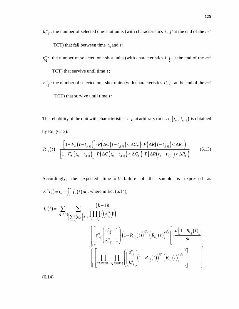
125

', '

m

i jk : the number of selected one-shot units (with characteristics ', 'i j at the end of the mth

TCT) that fail between time mt and t ;

,

m

i jr : the number of selected one-shot units (with characteristics ,i j at the end of the mth

TCT) that survive until time t ;

', '

m

i jr : the number of selected one-shot units (with characteristics ', 'i j at the end of the mth

TCT) that survive until time t ;

The reliability of the unit with characteristics ,i j at arbitrary time 1, m mt t t is obtained

by Eq. (6.13):

,

1

1

W F Fj j j j j j

i j

W m m F m Fj j j j j j

F t t P C t t C P R t t RR t

F t t P C t t C P R t t R

(6.13)

Accordingly, the expected time-to-kth-failure of the sample is expressed as

0

k m kE T t f t dt

, where in Eq. (6.14),

,

', ' ', '

', ' ,,

1

', ' ,

', ' , ,

', '

,

1 !

!

1 11

1

mi j

i j

m mi j i j

km

i j i ji j

k ki j

m

i j k r i jm

i j i j i jm

i j

i j

kf t

k

s d R ts R t R t

dtk

s

, ,

, ,

except ' except ',

1m mi j i j

m

k r

i j i jm

i i j ji j

R t R tk

(6.14)

126

When the units exhibit competing failure modes, then the sample’s time-to-kth-failure is

expected to occur earlier than that when the system exhibits a single failure mode.

6.3 Generalization of System Reliability Metrics Modeling

In this section, we generalize the scenario discussed in section 6.2 and investigate the

system reliability metrics when the units exhibit M failure modes without indictors and N

degradation modes. At the end of the mth TCT, the unit’s failure might be observed either

when any of the M failures occurs suddenly between the (m-1)th and the mth TCTs or when

any of the N degradation modes reaches its failure threshold. Similarly, the unit is repaired

either when any of the M failures occurs or when any of the N degradation modes reaches

its repair threshold. Under such circumstances, the system’s failure distribution can be

obtained by referring to Eq. (6.10); however, the probability that the unit has specific

characteristics ,i j and fails (survives) at the end of the mth TCT needs to be reinvestigated.

We define the following and calculate the ,

m

i jP k and ,

m

i jP r by referring to Eq. (6.14).

pR t : the unit’s reliability due to the pth failure mode (without an indicator) at time t,

1,2,...,p M ;

qR t : the level of the qth degradation mode at time t , 1,2,...,q N ;

F

qR : the failure threshold of the qth degradation mode;

127

R

qR : the repair threshold of the qth degradation mode;

q : a set of degradation modes (selected from the N degradation modes) which reach its

repair thresholds at the end of the TCTs in sequence j .

Appendix A shows the calculation of system reliability metrics.


In this section, we develop a simulation model to validate the proposed models in sections

6.2 and 6.3. For a comprehensive validation, we apply r replications and compare the

system reliability metrics (e.g., reliability, expected number of failures) obtained by the

proposed models and the simulation model in each replication. Each replication has one

set of randomly generated testing parameters (batch size, batch arrival time, test time and

temperatures). In one replication, the simulating procedure is repeated for 103 iterations.

The steps of simulating the number of failed units in the 1st batch (assuming 1 0w ) at the

end of the 1st (1

1k ) and 2nd (2 2 2 2

1 1 1,0 1,1, where k k k k ) TCTs in one iteration are illustrated

in the flow charts in Figures 6.1 and 6.2. We define the following notations:

, _

m

i j Wv : vector composed of random failure times at the mth TCT (with characteristics ,i j )

generated based on the Weibull distribution;

, _

m

i j Wv : the th element in vector , _

m

i j Wv ;

128

, _

m

i j GBSv : vector composed of random failure times (with characteristics ,i j ) generated

based on the GBS distribution;

, _

m

i j GBSv : the th element in vector , _

m

i j GBSv ;

, _

m

i j Resistorv : vector composed of random failure times (with characteristics ,i j ) generated

based on the resistance change model;

, _

m

i j Resistorv : the th element in vector , _

m

i j Resistorv .

Simulating random failures at time1t :

Figure 6.1 Steps of simulating the number of failures in the 1st batch after the 1st TCT

129

Simulating random failures at time2t :

130

Figure 6.2 Steps of simulating the number of failures in the 1st batch at

the end of the 2nd TCT

6.5 A Numerical Illustration

In this section, we numerically obtain the system reliability at arbitrary time t until the end

of the 3rd TCT, under competing failure modes.

131

Batches of one-shot units are produced and stored at times 1 2 30, 200 and 400w w w

with batch sizes 1 2 3 20n n n , respectively. TCTs are conducted at times

1 2 3100, 300 and 500t t t . In each temperature fluctuation cycle, the entire population

is subjected to temperature ( 350U

T K ) for 10UD s , and then cooled to a temperature

( 250L

T K ) for 20LD s , where ,L UD D are the dwell time in seconds at the lower and

upper temperatures, respectively. Units in the system might fail due to any of the following

reasons:

1. The sudden failure time is modeled by a Weibull distribution with CDF

1 expW

tF

where 450 and =2 ;

2. The probability of failure due to crack length C t reaching a predetermined

failure threshold FC due to the thermal stresses is modeled as:

F

F B B

U L F U L F

C t tP C t C

A T T C A T T C

,

where

40%FC , i.e., the crack length reaches 40% of the unit’s entire length;

132, 8 10 , -5, 0.5, 350 , 250U LA B T K T K ; and

132

3. The change of the resistance reaches a predetermined failure threshold FR with

the probability:

0

exp expUF Lm

m

U L U U L L

F

DR DE E

R t D D kT D D kTP R t R

where

5

0100 , 200 , 0.3eV, 8.62 1 V/ ; 0 e KFR R E k

0.5, 2, 0.02m

Repairs are conducted: 1) when the unit is observed to fail suddenly between two tests, or

2) when the repair threshold for the crack length 20%RC is reached, or 3) when the

repair threshold for the resistance change 40RR is reached. Defining the system as a

“k(t)-out-of-n(t): F” system with 25%k t n t , we plot the system reliability at

arbitrary time t until the end of the 3rd TCT in Figure 6.3. Besides the competing failure

modes, we also plot the system reliability under each failure mode independently to

identify the dominant failure/degradation mode that causes system’s failure.

133

Figure 6.3 System reliability until the 3rd TCT under different failure modes

It is observed that the “sudden” failure, characterized by the Weibull distribution, is the

dominant failure mode. However, when changes from 450 to 800 and A changes from

138 10 to 133 10 , the crack caused by the thermal fatigue becomes the dominant failure

mode, as plotted in Figure 6.4.

Figure 6.4 System reliability until the 3rd TCT under different failure modes

134

6.6 Conclusions

In this chapter, we propose efficient and effective approaches that model the reliability

metrics of systems subject to competing failure modes. The system has a mixture of

nonhomogeneous one-shot units that arrive at different times and subjected to sequential

TCTs. We develop and utilize statistics-based models and physics-statistics-based models

to characterize the failure/degradation modes. We state that more frequent NDT is required

to minimize the probability of system failure and validate that competing failure modes

result in worse system reliability than single failure mode. Moreover, the proposed models’

accuracy in estimating the system reliability metrics is validated by a simulation model.

135

CHAPTER 7

OPTIMAL SEQUENTIAL ALT PLANS

In many situations, it is difficult or impossible to obtain failure data under normal

conditions for highly reliable units. In such cases, accelerated life testing is applied by

subjecting the units to severer-than-normal stresses such that failures are induced in a much

shorter time. The accelerated data are utilized to estimate the units’ lifetime and other

reliability metrics under normal conditions by using ALT models. The accuracy of

reliability estimation depends on the ALT models that relate the failure data under

accelerated conditions to that under normal conditions and the design of the ALT plans.

Statistics-based models, physics-statistics-based models, and physics-experimental-based

models are typical types of ALT models which relate the failure data at accelerated

conditions to the normal conditions and predict the units’ reliability under normal stresses.

Statistics-based models utilize historical failure data but neglect the physics of the units’

failure mechanism, moreover, they do not apply to the situations when insufficient data are

available. Physics-based models are effective when the change in the unit’s physics (either

due to the unit’s material properties, or due to the unit’s working environments) is precisely

related to the reliability model parameters, however, it neglects the uncertainty during the

units’ failure processes. Physics-statistics-based models combine both the statistics-based

models and the physics-based models by predominately considering unit’s failures

mechanism as well as taking the uncertainty during the modeling process into account.

136

When selecting ALT models based on the units’ physics and statistical properties, an

optimal ALT plan is required to improve the accuracy and efficiency of the reliability

estimation. Specifically, an ALT plan optimizes a specific objective (usually specific

reliability metrics) meanwhile meets given constraints. An appropriate optimization

criterion for the ALT plan is important as it reflects the purpose of the ALT plan, ensures

the accelerated stress levels are within engineering range, as well as ensures that the

reliability estimation is accurate.

Usually, some or all of the types and levels of the applied stresses, the number of testing

units, the time to perform the test, and test duration need to be determined. These factors

are mainly decided by the functions that the units will be performing under normal

conditions. In this chapter, we design a sequence of accelerated NDTs plans, considering

the effect of population’s non-homogeneity. Only a sample is randomly selected and tested

in each test. The results show that a well-designed sequential accelerated NDT is an

effective approach for accurate reliability prediction with negligible effect on the residual

lives of the units and other system reliability metrics.

The accelerated NDTs plans are designed under the following two testing scenarios:

Testing scenario 1 (TS1): The NDTs (duration of the test is considered) are sequentially

performed under accelerated conditions at arbitrary time by

testing the selected samples, failed units are discarded;

137

Testing scenario 2 (TS2): The NDTs (duration of the test is considered) are repeatedly

performed under accelerated conditions at arbitrary time by

testing the selected samples, failed units are repaired and placed

back in the population with higher failure rates.

The remainder of this chapter is organized as follows: Section 7.1 investigates the lifetime

distribution of an individual unit in the system by developing a physics-statistics-based

model, which directly relates the applied stresses to system reliability metrics. In section

7.2, we design a sequence of accelerated NDTs plans by considering the population’s non-

homogeneity under TS1 and TS2. A numerical example is provided in section 7.3 to

demonstrate the design of the optimal sequential ALT plans. In section 7.4, we summarize

the conclusions of this chapter.

7.1 Power-Law Humidity Model

In chapter 3, we apply the general notations xF and xf to relate the system reliability

metrics to individual unit’s lifetime when calculating a specific system state’s probability

( , , , ,, ; ,m m m mi j i j i j i jP K k R r i j ). The specific form of unit’s lifetime model, which reflects

unit’s characteristics and applied stresses, is required. In this section, we develop a physics-

statistics-based model to analyze the individual unit’s lifetime, which relates the unit’s

lifetime under arbitrary environment to its working environment.

138

We consider the one-shot units that are affected by both temperature and humidity follow

a physics-based power-law model. The model relates the relative humidity (RH) and

temperature (T ) to the unit’s lifetime as shown in Eq. (7.1):

0 expn

B

QTF A RH

K T

(7.1)

Where TF is the time to failure; 0A is the process (material) dependent parameter and

serves to produce a distribution of the unit’s time-to-failure; RH and T are the relative

humidity and temperature, respectively; n is the power-law exponent; BK is the

Boltzmann constant and equals to5

8.62 10

andQ is the activation energy constant which

depends on the material.

The power-law humidity model determines the time to failure once the environmental

stresses and the unit’s specific property-dependent parameters are known. The parameters

of the model can follow specific probabilistic distributions due to the units’ production

processes variability, the variation of the unit’s material properties, and the environments

under which the units are tested. Without loss of generality, we assume that 0A follows

lognormal distribution with known mean and variance: 0 0

2

0 log ,A AA N u . Similarly,

the power-law exponent n is normally distributed with 2,n nn N u , which reflects the

uncertainty effect of RH on the unit’s reliability. Taking the logarithm of both sides of

Eq.(7.1), we obtain:

139

0 0

2 2 2ln ln , lnA n A n

B

QTF N u RH u RH

K T

, i.e. 2log ,TF N

where

0lnA n

B

Qu RH u

K T and

0

2 2 2lnA nRH

Specifically, the cdf and reliability of the units in the system are respectively:

1 1 ln

2 2 2

tF t erf

(7.2)

and

1 1 ln

2 2 2

tR t erf

(7.3)

Eqs. (7.2) and (7.3) are used in section 7.2 to design the optimal sequential accelerated

NDTs plans.

7.2 Optimal Sequential Accelerated NDTs Plans

There exists some circumstances that the reliability metrics of highly reliable units are not

attainable within a short testing period under working (normal) conditions. As an

140

alternative, conducting reliability tests under accelerated conditions yields acceptable

reliability metrics estimates in a shorter test duration. In this section, we design the optimal

sequential testing plans for a sequence of accelerated NDTs (including m NDTs, where m

could be an arbitrary value) with the objective of minimizing the difference between units’

reliability metrics estimates under normal and accelerated conditions while controlling the

testing duration within an acceptable level. In each accelerated NDT plan, we determine

the test duration as well as the applied stress levels; taking into account the effect of the

units’ nonhomogeneous and time-dependent characteristics and the previously conducted

accelerated NDTs. We design the optimal sequential testing plans based on the

sample’s/system’s reliability metrics under TS2 and TS3. At the end of this section, we

numerically illustrate how the first three accelerated NDTs are designed sequentially.

7.2.1 Mean Residual Life (MRL), Scenarios and Notations

When a unit has the lognormal lifetime distribution as given in Eq.(8), its MRL at time t

can be derived as the function of: time t , number of its prior repairs x, applied stresses Z

( RH andT ), and the material-dependent parameters (0

A and n):

2 22

2ln

1

ln1

te

MRL t tt

(7.4)

where

141

0

lnA n

B

Qx RH x

K T and

0

22 2lnA nRH

We formulate the optimization problem with the following statements:

a. In each accelerated NDT, sq ( 0 1

sq ) of the entire population are selected and

tested; the “stratified sampling” approach (samples are selected proportionally

according to the units’ characteristics) is adopted such that the sample represents the

population’s characteristics;

b. Samples are placed back into the population after the accelerated NDTs;

c. The applied stresses (temperature and relative humidity) and the test duration need to

be determined in each accelerated NDT;

d. The unit has a lifetime that follows the log-normal distribution and the MRL(t) as given

in Eq. (7.4).

We use the subscripts A and N to refer to reliability metrics associated with the accelerated

and normal NDTs, respectively. The yth accelerated NDT plan is affected by the previously

designed (y-1) NDT plans. The following notations are applicable for the problems

formulated under TS2 and TS3:

:yt time when the yth accelerated NDT starts, 1,2,...,y m ;

y : duration of the yth accelerated NDT;

,y y

U L : upper and lower bounds of the yth accelerated NDT duration;

142

yZ : the applied stresses (relative humidity yRH and temperature yT ) levels in the yth

accelerated NDT;

y

NZ : the applied stresses levels under normal operating conditions;

y

UZ : the upper bounds of the applied stresses levels in the yth accelerated NDT;

yN : the system state at yt , which is a combination of units with different characteristics

in the system, specifically, y yN n where

yn is a specific system state;

yS : the sample state at yt , which is a combination of units with different characteristics

in the sample, specifically, y yS s where

ys is a specific sample state;

; , , ; , , ; , , ; , :y y y y y y y y y y y y y

A A A AP K k Z TMRL s Z R Z E Z the

probability of having yk failed units, expected total mean residual life (TMRL) of the units

in the sample (with sample stateys ), the system reliability, and the expected number of

failed units at the end of the yth accelerated NDT, with applied stresses ,y y yZ RH T and

test duration y , respectively;

; , , ; , , ; , , ; ,y y y y y y y y y y y y y

N N N N N N N NP K k Z TMRL s Z R Z E Z : the

probability of having yk failed units, expected total mean residual life (TMRL) of the units

in the sample (with sample stateys ), the system reliability, and the expected number of

failed units at the end of the yth normal NDT, with normal stresses ,y y y

N N NZ RH T and test

duration y , respectively;

1

yq : the ratio of the sample’s expected TMRL after the yth accelerated and normal NDT;

2

yq : the ratio of the system reliability after the yth accelerated and normal NDT;

143

3

yq : the ratio of the expected number of failed units after the yth accelerated and normal

NDT;

7.2.2 Optimization of Sequential Accelerated NDTs under TS1

We first design the optimal sequential ALTs under TS1, i.e., at the end of each accelerated

NDT, the sample is placed back into the system without repairs. Under such circumstance,

the units in the system have different reliability characteristics due to their different arrival

times and accelerated NDT sequences under which they are tested. The following

additional notations are necessary for the optimization problem under TS1:

,

y

iN : at time yt , the number of units from the ith batch which are subjected to accelerated

NDT sequence . Specifically, under TS1, ,

y

i in n i always holds, where ,

y

in

ranges from 0 to in ;

,

y

iS : the number of testing units selected from ,

y

iN at yt , specifically, , , , , y y

i iS = s i .

Note that , , , y y

i is n i and , ,

, ,

y y

i s i

i i

S = q % N

always holds;

# : the number of elements/NDTs in NDT sequence , i.e., the number of accelerated

NDTs the ,

y

iN units subject to;

144

, ,

, ,

y A y N

i iK K : the number of failed units out of ,

y

iN at the end of the yth accelerated (normal)

NDT;

, ,

, ,

y A y N

i iR R : the number of survived units out of ,

y

iN at the end of the yth accelerated

(normal) NDT;

, ,; , ; ,y y y y y y

A i N i NMRL S Z MRL S Z : mean residual life of any of the ,

y

iS units at the

end of the yth accelerated (normal) NDT;

, ,; , ; ,y y y y y y

A i N i Nt S Z t S Z : “true” age of any of the ,

y

iS units at the end of the yth

accelerated (normal) NDT;

, ,; , ; ,y y y y y y

A i N i NR S Z R S Z : reliability of any of the ,

y

iS units at its true age

, ,; , ; ,y y y y y y

A i N i Nt S Z t S Z ;

: sum of test durations of all NDTs in sequence ;

and Z : accelerated stresses under all NDTs in NDT sequence ;

, ; , : y y y y

iS Z “equivalent” test duration of the yth accelerated NDT for any of the ,

y

iS

units;

, ; , :

y

iS Z sum of “equivalent” test durations of all accelerated NDTs in sequence

(in which the ,

y

iS units are tested) for any of the ,

y

iS units;

xf : pdf of the units’ lifetime distribution (lognormal) after its xth repair in Eq. (7.1);

145

The optimal testing plans for the first m accelerated NDTs are obtained successively by

first solving for 1 1

1, , and Z t in the first accelerated NDT; then optimal decision is found

for the second accelerated NDT. Generally, the yth accelerated NDT plan is affected by

previous (y-1) NDTs plans and the system state at time yt . We investigate the procedure of

optimizing the yth accelerated NDT, where 1,...,y m . Specifically, the applied stresses

(temperature and relative humidity) in the yth test, the time to conduct the yth test, and the

yth test duration are determined by optimizing the following problem:

Min

0

; , ; ,

ii

y

y y y y y y y y

A N N

n

k

P K k Z P K k Z

(7.5)

Subject to

y y y

N UZ Z Z (7.6)

and y y y y

U L y Ut t t y i (7.7)

1; , ; ,y y y y y y y y y y y

A N Ny ys s

P S s TMRL s Z q P S s TMRL s Z

(7.8)

2; , ; ,y y

N

y y y y y

A NE Z E Zq (7.9)

3; , ; ,y y y y y y y

A N NR Z q R Z (7.10)

Max ; , Max ; ,y y y y y y y y

A N Nk P K k Z k P K k Z (7.11)

146

To minimize the effect of acceleration on the system reliability metrics, we minimize the

sum of the difference between the failure distributions at the end of the yth accelerated NDT

and normal NDT (Eq. (7.5)). Constraint (7.6) ensures that applied stresses’ levels are

higher-than-normal and lower than specified thresholds such that failure modes remain

unchanged. The test duration of the accelerated NDT should not exceed its upper bound

and the test should be performed within certain time intervals (Eq. (7.7)). We require the

total expected mean residual life (TMRL) of the units in the sample at the end of the yth

accelerated NDT equals to or longer than 1

yq of total expected mean residual life after the

yth normal NDT (constraint (7.8)). According to constraint (7.9), the system’s expected

number of failures after the yth accelerated NDT should not be less than 2

yq of that after the

yth normal NDT. Similarly, the difference between system reliability after the yth

accelerated NDT and the yth normal NDT is less than 3

yq according to constraint (7.10). In

constraint (7.11), the peaks (maxima) of the number of failures distributions after the yth

accelerated and normal NDT are the same. This optimization problem can be solved by

using nonlinear optimization programming.

Assumingy yS s , i.e.,

, ,,y y

i iS s i

, the TMRLs of the units in the sample equals to:

, ,

,

; , ; ,y y y y y y y

A i A i

iA

TMRL s Z s MRL s Z

(7.12)

Term A in Eq. (7.12) (the MRL of any of the ,

y

is units at the end of the yth accelerated NDT)

is obtained as:

147

, ,

,, ; ,

1; , ; ,

; ,

y y y y y y

A i A iy y y

A iA

y y yA it s Z

MRL s Z f d t s ZR s Z

(7.13)

Term A in Eq. (7.13) is obtained as shown in Eq. (7.14) by reducing the sum of all

accelerated NDTs’ durations in sequence (term A in Eq. (7.14)), and adding the sum of

their corresponding “equivalent” test durations (term B and C in Eq. (7.14)):

, , ,; , ; , ; ,y y y y y y y

A i y i i i

AB C

t s Z t w s Z s Z

(7.14)

Term B in Eq. (7.14) can be obtained by letting the reliability of any of the ,

y

is units at yt

(if all NDTs in sequence are accelerated) equals to the reliability of any of the ,

y

is units

at its true age (if all NDTs in sequence are under normal conditions):

1 1 ,; , NDT in ; , ; , , NDT in y

y i y i i N NR t w Z R t w s Z Z

(7.15)

Similarly, the equivalent duration of the yth NDT for any of the ,

y

is units is obtained as:

, ,; , ; ,

; , , ,; , , , ,

y y y y y

y i i iy y y

y iy y

N N N

t w s Z s ZR t w Z Z R

Z Z

(7.16)

148

Then , ; , y y y

A iR s Z is obtained. The MRL of any of the ,

y

is units at the end of the yth

accelerated NDT is accordingly obtained.

Terms B and C in Eq. (7.14) reflect the effect of applied stresses on the units’ reliability

metrics as described in Eq. (7.2). The expected TMRL of the sample at the end of the yth

normal NDT can be calculated by following the same steps in Eqs.(7.12)-(7.14), only

replacing term C in Eq. (7.14) withy .

Eqs. (7.12)-(7.14) obtain the sample’s TMRL under a specific sample stateys . Obviously,

there exists many potential sample states at yt and the probability of having a specific

sample state ( y yP S s ) needs to be investigated. Under TS1, y yP S s is obtained

by applying the law of total probability. Specifically, for arbitraryys we consider all

possible system states (, ,, i.e., , y y y y

i iN n N n i ) that yieldys . Term A in Eq. (7.17))

uses a hypergeometric distribution to obtain all possible ys under system state

yn . All

possible system states that yield ys are considered and the conditional probabilities (term

B) are summed as:

149

, , , , , , , , ,

y

y y y y y y y y

BA

y y y y y y

i i i i i i

BA

n

P S s P S s N n P N n

P S s i N n i P N n i

,

,

, ,

,

,

,

,

,

%

y

i

yi i y y

i i

iB

i

s i

i

A

yi

yi

n i

n i

n

sP N n i

n

q n (7.17)

A specific system state is realized with the probability shown in Eq. (7.18), where the

numerator is the probability of having a specified system state and the denominator is the

sum of all potential system states’ probabilities. All potential system states are obtained by

solving Eqs. (7.19)-(7.21).

,

,

, ,

# #

,

#

#,

, , , satisfy

,

!1

!

!

! 1

yi

i

yi

i

y y y y

i i

ny-zi

s syi i

n

si

y y-zi i s

y yi iN n i

P N n = P N n i

nq - q

n

qn

n - q

ing Eqs.(7.19-7.21)

(7.18)

Assuming that in each accelerated NDT, any unit is equally selected and tested with

probability sq , the following equations always hold:

150

,

y

i iN = n i (7.19)

, 1

; including

;

i z

y

i i s i i

i w ti z

N n q z = z ,z ,..., y z represents the zth test (7.20)

, 0 , y

iN i (7.21)

In Eq. (7.19), the sum of number of units with different characteristics in the ith batch equals

to the ith batch’s size. Eq. (7.20) guarantees that in each accelerated NDT， sq units of the

total population are selected and tested. Moreover, ,

y

iN should be non-negative (constraint

(7.21)). To illustrate, assuming there are two batches in the system when the third NDT

starts ( 3t ), where the 1st batch arrives before the first NDT and the 2nd batch arrives between

the 1st and 2nd NDT, we obtain the number of all possible system states at 3t by solving

the following set of equations:

3 3 3 3

1,12 1,1 1,2 1,0 1

3 3

2,2 2,0 2

3 3

1,12 1,1 1

3 3 3

1,12 1,2 2,2 1 2

3 3 3 3 3 3

1,12 1,1 1,2 1,0 2,2 2,0, , , , , 0

s

s

N N N N n

N N n

N N q n

N N N q n n

N N N N N N

151

Distribution of failed units at the end of the yth accelerated NDT ( ; ,y y y y

AP K = k Z ) can

be obtained using Eq. (7.22) by enumerating all possible system states which satisfy

,

,

,

y A y

i

i

K = k

and summing their probabilities.

,,

,,

,

,

,

,

,

,

,,

,

; ,

; ,

!

; ,!

; ,

y Ai

y Ai

y y y y

A

y A y y y

A i

i

y

i

y A

i

ik

y y yyi A ii

ry y y

A i

P K k Z

P K k Z

n

kn

F t s Zn

R t s Z

, ,, ,

, ,

-

y A y Ay y

ii ii i i

k k r n k

(7.22)

Similarly, the distribution of failed units at the end of the yth normal NDT is obtained in

Eq. (7.23):

152

,,

,

,

,

,

,

,,

,

,,

,

; ,

; ,

!

; ,!

; ,

y Ni

y y y y

N N

y N y y y

N i N

y

i

y N

i

i

y y yyN i Ni

y y y

N i N

y Ni

i

k

i

r

P K k Z

P K k Z

n

kn

F t s Zn

R t s Z

, ,, ,

, ,

-

y N y Ny y

ii ii i i

k k r n k

(7.23)

Accordingly, the expected number of failed units and the system reliability at the end of

the yth accelerated (normal) NDT can be obtained. The optimization problem is flexible

and can be generalized to consider different scenarios.

7.2.3 Optimization of Sequential Accelerated NDTs Plans under TS2

We now design a sequence of optimal accelerated NDTs plans under TS2, where failed

units are repaired and placed back in storage. The following notations are necessary:

1 1

, ,

y y

i j i jK R : number of failed (survived) units in the system at the end of the (y-1)th

accelerated test, the 1 1

, ,

y y

i j i jK R units are from the ith batch and observed to

fail j times (which are observed at test sequence j ) until 1yt , j is composed

153

of arbitrary j NDTs/elements that are selected from the NDT sequence

and is the NDT sequence in which the units are tested.

1 1

, ,

y y

i j i jSK SR : the number of units selected from the 1 1

, ,

y y

i j i jK R units that are tested at yt ;

under TS2, a certain yS is determined by the values of

1 1 1

, , , and , ,y y y

i j i j i jSK SR R i j

, specifically, 1 1

, ,

y y

i j i jSK sk and

1 1

, , , ,y y

i j i jSR sr i j

1 1

, ,; , ; ,y y y y y y

A Ai j i jMRL SK Z MRL SR Z

: MRL of any of the 1 1

, ,

y y

i j i jSK SR units at

the end of the yth accelerated NDT;

1 1

, ,; , ; ,

y y y y y y

N Ni j i jMRL SK Z MRL SR Z : MRL of any of the 1 1

, ,

y y

i j i jSK SR units at

the end of the yth normal NDT;

1 1

, ,; , ; ,

y y y y y y

A Ai j i jt SK Z t SR Z : true age of any of the 1 1

, ,

y y

i j i jSK SR units at the end

of the yth accelerated NDT;

1 1

, ,; , ; ,

y y y y y y

N Ni j i jt SK Z t SR Z : true age of any of the 1 1

, ,

y y

i j i jSK SR units at the

end of the yth normal NDT;

1 1

, ,; , ; ,

y y y y y y

A Ai j i jR SK Z R SR Z : reliability of any of the 1 1

, ,

y y

i j i jSK SR units at its

true age

1 1

, , , ,; , ; ,

j j

y y y y y y

A Ai j l i j lt SK Z t SR Z ;

154

1 1

, ,; , ; ,

y y y y y y

N Ni j i jR SK Z R SR Z : reliability of any of the 1 1

, ,

y y

i j i jSK SR units at its

true age 1 1

, ,; , ; ,

y y y y y y

A Ai j i jt SK Z t SR Z ;

1 1

, ,; , ; ,

y y y y y y y y

A Ai j i jSK Z SR Z : equivalent test duration of the yth accelerated NDT

for any of the 1 1

, ,

y y

i j i jSK SR units;

jj

: duration of the th

j j NDT.

Under TS2, units in the system have different arrival times, testing sequences , and failing

sequences j . With the same objective and constraints as shown in Eqs. (7.5)-(7.11), the

sample’s TMRL with sample state y yS s (i.e., 1 1 1 1

, , , ,, ; , ,y y y y

i j i j i j i jSK sk SR sr i j

)

is calculated as:

1 1 1 1

, , , ,, ,

( ) ; , ; ,; ,

y y y y

A A A

y y y y y y y

i j i j i j i ji j

TMRL sk MRL SK Z sr MRL SR Zs Z (7.24)

When the yth accelerated NDT starts, unit that fails in the (y-1)th accelerated NDT has a

lifetime 1

1

y

y yt t

as it is repaired at the end of the (y-1)th test. Unit that survives in the

(y-1)th NDT has a lifetime

j

y j

j

jt t since its latest failure is observed at the end of

the j j th NDT. MRLs of units with different characteristics can be obtained. Specifically,

155

MRL of any of the 1

, y

i jsk units at the end of the yth accelerated NDT is obtained in Eq.

(7.25):

1

,; ,

1 1

, ,1

,

1; , ; ,

; , y y yA i j

y y j y y

A Ay y

t sk ZAA

y y

i j i jy

i j

MRL sk Z f d t sk ZR sk Z

(7.25)

Similarly, MRL of any of the 1

, y

i jsr units at the end of the yth accelerated NDT is obtained

by Eq. (7.26):

1

,; ,

1 1

, ,1

,

1; , ; ,

; ,

y y yA i j

y y j y y

A Ay y

t sr ZAA

y y

i j i jy

i j

MRL sr Z f d t sr ZR sr Z

(7.26)

Replacing the subscript A with N, we have the MRL of any of the 1

, y

i jsk ( 1

, y

i jsr ) units at

the end of the yth normal NDT:

1

,; ,

1 1

, ,1

,

1; , ; ,

; ,

y y yN Ni j

y y j y y

N N N Ny y

t sk ZN NA

y y

i j i jy

i j

MRL sk Z f d t sk ZR sk Z

(7.27)

and

1

,; ,

1 1

, ,1

,

1; , ; ,

; ,

y y yN Ni j

y y j y y

N N N Ny y

t sr ZN NA

y y

i j i jy

i j

MRL sr Z f d t sr ZR sr Z

(7.28)

156

Terms A in Eqs. (7.25)-(7.28) (true age of any of the 1

, y

i jsk ( 1

, y

i jsr ) at the end of the yth

accelerated (normal) NDT) are respectively obtained as:

1

1

1 1

, ,; ,

y y y y

A y A y

A

y y

i j i jt sk Z t sk t (7.29)

1 1 1

, , ,; , ; , ; ,

j j j j j j j j j j j jy y y

A y N N

A B

y y y

i j i j i jt sr Z t sr Z sr Z (7.30)

1 1

1,; ,y y y y y

N y yi jt sk Z t t

(7.31)

1 1

, ,; , ; ,

j j j j j j j jy y y y y

N N y Ni j i jt sr Z t sr Z (7.32)

Specifically, 1

, y y

A i jsk in Eq. (7.29) is calculated by letting:

1 1 1

1 1,; , ; ,

y y y y y y y y y

y y y A y Ni jR t t Z R t sk t Z (7.33)

Terms A and B in Eq. (7.30) can be obtained similarly.

Under TS2, the probability of yielding a specific sample stateys at time yt is calculated by

considering all possible system states 1yN at time 1yt as shown in Eq. (7.34):

157

1

1 1 1 1

1 1 1 1

, , , ,

1 1 1 1

, , , ,,

and , ,

and , ,

y

y y y y y y y y

y y y y

i j i j i j i j

y y y y

i j i j i j i ji j

nA

k

P S s P S s N n P N n

SK sk SR sr i j

P

K k R r i j

1 1 1 1

, , , ,

1

,

1 1,

and , ,

and

, ,

y y y y

i j i j i j i j

y

i j

y yi j

A

r i j

K k R rP

i j

k

sk

1

,

1 1

, ,

1 1

, ,

1 1, ,

and , ,

y

i j

y y

i j i j

i

i

s i

i

y y

i j i j

y yi j i j

i j

k r i j

r

sr

n

q n

P K k

1 1

, , and , ,y y

i j i jR r i j

(7.34)

Term A in Eq. (7.34) (units’ states (fail or survive) when the (y-1)th NDT ends) is obtained

by Eq. (7.35). It is affected by the characteristics of the units that are tested in previous (y-

1) NDTs (term B in Eq. (7.35)), which has been investigated by Eq. (7.18).

Details of term A in Eq. (7.34) (the units’ states (fail or survive) when the (y-1)th NDT ends,

conditional on term B) can be obtained by referring to the models in chapter 3, where the

failure probabilities of units with different characteristics are determined by their “true”

ages.

158

1 1, ,

1 1 1 1

, , , ,

1 11 1, ,

,

,

and , ,

,

y yi i

y y y y

i j i j i j i j

y yy yi i

NA

i

n i

K k R r i jP

N n iP N n

P N 1 1

, , y y

in i

(7.35)

The distribution of failed units at the end of the yth accelerated NDT ; ,y y y y

AP K = k Z

is obtained based on Eq. (7.34) by replacing 1y with y , then all y yP N n satisfying

,, ,

y y

i ji j

K k are summed. The expected number of failed units ; ,y y

AE Z and the

system reliability ; ,y y

AR Z are obtained accordingly.

Different scenarios can be developed based on TS2. For example, failed units are either

repaired to as-good-as new or to as-good-as old. Meanwhile, failed units are either repaired

and placed back in storage, or discarded after a specified number of failures.


In this section, we numerically design the optimal testing plans for the first three

accelerated NDTs under TS2 and TS3, respectively. We describe how the sequential

accelerated NDTs are conducted as well as the procedure of designing the sequential

optimal testing plans as follows:

159

Three batches of one-shot units arrive into storage at times 1 2 30, 300, 600w w w ,

respectively; the three batch sizes are 1 2 3100, 100, 100n n n , respectively.

The unit’s lifetime T follows lognormal distribution, specifically, 2log ,T N ;

where

0

lnA n

B

QRH

K T ;

010 0 001 0 00012 0 5 V e

A NQx x. . .; ; ; and

58 26 10 B

K .

0

2 2 2lnA nRH

02 A and 0 01

n. ;

The 1st, 2nd, and the 3rd accelerated NDT are conducted at times

1 2 3150 450 and 750t t t , ; the test durations are respectively 1 2 3, and (need to

be determined). In each NDT, 20% of the population is selected and tested

(1 2 3 20 s s s

q q q % ); i.e., 20, 40, and 60 units are tested under the first three NDTs,

respectively. The upper bound of each test duration is 100U ; meanwhile, the

following requirement needs to be satisfied when designing 1 2 3, and :

1 1 2 2 2 2 3 3 3 3, , Ut w w t w w t t ; 850Ut .

The temperature and the relative humidity in each of the three tests need to be

determined ( 1 2 3y yRH T y, ; , , ); the lower and upper bounds of the relative humidity

and temperature are: 0.7, 0.3, 373 , 293 y y y y

U N U NRH RH T K T K ;

The system is operational if no more than 20% of the entire population fail;

160

The ratio of the testing sample’s MRLs after the 1st, 2nd, and 3rd accelerated and normal

NDT needs to be respectively greater than 0 9 0 9 and 0.9. , . , (and less than 1 1 and 1, );

The ratio of the system reliability after the 1st, 2nd, and 3rd accelerated and normal NDT

needs to be respectively greater than 0 9 0 9 and 0.9. , . , (and less than 1 1 and 1, , );

The ratio of the expected number of failed units after the 1st, 2nd, and 3rd accelerated

and normal NDT needs to be respectively greater than1 15 1 15 and 1 15. , . . .

Under each testing scenario, we first determine the optimal testing plan for the 1st NDT;

accordingly, the equivalent test duration of the 1st accelerated NDT for units with different

characteristics, the system/sample reliability metrics are calculated and considered in the

design of the optimal testing plan for the 2nd accelerated NDT; followed by the 3rd

accelerated NDT.

We obtain the optimal testing plans for the first three accelerated NDTs under TS2 and

TS3 in Tables 7.1 and 7.2. In Table 7.3, we quantify the differences between the accelerated

and normal NDTs by calculating the objective values of the optimization problem

(differences between the distributions of failed units after the first three accelerated and

normal NDTs) under TS2 and TS3.

We observe that TS2 and TS3 yield the same optimal testing plan for the 1st accelerated

NDT, as no repair is conducted when designing the 1st NDT; besides, the distributions of

failed units after accelerated and normal NDTs are approximately the same as the

161

differences between the distributions of failed units after the accelerated and normal NDTs

for 1,2,3y are negligible as shown in Table 7.3.

As required, the ratios of the system reliability after the accelerated and normal tests as

well as the ratios of the sample’s TMRL after the accelerated and normal tests

approximately equal to 1 ( 1 20 9 0 9; 1 2 3 y yq q y. , . , , ); which implies that the optimal

accelerated NDTs have negligible effect on the system reliability metrics within a short test

duration. Furthermore, as the sample represents the population characteristics, y

sq does not

affect the yth optimal testing plan as the sampling error does not exist.

Table 7.1 Optimal testing plans for the first three accelerated NDTs under TS2

1st NDT 2nd NDT 3rd NDT

yRH

0.41 0.34 0.34

yT

294 300 300

y

13 34 57

Table 7.2 Optimal testing plans for the first three accelerated NDTs under TS3


yRH

0.41 0.44 0.39

yT

294 294 297

y

13 23 35

162

Table 7.3 Objective function values after the first three accelerated and normal NDTs

under TS2 and TS3


TS2 1.53e-5 6.98e-4 2.68e-3

TS3 1.53e-5 2.71e-5 1.62e-3

7.4 Conclusions

In this chapter, we study the individual unit’s reliability behavior by developing a statistics-

physics-based model, which directly relates the applied stresses to the system reliability

metrics. We then propose the optimal design of a sequence of accelerated NDTs on the

system level, taking system’s/sample’s reliability metrics under different testing scenarios

into account. The uncertainty during the sampling procedure as well as the units’ different

time-dependent characteristics are considered. We show that the accelerated NDTs have

insignificant effect on the system reliability metrics while reducing the test durations.

163

CHAPTER 8

OPTIMAL DESIGN OF HYBRID SEQUENTIAL TESTING PLANS

NDT is conducted to determine the functionality of the units without permanent damage.

It is also used to estimate the units’ reliability. However, it is difficult to make decisions

regarding system’s reliability by completely using the results of the NDT since the total

functionality of the units are not fully tested. In contrast, destructive test (DT) is conducted

to observe the failure times of the units. This results in a more accurate estimation of the

units’ reliability. However, after the DT, testing units are destroyed. This amplifies the

need to investigate the hybrid reliability testing which utilizes the advantages of both the

NDT and DT. In this chapter, we assume the units selected from the system are subjected

to a sequence of hybrid reliability testing. It is of great interest to optimally design the

hybrid sequential reliability testing which results in more accurate reliability estimation

and minimizes the number of units subjected to DT based on sampling. After conducting a

number of hybrid testing, we decrease the sample size of the DT as the accuracy of

reliability metrics estimation improves. Eventually, we conduct NDT only. We investigate

the problem under four testing scenarios. The proposed methods are validated through

numerical illustrations and extensive simulation studies.

This chapter is organized as follows: in sections 8.1 and 8.2, we design the optimal

sequential hybrid reliability testing plans. We formulate the optimization problem, update

the unit’s lifetime parameter based on the testing results and improve the accuracy of

164

system reliability prediction. We assume that NDT and DT are performed on two separate

samples in each hybrid test in section 8.1. In section 8.2, we assume that each hybrid test

is performed on the same sample (three testing scenarios are assumed and investigated in

details). In section 8.3, we develop extensive simulation studies to validate the optimization

problems and methods. In section 8.4, we provide a numerical example to illustrate the

proposed methods.

8.1 Optimal Sequential Hybrid Reliability Testing Plans based on Two Separated

Samples

One-shot units are produced in batches and kept in storage until placed into actual use.

Specifically, the ith batch of units with size in arrives into the storage at time iw

immediately after production. A sequence of hybrid reliability tests are conducted at

arbitrary time during the entire life horizon of the units by testing selected samples.

Specifically, in each hybrid reliability test NDT and DT are performed simultaneously on

two selected samples. The yth hybrid reliability test is performed at time yt . The reliability

tests are assumed to be instantaneous (duration of the test is ignored). Units subjected to

the DTs are removed from the system after the tests. Units that fail in the NDT are repaired

and placed back into the system. The units in the storage are subjected to different series

of hybrid reliability tests and thus have different characteristics. The system is referred to

a generalized “k-out-of-n: F” system.

165

We assume the lifetime of the units in the system follows exponential distribution. The

following are necessary notations:

:x xF f cdf (pdf) of the unit lifetime after the xth repair;

:yt time when the yth hybrid test is performed, 1,2,...,y m ;

:y

in number of units in the ith batch when the yth test starts;

:yN total number of units in the system at time yt ;

: sequence of NDTs that the testing units are subjected to;

# : number of NDTs in sequence ;

1;

y

i yM : number of expected failures of a unit (in the ith batch) until time yt based on

1y , the unit is subjected to NDT sequence ;

1; :y yp failure probability of the unit in the system at time yt based on 1y ;

:R threshold of the difference between the reliability estimate of the system and the

reliability estimation of the sample;

y y

N Ds s : number of testing units assigned to the yth NDT (DT);

:y y

N DK K number of units failed in the yth NDT (DT), respectively; ;y y y y

N N D DK k K k

= 0,1,..., y y

N Nk s ( 0,1,..., )y y

D Dk s ;

166

%:Nq percentage of units assigned to the yth NDT, %Nq is constant y ; specifically,

%y

N N ys q N ;

%q : the system fails if %q or more units fail;

:y unit’s updated lifetime parameter after the yth hybrid test; the initial value of the

parameter is recorded as ;

:true the true value of unit’s lifetime parameter;

:L Ut t lower and upper bounds of the time interval between two reliability tests;

y y

N Dk k : the sample assigned to the yth NDT (DT) is considered to fail if y y

N Dk k or more

units fail.

In section 8.1, two samples are selected in each hybrid test. One sample is for the NDT and

the other is for the DT. The following two factors significantly affect the testing results and

the accuracy of system reliability estimation:

1. Time when the yth hybrid test is performed ( yt );

2. The number of units in the samples of the yth NDT and DT, respectively ( and y y

N Ds s ).

The design of the yth test is affected by the previous (y-1) tests and the system state at time

yt . Specifically, the optimal solutions for the first m tests are obtained by first obtaining

167

1 1

1, and N Dt s s in the 1st test. Based on 1 1

1, , N Dt s s and the first test’s results, the units’ lifetime

parameter is updated from to 1 . An optimal testing design is then found for the second

hybrid test and the units’ lifetime parameter is updated from 1 to

2 . A sequence of

optimal hybrid testing can be determined by applying the above procedures. In the

following, we describe the steps when optimizing the yth hybrid test, where 1,...,y m .

Step 1: Determine the optimal time to start the yth test and the number of testing units

assigned to the yth NDT and DT. Note that the optimization of the test plan is

affected by 1y , which is updated based on the results of previous (y-1) tests;

Specifically, the time to start the yth hybrid reliability test and the number of units assigned

to the yth test ( , , and y y

y N Dt s s ) are determined by solving the following optimization

problem:

Min y

Ds (8.1)

Subject to

1L y y Ut t t t (8.2)

%y

N N ys q N (8.3)

168

1 1-out-of- ; , % -out-of- ; ,y y y y

sample D D y y system y y y yR k s t R q N N t R (8.4)

where

1

1; i y

y

y i D

i w t

N n s

(8.5)

The objective (Eq. (8.1)) is to minimize the number of units assigned to the yth DT. There

exist an upper and a lower bound for the time interval between two hybrid tests (Eq. (8.2)).

Note that for 1y , Eq. (8.2) is written as: 1 Ut t .

In the yth hybrid test, we randomly select %Nq of the units in the system to perform NDT

(Eq. (8.3). It is required that the difference between the reliability estimation of the system

and the sample should not be greater than a predetermined threshold such that the sample

represents the population’s characteristics in the yth DT (Eq. (8.4)). The total number of

units in the system equals to the total number of arrived units in the system minus the total

number of units assigned to the previous 1y DTs (Eq. (8.5)). The reliability of the

system is defined in Eq. (8.6):

1

%

0

% -out-of- ; , y y y

system y y y y

y

y

q N

k

R q N N t P K k

(8.6)

169

Similarly, the reliability of the sample subjected to the yth DT is obtained using Eq. (8.7)

as:

1

0

-out-of- ; ,

yD

yD

y y y y

D D y y D D

kysample

k

R k s t P K k

(8.7)

The failure distributions corresponding to Eqs. (8.6) and (8.7) are obtained by applying the

models proposed in section 3.2. Moreover, an alternative approach to approximately obtain

the failure distributions is using the binomial distribution. Specifically:

1 1; 1 ;yy

yyy y

y y y yy

N kkNP K k p p

k

(8.8)

1 1; 1 ;y yyD DD

y

Dy y

D D y y y yy

D

s kksP K k p p

k

(8.9)

The system’s failure probability 1;y yp is obtained by applying the renewal process.

Specifically:

# #

1 1

;

1; % 1 % ;i

i y

y zy y

y y i N N i y

i w ty

p n q q MN

(8.10)

The number of units in the ith batch when the yth test starts is obtained by solving Eq. (8.11)

recursively. We specifically have1

i in n .

170

1 11

1

y yy y D ii i

y

s nn n

N

(8.11)

The number of expected number of failures that one unit (from the ith batch) experiences

until time yt , which is tested in NDT sequence , is found by applying the RP in Eq.

(8.12):

1

1

1 +1, 1

0

: 1

1 1

1

; 1 ;

1 ;

i

i

ii

i

i

iz +i

iz +a+

z +a

y

i y z y y

m-z -

z +a+ , y y

α=

t -w

t -w

t -w

M = + M t f t dt

+ I + M t f t dt

(8.12)

where

1 if 1 0 if 1

i

i

z < m -I =

z = m -

1

+

1

1

+a

+a-

,m a,m

t -tm-

α= t -t

M t + M t f t dt

and 0m, mM t = i

Step 2: Perform the yth hybrid test and obtain the number of failed units in the yth NDT and

DT. Update the parameter of the unit’s lifetime from 1y to y based on the results

of the test;

171

Intuitively, we expect y y

N D

y y

N D

k k

s s since DT fully performs the testing units’ functionalities.

All potential failures are detected in the DT. The number of failed units in the yth NDT is

obtained as:

1 1ˆ 0

ˆ ˆ; ;

yN

yN

s

y y y y y

N N y N N y N

k

k E K P K k k

(8.13)

where

ˆˆ

1 1 1ˆ ; ; 1 ;

ˆ

y yyN NN

ys kkNy y

N N y y y y yy

N

sP K k p p

k

Utilizing the results of the yth NDT and DT, we update the unit’s lifetime parameter from

1y to y using Eqs. (8.14)-(8.17):

ˆ 0

ˆ ˆ;;

yN

yN

s

y y y

N N y Nyy yN y kN D

y y y y

N D N N

P K k kE Kk k

s s s s

(8.14)

where

ˆˆ

ˆ ; ; 1 ;ˆ

y yyN NN

ys kkNy y

N N y y y y yy

N

sP K k p p

k

(8.15)

# #

;

1; % 1 % ;

i

i y

y zy y

y y i N N i y

i w ty

p n q q MN

(8.16)

172

1 1: 1

1, 1

10

;

1 ; 1 ;

i

ii

i i

i

i iz + z +a+i

z +a

y

i y

m-z -

z y y z +a+ , y y

α=

t -w t -w

t -w

M

= + M t f t dt + I + M t f t dt

(8.17)

Assuming the units have an exponentially distributed lifetime distribution, the term

; yf t in Eq. (8.17) is ; yt

y yf t e

.

Step 3: Determine the optimal time to start the (y+1)th test and the number of testing units

assigned to the (y+1)th test. The optimal testing plan is based on y .

Based on the unit’s updated lifetime parameter y , the optimal 1 1

1, and y y

y N Dt s s

are

determined by solving the same optimization problem formulated in step 1. The units’

lifetime parameter is then updated from y to 1y based on the (y+1)th test’s results.

The accuracy of the system reliability estimation improves by applying the above

procedure. We gradually decrease the sample size of the DT and expect there exists a 'y

such that''

' '0

yy

ND

y y

D N

kk

s s . We then conduct NDT only as the difference between 'y and

its true value true becomes negligible.

173

The optimization problem formulated above is based on the assumption that units that fail

in the NDT are repaired and placed back into the system. Under some circumstances, failed

units are discarded after the NDT, therefore the total number of units in the system at time

yt is continuously updated after the NDTs as follows:

1 1

1 1; i y

y y

y i D N

i w t

N n s k

(8.18)

where the last term in Eq. (8.18) is the total number of units that failed in the previous (y-

1) NDTs.

8.2 Optimal Sequential Hybrid Testing Plans based on One Sample

In this section, we design the sequential testing plans by assuming that only one sample of

the units is tested in each hybrid test. Specifically, the sample is first subjected to the NDT

and then is subjected to DT. Specifically, the following testing scenarios in the yth hybrid

test are investigated:

Testing scenario a (TSa): The sample (with sample size ys ) is first subjected to the yth NDT.

Units that fail in the yth NDT (y

Nk ) are repaired and placed back

into the system, i.e., only units that survive in the yth NDT

(y

y Ns k ) are subjected to the yth DT;

174

Testing scenario b (TSb): The sample (with sample size ys ) is first subjected to the yth NDT.


Nk ) are repaired and placed back

into the sample with a higher failure rate, i.e., units that are

subjected to the yth DT are a mixture of the units that fail in the

yth NDT (y

Nk ) and the units that survive in the yth NDT (y

y Ns k );

Testing scenario c (TSc): The sample (with sample size ys ) is first subjected to the yth NDT.


Nk ) are discarded, i.e., only units

that survive in the DT (y

y Ns k ) are subjected to the yth DT;

We now design the optimal sequential hybrid testing plans for the above three scenarios.

The following two decision variables need to be determined:

1. The time to perform the yth hybrid test ( yt );

2. The number of units assigned to the yth test ( ys ).

8.2.1 Optimal Sequential Hybrid Testing Plans for the TSa

We describe the three steps when optimizing the yth hybrid test:

175

Step 1: Determine the optimal time to start the yth test and the number of testing units based

on 1y ;

Specifically, the time to start the yth test and the number of testing units ( and y yt s ) are

determined by solving the following optimization problem, which applies to arbitrary y

between 0 and m.

Min ys (8.19)

Subject to

1L y y Ut t t t (8.20)

1 1-out-of- ; , % -out-of- ; ,y y y

sample N y y y system y y y yR k s t R q N N t R (8.21)

where

1

1; i y

y

y i N

i w t

N n s k

(8.22)

The objective (Eq. (8.19)) is to minimize the number of units assigned to the yth test, which

minimizes the number of units assigned to the DTs. There exist an upper and a lower bound

for the time interval between the two hybrid tests (Eq. (8.20)).

176

The difference between the reliability of the system and the sample (when performing NDT)

should not be greater than a predetermined threshold (Eq. (8.21)). Under TSa, the total

number of units in the system at time yt equals to the total number of units arrived into the

system minus the units that survived in the previous (y-1) NDTs (those units are tested in

the previous (y-1) DTs), which is reflected by Eq. (8.22). The reliabilities of the system

and sample are given in Eqs. (8.23) and (8.24).

1

%

ˆ 0

ˆ% -out-of- ; ,

y

y

system y y y y y y

yq N

k

R q N N t P K k

(8.23)

1ˆ 0

ˆ-out-of- ; ,yN

yN

y y y y

sample N y y y N N

k

k

R k s t P K k

(8.24)

The failure distributions in Eqs. (8.23) and (8.24) are obtained approximately by using a

binomial distribution. Specifically:

1 1; 1 ;yy

yyy y

y y y yy

N kkNP K k p p

k

(8.25)

ˆˆ

1 1ˆ ; 1 ;

ˆ

yyy NN

s kkyy y

N N y y y yy

N

sP K k p p

k

(8.26)

The system’s failure probability 1;y yp is obtained as:

177

( ' 1) ( ' 2)

1

1

1

1

- ;1

;ˆ- ;

;

i

A

y z

B

i

y y i

y

C

y y

s s

N N

F t w

p nN F t t

F t t

;

i yi w t

(8.27)

where in Eq. (8.27), a represents the ath element in sequence a .

The terms A, B, and C are:

A: the probability that the units in the ith batch are tested in NDT sequence a ;

B: the probability that the units are observed to fail in a specific sequence ' , given they

are tested in NDT sequence a ;

C: the probability that the units with characteristics described in B fail in the yth NDT.

The number of units in the ith batch when the yth test starts can be obtained by solving Eq.

(8.28) recursively:

178

1

11

1

y

y iy y

i i

y

s nn n

N

(8.28)

Step 2:

Step 2.1: Subject the ys units to the yth NDT, obtain the number of failed unit and record it

asy

Nk . Repair failed units and place them back into the system;

Step 2.2: Subject the y

y Ns k units (that survive in the yth NDT) to the yth DT and obtain

the number of units fail in the yth DT, record it asy

Dk ;

Step 2.3: Update the unit’s lifetime parameter from 1y to y based on the results of the

yth test.

It is expected that 0y

Dk since not all potential failures can be detected in NDT. The

number of failed units in the yth NDT is obtained via Eq. (8.29):

1 1ˆ 0

ˆ ˆ; ;y

yN

s

y y y y y

N N y N N y N

k

k E K P K k k

(8.29)

where 1ˆ ;y y

N N yP K k is presented in Eq. (8.26).

179

Under all three scenarios in section 8.2, the number of units fail in the yth DT (y

Dk ) is

dependent on the number of units fail in the yth NDT (y

Nk ). Based on the result of the yth

DT, we update the unit’s lifetime parameter from 1y to y :

ˆ 0

ˆ ˆ

yy N

yD

s k

y y y y

D D D D

k

k P K k k

(8.30)

where

ˆ

ˆ

1

1 1

1 ; ; ;ˆ

ˆ 1 ; 1 ;

y yy N D

yD

s k kA

ky

y N y y y y y yy y

D D y yy y y yy N D

B

s k p t p t p tP K k

p t p ts k k (8.31)

In Eq. (8.31), term A is the probability that the unit survives in the yth DT and the term B is

the probability that the unit survives in the yth NDT. The ratio of terms A and B conditionally

provides the unit’s probability of surviving in the yth DT. We then combine Eqs. (8.30) and

(8.31) to update the units’ lifetime parameter.


based on y .

The optimal solution of 1 1 and y yt s is determined by solving the same optimization

problem formulated in step 1. We then update the units’ lifetime parameter from y to 1y

by following the procedures in step 2.

180

Intuitively, after conducting a number of hybrid tests, we expect there exists a 'y such that

'

'

'

y

D

y

y N

k

s k

. Specifically, the proportion of units that fail in the 'y th DT approximately

equals to 0 because the 'y th NDT reveals the entire population’s characteristics and

demonstrates the unit’s reliability performance. In other words, units that survive in the 'y

th NDT are expected to survive in the 'y th DT since the difference between 'y and its true

value true is negligible. There is no need to perform DT in the subsequent tests as NDT

provides accurate estimation of the system reliability.

8.2.2 Optimal Sequential Hybrid Testing Plans for the TSb

In the TSb (units that fail in the NDT are repaired and subjected to the DT), the following

additional notations are necessary:

:y

D FNk the number of units that fail in the yth NDT and the yth DT;

:y

D RNk the number of units that survive in the yth NDT and fail in the yth DT.

The three steps of the yth hybrid test for the TSb are:

181

Step 1: This step is the same as that proposed in section 6.2.1, except the following two

system characteristics are different:

1) The total number of units in the system at time yt equals to the total number of units

arrived into the system minus the total number of units that tested in the previous (y-1)

reliability tests (Eq. (8.32)):

1

1; i y

y

y i

i w t

N n s

(8.32)

Obviously, yN affects the testing plans as the system reliability is affected by the total

number of units in the system.

2) The system’s failure probability 1;y yp is now obtained as:

1

;

1; -

i y

y

y y i y i

i w ty

p n F t wN

(8.33)

where

1

11

1

y

y iy y

i i

y

s nn n

N

(8.34)

182

Step 2: Steps 2.1 and 2.3 for the TSb are the same as those proposed for the TSa. Step 2.2

is different:

Step 2.2: Subject the ys units to the yth DT (among these ys units: y

Nk units fail in the yth

NDT are repaired with higher failure rates, y

y Ns k units survive in the yth NDT)

and obtain the number of units fail in the yth DT, record asy

Dk ;

The number of failed units in the yth NDT (y

Nk ) is obtained by referring to Eq. (8.29). The

number of units fail in the yth DT is dependent ony

Nk . Based on Eqs. (8.35)-(8.38), we

update the unit’s lifetime parameter from 1y to y :

ˆ 0

ˆ ˆ y

yD

s

y y y y

D D D D

k

k P K k k

(8.35)

where

=

ˆ ˆ+ =

y y yD FN D RN D

y y

D FN D FNy y y y y

D D D FN D RN D y yk k k D RN D RN

P K kP K k P K K k

P K k (8.36)

; 1 ;y y yD FN N D FN

yk k k

Ny y

D FN D FN y y y yy

D FN

kP K k p t p t

k

(8.37)

and

183

1

1 1

1 ; ; ;

1 ; 1 ;

y y yy N D RN D RN

y y

D RN D RN

s k k ky

y N y y y y y y

y yy y y yy N D RN

P K k

s k p t p t p t

p t p ts k k

(8.38)

Eqs. (8.37) and (8.38) obtain the distributions of failed units in the yth DT with different

characteristics.


based on y .

Based on the unit’s lifetime parameter y , the optimal 1 1 and y yt s are determined by

solving the same optimization problem formulated in step 1. We then update the units’

lifetime parameter from y to 1y based on the test results.

In the TSb, there exists a 'y so that'y

D RN

y

y N

k

s k

after a number of hybrid tests. The 'y th NDT

provides accurate estimation of the system’s reliability metrics. Consequently, there is no

need to perform DT in subsequent reliability tests.

184

8.2.3 Optimal Sequential Hybrid Testing Plans for the TSc

The three steps of the problem formulation for the TSc (units that fail in the NDT are

discarded) are the same as those proposed in section 8.1.1. Only the total number of units

in the system at time yt is different as shown in Eq. (8.39):

1

1; i y

y

y i

i w t

N n s

(8.39)


In this section, we develop a simulation model to validate the methods investigated in

section 8.1 and 8.2. We introduce the objectives and the procedures of the simulation model.

We then generate the number of failed units in the sequential reliability tests and update

the units’ lifetime parameter by applying the simulation model.

We perform the simulation model and observe if the unit’s lifetime parameter approaches

its true value during the sequential hybrid tests. The following three testing scenarios are

addressed:

185

i) Each hybrid test is performed on two separate samples, units that fail in the NDT are

repaired and placed back into the system;

ii) Each hybrid test is performed on one sample, units that fail in the NDT are repaired and

placed back into the system;

iii) Each hybrid test is performed on one sample, units that fail in the NDT are repaired and

placed back into the sample (TSb).

To validate the proposed methods, we replicate the simulation model 1000 times. In each

replication, we obtain the number of failed units (in the simulation model, they are

measured as random failure times) in the sequential hybrid tests. We then calculate the

average number of failures in the 1000 replications. The simulated number of failures is

used to update the units’ lifetime parameter. We illustrate the first two hybrid reliability

tests by the simulation model.

The following notations are necessary:

, ,

y y

i j i js N s D : the number of units selected from the ith batch and fail in NDT (DT)

sequence j in each replication at time yt . These units are tested in

NDT (DT) sequence ;

, ,:

y y

i j i jk N k D the number of failed units selected from the ith batch and fail in NDT

(DT) sequence j in each replication at time yt . These units are tested

in NDT (DT) sequence ;

186

, ,:

y y

i j i js N s D the average number of 1000 , ,

y y

i j i js N s D ;

, ,:

y y

i j i jk N k D the average number of 1000 , ,

:

y y

i j i jk N k D .

Under testing scenario i), the number of failures in the first two hybrid tests (in one

replication) is simulated in the following:

Estimation of 1 1 and N Dk k :

1. Generate 1n random failure times that follow exponential distribution with parameter

; randomly select 1

Ns failure times from1n ; within the

1

Ns failure times, count the

number of failure times that occur between 10, t ; record it as 1

Nk .

2. Generate 1n random failure times exp true ; randomly select 1

Ds failure times from

1n ; within the 1

Ds failure times, count the number of failure times that occur between

10, t ; record it as 1

Dk .

3. Update to1 .

Estimation of 2 2 and N Dk k

5. Generate 1 1

1 N Dn s s random failure times 1exp ; randomly select 2

1,0 0s N

failure times from 1 1

1 N Dn s s ; count the number of failure times that occur between

20,t ; record it as 2

1,2 2k N ;

187

6. Generate 1

Nk random failure times 1exp ; randomly select 2

1,11s N failure times

from 1

Nk ; count the number of failure times that occur between 2 10,t t ; record it as

2

1,1212k N ;

7. Generate 1 1

N Ns k random failure times 1exp ; randomly select 2

1,01s N failure

times from 1 1

N Ns k ; count the number of failure times that occur between 1 2,t t ;

record it as 2

1,212k N ;

8. Generate 2n random failure times 1exp ; randomly select 2

2,0 0s N failure times

from 2n ; count the number of failure times that occur between 2 20,t w ; record as

2

2,12k N ;

The following constraint must be satisfied in steps 1-4:

2 2 2 2 2

1,0 0 1,11 1,01 2,0 0 Ns N s N s N s N s .

Meanwhile, we have: 2 2 2 2 2

1,2 2 1,212 1,1212 2,12Nk k N k N k N k N

9. Generate 1 1

1 N Dn s s random failure times exp true ; randomly select 2

1,0 0s D

failure times from 1 1

1 N Dn s s ; count the number of failure times that occur between

20,t ; record it as 2

1,2 2k D ;

188

10. Generate 1

Nk random failure times exp true ; randomly select 2

1,11s D failure times

from 1


2

1,1212k D ;

11. Generate 1 1

N Ns k random failure times exp true ; randomly select 2

1,01s D failure

times from 1 1

N Ns k ; count the number of failure times that occur between 1 2,t t ;

record it as 2

1,212k D ;

12. Generate 2n random failure times exp true ; randomly select 2

2,0 0s D failure times

from 2n ; count the number of failure times that occur between 2 20,t w ; record it as

2

2,12k D ;


2 2 2 2 2

1,0 0 1,11 1,01 2,0 0 Ds D s D s D s D s .

Meanwhile, we have: 2 2 2 2 2

1,2 2 1,212 1,1212 2,12Nk k D k D k D k D

13. Update 1 to

2 .

In the above procedures, we simulate and obtain 1 1 2 2, , and N D N Dk k k k in one replication. The

replication is repeated for 1000 times. The means of the above four terms are calculated

and compared with those obtained from the proposed methods.

189

For the testing scenario ii (TSb), 1 1 2 2, , and N D N Dk k k k in one replication are generated as

follows:

Estimation of 1 1 and N Dk k :

1. Generate 1n random failure times exp ; randomly select 1s failure times from 1n ;

count the number of failure times that occur between 10, t ; record it as 1

Nk ;

2. Generate 1

1 Ns k random failure times

1

1

1

0,;

1;

true

tUniform

R t

R t

; count the

number of failure times that occur between 10, t ; record it as 1

Dk ;

3. Update to1 .

Estimation of 2 2 and N Dk k

1. Generate 1 1n s random failure times 1exp ; randomly select 2

1,0 0s N failure

times from 1 1n s ; count the number of failure times that occur between 20,t ; record

it as 2

1,2 2k N ;

2. Generate 1

Nk random failure times 1exp ; randomly select 2

1,11s N failure times

from 1


2

1,1212k N ;

190




2

2,12k N ;


2 2 2 2

1,0 0 1,11 2,0 0 Ns N s N s N s .

Meanwhile, we have: 2 2 2 2

1,2 2 1,1212 2,12Nk k N k N k N .

4. Generate 2 2

1,0 0 1,2 2s k N random failure times

2

2

2 1

0,;

1;

true

tUniform

R t

R t

; count

the number of failure times that occur between 20,t ; record it as 2

1,2 2k D ;

5. Generate 2 2

1,11 1,1212s k N random failure times

2 1

2 1

2 1 1

0,;

1;

true

t tUniform

R t t

R t t

;

count the number of failure times that occur between 2 10,t t ; record it as 2

1,1212k D ;

6. Generate 2 2

2,0 0 1,2 2s k N random failure times

2 2

2 1

2 1 1

0,;

1;

true

t wUniform

R t t

R t t

;

count the number of failure times that occur between 2 20,t w ; record it as 2

2,2 2k D ;

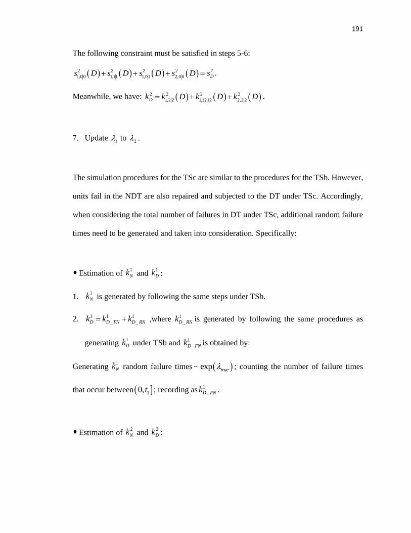
191


2 2 2 2 2

1,0 0 1,11 1,01 2,0 0 Ds D s D s D s D s .

Meanwhile, we have: 2 2 2 2

1,2 2 1,1212 2,2 2Dk k D k D k D .

7. Update 1 to

2 .

The simulation procedures for the TSc are similar to the procedures for the TSb. However,

units fail in the NDT are also repaired and subjected to the DT under TSc. Accordingly,

when considering the total number of failures in DT under TSc, additional random failure

times need to be generated and taken into consideration. Specifically:

Estimation of 1

Nk and 1

Dk :

1. 1

Nk is generated by following the same steps under TSb.

2. 1 1 1

_ _D D FN D RNk k k ,where 1

_D RNk is generated by following the same procedures as

generating 1

Dk under TSb and 1

_D FNk is obtained by:

Generating 1

Nk random failure times exp true ; counting the number of failure times

that occur between 10, t ; recording as1

_D FNk .

Estimation of 2

Nk and 2

Dk :

192

1. Generate 1 1n s random failure times 1exp ; randomly select 2

1,0 0s N failure

times from 1 1n s ; count the number of failure times that occur between 20,t ; record

it as 2

1,1,2 0k N ;




2

2,1,2 0k N ;


2 2 2

1,0 0 2,0 0 Ns N s N s .

Meanwhile, we have: 2 2 2

1,1,2 0 2,1,2 0Nk k N k N .

3. Generate 2

1,1,2 0k N random failure times exp true ; count the number of failure

times that occur between 20,t ; record it as 2

1,1,2 0k D ;

4. Generate 2

2,1,2 0k N random failure times exp true ; count the number of failure

times that occur between 2 20,t w ; record it as 2

2,1,2 0k D ;

We have 2 2 2 2

_1,1,2 0 2,1,2 0D D RNk k D k D k , where 2

_D RNk is generated by following the

same procedures when generating 2

Dk under TSb.

193


In this section, we illustrate the optimal sequential hybrid reliability testing design for

different testing scenarios and numerically compare the optimal testing plans obtained from

proposed methods with those obtained from the simulation model.

We show the design of the first four hybrid reliability tests with the following parameters:

6

3 3

200; 200 ; % 10%; 10 ;

2 10 ; 2.5 10 ; 50, 200

i i N

true L U

n w i q R

t t

In Tables 8.1-8.6, we show the optimal testing plans, the unit’s updated lifetime parameter

and other characteristics. We apply the proposed methods and the simulation model for

the three testing scenarios, respectively. Specifically, Tables 8.1-8.6 show the optimal

testing plans and unit’s updated lifetime for the testing scenarios investigated in section

8.1, TSa and TSb in section 8.2, respectively:


for the testing scenario investigated in section 8.1

Reliability Test 1 2 3 4

yt 182 391 596 799

194

y 32.35 10 32.41 10

32.44 10 32.46 10

y

Ds 38 37 40 44

Proportion of y

Ds in the

population

0.19 0.10 0.06 0.04

y

Ns 20 36 53 69

Table 8.2 First four optimal reliability tests based on the simulation model for the testing

scenario investigated in section 8.1


yt 182 398 598 792

y 32.35 10 32.42 10

32.45 10 32.46 10

y

Ds 38 38 41 46

Proportion of y

Ds in the

population

0.19 0.10 0.06 0.04

y

Ns 20 36 53 69


for the TSa


yt 182 334 565 734

Updated y 32.35 10 32.43 10

32.46 10 32.47 10

y

Ds 38 28 30 19

Proportion of y

Ds in the

population

0.19 0.08 0.06 0.03

y

Ns 20 36 53 70

Table 8.4 First four optimal reliability tests based on the simulation model for the TSa

195

Reliability Tests 1 2 3 4

yt 182 339 569 739

Updated y 32.35 10 32.45 10 32.47 10

32.48 10

y

Ds 38 30 31 20

Proportion of y

Ds in the

population

0.19 0.08 0.06 0.03

y

Ns 20 36 53 70


for the TSb


yt 182 334 565 734

Updated y 32.35 10 32.43 10

32.46 10 32.47 10

y

Ds 38 28 30 19

Proportion of y

Ds in the

population

0.19 0.08 0.06 0.03

y

Ns 20 36 53 70

Table 8.6 First four optimal reliability tests based on the simulation model for the TSb

Reliability Tests 1 2 3 4

yt 182 342 552 729

Updated y 32.35 10 32.44 10

32.45 10 32.46 10

y

Ds 38 29 29 18

Proportion of y

Ds in the

population

0.19 0.08 0.06 0.03

y

Ns 20 36 53 70

From the tables, we have the following observations:

196

1) 1y y decreases as y increases, which shows that the unit’s parameter converges;

2) 4 approximately equals to

true , which shows the efficiency of the methods;

3) The proportion of units assigned to the DTs shows a decreasing trend, which also

demonstrates the efficiency of the methods.

4) The proposed methods and the simulation model yield approximately the same updated

lifetime parameter, which validates the accuracy of the methods.

8.5 Conclusions

In this chapter, we design optimal hybrid sequential reliability testing plans during the one-

shot units’ storage life by performing NDT and DT in each reliability test. We determine

the optimal times to conduct the reliability tests as well as the numbers of units assigned to

the hybrid tests under different testing scenarios, such that the number of available units

after the tests is maximized. Based on the results of the sequential hybrid tests, the accuracy

of the system reliability estimation is improved such that DT is no longer needed after a

number of hybrid tests. We also develop a simulation model to validate the accuracy and

efficiency of the proposed methods. We use a numerical example to illustrate the proposed

methods.

197

CHAPTER 9

OPTIMAL SELECTION AND OPERATIONAL SEQUENCING OF

NONHOMOGENEOUS ONE-SHOT UNITS

One-shot units such as missiles, airbags, and most of the military weapons are deployed

after long terms of storage (or standby). It is important to ensure the stored units operate

its function properly when needed. In this chapter, we investigate the optimization of one-

shot units’ operational use at arbitrary time.

There exists many situations that the one-units are used consecutively when put into

operational use. To illustrate, a certain number of one-shot units (say, s) are selected from

the stored population and launched in sequence. Successful operation is achieved when the:

1) first k one-shot units are successfully launched and 2) no less than consecutive r out of

the remaining (s-k) one-shot units are successfully launched. The population has a mixture

of one-shot units with nonhomogeneous characteristics due to the units’ different arrival

times and the conduct of the sequential reliability tests during its storage period. Therefore,

it becomes interesting and challenging to determine the characteristics and sequence of the

one-shot units to be launched such that the operational use of the s launched units is

optimized. Defining the s launched one-shot units as a system, the reliability metrics of the

system (e.g., the probability that the system achieves the successful operation, the expected

number of successfully launched units) need to be investigated. In this chapter, we optimize

the system’s operational use at arbitrary time by formulating an optimization problem

which is applicable to a variety of objectives. We also provide the bounds of the system’s

198

successful operational probability estimation and develop a simulation study to validate the

proposed approach.

The chapter is organized as follows: in section 9.1, we state the problem and scenarios in

details and calculate the reliability of the one-shot units when they are put into operational

use. In section 9.2, we investigate the expected time-to-kth-failure of the system (with

nonhomogeneous units) and formulate an optimization problem to maximize the

operational use of the system. Specifically, we determine the characteristics and launching

sequence of the selected units by considering the system’s reliability metrics. In section

9.3, we analyze the detailed characteristics of the one-shot units and investigate the bounds

of the system’s probability of successful operation based on the optimal selection and

launching sequence obtained in section 9.2. In section 9.4, we develop a simulation model

to validate the optimality of the solution(s) obtained in section 9.2. In section 9.5, we

provide several numerical examples to illustrate the application of the optimization

problem. We then conclude our work in section 9.6.

9.1. One-shot Units’ Operational Use Reliability

One-shot units are produced and stored in batches at different times. To guarantee the one-

shot units’ operational use when needed, instantaneous NDTs are repeatedly conducted

during its entire storage life horizon. The following notations are needed when obtaining

the expected number of one-shot units with specific characteristics:

199

mt : the time when the mth NDT is conducted;

in : the number of units in the ith batch;

iw : the arrival time of the ith batch;

,mi jn : the number of one-shot units with characteristics ,i j (i.e., the one-shot unit is in the

ith batch and fails in NDT sequence j ) at time mt ;

j# : the number of tests in sequence j ;

j : the th test in NDT sequence j ; j j is the last test in j ;

,i jR t : reliability of the one-shot unit (with characteristics ,i j at timemt ) at time t;

xF : CDF of the one-shot unit’s lifetime after its xth repair; F is the CDF of units that

never repaired.

The expected numbers of one-shot units (with specific characteristics) at time mt are

obtained in Eqs. (9.1) and (9.2), where j j m means the unit fails at time t (its jth

failure is observed in the mth NDT) and j j m means the unit has survived at time t.

1 1 1

# -1

, 1 1 11

1# #

- - -

; - - -

- - -

i ij j

j

mi j i a aj j j j

a

m mj j j jj j

F t w F t w

E n j j m n F t t F t t

F t t F t t

(9.1)

200

1 1 1

# -1

, 1 1 11

#

- - -

; - - -

-

i ij j

j

mi j i a aj j j j

a

m j jj

F t w F t w

E n j j m n F t t F t t

R t t

(9.2)

The reliability of the one-shot unit (with characteristics i j, ) at time t (m

t t ) is accordingly

calculated:

#

,

#

-

-

j jj

i j

m j jj

R t tR t

R t t (9.3)

Under most circumstances, the one-shot units within the same batch have different

characteristics. Specifically, they have different repair conditions (the number of repairs

j# and the when the repairs are conducted ( j )). Based on Eqs. (9.1)-(9.3), we obtain

the mean and variance of the reliability ( iR t and iVar R t ) of the one-shot units in the

ith batch:

#

,

#

-

-

j jj mi j

j m j jj

i

i

R t t

E nR t t

R tn

(9.4)

2

#

,

#

-

-

j jj m

i i j

j m j jj

i

i

R t tR t E n

R t t

Var R tn

(9.5)

9.2 Optimal Selection and Operational Sequencing of One-shot Units

201

The stored one-shot units (with nonhomogeneous characteristics) are put into operational

use whenever needed (say, at time t ). Under most circumstances, a specific number of one-

shot units (say, s, where i

i

s n

) are selected and put into operational use. The successful

operation is achieved once 1) the first k one-shot units are successfully launched and 2)

consecutive r out of the rest (s-k) one-shot units are successfully launched. It is without

loss of generality to define the selected one-shot units as a “first-hit-k-consecutive-r-out-

of-(s-k)” system, where the time of selecting and launching the one-shot units is negligible.

In this section, we investigate the time-to-kth-failure of the system with nonhomogeneous

one-shot units and optimize the system’s operational use.

9.2.1 Optimal Selection and Operational Sequencing

In this section, we formulate an optimization problem to obtain the optimal selection and

launching sequence of the one-shot units. We first define the following:

: the sequence to launch the selected one-shot units, v is presented in terms of selected

one-shot unit’s batch number;

: the batch number of theth launched one-shot unit;

:R t expected reliability of the th launched one-shot unit at time t;

Var R t

: variance of the reliability of the th launched one-shot unit at time t;

: one-shot units in the th batch have the th lowest average reliability;

202

;systemR t v : expected probability that the system operates successfully at time t ;

;systemVar R t v : variance of the probability that the system operates

successfully at time t ;

:s the number of one-shot units selected from the th batch; s s

.

To optimize the operational use of the system (e.g., maximize the expected probability that

the system achieves the successful operation), the following two variables need to be

determined:

1) The characteristics of the selected one-shot units; i.e., the number of one-shot units

selected from each batch; and

2) The sequence to launch the selected one-shot units.

The above two variables determine the characteristics of the th launched one-shot units

( R t

and Var R t

). Note that the one-shot units’ launching sequence is

dependent on its characteristics. The expected probability that the system achieves the

successful operation at arbitrary time mt t ( 1,2,...m ) can be maximized by solving the

following problem:

Max

;systemR t v (9.6)

s.t.

203

1 1 1 1

; n s n R t

n s n R t

(9.7)

1;system s k rE T v t (9.8)

number of sucessfully laun one-shot unitsched ; ;systemE t v k r (9.9)

threshold;systemVar R t v Var (9.10)

s s

(9.11)

# : v v

R t R t R t s (9.12)

The objective is to maximize the expected probability that the system successfully operates

at arbitrary time t (Eq. (9.6)). Intuitively, the objective can be achieved by selecting one-

shot units in a decreasing order in terms of its average reliability at time t ( R t ).

However, the reliability metrics of unselected one-shot units also need to be considered for

future operational use. Therefore, we consider that a minimum number of less-reliable one-

shot units need to be selected (Eq. (9.7)). In Eq. (9.8), the system’s expected-time-to-(s-

k+r+1)th-failure must be later than time t. Similarly, the expected number of successfully

launched one-shot units at time t should be greater than (k+r) (Eq. (9.9)). As the

characteristics of the one-shot units are nonhomogeneous, the randomness of selected one-

shot units’ reliability metrics needs to be considered (Eq. (9.10)). Eqs. (9.11) and (9.12)

indicate that the launched one-shot units are selected from different batches.

204

Note that the above formulated optimization problem is general as the objective can be

exchanged with some of the constraints. To illustrate, the optimal operational use can be

realized by minimizing the variance of probability of the system’s success; meanwhile,

the expected probability that the system achieves a successful operation becomes a

constraint which should be less than a given threshold:

Min

;systemVar R t v (9.13)

s.t.

;system thresholdR t v R ; and (9.14)

Constraints as shown in Eqs. (9.7)-(9.8), (9.10)-(9.11).

We can also maximize the expected number of successfully launched one-shot units;

meanwhile the expected probability that system achieves a successful operation should be

less than a given threshold:

Max

system number of sucessfully launched one-shot units; ;E t v (9.15)

s.t.

;system thresholdR t v R ; and (9.16)

Constraints as shown in Eqs. (9.7)-(9.9), (9.11).

205

The probability that a “first-hit-k-consecutive-r-out-of-(s-k)” system successfully operates

is obtained by taking the product of the probability that the first k launched one-shot units

are successful (term A in Eq. (9.17)) and the probability that at least r out of the rest (s-k)

one-shot units are consecutively launched (term B). Specifically:

ˆ ˆ ˆ ˆ:1)#1

ˆ 2) consecutive elements in

; 1

B

A

k s k

system

r r r v r v rr r

R t v R t R t R t

(9.17)

where r̂ is the sequence of successfully launched one-shot units out of the (s-k) one-shot

units and ˆ# r is the number of elements (one-shot units) in r̂ . In term B, we consider all

possible combinations of launched one-shot units’ status (successful or not), where there

need to be r̂# ( 1r r r s k ˆ# , , ..., ) successfully launched one-shot units with at least

r one-shot units are consecutive.

As stated earlier, the probability that the system successfully operates is not deterministic.

We respectively obtain the expected probability that the system successfully operates and

the expected number of successfully launched one-shot units in Eq. (9.18) and (9.19):

ˆ ˆ ˆ ˆ:1)#1


; 1

B

A

k

system

r r r v r v rr r

R t v R t R t R t

(9.18)

206

system

ˆ ˆ ˆ ˆ1 :1)#ˆ 2) consecutive elements in

number of successfully launched one-shot units; ;

ˆ# 1

B

A

k

r r r v r v rr r

E t

R t r R t R t

(9.19)

In Eq. (9.15), the expected number of successfully launched one-shot units in the first k

one-shot units (term A) and in the remaining (s-k) one-shot units (term B) are respectively

calculated and summed. Similarly, referring to i

i

Var X

2 2

i i i

i i

Var X E X E X

and i i

i i

Var X Var X

if iX are

independent of each other, we obtain the variance of the probability that the system

operates successfully in Eq. (9.20):

system

2 2 2 2

; , 1, 2,...,Var R t R t s

Var A E A Var B E B E A E B

(9.20)

where

2 2

1 1

k k

v v vVar A Var R t R t R t

1

k

E A R t

2 2

ˆ ˆ:1)# 1 1ˆ 2) consecutive elements in

s s

v v vr r r k k

r r

Var B Var R t R t R t

ˆ ˆ ˆ ˆ:1)#


1r r r v r v r

r r

E B R t R t

207

The optimal solution(s) can be obtained by either searching for all feasible solutions or

using a nonlinear optimal algorithm. It is noted that some constraints are associated with

the characteristics of the selected units while some constraints are associated with units’

characteristics and launching sequence.

9.2.2 Time-to-kth-failure of a Population with Nonhomogeneous One-shot Units

Current research on time-to-kth-failure (kT ) of a population assumes that the population has

homogeneous units. In this section, we investigate kT of a population with

nonhomogeneous one-shot units. Specifically, we investigate the system’s expected time-

to-kth-failure since the last nondestructive test time mt .

9.2.2.1 Probability Density Function (pdf) of System’s Time-to-kth-Failure

The characteristics of the one-shot units have an important impact on system’s time-to-kth-

failure. We obtain the probability that kT happens at time t (

mt t ) with one-shot units’

characteristics known (i.e., the number of selected one-shot units with different

characteristics are known). We first define the following:

,

m

i js :the number of selected one-shot units with characteristics ,i j at time mt ;

, , ,m m

i j i js E n i j

208

', '

m

i js : the number of selected one-shot units with characteristics ', 'i j at time mt , specifically,

the kth failed one-shot units has the characteristics ', 'i j ;

,

m

i jk : the number of selected one-shot units (with characteristics ,i j at time mt ) that fail

between time mt and t ;

', '

m

i jk : the number of selected one-shot units (with characteristics ', 'i j at time mt ) that fail

between time mt and t ;

,

m

i jr : the number of selected one-shot units (with characteristics ,i j at time mt ) that survive

until time t ;

', '

m

i jr : the number of selected one-shot units (with characteristics ', 'i j at time mt ) that

survive until time t ;

We obtain the pdf of kT ( kTf t ) in Eq. (9.21):

209

,

', ' ', '

', ' ,, ,

1

', '

', '

', '

1 !

! !

1

11

k

mi j

i j

m mi j i j

A B

Tm m

i j i ji j i j

k ki j

k rm

i j j jj j j jm

i jm

j m j mj j j ji j

j j j

kf t

k r

s R t t R t ts

R t t R t tk

f t t R

, ,

2

,

except except ',

1

m mi j i j

C

j m j m jj j j j j j

j m j j

k rm

i j j jj j j j

mi j j j m j mj j j ji j

t t f t t R t t

R t t

s R t t R t t

R t t R t tk

'

D

i

(9.21)

where , , ,

m m m

i j i j i jr s k and', ' ', ' ', ' 1m m m

i j i j i jr s k .

The term A in Eq.(9.21) considers and sums of all possibilities that the kth failed one-shot

unit has specific characteristics ', 'i j , where ', 'i j could be any of the ,i j . The term B

considers the possible characteristics of previously failed (k-1) one-shot units, where the

(k-1) failures occur between time mt and t . The term C is the probability that out of the

', '

m

i js one-shot units: ', '

m

i jk one-shot units fail between time mt and t , one one-shot unit fails

at time t and ', '

m

i jr one-shot units survive until time t . The term D calculates the probability

that: out of the ,

m

i js one-shot units (with all potential characteristics except ', 'i j ), ,

m

i jk one-

shot units fail between time mt and t , and ,

m

i jr one-shot units survive until time t .

210

9.2.2.2 Expected Time-to-kth-Failure of the System

Based on Eq. (9.21), the expected time-to-kth-failure of the system ( kE T ) can be obtained

as 0

k m kE T t f t dt

. Note that kE T can only be numerically obtained under most

circumstances, except that when the unit’s lifetime is exponentially distributed (whose

failure rate is constant). Defining:

x : the one-shot unit’s failure rate after its xth repair;

m ys : the number of one-shot units selected from the thy batch that arrives after the mth

NDT;

m yw : the arrival time of the thy batch that arrives after the mth NDT.

We iteratively obtain kE T of the system:

Step 1:

1

1

0,#

,

,#,

,

,

1If

k

mm

i jji jm

i jj mi j

i j

i j

ws

ss

; where 0 1k , ...,

Stop,

1

0 ,#,

,#, ,

,

1

k

k m

i jji jm

i j mji j i j

i j

E Ts

ss

.

211

Otherwise go to step 2;

Step 2:

Find *

1k such that:

* *1 11

1

0 0, ,# #, ,

, ,# #, ,, ,

, ,

1 1,

k k

m m m

i j i jj ji j i jm m

i j i jm mj ji j i ji j i j

i j i j

ws s

s ss s

and

*1

*1

110 , 0 1#

,

,#, ,

,

1 1min ,

k

mmki j mj

i jm

i j mji j i j

i j

E T ws s

ss

.

If

*1

*1

1

210 , , 0 1# #

, ,*

, 0 1 1#, , , 1

, ,

1,

k k

mk m m

i j i j mj ji j i jm

i j m m mji j i j i j m

i j i j

E T ws s s

s s ks s s

Stop,

*1

*1

1

10 , , 0 1# #

, ,*

, 0 1 1#, , , 1

, ,

1;

k k

k k m m



i j i j

E T E Ts s s

s s ks s s

212

Otherwise, go to step 3;

Step 3

Find*

2k such that:

* *2 1

*1

*1

1

10 , , 0 1# #

, ,*

, 0 1 1#, , , 1

, ,

2

1

,#,*

, 0 1 1#, ,

1,

1

k k

k m m



i j i j

m

k m

i jji jm

i j mji j i j

E Ts s s

s s ks s s

w

E Ts

s s ks

* *2 1

0 , 0 1#,

, 1

, ,

k k

m

i j mji j

m m

i j m

i j i j

s s

s s

and

2

* *2 1

*1

1

10 , , 0 1# #

, ,*

, 0 1 1#, , , 1

, ,

2

0 2

1,

min

1

k

k k

k m m



i j i j

m

m

E T

E Ts s s

s s ks s s

ws

If

213

2 1

,#,*

, 0 1 2 1#, ,

,

, 0 1 , 0 1 2# #, ,* *

2 1

, 1 , 1 2

, ,

1k m

i jji jm

i j m m mji j i j

i j

m m

i j m i j m mj ji j i j

m m

i j m i j m m

i j i j

E Ts

s s s ks

s s s s s

k ks s s s s

*2 1

2

0

, k

mw

Stop,

*2 1

,#,*

, 0 1 2 1#, ,

,

, 0 1 , 0 1 2# #, ,* *

2 1

, 1 , 1 2

, ,

1k k m

i jji jm

i j m m mji j i j

i j

m m

i j m i j m mj ji j i j

m m

i j m i j m m

i j i j

E T E Ts

s s s ks

s s s s s

k ks s s s s

*2 1

0

k k

Otherwise, continue with step 4.

…

The above steps iterates until kE T is found. Note that the number of steps until stop is

dependent on the batches’ arrival times and sizes.

9.3 Bounds of System’s Successful Probability

As the one-shot units within a batch are nonhomogeneous, the system’s successful

operational probability based on the optimal selection and launching sequence (which only

shows the launched one-shot units’ batch numbers) varies within a certain range depending

214

on the specific unit selected from the batch. In this section, we investigate the lower and

upper bounds of system’s successful operational probability by considering the one-shot

units’ repair conditions (the number of repairs and when the repairs are conducted).

9.3.1 Bounds of System’s Successful Probability of Operation under Constant Failure Rate

If the one-shot units have an exponentially distributed lifetime, the reliability of one-shot

units with characteristics i j, at time t is presented by Eq. (9.22). It can be observed the

reliability of the one-shot units (with characteristics i j, ) at time t is independent of i and

j .

##

, #

# #

exp --exp

- exp -

j j jj j j

i j mj

mj j j j j j

t tR t tR t t t

R t t t t

(9.22)

Generally, one-shot unit’s reliability at time t decreases when its number of repairs

increases as presented in Eq. (9.23):

0 1 2 ii j j i j j i j j i j j m z

R t R t R t R t i

, :# , :# , :# , :#

... ; (9.23)

Based on the optimal selection and launching sequence obtained in section 9.2, the

system’s successful operational probability is guaranteed to be within the range in Eq.

(9.24):

215

; ;# ,

;

; ;# 0 ,

system v

system

system

R t v j m z

R t v

R t v j

(9.24)

where ;#v j x represents theth launched one-shot unit that has been repaired x

repairs.

The lower bound of the system’s successful operational probability is achieved if selecting

one-shot units with the largest number of repairs in the designated batches and the upper

bound is achieved by selecting one-shot units with no prior repairs.

9.3.2 Bounds of System’s Successful Probability under Time-dependent Failure Rate

If the one-shot units’ lifetime follows Weibull distribution with its shape parameter j

#

dependent on the one-shot units’ number of repairs j# , the reliability of the one-shot

units at time t is dependent on: the time when its last failure is observed and its number of

repairs. Specifically, the unit’s reliability at time t is an increasing function of j j and a

decreasing function of the unit’s number of prior repair (see Eq. (9.25)):

last failure observed at time

1 2

fails (and repaired) once fails (and repaired) twice fails (and repaired) times

m

i

i

t

i j j j j m i j j j j m i j j j j m z m

m z

R t R t R t

, : , : , :

...

1

1

last failure observed at time

1 1 2 1 1 1

one failure observed at time

1 1 1

m

i

zi

t

i j j j j m i j j j j m i j j j j m z m

t

i j j j i j

R t R t R t

R t R

, : , : , :

, : ,

... ...

no failure observed

0jt

:#

(9.25)

216

We randomly generate the batches’ arrival times, the times to conduct the sequential NDTs,

and the Weibull shape parameters j

#. The generation runs for 103 iterations. Specifically,

10w ; 1

0 50t randbetween , ; 2 10 50w t randbetween , ;

2 2 3 20 50 0 50t w randbetween w t randbetween , ; , ;

4 3 3 4 30 50 0 50 0 50w w randbetween t w randbetween t t randbetween , ; , ; , ;

0 12 4 0 1 1 3 1 2 3

j jrandbetween r randbetween j

# #, ; . , ;# , , ;

We calculate the means of i jR t

, of the 1000 iterations i j , . We numerically validate

that the one-shot unit’s reliability is lower when more repairs are conducted and/or when

the one-shot unit’s last repair happens earlier. The reliabilities of the one-shot units in the

four batches with different characteristics and the average reliabilities of the one-shot units

in the four batches at time t are shown in Table 9.1.

Table 9.1 Reliabilities of the one-shot units (with different characteristics) at time t

Reliabilities of

one-shot units in

the 1st batch

Reliabilities of one-

shot units in the 2nd

batch

Reliabilities of

one-shot units in

the 3rd batch

Reliabilities of

one-shot units in

the 4th batch

1 0R t

, 0.9805 2 0

R t,

0.9896 3 0R t

, 0.9960 4 0

R t,

0.9982

1R t 0.9813 2

R t 0.9897 3R t 0.9960 4

R t 0.9982

217

1 1R t

, 0.9827 2 2

R t,

0.9912 3 3R t

, 0.9993 4 3

R t,

0.9993

1 12,R t 0.9900 2 23

R t,

0.9991

1 2R t

, 0.9912 2 3

R t,

0.9993

1 123R t

, 0.0980

1 13R t

,

1 23R t

,

0.9991

1 3R t

, 0.9993

Therefore, Eq. (9.25) is numerically proven. Based on the optimal launching sequence

obtained in section 9.2, the system’s successful operational probability is guaranteed to be

within the range presented in Eq. (9.26):

; ;# 0 , ;

;

; ; : 1 0 ,

system

system

system

R t v j

R t v

R t v j j j j m

(9.26)

where ; : 1 0v j j j j m represents theth launched one-shot unit which is

selected from the designated batch with its last (also the 1st) repair conducted at time m

t .

The lower bound of the system’s successful operational probability is achieved by selecting

one-shot units with no prior repairs in the designated batches (i.e., one-shot units with the

218

“longest” age) and the upper bound is achieved by selecting one-shot units with one failure

(and repair) at time mt (i.e., one-shot units with the shortest age ( m

t t )).


In this section, we develop a simulation model to validate the optimality of the solution(s)

obtained in section 9.2. The steps of the simulation model are introduced as follows:

Step 1: Find all sequences satisfying the constraint of Eq. (9.7).

Step 2: Find all sequences satisfying Eq. (9.8):

Step 2.1: For a specific sequence v withis i , randomly determine

,

m

i js j such that

,

m

i j i

j

s s

and , ,

m m

i j i js E n .

Step 2.2: Generate ,

m

i js failure times ,i j where the ,

m

i js failure times follow the distribution

with CDF # j

F ; note that the , , :m

i js i j j j m failure times need to be

greater than m j j

t t ;

Step 2.3: Add mt to the

,

m

i js failure times , :i j j j m ; add j jt to the , , j

m

i j ls failure times

, :i j j j m ; sort all failure times in an increasing order and record the th

failure time as T ;

219

Step 2.4: Repeat steps 2.2-2.3 for 105 times and calculate the average of T as

systemE T ; let 1 1I if 1system s k r

E T

t ; otherwise 1 0I .

Step 2.5: Eliminate all sequences whose1 0I .

Step 3: Simulate ;systemR t v :

Step 3.1：For v in a specific sequence v , generate ,

100 m

v jE n

failure times j ,

where , ,

100 m

v j v jE n R t

failure times with index 1 and

, ,100 m

v j v jE n F t

failure times with index 0;

Step 3.2: randomly select one number out of ,

100 m

v jE n

, record its index as v

I

( vI

=1 or 0);

Step 3.3: Repeat steps 3.1-3.2 ;

Step 3.4: Record 1systemI if 1) 1 for 1,...,

vI k

and 2) at least consecutive r

=1 for = 1,...,

vI k s

; otherwise 0systemI .

Step 3.5: Repeat steps 3.1-3.4 106 times, we have: 610

6;

10

system

system

I

R t v

and

6

system

1 110

6

number of successfully launched one-shot units; ;

10

k s

k

E t v

I I I

where 1I if 2) in step 3.4 is satisfied and 0I otherwise;

220

Step 3.6: the variance of the probability that the system operates successfully is obtained

accordingly.

Step 4: Among the qualified sequences, select the sequence optimalv with the largest

;systemR t v .

We examine if the optimalv obtained by the simulation model is the same as that obtained in

section 9.2. The simulation model generally applies when the objective is exchanged with

some of the constraints as discussed in section 9.2.

9.5 Numerical Illustrations

In this section, we numerically illustrate the optimal selecting and launching sequencing of

one-shot units from the population. We also show the bounds of system’s successful

operational probability based on the optimal sequence(s). The following testing parameters

and one-shot units’ lifetime distributions are given as:

6, 2, 2 N k r ; 0.5;thresholdR 0.05thresholdVar ;

Testing parameters a): The one-shot units’ lifetime follows Exponential distribution:

1 expj jF t t , where 0 1 2 30.0001; 0.0003; 0.0005; 0.001;

221

1 2 3 4 1 2 30, 1200, 2500, 3000; 1000; 2000; 3500;w w w w t t t

1 2 3 43 4 5 6n n n n , , ,

Testing parameters b): The one-shot units’ lifetime follows Weibull distribution:

1 expj

j

tF t

, where 0 1 2 32.5; 2.8; 3; 3.2;

1 2 3 4 1 2 30, 200, 275, 350; 100; 250; 400.w w w w t t t

1 2 3 44, 5, 5, 6;n n n n

The following three objectives are considered:

Objective 1 (O1): Maximize the expected probability of system’s successful operation;

Objective 2 (O2): Maximize the expected number of successfully launched one-shot units;

Objective 3 (O3): Minimize the variance of the system’s successful probability.

The expected number of one-shot units with different characteristics and its reliability at

time t are calculated. We use the one-shot units in the 1st batch to illustrate the model,

where xR is the reliability of the units with x repairs.

3

1,123 1 1 1 1 2 1 2 3 2 1,123 4 3; ;E n n F t w F t t F t t R t R t t

3 23

1,12 1 1 1 1 2 1 2 3 2 1,12

3 3 2

; ; R t t

E n n F t w F t t R t t R tR t t

222

3

1,13 1 1 1 1 3 1 1 2 1 1,13 2 3; ;E n n F t w F t t F t t R t R t t

3

1,23 1 2 1 1 1 1 3 2 1,23 3 3; ;E n n F t w F t w F t t R t R t t

2 13

1,1 1 1 1 1 3 1 1,1

2 3 1

; ; R t t

E n n F t w R t t R tR t t

3 23

1,2 1 2 1 1 1 1 3 2 1,2

3 3 2

; ; R t t

E n n F t w F t w R t t R tR t t

3

1,3 1 3 1 2 1 1,3 1 3; ;E n n F t w F t w R t R t t

1 13

1,0 1 3 1 1,0

1 3 1

; .R t w

E n n R t w R tR t w

Accordingly, we have:

3

1, 1,

1,

1

1

j j

j

E n R t

R tn

and

2

3

1, 1 1,

1

1

j jR t R t E nVar R t

n

We then solve for the optimal solutions for different objectives with different testing

parameters. Generally, it is observed the batches’ arrival times and sizes, units’ failure rate,

the times to conduct the NDTs, and the time to select and launch the units affect the optimal

selection and launching sequence(s). Several illustrations are shown in Tables 9.2-9.4. The

optimal sequences are presented in terms of the selected units’ batch numbers. The

sequence (3, 4, 1, 2, 2, 1) means that the 1st launched unit is selected from the 3rd batch, the

2nd launched unit is selected from the 4th batch, and so on.

223


parameters a) at time 4000t

Objective Optimal Sequence(s) Objective Function

Value

O1 (3, 4, 1, 2, 2, 1) or (4, 3, 1, 2, 2, 1) 0.8784

O2 (1, 1, 2, 4, 3, 2) or (1, 1, 2, 3, 4, 2) 5.5616

O3 (1, 1, 4, 2, 2, 3) 0.0112


parameters a) at time 6500t

Objective Optimal Sequence Objective Function

Value

O1 (3, 4, 1, 2, 2, 1) or (4, 3, 1, 2, 2, 1) 0.6391

O2 (1, 1, 2, 3, 4, 2) or (1, 1, 2, 4, 3, 2) 4.7369

O3 (3, 4, 2, 1, 1, 2) or (4, 3, 2, 1, 1, 2) 0.0281


parameters b) at time 500t

Objective Optimal Sequence Objective Function

Value

224

O1 (2, 3, 1, 1, 2, 1) or (3, 2, 1, 1, 2, 1) 0.6941

O2 (1, 1, 1, 2, 3, 2) or (1, 1, 2, 3, 2, 1) 4.8623

O3 (2, 3, 1, 1, 1, 2) or (3, 2, 1, 1, 1, 2) 0.0357

With testing parameter a) at time 4000t , the system achieves its highest successful

probability at an average value of 0.8747, with sequence (3, 4, 1, 2, 2, 1) or (4, 3, 1, 2, 2,

1). Specifically, the average reliabilities of the one-shot units in the four batches at time

4000t are respectively:

1 24000 0 9156 4000 0 9303R t R t . ; . ;

3 44000 0 9426 4000 0 9468R t R t . ; .

We observe that: 04000 0 9512 4000

i iR t R t i

,. . Therefore, the upper bound

of the system’s probability of successful operation is 0.8986 by selecting the one-shot units

that have not experienced repairs in the designated batch. Similarly, the lower bound of the

system’s probability of successful operation is 0.6041 when selecting the one-shot units

with the highest numbers of repairs in the designated batches (Eq. (9.27)):

1 123 2 234000 0 6065 4000 0 7788R t R t

, ,. ; . ;

3 3 4 34000 0 8607 4000 0 8607R t R t

, ,. ; . . (9.27)

With testing parameters b) at time 500t , the system achieves the highest successful

probability at an average value of 0.6941 with launching sequence (2, 3, 1, 1, 2, 1) or (3, 2,

225

1, 1, 2, 1). In Eq. (9.28), we calculate the reliabilities of the one-shot units (that fail once

at time 3t ) in the four batches at time 500t :

1 3 2 3 3 3 4 3500 500 500 500 0 9890R t R t R t R t

, , , ,. ; (9.28)

We also obtain the reliabilities of one-shot units that have not experienced repairs in the

four batches in Eq. (9.29):

1 0 2 0500 0 6521 500 0 8372R t R t

, ,. ; . ;

3 0 4 0500 0 9007 500 0 9549R t R t

, ,. ; . ; (9.29)

Selecting and launching the one-shot units in sequence (2, 3, 1, 1, 2, 1) or (3, 2, 1, 1, 2, 1),

the system’s probability of successful operation is guaranteed to be within the range of

0 6071 0 9778. , . , where the upper bound is achieved if the one-shot units with one failure

at time 3t (Eq. (9.28)) are selected from the designated batches and the lower bound is

achieved if the one-shot units that have not experienced repairs are selected (Eq. (9.29)).

9.6 Conclusions

In this chapter, we investigate the optimal operational use of the one-shot units at arbitrary

time. We determine the characteristics of the one-shot units selected from the stored

population and the launching sequence to achieve the one-shot units’ optimal successful

operation. The reliability metrics of the launched one-shot units and a variety of objectives

are considered. The bounds of the launched one-shot units’ probability of successful

226

operation based on the optimal launching sequence are provided. We also develop a

simulation model to validate the optimality of the solution(s) obtained by the formulated

optimization problem.

227

CHAPTER 10

CONCLUSIONS

In this dissertation, we investigate several interesting and challenging problems regarding

the reliability metrics of systems with mixtures of nonhomogeneous one-shot units.

Batches of one-shot units arrive into storage at arbitrary time and a sequence of reliability

tests are conducted randomly to assess the reliability metrics of the units. Defining the

stored one-shot units as a system, we investigate the reliability metrics of the system under

a variety of failure modes such as failures with no indicator, thermal fatigue failures, and

competing failure modes. We also investigate the optimal design of sequential reliability

testing plans by considering different types of reliability tests. The one-shot units are

retrieved from storage and launched at arbitrary time during its storage, we also investigate

the optimal operational use of the one-shot units in this dissertation. In the following, we

briefly provide conclusions of this dissertation.

In chapter 3, we propose effective approaches to assess the reliability metrics of a

generalized “k-out-of-n: F” system with nonhomogeneous one-shot units under different

scenarios, taking into account the units’ characteristics during its storage period. We show

that aging has an important effect on the system reliability metrics. We also show that the

reliability metrics of such systems can be obtained by either testing the entire population

or testing selected samples. We propose that the system reliability metrics can be estimated

accurately and effectively even when the batch size is large or when the reliability tests are

228

performed extensively over the time horizon, by developing three computationally

effective alternatives which either mask some of the system conditions or yield negligible

estimation bias. An extensive simulation model validates that the proposed approaches

estimate system reliability metrics accurately.

In chapter 4, we propose stochastic approaches to assess the system reliability metrics when

the batches’ arrival time and sizes, and the time to conduct the reliability tests can be

described by specific probabilistic distributions. We show that the system reliability

metrics obtained by the stochastic approaches can be approximately predicted by those

obtained by the approaches proposed in chapter 3, by either testing the entire population or

testing a sample, and vice versa.

In chapter 5, we propose accurate and effective approaches that model the system reliability

metrics subjecting to thermal fatigue by utilizing the GBS distribution, where the system

has a mixture of nonhomogeneous one-shot units that are subjected to sequential ATCTs.

We demonstrate that the GBS distribution, though developed for mechanical fatigue failure,

is suitable for modelling thermal fatigue data. Moreover, compared with the commonly

used CM model, we show that the GBS distribution provides additional reliability metrics

and assesses the reliability at the system level which could not be accomplished by the CM

model. The proposed models’ flexibility and robustness in estimating/predicting the system

reliability metrics are validated by a simulation model.

229

In chapter 6, we propose efficient and effective approaches that model the reliability

metrics of systems subject to competing failure modes, where the system has a mixture of

nonhomogeneous one-shot units subject to sequential TCTs. We develop and utilize

statistics-based models and physics-statistics-based models to characterize the

failure/degradation modes. We validate that competing failure modes result in worse

system reliability metrics than single failure mode. Moreover, the proposed models’

accuracy in estimating the system reliability metrics is validated by a simulation model.

In chapter 7, we study the unit’s reliability metrics by developing a statistics-physics-based

model and show the temperature and humidity have significant effect on the system

reliability metrics. We then propose the optimal design of sequential accelerated NDTs on

the system level, taking system’s/sample’s reliability metrics under different testing

scenarios into account. We numerically prove that: 1) a randomly selected sample

represents the population’s characteristics in the long run when designing the optimal

testing plans; and 2) the sample size has negligible consequence on the design of optimal

testing plans. We also show that the accelerated NDTs have insignificant effect on the

system reliability metrics while reducing the test durations.

In chapter 8, we design optimal sequential hybrid reliability testing plans during the one-

shot units’ storage life under different scenarios, by performing both NDT and DT in each

reliability test. We therefore show that the number of available units after the tests can be

maximized by designing the optimal testing plan. We also prove that the accuracy of the

230

system reliability metrics estimation is improved based on the results of the sequential

hybrid tests, such that DT is no longer needed after a number of hybrid tests.

In chapter 9, we achieve the optimal operational use of the one-shot units at arbitrary time.

The characteristics of the one-shot units when launched are obtained. We optimize the

launched one-shot units’ optimal successful operation by determining its characteristics

and launching sequence. We show that the probability that the launched one-shot units

achieves a successful operation is guaranteed to be within a certain range based on the

proposed optimal launching sequence, by providing the bounds of the estimates of the

probability.

231

APPENDIX

The probability that the unit has specific characteristics are obtained in Eqs. (A1) and (A2):

1 1

1 1 1 1

1

1 10

1

1

1 10

1

,

1 ,

... ..., ...1

1 ,

... ..., ...1

1

...

R

iz Rji

i

R

iz j ji

i

jC

z jC C C

i z

jR

z jR R R

i z

Wm

i j

C j C

P d C d CC z C

R j R

P d R d RR z R

R jP k C j

P

1 1 1 1

1 1

1

1 10

1

1

1 10

1

1 ,

..., ...1

1 ,

... ..., ..1

R R

iz j ji

i

R

iz Rji

i

jC C

z jC C C

i z

jR

z jR R R

i z

C

d C d CC z C

R j R

P d R d RR z R

1 1 11 1 1 1W W R Rj j

F t F t P C j C P R j R

232

1 11 10

1 1

1 1

1 1

1

,

... ..., ...

1 1

,

... ..., ...

1 1

R

Rj j

j j

jC

j jC C C

j

j

j jR R

j

W j j

C j

C

P d C d C

C j

C

R j

R

P d R d R

R j

R

R t t

1 1 1

1 1 1

0

1 10

1 1

1 1

1 1

,

... ..., ...

1 1

,

... ...,

1 1

R

j

R R

j j j

R

R

jC C

j jC C C

j

j

j

j

C j

C

P d C d C

C j

C

R j

R

P d R

R j

R

1 1 0

1 1 1

...

1 1 1 1

R

Rj j

R

jR R R

W Wj j j j

R R

d R

F t t F t t

P C j j C P R j j R

2

j

1

11

10

1

10

1

,... ..., ...

1

,... ..., ...

1

...

R

m Fj j

R

m mj j

mC

mj jC C C

j j

mR

mj jR R R

j j

W m j j

C m CP d C d C

C j j C

R m RP d R d R

R j j R

R t t

C m CP

11

1

10

1

10

1

,..., ...

1

,... ..., ...

1

R F

m mj j

R

m Fj j

mC C

mj jC C C

j j

mR

mj jR R R

j j

d C d C

C j j C

R m RP d R d R

R j j R

1 1 1W m W m m R m Rj j j j j j j jF t t F t t P C t t C P R t t R

(A1)

233

1 1

1 1 1 1

11 10

1

11 10

1

,1

1 ,...,... ...

1

1 ,...,... ...

1

1

1 ,...,...

R

iz Rji

i

R

iz j ji

i

Cj

z jC C Ci z

Rj

z jR R Ri z

Wm

i jj

C j CP d C d C

C z C

R j RP d R d R

R z R

R jP r C j C

P

1 1 1 1

1 1

1 101

11 10

1

1 1 1

...1

1 ,...,... ..

1

R R

iz j ji

i

R

iz Rji

i

C C

z jC C Ci z

Rj

z jR R Ri z

W Wj j

d C d CC z C

R j RP d R d R

R z R

F t F t P C

1 1 1 1R Rj C P R j R

1 11 10

1 1

1 1

1 1

1

,

... ..., ...

1 1

,

... ..., ...

1 1

R

Rj j

j j

jC

j jC C C

j

j

j jR R

j

W j j

C j

C

P d C d C

C j

C

R j

R

P d R d R

R j

R

R t t

1 1 1

1 1 1

0

1 10

1 1

1 1

1 1

,

... ..., ...

1 1

,

... ...,

1 1

R

j

R R

j j j

R

R

jC C

j jC C C

j

j

j

j

C j

C

P d C d C

C j

C

R j

R

P d R

R j

R

1 1 0

1 1 1

...

1 1 1 1

R

Rj j

R

jR R R

W Wj j j j

R R

d R

F t t F t t

P C j j C P R j j R

2

j

234

11

11

10

1

10

1

,..., ...

1

,... ..., ...

1

R F

m mj j

R F

m mj j

mC C

mj jC C C

j j

W m j j

mR R

mj jR R R

j j

C m CP d C d C

C j j CR t t

R m RP d R d R

R j j R

(A2)

235

REFERENCES

Agarwal, M., Sen, K. and Mohan, P., 2007. GERT analysis of m-consecutive-k-out-of-n

systems. IEEE Transactions on Reliability, 56 (1), 26-34.

Akiba, T., Yamamoto, H., Komuro, T. and Nagatsuka, H., 2011. Analysis for a trend on

the optimal arrangements in a multi-state consecutive-k-out-of-n: F system. International

Conference on Quality, Reliability, Risk, Maintenance, and Safety Engineering

(ICQR2MSE), 2011 Xian. IEEE, 223-228.

Amari, S. V., Zuo, M. and Dill, G., 2009. A fast and robust reliability evaluation algorithm

for generalized multi-state k-out-of-n systems. IEEE Transactions on Reliability, 58 (1),

88-97.

Balakrishnan, N. and Ling, M., 2013. Best cosntant-stress accelerated life-test plans with

multiple stress factors for one-shot device testing under a Weibull distribution. IEEE

Transactions on Reliability, 63 (4), 944-952.

Bhattacharyya, G. K. and Fries, A., 1982. Fatigue failure models: Bimbaum-Saunders VS

Inverse Gaussian. IEEE Transaction on Reliability, 31 (5), 439 - 441.

Bosco, N., Silverman, T. J. and Kurtz, S., 2016. The influence of PV module materials and

design on solder joint thermal fatigue durability. IEEE Journal of Photovoltaics, 6 (6),

1407-1412.

Carvalho, A. A., Rebello, J. M. A., Souza. M. P. V., Sagrilo, L. V. S. and Soares, S. D.,

2008. Reliability of non-destructive test techniques in the inspection of pipelines used in

the oil industry. International Journal of Pressure Vessels and Piping, 85 (11), 745-751.

Chai, F., Osterman, M., Pecht, M., 2014. Strain-range-based solder life predictions under

temperature cycling with varying amplitude and mean. IEEE Transactions on Device and

Materials Reliability, 14 (1), 351-357.

Chang, Z. Z. and Zhao, G. Y., 2013. A calculation method for the reliability of a complex

k-out-of-n system. Quality, Reliability, Risk, Maintenance, and Safety Engineering

(QR2MSE), 2013 Chengdu. IEEE, 204-207.

Chaparala, S. C., Roggeman, B. D., Pitarresi, J. M., Sammakia, B. G., Jackson, J., Griffin,

G. and Mchugh, T., 2005. Effect of geometry and temperature cycle on the reliability of

WLCSP solder joints. IEEE Transactions on Components and Packaging Technologies,

28 (3), 441-448.

Chatterjee, K. and Modarres, M., 2012. A probabilistic physics-of-failure approach to

prediction of steam generator tube rupture frequency. Nuclear Science and Engineering,

170 (2), 136-150.

236

Che, F. and Pang, J. H., 2013. Fatigue reliability analysis of Sn–Ag–Cu solder joints subject

to thermal cycling. IEEE Transactions on Device and Materials Reliability, 13 (1), 36-49.

Darveaux, R., 2002. Effect of simulation methodology on solder joint crack growth

correlation and fatigue life prediction. Journal of Electronic Packaging, 124 (3), 147-154.

Deng, X., Yao, J., Yang, C. and Li, J., 2014. Study on storage-life modeling method of an

electric steering gear based on competing failure. Prognostics and System Health

Management Conference, 2014 Hunan. IEEE, 559-564.

Desmond, A. F., 1985. Stochastic models of failure in random environments. The

Canadian Journal of Statistics. 13 (3), 171-183.

Elsayed, E. A. 2012. Reliability Engineering. New Jersey: Wiley.

Elsayed, E. A. and Jiao, L., 2002. Optimal design of proportional hazards based accelerated

life testing plans. International Journal of Material and Product Technology, 17 (5-6),

411-424.

Eryilmaz, S., 2010. Review of recent advances in reliability of consecutive k-out-of-n and

related system. Proceedings of the Institution of Mechanical Engineers, Part O: Journal

of Risk and Reliability, 224 (3), 225-236.

Escobar, L. A. and Meeker, W. Q., 1995. Planning accelerated life tests with two or more

experimental factors. Technometrics, 37 (4), 411-427.

Escobar, L. A. and Meeker, W. Q., 2006. A review of accelerated test models. Statistical

Science, 21 (4), 552-577.

Fan, T. H., Balakrishnan, N. and Chang, C., 2009. The Bayesian approach for highly

reliable electro-explosive devices using one-shot device testing. Journal of Statistical

Computation and Simulation, 79 (9), 1143-1154.

Finkelstein, D. M., 1986. A proportional hazards model for interval-censored failure time

data. Biometrics, 42 (4), 845-854.

Ghaffarian, R., 2000. Accelerated thermal cycling and failure mechanisms for BGA and

CSP assemblies. Journal of Electronic Packaging, 122 (4), 335-340.

Godbole, A. P., 1993. Approximate reliabilities of m-consecutive-k-out-of-n: failure

systems. Statistica Sinica, 3 (2), 321-327.

Hall, P. L. and Strutt, J. E., 2003. Probabilistic physics-of-failure models for component

reliabilities using Monte Carlo simulation and Weibull analysis: a parametric study.

Reliability Engineering and System Safety, 80 (3), 233-242.

237

Hu, X. J., Lagakos, S. W. and Lockhart, R. A., 2009. Generalized least squares estimation

of the mean function of a counting process based on panel counts. Statistica Sinica, 19 (2),

561-580.

Hunt, E. E. and Wester, J. A., 2013. Optimizing the non-destructive test program for a

missile inventory. Reliability and Maintainability Symposium (RAMS), 2013 Proceedings,

2013 FL. IEEE, 1-6.

Kuo, W. and Zuo, M., 2003. Optimal reliability modeling: principles and applications.

New Jersey: Wiley.

Li, J., Karppinen, J., Laurila, T. and Kivilahti, J. K., 2009. Reliability of lead-free solder

interconnections in thermal and power cycling tests. IEEE Transactions on Components

and Packaging Technologies, 32 (2), 302-308.

Li, J., Ma, L., Zhang, L. X. and Zhang, C. H., 2014. A concept for PHM system for storage

and life extension of tactical missile. 2014 Prognostics and System Health Management

Conference, 2014 Hunan. IEEE, 689-694.

Liao, H. and Elsayed, E. A., 2010. Equivalent accelerated life testing plans for log-location-

scale distributions. Naval Research Logistics (NRL), 57 (5), 472-488.

Ma, H., Ahmad, M. and Liu, K. C., 2011. Reliability of lead-free solder joints under a wide

range of thermal cycling conditions. IEEE Transactions on Components, Packaging and

Manufacturing Technology, 1 (12), 1965-1974.

Mcpherson, J. W. 2010. Reliability Physics and Engineering. London: Springer

Nelson, W. and Meeker, W. Q., 1978. Theory for optimum censored accelerated life tests

for Weibull and extreme value distributions. Technometrics, 20 (2), 171-177.

Newby, M., 2008. Monitoring and maintenance of spares and one-shot devices. Reliability

Engineering and System Safety, 93 (4), 588-594.

Owen, W. J., 2006. A new three-parameter extension to the Birnbaum-Saunders

distribution. IEEE Transactions on Reliabiliy, 55 (3), 475-479.

.

Pan, N., Henshall, G., Billaut, F., Dai, S., Strum, M., Benedetto, E. and Rayner, J., 2008.

An acceleration model for Sn-Ag-Cu solder joint reliability under various thermal cycle

conditions. 2008 58th Electronic Components and Technology Conference 2008 IL. IEEE,

876-883.

Park, J. W. and Yum, B. J., 1996. Optimal design for accelerated life tests with two stresses.

Naval Research Logistic, 43 (6), 863-884.

238

Peckham, H. D., 1965. Problems in sensitivity testing of one-shot electro-explosive devices.

IEEE Transactions on Aerospace, 3 (2), 628-633.

Putaala, J., Salmela, O., Nousiainen, O., Kangasvieri, T. and Uusimaki, A., 2012. Lifetime

prediction of non-collapsible solder joints in ltcc/pwb assemblies using a recalibrated

Engelmaier's model. IEEE Transactions on Components, Packaging and Manufacturing

Technology, 2 (6), 994-1001.

Qi, H., Osterman, M. and Pecht, M., 2009. A rapid life-prediction approach for PBGA

solder joints under combined thermal cycling and vibration loading conditions. IEEE

Transactions on Components and Packaging Technologies, 32 (2), 283-292.

Qi, Y., Lam, R., Ghorbani, H. R., Snugovsky, P. and Spelt, J. K., 2006. Temperature

profile effects in accelerated thermal cycling of SnPb and Pb-free solder joints.

Microelectronics Reliability. 46 (2-4), 574-588.

Salehi, E., Asadi, M. and Eryılmaz, S., 2011. Reliability analysis of consecutive k-out-of-

n systems with non-identical components lifetimes. Journal of Statistical Planning and

Inference, 141 (8), 2920-2932.

Salmela, O., Andersson, K., Sarkka, J. and Tammenmaa, M., 2005. Reliability analysis of

some ceramic lead-free solder attachments. SMTA Journal of Surface Mount Technology,

18 (2), 15-22.

Schubert, A., Dudek, R., Walter, H., Jung, E., Gollhardt, A., Michel, B. and Reichl, H.,

2002. Reliability assessment of flip-chip assemblies with lead-free solder joints. 52nd

Electronic Components and Technology Conference Proceedings, 2002 CA. IEEE, 1246-

1255.

Shapiro, A. A., Tudryn, C., Schatzel, D. and Tseng, S., 2010. Electronic packaging

materials for extreme, low temperature, fatigue environments. IEEE Transactions on

Advanced Packaging, 33 (2), 408-420.

Shi, Y., Escobar, L. A. and Meeker, W. Q., 2009. Accelerated destructive degradation test

planning. Technometrics, 51 (1), 1-13.

Sun, J. G. and Fang, H. B., 2003. A nonparametric test for panel count data. Biometrika,

90 (1), 199-208.

Thall, P. F., 1988. Mixed Poisson likelihood regression models for logitudinal interval

count data. Biometrics, 44 (1), 197-209.

Tian, Z., Yam, R., Zuo, M. and Huang, H., 2008. Reliability bounds for multi-state-k-out-

of- n systems. IEEE Transactions on Reliability. 57 (1), 53-58.

239

Vasudevan, V. and Fan, X., 2008. An acceleration model for lead-free (SAC) solder joint

reliability under thermal cycling. 58th Electronic Components and Technology Conference,

2008 FL. IEEE, 139-145.

Wang, Z., Hu, C., Wang, W., Zhou, Z. and Si, X., 2014. A case study of remaining storage

life prediction using stochastic filtering with the influence of condition monitoring.

Reliability Engineering and System Safety, 132, 186-195.

Xie, J., He, J., Zhang, Y. and Freda, M., 2008. Determination of acceleration factor in

predicting the field life of plated through holes from thermal stress data. IEEE Transactions

on Components and Packaging Technologies, 31 (3), 634-641.

Yang, S. Y., Kim, I. and Lee, S. B., 2008. A study on the thermal fatigue behavior of solder

joints under power cycling conditions. IEEE Transactions on Components and Packaging

Technologies, 31 (1), 3-12.

Zhai, C. and Blish, R., 2003. Board level solder reliability versus ramp rate and dwell time

during temperature cycling. IEEE Transactions on Device and Materials Reliability, 3 (4),

207-212.

Zhang, H., 2007. Modeling and planning accelerated life testing with proportional odds.

thesis (PhD). Rutgers University.

Zhao, W. and Elsayed, E. A., 2005. Modeling accelerated life testing based on mean

residual life. International Journal of Systems Science, 36 (11), 689-696.

Zhao, X., Tong, X. and Sun, J., 2013. Robust estimation for panel count data with

informative observation times. Computational Statistics and Data Analysis, 57 (1), 33-40.

Zhu, Y. and Elsayed, E. A., 2013. Optimal design of accelerated life testing plans under

progressive censoring. IIE Transactions, 45 (11), 1176-1187.

Zuo, M., 1989. Optimal system reliability design of consecutive-k-out-of-n systems. thesis

(PhD). Iowa State University.

reliability modeling, testing and optimization of systems - RUcore

Documents

Transcript of reliability modeling, testing and optimization of systems - RUcore