© 2014

Ritu Sapra

ALL RIGHTS RESERVED

HIGHER EDUCATION AND MIGRATION

BY RITU SAPRA

A dissertation submitted to the

Graduate School-New Brunswick

Rutgers, The State University of New Jersey

in partial fulfillment of the requirements

for the degree of

Doctor of Philosophy

Graduate Program in Economics

Written under the direction of

Anne Morrison Piehl

and approved by

_____________________________________

_____________________________________

_____________________________________

_____________________________________

New Brunswick, New Jersey

October, 2014

ii

ABSTRACT OF THE DISSERTATION

Higher Education and Migration

by Ritu Sapra

Dissertation Director: Dr. Anne Morrison Piehl

This dissertation takes an in-depth look at the pathways to higher education in the

U.S., focusing on two key facets: college choice behavior of high school graduates, and internal

migration patterns of young educated adults in the U.S. (high school graduates and college

graduates). This dissertation should be of great interest to higher education and migration scholars

since it contributes to the literature on the determinants of mobility, especially at the top of the

distribution of skills. In addition, this dissertation helps identify the factors that are amenable to

policy influence by state legislators and university officials in order to target their desired student

population.

In Chapter 2, I empirically examine the role of academic ability and other factors in

influencing a high school graduate’s decision to attend college in-state or out-of-state. I find that

higher academic ability students as well as high school graduates who plan to major in

engineering/computer science are more likely to leave their home states to attend out-of-state

colleges. Thus, states which are net exporters of high school graduates for college are likely to

pay a price down the road in terms of a smaller engineering and computer science labor force.

Further, these states are experiencing a brain-drain since they tend to lose their best and brightest

homegrown college-bound students to other states. I also find that an increase in state financial

iii

aid, especially need-based grant aid, and a reduction in the price of attending an in-state public

college are policy levers available to state legislators for successfully recruiting high school

graduates to attend college in their home states.

In Chapter 3, I examine the impact of out-of-state college attendance in the U.S. and

immigrant status on the probability of out-migrating from the college state after graduation. I find

that out-of-state college attendance is positively associated with out-migration after graduation.

Also, contrary to popular belief, foreign-born graduates are not more likely to move out of their

college state after graduation, as compared to the U.S. born. A detailed analysis reveals that

graduate school attendance is the main cause for the ‘sticky’ behavior of foreign-born graduates.

In Chapter 4, I examine differences in selectivity of college attended by family income,

and determine how these gaps vary across the student ability distribution and over time. I find

that family income has a significant positive impact on the selectivity of college attended.

However, conditioning on factors like ability (measured by standardized test scores), the positive

income effect is diminished. A look across the joint income-ability distribution reveals that while

low ability students are mainly constrained along the extensive margin, high ability-low income

students are constrained on the quality margin. Further, I find that, for high ability students, the

effect of family income has declined over time.

iv

Acknowledgements

This thesis represents the contribution of great many people who have helped mein my

doctorate journey.

I was extremely fortunate to have Dr. Anne Piehl as my advisor, who has been an

ongoing source of support. I appreciate her willingness to read, comment on each and every draft

of my work and provide extensive feedback on how it could be improved. Dr. Piehl always

helped me visualize the big picture and figure out the story behind my results, which gave me a

better perspective. Her constructive comments and constant encouragement taught me how to be

a better researcher. I truly couldn’t have asked for a better advisor.

I am also extremely grateful to Dr. Hilary Sigman, Dr. Roger Klein and Dr. Frank

McIntyre for serving on my committee and providing me with valuable insights, prompt feedback

and suggestions. I would like to express my sincere thanks to Dr. Klein for his continuous

encouragement and for always helping me with the econometric techniques and programming

used in my research. Dr. Sigman taught me to always take a step back and frame my research

question better. Thanks to all my committee members for mentoring me throughout the different

stages of my PhD program.

A number of other people have proven to be invaluable along this long road. I’m

particularly grateful to my friend Vaibhavi Kulkarni who was a constant source of emotional

support throughout this journey. My parents, Ashok and Achla Sapra, I cannot thank enough for

their constant support, the sacrifices that they made on my behalf and for placing such a high

value on education. I would like to express my gratitude to my brother, Samir Sapra, for always

being there when I needed him. It would have been difficult to complete my PhD program

without the love and understanding of my father-in-law, Bhupesh Gupta and my mother-in-law,

Anjana Gupta.

v

My husband, Karan Gupta, deserves the greatest thanks, for his emotional support and

steady encouragement. Thank you, Karan, for your constant motivation, patience, faith, and

belief in my abilities. Without your love and support, this dissertation would never have been

completed.

vi

Table of Contents

Abstract ........................................................................................................................................... ii

Acknowledgements………………………………………………………………………………iv

List of Tables .............................................................................................................................. viiiii

List of Figures ................................................................................................................................. x

1. Introduction ................................................................................................................................ 1

2. Higher Education and Cross-State Migration ....................................................................... 11

2.1 Introduction .................................................................................................................... 11

2.2 Conceptual Framework .................................................................................................. 14

2.3 Research Design............................................................................................................. 21

2.4 Data, Sample Definition and Descriptive Statistics ....................................................... 23

2.5 Defining State Policy Measures ..................................................................................... 28

2.6 Results ............................................................................................................................ 36

2.7 Conclusion ..................................................................................................................... 49

3. Internal Migration of College Graduates in the U.S. ............................................................ 54

3.1 Introduction .................................................................................................................... 54

3.2 Migration and Higher Education.................................................................................... 56

3.3 Research Design............................................................................................................. 61

3.4 Data and Variable Description ....................................................................................... 64

3.5 Results ............................................................................................................................ 69

3.6 Conclusion ..................................................................................................................... 78

4. Income Disparities in Selectivity of College Attended: Variations Across the Student

Ability Distribution ...................................................................................................................... 83

4.1 Introduction .................................................................................................................... 83

4.2 Theoretical Framework .................................................................................................. 86

4.3 Research Design............................................................................................................. 90

4.4 Data, Sample Definition and Descriptive Statistics ....................................................... 92

4.5 Results .......................................................................................................................... 100

4.6 Conclusion ................................................................................................................... 114

Appendix A. Tables and Figures of Chapter 2 ........................................................................ 117

vii

A.1 Tables ................................................................................................................................ 117

A.2 Figures ............................................................................................................................... 133

Appendix B. Tables of Chapter 3 ............................................................................................. 134

Appendix C. Tables and Figures of Chapter 4 ........................................................................ 142

C.1 Tables ................................................................................................................................ 142

C.2 Figures ............................................................................................................................... 155

Bibliography ............................................................................................................................... 156

viii

List of Tables

A.1: Distribution of postsecondary choices for 2004 high school graduates across all student-level

variables ....................................................................................................................................... 117

A.2: Summary statistics of all state-level variables ..................................................................... 119

A.3: Correlation between college prices calculated according to different approaches .............. 121

A.4: Correlation between the different state policy measures ..................................................... 122

A.5: Students in Class of 2004 enrolling in a four-year out-of-state college, by test scores and

family income quartile ................................................................................................................. 123

A.6: Impact of ability on the probability of attending an out-of-state college conditional on

enrolling in a 4-year college (marginal effects), Class of 2004 ................................................... 124

A.7: Marginal effects for both a regular probit model and a probit model with sample selection,

Class of 2004 ............................................................................................................................... 125

A.8: Predicted probability of attending an out-of-state college conditional on enrolling in a 4-year

college, Class of 2004 .................................................................................................................. 127

A.9: Marginal effects of state policy changes; College prices vary based on ability (calculated

according to approach B1) ........................................................................................................... 128

A.10: Marginal effects of state policy changes; College prices vary based on ability (calculated

according to approach B2) ........................................................................................................... 130

A.11: Cost-effectiveness of various state policy measures .......................................................... 132

B.1: Summary statistics (weighted mean) of explanatory variables ............................................ 134

B.2: Mobility for different groups of interest and for different time periods............................... 135

B.3: Odds ratio estimates for logit regression analysis of college graduate migration, one year

after graduation ............................................................................................................................ 136

B.4: Odds ratio estimates for logit regression analysis of college graduate migration, one year

after graduation; Excluding graduate students ............................................................................ 138

B.5: Odds ratio estimates for logit regression analysis of college graduate migration over different

time periods (1 year after graduation, 4 years after graduation and 10 years after graduation)... 140

C.1: Distribution of postsecondary choices for 2004 high school graduates according to

selectivity ..................................................................................................................................... 142

C.2: Students in Class of 2004 enrolling in most selective four-year college, by test scores and

family income quartile ................................................................................................................. 144

C.3: Marginal effect of enrolling in most selective four-year college; Class of 2004 (Multinomial

logistic regressions) ..................................................................................................................... 145

C.4: Measures of fit to compare multinomial logit models with quadratic income term and linear

income term (Table C.3 details) ................................................................................................... 146

ix

C.5: Postsecondary choices across the joint income and ability distribution, Multinomial logit;

Class of 2004 (Marginal effects) .................................................................................................. 147

C.6: Higher education choice probabilities, Class of 2004 .......................................................... 149

C.7: Impact on application decisions and admission probabilities to four-year colleges ............ 150

C.8: Influence of changing characteristics and changing coefficients on probability of enrollment

in a most selective four-year colleges .......................................................................................... 151

C.9: Testing for pooled outcomes ................................................................................................ 151

C.10: Robustness check: Postsecondary choices (using different categorization of college sectors)

across the joint income and ability distribution; Class of 2004 (Marginal effects from a

multinomial logit model) ............................................................................................................. 152

C.11: Robustness check (continued) Higher education choice probabilities, Class of 2004........154

x

List of Figures

A.1: Proportion of freshmen leaving their home state to attend college in another state ............ 133

C.1: Log-odds of attending a four-year college of selectivity rank 2 versus a four-year least

selective college, by income ........................................................................................................ 155

1

Chapter 1

Introduction

The benefits of education beyond high school are shared by individuals and the societies

of which they are a part. Higher education leads to better employment prospects, higher income

and personal savings and, thus, greater upward economic mobility for individuals. It also provides

tools that help people live healthier and more satisfying lives, with a greater ability to transmit

cultural capital to future generations (Reardon et al., 2012). Further, as the share of college

graduates in the local labor market increases, wages of all workers increase (Moretti, 2004).

College graduates are also more likely than other workers to start new businesses, which creates

jobs for others. An understanding of issues pertaining to higher education is, therefore, extremely

essential.

This dissertation takes an in-depth look at the pathways to higher education in the

U.S., focusing on the college choice behavior of high school graduates and the internal migration

patterns of young educated adults in the U.S. (high school graduates and college graduates).

Higher-education policy considerations make studying the interstate migration behavior of high

school graduates and college graduates extremely critical. State governments in the U.S. have

implemented a number of policy initiatives (like low in-state tuition at public universities and

merit-based scholarships given to local high-school students) designed to increase the number of

students attending college in-state with the hope that they will enter the state’s workforce after

college graduation. It is hoped that, as result of these policies, states will be able to enjoy at least

some of the returns from their investments in education either by taxing their former graduates or

as a result of higher growth due to positive externalities generated internally.

Thus, it is imperative to clearly understand the economics of interstate migration for

college attendance, which is what I do in the seond chapter of my dissertation. Also, whether the

policies designed to encourage in-state college attendance are actually successful in meeting their

2

ultimate goal of retaining college graduates in the state’s workforce hinges on the mobility

behavior of students after college graduation, which is what I examine in the third chapter. The

final chapter of my dissertation, just like the second chapter, focuses on the college choice

behavior of high school graduates, examining the impact of family income on another important

aspect of students’ college choice decision – selectivity of the college attended.

This dissertation helps identify the factors that are amenable to policy influence by state

legislators and university officials in order to target their desired student population and create

more diverse classes at selective colleges. Thus, this research provides important inputs to policy

debates about how tuition and university slots are allocated, including eligibility for reduced

tuition at public colleges for in-state residents and fairness of price discrimination against foreign-

born students. In addition, this dissertation contributes to the literature on the determinants of

mobility, especially at the top of the distribution of skills.

The second chapter, titled “Higher Education and Cross-State Migration”, empirically

examines the individual-level and state-level factors that determine a high school graduate’s

decision to attend college in-state or out-of-state. Specifically, the impact of academic

ability/achievement in high school on the probability of out-migrating for college is investigated,

decomposing the impact into the indirect effects of differences in family background (family

income and parental education) and the direct effect of ability. If higher ability students are also

from more affluent families and thus better able to afford out-of-state college, then the effect of

ability on out-of-state attendance probabilities could potentially be traced to differences in family

income. This study also examines the role of various measures of state public policies (like

financial aid, tuition pricing and state appropriations for higher education) on the emigration

propensity for college. Further, I analyze whether and how these state policies differentially affect

the college location choices of high school graduates depending on their academic ability, income

and college major.

3

This is a subject of great interest for both university officials and state policymakers.

Postsecondary institutions have attempted to attract talented high school graduates from various

geographic regions to create regional diversity and expose resident students to diverse ideas.

Also, given that out-of-state students pay higher tuition at public institutions, they have a

financial incentive to favor out-of-state over in-state students. This is especially relevant today,

when most universities are facing a continuing decline in state funding for higher education. State

legislators, on the other hand, seek to stem the brain drain of the state’s top high school graduates

and retain them to attend college in-state. Past research suggests that those who attend college in

their home state (in-state) are more likely to remain in their home state post college graduation

than out-of-state students who migrated in for college (Kodrzyck, 2001; Perry, 2001; Groen,

2004; Gottlieb and Joseph, 2006).

Most of the research on students’ college choice decisions focuses on only the extensive

margin of college enrollment (the decision to enroll in college or not) or the choices between a

two-year and a four-year college or a public and a private institution. This chapter fills a void in

the literature by examining the college location choice, i.e., the choice between an in-state versus

an out-of-state institution. Further, this chapter investigates the role of ability and income gaps in

college choice decisions and the effectiveness of state policy interventions in reducing such gaps.

For this purpose, I use the Educational Longitudinal Study data set, collected by the National

Center for Education Statistics (NCES) and obtained under a restricted license after meeting

stringent security requirements. This is a relatively new micro data set that surveys a recent

cohort of high school graduates (2004 cohort). Also, as it currently stands, ELS is the most recent

survey in the U.S. that follows students through and out of high school. To the best of my

knowledge, this is the first study to use this data set for such an analysis. Because past studies

have considered state differences in tuition charges as the only source of variation in college

costs, my methodology of investigating the role of state policies using college price/tuition levels

for each student that not only vary by home state of the individual but also by student ability is

4

innovative. For the appropriate measure of ability, I draw on Dale and Krueger’s 2014 article on

the labor market returns to college quality in which students reveal their potential ability,

motivation and ambition by their college application behavior. More specifically, Dale and

Krueger adjust for unobserved student ability by controlling for the average SAT score of the

colleges that students applied to. This chapter employs a similar approach to measure student

ability and evaluate college prices specific to each individual’s ability.

The model estimated in chapter 2 specifies that the potential college student makes two

sequential decisions: (1) whether to enroll in a postsecondary institution or not and if so, (2)

whether to enroll in an institution in one’s home state or move out-of-state to attend college.

Since the outcome of interest, a high school graduate’s decision to enroll in an in-state versus an

out-of-state institution, is only observed for a select nonrandom sub-sample of students who

enroll in college, a probit model with sample selection is estimated. The advantage of this

specification is that it accounts for potential correlation between the college enrollment and

college location decisions and, thus, corrects for potential sample selection bias that could result

from separately estimating the two equations. Identification of the probit with sample selection

model is achieved through non-linearity of the model and the presence of at least one variable that

affects only the college attendance decision (selection) but not the in-state versus out-of-state

enrollment decision (outcome). I document that students’ postsecondary aspirations affect the

college attendance/non-attendance decision but not the college location decision and, thus, I

identify the model by excluding this variable from the latter estimation.

An important point to note is that I only analyze the migration behavior of freshmen

enrolling in four-year colleges. I limit the analysis in this way because the vast majority of

student migration happens at four-year institutions since students attending two-year institutions

mostly go to in-state colleges (94% in my study sample).

I find that higher academic ability students as well as high school graduates who plan to

major in engineering/computer science are more likely to leave their home states to attend out-of-

5

state colleges. Thus, states which are net exporters of high school graduates for college are likely

to pay a price down the road in terms of a smaller engineering and computer science labor force.

This might cause concern to state policymakers who would want to retain students from these two

top paying fields so that they contribute to the home state economy through their higher taxes and

their ability to exploit new knowledge and technology more effectively. Further, these states are

experiencing a ‘brain-drain’ since they tend to lose their best and brightest homegrown college-

bound students to other states.

I also find that an increase in state financial aid, both need-based and non-need based

grant aid, and a reduction in the price of attending an in-state public college are policy levers

available to state legislators for successfully recruiting high school graduates to attend college in

their home states (both high ability and engineering/computer science students). I find increasing

need-based grant aid may be more cost effective. Finally, the study’s findings show that students

from different income groups respond differently to various state policy measures in their college

location choice decision. For instance, upper-income students are not sensitive to changes in

public college costs. However, lower-income students, for whom college costs are more of a

binding constraint, reduce their probability of out-migrating in response to a drop in public

college costs in their home states. Also, when it comes to need-based aid, low-income students

are more likely to receive such aid and thus, an increase in state need-based grants reduces their

probability of out-migrating but does not have an impact in retaining students from more affluent

backgrounds. Increases in state non-need based aid helps in retaining students from both income

groups. Finally, if the goal of states is to encourage in-state college attendance for financially

disadvantaged students and create more diverse classes, then states should focus on providing

adequate financial aid to these students, especially need-based aid.

The third chapter, titled “Internal Migration of College Graduates in the U.S” models

the impact of various factors on the probability of out-migrating from the college state after

graduation. According to the general migration literature, past migration behavior is likely to

6

have a significant impact on future migration decisions. This chapter focuses on two such

measures of prior migration experience – (i) out-of-state college attendance, and (ii) immigrant

status (foreign born versus native born). In addition, I examine the affinity-grouping behavior of

immigrants to determine whether pre-existing immigrant communities play a major role in

attracting and retaining the foreign-born graduates.

An analysis of the emigration propensities of out-of-state students after college

graduation will help determine whether price discrimination against out-of-state students could be

economically justified. Also, examining the interstate migration behavior of foreign-born college

graduates is extremely critical in light of the fact that state policymakers often argue that foreign

students are more likely to leave their college state post-graduation and hence less likely than

native students to contribute to the local economy. This is frequently used as an argument for why

foreign-born students should receive lower public subsidies than domestic students. However, in

spite of the policy relevance, the mobility behavior of foreign-born graduates is still relatively

under researched and, thus, my research fills the gaps in the existing literature.

In my empirical analysis, I use another relatively unexplored NCES data set - the

Baccalaureate and Beyond data set: 1993/03. This data set tracks the experiences of students who

received a bachelor’s during the 1992–93 academic year. I model the migration behavior of this

particular cohort of college graduates over time (1 year, 4 years and 10 years after graduation)

using binary logit models, estimated using maximum likelihood techniques.

Two important facts have emerged from the analysis: first, out-of-state college attendance

is positively associated with the likelihood of out-migrating from the college state after

graduation. This is true within both the foreign-born and native populations, though the mobility

gap between out-of-state and in-state college students is somewhat smaller among the foreign

born. These results are found to be consistent irrespective of the time elapsed since graduation.

This suggests that state legislators are justified in price discrimination against out-of-state college

students. Second, contrary to popular belief, I find that foreign-born graduates are not more

7

mobile than the U.S. born and instead exhibit a ‘sticky’ behavior. In fact, four years after

graduation from college, I find that the foreign born are much more likely than their domestic

counterparts to remain in the same state as their college, a finding that is explained by their higher

rates of graduate study and the fact that the data shows that most students who joined a graduate

degree program post the 1993 bachelor’s degree went to graduate school in the same state as their

college state.

The fourth chapter, titled “Income Disparities in Selectivity of College Attended:

Variations Across the Student Ability Distribution”, examines the impact of family income on

selectivity of college attended, after taking into account differences in student ability, since the

influence of family income is potentially confounded by the effect of student academic ability.

Children from higher income households are likely to have access to better quality high schools

and, thus, might be better prepared for more selective colleges. Therefore, decomposing the

impact of family income into the indirect effects of differences in academic ability and the direct

effect of income will help in evaluating whether policies aimed at alleviating liquidity constrains

(like tuition and financial aid policies) or policies that improve the environments that shape pre-

collegiate ability are more effective in increasing access to highly selective colleges. Further, this

chapter analyzes two different cohorts of high school graduates to determine how the role of

family income has changed over recent history in the U.S and whether substantial progress has

been made in equalizing enrollment patterns over time.

This research is of preeminent importance since the postsecondary education system in

the U.S. is characterized by a high degree of stratification and heterogeneity in quality, with the

highest stratum containing a small number of elite schools at which students enjoy a wide array of

resources. Not surprisingly, the greater resources at highly selective colleges translate to

disproportionately better future labor market outcomes and educational outcomes. However,

financially disadvantaged high school graduates are constrained in their choice of college quality,

either because of income barriers or information constraints (Dynarski and Scott-Clayton, 2006).

8

Given the substantial returns to college selectivity, constraints in the quality dimension of college

choice can have a substantial impact on students’ future outcomes. Thus, determining how

students make decisions about which college to attend and, in particular, whether low family

resources deter students from attending more selective colleges has become increasingly

important as income inequality has grown substantially over the last three decades.

This study adds to the existing college choice literature by focusing on the intensive

margin (i.e., which college to attend). Further, this chapter provides a more comprehensive

picture of the college choice decision by investigating the impact of family income not only on

the selectivity of college actually attended by students but also on their application and admission

behavior. This allows me to dig more deeply into the mechanisms by which family income

impacts the quality of colleges in which students ultimately enroll. The findings of this study

should be of great interest to policymakers and educators who are increasingly concerned with

evaluating and instituting policies to promote underrepresented students’ (i.e. financially

disadvantaged students’) college enrollment, create more diverse classes at selective colleges and

ultimately affect economic mobility.

For this chapter, I make use of NCES data sets from two nationally-representative

samples of students -from the high school classes of 1992 (National Educational Longitudinal

Study) and 2004 (Educational Longitudinal Study). A multinomial logit model is estimated to

determine the impact of family income and ability on selectivity of college attended, categorized

according to Barron’s index of selectivity.

I find that family income has a significant positive impact on the selectivity of college

attended. However, conditioning on factors like academic ability/achievement in high school, the

positive income effect is diminished, implying that ability constitutes a significant portion of the

overall link between family income and selectivity of college attended. This suggests that higher

education policies emphasizing early interventions in family investment to improve the

environment that shapes student’s ability are potentially effective policy levers available for

9

improving access to quality colleges in the long run. However, given that, net of academic

variables and other individual characteristics, the marginal effect of family income is still

statistically significant, government policy efforts aimed at reducing the short-term borrowing

constraints for the college expenses of high school graduates during their college-going years

(through grants and borrowing) are also important vehicles for equalizing enrollment patterns

across colleges.

A look across the joint income-ability distribution reveals that while the importance of

family income is relatively more pronounced on the attendance margin for low ability, low

income students, it is much more evident in the quality dimension of college choice for high

ability, low income students. This makes sense as low ability students are typically ineligible to

attend the most selective colleges regardless of family income and, hence, highly selective

schools will not even be in their choice set. Further, I find that the impact of family income on

selectivity of college enrolled in is being driven by changes in students’ application and

enrollment behavior, not by changes in institutional admissions decisions.

Over time, I find that although the likelihood of enrolling in an elite college has increased

at each point in the ability-income distribution, income gaps in selectivity of college attended

have actually shrunk. This trend is consistent with the fact that while tuition, particularly at the

top of the college quality distribution, has been increasing rapidly, at the same time, merit-based

financial aid offered by the very top elite colleges has also risen considerably.

Finally, as far as the impact of other explanatory variables is concerned, I find that

parental education, high school quality, high school urbanicity and parental involvement, all have

a positive impact on the probability of attending a selective college after high school. Also,

compared to Whites, ethnic minority groups - Blacks and Hispanics - are underrepresented in

highly selective colleges (as revealed by the unconditional model). This is because they earn

lower test scores and have lower family incomes than Whites. However, when academic ability

10

and income is held constant, Blacks and Hispanics are, in fact, more likely to attend a selective

institution.

11

Chapter 2

Higher Education and Cross-State Migration

2.1 Introduction

Following high school, many students move to attend college, often in another state. The

National Center for Education Statistics (2011) reported that over 390,000 high school graduates

(18% of freshman students) moved across state lines to enroll in college in fall of 2010. However,

this aggregate figure masks significant variation in out-of-state enrollment among individual

states, ranging from only 7% of Mississippi’s freshman students to more than 45% of freshman

students from Vermont, New Hampshire and Connecticut (see Figure A.1). Moreover, the

number of students migrating out of state has increased steadily, with 55% more freshmen

attending an out-of-state college in fall 2010 than in fall 1992. This interstate migration of

college-bound students is a subject of great interest for both university officials and state

policymakers.

Postsecondary institutions, through tuition pricing and financial aid policies, have

attempted to attract talented high school graduates from various geographic regions to create

regional diversity, expose resident students to diverse ideas and cultures and raise the academic

reputation of the institution (Mixon and Hsing, 1994; Heller, 2002; Baryla and Dotterweich,

2006). Further, universities have an interest in maximizing revenue from tuition. And given that

out-of-state students pay higher tuition at public institutions, they have a financial incentive to

favor out-of-state over in-state students (Groen, 2004). This is especially relevant today, when

most universities are facing a continuing decline in state funding for higher education. On

average, state fiscal support for higher education fell by about 2 percent from 2009 to 2011 fiscal

years, according to the Grapevine Project (Illinois State University's annual survey of state

12

financing of higher education).1 In such a situation, attracting more out-of-state students can help

make up for lost revenue and subsidize the education costs of other students.

State legislatures should also be concerned about the economics of college student

migration because it has a direct impact on students’ probability of joining the work force in their

home state after graduating from college (Orsuwan and Heck, 2009). Research suggests that those

who attend college in-state are more likely to remain in their home state post college graduation

than out-of-state students who migrated in for college (Kodrzyck, 2001; Perry, 2001; Groen,

2004; Gottlieb and Joseph, 2006). However, there is a perception in many states that

academically talented high school graduates leave their home state for college and do not return.

State policymakers seek to stem this brain drain and retain the state’s top high school students to

attend college in-state (e.g. HOPE Scholarship Program in Georgia). Some states have also

developed programs to attract college freshman from other states (e.g. Campus Philly). The

rationale behind these efforts is that these college students will then contribute to the home state

economy through their tuition and daily living costs while studying, and then, after graduating

from college, at least some of them will be retained in the home state workforce. In this way, the

state could enjoy at least some of the returns from their investments in higher education, either by

taxing their former graduates or by higher regional economic growth due to positive externalities

generated internally (Groen, 2004).

With this in mind, I analyze the factors that determine a high school graduate’s decision

to attend college in-state or out-of-state. Specifically, I examine the impact of academic

ability/achievement in high school on the probability of out-migrating for college, decomposing

the impact into the indirect effects of differences in family background (family income and

parental education) and the direct effect of ability. Identifying the impact of student ability on

emigration propensity for college, after taking into account differences in family background, is

1 According to the same report, thirty two states reported declines in state appropriations from FY 2010 to FY

2011, with six states recording double digit percentage losses (Kelderman, 2011).

13

the starting point for determining whether ‘brain-drain’ is a legitimate concern for state

policymakers. If it turns out that among those with similar family background characteristics,

ability has a positive impact on the probability of attending college out-of-state, then this would

support the notion that states which are net exporters of high school graduates for college are

experiencing a ‘brain-drain’ since they tend to lose their best and brightest homegrown college-

bound students to other states.

This study also examines the impact of various measures of state public policies on an

individual’s decision to attend college in-state versus out-of-state, after controlling for student-

level variables and other state characteristics. This research looks at the role of three kinds of

state public policies: (i) direct appropriations to higher education institutions, (ii) college prices

(evaluated using several different approaches) and (iii) financial aid to students.

The recent economic downturn has resulted in very large state budget shortfalls which in

turn has forced many states to lower the appropriations towards postsecondary institutes. These

budget challenges have been particularly troubling for public institutions which rely heavily on

state funding. As a result, tuition prices have been rising rapidly.2 To combat rising tuition costs,

states have implemented various financial aid policies to promote college access and yield their

desired student population. Financial aid as a policy initiative has evolved over time. Since the

early 1990’s, the focus has shifted from a need-based criteria to a merit-based criteria (Dynarski,

2000). The main objective, cited by policymakers, for this shift to merit-based aid is the need to

stem the migration of top high school graduates to out-of-state colleges (Heller, 2006).3 The

statewide shift in financial aid policy away from need-based support to merit-based aid should

have negative implications for the decision of low-income and lower ability students to enroll in

2 From 2005-06 to 2011-12, the average public four-year college tuition increased by about 31 percent, after

adjusting for inflation (College Board, 2011).

3 Pioneered by the State of Georgia (which introduced its HOPE Scholarship Program in 1993), these

scholarships can be used only at in-state colleges. Fourteen other states have implemented similar statewide

merit-based scholarship programs since then (Orsuwan and Heck, 2009).

14

college. Thus, this study will also examine whether and how state policies differentially affect

high school graduates’ decision to attend college in-state or out-of-state depending on their

academic ability, income and college major.

Most of the research on students’ college choice decisions focuses on only the extensive

margin of college enrollment or the choices between a two-year and a four-year college or a

public and a private institution. This study fills a void in the literature by examining the interstate

migration of high school graduates. Its findings may assist policymakers in assessing the

differential impact of alternative state policy measures on the college choice decisions of students

from different ability and income groups. Thus, this research will provide deeper insights into the

ability and income gaps in college choice decisions and the effectiveness of state policy

interventions in reducing such gaps. For this purpose, I make use of a relatively new micro data

set (Education Longitudinal Study) that surveys a recent cohort of high school graduates (2004

cohort). To the best of my knowledge, this is the first paper to use this data set for such an

analysis.

The rest of the paper is organized as follows: The next section provides a conceptual

framework for understanding college location choices. Section 2.3 elaborates on the research

design used. Section 2.4 describes the dataset and variables used. Section 2.5 gives the results.

The last section includes a discussion of the empirical results and contains some concluding

remarks.

2.2 Conceptual Framework

2.2. 1 College choice

Most of the research on the college choice behavior of high school graduates views the

college decision as a process involving a number of broad stages. The process begins in high

school when students form aspirations to continue their formal education beyond high school and

attend college (predisposition). They next search for information about colleges and develop a set

of colleges to apply to for admission (search). In the final stage, students apply to these selected

15

colleges, compare alternatives among their admission offers and choose to enroll in a particular

college (choice) The student’s decision at each phase of the process is influenced by individual

characteristics like academic achievement in high school, socioeconomic background (usually

measured by means of family income and parental education), as well as state and institutional

policies. Most studies in this area have centered on the final stage of the process - the actual

choice stage, modeling the decision as either a binary selection between college and the labor

market or a multinomial selection involving a wider set of alternatives (including the decision

between a two-year college, a four-year college and the labor market or between a private

institution, a public institution and the labor market).4

2.2.2 College location choice

This paper also focuses on the final stage of the process, examining an important aspect

of students’ college choice decision - location. I investigate the factors that determine whether

high school graduates choose to attend college in their home state or out-migrate to a different

state for higher education. And since most of the college student migration happens at four-year

institutions, this study is limited to only analyzing the migration behavior of freshmen enrolling

in four-year colleges.5 Further, I make the assumption that supply is infinitely elastic i.e. supply is

completely responsive to demand changes in higher education. Given that 82% of students from

the high school class of 2004 in my data sample report being accepted at either all or all but one

college applied to, this seems to be a reasonable assumption. Thus, like most studies, I focus on

the demand side of the equilibrium but not the supply side.

4 There is an extensive literature in this area. Some examples include Becker (1964), Kane (1994), Behrman et al.

(1995), Ellwood and Kane (2000), Carneiro and Heckman (2002), Nguyen and Taylor (2003), Sa, Florax and

Rietveld (2004), Kane (2006), Belley and Lochner (2007), Lovenheim and Reynolds (2011) and Dale and

Krueger (2014).

5 Previous literature indicates that students enrolling in two-year colleges are much more likely than those

enrolling in four-year institutions to attend college in their home state. This is not surprising since the purpose of

community colleges is not to recruit nationally but to serve the local population. Further, most two-year

institutions do not have residence halls and students who choose two-year colleges are often making their

decision based on their need to be near their families or their need to work full-time, all of which requires them

to enroll in an in-state college (Zhang and Ness, 2010).

16

To study cross-state migration for four-year college attendance, this paper includes both

individual-level and state-level factors as controls to account for students’ behavior and

constraints from each phase of the college choice process. Becker’s (1964) human capital

investment theory views the college decision as an investment in human capital, with associated

costs and returns over time. A prospective student will migrate to a state to attend college if the

present value of the expected benefits from attending that out-of-state institution and moving to

that location exceeds the added costs of migration (e.g. out-of-state tuition, travel costs and

psychic costs of being away from home), given the individual's personal tastes and preferences

(Becker, 1964; Tuckman, 1970; McHugh and Morgan, 1984; Perna and Titis, 2004). For a

forward-looking agent, the benefits of moving to attend college in a given state could include

both non-monetary benefits associated with the state (e.g. warm climate, better recreation

facilities, independent living etc.), which are enjoyed while the student remains in school, and the

potential monetary benefits of locating in a state that offers better economic opportunities,

(usually coming in the form of higher future wages and salaries), should the student choose to

remain in the college state upon graduation (McHugh and Morgan, 1984; Mixon and Hsing,

1994; Mak and Moncur, 2003). Thus, a traditional economic perspective posits that college

location choice is influenced by anticipated benefits and costs, financial resources, academic

ability, perceived labor market opportunities, personal preferences and tastes, and uncertainty

(Becker, 1964; Perna and Titus, 2004).

College student migration might also be explained by a consumption theory of demand.

High school graduates may choose to attend a college outside their home state and be willing to

bear the additional costs of moving for the high current consumption benefits associated with that

college like location, climate, the local amenities (such as art galleries, recreational facilities etc.),

courses or student culture. Human capital theory is consistent with this consumption view of

college student migration (Tuckman, 1970; Mixon and Hsing, 1994; Sa, Florax and Rietveld,

2004).

17

In addition to the human capital investment and consumption motives, a high school

graduate’s college behavior is limited by choices of higher education institutions, as reflected in

their admission decisions. Access to high quality colleges is restricted to the more skilled and

intellectual students. Thus, postsecondary institutions serve as a screening or filtering device and

are selective in offering admission. Some research models the behaviors of institutions (e.g.

Kane, 1998; Rigol, 2003; Long, 2004; Clinedinst and Hawkins, 2009); those that don’t model it

explicitly must include controls for the attributes likely to be considered by college admission

officers in deciding whether to accept students or not. One of the most important factors used to

screen applicants is high school performance. Thus, test scores are an essential control.

Family income is also important empirically in the college location decision, and may

reflect elements of the mechanisms described above. The human capital theory in the literature

views college location choice as a long-term investment in human capital. With perfect capital

markets, students should be able to borrow at their internal rate of return to the investment and,

thus, changes in family resources should not really affect such long-term investment decisions.

However, since students can’t offer their future earnings as collateral to private lenders, they may

not be able to borrow at the theorized interest rate, creating the possibility for a binding liquidity

constraint that affects college location choice (Ellwood and Kane, 2000; Lovenheim and

Reynolds, 2012). In addition to this credit constraint, financially disadvantaged students may also

face information barriers, as children from less affluent backgrounds in low-informational

settings lack networks to provide information about colleges in different locations and the

different kinds of financial aid available (Avery and Hoxby, 2004; Dynarski and Scott-Clayton,

2006). For these reasons, family income is considered to have an important effect on college

location choice in my model. However, past research on students’ college choice behavior

suggests that family income may be subject to measurement error which could bias its impact.

Thus, most of the previous studies include parental education in their empirical models since

18

parental education is correlated to family income and is likely to be more accurately measured

(Ellwood and Kane, 2000). I follow a similar strategy and control for parental education.

As an important source of social capital, I expect parental involvement in the college

choice process to also influence students’ in-state versus out-of-state college location decision. In

fact, past research suggests that parent-student interactions about various educational issues

provide necessary social capital in the form of resources to help students plan, prepare for and

access college (Perna and Titus, 2004). In addition, I control for distance to a nearest college to

measure proximity from one’s home to a closest postsecondary institution, which may indicate

the availability of postsecondary educational opportunity in one’s residence. Further, I consider

whether foreign-born high school graduates differ from native-born in terms of their migration

behavior. However, it is important to note, right at the outset, that this paper does not speak to

foreign students moving to the U.S. for college. This is because the data used here only includes

those foreign-born students who arrived in the U.S. by the tenth grade.

Finally, I control for an indicator of whether a college enrollee planned to choose

engineering or computer science as a major. The main rationale for focusing on engineering and

computer science students’ interstate migration decisions for college is that these are the two

highest paying fields in the U.S. (National Association of Colleges and Employers, 2013). State

policymakers would, thus, like to retain these students to attend college in-state and then later join

the home state workforce so that they could contribute to the local economy through their higher

taxes. Further, individuals from these two fields are likely to determine the capacity of a state’s

workforce to respond to the engineering and technological needs of the marketplace in today’s

knowledge-based economy (Tornatzky et al., 2001).

Since individual students are nested within states, their college choice decisions may also

be subject to the state’s public policies. The direct cost of attending a higher education institution,

as measured by a state’s tuition policy, is one such policy measure to consider. While some

studies (McHugh and Morgan, 1984; Baryla and Dotterweich, 2001; Perna and Titus, 2004;

19

Smith and Wall, 2006) find that tuition rates do not significantly influence migration decisions of

college-bound students, other research suggests that cost does make a difference in the college

location choice and that states with high resident tuition policies have higher out-migration rates

(Tuckman, 1970; Mixon, 1992; Mak and Moncur, 2003). Although most of the previous literature

has considered state differences in tuition charges as the only source of variation in college costs,

an important issue in individual-level studies is that these prices are not specific to an individual’s

ability. Given this caveat and caution, one of the main challenges of this paper is determining the

appropriate college price/tuition level for each student that not only varies by home state of the

individual but also by student ability. This requires a measure of ability. For this I draw on Dale

and Krueger’s 2014 paper on the labor market returns to college quality in which students reveal

their potential ability, motivation and ambition by their college application behavior. More

specifically, Dale and Krueger adjust for unobserved student ability by controlling for the average

SAT score of the colleges that students applied to. This paper employs a similar approach to

measure student ability and evaluate college prices specific to each individual’s ability. The

technical details of how I constructed college prices will be discussed in detail later.

Actual college costs depend critically on financial aid. If costs pose an obstacle to college

going and constrain students’ decisions, financial aid is supposed to reduce the problem and

increase students' college choices. There is an extensive literature on the impact of state financial

aid on college student migration. Tuckman (1970) presented the first findings in this context and

concluded that home state financial aid seemed to be unimportant in determining student out-

migration. However, at the time of Tuckman’s study, the nature of financial aid was very

different from what it is today. More recent research shows that among various forms of student

financial aid, merit-based scholarship programs are most instrumental in retaining high school

graduates at in-state institutions (Mak and Moncur, 2003; Dynarski, 2004; Orsuwan and Heck,

2009; Zhang and Ness, 2010). Studies looking at the impact of Georgia’s HOPE program found

that the percentage of students out- migrating from Georgia to attend college in another state

20

declined significantly after the implementation of HOPE (Dynarski, 2004; Cornwell et al., 2006).

Binder et al. (2002) provided evidence to show that New Mexico’s Lottery Success Scholarship

program increased the enrollment of local high school graduates within the state. In total, these

findings demonstrate that a state’s financial aid policy is important in influencing migration for

college and, hence, I include it as a control in my empirical model.

In addition to state financial aid and tuition that directly impact students’ college

affordability, state appropriations for higher education is considered in the empirical model in

order to control for other potential enrollment effects attributable to states’ investment in

institutions. This paper also includes a covariate that measures variability in states' capacities to

retain students. Most past studies have used the actual count of schools to capture this effect

(Tuckman, 1970; Mixon and Hsing, 1994; Mak and Moncur, 2003). However, given that the sizes

of institutions vary from state to state, the number of schools in a state may not provide much

insight into the capacity of a state to retain or attract students. Thus, this paper makes use of a

more effective measure for capacity, which will be discussed in detail in the data section.

I also control for the selectivity or quality of higher education in given state. Past studies

have found mixed evidence, with some suggesting that migrants are attracted to states with high

quality institutions (Mixon, 1992; Baryla and Dottenveich, 2001) and others, like McHugh and

Morgan (1984), finding that students tend to migrate to states where a greater proportion of

colleges have low admission standards. Since college-going students are a diverse group with

different academic abilities, it could be that high ability students are attracted to quality, while

low ability students are drawn to states that have less selective institutions. Thus, this paper

examines the impact of quality of higher education in the individual’s home state by academic

background of the students.

An important point to note is that even after controlling for the above state-level

variables, there could be unmeasured state-specific differences in the propensity to out-migrate

for college. However, including state dummies will make it impossible to identify the main

21

effects of state-level policy measures in a cross-section of graduates. Thus, my empirical model

includes dummy variables indicating the geographic region of the student’s high school to

account for potential cross-region differences in the emigration propensity for college.

2.3 Research Design

Building upon the key insights from literature, the model estimated in this paper specifies

that the potential college student makes two sequential decisions: (1) whether to enroll in a

postsecondary institution or not and (2) if so, whether to enroll in an institution in one’s home

state (in-state) or move out-of-state to attend college. The model can thus be defined as:

Selection equation:

1 if individual i from state j enrolls in college (i.e. = β1X1ij + µ1ij ≥0)

Cij =

0 if individual i does not enroll in college (i.e. < 0)

Outcome equation:

1 if individual i enrolls in an out-of-state college(i.e. = β2X2ij + µ2ij ≥ 0 and Cij = 1)

OSij = 0 if individual i enrolls in an in-state college (i.e. < 0 and Cij = 1)

not observed (i.e. Cij = 0)

(µ1ij, µ2ij) BVN(0,0,1,1ρ)

where and

are the latent variables determining enrollment in college and in-state versus

out-of-state attendance decisions, respectively. Consistent with the conceptual framework

outlined earlier, .X1ij and X2ij are vectors of student-level variables (indexed by i) and state-level

variables (indexed by j) related to students’ human capital investment and consumption motives

and institutions’ admission decisions. Since the outcome of interest: a high school graduate’s

decision to enroll in an in-state versus an out-of-state institution, is only observed for a select

nonrandom sub-sample of students who enroll in college, a probit model with sample selection is

22

estimated. The advantage of this specification is that it accounts for potential correlation between

the college enrollment and college location decisions and, thus, corrects for potential sample

selection bias that could result from separately estimating the two equations. The model assumes

that the error terms µ1ij and µ2ij are distributed bivariate normal (BVN)6 with ρ representing the

correlation coefficient between the two. The appropriateness of these assumptions is addressed

later in the results section.

The log-likelihood function for N students, as specified by Meng and Schmidt (1985) is:

LnL(β1, β2, ρ) = ∑ CijOSijlnФ(β1X1ij, β2X2ij; ρ) + Cij(1-OSij)ln[F(β1X1ij)-Ф(β1X1ij, β2X2ij; ρ)] +

(1- Cij)ln[1- F(β1X1ij)]

where Ф and F respectively denote the bivariate standard normal cumulative density

function and the univariate standard normal cumulative density function for the errors in (1). The

parameters of the probit model with sample selection are estimated by maximizing this log-

likelihood function.

As discussed in detail in the data section, the Education Longitudinal Study used in this

study was obtained through a complex survey design. Thus, probability weights are applied in all

regressions used in this paper to account for unequal probability of selection and produce results

that can be generalized to the nationally representative population of high school graduates of

2004 (Dowd and Duggan, 2001; Ingels et al., 2007). The Taylor series linearization method is

used to compute sample variances.7 The resulting variance estimates of the regression coefficients

6 The normality assumption could be relaxed and other approaches (like semiparametric techniques) could be

used to estimate the model.

7 Statistical methods for the computation of sampling variances of non-linear statistics (like ratio estimates and

regression coefficients) in the case of complex survey data include Taylor series linearization and Replication -

Balanced Repeated Replication, and the Jackknife Replication (Charleston et al., 2003). Replication techniques

require more extensive computation than the Taylor series linearization method and are, thus, more computer-

intensive. Replication techniques are computer-intensive, mainly because they require the computation of a set of

replicate weights, which are the analysis weights, re-calculated for each of the replicates selected so that each

replicate appropriately represents the same population as the full sample (Yansaneh, 2003).

i=1

N

(1)

23

are adjusted for the design effects resulting from stratification.8 In the linearization method, the

regression coefficient estimates are linearized using a Taylor series expansion. The variance of

the estimate is then approximated by the variance of the first-order or linear part of the Taylor

series expansion (Charleston et al., 2003).

2.4 Data, Sample Definition and Descriptive Statistics

2.4.1 Data

To analyze the interstate migration of the 2004 cohort of high school graduates I use the

Educational Longitudinal Study (ELS: 2002) data set. These data are collected by the National

Center for Education Statistics (NCES), U.S. Department of Education. The ELS collects

information on a nationally representative cohort of about 16,000 high school students in the U.S.

from the time they were in the tenth grade in 2002 through 2006 (two years after their scheduled

2004 high school graduation). I obtained this data set from the NCES under a restricted license

after meeting stringent security requirements.

The sampling design of the ELS survey consists of a stratified two-stage sample selection

process. In the first stage, all high schools in the U.S. were stratified based on combinations of

school type, geographic region, urbanization and minority composition and a sample of schools

was drawn with probabilities inversely proportional to school size. In the second stage,

approximately 30 students9 were randomly sampled within each school and several additional

students were oversampled from Hispanic and Asian populations to obtain adequate subsamples

from these groups. 10

8 Design effect is defined as the ratio of the sampling variance of the statistic under the actual sampling design

divided by the variance that would be expected for a simple random sample of the same size.

9 All unweighted sample size numbers in this chapter are rounded to the nearest 10 in compliance with the

Institute of Education Sciences policy.

10

For more information on the ELS sample see Education Longitudinal Study of 2002: Base-Year to Second

Follow-up Data File Documentation (Ingels et al., 2007).

24

ELS includes information on students’ high school state and college state (for those who

enrolled in a postsecondary institution) using which I define individuals who went to college “in-

state” as those for whom both high school and college are located in the same state. In addition,

since the ELS collects data from multiple data sources (e.g., student interviews, parent interviews,

high school transcripts, standardized tests), it includes detailed information on an individual’s

socio-demographics, family background, high school performance, providing sufficient controls

for the mechanisms discussed earlier.

In order to identify the specific colleges that ELS participants applied to and attended, I

obtained college identifiers from ELS. I then matched these school identifiers to the Integrated

Postsecondary Education Data System (IPEDS), also collected by the NCES. In this way I

obtained detailed institutional information such as college names, zip codes, tuition, college

quality, faculty and student characteristics.

I collected state-level data on average tuition prices and annual state appropriations from

the Digest of Education Statistics (NCES 2005), financial aid information (both need and non-

need based aid) from the annual survey report of the National Association of State Student Grant

and Aid Programs (NASSGAP 2004), selectivity of postsecondary institutions from the Barron’s

Guide to American Colleges (Barron's College Division 2005), and other state characteristics like

unemployment rate, median earnings from the Current Population Survey (U.S. Bureau of the

Census 2005).

2.4.2 Sample definition

To focus on the college decision, the study sample for ELS is restricted to students who

graduate with a high school diploma or GED in 2004 (17% of sample dropped). I also exclude

students who attended high schools in the District of Columbia (less than 0.3% dropped) because

DC is not comparable to a state (e.g. the absence of public two-year institutions in DC). I

excluded cases with key missing variables i.e. individuals with missing information on whether

enrolled in college or not by end of study period in 2006 and cases who were college enrollees

25

but had missing information on in-state versus out-of-state attendance were dropped (about 16%

dropped). Further, high school graduates who attended private for-profit institutions are excluded

(only 310 high school graduates i.e. about 3%). These restrictions yield a study sample of 9870

high school graduates in 50 states.

2.4.3 Individual-level variable description and descriptive statistics

As discussed earlier in section 2.2 of the paper, the vast majority of student migration

happens at four-year institutions. Because outcome (out-of-state versus in-state enrollment) will

only be observed for those enrolled in a four-year college, there is concern about selection.

Accordingly, the dependent variable for the selection equation takes a value of 1 if the 2004 high

school graduate had enrolled in a four-year college by the end of the study period in 2006 (49%

or 5360 students in my data sample), and 0 if the individual had not (includes both - those who

enrolled in a two-year college and those who did not enroll in college at all). The dependent

variable for the outcome equation takes a value of 1 if the four-year college enrollee had enrolled

in an out-of-state institution and 0 if he/she had enrolled in an in-state institution. This study

focuses on the location of the first postsecondary institution attended by the student (excluding

summer schools). Within the sample of four-year college enrollees in my data, 3900 (73 %) chose

to enroll in an in-state college, while 1460 (27%) chose to enroll in an out-of-state college.

Table A.1 presents the distribution of the 2004 high school graduates across all the

student-level independent variables used in my analysis. To analyze the impact of ability and

achievement in high school on college student migration, I make use of the standardized

composite test scores on the reading and mathematics sections of tests conducted by NCES as

part of the ELS data collection in 2002. As is common in the literature (e.g. Kinsler and Pavan,

2011), I partition the distribution of test scores into quartiles. A second measure of achievement

in high school used is the GPA for all 12th grade courses. This is dichotomized into high GPA

(>2.5) and low GPA(≤2.5). As Table A.1 shows, as we move from the lowest to the highest test

score quartile, the proportion of high school graduates enrolling in four-year college, both in-state

26

and out-of-state, increased. About 27% of high school graduates in the top test score quartile

chose to attend a four-year out-of-state college as compared with 4% in the lowest quartile. The

percentage of high school graduates attending an in-state college also increased, albeit by a

smaller factor (from 15% to 54%), as we move from the bottom to top test score quartile. In

contrast, as we move from the lowest to the highest quartile, the proportion of high school

graduates who did not enroll in a four-year college decreased from 81% to 20%.

Table A.1 also shows that approximately 31% of college enrollees who reported plans to

choose engineering or computer science majors attended an out-of-state college as compared with

27% of those who planned to pursue other majors. In contrast, 69% of college-going individuals

with plans to pursue these two fields chose an in-state college, compared with 73% of those who

planned to major in other fields.

I also divide the distribution of total family income into quartiles.11

Dividing into

quartiles helps reduce the bias due to measurement error that may be present in family income

data12

and also helps in determining nonlinearities in the impact of income on college location

choice (Kinsler and Pavan, 2011). 13

As Table A.1 shows, among students in the lowest income

quartile 68% attended no four-year college, while only 25% of students in the top quartile did not

attend a four-year college. By contrast, in-state attendance among youth from the richest families

(45%) was almost twice that of in-state enrollment among students from the poorest families

(26%), while out-of-state enrollment increased by an even larger amount - students in top quartile

had an out-of-state enrollment (30%) which was as much as 5 times as that of out-of-state

enrollment among students in the lowest quartile (6%).

11

Family income, as well as any other monetary measures used throughout the paper have been converted to

2004 dollars using the CPI-U.

12

Note that family income reported in ELS refers to annual income in 2002. Such one year income data may

indicate transitory resources rather than the “permanent” (long term) economic position of childrens’ families. In

that sense, parental education could be thought of as a proxy for the permanent income of the family.

13

The four income groups in 2004 dollars are: $0- $37,330, $37,330- $80,000, $80,000 - $106,660 and

>$106,660.

27

I define parental education as the maximum education received by a parent in the

household. Three dummies were included: high school graduate or less, some college and college

graduate. The reference category is graduate degree. Table A.1 reports that in-state attendance

and out-of-state attendance both increased (27% to 46% and 5% to 27% respectively), as parental

education increased, while the proportion of students who did not enroll in college decreased

(from 68% to 26%).

Foreign-born students in my sample are divided into two categories – those who moved

to the U.S. closer to high school graduation and those who moved sometime back to the U.S. with

their parents to settle. The first type are defined as those foreign-born students who moved to the

U.S. within three years of the time they started tenth grade in the U.S. The second type are

defined as those who had been in the U.S. longer. As Table A.1 shows, in-state attendance was

highest amongst foreign-born students who moved to the U.S. closer to high school graduation

(41%), as compared to both foreign-born students who had moved sometime back to the U.S.

with their parents to settle (32%) and U.S.-born students (37%). On the other hand, foreign-born

students who had moved to the U.S. closer to high school graduation had the lowest out-of-state

attendance (6%) relative to the other type of foreign students and their domestic counterparts

(10% and 14% respectively).

The ELS data have several different variables that reflect how often parents and students

interact on various issues. Following Perna and Titus (2004), I construct a single measure of

parental involvement from eight of these variables using factor analysis.14

Table A.1 shows that

both in-state attendance and out-of-state attendance increased (26% to 39% and 7% to 15%

respectively), as parental involvement increased, while the proportion of students who did not

enroll in college decreased (from 68% to 47%).

14

The eight components are: frequency of discussions between parents and children about high school course

selections, school activities, course topics, grades, SAT or ACT preparation, plans for applying to college,

current events and troubling things. The alpha reliability coefficient for this factor is 0.9.

28

The distance from an individual’s high school location to the nearest four-year university

is calculated by first computing the distance from the high school a student attended to all four-

year degree granting institutions and then obtaining the minimum distance value. The list of four-

year degree granting institutions available for the year 2004 and their zip codes is obtained from

the IPEDS survey data. The ELS has information on an individual’s high school zip code. After

obtaining the geographic co-ordinates (latitude and longitude) for all the four-year institutions and

the students’ high schools, I calculated the minimum “great-circle distance” (“as the crow flies”)

between each student’s high school and the nearest four-year postsecondary institution (the earth

is assumed to be a perfect sphere with a radius of 3963 miles). As indicated by Table A.1,

students who attended an in-state college face the lowest average distance to the nearest four-year

college (8 miles).

2.5 Defining State Policy Measures

All state-level variables are measured as of 2004, the year of high school graduation for

the sample. Although some students enroll in 2005 or 2006, the 2004 state-level variables are

highly correlated with both 2005 and 2006 measures (over 0.9). Thus, including 2004, 2005 and

2006 state-level variables simultaneously in the regression models would introduce multi-

collinearity, which would lead to large standard errors and reduced stability of the estimated

coefficients. State-level measures are produced to capture college prices, both in-state and for

other states, and policy measures for the state of residence.

2.5.1 Calculating college prices

As mentioned in section 2.2 of this paper, one of the main challenges is determining the

appropriate home state and out-of-state college price/tuition level for each student. I consider two

approaches, both of which are outlined below.

A. College prices based on market basket of all four-year institutions in the U.S.

In the first approach, the cost of attending an in-state public college for each student is

measured by the average resident tuition at all public four-year institutions in the individual’s

29

home state, weighted by the fall 2003 full-time-equivalent (FTE) enrollment of undergraduates in

each college. In order to construct the summary measure of out-of-state tuition across the other 49

states, I, first, compute non-resident public tuition in each state as the average of non-resident

tuition at all public four-year institutions in that state, weighted by the fall 2003 enrollment of

first-time freshmen from out-of-state in each institute. Next, I sum these across the 49 states (all

states but the student’s home state) using two alternative aggregates:

(i) I compute the weighted average of non-resident tuition in the other 49 states and the set

of 49 weights for students from a particular home state is determined by the proportion of

students from that state out-migrating to each of the other 49 states for college. For example, of

the New Jersey students who out-migrate to attend college, 39% enroll in a college in

Pennsylvania and about 20% enroll in New York colleges. Thus, for a student from New Jersey, a

weight of 0.39 is assigned to the average non-resident tuition in Pennsylvania and 0.2 to non-

resident tuition in New York, etc.

(ii) As an alternative aggregation approach, I weight the non-resident tuition in each of the

other 49 states by the inverse of the distance between that state and the individual’s home state

and then compute the weighted average of non-resident tuition in the other 49 states.15

Similarly, I include the average tuition (weighted by FTE enrollment) at all private four-

year colleges in the individual’s home state as the cost of attending an in-state private college and

the constructed weighted average of tuition at four-year private colleges in the other 49 states as

the cost of attending a four-year private college out-of-state (weights calculated according to both

the above mentioned approaches).

Table A.2 presents summary statistics of all state-level variables across the different

postsecondary alternatives (non-enrollment, in-state and out-of-state enrollment). The table shows

that when prices are calculated according to the market based approach, the average cost of

15

The distance between any two states is defined as the distance between the population centroids of the states.

30

attending a public college in one’s home state varies between $5,141 and $5,515 (in 2004

dollars), depending on the college choice. The average cost of attending an out-of-state public

college ranges between $13,023 and $13,602. On the other hand, the average in-state cost of

attending a private college varies between $17,746 and $18,512, while the average out-of-state

private college cost varies between $16,400 and $18,358.

While it is relatively straightforward to calculate prices according to the market based

approach, the disadvantage is that all students from a particular state are assumed to face the same

price irrespective of their interest in schools or ability i.e. the prices are not specific to an

individual’s ability. The next approach corrects for this drawback.

B. College prices vary depending on student ability

B1. Ability measured by individual's SAT score relative to the median SAT score at the

college attended:

This approach allows college prices to vary based on ability, where ability is measured by

the student's SAT score relative to the median SAT score for the freshman class at the college

attended. In order to calculate the cost of attending a four-year in-state public college, I first

restrict my sample to those who attended a four-year public college in their home state and run

the following regression for the restricted sample.

Pi = β0 + β1

⁄ + β3hsqualityi + β4hsprivatei + β5 Si + εi (2)

Pi is the price of college attended for individual i (i.e. resident tuition at the public college

attended by individual i);

⁄ is the student's SAT composite score (Math

and Verbal) relative to the median SAT composite score for the freshman class at the college

attended by the individual16

; hsquality is a measure of quality of the high school attended by

individual i. I use percentage of 2003 high school graduates who attended a four-year college as a

16

For those colleges that don’t have information on median SAT composite score for the freshman class, I used

the median ACT composite score to SAT concordance.

31

measure of high school quality. hsprivate is an indicator for whether the high school attended is

private or public and Si is a vector of dummy variables indicating individual i’s home state.

I then use the OLS coefficient estimates obtained to get the predicted cost of attending an

in-state public college for all four-year college attendees in the sample.17

To calculate the cost of

attending a public college out-of-state, I estimate equation (2) for the sample that attends a four-

year public college outside their home state and then obtain the predicted cost of attending an out-

of-state public college for all four-year college attendees. Similarly, I get the cost of attending a

four-year private college in the individual’s home state and out-of-state.

Table A.2 shows that when prices are calculated according to this approach, the average

cost of attending a public college in one’s home state varies between $5,519 and $5,869,

depending on the college alternative. The average cost of attending an out-of-state public college

ranges between $14,299 and $14,809. On the other hand, the average in-state cost of attending a

private college varies between $19,872 and $20,368, while the average out-of-state private

college cost varies between $21,741 and $22,680. Another important point to note from Table

A.2 is that making price depend on ability increases the average public and private college costs

(in the home state and out-of-state) and increases the variance, suggesting that these measures

better fit real prices faced by students

In the next variant of college prices, I use the student's application behavior to provide a

signal of the individual’s potential ability.

B2. Potential ability signaled by the choice of schools applied to:

Following Dale and Krueger (2014), for each individual i, I calculate the average

Barron’s index of college selectivity of all four-year institutions the student applied to. This

provides a signal of the individual’s potential ability. Assuming that all colleges in the data

sample falling under that particular category of the Barron’s index are appropriate and potentially

17

College prices constructed according to this approach can only be computed for college attendees in the

sample since this price measure depends on the median SAT score of the freshman class at the college attended

(among other variables) and this information is only available for college attendees.

32

accessible to individual i, the cost of attending an in-state public college for student i is then

measured by the average resident tuition at all public four-year institutions falling under the

associated Barron’s category in the individual’s home state. The cost of attending a four-year

public college out-of-state is measured by constructing the weighted average of non-resident

tuition at four-year public colleges falling under the associated Barron’s category in the other 49

states. I weight the tuition in each of the other 49 states by the inverse of the distance between

that state and the individual’s home state. Similarly, I calculate the cost of attending a four-year

private college in the individual’s home state and out-of-state.

Table A.2 shows that when prices are calculated according to this approach, the average

cost of attending a public college in one’s home state varies between $4,434 and $4,647,

depending on the college alternative. The average cost of attending an out-of-state public college

ranges between $12,616 and $13,505. On the other hand, the average in-state cost of attending a

private college varies between $16,588 and $18,715, while the average out-of-state private

college cost varies between $17,384 and $19,105.

The main advantage of this approach is that it allows college costs to vary depending on

the individual’s ability. However, a potential limitation of using average selectivity of colleges

applied to as a signal of ability is that all students in the sample might not have similar application

strategies. It is possible that low income students apply to fewer schools and, thus, a lower

average Barron’s index of colleges applied to could be a reflection of financial constraints that

limit the college application choice rather than a signal of poor ability. However, the fact that

there is a very low correlation of about 0.2 between students’ family income and number of

colleges applied to in the ELS data sample indicates that this might not be a big problem.

Both measures that account for ability (approach B1 and B2) have the advantage of

within state variation. In other words, even students from the same state could face the different

college prices if they have different academic abilities. The correlation between these different

college price measures can be found in Table A.3. The main thing that jumps out from this table

33

is that the approach that allows college prices to vary based on student ability (approach B) is

very different from the market basket approach (approach A). This is evident from the fact that

prices based on the market basket of all four-year colleges are only weakly correlated with prices

that account for ability. For instance, if we look at the cost of attending an in-state public college,

calculated according to different approaches, we find that correlation between the market basket

measure and the measure that accounts for ability ranges between 0.5-0.6 depending on whether

ability is signaled by students’ college application behavior or by their SAT score relative to

median SAT score at the college attended. Similarly, looking at the cost of attending an out-of-

state public college, we find a very low correlation of about 0.2 between approach A and

approach B. The second important thing that emerges from Table A.3 is that within the approach

that allows college prices to vary based on ability, there is also a weak correlation between the

measure which uses college application behavior as a signal of ability and the measure which

varies based on the student’s SAT score relative to the median SAT score at the college attended.

For example, if we look at the cost of attending a public college in one’s home state, there is a

low correlation of 0.5 between the two measures that use different indicators of ability. An even

lower correlation of 0.1 is present between these two measures, when we look at cost of attending

a public college outside one’s home state. This suggests that results based on each of these

approaches of measuring college prices (approach A, approach B1 or approach B2) should be

very different.

Comparing college prices across the three postsecondary choices, Table A.2 demonstrates

that, irrespective of the approach used to measure college prices, students who decided to stay

back in their home state for college came from states with lower average public college resident

tuition and private college tuition, as compared with students who moved away from their home

state for college. For instance, when prices are calculated based on the market basket approach,

in-state college attendees faced an average public college resident tuition cost of $5230 (2004

dollars), which is about $285 less than what out-of-state college attendees faced. Students who

34

attended an in-state college also faced a lower average private college tuition cost in their home

states ($18,052) as compared to students who chose to move out-of-state for college ($18,512).

Interestingly, out-of-state college attendees also faced the highest cost of attending an out-of-state

college. This is once again true across all price measures. Looking at the market basket approach

of measuring college prices, the average cost of attending an out-of-state public college (weights

calculated as inverted distance measures) is $13,268 for students who chose to move out of their

home state for college, which is about $137 more than the out-of-state cost faced by in-state

college attendees. The difference ($340) is even larger when we compare the average cost of

attending an out-of-state private college for out-of-state college enrollees ($16,930) and in-state

college enrollees ($16,590).

2.5.2 Other state policy measures

I use several variables to control for other features of state policy that may be important

for student college choice. Total state spending on higher education per traditional college-age

(18 to 24 year old) population in the individual’s home state for the year 2004 is straightforward.

To measure state financial aid, I include the amount of state need-based and also non-need-based

grant aid per college-age person. Following the usual practice in cross-sectional studies on

college choice (e.g. Ellwood and Kane 2000; Perna and Titus 2004), I do not include federal grant

aid programs (e.g. federal Pell Grant), since federal programs are available to all students in the

country and, thus, such variation is not helpful in examining the impact of college costs on

student’s college location decisions in the cross-section. Further, I include the number of

enrollment slots or seats per college-age student in the individual’s home state as a measure of

state capacity.

Selectivity of higher education in the individual’s home state is measured by the Barron’s

index of college selectivity for the flagship institution in the home state. Because there were only

one or two colleges in some categories of the Barron’s index, I represent the index with an

admittedly crude continuous variable. The selectivity of flagship schools ranged from

35

“Competitive” (coded a 2 on my continuous measure) to “Most Competitive” (coded a 5 on my

continuous measure). As a second measure of quality of education in the individual’s home state,

I also constructed a composite college quality measure for the flagship institution in the home

state.18

This measure of quality is highly correlated (0.8) to the measure based on Barron’s

selectivity index and the results using both are qualitatively and quantitatively similar. As with

college price measures, I construct an out-of-state selectivity aggregate by taking the weighted

average of Barron’s index for flagship institutions in the other 49 states. The correlation between

these different state policy measures can be found in Appendix Table A.4.

Table A.2 shows that students who attended an in-state college came from states with

highest average state spending on higher education per college-age student ($6,295 compared to

$6,201 and $6,158 for out-of-state college enrollees and non-enrollees, respectively). Similarly,

average need-based aid per college-age student was highest in home states of in-state college

attendees ($174 compared to $163 for out-of-state college attendees and $155 for non-attendees).

The same holds true for non-need-based grant aid. In-state college attendees came from states

with an average non-need-based aid of $74 per college-age person, compared to $66 for out-of-

state college attendees and $59 for non-attendees. Further, in-state attendees lived in states with

the most selective flagship institutions, while students who chose to move out of their home state

for college lived in states with the least selective flagship colleges. Moreover, out-of-state

attendees had the highest weighted average selectivity measure in all states but their home state

(i.e. the highest out-of-state selectivity measure).

18

This composite measure is based on 6 equally weighted and standardized measures of college quality.

Following Lovenheim and Reynolds (2012), the 6 quality measures used are: flagship school's graduation rate,

instructional expenditures per full-time equivalent enrollment, faculty- student ratio, tuition and fees, 25th and

75th percentile of SAT Math scores of the entering freshmen class.

36

2.6 Results

2.6.1 Impact of academic ability/achievement in high school

Table A.1 is a simple one-way tabulation of out-of-state attendance rates by academic

ability/ achievement in high school (as measured by test scores) and, also, by family income and

parental education, among other variables. However, the impact of student academic ability on

the probability of enrolling in an out-of-state college cannot be studied in isolation and is likely to

be confounded by differences in family background variables like family income. It could be that

higher ability students are also from higher income families and, thus, are not only better

informed about opportunities for college outside their home state but are also better able to afford

an out-of-state college. So it is quite possible that differences in family background account for

much of the difference in out-of-state attendance rates between students in the low and high test

score quartiles. In order to study this proposition in greater detail, I compare the four year college

out-of-state attendance rates by test score quartiles for college enrollees with similar family

income.

I first present a simple cross-tabulation. For students in each family income quartile,

Table A.5 shows how the percentage of students enrolling in a four-year out-of-state college

varies by test score quartile. In addition to the reading and math composite test score quartiles, I

also use math test scores in the table (used by studies on college enrollment and college-choice

like Ellwood and Kane (2000) and Kinsler and Pavan (2011)), to see if there is a significant

difference in the impact between composite and math test scores.

Within each test score quartile, family income is found to be strongly correlated to out-

of-state enrollment. For instance, within the bottom test score quartile, out-of-state enrollment

rate rises from 3% to 12% as family income quartile rises from the lowest to the highest. For

college enrollees in the top test score quartile, out-of-state attendance rate rises from 14% to as

much as 42% when one compares students in the lowest income quartile to those in the highest.

However, as important as family income is in explaining out-of-state enrollment, Table A.5

37

illustrates that even when income is kept constant, test scores remain a powerful predictor as well.

If a student is in the lowest family income quartile, the odds of attending an out-of-state college

increased from 3% to 14% as test score quartile rose from lowest to highest. Results are even

more dramatic among students from the highest income families - about 12% of college enrollees

in the bottom test score quartile move out-of-state for college, while as many as 42% of those in

the top test score quartile do so.

Similar results are obtained when I use math test scores as a measure of achievement in

high school. As the bottom panel of Table A.5 demonstrates, family income continues to play a

powerful role in the probability of enrolling in an out-of-state college. But even within income

categories, significant differences in out-of-state attendance rates remain by math test scores. For

instance, even among students from the richest homes, it is striking that for those in the lowest

math test score category, only one student in nine attends an out-of-state college, while for

students in the top math test score quartile with the same family income, as many as one in three

attends an out-of-state college.

Thus, a preliminary analysis reveals that as important as family income is in explaining

out-of-state enrollment, the impact of test scores, at a given income, remains powerful as well.

But this is just a simple two-way table and does not take into account that, in addition to family

income, academic ability is likely correlated with a host of other factors (like parental education)

that also affect the probability of attending an out-of-state college.

Next, I address this issue with the aid of multivariate analyses that examines the

relationship between college location choice and ability (test cores) conditioning on family

income and many other explanatory variables. As discussed earlier, since the outcome of interest

(in-state vs. out-of-state enrollment) is only observed for those who enroll in college, I use probit

with sample selection models for the remainder of the paper. I, also, tried estimating a

multinomial logit model to test the appropriateness of an alternative discrete choice specification.

However, the Hausman and McFadden (1984) specification test for assessing the validity of the

38

Independence of Irrelevant Alternatives (IIA) property in the multinomial logit model strongly

rejects the null hypothesis of IIA. Thus, the probit with sample selection model is the more

appropriate specification, since by assuming that the two enrollment decisions (college vs. non-

attendance and in-state vs. out-of-state enrollment) are made sequentially, it does not rely on the

IIA property.19

In Tables A.6 through A.10, I report the marginal effects for the probability of attending

an out-of-state college conditional on enrolling in a four-year college, at the mean of all variables.

All regressions are clustered at the primary sampling unit level (high school level) and the

reported significance levels are based on first-order Taylor series standard error estimates that are

adjusted for design effects resulting from stratification.

In Table A.6, I begin with a model that includes only ability (test score) quartiles. This

gives the raw impact of academic ability on the probability of attending an out-of-state college

conditional on enrolling in college. I gradually add other variables to see how much of the

apparent effect of ability remains after inclusion of the different control variables. Each figure in

Table A.6 shows the difference in probability of out-of-state enrollment (conditional on attending

a four-year college) for persons from the top test score quartile (reference group) and each of the

other groups. The top panel of Table A.6 reports the marginal effects of ability measured by

composite test scores, while the bottom panel reports similar marginal effects of ability measured

by math test scores. The main finding of the table is that students in the top test score quartile are

significantly more likely to leave their home state to attend an out-of-state college, as compared

to students in lower quartiles. Further, the table shows that while the gap in out-of-state

enrollment rates between the top and lower test score quartiles declines as more explanatory

19

The Hasuman and McFadden IIA test is based on dropping a category from the estimation and observing

whether the estimated coefficients change between the unrestricted model (includes all alternatives) and

restricted model (excludes any one alternative). The test statistic based on dropping the in-state college

enrollment alternative is 2.54, with a p-value of 0. Therefore, we can reject the null of IIA at all significance

levels.

39

variables are controlled for, differences by test scores still remain. The top panel shows that, in

the unconditional model, students with the highest test scores are 11-12% points more likely to

out-migrate for college than those in the lower categories. In the remaining columns, as I control

for GPA, demographics, high school characteristics and state dummies, the results remain more

or less the same. But when I control for family income and parental education, the gaps decline

significantly (4-7% points). For example, the out-of-state enrollment gap between the highest and

lowest ability quartile falls from about 11% points to approximately 4% points (but still

significant) as we move from column (1) to column (7). Thus, about 36% (= 4/11 * 100) of the

apparent effect of test scores remains even after the inclusion of all controls, while little less than

64% (= 7/11 * 100) of the raw impact of test scores is associated with other factors. Similar

results are obtained when I use math test scores as the measure of achievement in high school

(bottom panel of Table A.6).

Taken together, the evidence in Table A.6 suggests that ability is important in

determining who moves out-of-state for college and students with the top test scores are more

likely to leave their home states. What these simple ability gradients miss, however, are any

changes across the joint ability-income distribution that may be masked by examining ability

separately. Thus, in Table A.7, in addition to all the controls included in the last column of Table

A.6, I also include a series of ability-income interaction terms.20

This will allow the effect of

student ability to vary across the income distribution.21

Although the nonlinearity of the probit

with sample selection specification will allow the impact of differences in test scores to vary

across the family income distribution, including the direct interaction terms allows for additional

flexibility.

20

I include 3 test score quartile dummies, 3 income quartile dummies and 9 interaction terms between these test

score and income dummies (omitted group is top test score-top income quartile category).

21

In all of the subsequent analysis, I use composite test scores, rather than math scores, as the measure of student

academic ability. This is because, as Table 4 shows, the results using composite test scores and math test scores

are very similar.

40

Table A.7 indicates that test scores have a significant effect on the in-state versus out-of-

state decision of the 2004 high school graduate. However, since the table includes interaction

terms between ability and income, it is hard to obtain marginal effects of ability directly from

Table A.7. To provide some greater context, Table A.8 shows the predicted probabilities of

enrolling in an out-of-state institution conditional on attending a four-year college for students in

each of the four income quartiles, as we vary ability. Other variables used to predict the

probability of enrollment are held constant at their mean values. Predicted probabilities are

generated using the probit with sample selection model results from Table A.7. Table A.8

illustrates that, regardless of family income, the top test score quartile students are significantly

more likely to out-migrate from their home state for college, as compared to those in the bottom

quartile. For college attendees in the highest income quartile, the probability of attending an out-

of-state college changes from 0.324 to 0.359 as test scores change from the bottom to the top

quartile. This equates to a marginal effect of 3.5% points, which is both economically and

statistically significant. One might think that for students from lower income families, credit

constraints would diminish the positive impact of academic ability on emigration propensity for

college. However, strikingly, for college attendees in the lower three income quartiles, the

positive impact of academic ability on the likelihood of out-migrating for college is actually

larger (marginal effect is a statistically significant 3.7% points, 5.7% points and 6.9% points for

students from the third income quartile, second income quartile and bottom income quartile,

respectively).

2.6.2 Other student-level determinants of out-migration for college

Looking at the outcome equation results from the complete probit with sample selection

model of Table A.7 (column (2)), I find that, in addition to test scores, parents educational

attainment, family income, immigrant status, college major plans, type of high school

(private/public), race, and students’ home state are all strong predictors of out-migration for

college. The results demonstrate that students whose parents have a graduate degree are

41

significantly more likely to attend an out-of-state college relative to children of less educated

parents. For instance, children of parents with graduate degrees are 8.5% points more likely to

attend an out-of-state college compared to children whose parents are high school graduates or

less. As far as the impact of family income is concerned, this depends on which test score quartile

we are considering (since the model has ability-income interaction terms). For college enrollees

with the lowest test scores, the probability of enrolling in an out-of-state college increases by a

statistically significant 15.3% points as family income increases from the lowest to the highest

quartile. For students’ with top test scores, the probability of out-migrating for college rises by

11.9% points, for a similar jump in family income. Looking at the impact of immigrant status,

while foreign-born students who moved to the U.S. closer to high school graduation are found to

be significantly less likely than natives to attend an out-of-state college (marginal effect is -14.1%

points), foreign-born students who had been in the U.S. longer are revealed to be no different

statistically from their U.S.-born counterparts in terms of their propensity to out-migrate for

college. Also, college enrollees who plan to pursue engineering and computer science as majors

are significantly more likely (1.6% point) to be enrolled in a college outside their home state than

students who plan to choose other majors. Students from private high schools are 8% points more

likely to leave their home states to attend college in other states

Examining the impact of race, Asians and Hispanics are significantly less likely (12%

points and 5% points, respectively) to attend an out-of-state college compared to white students.

However, surprisingly, blacks are significantly more likely (7% points) to attend an out-of-state

college than white students. To further explore this perplexing result, I first estimated a model

including only race dummies as explanatory variables to observe the raw impact of the black

dummy on out-of-state enrollment probability. I find that in this unconditional model, the

marginal effect of the black dummy is negative (-2% points) i.e. black students are less likely to

out-migrate for college compared to white students but the difference is statistically insignificant.

The out-of-state enrollment rate gap between black and white students remains insignificant as I

42

add other controls in the model. However, once I control for test scores and family income, the

marginal effect of the black dummy becomes significant and positive i.e. after accounting for

differences in ability and income, black students are revealed to have a higher likelihood of out-

migrating for college than whites. This is probably because black students in my data sample

have lower test scores and family incomes (82% of black high school graduates fall in the bottom

two test score quartiles, while the corresponding figure for white students is 40%; almost 50% of

black students come from the poorest homes compared to only 19% of white students). This is

likely what holds black students back, counteracting any natural tendency that they might have to

be more mobile than white students, since including test scores and family income in the model

makes the marginal effect of the black dummy significant and flips the direction from negative to

positive.

In order to examine which states have a higher tendency to lose its college-bound

students to other states, I examine the marginal effects of state dummies.22

I find that the marginal

effects of all 49 state dummies are negative (and all but 6 are statistically significant) when

compared to the reference group of New Hampshire, indicating that students from New

Hampshire are significantly more likely to leave their state to attend an out-of-state college as

compared to students from other states. A more in-depth examination reveals that students from

states in the Northeast region have the highest probability of out-migrating for college, with most

states in the region having an out-of-state enrollment rate of at least 30% (students from New

Hampshire have the highest emigration propensity for college at 56% and the average for states in

the region is 36%). In the West, while students from some states like Utah and California have a

low probability of attending an out-of-state college (9% and 15%, respectively), students from

states like Alaska, Hawaii, Colorado and New Mexico have a 34% or higher chance of relocating

for college. On average states in this region have an out-of-state enrollment rate of 27%. Students

22

Since the model includes 49 state dummies, Table A.7 does not report their marginal effects. Results can be

obtained from the author upon request.

43

from the Midwest region have an average out-of-state enrollment rate of about 23%. Students

from the South are the least likely to attend an out-of-state college, with out-of-state enrollment

rates ranging from 9% in Mississippi and Alabama to 18% in Kentucky (average for the region is

13%).

2.6.3 Probit model versus Probit with sample selection model

In addition to outcome equation results from the probit with sample selection model

(column (2)), Table A.7 also presents the marginal effects for a regular probit model (column

(3)). A likelihood ratio test rejects the null hypothesis that ρ (the correlation coefficient between

the error terms in the selection and outcome equations) is 0 at the 1% level.23

This provides

evidence in favor of joint normality between the error terms from the initial college enrollment

(selection) and the subsequent college location (outcome) decisions and points to a selection bias

in the model. Since ρ is positive (0.3) and statistically significant, the regular probit model (where

the selection bias is not considered) overestimates the impact of variables that positively affect

the college attendance selection decision, and underestimates the impact of variables that

negatively affect the selection decision. This suggests that the probit with sample selection model

is indeed the appropriate specification.

An important point to note is that identification of the probit with sample selection model

is achieved through non-linearity of the model and the presence of at least one variable that affect

only the four-year college attendance decision (selection) but not the in-state versus out-of-state

enrollment decision (outcome). Preliminary analysis suggests that students’ postsecondary

aspirations affect the four-year college attendance/non-attendance decision but not the college

23

For the likelihood ratio test, the restricted model is the one for which ρ=0 i.e. probit equations are estimated

separately for the two decisions (college attendance and in-state vs. out-of-state enrollment). Thus, the log-

likelihood for the restricted model is equal to the sum of the log likelihood of the probit model for the outcome

and the selection model. The unrestricted model is the one for which ρ≠0 and the bivariate probit with sample

selection model is estimated. The likelihood ratio test statistic is χ2(1)= 8.46 and p-value= 0.0036. Thus, I reject

the null that ρ=0.

44

location decision and, thus, I identify the model by excluding this variable from the latter

estimation (this instrument is listed with an empty cells in the outcome equation of Table A.7).24

2.6.4 Impact of state policy measures

Next, I investigate the influence of various state policy measures, including the impact of

college prices (calculated according to the different approaches discussed in section 2.5.1), on

students’ college location decision. Since different policy measures are correlated with each other

(see Table A.4), I add various policy measures to the model incrementally to better understand

their impact. In Table A.9, I begin with a model that only includes college costs, calculated

according to the market basket approach (approach A), in addition to the various student-level

controls25

(column (0)). I find that when college prices are calculated according to this approach,

cost of attending college (in the home state and out-of-state) has no statistically significant impact

on students’ out-of-state enrollment probability. Thus, the approach that allows college prices to

vary by the individual’s SAT score relative to median SAT score for the college attended

(approach B1) or by college application behavior (approach B2) seems to be the preferred method

for computing college costs. Accordingly, in Table A.9 and Table A.10, I make use of college

prices calculated based on these two approaches.

In column (1) of Table A.9, I estimate a model that only includes college costs, calculated

according to approach B1 (prices vary based on individuals’ SAT score relative to median SAT

score for the college attended), in addition to the various student-level controls. I include college

24

Since selection models are closely related to instrumental variable (IV) models, I also estimated a linear two‐stage least squares IV model where the same exogenous instrument is used to predict the selection but not the outcome. The results, which are not shown here, were similar to the results obtained using the probit with sample

selection model. The reason for estimating the two‐stage least squares model is that we can test the validity of the

instrument used. In the model, the F statistic (F(1,9790)) for the significance of the instrument in the first-stage

regression is 205.1 and highly statistically significant (p-value=0), indicating that I do not have the problem of

weak instruments (Note that Stock, Wright, and Yogo (2002) indicate that the F statistic should be greater than

10 for inference based on the 2SLS estimator to be reliable when there is one endogenous regressor).

25

All regressions in the previous section include state dummies to control for state-specific differences in the

propensity to out-migrate for college. However, since the aim in this section is to examine the impact of policy

measures, which are entered on the state-level, we cannot include state dummies. Instead, we include dummy

variables indicating the census region of the student’s high school to account for potential cross-region

differences in the emigration propensity for college

45

costs at public and private institutions, both in the individual’s home state and out-of-state.

Following the literature, I focus on the impact of cost at public colleges in the individual’s home

state and out-of-state since public college costs are what presumably represent the relevant price

for those making college attendance decisions (Ellwood and Kane, 2000). Column (1) shows that,

as expected, the marginal effect of the cost of attending a public college in one’s home state on

the out-of-state enrollment probability is positive and statistically significant. What is surprising

though is that the marginal effect of the cost of attending a public college outside one’s home

state is also positive, although it is statistically insignificant. In the next column, I control for

selectivity of higher education in the student’s home state and a weighted average selectivity

measure for the other 49 states (out-of-state selectivity aggregate). The cost of attending a public

college in one’s home state remains significant and becomes even more positively related to out-

migration. Strikingly, the cost of attending a public college out-of-state now becomes statistically

significant and the direction of the impact is reversed (i.e. the out-of-state public college cost

measure now has the expected negative sign). This leads me to believe that college prices are

mismeasured in more selective public colleges. As can be seen from Table A.4, the more

selective is higher education in one’s home state, the higher is the cost of attending college in the

home state. The same positive correlation holds true for the selectivity aggregate in the other 49

states and out-of-state cost measures. And since home state selectivity of higher education has a

negative influence on the likelihood of leaving one’s home state for college, the impact of the in-

state cost of public college cost is underestimated when the selectivity measures are not

controlled for. On the other hand, since the out-of-state selectivity measure of higher education

has a positive influence on the likelihood of out-migrating for college, the impact of the cost of

attending a public college out-of-state is overestimated when the selectivity measures are not

controlled for.

In the remaining columns of Table A.9 (column (3), (4) and (5)), I control for all other

policy variables - state spending on higher education, state seating capacity, state need-based and

46

non-need based grant aid. All the public cost measures remain statistically significant and the

direction of the impact remains the same. As column (5) shows, all else held constant, a $1000

drop in the cost of attending a public college in one’s home state reduces the likelihood of out-

migrating for college by a significant 1.5% points. Also, all else equal, a $1000 increase in the

cost of attending a public college outside one’s home state reduces the odds of out-migrating

from the state by 0.2% points. In order to assess the differential impact of public college prices on

students from different academic abilities, different fields of study and different income groups,

in column (6) I interact public college prices with indicators for students in the bottom two test

score quartiles and in the top two test score quartiles, in column (7) I interact these price measures

with indicators for engineering/ computer science major plans and all other majors and, finally, in

column (8) I interact public college costs with dummies for those in the low income group

(bottom two income quartiles) and high income group (top two quartiles). Column (6) results

show that a $1000 drop in in-state public college costs significantly reduces the likelihood of out-

migrating for college for both low and high ability students (2.1% pts. and 1.3% pts.

respectively). Column (7) shows that a similar drop in the cost of attending a public college in

one’s home state has no statistically significant impact on retaining students who plan to choose

engineering and computer science as majors but it does reduce the probability of students

planning to choose other majors from enrolling in an out-of-state college by a significant 1.5%

points. Column (8) results demonstrate that, while upper-income students are not sensitive to

changes in in-state public college prices (marginal effect is statistically insignificant), lower-

income students reduce their probability of out-migrating by a significant 1.7% points when

public college costs in the home state drops by $1000. In other words, a back-of-the-envelope

calculation reveals that a $1000 drop in in-state public college costs translates to approximately

90 additional students staying back in their home states for college, out of which 30 are high

ability students and 50 are low income students. Also, a $1000 rise in out-of-state public college

cost has a statistically significant impact in retaining in the home state only high ability students

47

(marginal effect = -0.2% pts.), students with non-engineering and non-computer science major

plans (marginal effect = -0.4% pts.) and low income students (marginal effect = -0.3% pts.).

Table A.9 also shows that college enrollees are attracted to states with more selective

postsecondary institutions. While the likelihood of out-migrating from the home state for college

decreases as higher education becomes more selective in the individual’s home state (marginal

effect= -3% points, significant), the probability of attending a college outside the home state

increases as the weighted average selectivity of higher education in the other 49 states increases

(marginal effect= 0.7% points, significant). Column (6) shows that these results seem to be driven

by those in the high end of the ability distribution.26

State spending and state seating capacity seem to have no statistically significant impact

on the probability of enrolling in an out-of-state college after taking into account all student-level

and state-level variables. On the other hand, column (5) shows that a $1000 increase in state

need-based aid per college-age student reduces the probability of leaving the home state for

college by a statistically significant 11% points. As per column (6), a rise in need-based aid has a

significant negative impact only for high ability students (-15% pts.), while column (7) shows that

need-based aid has a significant negative impact for both students with engineering/ computer

science major plans as well as students with other major plans (-6% pts. and -2% pts.). The last

column shows that need-based grant aid has a statistically significant influence on the college

location decisions of only low income students (-12% pts.). This means that for an additional

$1000 that states spend per college-age student on need-based grant aid, states retain

approximately 300 more students for college, out of which 180 are high ability students, 210 are

students with plans to major in engineering/computer science and 160 are low income students.

A similar increase in state non-need based grant aid per college-age student reduces the

likelihood of out-migrating from one’s home state for college by a significant 6% points. Also, as

26

I also estimated the model using the second measure of quality of higher education, described in section 2.5.2.

The results (not shown here) were very similar to those obtained using the barron’s index of selectivity.

48

column (6) and (7) show, non-need based aid plays a significant role in influencing the college

location decisions of only high ability students (marginal effect = -11% pts.) and students with

plans to choose engineering/computer science in college (marginal effect = -4% pts.). Further,

column (8) shows that a $1000 increase in non-need based aid retains students from both low

income and high income groups in the home state for college (marginal effect = -0.5% pts. for

both groups). Thus, a $1000 increase in per capita state non-need based aid spending results in an

additional 160 students attending colleges in their home states, out of which 90 are high ability

students, 70 are students with plans to major in engineering/computer science and 80 are low

income students.

In Table A.10, I make use of college costs that also vary according to student ability, but

here ability is signaled by student’s college application behavior (i.e. approach B2). Column (1)

shows that the cost of attending public college in one’s home state remains a statistically

significant and positive determinant of the probability of out-migrating for college, conditional on

student-level controls and other state-level policy measures. A $1000 drop in the in-state public

college cost reduces the likelihood of out-migrating for college by 1.3% points. As per column

(2), in-state public college costs have a significant and positive impact on emigration propensity

for college for both low and high ability students (1.5% pts. and 1.4% pts. respectively).

However, column (3) shows that a decrease in in-state public college costs plays a statistically

significant role in retaining in the home state only students with non-engineering and non-

computer science major plans (marginal effect = 1.3 % pts.). Also, the last column shows that, as

with the previous price measures, only low income students are responsive to changes in in-state

public college prices (marginal effect = 0.9% pts.). Thus, a $1000 drop in in-state public college

costs amounts to approximately 70 additional students staying back in their home states for

college, out of which 30 are high ability students and 50 are low income students. However,

unlike before, the impact of the cost of attending a public college out-of-state is statistically

insignificant. As before, selectivity of higher education in one’s home state has a significant and

49

negative impact on the odds of attending an out-of-state college, while the weighted average

selectivity in the other 49 states has a significant and positive impact.

Column (1) shows that a $1000 increase in state need-based aid per college-age student

reduces the probability of leaving the home state for college by a statistically significant 8%

points. The next column shows that a rise in need-based aid has a significant negative impact only

for high ability students (-9% pts.). On the other hand, column (3) suggests that need aid has a

significant negative impact for students who plan to major in engineering/ computer science in

college as well as students with plans to pursue other majors (-6% pts and -1% pts.). The last

column indicates that need-based aid impacts the emigration propensity for only low income

students (-10% pts.). This means that for a $1000 increase in state need-based grant aid spending

per college-age student, an additional 250 students attend colleges in their home states, out of

which 140 are high ability students, 200 are students who plan to major in engineering/computer

science and 160 are students from the lowest two income quartiles.

A similar increase in state non-need based grant aid reduces the likelihood of out-

migrating from one’s home state for college by a significant 5% points. Also, as the last three

columns show, while non-need based aid plays a significant role in influencing the college

location decisions of only high ability students (marginal effect = -12% pts.) and only students

with engineering/computer science major plans (marginal effect = -4% pts.), it has a significant

negative impact for students from both low income and high income categories (-4% pts and -6%

pts, respectively). Thus, a $1000 increase in per capita state non-need based aid spending

translates to additional 130 students being retained for college, out of which 80 are high ability

students, 40 are students who plan to choose engineering/computer science as majors and 50 are

low income students.

2.7 Conclusion

The findings of this paper show that higher academic ability students (as judged by

standardized composite test scores) are more likely to leave their home states to attend out-of-

50

state colleges. Thus, states that have a high rate of out-migration of its high school graduates

without a corresponding in-migration of talent are experiencing a ‘brain-drain’, since they tend to

lose their best and brightest students to other states. Such states are also likely to experience a

decline in quality, over time, of its human resource assets available for participation in the

knowledge economy and ultimately face a diminished intellectual and skilled workforce

(Tornatzky et al. 2001).

The results also demonstrate that high school graduates who plan to major in

engineering/computer science are less likely to stay home for college. Thus, states facing net out-

migration of high school graduates for college are likely to pay a price down the road in terms of

a smaller engineering and computer science labor force. This ought to be a cause of concern to

state policymakers who would want to retain students from these two top paying fields so that

they contribute to the home state economy through their higher taxes and their ability to exploit

new knowledge and technology more effectively.

Evidence presented in this paper indicates that there are several policies that states could

implement to maximize the attraction of high school graduates and encourage in-state college

attendance, especially for high ability and engineering/computer science students. Table A.11

summarizes the impact of state policies discussed in the results section and compares various

policy measures in terms of their cost effectiveness in retaining students for college. The Table

shows that an increase in both need-based grant aid and non-need based aid are important

vehicles by which states can replenish the pool of high school graduates attending college in-

state. Interestingly, while need-based grant aid seems to play a statistically significant role in

influencing the college location decisions of students from all majors (albeit the impact on

students with plans to major in engineering/computer science is larger), non-need based aid seems

to have a statistically significant impact in retaining only students with plans to pursue

engineering/computer science as majors. This suggests that if the goal of states is to retain

students from non-engineering and non-computer science fields as well then they might be well

51

served by focusing primarily on increasing need-based grant aid. However, if the goal is to recruit

engineering/computer science students, to aid in the state’s technological development, then

increasing both types of grant aid would be beneficial. Table A.11 also shows that a reduction in

the price of attending an in-state public college is another policy lever available to state

legislators for recruiting high school graduates to attend college in their home states. However,

changes in public college costs seem to have no statistically significant influence in retaining

engineering/computer science students. Further, comparing across the different policy measures,

an increase in state need-based grant aid seems to be the most cost effective policy for

encouraging in-state college attendance (for both high ability and engineering/computer science

students). I find that, for the same amount of money, an increase in need-based aid retains about

twice as many students as an increase in non-need based aid and about four times as many

students as a decrease in in-state public college costs

The results presented indicate that another ingredient in successfully retaining high

school students to attend college in-state is the selectivity/quality of higher education in the

student’s home state. This is particularly true for retaining high ability students. Thus, higher

education institutions in the U.S. need to focus resources on improving academic standards,

course structure, faculty quality and overall selectivity in order to attract the best and brightest.

This is more critical than ever for states that are plagued by a particularly high rate of net out-

migration.

The study’s findings also suggest that students from different income groups respond

differently to various state policy measures in their college location choice decision. Upper

income students do not seem to respond to changes in public college costs. However, lower-

income students, for whom college costs are more of a binding constraint, reduce their probability

of out-migrating in response to a drop in public college costs in their home states. Also, while the

availability of state need-based grants encourages students from poor families (who are more

likely to receive such aid) to attend postsecondary institutions in their home states, it does not

52

seem to have an impact in retaining students from more affluent backgrounds. Increases in state

non-need based aid seem to help in retaining students from both income groups (although the

marginal effect of need-based aid is higher than non-need based for the low income group). These

findings suggest that if the goal of states is to promote underrepresented students’ (i.e. financially

disadvantaged students’) college enrollment at in-state colleges and create more diverse classes,

then states should focus on providing adequate financial aid to these students, especially need-

based aid. A reduction in in-state public college costs would also help in meeting this goal, but

would be less cost less effective than increasing state financial aid (see Table A.11).

Another conclusion from the presented results pertains to the emigration propensity for

college of foreign-born high school graduates. Foreign students who moved sometime back to the

U.S. with their parents to settle are found to be no different than natives in terms of their

likelihood to attend an out-of-state college. This is not entirely surprising since, by the time

students in my study sample graduate from high school (2004), this category of immigrant

students had been in the country for a sufficiently long period. This is probably why they are

closer to natives in terms of their migration behavior for college. However, strikingly, foreign-

born students who moved to the U.S. closer to high school graduation are found to be more likely

than natives to attend an in-state college (i.e. attend college in the state where they ultimately

graduated from high school in the U.S.). One possible explanation is that foreign students who

moved to the U.S. closer to high school graduation are likely to have moved to the U.S. for

college. Thus, in all probability, these individuals would have moved to the U.S. state where they

would ultimately want to attend college. Moreover, having moved to the U.S. fairly recently, this

group of foreign students are likely to be less familiar with different locations within the U.S. as

compared to natives or even foreign students who had moved much earlier. That might make this

category less inclined to move out-of-state for college so soon after making one major move

(when they left their home country to come to the U.S.). This finding has implications for state

policymakers. Tornatzky et al. (2001) show that foreign-born graduates are more likely than

53

domestic-born graduates to stay and work in the place where they earned their most recent

degree. This, along with the findings of my paper, suggests that foreign-born students who move

to the U.S. closer to high school graduation are more likely to be retained in their high school

state for college and then in the state’s workforce after graduation. The policy implication of this

is that states and higher education institutions should make special efforts to assimilate and

integrate this category of foreign students into their states and colleges.

54

Chapter 3

Internal Migration of College Graduates

in the U.S.

3.1 Introduction

Empirical evidence reveals that college graduates have a higher propensity to migrate

than others. They often leave the state that subsidized their college education. Kodrzycki (2001)

found that 37% of people with a bachelor’s degree changed their state of residence between 1979

and 1996, compared to 19% of those with a high school education or less. State policymakers are

concerned about the out-migration of the college educated and have, thus, taken a variety of steps

to stem the brain drain of the state’s college graduates. The motivation for this arises from the fact

that state governments in the U.S. provide a huge amount of financial support for higher

education. Public colleges and universities account for about 65 percent of all bachelor’s degrees

awarded in the U.S. (National Center for Education Statistics, 2008). Given the large role of

states, they should be able to enjoy at least some of the returns from their investments in

education either by taxing their former graduates or by higher growth due to positive externalities

generated internally. Thus, state legislators make use of various higher education policies to

develop and retain college graduates in their workforce. The most commonly used policy

measures are designed to encourage attendance at in-state colleges through student financial aid.

Two such forms of state financial support include subsidies in the form of low in-state tuition at

public universities and scholarships given to local high-school students. Such programs lower the

price of attending college in the home state rather than in other states. In this way, these policies

seek to increase the number of students attending college in-state with the hope that they will

enter the state’s workforce after college graduation. Thus, the ultimate success of these programs

hinges on the mobility behavior of students after college graduation (Groen, 2004; Busch, 2007).

55

With this in mind, I analyze the factors influencing the migration decisions of graduates. More

specifically, I will investigate the impact of out-of-state college attendance on the probability of

out-migration after graduation (i.e. the impact of prior student mobility on mobility after

graduation). If it turns out that out-of-state students exhibit higher emigration propensities than

in-state students, after college graduation, then price discrimination against out-of-state students

could be economically justified.

Another segment of the population whose size has been increasing over the last few years

is the population of international immigrants. According to Census 2000, the foreign-born

population in the U.S. increased by 57 percent, from 19.8 million in 1990 to 30.1 million in 2000

(Schachter, 2003). In light of the substantial number of immigrants in the U.S., an understanding

of their internal migration behavior is extremely important. Higher-education policy

considerations make the study of the mobility behavior of foreign-born graduates even more

critical. State policymakers often argue that foreign-born students are more likely to leave their

college state post-graduation and hence less likely than native students to contribute to the local

economy (Selingo, 2003). This is frequently used as an argument for why foreign-born students

should receive lower public subsidies than domestic students. This paper examines the mobility

gap between foreign-born students and their domestic counterparts, after graduation. If foreign-

born graduates are found more likely than U.S.-born graduates to out-migrate from their college

state, then the argument of state legislators could be valid. However, if foreign-born graduates are

found to exhibit ‘sticky’ behavior – i.e. a lower propensity to leave their college state - then the

case for financial aid to foreign students may be strengthened.

The rest of the chapter is organized as follows: The next section provides a review of

existing literature. Section 3.3 elaborates on the research design used. Section 3.4 describes the

dataset and variables used. Section 3.5 gives the results. The last section includes a discussion of

the empirical results and contains some concluding remarks.

56

3.2 Migration and Higher Education

3.2.1 Young college educated adults are more mobile

The literature shows that young college-educated adults are more mobile than others

(Rosenzweig and Stark, 1997; Heuer, 2004). There could be a number of reasons for this. Young

adults tend to be less tied down by family and community responsibilities. Also, young adults

have a relatively higher frequency of life course events that could require moving to a different

location, such as starting college or a job (Schachter, 2004; Heuer, 2004). Further, age selectivity

is consistent with Sjaastad’s (1962) human investment model of migration, which forms the

theoretical basis of most migration studies in the literature. This theory views an individual’s

decision to migrate as an investment in human productivity, with associated costs and returns

over time. Rational actors choose to move if there is at least one destination for which the present

value of the expected future monetary benefits exceeds the monetary costs of moving (Sjaastad,

1962; DaVanzo, 1981; Heuer, 2004). Since the young have a relatively long time over which they

can reap the returns from migration, the chances of their making lasting, long-distance moves are

also higher (Davanzo, 1981; Heuer, 2004).

Higher education levels are associated with higher probabilities to migrate since

education provides general cognitive skills that help in gatsehering and processing information

about different locations and the employment opportunities and amenities available at these

alternative localities (Heuer, 2004; Malamud and Wozniak, 2008). Also, college education is an

investment in human capital which should improve one’s competitive advantage and provide

opportunity for a variety of jobs over broad geographical areas (Heuer, 2004).

3.2.2 Public policy and welfare implications

There is plenty of literature that analyzes the public policy and welfare implications of

the mobility of educated people. Most work in this area can be divided into two schools of

thought.

57

One school of thought is that mobility stimulates investments in education and is, hence,

welfare enhancing. This view finds support by Andersson and Konrad (2003) who argue that

increased mobility of skilled labor softens the well-known hold-up problem of human capital

investment. 27

Migration is also seen by some as a harbinger of human capital gain, rather than as

a culprit of human capital drain (Stark and Wang, 2002). The argument is that the returns to

private investments in human capital depend on the average level of human capital in the country.

Hence, in poor countries, the level of human capital is low and so are the returns to human capital

investments. The opening of these countries to migration towards more prosperous countries with

higher levels of human capital stimulates investments in education by all workers (including

those who do not emigrate). Thus, according to this view, migration is conducive to the formation

of human capital.

In contrast, the other, more widely believed, school of thought is that mobility of

educated workers between different jurisdictions serves as an impediment to welfare enhancing

public policies, since it generates a fiscal externality that leads to underinvestment in public

education (e.g., DelRey, 2001; Poutvaara and Kanniainen, 2000; Justman and Thisse, 2000).

Because regional governments have to invest in the education of the young before they decide

where to live, work, and pay taxes after graduation, expected returns to the local government are

lower the higher the probability that the student emigrates. Also, each government faces a

temptation to free-ride- instead of educating future professionals itself, the government may aim

to attract those educated elsewhere.

27

Human capital investment suffers from a severe hold-up problem. When a redistributive government is unable

to commit credibly to future tax schemes and chooses taxes when all education investment decisions are already

made, the resulting optimal time-consistent policy tends to overtax the returns to human capital and radically

redistribute earnings. This high tax is anticipated by young individuals at the stage when they make their

investment choices, and this reduces their incentives to invest in education. However, the tax competition

literature emphasizes that migration and the resulting threat of brain drain softens or even solves this hold-up

problem since it forces governments to curb taxes.

58

Justman and Thisse (2000) incorporate the fact that the educated are mobile into a formal

theoretical model of the public provision of higher education, and compare the centralized

(coordinated) output-maximizing allocation of resources to higher education with a decentralized

outcome (defined as Nash equilibrium among local governments). They consider a one-sector

economy comprising of two regions and having two factors of production: an immobile factor of

production and a mobile educated labor, which is assumed to move between regions with a

probability that depends on differences in wages and amenities. Human capital is assumed to

have been acquired entirely through publicly funded higher education. They find that if political

interests are primarily defined in geographic terms and local governments seek to maximize

regional output, then decentralization leads to underinvestment in education (i.e. less local

expenditure on education than global output maximization). This approach is closely related to an

earlier literature that finds that decentralization in the provision of local public goods leads to

under-provision (Weisbrod, 1964; Williams, 1966).

Several studies have empirically tested the view that mobility of the college educated

dampens the impact of welfare enhancing state higher education policies. For instance, Bound et

al. (2004) use U.S. census data to investigate the impact of increasing college attendance in a

state on the stock of college-educated workers in that state. The authors find at best only a modest

link between the number of college students graduating in a state (production of baccalaureate

degree recipients) and the number of college graduates living in that state (stock of baccalaureate

degree recipients) and attribute this to the potential mobility of skilled workers. Then there are

empirical papers showing that the mobility of college graduates between different states does

indeed lead to underinvestment in public education. Strathman (1994) estimated that a 1%

increase in the out-migration of college graduates was associated with a 2.1% decrease in state

university funding. Quigley and Rubinfeld (1993) also show that states with more mobile

populations spend less on higher education.

59

3.2.3 Determinants of out-migration after college graduation

In light of the welfare and policy implications of the mobility of educated people, an

understanding of their geographic labor mobility choices is extremely critical to policy analysis.

A detailed investigation of the factors that play a significant role in a college graduate’s decision

to leave his/her college state will help inform state legislators about the factors which are

amenable to policy influence. This would, thus, provide policy makers with opportunities to

create and maintain incentives that prevent public college and university graduates from

migrating to other states.

Surprisingly, despite the relatively high migration rates of young educated adults, there

has not been much focus on their migration patterns. In fact, for the U.S., there are only a few

empirical studies that examine mobility patterns of college graduates. There are, of course,

several empirical studies concerning internal migration in the U.S. in general. These studies will

build a valuable starting point regarding the covariates of interest. The few studies that do look at

college-to-work migration in the U.S. put forth a wide range of factors potentially affecting

mobility choices of college graduates, of which the impact of prior migration experience –

measured by out-of-state college attendance and the graduate’s country of birth (i.e. foreign-born

versus U.S. born) - form the focal point of this study.

(I) Out-of-state college attendance

One of the more consistent findings in the general migration literature is that those who

have moved in the past are more likely to move in the future. This holds true for young adults as

well (Heuer, 2004). One explanation advanced for this is that past moves may lower one’s

psychological inhibitions to make subsequent moves. Alternatively, young adults who have lived

in a community for shorter periods of time have not accumulated the location specific assets (e.g.,

friends, knowledge of local jobs, ties to the community), hence they are likely to have lower

economic and psychic costs of moving compared to those who have stayed in an area longer

(Black, 1983). By this logic, students who leave their home state to attend college elsewhere (i.e.

60

out-of-state students) should have a higher probability of out-migrating after graduation,

compared to in-state students. Support for this view is provided by Kodrzyski (2001), Tornatski et

al., (2001), Gottlieb and Joseph (2006) and Busch (2007) all of whom find that those who

attended college in-state are more likely to stay back after graduation.

On the other hand, Groen (2004) finds that going to college in the home state (i.e. in-state

college attendance) has only a small effect on the probability of staying in that state after

graduation. He makes use of two data sets (Mellon Foundation’s College and Beyond database

and the National Longitudinal Study of the High School Class of 1972) and finds that for both

data sets, attending college in the home state increases the probability of staying back in that state

after graduation by about 10 percentage points, compared to students who attended college

outside their home state. Groen finds the magnitude of the estimated effect to be small and

explains this in the context of an example: suppose a merit scholarship causes 100 additional

students to attend college in their home state rather than another state. The estimates suggest that

only about 10 of them would be staying back in the state 10–15 years after graduation. This is not

a one-for-one translation i.e. not all additional in-state students end up working in their college

state after graduation. Groen, thus, concludes that merit-aid programs may not be a cost-effective

way for states to increase the supply of college-educated labor.

(II) College graduate’s country of birth i.e. foreign born versus U.S. born

Foreign-born individuals are believed to have a higher migration propensity because they

are likely to have a greater knowledge of other places and lower psychological costs of moving

(having already made at least one major move in the past). However, a review of the existing

literature shows that there exists conflicting evidence on the effect of foreign-born status on

migration. While, Kritz and Gurak (2001) show that once differences in human capital, state

economic conditions and nativity concentration are taken into account, foreigners had higher

interstate migration rates than the native born, Tornatzky et al. (2001), Heuer (2004) and Gottlieb

61

and Joseph (2006) report the opposite28

. Busch (2007) finds that the foreign nationality indicator

is insignificant, implying that the foreign-born status of the individual has no influence on the

migration behavior.

The literature on internal migration of the foreign born also stresses on the affinity-

grouping behavior among these individuals. The group affinity hypothesis29

posits that pre-

existing ethnic communities have a strong effect in both attracting and retaining foreign-born

individuals (Ostrovsky et al., 2008). Previous empirical studies testing this hypothesis show

mixed results. Some studies have found that regions with pre-existing immigrant communities

have a strong ability to attract and hold on to the foreign born, thus reducing the likelihood of

their out-migration (Gottlieb and Joseph, 2006; Kritz and Gurak, 2001; Newbold, 1996).

However, a recent Canadian study by Hou (2007) finds that the size of the pre-existing immigrant

community does not have an independent effect on the mobility of foreign-born individuals when

location fixed effects are controlled for. This suggests that a location’s overall attractiveness to

immigrants, rather than the size sheer of pre-existing immigrant communities, plays a major role

in attracting or retaining the foreign born.

3.3 Research Design

The standard model of internal migration rests on utility maximizing behavior by a

rational individual i, who moves if the level of utility received from moving (Uim) is higher than

from staying (Uis), and vice versa. Further, utility of individual i is assumed to be some function

of labor market conditions (Li) and the individual’s personal characteristics (Xi). Next, let a

variable Mi be defined such that: Mi = 1 if individual i moves to another region and Mi = 0 if

individual i stays at the origin.

28

Gottlieb and Joseph’s (2006) findings on the staying behavior of foreign-born graduates does not extend to

foreign-born doctorates.

29

The argument goes as follows: social networks and institutional resources are more likely to flourish in large,

viable ethnic communities. Therefore, the social and economic amenities provided by these ethnic communities

should not only ease the adjustment of new arrivals, but should also attract more established immigrants (Hou

2007).

62

Then, given a set of personal characteristics - Xi, individual i’s decision to move out or to

stay at the origin can be expressed as:

Mi = 1 if Uim ≥Uis, or Uim - Uis ≥0; and

Mi = 0 if Uim <Uis, or Uim - Uis<0.

Therefore, a general model of inter-regional labor mobility is given as:

𝑀𝑖=𝑓 (Δ𝑈𝑖) =𝑓 (𝐿𝑖, Xi) 𝑤ℎ 𝑟 Δ𝑈𝑖= 𝑈im− 𝑈𝑖𝑠. (I)

This model forms the basis of my analysis which uses micro-data from the U.S. to gauge

the differences in mobility patterns of out-of-state and in-state college students, and foreign-born

and U.S.-born graduates.

A logit model is estimated using individual-level data, with maximum likelihood

techniques used in the empirical estimation. Since the dependent variable in my analysis is

dichotomous - either the individual out-migrated or didn’t, this study is modeling the

determinants of the probability of moving out of the place where the college is located. Results

are presented as odds ratios.

The form of the model is:

( (𝑀 )

(𝑀 ))

( (𝑀 )

(𝑀 ))

where i indexes individuals, P(Mi = 1) is the probability that Mi=1 i.e. the probability that

individual i out-migrates from the place of college graduation, F is the foreign-born, OS is an

indicator for whether the individual moved out of his/her home state to attend college and OS*F

63

is an interaction term between the foreign-born dummy and the out-of-state college attendance

indicator.30

The log of the odds that Mi =1 is estimated as a linear function of the explanatory

variables. I’m interested in the impact of attending college out-of-state on the probability of out-

migrating after graduation. Since the model contains an interaction term between the out-of-state

college dummy and the foreign-born dummy, the effect of out-of-state attendance will vary

depending on whether we consider the sub-sample of foreign-born students or U.S.-born students.

I’m also interested in the mobility difference between foreign-born and U.S.-born students. This

will also differ for the out-of-state students’ group and the in-state students’ group.

As discussed in detail in the data section, the Baccalaureate and Beyond survey used in

this study were obtained through a stratified multistage design. Unlike simple random samples,

where each case is selected with an equal probability and represents an equal number of cases in

the population, the Baccalaureate and Beyond study assigns a sampling weight (or probability

weight) to each student interviewed to account for the unequal probability of selection (Dowd and

Duggan, 2001; Charleston et al., 2003).31

Probability weights are applied in all regressions used

in this paper. These weights produce results that can be generalized to the population of graduates

and correct the standard errors, which would otherwise underestimate sampling variance.

The Taylor series linearization method is used to compute sample variances.32

In the

linearization method, the regression coefficient estimates are linearized using a Taylor series

30

These variables are defined in detail in the data section.

31

In general, the sampling weight assigned to a case indicates the number of cases in the population that the

respondent represents. The sampling weight is the inverse of the selection probability. The sampling weights for

the B&B study are obtained after adjusting for different non-response biases- adjustments made for sample

members not located, for refusals among those who were located, and for types of nonresponse other than

refusals among those who were located and did not refuse (Dowd and Duggan, 2001; Charleston et al., 2003).

32

Statistical methods for the computation of sampling variances of non-linear statistics (like ratio estimates and

regression coefficients) in the case of complex survey data include Taylor series linearization and Replication -

Balanced Repeated Replication, and the Jackknife Replication (Charleston et al. 2003). Replication techniques

require more extensive computation than the Taylor series linearization method and are, thus, more computer-

intensive. Replication techniques are computer-intensive, mainly because they require the computation of a set of

64

expansion. The variance of the estimate is then approximated by the variance of the first-order or

linear part of the Taylor series expansion (Charleston et al., 2003).

3.4 Data and Variable Description

3.4.1 Data

In this paper I examine the mobility patterns of out-of-state students relative to in-state

students and foreign-born relative to U.S.-born graduates using the Baccalaureate and Beyond

(B&B) data set: B&B: 1993/03. These data were collected by the Research Triangle Institute for

the National Center for Education Statistics (NCES), U.S. Department of Education. I obtained

this data set from the NCES under a restricted license after meeting stringent security

requirements.

The B&B: 1993/2003 survey tracked the experiences of the cohort of college graduates

who received a baccalaureate degree during the 1992–93 academic year. This cohort was

contacted for a follow-up interview in 1994, 1997 and finally in 2003.

The sampling design of the B&B survey consisted of three stratified stages. In the first

stage, a stratified sample of institutions was selected with probabilities proportional to size. At the

second stage, a stratified systematic sample of students was selected from these sample

institutions. In the third stage, the sample of students was restricted to only those identified as

confirmed recipients of a bachelor’s degree (between July 1, 1992 and June 30, 1993) and

potential baccalaureate recipients. While all of the confirmed baccalaureates were sampled for the

B&B study, the potential baccalaureate recipients were further subsampled using a stratified

sampling design.33

replicate weights, which are the analysis weights, re-calculated for each of the replicates selected so that each

replicate appropriately represents the same population as the full sample (Yansaneh 2003).

33

For more information on the B&B: 1993/03 sample see the 1993/03 Baccalaureate and Beyond Longitudinal

Study (B&B:93/03) Methodology Report (Wine et al. 2005).

65

The B&B: 1993/03 survey includes some questions on migration of the bachelor degree

recipients. In addition, the dataset includes a large number of other variables that describe

graduates’ education, demographics, and employment.

State-level data used in this analysis (like unemployment rate in the college state,

percentage of immigrants in the college state etc.) come from the 1990 U.S. Censuses. The

weather information (wind speed, number of clear days, number of degree days) was obtained

from the U.S. National Climatic Data Center.

3.4.2 Sample definition

This research focuses only on migration patterns of young adults who just entered the

labor market, so the sample is limited to those who started college at most two years after

graduating from high school.

The sample is further limited to only those who were 25 years and younger at the time of

college graduation. This is done to focus on traditional students who start college within a

relatively short period after graduating from high school and complete their studies in the usual

four to five academic years. A 25 age cut-off point allows for the possibility of students taking a

term or even a year off from their studies to work or pursue other interests.

Those B&B respondents who completed an abbreviated interview were also dropped

from the analysis, as several important variables required for analyses are missing data for these

cases. The analysis sample is further restricted to those who responded to all follow-up

interviews.34

This yields a sample of 4070 for the B&B: 1993/03 data set.35

34

Approximately 20% of the individuals who participated in the 1993 base year interview did not respond in

2003. Note that some of this attrition could be attributed to college graduates out-migrating from the U.S. by

2003 and thus leaving the sample. Since I exclude all individuals who did not respond in 2003, my dependent

variable will not capture this kind of out-migration.

35

All unweighted sample size numbers in this chapter are rounded to the nearest 10 in compliance with Institute

of Education Sciences (IES) policy.

66

3.4.3 Variable description

The dependent variable captures whether or not a college graduate’s location while in

college differs from his current residence. Accordingly, the dependent variable in my analysis

takes a value of 1 if, after graduating from college36

, the individual was living in a state different

from the one where he/she attended college.

The explanatory variables that I plan to use are meant to capture various costs and

benefits associated with moving and are based on earlier studies on internal migration. The

weighted means of all these variables are reported in Table B.1.

Out-of-state college attendance dummy and foreign-born indicator

To analyze the impact of out-of-state college attendance on mobility after graduation, I

include a dummy variable that takes the value 1 for all students who attended college in a state

different from their state of legal residence (home state) while enrolled in college. Foreign-born

individuals are defined as students born outside U.S. (this includes noncitizens and naturalized

citizens). As Table B.1 shows, approximately 6 percent of the respondents are categorized as

foreign born. Further, about 26 percent qualify as out-of-state students. And amongst these out-

of-state students, approximately 4 percent are foreign born.

Education related variables

The B&B survey identifies 12 broad major categories which were collapsed into 3 high

demand majors (business/management, computer/information science, and engineering) and then

all the others, based on Heuer (2004). As Table B.1 shows, approximately 33 percent of

respondents in the B&B: 1993/03 sample were classified as high-demand majors. A dummy

variable was created for each of the three high demand major categories, with the remaining 9

majors treated as the reference low demand category.

I also include two measures of college performance - cumulative grade point average

while in college and a dummy variable indicating whether the individual graduated with honors.

36

I have looked at different time periods after college graduation – 1 year, 4 years, and 10 years after graduation.

67

Approximately 19 percent of respondents reported graduating with honors in the B&B: 1993/03

sample.

The B&B: 1993/03 data set has information on the actual highest degree attained by

2003. Two dummies were defined, one for those who just had either a master’s degree or a post-

master’s certificate by 2003 (20 percent), and one for those who had completed a doctorate or

professional degree by 2003 (7 percent). Those who hadn’t pursued anything beyond the 1993

bachelor’s degree formed the reference category (73 percent). I also include a dummy indicating

whether the college from which the individual graduated is a private or public school.

Employment related variables

I include a dummy variable indicating whether currently employed. 87 percent of

respondents in B&B: 1993/03 sample were employed in 2003 (Table B.1).

Personal characteristics

Several standard background variables, such as age at the time of college graduation,

gender, race, marital status and presence of children (that the respondent supported financially)

have been included. Two dummies were created to capture the impact of marital status on

mobility. One of these is married and the other is formerly married (includes individuals

separated, divorced or widowed). The omitted category is comprised of individuals who are

single and have never been married.

Two dummy variables were included for parental educational attainment, one for less

than a bachelor’s degree (44 percent in the B&B: 1993/03 sample) and one for an advanced

degree (29 percent in the B&B: 1993/03 sample). The reference category is bachelor’s degree.

The B&B data includes an index of risk that is derived from seven characteristics known

to adversely affect college persistence and attainment. This index is also included as a regressor.37

37

This risk index is comprised of the following characteristics: delayed enrollment, no high school diploma, part-

time enrollment, financial independence, having dependents other than spouse, single parent status, and working

full-time while enrolled. Although the B&B respondents have obviously overcome these risks to complete their

68

State-level characteristics

I include the land area of the state where the individual graduated from. In addition, I

control for three indicators of labor market opportunities in the respondent’s state of college

graduation: the unemployment rate in the year of graduation, the state population and the median

earnings for college graduates (bachelor degree recipients) in the origin state relative to the

national average in the year of college graduation.

In addition to economic factors, I also include college state-specific amenities associated

with weather. These are average wind speed, number of clear days and number of degree days

(representing deviations in temperature from 65 degrees Fahrenheit) in the college state. These

amenities were used by Greenwood and Hunt (1989). The logic being that if migration responded

to only labor market differentials between different states, such as earnings or unemployment

differentials, then a mobile labor force would be expected to bid away any geographic differences

in real earnings over the long-run. But such inter-regional wage disparities continue to persist

because of these non-economic factors. This implies that in addition to labor market

opportunities, migration also responds to noneconomic factors like these location-specific

amenities.

I also include certain ‘group affinity variables’. These are: the percentage of total foreign

born in the respondent’s state of college graduation and an interaction term between this variable

and the foreign-born dummy. In order to identify group-affinity behavior among different

nationalities, I include a dummy for whether the individual is born in an Asian country, the

percentage of Asians in the college state and an interaction term between the two. I also include a

dummy for whether the individual was born in Canada or a European country, the proportion of

Europeans or Canadians in the college state and an interaction term between the two. This allows

me to identify whether Asians are attracted to college states with a high proportion of Asians and

bachelor’s degree, these same risks could still negatively affect their ability to land a good job and out-migrate

(Heuer, 2004).

69

whether Europeans or Canadians are attracted to areas with a high concentration of Europeans or

Canadians. Given the relatively small sample size for each nationality, it is not possible to

identify such behavior among nationalities other than Asians and Europeans or Canadians.

3.5 Results

Table B.2 makes use of the B&B: 1993/03 survey and shows details of how mobility

after college graduation varies for different groups of interest and for different time periods. After

a careful perusal, one of the main things that jumps out is that, irrespective of the time elapsed

since graduation, the percentage of out-of-state students out-migrating from their college state is

greater than the percentage of in-state students moving out. For instance, if we compare the

mobility of out-of-state students and in-state students amongst the foreign-born sub-sample (i.e.

columns (1) and (2)), we find that 72.1 percent of out-of-state students had moved out of the

college state one year after graduation, compared to 12.2 percent of in-state students. Also, ten

years after graduation, 82.2 percent of foreign-born out-of-state students had moved out of their

college state, relative to 32.2 percent of foreign-born in-state students. Similar results are obtained

when we compare relative mobility of out-of-state and in-state students for the U.S.-born sub-

sample (columns (3) and (4)).

The second important thing that emerges from Table B.2 is that, for both the sub-sample

of out-of-state students and in-state students, the percentage of foreign-born graduates moving is

smaller than the percentage of U.S.-born moving. If we look at the group of out-of-state students,

72.1 percent of foreign-born graduates move from their college state, one year after graduation,

compared to 84.1 percent of U.S.-born graduates (columns (1) and (3)). Amongst in-state

students, the corresponding figures for the foreign born and U.S. born are 12.2 percent and 16.1

percent respectively (columns (2) and (4)).

Thus, a preliminary analysis reveals that, out-of-state students are more mobile than in-

state students, irrespective of whether they are born abroad or in the U.S. Also, whether we

70

consider the sub-sample of out-of-state students or that of in-state students, foreign-born

graduates appear to be less mobile than U.S.-born graduates.

In Tables B.3 through B.5, I test these results more formally with the aid of a series of

logit regressions for the probability of out-migrating after college graduation. The reported

significance levels are based on first-order Taylor series standard error estimates that are adjusted

for design effects resulting from stratification. In all these regressions, out-migration is defined in

terms of an inter-state move from the individual’s college state to his/her current state of

residence.

3.5.1 Internal migration patterns of out-of-state and foreign-born students, one year

after graduation: 1993 to 1994

(a) Full sample (i.e. including graduate students)

I analyze the internal migration patterns of the 1993 cohort of graduate students over time

(both in the short-run and medium-run). I begin with using the first follow-up interview, in 1994,

to examine the impact of out-of-state attendance and country of birth (i.e. foreign born versus

U.S. born) on the propensity to out-migrate, one year after graduation. The results of this analysis

are presented in Table B.3.

The first logit regression run has only the out-of-state college attendance indicator as an

explanatory variable. As column (1) shows, in this unconditional model, the odds ratio for the

out-of-state dummy is 26.3 (>1) and significant. In other words, the odds of out-migrating, one

year after graduation, for students who attended college outside their home state are about 26

times higher than the odds for someone who attended college in their home state. Column (2)

shows that, in the unconditional model with the foreign-born dummy as the only control variable,

the foreign born are about half as likely to out-migrate as their domestically born counterparts

(odds ratio is 0.49 and significant).

Next, I investigate whether the effect of out-of-state college attendance on the emigration

propensity varies by whether the individual is foreign born or U.S. born. To this effect, I include

71

an interaction term between out-of-state attendance and the foreign-born dummy in column (3).

For both the foreign-born and U.S.-born sub-samples, the odds ratio for out-of-state attendance is

statistically significant and greater than one i.e. the odds of out-migrating for out-of-state students

is significantly greater than the odds of out-migrating for in-state students. For the foreign-born

group, the odds ratio for the out-of-state indicator is 15.96 38

, while for the U.S.-born group, the

odds ratio for the out-of-state dummy is 26.91. What is surprising though is that, although both

greater than one in magnitude, the odds ratio for out-of-state college attendance is relatively

smaller for the foreign-born sub-sample than the U.S.-born sub-sample. This means that,

irrespective of whether we consider the group of foreign-born graduates or U.S.-born graduates,

attending college out-of-state always has a positive impact on the probability of out-migration

one year after graduation. But for foreign-born students, the magnitude of this positive impact is

smaller, although still large in absolute terms.

As far as the impact of the foreign-born dummy on the likelihood of out-migrating is

concerned, this also depends on whether we are considering the sample of out-of-state students or

in-state students (since the model has an interaction term). For the out-of-state students’ group,

the odds ratio for the foreign-born indicator is 0.38 and statistically significant. For the in-state

students’ group, the odds ratio for the foreign-born indicator is statistically insignificant and quite

close to one, which means that for this sub-sample, foreign-born graduates are not different from

their U.S.-born counterparts in terms of their propensity to out-migrate one year after college

graduation.

The results obtained so far seem to indicate that foreign-born graduates exhibit a

somewhat ‘sticky’ behavior, one year after graduation. Contrary to expectations, they are either

less mobile than U.S.-born graduates or about as mobile. One of the potential explanations

advanced in the literature is the ‘group affinity’ behavior by the foreign born. That is, the

38

For the foreign-born group, the odds ratio for the out-of-state indicator is obtained by taking into account the

interaction between the out-of-state dummy and the foreign-born dummy. Contact author for details on the

calculation.

72

presence of immigrant enclaves in their home community may reduce the likelihood of their

moving. In order to test whether the affinity-grouping behavior of the foreign born is indeed what

holds them back, counteracting any natural tendency that they might have to be more mobile, I

add the percentage of foreign born in the individual’s college state and its interaction with the

foreign-born dummy. If the group-affinity behavior by foreign-born graduates is indeed the

reason for their ‘sticky’ behavior, then explicitly controlling for it should remove its effect and

the foreign born should be revealed to be more mobile than the U.S. born. But as column (4) of

Table B.3 demonstrates, running the regression with the group-affinity variables hardly has any

impact on the odds ratio of the foreign-born dummy, for either the out-of-state sub-sample or the

in-state student sub-sample. For the out-of-state students’ group, the odds ratio of the foreign-

born indicator remains about the same at 0.3939

and is still significant. For the in-state students’

group, the odds ratio remains statistically insignificant and close to one (0.78). Furthermore, the

impact of the percentage of foreign born in the college state on the probability of out-migration

turns out to be statistically insignificant for foreign-born graduates (although its impact is in the

direction predicted by theory i.e. odds ratio <1).

In the remaining columns I control for measures of ability, field of study, time taken to

complete the bachelor’s degree, indicator for whether the undergraduate school is private or

public, current employment status, personal characteristics, college state-level characteristics and

state dummies. The results remain more or less the same. Out-of-state students remain

significantly more mobile than in-state students one year after graduation. For the foreign-born

sub-sample, the odds ratio for out-of-state students is about 11-13, while for the U.S.-born sub-

sample, the odds ratio for out-of-state students is about 25-27. Also, for the out-of-state students’

group, foreign-born graduates remain significantly less mobile than U.S.-born graduates (odds

39

The odds ratio for the foreign-born indicator is obtained by taking into account its two interaction terms: the

interaction between the out-of-state dummy and the foreign-born dummy, and the interaction between the

percentage of immigrants in college state and the foreign-born dummy. Contact author for details on the

calculation.

73

ratio remains in the vicinity of 0.3 and 0.4). For the in-state students’ group, there is no

statistically significant mobility difference between foreign-born and U.S.-born students.

(b) Excluding graduate students

To avoid confounding influences of graduate school experience since the bachelor’s

degree attained in 1993, I re-estimated the above models excluding those individuals who had

enrolled in or completed a graduate degree program by 1994. As column 11 (i.e. the complete

model with the full set of variables included) of Table B.4 shows, the results of this analysis are

almost identical to the results obtained when the full sample was used. Irrespective of whether we

look at the sub-sample of foreign-born students or U.S.-born students, out-of-state college

attendance has a statistically significant positive impact on out-migration. But the magnitude of

this positive impact is smaller for foreign-born students.

As before, for the sub-sample of out-of-state students, foreign-born graduates are

significantly less mobile than U.S.-born students, while, for the sub-sample of in-state students,

no statistically significant difference is found between foreign-born graduates and natives.

3.5.2 Internal migration patterns of out-of-state and foreign-born students, four years

after graduation: 1993 to 1997

(a) Full sample (i.e. including graduate students)

The first year after finishing school is usually a time full of volatility in the employment

and residency status of graduates and this could affect results based on this data set. Hence, for a

more complete analysis, I also use the second follow-up interview of the 1993 graduate cohort,

conducted in 1997, to examine mobility patterns of out-of-state students and foreign-born

students, four years after graduation. Table B.5 shows how the results vary over time (one year

after graduation, four years after graduation and ten years after graduation), for both the sample

that includes graduate students (columns (1), (2) and (3)) and the sample that excludes them

(columns (4), (5) and (6)).

74

As can be seen from column (2) of Table B.5, even four years after graduation, out-of-

state college attendance is found to be a statistically significant and positive predictor of out-

migration, irrespective of whether we look at the foreign-born sub-sample or U.S.-born sub-

sample. Also, as before, the positive impact of out-of-state attendance on emigration propensity is

slightly smaller, though still large in absolute terms, for the foreign-born sub-sample. If we look

at the foreign-born group, the odds ratio for the out-of-state college attendance dummy is 9,

while, for the U.S.-born group, odds ratio for the out-of-state attendance indicator is 17.

Also, once again, the impact of foreign-born status on probability to out-migrate varies

according to whether the individual attended college out-of-state or in-state. For the sub-sample

of out-of-state students, the odds of leaving the college state for foreign-born graduates are about

70% lower than the odds for the U.S. born, four years after graduation. This result is similar to

what was obtained when we looked at out-migration one year after graduation (i.e. from 1993 to

1994). For the sub-sample of in-state students also, foreign-born students are found to have a

significantly lower emigration propensity relative to U.S.-born graduates, with an odds ratio of

about 0.6. This is different from what was obtained when we looked at out-migration from 1993

to 1994. In that case, no statistically significant mobility difference was found between the

foreign born and U.S. born, for the in-state students’ group.

Once again, no evidence is found in favor of any group-affinity behavior by foreign born

graduates. The percentage of immigrants in an individual’s college state has no statistically

significant impact on out-migration for the foreign born.

(b) Excluding graduate students

Column (5) of Table B.5 presents the results obtained after excluding individuals who

had enrolled in a graduate program since attaining the 1993 bachelor’s degree and then re-

estimating the above model. Interestingly, for both the out-of-state students’ group and the in-

state students’ group, foreign-born graduates go from being significantly less mobile than U.S.-

born graduates in the full sample to as mobile as natives when graduate students are left out of the

75

sample. (i.e. odds ratio for the foreign-born dummy goes from being statistically significant and

less than one to statistically insignificant).

The impact of out-of-state college attendance on the probability to out-migrate continues

to remain positive and statistically significant, for both foreign born and U.S.-born students, even

after graduate students are excluded from the sample.

3.5.3 Internal migration patterns of out-of-state and foreign-born students, ten years

after graduation: 1993 to 2003

(a) Full sample (including graduate students)

The final follow-up of the 1993 graduate cohort, which occurred in 2003, was used to

compare the emigration propensities of out-of-state students to in-state students and that of

foreign-born graduates to domestically born graduates, ten years after graduation. The results are

summarized in column (3) of Table B.5.

If we look at the impact of out-of-state college attendance on the probability of out-

migrating ten years after graduation, we find that, for both the foreign-born and U.S.-born sub-

samples, the mobility gap between out-of-state students and in-state students is positive and

statistically significant. The odds ratio for foreign-born out-of-state students is 7 while the odds

ratio for U.S.-born out-of-state students is 10 times. These numbers highlight that, once again,

out-of-state college attendance has a relatively smaller positive impact on mobility for the

foreign-born group.

Also, if we compare the impact of out-of-state attendance on mobility over a period of

time, we find that as times since graduation elapses, the mobility gap between out-of-state

students and in-state students reduces, but still remains statistically significant and positive. For

the foreign-born subsample: one year after graduation (i.e. 1993 to 1994), out-of-state students

are about 11 times more likely to move out than in-state students. Four years after graduation (i.e.

1993 to 1997), out-of-state students are about 9 times more likely to leave their college state

relative to in-state students. Ten years after graduation (i.e. from 1993 to 2003), out-of-state

76

students are about 7 times as mobile as in-state students. For the U.S.-born sub-sample: one year

after graduation, the odds ratio for out-of-state students is about 26. The odds ratio for the out-of-

state dummy drops to 17, four years after graduation and finally, to 10, ten years after

graduation.40

Further, irrespective of whether we consider the out-of-state students’ sub-sample or the

in-state students’ sub-sample, the odds ratio for the foreign-born dummy is close to one in

magnitude and statistically insignificant. In other words, ten years after graduation, no

statistically significant mobility difference is found between out-of-state, foreign-born graduates

and out-of-state, U.S.-born graduates or between in-state, foreign-born students and their in-state,

U.S.-born counterparts.

Finally, unlike previous cases, we do find evidence of affinity grouping behavior by

foreign-born graduates, for the period from 1993 to 2003. For foreign-born graduates, a one

percentage point increase in the proportion of foreign born in the college state decreases the odds

of their relocating by about 0.9 times. Also, separate evidence is found in favor of affinity-

grouping behavior among students born in Asian countries. However, this affinity-grouping

behavior by foreign-born graduates doesn’t seem to explain their mobility behavior. This is

because, before including the group-affinity variables in the model, the odds ratio for the foreign-

born dummy is close to 1 and statistically insignificant, and even after the group-affinity variables

are included, the odds ratio for the foreign-born indicator remains statistically insignificant and

close to 1.

(b) Excluding graduate students

Once again, I re-estimated the above model excluding those individuals who had

completed a graduate degree program by 2003. The results of this analysis are presented in

column (6) of Table B.5 and are almost identical to the results obtained when the full sample was

40

Note: these results are obtained when we look at the full sample (i.e. the sample that includes graduate

students).

77

used. Irrespective of whether we look at the sub-sample of foreign-born students or U.S.-born

students, out-of-state college attendance has a statistically significant positive impact on out-

migration.

Also, for both the out-of-state and in-state students’ group, the foreign-born dummy is

insignificant.

3.5.4 Other determinants of out-migration after graduation

If we look at the full sample that includes graduate students (columns (1), (2) and (3) of

Table B.5), we find that in most cases, the dummy indicating whether the individual planned to

pursue a doctorate degree or had already attained one, field of study, current employment status,

presence of children, parents’ educational attainment and college state population, were all strong

predictors of migration. One year after graduation, those who had aspirations of attaining a

doctorate degree were more likely to have moved compared to those who had no further degree

aspirations. Four years after graduation, respondents who had obtained a doctorate degree by

1997 were more likely to have out-migrated between 1993 and 1997 compared to those with no

additional education beyond the 1993 bachelor’s degree. The same holds true for individuals who

had attained a PhD by 2003. Engineering majors were found to be more mobile than those in low

demand majors. Also, those who were currently employed were less likely to have moved than

the unemployed. Further, the odds of migrating were higher for respondents without children than

for those with children, corroborating the findings in the literature. As expected, respondents

whose parents had more than a bachelor’s degree were more likely to have migrated than those

whose parents had a bachelor’s degree. Finally, greater the population in the college state, the

lower were the odds of relocating from that state. We get very similar results when we look at the

sample that excludes graduate students.

78

3.5.4 Robustness check

As a robustness check I re-estimated all the models in this paper using a probit model and

a linear probability model. The results, which are not shown here, were very similar to the results

obtained using logit regressions.

3.6 Conclusion

Out-of-state college attendance is positively associated with out-migration after

graduation. This extends to both the sub-sample of foreign-born students and U.S.-born students.

Put another way, foreign-born out-of-state college students are significantly more likely to leave

their college location after graduation, as compared to foreign-born in-state students. Similarly,

U.S.-born out-of-state college students are more mobile than U.S.-born in-state students.

However, what differs between the sub-sample of foreign-born students and U.S.-born students is

that, for the foreign born, the mobility gap between out-of-state college students and in-state

students is smaller than for U.S.-born students (albeit still positive and large in absolute terms).

These results are found to be consistent irrespective of the time frame considered.

The result that students going to college out-of-state are more mobile than in-state

students after graduation is important from a state policy perspective. It suggests that state

legislators are justified in price discrimination against out-of-state college students. This is

because an out-of-state student is more likely to leave his/her college state after completion of

studies and, hence, the college state is less likely to enjoy the returns from any investment that it

might have made in the out-of-state students’ college education. On the other hand, if state policy

makers encourage skilled high school students to attend college in their home state (by giving

incentives in the form of tuition breaks or merit-based scholarships to attend college), then the

probability that these accomplished students will ultimately stay back after graduation and settle

in their home state increases. This way, the state is ensuring that they get to enjoy the fruits of

their investment in higher education, since college graduates pay higher state taxes and contribute

to economic development.

79

However, I’d like to point out that one should be cautious in interpreting the statistical

results pertaining to the impact of out-of-state college attendance on mobility after graduation

because they could reflect a selection bias. As Gottlieb and Joesph (2006), Groen (2004) and

Groen and White (2003) point out, the decision to attend college in a particular state (i.e. whether

a student chooses to attend college in his/her home state or out-of-state) is correlated, amongst

other things, to locational preferences (like preference for a warm climate or proximity to family).

These same factors are also likely to play a role in deciding whether to stay or out-migrate from

the college state after graduation. Thus, the coefficient on the out-of-state dummy is not only

estimating the direct impact of out-of-state college attendance on the probability of out-migration

but also the indirect impact of a third unobservable factor and, thus, could be biased. In the

absence of any reliable instruments, one way of dealing with this endogeneity problem is to

explicitly include amenities associated with college location (like weather: wind speed, number of

clear days and degree days) that give some indication of an individual’s locational preferences

and, thus, could have had a bearing both on the choice of college location (i.e. decision to attend

college in-state or out-of-state) and on the choice of post-college location. This is what I have

done in this chapter. And, although including these variables reduces the selection bias in the out-

of-state college attendance coefficient, it is by no means completely eliminated. Thus, any policy

conclusions drawn on the basis of empirical estimates obtained in this chapter are tentative at

best. In fact, Groen (2004) talks about state scholarship programs that take the more direct

approach of offering financial assistance to students who stay to work in their college state after

graduation41

. He suggests that this sort of a direct approach might be a more effective way of

retaining students in the state’s workforce, as compared to the indirect approach of giving

financial aid to in-state students with the hope that will stay after graduation.

41

Maryland’s Science and Technology Scholarship is an example of one such scholarship. Recipients must work

full-time in Maryland after graduation, for each year they receive the award, or else repay the scholarship

(Groen, 2004).

80

The second key finding of this chapter is that, contrary to popular belief, foreign-born

graduates are not more likely to move out of their college state after graduation, as compared to

U.S.-born graduates. They are either less mobile or as mobile as their domestic counterparts. This

suggests that, from a state policy perspective, price discrimination against foreign-born students

can’t be economically justified (there could obviously be other political considerations that justify

it42

).

The fact that foreign-born graduates exhibit a somewhat ‘sticky’ behavior holds true over

time (i.e. one year after graduation, four years after graduation and ten years after graduation).

But what differs over time is the explanation for this ‘sticky’ behavior. One year after graduating

with a bachelor’s degree (1993-94), the foreign born are found to be less mobile than the U.S.-

born, for the out-of-state sub-sample, and as mobile as natives, for the in-state sub-sample. Also,

since very few enroll in a graduate program just one year after receiving their bachelor’s degree

(most individuals – about 66% - in the B&B: 1993/03 sample joined graduate school sometime

between late 1994 and late 1996), excluding graduate students has no major impact on the results.

Thus, graduate school attendance doesn’t appear to explain mobility behavior of foreign-born

students, one year after graduation. One can only conjecture about the other possible reasons. It

could simply be that, since, the U.S. is not their home country, the foreign born are not as familiar

with different locations within the U.S. as a native might be. Also, compared to U.S.-born

students, the foreign born are less likely to have local support. This might make moving for the

foreign born just one year after completing college difficult. Furthermore, the fact that the

foreign born have already made one major move (when they left their home country to come to

the U.S.) might make them want to put down roots and lead more settled lives. Thus, they might

be less inclined to pick up and leave just one year after graduation.

42

For instance, from a political stand point, state legislators could argue that foreign-born students are not their

constituents and, hence, their education costs should not be a burden on local taxpayers.

81

Four years after receiving the 1993 bachelor’s degree (1993-1997), foreign-born students

are found to be significantly less mobile than U.S.-born students (for both the out-of-state

students’ sub-sample and the in-state students’ sub-sample). This can be attributed to the fact that,

as mentioned before, it is during this period that most individuals enrolled in graduate school.

And out of the students who joined a graduate degree program post the 1993 bachelor’s degree,

most (approximately 60%) went to graduate school in the same state as the 1993 undergraduate

state.43

This is not entirely surprising since by the time students graduate with their bachelor’s

degree they are likely to have accumulated certain location-specific assets like a social and

professional network, knowledge of local markets etc. Thus, most individuals who decide to

pursue a graduate degree are likely to choose a graduate school in the same state as their

undergraduate school state. This makes students attending graduate school during this period less

mobile. Further, relative to U.S.-born students, a greater percentage of foreign-born respondents

in the B&B: 1993/03 sample went to graduate school (approximately 50% compared to about

40% of natives), tying a large proportion of the foreign born down to their origin state. This

makes the foreign born less mobile than their domestic counterparts in the four years after

graduating with the 1993 bachelor’s degree. However, when graduate students are excluded from

the sample, the foreign born are revealed to be as mobile as natives, indicating that graduate

school attendance is the main cause for the ‘sticky’ behavior of foreign born during this period.

Finally, by 2003, ten years after receiving the 1993 bachelor’s degree (1993-2003), most

students who had enrolled in a graduate degree program post the 1993 undergraduate degree had

already graduated (approximately 65%) and, hence, no longer bound to their origin state. And

since in the B&B: 1993/03 sample, a greater proportion of foreign-born students went to graduate

school, by 2003 most of them had graduated, allowing them to be as mobile as natives. Thus, ten

43

The B&B: 1993/03 survey doesn’t have a question on graduate school location in the 2003 interview. This

question was only asked in the 1997 interview. Thus, there is no data on the graduate school location for

individuals who joined a graduate program after 1997. This could potentially affect generalizability of results.

However, as discussed, most individuals enroll in a graduate program between late 1994 and late 1996 and only a

very small percentage join graduate school after 1997. Thus, impact of missing data points should be small.

82

years after graduation, foreign-born students are found to be no different than U.S.-born students

in terms of their mobility behavior. This result holds even when graduate students are excluded

from the sample. Besides, by the time 2003 rolls in, the foreign born had been in the country for

at least fourteen years (four years of college, followed by the ten years from 1993 to 2003). The

fact that, by 2003, the foreign born had been in the country for a sufficiently long period is,

probably, also why they are closer to natives in terms of their migration behavior, ten years after

graduation.

Finally, no evidence is found in favor of group-affinity behavior by foreign-born

graduates, except in the analysis from 1993 to 2003. But even then, the affinity-grouping

behavior by foreign-born students plays no role in explaining their ‘sticky’ mobility behavior.

83

Chapter 4

Income Disparities in Selectivity of College Attended: Variations

Across the Student Ability Distribution

4.1 Introduction

The postsecondary education system in the U.S. is characterized by a significant degree

of stratification and heterogeneity in quality. The highest stratum contains a small number of elite

schools at which students enjoy a wide array of resources, faculty attention and academically able

peers (Hoxby, 2009). Not surprisingly, the greater resources at highly selective colleges translate

to disproportionately better future labor market outcomes (Hoxby and Long, 1999; Brewer, Eide

and Ehrenberg, 1999; Black and Smith, 2004, 2006; Long, 2008; Hoekstra, 2009; Dale and

Krueger, 2014) and educational outcomes (Bound, Lovenheim and Turner, 2010).44

However,

financially disadvantaged students may be constrained in their choice of college quality, either

because of income barriers or information constraints.45

Given the substantial returns to college

selectivity, constraints in the quality dimension of college choice can have a substantial impact on

students’ future outcomes. Thus, determining how students make decisions about which college

to attend and, in particular, whether low family resources deter students from attending more

selective colleges has become increasingly important, especially in light of the fact that income

inequality have grown substantially over the last three decades (Piketty and Saez, 2003).

44

Favorable educational outcomes of more selective colleges include higher completion rates and lower time to

degree.

45

Although college selectivity and tuition are positively correlated, there is evidence showing that top quality

colleges also offer more financial aid, so that net price paid by students at these schools may have actually

declined (Kinsler and Pavan, 2011; Hoxby, 2009). However, in spite of the fact that quality may have become

cheaper, children from poor families in low-informational settings could still have limited access to quality

colleges because of the complexity of the aid system and inadequate information about the kinds of aid available

(Dynarski and Scott-Clayton, 2006).

84

If income barriers to college limit access to quality higher education, this in turn limits

the economic mobility of students from poor families.46

Thus, in analyzing the impact of family

resources on schooling outcomes, ignoring the quality margin will understate the role of

education in generating persistent income inequality across generations (Kinsler and Pavan,

2011).

College tuition, particularly at the top of the college quality distribution, has been

increasing rapidly. This might lead one to believe that, over time, the highly selective colleges

have become less accessible to financially constrained youth. Over the same period, financial aid

offered by the very top elite colleges has also risen considerably.47

Thus, it is unclear a priori

whether the role of family resources in influencing selectivity of college attended has

strengthened or diminished over time.

With all this in mind, I examine family income disparities in selectivity of college

attended, decomposing the impact of family income into the indirect effects of differences in

academic ability and the direct effect of income. The influence of family income is potentially

confounded by the effect of student academic ability - children from higher income households

are likely to have access to better quality high schools, be better prepared for more selective

colleges and, thus, their college choices might reflect their academic abilities (Ellwood and Kane,

2000; Huang et al., 2009). Identifying the direct impact of family income on selectivity of college

attended, after taking into account differences in student ability, will help in evaluating whether

policies aimed at alleviating liquidity constrains (like tuition and financial aid policies) or policies

46

Among children who grew up in low-income families, those who failed to graduate college were almost three

times more likely to remain in the bottom fifth as adults than those who went on to complete college (45% vs.

16%) (Haskins et al.,2009).

47

Although, adjusted for inflation, average published tuition and fees increased by about 15% and 20% from

2004–05 to 2009–10, at private not-for-profit 4-year and public 4-year colleges, respectively, the estimated

average 2009–10 net price for full-time students, accounting for grant aid and federal tax benefits, is actually

about $1,100 lower (in 2009 dollars) for private colleges and about $400 lower for public colleges than it was in

2004-05 (Kinsler and Pavan, 2011).

85

that improve the environments that shape pre-collegiate ability are more effective in increasing

access to highly selective colleges.

Further, I make use of data from two nationally-representative samples of students -from

the high school classes of 1992 and 2004 - to measure how the role of family income has changed

over recent history in the U.S. An analysis across two different cohorts of high school graduates

will help determine whether substantial progress has been made in equalizing enrollment patterns

over time.

Since most of the research on students’ college choice decisions focuses on only the two-

year versus four-year college decision or the extensive/attendance margin of college enrollment

(e.g. Ellwood and Kane, 2000; Carneiro and Heckman, 2002; Kane, 2006; Belley and Lochner,

2007; Lovenheim and Reynolds, 2011), this study adds to the existing literature by examining

how family income affects college choices on the intensive margin (i.e. where to attend college)

and how these choices have changed over time.48

An added dimension of my research is the

analysis of the choice of college selectivity across the joint distribution of ability and income.

Further, I provide a more comprehensive picture of the college choice decision by investigating

the impact of parental income and resources not only on the selectivity of college actually

attended by students but also on their application and admission behavior. This will allow me to

dig more deeply into the mechanisms by which family income impacts the quality of colleges in

which students ultimately enroll. The findings of my study should be of great interest to

48

There are a number of studies that look at how sensitive students from different family backgrounds are to

price when choosing between colleges (Fuller et al.,1982; Long, 2004). However, studies that directly look at

college quality are relatively sparse. Two such studies are Kinsler and Pavan (2011) and Lovenheim and

Reynolds (2012) both of which analyze the NLSY79 and NLSY97 – different data sets than the ones used in this

paper. Besides, while Lovenheim and Reynolds (2012) examine the effect of variation in housing wealth

generated by the timing of the housing bubble, my paper directly examines the impact of family income on

college quality. Another study by Hoxby and Avery (2013) compares the application and enrollment behavior of

low income high achieving students with their high income counterparts. My paper adds to this literature by

analyzing how differences in selectivity of college attended by family income have changed over time. Also,

while Hoxby and Avery (2013) make use of data from the College Board and ACT, and apply conditional logit

estimation techniques, my study makes use of a different data set and a different empirical strategy (discussed in

the data and methods section).

86

policymakers and educators concerned with evaluating and instituting policies to promote

underrepresented students’ (i.e. financially disadvantaged students’) college enrollment, create

more diverse classes at selective colleges and ultimately affect economic mobility. I make use of

a relatively new micro data set (Education Longitudinal Study) that surveys a recent cohort of

high school graduates (2004 cohort). This is a particularly good source of data for the research

question discussed in this chapter since in addition to information on the actual college enrolled

in, this dataset has extensive information on all colleges that respondents applied to and were

admitted in. This allows me to paint a complete picture of students’ transition from high school to

higher education. Further, since this dataset collects data from multiple data sources (e.g., student

interviews, parent interviews, high school transcripts, standardized tests), it includes detailed

information on an individual’s socio-demographics, family background, high school performance

- variables that are known to affect students' college choice decisions. To the best of my

knowledge, there is no paper that uses this data set for such an analysis.

The rest of the paper is organized as follows: The next section provides a theoretical

framework for understanding the impact of family income on selectivity of college attended.

Section 4.3 elaborates on the research design used. Section 4.4 describes the dataset and variables

used. Section 4.5 gives the results. The last section includes a discussion of the empirical results

and contains some concluding remarks.

4.2 Theoretical Framework

The college choice decision of high school graduates is the outcome of a process

involving a number of broad stages by the student (i.e. aspiration, application, and

choice/enrollment) and institutional access (i.e., admission). This paper focuses on the final stage

of the process- the actual choice/enrollment stage, examining an important aspect of students’

college choice decision – college selectivity. Since the 1950s, the market for postsecondary

education has become increasingly more stratified. And according to Hoxby (2009), college

quality (as determined by a college’s resources) is the main motivating factor behind the college

87

choice of well qualified students. In light of this, examining the quality dimension of college

choice is of extreme importance. I make the assumption that supply is infinitely elastic i.e. supply

is completely responsive to demand changes in higher education. Given that 82% of students

from the high school class of 2004 in my data sample report being accepted at either all or all but

one college applied to, this seems to be a reasonable assumption. Thus, like most studies, I focus

on the demand side of the equilibrium but not the supply side.

To examine the student’s decision pertaining to selectivity of college enrolled in, I

include a number of individual characteristics like family income, parental education,

demographics, admissions credential variables (academic achievement in high school), and state

policies as explanatory variables to account for students’ behavior and constraints from each

stage of the college choice process. However, the main emphasis of this paper is to explore the

impact of family income on students’ college choice behavior. A number of economic theories

have been put forth to explain this relationship and underpin the other explanatory variables to be

included in empirical analysis.

The first theory suggests that family borrowing/liquidity constraints around the time of

college entry are a deciding factor for high school graduate’s postsecondary education (Kane,

1994; Kane 1996; Ellwood and Kane, 2000). Becker’s (1964) human capital investment theory

views college choice as a long-term investment in human capital influenced by anticipated

benefits and costs over time. This theory predicts that students will enroll in the college that

maximizes their net rate of return. With perfect capital markets, students should be able to borrow

for their current education at their internal rate of return to the investment and, thus, changes in

family resources should not really affect such long-term investment decisions. However, because

the real market is not perfect – lenders do not have good information and students cannot offer

their future earnings as collateral to private lenders – families may not be able to borrow at the

theorized interest rate to invest in education for their children. This creates the possibility for a

binding liquidity constraint that affects college choice (Ellwood and Kane, 2000; Carneiro and

88

Heckman, 2002; Huang et al., 2009; Lovenheim and Reynolds, 2012). This is even more true for

attending selective postsecondary institutions since the most prestigious universities are often the

most expensive. Thus, low income families with borrowing constraints have difficulties financing

the high tuition fees, long distance travel and cost of living in residence, often associated with

more selective colleges. Current policy efforts aimed at helping children from poor families gain

greater access to quality higher education through grants and borrowing are based on relaxing this

constraint (Cameron and Heckman, 2001).

The connection between family income and selectivity of college attended can also be

explained by a consumption theory of demand. If there is a consumption value to attending

college, and in particular to college quality, then families with higher income may buy higher

quality education for their children. In this way, family resources can also impact selectivity of

college attended through an income effect, independent of whether there are credit constraints

(Carneiro and Heckman, 2002; Lovenheim and Reynolds, 2012).

Another type of family income impact can operate through an information channel, as

even high-ability children from less affluent backgrounds lack networks to provide information

about the academic marketplace and how to acquire competitive advantages. There are usually

“hassle costs” associated with navigating through the different types of financial aid available and

the confusing array of aid forms. Limited information makes these costs particularly high for low

income, first generation college students and, thus, reduces their chances of attending a good

quality college (Davies and Guppy, 1997; Ellwood and Kane, 2000; Dynarski and Scott-Clayton,

2006).

Some models also emphasize the long-term effect of higher family income to explain the

link between family resources and college choice (Cameron and Heckman, 2001; Carneiro and

Heckman, 2002; Cameron and Taber, 2004). Family income is strongly correlated over the life

cycle. Families with high income in the early childhood years have a greater chance of having

high income throughout the child’s life at home. Higher parental income in a child’s adolescent

89

years can affect quality of college attended in the long run because, to a large extent, children

with greater family resources are likely to have access to better quality high schools (largely

through residential location), and enjoy a more advantageous home environment which boosts

their cognitive and noncognitive skills. In this way, family income is likely to determine

individual’s academic ability and college readiness. Some policy approaches to higher education

emphasize early interventions to improve the environment that shapes children’s development

and ability (Huang et al., 2009).

The above argument supports the inclusion of the student’s academic ability in college

choice behavior models to further understand and interpret the income-education quality link. It is

important to note that academic ability, as measured by high school performance, also serves as

an important control for the attributes valued by college admission officers in deciding whether to

accept students or not. This is important since high school graduates’ choice of college quality is

determined not just by human capital investment and consumption motives but also limited by

choices of higher education institutions, as reflected in their admission decisions. The more

selective postsecondary institutions serve as screening or filtering devices and access is restricted

to skilled and intellectual students. Since my research doesn’t explicitly model the behaviors of

institutions, including precollegiate academic preparation variables accounts for the screening of

admission officers.

I also control for parental education in the empirical models. I follow the strategy of past

research on students’ college choice behavior which suggests that family income may be subject

to measurement error leading to a potentially biased impact. Thus, most previous studies include

parental education in their models since parental education is correlated to family income and is

likely to be more accurately measured (Ellwood and Kane, 2000). However, it is possible that

parental education has an effect on the college-going decision in its own right. More educated

parents have a greater likelihood of investing in quality education for their children and have

90

greater information about higher education. Moreover, parental education may reflect the amount

of intellectual heredity that high school graduates receive (Nguyen and Taylor, 2003).

As an important source of social capital, I expect parental involvement in the college

choice process to also influence the selectivity of college attended by high school graduates. In

fact, past research suggests that parent-student interactions about various educational issues

provide necessary social capital in the form of resources to help students plan, prepare for and

access quality colleges (Perna and Titus, 2004).

4.3 Research Design

In modelling the choice of college selectivity after high school, I assume that students can

choose from a set of postsecondary alternatives, categorized according to selectivity (discussed in

the data section). A high school graduate i from state j receives utility from each alternative b

such that:

𝑈 ( )

( ) ( )

Consistent with the theoretical framework outlined earlier, is a vector of student-level

variables (family income, demographics, precollegiate academic preparation variables) and state-

level variables that affect the student’s expected utility from each college choice option. A

rational student will choose an alternative out of his/her post-high school choice set that

maximizes utility. Thus, when there are a total of A choices, the probability that student i from

state j will choose alternative a is the probability that the utility from alternative a exceeds that of

all the other choices i.e.

( )

(𝑈 ( )

𝑈 ( )

) 𝑓 𝑟

(( ( )

( )) ( ( )

( )

) )

Since the postsecondary outcome variable is categorical (college choice is categorized according

to selectivity), a multinomial logit model will be estimated. The model assumes that all error

terms εij of the A choices are independent and identically distributed with the log Weibull

91

distribution i.e. Type I extreme value distribution of the form: ( ) ( ( ))

(McFadden , 1973). This gives us the probability that high school graduate i chooses

postsecondary choice a as:

( )

(

( ))

∑ ( ( ))

Thus, the odds ratio (

( )

( )) depends log-linearly on

and the model can also be represented as:

ln(

( )

( ))

( ( ) ( ))

where ( ) are the parameter vectors, for a = 1,2,3,…A, and are not uniquely identified; they are

identified by setting the ( ) = 0 for one reference alternative b. Thus, the multinomial logit

model creates A-1 logistic regression equations to describe the post-high school outcome variable

with A categories (one of the categories is the reference group). The A- 1 multinomial logit

equations contrast each of the categories with the reference category.

The log likelihood function of the multinomial logit model for N students is:

𝐿 𝐿 ∑ ∑ (

( ))

where if individual i chooses college alternative a and 0 otherwise. The parameters of the

model, ( ) are estimated by maximizing this log-likelihood function. Since the parameter

estimates from the multinomial logit model are difficult to interpret (they represent the change in

the log of the odds of the postsecondary outcome occurring relative to the base outcome in

response to a unit change in the independent variable), following past research, I only report the

marginal effects. The parameter of interest in this analysis is the marginal effect of a $1000

change in family income on the likelihood that the high school graduate experiences a particular

postsecondary outcome.

92

As discussed in detail in the data section, the Education Longitudinal Study and National

Education Longitudinal Study used in this paper were collected using a complex survey design.

Thus, probability weights are applied in all regressions used in this paper to account for unequal

probability of selection and produce results that can be generalized to the nationally

representative population of high school graduates of 2004 and 1992 (Dowd and Duggan 2001;

Ingels et al. 2007). The Taylor series linearization method is used to compute sample variances. 49

In the linearization method, the regression coefficient estimates are linearized using a Taylor

series expansion. The variance of the estimate is then approximated by the variance of the first-

order or linear part of the Taylor series expansion (Charleston et al. 2003).

4.4 Data, Sample Definition and Descriptive Statistics

4.4.1 Data

To analyze the impact of family income on selectivity of college attended for the 2004

cohort of high school graduates I use the Educational Longitudinal Study (ELS: 2002) data set.

These data are collected by the National Center for Education Statistics (NCES), U.S. Department

of Education. The ELS collects information on a nationally representative cohort of about 16,000

high school students in the U.S. from the time they were in the tenth grade in 2002 through 2006

(two years after their scheduled 2004 high school graduation). I obtained this data set from the

NCES under a restricted license after meeting stringent security requirements.

The sampling design of the ELS survey consists of a stratified two-stage sample selection

process. In the first stage, all high schools in the U.S. were stratified based on combinations of

school type, geographic region, urbanization and minority composition and a sample of schools

was drawn with probabilities inversely proportional to school size. In the second stage,

49

Statistical methods for the computation of sampling variances of non-linear statistics (like ratio estimates and

regression coefficients) in the case of complex survey data include Taylor series linearization and Replication -

Balanced Repeated Replication, and the Jackknife Replication (Charleston et al. 2003). Replication techniques

require more extensive computation than the Taylor series linearization method and are, thus, more computer-

intensive. Replication techniques are computer-intensive, mainly because they require the computation of a set of

replicate weights, which are the analysis weights, re-calculated for each of the replicates selected so that each

replicate appropriately represents the same population as the full sample (Yansaneh 2003).

93

approximately 30 students50

were randomly sampled within each school and several additional

students were oversampled from Hispanic and Asian populations to obtain adequate subsamples

from these groups.51

In order to identify the specific colleges that ELS participants attended, I obtained college

identifiers from ELS. Next, I matched these school identifiers to the Integrated Postsecondary

Education Data System (IPEDS), also collected by the NCES. In this way I obtained detailed

information on institutional characteristics including college names. I then merged data from

Barron’s (2004) Profiles of American Colleges to determine selectivity of postsecondary

institutions attended by students. Barron’s categorizations derive from a combination of high

school GPAs, average SAT/ACT score of enrolled students, high school ranks, and percentage of

applicants admitted.

To examine how differences in selectivity of college attended by family income have

changed over time, I compare the results of the 2004 cohort of high school graduates with those

obtained for the high school classes of 1992. To analyze the role of family income for the 1992

cohort I use another NCES dataset - the National Education Longitudinal Study (NELS: 1988)

data set. The NELS is a nationally representative sample of a cohort of high school students who

were in the eighth grade in 1988 and thus became seniors in 1992. These respondents were then

resurveyed in 1994 and then finally in 2000. NELS was also obtained through a stratified two-

stage sample selection process.

I collected state-level data on average tuition prices and annual state appropriations from

the Digest of Education Statistics (NCES, 1993, 2005), financial aid information from the annual

survey report of the National Association of State Student Grant and Aid Programs (NASSGAP

50

All unweighted sample size numbers in this chapter are rounded to the nearest 10 in compliance with the

Institute of Education Sciences policy.

51

For more information on the ELS sample see Education Longitudinal Study of 2002: Base-Year to Second

Follow-up Data File Documentation (Ingels et al. 2007).

94

1993, 2005), and other state characteristics like percentage of the state population bachelor’s

degree, unemployment rate, median earnings from the Current Population Survey (U.S. Bureau of

the Census 1993, 2005).

4.4.2 Sample definition

To focus on the college choice decision, the study sample is restricted to students who

graduate with a high school diploma or GED in 2004 for the ELS sample and 1992 for the NELS

sample. 52

For both analysis samples, I also excluded students who attended high schools in the

District of Columbia (less than 0.3% dropped) because DC is not comparable to a state (e.g. the

absence of public two-year institutions in DC). I excluded cases with key missing variables from

both datasets i.e. individuals with missing information on whether enrolled in college or not by

end of study period and cases who were college enrollees but had missing information on

selectivity of college attended or whether the college was a 2 year or 4 year one. Further, high

school graduates who attended private for-profit institutions are excluded from both samples

(only 310 high school graduates i.e. about 3% from the 2004 sample and 370 students i.e. about

4% from the 1992 sample). These restrictions yield a study sample of 9870 high school graduates

in 50 states for the 2004 cohort and 8490 high school graduates for the 1992 cohort.

4.4.3 Variable description and descriptive statistics

Dependent variable: The multinomial logit models that I estimate assume that all high

school graduates face a choice set that includes 6 categories: (a) not enrolled in any college, (b)

enrolled in a 2-year college, and enrolled in a 4-year college assigned a (c) selectivity rank of 4

i.e. least selective (includes colleges rated as “less competitive” or “non-competitive” on the

Barron’s scale), (d) selectivity rank 3 (“competitive”), (e) selectivity rank 2 (“very competitive”),

and (f) selectivity rank 1 i.e. most selective (includes colleges categorized by Barron’s as either

52

Note that GED recipients are quite different from high school graduates and future versions will investigate

sensitivity of results to their exclusion.

95

“most competitive” or “highly competitive”).53

It is important to note that the most recent

available follow-up for the ELS sample (2004 cohort) was conducted two years after high school

(i.e. in 2006). Thus, to be consistent across the 1992 and 2004 cohorts, when identifying whether

an individual enrolled in a college or not, I considered students who attended college within the

first two years of their high school graduation as college enrollees. 54

For students who attended

more than one college in this time, I focus on the first postsecondary institution they attended

(excluding summer schools). In 2004, within the 4-year college sector, colleges with a selectivity

rank of 3, i.e. those rated as “competitive” on the Barron’s scale, enrolled the largest percentage

of high school graduates (20%), followed by colleges with selectivity rank 2 i.e. “very

competitive” (12%), then least selective colleges with rank 4 i.e. “less or non- competitive”

(10%) and finally the most selective colleges with rank 1 i.e. “most or highly competitive” (8%).

The largest single sector of higher education is comprised of community colleges, at 31%.

Table C.1 presents the distribution of attendance patterns for the 2004 high school

graduates across all independent variables used in my analysis. To analyze the impact of family

resources on selectivity of college attended, I make use of total family income from all sources in

2001 reported by parents in ELS.55 Table C.1 shows that, as expected, enrollment in least

selective 4-year colleges declined with family income and enrollment in most selective 4-year

colleges increased. For the lowest income quartile, enrollment in most selective colleges was 3%,

while for the highest income quartile it was 21% - a sevenfold increase across quartiles. On the

53

Due to very low numbers of students from low income families enrolled in the “most competitive” institution

category, I combined “most competive” and highly competitive” categories on the Barron’s scale.

54

Thus, for the 2004 cohort of high school graduates (ELS sample), an individual is considered as a college

enrollee if he/she had enrolled in college during the two years after high school graduation i.e. by the end of the

study period in 2006. Similarly, for the 1992 cohort of high school graduates (NELS sample), an individual is

considered as a college enrollee if he/she had enrolled in college by 1994.

55

Family income, as well as any other monetary measures used throughout the paper have been converted to

2004 dollars using the CPI-U.

96

other hand, about 11% of high school graduates in the bottom income quartile chose to attend a

least selective four-year as compared with only 7% in the top quartile.

An important point to note is that the ELS records only the income brackets each student

falls under and using income as a categorical variable in multivariate analyses could result in

crucial loss of information. Thus, I converted income reported in the ELS to a continuous

variable. For this I made use of the distribution of income according to the 2002 CPS Annual

Social and Economic Supplement (March Supplement) to determine the appropriate mean income

for each income group. I first restricted the 2002 CPS sample to families that had at least one

member in the college-going age group (18-24 years). Next, I "discretized" the total family

income reported in CPS by dividing it into groups, using the same cutoffs as those used in ELS.

Finally, for each income group, I computed the mean income for all families falling under that

group in the 2002 CPS. I assigned these mean values to students in the ELS sample falling under

the corresponding income groups. In this way, use of an external source like CPS, that has

broader population coverage, ensures that any random sampling variation across the ELS sample

in the distribution of family income does not bias the results.56

To examine the impact of academic ability and achievement in high school, I make use of

the standardized composite test scores on the reading and mathematics sections of tests conducted

by NCES as part of the ELS data collection in 2002. A second measure of achievement in high

school used is the GPA for all 12th grade courses. As Table C.1 shows, enrollment in most

selective 4-year colleges increased by a factor of almost 24 as we move from the bottom to top

test score (from 1% to 24%). By contrast, among students in the lowest test score quartile 12%

attended a least selective 4-year college, while only 7% of students in the top quartile attended a

56

Note that an alternative approach for converting the categorical income variable reported in the ELS into a

continuous variable would be to simply use the mid-point of each income group. For e.g., a student falling under

the $5,000-$10,000 group, could be assigned an income value of $7,500. But there are a number of problems

with this approach. First, compared to the CPS, the ELS is a much smaller sample. Thus, the income distribution

according to the CPS might be more representative of the unconditional population distribution of income.

Also, income data reported in the ELS is top-coded, so that the upper bound of individuals falling under the

>$200,000 group is censored. Hence, the mid-point for this income group can’t be determined.

97

least selective college. Community college enrollment also declined with an improvement in test

scores (from 41% for the bottom quartile to 14% for the top quartile). Also, the mean high school

GPA of a student in a most selective 4-year college was 3.5, compared to 3.0 in a least selective

4-year school.

I define parental education as the maximum education received by a parent in the

household. Three dummies were included: high school graduate or less, some college and college

graduate. The reference category is graduate degree. Table C.1 reports that enrollment in most

selective 4-year colleges increased (2% to 21%), as parental education increased, while the

proportion of students who enrolled in a least selective 4-year college decreased (from 11% to

7%).

The ELS data have several different variables that reflect how often parents and students

interact on various issues. Following Perna and Titus (2004), I construct a single measure of

parental involvement from eight of these variables using factor analysis.57

Table C.1 shows that

as parental involvement increased enrollment in all categories of 4-year colleges increased.

However, attendance in the most selective 4-year colleges increased the most (from 3% to 9%),

while enrollment in least selective 4-year colleges increased the least (from 9% to 10%). On the

other hand, as parents became more involved in their children’s education, both community

college enrollment and non-attendance declined (from 37% to 30% and 30% to 17%,

respectively).

Table C.1 also shows that college choice varied by race. For Asians, enrollment in most

selective colleges was as high as 21%, for Whites it was 9%, for Hispanics it was 4%, while for

Blacks it was only 2%.

57

The eight components are: frequency of discussions between parents and children about high school course

selections, school activities, course topics, grades, SAT or ACT preparation, plans for applying to college,

current events and troubling things. The alpha reliability coefficient for this factor is 0.9.

98

The distance from an individual’s high school location to the nearest four-year university

is calculated by first computing the distance from the high school a student attended to all four-

year degree granting institutions and then obtaining the minimum distance value. The list of four-

year degree granting institutions available for the year 2004 and their zip codes is obtained from

the IPEDS survey data. The ELS has information on an individual’s high school zip code. After

obtaining the geographic co-ordinates (latitude and longitude) for all the four-year institutions and

the students’ high schools, I calculated the minimum “great-circle distance” (“as the crow flies”)

between each student’s high school and the nearest four-year postsecondary institution (the earth

is assumed to be a perfect sphere with a radius of 3963 miles). As indicated by Table C.1,

students who attended the most selective colleges faced the lowest average distance to the nearest

four-year college (6 miles).

As a measure of high school quality, I use percentage of 2003 high school graduates who

attended a 4-year college. Table C.1 indicates that enrollment in most selective 4-year colleges

increased (2% to 21%), as high school quality improved. For students who graduated from the

best high schools (more than 75% of the 2003 graduates from that school attended a 4-year

college), enrollment in most selective 4-year colleges was 20%, compared with only 1% for

students from poor quality high schools (less than 10% of the 2003 graduates from that school

went to a 4-year college).

To capture state-specific differences in the propensity to attend a more selective college, I

also control for a number of state-level variables that may be important for student college choice.

All state-level variables are measured as of 2004 - the year of high school graduation for the

sample.58

To measure state financial aid, I include the total amount of state need-based and non-

need-based grant aid per traditional college-age (18 to 24 year old) population in the individual’s

58

Although some students enroll in 2005 or 2006, the 2004 state-level variables are highly correlated with both

2005 and 2006 measures (over 0.9). Thus, including 2004, 2005 and 2006 state-level variables simultaneously in

the regression models would introduce multi-collinearity, which would lead to large standard errors and reduced

stability of the estimated coefficients.

99

home state. College costs are captured by the average tuition at all public 2-year and all public 4-

year institutions in the high school graduate’s home state, weighted by the fall 2003 full-time-

equivalent (FTE) enrollment of undergraduates in each college. Following the literature, I focus

on the cost at public colleges in the individual’s home state since the cost of tuition at public 2-

year or 4-year colleges in the individual’s state is what presumably represents the relevant price

for those making college attendance decisions (Ellwood and Kane 2000). In addition to these

direct college attendance costs, I also control for the indirect opportunity cost of college

attendance, as measured by an indicator of labor market opportunities in each high school

graduate’s home state in 2004: the unemployment rate for college-age students. Finally, as a

measure of educational attainment in the individual’s home state, I use the percentage of the state

population that has at least a bachelor’s degree.

Table C.1 shows that students who attended the most selective colleges came from states

with highest average state grant aid per college-age student ($250 compared to $232 for students

who went to least selective 4-year colleges, $215 for 2-year college enrollees and $214 for non-

enrollees). Further, the percentage of state population with at least a bachelor’s degree was

highest in home states of individuals who enrolled in the most selective colleges (19.2 %

compared to 17.6% for those who attended the least selective 4 –year colleges). Further, students

who chose to enroll in the most selective colleges lived in states with the lowest average

unemployment rate.

An important point to note is that even after controlling for the above state-level

variables, there could be unmeasured state-specific differences in the propensity to attend a more

selective college. However, including state dummies will make it impossible to identify the

effects of state-level variables in a cross-section of graduates. Thus, my empirical model includes

dummy variables indicating the census region of the student’s high school to account for potential

cross-region differences.

100

4.5 Results

4.5.1. Impact of income

Table C.1 is a simple one-way tabulation of enrollment in most selective 4-year colleges

by family income and, also, by academic ability/ achievement in high school (as measured by test

scores), among other variables. However, the impact of family income on the probability of

enrolling in a most selective college cannot be studied in isolation and is likely to be confounded

by the effect of student academic ability. It is quite possible that differences in academic ability

account for much of the difference in access to selective higher education between students in the

low and high income quartiles. In order to investigate this proposition in greater detail, I compare

the enrollment in the most selective 4-year colleges by income quartiles for high school graduates

with similar test scores.

I first present a simple cross-tabulation. For students in each test score (reading and math

composite score) quartile, Table C.2 shows how the percentage of students enrolling in most

selective 4-year colleges varies by family income quartile. Within each income quartile, academic

ability is found to be strongly correlated to enrollment in most selective colleges. For instance,

within the bottom income quartile, enrollment in most selective colleges rises from 0.3% to 6% as

test score quartile rises from the lowest to the highest. For high school graduates in the top

income quartile, enrollment in most selective colleges rises from 0.7% to as much as 30% for a

similar jump in test scores. However, as important as test scores are in explaining enrollment in

most selective colleges, Table C.2 illustrates that even when scores are kept constant, family

income remains an important predictor as well. Among students with test scores in the bottom

fourth of the class of 2004, the odds of attending a most selective college increased from 0.3% to

0.7% as income quartile rose from lowest to highest. Differences in enrollment by family income

are much more dramatic among students with test scores in the top fourth of their class – 6% of

youth from the bottom income category went on to enroll in top elite schools, compared with as

many as 30% of high-income, high-test-score students.

101

Thus, a preliminary analysis reveals that as powerful as test scores are in explaining

enrollment in most selective colleges, the impact of family income, at a given test score, remains

important as well. But this is just a simple two-way table and does not take into account that, in

addition to academic ability (test scores), family income is likely correlated with a host of other

factors (like parental education) that also affect the probability of attending selective colleges.

Next, I address this issue with the aid of multivariate analyses that examines the

relationship between selectivity of college attended and family income conditioning on academic

ability (test scores) and many other explanatory variables. As discussed earlier, I estimate

multinomial logit models for the remainder of the paper. I, also, tried estimating an ordered

logistic regression model (assuming that non-attendance and the Barron’s categories are ordinally

ranked) to test the appropriateness of an alternative discrete choice specification. However, I

found that the parallel regression assumption or the proportional odds assumption (Long and

Freese, 2005) on which ordered logistic regression is based was violated for my dependent

variable i.e. the coefficients that described the relationship between the lowest versus all higher

categories of the outcome variable was not the same as those that described the relationship

between the next lowest category and all higher categories.59

Thus, the multinomial logit model is

the more appropriate specification.

In all tables presented, I report the marginal effects from multinomial logit models, at the

mean of all variables. All regressions are clustered at the primary sampling unit level (high school

level) and the reported significance levels are based on first-order Taylor series standard error

estimates that are adjusted for design effects resulting from stratification.

In Table C.3, I begin with a model that includes only measures of student academic

ability (i.e. achievement in high school): standardized composite test scores and high school

59

The proportional odds assumption can be tested using a likelihood ratio test, where the null hypothesis is that

there is no difference in the coefficients between models. The chi-square test statistic that I get is 684.43, with a

p-value of 0. Therefore, we can reject the null at all significance levels.

102

GPA. I only report the marginal effects for the probability of enrolling in a most selective 4-year

college. Column (1) shows that a 1 standard deviation increase in test scores increases the

likelihood of attending a college categorized as most selective by 0.5% points (statistically

significant at 1% level). Also, if high school GPA increases by 1 point (on a 4 point scale), the

probability of enrolling in a most selective college increases by a statistically significant 2.9%

points. Thus, academic ability as measured by high school performance appears to be a strong

predictor of entry into selective colleges. In column (3), I add family income variables to the

empirical model in order to examine the impact of ability for students with similar family income.

The impact of ability remains largely unaffected when income is held constant. The marginal

effect of test scores is a statistically significant 0.4 % points, while that of GPA is 2.8% points

(also statistically significant). This demonstrates that even after accounting for differences in

family income, disparities in access to selective higher education remain strongly tied to

academic ability. This is not surprising since merit and academic ability are, after all, the

ostensible basis of competition in higher education.

Next, I investigate the role that family income plays in influencing selectivity of college

attended. In column (2), I include only family income variables to give the raw impact of income

on the probability of attending a most selective college. I gradually add other variables to see how

much of the apparent effect of income remains after inclusion of the different control variables.

Note that I include a quadratic income term in all regressions of Table C.3. This is because a

comparison of the measures of fit (deviance, pseudo R2s, information indices) for the model with

just the linear term and the model with the quadratic term seems to indicate that the quadratic

model better fits the outcome data than the model without the quadratic income term (refer Table

C.4). Although all of the reported pseudo R2s are same across both models, the deviance

(analogous to the sum of squared residuals in OLS regression) and both the Akaike's information

103

criterion (AIC) and the Bayesian information criterion60

(BIC and BIC’) are smaller for the

model with the quadratic income term.

Table C.3 shows that, in the unconditional model, family income has a statistically

significant positive impact on the selectivity of college attended. Including both linear and

quadratic effects, a $1000 increase in family income leads to a 0.13% points increase in the

probability of attending a most selective college. The table also shows that the impact of family

income declines as more explanatory variables are controlled for. For instance, when I control for

measures of academic ability in column (3), the impact of income on the likelihood of enrolling

in a most selective college declines significantly (0.03% points). The income effect falls further to

0.01% points, as parental education is included in the model (column (4)). In the remaining

columns, as I control for high school characteristics, parental involvement, postsecondary

aspirations, demographics, and state-level variables, the impact of income remains the same

(0.01% points). In other words, the positive impact of family income is greatly diminished once

factors like academic ability are held constant, implying that much of the effect of income on

enrollment in selective colleges is indirect through ability. In fact, for the high school class of

2004, only about 8% (= 0.01/0.13 * 100) of the apparent effect of income remains after the

inclusion of all controls, while approximately 92% (=0.12/0.13 * 100) of the raw impact of

income is associated with other factors like academic ability. However, this still does not rule out

borrowing constraints as a partial explanation of the link between family income and college

selectivity. For one, the marginal effect of family income is still statistically significant, net of

academic variables and other individual characteristics. For another, controlling for high school

performance could actually understate the importance of income in influencing selectivity of

college attended. This is because anticipated disparities in access to selective colleges may lead

students from poor families to focus less on their studies in primary and secondary school,

60

The BIC is based upon the deviance while the BIC' uses the likelihood ratio chi-square.

104

leading to poorer performance on standardized tests. In this way, poor high school performance

may actually be capturing some of the effects of family income on selectivity of college attended

and, thus, my estimates of the marginal effect of income after accounting for academic ability

could be thought of as just a lower bound on the effects of income on college selectivity (Ellwood

and Kane, 2000; Kane, 2001).61

4.5.2 Impact of family income across the student ability distribution

Next, in Table C.5, in addition to all the controls included in the last column of Table

C.3, I also include an interaction term between test scores and family income. This will allow me

to examine how the effect of income varies across the ability spectrum. Although the nonlinearity

of the multinomial logit specification will allow the impact of differences in income to vary

across the ability distribution, including the direct interaction terms allows for additional

flexibility.

Table C.5 indicates that income and ability have a significant effect on selectivity of

college attended by the 2004 high school graduate. However, since the table includes an

interaction term between income and test scores, it is hard to obtain the marginal effect of income

directly from Table C.5. To provide some greater context, Table C.6 shows the predicted

probabilities of enrolling in any college (2-year or any type of 4-year college) and a most

selective 4-year college at different values of income and test scores. Other variables used to

predict the enrollment probabilites are held constant at their mean values. Predicted probabilities

are generated using the multinomial logit model results from Table C.5. Columns (1)–(3) report

the probability of attending any college as family income increases (from 25th percentile to 75

th

61

Note that in Table C.3 the quadratic income term loses significance as more controls are added (from column

(4) onwards). Further, results are very similar whether the quadratic income term is included in the model or not.

Thus, in all of the subsequent analysis, I only include the linear income term. As Figure C.1 shows, the empirical

log-odds of enrolling in most selective colleges versus least selective colleges plotted against family income is

monotonically increasing, providing further support in favor of a model with just the linear income term.

105

percentile in panel A and from 10th percentile to 90

th percentile in panel B), and columns (4)–(6)

report the probability of attending a most selective 4-year college as family income increases.

The main finding of Table C.6 is that the importance of family income is relatively more

pronounced on the attendance margin for average ability, low income students, whereas it is

much more evident in the quality dimension of college choice for high ability, low income

students. For instance, looking at columns (4) to (6), for students with test scores in the 90th

percentile (high ability), a move from the 10th percentile of income to the 90

th percentile increases

the probability of enrolling in a most selective college from 10.6% to 13.3%. This equates to a

marginal effect of 2.7% points, which is statistically significant. On the other hand, if we look at

students with median test scores we find that a similar jump in family income raises the

probability of enrolling in a most selective college from 1.9% to a mere 2.6%. This amounts to a

change of 0.7% points, which is both economically and statistically insignificant. This indicates

that while for high ability students from poorly situated families, additional income has a

significant positive impact on the likelihood of going to a highly selective college after high

school, for average ability students from similar backgrounds, removing the income constraint

doesn’t have much of an impact on selectivity of college attended. Strikingly, when we compare

these results with those of columns (1) to (3) we find that for students with median scores, the

probability of attending any postsecondary institution after high school increases by a statistically

significant 7% points, as family income increases from the 10th percentile to the 90

th percentile.

This is significantly larger than the 0.7% points effect that an increase in family income has on

the probability of attending a most selective college for these low ability students. This implies

that family income has a large effect on the probability of attending any college but not the

selectivity of college attended for average ability students from less affluent backgrounds. This

makes sense as average ability students may not be eligible to attend the most selective 4-year

colleges regardless of family income and, hence, highly selective schools might not even be in

their choice set. Thus, when it comes to enrolling in selective 4-year colleges, average ability

106

students are relatively insensitive to changes in family income. On the other hand, for high ability

students, the impact of family income is highly concentrated at the top of the college quality

distribution. For example, for students with scores in the 90th percentile, a move from the 10

th

percentile of income to the 90th percentile increases the probability of enrolling in any college by

4% points, compared with the 2.7% points increase in the probability of enrolling in a most

selective 4-year college. Thus, for high ability students, most of the gradient between family

income and college attendance can be attributed to individuals in the most selective colleges. In

other words, if a student is highly academically prepared for college but is severely credit

constrained, he/she will be constrained on the quality dimension of college choice.

4.5.3 Other determinants of selectivity of college attended

Looking at the results from Table C.5, I find that, in addition to family income and

academic ability, parents educational attainment, high school urbanicity, high school quality,

students’ geographic region, 4-year college proximity, parental involvement, postsecondary

aspirations, and race are all strong predictors of selectivity of college attended. The results

demonstrate that students whose parents have a graduate degree are significantly more likely to

attend the top two Barron’s categories of colleges relative to children of less educated parents.

For instance, children of parents with graduate degrees are 1.7% points more likely to attend a

most selective college (rank 1) and 4.9% points more likely to attend a rank 2 college compared

to children whose parents are high school graduates or less. Parental education has exactly the

opposite impact on the probability of non-enrollment and community college enrollment. For

example, students with at least one parent who has a graduate degree are 10.5% points less likely

to not enroll in any college and 6.5% points less likely to enroll in a community college after high

school as compared to students whose parents are high school graduates or less. As far as the

impact of high school urbanicity is concerned, students from rural high schools are significantly

more likely to either not attend any college (3.7% points) or attend a 2-year college after high

school (8.1% points), compared to the base group from urban high schools. On the other hand,

107

students graduating from rural schools have a significantly lower probability of attending a 4-year

college regardless of its selectivity rank (all marginal effects are negative and statistically

significant). Interestingly, the magnitude of estimated coefficients are larger on the rural high

school variable for those enrolling in least selective 4-year colleges (-4.7% points) compared to

those enrolling in most selective 4-year colleges (-1% points). Looking at the impact of high

school quality, students graduating from the best quality high schools (more than 75% of the 2003

graduates from that school attended a 4-year college) are 12.8% points more likely to go to

college after high school, compared to students from the poorest quality high schools (less than

10% of their 2003 graduates attended a 4-year college). And within the higher education sector,

students from these top high schools are 31.4% points (statistically significant) less likely to

enroll in a community college and 3.8% points less likely to enroll in a least selective 4-year

college (though this marginal effect is statistically insignificant). On the other hand, this group of

students is 4.9% points more likely to enroll in a most selective 4-year college. Further, parental

involvement, 4-year college proximity and postsecondary aspirations all have a statistically

significant positive impact on the probability of enrolling in a most selective 4-year college (0.9%

points, 0.04% points and 0.9% points, respectively). Examining the region dummies I find that

the marginal effects of all 3 region dummies on the probability of enrolling in a most selective 4-

year college are negative (and statistically significant) when compared to the reference group of

Northeast, indicating that students from the Northeast are significantly more likely to attend a

most selective 4-year college as compared to students from other regions (1.6% points more

likely than students from the Midwest, 0.9% points more likely than students from the South and

1.3% points more likely than students from the West). On the other hand, students from the South

are significantly more likely (5% points) than students from the Northeast to attend a least

selective 4-year college (the marginal effects of the other region dummies on the probability of

enrolling in a least selective college are statistically insignificant).

108

Examining the impact of race on the probability of attending a most selective 4-year

college, I find that all ethnic minority groups (Blacks, Hispanics and Asians) are significantly

more likely to enroll in a most selective college than Whites. Blacks are found to be 0.4% points

more likely than Whites to enroll in a most selective college; the corresponding figures for

Hispanics and Asians are 1.5% points and 4.4% points, respectively. To dig more deeply into this

result, I first estimated a model including only race dummies as explanatory variables to observe

their raw impact and then gradually added other independent variables to see how the impact of

the ethnicity variables changed. Two interesting findings emerge. First, I find that Asians are

consistently more likely than Whites to attend a top ranking college, regardless of which

independent variables are included in the model. In the unconditional model the marginal effect

of Asians is a statistically significant 10.6% points, in the model with high school performance

and income as controls the marginal effect is a significant 8.1% points, and in the complete model

with all controls the marginal effect is a significant 4.4% points. Second, I find that in the

unconditional model, the marginal effect of Blacks and Hispanics on the likelihood of enrolling in

a most selective college is negative and statistically significant (-6.5% points and -4.2% points,

respectively) i.e. compared to Whites, Blacks and Hispanics are underrepresented in highly

selective colleges. However, once I control for academic ability and family income, the marginal

effects of both Blacks and Hispanics become positive and remain statistically significant i.e.

when ability and income is held constant, Blacks and Hispanics are revealed to have a higher

likelihood of attending a most selective college than Whites. This is probably because Blacks and

Hispanics in my data sample have lower test scores and family incomes (82% of Blacks and 70%

of Hispanics fall in the bottom two test score quartiles, while the corresponding figure for white

students is 40%; almost 50% of Blacks and 47% of Hispanics come from the poorest homes

compared to only 19% of white students). This could be the reason for the negative marginal

effect of the Black and Hispanic dummy on the probability of enrolling in a most selective

college in the unconditional model, since including test scores and family income in the model

109

flips the direction of the impact of the Black and Hispanic dummy from negative to positive. This

result is consistent with affirmative action policies adopted by many prestigious universities to

increase enrollment by ethnic minority groups.

4.5.4 Impact on applications and admissions

The evidence so far indicates that family income is important in determining selectivity

of college attended, particularly for high ability students. Following the approach used by

Lovenheim and Reynolds (2012) in their study of the impact of housing wealth on college

quality, in Table C.7, I examine the impact of income on students’ application and admission

behavior. This will allow me to understand the mechanisms by which family income impacts the

selectivity of colleges in which students ultimately enroll. Panel A reports the results from a

series of Poisson regressions of income on the number of applications at each of the four

selectivity categories of 4-year colleges (each column is a separate regression). The control

variables included are the same as those in Table C.5. I find that when family income increases

by $1000, the total number of applications to 4-year colleges increases by a statistically

significant 0.1%. Most of the positive effect of an increase in income on the total number of

applications stems from the positive impact of income on applications to 4-year colleges with the

top two selectivity ranks (0.2% and statistically significant). In fact, changes in income do not

seem to have any statistically significant effect on the number of applications to 4-year colleges

with the bottom two selectivity ranks. This makes sense since an increase in income could lead

high school graduates to believe that they would be better able to afford enrollment at more

selective colleges and, thus, induce them to apply to these schools (Lovenheim and Reynolds,

2012).

Panel B shows the impact of family income on number of admissions at four-year

colleges by selectivity rank, conditional on applying. I find that while the estimates for the

number of admissions to 4-year colleges with the top two selectivity ranks are positive and

statistically significant, they are much smaller than the estimates in Panel A. For instance, while a

110

$1000 increase in family income leads to a 0.2% increase in applications to the most selective 4-

year colleges, admissions to these colleges increase by only 0.02% (conditional on applying).

Thus, the impact of family income on selectivity of college actually attended is being driven by

changes in students’ application and enrollment behavior, not by changes in institutional

admissions decisions.

4.5.5 Changing patterns between 1992 and 2004

Table C.8 presents the probability of enrolling in a most selective 4-year college at

different values of income and test scores, estimated using identical multinomial logit models, for

the class of 1992 and class of 2004. 62

The control variables included for both samples are the

same as those in previous tables. Column (1) shows the 1992 characteristics and 1992 coefficient

estimates and thus gives the actual predicted probability of enrolling in a top college in 1992.

Column (4) does the same for 2004. Three main things are revealed in Table C.8. First,

comparing columns (1) and (4), I find that for a given point in the joint income-ability

distribution the predicted probability of enrolling in a most selective 4-year college has increased

over time (1992 to 2004). For instance, for students with test scores in the 75th percentile and

income in the 25th percentile (high ability, low income), the predicted probability of enrolling in a

most selective college is 3.6% in 1992, but 5.9% in 2004. For students with test scores and

income in the 75th percentile (high ability, high income), the predicted probability of enrolling in

a most selective college is 6.2% in 1992, but 7.3% in 2004.

Second, while the likelihood of enrolling in an elite college has increased at each point in

the ability-income distribution, income gaps in selectivity of college attended have actually fallen

over time. For instance, looking at the 1992 cohort (column (1)), for students with test scores in

62

Following previous literature (e.g. Astin and Oseguera, 2004; Posselt et al., 2012),in order to compare

selectivity categories of 4-year colleges over time, I assigned each college the selectivity category Barron’s

assigned it in the year that the most recent cohort would be applying to college (i.e., 2004). In other words, I

apply Barron’s 2004 rankings to 1992 as well and thus make cross-cohort comparisons. Since Barron’s criteria

and ranking have changed little since 1972, this approach seems reasonable.

111

the 75th percentile (high ability), the probability of attending a most selective college changes

from 3.6% to 6.2% as family income increases from the 25th percentile to the 75

th percentile. This

equates to a statistically significant marginal effect of 2.6% points. Looking at the 2004 cohort

(column (4)), for high ability students with scores in the 75th percentile, the same jump in income

increases the probability of enrolling in a most selective college by a smaller 1.4% points.

Similarly, for students with scores in the 90th percentile, the impact of a move from the 10

th

percentile of income to the 90th percentile decreases from 6.8% points in 1992 to 2.8% points in

2004.

Third, the decline in the importance of family income over time appears to be caused

primarily by changed behavior of people (i.e. coefficients) rather than altered characteristics of

high school graduates between 1992 and 2004. This result is based on a series of simulations

similar to the ones conducted by Ellwood and Kane (2000) in their study of the impact of income

on the probability of enrolling in college. Following their approach I see how well the probability

of enrolling in a top college is predicted in 2004 when the behavioral responses (i.e. coefficient

estimates) found in 1992 are applied to the characteristics of students in 2004. If the 2004

probabilities’ are predicted well using the coefficient estimates (behavior) of the 1992 cohort,

then one could conclude that the changes over time are the results of differences in characteristics

between the two cohorts rather than changed behavior. On the other hand, if the 2004

probabilities’ are predicted poorly, then one could conclude that behavior changes are more

important. Columns (2) and (3) of Table C.8 report the results of this simulation. They show the

predicted probabilities for each year using the coefficient estimates from one year and the

characteristics from another. Comparing columns (1) and (3), I find that for individuals with

scores in the 75th percentile, we would have predicted the positive effect of a rise in family

income (from the 25th percentile to the 75

th percentile) on the probability of enrolling in a top

college to increase from 2.6% points in 1992 to 5.5% points in 2004. However, as mentioned

before, it actually fell from 2.6% points to 1.4% points in 2004(columns (1) and (4)). Thus, we

112

would have predicted the role of family income to have increased when it actually decreased over

time. In other words, 2004 probabilities’ are predicted poorly when people in 2004 are assumed

to behave like similar students in 1992 and hence behavior changes appear to be the cause of the

changes observed over time.

4.5.6 Specification issue: pooling of postsecondary choices in the multinomial logit model

An important specification issue that must be addressed is whether six categories of

postsecondary choices for the outcome variable used so far are justified or whether a more

parsimonious multinomial logit model derived by combining outcome categories is better. In

order to test this I make use of a test proposed by Cramer and Ridder (1991) for pooling of

categories of the multinomial logit model. This is based on the fact that outcomes m and n are

said to be indistinguishable with respect to the variables in the model if none of the independent

variables significantly affect the odds of outcome m versus outcome n. The null hypothesis for

this test corresponds to testing whether all coefficients except intercepts associated with a given

pair of outcomes are 0. Cramer and Ridder (1991) implemented this through a Likelihood Ratio

test based on looking at the difference between the likelihood of a restricted model in which

different outcome categories are pooled together and a full model in which different outcome

categories are modeled separately (Nguyen and Taylor, 2003).63

Table C.9 reports test statistics for combining different outcome categories (e.g. pooling

4 –year colleges with the bottom two selectivity ranks, pooling 4-year colleges of selectivity rank

3 and rank 2, pooling 4-year colleges with the top two selectivity ranks etc.). I find that all these

poolings are strongly rejected in favor of the six-way multinomial logit model used in this paper.

63

The test statistic can be computed by first estimating the full model that contains all of the variables and then

estimating a restricted model in which category m is used as the base category and all the coefficients (except

intercept) in the equation for category n are constrained to 0. The resulting test statistic has a chi-squared

distribution with k degrees of freedom where k is the number of restrictions.

113

4.5.7 Robustness to alternate measure of selectivity

In all the models estimated in this paper, I categorize the 4-year college sector based on

Barron’s index of college selectivity. In this section I examine how sensitive my estimates of the

impact of family income on college quality are to an alternative categorization of the 4-year

postsecondary sector. I divide all 4-year colleges into 3 mutually exclusive categories: non-

flagship public colleges, flagship public colleges and private universities. Thus, I posit that all

high school graduates now face a choice set that includes 5 categories: not enrolled in any

college; 2-year college; and 4-year college in one of three options. Lovenheim and Reynolds

(2012) find substantial disparities in terms of resources and quality across the 3 categories of 4-

year colleges, particularly between flagship public and non-flagship public institutions. They find

that flagship universities have higher SAT scores, with a 71 point difference in the 75th

percentile. Further, there are huge gaps in both total and instructional expenditures per student,

and faculty-student ratios are 54% higher in the flagship public schools. All this results in high

returns to attending a flagship public college (Brewer, Eide and Ehrenberg, 1999; Lovenheim and

Reynolds, 2012; Hoekstra, 2009).

In Table C.10 I report the marginal effects from a multinomial logit model with the new

outcome categories. Since this model includes an interaction term between test scores and

income, to provide greater context, Table C.11 reports the predicted probabilities of enrolling in

any college (2-year or any type of 4-year college) and a 4-year flagship public college at different

values of income and test scores. Predicted probabilities are generated using the multinomial logit

model results from Table C.10. I find that the estimates of the effect of family income on college

quality are qualitatively the same as my baseline estimates of Table C.5 and C.6. For instance,

looking at columns (4) to (6) of Table C.11, for students with test scores in the 90th percentile

(high ability), a move from the 10th percentile of income to the 90

th percentile increases the

probability of enrolling in a flagship public college by a statistically significant 6.2% points.

However, if we look at students with test scores in the 50th percentile we find that a similar jump

114

in family income raises the probability of enrolling in a flagship public by only 2.5% points.

Also, similar to before, when we compare these results with those of columns (1) to (3) we find

that for students with median scores, the probability of attending any college increases by a

statistically significant 9% points as family income increases from the 10th percentile to the 90

th

percentile (versus the 2.5% point impact on the probability of attending a flagship public college).

This confirms the previous result that average ability, low income students are constrained on the

attendance rather than quality dimension of college choice. On the other hand, for high ability

students, the impact of family income is once again highly concentrated at the top of the college

quality distribution. In fact, for students with scores in the 90th percentile, the entire gradient

between family income and college attendance seems to stem from individuals in flagship public

colleges. For these students, a move from the 10th percentile of income to the 90

th percentile

increases the probability of enrolling in any college by 5% points, compared to the larger

increase, of 6.2% points, in the probability of enrolling in a flagship public 4-year college. Thus,

the gradient must be negative for all other college types to compensate for the large changes in

enrollment at flagship public colleges.

Finally, looking at the impact of other explanatory variables, I find that, as before,

academic ability (test score and high school GPA), parental education, high school quality, high

school urbanicity and parental involvement, all have a positive impact on the probability of

attending a flagship public college after high school. Also, ethnic minority groups (Blacks and

Hispanics) and students from high schools in the Northeast region are significantly more likely to

attend flagship public colleges.

4.6 Conclusion

The findings of this paper show that family income has a significant positive impact on

the selectivity of college attended. However, conditioning on factors like academic

ability/achievement in high school, the positive income effect is diminished. This implies that the

long-term effects of parental resources in a child’s early adolescent years, which largely shape

115

children’s academic ability and college readiness, is what constitutes a significant portion of the

overall link between family income and selectivity of college attended. In fact, for the high

school class of 2004, only about 8% of the apparent effect of income remains after the inclusion

of all controls, while approximately 92% of the raw impact of income is associated with other

factors like academic ability. This suggests that higher education policies emphasizing early

interventions in family investment to improve the environment that shapes student’s ability are

extremely effective policy levers available for improving access to quality colleges in the long

run. However, given that, net of academic variables and other individual characteristics, the

marginal effect of family income is still statistically significant, government policy efforts aimed

at reducing the short-term borrowing constraints for the college expenses of high school

graduates during their college-going years (through grants and borrowing) are also important

vehicles for equalizing enrollment patterns across colleges.

The results presented also indicate that, across the joint income-ability distribution, the

importance of family income is relatively more pronounced on the quality dimension of college

choice for high ability, low income students, whereas it is much more evident in the attendance

margin for low ability, low income students. In fact, low ability students are relatively insensitive

to changes in family income when it comes to quality of college attended. This makes sense as

low ability students are typically ineligible to attend the most selective colleges regardless of

family income and, hence, highly selective schools will not even be in their choice set. This result

hold true irrespective of the categorization of the 4-year postsecondary sector considered (i.e.

whether divide all 4-year colleges according to the Barron’s index of selectivity or consider the 4-

year sector as comprising of 3 mutually exclusive categories: non-flagship public colleges,

flagship public colleges and private universities).

Evidence presented in this paper indicates that fewer parental economic resources seem

to discourage at least some students from applying to, and thus enrolling in premium post-

secondary institutions. The study finds that an increase in family income leads to a significant

116

increase in the total number of applications and in applications to selective colleges. However,

conditional on applying, the impact of family income on admissions to selective colleges is

relatively smaller which implies that the impact of family income on selectivity of college

enrolled in is being driven by changes in students’ application and enrollment behavior, not by

changes in institutional admissions decisions.

The results also demonstrate that while the likelihood of enrolling in an elite college has

increased at each point in the ability-income distribution, income gaps in selectivity of college

attended have actually shrunk over time. This trend is consistent with the fact that while tuition,

particularly at the top of the college quality distribution, has been increasing rapidly, at the same

time, merit-based financial aid offered by the very top elite colleges has also risen considerably.

As far as the impact of other explanatory variables is concerned, the study’s findings

show that parental education, high school quality, high school urbanicity and parental

involvement, all have a positive impact on the probability of attending a selective college after

high school. Also, compared to Whites, ethnic minority groups - Blacks and Hispanics - are

underrepresented in highly selective colleges (as revealed by the unconditional model). This is

because they earn lower test scores and have lower family incomes than Whites. However, when

academic ability and income is held constant, Blacks and Hispanics are, in fact, more likely to

attend a selective institution. This could be attributed to the successful political mobilization of

minority groups that resulted in adoption of affirmative action policies by many elite universities

to increase enrollment by ethnic minority groups.

117

Appendix A

Tables and Figures of Chapter 2

A.1 Tables

Table A.1: Distribution of postsecondary choices for 2004 high school graduates across all

student-level variables

Unweighted sample size numbers are rounded to the nearest 10 in compliance with the IES policy. All sample statistics

are calculated using sample weights.

* Non- attendance refers to those who did not enroll in a 4 yr. college; in-state refers to those who attended a 4 yr.

institution in their home state; out-of-state refers to those who attended a 4 yr. out-of-state institution.

Data source: ELS

Non-attend* In-state Out-of-state

Overall average 50.6% 36.3% 13.1%

Sample size 4510 3900 1460

STUDENT-LEVEL VARIABLES (%)

Individual and family background

Gender

Female 49.0 37.6 13.4

Male 54.1 33.7 12.2

Race

White 42.5 40.5 17.0

Black 56.6 32.2 11.2

Asian 38.5 50.7 10.9

Hipanic 70.0 25.6 4.4

Other 53.7 31.8 14.4

Real family income

Top (first) income quartile 25.0 45.0 30.1

Second income quartile 37.9 44.8 17.3

Third income quartile 53.6 36.1 10.4

Bottom (fourth) income quartile 68.0 26.4 5.6

Family composition

Both parent family 40.4 42.7 17.0

Single parent family 57.8 31.8 10.4

Parent plus partner family 62.5 29.1 8.4

Only guardian family 70.6 22.2 7.2

Highest parental educ

Graduate degree 26.4 46.3 27.3

College graduate 39.1 44.2 16.8

Some college 59.1 32.7 8.2

HS graduate or less 67.8 27.1 5.1

High school performance

Composite test scores

Top (first) test score quartile 19.9 53.6 26.5

Second test score quartile 40.0 45.9 14.1

Third test score quartile 59.7 31.7 8.6

Bottom (fourth) test score quartile 80.5 15.4 4.0

High school GPA (4 pt. scale) 2.7 3.2 3.3

118

Table A.1: Distribution of postsecondary choices for 2004 high school graduates across all

student-level variables - Continued

All sample statistics are calculated using sample weights

Data source: ELS

* This variable is only defined for college enrollees

Non-attend In-state Out-of-state

Public/private h.s.

Private h.s. 25.7 45.3 29.1

Public h.s. 53.9 34.8 11.3

High school urbanicity

Urban 38.0 43.7 18.3

Suburban 52.8 34.2 13.0

Rural 56.5 33.5 10.0

High school region

Northeast 42.3 36.5 21.1

Midwest 48.7 37.9 13.5

South 52.4 37.8 9.8

West 61.1 29.2 9.7

Social capital

Frequency of discussions between parents and students

(constructed)

Sometime/often 47.0 38.5 14.5

Never 67.7 25.6 6.7

Immigrant status

U.S. born 48.7 37.3 14.0

Foreign-born moved to U.S. sometime back with

parents to settle57.4 32.4 10.2

Foreign-born moved to U.S. closer to hs. gradn. 53.4 41.1 5.5

College major plans*

Engineering/comp. sc. major 69.1 30.9

Other major 73.1 26.9

Postsecondary aspirations

Expect to receive BA or more 43.2 41.6 15.2

Expect to receive less that a BA 80.5 15.0 4.5

College proximity

 Distance from high school location to nearest 4 yr.

degree granting college (miles)14.1 7.5 8.9

Home state labor mkt. conditions

(indirect opportunity cost of college attendance)

Unemployment rate for college-age students (%) 9.6 9.5 9.2

Median earnings for college-age students (2004 $) 25007 25002 25600

119

Table A.2: Summary statistics of all state-level variables

Source: Based on author’s calculations using the ELS and Digest of Education Statistics (NCES, 2005).

All sample statistics are calculated using sample weights. Standard errors are reported in parenthesis.

* College prices constructed according to this approach can only be computed for college attendees in the sample since

this price measure depends on the median SAT score of the freshman class at the college attended (among other

variables) and this information is only available for college attendees.

** Prices constructed according to this approach can only be computed for those who applied to colleges and since the

majority of those who did not attend a college never actually applied to one, this measure is not available for those who

did not enroll in college.

Non-attend In-state Out-of-state

College price measures(2004 $)

A. Coll. prices based on mkt. basket of all 4yr. colleges

Cost of public coll. in home state 5141 5230 5515

(1534) (1625) (1701)

Cost of pub.coll. out-of-state (Wts-% of students 13272 13366 13602

out-migrating from home state to the other states for college) (1025) (1104) (1069)

Cost of pub.coll. out-of-state (Wts-inverted dist. 13023 13131 13268

between home state and the other states) (612) (630) (741)

Cost of pvt. coll. in home state 17746 18052 18512

(3756) (3565) (3701)

Cost of pvt.coll. out-of-state (Wts-% of students 17760 17864 18358

out-migrating from home state to the other states for college) (1700) (1768) (1984)

Cost of pvt.coll. out-of-state (Wts-inverted dist. 16400 16590 16930

between home state and the other states) (1312) (1291) (1422)

B. Coll. prices vary based on ability

B1. Ability measured by individual's SAT score relative to

median SAT score for the freshman class at coll. attended*

Cost of public coll. in home state 5519 5869

(1863) (1895)

Cost of pub.coll. out-of-state 14299 14809

(2197) (2247)

Cost of pvt. coll. in home state 19872 20368

(3838) (3939)

Cost of pvt.coll. out-of-state 21741 22680

(3492) (3527)

B2. Ability signalled by coll. appln. behavior**

Cost of public coll. in home state 4434 4647

(1769) (2129)

Cost of pub.coll. out-of-state (Wts-inverted dist. 12616 13505

between home state and the other states) (1723) (1715)

Cost of pvt. coll. in home state 16588 18715

(6165) (7170)

Cost of pvt.coll. out-of-state (Wts-inverted dist. 17384 19105

between home state and the other states) (2771) (3284)

120

Table A.2: Summary statistics of all state-level variables - Continued

Non-

attend In-state

Out-of-

state

State spending (2004 $)

Home state spending on higher ed.per college-age student 6158 6295 6201

(1026) (1072) (1035)

Home state need-based grant aid per college-age student 155 174 163

(113) (122) (127)

Home state non need-based grant aid per college-age student 59 74 66

(112) (126) (117)

Selectivity of higher ed. measure

Home state selectivity of higher ed 3.57 3.62 3.44

(1.00) (0.96) (0.91)

Wtd. avg. selectivity of higher ed. in other 49 states 2.93 2.95 2.97

Wts-inverted dist. between home state and the other states (0.13) (0.12) (0.12)

State seating capacity

Number of enrollment slots per college-age student 0.35 0.37 0.37

(0.08) (0.07) (0.07)

Data source: Digest of Education Statistics (NCES, 2005), NASSGAP (2004), and Barron's College Division (2005).

All sample statistics are calculated using sample weights. Standard errors are reported in parenthesis.

121

Table A.3: Correlation between college prices calculated according to different approaches

Data source: ELS

        Cost of attending an in-state public collegeApproach A Approach B1

A. Prices based on mkt. basket of all 4 yr. colleges 1.00

B. Prices vary based on student ability

B1. Ability measured by individual's SAT score relative to 0.58 1.00

median SAT score for the freshman class at coll. attended

B2. Ability signaled by college application behavior 0.45 0.53

A. Prices based on mkt. basket of all 4 yr. colleges 1.00

B. Prices vary based on student ability

B1. Ability measured by individual's SAT score relative to 0.51 1.00

median SAT score for the freshman class at coll. attended

B2. Ability signaled by college application behavior 0.38 0.38

        Cost of attending an in-state private college

        Cost of attending public college out-of-state Approach A1 Approach A2 Approach B1

A. Prices based on mkt. basket of all 4 yr. colleges

A1. Wts-% of students out-migrating from home state to the other states for coll. 1.00

A2. Wts-inverted dist. between home state and the other states 0.60 1.00

B. Prices vary based on student ability

B1. Ability measured by individual's SAT score relative to 0.16 0.17 1.00

median SAT score for the freshman class at coll. attended

B2. Ability signaled by college application behavior 0.18 0.24 0.10

    Cost of attending private college out-of-state

A. Prices based on mkt. basket of all 4 yr. colleges

Wts-% of students out-migrating from home state to the other states for college 1.00

Wts-inverted dist. between home state and the other states 0.71 1.00

B. Prices vary based on student ability

B1. Ability measured by individual's SAT score relative to 0.33 0.31 1.00

median SAT score for the freshman class at coll. attended

B2. Ability signaled by college application behavior 0.31 0.27 0.24

122

Table A.4: Correlation between the different state policy measures

Data source: ELS

Variable 1 2 3 4 5 6 7 8 9

1. Home state spending on higher ed.per college-age

student (2004 $)

2. Home state need-based grant aid per college-age 0.29

student (2004 $)

3. Home state non-need-based grant aid per college-age 0.14 -0.40

student (2004 $)

4. Home state selectivity of higher ed. 0.45 0.41 -0.14

5. Wtd. avg. selectivity of higher ed. In other 49 states -0.12 0.2 0.32 -0.21

Wts- inverted distance between home state and the other states

6. State seating capacity 0.21 0.14 -0.09 -0.54 0.42

Coll. prices vary based on ability

Ability measured by individual's SAT score relative to

median SAT score for the freshman class at coll. attended

7. Cost of public coll. in home state -0.19 0.39 -0.23 0.33 0.39 -0.34

8. Cost of public coll. out-of-state 0.09 0.07 -0.05 -0.13 0.45 0.07 0.21

9. Cost of private coll. in home state 0.24 0.31 -0.05 0.29 0.11 -0.23 0.52 0.21

10. Cost of private coll. out-of-state -0.04 0.10 0.03 0.14 0.15 0.04 0.21 0.39 0.54

123

Table A.5: Students in Class of 2004 enrolling in a four-year out-of-state college, by test

scores and family income quartile

Composite test score quartiles

Bottom

(fourth) Third Second Top (first)

Enrollment in 4 yr. out-of-state

college (%)

Highest (first) income quartile 12.3 24.1 30.7 42.2

Second income quartile 8.4 11.6 19.0 28.4

Third income quartile 4.3 7.2 12.6 22.1

Lowest (fourth) income quartile 2.6 6.1 9.3 13.9

Math test score quartile

Bottom

(fourth) Third Second Top (first)

Enrollment in 4 yr. out-of-state

college (%)

Highest (first) income quartile 11.6 20.0 32.1 38.5

Second income quartile 7.3 12.4 15.6 26.2

Third income quartile 4.3 6.3 10.5 19.8

Lowest (fourth) income quartile 2.3 5.3 7.7 11.5

Data source: ELS

All proportions are weighted with sampling weights.

124

Table A.6: Impact of ability on the probability of attending an out-of-state college conditional on enrolling in a 4-year college

(marginal effects), Class of 2004

(1) (2) (3) (4) (5) (6) (7)

Composite test

score

Second quartile -10.6%*** -10.9%*** -10.7%*** -10.0%*** -9.7%*** -8.0%*** -7.2%***

Third quartile -12.3%*** -12.7%*** -12.3%*** -11.1%*** -11.1%*** -8.8%*** -7.4%***

Bottom (fourth)

quartile -11.4%*** -11.8%*** -11.9%*** -9.3%*** -8.9%*** -5.8%** -4.2%*

Math test score

Second quartile -9.0%*** -9.0%*** -9.0%*** -8.3%*** -7.6%*** -6.7%*** -5.7% ***

Third quartile -9.6% *** -9.7% *** -9.3% *** -7.8% *** -7.1% *** -5.6% ** -4.1% *

Bottom (fourth)

quartile -9.6% *** -9.7% *** -9.8% *** -7.8% *** -7.6% *** -4.9% * -3.1%*

Controls

GPA No Yes Yes Yes Yes Yes Yes

Demographics No No Yes Yes Yes Yes Yes

High school

characteristics No No No Yes Yes Yes Yes

State dummies No No No No Yes Yes Yes

Family income No No No No No Yes Yes

Parental education No No No No No No Yes

Data source: ELS

The marginal effects are calculated at the average of the regressors. Each figure shows the difference in probability of out-of-state enrollment conditional on attending a

4-yr. college for persons from the top test score quartile (reference group) and each of the other groups.

All regressions are clustered at the primary sampling unit level (high school level). ***denotes significance at 1%; ** denotes 5% significance level; * denotes 10%

significance.

Sample size: 9870 (unweighted sample size numbers are rounded to the nearest 10 in compliance with the IES policy).

125

Table A.7: Marginal effects for both a regular probit model and a probit model with sample

selection, Class of 2004

Data source: ELS

The marginal effects are calculated at the average of the regressors. All regressions are clustered at the primary

sampling unit level (high school level).

Significance levels: ***: 1%; **: 5%, *: 10% significance; Sample size: 9870 (sample size numbers are rounded to the

nearest 10 in compliance with the IES policy).

Pr(C=1)

(1) (2) (3)

Second test score quartile -16.3% *** -6.0% *** -8.3% *

Third test score quartile -29.7% *** -6.7% *** -9.9% *

Bottom (fourth) test score quartile -57.3% *** -3.5% * -5.6% *

Second income quartile -3.9% ** -7.7% ** -8.8% ***

Third income quartile -9.5% *** -9.5% ** -9.8% ***

Bottom (fourth) income quartile -16.0% *** -11.9% ** -12.2% *

Second test score quart. x second income quart. -7.1% 0.1% -0.3%

Second test score quart. x third income quart. -4.6% * -2.7% * -3.2%

Second test score quart. x bottom income quart. -2.9% -4.4% * -4.5% *

Third test score quart. x second income quart. -5.9% * 0.8% 0.6%

Third test score quart. x third income quart. -6.5% -2.5% -2.6%

Third test score quart. x bottom income quart. -0.2% 0.8% 0.6%

Bottom test score quart. x second income quart. -3.4% -0.4% * -0.6% *

Bottom test score quart. x third income quart. 5.8% * -4.7% * -4.5%

Bottom test score quart. x bottom income quart. 8.6% -7.8% * -7.4%

High GPA 27% *** 0.1% 0.8%

Plans to choose engineering/computer sc. as majors 1.6% * 1.9% *

Foreign-born moved to U.S.closer to high school gradn. 6.3% * -14.1% * -13.2% *

Foreign-born moved to U.S. with parents to settle -3.9% 2.5% 2.1%

Parental educ.: College graduate -5.6% ** -4.8% *** -5.1% ***

Parental educ. :some college -17.6% *** -9.0% *** -10.4% ***

Parental educ. : hs or less-22.1% *** -8.5% *** -9.1% ***

Female 3.9% ** 0.8% 1.0%

Black 20.4% *** 7.1% *** 9.5% ***

Asian 15.5% *** -12.1% *** -11.5% ***

Hipanic 4.6% -5.1% ** -5.0% *

Other 6.7% * 2.1% 2.6%

Probit

Outcome eqn.Sel. eqn.

Pr(OS=1/C=1)

Probit with sample selection

126

Table A.7: Marginal effects for both a regular probit model and a probit model with sample

selection, Class of 2004 – Continued

Data source: ELS

The marginal effects are calculated at the average of the regressors. All regressions are clustered at the primary

sampling unit level (high school level).

***denotes significance at 1%; ** denotes 5% significance level; * denotes 10% significance; Sample size: 9870

(sample size numbers are rounded to the nearest 10 in compliance with the IES policy).

Pr(C=1)

(1) (2) (3)

Single parent family -1.9% 1.8% 1.8%

Parent plus partner family -8.5% *** 0.3% -0.7%

Only guardian family -8.0% 2.1% 2.1%

Discuss with parents 9.3% *** 2.1% 2.4%

Private h.s. 12.1% *** 8.0% *** 11.4% ***

Rural -7.9% *** -0.4% -1.2%

Suburban -8.8% *** -0.5% -0.5%

Distance -0.32% *** 0.03% 0.02%

State dummies Y Y Y

Expect to receive BA or more 21.6% ***

rho = 0.32***

LR test of indep. eqns. (rho = 0): chi2(1) = 8.46 Prob > chi2 = 0.0036

Probit

Sel. eqn. Outcome eqn.

Pr(OS=1/C=1)

Probit with sample sel

127

Table A.8: Predicted probability of attending an out-of-state college conditional on

enrolling in a 4-year college, Class of 2004

Ability (test score)

Bottom quartile Top quartile Change (marginal

effect)

Class of 2004

Top income quartile 0.324*

0.359***

0.035*

Second income

quartile

0.249 *

0.286***

0.037*

Third income

quartile

0.186**

0.243***

0.057**

Bottom income

quartile

0.171**

0.240***

0.069**

Data source: ELS

Predicted probabilities are generated using the probit with sample selection model results from Table A.7.

Predicted probabilities are calculated at the average of all controls other than test score and income.

***denotes significance at 1%; ** denotes 5% significance level; * denotes 10% significance.

128

Table A.9: Marginal effects of state policy changes; College prices vary based on ability (calculated according to approach B1)

Data source: ELS

All regressions include student-level controls related to high school performance, demographics, high school characteristics, family income and parental education. The marginal

effects are calculated at the average of the regressors. All regressions are clustered at the primary sampling unit level (high school level). *** significance at 1%; ** 5%

significance; * 10% significance.

(0) (1) (2) (3) (4) (5) (6) (7) (8)

B1. Ability measured by individual's SAT score relative to

mkt.

basket

approach

(A)

median SAT score for the freshman class at coll. attended

Cost of public coll. in home state 0.0005% 0.0014% ** 0.0017% ** 0.0016% ** 0.0016% * 0.0015% *

Cost of pub.coll. out-of-state -0.0032% 0.0003% -0.0002% * -0.0002% * -0.0003% * -0.0002% *

Cost of public coll. in home state x high test score 0.0013% *

Cost of public coll. in home state x low test score 0.0021% *

Cost of pub. coll. out-of-state x high test score -0.0002% *

Cost of pub. coll. out-of-state x low test score -0.0004%

Cost of public coll. in home state x eng./comp. sc. major -0.0010%

Cost of public coll. in home state x other majors 0.0015% *

Cost of pub. coll. out-of-state x eng./comp. sc. major 0.0010%

Cost of pub. coll. out-of-state x other majors -0.0004% *

Cost of public coll. in home state x high income 0.0015%

Cost of public coll. in home state x low income 0.0017% *

Cost of pub. coll. out-of-state x high income -0.0001%

Cost of pub. coll. out-of-state x low income -0.0003% *

Cost of pvt. coll. in home state -0.0001% -0.0001% 0.0001% * 0.0002% * 0.0002% * 0.0002% * 0.0003% * 0.0003% * 0.0002%

Cost of pvt. coll. out-of-state 0.0026% 0.0003% 0.0004% 0.0004% 0.0005% 0.0005% 0.0005% 0.0005% 0.0005%

Selectivity of higher ed. in home state -3.0% *** -3.3% *** -3.6% *** -3.0% ** -3.0% ** -3.0% **

Wtd. avg. selectivity of higher ed. in other 49 states 0.5% *** 0.6% *** 0.8% *** 0.7% ** 0.7% ** 0.7% **

Selectivity of higher ed. in home state x high test score -3.3% *

Selectivity of higher ed. in home state x low test score -2.4% *

Wtd. avg. selectivity of higher ed. in other 49 states x high test score 0.4% **

Wtd. avg. selectivityof higher ed. in other 49 states x low test score -0.03%

State spending on higher ed. per coll-age student -0.0013% -0.0012% -0.0008% -0.0008% -0.0009% -0.0008%

State seating capacity -15.7% -20.0% -20.6% -18.0% -20.0%

Need-based aid per coll-age student -0.011% *

Non-need-based aid per coll-age student -0.006% **

129

Table A.9: Marginal effects of state policy changes; College prices vary based on ability (calculated according to approach B1) –

Continued

Data source: ELS

All regressions include student-level controls related to high school performance, demographics, high school characteristics, family income and parental education.

The marginal effects are calculated at the average of the regressors. All regressions are clustered at the primary sampling unit level (high school level).

***denotes significance at 1%; ** denotes 5% significance level; * denotes 10% significance.

(0) (1) (2) (3) (4) (5) (6) (7) (8)

Need-based aid x high test score -0.015% *

Need-based aid x low test score -0.008%

Non-need-based aid x high test score -0.011% *

Non-need-based aid x low test score 0.010%

Need-based aid x eng./comp. sc. major -0.006% **

Need-based aid x other majors -0.002% *

Non-need-based aid x eng./comp. sc. major -0.004% *

Non-need-based aid x other majors -0.006%

Need-based aid x high income -0.009%

Need-based aid x low income -0.012% **

Non-need-based aid x high income -0.005% *

Non-need-based aid x low income -0.005% *

130

Table A.10: Marginal effects of state policy changes; College prices vary based on ability (calculated according to approach B2)

Data source: ELS

All regressions include student-level controls related to high school performance, demographics, high school characteristics, family income and parental education.

The marginal effects are calculated at the average of the regressors. All regressions are clustered at the primary sampling unit level (high school level).

***denotes significance at 1%; ** denotes 5% significance level; * denotes 10% significance.

(1) (2) (3) (4)

B2. Ability indicated by coll. appln. behavior

Cost of public coll. in home state 0.0013% *

Cost of pub.coll. out-of-state -0.0008%

Cost of public coll. in home state x high test score 0.0014% *

Cost of public coll. in home state x low test score 0.0015% *

Cost of pub. coll. out-of-state x high test score -0.0001%

Cost of pub. coll. out-of-state x low test score -0.0006%

Cost of public coll. in home state x eng./comp. sc. major -0.0001%

Cost of public coll. in home state x other majors 0.0013% *

Cost of pub. coll. out-of-state x eng./comp. sc. major 0.0004%

Cost of pub. coll. out-of-state x other majors -0.0005%

Cost of public coll. in home state x high income 0.0005%

Cost of public coll. in home state x low income 0.0009% *

Cost of pub. coll. out-of-state x high income 0.0002%

Cost of pub. coll. out-of-state x low income -0.0002%

Cost of pvt. coll. in home state -0.0003% -0.0003% -0.0003% -0.0003%

Cost of pvt. coll. out-of-state 0.0018% *** 0.0019% *** 0.0019% *** 0.0018% ***

Selectivity of higher ed. in home state -1.8% *** -2.0% ** -1.8% **

Wtd. avg. selectivity of higher ed. in other 49 states 0.3% *** 0.3% * 0.4% **

Selectivity of higher ed. in home state x high test score -1.9% **

Selectivity of higher ed. in home state x low test score -1.6% *

Wtd. avg. selectivity of higher ed. in other 49 states x high test score 0.3% **

Wtd. avg. selectivityof higher ed. in other 49 states x low test score 0.0%

State spending on higher ed. per coll-age student -0.0001% -0.0002% -0.0002% -0.0001%

State seating capacity -16.3% * -16.7% * -16.2% * -16.9% *

Need-based aid per coll-age student -0.008% **

Non-need-based aid per coll-age student -0.005% *

131

Table A.10: Marginal effects of state policy changes; College prices vary based on ability (calculated according to approach B2) –

Continued

Data source: ELS

All regressions include student-level controls related to high school performance, demographics, high school characteristics, family income and parental education.

The marginal effects are calculated at the average of the regressors. All regressions are clustered at the primary sampling unit level (high school level).

***denotes significance at 1%; ** denotes 5% significance level; * denotes 10% significance.

(1) (2) (3) (4)

Need-based aid x high test score -0.009% *

Need-based aid x low test score -0.004%

Non-need-based aid x high test score -0.012% **

Non-need-based aid x low test score 0.011%

Need-based aid x eng./comp. sc. major -0.006% **

Need-based aid x other majors -0.001% *

Non-need-based aid x eng./comp. sc. major -0.004% *

Non-need-based aid x other majors -0.007%

Need-based aid x high income -0.006%

Need-based aid x low income -0.010% *

Non-need-based aid x high income -0.006% *

Non-need-based aid x low income -0.004% *

132

Table A.11: Cost-effectiveness of various state policy measures

All unweighted sample size numbers are rounded to the nearest 10 in compliance with the IES policy.

Policy measure Pr(OS=1/C=1) Total students retained High abil. students retained Eng./comp. sc. majors retained Low inc. students retained

(% pts.)

College prices vary based on ability (individual's SAT score

relative to median SAT score for coll. attended)

$1000 drop in the cost of pub. college in home state -1.5 90 30 stat. insig 50

$1000 increase in need-based aid per college-age student -11 300 180 210 160

$1000 increase in non need-based aid per college-age student -6 160 90 70 80

College prices vary based on ability (coll. appln.)

$1000 drop in the cost of pub. college in home state -1.3 70 30 stat. insig 50

$1000 increase in need-based aid per college-age student -8 250 140 200 160

$1000 increase in non need-based aid per college-age student -5 130 80 40 50

133

A.2 Figures

Figure A.1: Proportion of freshmen leaving their home state to attend college in another

state

Source: Digest of Education Statistics, 2011.

Proportion of freshmen leaving their state to go to college in another state

7 to 12%

12 to 16%

16 to 22%

22 to 30%

30 to 50%

134

Appendix B

Tables of Chapter 3

Table B.1: Summary statistics (weighted mean) of explanatory variables

Variable description Weighted mean

Age when received BA degree (yrs) 22

Land area in college state (sq.miles) 70709

*Population in college state (thousands) 11400

*Unemployment rate in college state 6.605

*% Of immigrants in college state 6.569

Foreign-born 0.055

Out-of-state student 0.264

Out-of-state, foreign-born 0.044

Out-of-state, U.S. born 0.956

GPA 3.028

Graduated with honors 0.185

Comp. Science major 0.057

Business major 0.198

Engineering major 0.072

All other (low demand majors) 0.672

Highest degree by 2003: master's 0.201

Highest degree by 2003: doctorates 0.071

No graduate degree by 2003 0.729

Time taken to complete bachelor's degree: ≤ 4 yrs 0.462

Time taken to complete bachelor's degree: 5-6 yrs 0.473

Time taken to complete bachelor's degree: >6 yrs 0.066

Bachelor's degree inst. Is private one 0.319

Currently employed (as of 2003) 0.869

Data source: 1993/2003 B&B and 1990 U.S. Census

* These are measured as of 1990 (as a proxy for their value in 1993). For e.g. unemployment rate in the college state refers to

the unemployment rate as of 1990. The weighted mean of dummy variables represents their weighted frequencies

135

Table B.1: Summary statistics (weighted mean) of explanatory variables – Continued

VARIABLE DESCRIPTION Weighted mean

Male 0.455

Race: White 0.848

Race: Black 0.053

Race: Asian 0.048

Race: Hispanic 0.045

Race: Other 0.006

Married 0.163

Formerly married 0.004

Single 0.834

No children at the time of college graduation 0.965

No risk to college completion 0.534

Parents educ.: less than a bachelor's degree 0.443

Parents educ.: more than a bachelor's degree 0.289

SAMPLE SIZE 4070

Data source: 1993/2003 B&B.

The weighted mean of dummy variables represents their weighted frequencies. Unweighted sample size numbers are

rounded to the nearest 10 in compliance with the IES policy.

Table B.2: Mobility for different groups of interest and for different time periods

Years since graduation F, OS

(1)

F, IS

(2)

U.S., OS

(3)

U.S., IS

(4)

(%) (%) (%) (%)

1 yr. after graduation 72.1 12.2 84.1 16.1

4 years after graduation 76.2 20.8 85.0 23.6

10 years after graduation 82.2 32.2 83.2 30.4

Data source: 1993/2003 B&B.

The table gives the percentage of a particular group leaving their college state.

All proportions are weighted with sampling weights.

F: foreign-born, U.S.: U.S. born, OS: out-of-state, IS: in-state

136

Table B.3: Odds ratio estimates for logit regression analysis of college graduate migration, one year after graduation

Data source: 1993/1994 B&B

Sample size: 4070 (sample size numbers are rounded to the nearest 10 in compliance with the IES policy).

***denotes significance at 1%; ** denotes 5% significance level; * denotes 10% significance.

One year after graduation refers to the period from 1993 to 1994

Migration is defined as an inter-state move

Predictor variables (1) (2) (3) (4) (5) (6) (7) (8) (9) (10) (11)

Out-of-state college attendence 26.30 *** 26.91*** 26.38*** 26.09*** 26.82***25.14***25.46 *** 25.10 *** 24.67 *** 25.87 ***

Foreign-born 0.49 ***0.63 0.87 0.87 0.77 0.88 0.86 0.80 0.90 0.85

Out-of-state x foreign-born 0.59 0.50 0.45 0.49 0.44 * 0.46 0.44 0.42 0.43 *

% Of immigr. In coll. State 0.97 ** 0.97 ** 0.97 ** 0.97 ** 0.97 ** 0.97 *** 1.04 ** 1.12

% Of immigr. In coll. State x foreign-born 0.98 0.98 0.98 0.98 0.98 0.98 0.97 0.97

Gpa 1.00 1.00 * 1.00 1.00 1.00 1.00 1.00

Graduated with honors 1.09 1.06 1.05 1.04 1.04 1.08 1.06

Master's degree aspirations 1.23 1.20 1.19 1.18 1.16 1.18 1.25

Doctorate deg. aspirations 1.57 ** 1.58 ** 1.55 ** 1.40 * 1.33 1.37 * 1.42 *

Science major 1.36 1.35 1.32 1.23 1.18 1.16

Business major 1.14 1.13 1.16 1.13 1.19 1.21

Engineering major 2.17 *** 2.24 ***2.28 *** 2.08 *** 2.12 *** 2.16 ***

Time taken to complete bachelor's degree: 5-6 yrs 0.84 0.85 0.83 0.84 0.87

Time taken to complete bachelor's degree: >6 yrs 0.65 * 0.65 * 0.73 0.78 0.83

Attended a private school 1.03 1.04 1.02 1.05 1.08

Currently employed 0.58 *** 0.60 *** 0.59 *** 0.60 ***

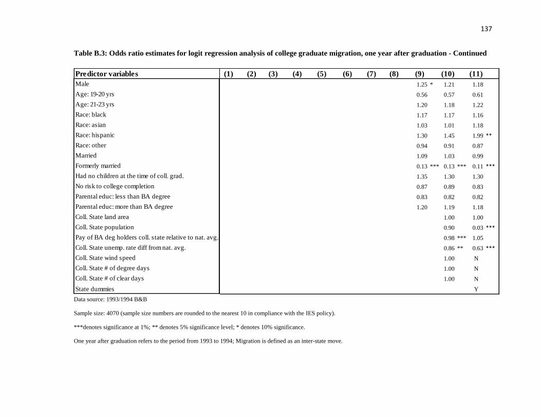
137

Table B.3: Odds ratio estimates for logit regression analysis of college graduate migration, one year after graduation - Continued

Data source: 1993/1994 B&B

Sample size: 4070 (sample size numbers are rounded to the nearest 10 in compliance with the IES policy).

***denotes significance at 1%; ** denotes 5% significance level; * denotes 10% significance.

One year after graduation refers to the period from 1993 to 1994; Migration is defined as an inter-state move.

Predictor variables (1) (2) (3) (4) (5) (6) (7) (8) (9) (10) (11)

Male 1.25 * 1.21 1.18

Age: 19-20 yrs 0.56 0.57 0.61

Age: 21-23 yrs 1.20 1.18 1.22

Race: black 1.17 1.17 1.16

Race: asian 1.03 1.01 1.18

Race: hispanic 1.30 1.45 1.99 **

Race: other 0.94 0.91 0.87

Married 1.09 1.03 0.99

Formerly married 0.13 *** 0.13 *** 0.11 ***

Had no children at the time of coll. grad. 1.35 1.30 1.30

No risk to college completion 0.87 0.89 0.83

Parental educ: less than BA degree 0.83 0.82 0.82

Parental educ: more than BA degree 1.20 1.19 1.18

Coll. State land area 1.00 1.00

Coll. State population 0.90 0.03 ***

Pay of BA deg holders coll. state relative to nat. avg. 0.98 *** 1.05

Coll. State unemp. rate diff from nat. avg. 0.86 ** 0.63 ***

Coll. State wind speed 1.00 N

Coll. State # of degree days 1.00 N

Coll. State # of clear days 1.00 N

State dummies Y

138

Table B.4: Odds ratio estimates for logit regression analysis of college graduate migration, one year after graduation

Excluding graduate students

Data source: 1993/1994 B&B

Sample size: 3280 (sample size numbers are rounded to the nearest 10 in compliance with the IES policy).

***denotes significance at 1%; ** denotes 5% significance level; * denotes 10% significance.

One year after graduation refers to the period from 1993 to 1994

Migration is defined as an inter-state move

Predictor variables (1) (2) (3) (4) (5) (6) (7) (8) (9) (10) (11)

Out-of-state college attendence 26.2 *** 26.1 *** 25.6 *** 25.4 *** 26.5 *** 25.3 *** 25.7 *** 25.4 *** 24.6 *** 26.3 ***

Foreign-born 0.48 *** 0.59 0.82 0.8 0.71 0.71 0.68 0.57 0.62 0.62

Out-of-state x foreign-born 0.94 0.75 0.69 0.75 0.74 0.74 0.73 0.72 0.64

% Of immigr. in coll. state 0.96 *** 0.96 *** 0.96 *** 0.96 *** 0.96 *** 0.96 *** 1.03 1.08

% Of immigr. in coll. state x foreign-born 0.99 0.99 0.98 0.98 0.98 0.99 0.98 0.97

GPA 1.00 1.00 1.00 1.00 1.00 1.00 1.00

Graduated with honors 1.11 1.08 1.08 1.07 1.08 1.1 1.09

Master's degree aspirations 1.32 * 1.29 * 1.29 * 1.3 * 1.28 * 1.29 * 1.34 *

Doctorate deg. aspirations 1.57 ** 1.6 ** 1.58 ** 1.47 * 1.41 * 1.42 * 1.43

Science major 1.42 1.43 1.39 1.27 1.23 1.19

Business major 1.19 1.19 1.21 1.18 1.24 1.29

Engineering major 2.19 *** 2.28 *** 2.3 *** 2.12 *** 2.13 *** 2.12 ***

Time taken to complete bachelor's degree: 5-6 yrs 0.85 0.85 0.82 0.84 0.85

Time taken to complete bachelor's degree: >6 yrs 0.65 0.64 0.66 0.69 0.69

Attended a private school 1.04 1.03 1.02 1.05 1.1

Currently employed 0.58 *** 0.61 *** 0.61 *** 0.6 ***

139

Table B.4: Odds ratio estimates for logit regression analysis of college graduate migration, one year after graduation

Excluding graduate students - Continued

Data source: 1993/1994 B&B

Sample size: 3280 (sample size numbers are rounded to the nearest 10 in compliance with the IES policy).

***denotes significance at 1%; ** denotes 5% significance level; * denotes 10% significance.

One year after graduation refers to the period from 1993 to 1994; Migration is defined as an inter-state move.

Predictor variables (1) (2) (3) (4) (5) (6) (7) (8) (9) (10) (11)

Male 1.23 1.2 1.17

Age: 19-20 yrs 0.61 0.63 0.7

Age: 21-23 yrs 1.07 1.03 1.07

Race: black 1.15 1.14 1.1

Race: asian 1.42 1.49 1.69

Race: hispanic 1.18 1.3 1.89

Race: other 1.26 1.23 1.24

Married 1.13 1.08 1.05

Formerly married 0.15 *** 0.14 *** 0.14 ***

Had no children at the time of coll. grad. 1.27 1.21 1.23

No risk to college completion 0.9 0.91 0.85

Parental educ: less than BA degree 0.85 0.83 0.83

Parental educ: more than BA degree 1.27 * 1.22 1.21

Coll. State land area 1 1

Coll. State population 0.85 ** 0.03 ***

Pay of BA deg holders coll. State relative to nat. avg. 0.99 ** 1.04

Coll. State unemp. rate diff from nat. avg. 0.87 ** 0.6 ***

Coll. State wind speed 1 N

Coll. State # of degree days 1 N

Coll. State # of clear days 1 N

State dummies Y

140

Table B.5: Odds ratio estimates for logit regression analysis of college graduate migration over different time periods (1 year after

graduation, 4 years after graduation and 10 years after graduation)

Data source: 1993/2003 B&B

***denotes significance at 1%; ** denotes 5% significance level; * denotes 10% significance; Migration is defined as an inter-state move.

All sample size numbers are rounded to the nearest 10 in compliance with the IES policy.

(1) (2) (3) (4) (5) (6)

Predictor variables 93/94 93/97 93/03 93/94 93/97 93/03

Out-of-state college attendence 25.87 *** 17.23 *** 9.85 *** 26.27 *** 23.59 *** 11.60 ***

Foreign-born 0.85 0.58 * 1.36 0.62 1.31 1.38

Out-of-state x foreign-born 0.43 * 0.52 * 0.67 0.64 * 0.44 0.50

% of immigr. in coll. state 1.12 1.02 0.93 * 1.08 1.10 0.92 **

% of immigr. in coll. state x foreign-born 0.97 0.99 0.92 ** 0.97 0.96 0.91 ***

Gpa 1.00 1.00 1.00 ** 1.00 1.00 1.00 *

Graduated with honors 1.06 1.05 0.94 1.09 1.38 0.81

Master's degree aspirations/ highest deg. Attained: MA 1.25 1.61 *** 1.15 1.34 *

Doctorate deg. Aspirations/ highest deg. Attained: PhD 1.42 * 1.42 * 1.90 *** 1.43

Science major 1.16 1.33 1.38 * 1.19 0.88 1.18

Business major 1.21 1.35 ** 1.05 1.29 1.56 ** 1.13

Engineering major 2.16 *** 1.97 *** 1.19 2.12 *** 1.69 ** 1.08

Time taken to complete bachelor's degree: 5-6 yrs 0.87 1.05 1.05 0.85 0.88 1.08

Time taken to complete bachelor's degree: >6 yrs 0.83 0.68 0.79 0.69 0.38 ** 0.68

Attended a private school 1.08 1.38 *** 1.40 *** 1.10 1.17 1.33 **

Currently employed 0.60 *** 0.60 *** 0.73 ** 0.60 *** 0.59 * 0.79

Sample size 4070 4070 4070 3280 2130 2900

INCLUDING GRAD STUDENTS EXCLUDING GRAD STUDENTS

141

Table B.5: Odds ratio estimates for logit regression analysis of college graduate migration over different time periods (1 year after

graduation, 4 years after graduation and 10 years after graduation) – Continued

Data source: 1993/2003 B&B

***denotes significance at 1%; ** denotes 5% significance level; * denotes 10% significance; Migration is defined as an inter-state move.

All sample size numbers are rounded to the nearest 10 in compliance with the IES policy.

Predictor variables 93/94 93/97 93/03 93/94 93/97 93/03

Male 1.18 1.23 * 1.14 1.17 1.02 1.01

Age: 19-20 yrs 0.61 0.58 1.13 0.70 0.51 0.81

Age: 21-23 yrs 1.22 1.27 1.37 1.07 0.93 1.10

Race: Black 1.16 1.24 1.50 ** 1.10 1.23 1.43

Race: Asian 1.18 0.92 0.93 1.69 0.71 0.93

Race: Hispanic 1.99 ** 2.13 ** 1.65 * 1.89 1.19 2.02 **

Race: Other 0.87 0.37 ** 0.88 1.24 0.33 * 0.45

Married 0.99 0.93 0.79 * 1.05 0.90 0.74 *

Had no children at the time of coll. grad. 1.30 1.87 ** 1.56 * 1.23 1.89 * 1.54

No risk to college completion 0.83 0.91 0.86 0.85 0.90 0.86

Parental educ: less than BA degree 0.82 0.94 0.84 0.83 1.08 0.82

Parental educ: more than BA degree 1.18 1.31 ** 1.15 1.21 1.34 1.10

Coll. State land area 1.00 1.00 1.00 1.00 1.00 1.00

Coll. State population 0.03 *** 0.12 *** 0.09 *** 0.03 *** 0.02 *** 0.05 ***

Pay of BA deg holders coll. State relative to nat. avg. 1.05 1.04 1.06 1.04 1.02 1.05

Coll. State unemp. rate diff from nat. avg. 0.63 *** 0.68 ** 0.79 ** 0.60 *** 0.58 ** 0.69 **

State dummies Y Y Y Y Y Y

Sample size 4070 4070 4070 3280 2130 2900

INCLUDING GRAD STUDENTS EXCLUDING GRAD STUDENTS

142

Appendix C

Tables and Figures of Chapter 4

C.1 Tables

Table C.1: Distribution of postsecondary choices for 2004 high school graduates according

to selectivity

Data source: ELS

All sample statistics are calculated using sample weights. All unweighted sample size numbers are rounded to the

nearest 10 in compliance with the IES policy.

Non-attend 2-yr coll.

4 (least sel.) 3 2 1 (most sel.)Overall average 19.4% 31.2% 9.7% 19.9% 11.8% 8.1%

Sample size 1660 2850 970 2030 1350 1010

Real family income:

Top (first) income quartile 5.1 19.2 7.2 23.2 24.1 21.1

Second income quartile 10.4 26.6 8.9 26.9 16.9 10.3

Third income quartile 19.6 33.1 10.2 20.9 10.2 6.1

Bottom (fourth) income quartile 30.8 36.7 10.5 13.4 5.5 3.2

Composite test score quartiles:

Top (first) test score quartile 5.7 13.8 6.8 25.5 24.6 23.7

Second test score quartile 11.2 28.8 9.6 27.5 15.7 7.2

Third test score quartile 23.1 37.1 10.4 20.6 6.7 2.0

Bottom (fourth) test score quartile 37.0 41.2 11.8 7.5 1.9 0.6

Race:

Asian 9.3 29.7 5.7 16.9 17.1 21.4

White 17.2 29.1 8.2 22.2 14.3 9.0

Other 27.9 26.4 9.9 19.3 8.8 7.7

Hipanic 26.4 43.3 11.2 9.8 4.9 4.4

Black 23.5 32.0 17.4 19.6 5.2 2.3

Gender

Female 16.2 31.8 9.8 21.5 12.4 8.3

Male 22.9 30.4 9.5 18.2 11.2 7.8

Family composition:

Both parent family 15.4 29.6 9.4 21.2 14.2 10.2

Single parent family 23.7 33.4 10.4 18.5 8.8 5.2

Parent plus partner family 27.2 33.6 9.7 18.1 7.4 4.1

Only guardian family 33.3 35.7 10.7 11.8 5.4 3.1

Highest parental educ:

More than college 6.7 18.1 7.0 25.3 21.7 21.2

College graduate 11.2 28.3 8.8 25.0 15.8 11.0

Some college 22.6 36.3 10.6 18.4 8.7 3.3

HS graduate or less 32.0 37.4 11.0 12.1 5.2 2.3

High school GPA (4 pt. scale) 2.5 2.8 3.0 3.2 3.4 3.5

selectivity rank of 4-yr coll. Non-attend 2-yr coll.

4 (least sel.) 3 2 1 (most sel.)Overall average 19.4% 31.2% 9.7% 19.9% 11.8% 8.1%

Sample size 1660 2850 970 2030 1350 1010

Real family income:

Top (fourth) income quartile 5.1 19.2 7.2 23.2 24.1 21.1

Third income quartile 10.4 26.6 8.9 26.9 16.9 10.3

Second income quartile 19.6 33.1 10.2 20.9 10.2 6.1

lowest (first) income quartile 30.8 36.7 10.5 13.4 5.5 3.2

Composite test score quartiles:

Top (fourth) test score quartile 5.7 13.8 6.8 25.5 24.6 23.7

Third test score quartile 11.2 28.8 9.6 27.5 15.7 7.2

Second test score quartile 23.1 37.1 10.4 20.6 6.7 2.0

Lowest test score quartile 37.0 41.2 11.8 7.5 1.9 0.6

Race:

Asian 9.3 29.7 5.7 16.9 17.1 21.4

White 17.2 29.1 8.2 22.2 14.3 9.0

Other 27.9 26.4 9.9 19.3 8.8 7.7

Hipanic 26.4 43.3 11.2 9.8 4.9 4.4

Black 23.5 32.0 17.4 19.6 5.2 2.3

Gender

Female 16.2 31.8 9.8 21.5 12.4 8.3

Male 22.9 30.4 9.5 18.2 11.2 7.8

Family composition:

Both parent family 15.4 29.6 9.4 21.2 14.2 10.2

Single parent family 23.7 33.4 10.4 18.5 8.8 5.2

Parent plus partner family 27.2 33.6 9.7 18.1 7.4 4.1

Only guardian family 33.3 35.7 10.7 11.8 5.4 3.1

Highest parental educ:

More than college 6.7 18.1 7.0 25.3 21.7 21.2

College graduate 11.2 28.3 8.8 25.0 15.8 11.0

Some college 22.6 36.3 10.6 18.4 8.7 3.3

HS graduate or less 32.0 37.4 11.0 12.1 5.2 2.3

High school GPA (4 pt. scale) 2.5 2.8 3.0 3.2 3.4 3.5

selectivity rank of 4-yr coll.

143

Table C.1: Distribution of postsecondary choices for 2004 high school graduates according

to selectivity – Continued

Data source: ELS, Digest of Education Statistics (NCES, 2005), NASSGAP (2005) and 2005 CPS.

All sample statistics are calculated using sample weights. All unweighted sample size numbers are rounded to the

nearest 10 in compliance with the IES policy.

Non-attend 2-yr coll.

4 (least sel.) 3 2 1 (most sel.)

High school sector:

Private h.s. 4.7 20.4 9.3 23.8 22.2 19.7

Public h.s. 20.8 32.2 9.7 19.5 10.8 6.9

High school quality ( % of 2003 hs. grads.

who attended a 4-yr. coll):

75-100% 6.7 15.8 9.5 27.3 20.7 20.0

50-74% 16.4 28.7 8.6 23.0 15.3 8.0

25-49% 23.3 34.7 11.0 18.3 7.8 5.1

11-24% 27.5 41.8 9.1 11.0 7.1 3.5

0-10% 32.3 45.9 9.0 9.7 1.8 1.4

High school urbanicity:

Urban 17.1 27.2 13.5 19.4 13.4 9.5

Suburban 19.4 32.4 7.8 20.2 11.7 8.5

Rural 22.5 33.2 9.7 19.8 10.0 4.9

High school region:

Northeast 15.7 26.1 7.2 26.0 11.7 13.3

South 21.9 29.2 12.6 18.1 10.3 8.0

West 20.4 39.6 7.3 17.1 9.5 6.2

Midwest 17.9 29.9 9.7 20.5 16.0 6.1

Postsecondary aspirations

Expect to receive BA or more 13.1 29.5 10.7 23.3 13.8 9.7

Expect to receive less that a BA 42.3 37.2 6.1 7.7 4.6 2.1

Social/cultural capital

Discuss high school with parents:

Sometime/often 16.5 29.5 9.9 21.5 13.1 9.4

Never 30.0 37.2 8.8 13.9 7.1 3.1

College proximity i.e. distance from high school location

to nearest 4 yr. degree granting college (miles)15 13 10 9 7 6

STATE-LEVEL VARIABLES

Home state grant aid per college-age student (2004 $) 214 215 232 237 234 250

(need-based and non need-based aid)

College costs

Avg. resident tuition at 2 yr. public colleges in home

state (2004 $) 2031 1949 2093 2171 2218 2057

Avg. resident tuition at 4 yr. public colleges in home

state (2004 $) 5152 5135 5185 5374 5299 5301

Home state labor mkt. conditions

(indirect opportunity cost of college attendance)

Unemployment rate for college-age students (%) 9.5 9.7 9.6 9.5 9.3 9.3

Median earnings for college-age students (2004 $) 24827 25085 24665 25145 25323 25508

Educational attainment in home state

% of state population that has at least a bachelor's degee 18.2 18.7 17.6 18.6 18.8 19.2

selectivity rank of 4-yr coll.

144

Table C.2: Students in Class of 2004 enrolling in most selective four-year college, by test

scores and family income quartile

Data source: ELS

All proportions are weighted with sampling weights

Bottom

(fourth) score

quartile

Third quartile Second quartile Top (first)

quartile

Distribution of students in most

selective 4 yr. colleges (%)

Highest (first) income quartile 0.7 3.2 8.6 30.1

Second income quartile 0.4 2.8 5.9 19.4

Third income quartile 0.3 1.6 4.5 12.0

Lowest (fourth) income quartile 0.3 0.9 3.3 6.0

B. Class of 2004

145

Table C.3: Marginal effect of enrolling in most selective four-year college; Class of 2004 (Multinomial logistic regressions)

Data source: ELS. The marginal effects are calculated at the average of the regressors. All regressions are clustered at the primary sampling unit level (high school level). *** 1%

significance level; ** 5% significance level; * 10% significance. Sample size: 9870 (sample size numbers are rounded to the nearest 10 in compliance with the IES policy).

1 2 3 4 5 6 7

Composite test score 0.52% *** 0.44% *** 0.40% *** 0.30% *** 0.29% *** 0.28% ***

GPA 2.92% *** 2.77% *** 2.58% *** 2.58% *** 2.55% *** 2.51% ***

Real family income ($1000, $2004) 0.16% *** 0.04% *** 0.01% *** 0.01% * 0.01% * 0.01% *

(Real family income)2 -0.0003% *** -0.00004% *** 0.000002% 0.000002% 0.000004% 0.000005%

Black 0.6% * 0.3% *

Asian 5.5% *** 4.4% ***

Hipanic 1.8% *** 1.4% **

Other 2.0% ** 1.7% **

Parents: college graduates -1.1% *** -0.7% *** -0.6% *** -0.6% ***

Parents:some college -3.0% *** -2.0% *** -1.8% *** -1.7% ***

Parents: hs or less -2.5% *** -1.7% *** -1.6% *** -1.5% ***

Private h.s. 0.05% 0.1% 0.1%

Rural -1.1% *** -0.8% *** -1.0% ***

suburban -0.6% ** -0.5% ** -0.8% ***

High school quality measure( % of 2003

hs. grads. who attended a 4-yr. coll):

11-24% 2.0% * 1.8% 1.5%

25-49% 2.1% * 2.2% * 1.9% *

50-74% 2.2% ** 2.3% * 2.0% *

75-100% 4.9% *** 5.1% ** 4.8% **

Midwest -1.6% *** -1.5% *** -1.1% ***

South -0.9% *** -0.9% *** 0.0%

West -1.3% *** -1.5% *** -1.0% ***

Distance (miles) -0.04% *** -0.03% *** -0.02% **

Discuss with parents 0.9% *** 1.0% *** 1.0% ***

Expect to receive BA or more 0.9% *** 0.8% *** 0.7% ***

Female -0.02% -0.1%

Single parent family -0.05% -0.1%

Parent plus partner family -0.7% *** -0.7% ***

Only guardian family 0.5% 0.6%

State-level variables

Grant aid per college-age student ($1000, $2004) 0.4%

146

Table C.3: Marginal effect of enrolling in most selective four-year college; Class of 2004 (Multinomial logistic regressions) –

Continued

Data source: ELS. The marginal effects are calculated at the average of the regressors. All regressions are clustered at the primary sampling unit level (high school

level). *** 1% significance level; ** 5% significance level; * 10% significance. Sample size: 9870 (sample size numbers are rounded to the nearest 10 in compliance

with the IES policy).

Table C.4: Measures of fit to compare multinomial logit models with quadratic income term and linear income term (Table C.3

details)

Model: Quadratic term Linear term Difference

N: 9870 9870 0

Log-Lik Intercept Only: -16943.741 -16943.741 0

Log-Lik Full Model: -13527.249 -13531.091 3.842

D: 27054.499(9654) 27062.183(9660) -7.684(-6)

McFadden's R2: 0.202 0.201 0

McFadden's Adj R2: 0.189 0.189 0

Maximum Likelihood R2: 0.192 0.192 0

Cragg & Uhler's R2: 0.264 0.264 0

Count R2: 0.316 0.316 0

Adj Count R2: 0.038 0.038 0

AIC: 2.784 2.785 -0.001

AIC*n: 27482.499 27486.183 -3.684

BIC: -61783.802 -61776.118 -7.684

BIC': -5959.243 -5951.559 -7.684

1 2 3 4 5 6 7

Avg. resident tuition at 2 yr. public colleges in home

state ($1000, $2004) -0.4% **

Avg. resident tuition at 4 yr. public colleges in home

state ($1000, $2004) 0.4% ***

UR -0.1%

% of state population that has at least a bachelor's degee 0.1% *

147

Table C.5: Postsecondary choices across the joint income and ability distribution, Multinomial logit; Class of 2004 (Marginal

effects)

Data source: ELS. The marginal effects are calculated at the average of the regressors. All regressions are clustered at the primary sampling unit level (high school level). ***denotes significance at 1%; ** denotes 5% significance level; * denotes 10% significance; Sample size: 9870 (sample size numbers are rounded to the nearest 10 in

compliance with the IES policy).

selectivity rank of 4-yr coll.

Composite test score -0.7% *** -1.0% *** -0.1% 0.8% *** 0.7% *** 0.3% ***

GPA -11.3% *** -12.1% *** 1.1% 11.2% *** 8.5% *** 2.6% ***

Real family income ($1000, $2004) -0.1% * 0.01% -0.1% * -0.002% 0.1% * 0.01% *

Family income x test scores 0.0004% -0.002% 0.001% 0.001% -0.0004% -0.00003%

Black -8.5% *** -13.5% *** 8.9% *** 11.5% *** 1.2% * 0.4% *

Asian -8.1% *** -2.7% -3.2% * 1.5% 8.1% *** 4.4% ***

Hipanic -4.5% *** 0.5% 5.2% ** -3.8% * 1.2% 1.5% ***

Other 1.4% -12.1% *** 3.6% 4.5% 0.9% 1.7% **

Parents: college graduates 0.2% 1.9% 2.8% * -2.7% -1.6% ** -0.7% ***

Parents:some college 6.5% *** 6.3% *** 1.7% -8.3% *** -4.2% *** -2.0% ***

Parents: hs or less 10.5% *** 6.5% ** -0.4% -10.1% *** -4.9% *** -1.7% ***

Private h.s. -5.2% *** 9.5% *** -0.4% -4.3% ** 0.3% 0.05%

Rural 3.7% ** 8.1% ** -4.7% *** -3.4% * -2.6% ** -1.0% ***

suburban 3.5% *** 9.5% *** -6.7% *** -3.2% * -2.4% ** -0.6% **

High school quality measure( % of 2003

hs. grads. who attended a 4-yr. coll):

11-24% -4.8% ** -11.7% ** -2.1% -0.2% 16.8% *** 2.0%

25-49% -7.4% *** -18.3% *** -0.4% 11.3% ** 12.7% *** 2.1% *

50-74% -8.7% *** -20.4% *** -3.9% 12.2% ** 18.6% *** 2.2% *

75-100% -12.8% *** -31.4% *** -3.8% 17.2% *** 25.8% *** 4.9% **

Midwest 2.0% 3.5% 1.9% -7.0% *** 1.1% -1.6% ***

South 3.5% ** 1.4% 5.1% *** -8.1% *** -0.9% -0.9% ***

West 1.5% 11.9% *** -2.7% -8.0% *** -1.4% -1.3% ***

1 (most sel.)3 2

2-yr coll.Non-attend

4 (least sel.)

148

Table C.5: Postsecondary choices across the joint income and ability distribution, Multinomial logit; Class of 2004 (Marginal

effects) – Continued

Data source: ELS

The marginal effects are calculated at the average of the regressors. All regressions are clustered at the primary sampling unit level (high school level).

***denotes significance at 1%; ** denotes 5% significance level; * denotes 10% significance; Sample size: 9870 (sample size numbers are rounded to the nearest 10 in

compliance with the IES policy).

selectivity rank of 4-yr coll.

Distance (miles) 0.1% *** 0.1% * -0.1% -0.1% -0.1% *** -0.04% ***

Discuss with parents -2.3% ** -4.6% *** 1.5% 3.2% ** 1.2% 0.9% ***

Expect to receive BA or more -16.6% *** -4.4% *** 4.6% *** 13.0% *** 2.5% *** 0.9% ***

Female -3.4% *** 2.3% -0.7% 1.9% -0.1% -0.1%

Single parent family 1.4% 0.5% -1.4% -0.3% -0.2% -0.01%

Parent plus partner family 6.2% *** 0.1% -1.2% -2.1% -2.4% *** -0.7% ***

Only guardian family 5.9% ** -0.2% -0.7% -5.2% -0.3% 0.6%

State-level controls Y Y Y Y Y Y

1 (most sel.)

Non-attend 2-yr coll.

4 (least sel.) 3 2

149

Table C.6: Higher education choice probabilities, Class of 2004

Data source: ELS

This table shows the predicted probabilities of enrolling in any college and a most selective four-year college for the

average respondent (average of all controls) at different values of income and test scores

Predicted probabilities are generated using the multinomial logit model results from Table C.5.

***denotes significance at 1%; ** denotes 5% significance level; * denotes 10% significance

Panel A

(1) (2) (3) (4) (5) (6)

income 25th income 75th change income 25th income 75th change

percentile percentile percentile percentile

0.838*** 0.877*** 0.039*** 0.020 0.023* 0.003

0.884*** 0.914*** 0.030** 0.053*** 0.063*** 0.01*

Panel B

(1) (2) (3) (4) (5) (6)

income 10th income 90th change income 10th income 90th change

percentile percentile percentile percentile

0.827*** 0.897*** 0.070*** 0.019** 0.026* 0.007

0.912*** 0.952*** 0.040** 0.106*** 0.133*** 0.027*

Any college Most selective 4-yr. college

Ability (test scores)

50th percentile

90th percentile

Any college Most selective 4-yr. college

Ability (test scores)

50th percentile

75th percentile

150

Table C.7: Impact on application decisions and admission probabilities to four-year colleges

Data source: ELS

All regressions include controls related to students’ demographics, parental involvement, post-secondary aspirations,

high school characteristics, and state-level variables.

Each column in both panels comes from a separate Poisson regression

All regressions are clustered at the primary sampling unit level (high school level).

***denotes significance at 1%; ** denotes 5% significance level; * denotes 10% significance.

Total 4 (least sel.) 3 2 1 (most sel.)

Composite test score 2.5 *** -1.0 *** 0.5 ** 2.9 *** 8.0 ***

GPA 38.3 *** -0.1 26.5 ** 31.5 *** 40.7 ***

Real family income ($1000, $2004) 0.1 *** -0.03 0.02 0.2 *** 0.2 ***

Black 28.9 *** 33.7 *** 25.5 *** 15.0 * 17.9 ***

Asian 45.8 *** -5.0 -3.3 33.1 *** 52.4 ***

Hipanic 4.2 ** 6.3 *** -5.6 -1.0 1.9 *

Other 24.4 19.6 27.5 22.1 20.5

Parents: college graduates -4.2 36.9 *** 11.2 ** -0.7 -18.2 *

Parents:some college -18.5 *** 28.5 *** 2.7 -20.2 *** -36.3 ***

Parents: hs or less -24.1 *** 26.5 ** -9.9 * -26.0 *** -41.0 ***

Additional Controls Y Y Y Y Y

Total 4 (least sel.) 3 2 1 (most sel.)

Composite test score 1.7 *** 0.7 *** 1.0 *** 1.6 *** 3.6 ***

GPA 29.6 *** 9.3 *** 15.1 *** 34.9 *** 64.3 ***

Real family income ($1000, $2004) 0.1 ** 0.1 0.004 ** 0.05 *** 0.02 **

Black 18.2 *** 16.1 *** 11.2 * -3.9 10.4

Asian 13.5 *** -0.3 ** -1.5 2.9 34.2 ***

Hipanic 5.1 ** 5.9 ** -1.6 2.9 1.6 **

Other 14.9 6.7 8.4 3.8 6.5

Parents: college graduates -4.7 * 12.3 *** 3.0 -6.6 * -16.9 ***

Parents:some college -11.3 *** 6.9 * -4.1 -11.7 *** -23.2 ***

Parents: hs or less -7.4 ** 9.5 ** -1.8 -4.7 -11.0

Additional Controls Y Y Y Y Y

selectivity rank of 4-yr coll.

A. Number of Applications

B. Number of Admissions conditional on applying

selectivity rank of 4-yr coll.

151

Table C.8: Influence of changing characteristics and changing coefficients on probability of

enrollment in a most selective four-year colleges

Data source: ELS and NELS

This table shows the predicted probabilities of enrolling in a most selective four-year college for the average respondent at

different points in the joint income-ability distribution.

***denotes significance at 1%; ** denotes 5% significance level; * denotes 10% significance

Table C.9: Testing for pooled outcomes

Likelihood Ratio tests for combining outcome categories; 0 = non-attendance, 1 = community college enrollment, 2 =

enrollment in least selective 4-yr. college, 3 = 4-yr. college of selectivity rank 3, 4 = 4-yr. college of selectivity rank 2

, and 5 = most selective 4-yr.

Ho: All coefficients except intercepts associated with given pair of outcomes are 0 (i.e., categories can be collapsed).

1992

coefficients

2004

coefficients

1992

coefficients

2004

coefficients

Actual 1992 Predicted 1992 Predicted 2004 Actual 2004

(1) (2) (3) (4)

75th percentile 25th percentile 00.036*** 0.074** 0.040** 0.059***

90th percentile 10th percentile 0.038*** 0.144 0.051* 0.111***

75th percentile 75th percentile 0.062*** 0.087 0.095** 0.073***

90th percentile 90th percentile 0.106*** 0.168 0.148* 0.139***

Difference

75th percentile score, (75th -25th)percentile income diff. 0.026* 0.012* 0.055* 0.014*

90th percentile score, (90th -10th)percentile income diff. 0.068* 0.024 0.097 0.028*

1992 characteristics 2004 characteristics

High test score but low income

High test score and high income

Outcomes No. of outcomes df P>chi2

0,1,2,3,4,5 6

0/1,2,3,4,5 5 32 <0.001

0/2,1,3,4,5 5 32 <0.001

0/3,1,2,4,5 5 32 <0.001

0/4,1,2,3,5 5 32 <0.001

0/5,1,2,3,4 5 32 <0.001

0,1/2,3,4,5 5 32 <0.001

0,1/3,2,4,5 5 32 <0.001

0,1/4,2,3,5 5 32 <0.001

0,1/5,2,3,4 5 32 <0.001

0,1,2/3,4,5 5 32 <0.001

0,1,2/4,3,5 5 32 <0.001

0,1,2/5,3,4 5 32 <0.001

0,1,2,3/4,5 5 32 <0.001

0,1,2,3/5,4 5 32 <0.001

0,1,2,3,4/5 5 32 <0.001

Unrestricted

Pool 3 with 5 1187.5

Pool 4 with 5 483.3

Pool 2 with 5 1695.7

Pool 3 with 4 428.2

Pool 2 with 3 361.0

Pool 2 with 4 967.2

Pool 1 with 4 2421.0

Pool 1 with 5 3367.0

Pool 1 with 2 543.3

Pool 1 with 3 1526.3

Pool 0 with 5 4280.6

Pool 0 with 2 1079.4

Pool 0 with 3 2651.3

Pool 0 with 1 732.2

Categories tested chi2

Pool 0 with 4 3471.9

152

Table C.10: Robustness check: Postsecondary choices (using different categorization of college sectors) across the joint income and

ability distribution; Class of 2004 (Marginal effects from a multinomial logit model)

Data source: ELS. The marginal effects are calculated at the average of the regressors. All regressions are clustered at the primary sampling unit level (high school level).

***denotes significance at 1%; ** denotes 5% significance level; * denotes 10% significance; Sample size: 9870 (sample size numbers are rounded to the nearest 10 in

compliance with the IES policy).

Composite test score -0.8% *** -1.0% *** 0.9% *** 0.4% *** 0.6% ***

GPA -11.1% *** -13.2% *** 12.1% *** 3.8% *** 8.4% ***

Real family income ($1000, $2004) -0.1% ** 0.2% * -0.1% 0.02% * -0.1% **

Family income x test scores 0.0005% -0.004% ** 0.001% 0.0002% 0.003% **

Black -9.1% *** -15.6% *** 16.0% *** 0.7% * 7.9% ***

Asian -8.0% *** -5.1% * 5.9% ** 6.1% *** 1.2%

Hipanic -4.7% *** -1.3% 1.1% 0.2% 4.8% **

Other 0.9% -11.9% *** 0.6% 2.9% * 7.6% **

Parents: college graduates -0.2% 2.8% 2.8% -0.6% -4.8% ***

Parents:some college 5.5% *** 7.9% *** -3.3% -2.6% *** -7.5% ***

Parents: hs or less 9.2% *** 7.3% *** -3.3% -3.0% *** -10.2% ***

Private h.s. -5.5% *** 6.9% ** -6.3% *** -1.3% ** 6.1% ***

Rural 1.0% 8.5% *** -4.2% * -2.3% *** -2.9% *

suburban 2.3% ** 9.5% *** -5.8% *** -2.0% *** -4.1% ***

High school quality measure( % of 2003

hs. grads. who attended a 4-yr. coll):

11-24% -4.2% ** -9.1% ** -0.8% 8.5% 5.5%

25-49% -7.2% *** -15.9% *** 5.4% 9.3% ** 8.5% **

50-74% -8.6% *** -16.9% *** 4.9% 13.4% ** 7.2% **

75-100% -12.1% *** -27.7% *** 7.4% 19.3% ** 13.0% ***

Midwest 1.0% 7.3% ** -3.4% -0.7% * -4.3% ***

South 4.3% * 0.8% 1.8% 0.9% -7.7% ***

West 3.7% 1.7% 1.7% -0.2% * -7.0% ***

Non-attend 2-yr coll.

Non-flagship pub. Flagship pub.

4-yr coll.

Private

153

Table C.10: Robustness check: Postsecondary choices (using different categorization of college sectors) across the joint income and

ability distribution; Class of 2004 (Marginal effects from a multinomial logit model) – Continued

Data source: ELS

The marginal effects are calculated at the average of the regressors. All regressions are clustered at the primary sampling unit level (high school level).

***denotes significance at 1%; ** denotes 5% significance level; * denotes 10% significance; Sample size: 9870 (sample size numbers are rounded to the nearest 10 in

compliance with the IES policy).

Distance (miles) 0.1% *** 0.2% ** -0.2% *** -0.01% -0.1% ***

Discuss with parents -2.1% ** -5.4% *** 4.1% ** 1.2% ** 2.1% *

Expect to receive BA or more -15.1% *** -5.0% *** 13.8% *** 0.7% 5.5% ***

Female -3.3% *** 2.1% -1.0% 0.7% 1.5%

Single parent family 0.8% 0.7% -2.6% 0.6% 0.5%

Parent plus partner family 6.0% *** 0.9% -2.8% -0.8% -3.2% **

Only guardian family 5.1% * 0.3% -9.1% *** 1.9% 1.8%

State-level controls Y Y Y Y Y

Non-attend 2-yr coll. 4-yr coll.

Non-flagship pub. Flagship pub. Private

154

Table C.11: Robustness check (continued) Higher education choice probabilities, Class of 2004

Data source: ELS

This table shows the predicted probabilities of enrolling in any college and a 4-yr. flagship public college for the average respondent at different values of income and

test scores

Predicted probabilities are generated using the multinomial logit model results from Table C.10.

***denotes significance at 1%; ** denotes 5% significance level; * denotes 10% significance.

Panel A

(1) (2) (3) (4) (5) (6)

income 25th income 75th change income 25th income 75th change

percentile percentile percentile percentile

0.843*** 0.895*** 0.052*** 0.041 0.055** 0.014*

0.892*** 0.930*** 0.038*** 0.069*** 0.095*** 0.026*

Panel B

(1) (2) (3) (4) (5) (6)

income 10th income 90th change income 10th income 90th change

percentile percentile percentile percentile

0.827*** 0.918*** 0.091*** 0.039** 0.064*** 0.025*

0.915*** 0.965*** 0.050*** 0.092*** 0.154*** 0.062*

Ability (test scores)

50th percentile

90th percentile

4-yr. flagship public college

Ability (test scores)

50th percentile

75th percentile

Any college 4-yr. flagship public college

Any college

155

C.2 Figures

Figure C.1: Log-odds of attending a most selective four-year college versus a least selective

four-year college, by income

Data source: ELS

-2

-1.5

-1

-0.5

0

0.5

1

1.5

2

5,000 15,000 24,181 31,829 44,834 65,956 91,715 136,556 339,689

Income ($)

Log

it

156

Bibliography

Astin, A., & Oseguera, L. (2004). The declining ‘‘equity’’ in American higher education. Review of

Higher Education, 27(3), 321–341.

Altbach, P. (1991). Impact and Adjustment: Foreign Students in Comparative Perspective. Higher

Education, 21, 305-323.

Andersson,F., & Konrad, K.A. (2003). Globalization and Risky Human-Capital Investment. International

Tax and Public Finance, 10(3), 211-228.

Baryla, E., & Dotterweich, D. (2001). Student migration: Do significant factors vary by region?

Education Economics, 9(3), 269–280.

Ballweg, L.A., & Li,L. (1992). Employment Migration among Graduates of Southern Land Grant

Universities. Southern Rural Sociology,9(1).

Barron’s. (2004). Barron’s profiles of American colleges 2005. New York, NY: Barron’s Educational

Series Inc., College Division.

Baryla,E., & Dotterweich, D. (2001). Student migration: Do significant factors vary by region? Education

Economics, 9(3), 269–280.

Baryla,E., & Dotterweich, D. (2006). Institutional focus and non-resident student enrollment.

International Journal of Educational Management, 20(4), 239-248.

Becker, G. (1964). Human Capital: A Theoretical and Empirical Analysis, with Special Reference to

Education. New York, NY: Columbia University Press.

157

Behrman, J., Kletzer, L., McPherson, M., & Schapiro, M. (1995). How Family Background Sequentially

Affects College Choices: High School Achievement, College Enrollment and College Quality.

Mimeo, Economics Department, University of Pennsylvania.

Behrman, J., Kletzer, L., McPherson ,M., & Schapiro, M. (1998). The Microeconomics of College

Choice, Careers, and Wages: Measuring the Impact of Higher Education. Annals of the American

Academy of Political and Social Science, 559, 12–23.

Belley, P., & Lochner, L. (2007). The Changing Role of Family Income and Ability in Determining

Educational Achievement. Journal of Human Capital, 1 (1), 37–89.

Binder, M., & Ganderton, P. T. (2002). Incentive effects of New Mexico’s merit-based state scholarship:

Who responds and how? In D. E. Heller, & P. Marin (Eds.), Who should we help? The negative

social consequences of merit scholarships (pp. 41–56). Cambridge, MA: The Civil Rights Project

at Harvard University.

Black, M. (1983). Migration of Young Labor Force Entrants. Socio-economic Planning Sciences, 17(5-

6),267-280.

Black, D.A., & Smith, J. (2004). How Robust Is the Evidence on the Effects of College Quality?

Evidence from Matching. Journal of Econometrics, 121:99-124.

Black, D.A., and Smith,J. (2006). Estimating the Returns to College Quality with Multiple Proxies for

Quality. Journal of Labor Economics, 24 (3): 701–28.

Borjas, G.J., Bronars, S.G., & Trejo,S.J. (1992). Self-Selection and Internal Migration in the United

States. Journal of Urban Economics, 32(2), 159-185.

Borjas, G.J. (1999). The Economic Analysis of Immigration. In O. Ashenfelter, & D. Card (Eds.),

Handbook of Labor Economics (pp. 1697-1760). North Holland.

158

Bound,J., Groen,J., Kezdi,G., & Turner,S.E. (2004). Trade in University Training: Cross-State Variation

in Production and Stock of College Educated Labor. Journal of Econometrics, 121(1-2), 143-173.

Bound, J., Lovenheim, M., & Turner,S. ( 2010). Why Have College Completion Rates Declined? An

Analysis of Changing Student Preparation and Collegiate Resources. American Economic

Journal: Applied Economics, 2(3), 1-31.

Bowles,S. (1970). Migration as Investment: Empirical Tests of the Human Investment Approach to

Geographic Mobility. Review of Economics and Statistics,52,356-362.

Bourdieu, P., & Passeron, J. C. (1977). Reproduction in education, society and culture. Beverly Hills,

CA: Sage.

Bradburn, N., & Cataldi. (2006). Where Are They Now? A Description of 1992–93 Bachelor’s Degree

Recipients 10 Years Later (NCES 2007–159). Washington, DC: National Center for Education

Statistics.

Brewer, D., Eide,E., & Ehrenberg, R. (1999). Does it Pay to Attend an Elite Private College? Cross-

Cohort Evidence on the Effects of College Type on Earnings. Journal of Human Resources,

34(1), 104-123.

Busch,O. & Weigert,B. (2007). Where Have All the Graduates Gone? Internal Cross-State Migration of

Graduates in Germany 1984-2004. The Annals of Regional Science,44,559-572 .

Cameron, S., & Taber,C. (2004). Estimation of Educational Borrowing Constraints Using Returns to

Schooling. Journal of Political Economy, 112(1), 132–82.

Cameron, S., & Heckman, J. (2001). The dynamics of educational attainment for Black, Hispanic, and

White males. Journal of Political Economy, 109(3), 455-499.

159

Carneiro, P., & Heckman,J. (2002). The Evidence on Credit Constraints in Post-secondary Schooling. The

Economic Journal, 112 (482), 705–34.

Charleston, S., Riccobono, J., Mosquin,P., Link,M., & Griffith,J. (2003). Baccalaureate and Beyond

Longitudinal Study: 2000–01 (B&B: 2000/01) Methodology Report (NCES 2003–156).

Washington, DC: National Center for Education Statistics.

College Board. (2011). Trends in college pricing 2011. Retrieved December 26, 2011 from

http://trends.collegeboard.org/downloads/college_pricing/PDF/Trends_in_College_Pricing_2011

_Tuition_Fees_Over_Time.pdf

Clinedinst, M. E., & Hawkins, D. A. (2009). State of college admissions. Alexandria: National

Association of College Admission Counseling.

Cornwell, C., Mustard, D. B., & Sridhar, D. J. (2006). The enrollment effects of merit-based financial aid:

Evidence from Georgia’s program. Journal of Labor Economics, 24(4), 761–786.

Cramer, J.S., & Ridder, G. (1991). Pooling States in the Multinomial Logit Model. Journal of

Econometrics, 47, 267–272.

Cushing, B. & Poot, J. (2004). Crossing Boundaries and Borders: Regional Science Advances in

Migration Modeling. Papers in Regional Science, 83, 317-338.

Dale, S., & Krueger, A.B. (2014). Estimating the Effects of College Characteristics over the career using

administrative earnings data. Journal of Human Resources, 49(2), 323-358.

DaVanzo, J. (1978). Does Unemployment Affect Migration? Evidence from Micro Data. Review of

Economics and Statistics, 60(4), 504-514.

DaVanzo, J. (1981). Microeconomic Approaches to Studying Migration Decisions. In G. De Jong, & R.

Gardner (Eds.), Migration Decision-Making. New York, NY: Pergamon Press.

160

Davies,S. & Guppy,N. (1997). Fields of study, college selectivity, and student inequalities in higher

education. Social Forces, 75(4), 1417-38

DelRey, E. (2001). Economic Integration and Public Provision of Education. Empirica,28(2), 203-218 .

Dean, R.D., Hunt, L., & Smith,R. (2006). Committing to Keep Illinois Students In-State : Understanding

College Choice, Student Migration Patterns, and Retention Strategies. Illinois: Center for the

Study of Education Policy, Illinois State University/ Illinois Board of Higher Education.

DesJardins, S. L. (2001). Assessing the effects of changing institutional aid policy. Research in Higher

Education, 42(6), 653-678.

Dowd, A.C. & Duggan,M.B. (2001). Computing variances from data with complex samplingdesigns: a

comparison of Stata and SPSS. Paper presented at the North American StataUsers Group

Meeting.

Dynarski, S. (2000). Hope for whom? Financial aid for the middle class and its impact on college

attendance. National Tax Journal, 53(3), 629–663.

Dynarski, S. (2004). The new merit aid. In C. M. Hoxby (Ed.), College choices: The economics of where

to go, when to go, and how to pay for it (pp. 63–100). Chicago: University of Chicago Press.

Dynarski, S., & Scott-Clayton, J. (2006). The Cost of Complexity in Federal Student Aid: Lessons from

Optimal Tax Theory and Behavioral Economics (Working Paper No. 12227). Retrieved from

National Bureau of Economic Research website: http://users.nber.org/~dynarski/w12227.pdf

Ellwood, D. T., & Kane,T. (2000). Who Is Getting a College Education? Family Background and the

Growing Gaps in Enrollment. In S. Danzinger, & J. Waldfogel (Eds.), Securing the Future:

Investing in Children from Birth to College (pp. 283-324). New York, NY: Russell Sage

Foundation.

161

Fuller, W.C., Manski, C., & Wise, D. (1982). New Evidence on the Economic Determinants of

Postsecondary Schooling Choices. Journal of Human Resources, 17 (4), 477–98.

Gottlieb, P.D., & Joseph, G. (2006). College-to-work migration of technology graduates and holders of

doctorates within the United States. Journal of Regional Science, 46(4), 627–649.

Greene, W. H. (2008). Econometric Analysis (6th ed.). Upper Saddle River, NJ: Pearson.

Greenwood, M.J. (1975). Research on Internal Migration in the United States: A Survey. Journal of

Economic Literature, 13, 397-433.

Greenwood, M. J. (1997). Internal migration in developed countries. In M.R. Rosenzweig, &

O. Stark (Eds.), Handbook of Population and Family Economics (pp. 647-720). Amsterdam:

Elsevier.

Greenwood, M.J., &. Hunt, G.L. (1989). Jobs versus Amenities in the Analysis of Metropolitan

Migration. Journal of Urban Economics, 25(1), 1--16.

Groen, J.A., & White, M.J. (2003). In-state versus out-of-state students: The divergence of interest

between public universities and state governments (CHERI Working Paper #25). Retrieved from

Cornell University, ILR School site: http://digitalcommons.ilr.cornell.edu/workingpapers/33/

Groen, J. (2004). The Effect of College Location on Migration of College-Educated Labor. Journal of

Econometrics, 121, 125–142.

Hall, A. R., Rudebusch,G.D., & Wilcox,D.W. (1996). Judging instrument relevance in instrumental

variables estimation. International Economic Review, 37, 283–298.

Hansen, S., Ban,C., & Huggins, L. (2003). Experiencing the Brain-Drain from Older Industrial Cities:

The Pittsburgh Region. The Economic Development Quarterly, 17 (2), 132-147 .

162

Haskins, R. (2009). Education and Economic Mobility. In J.B. Isaacs, I.V. Sawhill, & R. Haskins, (Eds.),

Getting Ahead or Losing Ground: Economic Mobility in America. Washington, DC: Brookings

and Pew Charitable Trusts.

Hausman, J., & McFadden, D. (1984). Specification Tests for the Multinomial Logit Model.

Econometrica, 52 (5), 1219-1240.

Heller, D. E. (2002). Is merit-based student aid really trumping need-based aid? Another view. Change,

34(4), 6–8.

Heller, D. E. (2006). Merit aid and college access. Madison: Wisconsin Center for the Advancement of

Postsecondary Education, University of Wisconsin.

Heuer, R. (2004). Migration of Recent College Graduates. Unpublished doctoral dissertation. North

Carolina State University.

Hoekstra, M. (2009). “The Effect of Attending the Flagship State University on Earnings: A

Discontinuity-Based Approach.” Review Economics and Statistics, 91 (4), 717–24.

Hossler, D., & Gallagher, K. (1987). Studying student college choice: A three-phase model and the

implications for policymakers. College and University, 62(3), 207-221.

Hou, F. (2007). Changes in the Initial Destinations and Redistribution of Canada's Major Immigrant

Groups: Reexamining the Role of Group Affinity1. Ottawa, Ontario: Socioeconomic and Business

Analysis Branch, Statistics Canada.

Hoxby, C. M., & Long, B. T. (1999). Explaining the rising income and wage inequality among the

college-educated (Working paper No. 6873). Retrieved from National Bureau of Economic

Research website: http://www.nber.org/papers/w6873

163

Hoxby, C. M. (2009). The Changing Selectivity of American Colleges. Journal of Economics

Perspectives, 23 (4), 95–118.

Hoxby, C. M., & Avery, C. (2013). The Missing “One-Offs:” The Hidden Supply of High-Achieving,

Low Income Students (Working Paper 18586). Retrieved from National Bureau of Economic

Research website: http://www.nber.org/papers/w18586

Huang, J., Guo, B., Kim, Y., & Sherraden, M. (2009). Parental Income, Assets, Borrowing Constraints,

and Children’s Post-Secondary Education. Children and Youth Services Review, 32 (4), 585–94.

Indiana Fiscal Project. (1999). Graduate Migration from Indiana's Postsecondary Institution.

Indianapolis: Indiana Fiscal Policy Institute.

Ingels, S.J., Pratt, D.J., Wilson, D., Burns, L.J., Currivan, D., Rogers, J.E., & Hubbard-Bednasz, S.(2007).

Education Longitudinal Study of 2002: Base-Year to Second Follow-up Data File Documentation

(NCES 2008-347). Washington, DC: National Center for Education Statistics.

Institute of International Education. (2006). International Students by Academic Level, 2004/05-2005/06.

Open Doors Report on International Educational Exchange. Retrieved June 24, 2013 from

http://www.iie.org/opendoors

Institute of International Education. (2012). International Students by Academic Level, 2010/11 -

2011/12. Open Doors Report on International Educational Exchange. Retrieved June 24, 2013

from http://www.iie.org/opendoors)

Justman, M., & Thisse, J.F. (2000). Local Public Funding of Higher Education When Skilled Labor is

Imperfectly Mobile. International Tax and Public Finance, 7, 247-258.

164

Kane, T. (1994). College entry by Blacks since 1970: The role of college costs, family backgrounds, and

the returns to education. Journal of Political Economy, 102(5), 878-911.

Kane, T. (1996). College cost, borrowing constraints and the timing of college entry. Eastern Economic

Journal, 22(2), 181-194.

Kane, T. (1998). Racial and Ethnic Preferences in College Admissions. In C. Jencks & M. Phillips

(Eds.), The Black-White Test Score Gap (pp. 431-456). Washington, DC: Brookings Institution

Press.

Kane, T. (2001). College-Going and Inequality: A Literature Review. School of Public Policy and Social

Research, UCLA.

Kane, T. (2006). Public Intervention in Post-secondary Education. In E. Hanushek & F. Welch (Eds.),

Handbook of the Economics of Education. New York, NY: Elsevier.

Kelderman, E. (2011). State Spending on Higher Education Edges Down, as Deficits Loom. Retrieved

August 30, 2011 from the Chronicle of Higher Education: http://chronicle.com/article/State-

Spending-on-Colleges/126020/

Kiernan, K. (1979). Characteristics of Young People who Move Inter-Regionally: A Longitudinal Study.

In J. Hobcraft & P. Rees (Eds.), Regional Demographic Development (pp211-227). London:

Croom-Helm.

Kinsler, J., & Pavan, R. (2011). Family Income and Higher Education Choices: The Importance of

Accounting for College Quality. Journal of Human Capital, 5(4), 453-477.

Kodrzyski, Y.K. (1999). Geographic Shifts in Higher Education. New England Economic Review,

July/August, 27-47 .

165

Kodrzycki, Y. K. (2001). Migration of recent college graduates: Evidence from the National Longitudinal

Survey of Youth. Federal Reserve Bank of Boston New England Economic Review, 1, 13–34.

Kritz, M., & Gurak, D. (2001). The Impact of Immigration on the Internal Migration of Natives and

Immigrants. Demography, 38(1), 133-45.

Kritz, M., & Nogle, J. (1994). Nativity Concentration and Internal Migration among the Foreign-Born .

Demography, 31(3), 509-524.

Lin, Z. (1998). Foreign-born vs. Native-born Canadian: A Comparison of their Inter-Provincial Mobility.

Ottawa, Ontario: Analytical Studies Branch Research series, Statistics Canada

Long, S. (1997). Regression Models for Categorical and Limited Dependent Variables. Thousand Oaks,

London: Sage.

Long, B.T. (2004). How Have College Decisions Changed Over Time? An Application of the Conditional

Logistic Choice Model. Journal of Econometrics, 121(1-2), 271-296.

Long, J. S., & Freese, J. (2005). Regression models for categorical dependent variables using Stata (2nd

ed.). College Station, TX: Stata Press.

Long, M.C. (2008). College quality and early adult outcomes. Economics of Education Review, 27(5),

588-602.

Long, M.C. (2004). College Applications and the Effect of Affirmative Action. Journal of

Econometrics,121, 319-342.

Lovenheim, M.F., & Reynolds, C. L. (2011). Changes in Postsecondary Choices by Ability and Income:

Evidence from the National Longitudinal Surveys of Youth. Journal of Human Capital 5 (1), 70–

109.

166

Lovenheim, M. F., & Reynold, C. L. (2012). The Effect of Housing Wealth on College Choice: Evidence

from the Housing Boom (Working Paper No. 18075). Retrieved from National Bureau of

Economic Research website: http://www.nber.org/papers/w18075

Mak, J., & Moncur, E. T. (2003). Interstate migration of college freshmen. The Annals of Regional

Science, 37(4), 603–612.

Malamud, O., & Wozniak, A. (2008). The Impact of College Graduation on Geographic Mobility:

Identifying Education Using Multiple Components of Vietnam Draft Risk. IZA Discussion Paper

no.3432.

McDonough, P. M. (1997). Choosing colleges: How social class and schools structure opportunity.

Albany, NY: State University of New York Press.

McFadden, D. (1973). Conditional Logit Analysis of Qualitative Choice Behaviour. In P. Zarembka

(Ed.), Frontiers in Econometrics (pp. 105–142). New York, NY: Academic Press.

McFadden, D., & Train, K.(2000). Mixed MNL Models for Discrete Response. Journal of Applied

Econometrics, 15, 447–470.

McHugh, R., & Morgan, J. N. (1984). The determinants of interstate student migration: A place to-place

analysis. Economics of Education Review, 3, 269–278.

McHugh, K.E. (1989). Hispanic Migration and Population Redistribution in the United States.

Professional Geographer, 41, 429-439.

Meng, C. L., & Schmidt, P. (1985). On the cost of partial observability in the bivariate probit model.

International Economic Review, 26, 71–85.

Mixon, F. G. (1992). A public choice note on college student migration. International Journal of

Manpower, 13(3), 63.

167

Mixon, F. G., & Hsing, Y. (1994). The determinants of out-of-state enrollments in higher education: A

Tobit analysis. Economics of Education Review, 13(4), 183–195.

Molho, I. (1987). Migration Decisions of Young Men in Great Britain. Applied Economics, 19, 221-243.

Moretti, E. (2004). Estimating the Social Return to Higher Education: Evidence from Longitudinal

and Repeated Cross-Sectional Data. Journal of Econometrics, 121, 175-212.

National Center for Educational Statistics. (2011). Digest of education statistics: 2011. Retrieved October

25, 2012 from http://nces.ed.gov/programs/digest/d09/tables/dt09_222.asp

National Association of Colleges and Employers. (2013). NACE salary survey – starting salary for new

college graduates. Retrieved June 24, 2013 from:

http://www.naceweb.org/uploadedFiles/NACEWeb/Research/Salary_Survey/Reports/salary-

survey-april-2013-executive-summary.pdf

Newbold, K. (1996). Internal Migration of the Foreign-born in Canada. International Migration

Review,30, 728–747.

Nguyen, A.N., & Taylor, J. (2003), Post-High School Choices: New Evidence from a Multinomial Logit

Model. Journal of Population Economics, 16(2), 287–306.

Orsuwan, M. & Heck,R. (2009). Merit-based student aid and freshman interstate college migration.

Research in Higher Education, 50(1), 24-51.

Ostrovsky, Y., Hou, F., & Picot, G. (2008). Internal Migration of Immigrants: Do Immigrants Respond to

Regional Labor Demand Shocks? Ottawa, Ontario: Analytical Studies Branch Research series,

Statistics Canada.

168

Paulsen, M. B., & St. John, E. P. (2002). Social class and college costs: Examining the financial nexus

between college choice and persistence. Journal of Higher Education, 73(2), 189-236.

Perna, L. W., & Titus, M. A. (2004). Understanding differences in the choice of college attended: The

role of state public policies. Review of Higher Education, 27(4), 507–525.

Perry, K. K. (2001). Where college students live after they graduate (ERIC Document Reproduction

Service No. ED453739). Washington, DC: National Center for Government Statistics.

Petersen, T. (1984). A comment on presenting results from logit and probit models. American

Sociological Review,50, 130-131.

Plane, D.A., & Heins, F. (2003). Age Articulation of U.S. Inter-Metropolitan Migration. Annals of

Regional Science, 37, 107-130.

Piketty, T., & Saez, E. (2003). Income Inequality in the United States, 1913-1998. The Quarterly Journal

of Economics, 118(1), 1-39.

Posselt, J.R., Jaquette, O., Bielby, R., & Bastedo, M.N. (2012). Access Without Equity: Longitudinal

Analyses of Institutional Stratification by Race and Ethnicity, 1972–2004. American Educational

Research Journal, 49 (6), 1074–1111.

Poutvaara, P., & Kanniainen, V. (2000). Why Invest in Your Neighbour?Social Contract on Educational

Investment. International Taxation and Finance, 7(4), 547-562 .

Prospero, L. (2001). Brain drain of students triggers state’ concern. Retrieved May 8, 2001 from San

Diego Union Tribune: http://www.uniontrib.com/

169

Quigley, J.M., & Rubenfield, D.L. (1993). Public Choices in Public Higher Education. In Clotfelter &

Rothschild (Eds.), Studies of Supply and Demand in Higher Education (pp. 243-278). Chicago:

University of Chicago Press.

Reardon, S.F., Valentino, R.A., & Kenneth, A.S. (2012). Patterns of literacy among U.S. students. The

Future of Children, 22(2), 17-38.

Reseck, R.W., Merriman, D.F., Hartter, S. R., McCarthy, D. M., & Byrne, P. F. (2000). Illinois higher

education: Building the economy, shaping society. Champaign-Urbana, IL: Institute of

Government and Public Affairs, University of Illinois / Illinois Board of Higher Education.

Rigol, G. (2003).Admissions decision-making models: How U.S. institutions of higher education select

undergraduate students. New York, NY: College Entrance Examination Board.

Rogers, A., & Hening, S. (1999). The Internal Migration Patterns of the Foreign-Born and Native-Born

Populations in the United States. International Migration Review, 33(2), 403-429 .

Roback, J. (1982). Wages, Rents, and the Quality of Life. Journal of Political Economy, 90(6), 1257–

1278

Sa, C., Florax, M., & Rietveld, P. (2004). Determinants of the Regional Demand for Higher Education in

the Netherlands: a gravity approach model. Regional Studies, 38(4), 375-392.

Sanderson, & Dugoni. (2002). Interstate Migration Patterns of Recent Science and Engineering

Doctorate Recipients. Washington, DC: National Science Foundation, Science Resources

Statistics.

Schmidt, P. (1998). More states try to stanch ‘brain drains,’ but some experts question the strategy.

Retrieved July, 2010 from Chronicle of Higher Education: http://jobs.chronicle.com/article/More-

States-Try-to-Stanch/97721/

170

Schachter, J. (2001). Why People Move: Exploring the March 2000 Current Population Survey.

Washington, DC: U.S. Department of Commerce, Economics and Statistics Administration, U.S.

Census Bureau.

Schachter, J. (2003). Migration of Natives and the Foreign Born: 1995 to 2000. Washington, DC: U.S.

Department of Commerce, Economics and Statistics Administration, U.S. Census Bureau.

Schachter, J. (2004). Geographic Mobility: 2002 to 2003. Washington, DC: U.S. Department of

Commerce, Economics and Statistics Administration, U.S. Census Bureau.

Schwartz, A. (1973). Interpreting the Effect of Distance on Migration. Journal of Political Economy, 8,

1153-1169.

Selingo, J. (2003). The Disappearing State in Public Higher Education. The Chronicle of Higher

Education, 49(25).

Sjaastad, L. (1962). The Costs and Returns of Human Migration. Journal of Political Economy, 70(5), 80-

93.

Smith, R. L., & Wall, A. F. (2006). Estimating the economic impact of college student migration from

Illinois. Carbondale, IL: Illinois Education Research Council, Southern Illinois University.

Stark, O., & Wang, Y. (2002). Introducing Human-Capital Formation:Migration as a Substitution for

subsidy. Journal of Public Economics, 86, 29–46 .

Stock, J. H., Wright, J. H., & Yogo, M. (2002). A survey of weak instruments and weak identification in

generalized method of moments. Journal of Business and Economic Statistics, 20, 518–529.

Strathman, J.G. (1994). Migration, Benefit Spillovers and State Support of Higher Education. Urban

Studies, 31(6), 913-920.

171

Todaro, M. (1980). Internal Migration in Developing Countries: A Survey in Population and Economic

Change. In R. Easterlin (Ed.), Developing Countries. Chicago, IL: University of Chicago Press.

Tornatzkey, L. G., Gray, D. O., Tarant, S. A., & Zimmer, C. (2001). Who will stay and who will leave.

Research Triangle Park, NC: Southern Growth Policies Board.

Tuckman, H. P. (1970). Determinants of college student migration. Southern Economic Journal, 37(2),

184–189.

Vachon, M., & Vaillancourt, F. (1998). Interprovincial Mobility in Canada, 1961-1996: Trends and

Determinants. Center for Inter-governmental Relations, Queens University .

Weisbrod, B. (1964). External Benefits of Public Education: An Economic Analysis. Princeton, NJ:

Princeton University Industry Relations Center.

Williams, A. (1966). The Optimal Provision of Public Goods in a System of Local Government. Journal

of Political Economy, 74, 18-33.

Wine, Cominole, Wheeless, Dudley, Franklin, & Perry. (2005). 1993/03 Baccalaureate and Beyond

Longitudinal Study (B&B: 93/03) Methodology Report (NCES 2006 - 166). Washington, DC:

National Center for Education Statistics.

Yansaneh, I.S. (2003). Estimation of sampling errors for complex survey data. Expert Group Meeting to

Review the Draft Handbook on Designing of Household Sample Surveys, Statistics Division,

United Nations Secretariat.

Zhang, L. & Ness, E. (2010). Does state merit-based aid stem brain drain. Educational Evaluation and

Policy Analysis, 32(2), 143-165.