Modeling Landslide-Induced Flow Interactions with Structures usingthe Material Point Method

Carter M. Mast

A dissertationsubmitted in partial fulfillment of the

requirements for the degree of

Doctor of Philosophy

University of Washington

2013

Reading Committee:

Pedro Arduino, Chair

Peter Mackenzie-Helnwein, Chair

Gregory R. Miller

Program Authorized to Offer Degree:Civil and Environmental Engineering

©Copyright 2013

Carter M. Mast

University of Washington

Abstract

Modeling Landslide-Induced Flow Interactions with Structures using the Material Point Method

Carter M. Mast

Co-Chairs of the Supervisory Committee:Professor Pedro Arduino

Civil & Environmental Engineering

Research Associate Professor Peter Mackenzie-HelnweinCivil & Environmental Engineering

Keywords: finite deformation, large displacement, granular flow, impact, contact, reaction force,

locking, porous media, multiphase, landslide, avalanche, debris flow, soil-structure interaction

Landslides cause significant damage and loss of life around the world each year. To help pro-

tect people, infrastructure, and lifelines against such disasters, it is critical to: a.) control the path

and/or redirect flow when potential interaction with the built environment exists, and b.) have

engineered structures that are capable of resisting the loads imparted by a landslide. Capturing

the mechanical behavior and structural interaction is challenging—as these flow events are highly

dynamic, unpredictable, and inherently complex in nature.

This dissertation presents the Material Point Method (MPM) as a continuum-based tool for

modeling landslides and other flow-like events, with an emphasis on capturing the force interaction

between the flow and rigid structures. Key challenges arising in this context are the ability to:

a.) model the transition between solid and fluid-like behavior within a single numerical environment,

b.) develop constitutive frameworks that can accommodate extremely large deformations while re-

maining computationally efficient and numerically stable, and c.) account for the different phases

and constituents that comprise these events This research addresses these challenges and includes

an anti-locking enhancement designed to improve kinematics and the quality of the stress field, a

volume constraint for multiphase simulations, and an evaluation of different elasto-plastic material

models suitable for large deformation analyses of granular materials. The current implementation

is used to model several examples from both the solid and fluid mechanics regime, including incom-

pressible fluid flow, the response of an elastic cantilever beam, three fully saturated porous media

analyses, a ductile hyper-velocity Taylor bar impact, a parametric investigation of planar granular

flow, snow avalanche simulation, and three landslide applications evaluating the nature of the force

interaction with structures.

TABLE OF CONTENTS

Page

List of Figures . . . . . . . . . . . . . . . . . . . . . . . . . . . . . . . . . . . . . . . . . . . . iii

List of Tables . . . . . . . . . . . . . . . . . . . . . . . . . . . . . . . . . . . . . . . . . . . . . ix

Chapter 1: Introduction and Overview . . . . . . . . . . . . . . . . . . . . . . . . . . . . 1

1.1 Scope of Work . . . . . . . . . . . . . . . . . . . . . . . . . . . . . . . . . . . . . . . 2

Chapter 2: The Material Point Method . . . . . . . . . . . . . . . . . . . . . . . . . . . 5

2.1 What is the Material Point Method? . . . . . . . . . . . . . . . . . . . . . . . . . . . 5

2.2 Traditional Implementation . . . . . . . . . . . . . . . . . . . . . . . . . . . . . . . . 7

2.3 Comparison to Other Numerical Methods . . . . . . . . . . . . . . . . . . . . . . . . 13

2.4 Literature Review . . . . . . . . . . . . . . . . . . . . . . . . . . . . . . . . . . . . . 15

2.5 Summary . . . . . . . . . . . . . . . . . . . . . . . . . . . . . . . . . . . . . . . . . . 24

Chapter 3: Material Models . . . . . . . . . . . . . . . . . . . . . . . . . . . . . . . . . . 25

3.1 Elasto-plastic Materials . . . . . . . . . . . . . . . . . . . . . . . . . . . . . . . . . . 25

3.2 Rate-Independent Plasticity . . . . . . . . . . . . . . . . . . . . . . . . . . . . . . . . 26

3.3 General Considerations . . . . . . . . . . . . . . . . . . . . . . . . . . . . . . . . . . . 38

3.4 Notation and Key Relationships . . . . . . . . . . . . . . . . . . . . . . . . . . . . . . 42

3.5 J2 Material Model . . . . . . . . . . . . . . . . . . . . . . . . . . . . . . . . . . . . . 44

3.6 Two Surface Drucker-Prager Material Models . . . . . . . . . . . . . . . . . . . . . . 48

3.7 Two Surface Matsuoka-Nakai Material Model . . . . . . . . . . . . . . . . . . . . . . 58

3.8 Model Verification . . . . . . . . . . . . . . . . . . . . . . . . . . . . . . . . . . . . . 61

3.9 Summary . . . . . . . . . . . . . . . . . . . . . . . . . . . . . . . . . . . . . . . . . . 67

Chapter 4: Anti-Locking Strategy . . . . . . . . . . . . . . . . . . . . . . . . . . . . . . 68

4.1 Introduction and Background . . . . . . . . . . . . . . . . . . . . . . . . . . . . . . . 68

4.2 Theoretical Overview . . . . . . . . . . . . . . . . . . . . . . . . . . . . . . . . . . . . 69

4.3 Anti-Locking Approaches . . . . . . . . . . . . . . . . . . . . . . . . . . . . . . . . . 72

4.4 Numeric Implementation . . . . . . . . . . . . . . . . . . . . . . . . . . . . . . . . . . 74

4.5 Algorithmic Overview . . . . . . . . . . . . . . . . . . . . . . . . . . . . . . . . . . . 80

4.6 Summary . . . . . . . . . . . . . . . . . . . . . . . . . . . . . . . . . . . . . . . . . . 81

i

Chapter 5: A Volume Constraint Approach and Other Considerations . . . . . . . . . . 82

5.1 Building an Appropriate Weak Formulation . . . . . . . . . . . . . . . . . . . . . . . 84

5.2 Incorporating the Volume Constraint in the MPM . . . . . . . . . . . . . . . . . . . 87

5.3 Algorithmic Overview . . . . . . . . . . . . . . . . . . . . . . . . . . . . . . . . . . . 92

5.4 Limitations of the Volume Constraint . . . . . . . . . . . . . . . . . . . . . . . . . . 95

5.5 Conclusions . . . . . . . . . . . . . . . . . . . . . . . . . . . . . . . . . . . . . . . . . 98

Chapter 6: Example Problems 1: Linear Elastic Simulations . . . . . . . . . . . . . . . 99

6.1 Applications to Fluid Dynamics . . . . . . . . . . . . . . . . . . . . . . . . . . . . . . 99

6.2 Application to Solid Mechanics: Vibrating Cantilever Beam . . . . . . . . . . . . . . 109

6.3 Volume Constraint Validation . . . . . . . . . . . . . . . . . . . . . . . . . . . . . . . 115

Chapter 7: Example Problems 2: Finite Deformation Elastoplastic Simulations . . . . . 131

7.1 Taylor Bar Impact . . . . . . . . . . . . . . . . . . . . . . . . . . . . . . . . . . . . . 131

7.2 Planar Sand Column Collapse . . . . . . . . . . . . . . . . . . . . . . . . . . . . . . . 140

7.3 Avalanche Control: Energy Dissipation Using Earthen Embankments . . . . . . . . . 164

7.4 Soil-Column Impact: Granular Flow into a Single Column/Wall . . . . . . . . . . . . 173

7.5 Soil-Column Impact: Varying Approach Angle . . . . . . . . . . . . . . . . . . . . . 199

Chapter 8: Conclusions . . . . . . . . . . . . . . . . . . . . . . . . . . . . . . . . . . . . 206

8.1 Summary . . . . . . . . . . . . . . . . . . . . . . . . . . . . . . . . . . . . . . . . . . 206

8.2 Key Findings . . . . . . . . . . . . . . . . . . . . . . . . . . . . . . . . . . . . . . . . 207

8.3 Moving Forward . . . . . . . . . . . . . . . . . . . . . . . . . . . . . . . . . . . . . . 211

Bibliography . . . . . . . . . . . . . . . . . . . . . . . . . . . . . . . . . . . . . . . . . . . . . 214

Appendix A: Yield Surface Examples . . . . . . . . . . . . . . . . . . . . . . . . . . . . . . 226

A.1 Generating Points on a Yield Surface . . . . . . . . . . . . . . . . . . . . . . . . . . . 226

A.2 Directional Derivatives of the Yield Surface . . . . . . . . . . . . . . . . . . . . . . . 229

Appendix B: Computational Framework . . . . . . . . . . . . . . . . . . . . . . . . . . . . 233

B.1 Overview . . . . . . . . . . . . . . . . . . . . . . . . . . . . . . . . . . . . . . . . . . 233

B.2 Pre-Processing . . . . . . . . . . . . . . . . . . . . . . . . . . . . . . . . . . . . . . . 234

B.3 Model Analysis . . . . . . . . . . . . . . . . . . . . . . . . . . . . . . . . . . . . . . . 250

B.4 Post-Processing . . . . . . . . . . . . . . . . . . . . . . . . . . . . . . . . . . . . . . . 255

Appendix C: Sample Files . . . . . . . . . . . . . . . . . . . . . . . . . . . . . . . . . . . . 259

ii

LIST OF FIGURES

Figure Number Page

2.1 Computational cycle for the standard Material Point Method. . . . . . . . . . . . . . 6

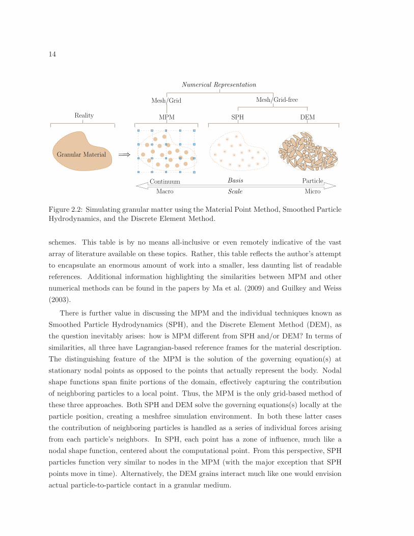
2.2 Simulating granular matter using the Material Point Method, Smoothed Particle Hy-drodynamics, and the Discrete Element Method. . . . . . . . . . . . . . . . . . . . . 14

2.3 Relationship between the particle characteristic function, χp, and MPM, GIMP, andCPDI. . . . . . . . . . . . . . . . . . . . . . . . . . . . . . . . . . . . . . . . . . . . . 22

3.1 Multiplicative decomposition of the deformation gradient. . . . . . . . . . . . . . . . 35

3.2 J2 yield surface. . . . . . . . . . . . . . . . . . . . . . . . . . . . . . . . . . . . . . . . 45

3.3 Drucker Prager yield surface. . . . . . . . . . . . . . . . . . . . . . . . . . . . . . . . 48

3.4 Smooth cap Drucker Prager yield surface. . . . . . . . . . . . . . . . . . . . . . . . . 52

3.5 Relationship between the effective friction angle, φF , critical state angle, φcs, and theplastic dilation angle, ψG. (a), (b), and (c) are consistent with a dense, moderatelydense, and loose arrangement of a granular medium (dry sand for example). . . . . . 57

3.6 Matsuoka Nakai yield surface. . . . . . . . . . . . . . . . . . . . . . . . . . . . . . . . 59

3.7 Failure points for dense and loose sand. Different yield criteria are plotted for com-parison purposes only. The primed axes denote the deviatoric plane. Source: Lade(1972); Lade and Duncan (1975); Andrade and Tu (2009) . . . . . . . . . . . . . . . 61

3.8 Simple shear results. (a) Shear stress σ12 and (b) normal stress σ33 as a function ofshear deformation. . . . . . . . . . . . . . . . . . . . . . . . . . . . . . . . . . . . . . 63

3.9 Simple shear results. (a) Relationship between pressure, p, and shear measure q. (b)Volumetric strain as a function of shear deformation. . . . . . . . . . . . . . . . . . . 64

3.10 Biaxial compression results. (a) q. (b) Volumetric strain. . . . . . . . . . . . . . . . 65

3.11 Error norm of the biaxial confining stress σ3. (a) Modified Drucker-Prager model aspresented in Section 3.6.3. (b) Matsuoka-Nakai yield surface, Eq. (3.120), coupledwith the two invariant plastic potential, Eq. (3.108). (c) Matsuoka-Nakai model aspresented in Section 3.7. . . . . . . . . . . . . . . . . . . . . . . . . . . . . . . . . . . 66

4.1 Cell-Based approach for determining unknown parameters α and β. (a) Exampleparticle configuration. (b) Particles within each cell are used to determine a cell-based αc and βc. (c) Each cell containing particles has unique values for α andβ. . . . . . . . . . . . . . . . . . . . . . . . . . . . . . . . . . . . . . . . . . . . . . . 75

4.2 Node-Based approach for determining unknown parameters α and β. (a) Exampleparticle configuration. (b) Particles within the support of each node are used todetermine a node-based αi and βi (shown support for center node assumes linearshape functions). (c) Each node containing particles within its support has uniquevalues for α and β. . . . . . . . . . . . . . . . . . . . . . . . . . . . . . . . . . . . . . 76

iii

5.1 Fundamental explanation of force transfer in the context of the MPM. (a) Wavecrashing in fluid simulation and (b) Accumulation of sand in the corners of a rotatingbox. . . . . . . . . . . . . . . . . . . . . . . . . . . . . . . . . . . . . . . . . . . . . . 94

5.2 Force balance and phase interaction. (a) Three multiphase scenarios, (b) Grid decom-position for first multiphase scenario, and (c) Force equilibrium. . . . . . . . . . . . 97

6.1 Dam break simulation: (a) Initial configuration, and (b) Configuration at normalizedtime T . . . . . . . . . . . . . . . . . . . . . . . . . . . . . . . . . . . . . . . . . . . . 100

6.2 Comparison between MPM simulations and experimental data for dam break analyses.The upper row compares the run out length, while the lower row compares the runout height. Experimental data is from Martin and Moyce Martin and Moyce (1952). 101

6.3 Dam break sequence for MPM simulations with h0/l0 = 2.0. . . . . . . . . . . . . . . 102

6.4 Time evolution for the dam break with barrier. . . . . . . . . . . . . . . . . . . . . . 104

6.5 Initial state for the tank drain analysis. (a) The particle pressure. (b) The reactionforce, f ir . . . . . . . . . . . . . . . . . . . . . . . . . . . . . . . . . . . . . . . . . . . 105

6.6 Reaction force along tank surface for the tank drain analysis. . . . . . . . . . . . . . 107

6.7 Nodal velocity for the tank drain analysis. . . . . . . . . . . . . . . . . . . . . . . . . 108

6.8 Cantilever beam with applied initial velocity field. . . . . . . . . . . . . . . . . . . . 109

6.9 Normalized stress distribution in cantilever beam. (a) Normal stress. (b) Shear stress.All stress values are normalized to the maximum value predicted by small deformationbeam theory, denoted by Σmax

11 and Σmax12 for the normal and shear components,

respectively. . . . . . . . . . . . . . . . . . . . . . . . . . . . . . . . . . . . . . . . . . 111

6.10 Energy norm convergence for cantilever beam. The left side considers all particleswhen calculating E , while the right side considers only those particles whose horizontalposition is greater than one beam depth away from the support. . . . . . . . . . . . 112

6.11 Amplitude ratio, A, and period ratio, T , as a function of Poisson’s ratio. . . . . . . . 113

6.12 Geometric description for volume constraint validation. (a) Saturated soil with foun-dation loading and (b) pressure drawdown schematic. . . . . . . . . . . . . . . . . . 115

6.13 Pore pressure and vertical stress distribution at tf with increasing depth. (a) Waterphase (θw = 0.1 shown), (b) solid phase (θs = 0.9 shown), and (c) mixture verticalstress, σmix

22 , for all mix combinations. . . . . . . . . . . . . . . . . . . . . . . . . . . 117

6.14 Vertical displacement history of the surface for the solid phase. (a) Raw data, (b)Simple moving average of data, and (c) relative error in the vertical displacement ofthe MPM hydrostatic simulations. . . . . . . . . . . . . . . . . . . . . . . . . . . . . 119

6.15 Volume fraction history for two mixtures. (a) θw = 0.1 , θs = 0.9 and (b) θw =0.5 , θs = 0.5. . . . . . . . . . . . . . . . . . . . . . . . . . . . . . . . . . . . . . . . 120

6.16 Prescribed conditions at top of chamber. (a) Variation of water height ha as a functionof time. (b) Prescribed pressure pa as a function of time. . . . . . . . . . . . . . . . 121

6.17 Pore pressure history at various heights, h, for a pressure drawdown time of td = 0.5 s.Three different time-dependent permeabilities coefficients are considered: (a) µ =1.0 (10)5 [N-s/m4], (b) µ = 5.0 (10)6 [N-s/m4], and (c) µ = 1.0 (10)7 [N-s/m4]. . . . . 124

iv

6.18 Vertical pore pressure distribution in the chamber at t = 5.0 s. The particle locationsare shown as circular points. The upper row is the actual value and the lower row isnormalized to the initial pressure, pw0. Each column represents a different drawdowntime, td. . . . . . . . . . . . . . . . . . . . . . . . . . . . . . . . . . . . . . . . . . . . 125

6.19 Pore pressure, reaction force, and velocity distribution. (a) Using the volume con-straint outlined in Chapter 5. The nodal vector field shows the relative velocitybetween the solid and fluid phases. (b) The u− p CMPM formulation by Zhang et al.(2008). The velocity field is for the mixture. . . . . . . . . . . . . . . . . . . . . . . . 128

6.20 Comparison of pore pressure and displacement between the volume constraint outlinedin Chapter 5, u − p CMPM formulation by Zhang et al. (2008), and a FEM u − pformulation from McGann et al. (2012). (a) Vertical pressure distribution under loadat t = 1.00 s. (b) surface displacement profile at t = 1.00 s. . . . . . . . . . . . . . . 129

7.1 Taylor bar geometric description. (a) Initial configuration. (b) Final configuration forStandard MPM. (c) Final configuration using an anti-locking strategy. . . . . . . . . 132

7.2 Comparison of various anti-locking strategies to the standard MPM. (a) Normalizedheight as a function of normalized time. (b) Normalized radius as a function ofnormalized time. (c) and (d) are zoomed in of (a) and (b), respectively. . . . . . . . 134

7.3 ‖s‖ at T = 0.25 for different MPM strategies. (a) The standard MPM [STD] (b) Cell-based full approximation [CB-FA] (c) Node-based volumetric approximation [NB-VA]and (d) Hybrid-based full approximation [HB-FA]. . . . . . . . . . . . . . . . . . . . 136

7.4 Normal stress component σ33 at T = 1.0 for different MPM strategies. (a) Thestandard MPM [STD] (b) Cell-based full approximation [CB-FA] (c) Node-based vol-umetric approximation [NB-VA] and (d) Hybrid-based full approximation [HB-FA]. . 137

7.5 Marc nonlinear FEM results from T = 0.95. Isometric view of equivalent stress toyield stress, normal stress component σ33, and top view comparing to the MaterialPoint Method. . . . . . . . . . . . . . . . . . . . . . . . . . . . . . . . . . . . . . . . 137

7.6 Average relative performance comparison. The table lists the algorithmic performancerelative to the standard MPM as well as the relative time strength of each algorithm.The pie-chart provides an overview of the time strength for each method. . . . . . . 139

7.7 Planar sand column description. The initial and final geometry is described by theheight, h, and length parameter, l. . . . . . . . . . . . . . . . . . . . . . . . . . . . . 140

7.8 Mobilized friction angle, φF . (a) Analysis A: peak strength (b) Analysis B: initialstrength (c) Analysis C: residual strength . . . . . . . . . . . . . . . . . . . . . . . . 142

7.9 Lf for Cases 0–9. Case 0 is plotted in each figure for comparison purposes. . . . . . 146

7.10 Hf for Cases 0–9. Case 0 is plotted in each figure for comparison purposes. . . . . . 148

7.11 Log-Log plot of Lf as a function of a for Cases 0–9. (a) DP model (b) MN with DP Gmodel and (c) All data points. . . . . . . . . . . . . . . . . . . . . . . . . . . . . . . 149

7.12 Log-Log plot of Hf as a function of a for Cases 0–9. (a) DP model (b) MN with DP Gmodel and (c) All data points. . . . . . . . . . . . . . . . . . . . . . . . . . . . . . . 151

7.13 Evolution of sand column geometry with respect to normalized time. Plots containall cases with a > 2.0. The upper row is the normalized variable L while the lowerrow is H . Subplots (a) and (c) follow from the DP model while subplots (b) and (d)follow from the MN with DP G. material model. . . . . . . . . . . . . . . . . . . . . 153

v

7.14 Case 2 H compared to free fall in a gravitational field. The free fall is denoted by thedashed line. Plots contain all cases with a > 2.0. Subplot (a) follows from the DPmodel data while subplot (b) follows from the MN with DP G. data. . . . . . . . . . 154

7.15 Evolution of the velocity field for a = 2.0, Case 2, and the MN with DP G materialmodel. The velocity vectors are generated from nodal data and plotted alongside theparticles. . . . . . . . . . . . . . . . . . . . . . . . . . . . . . . . . . . . . . . . . . . 155

7.16 Evolution of the velocity field for a = 4.0, Case 2, and the MN with DP G materialmodel. The velocity vectors are generated from nodal data and plotted alongside theparticles. . . . . . . . . . . . . . . . . . . . . . . . . . . . . . . . . . . . . . . . . . . . 156

7.17 Evolution of the velocity field for a = 8.0, Case 2, and the MN with DP G materialmodel. The velocity vectors are generated from nodal data and plotted alongside theparticles. . . . . . . . . . . . . . . . . . . . . . . . . . . . . . . . . . . . . . . . . . . . 157

7.18 Spatial comparison of particle locations for a = 2.0, a = 4.0, and a = 8.0. Particleswhose positions correspond initially are plotted with the same color at each snapshotin time. The normalized time, T , corresponds to a = 8.0 data. . . . . . . . . . . . . . 159

7.19 Evolution of the vertical stress, σ22, for Case 2. . . . . . . . . . . . . . . . . . . . . . 160

7.20 Evolution of the shear stress, σ12, for Case 2. . . . . . . . . . . . . . . . . . . . . . . 161

7.21 Reaction force profiles for Case 2 and the MN with DP G material model. The aspectratio is a = 8.0. (a) Horizontal/shear component and (b) vertical component. . . . . 162

7.22 Comparison of reaction force profiles. (a) raw data profile and (b) filtered profile. . . 163

7.23 Earthen embankments are used to protect infrastructure in the event of an avalanche.(a) Road protection in alpine setting. (b) Simulation schematic. . . . . . . . . . . . . 165

7.24 Representation of a sloped domain in a regular grid space. The desired environmentis shown on the left while the computational representation is depicted at right. . . . 166

7.25 Evolution of avalanche flow from initiation to static state. The embankments preventa majority of the flow from proceeding onto the level ground. . . . . . . . . . . . . . 169

7.26 Plan view comparing velocity magnitudes. The upper row is inhibited by the earthenmounds. The lower row is a simulation without the embankments (the mound outlineis shown for reference purposes only). . . . . . . . . . . . . . . . . . . . . . . . . . . 170

7.27 Side view comparing velocity magnitudes. The left column is inhibited by the earthenmounds. The right column is a simulation without the embankments (the moundoutline is shown for reference purposes only). . . . . . . . . . . . . . . . . . . . . . . 171

7.28 Reaction force exerted by mounds to ensure no flow penetration. . . . . . . . . . . . 172

7.29 Initial configuration for granular flow around column. (a) Plan view and (b) isometricview. . . . . . . . . . . . . . . . . . . . . . . . . . . . . . . . . . . . . . . . . . . . . . 173

7.30 Plan view as the soil flow wraps around the column. The color map shows magnitudeof the particle velocity. . . . . . . . . . . . . . . . . . . . . . . . . . . . . . . . . . . . 176

7.31 Isometric view as the soil flow wraps around the column. The color map shows thevertical stress, σ22. . . . . . . . . . . . . . . . . . . . . . . . . . . . . . . . . . . . . . 177

7.32 Isometric view of plastic deformation at t = 3.0 s for φF = 10 and Hb = 3.5 [m].The column width increases until it forms a rigid barrier. The red particles have|εp| = 10.0 while the blue particles have |εp| ≈ 0.0. . . . . . . . . . . . . . . . . . . . 178

vi

7.33 Isometric view as the soil flow wraps around the column. The color map shows themagnitude of the reaction force, |fr|, normal to the bounding surface. Each individualboundary node can be seen with corresponding reaction force vector. . . . . . . . . . 180

7.34 Net reaction force as a function of time for wc = 4.0 [m]. Positive value indicatesforce directed against flow. . . . . . . . . . . . . . . . . . . . . . . . . . . . . . . . . . 181

7.35 Moving average of reaction force as a function of time for wc = 4.0 [m]. Positive valueindicates force directed against flow. The averaged value is used to obtain the steadystate force measure. . . . . . . . . . . . . . . . . . . . . . . . . . . . . . . . . . . . . 182

7.36 Peak force values as a function of column width, wc, and initial height, Hb. Each rowrepresents a single friction angle. The center and right columns are horizontal andvertical cuts, respectively, through the contour plot shown in the left column. . . . 183

7.37 Steady state force values as a function of column width, wc, and initial height, Hb.Each row represents a single friction angle. The center and right columns are hor-izontal and vertical cuts, respectively, through the contour plot shown in the leftcolumn. . . . . . . . . . . . . . . . . . . . . . . . . . . . . . . . . . . . . . . . . . . . 185

7.38 Steady state force values as a function of friction angle, φF , and initial height, Hb.Each row represents a different column width. The center and right columns arehorizontal and vertical cuts, respectively, through the contour plot shown in the leftcolumn. . . . . . . . . . . . . . . . . . . . . . . . . . . . . . . . . . . . . . . . . . . . 186

7.39 Peak force coefficients, Cpk, as a function of column width, wc, and initial height,Hb. Each row represents a single friction angle. The center and right columns arehorizontal and vertical cuts, respectively, through the contour plot shown in the leftcolumn. . . . . . . . . . . . . . . . . . . . . . . . . . . . . . . . . . . . . . . . . . . . 189

7.40 Steady state force coefficients, Css, as a function of column width, wc, and initialheight, Hb. Each row represents a single friction angle. The center and right columnsare horizontal and vertical cuts, respectively, through the contour plot shown in theleft column. . . . . . . . . . . . . . . . . . . . . . . . . . . . . . . . . . . . . . . . . 190

7.41 Comparison of actual contact geometry to initial values. (a) The height of soil incontact with barrier for Hb = 3.0 and φF = 5. (b) Ratio of actual contact toprojected area for Hb = 3.0 and φF = 5. (c) Average ratio of actual contact toprojected area for all soil depths and φF = 5. . . . . . . . . . . . . . . . . . . . . . . 191

7.42 Comparison of actual contact geometry to initial values. Average ratio of actualcontact to projected area for all soil depths and all friction angles examined. . . . . . 192

7.43 Comparison of actual contact geometry to initial values. Average ratio of actualcontact to projected area for all soil depths and all friction angles examined. . . . . . 193

7.44 Ratio of peak force to static equivalent, Rpk, as a function of column width, wc, andinitial height, Hb. Each row represents a single friction angle. The center and rightcolumns are horizontal and vertical cuts, respectively, through the contour plot shownin the left column. . . . . . . . . . . . . . . . . . . . . . . . . . . . . . . . . . . . . . 195

7.45 Ratio of steady state force to static equivalent, Rss, as a function of column width,wc, and initial height, Hb. Each row represents a single friction angle. The center andright columns are horizontal and vertical cuts, respectively, through the contour plotshown in the left column. . . . . . . . . . . . . . . . . . . . . . . . . . . . . . . . . . 196

7.46 Peak and steady state to static force equivalent for select data points. . . . . . . . . 197

vii

7.47 Schematic drawing of a debris flow approaching a column at an arbitrary angle. (a)Plan view. (b) Side view. . . . . . . . . . . . . . . . . . . . . . . . . . . . . . . . . . 199

7.48 Plan view of the particle velocity magnitude for varying approach angles. The snap-shot coincides with the time that the peak reaction force occurs. . . . . . . . . . . . 202

7.49 Side view of impact for β = 30. . . . . . . . . . . . . . . . . . . . . . . . . . . . . . 202

7.50 Reaction force distribution for β = 0.0 − 45. The upper row is an isometric viewand the lower row a plan view. The arrow indicates the flow direction around thecolumn. . . . . . . . . . . . . . . . . . . . . . . . . . . . . . . . . . . . . . . . . . . . 203

7.51 Reaction force comparison. (a) Reaction force magnitude before and after smoothingas a function of time. (b) The x and z components of the reaction force as a functionof time for β = 30. (c) Peak force as a function of approach angle. . . . . . . . . . . 204

A.1 Needed ingredients to compute points on a yield surface. (a) Transformation fromprincipal space to orthonormal coordinate system aligned with hydrostatic axis. (b) Sliceof yield surface perpendicular to the hydrostatic axis. . . . . . . . . . . . . . . . . . . 227

B.1 The code components that make up the computational framework and dictate theflow of data. . . . . . . . . . . . . . . . . . . . . . . . . . . . . . . . . . . . . . . . . . 234

B.2 Base keywords for input file. . . . . . . . . . . . . . . . . . . . . . . . . . . . . . . . . 235

B.3 AnalysisOptions keywords for input file. . . . . . . . . . . . . . . . . . . . . . . . . . 236

B.4 Parameters keywords for input file. . . . . . . . . . . . . . . . . . . . . . . . . . . . . 239

B.5 Material keywords for input file. . . . . . . . . . . . . . . . . . . . . . . . . . . . . . 241

B.6 Boundary keywords for input file. . . . . . . . . . . . . . . . . . . . . . . . . . . . . . 243

B.7 OutputData keywords for input file. . . . . . . . . . . . . . . . . . . . . . . . . . . . 246

B.8 Object relation and process flow chart. . . . . . . . . . . . . . . . . . . . . . . . . . . 251

B.9 Output file structure. . . . . . . . . . . . . . . . . . . . . . . . . . . . . . . . . . . . . 254

B.10 XML piece data structure for use with ParaView and VTK. This example is for asingle time step and contains only particle data. . . . . . . . . . . . . . . . . . . . . . 256

C.1 Sample .pvd files linking the individual particle, node, and boundary node files to-gether for visualization in ParaView. . . . . . . . . . . . . . . . . . . . . . . . . . . . 263

viii

LIST OF TABLES

Table Number Page

2.1 Numerical methods and references. . . . . . . . . . . . . . . . . . . . . . . . . . . . . 13

3.1 Loading state. . . . . . . . . . . . . . . . . . . . . . . . . . . . . . . . . . . . . . . . . 29

3.2 Newton-Raphson iteration scheme. . . . . . . . . . . . . . . . . . . . . . . . . . . . . 33

3.3 Strain-driven return mapping algorithm for small deformation theory. . . . . . . . . 33

3.4 Strain-driven return mapping algorithm for finite deformation theory. . . . . . . . . 39

3.5 Sample values for constants a0−5. . . . . . . . . . . . . . . . . . . . . . . . . . . . . . 57

4.1 Algorithmic implementation of anti-locking strategy . . . . . . . . . . . . . . . . . . 81

5.1 Volume Constraint Algorithm. . . . . . . . . . . . . . . . . . . . . . . . . . . . . . . 93

6.1 Input parameters for dam break simulations . . . . . . . . . . . . . . . . . . . . . . . 101

6.2 Input parameters for tank drain . . . . . . . . . . . . . . . . . . . . . . . . . . . . . . 106

6.3 Input parameters for plane stress beam study . . . . . . . . . . . . . . . . . . . . . . 110

6.4 Input parameters for plane strain beam study . . . . . . . . . . . . . . . . . . . . . . 113

6.5 Hydrostatic analysis geometry, material description, and MPM parameters. . . . . . 116

6.6 Pressure head drawdown analysis geometry, material description, and MPM parameters.122

6.7 Planar foundation analysis geometry, material description, and MPM parameters foruse with the volume constraint algorithm in Chapter 5 and the u− p CMPM formu-lation by Zhang et al. (2008). . . . . . . . . . . . . . . . . . . . . . . . . . . . . . . . 127

7.1 Analysis geometry, material description, and MPM parameters. . . . . . . . . . . . . 132

7.2 Constant definitions for a0−4 for defining the friction angle curves in Figure 7.8. . . . 143

7.3 Best fit constants for determining Lf (a) via a power law. . . . . . . . . . . . . . . . 149

7.4 Lower and upper bound constants for determining Lf (a) via a power law. . . . . . . 150

7.5 Best fit constants for determining Hf (a) via a power law. . . . . . . . . . . . . . . . 151

7.6 Lower and upper bound constants for determining Hf (a) via a power law. . . . . . . 152

7.7 Initial avalanche geometry and tri-planar domain description. . . . . . . . . . . . . . 167

7.8 Material and MPM parameters for avalanche simulation. . . . . . . . . . . . . . . . . 168

7.9 Column and soil mass geometry. . . . . . . . . . . . . . . . . . . . . . . . . . . . . . 174

7.10 Material and MPM parameters for granular flow into a single column/wall. . . . . . 175

7.11 Initial soil configuration for bi-planar domain description. . . . . . . . . . . . . . . . 200

7.12 Material and MPM parameters for angled granular flow simulation. . . . . . . . . . . 201

ix

1

Chapter 1

INTRODUCTION AND OVERVIEW

This document contains several color figures and plots. The reader is best served by viewing

an electronic version or a color printout.

Each year landslides and avalanches cause significant damage and loss of life around the

world. In the United States alone, the annual economic costs of landslides can be estimated

to be between $1 and $2 billion, with an associated 25 to 50 yearly casualties (Highland,

2006). To help protect people, infrastructure, and lifelines against such disasters, it is

critical to: a.) control the path and/or redirect flow when potential interaction with the built

environment exists, and b.) have engineered structures that are capable of resisting the loads

imparted by a landslide. Capturing the mechanical behavior and structural interaction is

challenging—as these flow events are highly dynamic, unpredictable, and inherently complex

in nature.

Researchers have developed both physical and numerical models in an effort to build

understanding of these phenomena. Physical models typically require well-controlled, large-

scale experiments (see e.g, Denlinger and Iverson (2001); Iverson and Vallance (2001); Iver-

son et al. (1992); Lin and Wang (2006); Reid et al. (2003); Tohari et al. (2007)). While

these experiments provide valuable insight into the governing behavior and controlling mech-

anisms, their general effectiveness is limited due to scale restrictions and the inability to

accurately recreate in-situ conditions.

Application in general contexts requires numerical models that are capable of reproduc-

ing key aspects observed in the field and the ability to represent slides at their full scale.

Such models are necessary not only for prediction and design, but also for the guidance of

additional experimentation as well as furthering engineering understanding and education

in professional practice.

To this end various numerical simulation methodologies and techniques have been used

for predicting flow initiation, evaluating flow patterns, and analyzing the general flow dy-

namics of avalanche and landslides. This includes depth averaging techniques (see e.g,

Chen et al. (2007); Iverson and Denlinger (2001); Savage and Iverson (2003)). While these

methods do reasonably well in estimating global quantities such as runout patterns, there

can be limitations that make fully three-dimensional (3D) analyses cumbersome or impos-

2

sible, or there can be difficulties obtaining the force interaction between the flowing mass

and structures. These limitations follow primarily from the two-dimensional (2D) nature

of such techniques, which use depth-averaged variables. The end result is a smearing of

localized 3D phenomena and an inability to accurately assess obstacle interactions with the

flow. Alternately, purely Eulerian frameworks can provide a reasonable representation of

granular flow and the interaction with rigid objects. This includes finite difference tech-

niques, e.g, the work by Moriguchi et al. (2009) as well as control volume methods, e.g.,

Guimaraes et al. (2008). Different particle techniques, including smoothed particle methods

(Ataie-Ashtiani and Shobeyri, 2008; McDougall and Hungr, 2004) and the Discrete Element

Method (DEM), e.g, Teufelsbauer et al. (2011), can also be used. The primary drawback

of particle methods in this context is scale—particularly for the DEM.

This work uses the Material Point Method (MPM) as a continuum-based tool for mod-

eling landslides, and highlights the method’s suitability for obtaining the dynamic reaction

force interaction between the flow event and a rigid structure(s). Key challenges arising in

this context are the ability to a.) model the transition between solid and fluid-like behav-

ior within a single numerical environment, b.) develop constitutive frameworks that can

accommodate extremely large deformations while remaining computationally efficient and

numerically stable, and c.) account for the different phases and constituents that comprise

these events.

1.1 Scope of Work

This document provides an overview of the MPM and the current literature, identifies

different features and implementation strategies, and presents two enhancements designed

to improve shortcomings of the traditional MPM. Multiple elasto-plastic material models

suitable for both small and finite deformation analyses are explored, with an emphasis on

constructing a MPM-oriented constitutive framework capable of modeling a broad range

of granular material types. The current implementation is verified with examples from

both the solid and fluid mechanics regime, and concludes with several landslide simulations.

Each chapter contains either theoretical development, implementation details, or applica-

tion related contents. A brief synopsis of each chapter is given in the remainder of this

introduction.

Chapter 2

The goal for this chapter is to provide the unfamiliar reader with a basic introduction to

the Material Point Method. This is accomplished using both a qualitative and theory-based

3

overview of the technique. A brief comparison is made to other methods and the chapter

concludes with a literature survey of published work.

Chapter 3

Several elasto-plastic material models are presented following an in depth discussion of in-

tegration algorithms for both small and finite deformation computational inelasticity. The

models include one, two, and three invariant formulations. Three model variants are tested

in the context of granular material modeling using simple shear and biaxial compression

tests. Particular attention is paid here to constructing a MPM-oriented constitutive frame-

work capable of modeling a range of granular material types using physically meaningful

and numerically reasonable parameters.

Chapter 4

When coupled with linear shape functions the standard implementation is subject to kine-

matic locking—the accumulation of fictitious strains that lead to errant stress field and poor

kinematics. This chapter presents multiple strategies for isolating and removing kinematic

locking for both elastic and elasto-plastic materials.

Chapter 5

The point-wise nature of the traditional MPM assumes the mass associated with a given

integration point is confined to a singular location. Certain geometric configurations can

create situations in which the implied particle volume overlaps, effectively overloading space.

This chapter explores a volume constraint that develops a corrective pressure to prevent

this scenario from occurring.

Chapter 6

This is the first of two chapters highlighting the capabilities of the MPM. Chapter 7 focuses

on linear elastic materials and includes applications from both solid and fluid mechanics.

The anti-locking framework is verified through a series of examples, including a dambreak

simulation, water tank drain, and vibrating cantilever beam. The volume constraint algo-

rithm is used to model fully saturated soil in various configurations and loading conditions.

4

Chapter 7

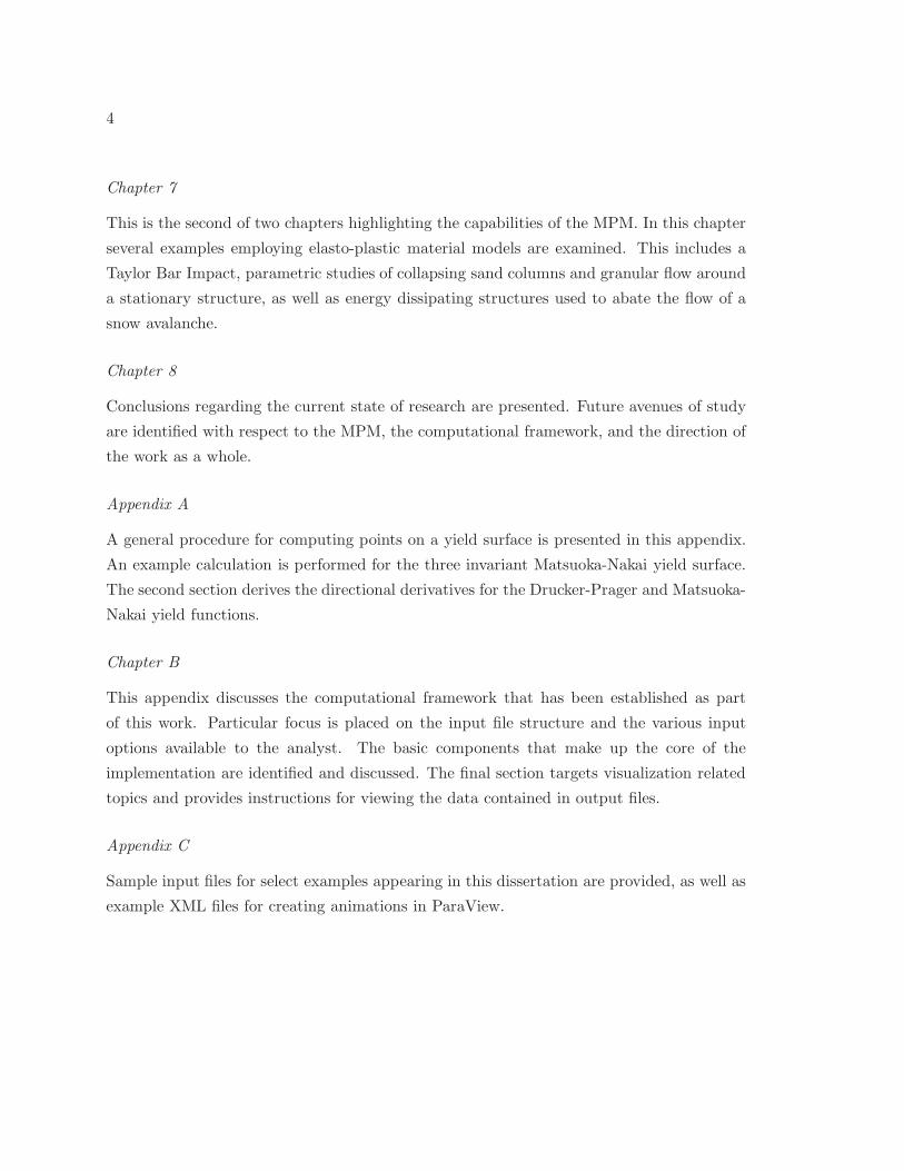
This is the second of two chapters highlighting the capabilities of the MPM. In this chapter

several examples employing elasto-plastic material models are examined. This includes a

Taylor Bar Impact, parametric studies of collapsing sand columns and granular flow around

a stationary structure, as well as energy dissipating structures used to abate the flow of a

snow avalanche.

Chapter 8

Conclusions regarding the current state of research are presented. Future avenues of study

are identified with respect to the MPM, the computational framework, and the direction of

the work as a whole.

Appendix A

A general procedure for computing points on a yield surface is presented in this appendix.

An example calculation is performed for the three invariant Matsuoka-Nakai yield surface.

The second section derives the directional derivatives for the Drucker-Prager and Matsuoka-

Nakai yield functions.

Chapter B

This appendix discusses the computational framework that has been established as part

of this work. Particular focus is placed on the input file structure and the various input

options available to the analyst. The basic components that make up the core of the

implementation are identified and discussed. The final section targets visualization related

topics and provides instructions for viewing the data contained in output files.

Appendix C

Sample input files for select examples appearing in this dissertation are provided, as well as

example XML files for creating animations in ParaView.

5

Chapter 2

THE MATERIAL POINT METHOD

The current chapter provides a qualitative overview as well as a basic discussion of the

standard implementation to set the stage for the enhancements and examples presented

later in this document. This basic theory is followed by a literature review, highlighting

the wide range of applications the method has seen to date. This chapter provides only

the basics of the method, as the mathematical foundations and underpinnings have been

explored in detail and are well documented in several publications. The curious reader is

encouraged to explore the supplied references for additional details.

2.1 What is the Material Point Method?

The Material Point Method (MPM) is a numerical technique that is best suited for model-

ing history dependent materials in a dynamic, large deformation setting. The formulation

tracks moving points relative to stationary nodes, and can be used to capture the behavior

of both fluids and solids in a unified framework. The standard, or traditional1, implemen-

tation solves the governing equation of motion at fixed nodes that collectively form a grid.

Each body or phase in the analysis is represented by a collection of discrete points known

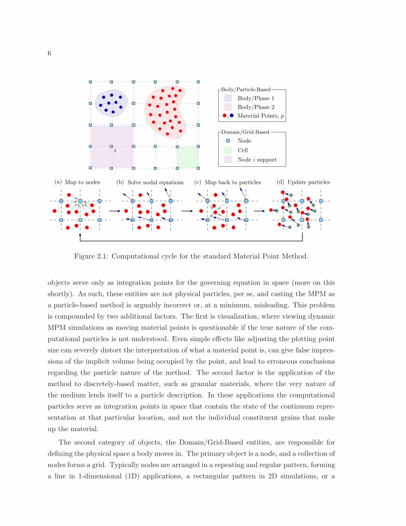
as material points or particles. This general concept is shown in the upper portion of Fig-

ure 2.1. Here the different components that make up an MPM simulation are classified as

either Body/Phase-Based or Domain/Grid-Based, and properly understanding the role and

interaction of these two categories will prove beneficial in later chapters.

The Body/Phase-Based group is comprised of the continuum body itself and the com-

putational points that, collectively, describe the object. Each particle represents a portion

of the total mass, and thus caries an implied volume as well as various state variables de-

pending on the application. For example, in solid mechanics each material point is assigned

initial values for position, velocity, stress, strain, and any other state variable needed for

the constitutive relationship. That being the case, these particles form a Lagrangian frame

of reference from which the state of the body is determined at any instant in time. A

crucial and fundamental characteristic of the Material Point Method is the following: these

1The adjectives standard and traditional will be used interchangeably and represent the original frame-

work presented by Sulsky et al. (1994, 1995)

6

(a) Map to nodes (b) Solve nodal equations (d) Update particles(c) Map back to particles

, Material Points, p

Body/Phase 2

Body/Phase 1

i

Body/Particle-Based

Domain/Grid-Based

Node

Node i support

Cell

Figure 2.1: Computational cycle for the standard Material Point Method.

objects serve only as integration points for the governing equation in space (more on this

shortly). As such, these entities are not physical particles, per se, and casting the MPM as

a particle-based method is arguably incorrect or, at a minimum, misleading. This problem

is compounded by two additional factors. The first is visualization, where viewing dynamic

MPM simulations as moving material points is questionable if the true nature of the com-

putational particles is not understood. Even simple effects like adjusting the plotting point

size can severely distort the interpretation of what a material point is, can give false impres-

sions of the implicit volume being occupied by the point, and lead to erroneous conclusions

regarding the particle nature of the method. The second factor is the application of the

method to discretely-based matter, such as granular materials, where the very nature of

the medium lends itself to a particle description. In these applications the computational

particles serve as integration points in space that contain the state of the continuum repre-

sentation at that particular location, and not the individual constituent grains that make

up the material.

The second category of objects, the Domain/Grid-Based entities, are responsible for

defining the physical space a body moves in. The primary object is a node, and a collection of

nodes forms a grid. Typically nodes are arranged in a repeating and regular pattern, forming

a line in 1-dimensional (1D) applications, a rectangular pattern in 2D simulations, or a

7

rectangular cuboid in fully 3D environments. This repeatable structure is not a requirement

of the method but is the most common scheme to date. The nodal arrangement also defines

cells, or the region contained between adjacent nodes, as well as nodal supports, defined by

piecewise continuous shape functions residing at each node in the domain. The interplay

between the grid, nodes, cells, and nodal support (assuming linear shape functions) is shown

in the upper region of Figure 2.1. Strictly speaking the nodal positions are arbitrary and

can potentially change without penalty at any point in time. However, nodes are most

commonly assumed to reside in a single location effectively creating a static grid. This

facilitates an Eulerian frame of reference when viewed relative to the particle motion.

The sharing of information between particles and nodes is governed solely by the shape

function that serve as an effective weight for determining the importance of a given particle

to any node in the domain. In general this process is referred to as mapping, and can occur

from particle-to-node, or in the opposite direction, from node-to-particle. The primary

goal of any analyses is to track the system in time while monitoring the evolution of key

quantities in both the Body and Domain categories. This is accomplished by splitting a finite

time increment into many smaller time intervals, ∆t = tn+1 − tn, and approximating key

equations over each ∆t. When the governing equation is conservation of linear momentum,

material point quantities of mass, momentum, and force are mapped to the appropriate

nodes as indicated in Figure 2.1(a). After collecting contributions from all particles in the

support, the nodal acceleration and velocity vectors are determined over ∆t as observed in

Figure 2.1(b). The velocity gradient and the corresponding strain increment are mapped

to the particle location using the updated nodal velocity. The particle stress and material

state variables are computed from the desired constitutive model as part of the third step

highlighted in 2.1(c). Finally, the incremental changes in nodal velocity and position are

mapped from the nodes to the particles, resulting in a fully updated system at the particle

level. After 2.1(d) the procedure begins again and the computational cycle is repeated for

a prescribed time duration.

2.2 Traditional Implementation

The traditional approach is built around conservation of linear momentum, which when

expressed in differential form appears as follows:

ρ v = divσ + b , (2.1)

with the mass density ρ(x, t) at position x and time t, v(x, t) as the material time derivative

of the velocity field—also known as the acceleration field—∇ the gradient operator, σ(x, t)

8

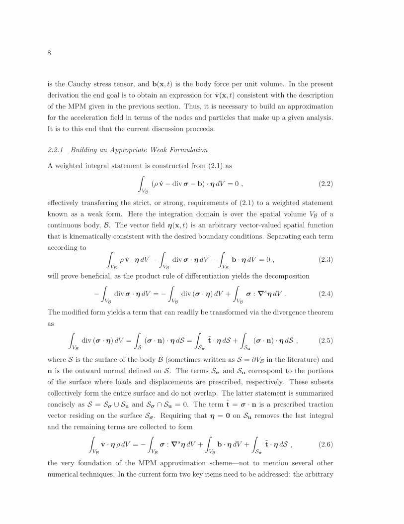
is the Cauchy stress tensor, and b(x, t) is the body force per unit volume. In the present

derivation the end goal is to obtain an expression for v(x, t) consistent with the description

of the MPM given in the previous section. Thus, it is necessary to build an approximation

for the acceleration field in terms of the nodes and particles that make up a given analysis.

It is to this end that the current discussion proceeds.

2.2.1 Building an Appropriate Weak Formulation

A weighted integral statement is constructed from (2.1) as∫

VB

(ρ v − divσ − b) · η dV = 0 , (2.2)

effectively transferring the strict, or strong, requirements of (2.1) to a weighted statement

known as a weak form. Here the integration domain is over the spatial volume VB of a

continuous body, B. The vector field η(x, t) is an arbitrary vector-valued spatial function

that is kinematically consistent with the desired boundary conditions. Separating each term

according to ∫

VB

ρ v · η dV −∫

VB

divσ · η dV −∫

VB

b · η dV = 0 , (2.3)

will prove beneficial, as the product rule of differentiation yields the decomposition

−∫

VB

divσ · η dV = −∫

VB

div (σ · η) dV +

∫

VB

σ : ∇sη dV . (2.4)

The modified form yields a term that can readily be transformed via the divergence theorem

as∫

VB

div (σ · η) dV =

∫

S(σ · n) · η dS =

∫

Sσ

t · η dS +

∫

Su

(σ · n) · η dS , (2.5)

where S is the surface of the body B (sometimes written as S = ∂VB in the literature) and

n is the outward normal defined on S. The terms Sσ and Su correspond to the portions

of the surface where loads and displacements are prescribed, respectively. These subsets

collectively form the entire surface and do not overlap. The latter statement is summarized

concisely as S = Sσ ∪ Su and Sσ ∩ Su = 0. The term t = σ · n is a prescribed traction

vector residing on the surface Sσ. Requiring that η = 0 on Su removes the last integral

and the remaining terms are collected to form∫

VB

v · η ρ dV = −∫

VB

σ : ∇sη dV +

∫

VB

b · η dV +

∫

Sσ

t · η dS , (2.6)

the very foundation of the MPM approximation scheme—not to mention several other

numerical techniques. In the current form two key items need to be addressed: the arbitrary

9

vector-valued spatial function, η(x, t), and the integration procedure for each term arising

in (2.6). These items are discussed sequentially in what follows.

The governing equations are solved at nodal points in the domain. That being the case

it makes sense to build the unknown field quantities v(x, t) and η(x, t) using the nodes

themselves. These approximations are constructed as

η(x, t) ≈ ηh(x, t) :=∑

i

Ni(x)ηi(t) and v(x, t) ≈ vh(x, t) :=∑

j

Nj(x) vj(t) (2.7)

where Ni(x) and Nj(x) are the shape functions associated with nodes i and j, respec-

tively. ηi(t) is an arbitrary, time-dependent nodal vector at a node i, and vj(t) is the time-

dependent nodal acceleration vector at a node j. In this work the superscript h indicates a

grid-based approximation. Closer inspection of the second integral term in Equation (2.6)

reveals that ηh(x, t) must be sufficiently smooth in order to accommodate non-zero action

of the differential operator, ∇. Thus, at a very minimum, the shape functions N (x) must

be linear in x (at least C0 continuous).

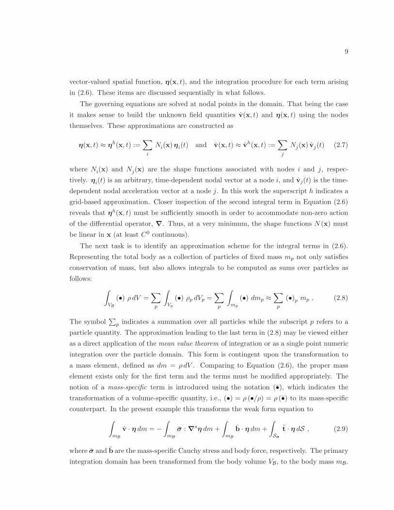
The next task is to identify an approximation scheme for the integral terms in (2.6).

Representing the total body as a collection of particles of fixed mass mp not only satisfies

conservation of mass, but also allows integrals to be computed as sums over particles as

follows:

∫

VB

(•) ρ dV =∑

p

∫

Vp

(•) ρp dVp =∑

p

∫

mp

(•) dmp ≈∑

p

(•)p mp . (2.8)

The symbol∑

p indicates a summation over all particles while the subscript p refers to a

particle quantity. The approximation leading to the last term in (2.8) may be viewed either

as a direct application of the mean value theorem of integration or as a single point numeric

integration over the particle domain. This form is contingent upon the transformation to

a mass element, defined as dm = ρ dV . Comparing to Equation (2.6), the proper mass

element exists only for the first term and the terms must be modified appropriately. The

notion of a mass-specific term is introduced using the notation (•), which indicates the

transformation of a volume-specific quantity, i.e., (•) = ρ (•/ρ) = ρ (•) to its mass-specific

counterpart. In the present example this transforms the weak form equation to

∫

mB

v · η dm = −∫

mB

σ : ∇sη dm+

∫

mB

b · η dm+

∫

Sσ

t · η dS , (2.9)

where σ and b are the mass-specific Cauchy stress and body force, respectively. The primary

integration domain has been transformed from the body volume VB, to the body mass mB.

10

2.2.2 Constructing the System of Equations

The discrete set of equations

∑

j

mij vj = f inti + f exti , (2.10)

with

f inti = −∑

p

σp ·∇Nipmp . and f exti =∑

p

bpNipmp +

∫

Sσ

tNip dS (2.11)

is obtained for the unknown nodal accelerations vj by substituting the grid-based definitions

given in listing (2.7) and the integral approximation scheme outlined in (2.8) into the weak

form Equation (2.9). The resulting system utilizes mij =∑

p NipNjpmp, the consistent

mass matrix coefficients with Nip as the shape function evaluated at the particle location,

i.e., Nip = Ni(xp). Frequently the off diagonal coupling terms in mij are eliminated by

approximating the mass matrix as a purely diagonal matrix: mi =∑

p Nipmp. In doing so

the system in (2.10) is reduced to a series of i uncoupled equations for the i nodes describing

the spatial domain.

The external surface force term in (2.11)2 can be problematic in the MPM. The root of

the problem lies in the fact that surface tractions must be applied on the body—a.k.a. the

particles—and these objects move throughout nodal supports in time. Thus, the particle

area and force orientation must be tracked appropriately so these terms can be applied

at the correct nodes for any given position/orientation of the particle/surface. This is in

contrast to other techniques, such as the Finite Element Method (FEM), where this term

is applied directly to nodal values.

2.2.3 Putting it All Together

The primary goal of any analyses is to track the system in time while monitoring the

evolution of key quantities at both the particle and nodal levels. This is accomplished

in part by splitting a finite time increment, T , into many smaller time intervals, ∆t =

tn+1 − tn ≪ T . Over each time step ∆t the current state is mapped to the nodes, a grid-

based time integration is performed, and particle values are updated. This computational

cycle is broken down and visualized as individual components in Figure 2.1. In this section

the details of each step are presented.

The first step involves the transfer of particle quantities to the nodes. This is shown in

11

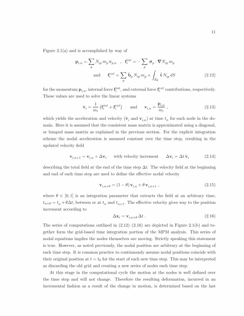
Figure 2.1(a) and is accomplished by way of

pi,n =∑

p

Nipmp vp,n , f inti = −∑

p

σp ·∇Nipmp

and f exti =∑

p

bpNipmp +

∫

Sσ

tNip dS (2.12)

for the momentum pi,n, internal force finti , and external force f exti contributions, respectively.

These values are used to solve the linear systems

vi =1

mi

(f inti + f exti

)and vi,n =

pi,n

mi, (2.13)

which yields the acceleration and velocity (vi and vi,n) at time tn for each node in the do-

main. Here it is assumed that the consistent mass matrix is approximated using a diagonal,

or lumped mass matrix as explained in the previous section. For the explicit integration

scheme the nodal acceleration is assumed constant over the time step, resulting in the

updated velocity field

vi,n+1 = vi,n +∆vi with velocity increment ∆vi = ∆t vi (2.14)

describing the total field at the end of the time step ∆t. The velocity field at the beginning

and end of each time step are used to define the effective nodal velocity

vi,n+θ = (1− θ)vi,n + θ vi,n+1 , (2.15)

where θ ∈ [0, 1] is an integration parameter that extracts the field at an arbitrary time,

tn+θ = tn+ θ∆t, between or at tn and tn+1. The effective velocity gives way to the position

increment according to

∆xi = vi,n+θ ∆t . (2.16)

The series of computations outlined in (2.12)–(2.16) are depicted in Figure 2.1(b) and to-

gether form the grid-based time integration portion of the MPM analysis. This series of

nodal equations implies the nodes themselves are moving. Strictly speaking this statement

is true. However, as noted previously, the nodal position are arbitrary at the beginning of

each time step. It is common practice to continuously assume nodal positions coincide with

their original position at t = t0 for the start of each new time step. This may be interpreted

as discarding the old grid and creating a new series of nodes each time step.

At this stage in the computational cycle the motion at the nodes is well defined over

the time step and will not change. Therefore the resulting deformation, incurred in an

incremental fashion as a result of the change in motion, is determined based on the last

12

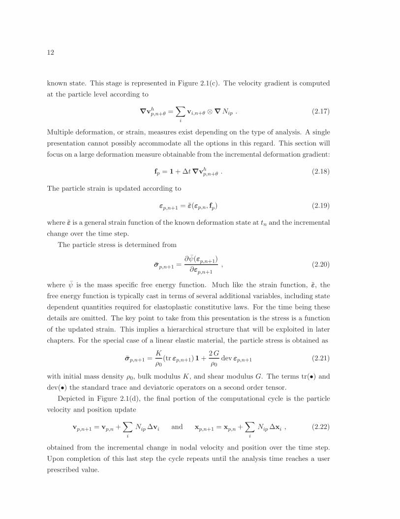
known state. This stage is represented in Figure 2.1(c). The velocity gradient is computed

at the particle level according to

∇vhp,n+θ =

∑

i

vi,n+θ ⊗∇Nip . (2.17)

Multiple deformation, or strain, measures exist depending on the type of analysis. A single

presentation cannot possibly accommodate all the options in this regard. This section will

focus on a large deformation measure obtainable from the incremental deformation gradient:

fp = 1+∆t∇vhp,n+θ . (2.18)

The particle strain is updated according to

εp,n+1 = ε(εp,n, fp) (2.19)

where ε is a general strain function of the known deformation state at tn and the incremental

change over the time step.

The particle stress is determined from

σp,n+1 =∂ψ(εp,n+1)

∂εp,n+1

, (2.20)

where ψ is the mass specific free energy function. Much like the strain function, ε, the

free energy function is typically cast in terms of several additional variables, including state

dependent quantities required for elastoplastic constitutive laws. For the time being these

details are omitted. The key point to take from this presentation is the stress is a function

of the updated strain. This implies a hierarchical structure that will be exploited in later

chapters. For the special case of a linear elastic material, the particle stress is obtained as

σp,n+1 =K

ρ0(tr εp,n+1)1+

2G

ρ0dev εp,n+1 (2.21)

with initial mass density ρ0, bulk modulus K, and shear modulus G. The terms tr(•) anddev(•) the standard trace and deviatoric operators on a second order tensor.

Depicted in Figure 2.1(d), the final portion of the computational cycle is the particle

velocity and position update

vp,n+1 = vp,n +∑

i

Nip∆vi and xp,n+1 = xp,n +∑

i

Nip∆xi , (2.22)

obtained from the incremental change in nodal velocity and position over the time step.

Upon completion of this last step the cycle repeats until the analysis time reaches a user

prescribed value.

13

Table 2.1: Numerical methods and references.

Numerical Method Selected References

Arbitrary Lagrangian-Eulerian (ALE) Benson (1992); Huerta and Casadei

(1994); Donea et al. (2004)

Finite Element (FEM) Hughes (1987); Bathe (1996);

Zienkiewicz et al. (2005a,c)

Meshfree or Meshless (MM) Belytschko et al. (1996); Fries and

Matthies (2003-03); Liu (2003); Liu

and Liu (2003)

Finite Difference (FD) Ghaboussi and Barbosa (1990);

LeVeque (2007); Radjai and Duboi

(2011)

The details provided here (as well as previous Section 2.1) highlight the very basics of

the Material Point Method. Of course, this traditional form is subject to change depending

on the implementation strategy or details arising due to the extension of the traditional

framework, such as the enhancements described in Appendix B, and Chapters 4 and 5, or

any one of the several modifications discussed in the remainder of this chapter. The current

state of the literature is examined next.

2.3 Comparison to Other Numerical Methods

A thorough overview and literature review would include a detailed comparison to other

numerical methods suitable for large deformation analyses. Such an approach is, however,

beyond the scope of the current chapter and could likely yield a chapter of its own if pre-

sented in moderate depth. Considering the MPM is nearly 20 years old the numerical com-

munity would likely benefit from such a presentation, especially if a survey of the method’s

enhancements and corresponding applications were included. For the time being it suffices

to say that the MPM shares many similarities with a bevy of numerical schemes, includ-

ing Arbitrary Lagrangian-Eulerian (ALE) methods, both Lagrangian and Eulerian Finite

Element Methods (FEM), meshless or meshfree methods, and select Finite Difference (FD)

techniques. The broad list is due in part to the combination of Lagrangian (computational

particles) and Eulerian (stationary grid) reference frames that make the MPM what it is.

The interested reader can consult Table 2.3 for a list of references to related numerical

14

Reality

Granular Material

Continuum Basis

Scale

Particle

Macro Micro

MPM SPH DEM

=⇒

Numerical Representation

Mesh/Grid-freeMesh/Grid

Figure 2.2: Simulating granular matter using the Material Point Method, Smoothed ParticleHydrodynamics, and the Discrete Element Method.

schemes. This table is by no means all-inclusive or even remotely indicative of the vast

array of literature available on these topics. Rather, this table reflects the author’s attempt

to encapsulate an enormous amount of work into a smaller, less daunting list of readable

references. Additional information highlighting the similarities between MPM and other

numerical methods can be found in the papers by Ma et al. (2009) and Guilkey and Weiss

(2003).

There is further value in discussing the MPM and the individual techniques known as

Smoothed Particle Hydrodynamics (SPH), and the Discrete Element Method (DEM), as

the question inevitably arises: how is MPM different from SPH and/or DEM? In terms of

similarities, all three have Lagrangian-based reference frames for the material description.

The distinguishing feature of the MPM is the solution of the governing equation(s) at

stationary nodal points as opposed to the points that actually represent the body. Nodal

shape functions span finite portions of the domain, effectively capturing the contribution

of neighboring particles to a local point. Thus, the MPM is the only grid-based method of

these three approaches. Both SPH and DEM solve the governing equations(s) locally at the

particle position, creating a meshfree simulation environment. In both these latter cases

the contribution of neighboring particles is handled as a series of individual forces arising

from each particle’s neighbors. In SPH, each point has a zone of influence, much like a

nodal shape function, centered about the computational point. From this perspective, SPH

particles function very similar to nodes in the MPM (with the major exception that SPH

points move in time). Alternatively, the DEM grains interact much like one would envision

actual particle-to-particle contact in a granular medium.

15

A natural way to link these three methods is shown in Figure 2.2 (this figure is applicable

only to granular-based material descriptions). Here the MPM is depicted as being on the

continuum end of the material spectrum, while the DEM serves as a particle-based repre-

sentation. SPH falls somewhere in between these two extremes. The other consideration

is the scale. Clearly DEM is superior for smaller scale simulations, where subtle nuances

are important. As the scale increases MPM becomes more appropriate, as individual grain

interactions become irrelevant and are smoothed out. Again, SPH finds itself in the middle

in terms of applicable scales. This illustration serves only as a reminder as to which regime

each of these numerical methods is best suited to represent. These are not hard and stead-

fast rules, and depending on the application all, some, or only one method may be the best

approach.

A common point of confusion is the classification of MPM as either a continuum- or

particle-based method. The point-wise nature of the integration scheme and body dis-

cretization instill a false sense of particle-ism. This, coupled with the other related issues

such as visualization and applications to granular, constituent-based matter, leads to an

erroneous classification of the MPM as a particle method. To be clear, the MPM is a

continuum-method. This classification is based on the formulation and integration details.

Of course, some will argue that the mere presence of particle-like objects make the tech-

nique a particle-based approach. However, when compared to other methods like SPH 2 or

the DEM, it is clear that the MPM cannot and should not be classified as a true particle

technique.

2.4 Literature Review

The Material Point Method was born out of a need to marry fluid-like, large deformations

with a history-dependent material response. While a large body of research has focused on

similar applications, much work has also been done in additional areas (many of which are

explored shortly)—pushing the capabilities of the MPM and investigating new applications.

In the remainder of this chapter a look at previous and current research will be examined

in moderate detail. In an effort to streamline the discussion this survey has been separated

into several different categories, each of which pertains to a different topic.

2Even classifying SPH as a true particle-method could be deemed as incorrect, as the particles in SPH

carry a fuzzy representation and often do not represent constituents. However, the important distinction is

that particles can represent constituents in SPH if need be.

16

2.4.1 Historical Development

The MPM follows from a more general class of numerical schemes known as PIC, or Particle-

in-cell methods. The first PIC technique was developed in the early 1950’s (Harlow, 1957)

and was used primarily for applications in fluid mechanics. Early implementations suffered

from excessive energy dissipation, rendering them obsolete when compared to other, more

valid methods. In 1986, Brackbill and Ruppel solved many of the inherent problems related

to energy dissipation and introduced FLIP—the Fluid Implicit Particle method. The FLIP

technique was modified and tailored for applications in solid mechanics and has since been

referred to as the Material Point Method.

One of the first publications on the topic was by Sulsky et al. in 1994. This pioneering

work, as well as a slight variant created for specific applications in solid mechanics (Sulsky

et al., 1995), successfully outlined the basic algorithmic implementation and shortly there-

after an axisymmetric form was published by Sulsky and Schreyer (1996). Using several

two dimensional impact examples, these seminal works showed that elastic and perfectly

plastic behavior was reasonably reproduced using the MPM. Also highlighted was the fact

that no-slip impact for elastic, inelastic, and rigid bodies is handled automatically by the

algorithm, further reinforcing the robustness of the proposed approach.

In the time since this initial research was published, several variations/extensions to the

MPM have been proposed—many of which are application specific and discussed later in

this chapter. Included in this list is one of the most prominent variants, the Generalized

Interpolation Material Point (GIMP) method. This technique, as well as a related extension

known as the Convected Particle Domain Interpolation (CPDI), provides an alternative

representation of the particle domain. These two variants are explored at the end of this

section.

2.4.2 General Implementation

The applications of the MPM vary significantly, ranging from various geotechnical imple-

mentations (Zhou et al., 1999; Wieckowski, 2004b), to anchor pullout (Coetzee et al., 2005),

to the modeling of sea ice dynamics (Sulsky et al., 2007). Several large deformation, flow-

like models have been reported (Wieckowski et al., 1999; Wieckowski, 2003, 2004a) while

the work by York et al. (1999, 2000) emphasizes membrane analysis with a specific focus on

fluid–membrane interaction. The method has even realized moderate success in the context

of multicellular constructs as shown in the work by Guilkey et al. (2006) and, more recently,

the numerical simulation of landslides (Andersen and Andersen, 2010b).

17

2.4.3 Contact, Impact/Penetration, and Material Interaction

The need to model contact and interaction of bodies has long been the focus of a significant

amount of MPM research. A robust MPM contact algorithm capable of handling sliding

and rolling friction, as well as separation, was first addressed in the paper by Bardenhagen

et al. (2000) and later improved in the publication by Bardenhagen et al. (2001). These

works introduce the idea of contact within the context of granular materials modeling and

are particularly significant for two reasons: they represent the first published attempt to

isolate a contact force (or traction) between interacting bodies, and they are the first to

propose the use of multiple, conforming grids to model contact or interaction.

In recent years the idea of using multiple grids to model contact and body interaction has

been explored by many researchers in various settings. These include the meshing process of

spur gears (Hu and Chen, 2003) and the development of general, three dimensional contact

algorithms by Pan et al. (2008) and Huang et al. (2011). The concept has also been extended

to model the drag interaction between material phases. This latter topic is addressed

by Mackenzie-Helnwein et al. (2010), where the drag force between two material phases

is a function of the relative material velocities—each of which is computed on a separate

grid. A similar approach is used by Zhang et al. (2008), where the treatment of several

phases is handled in a multi-grid environment, and care is taken to ensure the continuity

requirement is satisfied over a representative time step. Finally, in the publication by Shen

and Chen (2005), a multi-grid concept is used to continuously superimpose a boundary

layer in order to distribute viscous damping forces. The forces are applied along the moving

computational interface between two material phases.

Contact algorithms have now been expanded to include impact and simulation of explo-

sive phenomena. Two such examples are described in Ma and Zhang (2009) and Lian et al.

(2011). The interaction between saturated soil and impacting solid bodies is explored in

the work by Zhang et al. (2009). This research features the development of a u-p coupled

Material Point Method (CMPM) and is used to predict the dynamic response of saturated

soil.

2.4.4 Fracture and Material Failure

Material failure and fracture mechanics algorithms share many similar features with those

from the previous section. However, enough work has been done on these additional topics

to validate the creation of a separate category. Of the many similarities, perhaps the

most notable is the concept of using multiple grids. In the publications from Nairn (2003)

and Guo and Nairn (2006) this concept is exploited to develop separate grid velocities around

18

crack tip locations. This effectively serves as a discontinuity in the continuum and allows

the method to capture crack propagation. An additional paper by Guo and Nairn (2004)

evaluates crack parameters (e.g., the J-Integral and stress intensity factors) commonly used

in fracture analysis.

The modeling of general crack geometry is complicated in the MPM since the technique

is typically implemented using a regular, rectangular grid. Tan and Nairn (2001) address

the issue using a hierarchical mesh refinement algorithm that allows for better geometric

resolution of the discontinuity. The work by Wang et al. (2005) confronts this issue by

introducing an irregular grid, and corresponding mapping scheme, to handle arbitrary crack

geometry in a two dimensional framework.

Several techniques have been proposed in an effort to simulate material failure. A

straightforward evaluation of the MPM’s ability to capture dynamic failure with damage

diffusion is addressed by Chen et al. (2002). The publication by Schreyer et al. (2002)

presents a more specialized investigation into the delamination of layered composite mate-

rials by modeling the process as a strong discontinuity. The resulting framework effectively

captures the propagation of delamination with no sensitivity to mesh orientation. Sulsky

and Schreyer (2004) and Shen (2009) both develop decohesion constitutive models that are

used to predict and assess material failure.

2.4.5 Energy and Integration Considerations

A relatively small collection of research has been published regarding the mathematical

foundation of the Material Point Method. What has surfaced focuses primarily on en-

ergy conservation and integration errors in the formulation. The basic implementation

of the method ensures conservation of mass and momentum by construction. However,

no attention is given to the conservation of energy. This issue is addressed in the paper

by Bardenhagen (2002), where it is shown that the two available options for updating the

particle stress lead to dramatically different findings with respect to internal energy con-

servation of the system. Additional work regarding energy conservation can be found in

the papers by Love and Sulsky (2006a,b). These latter two documents examine energy

consistency from a thermodynamics perspective. Their findings show that the use of a con-

sistent mass matrix results in a numerical method that inherits the energy-dissipative and

momentum-conserving properties of the mesh solution.

An equal amount of attention has been given to mitigating integration errors. The first

work specifically addressing this issue is by Steffen et al. (2008b). This paper examines the

error associated with linear shape functions and proposes the use of quadratic B-splines basis

19

functions. A similar body of work by Andersen and Andersen (2010a) examines standard

linear and quadratic shape functions, as well as cubic splines. They too conclude that the

use of higher order basis functions leads to more accurate results. Alternatively, Htike et al.

(2011) use a radial basis function (RBF) in place of the traditional linear shape functions or

B-splines. The proposed RBF possesses a high degree of smoothness; thus eliminating non-

physical results associated with more traditional implementations. The RBF form of the

MPM is tested and validated through a series of benchmark problems from solid mechanics.

Finally, the publication from Steffen et al. (2010) develops a set of criteria relating the grid

size, number of particles, and time step. The premise of this research is based upon selecting

a time step that balances spatial and temporal errors.

2.4.6 Computational Implementation

There is little published work on efficient implementation strategies since the MPM is a

relatively young method compared to other, more established techniques. Nonetheless,

there are a limited number of publications on the topic. The nature of the algorithm is

well suited for parallel applications—particularly if using a lumped mass matrix as is often

the case. These ideas are explored in the work by Huang et al. (2008) where researchers

employ FORTRAN95 with OpenMP parallelization to investigate two separate implementa-

tion strategies. Ma et al. (2010b) examine the development of an object oriented framework

for large deformation analyses. Multiple particle update strategies are investigated with

an emphasis on reducing memory requirement and computational cost. The publication

by Shin et al. (2010) strives to also reduce memory requirements and computational cost

by presenting a dynamic meshing scheme. Their algorithm instantiates and searches only

cells containing matter—effectively avoiding useless storage of empty nodes and perform-

ing unneeded computations. The efficiency of the proposed approach is measured against

standard storage schemes and is shown to be quite effective.

2.4.7 Variations on the Material Point Method

Several extensions or variations have been proposed since the MPM’s inception. In fact,

most of the applications mentioned thus far modify or change the algorithm in one way

or another. Presented in this section are representative works that significantly alter the

implementation and provide noteworthy extensions.

Most implementations use a time-explicit discretization to solve dynamic problems. Sul-

sky and Kaul (2004) propose a time-implicit discretization and use various solution schemes

to solve the resulting non-linear equations. Their study shows the potential for large com-

20

putational savings by using an implicit approach with appropriate time step. A quasi-static

approach is developed in the research by Beuth et al. (2008,2010). These publications

feature several large strain examples that are presented and compared to the FEM.

One of the problems that has long beleaguered the MPM is partially full cells and linear

shape functions. In an effort to improve the kinematics an improved velocity projection is

developed in the paper by Wallstedt and Guilkey (2007). Their work shows that the quality

of the solution relies heavily on particle density, location, and orientation with respect to

the computational grid. An enhancement to the linear projection operator is proposed that

reduces the dependence on particle location and density, ultimately leading to a higher

quality solution. The main issue with partially filled cells is poor and/or non-physical nodal

accelerations, resulting in a numerical instability. Said instability is due in part to low nodal

mass coupled with a large nodal force, and can lead to significant numerical problems. Ma

et al. (2010a) have created a small mass nodal distribution coefficient matrix that attempts

to eliminate this shortcoming. Their mass and momentum conserving algorithm proposes a

redistribution of mass around those problematic nodes—effectively limiting the instability.

The algorithm is tested and validated through one and two dimensional applications. As

an alternative to nodal mass, the nodal force can be calculated differently to alleviate

problematic nodal accelerations. The force is directly proportional to the shape function

gradient and primarily responsible for “cell crossing” errors frequently referenced in the

literature. Zhang et al. (2011) have developed an enhanced gradient for the interpolation

functions to combat this issue. The enhancement eliminates the discontinuity in the gradient

for linear shape functions. The approach is highlighted through bending, vibration, and

projectile-target examples.

The previous paragraph provides an overview of research that aimed to fix or modify

the algorithm for issues associated with linear shape functions. Although these proposed

techniques effectively reduce the problem for select applications, they are unable to resolve

the issue completely. In order to fully eliminate the instability, one must examine the

root of the problem, which is actually the point-wise description of the body. Since any

material is represented as a collection of particles, a finite portion of the body is being

modeled as a singular point. Thus, the particle shape (volume), is not explicitly accounted

for in the standard algorithm. Bearing this information in mind, two primary variants have

been developed that take into consideration the particle shape when solving the equation

of motion.

21

The Generalized Interpolation Material Point Method

The Generalized Interpolation Material Point (GIMP) Method was initially introduced

by Bardenhagen and Kober (2004). The GIMP approach assigns a domain (typically rect-

angular) to each particle at the start of the analysis. In general, this leads to more accurate

spatial integration. However, the technique adds additional computational cost because the

overlap of particle domain and nodal support must be determined at each time step. There

are effective and efficient implementation strategies as outlined in the paper by Buzzi et al.

(2008).

Like the MPM, GIMP has tasted success in a wide variety of contexts and settings.

These include crack propagation and modeling (Daphalapurkar et al., 2007) as well as mul-

tiscale simulation with an emphasis on molecular dynamics (Ma et al., 2006c,a). Different

mesh refinement strategies are explored in the work by Ma et al. (2006b) while the paper

by Wallstedt and Guilkey (2008) evaluates different time integration schemes.

It should be noted that the standard MPM algorithm is recovered by selecting a particle

domain that is the Dirac delta function—implying that the Material Point Method itself

is a specialization of the GIMP technique. Thus, to call the GIMP method a variation of

the MPM may be a misnomer, but it is typically done so nonetheless. This relationship is

outlined in additional detail in the following sections.

Convected Particle Domain Interpolation

Sadeghirad et al. (2011a) propose a procedure that includes information about the particle

domain when integrating the standard weak form equations. In the Convected Particle

Domain Interpolation (CPDI) technique, particles are given parallelogram-shaped domains

that are constantly updated using the deformation gradient evaluated at the particle loca-

tion. What separates this technique from GIMP is the following: the particle domain is

described by shape vectors that evolve with the deformation gradient. Thus, shear deforma-

tions and volume changes are accounted for throughout the analysis that are not considered

when using the traditional GIMP technique (although, some variants of GIMP take into

account volumetric shape changes). Like GIMP, the CPDI procedure expands the support

of a particle and spreads out the influence of the internal force to those nodes whose sup-

port overlaps the particle domain. Spatial integration is significantly improved and the

technique reduces the number of particles needed to achieve reasonable results. A series of

two dimensional numerical examples validate the proposed approach in the aforementioned

reference.

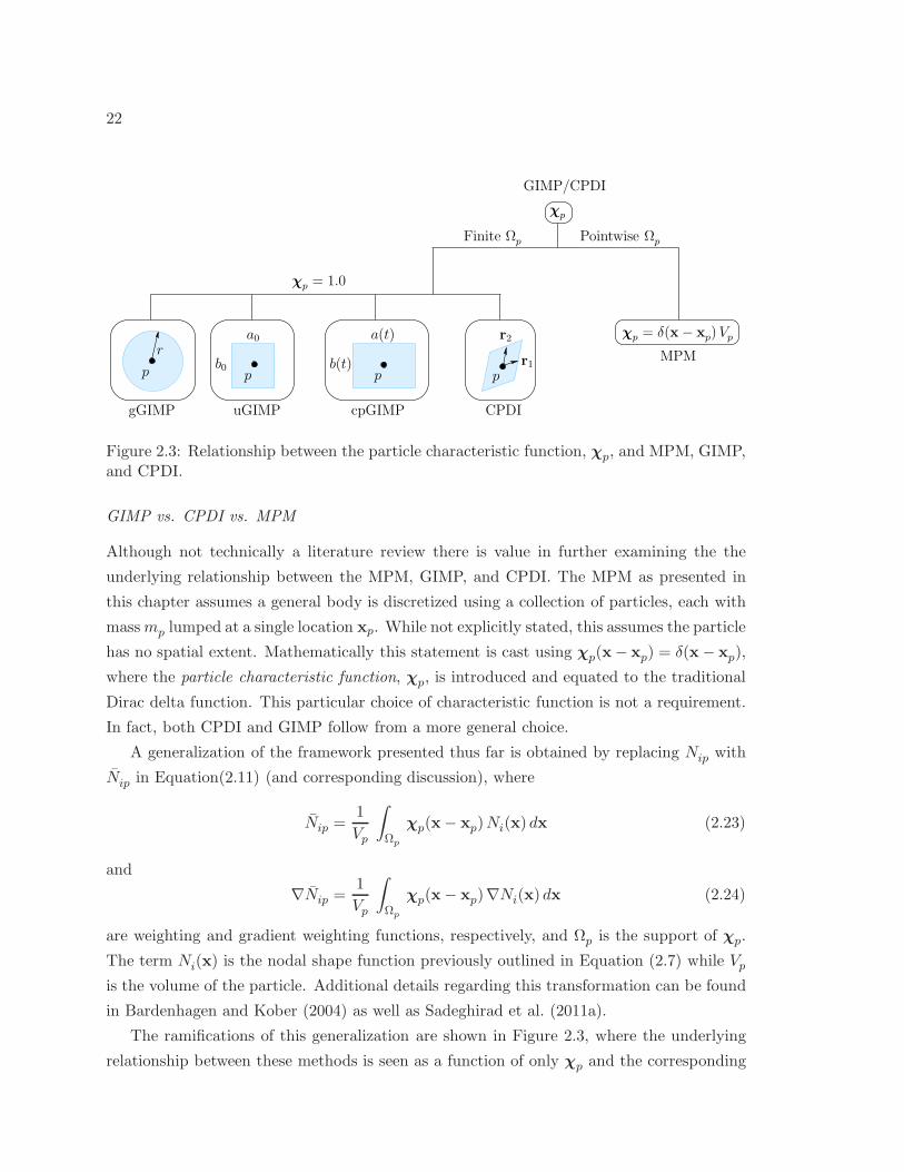
22

p

χp = δ(x− xp) Vp

p

GIMP/CPDI

b(t)

a(t)

p

χp

MPM

CPDIuGIMP cpGIMPgGIMP

pr1

r2a0

b0

χp = 1.0

r

Finite Ωp Pointwise Ωp

Figure 2.3: Relationship between the particle characteristic function, χp, and MPM, GIMP,and CPDI.

GIMP vs. CPDI vs. MPM

Although not technically a literature review there is value in further examining the the

underlying relationship between the MPM, GIMP, and CPDI. The MPM as presented in

this chapter assumes a general body is discretized using a collection of particles, each with

massmp lumped at a single location xp. While not explicitly stated, this assumes the particle

has no spatial extent. Mathematically this statement is cast using χp(x− xp) = δ(x− xp),

where the particle characteristic function, χp, is introduced and equated to the traditional

Dirac delta function. This particular choice of characteristic function is not a requirement.

In fact, both CPDI and GIMP follow from a more general choice.

A generalization of the framework presented thus far is obtained by replacing Nip with

Nip in Equation(2.11) (and corresponding discussion), where

Nip =1

Vp

∫

Ωp

χp(x− xp)Ni(x) dx (2.23)

and

∇Nip =1

Vp

∫

Ωp

χp(x− xp)∇Ni(x) dx (2.24)

are weighting and gradient weighting functions, respectively, and Ωp is the support of χp.

The term Ni(x) is the nodal shape function previously outlined in Equation (2.7) while Vp

is the volume of the particle. Additional details regarding this transformation can be found

in Bardenhagen and Kober (2004) as well as Sadeghirad et al. (2011a).

The ramifications of this generalization are shown in Figure 2.3, where the underlying

relationship between these methods is seen as a function of only χp and the corresponding

23

support Ωp. On the MPM side there is no extent to the particle domain; the Dirac delta

function in the integrand ensures Nip = Nip and ∇Nip = ∇Nip. For finite particle domains

there are additional options. The classic GIMP approach utilizes χp = 1.0 and a rectangular

particle domain described by a0 and b0. This approach is dubbed uGIMP by Sadeghirad

et al. (2011a). The particle domain is not required to be rectangular—but doing so eases

the integration process if geometrically simple shapes are used. There is nothing wrong with

using circular, or ellipsoid, domains as indicated by gGIMP (the name gGIMP is not used

in the literature and is assigned here to distinguish from uGIMP and cpGIMP). However,

there are no published GIMP studies using non-rectangular domains to date. The volume

of the particle domain can change by updating the particle dimensions with deformation,

as indicated by a(t) and b(t) in cpGIMP (again, the name follows from Sadeghirad et al.

(2011a)). Unfortunately this latter approach cannot capture particle distortion via shearing.

To combat this, the CPDI technique describes the particle extent using shape vectors r1 and

r2 that evolve with the deformation gradient. For CPDI the integrand in (2.23) and (2.24)

is approximated based on an interpolation of the values of the traditional shape functions

evaluated at the particle corners.

Coupling with Other Methods

One of the prominent trends in recent years is coupling the MPM with additional numerical

techniques. Such an approach allows analysts to reap the benefits of multiple solution

types and exploit each method’s strengths in multiphysic simulations. One example of this

is the paper by Lian et al. (2011), in which the MPM is mixed with the Finite Element

Method. Their approach treats boundaries and other objects using traditional FE and

does not require the meshes for the MPM and FEM to coincide. In doing so the authors

leverage the benefits of MPM with regards to large deformation simulations and capture

others, such as irregular shaped boundaries, with the FEM. Additional examples include

the coupling with purely Eulerian finite difference or finite volume schemes, e.g., the works

presented by (Zhang et al., 2008; Higo et al., 2010). In these formulations the governing

equations of different materials or phases are solved by methods well suited to do so. It

can be argued that coupling the MPM with other methods and exploiting each technique’s

strengths is far more practical for multiphysics applications than the alternative, which is

trying to build a single formulation that is an all-encompassing, super-method capable of

any feat. The latter may be viewed as unrealistic and an inefficient use of resources in a

numerical modeling context.

24

2.5 Summary

This chapter provided a basic overview of the MPM, including the implementation details

and the current state of the literature. In the remaining chapters the standard framework

is expanded with two enhancements. As stated in the Introduction, the primary goal is to

build a numerical framework capable of modeling landslides and debris flows. A key factor

in doing so is the ability to capture the mechanical response of granular media as well as

well other slide constituents, such as air and water. To this end several material models are

presented in the next chapter.

25

Chapter 3

MATERIAL MODELS

Because of its continuum basis MPM must be combined with suitable constitutive rela-

tions to properly capture local state behavior at the material point level. In this chapter all

the components needed to build a MPM-oriented constitutive framework are presented, in-

cluding basic concepts from computational inelasticity, small and large deformation theory,

and the development of specific material models capable of simulating several kinds of ma-

terials. Particular attention is paid here to developing a framework that can accommodate

extremely large deformations while remaining computationally efficient and numerically

stable in the context of granular media. The chapter closes with direct shear and bi-axial

examples.

3.1 Elasto-plastic Materials

Material models play an invaluable role in many areas of engineering. As such, an enormous

amount of research has gone into their development and application. While the complexity

of these models varies significantly, the primary goal of each is the same: to capture and

replicate material response observed in the field and in the laboratory. Quite often this

boils down to identifying key components that are decisive or fundamental in predicting a

material’s behavior when subjected to a given loading. Since there is some degree of non-

linearity associated with almost any material response, classifying and/or quantifying the

non-linearity remains (and perhaps will always be) the central focus of material modeling.

There are several techniques or methods readily available for classifying this behavior. In

this chapter the focus is on elasto-plasticity, arguably among the most reliable and widely

used frameworks to capture a non-linear, rate independent material response.

Elastoplastic models are used to simulate several kinds of materials, including isotropic

solids, aggregates, composites, and cohesive-frictional materials—such as granular media.

This chapter highlights multiple models that could be used to simulate the mechanical

response of ductile metals, semi-brittle concrete, and various soils (most notably, dry sands

and gravels). The purpose of this chapter is:

• Present the basic theory and implementation of computational elasto-plasticity for an

26

isotropic material. Particular emphasis is placed on the integration algorithm for both

small and-finite deformation theory.

• Highlight several different material models and outline their formulation.

• Develop a framework that can accommodate extremely large deformations while re-

maining computationally efficient and numerically stable in the context of granular

media.

The specific numerical integration scheme1 and various components of the theory pre-

sented herein were made popular and documented largely by J. C. Simo; most notably

in Numerical analysis and simulation of plasticity (Simo, 1998) and Computational Inelas-

ticity (Simo and Hughes, 1998). The first of these two publications highlights and credits

several historical contributors and researchers who are not directly cited here. The bulk

of the material presented in this chapter is not new, nor is it intended to have the math-

ematical completeness to stand alone. Rather, it is presented in an effort to be provide

the reader with additional details regarding the material classes as they are implemented

and developed in the current coding framework. In some instances equations are simply

stated without proof or with minimal explanation. For an in depth presentation the reader

is referred to the aforementioned publications. Section 3.2 provides formulation details of

rate-independent plasticity. This section may be skipped by any reader already familiar

with the concept.

An attempt has been made to use consistent and clear notation. The notation used here

largely follows Simo and that used by as R. I. Borja as well as his students, e.g., Borja et al.

(2003); Andrade and Tu (2009); Tu et al. (2009).

3.2 Rate-Independent Plasticity

This discussion is ultimately split into two subsections—one for small (or infinitesimal)

deformation theory and a second for finite strain theory. Prior to branching it is possible

to identify and elaborate on components that are consistent between the two classes of

application.

A general overview of the solution procedure is first examined in order to identify the

role a material model plays in the grand scheme of numerical simulation. In the current

1In the literature the scheme is commonly known as a return-map or return-mapping algorithm.

27

context the discretized form of the equations of motion are solved iteratively using three2

general steps (Simo and Hughes, 1998):

1. Solution of the discretized momentum equations generate incremental motions which

are used to calculate the incremental strain history.

2. For a given strain history, new values of the state variables are obtained by integrating

the local constitutive equations with given initial conditions.

3. The (discrete) momentum balance equation is tested for the computed stresses and,

if violated, the iterative process is continued by returning to the first step.

The material itself is concerned only with the second step above. This step is regarded

as the central problem of computational plasticity—as it corresponds to the primary role

played by the constitutive equations. The first step above dictates the solution must proceed

from a given deformation history, implying the formulation can be cast in a strain-driven

context. The following ingredients are required to formulate a rate-independent plasticity

model:

(i) Decomposition of the deformation measure into elastic and plastic parts — The de-

composition is different for the infinitesimal and finite strain algorithms. Additional

discussion is reserved for those specific sections.

(ii) Stress response — The stress is related to the elastic strain, ǫe, and strain-like

variables, α, using the relationship

σ =∂ψ(ǫe,α)

∂ǫe(3.1)

where σ is a general stress measure and ψ is the free energy function. If ψ can be

decoupled into an elastic stored energy function and a hardening potential function,

then (3.1) implies a stress relation of the form

σ = Ce : ǫe , (3.2)

with Ce as a general, 4th order tensor of elastic moduli.

2The actual number of steps required to solve the equations can vary depending on which numerical

method is employed. For most continuum based methods—including the MPM—the solution procedure can

be generalized in this minimalistic manner.

28

(iii) Yield function and plastic potential —The limit of the elastic deformation is captured

by the yield function F (σ,κ), where κ = ∂ψ/∂α is the vector of stress-like internal

variables. By requiring

F (σ,κ) ≤ 0 , (3.3)

a constraint is imposed on the elastic deformation. The locus of points in stress-space

that satisfy F (σ,κ) = 0 defines the yield surface. The normal to the yield surface is

obtained as

f =∂F

∂σ. (3.4)

(iv) Plastic potential and the Flow rule —The plastic potential is denoted by the function

G(σ,κ). The flow rule is defined from the relation

ǫp = γ g , (3.5)

where ǫp is the rate of plastic deformation, the tensor

g =∂G

∂σ(3.6)

is the plastic flow direction and γ is the consistency parameter and is discussed

in additional detail shortly. A flow rule is associative if the relationship g = f is

satisfied—implying the plastic potential is the same as the yield function. This,

however, is not a requirement and a non-associative flow rule is obtained if g 6= f .

(v) Loading/Unloading and consistency condition — The Kuhn-Tucker (or sometimes

Karush-Kuhn-Tucker) complimentary conditions serve two purposes: first and fore-

most they establish necessary conditions for optimally solving the nonlinear system

of equations that arise in elasto-plasticity . Second, these conditions provide an

intuitive notion of plastic loading and unloading. The conditions are stated as

γ ≥ 0 , F (σ,κ) ≤ 0 , and γ F (σ,κ) = 0 . (3.7)

From these conditions it is apparent that the consistency parameter, γ, is greater

than zero only during plastic loading or unloading. The actual value of γ must be

determined from the persistency (or sometimes consistency) condition which states

γ F (σ,κ) = 0 for F (σ,κ) = 0 (3.8)

The entire loading state can be ascertained from Equations (3.7) and (3.8). The

possible load state conditions are listed in Table 3.1.

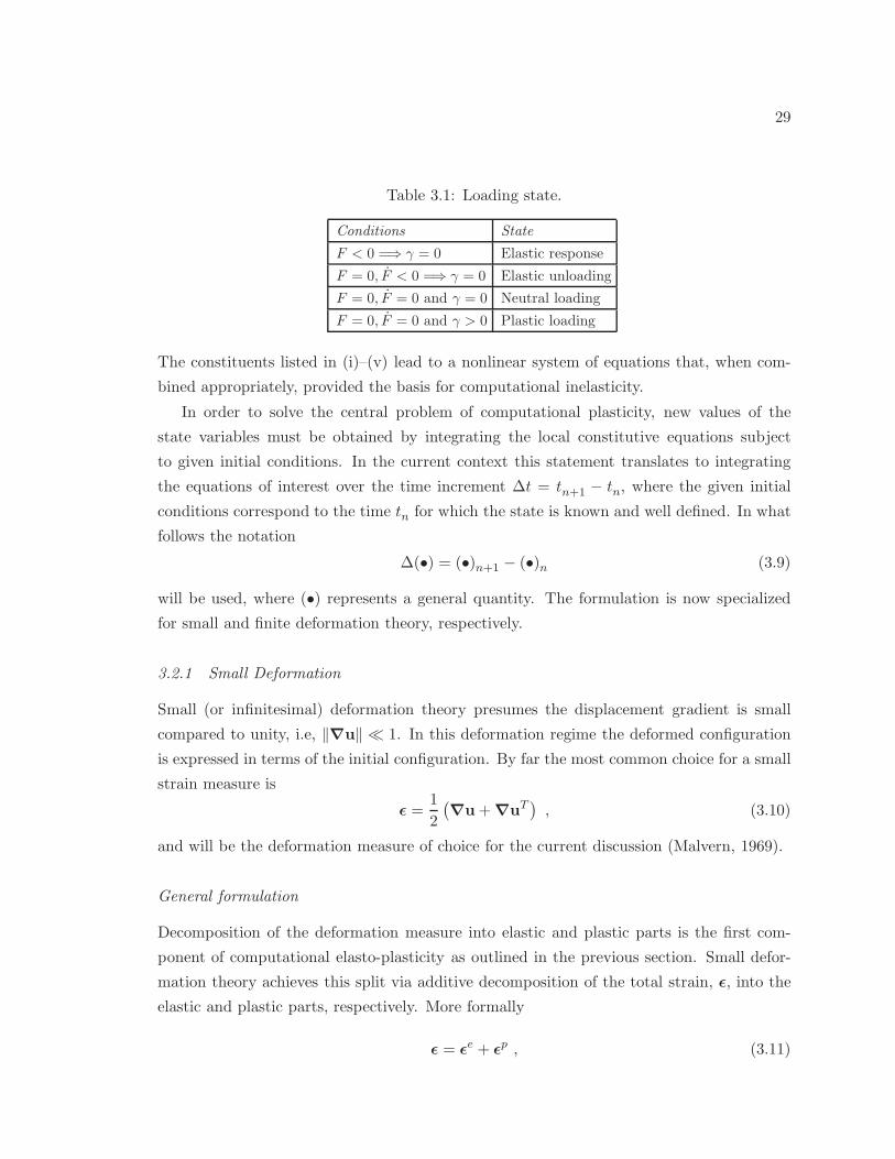
29

Table 3.1: Loading state.

Conditions State

F < 0 =⇒ γ = 0 Elastic response

F = 0, F < 0 =⇒ γ = 0 Elastic unloading

F = 0, F = 0 and γ = 0 Neutral loading

F = 0, F = 0 and γ > 0 Plastic loading

The constituents listed in (i)–(v) lead to a nonlinear system of equations that, when com-

bined appropriately, provided the basis for computational inelasticity.

In order to solve the central problem of computational plasticity, new values of the

state variables must be obtained by integrating the local constitutive equations subject

to given initial conditions. In the current context this statement translates to integrating

the equations of interest over the time increment ∆t = tn+1 − tn, where the given initial

conditions correspond to the time tn for which the state is known and well defined. In what

follows the notation

∆(•) = (•)n+1 − (•)n (3.9)

will be used, where (•) represents a general quantity. The formulation is now specialized

for small and finite deformation theory, respectively.

3.2.1 Small Deformation

Small (or infinitesimal) deformation theory presumes the displacement gradient is small

compared to unity, i.e, ‖∇u‖ ≪ 1. In this deformation regime the deformed configuration

is expressed in terms of the initial configuration. By far the most common choice for a small

strain measure is

ǫ =1

2

(∇u+∇uT

), (3.10)

and will be the deformation measure of choice for the current discussion (Malvern, 1969).

General formulation

Decomposition of the deformation measure into elastic and plastic parts is the first com-

ponent of computational elasto-plasticity as outlined in the previous section. Small defor-

mation theory achieves this split via additive decomposition of the total strain, ǫ, into the

elastic and plastic parts, respectively. More formally

ǫ = ǫe + ǫp , (3.11)

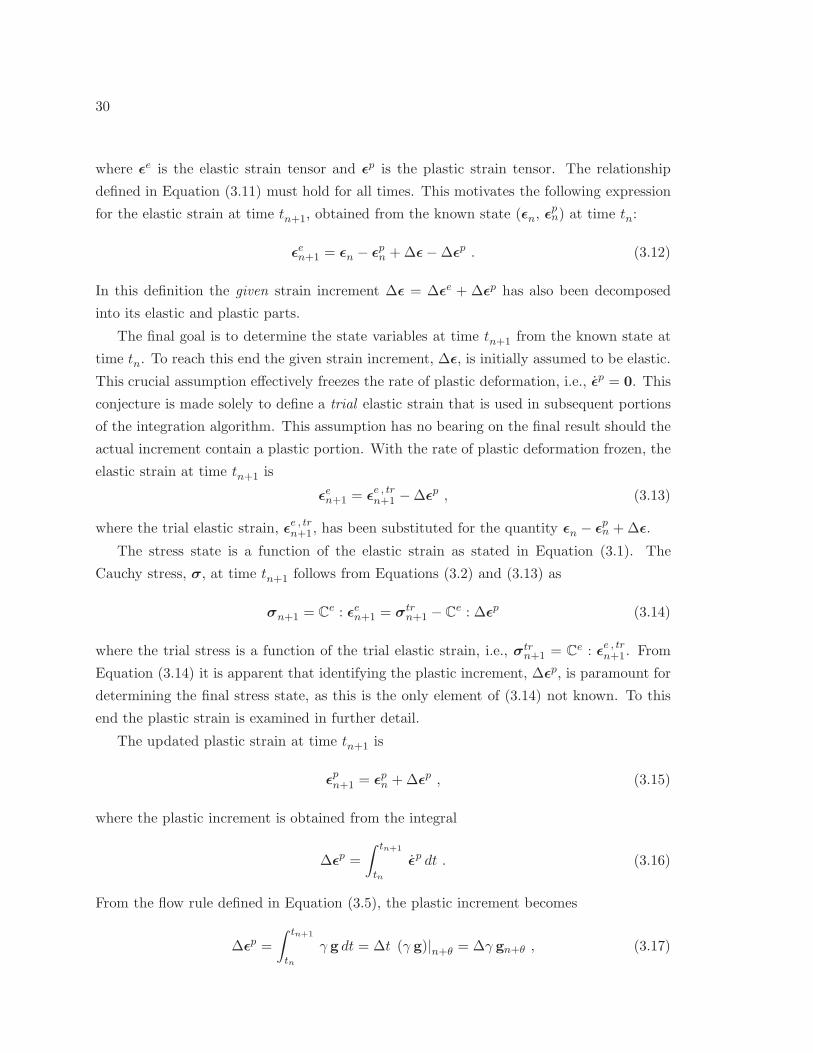
30

where ǫe is the elastic strain tensor and ǫp is the plastic strain tensor. The relationship

defined in Equation (3.11) must hold for all times. This motivates the following expression

for the elastic strain at time tn+1, obtained from the known state (ǫn, ǫpn) at time tn:

ǫen+1 = ǫn − ǫpn +∆ǫ−∆ǫp . (3.12)

In this definition the given strain increment ∆ǫ = ∆ǫe + ∆ǫp has also been decomposed

into its elastic and plastic parts.

The final goal is to determine the state variables at time tn+1 from the known state at

time tn. To reach this end the given strain increment, ∆ǫ, is initially assumed to be elastic.

This crucial assumption effectively freezes the rate of plastic deformation, i.e., ǫp = 0. This

conjecture is made solely to define a trial elastic strain that is used in subsequent portions

of the integration algorithm. This assumption has no bearing on the final result should the

actual increment contain a plastic portion. With the rate of plastic deformation frozen, the

elastic strain at time tn+1 is

ǫen+1 = ǫe , trn+1 −∆ǫp , (3.13)

where the trial elastic strain, ǫe , trn+1, has been substituted for the quantity ǫn − ǫpn +∆ǫ.

The stress state is a function of the elastic strain as stated in Equation (3.1). The

Cauchy stress, σ, at time tn+1 follows from Equations (3.2) and (3.13) as

σn+1 = Ce : ǫen+1 = σtr

n+1 − Ce : ∆ǫp (3.14)

where the trial stress is a function of the trial elastic strain, i.e., σtrn+1 = C

e : ǫe , trn+1. From

Equation (3.14) it is apparent that identifying the plastic increment, ∆ǫp, is paramount for

determining the final stress state, as this is the only element of (3.14) not known. To this

end the plastic strain is examined in further detail.

The updated plastic strain at time tn+1 is

ǫpn+1 = ǫpn +∆ǫp , (3.15)

where the plastic increment is obtained from the integral

∆ǫp =

∫ tn+1

tn

ǫp dt . (3.16)

From the flow rule defined in Equation (3.5), the plastic increment becomes

∆ǫp =

∫ tn+1

tn

γ g dt = ∆t (γ g)|n+θ = ∆γ gn+θ , (3.17)

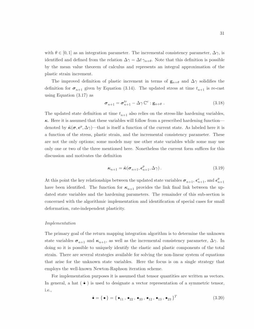
31

with θ ∈ [0, 1] as an integration parameter. The incremental consistency parameter, ∆γ, is

identified and defined from the relation ∆γ = ∆t γn+θ. Note that this definition is possible

by the mean value theorem of calculus and represents an integral approximation of the

plastic strain increment.

The improved definition of plastic increment in terms of gn+θ and ∆γ solidifies the

definition for σn+1 given by Equation (3.14). The updated stress at time tn+1 is re-cast

using Equation (3.17) as

σn+1 = σtrn+1 −∆γ Ce : gn+θ . (3.18)

The updated state definition at time tn+1 also relies on the stress-like hardening variables,

κ. Here it is assumed that these variables will follow from a prescribed hardening function—

denoted by κ(σ, ǫp,∆γ)—that is itself a function of the current state. As labeled here it is

a function of the stress, plastic strain, and the incremental consistency parameter. These

are not the only options; some models may use other state variables while some may use

only one or two of the three mentioned here. Nonetheless the current form suffices for this

discussion and motivates the definition

κn+1 = κ(σn+1, ǫpn+1,∆γ) . (3.19)

At this point the key relationships between the updated state variables σn+1, ǫen+1, and ǫ

pn+1

have been identified. The function for κn+1 provides the link final link between the up-

dated state variables and the hardening parameters. The remainder of this sub-section is

concerned with the algorithmic implementation and identification of special cases for small

deformation, rate-independent plasticity.

Implementation

The primary goal of the return mapping integration algorithm is to determine the unknown

state variables σn+1 and κn+1, as well as the incremental consistency parameter, ∆γ. In

doing so it is possible to uniquely identify the elastic and plastic components of the total

strain. There are several strategies available for solving the non-linear system of equations

that arise for the unknown state variables. Here the focus is on a single strategy that

employs the well-known Newton-Raphson iteration scheme.

For implementation purposes it is assumed that tensor quantities are written as vectors.

In general, a hat ( • ) is used to designate a vector representation of a symmetric tensor,

i.e.,

• = • = •11 , •22 , •33 , •12 , •13 , •23 T (3.20)

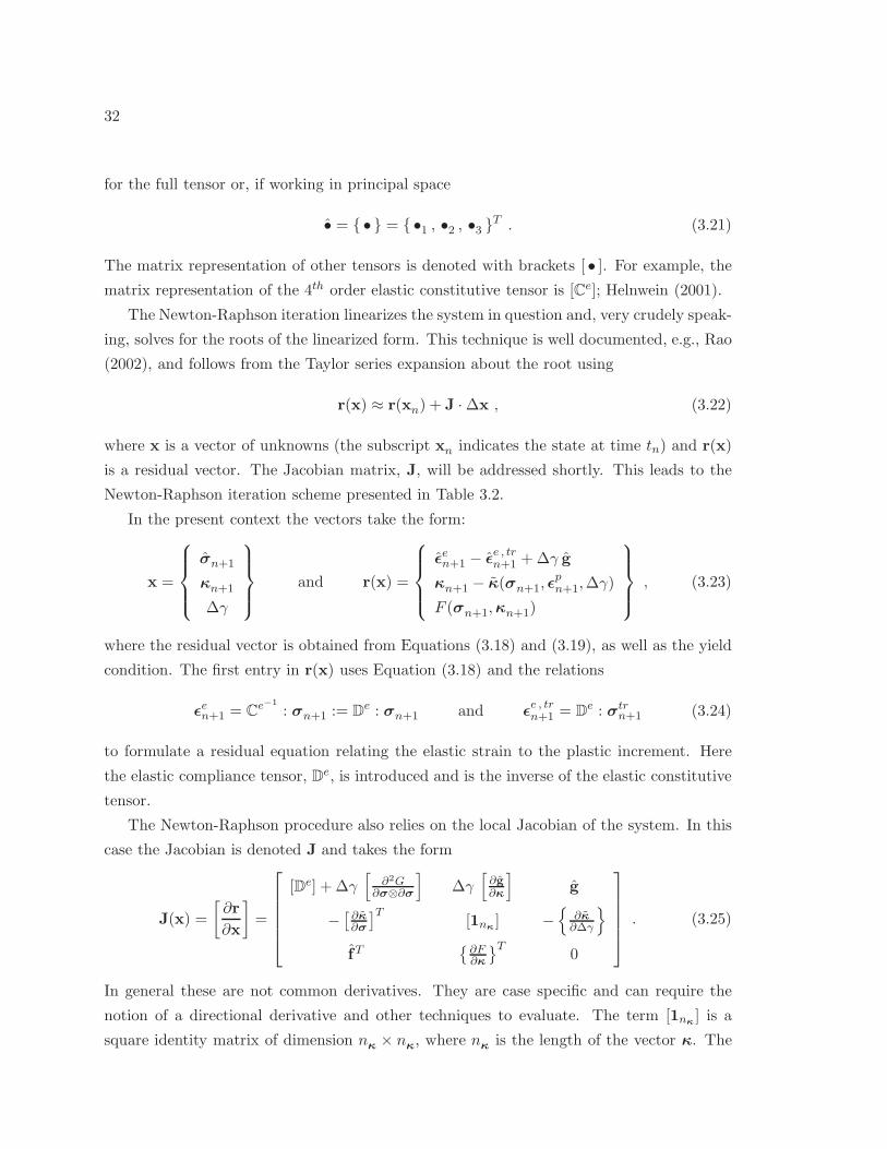
32

for the full tensor or, if working in principal space

• = • = •1 , •2 , •3 T . (3.21)

The matrix representation of other tensors is denoted with brackets [ • ]. For example, the

matrix representation of the 4th order elastic constitutive tensor is [Ce]; Helnwein (2001).

The Newton-Raphson iteration linearizes the system in question and, very crudely speak-

ing, solves for the roots of the linearized form. This technique is well documented, e.g., Rao

(2002), and follows from the Taylor series expansion about the root using

r(x) ≈ r(xn) + J ·∆x , (3.22)

where x is a vector of unknowns (the subscript xn indicates the state at time tn) and r(x)

is a residual vector. The Jacobian matrix, J, will be addressed shortly. This leads to the

Newton-Raphson iteration scheme presented in Table 3.2.

In the present context the vectors take the form:

x =

σn+1

κn+1

∆γ

and r(x) =

ǫen+1 − ǫe , trn+1 +∆γ g

κn+1 − κ(σn+1, ǫpn+1,∆γ)

F (σn+1,κn+1)

, (3.23)

where the residual vector is obtained from Equations (3.18) and (3.19), as well as the yield

condition. The first entry in r(x) uses Equation (3.18) and the relations

ǫen+1 = Ce−1

: σn+1 := De : σn+1 and ǫ

e , trn+1 = D

e : σtrn+1 (3.24)

to formulate a residual equation relating the elastic strain to the plastic increment. Here

the elastic compliance tensor, De, is introduced and is the inverse of the elastic constitutive

tensor.

The Newton-Raphson procedure also relies on the local Jacobian of the system. In this

case the Jacobian is denoted J and takes the form

J(x) =

[∂r

∂x

]

=

[De] + ∆γ[

∂2G∂σ⊗∂σ

]

∆γ[∂g∂κ

]

g

−[∂κ∂σ

]T[1nκ

] −

∂κ∂∆γ

fT∂F∂κ

T0

. (3.25)

In general these are not common derivatives. They are case specific and can require the

notion of a directional derivative and other techniques to evaluate. The term [1nκ] is a

square identity matrix of dimension nκ× n

κ, where n

κis the length of the vector κ. The

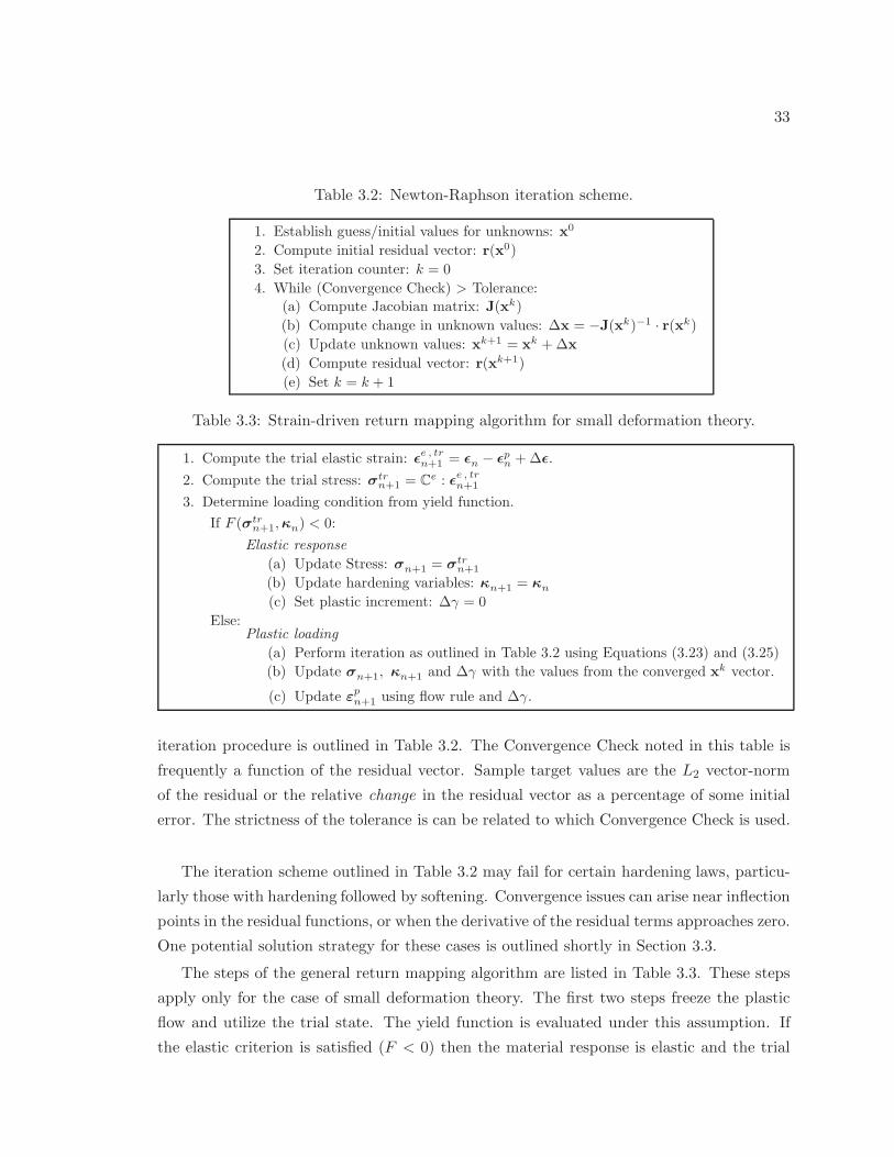
33

Table 3.2: Newton-Raphson iteration scheme.

1. Establish guess/initial values for unknowns: x0

2. Compute initial residual vector: r(x0)

3. Set iteration counter: k = 0

4. While (Convergence Check) > Tolerance:

(a) Compute Jacobian matrix: J(xk)

(b) Compute change in unknown values: ∆x = −J(xk)−1 · r(xk)

(c) Update unknown values: xk+1 = xk +∆x

(d) Compute residual vector: r(xk+1)

(e) Set k = k + 1

Table 3.3: Strain-driven return mapping algorithm for small deformation theory.

1. Compute the trial elastic strain: ǫe , trn+1 = ǫn − ǫpn +∆ǫ.

2. Compute the trial stress: σtrn+1 = Ce : ǫe , trn+1

3. Determine loading condition from yield function.

If F (σtrn+1,κn) < 0:

Elastic response

(a) Update Stress: σn+1 = σtrn+1

(b) Update hardening variables: κn+1 = κn

(c) Set plastic increment: ∆γ = 0

Else:Plastic loading

(a) Perform iteration as outlined in Table 3.2 using Equations (3.23) and (3.25)

(b) Update σn+1, κn+1 and ∆γ with the values from the converged xk vector.

(c) Update εpn+1 using flow rule and ∆γ.

iteration procedure is outlined in Table 3.2. The Convergence Check noted in this table is

frequently a function of the residual vector. Sample target values are the L2 vector-norm

of the residual or the relative change in the residual vector as a percentage of some initial

error. The strictness of the tolerance is can be related to which Convergence Check is used.

The iteration scheme outlined in Table 3.2 may fail for certain hardening laws, particu-

larly those with hardening followed by softening. Convergence issues can arise near inflection

points in the residual functions, or when the derivative of the residual terms approaches zero.

One potential solution strategy for these cases is outlined shortly in Section 3.3.

The steps of the general return mapping algorithm are listed in Table 3.3. These steps

apply only for the case of small deformation theory. The first two steps freeze the plastic

flow and utilize the trial state. The yield function is evaluated under this assumption. If

the elastic criterion is satisfied (F < 0) then the material response is elastic and the trial

34

values are used as the updated state for stress and elastic strain. If the elastic yield criterion

is not satisfied, then the Newton-Raphson iteration procedure outlined in Table 3.2 must

be performed to determine the converged value of xk, and hence the updated values for

σn+1, κn+1 and ∆γ.

The next subsection investigates the extension of the return mapping strategy for finite

strain measures. The structure of the algorithm is similar to that presented in Table 3.3—

permitting a seamless incorporation of both infinitesimal and finite deformation measures

into a single framework.

3.2.2 Finite Deformation

There are several finite deformation measures that can be used to characterize the deformed

material state; see, e.g., Malvern (1969); Holzapfel (2000). Such measures become necessary

when the norm of displacement gradient is no longer small when compared to unity. Unlike

small deformation theory, finite strain theories can be formulated in either the initial or

deformed configuration. As such, there are typically additional complexities associated

with constitutive laws and care must be taken to ensure frame indifference and objectivity;

e.g., Truesdell and Noll (1965); Marsden and Hughes (1983). A full discussion of these topics

is largely beyond the scope of this work. Here the emphasis is placed on the development

and application of the left Cauchy-Green deformation tensor

b = F · FT , (3.26)

where F is the deformation gradient. With appropriate manipulations this deformation

measure provides the basis for a return mapping algorithm that is remarkably similar to

the framework presented for small deformation measures.

General formulation

The simplicity of the small deformation return map algorithm3 provided in Table 3.3 is due

primarily to the additive decomposition of the deformation measure, i.e., the split outlined

in Equation (3.11). For finite deformations such a split is not permissible—the formulation

instead must rely on multiplicative decomposition of the tensor quantity in question. The

deformation gradient is decomposed using

F = v ·R = Fe · Fp , (3.27)

3This statement is intended in a relative sense. A majority of the general populace likely perceive the

return mapping algorithm to be quite complex regardless of which deformation measure is used.

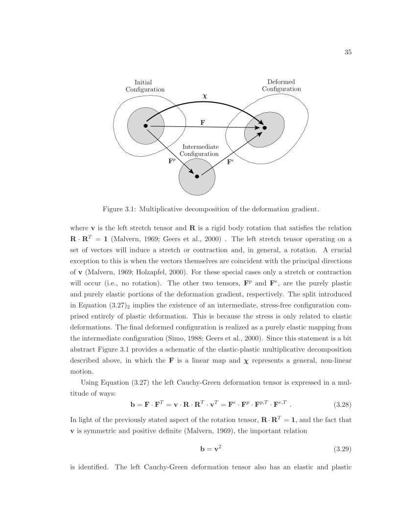
35

ConfigurationDeformed

ConfigurationIntermediate

ConfigurationInitial

χ

F

FeFp

Figure 3.1: Multiplicative decomposition of the deformation gradient.

where v is the left stretch tensor and R is a rigid body rotation that satisfies the relation

R · RT = 1 (Malvern, 1969; Geers et al., 2000) . The left stretch tensor operating on a

set of vectors will induce a stretch or contraction and, in general, a rotation. A crucial

exception to this is when the vectors themselves are coincident with the principal directions

of v (Malvern, 1969; Holzapfel, 2000). For these special cases only a stretch or contraction

will occur (i.e., no rotation). The other two tensors, Fp and Fe, are the purely plastic

and purely elastic portions of the deformation gradient, respectively. The split introduced

in Equation (3.27)2 implies the existence of an intermediate, stress-free configuration com-

prised entirely of plastic deformation. This is because the stress is only related to elastic

deformations. The final deformed configuration is realized as a purely elastic mapping from

the intermediate configuration (Simo, 1988; Geers et al., 2000). Since this statement is a bit

abstract Figure 3.1 provides a schematic of the elastic-plastic multiplicative decomposition

described above, in which the F is a linear map and χ represents a general, non-linear

motion.

Using Equation (3.27) the left Cauchy-Green deformation tensor is expressed in a mul-

titude of ways:

b = F · FT = v ·R ·RT · vT = Fe · Fp · Fp,T · Fe,T . (3.28)

In light of the previously stated aspect of the rotation tensor, R ·RT = 1, and the fact that

v is symmetric and positive definite (Malvern, 1969), the important relation

b = v2 (3.29)

is identified. The left Cauchy-Green deformation tensor also has an elastic and plastic

36

portion; the former is related to the elastic portion of stretches v—as well as Fe—and given

by

be = Fe · Fe,T . (3.30)

As discussed at earlier, the principal stretches/contractions are not rotated by successive

applications of the stretch tensor v. As such, it is beneficial to write the tensor be as a

polar decomposition of eigenvalues, bei , and eigenvectors, n(i):

be =3∑

i

bei m(i) where m(i) = n(i) ⊗ n(i) . (3.31)

This allows a useful relationship between the principal values of the elastic stretches, λi,

and the elastic components, bei , to be established via Equation (3.29) as

bei = λ2i . (3.32)

At this point a temporary digression is made to discuss yet another strain measure,

the natural or Hencky strain which is cast in terms of the principal stretches

εei = log λi . (3.33)

This measure is part of a larger family of generalized strain measures that encompass both

the initial and deformed configurations and was introduced by Seth (1961) and Hill (1968a,b,

1970). It proves convenient in classifying the elasto-plastic response of a given material,

particularly in the context of a numerical integration scheme (Simo et al., 1993; Simo, 1998;

Holzapfel, 2000). Moreover, when taking into account the influence of the strain path, it can

be shown that the natural strain provides the correct measure when the deformation takes

place as a series of incremental strains—as is the case for a strain driven problem (Rees,

2006).

The natural strain tensor is obtained from the elastic deformation measure be by com-

bining Equations (3.32) and (3.33) and by exploiting the properties of logarithmic functions.

The net result is a tensor of the form

εe =1

2log b =

3∑

i

1

2log bei m

(i) . (3.34)

Both tensors be and εe are with respect to the deformed configuration in Figure 3.1. In

Section 3.3 the benefits of using a logarithmic strain measure will become more apparent as

specific forms of the elastic tensor Ce are selected. Prior to that, however, is the discussion

of the return mapping integration algorithm for finite deformation elasto-plasticity.

37

Implementation

The implementation procedure for the return mapping algorithm is similar to the steps

outlined in Table 3.3. The final goal of the integration algorithm remains the same—to

determine the state variables at time tn+1 from the known state at time tn—however, there

are some key differences. Since the given strain increment can no longer be additively

decomposed for finite deformations, it is necessary to push forward values at time tn to

time tn+1. This is accomplished via the incremental deformation gradient, f . A trial elastic

state is obtained using the push forward operation applied to the last converged value of

the elastic deformation measure, bn as

be , trn+1 = f be

n fT . (3.35)

This trial elastic left Cauchy-Green tensor corresponds directly to a trial elastic Hencky

strain tensor via Equation (3.34), i.e.,

εe , trn+1 =

3∑

i

1

2log be , tri mtr(i) . (3.36)

A convenient stress measure commonly used in finite deformation is the Kirchhoff stress,

τ , which differs from the Cauchy stress by the volume ratio J as

τ = J σ where J = detF . (3.37)

Since it is necessary to decompose be into the principal values and directions bei and n(i),

respectively, it is computationally efficient—not to mention necessary from a formulation

standpoint—to work with only the principal values of the tensor quantities in question. In

doing so the yield function and plastic potential are cast in terms of principal Kirchhoff

stress values as opposed to the general stress measure presented in Equation (3.3). This

means the following notational tweaks must also be applied in order to remain consistent:

f =∂F

∂τ=⇒ f =

∂F

∂τ1,∂F

∂τ2,∂F

∂τ3

T

(3.38)

and

g =∂G

∂τ=⇒ g =

∂G

∂τ1,∂G

∂τ2,∂G

∂τ3

T

, (3.39)

where the hat ( • ) notation has been used to specify a vector in principal space, i.e.,

• = • = •1 , •2 , •3 T . (3.40)

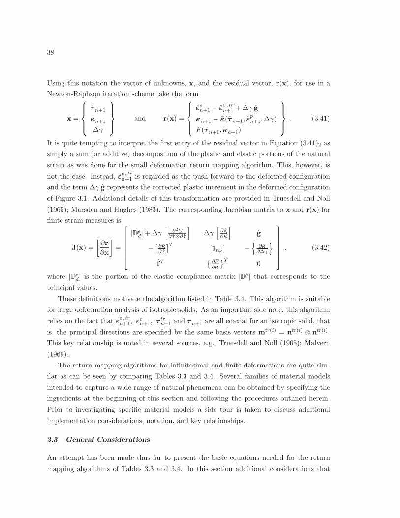
38

Using this notation the vector of unknowns, x, and the residual vector, r(x), for use in a

Newton-Raphson iteration scheme take the form

x =

τn+1

κn+1

∆γ

and r(x) =

εen+1 − εe , trn+1 +∆γ g

κn+1 − κ(τn+1, εpn+1,∆γ)

F (τn+1,κn+1)

. (3.41)

It is quite tempting to interpret the first entry of the residual vector in Equation (3.41)2 as

simply a sum (or additive) decomposition of the plastic and elastic portions of the natural

strain as was done for the small deformation return mapping algorithm. This, however, is

not the case. Instead, εe , trn+1 is regarded as the push forward to the deformed configuration

and the term ∆γ g represents the corrected plastic increment in the deformed configuration

of Figure 3.1. Additional details of this transformation are provided in Truesdell and Noll

(1965); Marsden and Hughes (1983). The corresponding Jacobian matrix to x and r(x) for

finite strain measures is

J(x) =

[∂r

∂x

]

=

[Ded] + ∆γ

[∂2G

∂τ⊗∂τ

]

∆γ[∂g∂κ

]

g

−[∂κ∂τ

]T[1nκ

] −

∂κ∂∆γ

fT∂F∂κ

T0

, (3.42)

where [Ded] is the portion of the elastic compliance matrix [De] that corresponds to the

principal values.

These definitions motivate the algorithm listed in Table 3.4. This algorithm is suitable

for large deformation analysis of isotropic solids. As an important side note, this algorithm

relies on the fact that εe , trn+1, εen+1, τ

trn+1 and τn+1 are all coaxial for an isotropic solid, that

is, the principal directions are specified by the same basis vectors mtr(i) = ntr(i) ⊗ ntr(i).

This key relationship is noted in several sources, e.g., Truesdell and Noll (1965); Malvern

(1969).

The return mapping algorithms for infinitesimal and finite deformations are quite sim-

ilar as can be seen by comparing Tables 3.3 and 3.4. Several families of material models

intended to capture a wide range of natural phenomena can be obtained by specifying the

ingredients at the beginning of this section and following the procedures outlined herein.

Prior to investigating specific material models a side tour is taken to discuss additional

implementation considerations, notation, and key relationships.

3.3 General Considerations

An attempt has been made thus far to present the basic equations needed for the return

mapping algorithms of Tables 3.3 and 3.4. In this section additional considerations that

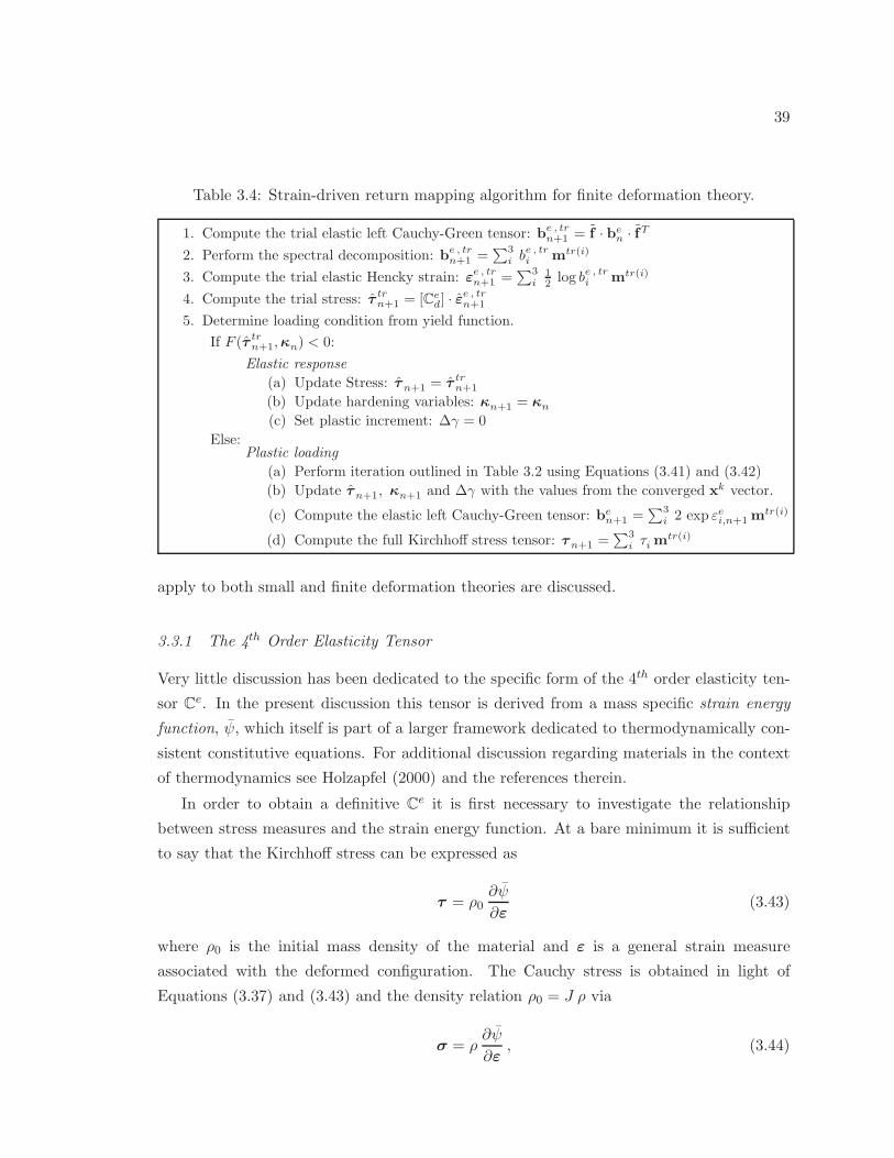
39

Table 3.4: Strain-driven return mapping algorithm for finite deformation theory.

1. Compute the trial elastic left Cauchy-Green tensor: be , trn+1 = f · be

n · fT2. Perform the spectral decomposition: be , tr

n+1 =∑3

i be , tri mtr(i)

3. Compute the trial elastic Hencky strain: εe , trn+1 =∑3

i12 log be , tri mtr(i)

4. Compute the trial stress: τ trn+1 = [Ce

d] · εe , trn+1

5. Determine loading condition from yield function.

If F (τ trn+1,κn) < 0:

Elastic response

(a) Update Stress: τn+1 = τtrn+1

(b) Update hardening variables: κn+1 = κn

(c) Set plastic increment: ∆γ = 0

Else:Plastic loading

(a) Perform iteration outlined in Table 3.2 using Equations (3.41) and (3.42)

(b) Update τn+1, κn+1 and ∆γ with the values from the converged xk vector.

(c) Compute the elastic left Cauchy-Green tensor: ben+1 =

∑3i 2 exp εei,n+1 m

tr(i)

(d) Compute the full Kirchhoff stress tensor: τn+1 =∑3

i τi mtr(i)

apply to both small and finite deformation theories are discussed.

3.3.1 The 4th Order Elasticity Tensor

Very little discussion has been dedicated to the specific form of the 4th order elasticity ten-

sor Ce. In the present discussion this tensor is derived from a mass specific strain energy

function, ψ, which itself is part of a larger framework dedicated to thermodynamically con-

sistent constitutive equations. For additional discussion regarding materials in the context

of thermodynamics see Holzapfel (2000) and the references therein.

In order to obtain a definitive Ce it is first necessary to investigate the relationship

between stress measures and the strain energy function. At a bare minimum it is sufficient

to say that the Kirchhoff stress can be expressed as

τ = ρ0∂ψ

∂ε(3.43)

where ρ0 is the initial mass density of the material and ε is a general strain measure

associated with the deformed configuration. The Cauchy stress is obtained in light of

Equations (3.37) and (3.43) and the density relation ρ0 = J ρ via

σ = ρ∂ψ

∂ε, (3.44)

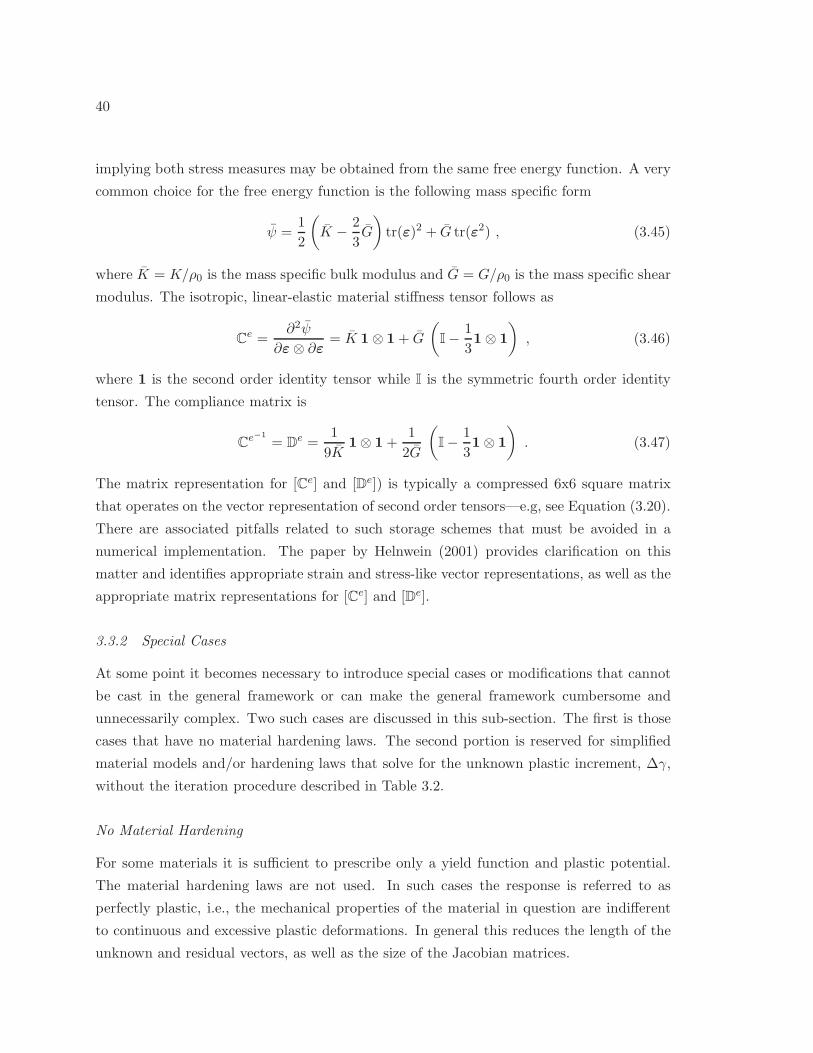
40

implying both stress measures may be obtained from the same free energy function. A very

common choice for the free energy function is the following mass specific form

ψ =1

2

(

K − 2

3G

)

tr(ε)2 + G tr(ε2) , (3.45)

where K = K/ρ0 is the mass specific bulk modulus and G = G/ρ0 is the mass specific shear

modulus. The isotropic, linear-elastic material stiffness tensor follows as

Ce =

∂2ψ

∂ε⊗ ∂ε= K 1⊗ 1+ G

(

I− 1

31⊗ 1

)

, (3.46)

where 1 is the second order identity tensor while I is the symmetric fourth order identity

tensor. The compliance matrix is

Ce−1

= De =

1

9K1⊗ 1+

1

2G

(

I− 1

31⊗ 1

)

. (3.47)

The matrix representation for [Ce] and [De]) is typically a compressed 6x6 square matrix

that operates on the vector representation of second order tensors—e.g, see Equation (3.20).

There are associated pitfalls related to such storage schemes that must be avoided in a

numerical implementation. The paper by Helnwein (2001) provides clarification on this

matter and identifies appropriate strain and stress-like vector representations, as well as the

appropriate matrix representations for [Ce] and [De].

3.3.2 Special Cases

At some point it becomes necessary to introduce special cases or modifications that cannot

be cast in the general framework or can make the general framework cumbersome and

unnecessarily complex. Two such cases are discussed in this sub-section. The first is those

cases that have no material hardening laws. The second portion is reserved for simplified

material models and/or hardening laws that solve for the unknown plastic increment, ∆γ,

without the iteration procedure described in Table 3.2.

No Material Hardening

For some materials it is sufficient to prescribe only a yield function and plastic potential.

The material hardening laws are not used. In such cases the response is referred to as

perfectly plastic, i.e., the mechanical properties of the material in question are indifferent

to continuous and excessive plastic deformations. In general this reduces the length of the

unknown and residual vectors, as well as the size of the Jacobian matrices.

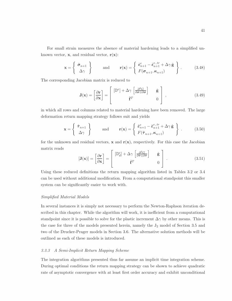
41

For small strain measures the absence of material hardening leads to a simplified un-

known vector, x, and residual vector, r(x):

x =

σn+1

∆γ

and r(x) =

ǫen+1 − ǫe , trn+1 +∆γ g

F (σn+1,κn+1)

. (3.48)

The corresponding Jacobian matrix is reduced to

J(x) =

[∂r

∂x

]

=

[De] + ∆γ[

∂2G∂σ⊗∂σ

]

g

fT 0

, (3.49)

in which all rows and columns related to material hardening have been removed. The large

deformation return mapping strategy follows suit and yields

x =

τn+1

∆γ

and r(x) =

εen+1 − εe , trn+1 +∆γ g

F (τ n+1,κn+1)

. (3.50)

for the unknown and residual vectors, x and r(x), respectively. For this case the Jacobian

matrix reads

[J(x)] =

[∂r

∂x

]

=

[Ded] + ∆γ

[∂2G

∂τ⊗∂τ

]

g

fT 0

. (3.51)

Using these reduced definitions the return mapping algorithm listed in Tables 3.2 or 3.4

can be used without additional modification. From a computational standpoint this smaller

system can be significantly easier to work with.

Simplified Material Models

In several instances it is simply not necessary to perform the Newton-Raphson iteration de-

scribed in this chapter. While the algorithm will work, it is inefficient from a computational

standpoint since it is possible to solve for the plastic increment ∆γ by other means. This is

the case for three of the models presented herein, namely the J2 model of Section 3.5 and

two of the Drucker-Prager models in Section 3.6. The alternative solution methods will be

outlined as each of these models is introduced.

3.3.3 A Semi-Implicit Return Mapping Scheme

The integration algorithms presented thus far assume an implicit time integration scheme.

During optimal conditions the return mapping strategy can be shown to achieve quadratic

rate of asymptotic convergence with at least first order accuracy and exhibit unconditional

42

stability (Simo, 1998; Simo and Hughes, 1998). Unfortunately, under less than optimal

circumstances hardening and evolution laws can become very complex and may include both

hardening/softening as well as non-smooth functions. In these cases convergence issues can

arise in the algorithm, and in particular computing the Jacobian matrix in (3.25) and (3.42)

becomes problematic. This leads to poor convergence rates and outright divergence of the

return mapping algorithm—particularly if a Newton-Raphson solution scheme is utilized to

find the roots of the system.

In order to combat these issues a semi-implicit return mapping algorithm is introduced

by Tu et al. (2009). The algorithm is based on the assumption that the rate of the stress-

like plastic hardening variables can be frozen over each time step. The updated hardening

variables κn+1 are updated after a converged value for the stress tensor σn+1 (or τn+1) and

plastic increment ∆γ are obtained. In other words, the reduced systems of Equations (3.48)–

(3.51) are used in the return mapping strategy with the hardening variables κn obtained

from the previous time step. The updated values κn+1 are determined from the converged

solution of the reduced system. In this manner the hardening variables lag the stress and

plastic deformation by a time step.

In the work by Tu et al. (2009) this algorithm is implemented and tested for smooth and

non-smooth evolution laws. Using a series of examples and iso-error maps they show suffi-

ciently that the proposed approach handles the evolution equations and material response

both accurately and efficiently. A clear distinction is made for those models in this chapter

based on that formulation.

3.4 Notation and Key Relationships

This short section addresses notation and other aspects common to all models presented in

this chapter. First and foremost, the symbol σ will be used to represent a general stress

tensor. This may be the Cauchy stress—as was previously assigned the symbol σ—but may

also represent the Kirchhoff stress previously denoted by τ . The reader is held accountable

for understanding the context in which these equations are presented. Two sets of coordi-

nates are discussed in what follows. The principal stress space is denoted by σ1, σ2, σ3.Alternatively, a transformed set of coordinates ξ1, ξ2, ξ3 is used in some figures in which

ξ3 is coaxial with the hydrostatic axis, i.e., σ1 = σ2 = σ3. This coordinate transformation

means the coordinates ξ1, ξ2 reside on the deviatoric plane. Both coordinate systems are

shown in Figure A.1. Appendix A outlines a procedure to identify those points in principal

stress space that are on the yield surface. This technique is used to generate all surface

data depicted in this chapter.

43

Each yield function and plastic potential appearing in this chapter can be written in

terms of the stress invariants, I1, I2, and I3. These are defined in terms of the principal

stress values as

I1 = trσ = σ1 + σ2 + σ3 , (3.52)

I2 =1

2

[(trσ)2 − tr(σ2)

]= σ1 σ2 + σ1 σ3 + σ2 σ3 , and (3.53)

I3 = detσ = σ1 σ2 σ3 . (3.54)

An additional parameter, c, is introduced for some models. This allows the yield function or

plastic potential to be shifted along the hydrostatic axis. An auxiliary stress, σ = σ− c1, isdefined using an overbar symbol. This is not to be confused with the mass-specific notation

used previously in other chapters. The shift by c leads to a set of modified invariants I1, I2,

and I3 that are defined in terms of their former selves and c by way of

I1 = tr σ = σ1 + σ2 + σ3 = I1 − 3 c , (3.55)

I2 =1

2

[(tr σ)2 − tr(σ2)

]= σ1 σ2+σ1 σ3+σ2 σ3 = I2−2 I1 c+3 c2 , and (3.56)

I3 = det σ = σ1 σ2 σ3 = I3 − I2 c+ I1 c2 − c3 . (3.57)

The deviatoric stress, s, is used extensively in what follows. This tensor is related to the

stress tensor and I1 through

s = s = σ − I131 . (3.58)

Note that the relation s = s holds, as the cohesion modifies only the volumetric portion of

the tensor. Largely of interest in the material models is the magnitude of the deviatoric

stress, ‖s‖, which is related to the other invariants by

‖s‖2 = s : s =2

3(I21 − 3 I2) . (3.59)

Both the plastic flow direction, g, and yield surface normal, f , invoke derivatives with

respect to the stress tensor. However, both F and G need to be expressed in terms of the

invariants—which are themselves a function of the stress tensor. The following differential

relations (Wriggers, 2008) are useful in computing said derivatives:

dI1 =∂I1∂σ

: dσ =⇒ ∂I1∂σ

= 1 , (3.60)

dI2 =∂I2∂σ

: dσ =⇒ ∂I2∂σ

= I1 1− σ , and (3.61)

44

dI3 =∂I3∂σ

: dσ =⇒ ∂I3∂σ

= I3 σ−1 . (3.62)

In light of the shifted invariant definitions of (3.55)–(3.57), as well as (3.60)–(3.62), the

differential of the shifted invariants are

dI1 =∂I1∂σ

: dσ =⇒ ∂I1∂σ

= 1 , (3.63)

dI2 =∂I2∂σ

: dσ =⇒ ∂I2∂σ

= I1 1− σ − 2 c1 , and (3.64)

dI3 =∂I3∂σ

: dσ =⇒ ∂I3∂σ

= I3 σ−1 − c (I1 1− σ) + c2 1 . (3.65)

With respect to the deviatoric stress two useful relationships are

ds =∂s

∂σ: dσ =⇒ ∂s

∂σ= I− 1

31⊗ 1 = Idev and (3.66)

d‖s‖ =∂‖s‖∂σ

: dσ =⇒ ∂‖s‖∂σ

=s

‖s‖ , (3.67)

and finally, the derivative of the inverse stress tensor can be determined (Wriggers, 2008)

as (∂σ−1

∂σ

)

iklm

= −1

2

(σ−1il σ−1

mk + σ−1im σ−1

lk

). (3.68)

Here index notation is used and the free indices i, k, l, andm range from 1–3. The remainder

of this chapter is dedicated to the presentation of multiple material models that utilize many

of the relations given in this section. These models are presented and implemented in a

framework consistent with the MPM. The explicit nature of the MPM does not require/use

the consistent elasto-plastic tangent operator, Cep. Therefore, the formulation of the tangent

operator is omitted in the following discussions.

3.5 J2 Material Model

The J2 material model predicts material failure when the second invariant of the devia-

toric stress tensor reaches a critical value. Of the many nonlinear material models and

failure theories, the J2 theory is perhaps the simplest from a formulation and implementa-

tion standpoint. Yet, despite the simplicity, this yield condition accurately replicates the

mechanical response of a wide variety of materials.

The yield function and plastic potential are written in terms of the stress and stress-like

hardening variables as

F (η,κkin, κiso) = G(η,κkin, κiso) = ‖η‖+ σEffY (3.69)

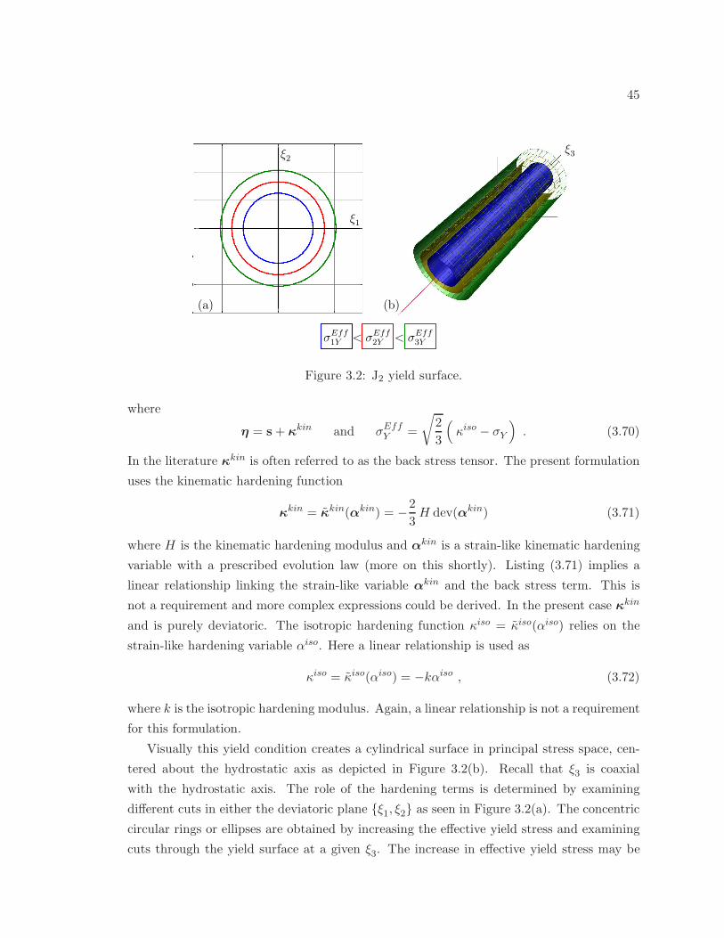
45

ξ3

σEff1Y < σEff

2Y < σEff3Y

(a)

ξ1

ξ2

(b)

Figure 3.2: J2 yield surface.

where

η = s+ κkin and σEffY =

√

2

3

(

κiso − σY

)

. (3.70)

In the literature κkin is often referred to as the back stress tensor. The present formulation

uses the kinematic hardening function

κkin = κkin(αkin) = −2

3H dev(αkin) (3.71)

where H is the kinematic hardening modulus and αkin is a strain-like kinematic hardening

variable with a prescribed evolution law (more on this shortly). Listing (3.71) implies a

linear relationship linking the strain-like variable αkin and the back stress term. This is

not a requirement and more complex expressions could be derived. In the present case κkin

and is purely deviatoric. The isotropic hardening function κiso = κiso(αiso) relies on the

strain-like hardening variable αiso. Here a linear relationship is used as

κiso = κiso(αiso) = −kαiso , (3.72)

where k is the isotropic hardening modulus. Again, a linear relationship is not a requirement

for this formulation.

Visually this yield condition creates a cylindrical surface in principal stress space, cen-

tered about the hydrostatic axis as depicted in Figure 3.2(b). Recall that ξ3 is coaxial

with the hydrostatic axis. The role of the hardening terms is determined by examining

different cuts in either the deviatoric plane ξ1, ξ2 as seen in Figure 3.2(a). The concentric

circular rings or ellipses are obtained by increasing the effective yield stress and examining

cuts through the yield surface at a given ξ3. The increase in effective yield stress may be

46

interpreted either as three separate materials, each with a larger yield stress, σY , or a single

material that accumulates isotropic hardening through plastic deformation. Either way the

net result is a cylindrical surface whose radius grows perpendicular to the hydrostatic axis.

The back stress, κkin, shifts/translates the yield surface about the hydrostatic axis (not

pictured).

As hinted above the strain-like terms follow from a prescribed hardening law. The

updated values at time tn+1 are obtained by time integration of the prescribed hardening

laws. Algorithmically these are expressed as

αkinn+1 = αkin

n +∆γ∂F

∂κkin

∣∣∣∣n+1

= αkinn +∆γ

η

‖η‖

∣∣∣∣n+1

(3.73)

and

αison+1 = αiso

n +∆γ∂F

∂αiso

∣∣∣∣n+1

= αison +∆γ

√

2

3

∂κiso

∂αiso

∣∣∣∣∣n+1

. (3.74)

Note that (3.73) follows from the linear kinematic hardening described by (3.71), while

listing (3.74) is not yet restricted to a linear isotropic hardening function. This motivates

the following definitions for the unknown and residual vectors, x and r(x) respectively:

x =

σn+1

αkinn+1

αison+1

∆γ

and r(x) =

ǫen+1 − ǫe , trn+1 +∆γ η

‖η‖

∣∣∣n+1

∆αkin −∆γ η

‖η‖

∣∣∣n+1

∆αiso −∆γ√

23

∂κiso

∂αiso

∣∣∣n+1

F (η,κkin, κiso)∣∣n+1

, (3.75)

from which the corresponding terms in the Jacobian matrix of either (3.25) or (3.42) can

be computed.

However, as noted in Section 3.3.2, for some material models it is possible to solve for

the plastic increment ∆γ by other means—and that is certainly the case here. Provided the

back stress is linearly related to αkinn , the relationship

ηn+1 = ηtrn+1 − (2G +

2

3H)∆γ

ηn+1

‖ηn+1‖(3.76)

can be established using (3.70)1 and (3.71). The trial term ηtrn+1 follows from the definition

ηtrn+1 = strn+1 + κkin

n , (3.77)

where the notion of a trial state is obtained by assuming the plastic flow is frozen over the

time step. Equation (3.76) can be reorganized to read[

1 +(2G+ 2

3H)∆γ

‖ηn+1‖

]

ηn+1 = ηtrn+1 , (3.78)

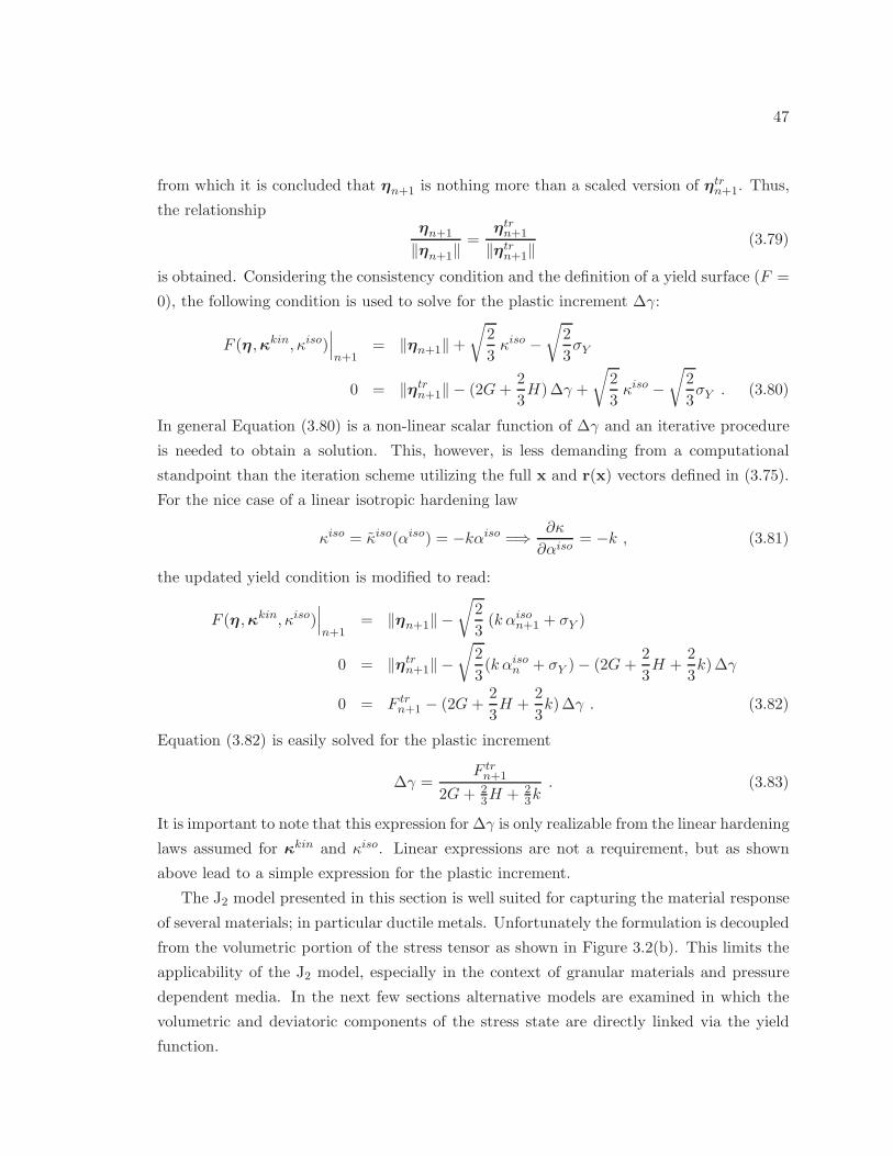
47

from which it is concluded that ηn+1 is nothing more than a scaled version of ηtrn+1. Thus,

the relationshipηn+1

‖ηn+1‖=

ηtrn+1

‖ηtrn+1‖

(3.79)

is obtained. Considering the consistency condition and the definition of a yield surface (F =

0), the following condition is used to solve for the plastic increment ∆γ:

F (η,κkin, κiso)∣∣∣n+1

= ‖ηn+1‖+√

2

3κiso −

√

2

3σY

0 = ‖ηtrn+1‖ − (2G+

2

3H)∆γ +

√

2

3κiso −

√

2

3σY . (3.80)

In general Equation (3.80) is a non-linear scalar function of ∆γ and an iterative procedure

is needed to obtain a solution. This, however, is less demanding from a computational

standpoint than the iteration scheme utilizing the full x and r(x) vectors defined in (3.75).

For the nice case of a linear isotropic hardening law

κiso = κiso(αiso) = −kαiso =⇒ ∂κ

∂αiso= −k , (3.81)

the updated yield condition is modified to read:

F (η,κkin, κiso)∣∣∣n+1

= ‖ηn+1‖ −√

2

3(k αiso

n+1 + σY )

0 = ‖ηtrn+1‖ −

√

2

3(k αiso

n + σY )− (2G +2

3H +

2

3k)∆γ

0 = F trn+1 − (2G +

2

3H +

2

3k)∆γ . (3.82)

Equation (3.82) is easily solved for the plastic increment

∆γ =F trn+1

2G+ 23H + 2

3k. (3.83)

It is important to note that this expression for ∆γ is only realizable from the linear hardening

laws assumed for κkin and κiso. Linear expressions are not a requirement, but as shown

above lead to a simple expression for the plastic increment.

The J2 model presented in this section is well suited for capturing the material response

of several materials; in particular ductile metals. Unfortunately the formulation is decoupled

from the volumetric portion of the stress tensor as shown in Figure 3.2(b). This limits the

applicability of the J2 model, especially in the context of granular materials and pressure

dependent media. In the next few sections alternative models are examined in which the

volumetric and deviatoric components of the stress state are directly linked via the yield

function.

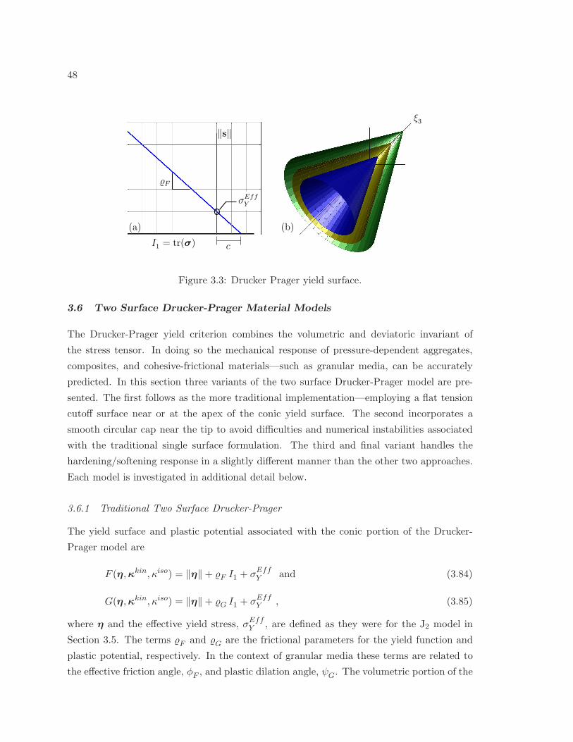
48

(a) (b)

σEffY

‖s‖

I1 = tr(σ)

F

ξ3

c

Figure 3.3: Drucker Prager yield surface.

3.6 Two Surface Drucker-Prager Material Models

The Drucker-Prager yield criterion combines the volumetric and deviatoric invariant of

the stress tensor. In doing so the mechanical response of pressure-dependent aggregates,

composites, and cohesive-frictional materials—such as granular media, can be accurately

predicted. In this section three variants of the two surface Drucker-Prager model are pre-

sented. The first follows as the more traditional implementation—employing a flat tension

cutoff surface near or at the apex of the conic yield surface. The second incorporates a

smooth circular cap near the tip to avoid difficulties and numerical instabilities associated

with the traditional single surface formulation. The third and final variant handles the

hardening/softening response in a slightly different manner than the other two approaches.

Each model is investigated in additional detail below.

3.6.1 Traditional Two Surface Drucker-Prager

The yield surface and plastic potential associated with the conic portion of the Drucker-

Prager model are

F (η,κkin, κiso) = ‖η‖+ F I1 + σEffY and (3.84)

G(η,κkin, κiso) = ‖η‖+ G I1 + σEffY , (3.85)

where η and the effective yield stress, σEffY , are defined as they were for the J2 model in

Section 3.5. The terms F and G are the frictional parameters for the yield function and

plastic potential, respectively. In the context of granular media these terms are related to

the effective friction angle, φF , and plastic dilation angle, ψG. The volumetric portion of the

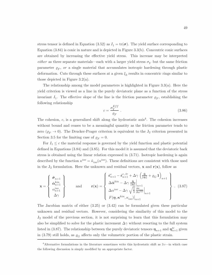
49

stress tensor is defined in Equation (3.52) as I1 = tr(σ). The yield surface corresponding to

Equation (3.84) is conic in nature and is depicted in Figure 3.3(b). Concentric conic surfaces

are obtained by increasing the effective yield stress. This increase may be interpreted

either as three separate materials—each with a larger yield stress σY but the same friction

parameter F , or a single material that accumulates isotropic hardening through plastic

deformation. Cuts through these surfaces at a given ξ3 results in concentric rings similar to

those depicted in Figure 3.2(a).

The relationship among the model parameters is highlighted in Figure 3.3(a). Here the

yield criterion is viewed as a line in the purely deviatoric plane as a function of the stress

invariant I1. The effective slope of the line is the friction parameter F , establishing the

following relationship

c =σEffY

F. (3.86)

The cohesion, c, is a generalized shift along the hydrostatic axis4. The cohesion increases

without bound and ceases to be a meaningful quantity as the friction parameter tends to

zero (F → 0). The Drucker-Prager criterion is equivalent to the J2 criterion presented in

Section 3.5 for the limiting case of F = 0.

For I1 ≤ c the material response is governed by the yield function and plastic potential

defined in Equations (3.84) and (3.85). For this model it is assumed that the deviatoric back

stress is obtained using the linear relation expressed in (3.71). Isotropic hardening is again

described by the function κiso = κiso(αiso). These definitions are consistent with those used

in the J2 formulation. Here the unknown and residual vectors, x and r(x), follow as

x =

σn+1

αkinn+1

αison+1

∆γ

and r(x) =

ǫen+1 − ǫe , trn+1 +∆γ

(η

‖η‖ + G 1)

n+1

∆αkin −∆γ η

‖η‖

∣∣∣n+1

∆αiso −∆γ√

23

∂κiso

∂αiso

∣∣∣n+1

F (η,κkin, κiso)∣∣n+1

. (3.87)

The Jacobian matrix of either (3.25) or (3.42) can be formulated given these particular

unknown and residual vectors. However, considering the similarity of this model to the

J2 model of the previous section, it is not surprising to learn that this formulation may

also be simplified to solve for the plastic increment ∆γ without resorting to the full system

listed in (3.87). The relationship between the purely deviatoric tensors ηn+1 and ηtrn+1 given

in (3.79) still holds, as G affects only the volumetric portion of the plastic strain.

4Alternative formulations in the literature sometimes write this hydrostatic shift as 3 c—in which case

the following discussion is simply modified by an appropriate factor.

50

The updated yield function at time tn+1 is expressed as

F (η ,κkin, κiso)∣∣∣n+1

= ‖ηn+1‖+ F tr(σn+1) +

√

2

3κiso −

√

2

3σY = 0 , (3.88)

which is generally a non-linear scalar equation in terms of ∆γ. The volumetric term tr(σn+1)

can be expanded to read

tr(σn+1) = tr(σtrn+1)− 9K G∆γ , (3.89)

whereK is the previously defined bulk modulus of the material. Employing linear kinematic

and isotropic hardening, and in light of Equation (3.89), the updated yield condition is

reduced to

F (η ,κkin, αiso)∣∣∣n+1

= F trn+1 −

(

2G+2

3H +

2

3k + 9K G F

)

∆γ = 0 . (3.90)

The trial condition F trn+1 is obtained as it has been for all other trial states, i.e., under the

assumption that no plastic deformation accumulates over the given time step. From (3.90)

the plastic increment is easily obtained as

∆γ =F trn+1

2G+ 23H + 2

3k + 9K G F. (3.91)

The above procedure is valid for all stress states when I1 < c (assuming that c ≥ 0). When

this secondary condition is not satisfied an alternative procedure must be implemented.

Tension Cutoff

At the point I1 = c and ‖s‖ = 0 in Figure 3.3 the model is numerically unstable and a

definitive flow direction does not exist. A second surface perpendicular to the hydrostatic

axis is defined to combat this problem. In general the second surface may be located at any

I1 along the hydrostatic axis. However, for this particular implementation it is assumed the

surface coincides with the tip of the Drucker-Prager cone.

The flat tension cutoff surface is active when the trial stress state satisfies the condition

Itr1 ≥ c. A linear combination of flow directions derived from both active surfaces are used

to map the trial state back to the tip of the Drucker-Prager envelope. The tension cutoff is

described by the yield function

F2(σ, κiso2 ) = I1 − c− κiso2 ) , (3.92)

51

where the hardening function κiso2 = κiso2 (αiso2 ) prescribes the evolution of this surface Petek

(2006). In general this is a non-linear function in terms of the strain-like isotropic hard-

ening parameter αiso2 . The surface resides exclusively at the cone tip as stated previously

thus κiso2 = 0. The yield function and plastic potential are modified to read

F2(σ, κiso) = I1 −

σEffY

Fand G2(σ, κ

iso) = I1 −σEffY

G. (3.93)

In what follows the subscript (•1) refers to those quantities derived from the traditional

Drucker-Prager yield function and plastic potential defined in Equations (3.84) and (3.85).

A subscript (•2) is in reference to the current tension surface.

An updated elastic strain is obtained as

ǫen+1 = ǫe , trn+1 −∆γ1 g1 −∆γ2 g2

= ǫe , trn+1 −∆γ1

(η

‖η‖ + G 1

)

n+1

−∆γ2 1 , (3.94)

from which the updated stress follows accordingly

σn+1 = σtrn+1 −∆γ1

(

2Gη

‖η‖ + 3K G 1

)

n+1

− 3K ∆γ2 1 . (3.95)

The volumetric term is expanded as

I1,n+1 = Itr1,n+1 − 9K G ∆γ1 − 9K∆γ2 . (3.96)

The updated yield conditions provide the final piece of the puzzle necessary to solve for the

two increments ∆γ1 and ∆γ2, i.e.,

F1,n+1 = F tr1,n+1 −

(

2G+2

3H +

2

3k + 9K G F

)

∆γ1 − 9K F ∆γ2 = 0 (3.97)

and

F2,n+1 = F tr2,n+1 − 9K G∆γ1 − 9K ∆γ2 = 0 . (3.98)

Equations (3.97) and (3.98) are expressed alternatively as the linear system

F tr1,n+1

F tr2,n+1

=

[

J11 J12

J21 J22

]

·

∆γ1

∆γ2

, (3.99)

with the coefficients

J11 = 2G+ 23H + 2

3k + 9K G F J12 = 9K F

J21 = 9K G J22 = 9K(3.100)

52

(a) (b)

tr(σ)

(c) ‖s‖

Rt

Tension Cap

It

Drucker Prager

ξ3ξ3

Figure 3.4: Smooth cap Drucker Prager yield surface.

The linear system in (3.99) is easily inverted to solve for ∆γ1 and ∆γ2. However, this form is

very much contingent upon the assumption that the isotropic hardening laws are linear and

the fact that the tension cutoff surface always resides at the tip of the Drucker-Prager cone.

If these conditions are not satisfied, an alternative solutions method is needed to determine

∆γ1 and ∆γ2.

3.6.2 Smooth-Cap Two Surface Drucker-Prager

The two surface model presented in the previous subsection uses a conic envelope and a

planar surface that is perpendicular to the hydrostatic axis. Both surfaces are active states

satisfying the trial condition Itr1 > c. This leads to a coupled linear system that must be

solved for the plastic increments. An alternative approach defines a smooth, circular tension

cap that intersects the linear Drucker-Prager envelope in a smooth fashion. This concept is

illustrated in Figure 3.4(a), (b), and (c). The tension cap is the largest circle of radius Rt

53

centered about the origin that can fit within the Drucker-Prager envelope. The point at

which the two surfaces intersect with the same tangent occurs at the tension transition point

It.

The model formulation and integration algorithm is outlined in the paper by Swan

and Seo (2006). Their presentation includes an additional circular compression cap that

is neglected in the current implementation. Most of the formulation is omitted in this

document since the details are described in the original. Here only the two yield functions

are given in piecewise form:

F (σ, Rt) =

F1(σ) = ‖s‖+ ρF I1 − µ for I1 ≤ It

F2(σ, Rt) = R2t − I21 for I1 > It

, (3.101)

where F1 is the Drucker-Prager criterion and F2 is the circular tension cap. The Drucker-

Prager yield criterion is written in a slightly different form to grant additional flexibility.

The traditional formulation is obtained by selecting µ =√

2/3σY . Unlike the previous two

surface formulation in which both surfaces are active for a trial state Itr1 > c—there is only

a single surface active at any given time in this formulation. Simple checks using the trial

state are performed to determine which yield surface is active. This simplifies the return

mapping algorithm considerably.

The only potential downside to the current implementation is the lack of hardening

functions describing the evolution of the yield surface. This, however, could easily be

modified for future applications.

3.6.3 Modified Two Surface Drucker-Prager

The traditional Drucker-Prager yield described by (3.84) is visualized in Figure 3.3(b).

The concentric conic sections can be interpreted as a single material that accumulates

hardening through plastic deformation as was stated previously. The net result is a shifting

or translating of the cone through space but no variation in the cone opening. Unfortunately

the simplicity of this model fails to account for more commonly observed behavior in the

context of granular media—namely the evolution of the effective friction angle, φF , and

plastic dilation angle, ψG. To this end a model is presented in which these variables evolve

as a function of the plastic deformation. The current formulation focuses exclusively on

the conic section of the yield surface; the tension cutoff surface outlined in Section 3.6.1 is

utilized for stress states beyond the tip of the cone in the tension regime.

One possible two invariant yield function (Chen, 1994a,b) is

F (σ, α, κ) =√

J2 + α I1 − κ = 0 , (3.102)

54

where α and κ denote hardening parameters for the time being. The deviatoric invariant

J2 can be expressed in terms of I1 and I2 as

J2 =1

3(I21 − 3 I2) . (3.103)

In light of the definition given in listing (3.59), it is possible to obtain the following equive-

lence:

‖s‖2 = 2J2 =⇒ ‖s‖ =√2√

J2 . (3.104)

Equation (3.102) is then recast using (3.104) as

F (σ, α, κ) = ‖s‖ +√2α I1 −

√2κ = 0 . (3.105)

The form of (3.105) allows a clear connection to be made with the yield function presented

in (3.84). In particular, by identifying F =√2α and σEff

Y = −√2κ, a nearly equivalent

form is obtained in

F (σ, φF ) = ‖s‖+ F I1 + σEffY = 0 . (3.106)

Here F and σEffY are hardening variables linked with the friction angle, φF , using the

relations

F =

√

2

3

2 sinφF(3− sinφF

) and σEffY = −

√

2

3

6σY cosφF(3− sinφF

) . (3.107)

Equations (3.107) follow from the Mohr-Coulomb criteria defined in Chen (1994a,b). Here

it should be noted that these values correspond to a yield function that circumscribes the

outer points of the Mohr-Coulomb criterion. Conversely, by changing the denominator to

(3 + sinφF ) in both Eqs. (3.107), the circular cross section of the Drucker-Prager model will

coincide with the inner points of the Mohr-Coulomb criteria (the relationship between the

Mohr-Coulomb and Drucker-Prager criterion is later visualized in Figure 3.7).

Not surprisingly the plastic potential is defined in a similar manner, i.e.,

G(σ, ψG) = ‖s‖+ G I1 − CG = 0 , (3.108)

where CG is a cohesion parameter that ensures the plastic potential coincides with the

current stress point on the yield surface. The hardening parameter G is obtained in terms

of the plastic dilation angle, ψG, from

G =

√

2

3

2 sinψG(3− sinψG

) . (3.109)

The denominator in (3.109) may be modified to 3 + sinψG to be consistent with a yield

surface coincident with the inner points of the Mohr-Coulomb criteria.

55

This particular formulation employs the semi-implicit return mapping srategy (Tu et al.,

2009) outlined in Equations (3.48)–(3.51). As such it is necessary to define the yield surface

tangent, f , and the plastic flow direction, g. These quantities are derived in Appendix A.2.1

as

f =s

‖s‖ + F 1 and g =s

‖s‖ + G 1 (3.110)

The remaining component is the second derivative of the plastic potential with respect to the

stress. This value is also derived in Appendix A.2.1 and is reproduced from listing (A.17):

∂2G

∂σ ⊗ ∂σ=

1

‖s‖

(

I− 1

31⊗ 1− s

‖s‖ ⊗ s

‖s‖

)

. (3.111)

Some important observations can be made by closer examination of both (3.110) and

(3.111). Two key points can be made about the plastic flow tensor g. When examining

the extents of the dilation angle, G = 0.8615 and G = 0 correspond to ψG = 90 and

ψG = 0, respectively. Clearly a dilation angle of ψG = 90 is unobtainable from a physical

perspective but nonetheless represents a valid limit. For these extrema—as well as all

values in between—the norm of ‖g‖ is constant for all points on the yield surface. When

the dilation angle vanishes, i.e., ψG = 0, the plastic flow is purely deviatoric and of unit

length in stress space. These particular observations will be highlighted shortly and play a

pivotal role in the context of granular materials.

The remaining portion of this section develops key equations for the mobilized friction

and plastic dilation angles; these parameters play a crucial role in defining both the yield

surface and plastic potential as shown in Equations (3.106)–(3.109). This topic is addressed

in its own sub-section—as the current and subsequent models make use of the framework.

3.6.4 Evolution of Friction Angle and Plastic Dilation

The mobilized friction and plastic dilation angles are two parameters that provide the basis

for capturing material hardening/softening in the context of granular media models. There

are different ways of linking these two angles. This work follows the arguments outlined

by many researchers, including Wood (1990); Chen (1994a,b); Andrade and Tu (2009), and

links the variables using the notion of a critical state, defined as a point in which continued

deformation does not accumulate additional stresses or changes in volume. This state—often

dubbed a constant volume state—is widely observed in experimental behavior of granular

materials and provides a benchmark in material modeling that even the basic simulations

capture. To this end the effective friction angle, φF , is linked to the plastic dilation angle,

ψG, via the critical state angle, φcs, and the relation

tanψG = tanφF − tanφcs . (3.112)

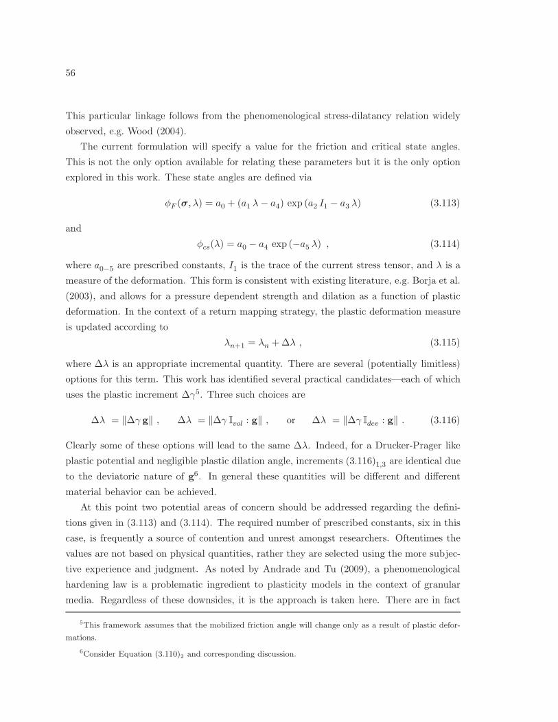
56

This particular linkage follows from the phenomenological stress-dilatancy relation widely

observed, e.g. Wood (2004).

The current formulation will specify a value for the friction and critical state angles.

This is not the only option available for relating these parameters but it is the only option

explored in this work. These state angles are defined via

φF (σ, λ) = a0 + (a1 λ− a4) exp (a2 I1 − a3 λ) (3.113)

and

φcs(λ) = a0 − a4 exp (−a5 λ) , (3.114)

where a0−5 are prescribed constants, I1 is the trace of the current stress tensor, and λ is a

measure of the deformation. This form is consistent with existing literature, e.g. Borja et al.

(2003), and allows for a pressure dependent strength and dilation as a function of plastic

deformation. In the context of a return mapping strategy, the plastic deformation measure

is updated according to

λn+1 = λn +∆λ , (3.115)

where ∆λ is an appropriate incremental quantity. There are several (potentially limitless)

options for this term. This work has identified several practical candidates—each of which

uses the plastic increment ∆γ5. Three such choices are

∆λ = ‖∆γ g‖ , ∆λ = ‖∆γ Ivol : g‖ , or ∆λ = ‖∆γ Idev : g‖ . (3.116)

Clearly some of these options will lead to the same ∆λ. Indeed, for a Drucker-Prager like

plastic potential and negligible plastic dilation angle, increments (3.116)1,3 are identical due

to the deviatoric nature of g6. In general these quantities will be different and different

material behavior can be achieved.

At this point two potential areas of concern should be addressed regarding the defini-

tions given in (3.113) and (3.114). The required number of prescribed constants, six in this

case, is frequently a source of contention and unrest amongst researchers. Oftentimes the

values are not based on physical quantities, rather they are selected using the more subjec-

tive experience and judgment. As noted by Andrade and Tu (2009), a phenomenological

hardening law is a problematic ingredient to plasticity models in the context of granular

media. Regardless of these downsides, it is the approach is taken here. There are in fact

5This framework assumes that the mobilized friction angle will change only as a result of plastic defor-

mations.

6Consider Equation (3.110)2 and corresponding discussion.

57

Table 3.5: Sample values for constants a0−5.

Constant i. ii. iii.

a0 20 20 20

a1 7750 2000 0

a2 [kPa]−1 3.33 (10)−4 1.67 (10)−5 0

a3 150 100 70

a4 20 20 20

a5 300 100 50

35

30

25

20

15

10

5

0

0.01

0.030.

020.04

0.05

0.06

0.01

0.030.

020.04

0.05

0.06

0.01

0.030.

020.04

0.05

0.06

Plastic Dilation Angle, ψGFriction Angle, φF Critical State Angle, φcs

Angle[deg

]

λ

(b)(a) (c)

Figure 3.5: Relationship between the effective friction angle, φF , critical state angle, φcs, andthe plastic dilation angle, ψG. (a), (b), and (c) are consistent with a dense, moderately dense,and loose arrangement of a granular medium (dry sand for example).

some easily identifiable physical parameters that aid in the selection of these constants.

Second, some individuals may have a slight issue in mobilizing the critical state angle. And

for good reason—as this lacks a direct physical meaning. Ideally the critical state angle is

a single, unique value. However, if such is the case, there are situations when the relation-

ship for dilation angle, as defined in (3.112), breaks down and erroneous values for dilation

angles are computed. If used judiciously, the current definition allows for a wide variety of

friction and dilation angles to be determined—provided the critical state angle approaches

a constant value with excessive deformation then (3.114) is a reasonable definition.

Three sets of curves highlighting the relationship between the friction, dilation, and crit-

ical state angle are shown in Figure 3.5(a), (b), and (c). The parameters used to construct

these curves are given in Table 3.5, where i., ii., and iii. correspond to curves 3.5(a), (b), and (c)

respectively . Note that these a0−5 values define the angle in degrees (as opposed to radi-

58

ans). Figure 3.5(a) and (b) are representative of a granular medium with a densely packed

particles. Conversely, curve 3.5(c) is more consistent with a loose arrangement. From these

figures the role of the constants can be partially identified. The term a0 represents the final

value that both φF and φcs tend to. The difference a0−a4 corresponds to the initial friction

angle of the medium in question. The width of the friction angle curve is determined by a2

and a3, while the same is true for a5 and the critical state angle. Finally, the constant a1

determines the peak (as well as the rate to get to the peak) friction angle.

Determining the value of these constants is challenging and the notion of a single, con-

crete approach for identifying suitable values does not exist. Rather, the process is largely

trial-and-error. The impact on the results can be extensive and is demonstrated in Chap-

ter 7 where these models are used to simulate granular flow. A good starting point for

parameter identification is to extract the quantity

ω = −qp

(3.117)

from experimental data, where

q =√

3/2 ‖s‖ and p = I1/3 . (3.118)

The ratio in (3.117) is linked with the effective friction angle via the relation

sinφexpF =ω

(2 + ω/3)(3.119)

which follows from the Mohr-Coulomb failure criterionChen (1994a,b); Tu et al. (2009).

In (3.119) the notation φexpF is used to distinguish between a value obtained experimentally

versus the curve definition of (3.113). Consistent with the definition of F given by (3.107)1,

φexpF assumes the yield function circumscribes the outer points of the Mohr-Coulomb criteria.

The denominator may be changed to (2− ω/3) to obtain a definition consistent with a yield

function that passes through the inner points of the Mohr-Coulomb criteria. The plot of

φexpF as a function of deformation provides a good template for constructing φF .

3.7 Two Surface Matsuoka-Nakai Material Model

The Matsuoaka-Nakai framework is built around the Mohr-Coulomb failure surface. The

theory was developed in numerous works by H. Matsuoka and T. Nakai; see, e.g., Matsuoka

and Nakai (1974, 1982, 1985). The isotropic, three invariant formulation has a successful

track record of capturing the behavior of granular materials with differing yield strengths in

tension or compression. The smooth, convex surface bypasses much of the implementation

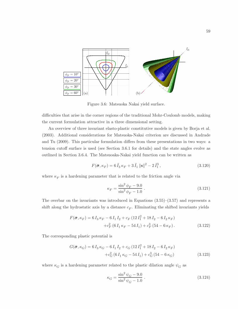
59

ξ3

φF = 60

φF = 30

φF = 20

φF = 10

(a) (b)

ξ1

ξ2

Figure 3.6: Matsuoka Nakai yield surface.

difficulties that arise in the corner regions of the traditional Mohr-Coulomb models, making

the current formulation attractive in a three dimensional setting.

An overview of three invariant elasto-plastic constitutive models is given by Borja et al.

(2003). Additional considerations for Matsuoka-Nakai criterion are discussed in Andrade

and Tu (2009). This particular formulation differs from these presentations in two ways: a

tension cutoff surface is used (see Section 3.6.1 for details) and the state angles evolve as

outlined in Section 3.6.4. The Matsuoaka-Nakai yield function can be written as

F (σ, κF ) = 6 I3 κF + 3 I1 ‖s‖2 − 2 I31 , (3.120)

where κF is a hardening parameter that is related to the friction angle via

κF =sin2 φF − 9.0

sin2 φF − 1.0. (3.121)

The overbar on the invariants was introduced in Equations (3.55)–(3.57) and represents a

shift along the hydrostatic axis by a distance cF . Eliminating the shifted invariants yields

F (σ, κF ) = 6 I3 κF − 6 I1 I2 + cF (12 I21 + 18 I2 − 6 I2 κF )

+c2F (6 I1 κF − 54 I1) + c3F (54 − 6κF ) . (3.122)

The corresponding plastic potential is

G(σ, κG) = 6 I3 κG − 6 I1 I2 + cG (12 I21 + 18 I2 − 6 I2 κF )

+c2G (6 I1 κG − 54 I1) + c3G (54 − 6κG) (3.123)

where κG is a hardening parameter related to the plastic dilation angle ψG as

κG =sin2 ψG − 9.0

sin2 ψG − 1.0. (3.124)

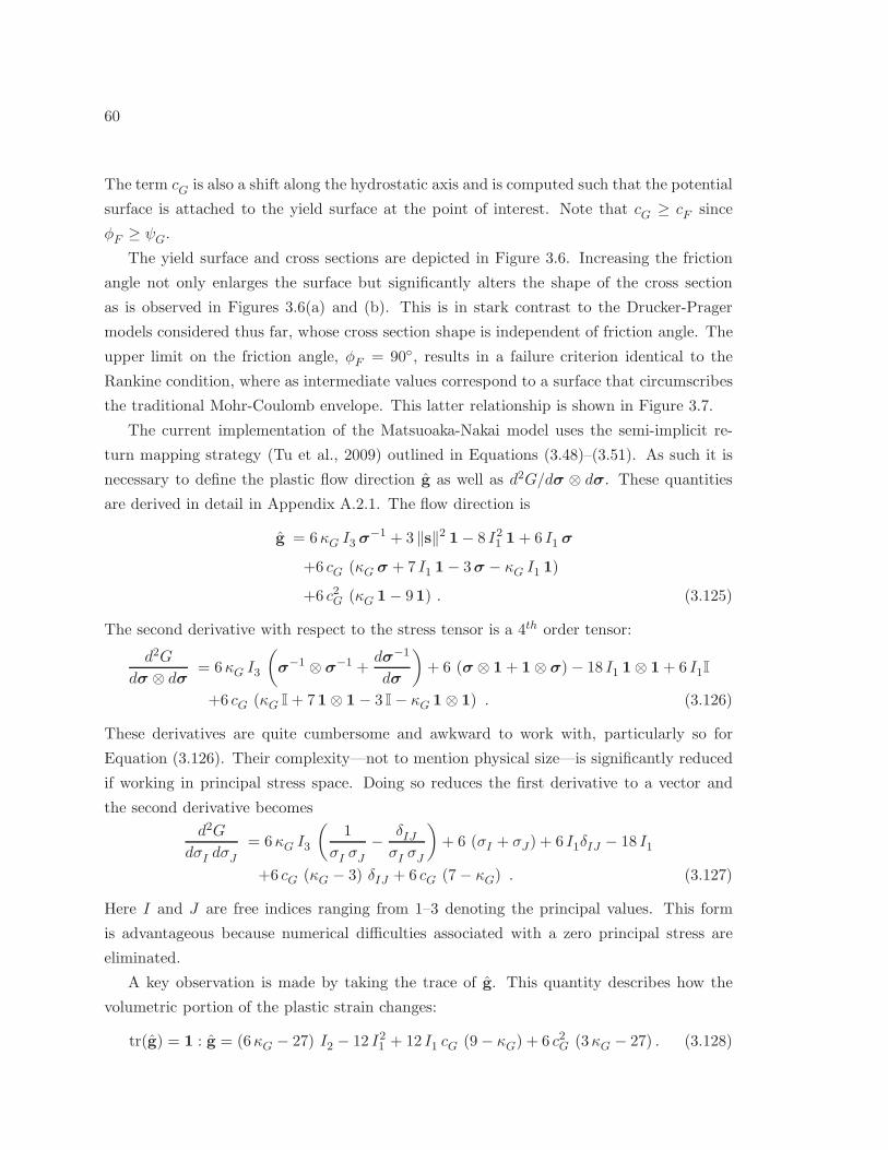
60

The term cG is also a shift along the hydrostatic axis and is computed such that the potential

surface is attached to the yield surface at the point of interest. Note that cG ≥ cF since

φF ≥ ψG.

The yield surface and cross sections are depicted in Figure 3.6. Increasing the friction

angle not only enlarges the surface but significantly alters the shape of the cross section

as is observed in Figures 3.6(a) and (b). This is in stark contrast to the Drucker-Prager

models considered thus far, whose cross section shape is independent of friction angle. The

upper limit on the friction angle, φF = 90, results in a failure criterion identical to the

Rankine condition, where as intermediate values correspond to a surface that circumscribes

the traditional Mohr-Coulomb envelope. This latter relationship is shown in Figure 3.7.

The current implementation of the Matsuoaka-Nakai model uses the semi-implicit re-

turn mapping strategy (Tu et al., 2009) outlined in Equations (3.48)–(3.51). As such it is

necessary to define the plastic flow direction g as well as d2G/dσ ⊗ dσ. These quantities

are derived in detail in Appendix A.2.1. The flow direction is

g = 6κG I3 σ−1 + 3 ‖s‖2 1− 8 I21 1+ 6 I1 σ

+6 cG (κG σ + 7 I1 1− 3σ − κG I1 1)

+6 c2G (κG 1− 91) . (3.125)

The second derivative with respect to the stress tensor is a 4th order tensor:

d2G

dσ ⊗ dσ= 6κG I3

(

σ−1 ⊗ σ−1 +dσ−1

dσ

)

+ 6 (σ ⊗ 1+ 1⊗ σ)− 18 I1 1⊗ 1+ 6 I1I

+6 cG (κG I+ 71⊗ 1− 3 I− κG 1⊗ 1) . (3.126)

These derivatives are quite cumbersome and awkward to work with, particularly so for

Equation (3.126). Their complexity—not to mention physical size—is significantly reduced

if working in principal stress space. Doing so reduces the first derivative to a vector and

the second derivative becomes

d2G

dσI dσJ= 6κG I3

(1

σI σJ− δIJσI σJ

)

+ 6 (σI + σJ) + 6 I1δIJ − 18 I1

+6 cG (κG − 3) δIJ + 6 cG (7− κG) . (3.127)

Here I and J are free indices ranging from 1–3 denoting the principal values. This form

is advantageous because numerical difficulties associated with a zero principal stress are

eliminated.

A key observation is made by taking the trace of g. This quantity describes how the

volumetric portion of the plastic strain changes:

tr(g) = 1 : g = (6κG − 27) I2 − 12 I21 + 12 I1 cG (9− κG) + 6 c2G (3κG − 27) . (3.128)

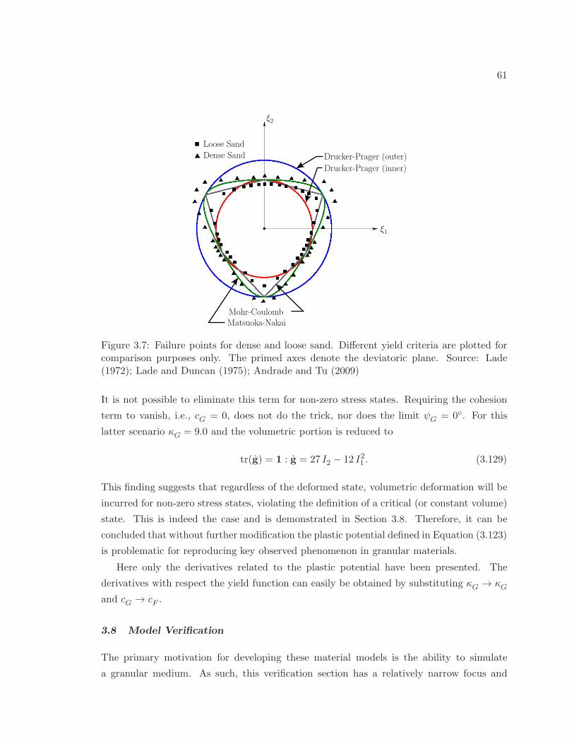
61

Loose Sand

Dense Sand

Mohr-CoulombMatsuoka-Nakai

Drucker-Prager (inner)

Drucker-Prager (outer)

ξ1

ξ2

Figure 3.7: Failure points for dense and loose sand. Different yield criteria are plotted forcomparison purposes only. The primed axes denote the deviatoric plane. Source: Lade(1972); Lade and Duncan (1975); Andrade and Tu (2009)

It is not possible to eliminate this term for non-zero stress states. Requiring the cohesion

term to vanish, i.e., cG = 0, does not do the trick, nor does the limit ψG = 0. For this

latter scenario κG = 9.0 and the volumetric portion is reduced to

tr(g) = 1 : g = 27 I2 − 12 I21 . (3.129)

This finding suggests that regardless of the deformed state, volumetric deformation will be

incurred for non-zero stress states, violating the definition of a critical (or constant volume)

state. This is indeed the case and is demonstrated in Section 3.8. Therefore, it can be

concluded that without further modification the plastic potential defined in Equation (3.123)

is problematic for reproducing key observed phenomenon in granular materials.

Here only the derivatives related to the plastic potential have been presented. The

derivatives with respect the yield function can easily be obtained by substituting κG → κG

and cG → cF .

3.8 Model Verification

The primary motivation for developing these material models is the ability to simulate

a granular medium. As such, this verification section has a relatively narrow focus and

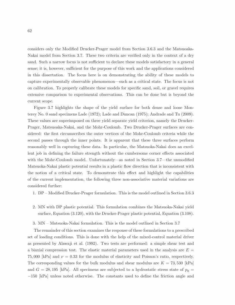
62

considers only the Modified Drucker-Prager model from Section 3.6.3 and the Matsuoaka-

Nakai model from Section 3.7. These two criteria are verified only in the context of a dry

sand. Such a narrow focus is not sufficient to declare these models satisfactory in a general

sense; it is, however, sufficient for the purpose of this work and the applications considered

in this dissertation. The focus here is on demonstrating the ability of these models to

capture experimentally observable phenomenon—such as a critical state. The focus is not

on calibration. To properly calibrate these models for specific sand, soil, or gravel requires

extensive comparison to experimental observations. This can be done but is beyond the

current scope.

Figure 3.7 highlights the shape of the yield surface for both dense and loose Mon-

terey No. 0 sand specimens Lade (1972); Lade and Duncan (1975); Andrade and Tu (2009).

These values are superimposed on three yield separate yield criterion, namely the Drucker-

Prager, Matsuoaka-Nakai, and the Mohr-Coulomb. Two Drucker-Prager surfaces are con-

sidered: the first circumscribes the outer vertices of the Mohr-Coulomb criteria while the

second passes through the inner points. It is apparent that these three surfaces perform

reasonably well in capturing these data. In particular, the Matsuoka-Nakai does an excel-

lent job in defining the failure strength without the cumbersome corner effects associated

with the Mohr-Coulomb model. Unfortunately—as noted in Section 3.7—the unmodified

Matsuoka-Nakai plastic potential results in a plastic flow direction that is inconsistent with

the notion of a critical state. To demonstrate this effect and highlight the capabilities

of the current implementation, the following three non-associative material variations are

considered further:

1. DP – Modified Drucker-Prager formulation. This is the model outlined in Section 3.6.3

2. MN with DP plastic potential. This formulation combines the Matsuoka-Nakai yield

surface, Equation (3.120), with the Drucker-Prager plastic potential, Equation (3.108).

3. MN – Matsuoka-Nakai formulation. This is the model outlined in Section 3.7

The remainder of this section examines the response of these formulations to a prescribed

set of loading conditions. This is done with the help of the mixed-control material driver

as presented by Alawaji et al. (1992). Two tests are performed: a simple shear test and

a biaxial compression test. The elastic material parameters used in the analysis are E =

75, 000 [kPa] and ν = 0.33 for the modulus of elasticity and Poisson’s ratio, respectively.

The corresponding values for the bulk modulus and shear modulus are K = 73, 530 [kPa]

and G = 28, 195 [kPa]. All specimens are subjected to a hydrostatic stress state of p0 =

−150 [kPa] unless noted otherwise. The constants used to define the friction angle and

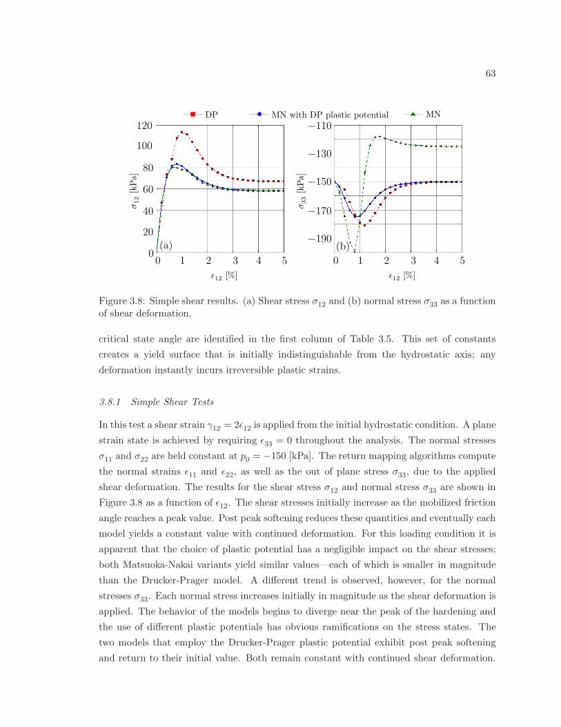
63

0 1 2 3 4 5

ǫ12

[%]

0 1 2 3 4 5

ǫ12

[%]

MN with DP plastic potential MNDP

σ33

[kPa]

0

20

40

80

120

100

60

σ12

[kPa]

−110

−130

−150

−170

−190(a) (b)

Figure 3.8: Simple shear results. (a) Shear stress σ12 and (b) normal stress σ33 as a functionof shear deformation.

critical state angle are identified in the first column of Table 3.5. This set of constants

creates a yield surface that is initially indistinguishable from the hydrostatic axis; any

deformation instantly incurs irreversible plastic strains.

3.8.1 Simple Shear Tests

In this test a shear strain γ12 = 2ǫ12 is applied from the initial hydrostatic condition. A plane

strain state is achieved by requiring ǫ33 = 0 throughout the analysis. The normal stresses

σ11 and σ22 are held constant at p0 = −150 [kPa]. The return mapping algorithms compute

the normal strains ǫ11 and ǫ22, as well as the out of plane stress σ33, due to the applied

shear deformation. The results for the shear stress σ12 and normal stress σ33 are shown in

Figure 3.8 as a function of ǫ12. The shear stresses initially increase as the mobilized friction

angle reaches a peak value. Post peak softening reduces these quantities and eventually each

model yields a constant value with continued deformation. For this loading condition it is

apparent that the choice of plastic potential has a negligible impact on the shear stresses;

both Matsuoka-Nakai variants yield similar values—each of which is smaller in magnitude

than the Drucker-Prager model. A different trend is observed, however, for the normal

stresses σ33. Each normal stress increases initially in magnitude as the shear deformation is

applied. The behavior of the models begins to diverge near the peak of the hardening and

the use of different plastic potentials has obvious ramifications on the stress states. The

two models that employ the Drucker-Prager plastic potential exhibit post peak softening

and return to their initial value. Both remain constant with continued shear deformation.

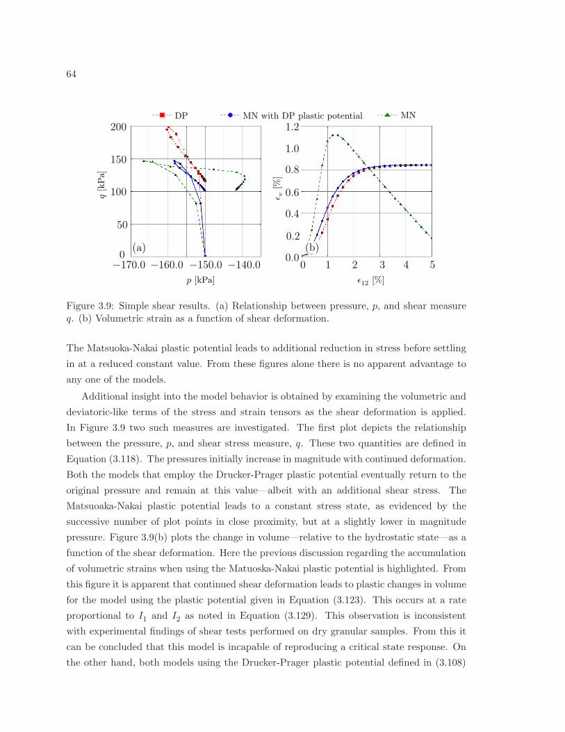
64

MN with DP plastic potential MNDP

0 1 2 3 4 5

ǫ12

[%]

q[k

Pa]

p [kPa]

200

150

100

50

0−170.0 −160.0 −150.0 −140.0

ǫ v[%

]

0.0

1.2

0.2

0.4

0.6

0.8

1.0

(b)(a)

Figure 3.9: Simple shear results. (a) Relationship between pressure, p, and shear measureq. (b) Volumetric strain as a function of shear deformation.

The Matsuoka-Nakai plastic potential leads to additional reduction in stress before settling

in at a reduced constant value. From these figures alone there is no apparent advantage to

any one of the models.

Additional insight into the model behavior is obtained by examining the volumetric and

deviatoric-like terms of the stress and strain tensors as the shear deformation is applied.

In Figure 3.9 two such measures are investigated. The first plot depicts the relationship

between the pressure, p, and shear stress measure, q. These two quantities are defined in

Equation (3.118). The pressures initially increase in magnitude with continued deformation.

Both the models that employ the Drucker-Prager plastic potential eventually return to the

original pressure and remain at this value—albeit with an additional shear stress. The

Matsuoaka-Nakai plastic potential leads to a constant stress state, as evidenced by the

successive number of plot points in close proximity, but at a slightly lower in magnitude

pressure. Figure 3.9(b) plots the change in volume—relative to the hydrostatic state—as a

function of the shear deformation. Here the previous discussion regarding the accumulation

of volumetric strains when using the Matuoska-Nakai plastic potential is highlighted. From

this figure it is apparent that continued shear deformation leads to plastic changes in volume

for the model using the plastic potential given in Equation (3.123). This occurs at a rate

proportional to I1 and I2 as noted in Equation (3.129). This observation is inconsistent

with experimental findings of shear tests performed on dry granular samples. From this it

can be concluded that this model is incapable of reproducing a critical state response. On

the other hand, both models using the Drucker-Prager plastic potential defined in (3.108)

65

0 1 2 3 4 5

ǫ22

[%]

50

0

100

350

300

250

150

200

abs(

σ11−

σ22)

[kPa]

MN with DP plastic potential MNDP

0 1 2 3 4 5

ǫ22

[%]

ǫ v[%

]

0.5

0.0

1.0

−1.0

−0.5

(a) (b)

Figure 3.10: Biaxial compression results. (a) q. (b) Volumetric strain.

exhibit ideal critical state behavior: continued deformation does not accumulate additional

stresses or changes in volume.

3.8.2 Biaxial Compression Tests

A compression test is also used for additional verification of the three model variants. For

this series of tests an axial deformation is applied to ǫ22 from the hydrostatic state. Both

σ11 and σ33 are held constant at p0 = −150 [kPa]. The return mapping algorithm computes

the normal stress σ22 as well as the normal strains ǫ11 and ǫ33. Figure 3.10 highlights both q

and volumetric strain, ǫv, as a function of the axial deformation ǫ22. This loading condition

is unique in that differences observed in the model behavior are attributed solely to the

choice of plastic potential. This statement follows from the fact the both the Drucker-

Prager and Matusoka-Nakai yield surfaces coincide in biaxial compression, cf. Figure 3.7.

Not surprisingly both models that use the Drucker-Prager plastic potential yield the same

plot points in both Figures 3.10(a) and (b). The third model begins to deviate only as

extensive plastic deformations are incurred. The departure coincides with the accumulation

of volumetric strains, already identified as problematic for proper representation of granular

materials. In Figure 3.10(b) it is observed that both models employing the Drucker-Prager

plastic potential initially contract and then expand before arriving at a constant volume

state. Such behavior is widely observed in dense arraignments of granular matter.

Additional tests have been conducted to get a sense of the model convergence as well

as the accuracy of the semi-implicit integration algorithm. Although the model driver is

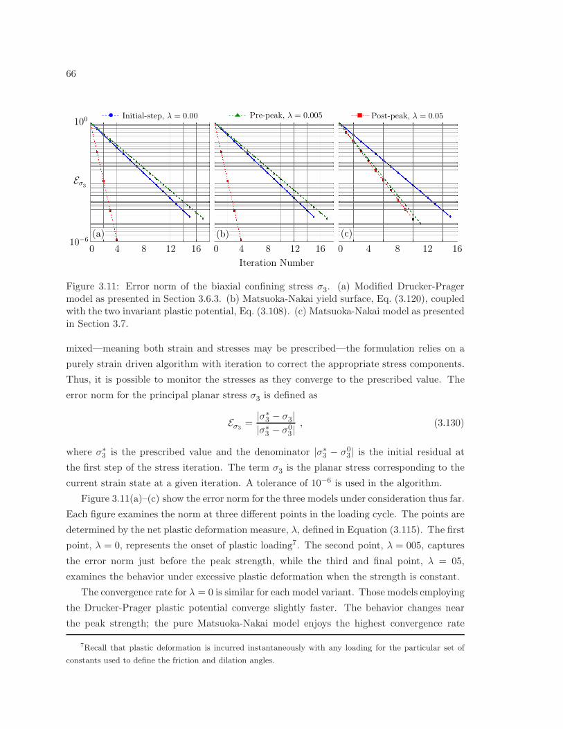
66

0 4 8 12 160 4 8 12 16

Post-peak, λ = 0.05Pre-peak, λ = 0.005Initial-step, λ = 0.00

10−6

Eσ3

100

0 4 8 1612

Iteration Number

(b)(a) (c)

Figure 3.11: Error norm of the biaxial confining stress σ3. (a) Modified Drucker-Pragermodel as presented in Section 3.6.3. (b) Matsuoka-Nakai yield surface, Eq. (3.120), coupledwith the two invariant plastic potential, Eq. (3.108). (c) Matsuoka-Nakai model as presentedin Section 3.7.

mixed—meaning both strain and stresses may be prescribed—the formulation relies on a

purely strain driven algorithm with iteration to correct the appropriate stress components.

Thus, it is possible to monitor the stresses as they converge to the prescribed value. The

error norm for the principal planar stress σ3 is defined as

Eσ3=

|σ∗3 − σ3||σ∗3 − σ03 |

, (3.130)

where σ∗3 is the prescribed value and the denominator |σ∗3 − σ03 | is the initial residual at

the first step of the stress iteration. The term σ3 is the planar stress corresponding to the

current strain state at a given iteration. A tolerance of 10−6 is used in the algorithm.

Figure 3.11(a)–(c) show the error norm for the three models under consideration thus far.

Each figure examines the norm at three different points in the loading cycle. The points are

determined by the net plastic deformation measure, λ, defined in Equation (3.115). The first

point, λ = 0, represents the onset of plastic loading7. The second point, λ = 005, captures

the error norm just before the peak strength, while the third and final point, λ = 05,

examines the behavior under excessive plastic deformation when the strength is constant.

The convergence rate for λ = 0 is similar for each model variant. Those models employing

the Drucker-Prager plastic potential converge slightly faster. The behavior changes near

the peak strength; the pure Matsuoka-Nakai model enjoys the highest convergence rate

7Recall that plastic deformation is incurred instantaneously with any loading for the particular set of

constants used to define the friction and dilation angles.

67

as indicated by Figure 3.11(c). As the critical state friction angle is approached, the two

variations sharing the Drucker-Prager plastic potential converge the fastest. However, these

plots need to be interpreted with caution and the convergence rate is not necessarily the best

measure to judge their performance. The stress iteration is performed with Ce as defined

in Equation (3.46) assuming a unit density. This value is not the consistent elastic tangent

at each time step8. Nonetheless, these findings verify the semi-implicit algorithm’s ability

to converge under the conditions defined thus far in this chapter.

3.9 Summary

This chapter presented several components necessary for building a MPM-oriented consti-

tutive framework. This included the basic concepts from computational inelasticity, small

and large deformation theory, and the development of specific material models capable of

simulating several kinds of materials. Particular attention was paid to developing a frame-

work that can accommodate extremely large deformations while remaining computationally

efficient and numerically stable in the context of granular media. The next two chapters

present key enhancements that aid in the simulation of landslides.

8This is not really a point of concern in the context of this dissertation; the MPM as defined in this

document enjoys a purely strain driven and explicit existence—in which case the consistent tangent plays

no role.

68

Chapter 4

ANTI-LOCKING STRATEGY

A vast majority of the theoretical framework presented in this chapter follows (verbatim

in some instances) from the paperMitigating kinematic locking in the Material Point Method

by Mast, Mackenzie-Helnwein, Arduino, Miller, and Shin (2012). The author is indebted

to Peter Mackenzie-Helnwein, Pedro Arduino, and Greg Miller for their contributions in

writing and publishing this paper.

This chapter contains the theoretical development of anti-locking routines designed to

mitigate the accumulation of fictitious strains when linear shape functions are used in con-

junction with the standard MPM algorithm. Multiple approaches are discussed, including

various control volumes defined using a regular grid. As will be shown in later chapters,

the anti-locking routines provided here are essential for modeling quality flow dynamics and

obtaining reasonable stress fields.

4.1 Introduction and Background

It is common to use standard linear shape functions defined on a regular, rectangular grid in

most implementations of the MPM. This is not, however, a limitation or requirement of the

technique. Researchers have demonstrated the benefits of using an irregular grid consisting

of either triangular or quadrilateral cells, e.g., Wieckowski (2004a); Wang et al. (2005). Oth-

ers have investigated the use of higher-order shape functions—2nd and 3rd order B-splines,

Andersen and Andersen (2010a); Steffen et al. (2008a), standard quadratic shape functions,

Andersen and Andersen (2010a), as well as a Radial Basis Function, Htike et al. (2011),—

in lieu of linear shape functions. In these cases the use of a higher order shape function

eliminates many of the non-physical results associated with traditional implementations.

However, the use of the non-linear functions can result in an increase in computational cost,

potentially limiting the effectiveness of such approaches. Given the simplicity of low-order

elements/cells, they remain a popular choice in FEM and MPM applications. To date,

linear interpolation functions are the most common choice found in the MPM literature.

The use of linear shape functions does not come without shortcomings. These include

volumetric locking due to the insufficient representation of an isochoric displacement/ve-

locity field, Belytschko et al. (2000), as well as shear locking due to non-physical coupling

69

of normal strains and shear strains, Andelfinger and Ramm (1993). In addition to locking,

the discontinuous gradient leads to cell-crossing errors which are attributed to the sudden

jump in strain rate as a particle moves from one cell to another. A potential solution to the

cell-crossing error is to counteract the discontinuity of the gradient at the interface between

adjacent cells by introducing an enhanced gradient, Zhang et al. (2011). Alternatively, the

particle can be represented using a finite domain, effectively smoothing out the discontinu-

ity. This idea was first developed in the Generalized Interpolation Material Point (GIMP)

method, Bardenhagen and Kober (2004) and has since been applied to wide variety of en-

gineering problems, e.g., Daphalapurkar et al. (2007); Ma et al. (2006a,b,c); Wallstedt and

Guilkey (2008). A similar variant of the MPM, the Convected Particle Domain Interpola-

tion (CPDI) technique by Sadeghirad et al. (2011b), effectively combats the discontinuous

gradient issue by introducing a parallelogram-shaped particle domain that is consistently

updated using the deformation gradient at the particle. These approaches effectively combat

the cell crossing problem with varying success depending on the application. Unfortunately

these approaches fail to address or alleviate kinematic locking.

In fact, until very recently the topic has not been reported in the literature, Andersen and

Andersen (2010a); Arduino et al. (2011); Mackenzie-Helnwein et al. (2011); Shin (2009). The

closest references are the works Andersen and Andersen (2010a); Htike et al. (2011); Steffen

et al. (2008a), which have found that representation and integration errors are reduced

significantly by introducing higher order shape functions on the background grid. This is in

agreement with related observations in the Finite Element Method (FEM), where increasing

the interpolation order not only improves accuracy but also reduces locking phenomena.

The approach presented in this chapter significantly improves both the kinematics and the

stress field—all the while supporting traditional linear shape functions. The remaining

sections introduce the anti-locking methodology and outline the implementation procedure

for application in the MPM. The effectiveness of the algorithm is highlighted throughout

Chapters 6 and 7 in both the elastic and inelastic material domain.

4.2 Theoretical Overview

Alleviating kinematic locking within the context of the FEM is not a new concept and there

is extensive literature on the topic, e.g, Bathe (1996); Belytschko et al. (2000); Wriggers

(2008); Zienkiewicz et al. (2005c,b). Many of the existing FEM strategies make use of

multi-field variational principles, and this work follows suit, applying similar concepts to

the MPM. More specifically, this work employs the well known Hu-Washizu multi-field

variational principle Washizu (1982). Traditional weak form equations are structured such

70

that the solution yields an approximation of the displacement field (or its time derivatives,

namely the velocity and/or the acceleration). The Hu-Washizu formulation is different in

that it seeks a weak form approximation not only to the displacement, but also to the

corresponding strain and stress fields as well. Such a formulation is developed from a

variational standpoint by first considering the total potential energy stored in a body with

mass mB. Subjecting the body to a general displacement field, u(x, t), the potential for an

isothermal problem is written as

Π(u) :=

∫

mB

ψ(ε(u)) dm −∫

mB

b · u dm−∫

ΓB

t · u dΓ . (4.1)

where b(x, t) is the mass specific body force at position x and time t, t(x, t) is the pre-

scribed external traction acting on the body’s surface, ΓB, and ψ(ε(u)) is the mass specific

Helmholtz free energy function. The strain, ε, derived from a displacement field, u, is given

by a strain function ε(u). For small deformations ε(u) := ∇su (note that small deformation

theory is not a requirement of the MPM, rather, it is done to simplify the explanation of the

current approach from a variational standpoint). The free energy is typically a function of

several variables needed to define the material state. For derivation purposes this function

is expressed only in terms of the strain (i.e., ψ := ψ(ε)) and thus applies to elastic materials.

However, this can easily be rewritten to allow for more general material behavior, and im-

poses no restriction on the subsequent treatment of locking. In general, (•) indicates a mass

specific form of a volume specific quantity, i.e., (•) = ρ(•) where ρ(x, t) is mass density.

Replacing the strain function, ε(u), with an independent strain field, ε(x, t), and ex-

pressing the kinematic relation through a constraint equation using a mass-specific Lagrange

multiplier field, σ, yields the Hu-Washizu style three-field functional

Π∗(σ, ε,u) :=

∫

mB

ψ(ε) dm−∫

mB

σ : [ε− ε(u)] dm−∫

mB

b · u dm−∫

ΓB

t · u dΓ . (4.2)

A weak form solution is found as a stationary point of Π∗(σ, ε,u), yielding the governing

system of weak-form equations as∫

mB

δσ : [ε− ε(u)] dm = 0 , (4.3)

∫

mB

δε :

[

σ − ∂ψ(ε)

∂ε

]

dm = 0 , and (4.4)

−∫

mB

∇sδu : σ dm+

∫

mB

δu · b dm+

∫

ΓB

δu · t dΓ = 0 , (4.5)

in which δσ, δε and δu are arbitrary independent variations of the three independent

fields σ, ε, and u, respectively. From Equation (4.4) the independent tensor field σ(x, t) is

71

identified as the mass-specific Cauchy stress tensor (Washizu, 1982). The standard formu-

lation of the MPM solves the dynamic version of the weak form equilibrium equation (4.5)

and yields an approximation to the acceleration field over the body domain. This procedure

is outlined in Chapter 2 and is well documented in the literature. Equations (4.3) and (4.4)

provide additional constraints that are used to build approximations for the strain and stress

fields, respectively.

Constructing an appropriate approximation field is composed of two steps for 2nd order

tensors. The first step isolates the portions of the field to be constructed, e.g., the volumetric

and/or the deviatoric portions of the tensor field in question. This is accomplished using

a filter matrix, M, and a reconstruction matrix, M∗. In the second step, the shape of

the desired approximation is specified by defining a shape matrix, S(x), that effectively

interpolates the generalized degrees of freedom used to represent the strain and stress fields,

respectively. Bearing these two steps in mind, the grid-based approximation (denoted by a

superscript h) is constructed for the strain and stress using

ε(x, t) ≈ εh(x, t) := M∗ · S(x) ·α(t) + P : ε (4.6)

and

σ(x, t) ≈ σh(x, t) := M∗ · S(x) · β(t) + P : ˜σ . (4.7)

The generalized degrees of freedom α(t) and β(t) are the unknown vectors to be solved

for. Note that specification of M and M∗ drives the dimensionality of S, and hence, the

unknown function spaces α and β. The term P is a projection operator, defined as

P := I−M∗ ·M (4.8)

with I as the 4th order identity tensor. The strain function, ε = ε(uh), is the strain derived

from the displacement field approximation. The mass specific stress is obtained from the

general constitutive relation ˜σ = ∂ψ/∂ε. Equations (4.6) and (4.7) reiterate the two-step

nature of the approximation: the shape matrix S(x) provides a spatial interpolation of

the generalized unknowns collected in α (or β). The matrix M∗ is used to reconstruct a

symmetric second-order tensor resulting from the interpolated components and is combined

with the unaltered complementary portion P : ε (or P : ˜σ) of the original tensor field.

Consistent with Equations (4.6) and (4.7) and sufficient for Equations (4.3)–(4.5), a

general set of admissible variations is constructed as

δε(x) := δα · S(x)T ·M and δσ(x) := δβ · S(x)T ·M . (4.9)

72

Substituting Equations (4.6), (4.7), and (4.9) into constraints (4.3) and (4.4) yields

∫

mB

δβ · ST ·M : [M∗ · S · α−M∗ ·M : ε] dm = 0 (4.10)

and ∫

mB

δα · ST ·M : [M∗ · S · β −M∗ ·M : ˜σ] dm = 0 . (4.11)

At first glance little has been gained by making this substitution. However, by requiringM :

M∗ = 1—where 1 is the unity operator of appropriate dimension—both Equations (4.10)

and (4.11) are simplified. α, β, δα and δβ can be taken outside the integrals, as these terms

are independent of the spatial domain. For arbitrary variations δα and δβ two systems of

equations are obtained:

α = H−1 ·∫

mB

ST ·M : ε dm and β = H−1 ·∫

mB

ST ·M : ˜σ dm , (4.12)

with

H =

∫

mB

ST · S dm . (4.13)

4.3 Anti-Locking Approaches

The type of anti-locking employed depends on the filter/reconstruction operators; indeed

there are multiple choices possible for the tensors M and M∗. The standard decomposition

of stress and strain into volumetric and deviatoric parts leads to two natural choices for M

andM∗. Clearly these are not the only feasible choices, but they are the only two considered

here.

4.3.1 Volumetric Approach

This technique constructs a constant approximation for only the volumetric portions of

the stress and strain fields over the desired control volume. The deviatoric fields remain

unmodified. This idea was first investigated in the work by Shin (2009). The volumetric

component of a tensor can be represented with a single scalar value, thus motivating the

following filter matrix definitions:

[M] = [Mvol] := [ 1 1 1 0 0 0 ] and [M∗] = [M∗vol] := [ 1/3 1/3 1/3 0 0 0 ]T , (4.14)

with M∗ · M = 1/31 ⊗ 1 being the volumetric operator and its complementary filter, P,

becomes the deviatoric operator Idev = I − 1/31 ⊗ 1. For this approximation scheme the

73

shape matrix contains a single entry: [S] = [ 1 ]. The unknown parameters α and β (as well

as their variations) assume the following form

α = α1 , δα = δα1 , β := β1 , and δβ = δβ1 . (4.15)

This approximation leads to

α1 = tr εh = θ and β1 = tr σh = 3 ˆp , (4.16)

where θ is the dilation and ˆp the mass specific isotropic stress, assumed constant throughout

the selected control volume. This approach will mitigate volumetric locking and, as will be

shown in the following chapters, is beneficial for all simulation types.

4.3.2 Volumetric-Deviatoric Approach

This anti-locking strategy builds approximations for both the volumetric and deviatoric

portions of the strain and stress tensor fields. This technique provides finer grained control,

as each portion is constructed independently. The following definitions are used for the

filter matrices

[M] :=

1 1 1 0 0 0

2/3 −1/3 −1/3 0 0 0

−1/3 2/3 −1/3 0 0 0

0 0 0 1 0 0

0 0 0 0 1 0

0 0 0 0 0 1

[M∗] :=

1/3 1 0 0 0 0

1/3 0 1 0 0 0

1/3 −1 −1 0 0 0

0 0 0 1 0 0

0 0 0 0 1 0

0 0 0 0 0 1

,

(4.17)

leading to M∗ ·M = I. Thus, the projection operator, P, is reduced to the 4th order zero

tensor, O. The shape matrix is

[S] :=

1 0 0 0 0 0 ξ η ζ 0 0 0 0 0 0

0 1 0 0 0 0 0 0 0 ξ η ζ 0 0 0

0 0 1 0 0 0 0 0 0 0 0 0 ξ η ζ

0 0 0 1 0 0 0 0 0 0 0 0 0 0 0

0 0 0 0 1 0 0 0 0 0 0 0 0 0 0

0 0 0 0 0 1 0 0 0 0 0 0 0 0 0

, (4.18)

where the local coordinates ξ, η, and ζ are parallel to global x, y, and z with the origin shifted

to the centroid of the control volume. Defining S in this way decouples the shear terms from

the the normal terms. In addition, the shear terms are assumed constant throughout the

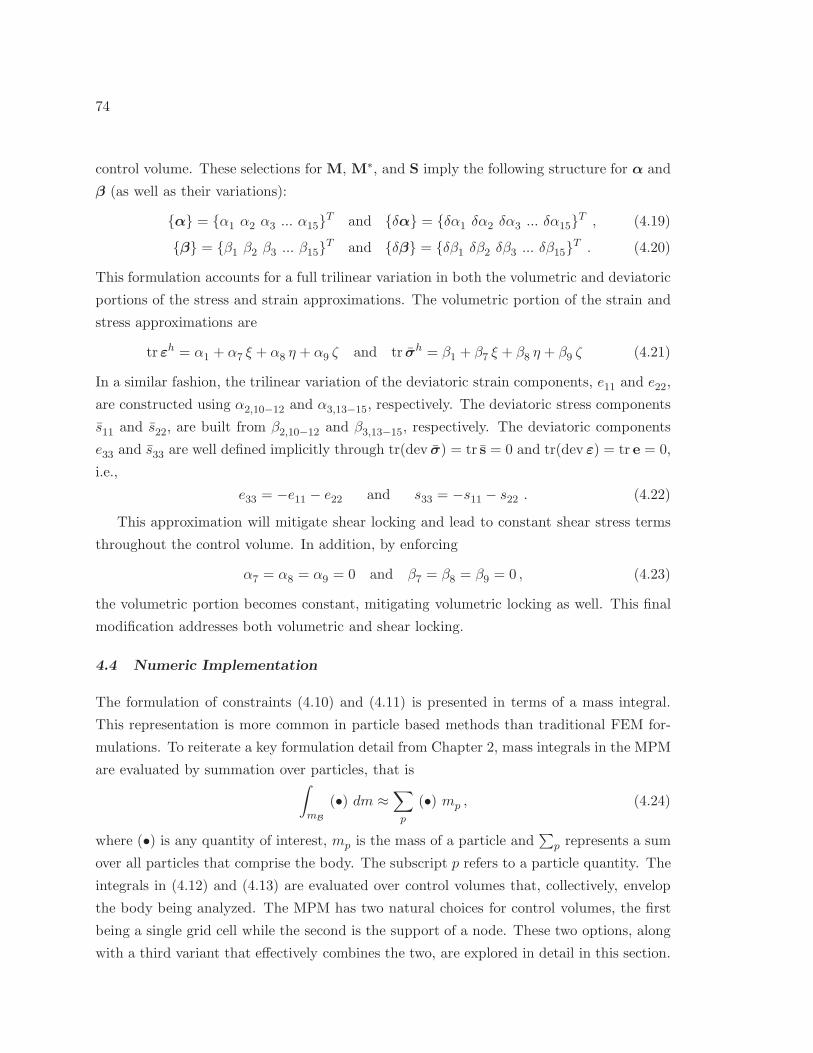
74

control volume. These selections for M, M∗, and S imply the following structure for α and

β (as well as their variations):

α = α1 α2 α3 ... α15T and δα = δα1 δα2 δα3 ... δα15T , (4.19)

β = β1 β2 β3 ... β15T and δβ = δβ1 δβ2 δβ3 ... δβ15T . (4.20)

This formulation accounts for a full trilinear variation in both the volumetric and deviatoric

portions of the stress and strain approximations. The volumetric portion of the strain and

stress approximations are

tr εh = α1 + α7 ξ + α8 η + α9 ζ and tr σh = β1 + β7 ξ + β8 η + β9 ζ (4.21)

In a similar fashion, the trilinear variation of the deviatoric strain components, e11 and e22,

are constructed using α2,10−12 and α3,13−15, respectively. The deviatoric stress components

s11 and s22, are built from β2,10−12 and β3,13−15, respectively. The deviatoric components

e33 and s33 are well defined implicitly through tr(dev σ) = tr s = 0 and tr(dev ε) = tr e = 0,

i.e.,

e33 = −e11 − e22 and s33 = −s11 − s22 . (4.22)

This approximation will mitigate shear locking and lead to constant shear stress terms

throughout the control volume. In addition, by enforcing

α7 = α8 = α9 = 0 and β7 = β8 = β9 = 0 , (4.23)

the volumetric portion becomes constant, mitigating volumetric locking as well. This final

modification addresses both volumetric and shear locking.

4.4 Numeric Implementation

The formulation of constraints (4.10) and (4.11) is presented in terms of a mass integral.

This representation is more common in particle based methods than traditional FEM for-

mulations. To reiterate a key formulation detail from Chapter 2, mass integrals in the MPM

are evaluated by summation over particles, that is∫

mB

(•) dm ≈∑

p

(•) mp , (4.24)

where (•) is any quantity of interest, mp is the mass of a particle and∑

p represents a sum

over all particles that comprise the body. The subscript p refers to a particle quantity. The

integrals in (4.12) and (4.13) are evaluated over control volumes that, collectively, envelop

the body being analyzed. The MPM has two natural choices for control volumes, the first

being a single grid cell while the second is the support of a node. These two options, along

with a third variant that effectively combines the two, are explored in detail in this section.

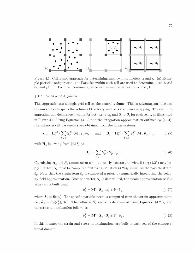
75

(a) (b) (c)

α1, β

1

α3, β

3

αc , βc α2, β

2

α4, β

4

Figure 4.1: Cell-Based approach for determining unknown parameters α and β. (a) Exam-ple particle configuration. (b) Particles within each cell are used to determine a cell-basedαc and βc. (c) Each cell containing particles has unique values for α and β.

4.4.1 Cell-Based Approach

This approach uses a single grid cell as the control volume. This is advantageous because

the union of cells spans the volume of the body, and cells are non-overlapping. The resulting

approximation defines local values for both α → αc and β → βc for each cell c, as illustrated

in Figure 4.1. Using Equation (4.12) and the integration approximation outlined by (4.24),

the unknown cell parameters are obtained from the linear systems

αc = H−1c ·

∑

p∈ c

STp ·M : εpmp and βc = H−1

c ·∑

p∈ c

STp ·M : ˜σpmp , (4.25)

with Hc following from (4.13) as

Hc =∑

p∈ c

STp · Spmp . (4.26)

Calculating αc and βc cannot occur simultaneously, contrary to what listing (4.25) may im-

ply. Rather, αc must be computed first using Equation (4.25)1 as well as the particle strain,

εp. Note that the strain term εp is computed a priori by numerically integrating the veloc-

ity field approximation. Once the vector αc is determined, the strain approximation within

each cell is built using

εhp = M∗ · Sp ·αc + P : εp , (4.27)

where Sp = S(xp). The specific particle stress is computed from the strain approximation,

i.e., ˜σp = ∂ψ(εhp)/∂εhp . The cell-wise βc vector is determined using Equation (4.25)2 and

the stress approximation follows as

σhp = M∗ · Sp · βc + P : ˜σp . (4.28)

In this manner the strain and stress approximations are built in each cell of the computa-

tional domain.

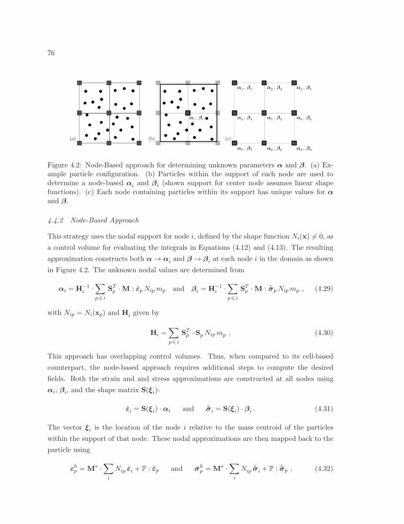
76

α3, β

3

α9, β

9

α6, β

6

α2, β

2

α8, β

8

α5, β

5

(b) (c)

α1, β

1

α7, β

7

α4, β

4

(a)

αi , βi

Figure 4.2: Node-Based approach for determining unknown parameters α and β. (a) Ex-ample particle configuration. (b) Particles within the support of each node are used todetermine a node-based αi and βi (shown support for center node assumes linear shapefunctions). (c) Each node containing particles within its support has unique values for α

and β.

4.4.2 Node-Based Approach

This strategy uses the nodal support for node i, defined by the shape function Ni(x) 6= 0, as

a control volume for evaluating the integrals in Equations (4.12) and (4.13). The resulting

approximation constructs both α → αi and β → βi at each node i in the domain as shown

in Figure 4.2. The unknown nodal values are determined from

αi = H−1i ·

∑

p∈ i

STp ·M : εpNipmp and βi = H−1

i ·∑

p∈ i

STp ·M : ˜σpNipmp , (4.29)

with Nip = Ni(xp) and Hi given by

Hi =∑

p∈ i

STp · SpNipmp . (4.30)

This approach has overlapping control volumes. Thus, when compared to its cell-based

counterpart, the node-based approach requires additional steps to compute the desired

fields. Both the strain and and stress approximations are constructed at all nodes using

αi, βi, and the shape matrix S(ξi):

εi = S(ξi) ·αi and ˆσi = S(ξi) · βi . (4.31)

The vector ξi is the location of the node i relative to the mass centroid of the particles

within the support of that node. These nodal approximations are then mapped back to the

particle using

εhp = M∗ ·∑

i

Nip εi + P : εp and σhp = M∗ ·

∑

i

Nipˆσi + P : ˜σp . (4.32)

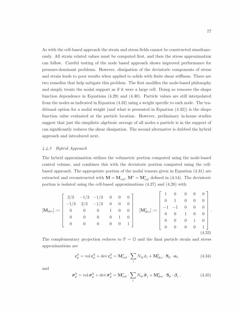
77

As with the cell-based approach the strain and stress fields cannot be constructed simultane-

ously. All strain related values must be computed first, and then the stress approximation

can follow. Careful testing of the node based approach shows improved performance for

pressure-dominant problems. However, dissipation of the deviatoric components of stress

and strain leads to poor results when applied to solids with finite shear stiffness. There are

two remedies that help mitigate this problem. The first modifies the node-based philosophy

and simply treats the nodal support as if it were a large cell. Doing so removes the shape

function dependence in Equations (4.29) and (4.30). Particle values are still interpolated

from the nodes as indicated in Equation (4.32) using a weight specific to each node. The tra-

ditional option for a nodal weight (and what is presented in Equation (4.32)) is the shape

function value evaluated at the particle location. However, preliminary in-house studies

suggest that just the simplistic algebraic average of all nodes a particle is in the support of

can significantly reduces the shear dissipation. The second alternative is dubbed the hybrid

approach and introduced next.

4.4.3 Hybrid Approach

The hybrid approximation utilizes the volumetric portion computed using the node-based

control volume, and combines this with the deviatoric portion computed using the cell-

based approach. The appropriate portion of the nodal tensors given in Equation (4.31) are

extracted and reconstructed with M = Mvol, M∗ = M∗

vol defined in (4.14). The deviatoric

portion is isolated using the cell-based approximations (4.27) and (4.28) with

[Mdev] :=

2/3 −1/3 −1/3 0 0 0

−1/3 2/3 −1/3 0 0 0

0 0 0 1 0 0

0 0 0 0 1 0

0 0 0 0 0 1

[M∗dev] :=

1 0 0 0 0

0 1 0 0 0

−1 −1 0 0 0

0 0 1 0 0

0 0 0 1 0

0 0 0 0 1

.

(4.33)

The complementary projection reduces to P = O and the final particle strain and stress

approximations are

εhp = vol εhp + dev εhp = M∗vol ·

∑

i

Nip εi +M∗dev · Sp · αc (4.34)

and

σhp = vol σh

p + dev σhp = M∗

vol ·∑

i

Nip ˆσi +M∗dev · Sp · βc . (4.35)

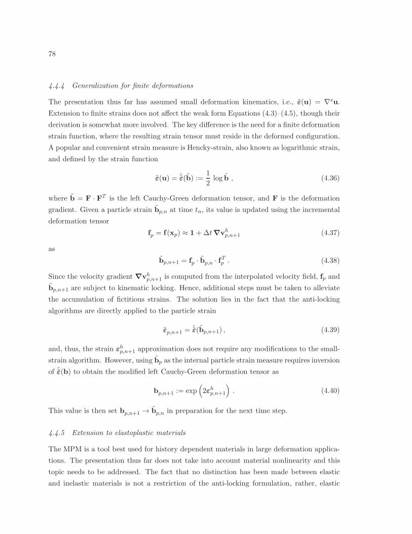
78

4.4.4 Generalization for finite deformations

The presentation thus far has assumed small deformation kinematics, i.e., ε(u) = ∇su.

Extension to finite strains does not affect the weak form Equations (4.3)–(4.5), though their

derivation is somewhat more involved. The key difference is the need for a finite deformation

strain function, where the resulting strain tensor must reside in the deformed configuration.

A popular and convenient strain measure is Hencky-strain, also known as logarithmic strain,

and defined by the strain function

ε(u) = ˜ε(b) :=1

2log b , (4.36)

where b = F · FT is the left Cauchy-Green deformation tensor, and F is the deformation

gradient. Given a particle strain bp,n at time tn, its value is updated using the incremental

deformation tensor

fp = f(xp) ≈ 1+∆t∇vhp,n+1 (4.37)

as

bp,n+1 = fp · bp,n · fTp . (4.38)

Since the velocity gradient ∇vhp,n+1 is computed from the interpolated velocity field, fp and

bp,n+1 are subject to kinematic locking. Hence, additional steps must be taken to alleviate

the accumulation of fictitious strains. The solution lies in the fact that the anti-locking

algorithms are directly applied to the particle strain

εp,n+1 = ˜ε(bp,n+1) , (4.39)

and, thus, the strain εhp,n+1 approximation does not require any modifications to the small-

strain algorithm. However, using bp as the internal particle strain measure requires inversion

of ˜ε(b) to obtain the modified left Cauchy-Green deformation tensor as

bp,n+1 := exp(

2εhp,n+1

)

. (4.40)

This value is then set bp,n+1 → bp,n in preparation for the next time step.

4.4.5 Extension to elastoplastic materials

The MPM is a tool best used for history dependent materials in large deformation applica-

tions. The presentation thus far does not take into account material nonlinearity and this

topic needs to be addressed. The fact that no distinction has been made between elastic

and inelastic materials is not a restriction of the anti-locking formulation, rather, elastic

79

properties were assumed for presentation purposes. This subsection expands the framework

to include elastoplastic materials and identifies two potential approaches.

The constraint given by Equation (4.3) is used to build an approximation for the strain

field. For an elastic material this is the end of the story. The same cannot be said for an

inelastic material. Careful distinction must be made between the total, elastic, and plastic

deformation as outlined in Chapter 3. This immediately poses the question: which strain

measure should be approximated? Two possible options are the elastic strain or the total

strain (presumably both measures could be approximated but this is not really necessary).

Aspects of each option are discussed below. This presentation is limited to elastoplastic

isotropic materials in an isothermal setting. Materials that do not satisfy this description

are not implemented in this framework and are beyond the primary scope of this work.

The first scheme is to approximate the elastic strain measure. This is arguably the most

logical choice. This statement is based on a couple considerations. The only deformation

measure that contributes directly to the mechanical stress is the elastic strain. Providing an

elastic strain measure that is free of kinematic locking is one way to help ensure the stress

measure will follow suit. Second, from a formulation standpoint, both the MPM and the

general return mapping algorithms presented in Chapter 3 need only the incremental strain

measure each time step. This value is tacked onto a previously known state. The material

models assume the increment is elastic (recall the notion of a trial state) and modify the

plastic variables as required should the yield condition be violated. Thus, a suitable elastic

deformation measure—be it a trial or actual—is all that is actually needed (assuming the

initial state of the material is given).

Extending this concept to the anti-locking strategy is straight forward. It is not possible

to approximate the actual elastic strain field without computing the updated stress values.

This would be a waste computationally since the stress is going to be re-computed using an

approximated strain measure. However, what can be determined with minimal effort is the

updated elastic trial at the particle level: εe,trp . It is this trial value that replaces εp in the

anti-locking discussion thus far. Note that large deformation analyses must first compute

a trial left Cauchy-Green deformation tensor, be,trp , before computing the corresponding

logarithmic strain measure. Substituting εe,trp for εp builds a suitable approximation to the

trial elastic strain field. As noted in several publications (e.g., Alawaji et al. (1992); Borja

et al. (2003); Simo (1998)) the principle directions of the trial elastic strain and converged

elastic strain coincide— thus ensuring the final shape of the elastic strain field is locking free.

Once the trial elastic strain field is known, εh, e,trp , the appropriate portion of the particle

strain is overwritten and the stress approximation proceeds unchanged. This approach does

80

not change or impact the accumulation of plastic strains and internal state variables.

The second alternative seeks an approximation to the total strain field within a given

control volume. From a formulation standpoint this approach is appealing; the variational

formulation presented in this chapter works directly with a strain function, presumably

derived from a displacement function. However, this approach does not consider how to

handle plastic variables. This is a concern because approximating the total strain field can

impart very large deformations on particles/points whose actual deformation history may

be very small. There is no way to properly capture this history unless the state variables

are modified as well. While this additional modification is possible, it presents a rabbit hole

scenario where the realized benefits are significantly diminished by the overhead required

to make it happen.

At one point or another both the elastic strain and the total strain approaches have

been implemented. From an algorithmic standpoint the two are nearly indistinguishable

but the findings are drastically different. Approximating the total strain is very problematic

and is best captured by a single word: chaos! Simulations blow up and are of no value.

On the other hand, approximating the elastic trial strain continues to provided favorable

results. For this reason it is the preferred method for incorporating material nonlinearity

into the anti-locking algorithm and is currently the only method implemented in the coding

framework.

4.4.6 Computational Considerations

Problems arise when particles reside exclusively on or close to a single plane (3D simulations)

or on a line (2D simulations), respectively. Under these conditions, Hc and/or Hi becomes

singular or sufficiently ill-conditioned such that no solution for the weak form Equations (4.3)

and (4.4) can be found. Typically, this happens if a body enters a new cell with just a few

particles. Only the constant volumetric stress/strain approach is immune to this condition.

Hence, if a singular matrix H is encountered for any given control volume (cell or nodal

support), a fall-back to the volumetric smoothing is used for that time step.

4.5 Algorithmic Overview

Incorporation of the anti-locking strategy requires minor changes to the standard algorithm.

Table 4.1 outlines the specific modifications to the standard algorithm for the cell-based,

node-based, and hybrid approaches. Large deformation analyses and/or elastoplastic mate-

rials require additional modifications as outlined in Sections 4.4.4 and 4.4.5. The anti-locking

81

Table 4.1: Algorithmic implementation of anti-locking strategy

1. Map particles to nodes. Update nodes from tn to tn+1 as outlined in Chapter 2.

2. Compute the velocity gradient and update the strain at the particle level. This is εp.

3. (a) IF Cell-Based Approach:

Compute αc from Equation (4.25)1

Compute εhp from Equation (4.27)

(b) IF Node-Based Approach:

Compute αi from Equation (4.29)1

Compute εi from (4.31)1

Compute εhp from Equation (4.32)1(c) IF Hybrid-Based Approach:

Perform Steps 3a AND 3b

Compute εhp from Equation (4.34)

4. Overwrite εp from Step 2 with the strain approximation, εhp , computed in Step 3.

5. Compute ˜σp corresponding to εhp (and particle state variables if applicable).

6. (a) IF Cell-Based Approach:

Compute βc from Equation (4.25)2

Compute σhp from Equation (4.28)

(b) IF Node-Based Approach:

Compute βi from Equation (4.29)2

Compute ˆσi from (4.31)2

Compute σhp from Equation (4.32)2

(c) IF Hybrid-Based Approach:

Perform steps 6a AND 6b

Compute σhp from Equation (4.35)

7. Overwrite ˜σp from Step 5 with the stress approximation, σhp , computed in Step 6

8. Update particle velocity and position as outlined in Chapter 2.

algorithm is highlighted through a series of example simulations in Chapters 6 and 7, where

both elastic and inelastic materials are considered for fluid and solid mechanics applications.

4.6 Summary

In this chapter the theoretical framework of different anti-locking strategies was presented.

Both cell- and node-based control volumes were identified, from which three anti-locking ap-

proaches emerged. In addition to multiple control volumes, different techniques for approx-

imating the volumetric and deviatoric portions of the strain and stress field were discussed.

In Chapters 6 and 7 the effectiveness of the anti-locking routines is highlighted.

82

Chapter 5

A VOLUME CONSTRAINT APPROACH AND OTHERCONSIDERATIONS

The pointwise nature of the traditional MPM assumes the mass associated with a given

integration point is confined to a single location. When describing this field in a mathemati-

cal sense the only option is the traditional Dirac delta function. This fundamental treatment

is argued here to be among the most basic premises upon which the Material Point Method

is built—and implies that each particle has an assumed, or implicit, volume definition ob-

tainable from the point-wise mass and current density. The particle volume definition can

lead to scenarios in which the implied volume is not consistent with the amount of space

available. Of course, the available space itself must be defined in terms of some global, all

encompassing frame of reference whereby the notion of an under- or over-filled volume is

physically meaningful. In the context of the MPM a natural choice for this frame of refer-

ence is the Eulerian computational grid. Physically this entity represents the global domain

the body lives in. The volume constraint presented in this chapter provides assurance that

the spatial volume occupied by the body throughout the simulation remains consistent with

the amount of space available as defined by the computational grid.

Before delving into the formulation it is necessary to identify the most basic goal of this

particular volume constraint. This is just one of many possible volume-based constraints.

The current constraint was initially conceived to prevent volume overloading of a region.

From a physical perspective this notion is very appealing: the amount of matter in a global

or reference space cannot exceed 100% of said space. This qualitative argument bred the

idea that a unique, compressive pressure must develop to prevent the overloading scenario

from occurring. Over time this idea has evolved to a general framework in which the goal

is to compute a constraint pressure that ensures the amount of space occupied by the

matter is consistent with the available space. The pressure can be compressive (negative)

or expansive (positive). In this context, the term consistent implies the volume occupied

by matter in a given region is unchanging, that is, if the reference volume is initially 100%

full, then the reference volume will remain 100% full at all times. The same is true for

any initial volume. For example, if the reference volume is initially 1.63254% full, then the

reference volume will remain 1.63254% full at all times. Thus, the analyst assumes some

83

responsibility for ensuring an appropriate spatial definition at the outset of a simulation.

In actuality this responsibility is no different than the traditional MPM—where the analyst

must ensure reasonable particle mass values that are consistent with the amount of space

occupied by the body.

An important point to keep in mind is the following: the entire premise of this work is

based on the singular, qualitative notion that a pressure must develop to ensure the matter

occupies a user prescribed percentage of the reference volume. This logic presupposes that

the volume constraint and corresponding pressure are the physical phenomena responsible

for obtaining desired behavior. If in fact the underlying physical phenomenon governing the

desirable response is something different, e.g., an alternative momentum exchange process,

then this entire framework is subject to scrutiny and the relative importance of the volume

constraint diminishes considerably. Indeed this was found to be the case, and this work has

shown the volume constraint is not capable of providing the unifying behavior the constraint

was originally thought to provide. Considerations supporting this viewpoint are presented

in Section 5.4, where discussions outlining the limitations imposed by the constraint far

exceed the capabilities in the context of the MPM.

The volume constraint formulation is presented from a mulitphase viewpoint, and in par-

ticular, a saturated or fully saturated porous media viewpoint. This is not strictly necessary

and is not a limitation of the constraint framework. Such an approach is taken here because

it provides a natural environment for which the constraint can be applied. That being the

case, several tidbits of notation and theory are pulled from existing multiphase frameworks

cast specifically in a geotechnical engineering context—including those by Zienkiewicz and

Shiomi (1984), Diebels and Ehlers (1996), and Lewis and Schrefler (1998). This chapter

does not provide a theoretical treatise on the background and development of the governing

equations of multiphase mechanics. Nor does this formulation address other momentum ex-

change processes that occur between phases, including drag or permeability related forces,

buoyancy forces, thermo-coupling forces, or the transformation of matter via phase change.

These are topics that exist independently of the volume constraint and unnecessarily com-

plicate the process of obtaining a pressure consistent with the amount of material in a given

space. Readers interested in alternative momentum exchange processes can consult the

large number of textbooks and papers available on the subject. Here the emphasis is placed

on presenting the general governing equations in a format immediately applicable to the

Material Point Method framework.

This chapter employs the following notation:

(•)α = θα (•)α , (5.1)

84

where (•) is a general quantity of interest, a superscript character denotes a bulk, or partial,

quantity of the phase indicator (α in the present case). A subscript indicates a constituent1

quantity. The term θα is the current volume ratio of the constituent volume to reference

volume—also known as the volume fraction.

5.1 Building an Appropriate Weak Formulation

The volume constraint itself has very little to do with the weak form of the momentum

balance equations. However, examining these equations in a multiphase context serves two

purposes. First, key relationships between constituent and bulk properties are identified

that are not readily observable from the weak form presentation in Chapter 2. For example,

this presentation will show the stress-like terms must be mass specific with respect to the

constituent density when the weak form is cast in terms of mass integrals. Second, this

discussion provides a road map (for lack of a better term) as to what portions of the

standard MPM algorithm are modified due the inclusion of a constraint pressure.

Since the end desire is to implement this formulation in the MPM only those equations

necessary to do so are presented in this chapter. The approach taken here assumes that each

phase will be modeled using a distinct motion. Individual phase equations are the initial

focus (as opposed to those commonly employed in mixture theories, such as momentum

balance of the mixture or other mixture balance equations). In the presence of more than

one phase, the balance of linear momentum of each constituent requires

ρα vα = divσα + bα + pα , (5.2)

where ρα is the bulk density, σα is the bulk Cauchy stress tensor, bα is the phase specific

body force per volume, following from ρα b, in which b is the previously defined mass-

specific body force acting on all phases, and pα is an additional volume-specific momentum

producing term that accounts for forces arising from the interaction of phase α with the other

phases present, Diebels and Ehlers (1996). This term is arguably the single most important

term in a multiphase formulation, as it is responsible for linking the phases that are present

in a given domain. Generally speaking this additional force term can take many forms. In

a multiphase setting this term can be used to capture, among other things, the drag force

interaction (and consequently permeability-related interactions) and/or buoyancy forces

1In the literature constituent values have been referred to as real or particle quantities. The latter

grammatical choice creates confusion in the context of the MPM. To disambiguate, the term particle is

reserved for computational particles used in an analysis. The term constituent as used here describes a

material’s components and is applicable beyond the context of a specific numerical method.

85

between phases. Closer examination identifies this term as the only thing distinguishing

Equation (5.2) from the traditional, single phase momentum balance equation presented in

Chapter 2. That is, if only a single phase is present, then the interaction term is reduced

to zero and the traditional momentum balance is obtained. Though this comment is quite

obvious, it is nonetheless a valid statement and serves as a reminder that, at any point in

time, the current multiphase formulation must reduce to the traditional formulation if only

a single phase is present and θα = 1.0 holds.

The weak form follows as∫

V(ρα vα − divσα − bα − pα) · η dV = 0 , (5.3)

where η is an admissible weight function. The integration domain is the total spatial

volume V occupied by the mixture and is not the individual phase volume Vα. Expanding

this equation yields

∫

Vρα vα · η dV −

∫

Vdivσα · η dV −

∫

Vbα · η dV −

∫

Vpα · η dV = 0 . (5.4)

Again, the final term in the weak form listing (5.4) is due to the interaction of phases.

Common practice in alternative mixture theories is to cast this interaction in terms of the

void ratio (and thus volume fraction), the relative phase velocity, and a material constant,

effectively linking the permeability of the solid phase with other phases present in the

analysis, e.g., Diebels and Ehlers (1996). Such an approach, however, requires the use of a

porous skeleton as the reference frame which conflicts with the desire to model each phase as

a distinct motion. Again, the goal here is to asses the effects of a confining pressure resulting

from a volume constraint—not to use existing mixture theory equations in the MPM. That

being the case, this term is omitted from the remainder of this presentation, as it has no

direct bearing on the volume constraint formulation. See the work by Mackenzie-Helnwein

et al. (2010) for one possible treatment of this term in a multiphase context.

The following transformation follows from the chain rule of differentiation

−∫

Vdivσα · η dV = −

∫

Vdiv (σα · η) dV +

∫

Vσα : ∇η dV , (5.5)

from which the term∫

Vdiv (σα · η) dV =

∫

Sσα · n · η dS = 0 (5.6)

is altered using the divergence theorem to reflect an integral over the body surface, S. Heren is the unit normal to said surface. Equation (5.6) may only be eliminated if the following

86

two conditions are met: η vanishes where geometric boundary conditions are prescribed and

there are no applied exterior loads. The latter requirement is not a limitation of this

framework (or the MPM in general); rather, is done here to reduce clutter as this has no

immediate impact on computing the constraint pressure. Collecting the remaining terms

gives ∫

Vρα vα · η dV +

∫

Vσα : ∇η dV −

∫

Vbα · η dV = 0 . (5.7)

The weak form in (5.7) provides a starting point for establishing a volume constraint

algorithm in the context of the MPM. To reach this end goal additional modifications are

necessary. Attention is first delegated to the bulk stress tensor, σα. Per notation consistent

with Diebels and Ehlers (1996), the bulk stress is decomposed as

σα = σαE − θα p1 , (5.8)

where σαE is the stress obtained by the prescribed constitutive relationship and p is the ad-

ditional constraint pressure this entire formulation seeks to obtain. Note that this definition

assumes p carries the correct sign, that is a compressive value is negative and an expansive

pressure is positive. Strictly speaking, the definition given in (5.8) is legitimate as it stands.

From a geotechnical engineering perspective, the literature often gives alternate labels to

these stress like variables. The σαE is cast as the effective stress and p is the pressure in the

voids or pores, and hence is the pore pressure. Writing σαE as

σαE =

∂ψα (εα,Kα, Gα)

∂εα=∂ψα

∂εα(5.9)

will provide additional insight shortly. For the time being, the free energy is written as a

function of the bulk quantities; including the bulk volumetric stiffness, Kα, and bulk shear

stiffness Gα. The free energy may also be a function of additional state variables but for

presentation purposes this functional dependence is omitted.

In light of (5.8), (5.9) and (5.1) applied to the bulk density, the weak form in (5.7)

becomes∫

Vvα · η θα ρα dV +

∫

V

(∂ψα

∂εα− θα p1

)

: ∇η dV −∫

Vb · η θα ρα dV = 0 , (5.10)

where the volume element, dV , is the entire space occupied by the mixture. There are al-

ternative integration domains, including the phase volume, dVα, as well as the mass element

dmα. The latter proves beneficial for the MPM. The relationship between these domains is

laid out as

dmα = ρ α dVα = ρ α θα dV =⇒ dV =

dmα

θαρ α

, (5.11)

87

which provides a framework from which a mass-based formulation can be isolated:

∫

mα

vα · η θα ραdmα

θαρ α

+

∫

mα

(∂ψα

∂εα− θα p1

)

: ∇ηdmα

θαρ α

−∫

mα

b · η θα ραdmα

θαρ α

= 0 .

(5.12)

This is reorganized to yield

∫

mα

vα · η dmα +

∫

mα

σα : ∇η dmα −∫

mα

b · η dmα = 0 , (5.13)

where

σα =1

θα

(∂ψα

∂εα

)

− p1 . (5.14)

This format leads to the critical observation that stress related measures must be mass

specific with respect to constituent density for a mass-based weak form. Again, compar-

ing (5.13) to the traditional form in Chapter 2 shows the standard form is easily realized

for a single phase with θα = 1.0 and no constraint pressure2. This similarity quickly iden-

tifies how the standard algorithm is augmented by the inclusion of a constraint pressure.

This topic is briefly explored in the next section where the volume constraint algorithm is

presented.

5.2 Incorporating the Volume Constraint in the MPM

In the Material Point Method the unknown acceleration field, vα, and arbitrary weight

function, η, are constructed and solved at the nodes that make up the computational grid.

Nodal values are projected into the domain via shape functions. The current implemen-

tation builds upon the multigrid framework developed by numerous MPM authors: each

phase or separate body is assigned a separate grid and the motion is tracked individually.

The interested reader can explore mulit-grid concepts in a contact or multiphase setting in

several works, including Bardenhagen et al. (2000, 2001); Hu and Chen (2003); Pan et al.

(2008); Zhang et al. (2008); Mackenzie-Helnwein et al. (2010). In these formulations there

are m+1 grids corresponding to m phases or bodies and a single common grid that contains

the contribution from all phases or bodies. This type of multigrid framework implies each

individual grid represents the physical space a phase or body lives in; for multiphase simu-

lations this treatment establishes node-based quantities on each individual grid as partial or

bulk values associated with a given phase α. The mixture quantities and properties, should

2Strictly speaking a single phase formulation does not require the volume fraction to be unity nor does

the pressure need to vanish. This framework can be shown to be very effective in MPM simulations for a

single phase with any non-zero volume fraction.

88

these values be desired3, then correspond to the common grid containing all phases. From

this perspective the relationship

(•)αi = θαi (•)p,α , (5.15)

is defined which provides a physical interpretation of the link between MPM computational

particles and node i values on each grid. Here a hat (•) is introduced to signify a volume

fraction relative to the space defined by the computational grid, thus establishing θα → θαi

as the volume fraction evaluated at a node. In this context, (•)p is intended to be read

as the particle contribution, e.g., a sum of applicable particles in a cell, or nodal support,

etc., and is not intended as a strong relation between a single particle and a nodal value.

The striking similarity between relation (5.15) and (5.1) leads to the important conclusion

that MPM computational particles represent constituent quantities for this formulation.

This statement is not to be interpreted as material points suddenly representing discrete

grains, or physical particles. Rather, in this setting the constituent matter is represented

as a continuum occupying a portion or all of the physical space defined by grid.

The system of governing equations is constructed in the same manner as outlined in

Chapter 2. This includes the solution of linear momentum balance as

∑

j

mαij v

αj = fαi, int + fαi, ext , (5.16)

where the force terms follow as

fαi, int = −∑

pα

σp,α ·∇Nipα mpα and fαi, ext =∑

pα

bpNipα mpα . (5.17)

The particle stress term—accounting for the constraint pressure, pp—is

σp, α =1

θα

(∂ψα

∂εα

)∣∣∣∣pα

− pp 1 , (5.18)

where it is noted again that (•) denotes a quantity that is mass specific with respect to

constituent density.

The remainder of this section emphasizes obtaining the time dependent constraint pres-

sure pp(t). Ultimately this value is obtained from the nodes using

pp =∑

i

Nipα pi,α with pi = ρ α pi,α . (5.19)

3Common grid values are used extensively in the multigrid contact algorithms. In the present multiphase

treatment the common grid is essentially ignored—as each phase is tracked with its own motion. The most

glaring of the limitations of the current volume constraint as outlined in Section 5.4 could be eliminated by

dropping the notion that individual phases must be tracked by individual grids.

89

The point mass nature of the MPM can create sceneries in which the presumed volume

occupied by the particles exceeds the amount of available space (an equivalent argument

can be made for under-filling space as well). The nodal pressure, pi(t) , combats this

shortcoming by ensuring the space occupied by matter at a node remains constant over any

given time step. This statement manifests itself in terms of volume fractions as

m∑

j=1

θji,n =

m∑

j=1

θji,n+1 (5.20)

for the m phases present at a node i. Such a treatment was first explored in the work

by Zhang et al. (2008) and this work follows suit, establishing a framework that is very

similar to theirs.

At any and all nodes the mass is conserved over a time step, ∆t = tn+1− tn. This means

that the bulk density at a node satisfies the relationship

ραn+1 =Jαn

Jαn+1

ραn =ραnjα

with jα = det fα =Jαn+1

Jαn

. (5.21)

The scalar Jα is the volume ratio, or Jacobian determinate (Holzapfel, 2000), at tn+1 and tn.

The incremental volume ratio, jα, follows from the incremental deformation gradient. Note

that (5.21) describes the action at a node. Unfortunately, the MPM formulation computes

the deformation gradient at the particles4. Thus, the current form of Equation (5.21) needs

to capture deformation related measures that occur at the body/phase (a.k.a. particle)

level, at the node location (which does not actually represent the body/phases). Invoking

the notion that computational particles represent constituent quantities and applying the

definition in (5.15), the constituent-based form of the mass conservation reads

ραn+1 =ραnjα

=⇒ θαi,n+1 ρα,n+1 =θαi,njα

ρα,n , (5.22)

from which the updated volume fraction is isolated to form the crux of this entire formula-

tion:

θαi,n+1 =θαi,n

jα︸︷︷︸

spatial change

ρα,n (pn)

ρα,n+1(pn+1)︸ ︷︷ ︸

volume change

. (5.23)

Equation (5.23) is the root of this volume constraint formulation. This value is computed

at a node but is based solely on constituent values in the nodal support or control volume.

4Node-centered deformation gradients are computed in purely Eulerian formulations. This is a potential

avenue that could be pursued in later research.

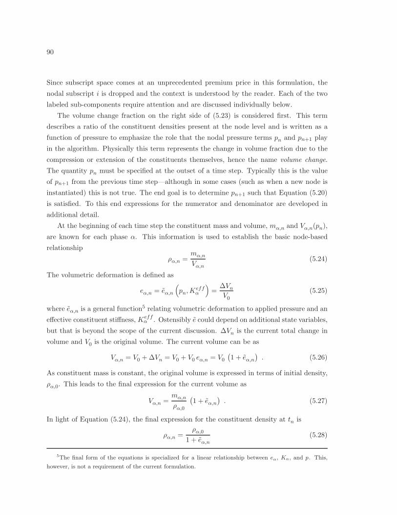
90

Since subscript space comes at an unprecedented premium price in this formulation, the

nodal subscript i is dropped and the context is understood by the reader. Each of the two

labeled sub-components require attention and are discussed individually below.

The volume change fraction on the right side of (5.23) is considered first. This term

describes a ratio of the constituent densities present at the node level and is written as a

function of pressure to emphasize the role that the nodal pressure terms pn and pn+1 play

in the algorithm. Physically this term represents the change in volume fraction due to the

compression or extension of the constituents themselves, hence the name volume change.

The quantity pn must be specified at the outset of a time step. Typically this is the value

of pn+1 from the previous time step—although in some cases (such as when a new node is

instantiated) this is not true. The end goal is to determine pn+1 such that Equation (5.20)

is satisfied. To this end expressions for the numerator and denominator are developed in

additional detail.

At the beginning of each time step the constituent mass and volume, mα,n and Vα,n(pn),

are known for each phase α. This information is used to establish the basic node-based

relationship

ρα,n =mα,n

Vα,n(5.24)

The volumetric deformation is defined as

eα,n = eα,n

(

pn,Keffα

)

=∆VnV0

(5.25)

where eα,n is a general function5 relating volumetric deformation to applied pressure and an

effective constituent stiffness, Keffα . Ostensibly e could depend on additional state variables,

but that is beyond the scope of the current discussion. ∆Vn is the current total change in

volume and V0 is the original volume. The current volume can be as

Vα,n = V0 +∆Vn = V0 + V0 eα,n = V0(1 + eα,n

). (5.26)

As constituent mass is constant, the original volume is expressed in terms of initial density,

ρα,0. This leads to the final expression for the current volume as

Vα,n =mα,n

ρα,0

(1 + eα,n

). (5.27)

In light of Equation (5.24), the final expression for the constituent density at tn is

ρα,n =ρα,0

1 + eα,n(5.28)

5The final form of the equations is specialized for a linear relationship between eα, Kα, and p. This,

however, is not a requirement of the current formulation.

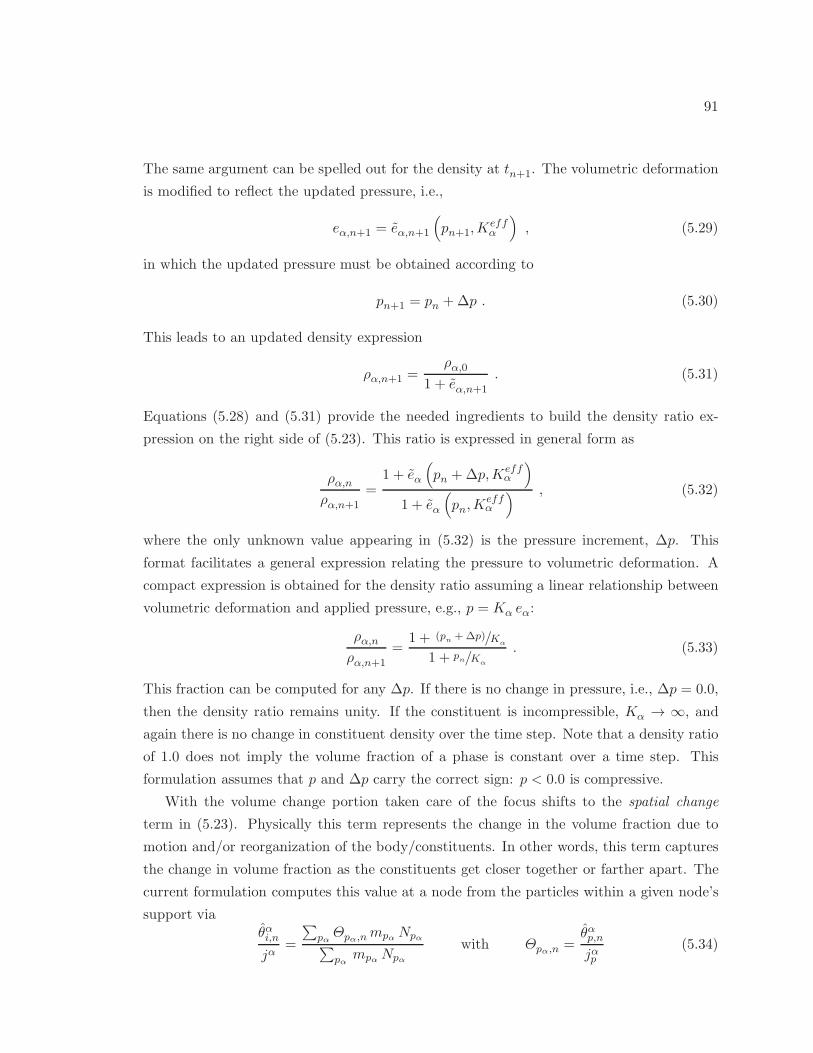
91

The same argument can be spelled out for the density at tn+1. The volumetric deformation

is modified to reflect the updated pressure, i.e.,

eα,n+1 = eα,n+1

(

pn+1,Keffα

)

, (5.29)

in which the updated pressure must be obtained according to

pn+1 = pn +∆p . (5.30)

This leads to an updated density expression

ρα,n+1 =ρα,0

1 + eα,n+1

. (5.31)

Equations (5.28) and (5.31) provide the needed ingredients to build the density ratio ex-

pression on the right side of (5.23). This ratio is expressed in general form as

ρα,nρα,n+1

=1 + eα

(

pn +∆p,Keffα

)

1 + eα

(

pn,Keffα

) , (5.32)

where the only unknown value appearing in (5.32) is the pressure increment, ∆p. This

format facilitates a general expression relating the pressure to volumetric deformation. A

compact expression is obtained for the density ratio assuming a linear relationship between

volumetric deformation and applied pressure, e.g., p = Kα eα:

ρα,nρα,n+1

=1 + (p

n+∆p)/K

α

1 + pn/K

α

. (5.33)

This fraction can be computed for any ∆p. If there is no change in pressure, i.e., ∆p = 0.0,

then the density ratio remains unity. If the constituent is incompressible, Kα → ∞, and

again there is no change in constituent density over the time step. Note that a density ratio

of 1.0 does not imply the volume fraction of a phase is constant over a time step. This

formulation assumes that p and ∆p carry the correct sign: p < 0.0 is compressive.

With the volume change portion taken care of the focus shifts to the spatial change

term in (5.23). Physically this term represents the change in the volume fraction due to

motion and/or reorganization of the body/constituents. In other words, this term captures

the change in volume fraction as the constituents get closer together or farther apart. The

current formulation computes this value at a node from the particles within a given node’s

support viaθαi,n

jα=

∑

pαΘpα,nmpα Npα

∑

pαmpα Npα

with Θpα,n =θαp,njαp

(5.34)

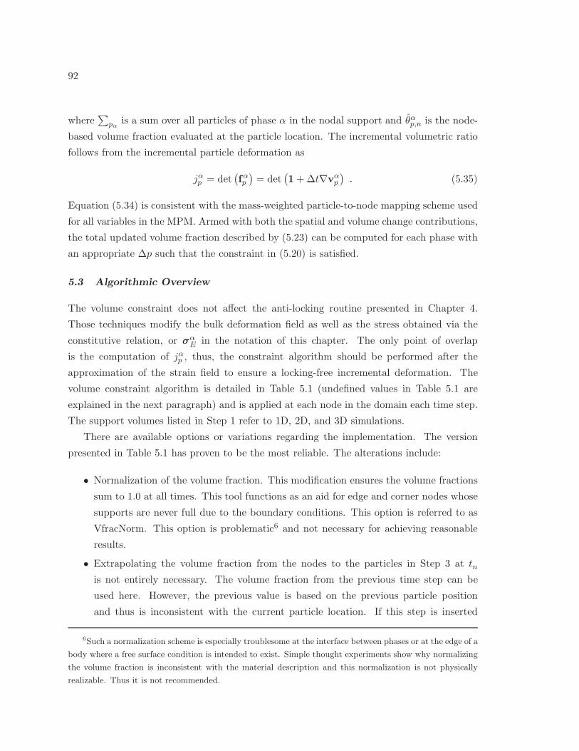
92

where∑

pαis a sum over all particles of phase α in the nodal support and θαp,n is the node-

based volume fraction evaluated at the particle location. The incremental volumetric ratio

follows from the incremental particle deformation as

jαp = det(fαp

)= det

(1+∆t∇vα

p

). (5.35)

Equation (5.34) is consistent with the mass-weighted particle-to-node mapping scheme used

for all variables in the MPM. Armed with both the spatial and volume change contributions,

the total updated volume fraction described by (5.23) can be computed for each phase with

an appropriate ∆p such that the constraint in (5.20) is satisfied.

5.3 Algorithmic Overview

The volume constraint does not affect the anti-locking routine presented in Chapter 4.

Those techniques modify the bulk deformation field as well as the stress obtained via the

constitutive relation, or σαE in the notation of this chapter. The only point of overlap

is the computation of jαp , thus, the constraint algorithm should be performed after the

approximation of the strain field to ensure a locking-free incremental deformation. The

volume constraint algorithm is detailed in Table 5.1 (undefined values in Table 5.1 are

explained in the next paragraph) and is applied at each node in the domain each time step.

The support volumes listed in Step 1 refer to 1D, 2D, and 3D simulations.

There are available options or variations regarding the implementation. The version

presented in Table 5.1 has proven to be the most reliable. The alterations include:

• Normalization of the volume fraction. This modification ensures the volume fractions

sum to 1.0 at all times. This tool functions as an aid for edge and corner nodes whose

supports are never full due to the boundary conditions. This option is referred to as

VfracNorm. This option is problematic6 and not necessary for achieving reasonable

results.

• Extrapolating the volume fraction from the nodes to the particles in Step 3 at tn

is not entirely necessary. The volume fraction from the previous time step can be

used here. However, the previous value is based on the previous particle position

and thus is inconsistent with the current particle location. If this step is inserted

6Such a normalization scheme is especially troublesome at the interface between phases or at the edge of a

body where a free surface condition is intended to exist. Simple thought experiments show why normalizing

the volume fraction is inconsistent with the material description and this normalization is not physically

realizable. Thus it is not recommended.

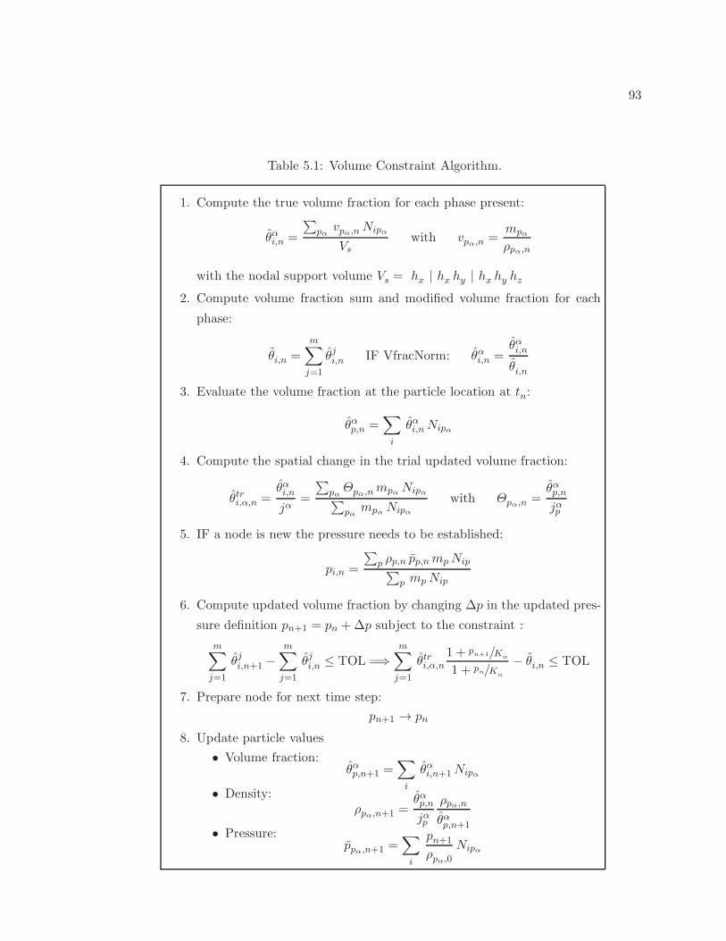
93

Table 5.1: Volume Constraint Algorithm.

1. Compute the true volume fraction for each phase present:

θαi,n =

∑

pαvpα,nNipα

Vswith vpα,n =

mpα

ρpα,n

with the nodal support volume Vs = hx | hx hy | hx hy hz2. Compute volume fraction sum and modified volume fraction for each

phase:

θi,n =

m∑

j=1

θji,n IF VfracNorm: θαi,n =θαi,n

θi,n

3. Evaluate the volume fraction at the particle location at tn:

θαp,n =∑

i

θαi,nNipα

4. Compute the spatial change in the trial updated volume fraction:

θtri,α,n =θαi,n

jα=

∑

pαΘpα,nmpα Nipα

∑

pαmpα Nipα

with Θpα,n =θαp,njαp

5. IF a node is new the pressure needs to be established:

pi,n =

∑

p ρp,n pp,nmpNip∑

p mpNip

6. Compute updated volume fraction by changing ∆p in the updated pres-

sure definition pn+1 = pn +∆p subject to the constraint :

m∑

j=1

θji,n+1 −m∑

j=1

θji,n ≤ TOL =⇒m∑

j=1

θtri,α,n1 + p

n+1/Kα

1 + pn/K

α

− θi,n ≤ TOL

7. Prepare node for next time step:

pn+1 → pn

8. Update particle values

• Volume fraction:θαp,n+1 =

∑

i

θαi,n+1Nipα

• Density:ρpα,n+1 =

θαp,njαp

ρpα,n

θαp,n+1• Pressure:ppα,n+1 =

∑

i

pn+1

ρpα,0Nipα

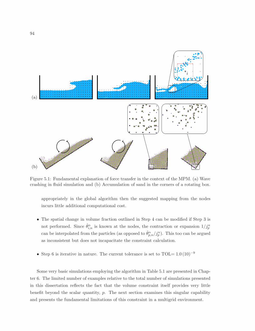
94

i

(b)

(a)

Figure 5.1: Fundamental explanation of force transfer in the context of the MPM. (a) Wavecrashing in fluid simulation and (b) Accumulation of sand in the corners of a rotating box.

appropriately in the global algorithm then the suggested mapping from the nodes

incurs little additional computational cost.

• The spatial change in volume fraction outlined in Step 4 can be modified if Step 3 is

not performed. Since θαi,n is known at the nodes, the contraction or expansion 1/jαp

can be interpolated from the particles (as opposed to θαp,n/jαp ). This too can be argued

as inconsistent but does not incapacitate the constraint calculation.

• Step 6 is iterative in nature. The current tolerance is set to TOL= 1.0 (10)−9

Some very basic simulations employing the algorithm in Table 5.1 are presented in Chap-

ter 6. The limited number of examples relative to the total number of simulations presented

in this dissertation reflects the fact that the volume constraint itself provides very little

benefit beyond the scalar quantity, p. The next section examines this singular capability

and presents the fundamental limitations of this constraint in a multigrid environment.

95

5.4 Limitations of the Volume Constraint

The presentation thus far has not restricted the problem type or phase distribution within

the domain. However, the only analyses the current formulation can handle effectively are

small-deformation and small displacement, linear elastic material simulations in which all

phases present span the entire domain at all times. The current formulation is unable

to handle phase boundaries or phase transitions in a physically reasonable fashion. This

section aims to identify why these restrictions exist and identify weaknesses with the current

formulation.

The volume constraint as presented in this chapter yields a single pressure. This pressure

ensures the total particle volume contribution maintains a user prescribed value at a given

node. Beyond this singular function the constraint serves no other purpose. Consider the

progression of images in the upper row of Figure 5.1(a) . A mass of water has rebounded off

the wall at right and the wave is about to experience a collapse. As the wave rolls over it

appears to ride, or hover, just above the flat free surface. The finger-like protrusion shuffles

along until the mass crashes into the left wall. This undesirable behavior is a fundamental

limitation of the MPM. The particles that make up the crashing wave interact with the free

surface as soon as they get into the support of a node containing both the wave and the

flat surface. One such node is labeled i in the close up image. Node i has no knowledge of

the underlying particle structure or arrangement. This node knows only a mass, force, and

velocity, and is not concerned with how these values came to be, the node is only concerned

with what these values are. The solution of the governing equation of motion proceeds

independently of the number of particles or the arrangement of these integration points in

the support of a node. Adding a pressure in the form of a volume constraint does not impart

knowledge of the underlying particle structure to node i, and it cannot mitigate the type of

behavior observed in this scenario. Nor will adding an additional phase in the form of air

solve this problem, as this too will suffer from the same shortcomings described above.

Another related example is shown in Figure 5.1(b). Here a drum is rotating about the

center point as indicated by the circular arrows. The sandy contents flops around as the

canister spins in a counter-clockwise direction. After the contents has been sufficiently jum-

bled situations arise in the corners like those shown in the close-up images of Figure 5.1(b).

Here the sand appears to not fill the spatial region. Again, this is a fundamental limita-

tion of the MPM that cannot be eliminated by adding a pressure to the simulation. The

force interaction of the sand and the surface begins to occur before the material reaches the

actual surface. In a sense this is merely an extension of the observation identified in the

previous paragraph and is consistent with observations documented in several MPM papers

96

and writings, as well as the work by Mast (2008), who investigated the intrinsic behavior

of computational particles near boundaries.

Initially there was hope that the volume constraint could provide the ability to model

mixing and separation, the idea being that the interaction of multiples phases can be prop-

erly captured by assigning each phase its own motion—thus establishing an individual grid

for each phase—and adding momentum exchange terms in a piecewise manner to achieve an

entire multiphase picture. Certain aspects of this paradigm are effective, such as modeling

the drag interaction in Mackenzie-Helnwein et al. (2010). However, the idea that the vol-

ume constraint can provide additional puzzle pieces in this regard has proven problematic.

Consider the series of two-phase examples shown in Figure 5.2(a). There is no restriction

on the types of phases in this algorithm, thus, it is reasonable to assume phase α is the

same material as phase β. By selecting a pressure dominant material, such as water, these

simple examples provide an ideal setting to test the current volume constraint’s capabilities.

Ideal behavior in this case is rather straightforward: the analysis should remain static and

a hydrostatic pressure distribution should develop due to the volume constraint.

Figure 5.2(b) helps explain why ideal behavior cannot be achieved with the current

formulation. Here the multiphase, multigrid framework is broken down grid-by-grid and the

force distributions, fαint and fβint, are shown for each phase. Note that this force develops as a

result of the pressure term supplied by the volume constraint as indicated in Equation 5.171.

The portion of the force distributions occurring along the container boundaries will be offset

perfectly by the reaction force that develops in these locations. That is, the reaction force

will ensure that the net force along the edges is zero and no net acceleration perpendicular

to the bounding surfaces is observed. The same cannot be said along the centerline of nodes

for the individual grids housing phase α and β. In Figure 5.2(c) basic equilibrium is applied

to centerline nodes and it is apparent that a net acceleration will occur on both Grid α

and Grid β. This in turn generates motion and the desired static response is not achieved.

The important point to take away from this discussion is the following: the desired

behavior for examples like those shown in Figure 5.2(a), or the ability to model mixing

and separation of multiple phases, or the ability to simulate the mechanical response of

partially/fully saturated porous media can be achieved using the MPM, but the mechanism

responsible for ensuring satisfactory behavior is not the volume constraint presented here.

One potential solution is to use the common grid values, as this grid takes into account

forces and motion from all phases. Starting from this mixture, begin dissecting the compo-

nents of existing mixture theory equations and identify which components of the individual

phase motions need to be modified to achieve this result. A second possible solution is to

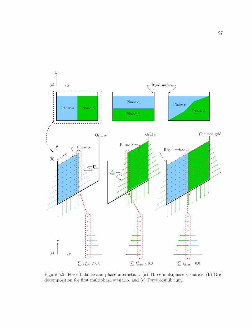
97

x

y

(c)

Phase α

Phase β

Phase βPhase α

x

y

Grid α Grid β Common grid

∑fαx,int 6= 0.0

y

∑fβx,int 6= 0.0

x

(b)

(a) Rigid surface

Phase α

Phase β

fβint

Rigid surface

fαint

Phase α

∑fx,int = 0.0

Phase β

Figure 5.2: Force balance and phase interaction. (a) Three multiphase scenarios, (b) Griddecomposition for first multiphase scenario, and (c) Force equilibrium.

98

use one of the several multigrid contact algorithms already designed and implemented in the

MPM, including those by Bardenhagen et al. (2000, 2001); Hu and Chen (2003); Pan et al.

(2008). These frameworks build an environment identical to that depicted in Figure 5.2(b),

but borrow (for lack of a better term) extra force from the common grid to balance each

individual grid. In this manner the force contribution from other bodies/phases present in

the analysis is explicitly accounted for. The disadvantage of this proposed solutions lies in

the inherent inability to model overlap and phase penetration in the current algorithms.

This, however, could potentially be overcome by using the relative volume fraction of each

body/phase on each individual grid, and borrowing a volume fraction corrected amount of

force from the common grid to replicate the desired behavior.

5.5 Conclusions

This chapter presents a volume constraint for use in the Material Point Method. The

overview includes a discussion of weak form equations in a multiphase context, and rep-

resents an extension to the traditional framework. The algorithmic details and possible

implementation alternatives are identified in Table 5.1 and corresponding discussion. In

Chapter 6 three example problem outlining some of the capabilities of the constraint are

presented. These examples represent the only types of problems the current formulation

can handle, namely small-deformation, linear elastic material simulations in which all phases

present span the entire domain. The current formulation is simply unable to handle phase

boundaries or phase transitions in a physically reasonable fashion for the reasons discussed

in Section 5.4.

99

Chapter 6

EXAMPLE PROBLEMS 1: LINEAR ELASTIC SIMULATIONS

Several examples presented in this chapter follow (verbatim in some instances) from

the paper Mitigating kinematic locking in the Material Point Method by Mast, Mackenzie-

Helnwein, Arduino, Miller, and Shin (2012). The author is indebted to Peter Mackenzie-

Helnwein, Pedro Arduino, and Greg Miller for their contributions in writing and publishing

said paper.

The primary focus of this chapter is to discuss a series of MPM simulations from fluid

and solid mechanics. The different examples show the effectiveness of the anti-locking

approach (see Chapter 4) applied to a wide variety of problem types. In particular, large

deformation, nearly incompressible flow simulations are examined in order to validate the

anti-locking strategy from a kinematic viewpoint. The ensuing pressure field and interaction

between fluid and bounding surface are examined. On the solid mechanics end of the

spectrum, a cantilever beam with prescribed velocity is analyzed and compared to small

deformation beam theory. The normal and shear stresses are examined throughout the beam

and the beam deformation is analyzed in detail. The final sections model saturated soil

specimens, validating the certain aspects of the volume constraint algorithm highlighted in

Chapter 5. This chapter contains only simulations of materials with linear elastic properties.

6.1 Applications to Fluid Dynamics

The constitutive equation for isotropic elasticity can be formulated in such a way that it

represents compressible and incompressible materials Hughes (1987). In the present case,

the constitutive relationship for a nearly incompressible fluid can be written as

σ = ρ k θ 1+ 2µd , (6.1)

where ρ is the mass density, k = k/ρ0 with k as the bulk modulus, θ is the volumetric

dilation, µ is the dynamic viscosity, and d is the rate of deformation tensor calculated from

the velocity field, v, as

d =1

2(∇v +∇vT ) . (6.2)

All fluid simulations appearing in this section are large deformation, plane strain analyses.

Gravity is the driving force and is applied in the vertical direction, i.e., g = −9.81j m/s2.

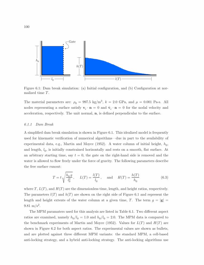
100

h(T )

l(T )

Gate

l0

h0

Figure 6.1: Dam break simulation: (a) Initial configuration, and (b) Configuration at nor-malized time T .

The material parameters are: ρ0 = 997.5 kg/m3, k = 2.0 GPa, and µ = 0.001 Pa-s. All

nodes representing a surface satisfy vi · n = 0 and vi · n = 0 for the nodal velocity and

acceleration, respectively. The unit normal, n, is defined perpendicular to the surface.

6.1.1 Dam Break

A simplified dam break simulation is shown in Figure 6.1. This idealized model is frequently

used for kinematic verification of numerical algorithms—due in part to the availability of

experimental data, e.g., Martin and Moyce (1952). A water column of initial height, h0,

and length, l0, is initially constrained horizontally and rests on a smooth, flat surface. At

an arbitrary starting time, say t = 0, the gate on the right-hand side is removed and the

water is allowed to flow freely under the force of gravity. The following parameters describe

the free surface runout:

T = t

√

h0 g

l20, L(T ) =

l(T )

l0, and H(T ) =

h(T )

h0(6.3)

where T , L(T ), and H(T ) are the dimensionless time, length, and height ratios, respectively.

The parameters l(T ) and h(T ) are shown on the right side of Figure 6.1 and represent the

length and height extents of the water column at a given time, T . The term g = |g| =9.81 m/s2.

The MPM paramaters used for this analysis are listed in Table 6.1. Two different aspect

ratios are examined, namely h0/l0 = 1.0 and h0/l0 = 2.0. The MPM data is compared to

the benchmark experiments of Martin and Moyce (1952). Values for L(T ) and H(T ) are

shown in Figure 6.2 for both aspect ratios. The experimental values are shown as bullets,

and are plotted against three different MPM variants: the standard MPM, a cell-based

anti-locking strategy, and a hybrid anti-locking strategy. The anti-locking algorithms use

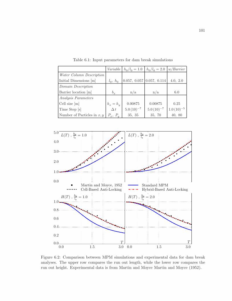
101

Table 6.1: Input parameters for dam break simulations

Variable h0/l0 = 1.0 h0/l0 = 2.0 w/Barrier

Water Column Description

Initial Dimensions [m] l0, h0 0.057, 0.057 0.057, 0.114 4.0, 2.0

Domain Description

Barrier location [m] bx n/a n/a 6.0

Analysis Parameters

Cell size [m] hx = hy 0.00875 0.00875 0.25

Time Step [s] ∆ t 5.0 (10)−7 5.0 (10)−7 1.0 (10)−5

Number of Particles in x, y Px, Py 35, 35 35, 70 40, 80

1.5 3.00.0T

0.0 1.5 3.0T

Standard MPMHybrid-Based Anti-LockingCell-Based Anti-Locking

Martin and Moyce, 1952

0.0

1.0

0.6

0.8

0.4

0.2

0.0

5.0

4.0

3.0

2.0

1.0

L(T ) ,h0

l0

= 1.0 L(T ) ,h0

l0

= 2.0

H(T ) ,h0

l0

= 2.0H(T ) ,h0

l0

= 1.0

Figure 6.2: Comparison between MPM simulations and experimental data for dam breakanalyses. The upper row compares the run out length, while the lower row compares therun out height. Experimental data is from Martin and Moyce Martin and Moyce (1952).

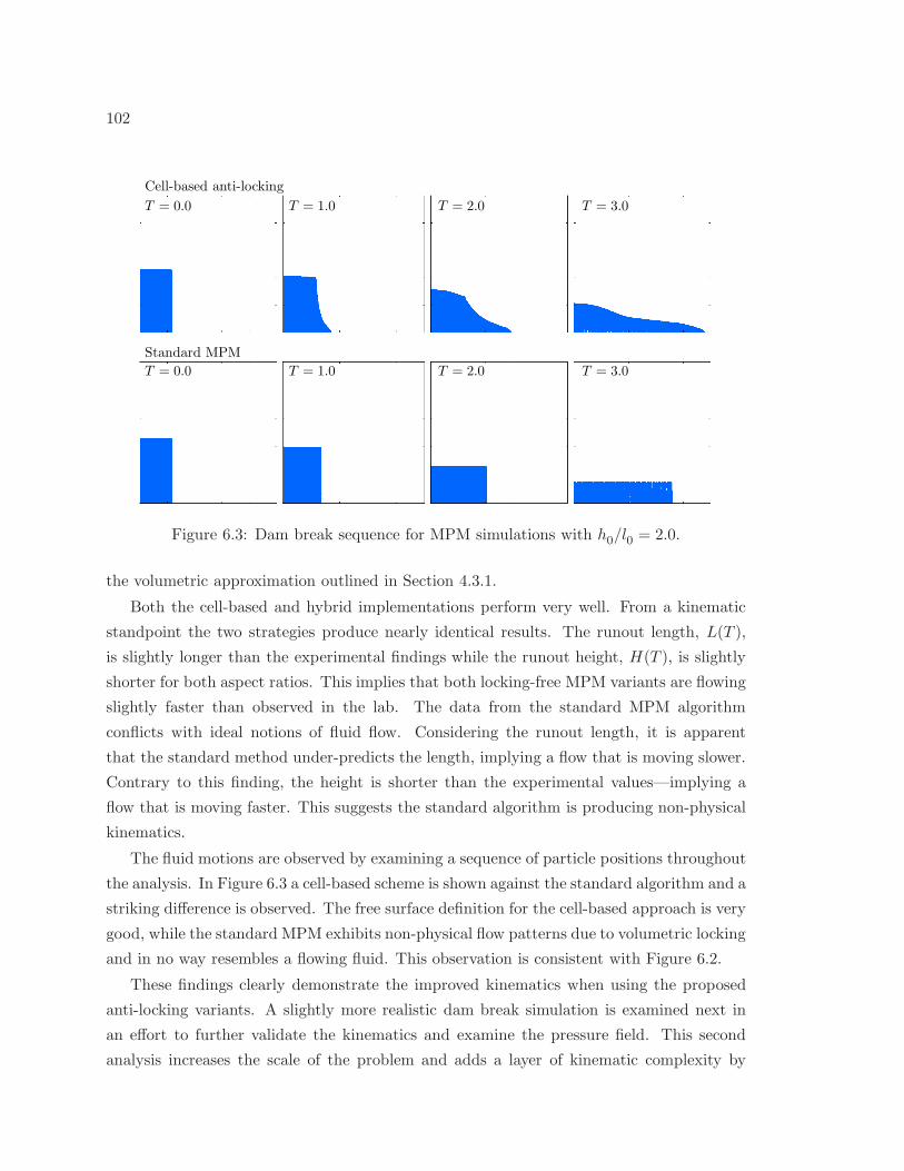
102

T = 2.0T = 1.0T = 0.0 T = 3.0

Standard MPM

Cell-based anti-locking

T = 0.0 T = 1.0 T = 2.0 T = 3.0

Figure 6.3: Dam break sequence for MPM simulations with h0/l0 = 2.0.

the volumetric approximation outlined in Section 4.3.1.

Both the cell-based and hybrid implementations perform very well. From a kinematic

standpoint the two strategies produce nearly identical results. The runout length, L(T ),

is slightly longer than the experimental findings while the runout height, H(T ), is slightly

shorter for both aspect ratios. This implies that both locking-free MPM variants are flowing

slightly faster than observed in the lab. The data from the standard MPM algorithm

conflicts with ideal notions of fluid flow. Considering the runout length, it is apparent

that the standard method under-predicts the length, implying a flow that is moving slower.

Contrary to this finding, the height is shorter than the experimental values—implying a

flow that is moving faster. This suggests the standard algorithm is producing non-physical

kinematics.

The fluid motions are observed by examining a sequence of particle positions throughout

the analysis. In Figure 6.3 a cell-based scheme is shown against the standard algorithm and a

striking difference is observed. The free surface definition for the cell-based approach is very

good, while the standard MPM exhibits non-physical flow patterns due to volumetric locking

and in no way resembles a flowing fluid. This observation is consistent with Figure 6.2.

These findings clearly demonstrate the improved kinematics when using the proposed

anti-locking variants. A slightly more realistic dam break simulation is examined next in

an effort to further validate the kinematics and examine the pressure field. This second

analysis increases the scale of the problem and adds a layer of kinematic complexity by

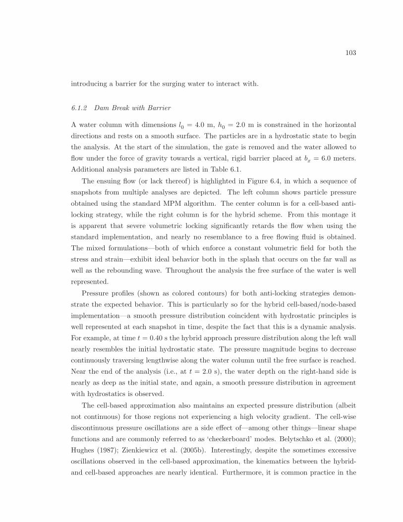
103

introducing a barrier for the surging water to interact with.

6.1.2 Dam Break with Barrier

A water column with dimensions l0 = 4.0 m, h0 = 2.0 m is constrained in the horizontal

directions and rests on a smooth surface. The particles are in a hydrostatic state to begin

the analysis. At the start of the simulation, the gate is removed and the water allowed to

flow under the force of gravity towards a vertical, rigid barrier placed at bx = 6.0 meters.

Additional analysis parameters are listed in Table 6.1.

The ensuing flow (or lack thereof) is highlighted in Figure 6.4, in which a sequence of

snapshots from multiple analyses are depicted. The left column shows particle pressure

obtained using the standard MPM algorithm. The center column is for a cell-based anti-

locking strategy, while the right column is for the hybrid scheme. From this montage it

is apparent that severe volumetric locking significantly retards the flow when using the

standard implementation, and nearly no resemblance to a free flowing fluid is obtained.

The mixed formulations—both of which enforce a constant volumetric field for both the

stress and strain—exhibit ideal behavior both in the splash that occurs on the far wall as

well as the rebounding wave. Throughout the analysis the free surface of the water is well

represented.

Pressure profiles (shown as colored contours) for both anti-locking strategies demon-

strate the expected behavior. This is particularly so for the hybrid cell-based/node-based

implementation—a smooth pressure distribution coincident with hydrostatic principles is

well represented at each snapshot in time, despite the fact that this is a dynamic analysis.

For example, at time t = 0.40 s the hybrid approach pressure distribution along the left wall

nearly resembles the initial hydrostatic state. The pressure magnitude begins to decrease

continuously traversing lengthwise along the water column until the free surface is reached.

Near the end of the analysis (i.e., at t = 2.0 s), the water depth on the right-hand side is

nearly as deep as the initial state, and again, a smooth pressure distribution in agreement

with hydrostatics is observed.

The cell-based approximation also maintains an expected pressure distribution (albeit

not continuous) for those regions not experiencing a high velocity gradient. The cell-wise

discontinuous pressure oscillations are a side effect of—among other things—linear shape

functions and are commonly referred to as ‘checkerboard’ modes. Belytschko et al. (2000);

Hughes (1987); Zienkiewicz et al. (2005b). Interestingly, despite the sometimes excessive

oscillations observed in the cell-based approximation, the kinematics between the hybrid-

and cell-based approaches are nearly identical. Furthermore, it is common practice in the

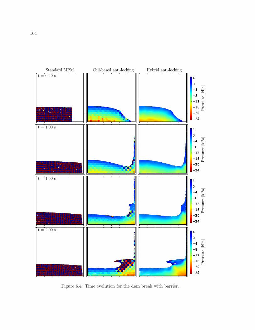
104

Pre

ssure

[kPa]

Pre

ssure

[kPa]

Pre

ssure

[kPa]

Pre

ssure

[kPa]

t = 0.40 s

t = 1.00 s

t = 1.50 s

t = 2.00 s

Standard MPM Cell-based anti-locking Hybrid anti-locking

Figure 6.4: Time evolution for the dam break with barrier.

105

Pre

ssure

[kP

a]

3 m

4 m

1 m

Rea

ctio

nFor

ce[k

N]

(a) (b)

Figure 6.5: Initial state for the tank drain analysis. (a) The particle pressure. (b) Thereaction force, fir.

FEM to use a stress smoothing/averaging technique for plotting and interpretation purposes.

Hughes (1987); Zienkiewicz et al. (2005b). The pressure field for the cell-based approach

would appear very similar to that of the hybrid technique if such a procedure were to be

implemented here.

The dam break simulations show the proposed anti-locking strategies significantly im-

prove the pressure field, and ultimately, are key for obtaining an ideal free surface definition

for the runout simulation, as well as the splash and rebounding wave due to the interaction

between the water and the barrier. The latter simulation with barrier suggests the MPM

with appropriate anti-locking extension is a valid tool for recovering or assessing the magni-

tude of the reaction force/traction between two media, e.g., a fluid-like material interacting

with a structure. This idea is explored in the following example.

6.1.3 Tank Drain

A rectangular water tank with a narrow drain located in the center is used as the model for

this series of simulations. Only half of the domain needs to be analyzed due to symmetry,

and the initial state is shown in Figure 6.5. Here, a hydrostatic stress state is shown alongside

the reaction force that develops in response to the fluid pressure exerting an outward force

on the tank surface. The edge of the computational domain is used to represent the rigid

exterior surface. The reaction force is calculated as fir = −fi · n, where fi is the nodal force

at a node representing the boundary. All other analysis parameters are listed in Table 6.2.

The nodal reaction force and velocity fields are shown in Figures 6.6 and 6.7. Particle

positions are shown only for reference purposes. Each figure consists of three columns;

the leftmost is for the standard MPM algorithm, the center is for a cell-based anti-locking

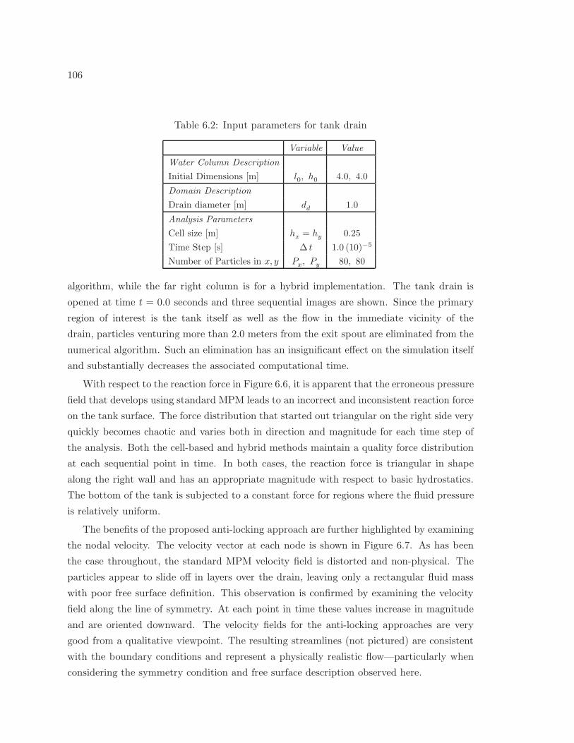
106

Table 6.2: Input parameters for tank drain

Variable Value

Water Column Description

Initial Dimensions [m] l0, h0 4.0, 4.0

Domain Description

Drain diameter [m] dd 1.0

Analysis Parameters

Cell size [m] hx = hy 0.25

Time Step [s] ∆ t 1.0 (10)−5

Number of Particles in x, y Px, Py 80, 80

algorithm, while the far right column is for a hybrid implementation. The tank drain is

opened at time t = 0.0 seconds and three sequential images are shown. Since the primary

region of interest is the tank itself as well as the flow in the immediate vicinity of the

drain, particles venturing more than 2.0 meters from the exit spout are eliminated from the

numerical algorithm. Such an elimination has an insignificant effect on the simulation itself

and substantially decreases the associated computational time.

With respect to the reaction force in Figure 6.6, it is apparent that the erroneous pressure

field that develops using standard MPM leads to an incorrect and inconsistent reaction force

on the tank surface. The force distribution that started out triangular on the right side very

quickly becomes chaotic and varies both in direction and magnitude for each time step of

the analysis. Both the cell-based and hybrid methods maintain a quality force distribution

at each sequential point in time. In both cases, the reaction force is triangular in shape

along the right wall and has an appropriate magnitude with respect to basic hydrostatics.

The bottom of the tank is subjected to a constant force for regions where the fluid pressure

is relatively uniform.

The benefits of the proposed anti-locking approach are further highlighted by examining

the nodal velocity. The velocity vector at each node is shown in Figure 6.7. As has been

the case throughout, the standard MPM velocity field is distorted and non-physical. The

particles appear to slide off in layers over the drain, leaving only a rectangular fluid mass

with poor free surface definition. This observation is confirmed by examining the velocity

field along the line of symmetry. At each point in time these values increase in magnitude

and are oriented downward. The velocity fields for the anti-locking approaches are very

good from a qualitative viewpoint. The resulting streamlines (not pictured) are consistent

with the boundary conditions and represent a physically realistic flow—particularly when

considering the symmetry condition and free surface description observed here.

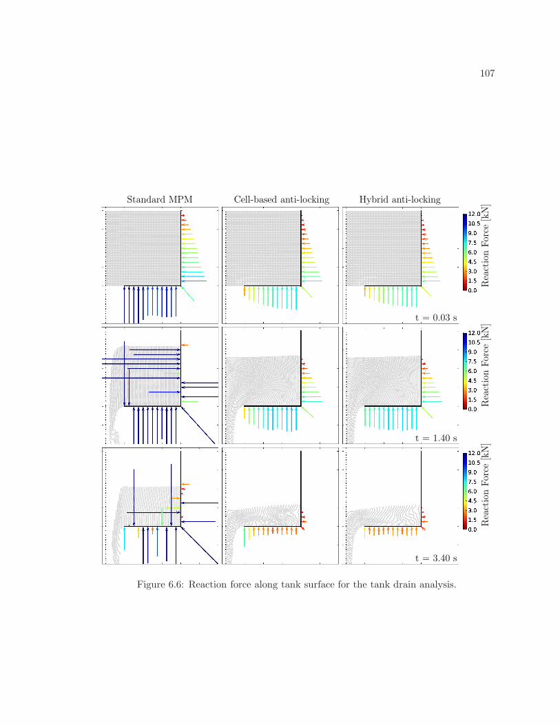
107

t = 0.03 s

t = 1.40 s

t = 3.40 s

Standard MPM

Rea

ctio

nFor

ce[k

N]

Rea

ctio

nFor

ce[k

N]

Rea

ctio

nFor

ce[k

N]

Hybrid anti-lockingCell-based anti-locking

Figure 6.6: Reaction force along tank surface for the tank drain analysis.

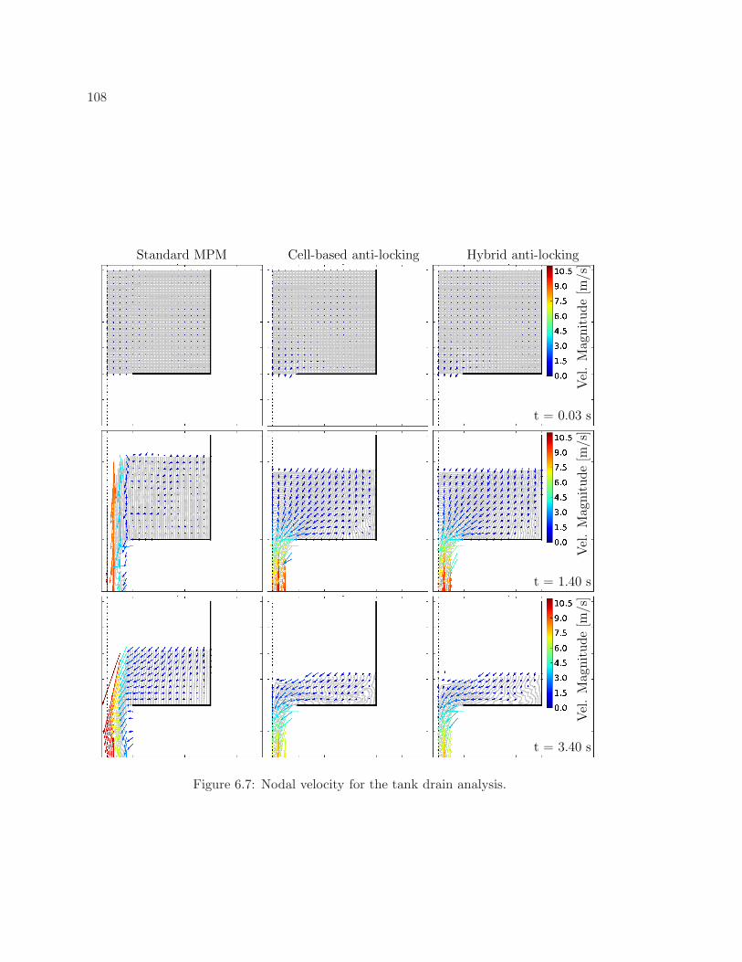
108

t = 0.03 s

t = 1.40 s

t = 3.40 s

Vel

.M

agnit

ude

[m/s

]V

el.

Mag

nit

ude

[m/s

]V

el.

Mag

nit

ude

[m/s

]

Standard MPM Cell-based anti-locking Hybrid anti-locking

Figure 6.7: Nodal velocity for the tank drain analysis.

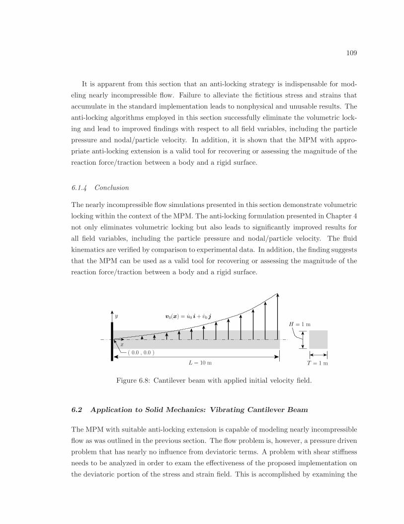
109

It is apparent from this section that an anti-locking strategy is indispensable for mod-

eling nearly incompressible flow. Failure to alleviate the fictitious stress and strains that

accumulate in the standard implementation leads to nonphysical and unusable results. The

anti-locking algorithms employed in this section successfully eliminate the volumetric lock-

ing and lead to improved findings with respect to all field variables, including the particle

pressure and nodal/particle velocity. In addition, it is shown that the MPM with appro-

priate anti-locking extension is a valid tool for recovering or assessing the magnitude of the

reaction force/traction between a body and a rigid surface.

6.1.4 Conclusion

The nearly incompressible flow simulations presented in this section demonstrate volumetric

locking within the context of the MPM. The anti-locking formulation presented in Chapter 4

not only eliminates volumetric locking but also leads to significantly improved results for

all field variables, including the particle pressure and nodal/particle velocity. The fluid

kinematics are verified by comparison to experimental data. In addition, the finding suggests

that the MPM can be used as a valid tool for recovering or assessing the magnitude of the

reaction force/traction between a body and a rigid surface.

( 0.0 , 0.0 )

y

L = 10 m

H = 1 m

T = 1 m

x

v0(x) = u0 i + v0 j

Figure 6.8: Cantilever beam with applied initial velocity field.

6.2 Application to Solid Mechanics: Vibrating Cantilever Beam

The MPM with suitable anti-locking extension is capable of modeling nearly incompressible

flow as was outlined in the previous section. The flow problem is, however, a pressure driven

problem that has nearly no influence from deviatoric terms. A problem with shear stiffness

needs to be analyzed in order to exam the effectiveness of the proposed implementation on

the deviatoric portion of the stress and strain field. This is accomplished by examining the

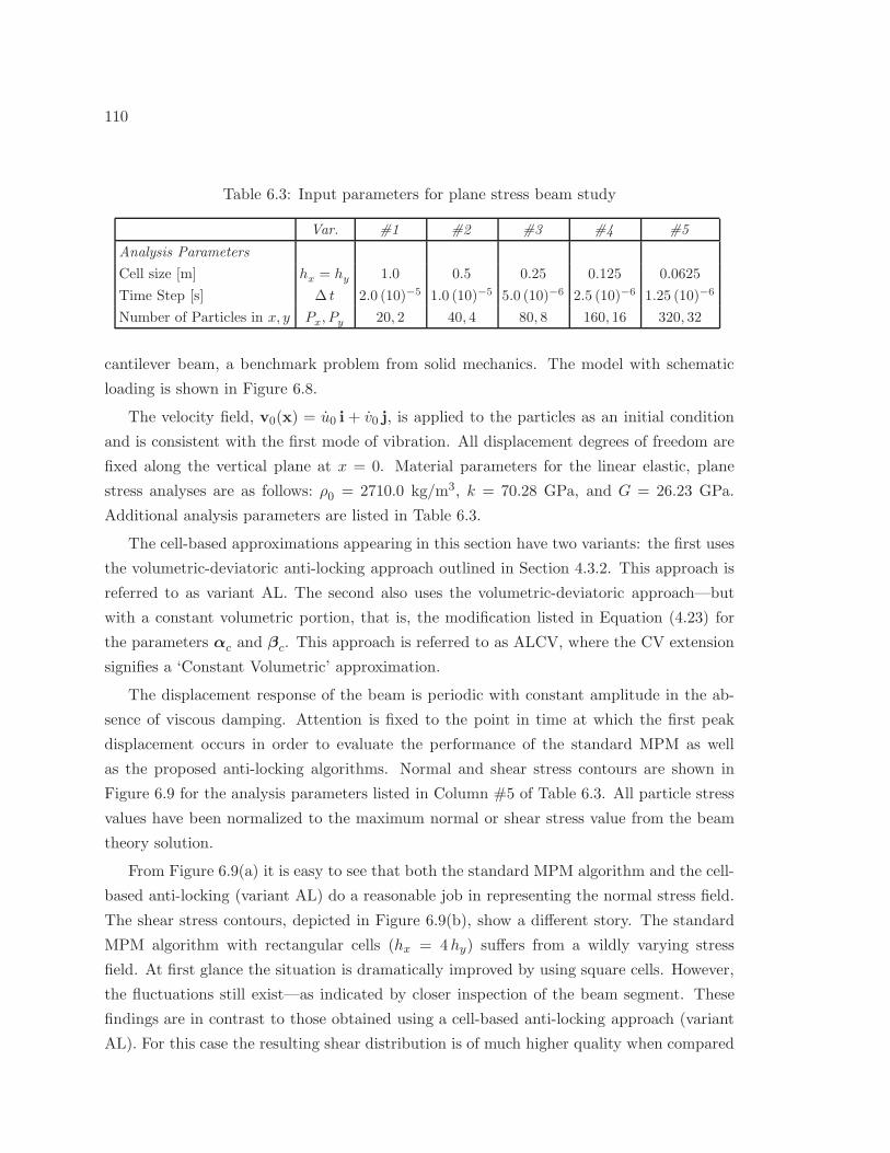
110

Table 6.3: Input parameters for plane stress beam study

Var. #1 #2 #3 #4 #5

Analysis Parameters

Cell size [m] hx = hy 1.0 0.5 0.25 0.125 0.0625

Time Step [s] ∆ t 2.0 (10)−5 1.0 (10)−5 5.0 (10)−6 2.5 (10)−6 1.25 (10)−6

Number of Particles in x, y Px, Py 20, 2 40, 4 80, 8 160, 16 320, 32

cantilever beam, a benchmark problem from solid mechanics. The model with schematic

loading is shown in Figure 6.8.

The velocity field, v0(x) = u0 i + v0 j, is applied to the particles as an initial condition

and is consistent with the first mode of vibration. All displacement degrees of freedom are

fixed along the vertical plane at x = 0. Material parameters for the linear elastic, plane

stress analyses are as follows: ρ0 = 2710.0 kg/m3, k = 70.28 GPa, and G = 26.23 GPa.

Additional analysis parameters are listed in Table 6.3.

The cell-based approximations appearing in this section have two variants: the first uses

the volumetric-deviatoric anti-locking approach outlined in Section 4.3.2. This approach is

referred to as variant AL. The second also uses the volumetric-deviatoric approach—but

with a constant volumetric portion, that is, the modification listed in Equation (4.23) for

the parameters αc and βc. This approach is referred to as ALCV, where the CV extension

signifies a ‘Constant Volumetric’ approximation.

The displacement response of the beam is periodic with constant amplitude in the ab-

sence of viscous damping. Attention is fixed to the point in time at which the first peak

displacement occurs in order to evaluate the performance of the standard MPM as well

as the proposed anti-locking algorithms. Normal and shear stress contours are shown in

Figure 6.9 for the analysis parameters listed in Column #5 of Table 6.3. All particle stress

values have been normalized to the maximum normal or shear stress value from the beam

theory solution.

From Figure 6.9(a) it is easy to see that both the standard MPM algorithm and the cell-

based anti-locking (variant AL) do a reasonable job in representing the normal stress field.

The shear stress contours, depicted in Figure 6.9(b), show a different story. The standard

MPM algorithm with rectangular cells (hx = 4hy) suffers from a wildly varying stress

field. At first glance the situation is dramatically improved by using square cells. However,

the fluctuations still exist—as indicated by closer inspection of the beam segment. These

findings are in contrast to those obtained using a cell-based anti-locking approach (variant

AL). For this case the resulting shear distribution is of much higher quality when compared

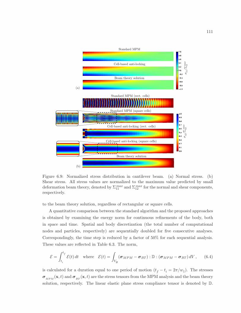
111

σ12/Σ

max

12

σ11/Σ

max

11

(b)

(a)

Beam theory solution

Cell-based anti-locking

Standard MPM

Standard MPM (rect. cells)

Standard MPM (square cells)

Cell-based anti-locking (rect. cells)

Cell-based anti-locking (square cells)

Beam theory solution

Figure 6.9: Normalized stress distribution in cantilever beam. (a) Normal stress. (b)Shear stress. All stress values are normalized to the maximum value predicted by smalldeformation beam theory, denoted by Σmax

11 and Σmax12 for the normal and shear components,

respectively.

to the beam theory solution, regardless of rectangular or square cells.

A quantitative comparison between the standard algorithm and the proposed approaches

is obtained by examining the energy norm for continuous refinements of the body, both

in space and time. Spatial and body discretization (the total number of computational

nodes and particles, respectively) are sequentially doubled for five consecutive analyses.

Correspondingly, the time step is reduced by a factor of 50% for each sequential analysis.

These values are reflected in Table 6.3. The norm,

E =

∫ tf

ti

E(t) dt where E(t) =∫

VB

(σMPM − σBT ) : D : (σMPM − σBT ) dV , (6.4)

is calculated for a duration equal to one period of motion (tf − ti = 2π/w1). The stresses

σMPM

(x, t) and σBT

(x, t) are the stress tensors from the MPM analysis and the beam theory

solution, respectively. The linear elastic plane stress compliance tensor is denoted by D.

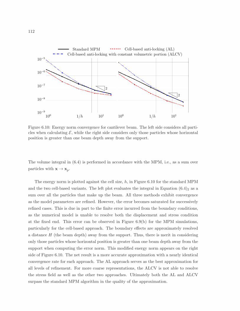
112

101 101

Standard MPMCell-based anti-locking with constant volumetric portion (ALCV)

Cell-based anti-locking (AL)

100 1/h 100 1/h

10−5

10−9

10−8

10−6

10−7

2

2

Figure 6.10: Energy norm convergence for cantilever beam. The left side considers all parti-cles when calculating E , while the right side considers only those particles whose horizontalposition is greater than one beam depth away from the support.

The volume integral in (6.4) is performed in accordance with the MPM, i.e., as a sum over

particles with x → xp.

The energy norm is plotted against the cell size, h, in Figure 6.10 for the standard MPM

and the two cell-based variants. The left plot evaluates the integral in Equation (6.4)2 as a

sum over all the particles that make up the beam. All three methods exhibit convergence

as the model parameters are refined. However, the error becomes saturated for successively

refined cases. This is due in part to the finite error incurred from the boundary conditions,

as the numerical model is unable to resolve both the displacement and stress condition

at the fixed end. This error can be observed in Figure 6.9(b) for the MPM simulations,

particularly for the cell-based approach. The boundary effects are approximately resolved

a distance H (the beam depth) away from the support. Thus, there is merit in considering

only those particles whose horizontal position is greater than one beam depth away from the

support when computing the error norm. This modified energy norm appears on the right

side of Figure 6.10. The net result is a more accurate approximation with a nearly identical

convergence rate for each approach. The AL approach serves as the best approximation for

all levels of refinement. For more coarse representations, the ALCV is not able to resolve

the stress field as well as the other two approaches. Ultimately both the AL and ALCV

surpass the standard MPM algorithm in the quality of the approximation.

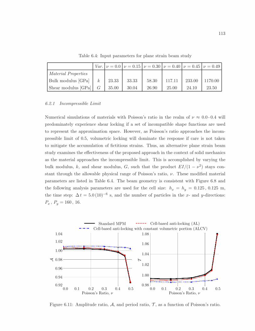
113

Table 6.4: Input parameters for plane strain beam study

Var. ν = 0.0 ν = 0.15 ν = 0.30 ν = 0.40 ν = 0.45 ν = 0.49

Material Properties

Bulk modulus [GPa] k 23.33 33.33 58.30 117.11 233.00 1170.00

Shear modulus [GPa] G 35.00 30.04 26.90 25.00 24.10 23.50

6.2.1 Incompressible Limit

Numerical simulations of materials with Poisson’s ratio in the realm of ν ≈ 0.0 - 0.4 will

predominately experience shear locking if a set of incompatible shape functions are used

to represent the approximation space. However, as Poisson’s ratio approaches the incom-

pressible limit of 0.5, volumetric locking will dominate the response if care is not taken

to mitigate the accumulation of fictitious strains. Thus, an alternative plane strain beam

study examines the effectiveness of the proposed approach in the context of solid mechanics

as the material approaches the incompressible limit. This is accomplished by varying the

bulk modulus, k, and shear modulus, G, such that the product EI/(1 − ν2) stays con-

stant through the allowable physical range of Poisson’s ratio, ν. These modified material

parameters are listed in Table 6.4. The beam geometry is consistent with Figure 6.8 and

the following analysis parameters are used for the cell size: hx = hy = 0.125 , 0.125 m,

the time step: ∆ t = 5.0 (10)−6 s, and the number of particles in the x- and y-directions:

Px , Py = 160 , 16.

0.0Poisson’s Ratio, ν

0.50.1 0.40.30.2 0.0Poisson’s Ratio, ν

0.50.1 0.40.30.2

Standard MPM Cell-based anti-locking (AL)

Cell-based anti-locking with constant volumetric portion (ALCV)

0.92

0.94

0.96

0.98

1.00

1.02

1.04

A

0.98

1.06

1.04

1.02

1.00

1.08

T

Figure 6.11: Amplitude ratio, A, and period ratio, T , as a function of Poisson’s ratio.

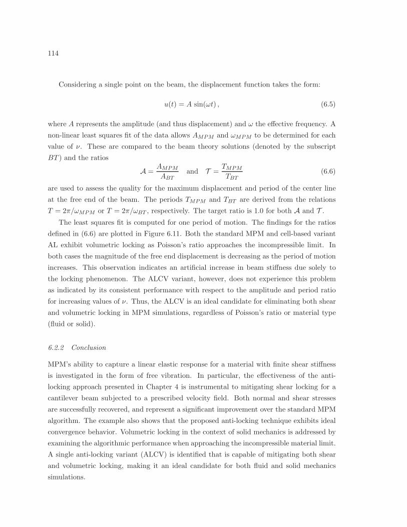
114

Considering a single point on the beam, the displacement function takes the form:

u(t) = A sin(ωt) , (6.5)

where A represents the amplitude (and thus displacement) and ω the effective frequency. A

non-linear least squares fit of the data allows AMPM and ωMPM to be determined for each

value of ν. These are compared to the beam theory solutions (denoted by the subscript

BT ) and the ratios

A =AMPM

ABTand T =

TMPM

TBT(6.6)

are used to assess the quality for the maximum displacement and period of the center line

at the free end of the beam. The periods TMPM and TBT are derived from the relations

T = 2π/ωMPM or T = 2π/ωBT , respectively. The target ratio is 1.0 for both A and T .

The least squares fit is computed for one period of motion. The findings for the ratios

defined in (6.6) are plotted in Figure 6.11. Both the standard MPM and cell-based variant

AL exhibit volumetric locking as Poisson’s ratio approaches the incompressible limit. In

both cases the magnitude of the free end displacement is decreasing as the period of motion

increases. This observation indicates an artificial increase in beam stiffness due solely to

the locking phenomenon. The ALCV variant, however, does not experience this problem

as indicated by its consistent performance with respect to the amplitude and period ratio

for increasing values of ν. Thus, the ALCV is an ideal candidate for eliminating both shear

and volumetric locking in MPM simulations, regardless of Poisson’s ratio or material type

(fluid or solid).

6.2.2 Conclusion

MPM’s ability to capture a linear elastic response for a material with finite shear stiffness

is investigated in the form of free vibration. In particular, the effectiveness of the anti-

locking approach presented in Chapter 4 is instrumental to mitigating shear locking for a

cantilever beam subjected to a prescribed velocity field. Both normal and shear stresses

are successfully recovered, and represent a significant improvement over the standard MPM

algorithm. The example also shows that the proposed anti-locking technique exhibits ideal

convergence behavior. Volumetric locking in the context of solid mechanics is addressed by

examining the algorithmic performance when approaching the incompressible material limit.

A single anti-locking variant (ALCV) is identified that is capable of mitigating both shear

and volumetric locking, making it an ideal candidate for both fluid and solid mechanics

simulations.

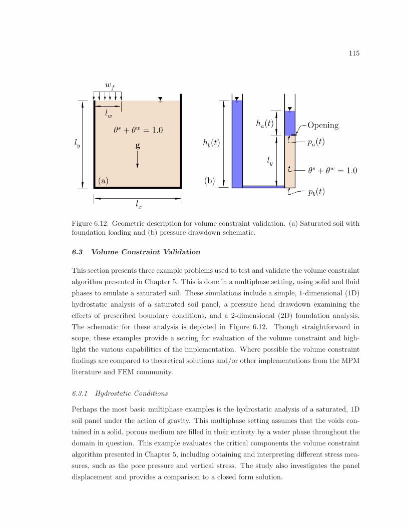
115

lx

g

(a)

ly

lw

wf

(b)

hb(t)

ly

ha(t)

pa(t)

pb(t)

Openingθs + θw = 1.0

θs + θw = 1.0

Figure 6.12: Geometric description for volume constraint validation. (a) Saturated soil withfoundation loading and (b) pressure drawdown schematic.

6.3 Volume Constraint Validation

This section presents three example problems used to test and validate the volume constraint

algorithm presented in Chapter 5. This is done in a multiphase setting, using solid and fluid

phases to emulate a saturated soil. These simulations include a simple, 1-dimensional (1D)

hydrostatic analysis of a saturated soil panel, a pressure head drawdown examining the

effects of prescribed boundary conditions, and a 2-dimensional (2D) foundation analysis.

The schematic for these analysis is depicted in Figure 6.12. Though straightforward in

scope, these examples provide a setting for evaluation of the volume constraint and high-

light the various capabilities of the implementation. Where possible the volume constraint

findings are compared to theoretical solutions and/or other implementations from the MPM

literature and FEM community.

6.3.1 Hydrostatic Conditions

Perhaps the most basic multiphase examples is the hydrostatic analysis of a saturated, 1D

soil panel under the action of gravity. This multiphase setting assumes that the voids con-

tained in a solid, porous medium are filled in their entirety by a water phase throughout the

domain in question. This example evaluates the critical components the volume constraint

algorithm presented in Chapter 5, including obtaining and interpreting different stress mea-

sures, such as the pore pressure and vertical stress. The study also investigates the panel

displacement and provides a comparison to a closed form solution.

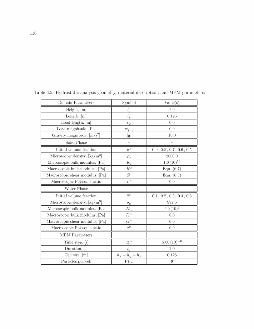
116

Table 6.5: Hydrostatic analysis geometry, material description, and MPM parameters.

Domain Parameters Symbol Value(s)

Height, [m] ly 2.0

Length, [m] lx 0.125

Load length, [m] lw 0.0

Load magnitude, [Pa] wfnd 0.0

Gravity magnitude, [m/s2] |g| 10.0

Solid Phase – –

Initial volume fraction θs 0.9 , 0.8 , 0.7 , 0.6 , 0.5

Microscopic density, [kg/m3] ρs 2600.0

Microscopic bulk modulus, [Pa] Ks 1.0 (10)16

Macroscopic bulk modulus, [Pa] Ks Eqn. (6.7)

Macroscopic shear modulus, [Pa] Gs Eqn. (6.8)

Macroscopic Poisson’s ratio νs 0.0

Water Phase – –

Initial volume fraction θw 0.1 , 0.2 , 0.3 , 0.4 , 0.5

Microscopic density, [kg/m3] ρw 997.5

Microscopic bulk modulus, [Pa] Kw 2.0 (10)6

Macroscopic bulk modulus, [Pa] Kw 0.0

Macroscopic shear modulus, [Pa] Gw 0.0

Macroscopic Poisson’s ratio νw 0.0

MPM Parameters – –

Time step, [s] ∆ t 5.00 (10)−6

Duration, [s] tf 2.0

Cell size, [m] hx = hy = hz 0.125

Particles per cell PPC 9

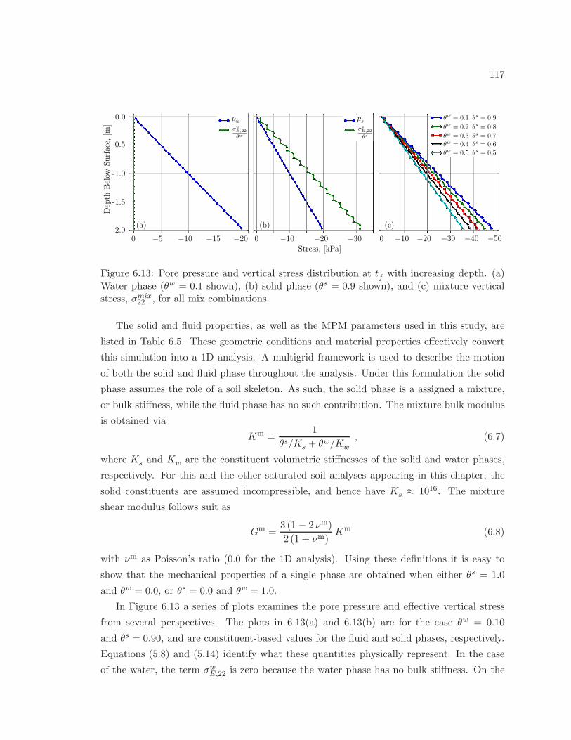
117

θw = 0.1 θs = 0.9

θw = 0.2 θs = 0.8

θw = 0.3 θs = 0.7θw = 0.4 θs = 0.6

θw = 0.5 θs = 0.5

Depth

Below

Surface,

[m]

0 0−5 −10 −15 −20 −10

Stress, [kPa]

−20 −30 0 −40 −50−30−20−10

-0.5

-2.0

-1.5

-1.0

0.0

(b) (c)(a)

pwσwE,22

θw

psσsE,22

θs

Figure 6.13: Pore pressure and vertical stress distribution at tf with increasing depth. (a)Water phase (θw = 0.1 shown), (b) solid phase (θs = 0.9 shown), and (c) mixture verticalstress, σmix

22 , for all mix combinations.

The solid and fluid properties, as well as the MPM parameters used in this study, are

listed in Table 6.5. These geometric conditions and material properties effectively convert

this simulation into a 1D analysis. A multigrid framework is used to describe the motion

of both the solid and fluid phase throughout the analysis. Under this formulation the solid

phase assumes the role of a soil skeleton. As such, the solid phase is a assigned a mixture,

or bulk stiffness, while the fluid phase has no such contribution. The mixture bulk modulus

is obtained via

Km =1

θs/Ks + θw/Kw

, (6.7)

where Ks and Kw are the constituent volumetric stiffnesses of the solid and water phases,

respectively. For this and the other saturated soil analyses appearing in this chapter, the

solid constituents are assumed incompressible, and hence have Ks ≈ 1016. The mixture

shear modulus follows suit as

Gm =3 (1 − 2 νm)

2 (1 + νm)Km (6.8)

with νm as Poisson’s ratio (0.0 for the 1D analysis). Using these definitions it is easy to

show that the mechanical properties of a single phase are obtained when either θs = 1.0

and θw = 0.0, or θs = 0.0 and θw = 1.0.

In Figure 6.13 a series of plots examines the pore pressure and effective vertical stress

from several perspectives. The plots in 6.13(a) and 6.13(b) are for the case θw = 0.10

and θs = 0.90, and are constituent-based values for the fluid and solid phases, respectively.

Equations (5.8) and (5.14) identify what these quantities physically represent. In the case

of the water, the term σwE,22 is zero because the water phase has no bulk stiffness. On the

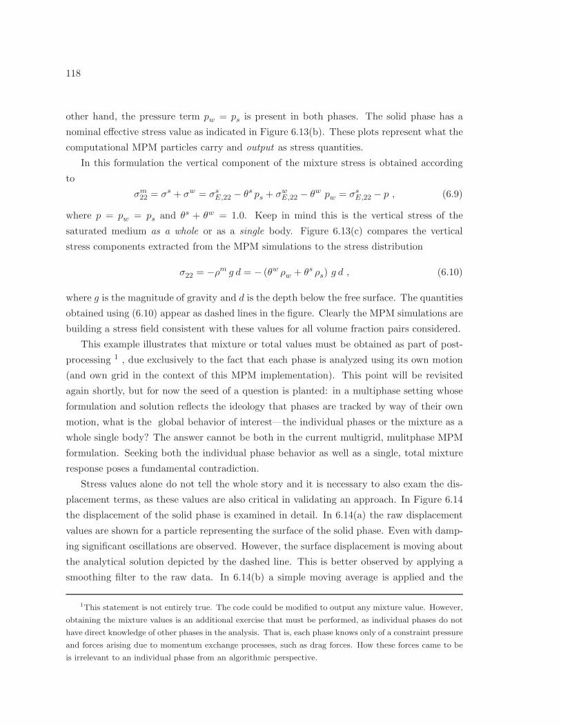
118

other hand, the pressure term pw = ps is present in both phases. The solid phase has a

nominal effective stress value as indicated in Figure 6.13(b). These plots represent what the

computational MPM particles carry and output as stress quantities.

In this formulation the vertical component of the mixture stress is obtained according

to

σm22 = σs + σw = σsE,22 − θs ps + σwE,22 − θw pw = σsE,22 − p , (6.9)

where p = pw = ps and θs + θw = 1.0. Keep in mind this is the vertical stress of the

saturated medium as a whole or as a single body. Figure 6.13(c) compares the vertical

stress components extracted from the MPM simulations to the stress distribution

σ22 = −ρm g d = − (θw ρw + θs ρs) g d , (6.10)

where g is the magnitude of gravity and d is the depth below the free surface. The quantities

obtained using (6.10) appear as dashed lines in the figure. Clearly the MPM simulations are

building a stress field consistent with these values for all volume fraction pairs considered.

This example illustrates that mixture or total values must be obtained as part of post-

processing 1 , due exclusively to the fact that each phase is analyzed using its own motion

(and own grid in the context of this MPM implementation). This point will be revisited

again shortly, but for now the seed of a question is planted: in a multiphase setting whose

formulation and solution reflects the ideology that phases are tracked by way of their own

motion, what is the global behavior of interest—the individual phases or the mixture as a

whole single body? The answer cannot be both in the current multigrid, mulitphase MPM

formulation. Seeking both the individual phase behavior as well as a single, total mixture

response poses a fundamental contradiction.

Stress values alone do not tell the whole story and it is necessary to also exam the dis-

placement terms, as these values are also critical in validating an approach. In Figure 6.14

the displacement of the solid phase is examined in detail. In 6.14(a) the raw displacement

values are shown for a particle representing the surface of the solid phase. Even with damp-

ing significant oscillations are observed. However, the surface displacement is moving about

the analytical solution depicted by the dashed line. This is better observed by applying a

smoothing filter to the raw data. In 6.14(b) a simple moving average is applied and the

1This statement is not entirely true. The code could be modified to output any mixture value. However,

obtaining the mixture values is an additional exercise that must be performed, as individual phases do not

have direct knowledge of other phases in the analysis. That is, each phase knows only of a constraint pressure

and forces arising due to momentum exchange processes, such as drag forces. How these forces came to be

is irrelevant to an individual phase from an algorithmic perspective.

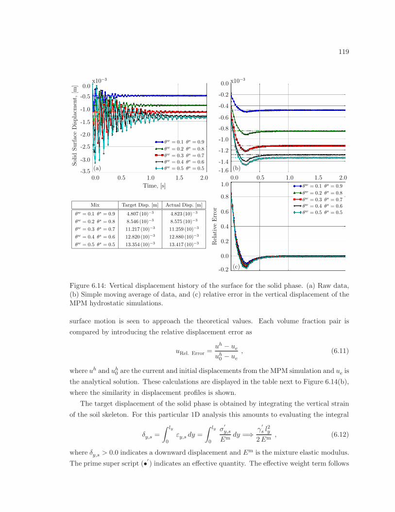
119

0.0x10−3

-3.5

-3.0

-2.5

-2.0

-1.0

-1.5

-0.5

0.0 0.5 1.0 1.5 2.0

θw = 0.1 θs = 0.9

θw = 0.2 θs = 0.8

θw = 0.3 θs = 0.7

θw = 0.4 θs = 0.6

θw = 0.5 θs = 0.5

Solid

SurfaceDisplacm

ent,[m

]

0.0 0.5 1.0 1.5 2.0

Time, [s]

RelativeError

Mix Target Disp. [m] Actual Disp. [m]

θw = 0.1 θs = 0.9 4.807 (10)−3 4.823 (10)−3

θw = 0.2 θs = 0.8 8.546 (10)−3 8.575 (10)−3

θw = 0.3 θs = 0.7 11.217 (10)−3 11.259 (10)−3

θw = 0.4 θs = 0.6 12.820 (10)−3 12.880 (10)−3

θw = 0.5 θs = 0.5 13.354 (10)−3 13.417 (10)−3

(a)

x10−30.0

-1.4

-1.2

-1.0

-0.8

-0.6

-0.4

-0.2

-1.6

0.0

1.0

0.8

0.6

0.4

0.2

-0.2

(b)

(c)

θw = 0.1 θs = 0.9

θw = 0.2 θs = 0.8

θw = 0.3 θs = 0.7

θw = 0.4 θs = 0.6

θw = 0.5 θs = 0.5

Figure 6.14: Vertical displacement history of the surface for the solid phase. (a) Raw data,(b) Simple moving average of data, and (c) relative error in the vertical displacement of theMPM hydrostatic simulations.

surface motion is seen to approach the theoretical values. Each volume fraction pair is

compared by introducing the relative displacement error as

uRel. Error =uh − ueuh0 − ue

, (6.11)

where uh and uh0 are the current and initial displacements from the MPM simulation and ue is

the analytical solution. These calculations are displayed in the table next to Figure 6.14(b),

where the similarity in displacement profiles is shown.

The target displacement of the solid phase is obtained by integrating the vertical strain

of the soil skeleton. For this particular 1D analysis this amounts to evaluating the integral

δy,s =

∫ ly

0εy,s dy =

∫ ly

0

σ′

y,s

Emdy =⇒

γ′

s l2y

2Em, (6.12)

where δy,s > 0.0 indicates a downward displacement and Em is the mixture elastic modulus.

The prime super script (•′

) indicates an effective quantity. The effective weight term follows

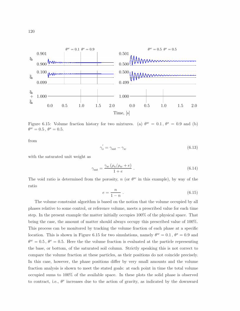
120

1.000

θw = 0.1 θs = 0.9

0.0 0.5 1.0 1.5 2.0

0.100

0.099

0.901

0.900

Time, [s]

1.000

0.0 0.5 1.0 1.5 2.0

0.500

0.501

0.500

0.499

θw = 0.5 θs = 0.5

θw+θs

θsθw

Figure 6.15: Volume fraction history for two mixtures. (a) θw = 0.1 , θs = 0.9 and (b)θw = 0.5 , θs = 0.5.

from

γ′

s = γsat − γw (6.13)

with the saturated unit weight as

γsat =γw (ρs/ρw + e)

1 + e. (6.14)

The void ratio is determined from the porosity, n (or θw in this example), by way of the

ratio

e =n

1− n. (6.15)

The volume constraint algorithm is based on the notion that the volume occupied by all

phases relative to some control, or reference volume, meets a prescribed value for each time

step. In the present example the matter initially occupies 100% of the physical space. That

being the case, the amount of matter should always occupy this prescribed value of 100%.

This process can be monitored by tracking the volume fraction of each phase at a specific

location. This is shown in Figure 6.15 for two simulations, namely θw = 0.1 , θs = 0.9 and

θw = 0.5 , θs = 0.5. Here the the volume fraction is evaluated at the particle representing

the base, or bottom, of the saturated soil column. Strictly speaking this is not correct to

compare the volume fraction at these particles, as their positions do not coincide precisely.

In this case, however, the phase positions differ by very small amounts and the volume

fraction analysis is shown to meet the stated goals: at each point in time the total volume

occupied sums to 100% of the available space. In these plots the solid phase is observed

to contract, i.e., θs increases due to the action of gravity, as indicated by the downward

121

0.0

0.2

0.6

0.4

0.8

1.0

5.04.03.02.01.00.0 5.04.03.02.01.00.0(a)

ha/ha0

−8

0

−4

−16

−12

(b)

pa[kPa]

Time, [s] Time, [s]

td = 0.5 std = 1.0 std = 2.0 std = 4.0 s

td = 4.0 std = 2.0 std = 1.0 std = 0.5 s

Figure 6.16: Prescribed conditions at top of chamber. (a) Variation of water height ha as afunction of time. (b) Prescribed pressure pa as a function of time.

displacement shown in Figure 6.14. To compensate for this change the water phase volume

fraction decreases proportionately. The size of the relative oscillations in the volume fraction

are a function of the water to soil ratio. Not surprisingly, the higher θs the faster the medium

achieves balance in the volume fraction. For these cases the mixture bulk modulus—the

driving quantity behind the volume constraint algorithm—is significantly higher and results

in smaller volume changes of each phase during each time step.

6.3.2 Pressure Head Drawdown

The setup for this numerical study is shown in Figure 6.12(b). A saturated soil column is

subjected to a prescribed pressure at both the top and bottom, pa and pb, resulting from the

fluid columns of height ha and hb, respectively. These two pressures can vary in time. Here,

however, it is assumed that the lower value, pb, is constant as hb is fixed in time. The upper

pressure is controlled by prescribing the opening size just above the saturated soil mass.

Under the action of gravity the upper water column will drain, continuously decreasing the

pressure magnitude at the surface of the saturated soil column. This in concert with the

constant pore pressure at the bottom induces a pressure gradient over the height of the

column.

This study has practical significance and can potentially help simulate the liquefaction

process in saturated sands. For example, in the Master’s research work by Heller (2003),

a physical specimen replicating the setup shown in Figure 6.12(b) is constructed in order

to examine the diffusion coefficient in sands, with the end goal of predicting beach scour

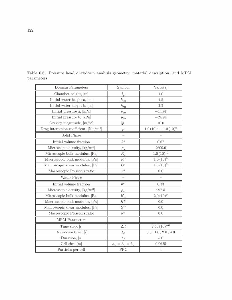
122

Table 6.6: Pressure head drawdown analysis geometry, material description, and MPMparameters.

Domain Parameters Symbol Value(s)

Chamber height, [m] ly 1.0

Initial water height a, [m] ha0 1.5

Initial water height b, [m] hb0 2.5

Initial pressure a, [kPa] pa0 −14.97

Initial pressure b, [kPa] pb0 −24.94

Gravity magnitude, [m/s2] |g| 10.0

Drag interaction coefficient, [N-s/m4] µ 1.0 (10)0 − 1.0 (10)8

Solid Phase – –

Initial volume fraction θs 0.67

Microscopic density, [kg/m3] ρs 2600.0

Microscopic bulk modulus, [Pa] Ks 1.0 (10)16

Macroscopic bulk modulus, [Pa] Ks 1.0 (10)9

Macroscopic shear modulus, [Pa] Gs 1.5 (10)9

Macroscopic Poisson’s ratio νs 0.0

Water Phase – –

Initial volume fraction θw 0.33

Microscopic density, [kg/m3] ρw 997.5

Microscopic bulk modulus, [Pa] Kw 2.0 (10)9

Macroscopic bulk modulus, [Pa] Kw 0.0

Macroscopic shear modulus, [Pa] Gw 0.0

Macroscopic Poisson’s ratio νw 0.0

MPM Parameters – –

Time step, [s] ∆ t 2.50 (10)−6

Drawdown time, [s] td 0.5 , 1.0 , 2.0 , 4.0

Duration, [s] tf 5.0

Cell size, [m] hx = hy = hz 0.0625

Particles per cell PPC 4

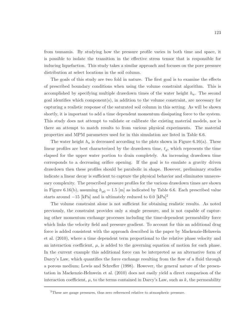
123

from tsunamis. By studying how the pressure profile varies in both time and space, it

is possible to isolate the transition in the effective stress tensor that is responsible for

inducing liquefaction. This study takes a similar approach and focuses on the pore pressure

distribution at select locations in the soil column.

The goals of this study are two fold in nature. The first goal is to examine the effects

of prescribed boundary conditions when using the volume constraint algorithm. This is

accomplished by specifying multiple drawdown times of the water height ha. The second

goal identifies which component(s), in addition to the volume constraint, are necessary for

capturing a realistic response of the saturated soil column in this setting. As will be shown

shortly, it is important to add a time dependent momentum dissipating force to the system.

This study does not attempt to validate or calibrate the existing material models, nor is

there an attempt to match results to from various physical experiments. The material

properties and MPM parameters used for in this simulation are listed in Table 6.6.

The water height ha is decreased according to the plots shown in Figure 6.16(a). These

linear profiles are best characterized by the drawdown time, td, which represents the time

elapsed for the upper water portion to drain completely. An increasing drawdown time

corresponds to a decreasing orifice opening. If the goal is to emulate a gravity driven

drawdown then these profiles should be parabolic in shape. However, preliminary studies

indicate a linear decay is sufficient to capture the physical behavior and eliminates unneces-

sary complexity. The prescribed pressure profiles for the various drawdown times are shown

in Figure 6.16(b), assuming ha0 = 1.5 [m] as indicated by Table 6.6. Each prescribed value

starts around −15 [kPa] and is ultimately reduced to 0.0 [kPa]2

The volume constraint alone is not sufficient for obtaining realistic results. As noted

previously, the constraint provides only a single pressure, and is not capable of captur-

ing other momentum exchange processes including the time-dependent permeability force

which links the velocity field and pressure gradient. To account for this an additional drag

force is added consistent with the approach described in the paper by Mackenzie-Helnwein

et al. (2010), where a time dependent term proportional to the relative phase velocity and

an interaction coefficient, µ, is added to the governing equation of motion for each phase.

In the current example this additional force can be interpreted as an alternative form of

Darcy’s Law, which quantifies the force exchange resulting from the flow of a fluid through

a porous medium; Lewis and Schrefler (1998). However, the general nature of the presen-

tation in Mackenzie-Helnwein et al. (2010) does not easily yield a direct comparison of the

interaction coefficient, µ, to the terms contained in Darcy’s Law, such as k, the permeability

2These are gauge pressures, thus zero referenced relative to atmospheric pressure.

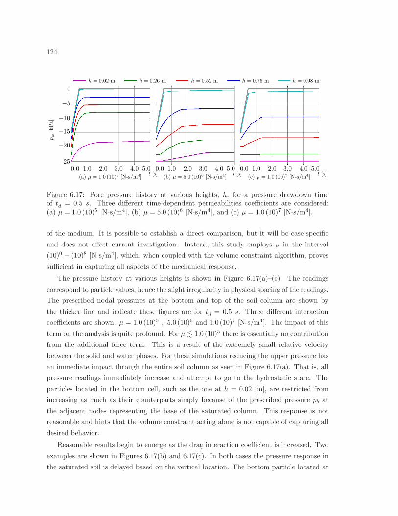
124

4.03.02.01.0 5.0(a) µ = 1.0 (10)5 [N-s/m4]

0.0 4.03.02.01.0 5.00.0(b) µ = 5.0 (10)6 [N-s/m4]

−25

−10

−15

−20

−5

0

pw[kPa]

4.03.02.01.0 5.00.0(c) µ = 1.0 (10)7 [N-s/m4]

t [s]t [s]t [s]

h = 0.02 m h = 0.26 m h = 0.52 m h = 0.76 m h = 0.98 m

Figure 6.17: Pore pressure history at various heights, h, for a pressure drawdown timeof td = 0.5 s. Three different time-dependent permeabilities coefficients are considered:(a) µ = 1.0 (10)5 [N-s/m4], (b) µ = 5.0 (10)6 [N-s/m4], and (c) µ = 1.0 (10)7 [N-s/m4].

of the medium. It is possible to establish a direct comparison, but it will be case-specific

and does not affect current investigation. Instead, this study employs µ in the interval

(10)0 − (10)8 [N-s/m4], which, when coupled with the volume constraint algorithm, proves

sufficient in capturing all aspects of the mechanical response.

The pressure history at various heights is shown in Figure 6.17(a)–(c). The readings

correspond to particle values, hence the slight irregularity in physical spacing of the readings.

The prescribed nodal pressures at the bottom and top of the soil column are shown by

the thicker line and indicate these figures are for td = 0.5 s. Three different interaction

coefficients are shown: µ = 1.0 (10)5 , 5.0 (10)6 and 1.0 (10)7 [N-s/m4]. The impact of this

term on the analysis is quite profound. For µ . 1.0 (10)5 there is essentially no contribution

from the additional force term. This is a result of the extremely small relative velocity

between the solid and water phases. For these simulations reducing the upper pressure has

an immediate impact through the entire soil column as seen in Figure 6.17(a). That is, all

pressure readings immediately increase and attempt to go to the hydrostatic state. The

particles located in the bottom cell, such as the one at h = 0.02 [m], are restricted from

increasing as much as their counterparts simply because of the prescribed pressure pb at

the adjacent nodes representing the base of the saturated column. This response is not

reasonable and hints that the volume constraint acting alone is not capable of capturing all

desired behavior.

Reasonable results begin to emerge as the drag interaction coefficient is increased. Two

examples are shown in Figures 6.17(b) and 6.17(c). In both cases the pressure response in

the saturated soil is delayed based on the vertical location. The bottom particle located at

125

−20 −25−15−10−5−20 −25−15−10−5−20 −25−15−10−5

0.2 0.4 0.6 0.8 1.00.0 0.2 0.4 0.6 0.8 1.00.0

µ = 1.0 (10)0 µ = 1.0 (10)5 µ = 1.0 (10)6 µ = 1.0 (10)7 µ = 1.0 (10)8 [N-s/m4]

0pw [kPa]

0.0

0.2

0.4

0.8

0.6

h[m

]

1.0

0.0

0.2

0.4

0.8

0.6

h[m

]

1.0

0.2 0.4 0.6 0.8 1.00.0pw/pw0

td = 2.0 s td = 4.0 s

td = 1.0 s td = 2.0 s td = 4.0 s

td = 1.0 s

Figure 6.18: Vertical pore pressure distribution in the chamber at t = 5.0 s. The particlelocations are shown as circular points. The upper row is the actual value and the lowerrow is normalized to the initial pressure, pw0. Each column represents a different drawdowntime, td.

h = 0.02 [m] exhibits no change for over half a second for µ = 1.0 (10)6 . The final pressure

distribution appears to be nearly linear with height. When the interaction coefficient is

increased to µ = 1.0 (10)7 the lower particle experiences no change in pressure throughout

the duration of the analysis. The end result is a pressure distribution that is quadratic over

the height of the column.

Figure 6.17 provides a great example of the pressure history for a given drawdown time.

But what about the spatial variation of the pressure? In Figure 6.18 the spatial distribution

is examined at t = 5.0 s for three different drawdown times: td = 1.0 , 2.0 and 4.0 s. The

particle values are plotted for several drag interaction values. The upper row of plots shows

the actual pressure while the lower row depicts the final pressure value normalized to the

initial pressure, pw0. The first observation made from this figure is that drawdown time is

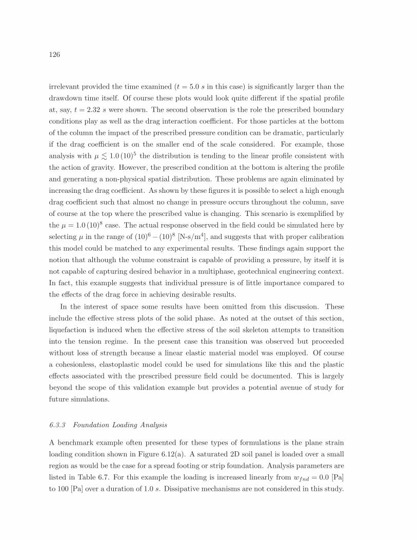
126

irrelevant provided the time examined (t = 5.0 s in this case) is significantly larger than the

drawdown time itself. Of course these plots would look quite different if the spatial profile

at, say, t = 2.32 s were shown. The second observation is the role the prescribed boundary

conditions play as well as the drag interaction coefficient. For those particles at the bottom

of the column the impact of the prescribed pressure condition can be dramatic, particularly

if the drag coefficient is on the smaller end of the scale considered. For example, those

analysis with µ . 1.0 (10)5 the distribution is tending to the linear profile consistent with

the action of gravity. However, the prescribed condition at the bottom is altering the profile

and generating a non-physical spatial distribution. These problems are again eliminated by

increasing the drag coefficient. As shown by these figures it is possible to select a high enough

drag coefficient such that almost no change in pressure occurs throughout the column, save

of course at the top where the prescribed value is changing. This scenario is exemplified by

the µ = 1.0 (10)8 case. The actual response observed in the field could be simulated here by

selecting µ in the range of (10)6− (10)8 [N-s/m4], and suggests that with proper calibration

this model could be matched to any experimental results. These findings again support the

notion that although the volume constraint is capable of providing a pressure, by itself it is

not capable of capturing desired behavior in a multiphase, geotechnical engineering context.

In fact, this example suggests that individual pressure is of little importance compared to

the effects of the drag force in achieving desirable results.

In the interest of space some results have been omitted from this discussion. These

include the effective stress plots of the solid phase. As noted at the outset of this section,

liquefaction is induced when the effective stress of the soil skeleton attempts to transition

into the tension regime. In the present case this transition was observed but proceeded

without loss of strength because a linear elastic material model was employed. Of course

a cohesionless, elastoplastic model could be used for simulations like this and the plastic

effects associated with the prescribed pressure field could be documented. This is largely

beyond the scope of this validation example but provides a potential avenue of study for

future simulations.

6.3.3 Foundation Loading Analysis

A benchmark example often presented for these types of formulations is the plane strain

loading condition shown in Figure 6.12(a). A saturated 2D soil panel is loaded over a small

region as would be the case for a spread footing or strip foundation. Analysis parameters are

listed in Table 6.7. For this example the loading is increased linearly from wfnd = 0.0 [Pa]

to 100 [Pa] over a duration of 1.0 s. Dissipative mechanisms are not considered in this study.

127

Table 6.7: Planar foundation analysis geometry, material description, and MPM parametersfor use with the volume constraint algorithm in Chapter 5 and the u−p CMPM formulationby Zhang et al. (2008).

Domain Parameters Symbol Value(s)

Height, [m] ly 30.0

Length, [m] lx 30.0

Load length, [m] lw 3.0

Load magnitude, [Pa] wfnd 100.0

Gravity magnitude, [m/s2] |g| 0.0

Solid Phase – –

Initial volume fraction θs 0.7

Microscopic density, [kg/m3] ρs 2670.0

Microscopic bulk modulus, [Pa] Ks 1.0 (10)16

Macroscopic bulk modulus, [Pa] Ks 2.08 (10)7

Macroscopic shear modulus, [Pa] Gs 9.62 (10)6

Water Phase – –

Initial volume fraction θw 0.3

Microscopic density, [kg/m3] ρw 997.5

Microscopic bulk modulus, [Pa] Kw 2.0 (10)9

Macroscopic bulk modulus, [Pa] Kw 0.0

Macroscopic shear modulus, [Pa] Gw 0.0

u− p CMPM – –

Mixture density, [kg/m3] ρm 2168.25

Mixture bulk modulus, [Pa] Km 2.08 (10)7

Mixture shear modulus, [Pa] Gm 9.62 (10)6

Biot’s constant α 1.0

Fluid permeability, [m/s] k 0.0

MPM Parameters – –

Time step, [s] ∆ t 1.25 (10)−4

Duration, [s] tf 5.0

Cell size, [m] hx = hy = hz 1.5

Particles per cell PPC 4

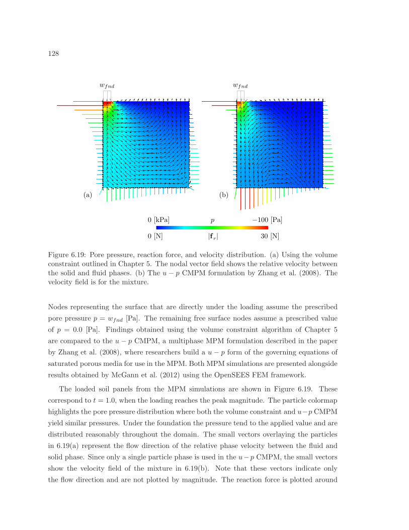
128

30 [N]0 [N] |f r|

wfndwfnd

(a) (b)

p −100 [Pa]0 [kPa]

Figure 6.19: Pore pressure, reaction force, and velocity distribution. (a) Using the volumeconstraint outlined in Chapter 5. The nodal vector field shows the relative velocity betweenthe solid and fluid phases. (b) The u − p CMPM formulation by Zhang et al. (2008). Thevelocity field is for the mixture.

Nodes representing the surface that are directly under the loading assume the prescribed

pore pressure p = wfnd [Pa]. The remaining free surface nodes assume a prescribed value

of p = 0.0 [Pa]. Findings obtained using the volume constraint algorithm of Chapter 5

are compared to the u− p CMPM, a multiphase MPM formulation described in the paper

by Zhang et al. (2008), where researchers build a u− p form of the governing equations of

saturated porous media for use in the MPM. Both MPM simulations are presented alongside

results obtained by McGann et al. (2012) using the OpenSEES FEM framework.

The loaded soil panels from the MPM simulations are shown in Figure 6.19. These

correspond to t = 1.0, when the loading reaches the peak magnitude. The particle colormap

highlights the pore pressure distribution where both the volume constraint and u−p CMPM

yield similar pressures. Under the foundation the pressure tend to the applied value and are

distributed reasonably throughout the domain. The small vectors overlaying the particles

in 6.19(a) represent the flow direction of the relative phase velocity between the fluid and

solid phase. Since only a single particle phase is used in the u−p CMPM, the small vectors

show the velocity field of the mixture in 6.19(b). Note that these vectors indicate only

the flow direction and are not plotted by magnitude. The reaction force is plotted around

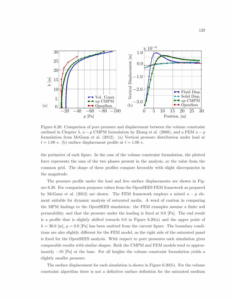
129

30

10

15

20

25

5

0

−1.0

−2.0

−3.0

VerticalDisplacement[m

]

(a) (b)

−20 −60 −80−40 −100

0.0

1.0x 10−4

0 5 1510 25 3020

h[m

]

p [Pa] Position, [m]

Fluid Disp.Solid Disp.up CMPMOpenSeesOpenSees

Vol. Const.up CMPM

Figure 6.20: Comparison of pore pressure and displacement between the volume constraintoutlined in Chapter 5, u− p CMPM formulation by Zhang et al. (2008), and a FEM u− pformulation from McGann et al. (2012). (a) Vertical pressure distribution under load att = 1.00 s. (b) surface displacement profile at t = 1.00 s.

the perimeter of each figure. In the case of the volume constraint formulation, the plotted

force represents the sum of the two phases present in the analysis, or the value from the

common grid. The shape of these profiles compare favorably with slight discrepancies in

the magnitude.

The pressure profile under the load and free surface displacements are shown in Fig-

ure 6.20. For comparison purposes values from the OpenSEES FEM framework as prepared

by McGann et al. (2012) are shown. The FEM framework employs a mixed u − p ele-

ment suitable for dynamic analysis of saturated media. A word of caution in comparing

the MPM findings to the OpenSEES simulation: the FEM examples assume a finite soil

permeability, and that the pressure under the loading is fixed at 0.0 [Pa]. The end result

is a profile that is slightly shifted towards 0.0 in Figure 6.20(a) and the upper point of

h = 30.0 [m], p = 0.0 [Pa] has been omitted from the current figure. The boundary condi-

tions are also slightly different for the FEM model, as the right side of the saturated panel

is fixed for the OpenSEES analysis. With respect to pore pressures each simulation gives

comparable results with similar shapes. Both the CMPM and FEM models tend to approx-

imately −10 [Pa] at the base. For all heights the volume constraint formulation yields a

slightly smaller pressure.

The surface displacement for each simulation is shown in Figure 6.20(b). For the volume

constraint algorithm there is not a definitive surface definition for the saturated medium

130

since each phases is modeled on separate grids. Thus, the surface of both the water and

soil phase is plotted. This rehashes an observation from Section 6.3.1 where the question

was asked what is the behavior of interest: the individual phases or the mixture as a

whole single body? In the current example it arguably makes more sense to claim the

mixture of the whole saturated mass is the behavior of interest, yet this contradicts the

premise of the multiphase formulation in a multigrid context. Certainly if a foundation

was placed on this panel the global displacement of the saturated medium as a whole is

the target value. The common grid cannot be used to settle this argument, as the particle

motion (acceleration, velocity, and position) are all determined using their unique motions,

thus rendering common grid kinematics obsolete. Comparing to the other methods yields

mixed results. For this example the water phase closely resembles the u − p CMPM in

Figure 6.20(b), whose particles represent the mixture as a whole. However, despite the

difference in boundary conditions for the OpenSEES model, the solid phase surface tends to

agree with the FEM approach. These comparisons are at at best inconclusive and highlight

some of the pitfalls associated with a multigrid treatment of different phases when the goal

is in fact to model a single mixture quantity.

6.3.4 Conclusion

This section presented three examples highlighting the capabilities of the volume constraint

algorithm. The saturated soil simulations were performed in a multigrid, multiphase frame-

work consistent with the approach presented in Mackenzie-Helnwein et al. (2010) and Chap-

ter 5. Analyses were limited to the linear elastic material regime. The 1D hydrostatic test

cases produced accurate distributions of the constituent, bulk, and mixture stresses. Solid

phase displacements were shown to converge to an analytical solution. The pressure head

drawdown simulations showed how prescribed conditions could potentially be used to cap-

ture the liquefaction process. The drawdown examples emphasized the need for alternative

momentum exchange mechanisms in addition to the pressure obtained from the volume

constraint, as it was shown that these alternative exchange processes are largely more im-

portant in a saturated soil context. The final example considered a 2D saturated panel

subject to a distributed foundation loading. Pore pressure distribution and surface dis-

placements were compared to the u− p CMPM formulation by Zhang et al. (2008) and an

FEM implementation using stabilized elements created by McGann et al. (2012). All results

compared favorably with respect to pore pressure. Surface displacement plots illuminated

some of the pitfalls associated with a multigrid treatment of different phases when the goal

is in fact to model a single mixture quantity.

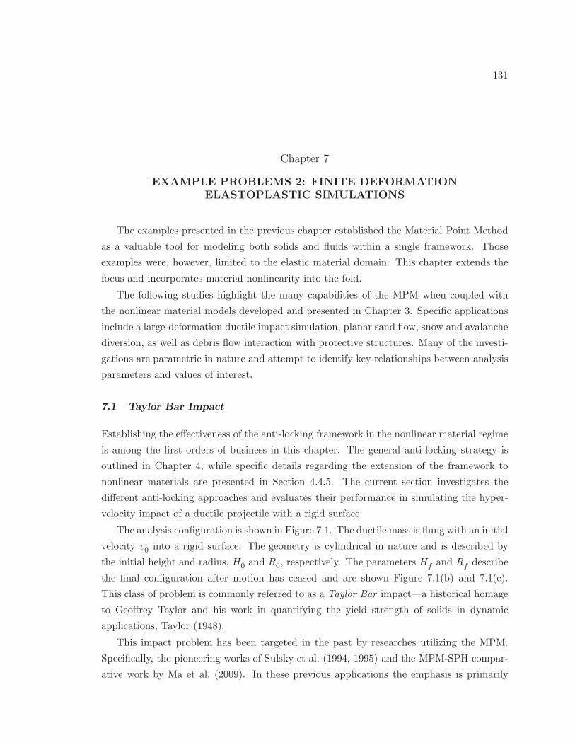
131

Chapter 7

EXAMPLE PROBLEMS 2: FINITE DEFORMATIONELASTOPLASTIC SIMULATIONS

The examples presented in the previous chapter established the Material Point Method

as a valuable tool for modeling both solids and fluids within a single framework. Those

examples were, however, limited to the elastic material domain. This chapter extends the

focus and incorporates material nonlinearity into the fold.

The following studies highlight the many capabilities of the MPM when coupled with

the nonlinear material models developed and presented in Chapter 3. Specific applications

include a large-deformation ductile impact simulation, planar sand flow, snow and avalanche

diversion, as well as debris flow interaction with protective structures. Many of the investi-

gations are parametric in nature and attempt to identify key relationships between analysis

parameters and values of interest.

7.1 Taylor Bar Impact

Establishing the effectiveness of the anti-locking framework in the nonlinear material regime

is among the first orders of business in this chapter. The general anti-locking strategy is

outlined in Chapter 4, while specific details regarding the extension of the framework to

nonlinear materials are presented in Section 4.4.5. The current section investigates the

different anti-locking approaches and evaluates their performance in simulating the hyper-

velocity impact of a ductile projectile with a rigid surface.

The analysis configuration is shown in Figure 7.1. The ductile mass is flung with an initial

velocity v0 into a rigid surface. The geometry is cylindrical in nature and is described by

the initial height and radius, H0 and R0, respectively. The parameters Hf and Rf describe

the final configuration after motion has ceased and are shown Figure 7.1(b) and 7.1(c).

This class of problem is commonly referred to as a Taylor Bar impact—a historical homage

to Geoffrey Taylor and his work in quantifying the yield strength of solids in dynamic

applications, Taylor (1948).

This impact problem has been targeted in the past by researches utilizing the MPM.

Specifically, the pioneering works of Sulsky et al. (1994, 1995) and the MPM-SPH compar-

ative work by Ma et al. (2009). In these previous applications the emphasis is primarily

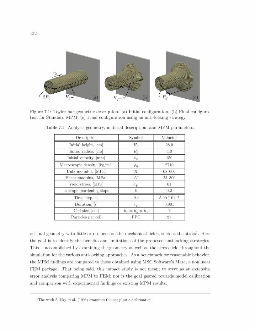
132

H0

v0

2R0 Rf(a) (b) (c)Hf

Figure 7.1: Taylor bar geometric description. (a) Initial configuration. (b) Final configura-tion for Standard MPM. (c) Final configuration using an anti-locking strategy.

Table 7.1: Analysis geometry, material description, and MPM parameters.

Description Symbol Value(s)

Initial height, [cm] H0 28.0

Initial radius, [cm] R0 4.0

Initial velocity, [m/s] v0 150

Macroscopic density, [kg/m3] ρ0 2710

Bulk modulus, [MPa] K 68, 600

Shear modulus, [MPa] G 23, 300

Yield stress, [MPa] σY 61

Isotropic hardening slope k 0.2

Time step, [s] ∆ t 5.00 (10)−8

Duration, [s] tf 0.001

Cell size, [cm] hx = hy = hz 1

Particles per cell PPC 27

on final geometry with little or no focus on the mechanical fields, such as the stress1. Here

the goal is to identify the benefits and limitations of the proposed anti-locking strategies.

This is accomplished by examining the geometry as well as the stress field throughout the

simulation for the various anti-locking approaches. As a benchmark for reasonable behavior,

the MPM findings are compared to those obtained using MSC Software’s Marc, a nonlinear

FEM package. That being said, this impact study is not meant to serve as an extensive

error analysis comparing MPM to FEM; nor is the goal geared towards model calibration

and comparison with experimental findings or existing MPM results.

1The work Sulsky et al. (1995) examines the net plastic deformation.

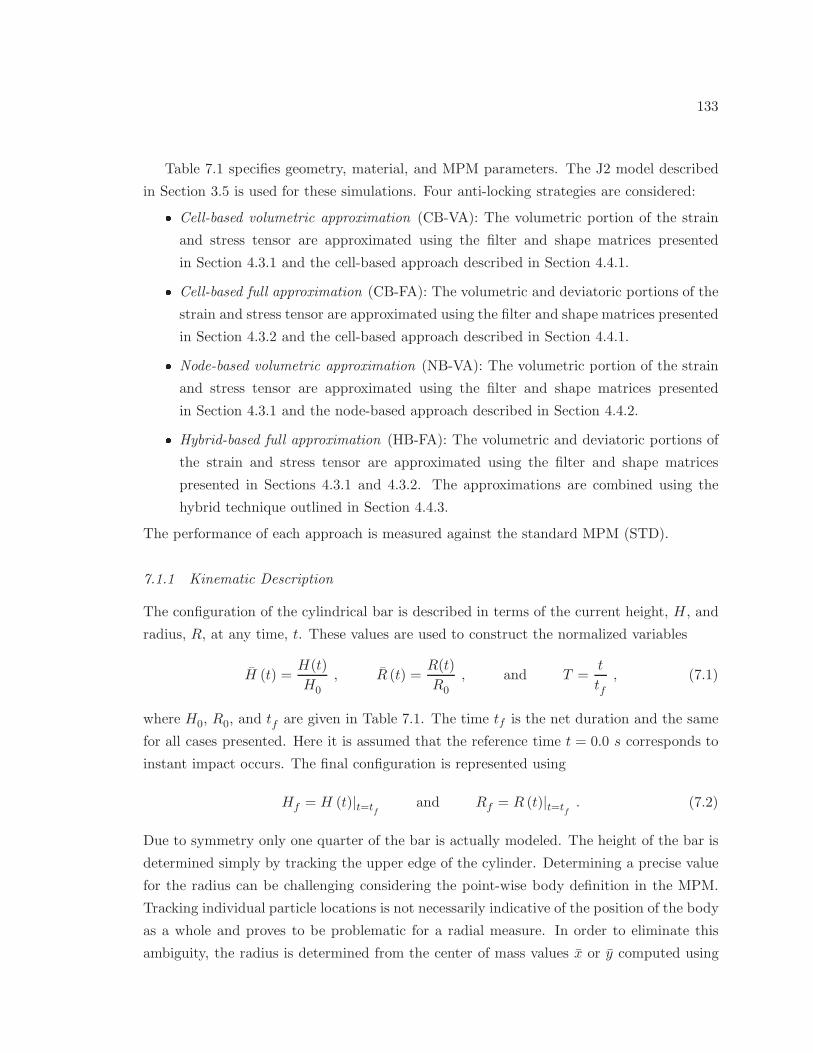
133

Table 7.1 specifies geometry, material, and MPM parameters. The J2 model described

in Section 3.5 is used for these simulations. Four anti-locking strategies are considered:

Cell-based volumetric approximation (CB-VA): The volumetric portion of the strain

and stress tensor are approximated using the filter and shape matrices presented

in Section 4.3.1 and the cell-based approach described in Section 4.4.1.

Cell-based full approximation (CB-FA): The volumetric and deviatoric portions of the

strain and stress tensor are approximated using the filter and shape matrices presented

in Section 4.3.2 and the cell-based approach described in Section 4.4.1.

Node-based volumetric approximation (NB-VA): The volumetric portion of the strain

and stress tensor are approximated using the filter and shape matrices presented

in Section 4.3.1 and the node-based approach described in Section 4.4.2.

Hybrid-based full approximation (HB-FA): The volumetric and deviatoric portions of

the strain and stress tensor are approximated using the filter and shape matrices

presented in Sections 4.3.1 and 4.3.2. The approximations are combined using the

hybrid technique outlined in Section 4.4.3.

The performance of each approach is measured against the standard MPM (STD).

7.1.1 Kinematic Description

The configuration of the cylindrical bar is described in terms of the current height, H, and

radius, R, at any time, t. These values are used to construct the normalized variables

H (t) =H(t)

H0

, R (t) =R(t)

R0

, and T =t

tf, (7.1)

where H0, R0, and tf are given in Table 7.1. The time tf is the net duration and the same

for all cases presented. Here it is assumed that the reference time t = 0.0 s corresponds to

instant impact occurs. The final configuration is represented using

Hf = H (t)|t=tf

and Rf = R (t)|t=tf. (7.2)

Due to symmetry only one quarter of the bar is actually modeled. The height of the bar is

determined simply by tracking the upper edge of the cylinder. Determining a precise value

for the radius can be challenging considering the point-wise body definition in the MPM.

Tracking individual particle locations is not necessarily indicative of the position of the body

as a whole and proves to be problematic for a radial measure. In order to eliminate this

ambiguity, the radius is determined from the center of mass values x or y computed using

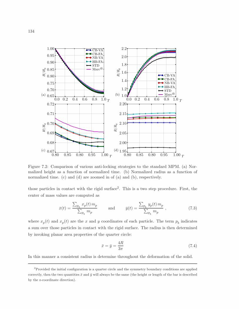
134

0.00080 0.00085 0.00090 0.00095 0.00100Time

0.67

0.68

0.69

0.70

0.71

H/H0

CBAS1CBAS2NBAS1HBAS2STDMPMMarc

0.00080 0.00085 0.00090 0.00095 0.00100Time

1.95

2.00

2.05

2.10

2.15

2.20

R/R0

CBAS1CBAS2NBAS1HBAS2STDMPMMarc

0.0000 0.0002 0.0004 0.0006 0.0008 0.0010Time

1.0

1.2

1.4

1.6

1.8

2.0

2.2

R/R0

CBAS1CBAS2NBAS1HBAS2STDMPMMarc

0.0000 0.0002 0.0004 0.0006 0.0008 0.0010Time

0.65

0.70

0.75

0.80

0.85

0.90

0.95

1.00H/H0

CBAS1CBAS2NBAS1HBAS2STDMPMMarc

1.000.85 0.950.800.80 1.000.85 0.950.800.80

1.00.0 0.60.40.2 0.8

1.00

0.90

0.85

0.95

0.75

0.80

0.70

0.65

H/H

0

1.00.0 0.60.40.2 0.8

2.2

2.0

1.2

1.4

1.6

1.8

1.0(b)

R/R

0

R/R

0

(d)

2.20

2.15

1.95

2.00

2.05

2.10

(c)

(a)

H/H

0

0.72

0.71

0.70

0.69

0.68

0.67T T

T T

CB-VA

HB-FANB-VACB-FA

STDMarc R©

CB-VA

HB-FANB-VACB-FA

STDMarc R©

Figure 7.2: Comparison of various anti-locking strategies to the standard MPM. (a) Nor-malized height as a function of normalized time. (b) Normalized radius as a function ofnormalized time. (c) and (d) are zoomed in of (a) and (b), respectively.

those particles in contact with the rigid surface2. This is a two step procedure. First, the

center of mass values are computed as

x(t) =

∑

pbxp(t)mp

∑

pbmp

and y(t) =

∑

pbyp(t)mp

∑

pbmp

, (7.3)

where xp(t) and xp(t) are the x and y coordinates of each particle. The term pb indicates

a sum over those particles in contact with the rigid surface. The radius is then determined

by invoking planar area properties of the quarter circle:

x = y =4R

3π(7.4)

In this manner a consistent radius is determine throughout the deformation of the solid.

2Provided the initial configuration is a quarter circle and the symmetry boundary conditions are applied

correctly, then the two quantities x and y will always be the same (the height or length of the bar is described

by the z-coordinate direction).

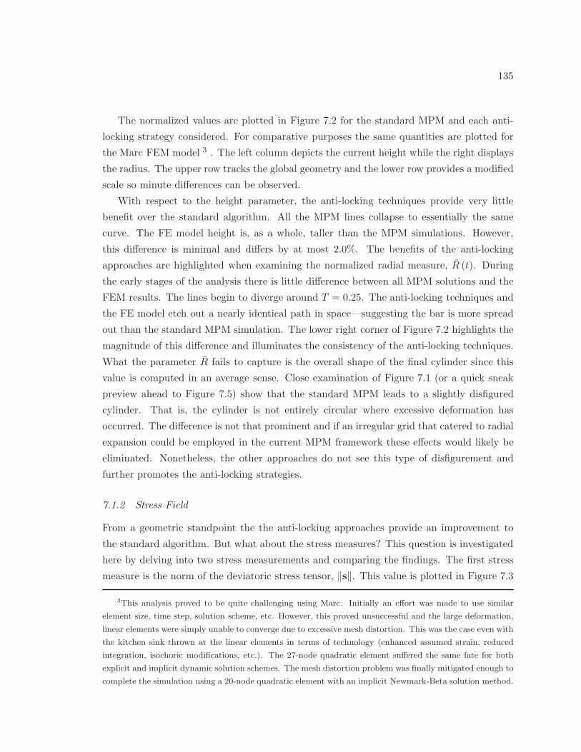
135

The normalized values are plotted in Figure 7.2 for the standard MPM and each anti-

locking strategy considered. For comparative purposes the same quantities are plotted for

the Marc FEM model 3 . The left column depicts the current height while the right displays

the radius. The upper row tracks the global geometry and the lower row provides a modified

scale so minute differences can be observed.

With respect to the height parameter, the anti-locking techniques provide very little

benefit over the standard algorithm. All the MPM lines collapse to essentially the same

curve. The FE model height is, as a whole, taller than the MPM simulations. However,

this difference is minimal and differs by at most 2.0%. The benefits of the anti-locking

approaches are highlighted when examining the normalized radial measure, R (t). During

the early stages of the analysis there is little difference between all MPM solutions and the

FEM results. The lines begin to diverge around T = 0.25. The anti-locking techniques and

the FE model etch out a nearly identical path in space—suggesting the bar is more spread

out than the standard MPM simulation. The lower right corner of Figure 7.2 highlights the

magnitude of this difference and illuminates the consistency of the anti-locking techniques.

What the parameter R fails to capture is the overall shape of the final cylinder since this

value is computed in an average sense. Close examination of Figure 7.1 (or a quick sneak

preview ahead to Figure 7.5) show that the standard MPM leads to a slightly disfigured

cylinder. That is, the cylinder is not entirely circular where excessive deformation has

occurred. The difference is not that prominent and if an irregular grid that catered to radial

expansion could be employed in the current MPM framework these effects would likely be

eliminated. Nonetheless, the other approaches do not see this type of disfigurement and

further promotes the anti-locking strategies.

7.1.2 Stress Field

From a geometric standpoint the the anti-locking approaches provide an improvement to

the standard algorithm. But what about the stress measures? This question is investigated

here by delving into two stress measurements and comparing the findings. The first stress

measure is the norm of the deviatoric stress tensor, ‖s‖. This value is plotted in Figure 7.3

3This analysis proved to be quite challenging using Marc. Initially an effort was made to use similar

element size, time step, solution scheme, etc. However, this proved unsuccessful and the large deformation,

linear elements were simply unable to converge due to excessive mesh distortion. This was the case even with

the kitchen sink thrown at the linear elements in terms of technology (enhanced assumed strain, reduced

integration, isochoric modifications, etc.). The 27-node quadratic element suffered the same fate for both

explicit and implicit dynamic solution schemes. The mesh distortion problem was finally mitigated enough to

complete the simulation using a 20-node quadratic element with an implicit Newmark-Beta solution method.

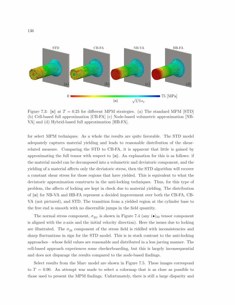
136

(a) (b) (c) (d)

0

STD CB-FA NB-VA HB-FA

√

2/3σY

75 [MPa]‖s‖

Figure 7.3: ‖s‖ at T = 0.25 for different MPM strategies. (a) The standard MPM [STD](b) Cell-based full approximation [CB-FA] (c) Node-based volumetric approximation [NB-VA] and (d) Hybrid-based full approximation [HB-FA].

for select MPM techniques. As a whole the results are quite favorable. The STD model

adequately captures material yielding and leads to reasonable distribution of the shear-

related measure. Comparing the STD to CB-FA, it is apparent that little is gained by

approximating the full tensor with respect to ‖s‖. An explanation for this is as follows: if

the material model can be decomposed into a volumetric and deviatoric component, and the

yielding of a material affects only the deviatoric stress, then the STD algorithm will recover

a constant shear stress for those regions that have yielded. This is equivalent to what the

deviatoric approximation constructs in the anti-locking techniques. Thus, for this type of

problem, the affects of locking are kept in check due to material yielding. The distribution

of ‖s‖ for NB-VA and HB-FA represent a decided improvement over both the CB-FA, CB-

VA (not pictured), and STD. The transition from a yielded region at the cylinder base to

the free end is smooth with no discernible jumps in the field quantity.

The normal stress component, σ33, is shown in Figure 7.4 (any (•)33 tensor component

is aligned with the z-axis and the initial velocity direction). Here the issues due to locking

are illustrated. The σ33 component of the stress field is riddled with inconsistencies and

sharp fluctuations in sign for the STD model. This is in stark contrast to the anti-locking

approaches—whose field values are reasonable and distributed in a less jarring manner. The

cell-based approach experiences some checkerboarding, but this is largely inconsequential

and does not disparage the results compared to the node-based findings.

Select results from the Marc model are shown in Figure 7.5. These images correspond

to T = 0.90. An attempt was made to select a colormap that is as close as possible to

those used to present the MPM findings. Unfortunately, there is still a large disparity and

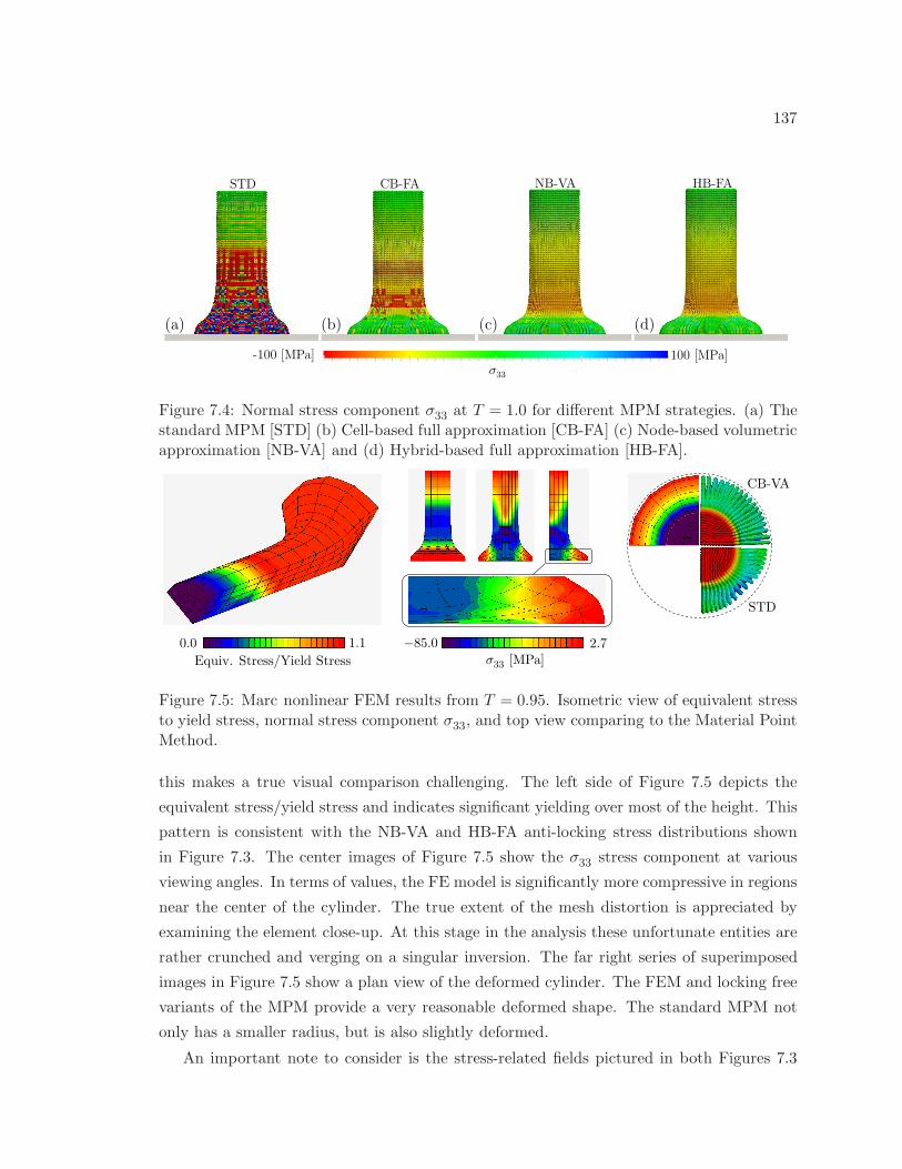
137

NB-VA HB-FACB-FASTD

(a) (b) (c) (d)

σ33

-100 [MPa] 100 [MPa]

Figure 7.4: Normal stress component σ33 at T = 1.0 for different MPM strategies. (a) Thestandard MPM [STD] (b) Cell-based full approximation [CB-FA] (c) Node-based volumetricapproximation [NB-VA] and (d) Hybrid-based full approximation [HB-FA].

−85.0σ33 [MPa]

STD

CB-VA

0.0

Equiv. Stress/Yield Stress

2.71.1

Figure 7.5: Marc nonlinear FEM results from T = 0.95. Isometric view of equivalent stressto yield stress, normal stress component σ33, and top view comparing to the Material PointMethod.

this makes a true visual comparison challenging. The left side of Figure 7.5 depicts the

equivalent stress/yield stress and indicates significant yielding over most of the height. This

pattern is consistent with the NB-VA and HB-FA anti-locking stress distributions shown

in Figure 7.3. The center images of Figure 7.5 show the σ33 stress component at various

viewing angles. In terms of values, the FE model is significantly more compressive in regions

near the center of the cylinder. The true extent of the mesh distortion is appreciated by

examining the element close-up. At this stage in the analysis these unfortunate entities are

rather crunched and verging on a singular inversion. The far right series of superimposed

images in Figure 7.5 show a plan view of the deformed cylinder. The FEM and locking free

variants of the MPM provide a very reasonable deformed shape. The standard MPM not

only has a smaller radius, but is also slightly deformed.

An important note to consider is the stress-related fields pictured in both Figures 7.3

138

and 7.4 are raw and unfiltered. Common practice in the FEM is to visualize smoothed

stress values; as a result, intra-element stress variations are largely eliminated and the field

appears much better than the raw data would. If such a practice were applied here to

the MPM results even the chaos depicted in Figure 7.4 for the STD algorithm would be

dramatically improved. So much so in fact, that there may be little observable difference

between the standard algorithm and the anti-locking techniques. Thus, the benefits of the

anti-locking techniques need be interpreted with caution depending on presentation format

and in concert with the improved geometric description afforded by such enhancements.

7.1.3 Efficiency of Anti-Locking Algorithms

The benefits of the anti-locking techniques are easily realized by examining kinematic quan-

tities and mechanical fields. However, increasing the quality requires effort and typically

arrives with an additional cost. In this context, the anti-locking strategies add computa-

tional effort and increase the CPU time. The algorithm presented in Chapter 4 augments

the standard algorithm and there is no way to make this enhancement more efficient than

the original form. To help quantify this expense, the computational time for 10 different

simulations is averaged for the standard MPM and the four anti-locking strategies inves-

tigated here. The timing from the standard algorithm provides a baseline reference; the

relative increase in computation time is shown in the center table column of Figure 7.6 for

each approach. Note that overall inefficiencies within the current framework are projected

to all approaches, thus, the relative figures provide an accurate estimate of the isolated cost

incurred by the anti-locking routines listed in Table 4.1. The minimum cost of employing

the anti-locking routine is a 27% increase in computational time. The additional time varies

from there up to nearly 3 times as long for a hybrid, full tensor averaging scheme.

The right table column presents the computational times in terms of a global time index.

This quantity is referred to as the Relative Strength and measures how a particular analysis

time stacks up relative to it counterparts. These values comprise the pie-chart shown on

the right side of Figure 7.6. From this alternative vantage point, the true costs of using a

node-based volumetric approximation are realized.

7.1.4 Conclusions

The anti-locking algorithms yield higher quality results with respect to geometric parameters

than the original algorithm with linear shape functions. Each anti-locking technique yields

very similar values that are consistent with the Marc model. This latter point should not

be taken lightly; the FE model employs higher order shape functions that are not subject

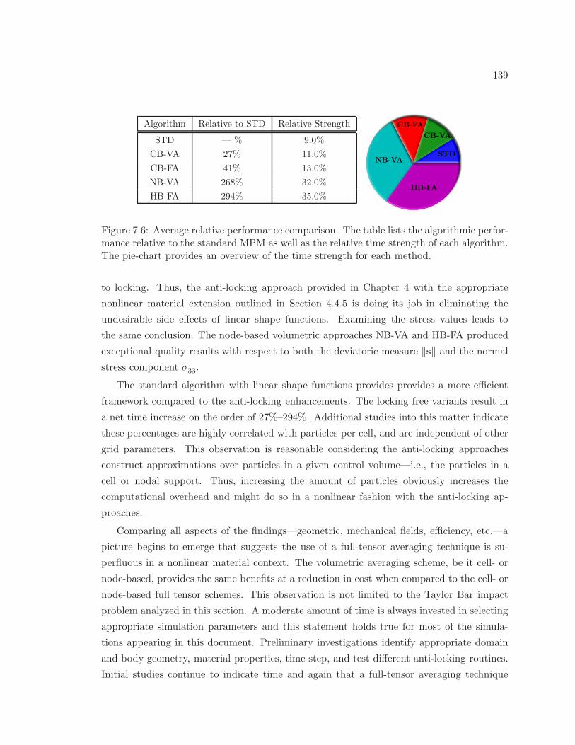
139

Algorithm Relative to STD Relative Strength

STD — % 9.0%

CB-VA 27% 11.0%

CB-FA 41% 13.0%

NB-VA 268% 32.0%

HB-FA 294% 35.0%

STD

CB-VA

CB-FA

NB-VA

HB-FA

Figure 7.6: Average relative performance comparison. The table lists the algorithmic perfor-mance relative to the standard MPM as well as the relative time strength of each algorithm.The pie-chart provides an overview of the time strength for each method.

to locking. Thus, the anti-locking approach provided in Chapter 4 with the appropriate

nonlinear material extension outlined in Section 4.4.5 is doing its job in eliminating the

undesirable side effects of linear shape functions. Examining the stress values leads to

the same conclusion. The node-based volumetric approaches NB-VA and HB-FA produced

exceptional quality results with respect to both the deviatoric measure ‖s‖ and the normal

stress component σ33.

The standard algorithm with linear shape functions provides provides a more efficient

framework compared to the anti-locking enhancements. The locking free variants result in

a net time increase on the order of 27%–294%. Additional studies into this matter indicate

these percentages are highly correlated with particles per cell, and are independent of other

grid parameters. This observation is reasonable considering the anti-locking approaches

construct approximations over particles in a given control volume—i.e., the particles in a

cell or nodal support. Thus, increasing the amount of particles obviously increases the

computational overhead and might do so in a nonlinear fashion with the anti-locking ap-

proaches.

Comparing all aspects of the findings—geometric, mechanical fields, efficiency, etc.—a

picture begins to emerge that suggests the use of a full-tensor averaging technique is su-

perfluous in a nonlinear material context. The volumetric averaging scheme, be it cell- or

node-based, provides the same benefits at a reduction in cost when compared to the cell- or

node-based full tensor schemes. This observation is not limited to the Taylor Bar impact

problem analyzed in this section. A moderate amount of time is always invested in selecting

appropriate simulation parameters and this statement holds true for most of the simula-

tions appearing in this document. Preliminary investigations identify appropriate domain

and body geometry, material properties, time step, and test different anti-locking routines.

Initial studies continue to indicate time and again that a full-tensor averaging technique

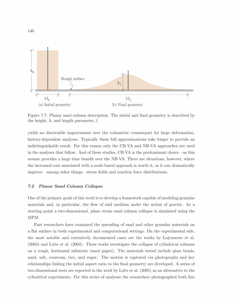
140

2 l0(a) Initial geometry (b) Final geometry

Rough surface

h0

2 lf

hf

Figure 7.7: Planar sand column description. The initial and final geometry is described bythe height, h, and length parameter, l.

yields no discernible improvement over the volumetric counterpart for large deformation,

history-dependent analyses. Typically these full approximations take longer to provide an

indistinguishable result. For this reason only the CB-VA and NB-VA approaches are used

in the analyses that follow. And of these studies, CB-VA is the predominant choice—as this

avenue provides a large time benefit over the NB-VA. There are situations, however, where

the increased cost associated with a node-based approach is worth it, as it can dramatically

improve—among other things—stress fields and reaction force distributions.

7.2 Planar Sand Column Collapse

One of the primary goals of this work is to develop a framework capable of modeling granular

materials and, in particular, the flow of said medium under the action of gravity. As a

starting point a two-dimensional, plane strain sand column collapse is simulated using the

MPM.

Past researchers have examined the spreading of sand and other granular materials on

a flat surface in both experimental and computational settings. On the experimental side,

the most notable and extensively documented cases are the works by Lajeunesse et al.

(2004) and Lube et al. (2004). These works investigate the collapse of cylindrical columns

on a rough, horizontal substrate (sand paper). The materials tested include glass beads,

sand, salt, couscous, rice, and sugar. The motion is captured via photographs and key

relationships linking the initial aspect ratio to the final geometry are developed. A series of

two-dimensional tests are reported in the work by Lube et al. (2005) as an alternative to the

cylindrical experiments. For this series of analyses the researchers photographed both fine

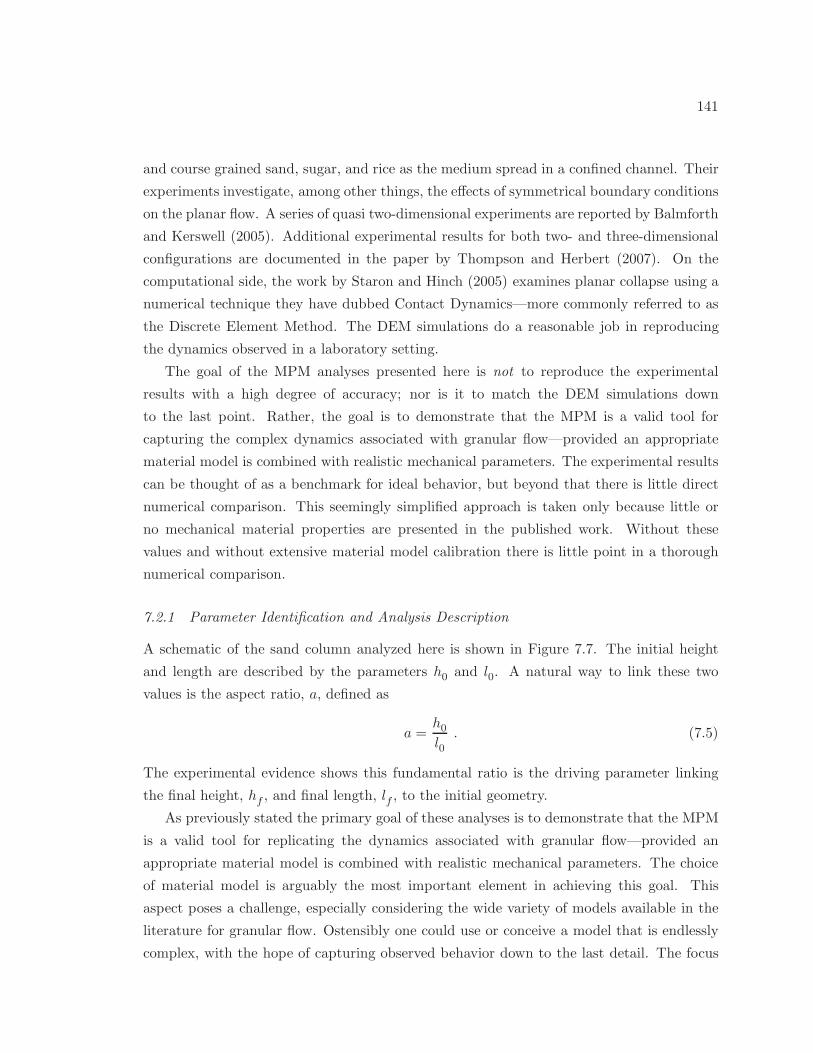
141

and course grained sand, sugar, and rice as the medium spread in a confined channel. Their

experiments investigate, among other things, the effects of symmetrical boundary conditions

on the planar flow. A series of quasi two-dimensional experiments are reported by Balmforth

and Kerswell (2005). Additional experimental results for both two- and three-dimensional

configurations are documented in the paper by Thompson and Herbert (2007). On the

computational side, the work by Staron and Hinch (2005) examines planar collapse using a

numerical technique they have dubbed Contact Dynamics—more commonly referred to as

the Discrete Element Method. The DEM simulations do a reasonable job in reproducing

the dynamics observed in a laboratory setting.

The goal of the MPM analyses presented here is not to reproduce the experimental

results with a high degree of accuracy; nor is it to match the DEM simulations down

to the last point. Rather, the goal is to demonstrate that the MPM is a valid tool for

capturing the complex dynamics associated with granular flow—provided an appropriate

material model is combined with realistic mechanical parameters. The experimental results

can be thought of as a benchmark for ideal behavior, but beyond that there is little direct

numerical comparison. This seemingly simplified approach is taken only because little or

no mechanical material properties are presented in the published work. Without these

values and without extensive material model calibration there is little point in a thorough

numerical comparison.

7.2.1 Parameter Identification and Analysis Description

A schematic of the sand column analyzed here is shown in Figure 7.7. The initial height

and length are described by the parameters h0 and l0. A natural way to link these two

values is the aspect ratio, a, defined as

a =h0l0

. (7.5)

The experimental evidence shows this fundamental ratio is the driving parameter linking

the final height, hf , and final length, lf , to the initial geometry.

As previously stated the primary goal of these analyses is to demonstrate that the MPM

is a valid tool for replicating the dynamics associated with granular flow—provided an

appropriate material model is combined with realistic mechanical parameters. The choice

of material model is arguably the most important element in achieving this goal. This

aspect poses a challenge, especially considering the wide variety of models available in the

literature for granular flow. Ostensibly one could use or conceive a model that is endlessly

complex, with the hope of capturing observed behavior down to the last detail. The focus

142

25

50

45

40

35

30

205 10 15 20 250 5 10 15 20 250 5 10 15 20 250

λ

Fri

ctio

nA

ngl

eφ

F[d

eg]

(a) (b) (c)

Case 2Case 3

Case 1Case 0

Case 5Case 6

Case 4Case 0

Case 8Case 9

Case 7Case 0

Figure 7.8: Mobilized friction angle, φF . (a) Analysis A: peak strength (b) Analysis B:initial strength (c) Analysis C: residual strength

here, however, is quite the opposite. Rather, emphasis is placed on utilizing comparatively

simple models that are capable of reproducing key observed phenomena, such as the notion

of a critical state.

The sand column collapse simulations use the pressure dependent models developed in

Chapter 3. In particular, two model variants are considered here:

1. Modified Drucker-Prager formulation (DP). This is the model outlined in Section 3.6.3

2. Matsuoka-Nakai yield surface with the Drucker-Prager plastic potential formulation (MN

with DP G) – This approach combines Matsuoka-Nakai yield surface, Equation (3.120),

with the Drucker-Prager plastic potential, Equation (3.108).

These models are referred to throughout by the name given above in parenthesis. The

validation of these models in the context of a granular medium is discussed in Section 3.8.

Both model variants rely heavily on the definition of the mobilized friction angle, φF ,

and the plastic dilation angel, ψG. The definition of these parameters is discussed in Sec-

tion 3.6.4. Preliminary studies of the collapse indicate that the evolution of the friction

angle plays a dominant role in determining the final geometry of the collapsed state. As

such, this study presents the effects of changing the mobilized friction angle. Ten total

friction angle curves are investigated. These curves fall into three analysis types. Each

analysis type is designed to target a different effect. The first class of curves examines the

role of peak strength. The second looks at how the initial strength impacts the final results,

and the third class evaluates the residual strength, or long term behavior under excessive

deformations. The curves are shown in Figure 7.8. Each curve is constructed using the

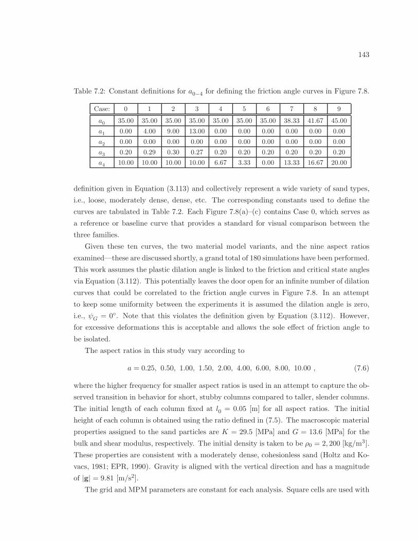
143

Table 7.2: Constant definitions for a0−4 for defining the friction angle curves in Figure 7.8.

Case: 0 1 2 3 4 5 6 7 8 9

a0 35.00 35.00 35.00 35.00 35.00 35.00 35.00 38.33 41.67 45.00

a1 0.00 4.00 9.00 13.00 0.00 0.00 0.00 0.00 0.00 0.00

a2 0.00 0.00 0.00 0.00 0.00 0.00 0.00 0.00 0.00 0.00

a3 0.20 0.29 0.30 0.27 0.20 0.20 0.20 0.20 0.20 0.20

a4 10.00 10.00 10.00 10.00 6.67 3.33 0.00 13.33 16.67 20.00

definition given in Equation (3.113) and collectively represent a wide variety of sand types,

i.e., loose, moderately dense, dense, etc. The corresponding constants used to define the

curves are tabulated in Table 7.2. Each Figure 7.8(a)–(c) contains Case 0, which serves as

a reference or baseline curve that provides a standard for visual comparison between the

three families.

Given these ten curves, the two material model variants, and the nine aspect ratios

examined—these are discussed shortly, a grand total of 180 simulations have been performed.

This work assumes the plastic dilation angle is linked to the friction and critical state angles

via Equation (3.112). This potentially leaves the door open for an infinite number of dilation

curves that could be correlated to the friction angle curves in Figure 7.8. In an attempt

to keep some uniformity between the experiments it is assumed the dilation angle is zero,

i.e., ψG = 0. Note that this violates the definition given by Equation (3.112). However,

for excessive deformations this is acceptable and allows the sole effect of friction angle to

be isolated.

The aspect ratios in this study vary according to

a = 0.25, 0.50, 1.00, 1.50, 2.00, 4.00, 6.00, 8.00, 10.00 , (7.6)

where the higher frequency for smaller aspect ratios is used in an attempt to capture the ob-

served transition in behavior for short, stubby columns compared to taller, slender columns.

The initial length of each column fixed at l0 = 0.05 [m] for all aspect ratios. The initial

height of each column is obtained using the ratio defined in (7.5). The macroscopic material

properties assigned to the sand particles are K = 29.5 [MPa] and G = 13.6 [MPa] for the

bulk and shear modulus, respectively. The initial density is taken to be ρ0 = 2, 200 [kg/m3].

These properties are consistent with a moderately dense, cohesionless sand (Holtz and Ko-

vacs, 1981; EPR, 1990). Gravity is aligned with the vertical direction and has a magnitude

of |g| = 9.81 [m/s2].

The grid and MPM parameters are constant for each analysis. Square cells are used with

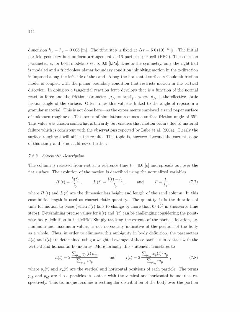
144

dimension hx = hy = 0.005 [m]. The time step is fixed at ∆ t = 5.0 (10)−5 [s]. The initial

particle geometry is a uniform arrangement of 16 particles per cell (PPC). The cohesion

parameter, c, for both models is set to 0.0 [kPa]. Due to the symmetry, only the right half

is modeled and a frictionless planar boundary condition inhibiting motion in the x-direction

is imposed along the left side of the sand. Along the horizontal surface a Coulomb friction

model is coupled with the planar boundary condition that restricts motion in the vertical

direction. In doing so a tangential reaction force develops that is a function of the normal

reaction force and the friction parameter, µfr = tan θfr, where θfr is the effective static

friction angle of the surface. Often times this value is linked to the angle of repose in a

granular material. This is not done here—as the experiments employed a sand paper surface

of unknown roughness. This series of simulations assumes a surface friction angle of 65.

This value was chosen somewhat arbitrarily but ensures that motion occurs due to material

failure which is consistent with the observations reported by Lube et al. (2004). Clearly the

surface roughness will affect the results. This topic is, however, beyond the current scope

of this study and is not addressed further.

7.2.2 Kinematic Description

The column is released from rest at a reference time t = 0.0 [s] and spreads out over the

flat surface. The evolution of the motion is described using the normalized variables

H (t) =h(t)

l0, L (t) =

l(t)− l0l0

, and T =t

tf, (7.7)

where H (t) and L (t) are the dimensionless height and length of the sand column. In this

case initial length is used as characteristic quantity. The quantity tf is the duration of

time for motion to cease (when l (t) fails to change by more than 0.01% in successive time

steps). Determining precise values for h(t) and l(t) can be challenging considering the point-

wise body definition in the MPM. Simply tracking the extents of the particle location, i.e.

minimum and maximum values, is not necessarily indicative of the position of the body

as a whole. Thus, in order to eliminate this ambiguity in body definition, the parameters

h(t) and l(t) are determined using a weighted average of those particles in contact with the

vertical and horizontal boundaries. More formally this statement translates to

h(t) = 2

∑

pvbyp(t)mp

∑

pvbmp

and l(t) = 2

∑

phbxp(t)mp

∑

phbmp

, (7.8)

where yp(t) and xp(t) are the vertical and horizontal positions of each particle. The terms

pvb and phb are those particles in contact with the vertical and horizontal boundaries, re-

spectively. This technique assumes a rectangular distribution of the body over the portion

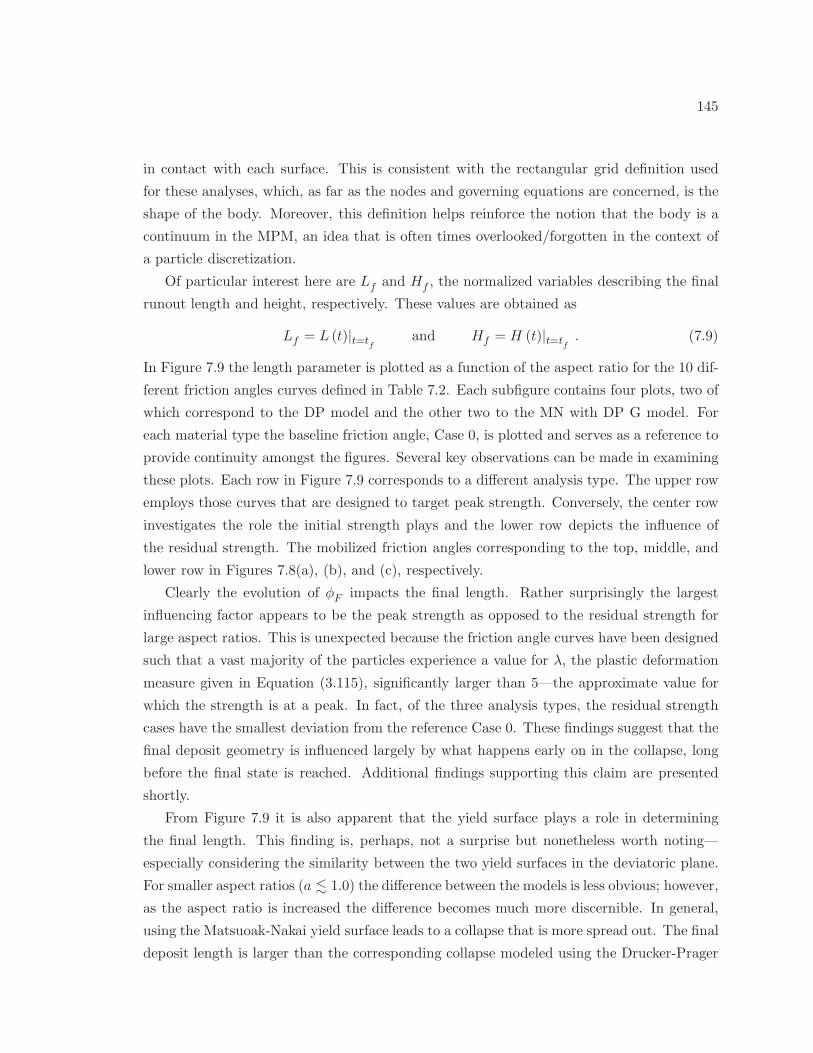
145

in contact with each surface. This is consistent with the rectangular grid definition used

for these analyses, which, as far as the nodes and governing equations are concerned, is the

shape of the body. Moreover, this definition helps reinforce the notion that the body is a

continuum in the MPM, an idea that is often times overlooked/forgotten in the context of

a particle discretization.

Of particular interest here are Lf and Hf , the normalized variables describing the final

runout length and height, respectively. These values are obtained as

Lf = L (t)|t=tf

and Hf = H (t)|t=tf. (7.9)

In Figure 7.9 the length parameter is plotted as a function of the aspect ratio for the 10 dif-

ferent friction angles curves defined in Table 7.2. Each subfigure contains four plots, two of

which correspond to the DP model and the other two to the MN with DP G model. For

each material type the baseline friction angle, Case 0, is plotted and serves as a reference to

provide continuity amongst the figures. Several key observations can be made in examining

these plots. Each row in Figure 7.9 corresponds to a different analysis type. The upper row

employs those curves that are designed to target peak strength. Conversely, the center row

investigates the role the initial strength plays and the lower row depicts the influence of

the residual strength. The mobilized friction angles corresponding to the top, middle, and

lower row in Figures 7.8(a), (b), and (c), respectively.

Clearly the evolution of φF impacts the final length. Rather surprisingly the largest

influencing factor appears to be the peak strength as opposed to the residual strength for

large aspect ratios. This is unexpected because the friction angle curves have been designed

such that a vast majority of the particles experience a value for λ, the plastic deformation

measure given in Equation (3.115), significantly larger than 5—the approximate value for

which the strength is at a peak. In fact, of the three analysis types, the residual strength

cases have the smallest deviation from the reference Case 0. These findings suggest that the

final deposit geometry is influenced largely by what happens early on in the collapse, long

before the final state is reached. Additional findings supporting this claim are presented

shortly.

From Figure 7.9 it is also apparent that the yield surface plays a role in determining

the final length. This finding is, perhaps, not a surprise but nonetheless worth noting—

especially considering the similarity between the two yield surfaces in the deviatoric plane.

For smaller aspect ratios (a . 1.0) the difference between the models is less obvious; however,

as the aspect ratio is increased the difference becomes much more discernible. In general,

using the Matsuoak-Nakai yield surface leads to a collapse that is more spread out. The final

deposit length is larger than the corresponding collapse modeled using the Drucker-Prager

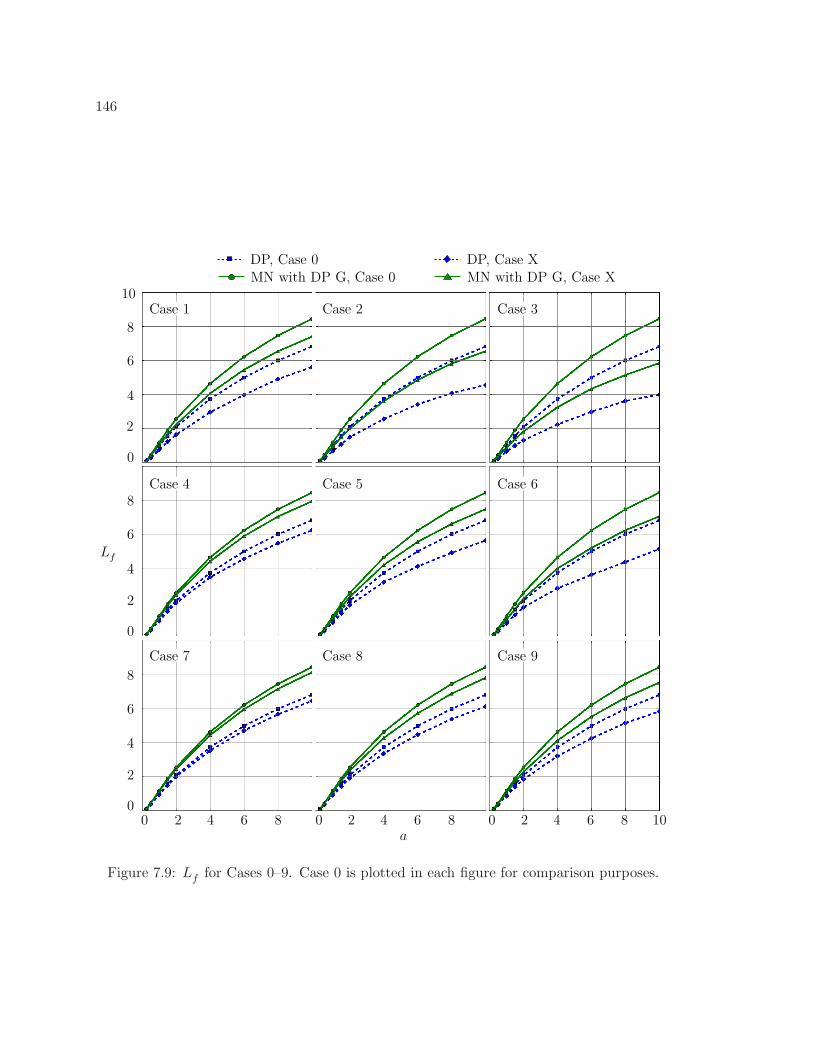
146

Case 3Case 2Case 1

Case 4 Case 5 Case 6

Case 7 Case 8 Case 9

MN with DP G, Case 0DP, Case 0 DP, Case X

MN with DP G, Case X

0

0

0

a

84 62 84 62 84 62

8

6

4

2

8

6

4

2

8

6

4

2

000 10

10

Lf

Figure 7.9: Lf for Cases 0–9. Case 0 is plotted in each figure for comparison purposes.

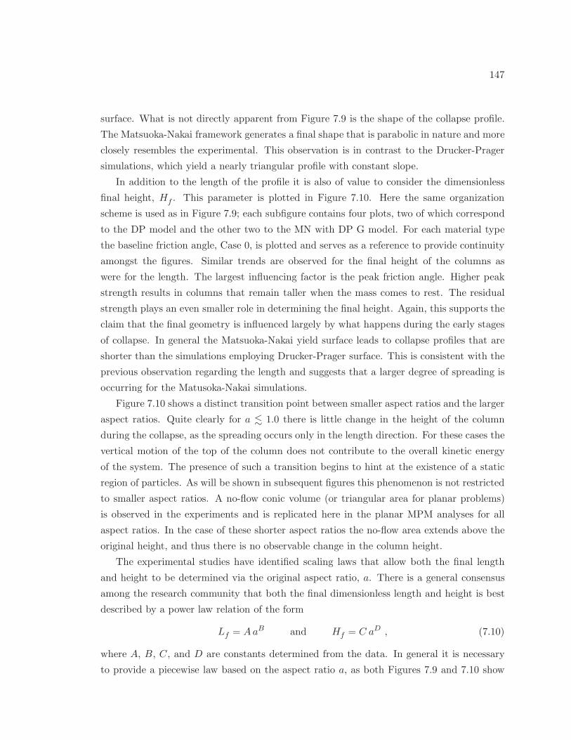
147

surface. What is not directly apparent from Figure 7.9 is the shape of the collapse profile.

The Matsuoka-Nakai framework generates a final shape that is parabolic in nature and more

closely resembles the experimental. This observation is in contrast to the Drucker-Prager

simulations, which yield a nearly triangular profile with constant slope.

In addition to the length of the profile it is also of value to consider the dimensionless

final height, Hf . This parameter is plotted in Figure 7.10. Here the same organization

scheme is used as in Figure 7.9; each subfigure contains four plots, two of which correspond

to the DP model and the other two to the MN with DP G model. For each material type

the baseline friction angle, Case 0, is plotted and serves as a reference to provide continuity

amongst the figures. Similar trends are observed for the final height of the columns as

were for the length. The largest influencing factor is the peak friction angle. Higher peak

strength results in columns that remain taller when the mass comes to rest. The residual

strength plays an even smaller role in determining the final height. Again, this supports the

claim that the final geometry is influenced largely by what happens during the early stages

of collapse. In general the Matsuoka-Nakai yield surface leads to collapse profiles that are

shorter than the simulations employing Drucker-Prager surface. This is consistent with the

previous observation regarding the length and suggests that a larger degree of spreading is

occurring for the Matusoka-Nakai simulations.

Figure 7.10 shows a distinct transition point between smaller aspect ratios and the larger

aspect ratios. Quite clearly for a . 1.0 there is little change in the height of the column

during the collapse, as the spreading occurs only in the length direction. For these cases the

vertical motion of the top of the column does not contribute to the overall kinetic energy

of the system. The presence of such a transition begins to hint at the existence of a static

region of particles. As will be shown in subsequent figures this phenomenon is not restricted

to smaller aspect ratios. A no-flow conic volume (or triangular area for planar problems)

is observed in the experiments and is replicated here in the planar MPM analyses for all

aspect ratios. In the case of these shorter aspect ratios the no-flow area extends above the

original height, and thus there is no observable change in the column height.

The experimental studies have identified scaling laws that allow both the final length

and height to be determined via the original aspect ratio, a. There is a general consensus

among the research community that both the final dimensionless length and height is best

described by a power law relation of the form

Lf = AaB and Hf = C aD , (7.10)

where A, B, C, and D are constants determined from the data. In general it is necessary

to provide a piecewise law based on the aspect ratio a, as both Figures 7.9 and 7.10 show

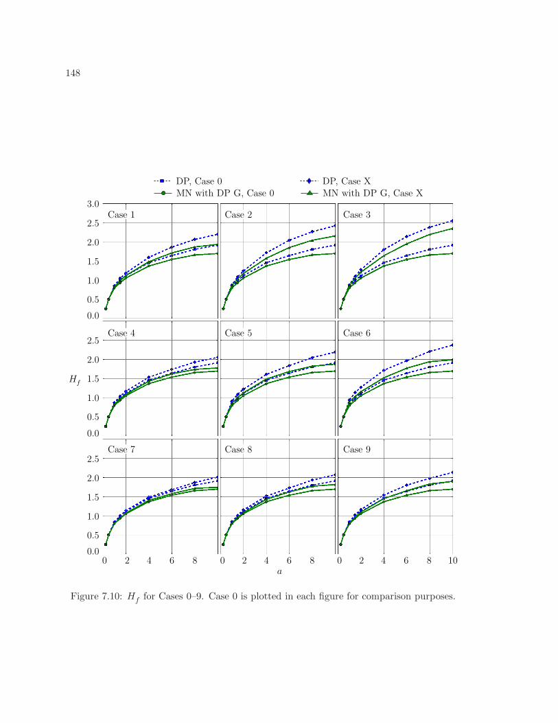
148

Case 3Case 2Case 1

Case 4 Case 5 Case 6

Case 7 Case 8 Case 9

MN with DP G, Case 0DP, Case 0 DP, Case X

MN with DP G, Case X

a

84 62 84 62 84 62000 10

3.0

1.5

2.5

2.0

0.5

1.0

0.0

1.5

2.5

2.0

0.5

1.0

0.0

1.5

2.5

2.0

0.5

1.0

0.0

Hf

Figure 7.10: Hf for Cases 0–9. Case 0 is plotted in each figure for comparison purposes.

149

101

100

10−1

Lf

a

100 100 101 100 10110−1 101 10−1 10−1

(a) (b) (c)

regiontransition

Figure 7.11: Log-Log plot of Lf as a function of a for Cases 0–9. (a) DP model (b)MN with DP G model and (c) All data points.

Table 7.3: Best fit constants for determining Lf (a) via a power law.

Material Model

DP MN with DP G. All Models

a . 1.5 0.791 a 1.542 1.007 a 1.516 0.893 a 1.560

a & 1.5 1.007 a 0.744 1.304 a 0.753 1.148 a 0.745

a distinct transition region based on this ratio.

A least squares fit of the data in log-log space is performed to determine the unknown

power law constants. Figure 7.11 examines the final length data for both models, as well

as all the data points combined. Each sub-figure contains multiple lines: a solid line cor-

responding to the best fit of the points, and dashed lines representing the lower and upper

bound of the data points. This approach is taken in an effort to provide a reasonable range

for the constants used to define the power law. From these figures it is apparent that a

single line cannot represent all cases; a transition region is introduced to describe the flow.

Based on the MPM analyses, a reasonable region is between 0.75 . a . 2.0 for Lf . This is

a relatively wide region and suggests that caution be used in comparing these findings too

closely to experimental results—as the log-log space is friendly to the researcher and can

lead to a subjective comparison. Nonetheless, an attempt is made to correlate these results

to the experimental findings.

In Table 7.3 the power law is given for the final length Lf . These are determined using

all the data points for a given model (or all the data for both models) and represent the

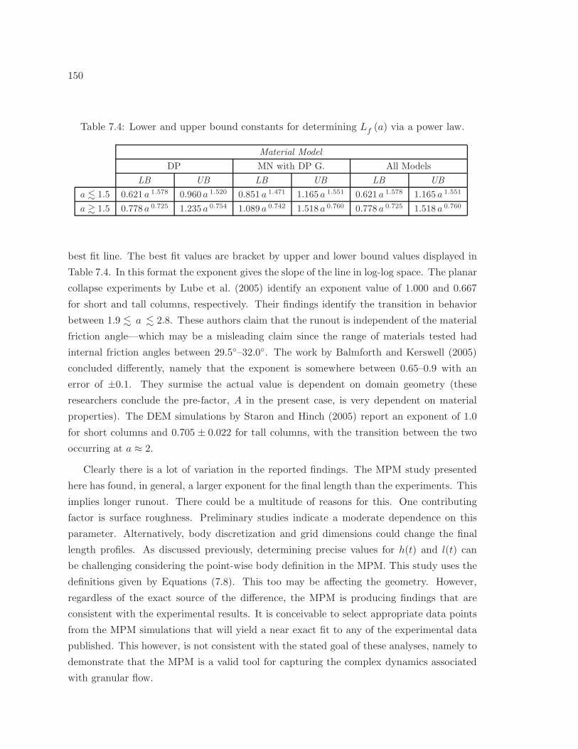
150

Table 7.4: Lower and upper bound constants for determining Lf (a) via a power law.

Material Model

DP MN with DP G. All Models

LB UB LB UB LB UB

a . 1.5 0.621 a 1.578 0.960 a 1.520 0.851 a 1.471 1.165 a 1.551 0.621 a 1.578 1.165 a 1.551

a & 1.5 0.778 a 0.725 1.235 a 0.754 1.089 a 0.742 1.518 a 0.760 0.778 a 0.725 1.518 a 0.760

best fit line. The best fit values are bracket by upper and lower bound values displayed in

Table 7.4. In this format the exponent gives the slope of the line in log-log space. The planar

collapse experiments by Lube et al. (2005) identify an exponent value of 1.000 and 0.667

for short and tall columns, respectively. Their findings identify the transition in behavior

between 1.9 . a . 2.8. These authors claim that the runout is independent of the material

friction angle—which may be a misleading claim since the range of materials tested had

internal friction angles between 29.5–32.0. The work by Balmforth and Kerswell (2005)

concluded differently, namely that the exponent is somewhere between 0.65–0.9 with an

error of ±0.1. They surmise the actual value is dependent on domain geometry (these

researchers conclude the pre-factor, A in the present case, is very dependent on material

properties). The DEM simulations by Staron and Hinch (2005) report an exponent of 1.0

for short columns and 0.705 ± 0.022 for tall columns, with the transition between the two

occurring at a ≈ 2.

Clearly there is a lot of variation in the reported findings. The MPM study presented

here has found, in general, a larger exponent for the final length than the experiments. This

implies longer runout. There could be a multitude of reasons for this. One contributing

factor is surface roughness. Preliminary studies indicate a moderate dependence on this

parameter. Alternatively, body discretization and grid dimensions could change the final

length profiles. As discussed previously, determining precise values for h(t) and l(t) can

be challenging considering the point-wise body definition in the MPM. This study uses the

definitions given by Equations (7.8). This too may be affecting the geometry. However,

regardless of the exact source of the difference, the MPM is producing findings that are

consistent with the experimental results. It is conceivable to select appropriate data points

from the MPM simulations that will yield a near exact fit to any of the experimental data

published. This however, is not consistent with the stated goal of these analyses, namely to

demonstrate that the MPM is a valid tool for capturing the complex dynamics associated

with granular flow.

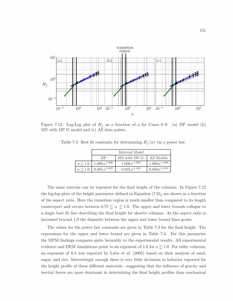
151

101

100

10−1

a

100 100 101 100 10110−1 101 10−1 10−1

Hf

(a) (b) (c)

regiontransition

Figure 7.12: Log-Log plot of Hf as a function of a for Cases 0–9. (a) DP model (b)MN with DP G model and (c) All data points.

Table 7.5: Best fit constants for determining Hf (a) via a power law.

Material Model

DP MN with DP G. All Models

a . 1.0 1.000 a 1.000 1.000 a 1.000 1.000 a 1.000

a & 1.0 0.865 a 0.425 0.825 a 0.404 0.850 a 0.414

The same exercise can be repeated for the final height of the columns. In Figure 7.12

the log-log plots of the height parameter defined in Equation (7.9)2 are shown as a function

of the aspect ratio. Here the transition region is much smaller than compared to its length

counterpart and occurs between 0.75 . a . 1.0. The upper and lower bounds collapse to

a single best fit line describing the final height for shorter columns. As the aspect ratio is

increased beyond 1.0 the disparity between the upper and lower bound lines grows.

The values for the power law constants are given in Table 7.3 for the final height. The

expressions for the upper and lower bound are given in Table 7.4. For this parameter

the MPM findings compares quite favorably to the experimental results. All experimental

evidence and DEM simulations point to an exponent of 1.0 for a . 1.0. For taller columns,

an exponent of 0.4 was reported by Lube et al. (2005) based on their analysis of sand,

sugar, and rice. Interestingly enough there is very little deviation in behavior reported for

the height profile of these different materials—suggesting that the influence of gravity and

inertial forces are more dominant in determining the final height profiles than mechanical

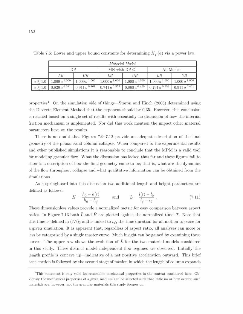
152

Table 7.6: Lower and upper bound constants for determining Hf (a) via a power law.

Material Model

DP MN with DP G. All Models

LB UB LB UB LB UB

a . 1.0 1.000 a 1.000 1.000 a 1.000 1.000 a 1.000 1.000 a 1.000 1.000 a 1.000 1.000 a 1.000

a & 1.0 0.820 a 0.381 0.911 a 0.461 0.741 a 0.353 0.860 a 0.450 0.791 a 0.353 0.911 a 0.461

properties4. On the simulation side of things—Staron and Hinch (2005) determined using

the Discrete Element Method that the exponent should be 0.35. However, this conclusion

is reached based on a single set of results with essentially no discussion of how the internal

friction mechanism is implemented. Nor did this work mention the impact other material

parameters have on the results.

There is no doubt that Figures 7.9–7.12 provide an adequate description of the final

geometry of the planar sand column collapse. When compared to the experimental results

and other published simulations it is reasonable to conclude that the MPM is a valid tool

for modeling granular flow. What the discussion has lacked thus far and these figures fail to

show is a description of how the final geometry came to be; that is, what are the dynamics

of the flow throughout collapse and what qualitative information can be obtained from the

simulations.

As a springboard into this discussion two additional length and height parameters are

defined as follows:

H =h0 − h(t)

h0 − hfand L =

l(t)− l0lf − l0

. (7.11)

These dimensionless values provide a normalized metric for easy comparison between aspect

ratios. In Figure 7.13 both L and H are plotted against the normalized time, T . Note that

this time is defined in (7.7)3 and is linked to tf , the time duration for all motion to cease for

a given simulation. It is apparent that, regardless of aspect ratio, all analyses can more or

less be categorized by a single master curve. Much insight can be gained by examining these

curves. The upper row shows the evolution of L for the two material models considered

in this study. Three distinct model independent flow regimes are observed. Initially the

length profile is concave up—indicative of a net positive acceleration outward. This brief

acceleration is followed by the second stage of motion in which the length of column expands

4This statement is only valid for reasonable mechanical properties in the context considered here. Ob-

viously the mechanical properties of a given medium can be selected such that little no or flow occurs; such

materials are, however, not the granular materials this study focuses on.

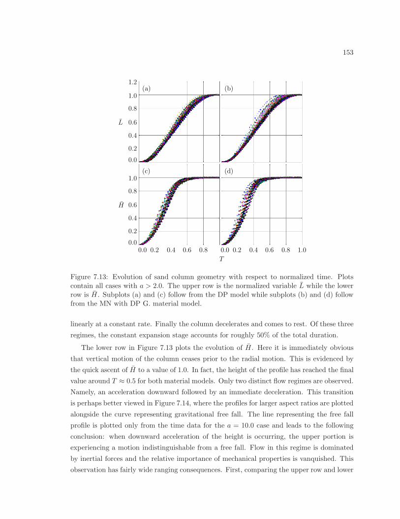
153

(a) (b)

(d)(c)

0.0 0.4 0.6 0.80.20.0

0.2

0.4

0.6

0.8

1.0

0.0

0.2

0.4

0.6

0.8

1.0

1.2

L

H

0.0 0.4 0.6 0.80.2 1.0

T

Figure 7.13: Evolution of sand column geometry with respect to normalized time. Plotscontain all cases with a > 2.0. The upper row is the normalized variable L while the lowerrow is H. Subplots (a) and (c) follow from the DP model while subplots (b) and (d) followfrom the MN with DP G. material model.

linearly at a constant rate. Finally the column decelerates and comes to rest. Of these three

regimes, the constant expansion stage accounts for roughly 50% of the total duration.

The lower row in Figure 7.13 plots the evolution of H. Here it is immediately obvious

that vertical motion of the column ceases prior to the radial motion. This is evidenced by

the quick ascent of H to a value of 1.0. In fact, the height of the profile has reached the final

value around T ≈ 0.5 for both material models. Only two distinct flow regimes are observed.

Namely, an acceleration downward followed by an immediate deceleration. This transition

is perhaps better viewed in Figure 7.14, where the profiles for larger aspect ratios are plotted

alongside the curve representing gravitational free fall. The line representing the free fall

profile is plotted only from the time data for the a = 10.0 case and leads to the following

conclusion: when downward acceleration of the height is occurring, the upper portion is

experiencing a motion indistinguishable from a free fall. Flow in this regime is dominated

by inertial forces and the relative importance of mechanical properties is vanquished. This

observation has fairly wide ranging consequences. First, comparing the upper row and lower

154

0.0 0.2 0.3 0.40.10.0

0.8

0.6

0.4

0.2

1.0

H

(a) (b)

0.0 0.1 0.2 0.3 0.4 0.50.5 T T

Figure 7.14: Case 2 H compared to free fall in a gravitational field. The free fall is denotedby the dashed line. Plots contain all cases with a > 2.0. Subplot (a) follows from the DPmodel data while subplot (b) follows from the MN with DP G. data.

row of Figure 7.13, the duration of gravitational acceleration corresponds directly to the

radial acceleration. In other words, when the height is accelerating downward the length

is accelerating outward. Second, it was previously noted that the peak friction angle has

the largest impact on the final geometry. This was surprising because the peak strength

occurs early on in the analysis. From this observation it is postulated that the early stages

of collapse play the largest role in determining the final geometry. A potential explanation

for this is given here—the material state at peak acceleration is the dominant factor in

determining final geometry.

The nodal velocity fields provide an alternative way to visualize the different flow

regimes. This is shown Figures 7.15–7.17, where the three aspect ratios a = 2.0, 4.0, and 8.0

are shown. Each figure contains four sequential snapshots of the flow configuration. This

data follows from the MN with DP G material model and the mobilized friction angle defined

as Case 2 in Table 7.2. A different velocity scale is used for each aspect ratio considered.

While each snapshot has a common color scale for the velocity field, the geometry is plotted

at different scales. Comparisons regarding the shape of the profile at the different snapshots

in time are ill advised and misleading, as these figures have been created to examine the

velocity profile.

During the early stages of the collapse (T . 0.10) the upper portion of all columns falls

in a strictly vertical manner for the three aspect ratios shown. As the analysis proceeds

the the difference in behavior becomes apparent. At time T = 0.30 the purely vertical

motion has ceased for a = 2.0 and lateral spreading is underway. Figure 7.16 shows the

upper region near the center line is still moving downward but outward effects are becoming

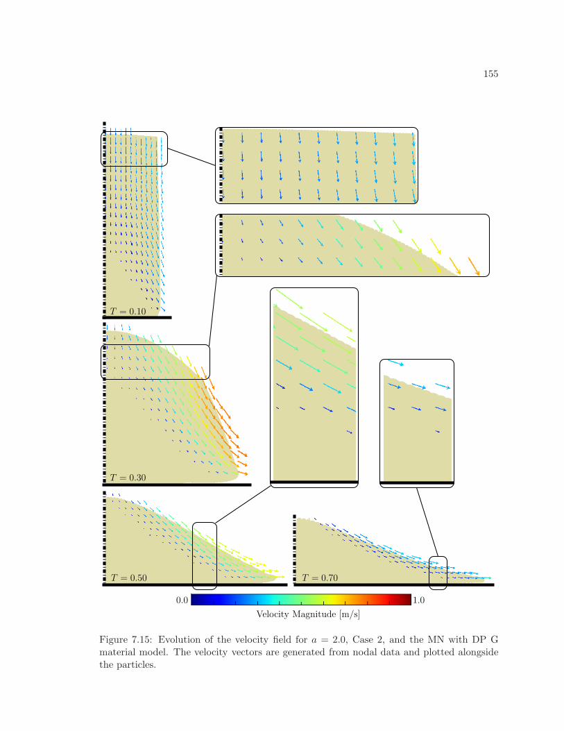
155

0.0 1.0

Velocity Magnitude [m/s]

T = 0.10

T = 0.30

T = 0.50 T = 0.70

Figure 7.15: Evolution of the velocity field for a = 2.0, Case 2, and the MN with DP Gmaterial model. The velocity vectors are generated from nodal data and plotted alongsidethe particles.

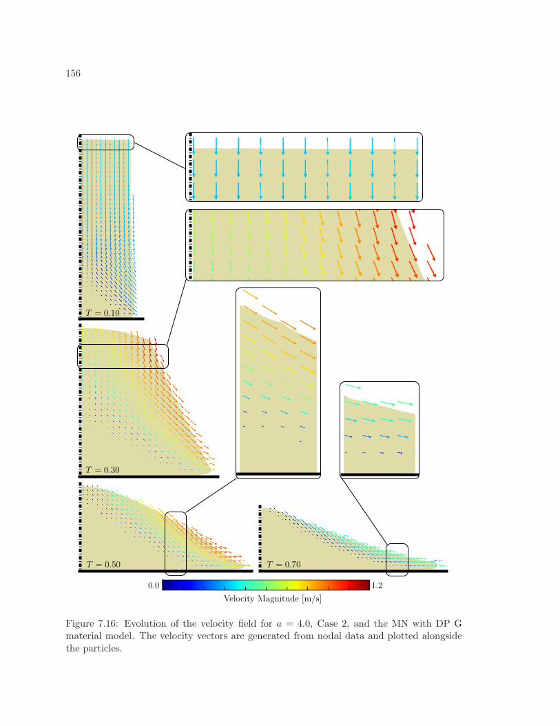
156

0.0 1.2

Velocity Magnitude [m/s]

T = 0.10

T = 0.30

T = 0.50 T = 0.70

Figure 7.16: Evolution of the velocity field for a = 4.0, Case 2, and the MN with DP Gmaterial model. The velocity vectors are generated from nodal data and plotted alongsidethe particles.

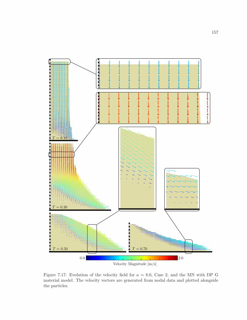
157

T = 0.10

T = 0.30

T = 0.50 T = 0.70

0.0

Velocity Magnitude [m/s]

2.0

Figure 7.17: Evolution of the velocity field for a = 8.0, Case 2, and the MN with DP Gmaterial model. The velocity vectors are generated from nodal data and plotted alongsidethe particles.

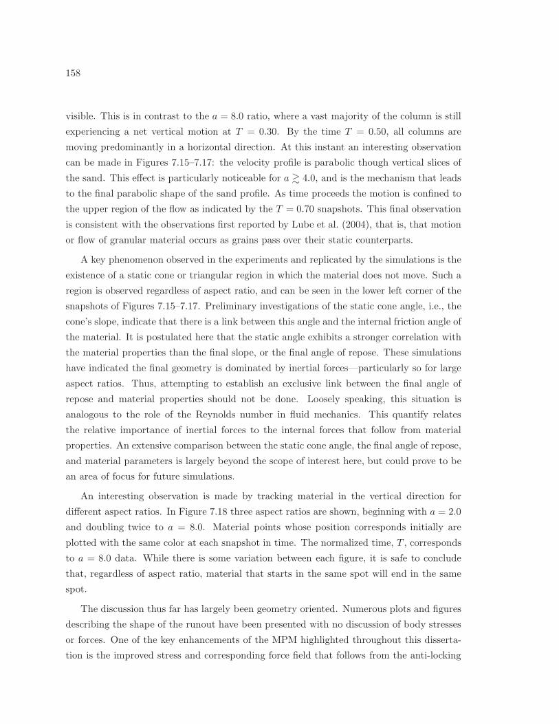
158

visible. This is in contrast to the a = 8.0 ratio, where a vast majority of the column is still

experiencing a net vertical motion at T = 0.30. By the time T = 0.50, all columns are

moving predominantly in a horizontal direction. At this instant an interesting observation

can be made in Figures 7.15–7.17: the velocity profile is parabolic though vertical slices of

the sand. This effect is particularly noticeable for a & 4.0, and is the mechanism that leads

to the final parabolic shape of the sand profile. As time proceeds the motion is confined to

the upper region of the flow as indicated by the T = 0.70 snapshots. This final observation

is consistent with the observations first reported by Lube et al. (2004), that is, that motion

or flow of granular material occurs as grains pass over their static counterparts.

A key phenomenon observed in the experiments and replicated by the simulations is the

existence of a static cone or triangular region in which the material does not move. Such a

region is observed regardless of aspect ratio, and can be seen in the lower left corner of the

snapshots of Figures 7.15–7.17. Preliminary investigations of the static cone angle, i.e., the

cone’s slope, indicate that there is a link between this angle and the internal friction angle of

the material. It is postulated here that the static angle exhibits a stronger correlation with

the material properties than the final slope, or the final angle of repose. These simulations

have indicated the final geometry is dominated by inertial forces—particularly so for large

aspect ratios. Thus, attempting to establish an exclusive link between the final angle of

repose and material properties should not be done. Loosely speaking, this situation is

analogous to the role of the Reynolds number in fluid mechanics. This quantify relates

the relative importance of inertial forces to the internal forces that follow from material

properties. An extensive comparison between the static cone angle, the final angle of repose,

and material parameters is largely beyond the scope of interest here, but could prove to be

an area of focus for future simulations.

An interesting observation is made by tracking material in the vertical direction for

different aspect ratios. In Figure 7.18 three aspect ratios are shown, beginning with a = 2.0

and doubling twice to a = 8.0. Material points whose position corresponds initially are

plotted with the same color at each snapshot in time. The normalized time, T , corresponds

to a = 8.0 data. While there is some variation between each figure, it is safe to conclude

that, regardless of aspect ratio, material that starts in the same spot will end in the same

spot.

The discussion thus far has largely been geometry oriented. Numerous plots and figures

describing the shape of the runout have been presented with no discussion of body stresses

or forces. One of the key enhancements of the MPM highlighted throughout this disserta-

tion is the improved stress and corresponding force field that follows from the anti-locking

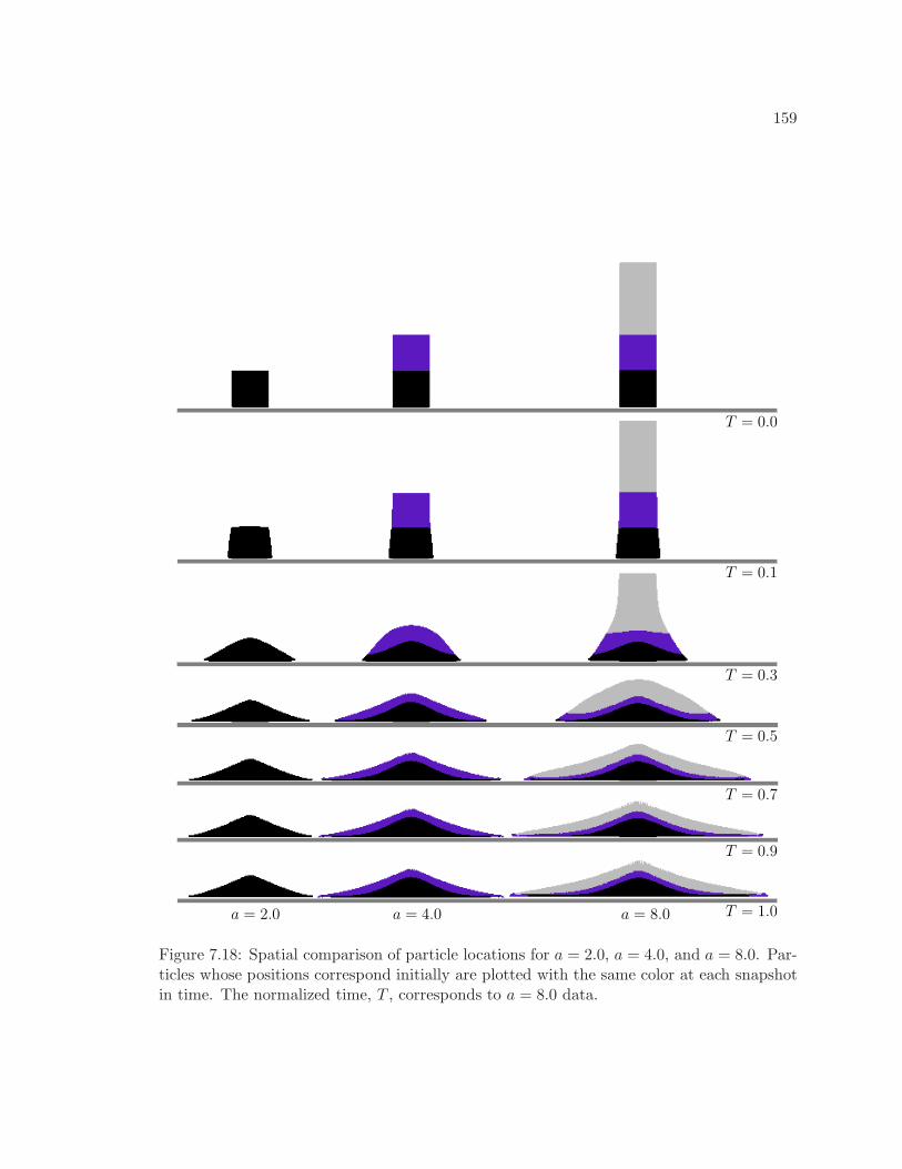
159

a = 2.0 a = 4.0 a = 8.0 T = 1.0

T = 0.0

T = 0.1

T = 0.3

T = 0.5

T = 0.7

T = 0.9

Figure 7.18: Spatial comparison of particle locations for a = 2.0, a = 4.0, and a = 8.0. Par-ticles whose positions correspond initially are plotted with the same color at each snapshotin time. The normalized time, T , corresponds to a = 8.0 data.

160

a = 8.0a = 1.0 a = 2.0 a = 4.0 T = 1.00

(a) Drucker-Prager Model

a = 8.0a = 1.0 a = 2.0 a = 4.0 T = 1.00

(b) Matsuoka-Nakai Model

T = 0.67

T = 0.33

T = 0.00

T = 0.67

T = 0.33

T = 0.00

σmin22 − 1.0 σmin

22 − 4.0 σmin22 − 8.0σmin

22 − 2.0

σmin22 − 1.0 σmin

22 − 4.0 σmin22 − 8.0σmin

22 − 2.0

0.1 [kPa] σmin22 [kPa]

Figure 7.19: Evolution of the vertical stress, σ22, for Case 2.

framework presented in Chapter 4. The remainder of this discussion evaluates these fields

and links these values to key geometric observations.

7.2.3 Internal Stresses

In Figure 7.19 the evolution of the vertical stress, σ22, is presented for both material mod-

els. The figure depicts the columns at several stages throughout the analysis, including the

initial and final states. The initial stress distribution is consistent with a confined column

subjected to gravity. As the analysis proceeds the vertical stress field behaves as expected for

shorter aspect ratios (a . 2.0): the initial triangular distribution is more or less maintained

throughout. In these cases the overall height of the column is not changing drastically. For

taller columns an interesting stress field emerges. For a & 4.0 there is a wedge shaped

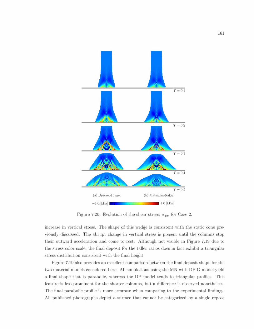
161

(b) Matsuoka-Nakai(a) Drucker-Prager

T = 0.2

T = 0.3

T = 0.4

T = 0.5

T = 0.1

4.0 [kPa]−1.0 [kPa]

Figure 7.20: Evolution of the shear stress, σ12, for Case 2.

increase in vertical stress. The shape of this wedge is consistent with the static cone pre-

viously discussed. The abrupt change in vertical stress is present until the columns stop

their outward acceleration and come to rest. Although not visible in Figure 7.19 due to

the stress color scale, the final deposit for the taller ratios does in fact exhibit a triangular

stress distribution consistent with the final height.

Figure 7.19 also provides an excellent comparison between the final deposit shape for the

two material models considered here. All simulations using the MN with DP G model yield

a final shape that is parabolic, whereas the DP model tends to triangular profiles. This

feature is less prominent for the shorter columns, but a difference is observed nonetheless.

The final parabolic profile is more accurate when comparing to the experimental findings.

All published photographs depict a surface that cannot be categorized by a single repose

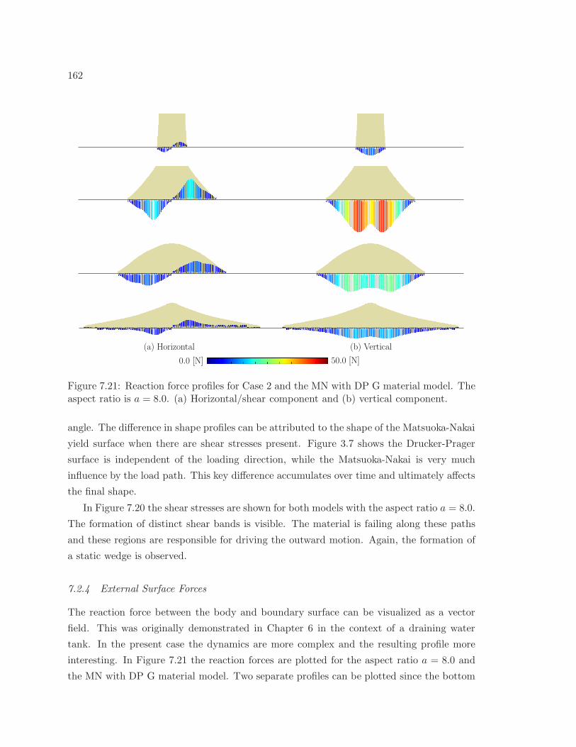
162

0.0 [N] 50.0 [N]

(a) Horizontal (b) Vertical

Figure 7.21: Reaction force profiles for Case 2 and the MN with DP G material model. Theaspect ratio is a = 8.0. (a) Horizontal/shear component and (b) vertical component.

angle. The difference in shape profiles can be attributed to the shape of the Matsuoka-Nakai

yield surface when there are shear stresses present. Figure 3.7 shows the Drucker-Prager

surface is independent of the loading direction, while the Matsuoka-Nakai is very much

influence by the load path. This key difference accumulates over time and ultimately affects

the final shape.

In Figure 7.20 the shear stresses are shown for both models with the aspect ratio a = 8.0.

The formation of distinct shear bands is visible. The material is failing along these paths

and these regions are responsible for driving the outward motion. Again, the formation of

a static wedge is observed.

7.2.4 External Surface Forces

The reaction force between the body and boundary surface can be visualized as a vector

field. This was originally demonstrated in Chapter 6 in the context of a draining water

tank. In the present case the dynamics are more complex and the resulting profile more

interesting. In Figure 7.21 the reaction forces are plotted for the aspect ratio a = 8.0 and

the MN with DP G material model. Two separate profiles can be plotted since the bottom

163

(a) Raw Profile (b) Filtered Profile

Figure 7.22: Comparison of reaction force profiles. (a) raw data profile and (b) filteredprofile.

surface is non-smooth: the shear force that develops due to friction and the normal force

preventing penetration into the boundary. The left side of Figure 7.21 examines the shear

profile. At all times the shear force is directed towards the center line of the column, leading

to a skew-symmetric distribution. The largest magnitude values occur when the vertical

velocity of the column is at its highest value. Local maximums for each snapshot occur at

the location where the shear stress band reaches the surface, as seen by comparing the shear

force profile to the shear stress from Figure 7.20.

The normal force perpendicular to the surface is plotted in Figure 7.21(b). This distri-

bution begins as a single parabolic shape. The profile grows and eventually reaches a global

peak when the vertical downward momentum is at its largest—that is, when the vertical

velocity is at its maximum value. Following said peak, the motion begins to move radi-

ally; two distinct parabolic regions are observed, each with a local maximum propagating

outward. These local maxima coincide with the shear profile maxima. The final profile is

shown in the bottom layer of Figure 7.21. Again the dual parabolic distribution is observed.

Here it is noted that the final shape of this profile is slightly counterintuitive: from static

principles one could argue for the existence of a force profile that mirrors the final geometric

profile of the collapse. Clearly that is not occurring, and can be explained by the internal

strength of the medium—diagonal stress bands emanating from the static cone leads to the

observed distribution

For aesthetic purposes the final reaction profiles have been smoothed over. Stress wave

propagation and checkerboard modes cause profile fluctuations in time. The filtering is done

as follows: the plot value for any given node is obtained by computing the average of itself

164

and its neighbors 5 . The resulting profile is smoothed—but the maximum and minimum

values of the original profile have been compromised. Since the value of interest is typically

the largest magnitude force, the smooth profile is normalized by the largest smoothed mag-

nitude, and then multiplied by the largest magnitude value from the original non-smooth

profile. Doing so maintains the absolute value of the local maximums of the force profile.

This technique is not the only option and alternative smoothing techniques could be em-

ployed. One alternative is to normalize with respect to the impulse at a given snapshot in

time. This would ensure that momentum is conserved. However, since the smoothing is be-

ing done for plotting purposes only and has no bearing on the actual dynamics of the body,

conserving momentum for the sake of a nice looking plot is unnecessary. The aforemen-

tioned technique is used here and provides a valid reaction force distribution. A comparison

of the raw and filtered data is shown in Figure 7.22. The maximum values from the raw

data are maintained, but as a side effect the minimum values are embellished—particularly

where the gradient of the profile changes rapidly.

7.2.5 Conclusions

This section has demonstrated the Material Point method is a viable tool for modeling

granular flow when coupled with an appropriate material model. Using a planar sand column

collapse as a proving ground, the MPM simulations reproduced key geometric observations

from published experiments. The analyses identified the peak material strength as being

the most influential factor in determining the final shape of the collapse. In addition to the

geometric aspects, it was shown that the MPM can be used to visualize other field variables

of interest; the velocity and stress fields were shown here but many other options exist. The

reaction force between the planar surface and the body of sand was investigated. Parabolic-

esque profiles were obtained for both. Future studies could investigate the influence of

surface roughness on the final geometry. Alternatively, the work could be expanded to 3-d

in an attempt to identify a link between planar behavior and the antisymmetric column

collapse.

7.3 Avalanche Control: Energy Dissipation Using Earthen Embankments

Mountainous areas are notorious breeding grounds for avalanches of various mediums, in-

cluding rocks, soil, trees and vegetation, and the most common culprit, snow. As a force of

nature these powerful occurrences are awe inspiring and truly a force to be reckoned with.

5in this case a centered, five node window width is used.

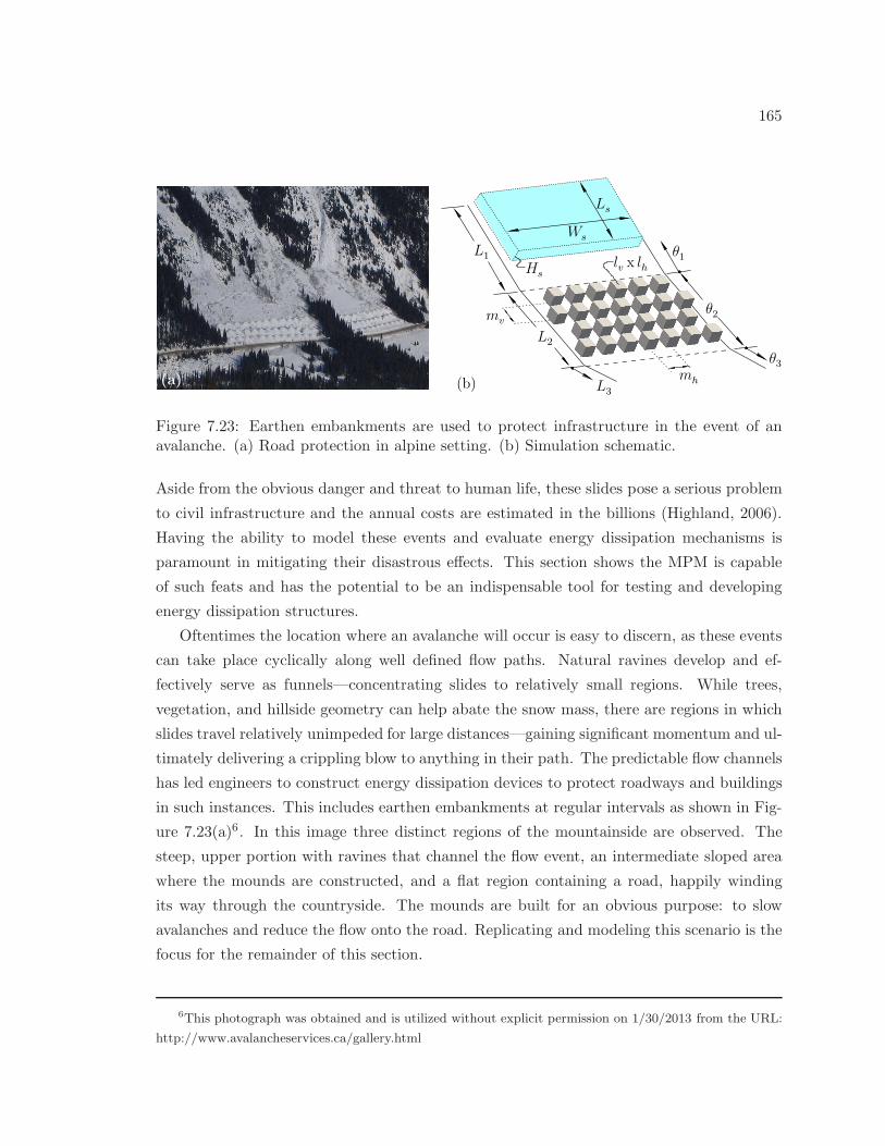
165

mh(a)

θ1

θ3

θ2

L1

L2

L3

Ws

Ls

Hs

mv

(b)

lv x lh

Figure 7.23: Earthen embankments are used to protect infrastructure in the event of anavalanche. (a) Road protection in alpine setting. (b) Simulation schematic.

Aside from the obvious danger and threat to human life, these slides pose a serious problem

to civil infrastructure and the annual costs are estimated in the billions (Highland, 2006).

Having the ability to model these events and evaluate energy dissipation mechanisms is

paramount in mitigating their disastrous effects. This section shows the MPM is capable

of such feats and has the potential to be an indispensable tool for testing and developing

energy dissipation structures.

Oftentimes the location where an avalanche will occur is easy to discern, as these events

can take place cyclically along well defined flow paths. Natural ravines develop and ef-

fectively serve as funnels—concentrating slides to relatively small regions. While trees,

vegetation, and hillside geometry can help abate the snow mass, there are regions in which

slides travel relatively unimpeded for large distances—gaining significant momentum and ul-

timately delivering a crippling blow to anything in their path. The predictable flow channels

has led engineers to construct energy dissipation devices to protect roadways and buildings

in such instances. This includes earthen embankments at regular intervals as shown in Fig-

ure 7.23(a)6. In this image three distinct regions of the mountainside are observed. The

steep, upper portion with ravines that channel the flow event, an intermediate sloped area

where the mounds are constructed, and a flat region containing a road, happily winding

its way through the countryside. The mounds are built for an obvious purpose: to slow

avalanches and reduce the flow onto the road. Replicating and modeling this scenario is the

focus for the remainder of this section.

6This photograph was obtained and is utilized without explicit permission on 1/30/2013 from the URL:

http://www.avalancheservices.ca/gallery.html

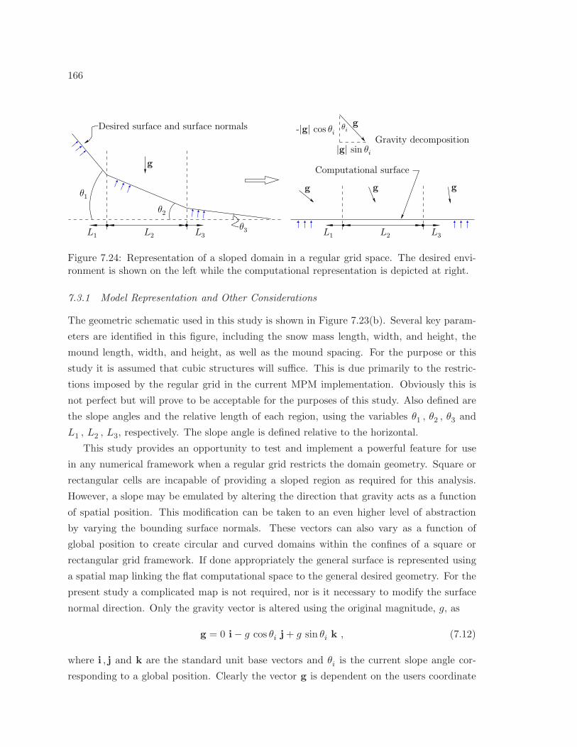
166

g

L3θ3L2L1

Desired surface and surface normals

θ2

θ1

L3L2L1

gg g

Computational surface

Gravity decomposition

g

|g| sin θi

-|g| cos θi θi

Figure 7.24: Representation of a sloped domain in a regular grid space. The desired envi-ronment is shown on the left while the computational representation is depicted at right.

7.3.1 Model Representation and Other Considerations

The geometric schematic used in this study is shown in Figure 7.23(b). Several key param-

eters are identified in this figure, including the snow mass length, width, and height, the

mound length, width, and height, as well as the mound spacing. For the purpose or this

study it is assumed that cubic structures will suffice. This is due primarily to the restric-

tions imposed by the regular grid in the current MPM implementation. Obviously this is

not perfect but will prove to be acceptable for the purposes of this study. Also defined are

the slope angles and the relative length of each region, using the variables θ1 , θ2 , θ3 and

L1 , L2 , L3, respectively. The slope angle is defined relative to the horizontal.

This study provides an opportunity to test and implement a powerful feature for use

in any numerical framework when a regular grid restricts the domain geometry. Square or

rectangular cells are incapable of providing a sloped region as required for this analysis.

However, a slope may be emulated by altering the direction that gravity acts as a function

of spatial position. This modification can be taken to an even higher level of abstraction

by varying the bounding surface normals. These vectors can also vary as a function of

global position to create circular and curved domains within the confines of a square or

rectangular grid framework. If done appropriately the general surface is represented using

a spatial map linking the flat computational space to the general desired geometry. For the

present study a complicated map is not required, nor is it necessary to modify the surface

normal direction. Only the gravity vector is altered using the original magnitude, g, as

g = 0 i− g cos θi j+ g sin θi k , (7.12)

where i , j and k are the standard unit base vectors and θi is the current slope angle cor-

responding to a global position. Clearly the vector g is dependent on the users coordinate

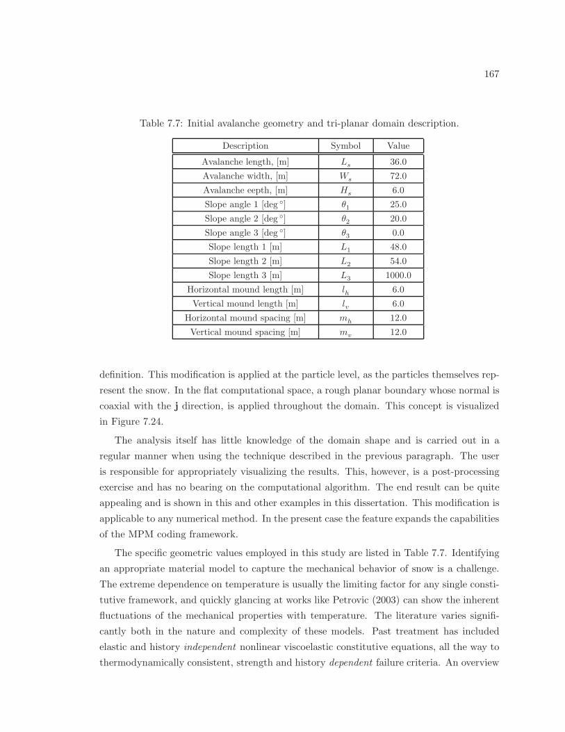
167

Table 7.7: Initial avalanche geometry and tri-planar domain description.

Description Symbol Value

Avalanche length, [m] Ls 36.0

Avalanche width, [m] Ws 72.0

Avalanche eepth, [m] Hs 6.0

Slope angle 1 [deg ] θ1 25.0

Slope angle 2 [deg ] θ2 20.0

Slope angle 3 [deg ] θ3 0.0

Slope length 1 [m] L1 48.0

Slope length 2 [m] L2 54.0

Slope length 3 [m] L3 1000.0

Horizontal mound length [m] lh 6.0

Vertical mound length [m] lv 6.0

Horizontal mound spacing [m] mh 12.0

Vertical mound spacing [m] mv 12.0

definition. This modification is applied at the particle level, as the particles themselves rep-

resent the snow. In the flat computational space, a rough planar boundary whose normal is

coaxial with the j direction, is applied throughout the domain. This concept is visualized

in Figure 7.24.

The analysis itself has little knowledge of the domain shape and is carried out in a

regular manner when using the technique described in the previous paragraph. The user

is responsible for appropriately visualizing the results. This, however, is a post-processing

exercise and has no bearing on the computational algorithm. The end result can be quite

appealing and is shown in this and other examples in this dissertation. This modification is

applicable to any numerical method. In the present case the feature expands the capabilities

of the MPM coding framework.

The specific geometric values employed in this study are listed in Table 7.7. Identifying

an appropriate material model to capture the mechanical behavior of snow is a challenge.

The extreme dependence on temperature is usually the limiting factor for any single consti-

tutive framework, and quickly glancing at works like Petrovic (2003) can show the inherent

fluctuations of the mechanical properties with temperature. The literature varies signifi-

cantly both in the nature and complexity of these models. Past treatment has included

elastic and history independent nonlinear viscoelastic constitutive equations, all the way to

thermodynamically consistent, strength and history dependent failure criteria. An overview

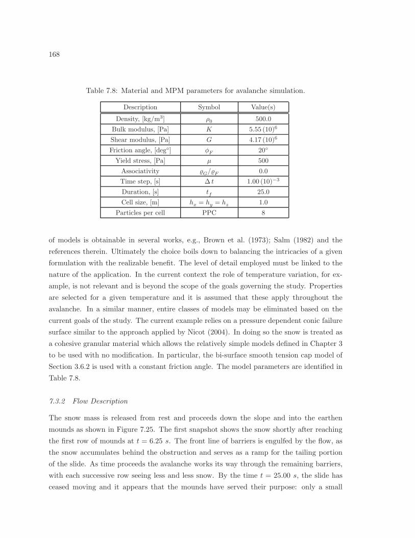
168

Table 7.8: Material and MPM parameters for avalanche simulation.

Description Symbol Value(s)

Density, [kg/m3] ρ0 500.0

Bulk modulus, [Pa] K 5.55 (10)6

Shear modulus, [Pa] G 4.17 (10)6

Friction angle, [deg] φF 20

Yield stress, [Pa] µ 500

Associativity G/F 0.0

Time step, [s] ∆ t 1.00 (10)−3

Duration, [s] tf 25.0

Cell size, [m] hx = hy = hz 1.0

Particles per cell PPC 8

of models is obtainable in several works, e.g., Brown et al. (1973); Salm (1982) and the

references therein. Ultimately the choice boils down to balancing the intricacies of a given

formulation with the realizable benefit. The level of detail employed must be linked to the

nature of the application. In the current context the role of temperature variation, for ex-

ample, is not relevant and is beyond the scope of the goals governing the study. Properties

are selected for a given temperature and it is assumed that these apply throughout the

avalanche. In a similar manner, entire classes of models may be eliminated based on the

current goals of the study. The current example relies on a pressure dependent conic failure

surface similar to the approach applied by Nicot (2004). In doing so the snow is treated as

a cohesive granular material which allows the relatively simple models defined in Chapter 3

to be used with no modification. In particular, the bi-surface smooth tension cap model of

Section 3.6.2 is used with a constant friction angle. The model parameters are identified in

Table 7.8.

7.3.2 Flow Description

The snow mass is released from rest and proceeds down the slope and into the earthen

mounds as shown in Figure 7.25. The first snapshot shows the snow shortly after reaching

the first row of mounds at t = 6.25 s. The front line of barriers is engulfed by the flow, as

the snow accumulates behind the obstruction and serves as a ramp for the tailing portion

of the slide. As time proceeds the avalanche works its way through the remaining barriers,

with each successive row seeing less and less snow. By the time t = 25.00 s, the slide has

ceased moving and it appears that the mounds have served their purpose: only a small

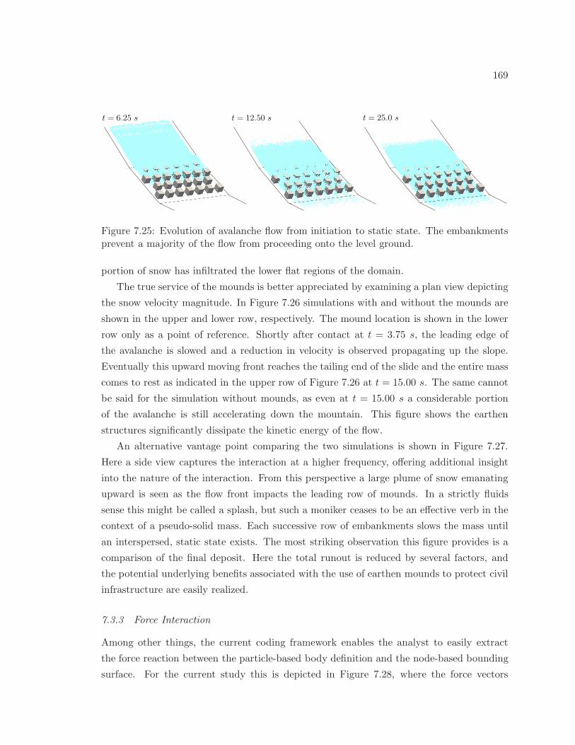
169

t = 6.25 s t = 12.50 s t = 25.0 s

Figure 7.25: Evolution of avalanche flow from initiation to static state. The embankmentsprevent a majority of the flow from proceeding onto the level ground.

portion of snow has infiltrated the lower flat regions of the domain.

The true service of the mounds is better appreciated by examining a plan view depicting

the snow velocity magnitude. In Figure 7.26 simulations with and without the mounds are

shown in the upper and lower row, respectively. The mound location is shown in the lower

row only as a point of reference. Shortly after contact at t = 3.75 s, the leading edge of

the avalanche is slowed and a reduction in velocity is observed propagating up the slope.

Eventually this upward moving front reaches the tailing end of the slide and the entire mass

comes to rest as indicated in the upper row of Figure 7.26 at t = 15.00 s. The same cannot

be said for the simulation without mounds, as even at t = 15.00 s a considerable portion

of the avalanche is still accelerating down the mountain. This figure shows the earthen

structures significantly dissipate the kinetic energy of the flow.

An alternative vantage point comparing the two simulations is shown in Figure 7.27.

Here a side view captures the interaction at a higher frequency, offering additional insight

into the nature of the interaction. From this perspective a large plume of snow emanating

upward is seen as the flow front impacts the leading row of mounds. In a strictly fluids

sense this might be called a splash, but such a moniker ceases to be an effective verb in the

context of a pseudo-solid mass. Each successive row of embankments slows the mass until

an interspersed, static state exists. The most striking observation this figure provides is a

comparison of the final deposit. Here the total runout is reduced by several factors, and

the potential underlying benefits associated with the use of earthen mounds to protect civil

infrastructure are easily realized.

7.3.3 Force Interaction

Among other things, the current coding framework enables the analyst to easily extract

the force reaction between the particle-based body definition and the node-based bounding

surface. For the current study this is depicted in Figure 7.28, where the force vectors

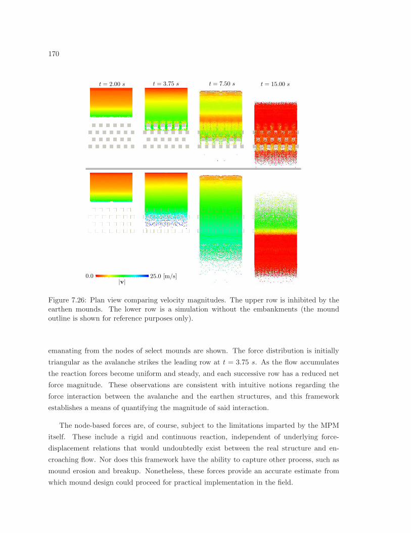
170

0.0 25.0 [m/s]|v|

t = 15.00 st = 7.50 st = 3.75 st = 2.00 s

Figure 7.26: Plan view comparing velocity magnitudes. The upper row is inhibited by theearthen mounds. The lower row is a simulation without the embankments (the moundoutline is shown for reference purposes only).

emanating from the nodes of select mounds are shown. The force distribution is initially

triangular as the avalanche strikes the leading row at t = 3.75 s. As the flow accumulates

the reaction forces become uniform and steady, and each successive row has a reduced net

force magnitude. These observations are consistent with intuitive notions regarding the

force interaction between the avalanche and the earthen structures, and this framework

establishes a means of quantifying the magnitude of said interaction.

The node-based forces are, of course, subject to the limitations imparted by the MPM

itself. These include a rigid and continuous reaction, independent of underlying force-

displacement relations that would undoubtedly exist between the real structure and en-

croaching flow. Nor does this framework have the ability to capture other process, such as

mound erosion and breakup. Nonetheless, these forces provide an accurate estimate from

which mound design could proceed for practical implementation in the field.

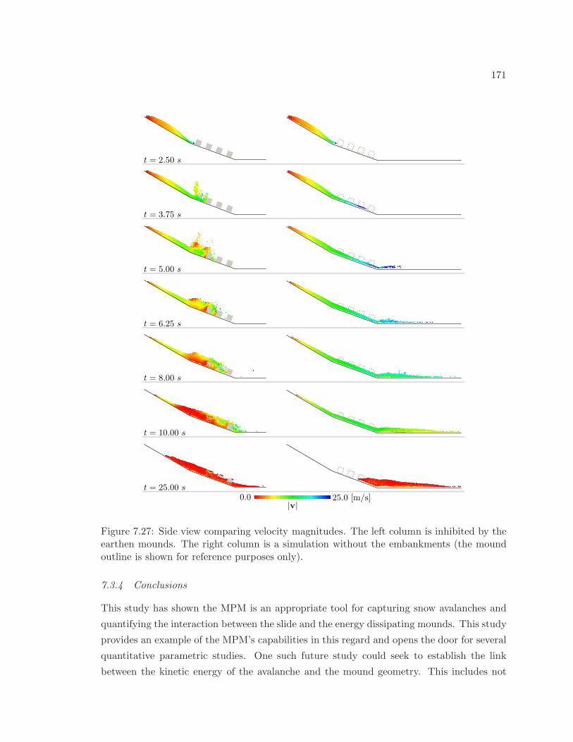
171

0.0 25.0 [m/s]|v|

t = 2.50 s

t = 3.75 s

t = 5.00 s

t = 6.25 s

t = 8.00 s

t = 10.00 s

t = 25.00 s

Figure 7.27: Side view comparing velocity magnitudes. The left column is inhibited by theearthen mounds. The right column is a simulation without the embankments (the moundoutline is shown for reference purposes only).

7.3.4 Conclusions

This study has shown the MPM is an appropriate tool for capturing snow avalanches and

quantifying the interaction between the slide and the energy dissipating mounds. This study

provides an example of the MPM’s capabilities in this regard and opens the door for several

quantitative parametric studies. One such future study could seek to establish the link

between the kinetic energy of the avalanche and the mound geometry. This includes not

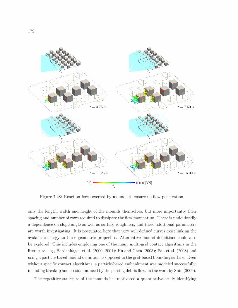
172

100.0 [kN]0.0|f r|

t = 3.75 s t = 7.50 s

t = 11.25 s t = 15.00 s

Figure 7.28: Reaction force exerted by mounds to ensure no flow penetration.

only the length, width and height of the mounds themselves, but more importantly their

spacing and number of rows required to dissipate the flow momentum. There is undoubtedly

a dependence on slope angle as well as surface roughness, and these additional parameters

are worth investigating. It is postulated here that very well defined curves exist linking the

avalanche energy to these geometric properties. Alternative mound definitions could also

be explored. This includes employing one of the many multi-grid contact algorithms in the

literature, e.g., Bardenhagen et al. (2000, 2001); Hu and Chen (2003); Pan et al. (2008) and

using a particle-based mound definition as opposed to the grid-based bounding surface. Even

without specific contact algorithms, a particle-based embankment was modeled successfully,

including breakup and erosion induced by the passing debris flow, in the work by Shin (2009).

The repetitive structure of the mounds has motivated a quantitative study identifying

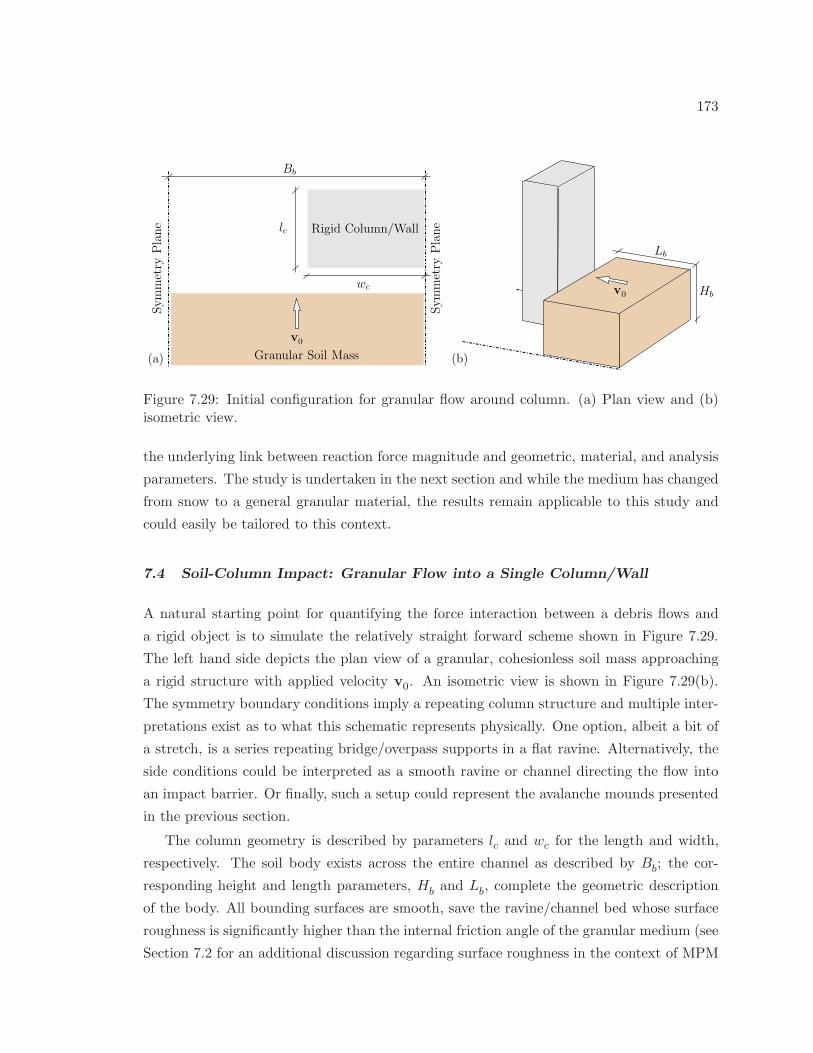
173

Bb

wc

Lb

lc

Hb

(a)

Symmetry

Plane

Symmetry

Plane

(b)

Rigid Column/Wall

v0

v0

Granular Soil Mass

Figure 7.29: Initial configuration for granular flow around column. (a) Plan view and (b)isometric view.

the underlying link between reaction force magnitude and geometric, material, and analysis

parameters. The study is undertaken in the next section and while the medium has changed

from snow to a general granular material, the results remain applicable to this study and

could easily be tailored to this context.

7.4 Soil-Column Impact: Granular Flow into a Single Column/Wall

A natural starting point for quantifying the force interaction between a debris flows and

a rigid object is to simulate the relatively straight forward scheme shown in Figure 7.29.

The left hand side depicts the plan view of a granular, cohesionless soil mass approaching

a rigid structure with applied velocity v0. An isometric view is shown in Figure 7.29(b).

The symmetry boundary conditions imply a repeating column structure and multiple inter-

pretations exist as to what this schematic represents physically. One option, albeit a bit of

a stretch, is a series repeating bridge/overpass supports in a flat ravine. Alternatively, the

side conditions could be interpreted as a smooth ravine or channel directing the flow into

an impact barrier. Or finally, such a setup could represent the avalanche mounds presented

in the previous section.

The column geometry is described by parameters lc and wc for the length and width,

respectively. The soil body exists across the entire channel as described by Bb; the cor-

responding height and length parameters, Hb and Lb, complete the geometric description

of the body. All bounding surfaces are smooth, save the ravine/channel bed whose surface

roughness is significantly higher than the internal friction angle of the granular medium (see

Section 7.2 for an additional discussion regarding surface roughness in the context of MPM

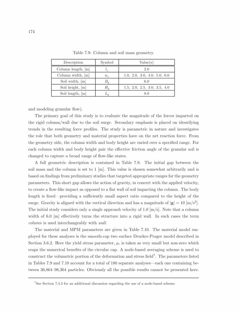
174

Table 7.9: Column and soil mass geometry.

Description Symbol Value(s)

Column length, [m] lc 2.0

Column width, [m] wc 1.0, 2.0, 3.0, 4.0, 5.0, 6.0

Soil width, [m] Bb 6.0

Soil height, [m] Hb 1.5, 2.0, 2.5, 3.0, 3.5, 4.0

Soil length, [m] Lb 8.0

and modeling granular flow).

The primary goal of this study is to evaluate the magnitude of the forces imparted on

the rigid column/wall due to the soil surge. Secondary emphasis is placed on identifying

trends in the resulting force profiles. The study is parametric in nature and investigates

the role that both geometry and material properties have on the net reaction force. From

the geometry side, the column width and body height are varied over a specified range. For

each column width and body height pair the effective friction angle of the granular soil is

changed to capture a broad range of flow-like states.

A full geometric description is contained in Table 7.9. The initial gap between the

soil mass and the column is set to 1 [m]. This value is chosen somewhat arbitrarily and is

based on findings from preliminary studies that targeted appropriate ranges for the geometry

parameters. This short gap allows the action of gravity, in concert with the applied velocity,

to create a flow-like impact as opposed to a flat wall of soil impacting the column. The body

length is fixed—providing a sufficiently small aspect ratio compared to the height of the

surge. Gravity is aligned with the vertical direction and has a magnitude of |g| = 10 [m/s2].

The initial study considers only a single approach velocity of 1.0 [m/s]. Note that a column

width of 6.0 [m] effectively turns the structure into a rigid wall. In such cases the term

column is used interchangeably with wall.

The material and MPM parameters are given in Table 7.10. The material model em-

ployed for these analyses is the smooth-cap two surface Drucker-Prager model described in

Section 3.6.2. Here the yield stress parameter, µ, is taken as very small but non-zero which

reaps the numerical benefits of the circular cap. A node-based averaging scheme is used to

construct the volumetric portion of the deformation and stress field7. The parameters listed

in Tables 7.9 and 7.10 account for a total of 180 separate analyses—each one containing be-

tween 36,864–98,304 particles. Obviously all the possible results cannot be presented here.

7See Section 7.4.3 for an additional discussion regarding the use of a node-based scheme.

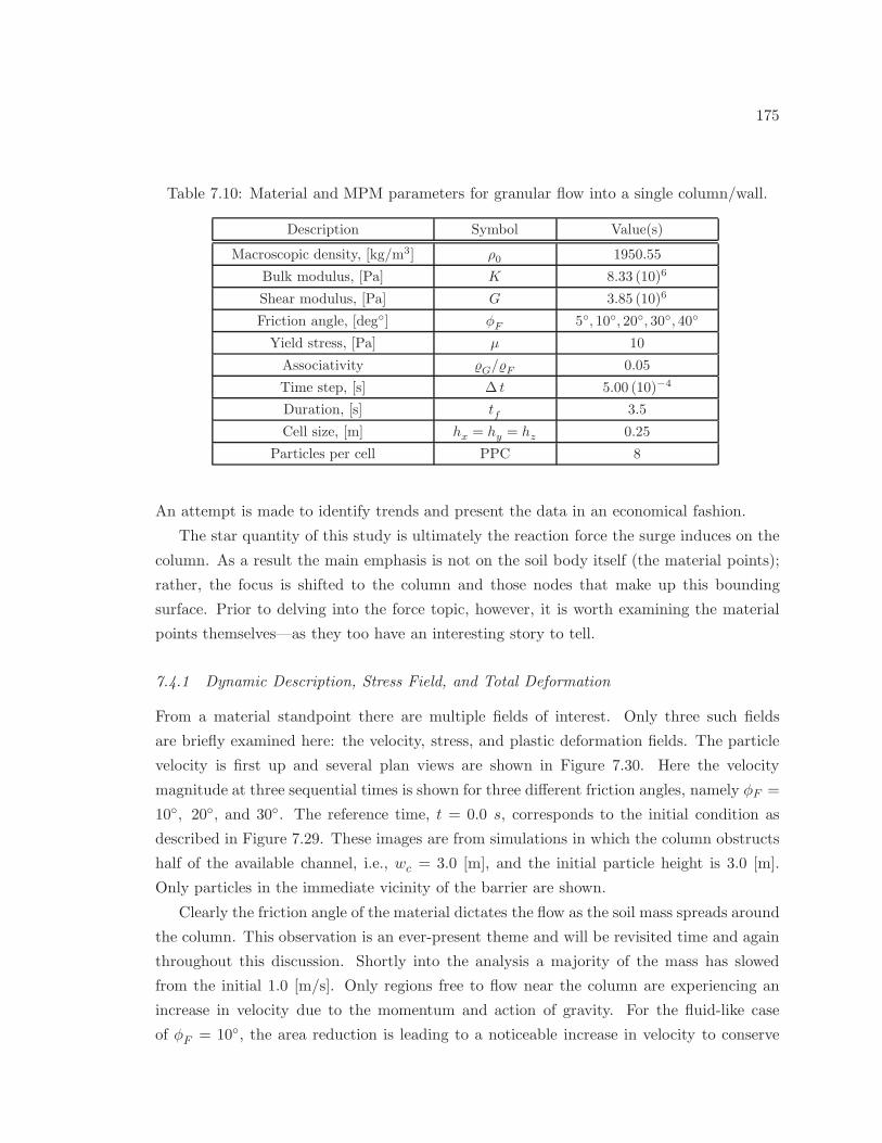
175

Table 7.10: Material and MPM parameters for granular flow into a single column/wall.

Description Symbol Value(s)

Macroscopic density, [kg/m3] ρ0 1950.55

Bulk modulus, [Pa] K 8.33 (10)6

Shear modulus, [Pa] G 3.85 (10)6

Friction angle, [deg] φF 5, 10, 20, 30, 40

Yield stress, [Pa] µ 10

Associativity G/F 0.05

Time step, [s] ∆ t 5.00 (10)−4

Duration, [s] tf 3.5

Cell size, [m] hx = hy = hz 0.25

Particles per cell PPC 8

An attempt is made to identify trends and present the data in an economical fashion.

The star quantity of this study is ultimately the reaction force the surge induces on the

column. As a result the main emphasis is not on the soil body itself (the material points);

rather, the focus is shifted to the column and those nodes that make up this bounding

surface. Prior to delving into the force topic, however, it is worth examining the material

points themselves—as they too have an interesting story to tell.

7.4.1 Dynamic Description, Stress Field, and Total Deformation

From a material standpoint there are multiple fields of interest. Only three such fields

are briefly examined here: the velocity, stress, and plastic deformation fields. The particle

velocity is first up and several plan views are shown in Figure 7.30. Here the velocity

magnitude at three sequential times is shown for three different friction angles, namely φF =

10, 20, and 30. The reference time, t = 0.0 s, corresponds to the initial condition as

described in Figure 7.29. These images are from simulations in which the column obstructs

half of the available channel, i.e., wc = 3.0 [m], and the initial particle height is 3.0 [m].

Only particles in the immediate vicinity of the barrier are shown.

Clearly the friction angle of the material dictates the flow as the soil mass spreads around

the column. This observation is an ever-present theme and will be revisited time and again

throughout this discussion. Shortly into the analysis a majority of the mass has slowed

from the initial 1.0 [m/s]. Only regions free to flow near the column are experiencing an

increase in velocity due to the momentum and action of gravity. For the fluid-like case

of φF = 10, the area reduction is leading to a noticeable increase in velocity to conserve

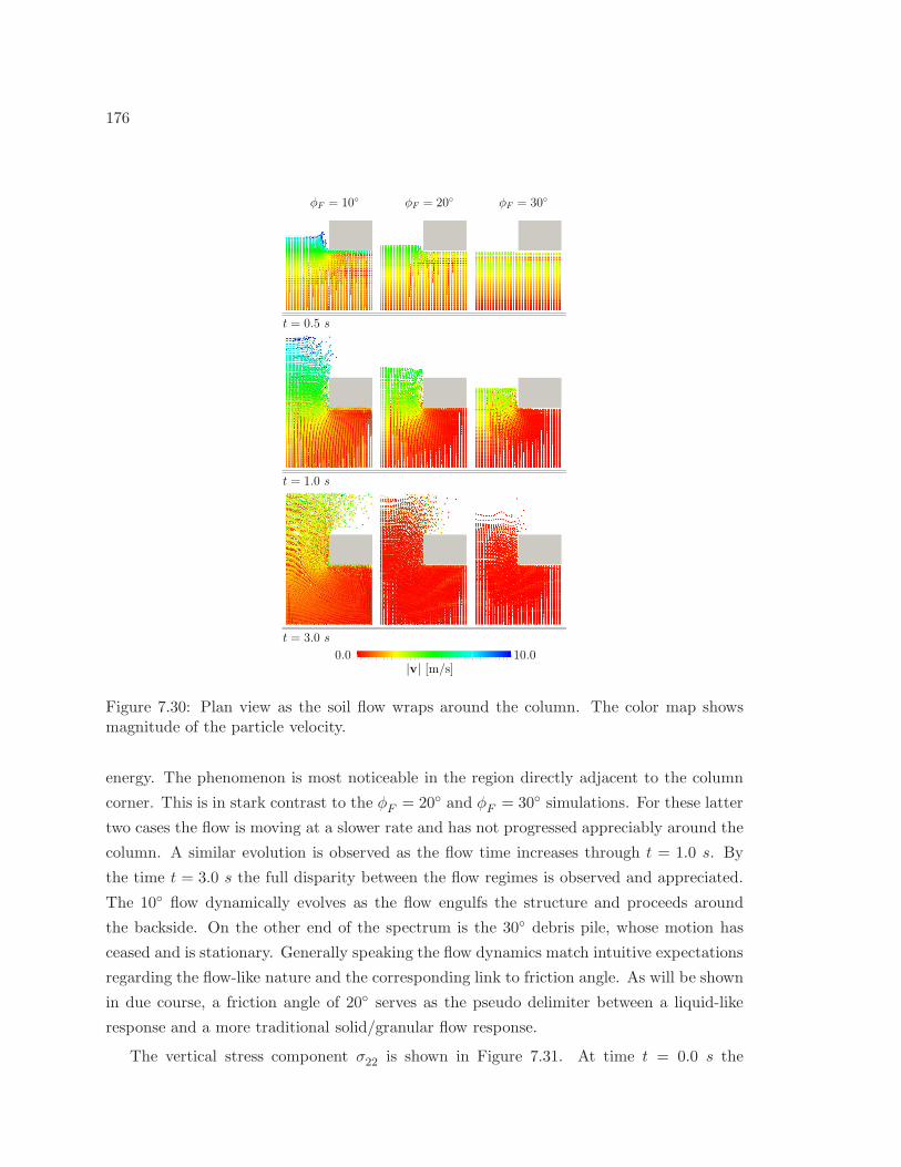
176

t = 1.0 s

t = 3.0 s

t = 0.5 s

φF = 10 φF = 20 φF = 30

|v| [m/s]10.00.0

Figure 7.30: Plan view as the soil flow wraps around the column. The color map showsmagnitude of the particle velocity.

energy. The phenomenon is most noticeable in the region directly adjacent to the column

corner. This is in stark contrast to the φF = 20 and φF = 30 simulations. For these latter

two cases the flow is moving at a slower rate and has not progressed appreciably around the

column. A similar evolution is observed as the flow time increases through t = 1.0 s. By

the time t = 3.0 s the full disparity between the flow regimes is observed and appreciated.

The 10 flow dynamically evolves as the flow engulfs the structure and proceeds around

the backside. On the other end of the spectrum is the 30 debris pile, whose motion has

ceased and is stationary. Generally speaking the flow dynamics match intuitive expectations

regarding the flow-like nature and the corresponding link to friction angle. As will be shown

in due course, a friction angle of 20 serves as the pseudo delimiter between a liquid-like

response and a more traditional solid/granular flow response.

The vertical stress component σ22 is shown in Figure 7.31. At time t = 0.0 s the

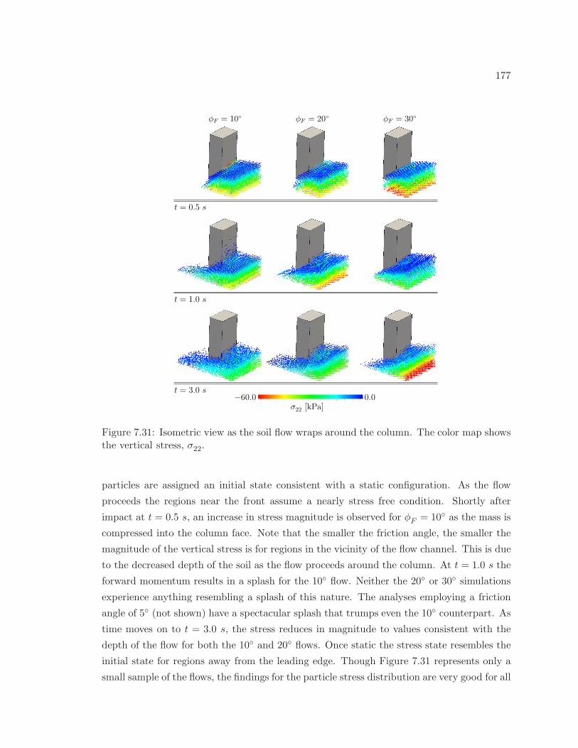
177

t = 1.0 s

t = 3.0 s

φF = 10 φF = 30φF = 20

t = 0.5 s

0.0−60.0σ22 [kPa]

Figure 7.31: Isometric view as the soil flow wraps around the column. The color map showsthe vertical stress, σ22.

particles are assigned an initial state consistent with a static configuration. As the flow

proceeds the regions near the front assume a nearly stress free condition. Shortly after

impact at t = 0.5 s, an increase in stress magnitude is observed for φF = 10 as the mass is

compressed into the column face. Note that the smaller the friction angle, the smaller the

magnitude of the vertical stress is for regions in the vicinity of the flow channel. This is due

to the decreased depth of the soil as the flow proceeds around the column. At t = 1.0 s the

forward momentum results in a splash for the 10 flow. Neither the 20 or 30 simulations

experience anything resembling a splash of this nature. The analyses employing a friction

angle of 5 (not shown) have a spectacular splash that trumps even the 10 counterpart. As

time moves on to t = 3.0 s, the stress reduces in magnitude to values consistent with the

depth of the flow for both the 10 and 20 flows. Once static the stress state resembles the

initial state for regions away from the leading edge. Though Figure 7.31 represents only a

small sample of the flows, the findings for the particle stress distribution are very good for all

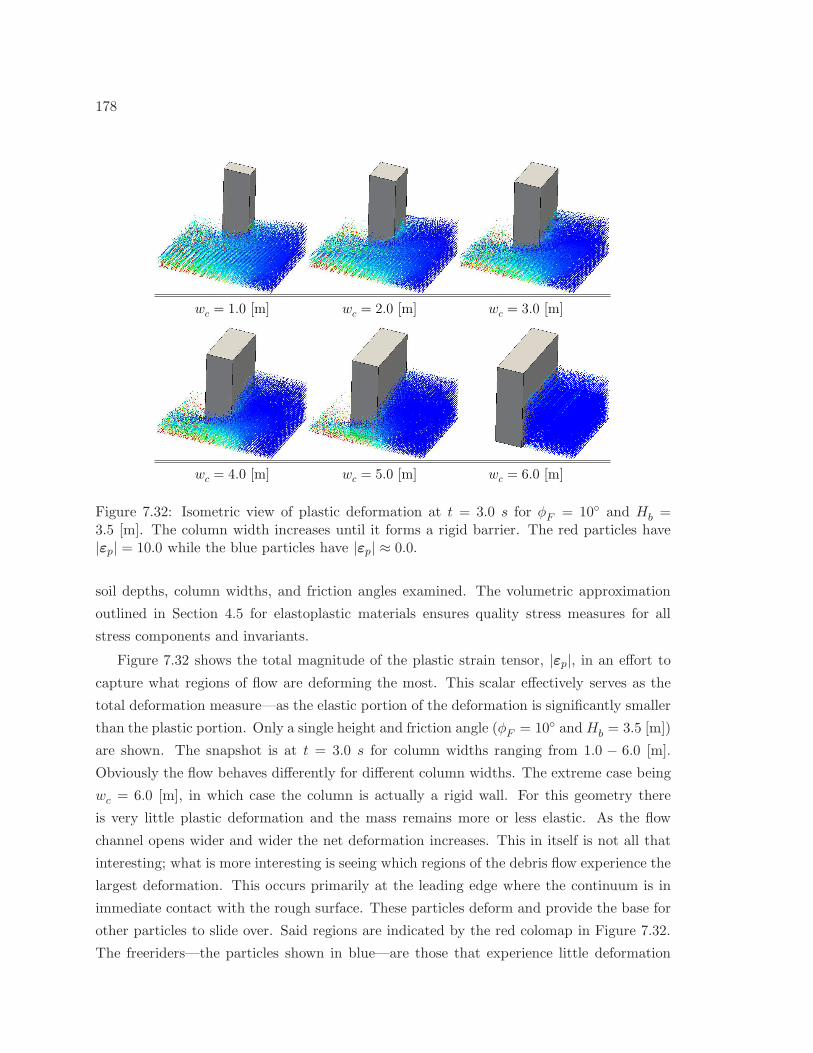
178

wc = 1.0 [m] wc = 2.0 [m] wc = 3.0 [m]

wc = 4.0 [m] wc = 5.0 [m] wc = 6.0 [m]

Figure 7.32: Isometric view of plastic deformation at t = 3.0 s for φF = 10 and Hb =3.5 [m]. The column width increases until it forms a rigid barrier. The red particles have|εp| = 10.0 while the blue particles have |εp| ≈ 0.0.

soil depths, column widths, and friction angles examined. The volumetric approximation

outlined in Section 4.5 for elastoplastic materials ensures quality stress measures for all

stress components and invariants.

Figure 7.32 shows the total magnitude of the plastic strain tensor, |εp|, in an effort to

capture what regions of flow are deforming the most. This scalar effectively serves as the

total deformation measure—as the elastic portion of the deformation is significantly smaller

than the plastic portion. Only a single height and friction angle (φF = 10 andHb = 3.5 [m])

are shown. The snapshot is at t = 3.0 s for column widths ranging from 1.0 − 6.0 [m].

Obviously the flow behaves differently for different column widths. The extreme case being

wc = 6.0 [m], in which case the column is actually a rigid wall. For this geometry there

is very little plastic deformation and the mass remains more or less elastic. As the flow

channel opens wider and wider the net deformation increases. This in itself is not all that

interesting; what is more interesting is seeing which regions of the debris flow experience the

largest deformation. This occurs primarily at the leading edge where the continuum is in

immediate contact with the rough surface. These particles deform and provide the base for

other particles to slide over. Said regions are indicated by the red colomap in Figure 7.32.

The freeriders—the particles shown in blue—are those that experience little deformation

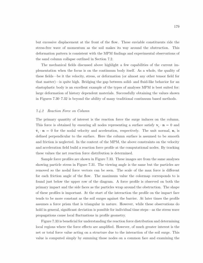
179

but excessive displacement at the front of the flow. These enviable constituents ride the

stress-free wave of momentum as the soil makes its way around the obstruction. This

deformation pattern is consistent with the MPM findings and experimental observations of

the sand column collapse outlined in Section 7.2.

The mechanical fields discussed above highlight a few capabilities of the current im-

plementation when the focus is on the continuum body itself. As a whole, the quality of

these fields—be it the velocity, stress, or deformation (or almost any other tensor field for

that matter)—is quite high. Bridging the gap between solid- and fluid-like behavior for an

elastoplastic body is an excellent example of the types of analyses MPM is best suited for:

large deformation of history dependent materials. Successfully obtaining the values shown

in Figures 7.30–7.32 is beyond the ability of many traditional continuum based methods.

7.4.2 Reaction Force on Column

The primary quantity of interest is the reaction force the surge induces on the column.

This force is obtained by ensuring all nodes representing a surface satisfy vi · n = 0 and

vi · n = 0 for the nodal velocity and acceleration, respectively. The unit normal, n, is

defined perpendicular to the surface. Here the column surface is assumed to be smooth

and friction is neglected. In the context of the MPM, the above constraints on the velocity

and acceleration field build a reaction force profile at the computational nodes. By tracking

these values the net reaction force distribution is determined.

Sample force profiles are shown in Figure 7.33. These images are from the same analyses

showing particle stress in Figure 7.31. The viewing angle is the same but the particles are

removed so the nodal force vectors can be seen. The scale of the max force is different

for each friction angle of the flow. The maximum value the colormap corresponds to is

found just below the upper row of the diagram. A force profile is observed on both the

primary impact and the side faces as the particles wrap around the obstruction. The shape

of these profiles is important. At the start of the interaction the profile on the impact face

tends to be more constant as the soil surges against the barrier. At later times the profile

assumes a force prism that is triangular in nature. However, while these observations do

hold in general, significant deviation is possible for individual time steps—as the stress wave

propagations cause local fluctuations in profile geometry.

Figure 7.33 is beneficial for understanding the reaction force distribution and determining

local regions where the force effects are amplified. However, of much greater interest is the

net or total force value acting on a structure due to the interaction of the soil surge. This

value is computed simply by summing those nodes on a common face and examining the

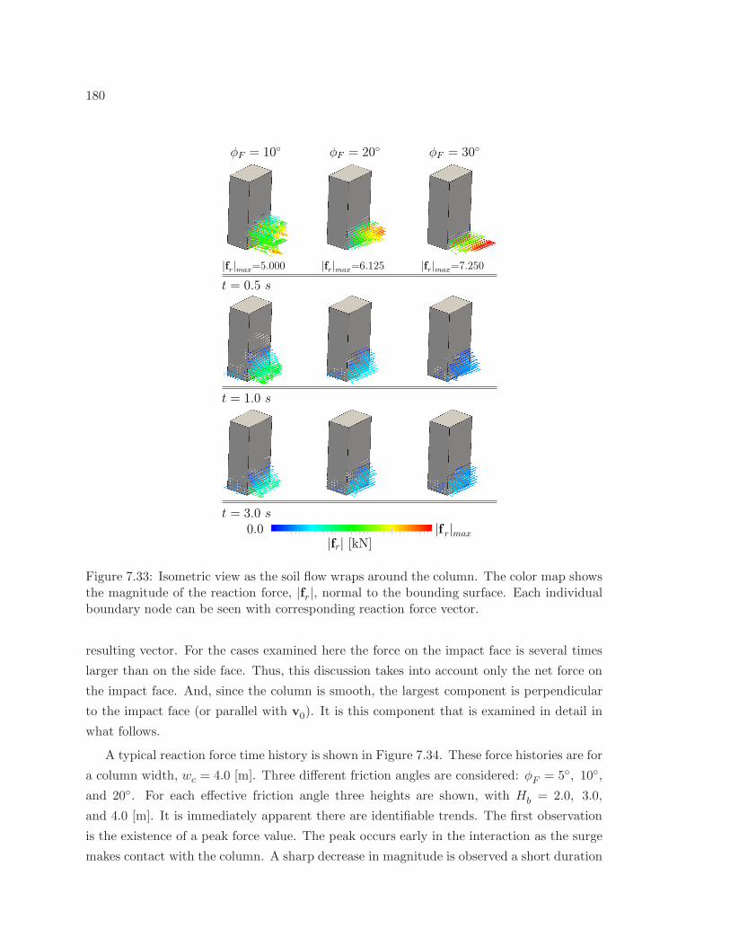
180

|f r|max0.0|fr| [kN]

φF = 10 φF = 20 φF = 30

|fr|max=5.000 |fr|max=6.125 |fr|max=7.250

t = 1.0 s

t = 0.5 s

t = 3.0 s

Figure 7.33: Isometric view as the soil flow wraps around the column. The color map showsthe magnitude of the reaction force, |fr|, normal to the bounding surface. Each individualboundary node can be seen with corresponding reaction force vector.

resulting vector. For the cases examined here the force on the impact face is several times

larger than on the side face. Thus, this discussion takes into account only the net force on

the impact face. And, since the column is smooth, the largest component is perpendicular

to the impact face (or parallel with v0). It is this component that is examined in detail in

what follows.

A typical reaction force time history is shown in Figure 7.34. These force histories are for

a column width, wc = 4.0 [m]. Three different friction angles are considered: φF = 5, 10,

and 20. For each effective friction angle three heights are shown, with Hb = 2.0, 3.0,

and 4.0 [m]. It is immediately apparent there are identifiable trends. The first observation

is the existence of a peak force value. The peak occurs early in the interaction as the surge

makes contact with the column. A sharp decrease in magnitude is observed a short duration

181

0.0 2.0 3.01.0 0.0 2.0 3.01.0 0.0 2.0 3.01.0

Hb = 2.0 [m] Hb = 3.0 [m] Hb = 4.0 [m]

800

600

400

200

1600

1400

1200

1000

ReactionForce[kN]

t [s]

φF = 20φF = 10φF = 5

Figure 7.34: Net reaction force as a function of time for wc = 4.0 [m]. Positive valueindicates force directed against flow.

after the initial peak. As time proceeds the magnitude of the force diminishes until the value

becomes more or less constant. This constant magnitude is referred to here as the steady

state force. Although the force is constant the flow may still be moving as the velocity

profiles in Figure 7.30 indicates. These two key forces—the peak and steady state—are

observed for all soil heights, columns widths, and material parameters considered in this

study.

Obtaining an accurate peak force is not entirely straight forward. The nature of the

implementation only records snapshots of the simulation at user-specified time intervals.

Unfortunately, it is quite unlikely the peak force experienced by the surface will occur

precisely during a time step in which data is being collected. The boundary class is modified

to collect the largest magnitude force exerted during a given analysis in order to resolve this

issue. Every boundary instance (each flat surface in this case) keeps track of the total sum

of all nodes it contains and the maximum over the entire interval is isolated and reported.

Thus, peak force values presented here are often slightly larger than the force history plots

indicate.

Collecting a reasonable steady state force also requires attention. While the existence

of a constant, steady state force is discernible from Figure 7.34, there are in fact small

fluctuations due to stress wave propagation in the medium. To combat these fluctuations a

modified running average is used. The average window (anywhere from 1-3 sample steps)

is computed to obtain an average profile. This profile is then modified such that the im-

pulse from the original signal is conserved. The final result is a very close fit to the data

that also maintains the momentum from the original signal. This scheme is highlighted

in Figure 7.35. Here the dashed lines represent the original signal and the solid line is the

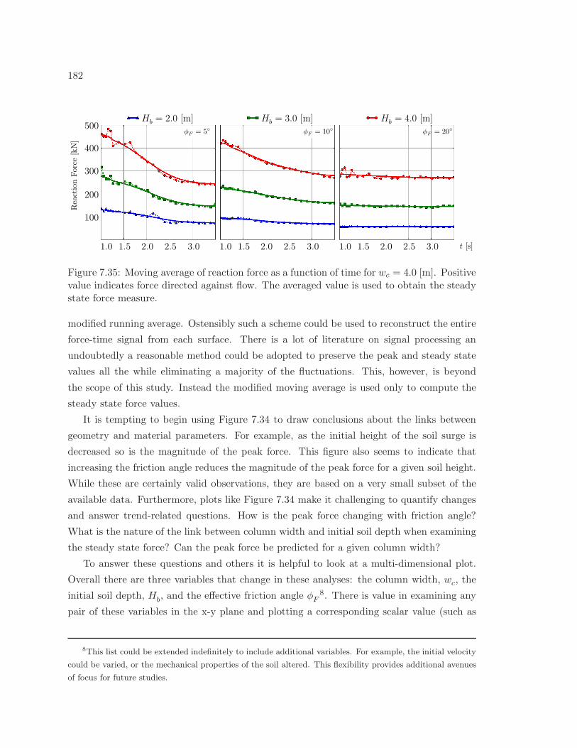
182

Hb = 2.0 [m] Hb = 3.0 [m] Hb = 4.0 [m]

1.0 2.0 3.02.51.51.0 2.0 3.02.51.5 1.0 2.0 3.02.51.5 t [s]

100

200

300

400

500

ReactionForce[kN]

φF = 20φF = 10φF = 5

Figure 7.35: Moving average of reaction force as a function of time for wc = 4.0 [m]. Positivevalue indicates force directed against flow. The averaged value is used to obtain the steadystate force measure.

modified running average. Ostensibly such a scheme could be used to reconstruct the entire

force-time signal from each surface. There is a lot of literature on signal processing an

undoubtedly a reasonable method could be adopted to preserve the peak and steady state

values all the while eliminating a majority of the fluctuations. This, however, is beyond

the scope of this study. Instead the modified moving average is used only to compute the

steady state force values.

It is tempting to begin using Figure 7.34 to draw conclusions about the links between

geometry and material parameters. For example, as the initial height of the soil surge is

decreased so is the magnitude of the peak force. This figure also seems to indicate that

increasing the friction angle reduces the magnitude of the peak force for a given soil height.

While these are certainly valid observations, they are based on a very small subset of the

available data. Furthermore, plots like Figure 7.34 make it challenging to quantify changes

and answer trend-related questions. How is the peak force changing with friction angle?

What is the nature of the link between column width and initial soil depth when examining

the steady state force? Can the peak force be predicted for a given column width?

To answer these questions and others it is helpful to look at a multi-dimensional plot.

Overall there are three variables that change in these analyses: the column width, wc, the

initial soil depth, Hb, and the effective friction angle φF8. There is value in examining any

pair of these variables in the x-y plane and plotting a corresponding scalar value (such as

8This list could be extended indefinitely to include additional variables. For example, the initial velocity

could be varied, or the mechanical properties of the soil altered. This flexibility provides additional avenues

of focus for future studies.

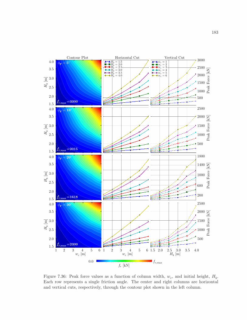
183

1 2 3 4 5 6Column Width

1.5

2.0

2.5

3.0

3.5

4.0

Initial Heigh

t

0.00

398.42

796.83

1195.25

1593.66

1992.08

2390.49

2788.91

Peak Force

1 2 3 4 5 6Column Width

1.5

2.0

2.5

3.0

3.5

4.0

Initial Heigh

t

0.00

268.82

537.64

806.46

1075.29

1344.11

1612.93

1881.75

Peak Force

1 2 3 4 5 6Column Width

1.5

2.0

2.5

3.0

3.5

4.0

Initial Heigh

t

0.00

215.71

431.43

647.14

862.86

1078.57

1294.29

1510.00

Peak Force

1 2 3 4 5 6Column Width

1.5

2.0

2.5

3.0

3.5

4.0

Initial Heigh

t

0.00

306.89

613.77

920.66

1227.54

1534.43

1841.31

2148.20

Peak Force

1.5

2.0

3.0

3.5

2.5

4.0

1.5

2.0

3.0

3.5

2.5

4.0

1.5

2.0

3.0

3.5

2.5

4.0

1.5

2.0

3.0

3.5

2.5

4.0

Hb[m

]H

b[m

]H

b[m

]H

b[m

]

1800

1000

1400

600

200

2500

2000

1500

1000

500

2500

2000

1500

1000

3000

500

31 4 5 62 31 4 52 6 1.5 2.0 3.0 3.5 4.02.5wc [m]wc [m] Hb [m]

PeakForce

[kN]

PeakForce

[kN]

PeakForce

[kN]

PeakForce

[kN]

2500

2000

1500

1000

500

Contour Plot Horizontal Cut Vertical Cut

φF = 30

φF = 20

φF = 10

φF = 5

fr,max0.0fr [kN]

fr,max =3000

fr,max =2015

fr,max =1618

fr,max =2300

Hb = 1.5Hb = 2.0Hb = 2.5Hb = 3.0Hb = 3.5Hb = 4.0

wc = 1wc = 2wc = 3wc = 4wc = 5wc = 6

Figure 7.36: Peak force values as a function of column width, wc, and initial height, Hb.Each row represents a single friction angle. The center and right columns are horizontaland vertical cuts, respectively, through the contour plot shown in the left column.

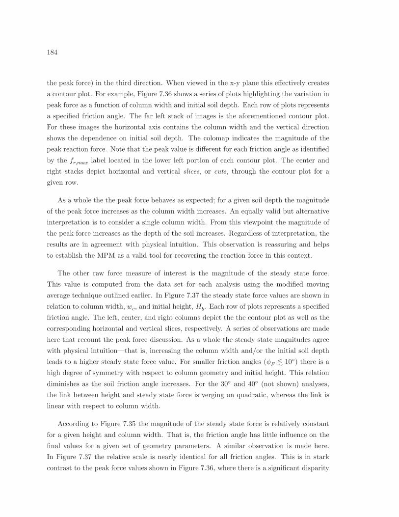
184

the peak force) in the third direction. When viewed in the x-y plane this effectively creates

a contour plot. For example, Figure 7.36 shows a series of plots highlighting the variation in

peak force as a function of column width and initial soil depth. Each row of plots represents

a specified friction angle. The far left stack of images is the aforementioned contour plot.

For these images the horizontal axis contains the column width and the vertical direction

shows the dependence on initial soil depth. The colomap indicates the magnitude of the

peak reaction force. Note that the peak value is different for each friction angle as identified

by the fr,max label located in the lower left portion of each contour plot. The center and

right stacks depict horizontal and vertical slices, or cuts, through the contour plot for a

given row.

As a whole the the peak force behaves as expected; for a given soil depth the magnitude

of the peak force increases as the column width increases. An equally valid but alternative

interpretation is to consider a single column width. From this viewpoint the magnitude of

the peak force increases as the depth of the soil increases. Regardless of interpretation, the

results are in agreement with physical intuition. This observation is reassuring and helps

to establish the MPM as a valid tool for recovering the reaction force in this context.

The other raw force measure of interest is the magnitude of the steady state force.

This value is computed from the data set for each analysis using the modified moving

average technique outlined earlier. In Figure 7.37 the steady state force values are shown in

relation to column width, wc, and initial height, Hb. Each row of plots represents a specified

friction angle. The left, center, and right columns depict the the contour plot as well as the

corresponding horizontal and vertical slices, respectively. A series of observations are made

here that recount the peak force discussion. As a whole the steady state magnitudes agree

with physical intuition—that is, increasing the column width and/or the initial soil depth

leads to a higher steady state force value. For smaller friction angles (φF . 10) there is a

high degree of symmetry with respect to column geometry and initial height. This relation

diminishes as the soil friction angle increases. For the 30 and 40 (not shown) analyses,

the link between height and steady state force is verging on quadratic, whereas the link is

linear with respect to column width.

According to Figure 7.35 the magnitude of the steady state force is relatively constant

for a given height and column width. That is, the friction angle has little influence on the

final values for a given set of geometry parameters. A similar observation is made here.

In Figure 7.37 the relative scale is nearly identical for all friction angles. This is in stark

contrast to the peak force values shown in Figure 7.36, where there is a significant disparity

185

1 2 3 4 5 6Column Width

1.5

2.0

2.5

3.0

3.5

4.0

Initial Heigh

t

0.00

73.73

147.45

221.18

294.90

368.63

442.36

516.08

Stea

dy State Force

1 2 3 4 5 6Column Width

1.5

2.0

2.5

3.0

3.5

4.0

Initial Heigh

t

0.00

81.49

162.99

244.48

325.97

407.46

488.96

570.45

Stea

dy State Force

1 2 3 4 5 6Column Width

1.5

2.0

2.5

3.0

3.5

4.0

Initial Heigh

t

0.00

62.32

124.64

186.96

249.28

311.60

373.92

436.23

Stea

dy State Force

1 2 3 4 5 6Column Width

1.5

2.0

2.5

3.0

3.5

4.0

Initial Heigh

t

0.00

49.14

98.29

147.43

196.58

245.72

294.87

344.01

Stea

dy State Force

1.5

2.0

3.0

3.5

2.5

4.0

1.5

2.0

3.0

3.5

2.5

4.0

1.5

2.0

3.0

3.5

2.5

4.0

1.5

2.0

3.0

3.5

2.5

4.0

Hb[m

]H

b[m

]H

b[m

]H

b[m

]

31 4 5 62 31 4 52 6 1.5 2.0 3.0 3.5 4.02.5wc [m]wc [m] Hb [m]

Contour Plot Horizontal Cut Vertical Cut

Stead

yState

Force

[kN]

Stead

yState

Force

[kN]

Stead

yState

Force

[kN]

Stead

yState

Force

[kN]

100

600

500

400

300

200

700

500

600

400

300

200

100

500

300

200

100

400

450400

350

300

250

200

150

100

φF = 30

φF = 20

φF = 10

φF = 5

fr,max0.0fr [kN]

fr,max =553

fr,max =612

fr,max =468

fr,max =464

Hb = 1.5Hb = 2.0Hb = 2.5Hb = 3.0Hb = 3.5Hb = 4.0

wc = 1wc = 2wc = 3wc = 4wc = 5wc = 6

Figure 7.37: Steady state force values as a function of column width, wc, and initial height,Hb. Each row represents a single friction angle. The center and right columns are horizontaland vertical cuts, respectively, through the contour plot shown in the left column.

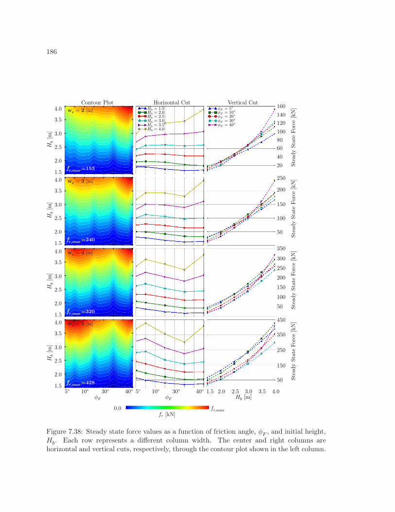
186

5 10 15 20 25 30 35 40Friction Angle

1.5

2.0

2.5

3.0

3.5

4.0

Initial Heigh

t

0.00

31.86

63.72

95.58

127.43

159.29

191.15

223.01

Stea

dy State Force

5 10 15 20 25 30 35 40Friction Angle

1.5

2.0

2.5

3.0

3.5

4.0

Initial Heigh

t

0.00

42.41

84.82

127.24

169.65

212.06

254.47

296.88

Stea

dy State Force

5 10 15 20 25 30 35 40Friction Angle

1.5

2.0

2.5

3.0

3.5

4.0

Initial Heigh

t

0.00

57.03

114.07

171.10

228.13

285.16

342.20

399.23

Stea

dy State Force

5 10 15 20 25 30 35 40Friction Angle

1.5

2.0

2.5

3.0

3.5

4.0

Initial Heigh

t

0.0

20.4

40.8

61.2

81.6

102.0

122.4

142.8

Stea

dy State Force

Hb[m

]H

b[m

]H

b[m

]H

b[m

]

1.5 2.0 3.0 3.5 4.02.5

Contour Plot Horizontal Cut Vertical Cut

φF φF

1.5

2.0

3.0

3.5

2.5

4.0

1.5

2.0

3.0

3.5

2.5

4.0

1.5

2.0

3.0

3.5

2.5

4.0

1.5

2.0

3.0

3.5

2.5

4.0 160

140

120

100

60

80

40

20

250

50

100

150

200

50

250

350

150

450

Hb [m]

Stead

yState

Force

[kN]

Stead

yState

Force

[kN]

Stead

yState

Force

[kN]

Stead

yState

Force

[kN]

100

150

200

250

50

300

350

φF = 5wc = 2 [m]

wc = 5 [m]

wc = 4 [m]

wc = 3 [m]

φF = 10

φF = 20

φF = 30

φF = 40

fr,max0.0fr [kN]

fr,max =153

fr,max =240

fr,max =320

fr,max =428

5 510 1030 3040 40

Hb = 1.5Hb = 2.0Hb = 2.5Hb = 3.0Hb = 3.5Hb = 4.0

Figure 7.38: Steady state force values as a function of friction angle, φF , and initial height,Hb. Each row represents a different column width. The center and right columns arehorizontal and vertical cuts, respectively, through the contour plot shown in the left column.

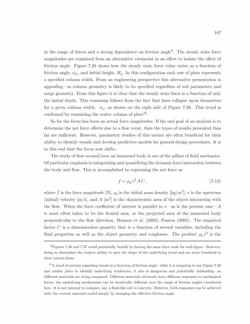
187

in the range of forces and a strong dependence on friction angle9. The steady state force

magnitudes are examined from an alternative viewpoint in an effort to isolate the effect of

friction angle. Figure 7.38 shows how the steady state force value varies as a function of

friction angle, φF , and initial height, Hb. In this configuration each row of plots represents

a specified column width. From an engineering perspective this alternative presentation is

appealing—as column geometry is likely to be specified regardless of soil parameters and

surge geometry. From this figure it is clear that the steady state force is a function of only

the initial depth. This reasoning follows from the fact that lines collapse upon themselves

for a given column width, wc, as shown on the right side of Figure 7.38. This trend is

confirmed by examining the center column of plots10.

So far the focus has been on actual force magnitudes. If the end goal of an analysis is to

determine the net force effects due to a flow event, then the types of results presented thus

far are sufficient. However, parametric studies of this nature are often beneficial for their

ability to identify trends and develop predictive models for general design procedures. It is

to this end that the focus now shifts.

The study of flow around/over an immersed body is one of the pillars of fluid mechanics.

Of particular emphasis is categorizing and quantifying the dynamic force interaction between

the body and flow. This is accomplished by expressing the net force as

f = ρ0 v2AC , (7.13)

where f is the force magnitude [N], ρ0 is the initial mass density [kg/m3], v is the upstream

(initial) velocity [m/s], and A [m2] is the characteristic area of the object interacting with

the flow. When the force coefficient of interest is parallel to v—as is the present case—A

is most often taken to be the frontal area, or the projected area of the immersed body

perpendicular to the flow direction, Munson et al. (2002); Panton (2005). The empirical

factor C is a dimensionless quantity that is a function of several variables, including the

fluid properties as well as the object geometry and roughness. The product ρ0 v2 is the

9Figures 7.36 and 7.37 could potentially benefit by having the same force scale for each figure. However,

doing so diminishes the readers ability to spot the shape of the underlying trend and are more beneficial in

their current form.

10A word of caution regarding trends as a function of friction angle: while it is tempting to use Figure 7.38

and similar plots to identify underlying tendencies, it also is dangerous and potentially misleading—as

different materials are being compared. Different materials obviously have different responses to mechanical

forces; the underlying mechanisms can be drastically different over the range of friction angles considered

here. It is not rational to compare, say, a fluid-like soil to concrete. However, both responses can be achieved

with the current material model simply by changing the effective friction angle.

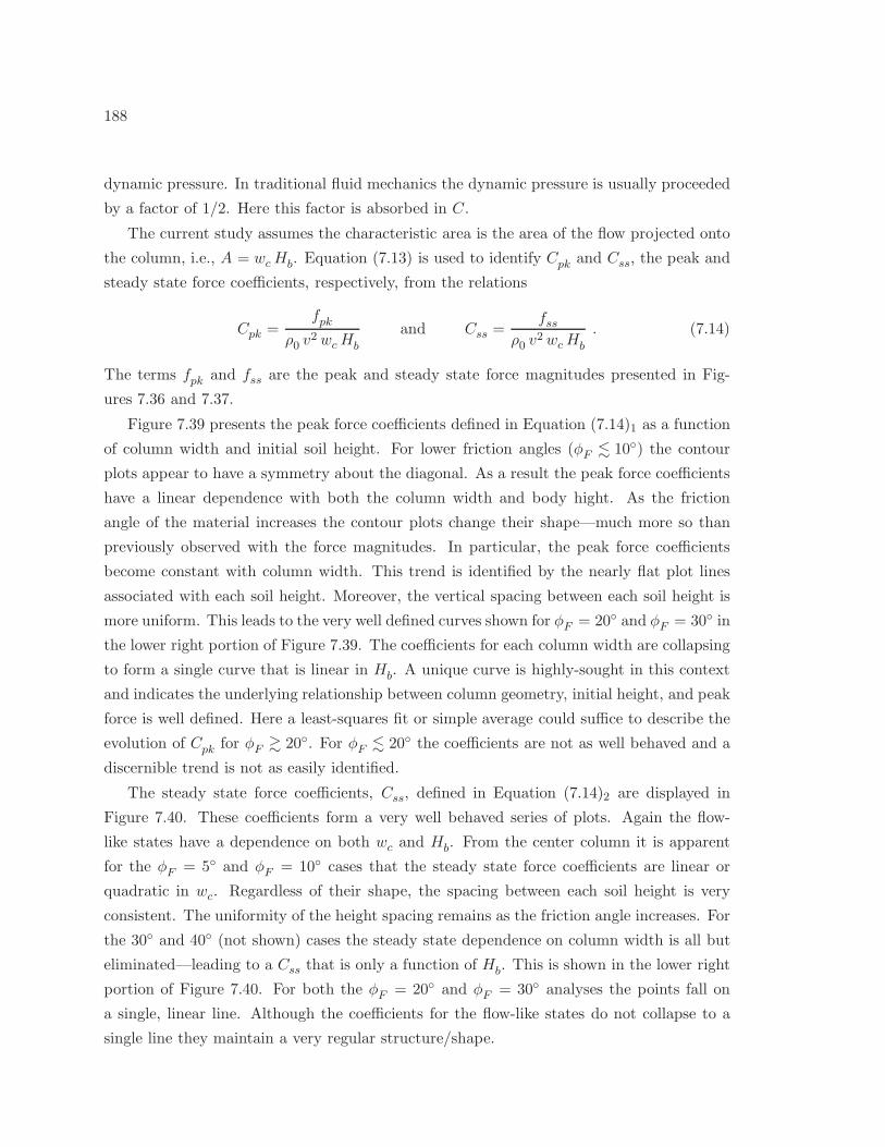
188

dynamic pressure. In traditional fluid mechanics the dynamic pressure is usually proceeded

by a factor of 1/2. Here this factor is absorbed in C.

The current study assumes the characteristic area is the area of the flow projected onto

the column, i.e., A = wcHb. Equation (7.13) is used to identify Cpk and Css, the peak and

steady state force coefficients, respectively, from the relations

Cpk =fpk

ρ0 v2 wcHb

and Css =fss

ρ0 v2wcHb

. (7.14)

The terms fpk and fss are the peak and steady state force magnitudes presented in Fig-

ures 7.36 and 7.37.

Figure 7.39 presents the peak force coefficients defined in Equation (7.14)1 as a function

of column width and initial soil height. For lower friction angles (φF . 10) the contour

plots appear to have a symmetry about the diagonal. As a result the peak force coefficients

have a linear dependence with both the column width and body hight. As the friction

angle of the material increases the contour plots change their shape—much more so than

previously observed with the force magnitudes. In particular, the peak force coefficients

become constant with column width. This trend is identified by the nearly flat plot lines

associated with each soil height. Moreover, the vertical spacing between each soil height is

more uniform. This leads to the very well defined curves shown for φF = 20 and φF = 30 in

the lower right portion of Figure 7.39. The coefficients for each column width are collapsing

to form a single curve that is linear in Hb. A unique curve is highly-sought in this context

and indicates the underlying relationship between column geometry, initial height, and peak

force is well defined. Here a least-squares fit or simple average could suffice to describe the

evolution of Cpk for φF & 20. For φF . 20 the coefficients are not as well behaved and a

discernible trend is not as easily identified.

The steady state force coefficients, Css, defined in Equation (7.14)2 are displayed in

Figure 7.40. These coefficients form a very well behaved series of plots. Again the flow-

like states have a dependence on both wc and Hb. From the center column it is apparent

for the φF = 5 and φF = 10 cases that the steady state force coefficients are linear or

quadratic in wc. Regardless of their shape, the spacing between each soil height is very

consistent. The uniformity of the height spacing remains as the friction angle increases. For

the 30 and 40 (not shown) cases the steady state dependence on column width is all but

eliminated—leading to a Css that is only a function of Hb. This is shown in the lower right

portion of Figure 7.40. For both the φF = 20 and φF = 30 analyses the points fall on

a single, linear line. Although the coefficients for the flow-like states do not collapse to a

single line they maintain a very regular structure/shape.

189

1 2 3 4 5 6Column Width

1.5

2.0

2.5

3.0

3.5

4.0

Initial Heigh

t

0.00

10.71

21.43

32.14

42.86

53.57

64.29

75.00

C_Pe

ak_Ide

al

1 2 3 4 5 6Column Width

1.5

2.0

2.5

3.0

3.5

4.0

Initial Heigh

t

0.00

6.14

12.28

18.42

24.57

30.71

36.85

42.99

C_Pe

ak_Ide

al

1 2 3 4 5 6Column Width

1.5

2.0

2.5

3.0

3.5

4.0

Initial Heigh

t

0.00

4.71

9.42

14.13

18.84

23.55

28.26

32.97

C_Pe

ak_Ide

al

1 2 3 4 5 6Column Width

1.5

2.0

2.5

3.0

3.5

4.0

Initial Heigh

t

0.00

6.56

13.12

19.68

26.24

32.80

39.35

45.91

C_Pe

ak_Ide

al

1.5

2.0

3.0

3.5

2.5

4.0

1.5

2.0

3.0

3.5

2.5

4.0

1.5

2.0

3.0

3.5

2.5

4.0

1.5

2.0

3.0

3.5

2.5

4.0

Hb[m

]H

b[m

]H

b[m

]H

b[m

]

31 4 5 62 31 4 52 6 1.5 2.0 3.0 3.5 4.02.5wc [m]wc [m] Hb [m]

Contour Plot Horizontal Cut Vertical Cut90

80

70

60

40

50

30

20

50

45

40

35

30

25

20

15

50

25

30

35

40

45

20

40

35

15

20

25

30

Cpk

Cpk

Cpk

Cpk

φF = 30

φF = 20

φF = 10

φF = 5

Cpk,max0.0Cpk

Cpk,max=49

Cpk,max=80

Cpk,max=46

Cpk,max=36

wc = 1wc = 2wc = 3wc = 4wc = 5wc = 6

Hb = 1.5Hb = 2.0Hb = 2.5Hb = 3.0Hb = 3.5Hb = 4.0

Figure 7.39: Peak force coefficients, Cpk, as a function of column width, wc, and initialheight, Hb. Each row represents a single friction angle. The center and right columns arehorizontal and vertical cuts, respectively, through the contour plot shown in the left column.

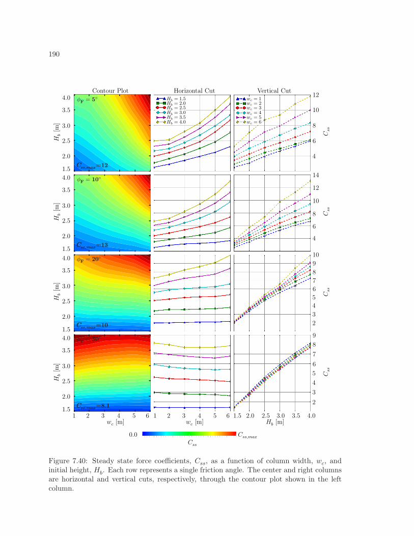
190

1 2 3 4 5 6Column Width

1.5

2.0

2.5

3.0

3.5

4.0

Initial Heigh

t

0.00

1.57

3.15

4.72

6.30

7.87

9.45

11.02

C_SS

_Ide

al

1 2 3 4 5 6Column Width

1.5

2.0

2.5

3.0

3.5

4.0

Initial Heigh

t

0.00

1.74

3.48

5.22

6.96

8.70

10.44

12.19

C_SS

_Ide

al

1 2 3 4 5 6Column Width

1.5

2.0

2.5

3.0

3.5

4.0

Initial Heigh

t

0.00

1.33

2.66

3.99

5.32

6.66

7.99

9.32

C_SS

_Ide

al

1 2 3 4 5 6Column Width

1.5

2.0

2.5

3.0

3.5

4.0

Initial Heigh

t

0.00

1.09

2.18

3.27

4.36

5.45

6.54

7.63

C_SS

_Ide

al

1.5

2.0

3.0

3.5

2.5

4.0

1.5

2.0

3.0

3.5

2.5

4.0

1.5

2.0

3.0

3.5

2.5

4.0

1.5

2.0

3.0

3.5

2.5

4.0

Hb[m

]H

b[m

]H

b[m

]H

b[m

]

31 4 5 62 31 4 52 6 1.5 2.0 3.0 3.5 4.02.5wc [m]wc [m] Hb [m]

Contour Plot Horizontal Cut Vertical Cut12

4

6

8

10

4

14

12

10

6

8

10

9

8

6

5

7

4

3

2

9

8

7

6

4

3

2

5 Css

Css

Css

Css

φF = 30

φF = 20

φF = 10

φF = 5

0.0 Css,max

Css

Css,max=12

Css,max=13

Css,max=10

Css,max=8.1

Hb = 1.5Hb = 2.0Hb = 2.5Hb = 3.0Hb = 3.5Hb = 4.0

wc = 1wc = 2wc = 3wc = 4wc = 5wc = 6

Figure 7.40: Steady state force coefficients, Css, as a function of column width, wc, andinitial height, Hb. Each row represents a single friction angle. The center and right columnsare horizontal and vertical cuts, respectively, through the contour plot shown in the leftcolumn.

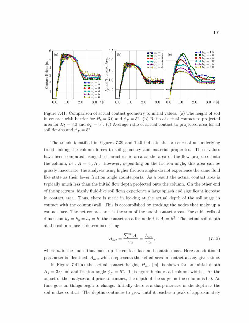
191

0.0 2.0 3.01.0

6

5

1

3

4

2

Contact

Height[m

]

0.0 2.0 3.01.0 0.0 2.0 3.01.0

2.5

0.5

1.0

1.5

2.0

Actual/Projected

Area

t [s] t [s]

(a) (b) (c)

wc = 1wc = 2wc = 3wc = 4wc = 5wc = 6

wc = 1wc = 2wc = 3wc = 4wc = 5wc = 6

Hb = 1.5Hb = 2.0Hb = 2.5Hb = 3.0Hb = 3.5Hb = 4.0

Figure 7.41: Comparison of actual contact geometry to initial values. (a) The height of soilin contact with barrier for Hb = 3.0 and φF = 5. (b) Ratio of actual contact to projectedarea for Hb = 3.0 and φF = 5. (c) Average ratio of actual contact to projected area for allsoil depths and φF = 5.

The trends identified in Figures 7.39 and 7.40 indicate the presence of an underlying

trend linking the column forces to soil geometry and material properties. These values

have been computed using the characteristic area as the area of the flow projected onto

the column, i.e., A = wcHb. However, depending on the friction angle, this area can be

grossly inaccurate; the analyses using higher friction angles do not experience the same fluid

like state as their lower friction angle counterparts. As a result the actual contact area is

typically much less than the initial flow depth projected onto the column. On the other end

of the spectrum, highly fluid-like soil flows experience a large splash and significant increase

in contact area. Thus, there is merit in looking at the actual depth of the soil surge in

contact with the column/wall. This is accomplished by tracking the nodes that make up a

contact face. The net contact area is the sum of the nodal contact areas. For cubic cells of

dimension hx = hy = hz = h, the contact area for node i is Ai = h2. The actual soil depth

at the column face is determined using

Hact =

∑mi Ai

wc=Aact

wc, (7.15)

where m is the nodes that make up the contact face and contain mass. Here an additional

parameter is identified, Aact, which represents the actual area in contact at any given time.

In Figure 7.41(a) the actual contact height, Hact [m], is shown for an initial depth

Hb = 3.0 [m] and friction angle φF = 5. This figure includes all column widths. At the

outset of the analyses and prior to contact, the depth of the surge on the column is 0.0. As

time goes on things begin to change. Initially there is a sharp increase in the depth as the

soil makes contact. The depths continues to grow until it reaches a peak of approximately

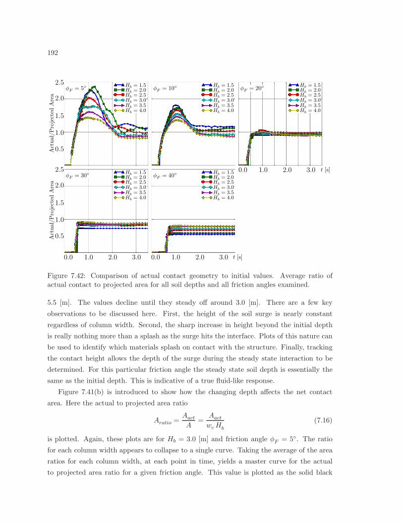
192

0.0 2.0 3.01.0 0.0 2.0 3.01.0

0.0 2.0 3.01.0 t [s]

2.5

0.5

1.0

1.5

2.0

Actual/Projected

Area

2.5

0.5

1.0

1.5

2.0

Actual/Projected

Area

t [s]

φF = 10 φF = 20

φF = 30 φF = 40

φF = 5Hb = 1.5Hb = 2.0Hb = 2.5Hb = 3.0Hb = 3.5Hb = 4.0

Hb = 1.5Hb = 2.0Hb = 2.5Hb = 3.0Hb = 3.5Hb = 4.0

Hb = 1.5Hb = 2.0Hb = 2.5Hb = 3.0Hb = 3.5Hb = 4.0

Hb = 1.5Hb = 2.0Hb = 2.5Hb = 3.0Hb = 3.5Hb = 4.0

Hb = 1.5Hb = 2.0Hb = 2.5Hb = 3.0Hb = 3.5Hb = 4.0

Figure 7.42: Comparison of actual contact geometry to initial values. Average ratio ofactual contact to projected area for all soil depths and all friction angles examined.

5.5 [m]. The values decline until they steady off around 3.0 [m]. There are a few key

observations to be discussed here. First, the height of the soil surge is nearly constant

regardless of column width. Second, the sharp increase in height beyond the initial depth

is really nothing more than a splash as the surge hits the interface. Plots of this nature can

be used to identify which materials splash on contact with the structure. Finally, tracking

the contact height allows the depth of the surge during the steady state interaction to be

determined. For this particular friction angle the steady state soil depth is essentially the

same as the initial depth. This is indicative of a true fluid-like response.

Figure 7.41(b) is introduced to show how the changing depth affects the net contact

area. Here the actual to projected area ratio

Aratio =Aact

A=

Aact

wcHb

(7.16)

is plotted. Again, these plots are for Hb = 3.0 [m] and friction angle φF = 5. The ratio

for each column width appears to collapse to a single curve. Taking the average of the area

ratios for each column width, at each point in time, yields a master curve for the actual

to projected area ratio for a given friction angle. This value is plotted as the solid black

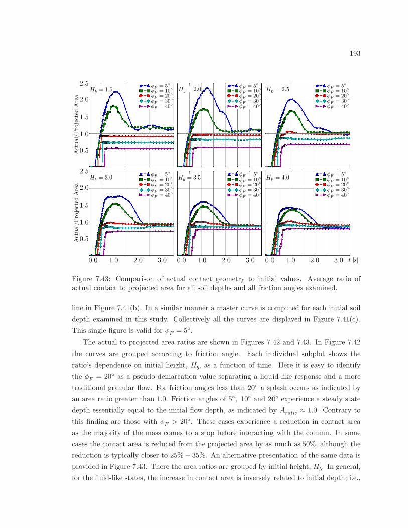
193

0.0 2.0 3.01.0

2.5

0.5

1.0

1.5

2.0

Actual/Projected

Area

2.5

0.5

1.0

1.5

2.0

Actual/Projected

Area

0.0 2.0 3.01.0 0.0 2.0 3.01.0 t [s]

φF = 10

φF = 20

φF = 30

φF = 40

φF = 5

φF = 10

φF = 20

φF = 30

φF = 40

φF = 5

φF = 10

φF = 20

φF = 30

φF = 40

φF = 5

φF = 10

φF = 20

φF = 30

φF = 40

φF = 5

φF = 10

φF = 20

φF = 30

φF = 40

φF = 5

φF = 10

φF = 20

φF = 30

φF = 40

φF = 5

Hb = 2.0

Hb = 4.0

Hb = 2.5

Hb = 3.5Hb = 3.0

Hb = 1.5

Figure 7.43: Comparison of actual contact geometry to initial values. Average ratio ofactual contact to projected area for all soil depths and all friction angles examined.

line in Figure 7.41(b). In a similar manner a master curve is computed for each initial soil

depth examined in this study. Collectively all the curves are displayed in Figure 7.41(c).

This single figure is valid for φF = 5.

The actual to projected area ratios are shown in Figures 7.42 and 7.43. In Figure 7.42

the curves are grouped according to friction angle. Each individual subplot shows the

ratio’s dependence on initial height, Hb, as a function of time. Here it is easy to identify

the φF = 20 as a pseudo demarcation value separating a liquid-like response and a more

traditional granular flow. For friction angles less than 20 a splash occurs as indicated by

an area ratio greater than 1.0. Friction angles of 5, 10 and 20 experience a steady state

depth essentially equal to the initial flow depth, as indicated by Aratio ≈ 1.0. Contrary to

this finding are those with φF > 20. These cases experience a reduction in contact area

as the majority of the mass comes to a stop before interacting with the column. In some

cases the contact area is reduced from the projected area by as much as 50%, although the

reduction is typically closer to 25%− 35%. An alternative presentation of the same data is

provided in Figure 7.43. There the area ratios are grouped by initial height, Hb. In general,

for the fluid-like states, the increase in contact area is inversely related to initial depth; i.e.,

194

a more shallow soil surge has a larger relative splash compared to an initially deeper surge.

This finding is somewhat counterintuitive.

The primary advantage of tracking the contact area is that the soil depth is realized

during steady state conditions. This depth provides yet another measure to correlate with

to the peak and steady state force magnitudes presented earlier. In an effort to tie these

dynamic forces to something familiar, the static equivalent force per column length is com-

puted as

bst =1

2K0 ρ0 |g|H2

act . (7.17)

The term K0 is coefficient of at-rest earth pressure and represents the ratio of horizontal to

vertical stress. Often times for granular material this coefficient is expressed as a function

of φF . Here, however, the material parameters listed in Table 7.10 dictate this value as K0 =

0.429. The leading coefficient of 1/2 follows from the assumption of a triangular force

distribution against the column (Das, 1984). Using Equation (7.17) the net, or total static

force equivalent acting on a column of width wc is computed according to

fst = bst wc =1

2K0 ρ0 |g|H2

act wc. (7.18)

Equation (7.18) represents the net force a dry soil mass of depth Hact would exert on the

structure in static conditions. And, more importantly, it provides a reference quantity by

which the dynamic peak and steady state forces can be compared to. The two ratios

Rpk =fpkfst

and Rss =fssfst

(7.19)

are defined for the peak and steady state force magnitudes depicted in Figures 7.36 and 7.37,

respectively.

The peak ratio is plotted in Figure 7.44 as a function of column width and initial

height Hb. The fact that no discernible trend is apparent in the contour plots is not

problematic—as the peak ratios are more or less constant for all friction angles. The steady

state ratio Rss is plotted in Figure 7.45. Again, these values are tending towards a relatively

narrow range, indicating the equivalent static force parameter is ideal for normalization.

Further examination of Figures 7.44 and 7.45 indicates that, as a whole, the analyses with

Hb = 1.5 [m] and wc = 1.0 [m] are causing significant deviation in the force ratios and

something is amiss. It is presumed that these two data series are suffering from refine-

ment issues—as they both represent the course end of their respective spectrum. For the

remainder of this discussion these values, as well as the single series of results with Hb = 4.0

and φF = 5.0 are omitted. Obviously removing questionable data from a given set is ill

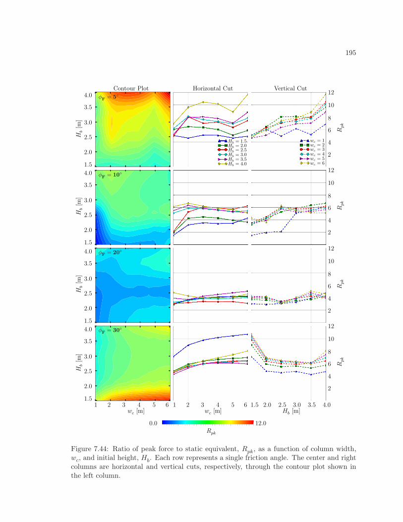
195

1 2 3 4 5 6Column Width

1.5

2.0

2.5

3.0

3.5

4.0Initial Heigh

t

0.0

1.6

3.2

4.8

6.4

8.0

9.6

11.2

Peak

Force

1 2 3 4 5 6Column Width

1.5

2.0

2.5

3.0

3.5

4.0

Initial Heigh

t

0.0

1.6

3.2

4.8

6.4

8.0

9.6

11.2

Peak

Force

1 2 3 4 5 6Column Width

1.5

2.0

2.5

3.0

3.5

4.0

Initial Heigh

t

0.0

1.6

3.2

4.8

6.4

8.0

9.6

11.2

Peak

Force

1 2 3 4 5 6Column Width

1.5

2.0

2.5

3.0

3.5

4.0

Initial Heigh

t

0.0

1.6

3.2

4.8

6.4

8.0

9.6

11.2

Peak

Force

1.5

2.0

3.0

3.5

2.5

4.0

1.5

2.0

3.0

3.5

2.5

4.0

1.5

2.0

3.0

3.5

2.5

4.0

1.5

2.0

3.0

3.5

2.5

4.0

Hb[m

]H

b[m

]H

b[m

]H

b[m

]

31 4 5 62 31 4 52 6 1.5 2.0 3.0 3.5 4.02.5wc [m]wc [m] Hb [m]

Contour Plot Horizontal Cut Vertical Cut

Rpk

Rpk

Rpk

Rpk

12

2

10

8

4

6

12

2

10

8

4

6

12

2

10

8

4

6

12

2

10

8

4

6

φF = 30

φF = 20

φF = 10

φF = 5

0.0Rpk

12.0

Hb = 1.5Hb = 2.0Hb = 2.5Hb = 3.0Hb = 3.5Hb = 4.0

wc = 1wc = 2wc = 3wc = 4wc = 5wc = 6

Figure 7.44: Ratio of peak force to static equivalent, Rpk, as a function of column width,wc, and initial height, Hb. Each row represents a single friction angle. The center and rightcolumns are horizontal and vertical cuts, respectively, through the contour plot shown inthe left column.

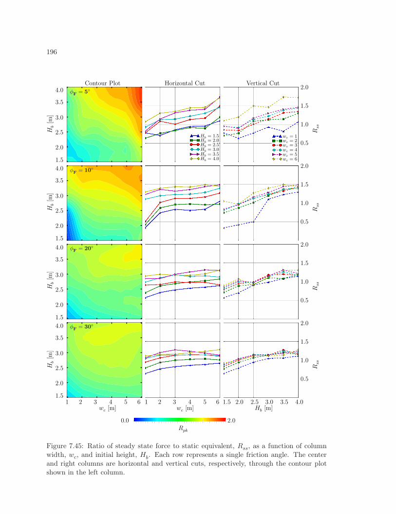
196

1 2 3 4 5 6Column Width

1.5

2.0

2.5

3.0

3.5

4.0

Initial Heigh

t

0.00

0.27

0.53

0.80

1.07

1.33

1.60

1.87

Stea

dy State Force

1 2 3 4 5 6Column Width

1.5

2.0

2.5

3.0

3.5

4.0

Initial Heigh

t

0.00

0.27

0.53

0.80

1.07

1.33

1.60

1.87

Stea

dy State Force

1 2 3 4 5 6Column Width

1.5

2.0

2.5

3.0

3.5

4.0

Initial Heigh

t

0.00

0.27

0.53

0.80

1.07

1.33

1.60

1.87

Stea

dy State Force

1 2 3 4 5 6Column Width

1.5

2.0

2.5

3.0

3.5

4.0

Initial Heigh

t

0.00

0.27

0.53

0.80

1.07

1.33

1.60

1.87

Stea

dy State Force

1.5

2.0

3.0

3.5

2.5

4.0

1.5

2.0

3.0

3.5

2.5

4.0

1.5

2.0

3.0

3.5

2.5

4.0

1.5

2.0

3.0

3.5

2.5

4.0

Hb[m

]H

b[m

]H

b[m

]H

b[m

]

31 4 5 62 31 4 52 6 1.5 2.0 3.0 3.5 4.02.5wc [m]wc [m] Hb [m]

Contour Plot Horizontal Cut Vertical Cut2.0

0.5

1.5

1.0

2.0

0.5

1.5

1.0

2.0

0.5

1.5

1.0

2.0

0.5

1.5

1.0

Rss

Rss

Rss

Rss

φF = 30

φF = 20

φF = 10

φF = 5

0.0Rpk

2.0

Hb = 1.5Hb = 2.0Hb = 2.5Hb = 3.0Hb = 3.5Hb = 4.0

wc = 1wc = 2wc = 3wc = 4wc = 5wc = 6

Figure 7.45: Ratio of steady state force to static equivalent, Rss, as a function of columnwidth, wc, and initial height, Hb. Each row represents a single friction angle. The centerand right columns are horizontal and vertical cuts, respectively, through the contour plotshown in the left column.

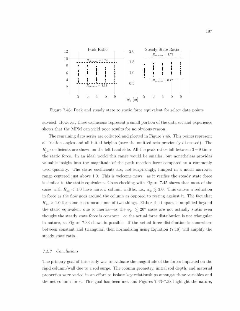
197

2.0

0.5

1.0

1.58

6

2

4

12

10

65432

Peak Ratio

65432

Steady State Ratio

wc [m]

Rpk,max = 8.79

Rpk,min = 3.11

Rss,min = 0.77

Rss,max = 1.74

Figure 7.46: Peak and steady state to static force equivalent for select data points.

advised. However, these exclusions represent a small portion of the data set and experience

shows that the MPM can yield poor results for no obvious reason.

The remaining data series are collected and plotted in Figure 7.46. This points represent

all friction angles and all initial heights (save the omitted sets previously discussed). The

Rpk coefficients are shown on the left hand side. All the peak ratios fall between 3−9 times

the static force. In an ideal world this range would be smaller, but nonetheless provides

valuable insight into the magnitude of the peak reaction force compared to a commonly

used quantity. The static coefficients are, not surprisingly, lumped in a much narrower

range centered just above 1.0. This is welcome news—as it verifies the steady state force

is similar to the static equivalent. Cross checking with Figure 7.45 shows that most of the

cases with Rss < 1.0 have narrow column widths, i.e., wc . 3.0. This causes a reduction

in force as the flow goes around the column as opposed to resting against it. The fact that

Rss > 1.0 for some cases means one of two things. Either the impact is amplified beyond

the static equivalent due to inertia—as the φF . 20 cases are not actually static even

thought the steady state force is constant—or the actual force distribution is not triangular

in nature, as Figure 7.33 shows is possible. If the actual force distribution is somewhere

between constant and triangular, then normalizing using Equation (7.18) will amplify the

steady state ratio.

7.4.3 Conclusions

The primary goal of this study was to evaluate the magnitude of the forces imparted on the

rigid column/wall due to a soil surge. The column geometry, initial soil depth, and material

properties were varied in an effort to isolate key relationships amongst these variables and

the net column force. This goal has been met and Figures 7.33–7.38 highlight the nature,

198

shape, orientation, and magnitude of the column forces during the soil-structure interaction.

Some general observations are listed below.

• The column/wall experiences a definitive peak and steady state (constant) force during

the interaction. The existence of a constant force does not imply a static flow state.

• Peak and steady state force magnitude increase linearly with column size.

• Peak and steady state force magnitude increases linearly with initial depth for φ . 10.

For friction angles greater than 10 the magnitude tends to increases quadratically.

• The steady state force magnitude is largely independent of friction angle.

In addition to the column forces the soil particles themselves provide great data. The ve-

locity, stress, and total deformation fields are displayed in Figures 7.30–7.32. The ability

to maintain these quality fields throughout the simulation exemplifies the MPM’s ability to

bridge the gap between solid- and fluid-like behavior for history dependent, large deforma-

tion analyses.

A secondary goal was to identify force related measures that aid in the development of

predictive models for general design procedures. Initially two coefficients were discussed:

Cpk and Css. These values are plotted in Figures 7.39 and 7.40. In both cases trends were

beginning to take shape for the various parameters investigated. Both Cpk and Css were

based off A, the initial projected frontal area of the soil. Figures 7.41–7.43 show that the

actual area in contact with the column, Aact, can be quite different than the projected area

A. This observation motivated the definition of a static equivalent net force, fst, which was

used as a normalization factor. This yielded the coefficients Rpk and Rss which represent the

expected increase in the dynamic forces compared to their static state counterparts. These

are appealing coefficients in that the static force is a tangible quantity more easily realized

than alternative measures. These latter coefficients are plotted in Figures 7.44–7.46.

The trends identified in this section for Cpk, Css, Rpk and Rss highlight the potential

for using the MPM as a predictive tool for identifying and quantify debris flow loadings

on rectangular columns. Clearly this study is preliminary and significant steps need to

be taken to validate and expand the results base before any additional conclusions can be

drawn. This includes studies examining the effects of initial velocity, as well as studies

investigating alternate material and MPM parameters, such as particles per cell, time step,

and/or cell size. Ultimately the numerical results need to be validated experimentally before

any real progress can take place.

Several additional results have not been presented in the interest of space. In most

cases the omitted findings do not provide any additional insight beyond what has already

been shown. Notable omissions include the coefficients Cpk,actual and Css,actual which are

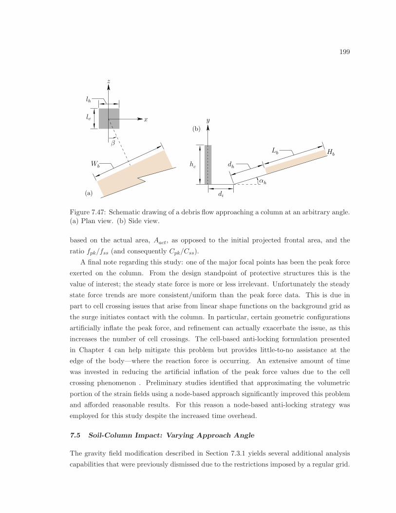
199

Wb

αh

dh

lv x

z

β

lh

(a)

HbLb

di

y

(b)

hc

Figure 7.47: Schematic drawing of a debris flow approaching a column at an arbitrary angle.(a) Plan view. (b) Side view.

based on the actual area, Aact, as opposed to the initial projected frontal area, and the

ratio fpk/fss (and consequently Cpk/Css).

A final note regarding this study: one of the major focal points has been the peak force

exerted on the column. From the design standpoint of protective structures this is the

value of interest; the steady state force is more or less irrelevant. Unfortunately the steady

state force trends are more consistent/uniform than the peak force data. This is due in

part to cell crossing issues that arise from linear shape functions on the background grid as

the surge initiates contact with the column. In particular, certain geometric configurations

artificially inflate the peak force, and refinement can actually exacerbate the issue, as this

increases the number of cell crossings. The cell-based anti-locking formulation presented

in Chapter 4 can help mitigate this problem but provides little-to-no assistance at the

edge of the body—where the reaction force is occurring. An extensive amount of time

was invested in reducing the artificial inflation of the peak force values due to the cell

crossing phenomenon . Preliminary studies identified that approximating the volumetric

portion of the strain fields using a node-based approach significantly improved this problem

and afforded reasonable results. For this reason a node-based anti-locking strategy was

employed for this study despite the increased time overhead.

7.5 Soil-Column Impact: Varying Approach Angle

The gravity field modification described in Section 7.3.1 yields several additional analysis

capabilities that were previously dismissed due to the restrictions imposed by a regular grid.

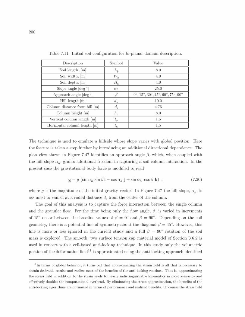
200

Table 7.11: Initial soil configuration for bi-planar domain description.

Description Symbol Value

Soil length, [m] Lb 8.0

Soil width, [m] Wb 4.0

Soil depth, [m] Hb 4.0

Slope angle [deg ] αh 25.0

Approach angle [deg ] β 0, 15, 30, 45, 60, 75, 90

Hill length [m] dh 10.0

Column distance from hill [m] di 4.75

Column height [m] hc 8.0

Vertical column length [m] lv 1.5

Horizontal column length [m] lh 1.5

The technique is used to emulate a hillside whose slope varies with global position. Here

the feature is taken a step further by introducing an additional directional dependence. The

plan view shown in Figure 7.47 identifies an approach angle β, which, when coupled with

the hill slope αh, grants additional freedom in capturing a soil-column interaction. In the

present case the gravitational body force is modified to read

g = g (sinαh sinβ i− cosαh j+ sinαh cos β k) , (7.20)

where g is the magnitude of the initial gravity vector. In Figure 7.47 the hill slope, αh, is

assumed to vanish at a radial distance di from the center of the column.

The goal of this analysis is to capture the force interaction between the single column

and the granular flow. For the time being only the flow angle, β, is varied in increments

of 15 on or between the baseline values of β = 0 and β = 90. Depending on the soil

geometry, there is a potential line of symmetry about the diagonal β = 45. However, this

line is more or less ignored in the current study and a full β = 90 rotation of the soil

mass is explored. The smooth, two surface tension cap material model of Section 3.6.2 is

used in concert with a cell-based anti-locking technique. In this study only the volumetric

portion of the deformation field11 is approximated using the anti-locking approach identified

11In terms of global behavior, it turns out that approximating the strain field is all that is necessary to

obtain desirable results and realize most of the benefits of the anti-locking routines. That is, approximating

the stress field in addition to the strain leads to nearly indistinguishable kinematics in most scenarios and

effectively doubles the computational overhead. By eliminating the stress approximation, the benefits of the

anti-locking algorithms are optimized in terms of performance and realized benefits. Of course the stress field

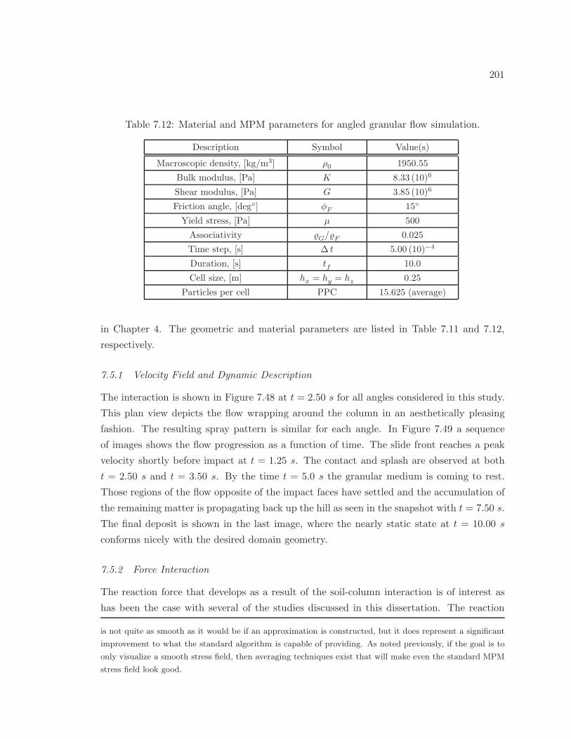
201

Table 7.12: Material and MPM parameters for angled granular flow simulation.

Description Symbol Value(s)

Macroscopic density, [kg/m3] ρ0 1950.55

Bulk modulus, [Pa] K 8.33 (10)6

Shear modulus, [Pa] G 3.85 (10)6

Friction angle, [deg] φF 15

Yield stress, [Pa] µ 500

Associativity G/F 0.025

Time step, [s] ∆ t 5.00 (10)−4

Duration, [s] tf 10.0

Cell size, [m] hx = hy = hz 0.25

Particles per cell PPC 15.625 (average)

in Chapter 4. The geometric and material parameters are listed in Table 7.11 and 7.12,

respectively.

7.5.1 Velocity Field and Dynamic Description

The interaction is shown in Figure 7.48 at t = 2.50 s for all angles considered in this study.

This plan view depicts the flow wrapping around the column in an aesthetically pleasing

fashion. The resulting spray pattern is similar for each angle. In Figure 7.49 a sequence

of images shows the flow progression as a function of time. The slide front reaches a peak

velocity shortly before impact at t = 1.25 s. The contact and splash are observed at both

t = 2.50 s and t = 3.50 s. By the time t = 5.0 s the granular medium is coming to rest.

Those regions of the flow opposite of the impact faces have settled and the accumulation of

the remaining matter is propagating back up the hill as seen in the snapshot with t = 7.50 s.

The final deposit is shown in the last image, where the nearly static state at t = 10.00 s

conforms nicely with the desired domain geometry.

7.5.2 Force Interaction

The reaction force that develops as a result of the soil-column interaction is of interest as

has been the case with several of the studies discussed in this dissertation. The reaction

is not quite as smooth as it would be if an approximation is constructed, but it does represent a significant

improvement to what the standard algorithm is capable of providing. As noted previously, if the goal is to

only visualize a smooth stress field, then averaging techniques exist that will make even the standard MPM

stress field look good.

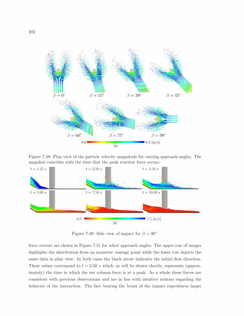
202

β = 60 β = 75 β = 90

β = 15 β = 30 β = 45β = 0

|v|0.0 8.5 [m/s]

Figure 7.48: Plan view of the particle velocity magnitude for varying approach angles. Thesnapshot coincides with the time that the peak reaction force occurs.

t = 1.25 s t = 2.50 s t = 3.50 s

t = 5.00 s t = 7.50 s t = 10.00 s

|v|0.0 7.5 [m/s]

Figure 7.49: Side view of impact for β = 30.

force vectors are shown in Figure 7.51 for select approach angles. The upper row of images

highlights the distribution from an isometric vantage point while the lower row depicts the

same data in plan view. In both cases the black arrow indicates the initial flow direction.

These values correspond to t = 2.50 s which, as will be shown shortly, represents (approx-

imately) the time in which the net column force is at a peak. As a whole these forces are

consistent with previous observations and are in line with intuitive notions regarding the

behavior of the interaction. The face bearing the brunt of the impact experiences larger

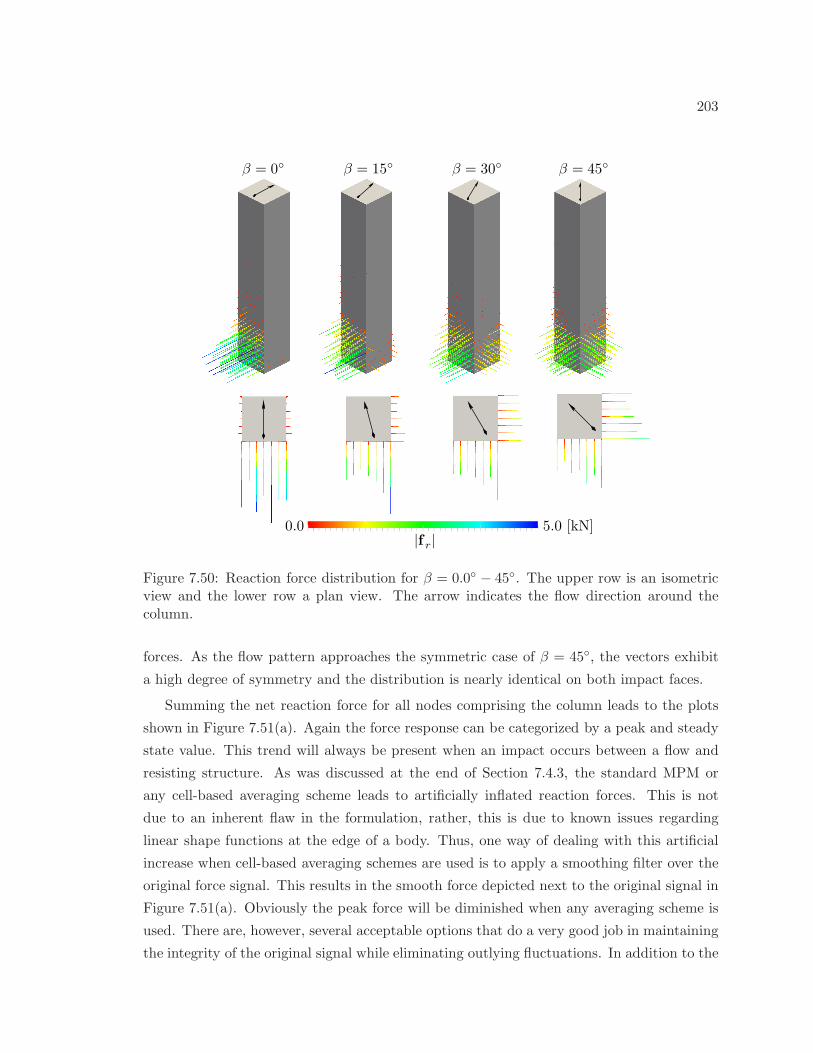
203

|f r|

β = 0 β = 15 β = 30 β = 45

5.0 [kN]0.0

Figure 7.50: Reaction force distribution for β = 0.0 − 45. The upper row is an isometricview and the lower row a plan view. The arrow indicates the flow direction around thecolumn.

forces. As the flow pattern approaches the symmetric case of β = 45, the vectors exhibit

a high degree of symmetry and the distribution is nearly identical on both impact faces.

Summing the net reaction force for all nodes comprising the column leads to the plots

shown in Figure 7.51(a). Again the force response can be categorized by a peak and steady

state value. This trend will always be present when an impact occurs between a flow and

resisting structure. As was discussed at the end of Section 7.4.3, the standard MPM or

any cell-based averaging scheme leads to artificially inflated reaction forces. This is not

due to an inherent flaw in the formulation, rather, this is due to known issues regarding

linear shape functions at the edge of a body. Thus, one way of dealing with this artificial

increase when cell-based averaging schemes are used is to apply a smoothing filter over the

original force signal. This results in the smooth force depicted next to the original signal in

Figure 7.51(a). Obviously the peak force will be diminished when any averaging scheme is

used. There are, however, several acceptable options that do a very good job in maintaining

the integrity of the original signal while eliminating outlying fluctuations. In addition to the

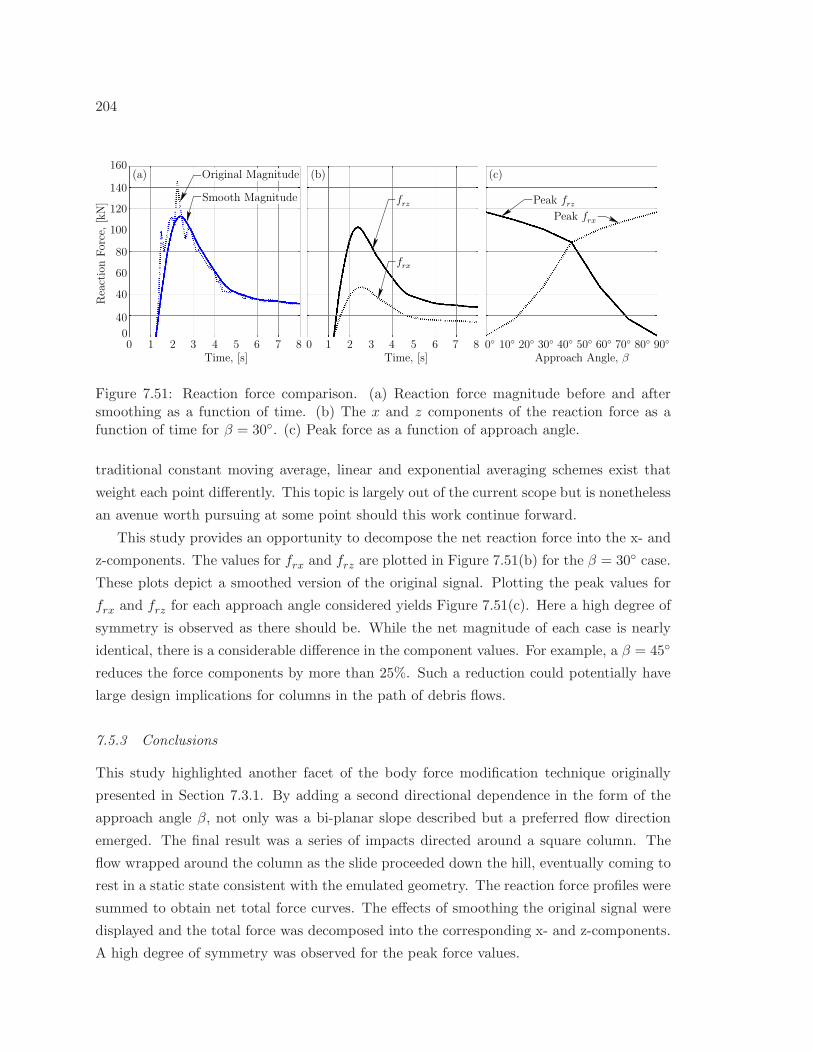
204

0 1 2 3 84 5 6 7Time, [s]

160

140

120

100

80

60

40

40

0

ReactionForce,[kN]

0 1 2 3 4 7 85 6Time, [s] Approach Angle, β

0 10 20 30 40 50 60 70 80 90

(a) (b) (c)

Smooth Magnitude

Original Magnitude

frz

frx

Peak frzPeak frx

Figure 7.51: Reaction force comparison. (a) Reaction force magnitude before and aftersmoothing as a function of time. (b) The x and z components of the reaction force as afunction of time for β = 30. (c) Peak force as a function of approach angle.

traditional constant moving average, linear and exponential averaging schemes exist that

weight each point differently. This topic is largely out of the current scope but is nonetheless

an avenue worth pursuing at some point should this work continue forward.

This study provides an opportunity to decompose the net reaction force into the x- and

z-components. The values for frx and frz are plotted in Figure 7.51(b) for the β = 30 case.

These plots depict a smoothed version of the original signal. Plotting the peak values for

frx and frz for each approach angle considered yields Figure 7.51(c). Here a high degree of

symmetry is observed as there should be. While the net magnitude of each case is nearly

identical, there is a considerable difference in the component values. For example, a β = 45

reduces the force components by more than 25%. Such a reduction could potentially have

large design implications for columns in the path of debris flows.

7.5.3 Conclusions

This study highlighted another facet of the body force modification technique originally

presented in Section 7.3.1. By adding a second directional dependence in the form of the

approach angle β, not only was a bi-planar slope described but a preferred flow direction

emerged. The final result was a series of impacts directed around a square column. The

flow wrapped around the column as the slide proceeded down the hill, eventually coming to

rest in a static state consistent with the emulated geometry. The reaction force profiles were

summed to obtain net total force curves. The effects of smoothing the original signal were

displayed and the total force was decomposed into the corresponding x- and z-components.

A high degree of symmetry was observed for the peak force values.

205

Among other things, this study identifies the benefits of an angled flow protector for

columns and bents in the path of a moving mass, be it soils, snow, or liquid. A reduction

in force components of more than 25% can be achieved simply by altering the orientation

of a square column or ensuring an angled geometry in the path of the flow.

206

Chapter 8

CONCLUSIONS

This document provides a comprehensive discussion and applications of the Material

Point Method, a numerical technique that is best suited for modeling history dependent

materials in a dynamic, large deformation setting. The formulation tracks moving points

relative to stationary nodes, and can be used to capture the behavior of both fluids and

solids in a unified framework.

In this closing chapter conclusions about this work are identified and discussed following

a brief summary of the dissertation. In general these conclusions are about the work as a

whole and are not necessarily application specific. Each example presented in Chapters 6

and 7 contains concluding remarks and the reader is referred to these chapters for specific

conclusions and future work regarding individual examples.

8.1 Summary

In Chapter 2 the method was outlined in moderate detail, providing a basic explanation

along with implementation details for the standard framework. A comparison to other

numerical techniques was made, in particular with regards to Smoothed Particle Hydro-

dynamics and the Discrete Element Method. The latter was made from the perspective

of granular media, one of the key focal points throughout this dissertation. The overview

chapter concluded with a literature review, highlighting past and current applications of the

MPM and its close friend, the Generalized Interpolation Material Point method. Additional

implementation details are given in Appendix B, where an overview of the computational

framework is discussed. From a global perspective the code was broken down into three

components: Pre-Processing, Model Analysis, and Post-Processing. Each component was

addressed and a particular emphasis was placed on how to construct input files from the

available features. Appendix B also contains example input files as well as instructions for

viewing existing MPM simulations using ParaView.

Multiple material model considerations were identified in Chapter 3. This included a

discussion of computational inelasticity, cast in terms of small and large deformations. The

return mapping integration algorithm was discussed in detail and a general framework for

isotropic media was outlined. Multiple material models were described for capturing the

207

response of isotropic solids, aggregates, composites, and cohesive-frictional materials, sev-

eral of which are appropriate for simulating ductile metals, concrete, and various soils (most

notably dry sands and gravels). The chapter concludes with biaxial and pure shear simula-

tions.

Both Chapters 4 and 5 highlight enhancements to the Material Point Method algorithm.

The latter provided an anti-locking strategy that helps mitigate the accumulation of ficti-

tious strains that result from the use of linear shape function. This is accomplished by

building separate approximations for the stress and strain fields in addition to displacement

related fields. Three strategies were introduced: a cell- and node-based approach, followed

by a third variant that effectively combines the first two strategies. The second major addi-

tion was a volume constraint for use in multiphase simulations. This technique was outlined

in Chapter 5, where the background theory and implementation were discussed.

The culmination of all things MPM discussed in Chapters 2–5 resides in Chapters 6

and 7, where a series of examples shows the broad range of applications the Material Point

Method is capable of modeling. The first of these two chapters focused exclusively on linear

elastic applications, and included validation of both the anti-locking and volume constraint

algorithms. The latter chapter emphasized the elastoplastic material models presented in

Chapter 3 and included large-deformation ductile impact simulation, planar sand flow, snow

and avalanche diversion, as well as debris flow interaction with protective structures. Many

of the elastoplastic investigations were parametric in nature and attempted to identify key

relationships between analysis parameters and values of interest.

8.2 Key Findings

Throughout Chapters 2–7 several noteworthy observations were made regarding MPM, its

capabilities and limitations, and overall performance when applied to a broad spectrum of

problem types.

8.2.1 Enhancements to the MPM

There is little doubt the single most valuable contribution this work provides to the aca-

demic community is the anti-locking framework discussed in Chapter 4. The extension

is applicable to both elastic and elastoplastic materials and is essential for improving the

kinematics and stress field for MPM simulations. Currently the approximation schemes

allow the volumetric or full tensor field to be constructed of both the strain and stress mea-

sures. This is accomplished using a cell- or node-based approach, or a third variant that

effectively combines the first two techniques. However, even this enhancements has its prac-

208

tical limitations and shortcomings. The Taylor Bar simulation of Section 7.1 indicates the

computational overhead incurred by using the anti-locking extensions is not justified with

the realized benefits of the full tensor approximation schemes. In general it is sufficient to

use the volumetric approximation for both the stress and strain. This trend was observed

for nearly all problems presented in Chapter 7. Here it is recommended that a cell based

approach be used unless the reaction force at nodes is desired. For the latter case a node

based approximation may be the best choice. Of course, it is always possible to fashion

examples that contradict the claim that a volumetric approximation is all that is necessary.

However, for those simulations the MPM is best suited to capture, i.e., large deformations

and displacements of history dependent materials, this claim holds true.

Another enhancement was the volume constraint of Chapter 5. This extension was

originally conceived to combat volume overloading of a spatial region that can occur due

to the point-wise material point description. From a qualitative perspective, the physical

basis for such a constraint was appealing, as it matched everyday intuitions regarding the

physical world. However, there are limitations to what having an appropriate amount of

matter in a given space can provide in a numerical context, and the expected capabilities

of the volume constraint were shown to be unobtainable. Specific problems associated with

this approach were identified final sections of Chapter 5.

Interestingly, in the author’s experience with MPM and the coding framework, some of

the most valuable extensions have followed from ad-hoc enhancements, quick fixes to prob-

lems that cannot be cast in terms of variational principals but follow from code hacks that

have little or no theoretical justification. Often these tricks are the sole reason a particular

analysis yields good results. This has been termed technology by those working close to the

author, and there is reason to believe such technology is ever-present in any numerical ana-

lysts’ tool belt. In the present case two such examples exist. The first being artificial viscous

damping. Regardless of the anti-locking routine, cell size, time step, particle density, etc.,

linear elastic simulations must employ damping to control the propagation of stress waves

and maintain valid stress fields. This is done using the ViscousDamping option described in

Appendix B. The second critical enhancement is the FrontSmoothing option, responsible

for detecting the edge of a body. The affected region(s) are updated using only kinematic

field variables from time tn to avoid problems associated with linear shape functions. Neither

of these tricks are needed if using higher order shape functions. It is postulated here that

the desired phase mixing and separation capabilities the volume constraint was intended to

provide will be solved by ad-hoc extensions that use multigrid contact algorithms coupled

with the appropriate phase volume fractions and mixture theories built using common grid

209

values (in addition to the individual phase motions).

8.2.2 Linear Elastic Simulations

The primary focus of Chapter 6 was to discuss a series of MPM simulations from fluid

and solid mechanics. The different examples were designed to show the effectiveness of

the anti-locking approach applied to a wide variety of problem types. Large deformation,

nearly incompressible flow simulations were examined in order to validate the anti-locking

strategy from a kinematic viewpoint. The ensuing pressure field and interaction between

fluid and bounding surface were examined. It is apparent from this chapter that an anti-

locking strategy is indispensable for modeling nearly incompressible flow. Failure to alleviate

the fictitious stress and strains that accumulate in the standard implementation leads to

nonphysical and unusable results. The anti-locking algorithms employed in these analyses

successfully eliminate the volumetric locking and lead to improved findings with respect to

all field variables, including the particle pressure and nodal/particle velocity. Here it was

shown that the MPM with appropriate anti-locking extension is a valid tool for recovering or

assessing the magnitude of the reaction force/traction between a body and a rigid surface.

On the solid mechanics end of the spectrum, MPM’s ability to capture a linear elastic

response for a material with finite shear stiffness was investigated in the form of free vibra-

tion. In particular, the effectiveness of the anti-locking approach presented in Chapter 4

was key to mitigating shear locking for a cantilever beam subjected to a prescribed velocity

field. Both normal and shear stresses were successfully recovered, and represent a signifi-

cant improvement over the standard MPM algorithm. The example also showed that the

proposed anti-locking technique exhibits ideal convergence behavior. Volumetric locking in

the context of solid mechanics was addressed by examining the algorithmic performance

when approaching the incompressible material limit. A single anti-locking variant (ALCV)

is identified that is capable of mitigating both shear and volumetric locking, making it an

ideal candidate for both fluid and solid mechanics simulations when using linear elastic

material models.

Chapter 6 also presented three examples highlighting the capabilities of the volume

constraint algorithm. The saturated soil simulations were performed in a multigrid, mul-

tiphase framework. The 1D hydrostatic test cases produced accurate distributions of the

constituent, bulk, and mixture stresses. Solid phase displacements were shown to converge

to an analytical solution. The pressure head drawdown simulations showed how prescribed

conditions could potentially be used to capture the liquefaction process. The drawdown

examples emphasized the need for additional momentum exchange mechanisms beyond the

210

pressure obtained from the volume constraint algorithm; there it was shown that the al-

ternative exchange processes are largely more important in a saturated soil context. The

final example considered a 2D saturated panel subject to a distributed foundation loading.

Pore pressure distribution and surface displacements were compared to the u − p CMPM

formulation and an FEM implementation using stabilized elements. All results compared

favorably with respect to pore pressure.

8.2.3 Elastoplastic Simulations

A Taylor Bar Impact problem was used to validate the anti-locking routines in the nonlinear

material regime. The deformed geometry and stress field were compared to results obtained

using commercial Finite Element Method software. The anti-locking algorithms yielded

higher quality results with respect to geometric parameters than the original algorithm

with linear shape functions. Each anti-locking technique yielded very similar values that

were consistent with the FEM model. This latter point should not be taken lightly; the FE

model employs higher order shape functions that are not subject to locking. The locking free

variants result in a net time increase on the order of 27%–294%. Comparing all aspects of

the findings—geometric, mechanical fields, efficiency, etc.—a picture emerged that suggested

the use of a full-tensor averaging technique is superfluous in a nonlinear material context.

The volumetric averaging scheme, be it cell- or node-based, provides the same benefits at

a significant reduction in cost. This observation is not limited to the Taylor Bar impact

problem analyzed in this section.

A series of simulations were designed to show the MPM is a valuable tool for model-

ing granular flow and landslides when coupled with an appropriate constitutive framework.

The first series of tests targeted a planar sand column collapse, where the MPM simula-

tions reproduced key geometric observations from published experiments. These analyses

identified the peak material strength as being the most influential factor in determining the

final shape of the collapsed profile. In addition to the geometric aspects, it was shown that

the MPM can be used to visualize other field variables of interest; the velocity and stress

fields were used as examples but many other options exist. The reaction force between the

planar surface and the body of sand was investigated and found to be parabolic in shape. A

second problem modeled a series of earthen mounds as energy dissipating devices to protect

civil infrastructure. The mounds proved to be quite efficient in impeding the flow, and the

resulting interaction was captured by way of a reaction force field. This study shows the

potential for the MPM in this context, and opens the door for several quantitative para-

metric studies of landslides. Also of importance from this study was the idea of a modified

211

gravitational field. By altering the direction of gravity—and in some cases the underlying

normal boundary definition—complex surface shapes can be created within the confines of

a regular grid.

The repetitive structure of the mounds described in the previous paragraph motivated

a quantitative study identifying the underlying link between reaction force magnitude and

geometric, material, and analysis parameters. To this end a parametric study consisting

of 180 separate analysis was conducted, each evaluating the impact of a soil mass with a

rectangular column. The column geometry and soil depth were varied, along with the soil

properties. Two distinct force regimes were observed in the force profiles, namely, a peak

force and steady state force. Several trends were identified between the flow parameters

and these two force measures. A method establishing the ratio between the dynamic force

magnitude and static design force was identified and found to be as high as 8. A final

study investigated soil structure interaction by varying the approach angle of the flow as it

impacts a lone column. The net force remains constant as the approach angle varies, yet

the force components in the axis directions varied appropriately with the approach angle.

This study identified the benefits of an angled flow protector for columns and bents in the

path of a moving soil, snow, or liquid mass.

8.3 Moving Forward

This work has identified different research options for future students to pursue. The fol-

lowing discussion categorizes potential work by topic.

8.3.1 Computational Framework

By and large the current framework is a development code. As such the focus was always

on adding features and capabilities. Considerable algorithmic issues that will arise if the

intent is to move towards an efficiency-centric implementation using the existing code. This

includes a troublesome transition to a parallel implementation with multiple processors or

computational nodes for a single simulation. On the other hand, running serial simulations

simultaneously has proven to be quite efficient and sufficient for the scale of analyses ran

to date. Beyond this, additional parallelization should not be pursued until there is a

significant need for speed up.

At one point there was talk of building an MPM specific GUI. The recent use of ParaView

as largely negated the need for a specialized visualization environment. This software is

advanced beyond what could feasibly be created and built specifically for viewing mechanics-

based analyses; thus there is little benefit in building a custom GUI. All that being said, it

212

is possible to embed ParaView scenes and features in custom built applications. Such an

approach is perhaps the most appropriate for the current situation if an MPM specific GUI

is built. There would be considerable benefit in developing a custom particle discretization

tool. That is, the ability to construct (or read in) arbitrary shapes and objects, then build a

particle based discretization of these entities according to user specified parameters (particle

density, max/min spacing, etc.).

Unfortunately the type of student capable of providing the computational extensions

discussed in this subsection is more likely to be found outside of civil engineering. This may

be an inaccurate statement. But at this point leaps in the coding framework are going to

be achieved by someone who a.) is very knowledgeable in efficient programing techniques,

or b.) already knows the MPM and can focus more on the efficient implementations as

opposed to trying to develop code (while learning good programming as well) and learn the

MPM at the same time.

8.3.2 Additional Capabilities

There is always room for improvement and additional simulation features. However, at this

point features should be added for specific reasons. Before adding a feature there should be

a sufficient need, or void, or hole, the current coding framework cannot meet.

There still remains a need for more general bounding surfaces within the current frame-

work. As a first step, existing multigrid contact algorithms could be added. The code setup

is well suited to handle this type of extension and would allow for particle based boundary

definitions and multibody contact. Alternatively, an irregular grid could be utilized. This

has already been addressed in this chapter but will allow for general boundary definitions.

The larger issue with an irregular grid in the context of structural engineering is the perfectly

rigid requirement imposed by the node-based boundary. This is unrealistic for a structure.

Perhaps the best solution is to couple the MPM with FEM. There are existing strategies in

place for this approach, and in the author’s opinion will provide the most flexible framework

for moving forward.

The use of higher order b-splines could also be quite beneficial if sticking with a regular

grid (assumes FEM will be added to deal with boundaries). These shape functions are su-

perior to the traditional quadratic element primarily because the don’t reduce node spacing

(and thus time step) and do not pose a problem with the lumped mass matrix. Further-

more, using such functions eliminates the locking phenomena associated with linear shape

functions. Higher order shape functions also eliminate problems at the edge of a body and

other stalwart problems like internal cell crossing errors that the anti-locking routines alone

213

cannot resolve. While there is no doubt an increase is incurred using higher order shape

functions, in the author’s opinion this additional computational cost is worth the better

results in several situations.

8.3.3 Applications

It is the author’s sincere hope that the coding framework is used more for additional appli-

cations in the future. These pages have demonstrated that even with the restrictions of a

regular grid, a single phase, or with the simple material models employed in these studies,

there are several opportunities to simulate complex engineering problems—problems that

the MPM community finds interesting and problems that can benefit the geotechnical engi-

neering community at large. Potential future studies include a debris flows and placing rigid

objects in the flow path, a comparison of landslide runout to existing runout models, the

use of MPM as a tool to assess the loads on pipeline structures, and additional parametric

studies quantifying the force reaction between flows and columns.

In looking at the diverse applications of the MPM and observing trends in recent publi-

cations, it is only a matter of time until other researchers begin using the MPM to simulate

landslide and debris flows in a context very similar to the work presented in this docu-

ment. The immediate focus following this research should be on sharing existing findings

and establishing the current MPM group at the University of Washington as team modeling

landslides and debris flows and their interactions with structures.

214

BIBLIOGRAPHY

Manual on Estimating Soil Properties for Foundation Design (EPRI), 1990. Cornel University.

H. Alawaji, K. Runesson, S. Sture, and K. Axelsson. Implicit integration in soil plasticity under

mixed control for drained and undrained response. International Journal for Numerical and

Analytical Methods in Geomechanics, 16(10):737–756, 1992. ISSN 1096-9853.

U. Andelfinger and E. Ramm. EAS-elements for two-dimensional, three-dimensional, plate and shell

structures and their equivalence to HR-elements. International Journal for Numerical Methods in

Engineering, 36(8):1311–1337, 1993.

S. Andersen and L. Andersen. Analysis of spatial interpolation in the material point method.

Computers & Structures, 88(7-8):506 – 518, 2010a.

S. Andersen and L. Andersen. Modelling of landslides with the material-point method. Computa-

tional Geosciences, 14:137–147, 2010b.

J. E. Andrade and X. Tu. Multiscale framework for behavior prediction in granular media. Mechanics

of Materials, 41(6):652 – 669, 2009. ISSN 0167-6636.

P. Arduino, P. Mackenzie-Helnwein, and G. R. Miller. Modeling multi-scale flow using the material

point method. In R. I. Borja, editor, Multiscale and Multiphysics Processes in Geomechanics.

Results of the Workshop on Multiscale and Multiphysics Processes in Geomechanics, Stanford,

June 23–25, 2010. Springer, 2011.

B. Ataie-Ashtiani and G. Shobeyri. Numerical simulation of landslide impulsive waves by incompress-

ible smoothed particle hydrodynamics. International Journal for Numerical Methods in Fluids,

56(2):209 – 32, 2008. ISSN 0271-2091. URL http://dx.doi.org/10.1002/fld.1526.

N. J. Balmforth and R. R. Kerswell. Granular collapse in two dimensions. Journal of Fluid Mechanics,

538:399–428, 2005.

S. G. Bardenhagen. Energy conservation error in the material point method for solid mechanics. J.

Comput. Phys., 180(1):383–403, 2002. ISSN 0021-9991.

S. G. Bardenhagen and E.M. Kober. The generalized interpolation material point method. Computer

Modeling in Engineering & Sciences, 5(6):477 – 495, 2004.

S. G. Bardenhagen, J. U. Brackbill, and D. Sulsky. The material point method for granular materials.

Computer Methods in Applied Mechanics and Engineering, 187(3–4):529–541, 2000.

215

S. G. Bardenhagen, J. E. Guilkey, K. M. Roessig, J. U. Brackbill, W. M. Witzel, and J. C. Foster. An

improved contact algorithm for the material point method and application to stress propagation

in granular material. Computer Modeling in Engineering & Sciences, 2:509–522, 2001.

K.J Bathe. Finite Element Procedures. Prentice Hall, 1996.

T. Belytschko, Y. Krongauz, D. Organ, M. Fleming, and P Krysl. Meshless methods: An overview

and recent developments. Computer Methods in Applied Mechanics and Engineering, Vol. 139:

3–47, 1996.

T. Belytschko, W. K. Liu, and B. Moran. Nonlinear Finite Elements for Continua and Structures.

John Wiley & Sons, Ltd., West Sussex, England, 2000.

D. Benson. Computational methods in Lagrangian and Eulerian hydrocodes. Computer Methods in

Applied Mechanics and Engineering, Vol. 99(2-3):235–394, 1992.

L. Beuth, T. Benz, and P. A. Vermeer. Large deformation analysis using a quasi-static material

point method. Journal of Theoretical and Applied Mechanics, 38(1–2):45–60, 2008.

L. Beuth, Z. Wieckowski, and P. A. Vermeer. Solution of quasi-static large-strain problems by the

material point method. International Journal for Numerical and Analytical Methods in Geome-

chanics, 2010. ISSN 1096-9853.

R. I. Borja, K. M. Sama, and P. F. Sanz. On the numerical integration of three-invariant elastoplastic

constitutive models. Computer Methods in Applied Mechanics and Engineering, 192(910):1227 –

1258, 2003. ISSN 0045-7825.

J. U. Brackbill and H. M. Ruppel. Flip: A method for adaptively zoned, particle-in-cell calculations

of fluid flows in two dimensions. Journal of Computational Physics, 65(2):314–343, 1986. ISSN

0021-9991.

R. L. Brown, T. E. Lang, W. F. St. Lawrence, and C. C. Bradley. A failure criterion for snow.

Journal of Geophysical Research, 78(23):4950–4958, 1973. ISSN 2156-2202.

O. Buzzi, D. Pedroso, and A. Giacomini. Caveats on the implementation of the generalized inter-

polation material point method. Computer Modeling in Engineering & Sciences, 31(2):85 – 106,

2008.

S.-C. Chen, S.-H. Peng, and H. Capart. Two-layer shallow water computation of mud flow intrusions

into quiescent water. Journal of Hydraulic Research, 45(1):13 – 25, 2007. ISSN 0022-1686.

W.F. Chen. Constitutive Equations for Engineering Materials, volume 1: Elasticity and Modeling.

Elsevier, 1994a.

W.F. Chen. Constitutive Equations for Engineering Materials, volume 2: Plasticity and Modeling.

Elsevier, 1994b.

216

Z. Chen, W. Hu, L. Shen, X. Xin, and R. Brannon. An evaluation of the MPM for simulating

dynamic failure with damage diffusion. Engineering Fracture Mechanics, 69(17):1873 – 1890,

2002. ISSN 0013-7944.

C. Coetzee, P. Vermeer, and A. Basson. The modeling of anchors using the material point method.

International Journal for Numerical and Analytical Methods in Geomechanics, Vol. 29(9):879–895,

2005.

N. Daphalapurkar, H. Lu, D. Coker, and R. Komanduri. Simulation of dynamic crack growth using

the generalized interpolation material point (gimp) method. International Journal of Fracture,

143:79–102, 2007.

B. M. Das. Principles of Foundation Engineering. Wadsworth, Inc., 1984.

R.P. Denlinger and R.M. Iverson. Flow of variably fluidized granular masses across three-dimensional

terrain. 2. numerical predictions and experimental tests. Journal of Geophysical Research, 106

(B1):553 – 66, 2001. ISSN 0148-0227.

S. Diebels and W. Ehlers. Dynamic analysis of a fully saturated porous medium accounting for

geometrical and material non-linearities. International Journal for Numerical Methods in Engi-

neering, 39(1):81–97, 1996. ISSN 1097-0207.

J. Donea, A. Huerta, J.-Ph. Ponthot, and A. Rodrıguez-Ferran. Arbitrary Lagrangian-Eulerian

Methods, chapter 14. John Wiley & Sons, Ltd., 2004.

T. P. Fries and H. G. Matthies. Classification and overview of meshfree methods. Informatikbericht-

Nr, 2003-03.

M. G. Geers, R. L. Ubachs, R. A. Engelen, and W.A.M.Brekelmans. Large deformation gradient-

enhanced hyperelasto-plasticity for ductile failure. Barcelona, Spain, 2000. European Congress on

Computational Methods in Applied Sciences and Engineering (ECCOMAS), incorporating the VI

International Conference on Computational Plasticity (COMPLAS VI).

J. Ghaboussi and R. Barbosa. Three-dimensional discrete element method for granular materials.

International Journal for Numerical and Analytical Methods in Geomechanics, 14:451–472, 1990.

J. E. Guilkey and J. A. Weiss. Implicit time integration for the material point method: Quantitative

and algorithmic comparisons with the finite element method. International Journal for Numerical

Methods in Engineering, 57:1323–1338, 2003.

J.E. Guilkey, J.B. Hoying, and J.A. Weiss. Computational modeling of multicellular constructs with

the material point method. Journal of Biomechanics, Vol. 39(11):2074 – 2086, 2006.

R.F. Guimaraes, R.A. Trancoso, G.E.O.A. De Carvalho Jr., N.F. Fernandes, E. Do Amaral Var-

gas Jr., and E.S. De Martins. Identification of the affected areas by mass movement through

217

a physically based model of landslide hazard combined with a two-dimensional flood routing

model for simulating debris flow. In International Geoscience and Remote Sensing Symposium

(IGARSS), pages 3035 – 3038, Barcelona, Spain, 2008. URL http://dx.doi.org/10.1109/

IGARSS.2007.4423484.

Y.J. Guo and J.A. Nairn. Calculation of J-integral and stress intensity factors using the material

point method. Computer Modeling in Engineering & Sciences, 6:295–308, 2004.

Y.J. Guo and J.A. Nairn. Three-dimensional dynamic fracture analysis using the material point

method. Computer Modeling in Engineering & Sciences, 1:11–25, 2006.

F. H. Harlow. Hydrodynamic problems involving large fluid distortions. J. ACM, 4(2):137–142,

1957. ISSN 0004-5411.

E. W. Heller. Extension of the material point method for the consideration of boundaries at arbitrary

locations. Master’s thesis, University of Washington, 2003.

P. Helnwein. Some remarks on the compressed matrix representation of symmetric second-order and

fourth-order tensors. Computer Methods in Applied Mechanics and Engineering, 190(2223):2753

– 2770, 2001. ISSN 0045-7825.

L. M. Highland. Estimating landslide losses—preliminary results of a seven-state pilot project.

Technical Report 2006:1032, USGS, http://pubs.usgs.gov/of/2006/1032/pdf/OFR-2006-1032.pdf,

2006.

Y. Higo, F. Oka, S. Kimoto, Y. Morinaka, Y. Goto, and Z. Chen. A coupled MPM-FDM analysis

method for multi-phase elasto-plastic soils. Soils and Foundations, 50(4):515–532, 2010.

R. Hill. On constitutive inequalities for simple materials I. Journal of the Mechanics and Physics of

Solids, 16(4):229 – 242, 1968a.

R. Hill. On constitutive inequalities for simple materials II. Journal of the Mechanics and Physics

of Solids, 16(5):315 – 322, 1968b.

R. Hill. Constitutive inequalities for isotropic elastic solids under finite strain. Proceedings of the

Royal Society of London. Series A, Mathematical and Physical Sciences, 314(1519):457–472, 1970.

R. D. Holtz and W. D. Kovacs. An Introduction to Geotechnical Engineering. 1981.

G. A. Holzapfel. Nonlinear Solid Mechanics - A Continuum Approach for Engineering. John Wiley

and Sons Ltd, 2000.

H. Htike, W. Chen, Y. Gu, and J. Yang. Material point method with RBF interpolation. Computer

Modeling in Engineering & Sciences, 72(4):247–272, 2011.

218

W. Hu and Z. Chen. A multi-mesh MPM for simulating the meshing process of spur gears. Computers

& Structures, 81(20):1991–2002, 2003.

P. Huang, X. Zhang, S. Ma, and H.K. Wang. Shared memor OpenMP parallelization of explicit MPM

and its application to hypervelocity impact. Computer Modeling in Engineering & Sciences, 38

(2):119–147, 2008.

P. Huang, X. Zhang, S. Ma, and X. Huang. Contact algorithms for the material point method in

impact and penetration simulation. International Journal for Numerical Methods in Engineering,

85(4):498–517, 2011.

A. Huerta and F. Casadei. New ALE applications in non-linear fast-transient solid dynamics. En-

gineering Computations, Vol. 11(4):317–345, 1994.

T. R. Hughes. The Finite Element Method: Linear Static and Dynamic Finite Element Analysis.

1987.

R.M. Iverson and R.P. Denlinger. Flow of variably fluidized granular masses across three-dimensional

terrain. 1. coulomb mixture theory. Journal of Geophysical Research, 106(B1):537 – 52, 2001. ISSN

0148-0227.

R.M. Iverson and J.W. Vallance. New views of granular mass flows. Geology, 29(2):115 – 118, 2001.

ISSN 0091-7613. URL http://dx.doi.org/10.1130/0091-7613(2001)029<0115:NVOGMF>2.0.

CO;2.

R.M. Iverson, J.E. Costa, and R.G. LaHusen. Debris-flow flume at H.J. Andrews Experimen-

tal Forest, Oregon, open-file report 92-483. Technical report, U.S. Geological Survey, 1992.

http://vulcan.wr.usgs.gov/Projects/

MassMovement/Publications/OFR92-483.

P. V. Lade. The stress-strain and strength characteristics of cohesionless soils. PhD thesis, University

of California, Berkeley, 1972.

P. V. Lade and J. M. Duncan. Elastoplastic stress-strain theory for cohesionless soil. Journal of the

Geotechnical Engineering Division, 101(10):1037–1053, 1975.

E. Lajeunesse, A. Mangeney-Castelnau, and J. P. Vilotte. Spreading of a granular mass on a

horizontal plane. Physics of Fluids, 16(7):2371–2381, 2004.

R. J. LeVeque. Finite Difference Methods for Ordinary and Partial Differential Equations. Society

for Industrial and Applied Mathematics, 2007.

R. W. Lewis and B. A. Schrefler. The Finite Element Method in the Static and Dynamic Deformation

and Consolidation of Porous Media. John Wiley and Sons Ltd, 1998.

219

Y.P. Lian, X. Zhang, X. Zhou, S. Ma, and Y.L. Zhao. Numerical simulation of explosively driven

metal by material point method. International Journal of Impact Engineering, 38(4):238 – 246,

2011.

M.-L. Lin and K.-L. Wang. Seismic slope behavior in a large-scale shaking table model test. Engi-

neering Geology, 86(2-3):118 – 133, 2006. ISSN 0013-7952. URL http://dx.doi.org/10.1016/

j.enggeo.2006.02.011.

G.R. Liu. Mesh Free Methods. CRC Press, 2003.

G.R. Liu and M.B. Liu. Smoothed Particle Hydrodynamics: A Meshfree Particle Method. World

Scientific Publishing Co., 2003.

E. Love and D. Sulsky. An energy-consistent material point method for dynamic finite deformation

plasticity. International Journal for Numerical Methods in Engineering, 65(10):1608 – 1638, 2006a.

E. Love and D.L. Sulsky. An unconditionally stable, energy-momentum consistent implementation

of the material-point method. Computer Methods in Applied Mechanics and Engineering, 195

(33-36):3903 – 3925, 2006b.

G. Lube, H. E. Huppert, R. S. J. Sparks, A. Freundt, and M. A. Hallworth. Axisymmetric collapses

of granular columns. Journal of Fluid Mechanics, 508:175–199, 2004.

G. Lube, H. E. Huppert, R. S. J. Sparks, and A. Freundt. Collapses of two-dimensional granular

columns. Phys. Rev. E, 72:041301, 2005.

J. Ma, Y. Liu, H. Lu, and R. Komanduri. Multiscale simulation of nanoindentation using the gen-

eralized interpolation material point (GIMP) method, dislocation dynamics (DD), and molecular

dynamics (MD). Computer Modeling in Engineering & Sciences, 16(1):41 – 55, 2006a.

J. Ma, H. Lu, and R. Komanduri. Stuctured mesh refinement in generalized interpolation material

point method (GIMP) for simulation of dynamic problems. Computer Modeling in Engineering

& Sciences, 12(3):213 – 227, 2006b.

J. Ma, H. Lu, B. Wang, R. Hornung, A. Wissink, and R. Komanduri. Multiscale simulation us-

ing the generalized interpolation material point (GIMP) method and molecular dynamics (MD).

Computer Modeling in Engineering & Sciences, 14(2):101 – 117, 2006c.

S. Ma and X. Zhang. Material point method for impact and explosion problems. In Computational

Mechanics, pages 156–166. Springer Berlin Heidelberg, 2009. ISBN 978-3-540-75999-7.

S. Ma, X. Zhang, and X.M. Qiu. Comparison study of MPM and SPH in modeling hypervelocity

impact problems. International Journal of Impact Engineering, 36(2):272 – 282, 2009.

220

X. Ma, P. T. Giguere, B. Jayaraman, and D. Z. Zhang. Distribution coefficient algorithm for small

mass nodes in material point method. Journal of Computational Physics, 229(20):7819 – 7833,

2010a.

Z.T. Ma, X. Zhang, and P. Huang. An object oriented MPM framework for simulation of large

deformation and contact of numerous grains. Computer Modeling in Engineering & Sciences, 55

(1):61–87, 2010b.

P. Mackenzie-Helnwein, P. Arduino, W. Shin, J. A. Moore, and G. R. Miller. Modeling strategies for

multiphase drag interactions using the material point method. International Journal for Numerical

Methods in Engineering, 83(3):295 – 322, 2010.

P. Mackenzie-Helnwein, P. Arduino, C. M. Mast, G. R. Miller, and W. Shin. Landslide and debris-

flow induced static and dynamic loads on protective structures—modeling framework within the

Material Point Method. In National Science Foundation Engineering Research and Innovation

Conference, Atlanta, GA., Jan. 4–7, page 14 pages, 2011. 14 pages.

L. E. Malvern. Introduction to the Mechanics of a Continuous Medium. Prentice Hall, 1969.

J. E. Marsden and T. J. R. Hughes. Mathematical Foundations of Elasticity. Prentice-Hall, 1983.

J.C. Martin and W.J. Moyce. Part IV: An experimental study of the collapse of liquid columns

on a rigid horizontal plane. Philosophical Transactions of the Royal Society of London, Vol. 244:

312–324, 1952.

C. M. Mast. Extension of the material point method for the consideration of boundaries at arbitrary

locations. Master’s thesis, University of Washington, December 2008.

C.M. Mast, P. Mackenzie-Helnwein, P. Arduino, G.R. Miller, and W. Shin. Mitigating kinematic

locking in the material point method. Journal of Computational Physics, 231(16):5351 – 5373,

2012.

H. Matsuoka and T. Nakai. Stress-deformation and strength characteristics of soil under three

different principal stresses. Proceedings, JSCE, (232):59–70, 1974.

H. Matsuoka and T. Nakai. A new failure criterion for soils in three-dimensional stresses. Interna-

tional Union of Theoretical and Applied Mechanics (IUTAM) Symposium on Deformation and

Failure of Granular Materials, Aug. 31- Sep. 3 1982.

H. Matsuoka and T. Nakai. Relationship among tresca, mises, mohr-coulomb and matsuoka-nakai

failure criteria. Soils and Foundations, 25(4):123–128, 1985.

S. McDougall and O. Hungr. A model for the analysis of rapid landslide motion across three-

dimensional terrain. Canadian Geotechnical Journal, 41(6):1084 – 1097, 2004. ISSN 0008-3674.

URL http://dx.doi.org/10.1139/T04-052.

221

ChristopherR. McGann, Pedro Arduino, and Peter Mackenzie-Helnwein. Stabilized single-point 4-

node quadrilateral element for dynamic analysis of fluid saturated porous media. Acta Geotechnica,

7:297–311, 2012. ISSN 1861-1125.

Shuji Moriguchi, Ronaldo I. Borja, Atsushi Yashima, and Kazuhide Sawada. Estimating the impact

force generated by granular flow on a rigid obstruction. Acta Geotechnica, 4(1):57–71, 2009. ISSN

1861-1125.

B. R. Munson, D. F. Young, and T. H. Okiishi. Fundamentals of Fluid Mechanics. John Wiley and

Sons Ltd, 2002.

J. A. Nairn. Material point method calculations with explicit cracks. Computer Modeling in Engi-

neering & Sciences, 4:649–664, 2003.

F. Nicot. Constitutive modelling of snow as a cohesive-granular material. Granular Matter, 6:47–60,

2004. ISSN 1434-5021. doi: 10.1007/s10035-004-0159-9.

X.-F. Pan, A.-G. Xu, G.-C. Zhang, P. Zhang, J.-S. Zhu, S. Ma, and X. Zhang. Three-dimensional

multi-mesh material point method for solving collision problems. Communications in Theoretical

Physics, 49(5):1129–1138, 2008.

R. L. Panton. Incompressible Flow. John Wiley and Sons Ltd, 2005.

K. Petek. Development and Application of Mixed Beam-Solid Models for Analysis of Soil-Pile In-

teraction Problems. PhD thesis, University of Washington, Seattle, WA, 2006.

J. J. Petrovic. Review mechanical properties of ice and snow. Journal of Materials Science, 38:1–6,

2003. ISSN 0022-2461.

F. Radjai and F. Duboi. Discrete-element Modeling of Granular Materials. Wiley, 2011.

S. S. Rao. Applied Numerical Methods for Engineers and Scientists. Prentice Hall, 2002.

D. Rees. Basic engineering plasticity: an introduction with engineering and manufacturing applica-

tions. Elsevier, 2006.

M.E. Reid, D.L. Brien, R.G. LaHusen, J.J. Roering, J. De La Fuente, and S.D. Ellen. Debris-

flow initiation from large, slow-moving landslides. In International Conference on Debris-Flow

Hazards Mitigation: Mechanics, Prediction, and Assessment, Proceedings, volume 1, pages 155 –

166, Davos, Switzerland, 2003.

A. Sadeghirad, R.M. Brannon, and J. Burghardt. A convected particle domain interpolation tech-

nique to extend applicability of the material point method for problems involving massive defor-

mations. International Journal for Numerical Methods in Engineering, 86(12):1435–1456, 2011a.

222

A. Sadeghirad, R.M. Brannon, and J. Burghardt. A convected particle domain interpolation tech-

nique to extend applicability of the material point method for problems involving massive defor-

mations. International Journal for Numerical Methods in Engineering, 86(12):1435–1456, 2011b.

B. Salm. Mechanical properties of snow. Reviews of Geophysics, 20(1):1–19, 1982. ISSN 1944-9208.

S.B. Savage and R.M. Iverson. Surge dynamics coupled to pore-pressure evolution in debris flows.

In International Conference on Debris-Flow Hazards Mitigation: Mechanics, Prediction, and As-

sessment, Proceedings, volume 1, pages 503 – 514, Davos, Switzerland, 2003.

H. L. Schreyer, D. L. Sulsky, and S. J. Zhou. Modeling delamination as a strong discontinuity with

the material point method. Computer Methods in Applied Mechanics and Engineering, 191(23-24):

2483 – 2507, 2002.

B. R. Seth. Generalized strain measure with applications to physical problems. Defense Technical

Information Center, 1961.

L. Shen. A rate-dependent damage/decohesion model for simulating glass fragmentation under

impact using the material point method. Computer Modeling in Engineering & Sciences, 49(1):

23–45, 2009.

L. Shen and Z. Chen. A silent boundary scheme with the material point method for dynamic

analyses. Computer Modeling in Engineering & Sciences, 7(3):305–320, 2005.

W. Shin. Modeling Mixing and Separation of Solid Matter and Fluid in Landslides and Debris

Flows by Representing the Multiphase Material through Distinct Phases. PhD thesis, University

of Washington, Seattle, WA, 2009.

W. Shin, G. R. Miller, P. Arduino, and P. Mackenzie-Helnwein. Dynamic meshing for material point

method computations. International Journal of Computational and mathematical Sciences, 4(8):

379–387, 2010.

J. C. Simo. Numerical analysis and simulation of plasticity. In P.G. Ciarlet and J.L. Lions, edi-

tors, Numerical Methods for Solids (Part 3) Numerical Methods for Fluids (Part 1), volume 6 of

Handbook of Numerical Analysis, pages 183 – 499. Elsevier, 1998.

J. C. Simo and T. J. R. Hughes. Computational Inelasticity. Springer, New York, 1998.

J.C. Simo. A framework for finite strain elastoplasticity based on maximum plastic dissipation and

the multiplicative decomposition: Part i. continuum formulation. Computer Methods in Applied

Mechanics and Engineering, 66(2):199 – 219, 1988.

J.C Simo, F Armero, and R.L Taylor. Improved versions of assumed enhanced strain tri-linear

elements for 3d finite deformation problems. Computer Methods in Applied Mechanics and Engi-

neering, 110(34):359 – 386, 1993.

223

L. Staron and E. J. Hinch. Study of the collapse of granular columns using two-dimensional discrete-

grain simulation. Journal of Fluid Mechanics, 545:1–27, 2005.

M. Steffen, R. Kirby, and M. Berzins. Analysis and reduction of quadrature errors in the material

point method MPM. International Journal for Numerical Methods in Engineering, 76(6):922–948,

2008a.

M. Steffen, P. Wallstedt, J. Guilkey, R. Kirby, and M. Berzins. Examination and analysis of imple-

mentation choices within the material point method (MPM). Computer Modeling in Engineering

& Sciences, 32(2):107–127, 2008b.

M. Steffen, R. M. Kirby, and M. Berzins. Decoupling and balancing of space and time errors in the

material point method (MPM). International Journal for Numerical Methods in Engineering, 82

(10):1207–1243, 2010.

D. Sulsky and A. Kaul. Implicit dynamics in the material-point method. Computer Methods in

Applied Mechanics and Engineering, 193(12-14):1137 – 1170, 2004.

D. Sulsky and H. L. Schreyer. Axisymmetric form of the material point method with applications to

upsetting and taylor impact problems. Computer Methods in Applied Mechanics and Engineering,

139:409–429, 1996.

D. Sulsky and H. L. Schreyer. MPM simulation of dynamic material failure with a decohesion

constitutive model. European Journal of Mechanics - A/Solids, 23(3):423 – 445, 2004. ISSN

0997-7538.

D. Sulsky, Z. Chen, and H.L. Schreyer. A particle method for history-dependent materials. Computer

Methods in Applied Mechanics and Engineering, 118(1-2):179 – 196, 1994.

D. Sulsky, S. Zhou, and H. L. Schreyer. Application of a particle-in-cell method to solid mechanics.

Computer Physics Communications, 87(1–2):236–252, 1995.

D. Sulsky, H. L. Schreyer, K. Peterson, R. Kwok, and M. Coon. Using the material point method

to model sea ice dynamics. Journal of Geophysical Research, 112(c2), 2007.

C. C. Swan and Y. K. Seo. A smooth, three-surface elasto-plastic cap model: Rate formulation,

integration algorithm, and tangent operators. 2006.

H. Tan and J. A. Nairn. Hierarchical, adaptive, material point method for dynamic energy release

rate calculations. Comput. Meths. Appl. Mech. Engrg, 191:2095–2109, 2001.

G. Taylor. The use of flat-ended projectiles for determining dynamic yield stress. i. theoretical

considerations. Proceedings of the Royal Society of London. Series A, Mathematical and Physical

Sciences, 194(1038):289–299, 1948.

224

H. Teufelsbauer, Y. Wang, S.P. Pudasaini, R.I. Borja, and W. Wu. DEM simulation of impact

force exerted by granular flow on rigid structures. Acta Geotechnica, 6(3):119–133, 2011. ISSN

1861-1125.

E. L. Thompson and H. .E Herbert. Granular column collapses: further experimental results. Journal

of Fluid Mechanics, 575:177–186, 2007.

Adrin Tohari, Makoto Nishigaki, and Mitsuru Komatsu. Laboratory rainfall-induced slope fail-

ure with moisture content measurement. Journal of Geotechnical and Geoenvironmental Engi-

neering, 133(5):575 – 587, 2007. ISSN 1090-0241. URL http://dx.doi.org/10.1061/(ASCE)

1090-0241(2007)133:5(575).

C. Truesdell and W. Noll. The Non-Linear Field Theories of Mechanics. Springer-Verlag, 1965.

X. Tu, J. E. Andrade, and Q. Chen. Return mapping for nonsmooth and multiscale elastoplasticity.

Computer Methods in Applied Mechanics and Engineering, 198(3032):2286 – 2296, 2009. ISSN

0045-7825.

P. C. Wallstedt and J. E. Guilkey. Improved velocity projection for the material point method.

Computer Modeling in Engineering & Sciences, 19(3):223 – 232, 2007.

P. C. Wallstedt and J. E. Guilkey. An evaluation of explicit time integration schemes for use with

the generalized interpolation material point method. Journal of Computational Physics, 227:9628

– 9642, 2008.

B. Wang, V. Karuppiah, H. Lu, S. Roy, and R. Komanduri. Two-dimensional mixed mode crack

simulation using the material point method. Mechanics of Advanced Materials and Structures,

12:471–484, 2005.

K. Washizu. Variational Methods in Elasticiy and Plasticity. Pergamon Press, 1982.

Z. Wieckowski. Modeling of silo discharge and filling problems by the material point method. Task

Quarterly, 7(4):701 – 721, 2003.

Z. Wieckowski. The material point method in large strain engineering problems. Computer Methods

in Applied Mechanics and Engineering, 193(39-41):4417 – 4438, 2004a.

Z. Wieckowski. The material point method in soil mechanics problems. In XXI International

Congress of Theoretical and Applied Mechanics—Proceedings, Warsaw, Poland, August 2004b.

Z. Wieckowski, S.-K. Youn, and J.-H. Yeon. A particle-in-cell solution to the silo discharging problem.

International Journal for Numerical Methods in Engineering, 45:1203–1225, 1999.

D. M. Wood. Soil Behaviour and Critical State Soil Mechanics. Cambridge University Press, 1990.

D. M. Wood. Geotechnical Modelling. Spon Press, 2004.

225

P. Wriggers. Nonlinear Finite Element Methods. Springer-Verlag, Berlin, 2008.

A. R. York, D. Sulsky, and H. L. Schreyer. The material point method for simulation of thin

membranes. International Journal for Numerical Methods in Engineering, 44(10):1429–1456, 1999.

A. R. York, D. Sulsky, and H. L. Schreyer. Fluid–membrane interaction based on the material point

method. International Journal for Numerical Methods in Engineering, 48(6):901–924, 2000. ISSN

1097-0207.

D. Z. Zhang, Q. Zou, W. B. VanderHeyden, and X. Ma. Material point method applied to multiphase

flows. Journal of Computational Physics, 227(6):3159 – 3173, 2008.

D. Z. Zhang, X. Ma, and P. T. Giguere. Material point method enhanced by modified gradient of

shape function. Journal of Computational Physics, 230(16):6379 – 6398, 2011.

H.W. Zhang, K.P. Wang, and Z. Chen. Material point method for dynamic analysis of saturated

porous media under external contact/impact of solid bodies. Computer Methods in Applied Me-

chanics and Engineering, 198(17-20):1456 – 1472, 2009.

S. Zhou, J. Stormont, and Z. Chen. Simulation of geomembrane response to settlement in landfills

by using the material point method. International Journal for Numerical and Analytical Methods

in Geomechanics, 23:1977–1994, 1999.

O. C. Zienkiewicz and T. Shiomi. Dynamic behaviour of saturated porous media; the generalized

biot formulation and its numerical solution. International Journal for Numerical and Analytical

Methods in Geomechanics, 8(1):71–96, 1984.

O.C. Zienkiewicz, R.L. Taylor, and P. Nithiarasu. The Finite Element Method for Fluid Dynamics,

volume 3. Elsevier Butterworth-Heinemann, 6 edition, 2005a.

O.C. Zienkiewicz, R.L. Taylor, and P. Nithiarasu. The Finite Element Method: Its Basis and

Fundamental, volume 1. Elsevier Butterworth-Heinemann, 6 edition, 2005b.

O.C. Zienkiewicz, R.L. Taylor, and P. Nithiarasu. The Finite Element Method for Solid and Struc-

tural Mechanics, volume 2. Elsevier Butterworth-Heinemann, 6 edition, 2005c.

226

Appendix A

YIELD SURFACE EXAMPLES

This appendix outlines a scheme to generate points on a yield surface and shows how to

obtain the yield function or plastic potential directional derivatives with respect to the stress

tensor. The Drucker-Prager and Matsuoaka-Nakai models are used as examples throughout

the appendix.

A.1 Generating Points on a Yield Surface

This section outlines a scheme to obtain points on a given yield surface, F (σ,κ). The

following formulation assumes that the yield function can be written in terms of the three

invariants of the stress tensor: I1, I2, and I3 as defined in Equations (3.52)–(3.54). In what

follows, a transformation of coordinates is used to construct slices in principal stress-space

that are perpendicular to the hydrostatic axis. This allows the points that reside on the sur-

face to be quickly computed and used for other purposes, such as plotting and visualization.

The technique discussed here is certainly not the only option; there are, perhaps, easier

ways—such as contour plots using Matlab and Mathematic—but this particular approach

is general and more powerful than brute-force shortcuts and is used to generate surface data

for all failure surfaces appearing in this document

A.1.1 Coordinate Systems

The first order of business is to determine a convenient choice of coordinates to represent

the yield function. This function is often cast in terms of stresses that represent the elastic

limit of the material in question. As such, principal stress space is a physically intuitive and

meaningful option. Principal stress space is not the most convenient choice if the intent is to

determine or solve for the collection of points that represent the yield surface. To this end

it is beneficial to seek an alternative set of coordinates and define their relation to principal

stress space.

One such option is to create an orthonormal bases that has a single direction aligned

with the hydrostatic axis. This is depicted in Figure A.1(a). This discussion adopts the

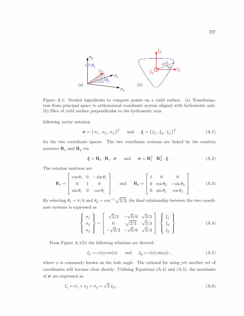
227

θ1

θ2σ1

σ3

σ2

φr(φ)

(b)(a)

ξ 3 ξ3ξ1

ξ2

Figure A.1: Needed ingredients to compute points on a yield surface. (a) Transforma-tion from principal space to orthonormal coordinate system aligned with hydrostatic axis.(b) Slice of yield surface perpendicular to the hydrostatic axis.

following vector notation

σ = σ1 , σ2 , σ3 T and ξ = ξ1 , ξ2 , ξ3 T (A.1)

for the two coordinate spaces. The two coordinate systems are linked by the rotation

matrices R1 and R2 via

ξ = R2 ·R1 · σ and σ = RT1 ·RT

2 · ξ . (A.2)

The rotation matrices are

R1 =

cos θ1 0 − sin θ1

0 1 0

sin θ1 0 cos θ1

and R2 =

1 0 0

0 cos θ2 − sin θ2

0 sin θ2 cos θ2

. (A.3)

By selecting θ1 = π/4 and θ2 = cos−1√

2/3, the final relationship between the two coordi-

nate systems is expressed as

σ1

σ2

σ3

=

√2/2 −

√6/6

√3/3

0√

2/3√3/3

−√2/2 −

√6/6

√3/3

·

ξ1

ξ2

ξ3

. (A.4)

From Figure A.1(b) the following relations are derived:

ξ1 = r(φ) cos(φ) and ξ2 = r(φ) sin(φ) , (A.5)

where φ is commonly known as the lode angle. The rational for using yet another set of

coordinates will become clear shortly. Utilizing Equations (A.4) and (A.5), the invariants

of σ are expressed as

I1 = σ1 + σ2 + σ3 =√3 ξ3, (A.6)

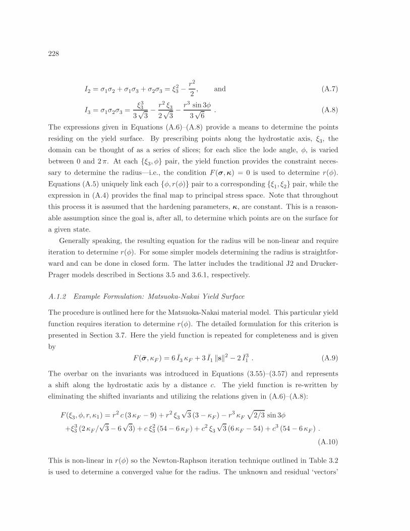
228

I2 = σ1σ2 + σ1σ3 + σ2σ3 = ξ23 −r2

2, and (A.7)

I3 = σ1σ2σ3 =ξ33

3√3− r2 ξ3

2√3− r3 sin 3φ

3√6

. (A.8)

The expressions given in Equations (A.6)–(A.8) provide a means to determine the points

residing on the yield surface. By prescribing points along the hydrostatic axis, ξ3, the

domain can be thought of as a series of slices; for each slice the lode angle, φ, is varied

between 0 and 2π. At each ξ3, φ pair, the yield function provides the constraint neces-

sary to determine the radius—i.e., the condition F (σ,κ) = 0 is used to determine r(φ).

Equations (A.5) uniquely link each φ, r(φ) pair to a corresponding ξ1, ξ2 pair, while the

expression in (A.4) provides the final map to principal stress space. Note that throughout

this process it is assumed that the hardening parameters, κ, are constant. This is a reason-

able assumption since the goal is, after all, to determine which points are on the surface for

a given state.

Generally speaking, the resulting equation for the radius will be non-linear and require

iteration to determine r(φ). For some simpler models determining the radius is straightfor-

ward and can be done in closed form. The latter includes the traditional J2 and Drucker-

Prager models described in Sections 3.5 and 3.6.1, respectively.

A.1.2 Example Formulation: Matsuoka-Nakai Yield Surface

The procedure is outlined here for the Matsuoka-Nakai material model. This particular yield

function requires iteration to determine r(φ). The detailed formulation for this criterion is

presented in Section 3.7. Here the yield function is repeated for completeness and is given

by

F (σ, κF ) = 6 I3 κF + 3 I1 ‖s‖2 − 2 I31 . (A.9)

The overbar on the invariants was introduced in Equations (3.55)–(3.57) and represents

a shift along the hydrostatic axis by a distance c. The yield function is re-written by

eliminating the shifted invariants and utilizing the relations given in (A.6)–(A.8):

F (ξ3, φ, r, κ1) = r2 c (3κF − 9) + r2 ξ3√3 (3− κF )− r3 κF

√

2/3 sin 3φ

+ξ33 (2κF /√3− 6

√3) + c ξ23 (54− 6κF ) + c2 ξ3

√3 (6κF − 54) + c3 (54 − 6κF ) .

(A.10)

This is non-linear in r(φ) so the Newton-Raphson iteration technique outlined in Table 3.2

is used to determine a converged value for the radius. The unknown and residual ‘vectors’

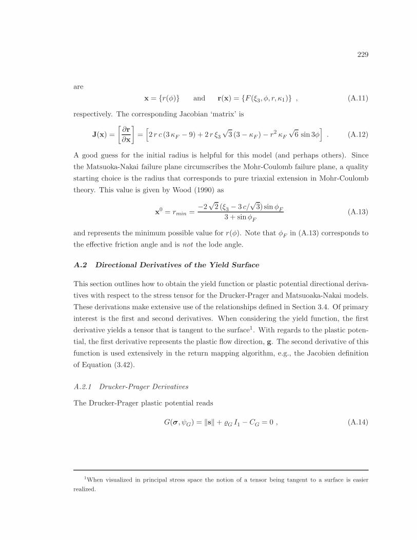
229

are

x = r(φ) and r(x) = F (ξ3, φ, r, κ1) , (A.11)

respectively. The corresponding Jacobian ‘matrix’ is

J(x) =

[∂r

∂x

]

=[

2 r c (3κF − 9) + 2 r ξ3√3 (3− κF )− r2 κF

√6 sin 3φ

]

. (A.12)

A good guess for the initial radius is helpful for this model (and perhaps others). Since

the Matsuoka-Nakai failure plane circumscribes the Mohr-Coulomb failure plane, a quality

starting choice is the radius that corresponds to pure triaxial extension in Mohr-Coulomb

theory. This value is given by Wood (1990) as

x0 = rmin =−2

√2 (ξ3 − 3 c/

√3) sinφF

3 + sinφF(A.13)

and represents the minimum possible value for r(φ). Note that φF in (A.13) corresponds to

the effective friction angle and is not the lode angle.

A.2 Directional Derivatives of the Yield Surface

This section outlines how to obtain the yield function or plastic potential directional deriva-

tives with respect to the stress tensor for the Drucker-Prager and Matsuoaka-Nakai models.

These derivations make extensive use of the relationships defined in Section 3.4. Of primary

interest is the first and second derivatives. When considering the yield function, the first

derivative yields a tensor that is tangent to the surface1. With regards to the plastic poten-

tial, the first derivative represents the plastic flow direction, g. The second derivative of this

function is used extensively in the return mapping algorithm, e.g., the Jacobien definition

of Equation (3.42).

A.2.1 Drucker-Prager Derivatives

The Drucker-Prager plastic potential reads

G(σ, ψG) = ‖s‖+ G I1 − CG = 0 , (A.14)

1When visualized in principal stress space the notion of a tensor being tangent to a surface is easier

realized.

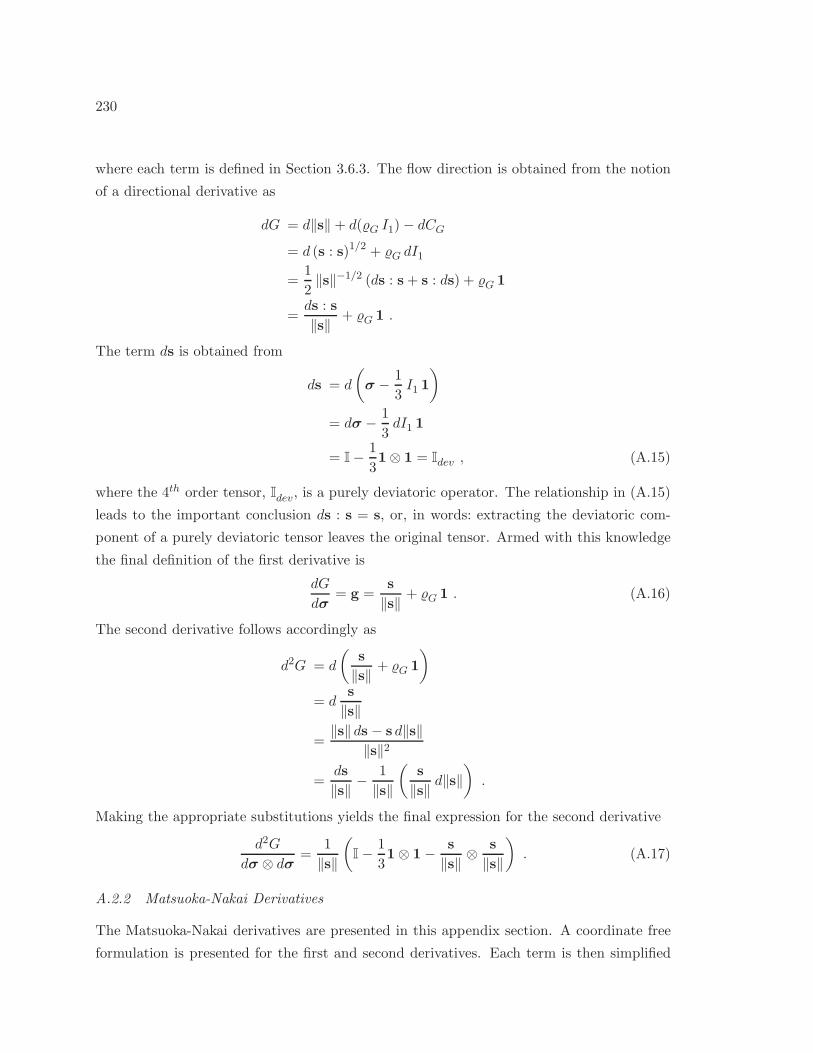
230

where each term is defined in Section 3.6.3. The flow direction is obtained from the notion

of a directional derivative as

dG = d‖s‖ + d(G I1)− dCG

= d (s : s)1/2 + G dI1

=1

2‖s‖−1/2 (ds : s+ s : ds) + G 1

=ds : s

‖s‖ + G 1 .

The term ds is obtained from

ds = d

(

σ − 1

3I1 1

)

= dσ − 1

3dI1 1

= I− 1

31⊗ 1 = Idev , (A.15)

where the 4th order tensor, Idev, is a purely deviatoric operator. The relationship in (A.15)

leads to the important conclusion ds : s = s, or, in words: extracting the deviatoric com-

ponent of a purely deviatoric tensor leaves the original tensor. Armed with this knowledge

the final definition of the first derivative is

dG

dσ= g =

s

‖s‖ + G 1 . (A.16)

The second derivative follows accordingly as

d2G = d

(s

‖s‖ + G 1

)

= ds

‖s‖

=‖s‖ ds − s d‖s‖

‖s‖2

=ds

‖s‖ − 1

‖s‖

(s

‖s‖ d‖s‖)

.

Making the appropriate substitutions yields the final expression for the second derivative

d2G

dσ ⊗ dσ=

1

‖s‖

(

I− 1

31⊗ 1− s

‖s‖ ⊗ s

‖s‖

)

. (A.17)

A.2.2 Matsuoka-Nakai Derivatives

The Matsuoka-Nakai derivatives are presented in this appendix section. A coordinate free

formulation is presented for the first and second derivatives. Each term is then simplified

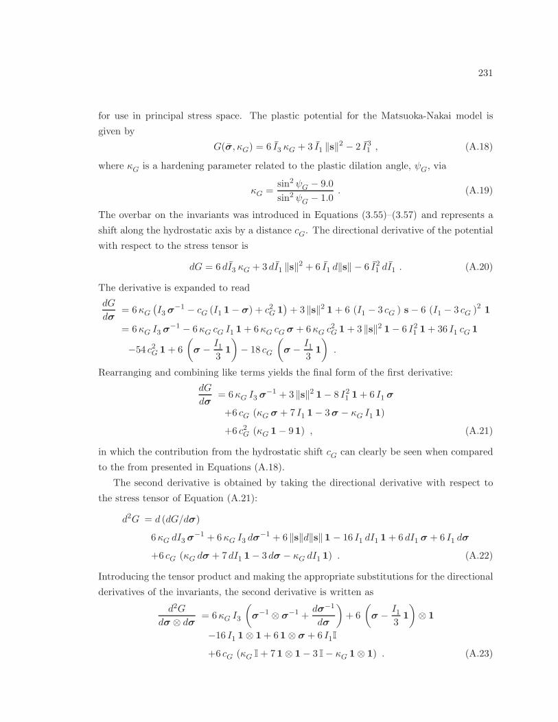
231

for use in principal stress space. The plastic potential for the Matsuoka-Nakai model is

given by

G(σ, κG) = 6 I3 κG + 3 I1 ‖s‖2 − 2 I31 , (A.18)

where κG is a hardening parameter related to the plastic dilation angle, ψG, via

κG =sin2 ψG − 9.0

sin2 ψG − 1.0. (A.19)

The overbar on the invariants was introduced in Equations (3.55)–(3.57) and represents a

shift along the hydrostatic axis by a distance cG. The directional derivative of the potential

with respect to the stress tensor is

dG = 6 dI3 κG + 3 dI1 ‖s‖2 + 6 I1 d‖s‖ − 6 I21 dI1 . (A.20)

The derivative is expanded to read

dG

dσ= 6κG

(I3 σ

−1 − cG (I1 1− σ) + c2G 1)+ 3 ‖s‖2 1+ 6 (I1 − 3 cG ) s− 6 (I1 − 3 cG )2 1

= 6κG I3 σ−1 − 6κG cG I1 1+ 6κG cG σ + 6κG c

2G 1+ 3 ‖s‖2 1− 6 I21 1+ 36 I1 cG 1

−54 c2G 1+ 6

(

σ − I131

)

− 18 cG

(

σ − I131

)

.

Rearranging and combining like terms yields the final form of the first derivative:

dG

dσ= 6κG I3 σ

−1 + 3 ‖s‖2 1− 8 I21 1+ 6 I1 σ

+6 cG (κG σ + 7 I1 1− 3σ − κG I1 1)

+6 c2G (κG 1− 91) , (A.21)

in which the contribution from the hydrostatic shift cG can clearly be seen when compared

to the from presented in Equations (A.18).

The second derivative is obtained by taking the directional derivative with respect to

the stress tensor of Equation (A.21):

d2G = d (dG/dσ)

6κG dI3 σ−1 + 6κG I3 dσ

−1 + 6 ‖s‖d‖s‖1 − 16 I1 dI1 1+ 6 dI1 σ + 6 I1 dσ

+6 cG (κG dσ + 7 dI1 1− 3 dσ − κG dI1 1) . (A.22)

Introducing the tensor product and making the appropriate substitutions for the directional

derivatives of the invariants, the second derivative is written as

d2G

dσ ⊗ dσ= 6κG I3

(

σ−1 ⊗ σ−1 +dσ−1

dσ

)

+ 6

(

σ − I131

)

⊗ 1

−16 I1 1⊗ 1+ 61⊗ σ + 6 I1I

+6 cG (κG I+ 71⊗ 1− 3 I− κG 1⊗ 1) . (A.23)

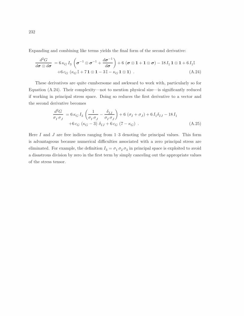
232

Expanding and combining like terms yields the final form of the second derivative:

d2G

dσ ⊗ dσ= 6κG I3

(

σ−1 ⊗ σ−1 +dσ−1

dσ

)

+ 6 (σ ⊗ 1+ 1⊗ σ)− 18 I1 1⊗ 1+ 6 I1I

+6 cG (κG I+ 71⊗ 1− 3 I− κG 1⊗ 1) . (A.24)

These derivatives are quite cumbersome and awkward to work with, particularly so for

Equation (A.24). Their complexity—not to mention physical size—is significantly reduced

if working in principal stress space. Doing so reduces the first derivative to a vector and

the second derivative becomes

d2G

σI σJ= 6κG I3

(1

σI σJ− δIJσI σJ

)

+ 6 (σI + σJ) + 6 I1δIJ − 18 I1

+6 cG (κG − 3) δIJ + 6 cG (7− κG) . (A.25)

Here I and J are free indices ranging from 1–3 denoting the principal values. This form

is advantageous because numerical difficulties associated with a zero principal stress are

eliminated. For example, the definition I3 = σ1 σ2 σ3 in principal space is exploited to avoid

a disastrous division by zero in the first term by simply canceling out the appropriate values

of the stress tensor.

233

Appendix B

COMPUTATIONAL FRAMEWORK

At the core of any numerical simulation is the computational framework that effec-

tively reads in data, performs the relevant calculations, and generates useful results for

analysis and visualization. The implementation developed for the present study employs

the C++ and Python programming languages. Visualization is accomplished using the

matplotlib Python module, as well as the 3rd party software ParaView 1 , an interactive

application that relies on the Visualization Toolkit (VTK) library. The goal of this chapter

is to present an overview of the computational framework so others using this coding base

have a starting point for future work. There are limitations in the extent to which the code

can be documented here. As such, primary emphasis is placed on defining input data and

viewing results.

B.1 Overview

The computational framework, referred to from here on as the code, contains approximately

22,500 lines of code 2 (loc). This metric and others are easily obtainable for any project

using the free utility cloc. Of course, loc is a bit vague and subject to change based

on coding style and the efficiency of the implementation, but does provide some frame of

reference as to the size of the application. The code is split naturally into three categories:

pre-processing, model analysis, and post-processing, each of which accounts for 5%, 70%,

and 25% of the total 22.5 kloc, respectively.

These code components are shown schematically in Figure B.1. In this perspective the

three entities create a pipeline directing the flow of data. Raw data comprising the spa-

tial domain and body is organized and used to generate an input file. The model analysis

portion, an object-oriented implementation written exclusively in C++ , does the primary

numerical analysis and writes a stream of values to an output file at user prescribed incre-

ments. A typical data set ranges in size from a few kilobytes to several gigabytes, and can

contain customizable input and output types unique to each analysis. The lack of a pre-

1http://www.paraview.org/

2This figure does not include comments and blank lines. Adding these yields approximately 41,000 loc.

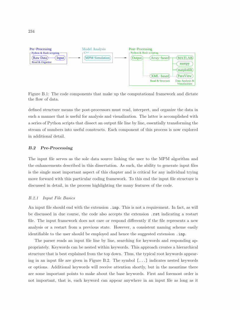
234

Python & Bash scripting

MPM Simulation

C++

Output MATLAB

numpy

matplotlib

ParaView

Array−based

XML−based

InputRaw Data

Pre−ProcessingPython & Bash scripting

Post−Processing

Read & Structure

Read & Organize

Data Analysis &Visualization

Model Analysis

Figure B.1: The code components that make up the computational framework and dictatethe flow of data.

defined structure means the post-processors must read, interpret, and organize the data in

such a manner that is useful for analysis and visualization. The latter is accomplished with

a series of Python scripts that dissect an output file line by line, essentially transforming the

stream of numbers into useful constructs. Each component of this process is now explored

in additional detail.

B.2 Pre-Processing

The input file serves as the sole data source linking the user to the MPM algorithm and

the enhancements described in this dissertation. As such, the ability to generate input files

is the single most important aspect of this chapter and is critical for any individual trying

move forward with this particular coding framework. To this end the input file structure is

discussed in detail, in the process highlighting the many features of the code.

B.2.1 Input File Basics

An input file should end with the extension .inp. This is not a requirement. In fact, as will

be discussed in due course, the code also accepts the extension .rst indicating a restart

file. The input framework does not care or respond differently if the file represents a new

analysis or a restart from a previous state. However, a consistent naming scheme easily

identifiable to the user should be employed and hence the suggested extension .inp.

The parser reads an input file line by line, searching for keywords and responding ap-

propriately. Keywords can be nested within keywords. This approach creates a hierarchical

structure that is best explained from the top down. Thus, the typical root keywords appear-

ing in an input file are given in Figure B.2. The symbol [...] indicates nested keywords

or options. Additional keywords will receive attention shortly, but in the meantime there

are some important points to make about the base keywords. First and foremost order is

not important, that is, each keyword can appear anywhere in an input file as long as it

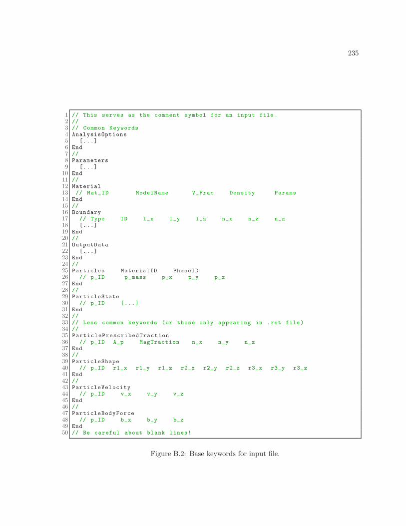
235

1 // This serves as the comment symbol for an input file .2 //3 // Common Keywords4 AnalysisOptions5 [...]6 End7 //8 Parameters9 [...]

10 End11 //12 Material13 // Mat_ID ModelName V_Frac Density Params14 End15 //16 Boundary17 // Type ID l_x l_y l_z n_x n_z n_z18 [...]19 End20 //21 OutputData22 [...]23 End24 //25 Particles MaterialID PhaseID26 // p_ID p_mass p_x p_y p_z27 End28 //29 ParticleState30 // p_ID [...]31 End32 //33 // Less common keywords (or those only appearing in .rst file )34 //35 ParticlePrescribedTraction36 // p_ID A_p MagTraction n_x n_y n_z37 End38 //39 ParticleShape40 // p_ID r1_x r1_y r1_z r2_x r2_y r2_z r3_x r3_y r3_z41 End42 //43 ParticleVelocity44 // p_ID v_x v_y v_z45 End46 //47 ParticleBodyForce48 // p_ID b_x b_y b_z49 End50 // Be careful about blank lines!

Figure B.2: Base keywords for input file.

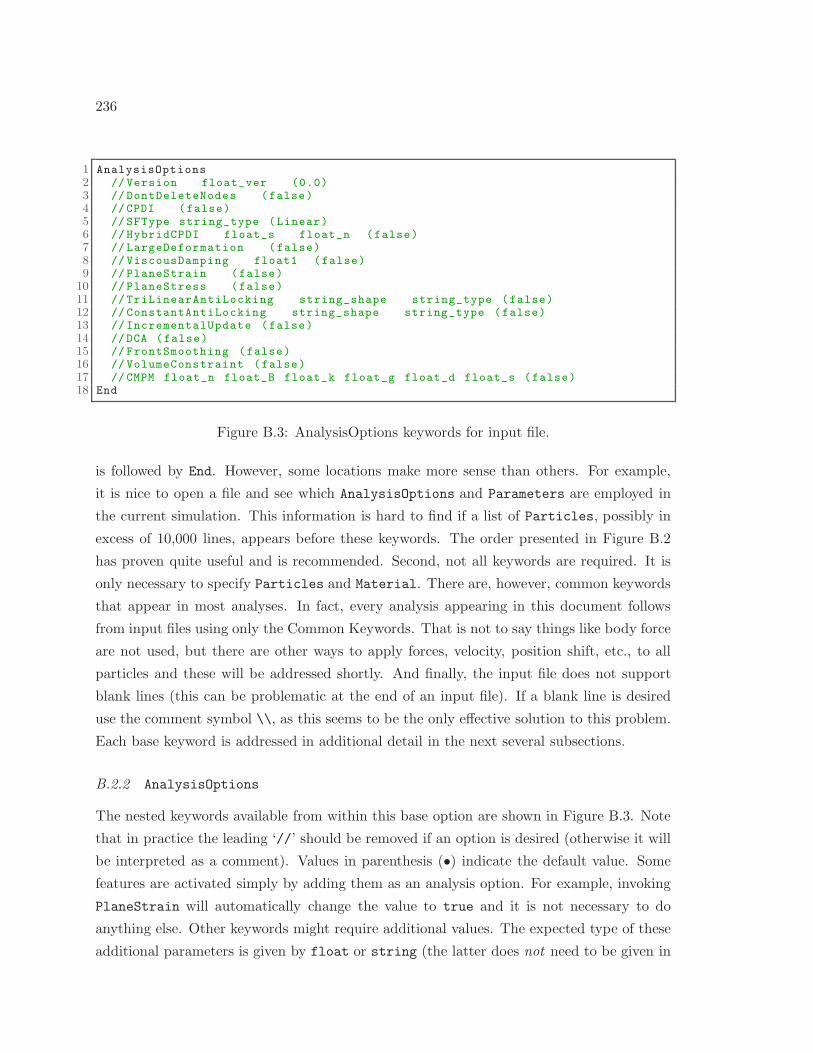
236

1 AnalysisOptions2 // Version float_ver (0.0)3 // DontDeleteNodes (false)4 // CPDI (false)5 // SFType string_type ( Linear)6 // HybridCPDI float_s float_n (false)7 // LargeDeformation ( false)8 // ViscousDamping float1 (false)9 // PlaneStrain (false)

10 // PlaneStress (false)11 // TriLinearAntiLocking string_shape string_type (false)12 // ConstantAntiLocking string_shape string_type (false)13 // IncrementalUpdate (false)14 // DCA (false)15 // FrontSmoothing (false)16 // VolumeConstraint (false)17 // CMPM float_n float_B float_k float_g float_d float_s (false)18 End

Figure B.3: AnalysisOptions keywords for input file.

is followed by End. However, some locations make more sense than others. For example,

it is nice to open a file and see which AnalysisOptions and Parameters are employed in

the current simulation. This information is hard to find if a list of Particles, possibly in

excess of 10,000 lines, appears before these keywords. The order presented in Figure B.2

has proven quite useful and is recommended. Second, not all keywords are required. It is

only necessary to specify Particles and Material. There are, however, common keywords

that appear in most analyses. In fact, every analysis appearing in this document follows

from input files using only the Common Keywords. That is not to say things like body force

are not used, but there are other ways to apply forces, velocity, position shift, etc., to all

particles and these will be addressed shortly. And finally, the input file does not support

blank lines (this can be problematic at the end of an input file). If a blank line is desired

use the comment symbol \\, as this seems to be the only effective solution to this problem.

Each base keyword is addressed in additional detail in the next several subsections.

B.2.2 AnalysisOptions

The nested keywords available from within this base option are shown in Figure B.3. Note

that in practice the leading ‘//’ should be removed if an option is desired (otherwise it will

be interpreted as a comment). Values in parenthesis (•) indicate the default value. Some

features are activated simply by adding them as an analysis option. For example, invoking

PlaneStrain will automatically change the value to true and it is not necessary to do

anything else. Other keywords might require additional values. The expected type of these

additional parameters is given by float or string (the latter does not need to be given in

237

quotes).

Version float_ver

This is the Version number with 0.0 the default. This feature is not important since

nothing special is done for different versions. Obviously this could be a powerful

feature with additional code releases.

DontDeleteNodes

Nodes with no mass are subject to deletion by default. By activating this option nodes

will not be removed even if they have no mass. The frequency with which nodes are

removed can be adjusted in OutputData.

CPDI

This is the Convected Particle Domain Interpolation feature by Sadeghirad et al.

(2011b). If this feature is active then the ParticleShape should be specified for each

particle in the input file. If not specified default shapes are assumed and may not

match the desired particle structure.

SFType string_type

Standard shape function type. Defaults to Linear , an 8-noded brick. Type

Quadratic is a 27-noded element. The solution scheme uses a lumped mass. This is

problematic for the quadratic element if particles are changing cells, thus Quadratic is

only recommended for small displacements.

HybridCPDI float_s float_n

False by default. This feature was developed in house and utilizes the CPDI option

only for particles actively crossing a cell boundary. float_s is a scalar multiplier that

decreases (or increases) the shape vectors that make up the particle. float_n is the

max number of particles in the new cell that will turn off this feature.

For example: HybridCPDI 0.75 8 will reduce the particle shape size by 25%

and only activate CPDI if 8 or less particles are in the new cell the particle is headed

into. Note that the size reduction is only applied in the search algorithm to see if a

particle is in multiple cells. This does not affect the actual particle mass or volume.

LargeDeformation

Small deformation by default, see Equation (3.10). Activating this feature changes

the deformation measure to the left Cauchy-Green deformation tensor, for use with

the logarithmic strain in (3.33).

238

PlaneStrain

False by default. Restricts deformation in the z-direction. Particles must reside in the

xy plane to use this feature. If activated the particles are automatically shifted to the

center of the cell in the z-direction. This feature impacts the anti-locking routines, as

the shape and filter matrices are changed by plane strain conditions.

PlaneStress

False by default. Restricts stress accumulation in the z-direction. Particles must

reside in the xy plane to use this feature. If activated the particles are automatically

shifted to the center of the cell in the z-direction. This feature impacts the anti-locking

routines, as the shape and filter matrices are changed by plane stress conditions. This

feature is valid only for linear elastic materials.

TriLinearAntiLocking string_shape string_type

False by default. string_shape can be either AS1,AS2,or AS3CV. Shape AS1 utilizes

those definitions in Section 4.3.1, shape AS2 uses those given in Section 4.3.2, while

shape AS3CV forces a constant volumetric approximation. string_type can be either

CellBased, NodeBased, or HybridBased. See Sections 4.4.1–4.4.3 for a discussion.

ConstantAntiLocking string_shape string_type

False by default. string_shape can be either AS1,or AS2. This option does not utilize

the diagonal terms in shape matrix definition.

ViscousDamping float1

This feature adds artificial volumetric damping similar to the approach given in Chen

et al. (2002) and is false by default. Note that this feature is not the same as adding

overall viscosity. This feature is the single most important feature for simulating

nearly incompressible fluids or elastic solids. Anti-locking alone cannot achieve the

degree of stabilization that this feature provides.

DCA

False by default. This is the Distributed mass Coefficient Algorithm as presented

by Ma et al. (2010a). This approach is useful for nodes that have small mass and

redistributes mass to regions near the edge of the body. This feature has not been

extensively evaluated and has shown to be problematic when large regions of a body

are moving into a new cell.

FrontSmoothing

False by default. This feature that automatically detects which nodes have a volume

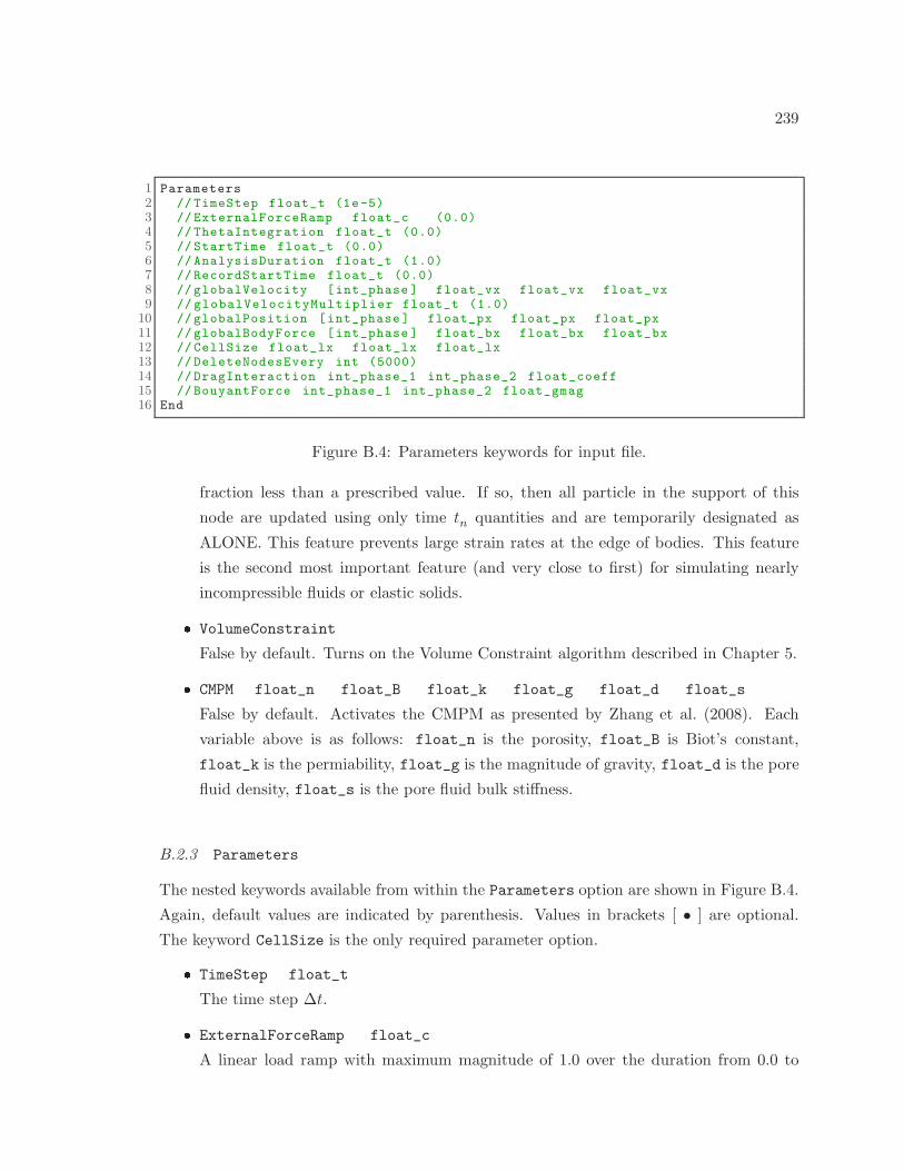
239

1 Parameters2 // TimeStep float_t (1e-5)3 // ExternalForceRamp float_c (0.0)4 // ThetaIntegration float_t (0.0)5 // StartTime float_t (0.0)6 // AnalysisDuration float_t (1.0)7 // RecordStartTime float_t (0.0)8 // globalVelocity [int_phase ] float_vx float_vx float_vx9 // globalVelocityMultiplier float_t (1.0)

10 // globalPosition [int_phase ] float_px float_px float_px11 // globalBodyForce [int_phase ] float_bx float_bx float_bx12 // CellSize float_lx float_lx float_lx13 // DeleteNodesEvery int (5000)14 // DragInteraction int_phase_1 int_phase_2 float_coeff15 // BouyantForce int_phase_1 int_phase_2 float_gmag16 End

Figure B.4: Parameters keywords for input file.

fraction less than a prescribed value. If so, then all particle in the support of this

node are updated using only time tn quantities and are temporarily designated as

ALONE. This feature prevents large strain rates at the edge of bodies. This feature

is the second most important feature (and very close to first) for simulating nearly

incompressible fluids or elastic solids.

VolumeConstraint

False by default. Turns on the Volume Constraint algorithm described in Chapter 5.

CMPM float_n float_B float_k float_g float_d float_s

False by default. Activates the CMPM as presented by Zhang et al. (2008). Each

variable above is as follows: float_n is the porosity, float_B is Biot’s constant,

float_k is the permiability, float_g is the magnitude of gravity, float_d is the pore

fluid density, float_s is the pore fluid bulk stiffness.

B.2.3 Parameters

The nested keywords available from within the Parameters option are shown in Figure B.4.

Again, default values are indicated by parenthesis. Values in brackets [ • ] are optional.

The keyword CellSize is the only required parameter option.

TimeStep float_t

The time step ∆t.

ExternalForceRamp float_c

A linear load ramp with maximum magnitude of 1.0 over the duration from 0.0 to

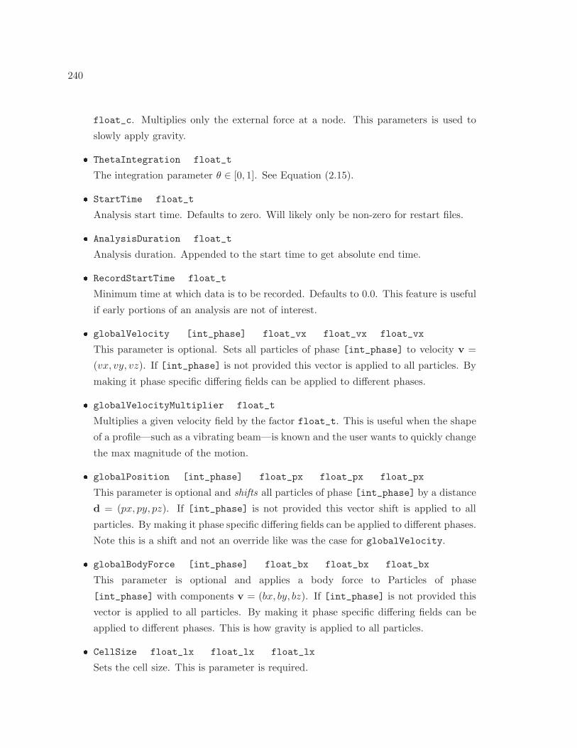
240

float_c. Multiplies only the external force at a node. This parameters is used to

slowly apply gravity.

ThetaIntegration float_t

The integration parameter θ ∈ [0, 1]. See Equation (2.15).

StartTime float_t

Analysis start time. Defaults to zero. Will likely only be non-zero for restart files.

AnalysisDuration float_t

Analysis duration. Appended to the start time to get absolute end time.

RecordStartTime float_t

Minimum time at which data is to be recorded. Defaults to 0.0. This feature is useful

if early portions of an analysis are not of interest.

globalVelocity [int_phase] float_vx float_vx float_vx

This parameter is optional. Sets all particles of phase [int_phase] to velocity v =

(vx, vy, vz). If [int_phase] is not provided this vector is applied to all particles. By

making it phase specific differing fields can be applied to different phases.

globalVelocityMultiplier float_t

Multiplies a given velocity field by the factor float_t. This is useful when the shape

of a profile—such as a vibrating beam—is known and the user wants to quickly change

the max magnitude of the motion.

globalPosition [int_phase] float_px float_px float_px

This parameter is optional and shifts all particles of phase [int_phase] by a distance

d = (px, py, pz). If [int_phase] is not provided this vector shift is applied to all

particles. By making it phase specific differing fields can be applied to different phases.

Note this is a shift and not an override like was the case for globalVelocity.

globalBodyForce [int_phase] float_bx float_bx float_bx

This parameter is optional and applies a body force to Particles of phase

[int_phase] with components v = (bx, by, bz). If [int_phase] is not provided this

vector is applied to all particles. By making it phase specific differing fields can be

applied to different phases. This is how gravity is applied to all particles.

CellSize float_lx float_lx float_lx

Sets the cell size. This is parameter is required.

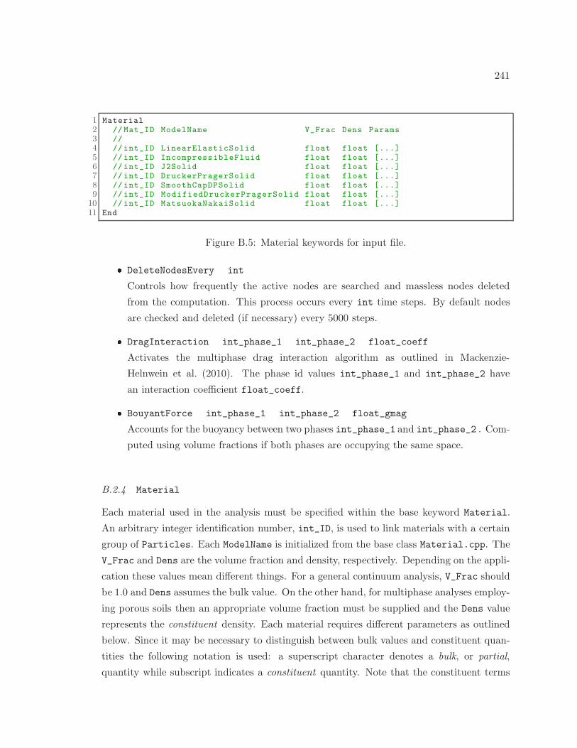
241

1 Material2 // Mat_ID ModelName V_Frac Dens Params3 //4 // int_ID LinearElasticSolid float float [...]5 // int_ID IncompressibleFluid float float [...]6 // int_ID J2Solid float float [...]7 // int_ID DruckerPragerSolid float float [...]8 // int_ID SmoothCapDPSolid float float [...]9 // int_ID ModifiedDruckerPragerSolid float float [...]

10 // int_ID MatsuokaNakaiSolid float float [...]11 End

Figure B.5: Material keywords for input file.

DeleteNodesEvery int

Controls how frequently the active nodes are searched and massless nodes deleted

from the computation. This process occurs every int time steps. By default nodes

are checked and deleted (if necessary) every 5000 steps.

DragInteraction int_phase_1 int_phase_2 float_coeff

Activates the multiphase drag interaction algorithm as outlined in Mackenzie-

Helnwein et al. (2010). The phase id values int_phase_1 and int_phase_2 have

an interaction coefficient float_coeff.

BouyantForce int_phase_1 int_phase_2 float_gmag

Accounts for the buoyancy between two phases int_phase_1 and int_phase_2 . Com-

puted using volume fractions if both phases are occupying the same space.

B.2.4 Material

Each material used in the analysis must be specified within the base keyword Material.

An arbitrary integer identification number, int_ID, is used to link materials with a certain

group of Particles. Each ModelName is initialized from the base class Material.cpp. The

V_Frac and Dens are the volume fraction and density, respectively. Depending on the appli-

cation these values mean different things. For a general continuum analysis, V_Frac should

be 1.0 and Dens assumes the bulk value. On the other hand, for multiphase analyses employ-

ing porous soils then an appropriate volume fraction must be supplied and the Dens value

represents the constituent density. Each material requires different parameters as outlined

below. Since it may be necessary to distinguish between bulk values and constituent quan-

tities the following notation is used: a superscript character denotes a bulk, or partial,

quantity while subscript indicates a constituent quantity. Note that the constituent terms

242

are needed exclusively for the VolumeConstraint algorithm. Constitutive parameters are

made mass-specific internally, as such the user should not attempt to account for this in the

input file.

LinearElasticSolid

This is a traditional linear elastic material in which

[...]= [ Kα, Kα, Gα ]

with Kα and Kα as the constituent and bulk stiffness, respectively, and Gα as the

bulk shear modulus.

IncompressibleFluid

Fluids derived from this material are bound to the LinearElasticSolidclass. This

concept is illustrated in Equation (6.1) and corresponding discussion. The input pa-

rameters are

[...]= [ Kα, Kα, µ ]

with µ as the dynamic viscosity. Obviously the notion of constituent vs. bulk proper-

ties can lose meaning when dealing with a fluid. See Section 6.3 for how to interpret

these quantities in the context of a fluid.

J2Solid

See Section 3.5 for a discussion of this model and implementation details. This model

contains optional input parameters designated by the | and ‖ symbol.

[...]= [ Kα, Kα, Gα, σY , | k, ‖ H]

Everything to the left of | is a required input, including the yield stress σY . If no

hardening is desired then these are the only inputs. Alternatively, isotropic hardening

is obtained by adding the modulus k to the parameters and including everything to

the left of ‖ symbol. Finally, by adding H, kinematic hardening is included and the

parameter vector is fully populated.

DruckerPragerSolid

See Section 3.6.1 for a discussion of this model and implementation details. For this

model the parameters are

[...]= [ Kα, Kα, Gα, F , σY , | G, ‖ k, H]

where F and G are additional model parameters related to the internal friction

angle and dilation angle, respectively. Again, the | and ‖ work as they did for the

J2Solidinput.

SmoothCapDPSolid

See Section 3.6.2 for a discussion of this model and implementation details. The

243

1 Boundary2 // Type ID l_x l_y l_z n_x n_z n_z3 //4 // Fixed int_ID fl_lx fl_ly fl_lz fl_nx fl_ny fl_nz5 // Planar int_ID fl_lx fl_ly fl_lz fl_nx fl_ny fl_nz6 // Eliminate int_ID fl_lx fl_ly fl_lz fl_nx fl_ny fl_nz7 // Size int_ID fl_sx fl_sy fl_sz8 // ForceTolerance int_ID float_tol9 // FrictionCoefficient int_ID float_coeff

10 // Phase int_ID int_PhaseID11 End

Figure B.6: Boundary keywords for input file.

parameters are

[...]= [ Kα, Kα, Gα, F , µ, | G]

with µ as an effective yield stress. Currently no material hardening or softening is

implemented in this model.

ModifiedDruckerPragerSolid and MatsuokaNakaiSolid

See Sections 3.6.3 and 3.7 for a discussion of these models and implementation details.

Both use identical parameters vectors by design and are as follows:

[...]= [ Kα, Kα, Gα, cF , a0, a1, a2, a3, a4, a5]

where cF is a cohesion parameter and a0−5 are the constants used to define the internal

friction and critical state angles.

B.2.5 Boundary

The current implementation is capable of modeling horizontal surfaces with arbitrary lo-

cations and orientations. Each flat surface is an instance of the Boundary.cpp object. At

this point only displacement boundary conditions are supported in a general sense. Other

conditions, such as force and velocity, can be added to the code to obtain certain effects

depending on the application. The two supported boundary types are Fixed and Planar.

Physical boundaries must be one of these two types. A third option exists and is outlined

below. Boundaries work best when they align with the grid. However, there is no require-

ment that boundary objects align with the grid. Indeed, by making many small boundary

objects, each with changing normal, curves and arbitrary surfaces can be composed. Of

course, the quality of the representation is still subject to the spatial discretization and the

cell size. Given the arbitrary nature of the boundary in MPM, a single node can have mul-

tiple boundary objects. In this case an equivalent normal vector representing all surfaces is

computed.

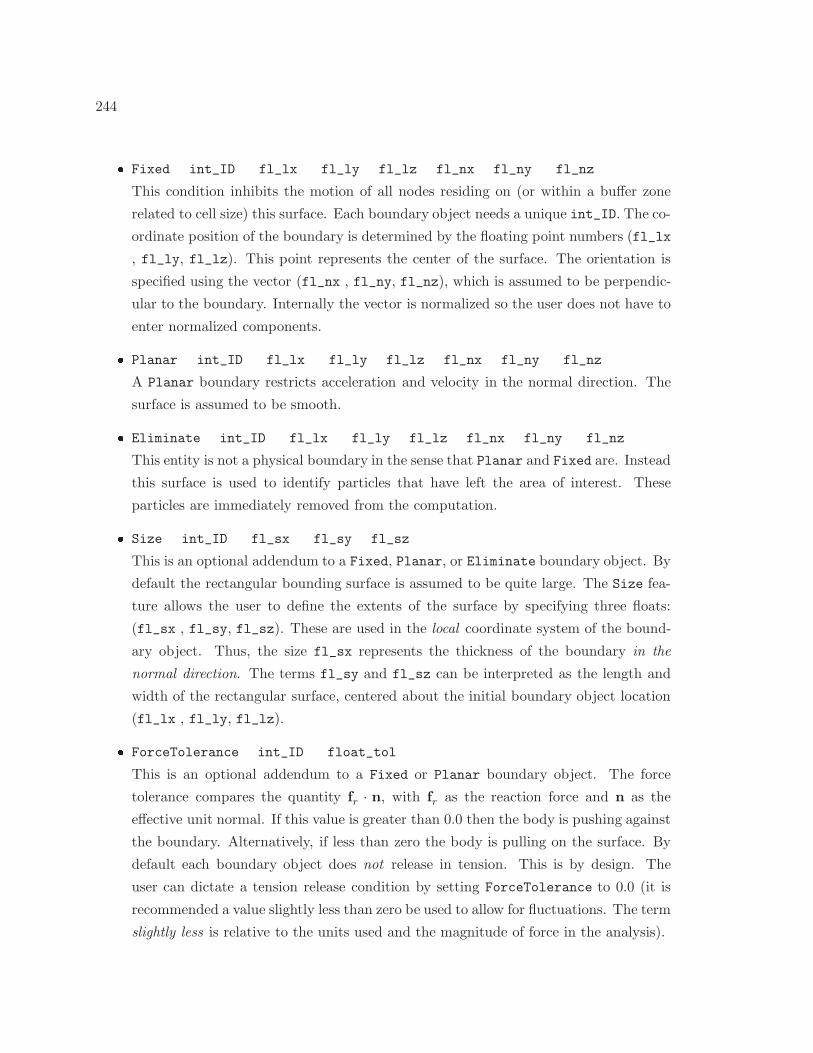
244

Fixed int_ID fl_lx fl_ly fl_lz fl_nx fl_ny fl_nz

This condition inhibits the motion of all nodes residing on (or within a buffer zone

related to cell size) this surface. Each boundary object needs a unique int_ID. The co-

ordinate position of the boundary is determined by the floating point numbers (fl_lx

, fl_ly, fl_lz). This point represents the center of the surface. The orientation is

specified using the vector (fl_nx , fl_ny, fl_nz), which is assumed to be perpendic-

ular to the boundary. Internally the vector is normalized so the user does not have to

enter normalized components.

Planar int_ID fl_lx fl_ly fl_lz fl_nx fl_ny fl_nz

A Planar boundary restricts acceleration and velocity in the normal direction. The

surface is assumed to be smooth.

Eliminate int_ID fl_lx fl_ly fl_lz fl_nx fl_ny fl_nz

This entity is not a physical boundary in the sense that Planar and Fixed are. Instead

this surface is used to identify particles that have left the area of interest. These

particles are immediately removed from the computation.

Size int_ID fl_sx fl_sy fl_sz

This is an optional addendum to a Fixed, Planar, or Eliminate boundary object. By

default the rectangular bounding surface is assumed to be quite large. The Size fea-

ture allows the user to define the extents of the surface by specifying three floats:

(fl_sx , fl_sy, fl_sz). These are used in the local coordinate system of the bound-

ary object. Thus, the size fl_sx represents the thickness of the boundary in the

normal direction. The terms fl_sy and fl_sz can be interpreted as the length and

width of the rectangular surface, centered about the initial boundary object location

(fl_lx , fl_ly, fl_lz).

ForceTolerance int_ID float_tol

This is an optional addendum to a Fixed or Planar boundary object. The force

tolerance compares the quantity fr · n, with fr as the reaction force and n as the

effective unit normal. If this value is greater than 0.0 then the body is pushing against

the boundary. Alternatively, if less than zero the body is pulling on the surface. By

default each boundary object does not release in tension. This is by design. The

user can dictate a tension release condition by setting ForceTolerance to 0.0 (it is

recommended a value slightly less than zero be used to allow for fluctuations. The term

slightly less is relative to the units used and the magnitude of force in the analysis).

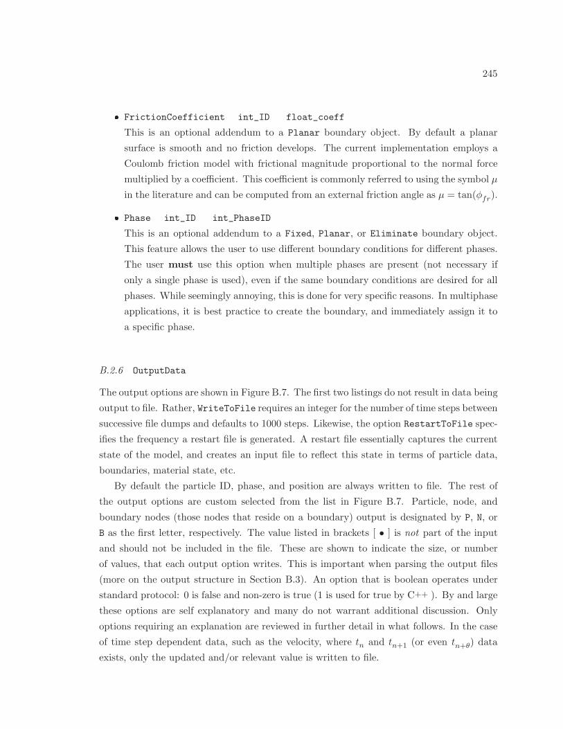
245

FrictionCoefficient int_ID float_coeff

This is an optional addendum to a Planar boundary object. By default a planar

surface is smooth and no friction develops. The current implementation employs a

Coulomb friction model with frictional magnitude proportional to the normal force

multiplied by a coefficient. This coefficient is commonly referred to using the symbol µ

in the literature and can be computed from an external friction angle as µ = tan(φfr).

Phase int_ID int_PhaseID

This is an optional addendum to a Fixed, Planar, or Eliminate boundary object.

This feature allows the user to use different boundary conditions for different phases.

The user must use this option when multiple phases are present (not necessary if

only a single phase is used), even if the same boundary conditions are desired for all

phases. While seemingly annoying, this is done for very specific reasons. In multiphase

applications, it is best practice to create the boundary, and immediately assign it to

a specific phase.

B.2.6 OutputData

The output options are shown in Figure B.7. The first two listings do not result in data being

output to file. Rather, WriteToFile requires an integer for the number of time steps between

successive file dumps and defaults to 1000 steps. Likewise, the option RestartToFile spec-

ifies the frequency a restart file is generated. A restart file essentially captures the current

state of the model, and creates an input file to reflect this state in terms of particle data,

boundaries, material state, etc.

By default the particle ID, phase, and position are always written to file. The rest of

the output options are custom selected from the list in Figure B.7. Particle, node, and

boundary nodes (those nodes that reside on a boundary) output is designated by P, N, or

B as the first letter, respectively. The value listed in brackets [ • ] is not part of the input

and should not be included in the file. These are shown to indicate the size, or number

of values, that each output option writes. This is important when parsing the output files

(more on the output structure in Section B.3). An option that is boolean operates under

standard protocol: 0 is false and non-zero is true (1 is used for true by C++ ). By and large

these options are self explanatory and many do not warrant additional discussion. Only

options requiring an explanation are reviewed in further detail in what follows. In the case

of time step dependent data, such as the velocity, where tn and tn+1 (or even tn+θ) data

exists, only the updated and/or relevant value is written to file.

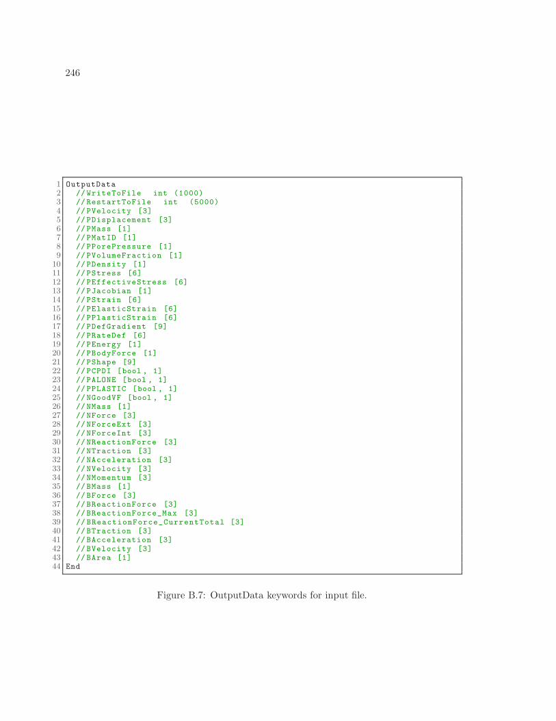
246

1 OutputData2 // WriteToFile int (1000)3 // RestartToFile int (5000)4 // PVelocity [3]5 // PDisplacement [3]6 // PMass [1]7 // PMatID [1]8 // PPorePressure [1]9 // PVolumeFraction [1]

10 // PDensity [1]11 // PStress [6]12 // PEffectiveStress [6]13 // PJacobian [1]14 // PStrain [6]15 // PElasticStrain [6]16 // PPlasticStrain [6]17 // PDefGradient [9]18 // PRateDef [6]19 // PEnergy [1]20 // PBodyForce [1]21 // PShape [9]22 // PCPDI [bool , 1]23 // PALONE [bool , 1]24 // PPLASTIC [bool , 1]25 // NGoodVF [bool , 1]26 // NMass [1]27 // NForce [3]28 // NForceExt [3]29 // NForceInt [3]30 // NReactionForce [3]31 // NTraction [3]32 // NAcceleration [3]33 // NVelocity [3]34 // NMomentum [3]35 // BMass [1]36 // BForce [3]37 // BReactionForce [3]38 // BReactionForce_Max [3]39 // BReactionForce_CurrentTotal [3]40 // BTraction [3]41 // BAcceleration [3]42 // BVelocity [3]43 // BArea [1]44 End

Figure B.7: OutputData keywords for input file.

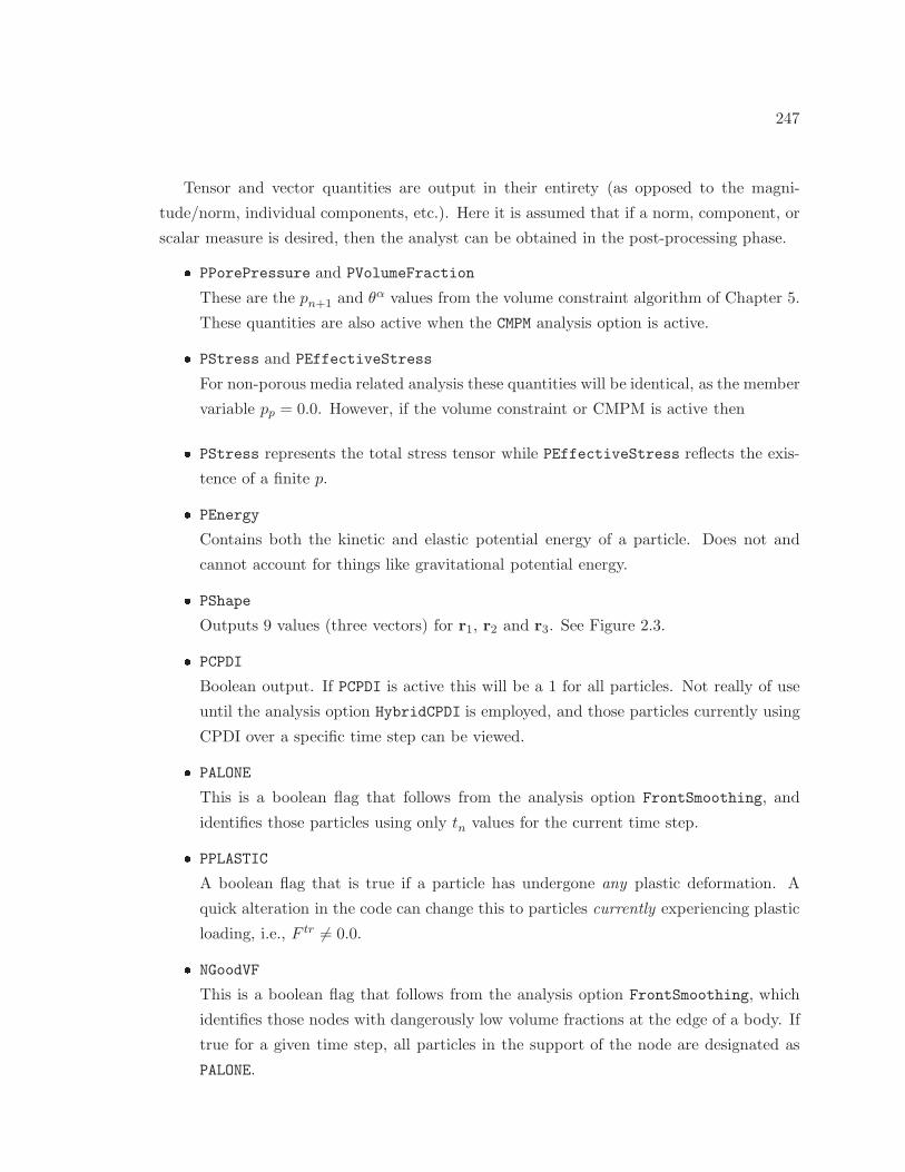
247

Tensor and vector quantities are output in their entirety (as opposed to the magni-

tude/norm, individual components, etc.). Here it is assumed that if a norm, component, or

scalar measure is desired, then the analyst can be obtained in the post-processing phase.

PPorePressure and PVolumeFraction

These are the pn+1 and θα values from the volume constraint algorithm of Chapter 5.

These quantities are also active when the CMPM analysis option is active.

PStress and PEffectiveStress

For non-porous media related analysis these quantities will be identical, as the member

variable pp = 0.0. However, if the volume constraint or CMPM is active then

PStress represents the total stress tensor while PEffectiveStress reflects the exis-

tence of a finite p.

PEnergy

Contains both the kinetic and elastic potential energy of a particle. Does not and

cannot account for things like gravitational potential energy.

PShape

Outputs 9 values (three vectors) for r1, r2 and r3. See Figure 2.3.

PCPDI

Boolean output. If PCPDI is active this will be a 1 for all particles. Not really of use

until the analysis option HybridCPDI is employed, and those particles currently using

CPDI over a specific time step can be viewed.

PALONE

This is a boolean flag that follows from the analysis option FrontSmoothing, and

identifies those particles using only tn values for the current time step.

PPLASTIC

A boolean flag that is true if a particle has undergone any plastic deformation. A

quick alteration in the code can change this to particles currently experiencing plastic

loading, i.e., F tr 6= 0.0.

NGoodVF

This is a boolean flag that follows from the analysis option FrontSmoothing, which

identifies those nodes with dangerously low volume fractions at the edge of a body. If

true for a given time step, all particles in the support of the node are designated as

PALONE.

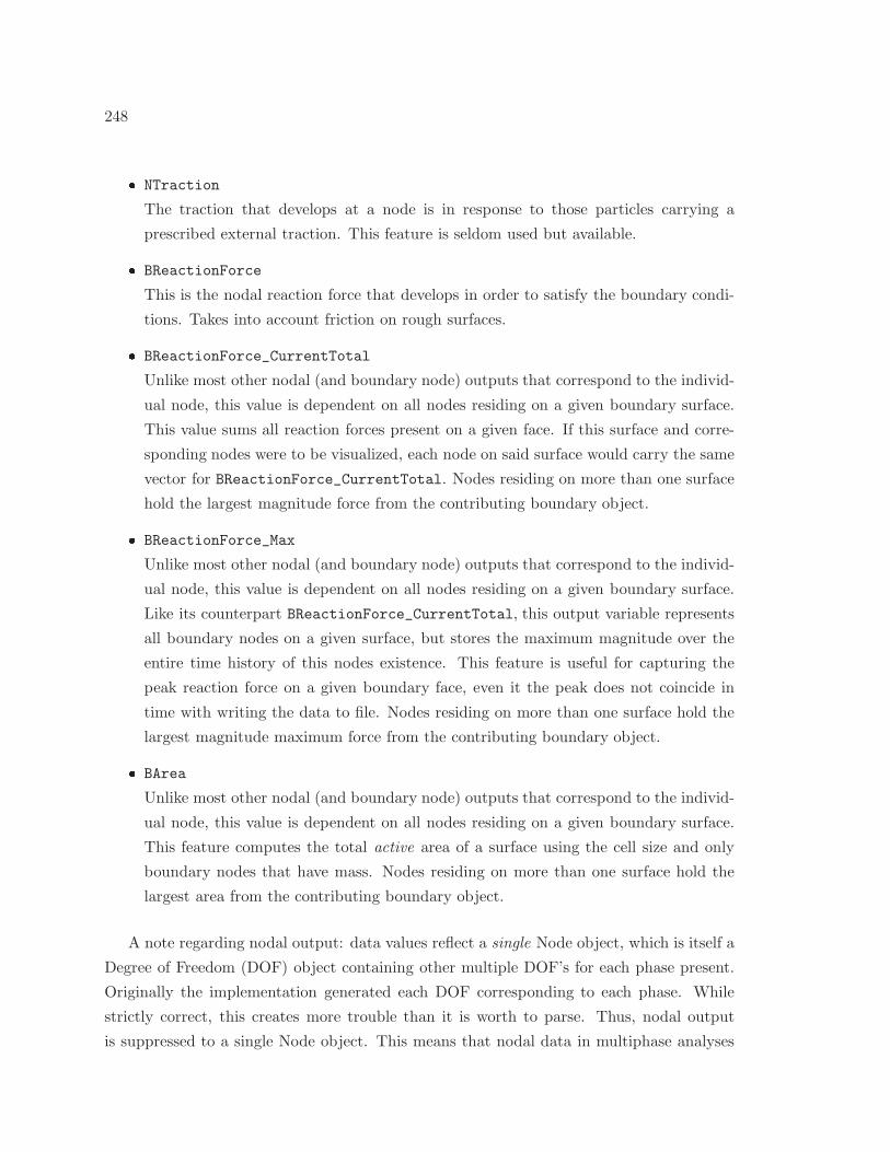
248

NTraction

The traction that develops at a node is in response to those particles carrying a

prescribed external traction. This feature is seldom used but available.

BReactionForce

This is the nodal reaction force that develops in order to satisfy the boundary condi-

tions. Takes into account friction on rough surfaces.

BReactionForce_CurrentTotal

Unlike most other nodal (and boundary node) outputs that correspond to the individ-

ual node, this value is dependent on all nodes residing on a given boundary surface.

This value sums all reaction forces present on a given face. If this surface and corre-

sponding nodes were to be visualized, each node on said surface would carry the same

vector for BReactionForce_CurrentTotal. Nodes residing on more than one surface

hold the largest magnitude force from the contributing boundary object.

BReactionForce_Max

Unlike most other nodal (and boundary node) outputs that correspond to the individ-

ual node, this value is dependent on all nodes residing on a given boundary surface.

Like its counterpart BReactionForce_CurrentTotal, this output variable represents

all boundary nodes on a given surface, but stores the maximum magnitude over the

entire time history of this nodes existence. This feature is useful for capturing the

peak reaction force on a given boundary face, even it the peak does not coincide in

time with writing the data to file. Nodes residing on more than one surface hold the

largest magnitude maximum force from the contributing boundary object.

BArea

Unlike most other nodal (and boundary node) outputs that correspond to the individ-

ual node, this value is dependent on all nodes residing on a given boundary surface.

This feature computes the total active area of a surface using the cell size and only

boundary nodes that have mass. Nodes residing on more than one surface hold the

largest area from the contributing boundary object.

A note regarding nodal output: data values reflect a single Node object, which is itself a

Degree of Freedom (DOF) object containing other multiple DOF’s for each phase present.

Originally the implementation generated each DOF corresponding to each phase. While

strictly correct, this creates more trouble than it is worth to parse. Thus, nodal output

is suppressed to a single Node object. This means that nodal data in multiphase analyses

249

reflects all phases present at a particular node. This could be changed in the future but will

require modifying all post processing files as well.

The remaining base keywords do not contain nested features, and are thus presented

without the itemized format of the previous subsections. The reader is referred to Figure B.2

for a quick reminder as to what the remaining base keywords represent.

B.2.7 Particles

A particle group must be flagged with an integer MaterialID and PhaseID as indicated in

Figure B.2. The MaterialID must correspond to the int_ID in Figure B.5. The PhaseID is

also required for multiphase analyses. These can be arbitrary and do not need to be any

specific value. Each phase is assumed to have its own motion, and thus its own grid. A single

phase can have multiple materials, designated by multiple groups of Particles statements.

Each particle gets its own line containing:

p_ID p_mass p_x p_y p_z.

where p_ID is an integer. The mass and position components are floats.

B.2.8 ParticleState

Each particle gets its own line in the input file of the form

p_ID [...]

where [...] indicates a list of state parameters needed for a full definition of the material.

This includes the current elastic and plastic deformation, deformation gradient, and all

state variables required to compute the current stress state. As such, this parameter list

is long. In the interest of saving space the user is referred first to the virtual functions

matGetState() and matReadState([...]) , defined in the general Material.cpp class.

Each of these functions are overloaded by the individual material class indicating the order

and contents of [...].

B.2.9 ParticlePrescribedTraction

This base option is used for prescribed tractions on a body’s surface. Since the particles

represent the body—and not the nodes like in the FEM—force-like boundary conditions

should (does not mean they always are) be applied to the particles. This option adds an

external traction to select particles using

p_ID A_p MagTraction n_x n_y n_z

where A_p is the representative area of the individual particle, MagTraction is the magnitude

250

of the traction, and the floats n_x, n_y, and n_z provide the orientation of said traction.

The orientation is updated with the deformation gradient, effectively describing a moving

force-like term that is consistent with the deformation. Each particle with a nonzero traction

contributes to the NTraction identified above.

B.2.10 ParticleShape

This base keyword is used to define the shape vectors r1, r2 and r3 when CPDI or

HybridCPDI is used. See Figure 2.3. The input file requires the following form

p_ID r1_x r1_y r1_z r2_x r2_y r2_z r3_x r3_y r3_z.

This keyword is recommended when using CPDI or HybridCPDI if a modified shape is de-

sired. If no shape data is provided, the coding framework assumes cubic particles based on

initial density and supplied mass, and will automatically compute the corresponding shape

vectors.

B.2.11 ParticleVelocity and ParticleBodyForce

These two features allow individual particle assignments of velocity and body force. When

invoked they require a format consistent with

p_ID v_x b_y b_z

with vi representing the appropriate velocity or body force component. There are situations

(like a vibrating beam) that require unique, prescribed particle velocities at the outset.

This feature is used with body force only for restart files and should not be used to apply

something like gravity, which affects all particles. Instead use globalBodyForce in the

analysis options.

B.2.12 Example Input Files

Examples are typically more beneficial than a written description. Two sample input files

from examples appearing in this dissertation are presented in Appendix C, which includes

the foundation loading analysis in Section 6.3.3 as well as the avalanche control example

in Section 7.3. For length reasons particle data has been elided, but the input structure

remains and shows the components needed for creating a successful analysis.

B.3 Model Analysis

The Model Analysis portion of the data flow shown in Figure B.1 accounts for the largest

portion of the coding framework. The goal in this section is to provide a global overview of

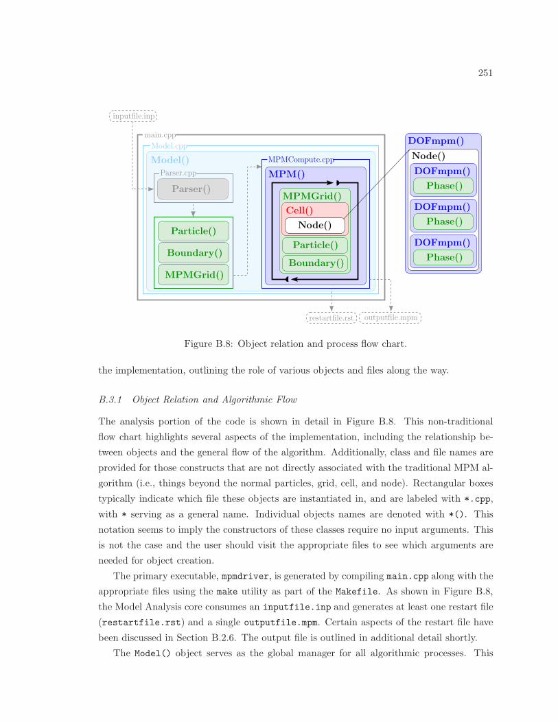
251

Model.cpp

outputfile.mpmrestartfile.rst

inputfile.inp

main.cpp

Model() MPMCompute.cpp

Parser.cpp

MPMGrid()

Boundary()

Particle()

Parser()MPMGrid()

Node()

DOFmpm()

MPM()

Particle()

Boundary()

Cell()

DOFmpm()

DOFmpm()

DOFmpm()

Node()

Phase()

Phase()

Phase()

Figure B.8: Object relation and process flow chart.

the implementation, outlining the role of various objects and files along the way.

B.3.1 Object Relation and Algorithmic Flow

The analysis portion of the code is shown in detail in Figure B.8. This non-traditional

flow chart highlights several aspects of the implementation, including the relationship be-

tween objects and the general flow of the algorithm. Additionally, class and file names are

provided for those constructs that are not directly associated with the traditional MPM al-

gorithm (i.e., things beyond the normal particles, grid, cell, and node). Rectangular boxes

typically indicate which file these objects are instantiated in, and are labeled with *.cpp,

with * serving as a general name. Individual objects names are denoted with *(). This

notation seems to imply the constructors of these classes require no input arguments. This

is not the case and the user should visit the appropriate files to see which arguments are

needed for object creation.

The primary executable, mpmdriver, is generated by compiling main.cpp along with the

appropriate files using the make utility as part of the Makefile. As shown in Figure B.8,

the Model Analysis core consumes an inputfile.inp and generates at least one restart file

(restartfile.rst) and a single outputfile.mpm. Certain aspects of the restart file have

been discussed in Section B.2.6. The output file is outlined in additional detail shortly.

The Model() object serves as the global manager for all algorithmic processes. This

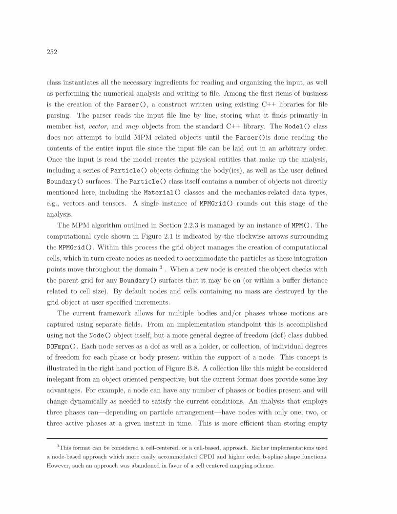
252

class instantiates all the necessary ingredients for reading and organizing the input, as well

as performing the numerical analysis and writing to file. Among the first items of business

is the creation of the Parser(), a construct written using existing C++ libraries for file

parsing. The parser reads the input file line by line, storing what it finds primarily in

member list, vector, and map objects from the standard C++ library. The Model() class

does not attempt to build MPM related objects until the Parser()is done reading the

contents of the entire input file since the input file can be laid out in an arbitrary order.

Once the input is read the model creates the physical entities that make up the analysis,

including a series of Particle() objects defining the body(ies), as well as the user defined

Boundary() surfaces. The Particle() class itself contains a number of objects not directly

mentioned here, including the Material() classes and the mechanics-related data types,

e.g., vectors and tensors. A single instance of MPMGrid() rounds out this stage of the

analysis.

The MPM algorithm outlined in Section 2.2.3 is managed by an instance of MPM(). The

computational cycle shown in Figure 2.1 is indicated by the clockwise arrows surrounding

the MPMGrid(). Within this process the grid object manages the creation of computational

cells, which in turn create nodes as needed to accommodate the particles as these integration

points move throughout the domain 3 . When a new node is created the object checks with

the parent grid for any Boundary() surfaces that it may be on (or within a buffer distance

related to cell size). By default nodes and cells containing no mass are destroyed by the

grid object at user specified increments.

The current framework allows for multiple bodies and/or phases whose motions are

captured using separate fields. From an implementation standpoint this is accomplished

using not the Node() object itself, but a more general degree of freedom (dof) class dubbed

DOFmpm(). Each node serves as a dof as well as a holder, or collection, of individual degrees

of freedom for each phase or body present within the support of a node. This concept is

illustrated in the right hand portion of Figure B.8. A collection like this might be considered

inelegant from an object oriented perspective, but the current format does provide some key

advantages. For example, a node can have any number of phases or bodies present and will

change dynamically as needed to satisfy the current conditions. An analysis that employs

three phases can—depending on particle arrangement—have nodes with only one, two, or

three active phases at a given instant in time. This is more efficient than storing empty

3This format can be considered a cell-centered, or a cell-based, approach. Earlier implementations used

a node-based approach which more easily accommodated CPDI and higher order b-spline shape functions.

However, such an approach was abandoned in favor of a cell centered mapping scheme.

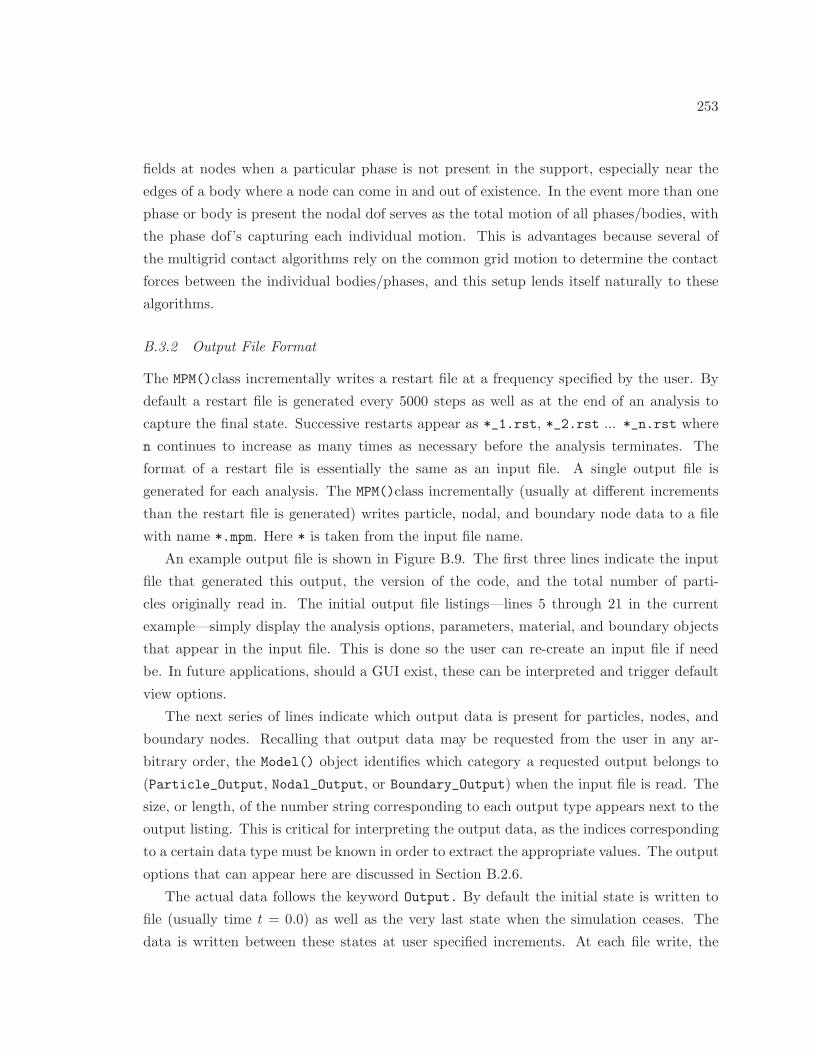
253

fields at nodes when a particular phase is not present in the support, especially near the

edges of a body where a node can come in and out of existence. In the event more than one

phase or body is present the nodal dof serves as the total motion of all phases/bodies, with

the phase dof’s capturing each individual motion. This is advantages because several of

the multigrid contact algorithms rely on the common grid motion to determine the contact

forces between the individual bodies/phases, and this setup lends itself naturally to these

algorithms.

B.3.2 Output File Format

The MPM()class incrementally writes a restart file at a frequency specified by the user. By

default a restart file is generated every 5000 steps as well as at the end of an analysis to

capture the final state. Successive restarts appear as *_1.rst, *_2.rst ... *_n.rst where

n continues to increase as many times as necessary before the analysis terminates. The

format of a restart file is essentially the same as an input file. A single output file is

generated for each analysis. The MPM()class incrementally (usually at different increments

than the restart file is generated) writes particle, nodal, and boundary node data to a file

with name *.mpm. Here * is taken from the input file name.

An example output file is shown in Figure B.9. The first three lines indicate the input

file that generated this output, the version of the code, and the total number of parti-

cles originally read in. The initial output file listings—lines 5 through 21 in the current

example—simply display the analysis options, parameters, material, and boundary objects

that appear in the input file. This is done so the user can re-create an input file if need

be. In future applications, should a GUI exist, these can be interpreted and trigger default

view options.

The next series of lines indicate which output data is present for particles, nodes, and

boundary nodes. Recalling that output data may be requested from the user in any ar-

bitrary order, the Model() object identifies which category a requested output belongs to

(Particle_Output, Nodal_Output, or Boundary_Output) when the input file is read. The

size, or length, of the number string corresponding to each output type appears next to the

output listing. This is critical for interpreting the output data, as the indices corresponding

to a certain data type must be known in order to extract the appropriate values. The output

options that can appear here are discussed in Section B.2.6.

The actual data follows the keyword Output. By default the initial state is written to

file (usually time t = 0.0) as well as the very last state when the simulation ceases. The

data is written between these states at user specified increments. At each file write, the

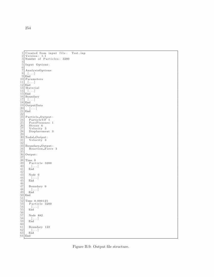
254

1 Created from input f i l e : Test . inp2 Vers ion : 1 . 13 Number o f P a r t i c l e s : 320045 Input Options :67 Analys i sOptions8 [ . . . ]9 End

10 Parameters11 [ . . . ]12 End13 Mater i a l14 [ . . . ]15 End16 Boundary17 [ . . . ]18 End19 OutputData20 [ . . . ]21 End2223 Par t i c l e Output :24 Partic l eVF 125 PorePressure 126 St r e s s 627 Veloc i ty 328 Displacement 32930 Nodal Output :31 Veloc i ty 33233 Boundary Output :34 Reaction Force 33536 Output :3738 Time 039 Pa r t i c l e 320040 [ . . . ]41 End4243 Node 044 [ . . . ]45 End4647 Boundary 048 [ . . . ]49 End50 End5152 Time 0.00012553 Pa r t i c l e 320054 [ . . . ]55 End5657 Node 88258 [ . . . ]59 End6061 Boundary 12262 [ . . . ]63 End64 End

Figure B.9: Output file structure.

255

keywords Time and End designate the current state. The number following the Time keyword

is the current analysis time. Within this keyword pair, particle, node, and boundary node

data are written using the appropriate keyword followed by the End statement. Since the

number of particles, nodes, and boundary nodes varies throughout the simulation, the

integer following the keyword indicates the number of active entities. This information

is needed for a number of reasons, including parsing the output data and creating useful

output constructs as explained in the next section.

B.4 Post-Processing

The post-processing scripts are written exclusively in the Python programming language.

Early implementations and examples were primarily two dimensional and consisted of less

than 10,000 particles. For these cases the plotting libraries contained in the matplotlib and

scipy Python modules were sufficient for data visualization, and several scripts written

around these libraries were developed. However, these tools are limited to smaller simula-

tions and are not efficient in terms of viewing all output variables in a timely fashion. Thus,

recent emphasis has been placed on transitioning away from these original scripts in favor

of ParaView, an open-source, multi-platform data analysis and visualization application.

In an effort to be complete this section contains a detailed overview of the ParaView file

format, as well as a description of the original Python scripts used for visualization.

B.4.1 ParaView and the VTK Piece Format

ParaView offers a fully three dimensional visualization environment built using the Visu-

alization Toolkit (VTK) Library. The interactive framework allows users to create videos,

snapshots, or extract quantities for plotting, and features a suite of batch processing capa-

bilities for automation. The interface is developed to analyze extremely large datasets and

utilizes distributed memory computing resources when necessary.

The VTK library consists of C++ , Tcl/Tk, Java, and Python and serves as an open

source software system for three dimensional computer graphics, image processing, and

visualization. ParaView can access several VTK features, including the pipeline architecture

and the more general vtkObject. That being the case there are multiple options available

for getting MPM data into a format that ParaView can read. In the present case the VTK

Piece format is used. This is not the only option, but is the only option explored in this

work.

ParaView can read and interpret XML files. An example VTK Piece format is shown

in Figure B.10. This example is for a single time step and contains particle data. An

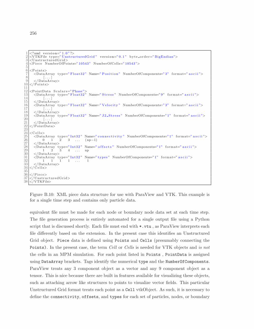
256

1 <?xml ve r s i on=” 1 .0 ”?>2 <VTKFile type=”UnstructuredGrid ” ve r s i on=” 0 .1 ” byte order=”BigEndian”>3 <UnstructuredGrid>4 <Piece NumberOfPoints=”10543” NumberOfCells=”10543 ”>56 <Points>7 <DataArray type=”Float32 ” Name=”Pos i t i on ” NumberOfComponents=”3” format=” a s c i i ”>8 [ . . . ]9 </DataArray>

10 </Points>1112 <PointData Sca l a r s=”Phase”>13 <DataArray type=”Float32 ” Name=” St r e s s ” NumberOfComponents=”9” format=” a s c i i ”>14 [ . . . ]15 </DataArray>16 <DataArray type=”Float32 ” Name=”Veloc i ty ” NumberOfComponents=”3” format=” a s c i i ”>17 [ . . . ]18 </DataArray>19 <DataArray type=”Float32 ” Name=” J2 St r e s s ” NumberOfComponents=”1” format=” a s c i i ”>20 [ . . . ]21 </DataArray>22 </PointData>2324 <Ce l l s>25 <DataArray type=” Int32 ” Name=” connec t i v i t y ” NumberOfComponents=”1” format=” a s c i i ”>26 0 1 2 3 . . . ( np−1)27 </DataArray>28 <DataArray type=” Int32 ” Name=” o f f s e t s ” NumberOfComponents=”1” format=” a s c i i ”>29 1 2 3 4 . . . np30 </DataArray>31 <DataArray type=” Int32 ” Name=” types ” NumberOfComponents=”1” format=” a s c i i ”>32 1 1 1 1 . . . 133 </DataArray>34 </ Ce l l s>3536 </Piece>37 </UnstructuredGrid>38 </VTKFile>

Figure B.10: XML piece data structure for use with ParaView and VTK. This example isfor a single time step and contains only particle data.

equivalent file must be made for each node or boundary node data set at each time step.

The file generation process is entirely automated for a single output file using a Python

script that is discussed shortly. Each file must end with *.vtu , as ParaView interprets each

file differently based on the extension. In the present case this identifies an Unstructured

Grid object. Piece data is defined using Points and Cells (presumably connecting the

Points). In the present case, the term Cell or Cells is needed for VTK objects and is not

the cells in an MPM simulation. For each point listed in Points , PointData is assigned

using DataArray brackets. Tags identify the numerical type and the NumberOfComponents.

ParaView treats any 3 component object as a vector and any 9 component object as a

tensor. This is nice because there are built in features available for visualizing these objects,

such as attaching arrow like structures to points to visualize vector fields. This particular

Unstructured Grid format treats each point as a Cell vtkObject. As such, it is necessary to

define the connectivity, offsets, and types for each set of particles, nodes, or boundary

257

nodes. These Cell fields are a function only of the number of points, np, and are to be

organized as shown in Figure B.10.

The Python script MPMOutputToVTKOutput.py generates all the necessary files and fold-

ers from a single .mpm output file. This primary script relies on two additional modules:

MPM2VTKFunctions.py and the class definition VTKFileWriter.py. Together these scripts

generate separate files for each time step consistent with the format shown in Figure B.10

for all particles, nodes, and boundary nodes (of course the XML files contain the user spec-

ified output instead of those terms shown in the example). The individual time step files

are strung together with a *.pvd file, an XML-based structure containing the name of the

individual *.vtu files. An example of this file type is provided in Appendix C. The user

needs only to open ParaView and select the appropriate *.pvd file to begin viewing the

data.

B.4.2 Original Visualization Scripts

Considering the convenience afforded by ParaView (or any interactive, fully three dimen-

sional visualization environment), there is little value in continuing forward with the original

series of Python scripts developed for visualization purposes. However, these scripts can still

serve a purpose, as they organize the data into matrix-like structures conducive to plotting

and/or analysis. That being the case each script and its capabilities are outlined below.

ParticlePlotter.py: This script extracts particle data from the output file. The

user may specify any number of particle IDs as well as any available output they wish

to obtain. The data is either viewed as a plot, or as is more commonly done, output

to file for later use. An example usage of this script was extracting the appropriate

data to create the error plots in Figure 6.10.

NodePlotter.py: This script extracts nodal data from the output file. The user may

specify any number of node IDs as well as any available output they wish to obtain.

The data is either viewed as a plot, or, as is more commonly done, output to file for

later use. This script was used to extract data for Figure 6.7.

ParticleVisualizer.py: This script utilizes a single MPM output file and creates a

series of images used to visualize the particles. The images may be viewed individually

or strung together to create a movie. The user may specify several options, including

which particle value to plot. The scatter plots show data and relate the magnitude of

the data via a color bar option. Despite the script name, the user may also visualize

nodal location, boundary node location, as well as several nodal output quantities. As

258

was the case with the particles, the data at nodal locations is output as a color with

corresponding magnitude obtained via the color bar. Examples plots created from

this script are Figures 6.4 and 7.19.

NodeVisualizer.py: This script visualizes the grid fields at user specified nodes via

colored vectors. As was the case with the particle visualizer, a series of images at

sequential times is created. The images may be used individually or combined to

create a movie. The vector orientation and size are obtained by appropriate window

scaling, whereas the magnitude is viewed via a color bar.

The above four files rely heavily on the numpy module, as well as several functions defined

in VisualizerFunctions.py.

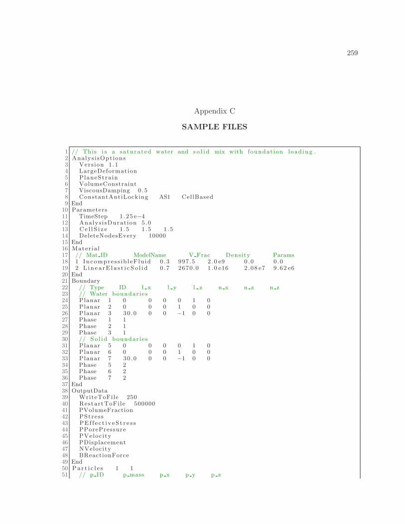
259

Appendix C

SAMPLE FILES

1 // This i s a satu rat ed water and s o l i d mix with foundat ion load ing .2 Analys i sOpt ions3 Vers ion 1 .14 LargeDeformation5 PlaneStra in6 VolumeConstraint7 ViscousDamping 0 .58 ConstantAntiLocking AS1 CellBased9 End

10 Parameters11 TimeStep 1 .25 e−412 Analys i sDurat ion 5 .013 Ce l l S i z e 1 .5 1 .5 1 .514 DeleteNodesEvery 1000015 End16 Mater ia l17 // Mat ID ModelName V Frac Density Params18 1 Incompres s ib l eF lu id 0 .3 997.5 2 .0 e9 0 .0 0 .019 2 L i n e a rE l a s t i c S o l i d 0 .7 2670.0 1 .0 e16 2 .08 e7 9 .62 e620 End21 Boundary22 // Type ID l x l y l z n x n z n z23 // Water boundar ies24 Planar 1 0 0 0 0 1 025 Planar 2 0 0 0 1 0 026 Planar 3 30 .0 0 0 −1 0 027 Phase 1 128 Phase 2 129 Phase 3 130 // So l i d boundar ies31 Planar 5 0 0 0 0 1 032 Planar 6 0 0 0 1 0 033 Planar 7 30 .0 0 0 −1 0 034 Phase 5 235 Phase 6 236 Phase 7 237 End38 OutputData39 WriteToFile 25040 RestartToFi le 50000041 PVolumeFraction42 PStress43 PE f f e c t i v eS t r e s s44 PPorePressure45 PVeloc i ty46 PDisplacement47 NVelocity48 BReactionForce49 End50 Pa r t i c l e s 1 151 // p ID p mass p x p y p z

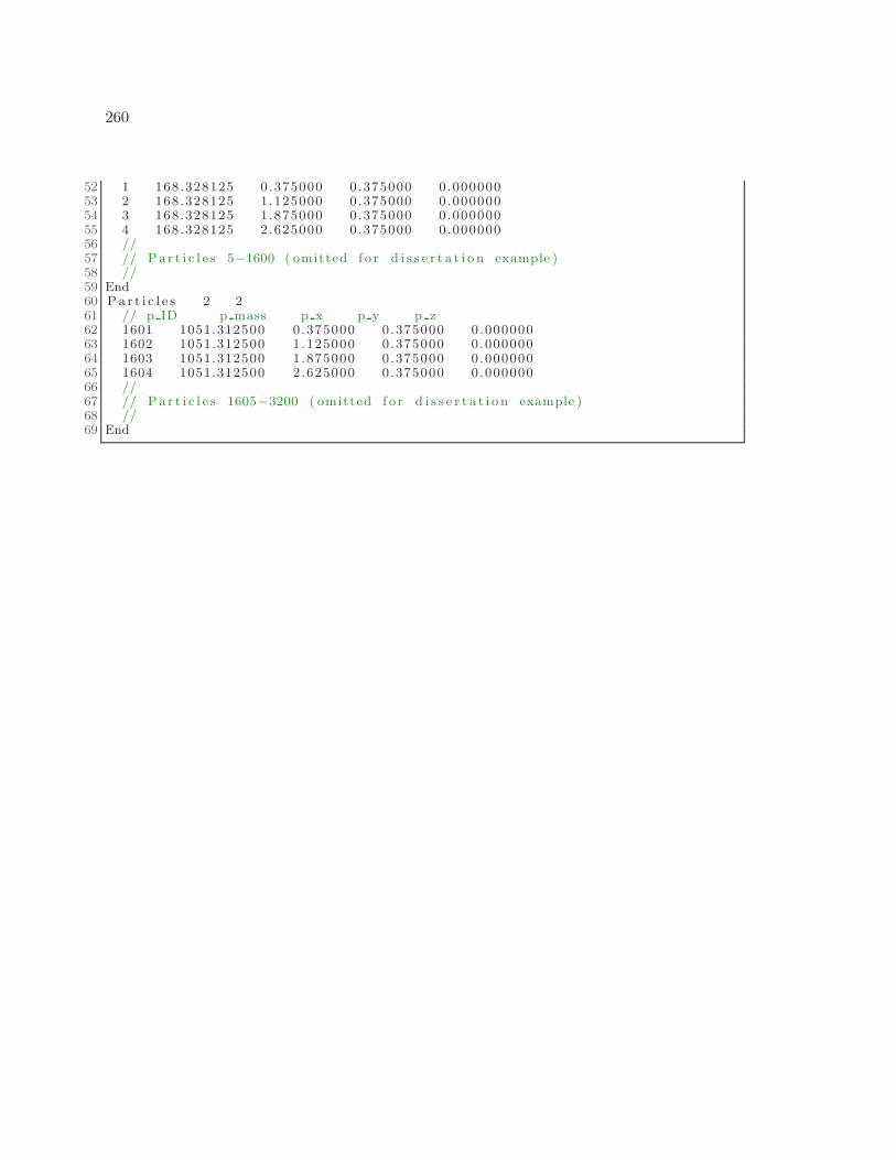
260

52 1 168.328125 0.375000 0.375000 0.00000053 2 168.328125 1.125000 0.375000 0.00000054 3 168.328125 1.875000 0.375000 0.00000055 4 168.328125 2.625000 0.375000 0.00000056 //57 // Pa r t i c l e s 5−1600 ( omitted f o r d i s s e r t a t i o n example )58 //59 End60 Pa r t i c l e s 2 261 // p ID p mass p x p y p z62 1601 1051.312500 0.375000 0.375000 0.00000063 1602 1051.312500 1.125000 0.375000 0.00000064 1603 1051.312500 1.875000 0.375000 0.00000065 1604 1051.312500 2.625000 0.375000 0.00000066 //67 // Pa r t i c l e s 1605−3200 ( omitted f o r d i s s e r t a t i o n example )68 //69 End

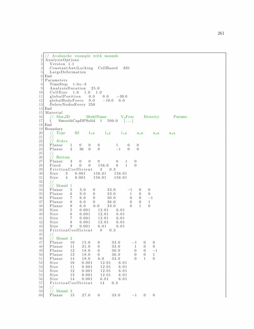
261

1 // Avalanche example with mounds2 Analys i sOpt ions3 Vers ion 1 .14 ConstantAntiLocking CellBased AS15 LargeDeformation6 End7 Parameters8 TimeStep 1 .0 e−39 Analys i sDurat ion 25 .0

10 Ce l l S i z e 1 .0 1 .0 1 .011 g l oba lPo s i t i o n 0 .0 0 .0 −30.012 globalBodyForce 0 .0 −10.0 0 .013 DeleteNodesEvery 25014 End15 Mater ia l16 // Mat ID ModelName V Frac Density Params17 1 SmoothCapDPSolid 1 500.0 [ . . . ]18 End19 Boundary20 // Type ID l x l y l z n x n z n z21 //22 // S ides23 Planar 1 0 0 0 1 0 024 Planar 2 36 0 0 −1 0 025 //26 // Bottom27 Planar 3 0 0 0 0 1 028 Fixed 4 0 0 156.0 0 1 029 F r i c t i o nCo e f f i c i e n t 3 0 .330 S i ze 3 0.001 156.01 156.0131 S ize 4 0.001 156.01 156.0132 //33 // Mound 134 Planar 5 3 .0 0 33 .0 −1 0 035 Planar 6 9 .0 0 33 .0 1 0 036 Planar 7 6 .0 0 30 .0 0 0 −137 Planar 8 6 .0 0 36 .0 0 0 138 Planar 9 6 .0 6 .0 33 .0 0 1 039 S ize 5 0.001 12.01 6 .0140 S ize 6 0.001 12.01 6 .0141 S ize 7 0.001 12.01 6 .0142 S ize 8 0.001 12.01 6 .0143 S ize 9 0.001 6 .01 6 .0144 F r i c t i o nCo e f f i c i e n t 9 0 .345 //46 // Mound 247 Planar 10 15 .0 0 33 .0 −1 0 048 Planar 11 21 .0 0 33 .0 1 0 049 Planar 12 18 .0 0 30 .0 0 0 −150 Planar 13 18 .0 0 36 .0 0 0 151 Planar 14 18 .0 6 .0 33 .0 0 1 052 S ize 10 0.001 12.01 6 .0153 S ize 11 0.001 12.01 6 .0154 S ize 12 0.001 12.01 6 .0155 S ize 13 0.001 12.01 6 .0156 S ize 14 0.001 6 .01 6 .0157 F r i c t i o nCo e f f i c i e n t 14 0 .358 //59 // Mound 360 Planar 15 27 .0 0 33 .0 −1 0 0

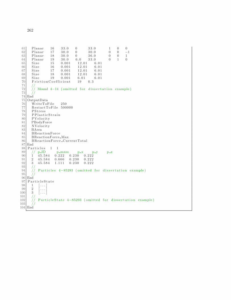
262

61 Planar 16 33 .0 0 33 .0 1 0 062 Planar 17 30 .0 0 30 .0 0 0 −163 Planar 18 30 .0 0 36 .0 0 0 164 Planar 19 30 .0 6 .0 33 .0 0 1 065 S ize 15 0.001 12.01 6 .0166 S ize 16 0.001 12.01 6 .0167 S ize 17 0.001 12.01 6 .0168 S ize 18 0.001 12.01 6 .0169 S ize 19 0.001 6 .01 6 .0170 F r i c t i o nCo e f f i c i e n t 19 0 .371 //72 // Mound 4−14 ( omitted f o r d i s s e r t a t i o n example )73 //74 End75 OutputData76 WriteToFile 25077 RestartToFi le 50000078 PStress79 PP la s t i cS t r a i n80 PVeloc i ty81 PBodyForce82 NVelocity83 BArea84 BReactionForce85 BReactionForce Max86 BReactionForce CurrentTotal87 End88 Pa r t i c l e s 1 189 // p ID p mass p x p y p z90 1 45.584 0.222 0.230 0.22291 2 45.584 0.666 0.230 0.22292 3 45.584 1.111 0.230 0.22293 //94 // Pa r t i c l e s 4−85293 ( omitted f o r d i s s e r t a t i o n example )95 //96 End97 Pa r t i c l e S t a t e98 1 [ . . . ]99 2 [ . . . ]

100 3 [ . . . ]101 //102 // Pa r t i c l e S t a t e 4−85293 ( omitted f o r d i s s e r t a t i o n example )103 //104 End

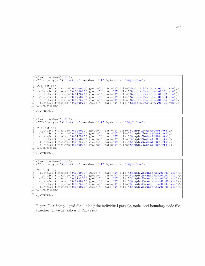
263

1 <?xml ve r s i on=” 1 .0 ”?>2 <VTKFile type=” Co l l e c t i on ” ve r s i on=” 0 .1 ” byte order=”BigEndian”>34 <Co l l e c t i on>5 <DataSet t imestep=” 0.000000 ” group=”” part=”0” f i l e=” Sample Par t i c l e s 00001 . vtu”/>6 <DataSet t imestep=” 0.000025 ” group=”” part=”0” f i l e=” Sample Par t i c l e s 00001 . vtu”/>7 <DataSet t imestep=” 0.012525 ” group=”” part=”0” f i l e=” Sample Par t i c l e s 00002 . vtu”/>8 <DataSet t imestep=” 0.025025 ” group=”” part=”0” f i l e=” Sample Par t i c l e s 00003 . vtu”/>9 <DataSet t imestep=” 0.037525 ” group=”” part=”0” f i l e=” Sample Par t i c l e s 00004 . vtu”/>

10 <DataSet t imestep=” 0.050025 ” group=”” part=”0” f i l e=” Sample Par t i c l e s 00005 . vtu”/>11 </ Co l l e c t i on>1213 </VTKFile>

1 <?xml ve r s i on=” 1 .0 ”?>2 <VTKFile type=” Co l l e c t i on ” ve r s i on=” 0 .1 ” byte order=”BigEndian”>34 <Co l l e c t i on>5 <DataSet t imestep=” 0.000000 ” group=”” part=”0” f i l e=”Sample Nodes 00001 . vtu”/>6 <DataSet t imestep=” 0.000025 ” group=”” part=”0” f i l e=”Sample Nodes 00001 . vtu”/>7 <DataSet t imestep=” 0.012525 ” group=”” part=”0” f i l e=”Sample Nodes 00002 . vtu”/>8 <DataSet t imestep=” 0.025025 ” group=”” part=”0” f i l e=”Sample Nodes 00003 . vtu”/>9 <DataSet t imestep=” 0.037525 ” group=”” part=”0” f i l e=”Sample Nodes 00004 . vtu”/>

10 <DataSet t imestep=” 0.050025 ” group=”” part=”0” f i l e=”Sample Nodes 00005 . vtu”/>11 </ Co l l e c t i on>1213 </VTKFile>

1 <?xml ve r s i on=” 1 .0 ”?>2 <VTKFile type=” Co l l e c t i on ” ve r s i on=” 0 .1 ” byte order=”BigEndian”>34 <Co l l e c t i on>5 <DataSet t imestep=” 0.000000 ” group=”” part=”0” f i l e=”Sample Boundaries 00001 . vtu”/>6 <DataSet t imestep=” 0.000025 ” group=”” part=”0” f i l e=”Sample Boundaries 00001 . vtu”/>7 <DataSet t imestep=” 0.012525 ” group=”” part=”0” f i l e=”Sample Boundaries 00002 . vtu”/>8 <DataSet t imestep=” 0.025025 ” group=”” part=”0” f i l e=”Sample Boundaries 00003 . vtu”/>9 <DataSet t imestep=” 0.037525 ” group=”” part=”0” f i l e=”Sample Boundaries 00004 . vtu”/>

10 <DataSet t imestep=” 0.050025 ” group=”” part=”0” f i l e=”Sample Boundaries 00005 . vtu”/>11 </ Co l l e c t i on>1213 </VTKFile>

Figure C.1: Sample .pvd files linking the individual particle, node, and boundary node filestogether for visualization in ParaView.