Modeling and imaging of electrocardiographic activity
158
HAL Id: tel-02066820 https://tel.archives-ouvertes.fr/tel-02066820 Submitted on 13 Mar 2019 HAL is a multi-disciplinary open access archive for the deposit and dissemination of sci- entific research documents, whether they are pub- lished or not. The documents may come from teaching and research institutions in France or abroad, or from public or private research centers. L’archive ouverte pluridisciplinaire HAL, est destinée au dépôt et à la diffusion de documents scientifiques de niveau recherche, publiés ou non, émanant des établissements d’enseignement et de recherche français ou étrangers, des laboratoires publics ou privés. Modeling and imaging of electrocardiographic activity Karim El Houari To cite this version: Karim El Houari. Modeling and imaging of electrocardiographic activity. Signal and Image processing. Université Rennes 1, 2018. English. NNT : 2018REN1S063. tel-02066820
-
Upload
khangminh22 -
Category
Documents
-
view
2 -
download
0
Transcript of Modeling and imaging of electrocardiographic activity

HAL Id: tel-02066820https://tel.archives-ouvertes.fr/tel-02066820
Submitted on 13 Mar 2019
HAL is a multi-disciplinary open accessarchive for the deposit and dissemination of sci-entific research documents, whether they are pub-lished or not. The documents may come fromteaching and research institutions in France orabroad, or from public or private research centers.
L’archive ouverte pluridisciplinaire HAL, estdestinée au dépôt et à la diffusion de documentsscientifiques de niveau recherche, publiés ou non,émanant des établissements d’enseignement et derecherche français ou étrangers, des laboratoirespublics ou privés.
Modeling and imaging of electrocardiographic activityKarim El Houari
To cite this version:Karim El Houari. Modeling and imaging of electrocardiographic activity. Signal and Image processing.Université Rennes 1, 2018. English. NNT : 2018REN1S063. tel-02066820

THÈSE DE DOCTORAT DE
L’UNIVERSITE DE RENNES 1COMUE UNIVERSITE BRETAGNE LOIRE
Ecole Doctorale N°601Mathèmatique et Sciences et Technologiesde l’Information et de la CommunicationSpécialité : Signal, Image, Vision
Par
Karim EL HOUARI
Modélisation et imagerie électrocardiographiques
Thèse soutenue à RENNES , le 14 Décembre 2018Unité de recherche : Laboratoire du Traitement du Signal et de l’ImageThèse N° :
Rapporteurs avant soutenance :
Christian Jutten (PU), GIPSA-LAB
Freddy Odille (CR-INSERM), IADI
Composition du jury :
Examinateurs
Sofiane Boudaoud (MCF-HDR), BMBI
Christian Jutten (PU), GIPSA-LAB
Freddy Odille (CR-INSERM), IADI
Directeur de thèse
Laurent Albera (MCF-HDR), LTSI
Co-directeurs de thèse
Alfredo Hernández (DR-INSERM), LTSI
Christelle Boichon-Grivot (IR), ANSYS


ACKNOWLEDGMENT
First and foremost, I would like to thank Professor Christian Jutten and Associate Professor Freddy
Odille for giving their time and expertise to review this manuscript. I am also thankful to them and
Associate Professor Sofiane Boudaoud for the interest they demonstrated for this work, and I very much
appreciated the constructive discussion that followed my defense.
I would like to express my deep and sincere gratitude to my research supervisors in the LTSI
laboratory: Associate Professor Laurent Albera, Research Director Alfredo Hernàndez and Research
Engineer Amar Kachenoura. Not only their valuable critiques, advice and close guidance were prominent
in the progress of my research, but their support, availability and kindness made this whole life
experience unforgettable.
This project wouldn’t have been possible without the help and financial support of the company
Ansys. In particular, I would like to thank Michel Rochette, head of Ansys research team in Lyon and
Christelle Boichon-Grivot, Research Engineer within Ansys, first for their management and investment
in this project, but also for offering such convenient working conditions. I would also like to extend my
thanks to my collegues in Ansys: Valéry Morgenthaler, François Chapuis and Frédéric Thevenon for
their valuable help in using Ansys Fluent and Ansys Mechanical software.
Many thanks go to Associate Professor Eric Darrigrand from the IRMAR laboratory for receiving me
several times in his office and for removing some mathematical modeling ambiguities.
I also wish to acknowledge the help provided by my colleagues in the LTSI: Ahmad Karfoul, Siouar
Bensaid and Paul Berraute, which saved me a lot of time in understanding and implementing various
elements of this PhD such as Finite Element Method operators, data whitening and Morozov discrepancy
principle. Special thanks go to Doctor Raphaël Martins and his colleagues of the university hospital of
Rennes for their warm welcome in the electrophysiology room, the clinical data they provided, and the
valuable explanations of the complex electrical mechanisms behind cardiac arrhythmia. More broadly, I
truly consider myself lucky to experience such a pleasant professional environment, this is why I would
like to thank all my colleagues in the LTSI for their warm welcome, their help, and the joyful time I have
had in and outside the lab.
I must also thank my friends and my dear housemates for their moral support and for making these
years I spent in Rennes such a thrill.
3

Finally, I owe my deepest gratitude to my family for their unconditional love, support and
encouragement throughout my study.
4

RÉSUMÉ SUBSTANCIEL
Cette thèse est le résultat de la collaboration entre le Laboratoire Traitement du Signal et de l’Image
(LTSI) et l’entreprise Ansys. Plus précisément, elle regroupe les compétences de deux équipes du
LTSI: celles de l’équipe SEPIA en modéllisation de l’électrophysiologie cardiaque, et celles de l’équipe
SESAME en termes de méthodes pour la localisation de sources épileptiques de manière non-invasive.
ANSYS est une entreprise qui est leader dans le domaine de la simulation numérique de systèmes
multiphysiques. Ce travail est destiné à initier une activité de recherche dans le domaine de la
modélisation électrique cœur-torse au sein de ces entités.
Motivation
Les maladies cardiovasculaires sont la cause majeure de mortalité dans le monde et représente un
fardeau économique et sanitaire conséquent [106]. La moitié des décès causés par ces maladies
est dûe à une mort cardiaque subite, qui est un arrêt soudain de la circulation du sang résultant de
l’incapacité du cœur à pomper dans le corps [105]. Cette insuffisance cardiaque est la plus part
du temps causée par une propagation anormale de l’activité électrique dans le cœur, phénomène
connu sous le nom d’arythmie. Parmi les arythmies cardiaques, la Tachycardie Ventriculaire (TV)
est la plus mortelle et représente 80% des morts subites. Malgré le développement de plus de 100
anti-arythmogènes, les efforts mis dans la prévention des arythmies ventriculaires sérieuses et fatales
restent décevants. L’utilisation des Défibrillateurs Cardiaques Implantables (DCIs) est préconisé à la
fois pour la prévention des morts subites chez les patients atteints de maladies structurelles et ceux
en cas d’insuffisance de la fraction d’éjection du ventricule. Cependant, l’implantation des DCIs est
très coûteuse et n’est pas curative. La perpétuation de la TV dépend de régions pathologiques dont
la conduction est relativement lente, donnant la possibilité aux segments adjacents dans le myocarde
de regagner de l’excitabilité lorsque l’impulsion se propage lentement dans la région pathologique. Le
mélange des conductions normales (tissu sain) et anormales (tissu ischémique) peut causer la formation
de circuits de ré-entrée et constitue le substrat arythmogène de la TV.
L’ablation par radiofréquence des substrats ventriculaires arythmogènes par cathéterization a montré
un grand succès dans le traitement de la TV. Afin de délimiter le circuit critique (isthme), une cartographie
5

Résumé substanciel
électro anatomique est effectuée dans une salle d’électrophysiologie. Les potentiels éléctriques de la
surface intramyocardique sont acquis à l’aide d’un cathéter placé à l’intérieur de la cavité cardiaque,
créant une cartographie partielle de l’activité électrique du cœur. Cette procédure est invasive, longue
et difficile à la fois pour le patient et pour le chirurgien. Les taux de récurrence sont significatifs et
le manque de consensus clinique sur la stratégie optimale d’ablation rendent cette option encore plus
complexe [5]. D’un autre côté, une étude récente montre que le succès d’une ablation multiplie les
chances de survie à l’arythmie par dix [62]. Cependant, la procédure n’aboutit que dans 41 à 89% des
cas [189]. C’est pourquoi des avancées sont nécessaires pour une identification plus précise et une
meilleure compréhension du substrat arythmogène ventriculaire.
Dans ce contexte, un intérêt grandissant pour l’Imagerie ElectroCardioGraphique (IECG) a emergé
dans la communauté scientifique. Cette technique consiste à fournir des images 3D de la distribution
spatiale de l’information électrique cardiaque, de manière non-invasive. Trois éléments sont requis pour
effectuer une procédure d’IECG :
• un modèle géométrique du corps obtenu à partir de données acquises par Imagerie par
Résonance Magnétique (IRM) ou par tomographie;
• de multiples mesures de potentiels à la surface du torse qui procurent une version attenuée de
l’activité électrique cardiaque;
• un modèle mathématique qui traduit le lien physique entre les sources électriques cardiaques et
les potentiels de surface observés.
Bien que l’IECG est prometteuse en théorie, elle demeure une tâche ardure pour trois raisons
principales. 1) Elle implique un modèle direct qui traduit de manière adéquate le lien physique entre
les ECGs observés et les sources électriques cardiaques à reconstruire. Ce modèle est soumis à
plusieurs incertitudes dont: les imprécisions géométriques liées à l’acquisition des images anatomiques
et à la déformation du cœur pendant la contraction et la relaxation, les conducitivités électriques des
tissus et leur anisotropies, la difficulté de représenter la directionnalité des fibres cardiaques et enfin
le bruit d’instrumentation des ECGs. 2) Elle requiert la résolution d’un problème mathématique rendu
difficile à cause de son caractère mal-posé. Cette nature provient du faible nombre d’observations
comparé nombre de sources à reconstruire mais aussi de l’atténuation de l’activité électrique lorsqu’elle
se propage entre le cœur et la surface torse. Ainsi, une solution du problème n’est pas unique, et
de petites variations sur les ECGs de surface peuvent engendrer des solutions divergentes. Afin de
contourner ce caractère mal-posé, une régularisation est souvent utilisée pour restreindre l’espace des
solutions acceptables de manière appropriée et garantir une solution unique au problème régularisé.
Plusieurs méthodes et algorithmes ont été proposés dans ce sens, mais des efforts restent à fournir
6

Résumé substanciel
dans l’incorporation d’a priori physiologiques sur la solution. 3) La validation clinique chez l’homme
reste très limitée puisque l’enregistrement simulanné de l’activité électrique en tout point du cœur est
inaccessible à la fois pour des raisons pratiques et éthiques. Une manière d’évaluer des algorithmes
inverses est par l’étude de leur performance sur des données simulées par des modèles de propagation
électriques cœur-torse. La première étape consiste à modéliser l’excitation et la propagation électrique
cardiaque. Un modèle direct est alors utilisé afin de calculer des ECGs de surface correspondant à des
cartographies de potentiels simulées connues. Certains ECGs et le modèle direct sont ensuite utilisés
comme entrée des méthodes inverses. Les cartographies estimées par ces méthodes sont finalement
comparées aux données de référence. De nombreuses études du problème inverse ont été basées sur
des donées simulées. Cependant, les modèles impliqués sont soit trop complexes soit ne produisent
pas des ECGs cohérents.
Figure 1: Etapes de résolution du problème inverse en utilisant des données simulées
Objectifs
L’objectif principal de cette thèse est l’évaluation quantitative de méthodes de résolution du problème
inverse en ECG en utilisant des données obtenues par des simulations numériques contrôlées. Pour
cela, nous procédons d’abord à i) la conception d’un modèle cœur-torse qui trouve un compromis
entre réalisme des données générées et complexité, puis à ii) l’exploration de nouvelles méthodes de
résolution du problème inverse en ECG et leur comparaison avec les méthodes classiques, en utilisant
des données générées par notre modèle. Ce travail s’inscrit dans la perspective de pouvoir évaluer
qualitativement les performances de plusieurs algorithmes de résolution du problème inverse sur une
multitude de scénarios en termes de géométrie, de conductivité électrique et de pathologies, en utilisant
divers modèles de sources.
7

Résumé substanciel
Contributions
La première partie de cette thèse est dédiée à la conception d’un modèle de propagation cœur-
torse rapide et simplifié générant des cartographies électriques cardiaques réalistes et des ECGs
morphologiques. Ce modèle est bâti sur une géométrie idélisée construite en utilisant le logiciel Ansys.
Il implémente le formalisme monodomaine augmenté couplé avec le modèle ionique phénoménologique
FitzHugh-Nagumo et utilise la méthode des élements finis pour la discrétisation des équations à dérivées
partielles. Les paramètres du modèle sont identifiés par le moyen d’une stratégie évolutionnaire et leur
influence est étudiée à travers une méthode de sensibilité de criblage. Une fois les paramètres identifiés
dans le cas sain, nous montrons que ce modèle est un outil efficace pour générer des scénarios variés
de cœurs sains et pathologiques produisant des ECGs cohérents. De plus, les résultats de l’analyse
de sensibilité suggèrent que seuls quelques paramètres de ce modèle sont suffisants à inférer un
comportement électrique cardiaque macroscopique à partir d’un ECG donné. Ce travail constitue un
cadre contrôlé afin de réaliser des simulations de problème inverse et a été en partie publié dans la
conférence internationale IEEE CAMSAP :
• EL HOUARI, K., KACHENOURA, A., ALBERA, L., BENSAID, S., KARFOUL, A., BOICHON-GRIVOT,
C., ROCHETTE, M., AND HERNÁNDEZ, A. A fast model for solving the ecg forward problem based
on an evolutionary algorithm. In Computational Advances in Multi-Sensor Adaptive Processing
(CAMSAP), 2017 IEEE 7th International Workshop on (2017), IEEE, pp. 1–5
Deuxièmement, nous implémentons et comparons la performance des approches classiques
de résolution du problème inverse en ECG en utilisant la formulation en potentiels épicardiques.
Les méthodes étudiées sont la famille des méthodes Tikhonov, et des méthodes basées sur une
régularisation de norme `1. Nous étudions d’abord l’influence du pré-traitement des données et celle de
l’algorithme d’optimisation utilisé.
Enfin, une nouvelle régularisation spatiotemporelle est proposée. Elle est basée sur la variation
totale entre deux échantillons temporels consécutifs. Cette méthode utilise l’algorithme des directions
alternées combinée avec le principe de contradiction de Morozov. Nous montrons que cette approche
surpasse les méthodes classiques de résolution du problème inverse en ECG dans plusieurs scénarios.
Une étude préliminaire faisant la comparaison entre méthodes régularisantes basées sur la norme `1 et
`2 a été publiée dans la conférence internationale IEEE SAM:
• EL HOUARI, K., KACHENOURA, A., BCRRAUTE, P., BENSAID, S., KARFOUL, A., BOICHON-GRIVOT,
C., HERNÁNDEZ, A., ALBERA, L., AND ROCHETTE, M. Investigating transmembrane current
source formulation for solving the ecg inverse problem. In 2018 IEEE 10th Sensor Array and
Multichannel Signal Processing Workshop (SAM) (2018), IEEE, pp. 371–375
8

Résumé substanciel
Organisation du manuscrit
Dans le premier chapitre, nous introduisons les notions de base en anatomie et en électrophysiologie
cardiaque. Nous décrivons comment l’activité électrique est générée ainsi que la manière dont elle
se propage dans le cœur et le torse. Nous expliquons ensuite les principales caractéristiques des
ECGs mesurés dans le système standard d’ECG 12-Dérivations. Finalement, les méchanismes et les
traitements relatifs à la TV sont présentés ainsi que les les défis reliés à la chirurgie par cathéterization
par radiofréquence.
Le deuxième chapitre présente le modèle que nous proposons. Nous présentons d’abord un état
de l’art des modèles électriques cœur-torse ainsi que des méthodes numériques de discreétisation
impliquées. Dans un second temps nous présentons la géométrie conçue et nous décrivons de manière
détaillée la dérivation et la discretisation spatiotemporelle des équations du modèle monodomaine.
Ensuite, nous présentons l’algorithme évolutionnaire utilisé pour identifier les paramètres et des résultats
en termes de cartographies électriques cardiaques et ECGs. Nous abordons par la suite le sujet
de la sensibilité du modèle vis à vis de ses paramètres et nous montrons que les paramètres non
physiologiques ont une influence faible sur les simulations de propagation cardiaque. Enfin, nous
montrons que le modèle est capable de produire des allures d’ECGs réalistes dans les cas d’une TV
monomorphe et polymorphe ainsi que dans le cas d’un infarctus du myocarde.
Le troisième chapitre porte sur le problème inverse en ECG. Après un état de l’art des méthodes
principales utilisées, nous analysons l’influence du pré-traitement des données et nous montrons qu’un
blanchiment des données améliore les solutions. Ensuite, nous étudions la performance de différents
algorithmes et de plusieurs termes de régularisation. Enfin, nous décrivons notre nouvelle approche
basée sur une variation totale spatiotemporelle combinée avec le principe de contradiction de Morozov
et nous étudions ses performances dans différents cas sains et pathologiques.
Le dernier chapitre contient une discussion générale des travaux présentés et les perspectives
reliées en termes de modélisation, des méthodes inverses envisagées et de validation clinique.
9


TABLE OF CONTENTS
Résumé substanciel 5
List of Tables 14
List of Figures 17
List of Abbreviations 18
Introduction 21
1 Cardiac electrophysiology 25
1.1 Anatomy and function of the heart . . . . . . . . . . . . . . . . . . . . . . . . . . . . . . . 25
1.2 Cardiac electrical activity . . . . . . . . . . . . . . . . . . . . . . . . . . . . . . . . . . . . 28
1.2.1 Cardiomyocytes . . . . . . . . . . . . . . . . . . . . . . . . . . . . . . . . . . . . . 29
1.2.2 Pacemaker cells . . . . . . . . . . . . . . . . . . . . . . . . . . . . . . . . . . . . . 30
1.3 Cardiac conduction system and Electrocardiograms . . . . . . . . . . . . . . . . . . . . . 30
1.4 Electrocardiography . . . . . . . . . . . . . . . . . . . . . . . . . . . . . . . . . . . . . . . 32
1.4.1 History . . . . . . . . . . . . . . . . . . . . . . . . . . . . . . . . . . . . . . . . . . 32
1.4.2 Modern Electrocardiography and 12-Lead ECG . . . . . . . . . . . . . . . . . . . . 33
1.5 Cardiac arrhythmia . . . . . . . . . . . . . . . . . . . . . . . . . . . . . . . . . . . . . . . . 37
1.5.1 Mechanisms underlying ventricular tachycardia . . . . . . . . . . . . . . . . . . . . 38
1.5.2 Treatment . . . . . . . . . . . . . . . . . . . . . . . . . . . . . . . . . . . . . . . . . 39
1.5.3 Catheter ablation procedure . . . . . . . . . . . . . . . . . . . . . . . . . . . . . . . 40
1.6 Catheter ablation and ECGI challenges . . . . . . . . . . . . . . . . . . . . . . . . . . . . 41
2 Cardiac modeling 43
2.1 State of the art . . . . . . . . . . . . . . . . . . . . . . . . . . . . . . . . . . . . . . . . . . 43
2.1.1 Cardiac cell models . . . . . . . . . . . . . . . . . . . . . . . . . . . . . . . . . . . 44
2.1.2 Macroscopic cardiac source models and extra-cardiac potentials . . . . . . . . . . 45
2.1.3 Simulating propagation in the heart . . . . . . . . . . . . . . . . . . . . . . . . . . . 47
11

TABLE OF CONTENTS
2.1.4 Numerical methods . . . . . . . . . . . . . . . . . . . . . . . . . . . . . . . . . . . 48
2.2 Proposal of a simplified heart-torso model . . . . . . . . . . . . . . . . . . . . . . . . . . . 49
2.2.1 Heart-torso geometry and meshing . . . . . . . . . . . . . . . . . . . . . . . . . . . 50
2.2.2 Model equations . . . . . . . . . . . . . . . . . . . . . . . . . . . . . . . . . . . . . 52
2.2.3 Spatio-temporal discretization . . . . . . . . . . . . . . . . . . . . . . . . . . . . . . 56
2.3 Parameter identification using an evolutionary strategy . . . . . . . . . . . . . . . . . . . . 61
2.3.1 Optimization problem formulation . . . . . . . . . . . . . . . . . . . . . . . . . . . . 64
2.3.2 Evolutuionary Algorithms . . . . . . . . . . . . . . . . . . . . . . . . . . . . . . . . 66
2.3.3 Numerical simulations . . . . . . . . . . . . . . . . . . . . . . . . . . . . . . . . . . 67
2.4 Sensitivity analysis and model reduction . . . . . . . . . . . . . . . . . . . . . . . . . . . . 78
2.4.1 Morris method . . . . . . . . . . . . . . . . . . . . . . . . . . . . . . . . . . . . . . 78
2.4.2 Numerical simulations . . . . . . . . . . . . . . . . . . . . . . . . . . . . . . . . . . 80
2.5 Pathology simulation . . . . . . . . . . . . . . . . . . . . . . . . . . . . . . . . . . . . . . . 81
2.6 Conclusions . . . . . . . . . . . . . . . . . . . . . . . . . . . . . . . . . . . . . . . . . . . . 93
3 ECG inverse problem 95
3.1 State of the art . . . . . . . . . . . . . . . . . . . . . . . . . . . . . . . . . . . . . . . . . . 96
3.1.1 Source formulations . . . . . . . . . . . . . . . . . . . . . . . . . . . . . . . . . . . 96
3.1.2 Classical methods . . . . . . . . . . . . . . . . . . . . . . . . . . . . . . . . . . . . 97
3.2 Methods . . . . . . . . . . . . . . . . . . . . . . . . . . . . . . . . . . . . . . . . . . . . . . 100
3.2.1 Data pre-processing . . . . . . . . . . . . . . . . . . . . . . . . . . . . . . . . . . . 100
3.2.2 Inverse problem formulation . . . . . . . . . . . . . . . . . . . . . . . . . . . . . . . 102
3.2.3 Optimization schemes . . . . . . . . . . . . . . . . . . . . . . . . . . . . . . . . . . 104
3.2.4 Determination of the regularization parameter . . . . . . . . . . . . . . . . . . . . . 106
3.2.5 A new spatiotemporal approach with two `1 constraints . . . . . . . . . . . . . . . 109
3.3 Numerical experiments . . . . . . . . . . . . . . . . . . . . . . . . . . . . . . . . . . . . . 110
3.3.1 Experiment 1: influence of whitening and regularizers . . . . . . . . . . . . . . . . 111
3.3.2 Experiment 2: evaluation of the ADMM combined with the discrepancy principle . 120
3.3.3 Experiment 3: Performance study of the double `1 constraint . . . . . . . . . . . . 122
3.4 Conclusions . . . . . . . . . . . . . . . . . . . . . . . . . . . . . . . . . . . . . . . . . . . . 123
General conclusion & perspectives 125
A The full heart-torso bidomain model 129
B Quasi-static approximation 133
12

TABLE OF CONTENTS
C Epicardial formulation of the forward problem 135
Bibliography 139
13

LIST OF TABLES
1.1 Normal ECG characteristics . . . . . . . . . . . . . . . . . . . . . . . . . . . . . . . . . . . 36
2.1 Reference ECG features . . . . . . . . . . . . . . . . . . . . . . . . . . . . . . . . . . . . . 68
2.2 Parameters variation domain . . . . . . . . . . . . . . . . . . . . . . . . . . . . . . . . . . 69
2.3 Reference features ciref and best solution features ci(p) . . . . . . . . . . . . . . . . . . . 72
3.1 Variation grid for parameter λ . . . . . . . . . . . . . . . . . . . . . . . . . . . . . . . . . . 112
3.2 Variation grid for parameter ρ . . . . . . . . . . . . . . . . . . . . . . . . . . . . . . . . . . 112
14

LIST OF FIGURES
1 Etapes de résolution du problème inverse en utilisant des données simulées . . . . . . . 7
2 Steps for solving the inverse problem using simulated data . . . . . . . . . . . . . . . . . 23
1.1 Human heart and body [13] . . . . . . . . . . . . . . . . . . . . . . . . . . . . . . . . . . . 25
1.2 Human heart anatomy [185] . . . . . . . . . . . . . . . . . . . . . . . . . . . . . . . . . . . 26
1.3 Heart layers [112] . . . . . . . . . . . . . . . . . . . . . . . . . . . . . . . . . . . . . . . . 27
1.4 Systole and Diastole in the atria and the ventricles [112] . . . . . . . . . . . . . . . . . . . 28
1.5 Typical myocite action potential . . . . . . . . . . . . . . . . . . . . . . . . . . . . . . . . . 29
1.6 Typical pacemaker cell action potential . . . . . . . . . . . . . . . . . . . . . . . . . . . . . 30
1.7 Action potential spread and resulting ElectroCardioGram (ECG) [102] . . . . . . . . . . . 32
1.8 An early commercial ECG device manufactured by Cambridge Scientific Instrument
Company of London, 1911 [193] . . . . . . . . . . . . . . . . . . . . . . . . . . . . . . . . 33
1.9 Electrodes placement and normal 12-Lead ECG graph [1] . . . . . . . . . . . . . . . . . . 35
1.10 12-Lead ECG angular representation [118] . . . . . . . . . . . . . . . . . . . . . . . . . . 35
1.11 Typical ECG signal and its components [6] . . . . . . . . . . . . . . . . . . . . . . . . . . 36
1.12 Cardioinsight ECG recording vest [2] . . . . . . . . . . . . . . . . . . . . . . . . . . . . . . 37
1.13 Ventricular Tachycardia illustration and corresponding ECG signal . . . . . . . . . . . . . 39
2.1 Heart-torso geometry . . . . . . . . . . . . . . . . . . . . . . . . . . . . . . . . . . . . . . 51
2.2 Heart geometry and its seven regions . . . . . . . . . . . . . . . . . . . . . . . . . . . . . 52
2.3 Heart-torso mesh . . . . . . . . . . . . . . . . . . . . . . . . . . . . . . . . . . . . . . . . . 53
2.4 SinoAtrial Node location . . . . . . . . . . . . . . . . . . . . . . . . . . . . . . . . . . . . . 59
2.5 Heart-torso geometry and 12-Lead ECG electrode configuration . . . . . . . . . . . . . . 61
2.6 Left: phase plane representation of the nullclines ∂vm
∂t = 0 (blue), ∂u∂t = 0 (red) and the
obtained trajectory (green). Right: transmembrane potential (top) and recovery variable
(bottom) . . . . . . . . . . . . . . . . . . . . . . . . . . . . . . . . . . . . . . . . . . . . . . 63
2.7 Action potentials generated by the FHN model by region . . . . . . . . . . . . . . . . . . . 64
2.8 Target ECG signal and its features . . . . . . . . . . . . . . . . . . . . . . . . . . . . . . . 65
2.9 Diagram explaining the basic idea of crossovers and mutations . . . . . . . . . . . . . . . 67
15

LIST OF FIGURES
2.10 Repolarization and repolarization times in an action potential . . . . . . . . . . . . . . . . 68
2.11 Boxplot of cost values evolution through generations . . . . . . . . . . . . . . . . . . . . . 70
2.12 Estimated regional transmembrane potentials . . . . . . . . . . . . . . . . . . . . . . . . . 71
2.13 Normalized ECG estimated by the EA (red) and reference ECG (blue) . . . . . . . . . . . 72
2.15 Transmembrane potential (up) and corresponding bipolar potential (down) at node 100 . . 73
2.14 Simulated 12-Lead ECGs . . . . . . . . . . . . . . . . . . . . . . . . . . . . . . . . . . . . 74
2.16 Transmembrane potentials spatial distributions at 9 key instants of the ECG . . . . . . . . 76
2.17 Local activation times (ms) . . . . . . . . . . . . . . . . . . . . . . . . . . . . . . . . . . . 77
2.18 Example of Morris method experiment plan in the simple case where P = 2, L = 9 and
R = 4 . . . . . . . . . . . . . . . . . . . . . . . . . . . . . . . . . . . . . . . . . . . . . . . 79
2.19 Sensitivity graphs of parameters by region . . . . . . . . . . . . . . . . . . . . . . . . . . . 83
2.20 Sensitivity graphs when the most influential parameters are omitted . . . . . . . . . . . . 84
2.21 Sensitivity graphs obtained for five different model outputs, each color corresponds to a
different ECG reference . . . . . . . . . . . . . . . . . . . . . . . . . . . . . . . . . . . . . 85
2.22 Sensitivity graphs obtained for five different model outputs when the most influential
parameters are omitted . . . . . . . . . . . . . . . . . . . . . . . . . . . . . . . . . . . . . 86
2.23 Separation between the least and the most influential parameters by region . . . . . . . . 87
2.24 Reference (black) and simulated ECGs corresponding to the best p (blue) and the best p′
(red) . . . . . . . . . . . . . . . . . . . . . . . . . . . . . . . . . . . . . . . . . . . . . . . . 88
2.25 Monomorphic VT simulation . . . . . . . . . . . . . . . . . . . . . . . . . . . . . . . . . . . 89
2.26 Polymorphic VT simulation . . . . . . . . . . . . . . . . . . . . . . . . . . . . . . . . . . . 90
2.27 Comaparison of healthy 12-Lead ECGs (blue) and those in the case of myocardial
infarction (red) . . . . . . . . . . . . . . . . . . . . . . . . . . . . . . . . . . . . . . . . . . 91
2.28 LAT mapping corresponding to the simulated ischemic condition . . . . . . . . . . . . . . 92
2.29 LAT mapping for the first ectopic beat of the simulated monomorphic VT . . . . . . . . . . 92
3.1 Selected times in Lead II for experiments 1 and 2 . . . . . . . . . . . . . . . . . . . . . . . 111
3.2 Graphical representation of `2 methods performance for raw and whitened data with
respect to G and to X . . . . . . . . . . . . . . . . . . . . . . . . . . . . . . . . . . . . . . 114
3.3 Graphical representation of `1 methods performance for raw and whitened data with
respect to G and to X . . . . . . . . . . . . . . . . . . . . . . . . . . . . . . . . . . . . . . 115
3.4 RE values when using `2 regularization at different times and optimal values of λ in the
search grid. Best case scenarios are highlighted in shaded gray . . . . . . . . . . . . . . 116
3.5 RE values when using `1 regularization at different times and optimal values of λ and ρ in
the search grids. Best case scenarios are highlighted in shaded gray . . . . . . . . . . . . 117
16

LIST OF FIGURES
3.6 Estimated cardiac mappings at instant 5 by the different methods when data are whitened
with respect to G . . . . . . . . . . . . . . . . . . . . . . . . . . . . . . . . . . . . . . . . . 118
3.7 Comparison of `2 − V and `1 − V along time when data are whitened with respect to G . 118
3.8 Influence of the TSVD index on the performance of `2 − V and `1 − V . . . . . . . . . . . 119
3.9 Comparison of `1 and `2 regularization when the gradient operator is used, for raw and
whitened data with respect to G and to X . . . . . . . . . . . . . . . . . . . . . . . . . . . 121
3.10 Comparison of our proposed approach with the `1 − V method when a pre-whitening of
G is applied . . . . . . . . . . . . . . . . . . . . . . . . . . . . . . . . . . . . . . . . . . . . 123
17

LIST OF ABBREVIATIONS
ADMM Alternating Direction Method of Multipliers.
ALM Augmented Lagrangian of Multipliers.
AVN Atrio Ventricular Node.
BEM Boundary Element Method.
CRESO Composite REsidual and Smoothing Operator.
CT Computed Tomography.
EA Evolutionary Algorithm.
ECG ElectroCardioGram.
ECGI ElectroCardioGraphy Imaging.
EDL Equivalent Double Layer.
FDM Finite Difference Method.
FEM Finite Element Method.
FHN FitzHugh-Nagumo.
FVM Finite Volume Method.
GCV Generalized Cross Validation.
IRN Iterative Reweighted Norm.
LAT Local Activation Time.
MRI Magnetic Resonance Imaging.
18

List of Abbreviations
PALM Proximal Alternating Linearized Minimization.
PDE Partial Differential Equation.
SAN Sino-Atrial Node.
SVD Singular Value Decomposition.
TSVD Truncated Singular Value Decomposition.
TV Total Variation.
UDL Uniform Double Layer.
VT Ventricular Tachycardia.
19


INTRODUCTION
This thesis is the result of the collaboration between the “Laboratoire Traitement du Signal et de l’Image”
(LTSI) and ANSYS company, within the framework of a CIFRE industrial research agreement. More
precisely, this work brings together two teams of the LTSI: the SEPIA team, with expertise in cardiac
electrophysiology modeling, and the SESAME team, with expertise on algorithms for non-invasive
cerebral source localization. ANSYS is a major company in the field of numerical simulation of 3D
multiphysics systems. This work is intended to initiate research in the field of whole heart and torso
modeling and electrocardiography imaging within these entities.
Motivation
Cardiovascular diseases are the leading cause of mortality worldwide and represent a huge health and
economic burden [106]. About half of these deaths are due to sudden cardiac death, which is a sudden
loss of blood flow resulting from the failure of the heart to effectively pump blood into the body [105].
This failure is in most cases caused by an abnormal propagation of electrical activity within the heart, a
phenomenon referred to as cardiac arrhythmia. Among these conditions, Ventricular Tachycardia (VT)
is the most life-threatening and is responsible for over 80% of sudden cardiac deaths [105]. VT is
associated with a fast, abnormal heart rate that originates in the heart’s lower chambers.
Despite the development of over 100 anti-arrhythmic medications, efforts at prevention of serious
and fatal ventricular arrhythmia have proved disappointing. Device-based therapies, involving the
use of Implantable Cardioverter-Defibrillators (ICDs), are indicated for prevention of sudden cardiac
death in patients with a structural disease. However, the implantation of such devices is expensive
and non-curative. Perpetuation of VT strongly depends upon pathological regions of relatively slow
conduction, enabling adjacent segments in the myocardium to regain excitability whilst the impulse
travels slowly through the pathological area. This mixture of normal conduction (healthy tissue) and
abnormal conduction (scar tissue) can lead to the formation of a re-entrant circuit and provide a substrate
for VT.
Catheter radiofrequency ablation of the ventricular arrhythmogenic substrate has been proven to
be a successful treatment for VT. In order to delineate the critical circuit (isthmus), conventional
21

Chapter 0 – Introduction
electro anatomical mapping is performed in an interventional electrophysiology room. Voltages from
the inner myocardial surface are acquired by a catheter placed inside the cardiac cavity, leading to a
partial mapping of the electrical activity of the heart. This procedure is invasive, time consuming and
challenging. There are significant recurrence rates and a lack of clinical consensus on the optimal
ablation strategy [5]. A recent systematic review shows that a successful ablation increases the chance
of future arrhythmia-free survival ten-fold [62]. However, only 41-89% of patients achieve the procedural
endpoint [189]. Therefore, improvements are necessary to better identify and understand the ventricular
arrhythmogenic substrate.
In this connection, ElectroCardioGraphy Imaging (ECGI) emerged as a novel tool for providing insight
on cardiac electrical activity in a non-invasive fashion. The ultimate goal is to reproduce personalized
cardiac spatiotemporal electrical patterns at a high resolution from ECG recordings and the acquisition
of the patient’s anatomy. However, although this technique represents a considerable potential for
enhancing VT catheter-based therapy, reducing exposure to angiographic X-ray radiation, and reducing
the cost and time of the procedures, it remains an arduous task for three main reasons. 1) It requires an
adequate model of the transfer between cardiac electrical activity and the ECG signals measured on the
torso surface. 2) It requires solving a mathematical inverse problem for which no unique solution exists.
3) Clinical validation in humans is very limited since simultaneous whole heart electrical distribution
recordings are inaccessible for both practical and ethical reasons.
One way to evaluate ECGI algorithms is by studying their performance on data simulated by
heart-torso propagation models (Figure 2). The first step is modeling cardiac electrical excitation
propagation. A forward model is then used for the synthesis of torso ECG potentials corresponding
to known, simulated cardiac potential mappings. The surface ECGs and the forward model are used as
an input to inverse methods. The estimated cardiac mappings by these methods are finally compared to
the reference. Numerous ECG inverse problem studies have been based on simulated data. However,
the involved models either suffer from their high complexity due to their high level of detail or do not
produce realistic ECGs.
Objectives
The main objective of this thesis is to quantitatively compare existing and new methods for solving
the inverse problem in the context of ECGI using a set of data obtained from controlled numerical
whole-heart and torso simulations. In order to achieve this goal we proceed to i) the design of
a heart-torso electrical model that finds a trade-off between the realism of the generated data and
complexity and ii) a quantitative evaluation of reference-based performance criteria of classical and
novel regularization-based ECGI algorithms.
22

Figure 2: Steps for solving the inverse problem using simulated data
Contributions
The first part of this thesis is dedicated to the design of a simplified and fast heart-torso propagation
model that generates meaningful cardiac electrical patterns and is able to synthesize ECGs with
realistic morphologies. This model is built on an idealized heart-torso geometry using ANSYS
software. It implements the augmented monodomain formalism, coupled with the phenomenological
FitzHugh-Nagumo (FHN) model and uses the Finite Element Method (FEM) for partial differential
equations discretization. In order to produce realistic ECG signals, model parameters are identified
by means of an evolutionary strategy and their influence is studied through a screening sensitivity
analysis. Once parameters are identified for the healthy case, we show that this model is a reliable
tool for generating various scenarios of the healthy and the diseased heart, producing realistic ECG
signals. Moreover, sensitivity analysis results suggest that only few parameters of this model are
sufficient to infer a desired macroscopic cardiac behavior from a given ECG observed from a patient.
This work constitutes a framework for building a controlled environment for ECGI simulations and was
partly published in the IEEE CAMSAP international workshop:
• EL HOUARI, K., KACHENOURA, A., ALBERA, L., BENSAID, S., KARFOUL, A., BOICHON-GRIVOT,
C., ROCHETTE, M., AND HERNÁNDEZ, A. A fast model for solving the ecg forward problem based
on an evolutionary algorithm. In Computational Advances in Multi-Sensor Adaptive Processing
(CAMSAP), 2017 IEEE 7th International Workshop on (2017), IEEE, pp. 1–5
In the second part, we implement and compare the performance of classical approaches for solving
the ECG inverse problem using the epicardial potential formulation. The studied methods are the
family of Tikhonov methods, and `1 regularization based methods. We first study the influence of data
pre-processing and that of the optimization algorithm used. We also propose a novel spatiotemporal
23

Chapter 0 – Introduction
regularization based on the Total Variation (TV) norm of consecutive time samples. This method uses
the Alternating Direction Method of Multipliers (ADMM) combined with Morozov’s discrepancy principle.
We show that this approach outperforms the classical methods for solving the inverse problem of ECG
in several case-scenarios. A preliminary study that compares between `1 et `2 based methods was
published in the IEEE SAM international workshop:
• EL HOUARI, K., KACHENOURA, A., BCRRAUTE, P., BENSAID, S., KARFOUL, A., BOICHON-GRIVOT,
C., HERNÁNDEZ, A., ALBERA, L., AND ROCHETTE, M. Investigating transmembrane current
source formulation for solving the ecg inverse problem. In 2018 IEEE 10th Sensor Array and
Multichannel Signal Processing Workshop (SAM) (2018), IEEE, pp. 371–375
Manuscript organisation
In the first chapter, we introduce basic concepts of anatomy and cardiac electrophysiology. We describe
how cardiac electrical activity is generated and propagated through the heart and the torso. We then
explain the main characteristics of ECGs recorded in the standard 12-Lead ECG system. Finally, VT
mechanisms and its treatment options are presented, as well as the underlying challenges of catheter
ablation procedures.
The second chapter presents our proposed model. We first review heart-torso electrical models
and the involved discretization methods. Secondly, we present the designed geometry and provide a
detailed description of monodomain equations derivation and spatio-temporal discretization. Next, we
describe the evolutionary algorithm used to identify model parameters and present results in terms of
cardiac mappings and ECGs. Thereafter, we address the topic of model sensitivity to its parameters
and show that non-physiological parameters have a low influence in cardiac simulations. Finally, we
demonstrate that the model is capable of producing clinical patterns of ECGs related to monomorphic
and polymorphic VTs as well as myocardial infarction.
The third chapter deals with the inverse problem in ECG. After a review of the main methods, we
analyze the influence of data pre-processing and demonstrate that data spatial whitening enhances
the solutions. Next, we study the performance of different algorithms with different regularization
terms. Finally, we introduce our new approach based on spatio-temporal TV norm combined with the
discrepancy principle and we study its performance through different case-scenarios.
The final chapter provides an overall discussion of this work and its perspectives in terms of modeling,
the intended inverse methods to be investigated and clinical validation.
24

CHAPTER 1
CARDIAC ELECTROPHYSIOLOGY
This chapter describes the clinical context in which this thesis is framed. First, a brief review on the
anatomy and function of the heart is provided. In particular, the generation of the cardiac electrical
activity and the means for recording it are presented. Mechanisms underlying VT are described as well
as the challenges raised by ablation-based procedures.
1.1 Anatomy and function of the heart
The heart is a hollow organ about the size of a closed fist located in the center of the chest, behind the
sternum (figure 1.1). It is the most important muscle of the body for being the major actor for a proper
blood circulation. Indeed, the heart is a muscle which regularly contracts and relaxes due to an electrical
impulse that spreads through the heart tissue, and thus pumps blood through the vessels to the organs,
muscles and nerves. The cardiac rhythm has to be sufficiently frequent in order to accomplish this
task. In fact, most of human organs cannot survive more than few minutes if they are not supplied with
oxygenated blood. An adult heart has a shape of a tilted cone which is about 12cm long, 9cm wide at its
Figure 1.1: Human heart and body [13]
25

Chapter 1 – Cardiac electrophysiology
furthest points, 6cm thick, and weighs 300g in average. It is composed of four major chambers, the right
atrium, the left atrium, the right ventricle and the left ventricle. The right side of the heart receives blood
that has a low concentration in oxygen from veins all over the body, it then pumps the blood through the
pulmonary trunk into the lungs where it will become re-oxygenated. The left side of the heart receives
oxygenated blood from the lungs, then it is pumped through the aorta back out to the rest of the body
through a complex network of arteries, arterioles and capillaries. The veins return the deoxygenated
blood to the right atrium and the cycle begins again (figure 1.2). The heart has four valves, each valve is
Figure 1.2: Human heart anatomy [185]
like a one-way door that keeps the blood flowing in the same direction. The valves are made up of two
or three small but strong flaps of tissue called leaflets. Leaflets open to allow blood to flow through the
valve and close to prevent blood from flowing backward. The openings and closings of the valves are
controlled by blood pressure changes within each heart chamber. The tricuspid valve is positioned on
the right side between the right atrium and the right ventricle, the pulmonary valve separates the right
ventricle from the pulmonary artery, the mitral valve is positioned between the left atrium and the left
ventricle, and the aortic valve separates the left ventricle from the aorta. The tricuspid and the mitral
valves are called atrioventricular valves, the pulmonic and the aortic valves are called semilunar valves.
The heart is composed of three different layers, as shown in figure 1.3:
• the pericardium is a double walled bag that wraps the heart and the blood vessels filled with fluid
that acts as a lubricant for the heart movements. The inner wall of the pericardium is a very dense
26

1.1. Anatomy and function of the heart
connective tissue that spreads the electrical stimulus of the heart;
• the myocardium is the muscle tissue of the heart, it forms a thick layer between the pericardium
and the endocardium and is responsible for the heart contraction and relaxation;
• the endocardium is the inner wall of the heart, it protects the heart’s four chambers and is also
made with connective tissue.
Figure 1.3: Heart layers [112]
Blood pressure and its circulation rhythm is defined by the precise moments at which ventricles and
atria contract and relax. This mechanical activity can be decomposed into two key periods for each
chamber: the systole and the diastole, described in figure 1.4.
Ventricular contraction causes the atrioventricular valves to close, which signals the beginning of
the ventricular systole. The semilunar valves were closed during this period. Continued ventricular
contraction increases the pressure above the pressure in the aorta and the pulmonary trunk, causing
the semilunar valves to open, which is the late ventricular systole. When the ventricles relax and
their pressure drop, blood flowing back towards the relaxed ventricles causes the semilunar valves to
close, which is the beginning of ventricular diastole. The atrioventricular valves remain closed during
this period. When the pressure in the ventricles becomes lower than the pressure in the atria, the
atrioventricular valves open and blood flows into the relaxed ventricles, the atria then contract and
complete the ventricular filling, which is the late diastole. As seen in figure 1.4, these mechanical
27

Chapter 1 – Cardiac electrophysiology
Figure 1.4: Systole and Diastole in the atria and the ventricles [112]
phases can be observed in the electrical signal recorded by an electrode on the chest. Indeed, the
cardiac mechanical activity is triggered by a complex electrical activity that follows a specific pattern.
1.2 Cardiac electrical activity
Cardiac cells are filled and surrounded by a ionic solution, mostly sodium Na+, potassium K+, and
calcium Ca2+. These charged atoms move between the inside and the outside of the cell through
proteins called ion channels. Cells are connected through gap junctions which form channels that allow
ions to flow from one cell to another. Two types of cardiac muscle cells can be discriminated: myocytes
and pacemaker cells. The heart is mostly constituted of long, tubular spirally oriented myocytes referred
to as muscle fibers.
28

1.2. Cardiac electrical activity
1.2.1 Cardiomyocytes
When exposed to electrical or chemical stimuli, small voltage variations occur across myocytes
membrane due to ionic exchanges. Theses variations define an action potential that can be described
in five steps [122] (figure 1.5):
• phase 4: during its resting period, the cell is polarized. The inside of the cellular membrane
is charged negatively if we take the exterior as a reference. The potential difference between the
intracellular and the extracellular spaces, called the transmembrane potential, is at this stage about
-90mV. This resting state is due to regulated outward leak of K+ and inward current from rectifier
channels;
• phase 0: when a cell is stimulated by a current coming from an adjacent cell and its voltage
exceeds a certain threshold, sodium fast channels open, which causes a quick depolarization.
The potential difference reaches about 30mV. The rise of Ca2+ concentration in the cytoplasm
induces changes in the molecules constituting the cell and causes its contraction;
• phase 1: this phase occurs with the inactivation of the fast Na+ channels. A small downward
deflection of the action potential is due to the movement of K+ ions;
• phase 2: a plateau phase is then observed, in which the cell remains depolarized and contracted,
caused by calcium ions flowing into the cell and potassium ions outside of it;
• phase 3: characterized by a slow repolarization, caused by the closing of calcium channels, while
potassium channels remain open.
Figure 1.5: Typical myocite action potential
When a cell is depolarized, gap junctions act as low resistive pathways interconnecting
cardiomyocytes, causing neighboring cells, in turn, to depolarize and generate an action potential.
29

Chapter 1 – Cardiac electrophysiology
1.2.2 Pacemaker cells
Pacemaker cells on the other hand are self excitable and fire action potentials on their own. This group
of cells constitute the natural pacemaker of the heart and determine heart rate in a healthy subject.
Pacemaker cells also pass through the same five phases as myocardial cells (figure 1.6). However, they
have a different shape and do not require external stimulation to fire action potentials.
Figure 1.6: Typical pacemaker cell action potential
In both types of cells, the period from phase 0 until the end of phase 3 is called the refractory period.
It is characterized by the fact that cells cannot produce another action potential during this period. This
is due to the closing of sodium channels as transmembrane voltage increases. They remain locked no
matter how strong the excitatory stimulus is.
1.3 Cardiac conduction system and Electrocardiograms
Action potentials shape and duration depend on local properties of the cardiac tissue in terms of ionic
channels in the cell membrane, electrical conductivity and wavefront curvature. Given cardiac cell
properties and cardiac action potentials, a depolarization wave travels through the heart followed by
repolarization, at each heartbeat. At a given time instant, the depolarization wave, also called the
activation wavefront, separates depolarized cells from those still at rest and is located at the narrow
transition region. If we take the extracellular space as a reference, the resting region is uniformly
positively charged, whereas the depolarized region is uniformly negatively charged. The depolarization
wavefront thus acts as a double layer of current sources or dipoles pointing towards resting cells and
originating from depolarized ones. Unlike the depolarization process, repolarization is not a propagating
phenomenon. It occurs because action potentials always have a finite duration and is not caused by
neighbouring stimulation. However, if action pulses had the same durations, the repolarization can be
also be approximated with a waveform-like phenomenon. This is the case in atria but not in ventricles.
30

1.3. Cardiac conduction system and Electrocardiograms
Indeed, the action potentials of the epicardial cells are shorter than those of endocardial cells, thus
acting as a waveform from epicardium to endocardium, contrarily to depolarization. Following the
same reasoning as that of the depolarization wave but with opposite charges, the cardiac repolarization
process can also be considered as a propagation of a double layer of dipoles, but with opposite polarity
than that of the activation wave.
Figure 1.7 describes the initiation and propagation of cardiac electrical activity and the corresponding
action potentials in each cardiac region. In a healthy heart, each heartbeat begins in the SinoAtrial
Node (SAN) or sinus node, located in the right atrium, which is mostly constituted of pacemaker cells.
The generated action potential causes neighbouring cells to depolarize. It then travels following the
orientation of the fiber structure of the heart at a velocity that depends on local electrical conductivity.
Fibers are organized in a counterclockwise rotation from epi- to endocardium, they have a laminar
organization and can be seen as a set of muscle sheets running radially from epi- to endocardium.
The electrical signal first spreads through the left atrium wall from the SA node to the AtrioVentricular
node (AVN) where it is delayed until the end of atrial contraction. The AVN is also mostly made
up of pacemaker cells and can take over electrical propagation when atrial rhythm is disrupted.
Action potentials then pass rapidly along atrioventricular bundle which extends from the AVN to the
interventricular septum. The atrioventricular bundle, called His bundle, divides into right and left bundle
branches with very high conductivity. The depolarization wave is thus rapidly shifted to the apex of each
ventricle. Action potentials are then carried by Purkinje fibers from the bundles to the ventricular walls.
This propagation of the action potential (figure 1.7) in a wavefront-like manner is responsible for the
synchronized mechanical contraction described in 1.1.
When electrodes are placed on the torso surface, the recorded signal with respect to a certain
reference on the torso is referred to as the ElectroCardioGram (ECG). Roughly speaking, it measures
the contributions of all potential variations in the whole heart scale. Figure 1.7 relates a normal ECG
and its key events to the action potential spread at the heart level. One can notice that 3 waves arise
from the trace of all the action potentials contributions:
• the P wave which represents the atria depolarization and contraction;
• the QRS complex corresponds to the ventricular depolarization and contraction;
• the T wave represents ventricular repolarization and release.
The durations and the amplitudes of these waves and the linking segments are very important for cardiac
pathologies diagnosis, as detailed in section 1.4.
31

Chapter 1 – Cardiac electrophysiology
Figure 1.7: Action potential spread and resulting ElectroCardioGram (ECG) [102]
1.4 Electrocardiography
1.4.1 History
The first time that electrical current was recorded from skeletal muscles was in 1786 by the italian
physician Luigi Galvani. Yet, it is only in 1842 thanks to the work of Dr. Carlo Matteucci that cardiac
electrical potentials existence is known. He demonstrated that an electrical current accompanies every
heartbeat in a frog. The first experiments were conducted in 1878 by John Burden Sanderson and
Frederick Page who recorded a frog’s heart electrical current with a capillary electrometer. They were
the first to detect what will be later called the QRS complex and the T wave. In 1887, Augustus D.
Waller published the first human ECG recorded by electrodes placed on the chest and the back. A
breakthrough came in 1895 when Willem Einthoven highlights the five deflections P, Q, R, S and T using
a correction formula and an improved electrometer. He then invented the string galvanometer in 1901,
which was the first electrocardiograph, and published the first organised presentation of normal and
abnormal ECGs in 1906. He was awarded the Nobel prize in 1924 for his work in electrocardiography.
The three lead electrocardiogram recorded from the two arms and one foot quickly became a widespread
tool for detecting cardiac arrhythmias from the 1900s till the 1930s. At that time, it was commonly
admitted that some myocardial infections could not be detected because some electrical information
32

1.4. Electrocardiography
were missing in the recordings. The reason was that, in theory, the recorded leads were defined with
respect to a remote electrode placed in the infinite medium, which was clearly not the case in practice.
In 1934, Dr. Frank N. Wilson introduced the ’Central Terminal’ concept. It consists in considering a
reference electrode defined by connecting a 5 kΩ resistor from each terminal of the limb leads to a
common point called the ’Central Terminal’. In 1938, the American Heart Association and the Cardiac
Society of Great Britain published their recommendation for recording exploring leads from six sites
named V1 through V6 across the chest, these were used in addition to the existing three limb leads.
In 1942, Emanuel Goldberger adds three signals to the existing 9 ECGs used in clinical practice. This
Figure 1.8: An early commercial ECG device manufactured by Cambridge Scientific InstrumentCompany of London, 1911 [193]
marked the birth of the standard 12-Lead ECG.
Since then, many advances have been made in the instrumentation in terms of device compactness,
numerical and electronic improvements. It is now an inevitable tool in any clinical setting and broadened
considerably the scope of possibilities in cardiac pathologies diagnosis and monitoring.
1.4.2 Modern Electrocardiography and 12-Lead ECG
Electrocardiography consists in tracing the heart’s electrical activity over a period of time via electrical
signals recorded on probes placed on the torso surface. It has revealed itself to be a fundamental tool
for cardiac pathologies diagnosis and cardiac monitoring since it is non-invasive, inexpensive and easy
33

Chapter 1 – Cardiac electrophysiology
to use. An ECG can help detect:
• arrhythmia: alteration of cardiac electrical system;
• coronary heart disease: obstruction of blood supply in arteries due to fatty substances;
• heart attacks: sudden block of blood supply to the heart;
• cardiomyopathy: enlargement and thickening of cardiac muscle.
The ECG is a tracing of projections of cardiac electrical potentials, called leads, on specific axes,
depending on probes placement. Those leads represent a view of the electrical activity of the heart from
a particular angle across the body. The 12-Lead ECG became a standard in clinical practice since the
American Heart Association published their recommendation in 1954. It consists in recording signals
from 10 electrodes respecting the following placement (see figure 1.9):
• V1: 4th intercostal space1 to the right of the sternum;
• V2: 4th intercostal space to the left of the sternum;
• V3: midway between V2 and V4;
• V4: 5th intercostal space at the midclavicular line;
• V5: anterior axillary line at the same level as V4;
• V6: midaxillary line at the same level as V4 and V5;
• RL: anywhere above the ankle and below the torso;
• RA: anywhere between the shoulder and the elbow;
• LL: anywhere above the ankle and below the torso;
• LA: anywhere between the shoulder and the elbow.
This configuration enables one to visualize cardiac activity from 12 different angles (figure 1.10) at
each moment of each recorded heartbeat. The observed leads can be decomposed into three main
categories:
• 6 precordial leads defined by the 6 electrodes V1, V2, V3, V4 , V5 , V6
• 3 limb leads I, II and III. Lead I is the voltage between the left arm electrode (LA) and the Right
Arm electrode (RA): I = LA - RA, lead II is the voltage between the Left Leg electrode (LL) and RA:
II = LL - RA and lead III is the voltage between LL and LA: III = LL - LA.1space between ribs 4 and 5
34

1.4. Electrocardiography
Figure 1.9: Electrodes placement and normal 12-Lead ECG graph [1]
• 3 augmented limb leads: aVR = RA − 12 (LA+LL), aVL = LA − 1
2 (RA+LL) and aVF = LL - 12 (RA+LA).
Figure 1.10: 12-Lead ECG angular representation [118]
35

Chapter 1 – Cardiac electrophysiology
P wave rate: 60 - 100 bpm 2, variation <10%
width <110ms in lead II
PR interval 112 to 120ms duration
QRS complex duration between 70 and 100ms
QT interval less than half the preceding RR 3 interval
ST segment slight upward concavity
T wave upright in all leads except aVR and V1
symmetrically peaked
Table 1.1: Normal ECG characteristics
As introduced in section 1.2, an ECG recording contains 3 main waves and 4 important segments
(figure 1.11). The duration, amplitude and polarity of those segments and waves observed on recorded
signals can directly be exploited to determine cardiac abnormalities.
Figure 1.11: Typical ECG signal and its components [6]
Recent advances in ECG analysis and diagnosis led to the emergence of High Resolution ECG
(HRECG) that provides information that cannot be visualized in the 12-Lead ECG. Unlike in High
Resolution ElectroEncephaloGraphy (HREEG) where the term high resolution refers to electrodes
spatial distribution on the scalp, HRECG stands for computerized signal processing techniques intended
to enhance 12-Lead ECGs. Indeed, HRECG is capable of detecting very low amplitude signals in
2beats per minute3time between 2 consecutive R peaks
36

1.5. Cardiac arrhythmia
the ventricles, called late potentials, that are otherwise unobservable when visualizing 12-Lead ECG
signals [11].
ECG recording techniques are also taken to another level and can now be obtained from electrodes
disposed all over the torso. This practice is not yet standardized and uses a number of electrodes in the
range of 60-300 (see figure 1.12).
Figure 1.12: Cardioinsight ECG recording vest [2]
1.5 Cardiac arrhythmia
Cardiac arrhythmia is any alteration in the heart’s electrical system that prevents it to beat properly. It
causes the heart to beat too fast (tachycardia), too slow (bradycardia), or in any other irregular pattern.
These abnormalities can influence the blood quality that is supplied to the rest of the body, or even
prevents it from flowing through the rest of the body. Many types of arrhythmia can be harmless, but
they can also be the origin of many annoying symptoms like dizziness, chest pain or even fainting. Other
types of arrhythmia are more dangerous and predispose to complications such as:
• stroke: incomplete cardiac cycles allow blood to pool in the atria thus forming clots. If these clots
go to the brain it can block a vital artery, thus preventing blood from flowing into the brain;
• heart attack: occurs when the heart is not receiving enough oxygen-rich blood due to the blockage
of coronary arteries;
37

Chapter 1 – Cardiac electrophysiology
• heart failure: the heart looses its ability to pump blood around the body properly because it became
too weak or too stiff;
• cardiac sudden death (or cardiac arrest): the heart beats dangerously fast, and is unable to pump
blood strongly enough. This condition needs emergency treatment and defibrillation.
Arrhythmia affects millions of people. It is a major cause of sudden cardiac death and is responsible
for about 15% of all-cause worldwide mortality. Arrhythmia arise from lesions assignable to many heart
diseases among which: coronary artery disease, a previous heart attack, high blood pressure and
cardiomyopathy. They can also occur in patients with normal hearts. In this case, they can originate
from genetic diseases, diabetes or endocrine disorders. Arrhythmia can be categorized by rate (slow,
fast), mechanism, duration or by site of origin (atria, ventricles). Over 20 types of arrhythmia can be
reported. ECG remains the most efficient way to diagnose arrhythmia. Experts are able to analyze
the heart rhythm using the 12-Lead ECG graph and deduce the underlying physiopathology. Ventricular
Tachycardia (VT) is the most life-threatening arrhythmia. It is responsible for over 80% of sudden cardiac
death.
1.5.1 Mechanisms underlying ventricular tachycardia
The vast majority of patients with VT either have coronary artery disease (ischemic heart disease),
heart failure, cardiomyopathy or valvular heart disease. VTs frequently emerge from the activation of
pathological pacing sites in the ventricles, additionally to those in the SAN. Two mechanisms can be the
origin of VT:
• abnormal automaticity: cells in the ventricle become self-excitable and act as pacemaker cells;
• scar related: most of scar area in the heart is dead and is thus electrically nonconducting. However,
some narrow electrical pathways form one or multiple mini re-entrant circuits spontaneously within
the ventricular myocardium.
These abnormal impulses increase ventricular contraction rate, which accompanied by already
disrupted ventricular function results in an incomplete filling of the ventricles. Thus, stroke volume and
cardiac output are reduced. When VT is sustained and not treated, ventricles start quivering (ventricular
fibrillation), which leads to cardiac arrest.
VT is characterized by a fast heart rate (>120 bpm) and at least three wide QRS complexes in an
ECG row.
38

1.5. Cardiac arrhythmia
Figure 1.13: Ventricular Tachycardia illustration and corresponding ECG signal
1.5.2 Treatment
All forms of treatments for VTs aim at restoring a sinus node. The therapeutic choice depends on the
myocardial condition and the risk of recurrence. Three treatment options exist for VT:
• pharmacological: anti-arrhythmic medications are used to decrease conduction velocity or
changing the duration of the effective refractory period. However, they come with side effects
and can even be proarrhythmic. Despite the development of over 100 antiarrhythmic medications,
efforts at prevention of serious and fatal ventricular arrhythmias have proved disappointing;
• Implantable Cardioverter-Defibrillator (ICD): an electronic device is surgically implanted in the
chest. It delivers precisely calibrated electrical shocks when needed to restore normal heart
rhythm. The first ICD was implanted in 1980 and technology evolved considerably since then.
Since this therapy does not alter the arrhythmogenic substrate, it does not cure the arrhythmia.
However it prevents the cardiac arrest that may follow from a sustained ventricular activation;
• catheter ablation: it consists in inserting a long thin wire through the veins of the leg and targeting
the site of the origin of the VT. The site of origin is then eliminated by radiofrequency, laser, thermal
or ultrasound stimulation. This concept was introduced in the 1990s with high rate of success.
Contrarily to the previous options, catheter ablation is curative, hence the emerging interest and
preference for this type of treatment.
39
Chapter 1 – Cardiac electrophysiology
1.5.3 Catheter ablation procedure
Patients are placed under local or general anesthesia to reduce movement and discomfort. Catheters
are introduced intravenously through the femoral artery, surgeons guide the catheter and reach the
region of interest. Then they proceed to the estimation of a cardiac voltage map, using a multielectrode
catheter that enables to record electrical potentials at several positions of the heart’s internal surface.
Another catheter is introduced and is used for the ablation and electrical stimulation. The recorded
potentials, called electrograms, can either be unipolar or bipolar. Unipolar electrograms are those
recorded from one electrode placed on the heart with respect to a reference electrode, typically located
remotely from the heart. They provide information for comparing electrical activity over space, but they
contain both local information and far fields which are attenuated fields from remote events. A bipolar
electrogram is a measure of the potential difference between two closely spaced electrodes (within the
mm range) on the heart. They have the advantage of giving a good insight into local activity, with reduced
far field. As the mapping catheter is moved on the heart surface, its position and the corresponding
electrograms are used to build a virtual 3D image of the heart surface potential values. Additionally, the
depolarization time of the inspected region is computed, according to some time reference (R peak of
lead V1 for instance). On average the whole procedure lasts 4 hours. The voltage map helps defining
ischemic regions by detecting recorded potentials that are of very low amplitude (< 1, 5mV ). The foci
responsible for arrhythmia are often located within or in the border of the scar tissue. The ablation
target(s) can then be identified by several methods:
• earliest Local Activation Time (LAT): during VT, the depolarization wave originates from a
ventricular focus and not from the SAN. Consequently, the tissue zone that depolarizes the earliest
is likely to be a successful ablation site;
• pacing: by exciting cardiac tissue using the stimulation catheter, cardiac electrical wavefront is
forced to originate from this artificial pacing site. One way to determine the anatomical site of
origin of the VT is by comparing the ECG morphology during artificial pacing with that of the
clinical VT. A successful ablation site would be the one that produces a very close clinical 12-Lead
ECG morphology;
• ECG Imaging (ECGI): ECGI is a recent technique of rising interest in clinical practice. It consists
in non-invasively reconstructing 3D maps of cardiac electrical information using ECGs recorded by
a high resolution vest of electrodes. ECGI aims at predicting the optimal ablation site by finding
the earliest activated regions using the obtained 3D cardiac maps. This solution is still at an early
stage because of many underpinning challenges that will be discussed in the next section. Except
40

1.6. Catheter ablation and ECGI challenges
for Cardio-Insight [3], which is the first and only ECGI device in the market since its release in 2017
[3], this technique remains in the field of active research.
1.6 Catheter ablation and ECGI challenges
Even if catheter ablation is a powerful and the only curative clinical tool for VT, it remains unsatisfactory
with 50-70% rates of success, representing a burden in the clinical process both for the surgeon and
the patient. This technique requires long and invasive electrophysiological studies conducted through
catheter mapping in order to detect the anatomical site of origin of the VT. Also, intracardiac electrical
information is only available locally during catheter mapping. This means that each LAT is defined during
admittedly similar but yet asynchronous heartbeats. Thus, a LAT map is valid under the assumption that
it is the same for two similar heartbeats. When the scar is diffuse, finding the ablation site becomes
very challenging since several pathways can be the origin of a VT. Clinical VT morphology is not always
available, which prohibits the use of the pacing method. Because of high recurrence rates and a lack
of clinical consensus on the optimal ablation strategy, a deeper understanding of the arrhythmogenic
substrate and a further insight in cardiac electrical activity in the case of arrhythmia is a milestone in
catheter ablation based therapy. In this connection, with the development of ECG recording devices
and imaging modalities, a recent and very promising technique referred to as ECGI emerged in the
scientific community. This has a great potential for fast, accurate, painless and affordable methods for the
localization of cardiac electrical events which would genuinely result not only in more suitable diagnosis
but also better procedure planning and easier assessment of ablation success. Three materials are
mandatory in order to perform an ECGI procedure on a patient:
• a geometrical/anatomical model of the patient’s torso built from data acquired through Magnetic
Resonance Imaging (MRI) or Computed Tomography (CT) scans;
• multiple body surface potentials that provide an attenuated version of cardiac electrical activity;
• a mathematical model that translates the physical relationship between cardiac electrical sources
and the observed potentials.
However, even if this approach is in theory promising for its clinical applications, its progress is
stunted by three major difficulties.
The first one is that ECGI requires modeling the physical link between the observed torso surface
potentials and the cardiac electrical sources to be recovered. This model, referred to as the forward
model of electrocardiography, is subject to many uncertainties. The main ones are geometrical
inaccuracies due to image acquisition and heart deformation during contraction and release, body tissue
41

Chapter 1 – Cardiac electrophysiology
conductivities and anisotropies, personalized cardiac fiber structure and ECG measurement noise.
Some studies have addressed the topic of how these uncertainties influence the forward model, but more
effort is to be made to quantify how faithful data obtained by forward models can be when compared to
real data.
The second point is that ECGI requires solving a mathematical inverse problem that is hindered by
two common aspects. The first one is the non-uniqueness of the mathematical solution, meaning that
several cardiac source configurations could result in the same observed ECG recordings. Besides, due
to the attenuation property of the medium separating the heart and the torso surface, small changes in
surface potentials arising from modeling and measurement errors can result in arbitrary large changes
in the equivalent source solution. Many algorithms were investigated to address this topic, but further
efforts can improve precision and reliability. Moreover, each study is conducted on a different data set,
which makes algorithms performance comparison difficult.
Finally, evaluation methods for the validation of the solution are still very limited. In fact, the only
way to truly validate an ECGI procedure in a clinical setup is to compare noninvasive reconstructions
with simultaneous whole heart electrical distribution recordings. This type of data is still inaccessible
in-vivo for both practical and ethical reasons. Alternatively, validation is either based on comparing
measured results from experiments or partial clinical measurements, or based on the comparison of
ground truth data obtained by mathematical simulation. In the latter case, computational models are
used to generate both cardiac electric sources, the propagation of the depolarization wavefront and the
resulting body surface potentials. In this case, validation consists in comparing ground truth sources
with the ones reconstructed based on simulated torso surface potentials and the corresponding forward
model. This entails producing meaningful cardiac electrical distributions that result in sufficiently realistic
ECGs.
The difficulties in ECGI raised by the inherent mathematical problem and the need for modeling made
ECGI one of the most difficult challenges in the research field of modern electrocardiology. On the one
hand, improvements in cardiac modeling are necessary to better understand arrhythmogenesis and is
a way to generate synthetic data for the evaluation of inverse algorithms. On the other hand, inverse
algorithms are to be compared in different scenarios to assess their performance, and new techniques
integrating more physiological knowledge are still to be proposed. In this thesis, we address the first
topic by proposing a low-complexity model that simulates realistic cardiac activity and ECGs. Secondly,
we compare existing algorithms for solving the ECG inverse problem based on synthetic data generated
by our model, and we investigate new approaches that incorporate spatiotemporal a priori on cardiac
electrical distributions.
42

CHAPTER 2
CARDIAC MODELING
Since the giant step made by Alan Hodgin and Andrew Huxley in the 1950s with their work on the ionic
basis of the squid axon action potential and its mathematical model [79], computational modeling of
biophysical systems has seen an ever-growing development. In this age of exploding computational
power and fast growth of new technologies, modeling and simulation is taken to another level, becoming
a useful tool part of clinical diagnosis and treatment [20, 58, 88]. Because cardiovascular disease
is the major cause of deaths worldwide, a particular attention is given to cardiac modeling in order
to understand physiopathologies at different scales and to provide valuable aid in pre- per- and
post-operative procedures. Cardiac modeling is a vast scientific topic that covers disciplines such as
mathematics, genetics, chemistry, electricity, mechanics and fluid dynamics. In the context of ECGI,
computer models play the essential role of a tool that performs low-cost and repeatable experiments in a
controlled environment. Simulation data may provide information that is difficult to obtain experimentally
and are extensively used as a means for ECGI algorithms verification [22, 71, 138, 154]. Within the
framework of evaluating inverse algorithms using model based data, a convenient model should be
able to generate sufficiently realistic cardiac patterns and their corresponding ECGs with sufficiently
low complexity in order to conduct various ECGI case scenarios simulations. Numerous ECGI studies
and cardiac models can be found in the literature. However, these models are either too complex with
simulations times in the range of several hours, or do not produce sufficiently realistic cardiac dynamics.
In this chapter, we first review the main cardiac models used in the perspective of ECGI studies. Then, a
framework for building a simplified heart-torso propagation model destined to generate various scenario
data-sets for inverse problem evaluation is presented.
2.1 State of the art
A famous application of cardiac modeling is the so-called ECG forward problem. The goal is to compute
the electric field on remote virtual sensors resulting from a given cardiac electrical activity. This is
a valuable tool for ECGI. In this context the forward problem usually entails modeling the cardiac
43
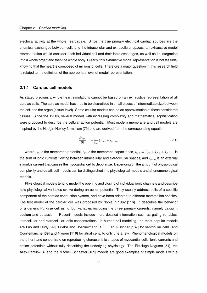
Chapter 2 – Cardiac modeling
electrical activity at the whole heart scale. Since the true primary electrical cardiac sources are the
chemical exchanges between cells and the intracellular and extracellular spaces, an exhaustive model
representation would consider each individual cell and their ionic exchanges, as well as its integration
into a whole organ and then the whole body. Clearly, this exhaustive model representation is not feasible,
knowing that the heart is composed of millions of cells. Therefore a major question in this research field
is related to the definition of the appropriate level of model representation.
2.1.1 Cardiac cell models
As stated previously, whole heart simulations cannot be based on an exhaustive representation of all
cardiac cells. The cardiac model has thus to be discretized in small pieces of intermediate size between
the cell and the organ (tissue-level). Some cellular models can be an approximation of these considered
tissues. Since the 1950s, several models with increasing complexity and mathematical sophistication
were proposed to describe the cellular action potential. Most modern membrane and cell models are
inspired by the Hodgin-Huxley formalism [79] and are derived from the corresponding equation:
∂vm∂t
= − 1cm
(iion + istim) (2.1)
where vm is the membrane potential, cm is the membrane capacitance, iion = ICa + INa + IK · · · is
the sum of ionic currents flowing between intracellular and extracellular spaces, and istim is an external
stimulus current that causes the myocardial cell to depolarize. Depending on the amount of physiological
complexity and detail, cell models can be distinguished into physiological models and phenomenological
models.
Physiological models tend to model the opening and closing of individual ionic channels and describe
how physiological variables evolve during an action potential. They usually address cells of a specific
component of the cardiac conduction system, and have been adapted to different mammalian species.
The first model of the cardiac cell was proposed by Noble in 1962 [116]. It describes the behavior
of a generic Purkinje cell using four variables including the three primary currents, namely calcium,
sodium and potassium. Recent models include more detailed information such as gating variables,
intracellular and extracellular ionic concentrations. In human cell modeling, the most popular models
are Luo and Rudy [99], Priebe and Boeckelmann [136], Ten Tusscher [167] for ventricular cells, and
Courtemanche [39] and Nygren [119] for atrial cells, to only cite a few. Phenomenological models on
the other hand concentrate on reproducing characteristic shapes of myocardial cells’ ionic currents and
action potentials without fully describing the underlying physiology. The FitzHugh-Nagumo [54], the
Aliev-Panfilov [4] and the Mitchell-Schaeffer [109] models are good examples of simple models with a
44

2.1. State of the art
reasonable number of variables and equations that reproduce physiologically shaped action potentials
with very low computational expense. Another advantage of these models is that the correct tuning of
their parameters can generate action potentials corresponding to cells of different regions of the cardiac
conduction system. Thus, they are much lighter when incorporated in whole heart models compared to
physiological models, and, under certain conditions, give results of comparable accuracy [124].
2.1.2 Macroscopic cardiac source models and extra-cardiac potentials
The earliest class of cardiac models that represent cardiac activity were dipole models. The dipole as
a cardiac source was introduced by Einthoven in 1913 and consists in considering the heart as two
electrical charges of opposite polarities and equal intensity [180]. This model evolved into the moving
dipole, oblique dipole and multiple dipoles [32, 59, 82]. The fixed dipole model and its further versions
give rather good qualitative interpretations of the ECG and provides a good idea of the physical intuition
behind observed potential on the torso. However, physiological meaning and precise quantitative
information on cardiac electrical distribution are missing.
A popular macroscopic source model that is closer to the heart’s electrical behavior is the Uniform
Double Layer (UDL) introduced by Wilson [188]. At each time instant, this model describes cardiac
electrical activity by the location, curvature, and direction of the depolarization wavefront that separates
depolarized regions from those still at rest. This wavefront is modeled by a boundary carrying dipoles
of uniform strength, remote extra-cardiac potentials are computed in an integral equation form based on
solid angle theory [81]. This model was mainly used to describe ventricular activity during depolarization.
The Equivalent Double Layer (EDL) is a successor to the UDL model and extends the concept of
wavefront propagation to describe the repolarization phase [60, 61, 177]. The EDL model relies on the
assumption of equal anisotropy between intracellular and extracellular spaces all over the heart. This
way, source currents can be expressed as a weighted sum of transmembrane potentials gradients of
active myocytes within the myocardium. In a homogeneous heart, all source activity within the heart can
be fully described by the distribution of transmembrane potentials on the heart surface S. A basic way
to express remote extra-cardiac potentials in an infinite homogeneous external medium is thus given by:
φ(x′, t) = −14πσ
∫S
σin(x)vm(x, t)dω(x′,x) (2.2)
where x′ is an external observation point, x the source location, σ and σin(x) are respectively the
remote and the local intracellular conductivity tensors, vm(x, t) is the transmembrane potential at time t,
S is the heart surface and dω(x′,x) denotes the so-called solid angle subtended by small segments of
S. Ultimately, equation (2.2) can be re-expressed so that remote potentials φ(x′, t) can be directly linked
45

Chapter 2 – Cardiac modeling
to the local activation times over S.
One of the most popular formulations and probably the dominant source model used in the ECG
inverse problem is the epicardial surface formulation [8]. Here, the idea is to consider epicardial
potentials on a closed surface inside the body as a virtual electrical source. This formulation is based on
the principle that in an electrically passive volume, there is a unique relationship between potentials on
the outer surface and the potential distribution over an inner closed surface. This means that a potential
distribution over any closed surface encompassing the heart fully reflects the inner primary currents in
the heart, and results in the same ECGs as those produced by these inner primary currents. This surface
is ideally chosen to be the epicardium. The resulting forward problem is expressed by the generalized
Laplace equation (2.3):
∇ · (σt∇φt) = 0 (2.3)
where σt and φt are the extra-cardiac conductivity and potential, respectively. Equation (2.3) reflects the
passive nature of regions outside the heart. This is completed with Neumann boundary condition on the
exterior torso surface and Dirichlet boundary condition on the epicardium: φt = φex where φex are the
known epicardial potentials.
Perhaps the most complete and the more physiologically meaningful approach used to model
cardiac activity is the bidomain method [108, 108, 149, 172]. First introduced by Schmitt [149] and
formulated mathematically by Tung [172], it consists in considering the myocardium as a syncytium
of two interpenetrating spaces separated by the cell membrane: the intracellular and the extracellular
spaces. This is a simplification that can be interpreted by considering average properties of clusters of
cells instead of describing each cell individually. This leads to a continuous definition of extracellular and
intracellular potentials and conductivities and allows for the possibility of considering unequal anisotropy
ratios. The major Partial Differential Equations (PDEs) of the bidomain model describe the primary
currents in the heart volume and are given by:
∇ · (σin∇vm) +∇ · (σin∇φex) = χ
(cm
∂vm∂t
+ iion + istim
)(2.4)
∇ · (σin∇vm) +∇ · ((σin + σex)∇φex) = 0 (2.5)
where σex and φex are the extracellular conductivity and potential, σin and φin the intracellular
conductivity and potential, vm = φin − φex is the transmembrane potential, cm is the membrane
capacitance, and χ is the surface to volume ratio representing how much membrane surface area is
present per volume of cardiac tissue. istim is a stimulation current that is only non zero in the chosen
region from which propagation is initiated. Equation (2.4) is a reaction-diffusion equation that can be
seen as a generalization of the cable equation in a 3D space [113]. To compute extra-cardiac potentials,
46

2.1. State of the art
this model is completed by the generalized Laplace equation in the extra-cardiac domain 2.3. Eventually,
coupling conditions are needed to obtain a full heart-torso model. Note that this full heart-torso model
does not only provide a relationship between ECGs and cardiac sources at one time instant but also
includes a way to simulate cardiac propagation over time. When equal anisotropy is assumed, the
bidomain model reduces to a lower-complexity version called the monodomain model. This model will
be treated in more detail in the next section.
In the field of ECG simulation based on cardiac models, most works neglect the mechanical
character of the heart. Yet, mechanical contraction causes a modification of the distance between BSPM
electrodes and the heart and also a change of the electrical activation wavefront. This topic has been
addressed in few studies [50, 103], but is still not deeply investigated. A reason why this assumption
is still widely used is due to the high complexity of a model involving electromechanical coupling in
a detailed realistic anatomical heart. Moreover, there is no consensus on the quantitative effects of
cardiac motion on the ECG in real conditions. Also, in the ECGI context, further improvements are still
to be made in the case of the fixed heart before focusing on electromechanical models.
2.1.3 Simulating propagation in the heart
Macroscopic source models describe the link between a cardiac configuration and the corresponding
remote ECG potential at one time instant. In order to be able to generate a full ECG, it is necessary to
simulate electrical propagation in the heart over time.
One of the first models consisted in cellular automata [94]. The concept uses a space grid in which
each element is an automaton describing the action potential generated by piece of cardiac tissue. An
automaton’s behavior depends on a set of rules that link its current state with that of its neighbors.
Propagation is initiated at a chosen element and evolves through local coupling of each element of the
grid with its neighbors. The main advantage of such a discrete method is its high speed in large scale
simulations compared to PDE based models like the bidomain. Very realistic simulations were performed
using such method on an anatomically based hearts [94, 186]. However, the shape of the propagation
wavefront may be very dependent on the structure of the defined grid. Another limitation comes from the
discrete character of such an approach. More precisely, action potentials shape are defined by a small
number of states and don’t arise from dynamic cellular electrophysiology. This makes this type of model
unsuitable for simulations in which electrical dynamics are important such as in ischemic tissues.
Another approach originally conceived for modeling electromagnetic waves propagation is the
Huygen’s principle [120, 160]. Because of the wave-like nature of the electrical cardiac wavefront, this
model is convenient for a fast generation of a simple temporal pattern of the wavefront evolution. Given
the wavefront location and direction at a given time instant, the idea consists in drawing wavelets of
47

Chapter 2 – Cardiac modeling
appropriate size around the current location. Regions within these wavelets depolarize in turn in the
next time instant.
A similar approach consists in solving an eikonal equation instead of Huygen’s parabolic equation.
The difference is in the inclusion of a diffusive term in the eikonal equation. Contrarily to Huygen’s
method, this approach allows the wavefront speed to be influenced by its curvature, and also gives the
wavefront position at all times by a one step calculation [29, 30, 169]. Similarly to cellular automata
models, Huygens and eikonal equations models are not built from electrophysiology background.
Moreover, it only gives information about the wavefront location at each time step, but don’t provide
local electrical features like the transmembrane or the extracellular potential.
Although computationally more demanding, the bidomain/monodomain models are the preferred
models when the objective is to simulate cardiac propagation with a high degree of accuracy,
physiological meaning and realism [12, 15, 96, 130, 132]. Not only do they provide a relationship
between cardiac activity and the resulting remote body surface potentials but also include a means
to simulate cardiac propagation through reaction-diffusion equations (2.4) and (2.5). These models
are usually coupled with some phenomenological model in order to define the term iion in (2.4).
The advantages are that they are continuous models, and provide extracellular and transmembrane
potentials based on parameters and equations that are meaningful with respect to the physics behind
the cardiac propagation process. Activation and recovery times can be computed from transmembrane
potentials upstrokes and downstrokes. Additionally, cardiac anisotropy can be taken into account in
order to best represent cardiac fibers [53, 78, 133] and thus electrical wave direction.
2.1.4 Numerical methods
Because the heart and the body shapes are highly irregular, analytical solutions cannot be obtained for
PDEs. Instead, the studied medium is discretized into a mesh of small elementary pieces that serve to
obtain an approximated numerical solution. Several methods can be employed, they can be classified
into surface methods such as the Boundary Element Method (BEM), and volume methods like the Finite
Difference Method (FDM), the Finite Element Method (FEM) and the Finite Volume Method (FVM). The
choice of these methods usually arises from the chosen diffusion model. Double layer and epicardial
source descriptions usually use the BEM to solve the forward problem in isotropic cases, whereas
bidomain/monodomain propagation in the heart volume is performed using the FEM. Surface methods
consist in discretizing only the interfaces of interest in the studied medium, namely the heart surface
and the torso surface. Rarely, inner structures interfaces like lungs and bones are also included in order
to take into account the non-homogeneity of the volume conductor [163]. However, volume methods
are the only way to include electrical anisotropy in the heart and torso. Indeed, volume discretization is
48

2.2. Proposal of a simplified heart-torso model
not only performed on the interfaces but also in the volume between them. This allows to set different
conductivity tensor values as a function of the position in the 3D space.
The simplest and most straightforward method is the FDM, it consists in partitioning the volume into a
uniform cubic grid. Partial derivatives are approximated with finite differences. Then, convergence of the
numerical scheme is obtained when the distance diminishes. FDM is a simple and very intuitive method,
but it is inadequate when dealing with irregular geometries [55]. Although it has been successfully used
in some cardiac modeling studies [144, 145], it is not as adapted as the FEM [31, 83, 91] and the
BEM [8, 51, 63, 134, 163], mainly because very high computational costs are required when using the
FDM, in order to obtain an equivalent accuracy as FEM and BEM, when using realistic anatomies. The
FEM and the BEM are quite similar in the sense that they both solve a weak form of the original PDE.
This weak formulation consists in minimizing a weighted residual expression of the original problem [93].
The difference occurs mainly in the number of unknowns involved. Since the FEM is a volume method,
the number of degrees of freedom is equal to the number nodes in the whole volume mesh, which is
obviously larger than that of the BEM. The matrices involved in the BEM forward problem are thus much
smaller than those in the FEM. However, FEM matrices contain very few non-zero elements whereas
BEM matrices are fully populated, which makes both approaches computationally comparable [150].
As the FEM, the FVM method is also based on a finite element volume mesh. The implementation is
simpler and it is ideally used in flux conservation contexts since conservation is solved for each element
of the mesh. FVM is more accurate than FEM in applications where flux is the important variable
but is more computationally demanding. Hence, FVM is generally more used in fluid dynamics and
FEM is more adapted to structural mechanics. For this reason, FVM is more rarely used in cardiac
electrical simulations, but seems to give comparable results [37, 38]. To sum up, each method has
its advantages and drawbacks and the method to employ depends on the targeted application [72].
Interestingly, combination methods were also used [53, 137, 162] in order to overcome the associated
limitations. Ultimately, all these numerical methods provide a linear expression that links cardiac sources
and the observed ECGs.
2.2 Proposal of a simplified heart-torso model
In this thesis, one important objective is to design a heart-torso model that is capable of generating
meaningful data that can be used to evaluate ECG inverse problem algorithms. Many works were
devoted to simulate ECGs with a high level of detail including fiber orientation, high resolution meshes,
novel heart-torso coupling techniques and anatomically detailed geometries [15, 27, 33, 84, 90, 96, 126,
129, 131–134, 148, 170, 171]. Nevertheless, when the goal is to evaluate, compare performance and
49

Chapter 2 – Cardiac modeling
study parameters influence on ECGI algorithms, these models are far too complex and computationally
demanding. Moreover, only few works are able to synthesize a complete and meaningful set of 12-Lead
ECG signals, since most of them only represent the ventricular activity. An interesting approach for
building a model that produces fairly good ECGs in an idealized geometry was presented in [161]. This
work shows that simplified models, even in idealized geometries, are able to produce complete ECGs
with coherent cardiac patterns. Even so, the presented model in [161] is still computationally expensive
due to the bidomain approach, and uses a phenomenological ionic model whose parameters tuning is
not described. Moreover, the bidomain model is suitable for anisotropic cardiac tissues, which was not
the case of the considered piecewise homogeneous model.
In this chapter, we propose a simplified, fast, and evolutive model that is capable of simulating
various scenarios of cardiac mappings. To this end, we choose the adapted monodomain model
which is a modification of the bidomain approach with lower complexity [12]. The monodomain model
is coupled with the phenomenological FitzHugh-Nagumo (FHN) model for describing transmembrane
currents. Parameters are defined for each region of the cardiac conduction system. This model includes
both atria and ventricles, and is able to synthesize meaningful ECGs while keeping a complexity level that
makes feasible the application of screening sensitivity analysis and parameter identification methods.
Contrarily to most studies in the field of ECG simulation based on whole heart models, we also pay a
particular attention to model equations derivation and spatiotemporal discretization.
2.2.1 Heart-torso geometry and meshing
Inspired by [161], we designed a new 3D geometry of heart-torso model (figure 2.1). It consists
of an elliptic-shaped torso and lungs and an ellipsoid heart that contains the main cardiac regions
of the cardiac conduction system: atria, Atrio-Ventricular Node (AVN), ventricles (endocardium and
epicardium), bundle of His, bundle branches and Purkinje fibers (see figure 2.2). Since electrical
connection between atria and ventricles is only allowed through the AVN in the real heart, an empty
space was created between the two chambers so they are physically connected only through the AVN.
Blood chambers and the valve plane were considered as vacuum when simulating cardiac propagation.
We integrate an isotropic but regionally heterogeneous structure representation, without adding fiber
orientation information.
Although fibers orientation is of great interest when the purpose is to represent cardiac activity
in the most realistic way, its influence on inverse algorithms performance is still to be proved. More
precisely, in-silico, the estimation of cardiac activity is to be compared with the one that produced the
simulated ECGs. Whether it was based on isotropic or anisotropic model is not likely to be influential on
reconstruction performance.
50

2.2. Proposal of a simplified heart-torso model
Figure 2.1: Heart-torso geometry
A major improvement in our geometry with respect to [161] is that we add another layer at the
ventricular level to distinguish between the epicardium and the endorcardium. In fact, the difference in
electrical properties of ventricular action potentials from the inner and outer layers is a major point to
the generation of appropriate ECG signals, and particularly the T-wave. More precisely, action potentials
duration diminishes smoothly as one moves from the outer layer to the inner layer of the heart. This gives
the effect of a repolarization wavefront traveling from the outside to the inside of the heart, contrarily to
depolarization.
This geometry is built using ANSYS DesignModeler software after a series of elementary operations.
It is then exported to ANSYS Mechanical in which a meshing step is performed before conducting FEM
based simulations. A first order tetrahedral uniform mesh is generated. It resulted in 4374 nodes and
17418 elements in the heart domain and in 43760 nodes and 244901 elements of 1cm side length for
51

Chapter 2 – Cardiac modeling
Figure 2.2: Heart geometry and its seven regions
the whole geometry (figure 2.3).
2.2.2 Model equations
The bidomain and the monodomain models are widely used to simulate cardiac electrical propagation
in current research and are largely accepted for their physiological relevance. Before providing the
monodomain equations used in our model, we first give some insight on the bidomain model and
explain how it reduces to the lower complexity monodomain model. The bidomain model is based
on the assumption that cardiac tissue can be partitioned into two separate conducting media: the
intracellular space, located inside the cardiac cells, and the extracellular space that connects cells
between them. These two spaces are separated by the cells membranes through which current flows
from one space to another. At the macroscopic scale, a homogenization process [114, 117] of the
bidomain model considers that these two spaces overlap so that each point of the 3D space has
intracellular and extracellular variables. The bidomain model arises from Maxwell’s equations under
quasi-static conditions. The quasi-static assumption consists in neglecting the temporal dynamics of the
electrical and the magnetic field in the body. Indeed, considering the size of the human torso and the
range of physiological variables in it, capacitive, inductive, and propagation effects of these fields can
52

2.2. Proposal of a simplified heart-torso model
Figure 2.3: Heart-torso mesh
largely be ignored. A detailed derivation of the bidomain equations and their coupling with the torso
domain is provided in appendix A. The quasi-static approximation is formally justified in appendix B.
The full heart-torso bidomain model provides the relationship between potentials in the heart domain,
namely the extracellular potentials φex and the transmembrane potentials vm, and the potentials in the
torso domain φt. The resulting equations within the heart domain H can be given in the following form:
∂u
∂t+ f(vm, u) = 0 (2.6)
∇ · (σin∇vm) +∇ · (σin∇φex) = χ
(cm
∂vm∂t
+ iion(vm, u) + istim
)(2.7)
∇ · (σin∇vm) +∇ · ((σin + σex)∇φex) = 0 (2.8)
where φex is the extracellular potential, σin and σex are the intracellular and extracellular electrical
conductivities, respectively, vm = φin − φex is the transmembrane potential that measures the
electrical potential difference between the intracellular and the extracellular space, cm is the membrane
capacitance, χ is the surface to volume ratio representing how much membrane surface area is present
per volume of cardiac tissue. istim is a stimulation current that is only non zero in the chosen region from
which propagation is initiated. iion is a function of the transmembrane potential vm and an introduced
variable u and represents the ionic current exchanges between intra- and extracellular spaces. This
variable u is a slow variable and characterizes the dynamics of ion channels opening and closing. The
definition of the expression iion(vm, u) and the function f in equation (2.6) are defined according to the
chosen ionic model. Equation (2.7) represents the reaction-diffusion dynamics that occur through the
53
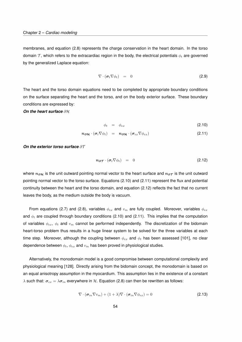
Chapter 2 – Cardiac modeling
membranes, and equation (2.8) represents the charge conservation in the heart domain. In the torso
domain T , which refers to the extracardiac region in the body, the electrical potentials φt are governed
by the generalized Laplace equation:
∇ · (σt∇φt) = 0 (2.9)
The heart and the torso domain equations need to be completed by appropriate boundary conditions
on the surface separating the heart and the torso, and on the body exterior surface. These boundary
conditions are expressed by:
On the heart surface ∂H
φt = φex (2.10)
n∂H · (σt∇φt) = n∂H · (σex∇φex) (2.11)
On the exterior torso surface ∂T
n∂T · (σt∇φt) = 0 (2.12)
where n∂H is the unit outward pointing normal vector to the heart surface and n∂T is the unit outward
pointing normal vector to the torso surface. Equations (2.10) and (2.11) represent the flux and potential
continuity between the heart and the torso domain, and equation (2.12) reflects the fact that no current
leaves the body, as the medium outside the body is vacuum.
From equations (2.7) and (2.8), variables φex and vm are fully coupled. Moreover, variables φex
and φt are coupled through boundary conditions (2.10) and (2.11). This implies that the computation
of variables φex, φt and vm cannot be performed independently. The discretization of the bidomain
heart-torso problem thus results in a huge linear system to be solved for the three variables at each
time step. Moreover, although the coupling between φex and φt has been assessed [101], no clear
dependence between φt, φex and vm has been proved in physiological studies.
Alternatively, the monodomain model is a good compromise between computational complexity and
physiological meaning [128]. Directly arising from the bidomain concept, the monodomain is based on
an equal anisotropy assumption in the myocardium. This assumption lies in the existence of a constant
λ such that: σex = λσin everywhere in H. Equation (2.8) can then be rewritten as follows:
∇ · (σin∇vm) + (1 + λ)∇ · (σin∇φex) = 0 (2.13)
54

2.2. Proposal of a simplified heart-torso model
Substituting ∇ · (σin∇φex) in (2.7) based on the previous equation gives:
λ
1 + λ∇ · (σin∇vm) = χ
(cm
∂vm∂t
+ iion(vm, u) + istim
)(2.14)
An additional boundary condition is considered, stating that transmembrane current doesn’t leave H.
n∂H · (σin∇vm) = 0 (2.15)
This expression has no physiological justification, but is convenient in the sense that variables vm
on the one hand, φex and φt on the other hand are decoupled. Consequently, the two bidomain
reaction-diffusion equations (2.7) and (2.8) linking φex and vm reduce to only one reaction-diffusion
equation that only involves vm. More importantly, bidomain and monodomain models seem to provide
very close results in whole heart simulation studies [128, 133].
Finally, an appropriate choice for defining f and iion(vm, u) is required in (2.6) and (2.7). Since
physiological models are two complex for whole heart simulations for our intended application,
phenomenological models are used instead. The oscillatory FitzHugh-Nagumo model [54] adds only
one ODE equation of the type (2.6) to the system. It is continuous, analytically tractable and presents
interesting uniqueness and existence properties [17, 34, 65]. Also, it presents the nice advantage of a
graphical analysis of its dynamics using a phase plane representation [141]. Moreover, it is capable of
precisely fitting physiological action potentials and has been successfully used in 3D cardiac propagation
models [43, 142, 161]. Within the FHN framework, the function f in (2.6) and the term iion(vm, u) in (2.7)
are defined as follows:
iion(vm, u) = kc1(vm − b2)(a1 −vm − b2a2
)(1− vm − b2a2
) + kc2u(vm − b2) (2.16)
f(vm, u) = −ke(vm − b2a2
− du− b1) (2.17)
where a1, a2, b1, b2, c1, c2, d, e and k, are non physiological parameters, but their tuning can result in
characteristic shapes of cardiac action potentials of different tissues [44].
To summarize, the final system of our proposed full heart-torso model is given by:
55

Chapter 2 – Cardiac modeling
In the heart domain H In the heart domain H
∂u
∂t+ f(vm, u) = 0 (2.18)
λ
1 + λ∇ · (σin∇vm) = χ
(cm
∂vm∂t
+ iion(vm, u) + istim
)(2.19)
On the heart surface ∂H
φt = φex (2.20)
n∂H · (σt∇φt) = n∂H · (σex∇φex) (2.21)
n∂H · (σin∇vm) = 0 (2.22)
In the volume conductor domain T
∇ · (σt∇φt) = 0 (2.23)
On the exterior torso surface ∂T
n∂T · (σt∇φt) = 0 (2.24)
where f and iion(vm, u) are defined according to (2.16) and (2.17).
2.2.3 Spatio-temporal discretization
In this section, we provide the spatio-temporal discretization of the previous system. As stated previously,
reaction-diffusion equations (2.18) and (2.19) can be solved first. Thereafter, extracellular potentials φex
and φt can be computed using the obtained values of vm. We first focus on reaction-diffusion equations
in H. Regarding the temporal integration, a semi-implicit Euler scheme is used. Equations (2.18)
and (2.19) become:
u(n+1) = u(n) + ∆tke(v
(n)m − b2a2
− du(n) − b1
)(2.25)
λ
1 + λ∇ · (σin∇v(n+1)
m ) = χ
(cm
v(n+1)m − v(n)
m
∆t + iion(v(n)m , u(n+1)) + istim
)(2.26)
where ∆t is the time resolution and n the current time step. Since cardiac electrical activity is to be
described in the whole heart volume, the FEM is adequate to our problem. The FEM is a numerical
56

2.2. Proposal of a simplified heart-torso model
method to solve equations with partial derivatives. It uses Galerkin variational analysis [164], and is
based upon two main procedures: 1) the generation of a finite element mesh that results in a setM of
M discrete points i ∈M called nodes whose coordinates are (xi)i∈M and N finite elements, and 2) the
definition of shape functions, usually referred to as test functions, defined on reference elements. The
discretization process in the FEM is achieved through the projection of the continuous field of interest
onto the basis formed by the M defined shape functions. In the rest of the section, we denote byMHand MT the set of nodes indexes in the heart and in the torso, respectively, and by MH and MT the
corresponding number of nodes. FEM resolutions start with writing the problem in a weak form, the
PDEs are linearized in each finite element so that an approximate solution is obtained on the nodes of
the mesh. Since (2.25) does not involve space derivatives, it is simply solved for each node defined in
H separately. The FEM is applied on (2.26) only. The weak form is a weighted residual obtained by
multiplying by some weighting function ψ and taking the integral over the studied domain. The weak
form of (2.26) reads:
∆t λ
1 + λ
∫H∇ · (σin∇v(n+1)
m )ψdx =∫Hχcm(v(n+1)
m − v(n)m )ψdx
+∆t∫Hχ(iion(v(n)
m , u(n+1)) + istim
)ψdx
(2.27)
where dx is the elementary volume displacement. Note that ψ can be any differentiable function, and
that this weak form is equivalent to its original strong form (2.26). Applying Green’s divergence theorem
to the left hand side of (2.27) yields:
∫H∇ · (σin∇v(n+1)
m )ψdx = −∫H
(σin∇v(n+1)m ) · ∇ψdx+
∫∂H
(σin∇v(n+1)m ) · n∂Hψds (2.28)
where ds is the the elementary surface displacement. This formula can be seen as an integration by
parts in multiple dimensions. Because of the boundary condition (2.22), the second term in the right
hand side vanishes. The discretization of the equation comes from the interpolation of field variables
over a finite element of the mesh by a set of shape functions (γi)i∈MH . These functions are associated
to the nodes of the mesh and are defined such that: γi(xj) = 1 when i = j, and decrease to reach
zero as x gets far from xi. We choose the simple case where functions γi : H → [0, 1] are piecewise
linear such that: γi(xj) = δij , ∀j ∈MH where δij is the Kronecker product. This results in a discretized
expression of the field variable vm:
vm(x) =∑i∈MH
vmiγi(x) (2.29)
where (vmi)i∈MH are the coordinates of the continuous field vm in the basis formed by the shape
functions (γi)i∈MH . If we replace in (2.27) the weighting function ψ, yet unspecified, by a shape function
57

Chapter 2 – Cardiac modeling
γk corresponding to some node k ∈MH, and inject the canonical form (2.29), we get:
−∆t λ
1 + λ
∑i∈MH
vmi(n+1)
∫H
(σin∇γi) · ∇γkdx =∑i∈MH
(vmi(n+1) − vmi(n))∫Hχcmγiγkdx
+∆t∑i∈MH
(iion(vmi(n), ui
(n+1)) + istim
)∫Hχγiγkdx (2.30)
Finally, writing the last equation for each value of k ∈ 1..NH results in the following linear system:
−∆t λ
1 + λAσin
v(n+1)m = Dχcm
(v(n+1)m − v(n)
m ) + ∆tDχ
(iion(v(n)
m ,u(n+1)) + istim)
(2.31)
where vm ∈ RMH and u ∈ RMH are vectors whose ith coefficient correspond to the values vm(xi) and
u(xi), Aσin is the so-called stiffness matrix, and Dχ and Dχcm are the so-called damping matrices.
Putting the unknowns on the left-hand side gives a system to be solved at each time step for v(n+1)m :
(∆t λ
1 + λAσin
+Dχcm)v(n+1)m = Dχcm
v(n)m −∆tDχ
(iion(v(n)
m ,u(n+1)) + istim)
(2.32)
The square matrices in (2.32) are defined by the following inner products:
Aσin =(∫H(σin∇γi) · ∇γkdx
)i∈MHk∈MH
Dχcm=(∫H χcmγiγkdx
)i∈MHk∈MH
Dχ =(∫H χγiγkdx
)i∈MHk∈MH
These matrices present nice computational properties. The most trivial one is that they are symmetric.
Secondly, if nodes i and k do not belong to the same finite element, the corresponding coefficient in these
matrices equals zero. Consequently, these matrices are sparse (contain few non-zero elements). The
third important property is that they are positive semi-definite [127]. The linear system can be solved
by iterative methods, but since only the right-hand side is different at each time step and the system
matrix remains unchanged, decomposition techniques are more suitable for solving (2.32). Because of
the properties described above, Cholesky Decomposition [179] is well adapted.
In order to solve the PDE system (2.32) and (2.26), an initial stimulation needs to be applied to initiate
the propagation process. To do so, the stimulation current istim is applied on a chosen node isan in the
exterior wall of the right atrium as the SAN region of the designed heart (figure 2.4). This stimulation is
applied for a certain period tstim, which is just the right duration necessary for this node to fire an action
potential. The complete procedure for solving the PDE system is given in Algorithm 1.
Now that transmembrane potentials vm are available, we describe how to obtain extracellular
potentials within the myocardium and those of the rest of the volume. Adding (2.23) to λ1+λ× (2.13)
58

2.2. Proposal of a simplified heart-torso model
Figure 2.4: SinoAtrial Node location
Algorithm 1 Algorithm for computing vm based on the monodomain formalism
Initialization: v(0)m = v0
m, u(0) = u0, istim = 0, istim(isan) 6= 0Assemble matrices Aσin
, Dχcmand Dχ
Compute the system matrix A = ∆t λ1+λAσin
+Dχcm
for n = 1 : T doif n∆t > tstim thenistim(isan) = 0
end ifCompute u(n+1)
i = u(n)i + ∆tke
(vm
(n)i−b2
a2− du(n)
i − b1)∀i ∈MH
Compute the right-hand side b = Dχcmv
(n+1)m −∆tDχ
(iion(v(n)
m ,u(n+1)) + istim)
Solve Av(n+1)m = b using Cholesky decomposition
end for
59
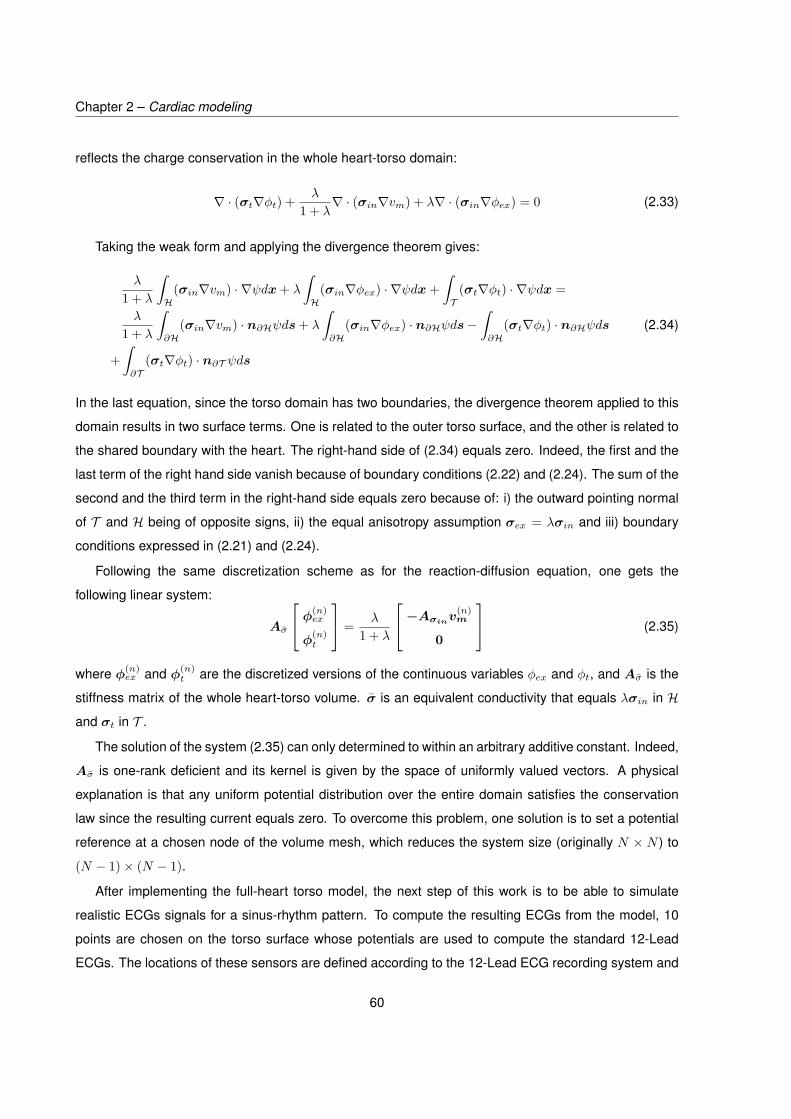
Chapter 2 – Cardiac modeling
reflects the charge conservation in the whole heart-torso domain:
∇ · (σt∇φt) + λ
1 + λ∇ · (σin∇vm) + λ∇ · (σin∇φex) = 0 (2.33)
Taking the weak form and applying the divergence theorem gives:
λ
1 + λ
∫H
(σin∇vm) · ∇ψdx+ λ
∫H
(σin∇φex) · ∇ψdx+∫T
(σt∇φt) · ∇ψdx =
λ
1 + λ
∫∂H
(σin∇vm) · n∂Hψds+ λ
∫∂H
(σin∇φex) · n∂Hψds−∫∂H
(σt∇φt) · n∂Hψds
+∫∂T
(σt∇φt) · n∂T ψds
(2.34)
In the last equation, since the torso domain has two boundaries, the divergence theorem applied to this
domain results in two surface terms. One is related to the outer torso surface, and the other is related to
the shared boundary with the heart. The right-hand side of (2.34) equals zero. Indeed, the first and the
last term of the right hand side vanish because of boundary conditions (2.22) and (2.24). The sum of the
second and the third term in the right-hand side equals zero because of: i) the outward pointing normal
of T and H being of opposite signs, ii) the equal anisotropy assumption σex = λσin and iii) boundary
conditions expressed in (2.21) and (2.24).
Following the same discretization scheme as for the reaction-diffusion equation, one gets the
following linear system:
Aσ
φ(n)ex
φ(n)t
= λ
1 + λ
−Aσinv(n)m
0
(2.35)
where φ(n)ex and φ(n)
t are the discretized versions of the continuous variables φex and φt, and Aσ is the
stiffness matrix of the whole heart-torso volume. σ is an equivalent conductivity that equals λσin in H
and σt in T .
The solution of the system (2.35) can only determined to within an arbitrary additive constant. Indeed,
Aσ is one-rank deficient and its kernel is given by the space of uniformly valued vectors. A physical
explanation is that any uniform potential distribution over the entire domain satisfies the conservation
law since the resulting current equals zero. To overcome this problem, one solution is to set a potential
reference at a chosen node of the volume mesh, which reduces the system size (originally N × N ) to
(N − 1)× (N − 1).
After implementing the full-heart torso model, the next step of this work is to be able to simulate
realistic ECGs signals for a sinus-rhythm pattern. To compute the resulting ECGs from the model, 10
points are chosen on the torso surface whose potentials are used to compute the standard 12-Lead
ECGs. The locations of these sensors are defined according to the 12-Lead ECG recording system and
60

2.3. Parameter identification using an evolutionary strategy
are given in figure 2.5. The 12-Lead ECGs are computed from the values in φt at these locations based
on section 1.4.2. The potential reference is set as in clinical practice at the RF electrode.
Figure 2.5: Heart-torso geometry and 12-Lead ECG electrode configuration
The heart-torso model equations were implemented in Matlab. After importing the created mesh
from ANSYS Mechanical, Finite Element matrices were assembled according to [25]. In order to
capture cardiac action potential events, ∆t was fixed to 0.1ms in equation (2.32). Then, the obtained
transmembrane potentials vm are sub-sampled at a resolution of 1ms and used in (2.35) for computing
φex and φt. Given some set of parameter values, the simulation time required for the full model is about
70s on a computer with Intel Xeon 3.47 Ghz processor.
Our model depends on many parameters that need to be tuned to obtain coherent surface ECGs.
The difficulty lies mainly in the non-physiological character of the FHN model parameters. A naive way
to proceed is to use parameters values from [161]. However, since the geometry, the mesh, the model
and the solver are different, this approach failed in giving realistic ECGs. Instead, we choose a different
approach to identify model parameters.
2.3 Parameter identification using an evolutionary strategy
In order to produce coherent cardiac activation patterns and realistic ECGs using our model, two
elements must fit physiological knowledge: i) the action potentials shapes produced by each defined
61

Chapter 2 – Cardiac modeling
region and ii) the cardiac propagation wavefront speed in each region. A natural way to proceed is by
first defining the FHN ionic model parameters that result in the desired action potential shapes and then
focus on the other parameters introduced by the monodomain model. In order to obtain different action
potential shapes, we first consider the FHN model applied to an isolated tissue. The corresponding
equations are given by:
∂vm∂t
= −iion(vm, u)− istim (2.36)
∂u
∂t= ke(vm − b2
a2− du− b1) (2.37)
where:
iion(vm, u) = kc1(vm − b2)(a1 −vm − b2a2
)(1− vm − b2a2
) + kc2u(vm − b2)
Here, the stimulation current istim plays the role of an inward current originating from neighboring nodes.
Because the FHN model only depends on two variables, it has the advantage of visualizing the solution
of the previous ODE system in a phase plane representation. This is done by plotting the so-called
nullclines [44], which are the curves defined by ∂vm
∂t = 0 and ∂u∂t = 0 in the plane where the x-axis
is represented by vm and the y-axis by u. The corresponding nullclines uvm and uu are obtained by
considering ∂vm
∂t = 0, ∂u∂t = 0 and expressing u as a function of vm in each equation (2.37) and (2.37):
uvm= −c1
c2(a1 −
vm − b2a2
)(1− vm − b2a2
) + istimkc2(vm − b2) (2.38)
uu = 1d
(vm − b2a2
− b1) (2.39)
This concept is illustrated in figure 2.6 for a given parameter set. The graphical representation of the
FHN model has the advantage to provide a direct interpretation of model parameters and their influence
on the nullclines, and thus on the generated action potential. Following physiological knowledge and
based on nullclines theory, a set of FHN parameters is defined for each region of the heart model (figure
2.7).
The second step consists in tuning the parameters introduced by the monodomain, namely χ, cm
and σin. Although the FHN model is a controllable oscillatory tool for generating various action potential
shapes in the isolated cell, it is another matter when integrated in a 3D reaction-diffusion model. The
manual tuning of monodomain parameters requires running Algorithm 1 and solving (2.35) for each
different parameter combination. Moreover, it is difficult to identify interactions between monodomain
and FHN parameters in the whole heart system. An adequate choice of a global set of parameters
62

2.3. Parameter identification using an evolutionary strategy
Figure 2.6: Left: phase plane representation of the nullclines ∂vm
∂t = 0 (blue), ∂u∂t = 0 (red) and the
obtained trajectory (green). Right: transmembrane potential (top) and recovery variable (bottom)
should take into account the mesh resolution, parameters interaction and thus system spatio-temporal
numerical stability. Thus, the resulting ECGs based on this first attempt were consequently unsatisfying.
Alternatively, another way to proceed is by seeking parameter values of the whole model that
produce ECGs that are close to reference sinus-rhythm ECGs. As seen previously, the ECG signal can
be decomposed into three waves resulting directly from the cardiac depolarization and repolarization
wavefronts: the P wave, the QRS complex and the T wave that have known characteristics in the case
of normal rhythm. This can help defining a measure of correctness of the ECGs simulated by our model.
Let us denote by p the set of parameters to identify, namely the FHN model parameters defined in
equations ( 2.16) and ( 2.17), completed with cm, σin and χ. The vector p is defined by:
p = σini, χ, cmi, a1i, a2, b1i, c1i, c2i, di, ei, ki
where i is the index of the considered region. It is noteworthy since our model is isotropic and regionally
homogeneous, the conductivity tensor σini reduces to a scalar parameter to be identified for each region.
Also, parameters a2 and χ take the same value for all regions of the heart. In fact, χ is the surface to
volume ratio. It is more related to the mesh resolution rather than cardiac regional characteristics.
Regarding a2, the justification comes from the fact that this parameter regulates action potentials
63

Chapter 2 – Cardiac modeling
Figure 2.7: Action potentials generated by the FHN model by region
amplitude, which is supposed to be roughly the same (around 30mV) everywhere in the healthy heart.
The equal anisotropy parameter λ is not identified since it is a scaling factor that is independent from
space and thus the considered region, and whose influence is absorbed in the value of σin. Moreover,
we impose that epicardium parameters take the same values as those of the endocardium, except
for parameter e that mainly regulates action potential duration. This parameter is denoted eepi for the
epicardium. Indeed, we assume the potentials of inner and outer layer of the epicardium to be of the
same shape but with different durations. Parameter b2i represents the resting potential and is fixed to
−85mV for all regions.
2.3.1 Optimization problem formulation
An appropriate cost function needs to be defined in order to solve the underlying optimization problem.
Our approach consists in maximizing a similarity measure between a real ECG ecgrefII and the one
simulated by our model ecgII(p), constrained by the signal waves durations and relative amplitudes.
We define the cost function based on the normalized scalar product between the two signals. Apart
64

2.3. Parameter identification using an evolutionary strategy
from providing a similarity measure, this choice also overcomes scaling issues. Equality constraints are
imposed based on features measured on the target ECG. The chosen features are: the durations of
the P wave (cref1 ), of the QRS complex (cref2 ), of the T wave (cref3 ) and of the PR interval (cref4 ), the
maximum peak amplitude ratios between the QRS complex and the P wave (cref5 ), and that between
the QRS complex and the T wave (cref6 ). Figure 2.8 shows the reference ECG and the corresponding
features.
Figure 2.8: Target ECG signal and its features
The optimization problem can then be expressed as follows:
p∗ =argminp
(1− | < ecgII(p), ecgrefII > |
||ecgII(p)||2||ecgrefII ||2
)2
(2.40)
s.t: c(p) = cref
where cref is the vectorized form of the features defined above, and c(p) those measured on the
simulated ECG with parameter set p.
The minimization problem (2.40) can be re-expressed as the unconstrained minimization of a
65

Chapter 2 – Cardiac modeling
Lagrangian function defined by:
L(p, λ) =(
1− (< ecgII(p), ecgrefII >)||ecgII(p)||2||ecgrefII ||2
)2
+6∑i=1
λi(ci(p)− crefi )2 (2.41)
where the so-called Lagrange multipliers λ = (λi)i∈1..6 were empirically fixed at values that ensure
the same order of magnitude between these non-homogenous constraints. The optimization problem
addressed in our context is non-convex, non-linear, non-differentiable and doesn’t have a unique
solution. Indeed, the system we are studying is weakly observable, meaning that the internal states
(cardiac signals) cannot be inferred directly from only one or only few target ECGs. Moreover, the size
of the parameter set to identify exceeds 60. The purpose here is to find a solution that is satisfying
regarding the constraints that have been imposed in equation (2.40). An appropriate algorithm for
solving this problem is one that does not require the existence of the derivative of the cost function with
respect to parameters, adapted to complex problems with potentially multiple local optima, and robust.
For these reasons, heuristic-based approaches, particularly Evolutionary Algorithms (EAs) [19, 80] are
more suitable than classical deterministic algorithms.
2.3.2 Evolutuionary Algorithms
EAs are guided random search approaches that originate from genetic algorithms [147]. They are
inspired by the evolution theory in which the strongest organisms are the ones that survive in the future
generations. We suppose that the solution of problem (2.41) can be encoded by a set of parameters,
called genes. Each set p is represented by a vector of genes called chromosome. A generation can
be defined by a population of several chromosomes. Following the principle of the survival of the
fittest, the algorithm starts from an initial population Pop0 of N chromosomes pj0, j ∈ 1..N. Then,
it evolves from one generation Popi−1 to the next Popi through genetic operations referred to as
mutations and crossovers. These operations are applied to a subset of Popi−1, giving birth to new
chromosomes Pop′i−1. Only the N fittest chromosomes in Pop′i−1 and Popi−1 are kept to constitute
the next population Popi. In the original definition of genetic algorithms, genes are discrete values
encoded in one bit. EAs are an extension to this concept in which genes are real valued. This entails
defining an appropriate variation domain with an upper and a lower boundary for each parameter.
The idea behind crossovers and mutations is described in figure 2.9 and the corresponding definitions
are given by:
• Crossovers: they are applied on several couples of chromosomes randomly selected from the
current generation. Crossovers consist in interchanging genes from two parent chromosomes in
66

2.3. Parameter identification using an evolutionary strategy
order to give birth to two chromosome children. Each child thus contains genes from both parents.
• Mutations: they are applied on a random subset of the current population. For each selected
chromosome, it consists in random perturbation of some genes values.
Figure 2.9: Diagram explaining the basic idea of crossovers and mutations
Convergence and robustness properties of EAs strongly depend on the cost function, the appropriate
encoding of individuals, and the choice of genetic operators (see [89] for further reading). A pseudo-code
of the used EA is given in Algorithm 2.
Algorithm 2 EA pseudo-codeInitialization: Provide a population Pop0 of N individuals and evaluate their associated costi = 1while i < Npopulations do
Select the best individuals from Popi−1Create new individuals Pop′i−1 using crossover and mutationEvaluate each individual of Pop′i−1Create Popi by keeping the N best individuals of Pop′i−1 ∪ Popi−1i = i+ 1
end while
2.3.3 Numerical simulations
This paragraph first describes the simulation steps followed in order to obtain realistically shaped
12-Lead ECGs and the corresponding cardiac propagation pattern. Then, we provide and discuss
quantitative and qualitative results in terms of convergence of the EA, ECGs and action potential shapes
and activation times mappings.
Simulation protocol The simulated surface ECGs are obtained following three main steps. In the first
step, a variation domain for each parameter in p is defined. Indeed, in order to run an EA, a necessary
prerequisite is the definition of the variation domain for each gene. To do so, a local study for each
parameter is conducted. Given a vector set p, we predefine a large range of values for each parameter.
We vary only one parameter in its predefined range and execute Algorithm 1 until a degenerate solution
is found. This is done successively for each parameter, and the upper and lower values for which
67

Chapter 2 – Cardiac modeling
degenerate solutions are obtained are taken to be the upper and lower bounds of the corresponding
parameter variation domain. In the second step, Algorithm 2 is run in order to identify the best parameter
vector p∗ according to the cost function (2.40). The last step consists in running Algorithm 1 using the
optimal parameter set p∗ to obtain and visualize the corresponding cardiac mappings, and solving (2.35)
to compute the 12-Lead ECGs.
We run Algorithm 2 for 35 generations of 70 chromosomes. The mutation probability is set to 0.25
and the selection rate is of 8%. The initial population is constituted of 38 manually chosen individuals, the
other 32 are chosen randomly in the defined parameter space. Regarding cost function computations,
reference features cref in (2.41) are directly extracted from ecgrefII and their values are given in table 2.1.
c1ref c2
ref c3ref c4
ref c5ref c6
ref
0.098 0.052 0.175 0.115 0.120 0.160
Table 2.1: Reference ECG features
Figure 2.10: Repolarization and repolarization times in an action potential
The P, QRS and T waves of the simulated surface ECG used in (2.41) were segmented directly from
the generated action potentials vm. The P wave duration is computed as the difference between the time
68

2.3. Parameter identification using an evolutionary strategy
of last depolarization in the atrial region with that of the first depolarization in the same region. Similarly,
the QRS complex duration is computed as the difference between the time of the last depolarization in
the ventricular region with that of the first depolarization in this region. Finally, the T wave duration is
obtained by substracting the time instant of the last repolarization in the ventricles with that of the first
repolarization. Depolarization and repolarization times are defined as the instant with maximum slope
and minimum slope in the action potential, respectively (see figure 2.10). Amplitude ratios are directly
computed on the simulated lead II. An infinite cost is assigned when at least 50% of nodes do not fire
action potentials, or when the solution diverges due to numerical instability.
Results After completing the first step, the obtained lower and upper bounds for each parameter are
provided in table 2.2.
Parameters σini χ cmi a1i a2 b1i c1i c2i di ei ki
Lower bound 4 0.01 0.15 0.09 0.01 -0.09 2.5 0.9 -0.5 0.0025 810
Upper bound 80 1 1.5 0.14 0.16 0.05 2.9 1.5 1.1 0.015 1400
Table 2.2: Parameters variation domain
Regarding the EA behavior, figure 2.11 shows the boxplot of cost values variability (y-axis) through
generations (x-axis). The red bar indicates the median of cost values at each generation, and the
bottom and top edges of the box indicate the 1st and 3d percentiles, respectively. The “whiskers” above
and below the box show the locations of the minimum and maximum values, and the outliers are plotted
individually using the “+” symbol. A rapid decrease in the median cost occurs in the first generations and
reaches a minimum cost of 0.1367 in generation 35. The first generation contains randomly selected
chromosomes in the variation domain of p. This population contains parameter sets that are inadequate
and produce infinite costs. It is interesting to see that these cases are rejected starting from generation
2. One can also notice that cost values are very close and don’t evolve between generations 15 and
21, but a jump occurs around generation 22. This leads to think that the algorithm went out of a local
minimum and that it is capable of exploring better solutions.
We display in figure 2.12 the obtained action potential in each region. Clearly, the general shape
of action potentials and their durations globally match physiological knowledge. Only bundle branches
action potentials are quite long compared to their average normal duration. In fact, since it is a relatively
small region in the heart domain, action potentials duration in this region do not contribute much in the
ECG shape. This means that information about their repolarization phase is difficult to integrate in the
cost function and any variations in the repolarization phase of this region won’t influence the simulated
ECG shape. However, the depolarization wave speed is important and is well identified since it regulates
69

Chapter 2 – Cardiac modeling
Figure 2.11: Boxplot of cost values evolution through generations
70

2.3. Parameter identification using an evolutionary strategy
the PR interval, which is a feature that is integrated in the cost function.
Figure 2.12: Estimated regional transmembrane potentials
Figure 2.13 shows a comparison between the reference (real) ECG and the best solution provided by
the EA. One can see that duration constraints have been respected, as well as the general characteristic
shape of the P wave, QRS complex and the T wave of the ECG signal. This is confirmed quantitatively
by a similarity value (<ecgII(p),ecgrefII
>)||ecgII(p)||2||ecgref
II||2
that reaches 89%, and features values that are close to the
reference as shown in table 2.3.
Note that adding an additional layer to the ventricles in the heart geometry enables to produce a
T wave with an appropriate duration because of the difference of repolarization times between the
ventricular layers. Without the additional ventricular layer, the repolarization wave in the ventricles
would naturally be of the same speed as that of depolarization, which would give a sharp T wave as
one can observe in [161]. The T wave amplitude in the simulated ECG is though of higher amplitude
compared to the reference. This can be explained by a strong gradient between the two ventricular
layers. Indeed, since the action potential duration does not vary smoothly in the ventricular region as
the repolarization front moves from the epicardium to the endocardium, an abrupt potential difference
71

Chapter 2 – Cardiac modeling
Figure 2.13: Normalized ECG estimated by the EA (red) and reference ECG (blue)
occurs in the boundary seperating the two layers, causing a T wave of higher amplitude. In this study, the
influence of the electrical axis of the heart is not investigated, which explains the difference in the S wave.
In fact, the observed surface ECGs depend on the heart orientation, which was not among parameters
to identify. As long as heart orientation is fixed, any model, no matter how realistic, may not be able
to exactly reproduce ECGs resulting from a different geometry configuration, especially regarding RS
patterns [115].
c1ref c1(p) c2
ref c2(p) c3ref c3(p) c4
ref c4(p) c5ref c5(p) c6
ref c6(p)
0.098 0.068 0.052 0.046 0.175 0.187 0.115 0.117 0.120 0.10 0.160 0.115
Table 2.3: Reference features ciref and best solution features ci(p)
Figure 2.14 depicts the simulated 12-Lead ECGs. Although the identification process was performed
only on lead II, the general shapes of the rest of the 12-Lead ECGs agree well with morphological
sinus-rythm ECGs in terms of polarity and durations: The P wave polarity is positive in all ECGs except
in aVR, and its duration is normally less or equal to 110ms. The QRS complex is represented by a
72

2.3. Parameter identification using an evolutionary strategy
positive deflection with a large, upright R in leads I, II, V4 - V6 and a negative deflection in aVR. Its
duration is less or equal to 120 ms. The ST segment is isoelectric, sloping upwards to the T wave. The
T wave polarity is the same as that of the QRS except in V2.
During electrophysiologial studies, the potential maps are constructed by measuring bipolar
potentials on the heart surface. The simulated extracellular potentials φex can be seen as unipolar
leads measured with respect to the defined reference RF. Bipolar leads can be obtained by subtracting
two extracellular potentials at two neighboring nodes. An example of a simulated bipolar potential is
given in figure 2.15. We find the same characteristic sharp signal shape at the local activation instant.
Figure 2.15: Transmembrane potential (up) and corresponding bipolar potential (down) at node 100
For visualization purposes, the data generated by the model in Matlab are exported back to ANSYS
Mechanical. Figure 2.17 presents the spatial distribution of transmembrane potential mappings at the
heart volume for 9 key events in the ECG. The activation pattern follows the characteristic sequence
in the normal conduction system. A depolarization wave is initiated at the SAN region and spreads
through the left and the right atrium (1-3). It is delayed in the AVN and spreads through bundle branches
(3-4). A rapid depolarization occurs in the Purkinje fibers (4-5), ventricles depolarize from the inner
layer to the outer layer (6-7) while atria are repolarizing. Finally, the repolarization wave goes from
the epicardium to the endocardium (7-9). Local Activation Time mappings provide valuable functional
and structural information about the initiation and the propagation pattern of cardiac electrical activity.
73

Chapter 2 – Cardiac modeling
Figure 2.14: Simulated 12-Lead ECGs
74

2.3. Parameter identification using an evolutionary strategy
From data simulated by our model, the Local Activation Time of each node can be obtained from the
corresponding transmembrane potential as seen in figure 2.10. These LATs can then be visualized for
all nodes at the heart level as shown in figure 2.17.
75

Chapter 2 – Cardiac modeling
Figure 2.16: Transmembrane potentials spatial distributions at 9 key instants of the ECG
76

2.3. Parameter identification using an evolutionary strategy
Figure 2.17: Local activation times (ms)
77

Chapter 2 – Cardiac modeling
2.4 Sensitivity analysis and model reduction
Since our model depends on many non-physiological parameters whose influence may be negligible in
the simulation of cardiac propagation, it is of interest to perform a sensitivity analysis of our model with
respect to its input parameters. An advantage lies in the fact that the parameter set on which the model
depends may be reduced in order to only keep parameters that are the most influential in the parameter
identification process. Moreover, in a concern of providing a quantitative measure of the validity of the
defined cost function (2.41) and parameters influence on the model, it is relevant to perform this study
on this same function.
Several sensitivity analysis methods exist and can be distinguished in two categories. Local
sensitivity methods rely on derivatives taken at a single point. They analyze the impact of one parameter
on the cost function at a time, while other parameters are fixed. This type of methods is unadapted when
dealing with complex models with discontinuities like ours. Moreover, it doesn’t provide information about
how model parameters interact with each other. Global sensitivity methods study model variations by
exploring the whole parameter space, usually by using monte carlo iterations. They are more costly
than local methods, but do not require assumptions on the studied function, and provide information
on parameters global influence and interaction. Interestingly, screening methods do not perform an
exhaustive study of the parameter space. Instead, they consider several inputs configuration and
evaluate the effects on the outputs when elementary perturbations are applied on the inputs, for each
configuration.
2.4.1 Morris method
One of the simplest and most popular screening approaches is the Morris method [111]. It is a one
at the time approach that is well adapted when the model depends on a high number of parameters.
The Morris method is a statistical analysis of model variations with respect to each parameter. The
assumption of a one at the time design is that if model parameters undergo elementary changes, those
that cause the largest variation in the model output are the most influential.
Let us consider a model output L that depends on set of P parameters p = (p1, p2, ..., pP ), a regular
grid that partitions each parameter variation domain into L levels, and an elementary displacement δ in
the grid that is the same for all parameters. The first step of the method is to define random trajectories
in the parameter space in which only one parameter at the time is varied. This consists in sampling
a random point p(0) in the defined grid. From this point, only one parameter p(0)i , i ∈ 1..P is varied
by δ to create a new point p(1). From p(1) this operation is performed for all resting parameters. This
results in P + 1 points such as only one parameter varies between p(i−1) and p(i). This scheme is then
78

2.4. Sensitivity analysis and model reduction
repeated for R− 1 different starting points so that R trajectories are created. This experiment plan ends
with R× (P + 1) different parameter sets (p(i,j))i∈0,..,Pj∈1,..,R
. A simple case where P = 2, L = 9 and R = 4
is presented in figure 2.18.
Figure 2.18: Example of Morris method experiment plan in the simple case where P = 2, L = 9 andR = 4
The second step consists in evaluating each of the created parameter sets by the model and
computing output variations corresponding to elementary displacements. The variation of the model
output for an elementary displacement in parameter pi (i ∈ 1, .., P) in the jth trajectory (j ∈ 1, .., R)
is given by:
d(i,j) = L(p(ki,j))− L(p(ki−1,j)) (2.42)
where ki and ki − 1 are the indexes for which only pi varied between pki−1,j and pki,j .
The third step consists in computing the mean µi and variance σi of elementary effects on all
79

Chapter 2 – Cardiac modeling
trajectories, for each parameter pi. These quantities are given by:
µi = 1R
R∑j=1| d(i,j) | (2.43)
σi =
√√√√ 1R
R∑j=1
(d(i,j) − µi)2 (2.44)
Finally, a graphical analysis where µi is reported on the x-axis and σi on the y-axis enables to study
the influence of each parameter:
• Parameters with low influence are close to the origin (0,0).
• Parameters with linear influence on the output are close to the x-axis.
• Parameters with non-linear influence or with strong interaction with others are close to the y-axis.
2.4.2 Numerical simulations
In this study, the parameter set p and its variation domain are the same as those defined in section 2.3,
to which we add lungs, torso and blood conductivities denoted by σlungs, σtorso and σblood respectively.
The output model value L is the cost function defined in equation (2.41). We choose: R = 3000, L = 50
and δ represents two unitary displacements in the uniform grid. The obtained sensitivity graphs are
presented in figure 2.19 and are categorized by region for better visualization. Each point on the graph
corresponds to each parameter values µi and σi.
The first remark is that extra-cardiac and blood conductivities are the least influential. Indeed, since
the whole domain is piece-wise homogeneous and isotropic, extra-cardiac conductivities act almost as
a scaling factor in the computation of the ECG. Our cost function L does not include an amplitude
constraint but rather constraints on waves relative amplitudes. This explains why the output is not
sensitive to these conductivities. Secondly, the regions with the highest mean value are those that
occupy the largest space in the heart volume, namely the atria and ventricles. The contribution of
parameters in small regions (AVN, His and bundle branches) is negligible compared to the influence
of the global parameter χ. This can be explained by the fact that χ acts on all regions, and more
specifically on atria and ventricles, whose contributions are the most important in the ECG. When the
most influential parameters are omitted (figure 2.20), a global remark is that parameters influence is
not the same depending on cardiac regions. For instance, in the AVN region, parameter b1 has a small
relative influence than in the His regions. Since our model output L depends on a reference ECG ecgrefII ,
these results may be compromised and may depend on the defined ECG reference. In order to assess
80

2.5. Pathology simulation
the previous results for different references, the sensitivity analysis was performed on four different other
ECGs of healthy cases. This results in five different cost functions L(k), k ∈ 1..5, each corresponding
to one of the chosen ECGs. The corresponding statistics µ(k)i σ
(k)i were computed based on the same
parameter samples (p(i,j))i∈0,..,Pj∈1,..,R
. The obtained graphs are given in figure 2.21 and figure 2.22.
These last results show that parameters sensitivity is globally the same for the different references.
Thus, for the considered cost function, the cost variability regarding each parameter is globally the same
for different ECG signals. Put differently, the contributions of model parameters regarding the defined
cost function are the same independently from the targeted ECG. Two conclusions can be drawn from
this analysis: i) this is an encouraging indicator in terms of reproducibility of the result shown in figure
2.13 and ii) some parameters influence is negligible regarding ECGs simulated by our model.
One way to assess the second statement is by running the EA in order to identify a parameter set
p′
that is a reduced version of p based on this sensitivity analysis. We first determine the regional
parameters that have that highest influence. To do so, we normalize mean and standard deviation
values regionally and we separate the least influential and the most influential parameters by a quadrant
of radius 0.4 as shown in figure 2.23. We define p′
by keeping only parameters that are out of
the quadrant. Then, we run the EA to identify this new set parameter with respect to ecgrefII . The
non-influential parameters are fixed to their values in the best estimation in the first generation. The
identified parameters p and p′
result in very close ECGs, which justifies the parameter set reduction.
2.5 Pathology simulation
We show in this section that our model is capable of simulating different pathology scenarios. In the
case of VT, an abnormal activation occurs in the myocardium at a fast rate due to one or several ectopic
sources. An ECG showing a VT is characterized by a large QRS and a heart rate > 120bpm. Two main
classes of VT can be distinguished. Monomorphic VTs are generated from an increased automacity of
a single point in the ventricle, or due to a reentry circuit within the ventricle. In this case, each beat of
the ECG looks the same. Polymorphic VTs occur is caused by abnormal ventricular repolarization. This
can be viewed as if several ectopic sources are activated at each heartbeat. Consequently, the ECG
beats are different. To simulate monomorphic VT and polymorphic by our model, either a single node
in the epicardium is stimulated to initiate abnormal propagation for successive heartbeats, or alternating
sites between endo- and epicardium are stimulated to initiate different pathological heartbeats. In both
cases, VT starts after a healthy ECG and the stimulation rate is fixed to 200 bpm. Figures 2.25 and 2.26
show the simulation results of a monomorphic and a polymorphic VT, respectively. In both cases, the
QRS complex is of less amplitude than the first healthy beat and is larger. A LAT mapping of an ectopic
81

Chapter 2 – Cardiac modeling
beat is given in figure 2.29 where the blue part in the ventricles is the activation region.
VT usually occurs in patients with acute myocardial infarction. In this case, a large scar in the
ventricular region is present and is electrically passive. The ECG of patients with ventricular infarction is
characterized by an ST segment elevation or depression. To simulate such conditions, a region close to
the septum was forced to maintain the same action potential value during the full simulated heartbeat.
This region can be seen in figure 2.28 in dark blue in the ventricular region. The obtained 12-Lead ECGs
are shown in figure 2.27. An elevation of the ST segment in leads II, III, aVL, aVF V1 and V2 is clearly
visible. These findings match their clinical usage as a diagnostic criterion of myocardial infarction.
82

2.5. Pathology simulation
Figure 2.19: Sensitivity graphs of parameters by region
83

Chapter 2 – Cardiac modeling
Figure 2.20: Sensitivity graphs when the most influential parameters are omitted
84

2.5. Pathology simulation
Figure 2.21: Sensitivity graphs obtained for five different model outputs, each color corresponds to adifferent ECG reference
85

Chapter 2 – Cardiac modeling
Figure 2.22: Sensitivity graphs obtained for five different model outputs when the most influentialparameters are omitted
86

2.5. Pathology simulation
Figure 2.23: Separation between the least and the most influential parameters by region
87

Chapter 2 – Cardiac modeling
Figure 2.24: Reference (black) and simulated ECGs corresponding to the best p (blue) and the best p′
(red)
88

2.5. Pathology simulation
Figure 2.25: Monomorphic VT simulation
89
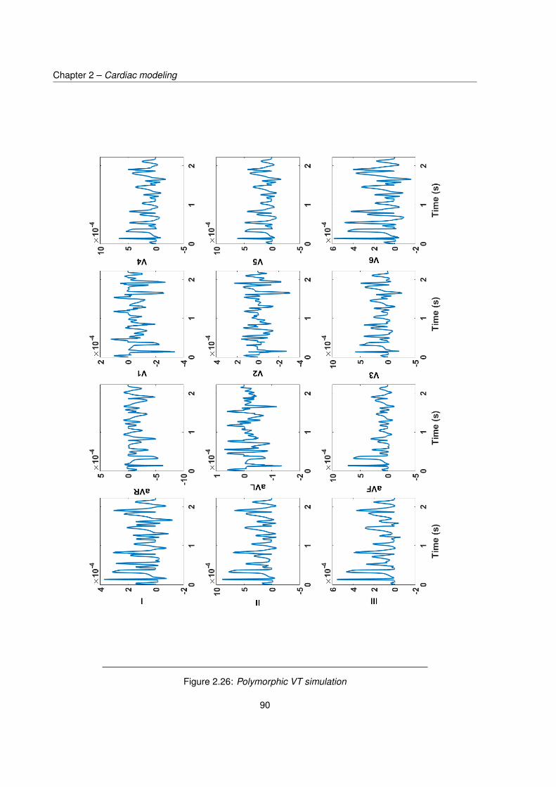
Chapter 2 – Cardiac modeling
Figure 2.26: Polymorphic VT simulation
90

2.5. Pathology simulation
Figure 2.27: Comaparison of healthy 12-Lead ECGs (blue) and those in the case of myocardial infarction(red)
91

Chapter 2 – Cardiac modeling
Figure 2.28: LAT mapping corresponding to the simulated ischemic condition
Figure 2.29: LAT mapping for the first ectopic beat of the simulated monomorphic VT
92

2.6. Conclusions
2.6 Conclusions
In this chapter, we present a low-resolution 3D model that produces realistic cardiac patterns
and morphological ECGs. This model is built upon the monodomain formalism coupled with the
phenomenological FitzHugh-Nagumo ionic model and enables to perform heart-torso simulations in
less than three minutes on a Intel Xeon 3.47 Ghz processor computer. Parameters were identified
using an evolutionary algorithm that optimizes a similarity measure between simulated ECGs and a
defined reference, observed from a patient. Such quick simulations allow for the investigation of model
sensitivity to its parameters and reveal the model parameters with higher influence. To our knowledge,
this kind of sensitivity analysis applied to a whole heart and torso model is original. Finally, we show that
this model is capable of generating different pathology scenarios that can be used for evaluating ECGI
algorithms. These modeling choices offer a controllable environment for easily studying the influence of
multiple aspects such as geometry variations, inclusion of anisotropy in the volume conductor and the
relationships between various cardiac patterns and the resulting ECGs.
93


CHAPTER 3
ECG INVERSE PROBLEM
In broad terms, the ECG inverse problem can be defined as the determination of cardiac electrical
function from body surface potential recordings. In this sense, even the visual analysis of a 12-Lead ECG
graph can be considered as an empirical inverse problem that uses previously documented information.
In the rest of this chapter, we denote by ECG inverse problem the mathematical manipulation of ECG
recordings in order to obtain a 3D mapping of cardiac electrical activity. Solving the ECG inverse problem
requires a set of ECG measurements acquired on the torso surface and a forward model that links
these observables to cardiac electrical sources in the considered geometry. Naively, one would simply
want to invert the forward model to obtain cardiac sources from ECGs. However, such solutions will
undoubtedly be inappropriate due the ill-posed nature of the ECG inverse problem. This term stems
from a definition given by Hadamard [73] and designates any problem for which one of the following
conditions is not satisfied: 1) a solution exists, 2) the solution is unique and 3) the solution’s behavior
changes continuously with the inputs. In the case of the ECG inverse problem, both conditions 2)
and 3) are dissatisfied. In fact, solution non-uniqueness arises from the small number of observations
compared to the number of cardiac electrical sources to be recovered. Solutions instability on the other
hand is due to the attenuation of electrical activity when propagating from the heart to the body surface.
As a result, several cardiac mappings can correspond to the same observed ECGs, and small modeling
uncertainties can result in large deviations in the obtained solutions. When the forward operator is
linear, this is translated by its low-rank and ill-conditioned character. To circumvent this obstacle, it is
necessary to mathematically constrain appropriately the solution space. This can certainly guarantee the
uniqueness of the solution but can still lead to inappropriate solutions if the penalty doesn’t adequately
fit the physiological nature of a cardiac electrical mapping. Numerous methods have been proposed for
solving the ECG inverse problem, but efforts are still to be made in finding penalties that best match
cardiac electrical physiology. Moreover, studies comparing these methods performance under unified
conditions in terms of source models, forward models and considered pathologies are still missing.
In this chapter, we first review the main approaches for solving the ECG inverse problem. Then, we
introduce the selected methods in terms of data pre-processing, the different regularizers choice and
95

Chapter 3 – ECG inverse problem
implementation, the determination of an adequate regularization parameter value and the optimization
algorithms. We finally provide results of the numerical experiments performed in healthy and pathological
cases.
3.1 State of the art
3.1.1 Source formulations
The ECG inverse problem can be formulated differently depending on the chosen cardiac source model
and consequently the underlying forward model. The main macroscopic cardiac source models are
presented in section 2.1.3. From an ECGI perspective, the choice of an adequate source model is even
more important than that of simulating ECGs by forward calculations. Indeed, although several source
formulations can result in similar ECG patterns, the source spatio-temporal nature strongly affects the
a priori to be imposed when solving the inverse problem. Moreover, some types of models involve
electrical sources that cannot be measured in practice, which renders validation difficult.
The earliest family of source models consisted of a distribution of equivalent current dipoles in
the heart [108, 166, 176]. These models served very well ever since for a qualitative explanation of
ECG waveforms. However, it is hard to capture the electrical events in the whole heart when it is
represented by only few dipoles [40, 46, 108]. The inverse problem based on UDL and EDL types
of models is referred to as activation time imaging [40, 85, 86]. In these cases, one directly seeks
the depolarization time corresponding to the upstroke of transmembrane potentials in the regions of the
heart. This approach is of great clinical interest because of the coherence of cardiac activation times, but
requires solving a non-linear inverse problem and does not provide the temporal information of cardiac
potentials. Moreover, it only focuses on cardiac electrical activity neighboring the electrical wavefront
and thus does not take into account activity that is far from it. More recently, efforts have been made
in directly recovering the transmembrane potentials in the heart volume [76, 107]. Nevertheless, the
underlying inverse problem is severely ill-posed since the number of sources to be recovered are that of
nodes in the whole heart mesh. Also, these potentials are difficult to measure in clinical routines, which
limits its use in clinical procedures. The preferred source formulation in the ECG inverse problem is in
terms of epicardial potentials [67, 104]. Indeed, this last formulation provides substantial information of
the local electrical activity everywhere on the epicardial surface. This formulation enables the recovery
of late potentials which are of major importance in identifying slow conduction pathways responsible for
VT. Local activation times can eventually be computed as the time when the local potential reaches an
optimum. Most importantly, these potentials are those that are measured and used in invasive clinical
routines of electrophysiological studies.
96

3.1. State of the art
3.1.2 Classical methods
Regarding methodological aspects, several approaches for solving the inverse problem can be found.
The most classical regroups regularization based methods. Originally proposed by Tikhonov [168],
these methods consist in finding the best fit to data solution in the least squares sense while considering
an additional penalty term. This additive penalty term, referred to as the regularization term, aims at
reducing the inverse solution’s high frequency content. The resulting formulation is given by:
z∗ = argminz
12 ||G(z)− x||22 + λ||R(z)||p (3.1)
where z represents the sources to be recovered, G is the forward model, x is the set of observed
ECGs, R is the regularization operator and λ a regularization parameter that balances between the
amount of data fidelity and regularization. In Tikhonov regularization, p = 2 and R is often taken
as the identity, the spatial gradient or the spatial Laplacian operator. This method presents the huge
advantage of providing an analytical solution when G and R are linear operators, which is mostly the
case in this context. Although this approach has been extensively used in the ECG inverse problem
[26, 56, 97, 155, 157, 184], it is often criticized for not taking into account the physiological nature of the
sought solution and providing over-smoothed solutions due to the use of the `2 norm in the penalty term.
The rising interest in sparsity-based approaches in the signal processing community led to investigating
`1-based regularization in the ECG inverse problem (p = 1), and more particularly Total Variation (TV)
regularization. TV regularization appeared in image denoising and is based on the principle that when
signals have spurious details, the integral of their absolute gradient (TV) is high [143]. Thus, minimizing
the TV of a signal removes unwanted details and enhances important information like contours. Since
the `1 norm is not differentiable, analytical solutions cannot be obtained and this formulation requires
the use of iterative algorithms. The most widely used algorithm in TV regularization is the Iterative
Reweighted Norm (IRN) [41, 157, 158, 190]. Other studies have investigated other types of optimization
methods, such as in [182] where inequality constraints were applied and the problem was solved by
an interior point method, or in [28] where the Alternating Direction of Multipliers (ADMM) was used. In
these studies, TV performed better than the more classical Tikhonov regularization. Interestingly, the
study in [139] shows that at some time courses when sources are neither focal nor diffused, `p norm
regularization when 1 < p < 2 may be more appropriate. However, it is still unclear how a link between
the appropriate value of p and the observed ECG can be established. In the same spirit of regularization,
Wang et. al [181, 183] proposed penalty terms that arise from the FEM variational definition of the
notions of identity, gradient and Laplacian. The choice of the regularization parameter value is critical in
regularization-based methods and a major difficulty lies in its determination. Several classical methods
97

Chapter 3 – ECG inverse problem
attempt to provide a balance between the solution and regularization norm. Among these, the most
straightforward is the optimal criterion solution that consists in minimizing an error criterion between
the exact epicardial solution and each of the regularized solutions obtained by testing values of λ in a
defined dense grid. This method is clearly not feasible clinically since it requires the knowledge of the
true solution but is convenient when the purpose is to evaluate inverse methods performance. The highly
used L-curve method plots the data fidelity term ||G(zλi) − x||22 against ||R(zλi
)||p obtained for a set
of estimated solutions zλiwith parameter λi and often results in a characteristic L-shaped curve. The
optimal λi in the L-curve is chosen to be the one corresponding to the corner of this curve since it ideally
balances between the two terms in the problem (3.1)[75]. Similarly to the L-curve, the Generalized
Cross Validation criterion (GCV) tests a set of values for λ and chooses the optimal parameter as the
one that minimizes a trade-off function between the data fidelity term and the regularization term [66].
The Composite REsidual and Smoothing Operator (CRESO) is also commonly used and chooses the
parameter value that generates the first local maximum of the difference between the partial derivatives
of the two terms in problem (3.1) with respect to λ [31]. In contrast with these a posteriori methods,
a priori methods rely on prior knowledge on the system such as noise variance in the case of the
discrepancy principle [135]. All these methods may provide convenient regularized solutions, but they
are very time consuming since they require defining and testing values in an exhaustive search space for
λ. Of major interest are methods that choose λ in an adaptive fashion, such techniques are successfully
implemented in other fields but haven’t been investigated in the context of ECG inverse problem [77].
Another well-known family of methods consists in approximating the forward operator G to a better
conditioned version G. In practice, this consists in considering a truncated version of the Singular Value
Decomposition (SVD) of G in which small singular values are rejected [74]. This has the effect of
keeping only the modes that are informative and thus diminishes numerical instability. In this case, the
regularization lies in truncating the singular values of G, and the sources are obtained by computing
the pseudo-inverse of G without adding penalty terms. First proposed by Greensite for ECGI [68], this
approach gained popularity and several versions of this approach can be found [26, 69, 156]. Although
conceptually different, the classical Truncated SVD method (TSVD) can be formally comparable to
Tikhonov regularization in the sense that they both filter the high frequency components of the solution
[74]. By analogy, the truncation level plays the role of the regularization parameter λ in Tikhonov
methods.
In regularized and SVD-based solutions, much attention has been given to methods that incorporate
knowledge both on the spatial and the temporal character of the sources [100]. The most common way to
do so is by spatially regularizing the difference between two consecutive potentials spatial distributions.
This method is known as Twomey regularization [121], and postulates that the sought solution does
98

3.1. State of the art
not significantly change between consecutive time samples. This has also been achieved by combining
TSVD as a temporal whitening and imposing explicit spatial constraints [21, 154]. Finally, using several
constraints as temporal and spatial regularization as in [22, 23, 49] seems to produce much more realistic
temporal patterns of the reconstructed signals, while spatial coherence is also respected.
Alternatively to deterministic methods, some studies solve the inverse problem from a Bayesian
perspective [9]. In this case, one seeks to estimate the Bayesian maximum a posteriori of a probabilistic
problem in which the sources and the noise are random variables. Van Oosterom was the first to
introduce such an approach in ECGI [173–175]. Few publications appeared later [151–153, 192], but
it is not as well established as regularization methods in ECGI community. The main reason lies in the
challenge raised by the difficulty in determining the mean, the covariance, and an adequate probabilistic
model for describing the noise and the sources.
Apart from the methods reported above, another main class of methods lie in solving the ECG inverse
problem by using cardiac propagation models. This emerging approach addresses the ECG inverse
problem by a parameter identification strategy. Rather than directly estimating the electrical sources,
it consists in finding the optimal set of parameters of a cardiac propagation model that results in the
simulated ECGs that are the closest to those observed. In [98], the problem is reformulated as an optimal
control problem where ECGs are simulated using the bidomain formalism and the control is the natural
onset of cardiac activation. In [64], a personnalized monodomain model with the Mitchell–Schaeffer’s
ionic model were used to train a machine learning algorithm in order to identify the onset activation
location and cardiac tissue conductivity. In [140] an adaptive inverse monodomain operator was used
to reconstruct potentials. In a quite similar way, authors in [36] use a Kalman filter and mechanical
observations to identify parameters of a bidomain electrical model coupled with a mechanical model. In
[16], a genetic algorithm is employed to identify ionic parameters of the Mitchell-Schaeffer model using a
bidomain formalism and a model reduction method. This type of approaches is promising since it relies
on well established models for simulating cardiac propagation. In this case, regularization may be seen
as constraining the solution space by that of the possible solutions of the forward problem. However,
they suffer from their high computational cost since they either rely on simulating one or several full
heartbeats at each algorithm iteration, or use an extensive database computed in advance. Moreover,
these methods require knowing the onset activation of the cardiac cycle beforehand, or estimate it during
the inverse procedure, which leads to an even more complex problem. Another limitation comes from
the fact that these methods may not be able to match the reference cardiac temporal patterns simply
because the involved models may not offer the possibility to do so. For these reasons, classical methods
are still preferred because they offer a solution space that is more likely to contain the true solution.
99

Chapter 3 – ECG inverse problem
3.2 Methods
In this thesis, we choose the epicardial source model for solving the inverse problem. From the model
proposed in chapter 2, the forward problem in (2.35) used to compute ECGs is equivalent to that in
terms of heart surface extracellular potentials. Indeed, cardiac extracellular potentials distribution over
any closed surface encompassing the heart fully reflects the inner primary currents within the heart.
Consequently, these epicardial potentials obtained by solving equation (2.35) result in the same ECGs
as those computed originally from this same equation. The discretization of the corresponding forward
problem using the FEM is detailed in Appendix C and is expressed by the linear system:
X = GZ (3.2)
where Z ∈ RN×T is a matrix whose ith row represents the time course of epicardial potential values
at the ith node on the heart surface, X ∈ RM×T is a matrix in which the ith row represents the time
course of the potential observed at the ith defined sensor on the torso surface, and G ∈ RM×N is
the linear instantaneous transfer matrix that translates the attenuation effect of the volume conductor
separating sensors and the source surface. This section first presents the data pre-processing step that
we investigate, we then provide the ECG inverse problem formulation that we consider, the classical
regularizers employed in our practical context, and the optimization algorithms used to solve the
inverse problem. We choose the Alternating Direction Method of Multipliers (ADMM) for solving the `1
norm-based ECG inverse problem. Indeed, the ADMM offers a good compromise between convergence
rate and numerical complexity. The application of Morozov discrepancy principle combined with ADMM
for `1 regularization is investigated in order to adaptively determine an adequate value of λ, and we
extend this method to the `2 case. Finally, we propose a new spatiotemporal approach that exploits two
`1-based regularization terms.
3.2.1 Data pre-processing
In addition of the raw data case, two types of data pre-processing are investigated, one where the system
GZ = X is whitened with respect to the transfer matrix G, and one where this system is whitened with
respect to the dataX. The prewhitening step is commonly used in various signal processing applications
and is intended to decorrelate data and to remove artifacts [7, 87, 146]. The whitening process is
achieved through a Singular Value Decomposition (SVD) which consists in factorizing a matrix in a
unitary basis [42]. Let C ∈ RMC×NC be a rectangular matrix such that NC > MC , the SVD of C consists
100

3.2. Methods
in writing this matrix in the form:
C = UCSCVTC =
MC∑i=1
σiuCivTCi
where UC ∈ RMC×MC and VC ∈ RNC×MC are matrices with orthonormal column vectors uCi and vCi
respectively, and SC is a diagonal matrix containing the singular values σi > 0 in decreasing order. This
decomposition is unique up to an orthogonal transformation. We now define the whitening process for
C by applying the linear transform: C = SC−1UC
TC where C is the whitened version of C. Since UC
is unitary, the previous expression results in C = VCT . The whitened version C is now constituted with
orthonormal row vectors, which is an interesting property when dealing with ill-posed problems or highly
correlated data.
Singular values ranking can be interpreted as the amount of information contained in C. Therefore,
high singular values are those that correspond to the relevant amount of information on the structure
of C while low singular values select singular vectors corresponding to high frequencies or artifacts in
C. As a result, when inverting SC , low singular values are highly amplified and the artifacts contribution
may be dominant relatively to the principal components of C. To overcome this problem, a manipulation
called Truncated SVD (TSVD) is often performed in order to substitute C by a low-rank approximation
of its SVD [191]. The TSVD of C at rank k simply consists in keeping only the k highest values and their
corresponding singular vectors in the SVD and is given by:
Ck = UCkSCk
V TCk
(3.3)
=k∑i=1
σiuCivTCi
where the matricesUCkand VCk are derived from the k first singular vectors ofUC and SC , respectively.
Note that k is chosen to be lower than MC and the case k = MC corresponds to the original SVD. The
corresponding truncated whitening transform Ck is then given by Ck = V TCk
where artifacts are no longer
amplified.
Transfer matrix whitening The whitening transform of the system (3.2) with respect to the transfer
101

Chapter 3 – ECG inverse problem
matrix G is obtained from the TSVD of G and is given by:
XG = S−1GkUTGkX (3.4)
= S−1GkUTGkGZ
= V TGkZ
= GkZ
where Gk is the truncated whitening transform ofG and XGkthe matrix of whitened ECG observations.
Data matrix whitening The whitening transform of the system (3.2) with respect to the data matrix
X is obtained from the TSVD of X and is given by:
Xk = S−1XkUTXkX (3.5)
= V TXk
= S−1XkUTXkGZ
= GXkZ
where Xk is the truncated whitening transform of X and GXkthe corresponding new transfer matrix.
These two processing steps may seem similar in the sense that they both express components of
the first dimension (which corresponds to potentials spatial distribution of observations) of matrices G
and X in an orthonormal manner. The whitening transform can thus be seen as a means of treating
each observation with equal importance.
3.2.2 Inverse problem formulation
Without loss of generality, we consider in the rest of this section the vector system x = Gz corresponding
to the case of one time sample, but the formulations and the algorithms are equivalently applied to
matrix equations (3.4) and (3.5). Then we formulate the epicardial inverse problem in the traditional
regularization scheme at one time instant as following:
z∗ = argminz
12 ||Gz − x||
22 + λ
p||R(z − z0)||pp (3.6)
where z ∈ RN and x ∈ RN are respectively the vector of epicardial potentials and the vector of observed
potentials on the torso surface at a given time instant, z0 is the estimated solution at the previous time
instant, R ∈ RR×M is a linear transform that maps the sources onto some defined transform domain,
|| · ||p is the classical definition of the p norm and λ is the regularization parameter. This optimization
102

3.2. Methods
problem has the advantage of being convex when p ≥ 1 and can be solved using convex optimization
methods.
The adequate choice of a regularizer ||R(z − z0)||pp is intrinsically linked to prior knowledge on the
spatiotemporal character of the sought solution. Cardiac potential maps at a given time instant reflect
the electrical excitation wave within the heart. This means that at a given time, most of the sources
should be of low amplitude, except for those that are on or close to the activation wavefront. Depending
on the considered time instant and pathology, the electrical wave can be either extended or focal, and
can be assumed to present either a smooth variation of potentials amplitudes between activated and
unactivated regions on the heart surface, or abrupt changes in amplitude (e.g ischemia). In the case
where only spatial regularization is applied (z0 = 0), these natures can be enforced by imposing spatial
smoothness or sparsity on the source character, either directly in the source domain or in a transformed
domain. This justifies the choice of || · ||p as being the `1 to enforce sparsity on the source structure and
the `2 norm to impose smoothness. R is taken to be either the identity matrix I (zero order regularization)
which limits the total magnitude of the solution, the gradient operator V (first order regularization) that
limits the solution steepness, or the Laplacian L (second order regularization) that restricts steepness
change. V maps the node space onto the edges space and plays the role of a spatial gradient. It is
defined as following:
Ve,n =
1 if n = ne,1
−1 if n = ne,2
0 otherwise
(3.7)
where ne,1 and ne,2 are the indexes of the nodes of the heart surface sharing the eth edge, and
where Ve,n is the (e, n)th component of matrix V . V is constructed so that each of its rows computes
the amplitude difference between two nodes belonging to the same edge of the heart surface mesh.
Following this scheme, we define the Laplacian as the difference between two neighboring edges. The
notion of numerical neighborhood between two edges is considered in the sense that neighboring edges
are all the couples of edges sharing one node. Formally, L can be computed as the product L = AV
where V is the numerical gradient and A is given by:
Ai,e =
1 if e = ei,1
−1 if e = ei,2
0 otherwise
(3.8)
with i representing an index in the set of couples of edges (ei,1, ei,2) sharing a node. To our knowledge,
this is the first time that a formal definition of the numerical Laplacian is provided.
Regarding the temporal character of the sources, a legitimate assumption consists in considering
103

Chapter 3 – ECG inverse problem
that the temporal change of heart surface potentials distribution is limited. This is referred to as Twomey
regularization that considers the regularization term ||z− z0||22. This approach is commonly found in the
literature for the `2 norm.
3.2.3 Optimization schemes
`2 regularization In the Tikhonov case (p = 2), an analytical solution of (3.6) is obtained from
1st order optimality conditions by finding the solution that cancels the cost function’s partial derivative.
The corresponding solution is given by:
z∗ = (GTG+ λT TT )−1(GTx+ λT TTz0) (3.9)
`1 regularization When p = 1, this doesn’t hold because of the non-differentiability of the `1 norm.
The Alternating Direction Method of Multipliers (ADMM) has received considerable attention recently
and is particularly suited for such problems. It consists in using the principle of variable splitting of
the Douglas-Rachford algorithm [45] with the Augmented Lagrangian Multipliers (ALM) method [95]
and uses partial updates for solving simpler subproblems. A major advantage of the ADMM in our
optimization problem is that it offers the possibility of using proximal approaches for handling the `1
norm. In the rest of this paragraph, we consider only spatial regularization (z0 = 0). The first step is
rewriting problem (3.6) for p = 1 in the following equivalent constrained form:
(z)∗ = argmin(z)
12 ||Gz − x||
22 + λ||w||1 (3.10)
s.t: Rz = w
Although this reformulation may seem trivial, the problem can now be tackled using methods of
constrained convex optimization, in this case the ALM method, and offers the possibility for solving
separately for z and for w. The augmented Lagrangian for (3.10) is given by:
Lρ(w,z,µ) = 12 ||Gz − x||22 + λ||w||1 + uT (Rz −w) + ρ
2 ||Rz −w||22 (3.11)
where u is the scaled Lagrangian multiplier and ρ the penalty parameter. The advantage of “augmenting”
the Lagrangian by adding the last term in equation (3.11) is that the method ALM converges under far
more general conditions than the classical Lagrangian, including cases where the objective function is
not strictly convex [18]. This equation can be equivalently written in a scaled form when considering
104

3.2. Methods
µ = 1ρu:
Lρ(w,z,µ) = 12 ||Gz − x||22 + λ||w||1 + ρ
2 ||Rz −w+ µ||22 −ρ
2 ||µ||22 (3.12)
A pair ((w,z),µ) is said to be a saddle point for Lρ if:
∀(z,w,µ) ∈ RM×R×R Lρ((w,z),µ) ≤ Lρ((w,z),µ) ≤ Lρ((w,z),µ) (3.13)
Based on duality theory and the saddle point theorem [187], if there exists µ ∈ RR such that ((w,z),µ)
is a saddle point for Lρ, then (w,z) solves problem (3.10). Conversely, if (w,z) is a solution to problem
(3.10) and the constraint Rz = w is satisfied, then there is a µ ∈ RR such that ((w,z),µ) is a saddle
point for Lρ. An optimal point Lρ of the Lagrangian can thus be approached either by solving the primal
problem (z,w)∗ = argmin(z,w)
Lρ(w,z,µ) or its dual problem µ∗ = argmaxµ
Lρ((w,z),µ). Interestingly,
the optimal point for the primal and the dual problem coincide in the saddle point Lρ((w,z),µ) when
the cost function and the constraint are strictly convex. Moreover, a solution to the saddle point problem
provides a solution to (3.10). Following the ALM method, the solution of the saddle point problem is given
by alternating the joint minimization with respect to (z,w) (primal problem) and the maximization with
respect to µ (dual problem). In the ADMM, the joint minimization is avoided and is instead performed
alternatively with respect to z andw, one after another. Convergence proofs of the ADMM algorithm can
be found in [18] and update rules are given by alternating the optimization with respect to each variable.
We have at iteration k + 1:
z(k+1) = argminz
12 ||Gz − x||22 + ρ
2 ||Rz −w(k) + µ(k)||22 (3.14)
w(k+1) = argminw
λ||w||1 + ρ
2 ||Rz(k+1) −w+ µ(k)||22 (3.15)
µ(k+1) = argmaxµ
ρ
2 ||Rz(k+1) −w(k+1) + µ||22 −
ρ
2 ||µ||22 (3.16)
The update of z is obtained by canceling the partial derivative of Lρ with respect to z, and the update
of µ is performed using the gradient ascent method. Since equation (3.15) involves the minimization
of a non-smooth function, a proximity operator is used in the update of w. The proximity operator has
first been introduced in [110], it is frequently used in non-differentiable optimization problems and more
particularly in TV denoising. The proximity operator proxf,β(·) of a convex function f and parameter β
is defined by:
proxf,β(w) = argminy
12 ||w− y||22 + βf(y) (3.17)
The idea behind this operator is that it compromises between minimizing f and being near to y. It can
be viewed as a generalization of projections onto convex sets [123]. In the case where f is the `1 norm,
105

Chapter 3 – ECG inverse problem
the elements wi of w∗ = proxf,β(w) ∈ RR are given by:
wi = wi|wi|
(|wi| − β)+ (3.18)
where (·)+ = max(·, 0). Finally the ADMM algorithm for solving (3.10) is given in Algorithm 3. It is
noteworthy that it was however proved recently in [24] that the ADMM algorithm may fail to converge
and a randomized version of it was proposed in [165], which was shown to converge in expectation
under some technical assumptions. Note that the use of such kind of randomized block-coordinate fixed
point algorithms was investigated in [35] where almost sure convergence properties were established.
Basically, the randomized form of ADMM is similar to (3.14-3.16) but, instead of updating the components
according to their index order 1, 2, they are updated following the order σk(1), σk(2), where σk : 1, 2 →
1, 2 is a permutation which is randomly chosen at each iteration k. Finally, it can be noticed that
another technique for dealing with criteria split in a sum of more than two functions is to resort to parallel
versions of ADMM [52, 125].
Note that the matrix that has to be inverted in the ADMM is GTG + ρRTR. In comparison with the
Tikhonov solution, each iteration of the ADMM requires inverting the same matrix except that ρ in the
ADMM plays the role of parameter λ in Tikhonov regularization.
Algorithm 3 ADMM algorithm
Initialize variables z(0) = 0,w(0) = 0,µ(0) = 0Compute and store P = GTG+ ρRTR
While ||z(k+1)−z(k)||2||z(k)||2
< ε
z(k+1) = P−1 (GTx+ ρRT (w(k) − µ(k)))
w(k+1) = prox`1,λ/ρ(Rz(k+1) + µ(k))µ(k+1) = µ(k) +Rz(k+1) −w(k+1)
end
3.2.4 Determination of the regularization parameter
As explained in section 3.1.1, the regularization parameter plays a significant role in regularization-based
solutions. In this paragraph, we describe the optimal criterion method and introduce a new iterative
method for determining λ based on the discrepancy principle.
Optimal criterion We define the optimal parameter value λ∗i by the one that minimizes the Relative
Error (RE) in euclidean norm between the exact, known epicardial solution z and the estimated solution
z∗λiusing λi by the algorithms described previously:
||z∗λi− z||2z
(3.19)
106

3.2. Methods
Adaptive choice based on the ADMM and the discrepancy principle The discrepancy principle is
a method that determines a value for λ when the noise variance is available [70]. It states that satisfying
solutions are the ones lying in the set S = z : ||Gz−x||22 ≤ c where c is computed from noise variance.
However, in regularized least square problems, it is very time-consuming to find an appropriate value for
λ, and Newton type methods are often used outside the original optimization scheme [159]. As shown in
[77], an additional splitting in the ADMM used in TV denoising combined with the discrepancy principle
results in a closed form for the update of the regularization parameter at each iteration. We use this
strategy for a variety of sparse regularization terms and extend it to Tikhonov based methods. Let us
reformulate problem (3.6) for p = 2 by adding the constraint y = Gz:
z∗ = argminz
λ
2 ||x− y||22 + 12 ||Rz||
22 (3.20)
s.t y = Gz
The scaled Lagrangian is given by:
Lρ(z, y,µ) = λ
2 ||x− y||22 + 12 ||Rz||
22 + ρ
2 ||Gz − y+ µ||22 −ρ
2 ||µ||22 (3.21)
The update of variable y is obtained by canceling the corresponding partial derivative of Lρ and is given
by:
y(k+1) = λx+ ρ(Gz + µ)λ+ ρ
(3.22)
Since the constraint states that y = Gz and that the update of y depends on λ, a convenient value
for λ according to the discrepancy principle can be obtained by solving the equation ||y(λ) − x||22 = c.
Inserting the update of y (3.22) in the last expression gives a closed form for λ at iteration k + 1:
λ(k+1) = ρ||y(k) −Gz(k+1) − µ(k)||2√c
− ρ (3.23)
This update needs to be performed only in the case where ||y(k+1) − x||22 > c. Following the same
ADMM scheme and inserting the update (3.23) results in the following algorithm:
In the same spirit, `1 regularization problems can be reformulated using two constraints:
z∗ = argmin(z)
||y − x||22 + λ||w||1 (3.24)
s.t: Rz = w
Gz = y
107

Chapter 3 – ECG inverse problem
Algorithm 4 ADMM algorithm and discrepancy principle for Tikhonov regularization
Initialize variables z(0) = 0,w(0) = 0,µ(0) = 0 and λ(0)
Compute and store P = ρGTG+RTR
While ||z(k+1)−z(k)||2||z(k)||2
< ε
z(k+1) = ρP−1 (GT (y(k) − µ(k)))
If ||Gz(k+1) + µ(k) − x||22 ≤ cλ(k+1) = 0
Elseλ(k+1) = ρ||y(k)−Gz(k+1)−µ(k)||2√
c− ρ
endy(k+1) = λx+ρGz(k+1)
λ(k+1)+ρµ(k+1) = µ(k) +Gz(k+1) − y(k+1)
end
The associated augmented Lagrangian involves two multipliers µ1 and µ2 and is given by:
Lρ(z,w, y,µ1, µ2) = λ
2 ||x− y||22 + 12 ||w||1 (3.25)
+ ρ1
2 ||Rz −w + µ1||22 −ρ1
2 ||µ1||22
+ ρ2
2 ||Gz − y + µ2||22 −ρ2
2 ||µ2||22
and the resulting algorithm is given in Algorithm 5.
Algorithm 5 ADMM algorithm and discrepancy principle for sparse regularization
Initialize variables z(0) = 0,y(0) = 0,w(0) = 0,µ(0)1 = 0,µ(0)
2 = 0 and λ(0)
Compute and store P = ρ2GTG+ ρ1R
TR
While ||z(k+1)−z(k)||2||z(k)||2
< ε
z(k+1) = P−1(ρ1R
T (w(k) − µ(k)1 ) + ρ2G
T (y(k) − µ(k)2 ))
If ||Gz(k+1) + µ(k)2 − x||22 ≤ c
λ(k+1) = 0Elseλ(k+1) = ρ2||y(k)−Gz(k+1)−µ(k)
2 ||2√c
− ρ2endy(k+1) = λx+ρ2Gz
(k+1)
λ(k+1)+ρ2
w(k+1) = prox`1,1/ρ1(Rz(k+1) + µ(k))µ
(k+1)1 = µ
(k)1 +Gz(k+1) − y(k+1)
µ(k+1)2 = µ
(k)2 +Rz(k+1) −w(k+1)
end
108

3.2. Methods
3.2.5 A new spatiotemporal approach with two `1 constraints
As stated in paragraph 3.1.1, methods that employ spatiotemporal constraints are of rising interest. Here
we extend the use of Twomey regularization to the `1 regularization in a transform domain. We consider
it as a complement to spatial regularization, leading to the following penalty term ||V (zt − zt−δt)||1. We
consider it as a complement to spatial regularization and we express the inverse problem as:
z∗ = argminz
12 ||Gz − x||
22 + λ1 (λ2||V z||1 + (1− λ2)||V (z − z0)||1) (3.26)
where z0 is the estimated solution at the previous time sample and V is the numerical gradient defined in
(3.7). The two regularization parameters λ1 and λ2 are defined such that λ1 represents the total amount
of regularization in the optimization problem and λ2 ∈ [0, 1] represents the relative contribution of the
two regularization terms. The term V (z−z0) reflects the difference between the spatial gradients at two
consecutive time samples and its `1 norm is intended to penalize abrupt temporal changes in the space
spanned by V . Following the same scheme as previously for adaptively choosing the regularization
parameter and handling the `1 norm, we re-express problem (3.26) as:
z∗ = argmin(z)
λ1
2 ||y − x||22 + λ2||w1||1 + (1− λ2)||w2||1 (3.27)
s.t: V z = w1
V (z − z0) = w2
Gz = y
The associated scaled augmented Lagrangian is given by:
Lρ(z,w1,w2, µ1, µ2) = λ1
2 ||y − x||22 + λ2||w1||1 + (1− λ2)||w2||1 (3.28)
+ ρ1
2 ||V z −w1 + µ1||22 −ρ1
2 ||µ1||22
+ ρ2
2 ||V z − V z0 −w2 + µ2||22 −ρ2
2 ||µ2||22
+ ρ3
2 ||Gz − y + µ3||22 −ρ3
2 ||µ3||22
The corresponding ADMM algorithm is given in Algorithm 6.
109

Chapter 3 – ECG inverse problem
Algorithm 6 ADMM algorithm for two spatiotemporal `1 constraints
Initialize variables z(0) = 0,y(0) = 0,w(0)1 = 0,w(0)
2 = 0,µ(0)1 = 0,µ(0)
2 = 0,µ(0)3 = 0
Compute and store P = ρ3GTG+ (ρ1 + ρ2)V TV
While ||z(k+1)−z(k)||2||z(k)||2
< ε
z(k+1) = P−1(ρ3G
T (y − µ3) + ρ1VT (w(k)
1 − µ(k)1 ) + ρ2V
T (V z0 +w(k)2 − µ(k)
2 ))
If ||Gz(k+1) + µ(k)3 − x||22 ≤ c
λ(k+1) = 0Elseλ(k+1) = ρ3||y(k)−Gz(k+1)−µ(k)
2 ||2√c
− ρ3endy(k+1) = λ1x+ρ3Gz
(k+1)
λ(k+1)1 +ρ3
w(k+1)1 = prox`1,λ2/ρ1(V z(k+1) + µ(k)
1 )w
(k+1)2 = prox`1,(1−λ2)/ρ2(V z(k+1) − V z0 + µ(k)
2 )µ
(k+1)1 = µ
(k)1 + V z(k+1) −w(k+1)
1µ
(k+1)2 = µ
(k)2 + V z(k+1) − V z0 −w(k+1)
2µ
(k+1)3 = µ
(k)3 +Gz(k+1) − y(k+1)
end
3.3 Numerical experiments
This section describes the numerical experiments that we conduct using the methods presented in
section 3.2 based on the data generated by our model as described in chapter 2.
Simulation protocol In a first numerical experiment, we perform a comprehensive study in a
sinus-rhythm cardiac cycle, the performance of spatial regularization based methods depending on i)
the regularization operator, ii) the norm used (`1 or `2), iii) the data whitening and iv) the parameters
introduced by the optimization problem. In a second experiment, we investigate the performance of the
used methods when λ is iteratively estimated using the ADMM combined with the discrepancy principle
and compare it to that of the best case scenarios with respect to experiment 1. These two experiments
are conducted on 9 key different instants selected from Lead II of the standard 12-Lead ECG as shown
in figure 3.1. In the third experiment, we evaluate the proposed approach and compare its performance
to that of classical regularization methods in the sinus-rhythm scenario used in experiments 1 and 2 but
also in the cases of an ectopic beat and an ischemic beat.
The source space is defined by the closed heart surface mesh which consists of 2111 nodes.
Epicardial potentials on this surface are obtained by first running Algorithm 1 for the considered cardiac
scenario, solving (2.35), and then extracting from φ(n)ex the coefficients that correspond to the heart
surface. The set of observations consists of 256 points randomly selected on the torso surface. The
corresponding potentials x are obtained through the equation x = Gz where G is constructed as
explained in Appendix C. It is noteworthy that data are not affected by noise in this study, and that we
110

3.3. Numerical experiments
evaluate the investigated methods under ideal modeling conditions. In the rest of the section we denote
by `p−R the method that employs the `p norm (either `1 or `2) and the regularization operator R (either
the identity I, the gradient V or the Laplacian L).
In our experience the ADMM algorithm for our problem converges in less than 300 iterations and we
fixed the maximum number of iterations Niterations accordingly. The convergence criterion ε if fixed to a
value of 10−3, the value of c used with the discrepancy principle and corresponding to noise variance is
fixed to 10−13. Methods performance is studied according to the RE between the estimated solution and
the exact solution, which is commonly accepted to be a good performance indactor.
Figure 3.1: Selected times in Lead II for experiments 1 and 2
3.3.1 Experiment 1: influence of whitening and regularizers
This experiment studies the performance of the different combinations in terms of pre-processing and
spatial regularization. The regularization parameter λ is chosen based on the optimal criterion defined
by the expression (3.19) and varied in a set of 13 values non uniformly distributed that we give in table
3.1. The penalty parameter ρ introduced when using the ADMM is also defined in a grid provided in
table 3.2. At this stage, we only apply a classical SVD when a whitening is performed and do not
111

Chapter 3 – ECG inverse problem
consider its truncated version. For more readability, we first provide the results separately for the `2 and
the `1 norms and then we compare them through their best case scenarios.
10−12 10−11 10−10 10−9 10−8 10−7 10−6 10−5 10−4 10−3 0.01 0.1 1 2 4 6 8 10
Table 3.1: Variation grid for parameter λ
0.001 0.005 0.01 0.015 0.1 0.5 1 2 4 6 8 10 15 20 40 100 1000
Table 3.2: Variation grid for parameter ρ
Figures 3.2 and 3.3 present results of the experiment at the considered different time instants in a
graphical form when the `2 and `1 norms are used, respectively. The first remark is that the considered
pre-processing enhance considerably the results in terms of RE. The whitening with respect to G and
the one with respect toX seem to perform equivalently both for the `1 and `2 norms. The second remark
is that for both norms, the Laplacian and gradient operators perform better than the identity, whether data
are pre-processed or not. Still, results are in general slightly better when the gradient is chosen. If one
looks along the time dimension, it is noticeable that the methods do not perform equivalently depending
on the time course of cardiac activity.
For a closer look, we provide RE values in tables 3.4 and 3.5 for methods using the `2 and `1 norms,
respectively. Each row RE of these tables represents the performance of one method through time. It is
interesting to see that REs are globally higher during atrial activity (instants 1-3) than during ventricular
activity (instants 4-9), which suggests that the inverse problem is harder during atrial activity, and that
these spatial regularizations are best suited for epicardial mappings in which most of nodes are active,
as it is the case during ventricular activity. These tables also provide the optimal values of λ and ρ
(when applied). In the case of `2, very low amount of regularization needs to be considered to achieve
good solutions in the case of raw data and data whitened with respect to G. This can be explained by
the difference in the low energy contained in the matrix GTG compared to that of RTR. Indeed, when
inverting GTG+ λRTR in the Tikhonov solution, it is advisable that the second term is of lower energy
in order to achieve good data fidelity. In our case ||GTG||2
||RTR||2 = 5.6 × 10⁻³, which explains the need for a
low value of λ. In the case of the ADMM, the parameter ρ plays the role of λ while inverting matrix P
in Algorithm 3. When whitening with respect to data is applied, the optimal value of λ is much higher.
This is due to the matrix inversion involved in the computing of the whitening matrix. The lowest singular
value is in the range of 10−13, which means that the whitened version of G has a much higher energy
than the operator R. In table 3.5, one can see that the optimal value of λ is globally as low as for the
112

3.3. Numerical experiments
`2 norm, but it is shown that the optimal value varies in time when a whitening with respect to G is
applied. Values of ρ vary more and are much higher in the raw data case, and even higher in the case
of whitening with respect to X, the same reasoning applies as for λ.
In figure 3.6, we represent the cardiac epicaridal mapping of the reference and the estimated
solutions at time 5 when a pre-whitening with respect to G is applied. The estimated mappings are
globally in line with the quantitative results: `1 and `2 regularization give similar performance, and the
estimation is more influenced by the regularization operator R than the used norm. Moreover, results
obtained when using the gradient and the Laplacian are very close whereas the solution obtained when
using the identity does not correspond to the reference. In figure 3.7 we present a graphical performance
comparison between the `1 and the `2-based methods. Since the best results are those obtained by
using the gradient for both norms and since data pre-whitening gives very close results for the `1 norm
and better results for `2 when the whitening is with respect toG, we only show this particular case in the
figure. Clearly, the spatial constraint involving the gradient and the `1 norm performs better than when
using the `2 during atrial activity. Their performance is quite similar during the other time instants. This
better performance in instants 1-3 can be explained by the wave-like aspect of the epicardial mapping at
these times. Since only atria are activated during this period, a sharp difference of amplitude is present
in the space neighboring the electrical wave while the rest of the source domain is not active. This
sparse nature is thus better expressed using an `1 norm and the sharp amplitude variation is better
represented when using the gradient. During ventricular activity, a higher RE is obtained at instant 6.
In fact, since most ventricular tissue is active, it is harder to find abrupt changes and the term V z has
many more high amplitude components than in the other instants.
In order to study the influence of a TSVD, we chose different truncation indexes and we applied a
TSVD on G. We use methods `1 − V and `2 − V to solve each corresponding problem and we report
the result in figure 3.8. The chosen indexes values are 256, 250, 240, 200 and 150. Clearly, the RE
increases when the index k decreases. Although the last singular values are very low (approximately
10−13), all the information in G is required for solving the ill-posed inverse problem. This may be
explained by G being full row rank, which means that as the truncation index decreases, substantial
information in the matrix is dropped.
113

Chapter 3 – ECG inverse problem
Figure 3.2: Graphical representation of `2 methods performance for raw and whitened data with respectto G and to X
114

3.3. Numerical experiments
Figure 3.3: Graphical representation of `1 methods performance for raw and whitened data with respectto G and to X
115

Chapter 3 – ECG inverse problem
Figure 3.4: RE values when using `2 regularization at different times and optimal values of λ in thesearch grid. Best case scenarios are highlighted in shaded gray
116

3.3. Numerical experiments
Figure 3.5: RE values when using `1 regularization at different times and optimal values of λ and ρ inthe search grids. Best case scenarios are highlighted in shaded gray
117

Chapter 3 – ECG inverse problem
Figure 3.6: Estimated cardiac mappings at instant 5 by the different methods when data are whitenedwith respect to G
Figure 3.7: Comparison of `2 − V and `1 − V along time when data are whitened with respect to G
118

3.3. Numerical experiments
Figure 3.8: Influence of the TSVD index on the performance of `2 − V and `1 − V
119

Chapter 3 – ECG inverse problem
3.3.2 Experiment 2: evaluation of the ADMM combined with the discrepancy
principle
The first experiment shows that the optimal value of λ is in most cases the lowest value. However,
although a lower bound of 10−6 is low, it may be possible that the true optimal value of λ is even
lower. Moreover, it has been shown that the optimal value for this parameter varies with time in the
case of whitening with respect to G. In this experiment we investigate the use of the discrepancy
principle combined with the ADMM and we compare its performance to solutions obtained with the
optimal criterion. Since the gradient is the best regularizer we only compare the `1 − V and the `2 − V
methods for the different pre-processings. The parameter ρ1 in Algorithm 5 is fixed according to the
optimal values obtained in experiment 1 and parameters ρ2 in Algorithms 5 and ρ in Algorithm 4 are
fixed to 1 in order to keep a unitary weight of the term GTG while inverting matrix P . In figure 3.9 the
blue bars correspond to `2 methods and the red bars correspond to `1 methods. Shaded colors indicate
the use of the discrepancy principle with ADMM and dark colors correspond to solutions estimated by
the optimal criterion and presented in the first experiment. This experiment uses the methods `1 − V
and the `2 − V since they give the best results according to experiment 1. In the case of raw data,
the discrepancy principle case largely outperforms the case of the optimal criterion when the `1 norm
is used. On the contrary, it gives higher errors when a whitening of data is applied in instants 1-3.
The discrepancy principle applied to the `2 norm gives similar results to those obtained with the optimal
criterion. When the `1 norm is used, the ADMM-discrepancy method gives better results at instants
1-3 when a whitening with respect to G compared to the case of whitening with respect to X. An
opposite tendency can be noticed at times 4-9 where whitening G performs better. Depending on the
chosen pre-processing, the ADMM with the discrepancy principle gives fairly comparable results to those
obtained with an exhaustive search of parameters λ and ρ. Interestingly, the ADMM algorithm with the
discrepancy principle converges much faster and stops in less than 20 iterations. This method thus
offers a good compromise between reasonable estimation accuracy and computational complexity.
120

3.3. Numerical experiments
Figure 3.9: Comparison of `1 and `2 regularization when the gradient operator is used, for raw andwhitened data with respect to G and to X
121

Chapter 3 – ECG inverse problem
3.3.3 Experiment 3: Performance study of the double `1 constraint
This experiment evaluates our approach, which is a spatiotemporal `1-based method that uses two
constraints and determines λ1 adaptively with the discrepancy principle. This method is evaluated under
a sinus-rhythm scenario, a VT scenario (with corresponding LAT in figure 2.29) and an ischemic scenario
(with corresponding LAT in figure 2.28). Since these pathologies originate from ventricular activity, we
compare our method with the method from experiment 2 that performs best during ventricular activity
and uses the discrepancy principle, namely the `1 − V method with a pre-whitening applied on G. For
consistency we apply the same pre-processing before running our method. In experiment 2, since the
value of penalty parameters was fixed according to the previous experiment, we also study the influence
of one of these parameters on the solutions obtained by the two selected methods. In algorithm 5, two
penalty parameters ρ1 and ρ2 are used. We choose to vary only parameter ρ1 since it is involved both
in the inversion of P and in the proximal operator. In Algorithm 6 used in the case of two `1 constraints,
the influence of parameter ρ1 in Algorithm 5 is split into two parameters denoted ρ1 and ρ2 in Algorithm
6. For any chosen ρ1 in Algorithm 5, we assign the half of its value to each of parameters ρ1 and ρ2
in Algorithm 6. In the case of two constraints, parameter λ2 is assigned to 0.5 in order to give equal
influence to each regularization term. For each cardiac scenario and for each chosen value of ρ1 in table
3.2, we run the two selected methods for a full cardiac cycle which consists of approximately 400 time
samples. We compute the RE of each method at each time instant and we compute the mean RE value
with respect to the temporal dimension. Results are reported in table 3.10. Except when ρ1 equals 1000,
for which both errors are the highest, our proposed approach performs better than the `1 −V method in
all cardiac conditions. Since the `1−V with a whitening of data with respect to G is the best scenario, it
is very likely that our approach outperforms methods presented in experiments 1 and 2. Moreover, the
lowest reported error corresponds to the ischemic case, which is not surprising since potentials in the
ischemic region are almost constant during the cardiac cycle, and that this is particularly the type of the
source character that is enforced in our method.
122

3.4. Conclusions
Figure 3.10: Comparison of our proposed approach with the `1 − V method when a pre-whitening of Gis applied
3.4 Conclusions
In this chapter, we proceed to a comprehensive study of regularization-based methods for solving the
ECG inverse problem. We study the influence of the algorithms, the regularization, data pre-processing
and the method for choosing an adequate regularization parameter. We show that both whitenings
with respect to G and X give better results when an adequate value of the regularization parameter is
chosen. Although performance of the methods depends on the time course at which the inverse problem
is solved, the source character seems to be generally be better represented when using the gradient
operator and the `1 norm. The choice of the regularization parameter is critical and often requires
defining a dense grid of search and a lot of computations. To circumvent this problem we combine the
ADMM with the discrepancy principle in order to adaptively estimate this parameter in the case of `1
regularization and we adapt this scheme to Tikhonov regularization. Results show that this algorithm
succeeds in reproducing similar performance to that when the regularization parameter is chosen with
an optimal criterion. Finally we propose a new spatiotemporal regularization based on two `1 constraints
and show that it outperforms the best method among those that are compared through the study in
normal and pathological cases.
123


GENERAL CONCLUSION &
PERSPECTIVES
The present work had as main objective to perform a quantitative comparison of existing and new
methods for solving the inverse problem of the ECG, using a set of data obtained from controlled
numerical whole-heart and torso simulations. Four main contributions can be highlighted from this work.
The first contribution consists in the proposal of a simplified, fast, controllable and evolving
whole-heart and torso model, destined to perform quantitative evaluations of inverse methods on
simulated data. ECGs generation by this model is made fast by the use of the monodomain formalism
and the FHN phenomenological model. Region-dependent model parameters, characterizing the
electrical properties of the main anatomical structures of the heart are used in order to best represent
the propagation of cardiac electrical activity. With the proposed model, the simulation of whole-hart
cardiac electrical activity propagation and the corresponding ECG synthesis for a whole cardiac beat
is performed in less than 3 minutes on an Intel Xeon 3.47 Ghz processor computer. We have shown
that this model is capable of synthesizing realistic normal ECG signals under sinus rhythm, as well as
realistic pathological activation patterns representing VT and the effect of myocardial ischemia.
A second contribution, which is a direct consequence of the above-mentioned model properties, is
the parameter identification process that has been used in order to generate ECG signals that best
fit a given observed reference. We show that, based on the proposed cost function, it is possible to
reproduce the main temporal features and the general aspect of an observed, real ECG.
The third contribution of this work is a sensitivity analysis of the monodomain model with respect to
its parameters. We identified the FHN parameters having the highest influence on the generated cardiac
electrical activity. The above-mentioned parameter identification process succeeds in giving the same
solution when only these highly-sensitive parameters are identified.
Building from these three first contributions, we consider the proposed modelling approach as an
interesting signal generator in the context of ECG inverse methods evaluation. The proposed model
is built on a evolutive perspective. The use of the FEM formalism allows us to consider anisotropic
structures and the simplified geometry offers the possibility to easily study the influence of geometrical
errors in the ECG inverse problem. Moreover, this model allows for the possibility of considering
125

Chapter 3 – General conclusion & perspectives
several source formulations when dealing with the inverse problem. Indeed, it provides volumetric
transmembrane potentials as well as epicardial potentials, LATs can be computed from transmembrane
potentials in order to consider an UDL or an EDL source model. Furthermore, the applied evolutionary
method has the potential to be used as, or included within an inverse algorithm, in which one seeks
model parameters that result in the best fit to reference data.
The fourth contribution of this work is the proposal of a novel spatiotemporal approach for solving
the ECG inverse problem and its performance comparison with classical inverse regularization-based
methods on data simulated by our model. This part of the work first analyzes the influence of several
aspects on the solution, namely: i) data-preprocessing using a whitening transform that is either
performed on the transfer matrix G or the data matrix X, ii) the regularization operator used, iii) the
regularization norm and iv) the penalty parameters. When `1 regularization is considered, we employ
the ADMM to solve the optimization problem for its good compromise between numerical complexity
and computation accuracy. To our knowledge, no study has ever used the ADMM in the context of ECGI
in a classical regularization formulation. We showed that a pre-processing step, either performed on
the data or on the transfer matrix enhances considerably the estimated solutions in terms of relative
error. Moreover, we find that the TV performs better than the other classical methods, meaning that it is
better suited to the epicardial source character than the Laplacian and the Identity. We also introduce the
discrepancy principle combined with the ADMM algorithm in order to adaptively determine a value for the
regularization parameter at each iteration of the ADMM. This has been used previously in the context of
TV denoising, we adopt the same scheme and we adapt this method to `2 regularization. Results show
that the discrepancy principle gives similar results than when using the optimal criterion for choosing the
regularization parameter. Finally, we propose a novel approach that uses two `1 constraints that reflects
both the spatial and the temporal character of the cardiac electrical source. The first constraint is the TV
norm of the source and the second one is the extension of Twomey regularization to an `1 regularization
term. We study the performance of these methods on sinus-rhythm and two pathological cases and we
show that the proposed method outperforms the best spatial regularization based method.
The perspectives of this work can be distinguished between the cardiac modeling part and the
inverse problem part. Regarding the modeling part, the sensitivity analysis is to be extended in order
to explore model parameters that can be linked to pathological cases. This can serve to better identify
methodologies for simulating certain cardiac pathologies. We have shown that our model is capable
of simulating ischemia and idiopathic VTs, the next step is to simulate re-entrant pathways in order
to assess the possibility of recovering such phenomena in an inverse procedure. In order to do so,
an improved spatial resolution should be included in the model. Finally, further improvements on the
computational costs associated with this model can be obtained by optimizing some implementation
126

aspects. Indeed, numerical simulations are performed using Matlab, which is an interpreted language.
Thus, re- implementing the full heart-torso propagation model in a compiled language such as C++
would incredibly reduce simulation time. Another improvement lies in the use of parallel computing for
the update of the latent variable in the FHN model. In fact, since this variable is computed independently
for each node of the heart mesh, considering a parallel computing instead of the present sequential
implementation would also reduce simulation time. A preliminary parallel version of the model has been
implemented in the Ansys Mechanical software. However, this version still doesn’t run in its optimal
speed due to some software architecture issues. The major one is that the current version reloads
the model matrices at each iteration time, which is an unnecessary step that precludes the model from
reaching the desired computation speed.
Regarding the ECG inverse problem, further work is warranted on investigating new regularization
strategies that best take into account the spatiotemporal character of the source. A first way to do so is by
combining assumptions on the sparse temporal character and the smooth spatial character of epicardial
potentials through the use of mixed norms constraints. These mixed norms have been successfully
applied in other contexts such as in EEG, where the `1,2 mixed norm is often used to promote spatially
focal sources with smooth temporal estimates [10]. Another interesting approach lies in considering the
notion of social sparsity which has proven to exploit well the structured sparsity of signals depending
on local neighborhoods [92, 178]. This approach might be a substitute to the TV norm in our context in
order to better represent the notion of sparsity in a transformed domain. We also intend to investigate
regularization that exploits our propagation model in order to enforce the propagating nature of cardiac
electrical activity. Future work also includes the comparison of the ADMM with other algorithms that
handle `1-based regularization (e.g Proximal Alternating Linearized Minimization (PALM) [14] and the
Iterative Reweighted Norm (IRN) [158]) in terms of convergence rate and speed, numerical complexity
and estimation accuracy. In this study, inverse ECG simulations were conducted without the presence
of noise. The results presented in this work might be compromised in the presence of noise and
methods robustness might not be the same. Another perspective is to consider real data originating from
electrophysiological procedures. Ongoing work with the Rennes University Hospital offers the possibility
of using invasive data obtained during surgical procedures as well as patients anatomy through CT
scans. This will be an opportunity to compare the performance of inverse methods that have been
obtained using data simulated by our model with those of real case geometries and electrophysiological
data. We have shown in chapter 3 that methods performance depend on the studied time instant, which
means that an adequate choice of the regularization parameter should be made depending on the
considered time instant. An idea to be investigated is the automatic tuning of λ depending on features
extracted from the observations.
127


APPENDIX A
THE FULL HEART-TORSO BIDOMAIN
MODEL
Like any electromagnetic system, the electrical activity in the body is governed by Maxwell’s equations:
∇ ·E = ρ
ε0(A.1)
∇ ·B = 0 (A.2)
∇×E = −∂B∂t
(A.3)
∇×B = µ0J + µ0ε0∂E
∂t(A.4)
where ∇· and ∇× are divergence and curl operators, respectively. E and B represent the electric and
magnetic fields, respectively. µ0 and ε0 are the vacuum permeability and permittivity, respectively. ρ is the
electric charge density, and finally J is the current density. Although cardiac sources are time-varying,
the temporal variation of the electrical and the magnetic field they generate can be neglected to a good
approximation. Indeed, considering the size of the human torso and the range of physiological variables
in it, capacitive, inductive, and propagation effects of these fields can largely be ignored. This assumption
is referred to as the quasi-static approximation and is treated in more detail in appendix B. Under these
conditions, temporal derivatives of E and B are neglected and simplified Maxwell equations are given
by:
∇ ·E = ρ
ε0(A.5)
∇ ·B = 0 (A.6)
∇×E = 0 (A.7)
∇×B = µ0J (A.8)
129

Based on vector analysis, (A.7) implies that E derives from a scalar electrical potential φ: E = −∇φ,
and ∇ · (∇ ×B) = µ0∇ · J = 0. The latter means that there is no charge accumulation everywhere in
the studied domain: any current entering a closed volume must be equal to the current going out of this
volume. Besides, Ohm’s local law writes: J = σE = −σ∇φ. The charge conservation is then given by
the generalized Laplace equation:
∇ · (σ∇φ) = 0 (A.9)
where σ is the conductivity tensor.
Following the Bidomain concept, intracellular and extracellular currents flow through each
macroscopic point in the heart domain H so that the total current density in the heart Jh is the sum
of intracellular Jin and extracellular Jex current densities: ∇ · (Jh) = ∇ · (Jin + Jex) = 0. Introducing
the corresponding potentials φin and φex and conductivity tensors σin and σex, this charge conservation
equation becomes:
∇ · (σin∇φin) +∇ · (σex∇φex) = 0 (A.10)
Equation (A.10) states that the inward current in a domain must be equal to the outward current of the
other domain. Since these currents flow through cellular membranes, they can be expressed as a sum
of a capacitive term and a ionic term according to Hodgin-Huxley formalism such that:
∇ · (σin∇φin) = −∇ · (σex∇φex) = χ
(cm
∂vm∂t
+ iion + istim
)(A.11)
where vm = φin − φex denotes the membrane potential, cm is the membrane capacitance, iion is the
sum of ionic currents flowing between intracellular and extracellular spaces. χ is a ratio coefficient that
adapts the originally surface membrane current to a volume current. The variables of interest are vm and
φex because they are measurable during clinical procedures. Using: φin = vm+φex and rewriting (A.10)
and (A.11) gives the two main equations of the bidomain model for variables vm and φex:
∇ · (σin∇vm) +∇ · (σin∇φex) = χ
(cm
∂vm∂t
+ iion + istim
)(A.12)
∇ · (σin∇vm) +∇ · ((σin + σex)∇φex) = 0 (A.13)
where the left hand side terms are the reaction terms which represent regions passive reaction to
neighboring activity, and the right hand side is the diffusion term that symbolizes the active membrane
activity. In general, the transmembrane ionic current iion is defined as a function of vm and some other
variable u, possibly vector valued. u usually satisfies an Ordinary Differential Equations (ODEs) system
of the form:∂u
∂t+ f(vm, u) = 0 (A.14)
130

where f is some chosen function depending on the considered ionic model.
Regarding the passive extra-cardiac region T , the absence of primary currents is expressed by the
generalized Laplace equation:
∇ · (σt∇φt) = 0 (A.15)
where φt and σt are respectively the potentials and the conductivity in the torso domain, outside the
heart.
In order to link the source domain and the volume conductor variables, coupling conditions between
the two domains are needed. Current continuity at the boundary ∂H separating the heart and the torso
links torso current density Jt and cardiac current density Jh by:
n∂H · Jt = n∂H · (Jin + Jex) (A.16)
where n∂H is the unit outward pointing normal vector to the heart surface.
A common and realistic assumption consists in considering that the intracellular domain is insulated
from the extra-cardiac regions, while the extracellular domain is contiguous to regions outside the heart.
This is mathematically formulated by: n∂H · Jin = 0 at the boundary ∂H and leaves:
n∂H · Jt = n∂H · Jex (A.17)
The final form of boundary conditions on the surface ∂H separating the heart and the body domain
is given by the following Dirichlet and Neumann boundary conditions:
φt = φex (A.18)
n∂H · (σt∇φt) = n∂H · (σex∇φex) (A.19)
Equations (A.18) and (A.18) thus translate potential and flux continuity respectively on the boundary
∂H. This means on the one hand that σt and φt can be considered as an extension to the extra-cardiac
regions of cardiac extracellular variables σex and φex. On the other hand, transmembrane potentials
and primary current sources are only defined in the heart domain.
Finally, since the body is surrounded by air, whose conductivity is assumed to be zero, no current
flows outside the torso. This leads to the last Neumann boundary condition on the torso surface ∂T :
n∂T · (σt∇φt) = 0 (A.20)
where n∂H is the unit outward pointing normal vector to the torso surface.
131

In the heart domain H
∂u
∂t+ f(vm, u) = 0 (A.21)
∇ · (σin∇vm) +∇ · (σin∇φex) = χ
(cm
∂vm∂t
+ iion(vm, u) + istim
)(A.22)
∇ · (σin∇vm) +∇ · ((σin + σex)∇φex) = 0 (A.23)
On the heart surface ∂H
φt = φex (A.24)
n∂H · (σt∇φt) = n∂H · (σex∇φex) (A.25)
In the volume conductor domain T
∇ · (σt∇φt) = 0 (A.26)
On the exterior torso surface ∂T
n∂T · (σt∇φt) = 0 (A.27)
132

APPENDIX B
QUASI-STATIC APPROXIMATION
The quasi-static approximation consists in neglecting the partial derivatives in the Maxwell equations
system, meaning:∂BBB
∂t≈ ∂EEE
∂t≈ 0
To validate this approximation for the electric field, we consider a frequency band between 0 and 1kHz,
which corresponds to the frequency domain of what we observe in ECG. The chosen values for tissue
permittivity and conductivity in the human body are respectively: ε ≈ 3.5× 10⁵ε0 = 3.1× 10⁻⁷F.m−1 and
σ ≈ 0.11S.m−1 [57].
We start by verifying that:
||ε∂EEE
∂t|| ||σEEE||
In the harmonic state, the electric field can be expressed as following:
EEE(xxx, t) = E0(xxx)e2πjft
Where E0(xxx) is the amplitude of the field and where xxx denotes the space point variable, characterized
by its three Cartesian coordinates (x,y,z).
In this case ε∂EEE∂t = 2πfεE0(xxx). The ratio between the two norms is reduced to:
2πf εσ
= 2.8× 10⁻⁴ 1
Consequently, the approximation is verified for the electric field, and equation (A.4) becomes:
∇×BBB = µ0JJJ
The second hypothesis is:∂BBB
∂t≈ 0
We consider, without loss of generality, a planar electrical wave EEE(rrr, t) = E0(rrr)e−2πjft. Applying ∇× to
133

(A.3) gives:
∇×∇×EEE = − ∂
∂t(∇×BBB)
= ∇(∇ ·EEE)−∆EEE
Where ∆ is the Laplace operator.
Since there is no current flow in the torso domain: ∇ ·EEE = 0, which implies:
∂
∂t(∇×BBB) = ∆EEE
Moreover, Ohm’s law is expressed by:
JJJ = σEEE + ∂PPP
∂t= σEEE + (ε− ε0)∂E
EE
∂t(B.1)
(A.4) and (B.1) give:
∂
∂t(∇×BBB) = 2iπfµ0(σ + 2iπfε)EEE
= ∆EEE
The propagation equation for the electric field is: ∆EEE− 1c2∂2EEE∂t = 000, where c is the celerity of the light,
which implies:
2iπfµ0(σ + 2iπfε)EEE − 1c2
(2iπf)2EEE = 000
Since c = λf , we finally have:
λ =
√2π
|2iπfµ0(σ + 2iπfε)|
Which gives a wavelength of λ = 290m for the electric field. The human body dimensions are much
smaller than λ, which verifies the quasi-static approximation. We can then write:
∇×EEE = 000
134

APPENDIX C
EPICARDIAL FORMULATION OF THE
FORWARD PROBLEM
This appendix describes how torso surface potentials can be obtained from heart surface potential
distributions. We recall that the epicardial formulation of the forward problem is given by the generalized
Laplace equation completed with Dirichlet boundary condition on the heart surface ∂H and Neumann
boundary condition on the exterior torso surface ∂T :
On the heart surface ∂H
φt = φex (C.1)
In the volume conductor domain T
∇ · (σt∇φt) = 0 (C.2)
On the exterior torso surface ∂T
n∂T · (σt∇φt) = 0 (C.3)
The weak form of the system is given by multiplying equation (C.2) by a shape function ψ and
integrating in the studied domain, namely the volume conductor T :
∫T∇ · (σt∇φt)dx = 0 (C.4)
135

Applying Green’s divergence theorem yields:
∫T∇ · (σt∇φt)dx = −
∫T
(σt∇φt) · ∇ψdx+∫∂T
(σt∇φt) · n∂T ψds (C.5)
+∫∂H
(σt∇φt) · n∂Hψds
= 0
where n∂T is the unitary outward pointing normal with respect to the outer torso boundary ∂T and the
inner torso boundary (heart surface) n∂H, respectively. Because of boundary condition (C.3), the second
term on the right hand side vanishes. Moreover, since the potential distribution on the heart surface ∂H,
the weighting function ψ is chosen to be equal to zero on this surface, which cancels the last term. The
equation in the volume conductor domain becomes:
∫T∇ · (σt∇φt)dx = −
∫T
(σt∇φt) · ∇ψdx+∫∂T
(σt∇φt) · n∂T ψds (C.6)
+∫∂H
(σt∇φt) · n∂Hψds
The discretization of the field variable φt over a finite element of the volume conductor mesh by the first
order basis functions (γi)i∈1,..,NH (defined in section 2.2.3) gives:
φt(x) =∑i∈MT
φtiγi(x) (C.7)
By injecting this expression in equation (C.6) and replacing ψ by a shape function γk we have:
∑i∈MT
φti
∫T
(σt∇γi) · ∇γkdx = 0 (C.8)
Now if we evaluate k for each node index inMT except those on the heart surface (for which potentials
are known through (C.1)), we get the linear system:
A
φ∂Ht
φT \∂Ht
= 0 (C.9)
where φ∂Ht is the discretized version of volume conductor potentials on the heart surface ∂H (known
through Dirichlet boundary condition (C.1)), φT \∂Ht is the discretized version of (unknown) potentials in
the rest of the volume conductor T \∂H, and A is rectangular matrix whose column indexes correspond
to the set MT of nodes in the whole volume conductor domain T , and whose rows correspond to the
136

set MT \∂H nodes in the volume conductor domain but outside the heart surface. Its coefficients are
given by:
A =(∫T
(σt∇γi) · ∇γkdx)i∈MT \∂Hk∈MT
Separating the known and the unknown potentials in the system (C.9) by splitting A gives:
A
φ∂Ht
φT \∂Ht
=[B C
] φ∂Ht
φT \∂Ht
⇐⇒ CφT \∂Ht = −Bφ∂Ht = 0 (C.10)
where C is a square matrix relating nodes in the domain T \∂H and B is a rectangular matrix whose
rows correspond to nodes in T \∂H and whose columns correspond to nodes in ∂H. Since φ∂Ht is
known, potentials in the rest of the volume conductor domain T can be obtained by solving the linear
system. MatrixC is the stiffness matrix in the discretization of the epicardial forward model. The Dirichlet
boundary condition ensures that this forward problem is well posed in the sense that matrix C is positive
definite, and thus invertible. Consequently, a unique solution exists and is obtained by invertingC. Torso
potentials in the volume conductor are thus linked to heart surface potentials at each time instant through
the linear system:
φT \∂Ht = Dφ∂Ht (C.11)
where D = C−1B is the transfer matrix between the source potentials on the heart surface and those
outside this surface. Since only few torso potentials are measured in reality, only a sub-vector of φT \∂Ht
is available. This can be modeled by a selection matrix S whose entries are ones and zeros that extracts
only the sub-vector x of available torso potentials such that:
x = SDφ∂Ht (C.12)
We get the final system:
x = Gφ∂Ht (C.13)
where G = SD is the ill-conditioned transfer matrix relating the observations and the source potentials
that is used in chapter 3.
137

BIBLIOGRAPHY
[1] https://www.healthcare4home.com/howto-12lead-home-ecg/p.html.
[2] The cardioinsight solution. http://www.medtronic.com/us-en/healthcare-professionals/
therapies-procedures/cardiac-rhythm/cardioinsight-cardiac-mapping.html.
[3] Medtronic cardioinsight mapping solution cleared by fda. http://newsroom.medtronic.com/
phoenix.zhtml?c=251324&p=irol-newsArticle&ID=2241264.
[4] ALIEV, R. R., AND PANFILOV, A. V. A simple two-variable model of cardiac excitation. Chaos,
Solitons & Fractals 7, 3 (1996), 293–301.
[5] ALIOT, E. M., STEVENSON, W. G., ALMENDRAL-GARROTE, J. M., BOGUN, F., CALKINS, C. H.,
DELACRETAZ, E., BELLA, P. D., HINDRICKS, G., JAÏS, P., JOSEPHSON, M. E., ET AL. Ehra/hrs
expert consensus on catheter ablation of ventricular arrhythmias: developed in a partnership with
the european heart rhythm association (ehra), a registered branch of the european society of
cardiology (esc), and the heart rhythm society (hrs); in collaboration with the american college of
cardiology (acc) and the american heart association (aha). Europace 11, 6 (2009), 771–817.
[6] ATKIELSKI, A. Sinus rhythm labels. Wikimedia Commons CC PD (2006).
[7] BAI, M. R., AND ELLIOTT, S. J. Preconditioning multichannel adaptive filtering algorithms using
evd-and svd-based signal prewhitening and system decoupling. Journal of sound and vibration
270, 4-5 (2004), 639–655.
[8] BARR, R. C., RAMSEY, M., AND SPACH, M. S. Relating epicardial to body surface potential
distributions by means of transfer coefficients based on geometry measurements. IEEE
Transactions on biomedical engineering, 1 (1977), 1–11.
[9] BASSETT, R., AND DERIDE, J. Maximum a posteriori estimators as a limit of bayes estimators.
Mathematical Programming (2016), 1–16.
[10] BECKER, H., ALBERA, L., COMON, P., GRIBONVAL, R., AND MERLET, I. Fast, variation-based
methods for the analysis of extended brain sources. In Signal Processing Conference (EUSIPCO),
2014 Proceedings of the 22nd European (2014), IEEE, pp. 41–45.
139

[11] BERBARI, E. J., AND LAZZARA, R. An introduction to high-resolution ecg recordings of cardiac
late potentials. Archives of internal medicine 148, 8 (1988), 1859–1863.
[12] BISHOP, M. J., AND PLANK, G. Bidomain ecg simulations using an augmented monodomain
model for the cardiac source. IEEE transactions on biomedical engineering 58, 8 (2011),
2297–2307.
[13] BODYPARTS3D/ANATOMOGRAPHY. Heart near. Wikimedia Commons CC BY-SA 2.1 jp (2014).
[14] BOLTE, J., SABACH, S., AND TEBOULLE, M. Proximal alternating linearized minimization or
nonconvex and nonsmooth problems. Mathematical Programming 146, 1-2 (2014), 459–494.
[15] BOULAKIA, M., CAZEAU, S., FERNÁNDEZ, M. A., GERBEAU, J. F., AND ZEMZEMI, N.
Mathematical modeling of electrocardiograms: a numerical study. Annals of biomedical
engineering 38, 3 (2010), 1071–1097.
[16] BOULAKIA, M., AND GERBEAU, J. F. Parameter identification in cardiac electrophysiology using
proper orthogonal decomposition method. In International Conference on Functional Imaging and
Modeling of the Heart (2011), Springer, pp. 315–322.
[17] BOURGAULT, Y., COUDIERE, Y., AND PIERRE, C. Existence and uniqueness of the solution for the
bidomain model used in cardiac electrophysiology. Nonlinear analysis: Real world applications
10, 1 (2009), 458–482.
[18] BOYD, S., PARIKH, N., CHU, E., PELEATO, B., AND ECKSTEIN, J. Distributed optimization and
statistical learning via the alternating direction method of multipliers. Found. Trends Mach. Learn.
3, 1 (2011).
[19] BREMERMANN, H. J. The evolution of intelligence: The nervous system as a model of its
environment. University of Washington, Department of Mathematics, 1958.
[20] BRO-NIELSEN, M., AND COTIN, S. Real-time volumetric deformable models for surgery simulation
using finite elements and condensation. In Computer graphics forum (1996), vol. 15, Wiley Online
Library, pp. 57–66.
[21] BROOKS, D. H., AHMAD, G., AND MACLEOD, R. S. Multiply constrained inverse
electrocardiography: Combining temporal, multiple spatial, and iterative regularization. In
Engineering in Medicine and Biology Society, 1994. Engineering Advances: New Opportunities
for Biomedical Engineers. Proceedings of the 16th Annual International Conference of the IEEE
(1994), vol. 1, IEEE, pp. 137–138.
140

[22] BROOKS, D. H., AHMAD, G., MACLEOD, R. S., AND MARATOS, G. M. Inverse electrocardiography
by simultaneous imposition of multiple constraints. IEEE Transactions on Biomedical Engineering
46, 1 (1999), 3–18.
[23] BROOKS, D. H., MARATOS, G. M., AHMAD, G., AND MACLEOD, R. S. Augmented inverse problem
of electrocardiography: combined time and space regularization. In Proceedings of the 15th
Annual International Conference of the IEEE Engineering in Medicine and Biology Society. Part 2
(of 3) (1993), Publ by IEEE.
[24] CHEN, C., HE, B., YE, Y., AND YUAN, X. The direct extension of ADMM for multi-block convex
minimization problems is not necessarily convergent. Mathematical Programming (2014).
[25] CHEN, L. Programming of finite element methods in matlab. arXiv preprint arXiv:1804.05156
(2018).
[26] CHENG, L. K., BODLEY, J. M., AND PULLAN, A. J. Comparison of potential-and activation-based
formulations for the inverse problem of electrocardiology. IEEE Transactions on Biomedical
Engineering 50, 1 (2003), 11–22.
[27] CLEMENTS, J. C., NENONEN, J., LI, P. K. J., AND HORÁCEK, B. M. Activation dynamics
in anisotropic cardiac tissue via decoupling. Annals of biomedical engineering 32, 7 (2004),
984–990.
[28] COLL-FONT, J., BURTON, B. M., TATE, J. D., EREM, B., SWENSON, D. J., WANG, D., BROOKS,
D. H., VAN DAM, P., AND MACLEOD, R. S. New additions to the toolkit for forward/inverse
problems in electrocardiography within the scirun problem solving environment. Computing in
cardiology 2014 (2014), 213.
[29] COLLI FRANZONE, P., GUERRI, L., PENNACCHIO, M., AND TACCARDI, B. Spread of excitation
in 3-d models of the anisotropic cardiac tissue. ii. effects of fiber architecture and ventricular
geometry. Mathematical biosciences 147, 2 (1998), 131–171.
[30] COLLI FRANZONE, P., GUERRI, L., PENNACCHIO, M., AND TACCARDI, B. Spread of excitation in
3-d models of the anisotropic cardiac tissue. iii. effects of ventricular geometry and fiber structure
on the potential distribution. Mathematical biosciences 151, 1 (1998), 51–98.
[31] COLLI FRANZONE, P., GUERRI, L., TACCARDI, B., AND VIGANOTTI, C. Finite element
approximation of regularized solutions of the inverse potential problem of electrocardiography and
applications to experimental data. Calcolo 22, 1 (1985), 91–186.
141

[32] COLLI FRANZONE, P., GUERRI, L., VIGANOTTI, C., MACCHI, E., BARUFFI, S., SPAGGIARI,
S., AND TACCARDI, B. Potential fields generated by oblique dipole layers modeling excitation
wavefronts in the anisotropic myocardium. comparison with potential fields elicited by paced dog
hearts in a volume conductor. Circulation Research 51, 3 (1982), 330–346.
[33] COLLI FRANZONE, P., PAVARINO, L., AND TACCARDI, B. Simulating patterns of excitation,
repolarization and action potential duration with cardiac bidomain and monodomain models.
Mathematical Biosciences 197, 1 (2005), 35 – 66.
[34] COLLI FRANZONE, P., AND SAVARÉ, G. Degenerate evolution systems modeling the cardiac
electric field at micro-and macroscopic level. In Evolution equations, semigroups and functional
analysis. Springer, 2002, pp. 49–78.
[35] COMBETTES, P. L., AND PESQUET, J.-C. Stochastic quasi-Fejér block-coordinate fixed point
iterations with random sweeping. SIAM Journal on Optimization (2015). to appear.
[36] CORRADO, C., GERBEAU, J. F., AND MOIREAU, P. Identification of weakly coupled multiphysics
problems. application to the inverse problem of electrocardiography. Journal of Computational
Physics 283 (2015), 271–298.
[37] COUDIERE, Y., PIERRE, C., ROUSSEAU, O., AND TURPAULT, R. 2d/3d discrete duality finite
volume scheme (ddfv) applied to ecg simulation. In Finite Volume For Complex Applications,
Problems And Perspectives. 5th International Conference (2008), pp. 313–320.
[38] COUDIERE, Y., PIERRE, C., AND TURPAULT, R. A 2d/3d finite volume method used to solve the
bidomain equations of electrocardiology. In ALGORITHMY 2009 (2009), pp. 1–10.
[39] COURTEMANCHE, M., RAMIREZ, R. J., AND NATTEL, S. Ionic mechanisms underlying human
atrial action potential properties: insights from a mathematical model. American Journal of
Physiology-Heart and Circulatory Physiology 275, 1 (1998), H301–H321.
[40] CUPPEN, J. J. M., AND VAN OOSTEROM, A. Model studies with the inversely calculated
lsochrones of ventricular depolarization. IEEE Transactions on Biomedical Engineering, 10 (1984),
652–659.
[41] DAUBECHIES, I., DEFRISE, M., AND DE MOL, C. An iterative thresholding algorithm for linear
inverse problems with a sparsity constraint. Communications on Pure and Applied Mathematics:
A Journal Issued by the Courant Institute of Mathematical Sciences 57, 11 (2004), 1413–1457.
142

[42] DE LATHAUWER, L., DE MOOR, B., AND VANDEWALLE, J. Blind source separation by higher-order
singular value decomposition. In Proc. EUSIPCO-94, Edinburgh, Scotland, UK (1994), vol. 1,
pp. 175–178.
[43] DOKOS, S., CLOHERTY, S. L., AND LOVELL, N. H. Computational model of atrial electrical
activation and propagation. In Engineering in Medicine and Biology Society, 2007. EMBS 2007.
29th Annual International Conference of the IEEE (2007), IEEE, pp. 908–911.
[44] DUCKETT, G., AND BARKLEY, D. Modeling the dynamics of cardiac action potentials. Physical
review letters 85, 4 (2000), 884.
[45] ECKSTEIN, J., AND BERTSEKAS, D. P. On the douglas—rachford splitting method and the proximal
point algorithm for maximal monotone operators. Mathematical Programming 55, 1-3 (1992),
293–318.
[46] EIFLER, W. J., MACCHI, E., VAN ECK, H. J. R., HORACEK, B. M., AND RAUTAHARJU, P. M.
Mechanism of generation of body surface electrocardiographic p-waves in normal, middle, and
lower sinus rhythms. Circulation research 48, 2 (1981), 168–182.
[47] EL HOUARI, K., KACHENOURA, A., ALBERA, L., BENSAID, S., KARFOUL, A., BOICHON-GRIVOT,
C., ROCHETTE, M., AND HERNÁNDEZ, A. A fast model for solving the ecg forward problem based
on an evolutionary algorithm. In Computational Advances in Multi-Sensor Adaptive Processing
(CAMSAP), 2017 IEEE 7th International Workshop on (2017), IEEE, pp. 1–5.
[48] EL HOUARI, K., KACHENOURA, A., BCRRAUTE, P., BENSAID, S., KARFOUL, A., BOICHON-
GRIVOT, C., HERNÁNDEZ, A., ALBERA, L., AND ROCHETTE, M. Investigating transmembrane
current source formulation for solving the ecg inverse problem. In 2018 IEEE 10th Sensor Array
and Multichannel Signal Processing Workshop (SAM) (2018), IEEE, pp. 371–375.
[49] EL-JAKL, J., CHAMPAGNAT, F., AND GOUSSARD, Y. Time-space regularization of the inverse
problem of electrocardiography. In Engineering in Medicine and Biology Society, 1995., IEEE 17th
Annual Conference (1995), vol. 1, IEEE, pp. 213–214.
[50] FAVINO, M., POZZI, S., PEZZUTO, S., PRINZEN, F. W., AURICCHIO, A., AND KRAUSE, R. Impact
of mechanical deformation on pseudo-ecg: a simulation study. EP Europace 18, suppl_4 (2016),
iv77–iv84.
[51] FERGUSON, A. S., AND STROINK, G. Factors affecting the accuracy of the boundary element
method in the forward problem. i. calculating surface potentials. IEEE Transactions on Biomedical
engineering 44, 11 (1997), 1139–1155.
143

[52] FIGUEIREDO, M. A. T., AND BIOUCAS-DIAS, J. M. Restoration of Poissonian images using
alternating direction optimization. IEEE Transactions on Image Processing 19, 12 (2010),
3133–3145.
[53] FISCHER, G., TILG, B., MODRE, R., HUISKAMP, G. J. M., FETZER, J., RUCKER, W., AND WACH,
P. A bidomain model based bem-fem coupling formulation for anisotropic cardiac tissue. Annals
of biomedical engineering 28, 10 (2000), 1229–1243.
[54] FITZHUGH, R. Mathematical models of threshold phenomena in the nerve membrane. The bulletin
of mathematical biophysics 17, 4 (1955), 257–278.
[55] FORSYTHE, G. E., AND WASOW, W. R. Finite-difference methods for partial differential equations.
[56] FRANCE, J., AND JOHNSON, C. R. Source localization probability maps for uncertainty
quantification in electrocardiographic imaging. In Computing in Cardiology Conference (CinC),
2016 (2016), IEEE, pp. 697–700.
[57] GABRIEL, C. Compilation of the Dielectric Properties of Body Tissues at RF and Microwave
Frequencies. 1996.
[58] GATENO, J., XIA, J. J., TEICHGRAEBER, J. F., CHRISTENSEN, A. M., LEMOINE, J. J.,
LIEBSCHNER, M. A. K., GLIDDON, M. J., AND BRIGGS, M. E. Clinical feasibility of computer-aided
surgical simulation (cass) in the treatment of complex cranio-maxillofacial deformities. Journal of
Oral and Maxillofacial Surgery 65, 4 (2007), 728–734.
[59] GESELOWITZ, D. B. Multipole representation for an equivalent cardiac generator. Proceedings of
the IRE 48, 1 (1960), 75–79.
[60] GESELOWITZ, D. B. On the theory of the electrocardiogram. Proceedings of the IEEE 77, 6
(1989), 857–876.
[61] GESELOWITZ, D. B. Description of cardiac sources in anisotropic cardiac muscle: application of
bidomain model. Journal of Electrocardiology 25 (1992), 65–67.
[62] GHANBARI, H., BASER, K., YOKOKAWA, M., STEVENSON, W., DELLA BELLA, P., VERGARA,
P., DENEKE, T., KUCK, K. H., KOTTKAMP, H., FEI, S., ET AL. Noninducibility in postinfarction
ventricular tachycardia as an end point for ventricular tachycardia ablation and its effects on
outcomesclinical perspective: A meta-analysis. Circulation: Arrhythmia and Electrophysiology
7, 4 (2014), 677–683.
144

[63] GHOSH, S., AND RUDY, Y. Accuracy of quadratic versus linear interpolation in noninvasive
electrocardiographic imaging (ecgi). Annals of biomedical engineering 33, 9 (2005), 1187–1201.
[64] GIFFARD-ROISIN, S., JACKSON, T., FOVARGUE, L., LEE, J., DELINGETTE, H., RAZAVI, R.,
AYACHE, N., AND SERMESANT, M. Noninvasive personalization of a cardiac electrophysiology
model from body surface potential mapping. IEEE Transactions on Biomedical Engineering 64, 9
(2017), 2206–2218.
[65] GIGA, Y., KAJIWARA, N., AND KRESS, K. Strong time-periodic solutions to the bidomain equations
with arbitrary large forces. arXiv preprint arXiv:1805.06813 (2018).
[66] GOLUB, G. H., HEATH, M., AND WAHBA, G. Generalized cross-validation as a method for
choosing a good ridge parameter. Technometrics 21, 2 (1979), 215–223.
[67] GREENSITE, F. Some imaging parameters of the oblique dipole layer cardiac generator derivable
from body surface electrical potentials. IEEE Transactions on Biomedical Engineering 39, 2
(1992), 159–164.
[68] GREENSITE, F. Two mechanisms for electrocardiographic deconvolution. In Engineering in
Medicine and Biology Society, 1996. Bridging Disciplines for Biomedicine. Proceedings of the
18th Annual International Conference of the IEEE (1996), vol. 4, IEEE, pp. 1425–1426.
[69] GREENSITE, F., AND HUISKAMP, G. An improved method for estimating epicardial potentials from
the body surface. IEEE Transactions on Biomedical Engineering 45, 1 (1998), 98–104.
[70] GROETSCH, C. W. Comments on morozov’s discrepancy principle. In Improperly posed problems
and their numerical treatment. Springer, 1983, pp. 97–104.
[71] GULRAJANI, R. M. The forward and inverse problems of electrocardiography. IEEE Engineering
in Medicine and Biology Magazine 17, 5 (1998), 84–101.
[72] GULRAJANI, R. M., R., F. A., AND MAILLOUX, G. E. The forward problem of electrocardiography.
Comprehensive electrocardiology 1 (1989), 197–236.
[73] HADAMARD, J. Sur les problèmes aux dérivées partielles et leur signification physique. Princeton
university bulletin (1902), 49–52.
[74] HANSEN, P. C. Truncated singular value decomposition solutions to discrete ill-posed problems
with ill-determined numerical rank. SIAM Journal on Scientific and Statistical Computing 11, 3
(1990), 503–518.
145

[75] HANSEN, P. C., AND O’LEARY, D. P. The use of the l-curve in the regularization of discrete
ill-posed problems. SIAM Journal on Scientific Computing 14, 6 (1993), 1487–1503.
[76] HE, B., LI, G., AND ZHANG, X. Noninvasive imaging of cardiac transmembrane potentials within
three-dimensional myocardium by means of a realistic geometry anisotropic heart model. IEEE
Transactions on Biomedical Engineering 50, 10 (2003), 1190–1202.
[77] HE, C., HU, C., ZHANG, W., AND SHI, B. A fast adaptive parameter estimation for total variation
image restoration. IEEE Transactions on Image Processing 23, 12 (2014), 4954–4967.
[78] HENRIQUEZ, C. S., MUZIKANT, A. L., AND SMOAK, C. K. Anisotropy, fiber curvature, and
bath loading effects on activation in thin and thick cardiac tissue preparations: Simulations in
a three-dimensional bidomain model. Journal of cardiovascular electrophysiology 7, 5 (1996),
424–444.
[79] HODGKIN, A. L., AND HUXLEY, A. F. A quantitative description of membrane current and its
application to conduction and excitation in nerve. The Journal of physiology 117, 4 (1952),
500–544.
[80] HOLLAND, J. H. Adaptation in natural and artificial systems: an introductory analysis with
applications to biology, control, and artificial intelligence. MIT press, 1992.
[81] HOLLAND, R. P., AND ARNSDORF, M. F. Solid angle theory and the electrocardiogram: physiologic
and quantitative interpretations. Progress in cardiovascular diseases 19, 6 (1977), 431–457.
[82] HOLT, J. H., BARNARD, A. C. L., LYNN, M. S., AND SVENDSEN, P. A study of the human heart
as a multiple dipole electrical source: I. normal adult male subjects. Circulation 40, 5 (1969),
687–696.
[83] HOPENFELD, B. Spherical harmonic-based finite element meshing scheme for modelling current
flow within the heart. Medical and Biological Engineering and Computing 42, 6 (2004), 847–851.
[84] HUISKAMP, G. Simulation of depolarization in a membrane-equations-based model of the
anisotropic ventricle. IEEE transactions on biomedical engineering 45, 7 (1998), 847–855.
[85] HUISKAMP, G., AND VAN OOSTEROM, A. The depolarization sequence of the human heart surface
computed from measured body surface potentials. IEEE Transactions on Biomedical Engineering
35, 12 (1988), 1047–1058.
[86] HUISKAMP, G., AND VAN OOSTEROM, A. Forward electrocardiography based on measured data.
In Engineering in Medicine and Biology Society, 1989. Images of the Twenty-First Century.,
146

Proceedings of the Annual International Conference of the IEEE Engineering in (1989), IEEE,
pp. 189–190.
[87] JAGANNATHAM, A. K., AND RAO, B. D. Whitening-rotation-based semi-blind mimo channel
estimation. IEEE Transactions on Signal Processing 54, 3 (2006), 861–869.
[88] JOSKOWICZ, L. Computer-aided surgery meets predictive, preventive, and personalized medicine.
EPMA Journal 8, 1 (2017), 1–4.
[89] JUN, H., AND XINGHUO, Y. Conditions for the convergence of evolutionary algorithms. Journal of
Systems Architecture 47, 7 (2001), 601 – 612. Evolutionary computing.
[90] KELLER, D. U. J., SEEMANN, G., WEISS, D. L., FARINA, D., ZEHELEIN, J., AND DOSSEL, O.
Computer based modeling of the congenital long-qt 2 syndrome in the visible man torso: From
genes to ecg. In Engineering in Medicine and Biology Society, 2007. EMBS 2007. 29th Annual
International Conference of the IEEE (2007), IEEE, pp. 1410–1413.
[91] KLEPFER, R. N., JOHNSON, C. R., AND MACLEOD, R. S. The effects of inhomogeneities and
anisotropies on electrocardiographic fields: a 3-d finite-element study. IEEE Transactions on
Biomedical Engineering 44, 8 (1997), 706–719.
[92] KOWALSKI, M., SIEDENBURG, K., AND DÖRFLER, M. Social sparsity! neighborhood systems
enrich structured shrinkage operators. IEEE transactions on signal processing 61, 10 (2013),
2498–2511.
[93] LAX, P. D., AND MILGRAM, A. N. Parabolic equations: Contributions to the theory of partial
differential equations. 1954. Annals of mathematical studies (1954).
[94] LEON, L. J., AND HORÁCEK, B. M. Computer model of excitation and recovery in the anisotropic
myocardium: Ii. excitation in the simplified left ventricle. Journal of electrocardiology 24, 1 (1991),
17–31.
[95] LIN, Z., CHEN, M., AND MA, Y. The augmented lagrange multiplier method for exact recovery of
corrupted low-rank matrices. arXiv preprint arXiv:1009.5055 (2010).
[96] LINES, G. T., BUIST, M. L., GROTTUM, P., PULLAN, A. J., SUNDNES, J., AND TVEITO, A.
Mathematical models and numerical methods for the forward problem in cardiac electrophysiology.
Computing and Visualization in Science 5, 4 (2003), 215–239.
[97] LIU, Z., LIU, C., AND HE, B. Noninvasive reconstruction of three-dimensional ventricular activation
sequence from the inverse solution of distributed equivalent current density. IEEE transactions on
medical imaging 25, 10 (2006), 1307–1318.
147

[98] LOPEZ-RINCON, A., BENDAHMANE, M., AND AINSEBA, B. On 3d numerical inverse problems
for the bidomain model in electrocardiology. Computers & Mathematics with Applications 69, 4
(2015), 255–274.
[99] LUO, C., AND RUDY, Y. A dynamic model of the cardiac ventricular action potential. i. simulations
of ionic currents and concentration changes. Circulation research 74, 6 (1994), 1071–1096.
[100] MACLEOD, R. S., AND BROOKS, D. H. Recent progress in inverse problems in electrocardiology.
IEEE Engineering in Medicine and Biology Magazine 17, 1 (1998), 73–83.
[101] MACLEOD, R. S., TACCARDI, B., AND LUX, R. L. The influence of torso inhomogeneities on
epicardial potentials. In Computers in Cardiology 1994 (1994), IEEE, pp. 793–796.
[102] MALMMIVUO, J., AND PLONSEY, R. Bioelectromagnetism, 1995.
[103] MAO, H. D., WANG, L. W., WONG, C. L., LIU, H. F., AND SHI, P. C. A coupled heart-torso
framework for cardiac electrocardiographic simulation. In Computing in Cardiology, 2011 (2011),
IEEE, pp. 225–228.
[104] MARTIN, R. O. Inverse electrocardiography: epicardial potentials... PhD thesis, Duke University,
1970.
[105] MEHRA, R. Global public health problem of sudden cardiac death. Journal of electrocardiology
40, 6 (2007), S118–S122.
[106] MEMBERS, W. G., BENJAMIN, E. J., BLAHA, M. J., CHIUVE, S. E., CUSHMAN, M., DAS, S. R.,
DEO, R., DE FERRANTI, S. D., FLOYD, J., FORNAGE, M., ET AL. Heart disease and stroke
statistics—2017 update: a report from the american heart association. Circulation 135, 10 (2017),
e146.
[107] MESSNARZ, B., TILG, B., MODRE, R., FISCHER, G., AND HANSER, F. A new spatiotemporal
regularization approach for reconstruction of cardiac transmembrane potential patterns. IEEE
transactions on Biomedical Engineering 51, 2 (2004), 273–281.
[108] MILLER 3RD, W. T., AND GESELOWITZ, D. B. Simulation studies of the electrocardiogram. ii.
ischemia and infarction. Circulation Research 43, 2 (1978), 315–323.
[109] MITCHELL, C. C., AND SCHAEFFER, D. G. A two-current model for the dynamics of cardiac
membrane. Bulletin of mathematical biology 65, 5 (2003), 767–793.
[110] MOREAU, J. Fonctions convexes duales et points proximaux dans un espace hilbertien. CR Acad.
Sci. Paris Ser. A Math. 255 (1965), 2897–2899.
148

[111] MORRIS, M. D. Factorial sampling plans for preliminary computational experiments.
Technometrics 33, 2 (1991), 161–174.
[112] MVULA, M., AND BSC IV, N. Anatomy & physiology.
[113] NAGARAJAN, S. S., AND DURAND, D. M. A generalized cable equation for magnetic stimulation
of axons. IEEE Transactions on Biomedical Engineering 43, 3 (1996), 304–312.
[114] NEU, J. C., AND KRASSOWSKA, W. Homogenization of syncytial tissues. Critical reviews in
biomedical engineering 21, 2 (1993), 137–199.
[115] NGUYÊN, U. C., POTSE, M., REGOLI, F., CAPUTO, M. L., CONTE, G., MURZILLI, R.,
MUZZARELLI, S., MOCCETTI, T., CAIANI, E. G., PRINZEN, F. W., ET AL. An in-silico analysis of the
effect of heart position and orientation on the ecg morphology and vectorcardiogram parameters
in patients with heart failure and intraventricular conduction defects. Journal of electrocardiology
48, 4 (2015), 617–625.
[116] NOBLE, D. A modification of the hodgkin—huxley equations applicable to purkinje fibre action and
pacemaker potentials. The Journal of physiology 160, 2 (1962), 317–352.
[117] NOBLE, D., VARGHESE, A., KOHL, P., AND NOBLE, P. Improved guinea-pig ventricular cell model
incorporating a diadic space, ikr and iks, and length-and tension-dependent processes. The
Canadian journal of cardiology 14, 1 (1998), 123–134.
[118] NPATCHETT. Ekg leads. Wikimedia Commons CC BY-SA 4.0 (2015).
[119] NYGREN, A., FISET, C., FIREK, L., CLARK, J. W., LINDBLAD, D. S., CLARK, R. B., AND GILES,
W. R. Mathematical model of an adult human atrial cell: the role of k+ currents in repolarization.
Circulation research 82, 1 (1998), 63–81.
[120] OKAJIMA, M., FUJINO, T., KOBAYASHI, T., AND YAMADA, K. Computer simulation of the
propagation process in excitation of the ventricles. Circulation Research 23, 2 (1968), 203–211.
[121] OSTER, H. S., AND RUDY, Y. The use of temporal information in the regularization of the inverse
problem of electrocardiography. IEEE transactions on biomedical engineering 39, 1 (1992), 65–75.
[122] PANFILOV, A. V., AND HOLDEN, A. V. Computational Biology of the Heart. Wiley, 1997.
[123] PARIKH, N., BOYD, S., ET AL. Proximal algorithms. Foundations and Trends® in Optimization 1,
3 (2014), 127–239.
149

[124] PASHAEI, A., ROMERO, D., SEBASTIAN, R., CAMARA, O., AND FRANGI, A. F. Comparison
of phenomenological and biophysical cardiac models coupled with heterogenous structures for
prediction of electrical activation sequence. In Computing in Cardiology, 2010 (2010), IEEE,
pp. 871–874.
[125] PESQUET, J.-C., AND PUSTELNIK, N. A parallel inertial proximal optimization method. Pacific
Journal of Optimization 8, 2 (2012), 273–305.
[126] PFEIFER, B., SEGER, M., HANSER, F., HINTERMÜLLER, C., FISCHER, G., MÜHLTHALER, H., AND
TILG, B. A training whole-heart model for simulating propagation and ecg patterns. Biomedical
Signal Processing and Control 2, 4 (2007), 323–330.
[127] PIERRE, C. Preconditioning the bidomain model with almost linear complexity. Journal of
Computational Physics 231, 1 (2012), 82–97.
[128] PIERRE, C., AND BOURGAULT, Y. A comparison of the Bidomain and the adapted monodomain
models in electro-cardiology. 2010.
[129] PIERRE, C., ROUSSEAU, O., AND BOURGAULT, Y. Segmented medical images based simulations
of cardiac electrical activity and electrocardiogram: a model comparison.
[130] POTSE, M. Scalable and accurate ecg simulation for reaction-diffusion models of the human heart.
Frontiers in physiology 9 (2018), 370.
[131] POTSE, M., BAROUDI, G., LANFRANCHI, P. A., AND VINET, A. Generation of the t wave in the
electrocardiogram: lessons to be learned from long-qt syndromes. In Canadian Cardiovascular
Congress (2007).
[132] POTSE, M., DUBÉ, B., AND GULRAJANI, M. Ecg simulations with realistic human membrane,
heart, and torso models. In Proceedings of the 25th Annual Intemational Conference of the IEEE
EMBS (2003), pp. 70–73.
[133] POTSE, M., DUBÉ, B., RICHER, J., VINET, A., AND GULRAJANI, R. M. A comparison of
monodomain and bidomain reaction-diffusion models for action potential propagation in the human
heart. IEEE Transactions on Biomedical Engineering 53, 12 (2006), 2425–2435.
[134] POTSE, M., DUBÉ, B., AND VINET, A. Cardiac anisotropy in boundary-element models for the
electrocardiogram. Medical & biological engineering & computing 47, 7 (2009), 719–729.
[135] POTYAGAYLO, D., SCHULZE, W. H. W., AND DOESSEL, O. A new method for choosing the
regularization parameter in the transmembrane potential based inverse problem of ecg. In
Computing in Cardiology (CinC), 2012 (2012), IEEE, pp. 29–32.
150

[136] PRIEBE, L., AND BEUCKELMANN, D. J. Simulation study of cellular electric properties in heart
failure. Circulation research 82, 11 (1998), 1206–1223.
[137] PULLAN, A. A high-order coupled finite element/boundary element torso model. IEEE transactions
on biomedical engineering 43, 3 (1996), 292–298.
[138] PULLAN, A. J., CHENG, L. K., NASH, M. P., BRADLEY, C. P., AND PATERSON, D. J. Noninvasive
electrical imaging of the heart: theory and model development. Annals of biomedical engineering
29, 10 (2001), 817–836.
[139] RAHIMI, A., XU, J., AND WANG, L. -norm regularization in volumetric imaging of cardiac current
sources. Computational and mathematical methods in medicine 2013 (2013).
[140] RINCON, A. L., BENDAHMANE, M., AND AINSEBA, B. Computing the electrical activity of the heart
with a dynamic inverse monodomain operator. In Engineering in Medicine and Biology Society
(EMBC), 2013 35th Annual International Conference of the IEEE (2013), IEEE, pp. 3797–3800.
[141] ROCSOREANU, C., GEORGESCU, A., AND GIURGITEANU, N. The FitzHugh-Nagumo model:
bifurcation and dynamics, vol. 10. Springer Science & Business Media, 2012.
[142] ROGERS, J. M., AND MCCULLOCH, A. D. A collocation-galerkin finite element model of
cardiac action potential propagation. IEEE Transactions on Biomedical Engineering 41, 8 (1994),
743–757.
[143] RUDIN, L. I., OSHER, S., AND FATEMI, E. Nonlinear total variation based noise removal
algorithms. Physica D: nonlinear phenomena 60, 1-4 (1992), 259–268.
[144] SACHSE, F. B., WERNER, C., K., M. W., AND DÖSSEL, O. Comparison of solutions to the forward
problem in electrophysiology with homogeneous, heterogeneous and anisotropic impedance
models. Biomedizinische Technik 42, 1 (1997), 277–280.
[145] SACHSE, F. B., WERNER, C. D., MEYER-WAARDEN, K., AND DÖSSEL, O. Development of a
human body model for numerical calculation of electrical fields. Computerized Medical Imaging
and Graphics 24, 3 (2000), 165–171.
[146] SADEK, R. A. Svd based image processing applications: state of the art, contributions and
research challenges. arXiv preprint arXiv:1211.7102 (2012).
[147] SASTRY, K., GOLDBERG, D., AND KENDALL, G. Genetic Algorithms. Springer US, Boston, MA,
2005, pp. 97–125.
151

[148] SCHENONE, E., COLLIN, A., AND GERBEAU, J. F. Numerical simulation of electrocardiograms for
full cardiac cycles in healthy and pathological conditions. 8–10.
[149] SCHMITT, O. H. Biological information processing using the concept of interpenetrating domains.
In Information processing in the nervous system. Springer, 1969, pp. 325–331.
[150] SEGER, M., FISCHER, G., MODRE, R., MESSNARZ, B., HANSER, F., AND TILG, B. Lead
field computation for the electrocardiographic inverse problem—finite elements versus boundary
elements. Computer methods and programs in biomedicine 77, 3 (2005), 241–252.
[151] SERINAGAOGLU, Y., BROOKS, D. H., AND MACLEOD, R. S. A bayesian approach to inclusion
and performance analysis of using extra information in bioelectric inverse problems. In Image
Processing, 2003. ICIP 2003. Proceedings. 2003 International Conference on (2003), vol. 1, IEEE,
pp. I–1089.
[152] SERINAGAOGLU, Y., BROOKS, D. H., AND MACLEOD, R. S. Bayesian solutions and performance
analysis in bioelectric inverse problems. IEEE Transactions on Biomedical Engineering 52, 6
(2005), 1009–1020.
[153] SERINAGAOGLU, Y., BROOKS, D. H., AND MACLEOD, R. S. Improved performance of bayesian
solutions for inverse electrocardiography using multiple information sources. IEEE Transactions
on Biomedical Engineering 53, 10 (2006), 2024–2034.
[154] SHAHIDI, A. V., SAVARD, P., AND NADEAU, R. Forward and inverse problems of
electrocardiography: modeling and recovery of epicardial potentials in humans. IEEE Transactions
on Biomedical Engineering 41, 3 (1994), 249–256.
[155] SHOU, G., XIA, L., AND JIANG, M. Solving the electrocardiography inverse problem by using an
optimal algorithm based on the total least squares theory. In Natural Computation, 2007. ICNC
2007. Third International Conference on (2007), vol. 5, IEEE, pp. 115–119.
[156] SHOU, G., XIA, L., JIANG, M., WEI, Q., LIU, F., AND CROZIER, S. Truncated total least squares:
a new regularization method for the solution of ecg inverse problems. IEEE Transactions on
Biomedical Engineering 55, 4 (2008), 1327–1335.
[157] SHOU, G., XIA, L., LIU, F., JIANG, M., AND CROZIER, S. On epicardial potential reconstruction
using regularization schemes with the l1-norm data term. Physics in Medicine & Biology 56, 1
(2010), 57.
[158] SHOU, G. F., XIA, L., DAI, L., AND JIANG, M. F. Spatial sparse constraint in the transmembrane
potential based ecg inverse problem. In Computing in Cardiology, 2011 (2011), IEEE, pp. 73–76.
152

[159] SIXOU, B., TOMA, A., DENIS, L., AND PEYRIN, F. Iterative choice of the optimal regularization
parameter in tv image deconvolution. In Journal of Physics: Conference Series (2013), vol. 464,
IOP Publishing, p. 012005.
[160] SOLOMON, J. C., AND SELVESTER, R. H. Simulation of measured activation sequence in the
human heart. American heart journal 85, 4 (1973), 521–524.
[161] SOVILJ, S., MAGJAREVI, R., LOVELL, N. H., AND DOKOS, S. A simplified 3D model of whole
heart electrical activity and 12-lead ECG generation. Computational and Mathematical Methods
in Medicine 2013 (2013).
[162] STANLEY, P. C., AND PILKINGTON, T. C. The combination method: A numerical technique for
electrocardiographic calculations. IEEE Transactions on biomedical engineering 36, 4 (1989),
456–461.
[163] STENROOS, M. The transfer matrix for epicardial potential in a piece-wise homogeneous thorax
model: the boundary element formulation. Physics in Medicine & Biology 54, 18 (2009), 5443.
[164] STEWARTSON, K. Variational methods in mathematical physics, 1966.
[165] SUN, R., LUO, Z.-Q., AND YE, Y. On the expected convergence of randomly permuted ADMM.
[166] TACCARDI, B., VERONESE, S., COLLI FRANZONE, P., AND GUERRI, L. Multiple components in the
unipolar electrogram: A simulation study in a three-dimensional model of ventricular myocardium.
Journal of cardiovascular electrophysiology 9, 10 (1998), 1062–1084.
[167] TEN TUSSCHER, K., NOBLE, D., NOBLE, P. J., AND PANFILOV, A. A model for human
ventricular tissue. American Journal of Physiology-Heart and Circulatory Physiology 286, 4
(2004), H1573–H1589.
[168] TIKHONOV, A. N., AND ARSENIN, V. Y. Solutions of ill-posed problems (winston, washington, dc,
1977). Google Scholar (1986), 100.
[169] TOMLINSON, K. A. Finite element solution of an eikonal equation for excitation wavefront
propagation in ventricular mycodium. PhD thesis, ResearchSpace@ Auckland, 2000.
[170] TRAYANOVA, N., EASON, J., AND AGUEL, F. Computer simulations of cardiac defibrillation: a look
inside the heart. Computing and Visualization in Science 4, 4 (2002), 259–270.
[171] TRUDEL, M. C., DUBÉ, B., POTSE, M., GULRAJANI, R. M., AND LEON, L. J. Simulation of qrst
integral maps with a membrane-based computer heart model employing parallel processing. IEEE
Transactions on Biomedical Engineering 51, 8 (2004), 1319–1329.
153

[172] TUNG, L. A bidomain model for describing ischemic myocardial dc potentials 1978.
Massachusetts Institute of Technology .
[173] VAN OOSTEROM, A. Incorporation of the spatial covariance in the inverse problem.
Biomedizinische Technik 42 (1997), 33–36.
[174] VAN OOSTEROM, A. The use of the spatial covariance in computing pericardial potentials. IEEE
Transactions on biomedical engineering 46, 7 (1999), 778–787.
[175] VAN OOSTEROM, A. The spatial covariance used in computing the pericardial potential distribution.
Computational Inverse Problems in Electrocardiography (2001), 1–50.
[176] VAN OOSTEROM, A. Source models in inverse electrocardiography. Int J Bioelectromagn 5 (2003),
211–214.
[177] VAN OOSTEROM, A. The equivalent double layer: source models for repolarization. In
Comprehensive Electrocardiology. Springer, 2010, pp. 227–246.
[178] VAROQUAUX, G., KOWALSKI, M., AND THIRION, B. Social-sparsity brain decoders: faster spatial
sparsity. In Pattern Recognition in Neuroimaging (PRNI), 2016 International Workshop on (2016),
IEEE, pp. 1–4.
[179] VIGMOND, E. J., DOS SANTOS, R. W., PRASSL, A. J., DEO, M., AND PLANK, G. Solvers for the
cardiac bidomain equations. Progress in biophysics and molecular biology 96, 1-3 (2008), 3–18.
[180] WALLER, A. D. Introductory address on the electromotive properties of the human heart. British
Medical Journal 2, 1449 (1888), 751.
[181] WANG, D., KIRBY, R. M., MACLEOD, R. S., AND JOHNSON, C. R. A new family of variational-
form-based regularizers for reconstructing epicardial potentials from body-surface mapping. In
Computing in Cardiology, 2010 (2010), IEEE, pp. 93–96.
[182] WANG, D., KIRBY, R. M., MACLEOD, R. S., AND JOHNSON, C. R. An optimization framework for
inversely estimating myocardial transmembrane potentials and localizing ischemia. In Engineering
in Medicine and Biology Society, EMBC, 2011 Annual International Conference of the IEEE
(2011), IEEE, pp. 1680–1683.
[183] WANG, D., KIRBY, R. M., MACLEOD, R. S., AND JOHNSON, C. R. Inverse electrocardiographic
source localization of ischemia: An optimization framework and finite element solution. Journal of
computational physics 250 (2013), 403–424.
154

[184] WANG, Y., AND RUDY, Y. Application of the method of fundamental solutions to potential-based
inverse electrocardiography. Annals of biomedical engineering 34, 8 (2006), 1272–1288.
[185] WAPCAPLET. Diagram of the human heart. Wikimedia Commons CC-BY-SA-3.0 (2006).
[186] WEI, D., OKAZAKI, O., HARUMI, K., HARASAWA, E., AND HOSAKA, H. Comparative simulation
of excitation and body surface electrocardiogram with isotropic and anisotropic computer heart
models. IEEE Transactions on biomedical engineering 42, 4 (1995), 343–357.
[187] WEN, Z., GOLDFARB, D., AND YIN, W. Alternating direction augmented lagrangian methods for
semidefinite programming. Mathematical Programming Computation 2, 3-4 (2010), 203–230.
[188] WILSON, F. N., MACLEOD, A. G., AND BARKER, P. S. The distribution of the action currents
produced by heart muscle and other excitable tissues immersed in extensive conducting media.
The Journal of general physiology 16, 3 (1933), 423–456.
[189] WISSNER, E., STEVENSON, W. G., AND KUCK, K. H. Catheter ablation of ventricular tachycardia
in ischaemic and non-ischaemic cardiomyopathy: where are we today? a clinical review. European
heart journal 33, 12 (2012), 1440–1450.
[190] XU, J., DEHAGHANI, A. R., GAO, F., AND WANG, L. A novel total variation based noninvasive
transmural electrophysiological imaging. In International Conference on Medical Image Computing
and Computer-Assisted Intervention (2013), Springer, pp. 501–508.
[191] XU, P. Truncated svd methods for discrete linear ill-posed problems. Geophysical Journal
International 135, 2 (1998), 505–514.
[192] YILMAZ, B., MACLEOD, R. S., PUNSKE, B. B., AND TACCARDI, B. Training set selection for
statistical estimation of epicardial activation mapping from intravenous multielectrode catheters.
Journal of Electrocardiology 36 (2003), 40.
[193] ZYWIETZ, C. A brief history of electrocardiography-progress through technology. Hannover:
Biosigna Institute for Biosignal Processing and Systems Research (2003).
155


Titre : Modélisation et Imagerie Électrocardiographiques
Mot clés : problème inverse, ECG, arythmies, modèle cardiaque, MEF
Résumé : L’estimation des solutions du prob-lème inverse en ElectroCardioGraphie (ECG)représente un intérêt majeur dans le diagnosticet la thérapie d’arythmies cardiaques par cathéter.Ce dernier consiste à fournir des images 3D de ladistribution spatiale de l’activité électrique du cœurde manière non-invasive à partir des donnéesanatomiques et électrocardiographiques. D’unepart ce problème est rendu difficile à cause deson caractère mal-posé. D’autre part, la validationdes méthodes proposées sur données cliniquesreste très limitée. Une alternative consiste àévaluer ces méthodes sur des données simuléespar un modèle électrique cardiaque. Pour cetteapplication, les modèles existants sont soit tropcomplexes, soit ne produisent pas un schéma depropagation cardiaque réaliste. Dans un premier
temps, nous avons conçu un modèle cœur-torsebasse-résolution qui génère des cartographies car-diaques et des ECGs réalistes dans des cas sainset pathologiques. Ce modèle est bâti sur unegéométrie cœur-torse simplifiée et implémente leformalisme monodomaine en utilisant la Méthodedes Éléments Finis (MEF). Les paramètres ontété identifiés par une approche évolutionnaire etleur influence a été analysée par une méthode decriblage. Dans un second temps, une nouvelleapproche pour résoudre le problème inverse a étéproposée et comparée aux méthodes classiquesdans les cas sains et pathologiques. Cette méth-ode utilise un a priori spatiotemporel sur l’activitéélectrique cardiaque ainsi que le principe de con-tradiction afin de trouver un paramètre de régulari-sation adéquat.
Title: Modeling & Imaging of Electrocardiographic Activity
Keywords: inverse problem, ECG, arrhythmia, cardiac model, FEM
Abstract: The estimation of solutions of theinverse problem of ElectroCardioGraphy (ECG)represents a major interest in the diagnosis andcatheter-based therapy of cardiac arrhythmia. Thelatter consists in non-invasively providing 3D im-ages of the spatial distribution of cardiac electricalactivity based on anatomical and electrocardio-graphic data. On the one hand, this problem ischallenging due to its ill-posed nature. On the otherhand, validation of proposed methods on clinicaldata remains very limited. Another way to proceedis by evaluating these methods performance ondata simulated by a cardiac electrical model. Forthis application, existing models are either toocomplex or do not produce realistic cardiac pat-
terns. As a first step, we designed a low-resolutionheart-torso model that generates realistic cardiacmappings and ECGs in healthy and pathologicalcases. This model is built upon a simplified heart-torso geometry and implements the monodomainformalism by using the Finite Element Method(FEM). Parameters were identified using an evolu-tionary approach and their influence was analyzedby a screening method. In a second step, anew approach for solving the inverse problem wasproposed and compared to classical methods inhealthy and pathological cases. This method usesa spatiotemporal a priori on the cardiac electricalactivity and the discrepancy principle for finding anadequate regularization parameter.