
Properties of a novel magnetized alginate for magnetic resonance imaging
Upload
khangminh22Category
view
0download
0

Functional Magnetic Resonance Imaging

F U N C T I O N A L Magnetic Resonance Imaging
Scott A. Huettel Brain Imaging and Analysis Center, Duke University
Allen W. Song Brain Imaging and Analysis Center, Duke University
Gregory McCarthy Brain Imaging and Analysis Center, Duke University a n d
Department of Veterans Affairs Medical Center, Durham, N.C.
Sinauer Associates, Inc • Publishers Sunderland, Massachusetts U.S.A.

Cover images: Inset: M. C. Escher's " R i n d " © 2003 Cordon A r t B. V. Baarn-Holland. A l l rights reserved.
The brain images are data from a fMRI experiment by Huettel, Guzeldere, & McCarthy (2001). Shown are areas associated w i t h visual search in a change blindness task. Subjects watched an alternating series of two nearly identical photographs that differed in one feature, such as the position of a single object. Because gray masks were introduced between the successive photographs, subjects could not automatically detect the difference between them, and thus a controlled visual search was required. Shown on the front cover is a dorsal view of the brain w i t h colors indicating regions wi th significant activity while subjects searched for changes in the display. On the back cover is a composite image that compares positive activity (left hemisphere) and negative activity (right hemisphere) dur ing visual search.
F U N C T I O N A L M A G N E T I C R E S O N A N C E I M A G I N G Copyright © 2004 by Sinauer Associates, Inc. A l l rights reserved. This book may not be reproduced in whole or in part for any purpose. For information address Sinauer Associates, Inc., 23 Plumtree Road, Sunderland, M A . 01375 U.S.A.
Fax: 413-549-1118 Email: [email protected] www.sinauer.com
Library of Congress Cataloging-in-Publication Data
Huettel, Scott A., 1973-Functional magnetic resonance imaging / Scott A. Huettel, Allen W. Song, Gregory McCarthy.—1st ed.
p . ; cm. Includes bibliographical references. ISBN 0-87893-288-7 (hardcover : alk. paper)
1. Brain—Magnetic resonance imaging. 2. Cognitive neuroscience. [ D N L M : 1. Magnetic Resonance Imaging. 2. Brain Mapping—meth-
ods. WN 185 H888f 2004] I. Song, Allen W., 1971- I I . McCarthy, Gregory, 1952- I I I . Title.
RC386.6.M34H84 2004 616.8'047548—dc22 2004000500
Printed in U.S.A.

We dedicate this book to our families, especially Lisa, Jan-Ru, and Paula,
for their patience and support during its development.
Brief Contents
1 An Introduction to fMRI 1
2 MRI Scanners 27
3 Basic Principles of MR Signal Generation 49
4 Basic Principles of MR Image Formation 75
5 MR Contrast Mechanisms and Pulse
Sequences 99
6 From Neuronal to Hemodynamic Activity 127
7 BOLD fMRI 159
8 Spatial and Temporal Properties of fMRI 185
9 Signal and Noise in fMRI 217
10 Preprocessing of fMRI Data 253
11 Experimental Design 283
12 Statistical Analysis 321
13 Applications of fMRI 359
14 Advanced fMRI Methods 399
15 Converging Operations 429

Contents
What Is fMRI? 2 Why Image Brain Function? 4 Key Concepts 6
History of fMRI 11 Early Studies of Magnetic Resonance 11
Box 1.1 W H A T IS F M R I U S E D FOR? 12 NMR in Bulk Matter: Bloch and Purcell 15 The First MR images 17 Growth of MR1 21
Organization of the Textbook 22 Physical Bases of fMRI 22 Principles of BOLD fMRI 23 Design and Analysis of fMRI Experiments 24 Applications and Future Directions 25
Summary 25 Suggested Readings 26
Chapter References 26
Physiological Monitoring Equipment 38 MRI Safety 39
Effects of Static Magnetic Fields upon Human Physiology 39
Box 2.1 O U T L I N E OF AN F M R I EXPERIMENT 40
Translation and Torsion 44 Gradient Magnetic Field Effects 45 Radiofrequency Field Effects 46 Claustrophobia 47 Acoustic Noise 47
Summary 48
Suggested Readings 48
Chapter References 48
3Basic Principles of MR Signal Generation 49
Overview of Key Concepts 49 Nuclear Spins 49 Spins w i t h i n Magnetic Fields 50 Magnetization of a Spin System 53 Spin Excitation and Signal Reception 53
Principles of MR Signal Generation 55 Spins: Magnetic Moment 55
An Introduction to fMRI 1
MRI Scanners 27 How MRI Scanners Work 27
Static Magnetic Field 27 Radiofrequency Coils 31 Gradient Coils 34 Shimming Coils 35 Computer Hardware and Software 37 Experimental Control System 37
viii C o n t e n t s
Spins: Angular Momentum 56 Spins w i t h i n Magnetic Fields 57 Spin Precession 59 Magnetization of Spins in Bulk Matter 62 Spin Excitation 63 Signal Reception 69 Spin Relaxation 70 The Bloch Equation 73
Summary 73 Suggested Readings 73
4 Basic Principles of MR Signal Formation 75 Introduction 75
Analysis of MR Signal 76 Longitudinal Magnetization (M Z ) 77 Solution for Transverse Magnetization ( M x y )
79 The MR Signal Equation 81
Slice Selection, Spatial Encoding, and Image Reconstruction 82
Slice Excitation 87 2-D Spatial Encoding 90 2-D Image Formation 92
3-D Imaging 93
Potential Problems in Image Formation 94
Summary 96
Suggested Readings 97
5MR Contrast Mechanisms and Pulse Sequences 99 Static Contrasts and Related Pulse
Sequences 100 Proton-Density Contrast 101 T1 Contrast 104 T 2 Contrast 106 T2
* Contrast 109 Motion-Weighted Contrast 110
MR Angiography 110 Diffusion-Weighted Contrast 113 Perfusion-Weighted Contrast 117 Fast Imaging Sequences for fMRI Image
Acquisition 120 Echo-Planar Imaging 120 Spiral Imaging 123
Summary 126
Suggested Readings 126
Chapter References 126
6From Neuronal to Hemodynamic Activity 127 Neuronal Activity 128
Ion Channels in Neurons 130 Neurotransmitters and Action Potentials 131
Cerebral Metabolism: Neuronal Energy Consumption 133 Adenosine Triphosphate (ATP) 134
The Vascular System of the Brain 136 Arteries, Capillaries, and Veins 138 Arterial and Venous Anatomy of the Human
Brain 139 Microcirculation 142
Blood Flow 143 Control of Blood Flow 144 Effects of Increased Blood Flow upon
Capillaries 146 Box 6.1 NEUROGENIC C O N T R O L OF
BLOOD FLOW 147
Box 6.2 PRIMER ON NEUROANATOMY 149
Summary 156 Suggested Readings 156 Chapter References 157
BOLD fMRI 159 History of BOLD fMRI 159
Discovery of BOLD Contrast 160 The Coupling of Glucose Metabolism and
Blood Flow 162 Glucose and Oxygen Metabolism 163
Box 7.1 PET IMAGING.164 Watering the Garden for the Sake of One
Thirsty Flower 165

C o n t e n t s ix
The Astrocyte-Neuron Lactate Shuttle Model 166
Box 7.2 T H E INITIAL DIP 168
Transit Time and Oxygen Extraction 169 Implications for BOLD fMRI 170
The Growth of BOLD fMRI 171 Evolution of Functional MRI 171 Early fMRI Studies 174
Components of the BOLD Hemodynamic Response 176
Box 7.3 FUNCTIONAL STUDIES U S I N G
CONTRAST AGENTS 177
Summary 181 Suggested Readings 182 Chapter References 183
Spatial and Temporal Properties of fMRI 185 Spatial Resolution of fMRI
Box 8.1 TERMINOLOGY OF F M R I 186
Spatial Specificity in the Vascular System 190 What Spatial Resolution Is Needed? 193
Box 8.2 MAPPING OF O C U L A R DOMINANCE
C O L U M N S U S I N G F M R I 194
Temporal Resolution of fMRI 197 The Timing of Brain Events 200 Effects of Stimulus Duration 202 Relative Timing across Brain Regions 204
Linearity of the Hemodynamic Response 206 Properties of a Linear System 207 Evidence for Rough Linearity 209 Challenges to Linearity 211 Using Refractory Effects to Study Neuronal
Adaptation 213 Summary 214 Suggested Readings 215 Chapter References 215
Signal and Noise in fMRI 217 Understanding Signal and Noise 219
Signal and Noise Defined 219 Functional SNR 222
Sources of Noise in fMRI 224 Thermal Noise 225 System Noise 227 Motion and Physiological Noise 228 Non-Task-Related Neural Variability 230 Behavioral and Cognitive Variability 231
Improving Functional SNR through Experimental Design 233
Box 9.1 INTERSUBJECT VARIABILITY IN THE
HEMODYNAMIC RESPONSE 234
Improving Functional SNR by Increasing Field Strength 236 Raw SNR and Spatial Resolution 237 Functional SNR and Spatial Extent 238 Spatial Specificity 239 Challenges of High-Field fMRI 241
Improving Functional SNR through Signal Averaging 242 Effects of Averaging on Estimation of the
Hemodynamic Response 242 Effects of Averaging on Detection of Active
Voxels 245 Box 9.2 POWER ANALYSES 248
Alternatives to Signal Averaging 249 Signal Averaging: Conclusions 249
Summary 249 Suggested Readings 250 Chapter References 250
Preprocessing of fMRI Data 253
Quality Assurance 254
Slice Acquisition Time Correction 256
Head Motion 258 Prevention of Head Motion 261 Correction of Head Motion 263
Distortion Correction 266
Functional-Structural Coregistration and Normalization 269 Functional-Structural Coregistration 269 Spatial Normalization 271
Spatial and Temporal Filtering 274
x Contents
Basic Principles of Experimental Design 284
Setting Up a Good Research Hypothesis 286 Are fMRI Data Correlational? 288 Confounding Factors 290
Box 11.1 AN EXAMPLE OF F M R I
EXPERIMENTAL DESIGN 2 9 2
Blocked Designs 294 Setting Up a Blocked Design 295 Advantages and Disadvantages of Blocked
Designs 2 9 7 Box 11.2 BASELINE Activity IN F M R I 301
Event-Related Designs 303
Early Event-Related fMRI Studies 304 Principles of Event-Related fMRI 3 0 7 Semirandom Designs 3 1 0 Advantages and Disadvantages of Event-
Related Designs 311 Mixed Designs 314 Summary 317 Suggested Readings 318 Chapter References 319
Statistical Analysis 321 Basic Statistical Tests 323
The t-Test 324 Correlation Analysis 328 Fourier Analysis 329 Displaying Statistical Results 3 3 3
The General Linear Model 336 Constructing a Design Matrix 338 Modeling BOLD Signal Changes 340 Additional Assumptions 342
Corrections for Multiple Comparisons 343
Box 12.1 D A T A - D R I V E N ANALYSES 344 Random Field Theory 346 Cluster-Size Thresholding 347
Region-of-Interest Analyses 349
Intersubject Analyses 351 Box 12.2 R E A L - T I M E ANALYSIS IN
PRESURGICAL PATIENTS 3 5 4
Summary 355 Suggested Readings 356
Chapter References 357
Applications of fMRI 359 Translational Research 359
Studying Human-Specific Topic Areas 362
Identifying Functional Relations among Brain Regions 364 From Coactivation to Connectivity 364
Box 13.1 METHODS FOR Connectivity MAPPING IN F M R I 368
Topic Areas 372 Attention 372 Memory 3 7 7 Executive Function 380
Box 13.2 U S E OF F M R I IN NONHUMAN
PRIMATES 386
Consciousness 3 8 9 Summary 393
Suggested Readings 393
Chapter References 394
Temporal Filtering 275 Spatial Filtering 276 Effects of Spatial Filtering on Functional SNR
278
Summary 279
Suggested Readings 280
Chapter References 280
Experimental Design 283

Contents xi
Advanced fMRI Methods 399
Spatial Resolution and Spatial Fidelity 400 Multiple-Channel Acquisition 402 Susceptibility Compensation and Weighting
405 Improving BOLD Contrast 408 Non-BOLD Contrasts 410 Spatial Connectivity 414
Temporal Resolution 416
Multiple-Channel Acquisition 416 Partial k-Space Imaging 417 Efficient k-Space Trajectories 419 Improved Experimental Designs 420
Box 14.1 D I R E C T MR1 OF NEURONAL ACTIVITY 422
Summary 425
Suggested Readings 425
Chapter References 426
Converging Operations 429 Cognitive Neuroscience 429
Strategies for Research in Cognitive Neuroscience 431
Changing Neuronal Activity 432 Direct Cortical Stimulation 432 Functional Consequences of Direct Cortical
Stimulation 434 Transcranial Magnetic Stimulation 436 Brain Lesions 438 Combined Lesion and fMRI Studies 440 Probabilistic Brain Atlases 441 Brain Imaging and Genomics 442
Measuring Neuronal Activity 443 Box 15.1 ELECTROGENESIS 444
Single-Unit Recording 447 Limitations of Single-Unit Recording 449 Field Potentials 450 Localizing the Neural Generators of Field
Potentials 451 Intracranially Recorded Field Potentials 453
BOX 15.2 LOCALIZATION OF FUNCTION U S I N G
F I E L D POTENTIAL RECORDINGS 454 Box 15.3 NEURONAL ACTIVITY AND BOLD
F M R I 458
Scalp-Recorded Field Potentials 460 Magnetoencephalography 462
Advice for the Beginning Researcher 463
Summary 464
Suggested Readings 465
Chapter References 466
Glossary 469
Illustration Credits 480
Index 481

Preface
By any measure, the growth of functional magnetic resonance imaging has been extraordinary. A decade ago, fMRI was the province of a handful of institutions and only a few papers had been published. Now, hundreds of laboratories publish thousands of studies annually. While much of this growth has occurred w i t h i n the core discipline of cognitive neuroscience, fMRI has become an important research technique in many other fields, from psychiatry and neurobiology to radiology and biomedical engineering. Yet, the very success of fMRI has created challenges for its instruction. H o w does one teach courses on a technique that is rapidly evolving, highly inter-disciplinary, and attracts students from more than a dozen disciplines?
Like many of our colleagues, we have struggled w i t h this question. When we offered our first fMRI courses at Duke University, we expected that the courses w o u l d attract pr imari ly undergraduate and graduate stu-dents w i t h a psychological background and that those students' interests would be largely l imited to psychological applications of fMRI . We soon recognized that these expectations were misguided. The course participants came from many programs; psychology was prevalent, to be sure, but there were also aspiring engineers, medical and pre-medical students, biologists, neurobiologists, and physicists. Nor were the students interested merely in fMRI applications—they wanted to understand how MR scanners worked, what physiological processes led to fMRI data, and how to actually conduct fMRI research. Yet, no textbook existed that introduced these topics at a level appropriate for students (or faculty!) who are new to the field. We have therefore designed this textbook to be a true introduction to fMRI , one that covers this technique in a systematic, accurate, and easy-to-understand fashion.
Because of the highly interdisciplinary nature of f M R I , a systematic review must necessarily encompass many fields. We begin the textbook by establishing strong foundations in the physics and biology of fMRI . Although these are complex topics, we believe that they can be described without unnecessary complication. We introduce physical concepts using both intuitive analogies and step-by-step explanations of theories, referring frequently to fMRI applications. We adopt a similarly functional approach to concepts in biology, progressing from the metabolic consequences of neu-ronal activity, through the supply of energy via the vascular system, to the

changes in blood oxygenation that form the basis for fMRI . As examples of the diversity of topics advance, students w i l l learn about proton spin, ions moving through membrane channels, neurovascular organization, the general linear model, signal processing, experimental design, and human consciousness. A n y student, regardless of background, w i l l f ind much new material throughout the text.
Nevertheless, we have not sacrificed accuracy to gain this breadth of coverage. Without accurate, careful discussion of key concepts, any text (especially one on such a youthful field) risks mystifying its readers. The beginning student of fMRI faces a bewildering array of terms, often only operationally defined. Many of the most tantalizing ideas await empirical support and have not yet crystallized into guiding theory. Therefore, we have worked to introduce key concepts in a logical, straightforward manner, wi th clear definitions of research jargon. Throughout the book, we illustrate ideas by describing the primary research studies that support (or disconfirm) them. We present abstract ideas in the context of their consequences for real-world fMRI studies, so that students can make informed decisions about research questions.
Finally, we have worked to ensure that this book can be easily understood by beginning researchers, whether undergraduate students, graduate students, postdoctoral fellows, or research faculty. We recognized from the outset that many aspects of fMRI are considered to be very technical by those new to the field. It is easy to become daunted when faced w i t h the physics of MR image formation, or the biological principles underlying neuroenergetics, or the statistical procedures of the general linear model. Yet these concepts are important and cannot be omitted simply to reduce the complexity of the book. Rather than simplifying the topical coverage, we instead have focused on simplifying the explanations of these topics. We have organized the text-book in a logical form that progresses across disciplines, so that each chapter builds on its predecessor. A n d , we have included a CD-ROM with fMRI data, a searchable glossary, and self-assessment questions, to provide students with additional instructional resources to complement the primary text.
We have included in the textbook a number of pedagogical tools for student instruction. Although these features were designed for undergraduate and graduate courses, we anticipate that they w i l l be appreciated by anyone learning fMRI for the first time. We recognize that many instructors may not have direct experience w i t h MRI , and thus we have included features to facilitate their development of new courses. Several of these features, espe-cially the comprehensive glossary and reading lists, w i l l also be of interest to practicing scientists in the field.
Key instructional features include: • Course-oriented organization. The textbook contains 15 chapters, each
covering a discrete topic, w i t h a clear progression across topics. • Boxes illustrating important examples or key topics. Throughout the
book, a large number of exciting concepts are set aside in boxes for spe-cial emphasis. These boxes make ideal stepping-off points for instruc-tors to delve more deeply into the literature.
• Copious use of color figures. More than 300 figures are included, many of fMRI data. The numerous figures w i t h i n the chapters on physics and physiology complement the detailed discussions of those often-challenging topics.
• A marginal glossary. In addition to the standard glossary at the end of the book, key terms are defined in the margins at their first occurrence in a chapter.
xiv Preface

• Thought problems in-line w i t h the text. Within each chapter, several thought problems are included to challenge the reader's understanding. The thought problems are intended to reinforce key ideas and promote critical evaluation of the material.
• Self-assessment questions. Included on the CD-ROM are self-assessment questions that allow students to evaluate their comprehension of the topics from each chapter. After reading each chapter, students can use the self-assessment questions to gauge which topics are mastered and which require future study.
• Comprehensive reference lists w i t h i n each chapter. Two types of references are included: Suggested Readings and Chapter References. The Suggested Readings, typically 6-8 per chapter, are selected for their comprehensiveness and accessibility. Annotations guide students to suggested readings of interest. A l l other primary source material are cited w i t h ful l bibliographic information in the Chapter References section.
• Clear summaries of equations. When equations are introduced, their terms are systematically described and all variables are labeled explicitly. These annotations allow students w i t h less mathematical background to work through the conceptual bases of the equations. Where a particular set of equations is not essential to the main text, those equations are indicated by a colored box.
• Discussion of the historical progression of ideas. Within the textbook are descriptions of the physical and physiological discoveries that led to the development of fMRI. Students learn about the earliest fMRI studies and how those studies sparked future research. Conversely, we include chapters that discuss the latest findings from cognitive neuroscience and MR physics, including many studies from 2003 and 2004.
• A focus on primary source material. We discuss the research of a large number of laboratories, many of which have graciously allowed use of images from their work.
• Included MR data and suggested exercises. To provide students w i t h an opportunity to analyze real fMRI data, we have supplied sample data sets on the included CD-ROM. These data sets are stored in a form that can be read by many freely available analysis packages, and suggested laboratory exercises are included.
We w o u l d like to thank the numerous colleagues, collaborators, and students who have contributed to this project. The many students in our fMRI courses have provided inestimable inspiration, criticism, and guidance, and our thinking has been greatly honed by their feedback. Thanks go to our fellow faculty at the Duke-UNC Brain Imaging and Analysis Center: Ayse Bel¬ger, Guven Guzeldere, Edith Kaan, Martin McKeown, Kevin Pelphrey, and Jim Voyvodic. Special thanks go to Jim and Martin for wr i t ing the boxes on Real-Time Analysis and Data-Driven Analyses, respectively. In addition, we thank our other collaborators at Duke University, including Liz Brannon, Roberto Cabeza, Al Johnson, Kevin LaBar, Greg Lockhead, James MacFall, Dave Madden, Mike Platt, and Marty Woldorff. Many discussions w i t h these talented individuals have shaped our thinking. We appreciate the institutional support of Ranga Krishnan and Carl Ravin, as well as the support and assistance from Dale Purves, Mark Williams, and the other faculty authors of Neuroscience.
We have been fortunate in this project to have received guidance from an extraordinarily conscientious group of external reviewers. Greg Berns,
Preface xv

xvi Preface
Amishi Jha, Noah Sandstrom, and several anonymous reviewers provided helpful comments on early drafts of sample chapters and helped us shape the direction of the manuscript. We greatly appreciate the comments of our chapter reviewers, including Kalina Christoff, Mark D'Esposito, Darren Gitelman, Fahmeed Hyder, Ravi Menon, Mary Meyerand, Kia Nobre (and her students), and Ken Paller. Special thanks go to reviewers of mult iple chapters, including Peter Bandettini and Doug N o l l , as well as Vince Clark for his comments on the entire book.
We also want to thank a number of individuals for their discussions about issues raised in the text, including Steve Baumann, Sarah Blakemore, Michael Chee, Michele Diaz, Guido Gerig, Katy Harris, Joe Hopfinger, Jim Hyde, Andre Jesmanowicz, Dae-Shik K i m , Tom L i u , Susumu M o r i , John Mosher, Mary Beth Nebel, Seiji Ogawa, and Charles C. Wood. We also want to single out Charles Michelich for particular thanks. Chuck has been an invaluable resource, both technical and theoretical, for shaping our thinking on many of the issues covered in the book. We appreciate the many scientists who contributed figures from their work, and we thank them individually w i t h their provided figure(s).
Production and technical assistance was provided by many of our students and colleagues at BIAC, including Dave Bernstein, Josh Bizzell, Elise Dagenbach, Evan Gordon, Todd Harshbarger, Kari Karcher, Tianlu L i , Richard Sheu, Melissa Slavin, H i r o m i Terawaki, and Michael Wu. Assistance in construction of many of the physics figures was provided by Hua Guo. We thank Sean Fannon, Harlan Fichtenholtz, and Wayne Khoe for their efforts as teaching assistants for our undergraduate classes. Francis Favorini, Susan Music, Carolyn Ross, and Ershela Sims provided technical guidance and support. Finally, we greatly appreciate the tireless efforts of Jon Smith throughout the entire process, from editing to production.
A number of funding agencies have supported our teaching efforts, our research programs, and many of the studies discussed in this book. They include N I D A , NINDS, NCRR, N I M H , NSF, and the Department of Veterans Affairs. We thank the Howard Hughes Medical Institute for support of the teaching laboratory used in our courses.
Finally, we would like to thank our friends at Sinauer Associates for their guidance throughout this process. We thank Andy Sinauer for his support of this project since its inception, Sydney Carroll for walking us through production, Jason Dirks for developing the CD-ROM, and Marie Scavotto for marketing the finished product. Under the guidance of Christopher Small, the production team at Sinauer Associates d i d excellent work, particularly Joan Gemme whose skill in design and layout are evident in this book. We also wish to thank Mark Via for his copyediting expertise, Joni Fraser for creating the index, and the talented artists at Imagineering Media Services, Inc., in Ontario, Canada for creating most of the figures in this text.
Special thanks go to our editor, Graig Donini , for leading us from concept to reality.
Scott A. Huettel Allen W. Song
Gregory McCarthy

Supplements to Accompany
Functional Magnetic Resonance Imaging
For the Student
Student CD (ISBN 0-87893-289-5)
Included w i t h each copy of Functional Magnetic Resonance Imaging, the Student CD provides a wealth of study material, lab exercises, and data sets. Contents include: • Study questions for each chapter of the textbook, both in H T M L and
Microsoft® Word® formats. These short-answer style questions are designed to test students' understanding of the material presented in each chapter. They can be used for student self-assessment or can be printed and submitted to the instructor as an assignment.

• 14 Suggested lab exercises. These lab exercises are adapted from exercises used at Duke University. They can be completed using a variety of data analysis software packages and used to explore the data sets provided on the CD.
• 13 fMRI data sets, including both functional and anatomical data. These data sets can be loaded into readily available software packages for fMRI data analysis. They can be used in conjunction w i t h the suggested lab exercises provided on the CD or w i t h custom lab exercises.
• A Tools section wi th information on obtaining suggested freely available software packages for fMRI data analysis.
• A complete glossary • A Links webpage listing online fMRI resources
For the Instructor
Instructor's Resource CD (ISBN 0-87893-293-3) The Instructor's Resource CD includes electronic versions of all of the figures from the textbook. Both line art and photographic images are included in high-resolution JPEG format, and all have been formatted and optimized for excellent legibil i ty and projection quality. In addition, a ready-to-use PowerPoint® presentation of all figures is provided for each chapter of the textbook. Also included are the study questions, lab exercises, and data sets from the Student CD.
xviii Supplements

An Introduction to fMRI
Few scientific developments have been more striking than the ability to image the functioning human brain. Why do images of the brain evoke such wonder? To many, the human brain represents a barely explored new w o r l d , w i t h each image providing a glimpse of hidden structure. Like the maps used by early explorers, our current understanding of brain function is r iddled w i t h errors, inconsistencies, and puzzles deserving of solution. Yet the di f f icul ty in understanding the brain has only added to the excitement of the quest.
The first popular mapping of brain function was proposed by the phrenologists in the early nineteenth century. The phrenologists believed that the amount of brain tissue devoted to a cognitive function determined its influence on behavior. Al though they were unable to measure cortical volume directly, they assumed that increases in brain size would translate into measurable bumps on the skull . So, a devoted mother should have a protrusion over the brain area supporting "love for one's offspring," whereas a common thief should have a flattening of the skull above the area supporting "honesty" (Figure 1.1). The most prominent advocates, notably Franz Joseph Gall and Johann Spurzheim, lectured widely on the new maps of brain function they had developed. Popular books used phrenology to explain differences among individuals, to provide self-improvement advice, and to advise employers on qualities desired for workers.
But, as the initial novelty of the phrenologists' maps wore off, other scientists began to dispute their validity. To create their maps of the brain, the phrenologists used correlational methods, relying largely on anecdotal descriptions of individuals w i t h an extreme characteristic. Notably absent were experimentation and statistical validation of their maps. The phrenologists were unable to document the mechanism by which cortex growth would lead to behavioral change, nor could they replicate their maps across individuals. Faced w i t h criticism, the phrenologists changed their maps, adding more and more areas to already complex systems of bumps and valleys. In the most extreme cases, phrenological systems contained more than 150 distinct areas and used obscure terms such as "comicality" and "veloci t y " to describe brain organs. By the late 1830s, the idea of mapping the brain through bumps on the skull had collapsed on scientific grounds.
phrenologists Adherents to the belief t h a t b u m p s a n d indentat ions o n the skull provided i n f o r m a t i o n about the m a g n i t u d e of some trait supported by the under ly ing brain region.
1

2 Chapter One
localization of function The idea that the brain may have distinct regions that support particular mental processes.
functional magnetic resonance imaging (fMRI) A neuroimaging technique that uses standard MRI scanners to investigate changes in brain function over time.
static magnetic field The strong magnetic field at the center of the MRI scanner whose strength does not change over time. The strength of the static magnetic field is expressed in Tesla (T).
pulse sequence A series of changing magnetic field gradients and oscillating electromagnetic fields that allows the MRI scanner to create images sensitive to a particular physical property.
Figure 1.1 The phrenological mapping system created by Franz Joseph Gall. The phrenologists believed that people with an extreme trait (e.g., very wise, prone to thievery) would have an abundance of cortex devoted to that function. To find out what brain area was associated with the trait, researchers would examine the skulls of such people for bumps or protrusions. Each numbered region in this figure represents a different trait, from "reproductive instinct" (I) to "firmness of purpose" (XXVII).
While phrenology failed as a description of brain organization, it introduced the idea of localization of function; different aspects of the human mind may be represented in different brain regions. In the succeeding decades, scientists abandoned the approach of examining bumps on the skull and began looking at changes in brain physiology, whether caused by lesions or recorded as electrical pulses. These measures, usually obtained in animals, could be related directly to brain function and could be validated across many cases. Yet the invasive nature of these measures prevented the systematic study of the human brain, and thus much of cognition remained inaccessible. Nearly 200 years later, a new group of modern-day explorers are mapping the human brain. These scientists use functional magnetic resonance imaging (fMRI) to take pictures of the active brain in both clinical and research settings. In l itt le more than a decade, fMRI has grown to become the dominant technique in cognitive neuroscience.
What Is fMRI?
As its name implies, magnetic resonance imaging (MRI) uses strong magnetic fields to create images of biological tissue (Figure 1.2). The static magnetic field created by an MRI scanner is expressed in units of Tesla (one Tesla is equal to 10,000 Gauss). Scanners used for fMRI are typically wi th in the range of 1.5 to 4.0 Tesla, w i t h even stronger fields of 7.0 Tesla now becoming available. For comparison, the earth's magnetic field is approximately 0.00005 Tesla. To create images, the scanner uses a series of changing magnetic gradients and oscillating electromagnetic fields, known as a pulse sequence. Depending on their frequency, energy from the electromagnetic fields may be absorbed by atomic nuclei. For MRI, scanners are tuned to the frequency of hydrogen nuclei, which are the most common in the human body due to their prevalence in water molecules. After it is absorbed, the electromagnetic energy is later emitted by the nuclei, and the amount of emitted energy depends on the number and type of nuclei present.
Depending on the pulse sequence used, the MRI scanner can detect different tissue properties to distinguish between tissue types. For example, an

An Introduction to fMRI 3
functional neuroimaging A class of research techniques that create images of the functional organization of the brain. Common functional neuroimaging techniques include fMRI, PET, SPECT (single-photon emission computerized tomography), and optical imaging.
positron emission tomography (PET) A functional neuroimaging technique that creates images based upon the movement of injected radioactive material.
Figure 1.2 A modern MRI scanner. The main magnetic field of the scanner shown is 1.5 Tesla, or about 30,000 times the strength of the earth's magnetic field. The subject lies down on the table at the front of the scanner, placing his or her head inside the volume coil at the center of the image. The table then moves back into the bore of the scanner until the head is positioned at the very center.
MRI of the knee can reveal whether ligaments are intact or torn, and an MRI of the brain can detect the difference between gray and white matter.
Different pulse sequences can be constructed that create images sensitive to tumors, abnormalities in blood vessels, bone damage, and many other conditions. The ability to examine mult iple biologically interesting properties of tissue makes MRI an extraordinarily flexible and powerful clinical tool.
While much knowledge about the brain has come from the study of its structure, notably by relating neurological disorders to the patterns of brain injury that cause them, structural studies are limited in that they cannot reveal short-term physiological changes associated w i t h the active function of the brain. To understand the workings of the normal human brain, funct ional neuroimaging studies are necessary. Functional neuroimaging attempts to localize different mental processes to different parts of the brain, in effect creating a map of which areas are responsible for which processes. However, unlike the phrenologists, who believed that very complex traits were associated w i t h discrete brain regions, modern researchers recognize that many functions rely upon distributed networks and that a single brain region may participate in more than one function.
Functional neuroimaging d i d not begin w i t h fMRI , which has only reached prominence w i t h i n the past decade. Before that time, the most commonly used functional neuroimaging technique was positron emission tomography (PET), which relies on the injection of radioactive tracers to measure changes in the brain, including blood f low and/or glucose metabolism. Using PET, researchers could identify parts of the brain that are meta-bolically associated w i t h a given perceptual, motor, or cognitive function,

4 Chapter One
like seeing faces, moving the right hand, or mentally reciting sentences. However, PET imaging suffers f rom several disadvantages, including the invasiveness of the radioactive injections, the expense of generating radioactive isotopes, and the slow speed at which images are acquired. As we w i l l discuss in Chapter 7, these limitations have slowed the growth of PET, although it still has important uses.
The development of fMRI has catalyzed an explosion of interest in functional neuroimaging. Most fMRI studies measure changes in blood oxygenation over time. Because blood oxygenation levels change rapidly following activity of neurons in a brain region, fMRI allows researchers to localize brain activity on a second-by-second basis and w i t h i n millimeters of its or ig in . A n d , because changes in blood oxygenation occur intrinsically (endogenously) as part of normal brain physiology, fMRI is a noninvasive technique that can be repeated as many times as needed in the same individual . Because of these advantages, fMRI has been rapidly adopted as a primary investigative tool by thousands of researchers at hundreds of institutions.
Why Image Brain Function? When evaluating the importance of functional neuroimaging, it is important to consider the other techniques available to the neuroscientist for studying brain function. Three major classes of non-imaging techniques are commonly used: lesion studies, drug manipulations, and recordings of electrical activity. Each provides important information about the brain, and all are central to modern neuroscience. By using neuroimaging in conjunction wi th these other approaches, scientists can address complex issues that may be beyond the scope of a single technique.
The most venerable approach is to evaluate the effects of damage to the brain upon behavior. A landmark result was reported by the French physician Paul Broca regarding his examination of a single patient named Leborgne. This patient was effectively unable to speak, being only able to repeat the word " t a n " in response to prompting. At Leborgne's autopsy in 1861, Broca demonstrated that the patient had damage to the brain that was largely restricted to the inferior frontal lobe in the left hemisphere. This demonstration provided conclusive evidence that language-production abilities are localized, at least in part, to the area of the brain that now bears Broca's name. Dur ing the fo l lowing decades, many other nineteenth-century researchers created lesions in animals to test whether a brain region must be intact for expression of a behavior.
Although lesion studies have unquestionable value for elucidating brain function and they remain an important part of the neuroscientist's arsenal, they are l imited in their applicability. A well-appreciated problem results from the network structure of the brain: The fact that damage to area X impairs behavior Y indicates that X is necessary for Y, but not that X is sufficient for Y. In an oft-cited analogy, damage to any one of the many parts of a radio, such as the speakers, the tuner, or even the power switch, w i l l result in its inability to play music, but one should not claim that one of these parts independently is the "music-playing" area of the radio. As an interconnected part of a complex system, a given brain region may support more than one function, and each function may be supported by mult iple brain regions. Furthermore, the effects of a lesion often change over time. As the brain heals, an injured region may once again be able to support processing; or, other regions may change their processing to compensate for the dam-

An Introduction to fMRI 5
age. It is therefore critical, in lesion studies, to evaluate the effects of many different lesion locations and to track the effects of those lesions over time.
A related problem for human lesion studies comes from the diff iculty in finding patients w i t h isolated damage. Many patients have diffuse damage resulting from head trauma or stroke, and as such their lesions may encompass mult iple functional brain regions. Given the infrequency of many kinds of brain damage, human lesion studies are often most interpretable when considered in the context of other techniques, including functional imaging. One way of overcoming this problem is to create lesions in a particular region, so that the researcher can control the spatial extent of the damage. The introduction of permanent lesions is limited to animal models, for obvious reasons, and thus it is not possible to address many aspects of human cognition, such as language or higher reasoning abilities. However, temporary interruption of function w i t h i n a brain region is possible using transcranial magnetic stimulation (TMS), which can be used in human subjects to complement imaging methods like fMRI.
A second method for studying functional systems in the brain comes from drug manipulations in both animals and humans. Neurons throughout the brain have receptors that are sensitive to particular neurotransmitters, such as acetylcholine or serotonin. Drugs that influence the action of these neurotransmitters may cause widespread changes across a number of brain regions. Drug studies are powerful, in that they allow investigation of large-scale brain systems that often are not associated wi th simple lesions; and they are clinically relevant, in that many drugs have well-understood effects upon brain disorders (e.g., Parkinson's disease and drugs that manipulate the availability of the neurotransmitter dopamine). A central disadvantage, however, is the difficulty in identifying functions of specific brain regions following systemic application of a drug. If the motor skills of a patient w i t h Parkinson's disease improve after administration of a drug that supplies dopamine to the brain, that improvement could be due to better function in the midbrain, the basal ganglia, the prefrontal cortex, or any number of regions responsive to that drug. In addition, many drug manipulations have relatively slow time courses, wi th functional changes that can take place over weeks, so inferences about short-term cognitive processes become challenging.
Measurement of electrical changes is a third major technique used for assessing brain function. Recordings of electrical potentials from electrodes that are inserted near or into single neurons provide the most direct measure of neuronal activity. For example, if a monkey is trained to remember a picture over a delay of a few seconds, individual neurons in its lateral frontal lobes exhibit increased activity during the delay interval. One cannot implant electrodes into healthy human subjects, although this is sometimes done in patients w i t h severe epilepsy to help localize the source of their seizures. However, the electrical and magnetic activity generated inside the brain can be measured outside the skull using techniques known as electroencephalography (EEG) and magnetoencephalography (MEG). Using these electromagnetic recording methods, very rapid changes in electrical potentials and magnetic flux can be measured, so these techniques are valuable for studying the t iming of brain processes.
Electrophysiological methods suffer from a trade-off between localization accuracy and invasiveness. Single-unit studies allow very precise localization of activity to a specific cell in a specific brain region, but require the insertion of electrodes directly into the brain and are thus restricted to animal studies. While extracranial EEG and MEG studies do not damage the
transcranial magnetic stimulation (TMS) A technique for temporarily stimulating a brain region to disrupt its function. TMS uses an electromagnetic coil placed close to the scalp; when current passes through the coil, it generates a magnetic field in the nearby brain tissue, producing localized electric currents.
electroencephalography (EEG) The measurement of the electrical potential of the brain, usually through electrodes placed on the surface of the
magnetoencephalography (MEG) A noninvasive functional neuroimaging technique that measures very small changes in magnetic fields caused by the electrical activity of neurons, with potentially high spatial and temporal resolution.
6 Chapter One
inverse problem The mathematical impossibility of determining the distribution of electrical sources within an object based upon the measurement of electrical or magnetic fields at the surface of the object.
brain, it is mathematically impossible to uniquely identify the locations of the neural sources that cause a given pattern of activity on the skull . This inverse problem has limited the value of EEG and MEG in creating maps of brain function.
In conclusion, functional neuroimaging is one tool among many available to neuroscientists. Lesion studies provide clear evidence that a brain region is necessary for a behavior but do not specify the t iming of that region's activity or the specific function it serves. Drug studies indicate the effects of distributed transmitter systems but are not appropriate for all experimental questions. Electrophysiological methods provide good information about the t iming of activity but, in human subjects, do not specify the precise locations of electrical sources. Al though each of these techniques can be improved by using animal, rather than human, subjects, many aspects of human cognition are impossible to study using animal models. Functional neuroimaging, and fMRI in particular, complements these studies by measu r i n g activity throughout the brain in healthy human subjects. However, this complementarity is not absolute, as w i l l be discussed in the fo l lowing section. We w i l l return to the discussion of these techniques and their relations to fMRI in Chapter 15.
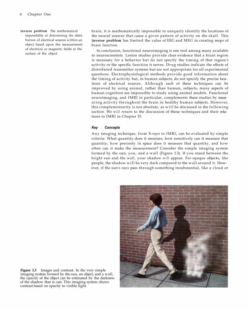
Key Concepts A n y imaging technique, from X-rays to fMRI , can be evaluated by simple criteria: What quantity does it measure, how sensitively can it measure that quantity, how precisely in space does it measure that quantity, and how often can it make the measurement? Consider the simple imaging system formed by the sun, you, and a wal l (Figure 1.3). If you stand between the bright sun and the wal l , your shadow w i l l appear. For opaque objects, like people, the shadow w i l l be very dark compared to the wall around it . However, if the sun's rays pass through something insubstantial, like a cloud or
Figure 1.3 Images and contrast. In the very simple imaging system formed by the sun, an object, and a wall, the opacity of the object can be estimated by the darkness of the shadow that is cast. This imaging system shows contrast based on opacity to visible light.

An I n t r o d u c t i o n to fMRI 7
a sheer curtain, the shadow w i l l be much lighter. In this imaging system, the quantity being measured is the number of photons of sunlight that strike the wal l and, by inference, the degree to which the intervening object absorbs photons. By comparing the shadows cast by different objects, like you or a cloud, one could estimate the optical opacity of the objects. Here, the difference between dark and light on the wal l indexes the opacity (i.e., light transmittance) of the object being imaged, w i t h dark areas indicating opaque objects and bright areas indicating transparency. In fact, this simple system captures the essence of the familiar X-ray technique.
The difference between the lightest and darkest shadows is a measure of the contrast available in our system for creating images of optical opacity. If the imaging technique is sensitive to small gradations in the quantity being measured, the resulting image w i l l have good contrast and w i l l enable us to make fine discriminations in our measurements of different objects. Contrast, however, is not an absolute quantity. Because no imaging method is perfect, there w i l l always be some amount of variation in the measured signal. For example, a plane passing overhead can momentarily block the sun and change the intensity of your shadow on the wal l . It is typical, then, to express contrast wi th respect to variation in contrast due to noise and to discuss results in terms of the contrast-to-noise ratio (CNR). We w i l l explore this topic in more detail later.
Depending on the pulse sequence used by the scanner, images can be created that differentiate low versus high proton density, gray matter versus white matter, or f lu id versus tissue. Thus, the quantity being measured is different for each of these image types. In this context, contrast has another special meaning that may be ini t ia l ly confusing. Shown in Figure 1.4 are images that have contrast based upon the intrinsic tissue properties T1 and T 2 . We w i l l describe these tissue properties and how these different types of images are created in Chapters 3 to 5. On T 1-weighted images, the difference, or contrast, between light and dark is a measure of the relative difference in T1 of the tissues. Thus, we also refer to these images as T 1-contrast
contrast The intensity difference between different quantities being measured by an imaging system. It also can refer to the physical quantity being measured (e.g., T1 contrast).
contrast-to-noise ratio (CNR) The magnitude of the intensity difference between different quantities divided by the variability in their measurements.
Figure 1.4 Contrast and contrast-to-noise in MR images. Shown in (A) and (B) are images sensitive to two different contrast types. (A) An image sensitive to T1 contrast, while (B) is an image sensitive to T2 contrast. Note that although much of the same brain structure is present in both images, the relative intensities of different tissue types are very differ
ent. Shown in (C) and (D) are two images with the same contrast type but different contrast-to-noise ratios. (C) An image with very high contrast-to-noise, and significant detail can be seen in the image. (D) An image with lower contrast-to-noise, and some distinctions such as the boundary between gray and white matter are more difficult to identify.
8 Chapter One
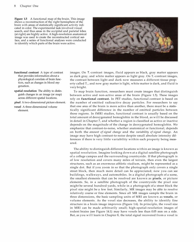
Figure 1.5 A functional map of the brain. This image shows a reconstruction of the right hemisphere of the brain with areas of statistically significant activity indicated in color. The experimental task involved visual search, and thus areas in the occipital and parietal lobes (at right) are highly active. A high-resolution anatomical image was used to create the reconstructed cortical surface, and a series of functional analyses were conducted to identify which parts of the brain were active.
functional contrast A type of contrast that provides information about a physiological correlate of brain function, such as changes in blood oxygenation.
spatial resolution The ability to distinguish changes in an image (or map) across different spatial locations.
pixel A two-dimensional picture element. voxel A three-dimensional volume
element.
images. On T1-contrast images, f lu id appears as black, gray matter appears as dark gray, and white matter appears as light gray. On T 2-contrast images, the contrast between light and dark now measures a different tissue property called T 2 , and now gray matter is light, white matter is dark, and f luid is very bright.
To map brain function, researchers must create images that distinguish between active and non-active areas of the brain (Figure 1.5). These images rely on functional contrast. In PET studies, functional contrast is based on the number of emitted radioactive decay particles. For researchers to say that one area of the brain is more active than another, there must be a statistically significant difference in the number of emitted particles between those regions. In fMRI studies, functional contrast is usually based on the total amount of deoxygenated hemoglobin in the blood, as w i l l be discussed in detail in Chapter 7, and whether a region is classified as active or inactive depends on the magnitude of the change in deoxygenated hemoglobin. We emphasize that contrast-to-noise, whether anatomical or functional, depends on both the amount of signal change and the variability of signal change. An image may have high contrast-to-noise despite small absolute intensity differences if there is very l itt le variabil ity w i t h i n each property being measured.
The ability to distinguish different locations w i t h i n an image is known as spatial resolut ion. Imagine looking d o w n at a digital satellite photograph of a college campus and the surrounding countryside. If that photograph is of low resolution and covers many miles of terrain, then even the largest structures, such as an enormous athletic stadium, might be represented as a single dot. But if you zoom in so that the photograph only covers a single street block, then much more detail can be appreciated; now you can see buildings, walkways, and automobiles. In a digital photograph of a scene, the smallest elements that can be resolved are k n o w n as pixels, or picture elements. So, in a satellite photograph of the countryside the pixel size might be several hundred yards, while in a photograph of a street block the pixel size might be a few feet. Similarly, MR images may be able to resolve relatively coarse or fine elements. Since all MR images sample the brain in three dimensions, the basic sampling units of MRI are known as voxels, or volume elements. As the voxel size decreases, the ability to identify fine structure in a brain image improves (Figure 1.6). In principle, the voxel size in MRI can be made arbitrarily small; high-spatial-resolution images of rodent brains (see Figure 14.1) may have voxels less than 0.05 mm on a side. But, as you w i l l learn in Chapter 8, the total signal recovered from a voxel is

An Introduction to fMRI 9
Figure 1.6 The human brain at different spatial resolutions. Spatial resolution refers to the ability to resolve small differences in an image. In general, we can define spatial resolution based upon the size of the elements used to construct the image. The images shown here present the same brain sampled at five different element sizes: (A) 8 mm, (B) 4 mm, (C) 2 mm, (D) 1.5 mm, and (E) 1 mm. Note that the gray-white structure is well represented in the latter three images, which all sample at more than twice the resolution of the typical gray-matter thickness of 5 mm.
proportional to its size, and voxels that are too small may have insufficient signal to create high-quality images. In structural MRI of the human brain, voxels are often about 1 to 2 mm in each dimension, whi le in functional MRI, voxels are typically about 3 to 5 mm on a side.
Although structural MR images are considered to be static representations of the brain, functional MRI is inherently dynamic, in that it measures changes in brain activity over time. The rate at which a technique acquires images, or its sampling rate, determines its temporal resolution. Across fMRI studies, the sampling rate typically varies from a few hundred milliseconds to a few seconds, which is much faster than earlier PET studies that integrated brain activity over intervals of about a minute or even longer. The fundamental rule for temporal resolution is that a signal must be sampled twice as frequently as the fastest change present in the signal. This l imit , known as the Nyquist frequency, w i l l be described further in Chapter 10. However, the theoretical Nyquist frequency is not the only l imi t on temporal resolution. Our ability to determine the t iming of functional activity in the brain is also limited by the sluggishness of the physiological changes that we seek to measure. Most fMRI studies measure changes in blood oxygenation, which resolve over a period of a few seconds to a few tens of seconds. Even if
sampling rate The frequency in time with which a measurement is made.
temporal resolution The ability to distinguish changes in an image (or map) across time.

1 0 C h a p t e r O n e
Figure 1.7 Neuroscience techniques differ in their spatial and temporal resolution. Functional M R I provides a good balance of spatial and temporal resolution and thus is appropriate for a wide range of experimental questions. Other approaches, including electrophysiology, lesion studies, and drug manipulations, can provide complementary information.
we sample the brain very rapidly, the hemodynamic changes may occur too slowly for us to make inferences about more rapid neuronal activity.
Together, spatial and temporal resolution have been used to describe a "technique space" that shows how different experimental methods provide potentially complementary information about brain function (Figure 1.7). The canonical example of complementarity combines the hemodynamic measurement of fMRI and the electrophysiological measurement of EEG. Since the former technique has very good spatial resolution (millimeters) and the latter technique has very good temporal resolution (milliseconds), it is argued that combining them would apply the best aspects of each to a single research question. While seductive, this argument conceals a deeper issue that is introduced here and discussed in more detail in Chapter 15. Spatiotemporal graphs like Figure 1.7 suggest that some fundamental quantity (i.e., brain activity) is a continuous variable that can be measured at different scales of time and space. However, no such fundamental quantity exists; rather, each of the methods represented provides a different measure of brain physiology. That these measures do not always correlate among themselves or, more importantly, do not always correlate w i t h the mental processes we study indicates that temporal and spatial resolution alone are not sufficient criteria to evaluate techniques. We suggest that the value of a technique is determined by its funct ional resolut ion, or ability to map physiological variation to cognitive or behavioral processing.
Although the above properties—contrast, spatial resolution, and temporal resolution—all contribute to functional resolution, other factors are also crit-
functional resolution The ability to map measured physiological variation to underlying mental processes.
ical. The brain property being measured determines, in several ways, how well one can localize function in the brain. The changes in blood oxygenation measured by fMRI reflect the local vascular structure of the brain, w i t h larger effects often measured around draining veins. In EEG studies using extracranial recording, the local vascular structure has little effect on activity, but the orientation and temporal synchrony of the active neurons has an enormous effect. So, while a given task might evoke significant activity using one technique, it might not evoke activity using a different technique. While fMRI is, in our view, the most promising technique for studying the intact human brain, it possesses many significant limitations on functional resolution. We w i l l return to this theme, the limitations of fMRI , throughout this book.
History of fMRI
The scientific developments leading to modern fMRI can be characterized through five main phases. Basic physics work in the 1920s to 1940s set forth the idea that atomic nuclei have magnetic properties and that these properties can be manipulated experimentally. Seminal studies reported by t w o laboratories in 1946 described the phenomenon of nuclear magnetic resonance (NMR) in solids and ushered in several decades of nonbiological studies. The first biological MR images were created in the 1970s and were coupled with advances in image acquisition methods. By the 1980s, MR imaging became clinically prevalent, and structural scanning of the brain was commonplace. Finally, in the early 1990s, the discovery that changes in blood oxygenation could be measured using MRI ushered in a new era of functional studies of the brain. We provide in this section a brief overview of the history of M R I , and we w i l l discuss specific physical principles in more detail in subsequent chapters.
Early Studies of Magnetic Resonance The beginnings of MRI can be traced to a single conjecture made by the Austrian physicist Wolfgang Pauli in 1924. At that time, very small (or hyper-fine) splitting of spectral lines emitted by excited atoms posed a problem for existing quantum mechanical theories. To account for these anomalies, Pauli postulated that atomic nuclei had two properties, called spin and magnetic moment, that could only take discrete values (or quanta). As an analogy, think of atomic nuclei as continually spinning tops. Pauli's suggestion, taken roughly, was that these tops could spin only at some frequencies but not others and exert only particular magnetic forces but not others. At that time, nuclear properties were poorly understood (indeed, the discovery of the neutron by the English physicist James Chadwick d i d not occur unti l 1931), and this suggestion would not be tested for more than a decade.
An early technique for investigating whether different atomic nuclei spin at discrete frequencies was the molecular beam apparatus developed by Stern and Gerlach. A gaseous beam of a single element was passed through
A n I n t r o d u c t i o n to fMRI 11
How could a technique have very good spatial and temporal resolution but very poor functional resolution?

1 2 C h a p t e r O n e
BOLD signal compared to baseline when subjects moved the device and the foam moved across their hand (B; self-produced tactile stimulation). However, when an experimenter moved the device and the foam moved across their hand (B; externally-produced tactile stimulation), there was increased BOLD signal. When no sensory stimulus was felt (other conditions) there was no change in BOLD signal. This study provided evidence that the cerebellum initiates an inhibitory signal that reduces the sensory experience of self-generated movements. (A from Blakemore et al., 1998; B after Blakemore et al., 1998.)
Figure 1.8 An fMRI study of tickling reveals that activity in the anterior cerebellum is reduced when people attempt to tickle themselves. Blakemore and colleagues used a simple tickling device to investigate why people cannot tickle themselves. The device could be moved by the subject or by an experimenter, and a piece of foam moved across the palm or not. The authors measured changes in blood-oxygenation-level dependent (BOLD) signal using fMRI. (BOLD signal will be discussed in detail in Chapter 7). They found that a region within the cerebellum (A; indicated by the arrow) had reduced
Condition
Self-produced tactile stimuli
Externally produced tactile stimuli
Self-produced movement; no tactile stimuli Rest
(B) (A)
Over the past few years, fMRI has been applied to a vast and ever growing set of research questions. To illustrate this point, we selected a recent issue of the journal Neurolmage and identified all of the studies using fMRI. Within that single issue, there were research articles describing object processing, speech, language plasticity in bil ingual individuals, how spatial extent of visual cortex activation changes under different conditions, visual attention, effects of neuronal interactions on blood flow, and connectivity between brain regions, as wel l as other studies describing the use of fMRI in conjunction wi th other techniques. And that was just one issue! Each year, many hundreds of fMRI studies are published wi th in dozens of academic journals by researchers from the fields of psychology, neurobiology, neurology, radiology, electrical engi
neering, biomedical engineering, and many others. In this box, we provide examples of some creative ways in which researchers have used fMRI.
Many fMRI studies attempt to discover patterns of brain activity that are associated with phenomena of interest. These patterns of activity are often called neural correlates, to emphasize that changes in the brain vary along with changes in some external phenomenon. As an example, consider the curious and remarkable fact that people cannot tickle themselves. If you are very ticklish, even a very slight touch from someone else might elicit peals of laughter, but you cannot tickle yourself no matter how hard you try. At one level, this may seem like an interesting but unimportant phenomenon, something more suited for light conversation than serious science. However, its simplicity cloaks an interesting question. Specifi-
neural correlates Patterns of brain activity that covary with another phenomenon, such as a mental state or behavior.
cally, why does the same physical stimulus (e.g., a motion across your palm) evoke very different experiences depending on its source? One possible explanation is that the brain discounts or cancels somatosensory cortex activity associated wi th self-generated, and therefore predictable, sensory stimuli. Blakemore and colleagues hypothesized that this cancellation signal was associated wi th the cerebellum, a part of the brain involved wi th organizing motor movements. Note that even though the authors scanned their subjects using fMRI of the entire brain, they were particularly interested in certain areas.
BOX 1.1 What is fMRI Used For?

An I n t r o d u c t i o n to fMRI 13
BOX 1 . 1 (continued)
They designed a simple tickling device consisting of a piece of foam attached to a long lever. The lever moved the foam up and down, and a pulley could retract or extend it to touch or not touch the palm. Their subjects lay down inside the fMRI scanner with the tickling device adjacent to their left hand. The device could be moved either by the experimenter or by the subject and would either touch (when extended) or not touch the subject when moved. The authors used fMRI to test two predictions: (1) that activity in sensory cortex would be increased when the experimenter moved the device compared to when the subjects moved it themselves, consistent with the tickling sensation in the former but not the latter case; and (2) that activity in the cerebellum would actually be decreased by the sensory feedback when subjects moved their hands compared to when no sensations were felt.
Their fMRI results supported their experimental hypotheses. As expected, activity in sensory cortex was evoked when the moving device touched the subjects but was greater when the experimenter moved the device than when the subject did. The authors suggest that this activity may underlie the sensation of tickling. However, a different pattern of results was found in a small region of the right cerebellum (Figure 1.8), which is involved with movements of the right side of the body. There brain activity, in response to self-generated movements wi th tactile stimulation, was less than that measured in response to similar movements without stimulation and was even less than activity found in rest conditions without movement or stimulation. The cerebellar activity, the authors speculate, represents a neural correlate of somatosensory predictions associated wi th self-generated movements.
While the Blakemore study used fMRI to study the relation between motor behavior and sensory experience, others use fMRI to investigate the relation between
emotion, affect, and perception. Even though emotion seems abstract and ephemeral, it has become a topic of great interest in cognitive neuroscience, and fMRI studies have played a large part in its resurgence. One brain region that is commonly associated with emotional processing is the amygdala, an almond-shaped region of cortex in the medial temporal lobe. It is well known that patients with amygdala damage show abnormal responses to emotional stimuli, but it is less clear what aspects of emotional processing are impaired. In a recent study,
Figure 1.9 Different parts of the brain are associated w i t h the intensity and the pleasantness of smells. Anderson and colleagues presented odors of differ-ent intensity and valence (i.e., pleasantness or unpleasantness) while measuring fMRI activity in brain systems that support emotional processing. Within the amygdala, circled at top in (A), the fMRI signal increased w i t h the perceived intensity of the odor but was unaffected by the valence of the odor (B, upper graphs). However, w i t h i n the orbitofrontal cortex, circled at bottom in (A), the fMRI signal d i d not depend upon the intensity of the odor but was greater for pleasant odors than for unpleasant odors (B, lower graphs). This result suggests that different components of an emotion may be processed in different brain regions. (From Anderson et al., 2003.)
Anderson and colleagues used fMRI to dissociate two aspects of emotion: valence and intensity. Valence refers to whether an emotion is positive or negative, and intensity refers to whether it is strong or weak. For most types of stimuli, these dimensions are interrelated, such that increasing intensity makes valence more extreme as well. An annoying sound, for example, becomes even more annoying when it is very loud. However, these factors can be dissociated for odor stimuli (Figure 1.9). The authors presented pleasant and unpleasant smells in low and high concen-
14 Chapter One
oscillating magnetic field A magnetic field whose intensity changes over time. Most such fields used in MRI oscillate at the frequency range of radio waves (megahertz, or MHz) and as such they are often called radiofrequency fields.
magnetic resonance The absorption of energy from a magnetic field that osci lates at a particular frequency.
resonant frequency The frequency of oscillation that provides maximum energy transfer to the system.
a strong static magnetic field before h i t t ing a detector plate. As described earlier, a static magnetic field is one whose intensity (ideally) does not change over space or time. If the spin frequencies of atomic nuclei could only take a number of discrete quantum states, then the static magnetic field would split the beam into some finite number of smaller beamlets before hitting the detector; whereas if the spin frequencies could take a continuous range of possible values, then there w o u l d be a similarly continuous distribution of intensity on the detector. The beams d i d split into different numbers of beamlets, as predicted by quantum theory.
These results proved that atomic nuclei have spin frequencies that can only take one of a number of discrete values. However, what these frequencies were for different atomic nuclei remained to be measured. In 1933, the American physicist Isidor Rabi modified the Stern-Gerlach technique to measure the quantum spins of hydrogen nuclei as well as nuclei of alkali metals. But Rabi felt that this beam technique was inelegant and sought a better method. The Dutch physicist Cornells Gorter visited Rabi's laboratory in 1937 and described his recent experiments wi th oscillating magnetic fields. Stimulated by this discussion, Rabi realized that if the frequency of the oscillating magnetic field matched the spin frequency of the atomic nucleus, then the nucleus would absorb energy from the field. This concept is called magnetic resonance. To understand this idea, consider the analogy of a swing set, to which we w i l l return in Chapter 3. If your friend is sitting on the swing set, you can help her swing back and forth by pushing her. A single hard push w i l l have only a limited effect. But by pushing her gently and at the right times, at each cycle she w i l l swing a little higher. The frequency of pushing that has the most effect is known as the resonant frequency. Energy can be given to atomic nuclei in the same way, by a large number of small "pushes" from a magnetic field that oscillates at the resonant frequency of the nucleus.
This idea catalyzed work in Rabi's lab, which had published a paper earlier that year that predicted such a result, and scant days after Gorter's visit the classic beam technique was modified to include an oscillating magnetic field. Rabi recognized that the resonant frequency needed for the oscillating
than electrophysiological methods. And there are many difficult decisions that researchers must make as they design and implement even simple studies. Nevertheless, fMRI has become the dominant technique in modern cognitive neuroscience because of its combination of strengths. It is very flexible and powerful, can be conducted with standard (albeit expensive) equipment, and has functional resolution sufficient for most current research questions. A number of extraordinary fMRI studies have been conducted already, and we hope to introduce the reader to many of them throughout this book.
While fMRI can be used to study such diverse topics as laughter and emotion, or sensation and smell, it is not an answer for all experimental questions. The scanning environment makes some research topics challenging to study, since subjects must remain confined for an hour or two within a small, restrictive, and noisy space. Areas of activity can be localized within a few millimeters, which allows identification of the gross brain regions that are active but may not be suitable for creation of functional maps within those brain regions. The timing of neural activity can be identified within a few seconds, which is much better than PET and much worse
trations and then examined which brain regions exhibited signal changes as a function of valence but not intensity, or vice versa. Activity in the amygdala increased with increasing stimulus intensity but did not change as a function of valence. In contrast, the orbitofrontal cortex was more active for pleasant stimuli than for unpleasant stimuli but was not influenced by the intensity of those stimuli. For these basic stimuli, at least, different parts of the brain seem to code different aspects of emotional responses. The authors speculate that the amygdala may be associated with extreme emotional events, regardless of whether they are positive or negative.
BOX 1 . 1 (continued)

A n I n t r o d u c t i o n t o f M R I 1 5
Figure 1.10 The determination of the magnetic moment of the l i th ium nucleus by Isidor Rabi (A). The beam technique devised by Rabi involved passing a beam of gaseous nuclei through several magnetic fields (B). The key innovation introduced by Rabi was an oscillating electromagnetic field (Magnet 3). If the oscillation rate was equal to the resonant frequency of an atomic nucleus (at the current strength of the static magnetic field), the spin of the atomic nuclei wou ld
change and then the subsequent magnetic field (Magnet 2) wou ld deflect the nuclei away from the detector. Shown in (C) are data from Rabi's experiment, in which he kept the oscillation rate fixed and changed the current in the static field magnet to modify its magnetic field strength. He found a sharp reduction in beam intensity at about 116 amperes, a l lowing him to calculate the spin properties of the l i th ium nucleus. (A ©The Nobel Foundation.)
field w o u l d depend upon the strength of the static magnetic f ie ld, just like the speed at which someone swings depends upon the strength of the gravitational field. So, he held the frequency of the oscillating field constant and changed the strength of the static field by adjusting the current in the magnet. (Note that this approach is the opposite of that used by modern MR scanners, as w i l l be discussed in the next chapter. Modern scanners keep the static field constant and vary the oscillating field to examine different atomic nuclei.) As the strength of the main field approached the resonant frequency of the sodium atoms in the beam, the atoms in the beam were deflected away from the detector (Figure 1.10A-C). This experiment represented the first demonstration of nuclear magnetic resonance effects, for which Rabi received the Nobel Prize in Physics in 1944.
NMR in Bulk Matter: Bloch and Purcell During the early 1940s, much basic research in physics stopped as top physicists worked on military applications, such as the development of the atomic bomb and the improvement of radar and counter-radar measures. As the war ended in 1945, two physicists, Felix Bloch at Stanford (Figure 1.11A) and Edward Purcell at MIT/Harvard (Figure 1.11B), resumed independent inves-
16 Chapter One
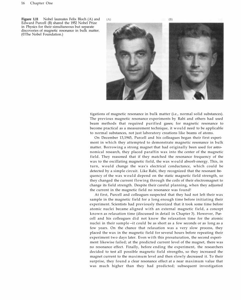
Figure 1.11 Nobel laureates Felix Bloch (A) and Edward Purcell (B) shared the 1952 Nobel Prize in Physics for their simultaneous but separate discoveries of magnetic resonance in bulk matter. (©The Nobel Foundation.)
tigations of magnetic resonance in bulk matter (i.e., normal solid substances). The previous magnetic resonance experiments by Rabi and others had used beam methods that required purif ied gases; for magnetic resonance to become practical as a measurement technique, it would need to be applicable to normal substances, not just laboratory creations like beams of atoms.
On December 13,1945, Purcell and his colleagues began their first experiment in which they attempted to demonstrate magnetic resonance in bulk matter. Borrowing a strong magnet that had originally been used for astronomical research, they placed paraffin wax into the center of the magnetic field. They reasoned that if they matched the resonance frequency of the wax to the oscillating magnetic field, the wax would absorb energy. This, in turn, would change the wax's electrical conductance, which could be detected by a simple circuit. Like Rabi, they recognized that the resonant frequency of the wax w o u l d depend on the static magnetic field strength, so they changed the current f lowing through the coils of their electromagnet to change its field strength. Despite their careful planning, when they adjusted the current in the magnetic field no resonance was found!
At first, Purcell and colleagues suspected that they had not left their wax sample in the magnetic field for a long enough time before init iating their experiment. Scientists had previously theorized that it took some time before atomic nuclei became aligned wi th an external magnetic f ield, a concept known as relaxation time (discussed in detail in Chapter 3). However, Purcell and his colleagues d i d not know the relaxation time for the atomic nuclei in their sample—it could be as short as a few seconds or as long as a few years. On the chance that relaxation was a very slow process, they placed the wax in the magnetic field for several hours before repeating their experiment two days later. Even w i t h this presaturation, the second experiment likewise failed; at the predicted current level of the magnet, there was no resonance effect. Finally, before ending the experiment, the researchers decided to test all possible magnetic field strengths, so they increased the magnet current to the maximum level and then slowly decreased it. To their surprise, they found a clear resonance effect at a near maximum value that was much higher than they had predicted; subsequent investigation

An Introduction to fMRI 17
revealed that they had simply miscalculated how much current was necessary to generate the appropriate magnetic f ield. Their discovery was reported in Physical Review in January 1946.
Nearly simultaneously at Stanford, Bloch and his colleagues were also attempting to measure resonance effects in bulk matter, although they were using a very different apparatus. They placed a sample of water in a brass box between the poles of a strong magnet, whose field strength they could manipulate. An adjacent transmitter coil sent electromagnetic energy into the sample, while a second detector coil was used to measure changes in the energy absorbed by the water (as emitted back to the environment). As in the MIT/Harvard experiment, the sample was presaturated for 24 hours in the magnetic field to ensure that relaxation would take place. These long presaturation periods turned out to be overly conservative; for bulk substances like paraffin and water, relaxation times are only a few seconds, three to four orders of magnitude less than the time allotted.
In a striking parallel to Purcell's experiment, Bloch's group also detected magnetic resonance effects in their water sample. They labeled this phenomenon nuclear induction, and reported their findings in Physical Review t w o weeks after Purcell's report. Nuclear induction, or nuclear magnetic resonance (NMR), forms the basis of all modern MR imaging techniques, and all MR scanners share the basic design principles of Bloch's simple apparatus: a strong static magnetic f ield, a transmitter coil that sends electromagnetic energy to the sample, and a detector coil that measures energy emitted back from the sample. For their independent contributions to the discovery of nuclear magnetic resonance, Purcell and Bloch were awarded a joint Nobel Prize in Physics in 1952.
While the discoveries that enabled N M R were made by physicists, the first applications of the new technique came from chemistry. By the early 1950s, the Varian Associates company had patented, wi th Felix Bloch's assistance, the basic ideas for using NMR to do chemical analysis of samples. NMR soon proved to be a very useful technique for understanding the chemical composition of a homogeneous substance, sharing both theory and methodology w i t h modern MRI spectroscopy. Despite (or perhaps because of) the considerable commercial success of NMR, at least in fields like geology and organic chemistry, the primary uses of the new technique would remain chemical, rather than biological, for more than two decades.
The First MR images By the late 1960s, NMR measurements had revealed differences between water molecules depending on whether or not they were within biological tissue. Specifically, the atomic nuclei composing water in biological tissue were shown to be constrained in their diffusion and orientation, and these differences could be identified using NMR. The American physician Raymond Damadian hypothesized that similar differences might be observed between cancerous and noncancerous cells; if so, NMR could become an extremely useful method for identifying cancerous tissue. Damadian tested this hypothesis in tissue samples taken from rats, and found that relaxation times were much longer in the cancerous tissue than in healthy tissue; this result was published in Science in 1971. Damadian's results were enormously influential in that, for the first time, research suggested a clear biological application for NMR. Yet it is important to also recognize that this application, assessing the properties of a tissue sample, still predated the advance that led to the explosion of interest in magnetic resonance: the ability to form spatial images.
transmitter coil An electromagnetic coil that generates an oscillating magnetic field at the resonant frequency of atomic nuclei within a sample.
detector coil An electromagnetic coil that measures energy emitted back to the environment after its initial absorption by the sample.
nuclear induction The initial term for nuclear magnetic resonance effects, as labeled by Bloch and colleagues.
nuclear magnetic resonance (NMR) The measurable changes in magnetic properties of atomic nuclei induced by the application of an oscillating magnetic field at the resonant frequency of the nuclei.

18 Chapter One
image A visual description of how one or more quantities vary over space.
spatial gradients (G) A magnetic field whose strength varies systematically over space. Note that since a given spatial location only experiences one magnetic field, which represents the sum of all fields present, spatial gradients in MRI act to change the effective strength of the main magnetic field over space.
In a formal sense, an image provides information about how one or more quantities vary over space. As examples, standard photographs are images of the intensity (and frequency) of visible light and X-ray films are images indicating the density of intervening matter. The first NMR studies d i d not create images, because they measured the total energy absorbed and emitted by the entire sample. In fact, in order to improve the interpretation of their results, early N M R researchers strove to remove spatial information from their samples to ensure homogeneity. Without image formation, N M R remained a relatively obscure curiosity.
Having seen the results of N M R experiments like those conducted by Damadian, the American physicist Paul Lauterbur recognized that NMR had considerable potential for biological and physical applications, if a method for image formation could be developed. In 1972 Lauterbur had a novel idea: If the strength of the magnetic field varied over space, the resonant frequencies of protons at different field locations would also vary. By measuring how much energy was emitted at different frequencies, one could identify how much of that object was present at each spatial location. This idea, of inducing spatial gradients (G) in the magnetic field, proved to be the fundamental insight that led to the creation of MR images. Lauterbur also realized that a single gradient could only provide information about one spatial dimension; to recover two-dimensional structure, it would be necessary to use a series of gradients at different orientations. By acquiring data using four gradients in succession, each turned 45° from its predecessor, Lauterbur created an image of a pair of water-filled test tubes (Figure 1.12A and B). This picture, which was reported in Nature in 1973, was the very first MR image.
Lauterbur's method, though revolutionary, was inefficient, since it essentially acquired a succession of one-dimensional projections through the object and then combined them into a two-dimensional image. Not only was
(A) (B)
Figure 1.12 The first MR image. The physicist Paul Lauterbur used a series of spatial gradients to take a succession of measurements of a beaker containing two water-filled test tubes (A). Data collected under each gradient provided different information about the object. By combining
this data using projection methods, Lauterbur was able to reconstruct the spatial organization of the object (B). The resulting picture was the first magnetic resonance image. The use of spatial variation in the magnetic field set the stage for modern MR imaging. (From Lauterbur, 1973.)
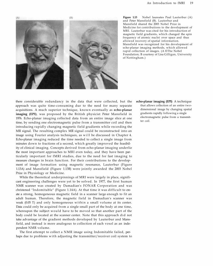
An Introduction to fMRI 19
Figure 1.13 Nobel laureates Paul Lauterbur (A) and Peter Mansfield (B). Lauterbur and Mansfield shared the 2003 Nobel Prize in Medicine for contributions to the development of MRI. Lauterbur was cited for his introduction of magnetic field gradients, which changed the spin frequency of atomic nuclei over space and thus allowed recovery of spatial information. Mansfield was recognized for his development of echo-planar imaging methods, which allowed rapid collection of images. (A ©The Nobel Foundation; B courtesy of Lisa Gilligan, University of Nottingham.)
there considerable redundancy in the data that were collected, but the approach was quite time-consuming due to the need for many separate acquisitions. A much superior technique, known eventually as echo-planar imaging (EPI), was proposed by the British physicist Peter Mansfield in 1976. Echo-planar imaging collected data from an entire image slice at one time, by sending one electromagnetic pulse from a transmitter coil and then introducing rapidly changing magnetic field gradients while recording the MR signal. The resulting complex MR signal could be reconstructed into an image using Fourier analysis techniques, as w i l l be discussed in Chapter 4. Echo-planar imaging reduced the time needed to collect a single image from minutes down to fractions of a second, which greatly improved the feasibility of clinical imaging. Concepts derived from echo-planar imaging underlie the most important approaches to MRI even today, and they have been particularly important for fMRI studies, due to the need for fast imaging to measure changes in brain function. For their contributions to the development of image formation using magnetic resonance, Lauterbur (Figure 1.13A) and Mansfield (Figure 1.13B) were jointly awarded the 2003 Nobel Prize in Physiology or Medicine.
While the theoretical underpinnings of MRI were largely in place, significant engineering challenges were yet to be solved. In 1977, the first human NMR scanner was created by Damadian's FONAR Corporation and was christened "Indomitable" (Figure 1.14A). At that time it was diff icult to create a strong, homogeneous magnetic field in a scanner large enough to fit an adult human. Therefore, the magnetic f ield in Damadian's scanner was weak (0.05 T) and only homogeneous w i t h i n a small volume at its center. Data could only be acquired from a single small part of the body at one time, whereupon the subject would have to be moved so that another part of the body could be located at the scanner center. Note that this approach d i d not take advantage of the gradient methods developed by Lauterbur and Mansfield, and instead is more analogous to collection of each voxel as an independent NMR volume.
The first attempt to collect a N M R image using Indomitable failed, perhaps due to problems w i t h adjusting the transmitter/receiver coil system to
echo-planar imaging (EPI) A technique that allows collection of an entire two-dimensional image by changing spatial gradients rapidly following a single electromagnetic pulse from a transmitter coil.

20 Chapter One
Figure 1.14 The first MR image of the human body. Raymond Damadian and colleagues constructed an early large-bore MRI scanner, which was called "Indomitable." Larry Minkoff, a postdoctoral fellow in the laboratory, was the first subject from whom data were recorded (A). The resulting image of his chest (B), while primitive by modern standards, shows the heart, lungs, and surrounding musculature. (A from FONAR corporation; B from Damadian et al., 1977.)
fit the large subject, Damadian himself (see Mattson and Simon for a complete narrative). After several months of additional adjustment and preparation, they were ready for another attempt. On the morning of July 3, 1977, one of the postdoctoral fellows in Damadian's laboratory, Larry Minkoff , entered the scanner. They s lowly collected data from one voxel at a time, changing Minkoff 's position slightly after each acquisition. Each voxel in the image took more than 2 minutes to acquire, and the complete image of 106 voxels took nearly 4 hours. At the end of the marathon session, the researchers' patience was rewarded wi th the first full-body MR image, a single slice through Minkoff 's torso (Figure 1.14B). Within 2 years, Damadian's group and other laboratories had created mult iple images of the abdomen, upper torso, and head. In addition, researchers acquired the first coronal and sagittal cross-sections of the brain, which were previously difficult to acquire using X-ray-based scanning.
With image formation using NMR a reality, many medical applications became evident. In the late 1970s, computerized tomography (or CT) imaging was commonly used to generate high-resolution images of the human body. CT uses a beam of X-rays that rotates around the body part of interest; the X-ray absorption at each angle is measured, and the resulting projections are combined to form a single picture representing one plane through the tissue. While CT is still commonly used even today, it does require concentrated X-ray exposure. Because NMR images could provide similar information to CT scans wi thout X-ray exposure, there was substantial interest in N M R as a potential diagnostic tool. Around the same time period, the term nuclear magnetic resonance fell into disfavor. As usually explained, the term NMR was abandoned in large part due to the negative health connotations of the word nuclear, which was justified because NMR does not use ionizing radiation. The change in terminology also can be attributed to the desire of

hospital officials to separate MR scanning from nuclear medicine departments. As a result of these factors, by the early 1980s, N M R became MRI : magnetic resonance imaging.
Growth of MRI As noted previously, MRI had three primary advantages over other imaging techniques. It had the potential of very high spatial resolution for both bones and soft tissue. It d i d not require ionizing radiation, as d i d X-rays or CT scans. And it could obtain images in any plane through the body. Nevertheless, the capital costs involved in setting up an MRI center were rather large, especially for hospitals facing the budgetary constraints of the recessionary economy of the early 1980s. A typical MRI scanner could cost up to one million dollars to purchase, wi th maintenance, personnel, and supply contracts adding hundreds of thousands of dollars annually. Many hospitals had just invested heavily in expensive CT scanners and were loathe to commit to an unproven technique. In addition, since MRI was only approved for research purposes by the U.S. Food and Drug Administration (FDA), insurance companies would not reimburse hospitals for the procedure. Nevertheless, there was enough appreciation of the potential of MRI that a number of companies, including FONAR, General Electric (GE), Philips, Siemens, and Varian, began developing MRI scanners for clinical use.
One consequence of the research and development investment in MRI was a substantial increase in scanner power. The use of superconducting magnets overcame limitations on field strength and homogeneity obtainable using standard resistive magnets, although expensive cooling agents were necessary to maintain superconductivity. GE created the first commercial human-body 1.5-T scanner in 1982, and began shipping them to hospitals shortly thereafter. While other companies focused on low- to medium-field scanners (0.1 to 1.0 T), GE's emphasis on high-field MRI resulted in considerable market success. As MRI grew, the 1.5-T scanner w o u l d be the standard workhorse for clinical imaging for more than two decades.
In 1985, the FDA approved MRI scanners for clinical use, opening the door for MRI scans to be prescribed by physicians and billed to insurance companies and Medicare. Rather than having to subsidize the enormous cost of a scanner that was used for research purposes, hospitals now saw scanners as a source of profit, both by bil l ing for the scans and by attracting new patients. Over the fol lowing decade, thousands of MRI scanners were installed in North America alone, making structural MRI one of the most common diagnostic imaging procedures (Figure 1.15). This prevalence of MRI scanners was a necessary precondition for the subsequent explosion of interest in functional MRI . Without the clinical need for MRI and the abundant resources provided by the installation of many new scanners, the
Thought Question What do you think about the awarding of the 2003 Nobel
Prize in Medicine to Paul Lauterbur and Peter Mansfield, but not to other pioneers like Raymond Damadian? What was the likely reasoning of the Nobel Committee, and do you
agree w i t h its decision?
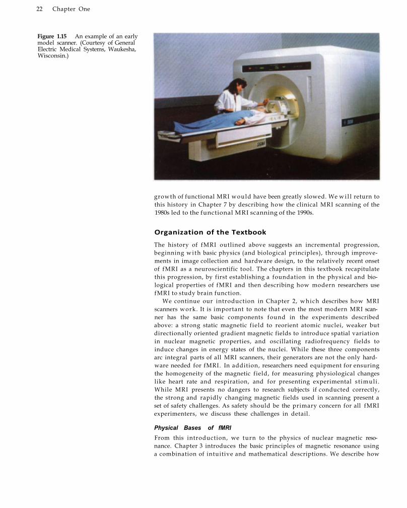
22 Chapter One
Figure 1.15 An example of an early model scanner. (Courtesy of General Electric Medical Systems, Waukesha, Wisconsin.)
growth of functional MRI would have been greatly slowed. We w i l l return to this history in Chapter 7 by describing how the clinical MRI scanning of the 1980s led to the functional MRI scanning of the 1990s.
Organization of the Textbook
The history of fMRI outlined above suggests an incremental progression, beginning wi th basic physics (and biological principles), through improvements in image collection and hardware design, to the relatively recent onset of fMRI as a neuroscientific tool. The chapters in this textbook recapitulate this progression, by first establishing a foundation in the physical and biological properties of fMRI and then describing how modern researchers use fMRI to study brain function.
We continue our introduction in Chapter 2, which describes how MRI scanners work. It is important to note that even the most modern MRI scanner has the same basic components found in the experiments described above: a strong static magnetic f ield to reorient atomic nuclei, weaker but directionally oriented gradient magnetic fields to introduce spatial variation in nuclear magnetic properties, and oscillating radiofrequency fields to induce changes in energy states of the nuclei. While these three components arc integral parts of all MRI scanners, their generators are not the only hardware needed for fMRI. In addition, researchers need equipment for ensuring the homogeneity of the magnetic field, for measuring physiological changes like heart rate and respiration, and for presenting experimental s t imul i . While MRI presents no dangers to research subjects if conducted correctly, the strong and rapidly changing magnetic fields used in scanning present a set of safety challenges. As safety should be the primary concern for all fMRI experimenters, we discuss these challenges in detail.
Physical Bases of fMRI From this introduction, we turn to the physics of nuclear magnetic resonance. Chapter 3 introduces the basic principles of magnetic resonance using a combination of intuitive and mathematical descriptions. We describe how

atomic nuclei behave in magnetic fields, and how the energy states of those
nuclei can be changed by applying oscillating magnetic fields at a particular
frequency� This discussion leads to the concept of relaxation processes, or the
recovery and decay of magnetization over time, which provide the contrast
we measure in MR imaging.
For "nuclear magnetic resonance" to become "magnetic resonance imag
ing," spatial information must be recovered from the raw MR signal. In
Chapter 4, we discuss how the introduction of magnetic gradients allows
measurement of signal changes across space. This process is known as
image formation. As discussed earlier in this chapter, image formation
sparked the explosive growth in the use of magnetic resonance for clinical
purposes. We introduce the concept of kspace, which provides a useful met
ric for understanding the relation between scanning hardware and the meas
ured data.
Our final chapter in this section, Chapter 5, links biology and physics by
describing the different approaches used by researchers to measure brain
structure and function. The extraordinary power of MRI for biological imag
ing comes from its flexibility; by changing the properties of the gradient and
oscillating magnetic fields of the scanner over time, images sensitive to
many different types of contrast can be obtained. We discuss t w o major
classes of contrasts, and the pulse sequences used to acquire them. Static
contrasts provide information about the characteristics of the atomic nuclei
at a spatial location, such as their density or tissue type. Mot ion contrasts
provide information about how atomic nuclei change position over time,
through diffusion through space or perfusion w i t h i n the local blood vessels.
We focus on how images can be made sensitive to changes in brain function,
which wil l set the stage for the discoveries outlined in the fol lowing section.
Principles of BOLD fMRI
Next, we introduce the biological underpinnings of fMRI . For neuroimaging
to be possible, there must be physiological markers of brain activity that can
be measured. In general, there are two types of markers that are of interest to
physiologists. On the one hand, researchers can measure direct conse
quences of neuronal activity, such as changes in electrical potentials or in
chemical gradients. Or, researchers can measure metabolic correlates of neu
ronal activity (but not activity itself). Functional MRI relies upon the latter
approach, in that it measures blood oxygenation level, which changes based
upon the metabolic demands of active neurons. In Chapter 6, we describe
the metabolic demands of the brain and how those demands are met by its
vascular function. We also provide a primer for gross brain anatomy, as
background for subsequent discussions of fMRI research.
Even if the metabolic consequences of neuronal activity are understood,
there remains the challenge of measuring how they change using MRI. The
technique that forms the basis for nearly all fMRI studies is bloodoxygena¬
tionlevel dependent (BOLD) contrast. Chapter 7 begins w i t h a history of the
developments that led to the discovery of BOLD contrast in the 1990s; this his
tory both parallels that described earlier in this chapter, and picks up where it
left off in the early 1990s. We discuss the early fMRI studies that first demon
strated the feasibility of this technique, and how those studies extended previ
ous neuroimaging work wi th PET. We also introduce a number of important
concepts that wi l l recur throughout the remainder of the book.
To demonstrate why fMRI has been such a successful imaging technique,
Chapter 8 discusses the spatial and temporal properties of fMRI , w i t h an
An Introduction to fMRI 23

24 Chapter One
emphasis on its limitations. We focus on three issues. First, we discuss the spatial resolution of fMRI , which is often claimed to be extremely good, such that images can be collected wi th millimeter or better resolution. We discuss challenges to spatial mapping, notably that introduced by the transformation between neuronal activity of interest and the measurable changes in the vascular system. Second, we discuss the temporal resolution of fMRI , which is often claimed to be rather poor. We describe approaches to improving temporal resolution and discuss studies in which fMRI has been used to identify subsecond changes in activity. Th i rd , we describe fMRI refractory effects, which arc introduced when st imuli are presented in rapid succession, as is common in many experiments. Throughout the chapter we emphasize how the design choices made by researchers influence these properties.
We next describe, in Chapter 9, issues related to signal and noise in fMRI data. The central problem in fMRI research is that the signal we measure is very small compared to other sources of variability in the data. We provide definitions of experimental signal and noise and show how different signal-to-noise ratios influence the spatial and temporal patterns of activity measured by f M R I . We also discuss methods for improving the detectability of fMRI signals, including improving experimental power through signal averaging and the elimination of extraneous physiological variability.
Design and Analysis of fMRI Experiments While fMRI can be an extraordinarily useful tool for understanding the workings of the human brain, even the most powerful tool can be rendered ineffective if used improperly. The next section of the book describes how to transform fMRI data from a raw time series of images into a statistically val id map of brain function. In Chapter 10, we begin w i t h a discussion of procedures for preprocessing, which have the goal of reducing variability in the data unrelated to the experimental task. The main topics include correction for head motion, time of slice acquisition, and coregistration and normalization of images to match shape, size, and orientation of the brain throughout a data set.
Next, in Chapter 11, we discuss the key concepts of experimental design, or the means by which researchers set up tests of their hypotheses. Most fMRI studies use either blocked or event-related designs. In a blocked design, subjects perform tasks for extended periods of time (e.g., 30 seconds), and activity while performing one task is compared to activity while performing another. Event-related designs, in contrast, examine activity associated w i t h discrete events that could occur at any time point in the experiment. We describe the advantages and disadvantages of each design type for addressing different experimental questions. Furthermore, we consider advanced design types that combine features of both designs.
Going hand in hand w i t h design is analysis, which describes the ways in which tests of hypotheses are evaluated statistically. We begin Chapter 12 by describing the major statistical tests used for fMRI studies, such as t-tests, correlation tests, and Fourier analyses. From these common tests we move to the general linear model, which subsumes them and allows more-complex analyses. While these approaches are similar to those used in other domains of science, their use in fMRI raises additional challenges. Chief among these is the problem of multiple comparisons, in that when tens of thousands of voxels are tested for statistical significance, many may appear to be significant merely by chance. We discuss the different approaches to compensating for the multiple

comparisons problem, including thresholding, smoothing, cluster analyses, and region-of-interest analyses. While the bulk of the chapter focuses on traditional hypothesis-driven analyses, we also introduce data-driven analyses, which are useful for discovering hidden structure in data sets.
Applications and Future Directions We close this book by looking to the future of fMRI. In Chapter 13, we examine some of the research areas where fMRI has made the greatest contributions. Because of the phenomenal success of fMRI , any such survey must be incomplete. Thus, we divide our review into two sections. First, we identify several themes that underlie many fMRI studies and have contributed to its growth as a technique. Though these themes are discussed in the context of particular studies, they can be extended more generally throughout the field. Second, we focus on a small set of topic areas where fMRI has been particularly successful, including attention, memory, and executive function. We discuss why fMRI has been profitably applied to these topic areas, and we describe notable studies wi th in each.
While this textbook necessarily focuses on current state of the art experimental methods, in Chapter 14 we describe a number of methodological advances that promise to change the way fMRI experiments are conducted. Many laboratories are investigating ways to improve spatial resolution, temporal resolution, or signal-to-noise ratio, all of which w i l l have significant benefits for many types of studies. Some researchers have even proposed alternative forms of contrast that could complement or replace the current BOLD imaging methods. We hope that the reader w i l l share our optimism that the pace of technological development w i l l continue to accelerate, facilitating new studies and discoveries.
Finally, Chapter 15 w i l l consider fMRI in the context of other neuroscien¬tific techniques. We end wi th this chapter to emphasize that fMRI is one of many techniques available to the neuroscientist. Al though in our view it is one of the most flexible and powerful , it nevertheless has many limitations that can be addressed by converging studies using other methods. We discuss the theoretical basis for combined studies, and we speculate on the future directions of fMRI research.
Summary Functional magnetic resonance imaging, or fMRI, is one of the most important techniques for understanding the human brain in action. Although fMRI is a relatively new technique, the developments that led to its current stage span nearly a century. Many of the advances that made fMRI possible resulted from basic physics research, and the experimental apparatuses used in these early studies laid the groundwork for modern MRI equipment. Unlike most structural MRI, which measures differences between tissues, most functional MRI studies measure changes in the blood oxygenation of the brain over time. From these changes, researchers make inferences about the underlying neuronal activity and how different brain regions may support different perceptual, motor, or cognitive processes. The strengths of fMRI include its noninvasiveness, its high spatial and temporal resolution, and its adaptability to many types of experimental paradigms. While fMRI cannot address every experimental question, it provides important information about the brain beyond that obtained from lesion, electrophysiological, or drug studies.
An Introduction to fMRI 25

26 Chapter One
Suggested Readings
*Bloch, F., Hansen, W. W., and Packard, M. (1946). Nuclear induction. Phys. Rev., 69:127. This very short note describes the discovery of nuclear magnetic resonance in solid matter, for which Felix Bloch would share the 1952 Nobel Prize in Physics with Edward Purcell.
Cabeza, R., and Nyberg, L. (2000). Imaging cognition II : An empirical review of 275 PET and fMRI studies. J. Cogn. Neurosci., 12: 1-47. A review article that provides a good perspective of the breadth of research questions that can be addressed with functional neuroimaging studies.
Finger, S. (2000). Minds behind the Brain. Oxford University Press, New York. This very accessible set of short biographies of neuroscience pioneers contains a description of the life and works of Franz Joseph Gall, who founded the discipline of phrenology.
*Lauterbur, P. C. (1973). Image formation by induced local interactions: Examples employing nuclear magnetic resonance. Nature, 242: 190-191. This seminal article describes the first use of magnetic field gradients for the formation of images using magnetic resonance.
*Mattson, J., and Simon, M. (1996). The Pioneers of NMR and Magnetic Resonance in Medicine: The Story of MRI. Dean Books, Jericho, NY. This encyclopedic text describes in detail the histories of major twentieth-century figures in the discovery of MRI, providing both personal and scientific context for their work.
*Purcell, E. M., Torrey, H. C, and Pound, R. V. (1945). Resonance absorption by nuclear magnetic moments in a solid. Phys. Rev., 69: 37-38. Published scant weeks before Bloch's similar report, this article describes the procedures and results from the very first study of nuclear magnetic resonance.
*Indicates a reference that is a suggested reading in the field and is also cited in this chapter.
Chapter References
Anderson, A. K., Christoff, K., Stappen, I . , Panitz, D., Ghahremani, D. G., Glover, G., Gabrieli, J. D., and Sobel, N. (2003). Dissociated neural representations of intensity and valence in human olfaction. Nat. Neurosci., 6: 196-202.
Blakemore, S. J., Wolpert, D. M., and Frith, C. D. (1998). Central cancellation of self-produced tickle sensation. Nat. Neurosci., 1: 635-640.
Churchland, P. S., and Sejnowski, T. J. (1988). Perspectives on cognitive neuroscience. Science, 242: 741-745.
Damadian, R., Goldsmith, M., and Minkoff, L. (1977). NMR in cancer: XVI. FONAR image of the live human body. Physiol. Chan. Phys., 9: 97-108.
Damadian, R. V. (1971). Tumor detection by nuclear magnetic resonance. Science, 171: 1151-1153.
Rabi, I. I., Zacharias, J. R., Millman, S., and Kusch, P. (1938). A new method of measuring nuclear magnetic moment. Phys. Rev., 53: 318.

2 MRI Scanners
Since the beginning of M R I , technological advances have resulted in continual improvements in the speed at which data can be acquired, in the ability to localize signal in space, and in the types of contrast that can be measured. Consequently, the practice of MRI today differs drastically from that of the early pioneers, and modern MRI scanners (Figure 2.1 A - C ) do not resemble the devices first used to detect nuclear magnetic resonance. However, the fundamental principles of MRI are unchanged. Just as Rabi used a strong magnetic field to measure spin properties of nuclei, today's MRI scanners use a strong magnetic field to induce changes in proton spin. Just as Bloch detected nuclear induction using transmitter and receiver coils, scanners now use similar coil systems to obtain MR signal. A n d just as Lauterbur manipulated magnetic field strength using changing gradient fields to create an image, every current MRI study relies on magnetic gradients for image acquisition. In this chapter, we identify the major components of MRI scanners, describe their use in practice, and discuss their safety implications.
How MRI Scanners Work
The three main components of an MRI scanner, as alluded to above, are the static magnetic f ield, radiofrequency coils, and gradient coils, which together allow collection of images. Yet these are not the only components important for fMRI . Also necessary are shimming coils, which ensure the homogeneity of the static magnetic f ield; specialized computer systems for controlling the scanner and the experimental task; and physiological monitoring equipment. This section introduces these components and their implementation on modern MRI scanners (Figure 2.2). We w i l l return to a detailed discussion of how they are used to change the magnetic properties of atomic nuclei in Chapters 3 to 5.
Static Magnetic Field The static magnetic field is an absolute necessity for MRI , providing the magnetic in magnetic resonance imaging. Magnetic fields were discovered in naturally occurring rocks, known as lodestones, by ancient Chinese almost 2000 years ago. By the eleventh century, the Chinese had recognized that the
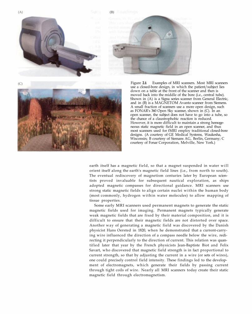
Figure 2.1 Examples of MRI scanners. Most MRI scanners use a closed-bore design, in which the patient/subject lies down on a table at the front of the scanner and then is moved back into the middle of the bore (i.e., central tube). Shown in (A) is a Signa series scanner from General Electric, and in (B) is a MAGNETOM Avanto scanner from Siemens. A small fraction of scanners use a more open design, such as FONAR's 360 Open Sky scanner, shown in (C). In an open scanner, the subject does not have to go into a tube, so the chance of a claustrophobic reaction is reduced. However, it is more difficult to maintain a strong homogeneous static magnetic field in an open scanner, and thus most scanners used for fMRI employ traditional closed-bore designs. (A courtesy of GE Medical Systems, Waukesha, Wisconsin; B courtesy of Siemans AG, Berlin, Germany; C courtesy of Fonar Corporation, Melville, New York.)
earth itself has a magnetic f ield, so that a magnet suspended in water w i l l orient itself along the earth's magnetic field lines (i.e., from north to south). The eventual rediscovery of magnetism centuries later by European scientists proved invaluable for subsequent nautical exploration, as ships adopted magnetic compasses for directional guidance. MRI scanners use strong static magnetic fields to align certain nuclei w i t h i n the human body (most commonly, hydrogen w i t h i n water molecules) to allow mapping of tissue properties.
Some early MRI scanners used permanent magnets to generate the static magnetic fields used for imaging. Permanent magnets typically generate weak magnetic fields that are fixed by their material composition, and it is diff icult to ensure that their magnetic fields are not distorted over space. Another way of generating a magnetic field was discovered by the Danish physicist Hans Oersted in 1820, when he demonstrated that a current-carrying wire influenced the direction of a compass needle below the wire, redirecting it perpendicularly to the direction of current. This relation was quantified later that year by the French physicists Jean-Baptiste Biot and Felix Savart, who discovered that magnetic field strength is in fact proportional to current strength, so that by adjusting the current in a wire (or sets of wires), one could precisely control field intensity. These findings led to the development of electromagnets, which generate their fields by passing current through tight coils of wire. Nearly all MRI scanners today create their static magnetic field through electromagnetism.

MRI Scanners 29
Figure 2.2 Schematic organization of the MRI scanner and computer control systems. Two systems are important for fMRI studies. The first is the hardware used for image acquisition, which in addition to the scanner itself consists of a series of amplifiers and transmitters responsible for creating gradients and pulse sequences (shown in black), as well as recorders of MR signal from the head coil (shown in red). The second system is responsible for controlling the experiment in which the subject participates and for recording behavioral and physiological data (shown in green).
There are, in general, two criteria for a suitable magnetic field in MRI. The first is uniformity (or homogeneity), and the second is strength. Uniformity is necessary in that we want to create images of the body that do not depend on which MRI scanner we are using or how the body is positioned in the field. If the magnetic field were inhomogeneous, the signal measured from a given part of the body would depend upon where it was located in the magnetic field. (In fact, MRI takes advantage of this effect by introducing controlled changes in magnetic field strength by adding magnetic field gradients.) A simple design for generating a homogeneous magnetic field is the
homogeneity Uniformity over space and time. In the context of MRI, a homogeneous magnetic field is one that has the same strength throughout a wide region near the center of the scanner bore.

30 Chapter Two
superconducting electromagnets A set of wires made of metal alloys that have no resistance to electricity at very low temperatures. By cooling the electromagnet to near absolute zero, a strong magnetic field can be generated with minimal electrical power requirements.
cryogens Cooling agents used to reduce the temperature of the electromagnetic coils in an MRI scanner.
Figure 2.3 Generation of a static magnetic field. The Helmholtz pair design (A) can generate a homogeneous magnetic field. It consists of a pair of circular current loops that are separated by a distance equal to their radius; each loop carries the same current. Modern MR scanners use a solenoid design (B), in which a coil of wire is wrapped tightly around a cylindrical frame. By optimizing the locations and density of the wire loops, a very strong and homogenous field can be constructed.
Helmholtz pair (Figure 2.3A), which is a pair of circular wire loops that carry identical current and are separated by a distance equal to the radius of the loops. An even more uniform magnetic field, however, can be generated by a solenoid, which is constructed by w i n d i n g wire in a helix around the surface of a cylindrical form (Figure 2.3B). If the solenoid is long compared w i t h its cross-sectional diameter, the internal field near its center is highly homogeneous. Modern magnets are based on a combination of these classic designs, w i t h the density of wires, and therefore the electrical current, numerically optimized to achieve a homogeneous magnetic field of the desired strength.
Field strength, in contrast to uniformity, requires force rather than finesse. To generate an extremely large magnetic field, one can inject a huge electric current into the loops of wire. For example, the very large electromagnets used to l i f t cars in junkyards have magnetic fields on the order of 1 T, similar to that in the center of some MRI scanners. To generate this f ield, they require enormous electrical power, and thus enormous expense. Modern MRI scanners use superconducting electromagnets whose wires are cooled by cryogens (e.g., l iquid helium) to reduce their temperature to near absolute zero. Coil windings are typically made of metal alloys such as niobium-t i tanium, which when immersed in l iquid helium reach temperatures of less than 12 K (-261°C). At this extremely low temperature, the resistance in the wires disappears, thereby enabling a strong and lasting electric current to be generated w i t h no power requirements and minimal cost.
Combining the precision derived from numerical optimization of the magnetic coil design and the strength afforded by superconductivity, modern MRI scanners can have homogeneous and stable field strengths in the range of 1 to 9 T for human use and up to 20 T for animal use. Since main-

MRI Scanners 31
taining a field using superconductive w i r i n g requires little electricity, the static fields used in MRI are always active, even when no images are being collected. For this reason, the static f ield presents significant safety challenges, as wi l l be discussed later in this chapter.
Radiofrequency Coils While a strong static magnetic field is needed for MRI , the static field itself does not produce any MR signal. MR signal is actually produced by the clever use of two types of electromagnetic coils, k n o w n as transmitter and receiver coils, that generate and receive electromagnetic fields at the resonant frequency of the atomic nuclei w i t h i n the static magnetic field. This process gives the name resonance to magnetic resonance imaging. Because most atomic nuclei of interest for MRI studies have their resonant frequencies in the radiofrequency portion of the electromagnetic spectrum (at typical field strengths for MRI), these coils are also called radiofrequency coils. Unlike the static magnetic field, the radiofrequency fields are turned on and off during small portions of the image acquisition process and remain off for any other period. Radiofrequency coils are evaluated on the same criteria as the static field: uniformity and sensitivity.
An equilibrium state exists when the human body is placed in any magnetic field, such that the net magnetization of atomic nuclei (e.g., hydrogen) within the body becomes aligned w i t h the magnetic f ield. The radiofrequency coils send electromagnetic waves that resonate at a particular frequency, as determined by the strength of the magnetic f ield, into the body, perturbing this equi l ibr ium state. This process is known as excitation. When atomic nuclei are excited, they absorb the energy of the radiofrequency pulse. But, when the radiofrequency pulse ends, the hydrogen nuclei return to the equil ibrium state and release the energy that was absorbed during excitation. The resulting release of energy can be detected by the radiofrequency coils, in a process known as reception. This detected electromagnetic pulse defines the raw MR signal.
One can think of the measurement of MR signal through excitation and reception as analogous to the weighing of an object by l i f t ing and releasing it in a gravitational field. If an object sits motionless on a supporting surface, so that it is in an equil ibrium state w i t h respect to gravitational force, we have no information about its weight. To weigh it, we first l i f t the object to give it potential energy and then release it so that it transfers that energy back into the environment. The amount of energy it releases, whether through impact against a surface or compression of a device l ike a spring (e.g., in a scale), provides an index of its weight. In the same way, we can perturb the magnetic properties of atomic nuclei (excitation) and then measure the amount of energy returned (reception) during their recovery to an equilibrium state.
The amount of energy that can be transmitted or received by a radiofrequency coil depends upon its distance from the sample being measured. In the case of fMRI, the radiofrequency coils are typically placed immediately around the head, either in a surface coil or volume coil arrangement (Figure 2.4). Surface coils are placed directly on the imaged sample, that is, adjacent to the surface of the scalp for functional imaging. The design of surface coils is based upon a single-loop inductor-capacitor (LC) circuit (Figure 2.4A). Within this circuit, the rapid charge and discharge of electricity between the inductor and capacitor generates an oscillating current that can be tuned to the frequency of interest. Because of their close spatial proximity to the brain, surface coils usually provide high imaging sensitivity and are often
radiofrequency coils Electromagnetic coils used to generate and receive energy at the sample's resonant frequency, which for field strengths typical to MRI is in the radiofrequency range.
excitation The application of an electromagnetic pulse to a spin system to cause some of the spins to change from a low-energy state to a high-energy state.
reception The process of receiving electromagnetic energy emitted by a sample at its resonant frequency (also called detection). As spins return to a low-energy state following the cessation of the excitation pulse, they emit energy that can be measured by a receiver coil.
MR signal The current measured in a detector coil following excitation and reception.
surface coil A radiofrequency coil that is placed on the surface of the head, very near to the location of interest. Surface coils have excellent sensitivity to signal from nearby regions but poor sensitivity to distant regions.
volume coil A radiofrequency coil that surrounds the entire sample, with roughly similar sensitivity throughout.

32 Chapter Two
Figure 2.4 Surface and volume coils. (A) Surface coils consist of a simple inductor (L) -capacitor (C) circuit, with additional resistance (R) also present. The rapid charging and discharging of energy between the inductor and resistor generates an oscillating magnetic field. The signal from the surface coil is modulated by a variable capacitor (shown with the arrow). (B) Volume coils repeat the same LC circuit around the surface of a cylinder. This results in better spatial coverage than is provided by a surface coil, at the expense of reduced local sensitivity. (C) A typical surface coil, and (D) volume coil.
used for fMRI studies that are targeted toward one specific brain region, such as the visual cortex. The trade-off w i t h high local sensitivity is poor global coverage. Since the amount of signal recovered from a given part of the brain depends on its distance from the surface coil , areas very near the coil provide a great deal of signal but areas far away provide very little (Figure 2.5A). Thus, the signal recovered by a surface coil is spatially inhomoge-
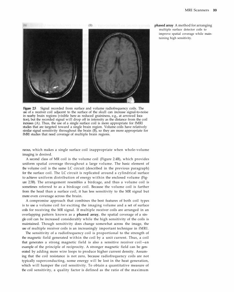
MRI Scanners 33
phased array A method for arranging multiple surface detector coils to improve spatial coverage while maintaining high sensitivity.
Figure 2.5 Signal recorded from surface and volume radiofrequency coils. The use of a receiver coil adjacent to the surface of the skull can increase signal-to-noise in nearby brain regions (visible here as reduced graininess, e.g., at arrowed location), but the recorded signal will drop off in intensity as the distance from the coil increases (A). Thus, the use of a single surface coil is more appropriate for fMRI studies that are targeted toward a single brain region. Volume coils have relatively similar signal sensitivity throughout the brain (B), so they are more appropriate for fMRI studies that need coverage of multiple brain regions.
neous, which makes a single surface coil inappropriate when whole-volume imaging is desired.
A second class of MR coil is the volume coil (Figure 2.4B), which provides uniform spatial coverage throughout a large volume. The basic element of the volume coil is the same LC circuit (described in the previous paragraph) for the surface coil. The LC circuit is replicated around a cylindrical surface to achieve uniform distribution of energy w i t h i n the enclosed volume (Figure 2.5B). The arrangement resembles a birdcage, and thus a volume coil is sometimes referred to as a birdcage coil. Because the volume coil is farther from the head than a surface coil, it has less sensitivity to the MR signal but more even coverage across the brain.
A compromise approach that combines the best features of both coil types is to use a volume coil for exciting the imaging volume and a set of surface coils for receiving the MR signal. If multiple receiver coils are arranged in an overlapping pattern known as a phased array, the spatial coverage of a single coil can be increased considerably while the high sensitivity of the coils is maintained. Though sensitivity does change somewhat across the image, the use of multiple receiver coils is an increasingly important technique in fMRI.
The sensitivity of a radiofrequency coil is proportional to the strength of the magnetic field generated w i t h i n the coil by a unit current. Thus, a coil that generates a strong magnetic field is also a sensitive receiver c o i l — a n example of the principle of reciprocity. A stronger magnetic field can be generated by adding more wire loops to produce higher current density. Assuming that the coil resistance is not zero, because radiofrequency coils are not typically superconducting, some energy w i l l be lost in the heat generation, which wi l l hamper the coil sensitivity. To obtain a quantitative measure of the coil sensitivity, a quality factor is defined as the ratio of the maximum
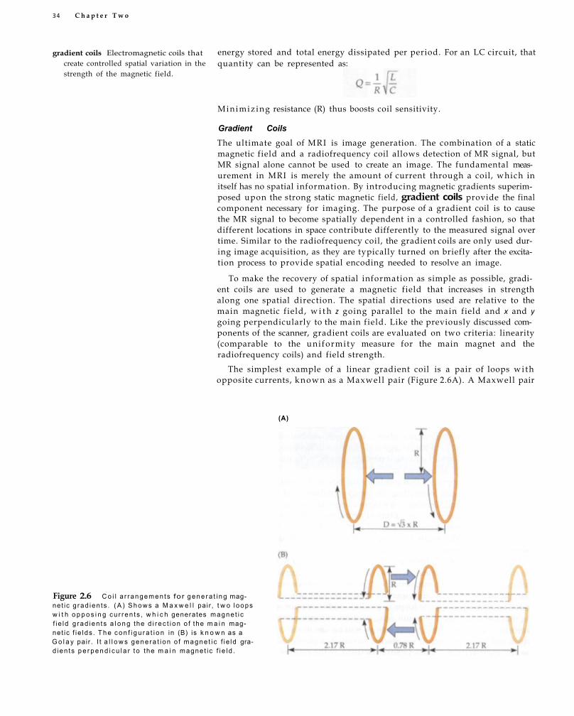
34 C h a p t e r T w o
Minimiz ing resistance (R) thus boosts coil sensitivity.
Gradient Coils The ultimate goal of MRI is image generation. The combination of a static magnetic field and a radiofrequency coil allows detection of MR signal, but MR signal alone cannot be used to create an image. The fundamental measurement in MRI is merely the amount of current through a coil, which in itself has no spatial information. By introducing magnetic gradients superimposed upon the strong static magnetic field, gradient coils provide the final component necessary for imaging. The purpose of a gradient coil is to cause the MR signal to become spatially dependent in a controlled fashion, so that different locations in space contribute differently to the measured signal over time. Similar to the radiofrequency coil, the gradient coils are only used during image acquisition, as they are typically turned on briefly after the excitation process to provide spatial encoding needed to resolve an image.
To make the recovery of spatial information as simple as possible, gradient coils are used to generate a magnetic field that increases in strength along one spatial direction. The spatial directions used are relative to the main magnetic f ield, w i t h z going parallel to the main field and x and y going perpendicularly to the main field. Like the previously discussed components of the scanner, gradient coils are evaluated on two criteria: linearity (comparable to the uni formity measure for the main magnet and the radiofrequency coils) and field strength.
The simplest example of a linear gradient coil is a pair of loops wi th opposite currents, k n o w n as a Maxwel l pair (Figure 2.6A). A Maxwell pair
(A)
Figure 2.6 C o i l a r rangemen ts for g e n e r a t i n g magnet ic g rad ien ts . ( A ) S h o w s a M a x w e l l pai r , t w o l oops w i t h o p p o s i n g c u r r e n t s , w h i c h generates magne t i c f i e ld g rad ien ts a l o n g the d i r e c t i o n o f the m a i n magnet ic f i e lds . T h e c o n f i g u r a t i o n in (B) is k n o w n as a G o l a y pair . I t a l l o w s gene ra t i on o f magne t i c f i e ld grad ien ts p e r p e n d i c u l a r t o the m a i n magne t i c f i e l d .
gradient coils Electromagnetic coils that create controlled spatial variation in the strength of the magnetic field.
energy stored and total energy dissipated per period. For an LC circuit, that quantity can be represented as:

generates opposing magnetic fields w i t h i n t w o parallel loops, effectively producing a magnetic field gradient along the line between the two loops. This design, in fact, is the basis for generating the z-gradient used today. Of course, the z-gradient coils have a more complicated geometry than a simple pair, but the same concept underlies their design.
The x- and y-gradients, also known as transverse gradients, are both created in the same fashion, since the coils that wrap around the scanner are circular and thus symmetrical across those directions. It is important to understand that the transverse gradients change the intensity of the main magnetic field across space (i.e., along z); they do not introduce smaller magnetic fields along x and y, as one might suppose. That is, the introduction of an x-gradient, for example, makes the main magnetic field slightly weaker at negative values along x and slightly stronger at positive values along x. Therefore, to generate a transverse gradient, one cannot simply place the Maxwell pair along the x or y axis (which would generate a magnetic field pointing perpendicular to the main field). Instead, scanners use a configuration similar to that shown in Figure 2.6B to generate these gradients. This slightly more complicated double-saddle geometry is k n o w n as a Golay pair. The final geometry that actually produces the x- or y-gradient field is numerically optimized and contains many more windings than the simple saddle coil shown here. Figure 2.7 illustrates the different patterns of coil windings used for the magnetic gradients and the static magnetic field.
The strength of the gradient coil is a function of both the current density and the physical size of the coil. Increasing the current density by increasing the electrical power supplied to the coil produces a stronger gradient field. Reducing the size of the coil , so that a given current travels through a smaller area, also produces a stronger gradient field. The trade-off between held strength, size, and power is not linear. In fact, as the bore size increases, the power required for generating a gradient of the same strength increases with the 5 t h power of the bore size. The implications of this fact can be appreciated in a simple example. Consider that a physicist wants to increase the bore size of a scanner by a factor of 2, while maintaining the same gradient strength. Although the bore size is only doubled, the power requirements increase by a factor of 2 5 , or 32. This constraint imposes a practical limitation on the bore size of an MRI scanner.
Shimming Coils
In an ideal MR scanner, the main magnet w o u l d be perfectly homogeneous and the gradient coils w o u l d be perfectly linear. This is hardly the case in reality, as the authors (and everyone who has ever conducted fMRI studies!) can attest. MRI scanners must correct for inhomogeneities in the static magnetic field; in some locations the field may be too strong, in others too weak. This process is analogous to what we do when a table is rocking—we simply put a wedge under one of the uneven legs to make it stable. This wedge is called a shim. In the scanner, additional coils generate high-order compensatory magnetic fields (like the analogous wedges) that correct for the inho-
Some manufacturers have begun developing "head-only" MRI scanners for clinical and functional studies of the brain.
Based upon what you k n o w so far, what w o u l d be the advantages of such scanners?
MRI S c a n n e r s 35

36 Chapter Two
(A) (B)
Figure 2.7 Generation of x-, y-, and z-gradients and the static magnetic field (B0). (A) A number of different electromagnetic coils are used within a single MRI scanner. (B) The coils are arranged as a series of concentric circles, beginning with the gradient coils at the interior and followed by the shimming coils and then the static field coils. The x- and y-gradients are generated using the Golay pair arrangement, and the only difference between them is that one is rotated 90° from the other. The z-gradient is generated using the Maxwell pair arrangement. The shimming coils are not shown here due to their complexity; as discussed in the text, there may be many different coil types depending on the scanner. Finally, the static field is generated using a series of Helmholtz pairs, with the distance between the pairs corresponding to their radius.
shimming coils Electromagnetic coils that compensate for inhomogeneities in the static magnetic field.
mogeneity of the magnetic field. These coils, intuitively, are named shimming coils.
Typically, shimming coils can produce first-, second-, or even third-order magnetic fields. For example, an x-shimming coil w o u l d generate a magnetic f ield that depends on position along the x-axis (first-order), while an x 3 -shimming coil could generate a magnetic field that depends upon the cube of the x position (third-order). Combinations of these high-order mag-

MRI Scanners 37
pulse sequence A series of changing magnetic field gradients and oscillating electromagnetic fields that allows the MRI scanner to create images sensitive to a particular physical property.
Computer Hardware and Software Digitizing, decoding, and displaying MR images require a considerable amount of computer processing power. A l l MRI scanners are equipped wi th at least one central computer to coordinate all hardware components (e.g., gradient coils, radiofrequency coils, digitizers), and often mult iple computers are used to control separate hardware clusters. The computer type, processor, and operating system vary greatly across scanner manufacturers. In addition to the hardware requirements, two types of specialized software are needed for fMRI. The first type of software sends a series of instructions to the scanner hardware so that images can be acquired. These programs, often called pulse sequences, coordinate a series of commands to turn on or off certain hardware at certain times. The type of pulse sequence used determines which kind of images are acquired. Usually the selection of parameters for a pulse sequence is done via a graphic user interface (Figure 2.8). The second type of software is the reconstruction and analysis package to create, display, and analyze the images. Creation of many images, especially anatomical, is done online at the scanner, but often images are sent to other more powerful computers for reconstruction and/or analysis. We w i l l discuss the principles of image formation and pulse sequence generation in Chapters 4 and 5.
Experimental Control System To induce changes in brain function in response to task manipulations, an experimental control system is necessary. Although the particular hardware and software used wi l l differ across laboratories, there are three basic components. First, the control system must generate the experimental stimuli, which may include pictures or words that subjects see, sounds that subjects hear, or even taps on the skin that subjects feel. Since normal computer monitors cannot go into the strong magnetic field of the scanner, visual stimuli are often shown to the subject by custom virtual-reality goggles that are MR compatible or by projecting an image onto a screen in the bore of the scanner. Second, the control system must record behavioral responses made by the subject, such as pressing a button or moving a joystick. Usually, both the t iming and the accuracy of the response are measured. Third, the presentation of stimuli and recording of responses must be synchronized to the t iming of image acquisition, so that the experimental paradigm can be matched to the fMRI data. This may be done through direct electrical connection of the scanner hardware and experimental control system, so that starting the scanner sends an electrical pulse to the control system that triggers the start of the experiment as well. Specialized software packages are often used for the experimental control system in conjunction wi th standard personal computers. The
netic fields can usually correct for the inhomogeneity of a typical magnet so that the magnetic field is uniform to roughly 0.1 part per mil l ion (ppm) over a spherical volume of 20-cm diameter. For a 1.5-T magnet, this represents a deviation of only 0.00000015 Tesla.
Unlike the other magnetic fields, the shim fields are adjusted for each subject. For fMRI studies, each person's head distorts the magnetic field slightly differently. Shimming procedures used in fMRI thus account for the size and shape of the subject's head so that the uni formity of the magnetic field can be optimized over the brain. Also unlike the radiofrequency and gradient coils, which are turned on and off throughout the imaging session, the shimming coils are usually adjusted once and then left on for the duration of the session.

38 Chapter Two
Figure 2.8 A graphic user interface used to control an MRI scanner. The operator of an MRI scanner will use an interface similar to this one to select the pulse sequence parameters for a given study. (Courtesy of General Electric Medical Systems, Waukesha, Wisconsin.)
key challenge for any experimental setup is to ensure that the equipment used in the scanner room, such as display devices or joysticks, is not attracted by the strong magnetic fields and does not interfere wi th imaging.
Physiological Monitoring Equipment Many MRI scanners have equipment dedicated to recording physiological measures like heart rate, respiratory rate, exhaled C 0 2 , and skin conductance. In clinical studies, such equipment allows attending physicians to monitor patients' vital signs. If a patient has trouble breathing or has heart problems dur ing the scanning session, a doctor may choose to remove the

MRI Scanners 39
individual from the scanner. Physiological monitor ing is especially important for patients who may be uncomfortable w i t h i n the MRI environment, including the elderly, the severely i l l , or young children. In functional MRI experiments, research subjects are often healthy young adults, and as such they have little risk of clinical problems. Physiological monitor ing in fMRI studies, therefore, often has a different goal: to identify changes over time that may contaminate the quality of the functional images. Each time the heart beats or the lungs inhale, for example, the brain moves slightly. Also, changes in the air volume of the lungs can affect the stability of the magnetic field across the brain. By recording the pattern of physiological changes over time, researchers can later compensate, at least partially, for some of the variability in fMRI data (see Chapter 10).
A second reason to record physiological data during fMRI sessions lies in the relation between physiology and cognition. Many physiological measures can be used as indices for particular cognitive processes. For example, the diameter of the pupi l can be used as an index of arousal, in terms of both alertness and amount of cognitive processing. If the size of the pupils increases more in response to one photograph than to another, a researcher may conclude that the former picture is more arousing than the latter. Skin electrical conductance provides another indicator of arousal. Addit ional ly, the position of the eyes can be used as an obvious indicator of the focus of a subject's attention. By examining the sequence of a subject's eye movements across a visual scene, a researcher may discover which objects are most important, due to the increased visual d w e l l time on them, and which are least important or ignored. Physiological monitoring thus has two primary purposes for fMRI studies: to improve the quality of the images and to provide additional information about subjects' mental states.
projectile effect The movement of an untethered ferromagnetic object through the air toward the bore of the MRI scanner.
MRI Safety
Since the inception of clinical MRI testing in the early 1980s, more than 200 million MRI scans have been performed, w i t h an additional 50,000 scans performed each day. The vast majority of these scans are performed without incident, confirming the safety of MRI as an imaging technique. However, the very serious exceptions to this generalization should give pause. The static magnetic field of an MRI scanner is strong enough to pick up even heavy ferromagnetic objects, like oxygen canisters, and pul l them toward the scanner bore at great speed. Implanted metal objects, like aneurysm clips or pacemakers, may move or malfunction w i t h i n the magnetic f ield. Only through constant vigilance and strict adherence to safety procedures can serious accidents be avoided.
Effects of Static Magnetic Fields upon Human Physiology The overriding risks for any MRI study result from the use of extremely strong static magnetic fields. The magnetic field generated by an MRI scanner is sufficiently strong to pick up heavy objects and pul l them toward the scanner at very high velocity. This motion of objects is known as a projectile effect. Given the dramatic influence of the MRI static field on metal objects, it is not surprising that many people assume that magnetic fields themselves have substantial biological effects. However, this is a misconception. Static magnetic fields, even the extremely strong fields used in MRI , have no known long-term deleterious effects on biological tissue.

40 C h a p t e r Two
A biology major at college, Emi ly has a lways been interested in the brain. O n e day, while walk ing back from class, she saw a flyer advert ising a "Functional Neuroimaging S tudy" that used MRI to study the brain. The flyer said that the study w o u l d last about two hours, she w o u l d be compensated for her time, and she w o u l d be able to see pictures of her o w n brain. The study sounded intriguing, and she called the laboratory to get more information.
Before the Experiment When she called the laboratory, Emi ly w a s nervous. She didn't know very much about MRI , and she wanted to learn more about the technique. T h e researcher on the phone told her about what would happen in the study. T h e primary goal of this research, he said , was to investigate wh ich parts of the brain were responsible for work ing memory, the ability to actively maintain information over time. Dur ing the experiment, she would lie in the MRI scanner and watch a series of shapes presented one after another. Whenever she saw a particular shape, she w o u l d press a button on a joystick. The MRI scanner would then measure the changes in her brain that occurred each time she pressed the button. T h e experiment sounded interesting to Emily, and she told the researcher that she wanted to participate.
The researcher then told Emi ly that he would need to ask her a set of questions to determine whether she w a s eligible to participate in the study. He asked her whether she had any metal in her body, like a pacemaker or aneurysm clip; whether she had any nonremovable body piercings; and whether she was claustrophobic. Emi ly did not have any medical condition that prevented her from participating, so she passed this screening test. T h e
researcher then scheduled Emi ly for an fMRI session the following week.
Setting Up the Subject On the day of the fMRI session, Emi ly was only s l ight ly apprehensive. She was prepared for the scanning w h e n she arr ived at the hospital MRI center, having left her wallet, jewelry, and
book bag in her dorm room. She had also worn clothing without any metal, as she had been instructed. She w a s greeted at the entrance by a graduate student, w h o escorted her to the MR console room. There she met an MR technologist, whose job it w a s to run the MR scanner. T h e console room was large and contained several computers.
BOX 2.1 Outline of an fMRI Experiment
Figure 2.9 A sample screening form used for functional MRI studies. T h i s form w o u l d be filled out by a prospective subject before a research study. T h e experimenter would then examine the form to make sure that the subject has no condit ion (e.g., ferrous metal in the body) that would preclude participation in the study.

MRI Scanners 41
Through a window, she saw the MR scanner, which was behind a locked door. The graduate student gave her several pieces of paperwork to fill out, including a consent form that described the study and a screening form that asked her questions about metal, medical conditions, and medications (Figure 2.9). The graduate student explained that Emily was participating in this experiment as a research volunteer, so she could quit the study at any time for any reason. Emily was also told that the experimenters would talk wi th her throughout the experiment to make sure that she was not having any problems. After Emily read and signed the consent and screening forms, she was ready to begin the study.
The technologist looked over Emily's forms to verify that she could participate and then asked her whether she had anything in her pockets or in her hair. At first, Emily thought that this was a strange question, but the technologist quickly explained that they wanted to make sure that people did not bring any metal w i th them into the scanner room. When Emily checked, she realized that she had left her keys in her pocket, and she placed them on a table. Once Emily made sure that she had no metal on her, the technologist unlocked the scanner room and escorted her inside. Emily sat down on the table at the front of the scanner, and the technologist handed her some earplugs. As Emily put the earplugs in, the technologist explained that the scanner would be loud and that the earplugs would reduce the noise to a comfortable level. Emily then lay down on the table. The technologist handed her a joystick and placed a pair of goggles over her eyes. The goggles had tiny computer screens inside! The technologist also gave her a squeeze ball that was connected to an alarm in the console room. If Emily became uncomfortable or needed help immedi
ately, she could squeeze the ball to summon the technologist.
Al though she couldn't see the scanner room anymore, due to the goggles, she could feel a pil low being wrapped around the sides of her head. The technologist told her that this was a vacuum pack that would support her head and help keep her from moving dur ing the experiment; after a few seconds, Emily heard a hissing sound and the pi l low hardened to form a solid cushion. A plastic cylinder called a volume coil then slid around her head (Figure 2.10). The technologist then told her that she was about to go into the scanner, and Emily found herself slowly moving back into the bore.
Structural and Functional Scanning
The technologist returned to the control room and then asked Emily over an
intercom how she was feeling. Emily said that she was doing fine; her nervousness had worn off, and she was pretty comfortable in the scanner. The technologist then told her that she would hear some knocking noises while the scanner took pictures, called structural images, of her brain anatomy. The first knocking noise startled her, because she had expected the scanner to be quiet, like an X-ray machine. After the initial shock wore off, she ignored the noise and just thought about the scanner session. She looked forward to seeing pictures of her brain and wondered whether it was normal. The structural images took about 10 minutes, and then the technologist told her that it was time for the experiment to begin. The graduate student had previously explained that she was supposed to watch for circles to be presented on the screen. Whenever she saw a circle,
Figure 2.10 Setting up a subject in the scanner. The experimental subject is being positioned in the scanner before a research study. She is holding a joystick in her right hand that w i l l be used for recording behavioral responses. The technologist standing next to the scanner is mov ing the table so that the subject's head is in a particular position. Once the subject is positioned properly, the technologist w i l l move the volume radiofrequency coil forward so that it fits around the subject's head and then send her into the bore of the scanner.
BOX 2.1 (continued)

4 2 C h a p t e r T w o
The study of the health effects of magnetic fields long predates MRI . In the 1920s, the prevalence of large industrial magnets in the factories of the day prompted the physiologists Drinker and Thompson to study the effects of magnetic fields upon both cells and animals. No health effects were found. Yet by the 1980s and 1990s, the possible health consequences of magnetic fields reemerged into public awareness, as people worried about exposure to power lines, cellular telephones, and MRI scanners. While a full dis-
Why do you think that belief in the biological effects of magnetic fields has persisted, in the absence of strong evidence in
support of such effects?
she was supposed to press a button on the joystick. Emily told the technologist that she was ready to begin.
The experiment was broken into a series of 6-minute runs. In each run, Emily saw .1 large number of different shapes. Each time she saw a circle she pressed the button. Once or twice, she was trying so hard to look for the circles that she pressed the button for another shape. Overall, though, she made very few mistakes. Between the runs, the technologist talked to her to see how she was doing. After about 10 runs, the experiment was finished and the technologist came into the room to bring her out of the scanner. Emily was a little tired from concentrating for an hour, but she had still enjoyed the experiment and she wanted to see the pictures of her brain.
After the Experiment
Emily sat down in a chair next to the MR console. The graduate student explained that they were investigating changes in the brain associated with how people remember and use rules for behavior. Each time a shape was presented, her brain had to identify the correct shape and to remember what rule to follow when that shape was presented. Emily asked which areas of her brain were active during
the experiment, and the graduate student told her that her data would have to be analyzed by computer programs back in the laboratory before they could answer that. They could, however, show her the structural images they had collected. The graduate student loaded the structural images onto the scanner console (Figure 2.11). They had collected two sets of structural images: a set of sagit
tal images that showed a side view of her brain and a set of axial images that showed a bottom-up view of her brain. After Emily was finished asking questions, she picked up her keys from the table, and the graduate student walked her back to the entrance to the scanner. Emily said she would be happy to participate in another session in the future, and then she went back to her dorm to rest.
Figure 2.11 Reviewing the anatomical MR images after the experiment. The graduate student who ran the experiment explains the nature and purpose of the experiment. She shows the subject pictures of her brain and discusses the goals of the research.
BOX 2.1 (continued)

cussion of the history of magnetic field safety is beyond the scope of this book, the outcome of a century of research can be stated succinctly: No replicable experimental protocol has ever been developed that demonstrates a long-term negative effect of magnetic fields upon human or animal tissue. Where plausible mechanisms for biological effects of magnetic fields have been postulated, they involve very high magnetic field strengths that are greater than those typically used in M R I — a n d orders of magnitude greater than those generated by power lines, cellular telephones, or other common sources. We refer the interested student to the comprehensive reviews cited in the references for fuller treatments of this issue.
There have been anecdotal reports of minor and short-lived effects associated with static field strengths greater than 2 T. These include reports of visual disturbances known as phosphenes, metallic taste sensations, sensations in teeth fillings, vertigo, nausea, and headaches. These sensations happen infrequently, but appear to occur when the subject's head is moved quickly within the static field. It is believed that some of these effects—particularly vertigo, nausea, and phosphenes—may be related to magnetohy¬drodynamic phenomena. When an electrically conductive f l u i d , such as blood, flows wi th in a magnetic f ield, an electric current is produced, as is a force opposing the flow. In the case of blood flow, magnetohydrodynamic forces are resisted by an increase in blood pressure. However, this effect is negligible, requiring a field strength of 18 T to generate a change of 1 mm Hg in blood pressure. These resistive forces could, however, impose torque upon the hair cells in the semicircular canals of the inner ear, causing vertigo and nausea, or upon the rods or cones in the retina, causing the sensation of phosphenes. We emphasize that these latter effects are l ikely to occur only during quick movements of the head w i t h i n the f ield. M o v i n g the subject slowly in and out of the scanner and restricting head movement should eliminate these sensations.
Given the paucity of evidence in support of magnetism-induced health risks, as well as the absence of any plausible mechanism for such effects, why have magnetic fields engendered such concern? We speculate that the issue of magnetic field safety is symptomatic of two larger problems in public understanding and evaluation of scientific findings. First, magnetic fields and electric currents are mysterious to most nonphysicists, acting invisibly and over large distances. Surely a force powerful enough to lift a car or p u l l an oxygen canister across the room must have some effect upon the human body! The mysterious nature of magnetic fields makes any consequence of exposure plausible, from the threat of cancer by prolonged exposure to power lines to the circulatory improvements of magnetic bracelets, even if those consequences are themselves contradictory. Indeed, some data suggest that the experiences related to magnetic field exposure may partially result from psychological suggestion. A group of researchers at the University of Minnesota put subjects into the bore of a 4-T scanner and found that 45% reported unusual sensations. The researchers noted that this high rate of self-reported effects was interesting, given that the magnet had been powered down for repair and there was no magnetic field present at the time of the study.
Second, people, even many scientists, tend to select evidence in support of a preconceived viewpoint and reject evidence that refutes their ideas. While the vast majority of studies (and all replicated studies) show absolutely no health risks for magnetic fields less than 2 T, there remain a few studies that have claimed specific consequences of exposure. Even
MRI Scanners 43

44 C h a p t e r T w o
though these results have failed under replication, they plant a seed of doubt that grows in the minds of believers. In closing, we note that the efforts to demonstrate health consequences, either positive or negative, from magnetic fields fall perilously close to what has been called "pathological" or "voodoo" science: a conjecture for which, despite more and more studies, the evidence never gets any stronger.
Translation and Torsion The primary risk of the static field used in MRI results not from the field itself but instead from the field's effects on metal objects. Objects that are constructed in part or whole w i t h ferromagnetic materials (iron, nickel, cobalt, and the rare earth elements chromium, gadolinium, and dysprosium) are strongly influenced by magnetic fields. Steel objects are highly ferromagnetic, and even some medical grades of stainless steel are ferromagnetic. Metals such as a luminum, t in, t itanium, and lead are not ferromagnetic, but objects are rarely made of a single metal. For example, ferromagnetic steel screws may secure titanium frames for glasses.
The most dramatic risks wi th a strong magnetic field are projectile effects that result in the translation, or movement, and subsequent acceleration of a ferromagnetic object toward the scanner bore. The magnetic pul l on an object can increase dramatically as it nears the scanner. A movement of just a few inches toward the bore of the magnet can exponentially increase the force experienced by the object, making it impossible for a person to hold on to a ferromagnetic object such as a wrench or screwdriver. Similarly, a pager may stay clipped to a belt at the doorway to the magnet room, but become propelled into the magnet bore at 20 to 40 mph when the wearer takes a few steps forward. Projectile injuries have resulted from a number of metal objects, including scissors, IV-drip poles, and oxygen canisters (Figure 2.12).
Figure 2.12 Ferromagnetic objects near MR scanners become projectiles. The primary safety risk in MRI scanning comes from the static magnetic field. External ferromagnetic objects, such as RF power supply, brought within the magnetic field (A) will become attracted to the scanner, accelerating toward the center of the bore. Shown in (B) is an oxygen canister (white arrow) lodged in the bore of an MRI scanner. The black arrow indicates damage to the scanner casing. Projectiles present a severe risk to subjects within the bore. (A from Schenck, 2000; B from Chaljub et al., 2001.)
translation The movement of an object along an axis in space (in the absence of rotation).

MRI Scanners 45
In a tragic example of the danger of projectile effects, a 6yearold boy was
killed in 2001 when a ferromagnetic oxygen canister was brought into the
MRI scanner room to compensate for a defective oxygen supply system.
Even if unable to translate toward the scanner center, ferromagnetic
devices and debris w i l l attempt to align parallel w i t h the static magnetic
field. This alignment process is k n o w n as torsion. Torsion poses an enor
mous risk for individuals w i t h implanted metal in their bodies. In 1992 a
patient with an implanted aneurysm clip died when the clip rotated in the
magnetic field, resulting in severe internal bleeding. Another potential prob
lem is metal wi th in the eyes, as may be present in someone who suffered an
injury while working w i t h metal shavings. If lodged in the vitreous portion
of the eye, the metal may have no i l l effects upon vision. Yet exposure to a
strong magnetic field may dislodge such fragments, b l inding the patient.
Torsion effects have also been used to explain the swelling and/or irritation
that have been reported for subjects w i t h tattoos and wearing certain
makeup—particularly mascara and eyeliner. The pigments in tattoos and
makeup may contain iron oxide particles in irregular shapes that attempt to
align with the magnetic field, producing local tissue irritation.
The cardinal rule of MRI safety is that no ferromagnetic metal should
enter the scanner room. A l l participants and medical personnel should
remove any ferromagnetic objects, such as pagers, PDAs, cell phones, stetho
scopes, pens, watches, paper clips, and hairpins, prior to entering the scan
ner room. Once the scanner is ramped to its fu l l field strength, the magnetic
field is always present, even if no one is in the scanner and no images are
being acquired. For this reason, it is the responsibility of all MRI researchers
and technicians to be ever vigilant for metal entering the scanner room.
Gradient Magnetic Field Effects
The main safety risk from the gradient magnetic fields is the generation of
electric currents w i t h i n the body. Because the gradient magnetic fields are
much weaker than the static magnetic f ie ld, typically changing the overall
magnetic field by a few thousandths of a Tesla (mT) per meter, they do not
cause translation or torsion. However, they change rapidly over time. The
effect of a gradient is calculated by d i v i d i n g the change in magnetic f ield
strength (ΔB, or dB) by the time required for that change (Δt, or dt), resulting
in the quantity dB/dt. Since the human body is a conductor, gradient switch
ing can generate small currents that have the potential to stimulate nerves
and muscles as well as to alter the function of implanted medical devices.
Currents induced in the body by dB/dt can cause peripheral nerve or
muscle stimulation. This stimulation may result in a slight t ingling sensation
or a brief muscle twitch that may startle the subject, but it is not recognized
as a significant health risk. Threshold sensations such as these should not be
ignored, however, because this sensation may become unpleasant or painful
at higher levels of dB/dt. Current operating guidelines in the United States
are based upon the threshold for sensation, rather than a specific numerical
value for dB/dt. To prevent peripheral nerve stimulation, subjects should be
instructed not to clasp their hands or cross their legs during scanning; these
actions create conductive loops that may potentiate dB/dt effects. Subjects
should also be instructed to report any tingling, muscle twitching, or painful
sensations that occur during scanning.
Gradient field changes can also induce currents in medical devices or in
implanted control wires that remain after device removal. If a patient w i t h a
pacemaker were to be scanned, gradient field effects might induce voltages
in the pacemaker that in turn could cause rapid myocardial contraction. This
torsion A rotation (twisting) of an object. Even if the motion of objects is restricted so that they cannot translate, a strong magnetic field will still exert a torque that may cause them to rotate so that they become aligned with the magnetic field.
dB/dt The change in magnetic field strength (dB) over time (dt).

46 Chapter Two
specific absorption rate (SAR) A quantity that describes how much electromagnetic energy is absorbed by the body over time.
uncontrolled contraction due to electrical malfunction, not the translation or torsion of the pacemaker, appears to be the primary cause of pacemaker-related fatalities in the MRI setting. At least six individuals w i t h pacemakers have died as a result of MRI sessions, and clinical or research centers do not allow patients w i t h pacemakers to enter MRI scanners. Other implanted devices, such as cochlear implants, also pose risks for MRI participation, and patients w i t h those devices should be excluded from research studies. To minimize the risks of gradient field effects, researchers should carefully screen potential subjects and exclude any subject who has an implanted medical device.
Radiofrequency Field Effects Electromagnetic energy f rom the radiofrequency coils is absorbed by protons in the brain and then re-emitted for measurement. While this emitted energy forms the basis for M R I , not all of the energy is re-emitted. Excess energy becomes absorbed by the body's tissues and is dissipated in the form of heat—through convection, conduction, radiation, or evaporation. Thus, a potential concern in MRI is the heating of the body dur ing image acquisi¬don. The specific absorption rate (SAR) determines how much electromagnetic energy is absorbed by the body, and is typically expressed in units of watts per ki logram, or W/kg. SAR depends upon the pulse sequence and the size, geometry, and conductivity of the absorbing object. Because the resonant frequency of atomic nuclei increases w i t h increasing field strength, and higher frequencies are more energetic than lower frequencies, there is a greater potential for heating at higher static field strengths. As w i l l be discussed in Chapter 5, larger-flip-angle pulses (180°) deposit more energy than smaller-flip-angle pulses (90°), and SAR is greater for pulse sequences that employ many pulses per unit time (such as fast spin echo) than those that employ fewer (such as gradient-echo echo-planar imaging).
To ensure participant safety, SAR is l imited in M R I studies to minimize body temperature increases. Accurately determining SAR is dif f icult ; it depends upon heat conduction and body geometry as well as upon the weight of the subject. Subjects regulate heat dissipation through perspiration and blood f low changes, so researchers should attend to patient comfort throughout a session. Thermoregulation is impaired in patients wi th fevers, cardiocirculatory problems, cerebral vascular disease, or diabetes, and thus SAR thresholds should also be lowered for these individuals.
Metal devices and wires also absorb radiofrequency energy and may become hotter than the surrounding tissue. The most common source of heating results from looped wires, such as electroencephalogram or electrocardiogram leads, that act as antennae and focus energy to a small locus. Metal necklaces can also focus radiofrequency energy and cause irritation or burning. Thus, the most significant safety risk caused by the radiofrequency fields used in MRI is local burning. Note that induced currents in conductors and loops due to time-varying magnetic fields associated w i t h gradient coils can also result in heating, through a different mechanism (described in the previous section).
To prevent radiofrequency heating, researchers should (1) screen subjects to exclude those w h o have metal devices or wires implanted w i t h i n their bodies; (2) ensure that subjects remove all metal prior to entering the scanner—inc luding nonferromagnetic jewelry such as necklaces, piercings, and earrings; and (3) make certain that any wire leads are not looped and that wires are not run over bare skin.

MRI S c a n n e r s 47
Claustrophobia The most common risk from participation in an f M R I study is claustrophobia. Most participants f ind the physical confinement of the M R I bore only somewhat uncomfortable, and any concern passes w i t h i n a few moments. For some subjects, however, confinement results in persistent anxiety and, in the extreme, panic. Roughly 10% of all patients experience claustrophobia during clinical M R I scans. This percentage is much lower for research studies, in our experience about 1 to 3%, as research subjects are generally younger and healthier than their clinical counterparts, and people who know that they are claustrophobic are unl ikely to volunteer for research studies.
There is no simple solution to the problem of claustrophobia. Subjects who state that they are claustrophobic d u r i n g a pre-experiment screening should be excluded from study. Anxiety in the scanner can be reduced by talking w i t h subjects frequently throughout the scan, particularly at its onset; by directing air f low through the bore to reduce heat and eliminate any fear of suffocation; and by providing the subject w i t h an emergency panic device. If subjects know that assistance is immediately available, and that they can quit the study at any time, they w i l l feel in control of the session. For first-time subjects, an experimenter should explain that the sounds they w i l l hear are a normal part of scanning. Subjects should also be told that m i l d apprehension in enclosed spaces is a normal reaction, but if they feel increasingly anxious, they can ask to stop the scan. An experimenter must listen for telltale signs of growing anxiety or discomfort, such as the subject repeatedly asking how much longer the scan w i l l last. Taking a few minutes to enter the scanner room and reassure a subject may help avoid an escalation of anxiety. However, if a subject appears to be more than m i l d l y anxious or declares himself or herself to be anxious, then the experimenter must remove the subject f rom the scanner immediately.
Acoustic Noise
The rapid changes of current in the gradient coils induce Lorentz forces, physical displacement of wires due to electric current, which in turn cause vibrations in the coils or their mountings. To the subject, the vibrations sound like knocking or tapping noises. The parameters of the noise depend on the particular pulse sequence used, but d u r i n g functional scanning sequences, which make up the bulk of any fMRI session, the noises are often very loud (>95 dB) and of high frequency (1000 to 4000 Hz). In general, fast sequences, such as echo-planar imaging, and sequences that tax the gradient coils, like diffusion-weighted imaging, are louder than conventional sequences. Without some protection, temporary hearing loss could result from the extended 1- to 2-hour exposure of a typical fMRI study. To reduce acoustic noise, fMRI participants should always wear ear protection in the
Under some conditions, clinical patients may have MRI scans even if they have some contraindication (e.g., an implanted device, claustrophobia) that would preclude their participation in a research study. Why should there be different stan
dards for clinical patients and research subjects?

4 8 C h a p t e r T w o
form of earplugs and/or headphones. Researchers should check the fit of the protective devices to ensure their effectiveness.
Summary
The basic parts of most M R I scanners include a superconducting magnet to generate the static f ield, radiofrequency coils (transmitter and receiver) to collect MR signal, gradient coils to provide spatial information in the MR signal, and shimming coils to ensure the uniformity of the magnetic field. Addit ional computer systems control the hardware and software of the scanner, present experimental stimuli and record behavioral responses, and monitor physiological changes.
Although fMRI is a noninvasive imaging technique, these hardware components do have associated safety concerns. Most important are issues related to the very strong static field, which can cause translation or torsion effects in ferromagnetic objects near the scanner. The changing gradients and radiofrequency pulses can also cause problems if researchers do not follow standard safety precautions. Some subjects report brief claustrophobic reactions upon entering the scanner, although for most people these feelings fade w i t h i n a few minutes. Since these risks can be minimized for most subjects, fMRI has become an extraordinarily important research technique for modern cognitive neuroscience.
Suggested Readings
Kanal, E., Borgstede, J. P., Barkovich, A. J., Bell, C, Bradley, W. G., Felmlee, J. P., Froelich, J. W., Kaminski, E. M. , Keeler, E. K., Lester, J. W., Scoumis, E. A., Zaremba, L. A., and Zinninger, M. D. (2002). American College of Radiology White Paper on MR safety. Am. J. Radiol, 178: 1333-1347. A report from leading experts on MR safety about recommended procedures in the MRI environment.
Schenck, J. F. (2000). Safety of strong, static magnetic fields. J. Magn. Reson. Imaging, 12: 2-19. This journal article provides a scholarly and comprehensive introduction to the effects of magnetic fields on biological tissue.
Shellock, F. G., and Crues, J. V. (2002). Commentary: MR safety and the American College of Radiology White Paper. Am. J. Radiol., 178: 1349-1352. This short commentary provides additional interpretation, and in some cases rebuttal, of the report authored by Kanal and colleagues.
Chapter References Chaljub, G., Kramer, L. A., Johnson, R. F, Johnson, R. F., Singh, H., and Crow, W. N.
(2001). Projectile cylinder accidents resulting from the presence of ferromagnetic nitrous oxide or oxygen tanks in the MR suite. Am. J. Roentgenol., 177: 27-30.
Drinker, C. K., and Thomson, R. M. (1921). Does the magnetic field constitute an industrial hazard? J. Ind. Hyg., 3:117-129.
Guidance for Industry and FDA Staff: Criteria for Significant Risk Investigations of Magnetic Resonance Diagnostic Devices. (2003). U.S. Food and Drug Administration, http://www.fda.gov/cdrh/ode/guidance/793.pdf
Reilly, J. P. (1998). Maximum pulsed electromagnetic field limits based on peripheral nerve stimulation. IEEE Trans. Biomed. Eng., 45: 137-141.

Basic Principles of MR Signal Generation
All magnetic resonance imaging, including f M R I , relies on a core set of
physical principles. These principles were discovered by Rabi, Bloch, Pur
cell, and other pioneers d u r i n g the first half of the twentieth century, and
they form the basis for the detection of signal based on magnetic properties
of atomic nuclei. In this chapter, we w i l l describe how MR signal is gener
ated. For the mathematically inclined, we have included equations that
compactly describe these basic principles. For those less comfortable w i t h
mathematical notation, we have included textual descriptions and analogies
that reinforce these same concepts.
Overview of Key Concepts
While the mathematical bases for concepts like spin and precession are
often dif f icult for nonphysicists to grasp, we nevertheless believe that an
understanding of these concepts is necessary for anyone who wants to be an
informed user of fMRI . Therefore, we begin this chapter w i t h an overview
of the signalgeneration process.
Nuclear Spins
All matter is composed of atoms, which contain three types of particles: pro
tons, neutrons, and electrons. The protons and neutrons w i t h i n an atom are
bound together in the atomic nucleus. Different atoms have different
nuclear composition; hydrogen nuclei, by far the most abundant in the
human body, consist of single protons. Because of its abundance, hydrogen
is the most commonly imaged nucleus in MRI , and we w i l l focus on the
properties of single protons throughout this discussion.
Consider a single proton of hydrogen. Under normal conditions, thermal
energy causes the proton to spin about itself (Figure 3.1A). The spin motion
of a proton has two effects. First, because the proton carries a positive
charge, its spin generates an electrical current, just as a moving electrical
charge in a looped wire generates current. This loop current induces a
torque when it is placed w i t h i n a magnetic f ield; this torque is called the
magnetic moment, or μ. Second, because the proton has an oddnumbered
atomic mass (i.e., 1), its spin results in an angular momentum, or J. Both μ
and J are vectors pointing in the same direction, as given by the righthand
magnetic moment (μ) The torque (i.e., turning force) exerted on a magnet, moving electrical charge, or currentcarrying coil when it is placed in a magnetic field.
angular momentum (J) A quantity given by multiplying the mass of a
spinning body by its angular velocity.

50 Chapter Three
(A) (B)
Figure 3.1 Similarity between a spinning proton (A) and a spinning bar magnet (B). Both have angular momen¬tums (J) and magnetic moments (μ.). The angular momentums are generated by the spinning masses. The magnetic moment for the spinning proton is generated by the electric current induced by the rotating charge, while the magnetic moment for the bar magnet comes from its internal magnetic field.
righthand rule A heuristic that can be
used to determine the direction of a
magnetic moment generated by a
moving charge or electrical current. If
the fingers of the right hand are curled
around the direction of spin, then the
magnetic moment will be in the direc
tion indicated by the thumb.
spins Atomic nuclei that possess the
NMR property; that is, they have both
a magnetic moment and angular
momentum.
net magnetization (M) The sum of the
magnetic moments of all spins within a
spin system.
rule, along the spin axis. To remember the difference between the magnetic
moment and angular momentum, think of the proton as a spinning bar mag
net. As the magnet spins, its moving magnetic field generates a magnetic
moment and its moving mass generates angular momentum (Figure 3.1 B).
For a nucleus to be useful for M R I , it must have both a magnetic moment
and angular momentum. If both are present, the nucleus is said to possess
the nuclear magnetic resonance (NMR) property. But if a nucleus does not
have both characteristics (i.e., if it has an evennumbered atomic mass), it
cannot be studied using magnetic resonance. A few commonly used nuclei
for N M R include 1 3 C , 1 9 F, 2 3 N a , and 3 1 P. A l l these NMRproperty nuclei can
be generally referred to as spins.
An average person who weighs 150 lbs. contains approximately 5 x 1027
hydrogen protons and a comparably very small amount of other NMR
property nuclei. Each individual proton possesses a magnetic moment and
angular momentum and is thus a potential contributor to the MR signal.
However, in the absence of any strong magnetic field, the spins of the hydro
gen protons are oriented randomly (Figure 3.2) and tend to cancel each other
out. Thus, the sum of all magnetic moments from spins of different orienta
tions, or the net magnetization (M), is infinitesimally small under normal
conditions. To increase the net magnetization of the protons, a strong mag
netic field must be applied.
Spins within Magnetic Fields
A classic demonstration of magnetism can be created by sprinkl ing some
iron filings around a standard bar magnet. The filings c lump most densely
around the poles of the magnet but also form a series of arcs between the
poles (Figure 3.3A). These arcs run along the field lines of the magnet and
result from the tendency of individual iron filings to align wi th the external
field. Figure 3.3B presents a schematic illustration of this alignment, which is
driven by the principle of energy minimization. Just as massive objects in a
gravitational field tend to lower their energy by falling rather than remain
ing suspended in midair, magnetically susceptible objects in a magnetic field
w i l l orient along the field lines rather than across them. For macroscopic
objects, like oxygen canisters or iron filings, the alignment process is known
as torsion and presents safety issues, as discussed in Chapter 2. Note that
the magnetic field is still present between the field lines. The pattern of field
lines is a mathematical description of the contours of the magnetic f ield,
wi th the density of lines in a location indicating the local strength, or flux, of
Figure 3.2 Protons in free space with random orientations.

B a s i c P r i n c i p l e s o f M R S i g n a l G e n e r a t i o n 5 1
Figure 3.3 Lines of flux in a magnetic f ield. (A) The alignment of iron shavings in the magnetic field surrounding a bar magnet. (B) A schematic illustration of alignment along the flux lines near a bar magnet.
the magnetic field. In magnetic resonance imaging, the main magnetic field of the scanner is often indicated w i t h the symbol B0.
Protons, like iron filings, change their orientation when placed w i t h i n an external magnetic field. However, instead of turning to align w i t h the magnetic field, the spinning protons initiate a gyroscopic motion k n o w n as precession (Figure 3.4A). To understand precession, imagine a spinning top on a desk (Figure 3.4B). The top does not spin perfectly upright; instead its axis of rotation traces a circle perpendicular to the earth's gravitational f ield. At any moment in time the top is t i l ted from the vertical, but it does not fall . Why does the top spin at an angle? Spinning objects respond to applied forces by moving their axes in a direction perpendicular to the applied force. A bicycle, for example, is very stable at high speeds, due to the gyroscopic
flux A measure of the strength of a magnetic field over an area of space.
B0 The strong static magnetic field generated by an MRI scanner.
precession The gyroscopic motion of a spinning object, in which the axis of spin itself rotates around a central axis, like a spinning top.
Figure 3.4 Precession. The movement of a rotating proton or magnet w i t h i n a magnetic field (A) is similar to the movement of a top in the earth's gravitational field (B). In addition to their spinning motion, their axis of spin itself wobbles around a vertical axis; this motion is known as precession.
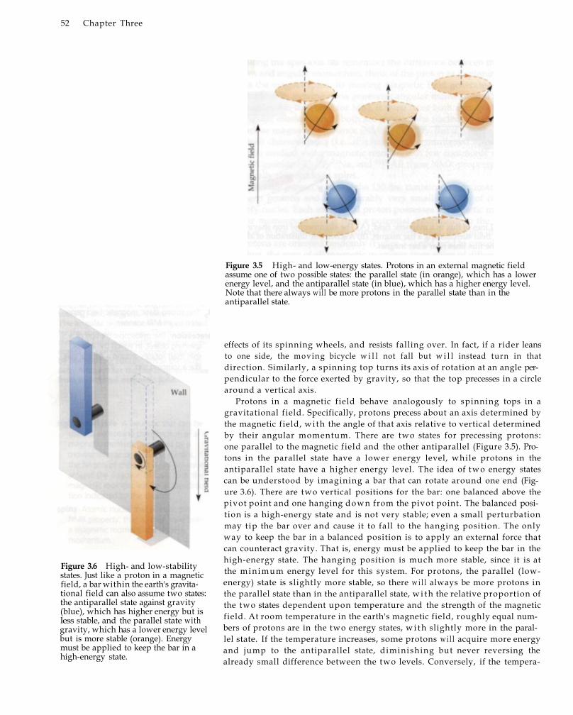
52 Chapter Three
Figure 3.5 High- and low-energy states. Protons in an external magnetic field assume one of two possible states: the parallel state (in orange), which has a lower energy level, and the antiparallel state (in blue), which has a higher energy level. Note that there always will be more protons in the parallel state than in the antiparallel state.
Figure 3.6 High- and low-stability states. Just like a proton in a magnetic field, a bar within the earth's gravitational field can also assume two states: the antiparallel state against gravity (blue), which has higher energy but is less stable, and the parallel state with gravity, which has a lower energy level but is more stable (orange). Energy must be applied to keep the bar in a high-energy state.
effects of its spinning wheels, and resists falling over. In fact, if a rider leans to one side, the moving bicycle w i l l not fall but w i l l instead turn in that direction. Similarly, a spinning top turns its axis of rotation at an angle perpendicular to the force exerted by gravity, so that the top precesses in a circle around a vertical axis.
Protons in a magnetic field behave analogously to spinning tops in a gravitational field. Specifically, protons precess about an axis determined by the magnetic field, wi th the angle of that axis relative to vertical determined by their angular momentum. There are two states for precessing protons: one parallel to the magnetic field and the other antiparallel (Figure 3.5). Protons in the parallel state have a lower energy level, while protons in the antiparallel state have a higher energy level. The idea of t w o energy states can be understood by imagining a bar that can rotate around one end (Figure 3.6). There are two vertical positions for the bar: one balanced above the pivot point and one hanging down from the pivot point. The balanced position is a high-energy state and is not very stable; even a small perturbation may t ip the bar over and cause it to fall to the hanging position. The only way to keep the bar in a balanced position is to apply an external force that can counteract gravity. That is, energy must be applied to keep the bar in the high-energy state. The hanging position is much more stable, since it is at the m i n i m u m energy level for this system. For protons, the parallel (low-energy) state is slightly more stable, so there w i l l always be more protons in the parallel state than in the antiparallel state, w i t h the relative proportion of the two states dependent upon temperature and the strength of the magnetic field. At room temperature in the earth's magnetic field, roughly equal numbers of protons are in the two energy states, w i t h slightly more in the parallel state. If the temperature increases, some protons w i l l acquire more energy and jump to the antiparallel state, diminishing but never reversing the already small difference between the two levels. Conversely, if the tempera-

B a s i c P r i n c i p l e s o f M R S i g n a l G e n e r a t i o n 5 3
ture decreases, spins w i l l possess less energy and even more w i l l stay at the
lower energy level.
Magnetization of a Spin System
It is important to emphasize that MR techniques do not measure single
nuclei, but instead measure the net magnetization of all spins in a volume.
We can think of the net magnetization as a vector w i t h two components: a
longitudinal component that is either parallel or antiparallel to the magnetic
field and a transverse component that is perpendicular to the magnetic
field. Because of the enormous number of spins w i t h i n even the smallest
volume, their transverse components w i l l tend to cancel out, and there w i l l
be no net magnetization perpendicular to the main magnetic f ield. The
amount of net magnetization, known as M, w i l l be proportional to the di f
ference in the number of the spins in the parallel and antiparallel states. The
more spins at the parallel state, the bigger the M (Figure 3.7).
In the previous section it was established that the number of parallel
spins increases wi th decreasing temperature, so one way to increase the net
magnetization would be to reduce the temperature. While theoretically pos
sible, this approach is rarely practical, as temperature changes of many
degrees Celsius are required for noticeable increases in net magnetization. A
more feasible approach is to increase the strength of the external field, based
on the Zeeman effect (Figure 3.8). Just as it would be more difficult to lift an
object in a stronger gravitational field than in a weaker gravitational field, it
takes more energy to shift from a lowenergy state to a highenergy state
when the external magnetic field is stronger. Therefore, the number of paral
lel spins wi l l increase as field strength increases. To increase the net magne
tization of protons, therefore, one can place those protons in a very strong
magnetic field. Scanners used for fMRI in humans usually have magnetic
fields of about 1.5 to 4 T, w i t h some having even stronger fields.
Figure 3.7 Net magnetization. T h e
net magnetization (M) is determined by
the difference between the number of
sp ins in the parallel state and the n u m
ber of sp ins in the antiparallel state.
T h e net magnetization is also called the
bulk magnetization.
longitudinal Parallel to the main magnetic field, or zdirection, of the scan
ner (i.e., into the bore).
transverse Perpendicular to the main
magnetic field of the scanner, in the
xy plane.
The net magnetization of spins w i t h i n a volume provides the basis for
MR signal generation, but net magnetization itself cannot be measured
directly under equil ibrium conditions. To understand this principle, recall
the analogy of an object whose weight you are t ry ing to estimate. You can
not know its weight just by looking at it; instead, you have to l i f t it . By l i f t
ing the object, you perturb its equilibrium state in the gravitational field, and
the reaction to that perturbation allows you to estimate its weight. Measur
ing net magnetization of spins in a magnetic field is no different; you must
perturb the equilibrium state of the spins and then observe how they react to
the perturbation. Just as l i f t ing enables measurement of the weight of an
object, excitation enables measurement of the net magnetization of a spin
system.
Spin Excitation and Signal Reception
Remember that all spins can take either a highenergy state or a lowenergy
state within a magnetic field (Figure 3.9A). When a spin in the highenergy
state falls to the lowenergy state, it emits a photon w i t h energy equal to the
Magnetic field strength
Figure 3.8 The Zeeman effect. The energy difference (ΔE) between the parallel and antiparallel states increases linearly w i t h the strength of the static magnetic field. As the energy difference between the states increases, spins are more likely to remain in the lowerenergy state.
What would happen to the proportion of parallel and antiparallel spins in the spin system if we reduced its
temperature to near absolute zero?

54 Chapter Three
excitation The process of sending electromagnetic energy to a sample at its resonant frequency (also called transmission). The application of an excitation pulse to a spin system causes some of the spins to change from a low-energy state to a high-energy state.
reception The process of receiving electromagnetic energy emitted by a sample at its resonant frequency (also called detection). As spins return to a low-energy state following the cessation of the excitation pulse, they emit energy that can be measured by a receiver coil.
Figure 3.9 Change between states due to absorption or transmission of energy. When spins are placed in an external magnetic field (A), more will be at the low-energy state (orange) than at the high-energy state (blue). If an excitation pulse with the right amount of energy is applied, some spins wil l absorb that energy and jump to the high-energy state (B). But after the excitation pulse is turned off, some of the spins in the high-energy state will return to the low-energy state, releasing the absorbed energy (C).
energy difference between the t w o states. Conversely, a spin in the low-energy state can jump to the high-energy state by absorbing a photon wi th energy matching the energy difference between the t w o states. To spark this state transition, radiofrequency coils w i t h i n MRI scanners bombard spins in the magnetic field w i t h photons, which are actually electromagnetic fields that oscillate at the resonant frequency of the nucleus of interest (e.g., hydrogen) Some spins in the low-energy state absorb this energy and change to the high-energy state, in a process known as excitation (Figure 3.9B). Since excitation disrupts the thermal equi l ibr ium, immediately after this irradiation the excess spins at the higher energy level return to the lower level, in order to reestablish the equi l ibr ium proportions of energy states (Figure 3.9C). Dur ing this reception period, the spins emit electromagnetic energy that can be detected by a radiofrequency coil. Since the frequencies of excitation and reception are both determined by the energy difference between the t w o states, oftentimes the same radiofrequency coil is used for both processes. The receiver detects a decaying signal that depends on the molecular environment of the spins. By analyzing this t ime-varying signal from the receiver coil , we can learn the properties of the spins and their surrounding environment.
In its essence, MR signal generation can be understood in very simple terms. Because of thermal energy, atomic nuclei wi th the NMR property spin around themselves. Within a strong magnetic f ield, the nuclei w i l l precess around an axis that is either parallel to the magnetic field (low-energy) or antiparallel to the magnetic field (high-energy). If energy is applied to the nuclei at a particular frequency, known as the resonant frequency, some low-

Basic Principles of MR Signal Generation 55
energy spins w i l l absorb that energy and change to the highenergy state.
And, after the energy source is removed, some spins w i l l return to the low
energy state by giving off that energy. Measurement of this emitted energy,
or MR signal, provides the data that go into our images.
Principles of MR Signal Generation
Keeping this intuitive perspective in mind , we now move to a more mathe
matically rigorous description of the excitationreception process. This
description w i l l both clarify the key concepts and provide a quantitative
description of the amount of MR signal measured under different condi
tions. Most of the descriptions below w i l l rely on simple algebra, and where
calculus is needed for the equations we have included additional verbal
description. We w i l l use the fol lowing terms and notation.
A scalar is a quantity representing the magnitude of some property. Prop
erties like mass, charge, length, and area are represented by scalars. Scalars
may have units; the mass of a person may be 70 kg, for example. Scalars are
indicated in italicized type. (M: The amount of M, scalar.) A vector is a quan
tity or phenomenon in which both magnitude and direction are stated. Exam
ples of vectors in nature include force, velocity, momentum, and electromag
netic fields. Vectors are denoted by boldface type. (M: The net magnetization,
vector.) Because vectors are directional, the rules for manipulation of vectors
are different than those for adding and mult iplying scalar numbers.
The dot product, also called the scalar product, of two vectors is a scalar
quantity obtained by summing the products of corresponding components.
Consider the twodimensional vectors A and B, which can each be repre
sented as the sum of vectors along the x and ydimensions. The dot product
of A and B is given by A●B = |A| |B| cos 0, where |A| and |B| are the
magnitudes of A and B and 0 is the angle between the t w o vectors when
they are placed tail to tail. The dot product may only be performed for pairs
of vectors having the same number of dimensions.
The cross product, or vector product, of t w o vectors produces a third
vector that is perpendicular to the plane in which the first two lie. The cross
product of vectors A and B may be defined by A x B = |A|| B| sin θ, where
|A| and |B| are the magnitudes of A and B and 0 is the angle between the
two vectors. The orientation of the cross product may be determined using
the righthand rule. As one's fingers curl through an angle θ from A to B, the
cross product, or the thumb, points toward the vector perpendicular to the
plane defined by A and B. The magnitude of the cross product is equal to the
area of the parallelogram defined by the two vectors. If the components of
vectors A and B are known, then the components of their cross product, C =
A x B, may be expressed as:
scalar A quantity that has magnitude but
not direction. Scalars are italicized in
this text.
vector A quantity with both magnitude
and direction. Vectors are boldface in
this text.
dot product The scalar product of two vectors, it is created by summing the
products along each dimension.
cross product The vector product of two vectors, its direction is perpendicular to
the plane defined by those vectors and
its magnitude is given by multiplying
their product times the sine of the
angle between them.
matrix A set of numbers arranged in a
grid of rows and columns.
A matrix is a set of numbers arranged in a rectangular gr id of rows and
columns. Matrices are a compact way to represent numbers, and matrix
addition and multiplication can be easily computed.
Spins: Magnetic Moment
As described earlier in the chapter, a nuclear spin can be visualized as a
small sphere of distributed positive charge that rotates at a high speed

56 Chapter Three
Figure 3.10 Torque on a current loop. A rectangular current loop (W x L) with electric current (I) would experience a torque if placed within a magnetic field B at an angle 6.
torque A force that induces rotational motion.
about its axis. Because of this rotation, it produces a current that in turn
generates a small magnetic f ie ld, k n o w n as the magnetic moment and
denoted as μ. Any moving magnet, currentcarrying coil , or moving charge
has a magnetic moment, which is defined as the ratio between (1) the max
i m u m torque on that magnet, coil , or charge exerted by an external mag
netic field and (2) the strength of that field (8). Magnetic moments are
measured in Amperes x meters squared, or A m 2 . To provide a visual repre
sentation, we consider a simple rectangular current loop [length (L), width
(W), and current level (I)] w i t h i n a magnetic field (Figure 3.10). Note that a
moving spin w i l l trace a circular loop through the magnetic field, so the rec
tangular loop is just a convenient simplif ication. The force (F) exerted on
the segment of wire w i t h length (L) that is perpendicular to the magnetic
field is defined by Equation 3.1:
[3.5]
Put simply, force is proportional to the strength of the magnetic field (B) and
the strength of the current (I). If the magnetic field increases, the force w i l l
also increase. The effect of this force upon objects in the field is to cause them
to rotate; this rotational force is known as torque. Torque can cause rotation,
and thus can also be thought of as the change in rotational momentum over
time. The maximum torque ( τ m a x ) exerted by the magnetic field is given by
mult iplying the force exerted on the current element by its width . The length
and w i d t h can be replaced in the equation by the area (A) of the loop:
[3.1]
[3.2]
Since the magnetic moment μ is defined as the maximum torque divided by
the magnetic field, its magnitude μ can now be represented as the product of
the current and the area of the current loop:
[3.3]
Note that the direction of the magnetic moment vector is defined by the
righthand rule based on the f low direction of the current.
Spins: Angular Momentum
Because the proton also has mass, its rotation produces an angular momen
t u m , often denoted as J. Angular momentum is a vector that defines the
direction and amount of angular motion of an object. Angular momentum is
initiated by external torques and conserved in the absence of external
torques. Quantitatively, the angular momentum is defined as the product of
the mass (m); velocity (v), and rotation radius (r), that is:
[34]
Since angular momentum is also a vector, its direction is defined by the
righthand rule based on the rotation direction. Since the vectors defining
the current f low and rotation are parallel to each other, there should exist a
scalar factor between the magnetic moment and angular momentum. This
scalar factor is denoted as γ, such that:

Basic Principles of MR Signal Generation 57
It is important to recognize that Equation 3.5 merely states that the magnetic
moment (from the rotating charge of the proton) and the angular momen
tum (from the rotating mass of the proton) are in the same direction, w i t h
one larger than the other by an unknown factor γ.
To understand what γ represents, let's consider the simplest atomic
nucleus, a single proton. First we must make some assumptions, namely
that the charge (q) of the proton is an infinitely small point source, the pro
ton rotates about a radius (r), and its rotation has a period (T). From Equa
tion 3.3, we know that the amount of magnetic moment of a moving charge
is given by multiplying two properties, the size of the current and the area of
the loop it traverses. The former is just the charge of the proton div ided by
the time it takes to move around the loop, while the latter is just the area of
the circle given by radius r, or πr2:
[3.6]
We also know that the velocity of the proton is equal to the circumference of
a circle (2πr) divided by the time it takes to go around the circle (T). Substi
tuting these values into Equation 3.4, we get the equation for the amount of J:
gyromagnetic ratio (γ) The ratio between the charge and mass of a spin. The gyromagnetic ratio is a constant for a given type of nucleus.
parallel state The lowenergy state in which an atomic spin precesses around an axis that is parallel to that of the main magnetic field.
antiparallel state The highenergy state in which an atomic spin precesses around an axis that is antiparallel (i.e., opposite) to that of the main magnetic field.
[3.7]
Substituting Equations 3.6 and 3.7 into Equation 3.5, it can be derived that:
[3.8]
Equation 3.8 demonstrates that the scaling factor (γ) depends only on the
charge (q) and mass (m) of the proton and not on any other quantity. Since
the charge and mass of the proton (or any other atomic nucleus) never
change, the scaling factor (γ) is a constant for a given nucleus, regardless of
the magnetic field strength, temperature, or any other factor. The constant (γ)
is known as the gyromagnetic ratio, and is critical for MRI .
In reality, the magnetic moment and angular momentum of a proton can
not be modeled by assuming a simple point charge engaged in circular
motion. A proton has a mass of about 1.67 x 1 0 2 7 kg and a charge of about
1.60 x 10¹⁹ C, so the estimated value of γ is 4.79 x 10 7 radian/T. However,
recent research has experimentally determined the real value of γ as 2.67 x 10⁸
radian/T. Nevertheless, while Equation 3.8 provides only a very rough esti
mate of the gyromagnetic ratio, it does demonstrate that γ is a unique quan
tity for a given nucleus. The gyromagnetic ratio has also been measured for
other common nuclei: for l 3 C it is 6.73 x 10 7; for 1 9 F it is 2.52 x 10⁸; for 2 3N it is
7.08 x 10⁷; and for 3 1 P it is 1.08 x 10⁸ (all units in radians per Tesla).
Spins within Magnetic Fields
If a uniform magnetic field is applied to an isolated proton spin (Figure 3.5),
the proton w i l l assume one of the two equi l ibr ium positions: the parallel
state (aligned wi th the magnetic field) or the antiparallel state (opposite of
the magnetic field). In MRI , the convention is to refer to the direction along
the main magnetic field B0 as the parallel state. Both states are at equilib
rium, although the energy at the parallel state is lower than that of the
antiparallel state and hence the spin is more stable at the parallel state.

The energy difference between the t w o states is a key concept in under
standing spin excitation and signal reception. As indicated in Equation 3.3, a
moving charge experiences maximum torque ( τ m a x ) when its motion is per
pendicular to the main magnetic field:
[3.10]
where d is a mathematical symbol indicating the changes, i.e., dθ indicating
the change of θ. Referring back to our analogy of a bar that could rotate
around a pivot point, to rotate the bar from the hanging position to the bal
anced position we must exert a force (torque) for the entire rotation angle.
Likewise, to change the spin state of a proton, we must apply enough torque
to complete the total amount of w o r k W. Note that W depends only on the
magnetic moment μ and the magnetic field B. For example, if field strength
increases, more work w i l l be required to change a spin from one state to
another.
We can think of W as equivalent to the energy difference between the
states (ΔE). Remember from the quantum mechanics point of view just
described that when a spin changes states it w i l l either emit or absorb
energy in the form of an electromagnetic pulse. The frequency v of this elec
tromagnetic pulse is determined by the energy difference between the states,
as given by the Bohr relation:
However, if the moving charge is not perpendicular to the main magnetic
f ield, but at some angle 8, then the amount of torque on that charge w i l l be
lessened. Specifically, only the component of the magnetic moment vector
that is perpendicular to the static field contributes to the torque. Examina
tion of Figure 3.10 reveals that the perpendicular component of the magnetic
moment vector μ is just μ sin θ, since the sine of a given angle represents the
opposite (perpendicular component) divided by the hypotenuse (vector):
or, in vector form:
To change a spin from a lowenergy (parallel) state to a highenergy
(antiparallel) state, we must apply energy. This amount of energy, or work,
can be calculated by integrating the torque over the rotation angle:
[3.9a]
[3.9b]
[3.11]
where h is called Planck's constant. Combining Equations 3.10 and 3.11, we
obtain:
[3.12]
It was measured experimentally by physicists that the longitudinal compo
nent (i.e., along the magnetic field) of the angular momentum J of a proton is
h/2 (h = h/2π); thus the longitudinal magnetic moment can be calculated
using Equation 3.5 to be:
[3.13]
5 8 C h a p t e r T h r e e

Basic Principles of MR Signal Generation 59
Substituting the result of Equation 3.13 into Equation 3.12, we find that the
frequency v is equal to the gyromagnetic ratio divided by 2π and multipl ied
by the magnetic field strength:
Larmor frequency The resonant frequency of a spin within a magnetic
field of a given strength. It defines the
frequency of electromagnetic radiation
needed during excitation to make spins
change to a highenergy state, as well
as the frequency emitted by spins
when they return to the lowenergy
state.
[3.15]
Following this series of equations, let us stop for a moment to catch our
breath and review what we know so far! First, all nuclear spins can be char
acterized by their magnetic moment and angular momentum, both expressed
as vectors with the same direction. The magnetic moment is larger than the
angular momentum vector by a factor λ, which is known as the gyromagnetic
ratio. Second, spins in a magnetic field can take one of two possible states,
either a lowenergy state parallel to the magnetic field or a highenergy state
antiparallel to the magnetic field. To change from the lowenergy state to the
highenergy state, a spin must absorb electromagnetic energy. Conversely,
when changing from a high to a lowenergy state, a spin emits electromag
netic energy. Third, Equation 3.14 demonstrates that the frequency of the
absorbed or emitted electromagnetic energy depends only on the gyromag
netic ratio of that spin and the magnetic field strength. So, for a given atomic
nucleus and MR scanner, we can calculate the frequency of electromagnetic
radiation that is needed to make spins change from one state to another! This
frequency v is known as the Larmor frequency.
Recognize that y/2π in Equation 3.14 is a constant for a given nucleus,
expressed in units of frequency div ided by field strength. For hydrogen, its
numerical value is given as 42.58 MHz/Tesla. So, for common MR scanners
with field strengths of 1.5 T, the Larmor frequency for hydrogen is approxi
mately 63.87 MHz. This frequency is w i t h i n the radiofrequency band of the
electromagnetic spectrum. If we place a human brain into a 1.5T MR scan
ner and apply electromagnetic energy at 63.87 M H z , some of the hydrogen
nuclei within water molecules w i t h i n that brain w i l l change from a low
energy state to a highenergy state. This idea, that energy at a particular fre
quency is needed for changing nuclei from one state to another, represents
the cardinal principle of magnetic resonance.
Spin Precession
Now let us consider the effects of the external magnetic field on the motion
of atomic nuclei. If we place a stationary magnetic bar into a static magnetic
field at an angle 9, it w i l l oscillate back and forth symmetrically to the main
field (Figure 3.11A). However, if the magnetic bar is not stationary, but is
instead spinning about its axis, it w i l l rotate around this field instead of
oscillating back and forth. This is what happens for atomic nuclei. Because
an atomic nucleus has intrinsic spin, its axis of rotation rotates around the
direction of the external magnetic field (Figure 3.11 B). This motion is known
as precession, and is conceptually described earlier in this chapter. Naturally,
it would be useful to determine the frequency of such precession. In this sec
tion, we wil l derive this frequency for hydrogen nuclei in a magnetic field.
Earlier in the chapter we learned that the cross product of two vectors is
derived by multiplying their magnitudes times the sine of the angle between
them. We can therefore rewrite Equation 3.9 in the fo l lowing form, which
means that the torque on the magnetic moment is given by the cross product
of the magnetic moment and the main field:
[3.14]

Figure 3.11 Movement within a magnetic field. If a magnetic bar is placed in an external magnetic field, it will oscillate back and forth across the main axis of the field (A). A spin within a magnetic field (B) has angular momentum and thus will precess around the magnetic field (B0). The cross product of μ and B0 determines the precession direction.
Recall also that since torque indicates the change in angular momentum
over time, it can be defined as the derivative of angular momentum over the
derivative of time:
To solve for the precession frequency, we need to s impli fy the vector
structure of Equation 3.18. We can do this by breaking d o w n the magnetic
moment μ, which is a vector, into scalar components along different dimen
sions. After defining the components along three directions as μx, μ y, and μz,
Replacing τ in Equation 3.15 w i t h that in Equation 3.16, we have the follow
ing equality:
From Equation 3.5 we learned that angular momentum J is equivalent to μ/γ.
By substitution, we get a generalized expression of the magnetic moment
under the main magnetic field, B0:
Equations 3.17 and 3.18 can be read as saying that the torque μ x B0) on a
spin induces changes in the angular momentum and magnetic moment of
that spin over time.
[3.18]
[3.17]
[3.16]
60 Chapter Three

Basic Principles of MR Signal Generation 61
the magnetic moment is simply the sum of the three components. Here, x, y,
and z are unit vectors along the three cardinal dimensions:
So, we can transform Equation 3.18 into three separate scalar equations, rep
resenting three different dimensions:
[3.20a]
[3.20b]
[3.20c]
We do not go through the entire derivation here, but the result can be sim
ply summarized as follows. The change in the xcomponent of the magnetic
moment at any point in time depends on the current ycomponent value; at
extreme yvalues, x changes quickly. The change in the ycomponent over
time depends on the xcomponent in a similar way. The zcomponent of the
magnetic moment never changes. While this set of equations may seem
complex, it merely specifies that the magnetic moment w i l l trace a circular
path around the zaxis. As we have already learned, this circular path is
known as precession.
Solving the set of differential equations (3.20) is beyond the scope of this
introduction and is left as an exercise for the interested student. The solu
tion, given the initial conditions at time zero (i.e., μx , μy, μz), is given by the
following equation:
where x, y, and z are unit vectors along three spatial dimensions. This indi
cates that magnetic moment precesses at angular velocity ω. Importantly,
the angular velocity ω is given by γB0, which is the same as the frequency
of an emitted or absorbed electromagnetic pulse dur ing spin state changes,
ν= (γ/2π)B0 (see Equation 3.14). Note that though the quantities ω and v are
identical, they are expressed in different units: ω is measured in radians per
second, while v is measured in Hertz (Hz), or cycles per second.
The correspondence between ω and ν means that a single quantity, the
Larmor frequency, governs two aspects of a spin w i t h i n a magnetic field: the
energy that spin emits or absorbs when changing energy states and the fre
quency at which it precesses around the axis of the external magnetic f ield.
This correspondence has deep and important consequences for understand
ing MR signal generation. The change in energy state is a concept from
quantum mechanics, in that spins can only take discrete energy levels w i t h a
fixed energy difference between them. The frequency of precession is a con
cept from classical mechanics, in that it describes the motion of a particle
(e.g., proton) through space. Yet, because ω and v represent the same quan
tity, these two perspectives, quantum and classical mechanics, are unified in
describing MR phenomena. This unification allows us to visualize the quan
tum behavior of spins using classical mechanics modeling to derive basic
equations for MR signal generation.
[3.19]
Magnetization of Spins in Bulk Matter
We now have completed analysis of the spin properties of a single atomic
nucleus in an external magnetic f ield. We know characteristics of its mag
netic moment and angular momentum, how to change it from a highenergy
state to a lowenergy state, and how it precesses through the field. While
properties of individual nuclei were of interest to Rabi and other early MR
physicists, we are not interested in the behavior of single atomic nuclei.
Instead, we are interested in characteristics of bulk matter like the human
brain, which consists of many protons w i t h potentially different properties.
Since the most abundant nuclei in the human body are hydrogen nuclei,
principally w i t h i n water molecules, we w i l l focus the subsequent discussion
on hydrogen.
In the absence of a magnetic field, the spin axes of all nuclei in bulk mat
ter are oriented in random directions, so that the net magnetization (i.e., the
sum of all individual magnetic moments) is zero. Once the bulk matter is
moved into the magnetic field, each individual magnetic moment must align
itself in either the parallel or antiparallel state. If we refer to the parallel state
as p and the antiparallel state as a, and we denote the probability for a given
nucleus to be found in the parallel state as Pp and that to be found in the
antiparallel state as P a ' each spin must be in one state or the other, w i t h the
sum of the probabilities being 1. That is,
The quantity Pp Pa indicates how many more spins are parallel to the mag
netic field than are antiparallel. Each of these spins contributes a magnetic
moment w i t h magnitude μ along the zdirection. Thus, the total magnetic
62 Chapter Three
[3.22]
If the spins are evenly distributed between these t w o states, such that there
are as many parallel spins as antiparallel spins, there w i l l be no net magneti
zation. Fortunately for MRI, there must always be more parallel spins (in the
more stable lowenergy state) than antiparallel spins (highenergy state), and
thus there w i l l always be a net magnetization. The relative proportion of the
two spin states depends upon their energy difference (ΔE) and the tempera
ture (T). This proportion can be determined using Boltzmann's constant, kB
(1.3806 x 10~23 J/K 1 ) , which governs the probabilities of spin distribution
under thermal equil ibrium.
Note that given the very small value of Boltzmann's constant, ΔE/kBT w i l l
be much less than 1 under normal conditions. For very small exponents x,
the exponential ex can be approximated by 1 + x. Thus, Equation 3.23 can be
replaced by:
[3.24]
[3.23]
[3.25]
Equation 3.24 is called the hightemperature approximation. By algebraically
solving Equations 3.22 and 3.24, we obtain:

Basic Principles of MR Signal Generation 63
moment, which is called the bulk magnetization or net magnetization, is
simply this proportion multipl ied by the number of protons per unit volume
(n) times the magnetic moment of each spin in the zdirection. The net mag
netization is represented by the symbol M. (Here z is a unit vector in the z
direction.)
At room temperature, the proportional difference between the numbers of
spins in the parallel and antiparallel states is 0.003% per Tesla, which is a
very small amount. Note that the net magnetization is parallel to the main
held (i.e., the zdirection) and that as long as the temperature remains
unchanged it w i l l not vary in amplitude. If the temperature increases, the
net magnetization w i l l decrease. Also, and more importantly, since the dif
ference between the energy states, ΔE, increases proportionally to the
strength of the main field, the net magnetization is also proportional to the
main field strength. This is w h y using a strong magnetic field increases the
amount of MR signal recorded.
While the net magnetization init ial ly points along the main magnetic
field, its precession angle is 0° at equi l ibr ium. When tipped away from this
starting position by an excitation pulse, the net magnetization w i l l precess
around the main axis of the field, just like a single magnetic moment. We can
describe the morion of the net magnetization, fol lowing an excitation pulse
at time point t = 0, in three scalar equations as follows:
[3.26]
Here, Mx0, My0 and Mz0 are initial conditions for the net magnetization. In
summary, the net magnetization of bulk matter behaves similarly to the
magnetic moment of a single spin, in that it precesses clockwise at the Lar
mor frequency around the axis of the main field. This suggests that we may
be able to affect the motion of the net magnetization vector in the same way
that we can affect the energy state of a single spin, by application of electro
magnetic energy at the Larmor frequency. We demonstrate this in the next
section.
Spin Excitation
By measuring the precession of the net magnetization of a spin system, we
can discover some of its properties. For example, based on Equation 3.26
above, we can estimate the number of protons w i t h i n a unit volume (i.e.,
proton density) based on the quantity n. But we cannot measure the net
magnetization of a spin system directly. Therefore, we need to find an indi
This equation group is nearly identical to Equation group 3.20, wi th the only
difference being that here the amount of net magnetization of a spin system
(M) replaces the amount of the magnetic moment of a single spin (μ). The
solution to this equation group is similar to that given in Equation 3.21:
[3.27a]
[3.27b]
[3.27c]
[3.28]

64 Chapter Three
B1 The magnetic field caused by the
application of an electromagnetic pulse
during excitation.
laboratory frame The normal reference frame that is aligned with the mag
netic field of the scanner.
rotating frame A reference frame that
rotates at the Larmor frequency of the
spin of interest. The rotating frame is
adopted to simplify mathematical
descriptions of the effects of excitation.
rect approach that perturbs the spin system away from equilibrium and then
measures the response of the system to that perturbation, just like the earlier
analogy of l i f t ing an unknown object to estimate its weight. This process is
called spin excitation.
In a typical MRI experiment, the object sample to be imaged is placed
w i t h i n a strong, uniform magnetic field at the center of the scanner. We now
know that the net magnetization of the sample precesses at the Larmor fre
quency. For hydrogen, the net magnetization oscillates around the main field
vector about 64 mi l l ion times per second if the magnetic field of the scanner
is 1.5 T. Because the magnetization rotates so rapidly, it is extremely difficult
to change the magnetization w i t h a single pulse of electromagnetic energy.
Instead, energy is applied at a given frequency for an extended period of
time. To understand the effects of frequency upon an oscillating system, con
sider again our example of the backyard swing set. If you apply energy at the
swing's natural frequency by pushing each time the person is in the same
place, even very small pushes w i l l help increase the velocity of the swing and
thereby increase the energy in the system. This phenomenon, where small
applications of energy at a particular frequency can induce large changes in a
system, is known as resonance. For similar reasons, MRI scanners use spe
cialized radiofrequency coils to transmit an electromagnetic excitation pulse
(B1) at the same frequency as the spin precession (i.e., the Larmor frequency),
exerting torque on the spins to perturb them (Figure 3.12).
[3.29]
We are now ready to examine the effect of this electromagnetic pulse
upon the sample. Because both the spins and excitation pulse are rotating at
the Larmor frequency, we can adopt a reference coordinate system that is
also rotating at that frequency. For clarity, we w i l l refer to the normal frame
of reference that is aligned w i t h the magnetic field of the scanner as the lab
oratory frame (Figure 3.13A) and the frame of reference rotating at the Lar
mor frequency as the rotating frame (Figure 3.13B). Imagine that you are
watching your young siblings ride a carousel at the amusement park. The
laboratory frame is analogous to the situation when you are standing on the
Figure 3.12 Generation of a circularly polarized magnetic field. By driving the birdcage coil using orthogonal currents, the MR scanner generates a circularly polarized electromagnetic field that allows moreefficient radiofrequency excitation.
B1 = B 1x cos ωt B 1y sin ωt

Basic Principles of MR Signal Generation 65
Figure 3.13 Laboratory and rotating reference frames. In the laboratory frame, the magnetization rotates at a given frequency about the main axis (A). But if a rotating frame (x'-y') is adopted that spins the transverse plane (x-y plane) at that frequency, the magnetization would appear stationary (B).
ground outside the carousel watching them ride around. The rotating frame corresponds to when you get on the carousel w i t h them and watch them as you both spin around. In the latter case, they w i l l appear stationary, since you are both rotating at the same speed. The unit vectors in the transverse plane within the rotating frame are represented by x' and y' and correspond to the following unit vectors in the laboratory frame:
Within the rotating frame, both the spins and the excitation pulse become stationary, making subsequent formulas much simpler. The net magnetization (M) becomes a stationary quantity along the z-direction, while the excitation pulse (B1) can now be thought of as a stationary vector along the new x'-direction. We therefore would have:
To assess combined magnetization, Equation 3.18 can be rewritten as Equation 3.33, which states that the change in net magnetization over time is the vector product of the net magnetization and the excitation pulse. As for Equation 3.18, this can be read as saying that applying a torque (M x B) to the net magnetization w i l l rotate its direction over time:
Note that here the torque on the net magnetization depends upon the total magnetic field B experienced by the spin system. However, this field is itself the sum of two magnetic fields, the static magnetic f ield B0 and the excitation pulse B1 ' The effect of the excitation pulse, when it is presented at the resonant frequency of the sample, or on-resonance, is a simple rotation of
[3.30]
[3.31]
[3.32a]
[3.32b]
[3.33]

66 Chapter Three
onresonance excitation The presenta-tion of an excitation pulse at the reso-nant frequency of the sample, resulting in maximal efficiency.
offresonance excitation The presenta-tion of an excitation pulse at a fre-quency other than the resonant fre-quency of the sample, resulting in reduced efficiency.
the net magnetization vector from the zdirection toward the transverse (x
y) plane. But if the pulse is presented at a slightly different frequency, so that
it is offresonance, its efficiency greatly decreases. While this loss of effi
ciency makes intuit ive sense, its mathematical derivation is complex. The
effective magnetic f ield experienced by the spin system is not just B, itself
but is instead a new field called B 1 e f f that is influenced by both B 1 and B 0.
We have included the derivation of B 1 e f f w i t h i n the fo l lowing box for inter
ested students, and its conclusion is given in Equation 3.37.
Expanding Equation 3.33 in the rotating frame results in the following, which illustrates how the magnetization vector changes over time in each direction:
[3.34]
[3.35]
where ωz. indicates ω as a vector pointing along the zdirection. A n d if we define the changing magnetization in the rotating frame as δM/δt, in addition to the changing magnetization in the laboratory frame, dM/dt, Equation 3.33 can be rewritten in the fo l lowing form (Equation 3.35). It states that the net magnetization (in the laboratory frame) can be considered to have two independent components, precession around the zdirection w i t h frequency ω and a rotation from the longitudinal to transverse planes (wi th in the rotating frame):
[3.36]
By reorganizing Equation 3.36 and substituting Equation 3.33, we can describe a new quantity, B 1 e f f , which depends on the frequency and amplitude of the applied B. field. This quantity is the applied magnetic field that the spin system actually experiences, and it governs the behavior of the net magnetization within the rotating frame of reference:
[3.37]
In conclusion, the change in the magnetization in the rotating frame over
time (δM / δt) is determined by a new quantity, B 1 e f f , not by B1 itself. The net
magnetization rotates around the vector B 1 e f f dur ing excitation:
Since it can be derived that:
[3.38]
The value of the effective excitation pulse experienced by a spin system,
B 1 e f f , is given by the fo l lowing equation (derived from Equation 3.37), such
that it has both longitudinal (z) and transverse (x') components:
[3.39]
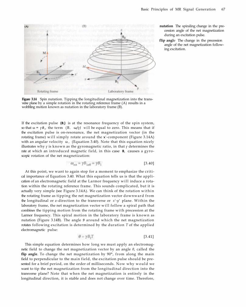
Basic Principles of MR Signal Generation 67
(A)
Figure 3.14 Spin nutation. Tipping the longitudinal magnetization into the transverse plane by a simple rotation in the rotating reference frame (A) results in a wobbling motion known as nutation in the laboratory frame (B).
nutation The spiraling change in the precession angle of the net magnetization during an excitation pulse.
flip angle The change in the precession angle of the net magnetization following excitation.
If the excitation pulse (B1) is at the resonance frequency of the spin system,
so that ω = γB 0 , the term (B 0 -ω/γ) w i l l be equal to zero. This means that if
the excitation pulse is onresonance, the net magnetization vector (in the
rotating frame) w i l l simply rotate around the x 'component (Figure 3.14A)
with an angular velocity ω r o t (Equation 3.40). Note that this equation nicely
illustrates why γ is known as the gyromagnetic ratio, in that γ determines the
rate at which an introduced magnetic f ield, in this case B1' causes a gyro
scopic rotation of the net magnetization:
[3.40]
[3.41]
At this point, we want to again stop for a moment to emphasize the cr i t i
cal importance of Equation 3.40. What this equation tells us is that the appli
cation of an electromagnetic field at the Larmor frequency w i l l induce a rota
tion within the rotating reference frame. This sounds complicated, but it is
actually very simple (see Figure 3.14A). We can think of the rotation w i t h i n
the rotating frame as t ipping the net magnetization vector downward from
the longitudinal or zdirection to the transverse or x'y' plane. Wi th in the
laboratory frame, the net magnetization vector w i l l follow a spiral path that
combines the tipping motion from the rotating frame w i t h precession at the
Larmor frequency. This spiral motion in the laboratory frame is k n o w n as
nutation (Figure 3.14B). The angle 9 around which the net magnetization
rotates following excitation is determined by the durat ion T of the applied
electromagnetic pulse:
This simple equation determines how long we must apply an electromag
netic field to change the net magnetization vector by an angle θ, called the
flip angle. To change the net magnetization by 90°, f rom along the main
field to perpendicular to the main field, the excitation pulse should be pre
sented for a brief period, on the order of milliseconds. N o w why w o u l d we
want to tip the net magnetization from the longitudinal direction into the
transverse plane? Note that when the net magnetization is entirely in the
longitudinal direction, it is stable and does not change over time. Therefore,

68 Chapter Three
its amplitude is impossible to measure. But if we t ip the magnetization into
the transverse plane w i t h an excitation pulse, there w i l l be very large
changes in the direction of magnetization over time as it rotates. This chang
ing magnetic field can be detected by external receiver coils. In short, by tip
ping the net magnetization we can create measurable MR signal.
The concept of the B 1 e f f (see Equation 3.39) is also very important in under
standing offresonance excitation due to application of an inhomogeneous
field, such that the actual rotation frequency does not match the Larmor fre
quency for a spin system. As such, the difference between B0 and w/γ is not
zero, which means that the excitation pulse would have a longitudinal compo
nent. Because the spins always rotate about the axis of B 1 e f f ' the effectiveness of
the excitation pulse wi l l be compromised. To understand the effects of offreso
nance excitation, think of an extreme condition in which the excitation pulse
has a zcomponent approaching the size of the main field, B0. As a result, the
B 1 e f f would be pointing along the zdirection. Because the B 1 e f f has the same
direction as the spins themselves, it w o u l d exert no torque on the spins, and
their angle of rotation would not change. (Mathematically speaking, the cross
product between two vectors wi th the same direction is equal to zero). Conse
quently, an excitation pulse along the same direction as B0 would have
absolutely no effect. In practice, if due to hardware problems the zcomponent
of B 1 e f f is sufficiently large, then full excitation may be impossible to achieve.
But what if B 1 e f f is only slightly offresonance? The rotational trajectories
of a perfectly onresonance pulse and a slightly offresonance pulse are illus
trated in Figure 3.15. Al though the onresonance pulse has a more efficient
rotation trajectory, which reduces the duration of the pulse needed to tip the
Figure 3.15 Onresonance and offresonance excitation. Application of an onresonance excitation pulse (A) wil l efficiently tip the longitudinal magnetization into the transverse plane (orange trajectory). But application of an offresonance excitation pulse (B) will result in an inefficient trajectory (blue) that takes longer to completely tip the magnetization. The goal of excitation is to achieve full rotation of the magnetization from the longitudinal axis to the transverse plane.
B1EFF The effective magnetic field experienced by a spin system during excitation.
What are the relative proportions of low-energy spins and high-energy spins following application of a 90°
excitation pulse?

B a s i c P r i n c i p l e s o f MR S i g n a l G e n e r a t i o n 6 9
magnetization into the transverse plane, it is still possible to achieve fu l l
excitation using the offresonance pulse. However, this ful l excitation comes
at the cost of additional time (required to traverse the longer path to the
transverse plane), and if the duration of the pulse is held constant there w i l l
only be incomplete excitation.
electromotive force A dif ference in
electrical potent ia l tha t can be used to
drive a current t h rough a circuit. The
MR signal is the e lectromot ive force
caused by the chang ing magnet ic f ie ld
across the detector coi l .
Signal Reception
So far, we have shown that an electromagnetic excitation pulse applied by a
transmitter coil can change the net magnetization of a spin system. To meas
ure this change, we need another receiver coil (or detector coil). Receiver
coils acquire signal through the mechanism of electromagnetic coupling, as
governed by Faraday's law of induction. After the magnetization of the sam
ple is tipped to the transverse plane, its precession at the Larmor frequency
sweeps across the receiver coil, causing the magnetic flux (Φ) experienced by
the receiver coil to change over time (Figure 3.16). This change of flux, dΦ/dt,
in turn induces an electromotive force (emf) in the coil. By definition,
[3.42]
where the magnetic flux penetrating the coil area is given by
Figure 3.16 MR s igna l recep t ion . As the net m a g n e t i z a h o n rotates t h r o u g h the
transverse plane, the a m o u n t o f magne t i c f l u x exper ienced by the rece iver co i l
changes over t ime (A and B). T h e c h a n g i n g f l u x generates an e l e c t r o m o t i v e force,
which prov ides the basis f o r the MR s igna l .
If the excitation pulse is only slightly offresonance, it is
still possible to reach full excitation, but if the pulse is consid
erably offresonance, t h e n full excitation cannot be reached.
Based on w h a t you have learned (and Figure 3.15), w h a t is
the threshold angle of B 1 e t f b e y o n d w h i c h full excitation
cannot be achieved?
The measurement of electromotive force in a receiver coil is known as reception.

70 Chapter Three
principle of reciprocity The rule stating that the quality of an electromagnetic coil for transmission is equivalent to its quality for reception (i.e., if it can generate a homogeneous magnetic field at excitation, it can also receive signals uniformly).
relaxation A change in net magnetization over time.
The additional scaling factor ω 0 comes from taking the time derivative of
M(t), which contains the term ω0t (consult Equation 3.28).
Note that the electromotive force (emf) oscillates at the Larmor frequency
like the excitation pulses themselves, so that the receiver coil must be tuned
to the resonant frequency to best measure the changes in MR signal. Since
both M and ω0 are proportional to the main field strength B 0, the measured
emf is proportional to B 02 . Simply stated, the amount of MR signal received
by the detector coil increases w i t h the square of the magnetic field strength.
Unfortunately for highfield M R I , the amplitude of noise in the MR signal is
also proportional to the strength of the magnetic field, so the signaltonoise
ratio increases only linearly w i t h B 0. The effects of f ield strength on signal
and noise w i l l be discussed in detail in Chapter 9.
Equation 3.44 also confirms that before the excitation pulse tips the net
magnetization into the transverse plane, there is no detectable emf and thus
no MR signal. This is because when the net magnetization is in its original
longitudinal direction, its amplitude and direction do not change, so there is
no signal to be measured by the receiver coil (Figure 3.17A and B). We
emphasize that only changes in the transverse plane contribute to the MR
signal.
Spin Relaxation
The MR signal created fo l lowing an excitation pulse does not last indefi
nitely; it decays over time, generally w i t h i n a few seconds. This phenomenon
is called spin relaxation. Two primary mechanisms contribute to the loss of
the MR signal: longitudinal relaxation (Figure 3.18A) and transverse relax
ation (Figure 3.18B). For a given substance (e.g., water, fat, or bone) in a mag
netic field of a given strength, the rates of longitudinal and transverse relax
ation are given as time constants, which we introduce in this section. (We
provide the mathematical derivation of these equations in the next chapter.)
When the excitation pulse is taken away, the spin system gradually loses
the energy absorbed dur ing the excitation. The simplest way to think about
this energy loss is by using the quantum mechanics perspective. As they lose
[3.44]
[3.43]
The excitationreception process simulates the scenario of mutual cou
pl ing of t w o coils. Just as a current change in one coil induces a similar cur
rent change in another nearby coil through mutual inductance, magnetic
f ield changes in a sample (i.e., the brain) induce magnetic f ield changes in
the receiver coil. The magnetic flux generated by the sample and penetrating
through the receiver coil can be represented as:
where B1bar is the magnetic field per unit current of the receiver coil and M(t) is
the magnetization created by the sample.
This relation shows that the magnetic flux through the receiver coil actu
ally depends on the magnetic field that could be produced by the coil. That
is, the stronger the magnetic field that can be generated by a coil, the better
its reception. Likewise, if a radiofrequency coil can generate a homogeneous
magnetic f ield w i t h i n a sample for transmission, it can also receive signals
uni formly w i t h i n the sample. These relations are consistent w i t h the princi
ple of reciprocity. Substituting Equation 3.43 into Equation 3.42, we get:

Basic Principles of MR Signal Generation 71
Figure 3.17 Effects of net magnetization orientation upon recorded MR signal. When the net magnetization is along the longitudinal axis (A), there is no detectable change in the magnetic field and thus no electromotive force in the detector coil. After the net magnetization has been tipped into the longitudinal axis (B), its motion causes changes in the measured current within the detector coil. Magnetization must be in the transverse plane for detection using MR.
energy, excited spins in the high-energy (antiparallel) state go back to their original low-energy (parallel) state. This phenomenon is known as longitudinal relaxation, or spin-lattice relaxation, because the indiv idual spins are losing energy to the surrounding environment, or lattice of nuclei. As
longitudinal relaxation (or spin-lattice relaxation) The recovery of the net magnetization along the longitudinal direction as spins return to the parallel state.
Longitudinal relaxation Transverse relaxation
Figure 3.18 T1 and T2 relaxation. Schematic illustration of longitudinal relaxation, or T1 recovery (A), and of transverse relaxation, or T2 decay (B). The time constant T1
governs the rate at which longitudinal magnetization recovers, while the time constant T2 governs the rate at which longitudinal magnetization decays. Note that T2* relaxation is similar to T1 relaxation, except that the decay of transverse magnetization results from both spin-spin interactions (as in T 2 ) and local field inhomogeneities.

72 Chapter Three
T1 (recovery) The time constant that describes the recovery of the longitudinal component of net magnetization over time.
transverse relaxation The loss of net magnetization within the transverse plane due to the loss of phase coherence of spins.
T2 (decay) The time constant that describes the decay of the transverse component of net magnetization due to accumulated phase differences caused by spin-spin interactions.
T2* (decay) The time constant that describes the decay of the transverse component of net magnetization due to both accumulated phase differences and local magnetic field inhomo¬geneities. T 2* is always shorter than T 2 . BOLD-contrast fMRI relies on T2* contrast.
An additional, extrinsic source of differential spin effects is the external magnetic f ield. More often than not, the external field is inhomogeneous. Because each spin precesses at a frequency proportional to its local field strength, variations in field f rom location to location cause spins at different spatial locations to precess at different frequencies, also leading to the loss of coherence. The combined effects of spin-spin interaction and field inhomo¬geneity lead to signal loss k n o w n as T2* decay, characterized by the time constant T2*. Note that T 2* decay is always faster than T 2 decay alone, since it includes an additional factor of field inhomogeneity, and thus for any substance the time constant T 2* is always smaller than T 2. The equation for T2* decay is similar to that for T 2 decay. We w i l l discuss T2* decay again in Chapter 5 because it plays a critical role in the BOLD contrast we use for fMRI .
These relaxation processes constrain how much MR signal can be acquired fol lowing a single excitation pulse. Since transverse magnetization decays over a short period of time, there is a l imited w i n d o w w i t h i n which MRI data can be collected. To acquire an entire image, a pulse sequence often must excite the sample many times to allow collection of all data points. The trade-offs between MR signal and acquisition time are discussed further in Chapter 5. It is important to realize that relaxation processes are not a problem for MRI , but instead they provide the capability for measur-
more and more indiv idual spins return to their low-energy state, the net magnetization likewise returns to be parallel to the main field. From a classical mechanics point of view, the transverse magnetization is gradually going back to the longitudinal direction, as it was before the excitation pulse. Because the total magnetization is constant, the growth of the longitudinal magnetization naturally results in a smaller transverse magnetization and hence also a smaller MR signal. The time constant associated w i t h this longitudinal relaxation process is called T1' and the relaxation process is called T1
recovery. The amount of longitudinal magnetization, Mz' present at time t following an excitation point is given by Equation 3.45, where M 0 is the original magnetization.
[3.45]
After the net magnetization is tipped into the transverse plane by an excitation pulse, it is initially coherent, in that all of the spins in the sample are precessing around the main field vector at about the same phase. That is, they begin their precession w i t h i n the transverse plane at the same starring point. Over time, the coherence between the spins is gradually lost and they become out of phase. This phenomenon is known as transverse relaxation. In general, there are t w o causes for transverse relaxation, one intrinsic and the other extrinsic. The intrinsic cause is from spin-spin interaction: When many spins are excited at once, there is loss of coherence due to their effects on one another. As an analogy, consider a single race car dr iv ing rapidly around a track; the driver can adopt a high and constant speed because no other cars are present. But in a pack of many cars, the movement of one car influences the speed of the others, making it impossible for all the cars to maintain a constant high speed. Likewise, interactions among spins cause some to precess faster, and some slower, causing the relative phases of the precessing spins to gradually fan out over time. The signal loss by this intrinsic mechanism is called T2 decay (Equation 3.46) and is characterized by a time constant known as T2.
[3.46]

Basic Principles of MR Signal Generation 73
Stated generally, the net magnetization vector of a spin system precesses around the main magnetic field axis at the Larmor frequency, w i t h its change in the longitudinal or z-direction governed by T1 and its change in the transverse plane governed by T 2 . This equation is called the Bloch equation, after the physicist Felix Bloch, and it describes the behavior of magnetization in the presence of a time-varying magnetic field. As we w i l l learn in the following chapters, solving this equation leads to mathematical representations of the evolution of magnetization at steady state, d u r i n g excitation, and during relaxation. It provides the theoretical foundation for all MRI experiments.
Summary A set of physical principles underlies the generation of MR signal. The primary concept is that of nuclear spin. Atomic nuclei wi th a magnetic moment and angular momentum are known as spins and exhibit rapid gyroscopic precession in an external magnetic field. The axis around which they precess is known as the longitudinal direction, and the plane in which they precess is known as the transverse plane. Each spin adopts either a low- or high-energy state, parallel or antiparallel to the magnetic field, respectively. Under normal conditions, the net magnetization across all spins is a vector parallel to the static magnetic field. By applying an electromagnetic pulse that oscillates at the resonant (Larmor) frequency of the spins, a process known as excitation, one can t ip the net magnetization vector from the longitudinal direction into the transverse plane. This causes the net magnetization to change over time in the transverse plane, generating MR signal that can be measured in an external detector coil. A single formula known as the Bloch equation forms the basis for the quantitative description of magnetic resonance phenomena.
Suggested Readings
Haacke, E. M., Brown, R. W., Thompson, M. R., and Venkatesan, R. (1999). Magnetic Resonance Imaging: Physical Principles and Sequence Design. John Wiley & Sons, New York. A comprehensive encyclopedia of the theoretical principles of MRI.
Jin, J. (1999). Electromagnetic Analysis and Design in Magnetic Resonance Imaging. CRC Press, Boca Raton, FL. This book describes the basic theory and design underlying the structure of MRI scanners.
Slichter, C. P. (1990). Principles of Magnetic Resonance (3 r d ed.). Springer-Verlag, New York. Provides a detailed mathematical treatment of the physics of MRI.
Bloch equation An equation that describes how the net magnetization of a spin system changes over time in the presence of a time-varying magnetic field.
[3.47]
ing different properties of bulk matter. The versatility of MRI as an imaging tool results from its sensitivity to different relaxation properties of tissues.
The Bloch Equation The physical principles introduced in this chapter provide an overview of MR signal generation, including establishment of net magnetization of a spin system within a magnetic f ield, excitation of those spins using electromagnetic pulses, reception of MR signal in detector coils, and relaxation of magnetization over time. Because these components are related, we can describe MR phenomena in a single equation, which modifies Equation 3.33 by adding T1 and T2 effects:

Basic Principles of MR Image Formation
Introduction
As its name implies, the goal of magnetic resonance imaging is the formation of an image. It is important to recognize, however, that in the context of MRI, an image is not a photograph of the object being scanned, but rather it is a map that depicts the spatial distribution of some property related to the spins within the sample. Those properties might reflect the density of the spins, their mobility, or the T1 or T2 relaxation times for the tissues in which the spins reside. For example, T 1-weighted images depict the spatial distribution of T1 values, so that voxels w i t h short T1 values are bright and voxels with long T1 values are dark. Similarly, T 2* images, as used in BOLD-con¬trast fMRI, are brighter where T2* values are long and darker where T2* values are short. Images can also be constructed that depict the spatial distribution of statistical properties, such as the difference between t w o experimental conditions. We w i l l return to the construction of this type of image in Chapter 12.
While creating an image from MR signal may seem to be trivial or commonplace, remember from Chapter 1 that more than 25 years passed between the first NMR experiment (1945) and the first MR image (1972). Indeed, during that period, researchers actively strove to make their samples as homogeneous as possible so that no spatial variability could corrupt the data. Remember also that the 2003 Nobel Prize in Physiology or Medicine was awarded not for the discovery of medical applications of magnetic resonance, but instead for the development of techniques for image formation. In this chapter, we describe the fundamental concepts of image formation by illustrating how spatial information is encoded and decoded by MRI scanners. Specific topics include slice excitation, frequency encoding, phase encoding, and the representation of MRI data in k-space.
The fundamental concept underlying image formation in MRI is that of the magnetic gradient, or spatially varying magnetic field. In the first MRI experiments conducted by Purcell, Bloch, and other early researchers, the magnetic fields used were uni form, so that all spins in the entire sample experienced the same magnetic field. But as Lauterbur later demonstrated, superimposition of a second magnetic field that varies linearly across space will cause spins at different locations to precess at different frequencies in a controlled fashion. By measuring changes in magnetization as a function of
image A visual description of how one or more quantities vary over space.
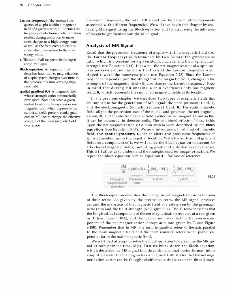
76 Chapter Four
Larmor frequency The resonant frequency of a spin within a magnetic field of a given strength. It defines the frequency of electromagnetic radiation needed during excitation to make spins change to a high-energy state, as well as the frequency emitted by spins when they return to the low-energy state.
B The sum of all magnetic fields experienced by a spin.
Bloch equation An equation that describes how the net magnetization of a spin system changes over time in the presence of a time-varying magnetic field.
spatial gradient (G) A magnetic field whose strength varies systematically over space. Note that since a given spatial location only experiences one magnetic field, which represents the sum of all fields present, spatial gradients in MRI act to change the effective strength of the main magnetic field over space.
precession frequency, the total MR signal can be parsed into components associated w i t h different frequencies. We w i l l thus begin this chapter by analyzing MR signal using the Bloch equation and by discussing the influence of magnetic gradients upon the MR signal.
Analysis of MR Signal
Recall that the precession frequency of a spin w i t h i n a magnetic field (i.e., the Larmor frequency) is determined by t w o factors: the gyromagnetic ratio, which is a constant for a given atomic nucleus, and the magnetic field strength (see Equation 3.14). Likewise, the net magnetization of a spin system precesses around the main field axis at the Larmor frequency when t ipped toward the transverse plane (see Equation 3.28). Since the Larmor frequency depends upon the strength of the magnetic f ield, changes in the strength of the magnetic field w i l l also change the Larmor frequency. Keep in mind that d u r i n g MR imaging, a spin experiences only one magnetic field, B, which represents the sum of all magnetic fields at its location.
In the previous chapter, we described t w o types of magnetic fields that are important for the generation of MR signal: the static (or main) field, B0, and the electromagnetic (or radiofrequency) f ield, B1. The static magnetic field aligns the precession axes of the nuclei and generates the net magnetization, M, and the electromagnetic field excites the net magnetization so that it can be measured in detector coils. The combined effects of these fields upon the net magnetization of a spin system were described by the Bloch equation (see Equation 3.47). We now introduce a third k ind of magnetic field, the spatial gradient, G, which alters the precession frequencies of spins dependent upon their spatial location. With the addition of gradient fields as a component of B, we w i l l solve the Bloch equation to account for all external magnetic fields, including gradient fields that vary over space. This w i l l allow us to understand the strategies used for image formation. We repeat the Bloch equation here as Equation 4.1 for ease of reference:
[4.1]
The Bloch equation describes the change in net magnetization as the sum of three terms. As given by the precession term, the MR signal precesses around the main axis of the magnetic field at a rate given by the gyromagnetic ratio and the field strength (see Figure 3.11). The T1 term indicates that the longitudinal component of the net magnetization recovers at a rate given by T1 (see Figure 3.18A), and the T2 term indicates that the transverse component of the net magnetization decays at a rate given by T 2 (see Figure 3.18B). Remember that in MR, the term longitudinal refers to the axis parallel to the main magnetic field and the term transverse refers to the plane perpendicular to the main magnetic field.
We w i l l next attempt to solve the Bloch equation to determine the MR signal at each point in time, M(t ) . First we break d o w n the Bloch equation, which describes the MR signal in a three-dimensional vector format, into a simplified scalar form along each axis. Figure 4.1 illustrates that the net magnetization vector can be thought of either as a single vector in three dimen-

Basic Principles of MR Image Formation 77
Figure 4.1 The net magnetization vector and its axis projections. While the net magnetization, M, of a sample can be represented as a single vector (shown in blue), it also can be described by a set of three vectors: M x , My' and Mz'
By convention, the z-axis is parallel to the main magnetic field and is known as the longitudinal axis. The x-y plane is perpendicular to the main magnetic field and is known as the transverse plane.
So, Equations 4.2a and 4.2b describe the changes in the x- and y-directions of the magnetization over time, as the spin precesses about the main axis. The time constant T2 specifies the rate of decay of magnetization in the transverse plane defined by the x- and y-axes, but it has no effect upon the longitudinal magnetization along the z-axis. Equation 4.2c describes the change in the longitudinal magnetization over time, as it recovers at a rate specified by T1.
Longitudinal Magnetization (Mz) The longitudinal magnetization depends only on a single equation (4.2c), which is a first-order ordinary differential equation. Thus, its solution is an exponential recovery function that describes the return of the main magnetization to the original state. Equation 4.3 replaces dMz/dt wi th a mathematical equivalent, d(Mz - M0)/dt, that represents the change in longitudinal magnetization from the ful ly relaxed state, M0:
sions or as a set of three vectors along each of the three cardinal axes. To represent the Bloch equation in scalar form, we need to isolate changes along each axis. Note that the behavior of the net magnetization in the x- and y-axes depends on both the precession term and the T 2 term. In contrast, the change in magnetization in the z-axis depends only on the T1 term. Considering the axes separately, we can rearrange Equation 4.1:
[4.2a]
[4.2b]
[4.2c]
[4.3]

78 Chapter Four
as shown in Figure 4.2C. This equation is important for determining the imaging parameters for T 1-contrast images. For example, by choosing when to acquire an image, we can make that image more or less sensitive to T1 dif-
Figure 4.2 The change in longitudinal magnetization over time is known as T1 recovery. When fully recovered (A), the longitudinal magnetization is at its maximum value, as shown by the dotted line, and does not change over time. However, following an excitation pulse that tips the net magnetization into the transverse plane, there will be zero longitudinal magnetization (B). As time passes following excitation, the longitudinal magnetization recovers toward its maximum value (C). The time constant T1 governs this recovery process.
To illustrate T1 recovery, let us consider some extreme values for the initial magnetization, M z 0 . Consider when the net magnetization is fully relaxed (Figure 4.2A). Here, M z 0 is equal to M 0, and the term (M z 0 - M 0) wil l therefore be zero. Once the net magnetization is fu l ly relaxed, it does not change over time, as indicated by the horizontal line segment. However, after an excitation pulse is applied (Figure 4.2B), the net magnetization is tipped entirely into the transverse plane and the net longitudinal magnetization is zero. The subsequent recovery of longitudinal magnetization is given by:
[4.7]
If we assume that the initial magnetization at time zero is given by M z 0, the solution for Mz at a later time point (t) is given by Equation 4.6. This equation states that the longitudinal magnetization (M z ) is equal to the fully relaxed magnetization, plus the difference between the initial and fully relaxed magnetization states, mult ipl ied by an exponential time constant. Note that since Mz 0 is always less than M0, the exponential term describes how much longitudinal magnetization is lost at a given point in time. As t increases, more longitudinal magnetization is recovered and the signal Mz approaches the fully relaxed signal M 0 :
[4.6]
Swapping sides for dt and Mz - M0, we get:
[4.4]
[4.5]
By integrating both sides of this equation, we obtain Equation 4.5. This equation states that the natural log of the change in longitudinal magnetization over time (0 to t') is equal to the change in time divided by the constant T1:

Basic Principles of MR Image Formation 79
ferences between tissues. The details of pulse sequences used for T1 contrast
generation are further discussed in Chapter 5.
Solution for Transverse Magnetization (M x y )
The solution for the transverse magnetization is complicated by the fact that
we must now consider the plane defined by two axes, x and y. Equations
4.2a and 4.2b reorganize the Bloch equation, treating the precession term as
onedimensional projections along the x and yaxes of an object undergoing
circular motion and the T, term as a decay factor (Figure 4.3). Solving for Mx
and My given an initial magnetization of ( M 0 , 0), we get the fo l lowing
equation pair:
Figure 4.3 the change in transverse magnetization over time (t). The magnetism in the transverse plane is a vector defined by its angle and magnitude. As time passes, its angle follows a circular motion with constant angular velocity ω, while its magnitude decays with time constant T 2. These two components combine to form the inward spiral path shown (dashed lines). Shown at the top and right sides of the spiral path are its projections onto the x and y¬axes, respectively. Within each axis, the projection of the transverse magnetization is a onedimensional oscillation, as illustrated by the blue and green lines. This oscillation is shown over time at the bottom of the figure, which illustrates the decaying MR signal.
Though these equations appear complex, each describes two components
that are illustrated in Figure 4.3. The parenthetical term (e.g., M0 cos cot)
describes a onedimensional projection of circular motion w i t h constant
velocity. The exponential term (i.e., et/T2) describes the decay of the circle
over time. Together, they form an inward spiral pattern. As time (t) increases,
the transverse magnetization w i l l spiral farther inward and more and more
transverse signal wi l l be lost. The constant T2 determines the rate at which the
[4.8a]
[4.8b]
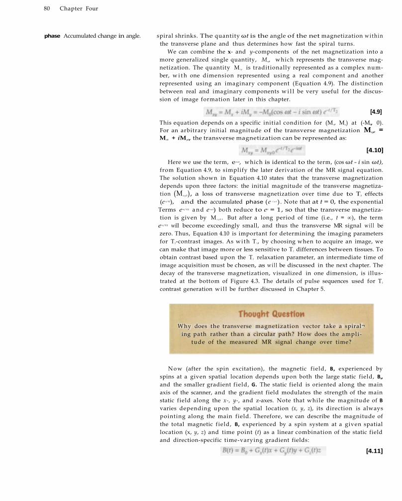
80 Chapter Four
phase Accumulated change in angle. spiral shrinks. The quantity ωt is the angle of the net magnetization w i t h i n
the transverse plane and thus determines how fast the spiral turns.
We can combine the x and ycomponents of the net magnetization into a
more generalized single quantity, Mxy, which represents the transverse mag
netization. The quantity Mx y is traditionally represented as a complex num
ber, w i t h one dimension represented using a real component and another
represented using an imaginary component (Equation 4.9). The distinction
between real and imaginary components w i l l be very useful for the discus
sion of image formation later in this chapter.
N o w (after the spin excitation), the magnetic f ield, B, experienced by
spins at a given spatial location depends upon both the large static field, B0,
and the smaller gradient f ield, G. The static field is oriented along the main
axis of the scanner, and the gradient field modulates the strength of the main
static field along the x, y-, and zaxes. Note that while the magnitude of B
varies depending upon the spatial location (x, y, z), its direction is always
pointing along the main field. Therefore, we can describe the magnitude of
the total magnetic f ield, B, experienced by a spin system at a given spatial
location (x, y, z) and time point (t) as a linear combination of the static field
and directionspecific timevarying gradient fields:
Here we use the term, eiωt, which is identical to the term, (cos ωt i sin ωt),
from Equation 4.9, to simplify the later derivation of the MR signal equation.
The solution shown in Equation 4.10 states that the transverse magnetization
depends upon three factors: the initial magnitude of the transverse magnetiza
tion (M x y 0), a loss of transverse magnetization over time due to T2 effects
(et/T2), and the accumulated phase (e i ω t ) . Note that at t = 0, the exponential
Terms et/T2 a n d eiωt) both reduce to e0 = 1, so that the transverse magnetiza
tion is given by M x y 0 . But after a long period of time (i.e., t = ∞), the term
et/T2 will become exceedingly small, and thus the transverse MR signal wi l l be
zero. Thus, Equation 4.10 is important for determining the imaging parameters
for T2contrast images. As wi th T 1, by choosing when to acquire an image, we
can make that image more or less sensitive to T2 differences between tissues. To
obtain contrast based upon the T2 relaxation parameter, an intermediate time of
image acquisition must be chosen, as w i l l be discussed in the next chapter. The
decay of the transverse magnetization, visualized in one dimension, is illus
trated at the bottom of Figure 4.3. The details of pulse sequences used for T2
contrast generation wi l l be further discussed in Chapter 5.
This equation depends on a specific initial condition for (Mx, My) at (M0, 0).
For an arbitrary init ial magnitude of the transverse magnetization Mxy0 = Mx0 + iMy0, the transverse magnetization can be represented as:
[4.9]
[4.10]
[4.11]
Why does the transverse magnetizat ion vector take a spiral¬
ing path rather than a circular path? How does the ampli
tude of the measured MR signal change over time?

Basic Principles of MR Image Formation 81
Note that this last factor is indicated as an integral over time because gradi
ents may change over time in some forms of MRI . If a constant gradient
along one direction were used (e.g., G along the xdirection), the accumu
lated phase it causes could be more simply described as γG x t .
Let us pause for a moment to review what we have learned so far. We
know that the net magnetization of a sample w i t h i n a magnetic field can be
thought of as a vector w i t h magnitude and direction. The net magnetization
vector can be broken down into longitudinal (along the static magnetic field)
and transverse (perpendicular to the static magnetic field) components.
After the net magnetization is tipped toward the transverse plane by an exci
tation pulse, it precesses around the longitudinal axis at the Larmor fre
quency. The precession of the net magnetization in the transverse plane
allows measurement of MR signal. We also have just learned that the intro
duction of a spatial magnetic gradient alters the transverse magnetization
over time because the frequency of precession depends upon the local mag
netic field strength. This last point suggests that spatial gradients may allow
encoding of spatial information w i t h i n the MR signal. We explore this possi
bility in the next section.
The MR Signal Equation
MRI does not use separate receiving antennae for individual voxels. Indeed,
such a setup would be impossible given that there may be 100,000 or more
voxels w i t h i n a single imaging volume. We use instead a single antenna
(e.g., a volume coil) that covers a large region. The MR signal measured by
the antenna reflects the sum of the transverse magnetizations of all voxels
wi th in the excited sample. We emphasize this important point because it
underlies all of the principles of image formation discussed later in this
chapter: The total signal measured in MRI combines the changes in net mag
netization generated at every excited voxel. This can be restated in the for
mal mathematical terms of Equation 4.13, which expresses the MR signal at
a given point in time, S ( f ) , as the spatial summation of the MR signal from
every voxel:
[4.13]
MR signal The current measured in a detector coil following excitation and reception.
Knowing that ω = γB, we can substitute the ω term in Equation 4.10 using
the magnitude of the total magnetic field described in Equation 4.11 and get
the fol lowing rather intimidating equation. Here we have split the exponen
tial eiωt into separate terms that describe the accumulated phase caused by
the strength of the static magnetic field (B0) and by the timevarying gradi
ent fields (Gx(t), G y(t), Gz(t)):
Again, although this equation has many components and seems complex,
it can be broken down into simpler and more understandable parts. It states
that the transverse magnetization for a given spatial location and time point,
Mxy(x, y, z, t), is governed by four factors: (1) the original magnetization at
that spatial location, Mxy0(x, y, z); (2) the signal loss due to T 2 effects, e t / T 2 ;
(3) the accumulated phase due to the main magnetic f ield, et/T2; and (4) the
accumulated phase due to the gradient fields:
[4.12]

82 Chapter Four
MR signal equat ion A single equation
that describes the obtained MR signal
as a function of the properties of the
object being imaged under a spatially
varying magnetic field.
slice A single slab of an imaging volume.
A slice has thickness defined by the
strength of the gradient and the band
width of the electromagnetic pulse
used to select it.
Equation 4.14 can be read as stating that the total MR signal measured at any
point in time reflects the sum across all voxels of the net magnetization at
time point zero, mult ipl ied by a decay factor based upon T 2 , w i t h accumu
lated phase given by the strength of the static magnetic field and of the gra
dient field at that point in space. This vastly important equation is known as
the MR signal equat ion , because it reveals the relationship between the
acquired signal, S ( f ) , and the properties of the object being imaged, M(x,y,z).
It is important to recognize that this equation is sufficiently general to
describe the MR signal in virtual ly all imaging methods.
In practice, the term e - i w 0 t is not necessary for calculation of MR signal,
because modern MRI scanners demodulate the detected signal w i t h the res
onance frequency ω0. That is, they synchronize data acquisition to the reso
nance frequency. This demodulation process is analogous to the idea of
transformation from laboratory to rotating reference frames, as introduced
in Chapter 3. Imagine that you were watching the precession of the trans
verse magnetization from the laboratory (i.e., normal) reference frame. You
w o u l d see the transverse magnetization spinning around the longitudinal
axis at the Larmor frequency. N o w imagine that you were rotating around
the longitudinal axis at the same speed as the precessing magnetization. The
magnetization vector would now appear to be still.
The T 2 decay term, e - t / T 2, affects the magnitude of the signal but not its
spatial location. Because it does not contain any spatial information, we can
ignore it for the moment. By removing these t w o terms, we arrive at a sim
pler version of the MR signal equation:
Combining Equations 4.12 and 4.13 results in Equation 4.14:
[4.14]
[4.15]
This equation illustrates the profound importance of the gradient fields for
encoding spatial information within an MR image. In principle, we can collect
a single MR image of an entire volume by systematically turning on gradient
fields along x, y, and z. However, because threedimensional (3D) imaging
sequences present additional technical challenges and are less tolerant of hard
ware imperfection, most forms of imaging relevant to fMRI studies use two
dimensional (2D) imaging sequences. For the sake of simplicity, we w i l l next
discuss the principles underlying common 2D imaging techniques. We w i l l
return to the less common 3D imaging techniques at the end of this chapter.
Slice Selection, Spatial Encoding, and Image Reconstruction
Note that the simplified MR signal equation (see Equation 4.15) is still in 3D
form, in that the signal contribution from each spatial location depends
upon all three spatial gradients. In order to reduce this signal equation to
two dimensions, there must be some way to eliminate variation over one
spatial dimension. This can be accomplished by separating the signalacqui
sition process into two steps. First we select a particular slice w i t h i n the total
imaging volume using a onedimensional excitation pulse. Then we use a
twodimensional encoding scheme w i t h i n the slice to resolve the spatial dis
tr ibution of the spin magnetizations. This twostep process forms the basis
for most pulse sequences used in MRI , including those used for acquisition

B a s i c P r i n c i p l e s of MR I m a g e F o r m a t i o n 8 3
of fMRI B O L D images. We w i l l discuss the theoretical bases for these steps
in this section, and describe their practical implementation in the fo l lowing
sections.
The basic concept of slice selection is the application of an electromag
netic pulse that excites spins w i t h i n one slice but has no effect on spins out
side the slice. The slice chosen by the selection process is defined by its loca
tion, orientation, and thickness. For example, let us assume that we want to
create an image of a plane centered at z = z0. For a given location (x, y)
within that slice, the total magnetization summed along the zdirection,
M(x,y), for a thickness Δz is given by Equation 4.16. This equation describes
the bulk magnetization of an individual voxel, or xy coordinate pair, w i t h i n
the slice.
[4.16]
Note that since we are integrating all signals along the zdirection, the mag
netization, M, is dependent only on x and y, but not on z. Thus, by first
selecting an imaging slice, the simplif ied MR signal equation (see Equation
4.15) can be further reduced into a 2 D form, as follows:
[4.17]
Equation 4.17 states that the total signal recorded from a slice depends
upon the net magnetization at every (x, y) location wi th in that slice, wi th the
phase of individual voxels dependent upon the strength of the gradient fields
at that location. Although the parts of Equation 4.17 are individual ly under
standable, this equation is difficult to visualize and solve in its present form.
To facilitate a better understanding of the relation between the MR signal,
S(f), and the object to be imaged, M(x,y), MR researchers have adopted a dif
ferent notation scheme known as kspace. Recognize that kspace differs in
an important way from normal image space, in which the object resides. Con
sider the terms kx and ky in Equation 4.18. Each equation represents the time
integral of the appropriate gradient multiplied by the gyromagnetic ratio:
[4.18a]
[4.18b]
These equations state that changes in kspace over time, or kspace trajectories, are given by the time integrals of the gradient waveforms. In other
words, the kspace trajectories are simply the areas under the gradient wave
forms, as illustrated in Figure 4.4 for a uniform gradient change over a time
interval (t). By substituting these terms into Equation 4.17, we can restate the
MR signal equation using kspace coordinates:
slice selection The combined use of a spatial magnetic field gradient and an
electromagnetic pulse to excite spins
within a slice.
kspace A notation scheme used to describe MRI data. The use of kspace
provides mathematical and conceptual
advantages for describing the acquired
MR signal in image form.
kspace trajectory A path through k
space. Different pulse sequences adopt
different kspace trajectories.
Equation 4.19 is remarkable, because it indicates that kspace and image
space have a straightforward relation: they are 2D Fourier transforms of
each other. Any signal that changes over time or space, no matter how com
plex, can be constructed from a series of simpler components in the fre
quency or spatialfrequency domain, respectively (Figure 4.5AC). The
[4 .19]

84 Chapter Four
Figure 4.4 The relation between the gradient waveform and it-space. The effect of a gradient, Gx ' upon a given voxel is expressed as the amplitude of the gradient signal over time. The change in k-space over time is given by the area under the square.
Fourier transform is one mathematical tool for this construction process. The mathematics of the Fourier transform are well established, so we can take advantage of those mathematics to decode the k-space representation of the MR signal, S(t), into the magnetization at each spatial location, M(x, y). creating a spatially informative image. Equation 4.19 suggests that an inverse Fourier transform can convert k-space data into an image, a process known
Figure 4.5 Constructing a complex waveform or image from simpler components. Any data, no matter how complex, can be constructed from simpler components. Shown in (A) are three sine waves, each with a different frequency. When combined, they form the waveform at right. By combining more and more sine waves of different frequencies and phases, very complex waveforms can be created, such as that of music. The same principle holds for two-dimensional data (B), except that here the components are gratings of particular spatial frequencies (i.e., how closely spaced are the bars), phases, and angles. By combining a very large number of these gratings, complex images can be created, such as those used in MRI. Shown in (C) is the k-space plot of the summed image; the individual gratings are associated with the three bright pixels.

B a s i c P r i n c i p l e s o f MR I m a g e F o r m a t i o n 8 5
Figure 4.6 Images and their Fourier transforms. (A) A single circle at the center of the image space and the representation of the circle in k-space. Note that the k:-space representation follows a sine function, with greatest intensity at the center and intensity bands of decreasing amplitude toward the edges of the k-space. Addition of a second circle to the image space (B) introduces a grating pattern to the k-space. An image of the brain (C) contains much more spatial information, and thus its representation in k-space is similarly more complex.
as image reconstruction. Conversely, a forward Fourier transform can convert image-space data into it-Space data.
To illustrate the relation between image space and k-space, Figure 4.6 shows some sample images and the resulting Fourier transforms. Think of each pair as showing an object and the acquired MR signal in its raw form within k-space. An image wi th a single circle at its center corresponds to a pattern of alternating light and dark circles throughout k-space (Figure 4.6A). As an aside, this pattern is equivalent to a 2-D Bessel sine function. Note that the center of k-space represents the point in time when signal from all voxels is at the same phase, so it represents the total transverse magnetization w i t h i n that slice. Thus, the center of k-space always has the highest signal of any point.
We can add a second circle to the image to illustrate another concept, that K-space reflects the spatial frequency of the object(s) in the image space. Spatial frequency defines how often some pattern occurs in space, just like temporal frequency (e.g., musical pitch) defines how often something occurs in time. Shown in Figure 4.6B are two circles, one offset from center. If we trace a line from the top left to the bottom right of the image, it w i l l encounter two circles separated by a distance between their centers. The k-space data w i l l thus have a spatial-frequency component along that line, w i t h frequency equal to the inverse of that distance. This is visible as a grating running from top left to bottom right in the k-space image, on top of the concentric pattern that results from the shape of the circles.
image reconstruction The process by which raw MR signal, as acquired in it-space form, is converted into spatially informative images.
spatial frequency The frequency with which some pattern occurs over space.
Any image, no matter how complex, can be represented as an ensemble of spatial-frequency components. The k-space representation of an anatomical image is shown in Figure 4.6C. The k-space image is brightest in the center and darkest near the edges. This illustrates that low-spatial-frequency data from near the center of k-space is most important for determining the
How w o u l d the k-space data in Figure 4.6B change if the lower circle were moved to the bot tom- le f t quadrant of the mage? How w o u l d the k-space data change if it were moved
farther t o w a r d the b o t t o m - r i g h t corner?

86 Chapter Four
signal-to-noise ratio of the image. In comparison, high-spatial-frequency data collected at the periphery of k-space helps to increase the spatial resolution of the image. Figure 4.7 illustrates this important distinction between the low-spatial-frequency and high-spatial-frequency regions of k-space. If from a normal photograph (Figure 4.7A) we take only the low-spatial-frequency region of its k-space data, the image would have most of the signal but would lack good spatial resolution (Figure 4.7B). But if we take only the high-spatial-frequency region of its k-space data, the image would have a low signal level but the spatial detail would be preserved (Figure 4.7C).
Contrary to intuit ion, there is not a one-to-one relation between points in k-space and voxels in image space. For an illustration of what each point in k-space represents, consider Figure 4.8. The center plot shows the k-space data (or raw MR signal). Each point in the k-space data is acquired at a different point in time and has contributions from all voxels w i t h i n the slice. We have highlighted four sample k-space points, each showing the net magnetization vectors w i t h i n each voxel (in image space) at the moment in time when that point in k-space was acquired. For the point at the center of k-space (Figure 4.8A), all of the magnetization vectors are at the same phase, and thus the total signal is at its maximum. At other k-space points (Figure 4.8B-D), the magnetization vectors differ across voxels, and the intensity of
Figure 4.7 How different parts of k-space contribute to image space. Images such as this photograph of Dr. Seiji Ogawa can be converted using a Fourier transform into k-space data (A). Different parts of the k-space data correspond to different spatial-frequency components of the image. The center of k-space (B) provides low-spatial-frequency information, retaining most of the signal but not fine details. The periphery of k-space (C) provides high-spatial-frequency information, and thus image detail, but contributes relatively little signal to the image.
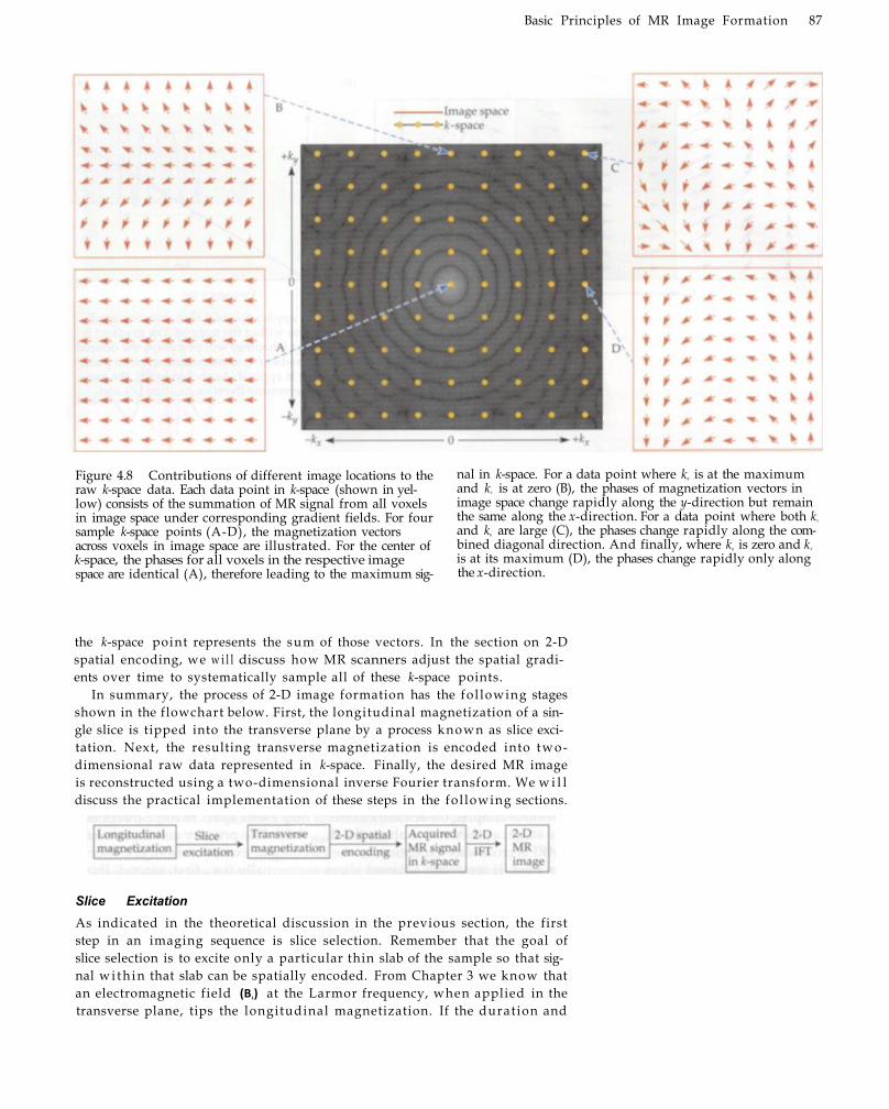
Basic Principles of MR Image Formation 87
Figure 4.8 Contributions of different image locations to the raw k-space data. Each data point in k-space (shown in yellow) consists of the summation of MR signal from all voxels in image space under corresponding gradient fields. For four sample k-space points (A-D), the magnetization vectors across voxels in image space are illustrated. For the center of k-space, the phases for all voxels in the respective image space are identical (A), therefore leading to the maximum sig
nal in k-space. For a data point where ky is at the maximum and kx is at zero (B), the phases of magnetization vectors in image space change rapidly along the y-direction but remain the same along the x-direction. For a data point where both kx
and ky are large (C), the phases change rapidly along the combined diagonal direction. And finally, where ky is zero and kx
is at its maximum (D), the phases change rapidly only along the x-direction.
the k-space point represents the sum of those vectors. In the section on 2-D spatial encoding, we w i l l discuss how MR scanners adjust the spatial gradients over time to systematically sample all of these k-space points.
In summary, the process of 2-D image formation has the fol lowing stages shown in the flowchart below. First, the longitudinal magnetization of a single slice is tipped into the transverse plane by a process known as slice excitation. Next, the resulting transverse magnetization is encoded into two-dimensional raw data represented in k-space. Finally, the desired MR image is reconstructed using a two-dimensional inverse Fourier transform. We w i l l discuss the practical implementation of these steps in the fol lowing sections.
Slice Excitation As indicated in the theoretical discussion in the previous section, the first step in an imaging sequence is slice selection. Remember that the goal of slice selection is to excite only a particular thin slab of the sample so that signal w i t h i n that slab can be spatially encoded. From Chapter 3 we know that an electromagnetic field (B1) at the Larmor frequency, when applied in the transverse plane, tips the longitudinal magnetization. If the durat ion and

88 Chapter Four
Figure 4.9 Slice selection. As shown in (A), application of a slice selection gradient (Gz) changes the Larmor frequency of spins within the sample. The gradient is chosen so that spins within the slice of interest (shading) will precess at the desired frequency. Following the application of the gradient, a subsequent excitation pulse at a given frequency (w) and bandwidth (Δw) is applied. As shown in (B), the excitation frequency and frequency bandwidth determine the slice location (Z) and slice thickness (ΔZ).
interleaved slice acquisition The collection of data in an alternating order, so that data is first acquired from the oddnumbered slices and then from the evennumbered slices, to minimize the influence of excitation pulses upon adjacent slices.
strength of the electromagnetic field are appropriately calibrated, the longi
tudinal magnetization w i l l rotate exactly into the transverse plane. Such a
calibrated electromagnetic field is k n o w n as an excitation pulse. But if the
magnetic field were uniform, the applied excitation pulse would affect all of
the spins w i t h i n the volume. However, by introducing a static gradient
along the slice selection axis (e.g., G z), we can tune the Larmor frequencies of
all spins in the slice (and only spins in the slice) to match the frequency of
the excitation pulse (Figure 4.9A and B).
ideally, we w o u l d like to excite a perfectly rectangular slice along the Z-
direction; for example, we might excite all spins from z = +10 mm to z = +15
mm and no spins outside of that range. One might think that this could be
achieved by a rectangular slice selection pulse, as shown in Figure 4.10A.
However, a rectangular pulse actually contains a distribution of frequencies
shaped like a sine function, so it does not excite a rectangular slice. Instead,
we must use a sincmodulated electromagnetic pulse (Figure 4.10B). Since
the Fourier transform of a sine function is a rectangular function, a sinc
modulated pulse has a rectangular frequency response; thus it contains all
frequencies w i t h i n a band and no frequencies outside that band.
Although a perfectly rectangular slice profile would be optimal, it is dif
f icult to achieve because of offresonance excitation. As discussed in the
previous chapter, offresonance effects may excite spins to some intermedi
ate stage, as they rotate about the B 1 e f f f ield. The primary consequence for
fMRI is crossslice excitation, or the bleeding of excitation from one slice to
the next. If we excite adjacent slices sequentially (i.e., first, second, th i rd ,
etc.), each slice w i l l have been preexcited by the previous excitation pulse,
leading to saturation of the MR signal. To minimize this problem, most
excitation schemes use inter leaved slice acquisi t ion. For example, if we
are to excite ten contiguous slices, we w i l l excite in order the first, th i rd ,
f i f th, seventh, ninth, second, fourth, sixth, eighth, and tenth slices. The use
of interleaved slice acquisition effectively eliminates excitation overlap
problems.

B a s i c P r i n c i p l e s of MR I m a g e F o r m a t i o n 8 9
Figure 4.10 Possible slice selection pulses. (A) A rectangular slice selection pulse that consists of a constant application of a radiofrequency field at frequency w0 for a time t. The slice selection profile of this pulse is given by its Fourier transform (FT) and shown at right as a sin function with fundamental frequency w0. This profile is not ideal for selection of a rectangular slice. However, (B) shows the use of a pulse with time amplitude given by a sinc function. This pulse gives a rectangular frequency profile and allows excitation of spins within a rectangular slice.
Slice location and thickness are determined by three factors: the center
frequency of the excitation pulse (w), the bandwidth of the excitation field
(Δw, and the strength of the gradient field (G z), as illustrated in Figure 4.11.
Together, the center frequency and the gradient field determine the slice
location, whi le the bandwidth and the gradient field determine the slice
thickness. By sl iding the center frequency up and d o w n over successive
acquisitions, MR signal f rom different slices can be selectively acquired.
Likewise, by choosing a wide or narrow excitation bandwidth, thick or thin
slices can be collected. Note that use of a stronger gradient, in principle,
means that spins at nearby spatial locations w i l l have greater differences in
their Larmor frequencies, al lowing moreselective excitation by a given elec
tromagnetic pulse. Thus, stronger gradients increase spatial resolution
across slices.
Assume that we doubled the strength of the gradient fields in our scanner. How would the frequency and bandwidth of the excitation pulse need to change to keep the same
slice selection?

90 Chapter Four
Figure 4.11 Changing slice thickness and location. (A) The combined use of a linear gradient (solid line) and a radiofrequency pulse with a center frequency (w) and bandwidth (Aw) to select a slice location (horizontal axis). By changing the slope of the gradient (B), the same radiofrequency pulse can be used to select a slice with a different location and thickness. (C) By changing the center frequency of the excitation pulse to w', the same gradient can be used to select a different slice location.
filling k-space The process of collecting samples from throughout k-space in order to collect data sufficient for image formation.
2-D Spatial Encoding Once spins are excited wi th in the desired slice, they can be spatially encoded so that MR signal from different parts of the image can be resolved. A unique frequency is assigned to all voxels w i t h i n the slice, in a process known as frequency and phase encoding, to facilitate later reconstruction of the signal using the Fourier transform. To do this, a gradient magnetic field that differs across two dimensions (e.g., Cx, Gy) is applied to the sample. These gradients influence the individual spin phases for different voxels, as illustrated in Figure 4.12. To understand how the scanner hardware and software accomplish the encoding process, we must return to the concept of k-space. As we learned earlier in this chapter, if we reorganize signal S(t) to S(kx(t), ky{t)) as indicated in Equation 4.19, then the MR signal can be represented by a 2-D function in a coordinate system where kx and ky are the two axes. This coordinate system defines k-space and has units in spatial frequency (1/distance). Because a complete sample of the k-space is usually required to construct an image, collecting the MR signal is often referred to as f i l l ing k-space.
Remember from Figure 4.4 that kx and ky are actually time integrals of the gradient waveform. Thus, by manipulating the gradient waveforms, we can

Basic Principles of MR Image Formation 91
Figure 4.12 Effects of magnetic field gradients on spin phase. Application of magnetic field gradients influences the frequency of spins over space, and thus the accumulated phase over time. Shown are examples of gradients in the x- and y-directions.
control the sampling path w i t h i n k-space during MR signal acquisition. For example, by altering the strength of different gradients over time, we could first collect data from the upper-left point in k-space, and then move right-ward, and then downward, and then leftward, etc., tracing a snakelike path throughout the image. While any path that covers all of k-space can be used to collect the k-space data, in practice regular paths such as straight lines are preferred.
In typical anatomical imaging sequences (Figure 4.13A), k-space is fil led one line at a time, fo l lowing a succession of individual excitation pulses. During each excitation the combination of the electromagnetic pulse and the Gz gradient selects the desired slice. Then the Gy gradient is turned on before the data acquisition period, so that it accumulates a certain amount of phase offset before the activation of the Gx gradient. This results in the movement
Figure 4.13 A typical two-dimensional gradient-echo pulse sequence. Shown in (A) are lines representing activity of the radiofrequency field (RF) and the three spatial gradients. The pulse sequence begins with a combined slice selection gradient (Gz) and excitation pulse. The Gy gradient is used for selecting one line of k-space following each excitation pulse, while the Gx gradient is turned on during data acquisition (DAQ). This sequence is known as a gradient-echo sequence, and it acquires each line of k-space following a separate excitation (B). Following n excitations, all of k-space is filled and image acquisition is complete.
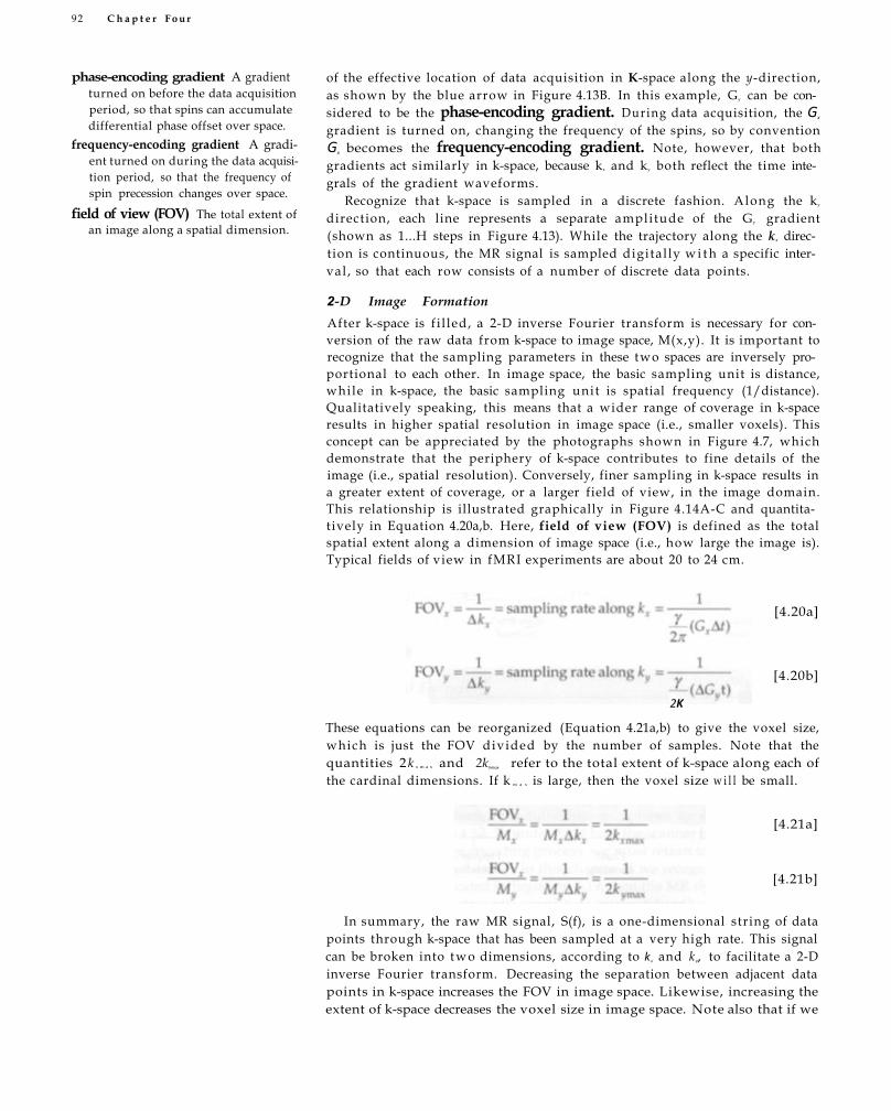
92 C h a p t e r F o u r
phase-encoding gradient A gradient turned on before the data acquisition period, so that spins can accumulate differential phase offset over space.
frequency-encoding gradient A gradient turned on during the data acquisition period, so that the frequency of spin precession changes over space.
field of view (FOV) The total extent of an image along a spatial dimension.
of the effective location of data acquisition in K-space along the y-direction, as shown by the blue arrow in Figure 4.13B. In this example, Gy can be considered to be the phase-encoding gradient. During data acquisition, the Gx
gradient is turned on, changing the frequency of the spins, so by convention Gx becomes the frequency-encoding gradient. Note, however, that both gradients act similarly in k-space, because kx and ky both reflect the time integrals of the gradient waveforms.
Recognize that k-space is sampled in a discrete fashion. Along the ky
direction, each line represents a separate amplitude of the Gy gradient (shown as 1...H steps in Figure 4.13). While the trajectory along the kx direction is continuous, the MR signal is sampled digital ly w i t h a specific interval , so that each row consists of a number of discrete data points.
2-D Image Formation
After k-space is f i l led, a 2-D inverse Fourier transform is necessary for conversion of the raw data from k-space to image space, M(x,y). It is important to recognize that the sampling parameters in these two spaces are inversely proportional to each other. In image space, the basic sampling unit is distance, while in k-space, the basic sampling unit is spatial frequency (1/distance). Qualitatively speaking, this means that a wider range of coverage in k-space results in higher spatial resolution in image space (i.e., smaller voxels). This concept can be appreciated by the photographs shown in Figure 4.7, which demonstrate that the periphery of k-space contributes to fine details of the image (i.e., spatial resolution). Conversely, finer sampling in k-space results in a greater extent of coverage, or a larger field of view, in the image domain. This relationship is illustrated graphically in Figure 4.14A-C and quantitatively in Equation 4.20a,b. Here, field of view (FOV) is defined as the total spatial extent along a dimension of image space (i.e., how large the image is). Typical fields of view in fMRI experiments are about 20 to 24 cm.
[4.20a]
2K
[4.20b]
These equations can be reorganized (Equation 4.21a,b) to give the voxel size, which is just the FOV divided by the number of samples. Note that the quantities 2 k x m a x and 2kymax refer to the total extent of k-space along each of the cardinal dimensions. If k m a x is large, then the voxel size w i l l be small.
[4.21a]
[4.21b]
In summary, the raw MR signal, S(f), is a one-dimensional string of data points through k-space that has been sampled at a very high rate. This signal can be broken into t w o dimensions, according to k x and ky, to facilitate a 2-D inverse Fourier transform. Decreasing the separation between adjacent data points in k-space increases the FOV in image space. Likewise, increasing the extent of k-space decreases the voxel size in image space. Note also that if we

Basic Principles of MR Image Formation 93
Figure 4.14 Effects of sampling in k-space upon the resulting images. Field of view and resolution have an inverse relation when applied to image space and k-space. (A) A schematic representation of densely sampled k-space with a wide field of view, resulting in the high-resolution image (D). (B) If only the center of k-space is sampled, albeit with the same sam
pling density, then the resulting image (E) has the same field of view but lower spatial resolution. (C) Conversely, if k-space is sampled across a wide field of view but with a limited sampling rate, the resulting image will have a small field of view but high resolution (F).
want to collect N x N voxels wor th of data in our image, then we need an equal number of k-space data points (N x N).
3-D Imaging
While 2-D imaging methods are common for most applications, not all MR imaging techniques are based on 2-D principles. Pulse sequences that collect k-space data in three dimensions are often used, especially for high-resolution anatomical images. Compared w i t h 2-D imaging, 3-D sequences provide the primary advantage of a high signal-to-noise ratio, due to the fact that the 3-D volume can be larger than a single slice and therefore more excited spins can contribute to the MR signal. The principles of 3-D imaging can be easily extrapolated from those of 2-D imaging, so in theory any 2-D imaging sequence can be converted to 3-D. Since slice selection is unnecessary, the traditional slice excitation step is replaced by a volume excitation step that uses a very small z-gradient to select a thick slab. To resolve spatial

94 Chapter Four
information along the zdirection, another phaseencoding gradient is pre
sented along that dimension dur ing the data acquisition phase. Therefore,
w i t h i n a typical 3D pulse sequence, there are two phaseencoding gradients
and one frequencyencoding gradient.
The concept of kspace can be expanded to three dimensions by adding kz'
defined by the time integral of the Gz gradient. To reconstruct the 3D
images, an inverse Fourier transform in three dimensions is executed. The
fol lowing flowchart summarizes the steps of 3D imaging:
Unfortunately, the advantages of 3D sequences are accompanied by sev
eral disadvantages. For example, the dimension of phase encoding usually
is more vulnerable to f ield inhomogeneities and motion artifacts than the
dimension of frequency encoding. Because 3D imaging methods have two
phaseencoding dimensions, they are more vulnerable to these artifacts.
Also, more time is required to fi l l kspace when an entire volume is excited
than when only a single slice is excited. Thus, movement of the head at any
point w i t h i n the acquisition w i n d o w w i l l cause distortions throughout the
entire imaging volume. Wi th in fMRI studies, 3D imaging is typically
restricted to anatomical scans, since the major classes of BOLD fMRI pulse
sequences use 2D methods.
Potential Problems in Image Formation
The goal of any image formation method is to achieve a true representation
of the imaged object. Of course, in an ideal scanning environment with a
perfectly uni form main magnetic f ield, exactly linear gradient fields, an
absolutely square excitation profile, and optimized image acquisition soft
ware, there could be no problems! Under such perfect conditions, the
acquired image w i l l exactly match the scanned object in every way. It wi l l be
of the same size and shape, w i t h local intensities dependent on the appro
priate proton density and relaxation characteristics. Yet, as anyone w i t h sub
stantial MRI experience w i l l attest, the images acquired under normal labo
ratory conditions are not always faithful to the original objects. We next
consider some of the typical problems encountered in forming MR images.
The first problem to consider is inhomogeneity of the static magnetic
f ield, meaning that the actual value of the field at one or more spatial loca
tions is not the same as the theoretically desired quantity. Note that inhomo¬
geneity of the static magnetic field across space becomes of increasing con
cern at higher field strengths, because it becomes more diff icult to
adequately shim the field to correct for local distortions. The imperfection in
the static f ield can be mathematically represented by a difference quantity,
ΔB 0 , representing the increased or decreased field strength at a given loca
tion. Equation 4.22 is a modified version of the MR signal equation that con
tains the new term ΔB 0 :
[4.22]
We usually do not know the exact nature of static field inhomogeneities, but
if present they w i l l introduce artifacts to images, fo l lowing conventional

Basic Principles of MR Image Formation 95
Figure 4.15 Spatial and intensity distortions due to magnetic field inhomogeneities. Under a homogeneous magnetic field, the image of a circular phantom is itself circular and of relatively similar intensity throughout (A). Local magnetic field inhomogeneities cause two types of distortions, geometric distortions and signal losses, both of which are visible on the distorted image (B).
inverse Fourier transformation. In practice, ΔB 0 can lead to t w o distinct
types of artifacts: geometric distortions and variations in signal intensity. We
can think of these artifact types, taken roughly, as macroscopic and micro
scopic effects.
Largescale inhomogeneities cause geometric distortions due to spatial
shifting of voxels. Because the frequency of spins depends upon the mag
netic field strength, magnetic field inhomogeneities w i l l lead to changes in
spin frequencies. Remember from earlier in this chapter that the position of
a voxel is encoded by its spin frequency. Thus, a voxel w i t h the incorrect
spin frequency w i l l be displaced to an incorrect spatial location. Smallscale
inhomogeneities cause spins w i t h i n a voxel to lose coherence due to T2*
effects. This reduces the total magnetization available w i t h i n a voxel and
thus reduces its signal intensity. These two effects may be present w i t h i n the
same image (Figure 4.15).
A second problem results f rom nonlinearities of the gradient fields.
Because the spatial gradients control the kspace trajectories, we use kspace
to evaluate their artifacts. Again, we consider a typical gradientecho pulse
sequence. First, if the xgradient Gx is off by a small amount, as shown in
Figure 4.16A, the resulting kspace trajectories w i l l have an error along the
kx direction. Second, if the ygradient Gy is off, the kspace trajectories w i l l be
skewed along the ky direction (Figure 4.16B). Note that this skew affects both
the onset of each line in kspace as well as the path taken through kspace.
The magnitude of this skew depends on the time integral of the gradient
amount. Third, if the zgradient Gz is off, the slope of the excitation gradient
wi l l be altered. Altering the slope of the sliceselection gradient can compro
mise the match between the gradientinduced changes in spin frequency
and the excitation pulse. However, because the kspace trajectory in the xy
plane w o u l d not change, the shape of the object w o u l d not be distorted.
Thus, problems w i t h the G z gradient can lead to changes in slice thickness
and signal intensity (Figure 4.16C).

96 Chapter Four
Figure 4.16 Image distortions caused by gradient problems. Each row shows the ideal image, the problem with acquisition in k-space, and the resulting distorted image. (A) Problems with the x-gradient will affect the length of the trajectory along the x-dimen¬sion in k-space, resulting in an image that appears compressed. (B) Problems with the y-gradient will affect the path taken through k-space over time, resulting in a skewed image. (C) Problems with the z-gradient wil l affect the match of excitation pulse and slice selection gradient, here resulting in a thinner slice and reduced signal intensity.
Summary The net magnetization of a spin system, as described by the Bloch equation, can be broken d o w n into separate spatial components along the x-, y-, and z-axes. By convention, the longitudinal magnetization is defined as Mz
and the transverse magnetization is defined as M x y . The recovery of the longitudinal magnetization fol lowing excitation is governed by the time constant T 1, while the decay of the transverse magnetization following excitation is governed by the time constant T 2 . The total MR signal measured is the combination of the transverse magnetization from all voxels in the sample and can be described using a single equation. The use of spatial gradients is necessary for measurement of spatial properties of a sample, in essence al lowing MR to become MRI . The simultaneous application of a Gz
gradient and an excitation pulse allows selection of a defined slice w i t h i n the imaging volume. The use of two additional gradients w i t h i n the slice allows unique encoding of spatial locations. Image acquisition can be considered using the concept of k-space, which reflects the Fourier transform of image space. Different pulse sequences sample k-space differently, and the inverse relation between sampling in k-space and sampling in image space is important to understand. Inhomogeneities in the magnetic field

Basic Principles of MR Image Formation 97
experienced by spins can cause systematic artifacts in the reconstructed images, in the form of geometric distortions and signal loss.
Suggested Readings
Bracewell, R. N. (1986). The Fourier Transform and Its Applications, McGraw-Hill, New York. A textbook for everything you want to know (and more) about the Fourier transform.
Haacke, E. M., Brown, R. W., Thompson, M. R., and Venkatesan, R. (1999). Magnetic Resonance Imaging: Physical Principles and Sequence Design, John Wiley & Sons, New York. A comprehensive encyclopedia of the theoretical principles of MRI.
Twieg, D. B. (1983). The k-trajectory formulation of the NMR imaging process with applications in analysis and synthesis of imaging methods. Med. Phys., 10(5): 610-621. An original description of the k-space trajectory formulation.

MR Contrast Mechanisms and Pulse Sequences
Compared to other methods for neuroimaging, MRI is extraordinarily versatile. Brain images can be generated to emphasize contrast due to different tissue characteristics. We now extend our previous discussion of contrast to include different contrast mechanisms. Static contrasts are sensitive to the type, number, and relaxation properties of atomic nuclei w i t h i n a voxel. Typical static contrasts include density (e.g., proton density), relaxation time (e.g., T 1, T 2 , T 2*), content of a particular molecular type (e.g., magnetization transfer to detect large or small molecules), and general chemical content (e.g., spectroscopy). We use images based upon static contrast to determine brain anatomy in fMRI experiments. Motion contrasts are sensitive to the movement of atomic nuclei. Typical motion contrasts provide information about the dynamic characteristics of the proton pools in the brain, such as blood f low through MR angiography, water diffusion through dif fusion-weighted imaging, or capillary irrigation through perfusion-weighted imaging. Since nearly all fMRI studies use fast imaging techniques, we w i l l also discuss some of the most common techniques and their pulse sequences in this chapter.
A further distinction can be drawn depending on whether contrast depends on intrinsic properties of biological tissue (i.e., endogenous contrast) or upon the presence of foreign substances that have been introduced into the body (i.e., exogenous contrast). The BOLD-contrast mechanism is an example of an endogenous contrast mechanism, in that it depends upon the amount of deoxygenated hemoglobin w i t h i n a brain region. An example of an exogenous contrast mechanism is the injection of gadolinium-DTPA, a rare earth compound that has extremely high magnetic susceptibility, which greatly distorts the surrounding magnetic field. The use of exogenous contrast agents is a common practice in clinical M R I , but it is less prevalent in functional studies due to the obvious safety issues associated wi th any injections. In the fol lowing sections, we w i l l focus on endogenous contrast measures, especially those commonly used in structural and functional brain imaging. Potentially valuable advances in exogenous contrast agents are considered in later chapters.
static contrasts Contrast mechanisms that are sensitive to the type, number, and relaxation properties of spins (e.g., T 1 , T 2 , proton density).
motion contrasts Contrast mechanisms that are sensitive to the movement of spins through space (e.g., diffusion, perfusion).
endogenous contrast Contrast that depends upon an intrinsic property of biological tissue.
exogenous contrast Contrast that requires the injection of a foreign substance into the body.

100 Chapter Five
repetition time (TR) The time interval between successive excitation pulses, usually expressed in seconds.
This equation illustrates that MR signal depends not only on the original magnetization (which in turn depends upon proton density) but also on the properties of the tissue being imaged, as expressed through both T 1 and T 2
constants (Table 5.1). Shown in this table are rough values for the time con-
Figure 5.1 Changes in longitudinal and transverse components of magnetization. (A) The time constant T1 is usually on the order of 1 s, so recovery of longitudinal magnetization (T1 recovery) occurs over a period of several seconds. (B) The time constant T2 is typically on the order of a few tens of milliseconds, so decay of transverse magnetization occurs over a period of about 100 ms. The values used for T1
and T2 in these plots are similar to those for gray matter at field strengths used for fMRI studies.
There are two important factors that govern the time at which MR images are collected. The first factor is the time interval between successive excitation pulses, which is known as repetition time, or TR. Oftentimes, consecutive excitations occur at time intervals not long enough to allow ful l recovery of the longitudinal magnetization. Under such short TRs, the transverse magnetization, which directly translates to detectable MR signal, should be described as
[5.3]
Equation 5.2 describes the transverse magnetization: [5.1]
[5.2
Static Contrasts and Related Pulse Sequences
Static contrast mechanisms have been widely used for MRI due to their ability to illustrate basic tissue characteristics. To understand how static contrast can be generated, we consider first the simple cases of T 1 and T 2 contrast. As derived in the previous chapters, there are two equations for magnetization after an init ial excitation of a ful ly recovered spin system (Figure 5.1 A and B). Equation 5.1 describes the longitudinal magnetization:

M R C o n t r a s t M e c h a n i s m s a n d P u l s e S e q u e n c e s 101
Proton-Density Contrast One of the simplest forms of MR contrast is proton-density imaging. The net magnetization of each voxel is composed of individual spins w i t h i n that voxel, typically hydrogen (i.e., protons). Proton-density images, as the name implies, provide contrast based on the sheer number of protons in a voxel, which of course differs across tissue types. To maximize proton-density contrast, researchers use pulse sequences that minimize T1 and T2 contrasts. To minimize T1 contrast, a pulse sequence must use either a very short or very long TR, and to minimize T2 contrast, a pulse sequence must use either a very short or very long TE. Logically, either long or short values for either parameter w o u l d work for proton-density weighting. In practice, however, the use of extremely short TR or long TE values results in l i tt le MR signal (see Figure 5.1). To maximize proton-density weighting while still recovering sufficient MR signal, pulse sequences are used that have very long TR
stants T1 and T2 at a field strength of 1.5 T, which is most common for fMRI . These values are only approximate, because these constants can vary according to field homogeneity and other factors, and are intended to serve as a guideline for th inking about the contrast mechanisms discussed in this chapter. Another value of interest is the T 2 * value for gray matter, which is about 40 ms at 1.5 T. This last value determines the TE used for BOLD-con¬trast fMRI images. In Equation 5.3, the term (1 - e - T R / T 1 ) accounts for the incomplete recovery of the longitudinal magnetization. If TR is much longer than T 1, then this term approaches 1 (i.e., fu l l recovery), and it can be removed from the equation.
The second factor is the time interval between excitation and data acquisition (of the center of k-space), which is k n o w n as echo time, or TE. Remember that the MR signal received at the center of k-space has the greatest amplitude, as described in the previous chapter, so at that point it resembles an echo of the initial transmission. We can replace the term t w i t h TE to give the MR signal for an image w i t h a given TE.
Equation 5.4 provides the foundation for manipulating the signal from a particular tissue type by controlling TR and TE. However, in MRI we are interested in comparing MR signal across multiple tissue types. The signal difference between any two types of tissue is known as contrast. For tissue types A and B, the contrast between them, CAB, is simply the difference between the MR signal associated wi th each (Equation 5.5). The terms M0A and M 0 B stand for the original magnetization for tissues A and B, the terms T1 A and T 1 B stand for the values of A and B, and T 2 A and T 2 B stand for the T2 values of A and B.
echo time (TE) The time interval between an excitation pulse and data acquisition (defined as the collection of data from the center of k-space), usually expressed in milliseconds.
proton-density imaging The creation of MR images that are sensitive to the number of protons present within each voxel.

102 Chapter Five
Figure 5.2 Selection of TR and TE values for proton-density contrast. The use of long TR (A) and short TE (B), (shown as vertical dashed lines in orange color) on two different tissues (red and blue), wil l minimize T1 and T 2 effects, leaving only differences in overall signal intensity due to proton density.
gradient-echo (GRE) imaging One of the two primary types of pulse sequences used in MRI; it uses gradients to generate the MR signal changes that are measured at data acquisition.
(Figure 5.2A) and very short TE (Figure 5.2B). Practically, a TR greater than T1 and a TE less than T2 satisfy the criteria. If the TR used is much greater than the T1 values of the tissue being imaged (e.g., 2 to 3 times as long), the protons w i l l be nearly ful ly recovered after each excitation. Likewise, if the TE value is much less than the T 2 value (e.g., 1 / ] 0 as long), there w i l l be minimal decay before image acquisition.
One disadvantage of using a very long TR is greatly increased imaging time. In many situations, such as when scanning patients who have difficulty tolerating lengthy MRI sessions, slow imaging sequences may not be feasible. To reduce acquisition time yet st i l l maintain proton-density contrast, a smaller f l ip angle (<90°) for excitation may be used to only partially t ip the longitudinal magnetization toward the transverse plane, which w i l l in turn require less time to achieve fu l l longitudinal recovery. The effect of using a smaller f l ip angle for partial excitation is illustrated in Figure 5.3, where it can be seen that a shorter TR can be used without introducing significant T 1 weighting, effectively reducing the imaging time. In summary, to generate images sensitive to proton density, we must collect those images using a pulse sequence w i t h a long TR and short TE.
As long as there is sufficient T1 recovery and minimal T2 decay, any type of pulse sequence, including common gradient-echo (GRE) imaging and spin-
How does the concept of proton density relate to the concept of net magnetization?
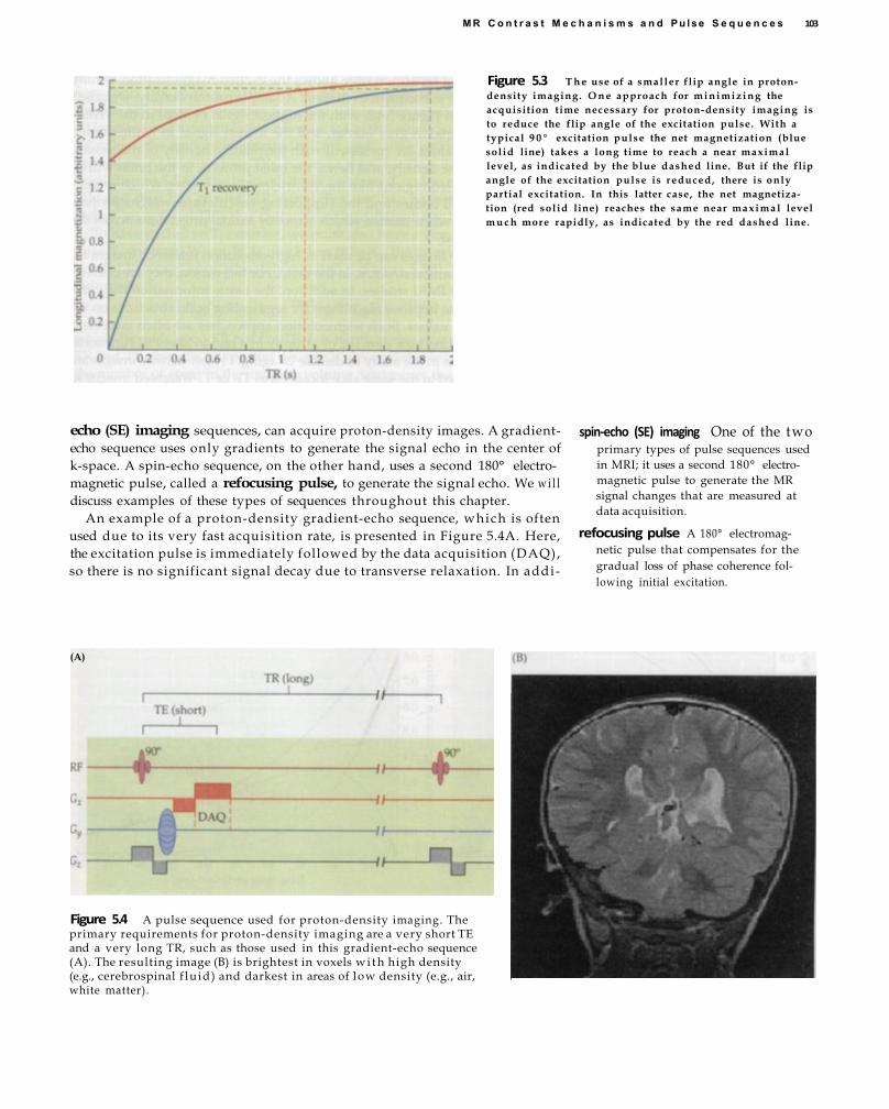
M R C o n t r a s t M e c h a n i s m s a n d P u l s e S e q u e n c e s 103
Figure 5.3 T h e use of a smaller flip angle in proton-density imaging. O n e approach for m i n i m i z i n g the acquisition time necessary for proton-density imaging is to reduce the flip angle of the excitation pulse. With a typical 9 0 ° excitation pulse the net magnetization (blue solid line) takes a long time to reach a near maximal level, as indicated by the blue dashed line. But if the flip angle of the excitation pulse is reduced, there is only partial excitation. In this latter case, the net magnetization (red solid line) reaches the same near m a x i m a l level m u c h more rapidly, as indicated by the red dashed line.
echo (SE) imaging sequences, can acquire proton-density images. A gradient-echo sequence uses only gradients to generate the signal echo in the center of k-space. A spin-echo sequence, on the other hand, uses a second 180° electromagnetic pulse, called a refocusing pulse, to generate the signal echo. We w i l l discuss examples of these types of sequences throughout this chapter.
An example of a proton-density gradient-echo sequence, which is often used due to its very fast acquisition rate, is presented in Figure 5.4A. Here, the excitation pulse is immediately followed by the data acquisition (DAQ), so there is no significant signal decay due to transverse relaxation. In addi-
(A)
Figure 5.4 A pulse sequence used for proton-density imaging. The primary requirements for proton-density imaging are a very short TE and a very long TR, such as those used in this gradient-echo sequence (A). The resulting image (B) is brightest in voxels w i t h high density (e.g., cerebrospinal f luid) and darkest in areas of low density (e.g., air, white matter).
spin-echo (SE) imaging One of the two primary types of pulse sequences used in MRI; it uses a second 180° electromagnetic pulse to generate the MR signal changes that are measured at data acquisition.
refocusing pulse A 180° electromagnetic pulse that compensates for the gradual loss of phase coherence following initial excitation.

104 Chapter Five
T1-weighted (T1-dependent) Images that provide information about the relative T1 values of tissue; also known as T1 images.
tion, the very long repetition time allows the excited magnetization to fully recover before the subsequent excitation. A sample proton density-weighted image is shown in Figure 5.4B, w i t h the highest signal evident in the ventricles, medium signal in gray matter, and the lowest signal in white matter. These intensity values are consistent w i t h the relative density of the tissues. The greatest tissue density, and hence the most protons, in the brain w i l l be found in f luid-f i l led regions like the ventricles. Gray matter, which is composed of both cell bodies and the supporting vasculature, weighs proportionally less, and white matter, which is mostly axonal projections across the brain, weighs least.
Proton-density images can be used as high-resolution reference images for determining anatomical structure in the brain. For this reason, they are often an important part of fMRI studies. In addition, the tissue information they provide can be used to improve algorithms for segmenting brain structures on the basis of intensity values. Such segmentation approaches are often important when understanding how damage or atrophy in a region alters its functional properties, such as in the study of disease or aging. Proton-density images are frequently acquired at the same slice locations as T1- or T 2-weighted images so that complementary anatomical information can be acquired.
7", Contrast While proton-density images have many uses, other forms of contrast emphasize different features of the brain. The most commonly used structural contrast for anatomical images of the brain is T1 weighting. Images are called T1-weighted, or T1-dependent, if the relative signal intensity of voxels within the image depends upon the T1value of the tissue. Figure 5.5 provides
Time since excitation (s) Time since excitation (ms)
Figure 5.5 Selection of TR and TE values for T1 contrast. The use of intermediate TR (A) and short TE (B), (shown as vertical lines in orange color) on two tissues (red and blue lines), will maximize the T1 differences between tissues and minimize the T2 differences between tissues. This combination provides T1 contrast. The green lines show the MR signal based on the T1 and T2 differences, respectively, along time. Green lines show MR signal differences based on the T1 and T2 differences, respectively, along time.
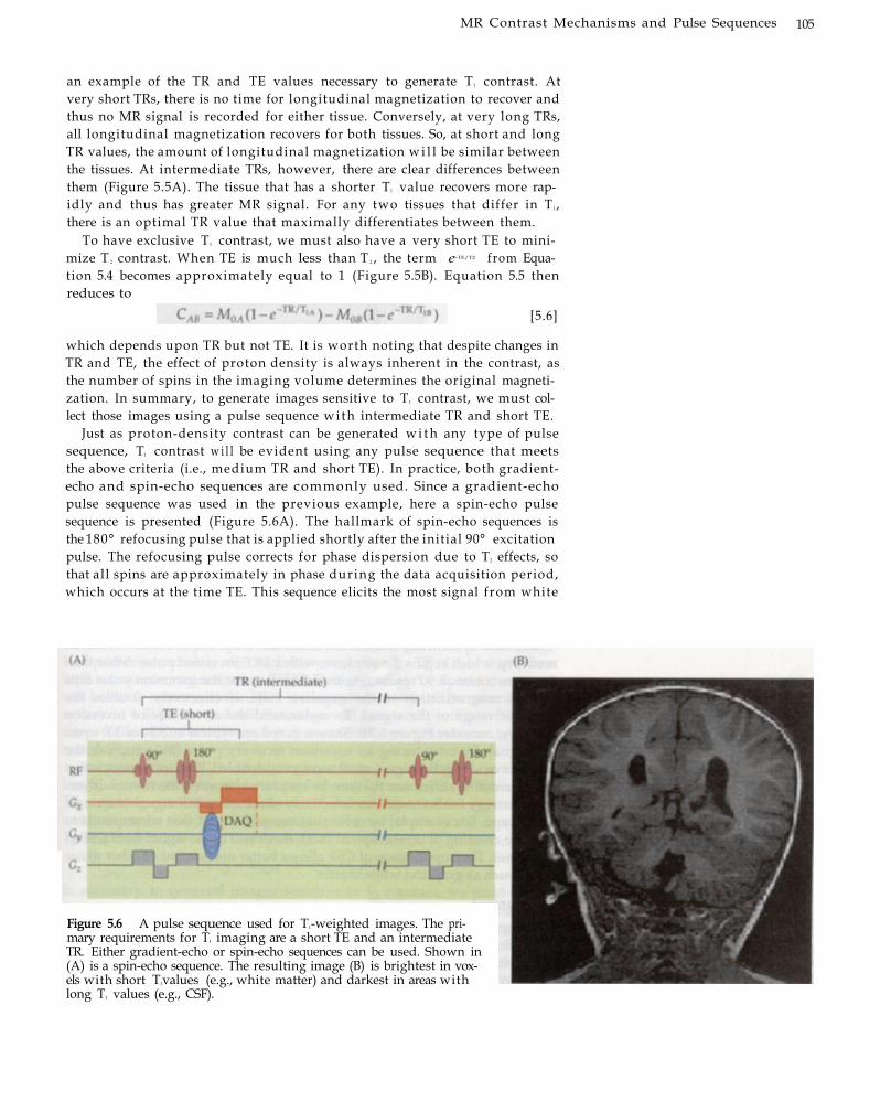
MR Contrast Mechanisms and Pulse Sequences 105
an example of the TR and TE values necessary to generate T1 contrast. At very short TRs, there is no time for longitudinal magnetization to recover and thus no MR signal is recorded for either tissue. Conversely, at very long TRs, all longitudinal magnetization recovers for both tissues. So, at short and long TR values, the amount of longitudinal magnetization w i l l be similar between the tissues. At intermediate TRs, however, there are clear differences between them (Figure 5.5A). The tissue that has a shorter T1 value recovers more rapidly and thus has greater MR signal. For any two tissues that differ in T 1, there is an optimal TR value that maximally differentiates between them.
To have exclusive T1 contrast, we must also have a very short TE to minimize T 2 contrast. When TE is much less than T 2 , the term e-TE/T2 from Equation 5.4 becomes approximately equal to 1 (Figure 5.5B). Equation 5.5 then reduces to
Figure 5.6 A pulse sequence used for T1-weighted images. The primary requirements for T1 imaging are a short TE and an intermediate TR. Either gradient-echo or spin-echo sequences can be used. Shown in (A) is a spin-echo sequence. The resulting image (B) is brightest in voxels with short T1values (e.g., white matter) and darkest in areas with long T1 values (e.g., CSF).
which depends upon TR but not TE. It is worth noting that despite changes in TR and TE, the effect of proton density is always inherent in the contrast, as the number of spins in the imaging volume determines the original magnetization. In summary, to generate images sensitive to T1 contrast, we must collect those images using a pulse sequence wi th intermediate TR and short TE.
Just as proton-density contrast can be generated w i t h any type of pulse sequence, T1 contrast w i l l be evident using any pulse sequence that meets the above criteria (i.e., medium TR and short TE). In practice, both gradient-echo and spin-echo sequences are commonly used. Since a gradient-echo pulse sequence was used in the previous example, here a spin-echo pulse sequence is presented (Figure 5.6A). The hallmark of spin-echo sequences is the 180° refocusing pulse that is applied shortly after the initial 90° excitation pulse. The refocusing pulse corrects for phase dispersion due to T2 effects, so that all spins are approximately in phase during the data acquisition period, which occurs at the time TE. This sequence elicits the most signal from white
[5.6]

106 C h a p t e r F ive
Figure 5.7 Use of inversion recovery to increase T1 contrast. By including a 180° inversion pulse before a typical gradient-echo or spin-echo sequence (A), the net magnetization can be flipped to the negative state. As a result, the net magnetization must recover over twice the dynamic range, and thus the relative difference in T1 recovery between the tissues is increased. As illustrated in (B), the T1 contrast is much greater
Time since excitation (s)
for the same pair of tissues following an inversion pulse (blue curves) than under normal conditions (red curves).The green and purple lines indicate the differences between red curves and blue curves, respectively. Inversion recovery sequences are also used to eliminate MR signal from tissue of a particular type, by collecting images at a TR that corresponds to the zero crossing for that tissue (arrow).
inversion recovery A technique for increasing T1 contrast by adding a 180° inversion pulse before a standard pulse sequence.
matter and bone marrow, due to their short T 1 values, and an intermediate amount of signal from gray matter. Since water has a very long T 1 value, very little signal is recovered from cerebrospinal f l u i d (CSF), which becomes nearly indistinguishable from air (Figure 5.6B).
To boost T1 contrast, researchers often use a technique called inversion recovery, which begins the sequence w i t h a 180° inversion pulse rather than the more common 90° pulse (Figure 5.7A). Because the inversion pulse flips the net magnetization to the negative state, it effectively doubles the dynamic range of the signal. To understand the advantage of inversion recovery, consider Figure 5.7B. Shown in red are typical effects of TR upon MR signal. By introducing an inversion recovery pulse (blue curves), the range over which the signal must recover is doubled. This in turn increases the maximal T1 difference that can be measured between the tissues. Inversion recovery is also useful for selectively eliminating MR signal of a single tissue type. For example, by collecting images at a TR that corresponds to the zero crossing of cerebrospinal f l u i d , there w i l l be no signal from CSF in any voxel. The suppression of CSF allows better assessment of other tissue types, such as gray and white matter.
T2 Contrast By using T 2-contrast imaging, images can be created that have maximal signal in f luid- f i l led regions, which is important for many clinical considerations. Many tumors, arteriovenous malformations (AVMs), and other pathological conditions show up most readily under T 2 contrast. High-resolution T 2 images are also used as anatomical references in fMRI studies, either in

MR Contrast Mechanisms and Pulse Sequences 107
Figure 5.8 Selection of TR and TE values for T1 contrast. The use of long TR (A) and intermediate TE (B) (shown as vertical lines in orange color) on two tissues (red and blue) will maximize the T 2 differences between tissues and minimize the T differences between tissues. This combination provides T2 contrast. The green lines show the MR signal based on the T1 and T2 differences, respectively, along time.
isolation or in conjunction wi th proton-density or T 1 images in a multi-contrast segmentation algorithm. Thus, common clinical protocols include both T 1- and T 2 -weighted images.
For T1-weighted, or T2-dependent images, the amount of signal loss depends upon the time between excitation and data acquisition, or echo time (TE). Again, an optimal combination of TR and TE exists for any two tissues to maximize the T 2 contrast between them (Figure 5.8A). If an image is acquired immediately after excitation, such that the TE is very short, then little transverse magnetization w i l l be lost regardless of T 2 and thus there wil l be no T 2 contrast. If the TE is too long, then nearly all transverse magnetization w i l l be lost and still the image w i l l have no T 2 contrast. But at an intermediate TE, the difference in transverse magnetization can be maximized (Figure 5.8B).
To have exclusive T 2 contrast, we must have a very long TR, so that the longitudinal recovery is almost complete and T 1 contrast is minimal . When TR is much greater than T1, the term e - T R / T 1 from Equation 5.4 approaches 0 and thus can be eliminated. The resulting formula for contrast is completely T 2-weighted and depends highly on TE:
[5.7]
In summary, to generate images sensitive to T 2 contrast, we must collect those images using a pulse sequence w i t h long TR and intermediate TE.
Unlike proton-density or T 1-weighted images, T 2 -weighted images can only be generated using spin echo-based pulse sequences. Only spin-echo sequences allow true spin-spin relaxation that does not depend on the field inhomogeneity. A typical pulse sequence is shown in Figure 5.9A. The resulting brain image w i l l be brightest in f luid-fi l led regions such as the ven-
T2-weighted (T2-dependent) Images that provide information about the relative T2 values of tissue; also known simply as T2 images.

108 C h a p t e r F ive
Figure 5.9 A pulse sequence used for T2-weighted images. The primary requirements for T2 imaging are an intermediate TE and a long TR. ( A ) Only spin-echo sequences can be used. The resulting image (B) is brightest in voxels with short T2
values (e.g., CSF) and darkest in areas with long T1 values (e.g., white matter).
susceptibility artifacts Signal losses on T2'-dependent images due to magnetic field inhomogeneities in regions where air and tissue are adjacent.
tricles, of medium brightness in gray matter, and darkest w i t h i n white matter (Figure 5.9B). These intensity values are consistent w i t h the relative T 2
values of the regions. Remember from the previous chapter that T 2 values depend on spin-spin interactions, and thus homogeneous tissues tend to have longer T 2 . For example, CSF has the longest T 2 value due to its high water content, gray matter has intermediate T 2 from its rich blood supply, and white matter has the lowest T 2 value.
Because the 180° pulse reverses the loss of phase coherence experienced by spins, spin-echo imaging is insensitive to static magnetic field inhomo¬geneities (e.g., T 2* effects). As shown in Figure 5.10, differences in the magnetic field strength experienced by different spins cause loss of phase coherence over time, as some spins w i l l precess faster and some slower. By introducing the 180° pulse at a time point exactly halfway between excitation and TE, the relative phase difference between the spins can be reversed. Therefore, the spins that precess faster w i l l now be behind the spins that precess more slowly, so the faster spins w i l l catch up at time TE. Spin-echo imaging can thus help eliminate the effects of magnetic field inhomo¬geneities around large blood vessels, minimizing the contaminating effects of those vessels on fMRI images. Another advantage of spin-echo imaging lies in its resistance to susceptibility artifacts, which are caused by mag-
Often, proton-density and T 2 -weighted images are acquired w i t h i n the same pulse sequence. What aspect of their pulse
sequences makes this possible?

MR Contrast Mechanisms and Pulse Sequences 109
Figure 5.10 Reversing phase coherence using a 180° excitation pulse. As time progresses following excitation, magnetic field inhomogeneities wil l cause a loss of phase coherence over time, as some spins have fast precession frequencies and some have slow precession frequencies. If a 180° refocusing pulse is presented at time TE /2, the precession direction will be flipped. At the precise time TE, all of the spins wil l have their original phase (as indicated here by their returning to the original location).
netic f ield inhomogeneities near air-tissue interfaces in the brain, as found in the ventral frontal and temporal lobes.
T2* Contrast Recall from Chapter 3 that there are t w o causes for transverse relaxation: spin-spin interaction (T 2 ) and changes in spin precession frequency due to inhomogeneities in the magnetic field. The combined effect of these t w o factors upon the decay of transverse magnetization is given by the time constant T 2*. Though T 2 and T 2* are related, the former constant is always greater than the latter, so T2 decay is always slower than T2* decay. Quantitatively, the relationship between T 2 and T 2* is given by 1 / T 2 * = (1/ T 2 ) + ( 1 / T 2 ' ) , where T 2 ' reflects the dephasing effect caused by field inhomogeneity. Because it forms the basis for BOLD-contiast f M R I , there has been a rapid increase in use of T2*-based imaging protocols since 1990. As is discussed further in Chapter 7, T 2*-weighted images are sensitive to the amount of deoxygenated hemoglobin present, which changes according to the metabolic demands of active neurons.
Like T 2 contrast, T 2* contrast is provided by pulse sequences w i t h a long TR and medium TE. An additional requirement is that the pulse sequence
T2*-weighted Images that provide information about the relative T2* values of tissue. T2*-weighted images are commonly used for BOLD-contrast fMRI.

110 Chapter Five
Figure 5.11 A pulse sequence used for T2*-weighted images. Like T2-weighted images, T2*-weighted images require an intermediate TE and a long TR. Gradient-echo sequences are most commonly used, because the refocusing pulses used in spin-echo images will eliminate the field inhomogeneity effects that form the basis of the T2* effect.
must use magnetic field gradients to generate the signal echo, because refocusing pulses w i l l eliminate field inhomogeneity effects. Most commonly used are gradient-echo sequences, as illustrated in Figure 5.11. Note the similarity to the proton-density sequence shown in Figure 5.4, which differs only in the echo time, TE. Here, an intermediate TE is used so that the image is sensitive to local f ield inhomogeneity and not just to the number of protons present. The pulse sequence shown can provide information about factors that decrease magnetic field homogeneity, such as the presence of deoxygenated hemoglobin. Because spin-echo pulse sequences have reduced T2* sensitivity, they are less frequently used for BOLD-contrast fMRI.
Motion-Weighted Contrasts
The human body is inherently dynamic. Wi th in the vascular system, for example, water molecules are in constant motion, f lowing on the order of 1 m/s in large arteries. Water also diffuses w i t h i n and among cells, such as along axons in white matter. Pulse sequences sensitive to motion provide important information about the brain, including both structural and functional measures. Structural techniques include MR angiography and diffusion tensor imaging, which are often used for mapping the neurovascular system and white-matter tracts, respectively. Functional techniques include diffusion imaging, which maps the motion of water molecules over time, and perfusion imaging, which maps blood f low through capillaries. These techniques are collectively k n o w n as motion-weighted contrasts.
MR Angiography Magnetic resonance angiography, or MRA, illustrates the structure of blood vessels using noninvasive MRI (Figure 5.12). In classic angiography, a contrast agent is injected into the bloodstream through an inserted catheter. X-ray images are then collected w i t h and without the contrast agent present to generate a difference image (i.e., angiogram) that maps the vascular system. Al though angiography provides good vascular images, it is a very
magnetic resonance angiography (MRA) The creation of images of the vascular system using MRI.

MR Contrast Mechanisms and Pulse Sequences 111
Figure 5.12 A sample magnetic resonance angiography (MRA) image.
invasive procedure, requiring both the insertion of foreign substances and exposure to ionizing radiation. Because MRA does not require ionizing radiation, it can noninvasively detect, diagnose, and aid in the treatment of many types of medical problems, including cardiac disorders, stroke, and vascular disease. MRA also complements fMRI studies by identifying major blood vessels that may confound experimental results. If identified, these vessels can be removed from analyses to improve localization of activity to the capillary bed.
MRA can use either exogenous or endogenous contrast. In some clinical settings, exogenous contrast-enhancing agents are used to increase the vessel signal. For a typical contrast-enhanced MRA, a small quantity (or bolus) of a gadolinium-based contrast agent is injected into the patient's bloodstream. The gadol inium itself is not visible on MR images, but it radically shortens the T 1 of nearby blood, a l lowing the use of specialized pulse sequences wi th extremely short TR (3 to 7 ms) and TE (1 to 3 ms) values. The short TR saturates signal from stationary tissues but not from the gadolinium-enhanced blood, while the short TE minimizes T 2 decay. Depending on the delay between bolus injection and image acquisition, the contrast agent may travel through different components of the vascular system, so the images can be calibrated to provide information about arterial or venous networks.
In research settings, MRA is usually obtained using noninvasive endogenous contrast. There are t w o primary techniques for endogenous contrast MRA. The most common is time-of-flight (TOF) MRA, which generates signal based upon blood displacement. The underlying principle of the TOF technique is spin saturation. By repeatedly and frequently applying excitation pulses or gradient pulses to a single imaging plane, the signal w i t h i n that plane can be suppressed. Thus, tissues whose spins remain w i t h i n the plane, such as gray or whi te matter, w i l l produce l itt le MR signal and w i l l appear to be very dark on TOF images. Blood vessels, however, are constantly replenished wi th new spins from outside the plane. These spins have not experienced the excitation or gradient pulses, and thus they contribute
bolus A quantity of a substance that is introduced into a system and then progresses through that system over time.
time-of-flight (TOF) MRA A type of MR angiography that generates contrast by suppressing signal from spins within an imaging plane so that voxels with inflowing spins (i.e., those with blood vessels) have high signal.

112 Chapter Five
Figure 5.13 Schematic illustration of the signalgeneration mechanism for TOF magnetic resonance angiography. In TOF MRA, repeated excitation pulses saturate the MR signal from spins within a plane, as shown by the dark bar at left. Then there is a waiting period during which voxels with flow (e.g., blood vessels) have new spins introduced whereas voxels without flow (e.g., white matter) do not. The amount of MR signal recorded following excitation and acquisition is greatest for voxels that had the most new spins enter during the waiting period.
Vessels
velocityencoded phase contrast (VENCPC) MRA A type of MR angiography that uses gradient fields
to induce phase differences associated
with vascular flow so that the flow
velocity of vessels can be measured.
normal MR signal. TOF images are typically acquired in the axial plane and
can be reformatted to other planes for ease of viewing.
The TOF signal is proportional to the amount of blood that enters the slice
(Figure 5.13). If a completely new column of blood enters the slice every TR,
the TOF signal w i l l be at its maximum. But if blood flow is weak or absent,
then the TOF signal w i l l be much reduced. Consequently, TOF contrast dif
ferentiates blood vessels based upon their amount of f low; thus it is a flow
dependent contrast technique. Because of its f low sensitivity, the TR and
slice thickness for TOF images must be chosen based upon the expected
flow.
To acquire MRAs w i t h TOF contrast, a specialized pulse sequence is
required (Figure 5.14). As described in the preceding paragraphs, the imag
ing plane is presaturated by the electromagnetic excitation pulse and gradi
ent saturation pulses. After a brief wait ing period during which fresh blood
can enter the plane, the MR signals are acquired by a gradientecho acquisi
tion technique, so that only the signal from this new blood w i l l be present.
A second technique is velocityencoded phase contrast (VENCPC) MRA, which uses gradient fields to produce a velocitydependent phase dif
ference, θ, between the vasculature and surrounding tissue (Figure 5.15). The
amount of phase difference accumulated depends on the velocity of the
moving spins and the strength and durat ion of the applied gradient. By
Figure 5.14 Pulse sequence used for TOF MRA. The TOF technique requires an initial saturation of a slice, followed by a wait time to allow blood to enter the slice. Then a standard gradientecho sequence can be used to acquire the images.
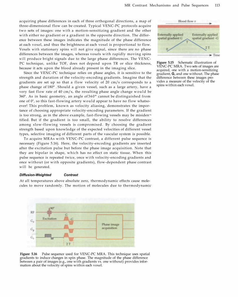
MR Contrast Mechanisms and Pulse Sequences 113
acquiring phase differences in each of three orthogonal directions, a map of three-dimensional f low can be created. Typical VENC-PC protocols acquire t w o sets of images: one w i t h a motion-sensitizing gradient and the other w i t h either no gradient or a gradient in the opposite direction. The difference between these images indicates the magnitude of the phase difference at each voxel, and thus the brightness at each voxel is proportional to flow. Voxels w i t h stationary spins w i l l not give signal, since there are no phase differences between the images, whereas voxels w i t h rapidly moving spins w i l l produce bright signals due to the large phase differences. The VENC-PC technique, unlike TOF, does not depend upon TR or slice thickness, because it acts upon the blood already present in the imaging slice.
Since the VENC-PC technique relies on phase angles, it is sensitive to the strength and duration of the velocity-encoding gradients. Imagine that the gradients are set up so that a f low velocity of 20 cm/s corresponds to a phase change of 180°. Should a given vessel, such as a large artery, have a very fast f low rate of 40 cm/s, the resulting phase angle change w o u l d be 360". As in basic geometry, an angle of 3 6 0 ° cannot be distinguished from one of 0", so this fast-flowing artery w o u l d appear to have no f low whatsoever! This problem, known as velocity aliasing, demonstrates the importance of choosing appropriate velocity-encoding parameters. If the gradient is too strong, as in the above example, fast-flowing vessels may be misiden¬tified. But if the gradient is too small, the ability to resolve differences among s low-f lowing vessels is compromised. By choosing the gradient strength based upon knowledge of the expected velocities of different vessel types, selective imaging of different parts of the vascular system is possible.
To acquire MRAs w i t h VENC-PC contrast, a different pulse sequence is necessary (Figure 5.16). Here, the velocity-encoding gradients are inserted after the excitation pulse but before the phase image acquisition. Note that they are bipolar in shape, which has no effect on static tissue. When this pulse sequence is repeated twice, once w i t h velocity-encoding gradients and once wi thout (or w i t h opposite gradients), flow-dependent phase contrast wi l l be generated.
Diffusion-Weighted Contrast At all temperatures above absolute zero, thermodynamic effects cause molecules to move randomly. The motion of molecules due to thermodynamic
Figure 5.16 Pulse sequence used for VENC-PC MRA. This technique uses spatial gradients to induce changes in spin phase. The magnitude of the phase difference between a pair of images (e.g., one with gradients vs. one without) provides information about the velocity of spins within each voxel.
Figure 5.15 Schematic illustration of VENC-PC MRA. Two sets of images are acquired, one with a motion-sensitizing gradient, G, and one without. The phase difference between these images provides a measure of the velocity of the spins within each voxel.

114 Chapter Five
Figure 5.17 Diffusion. Over time, molecules within gases or liquids will move freely through the medium. This motion is known as diffusion. Shown here are sample random paths that could be taken by molecules within a medium that allows isotropic (i.e., the same in every direction) diffusion. As time passes, the net distance traveled by a molecule increases.
effects is known as diffusion (Figure 5.17). In gases and liquids, the molecules can move relatively freely, as when a dye spreads through a glass of water or when the smell of freshly baked bread wafts through the house. In solids, however, the motion of molecules is restricted, and thus diffusion is much slower. The abundance of water molecules in the human body makes it possible to perform diffusion-weighted imaging using MRI . A n d , because of the different cellular environment experienced by different water molecules, diffusion-weighted MRI can provide a new dimension of image contrast based on mobility.
The original equation proposed by Bloch (see Equation 3.47) successfully explains MR phenomena including the effects of T1 and T2 relaxation. However, it does not contain a term that describes the effect of diffusion. Torrey modified the Bloch equation to account for the effects of diffusion:
Later we w i l l exploit the preference for water w i t h i n some tissues to diffuse in one direction and not others in our discussion of diffusion tensor imaging.
If the magnetic field were perfectly homogeneous, the effect of diffusion would be hardly visible, as the water molecules would experience the same
The new term (M - M 0 ) states that diffusion modulates the rate of MR signal change according to a new intrinsic tissue property, D, which describes the rate of molecular diffusion under a time-varying magnetic gradient. The symbol, is the mathematical representation of the gradient. Voxels with large D, such as those containing CSF, allow molecules to diffuse quickly and thus have a faster rate of signal decay. Voxels with small D, such as those containing lipids, have limited diffusion and thus a slower rate of signal decay. To allow easier visualization of its meaning, this equation can be further divided into three subequations that describe each of the three directional components:
[5.8]
[5.9a]
[5.9b]
[5.9c]
diffusion The random motion of molecules through a medium over time.

MR Contrast Mechanisms and Pulse Sequences 115
magnetic field regardless of their position over time. However, if the field were inhomogeneous, whether due to the intrinsic nonuniformity or externally applied gradients, the water molecules w o u l d experience different magnetic fields as they diffused in space over time. This w o u l d cause a loss of phase coherence, which in turn w o u l d attenuate the MRI signal. Unlike the loss of phase coherence due to static magnetic field inhomogeneity (e.g., T2* effects), this loss cannot be recovered even w i t h spin-echo pulse sequences. Because diffusion is random, the path taken by each molecule cannot be reversed. Thus, the refocusing pulse of a spin-echo sequence cannot recover signal lost to phase incoherence.
Diffusion weighting is the application of controlled gradient magnetic fields to quantify the amplitude and direction of diffusion. The presence of diffusion-weighting gradients further attenuates the MR signal beyond that caused by common T 2 relaxation. Assuming equal, or isotropic, diffusion along all directions (Figure 5.18A), the attenuation effect (A) due to diffusion weighting is given by the exponential
[5.10]
In this equation, D is the apparent diffusion coefficient, or ADC (i.e., the measured value of the diffusion coefficient), G the strength of the external diffusion-weighting gradient, and T the duration of the diffusion-weighting gradient. We can define the degree of diffusion weighting as the b factor:
To further simplify Equation 5.10:
[5.11]
[5.12]
Equation 5.12 quantifies the mean diffusivity w i t h i n a voxel without providing directional information. But water molecules in the brain do not diffuse equally in all directions. Most water is contained w i t h i n tissue that has considerable structure, such as the long processes of axons or the narrow
diffusion weighting The application of magnetic gradients to cause changes in the MR signal that are dependent upon the amplitude and/or direction of diffusion.
isotropic Having similar properties in all directions.
apparent diffusion coefficient (ADC) The quantification of diffusivity assuming isotropic diffusion.
b factor The degree of diffusion weighting applied within a pulse sequence.
Figure 5.18 Isotropic and anisotropic diffusion. If there are no restrictions on diffusion, molecules wil l diffuse equally in all directions (A). This is known as isotropic diffusion. However, if there are restrictions upon diffusion, as is the case within long neuronal axons, diffusion may occur primarily along one axis (B). This is an example of anisotropic diffusion. Note that the vector representations here are simplified versions of the random-walk paths taken by molecules, as indicated in the inset figure at upper center.

116 Chapter Five
anisotropic Having different properties in different directions; often referenced in the context of anisotropic diffusion, where molecules tend to diffuse along one axis but not others.
tensor A collection of vector fields governed by three principal axes.
diffusion tensor imaging (DTI) The collection of images that provide information about the magnitude and direction of molecular diffusion. It is often used to create maps of fractional anisotropy.
fractional anisotropy (FA) The preference for molecules to diffuse in an anisotropic manner. An FA value of 1 indicates that diffusion occurs along a single preferred axis, while a value of 0 indicates that diffusion is similar in all directions.
walls of blood vessels. Unequal, or anisotropic, diffusion (Figure 5.18B) refers to the preference in some tissues for water molecules to diffuse in one direction or another. In anisotropic diffusion, the motion of molecules over time does not resemble a sphere, in which molecules move equally in every direction, but instead resembles an ell ipsoid whose long axis indicates the fastest axis of diffusion. The diffusion ellipsoid is mathematically described as a three-dimensional tensor, which is a collection of vector fields governed by three principal axes.
Diffusion tensor imaging (DTI) can quantify the relative di f fusivi ty among directional components. For example, white matter, which is composed mostly of nerve fibers, shows prominent anisotropy, such that water molecules diffuse most quickly along the length of the fiber and most slowly across the w i d t h of the fiber. A scalar quantity k n o w n as fractional anisotropy (FA) can be computed for each voxel to express the preference of water to diffuse in an isotropic or anisotropic manner. FA values are bounded by 0 and 1 and are calculated using Equation 5.13, where Dx, Dy, and Dz represent the three principal axes of the diffusion tensor:
[5.13]
FA values approaching 1 indicate that nearly all of the water molecules in the voxel are dif fusing along the same preferred axis, while FA values approaching 0 indicate that the water molecules are equally likely to diffuse in any direction. Fractional anisotropy provides important information about the composition of tissue w i t h i n a voxel. Notably, some neurological diseases, such as multiple sclerosis and vascular dementia, are characterized by potentially severe white-matter pathology. The resulting axonal damage can be identified as decreased FA values in affected voxels. More-complex forms of diffusion tensor imaging can track nerve fibers as they travel between functionally associated brain regions. These advanced tensor imaging techniques are discussed in more detail in Chapter 14.
To determine diffusion coefficients, we must apply controlled gradients in a pulse sequence. These gradients must be spatially balanced to preserve MR signal. In spin-echo sequences (Figure 5.19A), this balance is achieved
Figure 5.19 Pulse sequences used for diffusion-weighted imaging. Shown are sample pulse sequences used for diffusion-weighted spin-echo imaging (A) and diffusion-weighted gradient-echo imaging (B). Note that the spin-echo sequence has a refocusing pulse between two gradients of similar sign, while the gradient-echo sequence alternates gradients of opposite sign.

MR Contrast Mechanisms and Pulse Sequences 117
by presenting the gradients before and after the refocusing pulse. In gradient-echo sequences (Figure 5.19B), successive positive and negative gradients are applied. In an ideal isotropic medium, application of a gradient along any axis w o u l d be sufficient for measuring the A D C . However, the brain contains many tissues that constrain dif fusion, and thus diffusion-weighting gradients must be applied in many directions to quantify the diffusion tensor.
perfusion Blood flow through capillaries. arterial spin labeling (ASL) A family of
perfusion imaging techniques that measure blood flow by labeling spins with excitation pulses and then waiting for the labeled spins to enter the imaging plane before data acquisition.
continuous ASL A type of perfusion imaging that uses a second transmitter coil to label spins within an upstream artery while collecting images.
Al though diffusion imaging has been pr imari ly applied to quantify white-matter structure and pathology in the human brain, it also has great potential ut i l i ty for fMRI . We discuss these applications in Chapter 14.
Perfusion-Weighted Contrast The human brain requires oxygen for metabolism (see Chapter 6). To ensure a constant supply of oxygen, hemoglobin molecules carry oxygen through the bloodstream to all parts of the brain. The irrigation of tissue via blood delivery is known as perfusion, and the family of imaging procedures that measure this process are known as perfusion MRI. Perfusion is expressed as the volume of blood that travels through a tissue mass over time. In the human brain, gray-matter perfusion is approximately 60 mL/100 g/min, and white-matter perfusion is smaller, about 20 mL/100 g/min. Unlike the MRA techniques described in the section on MR angiography, (which are often used for clinical reasons to measure the properties of large blood vessels), perfusion MRI is most frequently used to image blood flow specifically in capillaries and other small vessels.
Perfusion MRI may use either exogenous or endogenous contrast. Exogenous contrast approaches use intravascular contrast agents that freely perfuse through the vascular system. The attenuation of the MR signal in each voxel is proportional to the amount of the contrast agent present. Thus, signal changes can be interpreted as a function of perfusion, and images can be created that depict different perfusion properties, such as the relative cerebral blood f low (rCBF), relative cerebral blood volume (rCBV), and mean transit time (mTT). As their names imply, relative blood f low and relative blood volume express changes in how much blood comes into a voxel and how much blood is contained w i t h i n a voxel, respectively. The mean transit time measures how quickly blood passes through a particular voxel and can indicate brain regions w i t h delayed blood flow. The use of exogenous contrast agents provides very high signal change but has l imited use for research because of its invasiveness.
Endogeneous contrast perfusion imaging is noninvasive and has found use in fMRI research. Contrast is generated through the clever use of radiofrequency pulses to magnetically label, or tag, protons in blood water molecules before they reach the tissue of interest. This approach is known as arterial spin labeling, or ASL, of which there are two types: continuous and pulsed. Continuous ASL typically uses additional hardware, like a labeling coil, to saturate spins in upstream blood, such as in the carotid arteries of the
Why are the gradients used in the spin-echo pulse sequence of the same sign, whi le the gradients used in the gradient-
echo sequence are of opposite signs?

118 C h a p t e r F ive
Figure 5.20 Perfusion imaging mechanisms. (A) Continuous ASL techniques use an upstream transmission coil to saturate spins in an artery that feeds the brain. Images collected following spin saturation can be compared to images in the absence of saturation to determine flow into the imaging plane. There are two primary types of pulsed ASL techniques, EPISTAR (B) and FAIR (C). EPISTAR relies on alternating two labeling planes that are equidistant from the
imaging plane, one below the plane that includes feeding arteries and one above the plane that does not include any feeding vessels (i.e., is outside the head). FAIR alternates between labeling the entire brain and just the imaging plane. For either of the pulsed ASL techniques, differences between the two sets of images can be attributed to flow into the imaging plane.
pulsed ASL A type of perfusion imaging
that uses a single coil both to label
spins in one plane and to record MR signal in another plane, separated by a
brief delay period.
labeling plane The plane in which initial excitation pulse(s) are applied during perfusion imaging.
imaging plane The plane in which changes in MR signal are recorded dur
ing perfusion imaging.
neck (Figure 5.20A). Following this labeling process, the blood travels to the
brain and enters the imaging slice. The images can then be continuously
acquired in the brain in the presence of the labeled blood. After acquiring
the images w i t h the labeled blood, the labeling coil can be turned off and a
second set of images are acquired without the presence of the labeled blood.
The difference between the t w o sets of images reflects only the blood flow,
as any tissue that does not contain f low w i l l be similar in the t w o conditions.
A drawback of the continuous ASL technique is the requirement for a second
transmitter coil to label the inf lowing blood.
A n alternative approach, pulsed ASL, uses a single coil both to label
blood in the labeling plane and to record the MR signal change in the imaging plane (Figure 5.20F3 and C). Labeling pulses are broadcast for brief peri
ods and followed by a delay and then image acquisition. The delay period
must be calibrated to account for the distance between the labeling plane
and imaging plane, so the labeled bolus of blood water w i l l enter the imag
ing plane during image acquisition.
Regardless of the ASL method used, labeling blood only alters the longi
tudinal magnetization. Thus, we can describe the endogenous perfusion sig
nal quantitatively by modifying the T 1 term of the Bloch equation (Equation
4.1). To do so, we introduce an additional term, f(M'(t) M0), that accounts
for the effects of blood f low:
[5.14]
In this equation, f is the blood f low in mL/g/sec and T 1 a p p is the apparent T 1
value in the presence of blood flow. T 1 a p p can be calculated from 1 /T 1 a p p =
1/T1 + f/λ, where λ is the bloodbrain partition coefficient. This coefficient is
defined by the ratio between blood volume and brain tissue masses that

MR Contrast Mechanisms and Pulse Sequences 119
This equation defines the relation between the measured perfusion signal and blood f low in the brain.
Because the continuous ASL method uses a second transmitter coil to label blood, the images can be acquired w i t h any standard spin- or gradient-echo pulse sequence. To achieve the maximal signal difference, the echo time (TE) must be kept as short as possible, which minimizes signal loss due to T2* or T 2 relaxation effects.
Pulsed ASL techniques require specialized pulse sequences to label the blood. In one type of pulsed ASL, EPISTAR (echo-planar imaging at steady state w i t h alternating inversion recovery), alternating off-center inversion pulses are used to select labeling planes below and above the image plane (Figure 5.21A). For odd scans, the labeling plane is in the neck, below and upstream from the imaging plane. For even scans, the labeling plane is at an equal distance above the imaging plane, and can actually be outside of the brain. This is necessary to ensure that the inversion pulse has a similar effect on the spin system in both the odd and even scans.
EPISTAR is directionally specific, in that it is only sensitive to spins flowing from the labeling plane to the imaging plane. A second type of pulsed
Figure 5.21 Pulse sequences for pulsed ASL imaging. Shown are typical pulse sequences used for the EPIS¬TAR technique (A) and the FAIR technique (B). Both techniques require alternating between different labeling planes, as shown for the Gz gradient at left.
[5.16]
[5.15]
contain equal amounts of water; its typical value is about 0.9 mL/g. Because the blood is labeled w i t h an inversion pulse, its magnetization, M'(t), is given by -M 0 , so that the difference between the two conditions becomes:

120 Chapter Five
ASL, FAIR (flow-sensitive alternating inversion recovery), is not direction-ally specific (Figure 5.21 B). For odd scans, the entire brain is labeled. For even scans, only the imaging plane is labeled. The difference between these t w o labeling conditions reflects those spins that f low into the image plane from anywhere else in the brain; thus FAIR is insensitive to the direction of flow. However, flow with in the plane w i l l be similar between the conditions and does not contribute to the image. Because the inversion pulse is present for both acquisitions, its effect w i t h i n the imaging plane is identical.
Like the diffusion imaging techniques described in the previous section, perfusion imaging provides an alternative method for functional neu¬roimaging (see Chapter 14).
Fast Imaging Sequences for fMRI Image Acquisition
For anatomical images of the brain, contrast is more important than speed of acquisition, since structural parameters such as size and shape change little over the course of a single scanning session. However, understanding the function of the brain requires images to be acquired very rapidly, at approximately the same rate as the physiological changes of interest. Fast pulse sequences have been developed that acquire a very large number of images w i t h i n a short period of time; state-of-the art sequences may acquire a volume consisting of 20 or more images w i t h i n a single second. These sequences typically use variants of the gradient-echo approach described in Chapter 4 and are sensitive to T2* contrast. The basic principles underlying these sequences are described in the remainder of this chapter.
Echo-Planar Imaging The first human MR images were acquired using a laborious voxel-by-voxel procedure. The image shown in Figure 1.13 took about 4 hours to acquire, as collected at the slothlike pace of about 2 minutes per voxel. To put the current ultrafast methods in perspective, a modern pulse sequence that images 20 slices per second collects data at a rate approximately 10,000,000 times faster than that of the first MR image. The development of fast MR imaging can be traced to the work of Peter Mansfield and colleagues at the University of Nottingham. At that time, the traditional method for acquiring images was to fi l l up k-space in a line-by-line fashion, which necessitated a large number of separate excitations for even a moderate-resolution image. In 1977, Mansfield proposed a new method, known as echo-planar imaging, or EPI, in which the entire k-space is filled using rapid gradient switching fol lowing a single excitation. For this technique, Mansfield shared the Nobel Prize in Physiology or Medicine in 2003. Early MRI scanners were very l imited in terms of the strength of the gradients that they could produce and the slew rate wi th which they could change the gradients. While high-static-magnetic field scanners were available by the early 1980s, advanced gradient technology was not common until the late 1980s and early 1990s. The maturation of gradient technology has made EPI the most common fast imaging method for functional MRI . The basic EPI pulse sequence has changed little since its development by Mansfield (Figure 5.22A). Since all of k-space must be filled fol lowing a single excitation pulse, the data must be acquired before significant T2* or T2 decay can occur. However, to achieve reasonable spatial resolution, a relatively large k-space must be sampled, which takes time. To meet these constraints, k-space must be filled very rapidly. This requires a very strong gradient system. For EPI to be practical, gradients of about 2.5
echo-planar imaging (EPI) A technique, first proposed by Peter Mansfield, that allows collection of an entire two-dimensional image by changing spatial gradients rapidly following a single electromagnetic pulse from a transmitter coil.
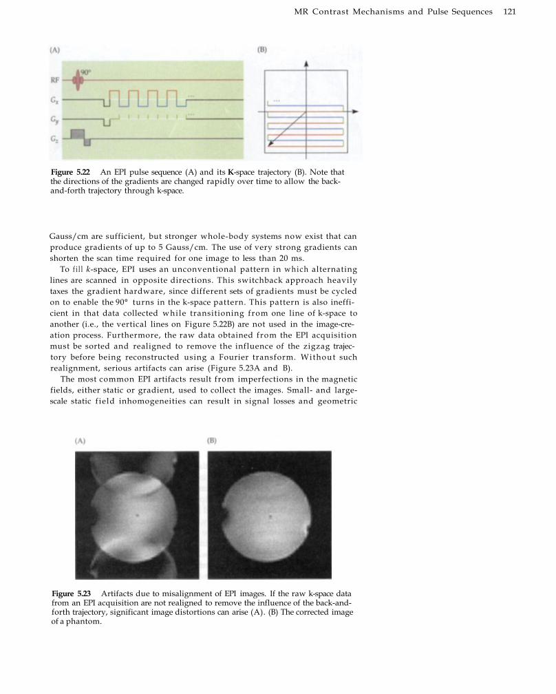
MR Contrast Mechanisms and Pulse Sequences 121
Figure 5.22 An EPI pulse sequence (A) and its K-space trajectory (B). Note that the directions of the gradients are changed rapidly over time to allow the back-and-forth trajectory through k-space.
Gauss/cm are sufficient, but stronger whole-body systems now exist that can produce gradients of up to 5 Gauss/cm. The use of very strong gradients can shorten the scan time required for one image to less than 20 ms.
To f i l l k-space, EPI uses an unconventional pattern in which alternating lines are scanned in opposite directions. This switchback approach heavily taxes the gradient hardware, since different sets of gradients must be cycled on to enable the 90° turns in the k-space pattern. This pattern is also inefficient in that data collected while transitioning from one line of k-space to another (i.e., the vertical lines on Figure 5.22B) are not used in the image-creation process. Furthermore, the raw data obtained from the EPI acquisition must be sorted and realigned to remove the influence of the zigzag trajectory before being reconstructed using a Fourier transform. Without such realignment, serious artifacts can arise (Figure 5.23A and B).
The most common EPI artifacts result from imperfections in the magnetic fields, either static or gradient, used to collect the images. Small- and large-scale static f ield inhomogeneities can result in signal losses and geometric
Figure 5.23 Artifacts due to misalignment of EPI images. If the raw k-space data from an EPI acquisition are not realigned to remove the influence of the back-and-forth trajectory, significant image distortions can arise (A). (B) The corrected image of a phantom.

122 Chapter Five
Figure 5.24 Signal loss due to susceptibility artifacts in EPI images. Shown here are a series of slices within an EPI image volume collected at a 4-T scanner (TE: 40 ms). In areas of the brain near interfaces between air and tissue, such as near the sinuses and auditory canals, there is significant signal loss due to magnetic field inhomogeneities.
distortions, respectively, and are discussed in Chapter 4. Figure 5.24 shows a set of typical EPI images, oriented axially w i t h the lowest slice in the upper left of the figure. Visible are significant losses of MR signal in the ventral frontal lobes and inferior medial temporal lobes, due to magnetic susceptibil i ty artifacts resulting from the field inhomogeneity present at the boundary between brain tissue and a nearby, air-filled sinus. The signal loss in the ventral frontal region results from the nasal and oral cavities, which sit just under the frontal lobe, and the loss in the inferior medial temporal region results from the auditory canals below.
Geometric distortion is also present in EPI images, due to the long readout time for each excitation. In anatomical images, which have short readout windows, small field variations in the image plane may cause only subpixel distortions. But in EPI images w i t h long readout periods, there can be noticeable distortions of up to several pixels. A long readout time makes the system more prone to geometric distortions due both to the reduced sam-

MR Contrast Mechanisms and Pulse Sequences 123
(B)
Figure 5.25 Effects of small field variation upon EPI images. A normal EPI image (A) w i l l be distorted by small variations in magnetic field strength along a single direction. If the variation is along x (B) or y (C), the image is systematically stretched or sheared. If the variation is along the slice selection axis 2 (D), the excitation is off-resonance and MR signal intensity is reduced.
(D)
pling frequency and the reduced readout gradient strength. Variation in the magnetic field along a single in-plane direction (e.g., x or y) causes stretching and shearing of the otherwise circular phantom image (Figure 5.25A-C). Rarely, however, w i l l geometric distortion be in a single direction; instead, gradient variation usually changes across the image in a complex fashion, resulting in more-complex patterns of distortion. A further problem results from small field variations along the z (i.e., slice-selective, or through-plane) direction, which cause off-resonance excitation and thus severe signal losses (Figure 5.25D).
Spiral Imaging While EPI enables fast image acquisition, its speed is constrained by the physical limitations of the MR scanner gradient hardware. A new family of fast imaging sequences called spiral imaging utilizes a very different trajectory in k-space from that of EPI. Spiral imaging sequences use sinusoidal changes in the gradients (Figure 5.26A) to trace a corkscrew path through k-space that typically begins at the center and winds its way to the perimeter
spiral imaging A technique for fast image acquisition that uses sinusoidally changing gradients to trace a corkscrew trajectory through k-space
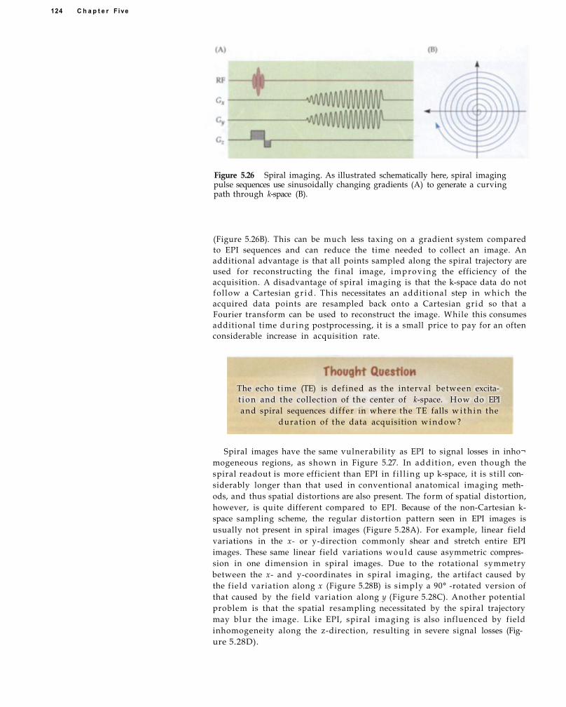
124 C h a p t e r F ive
Figure 5.26 Spiral imaging. As illustrated schematically here, spiral imaging pulse sequences use sinusoidally changing gradients (A) to generate a curving path through k-space (B).
(Figure 5.26B). This can be much less taxing on a gradient system compared to EPI sequences and can reduce the time needed to collect an image. An additional advantage is that all points sampled along the spiral trajectory are used for reconstructing the final image, improving the efficiency of the acquisition. A disadvantage of spiral imaging is that the k-space data do not fol low a Cartesian g r i d . This necessitates an additional step in which the acquired data points are resampled back onto a Cartesian grid so that a Fourier transform can be used to reconstruct the image. While this consumes additional time during postprocessing, it is a small price to pay for an often considerable increase in acquisition rate.
Spiral images have the same vulnerability as EPI to signal losses in inho¬mogeneous regions, as shown in Figure 5.27. In addit ion, even though the spiral readout is more efficient than EPI in f i l l ing up k-space, it is still considerably longer than that used in conventional anatomical imaging methods, and thus spatial distortions are also present. The form of spatial distortion, however, is quite different compared to EPI. Because of the non-Cartesian k-space sampling scheme, the regular distortion pattern seen in EPI images is usually not present in spiral images (Figure 5.28A). For example, linear field variations in the x- or y-direction commonly shear and stretch entire EPI images. These same linear field variations would cause asymmetric compression in one dimension in spiral images. Due to the rotational symmetry between the x- and y-coordinates in spiral imaging, the artifact caused by the field variation along x (Figure 5.28B) is s imply a 90°-rotated version of that caused by the field variation along y (Figure 5.28C). Another potential problem is that the spatial resampling necessitated by the spiral trajectory may blur the image. Like EPI, spiral imaging is also influenced by field inhomogeneity along the z-direction, resulting in severe signal losses (Figure 5.28D).
The echo t ime (TE) is defined as the interval between excitat i o n and the collection of the center of k-space. How do EPI and spiral sequences dif fer in where the TE falls w i t h i n the
durat ion of the data acquisition w i n d o w ?

MR Contrast Mechanisms and Pulse Sequences 125
(B)
Figure 5.27 Signal losses due to susceptibility artifacts in spiral images. Compared to anatomical images (A), spiral images (B) exhibit regions of signal loss similar to those of EPI images (compare to Figure 5.24).
(D)
Figure 5.28 Effects of small field variation upon spiral images. A normal spiral image (A) is distorted by small variations in magnetic field strength along a single direction, although the partern of distortion is different from that of EPI. If the variation is along x (B) or y (C), the image is systematically compressed along the y-direction or x-direc¬tion, respectively. As with EPI, however, variation along the slice selection direction (D) causes a reduction in overall MR signal intensity.
S u m m a r y There are t w o general types of contrast for magnetic resonance imaging of the brain. Static contrast provides information about the number or content of atomic nuclei, while motion contrast describes how atomic nuclei move w i t h i n a region of interest. Each basic type may use either endogenous mechanisms that rely on naturally occurring properties of biological tissue or exogenous mechanisms that typically involve the injection of paramagnetic compounds. Every contrast mechanism has associated pulse sequences describing the gradient changes and radiofrequency pulses that are used to collect the MR signal. By varying the parameters of a given pulse sequence, images can be collected that are sensitive to one form of contrast or another. Common static contrasts include proton-density, T 1-weighted, T 2 -weighted, and T 2*-weighted. In fMRI experiments, these static contrasts are typically used for collection of high-resolution images that provide anatomical detail. Motion contrasts include MR angiography, diffusion weighting, and perfusion imaging. Diffusion and perfusion imaging, in particular, have potential for improving localization of function in the brain, as they provide information complementary to that gained w i t h standard fMRI approaches. Gradient-echo imaging is the most common form of fMRI pulse sequence, for which both echo-planar and spiral imaging are used. The use of T 2*-weighted contrast provides the foundation for high-temporal-resolution study of functional changes in the human brain through fMRI.
Suggested Readings Buxton, R. (2001). Introduction to Functional Magnetic Resonance Imaging: Principles
and Techniques. C a m b r i d g e Univers i ty Press, C a m b r i d g e , U.K. Provides an advanced overv iew of many facets of M R I , including a detailed d iscussion of perfusion imaging.
Haacke , E . M., B r o w n , R. W., T h o m p s o n , M. R., and Venkatesan, R. (1999). Magnetic Resonance Imaging: Physical Principles and Sequence Design. John Wiley & Sons, N e w York. A comprehensive encyclopedia of the theoretical principles of MRI .
Slichter, C . P. (1990). Principles of Magnetic Resonance ( 3 r d ed.) . Springer-Verlag, N e w York. Provides a detailed mathematical treatment of the physics of MRI .
Chapter References Arlart , I. P., Bongartz, G . M., a n d Marcha l , G . (eds.) (1995). Magnetic Resonance
Angiography. Springer-Verlag, N e w York.
F e y n m a n , R. P., Le ighton, R. B., a n d S a n d s , M. (1964). Lectures on Physics, Vol. II. Addison-Wesley Publ ishing C o m p a n y , N e w York.
Le Bihan, D. (ed.) (1995). Diffusion and Perfusion Magnetic Resonance Imaging: Application to Functional MRI. Raven Press, N e w York.
Moonen, C . T. W., and Bandettini, P. A . (eds.) (1999). Functional Magnetic Resonance Imaging. Springer-Verlag, N e w York.
126 Chapter Five

From Neuronal to Hemodynamic Activity
In the previous chapters, we explained how the principles of magnetic resonance can be used to create images of the brain. We have further shown that by changing how electromagnetic pulses and gradient magnetic fields are applied, we can create MR images that have contrast based upon any number of different biophysical properties, including proton density, T 1 or T 2
relaxation, diffusion, or perfusion. However, another step is necessary for MRI to become fMRI . We must identify a biophysical property that is altered by information processing w i t h i n the brain, so images can be created that are sensitive to brain function.
Because information processing results from the activity of ensembles of neurons, a primary goal of functional neuroimaging is to create images sensitive to neuronal activity. Electrophysiological methods measure the ionic currents caused by the information transactions of neurons, and thus they directly measure neuronal activity. However, to make a whole-brain image of neuronal activity using electrophysiological methods, one w o u l d need to have closely spaced electrodes placed throughout the brain—a prospect that is neither practical nor ethical in humans. Electroencephalography (EEG) and magnetoencephalography (MEG) rely on sensors located outside of the brain, and thus these techniques can be used in humans, but they provide ambiguous spatial information that is insufficient for creating accurate images of function. Optical techniques measure neuronal activity using voltage-sensitive dyes that change their optical properties in response to changes in neuronal membrane potential. Optical imaging has very high spatial and temporal resolution, because changes in the optical properties of the dye occur w i t h i n milliseconds of neuronal activity. However, the invasiveness of optical measurements and the toxicity of the dyes used preclude this approach for the study of the intact human brain.
H o w does fMRI create images of neuronal activity? The short answer is that it does not! Instead, fMRI creates images of physiological activity that is correlated w i t h neuronal activity. As we describe in this chapter, the information-processing activity of neurons increases their metabolic requirements. To meet these requirements, energy must be provided. The vascular system supplies cells w i t h two fuel sources, glucose and oxygen, the latter bound to hemoglobin molecules. We w i l l continue this story in the fol lowing chapter, which discusses how differential magnetic properties of oxygenated and

128 C h a p t e r Six
Figure 6.1 A representation of the indirect relationship between fMRI signal and the sensory, motor, and cognitive processes that we wish to study. These processes are realized through signaling and integration within ensembles of neurons, and this neuronal activity requires energy in the form of adenosine triphosphate, or ATP. Because the brain does not store energy, it must create the ATP energy through the oxidation of glucose. Both oxygen and glucose are supplied through increased blood flow. The increase of blood flow and oxygen delivery flushes deoxyhemoglobin from the capillaries, venules, and small veins. Since deoxyhemoglobin molecules have magnetic field gradients that alter the spins of nearby diffusing hydrogen nuclei, the presence of deoxyhemoglobin reduces their MR signal intensity. By displacing deoxyhemoglobin with oxygenated hemoglobin, the increase in blood flow results in a local increase in MR signal.
blood-oxygenation-level dependent (BOLD) contrast The difference in signal on T2*-weighted images as a function of the amount of deoxy¬genated hemoglobin.
hemodynamic Having to do with changes in blood flow or other blood properties.
neuron A cell that is the basic information-processing unit of the nervous system.
cortex (neocortex) The thin wrapping of cell bodies around the outer surface of the brain.
soma The body of the cell; it contains cytoplasm, the cell nucleus, and organelles.
dendrite A neuronal process that receives signals from other cells, performing a primarily integrative function.
axon A neuronal process that transmits an electrical impulse from the cell body to the synapse, performing a primarily signaling function.
deoxygenated hemoglobin can be used to construct images based upon blood-oxygenation-level dependent (BOLD) contrast. It is important to recognize that BOLD contrast is a consequence of a series of indirect effects. It results from changes in the magnetic properties of water molecules, which in turn reflect the influence of paramagnetic deoxyhemoglobin, which is a physiological correlate of oxygen consumption, which itself is a correlate of a change in neuronal activity evoked by sensory, motor, and/or cognitive processes (Figure 6.1). Through investigation of this chain of processes, a number of important questions have arisen. H o w direct is the link between neuronal activity and the BOLD signal? H o w well is the spatial distribution of neuronal activity reflected in the spatial distribution of blood flow? How well does the relative timing of vascular, or hemodynamic, events reflect neuronal activity in different ensembles of neurons comprising a functional network? Understanding the answers to these questions is critical for being both an informed user of fMRI methods and an informed consumer of fMRI results. We consider, in this chapter and the next, the links between neuronal activity, energy consumption, cerebral metabolism, blood flow, and MR signal.
Neuronal Activity
We begin this inquiry w i t h the neuron (Figure 6.2), the basic information-processing unit of the central nervous system, focusing on the relation between information processing in the neuron and the resulting energy requirements. Modern stereological evidence has estimated that the human brain contains about 100 bi l l ion neurons. Of these, about 19 bil l ion to 23 billion are contained w i t h i n the cortex, or neocortex, a thin wrapping of cell bodies around the outer surface of the brain. Each cell body, or soma, of a neuron, as in other cells of the body, contains cytoplasm, organelles such as the Golgi apparatus and mitochondria, and a nucleus w i t h D N A . In a typical neuron, the cell body gives rise to branching protoplasmic processes called dendrites that vary greatly in number and spatial extent. Neurons also have protoplasmic processes called axons that transmit information to other neurons at specialized locations on their dendrites and cell bodies.
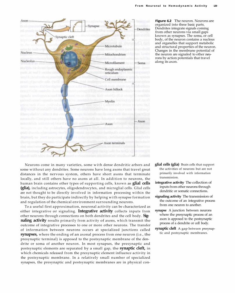
F r o m N e u r o n a l to H e m o d y n a m i c A c t i v i t y 129
Figure 6.2 The neuron. Neurons are organized into three basic parts. Dendrites integrate signals coming from other neurons via small gaps known as synapses. The soma, or cell body, of the neuron contains a nucleus and organelles that support metabolic and structural properties of the neuron. Changes in the membrane potential of the neuron are signaled to other neurons by action potentials that travel along its axon.
Neurons come in many varieties, some w i t h dense dendritic arbors and some without any dendrites. Some neurons have long axons that travel great distances in the nervous system, others have short axons that terminate locally, and still others have no axons at al l . In addi t ion to neurons, the human brain contains other types of supporting cells, k n o w n as glial cells (glia), including astrocytes, oligodendrocytes, and microglial cells. Glial cells are not thought to be directly involved in information processing wi th in the brain, but they do participate indirectly by helping w i t h synapse formation and regulation of the chemical environment surrounding neurons.
To a useful first approximation, neuronal activity can be characterized as either integrative or signaling. Integrative activity collects inputs from other neurons through connections on both dendrites and the cell body. Signaling activity results primari ly from activity of axons, which transmit the outcome of integrative processes to one or more other neurons. The transfer of information between neurons occurs at specialized junctions called synapses, where the ending of an axonal process from one neuron (i.e., the presynaptic terminal) is apposed to the postsynaptic membrane of the dendrite or soma of another neuron. In most synapses, the presynaptic and postsynaptic elements are separated by a small gap, the synaptic cleft, in which chemicals released from the presynaptic element influence activity in the postsynaptic membrane. In a relatively small number of specialized synapses, the presynaptic and postsynaptic membranes are in physical con-
glial cells (glia) Brain cells that support the activities of neurons but are not primarily involved with information transmission.
integrative activity The collection of inputs from other neurons through dendritic or somatic connections.
signaling activity The transmission of the outcome of an integrative process from one neuron to another.
synapse A junction between neurons where the presynaptic process of an axon is apposed to the postsynaptic process of a dendrite or cell body.
synaptic cleft A gap between presynaptic and postsynaptic membranes.

130 C h a p t e r Six
concentration gradient A difference in the density of a substance across space. Substances diffuse along a concentration gradient from areas of high concentration to areas of low concentration.
ion A charged atom. ion channel A pore in the membrane of
a cell that allows passage of particular ions under certain conditions.
pump A transport system that moves ions across a cell membrane against their concentration gradient.
sodium-potassium pump A transport system that removes three sodium ions from within a cell while bringing two potassium ions into the cell.
tact and electrical signaling events cross the membranes without intervening chemical messengers. A neuron may have hundreds or even thousands of synapses on its dendrites and soma, and it has been estimated that there are 100 tr i l l ion synapses in the human brain.
Ion Channels in Neurons Both neuronal integration and signaling depend upon the properties of neuronal membranes, which are l i p i d bilayers that separate the internal contents of the neuron from the external mil ieu. An important role of neuronal membranes is to restrict the f low of chemical substances into and out of the neurons. When substances are allowed to diffuse freely, they tend to diffuse from areas of high concentration to areas of low concentration. That is, they move along a concentration gradient unt i l equi l ibr ium is reached. However, neuronal membranes prevent free diffusion. They do, though, have embedded proteins that form pores or channels through which some ions, such as sodium (Na + ) , chloride (Cl - ) , potassium (K + ) , and calcium (Ca 2 + ), can diffuse (Figure 6.3). (Note that an ion is an atom that has a negative charge from having gained one or more electrons, or a positive charge from having lost one or more electrons.) These ion channels are selective, such that some species of ions can pass and others cannot. Furthermore, channels have gating mechanisms that can close them or open them to ion traffic. While some gating mechanisms depend on the actions of specific molecules, others are also voltage-dependent and open when the electrical potential difference across the membrane has reached a particular threshold.
While an open channel can allow ions to diffuse passively d o w n their concentration gradient, membranes also contain transporters, or pumps, that can move ions across the membrane against their concentration gradient and thereby create or maintain an unequal distribution of some ions (see Figure 6.3). One of the most important pumps is the sodium-potassium pump. The sodium-potassium p u m p uses a transporter molecule that forces three sodium ions (Na + ) out of the cell and then picks up and brings two potassium ions (K + ) into the cell on the return tr ip . Due to the action of the sodium-potassium p u m p and other transporters, as well as to the selective permeability of the membrane channels to different ions, a neuron at rest has a greater concentration of K+ inside its membrane and a greater concentration of N a + , Ca 2 + , and Cl - outside its membrane. A n y transient change in the permeability of the membrane w i l l cause an influx (movement into the cell) or an efflux (movement out of the cell) of these ions as the system attempts to eliminate the concentration gradient and establish equil ibrium.
Figure 6.3 Ion channels and pumps. Ion channels allow particular ions to diffuse across membranes along concentration gradients. They may be opened by the actions of particular molecules, or they may open when the voltage difference across the membrane reaches a threshold. Pumps move ions across membranes against their concentration gradients, usually at a cost of energy supplied by ATP. A very important pump transports sodium out of the cell while bringing potassium into the cell.

From Neuronal to Hemodynamic Activity 131
While the diffusion of substances through channels down their concentra
tion gradients requires only sufficient kinetic energy from heat, the operation
of pumps requires cellular sources of energy. For example, one turn of the
sodiumpotassium pump requires the energy of one molecule of adenosine
triphosphate, or ATP (we w i l l have more to say about ATP later in this chapter
in the section on cerebral metabolism). Consider the analogy of a water tower
where holes in the bottom of the water reservoir allow passage of the water
into descending pipes below. Here the gravity gradient is analogous to the
concentration gradient and the holes are analogous to open ion channels. The
water w i l l move through the holes and run through the pipes down the grav
ity gradient without additional energy. The situation is quite different, how
ever, if we want to return the escaping water to the water tower. Active pump
ing against the gravity gradient is now required, and the p u m p requires
energy to operate. Note that while this analogy is instructive, it is incomplete
with respect to ions. Because ions have electrical charge, their unequal distri
bution also results in an electrical potential (about 40 to 70 mV) between the
inside and outside of the membrane. Thus, the movement of ions across a
membrane is governed by both chemical and electrical gradients.
Neurotransmitters and Action Potentials
The primary locus for communication between neurons is the synapse (Fig
ure 6.4). The presynaptic process of the axon releases neurotransmitters, which are chemicals that diffuse across the synaptic cleft and interact w i t h
receptors on the postsynaptic membrane that gate ion channels. For exam
ple, the neurotransmitter glutamate opens normally blocked ion channels
that allow Na + to move d o w n its concentration gradient and through the
postsynaptic membrane into the neuron. This influx of Na+ ions decreases
the electrical potential between the inside and outside of the membrane at
the channel location. (Note that another type of glutamate receptor called
the N M D A [NmethylDaspartate] receptor admits Ca 2 + through its channel
when a threshold membrane potential is reached.) This local depolarization
of the postsynaptic cell membrane is referred to as an excitatory postsynaptic potential, or EPSP, and thus glutamate is k n o w n as an excitatory
neurotransmitter. Glutamate is the most common excitatory neurotransmit
ter in the brain, and it is released by about 90% of all neurons.
Other neurotransmitters, such as γaminobutyric acid, or GABA, interact
with other receptors to open chlorine or potassium channels. Either the
influx of the negatively charged CP into the neuron or the efflux of the posi
tively charged K+ out of the neuron results in a net increase in the resting
potential in the vicinity of these newly opened channels. This local hyperpo
larization of the neuronal membrane is referred to as an inhibitory postsynaptic potential, or IPSP, and thus G A B A is known as an inhibitory neuro
transmitter.
A single EPSP or IPSP is a l imited event. Afterward, the neurotransmitter
wi l l be deactivated or removed from the synaptic cleft and receptor, the
channel that was opened by the neurotransmitter w i l l close, and the pumps
wi l l restore both the unequal distribution of ions across the membrane and
the resting membrane potential. However, because a neuron may have thou
sands of synapses, i t may experience a barrage of individual EPSPs and
IPSPs throughout its dendritic trees and soma. These depolarizing and
hyperpolarizing membrane potentials are integrated by the neuron. Both
their t iming and spatial pattern influence the net polarization of a special
ized region of the soma called the axon hillock, which is located where the
axon emerges from the cell body.
neurotransmitters Chemicals released by presynaptic neurons that travel across the synaptic cleft to influence receptors on postsynaptic neurons.
glutamate One of the most important excitatory neurotransmitters.
excitatory postsynaptic potential (EPSP) A depolarization of the postsy
naptic cell membrane.
Yaminobutyric acid (GABA) One of the most important inhibitory neurotrans
mitters.
inhibitory postsynaptic potential (IPSP) A hyperpolarization of the post
synaptic cell membrane.
axon hillock A region of the cell body located at the emergence of the axon.
Changes in its electrical potential lead
to the generation of action potentials.
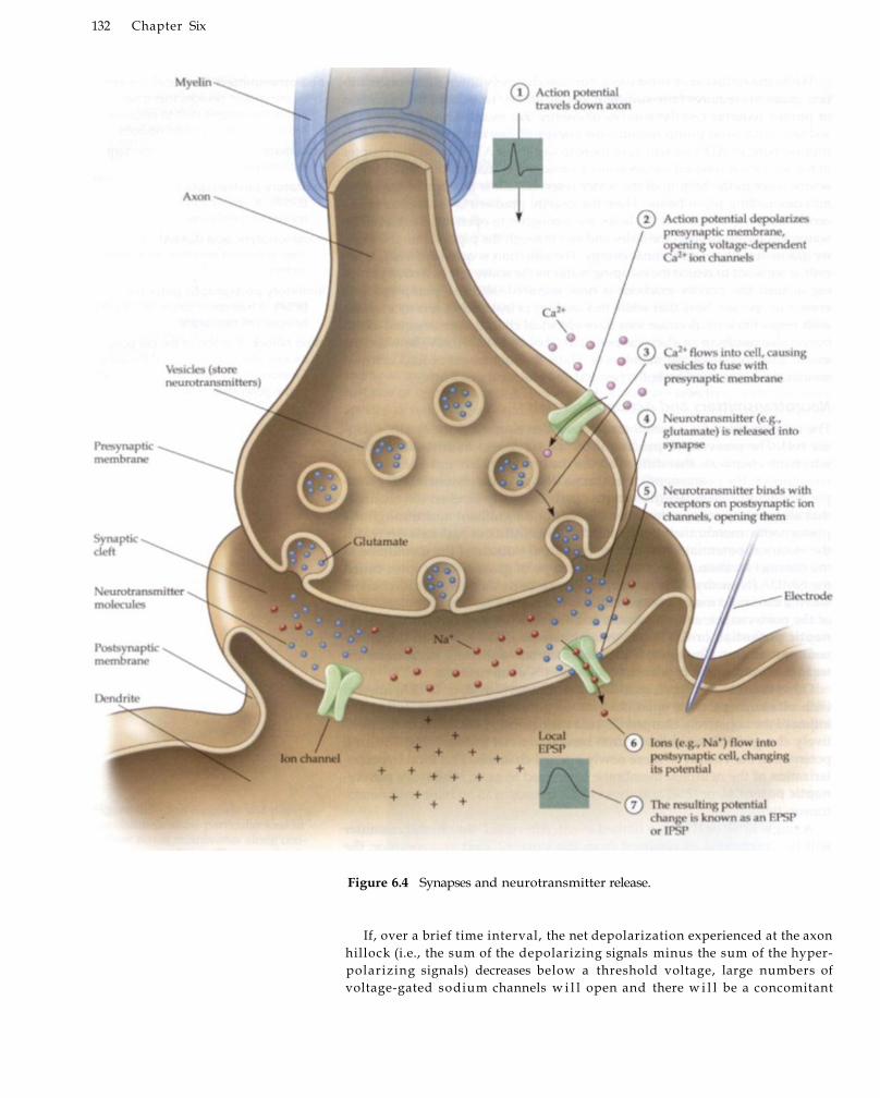
132 Chapter Six
Figure 6.4 Synapses and neurotransmitter release.
If, over a brief time interval, the net depolarization experienced at the axon hillock (i.e., the sum of the depolarizing signals minus the sum of the hyper-polarizing signals) decreases below a threshold voltage, large numbers of voltage-gated sodium channels w i l l open and there w i l l be a concomitant
F r o m N e u r o n a l to H e m o d y n a m i c A c t i v i t y 133
large influx of Na+ into the cell. This large depolarization spreads d o w n the axon, opening more voltage-gated sodium channels farther and farther down the membrane. This wave of depolarization, k n o w n as a nerve impulse or action potential, sweeps down the axon in a self-propagating manner, independently of the EPSPs that triggered it . Eventually, the nerve impulse w i l l reach the end of the axon, where a presynaptic terminal forms a synapse w i t h another neuron. Here the wave of depolarization w i l l open voltage-dependent channels in the presynaptic membrane that allow Ca 2 + inf lux into the presynaptic terminal. This influx of Ca 2 + initiates a cascade of events that causes the release of neurotransmitter into the synaptic cleft, which interacts wi th receptors that gate postsynaptic ion channels, and thus initiates either an IPSP or EPSP on the postsynaptic membrane of the target neuron.
One can think of information processing by neurons as the combination of their integrative and signaling roles. The spatiotemporal pattern of EPSPs and IPSPs, each generated at a synapse from another cell, determines the relative polarization of the neuron. If the axon hillock region of the neuron becomes sufficiently depolarized, an action potential occurs and the polarizations of other neurons are influenced by the action of that action potential upon their postsynaptic membranes. Note that only EPSPs can trigger action potentials. Hyperpolarizing IPSPs, in contrast, make action potentials less likely by making the membrane potential more negative. An EPSP that might have sufficient strength to depolarize the axon hil lock region below threshold when this region is at its normal resting potential may not be able to do so if the axon hillock was hyperpolarized by a preceding IPSP.
The generation of an EPSP, IPSP, or action potential does not in itself require an external source of energy, because the associated movements of ions are along concentration gradients. However, these potentials cause changes in ion concentration that require energy to restore. For example, the influx of Na+ d u r i n g an action potential causes a change in the local membrane potential of the neuron, so electrical gradients now oppose the reentry of the positively charged K* into the cell. To restore the asymmetric distribution of Na+ and K+ across the cell membrane and restore the resting membrane potential, the sodium-potassium p u m p removes three Na+ ions from with in the cell for every t w o K + ions it brings into the cell. The energy requirements for restoration of these concentration gradients are discussed in the next section.
Cerebral Metabolism: Neuronal Energy Consumption
Although integrative and signaling properties of neurons are ultimately important for understanding brain function, our immediate interest is in their energy requirements. Why are the energy demands of neurons important for fMRI? To help answer this question, imagine that neurons have sufficient local stores of energy available to buffer moderate changes in their neuronal f ir ing rates. Could we then construct meaningful theories of brain function based upon energy delivery by the blood supply? Or imagine that it were known that the main consumption of energy fol lowing neuronal firing was to increase the synthesis of protein, perhaps related to structural changes in the neurons initiated by learning. H o w would this change the interpretation of neuroimaging results? Finally, imagine that we learned (as was once thought true) that the generation of action potentials accounted for a tiny fraction, less than 3%, of the brain's energy budget. H o w then w o u l d one account for the enormous metabolic demands of the active brain?
action potential A wave of depolarization that travels down a neuronal axon.
134 Chapter Six
adenosine triphosphate (ATP) A nucleotide containing three phosphate groups that is the primary energy source for cells in the human body.
glucose A sugar made by the human body whose stored energy is used to form ATP.
glycolysis The process of breaking down glucose into other compounds to produce ATP.
aerobic glycolysis The process, consisting of glycolysis, the TCA cycle, and the electron transport chain, that breaks down glucose in the presence of oxygen, resulting in a gain of 36 ATP.
TCA cycle The second step in aerobic glycolysis; it involves the oxidation of pyruvate.
electron transport chain The third step in aerobic glycolysis; it generates an additional 34 ATP.
anaerobic glycolysis The conversion of glucose to lactate in the absence of oxygen.
We now know that these hypothetical situations are not true: Local brain regions require external sources of energy to support metabolic processes, and much of this energy facilitates the restoration of concentration gradients fo l lowing changes in membrane potential. Thus, functional neuroimaging methods that measure metabolic correlates of neuronal activity can be used to make inferences about brain activity. Stated another way, although our interests as neuroscientists may be in the relation between mind and brain (where in this context " b r a i n " is usually shorthand for the activity of neurons), our measures depend upon the relation between neuronal activity and the energy needed to support that activity. Here, we delve more deeply into the energy needs of neurons and how those needs are met by the vascular system.
Adenosine Triphosphate (ATP) The principal energy currency for cells in the human body is adenosine triphosphate, or ATP. ATP is a nucleotide that contains three phosphate groups. Free energy is released when the third phosphate group of ATP is removed by the insertion of a water molecule, in a reaction called hydrolysis. In body tissues, ATP can be produced from many substrates, including the sugar glucose, fatty acids, ketone bodies, and even proteins. Glucose is stored throughout the body in the form of glycogen. However, there is little glycogen in the brain, and thus, to maintain function, the brain requires that the blood provide a continuous supply of glucose and oxygen. Under normal circumstances, the brain extracts about 10% of the approximately 90 m g / d L of glucose in arterial blood. If the glucose concentration in blood falls below about 30 mg/dL, a coma may ensue.
The generation of ATP from glucose has three primary steps: glycolysis, the TCA cycle, and the electron transport chain (Figure 6.5). Glucose transporter molecules move glucose through the interstitial space from capillaries to neurons. Once in the cytoplasm of brain cells, glucose is broken d o w n through a reaction called glycolysis, in which the six-carbon glucose is cleaved into two three-carbon sugars, which are then catabolized through a series of steps into a compound called pyruvate. Glycolysis consumes 2 ATP molecules but produces 4 ATP molecules, for a net gain of 2 ATP. If oxygen is present, the process is called aerobic glycolysis and the pyruvate product then enters a reaction called the tricarboxylic cycle, or TCA cycle, also known as the citric acid cycle or the Krebs cycle. The TCA cycle uses oxygen extracted from the hemoglobin in the blood to oxidize pyruvate, and a network of proteins in the cell mitochondria, known as the electron transport chain, passes electrons across a series of compounds to release energy, which in turn is used by an enzyme known as ATP synthase to generate an additional 34 ATP molecules. So, while glycolysis itself produces only 2 ATP molecules from each glucose molecule, the addition of oxygen allows the production of a total of 36 ATP molecules from each molecule of glucose.
If oxygen is not present, the process is called anaerobic glycolysis and the pyruvate is reduced to the end product lactate. Dur ing strenuous exer-
Assume that the brain did indeed have large local stores of energy that could support neuronal activity. Based on what
you know so far, would fMRI be possible?

From Neuronal to Hemodynamic Activity 135
Figure 6.5 Anaerobic and aerobic glycolysis. In anaerobic glycolysis, glucose is converted to lactate via a fast process that produces 2 ATP. If oxygen is present, then the resulting aerobic glycolysis produces an additional 34 ATP.
cise w i t h insufficient oxygen, anaerobic glycolysis occurs in muscles, and it
is the bui ldup of lactate that can cause pain and fatigue. Lactate is removed
from the muscles by the vascular system. While anaerobic glycolysis is a rel
atively inefficient source of ATP, it is quite fast: it can occur at a rate about
100 times faster than the further oxidation of pyruvate into ATP through the
TCA cycle and electron transport chain. In addit ion, some cells can convert
lactate back into pyruvate and use it as a fuel for the TCA cycle and the pro
duction of more ATP. (Note that the tradeoff between fast but inefficient
anaerobic glycolysis and slow but efficient aerobic glycolysis is important
for the models of BOLD contrast, and is discussed in the next chapter.)
The energy provided by ATP supports many processes in the brain. For
example, there are housekeeping functions related to the synthesis of pro
teins, the maintenance and turnover of membranes, and axoplasmic trans
port that require energy. Neurons also require energy to synthesize, package,
and break d o w n neurotransmitters and to operate the pumps that restore
unequal distributions of ions fol lowing EPSPs, IPSPs, and action potentials.
Noting that the gray matter of the brain consumes about 30 to 50 μmol of
ATP every minute for each gram of tissue (i.e., 30 to 50 μmol/g/min of
ATP), while the brain in coma consumes only about 10 μmol/g/min of ATP,
Attwel l and Laughlin concluded that integrative and signaling activity in
neurons accounts for about 75% of the energy expenditure in gray matter
while housekeeping functions account for about 25%. Because the chemical
reactions associated w i t h neuronal integration and signaling are wel l
known, they were able to determine how the brain's energy budget was fur
ther allocated.
Attwel l and Laughlin estimated that the restoration of membrane concen
tration gradients fol lowing the passage of an action potential consumes 47%
of the energy expenditure, while restoring postsynaptic membrane concen
tration gradients fol lowing IPSPs and EPSPs consumes 34% (Figure 6.6). The

136 Chapter Six
Figure 6.6 The energy budget of the (rodent) brain. Data from the rodent brain, shown here, indicates the vast majority of energy required to support the restoration of concentration gradients following action potentials and postsynaptic potentials. While human data are not available for these categories, the differences in brain structure in humans compared with rodents would serve to increase the budget needed for restoring gradients after postsynaptic potentials. These results indicate that the primary energy expenditure of the brain supports the integrative and signaling roles of neurons. (Data from Atwell and Laughlin, 2001.)
authors commented that the energy cost of IPSPs is l ikely less than that of EPSPs, for two reasons: Cl - ions move d o w n a smaller electrochemical gradient than N a + ions, and inhibitory synapses are outnumbered by excitatory synapses in the brain by about an order of magnitude. The maintenance of the resting potential in neurons and glia was estimated to consume 13% of the energy expenditure. Note that the consumption of energy in each of these processes principally involves the operation of the sodium-potassium pump. Furthermore, given that glutamate is by far the dominant excitatory neurotransmitter in the brain, most of the energy budget associated wi th signaling and integration involves this single neurotransmitter. The uptake, breakdown, and repackaging of glutamate was estimated to consume 3% of the energy budget, and restoring Ca 2 + fluxes in presynaptic membranes accounted for the remaining 3%.
Atwel l and Laughlin's calculations were based upon data from the rodent brain. In extrapolating their results to primates, they argued that the greater number of synapses per neuron in primates w o u l d cause a greater proportion of the energy budget to be spent on restoring postsynaptic concentration gradients, perhaps as high as 74%. They concluded, therefore, that the metabolic demands of integrative and signaling activity of neurons form the bulk of the energy requirements of the human brain. A continuous supply of metabolites through the vascular system is necessary for these energy demands to be met.
The Vascular System of the Brain
The idea that changes w i t h i n the vascular system of the brain reflect changes in brain function is not new. The nineteenth-century British physiologists Roy and Sherrington postulated that changes in activity associated wi th specific brain functions might result in locally increased blood f low:
These facts seem to us to indicate the existence of an automatic mechanism by which the blood supply of any part of the cerebral tissue is varied in

From Neuronal to Hemodynamic Activity 137
accordance with the activity of the chemical changes which underlie the functional action of that part. Bearing in mind that strong evidence exists of localisation of function in the brain, we are of the opinion that an automatic mechanism, of the kind just referred to, is well fitted to provide for a local variation of the blood supply in accordance with local variations of the functional activity. (1890, p.105)
A variant of this idea, that activity could cause changes in blood f low, was tested in an early experiment conducted by the Italian physiologist Angelo Mosso in the late nineteenth century. Mosso had pioneered the use of plethysmographic measurement of comparative blood volume in the brain and extremities, and he was interested in whether th ink ing resulted in increased blood f low to the brain. His earlier studies had revealed that blood f low to the brain decreases dur ing sleep and increases w i t h waking , consistent w i t h the idea that brain activity requires a greater blood supply than inactivity. To directly test the hypothesis that active thought requires increased blood volume in the brain, Mosso constructed an ingenious apparatus (Figure 6.7), as reported by Wi l l iam James in his Principles of Psychology:
The subject to be observed lay on a delicately balanced table which could tip downward either at the head or at the foot if the weight of either end were increased. The moment emotional or intellectual activity began in the subject, down went the balance at the head end, in consequence of the redistribution of blood in his system. (1890, p. 98)
Though its results suggest a clear relation between the vascular system and cognitive function, this experiment is unlikely to have worked as well as Mosso reported. For the table to tip d o w n w a r d , the total blood volume of
Figure 6.7 The crude imaging apparatus used by Angelo Mosso in the late nineteenth century. Mosso theorized that thinking drew blood to the brain, and constructed a balance device to measure changes in weight associated with this increased blood flow. The subject lay down on a large table with a fulcrum at its center, so that any change in weight would cause the table to tip.

138 Chapter Six
the brain w o u l d need to increase by an appreciable amount. But blood volume is relatively constant across time, even if blood f low may change in response to metabolic demands. To use a hydraulic analogy, if pipes are filled w i t h water, they w i l l weigh essentially the same regardless of whether the water is f lowing quickly or slowly. Nevertheless, the idea that changes in blood f low may result from local functional changes in the brain was a remarkable insight. (The discussion of this issue in James's Principles, especially the difference between causal and correlational roles for blood flow, is highly recommended to the interested student.) We explore this idea over the fo l lowing sections, bui ld ing to the idea that functional activity of neurons may evoke changes in blood f low and thus changes in the local concen¬tration of metabolites.
Arteries, Capillaries, and Veins From our discussion earlier in this chapter, we know that integrative and signaling activity of neurons comprises a large proport ion of the brain's energy budget, and we also know that there is l i tt le energy stored in the brain. The energy needs of neurons and glia are met by the ATP created during glycolysis and during the subsequent oxidation of pyruvate. The oxygen and glucose fuel required for those reactions are delivered through the vascular system (Figure 6.8). The adult human brain consumes about 54 mL of blood for each 100 grams of tissue every minute. This adds up to about 750 m L / m i n for the average 1400-gram brain and represents about 15 to 20% of the blood f low in the entire human body. Thus, although the brain constitutes a mere 2 to 3% of total body weight, it consumes about 20% of blood oxygen.
The lungs are the source of the oxygen carried by the blood. Oxygen diffuses from the alveoli of the lungs, via small blood vessels, into red blood cells, where it binds to hemoglobin. Four oxygen molecules are attached to each hemoglobin molecule, and there are about 280 mi l l ion hemoglobin molecules in each red blood cell. The oxygen-rich blood returns to the heart from the lungs, where it enters the left atr ium, moves to the left ventricle, and is pumped from the left ventricle through the aorta. The aorta gives rise
Figure 6.8 Blood supply to the human cerebrum. As illustrated here, the surface pattern of blood supply to the human cerebrum is highly complex. The red vessels are tributaries of the middle cerebral artery, the green vessels are tributaries of the anterior cerebral artery, and the blue vessels are tributaries of the posterior cerebral artery. The veins are shown in black. (From Duvernoy, Delon, and Vannson, 1981.)

From Neuronal to Hemodynamic Activity 139
to several large arteries—thickwalled vessels that carry blood away from
the heart. Each artery branches into smaller arteries and then to even smaller
arterioles that eventually terminate in capillaries. The change in scale as
these vessels branch is remarkable. The diameter of the aorta in an adult
human is about 2.5 cm (about 1 inch), typical large arteries can be 4 to 10
mm in diameter, while the diameters of arterioles are in the range of 10 to 50
μm. Thus, the largest artery has a diameter about 2500 times that of the
smallest arteriole!
The extraction of oxygen and glucose from the blood and the removal of
waste carbon dioxide occurs at the surfaces of the capillaries. Capillaries are
thinwalled vessels comparable in diameter (5 to 10 μm) to the w i d t h of a
red blood cell (7.5 μm). The small size of individual capillaries is more than
made up for by their number and density (Figure 6.9). It has been estimated
that cells in the body are, on average, less than 50 μm from a capillary. If
lined up end to end, the capillary network in the human body w o u l d stretch
60,000 miles and have a total surface area of 800 to 1000 m 2 . Capillary den
sity provides an indication of cellular metabolism, such that areas w i t h high
metabolism have a higher density of capillaries than those w i t h low metab
olism. For example, in the cat brain, gray matter composed of neural cell
bodies has twice the capillary density as white matter composed largely of
axonal processes.
arteries Blood vessels that carry oxy
genated blood from the heart to the
rest of the body.
arterioles Small arteries.
capillaries Small and thinwalled blood
vessels. The extraction of oxygen and
glucose from the blood and the
removal of waste carbon dioxide occur
in the capillaries.
venules Small veins.
veins Blood vessels that carry blood from
the body to the heart. Blood in the
veins (except for the pulmonary vein) is
deoxygenated.
After the oxygen molecules are extracted f rom the
hemoglobin in the capillaries, the deoxygenated hemoglo
bin molecules, which now bind waste carbon dioxide, are
carried from the capillaries to small venules that are com
parable in size to arterioles. The venules collect into larger
and larger veins that eventually return the oxygenpoor
blood through the vena cava to the right atr ium of the
heart. The deoxygenated blood travels to the right ventri
cle, which pumps it to the lungs, where the waste carbon
dioxide is released as a gas and where oxygen once again
binds to the hemoglobin to start the cycle again.
Arterial and Venous Anatomy of the Human Brain
The flow of blood to the brain is supplied by two major arte
rial systems: the left and right internal carotid arteries and
the vertebral/basilar arteries (Figure 6.10A and B). A short
distance from the heart, the aortic arch gives rise to the right
and left common carotid arteries, which ascend in the neck
before each divides into the external and internal carotid
arteries. While the external carotid arteries supply the exter
nal head and face w i t h blood, the internal carotid arteries
enter through an opening in the base of the skull called the
foramen lacerum and supply blood to the brain. The aortic
Figure 6.9 Capillary structure. This electron microscope image shows the density of capillary beds within the cortex. (From Duvernoy, Delon, and Vannson, 1981.)
Many techniques in fMRI attempt to localize hemodynamic activity to the capillaries. Why is this desirable for studies of
brain function?

140 C h a p t e r Six
Figure 6.10 The arterial system of the human brain. The arterial distribution of blood to the human brain is shown in cross-section (A), and in a ventral view of the base of the brain (B). The box shows the anastomoses of the basilar artery and internal carotid arteries that form the circle of Willis.
circle of Willis The interconnection between the basilar artery and the carotid arteries at the base of the cranial vault.
arch also gives rise to the right and left subclavian arteries, which, in turn, give rise to the left and right vertebral arteries, which run along the anterior surface of the spinal cord and enter the brain through the foramen magnum. The vertebral arteries give rise to the descending arterial branches, which provide blood to the brain stem, medulla, and spinal cord. As the vertebral arteries ascend to the level of the pons, they fuse into the single basilar artery, which gives rise to arterial branches that perfuse the pons and cerebellum.
The basilar artery interconnects, or forms an anastomosis, w i t h the left and right internal carotid arteries to form the circle of Willis, named for the celebrated English physician Thomas Willis, who first illustrated this vascular structure in 1664. The circle of Willis sits on the floor of the cranial vault, surrounding the brain stem. Supplied by blood from both arterial systems, it gives rise bilaterally to the anterior, middle, and posterior cerebral arteries (Figure 6.11A and B). Each of these major cerebral arteries provides the blood supply to distinct regions of the brain: The anterior cerebral artery primarily supplies the medial surface of the brain and the head of the caudate, branches of the middle cerebral artery supply much of the lateral and superior cerebral cortex as wel l as the remainder of the basal ganglia, and the posterior cerebral artery supplies the posterior temporal and occipital cortex. This specificity has important implications for neurology, in that strokes w i t h i n particular arteries tend to affect particular regions of cortex and thus have functionally distinct cognitive consequences.
The venous drainage of the brain's circulation (Figure 6.11C and D) is accomplished through the left and right jugular veins, which exit the skull base through the jugular foramen, then join w i t h the subclavian vein and eventually the superior vena cava, progressing to the right atr ium and ven-
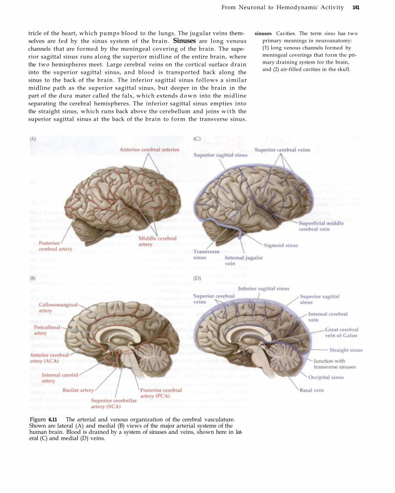
From Neuronal to Hemodynamic Activity 141
tricle of the heart, which pumps blood to the lungs. The jugular veins themselves are fed by the sinus system of the brain. Sinuses are long venous channels that are formed by the meningeal covering of the brain. The superior sagittal sinus runs along the superior midline of the entire brain, where the two hemispheres meet. Large cerebral veins on the cortical surface drain into the superior sagittal sinus, and blood is transported back along the sinus to the back of the brain. The inferior sagittal sinus follows a similar midline path as the superior sagittal sinus, but deeper in the brain in the part of the dura mater called the falx, which extends down into the midline separating the cerebral hemispheres. The inferior sagittal sinus empties into the straight sinus, which runs back above the cerebellum and joins w i t h the superior sagittal sinus at the back of the brain to form the transverse sinus.
sinuses Cavities. The term sinus has two primary meanings in neuroanatomy: (1) long venous channels formed by meningeal coverings that form the primary draining system for the brain, and (2) air-filled cavities in the skull.
Figure 6.11 The arterial and venous organization of the cerebral vasculature. Shown are lateral (A) and medial (B) views of the major arterial systems of the human brain. Blood is drained by a system of sinuses and veins, shown here in lateral (C) and medial (D) veins.

142 Chapter Six
Figure 6.12 Microcirculation of the human brain. The distribution of arteries (red) and veins (black) on the medial orbital gyrus of the human brain as shown in (A). A photograph of the same region is provided in (B). (From Duvernoy, Delon, and Vannson, 1986.)
The transverse sinus wraps around to the left and right of the base of the
brain, terminating in the left and right internal jugular veins.
Microcirculation
The blood supply to the cerebral and cerebellar cortices is derived from
meningeal arteries that traverse the pia on the cortical surface (Figure 6.12).
A distinction can be d r a w n between conducting and distr ibuting arteries.
Conducting arteries r un for long distances along the pial surface and are
about 700 μm in diameter (compared to the 4 to 5mm diameter of the inter
nal carotid and basilar arteries). In the cerebral cortex, many conducting
arteries r un along the sulci that demarcate adjacent gyr i , while others run
directly across the gyral surface. Many smaller distr ibuting arteries, each
about 150 to 200 urn in diameter, branch from the conducting arteries. Many
researchers have noted constrictions where the distributing arteries branch
from larger arteries, suggestive of the presence of muscular sphincters. The
possible role of these sphincters in the control of blood flow w i l l be dis
cussed in more detail shortly. The distributing arteries continue to ramify on
the cortical surface into yet smaller precortical arteries (or arterioles) of
about 50 to 70 μm in diameter. Anastomoses between arterioles have been
observed in several studies. According to Nonaka and colleagues, a distrib
uting artery supplies a 3.5by2mm area on the cortical surface, while each
precortical artery supplies an approximately 1by1mm area of cortical sur
face. Each precortical artery then ramifies into smaller arterioles of about 30
to 40 μm diameter that penetrate the cortical surface at right angles.
Duvernoy and colleagues have classified these intracortical arterioles into
six categories. The first five categories appear to vascularize different cortical
levels, wi th increasing vessel diameters noted for those that vascularize deeper
layers. The density of vascularization is not uniform across cortical layers;
noticeably denser vascularization is observed where the highest concentrations
of neural cell bodies are located (Figure 6.13). Some intracortical vessels have
been described as resembling a fountain or candelabra, w i t h dense ramifica
tions ascending into more superficial layers. The sixth category of intracortical
arterioles consists of the largestdiameter vessels, which appear to penetrate
straight though the cortex to vascularize the white matter below. The vascular
ization in white matter is considerably less dense than that of gray matter.
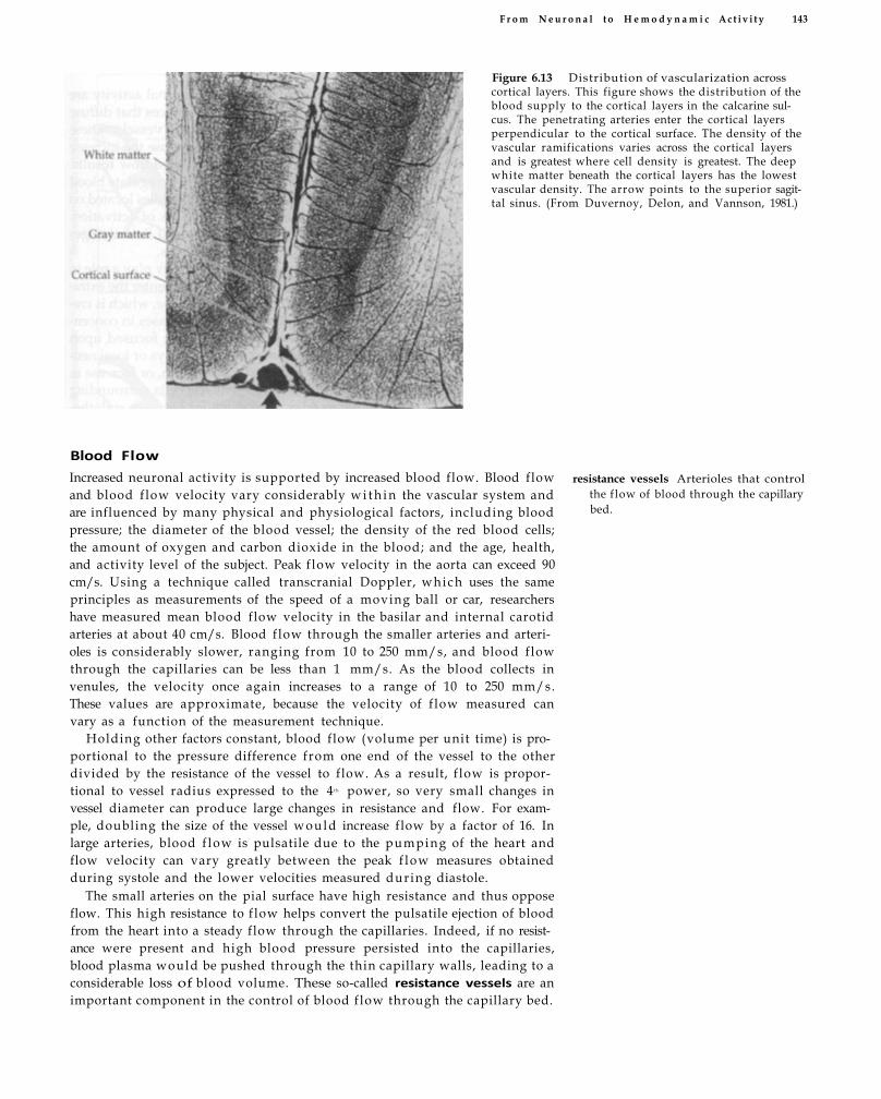
F r o m N e u r o n a l t o H e m o d y n a m i c A c t i v i t y 143
Figure 6.13 Distribution of vascularization across cortical layers. This figure shows the distribution of the blood supply to the cortical layers in the calcarine sulcus. The penetrating arteries enter the cortical layers perpendicular to the cortical surface. The density of the vascular ramifications varies across the cortical layers and is greatest where cell density is greatest. The deep white matter beneath the cortical layers has the lowest vascular density. The arrow points to the superior sagittal sinus. (From Duvernoy, Delon, and Vannson, 1981.)
Blood Flow
Increased neuronal activity is supported by increased blood flow. Blood flow and blood f low velocity vary considerably w i t h i n the vascular system and are influenced by many physical and physiological factors, including blood pressure; the diameter of the blood vessel; the density of the red blood cells; the amount of oxygen and carbon dioxide in the blood; and the age, health, and activity level of the subject. Peak f low velocity in the aorta can exceed 90 cm/s. Using a technique called transcranial Doppler, which uses the same principles as measurements of the speed of a moving ball or car, researchers have measured mean blood flow velocity in the basilar and internal carotid arteries at about 40 cm/s. Blood f low through the smaller arteries and arterioles is considerably slower, ranging from 10 to 250 mm/s, and blood f low through the capillaries can be less than 1 mm/s. As the blood collects in venules, the velocity once again increases to a range of 10 to 250 mm/s. These values are approximate, because the velocity of f low measured can vary as a function of the measurement technique.
Holding other factors constant, blood flow (volume per unit time) is proportional to the pressure difference from one end of the vessel to the other divided by the resistance of the vessel to flow. As a result, f low is proportional to vessel radius expressed to the 4 t h power, so very small changes in vessel diameter can produce large changes in resistance and flow. For example, doubling the size of the vessel would increase flow by a factor of 16. In large arteries, blood f low is pulsatile due to the pumping of the heart and flow velocity can vary greatly between the peak f low measures obtained during systole and the lower velocities measured during diastole.
The small arteries on the pial surface have high resistance and thus oppose flow. This high resistance to f low helps convert the pulsatile ejection of blood from the heart into a steady flow through the capillaries. Indeed, if no resistance were present and high blood pressure persisted into the capillaries, blood plasma would be pushed through the thin capillary walls, leading to a considerable loss of blood volume. These so-called resistance vessels are an important component in the control of blood f low through the capillary bed.
resistance vessels Arterioles that control the flow of blood through the capillary bed.
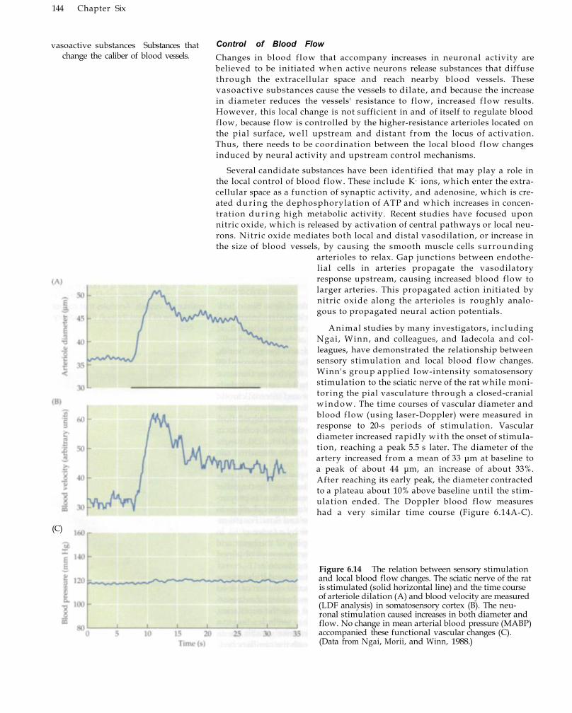
144 Chapter Six
vasoactive substances Substances that change the caliber of blood vessels.
(C)
Control of Blood Flow
Changes in blood f low that accompany increases in neuronal activity are
believed to be initiated when active neurons release substances that diffuse
through the extracellular space and reach nearby blood vessels. These
vasoactive substances cause the vessels to dilate, and because the increase
in diameter reduces the vessels' resistance to flow, increased f low results.
However, this local change is not sufficient in and of itself to regulate blood
flow, because flow is controlled by the higherresistance arterioles located on
the pial surface, wel l upstream and distant from the locus of activation.
Thus, there needs to be coordination between the local blood f low changes
induced by neural activity and upstream control mechanisms.
Several candidate substances have been identified that may play a role in
the local control of blood flow. These include K+ ions, which enter the extra
cellular space as a function of synaptic activity, and adenosine, which is cre
ated d u r i n g the dephosphorylation of ATP and which increases in concen
tration d u r i n g high metabolic activity. Recent studies have focused upon
nitric oxide, which is released by activation of central pathways or local neu
rons. Nitric oxide mediates both local and distal vasodilation, or increase in
the size of blood vessels, by causing the smooth muscle cells surrounding
arterioles to relax. Gap junctions between endothe
lial cells in arteries propagate the vasodilatory
response upstream, causing increased blood flow to
larger arteries. This propagated action initiated by
nitric oxide along the arterioles is roughly analo
gous to propagated neural action potentials.
Animal studies by many investigators, including
Ngai, Winn, and colleagues, and Iadecola and col
leagues, have demonstrated the relationship between
sensory stimulation and local blood f low changes.
Winn's group applied lowintensity somatosensory
stimulation to the sciatic nerve of the rat while moni
toring the pial vasculature through a closedcranial
window. The time courses of vascular diameter and
blood f low (using laserDoppler) were measured in
response to 20s periods of stimulation. Vascular
diameter increased rapidly wi th the onset of stimula
tion, reaching a peak 5.5 s later. The diameter of the
artery increased from a mean of 33 μm at baseline to
a peak of about 44 μm, an increase of about 33%.
After reaching its early peak, the diameter contracted
to a plateau about 10% above baseline until the stim
ulation ended. The Doppler blood flow measures
had a very similar time course (Figure 6.14AC).
Figure 6.14 The relation between sensory stimulation and local blood flow changes. The sciatic nerve of the rat is stimulated (solid horizontal line) and the time course of arteriole dilation (A) and blood velocity are measured (LDF analysis) in somatosensory cortex (B). The neuronal stimulation caused increases in both diameter and flow. No change in mean arterial blood pressure (MABP) accompanied these functional vascular changes (C). (Data from Ngai, Morii, and Winn, 1988.)

From Neuronal to Hemodynamic Activity 145
Figure 6.15 The change in diameter of arterioles following sciatic stimulation. Arterioles that perfuse the cortical region corresponding to the hindlimb of the rat (A 1 A 2 ) , increase in diameter. Nearby vessels (B) and those that perfuse the forepaw region (C and D) do not increase in diameter. (After Ngai, Morii, and Winn, 1988.)
Thus, in response to a sensory stimulus, the pial arteries dilate and blood flow increases. The authors also investigated the issue of the spatial extent, or coarseness, of these flow-related changes. Using an evoked field potential method to localize the neurons activated by the sciatic stimulation, the authors noted that the vasodilatory response was remarkably discrete in its anatomic distribution, and that other arterioles branching from the same distribution artery that perfused forepaw regions of the somatosensory cortex d i d not dilate (Figure 6.15).
Similar findings were obtained by Iadecola and colleagues. Electrical stimulation of parallel fibers in the rat's cerebellum produced focal neuronal stimulation that was exquisitely localized using evoked field potential mapping. The authors found that the arterioles supplying the activated neurons dilated by up to 26%. Larger arterioles upstream from the activated site showed a smaller diameter increase, about 8%. No field potentials were recorded in the vicinity of these larger arterioles, which were about 2 to 3 mm distant (Figure 6.16). This result demonstrated that blood flow can increase in vessels that are upstream of the local neuronal activity. In subsequent studies, these upstream responses were found to be highly attenuated in mice that were genetically deficient in an enzyme responsible for the production of nitric oxide. Thus, these data support the role of nitric oxide in triggering blood flow increases through the control of upstream resistance vessels.

146 C h a p t e r Six
Figure 6.16 Change in arteriole dilation as a function of distance from active neurons. Changes in the diameter of blood vessels on the surface of the rat's cerebellum during parallel fiber stimulation are measured. Neuronal field potential activity was recorded at the black dot. The dilation of surface vessels is indicated by the percent changes in diameter. The largest dilations occurred in the immediate vicinity of the neuronal activation However, upstream vessels 2 to 3 mm away also showed modest dilation. (After Iadecola et al., 1997.)
These data also put limits on the spatial specificity of blood flow changes as an indicator of neural activity. While the epicenter of the blood f low response was in the region of synaptic activity, arteriolar dilation and increased blood flow were also observed a few millimeters distant, where there was no synaptic activity. Iadecola and colleagues note that neural activity produces a hemodynamic change over an area larger than that in which neural activity is increased. This emphasizes that the distribution of hemodynamic responses measured using functional neuroimaging techniques w i l l be ultimately constrained by the architecture of the microvascular blood supply.
Effects of Increased Blood Flow upon Capillaries As we have reviewed, blood flow increases in arterioles as a function of neuronal activity, and such increases in f low can occur in vessels as much as several millimeters distal from the epicenter of neural activity. The result of increased blood f low in venules and veins is less well understood. In the studies of rat somatosensory cortex by Winn and colleagues discussed in the previous section, the diameters of both arterioles and venules were measured in response to sciatic nerve stimulation, and while arterioles dilated, no such effect was observed for venules. Many other studies have measured relative dilation of both arterioles and venules in response to physiological manipulations, such as hypocapnia (low levels of CO2 in the blood) and hypercapnia (excessive CO 2 in the blood), and pharmacological manipulations in which drugs were locally injected in the vessel. In general, these studies have shown that whi le venules do dilate, they do so much more modestly than arterioles. For example, under hypercapnia, the diameter of
Why do the results of Iadecola and colleagues limit the spatial resolution of neuroimaging techniques that depend upon
hemodynamic changes?

any cortical vessels are surrounded by intertwining neuronal processes, raising the pos
sibility that some aspects of blood flow may be controlled by direct neuronal innervation. For example, some large pial arteries receive projections from cranial nerves and sensory ganglia, and these projections surround the smooth muscles that encase the vessel. Studies have shown that the neurotransmitters released by these projections can dilate or constrict the vessel. However, the relation between neurogenic control of blood flow and local brain function remains unknown. Given that these large vessels supply extensive regions of cortex, changes in flow within these vessels would have to be constrained and shaped by local resistance vessels to direct the blood flow to the active neuronal region.
Krimer and colleagues examined the role that the neurotransmitter dopamine might play in the control of the microcirculation. Dopamine is produced centrally by a small cluster of cells in the substantia nigra, and these cells influence large regions of cortex through their widespread projections. Using histological staining techniques, light microscopy, and electron microscopy, these investigators demonstrated that dopamine terminals are found in apposition to small intracortical arterioles and capillaries. Moreover, at capillaries, the dopamine terminals are apposed to pericytes, contractile elements that can constrict or dilate the capillary and thus influence local flow patterns (Figure 6.17A-D). This pattern of apparent dopaminergic innervation of intracortical vessels was in marked contrast to the larger pial surface vessels, which were most heavily innervated by noradrenergic terminals (Figure 6.18A and B).
The direct application of dopamine onto small cortical arterioles caused a
F r o m N e u r o n a l to H e m o d y n a m i c A c t i v i t y 147
BOX 6.1 Neurogenic Control of Blood Flow
Figure 6.17 Evidence of direct innervation of capillaries by dopaminergic neurons. This figure shows the relationship between dopamine terminals and the microvasculature. (A) An electron micrograph that shows a large dopamine terminal (arrow) adjacent to a capillary. As can be seen in the light-microscopic inset, which shows a cross section of the same spatial location, this terminal is associated with this capillary over a large spatial extent. (B) An enlargement of this dopamine terminal. The terminal is separated from the basal lamina (b) of the blood vessel by only a process from an adjacent pericyte (p), a cell with contractile properties. The inset in (C) shows a light-microscopic image depicting a string of three terminals adjacent to a capillary. The electromicrograph in (C), enlarged in (D), shows that one of the terminals is directly apposed to the basal lamina of the capillary. (From Krimer et al., 1998.)
constriction of the diameter of the vessels that started about 18 to 40 s after application onset and reached a maximum constriction of 18 to 24%. Full recovery occurred over several minutes. The time course of these changes is slower than the change in MRI signal that is measured during BOLD-contrast fMRI, which can peak 4 to 5 s after the onset of a stimulus. However, these data raise the interesting possibility that central dopaminergic and noradrener
gic neurons could influence blood flow independently of local neuronal activity, perhaps in anticipation of need based upon learned stimulus-response contingencies. Such centrally stimulated blood flow changes might be associated with long-duration changes in MRI signal that are maintained over many minutes. If true, this would require a refinement of our conceptualization that the BOLD signal is strictly related to the energy needs of active neurons.

148 Chapter Six
capillary recruitment The idea that increased blood flow through the capil
lary bed results in perfusion of previ
ously unperfused capillaries.
arterioles 10 to 30 μm in diameter increased by 50%; similarly sized venules
increased in diameter by only 10%.
What are the consequences in the capillary bed for this increased blood
flow from the arterioles? One popular hypothesis is that a large reserve of
unperfused capillaries is available to accept this increased flow, leading to an
increase in total blood volume w i t h i n the capillaries. This hypothetical phe
nomenon is known as capillary recruitment. In vivo studies wi th highreso
lution microscopic techniques have failed to find evidence for significant cap
illary recruitment in response to increased blood flow. Another possibility is
that individual capillaries distend slightly and thus decrease their resistance to
flow, leading to increased flow w i t h i n the capillaries and, again, increased
overall blood volume with in the capillary bed. Studies that have manipulated
the amount of CO2 dissolved in the blood to stimulate vessel contraction and
dilation have reported that capillaries can, in fact, alter their diameters by about
20% when comparing the physiologically extreme conditions of hypocapnia
and hypercapnia. This capillary distension would increase the surface area of
individual capillaries, which could increase the area available for the transfer of
oxygen and glucose to active neurons. The degree to which this occurs during
normal physiological conditions, however, is not known.
The most likely result of increased flow into the capillaries is the regular¬
ization of flow. Studies of capillaries during baseline conditions have shown
a remarkable heterogeneity of flow velocities through individual capillaries.
Some capillaries have very high rates of flow, while others have very low
rates. With increased flow, the distribution of f low velocities increases and
becomes more uniform. This process bears similarities to capillary recruit
ment, as discussed in the previous paragraph. However, unlike capillary
recruitment, this scenario presumes that all vessels are perfused at some
baseline level. Thus, the principal response of the capillary bed to increased
blood f low appears to be an increase in overall f low velocity, w i t h an
u n k n o w n contribution from capillary distension. One consequence of this
increased rate of flow is that the transit time of hemoglobin molecules
through the capillaries decreases, which might affect the likelihood that an
individual hemoglobin molecule would have time for oxygen exchange. We
resume this story in Chapter 7, where we discuss how the properties of oxy
genated and deoxygenated hemoglobin can be measured by MRI .
Figure 6.18 Neuronal innervation of pial surface vessels. (A) A dense plexus of noradrenergic fibers surrounds pial cortical arteries on the surface of the brain. However, these arteries show little evidence for dopaminergic influence, as shown by the lack of stain (B). (From Krimer et al., 1998.)
BOX 6.1 (continued)

From Neuronal to Hemodynamic Activity 149
BOX 6.2 Primer on Neuroanatomy
quent use of neuroanatomical terms. After all, our subject is functional brain imaging! While a detailed treatment of human neuroanatomy is beyond the scope of this book, here we present a brief overview sufficient for the discussions in this text. More information on this fascinating topic can be found in the literature listed in the Suggested Readings section at the end of this chapter.
Taken together, the brain and spinal cord form the central nervous system, or CNS. Special, sometimes confusing terms are often used to describe the relative locations of anatomical structures. Imagine that the CNS is a long cylinder that rises as a vertical column from the beginning of your spinal cord near your tailbone into your skull, and then bends 90° toward your nose. Along this axis, the term caudal, from the Latin term for "tail," refers to the direction of the tail or hind limbs. The term rostral, derived from the Latin term for "beak," refers to the direction of the nose. Again relative to this axis, dorsal refers to the back while ventral refers to the front. So your chest is ventral to your back, and your back is dorsal to your chest (cf., the dorsal fin of sharks). Once inside the brain, where the axis of the CNS bends 90°, dorsal structures are now superior and ventral structures are inferior. So the top of your brain is dorsal to the bottom of your brain, and the bottom of your brain is ventral to the top of your brain. Structures that are closer to the midline of the brain are medial, and structures that are closer to the edge of the brain are lateral.
The CNS is composed of a number of cellular elements. The principal information-processing cells of the CNS are called neurons, which have cell bodies and protoplasmic processes called dendrites and axons (see the main text for a
hroughout this book, we will be making frequent reference to neuroanatomical structures and fre-
more complete description). Areas within the CNS composed primarily of cell bodies are sometimes called gray matter, while areas composed primarily of large axon bundles are called white matter. The white matter is so named due to the color of myelin, the fatty sheath that encases the axons of many neurons and speeds the propagation of action potentials. The myelin sheath is constructed by a support cell called the oligodendrocyte. Another type of support cell found in the CNS is the astrocyte, which helps regulate the extracellular environment within the CNS. The supporting oligodendrocytes and astrocytes are known collectively as glial cells, or glia (from the Greek for "glue").
Neurons come in different sizes, shapes, and typical patterns of connectivity. Two common neuron types are pyramidal cells, named for the triangular shape of their cell body, and stellate cells, which have a more spherical cell body. Pyramidal cells have long axons that can travel great distances within the brain, while stellate cells appear to play a primary role in local processing.
Three membranes, or meninges, cover the outside surface of the brain and spinal cord. The outermost covering is called the dura, which is quite thick and tough. The middle layer is called the arachnoid, its weblike appearance being the source of its name. The innermost layer is called the pia, which is a delicate membrane that closely adheres to the contours of the brain. The pia is highly vascularized and, as discussed in the main text, is the source of the small arteries that supply the cortex. The space between the arachnoid and pia is filled with cerebrospinal fluid, or CSF, a colorless liquid that bathes the brain and spinal cord. CSF is produced in the choroid plexus, an invagination of the pia into the ventricles of the brain. The ventricles are a continuous series of cavities within the brain
central nervous system (CNS) The brain and spinal cord.
caudal Toward the back of the brain
rostral Toward the front of the brain.
dorsal Toward the top of the brain. ventral Toward the bottom of the
brain.
medial Toward the middle of the brain.
lateral Toward the edge of the brain.
myelin A fatty substance that forms sheaths surrounding axons that serve to speed the transmission of action potentials.
oligodendrocyte A type of glial cell that constructs the myelin sheaths around axons.
astrocyte A type of glial cell that regulates the extracellular environment.
dura The outermost membrane covering the brain; its name comes from its thickness and toughness.
arachnoid The middle membrane covering the brain; its name comes from its weblike appearance.
pia The innermost membrane covering the brain; it closely adheres to the brain's contours.
cerebrospinal fluid (CSF) A colorless liquid that surrounds the brain and spinal cord and fills the ventricles within the brain.
ventricles Fluid-filled cavities within the brain.
that are filled with CSF. The CSF flows down from the third ventricle of the brain into the fourth ventricle in the region of the brain stem (see the next section), and then into the cisterns, where it flows both upward to bathe the surfaces of the cerebrum and downward into the spinal cord. The CSF is eventually absorbed into the vascular system in the superior sagittal sinus, part of the venous drainage system of the brain found between layers of the dura. The CSF forms a fluid cushion that protects
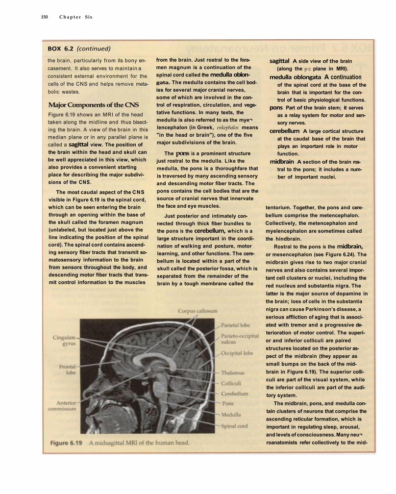
150 C h a p t e r Six
the brain, particularly from its bony encasement. It also serves to maintain a consistent external environment for the cells of the CNS and helps remove metabolic wastes.
Major Components of the CNS Figure 6.19 shows an MRI of the head taken along the midline and thus bisecting the brain. A view of the brain in this median plane or in any parallel plane is called a sagittal view. The position of the brain within the head and skull can be well appreciated in this view, which also provides a convenient starting place for describing the major subdivisions of the CNS.
The most caudal aspect of the CNS visible in Figure 6.19 is the spinal cord, which can be seen entering the brain through an opening within the base of the skull called the foramen magnum (unlabeled, but located just above the line indicating the position of the spinal cord). The spinal cord contains ascending sensory fiber tracts that transmit somatosensory information to the brain from sensors throughout the body, and descending motor fiber tracts that transmit control information to the muscles
BOX 6.2 (continued)
from the brain. Just rostral to the foramen magnum is a continuation of the spinal cord called the medulla oblongata. The medulla contains the cell bodies for several major cranial nerves, some of which are involved in the control of respiration, circulation, and vegetative functions. In many texts, the medulla is also referred to as the mye¬lencephalon (in Greek, enkephalos means "in the head or brain"), one of the five major subdivisions of the brain.
The pons is a prominent structure just rostral to the medulla. Like the medulla, the pons is a thoroughfare that is traversed by many ascending sensory and descending motor fiber tracts. The pons contains the cell bodies that are the source of cranial nerves that innervate the face and eye muscles.
Just posterior and intimately connected through thick fiber bundles to the pons is the cerebellum, which is a large structure important in the coordination of walking and posture, motor learning, and other functions. The cerebellum is located within a part of the skull called the posterior fossa, which is separated from the remainder of the brain by a tough membrane called the
sagittal A side view of the brain (along the y-z plane in MRI).
medulla oblongata A continuation of the spinal cord at the base of the brain that is important for the control of basic physiological functions.
pons Part of the brain stem; it serves as a relay system for motor and sensory nerves.
cerebellum A large cortical structure at the caudal base of the brain that plays an important role in motor function.
midbrain A section of the brain rostral to the pons; it includes a number of important nuclei.
tentorium. Together, the pons and cerebellum comprise the metencephalon. Collectively, the metencephalon and myelencephalon are sometimes called the hindbrain.
Rostral to the pons is the midbrain, or mesencephalon (see Figure 6.24). The midbrain gives rise to two major cranial nerves and also contains several important cell clusters or nuclei, including the red nucleus and substantia nigra. The latter is the major source of dopamine in the brain; loss of cells in the substantia nigra can cause Parkinson's disease, a serious affliction of aging that is associated with tremor and a progressive deterioration of motor control. The superior and inferior colliculi are paired structures located on the posterior aspect of the midbrain (they appear as small bumps on the back of the midbrain in Figure 6.19). The superior colliculi are part of the visual system, while the inferior colliculi are part of the auditory system.
The midbrain, pons, and medulla contain clusters of neurons that comprise the ascending reticular formation, which is important in regulating sleep, arousal, and levels of consciousness. Many neu¬roanatomists refer collectively to the mid-

From Neuronal to Hemodynamic Activity 151
BOX 6.2 (continued)
brain, pons, and medulla as the brain stem, as it appears to support the more rostral brain as a stem supports a flower.
Rostral to the midbrain are the hypothalamus and thalamus, which together with the epithalamus and pineal gland comprise the diencephalon. The hypothalamus is involved in autonomic functions and somatic functions, including the regulation of temperature, water intake, and hunger. The hypothalamus is also an important structure in the regulation of endocrine functions—particularly in its control of the pituitary gland.
The thalamus is a paired structure connected at the midline by the massa intermedia. The thalamus is composed of a large number of nuclei that are sometimes referred to as relay nuclei because they receive information from sensory, motor, and other regions of the brain; organize or process this information; and then project the information to specific regions of cortex. For example, the lateral geniculate is a nucleus of the thalamus that receives and processes visual information from the eyes before projecting that information to the visual cortex. Similar functions are carried out by the medial geniculate for auditory information and by the ventral posterolateral nucleus for the somatosensory sys
tem. Some thalamic nuclei are involved in relaying motor information in the brain. For example, the ventral lateral nuclei receive motor information from the cerebellum and project it to the motor cortex. Other thalamic nuclei appear to integrate information from other brain regions that are neither motor nor sensory. For example, the dorsal medial nucleus receives information from the amygdala, hypothalamus, and other thalamic nuclei and projects this information to the frontal lobes.
Rostral to the diencephalon is the telencephalon, or forebrain. The telencephalon is the largest, most complex, and most evolutionarily advanced part of the brain. It is composed of the cerebral cortical hemispheres (the cerebrum), large subcortical nuclei such as the amygdala, and complex structures such as the basal ganglia (composed of the caudate, putamen, and globus pal¬lidus) and the hippocampus. Interconnecting these brain regions are extensive white-matter tracts, which can be seen in Figure 6.20.
The Cortex
The cerebral hemispheres (cerebrum) are composed of a continuous sheet of cerebral cortex that has been folded into
brain stem The midbrain, pons, and medulla.
hypothalamus A brain nucleus that supports homeostatic functions, including the regulation of food anc water intake.
thalamus A brain nucleus that is important for many aspects of perception and cognition; it is highly interconnected with many regions of the cerebral cortex.
basal ganglia A set of nuclei in the forebrain that includes the caudate, putamen, and globus pallidus.
cerebrum The two hemispheres forming the major part of the brain.
gyri Rises in the cortical surface.
sulci Troughs in the cortical surface.
an undulating pattern of g y r i and sulci. Gyri are rises of cortex that are separated by infolded troughs, or sulci. If unfolded and laid out as a sheet, the cortex of the average human brain would have an area of 2500 c m 2 . The most evolutionarily recent region of the cortex is called the neocortex, which is about 4 to 5 mm thick and composed of six layers, or lamina (Figure 6.21). Layer 1 is the closest to the pial surface and is composed primari ly of axonal and dendritic processes w i t h few neurons. Layers 2 and 3 are composed primarily of pyramidal cells, w i t h layer 2 composed of pyramidal cells w i t h smaller cell bodies. Layer 4 is relatively devoid of py¬ramidal cells but is densely packed w i t h stellate cells. Layer 4 receives projections from other cortical regions and thus appears to be the primary input layer of the cortex. Layer 4 appears to project primari ly to layers 1 to 3, which appear to comprise the intracortical processing layers. Layers 5 and 6 contain large pyramidal cells that project their axons to other brain regions and thus appear to represent the output layers of the neocortex. Note that although

152 Chapter Six
BOX 6.2 (continued) cytoarchitecture The organization of the brain on the basis of cell structure.
Brodmann areas Divisions of the brain based on the influential cytoarchitectonic criteria of Korbin¬ian Brodmann.
functional brain activation measured by fMRI or by positron emission tomography (PET). Although these functional brain methods cannot measure the cytoarchitecture of the brain directly, sufficient similarities exist across individuals to permit the use of spatial transformations that warp an individual's brain into a common atlas space (such as the atlas of Talairach and Tournoux) that has been annotated with Brodmann areas.
Although the cortical sheet is continuous, the presence of several deep fissures in the typical brain has resulted in the subdivision of the brain into four major lobes: the frontal, parietal, temporal, and occipital lobes—so named for the skull bones that cover them. A fifth lobe, the insula, is hidden behind part of the anterior temporal lobe and inferior frontal lobe. Some neuroanatomists also describe a limbic lobe that is composed of midline structures including the cin¬gulate cortex, hippocampus, and amygdala. The cerebral hemispheres and their constituent lobes and nuclei are paired structures. Although the two hemispheres appear roughly similar in
Figure 6.21 An illustration of the six-layer structure of the neocortex.
detailed maps of the cortex based upon these differences in cytoarchitecture, w i t h the hope of differentiating function on the basis of structure. One popular cytoarchitectonic map published by Ko¬rbinian Brodmann in 1909 divides the cerebral cortex into 47 different regions (Figure 6.22). These regions, or Brodmann areas, are used today in many studies to communicate the location of a
fMRI studies currently lack the spatial resolution to distinguish among these layers, given typical voxel sizes on the order of a few millimeters, other techniques like electrophysiology are able to do so.
The cortical thickness, packing density, and composition and size of constituent cells distinguish among regions of cortex. Anatomists have developed
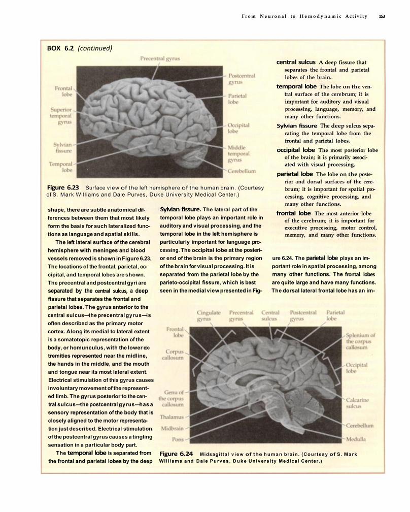
F r o m N e u r o n a l to H e m o d y n a m i c A c t i v i t y 153
BOX 6.2 (continued)
Figure 6.23 Surface view of the left hemisphere of the human brain. (Courtesy of S. Mark Will iams and Dale Purves, Duke University Medical Center.)
shape, there are subtle anatomical differences between them that most likely form the basis for such lateralized functions as language and spatial skills.
The left lateral surface of the cerebral hemisphere with meninges and blood vessels removed is shown in Figure 6.23. The locations of the frontal, parietal, occipital, and temporal lobes are shown. The precentral and postcentral gyri are separated by the central sulcus, a deep fissure that separates the frontal and parietal lobes. The gyrus anterior to the central sulcus—the precentral gyrus—is often described as the primary motor cortex. Along its medial to lateral extent is a somatotopic representation of the body, or homunculus, with the lower extremities represented near the midline, the hands in the middle, and the mouth and tongue near its most lateral extent. Electrical stimulation of this gyrus causes involuntary movement of the represented limb. The gyrus posterior to the central sulcus—the postcentral gyrus—has a sensory representation of the body that is closely aligned to the motor representation just described. Electrical stimulation of the postcentral gyrus causes a tingling sensation in a particular body part.
The temporal lobe is separated from the frontal and parietal lobes by the deep
Figure 6.24 Midsagittal v iew of the h u m a n brain. (Courtesy of S. Mark Wi l l iams and Dale Purves, D u k e Universi ty Medical Center.)
Sylvian fissure. The lateral part of the temporal lobe plays an important role in auditory and visual processing, and the temporal lobe in the left hemisphere is particularly important for language processing. The occipital lobe at the posterior end of the brain is the primary region of the brain for visual processing. It is separated from the parietal lobe by the parieto-occipital fissure, which is best seen in the medial view presented in Fig
ure 6.24. The parietal lobe plays an important role in spatial processing, among many other functions. The frontal lobes are quite large and have many functions. The dorsal lateral frontal lobe has an im-
central sulcus A deep fissure that separates the frontal and parietal lobes of the brain.
temporal lobe The lobe on the ventral surface of the cerebrum; it is important for auditory and visual processing, language, memory, and many other functions.
Sylvian fissure The deep sulcus separating the temporal lobe from the frontal and parietal lobes.
occipital lobe The most posterior lobe of the brain; it is primarily associated with visual processing.
parietal lobe The lobe on the posterior and dorsal surfaces of the cerebrum; it is important for spatial processing, cognitive processing, and many other functions.
frontal lobe The most anterior lobe of the cerebrum; it is important for executive processing, motor control, memory, and many other functions.

154 Chapter Six
BOX 6.2 (continued)
insula The "island" cortex hidden inside the anterior part of the Sylvian fissure; it is important for emotional processing and for the chemical senses.
corpus callosum The large white-matter bundle that is the primary connection between the cerebral hemispheres. The anterior portion is known as the genu and the posterior portion is known as the splenium.
portant role in executive processing— those processes involved with stimulus-response selection when many behaviors are possible.
Within the left hemisphere in most individuals is a region supporting language production known as Broca's area. The more ventral and medial parts of the frontal lobe appear to play a role in emotional processing. The insula, not visible in Figure 6.23 (see Figure 6.26), is hidden deep within the anterior part of the Sylvian fissure and inferior frontal lobe. The insula is important for the chemical senses such as olfaction and gustation.
The corpus callosum is a large white-matter bundle that connects the hemispheres of the brain (it can be easily seen in Figure 6.24). The most anterior part of the corpus callosum is known as the genu (or knee), while the posterior enlargement is called the splenium.
Figure 6.25 presents two views of the ventral surface of the brain. The photographed brain in Figure 6.25A has the cerebellum attached, but the surface blood vessels have been removed. The drawing in Figure 6.25B has omitted the cerebellum so that the gyri and sulci on the ventral surface of the temporal lobe can be identified. Many regions in the inferior temporal lobe play an important role in higher visual processes, including the perception of complex objects. The entorhinal cortex and
Figure 6.25 Ventral view of the human brain. Shown in (A) is a photograph of the ventral surface, with the cerebellum and brain stem visible. The drawing in (B) has the cerebellum removed, so that gyri can be identified. (A courtesy of S. Mark Williams and Dale Purves, Duke University Medical Center.)
Inferior temporal lobe
Olfactory
Optic chiasm
Colliculi
- Spinal cord
Olfactory nerve
Inferior frontal lobe
Inferior frontal lobe
Occipital lobe
Optic chiasm
Brain stem
Anterior temporal
lobe
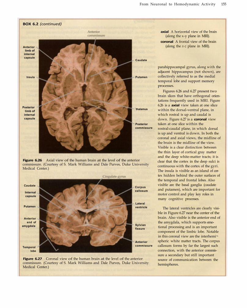
From Neuronal to Hemodynamic Activity 155
BOX 6.2 (continued)
axial A horizontal view of the brain (along the x-y plane in MRI).
coronal A frontal view of the brain (along the x-z plane in MRI).
parahippocampal gyrus, along with the adjacent hippocampus (not shown), are collectively referred to as the medial temporal lobe and support memory processes.
Figures 6.26 and 6.27 present two brain slices that have orthogonal orientations frequently used in MRI. Figure 6.26 is a axial view taken at one slice within the dorsal-ventral plane, in which rostral is up and caudal is down. Figure 6.27 is a coronal view taken at one slice within the rostral-caudal plane, in which dorsal is up and ventral is down. In both the coronal and axial views, the midline of the brain is the midline of the view. Visible is a clear distinction between the thin layer of cortical gray matter and the deep white-matter tracts; it is clear that the cortex in the deep sulci is continuous with the cortex of the gyri. The insula is visible as an island of cortex hidden behind the outer surfaces of the temporal and frontal lobes. Also visible are the basal ganglia (caudate and putamen), which are important for motor control and play key roles in many cognitive processes.
The lateral ventricles are clearly visible in Figure 6.27 near the center of the brain. Also visible is the anterior end of the amygdala, which supports emotional processing and is an important component of the limbic lobe. Notable in this coronal view are the interhemi¬spheric white matter tracts. The corpus callosum forms by far the largest such connection, with the anterior commissure a secondary but still important source of communication between the hemispheres.
Figure 6.26 Axial view of the human brain at the level of the anterior commissure. (Courtesy of S. Mark Williams and Dale Purves, Duke University Medical Center.)
Figure 6.27 Coronal view of the human brain at the level of the anterior commissure. (Courtesy of S. Mark Williams and Dale Purves, Duke University Medical Center.)
Anterior limb of
internal capsule
Insula
Posterior limb of internal capsule
Caudate
Putamen
thalamus
Posterior commissure
Corpus callosum
Lateral ventricle
Sylvian fissure
Anterior commissure
Caudate
Internal capsule
Putamen
Anterior end of
amygdala
Temporal lobe
156 Chapter Six
Summary The fundamental element of information processing in the human brain is the neuron. Neurons have t w o primary roles, integration and signaling. The activity of neurons consists of changes in cell membrane potential and release of neurotransmitters. Movements of ions across neuronal membranes support these functions. While the integrative and signaling activity itself does not require external sources of energy, the restoration of concentration gradients fol lowing this activity does require an energy supply. The primary metabolites supplied to active neurons are glucose and oxygen, which together are important in the synthesis of ATP. These metabolites are supplied by the vascular system. The main components of the vascular system are arteries, capillaries, and veins, each present at different spatial scales. Changes wi th in the vascular system in response to neuronal activity may occur in brain areas far from neuronal activity, initiated in part by flow-controlling substances released by neurons into the extracellular space. Direct neuronal control of pial arteries, arterioles, and capillaries may be exerted by central dopaminergic and noradrenergic projection systems, but it is unknown whether these systems influence fMRI measures. One facet of the vascular response to neuronal activity is the arterial supply of oxygenated hemoglobin, from which oxygen is extracted in the capillaries. The change in the oxygenation of hemoglobin is critical for fMRI.
Suggested Readings
Attwell, D., and Iadecola, C. (2002). The neural basis of functional brain imaging signals. Trends Neurosci., 25(12): 621-625. This article provides a succinct review of the energy budget of the brain and how it may relate to functional neuroimaging.
*Duvernoy, H. M., Delon, S., and Vannson, J. L. (1981). Cortical blood vessels of the human brain. Brain Res. Bull., 7(5): 519-579. This paper provides a thorough exploration of the blood supply to the human brain with numerous and spectacularly detailed photographs.
Iadecola, C. (1998). Neurogenic control of the cerebral microcirculation: Is dopamine minding the store? Nat. Neurosci., 1(4): 263-265. A brief and cogent commentary that accompanies the 1998 article written by Krimer et al., (see below).
*James, W. (1890). The Principles of Psychology. Dover, New York. The masterwork of a scientist who integrated brilliant introspections with a keen experimental sense, this classic compendium still provides useful insights on a wide range of topics. The chapter on brain physiology is highly recommended.
*Krimer, L. S., Muly, E. C, III , Williams, G. V., and Goldman-Rakic, P. S. (1998). Dopaminergic regulation of cerebral cortical microcirculation. Nat. Neurosci., 1(4): 286-289. This paper provides strong evidence that central dopamine projections may influence blood flow within arterioles and capillaries.
Purves, D., Augustine, G., Fitzpatrick, D., Katz, L., LaMantia, A., McNamara, J., and Williams, S. (eds.) (2001). Neuroscience (2 n d ed.). Sinauer Associates, Inc., Sunderland, MA. This wonderfully illustrated textbook provides detailed discussions of human brain anatomy, neuronal signaling and integration, and membrane channels and transporters.
*Roy, C. S., and Sherrington, C. S. (1890). On the regulation of the blood-supply of the brain. J. Physiol., (11): 85-108. A comprehensive and engaging description of the vascular system in the brain, it includes speculations in its final pages about the possible functional implications of blood flow.
*Indicates a reference that is a suggested reading in the field and is also cited in this chapter.
From Neuronal to Hemodynamic Activity 157
Chapter References
Attwell, D., and Laughlin, S. B. (2001). An energy budget for signaling in the grey matter of the brain. J. Cereb. Blood Flow Metab., 21(10): 1133-1145.
Branston, N. M. (1995). Neurogenic control of the cerebral circulation. Cerebrovasc. Brain Metab. Rev., 7(4): 338-349.
Duelli, R., and Kuschinsky, W. (1993). Changes in brain capillary diameter during hypocapnia and hypercapnia. J. Cereb. Blood Flow Metab., 13(6): 1025-1028.
Friedland, R. P., and Iadecola, C. (1991). A centennial reexamination of "On the regulation of the blood-supply of the brain." Neurology, 41(1): 10-14.
Hudetz, A. G. (1997). Blood flow in the cerebral capillary network: A review emphasizing observations with intravital microscopy. Microcirculation, 4(2): 233-252.
Iadecola, C. (2002). Intrinsic signals and functional brain mapping: Caution, blood vessels at work. Cereb. Cortex, 12(3): 223-224.
Iadecola, C, Yang, G., Ebner, T. J . , and Chen, G. (1997). Local and propagated vascular responses evoked by focal synaptic activity in cerebellar cortex. J. Neurophysiol., 78(2): 651-659.
Lee, S. P., Duong, T. Q., Yang, G., Iadecola, C, and Kim, S. G. (2001). Relative changes of cerebral arterial and venous blood volumes during increased cerebral blood flow: Implications for BOLD fMRI. Magn. Reson. Med., 45(5): 791-800.
Ludwig, E., and Klionger, J. (1956). Atlas Cerebri Huinani. Little, Brown and Co., Boston, MA.
McHedlishvili, G., and Kuridze, N. (1984). The modular organization of the pial arterial system in phylogeny. J. Cereb. Blood Flow Metab., 4(3): 391-396.
Menon, R. S., and Goodyear, B. G. (1999). Submillimeter functional localization in human striate cortex using BOLD contrast at 4 Tesla: Implications for the vascular point-spread function. Magn. Reson. Med., 41(2): 230-235.
Ngai, A. C, Ko, K. R., Morii, S., and Winn, H. R. (1988). Effect of sciatic nerve stimulation on pial arterioles in rats. Am. J. Physiol., 254(1 Ft 2): H133-H139.
Ngai, A. C, Meno, J. R., and Winn, H. R. (1995). Simultaneous measurements of pial arteriolar diameter and laser-Doppler flow during somatosensory stimulation. J. Cereb. Blood Flow Metab., 15(1): 124-127.
Nonaka, H. , Akima, M., Hatori, T, Nagayama, T, Zhang, Z., and lhara, F. (2002). The microvasculature of the human cerebellar meninges. Acta Neuropathologica, 104(6): 608-614.
Nonaka, H. , Akima, M., Nagayama, T., Hatori, T, Zhang, Z., and lhara, F. (2003). Microvasculature of the human cerebral meninges. Neuropathology, 23(2): 129-135.
Raichle, M. E., and Gusnard, D. A. (2002). Appraising the brain's energy budget. Proc. Natl. Acad. Sci. U.S.A., 99(16): 10237-10239.
Rodriguez-Baeza, A., Reina-De La Torre, F, Ortega-Sanchez, M., and Sahuquillo¬Barris, J. (1998). Perivascular structures in corrosion casts of the human central nervous system: A confocal laser and scanning electron microscope study. Anat. Rec, 252(2): 176-184.
Segebarth, C, Belle, V., Delon, C, Massarelli, R., Decety,)., Le Bas, J. F., Decorps, M., and Benabid, A. L. (1994). Functional MRI of the human brain: Predominance of signals from extracerebral veins. NeuroReport, 5(7): 813-816.
Sibson, N. R., Dhankhar, A., Mason, G. F., Rothman, D. L., Behar, K. L., and Shulman, R. G. (1998). Stoichiometric coupling of brain glucose metabolism and glutamatergic neuronal activity. Proc. Natl. Acad. Sci. U.S.A., 95(1): 316-321.
Vafaee, M. S., and Gjedde, A. (2000). Model of blood-brain transfer of oxygen explains nonlinear flow-metabolism coupling during stimulation of visual cortex. J. Cereb. Blood Flow Metab., 20(4): 747-754.
Williams, Mark S. (2000) Sylvius 2.0: Fundamentals of Human Neural Structure, CD-ROM. Sinauer Associates, Inc., Sunderland, MA.
Yang, G., Zhang, Y, Ross, M. E., and Iadecola, C. (2003). Attenuation of activity-induced increases in cerebellar blood flow in mice lacking neuronal nitric oxide synthase. Am. J. Physiol. Heart Circ. Physiol., 285(1): H298-H304.

BOLD fMRI
We have now established that it is the metabolic demands of active neurons and not neuronal activity per se that are measured by functional neu¬roimaging methods. Energy is required for the maintenance and restoration of neuronal membrane potentials necessary for integration and signaling. Even small increases in neuronal activity can result in a large increase in local energy demand. Because there are scant energy stores in the brain, energy must be continuously provided by the blood supply to the brain. The primary energy sources are glucose and oxygen, which are used to create ATP w i t h i n brain cells. Oxygen is attached to hemoglobin molecules and is exchanged for waste carbon dioxide in capillaries. H o w is it, though, that the delivery of oxygen and glucose to active neurons results in a signal that can be measured by fMRI? In this chapter, we w i l l consider in detail the physiological basis of blood-oxygenation-level dependent (BOLD) fMRI .
History of BOLD fMRI
In 1936, the American chemist and Nobel laureate Linus Pauling and his student Charles Coryell conducted a systematic investigation of the molecular structure of hemoglobin. In the course of these studies, they discovered a remarkable and (for our purposes) fortuitous fact of nature: The hemoglobin molecule has magnetic properties that differ depending upon whether or not it is bound to oxygen. Oxygenated hemoglobin (Hb) is diamag¬netic; that is, i t has no unpaired electrons and zero magnetic moment. In contrast, deoxygenated hemoglobin (dHb) is paramagnetic; i t has both unpaired electrons and a significant magnetic moment. Completely deoxygenated blood has a magnetic susceptibility about 20% greater than ful ly oxygenated blood. Pauling and Coryell noted w r y l y that this fact had eluded previous researchers, including the great nineteenth-century physicist Michael Faraday, only because they had not separated arterial blood (which contains only oxygenated hemoglobin) and venous blood (which contains both oxygenated and deoxygenated hemoglobin).
Remember that introducing an object w i t h magnetic susceptibility into a magnetic field causes spin dephasing, resulting in a decay of transverse magnetization that depends on the time constant T 2*. Because blood deoxy¬genation affects magnetic susceptibility, MR pulse sequences sensitive to T2*
oxygenated hemoglobin (Hb) Hemoglobin with attached oxygen; it is dia¬magnetic.
diamagnetic Having the property of a weak repulsion from a magnetic field.
deoxygenated hemoglobin (dHb) Hemoglobin without attached oxygen; it is paramagnetic.
paramagnetic Having the property of being attracted to a magnetic field, though with less concentration of magnetic flux than ferromagnetic objects.
magnetic susceptibility The intensity of magnetization of a substance when placed within a magnetic field.

160 Chapter Seven
Figure 7.1 Effects of blood deoxy¬genation upon MR relaxation constants Shown are the differential effects of blood deoxygenation upon transverse and longitudinal relaxation times, as expressed by the constants 1 /T 2 (blue circles) and 1 /T1 (red circles). The praxis indicates the square of the proportion of deoxygenated blood. Note that oxygenation increases from left to right. Clearly evident is the fact that 1 /T 2
decreases w i t h increasing oxygenation; that is, the more deoxygenated hemoglobin that is present, the shorter the T 2 . Note that T 1 is not affected by blood oxygenation level. (After Thulborn et al., 1982.)
should show more MR signal where blood is highly oxygenated and less MR signal where blood is highly deoxygenated. This prediction was verified experimentally in the early 1980s by Thulborn and colleagues, who found that the decay of transverse magnetization depended on the proport ion of oxygenated hemoglobin w i t h i n a test tube of blood (Figure 7.1). They noted that the magnitude of this effect increased w i t h the square of the strength of the static magnetic f ield. At low field strength (i.e., less than 0.5 T), there is little difference between the transverse relaxation values for oxygenated and deoxygenated blood, but in higher fields (i.e., 1.5 T or greater), their values differ significantly. So, strong static magnetic fields are necessary for MR imaging of T2*-based contrast in blood. These results provided a theoretical basis for measurement of blood oxygenation changes using MRI .
Discovery of BOLD Contrast During the late 1980s, Seiji Ogawa, a research scientist at Bell Laboratories, investigated the possibility of examining brain physiology using MRI . Ogawa and his colleagues recognized that it would be challenging to use MRI to examine physiological processes directly. Since standard MRI contrasts are based on properties of hydrogen, the commonness of hydrogen in water throughout the body precludes examination of the very subtle changes in concentration associated w i t h metabolic reactions themselves. For MRI to be useful in measuring physiology, it would need to be sensitive to some indirect measure of metabolism. One possibility was blood flow, since metabolic processes require oxygen that is supplied through hemoglobin w i t h i n red blood cells. Based on the previous f inding that deoxygenation decreases the T2* value of blood, Ogawa and colleagues (1990b) hypothesized that manipulating the proport ion of blood oxygen w o u l d affect the visibility of blood vessels on T 2*-weighted images.
They tested their hypothesis by scanning anesthetized rodents using high-field (7 T and greater) MRI. To manipulate blood oxygenation, they changed the proportion of oxygen that the animals breathed. When the rodents were breathing 100% oxygen or 100% carbon monoxide, gradient-echo images of

BOLD fMRI 161
their brains showed structural differences but few blood vessels (Figure 7.2A). But when the rodents breathed normal air (21% oxygen), the images took on a very different character. Thin dark lines became visible throughout the cerebral cortex, usually perpendicular to its surface (Figure 7.2B). If the oxygen content was further reduced to 0% (anoxic condition), the lines became even more prominent. Ogawa and colleagues concluded that these thin lines represented magnetic susceptibility effects caused by the presence of paramagnetic deoxygenated hemoglobin in blood vessels, which causes local field distortions on gradient-echo images. In the other conditions, because the hemoglobin was bound to oxygen or carbon monoxide, it was diamagnetic and had little effect on the surrounding magnetic field.
To verify this interpretation, they placed test tubes w i t h oxygenated or deoxygenated blood into a saline-filled container. Both spin- and gradient-echo images were taken of each tube. The tubes containing oxygenated blood appeared as black circles on both types of images, since the blood had a shorter T2* than the surrounding saline (Figure 7.3A and B). The spin-echo image of the deoxygenated blood was likewise nearly normal , although there was a slight shape distortion resulting from the effects of induced field inhomogeneity on the resonance frequency of the surrounding water (Figure 7.3C). The largest effect by far was observed for gradient-echo images of the deoxygenated blood, which showed a very large area of signal loss that extended wel l beyond the test tube (Figure 7.3D). These results demonstrated that the presence of deoxygenated blood decreases the measured MR signal on T2* images, relative to the presence of oxygenated blood.
Figure 7.2 A schematic illustration of blood-oxygenation-level dependent (BOLD) contrast. Ogawa and colleagues manipulated the amount of oxygen in the blood of rats by adjusting the contents of the air breathed. When the rats breathed pure oxygen, the cortical surface had a uniform texture (A) on images sensitive to T2* contrast. But, when they breathed normal air, there were areas of signal loss, shown in (B) as lines corresponding to blood vessels within the cortex. These lines indicate areas with increased amounts of deoxygenated hemoglobin. This forms the basis for BOLD contrast. (After Ogawa et al., 1990.)
Figure 7.3 Magnetic properties of oxygenated and deoxygenated hemoglobin. To verify that the effects illustrated in Figure 7.2 resulted from changes in blood oxygen level, a series of in vitro experiments were conducted that compared images of oxygenated and deoxygenated blood using both spin- and gradient-echo imaging. The images of oxygenated blood were not distorted, regardless of whether spin-echo (A) or gradient-echo (B) images were acquired. The spin-echo image of the deoxygenated blood (C) was slightly distorted, but the distortion did not extend to the area surrounding the test tube. However, there was substantial signal loss surrounding the gradient-echo image of the deoxygenated blood (D), showing that the presence of deoxygenated hemoglobin reduces the MR signal in adjacent space. (After Ogawa et al., 1990b.)

162 Chapter Seven
blood-oxygenation-level dependent (BOLD) contrast The difference in signal on T 2*-weighted images as a function of the amount of deoxygenated hemoglobin.
autoradiography An invasive imaging technique that labels molecules using radioactive isotopes and then measures the concentration of those molecules by exposing slices of tissue to photographic emulsions.
Ogawa and colleagues speculated that this f inding, which would come to be called blood-oxygenation-level dependent (BOLD) contrast, could enable measurement of functional changes in brain activity. They hypothesized two possible nonexclusive mechanisms for BOLD contrast: changes in oxygen metabolism or changes in blood flow. Under the first mechanism, neuronal activity w o u l d cause increased metabolic demands, and thus increased oxygen consumption. This w o u l d increase the amount of deoxygenated hemoglobin, given a constant blood flow. Under the second mechanism, increased blood f low in the absence of increased metabolic demand w o u l d decrease the amount of deoxygenated hemoglobin.
In their next in vivo experiment, Ogawa and colleagues (1990a), manipulated the gases inhaled by anesthetized rats while measuring BOLD contrast at high field. To verify that the BOLD contrast resulted, at least in part, from the metabolic demand for oxygen, they compared low and high anesthesia levels. At the higher anesthesia level (3.0% halothane), there was reduced spontaneous brain activity as measured by concurrent EEG BOLD contrast was much greater at low anesthesia levels (0.75% halothane) than at high anesthesia levels. These results indicated that the metabolic demand for oxygen was a prerequisite for BOLD contrast.
To evaluate the effect of blood flow changes upon BOLD contrast, they compared two inhalant conditions, pure (100%) oxygen and a mixture of 90% oxygen and 10% carbon dioxide. While significant BOLD contrast was observed in the pure oxygen condition, the contrast disappeared when the animals breathed the CO2 mixture. Why did adding CO2 have such a large effect? Carbon dioxide in the blood does not have significant paramagnetic effects in itself, but it does increase overall blood flow. Ogawa and colleagues found that the CO2 mixture increased blood velocity wi th in the sagittal sinus by a factor of 4. With greater blood flow in the absence of metabolic demand, the deoxygenated hemoglobin is essentially flushed from the venous system and replaced by excess oxygenated hemoglobin, causing a decrease in BOLD contrast.
In summary, BOLD contrast was found to depend upon the total amount of deoxygenated hemoglobin present in a brain region, which in turn depended upon the balance between oxygen consumption and oxygen supply. Al though it seems reasonable that increased neuronal activity would result in increased oxygen consumption and thus greater decreases in MR signal, as Ogawa and colleagues originally hypothesized, experimental observations have turned out to be considerably more complicated. Indeed, when we measure the brain d u r i n g increased neural activity, we find that there is an increase in the MR signal! H o w can this be? The answer requires a more complete exploration of the relations between cerebral blood flow, blood oxygenation level, and metabolism than we have thus far provided. We note in advance that a generally accepted model that relates BOLD contrast to blood flow and oxygen supply is still lacking. However, the competing models that have been offered to explain this relationship have different and profound implications for the ultimate functional resolution of BOLD-contrast f M R I . To understand these implications, we first need to consider more ful ly the relationship between glucose metabolism and blood flow, through the examination of data from other techniques.
The Coupling of Glucose Metabolism and Blood Flow Autoradiography is an invasive imaging technique used in animals in which biologically active molecules labeled by radioactive isotopes are identified by exposure of brain slices to photographic emulsions. In the 1970s,

B O L D f M R I 163
We see that six oxygen molecules are consumed for each glucose molecule oxidized, and thus the ideal oxygen-to-glucose index (OGI) w o u l d be 6:1 if all of the glucose that entered the brain were oxidatively (i.e., aerobi-cally) metabolized. Brain measurements performed under resting conditions have established an OGI of approximately 5.5:1, indicating that while the vast majority of the glucose metabolism in the brain is oxidative, a small but significant fraction of glucose may be metabolized nonoxidatively (i.e., anaerobically). The rate of oxygen and glucose consumption d u r i n g focal stimulation is different, however, and this fact has engendered considerable controversy that persists today.
In an influential series of PET experiments conducted in 1988 by Fox, Raichle, and their colleagues, cerebral blood f low (CBF), cerebral metabolic rate for glucose ( C M R g l u ) , and cerebral metabolic rate for oxygen (CMRO,) were measured d u r i n g rest and dur ing visual stimulation. When subjects were exposed to prolonged visual stimulation, CBF in the visual cortex increased by 50% and C M R g l u increased by 51%, consistent w i t h Sokoloff's autoradiographic findings in animals. However, C M R O 2 increased by only 5%. The authors concluded that most of the increased uptake of glucose during stimulation was not oxidized but rather was metabolized nonoxidatively through anaerobic glycolysis. Recalling our discussion from the previous chapter, anaerobic glycolysis is relatively inefficient (but fast), yielding only two ATP molecules for each glucose molecule consumed, and thus the energy produced from the increased glucose uptake w o u l d be relatively small. Corroborating evidence has come from studies by Prichard and colleagues, w h o demonstrated that prolonged visual stimulation results in increased lactate, which w o u l d be expected since lactate is the primary end product of anaerobic glycolysis.
A number of studies have found similar uncoupling between glucose metabolism and oxygen consumption, although the disparity has not always been quite as dramatic. But while there is general agreement on these facts, their interpretation is still controversial. This controversy has surprising relevance to BOLD fMRI , and several models have been advanced to explain this apparent uncoupling.
Glucose and Oxygen Metabolism
The observations of Fox and Raichle help explain the paradox we noted previously, namely that MR signal increases dur ing neuronal activity even though deoxygenated hemoglobin decreases MR signal. The disparity between oxygen utilization and oxygen delivery means that more oxygen is supplied to a brain region than is consumed. Fox and Raichle note that this is consistent wi th the experience of neurosurgeons, who have long observed that cortex becomes more pink in color when it becomes active. As the excess oxygenated blood flows through active regions, it flushes the deoxy-
Sokoloff and colleagues used autoradiography to establish that regional brain changes in the metabolic rate of glucose metabolism were coupled to an increase in blood f low to that same region. As you now know, glucose is the major energy source for the brain, and oxygen facilitates the most efficient conversion of glucose into ATP. The overall accounting of glucose and oxygen consumption dur ing oxidative metabolism is as follows:
[7.1] C6H12O6 + 6O2 = 6CO2 + 6H 2 O

164 Chapter Seven
BOX 7.1 PET Imaging
extensively to study the relationship between energy consumption and neuronal activity. PET uses positron-emitting radioactive tracers that are attached to molecules that enter biological pathways of interest (Figure 7.4A). For example, 18F, a radioactive isotope of fluorine, can be attached to glucose, creating the molecule fluoro-2-deoxy-D-glucose, or FDG. The fluorine tracer does not prevent FDG from entering into the normal pathways for glucose metabolism. Thus, researchers can inject a bolus of FDG into an artery and then use imaging to determine where it is taken up by cells.
ositron emission tomography, or PET, is a powerful functional imaging technique that has been used
As the radioactive isotope decays, it emits a positron (the antimatter counterpart of an electron). When the emitted positron collides w i t h a nearby electron, they are mutually annihilated and produce two gamma rays that take paths 180° apart and are subsequently detected by their near simultaneous impact on opposite sides of a r ing of scintillation crystals that surround the subject's head (Figure 7.4B). A computer algorithm then evaluates the number and timing of impacts at all of the crystals surrounding the head and traces the paths taken by the gamma rays back to their origins. Through this method, the distribution of glucose uptake in the brain can be measured, and changes in glucose uptake in differ
ent brain regions caused by sensory, motor, or cognitive activity can be determined (Figure 7.4C). PET imaging can also study oxygen metabolism or blood flow using 15O, a radioactive isotope of oxygen. Certain neurotransmitters can be similarly labeled. For example, 1 8F can be attached to dopamine to study its distribution in the human brain.
PET scanning provides a relatively direct and easily interpretable measure
positron emission tomography (PET) A functional neuroimaging technique that creates images based upon the movement of injected radioactive material.
these gamma rays. Depending on the tracer used, PET can be sensitive to several aspects of brain metabolism, including blood flow. The output of a PET scan indicates the number of events measured from each voxel during a long time period. These numbers can be converted to statistical maps, which then can be overlaid upon anatomical images, often from MRI. (C courtesy of Dr. David Madden, Duke University.)
Figure 7.4 Positron emission tomography (PET) imaging. Until the mid-1990s, the most common functional neuroimaging technique was PET, which relies on injection of a radioactive tracer into the bloodstream. As the tracer decays, it emits positrons, which travel a short distance before colliding with an electron (A). The collision results in a pair of emitted gamma rays that travel in opposite directions. The PET scanner (B) consists of a series of coincidence detectors that record the simultaneous arrival of

BOLD fMRI 165
genated hemoglobin from the capillaries supporting the active neural tissue and from the downstream venules. BOLD contrast fol lowing neuronal activity occurs not because the oxygenated hemoglobin increases the MR signal but because it displaces the deoxygenated hemoglobin that had been suppressing the MR signal intensity.
Here we consider three of the most influential explanations offered to explain the linkage between blood flow, glucose consumption, and oxygen utilization.
Watering the Garden for the Sake of One Thirsty Flower
Not all investigators accept the apparent uncoupling of CMRO 2 and CMR g l u
during stimulation as indicative of anaerobic metabolism. In 1996 Malonek and Grinvald used a high-resolution optical imaging method in which the surface of the visual cortex in the cat is exposed to a l ight source and the reflected light is analyzed. Because different molecules (e.g., oxygenated and deoxygenated hemoglobin) absorb light of different wavelengths, the spectrum of the reflected light can be used to determine their presence at any given location in the cortex. They selectively activated small, spatially segregated populations of neurons in the visual cortex by presenting line gratings at particular orientations. The expected spatial pattern of neuronal activation across the visual cortex could then be compared to the spatial patterns of oxygenated and deoxygenated hemoglobin accumulation, a l lowing their measurements wi th high spatial and temporal resolution.
The results of the experiment showed that the evoked changes in hemoglobin and deoxygenated hemoglobin were quite distinct (Figure 7.5). The
BOX 7.1 (continued)
of brain metabolism, and for many years it was the mainstay of human functional neuroimaging. However, its dependence upon high-energy gamma radiation (or ionizing radiation, as named for its potential to break chemical bonds) presents problems for human studies. Radiation exposure in human research is carefully regulated, and subjects can participate in only a few PET scans. There are other drawbacks to PET imaging. Its spatial resolution is limited by the distance the positron travels away from the labeled molecule before it collides w i t h an electron. This is dependent upon the particular isotope used; for example, the maximum distance that a positron emitted by 1 8 F w i l l travel before encountering an electron is about 2.6 mm. Recall that it is the location of the gamma ray emission that is localized and not the location of the molecule of interest. More l imiting, however, is the very poor tem
poral resolution of PET imaging. Because many emissions must be detected before an image w i t h sufficient signal-to-noise ratio can be produced, PET studies must collect data over a long period of time. For example, an image of blood flow based upon 1 5O may take 90 seconds to acquire, while an image of glucose metabolism based upon 1 8F may take 30 to 40 minutes to acquire. These acquisition times severely l imit the temporal resolution of PET imaging and restrict the types of experimental designs that can be used.
When compared with PET imaging, MRI has several advantages. Because MRI does not involve ionizing radiation, subjects can be run repeatedly without the cumulative health risks of radiation exposure. Images w i t h high signal-to-noise can be acquired in less than a second, and spatial resolution is limited primarily by the motion of the sample and signal-to-noise, not by the
inherent uncertainty in the measurement technique. But the potential resolution of MRI for anatomical studies should not be confused with the ability to resolve biological processes that influence the MRI signal. Even w i t h the caveats described above, PET does directly image glucose or oxygen consumption. BOLD fMRI, for comparison, does not provide any direct information about metabolic processes themselves, but instead reports an indirect correlate of those processes. Thus, for many research questions about brain metabolism, PET imaging remains of critical importance.
ionizing radiation Electromagnetic radiation that has sufficient energy to separate electrons from electrically neutral atoms, turning them into ions.
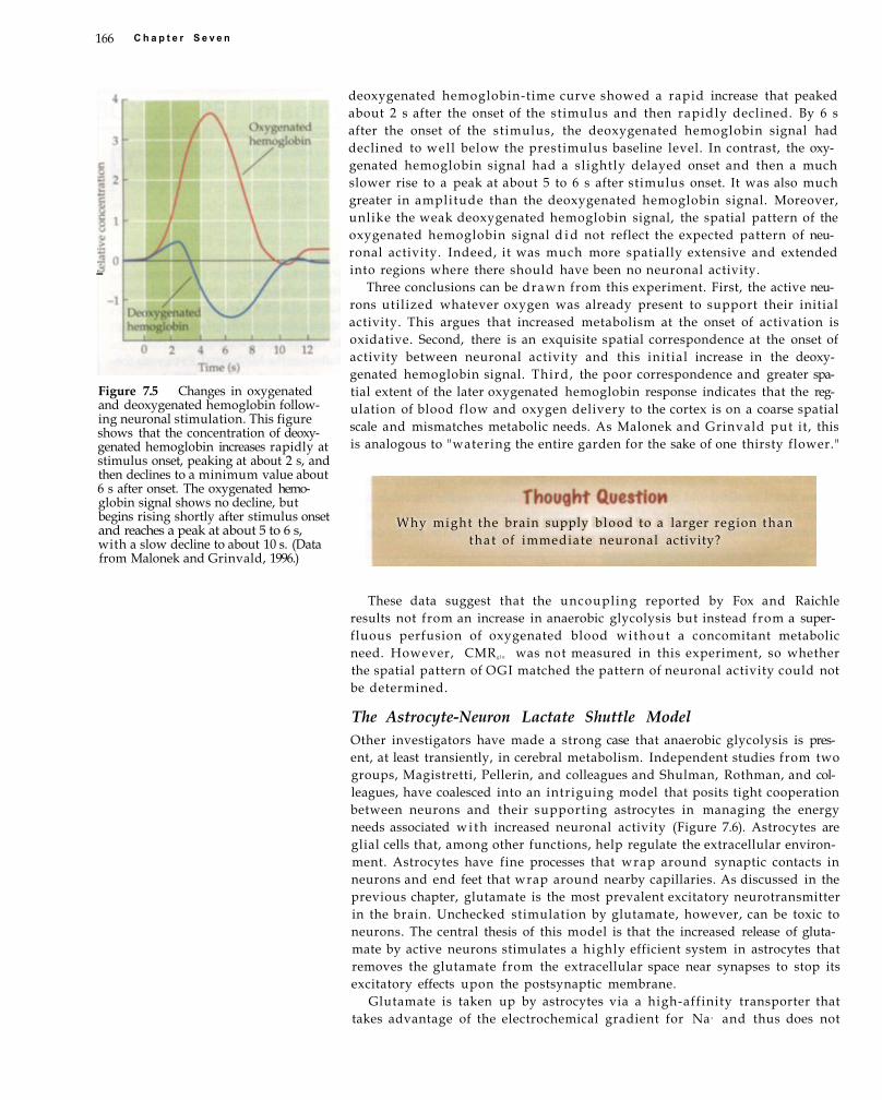
166 C h a p t e r S e v e n
—
Figure 7.5 Changes in oxygenated and deoxygenated hemoglobin following neuronal stimulation. This figure shows that the concentration of deoxygenated hemoglobin increases rapidly at stimulus onset, peaking at about 2 s, and then declines to a minimum value about 6 s after onset. The oxygenated hemoglobin signal shows no decline, but begins rising shortly after stimulus onset and reaches a peak at about 5 to 6 s, with a slow decline to about 10 s. (Data from Malonek and Grinvald, 1996.)
deoxygenated hemoglobin-time curve showed a rapid increase that peaked about 2 s after the onset of the stimulus and then rapidly declined. By 6 s after the onset of the stimulus, the deoxygenated hemoglobin signal had declined to well below the prestimulus baseline level. In contrast, the oxygenated hemoglobin signal had a slightly delayed onset and then a much slower rise to a peak at about 5 to 6 s after stimulus onset. It was also much greater in amplitude than the deoxygenated hemoglobin signal. Moreover, unlike the weak deoxygenated hemoglobin signal, the spatial pattern of the oxygenated hemoglobin signal d i d not reflect the expected pattern of neuronal activity. Indeed, it was much more spatially extensive and extended into regions where there should have been no neuronal activity.
Three conclusions can be drawn from this experiment. First, the active neurons utilized whatever oxygen was already present to support their initial activity. This argues that increased metabolism at the onset of activation is oxidative. Second, there is an exquisite spatial correspondence at the onset of activity between neuronal activity and this initial increase in the deoxygenated hemoglobin signal. Third, the poor correspondence and greater spatial extent of the later oxygenated hemoglobin response indicates that the regulation of blood flow and oxygen delivery to the cortex is on a coarse spatial scale and mismatches metabolic needs. As Malonek and Grinvald put it, this is analogous to "watering the entire garden for the sake of one thirsty flower."
These data suggest that the uncoupling reported by Fox and Raichle results not from an increase in anaerobic glycolysis but instead from a superfluous perfusion of oxygenated blood without a concomitant metabolic need. However, CMR g l u was not measured in this experiment, so whether the spatial pattern of OGI matched the pattern of neuronal activity could not be determined.
The Astrocyte-Neuron Lactate Shuttle Model Other investigators have made a strong case that anaerobic glycolysis is present, at least transiently, in cerebral metabolism. Independent studies from two groups, Magistretti, Pellerin, and colleagues and Shulman, Rothman, and colleagues, have coalesced into an intriguing model that posits tight cooperation between neurons and their supporting astrocytes in managing the energy needs associated wi th increased neuronal activity (Figure 7.6). Astrocytes are glial cells that, among other functions, help regulate the extracellular environment. Astrocytes have fine processes that wrap around synaptic contacts in neurons and end feet that wrap around nearby capillaries. As discussed in the previous chapter, glutamate is the most prevalent excitatory neurotransmitter in the brain. Unchecked stimulation by glutamate, however, can be toxic to neurons. The central thesis of this model is that the increased release of glutamate by active neurons stimulates a highly efficient system in astrocytes that removes the glutamate from the extracellular space near synapses to stop its excitatory effects upon the postsynaptic membrane.
Glutamate is taken up by astrocytes via a high-affinity transporter that takes advantage of the electrochemical gradient for Na+ and thus does not
Why might the brain supply blood to a larger region than tha t of immediate neuronal activity?

BOLD fMRI 167
Figure 7.6 The astrocyte-neuron lactate model. In this model, glutamate released at the synapse following a change in membrane voltage (Vm) is quickly transported into an adjacent astrocyte where it is converted into glutamine for transport back to the neuron. The glutamate-glutamine conversion process is powered by one ATP from a fast anaerobic glycolysis process, which has two additional products: lactate, which is released into the extracellular space; and another ATP, which provides energy for the sodium-potassium pump at the astrocyte membrane.
require ATP to operate. However, three ions of Na+ are cotransported into the cell w i t h every molecule of glutamate. The astrocyte now has to solve two problems. The first is to remove the three ions of Na+ to restore its electrochemical gradient. This is accomplished by the now familiar sodium-potassium pump, which transports the three Na+ ions from the cell at the cost of one ATP. The second problem is to recycle the glutamate molecule so that it can be returned to the neuron, but not in its excitatory neurotransmitter form. This is accomplished through a reaction that converts glutamate into nonac-tive glutamine, again at the cost of one ATP. The glutamine is then transported out of the astrocyte and taken up by the neuron, converted back into glutamate, and then repackaged into synaptic vesicles, where it awaits another action potential for its release into the synaptic cleft.
The total cost to the astrocyte for this rapid removal and recycling of glutamate is two ATP per glutamate molecule. In this model, the cost is exactly balanced by the anaerobic glycolysis of glucose, which you w i l l recall yields

168 Chapter Seven
Thus far, we have described the
time course of the BOLDcontrast
MR signal as an increase, or posi
tive signal change, over time. One of
the most interesting claims for BOLD
fMRI is that this positive change is pre
ceded by a smaller decrease in MR sig
nal. This postulated decrease has been
labeled the init ial dip , and was first
reported by Menon and colleagues in
1995. Building on the optical imaging
work of Grinvald discussed earlier,
they postulated that the BOLD signal
confounded two factors, oxygen extrac
tion and blood flow, that occur on dif
ferent spatial and temporal scales. They
hypothesized that fast imaging meth
ods could detect the former, which
would have a more focal spatial pattern
than the latter. They presented a visual
pattern that flashed for 10 s while col
lecting data using highfield (4 T) and
fastrate (TR of 100 ms) echoplanar
imaging. To further improve signalto
noise, they used a local surface coil,
which increases detection power in
nearby voxels. To detect voxels show
ing an initial dip , they compared each
voxel's mean activity between 0.5 and
2.5 s to a prestimulus baseline period
using a ttest. For comparison, voxels
showing a positive response were
defined by a ttest comparing activity at
5 to 15 s to that at baseline.
The results verified that a small frac
tion of the active voxels showed an in i
tial reduction in signal, the amplitude
of which was less than half as large as
the positive hemodynamic response
(Figure 7.7AC). The voxels showing
the initial d ip were found wi th in gray
matter along the calcarine sulcus,
which corresponds to primary visual
cortex. However, the later positive
response was more spatially diffuse
and extended into neighboring veins
and white matter.
In a study conducted in 2001, Duong
and colleagues examined the BOLD
response in the primary visual cortex of
anesthetized cats using highfield (4.7 T
and 9.4 T) fMRI . The stimuli were dri f t
ing sinewave gratings at different o r i
entations. In the primary visual cortex,
neurons are organized into columns
that respond preferentially to stimuli of
a particular orientation. By collecting
data at very high spatial resolution
(about 150 μm2), the researchers could
identify individual orientation columns
initial dip The shortterm decrease in MR signal immediately following the onset of neuronal activity, before the main positive component of the hemodynamic response. The initial dip may result from initial oxygen extraction before the later overcompensatory response.
(see Box 8.2 for related experiments
examining ocular dominance columns
in human subjects). Stimuli of perpen
dicular orientations (e.g., 45° and 135°)
should activate different sets of orienta
tion columns. The experimental test
was whether the initial dip or the later
positive response would better segre
gate voxels by orientation. The initial
dip showed good spatial specificity, in
that voxels with an initial dip to one
orientation did not show an initial dip
to the perpendicular orientation. In
contrast, the later positive BOLD
response was blurred over columns,
such that most voxels showed positive
BOLD activity to both orientations. The
authors noted that the spatial specificity
of the BOLD response was greatest
over the first 2 s and decreased over
time. This result suggests that the initial
ative response (i.e., the "initial dip") has fewer active voxels (B), suggesting that it may be more spatially specific. (C) The BOLD hemodynamic response across all voxels with an early negative response is shown. (From Menon et al., 1995.)
Figure 7.7 Spatial specificity of the BOLD initial dip. (A) A statistical map that shows all voxels in the visual cortex around the calcarine fissure that had a significant late positive hemodynamic response to visual stimulation. Note that the map of voxels that showed a significant early neg
BOX 7.2 The Initial Dip
BOLD fMRI 169
a net gain of t w o ATP for each molecule of glucose consumed. The astrocyte is then faced w i t h one remaining problem: what to do w i t h the lactate that accumulates as the end product of anaerobic glycolysis. The answer is to release the lactate into the extracellular space, where, due to its increased concentration, it diffuses into the neuron. Once inside the cytoplasm, the lactate is converted back into pyruvate through the action of the enzyme lactate dehydrogenase-1. The pyruvate is subsequently processed through the TCA cycle and electron transport chain to produce an additional 36 ATP that are used to support the energy costs of the neuron, as described previously.
In summary, the astrocyte-neuron lactate shuttle model proposes that an initial and rapid phase of anaerobic glycolysis is t ightly coupled w i t h the increase in excitatory glutamate release by neurons. In this way, it is consistent wi th the findings of Fox and Raichle. However, this model also predicts that oxygen is consumed in the normal way when the lactate produced in the anaerobic phase is converted to pyruvate in neurons and enters the TCA cycle. Thus, the model predicts only a transient shift to anaerobic glycolysis at the onset of stimulation. For this reason, it is interesting to note that recent studies by Mintun and colleagues using time-resolved PET have suggested that the uncoupling of C M R O 2 and C M R g l u observed by Fox and Raichle occurs early in stimulation and that these measures become coupled again as stimulation continues. This suggests that the brain may transiently utilize a fast but inefficient method for producing ATP when neuronal activity suddenly increases and glutamate must be removed from the synapse to avoid excitotoxic injury. However, as stimulation is sustained, the brain, using the lactate produced as an end product of anaerobic glycolysis, reverts to a slower but more efficient method of producing ATP through oxidation.
Transit T ime and Oxygen Extraction A third account for the uncoupling of glucose metabolism and oxygen utilization is presented in a formal biophysical model by Buxton and col-
BOX 7.2 (continued)
dip may reflect oxygenation changes that are localized to capillaries, as first hypothesized by Menon and colleagues. However, the overcompen-satory delivery of oxygenated blood that comprises the positive response causes more extensive changes in oxygenation wi th in the venous drainage system.
Despite these intriguing results, the initial d ip is a controversial topic for a simple reason: it is not re-ported in the vast majority of fMRI studies. So what could explain its infrequent observation? One likely factor is the rarity of high-field (e.g., ≥ 4 T) MR scanners for
functional studies. The amplitude of the
initial d ip seems to scale dramatically
with field strength. When measured at
1.5 T, the initial d ip was only 12% of the
magnitude of the positive response,
which is only one-third of the proportion measured at 4 T. This result is consistent w i t h the idea that the initial dip has a microvascular origin, since signal recorded from small blood vessels should scale more dramatically w i t h field strength than signal recorded from large blood vessels. It may simply be more difficult to detect the initial d ip at the field strengths most typical for fMRI. Another possible factor is that averaging over a large spatial region obscures the smaller-scale effects of the initial d ip . Even in some studies where an initial d ip was clearly present, it was reported to disappear if all voxels w i t h a positive response were averaged.
While the evidence in support of the initial d ip has strengthened in recent years, its underlying mechanisms still require further investigation. The hypothesis advocated by Menon and colleagues, that it represents an increase in oxygen extraction in advance of increased blood flow, remains consistent w i t h the experimental data. But, recall that the BOLD signal depends not only on oxygen extraction but also on blood flow and blood volume. A transient decrease in flow or increase in volume would also result in a decrease in the BOLD signal. While these latter possibilities have not yet been ruled out, the oxygen extraction hypothesis provides the best current theoretical interpretation of the initial dip.

170 Chapter Seven
leagues. This model also bears important similarities to an independent formulation by Gjedde. Like Grinvald and colleagues, these authors do not accept that the disparity between glucose consumption and oxygen utilization is evidence for anaerobic metabolism. This model is predicated upon four key assumptions. The first is that increased blood f low in response to neuronal activity is pr imari ly accomplished by an increase in its velocity rather than by an increase in the number of capillaries through which the blood flows (i.e., no capillary recruitment). The second is that oxygen transport from blood to brain tissue is l imited by several factors, and that the amount of oxygen extracted is proportional to transit time through the capillary bed. As blood velocity increases, the transit time decreases. The third assumption is that v ir tual ly all of the oxygen extracted from capillaries is metabolized, so there is no reserve pool of oxygen in brain tissue. The fourth assumption is that not all glucose that enters brain tissue is metabolized.
Buxton and colleagues argue that the likelihood of extracting an individual oxygen molecule (attached, of course, to hemoglobin) w i t h i n a capillary has a fixed probability per unit time. Because of the increased blood velocity w i t h neuronal activity, the resulting decrease in transit time reduces the overall l ikelihood that each oxygen molecule w i l l be extracted. The rate of delivery of oxygen to tissue is thus a nonlinear function of f low velocity. Due to this nonlinearity, a disproportionately large increase in blood f low is required to cause even a small increase in the amount of oxygen extracted.
If transit time l imits oxygen delivery, w h y doesn't it also l imi t glucose availability? Buxton states that the extraction of glucose is even more limited by transit time than that of oxygen, but, supported by data from Gjedde, he argues that less than half of the glucose extracted from capillaries is actually metabolized. Thus, the amount of glucose extracted from capillaries does not equal the amount metabolized in brain cells.
Implications for BOLD fMRI The three formulations presented above account in different ways for the disparity between glucose consumption and oxygen util ization. The observations by Grinvald demonstrate that hemoglobin is delivered over an extensive region of cortex in response to the activation of a smaller neuronal region. This suggests that the coarseness in the control of blood flow to a cortical region limits the spatial resolution of fMRI. However, early decreases in fMRI signal, or initial dips (Box 7.2), w o u l d be colocalized w i t h neuronal activity. In contrast, the astrocyte-neuron lactate shuttle model proposes a fast anaerobic response to neural activation and thus would not predict an initial dip. Indeed, definitive evidence for an initial d ip would be inconsistent wi th the anaerobic glycolysis proposed in the lactate shuttle model.
The transit-time model of Buxton and colleagues d i d not attempt to account for the initial d ip , but a later balloon model described the changes in blood volume that occur as a function of increased blood f low dur ing brain activity. In this model, the increase in blood f low evoked by neuronal activation causes an inflow of blood into the venous system that is initially greater than its outflow. The result is increased blood volume in the venous system as it expands like a balloon to accommodate the increased inflow. In explorations of this model, Buxton and colleagues noted that it predicts that the init ial increase in volume in small veins w o u l d be dominated by the presence of deoxygenated hemoglobin that was cleared first from the capillaries. This concentration of deoxygenated hemoglobin causes a loss of MR signal, and so the balloon model also predicts an initial d ip . However, Buxton's interpretation is much different from that of Grinvald (and Menon and
balloon model A model of the interaction between changes in blood volume and changes in blood flow associated with neuronal activity.
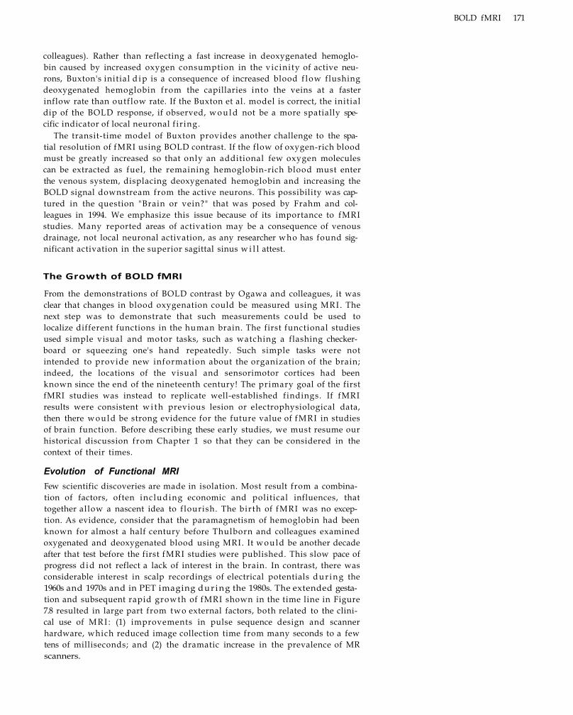
BOLD fMRI 171
colleagues). Rather than reflecting a fast increase in deoxygenated hemoglobin caused by increased oxygen consumption in the vic ini ty of active neurons, Buxton's initial d i p is a consequence of increased blood f low flushing deoxygenated hemoglobin from the capillaries into the veins at a faster inflow rate than outflow rate. If the Buxton et al. model is correct, the initial dip of the BOLD response, if observed, w o u l d not be a more spatially specific indicator of local neuronal f ir ing.
The transit-time model of Buxton provides another challenge to the spatial resolution of fMRI using BOLD contrast. If the flow of oxygen-rich blood must be greatly increased so that only an additional few oxygen molecules can be extracted as fuel, the remaining hemoglobin-rich blood must enter the venous system, displacing deoxygenated hemoglobin and increasing the BOLD signal downstream from the active neurons. This possibility was captured in the question "Brain or vein?" that was posed by Frahm and colleagues in 1994. We emphasize this issue because of its importance to fMRI studies. Many reported areas of activation may be a consequence of venous drainage, not local neuronal activation, as any researcher who has found significant activation in the superior sagittal sinus w i l l attest.
The Growth of BOLD fMRI
From the demonstrations of BOLD contrast by Ogawa and colleagues, it was clear that changes in blood oxygenation could be measured using MRI . The next step was to demonstrate that such measurements could be used to localize different functions in the human brain. The first functional studies used simple visual and motor tasks, such as watching a flashing checkerboard or squeezing one's hand repeatedly. Such simple tasks were not intended to provide new information about the organization of the brain; indeed, the locations of the visual and sensorimotor cortices had been known since the end of the nineteenth century! The primary goal of the first fMRI studies was instead to replicate well-established findings. If fMRI results were consistent w i t h previous lesion or electrophysiological data, then there would be strong evidence for the future value of fMRI in studies of brain function. Before describing these early studies, we must resume our historical discussion from Chapter 1 so that they can be considered in the context of their times.
Evolution of Functional MRI Few scientific discoveries are made in isolation. Most result from a combination of factors, often inc luding economic and political influences, that together allow a nascent idea to f lourish. The birth of fMRI was no exception. As evidence, consider that the paramagnetism of hemoglobin had been known for almost a half century before Thulborn and colleagues examined oxygenated and deoxygenated blood using MRI. It would be another decade after that test before the first fMRI studies were published. This slow pace of progress d i d not reflect a lack of interest in the brain. In contrast, there was considerable interest in scalp recordings of electrical potentials d u r i n g the 1960s and 1970s and in PET imaging dur ing the 1980s. The extended gestation and subsequent rapid growth of fMRI shown in the time line in Figure 7.8 resulted in large part from two external factors, both related to the clinical use of M R I : (1) improvements in pulse sequence design and scanner hardware, which reduced image collection time from many seconds to a few tens of milliseconds; and (2) the dramatic increase in the prevalence of MR scanners.

172 Chapter Seven
Figure 7.8 Milestones in the development of fMRI.
The first factor enabling fMRI was the development of pulse sequences and imaging hardware for rapid image acquisition. Early MR imaging was a slow process. The first MR image, for example, was acquired at a rate of more than 2 minutes per voxel. In modern imaging, where the brain may be composed of approximately 25,000 voxels, such a slow acquisition pace would correspond to approximately one volume per month! As discussed in Chapter 1, the development of echo-planar imaging (EPI), largely through the work of Peter Mansfield in the late 1970s, allowed an entire image to be collected fol lowing a single excitation pulse (Figure 7.9).
While the theoretical basis for EPI was developed relatively early, practical implementation of the theory was delayed by limitations in scanning hardware. The rapid changes in the gradient fields required by EPI could induce currents in metal parts w i t h i n the scanner, introducing artifacts in recorded images. Rather than change scanner design to ameliorate this problem, manufacturers adopted other approaches, such as fast low (flip) angle shot, or FLASH, sequences, that d i d not tax scanner hardware as significantly as EPI. Not unt i l about 1985 were active gradient-shielding techniques developed, largely through the work of Mansfield and colleagues, that incorporated an outer gradient w i n d i n g in the opposite direction. The outer w i n d i n g reduced eddy currents in the scanner hardware but added complexity and increased power requirements. Major manufacturers began adding actively shielded gradients to their standard scanner platforms over the fo l lowing years. By the early 1990s, advances in gradient technology proposed by Turner and by Wong and colleagues provided the fast switching capability and high linearity, respectively, needed for EPI to be practical.
Rabi uses magnetic resonance to measure nuclear magnetic moment
Pauling and Coryell study magnetic properties of blood
Purcell and Bloch simultaneously discover nuclear magnetic resonance
Damadian reports differences in relaxation times for biological tissues
Lauterbur creates first MR image using magnetic gradients
Mansfield proposes echo-planar imaging
Thulbom and colleagues report the effects of blood oxygenation on T2* contrast GE introduces first 1.5-T scanner Insurance reimbursements begin for MRI in United States Active gradient shielding developed Improved head coil designs developed
Ogawa proposes BOLD contrast as basis for fMRI
First fMRI studies published

BOLD fMRI 173
The second key factor was the increasing clinical applicability of structural MRI. Most of the relatively few scanners used in the 1970s were devoted to industrial applications, and almost none were being used in hospital settings. While clinical interest in MR imaging was lacking, there was substantial interest in computerized tomography (CT) scanners. Unlike standard X-ray imaging, which had remained largely unchanged since its discovery by Wi l -helm Roentgen in 1895, CT imaging allowed clinicians to assess damage to soft-tissue structures (Figure 7.10A-C). CT scanners were expensive, typically requiring a capital commitment of more than $300,000, but the improved images they provided became an important part of the radiologist's arsenal, and by the early 1980s more than 5000 were in use wor ldwide . CT scans began to be demanded by doctors and patients alike, serving both to draw new patients to hospitals that possessed the latest equipment and to generate new income from the expensive procedures.
By the early 1980s, hospitals began considering the use of MRI as a complement to CT scanning, in part due to the enthusiasm of pioneers like Raymond Damadian (see Chapter 1). Several medical device companies, including Damadian's FONAR Corporation, General Electric (GE), and Varian, developed high-field scanners that promised image resolution that w o u l d far surpass that of CT. The first 1.5-T scanner was installed at Duke University by GE in 1982. This would remain the most common field strength for both clinical and research purposes for more than two decades.
Figure 7.10 Computerized tomography imaging. CT uses a moving X-ray source to create a three-dimensional map of underlying tissue (A). Note that CT is sensitive to the same limitations on resolution and contrast as conventional X-rays (B). For comparison, a structural MRI image is shown in (C).
Figure 7.9 One of the earliest EPI images. This cross section of a human finger represents one of the very first uses of echo-planar imaging to scan living human tissue. (From Mansfield and Maudsley, 1977.)

174 C h a p t e r S e v e n
By 1985, MR scanning was sufficiently well established that insurance companies in the United States began reimbursing for MRI procedures. The cost of MRI scanners was still very high, often as much as $2 million, but hospitals were now able to recoup costs over many procedures. As had happened more than a decade earlier w i t h CT, this new clinical demand sparked an explosion in the number of MRI scanners. By the year 2002, a mere 20 years after the introduction of the first high-field scanner, there were more than 10,000 such scanners w o r l d w i d e . Al though most were devoted to patient care during normal business hours, researchers at many institutions were able to use the scanners at night and on weekends for research into brain function. These research studies were often facilitated by supplemental hardware, such as gradient insert coils, that improved upon the hardware provided by the clinical manufacturers. The advances that facilitated the first fMRI studies, therefore, were developed in large part to meet the clinical demand for structural MRI.
Early fMRI Studies The first BOLD fMRI studies were reported in 1992 by three groups. Kwong and colleagues used a gradient-echo EPI sequence at 1.5 T to study activity in the visual cortex. They evoked visual cortex acidity by alternating 60-s periods of visual stimulation (e.g., the flashing of an LED pattern) wi th 60-s baseline periods of darkness. At the onset of the stimulation period, there was a sharp increase in MR signal around the calcarine fissure, increasing by about 3% w i t h i n 10 s (Figure 7.11 A-C) . The activity increase was sustained for the duration of the visual stimulation, receding to the baseline level once darkness returned. These findings were replicated by a similar study published the fol lowing month by Ogawa and colleagues, who likewise evaluated changes in fMRI gradient-echo signal resulting from long-duration (e.g., 100 s) presentations of visual s t imuli . Unlike the K w o n g study, however, they used a pulse sequence that limited them to an effective TR of about 10 s, and they tested subjects at high field (4 T). Ogawa and colleagues manipulated TE to prove that the BOLD signal change depends upon T2* effects. At a very short TE of 8 ms, the stimulus effects previously seen at a TE of 40 ms disappeared. Since T 1-related effects should be independent of TE, as discussed in Chapter 5, the BOLD effect must depend on T 2* effects. Nearly simultaneously, a third paper published in 1992 by Bandettini and colleagues reported similar effects, using a motor task in which subjects repeatedly touched their fingers to their thumb for a long block of time. Data recorded using gradient-echo EPI at 1.5 T showed significant activity in the primary motor cortex.
While most early fMRI studies used long stimulus durations, some used shorter stimulus events to examine vascular responses to a single, punctuate stimulus. The first such results were reported later in 1992 by Blamire and colleagues, w h o investigated changes in visual cortex activity following st imuli of different durations. They acquired images using a spin-echo EPI sequence at 2.1 T. The longer st imuli (10 s to 90 s) resulted in signal increases of about 10% over baseline. This f inding was expected, based upon the studies described above. What was remarkable were the results from the short-duration s t imul i . Even the shortest stimulus (2 s) evoked a significant 4% signal change in active voxels w i t h i n the visual cortex (Figure 7.12). The authors noted that there was a short but measurable delay between the stimulus presentation and the MR signal change. On average, the first observable fMRI change in the primary visual cortex occurred about 3.5 s fo l lowing the onset of the stimulus. The results shown in the figure repre-

B O L D fMRI 175
Figure 7.11 The first use of BOLD fMRI for functional mapping of the human brain. In this study, two fMRI techniques are used: flow-sensitive spin-echo inversion recovery (IR) and BOLD-sensitive gradient-echo (GE). (A) The area of activity for the flow-sensitive IR sequence. (B,C) The time courses of activity measured using each technique. Note the use of a long-interval blocked design, consistent with PET studies of its time. (From Kwong et al., 1992.)
Figure 7.12 Changes in BOLD activity associated with presentations of single discrete events. This graph provides the first example of BOLD activity associated with single events. While event-related methods are extremely common in contemporary fMRI studies, their use did not become widespread until the late 1990s. (Data from Blamire et al., 1992.)

176 Chapter Seven
hemodynamic response (HDR) The change in MR signal on T2* images following local neuronal activity. The hemodynamic response results from a decrease in the amount of deoxygenated hemoglobin present within a voxel.
sent the very first demonstration of the time course of hemodynamic activity in response to a single stimulus event.
It is important to compare these early studies to current fMRI practice. At first glance, the procedures and equipment seem very similar. The field strengths reported above (i.e., 1.5 T, 2.1 T, 4.0 T) are similar to those of MRI scanners used now, more than a decade later. The use of EPI pulse sequences is also still common, though other sequences such as spiral imaging have g r o w n in popularity. Nevertheless, there are substantial differences. The gradient fields that could be generated by the older scanners were much weaker and could not be changed as rapidly as those on modern scanners. Furthermore, the earlier studies collected data from one or a few slices, despite having relatively long TRs. Improvements in gradient coil design now enable the collection of more than 20 slices per second.
In addit ion to hardware improvements, there have been significant advances in strategies for fMRI analyses. None of these early studies corrected for possible subject head motion or physiological variation. Blamire and colleagues noted that voxels on the edge of the brain showed systematic oscillations in signal intensity, which they attributed to pulsatile motion of the brain associated w i t h the cardiac cycle. Despite their recognition of this problem, no computational techniques were available for its solution. Today, however, the preprocessing of fMRI data to remove unwanted variability is an important aspect of fMRI analysis. In addit ion, the experimental designs used in these early studies were very simple, in that they evaluated only whether activity in a region of interest changed dur ing a task as compared to a control condition. While this comparison is appropriate for simple visual or motor tasks, more-complex experimental questions require more-complex experimental designs.
Nevertheless, the basic elements of modern fMRI practice can be traced back to these early studies. They hinted at what was possible using this new technique, setting the stage for later studies that expanded its use to other important research questions.
Components of the BOLD Hemodynamic Response
The change in the MR signal triggered by neuronal activity (Figure 7.14) is known as the hemodynamic response (HDR). Referring to the hemodynamic response is, however, a bit misleading, as the shape of the HDR varies wi th the properties of the evoking stimulus and, presumably, wi th the underlying neuronal activity. We might expect, therefore, that increasing the rate of neuronal f ir ing would increase HDR amplitude, whereas increasing the duration of neuronal activity would increase HDR w i d t h . Determining the exact relation between the neuronal events that trigger the HDR and the shape of the HDR, however, is complicated by their differing dynamics. Cortical neuronal responses occur w i t h i n tens of milliseconds fol lowing a sensory stimulus, but the first observable HDR changes do not occur unti l 1 to 2
Why is the finding of BOLD activity in response to short-duration stimuli important? What implications
does it have for fMRI experimentation?

B O L D f M R I 177
BOLD contrast depends on the paramagnetic properties of deoxy¬genated hemoglobin, which induce
changes in local magnetic fields that can be measured using T2* imaging. One potential way of increasing image contrast is to use exogenous contrast agent such as gadolinium diethylene-triaminepentaacetic acid (Gd-DTPA), highly paramagnetic substances that can be injected into the bloodstream but do not cross the intact blood-brain barrier. The agents used are well tolerated by most people, with mi ld headache and nausea as the most common side effects. Common contrast agents are shown in Table 7.1. Contrast agents have great importance for clinical imaging, especially in the detection of pathological tissue, including brain tumors. Under normal conditions, the diffusion of a contrast agent like Gd-DTPA through the bloodstream wi l l reduce T1 values of hydrogen protons in the blood, increasing signal within blood vessels but not elsewhere. But if there is damage to the blood-brain barrier due to brain pathology, the contrast agent may escape from the bloodstream and enter the surrounding tissue, resulting in increased signal on T|-weighted images.
This effect upon T1 relaxation, though clinically important, provides no information about brain function. Rather, it is the effect of contrast agents
upon local magnetic field properties that enables functional studies. Because the injected contrast agent is highly paramagnetic and has a very strong magnetic moment, there wi l l be a considerable inhomogeneity between the tissue outside of the blood vessel and the contrast-enhanced blood with in. Remember from Chapter 5 that sharp gradients in magnetic field homogeneity can cause signal losses known as susceptibility artifacts, due to differential effects of the magnetic gradient upon spin precession. When a pulse sequence sensitive to T2* effects is used, these signal losses enable measurement of the local concentration of the contrast agent over time. Unlike BOLD contrast, which depends on both blood flow and oxygen extraction, exogenous contrast methods generally rely only on blood volume changes associated wi th functional activity. In addit ion, they have a limited lifetime due to their passage through the brain and subsequent dispersal through the vascular system. But, because the exogenous contrast agent is much more paramagnetic than deoxygenated hemoglobin, the signal change observed wi l l be much larger, allowing meaningful data to be extracted from the first pass of the agent through the brain.
The first fMRI study to use exogenous contrast (and one of the first fMRI
contrast agent A substance injected into the body to increase image contrast.
bolus A quantity of a substance that is introduced into a system and then progresses through that system over time.
studies of any form) was reported by Belliveau and colleagues in 1991. They measured visual cortex activity using spin-echo EPI at 1.5 T fol lowing injection of a bolus of Gd-DTPA. In the test condition, subjects viewed a visual pattern that flashed at a rate of about 8 Hz, and in the control condition there was no visual stimulus. Based on electrophysiological data, this rate was known to robustly activate the primary visual cortex. The authors hypothesized that, fol lowing injection of the contrast agent, the raw MR signal would decrease due to increased magnetic susceptibility. Furthermore, the magnitude of this decrease should be greater for active brain regions due to local increases in blood volume. As shown in Figure 7.13A-C, there was a transient decrease in MR signal associated wi th passage of the contrast agent through the primary visual cortex. Note the delay of about 8 to 10 s between the injection of Gd-DTPA and the onset of the signal decrease. This delay reflects the time required for the contrast agent to travel from the injection site, which was the antecubital vein in the arm, through the heart to the primary visual cortex. Although decreases in signal intensity in the visual cortex were present in both the test and control conditions, the decrease was larger and occurred earlier for the flashing pattern than for darkness. From this result, the researchers concluded that blood volume had increased in the calcarine cortex and thus that neurons in that part of the brain are associated with visual perception.
Source: Torchilin, 1995.
BOX 7.3 Functional Studies Using Contrast Agents

178 Chapter Seven
seconds later. Thus, the HDR is said to lag the neuronal events that initiate it . Throughout the remainder of the book, we w i l l make frequent reference to different aspects of the HDR waveform, and so here we define some terms. Figure 7.15A and B provide an illustrative schematic of a typical HDR.
Remember that the BOLD signal in a voxel reflects the total amount of deoxygenated hemoglobin that is present, as well as noise resulting from several sources. As described in Box 7.2, some studies have reported an initial negative-going dip of 1 to 2 s duration that has been attributed to a transient increase in the amount of deoxygenated hemoglobin. After a short latency, the
BOX 7.3 (continued)
Figure 7.13 Functional MRI using exogenous contrast. This figure provides the first example of functional mapping of the human brain using MRI. Subjects were injected with the contrast agent Gd-DTPA and exposed to darkness or rapidly flashing lights. Compared with darkness (A), there was a significant increase in cerebral blood volume when the flashing lights were presented (B). The plot in
(C) shows the passage of the contrast agent through the visual cortex, in conditions of visual stimulation (red circles) and darkness (blue circles). Note that in both cases there are significant decreases in MR signal due to the magnetic susceptibility effects of the contrast agent. However, the decrease occurs earlier and is larger in the activated condition. (From Belliveau et al., 1991.)
The power of exogenous contrast agents comes from the enormous signal changes they induce. Even in this early experiment, the signal change observed due to the contrast injection was about 30%. The difference between the test and control conditions was on the order of 5%. To appreciate the magnitude of such changes, compare them to the much smaller signal changes observed in BOLD fMRI, which are typically only a few percent. Furthermore, the clear differences observed between experimental conditions by Belliveau and colleagues were obtained without signal averaging. That is, the data shown in Figure 7.13 represent two trials, one test
and one control, from a single subject. Modern BOLD studies, for comparison, usually represent the average of many subjects w i t h many trials per condition.
Despite this power, exogenous contrast agents are rarely used for fMRI research. One limitation can be seen in the time course of signal change. Because of the substantial transit delay of the agent, it is challenging to accurately measure the t iming of brain activity. A n d since a single bolus is used, one measurement of signal change is obtained per trial. If one wants to study two types of trials, like Belliveau and colleagues, two injections are required. In general, as more conditions are
added, more injections are needed. These requirements preclude some types of analyses that are possible w i t h endogenous BOLD contrast, such as the sorting of many trials based on accuracy or reaction time, fast event-related designs, evaluation of brain response as a function of stimulus sequence, and complex parametric studies. In addition, many subjects are less likely to participate in studies that require intravenous injection. So, while a number of researchers are actively investigating the use of contrast agents for fMRI (see Chapter 14), especially for studies in animals, nearly all current fMRI studies use endogenous BOLD contrast.

BOLD fMRI 179
Figure 7.14 Summary of BOLD signal generation. Under normal conditions, oxygenated hemoglobin is converted to deoxygenated hemoglobin at a constant rate within the capillary bed (A). But when neurons become active, there is an increase in the supply of oxygenated hemoglobin above that needed by the neurons (B). This results in a relative decrease in the amount of deoxygenated hemoglobin and a corresponding decrease in the signal loss due to T2* effects.
metabolic demands of increased neuronal activity over baseline levels result in an increased inflow of oxygenated blood. More oxygen is supplied to the area than is extracted, and this results in a decrease in the amount of deoxygenated hemoglobin w i t h i n the voxel. If we monitor such an active voxel's activity using BOLD fMRI, we find that its signal increases above baseline at about 2 s following the onset of neuronal activity, growing to a maximum value at about 5 s for a short-duration stimulus. This maximum is known as the peak of the hemodynamic response. If the neuronal activity is extended across a block of time, the peak may be similarly extended into a plateau.
After reaching its peak, the BOLD signal decreases in amplitude to a below-baseline level and remains below baseline for an extended interval. This effect is known as the poststimulus undershoot. To understand the undershoot, we need to consider the changes in blood f low and blood volume separately (Figure 7.16). Following cessation of neuronal activity, blood flow decreases more rapidly than blood volume. If volume remained above baseline levels, while flow was at baseline, then a greater amount of deoxygenated hemoglobin would be present. Thus, the overall fMRI signal w i l l be
peak The maximal amplitude of the hemodynamic response, occurring typically about 4 to 6 s following a short-duration event.
undershoot The decrease in MR signal amplitude below baseline due to the combination of reduced blood flow and increased blood volume.
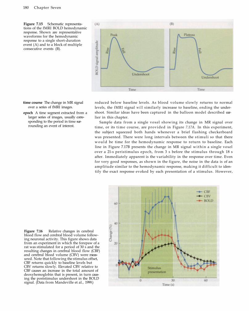
180 Chapter Seven
Figure 7.15 Schematic representations of the fMRI BOLD hemodynamic response. Shown are representative waveforms for the hemodynamic response to a single short-duration event (A) and to a block of multiple consecutive events (B).
time course The change in MR signal over a series of fMRI images.
epoch A time segment extracted from a larger series of images, usually corresponding to the period in time surrounding an event of interest.
reduced below baseline levels. As blood volume slowly returns to normal levels, the fMRI signal w i l l similarly increase to baseline, ending the undershoot. Similar ideas have been captured in the balloon model described earlier in this chapter.
Sample data from a single voxel showing its change in MR signal over time, or its t i m e course, are provided in Figure 7.17A. In this experiment, the subject squeezed both hands whenever a brief flashing checkerboard was presented. There were long intervals between the s t imul i so that there w o u l d be time for the hemodynamic response to return to baseline. Each line in Figure 7.17B presents the change in MR signal w i t h i n a single voxel over a 21-s peristimulus epoch, from 3 s before the stimulus through 18 s after. Immediately apparent is the variability in the response over time. Even for very good responses, as shown in the figure, the noise in the data is of an amplitude similar to the hemodynamic response, making it difficult to identify the exact response evoked by each presentation of a stimulus. However,
Figure 7.16 Relative changes in cerebral blood flow and cerebral blood volume following neuronal activity. This figure shows data from an experiment in which the forepaw of a rat was stimulated for a period of 30 s and the resulting changes in cerebral blood flow (CBF) and cerebral blood volume (CBV) were measured. Note that following the stimulus offset, CBF returns quickly to baseline levels but CBV returns slowly. Elevated CBV relative to CBF causes an increase in the total amount of deoxyhemoglobin that is present, in turn causing the poststimulus undershoot in the BOLD signal. (Data from Mandeville et al., 1999.)
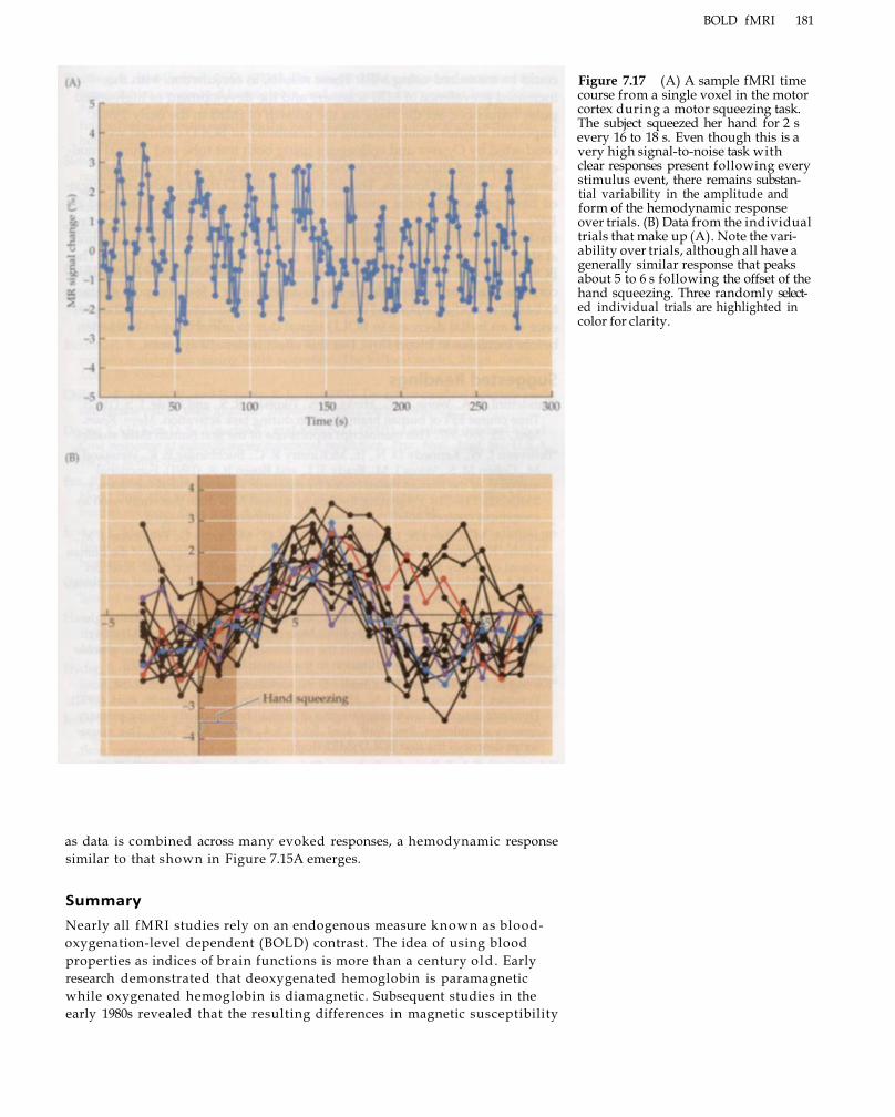
BOLD fMRI 181
Figure 7.17 (A) A sample fMRI time course from a single voxel in the motor cortex during a motor squeezing task. The subject squeezed her hand for 2 s every 16 to 18 s. Even though this is a very high signal-to-noise task with clear responses present following every stimulus event, there remains substantial variability in the amplitude and form of the hemodynamic response over trials. (B) Data from the individual trials that make up (A). Note the variability over trials, although all have a generally similar response that peaks about 5 to 6 s following the offset of the hand squeezing. Three randomly selected individual trials are highlighted in color for clarity.
as data is combined across many evoked responses, a hemodynamic response similar to that shown in Figure 7.15A emerges.
Summary
Nearly all fMRI studies rely on an endogenous measure known as blood-oxygenation-level dependent (BOLD) contrast. The idea of using blood properties as indices of brain functions is more than a century old . Early research demonstrated that deoxygenated hemoglobin is paramagnetic while oxygenated hemoglobin is diamagnetic. Subsequent studies in the early 1980s revealed that the resulting differences in magnetic susceptibility
could be measured using MRI. These results, in conjunction w i t h the increased prevalence of MRI scanners and the development of high-speed pulse sequences, set the stage for the growth of fMRI in the early 1990s. Important studies demonstrating the feasibility of BOLD contrast were conducted by Ogawa and colleagues using both test tube and animal models. They found that changes in blood oxygenation could be visualized using T 2*-weighted images. The first human BOLD fMRI studies investigated basic properties of the visual and motor cortices and were published in 1992. At the same time, researchers investigated the use of exogenous contrast agents. While contrast agents can improve signal-to-noise in functional studies, their invasiveness has made them less popular than BOLD. The BOLD response to brief neuronal activity, or the hemodynamic response, consists of a short onset delay, a rise to a peak after a few seconds, a return to baseline, and a prolonged undershoot. Some researchers report the presence of an initial decrease in BOLD signal due to initial oxygen extraction before increases in blood flow, but this effect is not always seen.
Suggested Readings
*Bandettini, P. A., Wong, E. C, Hinks, R. S., Tikofsky, R. S., and Hyde, J. S. (1992). Time course EPI of human brain function during task activation. Magn. Reson. Med., 25: 390-397, This manuscript reports one of the first human fMRI studies.
*Belliveau J. W., Kennedy D. N. , Jr., McKinstry R. C, Buchbinder B. R., Weisskoff R. M., Cohen M. S., Vevea J. M., Brady T. J., and Rosen B. R. (1991). Functional mapping of the human visual cortex by magnetic resonance imaging. Science, 254(5032): 716-719. Presenting the first functional MRI data, this study used an exogenous contrast agent rather than now common BOLD imaging.
*Blamire A. M., Ogawa S., Ugurbil K., Rothman D., McCarthy G., Ellermann J. M., Hyder F, Rattner Z., and Shulman R. G. (1992). Dynamic mapping of the human visual cortex by high-speed magnetic resonance imaging. Proc. Natl. Acad. Sci. U.S.A., 89(22): 11069-11073. This early study describes the first use of event-related designs in fMRI.
*Fox, P. T, Raichle, M. E., Mintun, M. A., and Dence, C. (1988). Nonoxidative glucose consumption during focal physiologic neural activity. Science, 241(4864): 462-464. This classic paper details the relationship between blood flow, glucose metabolism, and oxygen utilization in the human brain studied by PET.
*Kwong K. K., Belliveau J. W., Chesler D. A., Goldberg I. E., Weisskoff R. M., Poncelet B. P., Kennedy D. N., Hoppel B. E., Cohen M. S., Turner R., et al. (1992). Dynamic magnetic resonance imaging of human brain activity during primary sensory stimulation. Proc. Natl. Acad. Sci. U.S.A., 89(12): 5675-5679. This manuscript describes the first BOLD fMRI study.
*Magistretti, P. J., Pellerin, L., Rothman, D. L., and Shulman, R. G. (1999). Energy on demand. Science, 283(5401): 496-497. This paper provides a succinct review of the astrocyte-lactate shuttle hypothesis.
*Ogawa S., Lee T. M., Kay A. R., and Tank D. W. (1990a). Brain magnetic resonance imaging with contrast dependent on blood oxygenation. Proc. Natl. Acad. Sci. U.S.A., 87(24): 9868-9872. This report provided the initial demonstration of the effects of blood oxygenation on T2* contrast, through studies of rats at high magnetic field.
*Ogawa S., Tank D. W., Menon R., Ellermann J. M., Kim S. G., Merkle H., and Ugurbil K. (1992). Intrinsic signal changes accompanying sensory stimulation: Functional brain mapping with magnetic resonance imaging. Proc. Natl. Acad. Sci. U.S.A., 89(13): 5951-5955. One of the very earliest fMRI studies, this is of additional interest due to the difference between its methods and modern studies.
182 Chapter Seven

*Pauling, L., and Coryell, C. D. (1936). The magnetic properties and structure of hemoglobin, oxygenated hemoglobin, and carbonmonoxygenated hemoglobin. Proc. Natl. Acad. Sci. U.S.A., 22(4): 210-236. This accessible manuscript from a future Nobel laureate describes the basic chemical and physical properties of hemoglobin.
Stehling M. K., Turner R., and Mansfield P. (1991). Echo-planar imaging: Magnetic resonance imaging in a fraction of a second. Science, 254(5028): 43-50. This early review article provides a good description of high-speed echo-planar imaging and some of its potential uses.
*Indicates a reference that is a suggested reading in the field and is also cited in this chapter.
Chapter References Buxton, R. B., and Frank, L. R. (1997). A model for the coupling between cerebral
blood flow and oxygen metabolism during neural stimulation. J. Cereb. Blood Flow Metab., 17(1): 64-72.
Buxton, R. B., Wong, E. C, and Frank, L. R. (1998). Dynamics of blood flow and oxygen metabolism during brain activation: The balloon model. Magn. Reson. Med., 39: 855-S64.
Chih, C. P., Lipton, P., and Roberts, E. L., Jr. (2001). Do active cerebral neurons really use lactate rather than glucose? Trends Neurosci., 24(10): 573-578.
Duong T. Q., Kim D. S., Ugurbil K., and Kim S. G. (2001). Localized cerebral blood flow response at submillimeter columnar resolution. Proc. Natl. Acad. Sci. U.S.A., 98(19): 10904-10909.
Fox, P. T, and Raichle, M. E. (1986). Focal physiological uncoupling of cerebral blood flow and oxidative metabolism during somatosensory stimulation in human subjects. Proc. Natl. Acad. Sci. U.S.A., 83(4): 1140-1144.
Frahm, J., Merboldt, K. D., Hanicke, W., Kleinschmidt, A., and Boecker, H. (1994). Brain or vein—oxygenation or flow? On signal physiology in functional MRI of human brain activation. NMR Biomed., 7(1-2): 45-53.
Gjedde, A., Marrett, S., and Vafaee, M. (2002). Oxidative and nonoxidative metabolism of excited neurons and astrocytes. J. Cereb. Blood Flow Metab., 22(1): 1-14.
Harel, N. , Lee, S. P., Nagaoka, T., Kim, D. S., and Kim, S. G. (2002). Origin of negative blood oxygenation level-dependent fMRI signals. J. Cereb. Blood Flow Metabol, 22(8): 908-917.
Hyder, F., Rothman, D. L., and Shulman, R. G. (2002). Total neuroenergetics support localized brain activity: Implications for the interpretation of fMRI [Comment]. Proc. Natl. Acad. Sci. U.S.A., 99(16): 10771-10776.
Jones M., Berwick J., Johnston D., and Mayhew J. (2001). Concurrent optical imaging spectroscopy and laser-Doppler flowmetry: The relationship between blood flow, oxygenation, and volume in rodent barrel cortex. Neurolmage, 13(6 Pt. 1): 1002-1015.
Magistretti, P. J., and Pellerin, L. (1999). Cellular mechanisms of brain energy metabolism and their relevance to functional brain imaging. Philos. Trans. Royal Soc. London Ser. B Biol. Sci., 354(1387): 1155-1163.
Malonek, D., and Grinvald, A. (1996). Interactions between electrical activity and cortical microcirculation revealed by imaging spectroscopy: Implications for functional brain mapping. Science, 272(5261): 551-554.
Mandeville J. B., Marota J. J., Ayata C, Moskowitz M. A., Weisskoff R. M., and Rosen B. R. (1998). Dynamic functional imaging of relative cerebral blood volume during rat forepaw stimulation. Magn. Reson. Med., 39(4): 615-624.
Mandeville J. B., Marota J. J., Kosofsky B. E., Keltner J. R., Weissleder R., Rosen B. R., and Weisskoff R. M. (1999). MRI measurement of the temporal evolution of relative CMRO(2) during rat forepaw stimulation. Magn. Reson. Med., 42(5): 944-951.
B O L D fMRI 183

184 C h a p t e r S e v e n
Mansfield, P., and Maudsley, A. A. (1977). Medical imaging by NMR. Br. J. Radiol., 50(591): 188-194.
Menon R. S., Ogawa S., Hu X., Strupp J. P., Anderson P., and Ugurbil K. (1995). BOLD based functional MRI at 4 Tesla includes a capillary bed contribution: Echo-planar imaging correlates with previous optical imaging using intrinsic signals. Magn. Reson. Med., 33(3): 453-459.
Mintun, M. A., Vlassenko, A. G., Shulman, G. L., and Snyder, A. Z. (2002). Time-related increase of oxygen utilization in continuously activated human visual cortex. Neurolmage, 16(2): 531-537.
Ogawa, S., and Lee, T. M. (1990). Magnetic resonance imaging of blood vessels at high fields: In vivo and in vitro measurements and image simulation. Magn. Reson. Med., 16(1): 9-18.
Ogawa S., Lee T. M., Nayak A. S., and Glynn P. (1990b). Oxygenation-sensitive contrast in magnetic resonance image of rodent brain at high magnetic fields. Magn. Reson. Med., 14(1): 68-78.
Parri, R., and Crunelli, V. (2003). An astrocyte bridge from synapse to blood flow. Nat. Neurosci., 6(1): 5-6.
Prichard, J., Rothman, D., Novotny, E., Petroff, O., Kuwabara, T, Avison, M., Howseman, A., Hanstock, C, and Shulman, R. (1991). Lactate rise detected by 1H NMR in human visual cortex during physiologic stimulation. Proc. Natl. Acad. Sci. U.S.A., 88(13): 5829-5831.
Shulman, R. O, Hyder, F., and Rothman, D. L. (2001). Cerebral energetics and the glycogen shunt: Neurochemical basis of functional imaging. Proc. Natl. Acad. Sci. U.S.A., 98(11): 6417-6422.
Shulman, R. G., Hyder, F., and Rothman, D. L. (2002). Biophysical basis of brain activity: Implications for neuroimaging. Q. Rev. Biophys., 35(3): 287-325.
Shulman, R. G., and Rothman, D. L. (1998). Interpreting functional imaging studies in terms of neurotransmitter cycling. Proc. Natl. Acad. Sci. U.S.A., 95(20): 11993-11998.
Silva, A. C, Lee, S. P, Iadecola, C, and Kim, S. G. (2000). Early temporal characteristics of cerebral blood flow and deoxyhemoglobin changes during somatosensory stimulation. J. Cereb. Blood Flow Metab., 20(1): 201-206.
Smith, A. J., Blumenfeld, H., Behar, K. L., Rothman, D. L., Shulman, R. G., and Hyder, F. (2002). Cerebral energetics and spiking frequency: The neurophysio¬logical basis of fMRI. Proc. Natl. Acad. Sci. U.S.A., 99(16): 10765-10770.
Sokoloff, L., Reivich, M., Kennedy, C, Des Rosiers, M. H., Patlak, C. S., Pertigrew, K. D., Sakurada, O., and Shinohara, M. (1977). The 14C-2-deoxyglucose method for the measurement of local cerebral glucose utilization. Theory, procedure, and normal values in the conscious and anaesthetized rat. J. Neurochem., 28: 897-916.
Torchilin, V. P. (ed.) (1995). Handbook of Targeted Delivery of Imaging Agents. CRC Press, Boca Raton, FL.
Thulborn K. R., Waterton J. C, Matthews P. M., and Radda G. K. (1982). Oxygenation dependence of the transverse relaxation time of water protons in whole blood at high field. Biochim. Biophys. Acta, 714(2): 265-270.
Turner, R. (1988). Minimum inductance coils. J. Phys. E Sci. Instrum., (21): 948-952. Vanzetta, I . , and Grinvald, A. (1999). Increased cortical oxidative metabolism due to
sensory stimulation: Implications for functional brain imaging. Science, 286(5444): 1555-1558.
Wong, E. C, Jesmanowicz, A., and Hyde, J. S. (1991). Coil optimization for MRI by conjugate gradient descent. Magn. Reson. Med., 21: 39-18.
Yacoub, E., and Hu, X. (2001). Detection of the early decrease in fMRI signal in the motor area. Magn. Reson. Med., 45(2): 184-190.
Neuronal activity associated w i t h cognitive processes unfolds in both space and time. In investigating this activity using f M R I , we must consider its spatial and temporal properties. Spatial resolution refers to the ability to distinguish changes in a map across different spatial locations, whi le temporal resolution describes the ability to distinguish changes in activity at a single location over time. Both spatial and temporal resolution are determined by the sampling rates achievable by modern MRI scanners. Tremendous improvements in both spatial and temporal resolution of fMRI have been achieved in the past decade due to advances in scanner hardware. However, despite these technological advances, the ultimate l imitation upon the functional resolution of fMRI is the spatial and temporal concordance of the BOLD signal w i t h underlying neuronal activity. In this chapter, we w i l l consider both technological and physiological limitations upon the spatial and temporal properties of fMRI.
We w i l l also consider a th i rd property, the nonlinearity of the BOLD response, which reflects the temporal dynamics of activity w i t h i n a spatial location. To presage the fo l lowing discussion, repeated activation of the same brain region w i t h i n a short time interval evokes less activation wi th each repetition. Decreases in activity w i t h repeated stimulation are known as nonlinearities or refractory effects.
Spatial Resolution of fMRI
The spatial resolution of an fMRI experiment is given by its voxel dimensions. Voxels are three-dimensional rectangular prisms whose dimensions are specified by three parameters: field of view, matrix size, and slice thickness. The field of view describes the extent of the imaging volume with in a slice and is generally expressed in centimeters. The matrix size determines how many voxels are acquired in each dimension. Matrices used in fMRI are generally powers of 2, such as 64, 128, or 256, to facilitate use of the fast Fourier transform for image reconstruction. So, if the field of view for a pulse sequence is 24 by 24 cm, and the matrix size is 64 by 64, the resulting within-slice (in-plane) voxel size is 3.75 mm by 3.75 mm. Slice thickness provides the third dimension (through-plane) and is generally the same or larger than the in-plane voxel size (e.g., 5 mm). When the slice thickness is
spatial resolution The ability to distinguish changes in an image (or map) across different spatial locations.
temporal resolution The ability to distinguish changes in an image (or map) across time.
nonlinearity The property whereby the combined response to two or more events is not equivalent to the summation of the responses to the individual events in isolation.
Spatial and Temporal Properties of fMRI
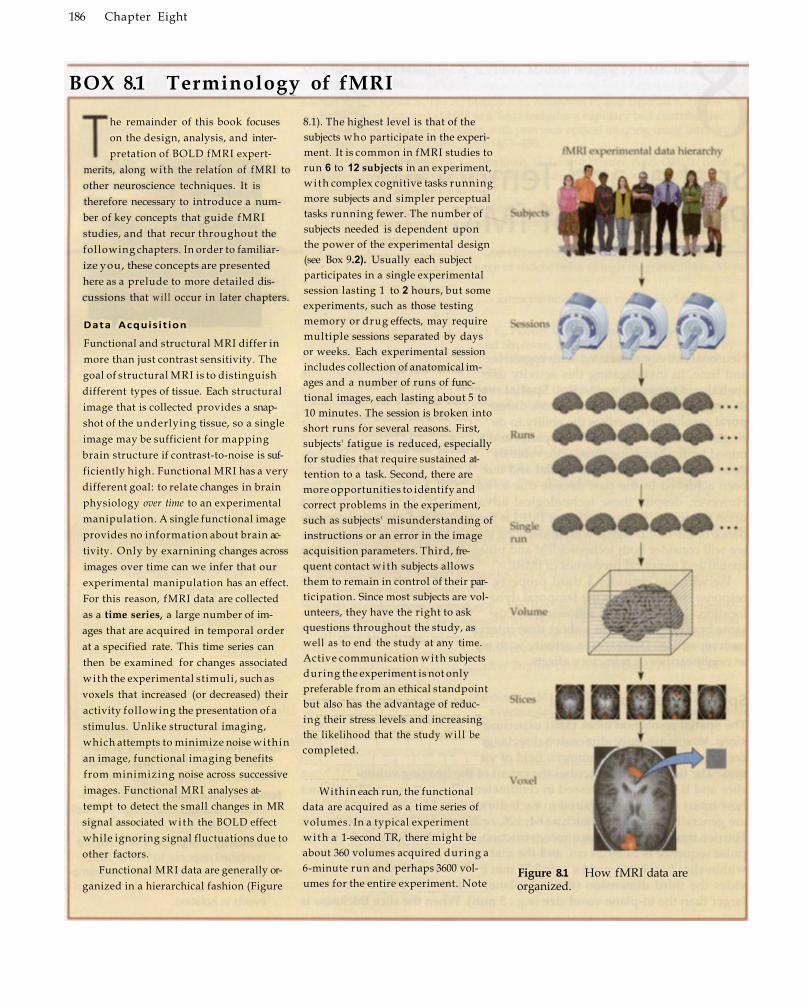
186 Chapter Eight
Figure 8.1 How fMRI data are organized.
8.1). The highest level is that of the subjects who participate in the experiment. It is common in fMRI studies to run 6 to 12 subjects in an experiment, wi th complex cognitive tasks running more subjects and simpler perceptual tasks running fewer. The number of subjects needed is dependent upon the power of the experimental design (see Box 9.2). Usually each subject participates in a single experimental session lasting 1 to 2 hours, but some experiments, such as those testing memory or drug effects, may require multiple sessions separated by days or weeks. Each experimental session includes collection of anatomical images and a number of runs of functional images, each lasting about 5 to 10 minutes. The session is broken into short runs for several reasons. First, subjects' fatigue is reduced, especially for studies that require sustained attention to a task. Second, there are more opportunities to identify and correct problems in the experiment, such as subjects' misunderstanding of instructions or an error in the image acquisition parameters. Third, frequent contact wi th subjects allows them to remain in control of their participation. Since most subjects are volunteers, they have the right to ask questions throughout the study, as well as to end the study at any time. Active communication with subjects during the experiment is not only preferable from an ethical standpoint but also has the advantage of reducing their stress levels and increasing the likelihood that the study w i l l be completed.
Within each run, the functional data are acquired as a time series of volumes. In a typical experiment with a 1-second TR, there might be about 360 volumes acquired during a 6-minute run and perhaps 3600 volumes for the entire experiment. Note
merits, along with the relation of fMRI to other neuroscience techniques. It is therefore necessary to introduce a number of key concepts that guide fMRI studies, and that recur throughout the following chapters. In order to familiarize you, these concepts are presented here as a prelude to more detailed discussions that w i l l occur in later chapters.
Data Acquis it ion
Functional and structural MRI differ in more than just contrast sensitivity. The goal of structural MRI is to distinguish different types of tissue. Each structural image that is collected provides a snapshot of the underlying tissue, so a single image may be sufficient for mapping brain structure if contrast-to-noise is sufficiently high. Functional MRI has a very different goal: to relate changes in brain physiology over time to an experimental manipulation. A single functional image provides no information about brain activity. Only by exarnining changes across images over time can we infer that our experimental manipulation has an effect. For this reason, fMRI data are collected as a time series, a large number of images that are acquired in temporal order at a specified rate. This time series can then be examined for changes associated with the experimental stimuli, such as voxels that increased (or decreased) their activity following the presentation of a stimulus. Unlike structural imaging, which attempts to minimize noise within an image, functional imaging benefits from minimizing noise across successive images. Functional MRI analyses attempt to detect the small changes in MR signal associated with the BOLD effect while ignoring signal fluctuations due to other factors.
Functional MRI data are generally organized in a hierarchical fashion (Figure
he remainder of this book focuses on the design, analysis, and interpretation of BOLD fMRI expert-
BOX 8.1 Terminology of fMRI

S p a t i a l a n d T e m p o r a l P r o p e r t i e s of f M R I 187
Figure 8.2 MR signal is elevated early in runs, before longitudinal magnetization reaches a steady state. Shown is a sample time course of activity in a single voxel for the first 40 images in a single run. Because of this increased activity, fMRI researchers often discard the first few images in a run. When they are removed before even being saved to disk, those images are known as "discarded data acquisitions," or disdaqs. Note that although the steady-state activity looks very flat at this scale, there is about a 4% variation across time points, much greater than the typical BOLD response.
BOX 8.1 (continued)
time series A large number of fMRI images collected at different points in time.
subject A participant in a research study.
session A single visit to the scanner by a subject. For fMRI studies, each session usually includes both structural and functional scans.
run An uninterrupted presentation of an experimental task, usually lasting 5 to 10 minutes for fMRI studies. It also refers to the set of functional images collected during that task presentation.
volume A single image of the brain, itself consisting of multiple slices and voxels.
disdaqs An abbreviation for "discarded data acquisitions"; it refers to images at the beginning of a functional run that are deleted without examination. This is done because MR signal is greatest in these first images, as the change in net magnetization following excitation has not yet reached a steady state.
blocked design The separation of experimental conditions into distinct blocks, so that each condition is presented for an extended period of time.
event-related design The presentation of discrete, short-duration events whose timing and order may be randomized.
that the overall MR signal is elevated in the first few volumes in each run, because the net magnetization has not yet reached a steady state (Figure 8.2). Therefore, the first few volumes are often excluded from further analysis. O n e term for these excluded volumes is disdaqs, a rough acronym for "discarded data acquisitions." Each of the remaining volumes is in turn composed of a variable number of slices, ranging from 1 to 4 in an experiment targeting a particular region, to 25 or more in a study designed to cover the entire brain. Note that each slice is acquired at a different point in time within the T R , but that all data within the slice are effectively acquired at the same time. Each slice consists of thousands of voxels that together form the image of the brain. Due to the Fourier approaches used for reconstructing MR data, slices usually consist of a 2n -by-2 n matrix of voxels, such as 64 x 64 or 128 x 128. When
we acquire data for an fMRI experiment, we can think of that data as a four-dimensional matrix: x by y by slice (z) by time (e.g., 64 x 64 x 25 x 3600).
Experimental Design and Analysis
Then- are two basic types of fMRI studies: blocked designs and event-related designs. A blocked design presents two or more conditions in an alternating pattern. Most early fMRI studies used blocked designs. For example, in the K w o n g and colleagues study described in the previous chapter, a bright visual pattern was presented for 60 s and then the display was dark for 60 s. This approach can be classified as an " A B A B A B . if blocked design. Another common paradigm when comparing two different tasks is to present both in alternation with a baseline period. If a researcher were investigating brain regions
associated with listening to spoken English, three block types might be used: test blocks consisting of English speech, comparison blocks consisting of speech in a foreign language, and baseline blocks in which no speech is present. A typical order of blocks would be " A C B -C A C B C . . . , " where the test (A) and comparison (B) conditions alternate with the baseline condition (C). In most fMRI studies, each block is about 10 to 30 s in duration, and there may be many alter-

188 Chapter Eight
equal to the in-plane resolution, the voxels are cubic and the spatial resolution is said to be isotropic.
The size of the voxel used in a study may depend on the research question. Studies that examine the entire brain w i l l use relatively large voxels, often around 4 to 5 mm on a side. In contrast, studies that examine a single brain region, such as the visual cortex, may use smaller voxels of 1 to 2 mm. For comparison, the letters making up this sentence are each about 2 to 3 mm in size. It is common to acquire anatomical images wi th smaller voxel dimensions (e.g., 1 mm x 1 mm in-plane), and functional data are often displayed on such high-resolution anatomical images. Note that the actual spatial reso-
nations between different block types in a single run.
In an event-related design, stimuli are presented as individual events, or trials. The study by Blamire and colleagues in 1992 was the first to present event-related data. In slow event-related designs (i.e., interstimulus intervals greater than about 10 s), the hemodynamic response decays to baseline after each stimulus, which allows the response to each trial to be individuated. In fast-rate experiments, the events are presented sufficiently close together (i.e., less than 10 s) so that the hemodynamic response does not have time to decay to baseline between successive stimuli. For fast designs, special analysis procedures are required to separate the hemodynamic responses to different events. Some analysis techniques are possible wi th event-related designs but are incompatible wi th blocked designs. For example, individual trials can be sorted according to the subject's response time or accuracy. The effects of one trial type upon another, such as when examining the effects of a warning signal upon a subsequent behavioral response, can also be studied using a fast event-related design.
Nearly all fMRI studies fall into one of these two design categories. However, there is also growing interest in mixed designs that combine features from both types. In a mixed design, there are discrete stimulus events, but those events occur in the context of other
BOX 8.1 (continued)
experimental factors that vary in a blocklike structure.
The choice of design type depends on several factors. Chief among these is the goal of the experiment. One possible goal is detection, the determination of which brain regions are active during a task. In general, blocked designs have high detection power. Another goal is estimation, knowing how activity within brain regions changes over time. Event-related designs, especially those that use fast stimulus-presentation rates, have high estimation power. Another factor is the type of cognitive process being measured. Blocked designs are good for processes that last a long period of time or that cause changes in a cognitive or emotional state of the subject, whereas event-related designs are stronger for discrete, short-term processes. While blocked and event-related designs have different strengths, their combination in a mixed design can provide the advantages of both. The choice of experimental design, as well as the effects of that choice upon experimental analyses, are discussed in considerable detail in Chapter 11.
With regard to the analysis of fMRI experiments, the key division is between voxelwise analysis and anatomical re-
gion-of-interest (ROI) analysis. In a voxelwise analysis, statistical tests are conducted on each voxel to evaluate its significance relative to the experimental hypothesis. Most fMRI studies use voxelwise approaches, and a number of soft
ware packages, both commercial and freely available, have been created to facilitate such analyses. In contrast, ROI analyses partition the brain into a smaller set of discrete regions, which are then individually analyzed for significance. The basic unit of an ROI approach is therefore not the voxel but a spatial set of voxels. ROI analyses can answer questions about the function of particular brain regions but are more time-consuming and labor-intensive than voxelwise analyses.
trial A single instance of the experimental manipulation.
mixed design A design that contains features of both the blocked and event-related approaches.
detection Determination of whether activity of a given voxel changes in response to the experimental manipulation.
estimation Measurement of the pattern of change over time within an active voxel in response to the experimental manipulation.
voxelwise analysis The evaluation of statistical tests at the level of individual voxels.
region-of-interest (ROI) analysis The evaluation of statistical tests on a predetermined collection of voxels, often chosen to reflect a priori anatomical distinctions within the brain.

S p a t i a l a n d T e m p o r a l P r o p e r t i e s of f M R I 189
lution of the fMRI data is not affected by the images on which it is displayed, but depends solely on the voxel size used for functional acquisition.
It seems straightforward that increased spatial resolution carries advantages for fMRI studies. As the distance between adjacent voxels decreases, one is better able to distinguish boundaries between neighboring functional areas. So if fMRI data can be collected at any voxel size, why do researchers not always use the smallest possible? There are two primary challenges for using small voxels in fMRI: reduced signal compared to noise and increased acquisition time.
First, variation in the BOLD signal measured by fMRI depends upon the change in the total amount of deoxygenated hemoglobin w i t h i n a voxel. So, if we reduce the size of our voxels by a factor of 2, the signal that we measure in each w i l l be half as large, resulting in a smaller signal-to-noise ratio. In some brain regions, such as the primary motor or visual cortex, a finger flexion or a visual flash may evoke a very large brain response, and thus the reduced signal amplitude generated from small voxels may not be a problem. But in other brain regions, like the frontal lobe, a choice—response task may evoke much smaller changes in the brain, and larger voxels may improve the ability to detect those changes in the presence of noise. We w i l l discuss the concepts of signal and noise in more detail in the fol lowing chapter.
Second, as voxel size decreases, the time needed to acquire a given volume of the brain increases. While slice acquisition rates w i l l vary across scanners and pulse sequences, doubl ing the matrix size of a gradient-echo pulse sequence can double or even quadruple acquisition time. Increasing the through-plane resolution also increases acquisition time, in this case exactly proportionally to the resolution change. If one halves the slice thickness, then twice as many slices w i l l be needed to cover the same volume, and twice the acquisition time w i l l be required.
In designing an fMRI study, there are trade-offs among spatial coverage, spatial resolution, and the time required for acquisition. On most high-field MR scanners, functional images could be acquired at extremely small voxel sizes of less than a cubic millimeter. But those images w o u l d be acquired very slowly, and a large number would be required to cover the entire brain. For example, on a typical scanner, one might acquire 16 slices per second at 4 mm x 4 mm x 4 mm resolution, but only 1 slice per second at 1 mm x 1 mm x 1 mm resolution. The vertical extent of the cerebrum is about 110 mm or less, so at 4-mm resolution, about 27 slices w o u l d be necessary for fu l l coverage. This imaging volume could be acquired in less than 2 s. At 1 -mm resolution, 110 slices w o u l d be needed, but it w o u l d take about 110 s for their acquisition. Though extreme, this example points out the diff iculty in using high spatial resolution for full-brain imaging. Increasing spatial resolution necessarily decreases temporal resolution. Conversely, increasing temporal resolution decreases spatial coverage. When planning an fMRI study, the researcher must weigh the relative importance of these factors in determining what pulse sequence to use for data acquisition.
A l l fMRI studies, especially those using relatively large voxels, suffer from partial volume effects. The MR signal measured at a given voxel reflects the sum of its entire volume. Even the smallest voxel may contain multiple types of tissue, each contributing part of the total volume. Figure 8.3 shows the possible contents of a single 4 mm x 4 mm x 5 mm voxel. In addition to the active neurons of interest and the local capillary bed, there may be other brain tissue that does not contribute to the measured activity. For example, voxels on the edge of the brain can contain gray matter, white matter, and
partial volume effects The combination, within a single voxel, of signal contributions from two or more distinct tissue types or functional regions.

190 Chapter Eight
Figure 8.3 Partial volume effects. A single voxel may contain many different types of tissue, including gray matter, white matter, cerebrospinal fluid, or blood vessels. The MR signal recorded from that voxel is the sum of signals recorded from all of these different tissue types. So, if a voxel on a T1 image contains 25% cerebrospinal fluid (with low signal), 50% gray matter (with medium signal) and 25% white matter (with high signal), the MR signal recorded from the voxel will contain contributions from all three.
cerebrospinal f lu id . Partial volume effects can significantly reduce the signal measured w i t h i n a voxel using fMRI. If only part of the voxel is active, then the total BOLD signal w i l l be smaller than if the entire voxel is active.
Spatial Specificity in the Vascular System As stated previously, the ultimate functional resolution of fMRI depends on more than voxel size; it depends upon the concordance of hemodynamic and neuronal activity (see Chapter 15 for an expanded discussion of this issue). In an important study conducted in 2001, Logothetis and colleagues investigated the correspondence between the BOLD signal and electrophysiological measures, using simultaneous recordings in the primary visual cortex of monkeys. They found good spatial correspondence between the measures, especially between BOLD and local field potentials that reflect summated EPSPs and IPSPs. In 2000, a similar spatial correspondence was reported by Disbrow and colleagues, who used both fMRI and separate microelectrode recordings to map hand and face representations in the somatosensory cortex in the monkey. They found that the centioids of activity measured using fMRI generally were localized w i t h i n the electiophysiologically mapped hand and face areas, but the areas mapped using fMRI were larger than those mapped wi th electrode recordings (Figure 8.4). The discrepancies observed between the measures were attributed to the filtering effects of the vascular system.
Let us consider the contributions of different parts of the vasculature to the BOLD effect. Recall that the BOLD signal results from the effects of deoxygenated hemoglobin, which is absent in fully oxygenated arterial blood. Thus, the BOLD signal only reflects the deoxygenated hemoglobin content of capillaries and veins. Because deoxygenated hemoglobin molecules are paramagnetic, they create magnetic field gradients w i t h i n the vessel that extend into surrounding tissue. The primary mechanism for BOLD signal is the dephasing of spins wi th in water molecules as they diffuse through these gradient fields. The spins located w i t h i n the vessel itself give rise to the intravascular component of the BOLD signal, while the spins located in the surrounding tissue (i.e., parenchyma) give rise to the extravascular component

S p a t i a l a n d T e m p o r a l P r o p e r t i e s o f f M R I 191
Figure 8.4 Spatial correspondence between fMRI and electrophysiological recordings. Both functional MRI and microelectrode recordings were used (in monkeys) to identify regions associated with motor/sensory responses. Note that the spatial extent of the regions mapped using fMRI (hatching) is much larger than that mapped using electrophysiology, although there is considerable overlap. (From Disbrow et al., 2000.)
of the BOLD signal. In a typical f M R I experiment using gradient-echo sequences, the BOLD signal reflects both intravascular and extravascular signal sources. Both of these signal components can arise from capillaries that are adjacent to and perfuse the active neurons. But because the paramagnetic deoxygenated hemoglobin is removed from the brain by the venous system, they can also arise from draining veins that are distant from the neuronal activity. Thus, the presence of signal changes in large draining veins limits the functional resolution of fMRI. These large-vessel effects can compromise studies that require high functional resolution (less than a centimeter).
large-vessel effects Signal changes in veins that drain a functionally active region but are distant from the neuronal activity of interest.

192 Chapter Eight
Several characteristics are indicative of large-vessel effects. The simplest is magnitude of signal change. Because veins have much greater volume than capillaries, there can be a greater change in the amount of deoxygenated hemoglobin and thus in the total signal change. Systematic changes in the phase of the MR signal may also be observed, since large vessels have specific orientation w i t h i n a voxel, unlike capillaries, which are randomly oriented (see Menon, 2002, for a description of how to overcome this problem). Voxels containing draining veins may be active across very different experimental conditions, since they may drain t w o distinct populations of neurons. A good example of such effects can be seen in the study of ocular dominance columns w i t h i n the visual system (Box 8.2), in that adjacent voxels may have neurons wi th diametrically opposed responses. Finally, the initial negative response that is sometimes observed at high field is thought to represent oxygen extraction in the capillaries, so it w i l l not be seen w i t h i n voxels containing primarily distant large vessels (see Box 7.2).
Advanced acquisition techniques can be employed to exclude components of BOLD signal that are distant from the neuronal activities. These techniques take advantage of the different magnetic properties of large- and small-caliber vessels and the different diffusion properties of extravascular and intravascular spins. It is generally understood that the BOLD magnetic field gradient around the large vessels extends further in space, while that around the small vessels has a smaller spatial extent. More importantly, the magnetic field generated by the deoxygenated hemoglobin in large vessels has a more shallow gradient as it extends into the parenchyma (Figure 8.5A) than the steeper gradients generated w i t h i n small vessels (Figure 8.5B). Thus, the magnetic field change experienced by extravascular spins traveling a given distance is different depending upon whether those spins are near large or small vessels.
Around large vessels, extravascular spins w i t h i n diffusing water molecules experience relatively small magnetic field changes as they travel. Indeed, wi th in the few tens of milliseconds that are typical for a BOLD fMRI acquisition, the magnetic field generated by deoxygenated hemoglobin w i t h i n large vessels can often be approximated as a constant field inhomo-
Figure 8.5 Different effects of large and small vessels on extravascular spins. The magnetic field gradient created by deoxygenated hemoglobin within a blood vessel depends upon the diameter of the vessel. For large vessels (A), the gradient changes slowly over space, so diffusing extravascular spins experience a relatively constant magnetic field over time. Spin-echo imaging can be used to refocus the loss of phase coherence and eliminate the large-vessel signal. For small vessels (B), the gradient changes rapidly over space, so extravascular spins experience different magnetic fields as they diffuse. Loss of phase coherence cannot be recovered by spin-echo imaging, and this spin-echo imaging is sensitive to the small-vessel extravascular component of the BOLD signal.

S p a t i a l a n d T e m p o r a l P r o p e r t i e s of f M R I 193
geneity over time. Recall that the refocusing 180° pulse in spin-echo sequences can reverse the loss of phase coherence resulting from a static field inhomogeneity; thus, we can use spin-echo acquisition strategies to remove the BOLD signal that arises from the extravascular compartment of large vessels. The situation is quite different for extravascular spins near small vessels. The steeper magnetic field gradients extending into the parenchyma outside of small vessels mean that spins in nearby water molecules experience a changing magnetic field inhomogeneity over time. The resultant loss of phase coherence cannot be completely refocused by the 180° pulse, and thus spin-echo sequences retain their sensitivity to the small-vessel extravascular component of the BOLD signal.
Spins w i t h i n intravascular diffusing water molecules also experience a dynamic magnetic field inhomogeneity, as their diffusion distance is large compared to the spatial extent of the deoxygenated hemoglobin-induced magnetic field gradient. For this reason, spin-echo sequences are still sensitive to the intravascular BOLD signal in both large and small vessels. Thus, while spin-echo pulse sequences can eliminate the extravascular large-vessel component of the BOLD signal, another approach must be employed to eliminate the intravascular large-vessel BOLD signal. Because these intravascular spins are in f lowing blood, they have a higher mobil i ty (especially w i t h i n large vessels), and thus motion-weighted image acquisition techniques can be used to isolate this population of fast-flowing spins. One such approach uses diffusion-weighted sequences to selectively suppress the intravascular component of large vessels (general approaches to diffusion weighting are discussed in Chapter 5, and advanced techniques are presented in Chapter 14).
Thus, the combined use of spin-echo and diffusion-weighted sequences can completely eliminate the signals from large vessels while preserving the small-vessel signals to achieve improved functional resolution. However, the overall effect of combining spin-echo and diffusion weighting is greatly reduced BOLD sensitivity. Such a combined approach may be practical only at high fields (>3 T), where the increase in overall signal can help offset the reduction in BOLD sensitivity.
What Spatial Resolution Is Needed? From the previous discussion, we can conclude that the smallest spatial scale that can possibly be measured using BOLD fMRI is determined by the spatial properties of capillaries. Capillaries are very small, typically much less than a millimeter in length, and are generally separated from each other by tens to hundreds of microns. This suggests that the absolute lower l imit for functional resolution of any hemodynamic measure of brain activity is about 100 microns. Even if the brain is sampled at a finer spatial resolution, the functional resolution would not be improved.
It is important to realize that the right spatial scale for an experiment depends on the question being asked. If you are a neurologist examining the effects of frontal lobe damage on intelligence tests, you may examine lesions that span 5 centimeters or more. If you are an electrophysiologist recording the f i r ing of layer 4 neurons wi th in the parietal lobe, you may need to localize the t ip of your microelectrode w i t h i n a few hundred microns. Table 8.1 provides a list of different spatial scales used in the study of the brain. It shows that research into the properties of the human brain spans about seven orders of magnitude, from large-scale anatomy to small-scale microbiology. The spatial resolution of fMRI is intermediate between these extremes, and fMRI is most suited for examining changes in brain function over millimeters to centimeters.
spin-echo (SE) imaging One of the two primary types of pulse sequences used in MRI; it uses a second 180° electromagnetic pulse to generate the MR signal changes that are measured at data acquisition.
diffusion weighting The application of magnetic gradients to cause changes in the MR signal that are dependent upon the amplitude and/or direction of diffusion.
TABLE 8.1 Different Spatial Scales in the Human Brain
Structure Scale
Brain 100 mm
G y r i 10 mm
Dominance co lumn 1 m m
Neuron 0.01 mm
S y n a p s e 0.001 mm
Ion channel 0.00001 mm

194 C h a p t e r E i g h t
BOX 8.2 Mapping of Ocular Dominance Columns Using fMRI
Neurons in the primary visual cor
tex of primates respond preferen
tially to visual stimuli from one
eye. A large number of electrophysio
logical studies in nonhuman primates
have demonstrated that these eye pref
erences are organized into vertical
columns, w i t h all neurons in a column
sharing the same preference (Figure
8.6). The presence of ocular dominance
columns in human visual cortex was
verified using postmortem cytochrome
oxidase staining in the early 1980s. Vas
cular responses have been shown by
optical imaging to be localized within
these columns, so hemodynamic tech
niques like fMRI could, in principle,
map the columnar structure of the pr i
mary visual cortex. However, in humans
the transition from one ocular domi
nance column to another occurs over
about 1 millimeter of cortex, near the
l imit of spatial resolution for fMRI .
An early attempt to distinguish ocu
lar dominance columns using fMRI was
reported by Menon and colleagues in
1997. They used a FLASH pulse se
queiuvon a highfield (4 T) scanner to
acquire veryhighresolution (547 μm by
547μm) images parallel to the calcarine
sulcus in the primary visual cortex. On
such slices, ocular dominance columns
w i l l often be oriented perpendicularly to
the slice plane. The visual stimulus was a
large red lightemitting diode (LED). To
ensure monocular stimulation, subjects
were instructed to open and close one
eye at a time in a blocked pattern. The
authors used a binocular stimulation
condition to identify voxels correspon
ding to primary visual cortex. For each
such voxel, they compared the relative
ocular dominance The degree to
which a given neuron in the visual
cortex responds more to stimuli pre
sented to one eye than to stimuli
presented to the other eye.
T2* blurring Distortions in T2* images
that result from having a data
acquisition window that is suffi
ciently long that significant T 2*
decay occurs over that interval.
signal change caused by stimuli present
ed to each eye. The results were consis
tent wi th previous data from other tech
niques, in that there were significant
BOLD changes in the primary visual cor
tex that changed in dominance from one
eye to another over about 1 mm of space
(Figure 8.7). While its results were ex
tremely interesting this early study had
several limitations, notably that the or
ganization of the dominance columns
was not replicated across multiple meas
urements. Without such replication, it is
difficult to assess whether the observed
fMRI data faithfully represents the true
pattern of ocular dominance, especially
since relatively few voxels showed ocu
lar preferences.
In a later study conducted in 2001,
Cheng and colleagues investigated
whether dominance patterns measured
using fMRI were stable across multiple
sessions. They also used highfield (4 T)
fMRI, but wi th a multishot gradientecho
echoplanar pulse sequence. Veryhigh
resolution voxels were used (470 μm by
470 μm). It is worth emphasizing that
these highresolution studies present a
different set of challenges than standard
fMRI. For example, here the authors ac
quired each slice through a series of 32
successive excitation pulses, resulting in
a total time between successive volumes
of nearly 10 s, even though only three
slices were acquired. This multishot tech
nique reduced the data acquisition time
needed for each excitation, which in turn reduced T2* blurring, which results from Figure 8.6 Ocular dominance columns. Within human p r i mary visual cortex, neurons sensitive to input from one eye are organized into vertical columns.

S p a t i a l a n d T e m p o r a l P r o p e r t i e s o f f M R I 195
Figure 8.7 Early results suggesting the identification of ocular dominance columns in visual cortex using fMRI. Shown in (A) are voxels in human primary visual cortex that responded predominantly to stimulation from one eye or the other. Arrows in (B) indicate transitions between nearby voxels within the calcarine cortex. Voxels responding mostly to left-eye stimulation are shown in red, while voxels responding mostly to right-eye stimulation are shown in blue. In-plane voxel dimensions are approximately 0.5 mm on a side. (From Menon et al., 1997.)
the T2* decay that occurs during the acquisition window. To understand T2* blurring, remember that data acquisition (e.g., filling k-space) takes time, about 40 ms for a typical 64 x 64 image and much longer for very-high-resolution images. During this acquisition window, the spins are continuously undergoing T2* decay, so if the window is very long compared to the T2* value of the tissues being imaged, there will be virtually no signal toward the end of the acquisition window. This significant decay process can cause blurring for BOLD images, especially those that acquire an entire slice at very high resolution following a single excitation.
As a result of the long acquisition time, the authors also used very long block intervals of 2 minutes of monocular stimulation interleaved with 1 minute of darkness. Comparing the patterns evoked by monocular stimulation provided strong evidence for ocular dominance columns in primary visual cortex, notably in areas where the calcarine fissure ran parallel to the imaging plane, but not in areas identified with the secondary visual cortical area, V2 (Figure 8.8A-D). The mean width of columns was about 1.1 mm, consistent with the results from both earlier postmortem staining and from Menon and colleagues' study. Replicability analyses re-
Figure 8.8 Ocular dominance columns in visual cortex. These results show repeatable measurements of ocular dominance columns across two sessions. The same subject participated in two sessions, shown in panels A and C. Note that the outlines of the areas of ocular dominance from the first session (B) correspond well to the results from the second session (D). (From Cheng et al., 2001.)
BOX 8.2 (continued)

196 Chapter Eight
BOX 8.2 (continued)
vealed that the observed patterns were significantly correlated for a given subject both between two experiments within the same session and across two different sessions.
The mapping of ocular dominance columns provides an example of the potential of very high-resolution fMRI. It has obvious value as a technical demonstration and will undoubtedly spur additional improvements in both pulse sequence design and image acquisition hardware. But does it add to the under
standing of the brain? At first glance, these studies merely replicate a phenomenon that was first demonstrated in animals more than four decades ago and in humans more than two decades ago. The existence of ocular dominance columns was never in question, regardless of the outcome of the fMRI studies. Nevertheless, fMRI can provide an important contribution through the in vim study of the human visual system, in contrast to in vitro or animal studies. For example, a topic of considerable interest is the pres
ence or absence of attentional influences upon early visual processing. Understanding whether spatial attention influences activity in dominance columns will provide information about the organization of the visual system. It is important to emphasize that here, as in many areas of neuroscience, fMRI provides a source of information about the brain that can complement results derived from other techniques.
normalization The transformation of MRI data from an individual subject to match the spatial properties of a standardized image, such as an averaged brain derived from a sample of many individuals.
Many aspects of brain function vary over the spatial range of fMRI. Brain regions identified by cytoarchitectonic features, such as used by Brodmann in 1909, generally are several centimeters in size. While the visual cortex includes much of the occipital lobe, along wi th pathways extending into the temporal and parietal lobes, individual functional regions w i t h i n the visual cortex extend in size from a few millimeters to a centimeter or more. Subcortical nuclei such as the caudate, putamen, and thalamus all are sufficiently large to encompass mult iple fMRI voxels. Nevertheless, many aspects of brain structure, including both horizontal cortical layers and vertical cortical columns, exist on a much smaller scale and are very diff icult to address using fMRI.
While this discussion has focused on effects of data acquisition upon spatial resolution, choices made in experimental analysis are also important. A common preprocessing step explicitly reduces spatial resolution by smoothing fMRI data using a three-dimensional Gaussian filter of several voxels in w i d t h (see Chapter 10). Typical smoothing parameters can increase the effective voxel size to 6 x 6 x 6 mm or greater. Note that such a voxel contains more than 3 times the volume of a voxel 4 mm on a side, and 27 times the volume of a voxel 2 mm on a side. While smoothing can reduce spatial resolution, it can improve the validity of statistical tests and comparisons across subjects. Other analysis steps also reduce spatial resolution, albeit not as obviously as spatial smoothing. A n y comparison across subjects w i l l reduce spatial resolution, since subjects w i l l differ in their anatomical structure. In addition, algorithms for transforming subjects to a common stereotaxic space, a process known as normalization, further reduce spatial resolution due to the dif f iculty in matching a person's individual anatomy to a stereotaxic template.
The decision to use anatomically based region-of-interest analyses has implications for spatial resolution as wel l . In an ROI analysis, the basic spatial unit changes from a single voxel to a region containing many voxels. Obviously, the ability to identify differences between adjacent voxels is lost, and thus spatial resolution is greatly reduced. However, to the extent that the chosen regions accurately map onto functional divisions w i t h i n the brain, the functional resolution of the data may be greatly increased by sig-

S p a t i a l a n d T e m p o r a l P r o p e r t i e s o f f M R I 197
nal averaging (since noise that is randomly distributed over space w i l l be reduced). For example, the putamen is a relatively small structure wi th in the basal ganglia that is associated wi th motor preparation, interval t iming, and some cognitive processing. Since there are clear anatomical divisions between the putamen and the surrounding white matter, it is simple to create an ROI that includes the entire putamen. By considering the putamen as a whole, subregions w i t h i n it cannot be distinguished; however, the ability to detect changes in the putamen as a whole w i l l be greatly increased through spatial averaging. As a general rule, many analysis steps sacrifice spatial resolution in order to increase functional resolution.
Temporal Resolution of fMRI
For many experimental questions, it is important to determine the relative timing of brain activity. However, neuroscience techniques differ in their ability to measure relative t iming. Recordings from microelectrodes w i t h i n the brain can identify the f i r ing of a single neuron as it occurs, localizing activity in time at the millisecond level, but these can only be made in nonhuman animals or in humans w h o are undergoing special tests associated with neurosurgical procedures. Lesion studies, in contrast, provide almost no information about the t iming of brain activity. The ability to separate brain events in time is known as temporal resolution. FMRI is considered to have an intermediate level of temporal resolution, because it can discriminate events that are separated by intervals on the order of a few seconds. Just as the basic sampling unit for spatial resolution is the voxel, the basic sampling unit for temporal resolution in fMRI is repetition time, or TR. For typical pulse sequences used in fMRI, one image of the brain is acquired per TR. Depending upon the experiment, TR may range from very short (e.g., 500 ms) to very long (e.g., 4000 ms), w i t h even more extreme values used in specialized experiments. While the value of TR contributes to the temporal resolution of an experiment, it is not the only factor.
Remember from the previous chapter that the fMRI BOLD hemodynamic response rises and falls over a period of more than 10 seconds, even if the duration of neuronal activity is very short (e.g., less than a second). So, when we collect fMRI data, we do not take snapshots of neuronal activity, but measure changes in the vascular system that provide an indirect estimate. Decreasing TR to better sample the fMRI hemodynamic response is beneficial because it improves our estimate of this response, which in turn improves the inferences we can make about neuronal activity.
We emphasize this framework because it suggests that there may be a preferred temporal resolution for a given experimental question. Consider the very simple event-related design in which a subject squeezes her hand whenever she sees a visual stimulus. If our goal is to determine whether an area of the brain becomes active due to hand motion (i.e., detection), a relatively slow sampling rate w i l l suffice. At a 3-s TR, the hemodynamic response may be easily identified when compared to the prestimulus baseline, but its exact shape may be dif f icult to estimate (Figure 8.9A). Halving the TR to 1500 ms improves our estimate of the shape of the response and the t iming of the peak but does not substantially change the measured amplitude (Figure 8.9B). Something very interesting becomes evident if we halve the TR again, to 750 ms. The measured hemodynamic response, though sampled twice as often, does not differ much in shape from the 1500-

198 C h a p t e r E i g h t
Figure 8.9 Effects of sampling rate (TR) upon the measured hemodynamic response. In each figure, an idealized hemodynamic response is sampled at a different rate.
ms condition (Figure 8.9C). Further reduction to 375 ms results in even less change in the measured shape of the hemodynamic response (Figure 8.9D).
It seems counterintuitive that dramatic increases in sampling rate would have little effect upon temporal resolution. However, think about the effect
How does the temporal resolution tha t is needed to detect significant activity change for long-interval
blocked designs? Is the required TR larger or smaller than for event-related designs?

Spatial and Temporal Properties of fMRI 199
interleaved stimulus presentation The presentation of events of interest at different points within a TR over trials (e.g., one-quarter, one-half, and three-quarters of TR in addition to TR onset), increasing the effective sampling rate of an experiment at the expense of fewer trials per condition.
of the additional samples on the estimate of the hemodynamic response. In the case of a 3-s TR, what do we know about the time points between samples (i.e., 1.5 s, 4.5 s, etc.)? Although they are not measured directly, a reasonable assumption might be that the hemodynamic amplitude at these points w o u l d be intermediate between the recorded samples. For now, we can consider simple linear interpolation, such that the midpoint w o u l d be given by the average of the t w o adjacent samples. At TRs greater than about 2 s, linear interpolation does not provide a good estimate of the values that would have been recorded from the intervening points. But as we shorten the TR to 1.5 s or less, even simple linear interpolation w i l l accurately reproduce intermediate values, because the hemodynamic response has reproducible structure. The changes in blood f low and oxygen extraction that form the basis of BOLD contrast occur as a result of slow physical processes and do not themselves change rapidly over short time periods. Only if these physical processes varied dramatically w i t h i n short intervals, say 100 ms, would increasing the sampling rate have a greater effect. Note that this example uses an event-related design, so that the hemodynamic response evolves over about 10 to 15 s. If a long-interval blocked design were used, then the changes in the hemodynamic response would be much slower and an even longer TR would be adequate. In summary, the temporal resolution of fMRI is determined both by the repetition time, TR, and by the limitations of the vascular system. For many experimental questions, temporal resolution of about 1 to 2 s is sufficient.
While decreasing the repetition time can improve temporal resolution, it can present some disadvantages to fMRI studies as wel l . In Chapter 3 we learned that one parameter of an MR pulse sequence is the f l ip angle, which reflects how far the net longitudinal magnetization is tipped toward the transverse plane by an RF pulse. Since the amount of measured MR signal is proportional to the projection of the magnetization vector on the transverse plane, large f l ip angles are associated w i t h greater MR signal. For typical gradient-echo sequences w i t h long TRs (i.e., greater than about 2 s), a f l ip angle of 90° can be used to recover maximal MR signal. But at shorter TRs, a smaller f l ip angle is required so that the magnetization w i l l reach a steady state over repeated excitations. As a result, the amplitude of the transverse magnetization fol lowing excitation w i l l be reduced at short TRs and less MR signal w i l l be measured. Short repetition times also reduce spatial coverage. If a scanner can acquire 14 slices per second w i t h a given pulse sequence, then only 7 slices could be acquired w i t h a 500-ms TR, whi le 28 could be acquired w i t h a 2000-ms TR.
Temporal resolution can be improved by using an interleaved stimulus presentation, in which the experimental st imuli are presented at different points w i t h i n a TR on different trials. Note that this should not be confused wi th interleaved slice acquisition, which refers to the order of slice excitation wi th in a TR. Figure 8.10A and B illustrates the basic approach. In a typical experiment w i t h a 3-s TR, the experimental st imuli would be presented at TR onset, so the hemodynamic response is sampled at 3 s, 6 s, 9 s, etc., following stimulus presentation. In an interleaved design wi th three presentation times, the stimuli could be presented either at TR onset, one second into the TR, or two seconds into the TR. Thus, one-third of the trials would sample normally, one-third would sample at 1 s, 4 s, 7 s, and one-third w o u l d sample at 2 s, 5 s, 8 s, etc. By combining data across all three sets of trials, the hemodynamic response can be estimated w i t h a temporal resolution of 1 s. In principle, additional delay conditions can be used, such as one-quarter, one-half, and three-quarters of a TR, to further increase temporal resolution.
Figure 8.10 Use of interleaved stimulus presentation. In an experimental design with interleaved presentation, the experimental stimulus is presented at different points relative to the TR on different trials (A). Although the hemodynamic response may be sampled coarsely on each trial, the sampling occurs at different phases within the TR. Thus, combining across trials (B) fills in intermediate points, improving effective temporal resolution at a cost of increased experiment length.
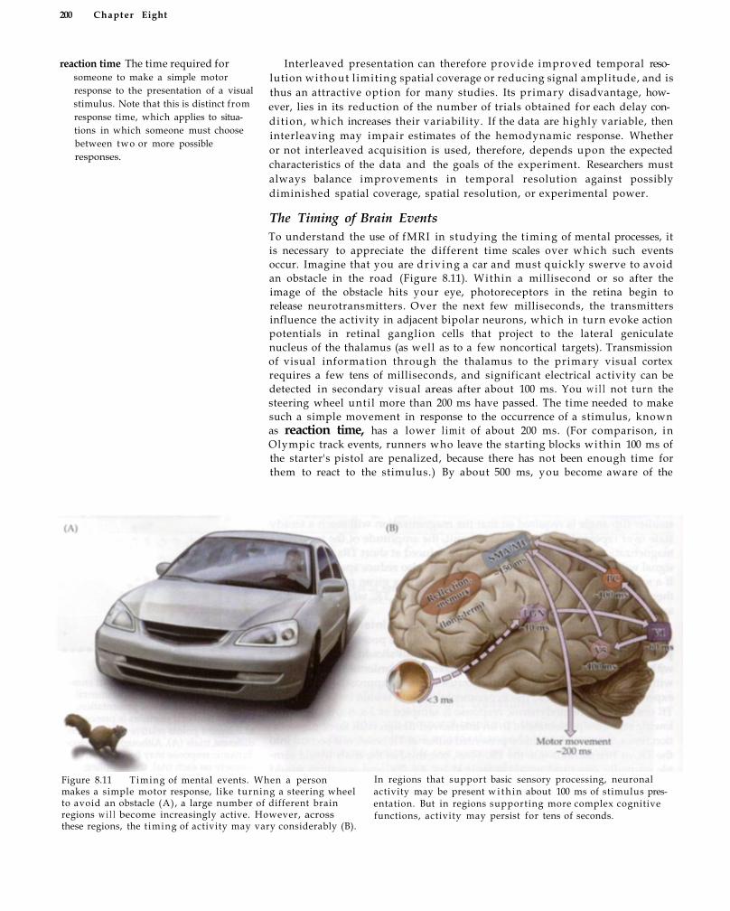
200 Chapter Eight
reaction time The time required for someone to make a simple motor response to the presentation of a visual stimulus. Note that this is distinct from response time, which applies to situations in which someone must choose between two or more possible responses.
Interleaved presentation can therefore provide improved temporal resolution without l imiting spatial coverage or reducing signal amplitude, and is thus an attractive option for many studies. Its primary disadvantage, however, lies in its reduction of the number of trials obtained for each delay condit ion, which increases their variability. If the data are highly variable, then interleaving may impair estimates of the hemodynamic response. Whether or not interleaved acquisition is used, therefore, depends upon the expected characteristics of the data and the goals of the experiment. Researchers must always balance improvements in temporal resolution against possibly diminished spatial coverage, spatial resolution, or experimental power.
The Timing of Brain Events To understand the use of fMRI in studying the t iming of mental processes, it is necessary to appreciate the different time scales over which such events occur. Imagine that you are d r i v i n g a car and must quickly swerve to avoid an obstacle in the road (Figure 8.11). Within a millisecond or so after the image of the obstacle hits your eye, photoreceptors in the retina begin to release neurotransmitters. Over the next few milliseconds, the transmitters influence the activity in adjacent bipolar neurons, which in turn evoke action potentials in retinal ganglion cells that project to the lateral geniculate nucleus of the thalamus (as well as to a few noncortical targets). Transmission of visual information through the thalamus to the primary visual cortex requires a few tens of milliseconds, and significant electrical activity can be detected in secondary visual areas after about 100 ms. You w i l l not turn the steering wheel unti l more than 200 ms have passed. The time needed to make such a simple movement in response to the occurrence of a stimulus, known as reaction time, has a lower l imit of about 200 ms. (For comparison, in Olympic track events, runners who leave the starting blocks within 100 ms of the starter's pistol are penalized, because there has not been enough time for them to react to the stimulus.) By about 500 ms, you become aware of the
Figure 8.11 Timing of mental events. When a person makes a simple motor response, like turning a steering wheel to avoid an obstacle (A), a large number of different brain regions w i l l become increasingly active. However, across these regions, the t iming of activity may vary considerably (B).
In regions that support basic sensory processing, neuronal activity may be present w i t h i n about 100 ms of stimulus presentation. But in regions supporting more complex cognitive functions, activity may persist for tens of seconds.

S p a t i a l a n d T e m p o r a l P r o p e r t i e s of f M R I 201
stimulus and begin reflecting on the near accident. More-complex processes, like retrieving the memory of a similar event, may take several seconds, and changes in your emotional or physiological state may last for minutes or hours. Finally, there may be long-term effects, such as learned changes in your dr iving patterns, that persist for days, months, or even indefinitely.
A single stimulus can thus evoke changes in the brain that span more than eight orders of magnitude, from milliseconds to days. While this range is very large, most psychological experiments manipulate cognitive processes over periods of a few seconds, well w i t h i n the range of f M R I . For example, response-selection studies typically present stimuli every few seconds, while short-term memory experiments may require the subject to remember an object for about 10 s. More dif f icult to study using fMRI are topics involving very small or very large time scales. A rough estimate of the lower l imit of fMRI's temporal resolution for most conditions is a few hundred milliseconds. For example, there are well-known reentrant circuits running from higher visual processing regions back to the primary visual cortex. Attending to a visual stimulus has been shown to increase fMRI activity in the primary visual cortex, but that increase may result from either initial activity or a recurrence of activity due to feedback from other brain regions that occurs hundreds of milliseconds later (see Chapter 13).
While there is no l imit , in principle, that precludes fMRI studies of long time scales, practical factors make such studies challenging. One common manipulation is to change experimental instructions between runs, so that the participant does one task for several minutes and then another. This approach is necessary for many sorts of experimental questions, such as memory studies that separate stimulus learning from memory retrieval. When using such an approach, the researcher should monitor for problems like head motion and scanner dr i f t that can cause systematic differences across runs. If the time scale needed is longer than an hour or two, as when examining long-term memory, then multiple scanner sessions w i l l be necessary. Comparison of data across sessions raises many additional problems, since there may be differences in head position, fatigue level, and practice with the task. Nevertheless, it is important to emphasize that while the lower and upper bounds expressed here reflect the limitations common to most fMRI BOLD studies, w i t h careful selection of imaging parameters and clever experimental design, these limits can be readily overcome.
The relation between t iming and hemodynamic amplitude is critical for models of fMRI activity. Depending on the constraints of the vascular system, larger responses might take longer to reach their peak than smaller responses. Alternatively, a large-amplitude response might reflect greater neuronal activity, and thus greater metabolic demand, which could cause an earlier supply of oxygen and an earlier peak. While both arguments are plausible, neither is correct. For a given stimulus and brain region, the amplitude of the fMRI hemodynamic response appears to be independent of the t iming of the response in both latency to onset and latency to peak (Figure 8.12). This means that if you measure the fMRI BOLD response in the auditory cortex to the presentation of a 2-s music video clip, there w i l l be no
How could experiments be designed to investigate feedback circuits in the brain using fMRI?

Figure 8.12 Amplitude and timing of the event-related fMRI hemodynamic response are uncorrelated. Two experiments were conducted in which hemodynamic responses in the visual cortex to a short-duration visual stimulus were measured. In both experiments, there was no correlation across subjects between the amplitude of the response and its time to peak. Note that in Experiment 2, the subject with the largest response (A) had an average time to peak, while the subject with the longest-latency response (B) had an average peak amplitude. (After Miezen et al., 2000.)
correlation across subjects between its amplitude and t iming. However, if you measure the activity in that region for several different stimulus durations, the response at longer durations w i l l be of both greater amplitude and increased latency. Likewise, if you compare activity in the auditory cortex to activity in another brain region (e.g., visual cortex), the two brain regions may differ in both amplitude and latency. These latter differences would reflect differences in neuronal processing as a function of stimulus duration or brain region, not differences in the hemodynamic response itself. In summary, changes in the amplitude of the fMRI hemodynamic response do not cause changes in the t iming of the response, or vice versa, although external factors may affect both measures similarly.
Effects of Stimulus Duration Over intervals from a few seconds to a few tens of seconds, the duration of the fMRI hemodynamic response provides a good estimate of the duration of neuronal activity. A good example of this was reported in 1999 by Menon and K i m , w h o investigated the role of the superior parietal lobe in mental rotation of complex objects. Decades of cognitive psychology studies have shown that the time needed to judge whether or not t w o similar objects are identical depends on the rotation angle between them. Thus, response time is twice as long for pairs that differ by 90° as for pairs that differ by 45°. Menon and K i m hypothesized that since the superior parietal lobe is critical for spatial processing, including mental rotation, its activity should extend in time for the entire rotation process. To test this idea, they measured the durat ion of the BOLD response in this region on each of 16 different trials that required objects to be rotated through different angles. They found that for each trial, the duration of the BOLD response matched well w i t h the subject's response time (Figure 8.13A-C). The onset of the BOLD response did
202 C h a p t e r E i g h t

Spatial and Temporal Properties of fMRI 203
Figure 8.13 The w i d t h of the fMRI BOLD response increases w i t h the duration of mental activity. Subjects were tested in a mental rotation task. Each trial measured how long it took the subjects to decide whether two stimuli were rotated versions of one another (A) , then the fMRI hemodynamic response across trials was measured (B). The remarkable f inding was that response time was a near perfect predictor of the w i d t h of the BOLD signal in the superior parietal cortex (C), which is important for spatial abilities, suggesting a good correspondence between duration of neuronal activity and the BOLD response. (After Menon and K i m , 1999.)
not differ across trials, suggesting that neuronal activity began at the start of the mental rotation process but stopped when mental rotation was complete.
Huettel and colleagues reported a similar result in a change detection task. In this task, t w o versions of the same picture were presented in rapid alternation, separated by a brief mask interval, for 40-s blocks. Each pair of photographs differed in one aspect, such as the position or color of a single object, and the subjects pressed a button when they identified what changed between them. Because the mask prevents the visual system from using motion transients to identify the changes, subjects cannot detect the changes automatically and the visual search may take anywhere from a few seconds to 30 seconds or more. The authors found that regions associated wi th visual search showed increases in BOLD activity that persisted for the duration of the search process, returning to baseline after the subjects found the change, even though the stimulus was visible to the subjects for the entire block. An interesting secondary result was the f inding that areas that showed deactivations during the task (see Box 11.2) also showed differential activity based on the duration of search, decreasing in activity at the beginning of the block and increasing in activity after the subject found the change.
Recognize, however, that the duration of the stimulus or behavior does not necessarily correspond to the duration of the neuronal activity. Imagine seeing a photograph of a familiar face that is presented for 5 seconds. Neurons in the primary visual cortex w i l l have their largest response over the first 100 ms or so, then become much less active. Neurons w i t h i n face-sensitive regions in the inferior temporal lobe w i l l be active at stimulus onset, as well

204 C h a p t e r E i g h t
as throughout the 5-second period due to feedback from other brain regions. Some neurons w i t h i n the frontal and parietal lobes may become active after the face disappears as you reflect upon what you just saw. While models for fMRI analysis are often constructed based upon stimulus duration, for most experimental questions the durat ion and t iming of neuronal activity are more important.
Relative Timing across Brain Regions Even though it is di f f icult to determine the absolute t iming of neuronal activity based upon the fMRI BOLD signal, the relative t iming of activity can be identified w i t h great precision (Figure 8.14). In 1998 this was shown in an elegant study by Menon and colleagues, w h o investigated relative t iming in t w o fMRI experiments using gradient-echo echo-planar fMRI at high field (4 T) and high temporal resolution (TR of 100 ms). Their first experiment used a visual checkerboard stimulus that was split into left and right hemifields, each presented for 2 s. The left hemifield was presented either before the right, wi th a delay interval ranging from 125 to 1000 ms, or at the same time. When they measured the difference in hemodynamic latency between the two hemispheres in the visual cortex, they found a near perfect correspondence w i t h the presentation delay. The second experiment extended this result by introducing a motor reaction time task. Each trial began w i t h the subjects watching a fixation cross at the center of the screen for 6 s. Then the screen turned bright yellow and a green start box and red target box
Figure 8.14 Using fMRI to identify the relative t iming of activity across brain regions. (A) Subjects moved a target square across the display w i t h a joystick when it changed color. The relative latency of the fMRI signal in different brain regions as a function of the subject's reaction t ime (RT) on the task was measured. The latency between BOLD activity in the primary visual cortex (V1) and in the supplementary motor area (SMA) increased roughly linearly w i t h RT, whi le the latency between SMA and the primary motor cortex (M1)
was unchanged w i t h RT. This result suggests that processes influencing the speed of a response occur between V1 and SMA but not between SMA and M1. (B) In a similar approach subjects pressed a button w i t h one hand at the onset of a 1.5-s-duration stimulus and a button w i t h the other hand at offset. The order of activity between motor cortex regions depended on the order of responses, while activity in the visual cortex was independent of response order. (A after Menon et al., 1998; B after Miezin et al., 2000.)
hemifield One half of a visual display, usually referring to the left or right half.
S p a t i a l a n d T e m p o r a l P r o p e r t i e s o f f M R I 205
Especially remarkable were the effects of reaction time, which varied across subjects from about 200 to 300 ms, upon these differences. The difference between V1 and SMA activation was proportional to reaction time, suggesting that the pathway between them may be associated w i t h decision or preparatory processes that differ between subjects (Figure 8.14A). However, the delay between SMA and Ml activation was constant across reaction times, indicating that that l ink supports more basic response-execution processes. To cognitive neuroscientists, such a result is extremely exciting because it suggests that variability in reaction time, which is the most commonly used measure in experimental psychology, can be restricted to particular brain regions. Note that the t iming difference found between these regions using fMRI is larger than that calculated from electrophysiological studies, where a latency of around 100 ms between V1 and Ml is more typical. This discrepancy illustrates the basic problem w i t h making inferences about the relative t iming of neuronal activity across brain regions based upon fMRI data: differences in vascular properties also contribute to the timing of activity. This caveat, however, does not call into question the results of Menon and colleagues, because they demonstrated that the t iming difference between regions depended on reaction time.
Within a single region, however, any vascular properties w i l l be similar across t iming conditions, a l lowing accurate estimation of small t iming differences. In 2000, Miezin and colleagues investigated the issue of relative timing using a clever visuomotor task. They presented checkerboard stimuli in a rapid event-related paradigm. Each stimulus was presented for 1 s, and the time between st imul i was randomly varied, a technique called jittering, in this case w i t h a mean of about 5 s. The subjects' task was to press a button w i t h one hand when the stimulus appeared and press another button w i t h the other hand when the stimulus disappeared. On one half of the trials, the right hand was used first, and on the other half, the left. They found that the estimated hemodynamic response in motor cortex corresponding to the onset of the stimulus was shifted earlier in time by about 0.75 to 1.0 s compared to the response to stimulus offset (Figure 8.14B). The fact that this shift was slightly less than the stimulus durat ion likely reflected preparation processes, since the subjects knew when the stimulus would disappear and could prepare for that button press. A subsequent power analysis suggested that t iming differences as small as 100 ms could be reliably detected using such a paradigm.
jittering Randomizing the intervals between successive stimulus events over some range.
appeared. The task was to use a joystick to move a cursor f rom the start box to the target box as quickly as possible. One second after the cursor was successfully moved, the screen returned to gray and the subjects returned the joystick back to its center. The authors investigated the t iming of activity in three cortical regions: primary visual cortex (V1), primary motor cortex ( M l ) , and the supplementary motor area (SMA). Act iv i ty in V1 was observed, on average, about 200 ms before activity in SMA, which in turn was about 30 ms before activity in M l .
How is it possible that researchers can identify t i m i n g differences of a f e w hundred milliseconds using fMRI if the hemodynamic response is delayed by a f e w seconds
f o l l o w i n g the neuronal activity?

206 Chapter Eight
Figure 8.15 Maps of BOLD latency to peak in visual cortical regions. A 500-ms visual stimulus was presented and the latency to peak in voxels with significant BOLD activity was measured. Data are shown for two subjects. The color of each voxel indicates its latency, with voxels that had an early peak shown in blue and voxels with a late peak shown in red. Peak latency was shortest in voxels near the calcarine cortex (A,C), as shown in the left figures, and was longest in the fusiform gyrus, as shown in the right figures (B,D). (From Huettel et al., 2001b.)
In summary, latency differences as small as a few hundred milliseconds can be measured between brain regions using fMRI (Figure 8.15). These differences may reflect changes in vascular response between brain regions and do not necessarily map directly to neuronal activity. In order to make inferences about relative t iming of neuronal activity, researchers must selectively manipulate or measure one mental process while holding another constant. For example, decision processes may be proportional to response time, while low-level perceptual processes may be independent of response time, as in the study by Menon and colleagues. Comparisons w i t h i n the same region do not suffer from such a problem, and thus very small intraregion timing differences can be identified.
Linearity of the Hemodynamic Response
So far we have considered the properties of the hemodynamic response to a single isolated stimulus. What happens when multiple stimuli are presented

Spatial and Temporal Properties of fMRI 207
Figure 8.16 Linear and nonlinear addition of hemodynamic responses. If the same fMRI hemodynamic response were evoked by every stimulus (A), then the combined hemodynamic response to two stimuli would be a linear combination of two identical responses (B). But if the hemodynamic response were attenuated when stimuli were presented in rapid succession (C), then the combined response would be reduced in amplitude (D).
in succession? One possibility is that the same hemodynamic response is evoked for every stimulus, independently of the other stimuli presented, as shown in Figure 8.16A. If the stimuli are sufficiently close together that their hemodynamic responses overlap, then the measured total change in MR signal w i l l be the sum of the individual responses (Figure 8.16B). This is known as a linear system, and its properties are discussed in the fol lowing section. Another possibility is that the hemodynamic response to a given stimulus depends on what other st imuli are presented (Figure 8.16C and D). If two stimuli are presented very close together, the combined response might be less than the sum of the two individual responses. Reductions in hemodynamic amplitude as a function of interstimulus interval are known as BOLD refractory effects. If refractory effects are present, then a linear model w i l l overestimate the hemodynamic response to closely spaced st imuli , potentially reducing the effectiveness of experimental analyses. It is critical, therefore, to consider the evidence for and against the linearity of the fMRI hemodynamic response.
Properties of a Linear System A basic framework for measurement of signal in fMRI is shown in Figure 8.17. Under this framework, when a stimulus is presented, it induces neuronal activity w i t h i n a particular region of the brain. Since the neuronal
linear system A system that obeys the principles of scaling and superposition.
refractory effects Changes in the amplitude and timing of a response based on the characteristics of preceding responses.

208 C h a p t e r E i g h t
Figure 8.17 The linear systems framework for fMRI. Boynton and colleagues investigated whether the fMRI hemodynamic response might be a linear transformation of neuronal input, combined with additive Gaussian noise. (After Boynton et al., 1996.)
impulse A single input to a system. Impulses are assumed to be of infinitely short duration.
scaling A principle of linear systems that states that the magnitude of the system output must be proportional to the system input.
activity requires that oxygen be provided by the blood, there are resulting f low and volume changes in that brain region, as discussed in Chapters 6 and 7. The reduction in magnetic susceptibility associated w i t h increased blood oxygenation then becomes measurable as BOLD contrast using fMRI. To reformulate this framework in terms of a linear system, we can consider the neuronal activity as a short-duration input, or impulse, to the hemodynamic system, whose output is measured in MR signal. For a given impulse, the hemodynamic system is assumed to always respond in the same manner. From this assumption fol low t w o basic properties of a linear system: scaling and superposition.
The principle of scaling states that the output of a linear system is proportional to the magnitude of its input (Figure 8.18A). If the input is doubled, then the output is likewise doubled; if the input is halved, then so is the output. For fMRI data, this principle would indicate that changes in the relative amplitude of neuronal activity should lead to similar changes in the amplitude of the hemodynamic response. Now, w h y is this important?
Figure 8.18 Scaling and superposition. (A) The principle of scaling states that the output of a linear system is proportional to the magnitude of the input. For fMRI, this implies that the amplitude of the hemodynamic response reflects the amount of underlying neuronal activity. (B) The principle of superposition states that the output of a linear system with more than one input is the sum of the responses to the individual inputs.

S p a t i a l a n d T e m p o r a l P r o p e r t i e s o f f M R I 209
Remember that the goal of fMRI is to determine changes in neuronal activity, which must be inferred from the amplitude changes in the hemodynamic response. So, a study may present a test condition and a control condition, find that activity in the brain region of interest is twice as large in the test condition, and then infer that neuronal activity was similarly larger in that condition. If the hemodynamic amplitude were independent of the amplitude of neuronal activity, then no such inferences would be possible.
Whereas scaling refers to the amplitude of activity, the principle of superposition refers to the t iming of activity (Figure 8.18B). Stated simply, superposition means that the total response to two or more events is the summation of the individual responses. If a single event generates a hemodynamic response, then two events presented in succession w i l l generate a combined response equal to t w o individual responses added together. To understand the importance of superposition, consider a very simple experiment. You are interested in studying the brain activity associated w i t h short-term memory of words, so you devise an experiment in which a w o r d is presented, followed by a 2-s delay and then another w o r d . The subject's task is to indicate whether or not the two words are the same. Since the two s t imul i are both words, they w i l l likely activate many of the same brain regions, and since they are presented so close together in time, their hemodynamic responses wi l l overlap. H o w can you distinguish whether an area is active in response to the first word , the second word , or both? By assuming superposition, you can create models for what combined hemodynamic response w o u l d be expected in each condition. If an area is active in response to the first w o r d but not the second, it w i l l show an early rise to a peak at about 5 s, whereas if i t is active only in response to the second word , the rise w i l l occur 2 s later. If i t is active in response to both words, there w i l l be an intermediate but larger peak. Understanding the superposition of hemodynamic responses is critical for fMRI analyses.
It is important to recognize that although we are discussing the linearity of the hemodynamic response, nonlinearities may be present in the neuronal response as wel l . Many electrophysiological studies have demonstrated that evoked potentials, especially those related to primary sensory or motor processing, are reduced in amplitude when preceded by a similar potential wi th in the previous second or two. Typical fMRI studies cannot distinguish between neuronal or vascular sources for nonlinearity without incorporating data on neuronal activity or employing adaptation methods.
Evidence for Rough Linearity The first study of the linearity of the fMRI BOLD response was reported by Boynton and colleagues in 1996. They investigated the effects of duration of visual stimulation upon activity in the primary visual cortex, using an EPI gradient-echo sequence at 1.5 T. The durations tested were 3, 6,12, and 24 s. The visual stimuli were checkerboard patterns that moved from right to left while flickering at a high rate (8 Hz). The contrast between dark and light squares on the checkerboard was manipulated over trials. To evaluate the scaling of the hemodynamic response, the authors examined the effects of two factors: stimulus contrast and stimulus duration. Their hypothesis was that these factors should have independent and additive effects on the BOLD signal if the hemodynamic response behaved as a linear system.
Boynton and colleagues found that for all stimulus durations, the amplitude of activity was greater at higher visual contrast levels but the hemodynamic response had the same basic shape. This confirmed the scaling principle of linearity. To test whether the superposition principle also held for
superposition A principle of linear systems that states that the total response to a set of inputs is equivalent to the summation of the independent responses to the inputs.

210 C h a p t e r E i g h t
Figure 8.19 Evidence for the linearity of the fMRI hemodynamic response. Boynton and colleagues investigated whether the addition of the fMRI responses to several short-duration stimuli (blue lines) predicted the fMRI response to a longer-duration stimulus (red lines). The prediction fit the observed data well, save for an overes¬timation of the response given by the addition of 3-s stimuli. (After Boynton et al., 1996.)
BOLD data, they investigated whether the response to a longer stimulus could be predicted by the sum of multiple shorter st imuli . Their results indicated linear superposition for most stimulus durations, such that the response to a 24-s stimulus was given by the addition of two 12-s stimuli or four 6-s st imuli (Figure 8.19). The one exception they noted was that the response given by the addition of 3-s stimuli was larger than predicted, and this discrepancy was attributed to neuronal adaptation effects (i.e., that the neurons themselves decrease in activity over the first few seconds of a stimulus). In total, these results provided strong evidence for the linearity of the hemodynamic response over stimulus durations ranging from a few to tens of seconds.
Following on the results of Boynton and colleagues, Dale and Buckner in 1997 investigated the linearity of the hemodynamic response to individual stimulus events, rather than extended stimulus blocks. They reasoned that neuronal adaptation effects could be eliminated by separating stimuli in time by an interval sufficiently long to allow complete neuronal recovery. To test whether complete linearity would be observed under such conditions, they presented clusters of one, two, or three st imuli at interstimulus intervals of either 2 or 5 s. The hemodynamic response to a second stimulus in a cluster was determined by subtracting the single-stimulus response from that to a pair of s t imuli . Likewise, the response to the third stimulus was determined by subtracting the two-stimulus response from the three-stimulus response. If the principle of superposition holds for fMRI BOLD data, then all responses should have the same amplitude and shape regardless of where they occur in the cluster. Dale and Buckner's evidence supported this interpretation, in that the responses to the second and third trials in the set

Spatial and Temporal Properties of fMRI 211
Figure 8.20 Linear addition of hemodynamic responses to individual stimulus events. (A) The hemodynamic responses evoked by presentation of one, two, or three identical stimuli (short-duration visual flashes) at short interstimulus intervals were measured. Shown here are data from a 2-s interval. The total hemodynamic response increased in a regular fashion as the number of stimuli in a trial increased. (B) By subtracting
the one-stimulus trial from the two-stimulus trial, and the two-stimulus from the three-stimulus, the contributions of the second and third stimuli in a trial were estimated. To a first approximation, the responses to the second and third stimuli were similar to that to the first, suggesting that the BOLD response scales in a roughly linear fashion. (From Dale and Buckner, 1997.)
were generally similar to that of the first tr ial , (Figure 8.20) especially for pairs of trials at a 5-s interval. They concluded that the fMRI BOLD response adds across s t imul i in a "roughly linear" fashion at intervals typical of experimental testing (e.g., a few seconds).
This f inding, that individual trials evoke recognizable hemodynamic responses even when separated by relatively short intervals, has become extremely influential for design and analysis of fMRI studies. At first interpretation, it suggests that individual trials can be closely spaced to increase the number of trials presented and thus experimental power, without loss of response amplitude (see Chapter 11 for discussion of this issue). But, as the authors themselves note, there are significant limitations for such fast-rate studies. Primary among these are the deviations from linearity at short intervals. Close examination of the data from 2-s interstimulus intervals (see Figure 8.20B) reveals that the response to the second and third stimuli in a cluster are reduced in amplitude and increased in latency compared to the response to a single stimulus. In the best case, such nonlinearities w o u l d reduce the power of experimental analyses but would have little additional effect. But in the worst case, large nonlinearities could preclude the use of very short intervals (e.g., 1 second) between experimental s t imuli .
Challenges to Linearity Subsequent work on nonlinearities in the fMRI hemodynamic response investigated whether there is a refractory period following stimulus presentation during which subsequent stimuli evoke smaller hemodynamic responses. A preliminary suggestion based on the above results is that the fMRI hemodynamic response may be nonlinear at intervals of about 2 to 6 s but linear at longer intervals, since superposition was found at durations of 6 s but not 3 s, and better scaling was observed at intervals of 5 s than 2 s. Tests of refractory periods have been conducted using both blocked and event-related designs. Blocked designs (e.g., the 1996 Boynton and colleagues study) usually manip-
refractory period A time period following the presentation of a stimulus during which subsequent stimuli evoke a reduced response. For BOLD fMRI, the refractory periods for many types of stimuli last approximately 6 s.
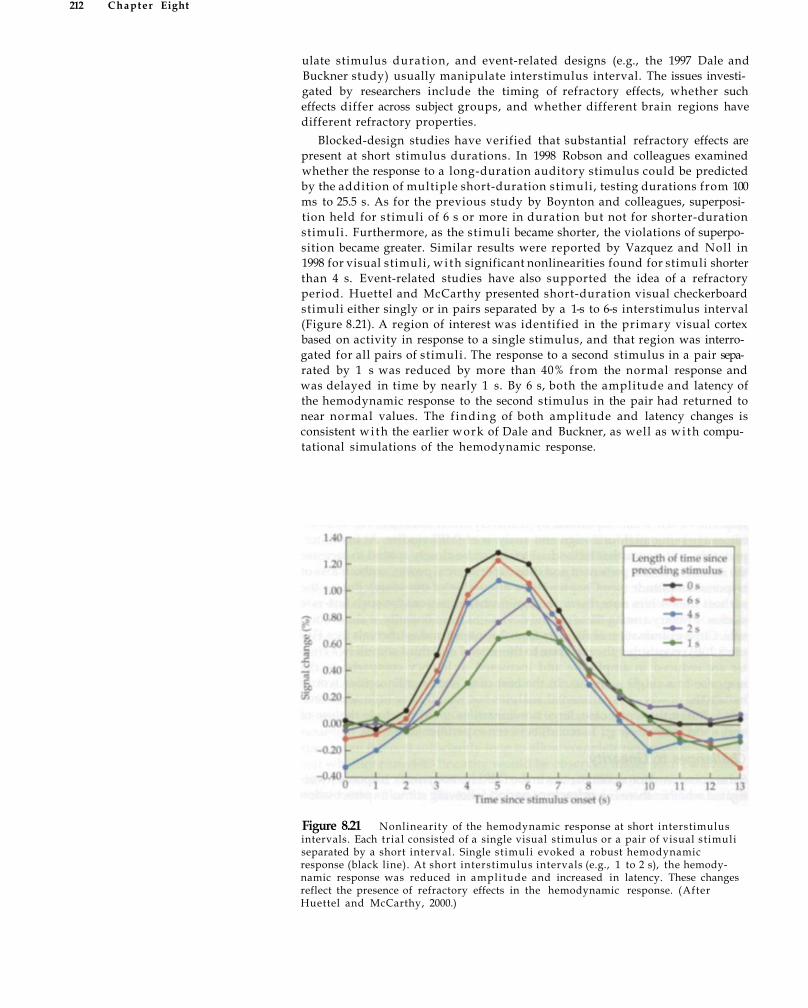
ulate stimulus duration, and event-related designs (e.g., the 1997 Dale and Buckner study) usually manipulate interstimulus interval. The issues investigated by researchers include the timing of refractory effects, whether such effects differ across subject groups, and whether different brain regions have different refractory properties.
Blocked-design studies have verified that substantial refractory effects are present at short stimulus durations. In 1998 Robson and colleagues examined whether the response to a long-duration auditory stimulus could be predicted by the addition of multiple short-duration stimuli , testing durations from 100 ms to 25.5 s. As for the previous study by Boynton and colleagues, superposition held for stimuli of 6 s or more in duration but not for shorter-duration stimuli. Furthermore, as the stimuli became shorter, the violations of superposition became greater. Similar results were reported by Vazquez and Noll in 1998 for visual stimuli, wi th significant nonlinearities found for stimuli shorter than 4 s. Event-related studies have also supported the idea of a refractory period. Huettel and McCarthy presented short-duration visual checkerboard stimuli either singly or in pairs separated by a 1-s to 6-s interstimulus interval (Figure 8.21). A region of interest was identified in the primary visual cortex based on activity in response to a single stimulus, and that region was interrogated for all pairs of stimuli. The response to a second stimulus in a pair separated by 1 s was reduced by more than 40% from the normal response and was delayed in time by nearly 1 s. By 6 s, both the amplitude and latency of the hemodynamic response to the second stimulus in the pair had returned to near normal values. The f inding of both amplitude and latency changes is consistent wi th the earlier work of Dale and Buckner, as well as wi th computational simulations of the hemodynamic response.
Figure 8.21 Nonlinearity of the hemodynamic response at short interstimulus intervals. Each trial consisted of a single visual stimulus or a pair of visual stimuli separated by a short interval. Single stimuli evoked a robust hemodynamic response (black line). At short interstimulus intervals (e.g., 1 to 2 s), the hemodynamic response was reduced in amplitude and increased in latency. These changes reflect the presence of refractory effects in the hemodynamic response. (After Huettel and McCarthy, 2000.)
212 Chapter Eight
Spatial and Temporal Properties of fMRI 213
Although the idea of rough linearity had permeated the literature, by the beginning of the twenty-first century the fMRI refractory period had become well accepted. Thus, experimental questions changed from whether it exists to how its properties might differ across individuals and brain regions. One of the first subject group comparisons was between young adults and healthy elderly adults. Given the many structural changes in the brain that accompany aging, including possible impairments in blood flow, it was predicted that refractory effects w o u l d be greater in elderly adults. This prediction, though sensible, turns out to be wrong. The magnitude of the refractory effect is similar for older and younger adults, as is the amplitude of the hemodynamic response itself. There is substantial interest in examining refractory effects in other subject groups. Patients w i t h schizophrenia, for example, exhibit abnormal sensory habituation, as shown by electrophysiological measures. While neurologically normal adults show a significant decrease in electrophysiological responses when a stimulus is presented twice in rapid succession, a phenomenon known as sensory gating, schizophrenic adults have a much smaller decrease. Studying changes in the fMRI refractory period may lead to a better understanding of the neural systems associated w i t h the sensory-gating deficits in schizophrenia.
Though sparse, some data exist that demonstrate differences in refractory effects across brain regions. Primary sensory or motor regions appear to have smaller refractory effects (i.e., are more linear) than a secondary regions. However, comparisons of refractory effects across brain regions may be confounded by differences in neuronal activity. In 2001, Birn and colleagues measured activity in the primary motor cortex and the SMA when subjects tapped their fingers for different durations. In the primary motor cortex, the hemodynamic response increased in amplitude w i t h increasing duration, although there were violations of superposition for s t imul i shorter than about 4 s. But in the SMA, which is involved w i t h the planning of motor behavior, activation amplitude was similar across all stimulus durations. Huettel and colleagues showed in 2004 that a similar relation holds for visual st imuli : activity in the primary visual cortex scales w i t h duration of a visual stimulus, but activity in the motion-sensitive region V5 is independent of duration. What is similar in both of these cases is that the secondary regions examined (SMA and V5) may be transiently active at the beginning of the stimulus, while the primary region may show sustained activity throughout stimulus presentation. It is therefore wor th reemphasizing that refractory effects measured using fMRI may result from neuronal adaptation or from changes in vascular responsiveness, either of which could differ across brain regions.
Using Refractory Effects to Study Neuronal Adaptation Though refractory effects are often seen as an impediment to fMRI research, through clever experimental design they can be used as indices of brain function. The basic idea comes from physiological studies of adaptation. If one repeatedly presents the same stimulus to a subject, as when g iv ing a mild electric shock to a rat or showing a bright red balloon to a human infant, the response to that stimulus w i l l diminish over time. After a number of presentations, the rat w i l l stop jumping to the harmless shock and the infant w i l l become bored wi th the balloon. When the response to a stimulus decreases wi th repeated presentation, the subject is said to have adapted to that stimulus. By changing the stimulus slightly, we can infer to which aspects of the stimulus the subject adapted. If we replace the red balloon with a red fire truck and the infant is still bored, then we can infer that she
adaptation A change in the response to a stimulus following its repeated presentation.
214 C h a p t e r E i g h t
fMRI-adaptation (fMRI-A) A reduction in the BOLD response to the repeated presentation of a set of stimuli that differ along some attribute, indicating that the brain region being studied is insensitive (as measured by fMRI) to the stimulus attribute being varied.
adapted to the color red. But if she is now very interested in the fire truck, then she must have adapted to some other property such as shape. Similarly, many neurons in the visual system w i l l preferentially fire for one type of visual stimulus, due to its particular shape, color, or way of movement. But w i t h repeated presentations of that stimulus, the neuron's f i r ing rate w i l l decrease dramatically.
Given the presence of refractory effects, we can apply the principles of adaptation to f M R I . First, we repeatedly present a stimulus that evokes activity in a particular brain region. After a short period of repetition, we then present another stimulus that differs in some fashion. If the region being investigated contains neurons that respond differently to the new stimulus, it w i l l show an increase in fMRI activity. But if the neurons do not distinguish between the old and new st imuli , the brain region remains adapted and fMRI activity w i l l be at a low level.
This approach was first used by Grill-Spector and Malach in a series of experiments reported in 2001. They investigated whether neurons in the lateral occipital complex, which contains the lateral occipital lobe and the posterior fusiform gyrus, are sensitive to changes in higher-order properties of objects. For one of their experiments, they presented the same face repeatedly wi th in a 10-s block. They compared the activation in this "identical face" condit ion to that measured in conditions where some property of the face was manipulated, such as position on the screen, viewpoint from left to right, illumination, size, or identity (i.e., different faces presented). Only one condition was varied w i t h i n each block. It is important to recognize that roughly similar activity would be observed in these brain regions in response to any of the faces presented in isolation, so differential activity in the blocks could be attributed to refractory effects across multiple stimulus presentations.
The researchers found that activity in the fusiform gyrus, for example, was greatly reduced in response to repeated presentations of identical, size-varying, or position-varying faces, compared to repeated presentations of entirely different faces. In contrast, variation in direction of i l lumination or viewpoint caused a recovery from adaptation. From these results, the researchers concluded that the fusiform gyrus recognizes facial identity despite size or position manipulations, but does treat i l lumination or viewpoint manipulations as new st imul i . This approach, which is known as fMRI-adaptation or fMRI-A, has since been used in other domains, including for other visual features and for processing of number representations. For example, the recent 2003 study by Boynton and Finney demonstrated that refractory effects in the secondary (but not primary) visual cortex depend upon the orientation of visual line gratings. Likewise, Soon and colleagues (also in a 2003 study) have shown that refractory effects in face-sensitive cortex are greater for pairs of identical faces than for pairs of different faces, and we have shown a similar effect for motion stimuli in motion-sensitive visual cortex. Taken together, these studies indicate that BOLD refractory effects may provide information about the functional properties of neurons w i t h i n a brain region.
Summary Functional MRI has become a dominant neuroimaging technique in large part because of its spatial and temporal properties. The spatial resolution of an fMRI study determines our ability to separate adjacent brain regions w i t h different functional properties. A key factor for spatial resolution is voxel size, which is typically about 3 to 5 mm for full-brain studies but can
Spatial and Temporal Properties of fMRI 215
be less t h a n 1 mm f o r s tudies targeted at a s ingle b r a i n r e g i o n . H o w e v e r , using v e r y s m a l l voxels has disadvantages , n o t a b l y decreases i n M R signal and increases in image a c q u i s i t i o n t i m e . Since the h e m o d y n a m i c response measured b y f M R I depends o n increased b l o o d f l o w , the B O L D effect can be measured in d r a i n i n g ve ins that are d i s t a n t f r o m the site of ac t iv i ty . Effective spat ia l r e so lu t ion can be i m p r o v e d by r e m o v i n g these large-vessel effects. The t e m p o r a l reso lu t ion of f M R I refers to the a b i l i t y to est imate the t i m i n g o f n e u r o n a l a c t i v i t y f r o m the measured h e m o d y n a m i c changes. T h e key pulse sequence parameter for t e m p o r a l reso lu t ion is r e p e t i t i o n t i m e (TR), w h i c h is u s u a l l y a b o u t 1 to 3 s . D e p e n d i n g u p o n the e x p e r i m e n t a l design, decreasing TR b e l o w th is range m a y have l i t t l e effect u p o n experimental p o w e r . W h i l e the absolute t i m i n g o f n e u r o n a l a c t i v i t y i s d i f f i c u l t t o determine u s i n g f M R I , the re la t ive t i m i n g o f a c t i v i t y b e t w e e n d i f f e r e n t s t i m u l i or d i f f e r e n t b r a i n regions can be d e t e r m i n e d w i t h i n a f e w h u n d r e d mil l iseconds. N o n l i n e a r i t i e s in the f M R I h e m o d y n a m i c response reflect the tempora l d y n a m i c s of a c t i v i t y in a s ingle spat ial loca t ion . I f the same b r a i n region becomes act ive twice in r a p i d succession, the h e m o d y n a m i c response to the second event i s reduced in a m p l i t u d e c o m p a r e d w i t h that e v o k e d by a s ingle event . Th is re f rac tory p e r i o d lasts a b o u t 6 s, w i t h larger effects seen at d u r a t i o n s less t h a n a b o u t 2 s. W h i l e re f rac tory effects present an analysis chal lenge for m o s t s tudies , some researchers h a v e taken advantage of these effects to s t u d y f u n c t i o n a l a d a p t a t i o n w i t h i n a b r a i n r e g i o n .
S u g g e s t e d R e a d i n g s
*Boynton, G. M. , Engel, S. A., Glover, G. H . , and Heeger, D. J. (1996). Linear systems analysis of functional magnetic resonance imaging in human V1. J. Neurosci., 16(13): 4207-4221. This early and influential study provides evidence supporting the idea that the fMRI BOLD signal results from a linear transformation of neuronal activity.
*Cheng, K., Waggoner, R. A. , and Tanaka, K. (2001). Human ocular dominance columns as revealed by high-field functional magnetic resonance imaging. Neuron, 32(2): 359-374. An interesting demonstration of the power of fMRI to identify fine spatial detail in the human brain.
*Dale, A. M . , and Buckner, R. L. (1997). Selective averaging of rapidly presented individual trials using f M R I . Hum. Brain Mapping, 5: 329-340. One of the early studies that provided evidence for the feasibility of event-related analyses.
*Huettel, S. A. , and McCarthy, G. (2000). Evidence for a refractory period in the hemodynamic response to visual st imuli as measured by MRI . NeuroImage, 11(5): 547-553. A clear demonstration of BOLD refractory effects in the visual cortex.
Kim, S. G., and Ogawa, S. (2002). Insights into new techniques for high resolution functional MRI . Curr. Opinion Neurobiol., 12(5): 607-615. A good review article that describes important issues relevant to the spatial properties of fMRI .
*Menon, R. S., and K i m , S. G. (1999). Spatial and temporal limits in cognitive neuroimaging w i t h fMRI . Trends Cogn. Sci., 3(6): 207-216. An interesting review of the properties of BOLD fMRI, w i t h emphasis upon the form of the hemodynamic response.
*Menon, R. S., Luknowsky, D. C, and Gati, J. S. (1998). Mental chronometry using latency-resolved functional MRI . Proc. Natl. Acad. Sci. U.S.A., 95(18): 10902-10907. This article provides str iking early demonstrations of the power of fMRI to distinguish very small differences in t iming between successive events.
*Indicates a reference that is a suggested reading in the field and is also cited in this chapter.
C h a p t e r R e f e r e n c e s
Bim, R. M . , Saad, Z. S., and Bandettini, P. A. (2001). Spatial heterogeneity of the nonlinear dynamics in the fMRI BOLD response. NeuroImage, 14(4): 817-826.

216 C h a p t e r E i g h t
Blamire A. M . , Ogawa S., Ugurbi l K., Rothman D., McCarthy G., Ellermann J. M . , Hyder F., Rattner Z., and Shulman R. G. (1992). Dynamic mapping of the human visual cortex by high-speed magnetic resonance imaging. Proc. Natl. Acad. Sci. U.S.A., 89(22): 11069-11073.
Boynton, G. M . , and Finney, E. M. (2003). Orientation-specific adaptation in human visual cortex. J. Neurosci., 23: 8781-8787.
Brodmann, K. (1909). Vergleichende Lokalisationslehre der Grosshirnrinde in ihren Prinzipien dargestellt auf Grund des Zellenbaues. Barth, Leipzig, Germany.
Buckner, R. L, Snyder, A. Z., Sanders, A. L., Raichle, M. E., and Morris , J. C. (2000). Functional brain imaging of young, nondemented, and demented older adults. J. Cogn. Neurosci., 12 (Supplement 2): 24-34.
D'Esposito, M . , Zarahn, E., Aguirre, G. K., and Rypma, B. (1999). The effect of normal aging on the coupling of neural activity to the BOLD HDR. NeuroImage, 10: 6-14.
Disbrow, E. A. , Slutsky, D. A., Roberts, T. P., and Krubitzer, L. A. (2000). Functional MRI at 1.5 Tesla: A comparison of the blood oxygenation level-dependent signal and electrophysiology. Proc. Natl. Acad. Sci. U.S.A., 97(17): 9718-9723.
Grili-Spector, K., and Malach, R. (2001). fMRI-adaptation: A tool for studying the functional properties of human cortical neurons. Acta Psychologica, 107(1-3): 293-321.
Huettel, S. A. , McKeown, M. J., Song, A. W., Hart, S., Spencer, D. D., All ison, T, and McCarthy, G. (2004). Linking hemodynamic and electrophysiological measures of brain activity: Evidence from functional MRI and intracranial field potentials. Cerebral Cortex., 14:165-173.
Huettel, S. A. , Guzeldere, G., and McCarthy, G. (2001a). Dissociating the neural mechanisms of visual attention in change detection using functional MRI . /. Cogn. Neurosci., 13: 1006-1018.
Huettel, S. A., Singerman, J., and McCarthy, G. (2001b). The effects of aging upon the hemodynamic response measured by functional MRI. NeuroImage, 13(1): 161-175.
Kwong, K. K., Belliveau, J. W., Chesler, D. A. , Goldberg, I. E., Weisskoff, R. M . , Poncelet, B. P., Kennedy, D. N . , Hoppel , B. E., Cohen, M. S., Turner, R., et al. (1992). Dynamic magnetic resonance imaging of human brain activity dur ing primary sensory stimulation. Proc. Natl. Acad. Sci. U.S.A., 89(12): 5675-5679.
Logothetis, N. K., Pauls, J., Augath, M . , Trinath, T., and Oeltermann, A. (2001). Neurophysiological investigation of the basis of the fMRI signal. Nature, 412(6843): 150-157.
Menon, R. S. (2002). Postacquisition suppression of large-vessel BOLD signals in high-resolution fMRI . Magn. Reson. Med., 47:1-9.
Menon, R. S., Ogawa, S., Strupp, J. P., and Ugurbi l , K. (1997). Ocular dominance in human V1 demonstrated by functional magnetic resonance imaging. J. Neuro-physiol., 77(5): 2780-2787.
Miezin, F. M . , Maccotta, L., Ollinger, J. M . , Petersen, S. E., and Buckner, R. L. (2000). Characterizing the hemodynamic response: Effects of presentation rate, sampl ing procedure, and the possibility of ordering brain activity based on relative t iming . NeuroImage, 11(6 Pt. 1): 735-759.
Obembe, O., Woldorff, M . , Song, A., and Huettel, S. A. (2003). Adaptation of the fMRI BOLD signal in human motion area V5 is specific to the direction of stimulus motion. Abstract presented at Annual Meeting of the Society for Neuroscience, November 12.
Robson, M. D., Dorosz, J. L., and Gore, J. C. (1998). Measurements of the temporal fMRI response of the human auditory cortex to trains of tones. NeuroImage, 7: 185-198.
Soon, C.-S., Venkatraman, V., and Chee, M. W. L. (2003). Stimulus repetition and hemodynamic response refractoriness in event-related fMRI . Hum. Brain Mapping, 20: 1-12.
Vazquez, A. L., and N o l l , D. C. (1998). Nonlinear aspects of the BOLD response in functional MRI . Neurolmage, 7: 108-118.
Signal and Noise in fMRI
In BOLD fMRI experiments, small but meaningful changes in brain activity lie buried w i t h i n highly variable measurements. Activat ion of neurons wi th in a brain region results in a BOLD signal increase of only about a few percent. To understand how small an effect this is, consider the t w o brain images shown in Figure 9.1 A and B. Both are T 2 *-weighted images taken from the same subject d u r i n g performance of a hand squeezing task. The image in Figure 9.1A was taken while the subject was resting, whi le the image in Figure 9.1 B was acquired a few seconds later at the maximum of the BOLD hemodynamic response evoked after she began squeezing her hand. Although these images appear nearly identical to the naked eye, there is actually an intensity change of about 5% in voxels w i t h i n the pr imary motor cortex (Figure 9.1C and D) , as shown on the plot of signal intensity changes over time (Figure 9.1 E). This discrepancy illustrates the first fundamental problem of fMRI data analysis: the measured BOLD signal change is very small compared to the total intensity of the MR signal.
Small absolute effects are not necessarily diff icult to measure: Thermometers can reliably identify temperature changes of a small fraction of a degree, while stopwatches can identify t iming changes of a few milliseconds. Nor are they unimportant: A 1% increase in body temperature (approximately 4 K or 4°C, or about 7°F) w o u l d have likely fatal consequences. However, there is a second fundamental problem for fMRI data analysis: the task-related BOLD signal change is very small compared to the total spatial and temporal variability across images. Figure 9.1D shows a map of the percent signal change between two brain images. Readily apparent is the large variabil ity across the image, especially in areas outside the brain or near its edges. Based on a single pair of images alone, it w o u l d be impossible to tell which increases in activity are due to the experimental task, and therefore meaningful, and which are due to other non-task-related sources and should be ignored.
In this chapter, we describe the sources of variabil ity in fMRI data that can potentially mask the BOLD effect. Some variability results from temperature fluctuations in the MR scanner or the subject's body, which can cause artifactual changes in the recorded signal. While a potential problem, thermal variabil ity tends to be highly random and independent of the experimental task. Thus, its effects can be minimized by averaging mult iple data points. More problematic are physiological effects like head motion, heart
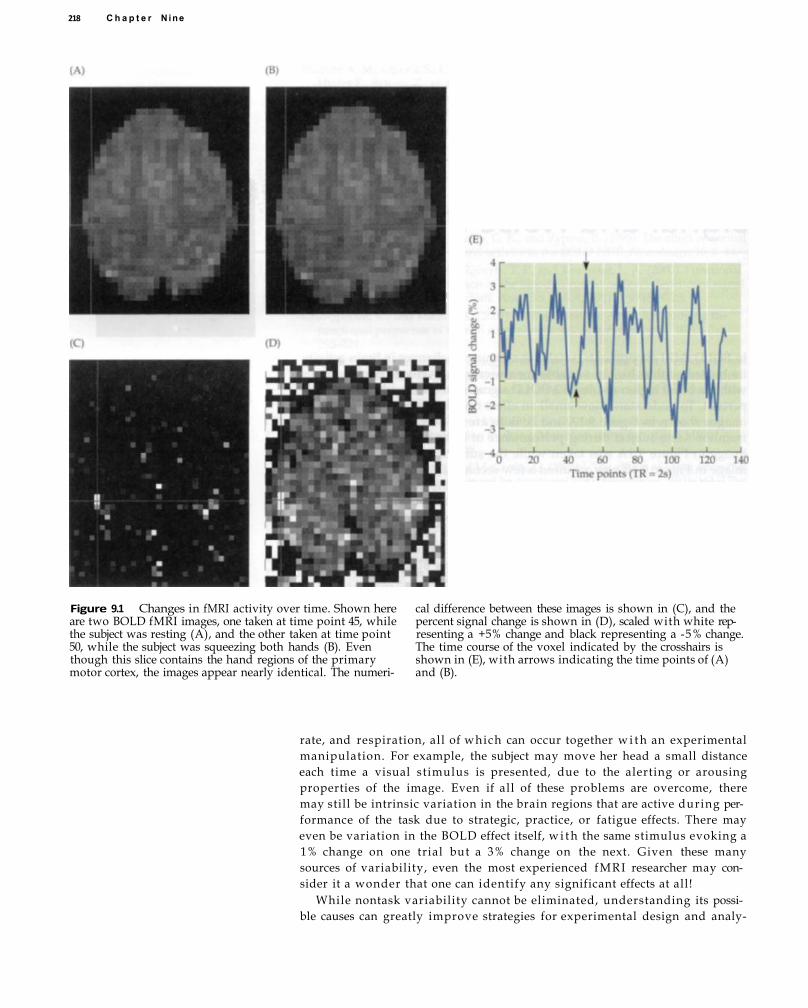
218 C h a p t e r N ine
Figure 9.1 Changes in fMRI activity over time. Shown here are two BOLD fMRI images, one taken at time point 45, while the subject was resting (A), and the other taken at time point 50, while the subject was squeezing both hands (B). Even though this slice contains the hand regions of the primary motor cortex, the images appear nearly identical. The numeri
cal difference between these images is shown in (C), and the percent signal change is shown in (D), scaled with white representing a +5% change and black representing a -5% change. The time course of the voxel indicated by the crosshairs is shown in (E), with arrows indicating the time points of (A) and (B).
rate, and respiration, all of which can occur together w i t h an experimental manipulation. For example, the subject may move her head a small distance each time a visual stimulus is presented, due to the alerting or arousing properties of the image. Even if all of these problems are overcome, there may still be intrinsic variation in the brain regions that are active during performance of the task due to strategic, practice, or fatigue effects. There may even be variation in the BOLD effect itself, w i t h the same stimulus evoking a 1% change on one trial but a 3% change on the next. Given these many sources of variability, even the most experienced fMRI researcher may consider it a wonder that one can identify any significant effects at all!
While nontask variability cannot be eliminated, understanding its possible causes can greatly improve strategies for experimental design and analy-

S i g n a l a n d N o i s e in f M R I 219
sis. Many common imaging problems cause characteristic noise patterns in the data; the ability to recognize these patterns is an important part of any quality assurance plan. Also, when planning studies, understanding how much variabil ity to expect allows the researcher to estimate the number of subjects needed to answer an experimental question. With costs for a single fMRI scanner session often approaching $1000, few researchers (or granting agencies) can afford many excess subjects.
Here, we discuss central concepts related to signal and noise in fMRI . We describe the sources of each and introduce the key idea of the signal-to-noise ratio. We then describe techniques for increasing signal-to-noise ratio through signal averaging, which underlies nearly all fMRI studies. Rather than presenting a stimulus once and examining the resulting BOLD changes, researchers present that stimulus many times under similar conditions in order to improve their estimate of the BOLD response.
Understanding Signal and Noise
Consider the fo l lowing analogy. You are at a party and you ask your companion a question. At the same time that your friend replies, you also hear many other sounds. Other guests are holding conversations, music is playing, and the air conditioner fan is humming . If these other sounds are loud enough, your companion may have to speak more loudly or you may need to reduce the volume of the music in order to hear his reply. In this analogy, we can refer to your question as the stimulus, your companion's response to your question as the signal, and the other sounds that interfere w i t h your ability to hear that response as noise. Note that what constitutes signal or noise depends upon your interests. If you wanted to eavesdrop on an adjacent conversation, you may stop listening to your friend. The new conversation w o u l d become the signal, and your friend's response w o u l d become noise. However, some sounds like the air conditioner's hum are unlikely to ever become signals.
We can use this analogy to think about fMRI . When we present a stimulus, we hope to measure a response in the brain, just as you expected to hear your companion's response to your question. However, in both cases the signal we hope to detect is mixed w i t h other irrelevant sources of variability. We can improve our ability to detect the signal by increasing its amplitude or by decreasing the noise, that is, by increasing the signal-to-noise ratio, or SNR. In f M R I studies, the def ini t ion of the signal also depends upon our interests, as w i l l be discussed in the next section. A n d , just like in the party environment, the noise may be decomposed into different sources. For these reasons, the term signal-to-noise ratio has different meanings in different contexts, and this can cause confusion. We w i l l attempt to carefully delineate these different meanings so as to avoid this terminological confusion.
Signal and Noise Defined Recall that in an fMRI experiment, only one physical quantity is measured, namely the magnitude of current in a detector coil measured by the M R I scanner hardware. This quantity is a composite of both signal and noise. The signal arises from changes in magnetization that we have heretofore referred to as the MR signal. The noise arises from thermal motions w i t h i n the spin system and w i t h i n the scanner hardware. Images reconstructed from this output of the detector coil current w i l l similarly be composed of signal and noise. Because of the random nature of thermal noise, the noise component of the image w i l l be equally distributed throughout the image. MR physi-
signal Meaningful changes in some quantity. For fMRI, an important class of signals includes changes in intensity associated with the BOLD response across a series of T2* images.
noise Nonmeaningful changes in some quantity. There are many sources of noise in fMRI studies, and some changes may be classified as either noises or signals depending upon the goals of the study.
signal-to-noise ratio (SNR) The relative strength of a signal compared to other sources of variability in the data.

220 Chapter Nine
raw signal-to-noise ratio (raw SNR) The ratio between the MR signal intensity associated with a sample (e.g., the brain) and the thermal noise that is measured outside the sample.
contrast-to-noise ratio (CNR) The magnitude of the intensity difference between different quantities divided by the variability in their measurements.
contrast The intensity difference between different quantities being measured by an imaging system. It also can refer to the physical quantity being measured (e.g., T1 contrast).
functional signal-to-noise ratio (functional SNR) The ratio between the intensity of a signal associated with changes in brain function and the variability in the data due to all sources of noise. Functional SNR is sometimes called dynamic CNR or functional CNR.
cists and engineers quantify this raw signal-to-noise ratio (raw SNR) by d i v i d i n g the intensity of the image in a region that contains the sample (the signal) by the intensity of the image in a region that is outside of the sample (the noise). Raw SNR is used to evaluate the performance of the scanner hardware, and you would likely compare such measures of SNR if you were deciding which MRI scanner to purchase for your inst i tution. Engineers strive to maximize raw SNR by using more-efficient detector coils and pulse sequences and by shielding the scanner from outside interference.
While a useful measure, raw SNR only provides part of the story. Since we want to create maps of brain anatomy or function, we need to be able to characterize differences in MR signal wi th in different regions of the brain, and not just between the inside and outside of the brain. For this purpose, we introduce a new measure, the contrast-to-noise ratio (CNR). As introduced in Chapter 1 the contrast of an MRI image refers to the physical property to which it is sensitive. So, an image sensitive to T1 contrast w i l l be bright for voxels wi th short T 1 values (like white matter) and dark for voxels wi th long T 1 values (like gray matter or cerebrospinal fluid). For anatomical images, the ability to identify differences between tissues depends upon the CNR, which is the intensity difference between the two tissues divided by the noise, as previously calculated.
Refer back to Figure 1.4 for a comparison of high-CNR and low-CNR images. On a T 1 -weighted image w i t h high CNR, a very clear boundary is observed between gray and white matter. This is especially evident for subcortical nuclei, which are visible at the center of Figure 1.4A. When CNR is reduced, it becomes more dif f icult to distinguish different tissue types (see Figure 1.4B). On this image, gray matter is still visible but often blurs into surrounding white matter. Subcortical nuclei, especially the thalamus, are very dif f icult to identify, and their edges have become indistinct. Roughly speaking, CNR describes the ease of seeing differences between tissues.
Two properties of CNR are important to understand. First, CNR is always relative to some comparison w i t h i n an image. For example, T 1-weighted pulse sequences have very good ability to distinguish gray and white matter (high CNR), but only l imited ability to distinguish cerebrospinal f lu id and air (low CNR). Conversely, a proton-density pulse sequence can easily show differences between air and f l u i d , which differ dramatically in their density, but have less ability to distinguish gray and white matter. Second, CNR does not depend solely upon the absolute difference in intensity between two tissue types. Consider t w o structural images taken on different scanners. On the first image, gray-matter voxels have a mean intensity value of 150, white-matter voxels have a mean intensity value of 250, and the noise value is 100. On the second image, gray-matter voxels have a mean intensity value of 60, white-matter voxels have a mean intensity value of 70, and the noise value is 5. Which image would have a higher CNR? The mean intensity difference between gray and white matter is about 100 units in the first image and only 10 units in the second. But the variability is 20 times larger in the first image than the second. Consequently, the CNR in the second image wi l l be about 2 times greater than that in the first image.
For most fMRI experiments, however, CNR is unimportant. Typical T 2 -weighted images have intrinsically low contrast (see Figure 9.1). It is hard to identify boundaries between different types of tissue in functional images, much less to distinguish active and inactive regions. Instead, the important quantity for fMRI studies is functional signal-to-noise ratio (functional SNR). (Some authors refer to this quantity as dynamic CNR or functional CNR). Here, we use the term signal to describe the difference between two

S i g n a l a n d Noise in fMRI 221
states of the brain caused by an experimental manipulation. The term noise refers to the variability in those states over time.
It is important to recognize that functional SNR is different from CNR. CNR depends upon the intensity difference between voxels (i.e., across space). Functional SNR depends upon the intensity difference wi th in a voxel, group of voxels, or region over time. The effects of increasing functional SNR are illustrated in Figure 9.2. Shown are activation plots for three voxels in and
Figure 9.2 Voxels w i t h low, medium, and high SNR. Shown in (A) are three adjacent voxels. As shown in (B), the uppermost voxel has little to no task-related signal change (low SNR), and the distributions of activity during task (red) and nontask (blue) periods are highly overlapping (C). (D)
The middle voxel has a medium SNR, but there is still substantial overlap between the distributions (E). However, the lowermost voxel (F) has a very high SNR, and the distributions have much less overlap (G).
Time points (TR = 2s) MR signal (arbitrary units)

222 C h a p t e r N i n e
adjacent to the pr imary motor cortex, dur ing performance of a blocked-design hand squeezing task. Note that the uppermost voxel shows little task-related activity, the middle voxel shows some task-related activity, and the bottom voxel shows clear and robust task-related activity. Plotted at right are simple histograms comparing time points during the hand squeezing blocks (in red) to those d u r i n g resting blocks (in blue). For the upper voxel, the distributions overlap completely, indicating that hand squeezing had no effect upon activity in this voxel. In the middle voxel, the distributions begin to diverge, w i t h more activity observed during task blocks. And in the lower voxel, there is a clear dissociation between the histograms. We can represent these histograms according to their means and standard deviations, which are indicated below each graph. If the difference between the means is large enough compared to the standard deviation, as in the bottom graph, we can identify significant activity. The concept of functional SNR is closely related to that of effect size in statistics. The statistical size of an effect is not the difference in percentage signal change but rather the difference between the conditions in units of standard deviation.
In summary, just as CNR reflects how easily we can see differences between tissues, functional SNR reflects how easily we can see differences between experimental conditions. For the remainder of this book, we w i l l focus our discussion on the ability of fMRI experiments to detect meaningful changes in brain activity. Therefore, we w i l l use the unmodif ied term SNR to denote functional SNR, whi le we w i l l use raw SNR to describe the signal and noise directly measured by the detector coil. We w i l l use CNR to refer to the contrast sensitivity of anatomical images.
Functional SNR The functional SNR measured in an fMRI experiment may vary over a wide range. One factor that influences functional SNR is the amplitude of the BOLD signal. As shown in Figure 9.2, a simple motor task, like periodically squeezing one's hand, may generate BOLD changes in primary motor cortex of approximately 6%, even at 1.5 T. Likewise, periodic flashing of a high-contrast visual checkerboard may cause BOLD changes of 1 to 5% or more in the primary visual cortex. As the strength of the stimulus decreases, the resulting BOLD signal change also decreases. If the hand is squeezed less frequently, or if the checkerboard is blurred and flashed at a slower rate, BOLD activity may decrease to less than 1%. In addit ion, signal magnitude also depends upon the area being measured. Most experimental tasks evoke activity in a set of related brain regions. For example, pressing a button whenever a bright pattern appears on a screen w i l l elicit activity in motor regions (e.g., primary motor cortex, supplementary motor cortex, cerebellum), visual regions (e.g., primary visual cortex, inferior temporal cortex), and decision regions (e.g., prefrontal cortex). As a rule of thumb, fMRI signal changes are largest in primary motor or sensory areas and generally decrease in amplitude in regions associated w i t h higher cognitive function.
Why might the amplitude of the BOLD response typically be larger in primary sensory and motor cortices than in brain
regions associated with complex cognitive processes?
effect size The numerical difference between means divided by the standard deviation.

S i g n a l a n d N o i s e in f M R I 223
Figure 9.3 Using fMRI to examine relative activation. Act iv i ty in fMRI is rarely all or none, but is often a matter of degree. Shown are hypothetical responses of a face-sensitive region of the brain to faces and other objects. The response to each stimulus is large compared to the difference between them.
The examples in the previous section compared the BOLD signal evoked by an experimental condition to that of a resting condition. If a study compares t w o experimental conditions, as in a memory test comparing remembered and forgotten words, the differences between conditions are usually much smaller than the amplitude evoked by each condition itself compared to rest. This issue is illustrated in Figure 9.3. Consider the fusiform gyrus in the temporal lobe, which plays an important role in the perception of objects, including faces. If an fMRI subject views a single face presented in isolation, activity in the fusiform gyrus increases by about 1% over baseline. Although a face is a good stimulus for evoking fusiform activity, other complex s t imuli , including tools, foods, and vehicles, also evoke activity in this brain region. If faces evoked, in one subject, a signal change of 1.1%, while tools evoked a signal change of 0.9%, the difference between the conditions w o u l d be a mere 0.2%. This example is not atypical, in that many f M R I experiments investigate differential activation of a single area by two or more stimulus types.
The second factor that determines functional SNR is the overall noise wi th in the data. The noise in fMRI studies is composed of many sources, and it is usually quantified as the standard deviation of the voxel intensity over time. Noise is usually larger than the magnitude of the BOLD signal changes that we wish to measure. Some of the noise in fMRI data results from thermal fluctuations, as in all MR imaging. However, thermal noise only contributes a small portion of the noise in functional SNR. Other, more significant noise components include artifacts such as head motion, physiological variations related to heart rate and respiration, unrelated neural activity, and cognitive or behavioral variability in how the subject performs an experimental task. These sources are discussed individually in the following sections.
To demonstrate what fMRI data look like at different functional SNR levels, Figure 9.4 presents data from a simulated experiment that consisted of two alternations of task and nontask blocks. As SNR decreases, it becomes progressively more diff icult to identify task-related changes in the data. At the highest value used, SNR = 4.0, the task and nontask blocks are clearly visible, but at the lowest value used, SNR = 0.5, the noise completely conceals any visible experimental effect.

224 C h a p t e r N i n e
Figure 9.4 The effects of SNR upon fMRI data. Shown are simulated time courses of a blocked-design task at four different signal-to-noise levels (4.0, 2.0, 1.0, and 0.5). At high signal-to-noise levels, the transitions between blocks are obvious, but as SNR decreases, the blocks become harder to identify.
power spectrum A representation of the strength of different frequency components within a signal. The Fourier transform converts a signal (i.e., changes in intensity over time) into its power spectrum.
Sources of Noise in fMRI
At a given field strength, the overall signal is mostly determined by the amount of magnetization available. However, the behavior of noise is more complex. Noise in fMRI data has both temporal and spatial features. The temporal features can be seen in Figure 9.5, which presents the power spectrum of a single experimental run. A power spectrum shows what frequencies are present in a time series of data and is created using the Fourier transform. Peaks w i t h i n a power spectrum can be thought of as regular oscillations in the intensity of the given voxel, reflecting changes over time due to the respiratory cycle, cardiac pulsations, or BOLD activity. These temporal components of fMRI noise are not distributed equally throughout the image, but rather have particular spatial distributions. Figure 9.6 displays an image of relative noise for a single run of an experiment in which subjects passively viewed high-contrast pictures. The most obvious feature of this image is that much of the anatomical structure of the brain is recovered, indicating that the variability inside the brain is much higher than the variability outside of the brain. If noise were constant across the image, then the image would be a uni form gray. Instead, the edges of the brain and even some of the interior structure are clearly recovered.

S i g n a l a n d N o i s e in f M R I 225
Figure 9.5 The power spectrum of an experimental voxel over a single run. The experimental task used an event-related design in which 1-s duration visual stimuli were separated by 9-s intervals. Visible are clear peaks at the respiratory and cardiac frequencies. The accuracy of these peaks was verified by physiological monitoring. To detect such high-frequency changes, a single slice was sampled at a TR of 250 ms. Note that the lowest frequencies are excluded from this plot because the very high power at low frequencies obscures the effects shown.
There are five main causes of temporal and spatial noise in fMRI: intrinsic thermal noise w i t h i n the subject and the scanner electronics; system noise associated w i t h imperfections in the scanner hardware; artifacts resulting from head motion, respiration, heart rate, and other physiological processes; variability in neuronal activity associated w i t h non-task-related brain processes; and changes in behavioral performance and cognitive strategy. We discuss each of these sources of noise in the fol lowing sections.
Thermal Noise All MR imaging, whether anatomical or functional, is subject to t h e r m a l noise, or changes in signal intensity over time due to thermal motion of electrons w i t h i n the subject and w i t h i n the scanner electronics. Thermal noise may also be called intrinsic noise. To understand the possible sources of thermal noise, recall from Chapter 2 the sequence of events that underlies acquisition of MRI data. Fol lowing its excitation, the sample (e.g., the brain), emits a radiofrequency signal that is detected by the receiver coil . The signal is then processed by a series of electronics hardware, replete with many conductors, resistors, and power amplifiers. Within each physical component in the receiver chain, free electrons collide w i t h atoms, resulting in an exchange of energy. The higher the temperature of the sys-
thermal noise Fluctuations in MR signal intensity over space or time that are caused by thermal motion of electrons within the sample or scanner hardware.
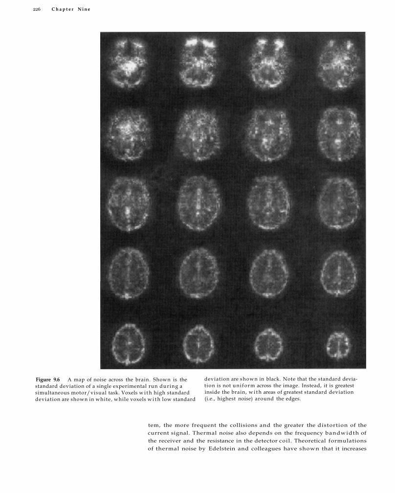
226 C h a p t e r N i n e
Figure 9.6 A map of noise across the brain. Shown is the standard deviation of a single experimental run dur ing a simultaneous motor/visual task. Voxels w i t h high standard deviation are shown in white , while voxels w i t h low standard
deviation are shown in black. Note that the standard deviation is not uni form across the image. Instead, it is greatest inside the brain, w i t h areas of greatest standard deviation (i.e., highest noise) around the edges.
tem, the more frequent the collisions and the greater the distortion of the current signal. Thermal noise also depends on the frequency bandwidth of the receiver and the resistance in the detector coil . Theoretical formulations of thermal noise by Edelstein and colleagues have shown that it increases
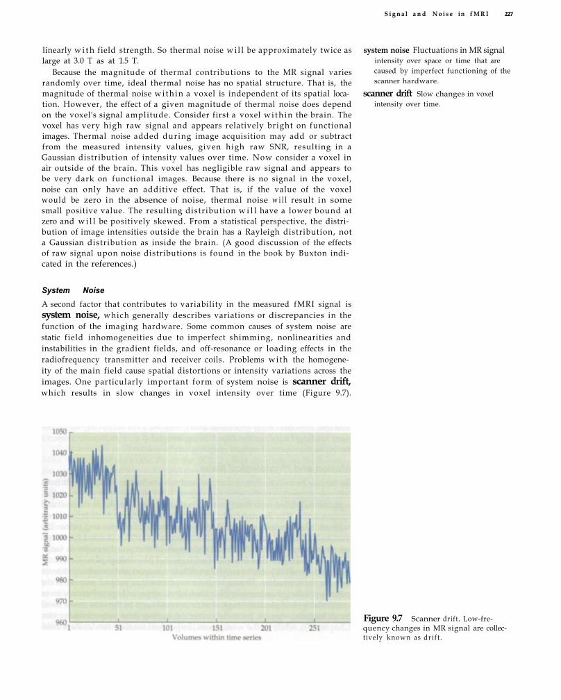
S i g n a l a n d N o i s e in f M R I 227
linearly w i t h field strength. So thermal noise w i l l be approximately twice as large at 3.0 T as at 1.5 T.
Because the magnitude of thermal contributions to the MR signal varies randomly over time, ideal thermal noise has no spatial structure. That is, the magnitude of thermal noise w i t h i n a voxel is independent of its spatial location. However, the effect of a given magnitude of thermal noise does depend on the voxel's signal amplitude. Consider first a voxel w i t h i n the brain. The voxel has very high raw signal and appears relatively bright on functional images. Thermal noise added during image acquisition may add or subtract from the measured intensity values, given high raw SNR, resulting in a Gaussian distribution of intensity values over time. Now consider a voxel in air outside of the brain. This voxel has negligible raw signal and appears to be very dark on functional images. Because there is no signal in the voxel, noise can only have an additive effect. That is, if the value of the voxel would be zero in the absence of noise, thermal noise w i l l result in some small positive value. The resulting distribution w i l l have a lower bound at zero and w i l l be positively skewed. From a statistical perspective, the distribution of image intensities outside the brain has a Rayleigh distribution, not a Gaussian distribution as inside the brain. (A good discussion of the effects of raw signal upon noise distributions is found in the book by Buxton indicated in the references.)
System Noise A second factor that contributes to variability in the measured fMRI signal is system noise, which generally describes variations or discrepancies in the function of the imaging hardware. Some common causes of system noise are static field inhomogeneities due to imperfect shimming, nonlinearities and instabilities in the gradient fields, and off-resonance or loading effects in the radiofrequency transmitter and receiver coils. Problems wi th the homogeneity of the main field cause spatial distortions or intensity variations across the images. One particularly important form of system noise is scanner drift, which results in slow changes in voxel intensity over time (Figure 9.7).
system noise Fluctuations in MR signal intensity over space or time that are caused by imperfect functioning of the scanner hardware.
scanner drift Slow changes in voxel intensity over time.
Figure 9.7 Scanner drif t . Low-frequency changes in MR signal are collectively known as dr i f t .
228 C h a p t e r N i n e
physiological noise Fluctuations in MR signal intensity over space and time due to physiological activity of the human body. Sources of physiological noise include motion, respiration, cardiac activity, and metabolic reactions.
Although dr i f t can result from any of several different sources, a common cause is change in the resonant frequency of hydrogen protons associated w i t h subtle changes in the strength of the static field. Even though it is powered by superconducting currents, the main magnet still experiences minute drifts in stability over time, often on the order of a few tenths of a part per mill ion per day. Expressed in terms of field strength and resonant frequency, such drifts might reflect an alteration in the main field strength on the order of 0.005 of a Gauss and variation in the resonant frequency by a few Hertz. Small changes in the local strength of the magnetic field, if uncorrected, can lead to signal instability and spatial displacement. Similarly, gradient nonlinearities and instabilities affect the shape and location of the recorded images from one time point to another, leading to spatially dependent variations in noise over time. These two problems are discussed in detail in Chapter 4.
Scanner dr i f t may result from factors other than system noise. In one of our subjects, we noticed an odd pattern of spatially correlated signal dri f t . Wi th in the first run , voxels at the very back of the brain slowly but consistently increased in intensity, while those at the front of the brain steadily decreased in intensity. The cause of this puzzling change was revealed by examination of the position of the head over time. Over the course of the run , the head slowly moved d o w n w a r d , consistent w i t h a slow leak in the vacuum pack that held the subject's head in place! Head movement can cause spatial distortions as w e l l , notably on anatomical images collected using three-dimensional acquisition methods.
Problems w i t h the radiofrequency coils can have several effects. If the frequency of the excitation pulse does not match the resonant frequency of the sample, excitation w i l l be inefficient and intensity variation may be introduced, causing the MR signal to fluctuate over time. Another problem results from the fact that the receiver coil is coupled to the sample via mutual inductance, meaning that a change in the current or voltage distribution in the sample induces a corresponding change in the current and voltage carried by the receiver coil. Thus, the properties of the imaged object influence the noise measured in the receiver coil. Because induction of sample noise in the receiver coil reduces sensitivity, an opt imum coupling scheme that matches impedance in the sample and the receiver coil is desired. This matching process is often referred to as achieving the dominant loading factor for the object being imaged (i.e., a particular subject's brain) so that optimal mutual coupling can be reached.
Motion and Physiological Noise So far we have considered thermal and system noise, which result from intrinsic properties of the scanning system. If we scan an inert phantom (i.e., a plastic ball filled w i t h f luid) , we w i l l still measure significant thermal and system noise. The human brain, though, is hardly inert. Muscles contract w i t h each breath or heartbeat. Blood pulses through arteries and veins. The metabolic demands of neurons drive chemical reactions needed for subsequent activity. This activity, in all the senses of that w o r d , results in variations in fMRI signal due to motion artifacts and physiological noise.
Signal variability due to subject motion is common and extremely disruptive for fMRI studies. Throughout an experiment, a subject may shift the position of their head; move their shoulders, arms, or legs to become more comfortable; and swallow more due to nervousness. In the best cases, small head motions may be partially corrected dur ing data preprocessing (see Chapter 10), while in the worst cases, large motions may render data com-
S i g n a l a n d N o i s e in fMRI 229
pletely uninterpretable. Smallscale motions result from the regular oscilla
tory activity of the heart and lungs. This activity is much faster and more
periodic than largescale head motion, introducing a different set of chal
lenges. If the rate of sampling is fast enough, it may be possible to character
ize and minimize motion due to heart and lung activity dur ing preprocess
ing (see the 1995 work of Hu and colleagues).
But in most fMRI studies, motion due to cardiac activity, in particular, is
too fast to be sampled effectively (i.e., for TRs >500 ms), and if the TR is long
enough (i.e., >2500 ms), respiratory activity may likewise be undersampled.
Under those circumstances, the variabilities associated w i t h these sources of
motion are still present but become distributed throughout the fMRI time
series in a manner that may be dif f icult to identify or correct. The misattri¬
bution of periodic noise sources by undersampling is known as aliasing (see
Chapter 10). Respiration also introduces variabil ity in the fMRI signal
through systematic distortions in the magnetic field. As the subject breathes,
the expansion of the lungs casts a magnetic susceptibility "shadow," i n f l u
encing field strength and homogeneity of the magnetic field and altering sig
nal intensity throughout the image ( including areas outside of the brain
itself), as demonstrated by Raj and colleagues in 2001.
It is important to recognize that the effects of motion in fMRI are usually
not due to motion dur ing image acquisition and resulting decrease in raw
SNR. Recall from Chapter 5 that typical fMRI pulse sequences (e.g., spiral or
echoplanar gradientecho imaging) have very short TEs, often about 30 to 40
ms. There is little opportunity for motion to occur during such a short acqui
sition window. Motion causes problems because of variability across the time
series of images, which is critical for functional SNR. A voxel near the edge of
the brain, for example, may begin by containing mostly gray matter but end
up, after motion, containing mostly cerebrospinal f l u i d . Note that if motion
were completely random, then it w o u l d introduce noise that reduces SNR
but that could be ameliorated w i t h signal averaging. Motion is rarely ran
dom, though, and is often correlated wi th the experimental task, as, for exam
ple, when subjects hold their breath each time they press a response button.
Motion also introduces both spatial correlations, since adjacent voxels move
together, and temporal correlations, since movements are extended in time.
We discuss strategies for preventing and correcting signal changes due to a
common form of motion, head motion, in the following chapter.
While motion is a serious and damaging component of variabil ity in
fMRI, it is not the only one. Since the BOLD effect depends on the interac
tion between several physiological factors, including blood flow, blood vol
ume, and oxygen metabolism, fluctuations in any of these factors w i l l in f lu
ence the observed signal. In 2001, Kruger and Glover investigated the spatial
distribution of physiological noise, separating it into one component (σ B)
associated wi th variability in the transverse relaxation rate and another com
ponent ( σ N B ) associated w i t h cardiac and respiratory motion. Since the for
mer component, like BOLD contrast itself, results from susceptibilityrelated
signal changes, its magnitude depends upon TE. The latter component, in
contrast, is independent of TE. Kruger and Glover found that the spatial dis
tribution of these two components differed (Figure 9.8AF). The former was
much greater in gray matter than in white matter, whi le the latter was
equally distributed throughout the brain. Furthermore, σB was typically
about twice as large as σ N B . These results suggest that physiological noise,
rather than thermal or system noise, is the dominant source of variability in
fMRI studies, especially at higher field strengths.
aliasing The sampling of a signal at a rate insufficient to resolve the highest fre
quencies that are present. The energy
at those frequencies becomes artifactu
ally expressed at lower frequencies, dis
torting the measured signal.

230 Chapter Nine
Figure 9.8 Distribution of physiological noise. For one subject, images showing anatomy (A), noise from all sources (B), physiological noise due to variation in blood flow and metabolic processes (C), and noise due to bulk head motion and cardiac and respiratory pulsations (D). Note that the noise in (C) is concentrated within gray matter, while that in (D) is more uniform, save for effects around the edge of the brain. For comparison are shown images from a phantom of noise from all sources (E) and physiological noise (F). Not surprisingly, physiological noise is negligible in the phantom. (From Kruger and Glover, 2001.)
Non-Task-Related Neural Variability In the party analogy described at the beginning of this chapter, we noted that after you had asked a question of your companion and awaited his answer, other conversations were occurring around you that were unrelated to your question and thus were constituents of the noise. However, unlike the other sources of noise discussed thus far, the words spoken in these other conversations were legitimate responses evoked by other questions asked by other speakers. These unrelated conversations, however, were not temporally synchronized to your question.
S i g n a l a n d N o i s e i n f M R I 231
Let's consider an fMRI experiment in which we stroke the thumb w i t h a brush to investigate which brain areas are activated by somatosensory stimuli . At the same time that the subject's brain experiences this discrete task-related sensory stimulus, the subject is also hearing the sounds of the scanner gradients, receiving varying visual s t imul i as he/she looks around with in the scanner, and activating brain systems associated w i t h memory and mental imagery as he/she thinks about appointments for later that day. Al l of these s t imul i—interna l and external—activate neural processes that translate into varying metabolic demands and thus influence BOLD contrast. What makes us consider these activity-evoked BOLD changes as noise is that they are unrelated to the st imulus of interest. However, if we changed our experiment to investigate the response of the brain to these other stimulus events, we w o u l d f ind reliable regions of activation. For example, synchronizing our analysis to our subject's eye movements w o u l d reveal activation of a part of the brain called the frontal eye fields. This illustrates that the task-related responses in which we are interested occur wi th in a highly active brain where routine neural processes are altering BOLD contrast at every moment. We can exploit the temporal synchrony between our stimulus of interest and evoked changes in BOLD contrast by signal averaging. We w i l l discuss this important strategy for improving functional SNR at the end of this chapter.
Behavioral and Cognitive Variability An often underappreciated source of noise in fMRI data comes from variability in how subjects perform the experimental task. In general, the more complex the task, the more performance w i l l vary across time and across subjects. Consider three sorts of common experimental designs: passive viewing of a visual stimulus, pressing a button in response to an auditory stimulus, and remembering a set of digits over a delay interval. Even though these are all very simple designs, the mental operations they evoke w i l l differ across trials.
The passive v iewing design requires no experimental response of any form, which suggests that the evoked brain activity should be the same on every trial . However, this assumption fails to consider changes in arousal and attention over time. Arousal levels always wax and wane over the course of a scanner session, w i t h accompanying changes in brain activity. Even when ful ly alert, subjects are often thinking about something other than the experimental task. As is discussed in Box 11.2, specific sets of brain regions have been implicated in daydreaming and other nontask processes.
Additional complications are introduced by tasks that require the subject to generate a response. The time it takes to execute a simple motor behavior, such as pressing a button or speaking a name in response to a stimulus, is known as reaction time or response time, depending on the experimental task. If the task simply requires detection of a stimulus, the behavioral measure is reaction time and is typically around a few hundred milliseconds. But if the task requires the subjects to make some judgment about a stimulus, such as whether or not they remember it from earlier in the experiment, then the behavioral measure is k n o w n as response time. Since response times require additional cognitive processes, they are always longer than reaction times. Depending on the experiment, response time may be as short as 300 ms or as long as several seconds. In any experiment, there w i l l be both inter-subject and intrasubject variability in reaction or response time. One source of variability is a speed-accuracy trade-off. For almost all experimental
reaction time The time required for someone to make a simple motor response to the presentation of a stimulus. Note that this is distinct from response time, which applies to situations in which someone must choose between two or more possible responses.
response time The time required for someone to execute a choice between two or more possible responses. Note that this is distinct from reaction time, which applies to situations when only one possible response is present.
speed-accuracy trade-off The improvement in the speed of a response at the expense of accuracy, or vice versa, within an experimental task.
tasks, subjects can perform the task more accurately if they do it more slowly. Imagine that you are shown a series of photographs of faces and are asked to judge the emotion they are expressing. If you try to guess the emotion as quickly as possible, you w i l l make many mistakes, especially on more complex emotions like disgust. Conversely, if you spend more time considering each face carefully, your accuracy w i l l increase but your response times w i l l slow.
Speed-accuracy trade-offs are important to consider when deciding what instructions to give subjects in an fMRI experiment. Since increasing one factor decreases the other, it is generally impossible for subjects to maximize both. That is, your subjects w i l l not be able to respond as accurately as possible while doing so as fast as possible. For many experiments, therefore, it is reasonable to tell subjects, "Respond as quickly as you can while maintaining a low error rate." This reduces variability in error rate across subjects, especially if you provide feedback about errors and the target error rate. Alternatively, you can emphasize one factor but not the other. Accuracy should be emphasized when the characteristics of the response are critical. In a study comparing remembered words to forgotten words, for example, the response that the subject makes determines in which category a stimulus is placed. If the subject responds inaccurately, then the integrity of the analyses w i l l be severely compromised. Speed should be emphasized when the processes of interest would change if the subject responded completely accurately. Tasks used in the study of attention often emphasize speed, because the effects of attention on behavior may disappear if the subject takes a long time to respond.
Shown in Figure 9.9A and B are histograms of response time data from a target detection task conducted as part of an fMRI experiment. While the input stimulus was similar on every trial, the output behavior differed considerably. On some trials, subjects responded in less than 500 ms, while on others, they d i d not respond for more than 1500 ms. Does the neuronal activity remain the same regardless of the time of the button press? To answer this question, we refer to the study from Menon and colleagues discussed in Chapter 8 (see Figure 8.14A). Recall that between some regions (i.e., from visual to supplementary motor), the relative t iming of BOLD activity was dependent upon reaction time, but between others (e.g., from supplementary to primary motor), the BOLD timing was independent of reaction time. These results clearly indicate that the relation between reaction time and brain activity is location-dependent: Some cognitive processes are delayed w i t h increasing response time while others are not. To deal w i t h this issue, many research studies include reaction time, or some other behavioral measure, as a covariate in their analyses.
Strategy changes are a third source of task-induced variability. In many cognitive tasks, there may be more than one strategy that can be used to solve a task. A frequently used task in psychology experiments is learning a set of digits, like "36013," and remembering them over a few seconds. One
How could differences in task performance confound fMRI studies tha t compare di f ferent subject groups, such as young
and elderly adults?
232 Chapter Nine

S i g n a l a n d Noise in fMRI 233
Figure 9.9 Variability in response time. (A) The distribution of response times across approximately 10,000 trials of a simple decision task. Note that the distribution is highly positively skewed, with a negative bound at about 400 ms and a mean of about 800 ms. (B) Distributions from two individual subjects. Note that even though these subjects were performing the same task, their patterns of performance across trials were very different.
strategy for doing this task is rehearsing, which involves repeating the set over and over again unt i l it is time to make a response. Another common strategy is chunking, which involves breaking d o w n the d ig i t set into smaller, but memorable, numbers. A subject might, for example, remember "36013" by labeling "360" as the number of degrees in a circle and coding "13" as an unlucky number. Both strategies may be used by the same subject at different times w i t h i n one experiment. Yet the strategies may be sufficiently distinct that they activate different brain regions, and thus the total activity would reflect some combination of the two.
Improving Functional SNR through Experimental Design
To improve functional SNR, we can attempt to increase the amplitude of the BOLD signal, decrease the noise, or do both. In this and the fo l lowing sections, we w i l l discuss three different strategies for doing so: improving experimental design, increasing field strength, and averaging data across trials.
Al though hardware and computational approaches w i l l dominate this discussion, it is important to recognize that very simple choices in the experimental design can have a large effect upon functional SNR. Consider an experiment designed to evoke BOLD activity in the primary visual cortex. Almost any visual stimulus w i l l suffice, whether a simple checkerboard pattern or a picture of a face, a moving array of dots or a rotating visual scene. But even though all of these activate the primary visual cortex, they do not all activate it equally. High-contrast patterns w i t h many visible sharp edges wil l induce very large activity, especially if flickered at a relatively rapid rate (e.g., about 10 Hz). But if the flicker frequency is much slower or faster, or if the contrast of the stimulus is reduced, then the measured BOLD activity

234 C h a p t e r N i n e
So far in this chapter we have considered sources of noise that contribute to intrasubject variability
in the BOLD hemodynamic response. It is also important to evaluate the possible impact of intersubject variability. To understand the distinction between intrasubject and intersubject variability, first imagine that a single subject is run in an experiment that consists of 50 trials in which he/she squeezes his/her hand when he/she sees a shape appear. Even though the subject sees the same stimulus and performs the same action in each trial, the measured fMRI signal w i l l be different on each trial due to the sources of intrasubject variability described in the previous sections. N o w imagine that two different subjects are run in the same experiment. Each subject's data w i l l have intrasubject variability that contributes to variability across trials, but there may be additional intersubject differences. For example, the shape of the hemodynamic response could be different, w i t h one subject's response peaking at 5 s and the other's at 7 s. Intersubject variability has important consequences for statistical analyses.
The idea of intersubject variability in the shape of the hemodynamic response was tested by Aguirre and colleagues in 1998. They collected fMRI data from 40 subjects who participated in one or more sessions of a simple response task. During the scanner sessions, subjects watched a small cross in the center of the display. The cross flickered every 16 s, at which time the subjects pressed buttons with both thumbs. The 16-s interstimulus interval was chosen to allow the hemodynamic response to return to baseline between successive stimuli. The data were acquired using a gradient-echo EPI sequence at 1.5 T, wi th a TR of 2000 ms and a TE of 50 ms. The authors used an
Figure 9.10 Variability in the hemodynamic response across subjects. The reproducibility of the fMRI hemodynamic response was examined. When hemodynamic responses across subjects (A and B) were compared, the shape of the response was highly variable. There was much less variability in the hemodynamic responses f rom a single subject collected across sessions (C and D) and even less variability in the responses collected w i t h i n a single session (E and F). Note that each pair of charts shows two different sets of subjects, sessions, or responses. (After Aguirre et al., 1998.)
BOX 9.1 Intersubject Variability in the Hemodynamic Response

Signal and Noise in fMRI 235
BOX 9.1 (continued)
intrasubject variability Variability in the fMRI data from a single subject associated with thermal, system, and physiological noise, as well as with variability in the pattern of brain activity during task performance.
intersubject variability Variability in fMRI data across a set of subjects; it includes the factors associated with intrasubject variability, along with between-subjects differences in task performance and physiology.
anatomical region-of-interest approach to identify the central sulcus and surrounding gray matter in each subject. The resulting ROIs included both the primary sensory cortex, which is immediately posterior to the central sulcus, and the primary motor cortex, which is immediately anterior. Within this ROI, they identified all voxels with significant power in the BOLD signal at the task frequency of 0.0625 Hz and its two succeeding harmonics (i.e., integer multiples of the task frequency) using a Fourier analysis. They then determined the average response in the active voxels across all trials and used that average as the estimated hemodynamic response for that subject. The experimental hypothesis to be tested was whether there was significant intersubject variability, defined as greater variability between different sessions of different subjects compared to different sessions of the same subject.
Across 32 subjects who each participated in a single session, there was considerable variability in the number of active voxels within the ROI (from 6 to 91), in the amplitude of the measured hemodynamic response (from 1 to 3%), and in the latency to peak response (from 3 to 6 s). The variability in the responses from different subjects was then compared to the variability in repeated sessions from the same subject. The results were striking (Figure 9.10A-F). Across
Figure 9.11 Reproducibility of fMRI activity across sessions. In what is likely a record, a single subject participated in 99 fMRI sessions, split among motor, visual, and cognitive paradigms. Even though the experimental procedures were repeated in exactly the same manner on every session, right down to repeating the quite familiar experimental instructions, the pattern of activity differed considerably across sessions (A, motor; B, cognitive). (From McGonigle et al., 2000.)

236 C h a p t e r N i n e
w i l l be smaller. Whenever possible, it is critical for researchers to select stimuli that w i l l evoke large and reproducible signal changes.
Functional SNR can also be improved by minimiz ing the influence of noise components. Some aspects of noise prevention are the responsibility of the MR center and not the indiv idual researcher. By ensuring that the MR scanner electronics are as stable as possible and by preventing extraneous radiofrequency signals from entering the scanner room, the research center can improve the stability of all data collected on that scanner. Researchers should become familiar w i t h the quality assurance procedures at their MRI center so they can recognize such problems as they arise, even if they cannot prevent them from occurring.
Other issues can be addressed by individual researchers, especially through minimization of physiological and cognitive variability. The effects of head motion can be ameliorated w i t h subject restraint and training, as we w i l l discuss in Chapter 10. Training also improves understanding of the experimental task and allows subjects to attain a steady-state performance level before entering the scanner session. For many of our experimental tasks, we train our subjects in practice sessions ahead of time to minimize the learning effects or strategy changes that typically occur at the beginning of an experiment. Subjects are carefully instructed so that they know what is expected, especially wi th regard to what strategies they should adopt to perform a behavioral task.
Improving Functional SNR by Increasing Field Strength
In many circumstances, the primary determinant of functional SNR is the amount of net magnetization, which is proportional to the strength of the static magnetic field. Remember, however, that the signal we measure in fMRI does not depend solely on the net magnetization. Because the net magnetization must be tipped into the transverse plane to become measurable,
BOX 9.1 (continued)
multiple runs within a single scanner session, the hemodynamic responses recorded from a single subject showed very little variability (Figure 9.10E and F). A comparison of multiple sessions from the same subject across different days showed that the data variability increased by a factor of 3.5, but the hemodynamic response was still generally similar across the sessions (Figure 9.10C and D). However, across different subjects, there was more than 16 times as much variability as found in a single session, providing conclusive evidence for the presence of intersubject variability in the shape of the hemodynamic response (Figure 9.10A and B).
It is important to note that although the form of the hemodynamic response is generally similar for a given subject
across different sessions, this similarity does not necessarily extend to the spatial extent of activation. That is, active voxels usually have the same time course across sessions, but the number of voxels that are active w i l l differ. This point was illustrated in a heroic study conducted by Mc¬Gonigle and colleagues in 2000, for which a single subject participated in 99 separate scanner sessions across a period of 2 months. Three blocked-design experimental tasks were used, each for 33 sessions: finger tapping, passive visual stimulation, and random-number generation. Every session was identically run on the same scanner, wi th the same room lighting and ambient sounds, wi th the same operator giving the same instructions. Indeed, the authors note that the subject had the same "I've done this before"
thoughts before every session! When they compared the activation maps across sessions, the authors found that there were striking differences in the patterns of activation (Figure 9.11 A and B). On some sessions, there were very clear activation foci in areas of interest, such as the motor cortex and the cerebellum for the finger tapping task. However, other sessions had almost no activation. Within the more cognitive random-number generation task, there was even greater variability in the overall pattern of activation that changed dramatically from session to session. These results demonstrate dearly that the data recorded from a single subject in a single research session are subject to considerable variability, even in very simple tasks that evoke robust fMRI activity.
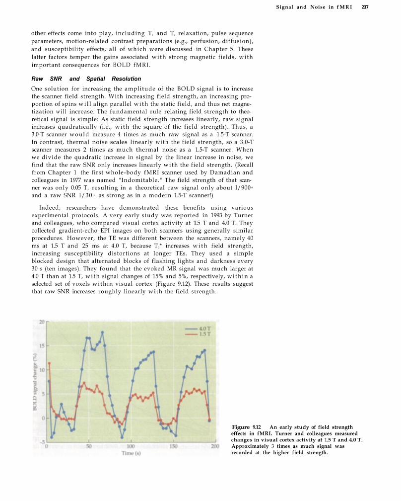
Signal and Noise in f M R I 237
other effects come into play, including T 1 and T 2 relaxation, pulse sequence parameters, motion-related contrast preparations (e.g., perfusion, diffusion), and susceptibility effects, all of which were discussed in Chapter 5. These latter factors temper the gains associated w i t h strong magnetic fields, wi th important consequences for BOLD fMRI.
Raw SNR and Spatial Resolution One solution for increasing the amplitude of the BOLD signal is to increase the scanner field strength. With increasing field strength, an increasing proportion of spins w i l l align parallel w i t h the static field, and thus net magnetization w i l l increase. The fundamental rule relating field strength to theoretical signal is simple: As static field strength increases linearly, raw signal increases quadratically (i.e., w i t h the square of the field strength). Thus, a 3.0-T scanner would measure 4 times as much raw signal as a 1.5-T scanner. In contrast, thermal noise scales linearly w i t h the field strength, so a 3.0-T scanner measures 2 times as much thermal noise as a 1.5-T scanner. When we divide the quadratic increase in signal by the linear increase in noise, we find that the raw SNR only increases linearly w i t h the field strength. (Recall from Chapter 1 the first whole-body fMRI scanner used by Damadian and colleagues in 1977 was named "Indomitable." The field strength of that scanner was only 0.05 T, resulting in a theoretical raw signal only about l/900 t h
and a raw SNR l/30 t h as strong as in a modern 1.5-T scanner!)
Indeed, researchers have demonstrated these benefits using various experimental protocols. A very early study was reported in 1993 by Turner and colleagues, who compared visual cortex activity at 1.5 T and 4.0 T. They collected gradient-echo EPI images on both scanners using generally similar procedures. However, the TE was different between the scanners, namely 40 ms at 1.5 T and 25 ms at 4.0 T, because T 2* increases w i t h field strength, increasing susceptibility distortions at longer TEs. They used a simple blocked design that alternated blocks of flashing lights and darkness every 30 s (ten images). They found that the evoked MR signal was much larger at 4.0 T than at 1.5 T, w i t h signal changes of 15% and 5%, respectively, w i t h i n a selected set of voxels w i t h i n visual cortex (Figure 9.12). These results suggest that raw SNR increases roughly linearly wi th the field strength.
Figure 9.12 An early study of field strength effects in fMRI. Turner and colleagues measured changes in visual cortex activity at 1.5 T and 4.0 T. Approximately 3 times as much signal was recorded at the higher field strength.

238 C h a p t e r N i n e
partial volume effects The combination, within a single voxel, of signal contributions from two or more distinct tissue types or functional regions.
As raw SNR increases, so does the total signal recovered from each voxel. This allows the image to be parceled into smaller voxels while maintaining sufficient SNR w i t h i n each, improving spatial resolution. Because many phenomena of interest, such as the ocular dominance columns we discussed in Box 8.2, have small spatial scale, an improvement in spatial resolution can greatly improve the functional resolution of an experiment. Studies of ocular dominance columns, for example, have been carried out at 4.0 T, and scanners w i t h field strength approaching 9.0 T have been installed for human imaging. Reductions in voxel size also minimize partial volume effects. If a small voxel is primari ly composed of active neural tissue that is responsive to the experimental task, it w i l l generate a larger BOLD signal change than the same amount of active neural tissue located w i t h i n a larger voxel. For this reason, decreasing voxel sizes can result in larger BOLD signal changes from active voxels.
Functional SNR and Spatial Extent While raw SNR depends solely on the net magnetization and thermal noise w i t h i n a voxel, functional SNR also includes physiological and neural variability, which we w i l l collectively call physiological noise. The strength of the static f ield has different effects upon thermal and physiological noise. While thermal noise increases linearly w i t h increasing field strength, physiological noise increases quadratically w i t h field strength. So, as field strength increases from 1.5 T to 3.0 T, raw signal w i l l quadruple, thermal noise w i l l double, and physiological noise w i l l quadruple. These relations suggest that at very high field strengths, physiological noise may become dominant, and thus the improvement of functional SNR w i t h increasing field strength may be considerably less than linear (i.e., smaller than for raw SNR). As shown in Figure 9.13, at high field strengths, gains in signal are offset by similar increases in physiological variability, so functional SNR w i l l not increase indefinitely. This conclusion is supported by Kruger, Glover, and their colleagues, who demonstrated that the relative contribution of physiological noise increases w i t h field strength. They found that at
Figure 9.13 Changes in signal and noise w i t h increasing static field strength. MR signal increases w i t h the square of the field strength, while thermal noise increases linearly w i t h field strength. The ratio of these quantities, raw SNR, thus increases linearly w i t h field strength. However, because physiological noise increases w i t h the square of field strength, functional SNR (which is dependent on both thermal and physiological noise) may reach an asymptote at high fields. Note that here the field strength is indicated in arbitrary units; the field strength beyond which such an asymptote w o u l d occur is not yet established.

1.5 T, physiological noise makes up about 40% of the total noise, but at 3.0 T, physiological noise composes more than 52%. At higher field strengths (e.g., 4.0 T), their calculations indicate that physiological noise could compose more than 60% of the total variation. As field strength increases above about 4.0 T, therefore, increases in physiological noise may counteract gains in signal (see Figure 9.13), setting an asymptotic upper l imi t for functional SNR.
A direct consequence of increased functional SNR is the increased spatial extent of activation (i.e., number of active voxels w i t h i n a region). As functional SNR increases w i t h i n a voxel, the probability of that voxel passing a threshold for statistical significance also increases. Thus, for a given experimental task, the spatial extent of activation can be used as an index of functional SNR. In their 1999 study, Yang and colleagues measured activity within the sensorimotor cortex whi le subjects performed a blocked-design finger tapping task at either 1.5 T or 4.0 T. Under o p t i m u m TR and TE parameters, there were approximately 70% more active voxels w i t h i n the region at the higher field strength. However, when nonoptimal imaging parameters were used at 4.0 T, many fewer active voxels were identified, demonstrating the importance of other factors besides field strength for detection. Kruger and colleagues also found that spatial extent depends upon field strength, wi th about 40% more voxels active across the motor and visual cortices at 3.0 T compared to 1.5 T.
While the above studies used simple visual and motor tasks, a 2003 study by Krasnow and colleagues examined the effects of field strength on several different tasks, including perceptual, memory, and emotional processing paradigms. They compared activity at field strengths of 1.5 T and 3.0 T to evaluate whether more-complex tasks would evince similar increases in functional SNR w i t h increasing field strength. They found that across brain regions there were substantial increases in the number of activated voxels with increasing field strength, w i t h increases of 35 to 83% observed across regions in a cognitive task, suggesting that detection power throughout the brain improves w i t h increasing field strength.
Spatial Specificity Increasing field strength also influences the degree to which different vascular components contribute to the BOLD signal. Because the T 2* value of blood decreases significantly w i t h increasing field strength, the intravascular contribution, especially from the large vessels, would drop out at high field. For extravascular components, theoretical arguments by Ogawa have indicated that the spins near large vessels scale linearly w i t h field strength, while those near small vessels increase quadratically (i.e., w i t h the square of the field). Therefore, as field strength increases, the small-vessel extravascular component of the BOLD response increases faster than the large-vessel extravascular component. A schematic illustration of the different effects of field strength on these various BOLD signal components is given in Figure 9.14, suggesting that the extravascular component of small vessels w o u l d prevail at very high magnetic field.
Small vessels are more likely to be colocalized wi th the neuronal activity of interest, and thus the BOLD response may be more spatially specific at higher field strengths. In 2001, Kruger and colleagues investigated the effects of field strength (1.5 T vs. 3.0 T) upon functional SNR in different types of voxels in a combined visual and motor task. In addition to an overall increase in functional SNR, they found that functional SNR increased by
Signal and Noise in fMRI 239

240 C h a p t e r N i n e
Figure 9.14 Effects of field strength upon the contributions of different vascular components to functional SNR. As field strength increases, the intravascular component of the BOLD signal drops out, leaving only the extravascular component. The small-vessel extravascular component increases more rapidly than that of large vessels, suggesting that BOLD fMRI may be more spatially specific to small vessels at high field strengths.
a factor of about 1.8 for small regions of activity that may correspond to large blood vessels, and by a factor of about 2.2 for larger regions of gray-matter activity, demonstrating the tendency of improved signal specificity to small vessels at high field in addition to the improved overall BOLD signal.
However, the extravascular component originating around large vessels would still be present despite its relatively reduced proportion in the overall BOLD signal (Figure 9.14). The presence of the large-vessel extravascular component at high field w o u l d still compromise spatial specificity. Thus, methods such as spin echo-based acquisition should be considered to reduce the large-vessel extravascular effect and regain spatial specificity.
The increased spatial specificity with field strength may appear to contradict the increased spatial extent discussed in the previous section. As the spatial extent of an activation increases, more voxels are labeled as being in a functional region, whereas increases in spatial specificity involve exclusion of voxels. No true contradiction exists, however. The former is an effect of increased functional SNR, which reflects our ability to determine whether or not a voxel's activity is predicted by our experimental hypotheses (see Chapter 12). We can use increased functional SNR in two ways. First, we w i l l identify more voxels as active at the same statistical threshold. Or, by increasing our statistical threshold, we can improve our estimates of which voxels are active without changing the spatial extent of activation. Spatial specificity, on the other hand, is an effect of changes in the weighting of different vascular components. The large-vessel extravascular component does increase wi th field strength; it just does not increase as rapidly as the small-vessel extravascular component.
What do the effects illustrated in Figure 9.14 predict for studies of the fMRI initial dip (see Box 7.2)?

S i g n a l a n d N o i s e in f M R I 241
Challenges of High-Field fMRI
It is also important to realize that as field strength increases, the MR properties of spin systems change. For example, the relaxation parameters T1 and T2*, which both affect signal recorded in fMRI experiments, change w i t h increasing field strength. The parameter T 1 increases w i t h field strength (by about 30% from 1.5 T to 3.0 T), which could reduce the effective signal recovery at short TR values. The parameter T2* decreases w i t h field strength (by about 25% in gray matter from 1.5 T to 3.0 T), which could reduce the time available to acquire signal. Researchers should be aware of these parameter changes and should account for them in pulse sequences. A more significant challenge comes f rom susceptibility artifacts that distort the uni formity of the magnetic f ield. Just as BOLD susceptibility effects increase w i t h field strength, so too do signal losses in regions of the brain near air-tissue boundaries (Figure 9.15). These regions include the ventral frontal and temporal lobes, which are adjacent to air-filled sinuses. Without the use of specialized pulse sequences that can partially compensate for susceptibility-induced signal loss (see Chapter 14), imaging of these regions becomes more difficult or impossible at higher field strengths. Field inhomogeneity can also lead to geometric distortions that require specialized software and hardware for their correction.
Figure 9.15 Susceptibility artifacts increase at higher f ield. While susceptibility artifacts at air-tissue boundaries are present on gradient-echo images at all field strengths, they increase in spatial extent at higher field strengths. Shown are images from three subjects, each of w h o m was scanned at
both 1.5 T (A) and 4.0 T (B). Visible in all images are areas of signal loss in the ventral frontal lobe, which is indicated by the arrows. Note that the areas of signal loss are more extensive in the 4-T images.

242 C h a p t e r N i n e
signal averaging The combination of data from multiple instances of the same manipulation in order to improve functional SNR.
mean The average value of a set of observations.
standard error of the mean The uncertainty in the observed mean value, as calculated based upon both the standard deviation of the data and the number of data points.
Improving Functional SNR through Signal Averaging
The most powerful and widely used approach for improving the signal-to-noise ratio of fMRI data is also the simplest: signal averaging. Other terms for signal averaging include epoch averaging, event averaging, and trial averaging. The basic assumption of signal averaging is that the signal of interest is identical over repeated stimulus presentations, whi le the noise is random. With sufficient numbers of repetitions, the noise w i l l tend to average out while the signal is preserved. Even a very weak signal is easily detected when averaged over many repetitions.
Signal averaging requires a reliable temporal relationship between the task event and the hemodynamic response. If subjects are required to make a complex decision about a visual stimulus, then it is possible that the neural activity associated w i t h a decision outcome may vary over a period of seconds. The hemodynamic events associated wi th that neural activity might have a similar temporal variability. A signal average synchronized to the onset of the visual stimulus may result in an average hemodynamic response that has been blurred over time due to the temporal variability of the decision process. In this case, a signal average synchronized to the subject's button press may reduce that temporal variability. Also, the evoked stimulus is assumed to be constant across repetitions. If the signal diminishes over repetitions due to fatigue or habituation, then signal averaging w i l l have limited value. Signal averaging does not require an explicit model of the noise, but it does require that the noise have a random relationship wi th the task event of interest. Artifacts or physiological noise synchronized to a stimulus or response event w i l l be enhanced by signal averaging.
Note that we describe here the effects of signal averaging upon data collected from a single subject, for which averaging improves both estimation and detection power. However, intersubject averaging is also critical for fMRI studies. At the most general level, averaging across subjects provides additional data samples that improve the estimates of the effects of interest. Taken this way, intersubject averaging has similar salutary effects upon data stability as intrasubject averaging, and the fol lowing discussion can be easily extended to more than one subject. Yet combining data across subjects has a second, more important purpose: it allows researchers to make inferences about the representativeness of an experimental effect w i t h i n the population. We consider statistical methods for combining data across subjects in Chapter 12.
Effects of Averaging on Estimation of the Hemodynamic Response In statistical terms, the result of averaging multiple observations (e.g., time point 1 across trials) is known as the mean, and its uncertainty is known as the standard error of the mean. The fundamental rule of signal averaging can be
Recall the difference between detection of active voxels and estimation of the t ime course of activity. Which ability, detect ion or estimation, do you th ink w o u l d be most affected by
signal averaging and why?

S i g n a l a n d N o i s e in f M R I 243
Figure 9.16 Reduction in the standard error of the mean with increasing number of trials sampled. As the number of trials in the sample increases, the precision with which the estimated mean of a sample improves, but only with the square root of the number of trials.
stated as follows: the standard error of the sample mean decreases wi th the
square root of the number of independent observations (Figure 9.16). Let us
consider the implication of this rule for fMRI data. Consider the MR signal
observed in one voxel in a single trial. We can think of the data at each time
point in the trial as composed of two parts, signal in the form of the hemody
namic response and additive Gaussian noise. As we know from Figure 9.4, the
amplitude of the noise is generally much greater than the signal, so it is often
difficult to see the hemodynamic response on single trials. Now, what happens
to our data if we collect a second trial and then average it wi th the first? Since
the noise follows a Gaussian (or normal) distribution, small values are more
likely than extreme values. If there is a very large amount of noise at time point
1 in the first trial, it is unlikely that there w i l l again be a large amount of noise
at that time point in the second trial. Thus, extreme values w i l l tend to be
reduced. Using real numbers, if the noise has a standard deviation of 10 units
on each trial, averaging 2 trials w i l l reduce the noise by a factor of √2, to a stan
dard deviation of about 7 units. Averaging 10 trials w i l l reduce the noise by
"√10, to a standard deviation of about 3 units. The number of trials averaged can
be thought of as the sample size for statistical purposes. In short, to double
experimental SNR, one must collect four times as many trials.
Signal averaging, therefore, does not increase signal, but instead decreases
noise. For fMRI data, as more trials are averaged, the amplitude of the hemo
dynamic response does not increase, but it can be characterized wi th better
and better precision. The effects of signal averaging upon estimation of the
hemodynamic response can be seen in Figure 9.17. In this experiment, we col
lected a very large number of experimental trials (>150) for each of two sub
jects in a visual stimulation task. In each trial, a single highcontrast checker
board stimulus was presented for 500 ms. FMRI data were acquired using a
gradientecho echoplanar pulse sequence (TR: 1000 ms; TE: 40 ms) at 1.5 T.
Within each subject, a region of interest in the medial occipital lobe was iden
tified, and the mean activity w i t h i n that region was measured in each of the
150+ trials. Each plot in the figure shows a set of 20 hemodynamic responses
derived by averaging a different number of trials, from 1 to 64. So, the first
sample size The number of observations
that are made by an experiment. For
fMRI data, sample size can refer to the
number of trials for a given subject or
to the number of subjects within an
experiment.
estimation Measurement of the pattern
of change over time within an active
voxel in response to the experimental
manipulation.

Figure 9.17 Effects of signal averaging upon the form of the hemodynamic response. As the number of trials in the sample increases, the precision of the hemodynamic response estimate increases and the noise in the response decreases. (From Huettel and McCarthy, 2001.)
plot shows 20 single-trial responses, the second shows a set of 20 samples each representing the average of 4 trials, and so forth. Note that the 8 plots increase incrementally in steps from 1 2 to 8 2 trials, representing equal decreases in the expected standard error of the mean.
Readily apparent are the substantial effects of signal averaging upon the stability of the hemodynamic response. If there is no signal averaging and individual trials are compared, as in the first plot, then the variability across samples is enormous. In some trials, there is an increase in activity of up to
244 Chapter Nine

Signal and Noise in fMRI 245
15 MR units (about 3% in this experiment), while in others the activity actually decreases dur ing the trial . So, it w o u l d be extremely diff icult to characterize the hemodynamic response in this region from only a single trial. But after averaging only a few trials (e.g., 4 or 9), the response begins to take a recognizable form. It tends to rise and fall in a regular fashion, and the different samples of trials tend to be more similar to one another. After about 25 or 36 trials, the hemodynamic response is essentially the same in every sample. Again, signal averaging has no effect on the signal itself, so the expected hemodynamic response is similar regardless of how many trials are averaged. However, the larger the sample size, the less effect noise has upon the observed data. If the noise is t ru ly random, we can calculate this effect of signal-averaging functional SNR by mul t ip ly ing the init ial SNR by the square root of the number of trials that are averaged. If our signal of interest is half the amplitude of the noise, our initial functional SNR is 0.5. However, if we average 25 trials, we improve the functional SNR by a factor of 5, resulting in an effective SNR of 2.5.
Recall from Chapter 8 that one model for fMRI data suggests that the measured MR signal can be thought of as the linear addition of signal (i.e., the hemodynamic response) and noise. The term linear in this context means that the effects of the t w o factors are independent; that is, the amount of noise at a given time point does not depend on the amount of signal at that time point. This assumption can be tested by comparing the variabil ity in the fMRI signal in the prestimulus baseline to the variabil ity around the peak of the response. In Figure 9.17, it is obvious that the variabil ity is greater around the peak of the hemodynamic response than dur ing the prestimulus baseline. In 2001, Huettel and colleagues quantified changes in variability by plotting the standard deviation at each time point relative to stimulus presentation. Variability near the peak of the hemodynamic response, compared to the prestimulus baseline, increased by a factor of about 3. These results indicate that variability in fMRI data does not merely result from the effects of addit ive noise, but instead is partly due to variability in the fMRI signal itself.
Effects of Averaging on Detection of Active Voxels Detection of fMRI activity also improves w i t h signal averaging. Most statistical tests use a thresholding approach, such that any voxel whose statistical value is greater than some predetermined threshold is labeled as significant, while values less than that threshold are nonsignificant. Although this labeling scheme is binary, the underlying statistics are distributed in a relatively continuous manner (Figure 9.18). Voxels near the center of cluster of activation tend to have the highest statistical values, whi le ones near the edges have the lowest. This continues outside of the nominally active region, such that nearby voxels tend to have positive statistical tests. To confirm that statistics are spatially graded, one merely has to lower the significance threshold, and the size, or spatial extent, of the active region w i l l increase. If the threshold is raised, the spatial extent w i l l decrease. In short, whether or not a voxel is labeled as active depends on only two factors, its statistical value (which in turn depends on SNR) and the threshold.
Given that functional SNR increases w i t h signal averaging, the spatial extent of activation w i l l also increase w i t h signal averaging, as activity in some of the subthreshold voxels becomes detectable. This effect can be seen in Figure 9.19, which presents data from the visual stimulation task described in the preceding section. If only a few trials are averaged, then very few vox-
detection Determination of whether or not activity within a given voxel changes in response to the experimental manipulation.
spatial extent The number of active voxels within a cluster of activity (i.e., the size of the active region).
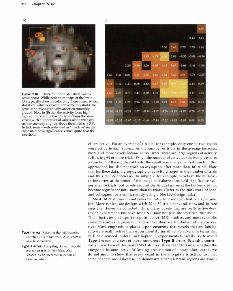
246 Chapter N i n e
(A) (B)
Figure 9.18 Distribution of statistical values across space. While activation maps of the brain (A) typically show in color only those voxels whose statistical value is greater than some threshold, the actual underlying statistics are often smoothly graded. Note in (B) that the activity focus highlighted in the white box in (A) contains the same voxels with high statistical values, along with others that are only slightly above threshold (t > 3.6). In fact, some voxels indicated as "inactive" on the color map have significance values quite near the threshold.
Type I error Rejecting the null hypothesis when it is in fact true. Also known as a false positive.
Type II error Accepting the null hypothesis when it is in fact false. Also known as an incorrect rejection or false negative.
els are active. For an average of 4 trials, for example, only one to two voxels were active in each subject. As the number of trials in the average increases, more and more voxels become active, unti l there are large regions of activity following 64 or more trials. When the number of active voxels was plotted as a function of the number of trials, the result was an exponential function that approached but did not reach an asymptote after more than 100 trials. Note that for these data, the topography of activity changes as the number of trials and thus the SNR increases. In subject 2, for example, voxels in the mid-cal-carine cortex at the center of the image had above-threshold significance values after 16 trials, but voxels around the lingual gyrus at the bottom did not become significant unti l more than 64 trials. (Refer to the 2003 work of Saad and colleagues for a similar study using a blocked-design task.)
Most fMRI studies do not collect hundreds of independent trials per subject. More typical are designs w i t h 20 to 50 trials per condition, and in rare cases even fewer are collected. Thus, many voxels that are really active during an experiment, but have low SNR, may not pass the statistical threshold. This illustrates an important point about fMRI studies, and most scientific research studies in general, namely that they are fundamentally conservative. More emphasis is placed upon ensuring that voxels that are labeled active are really active than upon identifying all active voxels. In terms that w i l l be discussed in detail in Chapter 12, experiments typically try to avoid Type I errors at a cost of more-numerous Type II errors. Scientific conservatism works well for most fMRI studies. If we want to know whether the amygdala becomes active fol lowing presentation of a scary photograph, we do not need to show that every voxel in the amygdala is active, just that some of them are. Likewise, to demonstrate which brain regions are associ-

S i g n a l a n d N o i s e i n f M R I 247
ated w i t h a particular task, researchers list the foci of significant activation and in which structures they are contained.
But for some questions, accurate measurement of the spatial extent of activation is critical. One increasingly important use of fMRI is to map areas of particular interest, such as the language and motor cortices, in patients awaiting neurosurgery (see Box 12.2). If fMRI reveals that a patient's tumor abuts Broca's area, for example, then the neurosurgeon may decide that the risks of surgery (e.g., the inability to produce language) w o u l d be too great, and another course of treatment would be prescribed. In order to make such judgments, knowledge of the boundaries of the active area is necessary. In other studies, researchers may want to quantify differences in activity between t w o groups of subjects. For example, a study might investigate whether there are fewer active voxels w i t h i n the frontal lobe in schizophrenia patients compared to neurologically normal subjects when they perform the Wisconsin Card Sorting Test.
Suppose that such a study found that the patients had fewer active voxels in a particular region of prefrontal cortex. Could you conclude, from those data alone, that schizophrenic subjects use less of the frontal lobe for this task than normal controls? To answer this question, recall that the l ikelihood that a voxel is detected by a statistical test is a function of its SNR. Differences in signal can cause SNR differences, of course, in that the schizophrenic subjects could indeed have less activity. However, differences in noise could also contribute to SNR differences. If the patient group had higher noise levels, for whatever reason, then their spatial extent of activity could be greatly reduced in the absence of any differences in signal. Stated another way, the two groups could have exactly the same areas of activity, but it could be more dif f icult to detect active voxels in one group than the other.
Huettel and colleagues investigated this issue in a comparison of visual processing between young adults and elderly adults. The amplitude of the hemodynamic response was identical between the groups for ROIs in both the calcarine and fusiform cortices. However, there were approximately twice as many active voxels in the young adult group as in the elderly. To determine whether this effect was l ikely to be real or an artifact of SNR differences, the SNR in each group was measured. The single-trial SNR was about 50% greater in the young than in the elderly. Based upon a simple simulation of the effects of SNR upon detection of active voxels, for the number of trials run in each group, SNR differences alone would predict about a 2:1 ratio of active voxels. Even more tellingly, the simulation suggested that had there been fewer experimental trials (e.g., about 30 to 35 compared to the 70 actually run), there would have been as much as 5 times as many active voxels in the young, due solely to the differences in noise between the groups. Similar results could occur for a variety of different comparisons, such as patient and nonpatient groups, patients on medication and off medication, or normal subjects in alert and fatigued states. It is critical, therefore, when averaging a small number of trials, to consider the activity measured to be a reflection of the SNR, which itself depends on other factors besides the activity of interest.
Figure 9.19 Spatial extent of fMRI activity increases with signal averaging. As the number of trials in the sample increases, the number of active voxels increases dramatically. (From Huettel and McCarthy, 2001.)
248 C h a p t e r N i n e
BOX 9.2 Power Analyses
effect, which is equivalent to 1 β. The
quantity 1 β defines the power of the
statistical test.
One can calculate the power of a sta
tistical test, given the Type 1 error rate, the
expected SNR, and the sample size (see
Equation 8.3). First, one must identify
how large an effect wi l l be needed for sig
nificance. Effect size, in a statistical sense,
is not the numerical difference between
the experimental conditions but is the nu
merical difference divided by the stan
dard deviation (i.e., μ 0 μ 1 / σ m ) . Note
that this is equivalent to SNR in the
framework described earlier in the chap
ter. The needed effect size can be ob
tained from a statistical table (tdistribu
tion) or from a statistical calculator. At an
alpha value of 0.001, for example, an ef
fect size of about 3.1 units is needed. Sec
ond, the expected effect size (za for the
sample must be calculated. Suppose that
the expected difference between hemo
dynamic amplitudes in conditions 1 and
2 was 0.3% and that there was a 0.2%
standard deviation in this value across 8
subjects. The expected effect size is the
mean divided by the sample standard
deviation, which is the standard devia
tion divided by the square root of the
number of subjects. For the numbers
above, the expected effect size is about 4.2
units. Third, the difference between the
expected and needed effect sizes is calcu
lated; in this case, 4.23.1 = 1.1 units. Fi
nally, this difference is converted back to
a probability using a ttable, resulting in a
β value of 0.12. The power of this test, or
1 β , would be 0.87.
power analysis A calculation that
estimates the likelihood of detecting
an effect of a given size based upon
the parameters of the experimental
design.
power The probability of detecting
an effect of the experimental
manipulation.
One could restate the results of the
power analysis in the following way:
Given a sample size of 8 subjects, an ex
pected change of 0.3%, and a standard
deviation of 0.2%, there is an 87% chance
that a real effect w i l l be detected at an
alpha value of 0.001. Based on such calcu
lations, a researcher may decide that 87%
is too low for comfort; about one out of
eight experiments would show no effects.
Recalculating the power analysis wi th 12
subjects increases the power to 0.98, and
for 16 subjects the power is more than
0.998. These results suggest that running
between 12 and 16 subjects in this experi
ment would make detection of real ef
fects very likely. Although this example
describes a power analysis to determine
how many subjects should be run, power
analyses can also be conducted to deter
mine how many trials are needed per
subject.
An important caveat for fMRI power
analyses raised by Zarahn and Slifstein in
2001 argued that the use of raw signal
units in power analyses may be inappro
priate since the amount of raw fMRI sig
nal change does not necessarily corre
spond to the amount of neural activity.
For example, changing the alternation
rate of a blocked design or changing a
fast eventrelated design from periodic to
randomized wi l l affect the recorded fMRI
hemodynamic response, even if the un
derlying neural activity is unchanged.
The authors suggest that to conduct
power analyses on underlying neural ac
tivity, rather than expected fMRI signal
change in a particular experimental de
sign, one must compare data from the de
sired paradigm to reference data taken
from another, simpler paradigm, for
which the pattern of neural activity can
be estimated. While this approach may
improve conceptualization of the units
for power analyses, it does not change
their basic properties, namely the calcula
tion of the likelihood of detecting a given
effect size for a given sample size.
crafting a justification for your research
program, clearly delineating the plan for
a sequence of experiments, and carefully
perfecting the design of each study. As
you finish writ ing the grant, you come to
the final section: the budget. You need to
specify how many subjects you want to
run in each experiment so you can re
quest adequate support. Given the cost of
each fMRI subject (around $1000), accu
rate estimation of the needed sample size
is critical. If you run more subjects than
needed, you w i l l waste both time and
money. If you run too few, you may not
be able to answer the experimental ques
tions. As you stare blankly at the budget
pages, you ask yourself, " H o w do I calcu
late how much data I need to test my hy
pothesis?" To answer this question, a
power analysis is needed. Power analy
ses estimate the likelihood of detecting a
significant effect, if one truly exists, given
the expected sizes of the effect and of the
sample. Here we wi l l explain power
analyses and introduce some basic statis
tical concepts related to hypothesis test
ing (for additional detail, see Hays, 1994).
Many of these concepts are elaborated on
in Chapter 12 and are briefly introduced
here to provide necessary background.
There are two types of mistakes you
can make in any statistical test, including
those used for fMRI. In one, you could
decide that your test had significant re
sults (i.e., the voxel was active) when no
effect really existed. This is known as a
Type I error. For most statistical tests, the
likelihood of a Type I error, or a, is set
ahead of time by the experimenter. The
other mistake is that you could decide
that the results of your test were not sig
nificant (i.e., the voxel was not active)
even though there really was an effect.
This is known as a Type II error, and its
probability is represented by the symbol
(J. The goal of a power analysis is to de
termine the probability of detecting a real
I magine that you are a newly minted as
sistant professor submitting your first
grant on fMRI. You have spent weeks
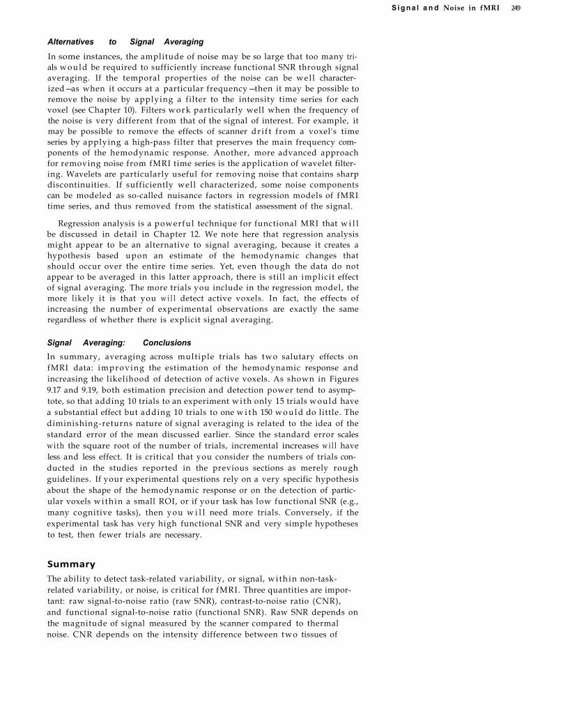
Alternatives to Signal Averaging
In some instances, the amplitude of noise may be so large that too many trials would be required to sufficiently increase functional SNR through signal averaging. If the temporal properties of the noise can be wel l characterized—as when it occurs at a particular frequency—then it may be possible to remove the noise by applying a filter to the intensity time series for each voxel (see Chapter 10). Filters work particularly well when the frequency of the noise is very different from that of the signal of interest. For example, it may be possible to remove the effects of scanner dr i f t from a voxel's time series by applying a high-pass filter that preserves the main frequency components of the hemodynamic response. Another, more advanced approach for removing noise from fMRI time series is the application of wavelet filtering. Wavelets are particularly useful for removing noise that contains sharp discontinuities. If sufficiently well characterized, some noise components can be modeled as so-called nuisance factors in regression models of fMRI time series, and thus removed from the statistical assessment of the signal.
Regression analysis is a powerful technique for functional MRI that w i l l be discussed in detail in Chapter 12. We note here that regression analysis might appear to be an alternative to signal averaging, because it creates a hypothesis based upon an estimate of the hemodynamic changes that should occur over the entire time series. Yet, even though the data do not appear to be averaged in this latter approach, there is still an implicit effect of signal averaging. The more trials you include in the regression model, the more likely it is that you w i l l detect active voxels. In fact, the effects of increasing the number of experimental observations are exactly the same regardless of whether there is explicit signal averaging.
Signal Averaging: Conclusions In summary, averaging across mult iple trials has two salutary effects on fMRI data: improving the estimation of the hemodynamic response and increasing the likelihood of detection of active voxels. As shown in Figures 9.17 and 9.19, both estimation precision and detection power tend to asymptote, so that adding 10 trials to an experiment wi th only 15 trials would have a substantial effect but adding 10 trials to one w i t h 150 w o u l d do little. The diminishing-returns nature of signal averaging is related to the idea of the standard error of the mean discussed earlier. Since the standard error scales wi th the square root of the number of trials, incremental increases w i l l have less and less effect. It is critical that you consider the numbers of trials conducted in the studies reported in the previous sections as merely rough guidelines. If your experimental questions rely on a very specific hypothesis about the shape of the hemodynamic response or on the detection of particular voxels w i t h i n a small ROI, or if your task has low functional SNR (e.g., many cognitive tasks), then you w i l l need more trials. Conversely, if the experimental task has very high functional SNR and very simple hypotheses to test, then fewer trials are necessary.
Summary The ability to detect task-related variability, or signal, w i t h i n non-task-related variability, or noise, is critical for fMRI. Three quantities are important: raw signal-to-noise ratio (raw SNR), contrast-to-noise ratio (CNR), and functional signal-to-noise ratio (functional SNR). Raw SNR depends on the magnitude of signal measured by the scanner compared to thermal noise. CNR depends on the intensity difference between t w o tissues of
S i g n a l a n d Noise in fMRI 249
interest compared to the variability in those intensity values. Functional SNR determines our ability to detect signal changes associated wi th experimental effects of interest and is critical for many aspects of fMRI. While raw SNR scales linearly wi th the strength of the magnetic field, functional SNR scales less than linearly w i t h field strength due to several sources of noise. Thermal and system variability in scanner hardware contribute to all types of MRI imaging but are much less important than physiological variability for fMRI , especially at high field strengths. The most common method for improving SNR in fMRI studies is signal averaging, the collection of multiple observations for each experimental condition. Signal averaging can substantially improve both estimation and detection power, but it can serve to mask potentially important effects.
Suggested Readings *Aguirre, G. K., Zarahn, E., and D'Esposito, M. (1998). The variability of human,
BOLD hemodynamic responses. NeuroImage, 8: 360-369. This influential paper provides important evidence for consistent differences in the form of the fMRI hemodynamic response across subjects.
*Huettel, S. A., and McCarthy, G. (2001). The effects of single-trial averaging upon the spatial extent of fMRI activation. NeuroReport, 12: 2411-2416. This short article documents the changes in hemodynamic response form and spatial extent of activation as more and more trials are averaged.
*Krasnow, B., Tamm, L., Greicius, M. D., Yang, T. T., Glover, G. H., Reiss, A. L., and Menon, V. (2003). Comparison of fMRI activation at 3 and 1.5 T during perceptual, cognitive, and affective processing. NeuroImage, 18: 813-826. Unlike most studies of field strength, which use simple visual or motor tasks, this report compares a variety of tasks at medium and high fields.
*Kruger, G., and Glover, G. H. (2001). Physiological noise in oxygenation-sensitive magnetic resonance imaging. Magn. Reson. Med., 46: 631-637. Provides a clear description of different components of physiological noise.
*McGonigle, D. J., Howseman, A. M., Athwal, B. S., Friston, K. J., Frackowiak, R. S., and Holmes, A. P. (2000). Variability in fMRI: An examination of intersession differences. NeuroImage, 11: 708-734. This remarkable study describes a set of 99 fMRI sessions conducted on a single subject over a period of several months.
Parrish, T. B., Gitelman, D. R., LaBar, K. S., and Mesulam, M. M. (2000). Impact of signal-to-noise on functional MRI. Magn. Reson. Med., 44: 925-932. A clear demonstration of how changes in signal-to-noise affect detection of activity; includes an example from a clinical patient.
*Indicates a reference that is a suggested reading in the field and is also cited in this chapter.
Chapter References Buxton, R. B. (2002). Introduction to Functional Magnetic Resonance Imaging: Principles
and Techniques. Cambridge University Press, New York. Edelstein, W. A., Glover, G. H. , Hardy, C. J., and Redington, R. W. (1986). The intrin
sic signal-to-noise ratio in NMR imaging. Magn. Reson. Med., 3: 604-618. Gati, J. S., Menon, R. S., Ugurbil, K., and Rutt, B. K. (1997). Experimental determina
tion of the BOLD field strength dependence in vessels and tissue. Magn. Reson. Med., 38: 296-302.
Hays, W. L. (1994). Statistics (5th ed.). Harcourt College, Fort Worth, TX. Hu, X., Le, T. H. , Parrish, T, and Erhard, P. (1995). Retrospective estimation and
correction of physiological fluctuation in functional MRI. Magn. Reson. Med., 34: 201-212.
250 C h a p t e r N ine
Huettel, S. A., Singerman, J., and McCarthy, G. (2001). The effects of aging upon the hemodynamic response measured by functional MRI. NeuroImage, 13:161-175.
Kruger, G., Kastrup, A., and Glover, G. H. (2001). Neuroimaging at 1.5 T and 3.0 T: Comparison of oxygenation-sensitive magnetic resonance imaging. Magn. Reson. Med., 45: 595-604.
Ogawa, S., Kim, S.-G., Ugurbil, K., and Menon, R. S. (1998). On the characteristics of fMRI in the brain. Ann. Rev. Biophys. Biomol. Struct., 27: 447-474.
Ogawa, S., Menon, R. S., Tank, D. W., Kim, S.-G., Merkle, H., Ellerman, J. M., and Ugurbil, K. (1993). Functional brain mapping by blood oxygenation level-dependent contrast magnetic resonance imaging. A comparison of signal characteristics with a biophysical model. Biophys. ]., 64: 803-812.
Raj, D., Anderson, A. W., and Gore, J. C. (2001). Respiratory effects in human functional magnetic resonance imaging due to bulk susceptibility changes. Phys. Med. Biol., 46: 3331-3340.
Saad, Z. S., Ropella, K. M., DeYoe, E. A., and Bandettini, P. A. (2003). The spatial extent of the BOLD response. NeuroImage, 19:132-144.
Turner, R., Jezzard, P., Wen, H. , Kwong, K. K., Le Bihan, D., Zeffiro, T, and Balaban, R. S. (1993). Functional mapping of the human visual cortex at 4 and 1.5 Tesla using deoxygenation contrast EPI. Magn. Reson. Med., 29: 277-279.
Wang, J., Alsop, D. C, Li, L., Listerud, J., Gonzalez-At, J. B., Schnall, M. D., and Detre, J. A. (2002). Comparison of quantitative perfusion imaging using arterial spin labeling at 1.5 and 4.0 Tesla. Magn. Reson. Med., 48: 242-254.
Yang, Y., Wen, H., Mattay, V. S., Balaban, R. S., Frank, J. A., and Duyn, J. H. (1999). Comparison of 3D BOLD functional MRI with spiral acquisition at 1.5 and 4.0 T. NeuroImage, 9: 446-451.
Zarahn, E., and Slifstein, M. (2001). A reference effect approach for power analysis in fMRI. NeuroImage, 14: 768-779.
S i g n a l a n d N o i s e in f M R I 251

Preprocessing of fMRI Data
As described in the previous chapters, one can consider fMRI data as consisting of a three-dimensional matrix of volume elements (voxels) that is repeatedly sampled over time. So, a single experiment might have an imaging volume of 64 x 64 x 20 voxels that is sampled every 2 seconds for a total of 10 minutes (300 time points per voxel). A straightforward way of analyzing such a data set w o u l d be to extract the raw time course for each voxel and compare each of these time courses to some hypothesis using a test of significance. While this approach indeed forms the basis of much of fMRI data analysis, as is discussed in Chapter 12, it contains some hidden assumptions. Notably, it assumes that each voxel represents a unique and unchanging location in the brain and that the sampling of that voxel occurs at a regular known rate. These assumptions, though seemingly plausible, are always incorrect. A l l fMRI data suffers from spatial and temporal inaccuracy caused by subject head morion, physiological oscillations like heartbeats and respiration, inhomogeneities in the static field, and/or differences in the t iming of image acquisition. If uncorrected, this variabil ity may reduce (or even eliminate) the detection power of an experiment.
Here, we discuss a series of computational procedures, k n o w n as preprocessing steps, that operate on fMRI data fol lowing image reconstruction but prior to statistical analysis. For example, researchers correct for head motion regardless of whether the experiment uses a blocked-design vision task or an event-related memory task. Preprocessing has t w o major goals. The first goal is to remove uninteresting variability from the data. In the prior chapter, we introduced a number of sources of variability that can be of large amplitude compared to the task-related signal. By reducing the total variance through preprocessing, we can increase functional signal-to-noise ratio (SNR). The second goal is to prepare the data for statistical analysis. Spatial smoothing, for example, can be used to reduce the effective number of statistical tests while maintaining detection power. Many of the statistical analyses used in fMRI make assumptions that can be met by application of preprocessing techniques. The general framework for preprocessing is shown in Figure 10.1.
preprocessing Computational procedures that are applied to fMRI data following image reconstruction but before statistical analysis. Preprocessing steps are intended to reduce variability in the data that is not associated with the experimental task and to prepare the data for statistical testing.
functional signal-to-noise ratio (functional SNR) The ratio between the intensity of a signal associated with changes in brain function and the variability in the data due to all sources of noise. Functional SNR is sometimes called dynamic CNR or functional CNR.
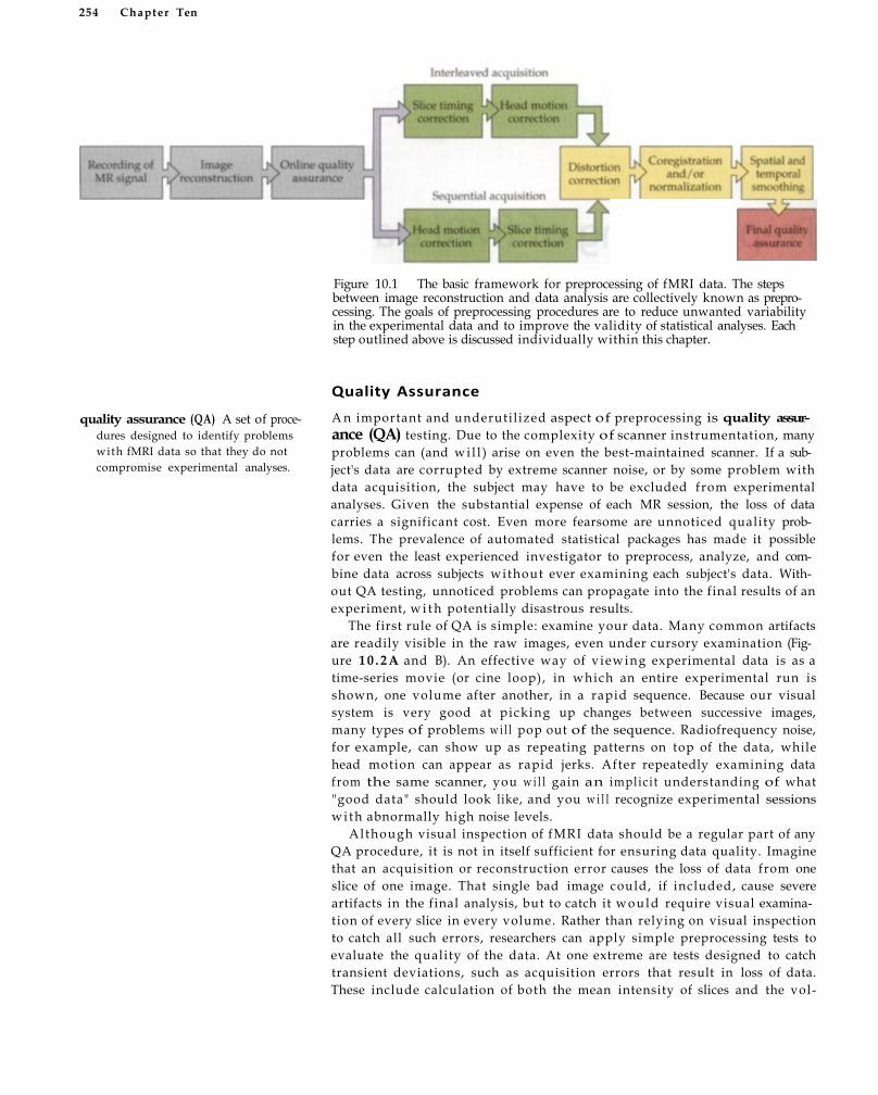
254 Chapter Ten
Figure 10.1 The basic framework for preprocessing of fMRI data. The steps between image reconstruction and data analysis are collectively known as preprocessing. The goals of preprocessing procedures are to reduce unwanted variability in the experimental data and to improve the validity of statistical analyses. Each step outlined above is discussed individually within this chapter.
quality assurance (QA) A set of procedures designed to identify problems with fMRI data so that they do not compromise experimental analyses.
Quality Assurance
A n important and underutil ized aspect of preprocessing is quality assurance (QA) testing. Due to the complexity of scanner instrumentation, many problems can (and wi l l ) arise on even the best-maintained scanner. If a subject's data are corrupted by extreme scanner noise, or by some problem with data acquisition, the subject may have to be excluded from experimental analyses. Given the substantial expense of each MR session, the loss of data carries a significant cost. Even more fearsome are unnoticed quality problems. The prevalence of automated statistical packages has made it possible for even the least experienced investigator to preprocess, analyze, and combine data across subjects without ever examining each subject's data. Without QA testing, unnoticed problems can propagate into the final results of an experiment, w i t h potentially disastrous results.
The first rule of QA is simple: examine your data. Many common artifacts are readily visible in the raw images, even under cursory examination (Figure 1 0 . 2 A and B). An effective way of v iewing experimental data is as a time-series movie (or cine loop), in which an entire experimental run is shown, one volume after another, in a rapid sequence. Because our visual system is very good at picking up changes between successive images, many types of problems w i l l pop out of the sequence. Radiofrequency noise, for example, can show up as repeating patterns on top of the data, while head motion can appear as rapid jerks. After repeatedly examining data from the same scanner, you w i l l gain an implici t understanding of what "good data" should look like, and you w i l l recognize experimental sessions wi th abnormally high noise levels.
Al though visual inspection of fMRI data should be a regular part of any QA procedure, it is not in itself sufficient for ensuring data quality. Imagine that an acquisition or reconstruction error causes the loss of data from one slice of one image. That single bad image could, if included, cause severe artifacts in the final analysis, but to catch it would require visual examination of every slice in every volume. Rather than relying on visual inspection to catch all such errors, researchers can apply simple preprocessing tests to evaluate the quality of the data. At one extreme are tests designed to catch transient deviations, such as acquisition errors that result in loss of data. These include calculation of both the mean intensity of slices and the vol-
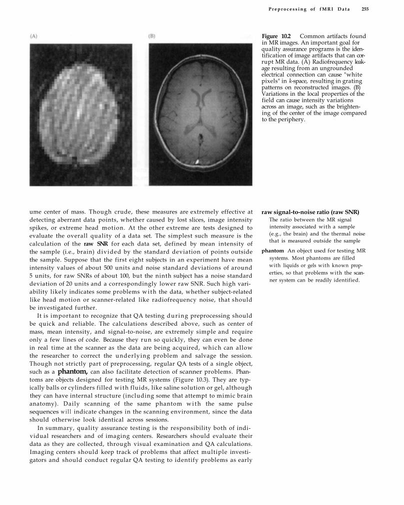
P r e p r o c e s s i n g of f M R I D a t a 255
Figure 10.2 Common artifacts found in MR images. An important goal for quality assurance programs is the identification of image artifacts that can corrupt MR data. (A) Radiofrequency leakage resulting from an ungrounded electrical connection can cause "white pixels" in k-space, resulting in grating patterns on reconstructed images. (B) Variations in the local properties of the field can cause intensity variations across an image, such as the brightening of the center of the image compared to the periphery.
ume center of mass. Though crude, these measures are extremely effective at detecting aberrant data points, whether caused by lost slices, image intensity spikes, or extreme head motion. At the other extreme are tests designed to evaluate the overall quality of a data set. The simplest such measure is the calculation of the raw SNR for each data set, defined by mean intensity of the sample (i.e., brain) divided by the standard deviation of points outside the sample. Suppose that the first eight subjects in an experiment have mean intensity values of about 500 units and noise standard deviations of around 5 units, for raw SNRs of about 100, but the ninth subject has a noise standard deviation of 20 units and a correspondingly lower raw SNR. Such high variability likely indicates some problems wi th the data, whether subject-related like head motion or scanner-related like radiofrequency noise, that should be investigated further.
It is important to recognize that QA testing dur ing preprocessing should be quick and reliable. The calculations described above, such as center of mass, mean intensity, and signal-to-noise, are extremely simple and require only a few lines of code. Because they run so quickly, they can even be done in real time at the scanner as the data are being acquired, which can allow the researcher to correct the underlying problem and salvage the session. Though not strictly part of preprocessing, regular QA tests of a single object, such as a phantom, can also facilitate detection of scanner problems. Phantoms are objects designed for testing MR systems (Figure 10.3). They are typically balls or cylinders filled wi th fluids, like saline solution or gel, although they can have internal structure (including some that attempt to mimic brain anatomy). Daily scanning of the same phantom w i t h the same pulse sequences w i l l indicate changes in the scanning environment, since the data should otherwise look identical across sessions.
In summary, quality assurance testing is the responsibility both of individual researchers and of imaging centers. Researchers should evaluate their data as they are collected, through visual examination and QA calculations. Imaging centers should keep track of problems that affect multiple investigators and should conduct regular QA testing to identify problems as early
raw signal-to-noise ratio (raw SNR) The ratio between the MR signal intensity associated with a sample (e.g., the brain) and the thermal noise that is measured outside the sample
phantom An object used for testing MR systems. Most phantoms are filled with liquids or gels with known properties, so that problems with the scanner system can be readily identified.

256 Chapter Ten
Figure 10.3 Examples of phantoms and their appearance on MR images. Phantoms are fluid- or gel-filled shapes that are used for testing MR scanners. They may be homogeneous (A, D), or have internal structure (B, C, E, F). (Phantoms courtesy of General Electric Corporation.)
interleaved slice acquisition The collection of data in an alternating order, so that data are first acquired from the odd-numbered slices and then from the even-numbered slices, to minimize the influence of excitation pulses upon adjacent slices.
as possible. A l l MR scanners are subject to image acquisition problems of one type or another. Without a diligent QA program, such problems w i l l corrupt experimental data and frustrate investigators.
Slice Acquisition Time Correction
Most fMRI data are acquired using two-dimensional pulse sequences that acquire images one slice at a time, due to the use of spatial gradients that l imit the influence of an excitation pulse to a single slice w i t h i n the brain. A typical pulse sequence might acquire 24 slices or more to cover the entire brain w i t h i n a TR of 1.5 to 3.0 s, depending on the capabilities of the scanner. Most pulse sequences use interleaved slice acquisition, such that the scanner first collects all of the odd slices and then collects all of the even slices to

P r e p r o c e s s i n g of f M R I D a t a 257
avoid cross-slice excitation. If there were 12 slices in the imaging volume, numbered f rom 1 at the bottom of the brain to 12 at the top, an interleaved acquisition sequence w o u l d collect the slices in the order 1-3-5-7-9-11-2-4-6-8-10-12. Less common is ascending/descending slice acquisition, in which the slices are collected consecutively: 1-2-3-4-5-6-7-8-9-10-11-12. Regardless of the order used, each slice is acquired at a different time point w i t h i n the TR. Timing differences are especially problematic for interleaved sequences, in which spatially consecutive slices are not acquired successively. In virtually all fMRI scanning, the slices are acquired w i t h equal spacing across the TR. Thus, assuming that the interleaved example above had a TR of 3 s and that slice 1 was acquired at 0 s, slice 2 would not be acquired unt i l 1.5 s later, and slice 12 w o u l d be acquired 2.75 s after slice 1.
ascending/descending slice acquisition The collection of data in consecutive order, so that slices are acquired sequentially from one end of the imaging volume to the other.
To illustrate how slice t iming affects fMRI analyses, Figure 10.4 presents a typical interleaved imaging sequence consisting of 24 slices acquired w i t h a
(A)
(C)
Figure 10.4 Effects of slice acquisition time upon the hemodynamic response. Imagine that a single brain region, shown in red (A), is uniformly active following presentation of a stimulus. This region spans three slices, 15 to 17, within the imaging volume, which is acquired with a standard interleaved sequence (B). Because these slices are acquired at different times within the 3-s TR, the hemodynamic response within the slices wil l have very different time courses. The actual recorded signal from the different slices is shown in (C). When plotted for each TR, there are different time courses for the slices acquired early in the TR and the slice acquired later (D). The hemodynamic response in slice 16 appears to peak earlier than those in the surrounding slices, even though the underlying activity is identical.
In most fMRI pulse sequences, the slices are equally spaced throughout a TR. Can you think of a type of experiment in which researchers might concentrate all of the slices at the
beginning of the TR, so that there is a period of time in which no acquisition takes place? (Hint: Refer to Chapter 2 to
consider what the subject experiences each time a slice is acquired.)

258 Chapter Ten
3-s TR. The region of interest is shown in red in the frontal lobe (Figure 10.4A and B), and the hypothetical hemodynamic response in that region is plotted below (Figure 10.4C and D ) . Since the region of interest spans three slices—15, 16, and 17—the actual times at which it is sampled differ across slices. Slices 15 and 17 are sampled at 1 s and 1.125 s, respectively, whereas slice 16 is sampled at 2.5 s. So, for each slice, the measured time course wil l have a particular sampling delay, which can greatly influence the correspondence between observed data and experimental hypotheses. The consequences of slice-timing errors are much greater for event-related designs than for blocked designs, since the former depend upon accurate modeling of the t iming of experimental events. Thus, correction for slice t iming is necessary for many forms of event-related designs. In contrast, blocked designs measure changes in BOLD activity over long intervals (e.g., 20 seconds), so errors in determining block onset w i l l have relatively little effect on the data and correction for slice t iming is less critical.
To correct for slice-timing errors, some experimental analyses modify the predicted hemodynamic responses so that each slice is compared to a hemodynamic response function wi th slightly different t iming. More common is correcting for slice t iming using temporal interpolation during preprocessing. Interpolation uses information from nearby time points to estimate the amplitude of the MR signal at the onset of the TR. Several strategies for interpolation are used in fMRI , including linear, spline, and sinc functions. It is important to emphasize that no interpolation technique can perfectly recover the missing information from between samples. The accuracy of interpolation depends on t w o factors: the variabil ity in the experimental data and the rate of sampling. If the experimental data change very rapidly over time (i.e., have high-frequency components) compared to the sampling rate, then interpolation w i l l be unable to capture changes between data points. But if the data change very slowly compared to the sampling rate, then interpolation w i l l be more effective. Given the typical temporal variation in fMRI data, interpolation to correct for time of slice acquisition is more effective for data acquired at relatively short TRs (e.g., 1 s) than for data acquired at long TRs (e.g., >3 s). Unfortunately, the need for accurate interpolation is greatest at long TRs because of the large intervals between successive acquisitions.
Slice-timing correction should be done before head-motion correction for data acquired using interleaved slice acquisition at a long TR. This is because small through-plane motions, as when part of a voxel moves from slice 12 to slice 13, w i l l cause the t iming of activity to be off by one-half of the TR value at affected time points. Thus, doing slice-timing correction first for interleaved sequences w i t h long TRs w i l l minimize t iming errors, at a cost of increased sensitivity to head motion. For data acquired using an ascending/descending sequence or w i t h a short TR, motion correction should be done before slice-timing correction. This w i l l minimize motion effects associated w i t h interpolation across adjacent voxels, at a cost of slight t iming uncertainty.
Head Motion Probably the most damaging (and frustrating!) problem for fMRI studies is head motion. To appreciate how little head motion is required to render data meaningless, examine the data shown in Figure 10.5A-C. Note the large intensity transition between adjacent voxels, as highlighted in the magnified
temporal interpolation The estimation of the value of a signal at a time point that was not originally collected, using data from nearby time points.

P r e p r o c e s s i n g of f M R I D a t a 259
(A) (B) Figure 10.5 Effects of head motion on fMRI data. Large intensity transitions exist at tissue boundaries, including the edges of the brain (A). Here we demonstrate the effects of head motion upon voxel intensity. The magnified views show the position of the brain before head motion (B) and after a movement of one voxel to the right (C). The numerical intensity values for the voxels within the blue square are shown below. Note that the intensity in a given voxel may change by more than a factor of 5 due solely to head motion. This compares to a change of only 1 to 2% for real brain activity.
version in panel B. N o w imagine that the subject moves his head almost imperceptibly, shifting by only 5 mm (i.e., the w i d t h of a single voxel) along a single axis. Even such a tiny movement has drastic effects upon the data, as shown in panel C. Remember that the scanner acquires images at absolute spatial locations, not relative to the brain's position. So if the subject moves his head by 5 m m , each voxel's time series w i l l contain data from two different parts of the brain that are separated by exactly 5 m m . If those t w o parts of the brain have very different properties, as w i l l certainly be the case at the edge of the brain, even this small head motion may cause very large changes in raw signal over time.
The basic problem introduced by head motion thus can be stated simply. FMRI analyses assume that each voxel represents a unique part of the brain; if the subject's head moves, then each voxel's time course is derived from more than one brain location. To consider the effects of head motion on statistical analyses, consider a blocked design similar to that used by K w o n g and colleagues in 1992 (see Chapter 7), in which periods of darkness and light alternate every minute for 4 minutes. Suppose that the subject moves her head exactly one voxel to her left at the beginning of the last block, just after the lights come on. Voxels that had included the right edge of the brain wil l now include f luid around the right side of the brain, whereas voxels just outside the left side of the brain w i l l now include gray matter. So, the overall signal w i l l be artificially decreased on the right side of the brain and artificially increased on the left side. This phenomenon results in characteristic ringing patterns on one or both edges of the brain due to uncorrected head motion (Figure 10.6). One commonly observed form of head motion is a large, abrupt change in position between experimental runs (see Figure 10.9). Most fMRI experiments are partitioned into a number of relatively short (e.g., 4- to 8-minute) runs to reduce subject fatigue and, in some cases, to overcome hardware constraints on data acquisition. Dur ing the breaks between runs, subjects typically relax and talk to the experimenters, often resulting in considerable head motion. In many cases, different experimental conditions are separated across runs, so motion becomes more associated with one condition than another.
Within runs, subjects often make numerous small movements of the head. As subjects lie in a small space, unable to move around for a 1- to 2-hour ses-

Figure 10.6 Edge effects of head motion in fMRI analyses. Because the intensity transitions in the brain are greatest at its edges, head motion often results in systematic rings of artifactual activation around the edges of the brain. Shown here are the results of a transient 4-s forward translation of two voxels at stimulus onset in one epoch. Note that the back of the brain, which changed from high intensity to low intensity as a result of the movement, exhibits a significant decrease in activity due entirely to the movement.
sion, they get increasingly tired and restless. If the experiment is set up so that one condition is at the beginning and another is at the end of the session, then the likelihood that fatigue-related motion w i l l affect the analyses increases. The experimental st imuli themselves may cause head motion as wel l . Many experimental tasks require subjects to make motor responses, usually by moving a joystick or pressing a button, which may in turn induce head motion. If a picture is particularly alerting or arousing, it may surprise or shock the subjects into moving. Anyone who has been a subject in an MRI study has experienced momentary drowsiness.. .only to be startled into alertness by the next stimulus. Motion effects that are time-locked to stimulus presentation pose challenges for analysis and preprocessing techniques, since it becomes dif f icult to separate real brain activity from artifacts of motion. Within- and between-runs movements are sometimes corrected separately because of their different spatial properties.
Even though head motion is an inherently spatial problem, it can have consequences for activation t iming. The examples in figures 10.5 and 10.6 considered in-plane motion, but motion frequently occurs between slice planes as well . Since most functional imaging sequences use interleaved slice acquisition, adjacent slices are acquired approximately one-half TR apart. For a long-TR imaging sequence, as is often used for full-brain imaging, head motion could result in misestimating the t iming of activity by 1 to 2 seconds. A second t iming problem is that motion w i t h i n an acquisition also changes the pattern of spin excitation in the brain. Recall that for functional pulse sequences, like gradient-echo EPI, each slice experiences an excitation pulse at the beginning of the TR. But if the head moves w i t h i n the acquisition of a single volume, then some of the slices may miss the excitation pulse. Those slices w i l l recover more than other slices, because the time since the last excitation was longer, and thus wi l l have different responses to subsequent excitations. A final consequence of head motion is the potential loss of data at the edges of the imaging volume. Most fMRI protocols use in-plane fields of view that are substantially larger than the brain, such as 20 or 24 cm. For such large fields of view, the resulting image is large enough that the head is sur-
260 C h a p t e r T e n

P r e p r o c e s s i n g of f M R I D a t a 261
rounded by a few centimeters of air, and so it is unlikely that any in-plane movement would be large enough to move the brain outside of the imaging volume. More problematic is through-plane movement. Imagine that a researcher sets up the pulse sequence for one subject to have exactly enough axial 4-mm slices to f i t the entire brain, from the top of the cerebrum to the bottom of the cerebellum. Later in the experiment, the subject moves his head slightly, about 4 m m , along the z-direction, and in doing so the top of his brain moves out of the imaging volume, so that data from that part of the brain is no longer acquired. In addition to all of the other problems wi th head motion described previously, this subject would have an irreversible loss of data from one slice. To prevent such data loss, additional slices should be acquired on the edges of the area of interest, whether the ful l brain or just a single region, so that small through-plane movements can be corrected.
Prevention of Head Motion
Like many other problems, head motion is more easily prevented than corrected. Most laboratories use head restraints of some form, such as bite bars, masks, vacuum packs, padding, or taping (Figure 10.7). The most effective
Figure 10.7 Head restraint systems. Because severe head motion can render fMRI data useless, several systems for head-immobilization exist. Shown in (A) is a standard volume head coil w i t h two motion-restraint systems. Attached to the top of the head coil is a bite bar system, while at the bottom is a vacuum pack. When the bite bar is used (B), the subject clenches his/her teeth on a dental mold that has been cus
tomized to their bite pattern. This greatly restricts the effective motion of the head. Vacuum packs (C) contain many soft foam beads wi th in a plastic casing. When air is pumped out, the pack hardens to form a shell around the contours of the subject's head. Thermoplastic masks (D) mold to the subject's face, and are anchored to a static support. (D from Med-Tec.)

262 Chapter Ten
mock scanner A simulated MRI scanner that does not have a magnetic field present, used for training research participants. Some mock scanners simulate scanner noises and measure subject head movement.
but difficult-to-use opt ion is the bite bar (Figure 10.7A and B). As its name implies, a bite bar immobilizes the head by requiring subjects to clamp their teeth firmly on a dental mold, which in turn is solidly attached to the scanning hardware. With the jaw immobil ized, potential head motion becomes very l imited. However, while effective, bite bars can introduce subject compliance problems. Some subjects dislike using bite bars, which can both increase the likelihood that a participant ends a session prematurely and decrease the rate of subject recruitment. Despite these disadvantages, researchers at a number of institutions use bite bars successfully to minimize head motion. Better tolerated are systems that use moldable plastic or mesh to create a mask around the subject's head (Figure 10.7D). Such masks passively restrict head motion without requiring jaw clenching and are individually molded to each participant's physiognomy. The primary disadvantage of mask systems lies in the customization: it takes time to adjust the mask for each subject, especially with thermoplastic systems that must be heated and cooled before scanning. A secondary disadvantage is that some subjects may feel claustrophobic due to the high degree of immobilization.
Vacuum-pack systems combine good motion reduction wi th improved patient comfort (Figure 10.7C). The vacuum pack consists of a large number of soft beads wi th in a flexible plastic casing. Once the subject is positioned in the scanner, the pack is fitted around the sides of the head and its air is pumped out. The loss of air hardens the vacuum pack into a shell molded to the contours of the skull . Since the face is left open, the risk of claustrophobia is not increased significantly. Many subjects, in fact, report preferring the vacu u m system to no restraint at all because its head support allows them to relax their neck muscles. Al though head motion, especially t i l t ing the head forward, is not as restricted as it is wi th bite bars or face masks, the improved patient comfort makes vacuum packs a desirable option.
While restraint systems play an essential role in minimizing head motion, probably the most important factor is subject compliance. Because most fMRI subjects are research volunteers and not clinical patients, they receive no direct benefit from the session. Therefore, when subjects become uncomfortable, they may choose to terminate the session or to move to relieve soreness or pain. Working to maximize subjects' comfort and interest in the study greatly improves the chances of acquiring a complete data set that is not corrupted by excessive motion. Researchers should regularly talk to their subjects; even a simple " H o w are you doing?" after each run w i l l help prevent anxiety and accompanying motion. We have also found that taping d o w n subjects' foreheads greatly reduces head motion. Although a single piece of tape in itself cannot prevent a subject from moving his or her head, it provides feedback (in the form of changes in tension) when the subject moves. If a subject makes a slight motion, the tape provides h im or her with a guide for how to return to the base position.
Head-motion effects can also be ameliorated through subject training. At our center, first-time subjects participate in training sessions w i t h i n an MRI simulator, or mock scanner, that was constructed from the parts of a decommissioned scanner (Figure 10.8A). Recorded scanner noises are played within the bore of the simulator for added realism. During the training session, a three-dimensional tracking device ( i . e., Polhemus sensor) is attached to the subject's head so that we can monitor head movements at millimeter resolution and caution the subject if head movements exceed a threshold (Figure 10.8B). We find that training in the simulator results in subjects who are more relaxed and comfortable d u r i n g their real scanning sessions. Subjects who cannot tolerate confinement in the mock scanner, or who cannot avoid mov-

P r e p r o c e s s i n g of fMRI D a t a 263
Figure 10.8 Use of a mock scanner system for prevention of head motion. By acclimating potential subjects to the MRI environment in a simulated or mock scanner (A) , head motion and other subject compliance problems can be greatly reduced. (B) An adolescent subject w i t h a Polhemus head-tracking system around her forehead. If she moves her head beyond a threshold amount, the movie that she is watching through the mirrored glasses w i l l stop playing.
ing their heads over the course of the scanning session, can be excused from further participation in the study. In summary, prevention of head motion takes two basic forms: physical restraints that immobilize the head and adoption of training and communication procedures that reduce the likelihood of head motion.
Correction of Head Motion When the head moves d u r i n g an experiment, some of the images w i l l be acquired w i t h the brain in the wrong location. The goal of motion correction is to adjust the time series of images so that the brain is in the same position in every image. The general process for spatially al igning t w o image volumes is called coregistration. For motion correction, successive image volumes in the time series are coregistered to a single reference volume. Because the brain is the same in every image of the time series, a rigid-body transformation is used. Rigid-body transformations assume that the size and shape of the t w o objects to be coregistered are identical, and that one can be superimposed exactly upon the other by a combination of three translations (i.e., moving the entire image volume along the x-, y-, and axes) and three rotations (rotating the entire image volume through the x-y, x-z, and y-z planes). The assumption of rigid-body movements is generally plausible in fMRI studies, although inhomogeneities in the magnetic f ield may lead to differential scaling of images as a function of their position in the scanner.
To determine the l ikely amount of head motion, computer algorithms identify the set of translation and rotation parameters that provides the best match to a reference volume, such as the first image acquired in the session (Figure 10.9). The mathematical measure of how well one image matches another is determined by a similarity measure, or cost function. In the ideal case of perfect coregistration between the corrected volume and the reference volume, a voxel-by-voxel subtraction would yield a difference volume
coregistration The spatial alignment of two images or image volumes.
reference volume A target image volume to which other image volumes are to be aligned.
rigid-body transformation A spatial transformation that does not change the size or shape of an object; it has three translational parameters and three rotational parameters.
translation The movement of an object along an axis in space (in the absence of rotation).
rotation The turning of an object around an axis in space (in the absence of translation).
cost function A quantity that determines the amount of residual error in a comparison.
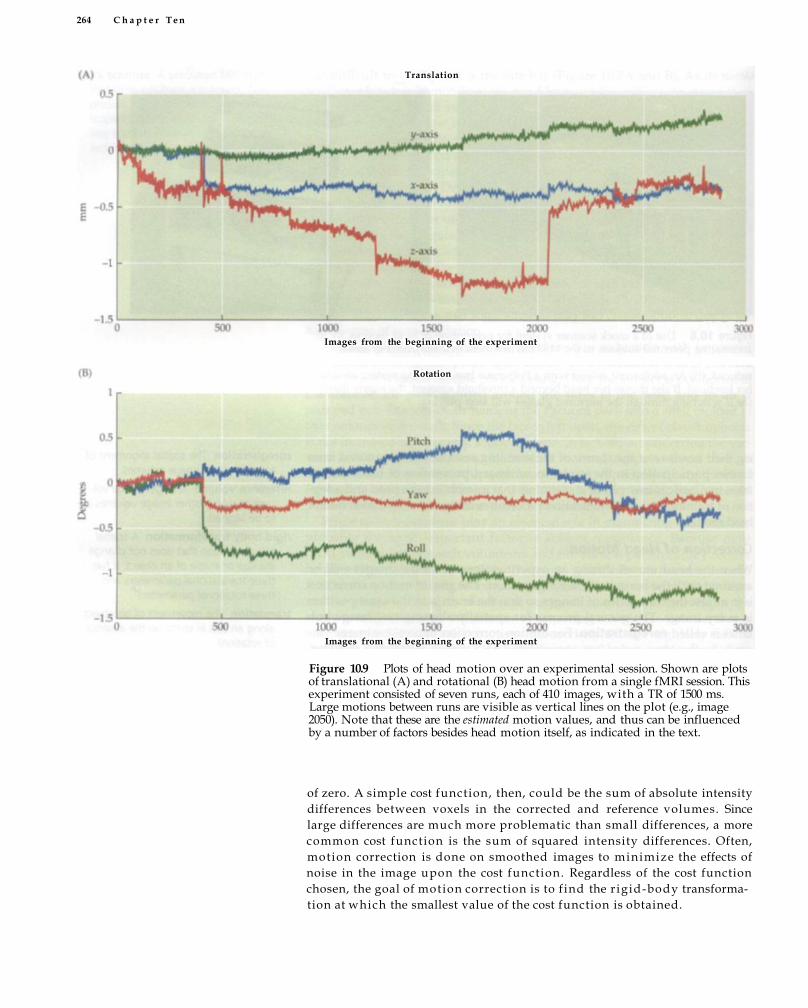
264 C h a p t e r T e n
Figure 10.9 Plots of head motion over an experimental session. Shown are plots of translational (A) and rotational (B) head motion from a single fMRI session. This experiment consisted of seven runs, each of 410 images, with a TR of 1500 ms. Large motions between runs are visible as vertical lines on the plot (e.g., image 2050). Note that these are the estimated motion values, and thus can be influenced by a number of factors besides head motion itself, as indicated in the text.
of zero. A simple cost function, then, could be the sum of absolute intensity differences between voxels in the corrected and reference volumes. Since large differences are much more problematic than small differences, a more common cost function is the sum of squared intensity differences. Often, motion correction is done on smoothed images to minimize the effects of noise in the image upon the cost function. Regardless of the cost function chosen, the goal of motion correction is to find the rigid-body transformation at which the smallest value of the cost function is obtained.
Translation
Images from the beginning of the experiment
Rotation
Images from the beginning of the experiment

Preprocessing of fMRI Data 265
One challenge to motion correction is that there are a very large number of possible ways in which the head can move. To illustrate this problem, consider a hypothetical subject who can translate her head by up to ±2.5 mm in any direction and can rotate her head by up to ±2.5° along any axis. For purposes of calculation, we w i l l assume that she only can move her head in 0.1-mm increments and can only rotate it in 0.1° increments. For each of the six motion parameters, therefore, there are 50 possible values for her movement, and thus there are more than 15 b i l l ion possible combinations of movement parameters at each time point! It is computationally infeasible, therefore, to test all possible small movements and compute the cost functions for each of the thousands of volumes acquired in an experiment.
To overcome this problem, realignment algorithms use iterative approaches for head-motion correction. First, an initial guess is tested, followed by small deviations from that guess. If none of those attempts provides a good match, as indicated by the value of its cost function, then another educated guess is made based on the first tests. This process is repeated unt i l a sufficiently good fit is obtained. Because testing all possible transformations is not possible, the solution obtained may not be the best solution available. For example, the coregistration algorithm may choose as a solution a transformation that minimizes the cost function compared to small deviations in all directions from that solution. However, a better solution w i t h a smaller cost function may have been obtained by testing larger deviations. Converging upon a local m i n i m u m in the cost function rather than finding the true global m i n i m u m is a common problem in iterative numerical techniques.
Once a set of realignment parameters is determined, the next step is to resample the original data to estimate the values that would have been obtained had there been no head motion. This process is called spatial interpolation and is similar to the temporal interpolation described earlier in the chapter, in the section on slice acquisition time correction. However, whereas temporal interpolation only considers points in time (one dimension), spatial interpolation considers points in two or three dimensions. The simplest forms of interpolation are linear methods, such as bilinear for t w o dimensions or trilinear for three, which assume that each interpolated point should be a weighted average of all adjacent points. How much each neighboring point contributes is determined by how close it is to the new value. The primary advantage of linear methods is that they are very simple and can be quickly computed. A computationally intensive, but more accurate, approach is sinc interpolation. The sine function is actually the Fourier transform of a rectangular or uniform function (see Figure 4.10). It is the optimal interpolation kernel for well-sampled images but may introduce artifacts if the data are not band-limited, that is, if there are important spatial frequencies in the brain that are not represented in the image. A good compromise is spline interpolation, which fits curves to the known data points in order to estimate u n k n o w n data. Common cubic spline interpolation methods create smooth curves by minimizing the second derivative of the connecting function. Spline techniques are intermediate in computational complexity between linear and sinc methods and provide good interpolation results for MRI data. While the standard approach is to minimize the effects of head motion during preprocessing using coregistration algorithms, it is also possible to isolate motion effects wi th in experimental analyses. By including the calculated motion parameters as a term in the analysis model, variabil ity related to head motion can be removed from the model. Since this approach
spatial interpolation The estimation of the intensity of an image at a spatial location that was not originally sampled, using data from nearby locations.

266 C h a p t e r T e n
mutual information In the context of MRI, the amount of information about one image that is provided by knowledge of another image. For example, T 1 a n d T2 images have different contrast and thus are very different on measures of squared deviation. However, the intensity of a voxel in a T, image can be predicted based on its intensity in a T2 image, so T1 and T2
images of the same brain would have high mutual information.
shimming coils Electromagnetic coils that compensate for inhomogeneities in the static magnetic field.
magnetic field mapping The collection of explicit information about the strength of the magnetic field at different spatial locations.
reduces the amount of error (i.e., unaccounted-for variability) in the model, it can increase experimental power for detecting effects of interest. However, as already noted, head motion is often correlated w i t h the experimental task, so including motion parameters in analysis models can also remove task-related activity.
It is important to recognize that algorithms for motion correction, whether conducted dur ing preprocessing or analysis, are not perfect. Indeed, even if the head movement were k n o w n perfectly, spatial interpolation w o u l d introduce errors due to the l imited resolution of functional images, resulting in residual motion effects w i t h i n the corrected time series. Different cost functions are sensitive to different aspects of the data, and some are more likely than others to converge on local minima. For example, in 2001 Freire and Mangin reported that using the sum of squared differences between the reference and corrected volume as a cost function sensitizes the coregistration to the presence of large task-related BOLD activations in the time series of data. The resulting transformations thus shift the images in a manner systematic w i t h the task and introduce spurious activations noticeable at high contrast borders (such as the edge of the images). Other cost functions that minimize the mutual information between the reference and corrected volume are less sensitive to these task-related effects. Mutual information is a measure roughly analogous to correlation that considers how well knowledge of a voxel's intensity in the reference volume predicts, or reduces the uncertainty about, the intensity of a voxel in the corrected image. Unlike the sum of squared deviations, mutual information does not assume that the intensities w i t h i n the coregistered images must match. For this reason, mutual information is often used as a cost function when coregistering image volumes from different modalities, such as PET wi th MRI or CT wi th MRI.
Despite the problems enumerated in this section, measurement of head motion provides an important QA index, and correction of head motion may improve the quality of many fMRI data sets.
Distortion Correction
As we learned in Chapter 5, functional images often suffer from geometric or intensity distortions that preclude simple matching to the high-resolution structural images. The most common culprits for such distortions are inhomogeneities in the static or excitation fields. Static field inhomogeneities usually cause geometric distortions, although they can also lead to signal losses under severe conditions. Excitation field inhomogeneities usually cause intensity variations w i t h i n the image. To ensure that images provide a true and undistorted representation of the functional neuroanatomy, researchers use specialized acquisition techniques and computational algorithms that correct the acquired images to account for these distortions.
A common method to prevent nonuniformity w i t h i n the static magnetic field is magnetic field shimming. By adjusting many first-, second-, and higher-order magnetic field gradients generated by shimming coils (see Chapter 2), most field distortions can be corrected and a reasonably homogeneous field can be created. However, when shimming conditions cannot be optimized, especially at very high magnetic field, residual magnetic field inhomogeneity may remain significant enough to induce noticeable geometric distortions (Figure 10.10A). A n alternative approach, called magnetic field mapping, can be adopted to provide explicit knowledge of the static magnetic f ield. A field map of the main magnetic field can be created by

P r e p r o c e s s i n g o f f M R I D a t a 267
Figure 10.10 Correction of geometric distortions in functional images. In this image of a circular phantom (A) , there is obvious geometric distortion. To correct for the distortion, a map of magnetic field intensity is acquired (B). The intensity map can be used to generate a corrected image (C).
acquiring two images of signal phase wi th slightly different echo times. The difference between the phase images (Figure 10.10B) is proportional to the strength of the field at any given location. If the field is completely uniform, then the phase difference induced by the different echo times w i l l be the same in all voxels, and the resulting image w i l l be a uni form gray. Field maps can be determined for a phantom or human brain and can be incorporated into the image reconstruction routine to correct for any geometric distortions (Figure 10.10C).
field map An image of the intensity of the magnetic field across space.
A common method to prevent nonuniformity in the excitation field is to construct very homogeneous volume transmitter and receiver coils. While the physical principles for producing such coils are well worked out (see Chapters 2 and 3 for additional discussion), in practice, even the best-constructed volume coils have residual intensity variations across space. This problem is exacerbated by the use of high-sensitivity surface coils, which by design introduce large, spatially dependent intensity variations. Thus, it would be useful to have explicit knowledge of the excitation field so intensity compensation algorithms could be applied post hoc based on such knowledge. To create a map of the excitation field, a large uni form object (e.g., a water-filled phantom) is placed in the center of the magnetic f ield. For each voxel in the phantom, the recorded signal depends upon t w o factors: the number of spins (e.g., hydrogen nuclei in a proton-density scan) and the strength of the excitation field at that location. The number of spins should be approximately constant across the phantom, since it is homogeneous; thus, any differences in intensity across the image w i l l be due to variations in the strength of the excitation field.
(A) (B) (C)
Why does acquiring images of spin phase at two different echo times provide a measure of local
magnetic field strength?

268 C h a p t e r T e n
New techniques can correct for intensity variations even when the user does not have explicit knowledge of the imperfections in the static or excitation fields. These techniques can be especially useful when field maps are not available (i.e., for previously acquired images). One promising technique is based on bias field estimation. With this technique, we estimate the inhomogeneity using the distorted image itself, as we know that the distorted image is based on a transformation that changes the true data. This transformation is characterized by the bias field, which can be represented as a map of the intensity variations across space due to excitation field inhomogeneity. Because the measured data are a combination of the true data and the bias field, we cannot solve analytically for their individual contributions. Rather, we must estimate the bias field through numerical techniques. By making assumptions about the properties of the noise and the smoothness of the signal, we can determine the most likely pattern of distortions and thus recover an estimate of the true data. Common methods rely on Markov random field models and associated expectation-maximization algorithms to create a map of global and local signal gradients. While a detailed explanation of these methods is beyond the scope of this book, we refer interested readers to the Guillemaud and Brady reference listed at the end of the chapter.
An example of bias field correction is shown in Figure 10.11. The sagittal image shown (Figure 10.11A) has substantial signal loss at the base of the image around the neck. Each tissue type, whether bone, muscle, or fat, shows a similar gradient of intensity decreases toward the base of the image. The consistency of these decreases allows a bias field map to be estimated (Figure 10.11B). By enhancing the remaining signal in areas of significant loss, the algorithms compensate for this loss and produce a corrected image (Figure 10.11C). Bias field estimation and correction can substantially improve aspects of analysis that are dependent upon image uniformity, such
(A) (B) (C)
Figure 10.11 Bias field estimation and correction. There is a decrease in MR signal at the bottom (indicated by arrows) of this structural image (A). To correct for this signal loss, the relative intensity of the magnetic field is estimated (B), and a correction factor is applied to the original image. The low-signal region is corrected in the resulting image (C).
bias field estimation A technique for estimating inhomogeneities in the magnetic field based upon intensity variation in collected images.

Preprocessing of fMRI Data 269
as tissue segmentation. For segmentation algorithms to be accurate, different tissue types need to have similar values throughout the brain. Large bias field differences can cause discrepancies in gray/white contrast in different locations. By estimating and correcting for such inhomogeneities, intensity values can be normalized throughout the brain, improving the accuracy of segmentation.
We note, however, that if there are too many local variations, the bias field does not always provide an accurate estimate of the field inhomogeneity. Under such conditions, the bias field correction could actually introduce errors in the segmentation of tissues of interest. Thus, f ield maps (whether for static field or excitation field) should always be acquired when high spatial and intensity f idel i ty is required, as for retinotopic mapping of the visual cortex.
Functional-Structural Coregistration and Normalization
The spatial and temporal corrections described in the previous sections ensure that each voxel contains data from a single brain region, as sampled at regular intervals throughout the time series. Such corrections are sufficient for analyses of the functional data from a single subject. Yet in most experiments, researchers want to address two questions that are diff icult to answer w i t h a single subject's functional data: how does activity map onto anatomy, and how consistent is that mapping across subjects? To answer these questions, we need to understand how our functional data correspond to the underlying neuroanatomy. Unfortunately, functional data typically are of low resolution and of little anatomical contrast, and they have geometric and intensity distortions, as we learned in the previous section. Because of these limitations, we often must map our functional data onto high-resolution and high-contrast structural images. To facilitate this mapping, coregistration algorithms l ink the functional images to high-resolution structural images from the same subject.
Even if brain activity can be well localized wi th in a subject through coregistration, there remains the problem of comparing activity across individuals, whether in the same study or across studies. Some subjects have very large brains, while others have very small brains, and there is wide variation in shape, orientation, and gyral anatomy. For intersubject comparison to be feasible, each subject's brain must be transformed so that it is the same size and shape as all of the others. This process is called normalization. Coregistration and normalization are important preprocessing steps for most fMRI studies, especially those that use voxel-based (i.e., not anatomical region-of-interest) analyses.
Functional-Structural Coregistration The differences between functional and structural images of the same brain region are striking. A typical functional image appears as a relatively undifferentiated and blurry blob, w i t h only the ventricles and the barest outlines of gray matter distinguishable (Figure 10.12A). High-resolution structural images appear remarkably detailed by comparison, w i t h clear sulcal outlines and distinct boundaries between gray and white matter (Figure 10.12B). This additional detail provides several advantages. Whereas anatomical boundaries are diff icult , if not impossible, to identify on functional images (e.g., where is the Sylvian fissure in the functional image?), such boundaries are easily seen on structural images and regions of interest can
retinotopic mapping A technique for delineating functional regions within the visual cortex based upon their responses to stimuli presented at different retinal locations.
normalization The transformation of MRI data from an individual subject to match the spatial properties of a standardized image, such as an averaged brain derived from a sample of many individuals.

270 C h a p t e r T e n
Figure 10.12 Comparison of functional and structural images. Functional (A) and structural (B) images have very different properties. Features that are readily visible on a structural image may be difficult to see or entirely absent on a lower-resolution, lower-contrast functional image of the same slice.
be easily located. Because the size, shape, and sulcal patterns of the brain are much more distinct on structural images, it also w o u l d be a great advantage if information from structural images could be used to guide normalization of functional images. Computational processes that map functional and structural images to each other are known as coregistration (Figure 10.13).
One may question the necessity of functional-structural coregistration, because both types of images are typically acquired in the same scanner session and should already be aligned. There are t w o reasons for this preprocessing step. The first occurs when the t w o types of images were acquired at different locations, either because different slices were wanted for each or because the subject moved slightly between their acquisitions. In either case, functional-structural coregistration is needed. As before, a rigid-body transformation may be conducted for coregistration in which a cost function is minimized. However, because structural and functional images often have different, sometimes even opposite, contrasts, some cost functions, such as the sum of squared differences, are not appropriate. Mutual information is often used for this purpose.
A second reason for functional-structural coregistration is image distortion. Some pulse sequences used to acquire functional images may introduce subtle geometric distortions; for example, echo-planar functional images may be slightly stretched along one axis relative to a high-resolution structural image obtained f rom the same subject in the same session. If present, these distortions cannot be corrected by the six-parameter r ig id-body transformation that we use for motion correction. If the distortion is linear, such that all voxels are s imilarly stretched along one or more axes, then a nine-parameter linear transformation can be used, in which three additional parameters are introduced to account for scaling differences along the x-, y-, or z-axes. If the distortion is more complex, w i t h regions of greater and lesser stretching, then more-complex warping algorithms must be employed.
(A) (B)
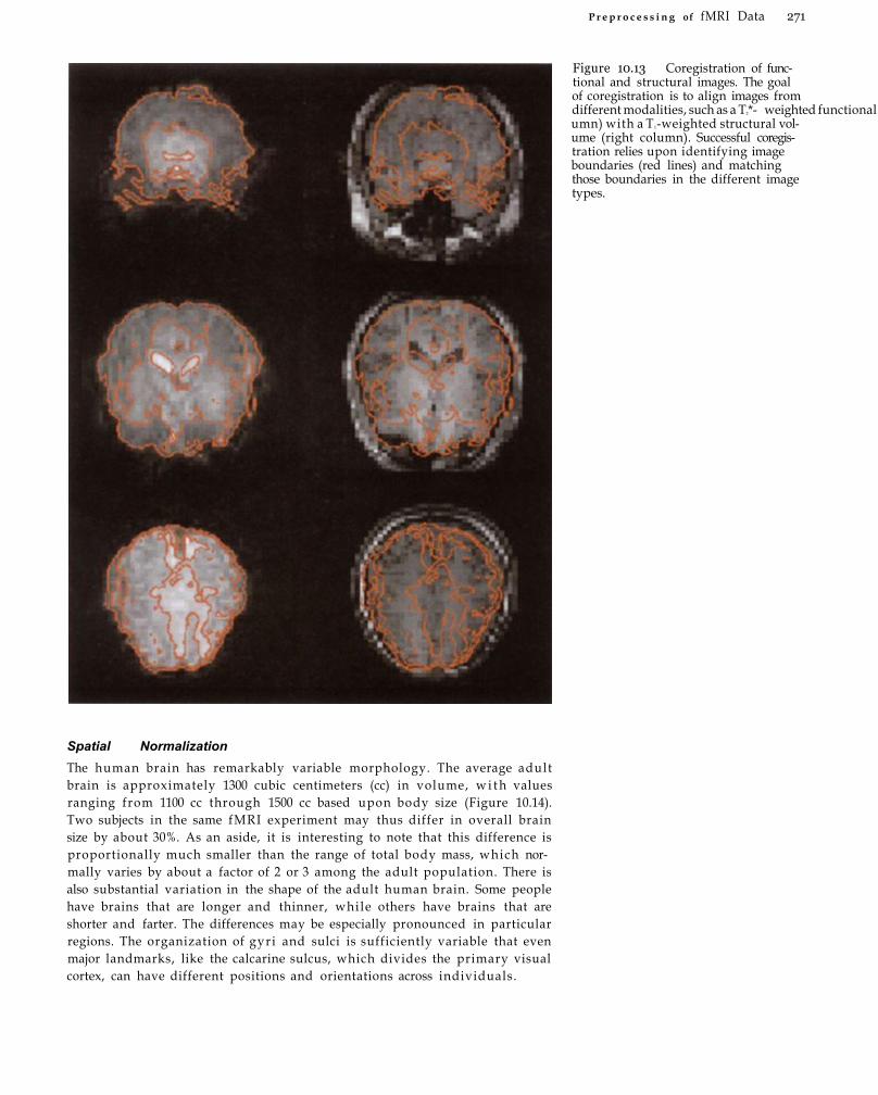
P r e p r o c e s s i n g of fMRI Data 271
Figure 10.13 Coregistration of functional and structural images. The goal of coregistration is to align images from different modalities, such as a T2* weighted functional volume (left column) with a T1-weighted structural volume (right column). Successful coregistration relies upon identifying image boundaries (red lines) and matching those boundaries in the different image types.
Spatial Normalization The human brain has remarkably variable morphology. The average adult brain is approximately 1300 cubic centimeters (cc) in volume, w i t h values ranging from 1100 cc through 1500 cc based upon body size (Figure 10.14). Two subjects in the same fMRI experiment may thus differ in overall brain size by about 30%. As an aside, it is interesting to note that this difference is proportionally much smaller than the range of total body mass, which normally varies by about a factor of 2 or 3 among the adult population. There is also substantial variation in the shape of the adult human brain. Some people have brains that are longer and thinner, while others have brains that are shorter and farter. The differences may be especially pronounced in particular regions. The organization of gyri and sulci is sufficiently variable that even major landmarks, like the calcarine sulcus, which divides the primary visual cortex, can have different positions and orientations across individuals.
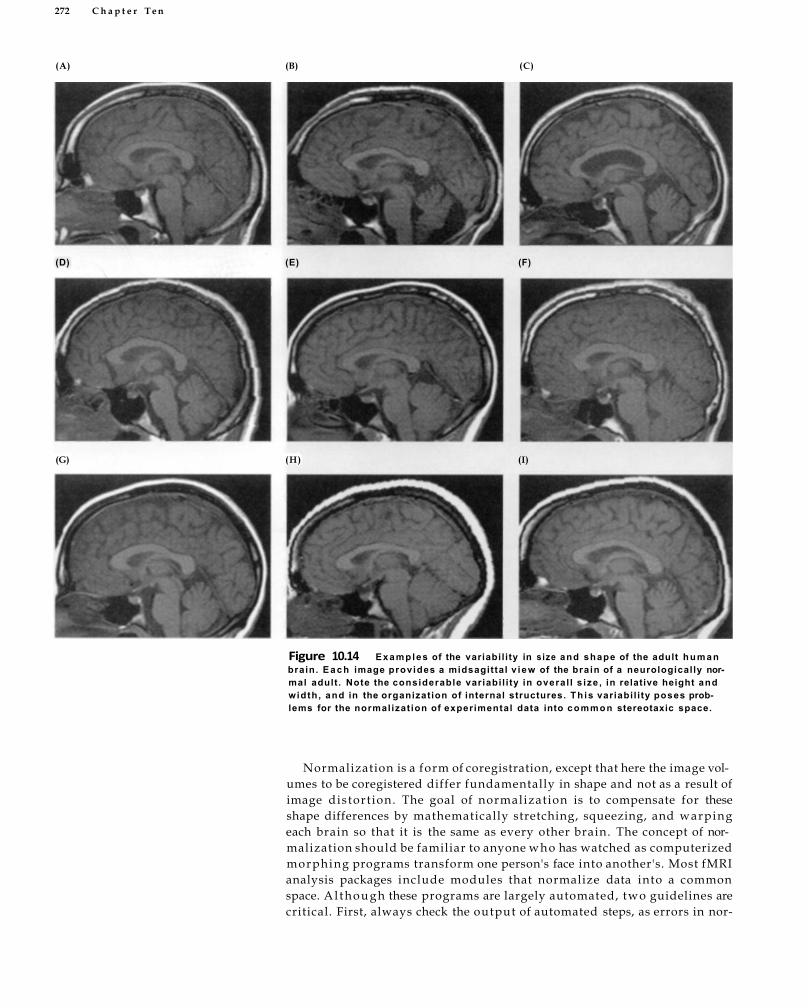
(A) (B) (C)
Figure 10.14 Examples of the variabil ity in size and shape of the adult h u m a n brain. E a c h image provides a midsagittal v iew of the brain of a neurologically normal adult . Note the considerable variabil i ty in overal l s ize , in relative height and width, and in the organization of internal structures. Th is variabil i ty poses problems for the normalizat ion of experimental data into common stereotaxic space.
Normalization is a form of coregistration, except that here the image volumes to be coregistered differ fundamentally in shape and not as a result of image distort ion. The goal of normalization is to compensate for these shape differences by mathematically stretching, squeezing, and warping each brain so that it is the same as every other brain. The concept of normalization should be familiar to anyone who has watched as computerized morphing programs transform one person's face into another's. Most fMRI analysis packages include modules that normalize data into a common space. Al though these programs are largely automated, two guidelines are critical. First, always check the output of automated steps, as errors in nor-
272 C h a p t e r T e n
(D) (E) (F)
(G) (H) (I)

P r e p r o c e s s i n g of fMRI D a t a 273
malization w i l l propagate throughout the remainder of the analyses. Second, adjusting the data by hand to an approximate match before invoking the automated algorithm often improves the final output . Because of the assumptions that are made in the warping process, it is common for normalization algorithms to be caught in local minima, missing the best match between data and template. User adjustment can greatly reduce the chance of such problems.
Normalization of data w i t h i n a study allows combination of data across individuals. Furthermore, if data wi th in two different studies have been normalized in the same fashion, then the areas of activity found in each study can be compared. For this reason, many journals encourage the reporting of experimental data as coordinates w i t h i n a common normalization scheme, or stereotaxic space. The most widely used stereotaxic space is Talairach space, which was created by the French physician Jean Talairach and colleagues and is based upon a simple stereotaxic framework derived from measurements on a single brain, that of an elderly woman. The origin of the space is set at the midpoint of the anterior commissure, w i t h the x- and y¬axes defined by the horizontal plane connecting the anterior and posterior commissures (Figure 10.15). While the standardization provided by this framework has been extraordinarily important for neuroscience, the use of a single brain presents many problems, notably that the brain used was unrepresentative of the population at large.
A better approach has come from recent attempts at probabilistic spaces based upon combining data from hundreds of indiv idual scans. A commonly used space was created by the Montreal Neurological Institute and consists of an average of 152 T 1 -weighted brain images. The M N I template has been scaled to match landmarks w i t h i n the well-established Talairach atlas. Most normalization algorithms are based upon such probabilistic templates. To warp a given brain to a template, normalization algorithms determine the overall size of the brain, as well as its gross anatomical features. Some algorithms also require identification of key landmarks in the brain, such as major sulci; this may be done automatically or require user input.
stereotaxic space A precise mapping system (e.g., of the brain) using three-dimensional coordinates.
Talairach space The most commonly used space for normalization of fMRI data.
Figure 10.15 Typical coordinate axes for fMRI data. T h e most common axes for fMRI data define the x-axis as left to right and the y -axis by connecting the anterior a n d posterior commissures. T h e z-axis is perpendicular to the plane created by the other two lines.
y
x
z

274 C h a p t e r T e n
cytoarchitecture The organization of the brain on the basis of cell structure.
filter Within the context of fMRI, an algorithm for removing temporal or spatial frequency components of data.
Even if normalization algorithms were able to transform t w o brains into the same stereotaxic framework, such success w o u l d not mean that the brains would have activation in exactly the same voxels. Remember that normalization is based upon gross morphological features of brains. These gross features do not necessarily indicate functional divisions between brain areas. More predictive of brain function are the regional cellular properties, or cytoarchitecture, which are usually not visible on MR images. Just as sulci and gyri are highly variable across individuals , so too are the boundaries between cytoarchitectonically distinct regions. (For an example of quantification of individual differences in the cytoarchitectonic organization of the human brain, consult the work of Rajkowska and Goldman-Rakic indicated in the references.)
Normalization is a powerful technique that enables the testing of complex hypotheses w i t h improved statistical power, and its positive impact upon functional neuroimaging cannot be overstated. However, there are some caveats. Variability in brain features across individuals introduces theoretical constraints upon normalization. Nearly all normalization approaches are based on subject samples drawn from the standard population of fMRI participants: young, typically college-age, adults who are healthy and neurologically normal. Many subject groups systematically differ from this population in the properties of their brains. The brains of elderly individuals may have atrophy, manifested as sulcal widening and enlarged ventricles. Young children may have differently shaped brains, due to delayed maturation of some regions (e.g., frontal cortex), as wel l as different contrast associated w i t h reduced neuronal myelination. Male and female brains also differ in subtle ways. Normalizing functional results across different subject groups may mask important group differences.
Variability in brain features across individuals also introduces practical constraints upon normalization. Many patient groups have a specific local pathology associated w i t h their disorder, while patients w i t h tumors may have brains that are apparently normal in most regions but have severe distortions in the lesion area. Since most normalization approaches attempt to minimize the differences between the subject's brain and some template, abnormal features may reduce the accuracy of the matching process. Some normalization approaches have been developed for nontypical subject populations, but this remains an area of considerable interest. Finally, by its very nature, normalization emphasizes that which is common among individuals and de-emphasizes that which is unique. Small but meaningful variations among individuals ' functional neuroanatomy may be lost through this process. Investigators interested in individual differences may wish to consider alternatives to normalization.
Spatial and Temporal Filtering
Filters are used to remove or retain different frequency components that are present in a composite signal. Filters can operate on one-dimensional temporal data, such as a voxel's time course of intensity changes, and on two or three-dimensional spatial data, such as adjacent voxels in a BOLD-contrast image volume. In neuroimaging, filters are used to remove uninteresting variation in the data that can be safely attributed to noise sources, while preserving signals of interest. Filtering, then, can be used to increase functional SNR. Filters have other implications for statistical processing of fMRI data. By reducing the dimensionality of the data, filters can reduce the problem of

P r e p r o c e s s i n g of fMRI D a t a 275
multiple statistical comparisons. In this section, we w i l l explore both uses of filters in fMRI preprocessing.
Temporal Filtering The use of temporal filters can substantially improve the quality of fMRI data by improving functional SNR. To describe how temporal filters work , we w i l l begin by reintroducing, from the previous chapter, the concept of the frequency spectrum of a signal. Consider the time series of data recorded from a single voxel, which describes the behavior of the voxel in the time domain. The same data can be converted, using a Fourier transform, to the frequency domain. The frequency range that is present in a sampled signal depends upon its sampling rate, which is given by the TR for fMRI data. The maximum frequency that can be identified, or the Nyquist frequency, is equal to one-half of the sampling rate. If the sampling rate is 0.5 Hz (TR of 2000 ms), for example, any frequencies in the underlying signal higher than 0.25 Hz would not be present in the sampled data. Instead, power at those frequencies would be aliased, or artifactually present at other frequency values. Because of the Nyquist l imitat ion, we must sample the brain at twice the rate of any phenomenon of interest.
Nyquist frequency The highest frequency that can be identified in a digitally sampled signal; it is defined as one-half of the sampling rate.
task frequency The rate of presentation of a periodic experimental task.
I n the e x a m p l e s h o w n i n F i g u r e 1 0 . 1 6 A - C , there i s c o n s i d e r a b l e p o w e r a t a b o u t 0 .025 H z , w h i c h a p p r o x i m a t e l y c o r r e s p o n d s to the t a s k frequency.
(A)
Figure 10.16 Comparison of the time and frequency domains for a single voxel. Shown are the raw time course (A) and power spectrum (B) from a single active voxel in the motor cortex (C). In this task, the subject alternated between
squeezing his hands for 20 s and resting for 20 s. Visible in the power spectrum is the considerable power at the task frequency. (Note that the time course was normalized to a mean of zero before the power spectrum was calculated.)
Time (s)
Based on w h a t you learned in earlier chapters, w h a t disadvantages are there for collecting images at very high tempo
ral resolution (short TR)?
(B)
Frequency (Hz)

276 C h a p t e r T e n
matched filters The principle that the filter of the same frequency as the signal of interest provides maximal signal-to-noise ratio.
We emphasize that the t w o graphs show exactly the same data, only transformed from one domain to another. In our analyses, we want to keep information about changes in the data that occur at the task frequency but minimize changes in the data that occur at other frequencies. That is, we wish to reduce the contribution of noise that is isolated in particular frequency ranges. Suppose that we knew, based on physiological measurement, that a subject breathed every 4 seconds (0.25 Hz), on average, dur ing this run (see Figure 9.5 for an example). Since we are not interested in breathing, but instead in the brain process occurring at the task frequency, we would like to remove the effects of breathing from the data. But how? To reduce the influence of breathing, we construct a temporal filter that selectively attenuates frequencies around 0.25 Hz but leaves other frequencies essentially intact. This is called a band-stop filter, since it attenuates a range or band of frequencies. A low-pass filter leaves low frequencies intact while attenuating high frequencies, and a high-pass filter stops only low frequencies.
The choice of filter depends on what sort of variabil ity should be eliminated. Typical heart rates dur ing an fMRI experiment vary, but are often between 1.0 and 1.5 Hz. The rate of respiration is slower, about 0.2 to 0.3 Hz. For comparison, a typical experimental design might present alternating blocks of 12 s of task and 12 s of rest, for a total presentation rate of 0.04 Hz. A low-pass filter that excluded frequencies above 0.2 Hz could remove physiological oscillations without significantly reducing the ability to detect the task effect of interest. However, if the experiment used a fast event-related design in which st imuli were presented more rapidly (i.e., every few seconds), the task and respiration would be at similar frequencies, and such filtering w o u l d be extremely diff icult . Very-low-frequency changes are also observed in fMRI experiments, such as those related to scanner dr i f t . These changes often take the form of near linear increases or decreases in absolute signal over the course of a several-minute experimental run. As noted in the prior discussion of head motion, such very slow changes can be extremely problematic for fMRI experiments, especially those using long-interval blocked designs. High-pass f i l tering of the data can remove slow drift l ike trends. It is important to recognize that none of these factors, whether task, physiology, or drift , contributes to only a single frequency. If the time course is not sufficiently well sampled, for example, a high-frequency factor like heart rate could be aliased to a lower frequency, perhaps w i t h i n the task range. A l l provide energy at many frequencies, and as a result, temporal filtering should be done wi th caution.
Spatial Filtering In many fMRI analyses, low-pass spatial filters are employed to reduce the high-frequency spatial components and " b l u r " the images. The most common blurr ing technique is the introduction of a Gaussian filter. A Gaussian filter has the shape of a normal (or "bell-curve") distribution. When a Gaussian spatial filter is applied, it effectively spreads the intensity at each voxel in the image over nearby voxels. The narrowness or wideness of the filter refers to the distance of its effect: A narrow filter only spreads data over a few voxels, while a wide filter spreads data over many voxels. Spatial filter w i d t h for fMRI data is generally expressed in millimeters at half of the maximum value ( ful l -width-half-maximum, or FWHM).
What are the advantages of spatially f i l tering fMRI data? The foremost advantage can be understood in terms of the principle of matched filters, which is that using a filter of the same frequency as the signal of interest

P r e p r o c e s s i n g of f M R I D a t a 277
maximizes SNR. This is similar to the concept of the band-stop filter for temporal data described in the previous section. In fMRI images, the w i d t h of the signal of interest can be understood in a literal sense: the typical spatial extent of regions of activity. If there were no spatial correlation in fMRI data, so that one could not predict whether a voxel would be active by whether its neighbors were active, then spatial filtering would reduce SNR. However, all fMRI data have spatial correlation, due both to functional similarity of adjacent brain regions and to b lurr ing introduced by the vascular system. The cerebral cortex itself has a depth of about 5 m m , so activation of even a single cortical column can result in t w o or three active voxels, depending on their size. Addit ional spatial correlation is introduced when comparing across subjects. Because all subjects' brains differ from one another in shape and size, and potentially even in functional organization, areas of activity are rarely represented in exactly the same voxels. Instead, combining data across many subjects distributes activity across a range of voxels. By using a filter that matches the expected spatial correlation of the data, one can increase SNR considerably wi th minimal loss of spatial resolution.
A second advantage lies in improving the val idity of statistical techniques. During the analysis of any fMRI data set, there w i l l be an enormous number of statistical tests. In a typical functional imaging volume, there may be more than 100,000 voxels, each of which is evaluated for significance. If the threshold for significance is set at a < 0.05, as is frequently done for psychological or medical experiments, then there should be more than 5000 voxels active due to chance alone. This is known as the multiple comparison problem, and is discussed in detail in Chapter 12. But if the data are spatially correlated, then there may be many fewer local maxima that exhibit significant activity (Figure 10.17A and B). In addition to its effects on false-positive rates, smoothing provides the additional benefit of improving the
multiple comparison problem The increase in the number of false-positive results (i.e., Type I errors) with increasing number of statistical tests. It is of particular consequence for voxelwise fMRI analyses, which may have many thousands of statistical tests.
Figure 10.17 Reduction of false-positive rate by spatial smoothing. Shown in these graphs is signal intensity (on the vertical axis) for each of 64 by 64 voxels in a randomly generated data set. A 4 by 3 voxel focus of activity has been added in both graphs. Since there are approximately 4000 voxels in this data set, a very large number may pass a threshold for
significance (e.g., alpha of 0.01), as shown in (A). Spatial smoothing wil l average data over adjacent voxels, reducing the likelihood that a cluster of voxels will pass the same threshold. As shown in (B) , only the active cluster passes the significance threshold after smoothing (note the difference in z-axis scale between the graphs).
(B)

validity of experimental tests by making parameter errors more normal. Any derived parameter, such as the significance value measured at a single voxel, can be considered to be a combination of its true value along w i t h some error. Many common statistical tests assume that error in measurement is normally distributed. Smoothing increases the normality of data, because averaging of mult iple observations tends toward the normal distribution regardless of the properties of the individual observations (i.e., the central l imi t theorem). Therefore, smoothing can have a salutary effect upon fMRI statistical analyses.
The primary disadvantages of spatial filtering result from the necessarily imperfect match between filter w i d t h and activation extent. If the filter used is too large, then meaningful activations could be attenuated below the threshold for significance. This is especially problematic for functional structures that are very small, such as nuclei w i t h i n the midbrain, where only a single voxel may be significantly active. If the filter used is too small, then it w i l l have little positive effect on SNR, while reducing spatial resolution. Typical filter widths for fMRI are about 6 to 10 mm F W H M (i.e., about two to three voxels), although greater or lesser smoothing may be indicated by the noise level of the data. It is important to emphasize that spatial smoothing is beneficial for voxelwise analyses but has little effect on region-of-interest analyses. In ROI approaches, by definit ion, the experimenter constructs bounded functional regions for subsequent analysis. The edges of these regions are considered to be meaningful, so their b lurr ing may introduce unwanted variability into the analysis.
Effects of Spatial Filtering on Functional SNR It is important to recognize that functional SNR varies across space. Signal is greater in voxels highly associated wi th the task than in voxels wi th little to no task-related activity. Partial volume effects also reduce SNR in voxels near the edge of an activation. Noise varies over space as wel l , due to the many factors discussed in Chapter 9. Therefore, w i t h i n any experiment, some voxels w i l l have relatively high functional SNR and others w i l l have low SNR. Parrish and colleagues conducted a set of simulations to determine the approximate SNR values needed to detect a BOLD signal change of a given amplitude, and how detection power changes w i t h spatial filtering. They then applied those calculations to an fMRI time series measured for a clinical patient wi th a vascular malformation near the boundary between the parietal and occipital lobes. The time series consisted of 16 blocks and alternated between task and nontask conditions every 7 TRs.
The authors found that SNR varied across the brain. Without spatial filtering, almost no voxels had sufficient SNR for detection of a 1% BOLD signal change (Figure 10.18A), whi le a 2% change was detectable throughout most of the brain, save for the site of the malformation, the inferior frontal lobe, and the posterior midline (Figure 10.18B). The frontal lobe problem was due to signal loss around the air-tissue interface above the frontal sinus; this signal loss, known as a susceptibility artifact, is evident in many functional images throughout this book (see Figure 9.15). To investigate the effects of spatial f i l tering, the authors applied a 6-mm Gaussian filter and repeated their analysis. Detection power increased considerably throughout the brain. Where before there were large gaps above the malformation and frontal lobe, now there was sufficient power to detect a response through nearly all of the brain. Note that spatial filtering provides an increase in SNR at a cost of reduced spatial resolution.
278 C h a p t e r T e n

Preprocessing of fMRI Data 279
(A) (B)
Non-smoothed Smoothed Non-smoothed Smoothed Motion corrected Motion corrected Motion corrected Motion corrected
Figure 10.18 Differences in detection power throughout the brain. Researchers investigated the spatial distribution of detection power for fMRI signals of different amplitudes within data taken from a single patient. Voxels with sufficiently low noise for detection of a given signal change are indicated in white. Almost no voxels had noise levels sufficiently small for detection of a 1% signal change in the absence of spatial smoothing (A; left). With spatial smoothing, a 1% change was detectable in most regions, with the notable exceptions of the ventral frontal lobe and the area around the malformation (A; right). A 2% signal change, however, was detectable in most regions with or without spatial smoothing (B). (From Parrish et al., 2000.)
The results of Parrish and colleagues support a simple and intuitive conclusion: the ability to detect an activation of interest relies fundamentally on SNR, which may vary considerably across brain regions, subject groups, or tasks. SNR may be increased in several ways, such as by the noise reduction and signal averaging approaches discussed in the previous chapter or the preprocessing approaches discussed in this chapter. In a deep sense, spatial filtering has similarities to signal averaging, in that both combine data across observations. When a spatial filter is applied, data are combined across multiple voxels, while under signal averaging, data are combined across multiple trials. In both cases, the variability of the data can be reduced, increasing functional SNR.
Summary
Preprocessing procedures measure and/or remove unwanted variability in fMRI data in order to improve experimental analyses. Regular quality assurance tests are important for preventing and diagnosing data problems. By evaluating raw SNR, checking for common image acquisition problems, and examining distortions in the images, researchers can ensure
that a hardware or software problem wi th the scanner can be quickly identified and corrected. Initial temporal and spatial preprocessing steps correct for variability both in the t iming of slice acquisition and in the spatial position of voxels. The most insidious cause of spatial error is head motion, which if uncorrected can introduce severe artifacts into analyses.
Prevention of head motion typically relies on the combination of restrictive devices, like bite bars or masks, and subject training. Spatial errors resulting from inhomogeneities in the static magnetic field or radiofrequency coil can be corrected through mapping or estimation of the resulting distortion field. To improve spatial localization of activity, images may be transformed both by functional-structural coregistration and by normalization. FMRI coregistration matches functional data to higher-resolution structural images, enabling better anatomical localization of activity within a subject. Normalization mathematically warps subjects' brains to a standard stereotaxic framework, a l lowing better comparison across individuals w i t h i n a study as well as reporting of data in common coordinates for comparison across studies. Functional resolution can be improved by judicious use of temporal and spatial filtering. Temporal filtering can remove selective noise components, like those introduced by physiological processes, and can correct for low-frequency scanner dri f t . Spatial filtering can increase functional SNR, reduce apparent noise, and increase the validity of comparisons across subjects. However, improperly applied filters can significantly reduce the quality of the data.
Suggested Readings
Del la-Maggiore, V., and C h a u , W. (2002). An empir ical compar ison of S P M preprocessing parameters to the ana lys is of fMRI data. NeuroImage, 17(1): 19-28. Th is intr iguing article describes some methods for evaluat ing the va lue of different preprocessing steps.
Jezzard, P., Matthews, P. M., and Smi th , S. M. (eds.) (2003). Functional MRI: An Introduction to Methods. Oxford Universi ty Press, Oxford . A wide- ranging book that contains several chapters on preprocessing steps in fMRI.
*Parr ish , T. B., G i te lman, D. R., LaBar , K. S. , a n d M e s u l a m , M. M. (2000). Impact of signal-to-noise on functional MRI . Magn. Reson. Med., 44: 925-932. A clear demonstrat ion of how changes in signal-to-noise affect detection of activity; includes an example from a cl inical patient.
*Tala i rach, J . , and Tournoux, P. (1988). Co-Planar Stereotaxic Atlas of the Human Brain. Thieme, N e w York. Th is atlas has become extraordinari ly influential as a reference for brain anatomy and function.
*Indicates a reference that is a suggested reading in the field and is also cited in this chapter.
Chapter References
Ashburner , J . , and Friston, K. (1997). Mul t imodal image coregistration and partit i o n i n g — a unif ied framework. NeuroImage, 6(3): 209-217.
Cox , R. W. (1996). A F N I : Software for ana lys is and visual izat ion of functional magnetic resonance neuroimages. Comput. Biomed. Res., 29(3): 162-173.
Freire, L. , and Mangin , J. F. (2001). Motion correction algorithms may create spurious brain activations in the absence of subject motion. NeuroImage, 14: 709-722.
G u i l l e m a u d , R., a n d Brady, M. (1997). Est imat ing the bias field of M R images. IEEE Trans. Med. Imaging, 16(3): 238-251.
280 C h a p t e r T e n

Preprocessing of fMRI Data 281
Kwong, K. K., Belliveau, J. W., Chesler, D. A., Goldberg, I. E., Weisskoff, R. M., Poncelet, B. P., Kennedy, D. N., Hoppel, B. E., Cohen, M. S., Turner, R., et al. (1992). Dynamic magnetic resonance imaging of human brain activity during primary sensory stimulation. Proc. Nail. Acad. Sci. U.S.A., 89(12): 5675-5679.
Rajkowska, G., and Goldman-Rakic, P. S. (1995). Cytoarchitectonic definition of prefrontal areas in the normal human cortex: I I . Variability in locations of areas 9 and 46 and relationship to the Talairach Coordinate System. Cereb. Cortex, 5: 323-337.
Thulbom, K. R. (1999). Visual feedback to stabilize head position for fMRI. Magn. Reson. Med., 41(5): 1039-1043.
Voyvodic, J. T. (1999). Real-time fMRI paradigm control, physiology, and behavior combined with near real-time statistical analysis. NeuroImage, 10(2): 91-106.
Experimental Design
All scientific research begins w i t h a question. For cognitive neuroscience research, that question may be as broad as "What brain regions are associated w i t h retrieval of information from long-term memory?" or as focused as "Does activity in the caudate nucleus precede or fol low activity in the primary motor cortex?" From the experimental question, a researcher derives a research hypothesis, which is a statement about how a given manipulation should change some measurement. Hypotheses, like research questions, may be very general or very specific. An example of a general hypothesis for fMRI research is the statement "Act iv i ty in the frontal cortex w i l l be reduced in depressed individuals ." Hypotheses may also make specific claims about the nature of the fMRI measurement, such as "The activity in the middle frontal gyrus evoked by an n-back working memory task w i l l decline proportionally to the degree of depression as measured by the Beck Depression Inventory." The key characteristic of a hypothesis is that it is fal¬sifiable, that is, it can be tested experimentally. More specific hypotheses can be more easily falsified and are thus more informative.
To test a hypothesis, a scientist designs an experiment. Experiments, in the technical sense of the w o r d , first manipulate some aspect of the w o r l d and then measure the outcome of that manipulation. The canonical example of an experiment is Galileo's test of the effects of mass on gravity. Galileo speculated that an object's acceleration due to gravitational effects does not depend on its mass. To test this hypothesis, he dropped two balls of different mass from a great height and found that they fell at the same rate. In this experiment, Galileo manipulated the mass of the objects being dropped and measured the relative time needed for them to fall a given distance. In modern fMRI experiments, scientists often manipulate some aspect of a stimulus, such as whether a picture is of a face or an object or whether a word is easy or di f f icul t to remember, and then measure the change in BOLD signal w i t h i n the brain. The way in which a scientist sets up the manipulations and measurements of an experiment is known as experimental design.
Scientists want to design their experiments in order to most efficiently answer meaningful questions about the w o r l d . A l l well-designed experi-
research hypothesis A proposition about the nature of the world that makes predictions about the results of an experiment. For a hypothesis to be well formed, it must be falsifiable.
experiment The controlled test of a hypothesis. Experiments manipulate one or more independent variables, measure one or more dependent variables, and evaluate those measurements using tests of statistical significance.
experimental design The organization of an experiment to allow effective testing of the research hypothesis.

284 C h a p t e r E l e v e n
variable A measured or manipulated quantity that varies within an experiment.
independent variables (IVs) Aspects of the experimental design that are intentionally manipulated by the experimenter and that are hypothesized to cause changes in the dependent variables.
conditions (or levels) Different values of the independent variable(s).
dependent variables (DVs) Quantities that are measured by the experimenter in order to evaluate the effects of the independent variables.
ments share several characteristics: they test specific hypotheses, they rule out alternative explanations for the data, and they minimize the cost of running the experiment. Advance planning to ensure good experimental design is especially important for fMRI experiments, given the significant resources they require in direct scanner costs and in the time spent by the experimenters, research assistants, and/or technologists in collecting and analyzing the data. If your experiment is inadequate for answering your hypotheses, all of that investment in time and money may be wasted. This chapter discusses the basic principles of experimental design for fMRI . Although we discuss the advantages and disadvantages of specific classes of experimental designs throughout the chapter, we want to emphasize a single overriding theme: the best experimental design is the one that lets you investigate your particular research question.
Basic Principles of Experimental Design
The fundamental element of an experiment is the variable, of which there are two types. Independent variables (IVs) are aspects of the experimental design that are expressly manipulated by the experimenter. The choice of IV depends upon the hypothesis to be tested. In Galileo's experiment, the IV was the mass of the objects, and there were two levels of mass (light and heavy). Different types of fMRI studies use different IVs. In a study of visual perception, one could use the variable stimulus category by showing subjects different types of objects (e.g., faces, houses, tools). A study of attention might manipulate whether or not subjects pay attention to a given object, so that one condition could be attended and the other unattended. And in a study of long-term memory, one could train subjects on a list of words one week before putt ing them in the scanner, and then compare remembered words to novel words that were not previously learned. The different values of an IV are often called conditions or levels.
Dependent variables (DVs) reflect the data measured by the experimenter. Different dependent variables provide different evidence for or against a hypothesis. Galileo compared how rapidly two objects fell; his dependent variable was relative time. Most fMRI studies use BOLD signal change as the primary dependent variable, although a few studies use other measures, as is described in Chapter 14. It is important to recognize that a single hypothesis can be evaluated using multiple dependent variables. For example, a common experiment in physics laboratories is to repeat Galileo's experiment whi le taking photographs of the fall ing masses at regular time intervals using a strobe-light system, as shown in Figure 11.1. The photographs provide information about the dependent variable, distance, from which velocity can be calculated. Similarly, a single hypothesis about the brain could be tested using fMRI , ERP (event-related potentials), magne-toencephalography (MEG), or lesion studies. Different neuroscience techniques provide different dependent measures, which can together provide converging evidence for a hypothesis.
Figure 11.1 A simple experiment. By dropping two objects of different masses and photographing their motion over time, an experimenter can verify that the independent variable, mass, has no effect upon the dependent variable, distance traveled over time.

Experimental Design 285
categorical variable A variable that can take one of several discrete values.
Note that behavioral measures like response time and error rate can be considered as either DVs or IVs depending on the context. In most cases, researchers collect behavioral data in order to validate the experimental manipulations, as when examining whether attention (IV) decreases response time (DV). However, if one is interested in the effects of errors (IV) on BOLD signal (DV), the behavioral data may become the manipulated factor. In the remainder of this text, we w i l l operationally define independent variables as those aspects of the experiment that serve as factors in an analysis, and dependent variables as those aspects that serve as data for the analysis.
Experimental variables, whether independent or dependent, may be categorical or continuous. A categorical variable can have one of a number of discrete values (Figure 11.2A). For example, if you want to map the hand regions of the motor cortex, you may set up an experiment in which the subject squeezes wi th either the left hand or the right hand. The IV in this experiment is hand, which obviously has only t w o values. But imagine that you are interested in measuring how activity in the motor cortex (DV) changes wi th pressure of squeezing (IV). Subjects could squeeze a sensor in their hand that measures how much force is exerted. In this experiment, force
Figure 11.2 Categorical vs. continuous variables. (A) A categorical variable is one that can take two or more discrete values. Thus, whether someone squeezes his or her left hand or right hand could be indicated by a categorical variable. (B) A continuous variable can take any of an infinite number of values, limited only by the precision of the measurement. How much force someone exerts when squeezing his or her
hand could be indicated by a continuous variable. Note that some continuous variables can be converted into categorical variables. Color, for example, is at root a continuous variable (C) since it results from the frequency of visible light, which can take any of a range of values. However, we see discrete color categories even in a continuous spectrum.
The idea of converging evidence is a very important one in science. Why does the collection of data using different techniques (and thus different dependent variables) improve our
ability to test research hypotheses?
(C) (B) (A)

286 Chapter Eleven
continuous variable A variable that can take any value within a range.
between-subjects A manipulation in which different conditions are assigned to different subject groups.
within-subjects A manipulation in which each subject participates in all experimental conditions.
w o u l d be a continuous variable, because it could take any value wi th in a range (Figure 11.2B). Categorical independent variables are generally easier to work w i t h in fMRI experiments, as they allow the use of treatment/control analyses, which are described in the next section. However, using continuous variables can in principle be much more powerful, and some experimental questions require them. One common procedure for fMRI studies is to discretize a continuous variable into a l imited number of categories in order to simplify analyses. For example, consider an experiment that investigates whether response time influences the t iming of activity in the basal ganglia. Response time is usually treated as a continuous variable that is measured in milliseconds. However, one could take all of the different trials in the experiment and classify them as "fast" or " s l o w " trials based on whether they were above or below the median. This procedure would change response time into a categorical variable.
An important distinction can also be made between two types of manipulations. In a between-subjects manipulation, different subject groups reflect different values of the IV. Note that the group difference may be some intrinsic qualifier, like males versus females or drug abusers versus abstainers, or it may be assigned by an experimental manipulation. In fMRI studies, between-subjects experiments are most common in examinations of the effects of a drug or disease state. To study the effects of schizophrenia upon executive processing in the frontal lobe, a researcher could run two groups of subjects, one w i t h the disorder and one without . Designs that have different groups of subjects do different tasks are used less commonly, because differences in the composition of the groups, such as age, gender, or education, could confound the results. However, as discussed in the prior two chapters, there is large intersubject variability in fMRI studies. For this reason, most fMRI studies use within-subjects manipulations, where each subject participates in all experimental conditions. As a rule of thumb, experimental designs should be within-subjects whenever possible.
These concepts apply not just to fMRI studies but to any research program. For additional discussion of general principles of experimental design, we refer the interested student to the references section, where several comprehensive texts are listed.
Setting Up a Good Research Hypothesis
Underlying any experimental design is a research hypothesis, which has the fol lowing basic structure: "Manipulat ing the independent variable (IV) wi l l cause changes in the measurement (DV) . " The hypothesis is validated if we manipulate the IV and the DV changes as expected, but it is falsified if the DV does not change. A hypothesis can be made more precise by specifying how IVs and DVs should relate to each other. For instance, "Increasing the IV should cause a decrease in the DV." While hypotheses can be stated in many different ways, at root they all have this same underlying structure of cause and effect.
In fMRI studies, there are three distinct levels of research hypotheses, representing three different types of questions that can be asked (Figure 11.3). At the most specific level are hypotheses about hemodynamic activity in the brain. Such hypotheses reflect questions about the BOLD effect itself, without making inferences about its causes. Many of the studies of refractory effects discussed in Chapter 8 fall into this category, such as the 2002 study by Birn and colleagues that investigated changes in the linearity of the hemodynamic

Experimental Design 287
Figure 11.3 Constructing research hypotheses. Hypotheses are statements about the relations between independent and dependent variables. For fMRI experiments, there are three types of research hypotheses. The most basic are hemodynamic hypotheses, statements about hemodynamic activity measured by f M R I . More complex are neuronal hypotheses, which make claims about how underlying neuronal activity should affect fMRI data. Finally, psychological hypotheses attempt to relate some aspect of cognition to observed f M R I results. Psychological hypotheses are the most challenging to construct, but they can have the greatest influence on the study of the brain.
response in different brain regions. A second class of hypothesis addresses questions about neuronal activity. Since fMRI does not measure neuronal activity directly, researchers must estimate that activity by transforming the measured BOLD signal. An example of a neuronal hypothesis for fMRI would be: "Neuronal activity w i t h i n the middle frontal gyrus increases wi th the number of items that must be held in memory." Note that although the fMRI measurement is still BOLD signal, the inference that is to be evaluated relates to the neuronal activity itself. The third type is psychological hypotheses. We can use fMRI to answer questions about psychological processes like attention, memory, or perception. One important hypothesis that has been studied using fMRI is "Encoding of items into memory and retrieval of items from memory are associated w i t h activity in different hemispheres." Note that this hypothesis relies on very general concepts like encoding and retrieval that are not uniquely defined, in that reasonable people can (and do!) disagree over what those terms mean.
Psychological hypotheses can be the most difficult to construct, but they are often the most influential. An influential psychological hypothesis about the organization of the visual system was advanced by Ungerleider and Mishkin in 1982. They suggested that visual information might be processed in two distinct pathways, a ventral occipitotemporal pathway that processes object features ("what") and a dorsal occipitalparietal pathway that processes spatial properties ("where"). From this simple statement have come literally hundreds of neuroimaging and electrophysiological s tudies— extensions of the initial hypothesis to include dorsal and ventral divisions in the frontal lobe as well as debates over exactly what sorts of spatial/object information are represented. This particular hypothesis has become sufficiently well supported that it forms the basis of a theory, a generalizable set of rules that shapes thinking on a topic, in this case the visual system. It is important to recognize that this influential idea began wi th a simple and fal-
theory An organized set of ideas that guides thinking on a topic and that can be used to generate a variety of experimental hypotheses.
Hemodynamic hypotheses
Neuronal hypotheses
Psychological hypotheses
B O L D

288 Chapter Eleven
experimental condition A condition that contains the stimuli or task that is most relevant to the research hypothesis. Also called the task condition.
control condition A condition that provides a standard to which the experimental condition(s) can be compared. Also called the baseline condition or nontask condition.
epiphenomenal Being of secondary consequence to a causal chain of processes, but playing no causal role in the process of interest.
sifiable hypothesis. Psychological hypotheses are l imited by how well we can define the concepts of interest. The "what/where" hypothesis depends on our intuit ive understanding of the differences between spatial information and object information. However, some researchers have suggested that spatial information includes how objects can be manipulated spatially, and thus the dorsal stream represents " h o w " information, not "where" information. The resulting debate has spawned new hypotheses about the organization of the visual system, changing the very terms used by the scientific community.
To test a hypothesis, scientists set up an experiment. Given the hypothesis "Manipulat ing the IV w i l l cause changes in the DV," the experiment must contain at least t w o values of the IV and must be able to measure changes in the DV. The simplest way to set up an experiment is to have two conditions that occur at different times. These are usually separated into an experimental condition and a control condition, which differ only in the effect of interest. The experimental condition is sometimes called the task condition, and the control condition is sometimes called the baseline condition or nontask condition. In Chapter 7 we discussed the first BOLD fMRI experiment, which was reported by K w o n g and colleagues in 1992. They hypothesized that manipulating the amount of visual stimulation would change the BOLD activity level in the primary visual cortex. Their experimental condition consisted of bright flashing lights that the subjects watched using LED goggles, whi le their control condition was darkness. When different levels of BOLD activity between conditions were measured in the visual cortex, they attributed that difference to the IV of brightness.
Are fMRI Data Correlational? A frequent criticism of fMRI data is that they are correlational, or epiphenomenal, implying that one cannot use them to make causal inferences and thus cannot conduct tests of experimental hypotheses (Figure 11.4A and B). This criticism is derived from the nature of the BOLD signal. As outlined in
Figure 11.4 Causal chains and epiphenomena. We can think of many phenomena as part of a causal chain of events. (A) Feeding coal to a steam engine provides power that allows the train to move. The engine also emits steam as a by-product, which is then released via a whistle. Thus, the whistl ing noise is an epiphenomenon or a secondary consequence of the use of coal to power a steam engine. (B) Analogously, when you see a
stimulus during an fMRI experiment, it causes your neurons to fire, which in turn evokes a behavioral response like pressing a button w i t h your index finger. The neurons require oxygen to support their metabolism, and that supply of oxygen can be measured using fMRI. Note that the fMRI BOLD response is not part of the causal chain, although it still can be used as an index of the neuronal activity.

Chapter 6, current theories of brain function assume that information processing results from neuronal activity. Of primary importance are axonal action potentials and dendritic field potentials, but other aspects, including synaptic changes and neurotransmission, are also critical. So, when a physiologist implants an electrode into the brain and measures changes in its electrical potential, she assumes that such changes reflect some form of information processing, although the specific mental operations represented may be unknown. Hemodynamic changes, in contrast, do not necessarily reflect information processing. Remember from Chapter 7 that early studies showed that BOLD contrast could be evoked by physiological manipulations, such as CO 2 inspiration. These manipulations influenced the magnitude of the BOLD signal, presumably w i t h little to no impact upon computations in the brain.
What does it mean for the BOLD signal to be epiphenomenal, that is, merely correlated w i t h neuronal activity? From a strong hypothesis-testing perspective, one could use fMRI data to falsify hemodynamic hypotheses, as described in the previous section, but not neuronal or psychological hypotheses. But nearly all fMRI studies investigate psychological questions! Fortunately for fMRI researchers, the correlational objection rests on an overly strict definition of hypothesis testing. Al l hypotheses are based on the principle that the experimental manipulation causes changes in the dependent variable. However, the chain of causation does not have to be fully elaborated. Consider the form of many studies of d r u g effects. To examine whether a drug has a beneficial effect, a researcher gives the d r u g to one group of subjects and a placebo to another group. If the experimental group does better than the control group on some measure, such as lower incidence of cancer or increased performance on a memory test, then the beneficial-effect hypothesis is supported. Such a result does not mean that the drug is a direct cause of the dependent measure; it could influence other factors (e.g., mood) that more proximally cause the effect. Nor does it mean that no other manipulation could cause the effect. From this example, it is easy to recognize that all experiments, save perhaps those of low-level physics phenomena, have implicit causal structure.
In summary, correlational is not equivalent to meaningless. As critics correctly note, the mechanisms of BOLD activity are still not completely understood. Therefore, making inferences about neuronal activity based on BOLD data is made challenging by many factors, including scanner noise and limits in recording hardware, intersubject and intersession variability, and even uncertainty in the form of the evoked hemodynamic response. But the inability to completely explain how neuronal activity leads to BOLD signal does not call into question that the two are related. Consider a simple analogy. You are standing next to a train track, wait ing for a steam locomotive. Within a few minutes, you hear the locomotive whistle far in the distance. Not being an engineer, in either sense of the w o r d , you do not know what causes the whist l ing sound. Nor do you know whether the whistle is needed for the train to move or is completely unnecessary and epiphenomenal. Despite your profound lack of knowledge about the mechanism behind the whistle, you are certain about one fact: when you hear a whistle, it means that a train is coming.
Just as the whistle serves as a reliable predictor of the train, so too do BOLD fMRI data serve as a reliable predictor of neuronal activity. We return to this issue in Chapter 15, through discussion of some strategies used to improve the power of fMRI studies for making inferences about neuronal activity, including double dissociation approaches and combination of information across techniques.
E x p e r i m e n t a l D e s i g n 289

290 Chapter Eleven
subtraction In experimental design, the direct comparison of two conditions that are assumed to differ only in one property, the independent variable.
confounding factor Any property that covaries with the independent variable within the conducted experiment but could be distinguished from the independent variable using a different experimental design.
Confounding Factors It is important for the researcher to make the experimental and control conditions as similar as possible. If the conditions differ in only one property, then any change in the dependent variable can be confidently attributed to the change in that property. This process is known as subtraction, since one can subtract the value of the dependent variable in the control condition from its value in the experimental condition to quantify the effect of the manipulation. But if the conditions differ in more than one way, then there could be mult iple explanations for experimental effects. A n y factor that covaries w i t h the IV in an experiment is known as a confounding factor. Perhaps the most important aspect of experimental design, but the most difficult to master, is selecting good experimental and control conditions so as to minimize confounding factors.
FMRI studies wi th psychological hypotheses are particularly susceptible to confounding factors, since the concepts they address are often difficult to define. To understand why, consider the hypothesis that face perception relies on the fusiform gyrus w i t h i n the inferior temporal lobe. The experimental condition seems obvious: present photographs of human faces (Figure 11 .5A -C) . But what is the appropriate control condition? One option w o u l d be to simply show nothing, making the design analogous to the K w o n g study previously described. The experimental and control conditions would thus differ along the intended IV, in that the experimental condit ion w o u l d present faces while the control condition w o u l d not, but they w o u l d also differ in other factors. In this case, confounds w o u l d include brightness, presence of edges, nameability, and visual interest, among many.
(A) (B) (C)
Figure 11.5 Selecting appropriate control stimuli. To study brain regions associated with face processing, you would want to manipulate the "faceness" of the stimuli in the experimental and control conditions. In the experimental condition, you could present a series of faces (A). However, many different control conditions are possible. One option is to present a series of simple objects in the control condition (B). The objects are visually interesting, like the faces, and have
smaller parts that are nameable. Another possible control condition would be to present faces that have been transformed so that low-level visual properties are kept constant but the faces are no longer visible. (C) Shows faces that have been Fourier transformed, phase-scrambled, and inverse Fourier transformed. The same spatial frequency components are present, but they no longer form a face.

E x p e r i m e n t a l D e s i g n 291
Another possible control condition would be to present faces that have been transformed in some way, so that parameters like brightness and spatial frequency composition are similar between the two conditions. Yet face perception means more than just the physical properties that make up the face. It also refers to seeing an image as a face as opposed to some other form of object. This psychological interpretation suggests another possible control condition, the presentation of random objects of generally similar complexity to the faces. Such a comparison w o u l d identify areas of the brain that respond more to the faces than to the otherwise similar objects.
An even more insidious type of confound in fMRI studies is the hidden causal factor. According to the oft-repeated mantra "Correlation does not imply causation," just because event A co-occurs w i t h event B does not mean that A causes B or that B causes A. Failure to heed this warning can lead to confirmation of bad hypotheses. A classic example can be found in the link between ice cream consumption and violent crime: both are highest in summer months and lowest in winter months. Does this mean that eating ice cream causes crime, or vice versa? Of course not. Both variables are influenced by a third factor: temperature. This example w i l l seem remedial to many students, but its basic logic holds even in more complex fMRI studies. Suppose that you are studying the effects of alcohol on motor cortex function. Your subjects watch a computer screen on which the letters " L " and "R" flash in a random sequence, and they squeeze their left or right hand when they see the corresponding letter. You f ind that BOLD signal in the motor cortex is reduced in subjects who drank alcohol compared to those who drank water. What do you conclude? One possibility, that alcohol reduces neuronal activity in the motor cortex, seems reasonable from the data. However, other interpretations should be considered. For example, the subjects may make many more mistakes under the influence of alcohol and squeeze their hands at the wrong times or not at al l . The reduced BOLD activity may thus result from poor behavioral performance, not directly from the alcohol. Note that you cannot identify which factor, alcohol or behavioral performance, causes the reduced response w i t h this single experiment. Addi t ional experiments w o u l d be necessary to determine the true cause of the effect.
Several approaches can help to prevent confounding factors. It is important that factors that vary w i t h i n your experiment do so randomly w i t h respect to the independent variable. This is known as randomization. For example, if your study compares older and younger subjects, you should not have one researcher run all of the older subjects and another run all of the younger subjects, as that w o u l d introduce experimenter identity as a confounding factor. When factors cannot be made completely random, scientists often try to ensure that a potential confound is equally present for all conditions, which is called counterbalancing. Imagine that your subject pool for an experiment consists of four men and eight women. If you randomly assign people to the two conditions, you might end up w i t h no men in one group. Instead, it may be better to divide the groups so that they have similar numbers of men and women. Similarly, if you have three different experimental runs, you could break up your subjects into three groups, one of which participates in the order 1-2-3, another in the order 2-3-1, and the third in the order 3-1-2. Such problems are especially important in fMRI studies where experimental conditions are broken into different runs, as when condition 1 occurs on runs 1 to 3 and condition 2 occurs on runs 4 to 6. On some tasks, subjects may get better over time (i.e., practice effects), and
randomization A process for removing confounding factors by ensuring that they vary randomly with respect to the independent variable.
counterbalancing A process for removing confounding factors by ensuring that they have equal influence upon the different conditions of the independent variable, usually by matching values across conditions.

292 C h a p t e r E l e v e n
BOX 11.1 An Example of fMRI Experimental Design
To see how scientists progress from research questions to experimental design, we will evaluate the
design logic of an interesting study conducted by Zacks and colleagues in 2001. We will not discuss the results or their importance here, but should your interest be piqued, the study's full citation is available in the references at the end of the chapter. The authors were interested in how people parse a continuous stream of events, like watching a movie, into constituent parts. Early in the article describing the study, they stated their research question: "How does the human perceptual system extract these parts, their beginnings and endings, and the relationships among them from the flux of sensory data?" In the fMRI experiment designed to address this question, subjects watched a set of four movies of normal daily activities, like washing dishes or fertilizing a plant. The movies were simple single-camera recordings of a single actor performing the activity, with no breaks or cuts.
Every subject watched each movie three times. The first time, the subjects were instructed to passively view it and learn from it, but they did not know the upcoming task. On the second and third viewings, the subjects were instructed to press a button to mark conceptual boundaries between different components of the activity. For example, they might press the button when the actor picked up a watering can and then press it again when he began watering the plant. On one viewing the subjects were instructed to use a coarse criterion, marking the largest parts that seemed meaningful, and on the other they used a fine criterion, marking the smallest parts. Some subjects did the coarse marking first while others did the fine marking first, and each group was not told about the other condition until the final viewing (Figure 11.6). The authors measured
BOLD MRI activity at 1.5 T. They analyzed each subject's BOLD data from the passive viewing condition in epochs around the time points he or she marked in the other two viewings. The authors advanced the research hypothesis that "if segmentation is an ongoing component of normal perceptual processing, one should expect to see transient changes in neural activity correlated
with perceptual event boundaries.... We predicted that we would observe differences between the response to fine and
coarse segment boundaries during passive viewing."
From this description of the research study, we can identify the major components of the experimental design, beginning with the independent and dependent variables. The first independent variable was event boundary. The authors determined whether each fMRI data point was a boundary or not based on the subject's button press. Note that although the boundaries between events were created by the subjects, and thus
Passive viewing Run 1:
Run 2 or 3: Fine segmentation
Coarse segmentation Run 2 or 3:
(5) (6) (7) (8)
(1) (2) (3) (4)
Run 1: Passive viewing
Fine segmentation Run 2 or 3:
Run 2 or 3: Coarse segmentation
Figure 11.6 The experimental design of Zacks and colleagues. Subjects repeatedly watched short movies showing an actor performing a simple daily activity, like making a fence. The first time each movie was shown, subjects watched passively. On the second and third viewings, subjects were told that they should press a button at each boundary between adjacent events (e.g., when a board is cut or nailed into place), using either a fine or coarse criterion for segmentation. The order of the fine/coarse conditions was randomized across subjects, and subjects did not know about any of the segmentation conditions until immediately before each trial.

E x p e r i m e n t a l D e s i g n 293
thus their performance may be better on later runs. On other tasks, subjects might tire over time (i.e., fatigue effects), and their performance may worsen as the experiment goes on. Practice and fatigue effects can be minimized by randomizing or by counterbalancing the experimental conditions across time so that all conditions are affected similarly.
A good way to identify confounding factors is to participate in your o w n experiments as a pilot subject. You may recognize an unexpected confound when you adopt a different strategy than expected or when you find that the
BOX 11.1 (continued)
could be considered a dependent variable in the context of a behavioral experiment, they served as an independent variable for the fMRI data. The second independent variable was segmentation instructions, which had three levels— none, coarse, and fine—that were partially counterbalanced across subjects. Both variables were categorical, since they had discrete values, and both were manipulated within subjects. The dependent variable was BOLD fMRI signal.
Based on these variables, we can next summarize the experimental hypotheses. First, manipulating whether or not a part of a video corresponds to an event boundary (IV) w i l l influence the magnitude of BOLD signal change (DV). Second, manipulating whether that event boundary is created using coarse or fine criteria (IV) wi l l influence the magnitude of BOLD signal change (DV). These are psychological hypotheses, since they make references to cognitive concepts (i.e., event boundary, coarseness of criteria) that are only operationally defined. Of note is the lack of specific predictions about the direction and magnitude of the BOLD signal change. While the authors predicted that there would be differences between the conditions, they did not predict whether the coarse or fine boundaries would evoke more activity. The absence of a directional prediction is not uncommon for fMRI studies, especially in exploratory studies that describe a novel phenomenon. As phenomena become better established, hypotheses become more precise.
Based on this cursory summary, we can evaluate whether the design of the
experiment is adequate for answering its research question (Figure 11.7). First, are the independent variables appropriate? The use of subject-generated event boundaries seems very reasonable, in that it provides a better estimate of how each subject views the displays as compared to having other people rate them. Because the subjects do not know that they are going to respond to the videos until after they have finished viewing them for the first time, no bias is introduced by this independent variable. The second independent variable, segmentation, is partially counterbalanced, so that there should be no order effects for the coarse and fine conditions. However, there are several differences between the active and passive conditions, in addition to the independent variable of interest (segmentation). In the active conditions, subjects wi l l be more familiar wi th the videos, have memories of their content, and have expectations about sequences of events. It would thus be problematic to compare the active segmentation conditions to passive viewing.
Second, is the dependent variable appropriate? The pulse sequence used can provide good BOLD contrast and thus can provide an appropriate dependent measure. Third, are the experimental hypotheses testable in this design? The primary hypothesis predicts a straightforward relation between the independent and dependent variables: that change in BOLD signal should preferentially occur at event boundaries compared to other time points. They are clearly falsifiable, in that it is possible for there to be no significant BOLD dif-
Figure 11.7 Questions to ask yourself when designing or evaluating a research study. These questions are critical for any study, regardless of whether it uses fMRI.
ferences associated w i t h event boundaries or segmentation conditions. Based on this evaluation, the study appears to be wel l designed and capable of answering its stated experimental question. However, to learn how the authors answered that question, you wi l l need to read the study!
This exercise is similar to, albeit more explicit than, the initial stages of the peer review process for manuscripts or grant applications. Conscientious reviewers attempt to understand whether the hypotheses and experimental design of a study are reasonable before considering the experimental results. We suggest that students conduct a similar evaluation of an fMRI study of their choosing.
Proceed with experiment
Are the hypotheses testable with this design?
Is the dependent variable appropriate?
Are the independent variables appropriate?
A new design
should be adopted

294 Chapter Eleven
block A time interval that contains trials from one condition.
blocked design The separation of experimental conditions into distinct blocks, so that each condition is presented for an extended period of time.
task is too easy or too difficult. Though one cannot always predict all possible confounding factors, the costs of f M R I experiments in time and money provide ample incentive for good experimental design. The best designs are able to efficiently answer the questions of interest and require a minimum number of experimental subjects and experimental trials per subject.
Blocked Designs
The simplest way to evaluate the effect of the independent variable on the dependent variable is to compare an experimental condition (in which the IV is present) to a control condition (in which it is absent or at a lower level). For example, imagine that you wanted to investigate whether listening to music improves studying for examinations. Your subjects listen to a list of 20 words read one at a time. For some subjects, during the first 10 words there is music playing in the background, while dur ing the last 10 the room is quiet. To counterbalance the order of presentation, other subjects listen to music during the last 10 words but not the first 10. In this experiment, the trials from each condition are grouped together in time to form blocks, as shown in Figure 11.8A. As a general definition, the independent variable is considered to be at a constant level throughout a block, and transitions between blocks represent changes in the level of an independent variable. Here there are two blocks, music and quiet, combined with in a single blocked design. The basic analysis of any blocked-design experiment, whether fMRI or not, involves
Figure 11.8 Basic principles of blocked designs. In a blocked fMRI design, the experimental tasks are separated into long-interval blocks. (A) A simple blocked design, in which subjects read a list of words presented one at a time. During the first block of 10 s t imul i , the subjects hear music playing, whi le dur ing the second block of 10 s t imuli , no music is heard. Note that although each of these blocks contains multiple individual s t imuli , in most blocked-design
analyses it is assumed that the cognitive processes of interest are constant throughout the block. The most common blocked design alternates between two conditions (B), al lowing identification of the difference in fMRI activity between them. For some research questions, a rest or baseline condition is introduced between the two blocks (C) so that activity independent to each condition can be measured.
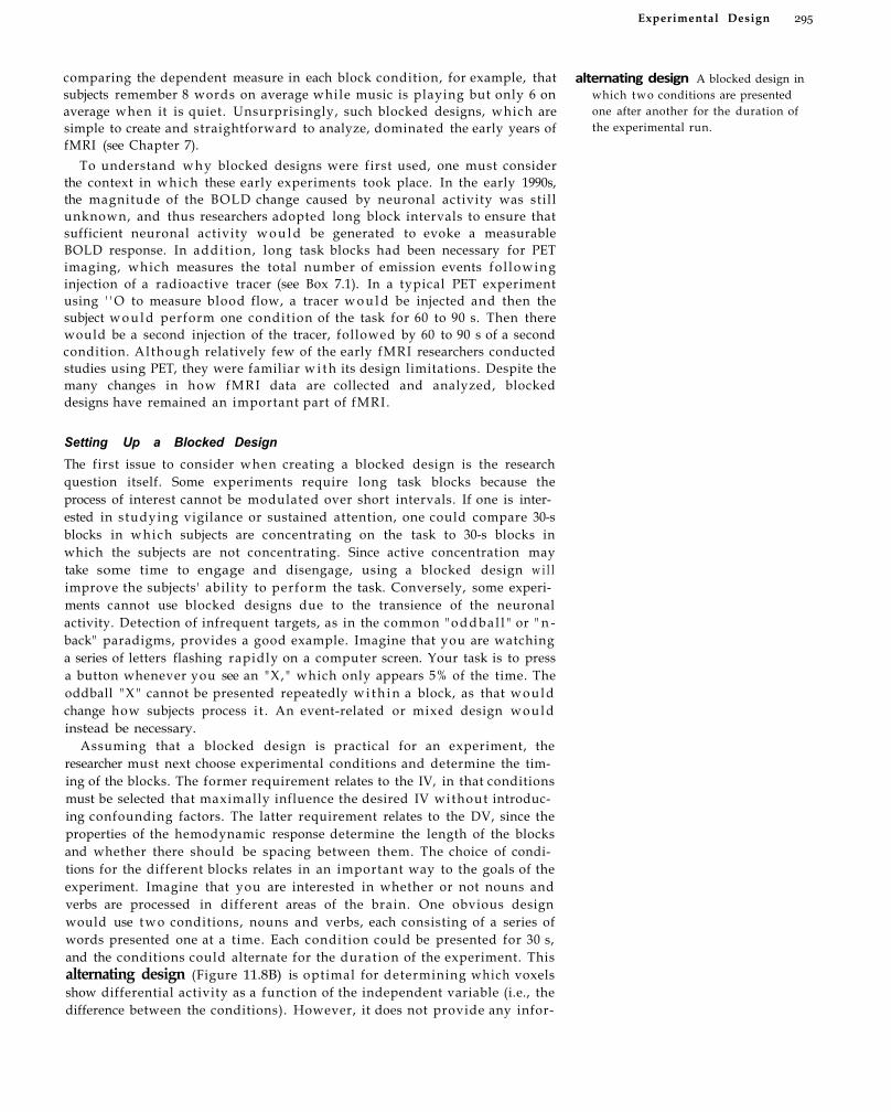
Experimental Design 295
comparing the dependent measure in each block condition, for example, that subjects remember 8 words on average while music is playing but only 6 on average when it is quiet. Unsurprisingly, such blocked designs, which are simple to create and straightforward to analyze, dominated the early years of fMRI (see Chapter 7).
To understand w h y blocked designs were first used, one must consider the context in which these early experiments took place. In the early 1990s, the magnitude of the BOLD change caused by neuronal activity was still unknown, and thus researchers adopted long block intervals to ensure that sufficient neuronal activity w o u l d be generated to evoke a measurable BOLD response. In addit ion, long task blocks had been necessary for PET imaging, which measures the total number of emission events fo l lowing injection of a radioactive tracer (see Box 7.1). In a typical PET experiment using ' ' O to measure blood flow, a tracer w o u l d be injected and then the subject w o u l d perform one condition of the task for 60 to 90 s. Then there would be a second injection of the tracer, followed by 60 to 90 s of a second condition. Although relatively few of the early fMRI researchers conducted studies using PET, they were familiar w i t h its design limitations. Despite the many changes in how fMRI data are collected and analyzed, blocked designs have remained an important part of fMRI.
Setting Up a Blocked Design The first issue to consider when creating a blocked design is the research question itself. Some experiments require long task blocks because the process of interest cannot be modulated over short intervals. If one is interested in studying vigilance or sustained attention, one could compare 30-s blocks in which subjects are concentrating on the task to 30-s blocks in which the subjects are not concentrating. Since active concentration may take some time to engage and disengage, using a blocked design w i l l improve the subjects' ability to perform the task. Conversely, some experiments cannot use blocked designs due to the transience of the neuronal activity. Detection of infrequent targets, as in the common " o d d b a l l " or " n -back" paradigms, provides a good example. Imagine that you are watching a series of letters flashing rapidly on a computer screen. Your task is to press a button whenever you see an "X, " which only appears 5% of the time. The oddball " X " cannot be presented repeatedly w i t h i n a block, as that would change how subjects process i t . An event-related or mixed design would instead be necessary.
Assuming that a blocked design is practical for an experiment, the researcher must next choose experimental conditions and determine the timing of the blocks. The former requirement relates to the IV, in that conditions must be selected that maximally influence the desired IV without introducing confounding factors. The latter requirement relates to the DV, since the properties of the hemodynamic response determine the length of the blocks and whether there should be spacing between them. The choice of conditions for the different blocks relates in an important way to the goals of the experiment. Imagine that you are interested in whether or not nouns and verbs are processed in different areas of the brain. One obvious design would use t w o conditions, nouns and verbs, each consisting of a series of words presented one at a time. Each condition could be presented for 30 s, and the conditions could alternate for the duration of the experiment. This alternating design (Figure 11.8B) is optimal for determining which voxels show differential activity as a function of the independent variable (i.e., the difference between the conditions). However, it does not provide any infor-
alternating design A blocked design in which two conditions are presented one after another for the duration of the experimental run.

296 C h a p t e r E l e v e n
control block A time interval that contains trials of the control condition.
null-task block A control block in which there are no task requirements for the subject. Also called a baseline block or nontask block.
mation about voxels that are active in both conditions or about the response to a single condition in isolation.
Another type of blocked design (Figure 11.8C) uses control blocks, such as watching a blank screen where there is nothing to read. Control blocks in which the subject does nothing are called null-task blocks. The presence of a control condition allows additional comparisons. Each experimental condition could be compared to the control condition to identify voxels that are activated by that condition independently. A comparison of noun reading and null-task blocks could f ind voxels associated w i t h all aspects of noun reading, including perceiving letters, sounding out words, and imagining objects. Note that none of these processes would be identified by the direct noun-verb contrast. Another common comparison is to combine the experimental conditions and contrast the combination wi th the control condition. In the example above, one could identify all voxels that are more active in response to the presentation of words than to the nul l condition. This is especially useful if you plan to use a region-of-interest approach. The combined condition has increased experimental power compared to individual conditions, so it can be used to find brain regions active across the two conditions. Then, one can probe those regions to see whether any show differences between the experimental conditions.
Under the direct subtraction logic that guides block analyses, the use of additional control conditions does not preclude direct comparison of conditions, as in an alternating design. One could still compare BOLD activity dur ing noun reading and verb reading, whi le ignoring any control condition. Additional conditions require additional time, however, and should not be added without necessity. Therefore, whenever you choose which conditions to include in a design, you should begin by evaluating whether a simple alternating design would be sufficient for answering your research questions. If not, consider what additional condition(s) would let you measure activity related to the general process of interest. Remember that control conditions may take many different forms. In the noun-verb example, possible controls could include a null-task condition, such as watching nonletter patterns or reading jumbled letter strings that do not form words. Depending on what aspect of reading is of interest, any of these control conditions might be reasonable.
After deciding on your experimental conditions, you should next consider the t iming of your task blocks. FMRI experiments have used blocks as short as several seconds and as long as a minute or two. Within that large range, the experimenter has considerable f lexibil i ty in the choice of timing parameters. Most important to consider is the effect of block length on the experimental task. Are there time constraints that preclude very short or very long blocks? In many working memory experiments, for example, subjects must rehearse a changing set of items over time. If the block is too short or too long, such a task may be too easy or too difficult. As in many psychology experiments, fatigue effects (and to a lesser extent, practice effects) should be considered. Very demanding tasks may be difficult to sustain over extended periods of time, and subjects may do worse at the end of a long block. In general, block length should be chosen so that the same mental processes are evoked throughout. We discuss trade-offs in functional SNR associated w i t h blocks of different lengths in the fol lowing section.
For most purposes, block length should be kept constant across the conditions. Remember that in an alternating design, the only statistical analysis that is possible is the difference between the two blocks. Even if one condition is labeled as the task and the other is called baseline, they are equally
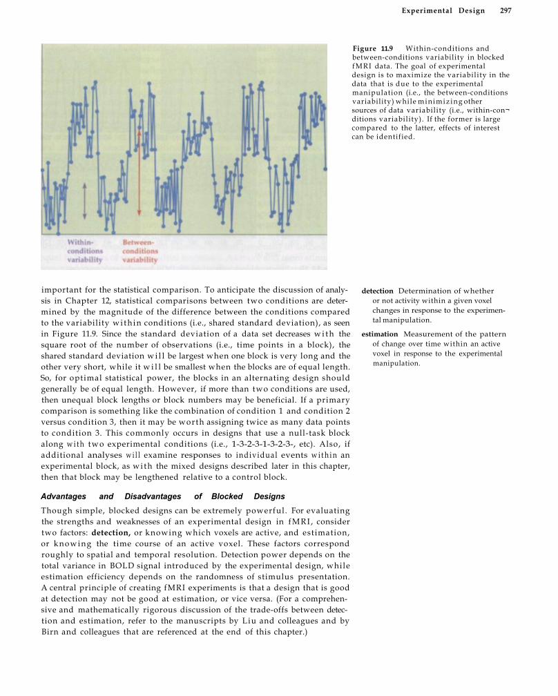
Experimental Design 297
Figure 11.9 Within-conditions and between-conditions variability in blocked fMRI data. The goal of experimental design is to maximize the variability in the data that is due to the experimental manipulation (i.e., the between-conditions variability) while min imiz ing other sources of data variability (i.e., within-con¬ditions variability). If the former is large compared to the latter, effects of interest can be identified.
important for the statistical comparison. To anticipate the discussion of analysis in Chapter 12, statistical comparisons between two conditions are determined by the magnitude of the difference between the conditions compared to the variability w i t h i n conditions (i.e., shared standard deviation), as seen in Figure 11.9. Since the standard deviation of a data set decreases w i t h the square root of the number of observations (i.e., time points in a block), the shared standard deviation w i l l be largest when one block is very long and the other very short, while it w i l l be smallest when the blocks are of equal length. So, for optimal statistical power, the blocks in an alternating design should generally be of equal length. However, if more than two conditions are used, then unequal block lengths or block numbers may be beneficial. If a primary comparison is something like the combination of condition 1 and condition 2 versus condition 3, then it may be worth assigning twice as many data points to condition 3. This commonly occurs in designs that use a null-task block along w i t h t w o experimental conditions (i.e., 1-3-2-3-1-3-2-3-, etc). Also, if additional analyses w i l l examine responses to individual events w i t h i n an experimental block, as wi th the mixed designs described later in this chapter, then that block may be lengthened relative to a control block.
Advantages and Disadvantages of Blocked Designs Though simple, blocked designs can be extremely powerful . For evaluating the strengths and weaknesses of an experimental design in f M R I , consider two factors: detection, or knowing which voxels are active, and estimation, or knowing the time course of an active voxel. These factors correspond roughly to spatial and temporal resolution. Detection power depends on the total variance in BOLD signal introduced by the experimental design, while estimation efficiency depends on the randomness of stimulus presentation. A central principle of creating fMRI experiments is that a design that is good at detection may not be good at estimation, or vice versa. (For a comprehensive and mathematically rigorous discussion of the trade-offs between detection and estimation, refer to the manuscripts by Liu and colleagues and by Birn and colleagues that are referenced at the end of this chapter.)
detection Determination of whether or not activity within a given voxel changes in response to the experimental manipulation.
estimation Measurement of the pattern of change over time within an active voxel in response to the experimental manipulation.
298 C h a p t e r E l e v e n
Figure 11.10 Effects of block interval on the fMRI hemodynamic response. These charts show simulated fMRI hemodynamic responses of voxels active only during the task block of an alternating on/off design. Note that as the block duration shortens below the width of the fMRI hemodynamic response, the response does not return to baseline. At very short block durations, there will be little to no difference between fMRI signal during active and inactive blocks. Note that the scales of the y-axes are reduced for block lengths of 8 s or less.
Blocked designs are very good for detecting significant fMRI activity. The detection power of a blocked design is determined by the balance between two factors. First, the difference in BOLD signal between conditions should be as large as possible. Figure 11.10 shows a simulation of how the measured BOLD activity changes as the length of the blocks changes from very long (40 s) to very short (2 s). At long block lengths, a very large response is evoked during the task blocks and the response returns to baseline during the nontask blocks. Thus, there is maximal variability between the blocks. If the block length is sufficiently short (i.e., less than about 10 s) that the hemodynamic response cannot return to baseline during the nontask blocks, BOLD amplitude w i l l be reduced. This reduces the total variability in the data, which in turn reduces the experimental power. In extreme cases, such as those with block lengths of only a few seconds, there w i l l be almost no difference between task and nontask conditions. In summary, the use of long block intervals provides maximal BOLD amplitude changes between conditions.
Second, there should be as many transitions as possible between the conditions, to minimize the noise present at the task frequency. Remember that the noise in a BOLD time course has its highest power at low frequencies and lowest power at high frequencies. For example, at very low frequencies, there can be significant scanner drift associated w i t h problems w i t h the scanner hardware. If your design has very long (e.g., 180 s) experimental and control blocks, it w i l l be diff icult to know whether signal changes from one block to the next result from the experimental manipulation or from low-frequency noise. As the block length is reduced, the task frequency increases and thus the design is more immune to low-frequency noise.
scanner drift Slow changes in voxel intensity over time.

E x p e r i m e n t a l D e s i g n 299
Together, these factors indicate that the signal change at the task frequency w i l l be greatest at relatively long block lengths, while the noise at the task frequency w i l l be smallest at relatively short block lengths. As a rough guideline, block lengths of approximately the duration of the hemodynamic response (i.e., 10 s) provide large signal changes while reducing noise at the task frequency to an acceptable level. However, depending on the spectrum of the noise, detection power may increase at even shorter block intervals of 6 to 8 s (see McCarthy and colleagues, 1996, for an example). Longer blocks are often required for experiments that test cognitive processes like memory and attention, since it is di f f icult to ensure that those processes begin promptly at the block onset. It is important to recognize that if design constraints necessitate the use of very short block periods, those blocks should be treated like single events and their order should be randomized. This procedure is described in the section on event-related designs.
While their detection power can be very good, blocked designs are relatively insensitive to the shape of the hemodynamic response. We can understand this insensitivity by returning to the idea of superposition, which was introduced in Chapter 8. Setting aside refractory effects for the moment, the hemodynamic response to two identical st imuli presented in succession is equal to the sum of the individual responses. As more and more st imuli are presented in succession, each contributes to the total hemodynamic response. With task blocks of about 10 s or longer, which are greater than the w i d t h of the hemodynamic response to a single stimulus, every time point wi th in the block contains a contribution from multiple stimuli , each at a different phase. The combined hemodynamic response thus rises rapidly at the onset of the task, thereafter remaining at a plateau value unti l the cessation of the block.
Since the plateau value represents contributions from all phases of the hemodynamic response, the particular shape of the response does not matter. Figure 11.11 shows four sample hemodynamic responses, each wi th a different shape, and how they w o u l d change as more events are presented. A l l four responses have the same total signal amplitude, as measured by the area under the curves. Consider the standard hemodynamic response shown in Figure 11.11 A. As the length of the response block is increased from 2 to 32 events, each 1 s in duration and separated by 2 s, there is a consistent and smooth increase in overall hemodynamic amplitude, reaching a plateau at block lengths of about 12 s or longer. N o w suppose that the hemodynamic response has a simple triangular form (Figure 11.11B). Obviously, this form differs considerably from that of the canonical hemodynamic response. But as the length of the block increases, the total hemodynamic response in panel B becomes more and more similar to that in panel A. As can be seen in the subsequent panels, the insensitivity of blocked designs to hemodynamic shape would hold if the hemodynamic response had two peaks (Figure 11.11C) and even if its values were completely randomized over the response duration (Figure 11.11D). For the same reasons, designs that use long stimulus blocks are also relatively insensitive to changes in the t iming of the hemodynamic response.
insensitivity to the shape and t iming of the hemodynamic response has both advantages and disadvantages. The primary advantage is that it makes experimental analyses extraordinarily simple. When blocked, any hemodynamic response can be robustly modeled using a smoothed trapezoidal shape consisting of a rise, plateau, and fall . To evaluate the effect of the IV, the magnitude of the BOLD response dur ing the task period can be compared to that dur ing a baseline period. If there is no effect, the random differences in activity between the blocks would fol low the t-distribution, so the magnitude of the t-statistic reveals the significance of the effect. Other
superposition A principle of linear systems that states that the total response to a set of inputs is equivalent to the summation of the independent responses to the inputs.
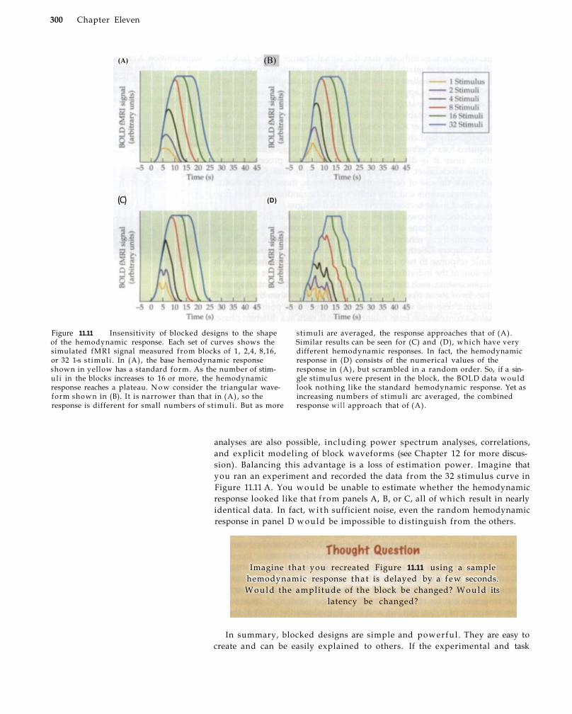
300 Chapter Eleven
analyses are also possible, including power spectrum analyses, correlations, and explicit modeling of block waveforms (see Chapter 12 for more discussion). Balancing this advantage is a loss of estimation power. Imagine that you ran an experiment and recorded the data from the 32 stimulus curve in Figure 11.11 A. You would be unable to estimate whether the hemodynamic response looked like that from panels A, B, or C, all of which result in nearly identical data. In fact, w i t h sufficient noise, even the random hemodynamic response in panel D would be impossible to distinguish from the others.
Figure 11.11 Insensitivity of blocked designs to the shape of the hemodynamic response. Each set of curves shows the simulated fMRI signal measured from blocks of 1, 2,4, 8,16, or 32 1-s st imuli . In (A), the base hemodynamic response shown in yellow has a standard form. As the number of stimuli in the blocks increases to 16 or more, the hemodynamic response reaches a plateau. N o w consider the triangular waveform shown in (B). It is narrower than that in (A) , so the response is different for small numbers of st imuli . But as more
stimuli are averaged, the response approaches that of (A) . Similar results can be seen for (C) and (D), which have very different hemodynamic responses. In fact, the hemodynamic response in (D) consists of the numerical values of the response in (A) , but scrambled in a random order. So, if a single stimulus were present in the block, the BOLD data would look nothing like the standard hemodynamic response. Yet as increasing numbers of stimuli arc averaged, the combined response w i l l approach that of (A) .
(C)
(A)
(D)
(B)
Imagine that you recreated Figure 11.11 using a sample hemodynamic response tha t is delayed by a f e w seconds. W o u l d the ampli tude of the block be changed? W o u l d its
latency be changed?
In summary, blocked designs are simple and powerful . They are easy to create and can be easily explained to others. If the experimental and task

E x p e r i m e n t a l D e s i g n 301
BOX 11.2 Baseline Activity in fMRI
The basic assumption of blocked designs is that block-related changes in BOLD signal result from differ
ences between the experimental conditions. In the usual subtractive approach, there are two conditions: task and control. The task condition is assumed to consist of all of the neural processes present in the control condition, along with additional processes of interest. Consider the results from the following simple task, which were reported by Binder and colleagues in 1999. During task blocks, subjects listened to sequences consisting of low and high tones and pressed a hut-ton if a given sequence included two high tones (e.g., L-L-H-L-H). In control blocks, the subjects lay still in the scanner with their eyes closed. Each block lasted 24 s. Not surprisingly, the tone task evoked more fMRI BOLD activity than control blocks within the auditory, prefrontal, parietal, and motor cortices, among many other regions. These areas reflect regions that are associated w i t h perception, decision, and response aspects of the task. The authors then looked for brain regions that were less active during the task blocks than during the rest blocks. Remarkably, a number of regions showed increased activity during rest, including the lateral parietal cortex (angular gyrus), the posterior cingu¬late or precuneus, the superior frontal gyrus, and the ventral prefrontal cortex. This pattern of results, which has been confirmed by many studies using both fMRI and PET, suggests that the assumptions of the subtractive method may be flawed. Some aspects of cognition may actually be inhibited during performance of psychological experiments, such that cognitive processes present in the control condition may not be present during the task condition. In the last few years, interpreting deactivations, or decreases in hemodynamic activity, has become an area of considerable interest.
What does it mean for fMRI activity to decrease during an experimental task? In answering this question, it is critical to recognize that blocked designs only provide information about the relative difference between two conditions, not about absolute levels of activity. Without a clear baseline to which both conditions can be compared, several different types of changes in absolute activity could result in similar changes in relative activity (Figure 11.12A-E). Gusnard and Raichle, in a 2001 comprehensive review of many research studies, suggest that the appropriate baseline condition for functional neuroimaging studies should be defined using the oxygen extraction fraction
(OEF), which is largely stable across the brain (Figure 11.13). Even though some areas of the brain have greater blood flow than others, and some areas have higher oxygen requirements than others, the proportion of oxygen that is extracted when the subjects are resting with their eyes closed is spatially uniform, with only a few exceptions. Remember from Chapter 7 that the OEF decreases as part of the BOLD response due to an overcompensatory increase in blood flow. Thus, decreases from baseline OEF indicate increased neuronal activity, whereas increases indicate decreased neuronal activity.
By measuring the OEF at rest and during experimental conditions, whether directly using PET or indirectly via fMRI , researchers have identified a set of brain regions that show decreases in activity during performance of a wide range of experimental tasks. These regions in-
Figure 11.12 Possible origins of increases and decreases observed in fMRI . When experimental and control tasks are compared using a blocked design, there are several possible causes of observed increases or decreases in hemodynamic activity. First, an increase in activity d u r i n g the experimental task could be observed when both tasks are either above baseline (A) or below baseline (B). Likewise, decreases in activity dur ing the experimental task could be observed when both are above baseline (C) or below baseline (D). Note than in (A) and (C), either task could have a positive effect compared to baseline, but in (B) and (D), either could have a negative effect compared to baseline. If the tasks result in opposite activity (E), comparisons of the tasks w i t h each other w o u l d be likely to yield a large effect, but neither may show a change versus baseline. (From Gusnard and Raichle, 2001.)
deactivations Decreases in BOLD activity during task blocks compared to nontask blocks.
oxygen extraction fraction (OEF) The proportion of available oxygen that is removed from the blood.
(A)
Increases Increases
(C)
Decreases Decreases
(E)
Indeterminate
(B)
(D)
Baseline Control task Task of interest

302 C h a p t e r E l e v e n
BOX 11.2 (continued)
clude medial and lateral aspects of the parietal cortex, as well as dorsomedial and ventromedial areas of the frontal cortex. What functions might these regions subserve? A likely possibility is that they may play important roles in the monitoring of external stimuli. Both the medial and lateral parietal cortices have been implicated in spatial and attentional processes. However, neuroimaging and single-unit studies indicate that these regions are not associated with attention to expected stimuli. Instead, they seem to be more associated with peripheral or unexpected events, consistent with the idea that they are part of a generalized monitoring system. The ventromedial frontal cortex, in contrast, is typically associated with emotional processing, including assessments of the likely reward consequences of future actions. The dorsomedial frontal cortex may mediate reflective thought, such as apper¬ceiving one's state of mind or evaluating what others might be thinking. Together, the monitoring and reflecting processes associated with baseline activity can be integrated into the construct of "self-directed thought" (see Gusnard and Raichle for discussion of this idea).
To experience self-directed thought, close your eyes and relax for at least 10 seconds. If you are like most people, you wil l feel an initial sense of withdrawal from the world around you, followed by a growing sensitivity to external stimuli. You wil l notice sounds that had previously been outside your awareness. You wil l become sensitive to heretofore unnoticed muscle tension or joint pain. In short, the baseline state of brain activity is very different from that evoked by a demanding task, like reading this book. This difference was recognized by Wil l iam James, w h o described introspection thusly: "When I try to remember or reflect, the movements [in the mind | in question, instead of being directed toward the periphery, seem to come from
the periphery inwards and feel like a sort of withdrawal from the outside wor ld ." (1890, p. 300)
Here, James emphasizes the essential difference between active and reflective states. The former is goal-directed, aimed at changing the surrounding environment or one's place in it. The latter is self-directed and passive, seeking information about the environment James also notes his awareness of particular body motions during introspection, and how those physical movements might relate to the movement of thoughts. As in much of James's writing, his well-reasoned reflections anticipate the present discussion of baseline brain activity by more than a century. Rest or baseline conditions are not absent of mental processes. Instead, they contain particular types of processes associated with reflection, daydreaming, self-assessment, bodily attention, and emotion.
When designing an fMRI experiment, you must account for reflective processes in your choice of experimental and control conditions. Should the control condition have no explicit task requirements, subjects wi l l naturally begin thinking about how they are doing in the experiment, what they wil l have for dinner, wh ich friends they wil l see this evening, or even a dull pain in their lower back that they only now are beginning to notice. For this reason, rest or null-task conditions are not recommended, at least as the sole control condition. Instead, conditions should be chosen so that subjects are a lways performing some active task or attending to a changing environment. For example, if the experimental condition consists of judging the familiarity of remembered words, consider a control condition where subjects read words and indicate whether they are presented in capital or lowercase letters. Both condi-
Figure 11.13 The oxygen extraction fraction (OEF) as a possible baseline for brain activity. Gusnard and Raichle suggest that the OEF, the proportion of available oxygen that is extracted from the blood, is highly stable across the brain and represents a good baseline for brain activity. Shown are four axial slices (z = -4, 12, 28, and 44 mm). Also shown here are relative cerebral blood flow (CBF) and cerebral metabolic rate for oxygen (CMRO 2 ) ; the ratio between these quantities gives the OEF. The arrows indicate the only regions of increased oxygen extraction relative to the remainder of the brain. These are in the visual cortex and likely reflect the fact that the subjects in this data set had their eyes closed. The baseline for these regions may reflect open eyes and normal visual stimulation. (From Gusnard and Raichle, 2001.)
CBF
Maximum
Minimum
OEF
CMRO2

E x p e r i m e n t a l D e s i g n 303
conditions are chosen carefully, then analysis becomes very straightforward. Blocked designs are very good at detecting voxels w i t h significant activity, and they are also robust to uncertainty in the timing and shape of the hemodynamic response. However, because the experimental condition is extended in time, the brain activity it evokes may be highly heterogeneous over time, and some tasks may be inappropriate for blocked designs. They are also poor at estimating the time course of activity in active voxels.
Event-Related Designs
The second major class of fMRI experiments is characterized by the use of event-related designs. The central assumption of an event-related design is that the neural activity of interest w i l l occur for short and discrete intervals, as when a brief flash of l ight evokes transient activity in the visual cortex. Stimuli that generate such short bursts of neural activity are known as events or trials. In most event-related designs, different conditions of the IV are associated w i t h different events, similar to the relationship shown in Figure 11.14. Each event is separated in time from the previous event, w i t h an interstimulus interval, or ISI, that can range from about 2 s to 20 s depending on the goals of the experiment. This differs from typical blocked designs, which may present many s t imul i consecutively w i t h i n a task block. Also unlike blocked designs, the different conditions are usually presented in a random order rather than an alternating pattern. Event-related designs have sometimes been called single-trial designs, to emphasize that s t imul i are presented one at a time rather than w i t h i n a block of trials. However, as data collection and analysis procedures have improved, analyses of changes in BOLD signal fol lowing only one stimulus presenta-
event-related design The presentation of discrete, short-duration events whose timing and order may be randomized.
event A single instance of the experimental manipulation. Also known as a trial.
interstimulus interval (ISI) The separation in time between successive stimuli. Usually refers to the time between the offset of one stimulus and the onset of the next, with the term stimulus-onset asynchrony (SOA) used to define the time between successive onsets.
Figure 11.14 Schematic diagram of an event-related fMRI design. The basic idea underlying event-related fMRI designs is that the processes of interest can be evoked transiently by brief presentations of individual stimulus events. Here, the
tions require attention and decision processes, thus precluding activity in the baseline system, but only the former invokes memory processes. Another suggested procedure is to explicitly include a null-task condition wi th in your design
to provide a baseline. By doing so, you can evaluate whether relative differences between your conditions reflect differential increases above baseline or an effect for one condition but not the other (see Figure 11.12). Understanding the effect of
baseline processing upon fMRI data is important for any researcher, but it is especially critical for those w h o use blocked designs.
B O X 11.2 (continued)
Time relative timing of a series of stimuli is shown by their positions along the axis. In the design shown here, the activity in response to the face stimuli can be compared to the activity in response to the object stimuli.

304 Chapter Eleven
electroencephalogram (EEG) The measurement of the electrical potential of the brain, usually through electrodes placed on the surface of the scalp.
time-locking Synchronization of analyses to events of interest, usually for the extraction of epochs.
signal averaging The combination of data from multiple instances of the same manipulation in order to improve functional SNR.
event-related potentials (ERPs) Small electrical changes in the brain that are associated with sensory or cognitive events.
tion have become possible, and thus the label single-trial should be reserved for such experiments.
Early Event-Related fMRI Studies Event-related designs were rarely used in the early years of fMRI . Most research used long-interval blocked designs, wi th the notable exception of the 1992 study by Blamire and colleagues discussed in Chapter 7. Furthermore, even the few studies that measured the BOLD response to short-duration stimuli failed to conduct the additional analyses (i.e., trial averaging, latency measurements) that event-related designs afford. Within a few years, however, the design concepts drawn from PET were joined by ideas from another source, electrophysiology. Since the first recordings of electrical activity in the human brain by Hans Berger in the 1920s, researchers had known of tonic changes in the electroencephalogram (EEG) associated wi th different states of arousal or alertness. These changes were identified by comparing the EEG pattern during one state (e.g., deep sleep) to the pattern during another state (e.g., waking). By the late 1950s and early 1960s, researchers began investigating whether signals associated wi th specific sensory or cognitive events could be identified w i t h i n the continuous EEG. By synchronizing or time-locking the EEG signal to the onset of a stimulus and signal averaging across many trials, they could extract small electrical changes known as event-related potentials, or ERPs, from the continuous EEG. Some ERPs, particularly those wi th short latencies (e.g., <100 ms), were associated wi th sensory processing. Others were associated wi th cognitive events. For example, the detection of an unexpected task-relevant stimulus evokes a systematic positive ERP deflection (now known as the P300) about 300 ms fol lowing the stimulus onset.
The key concepts underlying ERP studies, namely time-locking and signal averaging, became the basic principles of event-related fMRI. One of the first studies to compare event-related and blocked designs was reported by Buck¬ner and colleagues in 1996. Their subjects were shown w o r d stems, such as "ope-" or " f u t - , " and then were instructed to mentally generate completions of those stems (e.g., "opening," " future") . Previous blocked-design studies had shown that this task evokes activity in the visual and motor cortices, as well as in Broca's area, which is a language region wi th in the left inferior prefrontal cortex. In runs of the blocked design, the w o r d stems were presented about every 2 s wi th in 30-s blocks that alternated wi th 30-s rest periods. Runs using the event-related design consisted of singly presented word stems that were followed by interstimulus intervals of about 15 s. Each subject participated in five to six runs of each type, w i t h each run lasting 3 to 4.5 minutes. Note that many more words were presented in the blocked runs than in the event-related runs. During the task, BOLD fMRI data were recorded using an asymmetric spin-echo echo-planar pulse sequence at 1.5 T. Four subjects were tested at a TR of 2 s, and two were tested at a TR of 1 s. The authors hypothesized that similar patterns of activity would be elicited by both design types, which w o u l d validate the use of event-related designs. Furthermore, they anticipated that the event-related design could provide additional information about the t iming of BOLD activity.
In their first analyses, Buckner and colleagues identified active voxels using the blocked presentation runs, and then evaluated the time course of activity in those voxels fol lowing single stimuli in the event-related runs. As expected, they found regions w i t h block-related activity in the visual, motor, and left prefrontal cortices (Figure 11.15A). The critical test, however, was whether those same regions w o u l d show significant event-related activity
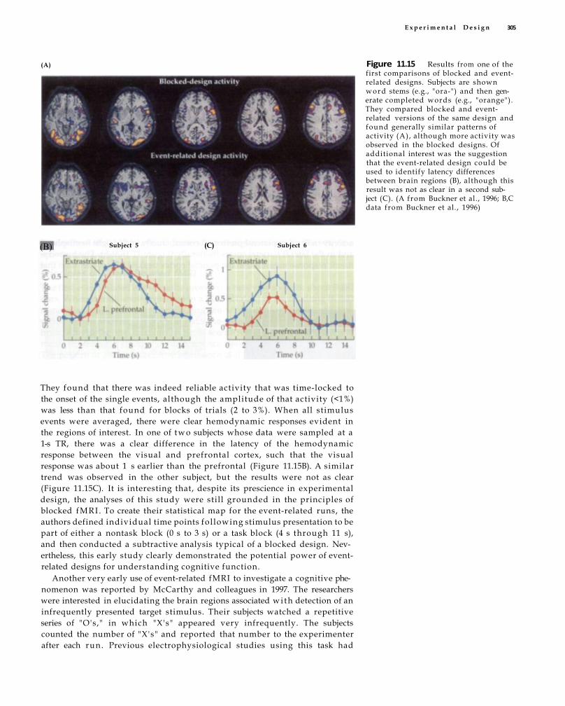
E x p e r i m e n t a l D e s i g n 305
(A) Figure 11.15 Results from one of the first comparisons of blocked and event-related designs. Subjects are shown word stems (e.g., "ora-") and then generate completed words (e.g., "orange"). They compared blocked and event-related versions of the same design and found generally similar patterns of activity (A), although more activity was observed in the blocked designs. Of additional interest was the suggestion that the event-related design could be used to identify latency differences between brain regions (B), although this result was not as clear in a second subject (C). (A from Buckner et al., 1996; B,C data from Buckner et al., 1996)
They found that there was indeed reliable activity that was time-locked to the onset of the single events, although the amplitude of that activity (<1%) was less than that found for blocks of trials (2 to 3%). When all stimulus events were averaged, there were clear hemodynamic responses evident in the regions of interest. In one of t w o subjects whose data were sampled at a 1-s TR, there was a clear difference in the latency of the hemodynamic response between the visual and prefrontal cortex, such that the visual response was about 1 s earlier than the prefrontal (Figure 11.15B). A similar trend was observed in the other subject, but the results were not as clear (Figure 11.15C). It is interesting that, despite its prescience in experimental design, the analyses of this study were still grounded in the principles of blocked fMRI . To create their statistical map for the event-related runs, the authors defined individual time points fol lowing stimulus presentation to be part of either a nontask block (0 s to 3 s) or a task block (4 s through 11 s), and then conducted a subtractive analysis typical of a blocked design. Nevertheless, this early study clearly demonstrated the potential power of event-related designs for understanding cognitive function.
Another very early use of event-related fMRI to investigate a cognitive phenomenon was reported by McCarthy and colleagues in 1997. The researchers were interested in elucidating the brain regions associated wi th detection of an infrequently presented target stimulus. Their subjects watched a repetitive series of "O's," in which "X's" appeared very infrequently. The subjects counted the number of "X's" and reported that number to the experimenter after each run. Previous electrophysiological studies using this task had
Subject 5 Subject 6 (C) (B)

306 C h a p t e r E l e v e n
epoch A time segment extracted from a larger series of images, usually corresponding to the period in time surrounding an event of interest.
averaged epoch The result of averaging a large number of epochs that are time-locked to similar events.
implicated the prefrontal cortex, parietal cortex, and hippocampus in the generation of the P300 event-related potential to infrequent target s t imuli , and the authors hypothesized that these brain regions w o u l d also evince BOLD activity. Note that this hypothesis could not be tested using a blocked design, since that requires the target events to be randomly separated in time from one another. That is, if you presented a block of "O's" and then a block of "X's," the "X's" w o u l d no longer be unexpected and infrequent. To test their hypothesis, the authors collected gradient-echo echo-planar images at a TR of 1.5 s using a 1.5-T scanner. From the overall time series of volumes, they identified when the target "X's" occurred and then excised segments consisting of the six images before and nine images after each target. Segments of a time series that are time-locked to the presentation of an event are known as epochs, and the result of averaging all the epochs from one condition is an averaged epoch. The significance of each voxel at each time point in the epoch was determined by t-test (see Chapter 12).
The authors found that detection of an infrequent target evoked BOLD activity in the dorsolateral prefrontal cortex, chiefly in the right hemisphere, and in the lateral parietal cortex bilaterally (Figure 11.16A-F). The hemodynamic response measured in the parietal cortex peaked 1.5 s earlier than that
(A) (B) (E)
Time since stimulus onset (s)
Figure 11.16 Use of event-related fMRI to study behavioral selection. Brain regions associated with selection of a response to a rare target stimulus are investigated. The target stimuli evoked activity in the dorsolateral prefrontal cortex
(A and B) and in the lateral parietal cortex (C and D). Shown are the event-related responses evoked by these target stimuli in the prefrontal (E) and parietal (F) cortices. (A-D from McCarthy et al., 1997; E,F data from McCarthy et al., 1997.)
(C) (D) (F)
E x p e r i m e n t a l D e s i g n 307
in the prefrontal cortex. No significant activity was found in the hippocampus, which may have reflected signal loss associated w i t h magnetic susceptibility artifacts in ventral portions of the brain. Two aspects of the experimental design are wor th noting, as they illustrate fundamental features of event-related fMRI . First, no matter what analysis is conducted, statistical tests must always evaluate BOLD activity associated w i t h changes in the independent variable. Regardless of whether the analysis uses a simple t-test, as in the McCarthy and colleagues study, or correlation or general linear model approaches, the significance of the analysis depends on the difference in the BOLD signal evoked by the task condition and a control condition. The control condition may be implici t , perhaps merely the absence of the task condition, but it is always there (see Box 11.2). Second, some experimental questions can only be answered w i t h event-related fMRI and not with blocked-design fMRI . Many cognitive processes, like attention, working memory, and target detection, may take on a fundamentally different character when repeated a number of times successively w i t h i n a block. Researchers should always evaluate what design is necessary for eliciting activity of interest.
Principles of Event-Related fMRI The first event-related experiments provided a new way to think about fMRI data. When stimuli were presented in a blocked design, the resulting BOLD signal was considered to reflect the magnitude of neural activity in one condition versus another. Thus, fMRI data were assumed to reflect steady-state brain activity at any moment in time. Event-related studies, in contrast, measured transient changes in brain activity associated w i t h discrete stimuli. The pattern of changes over time became critical for experimental analyses. For this reason, high temporal resolution is more important for event-related studies than for blocked studies. Often in event-related studies, successive images are acquired w i t h TRs of 1 to 2 s, in order to sample the hemodynamic response at a sufficiently fast rate. The temporal sensitivity of event-related designs has different consequences for detection and estimation. If the measured hemodynamic response differs from the hypothesized response, even by only a small amount (see Chapter 8), then the detection power of the experimental test w i l l be greatly reduced. More positively, estimation of the time course of the hemodynamic response is often very good, especially when events are presented in relative isolation or when sophisticated deconvolution strategies are applied.
From the linear systems framework that was discussed in Chapter 8, one can consider stimulus events as impulses, each of which evokes a hemodynamic response. As first demonstrated by Boynton and colleagues in 1996, the amplitude and t iming of a hemodynamic response depend upon both the intensity and the duration of the evoking stimulus. To the extent that the linear assumption holds (i.e., that the BOLD responses to successive stimuli do not interact), it is possible in principle to present events very rapidly and extract the hemodynamic response associated w i t h individual events. Dale and Buckner investigated this issue in a 1997 study (see Chapter 8 for related experiments). They hypothesized that signal averaging could be applied to event-related designs even if the events were presented only a few seconds apart, despite the much slower (10 to 15 s) rise and fall of the hemodynamic response. The stimuli were flashing checkerboards of 1-s duration presented to either the left visual field or the right visual field (remember that a visual stimulus presented to the left evokes activity in the right visual cortex, and vice versa). Importantly, the order of presentation of the st imuli was ran-
linear system A system that obeys the principles of scaling and superposition.
impulse A single input to a system. Impulses are assumed to be of infinitely short duration.

308 C h a p t e r E l e v e n
domized, not alternated, because alternation at such short interstimulus intervals would have removed any effects (see Figure 11.10, for example).
Figure 11.17 shows data from one of their experiments. At interstimulus intervals of only 2 s, robust activity for each trial type could be detected in the contralateral pr imary visual cortex. In fact, the observed activity was more easily detected at shorter intervals than at longer intervals. This seems counterintuitive, but remember that experimental power depends on the number of events that are averaged. In the 2-s condit ion, there were many more trials per experimental run than in the longer-interval conditions. When more trials are presented in rapid succession, the total variance in the BOLD signal increases, resulting in more experimental power. Dale and Buckner demonstrated that, provided that the events of interest are presented in a random order, areas of BOLD activity can be detected even using very short interstimulus intervals.
Figure 11.17 Rapid event-related fMRI w i t h randomized stimulus presentation. FMRI activity associated w i t h different stimulus types can be extracted from very rapid event-related designs, provided that the order of st imuli is randomized. In this experiment, visual st imuli were presented to either the left or r ight visual field w i t h 2-s, 5-s, or 10-s intertrial intervals. Differential patterns of activity in response to the two stimulus types could be easily established at all intervals. Interestingly, the least activity was found at the longest intertrial interval, due to the much reduced number of experimental trials that were presented there compared to the shorter-interval conditions. (From Dale and Buckner, 1997.)
Left-hemifield trials
Right hemifield trials
2-second intertrial interval
5-second intertrial interval
10-second intertrial interval
How would the assumptions of event-related fMRI be violated if the neuronal activity in response to an event was not an
impulse but instead had a long duration (e.g., 5 s)? How would the hemodynamic response change?

Experimental Design 309
Now, does this study imply that short intervals are best for event-related studies? Not necessarily, in that its results focused on detection of areas of activity, not estimation of the time course of the hemodynamic response. Remember from Chapter 8 that hemodynamic refractory effects are present at interstimulus intervals of about 6 s or less. Thus, at shorter intervals, the evoked hemodynamic response may be of less amplitude than at long intervals (i.e., 15 s or greater). For this reason, researchers may use longer intervals between st imuli when attempting to measure the time course of the hemodynamic response. Another advantage of using long intervals is that, since the hemodynamic response has time to complete its rise and fall, they allow estimation of the baseline level of activity measured in the absence of stimulation. Typically, the baseline is identified by averaging the few time points that immediately precede each stimulus, creating a prestimulus baseline. This allows comparison not only between experimental conditions but also between each experimental condition and the baseline. In addition, some tasks may require long intervals due to their very nature, such as those involved in studying w o r k i n g memory, retrieval from long-term memory, decision making, or hemodynamic refractory effects. While sometimes necessary, the use of long intervals reduces the number of experimental trials, reducing detection power (e.g., see Figure 9.19). When designing a study, researchers should strive to reduce the interstimulus interval as much as possible to maximize the number of experimental trials collected.
Also important for event-related studies, especially those where only a single type of event is presented, is whether the interstimulus intervals are periodic or jittered. As the name implies, a periodic event-related design presents the events of interest at regular intervals. Slow (>15-s ISI) periodic designs are conceptually very simple, and their analysis is straightforward. Each event evokes a complete hemodynamic response, and events can be combined through selective averaging. Slow periodic designs are inefficient, however, due to their low density of events over time. Fast periodic designs would seemingly be more efficient, following the logic of the previous paragraph, but in fact may be even less practical. In 2001, Bandettini and Cox attempted to determine the best interstimulus interval for periodic presentation of a short-duration (2-s) stimulus. They found that at intermediate intervals of 10 to 12 s, substantial stimulus-related variability was present in the data, as visible in Figure 11.18A and B. However, as they shortened the interstimulus interval, the effects of the individual trials became less and less apparent. At the shortest interval tested, 2 s, there was a transient increase in BOLD activity at the beginning of the run but a plateau thereafter, precluding analysis of any i nd i v idua l trials.
Note that the difference between this study and that of Dale and Buckner, who found significant effects at 2 s, was that the latter presented two types of st imuli in random order. Randomization effectively jitters the time between successive onsets of the same stimulus, so that sometimes it w i l l occur several times in a row and other times there w i l l be a long interval between successive presentations. Without jittering, the BOLD signal w i l l saturate to some maximal value wi th repeated presentations of the stimulus, becoming equivalent to a block of trials. However, the j ittering must be sufficiently large relative to the period of the hemodynamic response to have a meaningful effect.
We emphasize that the t iming constraints described here apply to the interval between successive events and not necessarily to the interval between successive stimuli. Imagine an experiment that presented two types
prestimulus baseline The calculation of a baseline value based on the BOLD signal present before events of interest.
periodic event-related design An experimental design in which events of interest occur at regular intervals.
jittering Randomizing the intervals between successive stimulus events over some range.

310 C h a p t e r E l e v e n
(A) (B)
Figure 11.18 Effects of interstimulus interval upon event-related fMRI activity. As the interval between successive events decreases, the overlap between consecutive hemodynamic responses reduces the variability in the BOLD signal. Subjects performed a finger tapping task whi le watching a flashing visual stimulus. Activity w i t h i n regions of interest in the visual cortex (A) and motor cortex (B) was measured
under a number of different experimental conditions. When there was a long interstimulus interval (ISI) of 20 s and a long stimulus duration (SD) of 20 s, mimicking a blocked design, there was clear alternating activation in both regions. However, for short-duration events of 2 s, periodic activity was present at long ISIs of 10 to 12 s but not at short ISIs. (From Bandettini and Cox, 2000.)
semirandom design A type of event-related design in which the probability that an event will occur within a given time interval changes systematically over the course of the experiment.
of st imuli , words and nonword letter strings. If you knew that a given brain region responded to the words but not the nonwords, you could embed the words in a rapidly presented series of nonwords and the words would still evoke a large hemodynamic response. For that brain region, only the words w o u l d serve as events. However, for another brain region that responds equally to both words and nonwords, both types of stimuli would serve as events and BOLD activity would be at a steady state throughout the experiment. This logic is identical to that used in the study by McCarthy and colleagues described in the last section, and bears similarities to the fMRI-adaptation paradigms described in Chapter 8.
Semirandom Designs In a periodic design, events are presented at a constant interstimulus interval , such as once every 16 s. In a randomized or jittered design, the interstimulus interval is determined by a fixed probability, expressed in terms of either the l ikelihood of a stimulus being presented at each time point (randomization) or the l ikelihood of a given ISI fol lowing each stimulus (jittering). While most event-related designs have used either a periodic or a jittered approach, a third type of design, semirandom design, has become increasingly popular (Figure 11.19A-C). In a semirandom design, stimulus probability varies systematically over time. One way to create such a design is to create "blocks" of stimulus probabilities. Imagine that your event is a flashing checkerboard presented for 500 ms, and you are sampling the brain at a TR of 1000 ms. You set up your experiment so that in the first 30-s block, each TR has a 25% chance of containing an event; in the next 60-s block, each TR has a 75% chance; and in the final 30 s, each TR has a 25% chance. The resulting design would look similar to Figure 11.19C. Another way to create a semirandom design is to have probability change smoothly over the exper-
Visual cortex Motor cortex

E x p e r i m e n t a l D e s i g n 311
(A)
(B)
imental run (i.e., in a sinusoidal fashion) from some maximum to some minimum value. Although composed of individual events, semirandom designs are similar to blocked designs in that some time periods contain many events while others contain very few. As wi th blocked designs, this clustering increases the total variability in the BOLD signal.
L i u and colleagues conducted a number of simulations in 2001 to determine the relative advantages of semirandom designs compared to similar blocked or event-related designs. They found that although a semirandom design w i l l always have slightly less detection power than a blocked design with the same number of events and blocks, due to its incomplete clustering, it w i l l show substantial increases in estimation efficiency. More recent work by Liu and colleagues has extended these results to experiments wi th multiple tr ial types. Semirandom designs may be a good choice for experiments that value both detection and estimation. However, if the process of interest differs across ISIs, then the basic assumption of the semirandom design is violated. K n o w n causes of ISI-related differences include hemodynamic refractory effects, especially at very short intervals, and changes in cognitive processes based on rate of presentation (i.e., a task may be simpler at slow rates than at fast rates). Nevertheless, semirandom design should be considered as a potentially valuable technique for opt imizing trade-offs between detection and estimation.
Advantages and Disadvantages of Event-Related Designs In general, the strengths of event-related designs mirror the weaknesses of blocked designs, and vice versa. While blocked designs are very poor at estimating the shape of the hemodynamic response, event-related designs have good estimation power. Estimation power is very important for many types of
Figure 11.19 Semirandom designs that combine features of blocked and event-related designs. Each line reflects the presentation time of a single stimulus, such as a flash of a visual checkerboard, and the solid curves reflect the expected hemodynamic response. The semirandom design contains large-scale structure, in that some time intervals have high event-probability and some have low event-probability, with small-scale randomness. (A) and (B) combine a blocked epoch with random and semirandom periods, respectively, while (C) is a completely semirandom design. Note that these three designs have equal estimation efficiency and detection power. (From Liu et al., 2001.)
Random Blocked
(C)

312 C h a p t e r E l e v e n
research questions. By characterizing the precise t iming and waveform of the hemodynamic response, researchers can make inferences about the relative t iming of neuronal activity, about feedback processes, and about sustained activity w i t h i n a region. Conversely, blocked designs are very good at detecting voxels wi th significant activity, because events are concentrated within the task blocks, whereas event-related designs have less detection power. By using semirandom event-related designs, researchers can improve detection power somewhat, so that it approaches that of blocked designs. Yet decisions about experimental design cannot be made solely on the basis of the relative importance of detection and estimation. An increasing proportion of fMRI experiments value both factors, for example, those that seek to measure the difference in timing between two brain areas that are known to be active.
A more important criterion for choosing event-related designs comes from the experimental flexibility they provide. One form of flexibility is associated wi th the t iming of events, in that researchers can use event-related methods to distinguish different brain processes associated w i t h specific parts of a task, based on their relative t iming. This flexibility is exemplified in an article written by Hopfinger and colleagues in 2000, that investigated the control of visual attention in a cue-target paradigm (Figure 11.20). Each of their experi-
Figure 11.20 Use of an event-related design to separate different phases of an experimental task. One advantage of event-related designs is that they allow individuat ion of closely spaced aspects of a single tr ial . An event-related design was used to tease apart activity associated w i t h an attention-directing cue from that associated w i t h an attended or unattended target (A). Cues evoked activity in a network of frontal and inferior parietal regions, while targets evoked
activity in motor, superior parietal, and ventrolateral frontal regions (B). Note that this analysis w o u l d have been impossible w i t h a blocked design. Regions of activity include the superior frontal gyrus (SFG), middle frontal gyrus (MFG), superior parietal lobule (SPL), intraparietal sulcus (IPS), supplementary motor area (SMA), cingulate gyrus, the precentral gyrus (preCG), and postcentral gyrus (postCG). (From Hopfinger et al., 2000.)

E x p e r i m e n t a l D e s i g n 313
mental trials began w i t h the presentation for 500 ms of a cue that directed attention either to the left or right. Then, after a variable interval, checkerboard targets were presented simultaneously to the left and right of fixation for 750 ms. The subjects' task was to identify whether the checkerboard in the cued location contained any gray-colored checks. Event-related analyses were used to identify voxels that responded to the cue, to the targets, to both events, or to neither. They found that different sets of brain regions responded to the cues and targets, wi th superior frontal and inferior parietal regions most active in response to the cues and motor and ventrolateral frontal regions most active in response to the targets.
This interesting result would have been very dif f icult to obtain using a blocked design. Note that the nature of their cuing task precluded the separation of the different types of events into different blocks; each cue had to be followed by a target, which was in turn followed by a cue on the next trial, and so on. If the authors had alternated task and nontask blocks, thus combining both cues and targets into a single block, then both sets of regions would have been active dur ing the task blocks. This illustrates one caveat of any fMRI study, and indeed of any neuroimaging study: A l l experimental tasks evoke mult iple cognitive and perceptual processes. While no design can ensure a one-to-one relation between the task and the change in the dependent variable, event-related designs facilitate identification of cognitive processes associated w i t h distinct time periods.
Event-related designs also provide researchers w i t h latitude in their assignment of events to experimental conditions. The same events can be analyzed in different ways depending on the goals of the experiment. A researcher interested in how the presentation of an image affects its perception might present two types of images (e.g., faces and objects) in t w o orientations (e.g., right side up and upside down), each one at a time and in random order. The s t imul i could be considered as one type of event, visual st imuli ; two types of events, faces or objects; or even four distinct types. Note that this flexibility means that researchers can even choose their events based on experimental data, often k n o w n as trial sorting. (Note that, like many of the characteristics of event-related fMRI analyses, the basic concepts of trial sorting are derived from earlier electrophysiological studies.)
One of the most common sorting practices is categorizing events based on accuracy or response time. The pattern of data evoked on a given trial may be different based upon whether or not the subject responds correctly. For instance, some brain structures, such as the anterior cingulate gyrus, are more active on error trials than on correct trials. These differences may reflect cognitive processes like recognizing the mistake, adjusting response plans to prevent future errors, or reflecting on the cause of the error. Many experimenters remove error trials from their analyses, since the different processing on those trials may corrupt the effects of interest. If the total number of trials is sufficiently large, it may be possible to analyze correct and error trials independently. However, most experiments have relatively few error trials, and simple exclusion is usually preferred.
Even more exciting have been experiments that define their experimental conditions based solely on the subjects' responses. An early and influential example was reported by Brewer and colleagues in 1998, who investigated the brain regions associated wi th encoding information into memory. (We discuss a similar early study by Wagner and colleagues in the section covering fMRI research on memory in Chapter 13.) While in the fMRI scanner, their subjects saw a series of 96 pictures and judged whether each represented an indoor or outdoor scene. Thirty minutes later, after leaving the scanner, the subjects
trial sorting The post hoc assignment of events to conditions, often based on behavioral data.

314 Chapter Eleven
were presented wi th the same 96 pictures, along wi th 32 new ones, and asked to judge whether each picture was distinctly remembered, somewhat familiar, or unrecognized. Note that the subjects had no advance warning of this memory test during the fMRI session. Based on the result of the memory test, the authors classified the presentation of each picture dur ing scanning into remembered, familiar, or unrecognized conditions. Their fMRI analyses identified voxels whose activity was greater for pictures that were subsequently remembered and lesser for pictures that were later forgotten. The authors found that two regions, the right dorsolateral prefrontal cortex and bilateral parahippocampal cortex, were more active to the presentation of items that were remembered later. They concluded that these two regions compose a circuit involved in memory encoding. The power of these results comes from the use of post hoc trial sorting; subjects did not know that they were going to do a memory task, and there were no cues telling the subjects to remember some items and forget others. Instead, the researchers could infer the cognitive processes that were present during the earlier fMRI experiment based upon a later behavioral test. The reverse experiment is also possible, in that one can collect fMRI data during the recollection portion of the task and sort events based upon whether the subjects correctly recalled an earlier picture, as reported by Konishi and colleagues in 20(H).
Trial sorting is at best very challenging in blocked designs. Removal of an entire block based on a single error trial is often impractical, and performance is often similar across different blocks due to averaging effects. Nor can differential effects of event t iming or different components of a compound event be easily identified, due to the insensitivity of blocked designs to the shape of the hemodynamic response. For this reason, a large and increasing proportion of fMRI experiments have adopted event-related designs. Yet this flexibility comes wi th a price, albeit a small one. Event-related designs generally have lower detection power than similar blocked designs, resulting in part from their sensitivity to the shape of the hemodynamic response. If the wrong model for the fMRI hemodynamic response is used, then significant activations may be missed. Nevertheless, for a wide range of experimental tasks, event-related designs provide the best combination of flexibility and experimental power.
Mixed Designs
A third type of fMRI design combines the basic elements of blocked and event-related approaches. In a mixed design, s t imuli are presented in discrete and regular blocks, but w i t h i n each block are multiple types of events. This is illustrated in Figure 11.21. An important difference between mixed
Figure 11.21 A sample mixed fMRI design. In a mixed design, events of interest are clustered within extended blocks. However, within each block the order of conditions is randomized. (After Huettel et al., 2004.)
mixed design A design that contains features of both blocked and event-related approaches.

E x p e r i m e n t a l D e s i g n 315
designs and the other types of designs is that mixed designs allow analysis of IVs that change on different time scales. The task blocks, which may last for 20 to 30 s or more, are associated w i t h sustained changes in task strategy, attention, or other cognitive processes. A subject may be attending to the left side of the visual display d u r i n g one block and then attending to the right side for the next block. The different blocks induce different cognitive states in the subject, and thus blocked analyses can measure state-related processes. Note that this differs conceptually from the semirandom designs described earlier, even though both incorporate elements of blocked designs. When creating a mixed design, the researcher assumes that the grouping of events into a task block w i l l cause the subject to adopt a particular cognitive state and maintain that state throughout the block. In contrast, the individual s t imul i in a semirandom design are each assumed to evoke the same cognitive processes independent of the surrounding stimuli , w i t h no higher-order states emerging. Thus, mixed designs are appropriate when one wants to examine sustained brain activity, while semirandom designs are preferred for optimal detection of transient brain activity.
As in an event-related design, the st imuli presented rapidly w i t h i n the block w i l l evoke separable short-term changes in the brain. For example, a subject may have been directed, when attending to the left, to quickly press a button to identify each stimulus. The particular processes evoked may differ depending on what stimulus is presented, as when comparing an object presented on the attended left to an object presented on the unattended right. Thus, the individual events w i t h i n a mixed design's blocks reflect item-related processes. Note that state- and item-related processes are not necessarily related w i t h i n a task; the brain structures responsible for attending to the left or right are not the same as those responsible for pressing buttons in response to targets. Mixed designs are thus extremely powerful for research questions that involve both a long-term cognitive process and short-term implementations of cognitive processes on individual trials.
state-related processes Changes in the brain that are assumed to reflect distinct modes, or states, of function. State-related processes are more easily measured with blocked designs.
item-related processes Changes in the brain that are assumed to be caused by the properties of individual stimuli, or items. Item-related processes are more easily measured with event-related designs.
The value of mixed designs can be seen in a study of recognition memory reported in 2001 by Donaldson and colleagues. They wanted to identify brain regions associated w i t h two types of memory processes: general processes associated w i t h attempted retrieval of items from memory regardless of their content, and specific processes associated w i t h successful or unsuccessful retrieval. They used a mixed design w i t h 105-s task blocks separated by 30-s nontask blocks. Dur ing each task block, 42 events were presented, randomized among three types: words that had been studied in a practice session beforehand, words that had not previously been studied, and fixation trials where the subject stared at a crosshair in the middle of the display. By randomly including fixation trials among the words presented, the authors effectively jittered the ISIs for the other stimulus types. Donaldson and colleagues collected BOLD fMRI data on a 1.5-T scanner using an asymmetric spin-echo pulse sequence. They found that a large number of regions showed event-related activity, including motor and visual regions,
Mixed designs can also be used to study transient processes that occur at the onset and offset of blocks. What sorts of
cognitive processes are likely to occur at the beginning and end of task blocks?

Figure 11.22 Transient and sustained activity measured using a mixed design. These data show patterns of event-related (A) and blocked (B) fMRI activity within a single mixed-design memory task. (From Donaldson et al., 2001.)
the frontal cortex, the insula, the thalamus, and the basal ganglia (Figure 11.22). A smaller set of regions had sustained increases in activity during the task blocks compared to the nontask blocks, including parts of the middle, inferior, and medial frontal gyr i , as well as the insula (Figure 11.22B). When compared across types of processing, some regions seemed to be associated w i t h both, notably the frontal and insular cortices, while other regions were associated independently w i t h one type or the other.
While Donaldson and colleagues used a mixed design to distinguish between two different sets of brain regions, these designs can also be used to better understand activity in a single brain region. For example, fMRI studies have implicated the dorsolateral prefrontal cortex in two types of psychological processes: maintenance of stimulus information in short-term or work ing memory, and inhibi t ion of a prepared behavior combined with selection of an unprepared behavior. These two types of processes have different fMRI signatures. Maintenance of information over time is, by its nature, a sustained process. Most fMRI studies that investigate maintenance, therefore, have used blocked designs or long-interval event-related designs. Behavioral inhibition and selection, by contrast, is a transient process, and
316 C h a p t e r E l e v e n

E x p e r i m e n t a l D e s i g n 317
most fMRI studies investigating it have used event-related designs. To investigate sustained and transient prefrontal activity w i t h i n a single study, Huettel and colleagues used a mixed design in which infrequent target events were presented w i t h i n task blocks, which alternated wi th perceptually similar nontask blocks (design shown in Figure 11.21). As this task had no explicit maintenance requirements, the authors hypothesized that any sustained activity must result from extended response-preparation processes and not maintenance. BOLD fMRI images were collected using a spiral gradient-echo series at 1.5 T. The dorsolateral prefrontal cortex showed event-related but not blocked activity, indicating that it was associated w i t h transient but not sustained processes for the task demands tested.
It is important to recognize—as noted by Donaldson and colleagues in their coda—that state-related activity does not necessarily result in increased activity during one block type compared to another block type. Changes in a cognitive state could instead have modulatory effects upon event-related activity, so that the hemodynamic response to individual events w i t h i n the block increases in amplitude. Consider a design in which task blocks involve attention to stimuli while nontask blocks do not. Within a region associated wi th the control of attention, there might be increased, steady-state activity throughout the task block. But in a region whose activity is influenced by attention, there might be larger hemodynamic responses to events w i t h i n unattended blocks than w i t h i n attended blocks. Mixed designs thus have great ut i l i ty for many types of cognitive questions, but require analysis strategies targeted to the expected activity of interest.
Summary The important issues in fMRI experimental design are the creation of a research hypothesis, the choice of experimental conditions to test that hypothesis, and the presentation of stimuli to manipulate the experimental conditions over time. When selecting conditions for an experiment, it is important to avoid confounding factors, or variables that unintentionally covary w i t h the independent variable of interest. There are two main types of fMRI experimental designs: blocked and event-related (Table 11.1). In a blocked design, each condition is presented continuously for an extended time interval and the different conditions are usually alternated over time. Some blocked-design studies incorporate a baseline period without an experimental task, to account for specific brain regions that are often more
TABLE 11.1 Advantages and Disadvantages of Each Type of fMRI Experimental Design
Advantages Disadvantages
Blocked Excellent detection power Useful for examining state changes Simple analysis
Poor estimation power Insensitive to shape of hemodynamic
response Potential problems with selection of
conditions
Event-related Good estimation power Allow determination of change from baseline Very flexible analysis strategies Best for post hoc trial sorting
Can have reduced detection power Sensitive to errors in predicted HDR Refractory effects can influence analyses
Mixed or semirandom Best combination of detection and estimation Can dissociate transient and sustained
components of activity
Most complicated analyses Relies on assumptions of linearity
active in baseline conditions. Event-related designs present stimuli one at a time rather than together in a block. Long-interval periodic event-related designs are useful when a prestimulus baseline is necessary but otherwise have poor experimental power. Jittered event-related designs, where the time between stimuli varies randomly, are preferable for most studies, and they increase in power w i t h decreasing interstimulus interval. Semirandom designs w i t h some periods of frequent stimulus presentation and other periods of infrequent presentation can potentially increase experimental power but require more-complex analyses. True mixed designs combine blocked and event-related analyses and are used for comparison of long-term sustained activity w i t h short-term transient activity.
In fMRI studies, there is no optimal experimental design. The fundamental rule when designing your study is that you should choose the design that best suits your experimental question. An optimal semirandom design is useless if the brain activity of interest cannot be initiated and terminated over short intervals, just as a blocked design cannot be used if the conditions cannot be separated into different blocks. When designing a research study, the most important factor to consider is the simplest: wi th which design w i l l my experimental manipulation evoke differential BOLD activity?
Suggested Readings
*Buckner, R. L., Bandettini, P. A. , O'Craven, K. M . , Savoy, R. L., Petersen, S. E., Raichle, M. E., and Rosen, B. R. (1996). Detection of cortical activation dur ing averaged single trials of a cognitive task using functional magnetic resonance imaging. Proc. Natl. Acad. Sci. U.S.A., 93:14878-14883. This early study anticipates the later power of event-related fMRI analyses.
*Gusnard, D. A., and Raichle, M. E. (2001). Searching for a baseline: Functional imaging and the resting human brain. Nat. Rev. Neurosci., 2(10): 685-694. This review article provides an overview of the issues involved w i t h comparing activation across conditions in neuroimaging studies, and also describes possible functions for regions that have shown consistent decreases in activity dur ing experimental tasks.
*Hopfinger, J. B., Buonocore, M. H . , and Mangun, G. R. (2000). The neural mechanisms of top-down attentional control. Nat. Neurosci., 3: 284-291. This influential article delineates networks associated w i t h different aspects of attentional control.
Keppel, G. (1991). Design and Analysis: A Researcher's Handbook. Prentice-Hall, Englewood Cliffs, NJ. A classic, readable textbook on experimental design.
* L i u , T. T., Frank, L. R., Wong, E. C, and Buxton, R. B. (2001). Detection power, estimation efficiency, and predictability in event-related fMRI . NeuroImage, 13: 759-773. Though challenging, this article provides detailed mathematical comparisons of the relative strengths and weaknesses of different experimental designs.
*Zacks, J. M . , Braver, T. S., Sheridan, M. A. , Donaldson, D. I . , Snyder, A. Z., Ollinger, J. M . , Buckner, R. L., and Raichle, M. E. (2001). Human brain activity time-locked to perceptual event boundaries. Nat. Neurosci., 4: 651-655. An interesting research article that investigates how people partit ion continuous events into discrete periods.
*Indicates a reference that is a suggested reading in the field and is also cited in this chapter.
318 C h a p t e r E l e v e n
Experimental Design 319
Chapter References Bandettini, P. A., and Cox, R. W. (2000). Event-related fMRI contrast when using
constant interstimulus interval: Theory and experiment. Magn. Reson. Med., 43(4): 540-548.
Binder, J. R., Frost, J. A., Hammeke, T. A., Bellgowan, P. S., Rao, S. M., and Cox, R. W. (1999). Conceptual processing during the conscious resting state. A functional MRI study. J. Cogn. Neurosci., 11(1): 80-95.
Birn, R. M., Cox, R. W., and Bandettini, P. A. (2002). Detection versus estimation in event-related fMRI: Choosing the optimal stimulus timing. NeuroImage, 15: 252-264.
Blamire, A. M., Ogawa, S., Ugurbil, K., Rothman, D., McCarthy, G., Ellermann, J. M., Hyder, F., Rattner, Z., and Shulman, R. G. (1992). Dynamic mapping of the human visual cortex by high-speed magnetic resonance imaging. Proc. Natl. Acad. Sci. U.S.A., 89: 11069-11073.
Boynton, G. M., Engel, S. A., Glover, G. H. , and Heeger, D. J. (1996). Linear systems analysis of functional magnetic resonance imaging in human V1. J. Neurosci., 16: 4207-4221.
Brewer, J. B., Zhao, Z., Desmond, J. E., Glover, G. H., and Gabrieli, J. D. (1998). Making memories: Brain activity that predicts how well visual experience wil l be remembered. Science, 281: 1185-1187.
Dale, A. M., and Buckner, R. L. (1997). Selective averaging of rapidly presented individual trials using fMRI. Hum. Brain Mapping, 5: 329-340.
Donaldson, D. I . , Petersen, S. E., Ollinger, J. M., and Buckner, R. L. (2001). Dissociating state and item components of recognition memory using fMRI. NeuroImage, 13: 129-142.
Huettel, S. A., Misiurek, J., Jurkowski, A., and McCarthy, G. (2004). Dynamic and strategic aspects of executive processing. Brain Res., in press.
James, W. (1890). The Principles of Psychology. Dover, New York. Konishi, S., Wheeler, M. E., Donaldson, D. I., and Buckner, R. L. (2000). Neural cor
relates of episodic retrieval success. NeuroImage, 12: 276-286. Liu, T. T, (2004). Efficiency, power, and entropy in event-related fMRI with multiple
trial types: Part I I : Design of experiments. NeuroImage, 21: 401-413. McCarthy, G., Luby, M., Gore, J., and Goldman-Rakic, P. (1997). Infrequent events
transiently activate human prefrontal and parietal cortex as measured by functional MRI. J. Neurophysiol. 77: 1630-1634.
McCarthy, G., Puce, A., Luby, M., Belger, A., and Allison, T. (1996). Magnetic resonance imaging studies of functional brain activation: Analysis and interpretation. Electroencephalogr. Clin. Neurophysiol. Suppl, 47: 15-31.
Raichle, M. E., MacLeod, A. M., Snyder, A. Z., Powers, W. J., Gusnard, D. A., and Shulman, G. L. (2001). A default mode of brain function. Proc. Natl. Acad. Sci. U.S.A., 98: 676-682.
Sutton, S., Braren, M., Zubin, J., and John, E. R. (1965). Evoked-potential correlates of stimulus uncertainty. Science, 150:1187-1188.
Ungerleider, L. G., and Mishkin, M. (1982). Two cortical visual systems. In Analysis of Visual Behavior (D. J. Ingle, M. A. Goodale, and R. J. W. Mansfield, eds.), pp. 549-586. MIT Press, Cambridge, MA.

You have just completed data collection for the first subject of your first fMRI experiment. After careful consideration, you decided to use a simple two-condition blocked design. During task blocks, a series of famous names (e.g., Bill Clinton, Michael Jordan) flashed across the screen, while during nontask blocks, the names were of people unknown to the subject. You hypothesized that the task condition w o u l d be associated w i t h greater activity in the fusiform gyrus, which is critical for face processing, because subjects would imagine the faces that go w i t h the famous names. So, to evaluate this hypothesis, you calculated that the mean activity in the fusiform gyrus was 500 units in the famous-names block and 498 units in the unknown-names blocks. As you stare at these numbers, you realize that your hypothesis remains unanswered. The averages are numerically different, to be sure, but is the difference meaningful?
This example illustrates the use of descriptive statistics, or summaries of a data set. Any set of numbers can be described using statistics like the mean, median, or standard deviation. But regardless of the experiment, the recorded data do not provide a complete and unerring description of the w o r l d . Instead, the data represent but a single sample, or one set of observations out of the many that might have occurred in the experiment. If our subject had performed the task differently, or if we had selected a different subject, our data could have been very different. It is possible that the numerical difference between blocks that we measured in this subject was due to random variation, such that it would disappear if the subject was run a second time. As experimenters, we want to do more than just describe our observations; we want to make inferences about the underlying processes that cause the data. Stated another way, we do not want to know merely whether the fMRI activity in the task block was greater than that in the nontask block within the particular data we recorded. Instead, we want to know whether the difference between conditions would be reliable across repeated observations from the same subject, from the same group of subjects, or from the population at large. To make such judgments, we must use inferential statistics that provide estimates of our certainty in the experimental hypothesis.
descriptive statistics Statistics that summarize the sample data but do not allow inferences about the larger population.
sample (1) A set of observations drawn from a larger population of potential observations. (2) An object to be imaged using magnetic resonance.
inferential statistics Statistics that make inferences about the characteristics of a population based upon data obtained from a smaller sample.
Statistical Analysis

322 Chapter Twelve
research hypothesis A proposition
about the nature of the world that
makes predictions about the results of
an experiment. For a hypothesis to be
well formed, it must be falsifiable.
null hypothesis The proposition that the
experimental manipulation will have no
effect upon the experimental data.
Most statistical analyses evaluate the
probability that the null hypothesis is
true, i.e., that the observed data reflect
chance processes.
significance testing The process of eval
uating whether the null hypothesis is
true. Also known as hypothesis testing.
Recall from the previous chapter that experiments should be designed to
test a research hypothesis, often symbolized H 1 , that states a possible rela
tion between independent and dependent variables. Al though often only
one hypothesis is stated, all experiments are designed to discriminate
between two possible hypotheses, the research hypothesis and another, null
hypothesis ( H 0 ) that usually states that the manipulation has no effect. For
the experiment example above, the nul l hypothesis ( H 0 ) w o u l d be "Reading
famous versus u n k n o w n names has no effect upon fMRI activity in the
fusiform gyrus." A l l well formed hypotheses must be falsifiable, in that
either the research or the nul l hypothesis, but not both, must be true. This
can be seen by examining the typical mathematical form of the hypotheses:
H 1 : Condition 1 ≠ Condition 2
H 2: Condition 1 = Condition 2
Since the n u l l hypothesis assumes that the independent variable has no
effect, it predicts that the observed values of the dependent variable w i l l be
similarly distributed between the conditions. In the blocked design in our
example, we might expect the data obtained in the two conditions to have
been drawn from the same distr ibution (i.e., mean intensity + Gaussian
noise), wi th any differences due to random chance. As loose examples, if the
mean fMRI response across different nontask blocks ranged from 450 to 550
units, a value of 500 in a task block would be consistent w i t h chance expec
tation. But if typical values for nontask blocks were from 497.95 to 498.05
units, then a task value of 500 w o u l d be unlikely to be due to chance. The
process of evaluating whether differences between conditions are l ikely to
be due to chance is known as significance testing.
In the fol lowing sections, we explore a number of different approaches to
significance testing of fMRI data. A l l the approaches differ in their assump
tions and goals, but they share some common features. First, they express
significance as the probability that the results could occur under the null
hypothesis. The color maps that form the basis of many figures in fMRI
manuscripts almost always express this probability, often wi th d u l l colors as
relatively high probabilities that the difference is due to chance and bright
colors as low probabilities that the difference is due to chance (Figure 12.1 A
(A)
Figure 12.1 Statistical maps of fMRI data. Functional MRI data are usually displayed using a background anatomical MRI image with an overlaid statistical map (A). In the statistical map, voxels whose activity passes some threshold value are shown in color, with the intensity of the color corresponding to the significance value (B). More extreme significance values (lower probabilities) are usually shown in brighter colors. It is critical to recognize that the colors represent the output of some statistical test, not absolute data values.
(B)
P < 0.000001
P < 0.001

Statistical Analysis 323
and B). Second, voxels whose probability levels are below a threshold probability, k n o w n as an alpha value, are labeled as significant, while voxels whose probability is above the threshold are labeled as nonsignificant. The alpha value provides the probability of a Type I error, or deciding that the null hypothesis is false when it is really true (Figure 12.2). In terms of fMRI analyses, a Type I error means that a voxel was labeled as active when it was not (i.e., a false positive). Since fMRI studies may involve statistical tests on thousands of voxels, it is challenging to decide upon an appropriate alpha value. Third, the approaches are generally conservative, in that they emphasize excluding inactive voxels more than detecting all active voxels. This results in high rates of Type II error, or accepting the nul l hypothesis when it is really false (i.e., a false negative).
Just as no single experimental design is appropriate for all research questions, no single analysis approach can be used for all experiments. The correct method for any given experiment depends on the nature of the experimental design, the hypotheses to be tested, and the type of error to be minimized. Therefore, in this chapter we discuss a number of different approaches to fMRI data analysis. We begin w i t h simple analyses such as t-and correlation tests and progress to the commonly used general linear model, which subsumes those simpler tests. We discuss key issues specific to fMRI studies, including choosing an appropriate alpha value based on the number of voxels tested and combining data across mult iple subjects. We also describe a different approach to fMRI data, region-of-interest analysis, that has considerable power in elucidating the function of anatomical regions. Throughout, we emphasize the theory behind the different analysis approaches, so that the researcher can make an informed selection for a given experiment. For equations and guidelines on implementing particular tests, we refer the reader to the statistical textbooks indicated in the references section.
Basic Statistical Tests
The simplest and oldest of all statistical tests can be used on the data in Figure 12.3. Shown are the BOLD changes in a motor cortex voxel associated w i t h brief hand movements d u r i n g the presentation of a 3-s durat ion stimulus. Following every presentation of a stimulus, there was an increase in signal that lasted about 10 s. H o w do we know whether this voxel is significantly active? In this case, we can use the venerable interocular trauma test, which can be stated succinctly: the comparison is significant if the data, when plotted, hit you between the eyes. In the plotted data, the effect of the independent variable is obvious, because every time the stimulus was presented there was a very large change in the dependent variable. If only all fMRI data were so simple to analyze! As discussed in Chapter 9, the signal-to-noise ratio in most fMRI experiments is quite low, so effects are very rarely so easy to spot in the raw data. Researchers must instead use signal averaging and significance testing to evaluate whether the experimental manipulation has any effect.
The particular statistical test to be used for a given experiment depends on the hypothesis to be tested. When evaluating whether a voxel has different mean signal levels in two experimental conditions, the common t-test is appropriate. If a hypothesis makes specific predictions about the form of the activity change, as when using a model for the expected hemodynamic response, then a correlation test may be useful. For periodic designs, notably
Figure 12.2 Types of experimental errors. When testing research hypotheses, there are four possible outcomes. The experimenter may reject the null hypothesis when it should be rejected; this is sometimes called a "hit ," and in fMRI it corresponds to successfully identifying an active voxel. Rejecting the null hypothesis when it is in fact true is known as a Type I error, and corresponds in fMRI to labeling a voxel as active when it is not. Accepting the null hypothesis when it is in fact false is a Type II error; in fMRI, this is labeling a voxel as inactive when it is active. Type II errors are common in fMRI. Finally, accepting the null hypothesis when it is indeed true is called a "correct rejection."
alpha value An a priori probability (e.g., 0.001) chosen as the threshold for statistical significance. If the probability that the data would be obtained under the null hypothesis is less than the alpha value, the data are considered to be statistically significant.
Type I error Rejecting the null hypothesis when it is in fact true. Also known as a false positive.
Type II error Accepting the null hypothesis when it is in fact false. Also known as an incorrect rejection or false negative.
interocular trauma test An intuitive test of significance based on highly visible effects of the experimental manipulation. It states that data are significant if, when plotted, they hit you between the eyes.
H 1 (active) H 0 (inactive) Hypothesis truth?

324 Chapter Twelve
Figure 12.3 Use of the interocular t rauma test for statistical significance. For some data, the effect of the experimental m a n i p u l a t i o n can be readily ascertained just by l o o k i n g at the data. In this voxel , each t ime a br ief v isual s t i m u l u s was presented (arrows) , there were significant increases in activity. From l o o k i n g at these data, it is completely obvious that s t i m u l u s presentation elicited an effect. Most f M R I data, however, are not so easily analyzed!
subtraction In experimental design, the direct comparison of t w o conditions that are assumed to differ only in one property, the independent variable.
distribution The pattern of variation of a variable under some conditions. For example, the normal distribution has a characteristic bell shape.
those w i t h al ternat ing blocks, Fourier analyses are useful for i d e n t i f y i n g regular changes in the f M R I data o c c u r r i n g at the task frequency. These tests a l l o w testing of hypotheses that compare t w o condit ions. For more-complex comparisons, the general l inear m o d e l may be used, as discussed later in this chapter.
The t-Test
In a standard two-condi t ion blocked design, the n u l l hypothesis is simple: the difference between the condi t ions has no effect on the f M R I data. As described in the i n t r o d u c t i o n to this chapter, a s i m p l e m i n d e d w a y to compare the conditions w o u l d be to calculate the difference between their means (i.e., 500 units vs. 498 units). This comparison fol lows the logic of subtrac t ion advanced in the previous chapter. However , a difference between condi t ion means, by itself, is uninformat ive . It is necessary to evaluate any difference in means in the context of their var iabi l i ty . So, under the n u l l hypothesis, any difference between the mean of the f M R I data recorded in C o n d i t i o n 1 and the mean of the data recorded in C o n d i t i o n 2 is due to r a n d o m chance. The t¬distribution describes the expected difference between t w o r a n d o m samples d r a w n from the same d i s t r i b u t i o n (Figure 12.4). The mean of the t -distr ibu-
Figure 12.4 The Student's t-distribution. A commonly used statistical distribution, especially for blocked-design fMRI, is the Student's t-distribution. The t-distribution describes the expected difference between two samples drawn from the same normal distribution. It resembles the normal distribution at larger sample sizes (n > 30), but at smaller sample sizes it is narrower near the center and has more of its values near the tails.
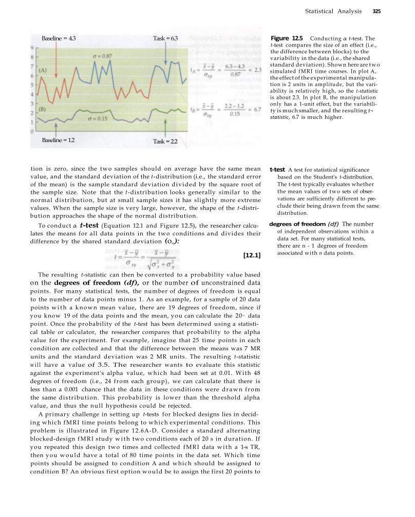
Statistical Analysis 325
Baseline = 4.3 Task = 6.3 Figure 12.5 Conducting a t-test. The t-test compares the size of an effect (i.e., the difference between blocks) to the variability in the data (i.e., the shared standard deviation). Shown here are two simulated fMRI time courses. In plot A, the effect of the experimental manipulation is 2 units in amplitude, but the variability is relatively high, so the t-statistic is about 2.3. In plot B, the manipulation only has a 1-unit effect, but the variability is much smaller, and the resulting t¬statistic, 6.7 is much higher.
The resulting t-statistic can then be converted to a probability value based on the degrees of freedom (df), or the number of unconstrained data points. For many statistical tests, the number of degrees of freedom is equal to the number of data points minus 1. As an example, for a sample of 20 data points w i t h a k n o w n mean value, there are 19 degrees of freedom, since if you know 19 of the data points and the mean, you can calculate the 20 t h data point. Once the probability of the t-test has been determined using a statistical table or calculator, the researcher compares that probability to the alpha value for the experiment. For example, imagine that 25 time points in each condition are collected and that the difference between the means was 7 MR units and the standard deviation was 2 MR units. The resulting t-statistic w i l l have a value of 3.5. The researcher wants to evaluate this statistic against the experiment's alpha value, which had been set at 0.01. With 48 degrees of freedom (i.e., 24 from each group), we can calculate that there is less than a 0.001 chance that the data in these conditions were d r a w n from the same distr ibution. This probability is lower than the threshold alpha value, and thus the nul l hypothesis could be rejected.
A primary challenge in setting up t-tests for blocked designs lies in deciding which fMRI time points belong to which experimental conditions. This problem is illustrated in Figure 12.6A-D. Consider a standard alternating blocked-design fMRI study w i t h two conditions each of 20 s in duration. If you repeated this design two times and collected fMRI data w i t h a 1-s TR, then you w o u l d have a total of 80 time points in the data set. Which time points should be assigned to condition A and which should be assigned to condition B? An obvious first option would be to assign the first 20 points to
t-test A test for statistical significance based on the Student's t-distribution. The t-test typically evaluates whether the mean values of two sets of observations are sufficiently different to preclude their being drawn from the same distribution.
degrees of freedom (df) The number of independent observations within a data set. For many statistical tests, there are n - 1 degrees of freedom associated with n data points.
Baseline = 1.2 Task = 2.2
tion is zero, since the two samples should on average have the same mean value, and the standard deviation of the t-distribution (i.e., the standard error of the mean) is the sample standard deviation divided by the square root of the sample size. Note that the t-distribution looks generally similar to the normal distribution, but at small sample sizes it has slightly more extreme values. When the sample size is very large, however, the shape of the t-distribution approaches the shape of the normal distribution.
To conduct a t-test (Equation 12.1 and Figure 12.5), the researcher calculates the means for all data points in the two conditions and divides their difference by the shared standard deviation (oxy):
[12.1]

326 Chapter Twelve
Figure 12.6 Assigning time points in a blocked design to t-conditions. Although t-tests are commonly used for blocked designs, they do pose some challenges. Consider the simple alternating blocked design shown in (A). If we convolve this design w i t h a hemodynamic response, we get the pattern of activity shown in (B). Because of the hemodynamic latency, the fMRI data do not correspond well to the t iming of the original experimental design. By introducing a lag to the design (C), we can better f i t the true t iming of activity, although the transition periods between the blocks are still analyzed. Excluding the block transitions (D) can further distinguish experimental conditions.
A, the next 20 to B, and so forth. But remember from Chapter 7 that the BOLD fMRI response lags behind neuronal activity. Therefore, a better approach would account for this lag by delaying the onset of all blocks (e.g., by about 6 s). But even this approach is imperfect. Because changes in the BOLD response are not instantaneous, there w i l l be transition periods at the onset of each block where the measured fMRI signal w i l l be changing from low to high or from high to low. By excluding these highly variable transition periods and sampling only the latter parts of each block, the researcher can select time points where the BOLD response has reached a steady state, maximizing the power of the t-test.
Although the t-test assumes that its data are drawn from normal distributions wi th equal variability, one of its strengths for fMRI is that it is relatively insensitive to violations of these assumptions. In even a short fMRI study, there w i l l be at least a few tens of time points collected per voxel, and many studies collect hundreds of data points in each condition. At these sample sizes, deviations from normality have no meaningful effect on the outcome of the test. Likewise, w i t h large samples, the conditions may have very different numbers of time points or have different variability without compromising the outcome of the t-test. While the t-test may be statistically valid for fMRI data, several potential concerns do exist. Any systematic difference between the experimental conditions, whether associated w i t h meaningful BOLD activity or w i t h uninteresting artifacts like scanner dr i f t or head motion, could result in a significant t-test (Figure 12.7). This is especially a problem for blocked studies that have only a few cycles of the task and nontask conditions. The t-test is also inappropriate for answering questions about the t iming of activity, since it combines across all time points wi th in a condition.
While this discussion has focused on blocked designs, t-tests are also useful for some analyses of event-related designs. Remember that the basic role of the t-test is to identify differences in the means of t w o samples of data. If
(A)
(B)
(C)
(D)

Statistical Analysis 327
Figure 12.7 Effects of scanner dr i f t on t-tests. Shown here is an activation map of a phantom, w i t h positively significant voxels shown in the green-to-yellow color map and negatively significant voxels shown in the blue-to-pink color map. The position of the phantom " m o v e d " slightly along the frequency-encoding direction (top to bottom) due to slow changes in the center frequency of the scanner over time. Even though there was no true activity, this motion w i t h i n the images was significant according to the t-test conducted.
a research question focuses on specific data points w i t h i n an event-related design, then a t-test may be appropriate. Many event-related designs, especially those studying work ing memory or attention, evaluate the magnitude of fMRI activity at a given time point . In an experiment conducted by Jha and McCarthy in 2000, subjects were shown photographs of one or more faces, to be remembered over a long delay interval of up to 27 s. One of the research questions was whether remembering more faces w o u l d result in increased activity during the delay interval, suggesting that the brain region being tested was involved in memory maintenance processes. The authors used a t-test to compare activity when subjects remembered mult iple faces to when they remembered only a single face, at each time point w i t h i n the delay interval. They found that there were significant differences at time points early in the interval, due to the presentation of the faces to be remembered. However, these differences disappeared as the interval progressed. The authors concluded, based on the nonsignificant t-test, that memory maintenance had no effect on fMRI activity. In summary, regardless of the experimental design, if the research question can be answered by evaluating whether or not two samples have statistically different means, then a t-test may be appropriate.
While the t-test evaluates differences between the means of two distributions, it is insensitive to differences in their variability or shape. To find such differences, a Kolmogorov-Smirnov (K-S test) can be used. The K-S test converts each distribution to a cumulative distribution function, which plots the proportion of the data at or below each possible value of the dependent variable. The statistic of interest in the K-S test, Dk, is the maximal difference between the cumulative distributions at any value of the dependent variable. The flexibility of the K-S test comes w i t h a price: greatly reduced sensit ivi ty to changes in sample means compared to the t-test. Thus, the t-test should be used when the experimental hypothesis predicts that the manipulation should have an additive effect on the dependent variable, whi le the
Kolmogorov-Smirnov (K-S) test A test for statistical significance that evaluates whether two samples are drawn from the same distribution. The K-S test is sensitive to differences in variability and skew between distributions, but it is much less sensitive to differences in mean than the t-test.
328 Chapter Twelve
K-S test should be restricted to situations where the manipulation is expected to have an effect on the variability of the dependent variable.
Correlation Analysis While the t-test and K-S test can be applied to many fMRI studies, neither analysis uses any information about the shape of the hemodynamic response. Indeed, when excluding transitions between task blocks, information about the shape of the response is explicitly removed. Nevertheless, the fMRI signal does contain important t iming information. As discussed in Chapter 7, the fMRI hemodynamic response takes about 5 s to rise to its maximum after the onset of neuronal activity. Fol lowing the cessation of neuronal activity, the hemodynamic response falls over an additional 5 to 10 s and then stabilizes at a below-baseline level for an extended interval. The consistency of the hemodynamic response allows prediction of the change in fMRI activity that should be evoked in an active voxel. Using a correlation analysis, a researcher can quantify the correspondence between the predicted hemodynamic response and the observed data. Correlation analyses were first reported in fMRI by Bandettini and colleagues in 1993 and have since been an important part of fMRI analyses.
Conducting a correlation analysis on fMRI data is very simple. First, identify two epochs, ideally of equal length, that correspond to the experimental data and to a predicted hemodynamic response. Second, calculate the covariance in the data, as indicated by the numerator of Equation 12.2:
correlation analysis A type of statistical test that evaluates the strength of the relation between two variables. For fMRI studies, correlation analyses typically evaluate the correspondence between a predicted hemodynamic response and the observed data.
correlation coefficient (or r-value) A number between -1 and 1 that expresses the strength of the correlation between two variables.
The K-S test is rarely used in fMRI because few experimental manipulations are designed to increase the variability of fMRI
data. Can you think of an experimental manipulation that would increase the variability of fMRI data, but not its mean?
[12.2]
Note that the covariance may be either positive or negative. If the covariance is positive, values of the experimental data were large when values of the predicted data were large, or they were small when small. But if the covariance is negative, the values of the experimental data tended to be small when the values of the predicted data were large, or vice versa. Third, normalize the covariance by d i v i d i n g by the product of the standard deviations of the t w o epochs. The resulting correlation coefficient, or r-value, can have values ranging from 1.0 to -1.0, or from perfect positive correlation to perfect negative correlation. A correlation of 0 indicates that the experimental data are unrelated to the prediction. As w i t h the statistics discussed in the previous section, the significance of the correlation coefficient can be evaluated using statistical tables based on the degrees of freedom; a correlation of 0.5 is more l ikely to be significant when based on 1000 data points than when based on 10. This basic correlation analysis is then repeated for every voxel in the brain to create the map of significant activity.
Given the differences between correlation and t-tests, it may surprise you that when they are applied to the same data set, they give identical results.

S t a t i s t i c a l A n a l y s i s 329
Remember that the t-test evaluates whether data in one condit ion differ f rom data in another condit ion. Exactly the same test could be conducted by correlating the experimental data w i t h a boxcar waveform (i.e., w i t h i n task blocks the response w i l l be 1, while in nontask blocks the response w i l l be 0). This similarity is often seen in graphical descriptions of experimental designs, in which the different conditions are plotted as different values along the y-axis, and can be demonstrated using any sample data set and Equations 12.1 and 12.2. For any value of r, there is a corresponding value of t, given the degrees of freedom in the data. Note also that both tests measure signal change div ided by nonsignal variability, w i t h the t-test using the difference between means and the correlation test using the more general measure of covariation. Thus, the power of the correlation coefficient (like the t-test) rests on having maximal variabi l i ty in the signal of interest compared to experimental noise. Furthermore, if the values of either the experimental or predicted data are distributed in a highly non-normal fashion, then the correlation statistic may not be meaningful . This may occur in fMRI studies if there are very long prestimulus or poststimulus baseline periods, so that most data points in the prediction epoch are near zero.
Correlation analyses are often used in conjunction w i t h signal averaging, but in principle, signal averaging is unnecessary. One could use the entire experimental session as a single time course, then compare that time course to a prediction composed of many individual hemodynamic responses. Indeed, this idea forms the basis of the general linear model, described later in this chapter. However, signal averaging can have very salutary effects upon correlation analyses in fMRI . If there are low-frequency changes in the data, as result from scanner dr i f t , then the overall correlation between data and prediction may be greatly reduced. Averaging across stimulus epochs before doing the correlation analysis minimizes the influence of low-frequency changes.
Signal averaging can also in form the choice of the predicted hemodynamic response. One way to generate the predicted hemodynamic response is to use an empirical function derived from another experiment. As the fMRI hemodynamic response is generally similar across subjects, the simplicity of using a canonical function may be attractive. However, recall from Chapters 9 and 10 that the characteristics of the hemodynamic response may differ across subjects, brain regions, and stimuli . Such differences can reduce the significance of correlation tests. One way of overcoming this problem is to generate a unique hemodynamic response for each subject, based on a screening run, partial data set, or region/voxel of interest. More-complex approaches begin by using the correlation w i t h a canonical response to identify a region of interest, then interrogating those voxels for their hemodynamic response, and then repeating these steps unti l they converge to a solution. If the init ial predicted hemodynamic response is reasonably well correlated w i t h the actual data, then such iterative or bootstrapping approaches can be very effective.
Fourier Analysis As discussed in Chapter 11, a blocked-design fMRI task presents stimulus conditions at regular intervals. As a consequence, the MR signal w i t h i n an active voxel regularly rises dur ing task blocks and falls d u r i n g nontask blocks. The periodic nature of this signal change can be quantified using a Fourier transform. The Fourier transform expresses a temporally (or spatially) varying signal as the linear sum of a series of sine waves of different
Fourier transform A mathematical technique for converting a signal (i.e., changes in intensity over time) into its power spectrum.

330 C h a p t e r T w e l v e
time domain The expression of a signal in terms of its intensity at different points in time.
frequency domain The expression of a signal in terms of its power at different frequencies.
frequencies, amplitudes, and phases. A plot of the magnitude of each sine-wave component necessary to recreate the original signal is called a power spectrum. Thus, the power spectrum itself is another way of representing the original data. In the language of signal processing, the raw fMRI time series data are in the time domain, meaning that they show the relative intensity of the signal at each time sample. The power spectrum represents the same data in the frequency domain, indicating the intensity of the signal at each component frequency. If a task-related signal rises and falls at a known frequency, then a peak w i l l occur at that frequency in the power spectrum (see Figure 10.16). We discussed in Chapter 10 the use of the Fourier transform to remove unwanted variabil i ty from the data, and here we extend that discussion to consider its use for statistical analysis of task-related variability.
In practice, the frequencies that can be measured by a Fourier analysis depend upon how often the BOLD time series is sampled. The basic rule of sampling, the Nyquist sampling theorem, states that to accurately measure a given frequency, you must sample at a m i n i m u m of twice that frequency. Thus, the Fourier transform of n time points sampled at a given TR contains n/2 frequencies ranging from 0 Hz to 1/(2 x TR) Hz, which are represented along the x-axis of the power spectrum. The first frequency component, at 0 Hz, represents the mean intensity of the signal and is often called the DC component, after the electrical term for direct current (i.e., a constant-voltage power source). Since fMRI time courses generally are represented in arbitrary units w i t h positive values proportional to the amount of current through the receiver coil, the DC component is generally positive and very large. Also present in almost all fMRI data, even from very stable scanners, is substantial low-frequency power associated w i t h scanner dr i f t , among other factors (see Chapter 9). There are also slow physiological changes due to vascular oscillations, although such effects are incompletely understood. Because of this power at low frequencies, very long block lengths are not ideal for fMRI .
Substantial high-frequency (i.e., >0.5 Hz) power is rare in fMRI experiments, save for that associated w i t h heart rate, even when the sampling rate is sufficiently fast. At fast stimulus-presentation rates, the sluggishness of the fMRI hemodynamic response tends to smooth the data considerably, serving to filter high-frequency components of the data. So, even if your two conditions alternated at a rate of 2 Hz, there w o u l d be no hemodynamic changes at that rate to be measured.
While Fourier approaches can be used for standard alternating blocked designs, more-complex designs are also possible. Imagine an experiment in which you wish to identify differential activity evoked by faces, animals, and objects. You could create blocks of faces that recur wi th a period of 12 s, blocks of animals w i t h a period of 14 s, and blocks of objects w i t h a period of 16 s, and then combine all of these blocks into a single stimulus series w i t h each stimulus category appearing at its specific frequency (Figure 12.8). Voxels that are activated by faces should have a peak in the power spectrum at 1/12 s, or 0.083 Hz; voxels activated by animals should have a peak at 0.071 Hz; and voxels activated by objects should have a peak at 0.063 Hz. Voxels that are activated by both faces and objects should have two spectral peaks, at both 0.083 and 0.063 Hz. Using blocks that overlap in time, as in this example, can be much more efficient than conducting a series of separate experiments.
Combining sine waves at the magnitude specified in a power spectrum is not sufficient to accurately recreate the original raw data. Imagine that a

Figure 12.8 The use of overlapping blocks w i t h different frequencies. If several different classes of s t imul i are presented at different frequencies, a Fourier transform can be used to separate activity associated w i t h each. Here, faces are presented at the highest frequency, animals are presented at an intermediate frequency, and objects are presented at the lowest frequency. Each is presented individual ly in an alternating blocked design, w i t h scrambled objects as the control condition. Note that what subjects see changes at different points in the task, as shown at top. Some of the time, all three categories w i l l be present, while at other times, only one or two of the categories w i l l be visible.
power spectrum informs us that our original data were composed of two sine waves, one at 4 Hz and the other at 5 Hz. In principle, we should be able to add a 4-Hz sine wave and a 5-Hz sine wave w i t h the appropriate magnitudes as indicated in the power spectrum and recreate our raw data. However, if we change the phase angle of one or both of these component sine waves, we can create many different waveforms. Happi ly for us, the Fourier transform also provides a phase spectrum, which specifies the phase angle that each sine-wave component must be shifted in order to recreate the original data. This is advantageous in fMRI studies where the sluggishness of the hemodynamic response causes a lag in the onset and offset of the stimulus blocks. The phase angle at the task frequency provides a frequency domain measurement of this time lag. This phase lag can be compared for voxels in different brain regions and can thus provide a measure of differential hemodynamic latency.
Differences in the phase of the BOLD signal at the task frequency can be purposively introduced by manipulating the task t iming. Figure 12.9 shows data from a study mapping the motor cortex in a single patient (see Box 12.2
S t a t i s t i c a l A n a l y s i s 331
High frequency
Medium frequency
Low frequency

332 Chapter Twelve
Figure 12.9 Use of frequency and phase information in cortical mapping. This patient, w h o had an arteriovenous malformation (AVM) in the left hemisphere (right side of image), participated in blocked-design motor squeeze tasks that began either w i t h a left-hand squeeze or a right-hand squeeze. The raw data are shown in the upper graphs, the power spectra are shown in the middle graphs, and the phase at the task frequency (peak in spectra) is shown at bottom. Note that although both hemispheres had peaks at about the same frequencies, the phases are different, a l lowing dissociation of right-hand and left-hand activity.
for related information). The task alternated squeezing the left and right hands (blocks of about 9 s), beginning w i t h each hand on one-half of the runs. Since both types of runs, left-first and right-first , had the same block lengths, they both had maximal power at the same task frequency (about 0.057 Hz). However, the responses at that frequency were 180° out of phase. Thus, by manipulating the phase of stimulus presentation across runs, we can introduce k n o w n phase changes into our BOLD data that can help distinguish true task-related activity from noise that may occur at the task frequency. Active voxels can be identified as those that both increase in power at the task frequency and change phase consistent w i t h the experimental manipulation.
In summary, the Fourier transform is an important tool for analyses of periodic fMRI data. It is most commonly used w i t h alternating blocked designs, but it can be used w i t h any design in which different conditions
Phase angle (°)
Frequency (Hz) Frequency (H z )
S t a t i s t i c a l A n a l y s i s 333
occur at different frequencies. It provides t w o measures at each frequency component, power and phase. Power can be used to evaluate whether significant activity is present at a frequency, and phase can be used to evaluate the t iming of that activity.
Displaying Statistical Results The goal of most fMRI statistical tests, regardless of their complexity, is to evaluate the probability that each voxel is consistent w i t h the nul l hypothesis. When statistical tests from all voxels in the brain are combined, the result is a statistical map, or statistical parameter map, of brain activity. The statistical map is usually color-coded according to the probability value for each voxel. For example, if the alpha value for an experiment were set at 0.01, a voxel w i t h a near alpha probability value of 0.009 might be displayed in a dark red, while a voxel w i t h an extremely low probabil i ty value of 0.000001 might be shown as a bright yellow. The association between probabil i ty values (or another statistic) and the colors that label them is known as a color map. In general, researchers use darker, desaturated colors to indicate low significance levels and brighter, highly saturated colors to indicate high significance levels. The statistical map is usually displayed on top of a base image that illustrates brain anatomy. However, it is important not to confuse the properties of a base anatomical image w i t h those of the overlaid statistical map. The former is usually of high resolution and has contrast dependent on a physical property of the brain (e.g., T 1 ) , while the latter is a calculated statistical map reflecting the correspondence of the data to an experimental hypothesis. (Note that although the vast majority of color maps display statistical significance, other properties such as percent signal change or latency can also be displayed; see, e.g., Figure 8.15).
There are many options for displaying fMRI data, each w i t h advantages and disadvantages. The most common option is the single anatomical slice w i t h overlaid color map (Figure 12.10A). In many experiments, the anatomical images are acquired at the same slice locations as the functional images, so little additional processing is necessary. Single slices are also generally easy to read, as foci of activity are highly visible. But given the variability in brain anatomy across subjects, it may be challenging to identify which gyrus or sulcus is active. Depending on the areas of interest, one slice orientation may be better than another. G y r i and sulci that run from left to right (e.g., the central sulcus) are diff icult to identify in coronal slices, whi le those running from front to back (e.g., most frontal gyri) are harder to interpret in axial slices. Another l imitation of single-slice displays is the choice of slices to include. Rarely w i l l all collected slices be displayed in a single poster, manuscript, or lecture slide, due to their sheer number. Instead, the researcher w i l l display selected slices that illustrate the major activation locations found in the study. When showing single slices, it is critical to explicitly label the left and right hemispheres, due to the axial symmetry of the human brain. Historically, MRI data have been displayed in radiological convention, such that the left side of the image corresponds to the right side of the brain and vice versa. This convention results from the way in which radiologists typically interact w i t h patients, who are generally facing them or ly ing in scanners w i t h their feet toward them. Displaying fMRI data in normal or neurological convention (i.e., based on a surgeon looking from the head to the feet) has become increasingly common in recent years.
While statistical maps are often calculated and displayed as two-dimensional slices, they also can be displayed in three-dimensional perspective
statistical map (or statistical parameter map) In fMRI, the labeling of all voxels within the image according to the outcome of a statistical test.
color map The association between numerical values of a parameter and a set of colors.
base image The image on which a statistical map is displayed, often a high-resolution anatomical image.
radiological convention The practice of displaying images of the brain so that the left side of the image is the right side of the brain and vice versa, as if one were facing the subject.
neurological convention The practice of displaying images of the brain so that the left and right sides of the image correspond to the same sides of the brain, as if one were behind the subject.

334 C h a p t e r T w e l v e
rendered image A display of MRI data in three-dimensional perspective.
glass-brain view A two-dimensional projection of fMRI data, as if the brain were made transparent and only the activations were visible.
Figure 12.10 Two- and three-dimensional representations of fMRI data. Statistical m a p s of fMRI data are typical ly s h o w n either as two-dimensional slices (A) or as three-dimensional rendered brains (B). (B from Huettel et a l . , 2001, created us ing FreeSurfer, C o r T e c h s / M a r t i n o s Imaging Center , Boston, MA. )
(Figure 12.1 OB). Such displays are often called rendered images. The major advantage of three-dimensional rendering is that one can easily identify the locations of brain activity, especially w i t h regard to prominent gyr i and sulci. Such images are also more easily interpreted by naive viewers who are more familiar wi th the general shape and external structure of the brain than wi th specific internal features. Hidden, however, are internal nuclei, such as the basal ganglia and thalamus, as wel l as internal cortical regions like the hippocampus, cingulate, and insula. It is also more di f f icul t to show both hemispheres simultaneously in a single image, so authors often include more than one rendered image w i t h i n a single figure. To overcome the problems introduced by the opacity of rendered images, some analysis programs generate transparent or semitransparent images, sometimes called glass-brain views (Figure 12.11 A) . These project all foci of activity onto an outline of the brain, a l lowing the researcher to see all of the activations at once. As wi th any projective display technique, a single glass-brain view is considerably underdetermined, in that many possible sets of activations could lead to the displayed image. For this reason, most programs generate a set of three orthogonal views of the brain, so that by comparing among them researchers can localize activations.
(A)
(B)
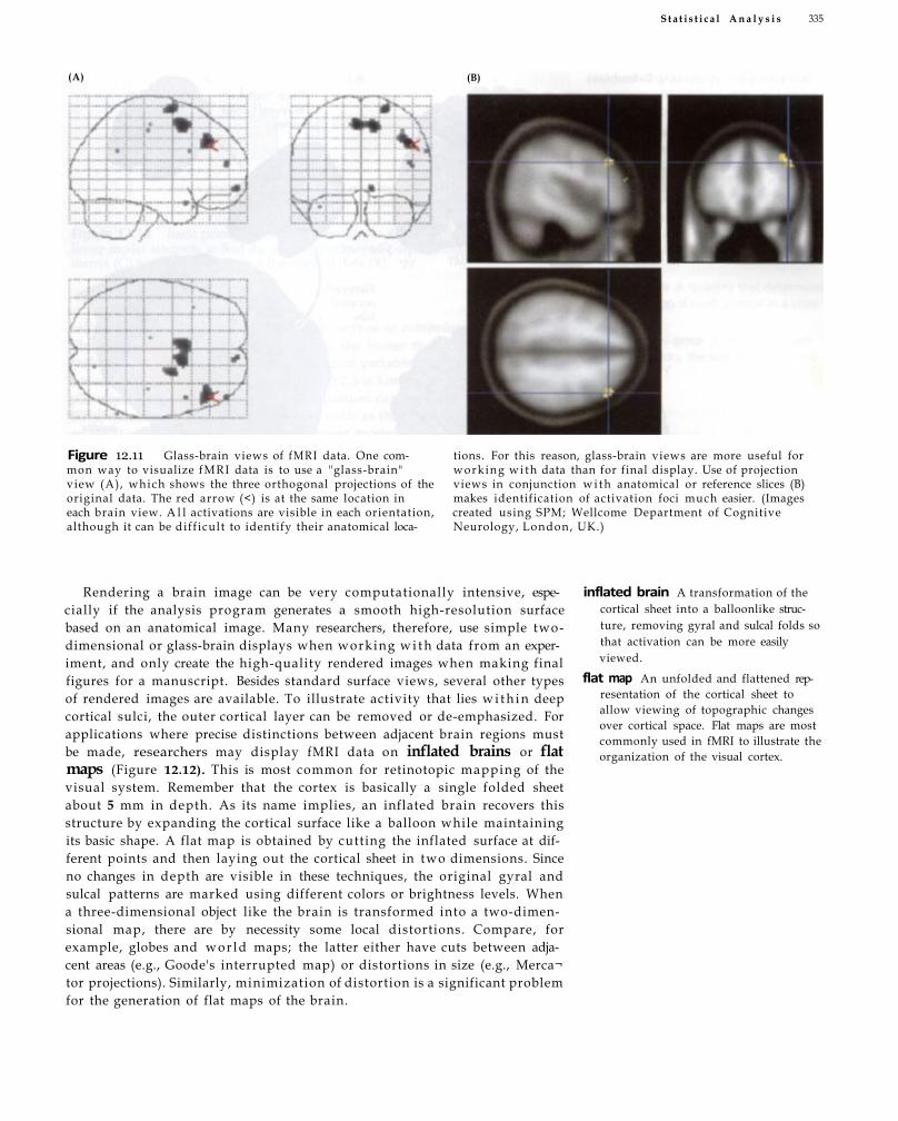
S t a t i s t i c a l A n a l y s i s 335
Figure 12.11 Glass-brain views of fMRI data. One common way to visualize fMRI data is to use a "glass-brain" view (A), which shows the three orthogonal projections of the original data. The red arrow (<) is at the same location in each brain view. A l l activations are visible in each orientation, although it can be diff icult to identify their anatomical loca
tions. For this reason, glass-brain views are more useful for working w i t h data than for final display. Use of projection views in conjunction w i t h anatomical or reference slices (B) makes identification of activation foci much easier. (Images created using SPM; Wellcome Department of Cognitive Neurology, London, UK.)
Rendering a brain image can be very computationally intensive, especially if the analysis program generates a smooth high-resolution surface based on an anatomical image. Many researchers, therefore, use simple two-dimensional or glass-brain displays when working w i t h data from an experiment, and only create the high-quality rendered images when making final figures for a manuscript. Besides standard surface views, several other types of rendered images are available. To illustrate activity that lies w i t h i n deep cortical sulci, the outer cortical layer can be removed or de-emphasized. For applications where precise distinctions between adjacent brain regions must be made, researchers may display fMRI data on inflated brains or flat maps (Figure 12.12). This is most common for retinotopic mapping of the visual system. Remember that the cortex is basically a single folded sheet about 5 mm in depth. As its name implies, an inflated brain recovers this structure by expanding the cortical surface like a balloon while maintaining its basic shape. A flat map is obtained by cutting the inflated surface at different points and then laying out the cortical sheet in two dimensions. Since no changes in depth are visible in these techniques, the original gyral and sulcal patterns are marked using different colors or brightness levels. When a three-dimensional object like the brain is transformed into a two-dimensional map, there are by necessity some local distortions. Compare, for example, globes and w o r l d maps; the latter either have cuts between adjacent areas (e.g., Goode's interrupted map) or distortions in size (e.g., Merca¬tor projections). Similarly, minimization of distortion is a significant problem for the generation of flat maps of the brain.
inflated brain A transformation of the cortical sheet into a balloonlike structure, removing gyral and sulcal folds so that activation can be more easily viewed.
flat map An unfolded and flattened representation of the cortical sheet to allow viewing of topographic changes over cortical space. Flat maps are most commonly used in fMRI to illustrate the organization of the visual cortex.
(B) (A)

336 Chapter Twelve
Figure 12 .12 Flat map views of the brain surface. Flat map views of the brain can be useful for determining the topographic organization of the cortex. The most common use of flattened views is for retinotopic mapping of the visual cortex. After identifying areas of activation, as shown here on lateral (A) and medial (B) views of the visual cortex, researchers inflate, cut, and flatten the cortical surface (C) to show the spatial distribution of active regions. (After Sereno et al., 1995.)
The General Linear Model
Chapter 8 introduced the idea of representing fMRI data in a linear model. The formula for a linear model is given in Equation 12.3:
y = a0 + a1x1 + a2x2 + ... + anxn + e [12.3]
model factors A set of hypothesized changes in BOLD activity associated with the manipulations of the independent variables or with other known sources of variability.
parameter weights For most fMRI analyses, quantities that reflect the relative contribution of the different model factors to the observed data within a given voxel.
The basic idea behind a linear model is that the observed data (y) is equal to a weighted combination of several model factors (x1) plus an additive error term (e). The parameter weights (n1) indicate how much each factor contributes to the overall data. The term a 0 reflects the total contribution of all factors that are held constant throughout the experiment. For fMRI data, this w o u l d include the raw T 2* values recorded in particular voxels in the absence of BOLD activation, as well as any activity that is constant throughout the experiment. In solving the linear model equation, the researcher has only one k n o w n quantity, the experimental data. The model factors represent hypothesized components of the data, but may or may not be meaningf u l . Given the data and a specified set of model factors, the researcher can
(A) Lateral (C)
(B) Medial Flattened occipital lobe
Brain "inflated" to reveal buried cortex

S t a t i s t i c a l A n a l y s i s 337
Figure 12.13 Basic principles of the general linear model in fMRI . The general linear model attempts to f ind the set of experimental parameters (B) for a design matrix (G) that best accounts for the original data (X).
calculate what combination of weights serves to minimize the error term.
The m i n i m u m error term after solving the linear model is k n o w n as the
residual. When there is only one dependent variable (e.g., predicting income
based on age and education), Equation 12.3 is known as a univariate mul t i
ple regression model. But the same equation can be extended to include a
large number of dependent variables, such as the many time points w i t h i n
an fMRI study, through the general linear model.
Figure 12.13 illustrates the use of the general linear model in fMRI . The
experimental data are represented as a twodimensional matrix consisting of
n time points by V voxels. Note that the spatial structure of the fMRI data is
not used in the general linear model, since the values of the parameter
weights and error term are calculated independently for all voxels. The vox
els are instead arranged along one dimension for ease of calculation. The
design matrix, which specifies the linear model to be evaluated, consists of
M model factors, each n t ime points in length (Figure 12.14). Depending on
the analysis strategy, the mean value for each voxel may be subtracted dur
ing preprocessing or a constant term may be included in the model. The
parameter matrix contains M rows and V columns, such that each cell indi
cates the amplitude of one of the model factors for a given voxel. Finally, the
error term is an nbyV matrix. In some notation systems, the design matrix
is denoted as G and the parameter matrix is denoted as β.
After setting up the general linear model for a given experiment, the
researcher calculates what combination of weights, when mult ipl ied by the
design matrix, gives the smallest error term. To understand this process, con
sider a simple experiment where the subject squeezes her hand every 20 s
while fMRI data are recorded w i t h a TR of 1 s over 60 time points. You
hypothesize that active voxels should show three distinct hemodynamic
responses, one fo l lowing each of the three hand squeezes. You then enter
this hypothesis as a single column in the design matrix. The general linear
model evaluates how much this hypothetical time course contributed to the
real data, compared to variability outside of the model. Since fMRI data con
sist of many time points, the residual error for a given voxel must be com
bined across all time points into a single value. As discussed earlier, the for
mula for combining many error values into one summary statistic is known
as a cost function. In the general linear model, the standard cost function is
leastsquares error, or the sum of all squared residuals. To test the signifi
cance of a model factor for a given voxel, the amplitude of its associated
parameter is d iv ided by the residual error. Under the n u l l hypothesis, this
quantity should fol low the F distr ibution, and so its statistical significance
can be evaluated as a function of the available degrees of freedom.
residual The variability in the data that remains unexplained after accounting
for the model factors.
general linear model A class of statisti
cal tests that assume that the experi
mental data are composed of the lin
ear combination of different model
factors, along with uncorrelated noise.
design matrix In fMRI implementations of the general linear model, the specifi
cation of how the model factors change
over time.
cost function A quantity that determines
the amount of residual error in a com
parison.
leastsquares error A commonly used cost function, the sum of the squared
residuals.
Figure 12.14 A design matrix for the general linear model. The set of model functions that attempts to explain the experimental data using the general l in ear model is known as the design matrix. In the experiment illustrated here, subjects listened to a series of tones w i t h constant pitch. Presented randomly wi th in the series were rare deviant tones w i t h a higher pitch. The expected fMRI signal over time for each run is shown in the six columns to the left, w i t h white indicating maximum signal and black indicating minimal signal. The six columns to the right reflect constant values included to remove the mean signal change for each r u n . Note that each run consists of roughly 200 brain images.
Total variability Variability explained
by the model
+ Noise
V columns (voxels)
X G x β + ε
+ ε
Model parameters
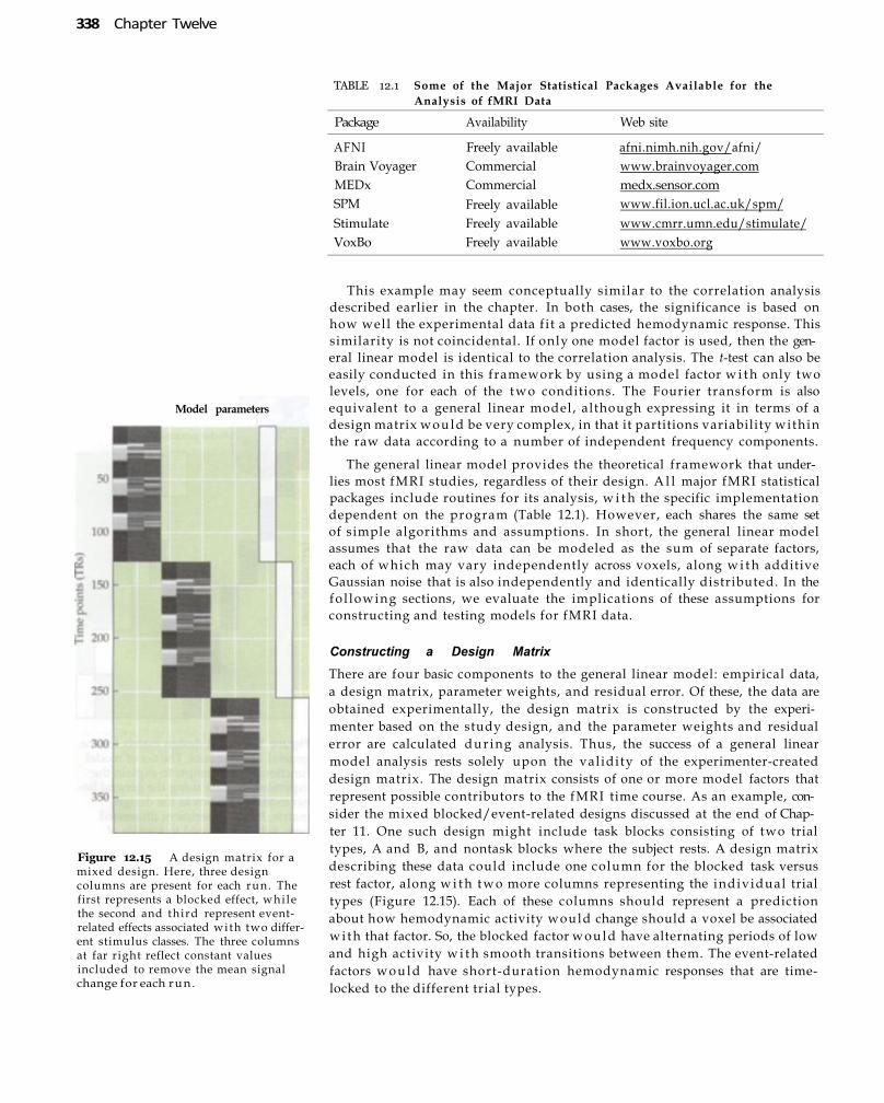
338 Chapter Twelve
TABLE 12.1 Some of the Major Statistical Packages Available for the Analysis of fMRI Data
Package Availability Web site
AFNI Freely available afni.nimh.nih.gov/afni/ Brain Voyager Commercial www.brainvoyager.com MEDx Commercial medx.sensor.com SPM Freely available www.fil.ion.ucl.ac.uk/spm/ Stimulate Freely available www.cmrr.umn.edu/stimulate/ VoxBo Freely available www.voxbo.org
Figure 12.15 A design matrix for a mixed design. Here, three design columns are present for each run. The first represents a blocked effect, whi le the second and third represent event-related effects associated with two different stimulus classes. The three columns at far right reflect constant values included to remove the mean signal change for each run.
This example may seem conceptually similar to the correlation analysis described earlier in the chapter. In both cases, the significance is based on how well the experimental data f i t a predicted hemodynamic response. This similarity is not coincidental. If only one model factor is used, then the general linear model is identical to the correlation analysis. The t-test can also be easily conducted in this framework by using a model factor w i t h only two levels, one for each of the t w o conditions. The Fourier transform is also equivalent to a general linear model, although expressing it in terms of a design matrix would be very complex, in that it partitions variability within the raw data according to a number of independent frequency components.
The general linear model provides the theoretical framework that underlies most fMRI studies, regardless of their design. A l l major fMRI statistical packages include routines for its analysis, w i t h the specific implementation dependent on the program (Table 12.1). However, each shares the same set of simple algorithms and assumptions. In short, the general linear model assumes that the raw data can be modeled as the sum of separate factors, each of which may vary independently across voxels, along w i t h additive Gaussian noise that is also independently and identically distributed. In the fo l lowing sections, we evaluate the implications of these assumptions for constructing and testing models for fMRI data.
Constructing a Design Matrix There are four basic components to the general linear model: empirical data, a design matrix, parameter weights, and residual error. Of these, the data are obtained experimentally, the design matrix is constructed by the experimenter based on the study design, and the parameter weights and residual error are calculated dur ing analysis. Thus, the success of a general linear model analysis rests solely upon the val idity of the experimenter-created design matrix. The design matrix consists of one or more model factors that represent possible contributors to the fMRI time course. As an example, consider the mixed blocked/event-related designs discussed at the end of Chapter 11. One such design might include task blocks consisting of two trial types, A and B, and nontask blocks where the subject rests. A design matrix describing these data could include one column for the blocked task versus rest factor, along w i t h t w o more columns representing the individual trial types (Figure 12.15). Each of these columns should represent a prediction about how hemodynamic activity would change should a voxel be associated wi th that factor. So, the blocked factor would have alternating periods of low and high activity w i t h smooth transitions between them. The event-related factors would have short-duration hemodynamic responses that are time-locked to the different trial types.
Model parameters

S t a t i s t i c a l A n a l y s i s 339
In graphical depictions of fMRI design matrices, the predicted value of a factor at each point in time is usually scaled on a dark- l ight color map. Black indicates that the factor is predicted to have no effect at that time point, while whi te indicates that it should have its largest effect. Model factors associated w i t h specific hypotheses are k n o w n as experimental factors. There are two types of experimental factors. Covariates are factors that can take any of a continuous range of values, where the value of the factor represents the amount of some k n o w n quantity. The most common covariates in fMRI design matrices are predicted hemodynamic responses. Others include response time and physiological changes like the respiratory cycle. Indicators are factors that have integral values that indicate a qualitative level. For f M R I , these may include experimental conditions, as in the t-test; subject treatment or demographic conditions; accuracy of a tr ial ; and many other factors. Covariates and indicators are mathematically equivalent w i t h i n the general linear model; the latter have a restricted set of values, while the former can vary freely.
In addit ion to the expected model factors, the design matrix often includes additional factors associated w i t h known nonexperimental sources of variability. These are k n o w n as nuisance factors. Suppose that the MR scanner on which this study is conducted often has a linear dr i f t dur ing experimental sessions. An additional factor could be introduced into the design matrix to account for this d r i f t . Or, if the subject's respiration was measured dur ing the session, the design matrix could include a factor for artifacts associated w i t h the repeated breathing. Of course, these factors have nothing to do wi th the experimental hypotheses, in that the experiment was not designed to test scanner dr i f t or subject respiration. So w h y are they included in the design matrix?
Nuisance factors serve two related purposes in experimental analyses. First, they can reduce the amount of residual variation included in the error term. If the intensity of a voxel were to d r i f t by a few percentage points through the course of a r u n , the overall variabil ity in the voxel w o u l d be very large, compared to the BOLD effect of interest. But if a linear factor were added to the design matrix, much of that variability would be assigned to that factor rather than to the error term, increasing the significance of the results. Second, assigning k n o w n variabil i ty to nuisance factors improves the val idity of the general linear model. The model assumes that residuals are independent and identically distributed as Gaussian noise, which may not be the case if a regular source of variation is excluded from the design matrix. It is therefore critical to include all anticipated changes in the BOLD signal, whether of interest or not. However, wanton inclusion of extra factors is not recommended. Each additional column in the design matrix reduces the number of degrees of freedom available. In the l imit ing case, one could reproduce perfectly any set of n time points w i t h a combination of n - 1 different model factors. Since the significance of any individual factor is evaluated as a function of the number of available degrees of freedom, it is in the researcher's interest for the number of factors to be as small as possible. In practice, however, the inclusion of a l imited number of nuisance factors makes statistical testing more conservative, due to the reduced number of degrees of freedom, but can improve the val idity of the general linear model.
In creating a design matrix, the experimenter should be careful to avoid including model factors that are themselves correlated. The inclusion of such collinear factors can complicate the interpretation of the results, as variance
experimental factors Model factors that are associated with specific experimental hypotheses.
covariates Experimental factors that can take any of a continuous range of values.
indicators Experimental factors that have integral values to indicate a qualitative level.
nuisance factors Model factors that are associated with known sources of variability that are not related to the experimental hypotheses.
collinear factors Model factors that are highly correlated with one another. The inclusion of collinear factors reduces the validity of general linear model analyses.

attributable to one such factor may become confused w i t h variance associated w i t h another.
Modeling BOLD Signal Changes While the general linear model can be an extremely powerful tool for analysis of fMRI data, its val idi ty rests on a series of assumptions. The first, and most important, of these is that the design matrix should contain factors that accurately reflect BOLD changes due to neuronal activity of interest. Consider a simple experiment where subjects see a picture of an object and then must retrieve a specific, elaborated memory of a past event associated with that object. The pictures are presented infrequently, w i t h interstimulus intervals ranging between 20 and 30 seconds. To investigate what voxels are active when subjects remember past events, the researcher sets up a column of the design matrix w i t h standard hemodynamic responses at the onset of each picture. But after completing the general linear model analysis, the researcher is surprised that visual cortical areas are active but memory-related areas are not. What could cause such a result? Imagine that you are the subject in this experiment, and you have been instructed to remember a detailed episode from your past based upon the picture on the screen. The first picture is a balloon. Now, recall a particular event in your life. If you are like most people, it took you between 5 and 15 seconds (or even longer, depending on the complexity of the memory) to recall and re-experience a particular event. A brain region associated w i t h the recollection process would be unlikely to have transient BOLD activity that peaked at 5 seconds; instead, its activity w o u l d be extended in time for perhaps tens of seconds. In order to detect memory-related activity, therefore, the design matrix would have to model extended BOLD changes, not standard short-duration hemodynamic responses.
This example illustrates the importance of thinking about the columns of the design matrix as predictions of the BOLD time course based upon hypothesized neuronal activity. The basic assumption of the design matrix is that the BOLD response can be estimated by convolving a hemodynamic response with the times of stimulus presentation. While this is often appropriate, the design matrix is intended to test hypotheses about hemodynamic activity, not about stimuli. Before creating your design matrix for an experiment, you should think carefully about the separate types of brain processes that are evoked in your experiment, along wi th their t iming and duration. In tasks where several processes are likely to be evoked sequentially, researchers often identify different phases of the task. These phases may be explicit, as when subjects view an attentional cue, which must be remembered over a delay interval, followed by a target that requires a response. The resulting design matrix could have separate columns corresponding to those three phases. Or they may be implicit, established by the experimenter based on an expectation of what the subjects w i l l do on the task. If the task was to remember a complex display of shapes presented for 10 s, the researcher might distinguish between two phases: a beginning encoding phase (2 s), where the subjects study the display; and a rehearsal phase (8 s), during which time the subjects commit particular aspects of the display to memory. It is worth emphasizing that no fMRI statistical analysis can be valid when the statistical test, here determined by the predictions of BOLD activity in the design matrix, does not reflect the actual changes in the brain associated wi th the experimental hypotheses.
Most analyses model BOLD activity based upon a standard hemodynamic response. However, more-complex design matrices can be created to
340 C h a p t e r T w e l v e

S t a t i s t i c a l A n a l y s i s 341
potentially improve the generalizability of the statistical model. To model small differences in hemodynamic onset or in the shape of the hemodynamic response, the design model can include additional factors k n o w n as time and dispersion derivatives. The hemodynamic response itself can be replaced w i t h a small number of basis functions, such as low-frequency sine and cosine waveforms or gamma functions. Since a wide range of hemodynamic responses can be expressed using a combination of mult iple basis functions, this approach can detect voxels whose activity does not follow the standard response, such as those w i t h a wider response or w i t h a later peak. However, the outcomes of such tests are much more complex and challenging to interpret.
Statistical models can ameliorate the effects of intersubject variabil ity in the BOLD response (see Box 9.1) by using subject-specific hemodynamic response functions. Aguirre and colleagues demonstrated this in 1998 by evaluating the mean correlation across subjects between the measured data and several models of the hemodynamic response, including a gamma function, a Poisson function, and the first eigenvector of part of their data set. Note that gamma and Poisson functions describe mathematical shapes that roughly match that of the hemodynamic response, and an eigenvector is a component of the data that explains some proportion of its variability. They found that the gamma function and eigenvector were generally good models for the observed data, w i t h mean correlations of about 0.83, while the Poisson function had a mediocre mean correlation of 0.49. As the authors noted, however, even a correlation of 0.83 explains less than 70% of the variance in the data, so there is considerable room for improvement. They then tested the effects of using subject-specific functions by evaluating data from four of their subjects who had each participated in five runs w i t h i n a single session. They used the first run to generate an estimated hemodynamic response for that subject, then measured the correlation between that response and the responses measured on subsequent runs. The mean correlation rose to more than 0.96, which accounts for about 92% of the variance in the data. By using subject-specific hemodynamic responses, rather than a generic response function, the authors achieved a substantial increase in experimental power.
Finally, a frequent source of confusion when thinking about the use of the general linear model in fMRI is the idea of linearity itself. Remember from Chapter 8 that the BOLD response does not obey the assumptions of linearity at short interstimulus intervals. So, how can it be analyzed using the general linear model? This confusion rests upon two distinct ideas about linearity. The hemodynamic response is nonlinear w i t h respect to stimulus presentation, because the combined response to two st imuli in succession is less than the sum of the responses to the t w o st imuli independently. But, stimulus presentation is not itself important in the general linear model. What is important is that the overall BOLD time course, whatever its form wi th respect to the st imuli , adds linearly wi th other sources of variability in the data. So, refractory effects in the BOLD response can be incorporated directly into the experimental design matrix wi thout compromising the val idity of the model. One way to do this is to adjust the columns of the design matrix directly by including interaction effects. Another method identified by Friston and colleagues in 1998 is to use Volterra kernels, which allow modeling of the influence of a stimulus upon subsequent s t imul i , to specify a second column in the design matrix. Without such corrections, the design matrix may not accurately capture the desired BOLD time course.

342 C h a p t e r T w e l v e
homoscedastic Having the property that the distributions of noise are similar for all experimental conditions.
heteroscedastic Having the property that the distributions of noise are different across experimental conditions.
multiple comparison problem The increase in the number of false-positive results (i.e., Type I errors) with increasing number of statistical tests. It is of particular consequence for voxelwise fMRI analyses, which may have many thousands of statistical tests.
Additional Assumptions
Provided that the design matrix is appropriate for testing the experimental hypotheses, several other conditions must be met for the general linear model to be appropriate. In this section, we document these assumptions, along w i t h their implications for fMRI studies. We emphasize that, although the general linear model framework has proven to be an effective tool for answering many questions about the brain, its l imitations have spurred many researchers to investigate alternative approaches to fMRI data analysis (refer to Box 12.1).
One assumption that has been the source of considerable debate is the use of the same design matrix throughout the brain. Al though each voxel w i l l have a different set of parameter weights, the model used to calculate those weights is identical. But we know that the properties of the hemodynamic response, especially its latency, may differ across brain regions. A model factor that is correct for one region may thus be incorrect for another, reducing the amount of variation explained by the model and increasing the residual error. The use of mul t ip le basis functions provides some flexibility, compared to using a single canonical hemodynamic response, but again complicates interpretation of the results. One way of overcoming the problem of regional variabil ity is to combine a general linear model approach with region-of-interest analyses, as discussed later in this chapter.
The residual variation is assumed to be distributed as Gaussian noise with similar properties at all time points. In other words, the amount of noise in a voxel does not depend on the task condition. That is, the data should be homoscedastic. If there is more noise in one condition than another, the data are heteroscedastic. Although the general linear model assumes the former, this assumption may not always be val id . Noise levels are higher during BOLD activity than during rest (see the work by Huettel and colleagues discussed in Chapter 9), although whether such changes are due to hemodynamic variability or to variability in neuronal processing remains unknown. This does not imply that all voxels must have similar noise properties. A voxel that contains a major blood vessel or that is near the edge of the brain may have much higher noise than most others in the brain. However, w i t h i n that voxel, the residuals should be equally variable at all time points.
Another assumption is that that all voxels are analyzed independently, even though adjacent voxels tend to have very similar properties. In fact, introducing correlation between adjacent voxels through spatial smoothing is a common step during preprocessing. While the general linear model framework cannot account for spatial correlation, the significance values it generates can be adjusted at later stages of analyses, as discussed later in this chap-
One criticism of general linear model approaches is that the models themselves are not tested. That is, just because a
model explains a significant proportion of the variability in the data, it is not necessarily the best model. What would happen, for example, if the design matrix in Figure 1 2 . 1 5
omitted the event-related columns? What sorts of erroneous conclusions could be drawn?

Statistical Analysis 343
ter. Likewise, the model assumes that each time point is independent of all others, in that the residuals should be similarly distributed throughout. Scanner dr i f t , thermal variation, head motion, and many other factors can cause the overall MR signal to change dramatically across time points, influencing the amplitude of the residual error. It is critical, therefore, to attempt to remove such unwanted variability before it reaches the error term, either during preprocessing or by including appropriate nuisance factors.
In summary, the general linear model has become the dominant statistical framework for fMRI analyses. The t-test, correlation test, and power spectrum analysis all represent special cases of this framework, each incorporating s impl i fying assumptions. The power of the general linear model comes from its flexibility. By incorporating appropriate model factors into the design matrix, a researcher may test nearly any experimental hypothesis. However, the choice of design matrix is critical for the val idity of the analysis. If an inappropriate model is specified, either through the inclusion of incorrect model factors or the exclusion of existing nuisance factors, then the analysis may give incorrect or nul l results.
Corrections for Multiple Comparisons
A typical fMRI data set contains about 20,000 voxels w i t h i n the brain and several times that number outside of the brain. Imagine, for the moment, that of those many voxels, you are only interested in one, a single voxel w i t h i n the gray matter adjacent to the right calcarine sulcus. Your experiment is a simple event-related visual task, and you calculate a t-statistic of 2.5 based on the voxel's correlation w i t h a predicted BOLD response. The chance that such an extreme t-statistic could occur under the nul l hypothesis, based upon the 20 degrees of freedom in the test, was only about 1 in 50 (p = 0.02), less than your alpha value of 0.05. Given such a low probability, you confidently reject the nul l hypothesis for that voxel. Flush w i t h the excitement of a significant result, you decide to analyze the remaining voxels. You run all of the voxels through the correlation test, calculate a t-value for each, and compare those t-values to your alpha value. Now, about a thousand voxels in the brain are active, distributed in seemingly random fashion (Figure 12.16A-C). Even worse, a few thousand voxels outside the brain appear to be active! You stare at the computer screen in disbelief. Why are so many voxels active?
This example illustrates one of the central problems of fMRI data analysis, that of multiple comparisons. Stated succinctly, the greater the number of statistical tests conducted, the greater the chance of a false-positive result. To illustrate this point, we created a random data set (64 x 64 x 20 voxels) where the intensity of each voxel at each time point was distributed as Gaussian noise. We then conducted a t-test on these data, comparing one set of 20 time points (Condition 1) to another set of 20 time points (Condition 2). Both conditions consisted of random data, so any difference between them
(B)
Figure 12.16 The problem of multiple comparisons. A simple analysis of random data at three different significance levels (p = 0.05, 0.01, and 0.001) was conducted. Note that since the data were random, any activation was due merely to chance. In this slice, which contains roughly 64,000 voxels, about 1600 had significant positive activation at a threshold of 0.05 (A) , about 360 had positive activation at a threshold of 0.01 (B), and 32 still had significant activity at a threshold of 0.001 (C).
(A)
(C)
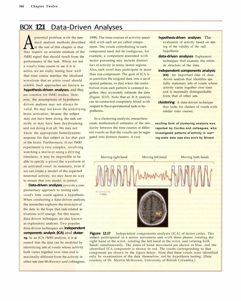
344 Chapter Twelve
BOX 12.1 Data-Driven Analyses
Apotential problem with the standard analysis methods described in the rest of this chapter is that
they require an accurate estimate of the fMRI signal that should result from the performance of the task. When we test a voxel's time course to see if it is active, we are really testing how well that time course matches the idealized waveform that an active voxel should exhibit. Such approaches are known as hypothesis-driven analyses, and they are common for fMRI studies. However, the assumptions of hypothesis-driven analyses may not always be valid. We may not know the underlying brain activation, because the subject may not have been doing the task correctly or may have been daydreaming and not doing it at all. We may not know the appropriate hemodynamic response for that subject or for that part of the brain. Furthermore, if our fMRI experiment is very complex, involving watching a movie or using a dr iv ing simulator, it may be impossible to be able to specify a priori the waveform of an activated voxel. In summary, even if we can create a model of the expected neuronal activity, we may have no way to ensure that our model is correct.
Data-driven analyses provide a complementary approach to testing each voxel's time course against a hypothesis. When conducting a data-driven analysis, the researcher explores the structure of the data in the hope that task-related activations w i l l emerge. For this reason, data-driven techniques are also known as exploratory analyses. Two popular data-driven techniques are independent components analysis (ICA) and clustering. In an ICA fMRI analysis, it is assumed that the data can be modeled by identifying sets of voxels whose activity both varies together over time and is maximally different from the activity in other sets (see McKeown and colleagues,
Figure 12.17 Independent components analysis (ICA) of motor cortex. This subject participated in a motor movement task w i t h three phases: rotating the right hand at the wrist , rotating the left hand at the wrist , and rotating both hands simultaneously. The times of hand movement are shown in blue, and the identified ICA component is shown in red. The voxels corresponding to that component are shown in the figure below. Note that these voxels were identified only by examination of the data themselves, not by hypothesis testing. (Data courtesy of Dr. Mart in McKeown, University of British Columbia.)
exciting form of clustering analysis w a s reported by Cordes and colleagues, w h o investigated patterns of activity in rest¬ing-state data (see also work by Biswal
1998). The time courses of activity associated w i t h each set are called components. The voxels contributing to each component need not be contiguous; for example, a component associated w i t h motor processing may include distinct foci of activity in many motor regions. Also, each voxel may participate in more than one component. The goal of ICA is to partition the original data into a set of spatial patterns, so that when the contribution from each pattern is summed together, they accurately estimate the data (Figure 12.17). Note that an ICA analysis can be conducted completely blind with respect to the experimental task or hypotheses.
In a clustering analysis, researchers create mathematical estimates of the similarity between the time courses of different voxels so that the voxels can be segregated into distinct clusters. A very
hypothesis-driven analyses The evaluation of activity based on testing of the validity of the null hypothesis.
data-driven analyses Exploratory techniques that examine the intrinsic structure of the data.
independent components analysis (ICA) An important class of data-driven analysis that identifies spatially stationary sets of voxels whose activity varies together over time and is maximally distinguishable from that of other sets.
clustering A data-driven technique that looks for clusters of voxels with similar time courses.
Moving right hand Moving left hand Moving both hands

was due solely to chance. At an alpha value of 0.05, there were about 4000
active voxels; at an alpha of 0.01, there were about 800 active voxels; and at
an alpha of 0.001, there were still 80 active voxels. A l l of these voxels are
false positives, since there was no signal present in the original data. In any
data set w i t h random noise, the number of falsepositive results for n statis
tical tests is simply n x α. The probability of having no falsepositive results
is given by Equation 12.4:
P (no Type I error) = (1 α)n [ 12.4]
Note that for the sorts of alpha values typically used in social science
experiments (e.g., 0.05, 0.01), this probability approaches zero for even small
fMRI data sets. If you analyzed only a single slice of 4096 voxels at α < 0.01,
the odds of having no false positives is 1.3 x 10 1 8 , or one quinti l l ion to one.
Stated differently, you are certain to make at least one Type I error of label
ing a voxel as active when it is not.
The standard strategy for overcoming the problem of multiple comparisons
is reducing the alpha value, so that voxels are less likely to pass the signifi
cance threshold due to chance. A common and stringent method for doing so
Statistical Analysis 345
BOX 12.1 (continued)
and colleagues discussed in detail in
Chapter 13). That is, they looked for cor
respondences across voxels in data col
lected while the subject was not perform
ing any experimental task. They deter
mined clusters of contiguous voxels
whose activity was highly correlated at
low frequencies (<0.1 Hz). They found
clear regions of activity in the primary
motor and sensory cortices, the frontal
lobes, the thalamus, and Broca's area.
These areas show a high degree of coac¬
tivation, which has been interpreted by
many to suggest functional interconnec¬
tiviry.
Datadriven methods are sometimes
referred to as modelfree analyses, since
they do not depend on estimates of the
hemodynamic response. This reference is
erroneous, though, because all datadriv
en methods rely on at least some under
lying assumptions, although those as
sumptions tend to be less stringent than
those of the general linear model. A pr i
mary challenge lies in deciding how
many components or clusters to isolate
from a given data set. As more compo
nents are included, more of the variance
in the original data is explained, but the
components become more difficult to in
terpret. Most datadriven methods also
assume that all voxels have similar statis
tical properties, although it can be easily
shown that this assumption is false (see
Chapter 9). Voxels at the edges of the
brain tend to have markedly different
statistical properties than voxels com
pletely in gray matter, which in turn are
different from voxels in white matter.
Small groups of voxels whose time
course of activity differs from the rest of
the voxels may therefore skew the results
of any method attempting to fit the over
all structure of the data. In some applica
tions, the voxels are first segmented into
broad categories like "gray matter" and
"white matter" so that a datadriven
method can be applied only to voxels
that have similar statistical properties.
Datadriven methods may also accentu
ate intersubject variability. While it is
possible to isolate ICA time courses that
are similar across subjects, the validity of
such intersubject comparison is unclear.
Datadriven analyses have been
shown to give comparable results to tra
ditional hypothesisbased approaches
when the two are compared directly,
and in some cases (e.g., when subjects
do not perform the task consistently),
they have proved superior at identify
ing accurate maps of activity. For this
reason, methods that attempt to com
bine the strengths of hypothesis and
datadriven approaches may prove
powerful . For instance, McKeown and
colleagues have shown that ICA com
ponents can be used to determine rea
sonable taskrelated regressors in a gen
eral linear model framework and to
estimate trialtotrial variability to de
termine the effects of signal averaging.
Conversely, incorporating knowledge
about the spatial properties of true fMRI
activation w i l l improve future data
driven analyses. We know that some
sources of noise in fMRI data, such as
artifacts from large blood vessels, have
different spatial properties compared to
areas of meaningful activity. Augment
ing current datadriven methods w i t h
techniques that look at both the spatial
and temporal aspects of the fMRI sig
nal, as determined by hypothesisdriv
en analyses, may provide a powerful
means to more accurately determine
brain activity from fMRI data.

346 Chapter Twelve
(A)
Figure 12.18 Effects of Bonferroni correction on fMRI data. Shown are data from a single subject at three different levels of significance. At the lowest P value of 0.05, there is substantial activity, including some clear regions of activity and scattered noise. At an intermediate P value of 0.001, the activity is
much reduced. After Bonferroni correction to an adjusted P
value of 0.05 (unadjusted P = 0.000001), the most active regions are still present, but many of the other potentially meaningful regions of activity are lost.
Bonferroni correction A stringent cor
rection for multiple comparisons in
which the alpha value is decreased
proportionally to the number of inde
pendent statistical tests.
is Bonferroni correction, in which the alpha value is decreased proportionally
to the number of independent statistical tests, as seen in Equation 12.5:
[12.5]
If 4096 voxels are being tested, apply ing Bonferroni correction reduces
the alpha value from 0.01 to 0.000002. At this new, much stricter level, there
is only a 0.01 probability that any voxel w i l l pass the statistical threshold
solely due to chance. In principle, Bonferroni correction effectively controls
for Type I error, increasing the researcher's confidence that positive statisti
cal tests correspond to meaningful activation. Yet in practice it has severe
disadvantages. While it decreases Type I error, it also increases the proba
b i l i ty of Type II error, or fai l ing to detect voxels w i t h real activity (Figure
12.18). For many research questions, especially those that are novel or
exploratory or have clinical relevance, an increased rate of Type II error
may be unacceptable. Imagine that you have conducted an fMRI study to
identify cortex necessary for language processing in a patient about to
undergo neurosurgery (refer to Box 12.2). A very conservative threshold
might identify some active voxels, but it risks missing other t ru ly active
voxels w i t h lower significance values. In such a situation, Type II errors
could lead to the resection of functional tissue and thus w o u l d have a real
consequence for the patient's outcome.
Some researchers developed moresensitive techniques that strike a bal
ance between Type I and Type II error. In 2002, Genovese and colleagues
proposed a method for correcting alpha to control the false discovery rate, or
the proport ion of statistically active voxels that results from chance varia
tion. The resulting correction is less stringent than Bonferroni, while allow
ing interpretation of the likelihood that an active voxel is meaningful.
Random Field Theory
Bonferroni correction adjusts the alpha value based on the number of inde
pendent statistical tests. Usually, this is taken to be the number of voxels; if
there are 20,000 voxels, there are 20,000 tests. But it is not the case that vox
(B) (C)
t = 2.10, P < 0.05 (uncorrected) t = 3.60, P < 0.001 (uncorrected) t = 7.15, P < 0.05 (Bonferroni corrected)
αbon = α/n

S t a t i s t i c a l A n a l y s i s 347
els are completely independent. Time courses in adjacent voxels tend to be highly correlated, for many reasons. Many sources of noise, notably head motion, affect voxels w i t h i n a brain region similarly. BOLD activity itself often spans large regions, especially if large-vessel effects are present in the data. A n d explicit spatial smoothing dur ing preprocessing ensures that no voxel is independent of its neighbors. Given these many sources of inter-voxel dependence in fMRI data, Bonferroni correction greatly overestimates the number of independent statistical tests, resulting in a corrected alpha value that is much too conservative. Techniques have been proposed that modify the denominator in Equation 12.5 based upon the degree of correlation between activated voxels, effectively reducing the stringency of the Bonferroni correction factor.
To determine a better correction factor, Worsley and colleagues applied the theory of Gaussian random fields to fMRI data. Random field theory estimates the number of independent statistical tests based upon the spatial correlation, or smoothness, of the experimental data (see Figure 10.17). Although smoothness depends heavily on the properties of the Gaussian filter used in preprocessing, intrinsic correlations also matter, and thus it is typically calculated by the statistical program used for analysis. Based on the smoothness, which is expressed in voxels, the number of independent tests in a data set can be calculated. If a data set consisting of x x y x z voxels had smoothness w i t h ful l -width-half -maximum of V voxels, the number of independent comparisons (R) w o u l d be given by:
Gaussian random fields A branch of mathematics that deals with the properties of smooth, spatially extended data. Application of random field theory to fMRI data can help ameliorate the multiple comparisons problem.
smoothness The degree to which the time courses of nearby voxels are temporally correlated.
resolution elements (or resels) The independent statistical tests within an fMRI volume.
Euler characteristic The number of clusters of significant activity due to chance that can be expected based upon the number of resels and the smoothness of the data.
R =(xxyxz)/V3 [12.6]
The independent comparisons are sometimes k n o w n as resolution elements or resels. With even small to moderate amounts of smoothness in the data, the number of resels w i l l be much less than the original number of voxels. At a smoothness of 3 voxels, there would be 1 /27 as many resels as voxels. From the number of resels (and secondarily from the shape of the brain volume), one can estimate how many clusters of activity should be found by chance at a given statistical threshold. This number is known as the Euler characteristic of the data. Note that for smooth data, the effect of threshold upon the Euler characteristic is not monotonic. At very low statistical thresholds, those only slightly above chance, there w i l l be very few clusters. However, these clusters w i l l be very large and interconnected since much of the brain w i l l be labeled as active. At medium thresholds (i.e., at thresholds of about P - 0.15 for typical studies), there w i l l be a very large number of smaller clusters merely by chance. But as the threshold increases, only very few small clusters should be present by chance. To calculate a new significance threshold, one determines the threshold whose Euler characteristic corresponds to the desired alpha value (e.g, 0.05). That is, given the number of resels in the data, at what threshold w i l l there only be a 0.05 probability of seeing a cluster of activation simply by chance? For smoothed data, this threshold w i l l always be much less than that of the Bonferroni correction, resulting in a less conservative test of significance.
Cluster-Size Thresholding Another approach for correction of multiple comparisons evaluates the size of any active clusters, not just their number. If only a single isolated voxel is active, then that voxel's activity may result from mere chance. It is much less likely, however, that a group of contiguous voxels w i l l all be active by

348 C h a p t e r T w e l v e
clustersize thresholding The adoption
of a minimum size, in voxels, for a
cluster of active voxels to be labeled
as significant.
chance. This can be seen by careful examination of the data from Figure
10.17. While about 200 voxels in this figure are active due to chance, very
few clusters of two or more adjacent voxels are present. Using clustersize thresholding, first introduced in separate 1995 studies by Xiong and col
leagues and Forman and colleagues, a researcher adopts a relatively liberal
alpha value (e.g., P < 0.01) for voxelwise comparisons, and then increases
the conservatism of the test by only counting clusters as significant if they
are as large as some threshold. The size of cluster to use in a given experi
ment depends upon the desired alpha value and the number of voxels in the
data set. Typical clustersize thresholds for fMRI data are around three to six
voxels. Tables of specific thresholds were reported in the Xiong and Forman
studies, and software analysis packages often suggest appropriate thresh
olds for a given data set.
Clustersize thresholding works because as cluster size C increases, the
number of such clusters (nc) increases much more slowly than the probabil
ity that a given cluster is active. In a single slice of 4096 voxels (64 x 64),
there are approximately 16,000 distinct clusters of t w o contiguous voxels
and approximately 55,000 clusters of three contiguous voxels. (In three
dimensional data, several times as many clusters are present at each size.) If
the alpha value for the cluster ( α c ) is set to 0.001, the expected number of
falsepositive voxels is 4096 x 0.001, or about 4. For the same alpha value, the
joint probability of two given voxels being active is just 0.001 x 0.001, which
comes out to one in one mil l ion. Thus, the expected number of falsepositive
clusters of two contiguous voxels is 16,000 x 0.000001, or 0.016. Finally, the
joint probability of any three voxels being active is 0.001 x 0.001 x 0.001,
which comes out to one in one bi l l ion. So, the expected number of falsepos
itive clusters of three contiguous voxels is about 55,000 x 0.000000001, result
ing in an expectation of 0.000055 falsepositive clusters.
In summary, the likelihood of a falsepositive result decreases wi th increas
ing cluster size. The effects of clustersize thresholding upon the falseposi
tive rate are indicated in Equation 12.7 (compare to Equation 12.4):
By reducing the alpha value used in an experiment, clustersize thresh
olding w i l l often reduce the number of Type II errors, or misses of true activ
ity. However, it makes several assumptions that, if violated, introduce poten
tially severe disadvantages. First, by definit ion, thresholding assumes that
all areas of significant activity extend over a large number of voxels. This
precludes small but meaningful activations. If your clustersize threshold is
six voxels, then detecting an active brain region of only four voxels in size
becomes extremely unlikely. Second, it assumes that activation foci are gen
erally convex, or spherical, when calculating probabilities. If an active region
has a very nonspherical shape, as when running linearly along the edge of a
gyrus, then cluster size analyses may not be appropriate. Th i rd , the above
logic assumes that activity in adjacent voxels is uncorrelated, so that the
probability of n voxels all being active is given by a". This assumption is
incorrect for fMRI data, as noted earlier. Clustersize calculations can be
adjusted based upon the intrinsic correlation of fMRI data, either through
estimates of their smoothness or by measuring the number of active clusters
in a nul l fMRI data set (i.e., one without an experimental task). For example,
if spatial smoothing and random field theory are applied, such adjustments
should be made.
[12 .7]

S t a t i s t i c a l A n a l y s i s 349
region-of-interest (ROI) analysis Evaluating statistical tests on a predetermined collection of voxels, often chosen to reflect a priori anatomical distinctions within the brain.
Region-of-interest Analyses
Voxelwise analyses look for significant effects in many different voxels, often encompassing the entire brain. This approach is preferred for a wide range of research hypotheses, especially those related to a particular cognitive process. Yet some hypotheses require a more targeted analysis approach. If you are interested in a particular brain region, you may form your hypothesis about that region, rather than the entire brain, e.g., "Is the caudate nucleus active dur ing recall of a w o r d from memory?" In this example, the caudate nucleus becomes an anatomical region of interest, whose identity is defined based upon anatomical criteria (Figure 12.19A and B). In a deep sense, the basic question addressed by a voxelwise analysis, "What brain regions evince a particular pattern of fMRI activity?" is the inverse of the question posed by a region-of - interest (ROI) a n a l y s i s , namely "What pattern of activity occurs in a particular brain region?"
For most studies, researchers establish the ROIs based upon a pr ior i expectations about the likely involvement of different brain areas in a task. A researcher interested in studying motor function might draw an ROI that encompasses the anatomical extent of the precentral gyrus, which contains the primary motor cortex. That ROI is considered to be a homogenous and indivisible unit , at least for the purposes of the ROI analysis. Usually, ROIs
Figure 12.19 Region-of-interest analysis. Region-of-interest (ROI) analyses divide the brain into sections based upon anatomical or functional criteria. (A) The inferior (IFG), middle (MFG), and superior frontal gyri (SFG), and the anterior cingulate gyrus (ACG), as well as a white-matter control region (WHM). (B) The intraparietal sulcus (IPS) and the fusiform gyrus (FFG). These ROIs were drawn based upon anatomical criteria. (From Jha and McCarthy, 2000.)
H o w could you change your data analysis strategy to minim i z e t h e problems of multiple comparisons if you w e r e only interested in voxels wi thin a small region of the brain, such
as t h e a m y g d a l a ?
(B) (A)

350 C h a p t e r T w e l v e
are drawn on structural T1 or T2 images collected at the beginning of a scanner session. The structural images are used for t w o reasons: they typically have higher resolution, often four times that of the functional images in each in-plane dimension; and they have much greater tissue contrast. They are then coregistered to the functional data. In most ROI approaches, the researcher draws the edges of a particular brain area, such as the sulci that demarcate a gyrus of interest, and then selects all circumscribed voxels. If anatomical ROIs are chosen beforehand and are drawn without consultation w i t h functional activity maps, then they can provide an unbiased estimate of activity w i t h i n a given brain area.
ROI analyses have several advantages over voxelwise methods. First, because there are always many fewer ROIs than voxels, the total number of statistical comparisons is greatly reduced, min imiz ing the need for correction for mult iple comparisons. For example, in a study of motor cortex, a researcher might draw two ROIs to encompass the primary motor cortex in each hemisphere. This number pales in comparison to the tens of thousands of voxels w i t h i n the brain. Second, each ROI combines data from many voxels, so there w i l l be a corresponding increase in signal-to-noise to the extent that the ROI is functionally homogenous. This spatial signal averaging complements temporal signal averaging common to both types of analysis. Another advantage is that ROI approaches allow identification of brain topography, as reflected in changes in activity level across slices. Comparisons across ROIs, whether in different regions in the same slice or in the same region across slices, can be used to create simple and easily understood parametric activity maps. Finally, ROI approaches ameliorate many of the problems of comparing data across subjects. Because brain regions are drawn on a subject-specific basis, they can be compared across subjects, thus eliminating inaccuracies introduced by normalization of an individual 's anatomy to a reference brain.
Both practical and theoretical problems constrain the universal use of ROI approaches. Simply put, drawing ROIs can be extremely challenging. There are some automated programs that attempt to part i t ion the brain into anatomical regions based on segmentation algorithms and templates of typical brain structure. Though much progress has been made, variation among subjects in the size, shape, and local organization of the brain has impeded the development of any program that is both universally valid and fully automated. Most ROI creation, therefore, uses a nonautomated, highly labor-intensive approach. Using specialized computer tools, researchers draw ROIs by hand directly on the structural images, referring to brain atlases as guides for the anatomy. The subjective nature of ROI drawing requires attention to correspondence between different drawers; statistical evaluation of their agreement is necessary. Of great interest are ROI creation programs that combine the best features of automated and by-hand approaches. These programs require the user to identify anatomical landmarks, such as some major sulci, and based upon those landmarks, the programs partition the brain into ROIs. This combination provides a good compromise between accuracy and speed of creation.
While ROI analyses provide important information about the functional properties of particular brain regions, they introduce a new problem: the potential mismatching of anatomical and functional regions of the brain. The idea that anatomically distinct regions of the brain are likely to have different functional properties is not new. An early and influential mapping of the brain was created by the German physician and neurobiologist Korbinian
anatomical ROI Region of interest that is chosen based on anatomical criteria.

S t a t i s t i c a l A n a l y s i s 351
Brodmann, who parsed the human cerebral cortex into nearly 50 anatomically distinct regions, k n o w n as Brodmann areas (see Figure 6.22). It is important to note that Brodmann's areas were defined by their cytoarchitecture—differences in the size, type, and distribution of neurons w i t h i n a brain region—and do not necessarily correspond to specific gyr i or sulci. Functional M R I , at least at the spatial resolution typical of human studies, provides no information about cytoarchitectonic features of the brain; thus, Brodmann areas cannot be directly determined for a particular MRI subject.
Even w i t h perfect mapping of anatomy, however, there would remain the problem of l ink ing anatomical regions to functional divisions w i t h i n the brain. Visual processing, for example, relies on defined occipitotemporal and occipitoparietal pathways that cross many anatomical regions. No one region could account for a complex function like vision. This problem can be partially overcome by drawing several ROIs that encompass different anatomical components of a functional network. Conversely, a single anatomical region may contain mult iple functional regions. If only a small subdivision of the anatomical ROI is activated by your task, then your functional SNR may be reduced by the inclusion of many inactive voxels. In this case, it may be beneficial to subdivide the anatomical ROI. One approach we have used is to slice the ROI along its long axis and plot the spatial distribution of activity. Such an approach, however, greatly increases the number of ROIs and once again raises the statistical issue of multiple comparisons.
Due to the variability in function w i t h i n any anatomical region, ROI approaches to fMRI should therefore be combined w i t h voxelwise approaches whenever possible. One potential combined approach is to use the anatomical ROI as a grouping factor. An investigator can then count and compare the number of activated voxels identified in a voxelwise analysis that occur w i t h i n the ROI for each experimental condition. The investigator can also remove the active voxels from the ROI and then examine the average time course of BOLD intensity in the remaining voxels. This approach can be used to search for voxels that may have a different temporal pattern of activation than that modeled in the general linear model.
We have thus far discussed regions of interest drawn on the basis of an individual 's anatomy. Another powerful approach is to create functional ROIs, which include only voxels that were activated by a particular stimulus. For example, in her 1997 studies of face processing in the fusiform gyrus, Kanwisher and her colleagues first identified voxels differentially activated by faces compared to other complex visual st imuli in a screening task. These face-activated voxels then defined a functional "face area" ROI that the researchers used to evaluate the effects of other experimental manipulations on face processing.
Intersubject Analyses
So far, we have focused on the issue of identifying areas of activity w i t h i n a single subject's data. Yet nearly all fMRI experiments collect data from multiple subjects, and most have samples of 10 or more subjects. H o w then can one combine data from multiple subjects to better test experimental hypotheses? Combining data across subjects presents several challenges. It is difficult to match anatomical locations across subjects, given the wide variabil ity in shape and size of the adult human brain. Most experiments overcome this challenge by normalizing all subjects' data to a common stereotaxic space during preprocessing, as described in Chapter 10. In conjunction w i t h spatial
Brodmann areas Divisions of the brain based on the influential cytoarchitectonic criteria of Korbinian Brodmann.
cytoarchitecture The organization of the brain on the basis of cell structure.
functional ROI Region of interest that is chosen based on functional criteria, such as the output of a voxelwise analysis.

352 C h a p t e r T w e l v e
fixed-effects analysis Intersubject analysis that assumes that the effect of the experimental manipulation is fixed across subjects, with differences between subjects caused by random noise.
random-effects analysis Intersubject analysis that treats the effect of the experimental manipulation as variable across subjects, so that it could have a different effect upon different subjects.
smoothing, normalization greatly reduces anatomical differences across subjects, at a cost of functional resolution. Less common, but very useful, are ROI analyses for identifying particular brain regions based on each subject's anatomy, as described in the preceding section. Even if one is confident that the same brain region is identified in all subjects, whether by normalization or ROI, a theoretical problem remains: combining data from that region into a single statistical test.
There are t w o common statistical approaches for fMRI studies. For simplicity of exposition, we w i l l consider how each approach affects the analysis of a single experiment w i t h eight subjects who participated in two blocks w i t h 10 data points in each. However, the basic concepts discussed here apply to any number of subjects, to any number of data points in any design, and to any statistical test. The first, and most obvious, analysis approach involves combining all data points from all subjects into a single analysis. The 80 data points in the task condition and the 80 data points in the control condition could be compared using a -test w i t h 158 degrees of freedom. A variant of this approach w o u l d be to average the time courses across subjects, resulting in a single time course. The result of this average could then be evaluated for significance using a t-test w i t h 18 degrees of freedom. The latter variant has fewer degrees of freedom, but the data w i t h i n each group w o u l d be more consistent due to intersubject averaging. These approaches are known as fixed-effects analyses (Figure 12.20A), because they assume that the experimental effect is fixed, or constant across subjects, save for the influence of random noise. Appl ied to fMRI data, fixed-effects models assume that the experimental manipulation has the same effect upon BOLD signal in every subject.
Though popular, fixed-effects analyses have an important disadvantage: they restrict statistical inferences to the particular sample of subjects collected in the study. Suppose that in two of your subjects you measure a very large effect, while in the other six there is no effect at all . After averaging across the subjects, you compare your conditions by t-test and find that they differ significantly. You immediately recognize that this significant result seems inconsistent w i t h the data, given that there was no effect in 75% of your subjects. This contradiction results from the sensitivity of fixed-effects models to extreme results from indiv idual subjects. Under the assumption that the experimental manipulation affects all subjects similarly, the best estimate for its true effect is the mean value across subjects.
In order to make inferences about the population from which subjects are drawn, one must incorporate into the experimental analyses information about the distribution of the effect across subjects. Each subject can be considered as one of many possible subjects who could have participated in the experiment. The experimental manipulation could have a different effect on each of these potential subjects; that is, some could have a large BOLD response, while others could have a small BOLD response. For our research hypothesis to be applicable to the larger population, a two-stage random-effects analysis must be conducted. In the first stage, summary statistics are calculated in the comparison of interest for each subject independently. If a voxelwise approach is used, then statistical maps are created for every subject. In the second stage, the distribution of the individual subjects' statistics is itself tested for significance. This can be done using a t-test that evaluates whether the individual subjects' summary statistics are drawn from a distribution wi th a mean of zero. If this second-stage statistical test is significant at the established alpha value, then it can be concluded that the experimental manipulation would have an effect on the population from which the subjects were drawn (Figure 12.20B). Note that the
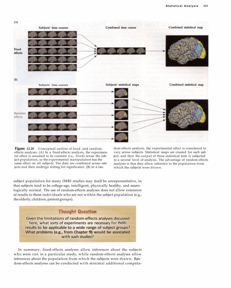
S t a t i s t i c a l A n a l y s i s 353
(A)
(B)
Figure 12.20 Conceptual outline of fixed- and random-effects analyses. (A) In a fixed-effects analysis, the experimental effect is assumed to be constant (i.e., fixed) across the subject population, so the experimental manipulation has the same effect on all subjects. The data are combined across subjects and then undergo testing for significance. (B) In a ran
dom-effects analysis, the experimental effect is considered to vary across subjects. Statistical maps are created for each subject, and then the output of those statistical tests is subjected to a second level of analysis. The advantage of random-effects analyses is that they allow inference to the population from which the subjects were drawn.
subject population for many fMRI studies may itself be unrepresentative, in that subjects tend to be college-age, intelligent, physically healthy, and neurologically normal. The use of random-effects analyses does not allow extension of results to those individuals who are not within the subject population (e.g., the elderly, children, patient groups).
In summary, fixed-effects analyses allow inferences about the subjects who were run in a particular study, whi le random-effects analyses allow inferences about the population from which the subjects were drawn. Random-effects analyses can be conducted w i t h minimal additional computa-
Subjects' time courses Combined time course Combined statistical map
Fixed effects
Subjects' statistical maps Combined statistical map Subjects' time courses
Given the limitations of random-effects analyses discussed here, what sorts of experiments are necessary for fMRI
results to be applicable to a wide range of subject groups? What problems (e.g., from Chapter 9) would be associated
with such studies?

354 C h a p t e r T w e l v e
BOX 12.2 Real-Time Analysis in Presurgical Patients
Acommon clinical application of fMRI is as a diagnostic tool for identifying functional areas that
need to be preserved during neurosurgery. For many patients w i t h brain tumors, vascular malformations, intractable epilepsy, or other types of pathology, surgical removal of the diseased portion of the brain provides the best clinical outcome. However, surgery may not be indicated for all subjects, and the amount of tissue to be removed may depend upon its functional properties. If tissue removal w o u l d result in damage to brain regions essential for human language function, memory, or primary sensory or motor processing, it could have a devastating effect on the patient's subsequent quality of life. For example, damage to the left temporal lobe may render him or her unable to comprehend speech. Thus, when deciding upon the course of treatment for a given patient, neurosurgeons want to be able to evaluate the likely functional consequences of removal of a particular brain region. Cortical mapping plays an important role in this evaluative process.
Since the 1950s, cortical mapping has typically been done during the surgery itself by temporarily probing selected brain regions using direct electrical stimulation of the cerebral cortex (see Chapter 15). This process involves placing a stimulating electrode on different parts of the exposed cortical surface. By sending a small electrical current through the electrode, the surgeon can inhibit or excite local neuronal activity. In most cases, direct stimulation impairs the function of a brain region; for example, stimulation of language areas may render patients temporarily unable to speak. In other cases, stimulation may actually cause the patient to hear sounds or see colors, motion, or shapes, if the electrode is near primary sensory areas. Although direct electrical stimulation is
widely used, it has some disadvantages. The procedure is highly invasive and time-consuming, the patient must be awakened during surgery, the range of functions that can be investigated is limited, and the only cortical areas that can be measured are those near the exposed surface of the brain.
To overcome these disadvantages, a number of hospitals have begun investigating the use of fMRI for cortical mapping in surgical patients (Figure 12.21 A and B). The advantages of fMRI are straightforward. It can be used to map functions anywhere in the brain, including within deep-brain structures difficult to reach using electrodes. It is noninvasive and can be conducted in advance of surgery to aid in surgical planning. A n d experimental tasks can be tailored to a wide range of cognitive, motor, and perceptual functions. Combining functional and conventional anatomical MRI in the same scanning session can provide maps of important functional areas superimposed on high-resolution images that show detailed anatomical structure and sites of tissue pathology. Mult iple brain functions can usually be mapped wi th in a 30- to 40-minute scanning session, providing neurosurgeons w i t h important information to aid in weighing treatment options and in planning the surgical approach to the lesion. FMRI can also be used in conjunction with traditional electrophysiological approaches, by guiding the placement of electrodes for subsequent intraoperative testing.
Despite its obvious potential, diagnostic fMRI has still seen l imited use, primarily because its analysis and interpretation is technically demanding. Whereas most fMRI research involves pooling results from many subjects, as described in the previous section, diagnostic fMRI must produce interpretable activation maps in every individual . It is critical, therefore, that each scan pro-
(A)
(B)
Figure 12.21 Cortical mapping of function. This patient was undergoing cortical mapping in preparation for neurosurgery. The subject underwent both direct electrical stimulation and fMRI . On the reconstruction of the patient's brain in (A), the locations of the electrodes in the gr id in (B) are shown as white circles. The electrodes are highlighted according to effects that direct stimulation had on different tasks: orange, speech arrest; green, induced mouth or face movements; and blue, deficits in auditory comprehension and object naming. The locus of fMRI activity d u r i n g a language comprehension task is shown on the brain surface in red. Note the overlap, albeit incomplete, between the fMRI and electrophysiological data.

S t a t i s t i c a l A n a l y s i s 355
tion, and most statistical packages now include them with in standard analysis procedures. While studies using fixed-effects models are still published, many reviewers for journals and granting agencies have recognized the importance of random-effects models and evaluate manuscripts and grants accordingly. Thus, random-effects analyses are strongly recommended for fMRI studies.
Summary Since fMRI studies rely on the detection of a weak signal in the presence of substantial noise, careful statistical analysis is necessary. Most fMRI analyses are based on hypothesis testing. The researcher sets up two hypotheses, an experimental hypothesis w i t h some prediction about the data and a null hypothesis based on random chance. The probability that the data could have occurred under the null hypothesis is compared to a threshold alpha value, and if the alpha value is exceeded, then the result is declared significant. Two types of errors are possible in hypothesis testing. Type 1 errors occur when a nonsignificant result is declared significant (a false positive),
duce high-quality MR images w i t h good functional resolution.
An important factor in achieving reliable diagnostic fMRI capabilities has been the development of real-time
analysis methods. In a real-time analysis, the fMRI data are reconstructed, preprocessed (if needed), and statistically analyzed immediately fol lowing acquisition of each image. Thus, the desired functional maps are available at the conclusion of the scanning session. Real-time analyses can be very useful for standard fMRI experiments, because they provide a way to monitor the quality of the results. If the subject moves his head excessively or is unable to perform the experimental task, real-time analyses can catch the problem dur ing the session so that it can be corrected. Real-time generation of statistical maps can also make scanning more efficient by allowing each scan to run only as long as necessary to reach a satisfactory confidence level. For clinical cortical mapping, the ability to assess task performance and activation map quality while the patient is still in the scanner is crucial. Rapid and efficient data processing also allows immediate planning of time-sensitive treatments.
Given the range of statistical approaches available for analyzing standard fMRI data, as discussed earlier in this chapter, it is not surprising that a similar range of analysis strategies have been used for real-time fMRI cortical mapping. Head morion is the most common cause of poor results, so some approaches correct for head motion during scanning. Other approaches emphasize on-line detection of motion so that the MR operator can repeat unsuccessful scans. Since the primary goal of cortical mapping is detection of active voxels, the experimental tasks used are generally simple and powerful blocked designs that can be analyzed using t-tests or correlation analyses. Use of fast computer resources and efficient software for analyses is critical.
Even when an fMRI activation map is successfully obtained, interpreting its significance presents another challenge. Many studies comparing fMRI and electrical stimulation mapping in the same patients have shown that these two approaches generally agree, but enough differences remain to make it difficult to make surgical treatment decisions based on the fMRI results alone. Also, it is difficult to assess which areas of fMRI activi-
cortical mapping The mapping of function to different areas of the cerebral cortex, in order to guide plans for clinical treatment.
real-time analysis A set of computational steps designed for rapid analysis of fMRI data, so that statistical tests are conducted immediately following acquisition of the images.
ty, as defined by a statistically significant BOLD hemodynamic response, are actually essential for a particular function. Just because an area is active during an fMRI experiment does not mean that its removal w i l l impair the studied function. Nor do traditional fMRI maps indicate how close to the border of an active area the surgeon can cut without damaging the associated brain function. Nevertheless, fMRI holds considerable promise for improving clinical cortical mapping. Careful clinical trials w i l l be needed to establish confidence criteria for interpreting fMRI maps and determining which analysis methods provide the most accurate and reliable diagnostic results. Such studies are likely to lead to an increased role for fMRI clinically and w i l l also result in improvements relevant to research applications of fMRI.
BOX 1 2 . 2 (continued)
while Type II errors occur when a significant result is missed (a false negative). FMRI analyses typically attempt to exclude Type I errors, but as a result they are prone to Type II errors. Significantly active voxels are displayed on statistical maps, usually wi th the degree of significance indicated using a color scale.
A number of basic statistical tests exist for testing single hypotheses using fMRI . Nearly all are variants of the general linear model, which treats the data as a linear summation of a number of dissociable factors. When using the general linear model to analyze fMRI data, an experimenter creates a design matrix that lists factors of interest (model factors) as wel l as other known, but uninteresting, sources of variability in the data (nuisance factors). The general linear model provides a powerful and flexible tool for data analysis, but some of its assumptions may not hold for fMRI data. Researchers have developed new data-driven analyses that seek to characterize relations among voxels over time, without creating an a priori statistical hypothesis. Regardless of the analysis approach used, a central problem for fMRI studies is the vast number of statistical tests they require, which leads to false-positive results. Standard corrections like the Bonferroni method are too strict and may eliminate true activations. One approach is to use information about spatial properties of activation, either through Gaussian random field theory or cluster-size thresholds. Another approach is to reduce the number of tests through region-of-interest analyses, which allow targeted studies of anatomical areas. Finally, for all statistical analyses, data should be combined across subjects to increase experimental power. Random-effects approaches enable inference to the population from which the subjects were drawn and are preferred over traditional fixed-effects analyses.
Suggested Readings *Brodmann, K. (1909). Vergleichende Lokalisationslehre der Grosshirnrinde in ihren
Prinzipien dargestellt auf Grund des Zellcnbaues. Barth, Leipzig, Germany. A remarkably detailed collection of anatomical studies of human and animal cortices. An English-language translation by L. J. Garey from Imperial College Press is now available.
Friston, K. J., Holmes, A. P., Worsley, K. J., Poline, J. P., Frith, C. D. , and Frackowiak, R. S. J. (1995). Statistical parametric maps in functional imaging: A general linear approach. Hum. Brain Mapping, 5: 189-210. Describes the use of the general linear model for analysis of PET and fMRI data; forms the basis for the popular SPM approach to data analysis.
*McKeown, M. J., Makeig, S., Brown, G. G., Jung, T. P., Kindermann, S. S., Bell, A. J., and Sejnowski, T. J. (1998). Analysis of fMRI data by bl ind separation into independent spatial components. Hum. Brain Mapping, 6: 160-188. Provides the theoretical framework for the application of independent components analysis (ICA) to fMRI .
*Worsley, K. J., Marrett, S., Neelin, P., Vandal, A. C, Friston, K. J., and Evans, A. C. (1995). A unified statistical approach for determining significant signals in images of cerebral activation. Hum. Brain Mapping, 4: 58-73. This paper establishes the mathematical underpinnings for spatial comparisons of functional brain images.
*Indicates a reference that is a suggested reading in the field and is also cited in this chapter.
356 C h a p t e r T w e l v e
Chapter References
Aguirre, G. K., Zarahn, E., and D'Esposito, M. (1998a). A critique of the use of the Kolmogorov-Smirnov (KS) statistic for the analysis of BOLD fMRI data. Magn. Reson. Med., 39: 500-505.
Aguirre, G. K., Zarahn, E., and D'Esposito, M. (1998b). The variability of human, BOLD hemodynamic responses. NeuroImage, 8: 360-369.
Bandettini, P. A., Jesmanowicz, A., Wong, E. C, and Hyde, J. S. (1993). Processing strategies for time-course data sets in functional MRI of the human brain. Magn. Reson. Med., 30:161-173.
Biswal, B. B., Van Kylen, J., and Hyde, J. S. (1997). Simultaneous assessment of flow and BOLD signal in resting state functional connectivity maps. NMR Biomed., 10(4-5): 165-170.
Biswal, B., Yetkin, F. Z., Haughton, V. M., and Hyde, J. S. (1995). Functional connectivity in the motor cortex of resting human brain using echo-planar MRI. Magn. Reson. Med., 34(4): 537-541.
Cordes, D., Haughton, V, Carew, J. D., Arfanakis, K., and Maravilla, K. (2002). Hierarchical clustering to measure connectivity in fMRI resting-state data. Magn. Reson. Imaging, 20: 305-317.
Cox, R. W. (1996). AFNI: Software for analysis and visualization of functional magnetic resonance neuroimages. Comput. Biomed. Res., 29: 162-173.
Forman, S. D., Cohen, J. D., Fitzgerald, M., Eddy, W. F., Mintun, M. A., and Noll, D. C. (1995). Improved assessment of significant activation in functional magnetic resonance imaging (fMRI): Use of a cluster-size threshold. Magn. Reson. Med., 33: 636-647.
Freedman, D., Pisani, R., and Purves, R. (1997). Statistics. Norton, New York. Friston, K. J., Josephs, O., Rees, G., and Turner, R. (1998). Nonlinear event-related
responses in fMRI. Magn. Reson. Med., 39(1): 41-52. Genovese, C. R., Lazar, N. A., and Nichols, T. (2002). Thresholding of statistical
maps in functional neuroimaging using the false discovery rate. NeuroImage, 15: 870-878.
Hays, W. L. (1994). Statistics (5th ed.). Harcourt College, Fort Worth, TX. Huettel, S. A., Guzeldere, G., and McCarthy, G. (2001). Dissociating the neural
mechanisms of visual attention in change detection using functional MRI. J. Cogn. Neurosci, 13(7): 1006-1018.
Jha, A. P., and McCarthy, G. (2000). The influence of memory load upon delay-interval activity in a working-memory task: An event-related functional MRI study. J. Cogn. Neurosci., 12(Suppl. 2): 90-105.
Kanwisher, N., McDermott, J., and Chun, M. (1997). The fusiform face area: A module in human extrastriate cortex specialized for the perception of faces. J. Neurosc, 17: 4302-1311.
McKeown, M. J. (2000). Detection of consistently task-related activations in fMRI data with hybrid independent component analysis. NeuroImage, 11: 24-35.
McKeown, M. J., Varadarajan, V, Huettel, S., and McCarthy, G. (2002). Deterministic and stochastic features of fMRI data: Implications for analysis of event-related experiments. J. Neurosci. Methods, 118: 103-113.
Schlosser, M. J., Luby, M., Spencer, D. D., Awad, I. A., and McCarthy, G. (1999). Comparative localization of auditory comprehension by using functional magnetic resonance imaging and cortical stimulation. J. Neurosurg., 91: 626-635.
Voyvodic, J. T. (1999). Real-time fMRI paradigm control, physiology, and behavior combined with near real-time statistical analysis. NeuroImage, 10(2): 91-106.
Xiong, J., Gao, J., Lancaster, J. L., and Fox, P. T. (1995). Clustered pixels analysis for functional MRI activation studies of the human brain. Hum. Brain Mapping, 3: 287-301.
S t a t i s t i c a l A n a l y s i s 357

Applications of fMRI
The success of any research technique can be judged by the importance of the research questions it has been used to answer. In that sense, the success of fMRI to date is undeniable. Investigators have used fMRI to answer questions rooted in a wide range of academic disciplines, including cognitive neuroscience, psychology, neurobiology, psychiatry, radiology, and many others. With increasing breadth of investigation has come a complementary depth of inquiry. As of the publication date of this book, more than 5000 articles describing fMRI research have been published in academic journals. To merely list all of the topics to which fMRI has been applied, much less to discuss those topics in any detail, w o u l d be an epic undertaking, one beyond the scope of any single review. Indeed, there have been more than 250 published review articles that discuss fMRI research.
Thus forsaking comprehensiveness, we review in this chapter selected key applications of fMRI. We have t w o goals. First, we identify three sets of advantages that result f rom the application of fMRI to research into brain function. Second, we document specific advances made wi th in a small set of topic areas: attention, memory, executive function, and consciousness. These topic areas are hardly exhaustive, and we could easily have chosen a completely different set that included such subjects as language, emotion, sensory and motor functions, and development. It is our hope that the studies discussed in this chapter w i l l illustrate how practicing scientists use fMRI as a tool for understanding the brain, and that the interested reader w i l l be able to extend the concepts discussed to other domains.
Translational Research
According to some critics, fMRI studies have provided little information beyond that already given by previous research methods (Figure 13.1A-D). It is hardly surprising, they w o u l d say, that watching a flashing checkerboard results in activity in the occipital visual cortex or that flexing the fingers of one's hand activates the primary motor cortex. While not yie lding this point, assume for a moment that this criticism was true and fMRI only provided a measure of wel l -known functional brain anatomy. Would it still

360 C h a p t e r T h i r t e e n
Figure 13.1 Development of understanding of the visual system. The basic organization of the visual system has been recognized for centuries. Shown in (A) is a schematic diagram of the eyes, the optic nerve, and the optic chiasm, from an eleventh-century Egyptian text. (B) By the eighteenth century, the crossing of information at the optic chiasm was wel l recognized, as shown in this drawing from 1750 by the English surgeon John Taylor. (C) Anatomical studies of nonhuman animals further revealed the system's retinotopic organization, demonstrating that foveal and peripheral parts of the visual field are represented in different anatomical locations, as shown in this 1879 drawing by Hermann M u n k . Key components of the visual system, including the lateral geniculate nucleus of the thalamus and primary visual cortex, can also be identified using fMRI . (D) These areas were active when the subject imagined a flashing checkerboard. The optic tracts are indicated by arrows. ( A - C from Finger, 1994; D from Chen et al., 1998.)
(A) (B)
(C) (D)
have value as a tool in neuroscience research? We argue an emphatic yes. In providing a noninvasive measure of functional activity, fMRI allows us to readily test that functional activity over a wide range of conditions. If finger movements activate the pr imary motor cortex, then consider a study that uses fMRI to observe the motor cortex over the course of learning a complex sequence of finger movements, or a study that observes motor cortex activity as a subject recovers the use of their hand fol lowing a stroke.
The possibilities grow as more-complex cognitive functions can be monitored w i t h fMRI . For example, several studies have demonstrated activation of the hippocampus dur ing the retrieval of an episodic memory. This is not surprising, as the relationship between the hippocampus and memory has
A p p l i c a t i o n s of fMRI 361
been well established by many prior methods, most prominently human and animal lesion studies. However, w i t h this demonstration, studies can now use hippocampal fMRI activation for a psychological study that examines the efficacy of different retrieval strategies, or for a study that examines memory retrieval dur ing childhood development or in normal aging, or for a study of the effects of a d r u g that may influence the rate of cognitive decline in Alzheimer's disease, or even for a study that evaluates the integrity of the hippocampus prior to a planned resection for temporal lobe epilepsy. Here, rather than using fMRI as a tool to identify the functions of as yet uncharted brain regions, fMRI is used as an outcome measure to quantify how function is altered by a host of experimental manipulations and/or intrinsic factors, such as attention, learning, disease progression, life span changes, or genetics.
Recent studies suggest that fMRI can also be used as a surrogate marker that substitutes for a clinical endpoint, such as the progression of a disease or the effectiveness of a drug therapy. Indeed, researchers are now investigating whether fMRI measures of functional activity in response to pharmacological manipulations can improve in development of novel compounds for a host of neurological and psychiatric diseases. These applications demonstrate the value of fMRI research in translational medicine, that aspect of clinical research that spans basic science and clinical practice.
surrogate marker A measurement that provides information about the clinical progression of a disease or condition.
translational medicine The practice of modifying clinical practice based on findings from basic science research and of modifying the direction of basic science research based on evidence from clinical studies.
FMRI is an excellent tool in research programs that translate between human and nonhuman animal biomedical research. Animal researchers can utilize tools that have much greater functional resolution than fMRI, but that added resolution is often achieved through invasive methods that could not be used in humans. Animals can be studied using a host of pharmacological interventions, invasive electrophysiological methods, and experimental lesions. With genetic manipulations that delete, or knock out, specific genes from an animal's genome, the influence of genetics upon a particular brain function can also be examined. Animals can also be studied using the same imaging methods described in this book. In many areas of study, investigators use similar experimental tasks in both humans and animals.
For example, fear conditioning is a standard manipulation used to study emotion. In a typical fear conditioning paradigm in a mouse or rat, a tone is paired w i t h a foot shock. In such situations, the mouse or rat engages in freezing behavior. After a sufficient number of pairings of tone and shock, the tone alone w i l l elicit freezing behavior. Extensive animal research by LeDoux and his colleagues established the central role of the amygdala (see Box 6.2) in a network of brain structures and pathways mediating conditioned fear, and has served as a model for such human diseases as depression and anxiety disorders. The fear conditioning paradigm in animals has enabled a host of additional studies, including many that probe the genetics of conditioned fear using knockout mice. But what links these animal models back to human diseases? A 1998 study by LaBar and colleagues investigated fear conditioning in human subjects using a vir tual ly identical parad i g m to that used in rats and mice, wi th fMRI providing the outcome
W h a t other applications might fMRI have for improving clinical practice?

362 C h a p t e r T h i r t e e n
Figure 13.2 Translational medicine. The ultimate goal of most medical research is to facilitate improvements in health care and treatment. FMRI research can play an important role in this process. Imagine that a researcher observes that a mouse strain displays behavior that is suggestive of a human clinical disorder. FMRI can be used to bui ld upon animal research by identifying candidate brain areas in humans that may be associated w i t h the disorder, and can further be used to test subjects w i t h the clinical disorder of interest. FMRI can also be used to evaluate the effects of proposed d r u g treatments on both the brain and the behavior, resulting in validation of new treatments or guidance for future animal studies.
measure. Strong activation of the amygdala was obtained in response to the conditioned fear stimulus, and it persisted into the extinction phase of the study, when the shock was no longer presented. This study and the many others that followed clearly established the role of the amygdala in emotional processing in humans, and thus provide a strong l ink between the human and animal studies. Moreover, a subsequent 2001 study by Sheline and colleagues used fMRI to demonstrate that patients suffering from depression had an exaggerated response in the left amygdala when viewing faces, particularly those depicting a fearful expression. Treatment of these patients w i t h the antidepressant medication sertraline reduced the amygdala's response to s t imul i . Such studies demonstrate the power of fMRI to close the loop between basic research in animals and clinical treatment in humans (Figure 13.2).
Studying Human-Specific Topic Areas
The examples in the previous section illustrate the potential value of using fMRI even when studying functional neuroanatomy that was established using another technique. While such examples are important, many fMRI studies investigate processes that are much more dif f icult to study using other techniques. An important class of such processes includes those that are pr imari ly characteristic of human cognition. No d i v i d i n g line exists between those aspects of cognition that are " h u m a n " and those that are shared w i t h other animals. However, even the most dogged supporter of animal cognition would have di f f icul ty arguing against the premise that some mental processes are more typical of the human mind while others are more generally present across mult iple species. For example, most people can readily generate a mental image of a familiar location, such as their home or workplace. The quality of this image undoubtedly varies across individuals , as some people report having only impoverished mental images while others report constructing elaborate and detail-filled scenes
FMRI studies in neurologically normal humans
Change in brain analomy / function
FMRI studies in humans with clinical disorder
Change in animal behavior
Evaluation of effect of drug on brain and behavior
New treatment alternative
Genetic manipulation (e.g., knockout mice)

A p p l i c a t i o n s of f M R I 363
that they can manipulate or transform. Nevertheless, if you are interested in mental imagery, you can study it in humans simply by asking them to imagine something. N o w consider trying to study mental imagery in nonhuman animals. Even putt ing aside whether imagery exists as a mental process for a chimpanzee or rat, it w o u l d be dif f icult at best to convince an animal to generate a mental image, much less to transform it on command.
A number of specific topics have been studied pr imari ly in human subjects and have thus been important areas of fMRI research. These topics can be generally described as those dealing wi th higher cognition. One class of higher cognitive functions requires the symbolic encoding of information and includes functions like language, episodic or autobiographical memory, conceptual categorization, and calculation. These processes are very different between language-using humans and nonhuman animals, though the study of animals may still be important (e.g., examining numerosity judgments by chimpanzees as a precursor to calculation). Another class contains functions related to internal mental states, such as goal setting, decision making, consciousness, and emotion. While there is no longer any doubt that animals can have mental representations (e.g., spatial maps, abstract relations between st imuli) , the contents of those states are likely to be very different from those of humans. Some topics must be studied in humans because we are interested in their expression as part of the human condition. For instance, to understand human social behaviors such as emotional responses to others' aversive eye movements or decision making in group situations, one must test people in the relevant social situations. Likewise, to understand changes in the m i n d and brain associated wi th human development, experiments that use similar tasks across the life span are necessary.
In contrast, many mental processes seem to be common across species. Chimpanzees have been taught to learn abstract rules, rats are quite good at interval t iming, and trained pigeons have become world-class visual discriminators. Even though the tasks that tap these abilities may be quite complex, animals can, w i t h sufficient training, learn to perform them. A good example of this is controlled visual attention, which is discussed later in this chapter. Because attention reflects an internal mental state, it may seem more suited to study in humans, who can verbally report where they are attending when it is different from where they are looking. Yet monkeys can be taught to attend to peripheral spatial locations while maintaining fixation at the center of a display. Through sophisticated behavioral paradigms (and much patience), researchers using electrophysiological recording w i t h nonhuman primates have mapped out the pr imary components of brain systems involved w i t h visuospatial attention.
While some of the most significant advances in the understanding of these higher cognitive functions have come from f M R I , we emphasize that other techniques remain extremely important. As described earlier in this section, even characteristically human processes share aspects of much simpler behaviors. To understand visual imagery, one must understand the organization of the visual system, for which electrophysiological and lesion studies have been central. Likewise, the understanding of language, that most human of all faculties, requires investigation of motor production systems, auditory comprehension systems, and even temporal sequencing systems, all of which are present in many organisms. Even for topics that may be restricted to human populations, fMRI is hardly the only option, as lesion, drug , and electrophysiological studies remain critical for many research questions.
higher cognition The set of processes that are considered to be more representative of the mental function of humans than of nonhuman animals. Examples include consciousness, executive function, abstract reasoning, and autobiographical memory.

364 C h a p t e r T h i r t e e n
phrenology The belief that bumps and indentations on the skull provide information about the magnitude of some trait supported by the underlying brain region.
Identifying Functional Relations among Brain Regions
The power of fMRI for generating maps of brain function has played an important role in popularizing cognitive neuroscience, both by making neuroimaging accessible to more researchers and by attracting new interest from the general public. To understand just how dramatic this popularization has been, consider that dur ing the late 1980s only a handful of laboratories were using PET to create functional images of the brain. Now, hundreds of institutions have scanners that are used to collect fMRI data, w i t h that number growing every year.
The popular impact of fMRI research comes in large part from the attractiveness of the images created. For an example, imagine that you are sitting (along wi th one of the authors of this textbook) in the audience of a research conference in the mid-1990s, shortly after the inception of fMRI. The potential use of neuroimaging would already be known to most of the psychologists in the audience, due in part to popularly aimed works like Posner and Raichle's 1994 book, Images of Mind. Yet at this time, few of the audience members use neuroimaging in their o w n laboratories. At the end of the session, the final speaker describes preliminary results using a new technique called "functional magnetic resonance imaging." After a short explanation of the research methods (including an experimental design that confounds the effect of interest w i t h several other factors!), the speaker shows a slide of BOLD activation overlaid upon high-resolution anatomical images. The slide is visually compelling and ful l of structure, and you look at the maps of activity with interest. A few moments later, you tear your eyes away and observe the reactions of those around you. The entire audience is staring intently at the slide, w i t h their gazes transfixed by the images. Despite the limitations of this study, the images it generated have an almost visceral effect.
Given the power of functional images of the brain to instil l wonder in even a sophisticated audience, it is unsurprising that they have rapidly permeated the popular consciousness (Figure 13.3). On a nearly daily basis, news agencies proclaim the discovery of the brain area for this or that higher-level function. Yet the very power of fMRI images raises an important caveat, specifically that one must avoid mistaking the quality of the image for the quality of the idea it represents. Because fMRI is a spatially localizing technique, it can create the false impression that complex psychological functions are localized in small bits of brain tissue. When reading about an fMRI study evaluating work ing memory, for example, it is tempting to conclude that " w o r k i n g memory" is a well-defined psychological process, that it is controlled by a specific area of the brain, and that the controll ing area is located here. The idea that single brain functions are mapped to discrete brain regions is a highly attractive one, as witnessed by the popular acceptance of phrenology two centuries ago. However, it is clear in most fMRI studies that many often spatially disparate brain regions are activated by the same task. This strongly suggests that complex functions are reflected by the coordinated activity of many discrete brain regions.
From Coactivation to Connectivity FMRI holds significant promise for elucidating the functional relations among brain regions because of its spatial coverage. Most fMRI studies collect data from the entire brain every few seconds, providing complete spatial coverage at moderate temporal resolution. Advanced pulse sequences now allow collection of more than 20 slices per second, enabling roughly 1-Hz

A p p l i c a t i o n s of f M R I 365
Figure 13.3 Functional MRI studies have elicited substantial media coverage, for better or worse. Many fMRI studies have been picked up by the popular media. While this has led to increased visibility for neuroimaging, as wel l as increased recognition of the influence of the brain upon behavior, many stories emphasize sensationalism over accuracy. Media reports of fMRI studies share some common properties. Anatomical regions are often generalized, because the intended audience knows neither the anatomy nor the jar
gon used to describe it (e.g., the frontopolar cortex vs. the prefrontal cortex). Complex concepts like personality, intelligence, and emotion are linked to specific areas, even when the research study describes activation in terms of brain systems. The study's results are applied to common behavior, for example, how one can become a better parent or stock market investor. A n d there is often a focus on studies of individual differences or social psychology that tap into common stereotypes about behavior.
sampling of whole-brain activity. Even if fMRI cannot characterize the activity w i t h i n a single brain region as completely as electrophysiological techniques, which may sample at 1000 Hz or faster, its spatial coverage makes it superior at describing functional relations between regions. In this section we discuss the theoretical principles that allow inferences about functional relations, and we describe the methodological implementation of these principles in Box 13.1.
The simplest relationship among regions is coactivation, in which t w o or more distinct brain regions show simultaneous activity dur ing an experimental task (Figure 13.4). A classic example of coactivation can be seen in motor tasks. Squeezing your left hand w i l l result in activity in the precentral
coactivation The simultaneous activity of two or more brain regions within a single experimental task. Coactivation of brain regions does not imply that the regions are functionally connected.

366 Chapter Thirteen
Figure 13.4 Coactivation of brain regions. Any complex experimental task w i l l evoke activity in several brain regions simultaneously. The regions indicated in this color map had significantly greater activity d u r i n g a rest condition than dur ing a visual search task w i t h similar perceptual characteristics. Even though these regions are coactive, they do not necessarily serve the same function. (From Huettel et al., 2001.)
connectivity The form of the relations between different brain regions, including whether they are directly or indirectly connected, whether one region influences another, and whether feedback processes exist.
network A description of the relations of a set of brain regions, including their connectivity and causal relations.
gyrus in the right hemisphere and in the cerebellum in the left hemisphere. Voxel-based fMRI analyses are designed to identify brain regions that show significant activity in response to some experimental manipulation, and thus by their very nature provide coactivation data. It is common for fMRI researchers to report that a given experimental task evoked concurrent activity in multiple brain regions (e.g., that a working memory task evoked activity in the prefrontal and parietal cortices) and to infer from this that these regions are part of a single functional system. (See Box 11.2 for additional discussion of coactivity dur ing rest/baseline conditions.)
However, while coactivity tells you that two brain regions are related, it tells you nothing about the form of that relation, or the connectivity between brain regions. Consider the simple task of encoding a set of three faces into w o r k i n g memory. If subjects perform this task whi le being scanned using fMRI, there w i l l be a set of coactive regions including the dorsolateral prefrontal cortex, superior parietal cortex, and fusiform gyrus. What can we conclude from this coactivity? One inference might be that top-down influences from the prefrontal cortex guide activity in the other regions. Another possibility is that visual processing in the temporal and parietal lobes may lead to prefrontal activity in a bottom-up fashion. Or, activity in all three regions may be triggered by signals from yet another source. Because of the inherent causal uncertainty in any single map of the brain, fMRI research has often been dismissed as being merely descriptive (i.e., describing patterns of coactivation) rather than mechanistic (i.e., explaining how the brain accomplishes a complex behavior). Patterns of coactive regions are often erroneously summarized as networks of brain activity. This misuses the term network, which should be restricted to descriptions of structural and connective relations that include the causal f low of information. For descriptions of simple associations among regions (i.e., w i t h unknown connectivity and causality), we reserve the term system.
Nevertheless, fMRI can be used to bui ld more-sophisticated models of connectivity. Some aspects of connectivity can be deduced by measuring the covariance in activity among regions across a number of experimental conditions. Consider a simple example that consists of three brain regions, A, B, and C, and two experimental conditions, X and Y (Figure 13.5). In condition X, brain regions A and C are coactivated, but B is not active. In condition Y, brain regions B and C are coactivated, but A is not active. From these results,

A p p l i c a t i o n s of fMRI 367
Figure 13.5 Using coactivity to make inferences about connectivity. By looking at patterns of coactivity across different experimental conditions, inferences about connectivity (i.e., the influence of brain areas upon each other) can be made. If one condition activates areas A and C, and another condition activates areas B and C, then one can begin to make inferences about the necessity and sufficiency of activity in one region for activity in another region.
there is a double dissociation between regions A and B, since one manipulation has an effect on A but not B and another on B but not A. This allows the inference that these regions have different functional properties. Furthermore, the information about region C provides information about connectivity. The observed pattern of associations and dissociations supports the hypothesis that regions A and B are functionally related to C but not to each other. Furthermore, because the presence of activation at C does not always predict the activation of A and B, the pattern of data suggests (but does not prove) directionality and causality. That is, A causes C to become active, and B causes C to become active. This conclusion w o u l d be strengthened if there was a measurable temporal delay (or phase lag) such that the measured activation of A or B preceded that of C, although differences in the latency of hemodynamic t iming throughout the brain can reduce the impact of such results. Of course, this example simplifies typical fMRI data, which often have a much more complex set of interrelations, but its basic logic underlies many of the more complex techniques introduced in Box 13.1.
double dissociation The demonstration that two experimental manipulations have different effects on two dependent variables. One manipulation affects the first variable but not the second, and the other manipulation affects the second but not the first.
Ideally, we w o u l d like models of connectivity to include information about unidirectional connections (i.e., A causes B) as wel l as feedback connections (i.e., A causes B, which in turn influences A ) . In order to constrain the possible functional connections w i t h i n a model, researchers incorporate information about the anatomical connections between brain regions. Although most connections between brain regions are highly reciprocal,
Condition X Condition Y
Many scientists believe that the demonstrat ion of a double dissociation is a necessary step for establishing a clear relat i o n between the independent and dependent variables.
Given w h a t you know so far, w h a t do double dissociations tell you that single dissociations do not?
BOX 13.1 Methods for Connectivity Mapping in fMRI
Most fMRI analysis approaches generate statistical maps that identify whether a given voxel
(or ROI) exhibits significant task-related signal changes. These analyses are conducted independently on all voxels so that each can be tested for significance. However, activity maps do not provide information about the relations among brain regions, save that regions are coactive. Coactivation in an fMRI study does not necessitate that two regions share a single function. For example, in a task that involves squeezing your hand when a bright light flashes, your motor and visual cortices could be simultaneously active, even though they serve very different functions. Yet because fMRI data are collected over time, they do contain substantial information suggesting how regions may be functionally related. Several approaches have been developed to generate func
tional connectivity maps, which describe the pattern of functional relations among brain regions, independent of particular task-induced activation. These include cross-correlation, partial least squares, iterative connectivity mapping, and structural equation modeling, all of which are discussed in this box, as well as independent components analysis (ICA), which was discussed in Box 12.1. Addit ional approaches excluded here for space considerations include multidimensional scaling, hierarchical clustering, and integration wi th data from diffu
sion tensor imaging (DTI) or transcranial magnetic stimulation (TMS). For a discussion of research using these latter approaches, we refer the reader to the 2002 review article by Passingham and colleagues cited in the Suggested Readings.
Because the fMRI signal has temporal structure, information about the coherence of activity over time can be used to guide connectivity mapping. It is
worth noting that this approach has been used for many decades in the measurement of high-frequency oscillations activity in the EEC waveform, as was first identified by Hans Berger in the late 1920s. By placing electrodes on the scalp, Berger discovered a regular change in electrical potential at about 10 Hz, which was later named the alpha rhythm. Subsequent EEG studies identified regular oscillatory activity at bands of higher frequencies (e.g., beta, -20 Hz; and gamma, >30 Hz) and lower frequencies (e.g., delta, <4 Hz; and theta, 4 to 7 Hz).
A similar approach was pioneered for fMRI by Biswal and colleagues in 1995, who measured fMRI activity in the sensorimotor cortex dur ing a rest condition in which subjects performed no motor task. They used a gradient-echo EPI pulse sequence with a TR of 250 ms to rapidly sample a single slice wi th in the brain. Cross-correlation analyses identified voxels whose BOLD activity time courses were significantly correlated with each other, even though no overt task was being performed. Such a correlation between two voxels would suggest that the voxels were functionally related. Note that this study, along with most other early studies, used a single time course derived from a voxel or ROI to seed the correlation analysis. The result was a single map showing connectivity with that seed location. More-advanced analyses, such as the partial least squares approach developed by Mcintosh and colleagues for PET and now applied to fMRI, provide sets of maps showing patterns of commonality and difference across experimental conditions.
In 1997, Biswal and colleagues found that time courses of activity in voxels within the sensorimotor cortex were significantly correlated at low frequencies (<0.08 Hz), both within a single hemisphere and across hemispheres. However, there was little correlation between
voxels within the sensorimotor cortex and those in other regions. Interestingly, the resulting functional connectivity map matched traditional activation maps obtained dur ing motor movement tasks. In a later study comparing BOLD and flow-dependent imaging (Figure 13.6), the authors found better matching between connectivity and activation maps for BOLD imaging than for flow imaging. This suggests that similar brain processes may underlie low-frequency oscillations and task-related BOLD signals. Subsequent studies by other groups, including a 1999 study by Xiong and colleagues, confirmed these results and extended them to additional brain regions. Although the exact mechanism of low-frequency BOLD oscillations is not yet known, both spontaneous neuronal activity along pathways that connect the regions and shared control of blood supply are likely contributions.
While analyses of data from resting or null-task blocks provide important information about functional connectivity, they face several limitations. The most critical of these potential problems is that the characteristics of the resting state are unconstrained (see Box 11.2). Imagine that you are a subject in one of these studies. As you enter the scanner, the experimenter instructs you to close your eyes and relax dur ing the session; you are to remain still without thinking about anything in particular. Such a task, of course, is impossible. One cannot shut off active thought in the same way that one closes a running faucet; indeed, the very act of remembering the task instructions violates them. For this reason, a number of researchers have investigated methods of extracting functional connectivity maps from data that contain task-related activity. Data-driven analyses, like those discussed in Box 12.1, provide one important set of tools for this process. In 2000, Arfanakis and colleagues collected data from the same set
368 Chapter Thirteen

Figure 13.6 BOLD imaging provides information about connectivity between regions. (A) FMRI data using BOLD-sensitive and (B) blood-flow-sensitive imaging was collected during performance of a bilateral finger tapping task. Both techniques found significant activity in the motor cortex. Resting-state data was collected using each type of imaging. Low-frequency oscillations that signal functional connectivity between regions were identified. The BOLD resting data clearly indicated that the hand areas of the motor cortex were functionally connected (C), matching the activation data, while the flow resting data exhibited much less functional connectivity (D). (From Biswal et al., 1997.)
of subjects in both resting and task conditions. The experimental tasks included finger tapping, passive viewing of a visual display, and auditory language comprehension, each presented in a 32-s-on/32-s-off blocked design. The authors used ICA to remove components of the data that had a significant cross-correlation w i t h a hypothesized hemodynamic
response and were located within a priori regions of interest. Using methods similar to those of Biswal and colleagues, the authors generated connectivity maps for each of the three tasks, based on both resting data and task data processed to remove task-related components. The connectivity maps were remarkably similar despite the different active task re
quirements, indicating that functional connectivity can be measured even when a task is present.
A novel extension of this technique was proposed by Hampson and colleagues in 2002. They collected separate data sets from the same subjects in two types of runs: resting and task. In the resting runs, nothing was presented and no response was required. The task runs used a blocked design in which the subjects listened to either a reading of a story or silence. The authors used an iterative comparison method that generated connectivity hypotheses based upon one data set and tested those hypotheses in the other data set. The basic approach is shown in Figure 13.7. First, the authors used a standard blocked analysis on the
statistical map (or statistical parameter map) In fMRI, the labeling of all voxels within the image according to the outcome of a statistical test.
functional connectivity map An image or diagram of the pattern of connectivity between different regions of the brain, independent of activity associated with experimental tasks.
diffusion tensor imaging (DTI) The collection of images that provide information about the magnitude and direction of molecular diffusion. It is often used to create maps of fractional anisotropy.
transcranial magnetic stimulation A technique for temporarily stimulating a brain region to disrupt its function. It uses an electromagnetic coil placed close to the scalp; when current passes through the coil, it generates a magnetic field in the nearby brain tissue, producing localized electric currents.
null-task block A control block in which there are no task requirements for the subject. Also called a baseline block or nontask block.
BOX 13.1 (continued) (A)
B O L D Flow
(B)
(D) (C)
Rest
Task
Applications of fMRI 369

Figure 13.7 A n iterative procedure for identifying functional connectivity between brain regions. A central challenge of any data analysis approach is to combine hypothesis testing and hypothesis formation, since using the same data for both purposes can introduce bias. One way to overcome this problem is to collect two data sets from the same subjects, such as a blocked-design language comprehension task and a steady-state n u l l task. Working back and forth between these data sets, researchers can identify regions of activity dur ing the task and evaluate hypotheses about their connectivity w i t h other regions. (From Hampson et al., 2002.)
task data set to create a task-related activity map. As expected, they found significant activity in Broca's area and Wernicke's area. This resulted in the hypothesis that these two regions are functionally related. To test this hypothesis, they used Broca's area as the seed for a connectivity analysis. The voxel time courses
from the resting data set were low-pass filtered to remove frequencies greater than 0.08 Hz and then correlated wi th the mean activity from Broca's area. Strong connectivity was found from Broca's area to the corresponding anatomical region in the right hemisphere, whi le weaker connectivity was noted both to Wer
nicke's area and to a region in the left pre-motor cortex. In the next iteration of their analysis, the authors defined a new ROI in the left premotor cortex based on this connectivity map. The hypothesis that Broca's area and the left premotor cortex are functionally connected was then tested, using both the auditory and silence conditions of the task data set independently. Both revealed significant correlations between these regions. Note that this iterative approach, in which one data set generates hypotheses to be tested by the other data set, could in principle be extended to additional brain regions (e.g., steps 3a and 3b).
The connectivity mapping techniques described so far have been used to confirm functional relations between brain regions. However, they do not provide information about the directionality of those relations, that is, whether area X influences activity in area Y, or vice versa. A powerful technique used to investigate such questions of causality is structural equation modeling (SEM), which attempts to determine what combination of causal relations between variables best accounts for the observed data. The process of evaluating potential sets of causal relations is known as path analysis. Applications of S E M to fMRI often use models that are constrained by the known anatomy, with pathways in the model reflecting connecting pathways between brain regions. The first use of S E M in fMRI was reported in 1997 by Buchel and Friston, w h o studied the effects of attention upon processing in the visual cortex. They found that attention increased the connectivity between extrastriate visual areas and the posterior parietal cortex, with the prefrontal cortex one potential source of this attentional control effect. More recent studies have used S E M both to evaluate models of connectivity between regions and to
3b)
Compute correlations to region D
Evaluate hypothesis of D -C connectivity
Third iteration
3a)
Identify region D based on correlations with C
Hypothesize D - C connectivity
2b)
Compute correlations to region C
Evaluate hypothesis of C - A connectivity
Second iteration
2a)
Identify region C based on correlation with A
Hypothesize C - A connectivity
lb)
Compute correlations to region A
Evaluate hypothesis of A - B connectivity
la) Identify regions A, B
Hypothesize functional connection between A and B
First iteration
BOX 13.1 (continued)
Blocked-design data set Steady-state data set
Resting runs
Task runs Blocked runs
Rest Task
370 C h a p t e r T h i r t e e n

Applications of fMRI 371
measure the effects of other factors upon that connectivity (see Figure 13.8).
Functional connectivity studies of the type described here are necessary to move fMRI studies from descriptive toward mechanistic explanations of complex behavior. However, it is important to understand that the models of connectivity provided by these formal tech
niques are only that—models. Additional data must be sought to verify that the supposed functional relationships actually exist. These data could be sought in human lesion studies in subjects in whom a stroke or surgical excision has damaged or removed a key component of the network model generated on the basis of SEM. Another approach might involve comparing different groups of subjects with known or presumed differences in the pattern of connectivity. For example, in 1998, Hor-witz and colleagues used PET data to develop a functional connectivity model that linked the left angular gyrus and extrastriate occipital and temporal cortex in single-word reading in normal individuals. This model was then tested in a population of dyslexic subjects, where a functional disconnection was observed. Such demonstrations serve to validate both a particular model derived from normal individuals and the functional connectivity approach in general.
In summary, fMRI provides sufficient spatial and temporal resolution to identify connectivity across brain regions. Simple correlation approaches can be used to reveal regions that are functionally related, even in data sets collected in the absence of an experimental task. More-complex hypothesis testing and modeling approaches intro
duce anatomical information into the analyses and allow measurement of the relative strength and directionality of the relations between regions. It is important to recognize that the success of connectivity mapping rests on a simple principle: the anatomical and functional specialization of the brain. Even though every region of the brain projects to many others, and even a simple task may evoke activity in a wide range of regions, considerable specialization remains. In 2002, Passingham and colleagues introduced the idea that each region has a unique connectional fingerprint, representing its pattern of connectivity with other regions. We believe that this concept is a useful one, as it emphasizes that neuroscience analysis approaches should be constrained by anatomical considerations. Although all voxels may be treated similarly by standard fMRI analysis methods, they have different anatomical (and functional) properties. Connectivity mapping has the potential to elucidate these properties, thereby greatly improving the inferences that can be made within fMRI experiments.
structural equation modeling (SEM) A mathematical technique for elucidating the causal relations between a set of variables. In fMRI studies, SEM can be used to create models of the connectivity between different brain areas.
connectional fingerprint The pattern of anatomical connections to and from a given brain region. The term fingerprint conveys that connectivity patterns are unique to particular brain regions.
Figure 13.8 Measurement of connectivity between brain regions. Subjects learned a set of arbitrary associations between visual patterns and finger movements while in the fMRI scanner. Structural equation modeling was used to identify the relations between activity in different brain regions across the entire fMRI time series (path coefficients indicate how large a change was evoked in the target region by a one-unit change in the source region). The paths between regions were chosen based on anatomical considerations. The regions shown here include the left and right calcarine fissures (CFL, CFR), the middle temporal gyrus (MTG), the anterior striatum (STR), the intraparietal sulcus (IPS), the inferior frontal gyrus (IFG), the inferior frontal sulcus (IFS), the opercular and dorsal parts of the precentral gyrus (PCo, PCd), and the rostral bank of the central sulcus (CSr). (From Toni et al., 2002.)
BOX 13.1 (continued)

there are a number of relatively unidirectional pathways or loops, especially between cortical and subcortical regions. The connection between the prefrontal cortex and the basal ganglia forms one such pathway, as the prefrontal cortex has heavy projections to the basal ganglia but receives little direct input in return. Instead, the basal ganglia project to the thalamus, which itself projects back to the prefrontal cortex. By incorporating information about these pathways into models of brain function, researchers can improve the models from simple patterns of coactive systems to more detailed and directional networks. Diffusion tensor imaging, which is described in Chapter 14, has become an important tool in this process.
Topic Areas
In the remainder of this chapter, we discuss some of the key research topics to which fMRI has been most profitably applied. Again, we emphasize that this set of topics is by no means complete. Functional MRI has made important contributions to many areas of research not considered here, and we urge the interested reader to select topics of personal interest for further exploration. Additional citations for review and primary research articles are included in the references section at the end of this chapter.
Attention Discussions of attention invariably begin w i t h definitions. Though "attent i o n " seems to be something that we all understand intuitively, our intuitions seem somehow inadequate for characterizing such an important process. It is curious, therefore, that the commonly cited definit ion comes from the psychologist/philosopher William James, whose wri t ing echoes his extraordinary capability for intui t ion and self-reflection. James described attention thusly: "Every one knows what attention is. It is the taking possession by the m i n d , in clear and v i v i d form, of one out of what seem several simultaneously possible objects or trains of thought." (1890, pp. 403-404)
We begin this section by considering three characteristics of attention identified by James. First, he described attention as something that acts to br ing the representation of one object (whether real or imagined) into the focus of consciousness, while excluding others. Second, attention can either be voluntarily initiated by the individual or reflexively drawn to an external object. Third, attention can be directed to objects or their properties, not just to locations in space.
The importance of visual attention can be seen in its effects on behavior. When subjects attend to a location in space or to an object feature, they make judgments about that spatial location or feature more rapidly and more accurately. An event-related fMRI study of spatial attention conducted by Small and colleagues in 2003 investigated whether these improvements in behavioral performance were correlated w i t h activity in particular brain regions. Subjects watched a display consisting of a center diamond and two flanking squares. At the beginning of the tr ial , either one side of the diamond flashed to point at one of the squares (cue trial) or both sides of the diamond flashed (neutral trial). The cue predicted the location of a later target 80% of the time. The authors hypothesized that brain regions associated w i t h shifting attention would be most active when a val id cue significantly speeded response time to the later target. Note that their comparison was between identical st imuli (validly cued trials) that were sorted based upon
372 C h a p t e r T h i r t e e n
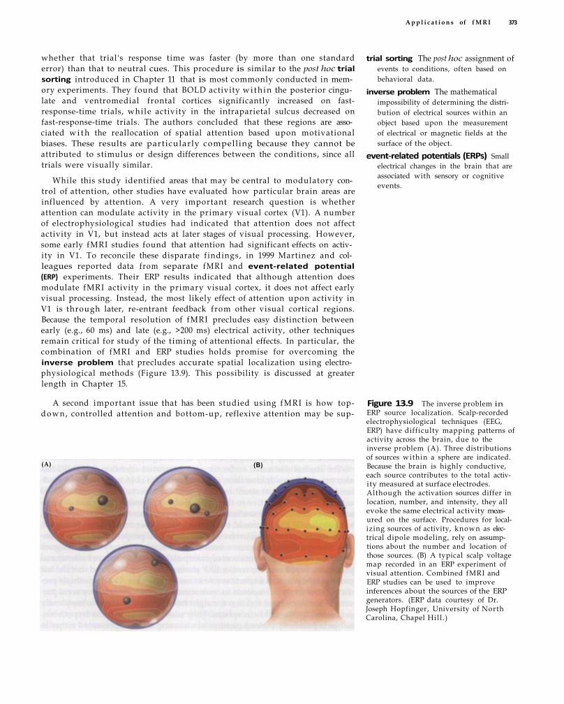
A p p l i c a t i o n s of f M R I 373
whether that trial's response time was faster (by more than one standard error) than that to neutral cues. This procedure is similar to the post hoc trial sorting introduced in Chapter 11 that is most commonly conducted in memory experiments. They found that BOLD activity w i t h i n the posterior cingulate and ventromedial frontal cortices significantly increased on fast-response-time trials, whi le activity in the intraparietal sulcus decreased on fast-response-time trials. The authors concluded that these regions are associated w i t h the reallocation of spatial attention based upon motivational biases. These results are particularly compelling because they cannot be attributed to stimulus or design differences between the conditions, since all trials were visually similar.
While this study identified areas that may be central to modulatory control of attention, other studies have evaluated how particular brain areas are influenced by attention. A very important research question is whether attention can modulate activity in the primary visual cortex (V1). A number of electrophysiological studies had indicated that attention does not affect activity in V1, but instead acts at later stages of visual processing. However, some early fMRI studies found that attention had significant effects on activity in V1. To reconcile these disparate findings, in 1999 Martinez and colleagues reported data from separate fMRI and event-related potential (ERP) experiments. Their ERP results indicated that although attention does modulate fMRI activity in the primary visual cortex, it does not affect early visual processing. Instead, the most likely effect of attention upon activity in V1 is through later, re-entrant feedback from other visual cortical regions. Because the temporal resolution of fMRI precludes easy distinction between early (e.g., 60 ms) and late (e.g., >200 ms) electrical activity, other techniques remain critical for study of the t iming of attentional effects. In particular, the combination of fMRI and ERP studies holds promise for overcoming the inverse problem that precludes accurate spatial localization using electrophysiological methods (Figure 13.9). This possibility is discussed at greater length in Chapter 15.
A second important issue that has been studied using fMRI is how top-d o w n , controlled attention and bottom-up, reflexive attention may be sup-
trial sorting The post hoc assignment of events to conditions, often based on behavioral data.
inverse problem The mathematical impossibility of determining the distribution of electrical sources within an object based upon the measurement of electrical or magnetic fields at the surface of the object.
event-related potentials (ERPs) Small electrical changes in the brain that are associated with sensory or cognitive events.
Figure 13.9 The inverse problem in ERP source localization. Scalp-recorded electrophysiological techniques (EEG, ERP) have difficulty mapping patterns of activity across the brain, due to the inverse problem (A). Three distributions of sources within a sphere are indicated. Because the brain is highly conductive, each source contributes to the total activity measured at surface electrodes. Although the activation sources differ in location, number, and intensity, they all evoke the same electrical activity measured on the surface. Procedures for localizing sources of activity, known as electrical dipole modeling, rely on assumptions about the number and location of those sources. (B) A typical scalp voltage map recorded in an ERP experiment of visual attention. Combined fMRI and ERP studies can be used to improve inferences about the sources of the ERP generators. (ERP data courtesy of Dr. Joseph Hopfinger, University of North Carolina, Chapel Hil l . )
(A) (B)
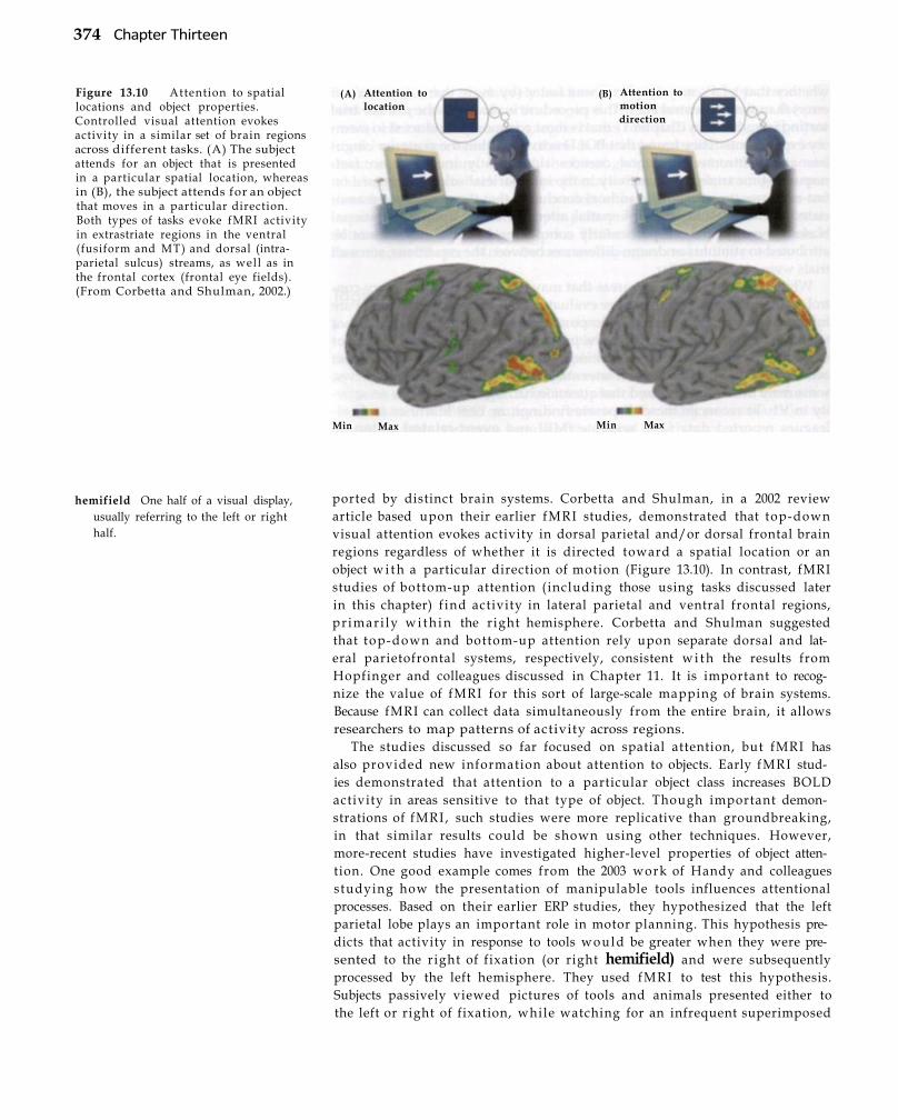
374 Chapter Thirteen
Figure 13.10 Attention to spatial locations and object properties. Controlled visual attention evokes activity in a similar set of brain regions across different tasks. (A) The subject attends for an object that is presented in a particular spatial location, whereas in (B), the subject attends for an object that moves in a particular direction. Both types of tasks evoke fMRI activity in extrastriate regions in the ventral (fusiform and MT) and dorsal (intraparietal sulcus) streams, as wel l as in the frontal cortex (frontal eye fields). (From Corbetta and Shulman, 2002.)
ported by distinct brain systems. Corbetta and Shulman, in a 2002 review article based upon their earlier fMRI studies, demonstrated that top-down visual attention evokes activity in dorsal parietal and/or dorsal frontal brain regions regardless of whether it is directed toward a spatial location or an object w i t h a particular direction of motion (Figure 13.10). In contrast, fMRI studies of bottom-up attention ( including those using tasks discussed later in this chapter) f ind activity in lateral parietal and ventral frontal regions, pr imar i ly w i t h i n the r ight hemisphere. Corbetta and Shulman suggested that top-down and bottom-up attention rely upon separate dorsal and lateral parietofrontal systems, respectively, consistent w i t h the results from Hopfinger and colleagues discussed in Chapter 11. It is important to recognize the value of fMRI for this sort of large-scale mapping of brain systems. Because fMRI can collect data simultaneously from the entire brain, it allows researchers to map patterns of activity across regions.
The studies discussed so far focused on spatial attention, but fMRI has also provided new information about attention to objects. Early fMRI studies demonstrated that attention to a particular object class increases BOLD activity in areas sensitive to that type of object. Though important demonstrations of fMRI , such studies were more replicative than groundbreaking, in that similar results could be shown using other techniques. However, more-recent studies have investigated higher-level properties of object attention. One good example comes from the 2003 work of Handy and colleagues studying how the presentation of manipulable tools influences attentional processes. Based on their earlier ERP studies, they hypothesized that the left parietal lobe plays an important role in motor planning. This hypothesis predicts that activity in response to tools would be greater when they were presented to the r ight of fixation (or right hemifield) and were subsequently processed by the left hemisphere. They used fMRI to test this hypothesis. Subjects passively viewed pictures of tools and animals presented either to the left or right of fixation, while watching for an infrequent superimposed
hemifield One half of a visual display, usually referring to the left or right half.
Attention to location
(A) (B) Attention to motion direction
Min Max Min Max

A p p l i c a t i o n s of fMRI 375
target, a black grating. As hypothesized, there was greater activity in the parietal cortex in response to tools presented to the right hemifield compared to those presented to the left hemifield. However, the parietal brain regions active in response to tools were not the same as those associated wi th spatial attention. Based on this result, the authors suggested that attention to manipulable objects and attention to spatial locations rely on different brain systems, a result that could not have been anticipated from the previous ERP data.
While James thought of attention as something that brings the representation of an object into consciousness, it is not necessary for an object to be consciously perceived for it to influence behavior. In the phenomenon known as visual extinction, which typically results from right parietal lobe damage, patients can identify singly presented objects regardless of their location. But if two objects are presented, one to the left and one to the right, the patients can only identify the object presented on the right. Even though patients only report seeing one of the objects, the other object still can affect behavior. In 2000, Rees and colleagues used fMRI to examine brain activity in a patient wi th visual extinction. They showed him pictures of houses and faces on the left, right, or left and right sides of a display and asked him to press a button to indicate on which side(s) st imuli were presented. His behavioral results showed clear evidence for extinction, in that he had 98% accuracy on unilateral trials but only 3% accuracy on bilateral trials. However, the fMRI results revealed activity in the primary visual cortex for both consciously seen and extinguished stimuli , although activity was greater for the former. This suggests that activity in the primary visual cortex can occur in the absence of visual awareness.
In addicted individuals, attention can be drawn preferentially to st imuli that are associated w i t h their disorder. As examples, smokers w i l l attend to an image of a hand holding a cigarette, while alcoholics w i l l attend to images of friends dr ink ing at a bar. An early PET study conducted in 1996 by Grant and colleagues showed that images of cocaine abuse increased activity in prefrontal and limbic brain regions of abusers. Subsequent fMRI studies by Schneider and colleagues in 2001, and by Due and colleagues in 2002, also found limbic activation in samples of alcoholics and smokers, respectively, although the latter study also reported that attention to irrelevant smoking cues evoked activity in regions associated w i t h detection of relevant targets. An important tool for investigating changes in attention (and decision making) associated w i t h disorders like addiction w i l l be virtual reality (Figure 13.11). By presenting stimuli in highly realistic environments, researchers can increase the effect of those st imuli on behavioral, emotional, and attentional processes.
To conclude, we want to emphasize t w o methodological advances that have had great effect upon the study of attention using fMRI. The first is that of fast-rate event-related f M R I , as introduced in Chapter 11. Attention has long been known to be a transient phenomenon, noted even by James, who commented on the difficulty of sustaining attention for more than a few seconds. Because of this transience, many attention experiments use cue-target paradigms in which attention is cued to a particular location and then a target is presented either at that location or at another location. Usually the cue-target interval is kept very short, spanning only a few seconds. For sample experiments, see the study by Hopfinger and colleagues presented in Chapter 11, and the study by Small and colleagues described earlier in this section. Neuroimaging techniques w i t h low temporal resolution, such as
visual extinction The loss of experience of a visual stimulus due to simultaneous presentation of another stimulus in another part of the visual field.
virtual reality Computer simulations of real-world experiences, often presented using immersive visual displays and manipulated using specialized tools.

376 Chapter Thirteen
(A)
Figure 13.11 Virtual reality and fMRI. An important goal for many types of experiments is ecological validity, or the degree to which the task faithfully replicates real-world challenges. Many fMRI researchers are using virtual-reality environments to study phenomena like attention, perception, spatial navigation, phobias, addiction, and even motor behavior. For example, looking around a bar (A) induces attention to drug-related stimuli and craving in smokers and alcoholics. Realistic environments (B) can be used to study route learning, spatial memory, and imagery. Interactive environments (C) allow the study of motor behavior and action planning, even when actual motion is restricted. (A, B courtesy of Dr. Steve Baumann, Psychology Software Tools; C courtesy of Dr. Martin McKeown, University of British Columbia.)
retinotopic mapping A technique for delineating functional regions within the visual cortex based upon their responses to stimuli presented at different retinal locations.
PET or blocked-design fMRI, cannot separate these events. However, event-related fMRI w i t h randomized trial types can be used to dissociate cue-related and target-related activity (see the 1998 article by Burock and colleagues, and the 2000 article by Hinrichs and colleagues, for examples).
The second advance is the development of f M R I paradigms for in vivo topographic mapping of sensory cortices. Functional mapping of the visual system is often called retinotopic mapping, because retinal eccentricity and angle are used to define boundaries between adjacent regions. Once functional regions are mapped in a given subject, then the effects of attention upon those regions can be identified. This can be seen in a 1999 report by Somers and colleagues, who mapped a set of eight distinct regions w i t h i n the visual cortex and then investigated the effects of foveal (i.e., near center of gaze) or extrafoveal attention upon BOLD activity in those regions. They found that attention had strong effects on activity in these regions, some of which have been investigated by subsequent experiments. These results demonstrate the power of fMRI for both spatial localization of function and subsequent analysis of how that function changes in response to manipulations like attention.
(C)
(B)

A p p l i c a t i o n s of f M R I 377
Memory
The study of memory long predates fMRI . Behavioral techniques for understanding and improving memory have been k n o w n for several millennia. Schools of oration in ancient Rome, for example, taught the use of complex schemes for place-object associations (i.e., the "method of loci") so that orators could more easily memorize long and complex speeches. Experimental studies of memory began almost concurrently w i t h the birth of psychology as a discipline, through the pioneering work of the German philosopher/ psychologist Hermann Ebbinghaus in the 1880s. Lesion studies of memory have provided clear evidence for the mnemonic functions of particular brain structures, most famously noted in patient H . M . , who lost the ability to form new long-term memories fol lowing resection of much of his medial temporal lobes more than 50 years ago.
Given this rich history, it is important to identify areas of research where fMRI has made a clear contribution. We highlight three such advances. First, fMRI studies have provided new evidence for the functional organization of human memory systems, complementing substantial previous work done wi th rodents and nonhuman primates. Second, the use of event-related fMRI in conjunction w i t h trial sorting has allowed researchers to identify links between brain activity and behavioral outcomes. Thi rd , the use of whole-brain imaging has demonstrated that memory is mediated by a distributed system rather than a few selected brain regions.
A fundamental division in memory research is between processes that support the encoding of information into long-term memory and those that support the retrieval of information from memory. Processes associated wi th explicitly encoded information are called declarative memory processes, and a further distinction can be made between episodic and semantic components of declarative memory. Episodic memory supports the recall of past occurrences of specific events, while semantic memory supports the recall of facts independently of past events. There are many other aspects of memory that are not declarative processes, including procedural memories, motor skills, short-term rehearsal, and classical conditioning, among others. We exclude these latter aspects from this discussion, primari ly for space considerations, and secondarily because most fMRI studies of long-term memory have used tasks that tap declarative processes. We refer those interested in other forms of memory to the relevant review chapter by Squire and Knowl¬ton for a clear introduction.
One of the first examples of the power of fMRI for elucidating the functional organization of brain systems for memory was reported by Gabrieli and colleagues in 1997 They investigated encoding and retrieval processes in separate runs w i t h i n the same scanning session. The encoding run alternated task blocks of novel, to-be-remembered photographs of scenes w i t h a control block of two familiar pictures presented repeatedly. The retrieval run alternated blocks where 90% of the pictures were remembered from a study session before the experiment and blocks where 90% of the pictures had not been previously seen. They found that different areas of the medial temporal lobe were active in response to encoding and retrieval. Although the specific division advanced by the authors has been modified based on subsequent research, the demonstration that encoding and retrieval processes were dissociable in the human brain served to catalyze subsequent work.
A powerful technique for studying brain systems for encoding is the subsequent memory paradigm (see Paller and Wagner for a review), which had been used in previous ERP studies in the 1980s. In this approach, the brain
encoding The conversion of information, such as stimuli in the sensory environment, into a mental representation suitable for storage in long-term memory.
retrieval The accessing of information from long-term memory stores so that it can guide thought or behavior.
declarative memory Processes that support the conscious encoding and retrieval of information about facts and events.
episodic memory Processes that support the conscious encoding and retrieval of information about occurrences of particular events.
semantic memory Processes that support the conscious encoding and retrieval of information about facts, independent of particular events.

378 C h a p t e r T h i r t e e n
response on each trial is sorted based on whether the stimulus was remembered or forgotten at a later test. In a 1998 study by Wagner and colleagues, subjects were scanned using fMRI while they judged whether each word in a rapidly presented series was abstract or concrete. Each of their six runs contained 40 abstract words, 40 concrete words, and 40 fixation trials (no word), presented in a random order for 750 ms w i t h an ISI of 1250 ms. Shortly after the end of the scanner session, the subjects took a memory test consisting of 960 items, half that they had seen in the scanner and half that were new. Based on this test, the authors identified encoding trials that were subsequently remembered wi th high confidence and encoding trials that were subsequently forgotten. Using an event-related analysis, they found greater activity in response to remembered items compared to forgotten items in the left inferior prefrontal cortex (Figure 13.12A-C), the parahippocampal gyrus, and the fusiform gyrus. The authors speculated that the degree of engagement of these regions during encoding determines the strength of the subse-
Figure 13.12 The use of trial sorting in the study of memory. With the advent of event-related f M R I , a number of investigators have begun using trial sorting based on item-specific effects, such as whether a w o r d is later remembered or forgotten. Act iv i ty in several brain regions, notably the posterior (A) and anterior (B) left inferior frontal gyri (LIFG) but also the frontal operculum (C), predicts whether subjects were able to remember a particular stimulus. (From Wagner et al., 1998.)
(A) Posterior L I F G
(B) Anterior L I F G
Time (s)
(C) Frontal operculum
P< 10-6 P<.01 Time (s)
Time(s)

A p p l i c a t i o n s of f M R I 379
quent memory trace. A similar procedure was used in 1999 by Henson and colleagues to investigate differences between conscious recollection (i.e., "remembering") and feelings of familiarity (i.e., "knowing") . They found that a region in the left frontal lobe showed increased activity in response to words that were subsequently given a "remember" judgment compared to those that were given a " k n o w " judgment.
Studies of retrieval of information from memory have also benefited from advances in fMRI methods. Using event-related designs, combined w i t h the trial sorting practices described earlier, researchers can identify distinct brain systems associated w i t h different aspects of retrieval (see Buckner and Wheeler for a comprehensive review). Attempting to retrieve an item from memory evokes activity in the left-lateralized posterior frontal cortex, seemingly independently of the content of the object to be remembered or the success of the attempt. Anterior regions of the frontal cortex are also active, although the role of these regions is less clear, perhaps involving self-monitoring of the retrieval process. In contrast, the success of memory retrieval seems to depend on activity in the medial temporal lobe, parietal cortex, and anterior frontal cortex, as shown by a number of fMRI studies. Retrieval also evokes activity in corresponding sensory cortices. That is, retrieval of spatial information evokes activity in the parietal cortex; retrieval of objects, scenes, and faces evokes activity in the ventral temporal cortex; retrieval of auditory information evokes activity in the superior temporal cortex; and so forth. This specialization based upon content is k n o w n as domain specificity. Whi le domain specificity in the sensory cortices is wel l established, specialization in frontal regions remains an important area of study.
Finally, functional neuroimaging, and f M R I in particular, has become a key tool for the study of distributed memory systems in the brain. Within the last decade, neuroimaging studies using PET and fMRI have generated large-scale models describing the functional organization of aspects of memory in the human brain (e.g., the HERA [hemispheric encoding / retrieval asymmetry] model of Tulving and colleagues). Yet despite these successes, describing distributed systems for memory using fMRI poses several challenges. Within a single process like "retrieval" is packed a multitude of sub-processes, including understanding instructions, accessing long-term stores, selecting candidate memories for reactivation, inhibi t ing inappropriate memories, and reporting the retrieved episode. These processes may be confounded in many studies. Memory is intimately tied to experience; as evidence, the word remember means literally "to bring into the mind again." As discussed later in the section on consciousness, the use of fMRI to study experiential phenomena suffers from a host of challenges.
Many aspects of memory, especially those dealing w i t h motor skills, are dif f icult to measure given the constraints of the MRI environment. To tap such processes, creative experimental designs w i l l be necessary. For example, to study memory for motor movements using fMRI , one might need to use imagined (rather than real) movements. In addit ion, some of the key regions involved in memory—those w i t h i n the medial temporal lobe—can be difficult to image using conventional fMRI due to susceptibility artifacts, especially at higher field strengths. Advances in pulse sequence design, as described in Chapter 14, w i l l help overcome this l imitation. Finally, combining information from fMRI and other techniques remains critical, especially for understanding disorders that have substantial effects upon memory (e.g., Alzheimer's disease, dementia, strokes).
domain specificity The segregation of functional regions in the brain according to the type of information that they process.

380 Chapter Thirteen
executive function The top-down control of cognition based on goals and context.
prefrontal cortex The parts of the frontal lobe anterior to regions that support motor processes.
sequence effects Changes in behavior in response to a stimulus based on the context formed by preceding stimuli.
Executive Function An increasingly important area of cognitive neuroscience is the study of executive function, which can be defined as the top-down control of thoughts and behavior based on goals and context. Just like attention and memory, the term executive function hardly reflects a unitary process. Postulated subcomponents include selecting among potential actions, monitoring performance for mistakes, maintaining information in w o r k i n g memory, switching from task to task, and preventing distracting s t imul i f rom influencing behavior. At one level, it may seem that the breadth of topics considered to be executive poses a challenge for f M R I studies. After all , how can we map out the brain areas that support a function if we cannot even define it? It is counterintuitive, therefore, that fMRI has played a particularly important role in the understanding of executive function, perhaps greater than that for any other topic discussed in this chapter. To illustrate why, we detail the key properties of executive function and how they match the strengths of fMRI .
Because fMRI can be easily used to study spatially extensive cognitive processes, it is ideally suited for studying executive function. Like the study of attention, research into executive function involves both understanding brain regions that exert top-down control and assessing the effects of that control upon other brain regions. Note, however, that executive processes differ from attentional processes in that the former act upon other cognitive processes while the latter act upon representations of objects or spatial locations. The brain region most associated w i t h executive function is the prefrontal cortex, which is heavily interconnected wi th other parts of the brain, notably the thalamus, basal ganglia, medial temporal cortex, and secondary sensory and motor cortices. For a good overview of prefrontal control processes, see the review article by Mil ler and Cohen indicated in the references section.
A second reason for the g r o w t h of fMRI studies in this area results from the tasks used to study executive function. More than any other area of cognitive neuroscience (and indeed of psychology), the study of executive function has generated a veritable Cambrian explosion of different experimental paradigms, all sharing a loose relation to control processes. Figure 13.13 illustrates a small sample of common tasks to emphasize one shared feature: because all contain infrequent events of interest, they adapt well to event-related fMRI . In the oddball task, for example, the subjects watch or listen to a series of stimuli (e.g., squares) and respond only when a infrequent target stimulus (e.g., a circle) is presented. Because of the very nature of the task, blocking the target events in time w o u l d mean that they were no longer infrequent, changing the cognitive processes they evoke. Event-related techniques are necessary for research into the influences of one trial upon the next, or sequence effects. In 2002, Huettel and colleagues used a classification task in which two s t imul i (i.e., a circle and a square) were presented wi th equal probability, each requiring a different button-press response (Figure 13.14A). Although the overall sequence was random, short-term patterns like five circles in a row arose by chance. FMRI activity w i t h i n regions of the lateral prefrontal cortex was evoked by st imuli that broke these short-term patterns (Figure 13.14B), w i t h the magnitude of that activity increasing w i t h increasing pattern length (Figure 13.14C). This effect, that the activity in response to a stimulus depends upon its context, could not be identified using blocked designs that collapse across adjacent st imuli .
Nevertheless, blocked fMRI designs can provide very useful information for studies of executive processing. While the tasks illustrated in Figure

A p p l i c a t i o n s of f M R I 381
Figure 13.13 Common executive processing tasks. Tasks that investigate executive processing often require the participant to make different responses based on context. In some cases, the contextual information interferes with responding, as in the Stroop task, in which subjects must name the ink color while ignoring the irrelevant word names. In the Simon task, subjects press buttons based upon the position of stimuli; subjects are faster when the assigned response hand matches the stimulus position. Other tasks require subjects to make infrequent responses, either based on stimuli held in working memory (the n-back task; shown here is a 3-back task) or to a particular target (the oddball task). In the go/no-go paradigm, subjects respond to most stimuli but must inhibit responses to others.
13.13 evoke transient fMRI activity, perhaps related to moment-to-moment response selection or behavioral monitor ing processes, the performance of such tasks itself evokes sustained executive processes that can be studied using blocked designs. Blocked n-back tasks, in particular, have been used in a number of studies investigating the manipulation of information in working memory. Because of the importance of both event-related and blocked approaches for different components of executive function, mixed designs w i l l likely be important for future studies.
While most fMRI executive processing research uses tasks derived from other modalities, like oddball or delayed-match-to-sample, a new and growing area of research employs event-related tasks derived from real-world sit-
Stroop
Congruent Incongruent Neutral
Incongruent Congruent
Simon
n-back
Oddball
Go / No-Go

382 Chapter Thirteen
(A)
Figure 13.14 Studying sequence effects using event-related fMRI. A central aspect of executive function is the changing of behavior based upon context. Subjects were presented with a random series of two stimuli (excerpt shown in A), each stimulus requiring a different button press. Within that random sequence, short-term patterns arose by chance, and activity in response to events that violated the patterns was measured. Shown in (B) are coronal slices at the plane shown at left; the areas in the lateral prefrontal cortex were more active in response to events that violated repeating (middle) and alternating patterns (right). The magnitude of activity in these regions increased with increasing length of the previous pattern (C), demonstrating the profound effect that context has upon executive function. (From Huettel et al., 2002.)
ecological validity The degree to which the processes studied in an experiment are similar to those produced in the natural environment.
uations. The degree to which an experiment maps onto real-world situations is k n o w n as its ecological validity. As an example, in most psychological experiments, research subjects may receive some payment for performing a decision or memory task, but their payment is not directly correlated to that performance. Yet outside of the laboratory, our actions often have very real consequences, as when we decide at which restaurant to eat or we remember (or forget) a loved one's birthday Some topics, like memory, may be best studied using tasks w i t h low ecological val idity but high experimental control . However, it is dif f icult , if not impossible, to map the brain systems underlying decision making without using st imuli (like real monetary payments) that evoke meaningful decisions. In 2002, Pochon and colleagues studied the interaction between executive processes and reward by testing subjects in an n-back task in which different trials had different reward values (totaling to $285, across all trials). Their fMRI results demonstrated that different sets of brain regions were sensitive to task di f f icul ty and to task reward, as shown in Figure 13.15A-D. The use of fMRI to study the brain systems for processing expectancy for rewards has become increasingly
Time since stimulus onset (s)
(C)

A p p l i c a t i o n s of fMRI 383
(A)
Time (TR)
Time (TR)
Figure 13.15 Different regions show increases in activity for task difficulty and reward. An fMRI n-back task w i t h both difficulty and reward varying over trials was conducted. A system of prefrontal, parietal, and cerebellar regions showed changes in activity w i t h task difficulty. For example, activity in the right dorsolateral prefrontal cortex (DLPFC) increased with increasing difficulty (A), while activity in the bilateral ventromedial
(B)
Time (TR)
Time (TR)
prefrontal cortex (VMPFC) decreased w i t h task difficulty (B). A different set of regions including the frontal, cingular, insular, and temporal cortices and the basal ganglia showed changes in activity associated with reward. In the left medial prefrontal cortex, activity decreased w i t h increasing reward (C), while in the left rostral dorsolateral prefrontal cortex, activity increased w i t h increasing reward (D). (From Pochon et al., 2002.)
common over the past several years, as researchers have extended results from single-unit studies in primates to fMRI studies in humans (see Montague and Berns for a review).
game theory A set of mathematical approaches for studying choices made by individuals in cooperative or competitive social situations.
Another way to improve ecological validity is to cloak decisions in social contexts, as by having subjects cooperate or compete w i t h other individuals. A small but growing number of studies have used game theory, a mathe-
Highest reward
Lowest reward
Left rostral D L P F C (BA 10/46) (D) Left medial prefrontal cortex (BA 10/32) (C)
Right D L P F C (BA 9/46) VMPFC (BA 25)
Highest difficulty
Lowest difficulty
Why are studies w i t h high ecological validity preferred to those w i t h low ecological validity?

384 C h a p t e r T h i r t e e n
matical framework relating choices in social situations to expected rewards. In a 2003 fMRI study by Sanfey and colleagues, subjects played an "ultima-rum game" w i t h a series of human and computer opponents. In this game, each opponent makes a monetary offer to the subject; some offers are fair and some are unfair. The subject chooses whether to accept or reject each offer; however, the consequences of rejecting an offer ($0) are always worse than those of accepting it . Yet many previous behavioral studies have revealed that people reject unfair offers w i t h high probability. The authors found that unfair offers evoked activity in the dorsolateral prefrontal cortex, anterior cingulate gyrus, and anterior insula. Of note was a trade-off between activity in the prefrontal and insular cortices. For unfair offers that were accepted, there was greater prefrontal activity than insular activity, while for unfair offers that were rejected, the pattern was reversed. This study points to the potential util ity of fMRI for studies typically thought to be the domain of economics rather than psychology. A number of laboratories have begun exploring ways in which people inside the MRI scanner can interact with other individuals , so that the neural correlates of social behavior, including social decision making, can be explored.
Finally, because of the number of different executive processing tasks that have been used, synthesis of information across experiments is extremely important. One experimenter may describe activity in terms of response selection, another in terms of working memory, and another in terms of task switching, even when they are all doing variations of the oddball task. An important tool for synthesizing findings across the literature is meta-analysis, or combining results f rom a number of different studies (usually already published) into a single new analysis. In 2000, Cabeza and Nyberg reported a comprehensive meta-analysis of a very large number of fMRI and PET studies (Figure 13.16A), and smaller meta-analyses have been reported for many individual areas of research.
Meta-analyses are most easily conducted when studies report their results in a common form. Neuroimaging approaches, like both PET and fMRI , typically report their results in one or both of two forms: the spatial coordinates of activity w i t h i n a stereotaxic space (e.g., Montreal Neurological Institute, Talairach) or the containing region in a cytoarchitectonic system (e.g., Brodmann's areas). If a study found activity in the middle frontal gyrus, for example, it might report that activity as occurring at coordinates x = - 42, y = 32, and z = 32, or that it was present in Brodmann's area 46. By looking for commonalities across mult iple studies, researchers can uncover general principles that span mult iple tasks. For example, in their meta-analysis of executive function studies conducted using PET and f M R I , Duncan and Owen combined data from 20 separate experiments (Figure 13.16B). Although the exact foci of activity differed across studies, the authors found that they tended to cluster in three primary regions: the mid-dorsolateral frontal cortex, mid-ventrolateral frontal cortex, and dorsal anterior cingulate cortex. One important caveat for meta-analytic strategies is that, by reducing neuroimaging data to a set of activation locations, they ignore other information from the original studies, such as the t iming of activity.
In summary, the study of executive processing faces particular challenges. Executive functions are supported by distributed brain systems, and the tasks used to study executive processing are often complex, rapidly presented, open-ended, and/or realistic. The strengths of fMRI are well suited to meet these challenges. Because of the dif f iculty in defining executive processes, we anticipate that collection of converging data across many studies using different paradigms w i l l play a large role in future advances.
meta-analysis The statistical analysis of data collected from multiple experiments.

A p p l i c a t i o n s of f M R I 385
Figure 13.16 (A) Meta-analysis across anatomical regions. Meta-analyses combine data from multiple studies in order to improve detection power or generalizability of the results. One form of meta-analysis for neuroimaging data codes studies by whether they found activity in particular anatomical regions, here broken d o w n by Brodmann areas. The upper table shows a meta-analysis of one type of executive function research, studies of working memory, which show activity predominantly in frontal, cingulate, and parietal regions. For comparison, the lower table shows studies of perception, which most frequently show activity in temporal and occipital regions. (B) Voxel-based meta-analysis. Another way of doing meta-analyses of neuroimaging data is to map activation coordinates. In the meta-analysis reported by Duncan and Owen, a number of different executive processing studies are mapped onto a standardized brain, revealing clusters of activity in the dorsolateral prefrontal cortex (around the inferior frontal sulcus; IFS), ventrolateral prefrontal cortex (above the Sylvian fissure; SF), and anterior cingulate cortex (CC). (A from Cabeza and Nyberg, 2000; B from Duncan and Owen, 2000.)
IFS (B)
IFS
SF
C C
(A)
386 Chapter Thirteen
BOX 13.2 Use of fMRI in Nonhuman Primates
The fMRI studies described so far in this book have been restricted to human subjects. Yet in principle,
other animals could serve as research subjects. Within the past few years, a handful of laboratories have begun fMRI studies of nonhuman primates, primarily using the rhesus monkey (Macaco mulatta) and other macaques. Although fMRI is not necessary for in v ivo study of the animal brain, given the power of intracranial electrophysiology, it does provide some important advantages (see the commentary written by Paradiso in 1999 for additional discussion). First, and most importantly, it can link human and animal research. In all fields of science, methodological advances can cause divisions that are based on techniques rather than topic. Researchers who conduct electrophysiological studies of decision making in monkeys may communicate w i t h other monkey electro-physiologists but not w i t h researchers using human neuroimaging. Studies using fMRI in monkeys can bridge the gap between human fMRI and monkey electrophysiology, allowing their results to be more easily integrated. This may be particularly important for domains like vision, whose basic neural organization was established primarily using animal electrophysiology.
Second, it provides information that can complement the limitations of existing techniques. In many ways, intracranial electrophysiology is considered to provide the clearest evidence for the function of a brain region, in that implanted electrodes can provide direct information about neuronal activity. However, each electrode records signals from only a small brain region (in some cases a single neuron), and therefore breadth of spatial coverage is sacrificed. Using fMRI to guide subsequent electrode placement could substantially improve the efficiency of electrophysiological re
search. A n d , since fMRI does not require surgery (e.g., to implant electrodes), it may have some ethical advantages for some forms of exploratory research. Animal fMRI studies can also inform human fMRI studies, even though both brain anatomy and cognitive function differ between species. More data can be collected in animal fMRI studies than is typical for human research, given that the same animal could participate in a large number of experimental sessions. Thus, functional SNR could potentially be much higher in animal fMRI , benefiting studies w i t h more experimental conditions or w i t h parametric changes in an independent variable. FMRI in monkeys also provides an opportunity to introduce other concurrent manipulations, such as simultaneous electrophysiological recording, use of contrast agents, or evaluation of drug effects. While these manipulations may not be practical in human volunteers, they may be conducted under the guidelines for acceptable care and use of laboratory animals.
The first studies using fMRI in nonhuman primates were reported by 1998, by two groups who simultaneously conducted very similar experiments. Ste¬fanacci and colleagues recorded fMRI BOLD data from the visual cortex of a rhesus monkey during a passive viewing task. The animal lay in a prone position within a specially designed "chair," which was itself contained within a local gradient coil inside a standard clinical 1.5-T MRI scanner (Figure 13.17). The animal's head was fixed into place using a headpost, so that it could look down the bore onto a display screen in front of it . Of note was the use of a mock scanner environment over a period of a month to familiarize the monkey with the confinement and noise levels of the scanner. During the scanning sessions, the monkey watched a video movie that was presented in a 16-s-on/16-s-off blocked design. The monkey also periodically
received a squirt of juice as reward for staying still during the session. Scanning procedures were generally similar to those used in human studies: gradient-echo EPI w i t h a 1-s TR and a 40-msTE. The authors found significant activation in occipital visual regions, as well as in higher visual regions within the superior temporal gyrus. A second study by Dubowitz and colleagues used a very similar apparatus and visual stimulation paradigm. Their results mirrored those of Stefanacci and colleagues, in that they were able to identify regions of significant activity in the visual cortex.
Though highly exploratory, these early studies demonstrated the feasibility of collecting BOLD fMRI data in monkeys. Subsequent studies from these groups and others replicated these results, while suggesting topics for future research. One area that holds particular promise is the use of exogenous contrast agents to increase SNR. Recall from Chapter 7 that injection of a highly paramagnetic substance into the bloodstream causes susceptibility-related signal loss on T 2*-weighted images. Because the magnitude of this signal loss depends upon the total amount of the contrast agent that is present in a voxel, it serves as an index of local cerebral blood volume. While exogenous contrast agents are not practical for most human fMRI studies, given the nonin¬vasiveness of standard BOLD measurement, they may offer significant advantages for studies in nonhuman animals. As an example, a 2002 study by Leite and colleagues demonstrated that the use of an exogenous contrast agent (monocrystalline iron oxide nanoparti¬cles, or MIONs) increased functional sensitivity by a factor of 2 to 3 over BOLD contrast, depending upon the experimental design. Another important research domain lies in using animal fMRI models to improve understanding of the basic principles of BOLD fMRI.

A p p l i c a t i o n s of fMRI 387
Stimulus
BOX 13.2 (continued)
"OFF" "ON"
Magnet bore
15 cm
29 cm
Head-holding apparatus Neckplate Door
26.5 cm
0 -20 mm
(A) (B)
(A) (B)
Figure 13.17 Collecting fMRI data in the monkey. Using fMRI w i t h nonhuman animals poses problems, particularly when they are awake and performing a task. This figure shows one of the first successful fMRI experiments using monkeys. A rhesus macaque monkey was placed in a special primate chair that was turned sideways to fit into the bore of a standard human 1.5-T scanner (top). The animal
watched a movie presented in a blocked on/off design. Significant B O L D activity was found in the temporal (A) and occipital ( B ) lobes. Researchers noted that there were substantial problems w i t h head motion, due in part to the use of scanning and restraint hardware that were not designed specifically for monkey f M R I . (From Stefanacci et al. , 1998.)
In a series of experiments, Logothetis and colleagues have investigated the relation between hemodynamic and electrophysiological measures of brain activity, using concurrent fMRI and ERP/EEG measures. While we discuss the results of these studies in detail in Chapter 15, one of their technical advances should be noted here, namely a custom vertical-bore MRI scanner designed specifically for use w i t h monkeys (Figure 13.18). Several other insti
tutions have installed monkey-specific scanners in recent years.
Although nearly all fMRI studies in monkeys have studied basic sensory functioning studies of more-advanced cognitive processes are also possible. A very interesting study of executive function, reported by Nakahara and colleagues in 2002, investigated the brain regions involved in shifting between response sets. An important hallmark of human prefrontal cortex damage is an
inability to shift from one mode of responding to another, as demonstrated by behavioral impairments in the Wisconsin Card Sorting Test. In order to study set shifting in monkeys, Nakahara and colleagues developed a modified version of this test that two macaque monkeys (Macaco fuscata) performed within a standard clinical scanner. The authors found significant activity in response to category shifts in the monkeys' inferior prefrontal cortex, as well as in the intrapari-

388 C h a p t e r T h i r t e e n
B O X 1 3 . 2 (continued)
(A) (B)
Figure 13.18 A custom M R I scanner for monkey studies. (A) Through the creation of hardware specific for studies of nonhuman animals, the quality of fMRI data can be greatly improved. Logothetis and colleagues have created a custom scanner that allows the animal to remain upright w i t h the head restrained (B). (Courtesy of Dr. Nikos Logothetis, Max Planck Institute, Tubingen, Germany.)
etal sulcus, posterior cingulate, precuneus, and insula. They then compared these regions of activity to those from an identical fMRI experiment conducted in humans (Figure 13.19). The authors found that the humans also showed significant activity in the inferior prefrontal cortex, in a region w i t h similar cytoarchitectonic properties to that identified in monkeys. Future studies of this type w i l l be critical for matching maps of brain function across species.
The use of fMRI in nonhuman animals has considerable potential, but it also presents a new set of challenges. In a sense, it combines all of the problems of fMRI w i t h all of the problems of animal studies. One difficulty that must be overcome is subject motivation. Human fMRI subjects may be motivated by several factors: the desire to help the experimenter, a sense of purpose in helping to advance science, or the thought of the payment they w i l l receive upon completion of the study. In contrast, animal subjects are more motivated by the d i -
(A)
E l
Figure 13.19 Comparison of fMRI in monkey and human. A potentially exciting use of fMRI in monkeys is for direct comparison to human data. Data was collected from both macaque monkeys (A) and humans (B) in a variant of the Wisconsin Card Sorting Test (height of slices, z, shown in mm). In both species, there was significant activity in the bilateral inferior frontal cortex in response to st imuli that require a shift from one response set to another. This result suggests that these regions may be functionally homologous between the species. Note that the brain images are shown at different scales; the human brain has more than 10 times the volume of the macaque brain. (From Nakahara et al., 2002.)

problem of scale involved w i t h imaging a rodent brain, consider that at a voxel size typical for human studies, only about 30 voxels would be needed to contain the entire brain of a rat, and only about 6 would be needed for the brain of a mouse. Yet despite these limitations, several fMRI studies in rodents have been conducted using ultra-high-field scanners. These studies have generated exquisite maps of sensory cortices, as exemplified by the work of Xu and colleagues in the olfactory bulb of the rat. Thus, fMRI studies of nonhuman primates and other animals are likely to become increasingly important, both for improving understanding of brain function and for clarifying the basic physiological mechanisms of fMRI.
have the potential to minimize such problems.
Finally, we note that animal models themselves have limitations. Monkeys are similar to humans in overall brain organization, but they are expensive to maintain and test, and relatively few institutions have large colonies. A less expensive option is to move to rodents, as is most typical for behavioral neurosci¬entific studies. Rats are cheaper, are common, and perform many tasks well , but they have extremely small brains (about 2 cc). Most genetic manipulations have been performed in mice, making them good candidates for studies of the effects of specific genes upon brain function, but their brains are much smaller still (about 0.4 cc). To emphasize the
rect rewards given for experimental compliance, such as squirts of juice. Though juice is a good reward system for behavioral studies, it is not ideal for fMRI . Swallowing a sip of juice requires contraction of muscles in the jaw and throat, which in turn causes both distortions in the local magnetic field and head motion. Even w i t h a periodic reward, an animal may have difficulty remaining still . For example, in the study by Stefanacci and colleagues, a number of the experimental runs were severely corrupted by large head motions. The authors noted that this head motion may have been exacerbated by the limitations of using a clinical MRI scanner w i t h a primate chair inserted wi th in the bore, so dedicated monkey scanners
BOX 13.2 (continued)
Consciousness
Of all the terms used by psychologists, the idea of consciousness is the most poorly defined. It can mean wakefulness, as in "He regained consciousness w i t h i n a few minutes of the accident." It can describe the belief system of a group of people: "The idea of personal freedom began to enter the popular consciousness fol lowing the revolut ion." Or it can mean something in between, like personal awareness: "I became conscious of the ringing phone, and walked across the room to answer i t . " It is the last of these conceptions, that of personal subjective experience, that has proven the most vexing for scientists.
To understand w h y consciousness is so diff icult to study, look up f rom this book and out at the w o r l d around you. Depending on your location, you may see desks in a classroom, stacks of books in a library, or, if you are fortunate enough to be reading this book outside on a w a r m spring afternoon, white clouds dri f t ing across a blue sky. N o w pick an object, any object. What is its color? As you are staring at the object, a series of physical processes take place. Photons from an external light source, whether the sun or a nearby lamp, reflect off of the object. Some of those photons collide wi th photoreceptors in your eye, where they induce chemical changes in particular photopigments, depending upon their frequency. This results in electrical activity w i t h i n the photoreceptors, which in turn propagates from the eye via the thalamus to the primary visual cortex, and from there on to higher cortical centers for vision. Though the details are amazingly complex, it is important to recognize that the series of processes that take place when you see the color blue are different from those when you see the color red. By mapping these two sets of processes, one could, in principle, recognize those aspects of brain function that differ according to what color is consciously experienced. However, consciousness poses a second, much more insidious problem. Think about the physical steps that seem to all add up to your experience of blue. Which of those steps make it possible for you to actually
Applications of fMRI 389
390 Chapter Thirteen
easy problem A research question tha t can be addressed, in principle, using existing experimental methods.
hard problem A research question that cannot be answered, even in principle, by existing experimental methods and scientific principles.
neural correlates Patterns of brain activity that covary with another phenomenon, such as a mental state or behavior.
binocular rivalry The alternation of images presented independently to each eye.
experience blueness? Put another way, how can low-level information processing in the brain actually translate into your awareness of the world around you?
The philosopher David Chalmers has labeled these two problems of consciousness as easy problems and hard problems. Here, easy and hard do not refer to complexity or difficulty, in the same sense that a 1 -digit multiplication problem is easy and a 10,000-digit mult ipl icat ion problem is hard. Instead, these terms refer to the sorts of methods that can be applied for their solution. Easy problems are those dealing w i t h the mechanisms of biological processes; they are easy because they can be explained in terms of lower-level physical principles. This chapter, and indeed this entire book, is filled w i t h examples of fMRI being applied to easy problems. The hard problems of consciousness are those that relate to personal experience. No scientific principles exist that state how the f i r ing of a neuron or the release of a neurotransmitter can generate a feeling, emotion, or sensation. H o w then can f M R I be applied to address the hard problems of consciousness? One approach that has been pursued by many investigators rests on the idea of neural correlates of consciousness; a neural correlate is a marker in the brain that may index consciousness, even if the causal relations between them are unknown (see also Box 1.1). By looking for neural correlates of consciousness, researchers can transform hard problems into easy ones, bypassing questions about how subjective experience can arise from objective, physical activity. As w i l l be evident from the fol lowing examples, nearly all fMRI studies of consciousness have focused on visual experience.
Thus, the basic framework used by most fMRI studies of consciousness is simple. The experimenter induces a change in the experience of the subject, then measures the patterns of activity associated w i t h those changes. Ideally, this change in experience is accompanied by minimal perceptual changes, to reduce the l ikelihood of confounding factors. A good example of this approach is found in a clever study conducted by Tong and colleagues in 1998, which investigated the effects of binocular rivalry upon activity in extrastriate visual cortex (Figure 13.20). Binocular r ivalry occurs when the two eyes see different visual displays, as when one sees a horizontal bar and the other a vertical bar. Rather than combine the displays into a single image (e.g., a plus symbol), the visual system switches between the two rivalrous images, usually every few seconds, so that sometimes you see one image and sometimes the other. The subjects in this study viewed pictures of faces in one eye and houses in the other eye and indicated when the display switched from one stimulus type to the other (Figure 13.20A).
While the physical display does not change d u r i n g these switches, the contents of conscious experience do change, and those changes evoked systematic variation in visual cortical activity. Face-to-house switches were associated w i t h decreased activity in the fusiform gyrus and increased activ-
Do you believe that there are aspects of the mind that cannot be addressed by science, even in principle? How would you defend your position against someone with
the opposite perspective?

A p p l i c a t i o n s of fMRI 391
Figure 13.20 Relating brain activity to perceptual experience. One way to investigate the neural correlates of consciousness is to relate changes in brain activity to changes in experience. In this figure, a binocular rivalry paradigm is used (A), in which one eye saw a face and the other eye saw a house, so that the subject's perception alternated frequently between faces and houses. fMRI activity in face-selective
regions (FFA) and place-selective regions (PPA) followed the subject's report of rivalrous switches from one stimulus type to another, as shown in (B). The time courses of activity in response to perceptual switches (where the stimulus did not change) were similar to those in a control condition in which the display in both eyes actually alternated between houses and faces (C). (From Tong et al., 1998.)
ity in the parahippocampal gyrus, while house-to-face switches resulted in the opposite pattern of activity (Figure 13.20B). These activity changes therefore represent a correlate of conscious experience, not merely a passive reflection of visual input. A control condition compared these results to real alternations between faces and houses in a non-rivalry paradigm, w i t h the t iming of switches matched to the rivalry condition. It found that subjective switches and real switches evoked very similar patterns of activity (Figure 13.20C). Note that this particular design could not be implemented w i t h PET, because the brain must be sampled at a faster rate than the frequency of switching. Similar approaches have been used for studies of attention, illusory perception, emotion, and imagery.
A second framework adopts the reverse approach: using subthreshold stimuli, the experimenter identifies what sorts of brain changes can occur in the absence of conscious experience. To present visual stimuli without inducing awareness, researchers often use a masking paradigm, in which the stimuli of interest are shown for only a short duration (<50 ms) and are followed by a complex visual image. In 1998, Whalen and colleagues used such a mask-
subthreshold stimuli Stimuli presented below the threshold for detection. In psychophysics, the threshold is also known as the limen, and thus subthreshold stimuli are also known as subliminal stimuli.
(A)
Rivalry
Stimulus
Time from reported perceptual switch (s)
Percept
Non-rivalry
Time from reported stimulus switch (s)
Rivalry
(B)
(C)
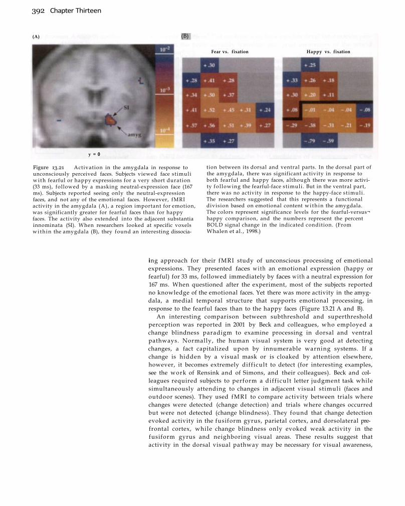
392 Chapter Thirteen
Figure 13.21 Activation in the amygdala in response to unconsciously perceived faces. Subjects viewed face st imuli w i t h fearful or happy expressions for a very short duration (33 ms), followed by a masking neutral-expression face (167 ms). Subjects reported seeing only the neutral-expression faces, and not any of the emotional faces. However, fMRI activity in the amygdala (A), a region important for emotion, was significantly greater for fearful faces than for happy faces. The activity also extended into the adjacent substantia innominata (SI). When researchers looked at specific voxels w i t h i n the amygdala (B), they found an interesting dissocia
tion between its dorsal and ventral parts. In the dorsal part of the amygdala, there was significant activity in response to both fearful and happy faces, although there was more activity fo l lowing the fearful-face s t imul i . But in the ventral part, there was no activity in response to the happy-face s t imul i . The researchers suggested that this represents a functional division based on emotional content w i t h i n the amygdala. The colors represent significance levels for the fearful-versus¬happy comparison, and the numbers represent the percent BOLD signal change in the indicated condition. (From Whalen et al., 1998.)
ing approach for their fMRI study of unconscious processing of emotional expressions. They presented faces w i t h an emotional expression (happy or fearful) for 33 ms, followed immediately by faces wi th a neutral expression for 167 ms. When questioned after the experiment, most of the subjects reported no knowledge of the emotional faces. Yet there was more activity in the amygdala, a medial temporal structure that supports emotional processing, in response to the fearful faces than to the happy faces (Figure 13.21 A and B).
An interesting comparison between subthreshold and superthreshold perception was reported in 2001 by Beck and colleagues, who employed a change blindness paradigm to examine processing in dorsal and ventral pathways. Normally, the human visual system is very good at detecting changes, a fact capitalized upon by innumerable warning systems. If a change is hidden by a visual mask or is cloaked by attention elsewhere, however, it becomes extremely diff icult to detect (for interesting examples, see the work of Rensink and of Simons, and their colleagues). Beck and colleagues required subjects to perform a di f f icul t letter judgment task while simultaneously attending to changes in adjacent visual st imuli (faces and outdoor scenes). They used fMRI to compare activity between trials where changes were detected (change detection) and trials where changes occurred but were not detected (change blindness). They found that change detection evoked activity in the fusiform gyrus, parietal cortex, and dorsolateral prefrontal cortex, while change blindness only evoked weak activity in the fusiform gyrus and neighboring visual areas. These results suggest that activity in the dorsal visual pathway may be necessary for visual awareness,
(A) (B)
Fear vs. fixation Happy vs. fixation
y = 0

A p p l i c a t i o n s of fMRI 393
complementing studies of the ventral visual pathway like that by Tong and colleagues described earlier.
FMRI studies can also be used to improve understanding of disorders of consciousness. Patients wi th lesions to part of the primary visual cortex report that they cannot see stimuli presented in the part of the visual field corresponding to their lesion. However, in some cases they can guess characteristics of the stimuli wi th considerable accuracy. This phenomenon has been given the evocative name blindsight to describe the dissociation between the patients' experience and apparent information processing by the visual system. In 2001, using fMRI , Goebel and colleagues demonstrated that stimuli presented wi th in the blindsight area evoke activity in higher visual regions. While stimuli evoked no BOLD activity in the damaged V1 area, a rotating spiral evoked activity in motion area V5 and objects evoked activity in the lateral occipital cortex and fusiform gyrus. These fMRI results extend the decades-old patient studies by showing that activity in extrastriate regions is not sufficient for visual awareness; activity in the primary visual cortex is also required. Another interesting disorder is Charles Bonnet syndrome, in which patients w i t h visual impairments experience v iv id and animated hallucinations, such as mosaic patterns of lines, common animals, or fantastic creatures. Using event-related fMRI, ffytche and colleagues showed that there were significant increases in activity in the fusiform gyrus during the period of hallucination, and there were suggestions that the content of the hallucinations governed the location of activity. These two studies point to the potential value of combined fMRI and lesion studies for refining theories about consciousness.
Summary Functional MRI studies have made substantial contributions to the understanding of the mind and brain. Replication of existing results, as early studies typically accomplished, validated the feasibility of fMRI research. But as fMRI became more established, replication gave way to extension. Researchers asked new questions about human cognition or functional relations between brain regions that were difficult to answer w i t h earlier methods. By the late 1990s, fMRI had made profound contributions to the democratization of cognitive neuroscience, making the brain more accessible to researchers and the public alike. While fMRI has had a substantial impact on a number of topic areas, perhaps the most visible advances have been made in the understanding of higher cognitive processes, including attention, memory, and executive function. Each of these domains has been shaped by results from fMRI, although other techniques remain of considerable interest. Even that most nebulous of all psychological topics, consciousness, has been attacked wi th some success. Despite many studies, however, fundamental questions remain about how fMRI can illuminate the relation between cognitive functions and brain activity.
Suggested Readings
Brett, M., Johnsrude, I. S., and Owen, A. M. (2002). The problem of functional localization in the human brain. Nat. Rev. Neurosci., 3: 243-249. The authors describe, in clear language, the technical and theoretical issues facing attempts to localize brain activity using neuroimaging.
*Buckner, R. L., and Wheeler, M. E. (2001). The cognitive neuroscience of remembering. Nat. Rev. Neurosci., 2: 624-634. A comprehensive review of studies of memory retrieval, including many using fMRI.
blindsight A phenomenon in which individuals with cortical damage have no experience of visual stimuli within the damaged part of the visual field, but can nevertheless report the characteristics of those stimuli under particular conditions.

Gazzaniga, M. S., ivry, R. B., and Mangun, G. R. (2002). Cognitive Neuroscience. Norton, New York. This accessible textbook provides a good introduction to the field of cognitive neuroscience, including all of the topics discussed in this chapter.
*Nakahara, K., Hayashi, T, Konishi, S., and Miyashita, Y. (2002). Functional MRI of macaque monkeys performing a cognitive set-shifting task. Science, 295: 1532-1536. This report contains an extremely interesting comparison between human and monkey fMRI data.
*Passingham, R. E., Stephan, K. E., and Kotter, R. (2002). The anatomical basis of functional localization in the cortex. Nat. Rev. Neurosci., 3: 606-616. An interesting and provocative review of the relation between anatomical connectivity and brain function.
Rees, G., Kreiman, G., and Koch, C. (2002). Neural correlates of consciousness in humans. Nat. Rev. Neurosci., 3: 264-270. A good review article describing attempts to map correlates of consciousness, notably of visual experience.
*Indicates a reference that is a suggested reading in the field and is also cited in this chapter.
Chapter References Arfanakis, K., Cordes, D., Haughton, V. M., Moritz, C. H., Quigley, M. A., and
Meyerand, M. E. (2000). Combining independent component analysis and correlation analysis to probe interregional connectivity in fMRI task activation datasets. Magn. Reson. Imaging, 18: 921-930.
Beck, D. M., Rees, G., Frith, C. D., and Lavie, N. (2001). Neural correlates of change detection and change blindness. Nat. Neurosci., 4: 645-650.
Biswal, B. B., Van Kylen, J., and Hyde, J. S. (1997). Simultaneous assessment of flow and BOLD signals in resting-state functional connectivity maps. NMR Biomed., 10:165-170.
Biswal, B., Yetkin, F. Z., Haughton, V. M., and Hyde, J. S. (1995). Functional connectivity in the motor cortex of resting human brain using echo-planar MRI. Magn. Reson. Med., 34: 537-541.
Buchel, C, and Friston, K. J. (1997). Modulation of connectivity in visual pathways by attention: Cortical interactions evaluated with structural equation modelling and fMRI. Cereb. Cortex, 7: 768-778.
Buckner, R. L. (2000). Neuroimaging of memory. In The New Cognitive Neurosciences, M. S. Gazzaniga (ed.), pp. 817-828. MIT Press, Cambridge, MA.
Burock, M. A., Buckner, R. L., Woldorff, M. G., Rosen, B. R., and Dale, A. M. (1998). Randomized event-related experimental designs allow for extremely rapid presentation rates using functional MRI. NeuroReport, 9: 3735-3739.
Cabeza, R., and Nyberg, L. (2000). Imaging cognition II : An empirical review of 275 PET and fMRI studies. J. Cogn. Neurosci., 12:1-47.
Chalmers, D. J. (1996). Facing up to the problem of consciousness. In Toward a Science of Consciousness, S. R. Hameroff, A. W. Kaszniak, and A. C. Scott (eds.), pp. 5-28. MIT Press, Cambridge, MA.
Chen, W., Kato, T, Zhu, X. H. , Ogawa, S., Tank, D. W., and Ugurbil, K. (1998). Human primary visual cortex and lateral geniculate nucleus activation during visual imagery. NeuroReport, 9: 3669-3674.
Corbetta, M., and Shulman, G. L. (2002). Control of goal-directed and stimulus-driven attention in the brain. Nat. Rev. Neurosci., 3: 201-215.
Dubowitz, D. J., Chen, D. Y, Atkinson, D. J., Grieve, K. L., Gillikin, B., Bradley, W. G., and Anderson, R. A. (1998). Functional magnetic resonance imaging in macaque cortex. NeuroReport. 9: 2213-2218.
Dubowitz, D. J., Chen, D., Atkinson, D. J., Scandeng, M., Martinez, A., Andersen, M. B., Andersen, R. A., and Bradley, W. G. (2001). Direct comparison of visual cortex activation in human and non-human primates using functional magnetic resonance imaging. J. Neurosci., 107: 71-80.
394 C h a p t e r T h i r t e e n

Due, D. L., Huettel, S. A., Hall, W. G., and Rubin, D. C. (2002). Smoking cues elicit activation in mesolimbic and visuospatial neural circuits: Evidence from fMRI. Am. J. Psychiatry, 159: 954-960.
Duncan, J., and Owen, A. M. (2000). Common regions of the human frontal lobe recruited by diverse cognitive demands. Trends Neurosci., 23: 475-483.
ffytche, D. H., Howard, R. J., Brammer, M. J., David, A., Woodruff, P., and William, S. (1998). The anatomy of conscious vision: An fMRI study of visual hallucinations. Nat. Neurosci., 1: 738-740.
Finger, S. (1994). Origins of Neuroscience. Oxford University Press, New York. Gabrieli, J. D, Brewer, J. B., Desmond, J. E., and Glover, G. H. (1997). Separate neu
ral bases of two fundamental memory processes in the human medial temporal lobe. Science, 276: 264-266.
Goebel, R., Muckli, L., Zanella, F. E., Singer, W., and Stoerig, P. (2001). Sustained extrastriate cortical activation without visual awareness revealed by fMRI studies of hemianopic patients. Vis. Res., 41: 1459-1474.
Grant, S., London, E. D., Newlin, D. B., Villemagne, V. L., Liu, X., Contoreggi, C, Phillips, R. L., Kimes, A. S., and Margolin, A. (1996). Activation of memory circuits during cue-elicited cocaine craving. Proc. Natl. Acad. Sci. U.S.A., 93: 12040-12045.
Hampson, M., Peterson, B. S., Skudlarski, P., Gatenby, J. C, and Gore, J. C. (2002). Detection of functional connectivity using temporal correlations in MR images. Hum. Brain Mapping. 15: 247-262.
Handy, T. C., Grafton, S. T, Shroff, N. M., Ketay, S., and Gazzaniga, M. S. (2003). Graspable objects grab attention when the potential for action is recognized. Nat. Neurosci., 6: 421-127.
Henson, R. N. , Rugg, M. D., Shallice, T, Josephs, O, and Dolan, R. J. (1999). Recollection and familiarity in recognition memory: An event-related functional magnetic resonance imaging study. J. Neurosci., 19: 3962-3972.
Hinrichs, H., Scholz, M., Tempelmann, C, Woldorff, M. O, Dale, A. M., and Heinze, H. J. (2000). Deconvolution of event-related fMRI responses in fast-rate experimental designs: Tracking amplitude variations [erratum appears in J. Cogn. Neurosci., 2000, 12(6), following table of contents]. J.Cogn. Neurosci., 12: 76-89.
Hopfinger, J. B., Buonocore, M. H., and Mangun, G. R. (2000). The neural mechanisms of top-down attentional control. Nat. Neurosci., 3: 284-291.
Horwitz, B., Rumsey, J. M., and Donohue, B. C. (1998). Functional connectivity of the angular gyrus in normal reading and dyslexia. Proc. Natl. Acad. Sci. U.S.A., 95: 8939-8944.
Huettel, S. A., Guzeldere, G., and McCarthy, G. (2001). Dissociating the neural mechanisms of visual attention in change detection using functional MRI. J. Cogn. Neurosci., 13: 1006-1018.
Huettel, S. A., Mack, P. B., and McCarthy, G. (2002). Perceiving patterns in random series: Dynamic processing of sequence in prefrontal cortex. Nat. Neurosci., 5: 485-490.
James, W. (1890). The Principles of Psychology. Dover, New York. LaBar, K. S., Gatenby, J. C, Gore, J. C, LeDoux, J. E., and Phelps, E. A. (1998).
Human amygdala activation during conditioned fear acquisition and extinction: A mixed-trial fMRI study. Neuron, 20: 937-945.
Leite, F. P., Tsao, D., Vanduffel, W., Fize, D., Sasaki, Y., Wald, L. L., Dale, A. M., Kwong, K. K., Orban, G. A., Rosen, B. R., Tootell, R. B., and Mandeville, J. B. (2002). Repeated fMRI using iron oxide contrast agent in awake behaving macaques at 3 Tesla. NeuroImage, 16: 283-294.
Logothetis, N. K., Pauls, J., Augath, M., Trinath, T., and Oeltermann, A. (2001). Neurophysiological investigation of the basis of the fMRI signal. Nature, 412: 150-157.
Mandeville, J. B., Marota, J. J., Kosofsky, B. E., Keltner, J. R., Weissleder, R., Rosen, B. R., and Weisskoff, R. M. (1998). Dynamic functional imaging of relative cerebral blood volume during rat forepaw stimulation. Magn. Reson. Med., 39: 615-624.
Applications of fMRI 395

Martinez, A., Anllo-Vento, L., Sereno, M. I . , Frank, L. R., Buxton, R. B., Dubowitz, D. J., Wong, E. C, Hinrichs, H., Heinze, H. J., and Hillyard, S. A. (1999). Involvement of striate and extrastriate visual cortical areas in spatial attention. Nat. Neurosci., 2: 364-369.
Mcintosh, A. R., Bookstein, F. L., Haxby, J. V., and Grady, C. L. (1996). Spatial pattern analysis of functional brain images using partial least squares. NeuroImage, 3: 143-157.
Miller, E. K., and Cohen, J. D. (2001). An integrative theory of prefrontal cortex function. Annu. Rev. Neurosci., 24: 167-202.
Montague, P. R., and Berns, G. S. (2002). Neural economics and the biological substrates of valuation. Neuron, 36: 265-284.
Paller, K. A., and Wagner, A. D. (2002). Observing the transformation of experience into memory. Trends Cogn. Sci., 6: 93-102.
Paradiso, M. A. (1999). Monkey business builds a bridge to the human brain. Nat. Neurosci., 2: 491-492.
Pochon, J. B., Levy, R., Fossati, P., Lehericy, S., Poline, J. B., Pillon, B., Le Bihan, D., and Dubois, B. (2002). The neural system that bridges reward and cognition in humans: An fMRI study. Proc. Natl. Acad. Sci. U.S.A., 99: 5660-5674.
Posner, M. I . , and Raichle, M. E. (1994). Images of Mind. Scientific American Library, New York.
Ranganath, C., and Rainer, G. (2003). Neural mechanisms for detecting and remembering novel events. Nat. Rev. Neurosci., 4: 193-202.
Rees, G., Wojciulik, E., Clarke, K., Husain, M., Frith, C., and Driver, J. (2000). Unconscious activation of visual cortex in the damaged right hemisphere of a parietal patient with extinction. Brain, 123: 1624-1633.
Rensink, R. A., O'Regan, J. K., and Clark, J. J. (1997). To see or not to see: The need for attention to perceive changes in scenes. Psychol. Sci., 8: 368-373.
Sanfey, A. G., Rilling, J. K., Aronson, J. A., Nystrom, L. E., and Cohen, J. D. (2003). The neural basis of economic decision-making in the Ultimatum Game. Science, 300: 1755-1758.
Schneider, F., Habel, U., Wagner, M., Franke, P., Salloum, J. B., Shah, N. J., Toni, I . , Sulzbach, C., Honig, K., Maier, W., Gaebel, W., and Zilles, K. (2001). Subcortical correlates of craving in recently abstinent alcoholic patients. Am. J. Psychiatry, 158: 1075-1083.
Sheline, Y. I., Barch, D. M., Donnelly, J. M., Ollinger, J. M., Snyder, A. Z., and Mintun, M. A. (2001). Increased amygdala response to masked emotional faces in depressed subjects resolves with antidepressant treatment: An fMRI study. Biol. Psychiatry, 50: 651-658.
Simons, D. J., and Chabris, C. F. (1999). Gorillas in our midst: Sustained inattencion¬al blindness for dynamic events. Perception, 28: 1059-1074.
Small, D. M., Gitelman, D. R., Gregory, M. D., Nobre, A. C., Parrish, T. B., and Mesulam, M. M. (2003). The posterior cingulate and medial prefrontal cortex mediate the anticipatory allocation of spatial attention. NeuroImage, 18: 633-641.
Somers, D. C, Dale, A. M., Seiffert, A. E., and Tootell, R. B. (1999). Functional MRI reveals spatially specific attentional modulation in human primary visual cortex. Proc. Natl. Acad. Sci. U.S.A., 96: 1663-1668.
Squire, L. R., and Knovvlton, B. J. (2000). The medial temporal lobe, the hippocampus, and the memory systems of the brain. In The New Cognitive Neurosciences, M. S. Gazzaniga (ed.), pp. 765-779. MIT Press, Cambridge, MA.
Stefanacci, L., Reber, P., Costanza, J., Wong, E., Buxton, R., Zola, S., Squire, L., and Albright, T. (1998). fMRI of monkey visual cortex. Neuron, 20: 1051-1057.
Tong, F., Nakayama, K., Vaighan, J. T., and Kanwisher, N. (1998). Binocular rivalry and visual awareness in human extrastriate cortex. Neuron, 21: 753-759.
396 Chapter Thirteen

Tong, F. (2003). Primary visual cortex and visual awareness. Nat. Rev. Neurosci., 4: 219-229.
Toni, I . , Rowe, J., Stephan, K. E., and Passingham, R. E. (2002). Changes of cortico¬striatal effective connectivity during visuomotor learning. Cereb. Cortex, 12: 1040-1047.
Tulving, E., Kapur, S., Craik, F. I., Moscovitch, M., and Houle, S. (1994). Hemispheric encoding/retrieval asymmetry in episodic memory: Positron emission tomography findings. Proc. Natl. Acad. Sci. U.S.A., 91: 2016-2020.
Wagner, A. D., Schacter, D. L., Rotte, M., Koutstaal, W., Maril, A., Dale, A. M., Rosen, B. R., and Buckner, R. L. (1998). Building memories: Remembering and forgetting of verbal experiences as predicted by brain activity. Science, 281: 1188-1191.
Whalen, P. J., Rauch, S. L., Etcoff, N. L., Mclnerney, S. C., Lee, M. B., and Jenike, M. A. (1998). Masked presentations of emotional facial expressions modulate amygdala activity without explicit knowledge. J. Neurosci., 18: 411-418.
Xiong, J., Parsons, L. M., Gao, J., and Fox, P. T. (1999). Interregional connectivity to primary motor cortex revealed using MRI resting state images. Hum. Brain Mapping, 8: 151-156.
Xu, F., Kida, I . , Hyder, F., and Shulman, R. G. (2000). Assessment and discrimination of odor stimuli in rat olfactory bulb by dynamic fMRI. Proc. Natl. Acad. Sci. U.S.A., 97: 10601-10606.
A p p l i c a t i o n s of fMRI 397

From their infancy in the early 1990s, fMRI methods have dramatically evolved. Many early studies acquired only one or two images, at slice acquisition rates as slow as one per 10 seconds. A pr imary goal of early studies was to provide proof-of-concept results, such as showing that the occipital lobe becomes active during a visual stimulation task, rather than to generate novel findings that were unexpected based on existing knowledge. Now, as fMRI research enters a period of adolescence, there has been an explosion of interest in studying a wide variety of cognitive processes beyond simple sensation, from attention to memory to decision making to consciousness. Fast event-related designs combined w i t h advanced pulse sequences have enabled acquisition and analysis of subsecond changes throughout the brain. Though this growth has been extraordinary, it is important to recognize that fMRI remains a relatively young technique. Just like an adolescent, its grasp reaches out to an ever widening w o r l d , while its thoughts are directed inward toward its o w n limitations.
In this chapter, we present some of the major recent advances in image acquisition and analysis that promise to benefit future fMRI research. These advances have been driven by the desire to collect images at the highest possible spatial resolution and w i t h the fastest possible acquisition speed, while maintaining sufficient spatial fidelity and functional SNR. We therefore have organized the discussion in this chapter thematically, separating advances that challenge the spatial l imits of fMRI from those that test its temporal limits. It is important to recognize that the methods discussed in this chapter reflect but partial snapshots of promising research breakthroughs. Given the enormous number of laboratories that are currently pushing the bounds of fMRI , it w o u l d be impossible to document all advances. Our goal, instead, is to orient the reader to the likely directions of future progress, while conveying some of the breathlessness of the current pace of research. Not only do many important research questions remain unanswered, but we still do not know what limits (if any) restrict the questions that can be asked. It is truly a remarkable time to be doing fMRI research.
Advanced fMRI Methods

400 C h a p t e r F o u r t e e n
ultrahighresolution MRI The acquisition of MR images with voxel sizes on
the order of tens of micrometers.
Applications of ultrahighresolution
MRI to animal tissue are known as MR
microscopy.
Spatial Resolution and Spatial Fidelity
Although the most striking advantage of MRI over previous neuroimaging
methods is its excellent spatial resolution, the possibility of further improve
ments has driven recent developments in pulse sequence design and imag
ing hardware. Increases in spatial resolution for anatomical M R I result in
advantages for fMRI research. Remember that although BOLD fMRI meas
ures a vascular response in the brain that may span a few centimeters, the
vascular response is evoked by neuronal activity that may be organized on a
submillimeter scale. The spatially restricted neuronal activity, not the more
widespread vascular response, controls the f low of information in the brain.
Therefore, improvements in the resolution of MRI down to the cellular level
may have significant consequences for functional studies. We w i l l refer to
studies that attempt to resolve image details on the order of tens of micro
meters as ultrahighresolution MRI or MR microscopy. Al though we discuss here how ultrahighresolution MRI benefits research into brain struc
ture and function, it has had significant consequences for other fields of
science as wel l , including studies of gene expression, animal phenotype
characterization, and stem cell migration. Because of the many advantages
of ultrahighresolution MRI , laboratories investigating a number of diverse
and interesting questions have pushed its spatial l imits such that fine reso
lution at a cellular level is achievable.
Imagine the possibility of imaging a single neuron! To understand the
challenge of such a task, consider that a typical fMRI voxel has dimensions
of about 4 mm on a side, roughly similar to the size of the w o r d "the" in this
book. Yet w i t h i n that tiny voxel exist more than a mi l l ion neurons. The cell
body, or soma, of a given neuron may be only a few tens of micrometers in
diameter, while its axon may stretch only a few millimeters. Despite the
challenges posed by such an extreme scale, there have been some promising
results in anatomical MRI . In 1999, Dodd and colleagues, for example, used
iron oxide as a contrast agent for imaging T cells, which are important com
ponents of the immune system. A single T cell is approximately 5 μm in
diameter, or 1 / 2 0 0 of a millimeter. In order to scan these cells directly, resolu
tion on the order of 1 to 2 μm would be necessary. However, if highly para
magnetic iron oxide is introduced into the cells, much larger regions of sus
ceptibilityinduced signal loss w i l l be measured on T2*sensitive images. In a
sense, this effect is very similar to the BOLD mechanism described in Chap
ter 7, but on a much smaller scale. The resulting susceptibility effects can be
used as indicators of iron oxide and thus of the position of the cells. Using a
smallbore scanner at 4.7 T, Dodd and colleagues collected images w i t h
extremely high resolution (voxel dimensions of about 25 μm on a side), and
the position of T cells became clearly visible.
While this result, along w i t h those f rom similar studies, has been
extremely promising, it is important to note its limitations. Chief among
them is that the use of iron oxide contrast does not allow identification of
structure w i t h i n a cell, as can be obtained w i t h electron microscopes, but
instead provides information about the location of cells. Note also that voxel
volume decreases w i t h the cube of spatial resolution, such that a voxel 0.5
mm on a side has only 1/8 the volume of one that is 1 mm on a side. A 25μm
voxel, like that obtained by Dodd and colleagues, has only 1/ 6 4 , 0 0 0 the volume
of a 1mm voxel. Since the total MR signal measured from a voxel is roughly
proportional to its volume, the MR signal at ultrahigh spatial resolution is
extraordinarily weak compared to that at normal spatial scales. As a result,

Advanced fMRI Methods 401
most of the ultrahighresolution MRI images have been acquired ex vivo or
in vitro on smallbore highfield MRI scanners.
volumetric Relating to the measurement
of volume.
morphometric Relating to the measure
ment of shape.
magnet diameter The diameter of the electromagnetic coil that generates
the strong static field used in MRI.
Ultrahighresolution MRI has become an increasingly important tool for
understanding brain anatomy. In recent years, spatial resolution on the
order of a few tens of micrometers has been regularly achieved, providing
similar resolution to that available w i t h traditional lightmicroscopic tech
niques. A sample ultrahighresolution image is shown in Figure 14.1. One
important advantage of MRI over other similar approaches is the relative
ease of quantitative analyses. Many researchers use vo lumetr i c and mor
phometric techniques to measure properties of size and shape, respectively.
Based on the tissue contrast used for the MR images (e.g., T 1 ) , researchers
can outline a given brain structure in t w o sets of animals (e.g., normal and
genetic knockout mice) and then investigate changes in brain anatomy
associated w i t h the group difference. The results can be readily stored in a
database for use by other investigators, such as the Biomedical Informatics
Research Network (www.nbirn.net ) . Because the MRI data are collected
electronically, they are more easily analyzed and disseminated than are tra
ditional microscopic slides.
We emphasize, however, that ultrahighresolution images are typically
only acquired at very high field strengths and long acquisition times and are
most commonly used for imaging small animals. There are two primary rea
sons for this l imitat ion. First, field homogeneity becomes increasingly
important wi th increasing strength of the static field, such that it is very dif
ficult to ensure the stability across space of an extremely strong magnetic
field. Veryhighfield MRI scanners w i t h bore sizes large enough to accom
modate human imaging are extremely expensive and dif f icult to maintain
and are thus very uncommon. Typical smallbore scanners for rodent imag
ing may have field strengths of 7 T or greater but magnet diameters of only
Figure 14.1 An ultrahighresolution MR microscopy image. Shown is an image of a male C57BL/6J mouse brain, collected at 43μm isotropic resolution. To appreciate the spatial resolution of this image, consider that approximately one million of its voxels would fit within a single 4 mm x 4 mm x 5 mm human fMRI voxel. (Courtesy of Dr. G. Allan Johnson, Center for Invivo Microscopy, Duke University.)
Based on what you learned in Chapter 9 about the sources of
noise in MRI, w h a t problems w o u l d you encounter w h e n
a t tempt ing ultrahiqhresolution MRI in vivo?

402 C h a p t e r F o u r t e e n
effective bore size The clearance within the bore of the MRI scanner that limits the maximum size of the sample that can be scanned.
phased array A method for arranging multiple surface detector coils to improve spatial coverage while maintaining high sensitivity.
multiple-channel imaging (or parallel imaging) The use of multiple receiver channels to acquire data following a single excitation pulse.
8 to 30 cm. For comparison, typical whole-body MRI scanners have magnet diameters of about 90 to 100 cm. Once outf i t ted w i t h other imaging hardware, the effective bore sizes for small-animal scanners may only be 4 to 20 cm, while human scanners have effective bore sizes of about 60 cm. Second, acquisition of sufficient MR signal for acceptable raw SNR requires an extremely long scan time, which may not be tolerable for human participants. Images of the sort shown in Figure 14.1 may require more than 24 hours of collection time, for example, and even relatively rapid acquisition methods require a few hours per subject. While the results from animal models cannot always be extrapolated to humans, the technical advances associated w i t h ultrahigh-resolution MRI studies have offered insight into problems associated w i t h high-field fMRI in humans. In the past few years, several human scanners at 7 T and above have been successfully installed, providing exciting new results and presenting new challenges.
In the fol lowing sections, we discuss some of the state-of-the-art imaging techniques that are being developed for improving the spatial characteristics of the functional signal. We begin w i t h hardware improvements that enhance the reception of signal using multiple channels in parallel, and then consider new techniques for measuring hemodynamic changes in the brain. While BOLD contrast has been extraordinarily useful for fMRI studies, its reliance on T2* imaging makes it vulnerable to susceptibility-induced signal losses in the ventral frontal and temporal lobes adjacent to the sinuses. We therefore discuss strategies for compensating for these losses through modification of standard pulse sequences. We end w i t h an explanation of new methods for doing fMRI that do not rely on BOLD contrast. Because the BOLD signal may not always be colocalized w i t h neuronal activity, these new methods have become increasingly important.
Multiple-Channel Acquisition Throughout this book, we have concentrated on single-channel reception methods. As discussed in Chapters 3 and 4, the precession of net magnetization w i t h i n the transverse plane induces a current in a nearby receiver coil. Changes in this current over time allow reconstruction of the spatial properties of the sample. While use of a single coil is most common, it is also possible to acquire data from mult iple coils in parallel, such as in a phased array design, as described in Chapter 2. This is known as multiple-channel acquisition or parallel imaging. The use of multiple-channel acquisition has two advantages. One is to increase the spatial resolution and raw SNR without increasing acquisition time; the other is to reduce the duration of the readout w i n d o w and thus minimize spatial distortion without compromising SNR.
To illustrate an example of increasing spatial resolution using multiple-channel acquisition, consider the schematic reception system shown in Figure 14.2A. Here, the four receiver coils simultaneously but independently cover the four quadrants of the imaging volume, each wi th a matrix size of n x n (e.g., 128 x 128). By simply combining all four images, an image with a large field of view that contains the entire sample can be obtained wi th a matrix size of 2n x 2n (e.g., 256 x 256), illustrated in Figure 14.2B. Note here that the imaging matrix dimensions are doubled, wi thout any increase in imaging time. Such an implementation is conceptually straightforward; however, each i n d i v i d u a l image usually contains signal f rom other quadrants due to aliasing that results from spatial subsampling. In addition, the signal intensity of the final image (Figure 14.2C) varies severely in space, depending upon the voxel position w i t h respect to the individual

A d v a n c e d fMRI M e t h o d s 403
(A) Figure 14.2 Use of multiplechannel acquisition w i t h independent fields of view. By using more than one reception coil simultaneously (A), spatial resolut ion can be improved considerably without increasing imaging time. The simplest example is shown in (B), where each coil samples an independent quadrant of the object (i.e., a reduced field of view). The final image (C) is obtained by simply combining the individual quadrants. Note that the final image has nonuniform signal intensity and w i l l suffer from aliasing artifacts (not shown here) due to the sensitivity of each coil to the other quadrants.
Signal combiner
(B) (C)
surface coils. For f M R I , this could result in different functional SNR across
the brain.
Multiplechannel imaging can also be used to increase spatial resolution
by collecting data from coils w i t h overlapping fields of view (Figure 14.3).
During the imaging session, all channels acquire data w i t h larger coverage
in kspace to reach higher resolution. To keep the time of data acquisition
short, the kspace data are subsampled for individual coils (Figure 14.3A),
resulting in the severely aliased images shown in Figure 14.3B. By incorpo
rating field maps from individual coils (Figure 14.3C) and using an iterative
reconstruction process to remove aliasing artifacts, a final image w i t h uni
form spatial coverage and high spatial resolution can be achieved (Figure
14.3D). The relation between the number of coils and the matrix size can be
expressed more generally in the fo l lowing way. Assuming the number of
receiver coils is M, the number of sampling points for each coil is P, and the
number of voxels desired in the final reconstructed image is n2, we must use
enough coils so that M x P > n2. Thus, as M coils are used, the matrix size
could increase by a factor of up to √M for a given acquisition time, as
demonstrated by Sodickson and colleagues and also by Pruessmann and
colleagues. In addition to increasing spatial resolution, multiplechannel
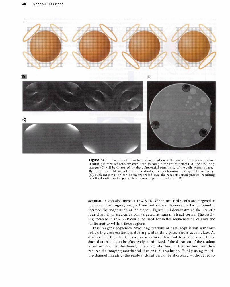
Figure 14.3 Use of multiple-channel acquisition w i t h overlapping fields of view. If mult iple receiver coils are each used to sample the entire object (A), the resulting images (B) w i l l be distorted by the differential sensitivity of the coils across space. By obtaining field maps from individual coils to determine their spatial sensitivity (C), such information can be incorporated into the reconstruction process, resulting in a final uniform image w i t h improved spatial resolution (D).
acquisition can also increase raw SNR. When mult iple coils are targeted at the same brain region, images from individual channels can be combined to increase the magnitude of the signal. Figure 14.4 demonstrates the use of a four-channel phased-array coil targeted at human visual cortex. The resulting increase in raw SNR could be used for better segmentation of gray and white matter wi th in these regions.
Fast imaging sequences have long readout or data acquisition windows fo l lowing each excitation, d u r i n g which time phase errors accumulate. As discussed in Chapter 4, these phase errors often lead to spatial distortions. Such distortions can be effectively minimized if the duration of the readout w i n d o w can be shortened; however, shortening the readout window reduces the imaging matrix and thus spatial resolution. But by using multiple-channel imaging, the readout duration can be shortened without reduc-
404 C h a p t e r F o u r t e e n
(B)
(A)
(C)

A d v a n c e d fMRI M e t h o d s 405
(A) Four-channel phased-array surface coil (B) Standard quadrature volume coil Figure 14.4 Effects of multiple-channel acquisition upon raw SNR. (A) An image collected using a four-channel phased-array surface coil, while (B) is an image collected using a standard volume coil. Both images were acquired on the same 4-T scanner in the same subject. The raw SNR is much improved by the use of four-channel parallel acquisition, as shown here in (A) by the better contrast between gray and white matter. The improved raw SNR facilitates tissue segmentation and also allows acquisition of higher-resolution images wi thout increasing acquisition time.
ing the imaging matrix. For example, by using four receiver coils for data acquisition, a 256 x 256 imaging matrix can be acquired in the same amount of time as a single coil can collect a 128 x 128 imaging matrix. In principle, the duration of the readout window can be shortened by up to a factor of M, given M receiver coils. An example of reduced image distortion in multichannel EPI is illustrated in Figure 14.5, demonstrating the value of multiple-channel imaging for preserving the spatial fidelity of an image.
Susceptibility Compensation and Weighting As discussed in Chapter 9, an increasing proportion of fMRI experiments are being performed at high-field scanners to increase functional SNR. Despite this advantage, high-field scanning poses significant challenges for fMRI . Major problems for BOLD fMRI studies are susceptibility artifacts, which manifest as signal losses and spatial distortions in ventral brain areas that are near interfaces between air and brain tissue. Susceptibility artifacts are present on any T 2 *-weighted image and are exacerbated by fast imaging
susceptibility artifacts Signal losses on T2*-dependent images due to magnetic field inhomogeneities in regions where air and tissue are adjacent.
Figure 14.5 Effects of multiple-channel acquisition upon spatial fidelity. Distortions often present in images acquired using a single reception channel (A) can be reduced by using multiple-channel acquisition (B). The improved spatial fidelity, especially in areas with susceptibility artifacts, results from
the use of a shortened data acquisition window in multiple-channel imaging. Both images are of the same slice in the same subject at the same spatial resolution (2.5 mm x 2.5 mm). (Courtesy of Dr. Susumu Mori, Johns Hopkins University.)
(A) (B)

406 C h a p t e r F o u r t e e n
Figure 14.6 Effects of susceptibility compensation. Shown in (A) are two representative axial slices acquired using gradient-echo echo-planar imaging. Visible is the typical pattern of susceptibility-induced signal losses in frontal and inferior temporal regions (indicated by arrows). (B) The same slices, here acquired using a single-shot susceptibility compensation sequence. Much greater signal is present in the regions of susceptibility artifact, and anatomical details are clearly visible w i t h i n those regions. Both pairs of images were collected at 4 T f rom the same subject.
(A) (B)
methods, long TEs, and high-field scanning. The areas of most common distortion are shown in Figure 14.6A. Note the near complete signal loss in the ventral frontal lobe and in the lateral inferior temporal lobe; the former is immediately above the sphenoid sinus, while the latter is above the auditory canals. Susceptibility artifacts have had a significant impact upon functional brain mapping. Because no fMRI signal can be measured from these regions, they are often excluded from characterization of functional brain systems. Nevertheless, evidence from other modalities has shown that these areas are important for many cognitive and perceptive processes, including memory, emotion, attention, language, and olfaction. It is thus critically important to develop methods for recovering fMRI signal from these regions.
Several research groups have developed methods for recovering signal from these regions. One approach that ameliorates, but does not eliminate, susceptibility artifacts is to use thinner slices (i.e., <1.5 mm) to reduce the field change through the slice. This approach reduces both SNR and spatial coverage to levels that are not practical for most fMRI studies, and therefore it is not commonly used. A second method is to use mult iple linear gradients to compensate for the susceptibility-induced field distortions. This approach was originally proposed for anatomical imaging by Frahm and colleagues in 1988 and was later adopted by a number of other groups for both anatomical and functional imaging. Despite its effectiveness in recover-
linear gradient A magnetic field gradient whose strength varies linearly across space.
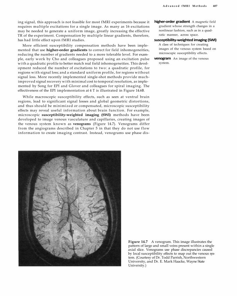
A d v a n c e d f M R I M e t h o d s 407
ing signal, this approach is not feasible for most fMRI experiments because it requires mult iple excitations for a single image. As many as 16 excitations may be needed to generate a uniform image, greatly increasing the effective TR of the experiment. Compensation by multiple linear gradients, therefore, has had little effect upon fMRI studies.
More efficient susceptibility compensation methods have been implemented that use higher-order gradients to correct for field inhomogeneities, reducing the number of gradients needed to a more tolerable level. For example, early work by Cho and colleagues proposed using an excitation pulse wi th a quadratic profile to better match real field inhomogeneities. This development reduced the number of excitations to two: a quadratic profile, for regions wi th signal loss; and a standard uniform profile, for regions without signal loss. More recently implemented single-shot methods provide much-improved signal recovery wi th minimal cost to temporal resolution, as implemented by Song for EPI and Glover and colleagues for spiral imaging. The effectiveness of the EPI implementation at 4 T is illustrated in Figure 14.6B.
While macroscopic susceptibility effects, such as seen at ventral brain regions, lead to significant signal losses and global geometric distortions, and thus should be minimized or compensated, microscopic susceptibility effects may reveal useful information about brain function. For example, microscopic susceptibility-weighted imaging (SWI) methods have been developed to image venous vasculature and capillaries, creating images of the venous system known as venograms (Figure 14.7). Venograms differ from the angiograms described in Chapter 5 in that they do not use f low information to create imaging contrast. Instead, venograms use phase dis-
higher-order gradient A magnetic field gradient whose strength changes in a nonlinear fashion, such as in a quadratic manner, across space.
susceptibility-weighted imaging (SWI) A class of techniques for creating images of the venous system based on microscopic susceptibility effects.
venogram An image of the venous system.
Figure 14.7 A venogram. This image illustrates the pattern of large and small veins present within a single axial slice. Venograms use phase discrepancies caused by local susceptibility effects to map out the venous system. (Courtesy of Dr. Todd Parrish, Northwestern University, and Dr. E. Mark Haacke, Wayne State University.)

408 C h a p t e r F o u r t e e n
diffusion weighting The application of magnetic gradients to cause changes
in the MR signal that are dependent
upon the amplitude and/or direction of
diffusion.
b factor The degree of diffusion weight
ing applied within a pulse sequence.
apparent diffusion coefficient (ADC) The quantification of diffusivity assum
ing isotropic diffusion.
crepancies associated w i t h slight differences in resonance frequency caused
by local susceptibility effects, which generates greater contrast for the vascu
lar system than found in intensitybased susceptibility imaging, such as
BOLD. Only the venous system can be imaged in this manner, since blood in
the arterial system is oxygenated and has minimal effect on susceptibility
images. Venograms have the sensitivity to image small vessels, on the order
of 100 μm. Since the BOLD signal results from changes in venous and capil
lary networks, the ability to map the venous system provides critical infor
mation about its origins.
Improving BOLD Contrast
The previous sections described techniques for improving the spatial resolu
tion, coverage, and fidelity of fMRI . However, these improvements are not
in themselves sufficient for ensuring accurate localization of fMRI signal to
the init iat ing neuronal activity. There still remains a fundamental gap
between our understanding of the underlying neuronal events and the
measured fMRI BOLD response. As discussed in Chapter 9, the contributing
sources of the BOLD signal are complex. Given the measured BOLD signal
w i t h i n a voxel, what do we know about the activity of neurons in that part
of the brain? Many laboratories are actively investigating the spatial corre
spondence between BOLD contrast and neuronal activity. While it is possi
ble to use intracranial recording data for spatial validation of BOLD data, as
is discussed in Chapter 15, such data are often not available. It is therefore
critical to develop noninvasive validation approaches.
One method that may improve understanding of the spatial origins of the
BOLD signal is diffusion weighting (see Chapter 5). Diffusion weighting
adjusts the contributions of voxels to the total MR signal according to the
mobil i ty of the protons they contain. Different components of the vascular
system have different proton mobility, and thus diffusionweighted imaging
can help visualize the vascular origins of the BOLD signal. Protons within
large vessels, for example, move quickly through space along the axis of the
vessel due to flow, while those w i t h i n capillaries move slowly and in more
directions due to the random geometry of the capillaries. Note that diffusion
weighting influences all motion of the protons, including blood flow, and
not solely diffusion due to thermal effects. For this reason, a more accurate
description of this technique would be "mobilityweighted imaging."
By adding different dif fusionweighting components to the acquisition
pulse sequence, one can selectively reduce the influence of largevessel con
tributions to the BOLD signal (Figure 14.8AD) in an attempt to improve
functional resolution. The amount of diffusion weighting introduced by a
pulse sequence is known as the b factor, w i t h typical units of seconds per
millimeter squared. The squared term in the units represents the fact that the
average movement by diffusion is essentially random, so the distance trav
eled increases proportionally to the square root of time, compared to blood
flow, in which particles move at a relatively constant rate and direction over
time. Larger b factors remove increasing amounts of the intravascular large
vessel signal (Figure 14.8C). Note that the map of diffusion rates, or static
apparent diffusion coefficient (ADC), across active voxels shows substan
tial largescale variability (Figure 14.8D), suggesting that much of the BOLD
signal results from largevessel effects. One problem raised by diffusion
weighted imaging techniques is correlating the amount of diffusion weight
ing w i t h the size of the affected vessels. For instance, diffusionweighted
acquisitions are often not effective in removing the extravascular parenchy

A d v a n c e d f M R I M e t h o d s 409
(A) (B)
(C)
Figure 14.8 BOLD maps acquired at different b factors and the resulting ADC map. A single subject passively viewed objects presented in a blocked design, whi le BOLD contrast was measured at 4 T using different values of diffusion weighting. Shown at upper left (A) is a map of BOLD activity w i t h no diffusion weighting (b = 0); this is equivalent to normal BOLD contrast measured in most fMRI studies. As diffusion weighting increases to b factors of 34 (B) and 108 s/mm 2 (C) , the region of significant activity reduces in extent due to the elimination of signal from large blood vessels. The data from the three different diffusion-weighting values can be combined into a single map of static ADC contrast (D), where red indicates voxels w i t h high spin mobility due to the presence of large vessels and blue indicates voxels w i t h low spin mobility that may reflect largely capillaries. The colormaps for (A-C) reflect t¬values of 3.6 to 8.0 (and greater), while the color map for (D) reflects ADC values of 0.4 to 4.0 x 10 -3 mm 2 /s.
mal component of the large-vein signal, since it usually has small diffusion coefficients. This results in corona-shaped activation patterns surrounding the large vessel. While promising, diffusion-weighted protocols for attenuating unwanted signals face challenges in both the strength and selectivity of their effects.
Another approach for potentially improving the spatial specificity of the BOLD signal takes advantage of the initial dip in the BOLD signal. Recall from Box 7.2 that the initial d ip is a transient negative BOLD signal that may result from the focal increase in oxygen consumption w i t h i n capillaries adjacent to active neurons, immediately fol lowing the onset of neuronal activity. Thus, the initial d ip could potentially be better localized to neuronal activity than the conventional later positive BOLD signal. In 2000, K i m and colleagues compared the spatial specificity of the initial d ip and positive BOLD response by investigating the columnar organization of cat visual cortex (Figure 14.9A-C). They presented visual gratings at specific orientations while collecting BOLD images at very high spatial resolution; for comparison, the scale bar in Figure 14.9A is 1 mm in length. By plott ing the amplitude of the initial d ip over space, they identified regions of visual cortex that
initial dip The short-term decrease in MR signal immediately following the onset of neuronal activity, before the main positive component of the hemodynamic response. The initial dip may result from initial oxygen extraction before the later overcompensatory response.
(D)
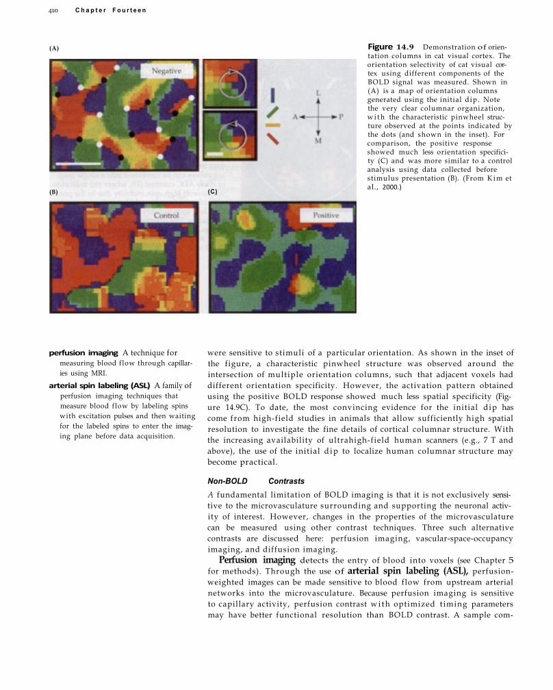
410 C h a p t e r F o u r t e e n
(B)
Figure 14.9 Demonstration of orientation columns in cat visual cortex. The orientation selectivity of cat visual cortex using different components of the BOLD signal was measured. Shown in (A) is a map of orientation columns generated using the initial d ip . Note the very clear columnar organization, w i t h the characteristic pinwheel structure observed at the points indicated by the dots (and shown in the inset). For comparison, the positive response showed much less orientation specificity (C) and was more similar to a control analysis using data collected before stimulus presentation (B). (From K i m et al., 2000.)
perfusion imaging A technique for measuring blood flow through capillaries using MRI.
arterial spin labeling (ASL) A family of perfusion imaging techniques that measure blood flow by labeling spins with excitation pulses and then waiting for the labeled spins to enter the imaging plane before data acquisition.
were sensitive to stimuli of a particular orientation. As shown in the inset of the figure, a characteristic pinwheel structure was observed around the intersection of mult iple orientation columns, such that adjacent voxels had different orientation specificity. However, the activation pattern obtained using the positive BOLD response showed much less spatial specificity (Figure 14.9C). To date, the most convincing evidence for the initial d ip has come from high-field studies in animals that allow sufficiently high spatial resolution to investigate the fine details of cortical columnar structure. With the increasing availability of ultrahigh-field human scanners (e.g., 7 T and above), the use of the initial d i p to localize human columnar structure may become practical.
Non-BOLD Contrasts A fundamental limitation of BOLD imaging is that it is not exclusively sensitive to the microvasculature surrounding and supporting the neuronal activity of interest. However, changes in the properties of the microvasculature can be measured using other contrast techniques. Three such alternative contrasts are discussed here: perfusion imaging, vascular-space-occupancy imaging, and diffusion imaging.
Perfusion imaging detects the entry of blood into voxels (see Chapter 5 for methods). Through the use of arterial spin labeling (ASL), perfusion-weighted images can be made sensitive to blood flow from upstream arterial networks into the microvasculature. Because perfusion imaging is sensitive to capillary activity, perfusion contrast w i t h optimized t iming parameters may have better functional resolution than BOLD contrast. A sample com-
(C)
(A)

Advanced fMRI Methods 411
(A)
Figure 14.10 Comparison of perfusion and BOLD contrasts. Shown are an anatomical reference image (A), a T1
image with regions of interest in motor cortical areas (B), and a T2 image (C). The resting-state perfusion map is shown in (D). During a simple motor task, there were significant
parison between optimized perfusion and BOLD contrasts is shown in Figure 14.10A-F, which indicates that cerebral blood flow contrast measured using ASL imaging is more spatially localized than blood oxygenation contrast measured using BOLD imaging. Similar results have been obtained in animal models in studies that resolved the columnar organization wi th in cat visual cortex. Perfusion imaging does have a significant l imitation, however, which precludes its use in some fMRI experimental designs. Because the labeled blood must travel from the labeling plane (e.g., in the neck) to the capillaries in the imaging plane, the temporal resolution of perfusion imaging is lower than that of BOLD imaging. Moreover, the travel time is not known a priori and must be determined experimentally. If too short an interval is used, the labeled spins may not have reached the capillary bed. But if too long an interval is used, T1 recovery effects w i l l reduce or eliminate altogether the perfusion signal. Perfusion imaging, therefore, may have its greatest success answering well-formed questions about the detection of activity
(B) (C)
(D) (E) (F)
increases in perfusion within the regions of interest, as shown in (E). The perfusion-related increases generally were similar to those obtained using BOLD contrast (F), but were more spatially specific. In all images, absolute signal intensity is shown using a grayscale color map. (From Luh et al., 2000.)

412 C h a p t e r F o u r t e e n
vascular-space-occupancy (VASO) imaging A technique for estimating cerebral blood volume through nulling of intravascular signal and measurement of changes in parenchymal signal.
intravoxel incoherent motion (IVIM) The uncorrelated motion of spins within a voxel.
dynamic IVIM imaging A technique for generating images based on changes in IVIM. It can be used to generate images sensitive to hemodynamic changes within capillaries.
w i t h i n targeted brain regions, rather than as a generally applicable or exploratory technique.
Another recent technique that may improve the spatial specificity of fMRI is vascular-space-occupancy (VASO) imaging, as developed by van Zij l and colleagues. Because the T1 of spins w i t h i n the blood vessels differs from the T1 of spins in the parenchyma, an inversion pulse (see Figure 5.7) can be used to selectively eliminate the signal from w i t h i n the blood while sparing the parenchymal signal. Using this inversion preparation technique, VASO imaging provides a measure of the total extravascular signal. Under the assumption that the total brain volume remains constant, a decrease in parenchymal signal between experimental conditions w o u l d indicate an increase in cerebral blood volume. Lu and colleagues demonstrated the feasibility of VASO imaging in a 2003 experiment that compared brain activation using a visual stimulation task, whi le measuring the hemodynamic responses of VASO f M R I , perfusion fMRI using ASL, and BOLD fMRI . By comparing the VASO signal to the perfusion and BOLD signals, the authors found that the VASO signal was confined to the microvasculature wi th in cortical gray matter. These properties make VASO imaging ideal for improving the spatial specificity of fMRI , although further validation of this new technique w i l l be necessary.
While static diffusion-weighting techniques may be valuable for improving BOLD contrast, as discussed in the previous section, dynamic diffusion contrasts hold potential as a replacement for BOLD imaging. Some researchers have investigated the use of dynamic diffusion-weighting techniques that are sensitive to task-induced intravoxel incoherent motion (IVIM). Le Bihan and colleagues applied this term to their technique for creating static images of perfusion. I V I M imaging was extended to measure brain function by Song and colleagues, who interleaved several b factors w i t h i n each acquisition to change the amount of diffusion weight ing over time (Figure 14.11). The resulting time series in each voxel has contrast that is sensitive to the change in its apparent diffusion coefficient (ADC). By choosing an appropriate range of b factors, the experimenter can make the resulting time course sensitive to task-induced changes in vessels wi th a particular size, such as capillaries.
Dynamic IVIM imaging has several advantages over BOLD imaging for spatial localization. Because it detects relative mobility rather than magnetic susceptibility, its spatial specificity does not depend on field strength. Compared to spin-echo BOLD or measurement of the initial d ip , it has high functional SNR. Dynamic I V I M imaging does not require labeling of blood and subsequent transit time to the imaging plane, and thus it does compromise temporal resolution and spatial coverage. Dynamic I V I M can also eliminate the extravascular large-vessel signal, because the mobil i ty of extravascular spins near large vessels does not change over time. A n d , by using a b factor of 0 w i t h one of the excitation pulses, it can be collected concurrently with standard BOLD contrast, albeit wi th a time penalty proportional to the number of b factors used. Thus, current implementations of dynamic I V I M are not suited for event-related fMRI designs. However, methods in development for acquisition of multiple b factors w i t h i n a single shot w i l l eliminate this time penalty, and may have more general applicability.
A close relative of the aforementioned ADC contrast uses very high b factors (400 to 1600 s/mm 2) to eliminate all vascular contributions to the MR signal, and thus make it exclusively sensitive to ADC changes in the parenchyma. As described earlier in this section, ADC values normally increase during neu-
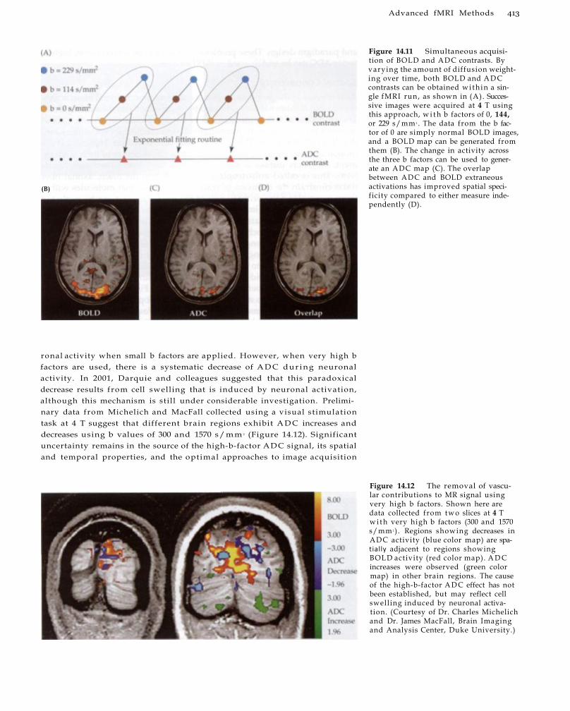
Advanced fMRI Methods 413
(B)
Figure 14.11 Simultaneous acquisition of BOLD and ADC contrasts. By varying the amount of diffusion weighting over time, both BOLD and A D C contrasts can be obtained wi th in a single fMRI run, as shown in (A). Successive images were acquired at 4 T using this approach, w i t h b factors of 0, 144, or 229 s/mm 2 . The data from the b factor of 0 are simply normal BOLD images, and a BOLD map can be generated from them (B). The change in activity across the three b factors can be used to generate an ADC map (C). The overlap between ADC and BOLD extraneous activations has improved spatial specificity compared to either measure independently (D).
ronal activity when small b factors are applied. However, when very high b factors are used, there is a systematic decrease of A D C dur ing neuronal activity. In 2001, Darquie and colleagues suggested that this paradoxical decrease results from cell swelling that is induced by neuronal activation, although this mechanism is still under considerable investigation. Preliminary data from Michelich and MacFall collected using a visual st imulation task at 4 T suggest that different brain regions exhibit A D C increases and decreases using b values of 300 and 1570 s / m m 2 (Figure 14.12). Significant uncertainty remains in the source of the high-b-factor ADC signal, its spatial and temporal properties, and the optimal approaches to image acquisition
Figure 14.12 The removal of vascular contributions to MR signal using very high b factors. Shown here are data collected from two slices at 4 T w i t h very high b factors (300 and 1570 s/mm 2 ) . Regions showing decreases in ADC activity (blue color map) are spatially adjacent to regions showing BOLD activity (red color map). A D C increases were observed (green color map) in other brain regions. The cause of the high-b-factor A D C effect has not been established, but may reflect cell swelling induced by neuronal activation. (Courtesy of Dr. Charles Michelich and Dr. James MacFall, Brain Imaging and Analysis Center, Duke University.)

414 C h a p t e r F o u r t e e n
isotropic Having similar properties in all directions.
anisotropic Having different properties in different directions; often referenced in the context of anisotropic diffusion, where molecules tend to diffuse along one axis but not others.
diffusion tensor imaging (DTI) The collection of images that provide information about the magnitude and direction of molecular diffusion. It is often used to create maps of fractional anisotropy.
Figure 14.13 Fiber tracking using diffusion tensor imaging. DTI allows measurement of the relative motion of water molecules w i t h i n the voxel. (A) An image showing, in three dimensions, a diffusion map of white-matter voxels. Each voxel is represented by an ellipsoid whose dimensions reflect the rate of diffusion, w i t h spheres reflecting isotropic diffusion and narrow ellipses showing diffusion along a preferred axis. White-matter tracts can be reconstructed from these data using algorithms that f ind continuous tracks of diffusion across voxels, as indicated schematically for a hypothetical 5-by-6 set of voxels (B). Visible in red is a curve obtained by tracing diffusion axes across adjacent voxels. (A courtesy of Dr. Guido Gerig, University of North Carolina at Chapel Hil l . )
and paradigm design. These problems w i l l have to be solved before high-b-factor A D C can be widely used in fMRI studies.
Spatial Connectivity As discussed in the previous chapter, a complete description of brain activation should include not only activated brain areas but also their connectivity. The properties of water diffusion can be used to provide information about anatomical connectivity. If unconstrained, water molecules w i l l diffuse randomly in all directions. This is called isotropic diffusion. However, if the motion of water molecules is constrained by the structure of their environment, they may diffuse in some directions more than others (see Figure 5.18). This is called anisotropic diffusion. Wi th in the brain, axonal fiber tracts constrain the diffusion of water molecules so that molecules w i t h i n them move along the pr imary axis of the tract. This fact can be exploited using diffusion tensor imaging, or DTI, which provides information about the location and orientation of white-matter tracts in the brain. Diffusion tensor data represent each voxel as a three-dimensional ellipsoid reflecting the rate of diffusion along the three principal axes (Figure 14.13A and B). Note that the voxels along fiber pathways, which are visible as white matter in Figure 14.13A, tend to form lines along the pathway. By connecting the long axis of each ellipsoid between given starting and end positions, we can trace the structure of fiber tracts, as illustrated in Figure 14.14A-C. A number of groups have been responsible for the development of DTI , including Mor i and colleagues, Basser and colleagues, and Poupon and colleagues.
DTI has been used primari ly to evaluate the integrity of white matter in the brain, as when investigating deficits due to aging, injury, or disease. However, it also provides information about functional connectivity. Because brain regions that are connected functionally are also likely to be connected anatomically, areas of functional activity may show direct or indirect connecting pathways on DTI images. Functionally defined brain regions can be used as seed points for DTI algorithms, to identify tracts l inking these regions to other areas of the brain. In principle, BOLD activity maps could be used to generate seed points for fiber tracking, thereby investigating functional connectivity. However, because BOLD activity may be more spatially extensive than the underlying neuronal activation, seed points selected based upon BOLD activity alone may lead to inaccurate connectivity maps. For example,
(A) (B)

A d v a n c e d f M R I M e t h o d s 415
(A) (B)
(C)
Figure 14.14 Comparison of anatomical and D T I fiber tracts. Diffusion tensor imaging can be used to reconstruct axonal tracts connecting different brain regions. Shown here are the white-matter radiations in a sagittal drawing of the brain (A) ; a two-dimensional map of fiber tracts obtained using DTI , shown at the midline of a solid brain (B); and a three-dimensional map of fiber tracts displayed on a glass brain (C). (A from L u d w i g and Klionger, 1956; B courtesy of Dr. Susumu M o r i , Johns Hopkins University.)
preliminary studies from Song and colleagues have compared the effectiveness of BOLD and dynamic A D C contrasts for generating seed points for fiber tracking (Figure 14.15). The BOLD activation (shown in blue) does not allow accurate selection of seed points. The ADC activation revealed by dynamic I V I M imaging (shown in red) can be used to create seed points for fiber tracking, as shown in green. Collection of fMRI data and DTI data wi th in a single experiment holds great promise for bridging the gap between neuroimaging and neuroanatomical techniques for understanding brain function.
Figure 14.15 Combined use of DTI, A D C fMRI, and BOLD fMRI . Fiber tracking using diffusion tensor imaging can provide important information about the functional properties of different brain regions. In yellow is shown the diffusion tensor vector f ield; straight lines across multiple vectors indicate fiber tracts. Tracts between visual areas are shown in green. Note that although BOLD contrast shows activity in an extended set of brain regions (blue), A D C contrast shows activity in a smaller set of regions (red) that more closely correspond to the connecting tracts. These activated areas likely correspond to visual processing areas V 1 , V2, and V5, representing primary, secondary, and motion-sensitive cortices.

416 C h a p t e r F o u r t e e n
electroencephalography (EEG) The measurement of the electrical potential of the brain, usually through electrodes placed on the surface of the scalp.
magnetoencephalography (MEG) A noninvasive functional neuroimaging technique that measures very small changes in magnetic fields caused by the electrical activity of neurons, with potentially high spatial and temporal resolution.
Temporal Resolution
Just as a number of new and exciting methods have been developed for improving the spatial resolution and fidelity of f M R I , novel approaches to improve temporal resolution have also been advanced. Because of the relatively coarse sampling rate of fMRI , improvements in its temporal resolution are particularly valuable. Electrophysiological techniques like electroencephalography (EEG) and magnetoencephalography (MEG) can detect changes in the brain w i t h roughly millisecond resolution, whereas fMRI samples the brain approximately once per second or slower. Temporal resolution in fMRI is l imited by three factors (see Chapter 8 for an extended discussion). First, although individual slices can be acquired w i t h i n a few tens of milliseconds, 20 or more slices are required to sample the entire brain wi th reasonable spatial resolution. Thus, the time between successive acquisitions of the entire brain is much longer than the acquisition time for a single slice. Second, the net magnetization of voxels requires time to recover between successive excitations. Thus, even if one wanted to repeatedly sample a single slice as rapidly as possible, the functional SNR in that slice would be greatly reduced at very short repetition times. Thi rd , the most common functional contrast mechanism, BOLD, does not image neuronal activity directly, but instead measures hemodynamic correlates of that activity. The uncertain delay between neuronal activity and its hemodynamic expression reduces temporal resolution. Unless these limitations are overcome, a number of important research questions w i l l remain outside the purview of fMRI.
In the second part of this chapter, we discuss some of the primary advances in pulse sequence development and experimental design that contribute to improved temporal resolution. Not discussed here are improvements in image acquisition rate that have resulted from improvements in MR scanners, notably through the development of more-efficient gradient systems. We note that although hardware improvements have contributed greatly to fast imaging methods, further advances w i l l have a relatively limited impact on temporal resolution due to the intrinsic l imitations of functional SNR. For images to be collected faster and w i t h greater SNR, new strategies for their acquisition w i l l be needed.
Multiple-Channel Acquisition Recall that the use of mult iple detector coils can improve spatial resolution without increasing imaging time (as shown in Figure 14.4), or reduce spatial distortions while maintaining the imaging matrix (as shown in Figure 14.5). However, if improved temporal resolution is desired instead, then multiple-channel acquisition can also improve temporal resolution without sacrificing spatial resolution or spatial coverage. Just as the unique spatial information provided by each channel can increase resolution over a single channel, the same data can be acquired in less time using mult iple channels simultaneously. Normally, a single coil is used to acquire an n x n image. Four independent coils can also be used to collect that same image, each acquiring n/2 x n/2 data points. Since each coil only acquires one-quarter of the original data, the image can be collected in one-quarter of the time. The temporal reduction factor could be smaller if the mult iple coils overlap spatially. In general, if there are M receiver coils each sampling P points, the requirement for redundancy means that there must be more samples than voxels in the image: MP > n2. Thus, temporal resolution improves proportionally to the
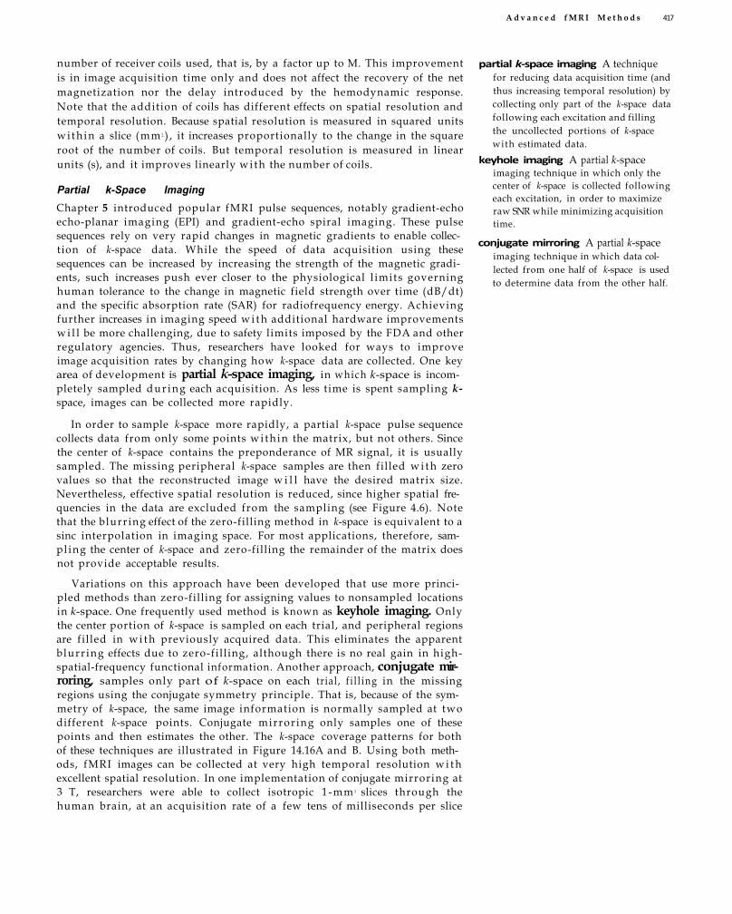
A d v a n c e d f M R I M e t h o d s 417
number of receiver coils used, that is, by a factor up to M. This improvement is in image acquisition time only and does not affect the recovery of the net magnetization nor the delay introduced by the hemodynamic response. Note that the addition of coils has different effects on spatial resolution and temporal resolution. Because spatial resolution is measured in squared units w i t h i n a slice (mm 2 ) , it increases proportionally to the change in the square root of the number of coils. But temporal resolution is measured in linear units (s), and it improves linearly wi th the number of coils.
Partial k-Space Imaging Chapter 5 introduced popular fMRI pulse sequences, notably gradient-echo echo-planar imaging (EPI) and gradient-echo spiral imaging. These pulse sequences rely on very rapid changes in magnetic gradients to enable collection of k-space data. While the speed of data acquisition using these sequences can be increased by increasing the strength of the magnetic gradients, such increases push ever closer to the physiological l imits governing human tolerance to the change in magnetic field strength over time (dB/dt) and the specific absorption rate (SAR) for radiofrequency energy. Achieving further increases in imaging speed w i t h additional hardware improvements w i l l be more challenging, due to safety limits imposed by the FDA and other regulatory agencies. Thus, researchers have looked for ways to improve image acquisition rates by changing how k-space data are collected. One key area of development is partial k-space imaging, in which k-space is incompletely sampled d u r i n g each acquisition. As less time is spent sampling k-space, images can be collected more rapidly.
In order to sample k-space more rapidly, a partial k-space pulse sequence collects data from only some points w i t h i n the matrix, but not others. Since the center of k-space contains the preponderance of MR signal, it is usually sampled. The missing peripheral k-space samples are then filled w i t h zero values so that the reconstructed image w i l l have the desired matrix size. Nevertheless, effective spatial resolution is reduced, since higher spatial frequencies in the data are excluded from the sampling (see Figure 4.6). Note that the blurr ing effect of the zero-filling method in k-space is equivalent to a sinc interpolation in imaging space. For most applications, therefore, sampl ing the center of k-space and zero-filling the remainder of the matrix does not provide acceptable results.
Variations on this approach have been developed that use more principled methods than zero-filling for assigning values to nonsampled locations in k-space. One frequently used method is known as keyhole imaging. Only the center portion of k-space is sampled on each trial, and peripheral regions are filled in w i t h previously acquired data. This eliminates the apparent b lurr ing effects due to zero-fi l l ing, although there is no real gain in high-spatial-frequency functional information. Another approach, conjugate mirroring, samples only part of k-space on each trial , f i l l ing in the missing regions using the conjugate symmetry principle. That is, because of the symmetry of k-space, the same image information is normally sampled at two different k-space points. Conjugate mirror ing only samples one of these points and then estimates the other. The k-space coverage patterns for both of these techniques are illustrated in Figure 14.16A and B. Using both methods, fMRI images can be collected at very high temporal resolution w i t h excellent spatial resolution. In one implementation of conjugate mirroring at 3 T, researchers were able to collect isotropic 1 -mm 3 slices through the human brain, at an acquisition rate of a few tens of milliseconds per slice
partial k-space imaging A technique for reducing data acquisition time (and thus increasing temporal resolution) by collecting only part of the k-space data following each excitation and filling the uncollected portions of k-space with estimated data.
keyhole imaging A partial k-space imaging technique in which only the center of k-space is collected following each excitation, in order to maximize raw SNR while minimizing acquisition time.
conjugate mirroring A partial k-space imaging technique in which data collected from one half of k-space is used to determine data from the other half.

418 C h a p t e r F o u r t e e n
Figure 14.16 Reducing imaging acquisition time through partial k-space imaging. Shown are two common methods for reducing k-space coverage to gain temporal resolution whi le maintaining the same imaging matrix and spatial resolution. (A) A keyhole pattern, where the center of k-space (shown in orange) is acquired for each image while the periphery of k-space (in blue) is fi l led w i t h previously acquired data. The use of previously acquired data avoids the b lurr ing effect induced by zero-filling methods. (B) A conjugate mirroring technique, in which data are acquired from one half of k-space (in orange) and mirrored into the other half (in blue). Note that the conjugate mirror ing technique acquires data from slightly more than half of k-space to ensure that the center is well represented to maximize raw SNR.
(A) (B)
(Figure 14.17A and B). This roughly matches the size of cortical columns and may reflect near optimal resolution for fMRI .
Because keyhole and conjugate mirror ing techniques ful ly sample the center of k-space, most of the MR signal (and thus raw SNR) is preserved. But when one is attempting to measure BOLD signal change w i t h i n a small region, the raw SNR may not be the most important factor. High-spatial-frequency changes that reflect small regions of functional activity may be more
Figure 14.17 Fast partial k-space fMRI w i t h cubic millimeter resolution. Use of a partial k-space acquisition strategy can greatly improve the speed of image acquisition. (A) is at 1 x 1 x 10 mm resolution, while (B) is at 1 x 1 x 1 mm resolution. These single-shot images were collected at roughly the same speed as normal fMRI images, despite having much higher resolution. The subject participated in a bimanual finger tapping task. (Courtesy of Dr. Andrzej Jesmanowicz and Dr. James S. Hyde, Medical College of Wisconsin.)
(A) (B)
What might be a disadvantage of conjugate mirroring? As a hint, consider what factors contribute to the raw MR signal
measured at each point in k-space. Why would it be better to collect two samples of the k-space data than just one sample?

Advanced fMRI Methods 419
(A) (B) (C)
(D)
Figure 14.18 Rapid fMRI using outer k-space imaging. Outer k-space imaging records data f rom the periphery of k-space on each image (A, orange) while f i l l ing the center of k-space w i t h previously acquired data (A, blue). The potential value of this technique for fMRI is that the peripheral points may contribute more to high-spatial-frequency effects, such as small BOLD activations. (B) A standard EPI image from a time series of volumes, and the BOLD significance map from that time series is shown in (C). For comparison, (D) shows an EPI image acquired using outer k-space f i l l ing, w i t h its significance map shown in (E). Note the substantial difference between the two types of EPI images, w i t h the image in (D) completely lacking low spatial frequencies, but also note the similarity in the activation maps. (Data courtesy of Dr. Gary Glover, Stanford University.)
important than low-spatial-frequency changes that reflect the overall MR signal. In order to assess the detailed spatial characteristics of small activations, it is often important to acquire data from peripheral regions of k-space that correspond to high-spatial-frequency components. A method known as outer k-space (OK) imaging has been proposed by Glover and colleagues to preserve potentially important changes in functional activity. The principle of outer k-space imaging is illustrated in Figure 14.18A-E. OK imaging can be thought of as the complement of the keyhole technique described in the last paragraph, in that the former samples only the peripheral portions of k-space while the latter samples only the center of k-space.
Partial sampling of k-space is analogous to the idea of filtering introduced earlier for signals in the time domain. If only part of k-space is sampled, then spatial frequencies outside the sampling range are effectively filtered. Thus, keyhole imaging is analogous to a low-pass spatial filter, while OK imaging is analogous to a high-pass filter. Recall from Chapter 10 that the correct filter to use for a given signal depends on the frequency of that signal, according to the principle of matched filters. If characteristics of the spatial pattern of activation are known, then an optimally matched k-space trajectory can be constructed that fully maintains the spatial integrity of the activation while maximizing temporal resolution.
Efficient k-Space Trajectories Echo-planar imaging is the most popular fast imaging method for fMRI, but it does not optimally use the scanner gradients. Traditional EPI implementations alternate between the x- and y-gradients to traverse a stepwise path through k-space (see Figure 5.22). Because the amplitude of the gradient determines the velocity of the k-space trajectory, turning on only one gradient at any given time limits the speed at which k-space data can be acquired. To overcome this l imitation and increase the speed of slice acquisition, pulse sequences have been developed that use both the x- and y-gradients simultaneously. A simple
outer k-space (OK) imaging A partial k-space imaging technique in which only the periphery of k-space is collected following each excitation, in order to ensure that high-spatial-frequency components of the MR signal are present.
matched filters The principle that the filter of the same frequency as the signal of interest provides maximal signal-to-noise ratio.
(E)
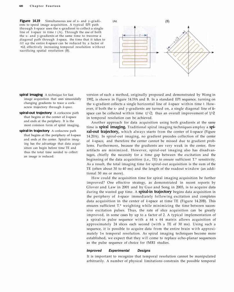
420 C h a p t e r F o u r t e e n
Figure 14.19 Simultaneous use of x and ygradients to speed image acquisition. A typical EPI path through kspace uses the xgradient to collect a single line of kspace in time t (A) . Through the use of both the x and ygradients at the same time to traverse a diagonal path through kspace, the t ime that it takes to f i l l u p the entire kspace can be reduced by a factor of •12, effectively increasing temporal resolution w i t h o u t sacrificing spatial resolution (B).
(A)
spiral imaging A technique for fast
image acquisition that uses sinusoidally
changing gradients to trace a cork
screw trajectory through kspace.
spiralout trajectory A corkscrew path
that begins at the center of kspace
and ends at the periphery. It is the
most common form of spiral imaging.
spiralin trajectory A corkscrew path
that begins at the periphery of kspace
and ends at the center. Spiralin imag
ing has the advantage that data acqui
sition can begin before time TE and
thus the total time needed to collect
an image is reduced.
version of such a method, originally proposed and demonstrated by Wong in
1992, is shown in Figure 14.19A and B. In a standard EPI sequence, turning on
the xgradient collects a single horizontal line of kspace w i t h i n time t. How
ever, if both the x and ygradients are turned on, a single diagonal line of k-
space can be collected wi th in time t/√2; thus an overall improvement of 1/√2
in temporal resolution can be achieved.
Another approach for data acquisition using both gradients at the same
time is spiral imaging. Traditional spiral imaging techniques employ a spiralout trajectory, which always starts from the center of kspace (Figure
14.20A). In spiralout imaging, no gradient precedes collection of the center
of kspace, and therefore the center cannot be missed due to gradient prob
lems. Furthermore, because the gradients are very weak in the center, flow
artifacts are minimized. However, spiralout imaging also has disadvan
tages, chiefly the necessity for a time gap between the excitation and the
beginning of the data acquisition (i.e., TE) to ensure sufficient T2* sensitivity.
As a result, the total imaging time for spiralout acquisition is the sum of the
TE (often about 30 to 40 ms) and the length of the readout window (an addi
tional 30 ms or more).
H o w could the acquisition time for spiral imaging acquisition be further
improved? One effective strategy, as demonstrated in recent reports by
Glover and Law in 2001 and by Guo and Song in 2003, is to acquire data
during the wasted gap time. A spiralin trajectory begins data acquisition in
the periphery of kspace immediately fo l lowing excitation and completes
data acquisition in the center of kspace at time TE (Figure 14.20B). This
ensures sufficient T 1* weighting while minimizing the time between succes
sive excitation pulses. Thus, the rate of slice acquisition can be greatly
improved, in some cases by up to a factor of 2. A typical implementation of
a spiralin pulse sequence w i t h a 64 x 64 matrix allows acquisition of
approximately 24 slices each second ( w i t h a TE of 30 ms). Using such a
sequence, it is possible to acquire data from the entire brain w i t h approxi
mately 1s temporal resolution. As spiral imaging techniques become more
established, we expect that they w i l l come to replace echoplanar sequences
as the pulse sequence of choice for fMRI studies.
Improved Experimental Designs
It is important to recognize that temporal resolution cannot be manipulated
arbitrarily. A number of physical limitations constrain the possible temporal
(B)

A d v a n c e d fMRI M e t h o d s 421
(A)
Figure 14.20 Spiral imaging sequences. Spiral sequences trace a spiral path through k-space, a l lowing more-efficient use of the gradients and more-rapid data acquisition. In the conventional spiral-out sequence (A), the gradients are turned on at time TE, but in the spiral-in technique (B), the gradients are turned on earlier so that the center of k-space is reached at time TE. The spiral-in sequence can thus acquire data more rapidly than the spiral-out sequence per unit time.
resolution that can be obtained using fMRI. Some of these limitations result f rom current imaging hardware and may change over time. As examples, typical static field strengths of MR scanners may increase, albeit slowly, as w i l l the capabilities of gradient systems. In addit ion, improved receiver characteristics w i l l al low higher sampling frequencies. However, there are also limitations that are intrinsic to the fMRI technique. The T1 and T2* properties of brain voxels restrict the maximum SNR that can be achieved at a given temporal resolution, just as the net magnetization of a voxel restricts the maximum SNR that can be achieved at a given spatial resolution. That is, as TR decreases, the raw SNR also decreases. At very short TRs (e.g., below 200 ms), the resulting decrease in functional SNR may preclude identification of BOLD changes. It is critical, therefore, to optimize experimental designs so that temporal resolution can be maximized.
We previously described the technique known as interleaved stimulus presentation (see Figure 8.10) as an approach for improving the effective sampling rate for a given TR. By j ittering the time of stimulus presentation w i t h i n the TR, one can sample hemodynamic time courses at different latencies relative to the stimulus onset on different trials. These mult iple time
interleaved stimulus presentation The presentation of events of interest at different points within a TR over trials (e.g., one-quarter, one-half, and three-quarters of TR in addition to TR onset), increasing the effective sampling rate of an experiment at the expense of fewer trials per condition.
(B)

422 C h a p t e r F o u r t e e n
BOX 14.1 Direct MRI of Neuronal Activity
All of the fMRI contrast techniques
described heretofore in this book
have relied on indirect measures
of neuronal activity. BOLD contrast relies
on relative oxygenation, diffusion con
trast relies on movement of water mole
cules, and perfusion relies on blood flow.
Yet none of these measures are them
selves thought to mediate information
processing in the brain. Ideally, we
would want to bypass all of these indi
rect markers and measure the activity of
neurons directly, whether singly, as in
singleunit recording, or collectively, as
in fieldpotential measures. Can MRI be
used to image neuronal activity directly?
At present the answer to this question is
a qualified no. The electrical activity of
neurons is weak, temporally transient,
and spatially inhomogeneous. Detection
even of large effects w i l l be challenging,
at best. However, there have been tanta
lizing results from recent studies that
suggest that direct neuronal imaging
may be possible.
A study conducted by Joy and col
leagues in 1989 provided intriguing re
sults. The authors used spinecho imag
ing to assess phase changes associated
with the field perturbation of electrical
currents, both in phantoms and in pe
ripheral human nerves. Their results
showed that physiological currents in bi
ological systems may be detected by ac
quiring phase maps during stimulation.
Since neuronal action potentials are es
sentially electrical depolarizations akin
to current changes in a wire, these results
suggested that it may be possible to
image neuronal activity directly using
MRI. However, the results have not been
confirmed by further studies, and the ap
plication of this technique to neurons in
the brain may be more challenging than
to peripheral nerves.
New methods for using MRI to detect
minute electrical activity have been pro
posed. One candidate technique involves
the measurement of Lorentz forces,
which arise from the movement of
charged particles through a magnetic
field. As the particles move through the
field, they experience a force that is per
pendicular to both the local magnetic
field and the particles' direction of mo
tion. This force acts to displace the parti
cles; if the particles are within a conduc
tor, the conductor w i l l be displaced
within the external medium. Similarly,
the components of neurons that contain
moving electrical charges, such as active
axons, w i l l experience small displacing
forces. The resulting displacements can
be measured using MRI, hence the term
Lorentz effect imaging ( L E I ) . Prelimi
nary results in gel phantoms were re
ported in 2001 by Song and Takahashi.
If we assume that the Lorentz force is
only along the xdirection, the displace
mentinduced phase change in a nearby
voxel can be estimated by Equation 14.1:
Here, G is the strength of the encoding
and decoding gradient, Ax the displace
(B) (A)
Figure 14.21 Lorentz effect imaging (LEI). Lorentz effect imaging relies on the behavior of a currentcarrying wire in a magnetic field. The wire is subject to a lateral force F perpendicular to both the direction of the field B shown in (A) and the direction of the moving charges i This force is known as the Lorentz force. (B) Shows results from a phantom containing a wire carrying different amounts of charge; from left, 0 μA, 100 μA, 200 μA, and 500 μA. Note
that the magnitude of the distortion increases w i t h increasing current. The potential application of LEI to fMRI is shown in (C). Within an active voxel, the electrical currents w i l l be largely randomly oriented. The random orientation means that the direction of the Lorentz effect w i l l differ across electrical sources, resulting in a signal loss due to loss of phase coherence that is analogous to the T2* effect.

A d v a n c e d f M R I M e t h o d s 423
BOX 14.1 (continued)
Lorentz force The force on a moving charge within a magnetic field.
Lorentz forces cause spatial dis
placements in conductors (e.g.,
wires, neuronal axons) if those
conductors are placed in MRI
scanners.
Lorentz effect imaging (LEI) A potential technique for direct visu
alization of electrical activity (e.g.,
of neurons) using MRI.
ment, T the duration of the encoding/
decoding gradients, and γ the gyromag
netic ratio. Note that even for very small
displacements, this phase shift could be
significant when the product GT is large
enough. If the phase shifts are coherent
wi th in the voxel, then phase images
could be used to detect the Lorentz ef
fect. However, given the random direc
tion of neuronal currents and the elastic
nature of brain tissue, the phase shifts are
likely to be incoherent within the voxel.
As such, the result of the Lorentz effect
upon MR images would be a loss of sig
nal intensity. Proofofconcept experi
ments conducted on phantoms using
G of 50 mT/m and T of 2 ms have sug
gested that the LEI technique may
have a spatial accuracy on the order of
10 μm, given a raw SNR of 100 (Figure
14.21AC). With improvements in imag
ing hardware and with increased signal
averaging, this technique may become
useful for detecting spatial displace
ments induced by neuronal electrical
currents.
Assuming that rapidly changing
magnetic fields are more likely to be as
sociated w i t h electrical activity of neu
rons, in 2002 Bodurka and Bandettini at
tempted to selectively detect rapidly
changing fields while suppressing slow
ly changing fields. The initial concept
was tested on a phantom with implanted
wires. The t iming of transient currents in
the wires was modulated relative to a
180° excitation pulse. Very small phase
differences were detected, demonstrat
ing the feasibility of the approach (Figure
14.22AC). To illustrate the potential im
portance of this effect, the magnetic field
changes measured were as brief as only
40 ms in duration and as small as only 2
x 1010 T (200 pT). These magnetic
changes are about 10 billion times small
er than typical static field strengths, illus
trating the profound technical require
ments of direct neuronal imaging. We
emphasize that studies of direct current
imaging have heretofore been conducted
in phantoms and w i l l undoubtedly be
more difficult to conduct in human sub
jects. Nevertheless, the successes so far
point to the eventual development of
these remarkable techniques as an alter
native to vascularbased fMRI.
Figure 14.22 Detection of minute electrical activity using MRI . Using a wirecontaining phantom, researchers investigated whether very small transient electrical currents could be detected by collecting images sensitive to phase changes. The location of the wires wi th in the phantom are shown as white arrows in (A), and the on/off frequency of the currents was 0.16 Hz. The Fourier spectrum of the voxel that contained the wire indicated by the left arrow revealed a currentinduced field shift (ΔB R ) of 2 nanoTesla (B). In a voxel 12.5 mm from the left wire (indicated by yellow arrow), they detected a field shift of 200 picoTesla (C), or about one tenbillionth the strength of a standard MR scanner. These results suggest that MRI can be used, in principle, to detect field changes of strength similar to neuronal activity. (From Bodurka and Bandettini, 2002.)
(A)
(B)
(C)
Frequency (Hz)

424 C h a p t e r F o u r t e e n
courses can be combined into a single time course w i t h the effective samp l i n g rate reduced from the actual TR by a factor equal to the number of interleaved steps. For example, w i t h an actual TR of 2000 ms and 10 jittering steps, one could sample at an effective rate of 200 ms. As we discussed in Chapter 8, the primary disadvantage of interleaved stimulus presentation is that the length of data acquisition increases w i t h the gain in temporal resolution. To increase the effective sampling rate by a factor of 10 while maintaining the same number of samples per condition, the experiment length must likewise be increased by a factor of 10.
Because of the uncertainty associated w i t h the relation between the fMRI hemodynamic response and neuronal activity, millisecond-level distinctions in the t iming of neuronal activity are challenging for fMRI studies. However, a number of researchers have investigated whether clever manipulation of experimental paradigms w i l l allow probing of very fast neuronal events. In 2000, Ogawa and colleagues reported a technique that induces either excitatory or inhibitory neural interactions by presenting consecutive stimuli separated by very short intervals, on the order of tens of milliseconds. By applying consecutive forepaw stimulations wi th variable interstimulus intervals to the rat, the research team was able to detect the inhibit ion due to neuronal refractoriness of the response to the second stimulus (Figure 14.23A and B).
Figure 14.23 Using neural interactions to improve the temporal resolution of fMRI . The electrophysiological and BOLD responses in the somatosensory cortex to bilateral stimulation of the rat forepaws were investigated. (A) Shows electrophysiological responses in the right somatosensory cortex. Normally, a somatosensory evoked potential (SEP; N1) is present following stimulation of the left forepaw (e.g., in 12.5- and 75-ms interstimulus interval conditions). But when the right stimulation precedes the left by about 40 ms, then there is suppression of the electrical activity. Importantly, that suppression is also present in the BOLD effect (B), suggesting that the use of fMRI suppression designs may be able to resolve very small differences in event t iming, on the order of tens of milliseconds. (From Ogawa et al., 2000.)
(A) SEP (B) MRI
Image number

Such an inhibition effect is subsequently manifested in the BOLD signal. This manipulation provides improved temporal resolution for neuronal events wi thout physically increasing the sampling interval, as neuronal interactions on the order of milliseconds can lead to very different hemodynamic responses. Similar effects have been used to make spatial judgments about brain regions in fMRI-adaptation paradigms (see Chapter 8).
Summary
Nearly all fMRI studies share the same constraints. They sample the brain w i t h a spatial resolution of a few millimeters and a temporal resolution of a few seconds. The resulting images are sensitive to BOLD contrast, which is an indirect measure of neuronal activity. Though a vast array of research questions can be answered despite these limitations, advances in the spatial and temporal resolution of fMRI w i l l expand its applicability. Many of the advances so far have been driven by hardware improvements, notably by increasing the strength of the static and gradient fields and by using more-advanced receiver coil arrangements. However, further improvements w i l l need to come from better acquisition strategies and pulse sequence designs. Spatial resolution w i l l be improved through better understanding of the spatial origins of the BOLD signal, including comparison to other forms of contrast. Spatial fidelity may be improved by new pulse sequences that have been developed to recover MR signal in areas affected by susceptibility artifacts. Temporal resolution w i l l be improved by new k-space acquisition methods, including partial k-space imaging and efficient data collection w i t h spiral sequences. Improvements in experimental design w i l l also contribute to better temporal resolution. Finally, some research groups have provided evidence for MR measurement of minute electrical currents, which may lead the way to direct MR imaging of neuronal activity.
Suggested Readings
*Dodd, S. J., Williams, M., Suhan, J. P., Williams, D. S., Koretsky, A. P., and Ho, C. (1999). Detection of single mammalian cells by high-resolution magnetic resonance imaging. Biophys. J., 76: 103-109. One of the first papers to demonstrate the feasibility of single-cell MRI.
*Glover, G. H., and Law, C. S. (2001). Spiral-in/out BOLD fMRI for increased SNR and reduced susceptibility artifacts. Magn. Reson. Med., 46(3): 515-522. The first demonstration of simultaneous image acquisition using both spiral-in and spiral-out trajectories to recover susceptibility-induced signal losses with high temporal efficiency.
Johnson, G. A., Cofer, G. P., Gewalt, S. L., and Hedlund, L. W. (2002). Morphologic phenotyping with MR microscopy: The visible mouse. Radiology, 222: 789-793. This manuscript discusses advances in MR microscopy and their applications.
*Kim, D. S., Duong, T. Q., and Kim, S. G. (2000). High-resolution mapping of iso-orientation columns by fMRI. Nat. Neurosci., 3(2): 164-169. Demonstrates that selective use of the initial dip in the BOLD response improves spatial localization of orientation columns within the visual cortex.
Logothetis, N. K., Guggenberger, H. , Peled, S., and Pauls, J. (1999). Functional imaging of the monkey brain. Nat. Neurosci., 2(6): 555-562. An important paper demonstrating improved neuronal localization using functional imaging in monkeys.
*Luh, W. M., Wong, E. C, Bandettini, P. A., Ward, B. D., and Hyde, J. S. (2000). Comparison of simultaneously measured perfusion and BOLD signal increases during brain activation with T1-based tissue identification. Magn. Reson. Med.,
Advanced fMRI Methods 425
426 C h a p t e r F o u r t e e n
44(1): 137-143. This manuscript demonstrates how ASL perfusion imaging may provide superior spatial localization compared to traditional BOLD fMRI.
*Ogawa, S., Lee, T. M., Stepnoski, R., Chen, W., Zhu, X. H., and Ugurbil, K. (2000). An approach to probe neural systems interaction by functional MRI at neural time scale down to milliseconds. Proc. Natl. Acad. Sci. U.S.A.. 97: 11026-11031. A convincing demonstration of how improved paradigm design may allow probing of neuronal events on the order of milliseconds using fMRI. The results expand the utility of fMRI for imaging neuronal interactions.
Song, A. W., Wong, E. C., Tan, S. G., and Hyde, J. S. (1996). Diffusion weighted fMRI at 1.5 T. Magn, Reson. Med., 35: 155-158. This early study applies diffusion-weighting methodology to fMRI to investigate the signal origins of BOLD contrast.
*Indicates a reference that is a suggested reading in the field and is also cited in this chapter.
Chapter References Allison, T., Puce, A., Spencer, D. D., and McCarthy, G. (1999). Electrophysiological
studies of human face perception. I: Potentials generated in occipitotemporal cortex by face and non-face stimuli. Cereb. Cortex, 9(5): 415-430.
Basser, P. J., Pajevic, S., Pierpaoli, C., Duda, J., and Aldroubi, A. (2000). In vivo fiber tractography using DT-MRI data. Magn. Reson. Med., 44(4): 625-632.
Bodurka, J., and Bandettini, P. A. (2002). Toward direct mapping of neuronal activity: MRI detection of ultraweak, transient magnetic field changes. Magn. Reson. Med., 47: 1052-1058.
Bulte, J. W., Zhang, S., van Gelderen, P., Herynek, V., Jordan, E. K., Duncan, I. D., and Frank, J. A. (1999). Neurotransplantation of magnetically labeled oligodendrocyte progenitors: Magnetic resonance tracking of cell migration and myelination. Proc. Natl. Acad. Sci. U.S.A., 96: 15256-15261.
Chen, N. K., and Wyrwicz, A. M. (1999). Removal of intravoxel dephasing artifact in gradient-echo images using a field-map based RF refocusing technique. Magn. Reson. Med., 42: 807-812.
Cho, Z. H., and Ro, Y. M. (1992). Reduction of susceptibility artifact in gradient-echo imaging. Magn. Reson. Med., 23: 193-196.
Constable, R. T. (1995). Functional MR imaging using gradient-echo echo-planar imaging in the presence of large static field inhomogeneities. J. Magn. Reson. Imaging, 5: 746-752.
Constable, R. T, and Spencer, D. D. (1999). Composite image formation in z-shimmed functional MR imaging. Magn. Reson. Med., 42: 110-117.
Darquie, A., Poline, J. B., Poupon, C, Saint-Jalmes, H., and Le Bihan, D. (2001). Transient decrease in water diffusion observed in human occipital cortex during visual stimulation. Proc. Natl. Acad. Sci. U.S.A., 98: 9391-9395.
Detre, J. A., and Wang, J. (2002). Technical aspects and utility of fMRI using BOLD and ASL. Clin. Neurophysiol., 113(5): 621-634.
Disbrow, E. A., Slutsky, D. A., Roberts, T. P., and Krubitzer, L. A. (2000). Functional MRI at 1.5 Tesla: A comparison of the blood oxygenation level-dependent signal and electrophysiology. Proc. Natl. Acad. Sci. U.S.A., 97(17): 9718-9723.
Duong, T. Q., Kim, D. S., Ugurbil, K., and Kim, S. G. (2001). Localized cerebral blood flow response at submillimeter columnar resolution. Proc. Natl. Acad. Sci. U.S.A., 98(19): 10904-10909.
Frahm, J., Merboldt, K. D., and Hanicke, W. (1988). Direct FLASH MR imaging of magnetic field inhomogeneities by gradient compensation. Magn. Reson. Med., 6: 474-480.
Guo, H. , and Song, A. W. (2003). Single-shot spiral image acquisition with embedded z-shimming for susceptibility signal recovery. J. Magn. Reson. Imaging, 18(3): 389-395.
Hu, X. (1994). On the "keyhole" technique. J. Magn. Reson. Imaging, 4(2): 231.

Jesmanowicz, A., Bandettini, P. A., and Hyde, J. S. (1998). Single-shot half k-space high-resolution gradient-recalled EPI for fMRI at 3 Tesla. Magn. Reson. Med., 40(5): 754-762.
Joy, M., Scott, G., and Henkelman, M. (1989). In vivo detection of applied electric currents by magnetic resonance imaging. Magn. Reson. Imaging, 7(1): 89-94.
Lai, S., Reichenbach, J. R., and Haacke, E. M. (1996). Commutator filter: A novel technique for the identification of structures producing significant susceptibility inhomogeneities and its application to functional MRI. Magn. Reson. Med., 36(5): 781-787.
Le Bihan, D., Breton, E., Lallemand, D., Grenier, P., Cabanis, E., and Laval-Jeantet, M. (1986). MR imaging of intravoxel incoherent motions: Application to diffusion and perfusion in neurologic disorders. Radiology, 161(2): 401-407.
Lu, H., Golay, X., Pekar, J. J., and van Zijl, P. C. M. (2003). Functional magnetic resonance imaging based on changes in vascular space occupancy. Magn. Reson. Med., 50(2): 263-274.
Ludwig, E., and Klionger, J. (1956). Atlas Cerebri Humani. Little, Brown and Co., Boston, MA.
Mao, J., and Song, A. W. (1999). Intravoxel rephasing of spins dephased by susceptibility effect for EPI sequences. Proc. 1SMRM, 1982.
Moore, A., Josephson, J., Bhorade, R. M., Basilion, J. P., and Weissleder, R. (2001). Human transferring receptor gene as a marker gene for MR imaging, Radiology, 221: 244-250.
Ordidge, R. J., Gorell, J. M., Deniau, J. C., Knight, R. A., and Helpern, J. A. (1994). Assessment of relative brain iron concentrations using T2-weighted and T2*-weighted MRI at 3 Tesla. Magn. Reson. Med., 32: 335-341.
Poupon, C., Clark, C. A., Frouin, V., Regis, J., Bloch, I., Le Bihan, D., and Mangin, J. (2000). Regularization of diffusion-based direction maps for the tracking of brain white matter fascicles. NeuroImage, 12(2): 184-195.
Pruessmann, K. P., Weiger, M., Scheidegger, M. B., and Boesiger, P. (1999). SENSE: Sensitivity encoding for fast MRI. Magn. Reson. Med., 42: 952-962.
Sodickson, D. K., and Manning, W. J. (1997). Simultaneous acquisition of spatial harmonics (SMASH): Fast imaging with radiofrequency coil arrays. Magn. Reson. Med., 38: 591-603.
Song, A. W. (2001). Single-shot EPI with signal recovery from susceptibility-induced losses. Magn. Reson. Med., 46: 407—111.
Song, A. W., Harshbarger, T., Li, T., Kim, K. H., Mori, S., and Kim, D. S. (2003). Functional activation using ADC contrast allows better spatial localization to the neuronal activity: Evidence using DTI fiber tracking. NeuroImage, 20: 955-961.
Song, A. W., and Takahashi, A. M. (2001). Lorentz effect imaging. Magn. Reson. Imaging, 19(6): 763-767.
Stenger, V. A., Boada, F. E., and Noll, D. C. (1999). Gradient compensation method for the reduction of susceptibility artifacts for spiral fMRI data acquisition. Proc. 1SMRM, 538.
Ugurbil, K., Garwood, M., Ellerman, J., Hendrich, K., Hinke, R., Hu, X., Kim, S.-G., Menon, R„ Merkle, H., Ogawa, S., and Salmi, R. (1993). Imaging at high magnetic field: Initial experience at 4T. Magn. Reson. Q., 9: 259-277.
van Vaals, J. J., Brummer, M. E., Dixon, W. T., Tuithof, H. H. , Engels, H., Nelson, R. C., Gerety, B. M., Chezmar, J. L., and den Boer, J. A. (1993). "Keyhole" method for accelerating imaging of contrast agent uptake. J. Magn. Reson. Imaging, 3(4): 671-675.
Wong, E. C. (1992). Diagonal single shot EPI. Proc. ISMRM, 4521. Xue, R., van Zijl, P. C., Crain, B. J., Solaiyappan, M., and Mori, S. (1999). In vivo
three-dimensional reconstruction of rat brain axonal projections by diffusion tensor imaging. Magn. Reson. Med., 42(6): 1123-1127.
A d v a n c e d f M R I M e t h o d s 427

Yang, Q. X., Dardzinski, B. J., L i , S., Eslinger, P. J., and Smith, M. B. (1997). M u l t i -gradient echo w i t h susceptibility compensation (MGES1C): Demonstration of fMRI in the olfactory cortex at 3T. Magn. Reson. Med., 37: 331-335.
Yang, Y, Engelien, W., Pan, H . , Su, S., Silbersweig, D. A., and Stern, E. (2000). A CBF-based event-related brain activation paradigm: Characterization of impulse-response function and comparison to BOLD. NeuroImage, 12(3): 287-297.
Yang, Y, Frank, J. A., H o u , L., Ye, F. Q., McLaughlin, A. C., and Duyn, J. H. (1998). Multi-slice imaging of quantitative cerebral perfusion w i t h pulsed arterial spin labeling, Magn. Reson. Med., 39: 825-832.
428 C h a p t e r F o u r t e e n

Converging Operations
In this final chapter, we consider more broadly the relations between fMRI and other methods used to study brain function. We adopt the broad perspective of a neuroscientist whose interest lies not in the technical intricacies of specific methods but rather in using those methods to understand brain function. Our discussion begins w i t h the assertion that no single technique yet available (even one as multifaceted and powerful as fMRI) is sufficient to fully explicate how perceptual, motor, and cognitive processes are instantiated w i t h i n the brain. A l l techniques have weaknesses that l imit the scope of their interpretative power. Indeed, one important motive that we had in wr i t ing this book was to make plain those limitations as they apply to fMRI in its current practice. To overcome the weakness of individual techniques, students of brain function should employ converging operations in their research programs. That is, they should br ing corroborating and complementary evidence f rom mult ip le techniques to bear on a single research question. By employing converging operations, researchers can increase the explanatory power of their findings.
In the sections that follow, we describe techniques that have been used frequently in concert wi th fMRI. Our goal is to present these techniques in sufficient detail that their strengths and weaknesses can be appreciated. These techniques are organized under two broad headings: those that change the state of neuronal activity in the brain and those that observe the state of neuronal activity in the brain. Before turning to these complementary techniques, however, we first consider the research program of cognitive neuroscience generally and functional brain mapping more specifically. No matter how advanced the methods, it is ultimately the precision of the research questions that determines the rate of scientific progress.
Cognitive Neuroscience
Cognitive neuroscience seeks to understand how complex behavior is produced by the functional repertoire of the brain. Like cognitive science, it studies mental processes that mediate between the sensory input that a system experiences and the behavior that a system produces. Like neuroscience, it seeks mechanistic explanations for behavior in the activity of neu-
converging operations The use of two or more techniques to provide complementary evidence used to test an experimental hypothesis or scientific theory.

430 C h a p t e r F i f t e e n
construct An abstract concept that explains behavior but which itself is not directly observable. Attention is an example of a psychological construct.
isomorphic Having an identical form. A physiological measurement that is isomorphic with a psychological construct would have the same sign and temporal dynamics as the construct.
localization of function The idea that the brain may have distinct regions that support particular mental processes.
rons and in the context of evolution. Given these similarities, one straightforward strategy for cognitive neuroscientists w o u l d be to use fMRI and other techniques to localize the mental processes identified by cognitive science to particular brain regions. Once the region that supports a given process is identified, its underlying neural circuitry can be studied in greater detail (perhaps using molecular, neurophysiological, and computational methods). If only brain mapping were so easy!
While the strategy introduced in the previous paragraph is purposefully oversimplified, it captures much of the logic used by many cognitive neuroscience studies. Is there anything unreasonable about this simple approach? One potential problem concerns the questionable biological reality of the postulated mental processes, or constructs, to be studied. Many cognitive scientists are attracted to functional neuroimaging precisely because it seems to provide the means to validate abstract psychological constructs. That is, if an experiment demonstrates that brain activity covaries w i t h manipulations of a postulated construct, the construct is assumed to exist. However, there is no requirement that any psychological construct necessarily exist as a biological entity. Indeed, a model of a cognitive process may have considerable explanatory power wi thout any of its parts corresponding to real brain regions or patterns of brain activity.
The history of science is replete w i t h psychological constructs that were once dominant but have been discredited and forgotten. Imagine that fMRI were available in Gall's time. Would it have made sense to conduct an fMRI experiment to search for neural activity associated w i t h approbativeness, a phrenological faculty associated w i t h one's personal vanity? Or imagine that fMRI were available in Vienna in 1920. Would it have made sense to conduct an fMRI experiment to search for the neural locus of the id? Or imagine that fMRI is available in your laboratory now. Does it make sense to conduct an f M R I study to search for the neural substrate of work ing memory, or altruism, or emotional intelligence? At one time or another, all of the above constructs have been used to explain complex behavior. Some are no longer credible, others are hotly debated, whi le others still have widespread currency.
A second potential problem results from assuming that a unitary psychological concept must be realized by a unitary biological entity. One might conclude, on the basis of a blob of active voxels found using fMRI or a new ERP component, that a construct as abstract and multifaceted as emotional intelligence is actually a discrete brain process instantiated in a particular gyrus. Yet this is unlikely to be the case. Complex constructs emerge from the activity of large numbers of more basic functions, and the mapping of any complex construct to a discrete anatomical focus seems improbable.
Third, the course of neural activity need not be isomorphic w i t h the presumed behavior of the construct. Does increased attention have to be manifest as an increased BOLD signal? Or could attention decrease BOLD activity in a brain region? Does maintaining a memory over a 20-second period require neurons to continually fire for 20 seconds? While many fMRI statistical analyses assume isomorphism between st imuli and the evoked neural activity, this assumption has been called into question by many studies.
Fourth, the very nature of most physiological methods in cognitive neuroscience ensures that researchers find evidence for localization of function. All of the many techniques discussed in this chapter provide data that are spatially differentiated. Thus, it is not surprising that studies using these techniques often conclude that the psychological construct tested is localized to a

small network of spatially discrete regions. A cognitive function that was equally distributed throughout brain tissue would be nearly invisible to the physiological techniques described in this book.
Finally, investigators often implicitly assume that, wi th in some limits, functions are localized in the same brain regions of different individuals. In many fMRI studies, great effort is expended to normalize each individual 's brain anatomy to a common standardized brain space or atlas (see Chapter 10). Normalization improves the statistical reliability of the inferences we draw from imaging data, while providing a degree of comfort to scientists who are suspicious of single observations. Similar methods have been devised to standardize electrophysiological and lesion data into common coordinate systems. While normalization methods have been extraordinarily useful for many research questions, they are not appropriate for functions that are located in different regions across individuals. For example, the hemispheric laterality of language can vary w i t h handedness or as a result of early brain injury. If a subject group contained some left-handed and some right-handed individuals, a group statistical analysis might reveal a widespread system of activation even though each subject had a highly focal pattern. When studying questions related to language function, therefore, investigators often select subjects w i t h an eye toward minimizing suspected differences in brain organization (e.g., choosing only right-handed individuals).
Strategies for Research in Cognitive Neuroscience In contrast to the idealized strategy discussed earlier in this chapter, the real practice of cognitive neuroscience is messy, iterative, and incremental. A research hypothesis may be initiated by a concept from psychology, like the distinction between short-term and long-term memory. Or, the spark may come from a neurological observation, for example, that bilateral lesions of the medial temporal lobe lead to a permanent inability for an individual to create new memories. Fol lowing the init ial hypothesis is a cycle of testing, refinements of the hypothesis, and more testing.
Physiological data, and in particular fMRI , can play an important role in this bootstrapping process, by breaking down complex behavior into functional subcomponents. One strategy is to assume that processes that occur at different anatomical loci or at different temporal latencies are different. Following this logic, if you run the perfect experiment to isolate your favorite psychological construct, and you reliably identify several discrete foci of activity, then your construct must have several subcomponents. You can then perform additional experiments to try to dissociate these subcomponents on the basis of psychological manipulations. A related strategy reverses the emphasis. You can test a wide range of experimental manipulations to see which alter the activity of a single brain region. To what stimuli is this area sensitive? Does its activity change w i t h learning? Must a stimulus be attended for activity to be evoked, or is activity evoked automatically? How does activity change if the subject is given extensive experience wi th nonpre-ferred stimuli?
By continually testing and revising hypotheses about brain function, cognitive neuroscientists can transform an ill-defined psychological construct into a clear theory whose components are associated w i t h specific brain structures. In the fo l lowing sections, we describe the various techniques used by cognitive neuroscientists to test their hypotheses. Within each section, we describe the technique, its applications, and its relation to fMRI research. We hope to convey how converging studies using these seemingly
C o n v e r g i n g O p e r a t i o n s 431

432 C h a p t e r F i f t e e n
direct cortical stimulation Applying small currents directly to brain tissue to excite or disrupt neural activity. Direct cortical stimulation is usually conducted in humans to localize critical brain regions in the context of neurosurgery.
microstimulation Applying currents through microelectrodes to stimulate activity in a small number of neurons.
transcranial magnetic stimulation (TMS) A technique for temporarily stimulating a brain region to disrupt its function. TMS uses an electromagnetic coil placed close to the scalp; when current passes through the coil, it generates a magnetic field in the nearby brain tissue, producing localized electrical currents.
equipotentiality The concept that a function is so widely distributed within the brain that it depends upon the activity of the brain as a whole. Equipotentiality is the antithesis to localization of function.
disparate techniques provide the best opportunity for advances in our understanding of brain function.
Changing Neuronal Activity
A n y scientific method can be described by what it measures and how that measure relates to some process of interest. Some methods directly measure a process of interest by quantifying its output. For example, if you are interested in the effects of an experimental manipulation upon the voltage across a wire , you can measure the voltage change directly using a voltmeter attached to electrodes on the wire. Analogously, to measure voltage changes associated w i t h neuronal activity, you can place electrodes directly on the brain surface. Other methods are indirect and measure another process that is correlated w i t h , but not necessarily caused by, the process of interest. Most brain imaging methods, including fMRI , provide indirect measures of neuronal activity. If the correlation between the measured process and the process of interest is high and reliable, then indirect measures can be very valuable. However, if these processes are only weakly correlated, or can be dissociated by the activities of yet other (often unknown) processes, then the value of indirect methods is diminished.
For research questions about psychological constructs, all methods of measuring brain activity are indirect (see Figures 11.3 and 11.4). Even when neuronal activity is measured directly, as in some electrophysiological techniques, it does not necessarily reflect the psychological construct of interest. For this reason, neuroimaging and electrophysiological techniques are commonly criticized as revealing correlations, not causation. That is, while they can demonstrate an association between a brain region and a psychological construct, they cannot establish that the brain region is necessary for the construct. Rephrasing this point as a question: If an investigator demonstrates w i t h fMRI that the performance of a working memory task activates a specific region of the dorsolateral prefrontal cortex, w o u l d the removal of that activated cortex impair w o r k i n g memory? To answer such a question, cognitive neuroscientists must manipulate neuronal activity and then measure the effects of that manipulation upon behavior.
Direct Cortical Stimulation An extremely important technique for establishing the necessity of a brain region for a cognitive construct is cortical stimulation, or the application of electrical current to evoke neuronal activity. Three pr imary stimulation techniques are in use today. In direct cortical stimulation, electrical current is introduced through relatively large electrodes that are placed on the surface of the brain or directly into brain tissue. Many modern animal studies use microstimulation techniques that activate only a small number of neurons. A n d , through the introduction of a focal magnetic field from outside the skul l , a process k n o w n as transcranial magnetic stimulation (TMS) (described later in this chapter), activity can be evoked in neurons w i t h i n a large brain region.
The first scientific studies of direct cortical stimulation were reported in the 1870s, as part of a period of transition in the understanding of brain function. Before this time, the dominant concept of brain organization had been the idea of equipotentiality, that cognitive functions were equally distributed throughout the cortex. This idea had been based in large part upon the work of the French physiologist Pierre Flourens, who lesioned the brains of

Converging Operations 433
rabbits and pigeons and observed the effects on behavior. Lesions to subcor
tical structures caused specific functional damage (e.g., lesioning the medulla
impaired respiration), but damage to the cortex never was functionally spe
cific. Based on these results and those from other laboratories using other
species, Flourens became a vocal opponent of the idea of localization of func
tion in the cortex and of its advocates (e.g., Gall). However, by Flourens's
death in 1867, evidence had begun to accumulate in favor of cortical localiza
tion, notably Broca's 1861 observation of aphasia caused by a circumscribed
left frontal lesion. Within this changing climate, the German physiologists
Gustav Fritsch and Eduard Hitzig reported that direct cortical stimulation of
anterior regions of the cortex in the dog caused muscular movements of the
contralateral side. Stimulation of other brain regions produced no such
movement. Their results precipitated an explosion of interest in cortical stim
ulation, and researchers such as the British scientist David Ferrier soon
mapped much of the sensory and motor cortices. By the 1876 publication of
Ferrier's influential book The Function of the Brain, the evidence against
equipotentiality had become overwhelming.
Today, direct cortical stimulation is most frequently used to map areas of
critical function (e.g., language, motor abilities) in patients await ing or
undergoing neurosurgery. Based on a map that delineates critical functional
regions, neurosurgeons may change the path taken through the brain sur
face to remove a deep tumor or may remove more or less tissue dur ing a
resection. This minimizes the chance that the patient w i l l suffer from motor,
language, or other deficits fo l lowing surgery. An early pioneer of this
approach was the Americanborn neurosurgeon Wilder Penfield, who
helped found the Montreal Neurological Institute. Dur ing the 1940s and
1950s, Penfield and his colleagues methodically mapped the human brain in
awake patients undergoing surgery. In addit ion to the sensory and motor
cortices, Penfield studied brain regions involved in language processing and
memory Within the discipline of neurosurgery, direct cortical stimulation
remains the standard for functional brain mapping.
In the modern practice of direct cortical stimulation, a pair of stimulating
electrodes are placed on the surface of the cortex (Figure 15.1 A) . One elec
trode, designated the anode, provides a source of electrical current, whi le
the second electrode, designated the cathode, provides a sink to which the
current w i l l flow. The stimulation usually consists of trains of weak (1 to 10
μA), rapidly presented (50 Hz) current pulses, each 100 to 500 us in duration.
During stimulation, brain tissue in the current path from the anode to the
cathode is depolarized. Stimulation mapping is often conducted during the
surgery itself. The surgeon moves the electrodes to different locations on the
(A) (B)
anode A source of positive charge or ions, and an attractor for free elec
trons.
cathode An attractor for positive charge
or ions, and a source of free electrons.
Figure 15.1 Direct cortical stimulat ion. In some neurosurgical procedures, it is important to localize particular functional brain regions that might be located near the planned excision. In direct cortical stimulation performed dur ing surgery, a surgeon places a pair of st imulating electrodes on the surface of the brain while testing the patient for language comprehension, speech, sensation, or movement. In (A) , the surgeon's gloved hand can be seen holding the cathode and anode above the brain's surface. In (B), functional areas of the brain are marked by sterile tickets that indicate what function was evoked or interrupted at that site. (Courtesy of Dr. Dennis D. Spencer, Yale University; photographs by Joseph Jasiorkowski.)
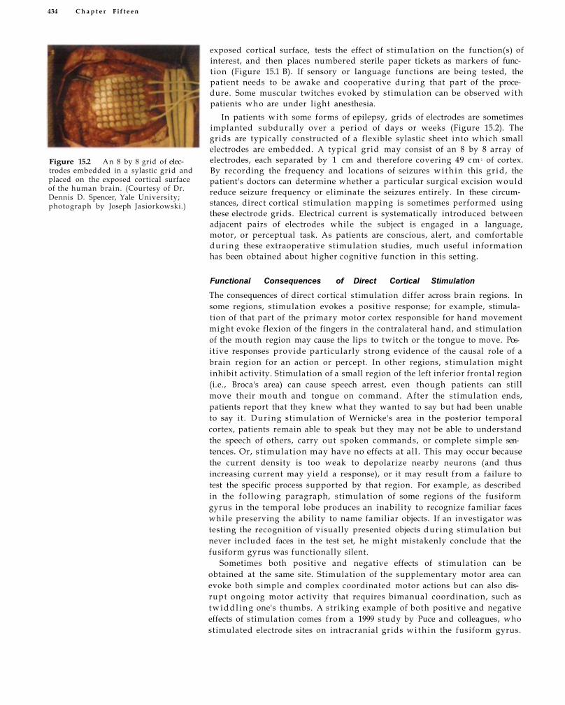
434 C h a p t e r F i f t e e n
Figure 15.2 A n 8 by 8 gr id of electrodes embedded in a sylastic gr id and placed on the exposed cortical surface of the human brain. (Courtesy of Dr. Dennis D. Spencer, Yale University; photograph by Joseph Jasiorkowski.)
exposed cortical surface, tests the effect of stimulation on the function(s) of interest, and then places numbered sterile paper tickets as markers of function (Figure 15.1 B). If sensory or language functions are being tested, the patient needs to be awake and cooperative d u r i n g that part of the procedure. Some muscular twitches evoked by stimulation can be observed with patients who are under light anesthesia.
In patients wi th some forms of epilepsy, grids of electrodes are sometimes implanted subdurally over a period of days or weeks (Figure 15.2). The grids are typically constructed of a flexible sylastic sheet into which small electrodes are embedded. A typical gr id may consist of an 8 by 8 array of electrodes, each separated by 1 cm and therefore covering 49 c m 2 of cortex. By recording the frequency and locations of seizures w i t h i n this gr id , the patient's doctors can determine whether a particular surgical excision would reduce seizure frequency or eliminate the seizures entirely. In these circumstances, direct cortical stimulation mapping is sometimes performed using these electrode grids. Electrical current is systematically introduced between adjacent pairs of electrodes while the subject is engaged in a language, motor, or perceptual task. As patients are conscious, alert, and comfortable dur ing these extraoperative stimulation studies, much useful information has been obtained about higher cognitive function in this setting.
Functional Consequences of Direct Cortical Stimulation The consequences of direct cortical stimulation differ across brain regions. In some regions, stimulation evokes a positive response; for example, stimulation of that part of the primary motor cortex responsible for hand movement might evoke flexion of the fingers in the contralateral hand, and stimulation of the mouth region may cause the lips to twitch or the tongue to move. Positive responses provide particularly strong evidence of the causal role of a brain region for an action or percept. In other regions, st imulation might inhibit activity. Stimulation of a small region of the left inferior frontal region (i.e., Broca's area) can cause speech arrest, even though patients can still move their mouth and tongue on command. After the stimulation ends, patients report that they knew what they wanted to say but had been unable to say it . Dur ing stimulation of Wernicke's area in the posterior temporal cortex, patients remain able to speak but they may not be able to understand the speech of others, carry out spoken commands, or complete simple sentences. Or, stimulation may have no effects at all . This may occur because the current density is too weak to depolarize nearby neurons (and thus increasing current may yield a response), or it may result from a failure to test the specific process supported by that region. For example, as described in the fo l lowing paragraph, stimulation of some regions of the fusiform gyrus in the temporal lobe produces an inability to recognize familiar faces while preserving the ability to name familiar objects. If an investigator was testing the recognition of visually presented objects dur ing stimulation but never included faces in the test set, he might mistakenly conclude that the fusiform gyrus was functionally silent.
Sometimes both positive and negative effects of stimulation can be obtained at the same site. Stimulation of the supplementary motor area can evoke both simple and complex coordinated motor actions but can also disrupt ongoing motor activity that requires bimanual coordination, such as t w i d d l i n g one's thumbs. A str iking example of both positive and negative effects of stimulation comes from a 1999 study by Puce and colleagues, who stimulated electrode sites on intracranial grids w i t h i n the fusiform gyrus.

C o n v e r g i n g O p e r a t i o n s 435
Before stimulation, the researchers showed the subjects photographs of familiar and famous faces, w h o m the subjects were able to identify. The faces, but not other stimulus categories, evoked large changes in electrical potential in electrodes w i t h i n the fusiform gyrus. The investigators then stimulated those electrodes. Several of the subjects became prosopagnosic dur ing the duration of the stimulation; that is, they could no longer recognize the faces, although they could recognize common objects. Once the stimulation ended, they could once again recognize these individuals. While the disruption of face recognition by stimulation was a noteworthy f inding, there was the possibility that the effect was not specific to faces. Perhaps the disruption would have also occurred for any object that had a specific ellipsoidal shape, was of the category of l iv ing things, or had bilateral symmetry. However, in two of the subjects, stimulation evoked a v i v i d hallucination of a face. This remarkable positive effect of stimulation provided strong evidence that the observed disruption was specific to faces.
While direct cortical stimulation is a potentially powerful technique, it has several limitations. First, it is invasive and may precipitate a seizure, particularly in patients who suffer from epilepsy. This risk underscores the fact that direct cortical stimulation can only be performed in a clinical context. Second, at high current levels, current sufficient to depolarize neurons may spread from the stimulating electrodes and excite brain regions at some distance. This can introduce uncertainty in the interpretation of the localization results. For this reason, the cathode and anode are usually kept in close proximity, and the investigator gradually increases the stimulating current so that the threshold at which a st imulation effect is first observed can be monitored. Third, positive or negative effects of stimulation do not necessarily indicate that the surgical removal of the stimulated region w i l l cause corresponding deficits. For example, a 1986 stimulation study by Luders and colleagues revealed the existence of a basal temporal language area in the left fusiform gyrus, whose stimulation leads to the inability to speak or understand language. Despite these striking deficits, surgical removal of this region does not typically lead to the same severe and lasting language deficits that would occur w i t h removal of Wernicke's or Broca's area. Why does damage to some brain areas lead to functional deficits, while damage to others results only in mi ld or transient deficits? As we w i l l consider in the discussion of lesion studies later in the chapter, this may reflect the ability of the brain to reorganize some functions fo l lowing damage, perhaps by engaging homotopic regions in the opposite hemisphere.
Several published studies have directly compared direct cortical stimulation and fMRI . In 1999, Schlosser and colleagues tested patients who were about to undergo surgery in the language-dominant temporal lobe (see Figure 12.21). To help guide the neurosurgeon, localization of temporal lobe language regions was attempted preoperatively using fMRI , and direct cortical stimulation was later performed either extraoperatively or intraopera-
homotopic The cortex in one cerebral hemisphere that corresponds to the same region in the other hemisphere.
Can you think of a circumstance where the evocation of a complex behavior by cortical stimulation of a brain region may not be evidence of a causal role of that region in that
behavior?

436 Chapter Fifteen
tively. The fMRI study used a blocked design in which native English-speaking subjects passively listened to speech that alternated between familiar (English) and unfamiliar (Turkish) languages. The same speaker was used throughout, and basic auditory properties were controlled between the two conditions. Thus, the subject heard a near continuous stream of speech, but his comprehension of speech varied between blocks. Greater activation was observed in response to the English speech in the lateral temporal (i.e., Wernicke's area) and inferior frontal (i.e., Broca's area) cortices in the language-dominant hemisphere of most subjects tested.
Direct cortical st imulation was also used to localize the lateral temporal language region in 14 of the fMRI subjects. At electrode locations near the locations of fMRI activity, cortical stimulation interfered w i t h auditory comprehension, object naming, or speech production tasks in 12 subjects. Stimulation therefore validated the results obtained from the fMRI task. However, whi le the correspondence between temporal lobe language areas identified by f M R I and by direct cortical st imulation was generally good, differences were noted in the spatial extent of activation using these different methods. As noted in Chapter 7, the spatial extent of fMRI activation may overestimate the area in which neuronal activation occurs, and so some discrepancies in spatial extent might be expected. However, because the spatial limits of the activation may influence the extent of a surgical resection, better methods to identify the boundaries of fMRI activation must be developed (see Box 12.2). Nevertheless, the results of Schlosser and colleagues suggest that information from direct cortical stimulation may provide important evidence that complements that obtained by fMRI studies.
Transcranial Magnetic Stimulation Heretofore, we have discussed invasive methods for direct cortical stimulation that involve opening the skull to place electrodes against the brain. An alternative method, transcranial magnetic stimulation (TMS), was introduced in the 1980s. In TMS studies, an electrical coil is placed on the outside of the skull and rapidly charged w i t h current (Figure 15.3A). This generates a strong magnetic field (as large as 2 T) that lasts less than a millisecond. This field extends through the skull and into the brain, where it produces an electrical current by electromagnetic induction (Figure 15.3B). The configuration of the coil influences the focality of the field and, thus, the spread of the electrical current. One popular coil design has the shape of a figure eight, for which the field is maximal near the midway point between the coils. TMS can be used to deliver a single brief electrical pulse to the brain, or it can be used to deliver a series of pulses for durations that span seconds to minutes (repetitive TMS, or rTMS). In addition to its value for functional brain studies, rTMS has also shown promise in the treatment of disorders such as depression, perhaps by increasing dopamine levels in the frontal cortex.
How is TMS related to the discussion of the effects of dB/dT explored in Chapter 2?
As currently practiced, TMS is considered a safe and noninvasive method and has been used in more than 2000 published studies of both normal vol-
repetitive TMS (rTMS) A series of closely spaced TMS stimulation pulses.

(A)
Figure 15.3 Transcranial magnetic stimulation (TMS). In TMS, an electromagnetic coil is placed on the surface of the skull (A) . Rapidly reversing the f low of a very strong current w i t h i n the coil induces a current field in the brain (B). The magnetic field lines associated w i t h a TMS pulse can be seen in the upper right of this coronal MRI phase map (C). (C from Drs. Daryl Bohning and Mark George, Medical University of South Carolina.)
unteers and patients. Indeed, one of the authors of this textbook was a volunteer subject in one of the first studies performed to test the safety of the single-pulse TMS method. It should be noted, however, that prior to the establishment of safe operating limits and procedures, rTMS evoked seizures in a small number of presumably normal subjects who had no prior history of seizure disorders. Also, due to current spread, the actual brain regions stimulated are even more uncertain than in the direct cortical stimulation studies discussed earlier. In 1997 Bohning and colleagues used MRI phase maps to visualize the distribution w i t h i n the brain of the magnetic field induced by TMS (Figure 15.3C) to help localize the sites of stimulation.
TMS has been used creatively in a large number of studies of brain function. By manipulating the latency at which a pulse is applied to a given brain region, researchers can interrupt processing at different points in time. For example, in 2003, Mottaghy and colleagues used single-pulse TMS to study verbal work ing memory in a two-back task (see Figure 13.13 for a depiction of the n-back task). The delay between the task stimulus and the delivery of the TMS was varied over a range of 140 to 500 ms. The authors found that work ing memory processes were impaired by shorter-latency TMS delivered to the parietal cortex and by longer-latency TMS delivered to the frontal cortex. This suggested that the f low of information was f rom parietal to frontal sites. Wi th in the frontal lobe, TMS delivered to the right hemisphere caused disruption at earlier delays than in the left frontal region, suggesting a f low of information from right to left hemispheres. It is important to note that the delivery of TMS d i d not disrupt a choice reaction time control task that d i d not have a work ing memory component. Thus, the effects of TMS were specific to work ing memory processes and specific to particular time points.
One of the most promising uses of TMS has been to determine whether regions activated in fMRI studies are essential for task performance. For example, in 2002 Rushworth and colleagues used fMRI to identify regions of
(B) (C)
C o n v e r g i n g O p e r a t i o n s 437

the frontal lobe that were activated dur ing t w o forms of task switching. In the response-switching condition, subjects switched between rules for selecting a response, whi le in the visual-switching condition, subjects switched between rules for selecting a stimulus. For each trial in each condition, the subject either kept or switched the rule from the previous trial . Although the t w o conditions evoked fMRI activity in different sets of brain regions, both activated the medial frontal cortex in the region of the pre-supplementarv motor area (pre-SMA). The authors thus hypothesized that this region plays an important role in task switching. To test this hypothesis, the authors later stimulated the pre-SMA using rTMS. This disrupted both tasks, but only on trials when the subject switched from the previous task rule. When the TMS stimulator was moved over motor cortex adjacent to the region of fMRI activity, st imulation had no effect on the task. Taken w i t h the fMRI results, these TMS data provide important converging evidence that the pre-SMA is a critical brain region in task switching and, furthermore, that its role is limited to the time of a switch. While combined or parallel use of TMS and fMRI is still in its infancy, such studies w i l l become increasingly important in corning years.
Brain Lesions The most venerable approach for studying the function of the brain is the observation of functional changes associated wi th brain lesions. Shortly after Broca's 1861 discovery, many other functional changes associated w i t h brain lesions in humans were reported. In 1868, Dr. John Har low described his observations of Phineas Gage, a railroad foreman in Cavendish, Vermont, who in 1848 had suffered a horrible accident in which an explosive charge blasted an iron tamping rod through his left cheekbone and out of the top of his head. Gage not only survived the accident (and was able to walk and speak w i t h i n minutes) but l ived for another 12 years. However, the frontal lobe injury caused a dramatic change in personality. His prior well-balanced and responsible bearing was replaced by a profane and irresponsible demeanor in which he showed little regard for others. Gage's case was one of the first cases in which a profound alteration of personality was linked to a lesion w i t h i n a specific brain region. Many early researchers, including the German neurologist Hermann M u n k , created controlled, experimental lesions in animals to make important discoveries about the organization of the cerebral cortex. Other scientists, like David Ferrier, used both lesion and cortical stimulation studies in animals in their research.
Lesion studies in both humans and animals are still an important method for the study of brain function. Like cortical stimulation, which can be considered to create a transient and reversible lesion, lesion studies provide information about the necessity of a brain region for a particular function. Yet by themselves, lesion studies have several disadvantages. Studies in humans depend pr imari ly upon naturally occurring lesions, such as those produced by a stroke, that can be large and extend across many functional brain regions. This variability makes it diff icult or impossible for investigators to assemble a group of patients wi th identical lesions. Furthermore, natural lesions often involve damage to white-matter pathways, impairing functions that are supported by distant brain regions that were undamaged but became disconnected. These problems can be ameliorated by studying patients w i t h well-defined surgical lesions, such as patients who have received a temporal lobectomy to relieve intractable epileptic seizures. How-
438 C h a p t e r F i f t e e n
C o n v e r g i n g O p e r a t i o n s 439
ever, these patients have suffered for many years from a preexisting neurological disorder and often continue to take powerful drugs that may alter normal brain function.
Lesion studies can also have interpretive difficulties. Unlike the positive results sometimes observed w i t h direct cortical stimulation, lesions do not produce complex behaviors. Thus, the loss of function fo l lowing a brain lesion does not guarantee that the damaged brain tissue was the locus for that particular function. For example, a large lesion in the pr imary visual cortex would impair not only basic visual perception but also many higher-order functions like object recognition, reading, and eye gaze perception. It would be absurd to suggest that all of these visually based functions resided in the primary visual cortex, yet this region was clearly essential for every one of them. For this reason, investigators who employ the lesion approach systematically compare the pattern of associations and dissociations between lesions in different brain regions and performance on different experimental tasks.
To this end, several groups around the world have established large databases, or registries, of individuals who have brain lesions and w h o have been studied in a large number of different tasks. One example is the Cognitive Neuroscience Patient Registry developed by Antonio and Hanna Dama¬sio and their many collaborators at the University of Iowa. Another is the patient registry developed by Robert Knight and his colleagues at the University of California, Berkeley. By evaluating the effects of damage to different brain regions, as determined by quantitative reconstructions of lesions across many subjects, researchers can identify patient groups who share a particular functional impairment. Figure 15.4 presents an example of this approach. By recording lesion characteristics from a large group of subjects, impairments across a spectrum of tasks can be mapped to particular regions of damage.
Lesion studies have considerable value for dissection of complex tasks into their subcomponents. In 1955, Teuber introduced the concept of the double dissociation (see Chapter 13 for a discussion of similar logic applied to fMRI). By demonstrating that a lesion to brain structure A impairs function X but not function Y, a researcher establishes a single dissociation between the functions. But w i t h the additional result that that a second lesion to structure B disrupts function Y while leaving function X intact, the researcher has established a double dissociation, and can make more-specific inferences about brain function. Consider the fol lowing example. An investigator creates a model for face processing that hypothesizes the existence of separate functions for retrieving face identity and for the recognition of emotional facial expression. A single dissociation would demonstrate that damage to a specific brain region (e.g., the ventral temporal lobe) impairs judgments of face identity but not judgments of emotional expressions. This result is consistent w i t h the model, but it might also have resulted from other factors, such as higher functional SNR on one task than the other. More-powerful support for this model would come from the second demonstration that damage to a different brain region (e.g., the right frontoparietal region) impairs judgments of emotional expressions but not of identity. Readers interested in additional discussion of lesion interpretation in the context of neuropsychological theory, including caveats concerning double dissociation, should refer to the book by Shallice listed in the suggested readings.
registry A patient database. A registry might include information about the locations of brain lesions in a large population of individuals who might then be asked to participate in experimental studies.
double dissociation The demonstration that two experimental manipulations have different effects on two dependent variables. One manipulation affects the first variable but not the second, and the other manipulation affects the second but not the first.
single dissociation The demonstration that an experimental manipulation has an effect upon one variable but not upon a second variable.

440 C h a p t e r F i f t e e n
Left dorsal prefrontal
Figure 15.4 Lesion maps from a patient registry. Shown are the extent of lesions in the left dorsal prefrontal cortex for eight subjects. The lesions are indicated by red shading on a stack of axial slices and on a surface reconstruction. The bottom row shows a color-coded summary that indicates the degree of lesion overlap in this sample. (Courtesy of Dr. Robert Knight, University of California, Berkeley.)
plasticity The change in the normal functional properties of brain tissue following injury or experience.
recovery of function The improvement in a previously impaired ability over time, due to functional or structural changes within the brain.
Combined Lesion and fMRI Studies
Evidence from lesion studies can greatly extend the interpretive power of fMRI . When a process both evokes fMRI activity in a brain region and is disrupted when that region is lesioned, researchers can more readily conclude that the process relies on the brain region for its execution. The benefits of converging lesion and fMRI studies are thus similar to those of combined direct cortical st imulation and fMRI studies, as discussed earlier.
Most studies that have combined lesion analysis and fMRI in the same individual have investigated the influence of a developmental lesion upon a well-localized function, such as language processes in the left hemisphere. For example, in 2002, Staudt and colleagues studied five individuals who had suffered left hemisphere lesions around the time of birth. When tested in language activation tasks, these individuals showed a pattern of right hemisphere activation that was vir tual ly the mirror result of the left hemisphere activation pattern obtained in age-matched controls wi thout brain lesions. From these fMRI results, the authors argued that early damage to left hemisphere regions supporting language results in the recruitment of homotopic regions in the undamaged right hemisphere. Another example comes f rom the 1997 work of Schlosser and colleagues, who studied a 19-year-old patient w i t h a large arteriovenous malformation in her right frontal and rostral parietal lobes. As a result, she had experienced poor motor control of the left side of her body (i.e., hemiparesis) since childhood. While she had no motor control over her left hand, sensation was preserved. An f M R I study was conducted using a blocked design in which the left and right hands were alternately stroked by a brush. Strong activation was obtained in response to both right- and left-hand sensation, but, as illustrated in Figure 15.5, stroking the left hand activated the primary sensory
region of the ipsilateral left hemisphere. That is, her brain was reorganized so that sensations from both sides of the body were (at least partially) represented in the same hemisphere. These fMRI studies provide strong evidence for the functional plasticity of the human cortex in response to early brain injury.
Combined fMRI and lesion methods have also been used to study recovery of function in individuals w h o acquired lesions in adulthood from stroke or other brain injury. Using f M R I , TMS, and magnetoencephalography, in 1998, Rossini and colleagues investigated changes in the brain of a poststroke patient w h o had recovered significant motor function. Their results suggested that the sensorimotor cortex in the affected hemisphere was enlarged, and shifted posteriorly, compared to the other hemisphere. In a similar study conducted in 1997, Cramer and colleagues used fMRI to study 10 patients who had recovered good motor function fol lowing stroke.

C o n v e r g i n g O p e r a t i o n s 441
Right hand stimulation
Figure 15.5 Evidence for functional plasticity from combined lesion/fMRI studies. Shown are the patterns of fMRI activations evoked by stroking the right hand (red) and left hand (blue) in a patient w i t h a large arteriovenous malformation (AVM) in the right hemisphere. Note that the response to the left hand occurs in the left, or ipsilesional, hemisphere. (From Schlosser et al., 1997.)
Left hand stimulation
When the patients performed a finger tapping task, activity in the sensorimotor cortex of the unaffected hemisphere was increased relative to controls. Increased activation was also found in the SMA and cerebellum. These results suggest that recovery of motor function after stroke involves the increased participation of homotopic regions of the unaffected hemisphere and midline motor regions. While some activation was obtained in the affected hemisphere of the stroke patients, it was restricted to the edge of the cortical infarct. Because of its localization power and noninvasiveness, fMRI can be used both to complement lesion studies in order to understand brain organization and to supplement lesion data in order to investigate functional changes associated wi th the lesions.
Probabilistic Brain Atlases To this point, we have discussed t w o forms of lesions: those in which brain tissue has been excised surgically and those where focal damage or injury has made the existing tissue nonviable. In many diseases that affect the brain (e.g., Alzheimer's disease, schizophrenia), such frank and focal lesions do not occur. Rather, regions w i t h i n the brain of an afflicted indiv idual may exhibit tissue volume loss that progresses over the course of the illness. As wi th lesions due to stroke or surgery, volume loss in particular regions may impair specific cognitive functions, and thus fMRI studies in these patient groups may be valuable as a prognostic indicator.
New image processing techniques take advantage of large MRI databases and advanced computational methods to determine which regions vary between normal and diseased brains. Recall that in Chapter 10, we discussed how preprocessing fMRI data often involves the warping of the brains from individual subjects into a stereotaxic space to simplify statistical
What properties of fMRI may m a k e it a poor choice for assessing function in patients with vascular lesions?

442 C h a p t e r F i f t e e n
Figure 15.6 Variability in brain anatomy. Overlaid upon the rendered brains are maps of the variability in brain anatomy in the cortex of control and schizophrenic subjects (both males and females). Areas of high variability across individuals are shown in red-purple, while areas of low variability across individuals are shown in blue. Increased variability is observed in the frontal cortex for both male and female schizophrenics. (Courtesy of Drs. Katherine Narr and Arthur Toga, Laboratory of Neuroimaging, University of California, Los Angeles.)
Control subjects Schizophrenic subjects
polymorphism A common variation in a gene or segment of DNA
imaging genomics A new field that investigates the effect of genetic variation upon brain structure and function.
analyses across subjects. The degree to which a brain must be warped to match a normalized space is itself of interest, because it provides a quantitative measure of regional brain variability. Investigators are using such measures to study structural differences between the diseased and normal brain. Figure 15.6 illustrates the relative variability of samples of brains from schizophrenic individuals and from normal controls. Note that the brains of the schizophrenic individuals show greater variabil ity (red-purple colors) in several regions of the frontal lobes, including the midline. This f inding corroborates fMRI results from many groups across a variety of tasks that have demonstrated that schizophrenic subjects show abnormal fMRI activation patterns in the prefrontal cortex. Readers interested in learning more about the use of probabilistic brain atlases to study human disease are referred to the article by Toga and colleagues in the suggested readings.
Brain Imaging and Genomics For a growing number of neurological and psychiatric disorders, there are variations, or polymorphisms, in some genes that signal increased risk for an individual developing the disease. As researchers begin to investigate the effects of these polymorphisms upon brain function, a new field has emerged that has been named by Hariri and Weinberger as imaging genomics.
An early and notable study conducted by Bookheimer and colleagues in 2000 used fMRI to investigate memory processes in people w i t h and without genetic risk factors for dementia. In their study, 30 individuals were tested, all of whom were neurologically normal and had memory scores w i t h i n the normal range for their age. However, 16 of the individuals carried the epsilon 4 allele of the apolipoprotein E gene (APOE-4), which is associated

C o n v e r g i n g O p e r a t i o n s 443
w i t h an increased risk of developing Alzheimer's disease in individuals experiencing cognitive decline. The remaining 14 individuals carried the epsilon 3 allele (APOE-3) and thus were not at increased risk. When participating in an fMRI experiment of retrieval of items from memory, the APOE-4 group showed increased activation of the hippocampus, the parietal cortex, and the prefrontal cortex. These structures have been implicated as important to memory by many experiments. When a subgroup of subjects were tested on memory tests t w o years later, the decline in their memory performance was predicted by the degree of increased activation. That is, APOE-4 individuals who had increased fMRI activity in these regions were more likely to have later memory impairments. These results suggest that fMRI can detect subtle patterns of damage that may result in later functional deficits, even prior to the development of clinically apparent memory deficits or disease onset. Also of interest is the suggestion that increased fMRI activation may reflect compensatory processes that offset the functional consequences of the incipient disease.
In 2002, Hariri and colleagues examined individuals w i t h a variation in a gene related to the neurotransmitter serotonin. This variation had previously been linked to increased behavioral measures of anxiety, but the relation was weak and unreliable across different studies. The researchers used fMRI to test two groups of subjects, one w i t h the genetic variation and one without , all of w h o m were healthy and had no neurological or psychiatric disorders. The subjects viewed pictures of faces that depicted fearful or angry expressions. Previous research had established that these pictures evoke significant activity in the amygdala, a region of the brain associated w i t h emotional processing. However, despite the fact that the groups d i d not differ on anxiety- or fear-related traits, the subjects w i t h the genetic variation showed a greater response in the r ight amygdala to the fearful and angry faces. This study demonstrated the power of fMRI to probe the functional consequences of genetic variation. Readers interested in this fascinating new field should consult the suggested readings.
In summary, information about brain structure provided by stimulation, lesion, or TMS studies complements information about brain function provided by fMRI . Inferences made using one technique are improved by converging studies using the other. Questions about causality that are raised by fMRI results can be answered using lesion studies, just as fMRI can answer questions about large-scale systems and recovery of function that are raised by lesion data. Furthermore, fMRI can assess the functional consequences of statistical differences in brain structure and in genetic variation. As a result, techniques that examine the consequences of changes in neuronal activity w i l l continue to be critical for research programs in cognitive neuroscience.
Measuring Neuronal Activity
The first electrophysiological studies were conducted in 1848 by the German physiologist Emil Du Bois-Reymond, who discovered that nerves in a frog exhibit action potentials. Shortly afterwards, Hermann von Helmholtz used action potentials to measure the speed of conduction along the frog's nerve. It is a scientific irony that Du Bois-Reymond and Helmholtz were both students of the physiologist Johannes Miiller, who believed in the vitalist ideas that activity of the nervous system was ephemeral and thus could not be measured experimentally. The studies of Du Bois-Reymond, Helmholtz, and their contemporaries such as Julius Bernstein d i d much to explain neural trans
action potential A wave of depolarization that travels down a neuronal axon.

444 C h a p t e r F i f t e e n
BOX 15.1 Electrogenesis Na+ is a positively charged sodium ion because it has lost an electron, while Cl -
is a negatively charged chlorine ion because it has gained an electron. Due to the selective permeability of a neuron's membrane and the action of ionic pumps, there is an unequal distribution of ions across the neuronal membrane and thus an unequal distribution of charge. An electrode placed inside of a neuron at rest would record a large potential difference compared to an electrode outside of the neuron, wi th the interior of the membrane about -70 mV relative to the outside.
Let's consider the sequence of events associated w i t h the depolarization of a small patch of a neuron's membrane. First, there is an inward positive current caused by inflow of positive sodium ions, creating a relative deficit in positive charge wi th in the surrounding extracellular space. The depolarized patch of membrane thus becomes a current
sink and attracts positively charged ions (Figure 15.7). The inrushing positive charge flows wi th in the neuron and away from the depolarized membrane, creating an intracellular accumulation of positive charge. This, in turn , causes an outward positive current from the unexcited portions of the neuronal membrane. This outward f low constitutes a current source, from which the positive ions flow back through the extracellular space toward the sink. To conserve charge, the efflux from the source is equal to the influx at the sink. The strong current flow wi th in the restricted intracellular space of the neuron is called the primary current, while the relatively weak return flow through the much larger extracellular conductive medium (or volume conductor) is called the volume current. While the primary current is confined to the intracellular space of the neuron, the volume currents extend throughout the conductive medium that contains the neuron.
The charge at the current source generates an electric field that is directed radially outward and whose strength decays w i t h the inverse square of distance. That is, doubling the distance from the current source increases the area occupied by the electric field by a factor of 4, and thus the intensity of the electric field is only one-fourth as strong. The
Figure 15.7 Current flow in a depolarized neuron. The patch of depolarization caused by synaptic activity becomes a current sink where current enters the neuron in the form of positively charged Na+ ions. The bui ldup of positive charge w i t h i n the neuron causes a current f low w i t h i n the neuron called the primary current. To conserve charge, positive current flow exits the unexcited portions of the neuron's membrane, creating a current source. In the extracellular space, return or volume currents flow back toward the sink. Although most dense nearest the neuron, these volume currents extend throughout the brain. When viewed from a distance, the close apposition of the current source and sink approximates a current dipole.
the neuronal membrane. While that discussion was in the context of the resulting metabolic demands, whose supply forms the basis of the fMRI BOLD signal, here we consider the electrophysiological consequences of membrane depolarization. Recall that the movement of ions through membrane channels supports information processing through the integrative and signaling activity of neurons. In this context, integration refers to the spatiotemporal summation of excitatory postsynaptic potentials (EPSPs) and inhibitory postsynaptic potentials (IPSPs) on the neuron's dendritic arbors and cell body. EPSPs and IPSPs vary in magnitude and duration depending upon the strength and timing of the synaptic input. If the spatiotemporal summation of EPSPs and IPSPs can be considered a computation performed upon a pattern of synaptic input, then the action potential is the output of this computation. Unlike postsynaptic potentials, action potentials are all-or-none; if the summation of EPSPs and IPSPs at the axon hillock surpasses a threshold, a self-propagating action potential w i l l be triggered. But if the threshold is not surpassed, no action potential w i l l occur. Because the action potential carries information to other interconnected neurons, we refer to action potentials as the signaling component of information processing in the brain.
What do we mean by electrophysio-logical? What properties of ions, membranes, and channels involve electricity? Atoms normally have as many negatively charged electrons as they have positively charged protons, and thus they are electrically neutral, having no net charge. However, if an atom gains or loses one or more electrons, it becomes an electrically charged ion.
n Chapter 6, we introduced the sequence of events associated with the depolarization of a small segment of
I

Converging Operations 445
Figure 15.8 The extracellular electric field in the brain associated w i t h neuronal activity. Shown is a representation of the consequences of the depolarization of the soma of a pyramidal cell. The volume currents are shown as solid isoflux lines, while the isopotential lines are shown as dashed. The zero potential line occurs where the flux lines begin to bend inward toward the sink. Relative to the zero potential line, positive potentials are measured above the line and negative potentials are measured below. Note that the field weakens w i t h increasing distance from the neuron. (After Cruetzfeldt, 1974.)
charge at the current sink generates an electrical field that is directed radially inward. Because the distance on the neuron between the source and sink is very small, we can idealize this close apposition of positive and negative point sources as a current dipole. The
electrical field produced by a dipole is simply the vector sums of the outward¬and inward-oriented radial electric fields of the current source and sink. The electric field generated by the current dipole can be conceptualized as a set of flux lines through the volume
conductor that connect the point charges (Figure 15.8).
A potential difference can be measured in volts (or, more typically for brain electrophysiology, microvolts) between locations in the electric field. Isopotential
integrative activity The collection of inputs from other neurons through dendritic or somatic connections.
signaling activity The transmission of the outcome of an integrative process from one neuron to another
excitatory postsynaptic potential (EPSP) A depolarization of the postsynaptic cell membrane.
inhibitory postsynaptic potential (IPSP) A hyperpolarization of the postsynaptic cell membrane.
ion A charged atom.
pump A transport system that moves ions across a cell membrane against their concentration gradient.
current sink An attractor of positive ions. A depolarized patch of neuronal membrane is a current sink because positively charged ions will flow toward it.
current source A source of positive ions.
primary current The current flow within a neuron caused by the inflow of ions through ionic channels opened by synaptic activity.
volume conductor A continuously conductive medium. The brain, meninges, skull, and scalp constitute a volume conductor throughout which currents created by ionic flow can be measured.
volume current The return current through the extracellular medium that balances the primary current within a neuron.
current dipole A positive and negative point charge separated by an infinitesimal distance. A current dipole is used as a simple and convenient model for the electromagnetic fields produced by an activated neuron.
B O X 1 5 . 1 (continued)
Cortex adjoining white matter

446 Chapter Fifteen
electroencephalogram (EEG) The measurement of the electrical potential of the brain, usually through electrodes placed on the surface of the scalp.
electrogenesis The explanation for electrophysiological phenomena such as EEG or evoked potentials based upon ionic current flows instigated by synaptic activity.
single-unit recording Collection of data about the electrophysiological activity (e.g., action potentials) of a single neuron.
field potentials Changes in electrical potential over space associated with postsynaptic neuronal activity
magnetoencephalography (MEG) A noninvasive functional neuroimaging technique that measures very small changes in magnetic fields caused by the electrical activity of neurons, with potentially high spatial and temporal resolution.
mission in peripheral nerves and muscle fibers. However, not until 1875 were the first electrical recordings of brain activity published by the physician Richard Caton of Liverpool. Strongly influenced by the studies of his contemporary David Ferrier, Caton wanted to measure electrical potential changes in the cortex. Because these electrical changes were extremely weak, he used a reflecting galvanometer that had a mirror attached to its coils. As the voltage changed in the cortex of an animal, the position of the mirror moved only very slightly, but sufficiently to cause a much larger change in the position of a reflected beam of light. This primitive amplification method made it possible to observe the very small voltages associated w i t h brain activity. A half century later, the Austrian psychiatrist Hans Berger extended Caton's work by measuring continuous changes in voltage on the scalp over time. The technique that he developed became known as electroencephalography, and its measure became known as the electroencephalogram (EEG).
Many different electrophysiological methods exist for studying different facets of neuronal electrical activity, or electrogenesis (Box 15.1). A t one extreme, these methods can measure changes in ionic conductances at an isolated patch of a single neuron's membrane, while at the other extreme, they can measure the synchronized activity of millions of neurons. We begin our examination of direct measures of neuronal activity wi th a discussion of the recording of action potentials from individual neurons, a technique known as single-cell or single-unit recording. We then discuss the recording of summated field potentials associated w i t h postsynaptic activity. Field potentials can be measured in different ways at different scales, using both intracranial electrodes and scalp electrodes. We conclude w i t h a consideration of magnetoencephalography (MEG), a technique that records the magnetic fields associated w i t h neuronal activity.
lines, along which the voltage is constant, can be drawn perpendicular to the electric field lines. Because the charges at the source and sink are equal and opposite, the zero potential line is located at the point where the outward-directed field from the source begins to bend inward to the sink. The isopotential lines on the outward-directed side of the field measure positive voltages, while the isopotential lines on the inward-directed side of the field measure negative voltages. In the case of a depolarized neuron, the electric field produced by the source and sink can be measured by electrodes at different points in the extracellular space. For example, if depolarization occurred in the apical dendrites, then an electrode near the dendrites would record a negative potential relative to an electrode near the soma. If the soma was depolarized, as
shown in Figure 15.8, the reverse would occur. The dipole is a convenient model for a depolarized neuron. Indeed, when observed from a distance, the fields generated by the coordinated activity of a larger ensemble of neurons can be modeled as though they were produced by a single equivalent dipole. This forms the basis for several of the techniques described later in this chapter.
In principle, the volume currents associated with neuronal depolarization can be detected anywhere within the volume conductor. Indeed, because the conductive medium around a neuron includes the entire brain and skull, neuronal activity can be detected with electrodes placed on the scalp. We will return to a discussion of scalp-recorded event-related potentials, or ERPs, later in this chapter.
apical dendrites The dendrites that are distant from the neuronal cell body. For typical pyramidal cells in the cortex, the apical dendrites extend to the superficial layers of cortex, while the cell bodies are located in deeper layers.
equivalent dipole A simplifying model that represents the electromagnetic field produced by a population of neurons as though it were produced by a single dipole.
event-related potentials (ERPs) Small electrical changes in the brain that are associated with sensory or cognitive events.
BOX 15.1 (continued)

Converging Operations 447
Single-Unit Recording
The most direct measure of neuronal electrical activity is the action potential. The pr imi t ive methods used by Du Bois-Reymond to record the action potential in 1848 were greatly advanced by the introduction of the microelectrode in the first half of the 20 t h century. Microelectrodes are placed either inside of a neuron or next to the neuron's cell body in the extracellular space. Studies measuring the rate of action potentials using microelectrodes, a technique k n o w n as single-unit recording, have generated some of the most important discoveries in all of neuroscience.
The value of single-unit recording was powerfully demonstrated in studies initiated in the late 1950s by David Hubel and Torsten Wiesel, who were w o r k i n g at that time in the laboratory of Steven Kuffler at Johns Hopkins University. Using single-cell recording, Kuffler had previously demonstrated that retinal ganglion cells had a center-surround organization. That is, these cells increased their activity when a l ight was flashed in the center of a receptive field and decreased their activity when a light was flashed in the periphery of their receptive field. Hubel and Wiesel extended those studies into the visual cortex (Figure 15.9). By presenting more-complex s t imuli , such as lines and edges, Hubel and Wiesel discovered that some cells in the primary visual cortex had receptive fields very different from those of retinal ganglion cells. Simple cells had a more rectangular receptive field w i t h adjacent rectangular inhibitory regions, as if combining the output of a line of ganglion cells, and their rate of f ir ing varied w i t h the orientation of the visible line or edge. A similar approach was used to identify a second population of complex cells, which responded best to lines of a particular orientation, regardless of their position w i t h i n the receptive field. Later studies bui lding upon this work described many important properties of the visual cortex, including its columnar arrangement and its changes during development. For these fundamental discoveries, Hubel and Wiesel received the Nobel Prize in Physiology or Medicine in 1981.
receptive field The part of the visual field that, when stimulated, will result in an increase in firing of a particular neuron.
simple cell A neuron in the visual cortex that responds with increased firing to a stimulus with a preferred orientation in its receptive field and with decreased firing to a stimulus in the region surrounding its receptive field.
complex cell A neuron in the visual cortex with a larger receptive field than a simple cell and that responds to a stimulus with preferred orientation anywhere within its receptive field.
(A) Experimental setup
Light bar stimulus projected on screen
(B) Stimulus orientation
Stimulus presented
Recording from visual cortex
Figure 15.9 Single-unit recording. This figure illustrates the recording of a simple cell from the visual cortex of the cat. The cat views slits of light, the orientation of which the experimenters systematically vary. The single-unit discharge is shown for each orientation. The preferred vertical orientation is determined by the abrupt burst of action potentials for this stimulus. Some degree of generalization can be seen by the response of the cells to slightly off-vertical orientations.

448 C h a p t e r F i f t e e n
Figure 15.10 Single-unit recording in an oculomotor delayed response task. Monkeys were trained to fixate at the center of a display whi le a target stimulus was i l luminated for 500 ms at one of eight peripheral locations. Following offset of the target, the monkey maintained fixation for an additional 3-s delay period. Any eye movement dur ing the presentation of the target or d u r i n g the delay period caused the trial to be aborted. At the conclusion of the delay period, the fixation cross disappeared and the monkey made a saccade to the remembered location of the visual target and, if correct, received a juice reward. Plotted in the surrounding panels are the single-unit responses f rom a neuron in the principal sulcus in the prefrontal cortex. Within each of these eight panels, the first pair of vertical lines demarcates the interval dur ing which the visual cue was presented. The last vertical line indicates the offset of the delay period. (From Chafee and Goldman-Rakic, 1998.)
raster A depiction of the firing rate of action potentials by a neuron in which time is represented along the horizontal axis and a dot indicates the occurrence of an action potential.
A more recent example of the value of single-unit recording in cognitive neuroscience is provided by the work of Patricia Goldman-Rakic and her colleagues, who explored the properties of neurons in the monkey's prefrontal cortex dur ing an oculomotor delayed response task. Monkeys were required to remember the location of a visual target that was briefly presented in the periphery, and to make an eye movement to the remembered location at the end of a delay period. The results shown in Figure 15.10 are from Chafee and Goldman-Rakic's 1998 study and illustrate a typical outcome for a neuron in the dorsolateral prefrontal cortex. Shown are eight location panels, each containing a series of rows, or rasters, in which a black dot indicates the occurrence of an action potential. Each of the rasters corresponds to one trial of the delayed response task. At the bottom of each panel is a histogram that indicates the number of times the neuron fired at a particular time d u r i n g the task across all trials. The spatial specificity of this neuron was striking, in that significant f i r ing was only observed when the target was presented at the lower-left location. Even more remarkable was the fact that the neuron fired robustly throughout the delay interval, when the monkey was maintaining the target location in memory. Because there was l itt le to no neuronal activity in the other seven locations, Chafee and Goldman-Rakic suggested that this neuron was coding the specific location of the remembered stimulus and was not responding in a general way to the delay interval. Other neurons in the same small region of cortex responded selectively to the other visual target locations. Due to the spatial selectivity of these neurons (like the primary visual cortex neurons discussed in the previous paragraph), Goldman-Rakic described these to-be-remembered spatial locations as their memory fields.
Because of the clarity of such results, single-unit studies have generated great excitement for the study of the neural basis of w o r k i n g memory. Many fMRI studies have used similar delayed response tasks to demon-
500 ms/div

strate sustained BOLD activation of the prefrontal cortex and other brain regions. For example, Courtney and colleagues used f M R I in 1997 to demonstrate sustained activity w i t h i n the dorsolateral prefrontal cortex during an 8-s delay interval between the presentation of to-be-remembered pictures of faces and a test face. Similarly, in 1998, Belger and colleagues presented subjects w i t h a series of delayed-response trials in which the nature of the items to be remembered varied on alternating trials. On spatial trials, the subject was shown successively three whi te dots in different spatial locations. After a delay of 3500 ms w i t h no stimulus present, a test dot was shown and the subject indicated whether or not it matched one of the remembered locations. On shape trials, the subject was shown successively three complex polygons and, again, was required to indicate after a stimulus-free delay whether a test polygon matched any of the remembered set. Control trials were similarly constructed, but the "memory set" st imuli stayed on the screen throughout the delay interval and thus the subject made a simple discrimination when the test item appeared that d i d not depend upon memory. As in the study by Courtney and colleagues, strong BOLD activation was observed in the dorsolateral prefrontal cortex in the memory trials but not the control trials. The strength of the activation also varied w i t h the stimulus materials, w i t h primari ly right hemisphere activation occurring for the spatial memory trials and bilateral activity occurring for the shape trials. Activation also occurred in the parietal lobe and intraparietal sulcus.
These are but two examples from a major area of fMRI research that was initiated largely on the basis of single-unit studies. Interested readers are directed to the reviews by Miller and Cohen and by Curtis and D'Esposito in the suggested readings. A more thorough discussion of BOLD activation during such executive processing tasks can be found in Chapter 13.
Limitations of Single-Unit Recording As can be appreciated from these t w o examples, single-unit recording has high spatial resolution, as it can identify adjacent neurons that differ in their receptive or memory fields. Moreover, the temporal resolution of single-unit recording is exquisite. Because the responses evoked by closely spaced s t imul i are clearly discriminable, Chafee and Goldman-Rakic were able to classify neurons on the basis of their responses to the target cue, the delay interval, or the response cue. Both the temporal and spatial resolution of single-unit recording are several orders of magnitude better than what can be obtained using fMRI . Given these advantages, it is unsurprising that single-unit recording has an outstanding record of accomplishment in neuroscience.
However, while the strengths of the single-unit recording technique far outweigh its weaknesses, the latter are still notable. Most significant is the fact that single-unit recording is an invasive technique that requires the brain to be penetrated by the recording electrode. Although single-unit recordings have been made on a limited basis in humans undergoing neurosurgery, its application is primarily restricted to animals. A second limitation is that single-unit recording does not establish a causal relationship between the f ir ing pattern of the neuron and the presumed underlying process. Thus, while it appears that the neuron illustrated in Figure 15.10 is coding the spatial location of the target and therefore is critical to w o r k i n g memory, the result demonstrates only a correlation. Would the removal of that single neuron render the animal incapable of remembering that specific spatial
C o n v e r g i n g O p e r a t i o n s 449
450 C h a p t e r F i f t e e n
PSP Any postsynaptic potential, excitatory or inhibitory, that results from synaptic activity.
location? It is unlikely that working memory w o u l d be so dependent upon a single neuron among the billions that comprise the monkey's brain.
One way to establish a causal relation between a brain region and a cognitive construct under study is to disable the brain region and observe whether the process of interest can proceed without the participation of the neurons populating the region. Techniques for disabling brain activity were discussed earlier in this chapter and include permanent or temporary brain lesions and transcranial magnetic stimulation. As an example, many lesion studies in monkeys have f i r m l y established that damage to the prefrontal cortex, whether permanent and caused by surgical lesions or reversible and caused by local cooling, produces a selective deficit in w o r k i n g memory performance. Thus, the integration of converging data from single-unit recordings and lesion studies makes a much stronger case that these neurons play a causal role in work ing memory processes than does either result alone.
A second way to establish a causal relation is to artificially control the firing of the neuron and observe its effect on behavior. Such an approach has been taken by Newsome and colleagues, who have altered the output of neurons in extrastriate visual cortex in the monkey using electrical microstimulation. For example, neurons w i t h i n motion-sensitive visual cortex (MT/V5) fire more frequently when a stimulus w i t h a preferred direction of motion is presented. In a 1994 study, Salzman and colleagues trained monkeys on a psychophysical task in which rewards are given for correctly indicating the correlated direction of moving dots. To make the task diff icult , dots w i t h random motion are added to dilute the proportion of dots moving in a correlated direction. Predictably, when the display contains a large proportion of dots moving in random directions, the performance of the monkeys degrades. However, when neurons w i t h the correct preferred direction were electrically stimulated dur ing the presentation of the moving dots, the monkeys' performance improved. These data demonstrate that increased neuronal f ir ing provides a code for direction preference that can cause monkeys to make particular judgments in a behavioral task.
Finally, while single-unit studies are dif f icult to conduct simultaneously wi th neuroimaging techniques like fMRI , research using both techniques can be conducted in parallel or in series. Many laboratories are combining exploratory fMRI studies wi th confirmatory single-unit studies or are using human fMRI to test hypotheses generated using single-unit recording. A good example of the value obtained by combining these methodologies can be found in the review by Mil ler and Cohen in the suggested readings.
Field Potentials The term field potential refers to the summation of extracellular excitatory and inhibitory postsynaptic potentials (we shall use the shorthand PSP to refer collectively to EPSPs and IPSPs). Because the configuration of sources and sinks changes from moment to moment wi th the strength and pattern of synaptic inputs, field potentials change on an instant-by-instant basis to reflect this input. For this reason, the change in voltage over time reflected by field potentials has high temporal fidelity to the changing neuronal activity. Field potentials can be recorded by electrodes located anywhere w i t h i n a conductive volume, including electrodes placed directly on the cortical surface, electrodes that penetrate deep structures in the brain, and electrodes placed on the surface of the intact scalp. In each of these cases, the electrode measures summated PSPs, and so in their essence all of these techniques are based upon the same principles. However, the relative proximity of the elec-
C o n v e r g i n g O p e r a t i o n s 451
trode to the sinks and sources that produce the extracellular volume currents has both practical and theoretical consequences that differentiate intracranial and scalp recordings.
Field potentials measured on all of these spatial scales have provided useful complementary information for fMRI studies. However, it is the prospect of combining scalp-recorded field potentials w i t h fMRI measurements that has excited the greatest interest. If field potential recording could provide information about the sequence of neural events while fMRI could provide information about the location of neural activity, then combining these methods could potentially provide an unparalleled description of the spa-tiotemporal activity of neurons dur ing cognitive tasks. Despite this promise, technical and theoretical limitations have retarded progress in achieving fusion between the techniques. We describe these challenges in this and the fol lowing section.
Four facts about postsynaptic potentials are relevant to our present interest. First, unlike the very brief (<1 ms) duration of a typical action potential, indiv idual PSPs can be tens of milliseconds in duration. Second, hundreds or even thousands of synapses may make contact w i t h the dendritic arbors and soma of a single neuron, and PSPs can occur at many synapses in close temporal succession. Thi rd , as explained in Box 15.1, the volume currents associated w i t h indiv idual PSPs extend into the extracellular space w i t h a strength that diminishes rapidly w i t h increasing distance f rom their source and sink. Fourth, the volume currents associated w i t h individual PSPs sum-mate in the extracellular space.
In principle, because field potentials represent the summation of activity across a large population of neurons, an electrode placed into the brain w i l l record the space-weigh ted sum of all of the PSPs produced at every synapse of every neuron in the brain! However, the contribution of an individual PSP to a field potential is strongly influenced by the geometry and t iming of synaptic activity, as we w i l l discuss next. A third factor, the distance between the source-sink associated w i t h that PSP and the recording electrode, is discussed in the fol lowing secdon.
Because a single extracellular field potential reflects the activity of many neurons, the geometric arrangement of the sources and sinks influences both its magnitude and shape. If all active neurons in a region have the same orientation and spatial arrangement of sources and sinks, the extracellular volume currents they generate w i l l summate to form a strong field. However, imagine that the same neurons were geometrically rearranged so that every other neuron was physically reversed in its orientation. The dipoles formed by adjacent source-sink pairs w o u l d now have opposite polarity, and the resulting extracellular fields w o u l d largely cancel. Cancellation could also occur if the dipoles had completely random orientations. The t iming of the synaptic input to a population of neurons also affects the resulting extracellular field potential. If the synaptic input occurs at the same time, such as when a number of signals are time-locked to an external sensory stimulus, then greater summation w i l l occur than if the input is not synchronous. Thus, field potential recording is biased toward fields produced by synchronous inputs on regularly arranged neurons, such as caused by simultaneous sensory input to a layer of pyramidal cells in the cortex.
Localizing the Neural Generators of Field Potentials If an electrode placed anywhere in the brain w i l l record the sum of all EPSPs and IPSPs of all synapses in the brain at any instant, how can field potential recording be used to localize active neurons? The answer is com-

452 Chapter Fifteen
inverse problem The mathematical impossibility of determining the distribution of electrical sources within an object based upon the measurement of electrical or magnetic fields at the surface of the object.
near field The strong electric field that occurs near the current source-sink where small changes in distance result in large changes in field strength.
far field The weak electric field distant from the current source-sink where small changes in distance result in very small changes in field strength.
plex and relies on different biophysical concepts than those discussed for fMRI. Remember that field potentials are measured as the difference in voltage (or electrical potential) between pairs of electrodes. For intracranial electrode recordings, one electrode might be placed in the brain and a second electrode might placed outside of the brain (e.g., on the scalp, chin, or earlobe). This external electrode is sometimes called the reference electrode, because it is relatively inactive when compared to the electrode in the brain. In another arrangement, both electrodes may be placed in the brain and the difference in their activity may be of interest. Regardless of the arrangement, the basic principles of field potential measurement are the same. Because the volume currents associated w i t h PSPs extend throughout the conductive medium (i.e., brain, f l u i d , scalp), differences in potential may be measured between any t w o points that are not on the same isopotential line. The magnitude of the measured potential difference depends on the spatial configuration of the electrodes relative to the location of the dipole generator.
Although an electrode in the brain might record a potential difference relative to a distant electrode outside of the brain, there is no localizing information in that single measurement. From a single electrode pair, a nearby dipole generating a weak field cannot be distinguished from a distant dipole generating a very strong field. To localize the neuronal generator, one must make several measurements of the field to estimate its shape. This process is illustrated in Figure 15.11.
The approach of localizing active neural tissue by mapping its electric field works well as long as there is only one spatially focal population of active neurons (i.e., one equivalent dipole). If several distinct populations of neurons are active (i.e., mult iple equivalent dipoles), their electric fields summate and their locations cannot be determined w i t h certainty from the combined field. This is known as the inverse problem (see Figure 13.9 for an example). However, due to the quadratic decay of electric field strength w i t h distance, a given dipole w i l l have very different effects on nearby electrodes (i.e., those in its near field) depending upon their distance. However, the dipole w i l l contribute similarly to distant electrodes (i.e., those in its far field), because their relative distance is similar. Thus, to constrain inferences about the location of the dipoles generating an electrical f ield, we need to sample that field across a large number of electrodes. FMRI can play an important role in this process by identifying candidate areas of brain activity that may be modeled as equivalent dipole sources.
In the fol lowing sections, we consider implementations of field potential recordings using intracranial and scalp electrodes. In our discussion of scalp recordings, we return again to the issue of dipole fields, because the great distance of scalp electrodes from all dipoles w i t h i n the brain complicates the localization of neuronal activity.
W h a t w o u l d have resulted in the example shown in Figure 15.11 if the electrode's vertical trajectory was not directly t h r o u g h the dipole's center, but was off to the left or the
right? W o u l d your conclusion about the localization of the dipole change?

Converging Operations 453
Figure 15.11 Localization of the generator of a field potential. Imagine that a stimulus evokes activity in a single ideal dipole located 5 cm below the skull's surface (isopotential, but not flux, lines shown here). To locate the dipole, researchers lower an electrode along a vertical trajectory. A second electrode is placed on the earlobe to serve as a reference, and all measurements of potential difference, or voltage, are made between the electrode within the brain and this reference. On the first measurement, the electrode is lowered 4 cm into the brain, the stimulus is presented, and a waveform is measured with a peak potential difference of 100 μV. This single measurement is insufficient to localize the dipole. If the electrode
is next raised 2 cm upward from this starting location so that it is now 2 cm deep, a potential difference of 25 μV is measured. Because the potential difference is smaller, the researchers conclude that they have moved the electrode farther away from the dipole. They reverse direction and move the electrode down 2.5 cm, to a position 4.5 cm into the brain. They now record a potential difference of 400 μV. By plotting their voltage measurements by distance, they recognize that the measurements follow an inverse square relationship and that the dipole must be located 5 cm deep. If the researchers lower their electrode past the zero isopotential line, an abrupt change in polarity occurs.
Intracranially Recorded Field Potentials
At any instant, there are immeasurable numbers of active dipoles w i t h i n the
brain. The spontaneous fluctuation of field potentials caused by these
dipoles is known as the electroencephalogram, or EEG. However, much of
the EEG activity may be unrelated to processing of the particular sensory or
cognitive events of interest and can therefore be considered physiological
noise. This noise can be reduced by application of the same signal averaging
techniques as used for eventrelated fMRI (see Chapter 9). If a sufficient
number of trials are averaged, local field fluctuations that are unsynchro¬
nized and thus unrelated to the stimulus event w i l l average to zero. Thus,
wi th signal averaging, only the field potentials associated wi th the synchro
nizing event w i l l remain. The discussions in these sections focus on signal
averaged field potentials that are timelocked to a stimulus, or evoked
potentials. Evoked potential recordings have been used in many seminal studies of
the sensory and motor organization of the brain. In the late 1930s, Clinton
Woolsey and colleagues measured evoked potentials from electrodes placed
on the surface of the sensory cortex (of cats and monkeys) to exquisitely
delineate its somatotopic organization. Although evoked potential mapping
evoked potential A field potential that
occurs in response to a sensory stimulus.

454 C h a p t e r F i f t e e n
ductive medium, field potentials can be recorded inside the brain or on the surface of the brain or skull. However, because the volume currents are denser nearer to the active neurons, the spatial resolution of field potential measurement is greatest at nearby locations. In this box, we demonstrate how field potentials evoked by a discrete stimulus (a brief electrical pulse to the median nerve at the wrist) are manifest at different recording scales—from an array of penetrating electrodes in monkey somatosensory cortex (15.12A), to a surface array of electrodes on the pial surface of the human brain that spans the central sulcus (15.12B), and to an array of electrodes on the intact scalp of a human (Figure 15.12C).
Shown in the upper left panel of Figure 15.12A is a sagittal view of the central sulcus. The primary motor cortex (Brodmann area 4) is on the precentral bank of the central sulcus, while the primary sensory cortex is located on the posterior bank of the central sulcus (area 3b) and the crown of the postcentral gyrus (area 1). The neurons in area 3b are oriented tangentially, or horizontally, to the cortical surface, wi th their apical dendrites oriented anteriorly in the direction of area 4. The neurons in area 1 are oriented radially, or vertically, w i t h their apical dendrites oriented upwards toward the crown of the postcentral gyrus. The dots
Figure 15.12 A comparison of field potential recordings made Intracranially in the monkey (A), Intracranially in the human (B), and on the surface of the human scalp (C). Anterior brain regions are shown to the right in (A) and to the left in (B) and (C).
BOX 15.2 Localization of Function Using Field Potential Recordings
ecause the volume currents associated with synaptic activity extend throughout the surrounding con-
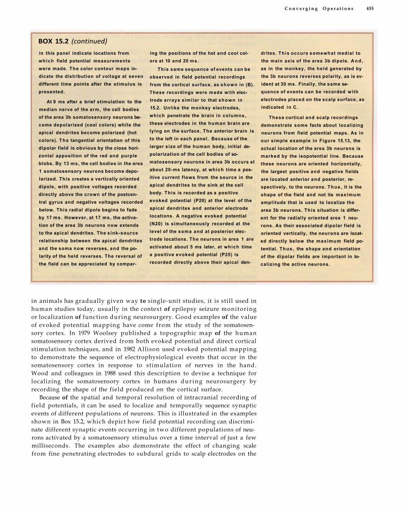
in animals has gradually given way to single-unit studies, it is still used in human studies today, usually in the context of epilepsy seizure monitor ing or localization of function during neurosurgery. Good examples of the value of evoked potential mapping have come from the study of the somatosensory cortex. In 1979 Woolsey published a topographic map of the human somatosensory cortex derived from both evoked potential and direct cortical stimulation techniques, and in 1982 Allison used evoked potential mapping to demonstrate the sequence of electrophysiological events that occur in the somatosensory cortex in response to stimulation of nerves in the hand. Wood and colleagues in 1988 used this description to devise a technique for localizing the somatosensory cortex in humans d u r i n g neurosurgery by recording the shape of the field produced on the cortical surface.
Because of the spatial and temporal resolution of intracranial recording of field potentials, it can be used to localize and temporally sequence synaptic events of different populations of neurons. This is illustrated in the examples shown in Box 15.2, which depict how field potential recording can discriminate different synaptic events occurring in two different populations of neurons activated by a somatosensory stimulus over a time interval of just a few milliseconds. The examples also demonstrate the effect of changing scale from fine penetrating electrodes to subdural grids to scalp electrodes on the
C o n v e r g i n g O p e r a t i o n s 455
BOX 15.2 (continued)
in this panel indicate locations from which field potential measurements were made. The color contour maps indicate the distribution of voltage at seven different time points after the stimulus is presented.
At 9 ms after a brief stimulation to the median nerve of the arm, the cell bodies of the area 3b somatosensory neurons become depolarized (cool colors) while the apical dendrites become polarized (hot colors). T h e tangential orientation of this dipolar field is obvious by the close horizontal apposition of the red and purple blobs. By 13 ms, the cell bodies in the area 1 somatosensory neurons become depolarized. This creates a vertically oriented dipole, with positive voltages recorded directly above the crown of the postcentral gyrus and negative voltages recorded below. This radial dipole begins to fade by 17 ms. However, at 17 ms, the activation of the area 3b neurons now extends to the apical dendrites. The sink-source relationship between the apical dendrites and the soma now reverses, and the polarity of the held reverses. The reversal of the field can be appreciated by compar
ing the positions of the hot and cool colors at 10 and 20 ms.
This same sequence of events can be observed in field potential recordings from the cortical surface, as shown in (B). These recordings were made with electrode arrays similar to that shown in 15.2. Unlike the monkey electrodes, which penetrate the brain in columns, these electrodes in the human brain are lying on the surface. The anterior brain is to the left in each panel. Because of the larger size of the human body, initial depolarization of the cell bodies of somatosensory neurons in area 3b occurs at about 20-ms latency, at which time a positive current flows from the source in the apical dendrites to the sink at the cell body. This is recorded as a positive evoked potential (P20) at the level of the apical dendrites and anterior electrode locations. A negative evoked potential (N20) is simultaneously recorded at the level of the soma and at posterior electrode locations. The neurons in area 1 are activated about 5 ms later, at which time a positive evoked potential (P25) is recorded directly above their apical den
drites. This occurs somewhat medial to the main axis of the area 3b dipole. A n d , as in the monkey, the held generated by the 3b neurons reverses polarity, as is evident at 30 ms. Finally, the same sequence of events can be recorded with electrodes placed on the scalp surface, as indicated in C .
These cortical and scalp recordings demonstrate some facts about localizing neurons from field potential maps. As in our simple example in Figure 15.13, the actual location of the area 3b neurons is marked by the isopotential line. Because these neurons are oriented horizontally, the largest positive and negative fields are located anterior and posterior, respectively, to the neurons. Thus , it is the shape of the field and not its maximum amplitude that is used to localize the area 3b neurons. This situation is different for the radially oriented area 1 neurons. As their associated dipolar field is oriented vertically, the neurons are located directly below the maximum field potential. Thus , the shape and orientation of the dipolar fields are important in localizing the active neurons.

recording of the field potentials generated by the same sequence of synaptic events.
Using the techniques developed in 1995 by All ison and Wood, Puce and colleagues compared evoked potential and fMRI techniques for localizing the hand region of the somatosensory cortex. The correspondence of localization by both techniques was quite good, suggesting that fMRI methods performed preoperatively may replace the necessity for cortical surface evoked potential studies performed intraoperatively. This conclusion was similar to that described earlier in the chapter for comparisons of direct cortical stimulation and fMRI . However, while useful for localization, the coarse temporal resolution of the fMRI data precluded distinction of separate populations of neurons w i t h i n the somatosensory cortex that had been previously identified using intracranial field potential recordings. Nor could fMRI provide information about the time course of synaptic events.
While the earliest field potential recordings using intracranial electrodes in humans investigated basic sensory processes, this technique has also been used to investigate human perception and cognition. When the eliciting event is considered to be a perceptual or cognitive event and not a simple sensory stimulus, the term event-related potential, or ERP, is often applied. Despite the change in terminology, ERP studies obey the same biophysical principles as other measurements of field potentials. As an example, in 1980 Halgren and colleagues studied ERPs recorded from multicontact depth electrodes in humans who were engaged in an oddball target detection task (see Figure 13.13). Because the ERPs recorded in the hippocampus exhibited sharp changes in amplitude and field polarity, the researchers concluded that the target events elicited activity in hippocampal neurons. Note that fMRI studies using this task have demonstrated that target detection evokes activity in a distributed set of brain regions, not just the hippocampus. While it is diff icult to investigate large-scale brain systems in a single intracranial ERP study, subsequent work by Halgren and others has measured the characteristics of activity of several other discrete regions activated by this prototypical executive function task.
Higher perceptual processes have been investigated by All ison and colleagues, who measured ERPs from intracranial electrodes w i t h the areas of the ventral occipitotemporal lobe associated w i t h complex vision. In their studies, patients are shown exemplars of many different stimulus categories, including letter strings, geometric shapes, cars, fruits and vegetables, and faces, and nonobject scrambled displays that matched the spatial frequency characteristics of other stimulus categories. Figure 15.13A and B demonstrate that faces, but not other stimulus categories, evoked focal ERPs from the surface of the fusiform gyrus. It is from this same region that direct cortical stimulation produced transient prosopagnosia and face hallucinations in some patients, as described earlier in this chapter. In 1997, Puce and colleagues compared the location of this face-specific region to that identified by fMRI . This study was conducted in t w o patients in w h o m both procedures were done, although not simultaneously. Good correspondence was obtained between the location of the face-specific ERPs and fMRI activation by faces. Some fMRI activity was found in other regions of the ventral extrastriate cortex where no electrodes had been located. Because of the limited temporal resolution of f M R I , the authors could not determine what sources of neuronal activity generated the BOLD response. This latter fact is of critical interest because localized neuronal activity can persist for hundreds of milliseconds after the first ERP changes are observed.
456 C h a p t e r F i f t e e n
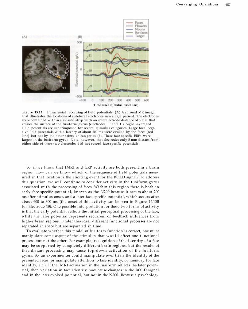
Figure 15.13 Intracranial recording of field potentials. (A) A coronal MR image that illustrates the locations of subdural electrodes in a single patient. The electrodes were contained wi th in a sylastic strip w i t h an interelectrode distance of 5 mm that crosses the surface of the fusiform gyrus (electrodes 10 and 11). Signal-averaged field potentials are superimposed for several stimulus categories. Large focal negative field potentials w i t h a latency of about 200 ms were evoked by the faces (red line) but not by the other stimulus categories (B). These face-specific ERPs were largest in the fusiform gyrus. Note, however, that electrodes only 5 mm distant from either side of these two electrodes d i d not record face-specific potentials.
So, if we know that fMRI and ERP activity are both present in a brain region, how can we know which of the sequence of field potentials measured in that location is the eliciting event for the BOLD signal? To address this question, we w i l l continue to consider activity in the fusiform gyrus associated w i t h the processing of faces. Within this region there is both an early face-specific potential, known as the N200 because it occurs about 200 ms after stimulus onset, and a later face-specific potential, which occurs after about 600 to 800 ms (the onset of this activity can be seen in Figure 15.13B for Electrode 10). One possible interpretation for these two forms of activity is that the early potential reflects the initial perceptual processing of the face, whi le the later potential represents recurrent or feedback influences from higher brain regions. Under this idea, different functional processes are not separated in space but are separated in time.
To evaluate whether this model of fusiform function is correct, one must manipulate some aspect of the stimulus that w o u l d affect one functional process but not the other. For example, recognition of the identity of a face may be supported by completely different brain regions, but the results of that distant processing may cause top-down activation of the fusiform gyrus. So, an experimenter could manipulate over trials the identity of the presented faces (or manipulate attention to face identity, or memory for face identity, etc.). If the fMRI activation in the fusiform reflects the later potential , then variation in face identity may cause changes in the BOLD signal and in the later evoked potential, but not in the N200. Because a psycholog
Converging Operations 457
Time since stimulus onset (ms)

458 Chapter Fifteen
BOX 15.3 Neuronal Activity and BOLD fMRI
Both single-unit f iring and field potentials provide direct, albeit different, measures of the informa
tional transactions of neurons. While we have emphasized so far in this chapter that these measures complement fMRI data, it is important to recognize that the direct relation between neuronal activity and the BOLD response remains unknown. Is there a strong correlation between BOLD fMRI measurements and these direct measures of neuronal activity? How might the integrative and signaling aspects of neuronal activity individually contribute to the BOLD signal? One might expect that both electrophysiological measures w o u l d have similar influences upon the BOLD response, since the EPSPs that trigger action potentials also generate field potentials. However, summated IPSPs generate field potentials as well , but inhibit the f ir ing of action potentials, so there are clear circumstances in which different electrophysiological measures could have different contributions. We w i l l thus consider separately single-unit (or m u l t i u n i t ) and field potential measures of neuronal activity.
Few studies have directly compared electrophysiological and BOLD fMRI measures. Most studies have compared data from different species. For example, in 2000 Rees and colleagues reported a positive correlation between BOLD fMRI activity in humans and single-unit activity in monkeys across parametric manipulations of perceived motion. However, in a landmark 2001 study, Logothetis and colleagues compared simultaneously recorded fMRI and electrophysiological measures in the primary visual cortex of the monkey. The monkeys viewed a rotating visual checkerboard parttern while being scanned in a 4.7-T scanner using gradient-echo echo-planar imaging. Single-unit, multiunit , and local field poten
tial recordings were obtained simultaneously with fMRI in 619 sessions performed with 10 monkeys. The results are shown in Figure 15.14. Single-unit activi
ty occurred transiently at the onset of the stimulus and did not persist over time, while the local field potentials showed both transient and persistent activity.
Figure 15.14 The relation between BOLD and neuronal activity. The time course of BOLD activation evoked by visual stimulation is shown as a solid green histogram, while the time course of multiunit activity (MUA) is shown in purple, the time course of single-unit activity (SUA) is shown in blue, and the time course of local field potentials (LFP) is shown in red. The onset and offset of the visual stimulus is shown as vertical gray bars and varies from 24 to 12 to 4 s in the top, middle, and bottom panels, respectively. Note that the BOLD activity and the local field potential activity are extended in time throughout stimulus presentation, while the single- and multiunit activity rapidly return to baseline. These results suggest that postsynaptic activity that generates local field potentials may be a primary contributor to the BOLD response. (From Logothetis et al., 2001.)
C o n v e r g i n g O p e r a t i o n s 459
ical construct may be associated w i t h some aspects of neural activity (e.g., BOLD signal change) but not others (e.g., N200), converging operations are critical. For example, a researcher w h o observes an fMRI response in the fusiform gyrus to judgments of face identity might infer that this response reflects neuronal activity at the time of the most prominent face-specific ERP, that is, at 200 ms. Thus, fMRI data, considered in isolation, may lead to the premature conclusion that judgments of face identity occur early in time w i t h i n the fusiform gyrus. Although hypothetical, this example reflects current debates concerning the sequence of events associated w i t h face processing in the brain, including the effects of directed attention, face memory, and emotional face expression. As great care must be taken in interpreting the timing of events when only fMRI evidence is available, intracranial electrode recordings can provide an important complementary source of information.
The local field potential activity better predicted the BOLD signal change than did the multiunit activity, although the latter still provided some predictive information. The authors concluded that the BOLD contrast mechanism reflects primarily the input and intracortical processing in a given area, that which we have characterized as the integrative aspect of neuronal processing, rather than its output reflected in action potential firing. Given this result, recall from Chapter 6 our discussion of Attwell and Laughlin's energy budget for the brain. On the basis of the large number of synapses per neuron in primates, they hypothesized that compared to lower animals, a greater proportion of the brain's energy budget would be required to restore postsynaptic concentration gradients. The results from the study of Logothetis and colleagues support this conjecture.
Support for the relation between field potential recordings and BOLD fMRI was obtained in a 2004 study of human subjects by Huettel and colleagues. As in the study by Logothetis and colleagues, the duration of a visual stimulus was manipulated and the time course of the BOLD signal was compared to the time courses of the Intracranially recorded field potentials.
Because of the logistical challenges involved with the study of human subjects, different subject groups participated in the electrophysiological and fMRI conditions. Field potentials were measured in a group of nine patients who had subdural grids and electrode strips implanted in the visual cortex as part of an evaluation for possible surgery to relieve seizure disorders. Because simultaneous measures were not obtained, the field potential responses were combined across electrodes in each of three anatomically defined regions of the visual cortex: the pericalcarine cortex (including V1), fusiform gyrus, and lateral temporal occipital cortex (likely including the motion-sensitive region MT/V5). A total of 74 electrodes were identified across these three regions. BOLD FMRI data from the same regions was recorded at 4 T from a sample of 12 neurologically normal young adult subjects.
The results from the pericalcarine region showed a strong relation between stimulus duration, the amplitude and duration of the field potentials, and the duration of the BOLD response. These data therefore confirm the results from this same region reported by Logothetis and colleagues. However, in other visual cortical regions, the relation between electrophysiological and BOLD meas
ures was less clear. In the lateral occipi¬totemporal cortex, neither the held potentials nor the BOLD response were systematically altered by stimulus duration. And in the fusiform gyrus, the BOLD fMRI response increased with increasing stimulus duration, as was found for the pericalcarine region, but the field potentials were unaffected by stimulus duration. Thus, for the fusiform, dissociation between BOLD and field potential measures was obtained. The reason for this dissociation is not known. One possibility is that the techniques measure different components of neuronal activity. The potentials measured in the fusiform gyrus may reflect more-distant current sources, or the BOLD changes in the fusiform may be distant from the precipitating neuronal events. If true, however, this possibility does not clarify the issue, as a robust BOLD response that varied with stimulus duration was measured in the fusiform. Another possibility is that another aspect of neuronal activity, such as the synchronicity across neurons within a region, plays a key role in the BOLD response. Future studies directly comparing fMRI and electrophysiological measures will be necessary to extend the results discussed in this section to additional brain regions, stimulus conditions, and subject populations.
BOX 15.3 (continued)
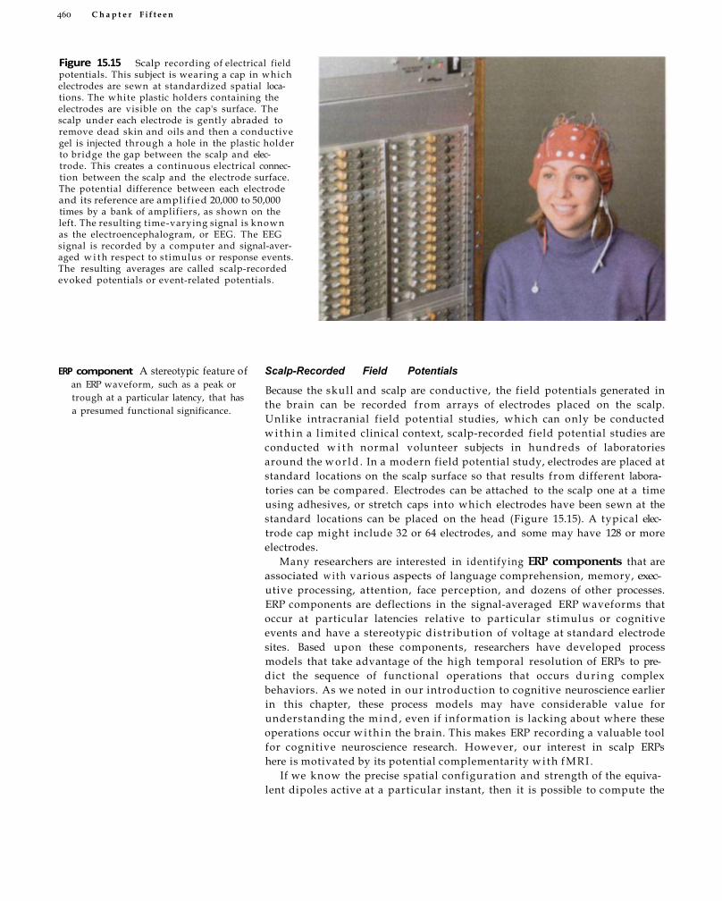
460 C h a p t e r F i f t e e n
Figure 15.15 Scalp recording of electrical field potentials. This subject is wearing a cap in which electrodes are sewn at standardized spatial locations. The white plastic holders containing the electrodes are visible on the cap's surface. The scalp under each electrode is gently abraded to remove dead skin and oils and then a conductive gel is injected through a hole in the plastic holder to bridge the gap between the scalp and electrode. This creates a continuous electrical connection between the scalp and the electrode surface. The potential difference between each electrode and its reference are amplif ied 20,000 to 50,000 times by a bank of amplifiers, as shown on the left. The resulting time-varying signal is known as the electroencephalogram, or EEG. The EEG signal is recorded by a computer and signal-averaged w i t h respect to stimulus or response events. The resulting averages are called scalp-recorded evoked potentials or event-related potentials.
ERP component A stereotypic feature of an ERP waveform, such as a peak or trough at a particular latency, that has a presumed functional significance.
Scalp-Recorded Field Potentials
Because the skull and scalp are conductive, the field potentials generated in the brain can be recorded from arrays of electrodes placed on the scalp. Unlike intracranial field potential studies, which can only be conducted w i t h i n a l imited clinical context, scalp-recorded field potential studies are conducted w i t h normal volunteer subjects in hundreds of laboratories around the w o r l d . In a modern field potential study, electrodes are placed at standard locations on the scalp surface so that results from different laboratories can be compared. Electrodes can be attached to the scalp one at a time using adhesives, or stretch caps into which electrodes have been sewn at the standard locations can be placed on the head (Figure 15.15). A typical electrode cap might include 32 or 64 electrodes, and some may have 128 or more electrodes.
Many researchers are interested in identifying ERP components that are associated w i t h various aspects of language comprehension, memory, executive processing, attention, face perception, and dozens of other processes. ERP components are deflections in the signal-averaged ERP waveforms that occur at particular latencies relative to particular stimulus or cognitive events and have a stereotypic distribution of voltage at standard electrode sites. Based upon these components, researchers have developed process models that take advantage of the high temporal resolution of ERPs to predict the sequence of functional operations that occurs dur ing complex behaviors. As we noted in our introduction to cognitive neuroscience earlier in this chapter, these process models may have considerable value for understanding the m i n d , even if information is lacking about where these operations occur w i t h i n the brain. This makes ERP recording a valuable tool for cognitive neuroscience research. However, our interest in scalp ERPs here is motivated by its potential complementarity wi th fMRI .
If we know the precise spatial configuration and strength of the equivalent dipoles active at a particular instant, then it is possible to compute the

C o n v e r g i n g O p e r a t i o n s 461
exact scalp distribution of potential that would result. This mathematically tractable process is k n o w n as the forward solution. Furthermore, we also established that the temporal sequence of neuronal events, even those separated by mere milliseconds, changes the scalp distr ibution of the electric fields in predictable ways. If fMRI can tell us the exact location of all brain regions activated by a stimulus, and if we know the orientation of the active neurons in those regions, and if we know the precise time course of activity in those regions, then we should be able to calculate the resulting scalp electric fields using forward solution techniques.
While this w o u l d be an impressive technical feat, its successful implementation depends upon us already knowing everything about the spa¬tiotemporal sequence of neuronal activity. What if you measured the electric field at the scalp? Could you then calculate the spatial configuration of neural generators and the temporal sequence of their activation? This reverse operation, computing the spatial configuration of dipoles f rom knowledge of the scalp distribution of voltage, is known as the inverse problem (see Figure 13.9). If the inverse problem could be solved, the need for localizing techniques like fMRI would be greatly reduced, as scalp-recorded ERP studies w o u l d provide complete information about both temporal and spatial properties of neuronal activity.
If we know for certain that only one dipole is active, we can solve for its location from an adequate sample of its potential distribution on the scalp. However, in the more likely event that many dipoles are simultaneously active, this approach w i l l not work , because different configurations of dipoles can create the same distribution of voltage at the scalp. Thus, the inverse problem has no unique solution. The inverse problem applies to all field potential recording, not just scalp ERPs. However, in intracranial recording we can move our electrode so close to the active neurons (i.e., in the near field) that the contribution from distant dipoles is negligible, so that it appears as though only one equivalent dipole is active. For scalp recording, all electrodes on the scalp are essentially in the far field of all dipoles in the brain. This problem is compounded by the presence of the skull , which has a much higher electrical resistance than the brain and which greatly reduces the spatial resolution of scalp-recorded ERPs. Despite the nonuniqueness of the inverse problem, many powerful techniques have been developed to approximate a solution by incorporating s impl i fying assumptions. Readers interested in additional details on this topic are directed to the paper by Bail-let and colleagues listed in the suggested readings.
What if, however, the spatial configuration of dipoles was known in advance? Under such conditions it w o u l d be possible to use the scalp ERP data to estimate the moment-by-moment changes in the strength of those dipoles and thus generate a time course of activity for each brain region. It has been asserted that fMRI activations may provide the locations of the dipole generators and thus that scalp-recorded ERPs can provide the information about their time course. In 1998, the val idity of this approach was tested by Liu and colleagues using Monte Carlo simulations. Their modeling attempted to account for two potential problems in combined fMRI and electrophysiological measurement: that some active neural generators would not be represented by an fMRI activation and that an fMRI activation might not be associated w i t h neural activity. The results of their simulations were encouraging, and the authors suggested that fMRI can be useful for seeding models of dipole structure.
forward solution The direct calculation of the electric and magnetic fields that would occur at an array of sensors based upon a given distribution of dipoles wi th known orientations and magnitudes.
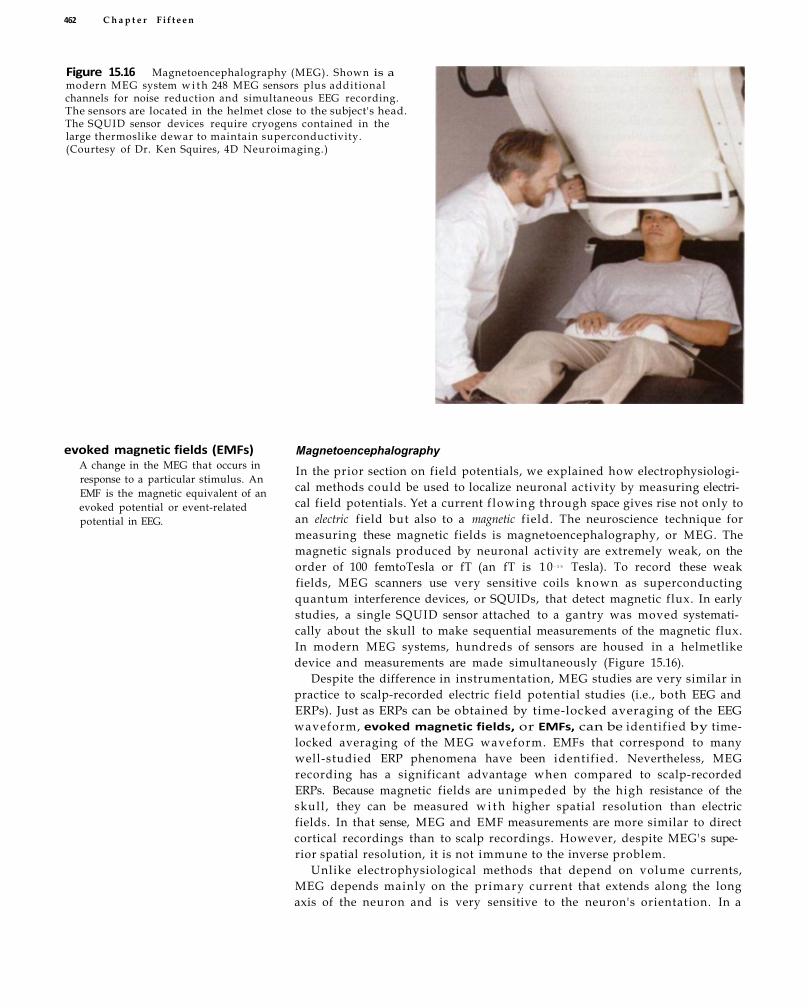
462 C h a p t e r F i f t e e n
Figure 15.16 Magnetoencephalography (MEG). Shown is a modern MEG system w i t h 248 MEG sensors plus additional channels for noise reduction and simultaneous EEG recording. The sensors are located in the helmet close to the subject's head. The SQUID sensor devices require cryogens contained in the large thermoslike dewar to maintain superconductivity. (Courtesy of Dr. Ken Squires, 4D Neuroimaging.)
evoked magnetic fields (EMFs) A change in the MEG that occurs in response to a particular stimulus. An EMF is the magnetic equivalent of an evoked potential or event-related potential in EEG.
Magnetoencephalography In the prior section on field potentials, we explained how electrophysiological methods could be used to localize neuronal activity by measuring electrical field potentials. Yet a current f lowing through space gives rise not only to an electric field but also to a magnetic f ield. The neuroscience technique for measuring these magnetic fields is magnetoencephalography, or MEG. The magnetic signals produced by neuronal activity are extremely weak, on the order of 100 femtoTesla or fT (an fT is 1 0 - 1 5 Tesla). To record these weak fields, MEG scanners use very sensitive coils known as superconducting quantum interference devices, or SQUIDs, that detect magnetic flux. In early studies, a single SQUID sensor attached to a gantry was moved systematically about the skull to make sequential measurements of the magnetic flux. In modern MEG systems, hundreds of sensors are housed in a helmetlike device and measurements are made simultaneously (Figure 15.16).
Despite the difference in instrumentation, MEG studies are very similar in practice to scalp-recorded electric field potential studies (i.e., both EEG and ERPs). Just as ERPs can be obtained by time-locked averaging of the EEG waveform, evoked magnetic fields, or EMFs, can be identified by time-locked averaging of the MEG waveform. EMFs that correspond to many well-studied ERP phenomena have been identif ied. Nevertheless, MEG recording has a significant advantage when compared to scalp-recorded ERPs. Because magnetic fields are unimpeded by the high resistance of the skull , they can be measured w i t h higher spatial resolution than electric fields. In that sense, MEG and EMF measurements are more similar to direct cortical recordings than to scalp recordings. However, despite MEG's superior spatial resolution, it is not immune to the inverse problem.
Unlike electrophysiological methods that depend on volume currents, MEG depends mainly on the primary current that extends along the long axis of the neuron and is very sensitive to the neuron's orientation. In a
spherical medium, l ike that approximated by the skull , the magnetic fields generated by a radially oriented dipole cannot be detected outside of the head. Thus, if the primary current does not have a component that is tangential to the surface of the skull , it cannot be detected by MEG. This can be both an advantage and a disadvantage. It is an advantage in that radially oriented neuronal populations can be ignored in modeling the generators of magnetic fields, and thus the models are simpler. It is a disadvantage in that MEG does not provide a complete description of neuronal activity. For this reason, MEG and EEG measurements are often obtained simultaneously.
Similar strategies have been advanced for combining EMF and fMRI studies as have been developed for combining ERP and fMRI . For example, Ahlfors and colleagues combined fMRI w i t h MEG in a study reported in 1999 that examined the neural response to a sudden change in perceived motion. They used fMRI to identify several motion-sensitive regions w i t h i n the visual cortex, including area MT+ (homologous to the motion-sensitive region V5 discussed earlier), as well as the primary (V1) and secondary (V2) visual cortices. The fMRI-derived location of the MT+ activation was very consistent w i t h a dipole model created to account for the peak in the EMF waveform in the time range of 130 to 170 ms. This same M T + region was also consistent w i t h EMF activity at about 260 ms. EMF responses from V1 and V2 were very small, and the dipole modeling for these regions peaked at about 200 to 260 ms. As these activations were longer in latency than the initial activity for area MT+, they may reflect feedback from other areas. This latter conclusion based upon the EMFs is important, because activity in V1 and V2 may be considered on the basis of fMRI alone to be early in the anatomical sequence of motion-processing areas.
The combined use of EMF or ERPs and fMRI is at a very early stage of development. Despite significant obstacles related to ambiguities in dipole modeling solutions, the addition of fMRI data to constrain the modeling of neural generators and to infer their time courses of activation holds much promise. The temporal ordering of neuronal activity in a widespread pattern of fMRI activations would be a tremendous leap forward in the development of network brain models of complex sensory, motor, and cognitive tasks.
Advice for the Beginning Researcher
We conclude by summarizing themes we have developed throughout this textbook. Although we offer them here as advice for the novice scientist, we believe their principles are important for all students and faculty, whether beginning researchers or experienced investigators.
From the many studies described in this book, it is clear that neuroimaging in general, and fMRI in particular, provides an extraordinarily powerful and flexible tool for answering questions about brain function. Technological developments w i l l continue to improve the spatial and temporal resolution of fMRI , further extending its interpretive reach. Yet, although the emphasis of this book has been upon a particular technique, we stress that science should be driven not by techniques but by questions. No method, regardless of its technical wizardry, is valuable unless it can answer interesting and important questions. Therefore, although scientists should master experimental techniques, just as a craftsman should become expert w i t h his or her tools, scientists should not become defined by the tools they use. A l l techniques have limitations, and the conscientious scientist should draw from mult iple techniques so that those limitations do not affect investigation of
C o n v e r g i n g O p e r a t i o n s 463

the dr iv ing research questions. For this reason, we advocate that researchers employ a mul t imodal , converging operations approach that combines different techniques.
Regardless of the technique, if there is one piece of advice that all scientists should heed, it is this: immerse yourself in your data. Understand the processes that generate your data, by examining both the technique and the experimental design. For f M R I , in particular, the processes that generate the data are not t r iv ia l to understand, and they require diligent work for their mastery. As a result, it is tempting to think that the physical and biophysical foundations of fMRI are hard but that the questions to be asked and the experimental designs needed to answer them are easy. We could not disagree more w i t h this perspective. The most diff icult part of any fMRI study is the design of an experiment that w i l l give you meaningful answers. Understanding how the data are generated is critical precisely because it facilitates effective experimental design. Even though tremendous advances in MR physics and engineering have made it very easy to acquire fMRI data, those advances should not be squandered on trivial questions or wasted on bad experimental designs. With this last point in m i n d , new researchers should remember that skepticism is a valued part of science, and it should be applied as liberally to one's o w n results as to others'. Do not bl indly trust canned analytical techniques, because all statistical approaches, like all research techniques, have strengths and weaknesses. Always evaluate whether your approach is the right one for your experimental question.
Finally, one trend more than any other defines modern research: the growth of interdisciplinary science. Like many fMRI researchers, we work regularly wi th psychologists, psychiatrists, physicists, radiologists, and neurobiologists, as well as scientists and clinicians from many other disciplines. Each of these fields has much to contribute to future fMRI research, and scientists should incorporate ideas f rom all of them into their research programs. As fMRI becomes more established and its physiological mechanisms become better validated, it w i l l become an increasingly important clinical tool. As many of the technical advances described in Chapter 14 become implemented, its applications in biomedical engineering w i l l become prevalent. And as its integration w i t h other neuroscientific approaches becomes increasingly feasible, cognitive neuroscientists w i l l answer an increasingly wide range of research questions. In wri t ing this textbook, we have been amazed by how far its concepts reach, frequently exclaiming to ourselves, "It 's all connected!" as we discover a new link to another discipline. In this textbook, we hope to have conveyed some of the excitement of these discoveries.
Summary
The field of cognitive neuroscience is presently in a data-driven phase where experimental observations are accruing at a rapid pace. In part, this reflects the vitality of a young field where only recently have powerful techniques—such as fMRI—that are appropriate to the nature of its questions become widely available. However, without the development of theoretical foundations that incorporate these observations and that could underlie future experiments, progress w i l l be slow. The development of these theoretical foundations w i l l require the reasoned integration of data from many methods, a process known as converging operations. Two classes of techniques are used by cognitive neuroscientists. The first class includes approaches that change neuronal activity, like direct cortical stimulation,
464 C h a p t e r F i f t e e n

TMS, genetics, and lesion studies. These techniques can inform inferences about the necessity of a brain region for a given cognitive process, providing important complementary evidence for fMRI studies. The second class of processes includes approaches that measure neuronal activity, notably electrophysiological studies of single-unit activity, local electrical field potentials, and local magnetic field changes. These approaches have superior temporal resolution compared to fMRI but have problems w i t h localization of neuronal generators. Combined fMRI and electrophysiological studies thus have promise for improving functional resolution, although many technical challenges remain. Researchers should adjust their experimental strategies, including techniques and experimental designs, based upon their experimental questions. This interdisciplinary approach is the future of cognitive neuroscience, and indeed of all of science.
Suggested Readings Allison, T, Wood, C. C., and McCarthy, G. (1986). The central nervous system. In
Psychophysiology: Systems, Processes ami Applications: A Handbook (E. Donchin, S. Porges, and M. Coles, eds.), p. 5-25. Guilford Press, New York. An introduction to the physiology of field potentials with a philosophical consideration of their use in localizing sensory, motor, and cognitive function.
*Baillet, S., Mosher, J. C, and Leahy, R. M. (2001). Electromagnetic brain mapping. IEEE Signal Processing Magazine, November, 14-30. A very accessible review of the use of mathematical techniques to localize neuronal generators of electrical and magnetic fields.
Brazier, M. A. B. (1988). A History of Neurophysiology in the 19th Century. Raven Press, New York. A fascinating history of the use and development of electrophysiological methods in neuroscience.
*Curtis, C. E., and D'Esposito, M. D. (2003). Persistent activity in the prefrontal cortex during working memory. Trends Cognitive Sci., 7(9): 415-423. A review of recent data concerning prefrontal activation in working memory tasks.
Hamalainen, M., Hari, R., Ilmoniemi, R., Knuutila, J., and Lounasmaa, O. (1993). Magnetoencephalography. Theory, instrumentation and applications to the noninvasive study of human brain function. Rev. Modern Phys., 65: 413-497. An excellent and comprehensive review of MEG, including neurophysiology, instrumentation, and modeling.
*Hariri, A. R., and Weinberger, D. R. (2003). Imaging genomics. Br. Med. Bull., 65: 259-270. A brief introduction to a newly emerging field that looks for structural and functional brain changes associated with genetic variation.
Logothetis, N. K. (2003). The underpinnings of the BOLD functional magnetic resonance imaging signal. J. Neurosci., 23(10): 3963-3971. A recent review of the relationship between neuronal activity and BOLD-contrast fMRI.
*Miller, E. K., and Cohen, J. D. (2001). An integrative theory of prefrontal cortex function. Annu. Rev. Neurosci., 24: 167-202. A review of prefrontal cortical function that emphasizes complementary results from single-unit neurophysiology in monkeys and fMRI in humans.
*Shallice, T. (1988). From Neuropsychology to Mental Structure. Cambridge University Press, Cambridge. A classic text that considers at length the interpretative issues associated with lesion studies in humans.
• Toga, A. W., Thompson, P. M., Mega, M. S., Narr, K. L., and Blanton, R. E. (2001). Probabilistic approaches for atlasing normal and disease-specific brain variability. Anat. Embryol., 204(4): 267-282. An interesting review of the use of probabilistic brain atlases to identify disease-related changes in brain morphometry.
"Indicates a reference that is a suggested reading in the field and is also cited in this chapter.
C o n v e r g i n g O p e r a t i o n s 465

Chapter References Ahlfors , S. P., Simpson, G. V., Dale, A. M, Belliveau, J. W., L i u , A. K., Korvenoja, A.,
Virtanen, J., Huoti lainen, M . , Tootell, R. B., Aronen, H. J., and I lmoniemi, R. J. (1999). Spatiotemporal activity of a cortical network for processing visual motion revealed by MEG and f M R I . J. Neurophysiol., 82(5): 2545-2555.
Al l ison, T. (1982). Scalp and cortical recordings of initial somatosensory cortex activity to median nerve stimulation in man. Ann. N.Y. Acad. Sci., 388: 671-678.
Al l ison, T., Puce, A. , Spencer, D. D., and McCarthy, G. (1999). Electrophysiological studies of human face perception. I: Potentials generated in occipitotemporal cortex by face and non-face s t imul i . Cereb. Cortex, 9(5): 415-430.
Belger, A., Puce, A. , Krystal, J. H . , Gore, J. C, Goldman-Rakic, P. S., and McCarthy, G. (1998). Dissociation of mnemonic and perceptual processes dur ing spatial and non-spatial working memory using f M R I . Hum. Brain Mapping, 6:14-32.
Berger, H. (1929). Uber das Elektroenkephalogram des Menschen. Arch. Psychiatr. Nervenkr., 87: 527-570.
Bohning, D. E., Pecheny, A. P., Epstein, C. M . , Speer, A. M . , Vincent, D. J., Dannels, W., and George, M. S. (1997). Mapping transcranial magnetic stimulation (TMS) fields in v ivo w i t h MRI . NeuroReport, 8(11): 2535-2538.
Bookheimer, S. Y, Strojwas, M. H . , Cohen, M. S., Saunders, A. M . , Pericak-Vance, M. A. , Mozziotta, J. C, and Small, G. W. (2000). Patterns of brain activation in people at risk for Alzheimer's disease. N. Engl. ]. Med., 343(7): 450-456.
Broca, P. (1861). Remarques sur le siege de la faculte du langage articule, suivies d'une observation d'aphemie (perte de la parole). Bulletins de la societe anatomique de Paris, annee 36, 2eme serie, tome 6: 330-357.
Caton, R. (1875). The electric currents of the brain. Br. Med. ]., 2: 278. Chafee, M . V , and Goldman-Rakic, P. S. (1998). Matching patterns of activity in pri
mate prefrontal area 8a and parietal area 7ip neurons dur ing a spatial w o r k i n g memory task. J. Neurophysiol., 79: 2919-2940.
Cohen, D. (1972). Magnetoencephalography: Evidence of magnetic fields produced by alpha rhythm currents. Science, 161: 664-666.
Courtney, S. M . , Ungerleider, L. G. , Keil , K., and Haxby, J. V. (1997). Transient and sustained activity in a distributed neural network for w o r k i n g memory. Nature, 386: 608-611.
Cramer, S. C, Nelles, G., Benson, R. R., Kaplan, J. D., Parker, R. A., Kwong, K. K., Kennedy, D. N . , Finklestein, S. P., and Rosen, B. R. (1997). A functional M R I study of subjects recovered from hemiparetic stroke. Stroke, 28: 2518-2527.
Cruetzfeldt, O. (1974). The neuronal generation of the EEG. In Handbook of Electroencephalography and Clinical Neurophysiology, Vol. 2, Part C (A. Remond, ed.). Elsevier, Amsterdam.
Dale, A. M . , L i u , A. K., Fischl, B. R., Buckner, R. L., Belliveau, J. W., Lewine, J. D., and Halgren, E. (2000). Dynamic statistical parametric mapping: Combining fMRI and MEG for high-resolution imaging of cortical activity. Neuron, 26(1): 55-67.
Di Russo, F, Martinez, A., and H i l l y a r d , S. A. (2003). Source analysis of event-related cortical activity dur ing visuo-spatial attention. Cereb. Cortex, 13(5): 486-499.
Du Bois-Reymond, E. (1848). Untersuchungen iiber thierische Elektricitat, Erster Band. Georg Reimer, Berlin.
Ferrier, D. (1876). The Functions of the Brain. Smith, Elder, London. Flourens, M.-J.-P. (1824). Recherches experimentales sur les proprietes et les fonctions du
systeme nerveux, dans les animaux vertebres. Crevot, Paris. Fritsch, G., and Hitz ig , E. (1870). Uber die elektrische Erregbarkeit des Grosshirns.
Archiv fiir Anatomie, Physiologie, und wissenschaftliche Medicin., 37: 300-332. Funahashi, S., Bruce, C. J., and Goldman-Rakic, P. S. (1989). Mnemonic coding of visu
al space in the monkey's dorsolateral prefrontal cortex. J. Neurophysiol., 61: 331-349.
466 C h a p t e r F i f t e e n
Gross, C. G., Rocha-Miranda, C. E., and Bender, D. B. (1972). Visual properties of neurons in inferotemporal cortex of the macaque. J. Neurophysiol., 35: 96-111.
Haaland, K. Y., Harrington, D. L., and Knight, R. T. (2000). Neural representations of skilled movement. Brain, 123: 2306-2313.
Halgren, E., Marinkovic, K., and Chauvel, P. (1998). Generators of the late cognitive potentials in auditory and visual oddball tasks. Electroenceplialogr. Clin. Neurophysiol., 106(2): 156-164.
Halgren, E., Squires, N. K., Wilson, C. L., Rohrbaugh, J. W., Babb, T. L., and Crandall, P. H. (1980). Endogenous potentials generated in the human hippocampal formation and amygdala by infrequent events. Science, 210(4471): 803-805.
Hariri, A. R., Mattay, V. S., Tessitore, A., Kolachana, B., Fera, F., Goldman, D., Egan, M. F, and Weinberger, D. R. (2002). Serotonin transporter genetic variation and the response of the human amygdala. Science, 297: 400-403.
Hubel, D. H., and Wiesel, T. N. (1959). Receptive fields of single neurons in the cat's striate cortex. J. Physiol, 148: 574-591.
Hubel, D. H. , and Wiesel, T. N. (1962). Receptive fields, binocular interaction and functional architecture in the cat's visual cortex. J. Physiol., 160: 106-154.
Huettel, S. A., McKeown, M. J., Song, A. W., Hart, S., Spencer, D. D., Allison, T., and McCarthy, G. (2004). Linking hemodynamic and electrophysiological measures of brain activity: Evidence from functional MRI and intracranial field potentials. Cereb. Cortex, 14: 165-173.
Keck, M. E., Welt, T., Muller, M. B., Erhardt, A., Ohl, F, Toschi, N., Holsboer, F, and Sillaber, I. (2002). Repetitive transcranial magnetic stimulation increases the release of dopamine in the mesolimbic and mesostriatal system. Neuropharmacology, 43(1): 101-109.
Kuffler, S. W. (1953). Discharge patterns and functional organization of mammalian retina. J. Neurophysiol., 16: 37-68.
Liu, A. K., Belliveau, J. W., and Dale, A. M. (1998). Spatiotemporal imaging of human brain activity using functional MRI constrained magnetoencephalography data: Monte Carlo simulations. Proc. Natl. Acad. Sci. U.S.A.. 95(15): 8945-8950.
Logothetis, N. K. (2002). The neural basis of the blood-oxygen-level-dependent functional magnetic resonance imaging signal. Philos. Trans. Royal Soc. London Series B Biol. Sci., 357(1424): 1003-1037.
Logothetis, N. K., Pauls, J., Augath, M., Trinath, T, and Oeltermann, A. (2001). Neurophysiological investigation of the basis of the fMRI signal. Nature. 412(6843): 128-130.
Luders, H., Lesser, R. P., Hahn, J., Dinner, D. S., Morris, H. , Resor, S., and Harrison, M. (1986). Basal temporal language area demonstrated by electrical stimulation. Neurology, 36(4): 505-510.
Marshall, W. H., Woolsey, C. N. , and Bard, P. (1937). Cortical representation of tactile sensibility as indicated by cortical potentials. Science, 85: 388-390.
Mottaghy, F. M., Gangitano, M., Krause, B. J., and Pascual-Leone, A. (2003). Chronometry of parietal and prefrontal activations in verbal working memory revealed by transcranial magnetic stimulation. Neurolmage, 18(3): 565-575.
Pascual-Leone, A., Valls-Sole, J., Brasil-Neto, J. P., Cohen, L. G., and Hallett, M. (1992). Seizure induction and transcranial magnetic stimulation. Lancet, 339(8799): 997.
Penfield, W. (1950). The Cerebral Cortex of Man: A Clinical Study of Localization of Function. Macmillan, New York.
Puce, A., Allison, T, and McCarthy, G. (1999). Electrophysiological studies of human face perception III. Effects of top-down processing on face-specific potentials. Cereb. Cortex, 9: 445-458.
Converging Operations 467

Puce, A., Allison, T., Spencer, S. S., Spencer, D. D., and McCarthy, G. (1997). A comparison of cortical activation evoked by faces measured by intracranial field potentials and functional MRI: Two case studies. Hum. Brain Mapping, 5: 298-305.
Puce, A., Constable, R. T., Luby, M. L., McCarthy, G., Nobre, A. C, Spencer, D. D., Gore, J. C., and Allison, T. (1995). Functional magnetic resonance imaging of sensory and motor cortex: Comparison with electrophysiological localization. J. Neurosurg., 83(2): 262-270.
Rees, G., Friston, K., and Koch, C. (2000). A direct quantitative relationship between the functional properties of human and macaque V5. Nat. Neurosci., 3: 716-723.
Rossini, P. M., Caltagirone, C, Castriota-Scanderbeg, A., Cicinelli, P., Del Gratta, C, Demartin, M., Pizzella, V., Traversa, R., and Romani, G. L. (1998). Hand motor cortical area reorganization in stroke: A study with fMRI, MEG and TCS maps. NeuroReport, 9(9): 2141-2146.
Rushworth, M. F, Hadland, K. A., Paus, T., and Sipila, P. K. (2002). Role of the human medial frontal cortex in task switching: A combined fMRI and TMS study. J. Neurophysiol., 87(5): 2577-2592.
Salzman, C. D., Britten, K. H. , and Newsome, W. T. (1990). Cortical microstimulation influences perceptual judgments of motion direction. Nature, 346(6280): 174-177.
Schlosser, M. J., Luby, M., Spencer, D. D., Awad, I. A., and McCarthy, G. (1999). Comparative localization of auditory comprehension using functional MRI and cortical stimulation. J. Neurosurg., 91: 626-635.
Schlosser, M. J., McCarthy, G., Fulbright, R. K., Awad, I. A., and Gore, J. C. (1997). Cerebral vascular malformations adjacent to sensorimotor and visual cortex: Functional magnetic resonance imaging studies before and after therapeutic intervention. Stroke, 28: 1130-1137.
Staudt, M., Lidzba, K., Grodd, W., Wildgruber, D., Erb, M., and Krageloh-Mann, I. (2002). Right-hemispheric organization of language following early left-sided brain lesions: Functional MRI topography. Neurolmage, 16(4): 954-967.
Talairach, J., and Tournoux, P. (1998). Co-planar Stereotaxic Atlas of the Human Brain. Thieme Medical Publishers Inc., New York.
Teuber, H. L. (1955). Physiological psychology. Annu. Rev. Psychol, 9: 267-296. Wernicke, K. (1874). Der aphasische Symptomencomplex. Eine psychologische Studie auf
anatomischer Basis. Breslau, Germany. Wood, C. C, Spencer, D. D., Allison, T., McCarthy, G., Williamson, P. D., and Goff,
W. R. (1988). Localization of human sensorimotor cortex during surgery by cortical surface recording of somatosensory evoked potentials. J. Neurosurg., 68(1): 99-111.
Woolsey, C. N., Erickson, T. C, and Gilson, W. E. (1979). Localization in somatic sensory and motor areas of human cerebral cortex as determined by direct recording of evoked potentials and electrical stimulation. J. Neurosurg., 51(4): 476-506.
468 C h a p t e r F i f t e e n

Glossary
Numbers in parentheses refer to the chapters in which the term is introduced.
action potential A wave of depolarization that travels down a neuronal axon. (6,15) adaptation A change in the response to a stimulus following its repeated presentation. (8) adenosine triphosphate (ATP) A nucleotide containing three phosphate groups that is the primary energy source for cells in the human body. (6) aerobic glycolysis The process, consisting of glycolysis, the TCA cycle, and the electron transport chain, that breaks down glucose in the presence of oxygen, resulting in a gain of 36 ATP. (6) aliasing The sampling of a signal at a rate insufficient to resolve the highest frequencies that are present. The energy at those frequencies becomes artifactually expressed at lower frequencies, distorting the measured signal. (9) alpha value An a priori probability (e.g., 0.001) chosen as the threshold for statistical significance. If the probability that the data would be obtained under the null hypothesis is less than the alpha value, the data are considered to be statistically significant. (12) alternating design A blocked design in which two conditions are presented one after another for the duration of the experimental run. (11) anaerobic glycolysis The conversion of glucose to lactate in the absence of oxygen. (6) anatomical ROI Region of interest that is chosen based on anatomical criteria. (12) angular momentum (J) A quantity given by multiplying the mass of a spinning body by its angular velocity. (3) anisotropic Having different properties in different directions; often referenced in the context of anisotropic diffusion, where molecules tend to diffuse along one axis but not others. (5,14) anode A source of positive charge or ions, and an attractor for free electrons. (15) antiparallel state The high-energy state in which an atomic spin precesses around an axis that is antiparallel (i.e., opposite) to that of the main magnetic field. (3)
apical dendrites The dendrites that are distant from the neuronal cell body. For typical pyramidal cells in the cortex, the apical dendrites extend to the superficial layers of cortex, while the cell bodies are located in deeper layers. (15) apparent diffusion coefficient (ADC) The quantification of diffusivity assuming isotropic diffusion. (5, 14) arachnoid The middle membrane covering the brain; its name comes from its weblike appearance. (6) arterial spin labeling (ASL) A family of perfusion imaging techniques that measure blood flow by labeling spins with excitation pulses and then waiting for the labeled spins to enter the imaging plane before data acquisition. (5) arteries Blood vessels that carry oxygenated blood from the heart to the rest of the body. (6) arterioles Small arteries. (6) ascending/descending slice acquisition The collection of data in consecutive order, so that slices are acquired from bottom to top or from top to bottom. (10) astrocyte A type of glial cell that regulates the extracellular environment. (6) autoradiography An invasive imaging technique that labels molecules using radioactive isotopes and then measures the concentration of those molecules by exposing slices of tissue to photographic emulsions. (7) averaged epoch The result of averaging a large number of epochs that are time-locked to similar events. (11) axial A horizontal view of the brain (along the x-y plane in MRI). (6) axon hillock A region of the cell body located at the emergence of the axon. Changes in its electrical potential lead to the generation of action potentials. (6) axon A neuronal process that transmits an electrical impulse from the cell body to the synapse, performing a primarily signaling function. (6)
b factor The degree of diffusion weighting applied within a pulse sequence. (5,14) B The sum of all magnetic fields experienced by a spin. (4)

470 G l o s s a r y
B0 The strong static magnetic field generated by an MRI scanner. (3) B1 The magnetic field caused by the application of an electromagnetic pulse during excitation. (3) B 1 e f f The effective magnetic field experienced by a spin system during excitation. (3) balloon model A model of the interaction between changes in blood volume and changes in blood flow associated with neuronal activity. (7) basal ganglia A set of nuclei in the forebrain that includes the caudate, putamen, and globus pallidus. (6) base image The image on which a statistical map is displayed, often a high-resolution anatomical image. (12) between-subjects A manipulation in which different conditions are assigned to different subject groups. (11) bias field estimation A technique for estimating inhomogeneities in the magnetic field based upon intensity variation in collected images. (10) binocular rivalry The alternation of images presented independently to each eye. (13) blindsight A phenomenon in which individuals with cortical damage have no experience of visual stimuli within the damaged part of the visual field, but can nevertheless report the characteristics of those stimuli under particular conditions. (13)
Bloch equation An equation that describes how the net magnetization of a spin system changes over time in the presence of a time-varying magnetic field. (3, 4) block A time interval that contains trials from one condition. (11) blocked design The separation of experimental conditions into distinct blocks, so that each condition is presented for an extended period of time. (8,11) blood-oxygenation-level dependent (BOLD) contrast The difference in signal on T2*-weighted images as a function of the amount of deoxygenated hemoglobin. (6, 7) bolus A quantity of a substance that is introduced into a system and then progresses through that system over time. (5,7)
Bonferroni correction A stringent correction for multiple comparisons in which the alpha value is decreased proportionally to the number of independent statistical tests. (12) brain stem The midbrain, pons, and medulla. (6) Brodmann areas Divisions of the brain based on the influential cytoarchitectonic criteria of Korbinian Brodmann. (6, 12)
capillaries Small and thin-walled blood vessels. The extraction of oxygen and glucose from the blood and the removal of waste carbon dioxide occur in the capillaries. (6)
capillary recruitment The idea that increased blood flow through the capillary bed results in perfusion of previously unperfused capillaries. (6) categorical variable A variable that can take one of several discrete values. (11) cathode An attractor for positive charge or ions, and a source of free electrons. (15)
caudal Toward the back of the brain. (6) central nervous system (CNS) The brain and spinal cord. (6)
central sulcus A deep fissure that separates the frontal and parietal lobes of the brain. (6) cerebellum A large cortical structure at the caudal base of the brain that plays an important role in motor function. (6) cerebrospinal fluid (CSF) A colorless liquid that surrounds the brain and spinal cord and fills the ventricles within the brain. (6)
cerebrum The two hemispheres forming the major part of the brain. (6) circle of Willis The interconnection between the basilar artery and the carotid arteries at the base of the cranial vault. (6)
clustering A data-driven technique that looks for clusters of voxels with similar time courses. (12) cluster-size thresholding The adoption of a minimum size, in voxels, for a cluster of active voxels to be labeled as significant. (12)
coactivation The simultaneous activity of two or more brain regions within a single experimental task. Coactivation of brain regions does not imply that the regions are functionally connected. (13)
collinear factors Model factors that are highly correlated with one another. The inclusion of collinear factors reduces the validity of general linear model analyses. (12) complex cell A neuron in the visual cortex with a larger receptive field than a simple cell and that responds to a stimulus with preferred orientation anywhere within its receptive field. (15)
concentration gradient A difference in the density of a substance across space. Substances diffuse along a concentration gradient from areas of high concentration to areas of low concentration. (6)
conditions (or levels) Different values of the independent variable(s). (11) confounding factor Any property that covaries with the independent variable within the conducted experiment but could be distinguished from the independent variable using a different experimental design. (11) conjugate mirroring A partial A:-space imaging technique in which data collected from one half of k-space is used to estimate data from the other half. (14) connectional fingerprint The pattern of anatomical connections to and from a given brain region. The term fingerprint conveys that connectivity patterns are unique to particular brain regions. (13) connectivity The form of the relations between different brain regions, including whether they are directly or indirectly connected, whether one region influences another, and whether feedback processes exist. (13) construct An abstract concept that explains behavior but which itself is not directly observable. Attention is an example of a psychological construct. (15) continuous ASL A type of perfusion imaging that uses a second transmitter coil to label spins within an upstream artery while collecting images. (5)

G l o s s a r y 471
continuous variable A variable that can take any value within a range. (11) contrast agent A substance injected into the body to increase image contrast. (7) contrast The intensity difference between different quantities being measured by an imaging system. It also can refer to the physical quantity being measured (e.g., T1 contrast). (1,9) contrast-to-noise ratio (CNR) The magnitude of the intensity difference between different quantities divided by the variability in their measurements. (1, 9) control block A time interval that contains trials of the control condition. (11) control condition A condition that provides a standard to which the experimental condition(s) can be compared. Also called the baseline condition or nontask condition. (11) converging operations The use of two or more techniques to provide complementary evidence used to test an experimental hypothesis or scientific theory. (15) coregistration The spatial alignment of two images or image volumes. (10) coronal A frontal view of the brain (along the x-z plane in MRI). (6) corpus callosum The large white-matter bundle that is the primary connection between the cerebral hemispheres. The anterior portion is known as the genu and the posterior portion is known as the splenium. (6)
correlation analysis A type of statistical test that evaluates the strength of the relation between two variables. For fMRI studies, correlation analyses typically evaluate the correspondence between a predicted hemodynamic response and the observed data. (12)
correlation coefficient (or r-value) A number between -1 and 1 that expresses the strength of the correlation between two variables. (12) cortex (neocortex) The thin wrapping of cell bodies around the outer surface of the brain. (6) cortical mapping The mapping of function to different areas of the cerebral cortex, in order to guide plans for clinical treatment. (12) cost function A quantity that determines the amount of residual error in a comparison. (10, 12) counterbalancing A process for removing confounding factors by ensuring that they have equal influence upon the different conditions of the independent variable, usually by matching values across conditions. (11) covariates Experimental factors that can take any of a continuous range of values. (12) cross product The vector product of two vectors, its direction is perpendicular to the plane defined by those vectors and its magnitude is given by multiplying their product times the sine of the angle between them. (3) cryogens Cooling agents used to reduce the temperature of the electromagnetic coils in an MRI scanner. (2) current dipole A positive and negative point charge separated by an infinitesimal distance. A current dipole is used as a simple and convenient model for the electromagnetic fields produced by an activated neuron. (15)
current sink An attractor of positive ions. A depolarized patch of neuronal membrane is a current sink because positively charged ions will flow toward it. (15) current source A source of positive ions. (15) cytoarchitecture The organization of the brain on the basis of cell structure. (6,10,12)
data-driven analyses Exploratory techniques that examine the intrinsic structure of the data. (12) dB/dt The change in magnetic field strength (dB) over time (dt). (2) deactivations Decreases in BOLD activity during task blocks compared to nontask blocks. (11) declarative memory Processes that support the conscious encoding and retrieval of information about facts and events. (13) degrees of freedom (df) The number of independent observations within a data set. For many statistical tests, there are n - 1 degrees of freedom associated with n data points. (12)
dendrite A neuronal process that receives signals from other cells, performing a primarily integrative function. (6) deoxygenated hemoglobin (dHb) Hemoglobin without attached oxygen; it is paramagnetic. (7) dependent variables (DVs) Quantities that are measured by the experimenter in order to evaluate the effects of the independent variables. (11) descriptive statistics Statistics that summarize the sample data but do not allow inferences about the larger population. (12) design matrix In fMRI implementations of the general linear model, the specification of how the model factors change over time. (12) detection Determination of whether or not activity within a given voxel changes in response to the experimental manipulation. (8, 9,11) detector coil An electromagnetic coil that measures energy emitted back to the environment after its initial absorption by the sample. (1) diamagnetic Having the property of a weak repulsion from a magnetic field. (7) diffusion tensor imaging (DTI) The collection of images that provide information about the magnitude and direction of molecular diffusion. It is often used to create maps of fractional anisotropy. (5,13,14) diffusion weighting The application of magnetic gradients to cause changes in the MR signal that are dependent upon the amplitude and/or direction of diffusion. (5, 8,14) diffusion The random motion of molecules through a medium over time. (5) direct cortical stimulation Applying small currents directly to brain tissue to excite or disrupt neural activity. Direct cortical stimulation is usually conducted in humans to localize critical brain regions in the context of neurosurgery. (15) disdaqs An abbreviation for "discarded data acquisitions"; it refers to images at the beginning of a functional run that are deleted without examination. This is done because MR signal is greatest in these first images, as the change in net

472 G l o s s a r y
magnetization following excitation has not yet reached a steady state. (8) distribution The pattern of variation of a variable under some conditions. For example, the normal distribution has a characteristic bell shape. (12) domain specificity The segregation of functional regions in the brain according to the type of information that they process. (13) dorsal Toward the top of the brain. (6) dot product The scalar product of two vectors, it is created by summing the products along each dimension. (3) double dissociation The demonstration that two experimental manipulations have different effects on two dependent variables. One manipulation affects the first variable but not the second, and the other manipulation affects the second but not the first. (13,15)
dura The outermost membrane covering the brain; its name comes from its thickness and toughness. (6) dynamic IVIM imaging A technique for generating images based on changes in IVIM. It can be used to generate images sensitive to hemodynamic changes within capillaries. (14)
easy problem A research question that can be addressed, in principle, using existing experimental methods. (13) echo-planar imaging (EPI) A technique that allows collection of an entire two-dimensional image by changing spatial gradients rapidly following a single electromagnetic pulse from a transmitter coil. (1, 5)
ecological validity The degree to which the processes studied in an experiment are similar to those produced in the natural environment. (13)
effect size The numerical difference between means divided by the standard deviation. (9) effective bore size The clearance within the bore of the MRI scanner that limits the maximum size of the sample that can be scanned. (14) electroencephalogram/electroencephalography (EEG) The measurement of the electrical potential of the brain, usually through electrodes placed on the surface of the scalp. (1,11, 15) electrogenesis The explanation for electrophysiological phenomena such as E E G or evoked potentials based upon ionic current flows instigated by synaptic activity. (15) electromotive force A difference in electrical potential that can be used to drive a current through a circuit. The MR signal is the electromotive force caused by the changing magnetic field across the detector coil. (3)
electron transport chain The third step in aerobic glycolysis; it generates an additional 34 ATP. (6) encoding The conversion of information, such as stimuli in the sensory environment, into a mental representation suitable for storage in long-term memory. (13) endogenous contrast Contrast that depends upon an intrinsic property of biological tissue. (5) epiphenomenal Being of secondary consequence to a causal chain of processes, but playing no causal role in the process of interest. (11)
episodic memory Processes that support the conscious encoding and retrieval of information about occurrences of particular events. (13) epoch A time segment extracted from a larger series of images, usually corresponding to the period in time surrounding an event of interest. (7,11) equipotentiality The concept that a function is so widely distributed within the brain that it depends upon the activity of the brain as a whole. Equipotentiality is the antithesis to localization of function. (15) equivalent dipole A simplifying model that represents the electromagnetic field produced by a population of neurons as though it were produced by a single dipole. (15) ERP component A stereotypic feature of an ERP waveform, such as a peak or trough at a particular latency, that has a presumed functional significance. (15) estimation Measurement of the pattern of change over time within an active voxel in response to the experimental manipulation. (8,9,11) Euler characteristic The number of clusters of significant activity due to chance that can be expected based upon the number of resels and the smoothness. (12) event A single instance of the experimental manipulation. Also known as a trial. (11) event-related design The presentation of discrete, short-duration events whose timing and order may be randomized. (8,11) event-related potentials (ERPs) Small electrical changes in the brain that are associated with sensory or cognitive events. (11,15) evoked magnetic fields (EMFs) A change in the M E G that occurs in response to a particular stimulus. An EMF is the magnetic equivalent of an evoked potential or event-related potential in E E G . (15)
evoked potential A field potential that occurs in response to a sensory stimulus. (15) excitation The process of sending electromagnetic energy to a sample at its resonant frequency (also called transmission). The application of an excitation pulse to a spin system causes some of the spins to change from a low-energy state to a high-energy state. (2, 3)
excitatory postsynaptic potential (EPSP) A depolarization of the postsynaptic cell membrane. (6,15) executive function The top-down control of cognition, based on goals and context. (13) exogenous contrast Contrast that requires the injection of a foreign substance into the body. (5) experiment The controlled test of a hypothesis. Experiments manipulate one or more independent variables, measure one or more dependent variables, and evaluate those measurements using tests of statistical significance. (11)
experimental condition A condition that contains the stimuli or task that is most relevant to the research hypothesis. Also called the task condition. (11) experimental design The organization of an experiment to allow effective testing of the research hypothesis. (11) experimental factors Model factors that are associated with specific experimental hypotheses. (12)

G l o s s a r y 473
far field The weak electric field distant from the current
sourcesink where small changes in distance result in very
small changes in field strength. (15)
field map An image of the intensity of the magnetic field
across space. (10)
field of view (FOV) The total extent of an image along a
spatial dimension. (4)
field potential Change in electrical potential over space
associated with postsynaptic neuronal activity. (15)
filling kspace The process of collecting samples from
throughout kspace in order to collect data sufficient for
image formation. (4)
filter Within the context of fMRI, an algorithm for removing
temporal or spatial frequency components of data. (10)
fixedeffects analysis Intersubject analysis that assumes
that the effect of the experimental manipulation is fixed
across subjects, with differences between subjects caused by
random noise. (12)
flat map An unfolded and flattened representation of the
cortical sheet to allow viewing of topographic changes over
cortical space. Flat maps are most commonly used in fMRI
to illustrate the organization of the visual cortex. (12)
flip angle The change in the precession angle of the net
magnetization following excitation. (3)
flux A measure of the strength of a magnetic field over an
area of space. (3)
fMRIadaptation (fMRIA) A reduction in the BOLD
response to the repeated presentation of a set of stimuli that
differ along some attribute, indicating that the brain region
being studied is insensitive (as measured by fMRI) to the
stimulus attribute being varied. (8)
forward solution The direct calculation of the electric and
magnetic fields that would occur at an array of sensors
based upon a given distribution of dipoles with known ori
entations and magnitudes. (15)
Fourier transform A mathematical technique for converting
a signal (i.e., changes in intensity over time) into its power
spectrum. (12)
fractional anisotropy (FA) The preference for molecules to
diffuse in an anisotropic manner. An FA value of 1 indicates
that diffusion occurs along a single preferred axis, while a
value of 0 indicates that diffusion is similar in all directions.
(5)
frequency domain The expression of a signal in terms of its
power at different frequencies. (12)
frequencyencoding gradient A gradient turned on during
the data acquisition period, so that the frequency of spin
precession changes over space.
frontal lobe The most anterior lobe of the cerebrum; it is
important for executive processing, motor control, memory,
and many other functions. (6)
functional connectivity map An image or diagram of the
pattern of connectivity between different regions of the
brain, independent of activity associated with experimental
tasks. (13)
functional contrast A type of contrast that provides infor
mation about a physiological correlate of brain function,
such as changes in blood oxygenation. (1)
functional magnetic resonance imaging (fMRI) A neu
roimaging technique that uses standard MRI scanners to
investigate changes in brain function over time. (1)
functional neuroimaging A class of research techniques
that create images of the functional organization of the
brain. Common functional neuroimaging techniques include
fMRI, PET, SPECT (singlephoton emission computerized
tomography), and optical imaging. (1)
functional resolution The ability to map measured physio
logical variation to underlying mental processes. (1)
functional ROI Region of interest that is chosen based on
functional criteria, such as the output of a voxelwise analy
sis. (12)
functional signaltonoise ratio (functional SNR) The ratio
between the intensity of a signal associated with changes in
brain function and the variability in the data due to all
sources of noise. Functional SNR is sometimes called
dynamic CNR or functional CNR. (9,10)
game theory A set of mathematical approaches for study
ing choices made by individuals in cooperative or competi
tive social situations. (13)
γaminobutyr ic acid (GABA) One of the most important
inhibitory neurotransmitters. (6)
Gaussian random fields A branch of mathematics that
deals with the properties of smooth, spatially extended data.
Application of random field theory to fMRI data can help
ameliorate the multiple comparisons problem. (12)
general linear model A class of statistical tests that assume
that the experimental data are composed of the linear com
bination of different model factors, along with uncorrelated
noise. (12)
glassbrain view A twodimensional projection of fMRI
data, as if the brain were made transparent and only the
activations were visible. (12)
glial cells (glia) Brain cells that support the activities of
neurons but are not primarily involved with information
transmission. (6)
glucose A sugar made by the human body whose stored
energy is used to form ATP. (6)
glutamate One of the most important excitatory neuro
transmitters. (6)
glycolysis The process of breaking down glucose into other
compounds to produce ATP. (6)
gradient coils Electromagnetic coils that create controlled
spatial variation in the strength of the magnetic field. (2)
gradientecho (GRE) imaging One of the two primary
types of pulse sequences used in MRI; it uses gradients to
generate the MR signal changes that are measured at data
acquisition. (5)
gyri Rises in the cortical surface. (6)
gyromagnetic ratio (7) The ratio between the charge and
mass of a spin. The gyromagnetic ratio is a constant for a
given type of nucleus. (3)
hard problem A research question that cannot be answered,
even in principle, by existing experimental methods and sci
entific principles. (13)
474 G l o s s a r y
hemifield One half of a visual display, usually referring to the left or right half. (8,13) hemodynamic response (HDR) The change in MR signal on T 2* images fo l lowing local neuronal activity. The hemodynamic response results from a decrease in the amount of deoxygenated hemoglobin present w i t h i n a voxel. hemodynamic Having to do with changes in blood flow or other blood properties. (6) heteroscedastic Having the property that the distributions of noise are different across experimental conditions. (12) higher cognition The set of processes that are considered to be more representative of the mental function of humans than of nonhuman animals. Examples include consciousness, executive function, abstract reasoning, and autobiographical memory. (13)
higher-order gradient A magnetic field gradient whose strength changes in a nonlinear fashion, such as in a quadratic manner, across space. (14) homogeneity Uniformity over space and time. In the context of MRI, a homogeneous magnetic field is one that has the same strength throughout a wide region near the center of the scanner bore. (2)
homoscedastic Having the property that the distributions of noise are similar for all experimental conditions. (12) homotopic The cortex in one cerebral hemisphere that corresponds to the same region in the other hemisphere. (15) hypothalamus A brain nucleus that supports homeostatic functions, including the regulation of food and water intake. (6) hypothesis-driven analyses The evaluation of activity based on testing of the validity of the null hypothesis. (12)
image reconstruction The process by which raw MR signal, as acquired in k-space form, is converted into spatially informative images. (4)
image A visual description of how one or more quantities vary over space. (1,4) imaging genomics A new field that investigates the effect of genetic variation upon brain structure and function. (15) imaging plane The plane in which changes in MR signal are recorded during perfusion imaging. (5) impulse A single input to a system. Impulses are assumed to be of infinitely short duration. (8,11) independent components analysis (ICA) An important class of data-driven analysis that identifies spatially stationary sets of voxels whose activity varies together over time and is maximally distinguishable from that of other sets. (12)
independent variables (IVs) Aspects of the experimental design that are intentionally manipulated by the experimenter and that are hypothesized to cause changes in the dependent variables, (11) indicators Experimental factors that have integral values to indicate a qualitative level. (12) inferential statistics Statistics that make inferences about the characteristics of a population based upon data obtained from a smaller sample. (12)
inflated brain A transformation of the cortical sheet into a balloonlike structure, removing gyral and sulcal folds so that activation can be more easily viewed. (12) inhibitory postsynaptic potential (IPSP) A hyperpolariza¬tion of the postsynaptic cell membrane. (6,15) initial dip The short-term decrease in MR signal immediately following the onset of neuronal activity, before the main positive component of the hemodynamic response. The initial dip may result from initial oxygen extraction before the later overcompensatory response. (7,14)
insula The "island" cortex hidden inside the anterior part of the Sylvian fissure; it is important for emotional processing and for the chemical senses. (6) integrative activity The collection of inputs from other neurons through dendritic or somatic connections. (6,15) interleaved slice acquisition The collection of data in an alternating order, so that data is first acquired from the odd-numbered slices and then from the even-numbered slices, to minimize the influence of excitation pulses upon adjacent slices. (4,10)
interleaved stimulus presentation The presentation of events of interest at different points within a TR over trials (e.g., one-quarter, one-half, and three-quarters of TR in addition to TR onset), increasing the effective sampling rate of an experiment at the expense of fewer trials per condition. (8, 14) interocular trauma test An intuitive test of significance based on highly visible effects of the experimental manipulation. It states that data are significant if, when plotted, they hit you between the eyes. (12) interstimulus interval (ISI) The separation in time between successive stimuli. Usually refers to the time between the offset of one stimulus and the onset of the next, with the term stimulus-onset asynchrony (SOA) used to define the time between successive onsets. (11)
intersubject variability Variability in fMRI data across a set of subjects; it includes the factors associated with intrasubject variability, along with between-subjects differences in task performance and physiology. (9) intrasubject variability Variability in the fMRI data from a single subject associated with thermal, system, and physiological noise, as well as with variability in the pattern of brain activity during task performance. (9) intravoxel incoherent motion (IVIM) The uncorrelated motion of spins within a voxel. (14) inverse problem The mathematical impossibility of determining the distribution of electrical sources within an object based upon the measurement of electrical or magnetic fields at the surface of the object. (1,13,15) inversion recovery A technique for increasing T1 contrast by adding a 180° inversion pulse before a standard pulse sequence.
ion channel A pore in the membrane of a cell that allows passage of particular ions under certain conditions. (6) ion A charged atom. (6,15)
ionizing radiation Electromagnetic radiation that has sufficient energy to separate electrons from electrically neutral atoms, turning them into ions. (7)

G l o s s a r y 475
isomorphic Having an identical form. A physiological
measurement that is isomorphic with a psychological con
struct would have the same sign and temporal dynamics as
the construct. (15)
isotropic Having similar properties in all directions. (5,14)
itemrelated processes Changes in the brain that are
assumed to be caused by the properties of individual stim
uli, or items. Itemrelated processes are more easily meas
ured with eventrelated designs. (11)
jittering Randomizing the intervals between successive
stimulus events over some range. (8,11)
keyhole imaging A partial kspace imaging technique in
which only the center of kspace is collected following each
excitation, in order to maximize raw SNR while minimizing
acquisition time. (14)
KolmogorovSmirnov (KS) test A test for statistical signif
icance that evaluates whether two samples are drawn from
the same distribution. The KS test is sensitive to differences
in variability and skew between distributions, but it is much
less sensitive to differences in mean than the ttest. (12)
kspace trajectory A path through kspace. Different pulse
sequences adopt different kspace trajectories. (4)
kspace A notation scheme used to describe MRI data. The
use of kspace provides mathematical and conceptual advan
tages for describing the acquired MR signal in image form.
(4)
labeling plane The plane in which initial excitation pulse(s)
are applied during perfusion imaging. (5)
laboratory frame The normal reference frame that is
aligned with the magnetic field of the scanner. (3)
largevessel effects Signal changes in veins that drain a
functionally active region but are distant from the neuronal
activity of interest. (8)
Larmor frequency The resonant frequency of a spin within
a magnetic field of a given strength. It defines the frequency
of electromagnetic radiation needed during excitation to
make spins change to a highenergy state, as well as the fre
quency emitted by spins when they return to the lowenergy
state. (3,4)
lateral Toward the edge of the brain. (6)
leastsquares error A commonly used cost function, the
sum of the squared residuals. (12)
linear gradient A magnetic field gradient whose strength
varies linearly across space. (14)
linear system A system that obeys the principles of scaling
and superposition. (8,11)
localization of function The idea that the brain may have
distinct regions that support particular mental processes. (1,
15)
longitudinal Parallel to the main magnetic field, or Zdirec¬
tion, of the scanner (i.e., into the bore). (3,4)
longitudinal relaxation (or spinlattice relaxation) The
recovery of the net magnetization along the longitudinal
direction as spins return to the parallel state. (3)
Lorentz effect imaging (LEI) A potential technique for
direct visualization of electrical activity (e.g., of neurons)
using MRI. (14)
Lorentz force The force on a moving charge within a mag
netic field. Lorentz forces cause spatial displacements in
conductors (e.g., wires, neuronal axons) if those conductors
are placed in MRI scanners. (14)
magnet diameter The diameter of the electromagnetic coil
that generates the strong static field used in MRI. (14)
magnetic field mapping The collection of explicit informa
tion about the strength of the magnetic field at different spa
tial locations. (10)
magnetic moment (μ) The torque (i.e., turning force) exert
ed on a magnet, moving electrical charge, or currentcarry
ing coil when it is placed in a magnetic field. (3)
magnetic resonance angiography (MRA) The creation of
images of the vascular system using MRI. (5)
magnetic resonance The absorption of energy from a mag
netic field that oscillates at a particular frequency. (1)
magnetic susceptibility The intensity of magnetization of a
substance when placed within a magnetic field. (7)
magnetoencephalogram/magnetoencephalography
(MEG) A noninvasive functional neuroimaging technique
that measures very small changes in magnetic fields caused
by the electrical activity of neurons, with potentially high
spatial and temporal resolution. (1,15)
matched filters The principle that the filter of the same fre
quency as the signal of interest provides maximal signalto
noise ratio. (10,14)
matrix A set of numbers arranged in a grid of rows and
columns. (3)
mean The average value of a set of observations. (9)
medial Toward the middle of the brain. (6)
medulla oblongata A continuation of the spinal cord at the
base of the brain that is important for the control of basic
physiological functions. (6)
metaanalysis The statistical analysis of data collected from
multiple experiments. (13)
microstimulation Applying currents through microelec
trodes to stimulate activity in a small number of neurons.
(15)
midbrain A section of the brain rostral to the pons; it
includes a number of important nuclei. (6)
mixed design A design that contains features of both
blocked and eventrelated approaches. (8,11)
mock scanner A simulated MRI scanner that does not have a
magnetic field present, used for training research participants.
Some mock scanners simulate scanner noises and measure
subject head movement. (10)
model factors A set of hypothesized changes in BOLD
activity associated with the manipulations of the independ
ent variables or with other known sources of variability. (12)
morphometric Relating to the measurement of shape. (14)
motion contrasts Contrast mechanisms that are sensitive to
the movement of spins through space (e.g., diffusion, perfu
sion). (5)
476 Glossary
MR signal equation A single equation that describes the obtained MR signal as a function of the properties of the object being imaged under a spatially varying magnetic field. (4) MR signal The current measured in a detector coil following excitation and reception. (2, 4) multiple comparison problem The increase in the number of false-positive results (i.e., Type I errors) with increasing number of statistical tests. It is of particular consequence for voxelwise fMRI analyses, which may have many thousands of statistical tests. (10,12)
multiple-channel imaging (or parallel imaging) The use of multiple receiver channels to acquire data following a single excitation pulse. (14) mutual information In the context of MRI, the amount of information about one image that is provided by knowledge of another image. For example, T, and T2 images have different contrast and thus are very different on measures of squared deviation. However, the intensity of a voxel in a T1
image can be predicted based on its intensity in a T2 image, so T1 and T2 images of the same brain would have high mutual information. (10)
myelin A fatty substance that forms sheaths surrounding axons that serve to speed the transmission of action potentials. (6)
near field The strong electric field that occurs near the current source—sink where small changes in distance result in large changes in field strength. (15) net magnetization (M) The sum of the magnetic moments of all spins within a spin system. (3) network A description of the relations of a set of brain regions, including their connectivity and causal relations. (13) neural correlates Patterns of brain activity that covary with another phenomenon, such as a mental state or behavior. (1, 13) neurological convention The practice of displaying images of the brain so that the left and right sides of the image correspond to the same sides of the brain, as if one were behind the subject. (12)
neuron A cell that is the basic information-processing unit of the nervous system. (6) neurotransmitters Chemicals released by presynaptic neurons that travel across the synaptic cleft to influence receptors on postsynaptic neurons. (6) noise Nonmeaningful changes in some quantity. There are many sources of noise in fMRI studies, and some changes may be classified as either noises or signals depending upon the goals of the study. (9)
nonlinearity The property whereby the combined response to two or more events is not equivalent to the summation of the responses to the individual events in isolation. (8) normalization The transformation of MRI data from an individual subject to match the spatial properties of a standardized image, such as an averaged brain derived from a sample of many individuals. (8,10) nuclear induction The initial term for nuclear magnetic resonance effects, as labeled by Bloch and colleagues. (1)
nuclear magnetic resonance (NMR) The measurable changes in magnetic properties of atomic nuclei induced by the application of an oscillating magnetic field at the resonant frequency of the nuclei. (1) nuisance factors Model factors that are associated with known sources of variability that are not related to the experimental hypotheses. (12) null hypothesis The proposition that the experimental manipulation will have no effect upon the experimental data. Most statistical analyses evaluate the probability that the null hypothesis is true, i.e., that the observed data reflect chance processes. (12)
null-task block A control block in which there are no task requirements for the subject. Also called a baseline block or nontask block. (11,13)
nutation The spiraling change in the precession angle of the net magnetization during an excitation pulse. (3) Nyquist frequency The highest frequency that can be identified in a digitally sampled signal; it is defined as one-half of the sampling rate. (10)
occipital lobe The most posterior lobe of the brain; it is primarily associated with visual processing. (6) ocular dominance The degree to which a given neuron in the visual cortex responds more to stimuli presented to one eye than to stimuli presented to the other eye. (8) off-resonance excitation The presentation of an excitation pulse at a frequency other than the resonant frequency of the sample, resulting in reduced efficiency. (3) oligodendrocyte A type of glial cell that constructs the myelin sheaths around axons. (6) on-resonance excitation The presentation of an excitation pulse at the resonant frequency of the sample, resulting in maximal efficiency. (3) oscillating magnetic field A magnetic field whose intensity changes over time. Most such fields used in MRI oscillate at the frequency range of radio waves (megahertz, or MHz) and as such they are often called radiofrequency fields. (1)
outer k-space (OK) imaging A partial k-space imaging technique in which only the periphery of k-space is collected following each excitation, in order to ensure that high-spatial-frequency components of the MR signal are present. (14) oxygen extraction fraction (OEF) The proportion of available oxygen that is removed from the blood. (11) oxygenated hemoglobin (Hb) Hemoglobin with attached oxygen; it is diamagnetic. (7)
parallel state The low-energy state in which an atomic spin processes around an axis that is parallel to that of the main magnetic field. (3) paramagnetic Having the property of being attracted to a magnetic field, though with less concentration of magnetic flux than ferromagnetic objects. (7) parameter weights For most fMRI analyses, quantities that reflect the relative contribution of the different model factors to the observed data within a given voxel. (12)

G l o s s a r y 477
parietal lobe The lobe on the posterior and dorsal surfaces of the cerebrum; it is important for spatial processing, cognitive processing, and many other functions. (6) partial k-space imaging A technique for reducing data acquisition time (and thus increasing temporal resolution) by collecting only part of the K-space data following each excitation and filling the uncollected portions of k-space with estimated data. (14) partial volume effects The combination, within a single voxel, of signal contributions from two or more distinct tissue types or functional regions. (8) peak The maximal amplitude of the hemodynamic response, occurring typically about 4 to 6 s following a short-duration event. (7) perfusion imaging A technique for measuring blood flow through capillaries using MRI. (14) perfusion Blood flow through capillaries. (5) periodic event-related design An experimental design in which events of interest occur at regular intervals. (11) phantom An object used for testing MR systems. Most phantoms are filled with liquids or gels with known properties, so that problems with the scanner system can be readily identified. (10) phase Accumulated change in angle. (4) phased array A method for arranging multiple surface detector coils to improve spatial coverage while maintaining high sensitivity. (2,14)
phase-encoding gradient A gradient turned on before the data acquisition period, so that spins can accumulate differential phase offset over space. (4) phrenologists Adherents to the belief that bumps and indentations on the skull provided information about the magnitude of some trait supported by the underlying brain region. (1)
physiological noise Fluctuations in MR signal intensity over space and time due to physiological activity of the human body. Sources of physiological noise include motion, respiration, cardiac activity, and metabolic reactions. (9) pia The innermost membrane covering the brain; it closely adheres to the brain's contours. (6) pixel A two-dimensional picture element. (1) plasticity The change in the normal functional properties of brain tissue following injury or experience. (15) polymorphism A common variation in a gene or segment of DNA. (15) pons Part of the brain stem; it serves as a relay system for motor and sensory nerves. (6) positron emission tomography (PET) A functional neuroimaging technique that creates images based upon the movement of injected radioactive material. (1, 7) power analysis A calculation that estimates the likelihood of detecting an effect of a given size based upon the parameters of the experimental design. (9) power spectrum A representation of the strength of different frequency components within a signal. The Fourier transform converts a signal (i.e., changes in intensity over time) into its power spectrum. (9)
power The probability of detecting an effect of the experimental manipulation. (9) precession The gyroscopic motion of a spinning object, in which the axis of spin itself rotates around a central axis, like a spinning top. (3) prefrontal cortex The parts of the frontal lobe anterior to regions that support motor processes. (13) preprocessing Computational procedures that are applied to fMRI data following image reconstruction but before statistical analysis. Preprocessing steps are intended to reduce variability in the data that is not associated with the experimental task and to prepare the data for statistical testing. (10) prestimulus baseline The calculation of a baseline value based on the BOLD signal present before events of interest. (11) primary current The current flow within a neuron caused by the inflow of ions through ionic channels opened by synaptic activity. (15) principle of reciprocity the rule stating that the quality of an electromagnetic coil for transmission is equivalent to its quality for reception (i.e., if it can generate a homogeneous magnetic field at excitation, it can also receive signals uniformly). (3)
projectile effect The movement of an untethered ferromagnetic object through the air toward the bore of the MRI scanner. (2) PSP Any postsynaptic potential, excitatory or inhibitory, that results from synaptic activity. (15) pulse sequence A series of changing magnetic held gradients and oscillating electromagnetic fields that allows the MRI scanner to create images sensitive to a particular physical property. (1,2) pulsed ASL A type of perfusion imaging that uses a single coil both to label spins in one plane and to record MR signal in another plane, separated by a brief delay period. (5) pump A transport system that moves ions across a cell membrane against their concentration gradient. (6,15)
quality assurance (QA) A set of procedures designed to identify problems with fMRI data so that they do not compromise experimental analyses. (10)
radiofrequency coils Electromagnetic coils used to generate and receive energy at the sample's resonant frequency, which for field strengths typical to MRI is in the radiofrequency range. (2) radiological convention The practice of displaying images of the brain so that the left side of the image is the right side of the brain and vice versa, as if one were facing the subject. (12) random-effects analysis Intersubject analysis that treats the effect of the experimental manipulation as variable across subjects, so that it could have a different effect upon different subjects. (12) randomization A process for removing confounding factors by ensuring that they vary randomly with respect to the independent variable. (11)

478 G l o s s a r y
raster A depiction of the firing rate of action potentials by a neuron in which time is represented along the horizontal axis and a dot indicates the occurrence of an action potential. (15) raw signal-to-noise ratio (raw SNR) The ratio between the MR signal intensity associated with a sample (e.g., the brain) and the thermal noise that is measured outside the sample. (9,10) reaction time The time required for someone to make a simple motor response to the presentation of a stimulus. Note that this is distinct from response time, which applies to situations in which someone must choose between two or more possible responses. (8, 9)
real-time analysis A set of computational steps designed for rapid analysis of fMRI data, so that statistical tests are conducted immediately following acquisition of the images. (12) reception The process of receiving electromagnetic energy emitted by a sample at its resonant frequency (also called detection). As spins return to a low-energy state following the cessation of the excitation pulse, they emit energy that can be measured by a receiver coil. (2, 3)
receptive field The part of the visual field that, when stimulated, will result in an increase in firing of a particular neuron. (15) recovery of function The improvement in a previously impaired ability over time, due to functional or structural changes within the brain. (15) reference volume A target image volume to which other image volumes are to be aligned. (10) refocusing pulse A 180° electromagnetic pulse that compensates for the gradual loss of phase coherence following initial excitation. (5) refractory effects Changes in the amplitude and timing of a response based on the characteristics of preceding responses. (8) refractory period A time period following the presentation of a stimulus during which subsequent stimuli evoke a reduced response. For BOLD fMRI, the refractory periods for many types of stimuli last approximately 6 s. (8) region-of-interest (ROI) analysis Evaluating statistical tests on a predetermined collection of voxels, often chosen to reflect a priori anatomical distinctions within the brain. (12)
registry A patient database. A registry might include information about the locations of brain lesions in a large population of individuals who might then be asked to participate in experimental studies. (15) relaxation A change in net magnetization over time. (3) rendered image A display of MRI data in three-dimensional perspective. (12) repetition time (TR) The time interval between successive excitation pulses, usually expressed in seconds. (5) repetitive TMS (rTMS) A series of closely spaced TMS stimulation pulses. (15) research hypothesis A proposition about the nature of the world that makes predictions about the results of an experiment. For a hypothesis to be well formed, it must be falsifiable. (11, 12)
residual The variability in the data that remains unexplained after accounting for the model factors. (12) resistance vessels Arterioles that control the flow of blood through the capillary bed. (6) resolution elements (or resels) The number of independent statistical tests within an fMRI volume. (12) resonant frequency The frequency of oscillation that provides maximum energy transfer to the system. (1) response time The time required for someone to execute a choice between two or more possible responses. Note that this is distinct from reaction time, which applies to situations when only one possible response is present. (9)
retinotopic mapping A technique for delineating functional regions within the visual cortex based upon their responses to stimuli presented at different retinal locations. (10,13) retrieval The accessing of information from long-term memory stores so that it can guide thought or behavior. (13) right-hand rule A heuristic that can be used to determine the direction of a magnetic moment generated by a moving charge or electrical current. If the fingers of the right hand are curled around the direction of spin, then the magnetic moment will be in the direction indicated by the thumb. (3)
rigid-body transformation A spatial transformation that does not change the size or shape of an object; it has three translational parameters and three rotational parameters. (10) rostral Toward the front of the brain. (6) rotating frame A reference frame that rotates at the Larmor frequency of the spin of interest. The rotating frame is adopted to simplify mathematical descriptions of the effects of excitation. (3)
rotation The turning of an object around an axis in space (in the absence of translation). (10) run An uninterrupted presentation of an experimental task, usually lasting 5 to 10 minutes for fMRI studies. It also refers to the set of functional images collected during that task presentation. (8)
sagittal A side view of the brain (along the y-z plane in MRI). (6) sample size The number of observations that are made by an experiment. For fMRI data, sample size can refer to the number of trials for a given subject or to the number of subjects within an experiment. (9)
sample (1) A set of observations drawn from a larger population of potential observations. (2) An object to be imaged using magnetic resonance. (12) sampling rate The frequency in time with which a measurement is made. (1) scalar A quantity that has magnitude but not direction. Scalars are italicized in this text. (3) scaling A principle of linear systems that states that the magnitude of the system output must be proportional to the system input. (8) scanner drift Slow changes in voxel intensity over time. (9, 11)

G l o s s a r y 479
semantic memory Processes that support the conscious encoding and retrieval of information about facts, independent of particular events. (13) semirandom design A type of event-related design in which the probability that an event will occur within a given time interval changes systematically over the course of the experiment. (11)
sequence effects Changes in behavior in response to a stimulus based on the context formed by preceding stimuli. (13) session A single visit to the scanner by a subject. For fMRI studies, each session usually includes both structural and functional scans. (8)
shimming coils Electromagnetic coils that compensate for inhomogeneities in the static magnetic field. (2,10) signal averaging The combination of data from multiple instances of the same manipulation in order to improve functional SNR. (9,11) signal Meaningful changes in some quantity. For fMRI, an important class of signals includes changes in intensity associated with the BOLD response across a series of T2* images. (9) signaling activity The transmission of the outcome of an integrative process from one neuron to another. (6,15) signal-to-noise ratio (SNR) The relative strength of a signal compared to other sources of variability in the data. (9) significance testing The process of evaluating whether the null hypothesis is true. Also known as hypothesis testing. (12) simple cell A neuron in the visual cortex that responds with increased firing to a stimulus with a preferred orientation in its receptive field and with decreased firing to a stimulus in the region surrounding its receptive field. (15) single dissociation The demonstration that an experimental manipulation has an effect upon one variable but not upon a second variable. (15) single-unit recording Collection of data about the electrophysiological activity (e.g., action potentials) of a single neuron. (15) sinuses Cavities. The term sinus has two primary meanings in neuroanatomy: (1) long venous channels formed by meningeal coverings that form the primary draining system for the brain, and (2) air-filled cavities in the skull. (6) slice selection The combined use of a spatial magnetic field gradient and an electromagnetic pulse to excite spins within a slice. (4)
slice A single slab of an imaging volume. A slice has thickness defined by the strength of the gradient and the bandwidth of the electromagnetic pulse used to select it. (4) smoothness The degree to which the time courses of nearby voxels are temporally correlated. (12) sodium-potassium pump A transport system that removes three sodium ions from within a cell while bringing two potassium ions into the cell. (6) soma The body of the cell; it contains cytoplasm, the cell nucleus, and organelles. (6) spatial extent The number of active voxels within a cluster of activity (i.e., the size of the active region). (9)
spatial frequency The frequency with which some pattern occurs over space. (4) spatial gradient (G) A magnetic field whose strength varies systematically over space. Note that since a given spatial location only experiences one magnetic field, which represents the sum of all fields present, spatial gradients in MRI act to change the effective strength of the main magnetic field over space. (1,4) spatial interpolation The estimation of the intensity of an image at a spatial location that was not originally sampled, using data from nearby locations. (10) spatial resolution The ability to distinguish changes in an image (or map) across different spatial locations. (1, 8) specific absorption rate (SAR) A quantity that describes how much electromagnetic energy is absorbed by the body over time. (2)
speed-accuracy trade-off The improvement in the speed of a response at the expense of accuracy, or vice versa, within an experimental task. (9) spin-echo (SE) imaging One of the two primary types of pulse sequences used in MRI; it uses a second 180° electromagnetic pulse to generate the MR signal changes that are measured at data acquisition. (5, 8)
spins Atomic nuclei that possess the NMR property; that is, they have both a magnetic moment and angular momentum. (3) spiral imaging A technique for fast image acquisition that uses sinusoidally changing gradients to trace a corkscrew trajectory through k-space. (5, 14) spiral-in trajectory A corkscrew path that begins at the periphery of k-space and ends at the center. Spiral-in imaging has the advantage that data acquisition can begin before time TE and thus the total time needed to collect an image is reduced. (14) spiral-out trajectory A corkscrew path that begins at the center of k-space and ends at the periphery. It is the most common form of spiral imaging. (14) standard error of the mean The uncertainty in the observed mean value, as calculated based upon both the standard deviation of the data and the number of data points. (9) state-related processes Changes in the brain that are assumed to reflect distinct modes, or states, of function. State-related processes are more easily measured with blocked designs. (11) static contrasts Contrast mechanisms that are sensitive to the type, number, and relaxation properties of spins (e.g., T1, T 2 , proton density). (5) static magnetic field The strong magnetic field at the center of the MRI scanner whose strength does not change over time. The strength of the static magnetic field is expressed in Tesla (T). (1)
statistical map (or statistical parameter map) In fMRI, the labeling of all voxels within the image according to the outcome of a statistical test. (12,13) stereotaxic space A precise mapping system (e.g., of the brain) using three-dimensional coordinates. (10) structural equation modeling (SEM) A mathematical technique for elucidating the causal relations between a set of
480 G l o s s a r y
variables. In fMRI studies, SEM can be used to create models of the connectivity between different brain areas. (13) subject A participant in a research study. (8) subthreshold stimuli Stimuli presented below the threshold for detection. In psychophysics, the threshold is also known as the limen, and thus subthreshold stimuli are also known as subliminal stimuli. (13)
subtraction In experimental design, the direct comparison of two conditions that are assumed to differ only in one property, the independent variable. (11,12) sulci Troughs in the cortical surface. (6)
superconducting electromagnets A set of wires made of metal alloys that have no resistance to electricity at very low temperatures. By cooling the electromagnet to near absolute zero, a strong magnetic field can be generated with minimal electrical power requirements. (2)
superposition A principle of linear systems that states that the total response to a set of inputs is equivalent to the summation of the independent responses to the inputs. (8,11) surface coil A radiofrequency coil that is placed on the surface of the head, very near to the location of interest. Surface coils have excellent sensitivity to signal from nearby regions but poor sensitivity to distant regions. (2)
surrogate marker A measurement that provides information about the clinical progression of a disease or condition. susceptibility artifacts Signal losses on T2*-dependent images due to magnetic field inhomogeneities in regions where air and tissue are adjacent. (5,14) susceptibility-weighted imaging (SWI) A class of techniques for creating images of the venous system based on microscopic susceptibility effects. (14) Sylvian fissure The deep sulcus separating the temporal lobe from the frontal and parietal lobes. (6) synapse A junction between neurons where the presynaptic process of an axon is apposed to the postsynaptic process of a dendrite or cell body. (6) synaptic cleft A gap between presynaptic and postsynaptic membranes. (6) system noise Fluctuations in MR signal intensity over space or time that are caused by imperfect functioning of the scanner hardware. (9)
T1 (recovery) The time constant that describes the recovery of the longitudinal component of net magnetization over time. (3)
T 1-weighted (T 1-dependent) Images that provide information about the relative T1 values of tissue; also known as T1
images. (5) T2 (decay) The time constant that describes the decay of the transverse component of net magnetization due to accumulated phase differences caused by spin-spin interactions. (3) T 2* (decay) The time constant that describes the decay of the transverse component of net magnetization due to both accumulated phase differences and local magnetic field inhomogeneities. T2* is always shorter than T 2 . BOLD-contrast fMRI relies on T2* contrast. (3)
T2* blurring Distortions in T 2* images that result from having a data acquisition window that is sufficiently long that significant T2* decay occurs over that interval. (8)
T 2*-weighted Images that provide information about the relative T2* values of tissue. T2*-weighted images are commonly used for BOLD-contrast fMRI. (5) T 2 -weighted (T 2-dependent) Images that provide information about the relative T2 values of tissue; also known simply as T2 images. (5) Talairach space The most commonly used space for normalization of fMRI data. (10) task frequency The rate of presentation of a periodic experimental task. (10) TCA cycle The second step in aerobic glycolysis; it involves the oxidation of pyruvate. (6) temporal interpolation The estimation of the value of a signal at a time point that was not originally collected, using data from nearby time points. (10) temporal lobe The lobe on the ventral surface of the cerebrum; it is important for auditory and visual processing, language, memory, and many other functions. (6)
temporal resolution The ability to distinguish changes in an image (or map) across time. (1, 8) tensor A collection of vector fields governed by three principal axes. (5) thalamus A brain nucleus that is important for many aspects of perception and cognition; it is highly interconnected with many regions of the cerebral cortex. (6) theory An organized set of ideas that guides thinking on a topic and that can be used to generate a variety of experimental hypotheses. (11) thermal noise Fluctuations in MR signal intensity over space or time that are caused by thermal motion of electrons within the sample or scanner hardware. (9) time course The change in MR signal over a series of fMRI images. (7) time domain The expression of a signal in terms of its intensity at different points in time. (12) time series A large number of fMRI images collected at different points in time. (8) time-locking Synchronization of analyses to events of interest, usually for the extraction of epochs. (11) time-of-flight (TOF) MRA A type of MR angiography that generates contrast by suppressing signal from spins within an imaging plane so that voxels with inflowing spins (i.e., those with blood vessels) have high signal. (5) torque A force that induces rotational motion. (3) torsion A rotation (twisting) of an object. Even if the motion of objects is restricted so that they cannot translate, a strong magnetic field will still exert a torque that may cause them to rotate so that they become aligned with the magnetic field. (2)
transcranial magnetic stimulation (TMS) A technique for temporarily stimulating a brain region to disrupt its function. TMS uses an electromagnetic coil placed close to the scalp; when current passes through the coil, it generates a magnetic field in the nearby brain tissue, producing localized electric currents. (1,13,15)

G l o s s a r y 481
translation The movement of an object along an axis in space (in the absence of rotation). (2, 10) translational medicine The practice of modifying clinical practice based on findings from basic science research and of modifying the direction of basic science research based on evidence from clinical studies. (13) transmitter coil An electromagnetic coil that generates an oscillating magnetic field at the resonant frequency of atomic nuclei wi th in a sample. (1)
transverse Perpendicular to the main magnetic field of the scanner, in the x-y plane. (3) transverse relaxation The loss of net magnetization w i t h i n the transverse plane due to the loss of phase coherence of spins. (3) trial sorting The post hoc assignment of events to conditions, often based on behavioral data. (11,13) trial A single instance of the experimental manipulation. (8) t-test A test for statistical significance based on the Student t-distribution. The t-test typically evaluates whether the mean values of two sets of observations are sufficiently different to preclude their being d r a w n from the same distribution. (12)
Type I error Rejecting the nul l hypothesis when it is in fact true. Also k n o w n as a false positive. (12) Type II error Accepting the nul l hypothesis when it is in fact false. Also known as an incorrect rejection or false negative. (12)
ultrahigh-resolution MRI The acquisition of MR images w i t h voxel sizes on the order of tens of micrometers. Applications of ultrahigh-resolution MRI to animal tissue are known as MR microscopy. (14)
undershoot The decrease in MR signal amplitude below baseline due to the combination of reduced blood f low and increased blood volume. (7)
variable A measured or manipulated quantity that varies wi th in an experiment. (11) vascular-space-occupancy (VASO) imaging A technique for estimating cerebral blood volume through n u l l i n g of intravascular signal and measurement of changes in parenchymal signal. (14)
vasoactive substances Substances that change the caliber of blood vessels. (6) vector A quantity w i t h both magnitude and direction. Vectors are boldface in this text. (3) veins Blood vessels that carry blood from the body to the heart. Blood in the veins (except for the pulmonary vein) is deoxygenated. (6) velocity-encoded phase contrast (VENC-PC) MRA A type of MR angiography that uses gradient fields to induce phase differences associated w i t h vascular flow so that the flow velocity of vessels can be measured. (5) venogram An image of the venous system. (14) ventral Toward the bottom of the brain. (6) ventricles Fluid-fil led cavities w i t h i n the brain. (6) venules Small veins. (6) virtual reality Computer simulations of real-world experiences, often presented using immersive visual displays and manipulated using specialized tools. (13) visual extinction The loss of experience of a visual stimulus due to simultaneous presentation of another stimulus in another part of the visual field. (13) volume coil A radiofrequency coil that surrounds the entire sample, w i t h roughly similar sensitivity throughout. (2) volume conductor A continuously conductive medium. The brain, meninges, skul l , and scalp constitute a volume conductor throughout which currents created by ionic flow can be measured. (15)
volume current The return current through the extracellular medium that balances the primary current within a neuron. (15) volume A single image of the brain, itself consisting of multiple slices and voxels. (8) volumetric Relating to the measurement of volume. (14) voxel A three-dimensional volume element. (1) voxelwise analysis The evaluation of statistical tests at the level of individual voxels. (8)
within-subjects A manipulation in which each subject participates in all experimental conditions. (11)

Illustration Credits
Chapter 1 1.8: © Nature Publishing Group, Nature Neuroscience, 1998.1.9: © Nature Publishing Group, Nature Neuroscience, 2003.1.12: © Nature Publishing Group, Nature, 1973.
Chapter 2 2.12A: © Wiley-Liss, Inc., 2000. Reprinted by permission of Wi ley-Liss, Inc., a subsidiary of John Wiley & Sons, Inc. 2.12B: © American Roentgen Ray Society, 2001. Reprinted with permission from the American journal of Roentgenology.
Chapter 6 6.8, 6.9, 6.12, 6.13: © Reprinted from Brain Research Bulletin with permission from Elsevier, 1981. 6.17,6.18: © Nature Publishing Group, Nature Neuroscience, 1998.
Chapter 7 7.9: © British journal of Radiology, 1977. 7.13: Reprinted with permission from Science, 1991. ©Amer ican Association for the Advancement of Sciences.
Chapter 8 8.4: © National Academy of Sciences, U.S.A., reprinted from Proceedings of the National Academy of Sciences, U.S.A., 2000. 8.7: © American Physiological Society, reprinted from journal of Neurophysiology, 1997. 8.20: © Wiley-Liss, Inc. Reprinted by permission of Wiley-Liss, Inc., a subsidiary of John Wiley & Sons, Inc., 1997.
Chapter 9 9.8: © Wiley-Liss, Inc. Reprinted by permission of Wiley-Liss, Inc., a subsidiary of John Wiley & Sons, Inc., 2001. 9.11: © Reprinted from Neurolmage, 2000, with permission from Elsevier.
Chapter 10 10.13: Results from the coregistration step of the analysis program S P M from the Wellcome Department of Imaging Neuroscience, University College, London. 10.18: © Wiley-Liss, Inc. Reprinted by permission of Wiley-Liss, Inc., a subsidiary of John Wiley & Sons, Inc.
Chapter 11 11.12,11.13: © Nature Publishing Group, reprinted from Nature Reviews Neuroscience, 2001.11.15: © National Academy of Sciences, U.S.A., reprinted from Proceedings of the National Academy of Science, U.S.A., 1996. 1 1 . 1 6 A - D : © American Physiological Society, reprinted from journal of Neurophysiology, 1997.11.17: © Wiley-Liss, Inc. Reprinted by permission of Wiley-Liss, Inc., a subsidiary of John Wiley & Sons, Inc. 11.18: © Wiley-Liss, Inc. Reprinted by permission of
Wiley-Liss, Inc., a subsidiary of John Wiley & Sons, Inc. 11.19, 11.22: © Reprinted from Neurolmage, 2001, with permission from Elsevier. 11.20: © Nature Publishing Group, reprinted from Nature Neuroscience, 2000.
Chapter 13 13.1D: © NeuroReport 1998.13.6: © John Wiley & Sons Limited. Reproduced from NMR in Biomedicine, 1997 with permission. 13.7: © Wiley-Liss, Inc., 2002. Reprinted by permission of Wiley-Liss, Inc., a subsidiary of John Wiley & Sons, Inc. 13.8: © Oxford University Press, 2002. By permission of Oxford University Press. 13.10: © Nature Publishing Group. Reprinted from Nature, 2002. 13.12: Reprinted with permission from Science. © American Association for the Advancement of Sciences, 1998.13.15: Reprinted with permission from Proceedings of the National Academy of Sciences, U.S.A. © National Academy of Sciences, U. S.A., 2002.13.16A: Reprinted from journal of Cognitive Neuroscience; © MIT Press Journals, 2000.13.16B: © 2002 Reprinted from Trends in Neurosciences with permission from Elsevier. 13.17: 1998© Reprinted from Neuron with permission from Elsevier. 13.19: Reprinted with permission from Science. © American Association for the Advancement of Sciences, 2002.13.20: © Reprinted from Neuron with permission from Elsevier. 13.21: © Society for Neuroscience, 1998. Reprinted from journal of Neuroscience.
Chapter 14 14.9: © Nature Publishing Group, 2000. Reprinted from Nature. 14.10,14.17,14.22: © Wiley-Liss Inc, 2000,1998, 2002. Reprinted by permission of Wiley-Liss, Inc., a subsidiary of John Wiley & Sons, Inc. 14.23: © National Academy of Sciences, U.S.A., 2000. Reprinted from Proceedings of the National Academy of Science, U.S.A.
Chapter 15 15.4, 15.15: © Oxford University Press, 2000, 1991. Reprinted from Brain, by permission of Oxford University Press. 15.5: © Lippincott & Williams, 1997. 15.10: © American Physiological Society, 1998. Reprinted from journal of Neurophysiology. 15.14: © Nature Publishing Group, 2001. Reprinted from Nature.

Index
A Acoustic noise, health risk of, 47-48 Action potentials, 133,444
measurement of, 447-48
neurotransmitters and, 131-33 Adaptation, use in experimental designs,
213-14
Addiction, changes in attention and, 375 Adenosine triphosphate (ATP)
in astrocyte-neuron lactate model, 167, 169
consumption by brain, 135
energy provided by, 134-36 in sodium-potassium pump, 131
Aerobic glycolysis, 134, 135 Aliasing, 229 Alpha value, 323
Alternating design. 294, 295, 296-97 Amygdala, 155
fMRI studies of, 13-14, 361-62, 392 Anaerobic glycolysis, 134-35 Analysis
data-driven, 344-45, 368
effects of on spatial resolution. 196 fixed-effects, 353-55
of fMRI experiments, 188
hypothesis-driven, 344 problems of, 217
random-effects, 353-55
region-of-interest (ROI) (See Region-of-interest (ROI) analysis)
regression, 249
voxelwise, 188 Anatomical region of interest (ROI), 350 Angiography
traditional contrast-agent, 110-11
See also Magnetic resonance angiography (MRA)
Angular momentum (J), 49
longitudinal component of, 58
and magnetic moment, 50 measurement of, 56
and spin, 56-57, 59, 60
in spinning proton, 50 Angular velocity, 61
Animal research, use of fMRI and, 361, 362, 386-89
Anisotropic diffusion, 115, 116, 414 Anisotropy, fractional, 116 Anode, 433
Anterior commissure, 150, 155 Antiparallel state, 57
effect of excitation on, 54
effect of temperature on, 52
energy difference in, 58, 59 probability of nucleus being in, 62
proportion of spins in, 62 of protons, 52
relaxation and, 71
and Zeeman effect, 53 Anxiety, as health risk, 47 Apparent diffusion coefficient (ADC) , 115,
408-9, 412-14, 415 Arachnoid, 149
Arterial spin labeling (ASL), 117
continuous, 117-18
pulsed, 118-20 Arteries, 139
basilar, 139, 140, 141
carotid, 117-18
cerebral, 140-41 conducting, 142
distributing, 142
internal carotid, 139, 140, 141
vertebral, 139, 140, 141 Arterioles, 139
change in diameter following sensory stimulation, 145, 146
intracortical, 142, 143 Artifacts, 254, 255
in echo-planar imaging (EPI), 121, 122
See also Susceptibility artifacts Ascending/descending slice acquisition, 257 Astrocyte, 149, 166-67 Astrocyte-neuron lactate shuttle model,
166-67, 169 ATP. See Adenosine triphosphate (ATP) Attention, as fMRI topic, 372-76
effects on primary visual cortex, 373 Attenuation effect, 115 Autoradiography, 162-63 Averaged epoch, 306 Axial, definition of, 155 Axon hillock, and action potentials, 131 Axons, 128, 129, 152
B B (total magnetic field), 76
magnitude of, 80
sum of B 0 and B1, 65 B0 (static magnetic field), 51
importance in generation of MR signal, 76
See also Static magnetic field B1 (radiofrequency field), 64
importance in generation of MR signal, 76
relation to gyromagnetic ratio, 67 within rotating frame, 65
B l e f f, 66
derivation of, 66
off-resonance excitation and, 68 ΔB0' 94
See also Inhomogeneities Band-stop filter, 276 Basal ganglia, 151, 155 Base image, 333
Baseline activity, for functional neuroimaging
studies, 301-3, 309 Basilar arteries, 139, 140, 141 Behavioral variability, 231-33 Berger, Hans, 368, 446 Between-subjects manipulation, 286 b factor, 115, 408-9, 412-14 Bias field correction, 268-69 Bias field estimation, 268-69 Binocular rivalry, 390-91 Bite bar, 261-62 Blindsight, 393 Bloch, Felix, 15-16, 27, 73, 75
experiments in magnetic resonance, 17 Bloch equation, 73,7 6
effects of diffusion on, 114
in perfusion MRI, 118
in transverse magnetization, 79 Block, 294
control, 296
effect on hemodynamic response, 298-300 null-task, 296, 368
Blocked design, 187, 199, 294
advantages and disadvantages of, 297-303, 317
basic principles of, 294 compared with event-related design,
304-5 creation of, 295-97
and executive function studies, 380-81 hemodynamic response and, 298-300 and refractory effects, 211-12 and slice-timing errors, 258

484 I n d e x
and Student's t-distribution, 324 trial sorting in, 314 and t-tests, 325-26
Blood flow effect of changes on B O L D contrast, 162,
180 effect of on capillaries, 146, 148 and glucose metabolism, 162-63 and increased neuronal activity, 143-49 neurogenic control of, 147-48 radius of vessel, relation to, 143 and sensory stimulation, 144 -46 velocity, 143
Blood-oxygenation-level dependent (BOLD) signal, 2
alternatives to, 410-14 amplitude of, 222 basis of, 128, 161 changes over time, 218 contrast in, 8, 128, 162 as dependent variable, 284 discovery of, 160-62 early studies, 174-76
compared to current practice, 176 effect of blood flow changes on, 162 epiphenomenal nature of, 288-89 evolution of, 171-74 example of experiment, 40-42 extravascular component of, 190-91, 193 generation of, 179 goal of, 127, 186 growth of, 171-76 history of, 11-21, 159-63 in vitro studies of, 161 increase in, 217
intravascular component of, 190-91, 193 key concepts, 6-11 measurement with fMRI, 12 mechanisms for, 161, 190 milestones in development of, 172 modeling changes in, 340-41 neuronal activity and, 458-59 and T2* contrast, 72 techniques for improving, 408-10 variation in, 189
BLOOD supply, to cerebrum, 138 Blood volume, effect of changes on B O L D
contrast, 180 Bohr relation, 58 B O L D contrast. See Blood-oxygenation-level
dependent (BOLD) signal BOLD fMRI. See Blood-oxygenation-level
dependent (BOLD) signal BOLD signal. See Blood-oxygenation-level
dependent (BOLD) signal Boltzmann's constant, 62 Bolus, 111, 177 Bonferroni correction, 346, 347 Bore size
effective, 402 limitations on, 35
Brain arterial and venous anatomy of, 139-42 atlases, 441-12 axial view of, 155 coronal view of, 155 cortex, 128, 151-56 cytoarchitecture of, 152, 274 energy needs of, 133-36 functional neuroimaging studies of, 3
glucose concentration in, 134 inflated, 335 left hemisphere of, 153 lesion studies (See Lesion studies) lobes of, 152-54 map of noise across, 226 membranes of, 149 microcirculation, 142 oxygen extraction fraction and, 301-2 regions, functional relations among,
364-72 sinuses of, 141-42 structural studies of, 3 riming of activity, 197, 200-2, 204-6 variable morphology of, 271, 272, 442 vascular system, 136-42 ventral surface of, 154 ventricles of, 149
Brain function and blood flow, 136-38 changes in blood oxygenation over time, 4,
9 Brain stem, 151, 154 Broca, Paul, 4 Broca's area, 154, 370 Brodmann, Korbinian, 350-51 Brodmann areas, 152, 351, 384, 385 Bulk magnetization, 53, 63
of individual voxel, 83 See also Net magnetization
c Calcarine sulcus, 153 Capillary, 139
effect of increased blood flow on, 146, 148 recruitment, 148 spatial properties of, 193
Carotid arteries, continuous arterial spin labeling (ASL) and, 117-18
Cathode, 433 Caton, Richard, 446 Caudal, definition of, 149 Caudate, 155 Causal factors, 288, 291 C B F (cerebral blood flow), 163, 180, 302 Cell
body, 128, 129, 152 complex, 447 simple, 447
Center of mass, calculation of, 255-56 Central nervous system, 149
components of, 150-51 Central sulcus, 153 Cerebellum, 150, 153, 154
fMRI activity in, 12-13 Cerebral blood flow (CBF), 163, 180, 302 Cerebral cortex, 151-56 Cerebral metabolic rate for glucose ( C M R g l u ) ,
163 and uncoupling of C M R O 2 , 165, 169
Cerebral metabolic rate for oxygen ( C M R 0 2 ) , 163, 302
and uncoupling of C M R g l u , 165, 169 Cerebrospinal fluid (CSF), 149
in proton density-weighted image, 103 suppression of, 106 in T,-weighted image, 105 in T 2-weighted image, 108
Cerebrum, 151 blood supply to, 138
Chain of causation, 288-89 Chalmers, David, 390 Charles Bonnet syndrome, 391 Cingulate gyrus, 150, 153, 155 Circle of Willis, 140 Circularly polarized magnetic field, 64 Classical mechanics, concepts of, 61, 72 Claustrophobia, health risk of, 47 Clustering, 344 -45 Cluster-size thresholding, 347-48
effect of on false-positive rate, 348 CMRglu (cerebral metabolic rate for glucose),
163 and uncoupling of CMR0 2 , 165 ,169
CMRO 2 , (cerebral metabolic rate for oxygen), 163, 302
and uncoupling of C M R g l u , 165, 169 Coactivation, of brain regions, 365-66, 367,
368 Cognition, as fMRI research topic, 363 Cognitive neuroscience, 429-31 Cognitive variability, 231-33 Coil
detector, 17 gradient, 34-35 radiofrequency (See Radiofrequency coil) receiver (See Receiver coil) shimming, 35-37, 266 surface, 31-33 transcranial magnetic stimulation, 436, 437 transmitter, 17, 31, 267 volume, 31-33, 267
Colliculi, 154 inferior, 150 superior, 150
Collinear factors, in experimental analyses, 339
Color map, 333, 339 Complex cell, 447 Compliance, role in minimizing head motion,
262 Computer hardware, 37 Computerized tomography (CT) imaging,
173-74 Computer software, 37, 338 Concentration gradient, 130 Condition, 284
control, 288, 290, 301 experimental, 288, 290, 301
Conducting arteries, 142 Confounding factors, 290
prevention of, 291-94 Conjugate mirroring, 417-18 Connectional fingerprint, 371 Connectivity
mapping, 368-71 use of diffusion tensor imaging (DTI) to
measure, 414-15 Consciousness, as fMRI topic, 389-93 Construct, psychological, 430, 432 Continuous arterial spin labeling (ASL),
117-18 pulse sequences in, 119
Contrast, 7, 101, 220 endogenous, 99, 111, 117
versus exogenous contrast, 178 exogenous, 99, 111, 117
limitations of, 178 use of in fMRI, 177-78
high and low, 7

I n d e x 485
motionweighted, 11020, 126
opacity as example of, 6 static, 99, 100110
between tissue types, 101
types of, 99 Contrast agents, 177 Contrasttonoise ratio (CNR), 7, 220, 222
dynamic, 220 Control blocks, 296 Control condition, 288, 290, 301 Converging operations, as research technique,
429
Coregistration, 263 functionalstructural, role in preprocess
ing, 26970, 271 Coronal, definition of, 155 Corpus callosum, 150, 153, 154, 155 Correlation analysis, 32829
and experimental hypothesis, 323 and general linear model, 338
Correlation coefficient (rvalue), 328 Cortex, 128
cerebral, 15156 layers of, 15152
prefrontal, 380, 382, 383, 388
See also Brain; Visual cortex Cortical mapping, use of fMRI for, 35455 Coryell, Charles, 159 Cost function, 26364, 266, 337 Counterbalancing, 291 Covariance, calculation of, 328 Covariates, in general linear model, 339 Cross product, of vectors, 55, 59, 60, 68 Cryogens, 30 CT scanning, 17374 Cuetarget paradigm, 31213, 37576 Current
dipole, 445
primary, 444
sink, 44446
source, 44446 , volume, 444
Cytoarchitecture, 152, 274, 351
D Damadian, Raymond, 1720, 173 Data acquisition, 18687
advanced techniques, 192 discarded (disdaqs), 187
effects of on spatial resolution, 196 Data analysis. See Analysis Data display, 33336
singleslice, 33334
threedimensional rendering, 333, 334 Datadriven analysis, 34445, 368 dB/dt(ΔB/Δt) ,45 ,417 Deactivations, 301 Declarative memory processes, 377 Degrees of freedom (df), 325 Dendrites, 128, 129,152
apical, 446 Dependent variable, 28485, 290, 29293 Depolarization, of neuronal membrane,
13133, 44446 Descriptive statistics, 321 Design
alternating, 294, 295, 29697 blocked (See Blocked design) eventrelated (See Eventrelated design) experimental (See Experimental design) mixed, 188, 31417
semirandom, 31011, 315, 317 Design matrix, 337
construction of, 33841
for general linear model, 33743 Detection, 188, 245, 297
power, differences in, 279 Detector coil, 17
SEE also Receiver coil Diagnostic fMRI, 35455 Diamagnetic, 159 Diencephalon, 151 Diffusion, 114, 414
anisotropic, 115, 116, 414
Bloch equation and, 114
isotropic, 115, 414 Diffusion tensor imaging (DTI), 116, 368, 372,
41415
Diffusionweighted contrast, 11317 dynamic, 412
pulse sequences for, 116 Diffusion weighting, 115, 193,4089
use to suppress intravascular largevessel signal, 193
Dipole current, 445
equivalent, 446 Direct cortical stimulation, 354, 43236
and fMRI studies, 43536
functional consequences of, 43436 Direct neuronal imaging, 42223 Discarded data acquisitions (disdaqs), 187 Display of data, 33336
singleslice, 33334
threedimensional rendering, 8, 333,334 Dissociation
double, 367, 439 single, 439
Distortion correction, role in preprocessing,
26769 Distributing arteries, 142 Distribution, 324 Domain specificity, 379 Dopamine, role in microcirculation, 14748 Dorsal, definition of, 149 Dot product, of vectors, 55 Double dissociation, 367, 439 Drift, 22728
Drug studies, limitations of, 5 Du BoisReymond, Emil, 443, 447 Dura, 149
Dynamic diffusionweighted contrast, 412 Dynamic intravoxel incoherent motion (IVIM)
imaging, 412
E Easy problems of consciousness, 390 Ebbinghaus, Hermann, 377 Echoplanar imaging (EPI), 19, 12023
artifacts in, 121, 122
early images, 172, 173 Echo time (TE), 101
in continuous ASL, 101
and physiological factors, 229 and transverse relaxation rate, 229
values for protondensity contrast, 101
values for T1 contrast, 104, 105
values for T2 contrast, 107 Ecological validity, 382 E E G . See Electroencephalography Effective bore size, 402 Effect size, 222, 248
Electrical dipole modeling, 373 Electrode, grid, 434
Electroencephalogram (EEG), 304, 446, 453, 460
Electroencephalography (EEG), 5, 127, 368, 416
Electrogenesis, 44446 Electromagnetic energy, frequency of, 59 Electromagnets
superconducting, 30
use in MRI scanners, 28 Electromotive force (emf), 69, 70 Electron transport chain, 134, 135 Electrophysiological studies
early, 44346
of eve preferences, 194
and fMRI, 19091, 304, 354, 373, 386, 45859
Emotional processing, fMRI studies and, 13 Encoding, role in memory, 377 Endogenous contrast, 99
with perfusion MRI, 11720
timeofflight (TOF) MRA, 11112 Energy budget of brain, 13536 Epiphenomena, 288 Episodic memory, 377 EP1STAR, 118, 11920
pulse sequences for, 119 Epoch, 180, 306
averaged, 306 Equipotentiality, concept of, 432 Equivalent dipole, 446 Errors, types, 323 Estimation, 188, 243, 297 Euler characteristic, 347 Eventrelated design, 187, 188, 199,21112,
303
advantages and disadvantages of, 31114, 317
compared to blocked design, 3045 early studies, 17476, 3047 and executive function studies, 380, 382 fast, 188
and memory studies, 37879 periodic, 309, 310 principles of, 30710 and refractory effects, 21112 schematic diagram of, 303 semirandom designs in, 31011 and slicetiming errors, 258 slow, 188
and ttests, 32627 Eventrelated potential (ERP), 304, 373, 446,
45657
components, 460 Events, 303
Evoked magnetic field, 46263 Evoked potentials, 45355 Excitation, 31, 54, 64
effect on energy state, 54
and required flip angle, 67
goal of, 68 influence on adjacent slices, 88 pulse, 64
radiofrequency coil and, 54 See also B 1 ; Offresonance excitation; On
resonance excitation Excitatory postsynaptic potential (EPSP), 131,
133, 444
Executive function, as fMRI topic, 380484 Exogenous contrast, 99

486 Index
with MRA, 111 with perfusion MRI, 117
use of in fMRI, 17778 Experiment, 283
characteristics of, 284
goal of, 188 Experimental condition, 288, 290 Experimental control system, components of,
3738
Experimental design, 18788, 189, 283, 297, 464
basic principles of, 28486, 297 example of, 29293 improvements in, 42125 improving functional signaltonoise ratio
(SNR) and, 23336 Experimental errors, types of, 323 Experimental factors, in general linear model,
339
Extravascular component, effect of field strength on, 23940
Extravascular spins, 19293
F FAIR, 118, 120
pulsed sequences for, 119 False discovery rate, 346 Faraday, Michael, 159 Faraday's law of induction, 69 Far field. 452
Fast eventrelated design, 188
Fast imaging sequences, 12024
Ferrier, David, 433, 438 Fiber tracking, 41415
Field maps, 26667
Field of view (FOV), 92, 185 independent in multiplechannel acquisi
tion, 402, 403
inverse relation in kspace with resolution, 93
overlapping in multiplechannel acquisition, 403, 404
Field potentials, 446, 45061
Intracranially recorded, 45359 localizing active neurons, 45152, 453
relation to fMRI studies, 451, 456, 45859
scalprecorded, 45455, 46062 Field strength, 30
and functional signaltonoise ratio, 23642
most common, 101
variations in, 123 Filling kspace, 90
in gradientecho sequence, 91 Filters, 274
as alternative to signal averaging, 249
bandstop, 276
Gaussian, 196, 276, 347
highpass, 276
lowpass, 276 matched, 276, 419
spatial, 27679, 419
temporal, 27576 Fixedeffects analysis, 35355 F L A S H (fast low [flip] angle shot) sequences,
172, 194 Flat map, 335 Flip angle, 67
repetition time (TR) and, 199 Flourens, Pierre, 43233
FMRI. See Functional magnetic resonance
imaging FMRIadaptation (fMRIA), 214 Forebrain, 151 Forward solution, 461 Fourier analysis, 32933
and experimental hypothesis, 324 Fourier transform, 84, 85, 89, 90, 121, 224, 275
2D, 83
2D inverse, 92 definition of, 32930 fast, 185
and general linear model, 338
and taskrelated variability, 33032 FOV. See Field of view Fractional anisotropy (FA), 116 Frequency domain, 330 Frequencyencoding gradient, 92 Frontal lobe, 150, 153, 154 Functional connectivity maps, 36871 Functional magnetic resonance imaging
(fMRI), 2
baseline conditions for, 3013
diagnostic, 35455 early studies, 17476
compared to current practice, 176, 399
evolution of, 17174 example of experiment, 4042
functional contrast and, 8
goal of, 127, 186
history of, 1121 key concepts of, 611
limitations of, 421
media coverage of, 364, 365 milestones in development of, 172
sample screening form, 40
terminology of, 18687 time scales of, 201
Functional neuroimaging studies, 2
alternatives to, 4
explosion of interest in, 4 Functional region of interest (ROI), 351 Functional relations, among brain regions,
36472
Functional resolution, 1011, 190 Functional signaltonoise ratio (SNR), 220,
222, 253
amplitude of BOLD signal and, 22223 and contrasttonoise ratio (CNR), 221 effect of field strength on, 238 effect of noise on, 223, 224 effect of on B O L D signal, 22122 effect of spatial filtering on, 27879 strategies for improving, 23349
Functionalstructural coregistration, role in preprocessing, 26970, 271
Fusiform gyrus, activity in, 214, 223, 43435, 45657
G G. See Spatial gradient y. See Gyromagnetic ratio G A B A (γaminobutyric acid), 131 Gadolinium diethylenetriaminepentaacetic
acid (GdDTPA), as contrast agent, 99, 17778
Gall, Franz Joseph, 1,433
phrenological mapping system of, 2 Game theory, 383484 Gauss, as unit, 2
Gaussian filter, 196, 276, 347
Gaussian random fields, 346
General linear model assumptions of, 340, 34243 basic principles of, 337 and correlation analysis, 338 design matrix of, 337, 33841, 34243 and experimental hypothesis, 324 and Fourier transform, 338
Genomics, imaging, 44243
Genu, 154
Geometric distortions, 95, 12122 Glassbrain view, 334, 335 Glial cells (glia), 129, 149 Glucose, 134, 135
consumption during oxidative metabolism, 163
metabolism
and blood flow, 16263 and oxygen metabolism, 16370
Glutamate, 131
in astrocyteneuron lactate model, 16667, 169
and energy budget of brain, 136 Glutamine, in astrocyteneuron lactate model,
167
Glycolysis, 134
aerobic, 13435 anaerobic, 13435
Golay pair, 3436 GoldmanRakic, Patricia, 448 Go/nogo task, 381 Gorter, Cornelis, 14 Gradient
coils, 3435, 36 constraints upon size of, 35
frequencyencoding, 92 higherorder, 407
linear, 4067
Kspace, relation to, 84
phaseencoding, 92
problems with, 9596 spatial (See Spatial gradient)
Gradientecho (GRE) imaging, 91, 1023
of deoxygenated hemoglobin, 161
for diffusionweighted images, 11617 of oxygenated hemoglobin, 161
for T2*weighted images, 110
for timeofflight magnetic resonance angiography (MRA), 112
twodimensional, 91 Gradient magnetic field, health effects of,
4546 Gray matter, 117, 149 Gyri , 151, 154
Gyromagnetic ratio (γ), 57, 59 illustration of, 67 relation to B1, 67 values of, 57
H Hard problems of consciousness, 390 Hardware
advances in, 172, 176, 416
computer, 37 H D R . See Hemodynamic response Head motion
correction of, 26366
and slicetiming correction, 258
effect on fMRI data, 25861

I n d e x 487
effect on t-tests, 326 prevention of, 261-63 rotational, 264 translational, 264
Head restraint systems, 261-62 Hearing loss, as health risk, 47 Helmholtz pair, 30, 36 Hemifield, 204, 374 Hemispheric encoding/retrieval asymmetry
(HERA) model, 379 Hemodynamic, definition of, 128 Hemodynamic hypotheses, 286-87 Hemodynamic response, 176
amplitude of, 201-2 components of, 176-81 design matrix and, 340-41 duration of, 202-4 effect of block interval on, 298-300 effect of signal averaging on, 244-45, 329 effect of slice acquisition time on, 257-58 effect of TR on, 197-200 latency of, 206 linearity of, 206-14 nonlinearity of, 211-13 peak of, 179 relation between timing and amplitude,
201-2 schematic representation of, 180 variability across subjects, 234-36
Hemoglobin deoxygenated, 8, 109, 110, 159
and B O L D contrast, 162 changes in following neuronal stimula
tion, 165-66 magnetic susceptibility of, 159, 161,
177, 192-93 molecular structure of, 159 oxygenated, 159
changes in following neuronal stimulation, 165-66
conversion to deoxygenated hemoglobin, 179
magnetic susceptibility of, 161 Heteroscedastic, property of data, 342 High-energy state, of protons. See Parallel
state Higher cognition, as fMRI research topic, 363 Higher-order gradient, 407 High-field scanning, 236-42, 405 High-pass filter, 276 Hindbrain, 150 Homogeneity, definition of, 29 Homogeneous magnetic field, 29-30,37 Homoscedastic, property of data, 342 Homotopic region, 435 Hubel, David, 447 Hydrogen nuclei
frequency of precession, 59 net magnetization, 64 spin, 49-50
Hypothalamus, 151 Hypothesis
null, 322,323,324 psychological, 287-88, 290, 293 research (See Research hypothesis)
Hypothesis-driven analyses. 344
I Image, 18, 75
distortion caused by gradient problems, 96
correction of, 270 formation
software, 37 three-dimensional (3-D), 93-94 two-dimensional (2-D), 92-93
stages in, 87 typical problems in, 94-95
reconstruction, 85 Image space, 92
relation to k-space, 83,85,86-87 Imaging genomics, 442—13 Imaging plane, in ASL, 118-20 Impulse, 208,307 Independent comparisons, formula for, 347 Independent components analysis (ICA), 344,
368,369 Independent variable, 284-85,290,292-93 Indicators, in general linear model, 339 Inductor-capacitor (LC) circuit, 31-32,33 Inferential statistics, 321 Inflated brain, 335 Inhibitory postsynaptic potential (IPSP), 131,
133,444 Inhomogeneities
correcting for, 266-69, 407 of dynamic magnetic field, 193 geometric distortions, 95,123 of static magnetic field, 94,95,108,109,
121-22 variations in signal intensity, 95 See also Susceptibility artifacts
Initial dip, 168-69,409-10 Insula, 152,154,155 Integrative activity, 129,133,444
and B O L D signal, 458-59 energy expenditure and, 135-136
Interleaved slice acquisition, 88,256-57 Interleaved stimulus presentation, 199,200,
421-24 Internal carotid arteries, 139,140,141 Interocular trauma test, 323,324 Interpolation
spatial, 265 temporal, 258
Interstimulus interval (ISI), 303,309,310 Intersubject analyses, 351-55 Intersubject variability, 234-36,341,345 Intracortical arterioles, 142,143 Intracranially recorded field potentials,
453-59 Intrasubject variability, 234-36 Intravascular component of B O L D signal,
effect of field strength on, 239-40 Intravascular spins, 193 Intravoxel incoherent motion (IVIM), 412 Inverse problem, 6,373,452,461 Inversion pulse, 106,412 Inversion recovery
advantages of, 106 T1 contrast and, 106
Ion, 130, 444 channels, 130-31 pumps, 130,444
Ionizing radiation, in PET imaging, 165 ISI. See Interstimulus interval Isomorphism, 430 Isopotential lines, 445-46 Isotropic diffusion, 115,414 Item-related processes, in mixed designs, 315
J J. See Angular momentum James, William, 137,138,372,375 Jittering, 205,309,310,421
K Keyhole imaging, 417,418 Kolmogorov-Smirnov (K-S) test, 327-28 Krebs cycle, 134,135 K-space, 83
basic sampling unit, 92 contributions of center and periphery, 86,
93 in echo-planar imaging, 120-21 filling, 90-92 and Fourier transform, 85,92 and gradient waveform, 84 outer imaging, 419 partial sampling of, 417-19 relation to image space, 83,85,86-87 and spatial resolution, 92,93 in spiral imaging, 123,124 in three-dimensional (3-D) imaging, 94 trajectory, 83
of echo-planar imaging (EPI) sequence, 121,419
errors in, 95, % of spiral imaging, 123-25,420,421
L Labeling plane, in pulsed A S L , 118-19 Laboratory frame, 64-65
changing magnetization in, 66 net magnetization in, 67 nutation in, 67
Lactate, in astrocyte-neuron lactate model, 167,169
Large-vessel effects, 191,408 comparison to small-vessel effects, 192
Larmor frequency, 59 for common MR scanners, 59 determination of, 76 precession of net magnetization at, 67 and slice selection, 88 and spin within magnetic fields, 61
Lateral, definition of, 149 Lateral ventricle, 155 Lauterbur, Paul, 18-19,27,75 LC circuit, 31-32,33 Least-squares error, 337 Lesion studies, 438-41
limitations of, 4-5 and timing of brain activity, 197 use with fMRI studies, 371,393,440-41 use with single-unit studies, 450
Linear gradient, 406-7 Linear model, equation for, 336
See also General linear model Linear system, 207,307
challenges to, 211-13 evidence of, 209-11,341 properties of, 207-9
Localization of function, 2,430,433 using field potential recordings, 454-55
Longitudinal component of angular momentum, 58 of magnetic moment, 58 of net magnetization, 53,76
change in, 100 Longitudinal magnetization, 77-79
change over time, 78,100 in early runs, 187

488 I n d e x
equation for, 100 incomplete recovery of, 101
in T,weighted images. 104,106, 107 Longitudinal relaxation, 71
effect of blood deoxygenation on, 160
illustration of, 71
and loss of MR signal, 70
T1 recovery and, 72 Lorentz effect imaging (LEI) , 42223 Uirentz forces, 47,422
Lowenergy state, of protons. See Parallel state Lowpass filter, 276
M M. See Net magnetization M x y , 7981
Bloch equation in, 79
See also Transverse magnetization Mz' 7779
change over time, 78
See also Longitudinal magnetization Magnet diameter, 4012 Magnetic field
circularly polarized, 64 evoked,46263
flux, 5051
gradient, 45—16
health effects of. 39,4246 mapping, 26667
shimming, 266
See also Static magnetic field Magnetic flux, 69,70 Magnetic moment (μ), 49,56
and angular momentum, 50 of bulk matter, 6263
determination of, 15
longitudinal, 58 measurement of, 56,57
property of atomic nuclei, 11
and spin, 50,56,59
and static magnetic field, 60 torque and, 56,58,59
Magnetic resonance, 14
cardinal principle of, 59 Magnetic resonance angiography (MRA),
11013
exogenous contrast. 111
sample image, 111
timeofflight, 11112
velocityencoded phase contrast (VENC¬PQ, 11213
Magnetic resonance imaging (MRI), 2
advantages of, 21,165
concept underlying image formation in, 75 first, 18
first of human extremity, 172 first of human torso, 20 goal of, 186
growth in use of, 2122
increased clinical demand for, 17374
perfusion, 11720
safety issues and, 39,4248 scanners (See Scanners)
theoretical foundation of, 73 Magnetic resonance (MR) microscopy, 4001 Magnetic resonance (MR) signal, 31,81
analysis of, 76412
creation of, 68,69
equation, 8182,82 2D form, 83 simplified, 82
using kspace coordinates, 83 importance of B0 and B1 in, 76 largevessel effects and, 192 measurement of, 31 noise in, 70 reception, 6970
in timeoffield angiography, 112
variations in intensity, 95 Magnetic susceptibility, 159,161 Magnetism, demonstration of, 50—51 Magnetization
bulk (Set Bulk magnetization)
longitudinal (See Longitudinal magnetization)
net (See Net magnetization) transverse (See Transverse magnetization)
Magnetoencephalography (MEG), 5,127,417,
446,46263 Magnetohydrodynamic forces, 43 Manipulation
betweensubjects, 286 withinsubjects, 286
Mansfield, Peter, 19,120,172 Maps
color, 333
field, 26667 flat, 335
functional connectivity, 36871 magnetic field, 26667
phrenological, 2
scalp voltage, 373 statistical, 322,33336,353,355
Matched filters, 276,419 Matrix, 55
size, 185,187 Maxwell pair, 34 Mean, definition of, 242 Mean intensity, calculation of, 25556 Mean transit time (mTT), in perfusion MRI,
117
Measurement of electrical changes, as nonimaging technique, 56
Medial, definition of, 149 Medulla oblongata, 150,153 MEG. See Magnetoencephalography Memory
as fMRI topic, 37779
singleunit studies of, 44849
types of processes, 377 Meninges, 149 Mesencephalon, 150,153 Metabolism, 13336 Metaanalysis, 384,385 Metencephalon, 150 Microcirculation
of brain, 142
role of dopamine in, 14748 Microscopy, magnetic resonance (MR),
400401 Microstimulation, 432,450 Midbrain, 150,153 Mixed design, 188,31417
design matrix for, 338 Mock scanner, in subject training, 26264 Model factors, in linear model, 336,339 Monkeys, use of fMRI and, 38689 Morphometric techniques, 401 Mosso, Angelo, 137 Motion
contrasts, 99,11020,126
effects on fMRI, 22829
See also Head motion Motionweighted contrasts, 11020,126 MRA. See Magnetic resonance angiography MRI. See Magnetic resonance imaging MR microscopy, 4001 Multiplechannel acquisition, 4025, 41617 Multiple comparison problem, 277, 34348,
351
effect of on falsepositive rate, 345 Mutual information, 266,270 Myelencephalon, 150,153 Myelin. 149
N nback task, 381
Near field, 452 Neocortex. See Cortex
Net magnetization (M), 50,62
in absence of magnetic field, 62 and Bloch Equation, 73
of bulk matter, 63
change in over time, 65 creation of MR signal, 68
determination of, 53,63
early within fMRI runs, 187 effect of orientation on MR signal, 71
effect of torque on, 65
and flip angle, 67 following an excitation pulse, 63
and functional signaltonoise ratio (SNR), 23637
of hydrogen, 64
in inversion recovery, 106
in laboratory frame, 67 longitudinal component of, 53,76 in rotating frame, 65,66
temperature and, 53,63
transverse component of, 53,72,76,77,100 vector, 77
Network, of brain activity, 366 Neural correlates, 12,390 Neuroanatomy, overview of, 14955 Neurological convention, in data display, 333 Neuron, 128,149
electrical activity of, 44445
energy needs of, 13336
ion channels in, 13031 membranes, 130
parts of, 129 Neuronal activity, 12830,287
and B O L D fMRI. 45859
direct imaging of, 42223
hemodynamic response and, 17678,424
manipulation of, 432—13 measurement of, 44363
timing of, 2002,2046 Neuronal hypotheses, 287 Neuronal membrane, depolarization of,
13133, 44446 Neuroscience
cognitive
assumptions of, 42931 research strategies, 43132
techniques, 10 Neurotransmitters
action potentials and, 13133
effects of drugs on, 5
glutamate, 131 Nitric oxide, in control of blood flow, 144, 145 NMR. See Nuclear magnetic resonance Noise, 219

I n d e x 489
acoustic, 47-48 effect on functional signal-to-noise ratio
(SNR), 223,224 in electroencephalogram (EEG), 453 health risk of acoustic, 47-48 map of across brain, 226 in MR signal, 70 physiological, 228-29,230,238 sources of, 224-33 system, 227-28 thermal, 225-27,238
Nonhuman primates, use of fMRI and, 386-89 Non-imaging techniques
drug manipulations, 5 lesion studies, 4-5 measurement of electrical changes, 5-6 spatial and temporal resolution of, 10
Nonlinearity of gradient fields, 95, 96 of hemodynamic response, 211-13
Normalization, 196, 269,431 algorithms, 273,274 role in preprocessing, 271-74,351-52
Nuclear induction, 17 Nuclear magnetic resonance (NMR)
as diagnostic tool, 20 first applications, 17 property, 50 spatial gradients and, 17 See also Magnetic resonance imaging
Nuclear spins. See Spins Nuisance factors, in experimental analyses,
339 Null hypothesis, 322,323
in blocked design, 324 Null-task blocks, 296, 368 Nutation, 67 Nyquist frequency, 9,275 Nyquist sampling theorem, 330
o Occipital lobe, 150,153,154 Ocular dominance, 194
columns, mapping of, 192,194-96 Oddball task, 381,456 Off-resonance excitation, 66
and Bleff, 68-69 in echo-planar imaging (EPI), 123 effects of, 68,88 rotational trajectory of, 68
Ogawa, Seiji, 160-62,171,174,239 Olfactory nerve, 154 Oligodendrocyte, 149 On-resonance excitation, 65-66
rotational trajectory of, 68 Optic chiasm, 154,360 Orbitofrontal cortex, fMRI activity in, 13-14 Orientation columns, 410 Oscillating magnetic fields, 14
generation by surface coil, 32 generation by volume coil, 32,64 inclusion in magnetic resonance experi
ments, 15 Outer k-space (OK) imaging, 419 Oxygen, consumption during oxidative
metabolism, 163 Oxygen extraction fraction (OEF), as baseline
for brain activity, 301-2 Oxygen metabolism, and glucose metabolism,
163-70 Oxygen-to-glucose index (OGI), 163
P Parallel imaging, 402-5,416-17 Parallel state, 57
effect of excitation on, 54 effect of temperature on, 52 energy difference in, 58, 59 probability of nucleus being in, 62 proportion of spins in, 53,62-63 of protons, 52 relaxation and, 71 Zeeman effect, 53
Paramagnetic, definition of, 159 Parameter weights, in linear model, 336 Parietal lobe, 150,153 Parietooccipital sulcus, 150 Partial k-space imaging, 417-19 Partial volume effects, 189,190,238 Patient registries, 439,440 Pauli, Wolfgang, 11 Pauling, Linus, 159
Peak, of hemodynamic response, 179,202 Penfield, Wilder, 433 Perfusion, 117 Perfusion MRI
endogenous contrast, 117-20 exogenous contrast, 117 uses of, 117
Perfusion-weighted contrast, 117-20 compared to B O L D contrast, 410-11
Periodic event-related design, 309,310 PET. See Positron emission tomography Phantom, use in quality assurance tests, 255,
256 Phase, definition of, 80 Phased array, 33,402-5 Phase-encoding gradient, 92 Phase spectrum, 331 Phrenology, 1-2,364 Physiological monitoring
equipment, 38-39 purpose in fMRI sessions, 39
Physiological noise, 228-29, 230, 238 in power spectrum, 225
Pia, 149 Pixel, definition of, 8 Planck's constant, 58 Plasticity, of human cortex, 440,441 Polhemus sensor, 262,263 Polymorphisms, 442 Pons, 150,153,154 Positron emission tomography (PET), 3,
164-65 compared to fMRI, 165 disadvantages of, 4,165 experiments to measure flow and metabo
lism, 163 as functional neuroimaging technique, 3,
295 scanner, 164 use with functional connectivity studies,
371 Postcentral gyrus, 153 Posterior commissure, 155 Postsynaptic membrane, 129 Postsynaptic potential (PSP), 131,450-52
excitatory, 131,133,444 inhibitory, 131,133,444
Power, of statistical test, 248 Power analysis, 248 Power spectrum, 224,275,330-32 Precentral gyrus, 153
Precession, 51-52,59-61 determination of direction, 60 excitation at frequency of, 64 frequency of, 61
Prefontal cortex, role in executive function, 380,382,383,388
Preprocessing, 253-80 framework for, 254 goals of, 253
Prestimulus baseline, 307 Presynaptic membrane, 129 Primary current, 444 Primary motor cortex, timing of activity in,
204-5 Primary visual cortex
effect of attention on, 373 timing of activity in, 204-5
Primates, nonhuman, use of fMRI and, 386-89 Principle of reciprocity, 70 Probabilistic brain atlases, 441-42 Probabilistic templates, 273 Projectile effect, 39 Proton
antiparallel state, 52 behavior in magnetic field, 52 charge of, 57 high-energy state, 52 low-energy state, 52 parallel state, 52 precession of, 51,52
Proton-density imaging, 101 primary requirements for, 103 pulse sequences for, 101,102,103 slice locations, 104 TR and TE values in, 101-2 use of smaller flip angle in, 102,103 uses of, 104
Psychological construct, 430,432 Psychological hypotheses, 287-88,290,293 Pulsed arterial spin labeling (ASL), 118-20
EPISTAR, 118,119-20 FAIR, 118,120 imaging plane in, 118 labeling plane in, 118
Pulse sequence, 2 basis for, 82-83 for continuous ASL, 119 for diffusion-weighted imaging, 116 for proton-density contrast, 101,102, 103 for pulsed ASL, 119 selection of parameters, 37,38 for time-of-flight MRA, 112 for T 1-weighted images, 105 for T 2-weighted images, 108 for T2*-weighted images, 110
Pumps ionic, 130,444 sodium-potassium (See Sodium-potas
sium pump) Purcell, Edward, 15-16,75
experiments in magnetic resonance, 16-17 Putamen, 155 Pyramidal cells, 149
Q Quality assurance tests, role in preprocessing,
254-56 Quantum mechanics, concepts of, 58,61,
70-71
R Rabi, Isidor, 14-15,27

490 I n d e x
Radiofrequency coils, 31 excitation and, 54 health effects of, 46 phased array, 33 principle of reciprocity and, 70 problems with, 228 reception period and, 54 sensitivity of, 33-34 surface coil, 31-33 transmission of excitation pulse, 64 volume coil, 31-33
Radiofrequency fields, health effects of, 46 Radiological convention, in data display, 333 Random-effects analysis, 353-55 Random field theory, 346-47 Randomization, 291,309,310 Raster, definition of, 448 Raw signal-to-noise ratio (SNR), 220,222, 255
calculation of, 255 effect of field strength on, 238 and spatial resolution, 237-38
Reaction time, 200,231 Real-time analysis, 355 Receiver coil, 31,267
changing flux and, 69 multiple, 33,402-5,416-17 problems with, 228 signal reception and, 69-70 See also Radiofrequency coils
Reception, 31,54,69-70 radiofrequency coil and, 54
Receptive field, 447 Reciprocity, principle of, 70 Recovery of function, studies of, 440 Rectangular slice selection pulse, 88,89 Reference volume, 263 Reflective processes, and experimental
design, 302 Refocusing pulse
phase coherence and, 109 in T1-weighted images, 105
Refractory effects, 207-12,286 differences across brain regions, 213 as indices of brain function, 213-14 in neuronal activity, 424
Refractory period, tests of, 211-13 Region-of-interest (ROI) analysis, 188,278,
296, 342,349-51 advantages and disadvantages of, 350-51 anatomical, 350 functional, 351 and multiple comparisons problem, 350 and spatial resolution, 196-97
Regression analysis, as alternative to signal averaging, 249
Relative cerebral blood flow (rCBF), in perfusion MRI, 117
Relative cerebral blood volume (rCBV), in perfusion MRI, 117
Relaxation, 70 concept of in early experiments, 16 importance of in MRI imaging, 73 and loss of MR signal, 70 See also Longitudinal relaxation;
Transverse relaxation Rendered image, 334 Repetition time (TR), 100
disadvantage of long, 102 temporal resolution and, 197-200 for time-of-flight magnetic resonance
angiography (MRA), 110
values for proton-density contrast, 101 values for T1 contrast, 104,105 values for T2 contrast, 107
Repetitive transcranial magnetic stimulation (rTMS), 436
Research popular impact of, 364 studies, 12-14 topic areas of, 362,372 translational, 359-62
Research hypothesis, 283,322,431 example of, 293 in functional connectivity studies, 370 levels of, 286-88 structure of, 286
Resels, formula for, 347 Residual, in linear model, 337 Resistance, 32,34
vessels, 143 Resolution
elements, formula for, 347 spatial (See Spatial resolution) temporal (Sec Temporal resolution)
Resonance, definition of, 64 Resonant frequency, 14,54
See also Larmor frequency Response time, 231
variability in, 233 Retinotopic mapping, 269,377 Retrieval, role in memory, 377, 379 Reward, study of brain systems and, 382-84 Right-hand rule, 49-50, 56 Rigid-body transformation, 263 ROI analysis. See Region-of-interest (ROI)
analysis Rostral, definition of, 149 Rotating frame, 64-65
changing magnetization in, 66 excitation pulse and, 65 net magnetization and, 65,66
Rotation, definition of, 263 Run, definition of, 186,187
s Safety, 39-48
screening form, 40 Sagittal, definition of, 150 Sample, 321
size, 243 Sampling rate, 9 SAR, 46,417 Saturation, 111-112,118 Scalar
definition of, 55 factor, 56,57 product, 55
Scaling, principle of, 208,209 Scalp-recorded field potentials, 454-55,
460-62 Scalp voltage map, 373 Scanner drift, 227,298
effect on t-tests, 326,327 Scanners
bore size, 35,402 closed-bore design, 28 computer hardware and software, 37,38,
172 early, 22,120,172 electromagnets and, 28 experimental control system, 37-38 gradient coils, 34-35
graphical user interface, 38 mock, 262-63 modem, 3, 28 open design, 28 radiofrequency coils, 31-34 safety issues, 39,42-48 schematic organization, 29 shimming coils, 34-35 static magnetic field, 2,27-31,51 ultrahigh-field, 410 vertical-bore design, 387,388
Screening form for fMRI, 40 Self-directed thought, 302 Semantic memory, 377 Semirandom design, 310-11,315,317 Sensory stimulation, and blood flow changes,
144-46 Sequence effects, 380,382 Session, 186,187
variability across, 234-36 Shimming coils, 35-37, 266 Signal
definition of, 219 generation, 55-73 reception, 69-70 (See also Magnetic resonance (MR) signal)
Signal averaging, 304 alternatives to, 249 and correlation analyses, 329 effect of number of trials on standard error
of mean, 243 effect on hemodynamic response, 244-45 and event-related design, 307 and field potentials, 453 fundamental rule of, 242-43 and improved functional signal-to-noise
ratio (SNR), 242-19 and predicted hemodynamic response, 329 similarity to spatial filtering, 279 summary of effects on fMRI data, 249
Signaling activity, 129,133,444 and BOLD signal, 458-59 energy expenditure and, 135,136
Signal-to-noise ratio (SNR), 70,86,93,165, 219,279
functional (See Functional signal-to-noise ratio)
raw (See Raw signal-to-noise ratio) Significance testing, 322 Simon task, 381 Simple cell, 447 Sinc interpolation, 265 Sinc-modulated electromagnetic pulse, 88,89 Single dissociation, 439 Single-unit recording, 446,447-50
and fMRI, 458-59 limitations of, 449-50 use with lesion studies, 450
Sinuses, of brain, 141-42 Slice, 82
acquisition ascending/descending, 257 effect on hemodynamic response,
257-58 interleaved, 88,256-57
composition of, 187 excitation, 87-89 location, 88,89,90 selection, 82-83,90
goal of, 87 gradient, 88

I n d e x 491
pulses rectangular, 88,89 sine-modulated electromagnetic,
88,89 thickness, 88,89,90,112,185-88
Slice-timing correction and head-motion correction, 258 role in preprocessing, 256-58
Slow event-related design, 188 Smoothing, 1%, 277-78,279,342,347 Smoothness, 347 SNR. See Signal-to-noise ratio Sodium-potassium pump, 130,133
in astrocyte-neuron lactate model, 167 energy expended by, 136
Software image formation, 37 statistical, 338
Solenoid, 30 Soma. See Cell body Spatial encoding, two-dimensional (2-D), 87,
90-92 Spatial extent, 245
importance of accurate measurement of, 247
and increased functional signal-to-noise ratio (SNR), 239
increase with signal averaging, 245,247 Spatial fidelity, improvements in, 400-15 Spatial filters, 276-78,419
effect on functional signal-to-noise ratio (SNR), 278-79
similarities to signal averaging, 279 Spatial frequency, 84-85 Spatial gradient, 18,76
effect on spin phase, 91 in gradient-echo pulse sequence, 91 problems, 95-96 slice selection and, 88
Spatial interpolation, 265 Spatial normalization, role in preprocessing,
271-74 Spatial resolution, 8,185
effect of analysis on, 196 effect of data acquisition on, 196 examples of differing, 9 needed for fMRI, 193-97 and raw signal-to-noise ratio (SNR),
237-38 and region-of-interest (ROI) analysis,
196-97 and smoothing parameters, 196 techniques for improving, 400-15 and voxel dimension, 185-90
Spatial scales, in fMRI, 10,193 Spatial smoothing, 196,277-78, 279, 342,347 Spatial specificity, and field strength, 239-40 Spatiotemporal graph, 10 Specific absorption rate (SAR), limiting of, 46,
417 Speed-accuracy trade-off, 231-32 Spinal cord, 150,154 Spin-echo (SE) imaging sequences, 103,193
advantages of, 108-9 of deoxygenated hemoglobin, 161 for diffusion-weighted images, 116 effect on magnetic field inhomogeneities,
108,109 of oxygenated hemoglobin, 161 refocusing pulse in, 103,105 resistance to susceptibility artifacts, 108-9
for T1-weighted images, 105 for T 2-weighted images, 107,108 use to minimize large-vessel effects,
192-93 Spin excitation. Sec Excitation Spin-lattice relaxation, 71 Spin relaxation. See Relaxation Spins, 50,55-56
angular momentum and, 56 change of states and, 58 extravascular, 192-93 intravascular, 193 magnetic moment and, 56 as property of atomic nuclei, 11,14 of single hydrogen nuclei, 49-50 stability in parallel state, 57
Spiral imaging, 123-25,420,421 disadvantages of, 124,420
Spiral-in trajectory, 420,421 Spiral-out trajectory, 420,421 Splenium, 154 Spline interpolation, 265 Spurzheim, Johann, 1 Standard error of the mean, 242 State-related processes, in mixed designs, 315 Static contrasts, 99,100-10 Static magnetic held, 2
effect on atomic nuclei, 53,59 effects of strength on functional SNR,
236-40 generation of, 30,36 health effects of, 39,42-44 inhomogeneities, 94,95,108,109,121-22,
266 and magnetic moment, 60 of MRI scanner, 27-31,36,51 Sec also B0
Statistical maps, 322,333-36,353,355,368 Statistical packages, 338 Statistical tests
basic, 323-24 display of, 333-36
Statistical values, distribution across space, 246
Statistics descriptive, 321 inferential, 321
Stellate cells, 149 Stereotaxic space, 273 Stern-Gerlach beam technique, 11-12,14-15 Stimulation
direct cortical, 354,432-36 transcranial magnetic, 5,368,432,436-38
Stimulus, duration of, 202-4 Strategy changes, as source of task-induced
variability, 233-34 Stroop task, 381 Structural equation modeling, 370,371 Student's t-distribution, 324 Subject, 186,187
compliance, 262 fatigue and stress in, 186 variability across, 234-36
Substantia nigra, 150 Subthreshold stimuli, 391 Subtraction, in experimental design, 290,301,
324 Sulci, 151,154 Superconducting electromagnets, 30 Superposition, principle of, 208-9,210,299
Supplementary motor area, riming of activity in, 204-5
Surface coil, 31-33,402-5 Surrogate marker, fMRI as, 361 Susceptibility artifacts, 108,122,405-7
in echo-planar imaging, 122 at higher field strengths, 241 reducing, 406-7 and signal loss, 278,406-7 in spiral imaging, 125
Susceptibility-weighted imaging (SWI), 407 Sylvian fissure, 153,155 Synapse, 129
and neurotransmitter release, 131-33 Synaptic cleft, 129 System noise, 227-28
See also Noise
T t-distribution, 324 t-test, 324-28
and blocked designs, 325-26 calculation of, 325 and correlation analysis, 328-29 effect on scanner drift, 326,327 and event-related designs, 326-27 and experimental hypothesis, 323 strengths for fMRI, 326
T1
contrast, 104-6 equation for determining imaging param
eters, 78 images, 741 and increasing field strength, 241 minimizing of, 101,102 primary requirements for, 105 pulse sequences for, 105-6 recovery, 72 time constant, values for, 100,101 TR and TE values in, 104,105
T1-dependent images. Sec T1-weighted images T1-weighted images, 104
contrast in, 7-8 pulse sequences for, 105
T2
contrast, 106-9 decay, 72 equation for determining imaging param
eters, 80 images, 741 minimizing of, 101, 102 primary requirements for, 108 relation to T2* decay, 109 time constant, values for, 100,101 TR and TE values in, 107 in transverse magnetization, 79
T2-dependent images. See T 2-weighted images T2-weighted images, 107
signal loss in, 107 spin-echo sequences for, 107,108
blurring, 194-95 contrast, 109-10 decay, 72 deoxygenated blood and, 159-60,161 and increasing field strength, 241 relation to T, decay, 109 TR and TE values in, 109-10 value, for gray matter, 101
T2*-dependent images. See T2*-weighted images

492 I n d e x
T2*-weighted images, 109 gradient-echo sequences for, 110 pulse sequences for, 110 requirements for, 110
Talairach space, 273,384 Task condition, 301 Task frequency, 275,331-32 T C A . See Tricarboxylic cycle TE . See Echo time Telencephalon, 151 Temperature, and net magnetization, 53,63 Temporal filters, 275-76 Temporal interpolation, 258 Temporal lobe, 153,154,155 Temporal resolution, 9,185
of fMRI. 197-206 importance in event-related studies, 307 limitations of, 416 lower limit of, 201 of neuroscience techniques, 10 techniques for improving, 416-24 and TR (repetition time), 197-200
Tensor, definition of, 116 Terminology of fMRI, 186-87 Tesla, as unit, 2 Tests, statistical, 323,324,333-36 Thalamus, 151,153,155
nuclei of, 151 Theory, definition of, 287 Thermal noise, 225-27,238 Thermoplastic masks, 261,262 Three-dimensional (3-D) image formation, 82,
93-94 advantages of, 93 disadvantages of, 94 steps of, 94
Thresholding, cluster-size, 347-18 Tickling fMRI study of, 12 Time course, of single voxel, 180,181 Time domain, 330 Time-locking, 304
See also Signal Averaging Time-of-flight (TOF) magnetic resonance
angiography (MRA), 111 as endogenous contrast, 111-12 pulse sequence for, 112 signal generation mechanism in, 112
Time series, 186,187 Timing
of brain events, 200-2,204-6 and hemodynamic response, 201-2
TMS. Sec Transcranial magnetic stimulation Torque, 56,60
magnetic moment and, 56,58,59 on net magnetization, 65
Torsion, 45 in alignment process, 50 as health risk, 45
TR. See Repetition time Transcranial Doppler, 143 Transcranial magnetic stimulation (TMS), 5,
368,432,436-38 and fMRI studies, 437-38
Translation, 44,263 Translational medicine, 359-62 Transmission. See Excitation
Transmitter coil, 17,31,267 See also Radiofrequency coils
Transverse component, of net magnetization, 53,72,76,77
changes in, 100 Transverse gradients, 35
See also x-gradients; y-gradients Transverse magnetization
Bloch equation in, 79 changes in, 100 decay of, 79,100,109 equation for, 100 in T1-weighted images, 104,106 in T 2-weighted images, 107
Transverse relaxation, 72 causes for, 72,109 and echo time (TE), 229 effect of blood deoxygenation on, 160 illustration of, 71 and loss of MR signal, 70
Trial, 188 sorting, 313,373,378
Tricarboxylic cycle (TCA), 134,135 Two-dimensional (2-D) image formation,
92-93 steps in, 87
Two-dimensional (2-D) imaging techniques, principles of, 82-93
Two-dimensional (2-D) spatial encoding, 87, 90-92
Type I error, 246,248,323,346 Type II error, 246,248,323,346
u Ultrahigh-resolution MRI, 400-401 Undershoot, 179 Uniformity, definition of, 29 Univariate regression model, 337
V Vacuum packs, 261,262 Variability
behavioral, 231-33 cognitive, 231-33 intersubject, 234-36 intrasubject, 234-36
Variable, 284 categorical, 285 continuous, 285,286 dependent, 284-85,290,292-93 independent, 284-85,290,292-93
Vascular-space-occupancy (VASO) imaging, 412
Vasoactive substances, 144 Vector, 55
cross product of, 55 dot product of, 55
Veins, 139-141,407 Velocity-encoded phase contrast (VENC-PC)
MRA, 112 importance of gradients in, 113 pulse sequence for, 113 schematic illustration of, 113
Venogram, 40741 Ventral, definition of, 149 Ventricles, 149
lateral, 155
Venules, 139 Vertebral arteries, 139,140,141 Vessel size, effect on extravascular spins,
192-93 Virtual reality, 375,376 Visual cortex
ocular dominance columns in, 194-95 properties of, 447 use of flat maps to view, 335,336
Visual extinction, fMRI studies of, 375 Visual system, study of organization of, 360 Volterra kernels, 341 Volume, 186,187
coil, 31-33,267 current, 444
Volumetric techniques, 401 Von Helmholtz, Hermann, 443 Voxel, 8-9
bulk magnetization of, 83 effect of gradient upon, 84 effect of SNR on functional signal of,
221-22 impact of size on fMRI, 188-89 net magnetization of, 101 parameters of, 185,187 partial volume effects within, 189, 190,238 sizes, 9 time course of, 180,181 tissue content of, 190
Voxelwise analysis, 188,351,366
w Waveform of gradient, and k-space, 84 Wavelet filtering as alternative to signal aver
aging, 249 White matter, 117,149
in proton density-weighted image, 103 tracts, 151,155,414-15 in T1-weighted image, 105 in T 2-weighted image, 108
Wiesel, Torsten, 447 Within-subjects manipulation, 286 Woolsey, Clinton, 453-55 Work, calculation of, 58
X x-axis, definition of, 273 x-gradient
generation of, 35,36 problems with, 95, % use with y-gradient, 419-20
Y y-axis, definition of, 273 y-gradient
generation of, 35,36 problems with, 95, 96 use with x-gradient, 419-20
z z-axis, definition of, 273 z-gradient
generation of, 35,36 problems with, 95,96
Zeeman effect, 53 Zero potential line, 445-46

Copyright © 2022 FDOKUMEN