i

FACULTY OF ENGINEERING

DEPARTMENT OF ELECTRICAL and ELECTRONICS

ENGINEERING

COMPARISON OF HIGH RESOLUTION TECHNIQUES

IN ISAR IMAGING APPLICATIONS

Gonca EŞTÜRK

Thesis Advisor : Asst. Prof. Dr. Mustafa SEÇMEN

İZMİR, 2013

ii

THESIS EVALUATION FORM

We certify that we have read this thesis and that in our opinion it is fully adequate, in scope

andqualify as an undergraduate thesis, based on the result of the oral examination taken place on

…/.../201...

…......................................

….........................................

Asst. Prof. Dr. Mustafa SEÇMEN

(Advisor)

Asst. Prof. Dr. Nalan ÖZKURT

(Committee Member)

Prof. Dr. Mustafa GÜNDÜZALP

(Chairman)

iii

I hereby declare that all information in this document has been obtained and presented in accordance

with academic rules and ethical conduct. I also declare that, as required by these rules and conduct, I

have fully cited and referenced all material and results that are not original to this work.

Name, Last name : Gonca Eştürk

Signature :

iv

ABSTRACT

COMPARISON OF HIGH RESOLUTION TECHNIQUES IN ISAR

IMAGING APPLICATIONS

Eştürk, Gonca

Department of Electrical and Electronics Engineering

Supervisor : Asst. Prof. Dr. Mustafa SEÇMEN

June 2013, 66 pages

ISAR (Inverse Synhtetic Aperture Radar), which is used for distinguishing of radar targets

(classification) purpose, is a common technique to create 2D high resolution radar maps and target

scattering images. In this project, as being related to scatterer target’s scattering centers, which lie

on the basis of creating ISAR image, the positions and sizes of scatterers are obtained and ISAR

images has been created from these information. The approaches, which are used to get ISAR

imaging, help to explain the relationship between 2D frequency-angle (f, θ) response and 2D radar

image (range-cross range) of the scattering target.

In this study, first, standard IFFT (Inverse Fast Fourier Transform) was used to obtain ISAR

images. Afterwards, MUSIC (Multiple SIgnal Classification), Min-Norm (Minimum Norm) and

ESPRIT (Estimation of Signal Parameters by Rotational Invariance Techniques) algorithms, which

are known as high resolution techniques in literature, are applied to ISAR imaging for comparison

and the gathered results were compared with the results of classical IFFT. In order to visualize and

v

analyze the results, each algorithm was applied to 2D backscattered data (frequency and angle),

which get from the real aircraft modeled by possible scattering points and the corresponding ISAR

images are obtained. Scattering positions in ISAR images obtained as the result of the simulations

realized in MATLAB environment, were compared with the original model’s scattering points, and

an accuracy analysis and comparison were made.

In simulations during the analysis, initially, noiseless backscattered data were used, and the

mentioned algorithms/methods were applied to these data. According to the results, in the ISAR

images obtained by using IFFT, although generated within a very short runtime, it is observed that

especially weak scatterers (where the scattering amplitude is of one-fifth or less of the magnitudes

of the others) can not be detected. In case of the ISAR images obtained by using IFFT, the

realization of the detection of weak scatterers and consequently the detection of all scatterers in the

model successfully is observed. On the other hand, ISAR method using MUSIC algorithm has

higher runtime as compared to IFFT. Especially, in order to make an improvement in this runtime,

an ISAR imaging using Min-norm was carried out. In ISAR imaging simulations made with

Min-Norm, in spite of being observed a decrease in runtime, especialy in some cases, the extra false

scatterers were observed being different from the scatterers of the original model. In this sense,

although the runtime of Min-Norm is lower than MUSIC algorithm, it was concluded that the

accuracy performance of imaging with Min-norm was not good enough as MUSIC. While the

ESPRIT algorithm, which is the other high resolution method in this project, commonly finds the

coordinates of the scattering points, it does not show how to convert these coordinate information to

an ISAR image (map). In this sense, a model (formulation) was developed, which converts

coordinate data to ISAR imaging, and this formulation was used in the generation stage of the ISAR

images. In the ESPRIT-ISAR method using this model, as being similar to MUSIC algortihm, the

images, which do not contain any false or missing scattering points, are found, and these images are

obtained in shorter time intervals compared to the MUSIC algorithm. In last part of the project, all

methods (IFFT, MUSIC, Min-norm, ESPRIT) were applied to the noisy scatterer data, and

especially, the observations showed that in the cases where the weak scatterers exist, the high

resolution techniques have better performances than IFFT algorithm.

Key Words: ISAR, Inverse Synhtetic Aperture Radar, Image Reconstruction, High Resolution

Techniques.

vi

ÖZ

ISAR GÖRÜNTÜLEME UYGULAMALARINDA YÜKSEK

ÇÖZÜNÜRLÜK YÖNTEMLERİNİN KARŞILAŞTIRILMASI

Eştürk, Gonca

Elektrik-Elektronik Mühendisliği Bölümü

Danışman : Yrd. Doç. Dr. Mustafa SEÇMEN

Genellikle radar hedeflerini birbirlerinden ayırt etmek (sınıflandırmak) amacıyla kullanılan

Ters Yapay Açıklıklı Radar (ISAR), iki boyutlu yüksek çözünürlüklü radar haritaları veya hedef

saçılma görüntüleri oluşturmak için oldukça yaygın bir tekniktir. Bu projede, ISAR görüntüsü

oluşturmanın temelinde yatan saçıcı cismin saçınım merkezleri ile ilgili olarak saçıcıların özellikle

konum ve büyüklük bilgileri elde edilmiş ve bu bilgilerden yararlanılarak ISAR görüntüleri

oluşturulmuştur. ISAR görüntüleri elde edilirken kullanılan yaklaşımlar, saçıcı cismin iki boyutlu

frekans-açı tepkisi ile iki boyutlu radar görüntüsü (menzil-çapraz menzil) arasındaki ilişkinin

açıklanmasında yardımcı olmuşlardır.

Yapılan çalışmada, öncelikli olarak ISAR görüntülerini elde etmek için standart IFFT (ters

Fourier dönüşümü) kullanılmıştır. Daha sonra kıyaslama amacıyla literatürde özellikle yüksek

çözünürlük teknikleri olarak bilinen çoklu sinyal sınıflandırma (MUSIC) algoritması, minimum

norn (Min-Norm) tekniği ve döngüsel değişmezlik teknikleri ile sinyal parametreleri tahmini

(ESPRIT) algoritmaları ISAR görüntülemeye uygulanmış ve elde edilen sonuçlar, klasik IFFT ile

elde edilen sonuçlar ile karşılaştırılmıştır. Sonuçları görselleştirmek ve analiz etmek amacıyla her

algoritma, gerçek uçakların olası saçılım noktaları ile modellenmiş durumlarından elde edilen iki

boyutlu (frekans ve açı) geri saçılım verilerine uygulanmış ve ilgili ISAR görüntüleri elde

edilmiştir. MATLAB ortamında gerçekleştirilen bu simülasyonlar sonucu elde edilen ISAR

görüntülerindeki saçıcı konumlarının orijinal modeldeki saçıcı konumlarına ne kadar uyumlu

vii

olduğuna göre bir doğruluk analizi ve karşılaştırılması yapılmıştır.

Analiz sırasında gerçekleştirilen simülasyonlarda, ilk olarak gürültüsüz geri saçılım verileri

kullanılmış ve bahsedilen algoritma ve yöntemler bu verilere uygulanmıştır. Elde edilen sonuçlara

göre, IFFT kullanılarak elde edilen ISAR görüntülerinde, oldukça kısa koşturum sürelerinin

sonunda oluşturulmuş olmasına rağmen özellikle zayıf saçıcıların (saçıcı genliğinin diğer saçıcı

genliklerinin beşte biri veya daha az olduğu durumlarda) tespit edilemediği gözlemlenmiştir.

MUSIC algoritması sonucu elde edilen ISAR görüntülerinde ise, zayıf saçıcıların tespitinin ve

dolayısıyla orijinal modeldeki bütün saçıcıların tespit edilmesinin başarılı bir şekilde gerçekleştiği

gözlemlenmiştir. Bununla beraber, MUSIC algoritması kullanan ISAR yönteminin koşturum

süresinin daha yüksek olduğu görülmüştür. Özellikle bu koşturum süresinde iyileştirme yapmak

amacıyla, Min-norm yöntemi kullanan bir ISAR görüntüleme gerçekleştirilmiştir. Min-norm ile

yapılan ISAR görüntüleme simülasyonlarında, koşturum süresinde azalma gözlemlenmesine

rağmen özellikle bazı durumlarda orijinal modellerdeki saçıcıların dışında fazladan yanlış (false)

saçıcılara rastlanılmıştır. Bu anlamda Min-norm yönteminin koşturum süresi, MUSIC algoritmasına

göre daha düşük olmasına rağmen görüntülemedeki doğruluk performansının MUSIC kadar iyi

olmadığı sonucuna ulaşılmıştır. Bu projede kullanılan diğer yüksek çözünürlük yöntemi olan

ESPRIT algoritması, genellikle saçıcı noktaların koordinatlarını bulmakta olup bu koordinat

bilgilerinin ISAR görüntüsüne (haritasına) nasıl dönüştürüleceğini göstermemektedir. Bu anlamda

bu çalışmada, koordinat bilgilerinin ISAR görüntüsüne dönüştüren bir model (formülasyon)

geliştirilmiş ve ISAR görüntüleri oluşturulurken bu model kullanılmıştır. Bu modeli kullanan

ESPRIT-ISAR yönteminde, yine MUSIC algoritmasına benzer şekilde eksik ya da fazla saçıcı

noktalar içermeyen görüntüler bulunmuş ve bu görüntüler MUSIC algoritmasına göre daha kısa

sürelerde elde edilmiştir. Projede son olarak, bütün yöntemler (IFFT, MUSIC, Min-norm, ESPRIT)

gürültü saçılım verilerine uygulanmış ve özellikle zayıf saçıcıların bulunduğu durumlarda yüksek

çözünürlük tekniklerinin klasik IFFT algoritmasına göre yine daha iyi performanslara sahip olduğu

görülmüştür.

Anahtar Kelimeler: Ters Yapay Açıklıklı Radar, Görüntü Oluşturma, Yüksek çözünürlük teknikleri.

viii

ACKNOWLEDGEMENTS

I would like to express my deepest gratitude to my supervisor Asst. Prof. Dr. Mustafa SEÇMEN for

his encouragements, guidance, advice, criticism and insight throughout the research.

ix

TABLE OF CONTENTS

ABSTRACT………………………………………………………………………………. ix

ÖZ…………………………………………………………………………………………. vi

ACKNOWLEDGEMENTS……………………………………………………………… viii

TABLE OF CONTENTS………………………………………………………………… ix

LIST OF TABLES………………………………………………………………………... xi

LIST OF FIGURES………………………………………………………………………. xii

CHAPTER

1. INTRODUCTION……………………………………………………………….. 1

1.1. Theory of ISAR Imaging………………………………………………….. 1

1.2. Scope of the Thesis……………………………………………………….. 2

2. 2D ISAR FORMATION………………………………………………………… 3

2.1. ISAR Geometry and Signal Modelling……………………………........... 3

2.2. Range Resolution ……………………………………………………….. 5

2.3. Cross- Range Resolution …………………………………………. 5

3. PROCEDURE FOR DESIGNING AN ISAR IMAGE…………………………. 7

4. ISAR IMAGING WITH IFFT……………………………………………………. 9

5. ISAR IMAGING WITH HIGH RESOLUTION METHODS…………………. 13

5.1. 2D MUSIC (Multiple Signal Classification) Algorithm…………………... 13

5.2. Min –Norm (Minimum Norm) Algorithm…………………………………. 17

5.3. ESPRIT Algorithm…………………………………………………........... 19

6. SIMULATIONS AND RESULTS………………………………………………… 22

6.1 Simulation with Noiseless Scattered Field……………………………………... 23

6.1.1. Simulations for 3 points …………………………………………………… 23

6.1.2. Simulations with point-scatterer model of AAIRBUS A380 aircraft …….. 25

6.1.3. Simulations with point-scatterer model F14 Tomcat aircraft …………….. 28

6.1.4. Simulations with point-scatterer model of A-10 Thunderbolt 11 aircraft.... 31

6.1.5. Sample Points Simulations ………………………………………………. 35

x

6.2 Simulation for Noisy Scattered Fields ……………………………………….. 37

6.3 Discussion 41

7. CONCLUSIONS………………………………………………………………… 43

REFERENCES…………………………………………………………………………. 44

APPENDIX 53

xi

LIST OF TABLES

Table 6.1 : Simulations parameters …………………………………………………….. 22

Table 6.2 : Scattering Center Coordinates of Three Points …………………………… 26

Table 6.3 : AIR BUS A-380 (Original Points)……………………………………………… 29

Table 6.4 : F-14 Tomcat (Original Points)………………………………………………… 32

Table 6.5 : A-10 Thunderbolt 11 (Original Points)……………………………………….. 35

Table 6.6 : Sample variables……………………………………………………………. 35

Table 6.7 Comparisons …………………………………………………………………. 42

xii

LIST OF FIGURES

Figure 2.1: ISAR Geometry…………………………………………………………… 4

Figure 3.1: The scattering model of a single scatterer [1] …………………………… 7

Figure 4.1 : The model of Scattering Points [1] …………………………………….. 10

Figure 4.2 : Polar reformatting from (f; θ) domain to (fx; fy) domain [1]…………… 11

Figure 5-1: Frequency-angular domain of scattered radar data and the rectangular grid

for the interpolation process………………………………………………..

14

Figure 5.2: Autocorrelation Matrix Estimation by Using Subarrays of Radar Echo Data 27

Figure 6.1 Simulation with sample 3 points ( for the

methods of (a) IFFT, (b) MUSIC, (c) Min-Norm, (d) ESPRIT

24

Figure 6.2 : Simulation with sample 3 points ( for

the methods of (a) IFFT, (b) MUSIC, (c) Min-Norm, (d) ESPRIT

25

Figure 6.3 : AIRBUS A380…………………………………………………………….. 25

Figure 6.4 : AIRBUS A380…………………………………………………………….. 26

Figure 6.5 : Simulation with IFFT for AIRBUS A380 ………………………………… 26

Figure 6.6 : Simulation with MUSIC for AIRBUS A380 ……………………………. 27

Figure 6.7: Simulation with Min-Norm for AIRBUS A380…………………………… 27

Figure 6.8 : Simulation with ESPRIT for AIRBUS A380……………………………… 28

Figure 6.9: F14 Tomcat ……………………………………………………………….. 28

Figure 6.10: F14 Tomcat ………………………………………………………………. 29

Figure 6-11: Simulation with IFFT for F14 Tomcat…………………………………… 29

Figure 6.12: Simulation with MUSIC for F14 Tomcat………………………………… 30

Figure 6.13 : Simulation with Min-Norm for F14 Tomcat…………………………….. 30

Figure 6.14: Simulation with ESPRIT for F14 Tomcat ………………………………... 31

Figure 6.15: A-10 Thunderbolt 11 ……………………………………………………... 31

Figure 6.16: A-10 Thunderbolt 11 …………………………………………………….. 32

Figure 6.17: Simulation with IFFT for A-10 Thunderbolt 11 33

Figure 6.18 Simulation with MUSIC for A-10 Thunderbolt 11 33

Figure 6.19: Simulation with Min-Norm for A-10 Thunderbolt 11 34

Figure 6.20: Simulation with ESPRIT for A-10 Thunderbolt 11 ……………………… 34

Figure 6.21: Simulation with IFFT for Sample points ………………………………… 35

Figure 6.22: Simulation with MUSIC for Sample points ……………………………… 35

Figure 6.23: Simulation with Min-norm for Sample points ………………………….. 36

xiii

Figure 6.24: Simulation with ESPRIT for Sample points ……………………………... 36

Figure 6.25: Reflected waves from different parts of aircraft …………………………. 37

Figure 6.26: Simulations for F14 Tomcat for the methods of (a) IFFT, (b) MUSIC, (c)

Min-Norm, (d) ESPRIT with SNR = 5 dB

38

Figure 6.27: Simulations for F14 Tomcat for the methods of (a) IFFT, (b) MUSIC, (c)

Min-Norm, (d) ESPRIT with SNR = 10 dB

39

Figure 6.28: Simulations for F14 Tomcat for the methods of (a) IFFT, (b) MUSIC, (c)

Min-Norm, (d) ESPRIT with SNR = 15 dB

40

Figure 6.29 : Simulations for F14 Tomcat for the methods of (a) IFFT, (b) MUSIC, (c)

Min-Norm, (d) ESPRIT with SNR = 20 dB

41

1

CHAPTER 1

INTRODUCTION

1.1 Theory of ISAR Imaging

The principle aim of radar target recognition is identification of an unknown target by

analyzing a backscattered field data from the target. ISAR uses the relative motion between the

radar and the target to obtain the image of the target. The scattering centers and inverse synthetic

aperture radar (ISAR) image are widely used for scattering analysis, radar signature modeling, radar

target recognition, and so on. ISAR is a signal processing technique for imaging of the moving

targets in range and cross range spaces. In ISAR system, fixed radar collects the angular data with

moving of target. 2D ISAR images are producted by range and cross range of backscatterer signals.

Therefore, the received data is collected different frequency and angular with 2D data ranges. The

resulting image is directly proportional to the density of a point or image brightness.

The basis of creating inverse synhtetic aperture radar image lied in obtaining of position and

size of scatterer objects. The coordinate system selected such that the source is set a point in the

target and the y axis is oriented of the radar at this point. Inverse synthetic aperture radar images

represent the two-dimensional (2D) spatial distribution of the radar cross section (RCS) of an object

and, thus, that can be applied to the problem of target identification. Estimating 2D scattering

centers and formating ISAR image of a target are very challenging tasks in radar target recognition.

In general, the IFFT-based method is widely used to estimate the location and amplitude of

scattering centers and obtain ISAR image of targets. This method is computationally efficient, but is

weak in terms of resolution. To achieve the good resolution, the radar system should have a wide

bandwidth and the target should be observed over a large angular sector. However, in real-life

applications, the radar system has narrow and limited bandwidth, and the target may not be

observed over a large angular sector. The difference between the approaches used in the ISAR

image, basically arises due to the difference in the methods used to obtain the scatterer centers of

the object.

2

1.2 Scope of the Thesis

Chapter 1 presented an introduction for theory of ISAR imaging, and radar imaging problem

is mentioned.

Chapter 2 mentions about ISAR geometry and how to change range and cross range, and

importances of these changes on resolutions. Chapter 3 shows the procedure of designing ISAR

image.

Chapter 4 gives an introduction of ISAR imaging with IFFT. The way of imaging with IFFT

will be shown. Chapter 5 includes high resolution techniques for ISAR imaging and it shows how to

obtain the images with these methods.

Chapter 6 includes the simulations of the mentioned methods and corresponding results.

Besides, the noise effects on high-resolution and IFFT methods and relevant formulations will be

given. The discussion about the results and comparison analysis will be also emphasized.

Chapter 7 concludes the thesis report, and MATLAB codes of the mentioned methods and

simulations will be given in Appendix.

3

CHAPTER 2

2D ISAR FORMATION

The training of 2D ISAR images for the identification of radar targets keep promising for

more distinction-capacity between the objectives. 2D ISAR image is nothing but the view of the

range profile that one axis and cross-spectrum profile to the other axis, the scattering field must be

gathered different frequencies and the dimension ability to create the 2D ISAR image. Since the

images contain important information from a wide range scale, and this information is often

independent of a scale to another, the usage of a transformation provides a method to identify the

angle-frequency response of the image and the local areas. The suggested procedure is carried out in

that the radial backward scattering signals are handled in the forms of 2D ISAR images. The

traditional way of describing ISAR images is by range-Doppler formulation. A scatterer on the

target is situated in the range of radar set settlement.

In the following part of this chapter, the fundamental concepts of ISAR will be presented.

Then, ISAR target geometry and the received signal model are constructed. Finally, basic ISAR

terms such as range and cross range resolutions are described.

2.1 ISAR Geometry and Signal Modelling

In each type of radar, the distance resolution is determined by the bandwidth of the radar. In

order to get high range resolution, the radar should be wideband. In the same resolution and

azimuth angle of a radar target, but with different track that is the ability to distinguish between two

or more targets. Target to be imaged is modeled as a rectangular grid of point scatterers, with

corresponding scattering intensities describing the geometrical shape of the target. The geometry of

basic ISAR image is shown in Figure 2-1.

4

Figure 2-1: ISAR Geometry

The target consists of the section scatterers and ISAR can get the signal as the superposition

of returning signal from the each scatterer. As it is known that the backscatter signing can be

modeled by a very rare group of section heaters called as spreading centers of objectives. These

scattering centers may also be considered as a secondary position heaters, also referred toas

radiation centers in certain applications. The incident field comes on the object, and the surface

currents flow on the surface of the object. At some regions of the target, these area flows show

constructive effect. The resulting dispersion of flood magnitude becomes larger. The dominance of

radiation sources is called as scattering centers in radar documentation. Corner reflective structures

and flat surfaces are able to provide strong reflective dispersion that can be considered as the

dispersal centers. In some part of the target, the area flows can influence the destructive effect and

the total dispersion of the amplitude is reduced. This is provided by planar regions. The basis idea in

the spreading of centre view stems from the fact that the dispersed field in a destination can be

approached as if it comes from a limited number of section scatterers on the target. These section

scatterers happen to be around the scattering centers on the target. With the model, these scattering

centres are responsible for all the dispersion of energy, a dispersed field is paramaterized on a

limited number of discrete item scatterers.

Es(k, )

=

(2.1)

5

=

where An is the scattering coefficient of nth

scatterer, and is the direction of propagation vector.

2.2 Range Resolution

The term range (or slant-range) corresponds to the distance from the radar to the target which

is desired to be imaged. In the cases where two aircraft have the same distance from the radar

station, the radar displays these two aircraft as a single aircraft if second aircraft's pulse reaches the

station before the arrival of the first aircraft's pulse. Once the set of resolution is established, the

selection of numbers of sampling points determine the space stretches in these areas. That is, how

much the window to extends in the range of instructions in the ISAR image. When the 2D

backscattering area data is collected and numeric values are saved, the Fourier component is

computed numerically with the aid of discrete Fourier analysis. There is direct relation between

frequency of varying f and range from variables x. Representing of the frequency range as B, the

Fourier theorem is imposed the following equation to the range resolution for ISAR.

(2.2)

where c is the speed of light. This equation actually shows that the range resolution is purely a

function of total effective bandwidth and thus independent of the instantaneous bandwidth from any

individual pulse. Therefore, by keeping the total bandwidth constant, the resolution in the range can

be always kept constant.

2.3 Cross- Range Resolution

The term cross range is used for the dimension that is perpendicular to range or parallel to the

radar’s along-track axis. The next step is to speak of the cross range resolution to the ISAR radial.

Points A and B located on a target that rotates with angular rate of w, these points will have

separable rate. The cross-range resolution Δy can be calculated as the following: The Fourier

relationship between the aspect variable Ø and the cross-range distance variable y. If the

6

backscattered data are collected within the finite bandwidth of Ω in azimuth (or elevation) angles,

the cross-range resolution of ISAR is equal to

ΔCR =

=

(2.3)

where fc is the center frequency of the frequency band.

7

CHAPTER 3

Procedure to Obtain an ISAR Image

When start to design for a succesful ISAR image, first image size is selected, then range and

cross range are extended. If the range extension is Xmax and cross-spectrum screen extension Ymax,

then the size of a ISAR image, Xmax by Ymax must be selected for the actual size of target to be

imaged. It is important to note the size of the destination change in the ISAR image based on the

appearance of the angle for radar. Secondly, The range and cross range resolution must be specified,

Δx and Δy, respectively. These is so important that they identify the number of pixels will reside on

the target. After the resolution values was specified, the sampling point in range, Nx and the

sampling point in cross range is decided. These formulas can help to find sampling points:

After ISAR size is determined, the resolutions in frequency, Δf and aspect, Δϕ, should be

determined. By considering a single scatterer as shown in Figure 3.1, the scattered electric field can

be given as in equation (3.1),

Figure 3-1: The scattering model of a single scatterer [1].

Es(k, ) = Ao.

(3.1)

8

By using the Fourier relationship between frequency–range and angle-cross-range, the

corresponding resolutions can be given by

(3.2)

(3.3)

Then, we can calculate frequency bandwith B and angular bandwidth Ω as given in equation (3.4)

and equation (3.5)

B=Nx.Δf =

(3.4)

Ω = Ny.Δϕ =

(3.5)

If frequency is centered around fc and radar find corners will be centered in ϕc, then the

backscattering electrical field must be collected in the following several frequency and angles:

(3.6)

Then, gather the backscattering electric field these frequencies and angles are Es(f, ). At last

step, the 2D IFFT can be taken to obtain last ISAR image.

9

CHAPTER 4

ISAR Imaging with IFFT

ISAR (Inverse Synthetic Aperture Radar) images represent the 2D spatial distribution of RCS

(Radar Cross Section) of an object, and theory can be applied to the problem of target identification.

A traditional approach to ISAR imaging is to use a 2D IFFT (Inverse Fast Fourier Transform).

However, the 2D IFFT results in low resolution ISAR images especially when the measured

frequency bandwidth and angular region are limited.

In ISAR application, broad message of bandwidth and synthetic- aperture that is the result of

rotational movement of the target are used to obtain high-resolution. Range of the scatterers is

found using a pulse compression and inversion FFT approaches. As object’s rotation, dispersal

centers crossed over the range the cell causing the signal corresponds to the cell to change. During

rotate, scatteres that are far from the spin center creating higher Doppler change in signals. This

difference between a certain range cell may be handled to get cross-range of scatteres. Fourier

samples for each viewing angle are processed by using inverse FFT operation, so that range profiles of

target can be created. The returns for each range cell which is a function of rotation angle are processed

by FFT to find the cross-range of the scatterers.

In general, 2D IFFT is widely used to obtain 2D scattering center and ISAR image. The

range-Doppler is the simplest non parametric technique implemented by two-dimensional inverse

Fourier transform (2-D IFFT). Due to significant change of the effective rotation vector or large

aspect angle variation during integration time the image becomes blurred, then motion

compensation is applied, which consist in coarse range alignment and fine phase correction, called

autofocus algorithm.

According to Figure 4.1, a received electric field y(f, θ) of a target at the frequency f, and

aspect angle of θ can be represented as given in equation (4.1), which is also the scattered field

model used in our simulations.

10

Figure 4-1: The model of Scattering Points [1].

(4.1)

where L is the number of scatterimg centers on the target, ak is the amplitude of the kth

scattering

center, and (xk ,yk) is the position of the kth

scattering center in the spatial domain. The obtain RCS

information a uniform sampling in frequency–point field (f, ) does not match the evenly sampling

data of spatial frequency domain, because (f, )and (fx, fy) are related by (4.2):

fx =

, fy =

(4.2)

where this situation can be clearly observed in Figure 4.2. Evenly spaced information in spatial

frequency domain (fx, fy) is critical for Fourier transformation or high-resolution estimation PSD.

Therefore, in order to produce a concentrated ISAR image, the receive data should be converted

from polar-formatted samples to cartesian-formatted samples with uniform spatial frequency

sampling space. Overall reflection function in a fourier domain are limited to a total angular change

Δθ and the total signal bandwidth β. The range and cross range resolution are inreased by large

bandwidth and angle variation. In request Fourier domain examples are separete and they locate in

11

the grid of spatial frequency domain. The frequency is the radius of the point angle of angle of part

of a polar grid.

Figure 4-2: Polar reformatting from (f; θ) domain to (fx; fy) domain [1].

The discrete restructuring formulas and mathematics for received electric fields by assuming these

rectangle alignments can be written as:

sr(f , ) =

(4.3)

where

X =

and Y =

(4.4)

Under the certain assumptions, the frequency spectrum of received signal can be defined as

sr(f , ) =

(4.5)

Now 2D-IFFT operation through the frequency-angle matrix (given in equation (4.6)) can be

implemented to reconstruct mapping onto physical target (x - y plane).

12

(4.6)

13

CHAPTER 5

ISAR Imaging with High Resolution Methods

ISAR imaging with 2D IFFT can often result in low resolution ISAR images, particularly

when the measurement frequency range and angular region is limited. Instead of Fourier

transformation, high resolution spectrum estimation methods may be taken to improve the

settlement of ISAR images. These high resolution methods are the MUSIC (Multiple Signal

Classification), Min-Norm (Minimum Norm), and ESPRIT (Estimation of Signal Parameters by

Rotational Invariance Techniques). In the following part of this chapter, the theories of these

methods about the ISAR imaging will be explained.

5.1 2D MUSIC (Multiple Signal Classification) Algorithm

ISAR image is technique for generating high resolution 2D image of the target. It can be

generated from synthesis made signal derived from multiple monitoring points. Spectral estimation

technique which name is MUSIC, also member of the wide class of parametric methods, simulated

to obtain 2D radar images. This method was used for a radar target dedection applications, provide

super-resolution set the profile compared with those of the traditional IFFT in the same frequency

range. In the following paragraphs, the mathematical backgroung of MUSIC for range profile

generation is presented.

The radar data equation can be given as:

By starting of 2D on radar formats described in Figure 5-1, the basic theory of the 2D MUSIC

as following:

(5.1)

14

Figure 5-1: Frequency-angular domain of scattered radar data and the rectangular grid for the

interpolation process.[3]

where x= is the column-ordered

received electric-field data vector, u= -

is the column-ordered noise vector, s= is the scattering intensity vector, and

A=[a( ), …, a( )] is a matrix with columns the direction vectors of the form of

a( , )=

(5.3)

The first step of the 2D MUSIC algorithm is the computation of the correlation matrix, based

on one snapshot of 2D radar data. The matrix is shown as

Rxx=E[x xH]

(5.4)

where E[ ] indicates expected value for the set of data, [ ]H

denotes complex conjugate traspose. 2D

MUSIC method requires the estimate of auto-correlation matrices from data received. Actually an

x=As+u (5.2)

15

estimated relationship matrix to the average of the various snapshops, but in radar images

application only one snapshot of received data are available.

The eigenvectors of the autocorrelation matrix Rxx are divided into two subspace as the signal

subspace and the noise subspace. An O matrix to be a MN (MN-K) is defined, which has the

(MN-K) columns. These columns are noise eigenvectors of the autocorrelation matrix, and K is the

signal eigenvectors. All eigenvectors have the same length as the data vector. The location of each

spreading centre can then be calculated by finding maximum location of spatial range function

given in equation (5.5)

(5.5)

where a(x,y) is the searching vector.

The tops indicates the location of the scattering centers. However a height peaks contain no

information with respect to dispersion of intensity of scattering centers. Therefore, have estimated

that the location of the dispersal centres, magnitude estimate of the dispersion centre continues to

remain.

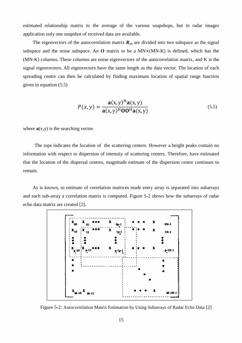
As is known, to estimate of correlation matrices made entry array is separated into subarrays

and each sub-array a correlation matrix is computed. Figure 5-2 shows how the subarrays of radar

echo data matrix are created [2].

Figure 5-2: Autocorrelation Matrix Estimation by Using Subarrays of Radar Echo Data [2]

16

From the figure, set of subarrays with dimensions p1 p2 can be seen. If a subarray is

redesigned in a column sorted array, then each autocorrelation matrices x1 corresponds tot he sub-

array may be written as:

=

(5.6)

By setting a p1 p2 submatrix, as shown in figure, the radar data matrix contains L= L1 L2 =

(M+1- p1)(N+1-p2) submatrices. Here xp1p2 is column-ordered vector of the submatrix, which is the

l1 th in row and the l2 th in column. Then, it is possible to assess the overall autocorrelation matrix

using the following formula (5.7):

=

(5.7)

where * denotes the conjugate operation and the matrix J, which is an exchange matrix with

dimension (p1p2) (p1 p2) and constructed as (5.8):

J =

(5.8)

The estimated autocorrelation matrix has the size of (p1p2) (p1 p2). After the estimate of

autocorrelation matrix, the eigenvectors are splitted into noise and the signal subspaces. Since the

radar echoes include K scatterers having exponential information within the matrix, there are (p1p2 -

K) vectors, which span the noise subspace. Let‘s make definition of a matrix as a (p1p2) x

(p1p2 - K) matrix that its columns are noise subspace eigenvalues of [2]. It can find the times

non-zero eigenvectors of the estimated autocorrelation array and adopt other eigenvalues

corresponds to no eigenvectors. Next step is to obtain of the column-ordered vector, approximation

(x y) with a length of p1 p2 . It can be shown as :

(x y) =

(5.9)

17

So, the location of each spreading centre can be calculated by finding the peak location of spatial

range function:

(5.10)

which will be our ISAR image map as similar to equation (4.6).

5.2 Min-Norm ( Minimum Norm) Algorithm

The minimal standard approach addresses the problem of handling of the M-K false origins of

each noise eigenvalue in a different manner the MUSIC method. In MUSIC algorithm, it is used

(M-N) linearly independent vectors in to obtain the frequency estimated.Since any vector in

is (asymptotically) orthogonal to , we may think of using only one such vector for

frequency estimation. By doing so, we may achieve some computational saving, hopefuly without

sacrificing too much accuracy. An undesirable side-effects the average dummy-spectra of the

MUSIC the algorithms that the tops of the K wish the signal source are dimished the amplitude. The

method of a minimum norm approach is to form the projection matrices from noise eigenvalues and

select a new vector of the orthogonal projection of only K roots. Since the M (M-K) matrix to the

noise eigenvalues, Qn a projection into a noise subspace specified by (5.11):

(5.11)

and similar screening can be found on the signal subspace (5.12):

(5.12)

A new vector u is desired to be found that is perpendicular to a signal subspace and is in the

direction of noise subspace as

u = 0 and u = 0 (5.13)

18

The minimum standard method is to minimize the norm for u in order to prevent false peaks

in ist faux-range object of the constraint that the first item of u is 1 (obtained by normalisation).

After some manipulation, the vector that satisfies this conditon is given by:

(5.14)

where 1= is the normalisation vector. The corresponding minimum norm pseudo-

spectrum is:

(5.15)

As described in detail in [12], it remains to determine the vector which is the vector in

R( ) , with first element equal to one, that has minimum Euclidean norm, and in particular, to show

that its first element can always be normalized to one. Partition the matrix :

=

(5.16)

As R( ), it must satisfy the equation

(5.17)

By considering the derivation steps in [12] which are omitted here for simplicity, the vector can

be written as:

(5.18)

Alternatively, we can also obtain as a function of the entries in . To do so, partition as

(5.19)

which leads to the following equivalent expression for [12]:

19

(5.20)

If M - K K, then it is computationally more advantageous to obtain from (5.18); otherwise,

(5.20) should be used.

The statistical precision of the Min-Norm is similar to that corresponds to the MUSIC

algorithm. Hence, Min-Norm reaches MUSIC’ s performance in the reduced calculation price. It

should be pointed out that the choice of of the vector of , used for the Min-Norm

method, is crucial to obtain rate estimates of acceptable statistical precision.

In our ISAR imaging simulations, the steps of MUSIC algorithm up to the generation of

matrix are also same in the Min-norm algorithm. Then, by using this matrix, which is actually

matrix in equation (5.19), the vector is constructed by using (5.20). Finally, the location of each

spreading centre can be calculated by finding the peak location of spatial range function:

(5.21)

which will be our ISAR image map as similar to equations (4.6) and (5.10).

5.3 ESPRIT Algorithm

Estimation of signal parameters via rotational invariance techniques (ESPRIT) seems to be

the best of known spectrum analytical method. It has maximum resolution, has no spectrum splash

and a robust presence of the noise. 2D spectrum analysis applied to the series of bandwidth radar

will return to create a variety of targets. Typically each 2D spectrum part of the data is associated

with a specific diffuser on the target. The basic idea is as easy as it is ingenious. Consider the

antenna array to Nr components. Based on the 2-dimensional image mathematic model, super-

resolution methods are taken into consideration to cope with the near field dispersion centres to

extract. A 2-D ESPRIT algorithm is the ability of wavefront damages while ball round lighting.

By considering the equation (4.5), the sampling backscattering radial back on frequency

+ from the uniform move scattering point at variety

can be written

20

=

(5.22)

where and are the cross-range and range, respectively, at time zero of scatterer i. The

presence of the cross product may have a significant negative impact on ESPRIT

processing of practical of values for these stretches. However, if the time-frequency distribution of

data is small enough, this term has minor effect and can be ignored. Then, the prescribed data

matrix can be written as

(5.23)

with = , = and , where now is the

original angle sampling interval and the ranges of both and over the rows and columns of Y are

centered on zero. To create the shift matrices of block-Hankel structure with the

properties [7]:

Every column is another linear combination of all of the sep rate spectrum assessments;

The rank, in the absence of noise, equal to the total number of M the spectral components of

the information;

The contribution to the spectral elements M to , differs only by the shift factor

exp or exp from the contribution of the same spectral component to .

If the elements for each sub-array rearranges in a systematic way in a single column vector

and the column vectors of merged to form the matrix H, each column in the H will be different

linear combinations the same S spectrum parts [7]. H is t he rearrangement Y into block Hankel

form. First a Hankel matrix is created from each column of Y. [Hankel Matrix element ( ) is

column element ( )]. Then the block Hankel matrix is assembled from Hankel matrices.

Next, the unique value breakdown is used to shorten the second aspect of to match the

key value by keeping only those corresponds to the important unique values.

21

A block-Hankel reorganization of Y means that the input section diffuser S to one line of U

different from their contribution to the last line on the same block factor exp , from its

contribution to the corresponding row in the previous block by the factor exp . Delete from U

the last row of each blocks of rows and also th entire final blocks of lines created . Delete the first

row of each block and the entire final block of lines to create . Deleting the last row of each block

and the whole of the first block of lines created . The range and cross-range of the scatterers can

then be evaluated from the eigenvalues τi = exp and νi = exp using =

and = . ESPRIT is similar to the MUSIC and Min-Norm which was mentioned

previosly. In fact, more exact frequency estimates can be provided by ESPRIT method.

As described in the Introduction chapter, the mentioned version of ESPRIT algorithm only

provides the (x, y) coordinates of the scatterers; but not gives any ISAR-related space coordinates

map. In this thesis, as a contribution to the literature, the information of (x, y) coordinates of the

scatterers is converted to an ISAR map as being similar to ones obtained by IFFT, MUSIC, Min-

norm. By considering the Appendix section of [7], τi and νi are found from the two eigenvalue

problems of

=0, = 0 (5.24)

where the matrices Rt and Rf can be found in [7]. By using these matrices, the spatial range function

for ISAR mapping are constructed as

(5.25)

where the columns of matrix V contains the eigenvectors of matrix Rt (and also matrix Rf ), and

τ(x) = exp , ν (y) = exp .

22

CHAPTER 6

Simulations and Results

In this chapter, ISAR imaging was made by using all methods for target of aircraft models.

Firstly, noiseless simulations was made, then noisy simulations was made. All parameters are same

which was used in simulations as given Table 6.6.

Image reconstruction was given which made by using Table 6.6 target simulation.

Table 6.1 : Simulations parameters

As it was indicated in the equations (2.2) and (2.3), and was found as 0.5. In this

thesis, our X is cross range and Y is range because of position of the radar, and are equal

to 0.5. Δ = and is in the target . Frequency range is between

because of center frequency = 10 GHz.

SYMBOL NAME VALUE

M Number of

Frequency Samples

40

N Number of Bursts

60

fc Carrier Frequency

10

T Pulse Repetition

Interval 1 ms

B Signal Bandwidth

300 MHz

Δf Frequency Step Size

7.5 MHz

ω Angular Velocity

0.5

23

6.1 Simulation with Noiseless Scattered Fields :

Simulations was made with using high resolution techniques and IFFT then all simulations

was compared.

6.1.1. Simulations for 3 points

In this part, simulations will showed which belongs to random 3 points for showing the work of

methods,

Table 6.2 : Scattering Center Coordinates of Three Points

Scatterer # 1 2 3

x 8.1 5.4 -5.2

y -1 -5 6.25

In these simulations, as it was indicated in the equation (4.3), firstly ai values was taken

, and some results was observed. For example IFFT is

better because IFFT is connected with amplitude.

(a) (b)

24

(c) (d)

Figure 6.1 : Simulation with sample 3 points ( for the methods of (a)

IFFT, (b) MUSIC, (c) Min-Norm, (d) ESPRIT

But when ai values was changed as ; (for 3

Points), simulations changed because of this relation. In other part, high resolution method did not

affected by this change because they are not connected with amplitude like IFFT, just frequency is

important for them.

For example; in Figure 6.1 shows that IFFT simulation when ai =1, in Figure 6-2, different ai

values was given and the results.

(a) (b)

25

(c) (d)

Figure 6.2 : Simulation with sample 3 points ( for the methods of

(a) IFFT, (b) MUSIC, (c) Min-Norm, (d) ESPRIT

As can seen, while IFFT method can find the 3 points in Figure 6.1(a) thanks to being coefficient

are 1, in Figure 6.2(a) shows that, just a point was found, because second point on resolution point

and the coefficient a2 = 0.1. In addition, although third point’s coefficient is higher than second one,

this point could not be found by IFFT because of being on resolution point. On the other hand, as

Figures 6.1 and 6.2 shows that the high resolution methods were not be affected by amplitude

coefficients.

6.1.2. Simulations with point-scatterer model of AAIRBUS A380 aircraft

Figure 6.3 : AIRBUS A380

26

Table 6.3 : AIR BUS A-380 (Original Points)

Scatterer # 1 2 3 4 5 6 7 8 9 10 11

X 4.1 4.1 0 10.4 -10.4 6.6 -6.6 3.75 -3.75 0 0

Y 8.5 -8.5 9.3 4 4 -1.5 -1.5 -3.7 -3.7 -9.3 8.4

ai 1 0.1 0.15 1 0.1 0.15 0.1 0.15 0.15 1 0.15

Figure 6.4 : AIRBUS A380

In Figure 6.4 shows that the scatterer points of original aircraft. In Figure 6.5 is the first simulation

for AIRBUS A380 with IFFT method. AIRBUS A380 has eleven scatterer points, but because of

different coefficients, IFFT could nor find the all data. 5 point could seen in simulation which made

for AIRBUS A380, but there are 11 points, IFFT can not show the other points.

Figure 6.5: Simulation with IFFT for AIRBUS A380

27

In Figure 6.6, MUSIC algorithm’s simulation is shown for AIRBUS A380. All points can be found

by MUSIC algorithm.

Figure 6.6 : Simulation with MUSIC for AIRBUS A380

11 points easily can saw if MUSIC algorithm is used. We can see all points which could not see

with IFFT method. In Figure 6.7,it is shown that Min- Norm simulation for AIRBUS A380. Aircraft

can seen easily because Min-Norm method find the all points. While Min-Norm method find the all

scatterer points, lots of false points can be observed.

Figure 6.7 : Simulation with Min-Norm for AIRBUS A380

In Figure 6.8, ESPRIT method was used for simulation of AIRBUS A380, and ESPRIT method can

find all scatterer points. In this simulation, ESPRIT method found all scattered points but there is a

small slip in tail.

28

Figure 6.8 : Simulation with ESPRIT for AIRBUS A380

6.1.3. Simulations with point-scatterer model F14 Tomcat aircraft

In this part of thesis, F14 Tomcat aircraft is simulated with IFFT and all high resolution

methods. The coefficients and the scatterer points was given in Table 6.3. All simulations are shown

in the figures which was made by using Table 6.3.

Figure 6.9: F14 Tomcat

29

Table 6.4 : F-14 Tomcat (Original Points)

In Figure 6.10 shows that the scatterer points of original aircraft.

Figure 6.10 : F14 Tomcat

Figure 6-11 shows that F14 simulation with IFFT, but it is not good enough because it is not look

like the original data. Actually, there are twelve points in original model, bur IFFT can find just six

points as Figure 6-12.

Figure 6.11 : Simulation with IFFT for F14 Tomcat

Scatterer # 1 2 3 4 5 6 7 8 9 10 11 12

X 1 -1 3.5 7 -7 2.5 -2.5 -2 2 0 0 -3.5

Y 6.9 6.9 7.2 4.8 4.8 -0.9 -0.9 -1.2 -1.2 -7.5 7.5 7.2

ai 1 0.6 0.15 1 0.1 0.1 0.1 0.1 0.1 0.1 1 0.15

30

Simulation of F14 Tomcat with MUSIC algorithm is shown in Figure 6.13, and all points was

found by MUSIC.

Figure 6.12: Simulation with MUSIC for F14 Tomcat

Because of finding all points by MUSIC algorithm, original aircraft model can be understood easily.

Figure 6-16 Min-Norm simulations which was made for F14 Tomcat for twelve points, and as

previous simulation, there alr lots of false points.

Figure 6.13: Simulation with Min-Norm for F14 Tomcat

31

Figure 6.14: Simulation with ESPRIT for F14 Tomcat

Figure 6.14 shows that, ESPRIT method can find all scatterer points in a short time.

6.1.4. Simulations with point-scatterer model of A-10 Thunderbolt 11 aircraft

In this part, there are some simulation for A-10 Thunderbolt 11, as previously IFFT, MUSIC, Min-

Norm and ESPRIT methods was used and all simulations was compared.

Figure 6.15 : A-10 Thunderbolt 11

32

Table 6.5 : A-10 Thunderbolt 11 (Original Points)

The all simulations was made by using Table 6.4 for all methods. In Figure 6.17, it is shown that

the original aircraft scatterer points of A-10 Thunderbolt 11.

Figure 6.16 : A-10 Thunderbolt 11

First simulations was made by IFFT, and could not be found original datas as previously. There are

twelve points in original data, but in Figure 6.18, as can seen, there are just seven points. Especially,

some points which coefficients are 0.1, can not be seen in Figure 6.18.

Scatterer # 1 2 3 4 5 6 7 8 9 10 11 12

X 0 0 2.5 -2.5 2.1 -2.1 8 -8 4.9 -4.9 2.3 -2.3

Y 7.4 -7.4 5.3 5.3 2.61 2.61 1.1 1.1 -1.3 -1.3 -1.1 -1.1

ai 1 0.1 0.15 1 0.1 0.15 0.1 0.15 0.15 0.15 0.15 0.1

33

Figure 6.17 : Simulation with IFFT for A-10 Thunderbolt 11

When the same simulation was made with using MUSIC method, Simulation A-10 Thunderbolt 11

can be shown easily original data and aircraft model can be understand. From Figure 6.19, aircraft‘

s model can understant easily.

Figure 6.18:Simulation with MUSIC for A-10 Thunderbolt 11

As Figure 6-21, aircraft model can be understand exactly in figure 6-22 because of Min-Norm

method, but some false points can be observed.

34

Figure 6.19: Simulation with Min-Norm for A-10 Thunderbolt 11

In figure 6.20 shows that in spite of aircraf’s nose can not be seen, ESPRIT is better than a

lot of methods.

Figure 6.20: Simulation with ESPRIT for A-10 Thunderbolt 11

35

6.1.5. Sample Points Simulations

Table 6.6 : Sample variables

Scatterer# 1 2 3 4 5 6 7 8

x 20 4 7 -10 10 -20 16 -16

y -4 10 10 0 20 10 -16 18

ai 1 0.1 0.15 1 0.1 0.15 0.1 0.15

Although there are eight points in original data, IFFT can not find all points as Figure 6.21.

The original datas are shown in Table 6.5 and all simulations was made with using this datas.

Figure 6.21: Simulation with IFFT for Sample points

Figure 6.22: Simulation with MUSIC for Sample points

36

Figure 6.22 shows that MUSIC method can find all points as previously. Min-Norm simulation for

Sample points was given in Figure 6.23. There are eight points as original data but there are lots of

false points different from original data. In simulation of ESPRIT can observed all points which was

given in original data as shown in Figure 6.24.

Figure 6.23: Simulation with Min-norm for Sample points

Figure 6.24 : Simulation with ESPRIT for Sample points

In all simulations, there were scatterer points which belongs to any aircraft. These points was

selected. Because these points are the best reflective points as aircraft’s nose, wing as soon as

Figure 6.25.

37

Figure 6.25 : Reflected waves from different parts of aircraft

6.2 Simulation for Noisy Scattered Fields:

In the part of this chapter, simulations was evaluated without noisy, but in the chapter, noisy

effects on high resolution techniques was observed because of adding AWGN. Particular SNR

offers a noisy image creation. Varying entry SNR to adjust the noisy difference is addedto the

input, multiple output of samples was observed for each algorithm. Useful analytical expressions

for evaulation of both estimators are derived and etimators are providing to be the asymptotic

impartial in high SNR and have the error variance which rots the exponential with the sequence

length of a franchise which is dependent on the SNR. SNR formula was obtained as:

SNR

(6.1)

show the variance of noise, and simulations was made for different SNR values.

38

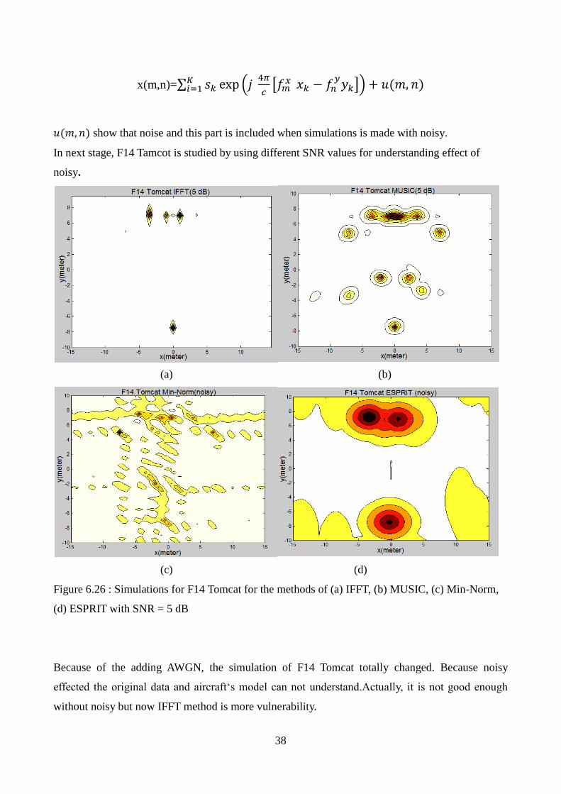
x(m,n)=

show that noise and this part is included when simulations is made with noisy.

In next stage, F14 Tamcot is studied by using different SNR values for understanding effect of

noisy.

(a) (b)

(c) (d)

Figure 6.26 : Simulations for F14 Tomcat for the methods of (a) IFFT, (b) MUSIC, (c) Min-Norm,

(d) ESPRIT with SNR = 5 dB

Because of the adding AWGN, the simulation of F14 Tomcat totally changed. Because noisy

effected the original data and aircraft‘s model can not understand.Actually, it is not good enough

without noisy but now IFFT method is more vulnerability.

39

(a) (b)

(c) (d)

Figure 6.27 : Simulations for F14 Tomcat for the methods of (a) IFFT, (b) MUSIC, (c) Min-Norm,

(d) ESPRIT with SNR = 10 dB

The simulations with SNR = 10dB is better than 5 dB as shown in Figures 6.27. For example, while

there are some false points in F14 Tomcat MUSIC simulation with SNR = 5dB, false scatterer

points can not be observed in 10dB as Figure 6.27(b).

40

(a) (b)

(c) (d)

Figure 6.28 : Simulations for F14 Tomcat for the methods of (a) IFFT, (b) MUSIC, (c) Min-Norm,

(d) ESPRIT with SNR = 15 dB.

Figure 6.28 shows that when SNR is increase, methods works more efficient. Scattered points of

original model can be found easily when SNR become 15, next part, SNR = 20 dB is indicated.

41

(a) (b)

(c) (d)

Figure 6.29 : Simulations for F14 Tomcat for the methods of (a) IFFT, (b) MUSIC, (c) Min-Norm,

(d) ESPRIT with SNR = 20 dB.

6.3 Discussion

In this article, SNR and the resolution performance of various ISAR images rebuilding

techniques in comparison to the input that is generated by ISAR simulation. FFT basis images do

not have the exact mountains as MUSIC basis images. MUSIC algorithm ist he most correct choice

and the cross-spectrum profile oft he target. But for small SNR, MUSIC algorithm may result in

unnecessary tops. Spectral estimate- built ISAR images are characterised by sadisfactory high-

resolution, even in every small sets of data. Whereas 2D-FFT performing highly depend on the

number of frequency and appearance corner. We can see at previous simulatins that MUSIC

algorithm can find more estimated frequency different from 2D-FFT. In addition, when the value of

42

the is taken different from 1, MUSIC algorithm do not affected. Because MUSIC is not

associated with the amplitude as FFT. Instead of the FFT, high-resolution spectrum estimation

methods, which will be described below, can significantly improve the settlement capacity of ISAR

images, even the limited information in the area, at the cost of extra computing time. In

addition, 2D MUSIC algorithm has high resolution and is more accuratein detail than IFFT. In

MUSIC simulations more look alike original model. This results are valid for Min-Norm and

ESPRIT, but the time is more important for these simulations so in spite of ESPRIT has the

shortest time, there are some false points. Some ways can be made but in this time, it cause time

redundancy

Table 6.7 : Comparison

3 Points AIRBUS A380(11) F14 Tomcat(12) A10Thunderbolt(12) Sample Points(8)

Point

number

Runtime

(sec.)

Point

number

Runtime

(sec.)

Point

number

Runtime

(sec.)

Point

number

Runtime

(sec.)

Point

number

Runtime

(sec.)

IFFT 1 0.086 7 0.048 6 0.05 7 27 4 0.4

MUSIC 3 27 11 15.89 12 17.3 12 45.6 8 27.1

MinNorm 3+false 25.9 10+false 14.71 11+false 16.74 12+false 28.96 8+false 25.11

ESPRIT 3 1.1 10 0.68 10 0.69 11 5 8 1.7

43

CHAPTER 7

CONCLUSIONS

In this project primary concern is comparing different ISAR images reconstructing algorithm

in term of its performances. In project, performances was compared as speed, verity of data. In view

of radar target recognition, ISAR images should be very resolved (high resolution imaging), in

order to allow for decision making with regard to the target categories and types. An important step

forward in ISAR image is the implementation of high resolution spectrum estimation method. In

deed, it is known that, in most cases, traditional FFT processing the 2D line of radar is not enough

to produce high resolution radial aircraft images. Therefore, several spectral estimation techniques,

both nonparametric and parametric, are applied in order to improve the resolution of 2D radar target

images. Traditional IFFT method is not enough as other high resolution methods. Because when

scattered points coefficients become different from 1, all simulation change, because IFFT method

is connected with amplitude. So because of not finding all points, aircraft model can not be

understood. In other part, MUSIC method is better than IFFT, although 2D-MUSIC algorithm works

on the rectangular data like 2D-FFT. MUSIC method can find all points as seen in simulations. Because

MUSIC is not connected with coefficient as IFFT. So Coefficient changes does not effect MUSIC

method. In addition, 2D MUSIC algorithm has high resolution and is more accuratein detail than IFFT.

In MUSIC simulations more look like original model. This results are valid for Min-Norm, and ESPRIT,

but Min-Norm simulations shows that there are lots of false points except original data. ESPRIT has a

short runtime and because of this reason this method is more efficient.

44

APPENDIX

In this appendix, some useful Matlab codes are represented for the mentioned method.

A.1 IFFT METHOD

clear all close all T= 1e-3; %ai=[1 0.10 0.15 1 0.10 0.15 0.1 0.1 0.15 0.15 0.15]; %airbus %ai=[1 0.10 0.15 1 0.10 0.15 0.1 0.15 1 0.10 0.15 1]; %f-14 %ai=[1 0.10 0.15 1 0.10 0.15 0.1 0.15 0.15 0.15 0.15 0.1]; % thunder %ai=[1 0.10 0.15 ]; % 3 nokta %ai=[1 0.10 0.15 1 0.10 0.15 0.1 0.15 ]; %tez

M=40; N=60;

% M=80; % N=120; w=0.12*250/60; deltaf=0.0075; c=0.3; fc=10-deltaf*M/2; xi=[ 1 -1 3.5 -3.5 7 -7 2.5 -2.5 2 -2 0 0]; yi=[6.9 6.9 7.2 7.2 4.8 4.8 -0.9 -0.9 -1.2 -1.2 -7.4

7.2];%F14

%xi=[0 0 2.5 -2.5 2.1 -2.1 8 -8 4.9 -4.9 2.3 -2.3]; %yi=[7.4 -7.4 5.3 5.3 2.61 2.61 1.1 1.1 -1.3 -1.3 -1.1 -1.1];

%thunder

% xi=[4.1 -4.1 0 10.4 -10.4 6.6 -6.6 3.75 -3.75 0 0

];%Airbus % yi=[8.5 8.5 9.3 4 4 -1.5 -1.5 -3.7 -3.7 -9.3 8.4];

% xi=[8.1 15.4 25.2]; % yi=[-20 -15 -26.25]; % 3 nokta

% xi=[20 4 7 -10 10 -20 16 -16]; % yi=[-4 10 10 0 20 10 -16 18]; % tez %

dy=0.3/(2*deltaf*M); dx=0.3/(2*10*w*T*(N)); X = -dx*(N)/2:dx:dx*(N)/2-dx/2; Y = -dy*(M)/2:dy:dy*(M)/2-dy/2; tic

45

image1 = zeros(N,M); for k=1:N

wt=-w*T*N/2+w*T*(k-1); %k=k+1

for u=1:M

%i=i+1

%x(i)=xi+1; %y(i)=yi+1;

%n=n+1; f=fc+(u-1)*deltaf; % Sr(n,k)=ai*exp((-j*2*pi*(2*f*sin(k*w*T)/c*xi+(2*f*cos(k*w*T)/c*yi))); S= 0; 45ors c=1:size(xi,2)

S=S+ai(sc)*exp(-1i*2*pi*(2*f*sin(wt)*xi(sc)+2*f*cos(wt)*yi(sc))/c); image1(k,u)=S; end end end

toc

contourf(abs(image1))

SNR=5;

se=10*log10(sum(sum((abs(image1)).^2))/(N*M)) c1=wgn(N,M,-(SNR-se),’complex’); pow=10*log10(sum(sum((abs(c1)).^2))/(N*M)) image1_noisy=image1+c1;

ISAR = ifftshift(ifft2(image1_noisy.’)); figure contourf(X,Y,abs(image1_noisy.’)) figure % imagesc(1:N,M:-1:1,abs(ISAR)) % xlabel(‘Range [m]’); ylabel(‘Cross – range [m]’);

46

A.2 MUSIC ALGORITHM

clear all close all T= 1e-3; % ai=[1 0.10 0.15 1 0.10 0.15 0.1 0.1 0.15 0.15 0.15]; %airbus %ai=[1 0.10 0.15 1 0.10 0.15 0.1 0.15 1 0.10 0.15 1]; %f-14 %ai=[1 0.10 0.15 1 0.10 0.15 0.1 0.15 0.15 0.15 0.15 0.1]; % thunder % ai=[1 0.10 0.15 ]; % 3 nokta %ai=[1 0.10 0.15 1 0.10 0.15 0.1 0.15 ]; %tez

M=40; N=60;

% M=80; % N=120; w=0.12*250/60; deltaf=0.0075; c=0.3; fc=10-deltaf*M/2; % xi=[ 1 -1 3.5 -3.5 7 -7 2.5 -2.5 2 -2 0 0]; % yi=[6.9 6.9 7.2 7.2 4.8 4.8 -0.9 -0.9 -1.2 -1.2 -7.4

7.2];%F14

%xi=[0 0 2.5 -2.5 2.1 -2.1 8 -8 4.9 -4.9 2.3 -2.3]; %yi=[7.4 -7.4 5.3 5.3 2.61 2.61 1.1 1.1 -1.3 -1.3 -1.1 -1.1];

%thunder

% xi=[4.1 -4.1 0 10.4 -10.4 6.6 -6.6 3.75 -3.75 0 0

];%Airbus % yi=[8.5 8.5 9.3 4 4 -1.5 -1.5 -3.7 -3.7 -9.3 8.4];

% xi=[8.1 15.4 25.2]; % yi=[-20 -15 -26.25]; % 3 nokta

% xi=[20 4 7 -10 10 -20 16 -16]; % yi=[-4 10 10 0 20 10 -16 18]; % tez % dy=0.3/(2*deltaf*M); dx=0.3/(2*10*w*T*(N)); X = -dx*(N)/2:dx:dx*(N)/2-dx/2; Y = -dy*(M)/2:dy:dy*(M)/2-dy/2; tic

image1 = zeros(N,M); for k=1:N

wt=-w*T*N/2+w*T*(k-1); for u=1:M f=fc+(u-1)*deltaf; S= 0; for sc=1:size(xi,2) S=S+ai(sc)*exp(-1i*2*pi*(2*f*sin(wt)*xi(sc)+2*f*cos(wt)*yi(sc))/c); image1(k,u)=S; end end end

47

toc

%contourf(abs(image1)) SNR=300;

se=10*log10(sum(sum((abs(image1)).^2))/(M*N)) c1=wgn(N,M,-(SNR-se),'complex'); pow=10*log10(sum(sum((abs(c1)).^2))/(M*N)) image1_noisy=image1+c1;

p=15; temp=zeros(p^2,p^2); B=zeros(p^2,p^2); J=(fliplr(diag(ones(1,p^2)))); tic for p1=1:N-p+1 for p2=1:M-p+1 x=image1_noisy(p1:p1+p-1,p2:p2+p-1); B=x(:)*x(:)'; temp=temp+B+J*B.'*J; end end toc temp=temp/(N+1-p)/(M+1-p)/2; [U,D,V]=svd(temp); O=V(:,size(xi,2)+1:p^2); %xk=-12;yk=3; P=zeros(N+1,M+1); tic for xk=-15:0.5:15 for yk=-10:0.5:10 for p1=1:p for p2=1:p a(p1+(p2-1)*p,1)=exp(-j*4*pi/0.3*(xk*10*w*T*(-N/2+p1-

1)+yk*(fc+(p2-1)*deltaf))); end end P((1/0.5)*(xk+15)+1,(1/0.5)*(yk+10)+1)=(1)/(a'*O*O'*a);

end end toc

figure contourf(-15:0.5:15,-10:0.5:10,10*log10(abs(P'))+1.1)

48

A.3 MIN-NORM ALGORITHM

T= 1e-3; %ai=[1 0.10 0.15 1 0.10 0.15 0.1 0.1 0.15 0.15 0.15]; %airbus ai=[1 0.10 0.15 1 0.10 0.15 0.1 0.15 1 0.10 0.15 1]; %f-14 %ai=[1 0.10 0.15 1 0.10 0.15 0.1 0.15 0.15 0.15 0.15 0.1]; % thunder %ai=[1 0.10 0.15 ]; % 3 nokta %ai=[1 0.10 0.15 1 0.10 0.15 0.1 0.15 ]; %tez

% M=40; % N=60;

M=80; N=120; w=0.12*250/60; deltaf=0.0075; c=0.3; fc=10-deltaf*M/2; % xi=[ 1 -1 3.5 -3.5 7 -7 2.5 -2.5 2 -2 0 0]; % yi=[6.9 6.9 7.2 7.2 4.8 4.8 -0.9 -0.9 -1.2 -1.2 -7.4

7.2];%F14

% xi=[0 0 2.5 -2.5 2.1 -2.1 8 -8 4.9 -4.9 2.3 -2.3]; % yi=[7.4 -7.4 5.3 5.3 2.61 2.61 1.1 1.1 -1.3 -1.3 -1.1 -1.1];

%thunder

%xi=[4.1 -4.1 0 10.4 -10.4 6.6 -6.6 3.75 -3.75 0 0

];%Airbus %yi=[8.5 8.5 9.3 4 4 -1.5 -1.5 -3.7 -3.7 -9.3 8.4];

% xi=[8.1 15.4 25.2]; % yi=[-20 -15 -26.25]; % 3 nokta

% xi=[20 4 7 -10 10 -20 16 -16]; % yi=[-4 10 10 0 20 10 -16 18]; % tez %

dy=0.3/(2*deltaf*M); dx=0.3/(2*10*w*T*(N)); X = -dx*(N)/2:dx:dx*(N)/2-dx/2; Y = -dy*(M)/2:dy:dy*(M)/2-dy/2; tic image1 = zeros(N,M); for k=1:N

wt=-w*T*N/2+w*T*(k-1); %k=k+1

for u=1:M

%i=i+1

%x(i)=xi+1; %y(i)=yi+1;

%n=n+1;

49

f=fc+(u-1)*deltaf; S= 0; for sc=1:size(xi,2)

S=S+ai(sc)*exp(-1i*2*pi*(2*f*sin(wt)*xi(sc)+2*f*cos(wt)*yi(sc))/c); image1(k,u)=S; end end end

toc

contourf(abs(image1)) SNR=100;

se=10*log10(sum(sum((abs(image1)).^2))/(M*N)) c=wgn(N,M,-(SNR-se),'complex'); pow=10*log10(sum(sum((abs(c)).^2))/(M*N)) image1_noisy=image1+c;

p=15; temp=zeros(p^2,p^2); B=zeros(p^2,p^2); J=(fliplr(diag(ones(1,p^2)))); tic for p1=1:N-p+1 for p2=1:M-p+1 x=image1_noisy(p1:p1+p-1,p2:p2+p-1); B=x(:)*x(:)'; temp=temp+B+J*B.'*J; end end toc temp=temp/(N+1-p)/(M+1-p)/2; [U,D,V]=svd(temp); O=U(:,size(xi,2)+1:p^2); g_sapka=O(2:end,:)*O(1,:)'/norm(O(1,:)')^2; G=[1; g_sapka]; %xk=-12;yk=3; P=zeros(N+1,M+1); tic for xk=-15:0.5:15 for yk=-10:0.5:10 for p1=1:p for p2=1:p a(p1+(p2-1)*p,1)=exp(-j*4*pi/0.3*(xk*10*w*T*(-N/2+p1-

1)+yk*(fc+(p2-1)*deltaf))); end end P((1/0.5)*(xk+15)+1,(1/0.5)*(yk+10)+1)=(a'*a)/norm(a'*G)^2;

end end toc figure contourf(-15:0.5:15,-10:0.5:10,10*log10(abs(P'))+1.1)

50

A.4 ESPRIT ALGORITHM

close all clear all temp=0; T= 1e-3; %ai=1; % M=40; % N=60;

M=80; N=120; w=0.12*250/N; deltaf=0.3/M; c=0.3; %T= 1e-3; %ai=[1 0.50 0.25 1 0.10 0.15 0.4 0.2 1 0.0

0.25 1];

fc=10-deltaf*M/2;

% xi=[4.1 -4.1 0.02 10.4 -10.4 6.6 -6.6 3.75 -3.75 0 -0.02

];%Airbus_new % yi=[8.5 8.5 9.3 4 4 -1.5 -1.5 -3.7 -3.7 -9.3 8.4];

dy=0.3/(2*deltaf*M); dx=0.3/(2*10*w*T*(N)); X = -dx*(N)/2:dx:dx*(N)/2-dx/2; Y = -dy*(M)/2:dy:dy*(M)/2-dy/2; er=12;

tic image1 = zeros(N,M); for k=1:N

wt=-w*T*N/2+w*T*(k-1);

%k=k+1

for u=1:M

f=fc+(u-1)*deltaf; S= 0;

for sc=1:er

S=S+ai(sc)*exp(-1i*2*pi*(2*10*sin(wt)*xi(sc)+2*f*cos(wt)*yi(sc))/c); image1(k,u)=S; end end end

toc

51

contourf(abs(image1))

SNR=20;

se=10*log10(sum(sum((abs(image1)).^2))/(N*M)) c1=wgn(N,M,-(SNR-se),'complex'); pow=10*log10(sum(sum((abs(c1)).^2))/(N*M)) image1_noisy=image1+c1;

t1=20; t2=20; tic for k=1:t1 for l=1:t2 h=hankel(image1_noisy(:,k+l-1)); f1(:,:,k+l-1)=h(1:t1,1:t1); end end for k=1:t2 for l=1:t2 H(1+(k-1)*t2:t1+(k-1)*t2,1+(l-1)*t2:t1+(l-1)*t2)=f1(:,:,k+1-1); end end

[U,D,V]=svd(H); S=U(:,1:er); %S0_ilk=S(:,1:end-1);

a=1:t2^2; a(mod(a,t2)==0)=[]; sa=a(1:end-t2+1); b=1:t2^2; b(mod(b,t2)==1)=[]; sb=b(1:end-t2+1); sc=a(t2:end);

S0(:,:)=S([sa],:); ST(:,:)=S([sb],:); SF(:,:)=S([sc],:);

RT=(pinv(S0)*ST); RF=(pinv(S0)*SF); [V1,D1]=eig(1*RT+RF);

for num=1:er x(num)=-angle(V1(:,num)'*RT*V1(:,num))*0.3/(10*4*pi*w*T); y(num)=-angle(V1(:,num)'*RF*V1(:,num))*0.3/(4*pi*deltaf); end x; y;

for num=1:er for den=1:50

52

tau(num)=V1(:,num)'*RT*V1(:,num); nu(num)=V1(:,num)'*RF*V1(:,num); te=RT-tau(num)*eye(er,er); fe=RF-nu(num)*eye(er,er); bracket=te'*te+fe'*fe; [V3,D3]=eig(bracket); d3=diag(D3); [sa3,index1]=min(abs(d3)); V1(:,num)=V3(:,index1); end end tau; nu;

for num=1:er x1(num)=-angle(tau(num))*0.3/(10*4*pi*w*T); y1(num)=-angle(nu(num))*0.3/(4*pi*deltaf); end x1; y1; toc P2=zeros(N+1,M+1); tic for xk=-0.5*N/2:0.5:0.5*N/2 for yk=-0.5*M/2:0.5:0.5*M/2

tau_k=exp(-j*xk*4*pi*10*w*T/0.3); nu_k=exp(-j*yk*4*pi*deltaf/0.3); x_dim=(RT-tau_k*eye(er,er))*V1; y_dim=(RF-nu_k*eye(er,er))*V1; %toplam=x_dim+y_dim; ab=sum(abs(x_dim).^2,1)+sum(abs(y_dim).^2,1); [sa,index]=min((ab)); P2((1/0.5)*(xk+0.5*N/2)+1,(1/0.5)*(yk+0.5*M/2)+1)=(1/sa);

end end

toc

figure contourf(-0.5*N/2:0.5:0.5*N/2,-0.5*M/2:0.5:0.5*M/2,(abs(P2'))) colormap(flipud(hot)) figure contourf(-0.5*N/2:0.5:0.5*N/2,-0.5*M/2:0.5:0.5*M/2,20*log10(abs(P2'))) colormap(flipud(hot))

53

REFERENCES

[1]. Caner Özdemir, Inverse Synthetic Aperture Radar with Matlab Algorithms, Wiley Series in

Microwave and Optical Engineering (Volume 1)

[2] . A. Tufan , Comparative Evaluation of ISAR Processing Algorithm, M.Sc. Thesis , Middle

East Technical University, Ankara, Turkey,Sep 2012

[3] . A. Karakasiliotis and P. Frangos, Comparison of Several Spectral Estimation Methods for

Application to ISAR Imaging, http://ftp.rta.nato.int/public/PubFullText/RTO/MP/RTO-MP-SET-

080/MP-SET-080-11.pdf

[4]. Kyung-Tae Kim, Dong-Kyu Seo, and Hyo-Tae Kim, Efficient Radar Target Recognition Using

the MUSIC Algorithm and Invariant Features, IEEE TRANSACTIONS ON ANTENNAS AND

PROPAGATION, VOL. 50, NO. 3, MARCH 2002.

[6]. Xiang Gu, Yunhua Zhang,” Synthetic Aperture Radar”, Effectiveness and uniqueness conditions

for 2-D MUSIC algorithm used in ISAR imaging, Beijing, China,2009

[7]. Burrows, M.L., Two-dimensional ESPRIT with tracking for radar imaging and feature

extraction, IEEE Antennas and Propagation Society, Volume:52, Feb. 2004.

[8]. J.-I. Park, K.-T. Kim, A Comparative Study on ISAR Imaging Algorithm For Radar Target

Identification, Progress In Electromagnetics Research, Vol. 108, 155-175, 2010.

[9]. David C.Munson, “A Tomographic Formulation of Spotlight-Mode Synthetic Aperture Radar,”

Proceedings of the IEEE vol. 71, no.8, August 1983.

[10]. R. O. Schmidt, “Multiple emitter location and signal parameter estimation,” IEEE Trans.

Antennas & Propagation, vol. 34, no. 3, March 1986

[11]. Y. Hua, E. Baqai, Y. Zhu, and D. Heilbronn, “Imaging of point scatterers from step-frequency

ISAR data”, IEEE Transactions Aerospace Electron Systems 29 (1992), 195–205.

[12]. P. Stoica, R. Moses, “Introduction to Spectral Analysis”, London(1997),pp.160-167