Formation of silver sulfide in the photographic image during ...
Upload
khangminh22Category
view
3download
0
8Reviews in Mineralogy & GeochemistryVol. 61, pp. 421-504, 2006Copyright © Mineralogical Society of America
1529-6466/06/0061-0008$10.00 DOI: 10.2138/rmg.2006.61.8
Metal Sulfi de Complexes and Clusters
David RickardSchool of Earth, Ocean and Planetary Sciences
Cardiff UniversityCardiff CF103YE, Wales, United Kingdom
e-mail: [email protected]
George W. Luther, IIICollege of Marine Studies
University of DelawareLewes, Delaware, 19958, U.S.A.
e-mail: [email protected]
INTRODUCTION
In this chapter we show that
1. Metal sulfi de complexes and clusters enhance the solubility of metal sulfi de minerals in natural aqueous systems, explaining the transport of metals in sulfi dic solutions and driving the biology and ecology of some systems.
2. There is little or no evidence for the composition or structure of many of the metal sulfi de complexes proposed in the geochemical and environmental literature.
3. Voltammetry appears to be a powerful tool in providing additional evidence about the composition of metal sulfi de complexes and clusters which complements the increasing use of techniques such as UV-VIS, Raman and IR spectroscopy, EXAFS, XANES and mass spectrometry.
4. Many of the stability constants for metal sulfi de complexes are very uncertain because of the lack of independent evidence for their existence.
5. Experimental measurements of metal sulfi de complex stability constants is constrained by the lack of knowledge about the composition, structure and behavior of, often nanoparticulate, low temperature metal sulfi de precipitates.
6. The competitive kinetics of metal sulfi de complex and cluster formation in complicated natural sulfi dic systems contributes to the distribution of metals in the environment.
7. The mechanisms of the formation of metal sulfi de complexes and clusters provide basic information about the mechanism of formation of metal sulfi de minerals and explain the stabilities and compositions of the complexes and clusters.
8. There appears to be a continuum between metal sulfi de complexes, metal sulfi de clusters and metal sulfi de solids.
9. The nature of the fi rst-formed metal sulfi de mineral, which is often metastable, can be largely determined by the structure of the metal sulfi de cluster in solution.
Background
The metal chemistry of anoxic systems is dominated by reactions with reduced sulfur spe-cies. These reduced sulfur systems presently characterize the Earth’s subsurface and are occa-

422 Rickard & Luther
sionally important in marine and freshwater systems. In the fi rst half of Earth history, of course, the surface environments were also anoxic and the reduced sulfur chemistry played an even more widespread role in the geochemistry of base metals (e.g., Canfi eld 1998; Holland 2004).
In order for metals to be transported within anoxic systems, the metals must be held in solution. Intuitively, this would appear problematical because of the widespread assumption of relative insolubility of metal sulfi de minerals. In fact, as shown in Table 1, this assumption is misplaced. Even with the simplest of solubility computations, some 35% of the metals listed are more soluble in sulfi dic systems. The system considered in Table 1 is for pure water so that side reactions, such as chloride complexing in seawater or the formation of carbonate solids, are not included. In some of these more complex environments, the solubility of the sulfi des may be even more signifi cant. We used +0.5 V for the Eh in oxidized systems here, since this is the average Eh of aqueous environments in contact with the atmosphere, according to the classical studies of Baas Becking et al. (1960). We assumed an Eh of −0.2 V for the sulfi de systems and this is a maximum value for microbiological sulfate reduction. Lower Eh values would increase sulfi de solubility.
This problem of the solubility of metals in sulfi dic environments is of current interest because of its effect on the bioavailability of these metals, all of which are variously critical to fundamental biochemical processes (Williams and Frausto da Silva 1996). Indeed, in the geologic past when life developed, the availability of metals may have been a kinetic inhibitor to key reactions.
In fact, at low temperatures, metastable metal sulfi des are kinetically signifi cant and these have enhanced solubilities compared to their more stable counterparts. Furthermore a number
Table 1. Comparison of solubilities of oxides and sulfi de solids of metals considered in this chapter. Bold script is used for the most soluble solid. The solubilities are presented in both molal, m, and ppm values of total dissolved metal. The solubilities are calculated for pure water at 25 °C, 1.013 bars total pressure, pH = 7, Eh = 0.5 V (oxide), Eh = −0.2 V, total S(−II) =10−3 m (sulfi des). The Davies equation is used for activity computations (see text). Where at least 1 g of solid dissolves in 1000 g H2O, this is indicated. Data are mainly from the standard thermo.com. v8.r6 database which in turn derives mostly from Helgeson and his co-workers, modifi ed with pK2,H2S = 18. FeS data is taken from Rickard (unpublished). Mo and As, which form molybdates and arsenates in oxidized conditions, are excluded.
Oxides and Metals Sulfi des
solid m ppm solid m ppm
Cr2O3 2×10⁻⁹ 1×10⁻⁴ CrS dissolvesMnO2 5×10⁻⁴ 3×101 MnS 1×10⁻⁴ 6×100
FeOOH 3×10⁻¹² 2×10⁻⁷ FeS 2×10⁻⁶ 6×10⁻²
Co3O4 5×10⁻⁵ 3×100 CoS 1×10⁻¹⁰ 5×10⁻³
NiO 9×10⁻² 5×10³ NiS 3×10⁻¹⁰ 2×10⁻⁵
CuO 2×10⁻⁶ 1×10⁻¹ CuS 5×10⁻¹⁹ 3×10⁻¹⁴
ZnO 2×10⁻³ 1×10² ZnS 1×10⁻¹³ 8×10⁻⁹
CdO dissolves CdS 1×10⁻¹⁸ 4×10⁻¹³
PbO dissolves PbS 4×10⁻¹⁷ 1×10⁻¹³
SnO2 3×10⁻⁸ 3×10⁻³ SnS2 3×10⁻⁵ 3×10⁻⁵
Sb2O5 4×10⁻¹² 1×10⁻¹⁷ Sb2S3 4×10⁻⁸ 5×10⁻³
Ag 9×10⁻⁶ 1×100 Ag2S 1×10⁻¹⁹ 2×10⁻¹⁴
Au 7×10⁻²¹ 1×10⁻¹⁵ Au 1×10⁻³² 2×10⁻²⁷
Hg 2×10⁻¹⁰ 4×10⁻⁵ HgS 3×10−41 6×10−36

Metal Sulfi de Complexes and Clusters 423
of metal sulfi de complexes with considerable thermodynamic stabilities has been identifi ed at concentrations which are very low experimentally but signifi cant in natural systems. These are not considered in the calculations listed in Table 1, since they are the major subject of this chapter. These observations provide possible explanations for the mobility and bioavailability of metals in anoxic systems.
In this chapter we consider current knowledge about dissolved metal sulfi de clusters. We examine the complexation of S(−II) and Sn(−II) ligands with base metal sulfi des. We do not consider the more oxidized sulfur species, such as the sulfur oxyanions. We also limit our discussion to low temperatures (0-100 °C), where these species play a particularly important role, and aqueous solutions, since these are more important geochemically. In fact, from a theoretical or experimental point of view, water is the least suitable medium to consider, and much of the pure chemical literature on complexation is concerned with less polar to non-polar, usually organic, solvents.
Metals considered in this chapter
The formal chemical defi nition of a metal is all-embracing and of little application to the natural sciences. Here we have focused on those metals which are of signifi cance to environmental science. These are fundamentally the metals which form fairly common sulfi de minerals or where sulfi de complexes are signifi cant in their (bio)geochemistry. We have also incorporated some metalloids, such as As and Sb because of their close association with metal sulfi des. The metals and metalloids considered are conveniently listed in the form of a periodic table (Fig. 1).
The metals discussed form a diverse group of elements. As with all elements in the Periodic Table, their properties can be considered in terms of horizontal rows (the Periods) or vertical columns (the Groups). Both approaches have advantages. The Periods show large numbers of elements whose properties change, often systematically, as the electrons fi ll a given shell. Elements in individual Groups have related properties, since their electronic confi gurations are similar, even if these confi gurations are situated in different shells (Table 2). As can be seen from Table 2, the metals Sc in the fi rst transition series through to Hg in the third, constitute the d-block elements, where chemical properties are infl uenced by the electron confi guration of the nd-electrons.
We consider the metals in both classifi cations. Thus the largest single homologous series is the metals of the fi rst transition series Sc–Cu. Of these, Cr–Cu have sulfi de complexes which
s-block d-block p-block
1
H2
He3
Li4
Be5
B6
C7
N8
O9
F10
Ne11
Na12
Mg13
Al14
Si15
P16
S17
Cl18
Ar19
K20
Ca21
Sc22
Ti23
V24
Cr25
Mn26
Fe27
Co28
Ni29
Cu30
Zn31
Ga32
Ge33
As34
Se35
Br36
Kr37
Rb38
Sr39
Y40
Zr41
Nb42
Mo43
Tc44
Ru45
Rh46
Pd47
Ag48
Cd49
In50
Sn51
Sb52
Te53
I54
Xe55
Cs56
Ba57
La72
Hf73
Ta74
W75
Re76
Os77
Ir78
Pt79
Au80
Hg81
Tl82
Pb83
Bi84
Po85
At86
Rn87
Fr88
Ra89
Ac90
Th91
Pa92
U
Figure 1. Periodic table of elements (excluding lanthanides and actinides) highlighting metals and metalloids considered in this chapter.

424 Rickard & Luther
are of potential geochemical interest. Other metals are considered most effectively in Groups. We look at Mo as a Group 6 element since its chemistry and biochemistry are becoming increasingly important geochemically. Mo sulfi de also forms a number of classical polynuclear forms, known as cages or clusters, which enlighten discussions of these types of complexes in other metals. Mo is part of the group with Cr, which is considered with the fi rst row transition metals. The precious metals include Au and Ag from Group 10, both situated to the right of the d-block where the d-electron orbitals tend to be fi lled and the elements become resistant to common environmental reactions, such as oxidation. Ag and Au are also related to Cu. We consider the Group 12 metals, Zn, Cd and Hg separately, since with these elements the d orbital confi guration becomes less signifi cant and the chemistry is largely determined by the outer ns-electrons. To the right of the d-block elements are the p-block where the ns- and np-electron orbitals determine the chemistry. Sn and Pb are important p-block metals although their properties are really extensions of the non-metals C, Si and Ge in the same group. Finally, we look at the metalloids, As and Sb, from Group 15. These are important elements geochemically and have a signifi cant, and burgeoning, sulfi de chemistry.
The metals considered in this chapter display various oxidation state numbers. This is signifi cant in the consideration of metal sulfi de complex and clus-ter chemistry since the sulfi de moiety is an effective electron donor which means that only selective metal oxidation states are likely to form stable sulfi de spe-cies. The oxidation states of the metals considered in this chapter are summarized in Table 3.
Lewis acids and bases
At the same time that Brønsted and Lowry defi ned acids in terms of the transfer of a proton between species, Lewis (1923) proposed a more general defi nition A Lewis acid is a compound that possesses an empty orbital for the acceptance of a pair of electrons. A Lewis base is a substance that acts as an electron pair donor. The fundamental reaction for Lewis acids and bases is complex
Table 2. Ground state electronic properties of the elements considered in this chapter.
Mn Fe Co Ni Cu Zn As
[Ar] 3d54s2 3d64s2 3d74s2 3d84s2 3d104s1 3d104s2 3d104s24p3
Ag Cd Sn Sb
[Kr] 4d105s1 4d105s2 4d105s25p2 4d105s25p3
Au Hg Pb
[Xe] 4f145d106s1 4f145d106s2 4f145d106s26p2
Table 3. Oxidation states of metals con-sidered in this chapter. Only compounds are considered. Bold are the most common and [ ] indicate rare oxidation states. Sb also displays a −3 oxidation state which appears not to be signifi cant in natural systems.
Mn Fe Co Ni Cu Zn As
0 0 0 0 [0] [0]1 1 1 1 1 12 2 2 2 2 23 3 3 3 3 34 4 4 4 [4]5 56 67
Mo Ag Cd Sn Sb0 0
12 2 23 3 34 45 56
Au Hg Pb
[0] [0]1 1
[2] 2 23
45

Metal Sulfi de Complexes and Clusters 425
formation where bonds are formed between the acid and base by sharing the electron pair supplied by the base. In kinetics, equivalent forms would be the nucleophile for the donor and the electrophile for the acceptor. Any proton is a Lewis acid because it can attach to an electron pair, as HS−, for example. Thus any Brønsted acid, like H2S, exhibits Lewis acidity.
Thus H2O is a weak Lewis base, but the H2O coordinated to metal ions in the hydration shell (see below) are stronger acids because of the repulsion of the protons in the H2O molecules by the metal (hydrolysis reactions). Thus the metal cations can be regarded as Lewis acids and their acidity will vary according to their size and charge. Similarily, the sulfi de complexes such as [MeHS]+ are Lewis acids because the metal can accept electrons from the Lewis base, HS−, to form [Me(HS)2].
Hard A and soft B metals
Ahrland et al. (1958) and Schwarzenbach (1961) divided metal ions into two classes, A and B, based on whether they formed their most stable complexes with the fi rst ligand atom of each periodic group (F,O,N) or with later members (I,S,P). Stumm and Morgan (1970) promulgated this approach in geochemistry. The A-B classifi cation is basically a refl ection of the number of outer shell electrons and the deformability (i.e., polarizability) of the electron confi guration. Thus, Class A metal ions have inert gas-type electron confi gurations with essentially spherical symmetries which are not easily deformed. Class A metals are referred to as being hard. In contrast, Class B metals have more readily deformable electron confi gurations and are referred to as soft. Pearson (1965) expanded the Class A hard metal classifi cation to include metals that have a tendency to form ion pairs with ligands with low polarizability.
In this classifi cation scheme, the transition metals form an intermediate group. These have between zero and 10 d-electrons. Irving and Williams (1953) showed that there is a systematic change in complex stability for these metals with multidentate chelates, known as the Irving-Williams order, where the stability increases Mn2+<Fe2+<Co2+<Ni2+<Cu2+>Zn2+. Irving and Williams (1953) explained this trend in terms of increased effective nuclear charge and crystal fi eld theory (see below): the stability increases through the increased crystal fi eld stabilization energy (CFSE) resulting from d-electrons preferentially occupying lower energy d-orbitals. Thus Mn2+ (5 d-electrons) and Zn2+ (10 d-electrons) have no CFSE, but the CFSE will increase from Mn2+ to the d 9 Cu2+ ion.
Pearson (1965) extended the hard and soft classifi cation for metals into acids and bases. This idea, sometimes referred to with the acronym HSAB, classifi es F−, I−, Cl−, OH− and NH3 as hard bases and S(−II) as the classical example of a soft base. From the defi nition of hardness it follows that hard acids tend to bind more readily with hard bases and soft bases bind with soft acids. In this classifi cation then, S(−II), HS(−I) and Sn(−II) are soft bases and have a strong tendency to form strong complexes with the class B, or soft, metals (Fig. 2). The hard base-hard acid and soft base–soft acid approach is especially valuable in geochemistry since it explains some parts of Goldschmidt’s classifi cation into lithophile and chalcophile elements. The lithophile elements are generally hard cations and are associated with the hard base O2−. The chalcophile elements, which are the main subject of this book tend to be soft and are found in association with the soft base, S(−II).
C N O F
Si P S Cl
As Se Br
Sb Te I
Figure 2. Hard (black), borderline (gray) and soft (white) acids according to Pearson (1963). Sulfur is a border-line acid because species such as SO3 are hard, SO2 are borderline and S(−II), HS(−I) and Sn(−II) are soft.

426 Rickard & Luther
The Irving-Williams order (Irving and Williams 1953) predicts that the transition metals will have a gradational increase in forming sulfi de complexes from Mn2+ through Cu2+. Interestingly for the sulfi de geochemist, Zn2+ is defi ned as borderline whereas Cd2+ is soft. That is, the common geochemical assumption that Zn2+ and Cd2+ would be predicted to behave similarly with respect to sulfi de might be questioned by a chemist. However, as shown in Figure 3, the metals considered in this chapter are all soft or borderline and can be expected to have a signifi cant chemistry with the soft base, S(−II).
Complexes and clusters
In the standard defi nition (e.g., Cotton et al. 1999), a complex is identifi ed as a coordination compound, where a central atom or ion, M, unites with one or more ligands, L, to form a species of the form MLiLjLk. In these species the metal and the ligand may all bear charges. Cotton et al. (1999) place further restraints on complexes: (1) the central metal ion should be capable of signifi cant existence and (2) the reaction forming the complex can occur in signifi cant conditions. The idea of signifi cance is a subjective one, of course. What Cotton et al. (1999) are addressing is the problem that, statistically, it is probable that all imagined combinations of metals and ligands occur—but the ones that are signifi cant are those that exist for a substantial period of time and contribute a measurable amount to the total dissolved concentrations of metals and/or ligands. This is a typical pragmatic view of an equilibrium chemist; kineticists fi nd that ephemeral complexes, such as the transition state complex in many reactions, are exceptionally important since they determine the rate and direction of the reaction.
This problem becomes apparent when we address clusters. It is obviously possible for complexes to be formed with no central metal atom and with metal atoms which are bonded to each other. These complexes are called clusters or cages. Cotton et al. (1999, p 9) distinguish clusters (or cages) from complexes:
“In each type of structure a set of atoms defi ne the vertices of a polyhedron, but in a complex these atoms are each bound to a central atom and not to each other, whereas in a cage or cluster there need not be a central atom and the essential feature is a system of bonds connecting each atom directly to its neighbors in the polyhedron.”
In this defi nition, a cluster is essentially a polynuclear complex. In contrast, in the surface science and physics literature, clusters are also equated to embryos, the groups of molecules that ultimately develop into the nucleus of the condensed phase. As we demonstrate below, the aqueous iron, copper and zinc sulfi de clusters defi ned and characterized by Buffl e et al. (1988), Davison (1980), Davison and Heaney (1980), Theberge and Luther (1997), Theberge (1999), Helz et al. (1992), Luther et al. (1999, 2002) display both properties: they are multinuclear complexes which may develop to form the nuclei of the fi rst condensed phase. As pointed out by Luther and Rickard (2005) this defi nition is determined to a large extent by the present
23 24 25
Mn
26
Fe
27
Co
28
Ni
29
Cu
30
Zn
31 32 33
As
41 42
Mo
43 44 45 46 47
Ag
48
Cd
49 50
Sn
51
Sb
73 74 75 76 77 78 79
Au
80
Hg
81 82
Pb
83
Figure 3. Hard (black), borderline (gray) and soft (white) classifi cation of the metals considered in this chapter, according to Pearson (1963).

Metal Sulfi de Complexes and Clusters 427
diffi culty in distinguishing between true aqueous clusters and electroactive nanoparticles in in situ analyses of natural systems using electrochemical methods.
Care has to be taken in critically assessing literature reports regarding metal sulfi de clusters, because of contrasting defi nitions of exactly what the authors are referring to as clusters. Thus, for example, Sukola et al. (2005) defi ne their “clusters” or “nanoclusters” as something between colloids and truly dissolved species ranging in size from 2–10 nm. In the geochemical literature these forms are usually termed nanoparticles (Banfi eld and Zhang 2001). Zhang et al. (2003) described 3 nm ZnS nanoparticles, for example, and Ofhuji and Rickard (2006) characterized 4 nm FeS nanoparticles (see also in this volume Pattrick et al. 2006).
As discussed by Luther and Rickard (2005), although there may appear to be an electrochemical operational continuum between clusters and the fi rst condensed solid, theoretically there is an abrupt change of state. A solid can be defi ned as a state with a surface, although this is often not very helpful practically in low temperature aqueous systems where the fi rst particles are nanometer-sized. Rather more interesting is the sudden increase in density from the aqueous cluster to the solid. We discuss present knowledge about the relationship between dissolved clusters and solids in more detail below.
Coordination numbers and symmetries
In the classical chemical defi nition there is little difference between complexes and coordination compounds—except that nearly all chemical compounds are coordination compounds. In this view, complexes are a special class of coordination compounds which, as we use the term in this chapter, occur as dissolved species in aqueous solutions. The idea of coordination number and symmetry at a metal center therefore plays a central role in understanding the chemistry and behavior of complexes.
Coordination theory was developed by the Swiss chemist, Alfred Werner, and he received the Nobel Prize for this in 1913. Werner (1904) noted that individual atoms in a chemical species have two different attributes in aqueous solutions: (1) the oxidation number or valence and (2) the coordination number or the number of other atoms directly linked it. The concept of coordination number and the consequent geometry provides a point of divergence for classical equilibrium chemistry. We are no longer considering the state of the system but looking at the real world.
The coordination number refl ects the bonding between any atom in a chemical species and its neighbors (see Cotton et al. 1999). In inorganic chemistry, the coordination number is the number of σ-bonds formed between the metal and the ligand, and π-bonds are not included. σ-bonds are the strongest type of covalent bonds. σ-bonds form when (1) the ligand donates a pair of electrons directly to the metal on one of the metal’s bond axes defi ned by the x, y, z axes in Cartesian coordinates or (2) the metal and ligand each share an electron on the metal’s bond axis. In the latter case, both atoms give an electron from the s-orbital (or a hybrid orbital) in conjunction with additional electrons from the p- and sometimes d- (and above) orbitals. In contrast, π-bonds are those bonds between two atoms in a molecule that do not have electron density on the bond axis and do not exhibit orbital hybridization. π-bonds directly share electrons between the p-orbitals that are parallel to each other, between a p-orbital and 2 lobes of the d-orbitals, or between 2 lobes of d-orbitals from two different atoms.
There is no simple way of predicting the coordination number of any particular atom in a solution chemical species. Note that this is different from coordination in crystals where Pauling’s rules will give a fi rst approximation (Pauling 1960). Although the concept of coordination number applies to main group elements, coordination compounds in the classical sense include mostly transition metals.

428 Rickard & Luther
Equilibrium constants of complexes
For the reaction between a metal, M, and a ligand, L, to form a complex MmLl (Eqn. 1):
mM + lL = MmLl (1)
the state at equilibrium can be defi ned by an equilibrium constant, K, (Eqn. 2) where:
KM L
M Lm lm l
= { }{ } { }
( ) 2
where {} refers to the activities of the species. It is convenient to take logarithms of this relationship (Eqn. 3) since: logK= log{MmLl} − mlog{M} −llog{L} (3)
and the equibrium constant for an overall reaction which can be represented as a series of simple reactions is then merely the sum of the logarithms of the equilibrium constants for each reaction. For example, the sum of the reactions (Eqns. 4, 5):
H2S = HS− +H+ (4)
for which the equilibrium constant is K1 and
HS− = S2− + H+ (5)
with the constant K2 at equilibrium is (Eqn.6):
H2S = S2− + 2H+ (6)
for which the equilibrium constant K12 is given by relationship (Eqn. 7):
logK12 = logK1 + logK2 (7)
The logarithmic approach has a further advantage since pH is defi ned as −log{H+}. Then the equilibrium constant for reaction (Eqn. 4) is given by (Eqn. 8):
log K1 = log{HS−} − log{H+} = log{HS−} + pH (8)
This has led to equilibrium constants being listed in terms of pK values (Eqn. 9) where, by analogy with pH,
pK = − logK (9)
A further modifi cation of the equilibrium constant nomenclature is the use of β to describe formation constants. The equilibrium constant can be written for the forward or back reaction (e.g., Eqn. 4) and the logarithm of the constants will have opposite signs. The use of formation constants overcomes this possible confusion. The formation constant for a complex is written is the form of a reaction, which results in the production of the complex. Thus, reaction (Eqn. 4) becomes (Eqn. 10):
HS− + H+ = H2S (10)
and the formation constant, β, (Eqn. 11) is given by
β = − +{ }
{ }{ }( )
H S
HS H2 11
In general,
β° =mlm lm l
M L
M L
{ }{ } { }
( )12
In reality, concentrations, [ ], are measured and these are related to the activities through

Metal Sulfi de Complexes and Clusters 429
the activity coeffi cients, γi, so that Equation (12) becomes Equation (13)
βγ
γ γmlM L m l
M Lm l
m lM L
M L=
[ ]
[ ] [ ]( ) 13
Simple inspection shows that βml only equals β°ml where γMmLl = γMγL, or where the activity coeffi cients approach 1 in solutions at infi nite dilution. So β°ml is the thermodynamic equilibrium formation constant or the constant at infi nite dilution. Operational equilibrium constants are commonly employed in geochemistry since several of the natural media, such as seawater, can be approximated as having a constant ionic strength. In seawater, for example, the ionic strength is around 0.7 and at this sort of concentration the estimation of individual ion activity constants can be a source of serious uncertainty. Various algorithms for activity coeffi cients are used (Table 4). Each of these has limited applicability in terms of the ionic strength, I. Several equilibrium computer programmes use the Davies equation, but even here the deviation from measured values becomes more uncertain above I = 0.5, which is still less than seawater. The Pitzer approach, which is based on knowledge of a series of coeffi cients shows excellent agreement in these high ionic strength solutions, but requires a priori knowledge of the values of the coeffi cients for each species under consideration. And these values are commonly not available.
The uncertainties associated with individual activity coeffi cient estimates can be considerable (Fig. 4). The divergence in the interesting range for natural waters, with ionic strengths between 0.1 and 0.7 M, is apparent from the diagram. The activity coeffi cient diverges at seawater ionic strengths from around 0.75 to 0.6, and this is a multiplier to the measured concentration. For divalent ions, such as Fe2+
aq, the problem is exacerbated by the small value of the activity coeffi cient ranging from 0.4 at I = 0.1 M to 0.2 at 0.7 M, according to the Davies equation, for example. This constitutes a substantial correction to an analytical concentration approaching a factor of 5. For this reason, thermodynamic stability constants are often not cited but the data presented in the form of conditional stability constants; that is, a stability constant which is only valid for the conditions stated, such as an ionic strength of 0.7.
For some metals [e.g.; Cu(I,II), Ag(I), Cd(II), Pb(II), Hg(I,II)], the ionic strength is not the key factor in determining the activity of the metal, which can bind strongly to chloride, hydroxide, carbonate or other ligands naturally present. These metal inorganic complexes are
Table 4. Approximations for individual activity coeffi cient estimations.
Name Equation Range (I)
Debye -Huckel log = 1+
γii2
i
Az I
a B I− <10−2.3
Davies log =1+
0.3γi i2Az
I
II− −
⎡
⎣⎢
⎤
⎦⎥ <0.5
B-Dot log γii
i
A z I
a B IBI= −
++
2
1< 0.3 −1
Pitzer ln ln ( ) γ γi idh
ij j ijk j kkjj
D I m E m m= + + ∑∑∑ >6
i,j,k = species; A, B = coeffi cients; z = electrical charge; I = ionic strength; å = ion size parameter; B = coeffi cient; γi
dh = Debye-Huckel activity; Dij, Eijk = virial coeffi cients

430 Rickard & Luther
well known. Thus, the free metal [Mn+] plus the metal bound to other inorganic ligands, MXi, equals [M′] (Eqn. 14) and
[ ] [ ] ( )′ = ++ ∑M M MXni 14
and the fraction of free metal, αM, in the solution without sulfi de (or other strong organic ligands) is given by Equations (15) and (16):
[Mn+] = [M′] αM (15)
where
αMMX iK X
i
=+ ∑
1
116
( [ ] )( )
This has also been expressed as the side reaction coeffi cient for M′, αM′, (Eqn. 17) which is the reciprocal of αM:
aM
MM n′ +=
′[ ]
[ ]( )17
The side reaction coeffi cients for inorganic ligands bound to metals in seawater have been tabulated by Turner et al. (1981).
The conditional constant for M′L is related to Mn+L by
KML
Mn LKcond ML n cond M L M=
′=+ ′ ′
[ ]
[ ] [ ]( ) ( )
α 18
Similar equations can be written for sulfi de or other anions binding with protons (and common metal ions such as Na, K, Ca and Mg) to give a thermodynamic or pH independent stability constant, Ktherm (or βtherm) (Eqn. 19):
KML
M LKtherm n n cond M L M L= =+ − ′ ′ ′
[ ]
[ ] [ ]( ) ( ) ( )
α α 19
METHODS FOR MEASUREMENT OF METAL SULFIDE STABILITY CONSTANTS
Rickard and Nriagu (1978) commented that if the stability constant for a complex appears to be known to within one logarithmic unit, then it probably has not been measured enough
1.0
0.8
0.6
-3 -2 -1 0 0.5
�i
log ionic strength (molal)
Davies
Debye-Huckel
B-dot
seaw
ate
r
Figure 4. Calculated activity coeffi cient, γ, for a singly charged ion such as HS− with å = 4 Å using different algorithms. Seawater ionic strength is indicated for reference.

Metal Sulfi de Complexes and Clusters 431
times! Inspection of any non-critical compilation of stability constants (e.g., Sillén and Martell 1964; IUPAC 2006) might suggest that this is case. There are numerous listings of selected values used as a basis for popular equilibrium calculation algorithms. (Smith and Martell 1976; Robie et al. 1978; Lindsay 1979; Wolery 1979; Helgeson et al. 1981; Högfeldt 1982; Wagman et al. 1982; Ball et al 1987; Cox et al. 1989; Delany and Lundeen 1990; Johnson et al. 1991; Robie and Hemingway 1995; Parkhurst 1995; NIST 2005; van der Lee 2005). Lars-Gunnar Sillén himself, when asked how he chose a particular constant, replied that he did this on the basis of his personal knowledge of the laboratory that produced it.
Sillén was being a tad disingenuous: the real work in selecting constants, involves ensuring compatibility between different data sets. We illustrate this with reference to the Fe system. The problem is that popular compilations, such as Wagman et al. (1969, 1982) listed a series of stability constants which were based on the NBS Gibbs free energy of formation for the hexaqua Fe2+ ion at 25 °C and 1 atmosphere pressure, ∆G°f (Fe2+
aq), value of −78.9 kJ·mol−1. This value was ultimately derived from the measurements collected by Randall and Frandsen (1932) of 84.9 kJ·mol−1. This value was used in compilations in some very infl uential textbooks such as Latimer (1952) and Pourbaix (1966) and was later apparently confi rmed by the work of Patrick and Thompson (1953) who obtained −78.8 kJ·mol−1 and Whittemore and Langmuir (1972) (∆G°f = −74.3 kJ·mol−1) which were similar to the value selected by the NBS group. In contrast, Hoar and Hurlen (1958) found −90.0 kJ·mol−1, Larson et al. (1968) found −91.1 kJ·mol−1, Cobble and Murray (1978) −91.5 kJ·mol−1, Sweeton and Baes (1970) −91.8 kJ·mol−1, Tremaine and LeBlanc (1980) −88.92 ± 2 kJ·mol−1. The whole matter was critically reviewed on behalf of the CODATA Task Force on Chemical Thermodynamic Tables by Parker and Khodakovskii (1995) and published in the International Union for Pure and Applied Chemistry (IUPAC) Journal of Physical and Chemical Reference Data. Parker and Khodakovskii (1995) recommended the lower values of −90.53 ± 1 kJ·mol−1. They also reviewed the experimental problems encountered in measurements of this value and showed how the various values had been obtained. The higher values had come about through errors in the measurements of the standard potential of the Fe2+/Fe couple using Fe electrodes. Latimer (1952) had warned about the problems this method involved and Hoar and Hurlen (1958) demonstrated how these problems could be overcome with a kinetic approach. In contrast, Larson et al (1958) used measurements of the specfi c heat of hydrous Fe(II) sulfate and Cobble and Murray (1978) measured the specifi c heat of ferrous chloride. Sweeton and Baes (1970) and Tremaine and LeBlanc (1988) measured the solubility of magnetite to obtain their value.
The signifi cance in the uncertainty in the values for ∆G°f (Fe2+aq) is that this value is
fundamental to all computations based on Fe species in complex natural systems. A system of stability constants, or network, needs to be internally consistent so that relationships between the phases and species can be accurately predicted. The difference between the NBS network ∆G°f (Fe2+
aq) value of −78.9 kJ·mol−1 and the modern IUPAC value of −90.53 ± 1 kJ·mol−1 is substantial. Fe2+
aq is far more stable in computations using the IUPAC value than with the old NBS value. The result is that the relative distribution of dissolved species and solids in Fe-bearing systems based on the older NBS value is erroneous. The problem is more extensive since the compatibility between networks of different cation species is required to determine the relative stabilities of Fe and other cation species. For example, Langmuir (1969) produced an excellent set of Fe stability data which is internally very consistent but which is based on the higher NBS ∆G°f (Fe2+
aq) value. It cannot therefore be used for considerations of the stability of Fe species in systems containing components from other networks.
Since Sillén’s time, IUPAC has been steadily producing detailed critical analyses of stability constant data for specifi c systems. These reports not only recommend a value but also give detailed reasons for why this is done. At the time of writing, an IUPAC team is examining iron sulfi de complexes and their results will be an invaluable addition to this area of chemistry.

432 Rickard & Luther
One approach which partially obviates the ∆G°f uncertainty problem is to consider only measured equilibrium constants. Geochemists and environmental chemists like the ∆G°f approach because it permits the prediction of the chemical equilibrium state into any system, especially if supported by enthalpy and entropy values. Using only measured equilibrium constants means that the data are not necessarily internally consistent and the application of the data is somewhat restricted to the measured systems. This approach is widely used by solution chemists. It has the advantage that the errors and uncertainties can be minimized: ∆G°f is always a derived constant and therefore any measurement errors are promulgated through the derivation and may be relatively signifcant. However, equilibrium constants may also be prone to signifi cant error. For example, using the early Fe electrode measurements of the standard potential of the Fe2+/Fe couple in a system of chemical equations will result in a similar error to that using the NBS ∆G°f (Fe2+
aq) approach. And note that such errors may not be obvious unless the source measurement report is consulted. So to be sure that the results of equilibrium computations—the prediction of the chemical state of environmental or geological systems—are not spurious, it is always necessary to examine the source of the data used. In using the major computer-based equilibrium computation engines, this requirement becomes even more important since it is all too easy to press a button and get what appears to be a meaningful result. In fact, the acronym GIGO of the early computing business applies directly to this area of science: Garbage In, Garbage Out.
Theoretical approaches to the estimation of stability constants
There are two basic approaches to evaluating complex stability constants (a) theoretical and (b) experimental. The theoretical approach in geochemistry was pioneered by R.A. Garrells and established by H. Helgeson and their co-workers in some detail. It is popular in geochemistry since it reaches those parts of the system which experimentation cannot presently reach, such as large ranges of temperature and pressure. Even so attempts to predict standard enthalpies and free energies have not been very successful. The problem is that an error of only 6 kJ·mol−1 in reaction energies leads to an error in predicting an equilibrium constant of a factor of 10. Therefore reaction energy computations need to be highly precise in order to be useful. Much of the problem stems from the need to account for the interaction of the solvent with the species of interest. Thus whilst the energetics of gas phase reactions can be computed relatively precisely, the energetics of condensed phase reactions have a considerable uncertainty. Methods for computation of the energetics of metal sulfi de complexes have been discussed by Tossell and Vaughan (1992, 1993) and Tossell (1994), but these tend to be semi-empirical rather than strictly ab initio.
In the absence of ab initio computational methods, straightforward, empirical methods have been used for the prediction of metal sulfi de complex stability characteristics. These include correlations based on isovalent-isostructural analogues, ligand valence or number and electrostatic models. These empirical techniques have little grounding in theory. They may work as an approximation for a particular complex or series of complexes but they are not generally applicable. They are useful in checking the consistency of experimental data and strong deviations in behavior of a set of complexes from a similar series requires, at least, some explanation.
Dyrssen (1985, 1988) for example used the isovalent-isostructural analogue approach to estimate stability constants for metal sulfi de complexes. Dyrssen’s anchor points were experimental measurements of Hg(II) and Cd(II) sulfi de complexes and the formation constants of extractable dithizonates (Tables 5-7).
Using these data, Dyrssen (1985) found a relationship for Hg(II) and Cd(II) sulfi de stability constants and the dithizone extraction coeffi cients for Hg(II) and Cd(II) (Eqns. 20-23):
M2+ + 2H2 S = M(HS)2 + 2H + (K22) (20)
Metal Sulfi de Complexes and Clusters 433
and
M+ + 2H2S = MHS2− + 3H+ (K12) (21)
to be
log K22 = 0.945 log Kex − 1.42 (22)
and
log K12 = 0.948 log Kex − 7.69 (23)
Dyrssen (1988) then produced a complete matrix of stability constants (Table 8) for metal sulfi de complexes, based on the same approach.
The problem with the method (apart from the need for correcting these data for errors in pK1,H2S and pK2,H2S) is the absence of experimental evidence for the existence of the complexes. Even the data for the Hg(II) and Cd(II) sulfi de complexes, on which the scheme is anchored, was based on arithmetic fi tting to titration data and lacks direct evidence for the assumed complexes. The Cd(II) sulfi de data set in particular appears to include some gross anomalies which are inconsistent with a regular trend. Elliot (1988) also noted problems in the variations in the nature of the aqua ions used in the estimation and in the two order of magnitude spread in the values of Kex for dithizone extraction. Elliot concluded that the resulting estimated metal sulfi de stability constants may display errors of several magnitudes. This indeed appears to be the case, as is suggested below in the discussion of metal sulfi de stability constants.
Table 5. Equilibrium constants for Hg(II) sulfi de complexes by Schwarzenbach and Widmer (1963) assuming pK1,H2S = 6.88 and pK2,H2S = 14.15.
logK
HgS(s) = Hg2+ + S2− −50.96HgS(s) + H2S = Hg(HS)2 −5.97Hg(s) + HS− = HgHS2
− −5.28Hg(s) + HS− = HgS2
2− + H+ −13.58Hg2++ 2H2S = Hg(HS)2 + 2H+ 23.96Hg2+ + 2H2S = HgHS2
− + 3H+ 17.77
Table 6. Equilibrium constants for Cd(II) sulfi de complexes suggested by Dyrrsen (1985) to fi t the data of Ste-Marie et al. (1964), assuming pK1,H2S = 6.9 and pK2,H2S = 13.58.
logK
CdS(s) + 2H+ = Cd2+ + H2S −4.64CdS(s) + H2S = Cd(HS)2 −4.57CdS(s) + HS− = CdHS2
− −3.93Cd2+ + 2H2S = Cd(HS)2 + 2H + 0.07Cd2+ + 2H2S = CdHS2
− + 3H + −6.19
Table 7. Selected extraction constants (Kex) for dithizone in carbon tetrachloride, M 2+ + 2HDz(CC14) = MDz2 (CC14) + 2H+
compiled by Dyrrsen (1985).
log Kex (CCl4 )
Mn −6.5Fe 3.4Co 1.59Ni 1.19Cu 10.53Zn 2.26Cd 1.58Hg 26.86Pb 0.38

434 Rickard & Luther
This computational approach for estimating stability constants was taken to its modern limit by Helgeson (1969) and Helgeson et al. (1978). In these compilations of thermodynamic data, Helgeson used standard molal entropies, heat capacities and volumes derived from correlation algorithms and Clapeyron slope constraints to obtain an internally consistent set of data for around 70 minerals and a large number of soluble species for temperatures between 25 °C and 300 °C. Helgeson’s data set is largely based on experimental measurements. Apart from the uncertainties in interpolating these values to other conditions, which was ameliorated to some extent by the iterative nature of the computing process, the Helgeson data set still suffers from the basic uncertainties in the experimental values used as the anchor points. To some extent, assuming that the change in values with temperature and pressure is a continuous function, the computational method allowed selection of a best value for the experimental value too. However, the problem of the nature of the complex used in the data set remains. For example, the Helgeson data set still used pK2,H2S ~ 14 at 25 °C and 1 atm, and did not foresee the experimental data which showed that pK2,H2S > 18. This means that all the sulfi de complex data in the Helgeson set are affected by this choice of pK2,H2S ~ 14. The Helgeson data set still provides the basis for the thermodynamic data used in many equilibrium computational programs.
Experimental approaches to the measurement of metal sulfi de stability constants.
Titrations. Simple acid-base titrations have been widely used to determine metal sulfi de stability constants, especially protonation constants. In this type of approach, acid or alkali is titrated against a solution containing the metal and sulfi de, or sulfi de is titrated against metal solutions and the results are fi tted to model complexes and stabilities. The classical example is the titration of acid against a sulfi de solution in water and the determination of pK1,H2S. This constant forms the basis of all measurements of metal sulfi de complex stability constants and thus an accurate assessment of its value is fundamental. And this is not a trivial exercise.
The commonly used modern value for pK1,H2S at 25 °C is 6.998 and is derived from the work of Suleimenov and Seward (1997). They used a spectrophotometric method which required the measurement of absorbances of dilute sulfi de solutions (e.g., 10−4 M). Charge-transfer-to-solvent transitions cause intense absorption in the ultraviolet region specifi c only to the HS− ion (λ = 231 nm). The preparation and analyses of dilute sulfi de solutions is diffi cult
Table 8. Estimated formation constants (logβ) and solubility products (logKs) for various metal sulfi des and their complexes (Dyrrsen 1988).
logβ1 (MS)
logβ1(MHS)
logβ2(MHS)
logKs
(MS)
Cu+ 23.7 13.3 17.2 —Ag+ 23.7 13.3 17.2 —Tl+ 12.4 2.27 —Mn2+ 11.4 −0.5 7.0 1Fe2+ 13.3 1.4 8.9 −4.7Co2+ 16.6 4.7 12.2 −4.6Ni2+ 15.7 3.8 11.4 −3.6 to −7.3Cu2+ 26.0 14.1 21.6 −10Zn2+ 18.5 6.5 14.0 −5.87Cd2+ 18.2 6.4 13.8 −6.85Hg2+ 42.0 30.1 37.7 −9Sn2+ 14.6 2.7 10.2 −11.3Pb2+ 16.9 5.0 12.5 −10.5Pd2+ 56.9 45.0 52.5 —

Metal Sulfi de Complexes and Clusters 435
as H2S is volatile and oxygen sensitive. They also used a spectrophotometric method based on the conversion of sulfi de sulphur (H2S and HS−) to methylene blue (Gustafsson 1960). This method is not entirely hydrogen sulfi de specifi c as the S(−II) sulphur in polysulfi des is measurable but not in a quantitative manner (Luther et al. 1985). Since polysulfi des determined by in situ techniques (Luther et al. 2001) are not normally a signifi cant fraction of the S(−II) pool, this method can be considered a very precise analytical method for the determination of dilute concentrations of H2S and HS−. At ambient temperatures, the pH can be measured with a pH electrode. Even here, there are experimental diffi culties since H2S will react to form metal sulfi des which will clog the electrode sinter. Rickard (1989) used an agar-KCl salt bridge to overcome this problem.
Suleimenov and Seward (1997) showed a plot which is familiar to sulfi de chemists (Fig. 5) of HS− versus pH in an aqueous 0.001 M Na+ matrix. This shows that extremely small changes in HS− concentration result in extremely large pH changes around pH = 7. This in turn means that the analytical precision for sulfi de must be extreme in this area. Suleimenov and Seward (1997) therefore had to buffer the system, and the addition of buffer introduces other complications into the measurements. The nice thing about Suleimenov and Seward’s (1997) approach is that they were also able to obtain some information about the structure of the solvated HS− ion from the spectroscopic data. In particular, they were able to measure the radius of the solvent cavity around the HS− ion.
Voltammetry: general. There has been some discussion about the application of electrochemical methods, especially voltammetry (current, I vs. potential, E curves), to the measurement of metal sulfi de stability constants. To date fi ve methods have been used to determine stability constants. Most methods measure the sulfi de (or polysulfi de) signal at the mercury electrode which reacts at the Hg electrode according to the following reaction (Eqn. 24) which is expressed in Nernstian form as Equation (25):
HS− + Hg ↔ HgS + H+ + 2 e− (24)
E ERT
nF
HS
H= ′° −
⎛
⎝⎜⎜
⎞
⎠⎟⎟
⎧⎨⎪
⎩⎪
⎫⎬⎪
⎭⎪
−
+ln[ ]
[ ]( )25
where the activity of HgS = 1; n = −2; E = Ep (experimentally determined) and E°′ is the formal potential. Increasing H+ (decreasing pH) shifts the Ep to positive potentials. Plots of Ep vs. acid/base equivalent give standard “s” shaped curves. Plots of Ep vs. pH from these titrations produce straight line segments of nonzero or zero slope and are related to the number of protons bound to the sulfi de (Meites 1965). The operative general reaction for electroactive species, which are not appreciably acidic or basic over the pH range studied, is Equation (26) where R = reduced species and O = oxidized species:
3
4
5
6
7
8
9
10
116 7 8 9 10 11 12
HS- mM
pH
Figure 5. HS− versus pH in aqueous solution at 25 °C and in the presence of 0.001 M Na+ (after Suleimenov and Seward 1997).

436 Rickard & Luther
RHq → O + qH+ + ne− (26)
where n = −2 for sulfi de electron transfer at the electrode (Eqn. 24). From Meites (1965), q can be evaluated by Equation (27):
dE
d
q
np
( ). ( )
pH= −0 05915 27
The slope, dEp/d(pH), is evaluated from the Ep vs. pH plot over a given pH region. In the neutral to slightly acidic pH region, the uncharged protonated species predominates (for the sulfi de case, H2S exists in this region) and the Ep is independent of pH because no protons are released in the redox reaction (Meites 1965; zero slope for Eqn. 27). The intersection of the basic line segment with the zero slope segment gives pH = pK/q where pK is the dissociation constant of the acid species (e.g.; pK1 for H2S; Eqn. 27). The above demonstrates that the stoichiometry of a given sulfur species with H+ can be determined. Luther et al. (1996) and Chadwell et al. (1999, 2001) used this approach to measure the fi rst pKa of H2S and the second pKa of S4
2− and S5
2−. Their values agree with previous methods used to determine these constants.
There is a possible problem during the determination of the stability constant of a complex in a system where precipitation can occur. For voltammetry this problem has been addressed by Bond and Hefter (1972), who verifi ed that rapid scan voltammetric techniques without a deposition step are amenable to determine stability constants in systems with sparingly soluble salts. They monitored a metal’s voltammetric reduction peak while titrating with a known ligand anion. They used the DeFord and Hume (1951) formalism for calculating stability constants which is now discussed.
Voltammetry: titration of sulfi de with added metal at constant pH. The fi rst method for determining metal sulfi de stability constants is a titration method of sulfi de with added metal at constant pH. Here both the decrease in current and the positive shift in sulfi de peak potential are monitored. There is no deposition step to preconcentrate the sulfi de so that the experiment is performed under diffusion controlled conditions. The DeFord and Hume (1951) equations are used to detect complexes [M(HS)]+, [M2(HS)]−, [M3(HS)]−3, etc. This method has been verifi ed with known metal ligand complexes (metal thiol and thiosulfate complexes) over a variety of metal concentrations (Luther et al. 2000). For complexes that are labile at the Hg electrode, the method of DeFord and Hume (1951), as modifi ed by Heath and Hefter (1970) determines the successive formation constants of complexes (β1, β2, ..., βn) formed (Eqns. 28 and 29, charges omitted for simplicity):
M L M LML
M L+ → =( )
[ ]
[ ] [ ]( )β1 28
nM L M LM L
M Ln n
nn
+ → =[ ( )][ ]
[ ] [ ]( )β 29
The stability constants can be determined by the relation (Eqn. 30):
F0(X) = Σβn[X]n = β0 + β1[X] + β2[X]2 + ..... + βn[X]n (30)
where F0(X) is a polynomial function representing the sum of the βn[X]n for all complexes, βn is the overall stability constant of the nth complex, [X] is the analytical or total concentration of the added species (M2+ in this case), and β0 = 1 for the zeroth complex. F0(X) is related to the current and potential data by Equation (31):
F XnF
RTE
I
Ipp s
p c0 0 434( ) log . [ ]
log( )( )
anti = ⎡⎣⎢
⎤⎦⎥
+⎡
⎣⎢⎢
⎤
⎦⎥∆⎥⎥
⎧⎨⎪
⎩⎪
⎫⎬⎪
⎭⎪( )31

Metal Sulfi de Complexes and Clusters 437
where ∆Ep = (Ep)s − (Ep)c; n = −2 for the electrochemical oxidation reaction for sulfi de as discussed here (+2 for the electrochemical reduction reaction of divalent cations discussed by DeFord and Hume when the metal concentration is monitored); Ip indicates the peak current; c indicates complexed anion and s indicates free or uncomplexed anion. A plot of F0(X) versus the metal concentration should give a curve from which the following functions (Eqn. 32) can be evaluated:
F XF X
XF X
F X
XF X
Fn
n1
02
1 11( ) [ ( ) ][ ]
; ( ) [ ( ) ][ ]
; .... ; ( ) [= − = − = − β 11 1 32( ) ][ ]
( )X
Xn− −β
F1(X) can be evaluated from F0(X) and plotted versus ligand concentration. The intercept with the F1(X) axis is determined by least squares curve fi tting and gives β1. In the original method of DeFord and Hume (1951), the process of calculating Fn(X) from Fn−1(X) graphically is repeated until a straight line parallel to the concentration axis (corresponding to the last complex) is obtained. If the F0(X) plot is a straight line, then the F1(X) plot is parallel to the concentration axis and only one complex exists. Since the original method, several groups have developed methods to fi t the data from the F0(X) function, but it has become easier to use commercial software to perform (non)linear regression analysis on each Fn(X) vs. [X] curve. In neither DeFord and Hume (1951) nor Heath and Hefter (1977) is there a stipulation that the treatment must be performed on either a reduction wave, or a metal ion, and the general form of the equations is presented in Crow (1969).
Klatt and Rouseff (1970) discussed the Lingane formalism (a simple plot of ∆Ep vs. log[X] to determine logβ for a single complex) relative to the DeFord and Hume formalism. They showed that even when the ligand concentration was not in large excess (e.g., βjCx
j ~ 1) all the signifi cant stability constants can be determined by the DeFord and Hume formalism. In the case of βjCx
j ~ 1, a plot of ∆Ep vs. log[X] shows signifi cant curvature when successive formation constants can be determined. The metal-bisulfi de system (Luther et al. 1996, 2000) meets these requirements, as do other metal-ligand systems (El-Maali et al. 1989).
Voltammetry: sulfi de concentration method. The second method that has been used to determine metal sulfi de stability constants is another titration of sulfi de with given added metal ion at constant pH (Zhang and Millero 1994; Al-Farawati and van den Berg 1999). The concentration of sulfi de (measured as a decrease in current) is monitored during the titration’s progress. The sulfi de measured is labile and the sulfi de not measured is assumed to be tied up in strong, possibly inert complexes but is assumed to be protonated as bisulfi de ion (HS−). There is a deposition step to preconcentrate the sulfi de so that the experiment is not performed under diffusion-controlled conditions. To avoid sulfi de loss with the Hg pool at the bottom of the cell, Al-Farawati and van den Berg (1999) used a fl ow analysis method to measure sulfi de. A series of simultaneous equations are setup to calculate stability constants for [M(HS)]+, [M(HS)2], etc. complexes. In the work of Zhang and Millero (1994) only the fi rst two stepwise constants were evaluated by a polynominal regression analysis. Al-Farawati and van den Berg (1999) set up their expression so that higher order HS− complexes could be measured but, under the conditions of their experiments, only the 1:1 and 1:2 M:HS complexes were reported.
The equations to calculate stability constants are related to the current when sulfi de is present, IP,S, and when sulfi de is not present, Imax [HS]T. The ratio, R, is given in Equation (33) and is related to:
RI
I= =
′P,S
max T
HS
HS
[ ]
[ ]( )33
the sulfi de that is measurable in the presence of metal, [HS′], with that in the absence of metal, [HS]T. The mass balance for the sulfi de (Eqn. 34) is:

438 Rickard & Luther
[HS]T = [HS′] + [MHS]T (34)
where [MHS]T (Eqn. 35) is the total concentration of all metal-sulfi de species:
[ ] [ ( ) ] ( )( )M m M mn mHS HST = −∑ 35
assuming several stepwise complexes can form from the addition of metal to sulfi de (Eqn. 36):
Mn+ + mHS− = [M(HS)m](n−m) (36)
Combining the mass action expression with these equations gives Equation (37):
[ ] [ ] [ ][ ] ( )HS HS HST = ′ + ′ ′+∑m Mmn mβ 37
so that R becomes:
Rm M m Mm
n mm
n m=
′′ + ′ ′
=+ ′ ′+ + −∑ ∑
[ ]
[ ] [ ][ ] [ ] [ ]( )
HS
HS HS HSβ β1
138
1
Values for β′m are then obtained by fi tting R in Equation (38) using non-linear, least square curve-fi tting as a function of [Mn+].
Voltammetry: The competitive ligand approach.The third method used by Al-Farawati and van den Berg (1999) is a competitive ligand approach where a metal complex with 8-hydroxyquinoline (or metal-oxine) exhibits a peak that is monitored as sulfi de is added to the metal-oxine complex in seawater solutions. The metal-oxine complex current decreases as metal sulfi de complexation increases. This method also uses a cathodic stripping experiment with a deposition step to detect the metal in the oxine complex, which is termed labile, as it is not bound to sulfi de.
The equations to calculate stability constants are related to the current when sulfi de is present, IS, and when sulfi de is not present, Imax. This ratio, Q, is also related to the metal that is measurable in the presence of sulfi de, [Mn+]S, with that in the absence of sulfi de, [Mn+]:
QI
I
M
M
n
n= =
+
+S
max
S[ ]
[ ]( )39
The mass balance for the metal in the absence of sulfi de is given as:
[MT] = [Mn+] [αM′ + αM-oxine′] (40)
where αM is the metal side reaction coeffi cient for binding with the major anions in solution and αM-oxine is the side reaction coeffi cient for the metal binding with oxine. In the presence of sulfi de, [MT] is given by:
[MT] = [Mn+]S [αM′ + αM-oxine′ + αMHS′] (41)
where αMHS is the side reaction coeffi cient of metal with sulfi de which is related to the stability constant, β′m, by:
αMHS′ = β′m[HS′]m (42)
so that [MT] becomes:
[MT] = [Mn+]S {αM′ + αM-oxine′ + β′m[HS′]m} (43)
Subsituting [Mn+]S and [Mn+] into Equation (39), we obtain:
HS
-oxine
-oxine
Q M M
M M mm
=′ + ′
′ + ′ + ′ ′α α
α α β [ ]( )44

Metal Sulfi de Complexes and Clusters 439
[HS′] is calculated from the sulfi de mass balance:
[HS′] = [HS]T − ([M]T − [M]labile) (45)
where [M]labile is the metal that is measurable for each sulfi de addition. Values for β′m are then obtained by fi tting Q in Equation (45) using non-linear, least square curve-fi tting as a function of sulfi de concentration.
Voltammetry: mole ratio method. A fourth method used by Luther et al. (1996, 1999b, 2002) and Luther and Rickard (2005) uses the mole ratio method to determine stability constants for complexes which do not exhibit their own discrete voltammetric wave (peak) and do not dissociate at the electrode (non-labile or inert). The mole ratio method can be used to estimate both the conditional and thermodynamic constants of the complexes. Either the sulfi de or metal peak currents can be used to obtain data. Calculations for MmSn complexes require that the second dissociation constant for H2S be known for the calculation. The pK2 value has changed from 13.78 to 18.5 over the last 40 years and its uncertainty is due to the oxidation of sulfi de at high pH to polysulfi des (Morse et al. 1987; Schoonen and Barnes 1988). It is possible to calculate the stability constants for metal sulfi de complexes without dependence on pK2. In terms of readily measurable reactants and products, the equations for complex formation and free ligand protonation are Equations (46) and (47), where charges are omitted for simplicity. Equation (46) shows complex formation as a water loss reaction:
mM + nHS + nOH → [MmSn] + nH2O (46)
HS + H → H2S (47)
Equation (46) is a two component system because the reaction is performed at constant pH. The concentration of a metal is well known from the titration data. Although the sulfi de is not readily detected under diffusion control conditions, it can be calculated from titration data. Examples for Zn and Ag are shown in Figure 6 which is plotted as a mole ratio (M/S).
The slopes of the lines in Figure 6 give the stoichiometry of the reaction as the titration progresses. The stability constant, βMmHSnOHn
, for the formation of a metal sulfi de species is Equation (48):
β HS OH
S
HS OHMm n
m n nm n n
M
M= [ ]
[ ] [ ] [ ]( )48
Figure 6. (A) Plot of Zn(II) measured as sulfi de is added to a seawater solution with an initial concentration of 10 µM Zn(II). (B) Plot of HS− measured as Ag(I) is added to a sodium nitrate solution containing 10 µM sulfi de (from Luther and Rickard 2005).
Sulfide added ( M)
0 2 4 6 8 10 12 14 16 18 20
Zn
measu
red
(M
)
0
2
4
6
8
10 [Zn] = 10.2 - 0.648 [sulfide]
r2 = 0.996; 2 Zn : 3 sulfide
[Zn] = 9.98 - 0.916 [sulfide]
r2 = 0.998; 1 Zn : 1 sulfide
(A) (B)
Ag(I) added ( M)
0 2 4 6 8 10 12
HS
- m
easu
red
(M
)
0
2
4
6
8
10 2 : 1 complexation
1 : 1 complexation

440 Rickard & Luther
The total ligand and metal concentrations are given in Equations (49) and (50):
cS = [S] + [HS] + [H2S] + 3n[MmSn] (49)
cM = [M] + 3m[MmSn] (50)
In a typical molar-ratio method, the mole fraction of the complexed metal, αM (Eqn. 51), is determined experimentally where:
S
αMm n
M
m M
c= [ ]
( )51
and [M] is:
[M] = (1 − αM ) cM (52)
From Equation (49), the total sulfi de concentration (H2S + HS− + S2−) in terms of bisulfi de (HS−) is:
[ ][ ]
[ ][ ] ( )HS
H
HS S
− + +⎛
⎝⎜
⎞
⎠⎟ = − ∑K
Kc n Mm n
2
1
1 53
which becomes Equation (54) after substituting with Equation (51):
[ ][ ]
[ ]( )HS
H
HS
− + +⎛
⎝⎜
⎞
⎠⎟ = − ⎛
⎝⎜⎞⎠⎟
K
Kc
n
mcM M
2
1
1 54α
where K1 and K2 are the fi rst and second dissociation constants of H2S. Because K2 is small relative to K1, the fi rst term is insignifi cant whether a value of 10−13.78 or 10−18.5 is used. To calculate the thermodynamic constants, only the well documented K1 value is needed (Morse et al. 1987). Substituting for [M] from Equation (52), [HS−] from Equation (54) and [MmSn] from Equation (51) yields
β
α
αM
M
n
Mm
Mm
m n n
K
Kc
m c
HS OH
S
HH
=
+ +⎛
⎝⎜
⎞
⎠⎟
⎧⎨⎪
⎩⎪
⎫⎬⎪
⎭⎪
−( ) −
−2
1
11
1
[ ][ ]
nn
mcM M
nnα⎛
⎝⎜⎞⎠⎟
⎧⎨⎪
⎩⎪
⎫⎬⎪
⎭⎪[ ]
( )
OH
55
These constants for MS clusters are proton independent as determined by acid-base titrations of the cluster. The metals Zn(II), Cu(II), Pb(II) or Ag(I) with sulfi de do not produce an electroactive sulfi de signal at circumneutral pH. By adding acid, a sulfi de signal was measurable once the the metal sulfi de complex or cluster dissociated to produce free sulfi de. For AgS clusters, free sulfi de only becomes measurable at pH = 2 so the complex is stable to a pH of 2, and that value is used in Equation (55) to calculate βMmHSnOHn
. The values for Zn, Pb and Cu are 6.7, 6.0 and 5.0, respectively (Luther et al. 1996; Rozan et al. 2003).
If pH is kept constant, substitution of the appropriate m and n values must satisfy the relationship (Eqn. 56):
K
m cn
mc
n M
Mm
M M
nCOND
S
=− −⎛
⎝⎜⎞⎠⎟
α
α α( )
( )
1
56
Normalizing for m = 1 gives Equation (57):

Metal Sulfi de Complexes and Clusters 441
Km c
n
mc
M
M M M
n
nm
nCOND
S
=− −⎛
⎝⎜⎞⎠⎟
α
α α
1
11
57( )
( )
Voltammetry: chelate scale approach. A fi fth method employed the chelate scale approach, which Chadwell et al. (1999, 2001) used to measure Zn and Cu polysulfi de stability constants. When a metal ligand complex is reduced to a metal amalgam (Eqn. 58):
ML + 2e− → M(Hg) + L (58)
the half-wave potential of a metal complex, E1/2′, or the peak potential, Ep, can be directly related to the thermodynamic stability constant, Ktherm (Lewis et al. 1995; Croot et al. 1999; Rozan et al. 2003) by Equation (59):
E ERT K
nF1 2 1 2
2 30359/ /
. log( )′ = −
therm
A plot of E1/2′ vs. logKtherm for a series of known metal ligand complexes can be constructed from the literature or from experiment to derive information on Ktherm for newly formed complexes. This particular form of the Lingane equation assumes:
(a) No dependence on the reduced metal since it is an amalgam. Thus the complex is destroyed and this is a measure of the bond strength and Ktherm;
(b) E1/2′ is independent of ligand concentration, which can be checked by titrating the metal with ligand until no further change in E1/2′ is observed.
This method has not been able to measure metal sulfi de stability constants for the metals Cu, Pb, Cd and Zn as no metal sulfi de peak was observed. These data indicate that these metal sulfi de complexes have stability constants greater than logK = 40.
In summary, the titration studies of Zhang and Millero (1994), Luther et al. (1996) and Al-Farawati and van den Berg (1999) were normally performed only at pH 8 in seawater and at low total sulfi de concentrations (<10 µmolar). Zhang and Millero (1994) and Al-Farawati and van den Berg (1999) assumed HS− complexes for all metals. Luther et al. (1996) observed free HS− in solution with Mn, Fe, Co and Ni and assigned these as HS− complexes. However, no free HS− was observed in titration studies with Cu and Zn (Luther et al. 1996), Pb (Rozan et al. 2003) and Ag (Rozan and Luther 2002; Luther and Rickard 2005) until the pH was lowered. These complexes were assigned as S2− species at pH > 7.
Solubility methods. These methods use pure or synthesized metal sulfi de minerals or solids as the starting material. Sulfi de, usually at millimolar concentrations, is then added to the solids in sealed tubes over a range of pH values and equilibrated. Filtration is normally used to sepa-rate soluble complexes from the solid material after equilibration. Unfortunately earlier work did not always specify the type of fi lter. Recently, 0.20 µm fi lters or dialysis membranes have been used for separation. After separation, the total metal and sulfi de present in the fi ltered solu-tion are measured. These data are then modelled to obtain metal sulfi de stability constants.
The basic problem of this approach is that curve fi tting of a series of supposed complexes with estimated stability constants does not necessarily provide a unique solution. The question of the uniqueness of the solution is rarely addressed although the uncertainty in the reported solution is usually computed. Independent evidence regarding, for example, the degree of protonation or the complex stoichiometry, is required before any reliability can be placed on the computed stability constants. One of the astonishing things the uninitiated reader will discover in this chapter is the large number of sulfi de complexes that have been proposed and even modeled with little or no evidence to support their existence in the fi rst place.

442 Rickard & Luther
For example, a problem with some of the models (Ste-Marie et al. 1964; Gubeli and Ste-Marie 1967; Hayashi et al. 1990; Daskalakis and Helz 1992) is that they assume that mixed complexes with sulfi de and hydroxide can exist, e.g., [CdOH(S)]−, [Zn(OH)(SH)] and [Zn(OH)(HS)2]−. Dyrssen (1991) pointed out that the stoichiometry of water cannot be determined in aqueous solutions since the activity of water is almost constant; thus, there is limited experimental support for such complexes. Wang and Tessier (1999) also concluded in their experimental study on the Cd-S system that [CdOH(S)]− does not exist.
Most solubility studies model complexes as successive HS− addition to a single metal cation as in [M(HS)]−, [M(HS)2], etc. The problem here is that the proposed stoichiometries, in the absence of independent information, are ambiguous and are not in themselves unique. Therefore, for example, several workers have pointed out that a M(HS)3
− species is indistinguishable from a [M4S6] species whose existence is supported by molecular experimental data. Thus, a [Cu2S(HS)2]2−species (i.e., [Cu2S3] ) has been suggested by Mountain and Seward (1999) and this species would be analogous to an [M4S6] species.
A generalized approach to determining stability constants begins with knowledge of the solubility product (Eqns. 60, 61) of the MS solid:
MS(s) + H+ → M2+ + HS− (60)
KM
sp
HS
H=
+ −
+{ }{ }
{ }( )
2
61
Equation (61) is combined with equations for stepwise metal bisulfi de (Eqn. 62), hydroxide (Eqn. 63) and mixed hydroxide-bisulfi de (Eqn. 64) complexes:
M n M K
M q r M
nn
n
r qr
2 2
2 2
62+ − −
+ − −
+ →
+ + →
HS HS
HS H O OH HS
2
[ ( ) ] ( )
[ ( ) ( ) ] −− +
+ − +
+
+ → +
qrq
mm
m
r K
M m M m K
H
H O OH H 2
( )
[ ( ) ] * ( )
63
642 2
The total soluble metal, [M], (Eqns. 65, 66) is then a function of the individual metal species:
[ ] [ ] [ ( ) ] [ ( ) ( ) ] [ ( ) ] (M M M M Mnn
r qr q
mm∑ ∑ ∑ ∑= + + ++ − − − −2 2 2 2 6HS OH HS OH 55
66
)
[ ] ( , , , * , , ( ), ) ( )M f K K K Kn rq m∑ ∑= −sp pH S II γ
and multiple-regression analysis of these expressions is used to identify the metal bisulfi de complexes that best fi t the experimental data. Expressions can also be written that include the S2− ion as a metal ligand.
METHODS USED TO DETERMINE THE MOLECULAR STRUCTURE AND COMPOSITION OF COMPLEXES
There are two distinct aspects to characterizing complexes: (1) measuring their stability and (2) determining their structure and composition. Although, ideally both attributes are described in published reports on complexes, this is not always the case; in fact, it is relatively rare in the geochemical literature. One reason is that natural concentrations of some signifi cant complexes are very small (as is the case in the sulfi de complexes) and isolation in suffi cient quantities for structural analysis is not possible. Another is that many geochemists live in an equilibrium world where the actual form of the complex is less important than its stability constant, which can be used to predict its distribution. This results in confl icting reports in the published literature about the stability of complexes and indeed about their actual existence in signifi cant concentrations

Metal Sulfi de Complexes and Clusters 443
in the real world. This is currently the situation with regard to many aspects of metal sulfi de complexes, few of which have been conventionally isolated and characterized.
Commercial programs, such as PEAKFIT®, are widely used for deconvolution of the data obtained by solubility, titration and spectroscopic methods. Such programmes include quite sophisticated fi tting engines involving, for example, non-linear peak fi tting, and include various data smoothing algorithms. Some groups have developed their own programs for the non-linear treatment of data (e.g., Seward and his co-workers) and these are often based on the same algo-rithm as the commercial programs. For example, the Marquardt–Levenberg non-linear minimi-zation algorithm is integral to both the PEAKFIT and Seward group approach (Suleimenov and Seward 2000). The problem is that simple titrations or solubility measurements in themselves do not necessarily give a unique solution to complex stability constants (see Suleimenov and Seward 2000). This is because the data are being used to determine the solution to an inverse problem. That is, the experimental data provide the result but mathematical analysis is required to determine, or deconvolute, the characteristics of the parameters producing this result. It’s the other way around to many mathematical problems where you input the parameters and calculate the result. The parameters to be determined in a stability constant problem usually involve two phenomena: (1) the complexes which are present in the solution and (2) the stability constants for those complexes. Since these two phenomena are interdependent, the problem to be solved is typically non-linear, which usually makes it impossible mathematically to determine unique solutions to the problem. It is important to note that this is not a function of the experimental design but an intrinsic property of the mathematical system. Thus, although the stability algo-rithms derived may describe the experimental results with apparent precision, the application of these results to the real world may involve large uncertainties.
Chemical synthesis of complexes
The chemical approach to complexes is different to that of the geochemist. The chemist is interested in the nature of the complexes rather than simply in stability constants. Thus the chemical literature on metal sulfi de complexes is dominated by syntheses, with most performed in organic solvents (see the mini-review by Rauchfuss 2004). The complexes are then traditionally crystallized as a salt and the structure probed, basically by X-ray analysis. The problem then is to extend the data from the solid phase to information about the complex in solution. It is fairly obvious that the structure and composition of the complex moiety in the crystalline salt is not a priori identical to that of the complex in solution because the soluble complex undergoes more molecular motion.
In fact the data obtained on the composition and structure of the complex from the crystal data provides a fi rm platform from which to go hunting for the complex in solution. The structure and composition of the complex in the solid phase may suggest a number of methods, including extended X-ray absorption fi ne-structure spectroscopy (EXAFS), X-ray absorption near edge structure (XANES), nuclear magnetic resonance (NMR), Raman, infra-red (IR) and ultraviolet-visible (UV-VIS) spectroscopy and mass spectrometry which can provide further information on the complex in solution. In the study of Cu sulfi de complexes, for example, we have listed the complexes formed in organic solvents by Achim Müller and his Bielefi eld group where both crystal chemical and solution spectroscopic evidence are provided. The contrast between this approach and the confl icting and often confused reports in the geochemical literature is marked. On the other hand, the geochemical literature does give stability constants, which is lacking in the chemist’s approach.
So you have a choice. You can either chose to compute solution speciation based on a number of complexes that may or may not actually exist—remembering that these are often interdependent; or, you can discuss the chemistry qualitatively in terms of the real entities—but you will not be able to predict the likely solubility in diverse environmental situations. It

444 Rickard & Luther
would be nice if someone were to put both approaches together and, indeed, this must be a primary target for future geochemical research.
LIGAND STABILITIES AND STRUCTURES.
Molecular structures of sulfi de species in aqueous solutions
The primary species for sulfi de in aqueous solution are H2S and HS− (see below). As we show below, HS− is a Lewis base whereas H2S can act as a Lewis base or acid.
Qualitative molecular orbital theory provides insights on how electron orbitals interact to control the outcome of reactions. For reactivity the most important orbitals in molecules are the two frontier orbitals: the highest occupied molecular orbital (HOMO) and the lowest unoccupied molecular orbital (LUMO). The LUMO receives electrons donated by the HOMO. The frontier orbitals for the bent molecule H2S (S-H-S bond angle 92°) are well known (see the compilation of Gimarc 1979). Figure 7 shows the molecular orbital energy level diagram for H2S which results from the linear combination of the two hydrogen atom’s 1s orbitals and the sulfur atom’s 3s and 3p orbitals. It also compares the energy level diagrams of HS− with H2S. The energies of these orbitals are an important feature of their reactivity.
In electron-transfer processes the HOMO of the reductant overlaps the LUMO of the oxidant with the same symmetry in order to initiate outer sphere electron transfer. In chemical reactions, a Lewis base HOMO combines with a Lewis acid LUMO. Again the orbitals must have similar symmetries with respect to the bond axis so that they can overlap (Pearson 1976). The reaction is symmetry-allowed if (a) the molecular orbitals are positioned for good overlap (b) the energy of the LUMO is lower than, or less than 6 eV above, that of the HOMO and (c) the bonds thus created or broken are consistent with the expected end-products of the reaction.
The Lowest Unoccupied Molecular Orbital (LUMO) for HS− was calculated to be +8.015 eV (Rickard and Luther 1997) with no experimental data available for comparison. However, the high positive energy indicates HS− cannot be an electron acceptor. The Highest Occupied Molecular orbital (HOMO) for HS− was calculated to be −2.37 eV, which compares well with the experimental value of −2.31 eV (Drzaic et al. 1984; Radzig and Smirnov 1985). The HOMO for HS− is less stable than that for H2S (−10.47 eV; see below) indicating that HS− is more nucleophilic and basic than H2S, consistent with known reactivity.
The HOMO orbital for H2S was calculated to be −9.646 eV whereas the experimental value from ionization energy data is −10.47 eV (Drzaic et al. 1984; Radzig and Smirnov
(s)
p(z)
p*
nb(y), (x)
*(z); 3a1
*(x); 2b2
(z); 1b2
b(s); 1a1
(x)nb
; 2a1
(y)nb
; 1b1
-1.1 eV
-10.47 eV
8.015 eV
-2.31 eV
HS- H2S
Figure 7. Molecular orbital energy level diagrams for HS− and H2S.

Metal Sulfi de Complexes and Clusters 445
1985). Thus, H2S is not an excellent electron donor because the HOMO is so stable. This is in accord with known metal sulfi de complexes, which have metals bound to HS− and S2−. At low pH, a ligand fi eld stabilized H2S complex in water has been documented only for Ru(II) (Kuehn and Taube 1976), which is a low spin metal with a t2g
6 electron confi gurations. H2S can act as an electron donor to metals because metal cations have LUMO orbitals of similar energy or more stable energies compared to the HOMO of H2S or have an empty orbital due to water exchange.
The LUMO orbital for H2S using the semi-empirical approach was calculated to be +0.509 eV (Rickard and Luther 1997) whereas the experimental value is −1.1 eV based on electron affi nity data compliled by Radzig and Smirnov (1985). These data indicate that H2S can be an excellent electron acceptor; in comparison, the LUMO for oxygen is only −0.47 eV. Thus, on energetic considerations alone, H2S can be an effective electron acceptor. In the reaction of FeS with H2S to form pyrite, H2S is the electron acceptor (Rickard 1997; Rickard and Luther 1997).
The LUMO orbital for H2S (termed 3a1) is made from the combination of 1s orbitals from each hydrogen and the px orbital of sulfur which also mixes with the s orbital of sulfur (Gimarc 1979). The molecular orbital is delocalized across all three atoms since the sign of the wavefunction encompasses all atomic centers. Figure 8 shows the molecular orbital and the charges from the ab initio calculations of Trsic and Laidlaw (1980). Because the LUMO is an antibonding orbital in the bent H2S molecule, it is more destabilized relative to similar molecular orbitals for linear molecules such as BeH2 (Gimarc 1979). Because of this destabilization, electrons added to this LUMO orbital cause a weakening of both S-H bonds.
Polysulfi de ions consist of chains of sulfur atoms. A neat way of illustrating the nature of these chains was developed by Müller and Diemann (1987) and is shown in Figure 9. For polysulfi des the dihedral angles vary between 60 and 110°. In Figure 9 the angle is schematically fi xed at 90°. The S3
2− ion is necessarily co-planar. Adding a further S atom leads to two possible forms, the d- and l- isomers. Adding a further S atom to produce S5
2− also provides two possibilities giving rise to cis and trans forms. The S6
2− ion then can form three enantiomers cis,cis, trans,trans and cis,trans each d- and l-isomers respectively (Fig. 9). The cis-S5
2− and the cis,cis-S62− ions effectively constitute
fragments of an S8 ring. In contrast, the trans-S52−
and the trans,trans-S62− really correspond to parts
of an infi nite helical chain, as in fi brous sulfur. In complexes, the normal arrangement is all-trans conformations, although the cis-conformation has been detected in α-Na2S5. Interestingly, as shown below, the S4
2−, S52− and S6
2− ions are the most abundant in polysulfi de solutions at pH > 7. The structures and charges for the S2, S3, S4 and
H2S LUMO
H H
S
+
-++
-+ +
+
-.67
-.33
3D
2D
H H
S
Figure 8. LUMO for H2S. Upper panel is a three dimensional representation; lower panel is a two dimensional representation with charges from Trsic and Laidlaw (1980). The positive sign indicates the positive part of the orbital’s wavefunction and the negative sign the negative part of the orbital’s wavefunction.

446 Rickard & Luther
S5 systems are given in Figure 10. The charges indicated on the S atoms are from the extended Hückel calculations by Meyer et al. (1977), who looked at Sn where n = 2-8. They are in reasonable agreement with the charges from the ab initio calculations of Trsic and Laidlaw (1980) who only looked at n = 1-4.
S (−II) equilibria in aqueous solutions
The chemistry of S(−II) in aqueous environmental systems has been well constrained (Morse et al. 1987). pK1,H2S is close to 7 (e.g., Suleimenov and Seward 1997) which means that H2S dominates the system at acid pH values and HS− is the dominant species in alkaline solutions. pK2,H2S is less precisely constrained but is estimated to be around 18 (Giggenbach 1971; Schoonen and Barnes 1988). This means that the aqueous sulfi de ion, S2−, has no signifi cant activity in natural aqueous systems even though MS solids eventually form on precipitation. The problem is that some compilations of stability constants still include older pK2,H2S values around 12 or 14, or include sulfi de solubility constants which are based on these older values. These still slip readily into the literature since thermodynamic databases may include these intrinsic errors as pointed out originally by Schoonen and Barnes (1988).
In conventional equilibrium diagrams (e.g., Fig. 11), a boundary is often drawn at pH = 7 between areas dominated by H2S and HS− since pK1,H2S is close to 7. At this point the activities of H2S and HS− are equal. However, it is important to remember that H2S exists in quite substantial quantities in solutions at pH > 7, although its relative proportional declines logarithmically-likewise with HS− in acidic solutions. Also the boundary only refers to
S42-
S32-
S52-
S62-
d
l
cis
trans
trans,trans
Figure 9. Schematic representation of polysulfi de ions Sn2− (where n = 3-6) showing the origin of
isomerism in higher chain polysulfi des (after Müller and Diemann 1987).
S22-
-1.00 -1.00
H2S2
S32-
-.697 -.697-.607
H2S3
.028
.028
.036
-.480
-.263-.161
HS3-
-.345-.512
HS2-
.036
.036
Figure 10. Structures for the S2, S3, S4 and S5 polysulfi de species. Charges are from Meyer et al. (1977).

Metal Sulfi de Complexes and Clusters 447
equality of the activites of the two species. In fact, the empirical Setchenow equation suggests that the activity coeffi cient for H2S is close to unity even at seawater ionic strengths (Millero and Schreiber 1982), whereas the Davies equation suggests that the activity coeffi cient for HS− approaches 0.6. That is in seawater at pH = 7, there may be equal activities of H2S and HS−, but the concentration of HS− is 40% greater than that of H2S.
The situation is even more misleading in considering the boundary between aqueous SO4(−II) and S(−II) species. This boundary is often considered to denote the divide between “oxidizing” and “reducing” environments. In fact, of course, oxidation and reduction is all relative to the species being oxidized or reduced and can occur at any potential. For example, as noted above, H2S itself is a decent oxidizing agent even when compared with O2. Another common view is that the boundary marks the limit of oxic systems and below this boundary the conditions are “anoxic”. In fact of course, this is not the case, thermodynamically at least. The O2 partial pressure decreases with decreasing electrode potential but (a) the electrode potential is not in equilibrium with dissolved O2 in natural aqueous solutions and (b) the calculated O2 partial pressures are thermodynamic concepts which may have no physical meaning.
The SO42−/S(−II) boundary is again a locus where the activities of SO4
2− and S(−II) species are equal. This means that SO4
2− still occurs in substantial quantities below this boundary and, probably more importantly, S(−II) species occur in quite substantial quantities above this boundary—that is, in apparently oxic water. The activity coeffi cients for the various sulfur species are not equal, as was pointed out for H2S and HS− above. In this case we have a divalent species involved and the Davies equation would suggest that the activity coeffi cient for SO4
2− in seawater approaches 0.2. This means that the concentration of SO42−
where the activities with S(−II) species are equal is 80% greater that H2S and 40% greater than HS−.
Of course, this is all presented in terms of equilibrium thermodynamics, so that it only refers to the state of the system at equilibrium and not to the real world. In the real world, a number of sulfur oxyanions as well as polysulfi des (see below) occur and these are not
0 2 4 6 8 10 12 14
–.5
0
.5
1
pH
Eh
(volts)
SO4--
HS-
H2S(aq)
HSO4-
Sulfur-Rhmb
25°C
Figure 11. Conventional pH-Eh diagram for stable dissolved sulfur species at 25 °C, 1.013 bars total pressure and a total S activity of 10−3. The hatched areas indicate the limits of the diagram where the activity coeffi cients of the species become much different from unity. The dashed lines indicate the “stability limit of water” where O2 and H2 gas pressures exceed 1.013 bars pressure. See text for discussion.
448 Rickard & Luther
considered in the equilibrium treatment. Equilibrium diagrams can be constructed for these species, but there is some question as to whether the system approaches equilibrium between individual species in the aqueous sulfur system. This together with the intrinsic uncertainty in the stability constants and activity coeffi cients for these species means that there may be considerable uncertainty in the application of the results of such an approach to natural systems.
Counter intuitively, biologically-mediated processes may help. Microorganisms are intimately involved in many of the transformations involved in sulfur species in natural systems. However, the microorganisms do not produce reactions that are thermodynamically impossible. An example is bacterial sulfate reduction, which produces most of the S(−II) in sedimentary systems. The reduction of SO4
2− to S(−II) is possible inorganically but requires extreme chemical conditions at low temperatures in order to break down the very stable symmetrical SO4
2− molecule. Bacteria bring a very effective enzyme system to bear on the reaction which catalyses an otherwise kinetically hindered process. In this sense, it may well be that biological processes in the sulfur system actually promote the approach to equilibrium rather than complicate it.
Polysulfi de stabilities
Much of the published work on the geochemistry of the short chain (n ≤ 5) polysulfi des in low temperature aqueous conditions uses free energy data for these species from Boulegue and Michard (1978), Cloke (1963a,b), Giggenbach (1972), Maronny (1959) and Teder (1971). Rickard and Morse (2005) reviewed the published data and underlined the importance of the report by Kamyshny et al. (2004) which has provided a more secure underpinning for understanding polysulfi de geochemistry.
In their classical study, Schwarzenbach and Fischer (1960) titrated HCl against Na2S4 and Na2S5 solutions. They extrapolated these measurements to S3(−II) and S2(−II) species. Kamyshny et al. (2004) trapped aqueous polysulfi des with methyl trifl uoromethanesulfonate and determined the dimethylpolysulfi des formed with HPLC. They used the Schwarzenbach and Fischer (1960) data set in combination with measured data to derive their stability constants. They employed a linear algorithm similar to that originally derived by Cloke (1963a,b), Schoonen and Barnes (1988) and Williamson and Rimstidt (1992) to determine the protonation constants for polysulfi des from the original data.
Schwarzenbach and Fischer (1960) only measured protonation constants for S42− and S5
2− and their data for S3
2− and S22− are in themselves extrapolated. So these linear extrapolations
are based on two experimental points. Independent voltammetric measurements of pK2 for S42−
and S52− were reported by Chadwell et al. (1999, 2001). Chadwell et al. (2001) found a pK2
for S42− of 6.6 and Chadwell et al. (1999) found that pK2 = 6.05 ± 0.5 for S5
2−. These values agree with Schwarzenbach and Fischer (1960) but are somewhat higher than Kamyshny et al.’s (2004) values. Even so, precise measurements of the protonation constants for the polysulfi des are urgently required. The shorter chain polysulfi des {Sn(−II) where n < 4} and the longer chain polysulfi des (n > 5) have never been individually isolated in aqueous solutions. Their occurrence is based on an arithmetic analysis of spectroscopic or mass data for total polysulfi de solutions under varying conditions.
Stability data for the polysulfi des are listed in Tables 9 and 10. Using the Kamyshny et al. (2004) data it is possible to determine polysulfi de speciation versus pH (Fig. 12) in the presence of excess S(0). The calculations based on these data show that polysulfi des become the dominant species in alkaline solutions relative to S(−II). In the model solution chosen, for example, polysulfi des become the dominant species at pH > 9. The most important species in this pH range are S4
2−, S52− and S6
2−. Rickard and Morse (2005) commented that one of the features of the Kamyshny et al. (2004) data set is the remarkable relative stability of

Metal Sulfi de Complexes and Clusters 449
the hydrodisulfi de ion, HS2−, over the environmentally signifi cant pH range of 6-8. It is the
dominant polysulfi de at pH < 7 and contributes to ca. 1% of the total dissolved sulfi de in much of the system. Rickard and Morse (2005) noted this because of the signifi cance of the disulfi de ion in key minerals such as pyrite.
The S(−II) system is highly sensitive to oxidation and the exclusion of air during the sampling and analytical procedures is not entirely possible. The result is that most ex situ analyses of environmental polysulfi des are probably on the high side, due to artefactual polysulfi de production during sampling and analysis. This is particularly true of work on natural sediments as sectioning of sediments could lead to the mixing of oxidized material (including Fe(III) and Mn(III,IV) phases) with reduced sediments. The development of in situ analytical methods (Brendel and Luther 1995; Rozan et al. 2000b) has provided a more accurate insight into the distribution of polysulfi des in natural aqueous systems (e.g., Luther et al. 2001). Rozan et al. (2000b), for example, found that the presence of polysulfi des in estuarine sediments was limited to a thin transition zone between sediments with S(0) dominant and the deeper sulfi de zone. The Sx(−II) concentration was 13.9 µM or about 20% of the S(−II) concentration. Some more general implications were derived from examining deep hydrothermal vent systems (Rozan et al. 2000b). Here polysulfi des occur in diffuse fl ow
Table 9. Thermodynamic constants (pK1,Sn2−) for polysulfi de formation
(from Rickard and Morse (2005): (n−1)/8 S8(s) + HS− → Sn2− + H+
n Maronny(1959)
Cloke (1963a,b)
Teder (1971)
Giggenbach(1972)
Boulegue andMichard
(1978)
Kamynshy et al. (2004)
2 12.16 14.43 No data 12.68 12.68 11.46 ± 0.233 10.85 13.19 11.75 11.29 12.50 10.44 ± 0.214 9.86 9.74 10.07 9.35 9. 52 9.70 ± 0.075 9.18 9.50 9.41 9.52 9.41 9.47 ± 0.056 Does not exsit 9.79 9.43 Does not exsit 9.62 9.6 ± 0.077 Does not exist 10.24 ± 0.138 Does not exist 10.79 ± 0.16
Table 10. Acid dissociation constants for polysulfi des
pK1,H2Sn H2Sn → H+ + HSn
− pK2,HSn− HSn
− → H+ + Sn2−
These are corrected values from Rickard and Morse (2005). The Kamyshny data set listed in Rickard and Morse (2005) were uncorrected for ionic strength. The Kamyshny vaues for n = 2−5 are derived from those of Schoonen and Barnes (1998) and both sets are based on the Schwarzenbach and Fisher (1960) data set.
pK1,H2Sn pK2,HSn
−
nSchoonen and Barnes (1988)
Kamyshny et al. (2004)
Schoonen and Barnes (1988)
Kamyshny et al. (2004)
2 5.12 5.11 10.06 10.033 4.32 4.31 7.86 7.834 3.92 3.91 6.66 6.635 3.58 3.61 6.02 6.036 — 3.58 — 5.517 — 3.48 — 5.188 — 3.40 — 4.94

450 Rickard & Luther
regions where trace O2 is present. The Sn(−II) concentration was estimated to be 0.27 µM or around 5% of the S(−II). The implication of these observations is that polysulfi des are likely to be present in more oxidized zones in sediments where trace O2 is a possible constituent.
METAL SULFIDE COMPLEXES
The fi rst transition series: Cr, Mn, Fe, Co, Ni, Cu
The chemistry of the fi rst transition series metals is determined largely by the 3dn electron shell and these can be described as the d-block elements. The chemistry of their complexes has been central to the development of coordination chemistry, as mentioned above. The classical chemistry of the d-block elements developed from the perspective of complexes with a single central metal. Improved techniques for structural determination of the complexes have shown that many d-block complexes have metal-metal bonding, which are described as clusters or cages. In fact, cluster complexes are known throughout the periodic table, but are most numerous in d-block elements.
Chromium. Cr(III) forms a simple [Cr(H2O)5HS]2+ complex (Ardon and Taube 1967) which was synthesized by the redox reaction of Cr(II) with polysulfi de. Because of the stable t2g
3 electron confi guration of Cr(III), it is a stable complex to water exchange with a half life of 55 hr at pH 2 and 25 °C, and slowly oxidizes to S8 in oxygenated waters even in 1 M acid. It has a well-defi ned Ultraviolet –Visible (UV-VIS) spectrum with peaks at 575 nm (27.5 M−1cm−1), 435 nm (43.1 M−1cm−1) and 258 nm (6520 M−1cm−1). The complex has been precipitated and characterized by total elemental composition (Rasami and Sykes 1976). Al-Farawati and van den Berg (1999) have determined the stability constant, logK = 9.5 (corrected for the side reaction coeffi cient of Cr(III) in seawater). This complex likely exists in nature and forms directly from the reaction of [Cr(H2O)6]3+ with H2S. The reaction of Cr(VI) with excess sulfi de to form this complex has not been verifi ed in fi eld or laboratory studies.
Manganese. Manganese occurs in a number of oxidation states in natural systems. However, the Mn(II) ion is the only species which has a signifi cant sulfi de chemistry. Mn(II)
S52-
S62-
S42-
S72-
S32-
S82-
S22-
H2S
HS-
HS2-
HS3-
HS4-
HS5-
H2S2 HS6-
0
2
4
6
6 7 8 9 10
pH
-lo
gC
total sulfur
Figure 12. Polysulfi de speciation in aqueous solution in terms of log concentration versus pH based on the Kamyshyny et al. (2004) experimental data set for a supersaturated 50 mM total sulfur concentration in the form of a K2S5 precursor and I = 0.3, with activity coeffi cients estimated by the Davies equation (from Rickard and Morse 2005).

Metal Sulfi de Complexes and Clusters 451
constitutes a member of the Irving-Williams series of divalent metals from the fi rst transition series. It is therefore classifi ed as a borderline hard-soft metal, but it is placed more towards the harder edge of the group where more ionic bonding is dominant. It thus forms sulfi des which are not as stable as subsequent members of this group. For example, Mn(II) forms a number of relatively soluble sulfi de phases, including alabandite (α-MnS). The solubility of crystalline, bulk alabandite appears to be well established, but there seems to be a discontinuity between solubility measurements and Mn sulfi de complex formation and stabilities. There is a practical problem in controlling the chemistry and structure of the synthetic Mn sulfi de precipitates in low temperature aqueous solutions which provides an added uncertainty to solubility measurements. Furthermore, the solubility of alabandite has been measured assuming that the dissolved Mn(II) is entirely in the form of the Mn(II) aqua ion, [Mn(H2O)6]2+.
Studies of Mn sulfi de complexes have mainly been made by voltammetric methods (Zhang and Millero 1994; Luther et al. 1996; Al-Farawati and van den Berg 1999) although Dyrssen (1985, 1988) applied linear free energy estimates to obtain stability constants for the Mn sulfi de complexes. These studies have proposed that the [Mn(HS)]+ complex dominates, although the complex has not actually been observed and the results are mainly derived by curve fi tting. Some support for the formulation comes from the observation of protons being involved in the complex. Al-Farawati and van den Berg (1999) found evidence for [Mn(HS)2]0 from curve fi tting, but this was not observed by Zhang and Millero, (1994) or Luther et al. (1996). Figure 13 shows structures for these possible complexes. The other metals considered in this chapter with six-coordination would have similar structures.
Polysulfi de complexes with compositions [MnS4]0, [Mn2S4]2+, [MnS5]0 and [Mn2S5]2+ have been described by Chadwell et al. (1999, 2001). They found no evidence for sulfi de rich complexes of the form [Mn(Sn)2]2−. Nor did they fi nd any protonated complexes, which is consistent with H+ outcompeting the metal for the terminal polysulfi de site. They found that the [MnS4]0 and [MnS5]0 complexes were monodentate (based on similar stability constants to the [Mn(HS)]+ complex) where only one terminal S from the polysulfi de binds to one metal (η1) giving a structure like Mn-S-S-S-S and a formulation [Mn(η1−S4)]. In [Mn2S4]2+and [Mn2S5]2+, the Sn ligand binds two metal centers (µ), with molecular arrangements like Mn-S-S-S-S-Mn and a formulation [Mn2(µ-S4)]2+. Figure 14 shows molecular models for these possible complexes with the Mn(II) in octahedral site geometry. The other metals considered in this chapter with six-coordination would have similar structures.
Using organic solvents, Coucouvanis et al. (1985) synthesized and characterized [Mn(S6)(S5)2]2− where the Sn
2− species are bidentate. In this complex, the Mn is tetrahedral (Fig. 15) not octahedral. Organic solvents do not signifi cantly solvate or bind to the metal ion, and this permits the polysulfi de to complex the metal with both of its terminal sulfur atoms.
A summary of suggested Mn sulfi de complexes and their stability complexes is given in Table 11.
Mn(H2O)5(SH)+
Mn(H2O)5(SH)20
Mn
Mn
S
S
S
Figure 13. Molecular structures of [Mn(HS)]+ and [Mn(HS)2]0. There is actually limited evidence for the proposed composition of these species but other metals with 6-coordination would display similar structures.

452 Rickard & Luther
Iron (II). Iron (II) forms a number of simple Fe sulfi de minerals, one of the most important of which at low temperatures is mackinawite, tetragonal FeS. Several studies of sulfi de complexation of Fe(II) have been reported using both solubility and voltammetric approaches (e.g., Buffl e et al. 1988; Zhang and Millero 1994; Wei and Osseo-Asare 1995; Luther et al. 1996; Theberge and Luther 1997; Davison et al. 1999; Al-Farawati and van den Berg 1999; Chadwell et al. 1999, 2001; Rozan 2000; Luther et al. 2003; Rickard and Morse 2005; Luther and Rickard 2005; Rickard in press). Earlier work was reviewed by Emerson et al. (1983), Davison (1980 1991) and Morse et al. (1987). Somewhat confl icting results have been obtained both as to the form and stability of the complexes.
As with Mn(II) the results of voltammetric titrations provide evidence for [Fe(HS)]+ but no evidence for [Fe(HS)2]0. The results of the voltammetric experiments are consistent for the
MnS40
H
S
O
Mn
Mn
Mn
S
O
HS
Mn2S42+
Figure 14. Molecular models for [MnS4]0 and [Mn2S4]2+. S4
2− is a monodentate ligand in these structures.
Mn(S5)(S6)2-
Mn
Figure 15. Molecular structure of the tetrahedral Mn complex, [Mn(S5)(S6)]2− which demonstrates the possibility of mixed polysulfi de species.
Table 11. Summary of proposed Mn sulfi de complexes and the methods used. The stability of the complex, logK, is listed for specifi c solutions ionic strengths, I, and the method of measurement.
Species logK I Method Reference
[Mn(HS)]+ 4.27 0.7 sulfi de titration Al-Farawati & van den Berg (1999)6.7 0.7 sulfi de titration Zhang & Millero (1994)4.76 0.7 sulfi de titration Luther et al (1996)
[Mn(HS)2]0 9.9 0.7 sulfi de titration Al-Farawati & van den Berg (1999)[Mn2(HS)]3+ 9.67 0.7 sulfi de titration Luther et al. (1996)[Mn3(HS)]5+ 15.43 0.7 sulfi de titration Luther et al. (1996)[Mn(S4)]0 5.81 0.55 sulfi de titration Chadwell et al. (2001)[Mn2(S4)]2+ 11.26 0.55 sulfi de titration Chadwell et al (2001)[Mn(S5)]0 5.57 0.55 sulfi de titration Chadwell et al. (1999)[Mn2(S5)]2+ 11.54 0.55 sulfi de titration Chadwell et al. (1999)

Metal Sulfi de Complexes and Clusters 453
stability constant for this complex within one order of magnitude. Wei and Osseo-Asare (1995) also measured a lower stability constant of logK = 4.34 ± 0.15 at 25 °C (I = 0) for [Fe(HS)]+ by using a stopped-fl ow spectrophotometric technique. They monitored the peak at 500 nm which they attributed to the fi rst formed transient intermediate, [Fe(HS)]+,when Fe(II) and sulfi de react at pH > 7. This species is metastable and eventually decomposes to FeS via several possible pathways.
However, curve fi tting from solubility studies (Davison et al. 1999) shows that the [Fe(HS)]+ stability constant does not fi t the measured solubility. This result has been confi rmed by Rickard (in press). Davison et al. (1999) found that the solubility of FeS could be explained by [Fe(HS)]+ using a constant at least two logarithmic units smaller than the measured values and [Fe(HS)2]0, which is not found with the voltammetric data.
FeS clusters, termed here as FeSaq, are well-known in biochemistry where they constitute the active centers of FeS proteins, such as ferredoxins, and occur in all organisms where they are responsible for basic electron transfer in many key biochemical pathways. Aqueous FeS clusters, in which various numbers of FeS molecules are ligated directly to H2O molecules, were fi rst observed by Buffl e et al. (1988) in lake waters. They were characterized by Theberge and Luther (1997) and Theberge (1999) and are routinely probed electrochemically (Fig. 16). Theberge and Luther (1997) analysed the characteristic wave form from the FeS clusters and showed that the 0.2 V split is consistent with the splitting of Fe(II) in tetrahedral geometries (Fig. 17, modifi ed from data in Theberge and Luther 1997; Theberge 1999).
The stoichiometry of this FeS cluster species is presently unknown, although it has been suggested to be a Fe2S2 form (Buffl e et al. 1988; Theberge and Luther 1997). However, The-berge and Luther (1997) pointed out that the data could actually fi t any FeS phase with a 1:1 stoichiometry. Davison et al. (1988) argued against this species and could not fi nd any evidence in solubility measurements (Davison et al. 1999). However, Rickard (in press) showed that the
0.20
0.15
0.10
0.05
0
-0.9 -1.1
0.2V
Potential (V vs. SCE)
cu
rre
nt
(nA
)
0
10
20
30
40
50
60
-1.4 -1.2 -1
Potential (V)
Cur
ren
t(n
A)
-0.8 -0.6 -0.4
FeS(aq)
HS-
Figure 16 (above). Conventional square wave voltammetric scan of an Fe-S solution showing the typical split peak at around −1.1 V which is assigned to FeS(aq) (from Rickard and Morse 2005).
Figure 17 (at right). Sampled DC polarogram of an FeS cluster showing two waves with 0.2 V center-center distance which refl ect two single electron transfers at the Hg electrode: Fe2+ + 2e− → Fe0 (after Theberge and Luther 1997 and Theberge 1999).

454 Rickard & Luther
solutions developing from FeS solubilization in neutral-alkaline systems showed the charac-teristic voltammetric signature of the aqueous FeS cluster and modeled the solubility using the monomer FeS0 with a stability constant of 102.2 for the acid dissociation reaction (Eqn. 67).
FeS0 + H+ → Fe2+ + HS− (67)
The molecular form of the FeS clusters has been modeled by Luther and Rickard (2005) with the HYPERCHEM™ program, using molecular mechanical calculations with the Polak-Ribiere algorithm where lone pair electrons are considered and the most stable confi guration is computed (Fig. 18). The interesting feature of these model structures is that they are very similar in form to the structure of the FeS centers in ferredoxins and show planar and cubane geometries. Since these are neutral species the molecules are liganded directly to water.
Other FeS cluster stoichiometries have been suggested by the work of Rozan (2000) and Luther et al. (2003). These include sulfur rich varieties, such as [Fe2S4]4−
and metal-rich species like [FenSm](n−m)+. These are consistent with the sulfi de titrations of Luther et al. (1996) (Table 12). It is important to note that these species will probably incorporate a counter ion in natural systems to neutralize the charge. It appears that these counter ions may be organic molecules.
Pyrite, the isometric iron (II) disulfi de, is the most common sulfi de mineral on the Earth’s surface, and thus it is to be expected that Fe(II) should have a signifi cant polysul-fi de chemistry. Chadwell et al. (1999, 2001) showed Fe polysulfi de complexes analogous
O S
S
FeFe
H
FeFe
Fe
Fe
S
S
S
S
OH
Fe2S2(H2O)4 Fe4S4(H2O)4
Figure 18. Molecular models of aqueous FeS clusters (modifi ed from Luther and Rickard 2005).
Table 12. Summary of stability constants for proposed Fe sulfi de complexes and the methods used.
Species logK I Method Reference
[Fe(HS)]+ 5.94 0.7 sulfi de titration Al-Farawati and van den Berg (1999)5.3 0.7 sulfi de titration Zhang and Millero (1994)4.34 0.0 spectrophotometry Wei and Osseo-Ware (1995)5.07 0.7 sulfi de titration Luther et al. (1996)
[Fe2(HS)]3+ 10.07 0.7 sulfi de titration Luther et al. (1996)[Fe3(HS)]5+ 16.15 0.7 sulfi de titration Luther et al. (1996)[Fe(S4)]0 5.97 0.55 sulfi de titration Chadwell et al. (2001)[Fe2(S4)]2+ 11.34 0.55 sulfi de titration Chadwell et al. (2001)[Fe(S5)] 5.69 0.55 sulfi de titration Chadwell et al. (1999)[Fe2(S5)]2+ 11.30 0.55 sulfi de titration Chadwell et al. (1999)

Metal Sulfi de Complexes and Clusters 455
to the Mn species with compositions [Fe(η1−S4)], [Fe(η1−S5)], [Fe2(µ−S4)]2+ and [Fe2(µ−S5)]2+. The formation of these Fe(II) polysulfi de complexes is interesting since they further suggest that non-pro-tonated Fe sulfi de complexes could have a signifi cant stability. Molecular models of these species would be similar to those in Figure 14. Coucouvanis et al. (1989) synthesized an interesting bidentate penta-sulfi do complex, [Fe2S2(S5)]4−, which has a Fe2S2 core similar to rubredoxin (Fig. 19). Table 12 lists the iron-sulfi de complexes reported in aqueous solution.
Iron (III). Although an iron(III) sulfi de, Fe2S3, appears widely in the earlier literature, the sulfi de analog of hematite has not been isolated. However, the sulfi de analog of magnetite, the cubic thiospinel greigite, Fe3S4, is a well-established mineral phase, which can be readily synthesized at low temperatures. The synthesis always involves the precursor phase, mackinawite, and proceeds via a solid state transformation (Lennie et al. 1997; Rickard and Morse 2005). The solid state transformation would seem to preclude the formation of Fe(III)-bearing sulfi de complexes and no such complexes have been isolated in aqueous solutions. However, the active centers of some FeS proteins are Fe(III) bearing units and the Fe(II)- Fe(III) transition in these moieties are key to the biological electron transfer processes. These clusters have similar cubane forms to the basic structural unit of greigite, and the occurrence of Fe(III)-bearing sulfi de clusters in aqueous solutions stabilized by organic ligands is possible.
Cobalt. Cobalt (II) forms a number of sulfi de minerals, including CoS. Relatively little is known about the properties of the fi rst formed precipitate from aqueous solutions at low temperatures, and most information derives from studies of well-crystalline bulk material. Recent EXAFS work,(Rickard, Vaughan and coworkers, unpublished data) found that the Co–S distance in the fi rst formed nanoparticulate precipitate is similar to that of cobaltian pentlandite, a cubic phase with a bulk composition given as Co9S8.
Co(II) sulfi de complexes have not been observed, but electrochemical titration data suggest that forms like [Co(HS)]+ and [Co(HS)2]0 fi t the observed data. Al-Farawati and van den Berg (1999) found that both [Co(HS)]+ and [Co(HS)2]0 fi tted the titration data whereas Zhang and Millero (1994) and Luther et al. (1996) found no evidence for [Co(HS)2]0. Luther et al. (1996) showed that the complex was protonated. The values for the stability constants for [Co(HS)]+, which is reported for all three studies, show a range of almost 2 orders of magnitude. Molecular models of these bisulfi de species would be similar to those in Figure 13. Chadwell et al. (1999, 2001) showed that Co polysulfi de complexes analogous to other members of the iron group, with compositions [Co(η1−S4)], [Co(η1−S5)], [Cο2(µ−S4)]2+ and [Co2(µ−S5)]2+. Molecular models of these polysulfi des species would be similar to those in Figure 14. Table 13 lists the cobalt sulfi de complexes reported in aqueous solution.
Nickel. Nickel (II) precipitates mainly as the mineral millerite, α-NiS, from low temperature aqueous solutions although a number of other phases have been reported and the chemistry of the process is poorly understood. Millerite is an hexagonal phase, and this structural change amongst members of the iron group of sulfi des from isometric alabandite, MnS, through tetragonal mackinawite, FeS, and isometric cobaltian pentlandite, CoS, to hexagonal millerite, NiS, continues an unexplained variation in the form of the fi rst precipitated sulfi de phases in this homologous group of elements.
[Fe2S2(S5)2]2-
Fe Fe
Figure 19. Molecular model for the tetrahedral [Fe2S2(S5)]4− complex. Note the similarity to the structures in Figure 18.

456 Rickard & Luther
In contrast, the Ni(II) sulfi de and polysulfi de complexes are apparently consistent with the members of the group. Thus Al-Farawati and van den Berg (1999) found that both [Ni(HS)]+ and [Ni(HS)2]0 fi tted their titration data whereas Zhang and Millero (1994 ) and Luther et al. (1996) found no evidence for [Ni(HS)2]0. Luther et al. (1996) showed that the [Ni(HS)]+ complex was protonated. The values for the stability constants for [Ni(HS)]+, which is reported for all three studies show a close correlation with a variation of only 0.3 logarithmic units. Chadwell et al. (1999, 2001) reported Ni polysulfi de complexes with compositions [Ni(η1−S4)], [Ni(η1−S5)], [Ni2(µ−S4)]2+ and [Ni2(µ−S5)]2+.Using organic solvents, Coucouvanis et al. (1985) synthesized and characterized [Ni(S4)2]2−. The molecular structure of this complex is shown in Figure 20 and shows tetrahedral Ni(II) and bidentate polysulfi de chelation.
Reported Ni sulfi de complexes and their stability constants are listed in Table 14.
Copper. Cu occurs in oxidation states (I) and (II) in natural systems and these forms have contrasting properties. Thus Cu(II) is a transition metal and a typical borderline hard-soft metal whereas Cu(I) is a soft, B-class metal with a particular predilection for sulfi des. The distinction was neatly shown by Luther et al. (2002) where an electron paramagnetic resonance study of the reaction between dissolved S(−II) and Cu(II) in aqueous solution demonstrated that Cu(I) was produced in solution before the formation of the CuS precipitate. That is, that Cu complexed with the soft base S(−II) in solution is soft Cu(I) whereas that complexed with hard H2O in the Cu aqua ion is the relatively hard Cu(II). It appears that in most sulfi de minerals Cu occurs as Cu(I). Even the mineral CuS, covellite, is a Cu(I) sulfi de (Van der Laan et al. 1992). However, the aqueous Cu(I) species has very limited stability in aqueous solution, and the hexaqua and pentaqua Cu(II) species dominate.
Some debate is on-going about the nature and characteristics of Cu sulfi de complexes since the measured solubilities of the fi rst formed phases from aqueous solutions at low temperatures appear to be considerably higher than might be expected from that calculated from the Gibbs free energies of the bulk crystalline equivalents. For this reason there have been many studies of the solubilities of copper sulfi des in the geochemical literature which have
Table 13. Summary of stability constants for reported Co sulfi de complexes and the methods used.
Species logK I Method Reference
[Co(HS)]+ 6.45 0.7 ligand competition Al-Farawati and van den Berg (1999)5.3 0.7 sulfi de titration Zhang and Millero (1994)4.68 0.7 sulfi de titration Luther et al. (1996)
[Co(HS)2]0 10.15 0.7 ligand competition Al-Farawati & van den Berg (1999)[Co2(HS)]3+ 9.52 0.7 sulfi de titration Luther et al (1996)[Co3(HS)]5+ 15.50 0.7 sulfi de titration Luther et al. (1996)[Co(S4)]0 5.63 0.55 sulfi de titration Chadwell et al. (2001)[Co2(S4)]2+ 11.59 0.55 sulfi de titration Chadwell et al (2001)[Co(S5)]0 5.39 0.55 sulfi de titration Chadwell et al. (1999)[Co2(S5)]2+ 11.34 0.55 sulfi de titration Chadwell et al. (1999)
Ni(S4)22-
Ni
S
Figure 20. Molecular model for the tetrahedral [Ni(S4)]2− complex.
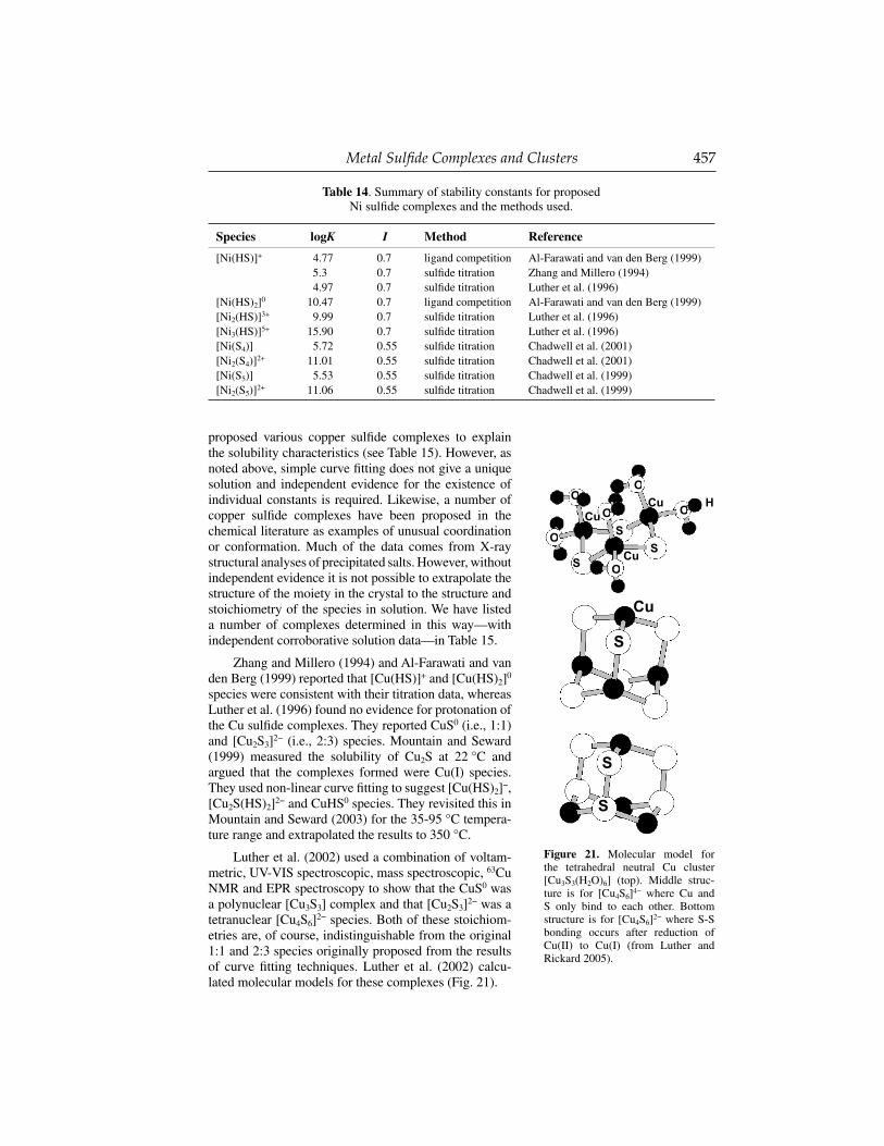
Metal Sulfi de Complexes and Clusters 457
proposed various copper sulfi de complexes to explain the solubility characteristics (see Table 15). However, as noted above, simple curve fi tting does not give a unique solution and independent evidence for the existence of individual constants is required. Likewise, a number of copper sulfi de complexes have been proposed in the chemical literature as examples of unusual coordination or conformation. Much of the data comes from X-ray structural analyses of precipitated salts. However, without independent evidence it is not possible to extrapolate the structure of the moiety in the crystal to the structure and stoichiometry of the species in solution. We have listed a number of complexes determined in this way—with independent corroborative solution data—in Table 15.
Zhang and Millero (1994) and Al-Farawati and van den Berg (1999) reported that [Cu(HS)]+ and [Cu(HS)2]0 species were consistent with their titration data, whereas Luther et al. (1996) found no evidence for protonation of the Cu sulfi de complexes. They reported CuS0 (i.e., 1:1) and [Cu2S3]2− (i.e., 2:3) species. Mountain and Seward (1999) measured the solubility of Cu2S at 22 °C and argued that the complexes formed were Cu(I) species. They used non-linear curve fi tting to suggest [Cu(HS)2]−, [Cu2S(HS)2]2− and CuHS0 species. They revisited this in Mountain and Seward (2003) for the 35-95 °C tempera-ture range and extrapolated the results to 350 °C.
Luther et al. (2002) used a combination of voltam-metric, UV-VIS spectroscopic, mass spectroscopic, 63Cu NMR and EPR spectroscopy to show that the CuS0 was a polynuclear [Cu3S3] complex and that [Cu2S3]2− was a tetranuclear [Cu4S6]2− species. Both of these stoichiom-etries are, of course, indistinguishable from the original 1:1 and 2:3 species originally proposed from the results of curve fi tting techniques. Luther et al. (2002) calcu-lated molecular models for these complexes (Fig. 21).
Table 14. Summary of stability constants for proposed Ni sulfi de complexes and the methods used.
Species logK I Method Reference
[Ni(HS)]+ 4.77 0.7 ligand competition Al-Farawati and van den Berg (1999)5.3 0.7 sulfi de titration Zhang and Millero (1994)4.97 0.7 sulfi de titration Luther et al. (1996)
[Ni(HS)2]0 10.47 0.7 ligand competition Al-Farawati and van den Berg (1999)[Ni2(HS)]3+ 9.99 0.7 sulfi de titration Luther et al. (1996)[Ni3(HS)]5+ 15.90 0.7 sulfi de titration Luther et al. (1996)[Ni(S4)] 5.72 0.55 sulfi de titration Chadwell et al. (2001)[Ni2(S4)]2+ 11.01 0.55 sulfi de titration Chadwell et al. (2001)[Ni(S5)] 5.53 0.55 sulfi de titration Chadwell et al. (1999)[Ni2(S5)]2+ 11.06 0.55 sulfi de titration Chadwell et al. (1999)
O
S
S
SO
O O
O
OHCu
Cu
Cu
Cu
S
S
S
Figure 21. Molecular model for the tetrahedral neutral Cu cluster [Cu3S3(H2O)6] (top). Middle struc-ture is for [Cu4S6]4− where Cu and S only bind to each other. Bottom structure is for [Cu4S6]2− where S-S bonding occurs after reduction of Cu(II) to Cu(I) (from Luther and Rickard 2005).

458 Rickard & Luther
Table 15. Summary of proposed Cu sulfi de complexes and the methods used.
Complex Method(s) Reference
[Cu(HS)]+ voltammetric titration sulfi de concentration Zhang and Millero (1994)
ligand competition Farawati and van den Berg (1999)
[Cu(HS)2]0 voltammetric titration sulfi de concentration Zhang and Millero (1994)
ligand competition Farawati and van den Berg (1999)
[CuS]0, [Cu3S3] voltammetry, UV-VIS spectroscopic, mass spectroscopy, 63Cu NMR, EPR spectroscopy
mole ratio Luther et al (1996)Luther et al. (2002)
[Cu2S3]2−, [Cu4S6]2− voltammetry, UV-VIS spectroscopic, mass spectroscopy, 63Cu NMR, EPR spectroscopy
mole ratio Luther et al (1996)Luther et al. (2002)
[Cu(HS)2]− curve fi tting Cu2S solubility Mountain and Seward (1999)
[Cu2S(HS)2]2− curve fi tting Cu2S solubility Mountain and Seward (1999)
[CuHS]0 curve fi tting Cu2S solubility Mountain and Seward (1999)
[Cu(HS)3]2−, [Cu3S4H2]2−, etc.
curve fi tting CuS solubility Thompson and Helz (1994)
[Cu2S(HS)2]2−, [Cu4S4H2]2−, etc.
curve fi tting CuS solubility Thompson and Helz (1994)
[Cu2S2(HS)3]3− curve fi tting CuS solubility Shea and Helz (1989) as re-interpreted by Thompson and Helz (1994)
[Cu2(S3)(S4)]2− curve fi tting CuS solubility Shea and Helz (1989) as re-interpreted by Thompson and Helz (1994)
[Cu(S9)(S10)]3− curve fi tting CuS solubility Shea and Helz (1989) as re-interpreted by Thompson and Helz (1994)
Multinuclear Cu complexes
EXAFS CuS in sulfi de solutions Helz et al. (1993)
[Cu3(S4)3]3− Raman, X-ray structure analysis Synthesis Müller et al. (1984b)
[Cu3(S6)3]3− IR, Raman, ESCA, UV/VIS spectroscopy, X-ray structure analysis
Synthesis Müller and Schimanski (1983)
[Cu6(S5)(S4)3]2− Raman, X-ray structure analysis Synthesis Müller et al. (1984a)
[Cu4(S5)3]2− Raman, X-ray structure analysis Synthesis Müller et al. (1984b)
[Cu4(S4)(S5)2]2− Raman, X-ray structure analysis Synthesis Müller et al. (1984b)
[Cu4(S4)2(S5)]2− Raman, X-ray structure analysis Synthesis Müller et al. (1984b)
[Cu(S4)]2 voltammetry chelate scale Chadwell et al. (1999)
[Cu(S5)]2 voltammetry chelate scale Chadwell et al. (2000)
[Cu(S4)2]3− curve fi tting CuS solubility in polysulfi de solution
Cloke (1963) from Höljte and Beckert (1935)
[Cu(S5)(S4)]3− curve fi tting CuS solubility in polysulfi de solution
Cloke (1963) from Höljte and Beckert (1935)

Metal Sulfi de Complexes and Clusters 459
Ciglenečki et al. (2005) proposed that all the previously reported Cu sulfi de complexes were actually nanoparticulate CuS. They stated that, not only the proposal for dissolved Cu sulfi de clusters by Luther et al. (2002) was suspect, but also the Cu complexes suggested by the results of Zhang and Millero (1994) and Al-Farawati and van den Berg (1999). They did not cite or comment upon the results of Mountain and Seward (1999, 2003). Earlier, Helz et al. (1993) had proposed multinuclear Cu sulfi de complexes on the basis of EXAFS studies. Thompson and Helz (1994) reported that Cu sulfi de solubility data suggested the presence of two Cu sulfi de complexes, one containing an odd number of Cu atoms (e.g., [Cu(HS)3]2− or [Cu3S4H2]2− or an even higher multimers) and one containing an even number of Cu atoms (e.g., [Cu2S(HS)2]2−, [Cu4S4H2]−, etc). Earlier, Shea and Helz (1989) had measured covellite solubility and Thompson and Helz (1994) reinterpreted these results in terms of species [Cu2S2(HS)3]3−, [Cu2(S3)(S4)]2− and [Cu(S9)(S10)]3−. However, Ciglenečki et al. (2005) then re-reinterpreted these results with the comment that the “measurement precision was insuffi cient to exclude mononuclear and dinuclear complexes as predominant species.”
And fi nally, they appeared to accept that the Cu clusters proposed by Helz et al. (1993) existed on the grounds that “the measured Cu-S and Cu-Cu distances were similar to those in known Cu4(RS)6
2− clusters and different from distances in Cu-S solid phases or linear Cu2S(HS)2
2− complexes” but then go on to state that the “existence of clusters as major dissolved Cu species in equilibrium with Cu sulfi de minerals is suggested by both studies but remains to be proven.”
Cluster-type complexes of polysulfi de with Cu are known and are reviewed by Müller and Diemann (1987). Müller and Schimanski (1983) and Müller et al. (1984a,b) suggested [(S6)Cu(S8)Cu(S6)]4−, [Cu3(S4)3]3−, [Cu3(S6)3]3−, [Cu6(S5)(S4)3]2− and the series [Cu4(S5)3]2−, [Cu4(S4)(S5)2]2− and [Cu4(S4)2(S5)]2. Chadwell et al. (1999, 2000) found evidence for the dimers [Cu2(S4)]2 and [Cu2(S5)]2 in aqueous solutions. Electrochemical evidence demonstrated proton-free 1:1 complexes but the ESR signal was silent. Since Cu(II) is d 9, an ESR signal is expected. Chadwell (1999, 2000) concluded that the complex was a dimer and has an unpaired electron on each of the Cu(II) antiparallel thus producing a silent ESR signal. This type of behavior has been observed for ferredoxins: e.g., complexes of the type [Fe2S2(SR)4]2−,3− and [Fe4S4(SR)4]2−,3− (Holm 1974; Papaefthymiou et al. 1982; Rao and Holm 2004). Chadwell et al. (1999, 2000) also noted some evidence for protonated Cu(II) polysulfi de complexes at pH below 6, but the nature of these complexes was not determined. Cloke (1963b) refi tted the solubility data from Höljte and Beckert (1935) with covellite in polysulfi de solutions and deduced two complexes from the data: [Cu(S4)2]−3 and [Cu(S5)(S4)]−3. These data are similar to those of Chadwell et al. (1999, 2001).
The polysulfi de data for Cu(II) are consistent with the sulfi de results proposed by Luther et al. (2002). It suggests that Cu(II) forms non-protonated complexes in neutral-alkaline solutions but possible protonated species in acid conditions. In addition, Müller and Schimanski (1983) recognized the central role that the Cu3S3 (formally Cu3(µ−S)3) ring confi guration, independently reported by Luther et al. (2002), played in the structure of Cu sulfi de clusters. Figure 22 shows the structure for [Cu3(S6)3]3− in which one terminal S atom from S6
2− binds to one Cu and the other terminal S atom binds to two Cu atoms. They described this as a “paradigmatic unit.” The polysulfi de data also seem similar to the results produced by Ciglenečki et al. (2005) and may provide an alternative explanation for their observations. As pointed out by
Cu3S183-
Cu
S
Figure 22. Molecular structure of the Cu polysulfi de complex, [Cu3(S6)3]3−.
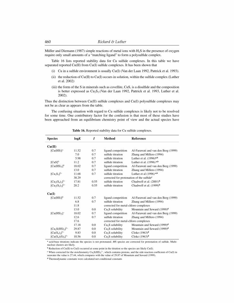
460 Rickard & Luther
Müller and Diemann (1987) simple reactions of metal ions with H2S in the presence of oxygen require only small amounts of a “matching ligand” to form a polysulfi de complex.
Table 16 lists reported stability data for Cu sulfi de complexes. In this table we have separated reported Cu(II) from Cu(I) sulfi de complexes. It has been shown that
(i) Cu in a sulfi de environment is usually Cu(I) (Van der Laan 1992, Pattrick et al. 1993).
(ii) the reduction of Cu(II) to Cu(I) occurs in solution, within the sulfi de complex (Luther et al. 2002)
(iii) the form of the S in minerals such as covellite, CuS, is a disulfi de and the composition is better expressed as Cu2S2.(Van der Laan 1992, Pattrick et al. 1993, Luther et al. 2002).
Thus the distinction between Cu(II) sulfi de complexes and Cu(I) polysulfi de complexes may not be as clear as appears from the table.
The confusing situation with regard to Cu sulfi de complexes is likely not to be resolved for some time. One contributory factor for the confusion is that most of these studies have been approached from an equilibrium chemistry point of view and the actual species have
Table 16. Reported stability data for Cu sulfi de complexes.
Species logK I Method Reference
Cu(II)[Cu(HS)]+ 11.52 0.7 ligand competition Al-Farawati and van den Berg (1999)
7.0 0.7 sulfi de titration Zhang and Millero (1994)5.98 0.7 sulfi de titration Luther et al. (1996)a,b
[CuS]0 11.2 0.7 sulfi de titration Luther et al. (1996) a,b
[Cu(HS)2]0 18.02 0.7 ligand competition Al-Farawati and van den Berg (1999)13.0 0.7 sulfi de titration Zhang and Millero (1994)
[Cu2S3]2− 11.68 0.7 sulfi de titration Luther et al (1996) a,b
38.29 corrected for protonation of the sulfi dec
[Cu2(S4)2]2− 17.81 0.55 sulfi de titration Chadwell et al. (2001)b
[Cu2(S5)2]2− 20.2 0.55 sulfi de titration Chadwell et al. (1999)b
Cu(I)[Cu(HS)]0 11.52 0.7 ligand competition Al-Farawati and van den Berg (1999)
6.8 0.7 sulfi de titration Zhang and Millero (1994)11.8 corrected for metal-chloro complexes13.0 0.0 Cu2S solubility Mountain and Seward (1999)d
[Cu(HS)2]− 18.02 0.7 ligand competition Al-Farawati and van den Berg (1999)12.6 0.7 sulfi de titration Zhang and Millero (1994)17.6 corrected for metal-chloro complexes17.18 0.0 Cu2S solubility Mountain and Seward (1999)d
[Cu2S(HS)2]2− 29.87 0.0 Cu2S solubility Mountain and Seward (1999)d
[Cu(S4)2]3− 9.83 0.0 Cu2S solubility Cloke (1963)d
[Cu(S4)(S)5]3− 10.56 0.0 Cu2S solubility Cloke (1963)d
a acid-base titrations indicate the species is not protonated. MS species are corrected for protonation of sulfi de. Multi-nuclear clusters are likely. b Reduction of Cu(II) to Cu(I) occurred at some point in the titration so the species are likely Cu(I). c When corrected for the stoichiometry Cu2S(HS)2
2−, which contains protons, and the side reaction coeffi cient of Cu(I) in seawater the value is 27.44, which compares with the value of 29.87 of Mountain and Seward (1999).d Thermodynamic constants were calculated not conditional constants

Metal Sulfi de Complexes and Clusters 461
not obviously been seen. The exception is the EXAFS data presented by Helz et al. (1993), the protonation data presented by Luther et al. (1996) and the EPR, 63Cu NMR and mass spectroscopic data of Luther et al. (2002). One way around the impasse is to examine the molecular mechanisms involved in the formation of the Cu sulfi de species and this, together with supporting Cu isotopic data, is discussed below.
Molybdenum
Molybdenum is a borderline hard-soft member of Group 6. It sits between Cr, a transition metal with characteristic borderline properties and W, a metal which is fi rmly in the hard category. So Mo has signifi cant oxide and sulfi de chemistries with the sulfi de MoS2, molybdenite, being the most important Mo mineral with the molybdate wulfenite, PbMoO4, being also signifi cant, whereas W occurs almost exclusively as tungstates.
MoS2 occurs in three polytypes, hexagonal molybdenite-2H which is hexagonal, molybdenite-2R, which is rhombohedral, and jordisite, which is apparently amorphous. The term molybdenite usually refers to the 2H polymorph. Even though this is a relatively common mineral, the importance of molybdenum sulfi de complexes is related to the use of molybdenum as a potential proxy for redox conditions (Dean et al. 1997) and the well-established molybdenum sulfi de cluster chemistry.
The electronic confi guration of Mo is [Kr]5s14d5 and all six outer electrons can be involved in bonding leading to oxidation states in complexes that vary between 0 and +6. Even the −2 state is known in organometallic complexes. Mo forms a variety of sulfi de complexes, the thiomolybdates, with a general formula [MoOxS4−x]n− where x = 0-3: [MoS4]2−, [MoOS3]2−, [MoO2S2]2− and [MoO3S]2−. These are bright yellow to red materials and have been the subject of interest since Berzelius’s time. The remarkable feature of these complexes is that Mo is in the highest oxidation state in coordination with reductive S(−II) ions. The other notable feature is that the Mo-S distance is consistent at 2.15-2.18 Å for all of these species, and this feature extends to analogous complexes with W, Re, Ta, Nb and V. This suggests some π character in the M2S bonds—as also suggested from MO calculations (Diemann and Müller 1973). Electron delocalisation through π bonding also explains why these anions do not undergo a spontaneous internal redox reaction. [MoS4]2− has been the most studied species since it is readily synthesised, easily converts to other dimolybdenum-thiols and has relatively high thermal and hydrolytic stability. It is also central to several key biological processes and has been implicated in geochemical processes. [MoS4]2− is easily prepared by passing H2S through an ammoniacal molybdate solution. After 20 minutes (NH4)MoS4 precipitates as very pure red crystals (Mellor 1943). Formation of [MoS4]2− from [MoO4]2− clearly proceeds via successive replacement of oxygen, as evidenced from the colour sequence change in solution: [MoO4]2−(colorless) → R[MoO3S]2−(yellow) → R[MoO2S2]2−(orange) → R[MoOS3]2−(orange-red) → R[MoS4]2−(red). This can be readily traced with UV-VIS spectroscopy and the kinetics of the process have been established (Harmer and Sykes 1980). Its complete formation in aqueous solution requires high S-Mo ratios and its rate of hydrolysis increases with increasing H+ concentrations without the formation of the intermediate oxythio ions (Clarke et al. 1987). These data were later used by Erickson and Helz (2000) to suggest a “geochemical switch” in which Mo exists in two distinct regimes in natural environments, as [MoO4]2− in oxic and low sulfi dation (Rickard and Morse 2005) regimes and [MoS4]2− in high sulfi dation environments. The H+ dependence of the geochemical switch was considered by Tossell (2005) in terms of equilibrium chemistry, and he noted that it would be inhibited at high pH where HS− dominated.
Earlier claims that [MoS4]2− polymerises at low pH have not been substantiated (Laurie 2000). Treatment with polysulfi des produces dimeric and trimeric species in which the Mo centres have been reduced to Mo(V) and Mo(IV), e.g., (NH4)2[Mo(V)2(S2)6]·2H2O and (NH4)2[Mo(IV)3S(S2)6] (Müller et al. 1978, 1980; Coucouvanis and Hadjikyriacou 1986).

462 Rickard & Luther
The thiomolybdates form a variety of complexes with ligands where the basic [MoOxS4−x]n− moiety is retained. The S(−II) ions act as bridging ligands in which they bridge 2, 3 or 4 metal centers. These complexes range from simple linear structures to cubanes and more complex forms (Fig. 23). They have been widely reviewed (Müller and Diemann 1987; Dance and Fischer 1991; Eichhorn 1994; Wu et al. 1996) since they have been used as nonlinear optical materials, industrial catalysts and as models for the active [Fe2Mo2S] cluster site in the metalloenzyme nitrogenase. Bostick et al. (2003) showed that when [MoS4]2− reacts with the surface of pyrite Fe-Mo-S cuboidal clusters form where the original Mo(VI) has been reduced to Mo(IV) and Mo(III) (Mascharak et al. 1983; Osterloh et al. 2000). Vorlicek et al. (2004) noted that the formation of polymeric species of Mo polysulfi des (Müller et al. 1978, 1980; Coucouvanis and Hadjikyriacou 1986) is consistent with this observation. The sorption of Mo on pyrite is an important process since Mo has been proposed to be a proxy for anoxic, sulfi dic conditions, and much of the Mo in this environment appears to be associated with pyrite (Raiswell and Plant 1980; Coveney 1987; Huerta-Diaz and Morse 1992; Dellwig et al. 2002; Müller 2002).
Silver and gold
Groups 8 through 11 of the periodic table include the noble metals. These are d-block elements whose characteristic property is that they are resistant to oxidation. They are typical soft metals with a strong predilection for forming sulfi de complexes. We consider the sulfi de complex chemistry of Ag and Au here since these have some geochemical signifi cance. Ag and Au are Group 11 elements together with Cu of the fi rst transition series. They all have a single s electron outside the fi lled d shell. Even so the properties of these three elements vary more than might be expected from the similar electronic structures. Of course, relativistic effects on the 6s electron might explain some of the differences between Ag and Au. This leads to the relativistic contraction: i.e. Au displays similar, or even smaller, covalent radii in similar compounds to Ag. In contrast, the ionic radius of Au+ is substantially larger than Ag+ (Ishikawa et al. 1995). The result is that in mainly covalent compounds such as sulfi des, the stability of the Au+ complexes is similar to or slighty greater than the stability of the Ag+ complexes.
Oxidation states in this group appear erratic. Thus, as we have seen, Cu is commonly Cu(I) or Cu(II), whereas Ag is typically Ag(I) and Au is Au(I) or Au(III). Cu(I), Ag(I) and Au(I) display soft character because of the relatively small energy difference between the frontier orbitals of these ions.
CuCu Mo
P
P
P
S S
SS
Mo
P P
P P
S
S S
S
Ag Ag
Mo
P
P
S
SS
Ag
Cu
O
CN
Mo
P
P
P
S
S
S S
Cu
CuCu
Cl
Figure 23. Some simple linear and cubane structures in schematic form illustrating the ability of thiomolybdate anions to act as ligands and as building blocks for more complex structures (P = triphenylphosphane) (adapted from Laurie 2000).

Metal Sulfi de Complexes and Clusters 463
Silver. The black precipitate that occurs through the reaction between S(−II) and Ag salts in aqueous solution at room temperature is monoclinic Ag2S, acanthite. Above 177 °C this transforms rapidly and reversibly to the isometric polymorph, argentite. It is claimed that Ag2S is the least soluble of all known silver compounds (e.g., Cotton et al. 1999). However, it was known as long ago as 1949 that the solubility is pH independent in acid solutions but increases markedly with pH in alkaline systems (Treadwell and Hepenstick 1949). Schwarzenbach and Widmer (1966) measured the solubility of Ag2S and proposed that [AgHS], [Ag(HS)2]− and [Ag2S(HS)2]2− complexes dominated successively with increasing pH. Sugaki et al. (1987) interpreted the results of similar solubility experiments in terms of binuclear Ag sulfi de complexes, [Ag2S(H2S)]0, [Ag2S(H2S)(HS)]−, [Ag2S(H2S)(HS)2]2− and [Ag2S(HS)2]2−. Gammons and Barnes (1989) proposed that [Ag(HS)2]− was the dominant sulfi de complex between pH 5.8 and 7.3. Stefánsson and Seward (2003) studied the solubility of crystalline Ag2S between 25-400°C and treated the data with a non-linear least squares fi tting routine which considered all the hitherto proposed complexes. They found that the data were consistent with [AgHS], [Ag(HS)2]− and [Ag2S(HS)2]2− being the dominant species.
The result of Stefánsson and Seward’s (2003) model for Ag sulfi de complexing is shown graphically in Figure 24. This suggests that [AgHS]0 and [Ag2S(HS)2]2− are the most important complexes in seawater systems. Zhang and Millero (1994) using voltammetric titrations, provided evidence for [AgHS]0 and [Ag(HS)2]− complexes. Al-Farawati and van den Berg
0
20
40
60
100
80
4 6 8 10 12
AgHS0 Ag2S(HS)2
2-
%
pH
Figure 24. Percentage distribution of Ag(I) species versus pH for a deep anoxic seawater system with total dissolved S(−II) = 5 × 10⁻⁴ M and total dissolved Cl(−I) = 0.55 at 25 °C from the data in Stefansson and Seward (2003).
Table 17. Comparison of stability constant data for the [Ag(HS)]0 and [Ag(HS)2]− species, corrected for Ag side reaction coeffi cients.
logKCONDMethod Reference
1:1 1:2
10.8 — Titration Luther and Rickard (2005)≥9.5 ≥15.3 Titration Zhang and Millero (1994)13.6 17.7 Solubility of Ag2S Schwarzenbach and Widmer (1966)
13.49 — Solubility of Ag2S Gammons and Barnes (1989)11.6 — Titration Al-Farawati and van den Berg (1999)

464 Rickard & Luther
(1999) provided evidence only for [AgHS]0. Table 17 shows a comparison of stability constant data for the [AgHS]0 and [Ag(HS)2]− species, corrected for Ag side reaction coeffi cients.
The infl uence of the fi lled d10 shell on Ag chemistry is exemplifi ed by the abundance of Ag cluster compounds. Many compounds show weak Ag-Ag interactions giving rise to the possibility of polynuclear complexes. In many of these, the Ag appears to be zero or even subvalent. Indeed the Ag13 unit has been found to be central to a series of superclusters, including both simple carbonyls and more complex mixed Au-Ag species. Rozan and Luther (2002) looked at Ag sulfi de complexing in a different way. They found that they could replace Zn and Cu in aqueous ZnS and CuS clusters to produce relatively stable AgS clusters, with suggested [AgS]− and [Ag3S3]3− stoichiometries. They found that these forms were relatively stable and could explain enhanced dissolved Ag(I) concentrations in fresh water systems. Some support for this idea comes from the voltammetric acid-base titrations reported by Luther and Rickard (2005). These showed evidence for 1:1 and 2:1 Ag-S complexes and also demonstrated that the Ag-S species are not protonated and are likely multi-nuclear clusters. Using the side reaction coeffi cients for both Ag and sulfi de, they obtained stability constants of logKtherm = 22.8 for [AgS]− and logK therm = 29.1 for the [Ag2S]0 complexes.
Cloke (1963b) investigated the solubility of acanthite in polysulfi de solutions and proposed [Ag(S4)2]3−, [Ag(S4)(S5)]3− and [Ag(HS)S4]2− complexes. Cloke (1963b) was handicapped by a lack of good polysulfi de data but, even so, his work shows the potential importance of polysulfi des in Ag solution chemistry. Cloke (1963b) suggested similar stoi-chiometries for Cu polysulfi de species which are now known to be Cu2(S4)2 and Cu2(S5)2 (Chadwell et al. 1999, 2002). It is possible, therefore, that the Ag polysulfi de species have similar stoichiometries. It is surprising that it appears that no further work on these Ag poly-sulfi de complexes has been published.
Table 18 lists the stability constants reported for Ag sulfi de complexes.
Gold. Gold forms two simple sulfi des, Au2S and Au2S3, both of which are metastable and neither of which are known to occur naturally as discrete minerals. The nearest minerals are the rare Au-Ag sulfi des. Both Au2S and Au2S3 dissociate readily to form metallic Au, which refl ects the extra stability of the Au nuclide in its ground state. This is a major technical problem in experimental studies of Au sulfi de complexes (cf. Stefánsson and Seward 2004). Although Au2S can be formed as a pure compound (Gurevich et al. 2004) its synthesis is not simple and the product risks including nanoparticulate Au0. Since, except for Tossell’s (1996) theoretical study, Au sulfi de complexes have only been proposed through curve fi tting of solubility data, this has led to some uncertainty in their defi nition.
Au solubilility in sulfi de solutions is enhanced by the formation of Au sulfi de complexes. This has important consequences for the transport of gold in natural systems, especially at elevated temperatures (see Stefánsson and Seward 2004 for a review of this work). Belevantsev et al. (1981) measured the solubility of Au2S in sulfi de solutions at 25 °C and proposed that [Au(HS)2]−, [Au2(HS)2S]2− and [Au(HS)(OH)]− were the dominant complexes. This was a diversion from the classical view that Au existed as [AuS]− (Latimer 1952). Renders and Seward (1989) measured the solubility of Au2S at 25 °C and proposed that [Au(HS)]0, [Au(HS)2]− and [Au2S2]2− complexes dominated. Zotov et al. (1996) proposed [Au(HS)2]− at near neutral conditions. Baranova and Zotov (1998) fi tted [Au(HS)]0 and [Au(HS)2]− to Au solubility data in acid sulfi dic solutions. Tossell (1996) used quantum mechanical computations to suggest that the species at low pH would be coordinated with H2O and thus be represented as [Au(HS)(H2O)]0. He confi rmed [Au(HS)2]− at neutral pH but suggested that [Au(HS)(OH)]− would predominate at high pH rather than dimers like [Au2S2]2−.
The results of the Renders and Seward (1989) measurements are shown in Figure 25. The data suggest, even taking into account later strictures on the possibility of Au0 contamination

Metal Sulfi de Complexes and Clusters 465
Table 18. Reported stability constants for Ag sulfi de complexes.
Species logK I Method Reference
[Ag(HS)]0 6.38 0.7 sulfi de titration Al-Farawati and van den Berg (1999)
11.6 corrected for metal-ligand complexes in seawater
≥9.5 0.7 sulfi de titration Zhang and Millero (1994)
13.6 1.0 Ag2S solubility Schwarzenbach and Widmer (1966)b
13.48 0.0 Ag2S solubility Renders and Seward (1989) b
15.89 0.0 Ag2S solubility Stephansson and Seward (2003)b
10.8 0.7 sulfi de titration Luther and Rickard (2005)a
[AgS]− 22.8 0.7 sulfi de titration Luther and Rickard (2005)a,b
[Ag(HS)2]− ≥15.3 0.7 sulfi de titration Zhang and Millero (1994)
17.17 1.0 Ag2S solubility Schwarzenbach and Widmer (1966)b
17.28 0.0 Ag2S solubility Gammons and Barnes (1989)b
17.43 0.0 Ag2S solubility Renders and Seward (1989)b
17.54 0.0 Ag2S solubility Stephansson and Seward (2003)b
[Ag2S(HS)2]2− 72.9 1.0 Ag2S solubility Schwarzenbach and Widmer (1966)b
31.43 0.0 Ag2S solubility Renders and Seward (1989)b
31.24 0.0 Ag2S solubility Stephansson and Seward (2003)b
[Ag2S]0 29.1 0.7 sulfi de titration Luther and Rickard (2005)a,b
[Ag(HS)(S4)]2− 7.40 0.0 Ag2S solubility Cloke (1963)b
[Ag(S4)2]3− 16.46 0.0 Ag2S solubility Cloke (1963)b
[Ag(S4)(S5)]3− 16.78 0.0 Ag2S solubility Cloke (1963)b
a acid-base titrations indicate the species is not protonated. MS species are corrected for protonation of sulfi de. Multi-nuclear clusters are likely.b Thermodynamic constants were calculated not conditional constants.
Au2S22-
Au(HS)2-
AuHS+
-3
-4
-5
-6
-7
-8
-9
2 4 6 8 10 12
pH
log
AuT
M
Figure 25. Solubility of Au2S at 25 °C in the presence of 0.01 m total reduced S from Renders and Seward (1989) in terms of the concentration of total dissolved Au (AuT) and pH. The bold curve is the locus of the measured experimental data and the thin lines represent the theoretical species boundaries.
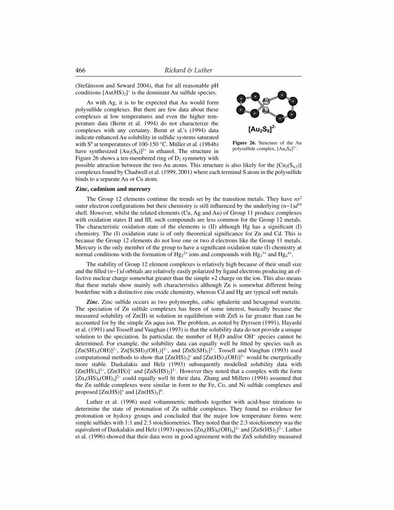
466 Rickard & Luther
(Stefánsson and Seward 2004), that for all reasonable pH conditions [Au(HS)2]− is the dominant Au sulfi de species.
As with Ag, it is to be expected that Au would form polysulfi de complexes. But there are few data about these complexes at low temperatures and even the higher tem-perature data (Bernt et al. 1994) do not characterize the complexes with any certainty. Bernt et al.’s (1994) data indicate enhanced Au solubility in sulfi dic systems saturated with S0 at temperatures of 100-150 °C. Müller et al. (1984b) have synthesized [Au2(S8)]2− in ethanol. The structure in Figure 26 shows a ten-membered ring of D2 symmetry with possible attraction between the two Au atoms. This structure is also likely for the [Cu2(S4,5)] complexes found by Chadwell et al. (1999, 2001) where each terminal S atom in the polysulfi de binds to a separate Au or Cu atom.
Zinc, cadmium and mercury
The Group 12 elements continue the trends set by the transition metals. They have ns2 outer electron confi gurations but their chemistry is still infl uenced by the underlying (n−1)d10 shell. However, whilst the related elements (Cu, Ag and Au) of Group 11 produce complexes with oxidation states II and III, such compounds are less common for the Group 12 metals. The characteristic oxidation state of the elements is (II) although Hg has a signifi cant (I) chemistry. The (I) oxidation state is of only theoretical signifi cance for Zn and Cd. This is because the Group 12 elements do not lose one or two d electrons like the Group 11 metals. Mercury is the only member of the group to have a signifi cant oxidation state (I) chemistry at normal conditions with the formation of Hg2
2+ ions and compounds with Hg33+ and Hg4
4+.
The stability of Group 12 element complexes is relatively high because of their small size and the fi lled (n−1)d orbitals are relatively easily polarized by ligand electrons producing an ef-fective nuclear charge somewhat greater than the simple +2 charge on the ion. This also means that these metals show mainly soft characteristics although Zn is somewhat different being borderline with a distinctive zinc oxide chemistry, whereas Cd and Hg are typical soft metals.
Zinc. Zinc sulfi de occurs as two polymorphs, cubic sphalerite and hexagonal wurtzite. The speciation of Zn sulfi de complexes has been of some interest, basically because the measured solubility of Zn(II) in solution in equilibrium with ZnS is far greater than can be accounted for by the simple Zn aqua ion. The problem, as noted by Dyrssen (1991), Hayashi et al. (1991) and Tossell and Vaughan (1993) is that the solubility data do not provide a unique solution to the speciation. In particular, the number of H2O and/or OH− species cannot be determined. For example, the solubility data can equally well be fi tted by species such as [Zn(SH)3(OH)]2−, Zn[S(SH)2(OH2)]2−, and [ZnS(SH)2]2−. Tossell and Vaughan (1993) used computational methods to show that [Zn(HS)3]− and [Zn(HS)3(OH)]2− would be energetically more stable. Daskalakis and Helz (1993) subsequently modelled solubility data with [Zn(HS)4]2−, [Zn(HS)]− and [ZnS(HS)2]2−. However they noted that a complex with the form [Zn4(HS)6(OH)4]2− could equally well fi t their data. Zhang and Millero (1994) assumed that the Zn sulfi de complexes were similar in form to the Fe, Co, and Ni sulfi de complexes and proposed [Zn(HS)]+ and [Zn(HS)2]0.
Luther et al. (1996) used voltammetric methods together with acid-base titrations to determine the state of protonation of Zn sulfi de complexes. They found no evidence for protonation or hydoxy groups and concluded that the major low temperature forms were simple sulfi des with 1:1 and 2:3 stoichiometries. They noted that the 2:3 stoichiometry was the equivalent of Daskalakis and Helz (1993) species [Zn4(HS)6(OH)4]2− and [ZnS(HS)2]2−. Luther et al. (1996) showed that their data were in good agreement with the ZnS solubility measured
[Au2S8]2-
Au
Au
Figure 26. Structure of the Au polysulfi de complex, [Au2S8]2−.

Metal Sulfi de Complexes and Clusters 467
by Gubeli and Ste Marie (1967), which had been found to be far too high by Daskalakis and Helz (1993). The key is replacing Gubeli and Ste Marie’s (1967) assumed [Zn(OH)(HS)] form with the actual [Zn2S3]2−. Daskalakis and Helz (1993) had found colloidal ZnS in their systems and had explained the high Gubeli and Ste Marie (1967) numbers by proposing that these investigators were also measuring colloidal suspensions.
Luther et al. (1999) reported that their polymetallic Zn sulfi de complexes were essentially clusters according to Cotton et al’s (1999) defi nition cited above. They probed the Zn sulfi de complexes with UV-VIS spectroscopy and modelled the species using molecular mechanical calculations. The resulting structures are shown in Figure 27. Luther et al. (1999) agreed with Daskalakis and Helz (1993) that Zn thiolate chemistry (Blower and Dilworth 1987; Prince 1987) suggest that the ZnS cluster with 2:3 stoichiometry is likely to be a tetramer and the acid-base titration data of Luther et al. (1996) suggested a formulation, Zn4S6
4−. In water, this combines with 4 inner shell H2O molecules to give an overall formulation of [Zn4S6(H2O)4]4−. For the complex with 1:1 stoichiometry they concluded that the probable formulation was [Zn3S3(H2O)6] based on the structure of known ZnS clusters with thiols. Table 19 lists the evidence for clusters. We list this table, taken from Luther et al. (1999), to demonstrate the sort of independent evidence that can be aquired for the composition of complexes and the methods by which these data can be collected.
As mentioned above, Sukola et al. (2005) defi ned their “clusters” as what would be called nanoparticles in the geochemical literature. Surprisingly they found no evidence for nanoparticulate ZnS even though it has been characterized in some detail by Zhang et al. (2003). They suggested that the Zn sulfi de solutions were a mixture of dissolved Zn sulfi de complexes and ZnS colloids.
Chadwell et al. (1999, 2000) characterized Zn polysulfi de complexes. They reported monodentate [Zn(η1−S4)] and [Zn(η1−S5)] above pH = 6 and their conjugate acids at pH < 6 similar to the forms found for Cu. Again the Zn polysulfi de complexes are non-protonated above pH = 6, and this result is consistent with the non-protonated Zn sulfi de complexes described above. Using organic solvents, Coucouvanis et al. (1985) synthesized and characterized several bidentate polysulfi de complexes including [Zn(S4)2]2−, [Zn(S5)2]2−, [Zn(S6)2]2−.
Proposed Zn sulfi de complexes and their reported stability constants are listed in Table 20.
Cadmium. Cadmium (II), in contrast to zinc (II), is classed fi rmly as a soft metal ion. This is refl ected in the relative instability of the cadmiate ion compared to zincates. It is therefore expected that Cd(II) will have a signifi cant sulfi de chemistry. Cd(II) is also a toxic metal and thus its sulfi de chemistry has some environmental interest. In view of this, it is surprising how little, comparatively speaking, is known about Cd sulfi de complexes. None have ever been observed and all the evidence stems from curve fi tting of solubility data or voltammetric titrations. Little other evidence for their composition or structure has been reported.
Ste-Marie et al. (1964) explained their solubility data in terms of the complexes [Cd(HS)]+, [Cd(HS)2]0, [Cd(HS)3]− and [Cd(HS)4]2−. However, Dyrssen (1985) re-evaluated
Zn
ZnZn
Zn
SS
SS
S
S
OH
Zn
Zn
Zn
S
S
S
OH
a) Zn4S6(H2O)42-
b) Zn3S3(H2O)6
Figure 27. (a) Structure for the cluster [Zn4S6(H2O)4]4−. (b) Structure for the ring [Zn3S3(H2O)6]0.

468 Rickard & LutherTa
ble
19. S
umm
ary
of e
xper
imen
tal d
ata
supp
ortin
g so
lubl
e Z
nS c
lust
er s
peci
es. (
From
Lut
her
et a
l. 19
99).
Rea
ctio
n st
ep
Zn(
II) +
S(I
I−) →
[Zn 3
S 3]
[Zn 3
S 3] →
[Zn 4
S 6]4−
+ Z
n(II
) [Z
n 4S 6
4−] →
ZnS
↓
Des
crip
tion
Aqu
eous
Zn(
II) r
eact
s w
ith a
queo
us S
(−II)
to
prod
uce
an a
queo
us Z
n 3S 3
, clu
ster
Zn3S
3 cl
uste
rs r
eact
with
aqu
eous
S(−
II) t
o pr
oduc
e an
aq
ueou
s [Zn
4S6 4−
] clu
ster
Aqu
eous
[Zn
4S64−
] cl
uste
rs c
onde
nse
with
Zn
3S3
to f
orm
sol
id Z
nS w
ith a
cha
nge
of
coor
dina
tion
in S
from
2 to
4
Clu
ster
MW
Zn
3S3(H
2O) 6
(MW
= 4
00.4
Da)
[Z
n 4S 6
(H2O
) 4]4−
(M
W =
526
.0 D
a)
Evi
denc
e el
ectro
chem
ical
Ti
tratio
ns s
how
an
initi
al 1
:1 (
S(−I
I) co
mpl
ex
with
Zn(
II). T
o be
iner
t the
ZnS
spe
cies
mus
t co
ntai
n S-
Zn-S
bon
ds
Furth
er ti
tratio
n sh
ows
a 2:
3 S(−I
I) co
mpl
ex w
ith Z
n(II)
. Zn
(II)
is re
leas
ed in
to s
olut
ion
and
can
be a
ccou
nted
for
ac
cord
ing
to st
oich
iom
etric
cal
cula
tions
.
spec
trosc
opic
Lo
ss o
f HS−
pea
k an
d p
rodu
ctio
n of
ZnS
pea
ks.
Qua
ntum
confi n
emen
t ca
lcul
atio
ns sh
ow a
size
of
1.6
nm
(16
Å) o
r les
s
Filtr
atio
n re
sults
indi
cate
a s
ize
for t
he in
itial
clu
sters
less
th
an 1
000
dalto
ns b
ased
on
the
200
nm a
bsor
ptio
n pe
ak.
Bul
k Z
nS h
as a
n ab
sorp
tion
at lo
nger
λ (
380
nm)
than
the
mol
ecul
ar c
luste
rs
gel e
lect
roph
ores
is
Neg
ativ
ely
char
ged
ZnS
clus
ter
grav
itate
s to
the
posit
ive
elec
trode
. Mas
s is b
etw
een
350
and
750
dalto
ns
Mol
ecul
ar m
odel
ing
Kno
wn
ZnS
clus
ters
with
thi
ols
have
Zn 3
S 3
confi
gur
atio
ns. Z
n 3S 3
(H2O
) 6 ha
s a
size
near
7
Å C
alcu
latio
ns sh
ow c
luste
r siz
e is
smal
ler t
han
equi
vale
nt st
ruct
ured
uni
ts in
the
min
eral
Zn4S
64− is
the
mos
t sta
ble
confi
gur
atio
n w
ith a
siz
e of
9.7
Å
. Mol
ecul
ar o
rbita
l (M
O) c
alcu
latio
ns sh
ow th
at c
luste
rs
form
fro
m t
he o
verla
p of
Zn 3
S 3 r
ings
(B
urde
tt 19
80).
Cal
cula
tions
sho
w c
luste
r siz
e is
smal
ler t
han
the
min
eral
sin
ce S
is 2
-coo
rdin
ated
in th
e cl
uste
r an
d 4-
coor
dina
ted
in th
e m
iner
al
Zn3S
3 rin
gs o
f Zn 4
S 64−
hav
e ch
air c
onfi g
ura-
tions
as i
n sp
hale
rite.
MO
theo
ry sh
ows t
hat
addi
tiona
l cr
ossli
nkin
g re
sults
in
min
eral
fo
rmat
ion
(Bur
dett
1980
)
Kin
etic
s Pr
oton
loss
occ
urs i
n th
e in
itial
reac
tion
(Lut
her
et a
l. 19
96).
Obs
erve
d fo
r Fe(
II) (R
icka
rd 1
989,
19
95;
Theb
erge
and
Lut
her
1997
) D
iffus
ion
cont
rolle
d re
actio
n re
late
d to
rate
of w
ater
loss
fro
m Z
n(II)
UV-
VIS
resu
lts s
how
on
agin
g th
at th
e Zn
S ab
sorp
tion
at
200
nm s
hifts
to 2
40, 2
60 a
nd 2
90 n
m Z
n 4S 6
4– a
nd Z
n 3S 3
ar
e el
ectro
chem
ical
ly in
ert
Clu
sters
ag
e to
fo
rm
larg
er
parti
cles
(S
ookl
al e
t al.
1996
) U
V-V
IS r
esul
ts sh
ow
a ve
ry s
low
inc
reas
e in
abs
orba
nce
of a
Zn
S sp
ecie
s at
380
nm
.Thi
s pe
ak a
ppea
rs
(0.0
04 a
bsor
banc
e un
its) a
fter 2
hou
rs a
nd is
sim
ilar
to b
ulk
sem
icon
duct
or Z
nS (
Kor
tan
et a
l. 19
90)
Oth
er w
ork
Sign
ifi ca
nt c
oval
ent
bond
ing
in Z
n-S
is in
ac
cord
ance
with
pre
viou
s re
sear
ch w
ith t
hiol
ca
pped
mol
ecul
ar c
luste
rs (
Her
ron
et a
l. 19
90;
Kor
tan
et a
l. 19
90,
Ned
eljk
ovic
et
al.
1993
; Vo
ssm
eyer
et a
l. 19
95)
Ther
mod
ynam
ic
mod
elin
g of
di
ssol
utio
n ex
perim
ents
show
s a
Zn:S
com
plex
with
pos
sible
4:6
sto
ichi
omet
ry
(Das
kala
kis
and
Hel
z 19
93a)
Mas
s sp
ectro
met
ry o
f cl
us-
ters
con
tain
ing
thio
ls sh
ow 4
Zn:
6 S
stoi
chio
met
ry (L
øver
et
al.
1997
) EX
AFS
dat
a in
dica
te p
artic
les,
200
Å th
at a
re
not i
n re
vers
ible
equ
ilibr
ium
with
the
solu
tion
phas
e (H
elz
et a
l. 19
93)
Solid
ZnS
for
ms
initi
ally
as
an a
mor
phou
s pr
ecip
itate
whi
ch d
evel
ops a
mai
nly
spha
ler-
ite s
truct
ure
(Ric
kard
and
Old
royd
, unp
ub.)
Bul
k se
mi-c
ondu
ctor
ZnS
has
an
abso
rptio
n at
lon
ger
λ (3
80 n
m)
than
the
mol
ecul
ar
clus
ters
(Kor
tan
et a
l. 19
90)

Metal Sulfi de Complexes and Clusters 469
their experimental measurements and showed that these could be better explained by complexes such as [Cd(HS)2]0 and [CdHS2]−, by analogy with the Hg complexes proposed by Schwarzenbach and Widmer (1963). Since these were actually derived by curve fi tting too, the extrapolation is uncertain. Dyrssen (1988) revisited the Ste-Marie et al. (1964) experimental data in 1988 and proposed that the best fi t would be obtained with the complexes, [CdS]0, [Cd(HS)]+ and [Cd(HS)2]0. The solubility studies of Wang and Tessier (1999) gave similar results to those of Ste-Marie et al. (1964). However, Daskalakis and Helz (1992) using similar methods found evidence for only [CdOHS]−, [Cd(HS)3]− and [Cd(HS)4]2−. Zhang and Millero (1994) investigated voltammetric titrations of Cd(II) versus S(−II) and proposed [CdHS]+ and [Cd(HS)2]0 as the dominant species, an idea which was followed by Al-Farawati and van den Berg (1999). If [Cd(HS)3]− and [Cd(HS)4]2− exist as discrete entities, these would have a tetrahedral Cd(II) center with a structure similar to that in [Cd(HS)3]− (Fig. 28). Proposed Cd sulfi de complexes are listed in Table 21.
The Cd-S system has been studied by several workers using both electrochemical and solubility methods with reasonable agreement for 1:1 and 1:2 Cd-S complexes (Table 22).
By analogy with the Zn-S system, the [Cd(HS)3]− species is likely a [Cd4S6] cluster species, but Wang and Tessier (1999) as well as Daskalakis and Helz (1992) did not discuss this possibility. Tsang et al. (in press) performed mole
Table 20. Proposed Zn sulfi de complexes and their reported stability constants.
Species logK I Method Reference
[Zn(SH)(OH)]0 19.02 1.0 ZnS solubility Gubelie and Ste-Marie (1967)b, c
[Zn(HS)]− 5.78 0.7 ligand competition Al-Farawati and van den Berg (1999)6.0 0.7 sulfi de titration Zhang and Millero (1994)6.63 0.7 sulfi de titration Luther et al. (1996)a
[ZnS]0 11.74 0.7 sulfi de titration Luther et al. (1996)a,b
[Zn(HS)2]0 12.9 0.0 ZnS solubility Dyrssen (1991)d
9.88 0.7 ligand competition Al-Farawati and van den Berg (1999)13.7 0.7 sulfi de titration Zhang and Millero (1994)
[ZnS(HS)]− 13.83 0.0 ZnS solubility Daskalakis and Helz (1993)[Zn(HS)3]− 14.9 0.0 ZnS solubility Dyrssen (1991)d
[ZnS(HS)2]2− 13.14 0.0 ZnS solubility Daskalakis and Helz (1993)[Zn(HS)4]2− 14.8 0.0 ZnS solubility Dyrssen (1991)d
14.64 0.0 ZnS solubility Daskalakis and Helz (1993)[Zn2S3]2− 13.83 0.7 sulfi de titration Luther et al. (1996)
41.09 corrected for protonation of the sulfi dec
[Zn(S4)]0 8.37 0.55 sulfi de titration Chadwell et al. (2001)[Zn(S5)]0 8.74 0.55 sulfi de titration Chadwell et al. (1999)
a acid-base titrations indicate the species is not protonated. MS species are corrected for protonation of sulfi de. Multi-nuclear clusters are likely.b Thermodynamic constants were calculated not conditional constants.c Correcting for Zn2S3
2− gives a value of 44.34 which compares with the value of 41.09 of Luther et al (1996).d Dyrssen’s recalculation of Hayashi et al (1990).
Cd
SS
S
O
Cd(SH)3(OH2)-
Figure 28. The theoretical structure of an ion with the composition [Cd(SH)3(H2O)]−.

470 Rickard & Luther
ratio titration methodology at pH ~ 7 and showed that 1:1 and 1:2 Cd:S complexes formed. Other titrations at higher pH showed evidence for a [Cd2S3] (or [Cd4S6]) species (Mullaugh and Luther, unpublished). However, the Cd complexes were not protonated based on acid-base titrations. The conditional stability constant for the 1:1 complex agrees with that of the other groups, and correction for the proton side reaction coeffi cient of sulfi de gives a stability constant of logKtherm = 23.4 for CdS. As there was no detectable Cd signal for Cd in sulfi de solutions, the chelate scale approach indicated that the logKtherm is greater than 34.4. Thus a cluster complex [Cd4S6] is likely based on these data. Using organic solvents, Coucouvanis et al. (1985) synthesized and characterized [Cd(S6)2]2−.
Mercury. Addition of S(−II) to aqueous Hg2+ produces black mercuric sulfi de, HgS or metacinnabar, which has a ZnS structure. Metacinnabar is unstable with respect to red, rhombohedral HgS or cinnabar, at temperatures lower than 344°C (Barnes and Seward 1979), and the transformation is kinetically rapid. A third polymorph, hypercinnabar, a dark purple-black phase with a hexagonal structure is also known. Mercury is relatively toxic and its sulfi de chemistry is therefore of considerable environmental interest.
Mercury is unique amongst the metals in being a liquid at room temperature. Its fi lled 4f shell and relativistic effects increase the binding of Hg electrons so that its fi rst ionization potential is greater than any other metal. Relativistic effects are the relative mass increase for a moving particle, and these begin to be signifi cant for the heavier elements, such as Hg. The
Table 21. Proposed Cd sulfi de complexes.
Species logK I Method Reference
[Cd(HS)]+ 6.85 0.7 ligand competition Al-Farawati and van den Berg (1999)6.3 0.7 sulfi de titration Zhang and Millero (1994)7.55 1.0 CdS solubility Ste-Marie et al. (1964)7.38 0.0 CdS solubility Wang and Tessier (1999)
[Cd(HS)2]0 13.95 0.7 ligand competition Al-Farawati and van den Berg (1999)12.7 0.7 sulfi de titration Zhang and Millero (1994)14.61 1.0 CdS solubility Ste-Marie et al. (1964)14.43 0.0 CdS solubility Wang and Tessier (1999)
[Cd(HS)3]− 16.49 1.0 CdS solubility Ste-Marie et al. (1964)16.44 0.0 CdS solubility Daskalakis and Helz (1992)16.26 0.0 CdS solubility Wang and Tessier (1999)
[Cd(HS)4]2− 18.85 1.0 CdS solubility Ste-Marie et al. (1964)17.89 0.0 CdS solubility Daskalakis and Helz (1992)18.43 0.0 CdS solubility Wang and Tessier (1999)
Table 22. Comparison of stability constant data for the Cd(HS)− and Cd(HS)2 species, corrected for Cd side reaction coeffi cients.
log KCONDMethod Reference
1:1 1:2
8.7 ± 0.3 14.0 ± 0.4 Titration Tsang et al (in review)7.84 14.2 Titration Zhang and Millero (1994)
7.55 ± 0.16 14.61 ± 0.16 Solubility of CdS Ste-Marie et al. (1964)7.38 ± 0.68 14.43 ± 0.01 Solubility of CdS Wang and Tessier (1999)9.13 ± 0.02 — Titration Al-Farawati and van den Berg (1999)
8.4 15.5 Competitive ligand Al-Farawati and van den Berg (1999)

Metal Sulfi de Complexes and Clusters 471
effect causes the 6s electrons to be more tightly bound and relatively inaccessible to metallic bonding. The relativistic stabilization of the Hg 6s orbital provides an energetic advantage when two Hg+ ions share a pair of 6s electrons which results in the relatively stable Hg2
2+ ion, where Hg has a (I) oxidation state, and compounds with Hg3
3+ and Hg44+.
A number of Hg sulfi de complexes have been proposed and are listed in Table 23. The fi rst group stems from the original work of Schwarzenbach and Widmer (1963) who measured HgS solubility and showed that [Hg(SH)2], [HgS2H]−, [HgS2]2− fi tted the titration curves. Schwarzenbach and Widmer used the black HgS precipitate and therefore were probably examining metacinnabar solubility. Dyrssen (1985) noted that [HgS]0 would not be detected by the curve fi tting of solubility results and Dyrssen and Wedborg (1989, 1991) and Dyrssen (1989) suggested a stability constant for this constant based on the solubility of ZnS and CdS. Benoit et al. (1999) found that the fraction of Hg partitioned into 1-octanol decreased when the sulfi de concentration increased and concluded that this was due to the neutral Hg sulfi de species, [HgS]0. Paquette and Helz (1997) also found that cinnabar solubility could be explained without a neutral complex in agreement with the conclusion of Schwarzenbach and Widmer (1963). Tossell (2001) pointed out that isolated molecules with Hg in one-coordination are not known in crystalline solids. Using quantum mechanical computations he found that HgS0 was probably unstable in aqueous solutions, and probably existed as a neutral [Hg(SH)(OH)] complex hydrated with 4 water molecules. With increasing HS- concentration, [Hg(SH)2(OH)]− forms.
There is very limited spectroscopic information on Hg sulfi de complexes. Cooney and Hall (1966) used Raman to demonstrate that HgS2
2− was the likely composition in alkali sulfi de solutions. Lennie et al. (2003) used EXAFS to demonstrate that Hg was in two coordination with S in alkaline sulfi de solutions, which is not inconsistent with this result.
Paquette and Helz (1997) and Jay et al. (2000) showed that the solubility of cinnabar was increased in the presence of elemental sulfur and proposed a series of Hg polysulfi de complexes. Paquette and Helz proposed Hg(Sn)HS− and Jay et al. proposed Hg(Sn)2
2− in the presence of elemental sulfur and HgSnOH− at lower sulfi de concentrations and high pH. Jay et al. also suggested HgS5 as a possible minor species, which is analogous to the pentasulfi de complexes of the transition metals characterized by Chadwell et al. (1999). In fact, Müller et al. (1984c) synthesized [Hg(S6)2]2− in methanol. The structure (Fig. 29) shows a tetrahedral Hg
Table 23. Proposed Hg sulfi de complexes.
Complex Method Reference
[HgS2]2− HgS solubility Schwarzenbach and Widmar (1963) [HgS2H]− HgS solubility Schwarzenbach and Widmar (1963) [Hg(SH)2]0
HgS solubility Schwarzenbach and Widmar (1963) [HgSH]+ HgS solubility Dyrssen and Wedborg (1991) [HgS]0 HgS solubility
Octanol separation
Dyrssen (1989) Dyrssen and Wedborg (1991) Benoit et al (1999)Jay et al.(2000)
[Hg(SH)(OH)] Quantum mechanical computation Tossell (2001)[Hg(SH)2(OH)]− Quantum mechanical computation Tossell (2001)[Hg(Sn)HS]− HgS solubility in presence of S0 Paquette and Helz (1997) [Hg(Sn)2]2− HgS solubility in presence of S0 Jay et al. (2000)[Hg(Sn)OH]− HgS solubility Jay et al. (2000)[HgS5]0 HgS solubility in presence of S0
and octanol separationJay et al. (2000)

472 Rickard & Luther
bound with two hexasulfi do bidentate ligands. Jay et al. (2000) pointed out that the solubility data gave no direct evidence for these species but noted (p. 2199) that “the indirect evidence provided by the variations in cinnabar solubility with pH and S(−II)T is fairly strong.”
The potential importance of the Hg polysulfi de complexes is illustrated in Figure 30. The Hg polysulfi des dominate at the environmentally signifi cant neutral pH area in the presence of S0. In the absence of S0, and with total dissolved sulfi de > 10−10 M, sulfi de complexes dominate even in the presence of substantial chloride. A summary of Hg sulfi de complexes and their reported stability constants is given in Table 24.
The present data for Hg sulfi de complexes are generally displayed in terms of a system being in equilibrium with cinnabar. In fact, in low temperature aqueous systems, this is an unlikely scenario away from Hg ore deposits. The reason is that Hg appears to be equally attracted to thiols as it is to inorganic sulfi de species. In fact, the old name for thiol, mercaptan, derives from the attraction of this ligand to mercury.
Tin and lead
Tin and lead are members of Group 14 with carbon, silicon and germanium. Although an apparently disparate group, there are clear trends from C (non-metallic), Si (mainly non-metallic), Ge (metalloid) through Sn and Pb which are increasingly metallic. Catenation, which dominates C chemistry, decreases steadily down the group with Sn showing a more marked tendency to produce Sn-Sn bonds than Pb is to produce Pb-Pb bonds. Oxidation states (II) and (IV) dominate in this group with (IV) decreasing in importance with increasing mass. Thus Sn(IV) has a substantial chemistry but Pb(II) is by far the most important Pb state.
Tin. Although in classical geochemistry, tin is considered essentially as a lithophilic element, it does have a signifi cant sulfi de chemistry. SnS may be prepared by reaction of S(−II) with Sn(II) salts. Sn2S3 with Sn(III) is also known. However, very little appears to be known about Sn sulfi de complexes. The main interest has been in polynuclear Sn sulfi de clusters, which display complex structures. For example, [Sn5S12
−4]∞ occurs as a Cs salt and contains both trigonal bipyrimidal and octahedral Sn(IV) (Sheldrick 1988). Similarly, [Sn3S7
2−]∞ in Rb salts includes both SnS4 octahedra and SnS6 octahedra (Sheldrick and Schaaf 1994). These are all crystalline forms. However, Gu et al. (2005) report [Sn2S6]4− anions being produced by reactions between SnCl4, S(−II) and ethylenediamine.
Seby et al. (2001) reviewed all published inorganic thermodynamic data on Sn sulfi des and only noted various measurements of the solubility of SnS to produce the Sn(II)aq ion and free S(−II). No data on Sn sulfi de complexes were reported. It appears that it is possible that a signifi cant inorganic Sn sulfi de complex chemistry exists which has not been widely investigated as yet.
Lead. Lead forms the well-known isometric sulfi de phase PbS, galena, which is renowned for its insolubility. In fact in sulfi de solutions, Pb displays enhanced solubility over that expected for aqueous Pb2+ and a series of sulfi de complexes have been assigned. None of these has actually been observed and all are theoretical constructs. Both [Pb(HS)]+ and [Pb(HS)2]0 have been assumed by a number of authors (e.g., Dyrssen 1985, 1988; Zhang and Millero 1994; Al-Farawati and van den Berg 1999). Earlier suggestions (e.g., Smith and Martell 1976) that higher complexes, such as [Pb(HS)3]−, might contribute to the total PbS solubility have not been followed up.
Rozan et al. (2003) used mole ratio titration methodology and showed that only a 1:1 complex formed. However, the Pb complexes were not protonated based on acid-base titrations. The logarithm of the PbS conditional stability constant value (corrected for the Pb side reaction coeffi cient but not for sulfi de protonation) was found to be 8.29 by Rozan et al. (2003), 8.0 by Al-Farawati and van den Berg (1999) and 8.64 by Zhang and Millero (1994). These values are

Metal Sulfi de Complexes and Clusters 473
[Hg(S6)2]2-
Hg
Figure 29. Structure of the Hg polysulfi de complex, [Hg(S6)2]2−.
Table 24. Reported stability constants for Hg sulfi de complexes.
Complex logK I Method Reference
[Hg(HS)]+ 7.8 0.7 sulfi de titration Zhang and Millero (1994)20.6 corrected for metal-chloro complexes
[Hg(HS)2]0 12.8 0.7 sulfi de titration Zhang and Millero (1994)25.6 corrected for metal-chloro complexes37.71 1.0 HgS solubility Schwarzenbach and Widmer (1963)a
[HgS(HS)]− 43.23 1.0 HgS solubility Schwarzenbach and Widmer (1963)a
[HgS2]2− 51.53 1.0 HgS solubility Schwarzenbach and Widmer (1963)a
a Thermodynamic constants were calculated not conditional constants.
Hg(Sx)22-
HgS22-
Hg2SH -
HgS0
HgSsHg(SH
)2
HgSxOH
-
-4
-6
-8
-10
-12
-14
4 5 6 7 8 9 10 11
pH
log
HgT
M
Figure 30. Speciation of total dissolved mercury, HgT, in equilibrium with cinnabar, HgSs, and elemental sulfur at 1 mM total dissolved S(−II) as a function of pH, according to Jay et al. (2000). The bold curve shows the measured concentration of dissolved Hg and the fi ne lines the species boundaries.

474 Rickard & Luther
very similar. Correction for the proton side reaction coeffi cient of sulfi de (Rozan et al. 2003) gives a stability constant of logKtherm = 16.83 for PbS. As there was no detectable Pb signal for Pb in sulfi de solutions, the chelate scale approach indicated that the logKtherm is greater than 39. Thus a cluster species is likely based on these data. Mass spectrometry data from fi ltered and freeze dried samples prepared in aqueous solutions indicated a Pb3S3 species was present. Pb sulfi de complexes and their reported stability constants are listed in Table 25.
Arsenic and antimony
Group15 elements are known collectively as the pnictides and include N, P, As, Sb and Bi. The shielding effects of the d10 and f14 electrons, which were noted as being particularly important for the Group 12 elements, are not as marked in Group 15. The trend across the group is for the heavier elements to show quasi-metallic behavior and As, Sb and Bi are described as metalloids. From the point of view of metal sulfi de complexes, As and Sb are particularly important geochemically since they are both relatively toxic and their association with sulfi dic natural systems has both environmental and economic implications.
The oxidation states are dominated by (III) and (V) confi gurations. The acceptance of 3 electrons results in the development of the (−III) oxidation state but this confi guration is not energetically favorable and of little signifi cance to most environments. As and Sb do not form free aqua cations such as As5+ or Sb5+ because of the high ionization energies. Free As3+ and Sb3+ are improbable although the observation that highly acidic solutions of bismuth perchlorate may contain hydrated Bi3+ ions suggests that such forms may be theoretically possible in extreme environments.
Arsenic. Arsenic is a metalloid which forms the common sulfi de minerals, realgar AsS and orpiment, As2S3, apart for being a key constituent of multielement minerals such as arsenopyrite FeAsS. It displays a number of oxidation states in complexes, the most important in the natural environment being As(III) and As(V). The arsenic sulfi de complexes have engendered some interest in geochemistry because of the toxicity of As in groundwaters as well as the association of the element with Au.
The arsenic complexes with sulfi de are designated thioarsenites if they contain As(III) and thioarsenates if they contain As(V). For convenience, even the O containing species can be generally referred to with the same sobriquets. All of the sulfi de complexes with As are thioarsenites, mostly with an As:S ratio of 1:2. Höltje (1929) and Babko and Lisetskaya (1956) proposed a series of monomers. A cyclic trimer was suggested by Angeli and Souchay (1960), Spycher and Reed (1989), Webster (1990) and Eary (1992). However, Mironova et al. (1990) used the same solubility method and concluded that dimeric thioarsenites exist and Krupp (1990) argued for the existence of dimeric thioarsenites by analogy with thioantimonates. Helz et al. (1996) suggested that both monomers and trimers exist. They suggested that
Table 25. Proposed Pb sulfi de complexes and their reported stability constants.
Complex log K I Method Reference
[Pb(HS)]+ 6.46 0.7 ligand competition Al-Farawati and van den Berg (1999)7.1 0.7 sulfi de titration Zhang and Millero (1994)6.75 0.7 sulfi de titration Rozan et al (2003)a
[PbS]0 16.83 0.7 sulfi de titration Rozan et al (2003)a
[Pb(HS)2]0 13.86 0.7 ligand competition Al-Farawati and van den Berg (1999)13.5 0.7 sulfi de titration Zhang and Millero (1994)
a acid-base titrations indicate the species is not protonated. MS species are corrected for protonation of sulfi de. Multi-nuclear clusters are likely.

Metal Sulfi de Complexes and Clusters 475
the monomers [HAsS2O]− and [HAsS]3− are present in sulfi dic waters undersaturated with respect to orpiment whereas, in nearly saturated solutions, the trimer As3S6
3− dominates. Wilkin et al. (2003) found four arsenic-sulfur species with As:S ratios from 1:1 to 1:4 using ion chromatography with inductively coupled plasma mass spectrometry (IC-ICPMS). The suggested species with ratios from 1:1 to 1:3 are equivalent to the thioarsenites proposed by Höltje (1929) whereas the 1:4 ratio was assigned to the Srivastava and Gosh (1954) species, [H4AsS4]−. Nordstrom (2003 in Stauder et al. 2005) presented a monomeric and a trimeric thioarsenite as the most probable arsenic sulfur complexes in sulfi dic waters.
Schwedt and Rieckhoff (1996) detected monothioarsenate by capillary zone electrophoresis and IC-ICPMS. However, they investigated extracts of arsenic slags and minewaters, which probably contained oxygen. Wood et al. (2002) reported up to 8 possible arsenic sulfi de complexes in sulfi dic solutions and noted that their Raman data suggested the possibility of thioarsenates. However, this possibility was excluded by Stauder et al. (2005) on the basis that the experimental system did not contain oxygen. McCay (1901) showed that in the reaction between H2S and arsenate, thioarsenates are formed by reactions like Equation (68):
5[H3AsO3] + 3H2S → 2As + 3[H2AsO3S]− + 6H2O + 3H+ (68)
The thioarsenates are reduced to arsenites with the separation of sulfur. Rochette et al. (2000) studied the kinetics of this reaction and proposed that thioarsenites are formed as intermediaries in this reaction. Stauder et al. (2005) report that the observations of Spycher and Reed (1989), Webster (1990), Mironova et al. (1990) and Eary (1992) on the solubility products of orpiment dissolution are in error. They found no thioarsenites in 120 samples of hydrogen sulfi de with arsenate or arsenide. Only arsenite, arsenate and four thioarsenates, [HAsO3S]2−, [HAsO2S2]2−, [AsOS3]3−, and [AsS4]3−, were detected. They conclude that thioarsenates rather than thioarsenites dominate in sulfi dic arsenic bearing natural solutions. Table 26 lists the arsenic-sulfi de complexes to date. However, we are reluctant, in the absence of any defi nitive data, to recommend any stability constants at present. The debate over the composition of As sulfi de complexes is still unresolved.
Table 26. Proposed compositions for soluble, sulfur containing As species in sulfi dic solutions (modifi ed from Staudel et al. 2003).
Composition Method Reference
H2AsO2S−, HAsOS2, AsS33− orpiment solubility Höltje (1929)
AsS2−, H2AsOS2
−, AsS33− orpiment solubility Babko and Lisetskaya (1956)
AsS45− — Srivastava and Gosh (1957)
As3S63−, As2S5
4− titration freezing point depression
Angeli and Souchay (1960)
HAs3S62−, As3S6
3− orpiment solubility Spycher and Reed (1989) HAs2S4−, As2S4
2−, H2As2O2S2 — Krupp (1989)H2As2OS3, HAs2S4
−, As2S42− titration
freezing point depression Mironova et al. (1990)
H2As3S6− orpiment solubility Webster (1991)H2As3S6
− orpiment solubility Eary (1993)H2As3S6
−, H2AsOS2−, H2AsS3
− solubilityspectroscopyMO calculations
Helz et al. (1996)
H2AsOS−, HAsOS22− , HAsS3
2−, H4AsS4− Ion chromatography
ICP-MS analysisWilkin et al. (2003)
H2As3S6−, H2AsOS2
− — Nordstrom (in Stauder et al. 2005)

476 Rickard & Luther
Antimony. Antimony forms a common sulfi de mineral stibnite, monoclinic Sb2S3, with Sb formally being in the Sb(III) state. The chemistry of antimony in natural waters has been reviewed by Filella et al. (2002). A summary of proposed antimony sulfi de complexes, adapted from their study, is shown in Table 27. Their analysis shows the degree of uncertainty in this fi eld at present. Filella et al.’s analysis of the reasons for these discrepancies is instructive in general for both experimentalists and for researchers using metal sulfi de complex stability data: “Discrepancies among published results may be due to:(i) the somewhat wide range of Na2S concentrations employed in the different studies; (ii) the oxidation in air of Sb(III) species, present in Na2S solutions in equilibrium with stibnite, to Sb(V) species such as SbS4
3− ; (iii) solid phases other than the phases of interest being present in the experimental solutions(i.e., Sb2O3(s)); (iv) the nature of Sb2S3 used in the experiments, crystalline or amorphous (not always identifi ed); and (v) the different experimental pH ranges used (not always given). However, much of the diffi culty in determining the speciation may be attributed to the inability of the traditionally used solubility and potentiometric methods to differentiate precisely among species with similar metal/S ratios (case of polymeric species). Stoichiometry often appears to have been simply assumed rather than proved.” (Filella et al. 2002 p. 268).
Krupp (1988) and Spycher and Reed (1989) discussed earlier Sb sulfi de solubility data and agreed that when Sb2S3 is dissolved in H+-containing solutions the predominant Sb sulfi de species were dimeric, [Sb2S2(SH)2] to [Sb2S4
2], depending upon pH. Solubility data for Sb2S3 were reported by Krupp (1988). The Raman spectra of species formed by dissolving Sb2S3 in alkaline sulfi dic solutions appear to be monomeric (Wood 1989). Wood (1989) concluded that polymeric species were unlikely with Sb concentrations <0.1 M. A number of different Sb sulfi de species have been proposed by the different investigators studying the solubility of Sb2S3 as a function of pH and total sulfi de (Krupp 1988). These include many species containing Sb (III) in two- or three-coordination, such as the monomeric species ([SbS2]−, [SbS3]3−, and their conjugate acids), oligomeric species (e.g., [Sb2S4]2−, [Sb2S5]4−, [Sb3S6]3−, and their conjugate acids), and the high temperature mixed ligand species (e.g., [Sb2S2(OH)2]). Four coordinate Sb(III) and Sb(V) sulfi de species have not been suggested. The results of Tossell’s (1994) semi-empirical quantum mechanical calculations (Fig. 31) were consistent with the experimental observations of Wood (1989) and Krupp (1988).
The Eh–pH diagram for the system Sb–S–H2O at environmentally relevant concentrations might look something like Figure 32. As noted above, these types of diagrams only refer to the equilibrium state of the system and are only valid for the species
Sb
H
H
H
H
O
S
S
S
Figure 31. Calculated equilibrium geom-etry for the [Sb(SH)3H2O] complex (after Tossell 1994).
Sb(OH)6-
Sb(OH)4-
Sb(OH)3
SbS2-
Sb2S3s
O2
H2
1.0
0.5
0
-0.5
2 4 6 8 10 12
Eh
(V)
pH
Figure 32. Eh–pH diagram of antimony in the Sb–S–H2O system at a dissolved antimony concentration of 10−8 mol/l and a dissolved sulfur concentration of 10−3 mol/l. (adapted from Filella et al. 2002).

Metal Sulfi de Complexes and Clusters 477
Table 27. Proposed Sb sulfi de species in aqueous solution at T < 30 °C (after Filella et al. 2002).
Species pH S (mol/l) Method Reference
SbS4(H2O)23− >12a 2.0 (NH4)2S Brintzinger and Osswald
1934
SbS2− , SbS33− , Sb2S5
4 − >12a 0.005–3.0 Na2S chemical analysis and microscopy
Fiala and Konopik 1950
SbS2−, SbS33− 0.6–12.3 0.005–0.1 H2S, K2S solubility Akeret 1953
SbS2− 8–9 0.04 H2S solubility Babko and Lisetskaya 1956
SbS(OH)2− 10–11 no sulfi de solubility Babko and Lisetskaya 1956
SbS33− >12a 0.005–0.1 Na2S solublity Wei and Saukov 1961
Sb2S42− 12.5 0.03–0.06 Na2S solubility Dubey and Ghosh 1962
Sb4S72− >12a 0.06–0.92 Na2S solubility Arnston et al. 1966
SbS33− >12a excess Na2S solubility Milyutina et al. 1967
Sb2S42−, H2Sb2S4, HSb2S4 3–9 reinterpretation
of Babko and Lisetskaya 1956, Akeret 1953
Kolpakova 1971
SbS33− ,Sb2S5
4− , Sb4S72− >12a 0.25–2.5 Na2S w/
0.0–0.12 Sb2S3
potentiometry Shestitko and Demina 1971
SbS43− >12a 0.13–1.0 Na2S w/
0.02–0.06 Sb2S5
potentiometry Shestitko et al. 1975
SbS33−, SbS2O3
− excess Na2S defi ciency Na2S
crioscopy, potentiometry
Chazov 1976
H2Sb2S4 (high pH), HSb2S4−
(pH 5–9), Sb2S42 −
3–11 TF Sb = 0.1–0.001 solubility Krupp 1988
H2Sb2S4, HSb2S4−, Sb2S4
2 − 2–13 reinterpretation of published solubility data
Spycher and Reed 1989
Sb2S42− or Sb4S7
2− (0.1 m c Sb);SbS2
− or SbS33 −
(< 0.06 m c Sb)
12.95 0.95 m c Na2S Raman Wood 1989
SbS2(SH)2−, Sb2S2(SH)2, SbS(SH)2−
ab initio quantum mechanical calculations
Tossell 1994
Sb2S42− >12a 0.914 m c Na2S4 Raman Guschina et al. 2000
SbS43−, multimeric species,
Sb2S2(SH)2
8–14 0.009–2.5 HS − EXAFS Mosselmans et al. 2000
Sb(HS)4+ (a) 1.15 m c Na2S
(b) 0.2 m c NaHS + 0.06 NaOH(c) 0.2 m c NaHS + 0.66 NaOH
EXAFS Sherman et al. 2000
a Not stated by the authors but deduced by Filella et al (2002) from other conditions of the experiments.b TFSb = total free Sb (mol/kg)c mol/kg H2O

478 Rickard & Luther
considered. They thus do not describe the real system. However, they can be interesting in pictorially rendering the general trends. Figure 32. refl ects the generally accepted view that Sb(V) dominates oxic systems and Sb(III) anoxic systems. The plot suggests that, at environmentally possible Sb and S(−II) concentrations, antimony is present as [Sb(OH)6]− in oxic systems and as [Sb(OH)3] in anoxic ones . Under reducing conditions, and in the presence of sulfur, stibnite, Sb2S3(s), is formed at low to intermediate pH values. At higher pH values, the [SbS]− species replaces stibnite. However, the evidence for the composition of Sb sulfi de species remains equivocal and we do not list any selected stability constants.
Selected metal sulfi de complex stability constants
The reader will have gathered by now that the evidence for the composition of many complexes in the metal sulfi de system is at least uncertain and in some cases absent. The problem is that some complexes have been assumed to occur and little evidence has been forwarded to support their existence. Many of the complexes have been assumed to exist because of curve-fi tting of titration or solubility experiments. The problem here is that there is usually no unique solution to the curves obtained. This has often been associated with the proposal of stability constants for the theoretical complexes. So that the experimenter has three unknown variables: (1) composition, in terms of protonation, hydration and the occurrence of other anions, such as oxygen or the halogens; (2) stoichiometry and the actual number of cations and anions involved in the formula, and (3) stability constant, the arithmetic ratio between the product of the undefi ned products and the reactants. If the experimental data involves three or less variables (e.g., pH, metal concentration, sulfi de concentration) then, a priori, the solution is not unique. The situation is further compounded by the experimental diffi culty in defi ning the metal sulfi de reactants, which are often nanoparticulate materials highly sensitive to the environment of preparation. In the case of FeS, for example, Rickard and Morse (2005) pointed out that the composition of the reactant FeS is rarely determined or reported in the experiments used to measure either its solubility or the Fe sulfi de complexes that may be formed. Furthermore the other components in the system are often not well-defi ned. Because of the sensitivity of sulfi de species to oxidation, in particular, experimentation needs to be carried out in very well defi ned systems—and this has not always been the case.
We present a listing of selective stability constants for metal sulfi de complexes in Table 28. This is admittedly a subjective listing. The fi rst thing that will strike the reader about the listing is the relatively small number of complexes compared to the large number of proposed complexes that are discussed under the specifi c metals above. In fact, many of the complexes for which information does exist for their composition lack data on their stability. This is due to the difference in approach of the chemist and geochemist as noted above. Even in our selective listing there are many constants for which compositional evidence is lacking. And even in some of the complexes for which we have compositional data, it is at best sketchy and often the subject of debate in the literature. In some cases the same constant has been measured in the same medium by more than one group of researchers. However, as seen in Table 28, this does not necessarily mean that there is independent evidence for the composition of the complex. Assumptions often develop a life of their own.
The importance of independent evidence for complexes cannot be overstated. The reported stability constants are only valid for complexes with the stated compositions. If the composition is incorrect, the stability constant is invalid.
The constants we have listed are mainly conditional constants which are only valid for the ionic strength noted. Corrections for other ionic media can be made by the reader but the uncertainties increase as the conditions diverge as discussed above. We list the measured uncertainties where multiple measurements have been made. Where these are absent the uncertainty is at least one log unit.

Metal Sulfi de Complexes and Clusters 479
For [MnHS]+, Zhang and Millero (1994) reported logK = 6.7 at I = 0. This is two logarithmic units higher than the other reported values and is not included in our selective value. The values for the Mn, Fe, Co and Ni monodentate bisulfi de complexes, [MnHS]+, are generally similar or have a slight increase. These data are consistent with their known molecular orbital stabilization energies (see below) and their increasing effective nuclear charge. Wei and Osseo-Ware (1995) reported logK = 4.34 for [Fe(SH)]+ at I = 0 and this is probably within the uncertainties of the listed conditional constants at I = 0.7. However, FeS solubility measurements are not consistent with a logK value for [Fe(SH)]+ > 3 (Davison et al. 1999; Rickard unpublished). The reason for the different results for the solubility and titration methods is currently unknown. However, the solubility measurements are not specifi cally aimed at the determination of complex stability constants or transient intermediates, and this may be a general problem in the use of solubility measurements in investigating the chemistry of dissolved metal sulfi de complexes. Also, Wei and Osseo-Ware (1995) noted that [Fe(SH)]+ was an intermediate in their study which decomposed to FeS species.
Al-Farawati and van den Berg (1999) reported logK = 11.52 for [CuHS]+ which is very divergent from other measurements and is not included in our selective values. As noted in footnote to Table 28, Cu appears to be in the form of Cu(I) in most mineral sulfi des and there is evidence (Luther et al. 2002) that the reduction takes place in solution (i.e., in the complex). The net result of this is that it is expected that Cu sulfi de complexes would have some Cu(I). Likewise, since covellite is effectively a Cu(I) disulfi de (i.e., Cu2S2) it is probable that the Cu(II) reduction step is accompanied by an effective oxidation of S(−II) to S(−I). The presence of polysulfi de in Cu sulfi de complexes would explain much of the confusion presently in the literature regarding these species (see above).
Cloke (1963b) lists a table of free energies in his report but this is not properly referred to in his text and thus his Cu and Ag polysulfi de complexes are somewhat uncertain. His values for [Cu(S4)(S5)]3− or [Cu(S4)2]3− are 50% of the Chadwell et al. (1999, 2002) values for [Cu2(S4)2]2− and [Cu2(S5)2]2−, which suggests that his complexes have just two Cu-S bonds whereas Chadwell et al. have 4 Cu-S bonds. This is supported by the [Au2(S4)2]2− structure (Fig. 26) found by Müller et al. (1984b).
Ste-Marie et al. (1964) reported logK = 7.55 and 14.61 at I = 1.0 for [CdHS]+ and [Cd(HS)2] respectively and Wang and Tessier (1999) reported 7.38 and 14.43 at I = 0. These values appear to be divergent and are not included in our sected listing. Ste-Marie et al. (1964) also reported logK = 16.49 and 18.85 at I = 1.0 for [Cd(HS)3]− and [Cd(HS)4]2− respectively. Again, although the numbers are similar, the considerable difference in ionic strengths for these measurements and those listed in out selected values casts some doubt on these values.
Zhang and Millero (1994) reported logK ≥ 9.5 (I = 0.7) for [AgHS]0 and logK ≥ 15.3 (I = 0.7) for [Ag(HS)2]− both of which are consistent with our selected values. However, Schwarzenbach and Widmer’s (1966) value of 72.9 (I = 1.0) for [Ag2S(HS)2]2− appears very divergent from the Seward group’s work and has been neglected. Likewise, Schwarzenbach and Widmer’s (1963) value of 37.71 (I = 1.0) for [Hg(HS)2] is neglected.
No evidence is reported for the composition of [Fe(HS)2]0, [Co(HS)2]0, [Ni(HS)2]0, [Cu(HS)2]0, [Zn(HS)2]0, [Ag(HS)2]−, [Hg(HS)2]0 and [Pb(HS)2]0. Luther et al. (1996) could fi nd no evidence for [Fe(HS)2]0, [Co(HS)2]0, [Ni(HS)2]0, [Cu(HS)2]0 or [Zn(HS)2]0. It appears that [Fe(HS)2]0 could be a possible kinetic reaction intermediary in the formation of FeS and FeSaq (Rickard 1995) with limited stability and transient existence.
As mentioned above, As and Sb sulfi de stability constants are omitted from the table in the absence of more consistent information about their composition.
Metal sulfi de cluster stability. The stability constants for the sulfi de complexes are

480 Rickard & Luther
Table 28. Recommended values for association or stability constants for metal sulfi des at 25 °C. Complexes for which there is some independent evidence for their composition are in bold. However, this does not mean that the composition has necessarily been entirely proven. Corrections for metal or sulfi de side reaction coef-fi cients with other ligands or protons, respectively, are specifi ed. Where more than one source is given the val-ue is the arithmetic mean. The measured uncertainty, ± , covers the range of values cited. In the absence of any duplicate measurements no uncertainty is listed. I is the ionic strength at which the constant is measured.
Metal Complex logK ± I Reference
Cr(III) [CrHS]+ 3.9 0.7 Al-Farawati and van den Berg (1999)Mn(II) [MnHS]+ 4.5 0.3 0.7 Al-Farawati and van den Berg (1999)
Luther et al. (1996)[Mn(HS)2]0 9.9 0.7 Al-Farawati and van den Berg (1999)[Mn2(HS)]3+ 9.7 0.7 Luther et al. (1996)[Mn3(HS)]5+ 15.4 0.7 Luther et al. (1996)[MnS4]0 5.8 0.55 Chadwell et al. (2001)[Mn2(S4)]2+ 11.3 0.55 Chadwell et al (2001)[MnS5]0 5.6 0.55 Chadwell et al. (1999)[Mn2(S5)]2+ 11.5 0.55 Chadwell et al. (1999)
Fe(II) [FeHS]+ 5.4 0.5 0.7 Al-Farawati and van den Berg (1999)Zhang and Millero (1994)Luther et al. (1996)
[Fe2(HS)]3+ 10.07 0.7 Luther et al. (1996)[Fe3(HS)]5+ 16.2 0.7 Luther et al. (1996)[FeS4]0 6.0 0.55 Chadwell et al. (2001)[Fe2(S4)]2+ 11.3 0.55 Chadwell et al. (2001)[FeS5]0 5.7 0.55 Chadwell et al. (1999)[Fe2(S5)]2+ 11.3 0.55 Chadwell et al. (1999)
Co(II) [CoHS]+ 5.5 1.0 0.7 Al-Farawati and van den Berg (1999)Zhang and Millero (1994) Luther et al. (1996)
[Co(HS2)]0 10.2 0.7 Al-Farawati and van den Berg (1999)[Co2(HS)]3+ 9.5 0.7 Luther et al (1996)[Co3(HS)]5+ 15.5 0.7 Luther et al. (1996)[CoS4]0 5.6 0.55 Chadwell et al. (2001)[Co2(S4)]2+ 11.6 0.55 Chadwell et al (2001)[CoS5]0 5.4 0.55 Chadwell et al. (1999)[Co2(S5)]2+ 11.3 0.55 Chadwell et al. (1999)
Ni(II) [NiHS]+ 5.0 0.3 0.7 Al-Farawati and van den Berg (1999)Zhang and Millero (1994) Luther et al. (1996)
[Ni(HS)2]0 10.5 0.7 Al-Farawati and van den Berg (1999)[Ni2(HS)]3+ 10.0 0.7 Luther et al. (1996)[Ni3(HS)]5+ 15.9 0.7 Luther et al. (1996)[NiS4]0 5.7 0.55 Chadwell et al. (2001)[Ni2(S4)]2+ 11.0 0.55 Chadwell et al. (2001)[NiS5]0 5.5 0.55 Chadwell et al. (1999)[Ni2(S5)]2+ 11.1 0.55 Chadwell et al. (1999)
Cu(II) [CuHS]+ 6.5 0.5 0.7 Zhang and Millero (1994) Luther et al. (1996)a,b
[CuS]0 11.2 0.7 Luther et al. (1996) a,b
[Cu(HS)2]0 15.5 2.5 0.7 Al-Farawati and van den Berg (1999) Zhang and Millero (1994)
[Cu2S3]2− 38.3 0.7 Luther et al (1996) a,b [Cu2(S4)2]2− 17.8 0.55 Chadwell et al. (2001)b
[Cu2(S5)2]2− 20.2 0.55 Chadwell et al. (1999)b
Cu(I) [CuHS]0 12.1 0.9 0.7 Al-Farawati and van den Berg (1999) Zhang and Millero (1994)g Mountain and Seward (1999)d
[Cu(HS)2]− 17.6 0.4 0.7 Al-Farawati and van den Berg (1999) Zhang and Millero (1994)g Mountain and Seward (1999)d
[Cu2S(HS)2]2− 29.9 0.0 Mountain and Seward (1999)d
[Cu(S4)2]3− 9.8 0.0 Cloke (1963)d
[Cu(S4)S5)]3− 10.6 0.0 Cloke (1963)d
Zn(II) [Zn(SH)(OH)]0 19.0 1.0 Gubelie and Ste-Marie (1967)d, e
[ZnHS]+ 6.1 0.5 0.7 Al-Farawati and van den Berg (1999) Zhang and Millero (1994)Luther et al. (1996) a
Table continued on facing page

Metal Sulfi de Complexes and Clusters 481
Table 28. continued from facing page
Metal Complex logK ± I Reference
[ZnS]0 11.7 0.7 Luther et al. (1996)a,d
[Zn(HS)2]0 11.8 1.9 0.7 Al-Farawati and van den Berg (1999)Zhang and Millero (1994)
[ZnS(HS)]− 13.8 0.0 Daskalakis and Helz (1993)[Zn(HS)3]− 14.9 0.0 Dyrssen (1991)f
[ZnS(HS)2]2− 13.1 0.0 Daskalakis and Helz (1993)[Zn(HS)4]2−
14.70.1 0.0 average of Dyrssen (1991)f
Daskalakis and Helz (1993)[Zn2S3]2− 41.09 0.7 Luther et al. (1996)[ZnS4]0 8.37 0.55 Chadwell et al. (2001)[ZnS5]0 8.74 0.55 Chadwell et al. (1999)
Mo(VI) MoO3S2− 4.91 0.24 I > 0.0 Harmer and Sykes (1986)Brule et al. (1988)Helz and Erickson (2000)
MoO2S22− 10.84 1.21 I > 0.0 Brule et al. (1988)
Helz and Erickson (2000)MoOS3
2− 16.24 2.06 I > 0.0 Brule et al. (1988)Helz and Erickson (2000)
MoS42− 22.74 4.3 I > 0.0 Brule et al. (1988)
Helz and Erickson (2000)Cd(II) [CdHS]+ 6.6 0.3 0.7 Al-Farawati and van den Berg (1999)
Zhang and Millero (1994)[Cd(HS)2]0 13.3 0.7 0.7 Al-Farawati and van den Berg (1999)
Zhang and Millero (1994)[Cd(HS)3]− 16.3 0.2 0.0 Daskalakis and Helz (1992)
Wang and Tessier (1999)[Cd(HS)4]2− 18.2 0.3 0.0 Daskalakis and Helz (1992)
Wang and Tessier (1999)Ag(I) [AgHS]0 11.2
13.5
0.4
0.1
0.7
0.0
Al-Farawati and van den Berg (1999) h Luther and Rickard (2005)a
Renders and Seward (1989)d
Schwarzenbach and Widmer (1966)d
[AgS]− 22.8 0.7 Luther and Rickard (2005)a,d
[Ag(HS)2]− 17.35 0.16 1.00.0
Schwarzenbach and Widmer (1966)d
Renders and Seward (1989)d
Gammons and Barnes (1989)d
Stephansson and Seward (2003)d
[Ag2S3H2]2− 31.33 0.1 0.0 Renders and Seward (1989)d
Stephansson and Seward (2003)d
[Ag2S]0 29.1 0.7 Luther and Rickard (2005)a,d
[Ag(HS)S4]2− 7.4 0.0 Cloke (1963)d
[Ag(S4)2]3− 16.5 0.0 Cloke (1963)d
[Ag(S4)(S5)]3− 16.8 0.0 Cloke (1963)d
Au(I) [AuHS]0 24.5 0.0 Renders and Seward (1989)d
[Au(HS)2]− 30.1 0.0 Renders and Seward (1989)d
[Au2S2]− 41.1 0.0 Renders and Seward (1989)d
Hg(II) [HgHS]+ 20.6 0.7 Zhang and Millero (1994)g
[Hg(HS)2]0 25.6 0.7 Zhang and Millero (1994)g
[HgS(HS)]− 43.2 1.0 Schwarzenbach and Widmer (1963)d
[HgS2]2− 51.5 1.0 Schwarzenbach and Widmer (1963)d
Pb(II) [PbHS]+ 6.8 0.4 0.7 Zhang and Millero (1994)Al-Farawati and van den Berg (1999) Rozan et al (2003)a
[PbS]0 16.8 0.7 Rozan et al (2003)a
[Pb(HS)2] 13.8 0.2 0.7 Al-Farawati and van den Berg (1999) Zhang and Millero (1994)
a acid-base titrations indicate the species is not protonated. MS species are corrected for protonation of sulfi de. Multi-nuclear clusters are likely.b Reduction of Cu(II) to Cu(I) occurred at some point in the titration so the species are likely Cu(I). c When corrected for the stoichiometry Cu2S(HS)2
2− which contains protons and the side reaction coeffi cient of Cu(I) in seawater the value is 27.44, which compares with the value of 29.87 of Mountain and Seward (1999).d Thermodynamic constants were calculated not conditional constants.e Correcting for Zn2S3
2− gives a value of 44.34 which compares with the value of 41.09 of Luther et al (1996).f Dyrssen’s recalculation of Hayashi et al (1990).g Corrected for metal chloro complexes.h corrected for metal-ligand complexes in seawater

482 Rickard & Luther
signifi cant and increase with clustering (Table 29). Although a voltammetric signal is observed for the destruction of FeSaq clusters, we have not observed a comparable signal for Cu, Pb and Zn sulfi de clusters. These divalent cations have measurable reduction peaks as free ions (Cu −0.20 V; Pb −0.45 V; Zn −1.05 V) and with various organic complexes at the mercury electrode. Lewis et al. (1995) demonstrated that Zn-organic complexes give discrete reduction potentials at more negative potentials up to the sodium ion reduction limit. They also showed that the reduction potential for Zn-organic complexes linearly becomes more negative with increasing logKtherm of the complexes. The upper limit of detection for Zn-organic complexes is about logKtherm = 19. Croot et al. (1999) and Rozan et al. (2003) have performed similar experiments with Cu and Pb, respectively. The upper limit of detection for Cu-organic complexes is logKtherm = 47 and for Pb-organic complexes is logKtherm = 39. These upper limits are smaller than the stability constants for the M3S3 complexes of Cu, Zn and Pb given in Table 29. Thus, discrete metal (Cu, Pb, Zn) sulfi de complexes with a cluster stoichiometry of 3:3 or greater will not have a discrete voltammetric signal (Rozan et al. 2000; Rozan et al. 2003) and cannot be detected directly by electrochemical experiments. However, in fi eld samples, comparison of total metal data with either the data obtained from selected acidifi cation or separation experiments (Landing and Lewis 1991; Radford-Knoery and Cutter 1994; Rozan et al. 1999, 2000) or from the amount of metal measured by the pseudovoltammetry method (Lewis et al. 1995; Croot et al. 1999; Rozan et al. 2003) or from the amount of sulfi de by other electrochemical or gas chromatographic methods (Kuwabara and Luther 1993; Luther and Tsamakis 1989; Luther and Ferdelman 1993; Radford-Knoery and Cutter 1994) indicate that MSaq complexes can complex up to 90-100% of the metal in sewage treatment plant waters (Rozan et al. 2000; Rozan and Luther 2002) and in oxic waters of rivers, lakes and the ocean.
Table 29 also shows that the order of strength for sulfi de complexes is [AgnSm] > [CunSm] > [PbnSm] > [ZnnSm]. This is consistent with metal replacement reactions as shown in Equations 69-74, all of which have been demonstrated experimentally (Luther and Rickard 2005):
Cu2+ + [ZnSaq] → Zn2+ +[CuSaq] (69)
[Cu(EDTA)]2− + ZnSaq → Zn2+ + [EDTA]4− + CuSaq (70)
Ag+ + ZnSaq → Zn2+ + AgS−aq (71)
[Ag(S2O3)]2− + ZnSaq → Zn2+ + S2O32− + AgS−
aq (72)
Ag+ + CuSaq → Cu2+ + AgS −
aq (73)
[Ag(S2O3)]2− + CuSaq → Cu2+ + S2O32− + AgS−
aq (74)
For example Cu2+ replaces Zn in ZnSaq clusters within 2 min (Eqn. 69). The experimental data suggest that the reaction is associative (inner sphere) and that dissociation of the MSaq cluster does not occur because free sulfi de is not detected as a dissolved intermediate. For 2 µM [Cu(EDTA)]2− (Eqn. 70), the reaction is slower but complete within 15 min. The copper
Table 29. Thermodynamic stability constants calculated for MS clusters using the mole ra-tio method (after Luther and Rickard 2005).
Mm Sn logβ [MmSn]
[AgmSn] 2 1 29.1 ± 1.21 1 22.8 ± 0.62 2 50.5 ± 1.13 3 78.3 ± 1.74 4 106.2 ± 2.2
[CunSm] 1 1 11.2 ± 0.783 3 54.7 ± 0.894 6 96.4 ± 1.8
[PbnSm] 1 1 16.8 ± 0.332 2 36.4 ± 0.473 3 62.9 ± 0.61
[ZnnSm] 1 1 11.7 ± 0.143 3 48.5 ± 1.524 6 84.4 ± 1.2

Metal Sulfi de Complexes and Clusters 483
values in Table 29 are calculated with side reaction coeffi cients for Cu(II) and are considered approximate as copper reduction to Cu(I) occurs (Luther et al. 2002; Rozan et al. 2002). The side reaction coeffi cient for Cu(I) is larger than that for Cu(II) and Cu(I)Saq complexes should be stronger than comparable Cu(II)Saq complexes; in addition, S-S bonding also occurs in Cu(I) complexes but not in Cu(II) and the other metal complexes in this study.
The formation of MSaq clusters is of signifi cant importance in different environmental and biological settings. In oxic waters, formation of MSaq clusters is a metal detoxifi cation mechanism. In a recent set of toxicology experiments, Bianichi et al. (2002) showed that silver was not toxic to Daphnia magna neonates when free Ag(I) was added to a solution of ZnSaq clusters as the Ag(I) replaced the Zn in the ZnSaq (see Eqn. 71) to form free Zn2+, which is not toxic to the organisms. Samples from a variety of environments including oxygenated waters have measurable sulfi de as determined by addition of acid to the sample and subsequent trapping and measurement of the sulfi de. Based on the order of stability of MSaq clusters in Table 29 the metals Ag and Cu would be expected to have higher sulfi de complexation and thus be less toxic to organisms. Field results confi rm the higher percentage of sulfi de complexes for Ag (Rozan and Luther 2002) and Cu (Rozan et al. 2000) relative to Zn.
Using in situ or real time voltammetry at hydrothermal vents 2500 m below the surface of the ocean, Luther et al. (2001b) demonstrated that Alvinella pompejana do not reside in areas where only free sulfi de is present but they do reside where FeSaq clusters are the dominant sulfur chemical species. These data indicate that FeSaq clusters are a metal and sulfi de detoxifi cation mechanism. Conversely, they found that Riftia pachyptila and other organisms dependent on chemosynthesis at hydrothermal vents reside only where free sulfi de dominates chemical speciation. Chemosynthetic dependent organisms do not reside where only FeSaq clusters exist, because free sulfi de is required by bacteria to perform chemosynthesis.
KINETICS AND MECHANISMS OF METAL SULFIDE FORMATION
Properties of metal aqua complexes
Metal sulfi de complexes and clusters are often derived from reactions involving the “free metal ions”. In order to consider the kinetics and mechanisms of metal sulfi de complex formation, which is an important guide to the probable structure and composition of metal sulfi de complexes, we need to address the properties of their building blocks, the “free metal ions” in aqueous solution.
The “free metal ions” in solution are, of course, aqua ions with the metal coordinated to a number of water molecules and their physical-chemical properties are listed in Table 30. The usual way of writing the ferrous ion in aqueous solution, Fe2+, for example, is essentially a shorthand which derives from tiresome balancing of the water molecules in chemical equations. Thus a reaction which might be written in equilibrium shorthand (Eqn. 75) as:
Fe2+ + HS− = FeS↓ + H+ (75)
is, in reality, equivalent to the overall reaction (Eqn. 76):
[Fe(H2O)6]2+ + HS− = FeS↓ + H+ + 6H2O (76)
ignoring for the moment the fact that the proton is likely to be in the form of the hydronium ion, H3O+, and HS− may be surrounded by coordinated H2O molecules.
An ion in a solvent like water is solvated; that is, it is surrounded by water molecules (Fig. 33). In equilibrium thermodynamics, the ignoring of the water molecules makes little difference to the resultant state of the system. In contrast, in the real world, the water molecules can determine what products are formed, the rate of formation of the products and

484 Rickard & Luther
Table 30. Properties of selected metal aqua ions: electronic confi guration (confi g), ligand fi eld stabilization energy (LFSE), molecular orbital stabilization energy (MOSE), negative logarithm of equilibrium constant for hydrolysis reaction Mn+(aq) + H2O = M(OH)aq
(n−1) + H+ (pK11), water exchange rate constant kH2Oex
and the activation volume (∆V‡H2Oex
) (from compilations in Richens et al. 1997 and Lincoln et al. 2003).
Ion confi g LFSE MOSE M-OH2
(pm)pK11
(hydrolysis)kH2Oex
(s−1)∆V‡
H2Oex
(cm3 mol−1)
[V(OH2)6]3+ t22g −0.8∆0 12 βSσ
2 199 2.26 5.0 × 10² −8.9[Cr(OH2)6]3+ t3
2g −1.2∆0 12 βSσ2 198 4.00 2.4 × 10⁻⁶ −9.6
[Mo(OH2)6]3+ t32g −1.2∆0 12 βSσ
2 209 ? 0.1−1.0 ?[Mn(OH2)6]3+ t3
2ge1g −0.6∆0 9 βSσ
2 199 0.70 103 ?[Fe(OH2)6]3+ t3
2ge2g −0.0∆0 6 βSσ
2 200 2.16 1.6 × 10² −5.4[Co(OH2)6]3+ t4
2ge2g −2.4∆0 6 βSσ
2 187 1.8 ? ?
[V(OH2)6]2+ t32g −1.2∆0 12 βSσ
2 212 8.7 × 101 −4.1[Mn(OH2)6]2+ t3
2ge2g −0.0∆0 6 βSσ
2 218 10.60 2.1 × 10⁷ −5.4[Fe(OH2)6]2+ t4
2ge2g −0.4∆0 6 βSσ
2 213 9.50 4.4 × 10⁶ +3.8[Co(OH2)6]2+ t5
2ge2g −0.8∆0 6 βSσ
2 209 9.65 3.2 × 10⁶ +6.1[Ni(OH2)6]2+ t6
2ge2g −1.2∆0 6 βSσ
2 207 9.86 3.4 × 10⁴ +7.2[Zn(OH2)6]2+ t6
2ge4g −0.0∆0 0 βSσ
2 209 8.96 107 +5
[Cd(OH2)6]2+ t62ge4
g −0.0∆0 0 βSσ2 230 10.08 108 −7
[Hg(OH2)6]2+ t62ge4
g −0.0∆0 0 βSσ2 233 3.4 109 ?
[Cr(OH2)5(OH)]2+ 199, 230 ? 10.8 ×10⁻⁴ +2.7
[Cu(OH2)6]2+ d 9 −0.6∆0 3 βSσ2 7.53 4.4 × 10⁹ +2.0
[Cu(OH2)5]2+ d 9 5.3 ×10⁹
O
O
M +n
O
OO
O
OO
H HH
H
H
HHH
H
H
H
H
OO
O
O
O
O
OO
O
O
O
O
H
H
H H
HH
H
H
H
H
H
H
HH
HHH
H
H
H
H
H
H
H
O
O
H
H
H
H
O
O
H
H
H
H
O
O
H
H
H
H
O
O
H
H
H
H
O
H
HO
H
HO
O
O
H
O
H
O
O
H
H
H
H
O
H
HO
H
H
O
H
O
H
O
O
H
H
H
H
H
O
H
O
O
Figure 33. Localized structure of a hydrated metal ion (with coordination number six) in aqueous solution showing primary solvation shell as the inner sphere and secondary solvation shell as the outer sphere. There is still some structure in the outermost tertiary solvation shell which has a diffuse boundary to the bulk where the effects of the metal ion are not signifi cant.

Metal Sulfi de Complexes and Clusters 485
the mechanism of formation. The formation of the metal sulfi de complexes therefore basically involves a ligand substitution reaction, where the sulfi de species replaces the water in the fi rst coordination sphere of a free metal ion.
Coordination number 6 is common amongst transition metals and usually gives rise to an octahedral geometry. The reason is that six-coordination possesses a very high symmetry. The arrangement also produces a cavity of appropriate size such that the Mn+ ion can be contained whilst providing enough space for signifi cant M-OH2 bonding interaction. Ligand-fi eld effects determine the M-OH2 distance and the lability. In the crystal fi eld model, the electrons in the dx2−y2 and dz2 orbitals point directly at the electron density on the ligands. They are then regarded as experiencing a greater electrostatic repulsion than those residing in the dxy, dyz and dxz orbitals. Thus in an octahedral [M(OH)2)6]n+ ion, 3 orbitals with the same energy but different geometries or degenerate orbitals (the t2g set) are at a lower energy than the 2 degenerate orbitals in the eg set. The ligand fi eld splitting parameter, ∆o, (for an octahedral complex) is the energy required for an electron to jump from one set to the other. For a tetrahedral arrangement, none of the orbitals would be pointing directly at the ligands and the resultant tetrahedral ligand fi eld splitting parameter, ∆t, is lower than ∆o so that ∆t≈ 4/9 ∆o.
Energy is required to pair up electrons in the same orbital in order to overcome the extra repulsion. If ∆o > P, the pairing energy, a low-spin complex results with some of the electrons in pairs in the orbitals. If P > ∆o, the high-spin form is produced, with the electrons unpaired, determined by Hund’s rule which states that one electron is added to each of the degenerate orbitals in a subshell before two electrons are added. All fi rst row transition metal [M(OH)2)6]2+ ions (where M = V to Zn) are high spin. However, all fi rst row transition metal [M(OH)2)6]3+ ions, excepting Mn3+ and Fe3+, are low spin. Ligand fi eld theory uses a molecular orbital approach (MO) to arrive at a similar picture of the bonding orbitals for octahedral complexes except that the repulsive doubly degenerate eg set is interpreted as antibonding (eg*). The interesting feaure of the MO approach is that it predicts a change in coordination from six to four when electrons are added into the eg* orbitals of an octahedral metal ion. Molecular orbital stabilization energy goes from 12 βSσ
2 (6 σ bonds predicted to the metal) for the high spin metals up to V2+ and begins to decrease towards 0 βSσ
2 (4 σ bonds predicted to the metal) for Zn2+ (Table 30).
However, the LFSE accounts for less than 10% of the total hydration energy of a typical divalent metal ion, despite its effect on M-OH2 bond distance, hydration number and the kinetic lability of the primary shell. The hydration enthalpy is closely correlated with the degree of hydration or hydration radius. V2+ has a large size and the lowest hydration enthalpy of all the fi rst row transition metals and yet its hexa aqua ion, [V(OH)2)6]2+, is the most inert. This appears to result from a particular kinetic stability of the singly fi lled t2g
3 set. [Cr(OH)2)6]3+ is also t2g3
and is even less labile than [V(OH)2)6]2+. The Jahn-Teller effect means that the octahedral stuctures of [Cr(OH)2)6]2+ (t3
2ge1g) and [Cu(OH)2)6]2+ (t6
2ge3g) are tetragonally distorted and
very labile. A similar phenomenon is observed for [Mn(OH)2)6]3+ (t32ge1
g) and [Ag(OH)2)6]2+ (t6
2ge3g). Although Co(II) forms the octahedral [Co(OH)2)6]2+ complex at lower temperatures,
it tends to form tetrahedral rather than octahedral complexes with other ligands, because of the small differences in LFSE between high spin d7 octahedral and tetrahedral geometries with the same ligands. Ni(II) forms the paramagnetic [Ni(OH)2)6]2+ ion because the LFSE is less than the energy required to pair up the two 3d electrons in the doubly degenerate eg set which would lead to distortion.
Mechanisms of formation of metal sulfi de complexes
A ligand substitution mechanism is a theoretical construct designed to explain the energetic and stereochemical changes which occur as reactants progress through one or more transition states to the products. Kinetic measurements provide information about the transition state stoichiometry and the enthalpic and entropic changes characterizing the transition state. However, these do not directly provide details of stereochemical changes occurring along

486 Rickard & Luther
the reaction coordinate. The data for metal sulfi de complexes are extremely limited, but the fundamental chemical properties of the metal aqua ions permit some predictions to be made with a degree of confi dence.
Two extreme mechanistic possibilities arise for the substitution of a water ligand in a metal, M, aqua ion [M(H2O)n]m+ by a ligand, Lx−, and are conveniently discussed using the nomenclature of Langford and Gray (1965). The fi rst occurs when [M(H2O)n]m+ and Lx− pass through a fi rst transition state to form a reactive intermediate, [M(H2O)nL](m−x), in which the coordination number of Mm+ is increased by one:
[ (H O) ] [ (H O) ] [2 2( )+M L M Ln
m x k
k nm x k
k
+ − −+− −
1
1
2
2MM Ln
m x(H O) ] + H O2 ( 1)( )+
2−− ( )77
This intermediate survives several molecular collisions before passing through a second transition state to form the product [M(H2O)(n−1)L](m−x). Thus, the rate determining step (k2) is the bond making between Lx− with Mm+ and the mechanism is termed associatively activated and the mechanism associative, A. The rate of approach to equilibrium in the presence of excess [Lx−], characterized by kobs in Equation (78) is dependent on the nature of Lx−:
kobs = k2 [M(H2O)n]m+ [Lx−] (78)
The second extreme mechanism operates when [M(H2O)n]m+ passes through a fi rst transition state to form a reactive intermediate, [M(H2O)(n−1)]m+, in which the coordination number of Mm+ is decreased by one:
[ ( ) ] [ ( ) ]( )M L M Lnm x k
k nm x k
kH O H O2 2
+ −−
+ −+ +− −
1
1
2
21 [ ( ) ] ( )( )
( )M Lnm xH O H O2 2−
− + +1 79
This intermediate also survives several molecular collisions before passing through a second transition state to form the product [M(H2O)(n−1)L](m−x)+. Thus, the rate determining step (Eqn. 80; k1) is bond breaking and the mechanism is dissociatively activated and the mechanism is dissociative, D:
kobs = k1 [M(H2O)n]m+ (80)
However, the tendency for oppositely charged reactants to form outer-sphere complexes often prevents the observation of either of the rate laws shown in Equations (78) and Equation (80), but this does not preclude the operation of either an A or a D mechanism within an outer-sphere complex. Between the A and D mechanistic extremes there exists a continuum of mechanisms in which the entering and leaving ligands make varying contributions to the transition state energetics.
Some indication of the mechanism can be assigned through investigations of the activation volume, ∆V‡. For water exchange on [M(H2O)n]m+, ∆V‡ is the difference between the partial molar volumes of the ground state and the transition state and is related to the variation of kH2O with pressure. In simplistic terms, if bond making and bond breaking balance each other in the mechanism, then ∆V‡ → 0; the A-type mechanism will dominate where ∆V‡ < 0 and the D-type mechanism where ∆V‡ > 0. Thus inspection of Table 30 suggests that ligand substitution in the divalent aqua metal ions [Fe(OH2)6]2+, [Co(OH2)6]2+, [Ni(OH2)6]2+ and [Zn(OH2)6]2+ proceeds through a D mechanism and the rate of ligand substitution shows little dependence on the ligand. This is an important observation for the formation of sulfi de complexes of these metals, for which kinetic information is not available, since it suggests that the rate of formation of the HS− complexes is similar to the rate for the substitution of other ligands. The limited data available also suggests that there is little variation in the rate of ligand substitution for [V(OH2)6]2+ (t2g
3) and [Mn(OH2)6]2+ (t2g3eg
2). Although these show negative ∆V‡ values, this probably results from a small range of nucleophilicity caused by these ions being borderline hard acids and the substituting ligands are restricted to hard bases.

Metal Sulfi de Complexes and Clusters 487
In contrast, the Cu2+ aqua ion displays well-known enhanced lability. The aqua ion exists in water in two forms [Cu(OH2)6]2+ and [Cu(OH2)5]2+ (Fig. 34). The rapid interconversion be-tween square pyramidal and trigonal-bipyramidal stereochemistries of these forms leads to the enhanced lability. Cr2+, a t2g
3eg1 ion, shows similar Jahn-Teller distortions to the t2g
6eg3 Cu2+.
The lability toward water exchange and ligand substitution for the fi rst row divalent transition metal ions then increases in the sequence Cu2+ ~ Cr2+ > Zn2+ ~ Mn2+ > Fe2+ > Co2+ > Ni2+ > V2+. This sequence results from variations in occupancy of their d orbitals. For Zn2+, Mn2+, Fe2+, Co2+, Ni2+ and V2+, the rate of formation of sulfi de complexes is probably similar to the rate of water exchange, since the rate is approximately independent of ligand type. Ab initio calculations for water exchange on the d0 to d10 fi rst-row hexa-coordinate transition metal ions ranging from Sc3+ to Zn2+ predict a change from a- to d-activation so that only A mechanisms are possible for Sc3+, Ti3+, and V3+, only D mechanisms are possible or Ni2+, Cu2+, and Zn2+, while a gradual change from a- to d-activation is predicted for other fi rst-row transition metal ions with d2 to d7 electronic confi gurations. In agreement with these conclusions, density function calculations show that water exchange on [Zn(H2O)6]2+ occurs through a D mechanism (Hartmann et al. 1997) . The great labilities of Cu2+ and Cr2+ probably arise from stereochemical effects induced by their d 9 and d4 electronic confi gurations (Jahn-Teller effect).
The practical kinetics of this substitution process can be addressed via the Eigen-Wilkins approach (Eigen and Wilkins 1965) whereby interchange of ligands takes place within a pre-formed outer sphere complex. Then, a metal aqua ion, [M(H2O)x]m+ reacts with an incoming ligand, Ln−, to form an outer sphere complex, [M(H2O)xL(m−n)]. The lifetime of this outer sphere complex in water is controlled by the rate of diffusional encounters and is of the order of 1 ns. Therefore, for all reactions taking longer than tens of ns, the formation of the outer sphere complex (Eqn. 81) can be described by the equilibrium constant Kos (Eqn. 82) for the reaction:
[ ( ) ] [ ( ) ] ( )
[ ( ) ]
[ (
( )
( )
M L M L
KM L
M
xm n
xm n
xm n
H O H O
H O
H
2 2
os2
+ − −
−
+ =
=
81
22O
) ][ ]( )
xm nL+ 82
H2O
H2O
H2O
H2O
OH2
OH2
Cu2+
H2O
H2O
H2O
H2OOH2
OH2Cu
2+
H2O
H2O
H2O
H2O
OH2Cu2+
H2O
H2O
H2O
H2O
OH2
OH2Cu2+
H2O
H2O
H2O
OH2
OH2Cu
2+
H2O
H2O
H2O
OH2
OH2
Cu2+
Figure 34. Enhanced lability of the Cu2+ aqua ion is caused by the existence of two forms in aqueous solution [Cu(OH2)6]2+ (top) which shows a bond elongation for each coordinated water and [Cu(OH2)5]2+ (bottom) in which the square-pyramidal OH2 exchanges readily with the planar OH2 via the trigonal-bipyramidal intermediate.

488 Rickard & Luther
The next step is the exchange of inner sphere water with the outer sphere ligand to produce an inner sphere complex, [M(H2O)x−1L](m−n):
[M(H2O)xL(m−n)] → [M(H2O)x−1L(H2O)](m−n) → [M(H2O)x−1L](m−n) + H2O (83)
The rate of formation of the inner sphere complex, [M(H2O)x−1L](m−n), is given by:
d M L
dtk M Lx
m n
f xm n[ ( ) ]
[ ( ) ] [ ] ( )( )H O
H O 22
−−
+ −=1 84
where kf is the rate constant (Eqn. 85) given by:
kf = kH2OexKos (85)
The kinetics and mechanism of the formation of metal sulfi de complexes has only been established in the case of FeS by Rickard (1989, 1995). In this reaction, there are two ligands involved, HS− and H2S, dependent on pH. Therefore there are two competing reaction pathways and the formation of metal sulfi des is pH dependent. The rate laws for both reactions are con-sistent with Eigen-Wilkins mechanisms (Eigen and Wilkins 1965) where the rate is determined by the exchange between water molecules in hexaqua iron(II) sulfi de outer sphere complexes [Fe(H2O)6
2+·H2S] and [Fe(H2O)62+·HS−] and the inner sphere complexes, [FeH2S·(H2O)5
2+] and [Fe(HS)·(H2O)5+]. The rates are fast and the rate constant for formation of the inner sphere
complexes during the formation of FeS with millimolar solutions of reactants is >107 M−1 s−1. The subsequent rate of nucleation of FeS is even faster. There is no observable lag phase and, as discussed above, it is probable that aqueous FeS clusters, with the same structures as the fundamental structural elements in mackinawite, are involved. Even so, current EXAFS work (Rickard, Vaughan and coworkers, unpublished data) has shown the co-existence of both Fe-H2O and Fe-S bonds in the aqueous Fe sulfi de solutions at ca. 100 ns reaction time in support of the theory. The process of the formation of the condensed phase, synthetic mackinawite which is the normal product of the reaction, has recently been elucidated and is discussed below.
The implications of the FeS kinetics for the natural environment are interesting. They suggest that the rate of the H2S pathway becomes equal to and greater than that of the HS−
pathway as ΣS(−II) reaches 10−5 M, or less, under near neutral conditions. In environments with micromolar or greater ΣS(−II) concentrations, the rate of sulfi de removal is two orders of magnitudes greater in neutral to alkaline solutions than in acid environments, whereas in sulfi de-poor systems the rate is greater in neutral to acid conditions.
The importance of the establishment of the Eigen-Wilkins mechanism for iron sulfi de complex formation cannot be overestimated. Equation (85) shows that the rate is determined by the rate of exchange of inner sphere H2O, kH2Oex, and this is mostly independent of the ligand and dependent on the characteristic of the metal. Therefore the values for kH2Oex for selected metal aqua ions listed in Table 30 can be used as a fi rst order estimate of the relative rates of formation of the metal sulfi de complexes from aqueous solution. Since the rate of formation of the condensed metal sulfi de from the inner sphere complex is likely to be very fast, the kH2Oex values also indicate the relative rate of metal monosulfi de mineral formation.
The kH2Oex values for all the other metals listed in Table 30, except V, Cr and Mo, are larger than that for Fe(II) by one order of magnitude or more and thus the rate of formation of Cu, Zn, Ag and Pb sulfi de complexes as discrete [MS] species should be accordingly faster. Based on these data, we calculate a rate constant >108 M−1 s−1 for the formation of Cu, Zn, Ag and Pb sulfi de complexes. This calculation indicates that these reactions are diffusion controlled (Atkins 1978) and much faster than what we can experimentally determine. Unfortunately, comparative experimental kinetic data are unavailable at present to support the theory. However, qualitatively it has been found that the rates are in the order of CuS > ZnS > FeS (Rickard and coworkers, unpublished data), which is consistent with the theory.

Metal Sulfi de Complexes and Clusters 489
Metal isotopic evidence for metal sulfi de complexes
Metal isotopes would appear to be potentially powerful probes into metal sulfi de complexes and provide additional information about their mechanisms of formation. The widespread availability of multi-collector inductively-coupled plasma mass spectrometers (MC-ICPMS) makes investigations of metal isotope effects possible. However, surprisingly, little experimental work appears to be published in this area.
Butler et al. (2005) demonstrated that kinetic Fe isotope fractionations occur on the formation of FeS by addition of aqueous sulfi de to excess Fe(II) solution. The condensed phase Fe(II) is isotopically light relative to its aqueous counterpart. The result is signifi cant since it shows that a signifi cant Fe isotope fractionation can occur in the absence of any redox process in the system. The results support the Eigen-Wilkins mechanism for FeS formation outlined by Rickard (1995). Isotopic fractionation occurs during inner sphere exchange of sulfi de and water ligands, with isotopically light Fe reacting fastest and becoming enriched in the condensed phase.
Erlich et al. (2004) investigated the Cu isotopic fractionation between aqueous Cu(II) and CuS, the synthetic equivalent of the mineral covellite. Since CuS is a Cu(I) sulfi de the reaction involves a redox process. Erlich et al. (2004) found that the Cu isotopic fractionation in the formation of CuS is of similar magnitude to that of known Cu(II)-Cu(I) redox pairs. The fractionation occurs on the condensation of Cu3S3 rings to Cu4S5 and Cu4S6 clusters which is associated with a release of Cu(II) back into solution (Fig. 35, Luther et al. 2002). During this condensation step the reduction of Cu(II) to Cu(I)—and the oxidation of S(−II) to S(−I)—occurs. The implication of these results, apart from neatly confi rming the chemical mechanistic observations, is that the Cu isotopic composition of CuS as well as its structure may be determined in solution.
Currently work is proceeding on Zn isotope fractionations during the reaction of aqueous Zn(II) with sulfi de (Rickard and coworkers, unpublished data). Again Zn isotope fractionations have been measured during this process. As with the Fe system, there is no redox involved in the Zn sulfi de formation process. The fractionation must therefore refl ect a separation of the nuclides during the ZnS formation process, which is again consistent with the involvement of Zn sulfi de cluster complexes in the process.
COMPLEXES, CLUSTERS AND MINERALS
In classical nucleation theory, a cluster is defi ned as a group of molecules preceding the formation of a nucleus with critical radius. However, it has become apparent that the formation
2 Cu3S3 + HS- Cu4S6 + Cu2S
S binds to S
S
S
Cu
S
S
Figure 35. Schematic showing the formation of S-S bonds between two Cu3S3 rings. This process implies reduction of all Cu(II) to Cu(I) with formation of S2
2−. S atoms on one ring bind with S atoms on the other with loss of Cu2S2+. This complex would have the solution stoichiometry of [Cu4S6(H2O)7]2−. Note that three of the Cu atoms are bound to only two S atoms. (after Luther et al. 2002).

490 Rickard & Luther
of supernuclei (clusters larger than the critical size) is important in nucleation theory because these are capable of spontaneous growth (e.g., Kashchiev 2000). Recent research has shown that clusters are prevalent in the environment and are possible building blocks in mineral formation (Labrenz et al. 2001; van der Zee et al. 2003; Wolthers et al. 2003).
As discussed above, in chemistry, a cluster is defi ned as a polynuclear complex; e.g., Fe4S4. This has led to some confusion in the literature regarding the nature of sulfi de clusters. Luther and Rickard (2005) defi ned cluster complexes as an operational defi nition for environmental cluster investigations, since nanoparticles may be electroactive and indistinguishable practically from dissolved species.
As shown by Luther and Rickard (2005), to date we have only defi ned the boundary between dissolved sulfi de species and a nanoparticulate sulfi de solid for FeS and ZnS. And even here, there appears to be a possible overlap in the dimensions of aqueous clusters and nanoparticles, such that nanoparticles are small enough to be electroactive and indistinguishable from dissolved species in environmental analyses.
The classical view of the physics of nucleation and crystal growth processes involved in mineral formation is relatively well established (e.g., Adamson 1990; Stumm 1992). In contrast, the chemical or molecular processes involved in the transformation of simple dissolved species to solid products are not as well understood. The schematic diagram (Fig. 36) summarises the processes involved. Thus typical divalent hexaqua complexes of fi rst transition metals are six-coordinate (see above) but they are four-coordinate in the solid phase sulfi de, MS, (Krebs 1968; Wells 1986). In addition, the sulfi de expands its coordination from 1 or 2 to 4 going from the solution to solid phase. Thus major intra- and inter- molecular arrangements occur during the transformation of the reactants to products in the metal sulfi de system. In order to get from one state to the other, a series of reactions or steps must occur between the M(II) and S(−II) species which involve the initial substitution of water by sulfi de.
Metal
M(H2O)62+ + HS- 6 CN 4 CN
mineral (MScryst.) Sulfide
2 CN 4 CN
soluble metal sulfide clusters M3S3, M4S62- (MSaq)
Proton & water loss
NANO
particles
metal (bi)sulfide complexes [M(HS)(H2O)5]+ + H2O
millisec
Figure 36. Summary of processes involved in the transformation of dissolved hexaqua metal ions [M(H2O)6]2+ where the metal is 6 coordinate (CN) and the sulfur 1 or 2 coordinate to the sulfi de mineral MScryst where both the metal and sulfur are both 4-coordinate (from Luther and Rickard 2005).
Metal Sulfi de Complexes and Clusters 491
The kinetics of the process were originally described for iron sulfi des by Rickard (1995) and are described above. Reaction intermediates then form that condense, and the coordination of both M and S changes. The process is further complicated by the release of protons, since S2−
does not have any meaningful activity in aqueous solutions.
The Ostwald Step Rule or “the rule of stages” postulates that the precipitate with the highest solubility (i.e., the least stable solid phase) will form fi rst in a consecutive precipitation reaction. This rule is well documented in geochemistry (Morse and Casey 1988) and suggests that mineral formation occurs via precursors (intermediates) that can be recognized at the molecular level (Weissbuch et al. 1991). The precipitation sequence results because nucleation of a more soluble phase is kinetically favored over that of a less soluble phase due to the lower solid-solution interfacial tension of the more soluble phase. The classical interpretation of the Ostwald Step Rule is that the metastable phase forms fi rst because it is more soluble than the stable phase. As shown by Luther and Rickard (2005), the formation of aqueous metal sulfi de cluster complexes provides an alternative mechanism for the Ostwald Step Rule.
There is a considerable body of information in the biochemical, chemical and semiconductor literature that shows that metal sulfi de species yield quantum-size clusters with the metals Fe, Zn, Cu, Cd and Pb. For the FeS system, ferredoxins containing thiols attached to Fe-S clusters are well known (e.g., Huheey et al. 1993). The preparation of other metal-sulfi de clusters (e.g., ZnS, CuS, CdS and PbS) has been performed in laboratory studies (Herron et al. 1990; Kortan et al. 1990; Silvester et al. 1991; Nedeljkovic et al. 1993; Vossmeyer et al. 1995; Løver et al. 1997). In these studies, the ion activity product, IAP, would exceed the solubility constant for the bulk metal sulfi de, and to prevent precipitation, an organic protective agent (which terminates polymerization or condensation) such as thiols was added to interact with the clusters—sometimes in non-aqueous solvents. The concentration of reactants is often 0.1 mM or higher so that spectroscopic studies could be easily performed for structural elucidation of the clusters. Metal sulfi de clusters have also been observed during the dissolution of minerals by molal concentrations of sulfi de (Daskalakis and Helz 1993; Helz et al 1993; Pattrick et al. 1997). Methods employed include UV-VIS spectrophotometry, 113Cd NMR, electrospray mass spectrometry, EXAFS, X-ray diffraction, and electron micrographs of powders dispersed in organic solvents. Several of these methods yield information but the interpretation of the data at environmentally relevant concentrations < 2 µM is often ambiguous.
Zinc sulfi de clusters
Luther et al. (1999) and Luther and Rickard (2005) tracked the conversion of aqueous Zn(II) and S(−II) to ZnS using UV-VIS spectroscopy. Figure 37 shows spectra of 10 µM Zn(II) and 15 µM HS− alone, as well as the algebraic sum of the two spectra compared with the unfi ltered mixture of Zn(II) and HS−. For the mixture, the HS− peak at 230 nm decreases, and new peaks at 200 and 290 nm appear and a broad shoulder near 264 nm develops demonstrating that new zinc-sulfi de products are produced. The Zn sulfi de peaks at 200 and 290 nm shift toward longer wavelengths with time. A peak at 380 nm forms after two hours; this wavelength is similar for semiconductor ZnS (Kortan et al. 1990). The broad shoulder near 264 nm is similar to the shoulder at 264 nm observed by Sooklal et al. (1996) who used a much higher concentration (0.2 mM each) of reactants without the use of thiols and indicated that the ZnS species in solution are molecular clusters. The data in Figure 37 are consistent with the quantum confi nement effect (Nedeljkovic et al. 1993; Sooklal et al. 1996) and it is possible to calculate the maximum size of the clusters in solution based on the absorption peaks at 200, 230, 264 and 290 nm. The maximum diameter of the particles is calculated to be 1.6 nm, 2.0 nm, 2.4 nm, and 2.8 nm respectively for the above wavelengths. The 2.4 nm size agrees with the calculations of Sooklal et al. (1996) who detected the 264 nm absorption.
In support of small clusters, we performed fi ltration experiments. UV-VIS spectroscopic data obtained after fi ltering through 0.1 µm Nuclepore fi lters indicated that 95 % or more of the

492 Rickard & Luther
Zn sulfi de species formed passed through the fi lter. Figure 37A shows distinct peaks at 200, 230, 264 and 290 nm. When 1000 dalton fi lters were used to fi lter this stock solution, only the 200 nm peak was observed (Fig. 37B). These data support soluble molecular clusters in solution.
Zn(II) solutions combined with sulfi de were also passed through sephadex gel columns which were calibrated with 350 and 750 dalton dyes. A ZnS cluster was observed using UV-VIS spectroscopy and had a retention volume that was intermediate to the two dyes. In addition, gel electrophoresis of ZnS solutions showed that a cluster gravitated to the positive pole and had a retention time intermediate to the 350 and 750 dalton dyes. These data indicate that the stoichiometry is greater than ZnS or ZnS2 for these solutions and that a negatively charged ion is present in these solutions, which is in agreement with the electrochemical titration data discussed above (Fig. 6). Using anion chromatography on ZnSaq solutions, two peaks were obtained. One occurred near or just after the dead volume peak suggesting a neutral material and the other occurred with a retention time of 14 min. The 200 nm wavelength used for detection indicates that the maximum size of the cluster is 1.6 nm. Luther and Rickard (2005) tracked ZnS particle formation over time with UV-VIS. They showed that the cluster concentrations increased rapidly over 1 day but declined slowly over 30 days. The rapid buildup and decay indicate that aggregation occurs, which removes the ZnS clusters from solution as nanoparticles (Labrenz et al. 2001).
The UV results provide information about the dimensions of the ZnS clusters but not about their mass. The calculated sizes range from 1.6 to 2.8 nm. Banfi eld and Zhang (2001) reported that the smallest ZnS nanoparticles approach ~1.5 nm diameter, which is closely coincident with the 1.6 nm size calculated from the UV peak at 200 nm. The shape of the ZnS nanoparticles is unknown. Assuming a spherical form, a 1.6 nm ZnS nanoparticle would contain just 13 standard sphalerite unit cells. This indicates 52 ZnS subunits with a molecular weight of 5065 daltons. For wurtzite, the metastable hexagonal ZnS polytype, a 1.6nm
Figure 37. (a) Individual UV–VIS spectra of solutions of 10 µM Zn(II) and 15 µM HS−
before reaction, the algebraic sum of these spectra and the chemical mixture of these concentrations of Zn(II) and HS−. (b) UV–VIS spectra of the reaction of 10 µM Zn(II) and 15µM HS−. The peaks at 230, 264 and 290 nm are not observed in the fi ltered solution indicating they are due to zinc-sulfi de species >1000 Da (from Luther and Rickard 2005).
Metal Sulfi de Complexes and Clusters 493
spherical nanoparticle would have a mass of 3312 daltons. Although the estimates are based on the dimensions of the bulk crystalline phase and the spherical form is an assumption, the calculation indicates that 1.6 nm spherical ZnS nanoparticles would not pass through a 1000 dalton fi lter. We thus conclude that at least part of this ZnS material from the UV peak at 200 nm, is in the form of less massive ZnS. The results of dye calibration on sephadex columns indicates that the mass of this fraction is between 350 and 700 daltons. This is equivalent to a maximum between 3 and 7 ZnS subunits.
The electrochemical results show two ZnS cluster species, one neutral with a Zn:S ratio of 1:1 and another, which is anionically charged, with a Zn:S ratio of 2:3 (Fig. 6). Species, which satisfy these parameters, are [Zn3S3] (MW = 292) and [Zn4S6]4− (MW = 454). In aqueous solutions, both of these species must be coordinated with H2O giving [Zn3S3(H2O)6] (MW = 400.4) and [Zn4S6(H2O)4]4− (MW = 526) and four-coordination is likely as is hydrolysis. Molecular modeling of these structures (Luther et al. 1999) indicates that [Zn3S3(H2O)6] has a size of 0.7 nm, and [Zn4S6(H2O)4]4− has a size of 0.95 nm. The masses would permit fi ltration through 1000 dalton fi lters, and the sizes are lower that the maximum limit calculated from the 200 nm peak in the UV data.
The essential difference between the aqueous ZnS cluster complexes and ZnS nanoparticles is the density. In [Zn3S3(H2O)6], there are 3 ZnS monomers in a sphere with a diameter of 0.7nm, giving a molecular density of 0.057 ZnS monomers nm−3. This compares with sphalerite, which has a molecular density of 1.024 ZnS monomers nm−3. In other words, the condensation of the nanoparticulate sphalerite is accompanied by an increase in ZnS molecular density of ~ 200. The density contrast between condensed ZnS and the bulk provides a defi ned surface which is visible as defi ning the boundaries of the nanoparticle.
The monomeric unit for converting clusters into higher ordered materials is cyclic six-membered Zn3S3 rings with alternating Zn and S atoms (Fig. 27B; Hulliger 1968; Wells 1986). Each metal has two additional water molecules to satisfy four-coordination. For Zn, anion chromatography results suggest that a peak occurs near the dead volume and represents a neutral species. The reaction of this monomeric unit to form higher ordered clusters has been modeled in Luther et al. (1999, 2002). Briefl y the overall reaction sequence can be described by Equation (86) (sulfi de substitution for water) and Equation (87) (proton and water loss followed by ring formation) with subsequent higher order cluster formation as in Equation (88):
1. HS− substitution
3[Zn(H2O)6]2+ + 3HS− → 3[Zn(H2O)5(SH)]+ + 3H2O (86)
2. Ring formation; H+ and H2O loss
3[Zn(H2O)5(SH)]+ → [Zn3S3(H2O)6] + 3H+ + 9H2O (87)
3. Higher order cluster formation
5[Zn3S3(H2O)6] + 3HS− → 3[Zn4S6(H2O)4]4− + 3[Zn(H2O)6]2+ + 3H+ (88)
One result of Equations (86)-(88) is strong covalent M-S bond formation. However, the overall effect is a change in metal coordination from 6 to 4 to form the cyclic 6-membered rings, which are found in the mineral sphalerite (Hulliger 1968; Wells 1986). Table 30 shows that the fi lling of Zn eg* orbitals should favor four coordination because of loss of molecular orbital stabilization energy. The loss of water molecules (Eqn. 87) results in a substantial increase in entropy and hence Gibbs free energy. These reactions are termed entropy driven.
Iron sulfi de clusters
The formation of FeS from solution is the only metal monosulfi de system for which the kinetics and mechanism have been determined (Rickard 1995). The process, discussed

494 Rickard & Luther
above, is similar to that proposed for ZnS in that it is entropy driven and characterized by the progressive exclusion of H2O from the metal complex. FeS clusters were discovered after the Rickard (1995) study. However, their inclusion in the chemical reaction scheme described above would not change the scheme but add more detail to the development of the inner sphere sulfi de complexes to the solid phase.
In the case of FeS, the smallest observed particles consist of nanoparticulate mackinawite down to 2.2 nm in size (Wolthers et al. 2003; Michel et al. 2005; Ohfuji and Rickard 2006). Analyses using X-ray Diffraction (XRD; Ohfuji et al. 2006) and High Resolution Transmission Electron Microscopy (HRTEM; Ohfuji and Rickard 2006) show that this material has a well-developed planar structure, defi ned by sheets of Fe(II) atoms with strong Fe-Fe bonds. A lath-shaped FeS nanoparticle with this structure contains around 150 FeS subunits.
Aqueous FenSn clusters are electrochemically neutral, and mass spectral data from a fi eld sample indicate that Fe2S2 is the likely monomeric unit (Luther and Rickard 2005). The form of this monomeric unit is very similar to the basic structural element of mackinawite (Fig. 38). The calculated Fe-Fe distance in the Fe2S2·4H2O cluster complex is 0.283 nm whereas that estimated for the 2 nm mackinawite phase from Wolthers et al.’s (2003) crystallographic parameters is about 0.28 nm and the spacing found by Michel et al. (2005) is 2.61 nm.
The formation of nanoparticulate mackinawite from aqueous FeS cluster complexes is accompanied by a similar discontinuity in density as shown with ZnS. In the case of FeS, this increase in density continues during growth of the nanoparticulate material.
A scheme indicating the development of the nanoparticulate phase is illustrated diagrammatically for FeS in Figure 39. The free energies of the clusters decrease until at 150 FeS subunits condensation occurs. In this model, a spectrum of higher ordered cluster complexes are formed which have relatively short life-times. It is probable, by analogy with atomic cluster theory, that there are certain stoichiometries (or magic numbers) which have greater stability that their neighbors (e.g.; Echt et al. 1981, 1982). We note that, coincidently, 150—the approximate number of FeS subunits in the fi rst observed condensed phase—is close to such a magic number.
The relationship between complexes, clusters and the solid phase
Luther and Rickard (2005) clearly demonstrate that sulfi de cluster complexes exist for the metals Fe, Cu, Zn, Ag and Pb. These MSaq clusters form rapidly; e.g., after addition of sulfi de to a metal ion the reaction is complete within 5 s or less. Monomeric units of these clusters are essential for the rapid self assembly reactions to form higher ordered materials, such as nanoparticles, if suffi cient amounts of both reactants are available.
In both cases discussed above, it appears that there is an overlap in size between cluster complexes and the fi rst-formed nanoparticulate solid phase. The main difference between the clusters and the fi rst condensed phase is a discontinuous increase in density which leads to sub-stantial increases in the mass of the solid metal sulfi des compared with the aqueous forms. In environmental analyses based only on voltammetric analyses (Rozan et al. 1999), both nanopar-ticulate and aqueous forms may react and they cannot be readily distinguished by this means.
Once the cyclic six-membered rings are formed, M-S bonds are not readily dissociated and crosslinking of rings to form higher ordered clusters and nanoparticles is more likely. Thus MSaq clusters of Zn and Cu, as well as Ag and Pb, are not oxidized rapidly and have long half-lives even in oxygenated waters (Luther and Rickard 2005). This is shown in the relatively high stability constants measured for these clusters (Table 30).
In solution, the M3S3 rings have two additional water molecules bound to the metal to satisfy four-coordination but are drawn without water attached to the metals. The overlap of sulfur atoms on one M3S3 ring with Zn or Cu atoms on another M3S3 ring permits formation

Metal Sulfi de Complexes and Clusters 495
of Zn4S6 or Cu4S6 species when concentrations of the reactants are small. The loss of metal in this reaction is consistent with the electrochemical titration results and with the isotopic data as discussed above.
The model seems to be generally applicable to the development of solid phases in low temperature aqueous metal sulfi de systems. It implies the lack of any major energy barrier in the nucleation of metal sulfi des from aqueous solutions. It provides an alternative explanation of Ostwald’s Step Rule—the form of the fi rst solid product is determined by the form of the solution moiety. The process is consistent with the principles of Chimie Douce (e.g., Rouxel et al. 1994) applied to environmental chemistry.
ACKNOWLEDGMENTS
Financial support was provided by NERC to DR (NRE/L/S/2000/0061) and NSF to GWL (OCE-0240896, OCE-0326434 and OCE-0424789). We thank the David Vaughan and an anonymous referee for their comments on the draft manuscript.
Figure 38. Homology between the structure of the aqueous Fe2S2 cluster and mackinawite. Similar structural congruities between aqueous clusters and the fi rst condensed phase were found in the Cu-S and Zn-S systems and led to the theory that the form of the fi rst condensed phase is controlled by the structure of the cluster in solution (from Rickard and Morse 2005).
Figure 39. Representation of the relationship between FeS cluster complexes and nanoparticulate FeS solids in terms of energy versus numbers of FeS subunits, from Fe2S2 to Fe150S150. Certain confi gurations are more stable than their immediate neighbors and these appear to decrease in frequency with increasing cluster size. A similar diagram could be constructed for ZnS and it may be generally applicable to low temperature aqueous metal sulfi de systems.
Fre
eE
nerg
y
Number of FeS molecules
2 150
condensedphase
smallest FeScluster
aqueous FeSclusters

496 Rickard & Luther
REFERENCES
Adamson AW (1990) Physical Chemistry of Surfaces. 5th edition. John WileyAhrland S, Chatt J, Davies NR (1958) The relative affi nities of ligand atoms for acceptor molecules and ions. Q
Rev Chem Soc London 12:265–276Akeret R (1953) Uber die Löslichkeit von Antimon(3)sulfi d. PhD thesis, ETH ZurichAl-Farawati R, van den Berg CMG (1999) Metal complexation in seawater. Mar Chem 63:331-352Angeli J, Souchay P (1960) Sur les thioarsenites en solution. C R Acad Sci Paris 250:713-715Ardon M, Taube H (1967) The thiolchromium (III) ion. J Amer Chem Soc 89:3661-3663Arntson RH, Dickson FW, Tunell G (1966) Stibnite (Sb2S3) solubility in sodium sulfi de solutions. Science 153:
1673-1674Atkins PW (1978) Physical Chemistry. W. H. Freeman and Co.Baas Becking LGM, Kaplan IR, Moore D (1960) Limits of the natural environment in terms of pH and
oxidation-reduction potentials. J Geol 68:243-284Babko AK, Lisetskaya GS (1956) Equilibrium in reactions of formation of thiosalts of tin, antimony, and arsenic
in solution. Russian J Inorg Chem 1:95-107Ball JW, Nordstrom DK, Zachmann DW (1987) WATEQ4F - A personal computer FORTRAN translation
of the geochemical model WATEQ2 with revised data base. US Geological Survey, Water Resources Investigation Report 87-50
Banfi eld JF, Zhang H (2001) Nanoparticles in the environment. Rev Min Geochem 44:1-58Baranova NN, Zotov AV (1998) Stability of gold sulphide species (AuHS°(aq)) and (Au(HS)2
−) at 300, 350°C and 500 bar: Experimental study. Min Mag 62A:116–117
Barnes HL, Seward TM (1997) Geothermal systems and mercury deposits. In: Geochemistry of Hydrothermal Ore Deposits, 3rd ed. Barnes HL (ed) Wiley, p 699-736
Benoit JM, Gilmour CC, Mason RP, Heyes A (1999) Sulfi de consitrols on mercury speciation and bioavailability to methylating bacteria in sediment pore waters. Environ Sci Technol 33:951-957
Berndt ME, Buttram T, Earley D, Seyfried WE (1994) The stability of gold polysulfi de complexes in aqueous sulfi de solutions −100 to 150°C and 100 bars. Geochim Cosmochim Acta 58: 587-594
Bhattacharyya R, Chakrabarty PK, Ghosh PN, Mukherjee AK, Podder D, Mukherjee M (1991) Reaction of MoO4
2- and WO42- with aqueous polysulfi des: synthesis, structure, and electrochemistry of η2-polysulfi do
complexes containng a bridging S,S {M2O2S2}2+ (M = Mo, W) core. Inorg Chem 30: 3948-3955.Bianchi AA, Domenech E, Garcia-Espana E, Luis SV (1993) Electrochemical studies on anion coordination
chemistry - application of the molar-ratio method to competitive cyclic voltammetry. Anal Chem 65:3137-3142
Bianchini A, BowlesKC, Brauner CJ, Gorsuch JW, Kramer JR, Wood CM (2002) Evaluation of the effect of reactive sulfi de on the acute toxicity of silver(I) to Daphnia magna, Part 2. Toxicity results. Environ Toxicol Chem 21:1294-1300
Blower PJ, Dilworth JR (1987) Thiolato-complexes of the transition metals. Coord Chem Rev 76:121-185Bond AM, Hefter G (1972) Stability constant determination in precipitating solutions by rapid alternating
current polarography. J Electroanal Chem 34:227-237Bostick BC, Fendorf S, Helz G R (2003) Differential adsorption of molybdate and tetrathiomolybdate on pyrite
(FeS2). Environ Sci Technol 37:285-291Boulegue J, Michard G (1978) Constantes de formation des ions polysulfures S6
2-, S52-, et S4
2- en phase aqueuse. J Francais d’Hydrologie 25:27-34
Brendel PJ, Luther III GW (1995) Development of a gold amalgam voltammetric microelectrode for the determination of dissolved Fe, Mn, O-2, and S(-II) in porewaters of marine and fresh-water sediments. Environ Sci Technol 29:751-761
Brintzinger H, Osswald H (1934) Die Anionengewichte einiger Sulfosalze in waßriger Lösung. Z Anorg Allg Chem 220:172–176
Brule JE, Haden YT, Callahan KP, Edwards JO 1988 Equilibrium and rate constants for mononuclear oxythiomolybdate interconversions. Gazzetta Chim Italiana 118: 93-99
Buffl e J, de Vitre RR, Perret D, Leppard GG (1988) Combining fi eld measurements for speciation in non perturbable waters. In: Metal Speciation: Theory, Analysis and Application. Kramer JR, Allen HE (eds) Lewis Publishers Inc, p 99-124
Butler IB, Archer C, Vance D, Rickard D, Oldroyd A (2005) Fe isotope fractionation on mackinawite formation. Earth Planet Sci Lett 236:430–442
Canfi eld DE (1998) A new model for Proterozoic ocean chemistry. Nature 396:450-453Chadwell SJ, Rickard D, Luther III GW (1999) Electrochemical evidence for pentasulfi de complexes with Mn2+,
Fe2+, Co2+, Ni2+, Cu2+ and Zn2+. Aquat Geochem 5:29-57Chadwell SJ, Rickard D, Luther III GW (2001) Electrochemical evidence for metal polysulfi de complexes:
Tetrasulfi de (S42-) reactions with Mn2+, Fe2+, Co2+, Ni2+, Cu2+ and Zn2+. Electroanalysis 13:21-29

Metal Sulfi de Complexes and Clusters 497
Chazov VN (1976) Determination of the composition and certain standard potentials of water-soluble sodium thioantimonite. Russian J Phys Chem 50:1793
Ciglenečki I, Krznarić D, Helz G (2005) Voltammetry of copper sulfi de nanoparticles: investigation of the cluster hypothesis. Environ Sci Technol 39:7492-7498
Clarke NJ, Laurie SH, Blandamer MJ, Burgess J, Hakin A (1987) Kinetics of the formation and hydrolysis reactions of some thiomolybdate(VI) anions in aqueous solution. Inorg Chim Acta 130:79–83
Cloke PL (1963a) The geologic role of polysulfi des - Part I. The distribution of ionic species in aqueous sodium polysulfi de solutions. Geochem Cosmochim Acta 27:1265-1298
Cloke PL (1963b) The geologic role of polysulfi des - Part II. The solubility of acanthite and covellite in sodium polysulfi de solutions. Geochem Cosmochim Acta 27:1299 -1319
Cobble JW, Murray RC Jr. (1978) Unusual ion solvation energies in high temperature water. Faraday Disc Chem Soc 64:144–149
Cooney RPJ, Hall JR (1966) Raman spectrum of thiomercurate(II) ion. Aust J Chem 19:2179–2180Coucouvanis D, Swenson D, Stremple P, Baenziger NC (1979) Reaction of [Fe(SC6H5)4]2- with organic
trisulfi des and implications concerning the biosynthesis of ferredoxins. Synthesis and structure of the [(C6H5)4P]2Fe2S12 complex. J Amer Chem Soc 101:3392-3394
Coucouvanis D, Patil PR, Kanatzidis MK, Detering B, Baenziger NC (1985) Synthesis and reactions of binary metal sulfi des. Structural characterization of the [(S4)2Zn]2-, [(S4)2Ni]2-, [(S5)Mn(S6)]2-, and [(CS4)2Ni]2-. Inorg Chem 24:24-31
Coucouvanis D, Hadjikyriacou A (1986) Synthesis and structural characterization of the PH4P+ salts of the [MoS(MoS4)(S4)]2- anion and its [MO2S6]2- and [MO2S7]2- desulfurized derivatives. Inorg Chem 25:4317-4319
Cotton FA, Wilkinson G, Murillo CA, Bockman M (1999) Advanced Inorganic Chemistry. 6th Edition. John Wiley
Coveney Jr RM, Leventhal JS, Glascock MD, Hatch JR (1987) Origins of metals and organic matter in the Mecca Quarry Shale member and stratigraphically equivalent beds across the Midwest. Econ Geol 82:915–933
Cox JD, Wagman DD, Medvedev VA (1989) CODATA Key Values for Thermodynamics. Hemisphere Publishing Corp
Croot PL, Moffett JW, Luther III GW (1999) Polarographic determination of half-wave potentials for copper-organic complexes in seawater. Mar Chem 67:219-232
Crow DR (1969) Polarography of Metal Complexes. Academic Press IncDance I, Fisher K (1994) Metal chalcogenide cluster chemistry. Prog Inorg Chem 41:637-803Daskalakis KD, Helz GR (1992) Solubility of CdS greenockite in sulfi dic waters at 25 °C. Environ Sci Technol
26:2462–2468Davison W (1980) A critical comparison of the measured solubilities of ferrous sulphide in natural waters.
Geochim Cosmochim Acta 44:803-808Davison W (1991) The solubility of iron sulphides in synthetic and natural waters at ambient temperature.
Aqautic Sci 35:309-329Davison W, Heaney SI (1980) Determination of the solubility of ferrous sulfi de in a seasonally anoxic basin.
Limnol Oceanog 25:153-156Davison W, Phillips N, Tabner BJ (1999) Soluble iron sulfi de species in natural waters: Reappraisal of their
stoichiometry and stability constants. Aquat Sci 61:23-43Dean WE, Gardner JV, Piper DZ (1997) Inorganic geochemical indicators of glacial-interglacial changes in
productivity and anoxia on the California continental margin. Geochim Cosmochim Acta 61:4507–4518Delany JM, Lundeen SR (1990) The LLNL Thermodynamic Database. Technical Report UCRL-21658,
Lawrence Livermore National LaboratoryDellwig O, Böttcher ME, Lipinski M, Brumsack H-J (2002) Trace metals in Holocene coastal peats and their
relation to pyrite formation (NW Germany). Chem Geol 82:423–442DeFord DD, Hume DN (1951) The determination of consecutive formation constants of complex ions from
polarographic data. J Amer Chem Soc 73: 5321-5322Draganjac M, Simhon E, Chan LT, Kanatzidis M, Baenziger NC, Coucouvanis D (1982) Synthesis,
interconversions, and structural characterization of the [(S4)2MoS][(S4)2MoO]2–, [(S4)2MoS][(S4)2MoO]2–, (Mo2S10)2–, and (Mo2S12)2– anions. Inorg Chem 21:3321–3332
Drzaic PS, Marks J, Brauman JI (1984) Electron photodetachment from gas phase molecular anions. Gas Phase Ion Chemistry 3:167-211
Dubey KP, Ghosh S (1962) Studies on thiosalts. IV. Formation of thiosalt from antimonous sulphide. Z Anorg Chem 319:204–208
Dyrssen D (1985) Metal complex formation in sulphidic seawater. Mar Chem 15:285-293Dyrssen D (1988) Sulfi de complexation in surface seawater. Mar Chem 24:143-153Dyrssen D (1991) Comment on “Solubility of sphalerite in aqueous sulfi de solutions at temperatures between 25
and 240 °C”. Geochim Cosmochim Acta 55: 2682-2684

498 Rickard & Luther
Dyrssen D, Wedborg M (1989) The state of dissolved trace sulfi de in seawater. Mar Chem 26: 289-293Dyrssen D, Wedborg M (1991) The sulfur-mercury(II) system in natural-waters. Water Air Soil Poll 56:507-
519Eary LE (1992) The solubility of amorphous As2S3 from 25 to 90°C. Geochim Cosmochim Acta 56:2267-2280Echt O, Sattler K, Recknagel (1981) Magic numbers for sphere packings - experimental-verifi cation in free
xenon clusters. Phys Rev Let 47:1121-1124Echt O, Flotte AR, Knapp M, Sattler K, Recknagel E (1982) Magic numbers in mass-spectra of Xe, C2F4Cl2 and
SF6 clusters. Ber Bunsen-Gesellschaft-Phys Chem Chem Phys 86:860-865.Eichhorn BW (1994) Ternary transition-metal sulfi des. Prog Inorg Chem 42:139-237Eigen M, Wilkins RG (1965) The kinetics and mechanism of formation of metal complexes. In: Mechanisms of
Inorganic Reactions. Advanced Chemistry Series 49:55-60Elliott S (1988) Linear free energy techniques for estimation of metal sulfi de complexation constants. Mar Chem
24:203-213El-Maali NA, Ghandour MA,Vire J-C, Patriarche GJ (1989) Electrochemical study of cadmium complexes with
folic acid and its related compounds. Electroanalysis 1:87-92Emerson S, Jacobs L, Tebo B (193) The behaviour of trace elements in marine anoxic waters: solubilities at
the oxygen-hydrogen sulphide internface. In: Trace Metals in Seawater. Wong CS, Boyle E, Bruland KW, Burton JD, Goldberg ED (eds) Plenum Press, p 579-609
Erickson BE, Helz GR (2000) Molybdenum(VI) speciation in sulfi dic waters: Stability and lability of thiomolybdates. Geochim Cosmochim Acta 64:1149–1158
Erlich S, Butler IB, Halicz L, Rickard D, Oldroyd A, Matthews A (2004) Experimental study of the copper isotope fractionation between aqueous Cu(II) and covellite, CuS. Chem Geol 209:259-269
Fiala R, Konopik N (1950) Uber das Dreistoffsystem Na2S–Sb2S3–H2O. II. Die auftretenden Bodenkörper und ihre Löslichkeit. Monatsh Chem 81:505–519
Filella M, Belzile N, Chen Y-W (2002) Antimony in the environment: a review focused on natural waters II. Relevant solution chemistry. Earth Sci Rev 59:265–285
Gammons CH, Barnes HL (1989) The solubility of Ag2S in near-neutral aqueous sulfi de solutions at 25 to 300 °C. Geochim Cosmochim Acta 53:279–290
Giggenbach W (1971) Optical spectra of highly alkaline sulfi de solutions and the second dissociation constant of hydrogen sulfi de. Inorg Chem 10:1333-1338
Giggenbach W (1972) Optical spectra and equilibrium distribution of polysulfi de ions in aqueous solutions at 20 °C. Inorg Chem 11:1201-1207
Gimarc BM (1979) Molecular Structure and Bonding: The Qualitative Molecular Orbital Approach. Academic Press
Gobeli AO, Ste-Marie J (1967) Constantes de stabilité de thiocomplexes et produits de solubilité de sulfures de metaux II. Sulfure de zinc. Canadian J Chem 45:2101-2108
Gu XM, Dai J, Jia D X, Zhang Y, ZhuQ-Y (2005) Two-step solvothermal preparation of a coordination polymer containing a transition metal complex fragment and a thiostannate anion: [{Mn(en)(2)}(2)(µ-en)(µ-Sn2S6)]∞ (en, ethylenediamine). Crystal Growth Design 5:1845-1848
Gushchina LV, Borovikov AA, Shebanin AP (2000) Formation of antimony(III) complexes in alkali sulfi de solutions at high temperatures: an experimental Raman spectroscopic study. Geochem Int 38:510–513
Gurevich VM, Gavrichev KS, Gorbunov VE, Baranova NN, Tagirov BR, Golushina LN, Polyakov VB (2004) The heat capacity of Au2S(cr) at low temperatures and derived thermodynamic functions. Thermochim Acta 412:85–90
Gustafsson L (1960) Determination of ultramicro amounts of sulphate as methylene blue - I. Talanta 4:227-235.
Harmer MA, Sykes AG (1980) Kinetics of the interconversion of sulfi do- and oxomolybdate species MoOxS4-x2-
in aqueous solutions. Inorg Chem 19: 2881-2885Hartmann M, Clark T, van Eldik R (1997) Hydration and water exchange of zinc (II) ions. Application of density
functional theory. J Am Chem Soc 119:7843-7850Hayashi K, Sugaki A, Kitakaze A (1990). Solubility of sphalerite in aqueous sulfi de solutions at temperatures
between 25 and 240 °C. Geochim Cosmochim Acta 54:715-725Heath GA, Hefter G (1977) The use of differential pulse polarography for the determination of stability
constants. J Electroanal Chem 84:295-302Helgeson HC (1964) Thermodynamics of hydrothermal systems at elevated temperatures and pressures. Am J
Sci 267:729-804Helgeson HC, Delany JM, Nesbitt HW, Bird DK (1978) Summary and critique of the thermodynamic properties
of rock-forming minerals. Am J Sci 278A:1-229Helz GR, Charnock JM,Vaughan DJ, Garner CD (1993) Multinuclearity of aqueous copper and zinc bisulfi de
complexes. An EXAFS investigation. Geochim Cosmochim Acta 57:15-25

Metal Sulfi de Complexes and Clusters 499
Helz GR, Tossell JA, Charnock JM, Pattrick RAD,Vaughan DJ, Garner CD (1996) Oligomerization in As (III) sulfi de solutions: Theoretical constraints and spectroscopic evidence. Geochim Cosmochim Acta 59:4591-4604
Herron N, Wang Y, Eckert H (1990) Synthesis and characterization of surface-capped, sized-quantizied CdS clusters. Chemical control of cluster size. J Amer Chem Soc 112:1322-1326
Hoar TP, Hurlen T (1958) Kinetics of Fe/Feaq2+ electrode. Proc Intern Comm Electrochem Thermodyn Kinetics,
8th Meeting, 445–447Holland HD (2004) The geologic history of seawater. In; Treatise on Geochemistry, Vol. 6. Oceans and Marine
Geochemistry. Elderfi eld H (ed) Academic Press, p 583-625Högfeldt E (1982) Stability constants of metal ion complexes: Part A. Inorganic ligands. IUPAC Chemical Data
Series 21. Pergammon Press, OxfordHöltje R. (1929) Uber die Löslichkeit von Arsentrisulfi d und Arsenpentasulfi d. Z Anorg Chem 181:395-407Höltje R, Beckert J (1935) Die Löslichkeit von Kupfersulfi d in Alkalipolysulfi dlösungen. Z Anorg Chem 222:
240-244Holm RH (1974) Equivalence of metal centers in iron-sulfur protein active-site analogs [Fe4S4(SR)4]2. J Amer
Chem Soc 96:2644 1974Huerta-Diaz MG, Morse JW (1992) Pyritization of trace metals in anoxic marine sediments. Geochim
Cosmochim Acta 56:2681–2702Huheey JE, Keiter EA, Keiter RL (1993) Inorganic Chemistry: Principles of Structure and Reactivity. 3rd ed
Harper CollinsIrving H, Williams RJP (1953) The stability of transition-metal complexes. J Chem Soc 10:3192-3210Ishikawa K, Isonaga T, Wakita S, Suzuki Y (1995) Structure and electrical properties of Au2S. Solid State Ionics
79:60-66IUPAC (2006) The IUPAC Stability Constants Database. www. iupac. org.Jay JA, Morel FMM, Hemond HF (2000) Mercury speciation in the presence of polysulfi des. Environ Sci
Technol 34:2196-2200Johnson JW, Oelkers EH, Helgeson HC (1992) SUPCRT92: A software package for calculating the standard
molal thermodynamic properties of minerals, gases and aqueous species from 0 to 1000 °C and 1 to 5000 bar. Comp Geosci 18:799–847
Kamyshny AJ, Goifman A, Gun J, Rizkov D, Lev O (2004). Equilibrium distribution of polysulfi de ions in aqueous solutions at 25°C: A new approach for the study of polysulfi des equilibria. Environ Sci Technol 38:6633-6644
Kaschiev D (2000) Nucleation: Basic Theory with Applications. Butterworth HeinemannKlatt LN, Rouseff RL (1970) Analysis of the polarographic method of studying metal complex equilibria. Anal
Chem 42:1234-1238Kolpakova NN (1982) Laboratory and fi eld studies of ionic equilibria in the Sb2S3–H2O–H2S system. Geochem
Int 19:46–54Kortan AR, Hull R, Opila RL, Bawendi MG, Steigerwald ML, Carroll PJ, Brus LE (1990) Nucleation and
growth of CdSe on ZnS quantum crystallite seeds, and vice versa, in inverse micelle media. J Amer Chem Soc 112:1327-1332
Krebs H (1968) Fundamentals of Inorganic Crystal Chemistry. McGraw HillKrupp RE (1988) Solubility of stibnite in hydrogen sulfi de solutions, speciation, and equilibrium constants,
from 25 to 350 °C. Geochim Cosmochim Acta 52:3005–3015Krupp RE (1990) Comment on “As(III) and Sb(III) sulfi de complexes:An evaluation of stoichiometry and
stability from existing experimental data by N. F. Spycher and M. H. Reed” Geochim Cosmochim Acta 54:3239–3240
Kuehn CG, Taube H (1976) Ammineruthenium complexes of hydrogen sulfi de and related sulfur ligands. J Amer Chem Soc 98:689-702
Kuwabara JS, Luther III GW (1993) Dissolved sulfi des in the oxic water column of San Francisco Bay, California. Estuaries 16:567-573
Labrenz M, Druschel GK, Thomsen-Ebert T, Gilbert B, Welch SA, Kemner KM, Logan GA, Summons RE, De Stasio G, Bond PL, Lai B, Kelly SD, Banfi eld JF (2001) Formation of sphalerite (ZnS) deposits in natural biofi lms of sulfate-reducing bacteria. Science 290:1744-1747
Landing WM, Lewis BL (1991) Thermodynamic modeling of trace metal speciation in the Black Sea. In: Black Sea Oceanography. Izdar E, Murray J (eds) NATO ASI Series p 125-160
Langford CH, Gray HB (1965) Ligand Substitution Processes. W.A. Benjamin Inc.Langmuir D (1969) The Gibbs free energies of substancies in the system Fe-O2-H2O-CO2 at 25°C. USGS Prof
Paper 650-BLarson JW, Cerruti P, Garber HK, Hepler LG (1968) Electrode potentials and thermodynamic data for aqueous
ions. Copper,zinc, cadmium, iron, cobalt and nickel. J Phys Chem 72:2902–2907

500 Rickard & Luther
Latimer WM (1952) The Oxidation States of the Elements and Their Potentials in Aqueous Solutions. Prentice Hall
Laurie SH (2000) Thiomolybdates—simple but very versatile reagents. Eur J Inorg Chem 2000:2443–2450Lennie AR, Redfern AT, Champness PE, Stoddart CP, Schofi eld PF, Vaughan DJ (1997) Transformation of
mackinawite to greigite: An in situ X-ray powder diffraction and transmission electron microscope study. Am Mineral 82:302-309
Lennie AR, Charnock JM, Pattrick RAD (2003) Structure of mercury(II)–sulfur complexes by EXAFS spectroscopic measurements. Chem Geol 199:199–207
Lewis GN (1923) Valence and the Structure of Atoms and Molecules. The Chemical Catalog CompanyLewis BL, Luther III GW, Lane H, Church TM (1995) Determination of metal-organic complexation in natural
waters by SWASV with pseudopolarograms. Electroanalysis 7:166-177Lincoln SF, Richens DT, Sykes AG (2003) Metal aqua ions. In: Comprehensive Co-ordination Chemistry II. Vol
1. McCleverty JA, Meyer TJ (eds) Elsevier, p515-555Lindsay WL(1979) Chemical Equilibria in Soils. WileyLøver T, Henderson W, Bowmaker GA, Seakins JM, Cooney RP (1997) Electrospray mass spectrometry of
thiophenolate-capped clusters of CdS, CdSe, and ZnS and of cadmium and zinc thiophenolate complexes: Observation of fragmentation and metal, chalcogenide, and ligand exchange processes. Inorg Chem 36:3711-3723
Luther III GW, Ferdelman TG (1993) Voltammetric characterization of iron (II) sulfi de complexes in laboratory solutions and in marine waters and porewaters. Environ Sci Technol 27:1154-1163
Luther III GW, Giblin AE, Varsolona R (1985) Polarographic analysis of sulfur species in marine porewaters. Limnol Oceanogr 30:727-736
Luther III GW, Glazer BT, Hohman L, Popp JI, Taillefert M, Rozan TF, Brendel PJ, Theberge S, Nuzzio DB (2001a) Sulfur speciation monitored in situ with solid state gold amalgam voltammetric microelectrodes: polysulfi des as a special case in sediments, microbial mats and hydrothermal vent waters. J Environ Monitoring 3:61-66
Luther III GW, Glazer B, Ma S, Trouwborst R, Shultz BR, Druschel G, Kraiya C (2003) Iron and sulfur chemistry in a stratifi ed lake: evidence for iron rich sulfi de complexes. Aquat Geochem 9:87-110
Luther III GW, Rickard D (2005) Metal sulfi de cluster complexes and their biogeochemical importance in the environment. J Nano Res 7: 389-407
Luther III GW, Rickard D, Theberge SM, Oldroyd A (1996) Determination of metal (bi)sulfi de stability constants of Mn, Fe, Co, Ni, Cu and Zn by voltammetric methods. Environ Sci Technol. 30:671-679
Luther III GW, Rozan TF, Taillefert M, Nuzzio DB, Di Meo C, Shank TM, Lutz RA, Cary SC (2001b) Chemical speciation drives hydrothermal vent ecology. Nature 410:813-816
Luther III GW, Theberge SM, Rickard D (1999) Evidence for aqueous clusters as intermediates during zinc sulfi de formation. Geochim Cosmochim Acta 63:3159-3169
Luther III GW, Theberge SM, Rickard D (2000) Determination of stability constants for metal-ligand complexes using the voltammetric oxidation wave of the anion/ligand and the DeFord and Hume formalism. Talanta 5:11-20
Luther III GW, Theberge SM. Rozan TF, Rickard D, Rowlands CC, Oldroyd A (2002) Aqueous copper sulfi de clusters as intermediates during copper sulfi de formation. Environ Sci Technol 35:94-100
Luther III GW, Tsamakis E (1989) Concentration and form of dissolved sulfi de in the oxic water column of the ocean. Mar Chem 27:165-177
Maronny G (1959) Constants de dissociation de l’hydrogene sulfure. Electrochim Acta 1: 58-69Mascharak PK, Papaefthymiou GC, Armstrong WH, Foner S, Rankel RB, Holm RH (1983) Electronic
properties of single and double- MoFe3S4 cubane type clusters. Inorg Chem 22: 2851–2858McCay LW (1901) Die Einwirkung von Schwefelwasserstoff auf Arsensäure. Z Anorg Chem 29:36-50Meites L (1965) Polarographic Techniques 2nd Ed. Wiley InterscienceMellor JW (1943) A Comprehensive Treatise on Inorganic and Theoretical Chemistry. Vol 11. LongmansMeyer B, Peter L, Spitzer K (1977) Trends in the charge distribution in sulfanes, sulfanesulfonic acids,
sulfanedisulfonic acids, and sulfuous acid. Inorg Chem 16:27-33Millero FJ, Schreiber DR (1982) Use of the ion pairing model to estimate activity coeffi cients of the ionic
components of natural waters. Amer J Sci 282:1508-1540Michel FM, Antao SM, Chupas PJ, Lee PL, Parise JB, Schoonen MAA (2005) Short- to medium-range atomic
order and crystallite size of the initial FeS precipitate from pair distribution function analysis. Chem Mat 17:6246-6255
Milyutina NA, Polyvyanny IR, Sysoev LN (1967) Solubilities of some sulfi des and oxides of some minor metals in aqueous solution of sodium sulfi de. Tr Inst Metall Obogashch Akad Nauk Kaz SSR 21: 14–19; CA 76676d
Mironova GD, Zotov AV, Gul’ko NI (1990) The solubilityof orpiment in sulfi de solutions at 25-150 °C and the stability of arsenic sulfi de complexes. Geochem Intl 27: 61-73

Metal Sulfi de Complexes and Clusters 501
Morse JW, Casey WH (1988) Ostwald processes and mineral paragenesis in sediments. Amer J Sci 288:537-560
Morse JW, Millero J, Cornwell JC, Rickard D (1987) The chemistry of the hydrogen sulfi de and iron sulfi de systems in natural waters. Earth-Sci Rev 24:1-42
Mosselmans JFW, Helz GR, Pattrick RAD, Charnock JM, Vaughan DJ (2000) A study of speciation of Sb in bisulfi de solutions by X-ray absorption spectroscopy. Appl Geochem 15: 879-889
Mountain BW, Seward TM (1999) The hydrosulphide/sulphide complexes of copper(I): Experimental determination of stoichiometry and stability at 22 °C and reassessment of high temperature data. Geochim Cosmochim Acta 63: 11-29
Mountain BW, Seward TM (2003) Hydrosulfi de/sulfi de complexes of copper(I): Experimental confi rmation of the stoichiometry and stability of Cu(HS)2 to elevated temperatures. Geochim Cosmochim Acta 67: 3005-3014
Müller A, Nolte W-O, Krebs B (1978) [(S2)2Mo(S2)2Mo(S2)2]2, a novel complex containing only S22- ligands and
a Mo-Mo bond. Angew Chem Int Ed Engl 17:279Müller A, Diemann E (1987) Polysulfi de complexes of metals. Adv Inorg Chem 31:89-122Müller A, Krickemeyer E, Reinsch U (1980) Reactions of coordinated S2
2− ligands 1. Reaction of [Mo2(S2)6]2- with nucleophiles and a simple preparation of the bis-disulfi do complex [Mo2O2S2(S2)2]2- . Z Anorg Allg Chemie 470:35-38
Müller A, Romer M, Bugge H, Krickemeyer E, Bergmann D (1984a) [Cu6S17]2–, a novel binary discrete polynuclear CuI complex with several interesting structural features: the arrangement of the metal atoms and co-ordination of ligands. J Chem Soc Chem Commun 6: 348-349
Müller A, Romer M, Bugge H, Krickemeyer E, Schmitz K (1984b) Novel soluble cyclic and polycyclic polysulfi do species: [Au2S8]2-, [Cu4Sx]2- (x = 13-15) and other copper clusters. Inorg Chim Acta 85:L39-L41.
Müller A, Schimanski J, Schimanski U (1984c) Isolation of a sulphur-rich binary mercury species from a sulphide-containing solution: [Hg(S6)2]2-, a complex with S6
2- ligands. Angew Chem Int Ed Engl 23:159-160
Müller A, Schimanski U (1983) [Cu3S18]3-, a novel sulfur rich complex with different kinds of puckered copper sulfur heterocycles, a central Cu3S3 and three outer CuS6 ones. Inorg Chim Acta 77: L187-L188
Nedeljkovic JM, Patel RC, Kaufman P, Joyce-Pruden C, O’Leary N (1993) Synthesis and optical properties of quantum-size metal sulfi de particles in aqueous solution. J Chem Ed 70: 342-345
NIST (2005) NIST Critically Selected Stability Constants of Metals Complexes Database. Version 8.0. NIST Standard Reference Database 46. U. S. Department of Commerce
Ohfuji H, Light M, Rickard D, Hursthouse M (2006) Single crystal XRD study on framboidal pyrite. Eur J Min 18:93-98
Ohfuji H, Rickard D (2006) High resolution transmission electron microscopic study on synthetic nanocrystalline mackinawite. Earth Planet Sci Lett 241:227-223
Osterloh F, Segal FM, Achim C, Holm RH (2000) Reduced mono-, di-, and tetracubane-type clusters containing the [MoFe3S4]2- core stabilized by tertiary phosphine ligation. Inorg Chem 39:980–989
Papaefthymiou GC, Laskowski EJ, Frotapessoa S, Frankel RB, Holm RH (1982) Anti-ferromagnetic exchange interactions in [Fe4S4(SR)4]2-,3- clusters. Inorg Chem 21:1723-1728
Paquette K, Helz G (1997) Inorganic speciation of mercury in sulfi dic waters: the importance of zero-valent sulfur. Environ Sci Technol 31:2148–2153
Parkhurst DL (1995) User’s Guide to PHREEQC - A computer program for speciation, reaction path, advective-transport and inverse geochemical calculations’, US Geological Survey, USGS 95-4227
Patrick WA, Thompson WE (1953) Standard electrode potential of the iron-ferrous ion couple. J Am Chem Soc 75:1184–1187
Pattrick RAD, van der Laan G, Vaughan DJ, Henderson CMB (1993) Oxidation state and electronic confi guration determination of copper in tetrahedrite group minerals by L-edge X-ray absorption spectroscopy. Phys Chem Mineral 20:395-401
Pattrick RAD, Mosselmans JFW, Charnock JM, England KER, Helz GR, Garner CD, Vaughan DJ (1997) The structure of amorphous copper sulfi de precipitates: An X-ray absorption study. Geochim Cosmochim Acta 61:2023-2036
Pauling L (1960) The Nature of the Chemical Bond and the Structure of Molecules and Crystals: An Introduction to Modern Structural Chemistry. Oxford University Press
Pearson RG (1968) Hard and soft acids and bases. J Chem Educ 45:581-587Pourbaix M (1966) Atlas of electrochemical equilibria in aqueous solutions. Pergamon PressPrince RH (1987) Zinc and cadmium. Comp Coord Chem 5:925-1046Radford-Knoery J, Cutter GA (1994) Biogeochemistry of dissolved hydrogen sulfi de species and carbonyl
sulfi de in the western North Atlantic Ocean. Geochim Cosmochim Acta 58:5421-5431Radzic AA, Smirnov BM (1985) Reference Data on Atoms, Molecules, and Ions. Vol. 31, Springer-Verlag

502 Rickard & Luther
Raiswell R, Plant J (1980) The incorporation of trace elements into pyrite during diagenesis of black shales. Yorkshire, England. Econ Geol 75:684–699
Ramasani T, Sykes AG (1976) Further characterization and aquation of the thiolpentaaquochromium (III), CrSH2+, and its equilibration with thiocyanate. Inorg Chem 15:1010-1014
Randall M, Frandsen M (1932) The standard electrode potential ofi ron and the activity coeffi cient of ferrous chloride. J Am Chem Soc 54:47–54
Rao PV, Holm RH (2004) Synthetic analogues of the active sites of iron-sulfur proteins. Chem Rev 104:527-559
Rauchfuss TB (2004) Research in soluble metal sulfi des: from polysulfi do complexes to functional models for the hydrogenases. Inorg Chem 43:14-26
Renders PJ, Seward TM(1989) The stability of hydrosulphido and sulphido complexes of Au(I) and Ag(I) at 25 °C. Geochim Cosmochim Acta 53:245–253
Richens DT (1997) The Chemistry of Aqua Ions. John Wiley & SonsRickard D (1989) Experimental concentration-time curves for the iron(II) sulphide precipitation process in
aqueous solutions and their interpretation. Chem Geol 78:315-324Rickard D (1995) Kinetics of FeS precipitation. 1. Competing reaction mechanisms. Geochem Cosmochim Acta
59:4367-4379Rickard D (1997) Kinetics of pyrite formation by the H2S oxidation of iron(II) monosulfi de in aqueous solutions
between 25 °C and 125 °C: the rate equation. Geochim Cosmochim Acta 61:115-134Rickard D (in press) The solubility of mackinawite. Geochim Cosmochim ActaRickard D, Luther III GW (1997) Kinetics of pyrite formation by the H2S oxidation of iron(II) monosulfi de in
aqueous solutions between 25°C and 125°C: the mechanism. Geochim Cosmochim Acta 61:135-147Rickard D, Morse J (2005) Acid volatile sulfi de. Mar Chem 97:141-197Rickard D, Nriagu JO (1978) Aqueous environmental chemistry of lead. In: The Biogeochemistry of Lead in the
Environment, Part A. Ecological cycles. Nriagu JO (ed) Elsevier, p 219-284Robie RA, Hemingway BS, Fisher JR (1978) Thermodynamic properties of minerals and related substances at
298.15 K and one atmosphere presure and at higher temperatures. USGS Bull 1259Robie RA, Hemingway BS (1995) Thermodynamic properties of minerals and related substances at 298.15 K
and 1 Bar (105 Pascals) pressure and at higher temperatures. USGS Bull 2131Rochette EA, Bostick BC, Li G, Fendorf S (2000) Kinetics of arsenate reduction by dissolved sulfi de. Environ
Sci Technol 34:4714-4720Rouxel J, Tournoux M, Brec R (eds) (1994) Soft chemistry routes to new materials. Proceedings of the
International Symposium on Soft Chemistry Routes to New Materials, Nantes, France, September 1993. Materials Science Forum, Vols 152 -153
Rozan TF, Benoit G, Luther III GW (1999) Measuring metal sulfi de complexes in oxic river waters with square wave voltammetry. Environ Sci Technol 33: 3021-3026
Rozan TF, Luther III GW (2002) Voltammetric evidence suggesting Ag speciation is dominated by sulfi de complexation in river water. 2002. In: Environmental Electrochemistry: Analyses of Trace Element Biogeochemistry. Taillefert M, Rozan T (eds) American Chemical Society Symposium Series 811: 371-380
Rozan TF, Luther III GW, Ridge D, Robinson S (2003) Determination of Pb complexation in oxic and sulfi dic waters using pseudovoltammetry. Environ Sci Technol 37:3845-3852
Rozan TF, Theberge SM, Luther III GW (2000) Quantifying elemental sulfur (S0), bisulfi de (HS−) and polysulfi des (Sx
2−) using a voltammetric method. Anal Chim Acta 415:175-184Schoonen MAA, Barnes HL (1988) An approximation of the second dissociation constant for H2S. Geochim
Cosmochim Acta 52:649-654Schwarzenbach G (1961) The general, selective and specifi c formation of complexes by specifi c metallic
cations. Adv Inorg Radiochem 3:265-270Schwarzenbach G, Fischer A (1960) Die Aciditat der Sulfane und die Zusammensetzung wasseriger
Polysulfi dlosungen. Helv Chem Acta 43:1365-1390Schwarzenbach G, Widmer G (1963) Die Löslichkeit von Metallsulfi den. I Schwarzes Quecksilbersulfi d. Helv
Chim Acta 46:2613-2628Schwarzenbach G, Widmer G (1966) Die Löslichkeit von Metalsulfi den. II Silbersulfi d. Helv Chim Acta 49:
111-123Schwedt G, Rieckhoff M (1996) Separation of thio- and oxothioarsenates by capillary zone electrophoresis and
ion chromatography. J Chromatog A736:341-350Seby F, Potin-Gautier M, Giffaut E, Donard OFX (2001) A critical review of thermodynamic data inorganic tin
species. Geochim Cosmochim Acta 65:3041-3053Shea D, Helz G (1989) Solubility product constants of covellite and a poorly crystalline copper sulfi de
precipitate at 298 K. Geochim Cosmochim Acta 53:229-236

Metal Sulfi de Complexes and Clusters 503
Sheldrick WS (1988) On CS4SN5S12.2H2O, a cesium(I) thiostannate(IV) with 5-fold and 6-fold coordinated tin. Z Anorg Allg Chem 562:23-30
Sheldrick WS, Schaaf B (1994) Preparation and crystal-structure of Rb2Sn3S7.2H2O and Rb4Sn2Se6. Z Anorg Allg Chem 620:1041-1045
Sherman DM, Ragnarsdottir KV, Oelkers EH (2000) Antimony transport in hydrothermal solutions: and EXAFS study of antimony(V) complexation in alkaline sulfi de and sulfi de -chloride brines at temperatures from 25 °C to 300 °C at Psat. Chem Geol 167:161–167
Shestitko VS, Titova AS, Kuzmichev GV (1975) Potentiometric determination of the composition of the thio-anions of antimony(V). Russ J Inorg Chem 20:297–299
Sillén LG, Martell AE (1964) Stability constants of metal-ion complexes. The Chemical Society London, Spec Pub 17
Silvester EJ, Grieser F, Sexton BA, Healy TW (1991) Spectroscopic studies on copper sulfi de sols. Langmuir 7:2917-2922
Smith RM, Martell AE (1976). Critical Stability Constants. Vol. 4 Inorganic Complexes. Pergamon PressSooklal K, Cullum BS, Angel SM, Murphy CJ (1996) Photophysical properties of ZnS nanoclusters with
spatially localized Mn2+. J Phys Chem 100:4551-4555Spycher NF, Reed MH (1989) As(III) and Sb(III) sulfi de complexes: an evaluation of stoichiometry and stability
from existing experimental data. Geochim Cosmochim Acta 53: 2185-2194Stefánsson A, Seward TM (2003) The stability and stoichiometry of sulphide complexes of silver(I) in
hydrothermal solutions to 400 °C. Geochim Cosmochim Acta 67:1395–1413Stefánsson A, Seward TM (2004) Gold(I) complexing in aqueous sulphide solutions to 500 °C at 500 bar.
Geochim Cosmochim Acta 68:4121-4143Stauder S, Raue B, Sacher F (2005) Thioarsenates in sulfi dic waters. Environ Sci Technol 39:5933-5939Ste-Marie J, Torma AE, Gubeli AO (1964) The stability of thiocomplexes and solubility products of metal–
sulfi des: I. Cadmium sulfi de. Can J Chem 42:662–668Stumm W (1992) Chemistry of the Solid-Water Interface. John Wiley & Sons IncStumm W, Morgan JJ (1996) Aquatic Chemistry. Wiley InterscienceSugaki A, Scott SD, Hayashi K, Kitakaze A (1987) Ag2S solubility in sulfi de solutions up to 250°C. Geochem
J 21:291–305Sukola K, Wang F, Tessier A (2005) Metal-sulfi de species in oxic waters. Anal Chim Acta 528:183-195Suleimenov OM, Seward TM (1997) A spectrophotometric study of hydrogen sulphide ionisation in aqueous
solutions to 350°C. Geochim Cosmochim Acta 61:5187-5198Suleimenov, OM, Seward, TM (2000) Spectrophotometric measurements of metal complex formation at high
temperatures: the stability of Mn(II) chloride species. Chem Geol 167:177-192Sweeton FH, Baes CF Jr. (1970) Solubility of magnetite and hydrolysis of ferrous ion in aqueous solutions at
elevated temperatures. J Chem Thermodyn 2:479–500Teder A (1971) The equilibrium between elemental sulfur and aqueous polysulfi de solutions. Acta Chem Scand
25:1722-1728Theberge SM (1999) Investigations of Metal-Sulfi de Complexes and Clusters: A Multimethod Approach. PhD.
Dissertation, University of Delaware, Lewes, DelawareTheberge S, Luther III GW (1997) Determination of the electrochemical properties of a soluble aqueous FeS
species present in sulfi de solutions. Aquat Geochem 3:191-211Thompson RA, Helz GR (1994) Copper speciation in sulfi dic solutions at low sulfur activity: Further evidence
for cluster complexes? Geochim Cosmochim Acta 58:2971–2983Tossell JA (1994) The speciation of antimony in sulfi dic solutions: A theoretical study. Geochim Cosmochim
Acta 58:5093-5104Tossell JA (1994) Calculation of the UV-visible spectra and the stability of Mo and Re oxysulfi des in aqueous
solution. Geochim Cosmochim Acta 69:2497–2503Tossel JA (1996) The speciation of gold in aqueous solution: A theoretical study. Geochim Cosmochim Acta
60:17–29Tossel JA (2001) Calculation of the structures, stabilities, and properties of mercury sulfi de species in aqueous
solution. J Phys Chem A 105:935–941Tossell JA, Vaughan DJ (1992) Theoretical Geochemistry: Application of Quantum Mechanics in the Earth and
Mineral Sciences. Oxford University PressTossell JA, Vaughan DJ (1993) Bisulfi de complexes of zinc and cadmium in aqueous solution: Calculation of
structure, stability, vibrational, and NMR spectra, and of speciation on sulfi de mineral surfaces. Geochim Cosmochim Acta 57:1935-1945
Treadwell WD, Hepenstick H (1949) Uber die Löslichkeit von Silbersulfi d. Helv Chim Acta 32:1872–1879Tremaine PR, LeBlanc JC (1980) The solubility of magnetite and the hydrolysis and oxidation of Fe2+ in water
to 300°C. J Sol Chem 9:415-442Trsic M, Laidlaw WG (1980) Ab initio Hartree-Fock-Slater calculations of polysulfanes H2Sn (n=1-4) and the
ions HSn- and Sn
2-. Internat J Quantum Chem XVII: 969-974

504 Rickard & Luther
Tsang JJ, Rozan TF, Hsu-Kim H, Mullaugh KM, Luther III GW (in press) Pseudopolarographic determination of Cd2+ complexation in freshwater. Envir Sci Technol
Turner DR, Whitfi eld M, Dickson AG (1981) The equilibrium speciation of dissolved components in freshwater and seawater at 25 °C and 1 atm. Geochim Cosmochim Acta 45:855-881
Van der Laan G, Patrick RAD, Henderson CMB, Vaughan DJ (1992) Oxidation-state variations in copper minerals studied with Cu 2p X-ray absorption-spectroscopy. J Phys Chem Solids 53:1185-1190
Van der Lee J (2005) Common thermodynamic database project. Ecole des Mines de Paris. http://ctdp.ensmp.fr
Van der Zee C, Roberts DR, Rancourt DG, Slomp CP (2003) Nanogoethite is the dominant oxyhydroxide phase in lake and marine sediments. Geology 31:993-996
Vorlicek TP, Kahn MD, Kasuya Y, Helz GR (2004) Capture of molybdenum in pyrite-forming sediments: Role of ligand-induced reduction by polysulfi des. Geochim Cosmochim Acta 68:547–556
Vossmeyer T, Reck G, Katsikas L, Haupt ETK, Schulz B, Weller H (1995) A “double-diamond superlattice” built of Cd17S4(SCH2CH2OH)26 clusters. Science 267:1476-1479
Wagman DD, Evans WH, Parker VB, Halow I, Bailey SM, Schumm RH (1969) Selected values of chemical thermodynamic properties. Nat Bur Standards Tech Note 270-4
Wagman DD, Evans WH, Parker VB Schumm RH, Halow I, Bailey SM, Churney KL, Nuttall RL (1982) The NBS tables of chemical thermodynamic properties: selected values for inorganic and C1 and C2 organic substances in SI units. J Phys Chem Ref Data 11:1-392
Wang F, Tessier A (1999) Cadmium complexation with bisulfi de Environ Sci Technol 33:4270–4277Webster JG (1990) The solubility of As2S3 and speciation of As in dilute and sulphide-bearing fl uids at 25 and
90 °C. Geochim Cosmochim Acta 54:1009-1017Wei D, Osseo-Asare K (1995) Formation of iron monosulfi de: a spectrophotometric study of the reaction
between ferrous and sulfi de ions in aqueous solutions. J Coll Interfac Sci 174: 273-282Wei D-Y, Saukov AA (1961) Physicochemical factors in the genesis of antimony deposits. Geochemistry 6:
510–516.Weissbuch I, Addadi L, Lahav M, Leiserowitz L (1991) Molecular recognition at crystal interfaces. Science
253:637-645Wells AF (1986) Structural Inorganic Chemistry, 5th ed. Clarendon PressWerner A (1904) Lehrbuch der Stereochinie. G. Fischer, Jena.Whittermore DO, Langmuir D (1972) Standard electrode potential of Fe3+ +e- =Fe2+ from 5-35°C. J Chem Engin
Data 17:288-290Wilkin RT, Wallschlager D, Ford RG (2003) Speciation of arsenic in sulfi dic waters. Geochem Trans 4:1-7Williams RJP, Frausto da Silva JJR (1996) The Natural Selection of the Chemical Elements. Clarendon PressWilliamson MA, Rimstidt JD (1992) Correlation between structure and thermodynamic properties of aqueous
sulfur species. Geochim CosmochimActa 56:3867-3880Wolery TJ (1979) Calculation of chemical equilibrium between aqueous solution and minerals: the EQ3/6
software package. Lawrence Livermore Laboratory UCRL-52658Wolthers M, Van der Gaast SJ, Rickard D (2003) The structure of disordered mackinawite. Am Mineral 88:
2007-2015Wood SA (1989) Raman spectroscopic determination of the speciation of ore metals in hydrothermal solutions:
I. Speciation of antimony in alkaline sulfi de solutions at 25 °C. Geochim Cosmochim Acta 53:237–244Wood SA, Tait CD, Janecky DR (2002) A Raman spectroscopic study of arsenite and thioarsenite species in
aqueous solution at 25°C. Geochem Trans 3:31-39Wu DX, Hong MC, Cao R, Liu HQ (1996) Synthesis and characterization of [Et(4)N)(4)[MoS4Cu10Cl12]: A
polynuclear molybdenum-copper cluster containing a central tetrahedral MoS4 encapsulated by octahedral Cu-6 and tetrahedral Cu-4 arrays. Inorg Chem 35:1080-1082
Zhang J-Z, Millero FJ (1994) Investigation of metal sulfi de complexes in sea-water using cathodic stripping square-wave voltammetry. Anal Chim Acta 284:497-504
Zhang H, Gilbert B, Huang F, Banfi eld JF (2003) Water-driven structure transformation in nanoparticles at room temperature. Nature 424:1025-1029
Zotov AV, Baranova NN, Dar’yina TG, Bannykh LM(1991) The solubility of gold in aqueous chloride fl uids at 350-500°C and 500-1500 atm: Thermodynamic parameters of AuCl2
- up to 750°C and 5000 atm. Geochem Int 28:63–71
Copyright © 2022 FDOKUMEN