On the nature of dynamic capabilities: clusters of organizations or organizational clusters?♣

Riccardo Leoncini♠

Sandro Montresor♦

May 10, 2004

Abstract

The aim of this paper is to explore the role of dynamic capabilities in explaining the performance ofthe firm. The framework utilised views firms as open systems whose dynamics depends both frominternal elements and from the entropy exchange with the environment, thus stressing theimportance of considering both the internal and the external environment of firms. An empiricalapplication is then performed on a sample of italian firms located in the province of Treviso bymeans of a very detailed questionnaire.The resulting dataset is then analysed with multiplecorrespondence analysis, with which it is possible to take into consideration answers to multiplechoices questions.The main results of this application refer, primarily to the close interaction between organisationaland environmental elements in determining firm performance. Infact, a meta variable emerges aboutthe relationships extension of firms in the sample, which depends heavily on environmentalvariables, while another meta variable seems to relate the market capabilities more to production-marketing type of competences. Moreover, there emerge two different profiles of firms in the areaconsided, one related to firms with a high level and another one related to low level of dynamiccapabilities: a set of further variables better qualify these two groups. As expected, the moredynamic group results to be associated (among the other) to variables reflecting a deeperdevelopment of dynamic capabilities (ICT, placement in the infrastructural set-up, participation to agroup with an important role, diversification strategies, cooperation with competitors, etc.). The lessdynamic one has instead (among the other) local kind of linkages both with suppliers andcustomers, more based on informal group relations, outsorcing of auxiliary activities rahter thancore ones.

The authors are grateful to Gian Demetrio Marangoni and Anna Montini. The usual caveats apply. University of Bologna and CERIS/DSE-CNR, Milan, e-mail: leoncini@dse.unibo.it University of Bologna, e-mail: montreso@spbo.unibo.it

1

1. Introduction

Although it has germinated in the field of strategic management, the concept of ‘dynamic

capabilities’ (DC) has progressively flourished also in other areas of investigation of the firm and

organisation behaviour and is trying to find its place in the tool-box of economics. Introduced in

order to provide an ‘alternative’ explanation of the competitive advantage of the firms, more

focused on the firm resources and competences than the standard Porter view (Teece et al., 1997),

DC have in fact turned out to be very fruitful in addressing a more general issue, that is “the way

organizations deal, or fail to deal, with technological challenges” (Dosi et al., 2000, p. 15).

Such a research program obviously requires to go further the pragmatic account of DC one can

find in the strategic literature (see, among the others, Lieberman and Montgomery (1988) and

Reinganum (1989)), and to provide for them a more rigorous theoretical analysis: stating that DC

are nothing but capabilities to be ‘pro-active’ is of course not enough. Furthermore, and side-by-

side, the question of their measurement has to be addressed more extensively than on a case-study

base, and at least tentative predictions have to be searched: ex-post rationalization (‘show me a

success/failure story and I will show you that there are/are not DC’) are in fact useful, but just as an

illustrative starting point.

As far as the theoretical analysis of DC is concerned, a critical reappraisal of the massive

literature on the topic suggests the need to explain DC on the basis of both organizational and

environmental factors, and to combine them consistently with the firm dynamics: a need that an

appropriate analysis of the firm as a ‘complex adaptive system’ seems able to satisfy effectively

(Leoncini et al., 2003). As for the empirics, the application of an integrated approach to DC on an

extensive basis, rather than on individual case studies, is hampered by some relevant problems.

Apart from the crucial issue of the proxy used to measure DC, the problem remains to relate them

simultaneously and consistently to both organizational and environmental variables for several firms

at the same time: detailed and specific information is in fact needed, that only direct and purposeful

questionnaires are able to satisfy.

Using the results of a recent questionnaire of this kind, in the paper we aim at providing an

empirical analysis of the DC of a large sample of Italian firms based in the province of Treviso

(North-East). Although the data are of category type, we were could eventually use a multiple

correspondence analysis that, with all the needed caveats allowed us to detect interesting

associations among the categories which graduate the organizational and the environmental

determinants of the DC, and among these and the categories accounting for the structural features of

the firms themselves. Furthermore, the same analysis allows us to identify and interpret a limited

number of factors (the equivalent of the components of the principal components analysis) which,

by providing a synthetic representation of the several DC variables of the sample, can work as a

2

basis to express the observations of the sample and to carry out further econometric analysis on

them.

The paper is structured as follows. Section 2 briefly recalls the main issues which are at stake in

looking for a serious theoretical analysis of DC and stresses the need for an integrated systemic

analysis of them. Section 3 discusses the main lines along which such an integrated approach has

been empirically applied to a sample of North-Eastern firms. Section 4 presents the main results and

their use in future work. Some concluding remarks close the paper (Section 5).

2. On the nature of dynamic capabilities: some theoretical considerations

In investigating the nature of DC, a promising line of research has concentrated on the linkage

between DC and learning, that is on a cognitive kind of analysis of DC. In adapting their existing

capabilities over time, in acquiring or in developing new ones, it has been claimed, organisations

engage themselves in a process of learning something new. The dynamics of the firm capabilities is

thus rooted in the firm knowledge base and the theory of organisational learning thus becomes the

‘shelf’ where to search the tool-box for investigating them. Indeed, several approaches have used an

organizational point of view to relate DC to, alternatively, the firm competences to address change

(e.g. Teece and Pisano, 1994), its technology (e.g. Iansiti and Clark, 1994), its organizational

knowledge (e.g. Nonaka and Takeuchi, 1997), its operational routines (e.g. Zollo and Winter, 1999),

while neglecting, or just sketching, their relationships with the firm outer environment.1

The results of these investigations are for sure extremely important. Their interpretative power

could be however increased by retaining that the DC of the firm are also affected by a ‘collective’

kind of learning, which occurs beyond the boundaries of the firm, and which is hosted both in the

organizational relationships it entertains with other firms in a specific institutional and territorial set-

up. Indeed, this is an insight that the massive literature on the local systems of production (and,

although in different respects, also that on multinational corporations) have elaborated since long,

but quite independently from the DC debate. In these accounts the attention is in fact for those

‘environmental’ factors, mainly and roughly firm relationships and institutions, which make some

places (e.g. milieus, regions, districts, just to mention a few) more innovative than others, while

organisational issues, and thus DC, are usually neglected or superficially by-passed (Leoncini et al.,

2003).

In other words, an over-emphasis on the firm internal mechanisms, on the organizational side,

and a certain neglect of the firm organization, on the environmental side, have somehow hampered a

comprehensive analysis of the firm DC. On the other hand, this broader kind of analysis of DC is

urged by a proper understanding of the firm as a complex adaptive system (CAS). An increasing

1 For a more extensive analysis see Leoncini et al. (2003).

3

number of contributions has in fact started showing that firms (and more in general organizations)

actually present the traits of a wide range of open systems in natural and physical worlds, whose

‘adaptation’ to their hosting environment resolves in a ‘complex’ process of evolution/co-evolution.

By conceiving of the firm as a CAS, it is possible to interpret its ‘emergent structures’, not only of

organizational nature (Montresor and Romagnoli, 2003), in terms of its degree of internal order (i.e.

its entropy). More precisely, such an internal degree of ‘order’ can be maintained only dynamically,

that is by exporting entropy towards the environment.2

Endorsing such a metaphor, it is possible to show that the inner determinants of this non-linear

process can be directly related to the DC of the firm, and in a way which requires to consider both

organizational and environmental factors in a consistent way. The starting point of this argument is

the idea that the non-linear firm dynamics can be sketched as a process triggered and fuelled by the

intertwining of two factors: (1) the threshold level in the firm response mechanisms to

environmental flows; (2) the relative balance between environmental ‘turbulence’ and inner

‘entropy’. Once the firm dynamics is figured out in this way, its DC assume a two-fold nature. On

the one side, they refer to the capacity of the firm to fine-tuning its capabilities set and its

organisational structure in order to fit its competitive relationships with the outer environment. On

the other side, they also refer to the capacity of the firm to (strategically) shift its boundaries (e.g.

through the integration channel) in order not to be overwhelmed by excessive environmental

pressure. The two sides have a different nature, since the first represents the so–to–say static

component of DC, while the second is instead the most inherently dynamic, referring to the firm

capacity to suitably stretch its boundaries to redistribute the pressure between several internal

components, and between inner and outer environment. However, these two components of DC are

strictly interrelated, as the firm boundaries which somehow separate them are intrinsically dynamic.

Indeed, the firm boundaries are not simply a ‘red line’ between the inner and the outer firm

environment, but they are defined, consistently with a system approach, on a functional basis.

3. The empirical analysis of DC: the problems of an integrated application

That the organisational and the environmental accounts of the firm DC have to be properly

combined is not only a theoretically based recommendation, but also a requirement suggested by the

empirical evidence. On the one hand, some applied studies on the organizational nature of DC also

point to the relevance of so to say ‘external factors’: in Iansiti and Clark (1994), for example, the

DC of the investigated firms in the automobiles and mainframe computers sectors turn out to be

affected by their “technology integration capacity” (Iansiti and Clark, 1994, p. 571). This refers to

2 See Kauffman (1995) for the general case of CAS, and Fuller and Moran (2000) and (2001) for the application tosimilar mechanisms to firm behaviour.

4

an ability to ‘pick-up’ those pieces of the technical knowledge evolving around the firm, which are

more suitable to be linked with the existing knowledge base of the firm, and to actually implement

this linkage. On the other hand, an increasing number of empirical studies on local systems of

production has captured the role of the firm organisation and organisational settlements in driving

their collective dynamics: in Brioschi et al. (2003), for example, the analysis of the dynamic

performances of some traditional districts in Emilia Romagna is informed by the structure of firms

ownership and by the organizational relationships they establish by constituting formal groups.

Although highly instructive, these kinds of studies are affected by some problems. First of all,

they are usually carried out on the basis of very scanty and selected units of analysis which are

known to have experienced a certain DC feature (in Iansiti and Clarck, for example, a certain

number of development projects): ex-post rationalisations thus hamper wider generalisations, not to

say predictions. Second, although they recognise the relevance of both kinds of factors, they remain

anchored in either the organisational or environmental approach and they do not try to compare their

relevance, not even their relationships.

In trying to remedy these two problems, in this paper we aim at carrying out an empirical

analysis of DC which, consistently with the theoretical framework sketched above, considers them

as simultaneously and interactively driven by the firm organizational structure and relationships and

by the distinguishing features of the environment in which they are set. Evidently, such a kind of

analysis is extremely demanding in terms of proxy, as the nature of the aspects under investigation

is quite specific. Accordingly, in order to be as specific as possible, we have resorted to a direct

kind of analysis, in which firms have been directly asked to answer detailed questions about their

DC, organizational and environmental factors, and to pick-up from a list of pre-compiled answers

the most appropriate category for each question.

While it allows us to capture precisely those aspects we are more interested in, this kind of

empirical analysis has in turn two limitations. First of all, it is highly costly to carry out on a large

group of firms. Second, it ends up with being based on category variables, whose study can be

accomplished with a limited array of techniques, and with limited interpretative power.

Because of the first problem, we have based our empirical analysis on a suitable re-elaboration of

the results of a survey, recently undertaken by a research group at the University of Padua (Italy),

on a sample of 89 firms located in North-East Italy (Treviso). The survey, carried out in year 2002,3

contains detailed information to accomplish a cross-section investigation of the different

performances revealed by a sample of firms which, although by sharing a common (district-like)

‘industrial atmosphere’, differently ‘pro-react’ to it – adopting or introducing different kinds of

innovations (process or product, incremental or radical, …) – by taking on different organizational

set-ups (in terms of upward or downward vertical integration, diversification, specialisation,

3 But many questions refer explicitly to the trends of the preceding three-year period, 2000-2002.

5

delocalised production, outsourcing, spin-off, …) and different relationships with their hosting

environment (in terms of competitive and cooperative relationships with rivals, suppliers and

customers, and of localisation/internationalisation strategies).

As far as the second problem is concerned, as we said, the dataset we chose to use is made up

exclusively by a set of category variables for the 89 firms of the sample. Accordingly, in this first

bit of application we have investigated it through a multiple correspondence analysis, whose aim is

two-fold: (i) to detect qualitative relationships among the categories which graduate the

organizational and the environmental determinants of the DC, and among these and those which

account for the structural features of the firms themselves; (ii) identify and interpret a limited

number of factors (the equivalent of the components of the principal components analysis) which

provide an accurate synthetic representation of the several DC variables of the sample. This latter

aim is functional to the second bit of the empirical analysis, which will consist of expressing the

observations of the sample in terms of factor-based marks and of carrying out further econometric

analysis on them.

4. The DC of a group of North-Eastern firms: a multiple correspondence analysis of theprovince of Treviso

Although the system kind of analysis of the DC we propose is quite general, in order to make its

added value and rational more visible, we have chosen to start setting it at work in a case study with

a certain degree of ‘ad-hocness’. Indeed, the interpretive power of an analysis of DC which

considers both organizational and environmental aspects appears more evident by focusing on a

geographical area which combines the presence of idiosyncratic local systems of production, for

example of district nature, with a certain variety of typical organizational structures and

arrangements, such as, for example, vertically integrated or quasi-integrated companies with

diffused delocalisation policies. Searching for such an area, and crossing these search criteria with

data availability, we have ended out with focusing on the province of Treviso, one of the most

dynamic provinces of the North-East of Italy, where the tradition of the industrial districts has

recently coupled with a certain organizational turmoil.

4.1. The province of Treviso: local linkages and internationalisation processes

Located in the core of the North-East of Italy, one of the richest regions of Europe (with income

well above 20% the European average), the province of Treviso has some peculiarities that make of

it a very interesting case-study for an integrated analysis of DC (Appendix 1).

6

On the one hand, it is an area of high district intensity, in which we find 5 of the most

competitive Italian local systems of production, with the following specialisation and localization:

(i) shoes and sport boots (Montebelluna), (ii) glasses (Segusino-Valdobbiadene), (iii) food-service

equipment (Conegliano-Vittorio Veneto), (iv) wood and furniture (Quartiere del Piave and

Opitergino-Mottense), (v) textiles and clothing (North of Treviso). Although with strong

idiosyncratic elements, mainly due to the high technological content of some of their products (e.g.

sky boots), we thus find in Treviso the typical relational features of the industrial district, whose

effect on the firm DC we are particularly interested in: a virtuous industrial atmosphere, a particular

mixture of competitive and collaborative relationships, a high degree of labour division and an

articulated chain of value, just to mention a few (Anastasia and Corò, 1993).

On the other hand, possibly more than other Italian district areas, the province of Treviso, starting

from the last decade has undertaken a process of internationalisation and transformation of the

industrial structure which has increased the ‘thickness’ of the organizational framework of the local

firms, rather than their size. Indeed, the process of internationalisation has evolved quite

substantially from an export-oriented model, to a model based on the transfer of production phases

abroad, and this has implied the adoption of different strategies aimed at creating a ‘learning’

organisation, capable of establishing linkages, collaboration agreements, exchange of knowledge

and information (Bresolin and Biscaro, 2001): the massive process of delocalization the firms of the

province have recently undertaken, in particular towards Romania, is just the most illustrative

example. Furthermore, the organisational patterns have been redirected towards new forms of

coordination (e.g. in distribution, centralisation of acquisition of inputs, in marketing, etc.), some of

which are quite sophisticated (such as franchising, joint venture or network organisation in

distribution and innovation acquisition). Last but not least, the diffusion of these new heterarchical

organizational forms have been recently accompanied by an increasing process of creation of

business groups which couple the flexibility of the individual firm with the externalities of the firm

network. Indeed, in 1999 Treviso had the highest concentration of firms belonging to groups of the

Veneto region (19.3%), with a total of 2281 group firms, 839 of which were parent companies.

Re-designing the industrial structure of Treviso, from the idea of network of firms to that of firm

network (Brioschi et al., 2003), this process has affected the internationalisation of the province,

although to a less extent than other Veneto provinces: indeed, the ratio between the number of firms

controlled by external companies and the total number of controlled firms of the province, as well as

the ratio between the number of firms a resident company control outside and inside the province

are relatively lower (Osservatorio Unioncamere di Treviso, 2004). Evidently, these and other recent

elements of transformation have increased the role that organizational aspects have with respect to

environmental ones.

7

4.2 The questionnaire and the structure of the sample

The sample of firms used for the empirical analysis is taken from a survey recently undertaken at

the University of Padua (Italy) (Marangoni and Solari, 2003). The coverage of the survey, although

extemely detailed, is not extremely large and not entirely consistent with the structure of the

population: 89 firms, which represent almost 8% of the total firms in the province.

The majority of the firms of the sample are small-medium enterprises (90%, more than half of

which are small enterprises, with less than 50 employees), with a high concentration in traditional

sectors (textiles and furniture concentrate nearly 30% of the firms of the sample) and in the

mechanical sector (17%). High-tech and science-based firms have a small share (6% and 8% of the

firms are in, respectively, the chemical and the electronic sector), while that of services is

appreciable (13%).4

The dataset of the survey is based on an extensive questionnaire which contains many questions

on the organizational and environmental aspects we are interested in. Indeed, it is made up of as

many as 67 questions which, in addition to the structural features of the investigated firms (sector,

number of employees, …) and to their performances (sales, exports, employment trends, …), also

capture relevant information about as many aspects as: their organizational structure and their

delocalisation strategies, the characteristics of their product, their innovative activity and human

capital, their competitive environment and their internationalisation degree, just to mention a few.

What is more, a couple of questions of the questionnaire is directed to ‘elicitate’ the DC of the firm,

with respect to different sources of dynamics, and this of course has made the questionnaire an

important starting point for our analysis.

Apart from very few cardinal variables, the questionnaire is entirely made up of multiple choice

questions. Each question actually refers to a very specific activity and/or aspect and asks the

interviewed firm to pick up one or more among a variable number of alternatives: from a minimum

of 2 to a maximum of 6. In the vast majority of the cases, the answer amounts to a ‘modality’ and

this has crucially affected the analytical tool chosen: the multiple correspondence analysis.

4.3 The multiple correspondence analysis: a concise description

Multiple correspondence analysis (MCA) is a special version of the more popular principal

component analysis (PCA) introduced to deal with nominal variables, rather than cardinal ones,

containing an appreciable number of categories (Benzécri, 1973). Although largely diffused in

sociological analyses, where questionnaires of this type are largely used, MCA turns out to be a

useful technique also to explore, describe and synthetise large matrices of data which report, for a

4 For a more detailed description of the sample, see Marangoni and Solari (2003).

8

remarkable number of interviewed units of analysis, answers to questions of economic nature which

are highly specific and/or of qualitative nature.

As we said, all the questions of the University of Padua questionnaire are of such a kind, as they

intend to capture aspects whose cardinal measurement would have otherwise required a complex

crossing of heterogeneous information – such as for the questions about the kind of integration

strategies the firms have implemented, or about their placing in the infrastructural set-up – or the

resort to tentative and possibly inaccurate proxies – such as for the questions about their innovative

and market capabilities.

While it allows us to deal with this very special kind of data, MCA remains a factorial kind of

multivariate analysis, whose interpretative power is quite limited. First of all, it always provides the

researcher with a result, that the researcher is ‘just’ asked to interpret and to retain either useful or

useless. Second, it mainly serves to explore and describe data with respect to which hypotheses of

relationships are neither required nor returned by its application: however, its results might be used

as ‘intermediate products’ for further econometric analysis. Third, it analyses specific matrices of

data and it does not consider, nor allow for, the inference of the results from them to the population.

The rational of MCA is basically the same of PCA. Its final objective is that of identifying a

limited number of ‘factors’ (the equivalent of the PCA ‘components’) which are able to reproduce

as much as possible of the ‘inertia’ (the equivalent of the PCA ‘variance’) revealed by a ‘bunch’ of

points in a vectoral space. Once the factors are identified, the variables/categories and/or the

observations can be projected on a limited number of factoral spaces, which result from their

orthogonal combination, and two kinds of analysis can be carried out for them: (I) a ‘structural

analysis’, which investigates the shape of the projections and the distances among the points, in

order to detect clusters and possible associations; (II) a ‘factorial analysis’, which aims at

identifying a semantic meaning for the axes, in order to re-interpret the original observations on the

basis of them, and to carry out further econometric analysis starting from new ‘meta’ kinds of

variables.

MCA shares many of the features of PCA. The analysis moves from a matrix, the so-called ‘Burt

matrix’, playing a role equivalent to that of the ‘correlation matrix’ in PCA, but with relevant

differences: this matrix in fact rearranges the answers provided by n interviewed to p nominal

questions (variables) by working out the frequencies of their categories. Making q the total number

of categories for all the p, the Burt matrix is in fact a (q x q) matrix made up of as many as (p x p)

contingency tables which represent, respectively: those along the main diagonal, the total marginal

frequency of each category for each variable; those out of the diagonal, the joined frequency of each

of all the possible couples of categories that can be obtained. On the basis of such a matrix,

‘profiles’ are worked out for both rows and columns, by relating each of them to the correspondent

total marginal (frequency) vector. The total inertia is then obtained by working out and adding up

9

the distances of each profile from the correspondent ‘centroid’, that is the marginal row or column

profile. The crucial distinction with respect to PCA is that here distances are calculated with the 2

metrics, that is by weighting the square distance of each element profile from the correspondent

centroid element with the inverse of its relative frequency, or mass.5

In the same way as PCA, MCA extracts from the Burt matrix its maximum number of

eingevalues (here equal to q-1), each of which represents one of the searched factors. As in PCA,

factors are orthogonal between them (that is mutually independent), they are combinations of the

variables/categories of the reference matrix (here the Burt matrix) and they reproduce its total

variance (here inertia): either the whole of it (by retaining all the factors) or a decreasing and

independent proportion of it (by retaining each factor individually). Furthermore, as in PCA,

variables (and here also categories) can be distinguished in ‘active’, which enter directly in the

construction of the factors, and ‘supplementary’ or ‘illustrative’, when they are just used to interpret

the factors and to detect possible linkages with them.

In spite of these similarities, the nature of the data to which it is applied makes MCA more

difficult to be used and interpreted than PCA. While PCA mainly requires to analyse the

‘component weights’ of each variable on each of the identified principal components, in order to

avoid misleading interpretations MCA requires to consider simultaneously more statistical

coefficients, which provide complementary information. Among these, six are particularly relevant.

(i) The percentage share of inertia of each eigen-value ( ). Defined as the percentage ratio

between each of the extracted eigen-values and their total sum, in turn amounting to the total inertia

of the data in the (q x q) vectoral space. This is an indicator of the accuracy of their projection on

each of the correspondent factor. This percentage, along with the cumulated share of inertia

explained by the first k factors to be retained, is the principal information on the basis of which, as

in PCA, the identity and the number (k) of the relevant factors are selected.6

While there is not a precise diagnostic which informs about the significance of the axis, and thus

about the choice of the number of axes to be used in analysing the data,7 a rule of thumb is that of

considering significant those eigen-values which are no lower than 1/p, where p is the number of

the active variables.

5 For a more detailed analysis, see also Bouroche and Saporta (1980) and Amaturo (1989).6 However, unlike in PCA, this indicator depends very much on the way the data are codified, as well as on thedimension of the reference matrix: in general, the higher the number of variables and categories, the higher is thedistortion degree. For this reason, the representation provided by MCA could be accurate even if the share of a certainfactor is not as high as in the PCA applications, while the same share should be used comparatively, that is incontrasting two or more factors, rather than in absolute terms. Furthermore, the same share is somehow ‘devaluated’ bythe transformation of the original data into those of the Burt matrix, so that a re-evaluation technique is usually used toexpress it with respect to the number of the original variables rather than of the transformed ones (see Benzécri, 1973).7 The choice is in fact usually informed by a pragmatic criterion: for example, by a structural break in the curve of thedecay of the explained inertia.

10

(ii) The mass, or relative weight, of each active variable/category (f). The ratio between the

frequency of each active variable/category and the total number of active variables/categories, this

indicator informs about the peripheral (low values) or central (high values) character of certain

variables/categories. Given the 2 distributive way distances are calculated, this and other related

indicators (such as the distortion index, or distance from the origin) are important in detecting those

categories which, having too low frequency, might introduce distortions in the analysis.

Once more, in the absence of a precise test, the interpretation of the results should not rely on

categories and/or variables characterised by distortions which are relatively very high.

(iii) The absolute contribution of each active variable/category (ac). It represents the part of

inertia of a certain factor which is due to a certain variable/category and is proportional to its mass

and to its factorial coordinate (see point (v)). More precisely, the ac of a certain variable can be

obtained by adding up the ac of its constituent categories, while the sum of the ac of all the

variables with respect to a certain factor is evidently equal to 1.

Although purely indicative, a criterion to evaluate the ac of a certain category (variable) is that of

comparing it with the ‘average’ ac, in turn obtained by dividing 100, the sum of all the ac to a

certain factor, by q (p), that is the total number of the active categories (variables). Of course, it is

reasonable to argue that significant categories/variables should have at least an ac higher than the

average.

(iv) The relative contribution, or quality of the representation, or cos2 (rc) of a certain

variable/category. This is an indicator which evaluates the contribution of a certain factor to the

reproduction of the inertia of a certain active variable/category: if the rc of a certain

variable/category is high (low), this variable/category is (not) well represented by a certain factor.

Given that all the q-1 factors which can be extracted by a matrix reproduce the whole inertia of a

certain variable/category, each factor represents on average 1/(q-1) of each variable/category:

should rc be higher than this value, the role played by a certain variable/category in the construction

of that axis would appear particularly relevant.

(v) The factorial coordinates of each variable/category (active and illustrative) and of each

individual observation. Both variables/categories and individual observations can be fitted in the

factorial space generated by a couple of factors through a couple of coordinates which denote their

position both from the origin and from the factorial axes.

Although, in general, variables/categories with the highest coordinates are those which

contribute more to the formation of a certain factorial axis, given that the coordinates also depend on

the mass and the cos2 of a certain variable/category, ‘distant points’ might be simply due to rare

categories, with very low frequencies. For this reason, the factorial coordinates, and the other

indicators, should be read along with the values of the mass and of the distortion. Let us also

11

observe that, unlike for the simple (bi-univocal) correspondence analysis, in MCA the proximity

among two categories can be directly interpreted as association: the distance is in fact calculated by

retaining all the observations which are the object of the analysis.

(vi) The test values of each active and illustrative variable/category control for the significance of

the association between a certain variable/category and a certain factor. Particularly useful in

investigating the role of illustrative variables/categories, these values are to be read with respect to

the standard normal distribution of t, so that those coefficients whose absolute value is higher than 2

are significant with a 5% probability level.

Those which have been just illustrated are only some of the criteria to be taken into account in

carrying out a sound MCA. Some others are more pragmatic and should assist the researcher both in

the construction of the dataset, to be then transformed into the Burt matrix, and in the selection and

interpretation of the relevant active and illustrative variables. The most relevant of these criteria will

be briefly illustrated in the following.

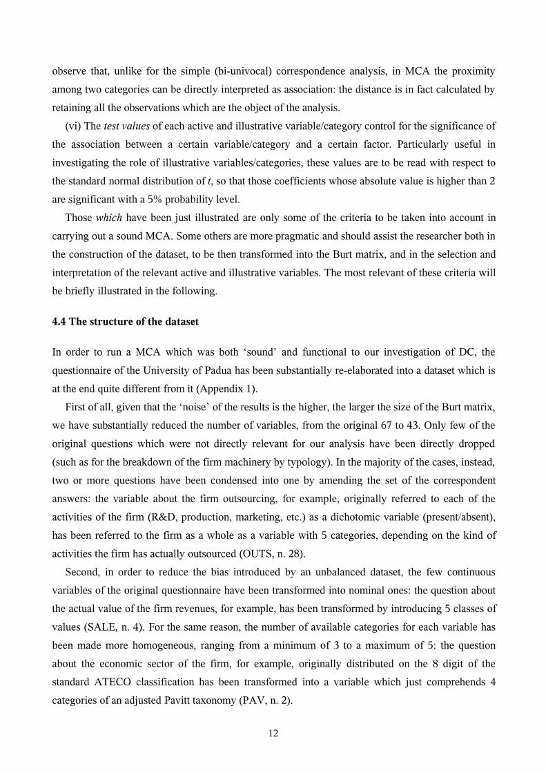
4.4 The structure of the dataset

In order to run a MCA which was both ‘sound’ and functional to our investigation of DC, the

questionnaire of the University of Padua has been substantially re-elaborated into a dataset which is

at the end quite different from it (Appendix 1).

First of all, given that the ‘noise’ of the results is the higher, the larger the size of the Burt matrix,

we have substantially reduced the number of variables, from the original 67 to 43. Only few of the

original questions which were not directly relevant for our analysis have been directly dropped

(such as for the breakdown of the firm machinery by typology). In the majority of the cases, instead,

two or more questions have been condensed into one by amending the set of the correspondent

answers: the variable about the firm outsourcing, for example, originally referred to each of the

activities of the firm (R&D, production, marketing, etc.) as a dichotomic variable (present/absent),

has been referred to the firm as a whole as a variable with 5 categories, depending on the kind of

activities the firm has actually outsourced (OUTS, n. 28).

Second, in order to reduce the bias introduced by an unbalanced dataset, the few continuous

variables of the original questionnaire have been transformed into nominal ones: the question about

the actual value of the firm revenues, for example, has been transformed by introducing 5 classes of

values (SALE, n. 4). For the same reason, the number of available categories for each variable has

been made more homogeneous, ranging from a minimum of 3 to a maximum of 5: the question

about the economic sector of the firm, for example, originally distributed on the 8 digit of the

standard ATECO classification has been transformed into a variable which just comprehends 4

categories of an adjusted Pavitt taxonomy (PAV, n. 2).

12

Finally, even the categories of the original dataset which were not so unbalanced have been

rearranged in order to eliminate categories with nil or very low frequencies, while missing answers

have been recovered as an extra category: this is the case, for example, of the variables about the

number of suppliers (SUPN, n. 31) and of competitors (COM, n. 37), originally defined on ranges

of values with different boundaries.

For the scope of our investigation, the variables have been collected into several broad groupings

in order to reflect the various typologies of characteristics along which the analysis has been

performed (Appendix 2). The groups describe, besides to the most usual set of variables (e.g. of

structure, performance, efficiency, innovation, …), other key aspects of this analysis (such as

organisation, relationships with customers/suppliers, relationships with the environment, existence

of capabilities). Indeed, we have been rearranging the dataset in order to get useful information

about the patterns of vertical (INTV, n. 26) and horizontal (INTH, n. 27) dis/integration,

outsourcing (OUTS, n. 28), and delocalisation (LOCD, n. 29). Also all the different activities

related to the linkages with suppliers and customers are quite important for our analysis, as well as

cooperation with competitors (see the section ‘relationships’). To them we have added two other

important variables on how the firms perceive their placement within both the material (MIFR, n.

40) and the immaterial (IFR, n. 41)infrastructural set-up. More precisely, the categories of these

variables have been obtained by analysing the different answers the firms have given to a numerous

set of detailed questions in which they have been asked to consider a large set of both material (e.g.

roads, railroads, etc.) and immaterial (e.g. universities, chambers of commerce, etc.) infrastructures

as either a strength or a weakness for their business. This information is necessary for at least two

reasons. First, because of our framework, which is mainly focused upon the relationships between

inner and outer environment. Second, because of the particular industrial structure of this part of

Italy, characterised by the heavy presence of industrial districts, and for which these variables all

contribute to building the ‘industrial atmosphere’.

A final remark must be made about the crucial variables of the present application, those related

to the firm capabilities. First of all, the high level of detail of the questionnaire has allowed us to

distinguish two kinds of capabilities variables related to, respectively, the innovative and the market

sides. In this way we have been able to take into account the firm capabilities in front of two sources

of change: one due to technological change (CDIN, n. 42), another one to due a change in the

market fundamentals (CDMK, n. 43). The two variables refer to the ability of the firms to anticipate

or not the future evolution of technology and market and have been built up by investigating

whether they have had “difficulties or not” in doing that. In both cases, the choices are between

“yes, there are difficulties” (CDIN and CDMK = 10), “no, we anticipate it” (CDIN and CDMK =

40), “no, we can adapt quickly” (CDIN and CDMK = 30), “no, we adapt only when necessary”

(CDIN and CDMK = 20). It is thus clear that we have here different types and combinations of

13

different abilities to respond/adapt to external stimuli, either from the technical or from the market

side.8

4.5 Significant eigen-values and semantic interpretation of the axes

The first set of results that we present is based on a MCA run with respect to 27 active variables

(Appendix 3). The subset of variables with respect to which the identification of the factors has

been accomplished does not comprehend the 5 structural ones, which will be used as supplementary

variables, and other 11 non-structural variables which in previous attempts have turned out to

introduce either relevant distortions or irrelevant explanations of the total inertia of the data.

With as many as 27 active variables and 111 categories, we have decided to focus our attention

on the first four eigen-values, which explain, individually, more than 4% of the total inertia of the

observations (the average eigen-value is 3.7% = 1/27) and, altogether, nearly 20% (Table 1).

The cross-analysis of the absolute and relative contributions of the active variables/categories

(Table 2) shows that CDIN is relatively well represented by the first factor, along which only two of

the four correspondent categories are significant (CDIN = 20 and CDIN = 40). In other words, the

first axis discriminates between a group of firms which perceive themselves as pro-active and thus

revealing dynamic capabilities in front of innovations (CDIN = 40) and another one which instead

just react to innovations by substituting the old technology with no adaptive effort (CDIN = 20) (in

the following, we will briefly refer to the two groups as, respectively, the ‘pro-active’ and the

‘reactive’ group). Let us observe that ‘non reactive’ (CDIN = 10) and ‘adaptive’ firms (CDIN = 30)

have instead a negligible explanatory power: in other words, the firms of the sample are always alert

to innovation turbulences, but either to the minimum (CDIN = 20) or to the maximum (CDIN = 40)

extent, with no intermediate solutions.

Searching for those active categories which can be more directly associated to the two groups of

firms, we have at first checked the absolute contribution and the mass of those whose inertia is

accounted by to a greater extent by the first axis, namely: the location of the firm competitors

(COMS) and of their customers (CUSS), the diffusion of information technologies (DINF and

WEB) and the introduction of technological innovations (INNO), the recent trend of the firm

investments (DINV) and when the firm is located into a group (GRUP). Considering also the

location of the firm suppliers (SUPS), for which the first factor is a non distant second best, the first

axis can be taken as a proxy of a combination of variables whose nature is to a certain degree

homogeneous: indeed, nearly all refer to the extension of the main firm relationships, according to a

broad idea of distance – both geographical (COMS, CUSS and SUPS) and organizational (GRUP) –

8 It must be stressed that these answers refer to the auto-perception of each firm, and not to effective capabilities.However, we have built also composite capabilities indicators, by weighting CDIN and CDMK with some objectiveperformance variables, to find that there are very minor differences, and that the results are not so different to justify theinsertion of another distortion in building the dataset, especially with regard to these two crucial variables.

14

and of the relationships themselves – i.e by considering the role of information technologies in

managing them (DINF and WEB). Also the remaining variables can be related to this semantic

meaning of the axis, once it is considered that investments and innovations are, respectively,

important pre-conditions and outcomes of sound user-producer and producer-producer relationships.

Accordingly, the first axis will be used in the following to redistribute the original observations

along what we will call the meta-variable of the ‘relationships extension’.

As far as the second factor is concerned, the greatest contributors to its inertia are one variable of

performance - that is the recent trend of the firm revenues (DSAL) - and one variable of

environmental placement, which captures the effect of the intangible infrastructures of the firm

environment (e.g. business services, universities, etc.) on the firm itself (IFR). If we observe that

also the other variables the second axis explains more satisfactorily are either performance variables

- such as for the recent trend in employment (EMP) – and environmental variables – such as for the

effect of the physical infrastructures (MIFR) and for the availability of adequate (qualified)

employment (DEMPS) – it seems reasonable to consider the second axis as a proxy of the firm

capacity to settle effectively in its local system of production. Accordingly, the axis will be used as

a meta-variable for the ‘settling capacity’ of the firms in their business environment.

If we exclude variables already considered, the third factor explains significant shares of inertia

of other few variables. On the one hand, we have the capabilities (CDMK) and the diversification

strategies (INTH) with which firms deal with changes in the consumer preferences, along with the

success with which they do it on the international markets (DEXP). On the other hand, we have the

degree of utilization of their productive capacity (CAPR) and the efficiency with which they do it

(COST). Although discounting the contribution of other non directly related variables, the third axis

thus accounts for the production efficiency and the distributive effectiveness of the firms. Hence,

the correspondent meta-variable would refer to their ‘production-marketing competences’.

Finally, the fourth axis is dominated by the contribution of two quite homogeneous variables,

which inform about the kind of organizational relationships through which the firms interact with

their suppliers – depending on their being first-suppliers or sub-suppliers (SUPK) – and customers –

being them general or dedicated ones (CUSK). Appreciable contributions to the same axis then

come from their strategies in terms of outsourcing typology (OUTS) and delocalisation areas

(LOCD). Adding the marginal contributions of the variables which account for the firm spin-offs

(SPIN) and for the collaboration relationships with the competitors (COMR), it seems possible to

associate to the fourth axis a meta-variable of ‘organizational arrangements’. Table 3 sums up the

composition of the 4 meta-variables which have been identified.9

9 In addition to the main contributors described above, each meta-variable also comprehends other variables whose ac isdefinitively inferior (i.e. lower than 5%) and which have been allocated among them on the basis of the distribution oftheir ac among the four axes.

15

4.6. Associations among categories: characterising pro-active and reactive firms

Given that in MCA closeness among points can be directly read as an association measurement

among categories (according to a distributive kind of distance), we can use their plot on the three

systems of axis which is possible to build up in order to identify some distinguishing characteristics

of the pro-active and of reactive firms. In drawing the plots we have retained and drawn just those

categories whose ac is greater than the average (i.e. 1/111 = 0.9%), but left out those whose ac is

due to rare frequencies and which are thus affected by large distortions (Table 2).

Considering the first couple of axes (Figure 1), a first clear association emerges between the

dynamic capabilities of the interviewed firms and their degree of office automation. Pro-active firms

appear associated to the cases in which information technologies are pervasively diffused (DINF =

10), while the reactive firms are closer to the case where ICT are just used in running auxiliary

activities (e.g. accounting) and missing from the core ones (e.g. marketing and production) (DINF =

20). The correlation that some scholars are investigating between DC and office automation (e.g.

Masini, 2004) finds therefore some confirmation also in our application. The other associations

instead seem to recover in the analysis the role that environmental and relational aspects play in

building up DC, as suggested by the local systems of production approaches. On the one hand,

reactive firms are associated with a non satisfactory placement in their infrastructural set-up (IFR =

10): that this might an important source to feed up the innovation capabilities of the firm, an insight

provided by the literature on innovation systems since long (e.g. Edquist, 1997) appears therefore a

testable suggestion. On the other hand, as stressed by several of the approaches on the local systems

of production, also the placement in geographical territory turns out to be important. And indeed,

pro-active firms are associated with a satisfactory placement in the set-up of the physical

infrastructures (MIFR = 20). Let us also observe that, unlike the reactive ones, the pro-active firms

are associated with a business environment with a high degree of internationalisation: both as far as

the competitors (COMS = 40) and the customers (CUSS = 30) are concerned. The participation to a

group (in the form of parent company (GRUP = 20)) and the resort to vertical integration (namely

upward (INTV = 10)) add two further associations to the pro-active firms which seem to suggest

how their CDIN might be crucially affected by or/and might affect their business relationships.

Further interesting associations can be found by plotting the first axis against the third one, and

thus looking at the production-marketing competencies of the firms (Figure 2).10 Quite interestingly,

the pro-active firms in terms of innovation (CDIN = 40) are associated with the pro-active ones in

terms of market (CDMK = 40), hinting to a possible complementarity between the two. In turn,

dynamic and market capabilities are associated to the presence of diversification strategies (INTH =

10 Categories are again selected by crossing their absolute contributions and by checking their distortion (Table 2).

16

10), while the absence of any strategy of horizontal integration (INTH = 40) is coupled with the

reactive firms. Hence, the notable debate between polarised and diffused specialisation patterns

appears relevant in this last respect, pointing to the Schumpeterian idea according to which those

firms which better anticipate innovation and market change have distributed rather than

concentrated production and marketing capabilities. Let us observe that the third axis, while

‘qualifying’ the association between pro-active firms and ICT diffusion (DINF = 10) with their

association to an early adoption date (YINF = 10), confirms the interpretation we have put forward

about the extension of the firm relationships. Purely reactive firms (CDIN = 20) reveal a certain

proximity with the categories denoting local kinds of relationships: both as far as their suppliers

(SUPS = 10) and their customers (CUSS = 10) are concerned. As several studies on local systems

of production have pointed out (e.g. Chiarvesio et al., 2003), the internationalisation of the firm

productive relationships, rather than that of the firm market, could have very much to say about the

development of strong dynamic capabilities. Also the way these relationships are run of course

matter: in this last respect, let us observe that, unlike the pro-active firms, the reactive ones are

associated to a non formal (i.e. non ownership intensive, or group like) kind of relationships (GRUP

= 10).

Let us conclude our analysis of the categories association by considering the first and the fourth

axis, recovering some other variables about the firm organizational arrangements (Figure 3). On the

one hand, this factorial space further specifies the previous insight about the different extension of

the business environment of the two groups of firms. The reactive firms are in fact associated with

competitors of (at most) national scale (COMS = 20) and with customers which are mainly

dedicated clients (CUSK = 20). The pro-active firms, instead, are associated with competitors with

which they have virtuous collaboration relationships, driven neither by the attempt at reducing

costs, nor by that of ‘bringing home’ missing capabilities (COMR = 40). On the other hand, the

same couple of axes tells us something about the way the business environment of the two groups of

firms is organised. First of all, reactive firms are associated with the outsourcing of auxiliary

activities (OUTS = 20): a ‘weak’ version of the strategic idea of the ‘cave firm’ (Prahalad and

Hamel, 1990), according to which the outsourcing of certain activities (in the strong version, the

core activities) might empty the firm from its dynamic capabilities, could be invoked in this last

respect. Reactive firms are also associated to the absence of delocalization strategies (LOCD = 40),

which appears consistent with the local scale of their associations with both customers (CUSS = 10)

and suppliers (SUPS = 10). On the opposite side, pro-active firms couple their dynamic innovative

capabilities with the generation of further entrepreneurial activities by spin-off (SPIN = 10),

pointing to a factor which might turn out to be important in revitalising the demography of the

industrial system of Treviso.

17

4.7. Active vs. supplementary variables

The characterisation of the firm categories we have identified can be further refined by inserting in

the MCA analysis that we have just run some illustrative or supplementary variables. As it is

usually the case, we have decided to illustrate our results by referring to some of the structural

variables of the dataset: the age of the firms (AGE), their location in our enlarged Pavitt taxonomy

(PAV), their size in terms of both employment (EMP) and class of revenues (SALE).

Given that these variables do not enter in the identification of the factors, in the following we

will reproduce the systems of axes of the previous section and report on them, along with the CDIN

categories we are interested in (CDIN = 20 and CDIN = 40), just those illustrative categories which

are significantly correlated with each couple of factors (Table 4). The two series of figures have

thus to be read simultaneously.

Starting from the plot of the first two axes (Figure 4), the pro-active firms add to the previous

associations (see Figure 1) close connections with the largest firms of the sample: both in terms of

employment (EMP = 50) and of revenues (SALE = 50). That DC are more promptly developed by

firms with both a complex organization and a wide market volume is nothing but a tentative

interpretation, somehow reinforced by the fact that reactive firms are here associated with a

definitively smaller class of revenues (SALE = 20). Let us observe that the same illustrative

categories appear consistent with the other active categories which have been identified on the same

axes (see Figure 1): particularly, a superior internationalisation degree and a group structure. A

further important qualification comes from the sectoral illustrative variables. Quite interestingly,

operating with large economies of scale or with natural resources (PAV = 20), rather than in

traditional sectors, is associated with at least a certain level of capabilities to deal with technological

change. On the other hand, a pro-active behaviour is associated, rather than with science-based

firms, with those firms which in the present local system of production typically have the most

satisfactory performances, that is specialised supplier firms (PAV = 30). Rather than having an ideal

sectoral structure, DC thus seems to show different specifications in different productive contexts.

Crossing factor 1 with factor 3 (Figure 5), the associations between the two relevant CDIN

categories and the firm size get confirmed. Furthermore, the same illustrative size categories fit

quite well the other active categories associated with the pro-active and reactive firms: the latter, in

particular, associate the local scale of their operations with a size which is at most medium. Further

confirmation comes from the last plot (Figure 6). In particular, those organizational arrangements

that in the previous correspondent factorial space had been related to the pro-active firms (see

Figure 3), are here further qualified with a significant association to the specialised supplier firms of

the sample (PAV = 30). On the other hand, the outsourcing and the delocalisation strategies which

18

had been associated with the reactive ones are specified mainly with the association to scale and

resource intensive sectors of activities, and, although marginally, to supplier dominated ones.

5. Conclusions

The aim of this paper is to to explore the role of dynamic capabilities in explaining the performance

of the firm. From a theoretical point of view, as we have already argued elsewhere (Leoncini et al.,

2003), there is a need to take into account two dymensions of DC: one organisational and one

environmental. This results from the view of the firm as an open systems, whose dynamics depends

on the intercourse between the internal production of disorder and the exportation of it towards the

environment. The entropy exchange with the environment is at the origin of non-linear dynamics

that have been analysed, for instance, by referring to firms as complex adaptive systems, for which

it is possible to envisage a complex process of co-evolution with the environment. It is therefore

important to stress how the firm performance is the result of a dynamic exchange of flows with the

outer environment, and that an order can be mainatained only dynamically by balancing the export

and import of disorder from the outside.

An empirical application is then performed on a sample of italian firms located in the province of

Treviso by means of a very detailed questionnaire produced at the University of Padua. The

province of Treviso is interesting for several reasons. In particular, it must be stressed that many

characteristics (the process of internationalisation based on delocalisation of production rather than

on export, the presence of industrial districts, etc.) lend themselves very well to the scope of our

analysis. The resulting dataset is then analysed with multiple correspondence analysis, with which it

is possible to take into consideration answers to multiple choices questions, which are the main

modality of answer to the questionnaire used.

The main results of this application refer, primarily to the close interaction between

organisational and environmental elements in determining firm performance. The empirical analysis

in fact produces quite clear evidence about the need of building linkages in order to benefit from the

virtuous interactions offered by the industrial model existing in the province of Treviso. Indeed, a

meta variable emerges about the relationships extension of firms in the sample, which depends

heavily on environmental variables. Another meta variable seems to relate the market capabilities

more to production-marketing type of competences. In this way we are able to distinguish those

firms that relied more on their capacity to react to market shifts with different instruments related to

marketing and production , from other firms that are more keen to innovative kind of activities.

By analysing the associations among categories we obtained more imformation. Two different

profiles of firms in the area consided in fact emerge: pro-active firms (related to firms with a high

level of DC) and reactive ones (related to low level of DC). A set of further variables better qualify

19

these two groups. As expected, the more dynamic group results to be associated (among the others)

to variables reflecting a deeper development of dynamic capabilities (ICT, placement in the

infrastructural set-up, participation to a group with an important role, diversification strategies,

cooperation with competitors, etc.). The less dynamic one has instead (among the others) local kind

of linkages both with suppliers and customers, more based on informal group relations, outsorcing

of auxiliary activities rahter than core ones.

Bibliography

Amaturo, F. (1989), Analyse des Données & Analisi dei Dati nelle Scienze Sociali, Turin, CentroScientifico Editore.

Anastasia, B. and Corò, G. (1993), I distretti industriali in Veneto, Nuova Dimensione-Ediciclo,Portogruaro.

Benzécri, J.P. (1973), L’Analyse des Données. Tome II. L’Analyse des Corrispondances, Paris,Dunod.

Bouroche, J.M. and Saporta, G. (1980), L’Analyse des Données, Paris, Universitaires de France.Bresolin, F. and Biscaro, Q. (2001), Problematiche di internazionalizzazione dei distretti industriali

della provincia di Treviso, mimeo, Camera di Commercio Industria Artigianato Agricoltura diTreviso

Brioschi, F., Brioschi, M.S. and Cainelli G. (2003), From the industrial district to the district group.An insight into the evolution of local capitalism in Italy, Regional Studies, forthcoming.

Chiarvesio, M., Di Maria, E. and Micelli, S. (2003), Innovation and internationalisation of Italiandistricts: exploitation of global competencies or transfer of local knowledge?, Paper presented atthe 2003 Regional Studies Association International Conference, “Reinventing Regions in theGlobal Economy”

Dosi G., Nelson R.R. and Winter S.G. (2000), Introduction in Dosi G., Nelson R.R. and Winter S.G.(eds.), The Nature and Dynamics of Organizational Capabilities , Oxford, Oxford UniversityPress, pp. 1-22.

Edquist, C. (1997), Systems of innovation approaches - their emergence and characteristics, inEdquist, C. (ed.), Systems of Innovation. Technologies, Institutions and Organisations, London,Pinter Publishers, pp. 1-35.

Fuller, T. and Moran, P. (2000), Complexity as a social science methodology in understanding theimpact of exogenous systemic change on small business, Paper presented at the InternationalConference on Complex Systems, Nashua, NH, May 21-26, 2000.

Fuller, T. and Moran, P. (2001), Small enterprises as complex adaptive systems: a methodologicalquestion?, Entrepreneurship & Regional Development, vol. 13, pp. 47-63.

Iansiti, M. and Clark, K.B. (1994), Integration and dynamic capability: evidence from productdevelopment in automobiles and mainframe computers, Industrial and Corporate Change, vol. 3,n. 3, pp. 557-606.

Jones, N. (2001), Exploring dynamic capability: a longer-term study of product developmentfollowing radical technological change, INSEAD R&D Working Papers, 2001/20/TM.

Kauffman, S. (1995), At Home in the Universe: the Search for Laws of Complexity, Oxford, OxfordUniversity Press.

Leoncini, R., Montresor, S and Vertova, G. (2003), Dynamic capabilities: evolving organisations inevolving (technological) systems, Working Paper University of Bergamo, Department ofEconomics.

Lieberman, M.B. and Montgomery, D.B. (1988), First-mover advantages, Strategic ManagementJournal, n. 9, pp. 41-58.

20

Masini, A. (2004), The impact of IT adoption on the genesis of dynamic capabilities, Paperpresented at the I Workshop of the Research Project on “Dynamic capabilities between firmorganization and local systems of production”, Bologna, December 17, 2003.

Montresor, S. and Romagnoli, A. (2003), Modelling the firm from a system perspective: somemethodological insights, mimeo, University of Bologna.

Nonaka, I. and Takeuchi, H. (1997), The Knowledge Creating Company, Guerini e Associati,Milan.

Osservatorio Unioncamere di Treviso (2004), Company groups in Treviso: holding companies orreceivership enterprises in Province, mimeo, Unioncamere di Treviso.

Prahalad, C.K. and Hamel, G. (1990), The core competence of the corporation, Harvard BusinessReview, May, pp. 79-91.

Reinganum, J.F. (1989), The timing of innovation: research, development and diffusion, inSchmalensee, R. and Willig, R. (eds.), Handbook of Industrial Organization, vol. I, Amsterdam,North-Holland, pp. 849-908.

Teece, D.J. and Pisano, G. (1994), The dynamic capabilities of the firms: an introduction, Industrialand Corporate Change, vol. 3, n. 3, pp. 537-556.

Teece, D.J., Pisano G., and Shuen, A. (1997), Dynamic capabilities and strategic management,Strategic Management Journal, vol. 18, n. 7, pp. 509-533.

Zollo, M. and Winter, S.G. (1999), From organizational routines to dynamic capabilities, INSEADR&D Working Papers: 99/48/SM.

21

Appendix 1Structurale indicators of the province of Treviso (1999-2001)

1999 2000 2001GDP total million of € 16,554 GDP per capita million of € 21,100 Exports million of € 7,065 8,002 Imports million of € 3,103 3,65 Export/import rate % 228.3 219.3 (export/import)/GDP % 60.9 Unemployment rate % 2.7 2.6 Employment rate % 50.6 51.5 Activity rate % 52.0 52.8 53.8

Appendix 2: The structure of the datasetVariables Categories

n. Subject Lable 10 20 30 40 50 STRUCTURE 1 Set-up year AGE 1920/1969 1970/1979 1980/1989 19990/1999 2000/2002

2Pavitt sector

(enlarged taxonomy) PAVsupplier

dominated

scaleintensive &resource

based

specialisedsuppliers

science-based &services

3Employment class(n. of employees)

EMP <20 [20; 49] [50: 99] [100; 249] >249

4Revenues by class (Milions of Euros)

SALE <2,5 [2,1; 5,5] [5,51; 12,5] [12,51; 25] > 25

PERFORMANCE

5Revenues trend

(yearly rate of change in thelast 3 years)

DSAL -10% [-3%; -10%] [-2.9%; +2.9%] [+3%; +10%] +10%

6Exports trend

(yearly rate of change in thelast 3 years)

DEXP -10% [-3%; -10%] [-2.9%; +2.9%] [+3%; +10%] +10%

7Employment trend

(yearly rate of change in thelast 3 years)

DEMP -10% [-3%; -10%] [-2.9%; +2.9%] [+3%; +10%] +10%

8Investments trend

(yearly rate of change in thelast 3 years)

DINV -10% [-3%; -10%] [-2.9%; +2.9%] [+3%; +10%] +10%

EFFICIENCY

9 Costs incidence(on revenues)

COST [0; 20%] (20%; 50%] (50%; 70%] missing

10Employment shortage

(in which activities)EMPS core auxiliary both none missing

11Productive capacity

(average rate of utilization)CAPR [0%; 70%] (70%; 80%] (80%; 90%] (90%; 100%]

INVESTMENTS

12Fixed investments

(on total investments) INFI [0%; 10%] (10%; 50%] (50%; 70%] (70%; 100%] missing

13R&D investments

(on total investments) INRS [0%; 10%] (10%; 50%] (50%; 70%] (70%; 100%] missing

14Human capital investments

(on total investments) INHC [0%; 10%] (10%; 50%] (50%; 70%] (70%; 100%] missing

15Marketing investments(on total investments) INMK [0%; 10%] (10%; 50%] (50%; 70%] (70%; 100%] missing

16 ICT investments(on total investments)

INCT [0%; 10%] (10%; 50%] (50%; 70%] (70%; 100%] missing

n. Subject Lable 10 20 30 40 50

INFORMATION-AUTOMATION

17 Informatisation year YINF pre-1980 1980-1990 1991-1995 1996-2000 2000-2002

18 Informatisation diffusion(missing in which activities?)

DINF none core auxiliary both

19Web-site(function)

WEB absent window window + B2

20Automation

(% of the machinery park)HTMA [0%; 10%] (10%; 30%] (30%; 50%] (50%; 80%]

(80%;100%]

PRODUCT

21Product techn. Content

(level)HTPR low medium-low medium-high high

22 Product price elasticity(level)

ELPR low medium high

INNOVATION

23Innovativeness

(kind of product/processinnovations)

INNO high (rad/rad)medium-high

(rad/inc -inc/rad))

Medium(inc/inc)

medium-low(inc/no - no/inc)

low(no/no)

24Patents

(actions in the last 3 years) PAT registred sold bought both none

ORGANIZATION 25 Group position GRUP no group parent subsidiary missing

26Vertical integration(recent strategies) INTV upward downward both none

27Horizontal integration

(recent strategies) INTH divers. special. both none

28Outsourcing

(of which activities?) OUTS core auxiliary both none missing

29Delocalization

(mainly where?) LOCD local rest of Italy abroad absent

30Spin-offs

(of which kind?) SPIN outward inward both none

RELATIONSHIPS 31 Number of suppliers SUPN [1; 3] [4; 10] >10

32Kind of suppliers

(mainly) SUPK suppliers sub-suppliers both missing

33Suppliers location

(mainly) SUPS local rest of Italy abroad

34 Number of customers CUS [1; 10] [11; 50] >50

35Kind of customers

(mainly)CUSK standard commission both missing

36Customers location

(mainly)CUSS local rest of Italy abroad

37 Number of competitors COM [0; 3] [4; 10] >10

38Competitors location

(mainly)COMS local

rest of Italy(alone or also

abroad (alone oralso)

rest of Italy andabroad (alone

and also)

39Competitors collaboration

(main reason) COMR absentcapabilitiesacquisition cost reduction other reasons

Missing

Variables Categoriesn. Subject Lable 10 20 30 40 50 ENVIRONMENT

40Placing in mat. infrastr.

(perceived) MIFR bad good enough good very good missing

41Placing in imm. infrastr.

(perceived) IFR bad good enough good very good missing

CAPABILITIES

42Innovation capabilities

(response in front of TC)CDIN absent substitutive adaptive dynamic

43Market capabilities

(response in front of pref.change)

CDMK absent substitutive adaptive dynamic

Appendix 3: Active and supplementary variablesActive Variablesn. Subject Lable6 Revenues trend (yearly rate of change in the last 3 years) DSAL7 Exports trend (yearly rate of change in the last 3 years) DEXP8 Employment trend (yearly rate of change in the last 3 years) DEMP9 Investments trend (yearly rate of change in the last 3 years) DINV

10 Costs incidence (on revenues) COST11 Employment shortage (in which activities) EMPS12 Productive capacity (average rate of utilization) CAPR18 Informatisation year YINF19 Informatisation diffusion (missing in which activities?) DINF20 Web-site (function) WEB24 Innovativeness (kind of product/process innovations) INNO26 Vertical integration (recent strategies) INTV27 Horizontal integration (recent strategies) INTH28 Outsourcing (of which activities?) OUTS29 Delocalization (mainly where?) LOCD30 Spin-offs (of which kind?) SPIN32 Kind of suppliers (mainly) SUPK33 Suppliers location (mainly) SUPS35 Kind of customers (mainly) CUSK36 Customers location (mainly) CUSS38 Competitors location (mainly) COMS39 Competitors collaboration (main reason) COMR40 Placing in mat. infrastr. (perceived) MIFR41 Placing in imm. infrastr. (perceived) IFR42 Innovation capabilities (response in front of TC) CDIN43 Market capabilities (response in front of pref. change) CDMK

Supplementary Variables1 Set-up year AGE2 Pavitt sector (enlarged taxonomy) PAV3 Employment class (n. of employees) EMP4 Revenues by class (Milions of Euros) SALE

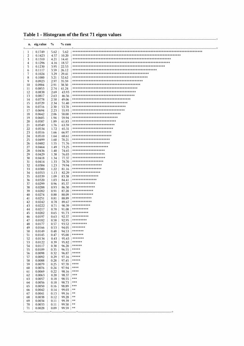
Table 1 - Histogram of the first 71 eigen values+------+------------+---------+---------+-----------------------------------------------------------------------------------------------------------------------------+

n. eig.value % % cum+------+------------+---------+---------+-----------------------------------------------------------------------------------------------------------------------------+| 1 | 0.1749 | 5.62 | 5.62 | ******************************************************************************** | 2 | 0.1423 | 4.57 | 10.20 | ******************************************************************| 3 | 0.1310 | 4.21 | 14.41 | ************************************************************ | 4 | 0.1296 | 4.16 | 18.57 | ************************************************************ | 5 | 0.1230 | 3.95 | 22.53 | ********************************************************* | 6 | 0.1117 | 3.59 | 26.12 | **************************************************** | 7 | 0.1024 | 3.29 | 29.41 | *********************************************** | 8 | 0.1000 | 3.21 | 32.62 | ********************************************** | 9 | 0.0923 | 2.97 | 35.59 | ******************************************* | 10 | 0.0904 | 2.91 | 38.50 | ****************************************** | 11 | 0.0853 | 2.74 | 41.24 | **************************************** | 12 | 0.0838 | 2.69 | 43.93 | *************************************** | 13 | 0.0817 | 2.63 | 46.56 | ************************************** | 14 | 0.0778 | 2.50 | 49.06 | ************************************ | 15 | 0.0729 | 2.34 | 51.40 | ********************************** | 16 | 0.0716 | 2.30 | 53.70 | ********************************* | 17 | 0.0694 | 2.23 | 55.93 | ******************************** | 18 | 0.0642 | 2.06 | 58.00 | ****************************** | 19 | 0.0605 | 1.94 | 59.94 | **************************** | 20 | 0.0587 | 1.89 | 61.83 | *************************** | 21 | 0.0549 | 1.76 | 63.59 | ************************** | 22 | 0.0534 | 1.72 | 65.31 | ************************* | 23 | 0.0516 | 1.66 | 66.97 | ************************ | 24 | 0.0510 | 1.64 | 68.61 | ************************ | 25 | 0.0499 | 1.60 | 70.21 | *********************** | 26 | 0.0482 | 1.55 | 71.76 | *********************** | 27 | 0.0464 | 1.49 | 73.25 | ********************** | 28 | 0.0436 | 1.40 | 74.65 | ******************** | 29 | 0.0429 | 1.38 | 76.03 | ******************** | 30 | 0.0418 | 1.34 | 77.37 | ******************** | 31 | 0.0414 | 1.33 | 78.70 | ******************* | 32 | 0.0384 | 1.23 | 79.94 | ****************** | 33 | 0.0380 | 1.22 | 81.16 | ****************** | 34 | 0.0353 | 1.13 | 82.29 | ***************** | 35 | 0.0339 | 1.09 | 83.38 | **************** | 36 | 0.0320 | 1.03 | 84.41 | *************** | 37 | 0.0299 | 0.96 | 85.37 | ************** | 38 | 0.0288 | 0.93 | 86.30 | ************** | 39 | 0.0282 | 0.91 | 87.20 | ************* | 40 | 0.0274 | 0.88 | 88.09 | ************* | 41 | 0.0251 | 0.81 | 88.89 | ************ | 42 | 0.0242 | 0.78 | 89.67 | ************ | 43 | 0.0222 | 0.71 | 90.39 | *********** | 44 | 0.0217 | 0.70 | 91.08 | ********** | 45 | 0.0202 | 0.65 | 91.73 | ********** | 46 | 0.0197 | 0.63 | 92.37 | ********** | 47 | 0.0182 | 0.58 | 92.95 | ********* | 48 | 0.0177 | 0.57 | 93.52 | ********* | 49 | 0.0166 | 0.53 | 94.05 | ******** | 50 | 0.0149 | 0.48 | 94.53 | ******* | 51 | 0.0145 | 0.47 | 95.00 | ******* | 52 | 0.0134 | 0.43 | 95.43 | ******* | 53 | 0.0122 | 0.39 | 95.82 | ****** | 54 | 0.0117 | 0.38 | 96.20 | ****** | 55 | 0.0109 | 0.35 | 96.55 | ***** | 56 | 0.0098 | 0.32 | 96.87 | ***** | 57 | 0.0092 | 0.29 | 97.16 | ***** | 58 | 0.0088 | 0.28 | 97.45 | ***** | 59 | 0.0079 | 0.25 | 97.70 | **** | 60 | 0.0076 | 0.24 | 97.94 | **** | 61 | 0.0069 | 0.22 | 98.16 | **** | 62 | 0.0063 | 0.20 | 98.37 | *** | 63 | 0.0057 | 0.18 | 98.55 | *** | 64 | 0.0056 | 0.18 | 98.73 | *** | 65 | 0.0050 | 0.16 | 98.89 | *** | 66 | 0.0042 | 0.14 | 99.03 | ** | 67 | 0.0041 | 0.13 | 99.16 | ** | 68 | 0.0038 | 0.12 | 99.28 | ** | 69 | 0.0034 | 0.11 | 99.39 | ** | 70 | 0.0033 | 0.11 | 99.50 | ** | 71 | 0.0028 | 0.09 | 99.59 | ** +--------+------------+----------+----------+----------------------------------------------------------------------------------+

Table 2 – Co-ordinates, absolute and relative contributions of the active categorieson the first 5 axes+-----------------------------------------------+----------------------------------+--------------------------+-----------------------------+| CATEGORIES | COORDINATES | ABS. CONT. | REL. CONT. ||------------------------------------------------+----------------------------------+--------------------------+----------------------------- || LABEL MASS DIST| 1 2 3 4 5 | 1 2 3 4 5 | 1 2 3 4 5 |+----------------------------------------------+-----------------------------------+--------------------------+-----------------------------+| 4 . GRUP [AD] | AD10 - GRUP=10 2.50 0.48 | 0.27 -0.08 0.10 -0.01 0.02 | 1.0 0.1 0.2 0.0 0.0 | 0.15 0.01 0.02 0.00 0.00 || AD20 - GRUP=20 0.67 4.56 | -0.88 0.30 -0.23 -0.31 0.09 | 2.9 0.4 0.3 0.5 0.0 | 0.17 0.02 0.01 0.02 0.00 || AD30 - GRUP=30 0.46 7.09 | -0.19 -0.12 0.08 0.42 -0.34 | 0.1 0.0 0.0 0.6 0.4 | 0.00 0.00 0.00 0.03 0.02 || AD40 - GRUP=40 0.08 43.50 | -0.08 0.76 -1.55 0.34 0.67 | 0.0 0.3 1.5 0.1 0.3 | 0.00 0.01 0.06 0.00 0.01 |+----------------------------------------------+----- CUMULATED----------+ 4.1 0.9 2.0 1.2 0.8 +-----------------------------+| 6 . DSAL [AF] | AF10 - DSAL=10 0.12 28.67 | -0.67 0.67 0.38 -1.40 -0.24 | 0.3 0.4 0.1 1.9 0.1 | 0.02 0.02 0.01 0.07 0.00 || AF20 - DSAL=20 0.29 11.71 | 0.37 0.77 1.16 -0.14 -1.14 | 0.2 1.2 3.0 0.0 3.1 | 0.01 0.05 0.11 0.00 0.11 || AF30 - DSAL=30 1.12 2.30 | 0.46 0.24 -0.02 0.64 -0.06 | 1.3 0.5 0.0 3.5 0.0 | 0.09 0.03 0.00 0.18 0.00 || AF40 - DSAL=40 1.25 1.97 | -0.19 0.44 -0.47 -0.27 0.09 | 0.3 1.7 2.1 0.7 0.1 | 0.02 0.10 0.11 0.04 0.00 || AF50 - DSAL=50 0.92 3.05 | -0.33 -1.23 0.24 -0.18 0.34 | 0.6 9.7 0.4 0.2 0.8 | 0.04 0.49 0.02 0.01 0.04 |+----------------------------------------------+------ CUMULATED----------+ 2.7 13.4 5.6 6.4 4.1 +-----------------------------+| 7 . DEXP [AG] | AG20 - DEXP=20 0.21 16.80 | -0.58 0.45 1.62 -1.39 -1.49 | 0.4 0.3 4.2 3.1 3.8 | 0.02 0.01 0.16 0.11 0.13 || AG30 - DEXP=30 2.25 0.65 | 0.43 0.01 -0.12 -0.13 0.25 | 2.3 0.0 0.2 0.3 1.2 | 0.28 0.00 0.02 0.03 0.10 || AG40 - DEXP=40 1.04 2.56 | -0.63 0.17 -0.28 0.47 -0.25 | 2.4 0.2 0.6 1.8 0.5 | 0.16 0.01 0.03 0.09 0.03 || AG50 - DEXP=50 0.21 16.80 | -0.85 -1.48 1.06 0.44 0.01 | 0.9 3.2 1.8 0.3 0.0 | 0.04 0.13 0.07 0.01 0.00 |+-----------------------------------------------+------CUMULATED----------+ 6.0 3.7 6.8 5.5 5.5 +-----------------------------+| 8 . DEMP [AH] | AH10 - DEMP=10 0.12 28.67 | -0.41 1.47 2.23 -1.25 -1.17 | 0.1 1.9 4.7 1.5 1.4 | 0.01 0.08 0.17 0.05 0.05 || AH20 - DEMP=20 0.25 13.83 | -0.45 -0.62 0.00 0.81 -0.88 | 0.3 0.7 0.0 1.3 1.6 | 0.01 0.03 0.00 0.05 0.06 || AH30 - DEMP=30 2.00 0.85 | 0.46 0.24 -0.07 0.15 -0.11 | 2.4 0.8 0.1 0.3 0.2 | 0.24 0.07 0.01 0.03 0.01 || AH40 - DEMP=40 1.08 2.42 | -0.63 -0.14 -0.36 -0.22 0.35 | 2.5 0.2 1.1 0.4 1.1 | 0.17 0.01 0.05 0.02 0.05 || AH50 - DEMP=50 0.25 13.83 | -0.24 -1.40 0.97 -0.40 0.82 | 0.1 3.5 1.8 0.3 1.4 | 0.00 0.14 0.07 0.01 0.05 |+-----------------------------------------------+----- CUMULATED-----------+ 5.4 7.0 7.7 3.8 5.6 +-----------------------------+| 9 . DINV [AI] | AI20 - DINV=20 0.37 8.89 | 0.27 0.67 1.17 0.11 -0.47 | 0.2 1.2 3.9 0.0 0.7 | 0.01 0.05 0.15 0.00 0.02 || AI30 - DINV=30 0.96 2.87 | 0.73 0.51 -0.09 0.15 0.05 | 2.9 1.8 0.1 0.2 0.0 | 0.18 0.09 0.00 0.01 0.00 || AI40 - DINV=40 1.37 1.70 | -0.04 -0.30 -0.41 0.14 -0.30 | 0.0 0.8 1.7 0.2 1.0 | 0.00 0.05 0.10 0.01 0.05 || AI50 - DINV=50 1.00 2.71 | -0.74 -0.34 0.21 -0.38 0.53 | 3.1 0.8 0.3 1.1 2.3 | 0.20 0.04 0.02 0.05 0.10 |+------------------------------------------------+--- CUMULATED-----------+ 6.2 4.6 6.0 1.5 4.0 +-----------------------------+| 10 . COST [AJ] | AJ10 - COST=10 0.08 43.50 | 1.57 0.33 -0.74 0.61 -1.54 | 1.2 0.1 0.3 0.2 1.6 | 0.06 0.00 0.01 0.01 0.05 || AJ20 - COST=20 0.25 13.83 | -0.41 -1.17 -0.72 -0.86 -1.86 | 0.2 2.4 1.0 1.4 7.0 | 0.01 0.10 0.04 0.05 0.25 || AJ30 - COST=30 0.79 3.68 | 0.16 -0.26 -0.47 0.26 0.09 | 0.1 0.4 1.4 0.4 0.1 | 0.01 0.02 0.06 0.02 0.00 || AJ40 - COST=40 2.41 0.53 | -0.10 0.27 0.16 -0.08 0.23 | 0.1 1.2 0.5 0.1 1.0 | 0.02 0.13 0.05 0.01 0.10 || AJ50 - COST=50 0.17 21.25 | 0.60 -1.03 1.36 0.92 -0.14 | 0.3 1.2 2.4 1.1 0.0 | 0.02 0.05 0.09 0.04 0.00 |+-----------------------------------------------+---- CUMULATED-----------+ 2.0 5.3 5.5 3.3 9.7 +-----------------------------+| 11 . EMPS [AK] | AK10 - EMPS=10 1.29 1.87 | 0.26 0.04 -0.05 -0.36 -0.01 | 0.5 0.0 0.0 1.3 0.0 | 0.04 0.00 0.00 0.07 0.00 || AK20 - EMPS=20 0.12 28.67 | -0.57 -2.71 0.84 -0.48 -1.05 | 0.2 6.5 0.7 0.2 1.1 | 0.01 0.26 0.02 0.01 0.04 || AK30 - EMPS=30 2.29 0.62 | -0.11 0.12 -0.02 0.23 0.06 | 0.2 0.3 0.0 0.9 0.1 | 0.02 0.03 0.00 0.08 0.01 |+-----------------------------------------------+----- CUMULATED-----------+ 0.9 6.7 0.7 2.4 1.2 +-----------------------------+| 12 . CAPR [AL] | AL10 - CAPR=10 0.67 4.56 | 0.32 -0.03 -0.81 -0.34 0.22 | 0.4 0.0 3.4 0.6 0.3 | 0.02 0.00 0.14 0.02 0.01 || AL20 - CAPR=20 0.75 3.94 | -0.62 -0.01 0.40 -0.24 0.00 | 1.6 0.0 0.9 0.3 0.0 | 0.10 0.00 0.04 0.01 0.00 || AL30 - CAPR=30 1.50 1.47 | 0.12 0.33 0.19 0.11 0.12 | 0.1 1.1 0.4 0.2 0.2 | 0.01 0.07 0.03 0.01 0.01 || AL40 - CAPR=40 0.79 3.68 | 0.09 -0.60 -0.06 0.29 -0.40 | 0.0 2.0 0.0 0.5 1.0 | 0.00 0.10 0.00 0.02 0.04 |+-----------------------------------------------+----- CUMULATED-----------+ 2.2 3.1 4.7 1.6 1.5 +-----------------------------+| 18 . YINF [AR] | AR10 - YINF=10 0.92 3.05 | -0.21 0.04 -0.53 0.25 0.23 | 0.2 0.0 1.9 0.4 0.4 | 0.01 0.00 0.09 0.02 0.02 || AR20 - YINF=20 1.71 1.17 | -0.07 0.12 0.14 0.05 -0.33 | 0.0 0.2 0.2 0.0 1.5 | 0.00 0.01 0.02 0.00 0.09 || AR30 - YINF=30 0.37 8.89 | 0.29 0.33 0.24 -0.17 0.92 | 0.2 0.3 0.2 0.1 2.6 | 0.01 0.01 0.01 0.00 0.09 || AR40 - YINF=40 0.62 4.93 | 0.28 -0.53 0.35 -0.33 -0.09 | 0.3 1.2 0.6 0.5 0.0 | 0.02 0.06 0.03 0.02 0.00 || AR50 - YINF=50 0.08 43.50 | 0.30 -0.29 -0.75 -0.50 0.83 | 0.0 0.0 0.4 0.2 0.5 | 0.00 0.00 0.01 0.01 0.02 |+-----------------------------------------------+---- CUMULATED-----------+ 0.8 1.7 3.3 1.2 5.0 +-----------------------------+| 19 . DINF [AS] | AS10 - DINF=10 1.50 1.47 | -0.69 0.20 -0.10 0.19 -0.19 | 4.1 0.4 0.1 0.4 0.4 | 0.33 0.03 0.01 0.02 0.02 || AS20 - DINF=20 0.75 3.94 | 0.72 0.13 -0.49 -0.11 -0.34 | 2.2 0.1 1.4 0.1 0.7 | 0.13 0.00 0.06 0.00 0.03 || AS30 - DINF=30 0.29 11.71 | 0.31 0.01 -0.32 0.20 0.72 | 0.2 0.0 0.2 0.1 1.2 | 0.01 0.00 0.01 0.00 0.04 || AS40 - DINF=40 1.17 2.18 | 0.35 -0.35 0.52 -0.23 0.28 | 0.8 1.0 2.4 0.5 0.8 | 0.06 0.06 0.12 0.02 0.04 |+-----------------------------------------------+----- CUMULATED----------+ 7.3 1.5 4.1 1.0 3.1 +-----------------------------+| 20 . WEB [AT] | AT10 - WEB=10 0.21 16.80 | 1.58 0.45 -0.79 -1.04 -0.70 | 3.0 0.3 1.0 1.7 0.8 | 0.15 0.01 0.04 0.06 0.03 || AT20 - WEB=20 1.62 1.28 | 0.23 0.07 0.33 0.14 -0.14 | 0.5 0.0 1.3 0.2 0.3 | 0.04 0.00 0.08 0.02 0.02 || AT30 - WEB=30 1.87 0.98 | -0.37 -0.11 -0.20 0.00 0.20 | 1.5 0.2 0.6 0.0 0.6 | 0.14 0.01 0.04 0.00 0.04 |+-----------------------------------------------+----- CUMULATED----------+ 5.0 0.5 2.9 2.0 1.7 +-----------------------------+

+-----------------------------------------------+----------------------------------+--------------------------+-----------------------------+| CATEGORIES | COORDINATES | ABS. CONT. | REL. CONT. ||------------------------------------------------+----------------------------------+--------------------------+----------------------------- || LABEL MASS DIST| 1 2 3 4 5 | 1 2 3 4 5 | 1 2 3 4 5 |+----------------------------------------------+-----------------------------------+--------------------------+------------------------------+| 24 . INNO [AX] | AX10 - INNO=10 0.42 7.90 | -0.44 0.37 -0.76 -0.92 0.17 | 0.5 0.4 1.8 2.7 0.1 | 0.02 0.02 0.07 0.11 0.00 || AX20 - INNO=20 1.66 1.22 | -0.04 -0.21 -0.07 0.28 -0.19 | 0.0 0.5 0.1 1.0 0.5 | 0.00 0.04 0.00 0.07 0.03 || AX30 - INNO=30 0.87 3.24 | -0.18 -0.25 0.30 0.01 0.23 | 0.2 0.4 0.6 0.0 0.4 | 0.01 0.02 0.03 0.00 0.02 || AX40 - INNO=40 0.62 4.93 | 0.13 0.60 0.38 -0.04 0.31 | 0.1 1.6 0.7 0.0 0.5 | 0.00 0.07 0.03 0.00 0.02 || AX50 - INNO=50 0.12 28.67 | 2.61 0.32 -0.51 -0.56 -1.20 | 4.9 0.1 0.2 0.3 1.5 | 0.24 0.00 0.01 0.01 0.05 |+----------------------------------------------+----- CUMULATED----------+ 5.6 3.0 3.4 4.0 2.9 +-----------------------------+| 26 . INTV [AZ] | AZ10 - INTV=10 0.37 8.89 | -0.48 0.87 0.41 -0.24 0.31 | 0.5 2.0 0.5 0.2 0.3 | 0.03 0.09 0.02 0.01 0.01 || AZ20 - INTV=20 0.12 28.67 | -0.33 -1.16 0.88 1.36 -0.79 | 0.1 1.2 0.7 1.8 0.6 | 0.00 0.05 0.03 0.06 0.02 || AZ30 - INTV=30 2.87 0.29 | -0.02 0.01 -0.04 -0.11 0.04 | 0.0 0.0 0.0 0.3 0.0 | 0.00 0.00 0.00 0.05 0.01 || AZ40 - INTV=40 0.33 10.12 | 0.84 -0.65 -0.49 0.74 -0.44 | 1.4 1.0 0.6 1.4 0.5 | 0.07 0.04 0.02 0.05 0.02 |+---------------------------------------------+--------- CUMULATED-------+ 1.9 4.2 1.8 3.7 1.5 +-----------------------------+| 27 . INTH [BA] | BA10 - INTH=10 1.54 1.41 | -0.17 -0.03 -0.28 -0.11 0.07 | 0.3 0.0 0.9 0.1 0.1 | 0.02 0.00 0.05 0.01 0.00 || BA20 - INTH=20 0.17 21.25 | 0.46 0.10 -1.78 -0.84 -1.36 | 0.2 0.0 4.0 0.9 2.5 | 0.01 0.00 0.15 0.03 0.09 || BA30 - INTH=30 0.21 16.80 | -0.36 0.77 0.34 -0.11 0.05 | 0.2 0.9 0.2 0.0 0.0 | 0.01 0.04 0.01 0.00 0.00 || BA40 - INTH=40 1.79 1.07 | 0.15 -0.07 0.36 0.18 0.06 | 0.2 0.1 1.8 0.5 0.1 | 0.02 0.01 0.12 0.03 0.00 |+----------------------------------------------+------ CUMULATED---------+ 0.8 1.0 6.9 1.5 2.6 +-----------------------------+| 28 . OUTS [BB] | BB10 - OUTS=10 0.25 13.83 | -0.23 0.27 -0.53 0.43 -0.01 | 0.1 0.1 0.5 0.4 0.0 | 0.00 0.01 0.02 0.01 0.00 || BB20 - OUTS=20 1.29 1.87 | 0.22 0.18 -0.20 -0.54 0.15 | 0.4 0.3 0.4 2.9 0.2 | 0.03 0.02 0.02 0.16 0.01 || BB30 - OUTS=30 1.12 2.30 | 0.02 -0.01 0.06 0.46 0.22 | 0.0 0.0 0.0 1.8 0.5 | 0.00 0.00 0.00 0.09 0.02 || BB40 - OUTS=40 0.96 2.87 | -0.36 -0.24 0.32 -0.05 -0.50 | 0.7 0.4 0.7 0.0 2.0 | 0.05 0.02 0.04 0.00 0.09 || BB50 - OUTS=50 0.08 43.50 | 1.23 -0.72 0.24 1.53 0.41 | 0.7 0.3 0.0 1.5 0.1 | 0.04 0.01 0.00 0.05 0.00 |+----------------------------------------------+------ CUMULATED---------+ 1.9 1.1 1.7 6.6 2.8 +-----------------------------+| 29 . LOCD [BC] | BC10 - LOCD=10 1.00 2.71 | -0.46 0.30 -0.38 0.23 0.18 | 1.2 0.7 1.1 0.4 0.3 | 0.08 0.03 0.05 0.02 0.01 || BC20 - LOCD=20 0.21 16.80 | -0.84 -0.23 1.03 -0.87 0.20 | 0.8 0.1 1.7 1.2 0.1 | 0.04 0.00 0.06 0.05 0.00 || BC30 - LOCD=30 0.42 7.90 | -0.71 -0.01 -0.23 1.23 -0.81 | 1.2 0.0 0.2 4.9 2.2 | 0.06 0.00 0.01 0.19 0.08 || BC40 - LOCD=40 2.08 0.78 | 0.44 -0.12 0.12 -0.27 0.05 | 2.4 0.2 0.2 1.2 0.0 | 0.25 0.02 0.02 0.09 0.00 |+-----------------------------------------------+----- CUMULATED----------+ 5.6 0.9 3.2 7.7 2.6 +-----------------------------+| 30 . SPIN [BD] | BD10 - SPIN=10 0.42 7.90 | -0.58 0.53 -0.67 -0.86 -0.80 | 0.8 0.8 1.4 2.4 2.1 | 0.04 0.03 0.06 0.09 0.08 || BD20 - SPIN=20 0.62 4.93 | 0.68 0.28 0.34 0.11 0.53 | 1.6 0.3 0.5 0.1 1.4 | 0.09 0.02 0.02 0.00 0.06 || BD40 - SPIN=40 2.66 0.39 | -0.07 -0.15 0.02 0.11 0.00 | 0.1 0.4 0.0 0.2 0.0 | 0.01 0.06 0.00 0.03 0.00 |+----------------------------------------------+------ CUMULATED---------+ 2.5 1.6 2.0 2.7 3.6 +------------------------------+| 32 . SUPK [BF] | BF10 - SUPK=10 3.29 0.13 | 0.06 -0.05 0.02 0.16 0.06 | 0.1 0.1 0.0 0.6 0.1 | 0.03 0.02 0.00 0.20 0.03 || BF20 - SUPK=20 0.25 13.83 | -0.20 1.10 0.23 -0.69 -0.11 | 0.1 2.1 0.1 0.9 0.0 | 0.00 0.09 0.00 0.03 0.00 || BF30 - SUPK=30 0.08 43.50 | 0.01 -1.41 -1.32 -2.88 -2.93 | 0.0 1.2 1.1 5.3 5.8 | 0.00 0.05 0.04 0.19 0.20 || BF40 - SUPK=40 0.08 43.50 | -1.96 0.24 -0.18 -1.35 0.86 | 1.8 0.0 0.0 1.2 0.5 | 0.09 0.00 0.00 0.04 0.02 |+----------------------------------------------+----- CUMULATED----------+ 2.0 3.4 1.2 8.1 6.5 +-----------------------------+| 33 . SUPS [BG] | BG10 - SUPS=10 0.79 3.68 | 0.80 -0.26 0.32 -0.59 -0.26 | 2.9 0.4 0.6 2.2 0.4 | 0.17 0.02 0.03 0.10 0.02 || BG20 - SUPS=20 2.25 0.65 | -0.10 0.13 -0.18 -0.03 0.27 | 0.1 0.3 0.5 0.0 1.4 | 0.02 0.03 0.05 0.00 0.12 || BG30 - SUPS=30 0.67 4.56 | -0.60 -0.15 0.22 0.81 -0.62 | 1.4 0.1 0.3 3.4 2.1 | 0.08 0.00 0.01 0.15 0.08 |+----------------------------------------------+------ CUMULATED---------+ 4.4 0.8 1.4 5.6 3.9+-----------------------------+| 35 . CUSK [BI] | BI10 - CUSK=10 2.70 0.37 | -0.12 -0.18 -0.21 0.27 0.11 | 0.2 0.6 0.9 1.6 0.3 | 0.04 0.09 0.12 0.20 0.03 || BI20 - CUSK=20 0.83 3.45 | 0.43 0.37 0.85 -0.66 -0.30 | 0.9 0.8 4.6 2.8 0.6 | 0.05 0.04 0.21 0.12 0.03 || BI30 - CUSK=30 0.08 43.50 | 0.71 1.49 0.18 0.02 0.50 | 0.2 1.3 0.0 0.0 0.2 | 0.01 0.05 0.00 0.00 0.01 || BI40 - CUSK=40 0.08 43.50 | -1.04 0.63 -1.89 -2.34 -1.12 | 0.5 0.2 2.3 3.5 0.8 | 0.02 0.01 0.08 0.13 0.03 |+----------------------------------------------+----- CUMULATED---------+ 1.9 2.9 7.8 7.8 1.9 +-----------------------------+| 36 . CUSS [BJ] | BJ10 - CUSS=10 0.58 5.36 | 0.77 -0.61 0.17 -0.24 0.04 | 2.0 1.5 0.1 0.3 0.0 | 0.11 0.07 0.01 0.01 0.00 || BJ20 - CUSS=20 2.12 0.75 | 0.10 -0.13 -0.22 0.12 0.21 | 0.1 0.3 0.8 0.2 0.8 | 0.01 0.02 0.07 0.02 0.06 || BJ30 - CUSS=30 1.00 2.71 | -0.66 0.64 0.37 -0.11 -0.47 | 2.5 2.9 1.0 0.1 1.8 | 0.16 0.15 0.05 0.00 0.08 |+---------------------------------------------+------ CUMULATED---------+ 4.6 4.6 2.0 0.6 2.6 +------------------------------+| 38 . COMS [BL] | BL10 - COMS=10 0.17 21.25 | 0.28 -0.82 0.77 -0.04 0.40 | 0.1 0.8 0.8 0.0 0.2 | 0.00 0.03 0.03 0.00 0.01 || BL20 - COMS=20 1.58 1.34 | 0.63 -0.34 -0.18 -0.25 0.26 | 3.6 1.3 0.4 0.8 0.9 | 0.30 0.09 0.02 0.05 0.05 || BL30 - COMS=30 0.29 11.71 | -0.68 0.88 -0.80 1.08 -1.03 | 0.8 1.6 1.4 2.6 2.5 | 0.04 0.07 0.05 0.10 0.09 || BL40 - COMS=40 1.66 1.22 | -0.51 0.25 0.23 0.06 -0.11 | 2.5 0.8 0.7 0.0 0.2 | 0.21 0.05 0.04 0.00 0.01 |+-----------------------------------------------+---- CUMULATED-----------+ 7.0 4.4 3.2 3.4 3.8 +-----------------------------+| 39 . COMR [BM] | BM10 - COMR=10 2.58 0.44 | 0.09 0.20 -0.07 0.18 -0.17 | 0.1 0.7 0.1 0.7 0.6 | 0.02 0.09 0.01 0.08 0.06 || BM20 - COMR=20 0.17 21.25 | 0.29 -0.77 0.85 0.04 0.24 | 0.1 0.7 0.9 0.0 0.1 | 0.00 0.03 0.03 0.00 0.00 || BM30 - COMR=30 0.42 7.90 | 0.07 -0.68 0.07 -0.07 0.90 | 0.0 1.4 0.0 0.0 2.8 | 0.00 0.06 0.00 0.00 0.10 || BM40 - COMR=40 0.54 5.85 | -0.59 -0.21 0.01 -0.83 0.02 | 1.1 0.2 0.0 2.9 0.0 | 0.06 0.01 0.00 0.12 0.00 |+------------------------------------------------+--- CUMULATED------------+ 1.3 3.0 1.0 3.5 3.4 +-----------------------------+

+-----------------------------------------------+----------------------------------+--------------------------+-----------------------------+| CATEGORIES | COORDINATES | ABS. CONT. | REL. CONT. ||------------------------------------------------+----------------------------------+--------------------------+----------------------------- || LABEL MASS DIST| 1 2 3 4 5 | 1 2 3 4 5 | 1 2 3 4 5 |+----------------------------------------------+-----------------------------------+--------------------------+------------------------------+| 40 . MIFR [BN] || BN10 - MIFR=10 1.91 0.93 | 0.14 -0.17 -0.14 -0.05 0.50 | 0.2 0.4 0.3 0.0 3.8 | 0.02 0.03 0.02 0.00 0.26 || BN20 - MIFR=20 1.08 2.42 | -0.15 0.62 0.45 -0.17 -0.16 | 0.1 2.9 1.6 0.3 0.2 | 0.01 0.16 0.08 0.01 0.01 || BN30 - MIFR=30 0.42 7.90 | 0.09 0.04 -0.15 1.25 -0.92 | 0.0 0.0 0.1 5.0 2.8 | 0.00 0.00 0.00 0.20 0.11 || BN40 - MIFR=40 0.17 21.25 | -0.95 -1.36 -0.02 -0.95 -1.52 | 0.9 2.2 0.0 1.2 3.1 | 0.04 0.09 0.00 0.04 0.11 || BN50 - MIFR=50 0.12 28.67 | 0.09 -1.04 -1.13 -0.68 -1.10 | 0.0 1.0 1.2 0.4 1.2 | 0.00 0.04 0.04 0.02 0.04 |+----------------------------------------------+----- CUMULATED----------+ 1.2 6.5 3.2 6.9 11.3 +-----------------------------+| 41 . IFR [BO] | BO10 - IFR=10 1.00 2.71 | 0.76 0.36 -0.26 0.24 -0.06 | 3.3 0.9 0.5 0.5 0.0 | 0.21 0.05 0.02 0.02 0.00 || BO20 - IFR=20 0.79 3.68 | -0.27 0.31 0.34 -0.28 0.49 | 0.3 0.5 0.7 0.5 1.5 | 0.02 0.03 0.03 0.02 0.06 || BO30 - IFR=30 0.71 4.24 | -0.21 0.06 0.70 0.50 0.08 | 0.2 0.0 2.7 1.4 0.0 | 0.01 0.00 0.12 0.06 0.00 || BO40 - IFR=40 1.00 2.71 | -0.47 -0.17 -0.60 -0.35 -0.21 | 1.3 0.2 2.7 0.9 0.4 | 0.08 0.01 0.13 0.04 0.02 || BO50 - IFR=50 0.21 16.80 | 0.37 -2.29 0.42 -0.15 -0.82 | 0.2 7.7 0.3 0.0 1.1 | 0.01 0.31 0.01 0.00 0.04 |+---------------------------------------------+------ CUMULATED---------+ 5.2 9.3 6.9 3.3 3.1 +------------------------------+| 42 . CDIN [BP] | BP10 - CDIN=10 0.17 21.25 | -0.17 -0.03 -0.04 0.86 -0.75 | 0.0 0.0 0.0 0.9 0.8 | 0.00 0.00 0.00 0.03 0.03 || BP20 - CDIN=20 0.83 3.45 | 0.91 0.54 0.02 -0.09 -0.07 | 3.9 1.7 0.0 0.1 0.0 | 0.24 0.08 0.00 0.00 0.00 || BP30 - CDIN=30 2.04 0.82 | -0.12 -0.32 0.06 0.03 0.00 | 0.2 1.5 0.1 0.0 0.0 | 0.02 0.13 0.00 0.00 0.00 || BP40 - CDIN=40 0.67 4.56 | -0.73 0.33 -0.21 -0.19 0.28 | 2.0 0.5 0.2 0.2 0.4 | 0.12 0.02 0.01 0.01 0.02 |+----------------------------------------------+----- CUMULATED---------+ 6.1 3.7 0.3 1.2 1.2 +-----------------------------+| 43 . CDMK [BQ] | BQ10 - CDMK=10 0.42 7.90 | -0.50 0.26 0.91 -0.31 -0.11 | 0.6 0.2 2.6 0.3 0.0 | 0.03 0.01 0.10 0.01 0.00 || BQ20 - CDMK=20 0.42 7.90 | 1.28 -0.29 -0.22 -0.61 -0.90 | 3.9 0.2 0.2 1.2 2.7 | 0.21 0.01 0.01 0.05 0.10 || BQ30 - CDMK=30 1.96 0.89 | 0.04 0.14 0.08 0.32 0.00 | 0.0 0.3 0.1 1.5 0.0 | 0.00 0.02 0.01 0.11 0.00 || BQ40 - CDMK=40 0.92 3.05 | -0.45 -0.28 -0.49 -0.26 0.46 | 1.0 0.5 1.6 0.5 1.6 | 0.07 0.03 0.08 0.02 0.07 |+-----------------------------------------------+--- CUMULATED----------+ 5.6 1.2 4.5 3.5 4.3 +------------------------------+

Table 3 – Semantic interpretations of the axes: relevant contributors (ac > 5%)Factor n. Meta-variable Contributors1 Relationship extension CDIN, GRUP, DINV, DINF, WEB, INNO, SUPS,

CUSS, COMS2 Settling capacity DSAL, DEMP, EMPS, INTV, MIFR, IFR3 Production-marketing competences DEXP, COST, CAPR, YINF, INTH, CDMK4 Organizational arrangements OUTS, LOCD, SPIN, SUPK, CUSK, COMR

Table 4 – Diagnostic of the illustrative categories (5% significance level): first 5 axes

| Categories | Test values | Coordinates | ||---------------------------------------------|-------------------------------|------------------------------------|----------|| Variables MASS P.ABS | 1 2 3 4 5 | 1 2 3 4 5 | DISTO. |+---------------------------------------------+-------------------------------+------------------------------------+----------+| 1 . AGE [AA] || AA10 - AGE=10 21 21.00 | -1.3 0.4 0.1 -0.6 -0.7 | -0.26 0.08 0.01 -0.12 -0.14 | 3.24 || AA20 - AGE=20 18 18.00 | 0.8 1.0 -0.1 1.6 0.0 | 0.18 0.21 -0.02 0.34 0.00 | 3.94 || AA30 - AGE=30 20 20.00 | -0.3 0.3 0.6 1.3 -0.7 | -0.06 0.07 0.11 0.25 -0.14 | 3.45 || AA40 - AGE=40 24 24.00 | 0.2 -1.4 -0.7 -1.5 0.1 | 0.04 -0.24 -0.12 -0.26 0.01 | 2.71 || AA50 - AGE=50 6 6.00 | 1.0 -0.4 0.4 -0.9 2.3 | 0.41 -0.17 0.14 -0.37 0.91 | 13.83 |+---------------------------------------------+-------------------------------+------------------------------------+----------+| 2 . PAV [AB] || AB10 - PAV=10 36 36.00 | 0.2 0.7 0.0 2.1 -1.7 | 0.03 0.09 0.00 0.27 -0.22 | 1.47 || AB20 - PAV=20 19 19.00 | 2.1 0.1 -1.7 -0.7 1.7 | 0.43 0.02 -0.36 -0.15 0.34 | 3.68 || AB30 - PAV=30 21 21.00 | -2.1 1.9 1.1 -0.7 -0.2 | -0.41 0.36 0.21 -0.13 -0.04 | 3.24 || AB40 - PAV=40 13 13.00 | -0.1 -3.3 0.7 -1.2 0.7 | -0.04 -0.85 0.18 -0.31 0.18 | 5.85 |+---------------------------------------------+-------------------------------+------------------------------------+----------+| 3 . EMP [AC] || AC10 - EMP=10 20 20.00 | 3.4 -2.5 -1.6 0.1 0.3 | 0.67 -0.50 -0.31 0.03 0.07 | 3.45 || AC20 - EMP=20 22 22.00 | 2.5 -0.2 0.6 -1.2 1.2 | 0.46 -0.03 0.11 -0.22 0.22 | 3.05 || AC30 - EMP=30 19 19.00 | -1.7 0.5 1.7 -0.9 -1.1 | -0.34 0.10 0.35 -0.19 -0.22 | 3.68 || AC40 - EMP=40 19 19.00 | -1.8 1.2 -0.5 1.0 -0.3 | -0.36 0.25 -0.10 0.20 -0.07 | 3.68 || AC50 - EMP=50 9 9.00 | -3.5 1.4 -0.3 1.5 -0.3 | -1.13 0.45 -0.09 0.46 -0.09 | 8.89 |+---------------------------------------------+-------------------------------+------------------------------------+----------+| 5 . SALE [AE] || AE10 - SALE=10 14 14.00 | 2.9 -3.6 -0.1 -0.9 0.3 | 0.71 -0.89 -0.03 -0.22 0.08 | 5.36 || AE20 - SALE=20 23 23.00 | 2.4 1.1 0.3 -0.9 1.7 | 0.43 0.21 0.05 -0.16 0.31 | 2.87 || AE30 - SALE=30 18 18.00 | 0.2 -0.9 0.8 -1.5 -0.2 | 0.04 -0.18 0.17 -0.32 -0.05 | 3.94 || AE40 - SALE=40 15 15.00 | -1.8 2.0 -0.3 0.9 -2.2 | -0.42 0.47 -0.07 0.21 -0.52 | 4.93 || AE50 - SALE=50 19 19.00 | -3.7 1.0 -0.7 2.4 0.1 | -0.75 0.21 -0.14 0.49 0.03 | 3.68 |+---------------------------------------------+-------------------------------+------------------------------------+----------+

Figure 1 – Association among categories: factor 1 – factor 2

Figure 2 – Association among categories: factor 1 – factor 3

Figure 3 – Association among categories: factor 1 – factor 4

Figure 4 - Active vs. supplementary variables: factor 1 – factor 2

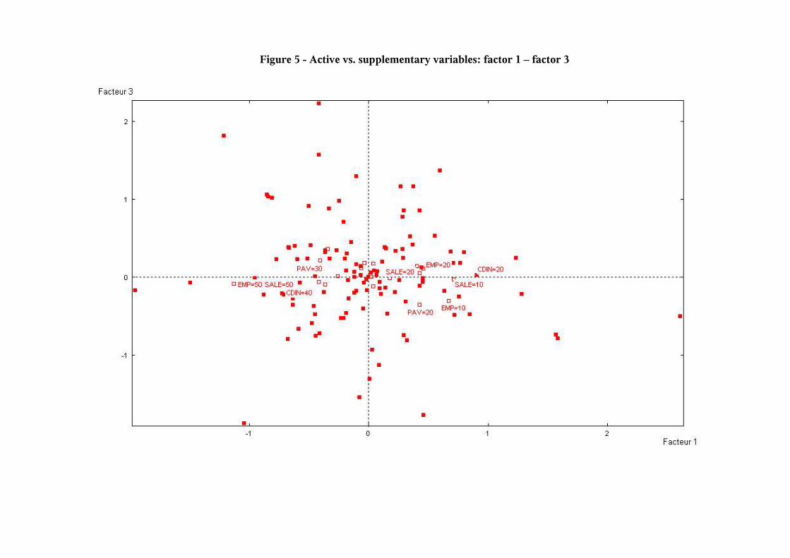
Figure 5 - Active vs. supplementary variables: factor 1 – factor 3

Figure 6 - Active vs. supplementary variables: factor 1 – factor 4