NASA/CR-2010-216709NIA Report No. 2010-03

Assessment of Static Delamination PropagationCapabilities in Commercial Finite ElementCodes Using Benchmark Analysis

Adrian C. OrificiRMIT University, Melbourne, Victoria, Australia

Ronald KruegerNational Institute of Aerospace, Hampton, Virginia

June 2010

NASA STI Program . . . in Profile

Since its founding, NASA has been dedicated tothe advancement of aeronautics and space science.The NASA scientific and technical information (STI)program plays a key part in helping NASA maintainthis important role.

The NASA STI program operates under theauspices of the Agency Chief Information Officer. Itcollects, organizes, provides for archiving, anddisseminates NASA’s STI. The NASA STI programprovides access to the NASA Aeronautics and SpaceDatabase and its public interface, the NASA TechnicalReport Server, thus providing one of the largestcollections of aeronautical and space science STI inthe world. Results are published in both non-NASAchannels and by NASA in the NASA STI ReportSeries, which includes the following report types:

TECHNICAL PUBLICATION. Reports ofcompleted research or a major significant phaseof research that present the results of NASAprograms and include extensive data ortheoretical analysis. Includes compilations ofsignificant scientific and technical data andinformation deemed to be of continuingreference value. NASA counterpart of peer-reviewed formal professional papers, but havingless stringent limitations on manuscript lengthand extent of graphic presentations.

TECHNICAL MEMORANDUM. Scientificand technical findings that are preliminary or ofspecialized interest, e.g., quick release reports,working papers, and bibliographies that containminimal annotation. Does not contain extensiveanalysis.

• CONTRACTOR REPORT. Scientific andtechnical findings by NASA-sponsoredcontractors and grantees.

• CONFERENCE PUBLICATION. Collectedpapers from scientific and technicalconferences, symposia, seminars, or othermeetings sponsored or co-sponsored by NASA.

• SPECIAL PUBLICATION. Scientific,technical, or historical information from NASAprograms, projects, and missions, oftenconcerned with subjects having substantialpublic interest.

• TECHNICAL TRANSLATION. English-language translations of foreign scientific andtechnical material pertinent to NASA’s mission.

Specialized services also include creating customthesauri, building customized databases, andorganizing and publishing research results.

For more information about the NASA STIprogram, see the following:

• Access the NASA STI program home page athttp://www.sti.nasa.gov

• E-mail your question via the Internet tohelp@sti.nasa.gov

• Fax your question to the NASA STI Help Deskat 443-757-5803

• Phone the NASA STI Help Desk at443-757-5802

• Write to:NASA STI Help DeskNASA Center for AeroSpace Information7115 Standard DriveHanover, MD 21076-1320

NASA/CR-2010-216709NIA Report No. 2010-03

Assessment of Static Delamination PropagationCapabilities in Commercial Finite ElementCodes Using Benchmark Analysis

Adrian C. OrificiRMIT University, Melbourne, Victoria, Australia

Ronald KruegerNational Institute of Aerospace, Hampton, Virginia

National Aeronautics andSpace Administration

Langley Research Center Prepared for Langley Research CenterHampton, Virginia 23681-2199 under Cooperative Agreement NNL09AA00A

June 2010

Trade names and trademarks are used in this report for identification only. Their usage does not constitutean official endorsement, either expressed or implied, by the National Aeronautics and SpaceAdministration.

Available from:

NASA Center for AeroSpace Information7115 Standard Drive

Hanover, MD 21076-1320443-757-5802

ASSESSMENT OF STATIC DELAMINATION PROPAGATION CAPABILITIES INCOMMERCIAL FINITE ELEMENT CODES USING BENCHMARK ANALYSES

Adrian C. Orifici 1 , Ronald Krueger2

ABSTRACTWith the increasing implementation into commercial finite element (FE) codes ofcapabilities for simulating delamination growth in composite materials, the need forbenchmarking and assessing these capabilities is critical. In this study, benchmark analyseswere performed to assess the delamination propagation simulation capabilities of the VCCTimplementations in Marc "m 2008r1 and MD Nastran"m R3 v2008.0 in solution sequencesSOL 400 and SOL 600. Benchmark delamination growth results for Double CantileverBeam (DCB), Single Leg Bending (SLB) and End Notched Flexure (ENF) specimens weregenerated using a numerical approach. This numerical approach was developed previously,and involves comparing results from a series of analyses at different delamination lengths toa single analysis with automatic crack propagation. Experimental and analytical benchmarkdelamination growth results were also taken from the literature for a second DCB specimen.Specimens were analyzed with three-dimensional and two-dimensional models, andcompared with previous analyses using Abaqus ¨ with the VCCT implemented. The resultsdemonstrated that the VCCT implementation in Marc"m and MD Nastran"m was capable ofaccurately replicating the benchmark delamination growth results. The analyses in Marc "m

and MD Nastran"m were significantly more computationally efficient than previous analysesconducted in Abaqus¨ . This was due to a lack of convergence issues, and a solution processthat maintained the use of large time increments. The Marc"m and MD Nastran"m solversencountered problems for some models with determining the appropriate crack growthdirection, which required overriding the default automatic procedure. The results alsodemonstrated that the use of the numerical benchmarks was efficient and offers advantagesover benchmarking using experimental and analytical results.

1. INTRODUCTIONOne of the most common failure modes for composite structures is delamination [1-4]. To

characterize the onset and propagation of delamination, the use of fracture mechanics has becomecommon practice over the past two decades [1, 5, 6]. The strain energy release rate, GT, is typicallyused as a measure of the driving force for delamination growth in composite laminates. Dependingupon external loading conditions, GT can be any combination of the three strain energy release ratecomponents, GI, GII, and GIII, illustrated in Figure 1. The mode I component, GI, arises from loadingacting normal to the delamination plane, GII arises from in-plane shear stresses acting perpendicularto the delamination front, and GIII arises from in-plane shear stresses acting parallel to thedelamination front. To predict delamination onset or propagation, the total strain energy release rateis compared to the interlaminar fracture toughness, Gc, which is dependent on the relativeproportions of the mode components. Due to the availability of test methods for characterizingmode I, II and mixed mode I/II delamination, efforts [7-9] have focused on evaluating thedependence of Gc on this range of mode mix. Such a quasi-static mixed-mode I/II fracture criterion

RMIT University, GPO Box 2476, Melbourne, Victoria 3001, Australia.

2 National Institute of Aerospace (NIA), 100 Exploration Way, Hampton, VA 23666, resident at Durability, DamageTolerance and Reliability Branch, NASA Langley Research Center, MS 188E, Hampton, VA, 23681.

is determined by plotting G, versus the mixed-mode ratio, GII/G7. The mixed-mode ratio isdetermined from data generated using pure mode I Double Cantilever Beam (DCB) (GII/G7=0),pure mode II End-Notched Flexure (ENF) (GII/G7=1), and Mixed-Mode Bending (MMB) tests ofvarying ratios. Examples are shown in Figure 2a for T300/914C and Figure 2b for C12K/R6376[ 10, 11 ]. A curve fit of the data is performed to determine a mathematical relationship between G,and GII/G7. [12, 13]. An interaction criterion incorporating mode III was recently proposed byReeder [14]. Application of Reeder’s 3D criterion is restricted due to the absence of a reliablemeans for measuring GIII,. Although, a standardized test for measuring this property is currentlybeing investigated [ 15, 16], and several candidate specimens have been proposed in the literature[17, 18].

The virtual crack closure technique (VCCT) is widely used for computing energy releaserates, based on results from continuum (2D) and solid (3D) finite element (FE) analyses, and tosupply the mode separation required when using mixed-mode fracture criteria [19, 20]. The VCCThas been used mainly by scientists in universities, research institutions and government laboratories,and is usually implemented in their own specialized codes or used in post-processing routines inconjunction with general purpose FE codes. An increased interest in fracture mechanics to assessthe damage tolerance of composite structures in design and certification has also renewed interest inthe VCCT. As such, the VCCT has been implemented into the commercial FE codes Abaqus ®

1 [21]as well as MD Nastran TM [22] and MarcTM2 [23], among others. The implementation into thecommercial FE code SAMCEFTM3 [24] is a mix of the VCCT and the Virtual Crack ExtensionMethod suggested by Parks [25].

As new approaches for analyzing composite delamination are incorporated into FE codes,the need for comparison and benchmarking becomes important. The implementation oftechnologies into FE codes involves numerical parameters, which can be unique to each code, andneed to be understood and calibrated for any analysis. Experimental results used as benchmarks arevaluable, but are complicated by aspects such as fiber bridging, crack branching, and experimentalvariance. Analytical results are also useful as benchmarks, but are not available for all specimentypes and configurations, and can become complicated when dealing with aspects such asnonlinearity and three-dimensional (3D) effects. In response, a numerical benchmarking approachwas developed in which results for delamination growth are first generated from a series of staticanalyses with different delamination lengths [26]. These benchmark results are then compared tosimulation of delamination propagation using a single analysis. In previous work, this numericalbenchmarking approach was applied to DCB and Single Leg Bending (SLB) specimens to assessthe implementation of VCCT in Abaqus® /Standard [26].

In this study, the delamination propagation simulation capabilities of the commercial FEcodes MarcTM 2008r1 and MD NastranTM v2008.0 with the VCCT were assessed. Benchmarkdelamination growth results for DCB, SLB and ENF specimens were generated using a previouslydeveloped numerical approach [26]. Experimental and analytical benchmark delamination growthresults were taken from the literature for a second DCB specimen [27]. Specimens were analyzedusing two-dimensional (2D) plane strain and full 3D models and results were compared to previousanalyses using Abaqus® /Standard with the VCCT implemented.

1 Abaqus® is manufactured by Dassault Systemes Simulia Corp. (DSS), Providence, RI, USA.2 MD NastranTM, MSC NastranTM, MSC PatranTM, MarcTM and MentatTM are manufactured by MSC.Software Corp.,Santa Ana, CA, USA. NASTRAN ® is a registered trademark of NASA.3 SAMCEFTM is manufactured by Samtech, Liege, Belgium.

2

2. SPECIMEN DESCRIPTIONFor the current investigation, specimens were selected to investigate single mode (I and II)

and mixed-mode I/II delamination growth with unidirectional and multi-directional laminates, usingbenchmark results from numerical and experimental studies. Two DCB specimens (labeled “DCB-1” and “DCB-2”), one SLB specimen and one ENF specimen were chosen, as shown in Figure 3,Figure 4 and Figure 5, respectively. The specifications for the DCB-1 and SLB specimensoriginated in previous work, in which experimental and numerical studies were performed and thecritical strain energy release rates evaluated [28-31]. In this work, the DCB-1 and SLB specimenswere selected as they were used to generate numerical benchmark delamination growth resultspreviously [26]. The ENF specimen is the three-point bending 3ENF variant, and the specificationswere set based on commonality with the DCB-1 specimen. The DCB-2 specimen (shown inFigure 3) was selected as benchmark experimental and analytical results were available in theliterature [27]. The DCB and ENF specimens are used to determine the mode I and II interlaminarfracture toughness, GIB [7] and GIIB [9], respectively. The SLB specimen is used to evaluate themixed-mode I/II interlaminar fracture toughness [30, 32].

The DCB-1 and ENF specimens consisted of T300/1076 graphite/epoxy with aunidirectional layup and the DCB-2 specimen consisted of T800/924 graphite/epoxy with aunidirectional layup. The SLB specimen used C12K/R6376 graphite/epoxy with a multi-directionallayup of stacking sequence [±30/0/-30/0/30/04/30/0/-30/0/-30/30//-30/30/0/30/0/ -30/04/-30/0/30/0/±30], where the double slash (//) denotes the location of the delamination. The materialproperties are given in Table 1. In general, mode I, mode II, and mixed-mode tests are performed onunidirectionally reinforced laminates where all fibers are aligned with the 0 direction. This meansthat delamination propagation occurs at a [0/0] interface and delamination propagation is parallel tothe fibers. Although this unidirectional layup is desired for standard test methods to generatefracture toughness data, delamination propagation between layers of the same orientation will rarelyoccur in real structures. Therefore, effects such as fiber bridging that are observed in DCB testsmay not be be present during mode I-dominated delamination growth between plies of dissimilarorientation.

3. METHODOLOGY3.1 Fracture Criteria

Linear elastic fracture mechanics analysis of delamination in composite laminates involvesdetermining the total strain energy release rate, GT, and the individual components GI, GII and GIII,

shown in Figure 1. The onset of delamination growth is predicted using the failure index:

GT

a1 (1)

where GT is the sum of all mode components and Gc is the interlaminar fracture toughness. Thefracture toughness is dependent on the relative proportions of the mode components, or the modemix. A 2D relationship between Gc and modes I and II was suggested by Benzeggah and Kenane[13] and is given by:

Gc G

Ic GIIc GIc

GII (2)GT

3

where GI, and GII, are determined experimentally from DCB tests [7] and ENF tests [9],respectively, and the 2D mixed-mode exponent is determined from MMB tests of varying ratiosof GI and GII [8]. Figure 2a and 2b show the determination of these parameters from experimentaldata for the materials applied in this work, where was determined by a curve fit using theLevenberg-Marquardt algorithm in KaleidaGraph TM3 graphing and data analysis software [33].

Recently, Reeder [ 14] suggested a modification to Equation 2 that incorporates the mode IIIcomponent, which is given by:

Gc = GIc

+ (GIIc GIc)

GII

+GIII + (G

IIIc— G

IIc )

GIII

GII

+GIII

. (3)

GT GII + GIII GT

As no standards currently exist for determining GIII, , or a mixed-mode exponent involving mode III,in this work GIII, was taken as GII, and was taken as the value characterized from 2D mode I/IIdata as shown in Figure 2.

3.2 Virtual Crack Closure Technique3.2.1 Theory

The VCCT [19, 20] is based on the assumption that the energy released in extending a crackby a small amount, a, is equivalent to the work necessary to close the crack to its original length.In an FE analysis using the VCCT, the three strain energy release rate components are calculated ata crack front node by

G = F S(4)

2A

where G is the column vector of strain energy release rate components, F consists of the forces atnodes along the delamination front, is a row vector that consists of the relative displacements ofthe node pairs behind each corresponding crack front node, and A is the surface area created bycrack growth. Equation 4 requires the calculation of a local crack front coordinate system andmodification to account for arbitrary element sizes. The VCCT is applicable for 2D or 3D analysiswith linear and quadratic elements [20].

Previous investigations have shown that the VCCT results can be mesh-dependent fordelaminations between two dissimilar solids, such as between plies of different orientation. This isdue to the oscillatory nature of stresses in the vicinity of a crack front at a bi-material interface. Toavoid mesh dependency issues, it is recommended to use consistent crack tip element lengthsbetween analyses that are being compared. Further detail on this issue is provided in Reference [20].In the current work, the finite element meshes were all based on those used in previous analyses[26], where mesh convergence studies had been conducted.

3 KaleidaGraphTM is manufactured by Synergy Software, Reading, PA, USA.

4

3.2.2 VCCT in Marc ª

The VCCT is implemented into Marcª as a procedure to determine the strain energy releaserate distribution at a crack front [23]. This is done at a single node in a 2D model, or along a seriesof nodes in a 3D model. Multiple cracks can also be modeled. The user only needs to define thecrack front nodes, and the solver determines the appropriate nodes, forces and areas to use for thecrack growth calculation. This implementation follows the description given by Krueger [20], whichaccounts for a crack front of arbitrary shape.

For propagating a crack front, there are several options: growth by remeshing, where thelocal mesh around the crack tip is moved and the surrounding mesh is adapted; growth alongelement edges, where the elements at the crack front are disconnected by creating duplicate nodesand modifying the element connectivity; growth by releasing constraint, where a fixed contact or tierestraint is released. In the current work, only the latter approach was applied, as this was the onlyapproach that could be used with 3D solid elements.

For crack growth by releasing constraints, the user defines two surfaces that are initiallybonded with a “glued” [23] constraint, or a set of multi-point constraints (MPCs) between nodesacross an interface. In the current work, the contact-based approach was used, which is similar tothe approach implemented within Abaqus¨ [21]. It is possible to define a completely bondedinterface, and then to select certain nodes that are unbonded, or have the bond function“deactivated” [23], so that a pre-crack can be modeled. An example of this is shown in Figure 6,where a specimen with a pre-crack (shown in Figure 6a) is modeled using only a bonded interface(shown in Figure 6b), or with a combination of a bonded and unbonded contact interface (shown inFigure 6c).

At the end of every nonlinear analysis increment, the strain energy release rates arecalculated using the VCCT. Crack growth onset is detected using Equation 1, with either single-mode or mixed-mode criteria for Gc. For single-mode criteria, three equations are used to considereach mode independently, and for mixed-mode, the Reeder (Equation 3) or Power law criteria areavailable [14]. The crack is “grown” by releasing the constraint at the crack front node, whichextends the crack to the next node in the bonded contact region. If crack growth is detected at theend of the increment, the appropriate nodes are released, and the increment is restarted. Restartingthe increment is repeated until Equation 1 is no longer satisfied at any crack front node, and is acritical step in ensuring that enough crack growth occurs within an increment. This aspect is detailedfurther in the Discussion section.

Another aspect that can become important is the way in which the VCCT algorithm locatesthe most appropriate node in the intact region to “grow” the crack, once propagation has beendetected at a crack front node. In Marcª, this is based on the definition of the crack growthdirection, where once this direction is determined, the solver will select the closest appropriate nodefrom those available in the intact region. The default option in Marc ª is an automatic determinationof the crack growth direction based on a maximum principal stress criterion, which defines thecrack growth as being normal to the direction of greatest tension [23]. There are other options forspecifying the crack growth direction that the user can select instead of the default, where thegrowth direction is instead aligned with either the most critical mode, with the mode I component,or with a fixed user-defined vector. The effect of this option is discussed further in the results foreach specimen, and further detailed in the Discussion section.

5

3.2.3 VCCT in MD NastranTM

SOL 400The VCCT is implemented into MD Nastran TM solution sequence SOL 400, and follows the

same general approach as outlined above for Marc TM .

The SOL 400 solution sequence is anintegration of the traditional nonlinear solver (SOL 106) with advanced nonlinear technologies [23].This includes functionality developed originally in Marc TM ,

such as contact and the VCCT

technology for crack growth modeling. Critically though, not all aspects of the Marc TM

implementation within a given software version are available in the MD Nastran TM version of thesame release date [23, 22, 34]. As a key example of this limitation, in the SOL 400 version appliedin this work (version 2008.0), the VCCT technology did not incorporate mixed-mode crack growth.Another important example is that only the default option for determining the crack growthdirection could be specified as input.

3.2.4 VCCT in MD NastranTM

SOL 600The VCCT is available in MD Nastran TM solution sequence SOL 600. The SOL 600 solution

sequence is a “wrapper” application for Marc TM, in which the user generates an MD NastranTM

inputfile, and the solver converts this into a MarcTM input file, runs the analysis natively in MarcTM, andtranslates the Marc

TM output into MD Nastran

TM format [22]. However, despite running Marc TM

natively, this solver can be limited by the translation process, which includes options available inMarc

TM not being easily available within the MD Nastran TM input format, and some difficulties in

“mapping” functionality between the two codes. As with the SOL 400 solver, a key example of thelimitations of the SOL 600 solver in the version applied in this work was that the VCCT technologydid not incorporate mixed-mode crack growth, and could only be used with the default option fordetermining the crack growth direction. While the SOL 400 solution sequence is exclusive to theMD Nastran

TM analysis package, the SOL 600 solution sequence is also available within MSC

NastranTM. As such, references made in this work to MD Nastran TM SOL 600 are identicallyapplicable to MSC Nastran TM SOL 600.

4. FINITE ELEMENT MODELINGTypical 2D and 3D FE models of the DCB, SLB and ENF specimens are shown in Figure 7

to Figure 9, which also illustrates the boundary conditions applied for these models. The modelswere based on those presented previously [26]. An additional ENF model with a refined mesh wasgenerated, which is shown in Figure 10 with boundary conditions, and discussed further in theresults section. All models are summarized in Table 2, which lists the analysis solver and dimension(2D or 3D) for each model, with a reference to the corresponding mesh.

Along the specimen length, all models were divided into various sections with differentmesh refinement. Although the dimensions of the elements varied, all meshes were based on arefined mesh region that used elements of 0.5 mm length in the crack growth direction in the regionimmediately around the delamination front. This element length was selected in previous studies[28, 31], in which mesh convergence investigations were performed. All models used a uniformmesh across the width direction. The specimens with unidirectional laminates used six elementsthrough the specimen thickness (2h), while the multi-directional laminate specimens used a refinedmesh based on a ply level mesh refinement around the delamination interface, as shown in Figure 8.Elements away from the delamination interface used a smeared material property for eachsublaminate based on the rule of mixtures. Further detail and justification of the modeling is givenin Reference [26].

6

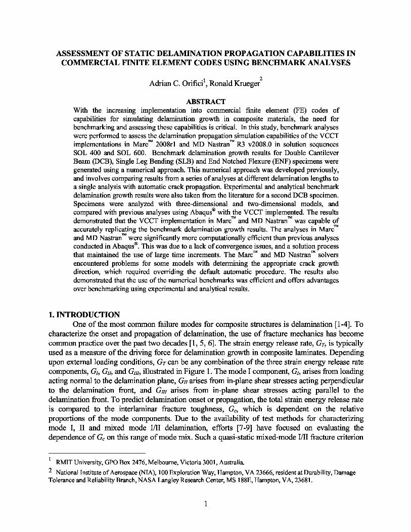
For all models, the plane of delamination was modeled as a discrete discontinuity in thecenter of the specimen. To create the discrete discontinuity, each model was created from separatemeshes for the upper and lower part of the specimens with identical nodal point coordinates in theplane of delamination. Two surfaces (top and bottom) were created on the meshes as illustrated inFigure 6, and a bonded (glued) contact specified between them. For the DCB and SLB specimens,the pre-crack was not included in the contact definition as no interaction between the two surfaces inthis region was expected. For the ENF specimens, contact was required across the pre-crackedinterface, so the entire surface was included in the bonded contact, and the pre-cracked region wascreated by deactivating the bonded contact for some nodes. For models that were analyzed withoutcrack propagation (calculation of strain energy release rate only) as part of developing benchmarkresults as described later, the crack propagation capability was turned off.

The delaminated surfaces of the DCB and SLB specimens do not come into contact duringtheir respective deformation, and thus unbonded contact was not necessary when analyzing thesespecimens. Avoiding the use of contact modeling is advantageous, as the inclusion of a contactalgorithm significantly increases the solution time of an analysis. In these cases, only bondedcontact was required in order to simulate delamination growth. The ENF specimen on the otherhand does involve contact of the delaminated surfaces during deformation, and so unbonded contactwas necessary to ensure that these surfaces did not interpenetrate during an analysis.

All specimens were analyzed with 3D models. Additionally 2D models of the DCB andENF specimens were created. A summary of all models run in the current work is presented inTable 2. The 3D models used 8-node reduced integration solid brick elements (Marc

TM element type

117 [23] and MD NastranTM

element type CHEXA [22]). The 2D models used two-dimensional 4-node plane strain elements (Marc TM element type 11 and MD Nastran

TM element type CQUAD4).

The 2D and 3D models for a specimen used the same mesh scheme, as shown in Figure 7 andFigure 9. The nonlinear solvers in Marc

TM and MD Nastran

TM were used, which applied a full

Newton-Raphson solution procedure with a load residual tolerance of 0.001. The specimen loadingwas defined in terms of applied displacements, to minimize problems with numerical stability of theanalysis caused by the unstable propagation. All models were run on a 32-bit Intel Core 2 Duo 2.25GHz CPU processor.

Comparing codes, the input requirements for the VCCT analysis were the same, except forthe lack of mixed-mode parameters in SOL 400 and SOL 600 as previously discussed. Details onthe specific keywords and parameters required for a VCCT analysis in each code are given in theAppendix. The differences between the codes in terms of the more practical aspects of theapplication are detailed in the Discussion section.

5. ANALYSIS5.1 Computation of Strain Energy Release Rates

For each of the specimens, the computed strain energy release rate distribution across thedelamination front was plotted versus the normalized specimen width, y/B, as shown in Figure 11 toFigure 13, for the 3D and 2D models. Distributions were calculated for a range of differentdelamination lengths, as part of the numerical benchmark results generation described in the nextsection. As strain energy release rate distributions for different delamination lengths werepreviously presented for the DCB and SLB specimens [26], the results in Figure 11 and Figure 12,respectively, are given for only one delamination length. The ENF results in Figure 13 are given forall delamination lengths investigated, for the same applied displacement. For the DCB and ENFspecimens, only the dominant mode component is shown (I and II respectively), as the others were

7

negligible, and there was no 2D model for the SLB specimen. For the DCB and SLB specimens,Figure 11 and Figure 12 demonstrate the excellent agreement between the results in Marc ª andthose calculated using Abaqus¨ in previous work [26]. The results for all specimens demonstratethat due to 3D effects, such as anticlastic bending of the loading specimen arms, the strain energyrelease rate distribution was non-constant across the delamination front, even for single-modedominated specimens. These curved distributions can cause an initial straight front to grow into acurved front. This process has been observed both analytically and experimentally [26, 35-39].

For the ENF specimen, the results in Figure 13 show that the strain energy release ratesinitially increased with increasing delamination length, which would cause unstable delaminationgrowth. This trend changed with respect to the location of the central loading pin, whichcorresponds to a delamination length of 70 mm. The average strain energy release rate initiallydecreased with an increase in delamination length, up to a maximum length corresponding to theloading pin location, and then began to increase with longer delamination lengths. This suggests thatcrack growth at delamination lengths past the loading pin was stable. From the results in Figure 13,it was found that the distribution of GII across the delamination front changed slightly withdelamination length. In this case, GII peaks on the edges of the delamination front at shorterdelamination lengths, and peaks in the center at longer delamination lengths. The distribution alsobecomes more curved at delamination lengths approaching the loading pin. The unstable nature ofdelamination growth in ENF specimens loaded quasi-statically, under displacement control, is welldocumented in the literature [40-42].

5.2 Creating Benchmark Delamination Growth ResultsThe approach developed previously for generating numerical benchmark delamination

growth results [26] was applied to the DCB-1, SLB and ENF specimens. For these specimens, abenchmark result set was extracted from a series of models with different delamination lengths.These models did not simulate delamination propagation, and were only used to get the load-displacement response and the strain energy release rate distribution for different delaminationlengths. For each delamination length modeled, a failure index was calculated across thedelamination front using Equation 1, with the Reeder mixed-mode criterion used to compute Gc

(Equation 3). Delamination growth onset was assumed when the failure index at the center of thespecimen (y/B = 0) reached a value of unity. Specimen load-displacement response up to this pointwas also assumed to be linear. Subsequently, the displacement and load at delamination growthonset, crZt and PcrZt, respectively, was computed by linearly scaling the prescribed displacement andload in each analysis ( and P respectively), using the following relations [26]:

zGT =

P 2

P =

>Pc it = P

VG

, '^r =

bVG, (5)

Gc c it

The benchmark result set is constructed by plotting the displacement at delamination growth onsetversus delamination length, as illustrated in Figure 14 for the DCB-1 specimen. This form is usedfor the benchmark result because all specimens were loaded via a prescribed displacement, and thechange in delamination length is the most appropriate output for assessment of delaminationgrowth. In previous work [26], the benchmark results were presented as load-displacement curves,to illustrate the application of Equation 5.

8

The benchmark delamination growth results for the DCB-1, SLB and ENF specimens arepresented in Figure 14, Figure 15 and Figure 16, respectively. Results from previous analyses withAbaqus¨ [26] are also included for the DCB-1 and SLB specimens. The DCB-1 results show thatthe applied opening displacement increased with increasing delamination length, which indicatesstable growth under displacement control. In contrast, both the SLB and ENF results indicate initialunstable delamination growth, as the critical displacement decreases with increasing delaminationlength. The comparison between the Abaqus ¨ and Marcª results in Figure 14 and Figure 15 showsthat the two solvers gave almost identical results for these models.

5.3 Delamination Propagation Analysis: DCB-1For the DCB-1 specimen, the previous results in Figure 14 show that delamination

propagation was predicted to initiate at an applied opening displacement (/2) of 0.75 mm. Based onthis, a two-step loading procedure was applied for the delamination propagation analysis, whichinvolved using coarse time increments until just before failure, and fine increments for the regioninvolving delamination propagation. Dividing the first step into relatively coarse time incrementswas possible as the load-displacement behavior of the specimen up to failure was expected to belinear. In the first step, a prescribed opening displacement of /2 = 0.7 mm was applied in 10increments. In the second step, the total prescribed displacement was increased to /2 = 1.0 mm.This was applied with a fixed time increment scheme of 50 increments (/2 = 0.006 mm eachincrement).

In both Marcª and MD Nastran ª, the solver has the capability to cut back the incrementsize in the event of convergence issues. In addition, the Marc ª solver has the capability to activatedamping when the time step is reduced below a defined minimum. Critically, no convergence issueswere seen throughout any analyses, and damping was not required. This is quite different behaviorfrom that seen previously with Abaqus¨ [26], where convergence issues associated withdelamination growth caused significant cutbacks in the time increment, required investigation ofsuitable damping parameters and involved an increase in computational expense. As a result, runtimes for delamination propagation analyses were within a minute for the 2D models and generallywithin a few hours for the 3D models, depending on the selection of increment size and amount ofdelamination growth. The efficiency of the solver is discussed further in a later section.

The DCB-1 specimen was analyzed with Marc ª, MD Nastranª SOL 400 and MD Nastranª

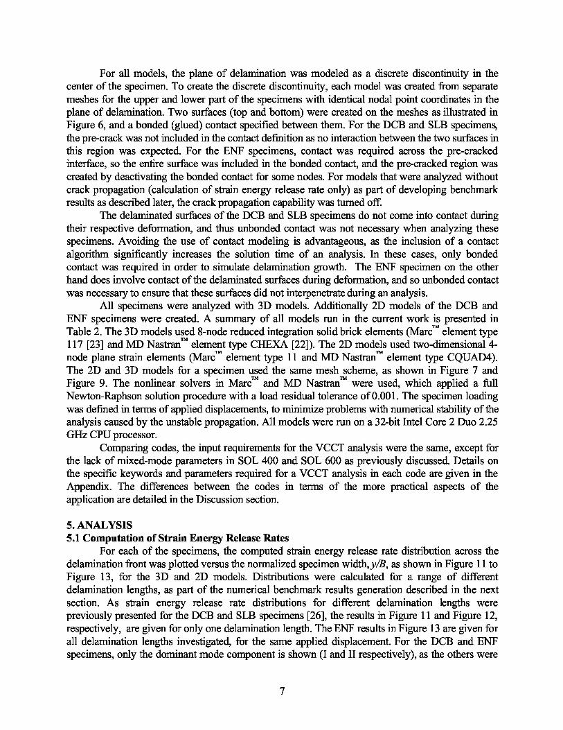
SOL 600, with both 2D and 3D models, as shown in Table 2. All solvers detected delaminationpropagation using simple single-mode criteria, as the SOL 400 and SOL 600 solvers did not haveany mixed-mode criteria as previously discussed. The results of all analyses are shown in Figure 17to Figure 19, where Figure 17 to Figure 18 are the results from only the Marcª analysis, and Figure19 is a comparison of the delamination growth results from all solvers.

From the delamination growth results in Figure 17, the VCCT technology gave very closecomparison with the benchmark results, for both 2D and 3D models. The 3D models showeddelamination growth at slightly lower applied displacements, which was due to the slightly higherstrain energy release rates in the 3D models as shown in Figure 11.

From Figure 18, the delamination was seen to propagate as a straight crack front, whichcontradicts the curved strain energy release rate distribution shown in Figure 11. This propagationof a straight front is related to the coarse element size and was also seen in previous analyses [26,43].

From Figure 19, all solvers produced almost identical results, for both 2D and 3D models.This indicates that the implementation of the VCCT technology is common across solvers. The only

9

discrepancy of note was seen for the 3D model, where on two occasions the SOL 400 modelshowed delamination growth an increment earlier than the Marcª and SOL 600 models. This can beseen in Figure 19 for the first and last delamination growth increments shown (at a = 0 mm and

a = 4.5 mm). This was attributed to slight numerical differences between the solvers.The characteristic step pattern seen in the delamination growth results in Figure 17 and

Figure 19 was caused by the step change in length as the delamination was grown one elementlength at a time. In the case of the 3D models, the delamination was seen to propagate across thecrack front within the same increment. This step pattern is illustrated in Figure 20, where thenumbered stages show the initial increase in applied displacement (1-2), sudden nodal release (2-3),increase in displacement until next delamination growth (3-4), and repetition (4-5, 5-6, etc.). Thesestep changes in delamination length at a fixed applied displacement would produce a sequence ofdrops in the reaction load and the corresponding “saw-tooth” pattern in the load-displacementresponse [43, 44]. The results also show that the corners of the steps, just before a delaminationgrowth event, provide the most suitable comparison with the benchmark results, which also allowscoarse meshes to be adequately used.

5.4 Delamination Propagation Analysis: DCB-2For the DCB-2 specimen [27], the analysis used the model shown in Figure 7, with the

width across the delamination front increased from 25 mm to 30 mm. The analysis used two loadsteps with coarse and fine time step incrementation, as discussed for the DCB-1 specimen. In thefirst step, a prescribed displacement of /2 = 0.9 mm was applied in 2 increments, while in thesecond step the total prescribed displacement was increased to /2 = 6.0 mm in 250 increments(/2 = 0.0204 mm each increment). As with the DCB-1 specimen, no significant convergenceissues were seen and damping was not required.

The DCB-2 specimen was analyzed in Marcª with both 2D and 3D models as shown inTable 2. Delamination propagation was detected using single-mode criteria. Numerical results werealso taken from a previous publication [45], in which the DCB-2 specimen was analyzed usingAbaqus¨ 6.8. Further detail on the modeling approach adopted in that work is given in References[21, 26, 45], which includes discussion on the damping and other parameters required. Benchmarkanalytical solutions for delamination growth were taken from Reference [27], where relationshipsbetween the applied displacement and delamination length are presented based on beam theory.Experimental delamination growth results were taken from Reference [46], where the delaminationlength was measured at intervals on the edge of the specimen. The experimental results wereincluded since the original experiments showed very little fiber bridging [46], which is notaccounted for in the analysis. The delamination growth results of all analyses and benchmarks areshown in Figure 21.

It is observed from Figure 21 that the VCCT technology was capable of accuratelyrepresenting the analytical and experimental benchmark results in terms of delamination growthbehavior. Excellent agreement was seen between the two analysis codes, and between the numericalanalyses and both the experimental and analytical results. The change in character of the Marc ª

results at a delamination growth a = 40 mm was due to the delamination reaching a region of themesh with larger elements, which led to larger step changes in delamination growth. At thetransition between the fine and coarse mesh regions, the Marc ª results showed a deviation fromthe expected behavior. As discussed previously for the DCB-1 specimen and illustrated in Figure20, the peak displacements just prior to delamination propagation in each step give a consistent

10

alignment with numerical benchmark results. The results at the mesh transition region indicatedin Figure 21 demonstrate an error in the VCCT implementation, caused by the difference betweenelement lengths ahead and behind the delamination front. The Abaqus¨ results shown in Figure 21do not show this error since a consistently fine mesh was used. However, this error was seen inother Abaqus¨ results [45], and indicates a similar implementation error in both codes. The issue ofmesh transition is further investigated and discussed in detail in Section 6.1.

The results for the DCB-2 specimen demonstrate the difference between codebenchmarking using experimental and analytical approaches, in comparison with the use of thenumerical benchmark results for the DCB-1. The use of experimental and analytical results ishighly valuable in validating that the simulation is capable of capturing the physical phenomena.These approaches, however, may introduce additional factors that can influence an assessment ofsimulation capabilities, which include statistical variance, the use of approximations, orcomplications such as fiber bridging. As these aspects were not expected to be significant in thiswork, the comparisons with benchmark results for the DCB-1 and DCB-2 specimens producedsimilar conclusions. Further, the results for the two specimens demonstrate that numericalbenchmarks are suited for efficiently isolating and assessing code capabilities as they involve adirect comparison between the behavior of identical models. The use of numerical benchmarkswould also be highly valuable where experimental and analytical results are unavailable ordifficult to obtain, such as for complex specimens and structures.

5.5 Delamination Propagation Analysis: SLBFor the SLB model, shown in Figure 8, the analysis used two load steps with coarse and

fine time step incrementation as discussed for the DCB-1 specimen. In the first step, a prescribedcenter displacement of w = 3.0 mm was applied in 6 increments, while in the second step thetotal prescribed displacement was increased to w = 4.0 mm in 100 increments(w = 0.01 mm each increment). As with the DCB specimens, no significant convergence issueswere seen and damping was not required.

One aspect that was critical for the analysis of the SLB specimen was that the crack growthdirection needed to be specified with a user-defined vector, instead of with the default automaticalgorithm that, as previously discussed, is based on a principal stress criterion. In preliminary SLBmodels using the default approach, errors were found in the propagation of the delamination front,where the solver would detect the critical node but not be able to locate the appropriate node in theintact region to grow the delamination front. This was found to be due to the calculated crackgrowth direction, which in some instances pointed in directions from which no suitable nodes couldbe found. This problem was also found to be particularly critical for edge nodes, and was found tooccur for both coarse and fine meshes. In instances where the delamination could no longer bepropagated due to the inappropriate crack growth direction, the entire delamination was made“inactive”, and all VCCT calculations were ceased.

In order to address this problem, it was necessary to specify a user-defined vector for thecrack growth direction, which was possible for the SLB specimen, as the crack growth directionwas known. For the SLB specimen as shown in Figure 8, the crack growth direction was alignedwith the global x-direction (i.e. the user-defined crack growth direction vector was set to<1,0,0>). It should be stated that the calculation of the strain energy release rates is not based on thecrack growth direction, but uses a local crack front coordinate system as previously described. Assuch, setting the crack growth direction to be fixed acts only to assist the solver in locating thecorrect node for crack propagation, and does not influence the mode mixity at the crack front.

11

The consequence of this issue was that SOL 400 and SOL 600 could not be used to analyzethe SLB specimen, as only the default crack growth direction option was available to be selected inthe version of MD Nastran ª appied in this work. More critically, the SLB specimen is a mixed-mode problem, so that in any event, as only single-mode crack growth could be implemented, SOL400 and SOL 600 could not have been used.

The SLB specimen was analyzed in Marcª with a 3D model as shown in Table 2.Delamination propagation was detected using the Reeder mixed-mode criterion. A 2D model wasnot analyzed, as the multi-directional laminate could not be modeled correctly. The delaminationgrowth results are shown in Figure 22, and the progression of the delamination front is illustrated inFigure 23.

From these results, the VCCT technology was again capable of accurately representing thedelamination growth benchmark results for this mixed-mode case as shown in Figure 22. Thebenchmark results show that the SLB specimen exhibited an initial period of unstable delaminationgrowth. This was caused by the strain energy release rates remaining critical with increasingdelamination length. In the benchmark curve, unstable delamination growth is indicated by areduction in applied displacement below the initiation point. As the analysis was run indisplacement control, it was not possible to get a reduction in displacement, so the unstabledelamination growth is seen as a large crack growth step. This corresponded to the delaminationextending by 21 mm within one increment, which is shown in both Figure 22 and Figure 23. Thiswas followed by stable delamination growth, where the benchmark and FE results correlated veryclosely. The delamination growth behavior as shown in Figure 23 demonstrated that a curveddelamination front developed and propagated. This was caused by the curved strain energy releaserate distribution as shown in Figure 12. As described for the DCB-1 specimen, this led to a slightdifference compared to the benchmark results, which were generated based on a straightdelamination front. It is possible that the exact shape of the delamination front shown in Figure 23was affected by the delamination propagating through a mesh transition, which is furtherdemonstrated for the ENF specimen and investigated in detail in the Discussion section.

5.6 Delamination Propagation Analysis: ENFFor the ENF model shown in Figure 9, the analysis used two load steps with coarse and

fine time step incrementation as discussed for the DCB-1 specimen. In the first step, a prescribedcenter displacement of w = 4.0 mm was applied in 2 increments, while in the second step thetotal prescribed displacement was increased to w = 8.0 mm in 100 increments (w = 0.04 mm eachincrement). As with all previous specimens, no significant convergence issues were seen anddamping was not required. However, as found for the SLB specimen, the default crack growthdirection algorithm resulted in delamination propagation errors, and a user-defined vector wasused. Again, due to the requirement for a user-defined crack growth vector, MD Nastran ª SOL400 and SOL 600 could not be used.

The ENF specimen was analyzed in Marcª with both 2D and 3D models as shown inTable 2. Delamination propagation was detected using single-mode criteria. The results of theanalyses are shown in Figure 24 and Figure 25. As observed from these results, the VCCTtechnology was capable of accurately representing the benchmark delamination growth results forthe baseline ENF mesh. As with the DCB-1 specimen, delamination growth was initiated in the 3Dmodel at a slightly lower applied displacement than the 2D model, which was due to a slightlyhigher strain energy release rate as shown in Figure 13 for a = 30 mm.

12

The results for the ENF specimen showed initial unstable delamination propagationfollowed by stable propagation, in the same way as described for the SLB specimen. The firstdelamination growth event corresponded to a delamination growth step of 41 mm, as shown inFigure 24. The unstable delamination growth was followed by stable growth, where the benchmarkand FE results correlated very closely. As previously discussed, the change from unstable to stabledelamination growth is associated with the inflection point of the applied displacement versusdelamination growth behavior, which is indicated in Figure 24. Although in experimental testingfocused on material characterization, the delamination is not extended past this point, for thenumerical analysis this region remains valuable for benchmarking purposes.

From Figure 25, the delamination front formed in the baseline mesh by the unstabledelamination growth was jagged and non-straight across the width. This irregular and unexpectedpattern was considered a product of the delamination propagating through a mesh transition region,in addition to insufficient mesh density across the width. A refined model, shown in Figure 10, wasanalyzed in which the delamination propagation only occurred in the fine mesh region, where theelement length was 0.5 mm in the crack growth direction. Rather than using a large fine meshregion to capture all of the unstable delamination growth from a = 30 mm to a = 71 mm, it wasdecided to instead increase the length of the initial delamination to 65 mm. This located thedelamination within the unstable delamination growth region, so that the stable delaminaiton growthbehavior would still be identical to the baseline case, while keeping the model size reasonable.Additionally, the mesh density across the width was doubled, while for efficiency the length of thefine mesh region was reduced.

The results of the analysis of the ENF refined mesh model are shown in Figure 26, wherethe increased mesh density and initial delamination of 65 mm produced a straight delamination frontwithout the jaggedness across the width. The delamination growth results for the models are shownin Figure 27, where the initial delamination length of a = 65 mm is represented as a delaminationgrowth a = 35 mm, so that the baseline for delamination growth in the two numerical analyses isthe same. From the delamination growth results, it can be seen that despite different delaminationfront patterns, the models gave very close comparison with the benchmark curve for the stabledelamination propagation stage. These results demonstrate that crack propagation through a meshtransition region could lead to an incorrect delamination front developing and propagating, and thatthe mesh refinement level was critical to accurately capturing the shape of the delamination front.The results in Figure 27 also clearly demonstrate the effect of large elements on the delaminationgrowth, where the peaks of the large steps just prior to delamination growth gave the most suitablecomparison with the benchmark results.

6. DISCUSSION6.1 Mesh transition

The results in Figure 21 and Figure 25 demonstrated an error in the implementation of theVCCT in Marcª, with regards to calculation of strain energy release rates, where elements aheadand behind the delamination front had different lengths. This was also seen for the Abaqus ¨ solverin Reference [45]. As detailed in References [19, 20], the VCCT equations require a modificationfactor to account for uneven element lengths ahead and behind the crack front. The results inFigure 21 and Figure 25 demonstrate that this has not been implemented, so that uneven elementlengths, such as those seen as a crack propagates through a mesh transition region, result in incorrectcalculation of the strain energy release rate. To illustrate this effect further, a 2D DCB-1 model with

13

several mesh transition regions was analyzed in Marc TM , with the mesh and the results shown in

Figure 28. The errors are most clear for the transition to smaller elements, as is shown ata = 5.25 mm, where an under-estimation of the strain energy release rates due to the mesh

transition prevents delamination growth from occurring and following the benchmark results. Thesame error is less evident though still occurring in the two transitions to larger meshes at a = 1.0mm and a = 7.25 mm. For the 2D DCB-1 model in this example, the errors did not propagate, sothat predictions in a regular mesh following a mesh transition region returned to follow thebenchmark solution. However, the results for the 3D ENF model demonstrated that an incorrectdelamination front could develop due to a mesh transition region and be propagated.

6.2 Solver comparison: Marc ª and Abaqus®

Comparing MarcTM

results in this work (which includes the adaptation of the Marc TM

implementation into MD NastranTM) with previous Abaqus¨ results [26], one clear difference wasthe solution process. Critically, in the Marc TM implementation of VCCT [23], once crack growth isdetected in an increment the crack front node is released and the increment is restarted. This allowsfor multiple crack growth instances to occur in one increment, and allows for coarse timeincrements to be used, which is computationally efficient. By comparison, in the Abaqus ¨

implementation [21], only one crack growth instance can occur in each increment, so it is necessaryto reduce the increment size considerably in order to ensure that no over-estimation occurs. Thefailure index determined from the strain energy release rates is monitored, and the user defines alimit on the amount that the failure index can exceed a value of 1.0. This overshoot limit, or “releasetolerance”, as such becomes another parameter in the model that requires careful selection [26]. So,while the Abaqus¨ approach decreases the increment size to suit the crack growth, in Marc TM thecrack growth is increased to suit the increment size, so that larger increments can be used withincreased computational efficiency.

The convenience of using large increments needs to be managed carefully with the need tocapture the initiation point for crack growth. This is illustrated in Figure 29, where a DCB-1specimen is analyzed in Marc

TM with fine and coarse time incrementation. With fine time

increments, a step pattern of crack growth is observed, which indicates that no over-estimation isoccurring due to the increment size. The analysis with coarse time increments is seen to follow thefine solution closely, though the use of coarse increments means that the exact initiation point forcrack growth is not captured. This issue can be addressed by using different time incrementationthroughout the analysis, where for example coarse increments are used until just before crackgrowth initiation (which could be determined from a preliminary coarse analysis), fine incrementsare used to capture the crack growth initiation, and if necessary coarse increments can be re-used tocapture crack propagation. This is similar to the two-step approach applied in this work.Alternatively, it may be considered that the benefit of using coarse increments outweighs the slightincrease in accuracy in capturing the initiation point, which may be more appropriate for analysis oflarge structures.

Another important difference between Marc TM and Abaqus¨ is the convergence difficultiesand the subsequent damping required. In previous work using Abaqus ¨ [26], it was found thatdamping, or “stabilization”, needed to be added to the solver, in order to get a solution in light of theconvergence issues. The introduction of stabilization parameters requires considerable effort inparametric investigation in order to determine a suitable compromise between damping and solutionaccuracy. In contrast, for the models considered in this work with MarcTM, no severe convergenceissues were recorded and damping was not applied in any of the solutions.

14

The two aspects of differing time increment requirements (caused by allowing multiplecrack growth events in an increment) and the requirement for damping meant that the Marc rm solverwas considerably more computationally efficient than the Abaqus¨ solver for the models analyzed.This was most noticeable for the 3D models, where for example, the Abaqus ¨ solver required runtimes of up to several days [26], while the Marcrm solver experienced run times of only severalhours. Although the analyses were run on different machines, the comparison clearly highlights theconsiderable difference between the two solvers. This difference is further exacerbated by theintroduction of the release tolerance and stabilization parameters in Abaqus ¨ , which typicallyrequire parametric investigations to determine.

One aspect that required attention in the Marcrm analysis was the definition of the crackgrowth direction, where the default automatic algorithm was unable to propagate the crackcorrectly. With the user-defined vector, it was possible to achieve the correct solution for theproblems considered. However, for problems where the crack growth direction is unknown orchanges along the delamination front, this may present further difficulties. While information on theexact procedure implemented in Abaqus ¨ is not available in the documentation, none of theprevious analyses of DCB and SLB specimens indicated any issues with locating the correct nodesfor crack propagation [26, 45].

The use of the crack growth direction in Marcrm is an important difference from theimplementation in Abaqus¨ , and has both advantages and disadvantages. In Abaqus¨ , the crackfront node is simply “released” from contact, and the new crack front is found by determiningwhich nodes lay on the boundary of the contact definition. This is a simple technique that ensuresthat there are no issues with propagation in terms of locating the correct nodes, which are locatedimplicitly. In Marc rm, the use of the crack growth direction as a search vector is disadvantageous, asit introduces the possibility that either incorrect nodes are found, or no nodes are found at all. Thedifficulty in determining the correct crack growth direction is likely to be caused by the applicationof the principal stress criterion, where the accuracy of this criterion at the interface between twodifferent orthotropic materials is uncertain, as the method was originally developed for isotropicmetals.

On the other hand, the use of the crack growth direction in Marc rm has the advantage ofallowing the crack growth to be explicitly tracked for each node. As the crack front moves from onenode to another, information regarding the accumulated crack growth is directly passed betweennodes. In this way, each crack front node at any increment maintains the total crack growth it hastaken for the crack to reach that node since the beginning of the analysis. This makes it very easy totrack the crack growth at each node across the crack front, and also to implement R-curve behaviorwhere the fracture toughness parameters vary with crack length.

Despite the advantages in explicitly tracking the crack growth data, it is possible to achievea determination of the total crack growth for any node and a capacity to implement R- curvebehavior without requiring the use of the crack growth direction. For R-curve behavior, this can beachieved by defining a spatially varying field, where the fracture parameters are set as a function ofgeometric coordinates. In the examples in this work, the fracture parameters could be madedependent on one coordinate (the x-coordinate for all specimens as shown in Figure 3 to Figure 5)though this would change depending on the configuration of the specimen and the pre-crack. Thisapproach would be possible within Abaqus¨ , where fracture parameters can be made dependent ona state variable, which can vary according to a given field. Separately, for tracking crack growthdata at each node, this can be achieved by determining the minimum distance between a crack frontnode and any node defined as part of the initial crack front. This capability is currently not

15

implemented into either code, though could easily be done during post-processing or with a usersubroutine.

More broadly, there are other differences between the implementation of the VCCT intoMarcTM and Abaqus¨ . Both codes implement the crack propagation modeling as a disconnection of acontact surface between two initially bonded or “glued” interfaces. However, while in Abaqus¨ thisimplementation is only available for use with a contact definition, in Marc

TM it is possible to apply

this to multi-point constraints. Furthermore, in MarcTM, the VCCT can be used to model crackpropagation by remeshing or by disconnecting elements along their edges, though at this stage thesetechniques are only available for 2D solid (plane stress/strain) or shells. Marc TM also offers a usersubroutine “ucrackgrow.f”, so that the crack growth behavior using the VCCT can be customized tospecific requirements. This allows the user to control the crack growth direction, which is used tolocate where the crack will propagate, and the amount of crack growth in an increment.

6.3 Solver comparison: Marc ª and MD Nastran ª

Comparing Marc TM , MD NastranTM

SOL 400 and SOL 600, the results presented in this workindicate that the implementation of the VCCT is identical. However, as discussed previously, ingeneral the range of technologies and options implemented into MD Nastran TM tends to be limited,as it can take some time and several releases for aspects developed natively in Marc

TM to be migrated

within the MD NastranTM

environment [34]. As such, comparison of the codes is simplified todetermining which of the technologies and options that are in Marc TM are actually available withinMD NastranTM, and understanding what additional options need to be added to an MD NastranTM

model to apply the VCCT technology. Critically, in this work MD NastranTM could not be used forany mixed-mode delamination growth specimens such as the SLB specimen as there were nomixed-mode criteria implemented. Additionally, SOL 400 and SOL 600 could not be applied withthe SLB and ENF specimens due to the difficulties in using the default algorithm for determiningthe crack growth direction.

In terms of SOL 400, the VCCT implementation is integrated within the MD Nastran TM

nonlinear solver. In the analysis in this work, and in previous benchmark studies [47], the MDNastran

TM nonlinear solver was more robust and efficient than in Marc TM . This is partly due to a

difference in the control of the increment size. In MD Nastran TM, this is based on the convergenceparameters, while in Marc

TM control is framed around either the number of iterations in an increment

or the damping parameter. Additionally, the SOL 400 solver in the version of MD Nastran TM appliedin this work (v2008.0) could not be used with user subroutines in order to customize the solverbehavior. In MarcTM, the “ucrackgrow.f ” subroutine can be used to define the crack growth directionand amount of crack growth, as previously discussed, and there are a wide range of othersubroutines available to customize different aspects of the solver [23]. It was also seen that the SOL400 had larger memory requirements, and generated larger output files and larger temporary fileswhile running.

For SOL 600, as the solution runs natively in Marc TM, care needed to be taken with the MDNastranTM input deck to ensure that the model was translated into Marc TM as intended. This requiredensuring aspects such as the material orientations, element types and output requests were translatedcorrectly, and that the cards controlling the VCCT technology were included. This was particularlychallenging where aspects of one code did not easily “map” or translate into the other, or whereaccess to Marc

TM functionality was limited by the keywords available in the MD Nastran TM

framework. To this end, an understanding of the MarcTM

input file and solver technologies was

16

considerably beneficial in ensuring that the MD NastranTM

input file was translated into a Marc TM

input file with the appropriate format and content.

7. SUMMARY AND CONCLUSIONSThe delamination propagation simulation capabilities of the commercial FE codes Marc TM

2008r1 and MD NastranTM

v2008.0 with the VCCT were assessed. Benchmark delamination growthresults for DCB, SLB and ENF specimens were generated using a previously developed numericalapproach [26]. Experimental and analytical benchmark delamination growth results were takenfrom the literature for a second DCB specimen. Specimens were analyzed using 3D and 2D models,and compared to previous analyses using Abaqus¨ with the VCCT implemented. The resultsshowed the following:

• The approach previously developed for using numerical benchmarks is a practical andefficient method for assessing delamination growth behavior. This approach offersadvantages over benchmarking using experimental and analytical results for isolatingcode capabilities as it involves a direct comparison between identical models.

• The VCCT implementation in MarcTM

and MD Nastran TM was capable of replicating thebenchmark data for the DCB, ENF and SLB specimens, in terms of delamination growthbehavior.

• For the MarcTM

and MD Nastran¨ analyses, no issues were seen with convergence, sothat no damping was applied, and in general, the analyses were not considered highlysensitive to the solver input parameters.

• The capacity in MarcTM

and MD NastranTM

to automatically internally restart theincrement after crack growth, and hence capture multiple crack growth events in oneincrement, was highly beneficial in terms of computational efficiency.

• Based on the previous two points, the analyses in MarcTM

and MD NastranTM

wereconsiderably more computationally efficient than those previously conducted inAbaqus¨ . Problems involving identical meshes across all codes took several hours inMarc

TM and MD NastranTM, and several days in Abaqus¨ , although these were run on

different machines.• The implementation of VCCT in Marc

TM and MD Nastran¨ uses a principal stress

criterion to automatically determine the crack growth direction and hence explicitlylocate the nodes required for crack propagation. This procedure was problematic for theproblems considered and was not required in the Abaqus ¨ analyses.

• For the SLB and ENF specimens, problems with the default automatic algorithm fordetermining crack growth direction in Marc TM and MD Nastran¨ were overcome bymanually defining a suitable vector.

• The implementation of the VCCT in MD NastranTM

is a nominally identical, yet limitedversion of that available in MarcTM, where the absence of mixed-mode crack growth andthe option to specify a user-defined crack growth direction were critical in this work.

• The implementation of the VCCT in MarcTM

and MD NastranTM

does not account forirregular mesh lengths ahead and behind the crack front.

• The use of mesh transition and fine mesh regions needed to be managed carefully inorder to ensure an appropriate delamination front was formed.

17

Overall, it is clear that delamination propagation modeling is rapidly evolving incommercial FE codes, with each new software release introducing new technologies as well asrefinements and extensions on previous technologies. This highlights the need for benchmarkingtechniques and examples that are capable of isolating and assessing the key requirements fordelamination propagation simulation.

ACKNOWLEDGEMENTSThis material is based on work supported by National Aeronautics and Space

Administration, Langley Research Center under Research Cooperative Agreement No.NNL09AA00A awarded to the National Institute of Aerospace. The research was supported by theAircraft Aging and Durability Project as part of NASA’s Aviation Safety Program. The analyseswere performed at the Durability, Damage Tolerance and Reliability Branch at NASA LangleyResearch Center, Hampton, Virginia, USA. The authors would like to thank Per Nordlund ofMSC. Software Corporation for his support and advice.

18

REFERENCES

[1] T.K. O'Brien, Characterization of Delamination Onset and Growth in a Composite Laminate, in Damage inComposite Materials, ASTM STP 775: American Society for Testing and Materials, pp. 140-167, 1982.

[2] A.C. Garg, Delamination - A Damage Mode in Composite Structures, Engineering Fracture Mechanics, vol.29, pp. 557-584, 1988.

[3] V.V. Bolotin, Delaminations in Composite Structures: Its Origin, Buckling, Growth and Stability, CompositesPart B: Engineering, vol. 27B, pp. 129-145, 1996.

[4] T.E. Tay, Characterization and Analysis of Delamination Fracture in Composites - An Overview ofDevelopments from 1990 to 2001, Applied Mechanics Reviews, vol. 56, pp. 1-32, 2003.

[5] R.H. Martin, Incorporating Interlaminar Fracture Mechanics into Design, in International Conference onDesigning Cost-Effective Composites: IMechE Conference Transactions, London, U.K., pp. 83-92, 1998.

[6] T.K. O'Brien, Fracture Mechanics of Composite Delamination, in ASM Handbook, Volume 21, Composites:ASM International, pp. 241-245, 2001.

[7] ASTM D 5528-94a, Standard Test Method for Mode I Interlaminar Fracture Toughness of UnidirectionalFiber-Reinforced Polymer Matrix Composites, in Annual Book of ASTM Standards, vol. 15.03: AmericanSociety for Testing and Materials, 2000.

[8] ASTM D 6671-01, Standard Test Method for Mixed Mode I-Mode II Interlaminar Fracture Toughness ofUnidirectional Fiber Reinforced Polymer Matrix Composites, in Annual Book of ASTM Standards, vol. 15.03:American Society for Testing and Materials, 2000.

[9] A.J. Russell and K.N. Street, Factors Affecting the Interlaminar Fracture Energy of Graphite/Epoxy Laminates,in Progress in Science and Engineering of Composites, T. Hayashi, K. Kawata, and S. Umekawa, Eds.: ICCM-IV, ASM International, Tokyo, pp. 279, 1982.

[10] M. Kšnig, R. KrŸger, K. Kussmaul, M. v. Alberti, and M. GŠdke, Characterizing Static and FatigueInterlaminar Fracture Behaviour of a First Generation Graphite/Epoxy Composite, in Composite Materials:Testing and Design - (13th Vol.), ASTM STP 1242, S.J. Hooper, Ed.: American Society for Testing andMaterials, pp. 60-81, 1997.

[11] B.D. Davidson and W. Zhao, An Accurate Mixed-Mode Delamination Failure Criterion for Laminated FibrousComposites Requiring Limited Experimental Input, submitted to, Composites Science and Technology, 2006.

[12] T.K. O'Brien, Composite Interlaminar Shear Fracture Toughness, GIIc: Shear Measurement or Sheer Myth?, inComposite Materials: Fatigue and Fracture, Seventh Volume, ASTM STP 1330: American Society for Testingand Materials, pp. 3-18, 1998.

[13] M.L. Benzeggagh and M. Kenane, Measurement of Mixed-Mode Delamination Fracture Toughness ofUnidirectional Glass/Epoxy Composites with Mixed-Mode Bending Apparatus, Composites Science andTechnology, vol. 56, pp. 439-449, 1996.

[14] J. Reeder, 3D Mixed-Mode Delamination Fracture Criteria - An Experimentalist's Perspective, presented atAmerican Society for Composites, 21 st Annual Technical Conference, Dearborn, MI, USA, 2006.

[15] S.M. Lee, An Edge Crack Torsion Method for Mode III Delamination Fracture Testing, Journal of CompositeTechnology and Research, pp. 193-201, 1993.

[16] J.G. Ratcliffe, Characterization of the Edge Crack Torsion (ECT) Test for Mode III Fracture ToughnessMeasurement of Laminated Composites, National Aeronautics and Space Administration NASA/TM-2004-213269, 2004.

[17] R.H. Martin, Evaluation of the Split Cantilever Beam for Mode III Delamination Testing, in CompositeMaterials: Fatigue and Fracture (Third Volume), ASTM STP 1110: American Society for Testing andMaterials, pp. 243-266, 1991.

[18] P. Robinson and D.Q. Song, A New Mode III Delamination Test for Composites, Advanced CompositesLetters, vol. 1, pp. 160-164, 1992.

[19] E.F. Rybicki and M.F. Kanninen, A Finite Element Calculation of Stress Intensity Factors by a Modified CrackClosure Integral, Engineering Fracture Mechanics, vol. 9, pp. 931-938, 1977.

[20] R. Krueger, Virtual Crack Closure Technique: History, Approach and Applications, Applied MechanicsReviews, vol. 57, pp. 109-143, 2004.

[21] Abaqus® 6.8 Documentation: Dassault Systemes Simulia Corporation, Providence, RI, USA. 2008.[22] MD NastranTM 2008 r1 Documentation: MSC.Software Corporation, Santa Ana, CA, USA. 2008.[23] MarcTM and MentatTM 2008 r1 User Manuals: MSC.Software Corporation, Santa Ana, CA, USA. 2008.

19

[24] M. Bruyneel, P. Morelle, and J.-P. Delsemme, Failure Analysis of Metallic and Composite Structures withSAMCEF, in NAFEMS Seminar: Materials Modeling – FE Simulations of the Behavior of Modern IndustrialMaterials Including their Failure, Niedernhausen, Germany. 2006.

[25] D.M. Parks, The Virtual Crack Extension Method for Nonlinear Material Behavior, Computer Methods inApplied Mechanics and Engineering, vol. 12, pp. 353-364, 1977.

[26] R. Krueger, An Approach to Assess Delamination Propagation Simulation Capabilities in Commercial FiniteElement Codes, National Aeronautics and Space Administration NASA/TM-2008-215123, 2008.

[27] G.A.O. Davies, Benchmarks for Composite Delamination, NAFEMS. East Kilbride, UK Report R0084, 2002.[28] R. KrŸger, Three Dimensional Finite Element Analysis of Multidirectional Composite DCB, SLB and ENF

Specimens, Institute for Statics and Dynamics of Aerospace Structures, University of Stuttgart ISD-Report No.94/2, 1994.

[29] B.D. Davidson, R. KrŸger, and M. Kšnig, Effect of Stacking Sequence on Energy Release Rate Distributions inMultidirectional DCB and ENF specimens, Engineering Fracture Mechanics, vol. 55, pp. 557-569, 1996.

[30] B.D. Davidson, R. KrŸger, and M. Kšnig, Three Dimensional Analysis of Center Delaminated Unidirectionaland Multidirectional Single Leg Bending Specimens, Composites Science and Technology, vol. 54, pp. 385-394, 1995.

[31] R. Krueger and D. Goetze, Influence of Finite Element Software on Energy Release Rates Computed Using theVirtual Crack Closure Technique, National Institute of Aerospace NIA Report No. 2006-06, NASA/CR-214523, 2006.

[32] A. Pieracci, B.D. Davidson, and V. Sundararaman, Nonlinear Analyses of Homogeneous, SymmetricallyDelaminated Single Leg Bending Specimens, Journal of Composites Technology and Research, vol. 20, pp.170-178, 1998.

[33] KaleidaGraph User Manual: Synergy Software. 1996.[34] P. Nordlund, pers. comm. 2010.[35] B.D. Davidson, An Analytical Investigation of Delamination Front Curvature in Double Cantilever Beam

Specimens, Journal of Composite Materials, vol. 24, pp. 1124-1137, 1990.[36] B.D. Davidson and R.A. Schapery, Effect of Finite Width on Deflection and Energy Release Rate of an

Orthotropic Double Cantilever Specimen, Journal of Composite Materials, vol. 22, pp. 640-656, 1988.[37] M. Kšnig, R. KrŸger, and S. Rinderknecht, Finite Element Analysis of Delamination Growth in a

Multidirectional Composite ENF Specimen, in Composite Materials: Theory and Practice, ASTM STP 1383, P.Grant and C.Q. Rousseau, Eds.: American Society for Testing and Materials, pp. 345-365, 2000.

[38] R. KrŸger, M. Kšnig, and T. Schneider, Computation of Local Energy Release Rates Along Straight andCurved Delamination Fronts of Unidirectionally Laminated DCB- and ENF - Specimens, in Proceedings of the34th AIAA/ASME/ASCE/AHS/ASC SSDM Conference, La Jolla, CA: American Institute of Aeronautics andAstronautics, Washington, pp. 1332-1342, 1993.

[39] I.S. Raju, K.N. Shivakumar, and J.H. Crews, Three-Dimensional Elastic Analysis of a Composite DoubleCantilever Beam Specimen, AIAA Journal, vol. 26, pp. 1493-1498, 1988.

[40] L.A. Carlsson, J.W. Gillespie, and R.B. Pipes, On the Analysis and Design of the End Notched Flexure (ENF)Specimen for Mode II Testing, Journal of Composite Materials, vol. 20, pp. 594-604, 1986.

[41] P. Davies, B.R.K. Blackman, and A.J. Brunner, Standard Test Method for Delamination Resistance ofComposite Materials: Current Status, Applied Composite Materials, vol. 5, pp. 345-364, 1998.

[42] T.K. O'Brien, G.B. Murri, and S.A. Salpaekar, Interlaminar Shear Fracture Toughness and Fatigue Thresholdsfor Composite Materials, in Composite Materials: Fatigue and Fracture, Second Volume ASTM STP 1012,P.A. Lagace, Ed.: American Society for Testing and Materials, pp. 222-250., 1989.

[43] A.C. Orifici, R.S. Thomson, R. Degenhardt, C. Bisagni, and J. Bayandor, Development of a Finite-ElementMethodology for the Propagation of Delaminations in Composite Structures, Mechanics of CompositeMaterials, vol. 43, pp. 9-28, 2007.

[44] A.C. Orifici, R.S. Thomson, R. Degenhardt, S. BŸsing, and J. Bayandor, Development of a Finite ElementMethodology for Modelling Mixed-Mode Delamination Growth in Composite Structures, in 12th AustralianInternational Aerospace Congress, Melbourne, Australia. 2007.

[45] R. Krueger, Assessment of Delamination Propagation Capabilities in Commercial Finite Element Codes, inASC 23rd Technical Conference on Composite Materials, Memphis, TN, USA. 2008.

[46] P. Robinson and D.Q. Song, A Modified DCB Specimen for Mode I Testing of Multidirectional Laminates,Journal of Composite Materials, vol. 26, pp. 1554-1577, 1992.

20

[47] A.C. Orifici, R.S. Thomson, A.J. Gunnion, R. Degenhardt, H. Abramovich, and J. Bayandor, Benchmark FiniteElement Simulations of Postbuckling Composite Stiffened Panels, in 11th Australian International AerospaceCongress, Melbourne, Australia. 2005.

21

TABLE 1. MATERIAL PROPERTIES.

T300/1076 Unidirectional Graphite/Epoxy PrepregE1 1 = 139.4 GPa E22 = 10.16 GPa E33 = 10.16 GPa

12 = 0.30 13 = 0.30 23 = 0.436G12 = 4.6 GPa G13 = 4.6 GPa G23 = 3.54 GPa

C12K/R6376 Unidirectional Graphite/Epoxy PrepregE1 1 = 146.9 GPa E22 = 10.6 GPa E33 = 10.6 GPa

12 = 0.33 13 = 0.33 23 = 0.33

G12 = 5.45 GPa G13 = 5.45 GPa G23 = 3.99 GPa

T800/924 Unidirectional Graphite/Epoxy PrepregE1 1 = 126 GPa E22 = 7.5 GPa E33 = 7.5 GPa

12 = 0.263 13 = 0.263 23 = 0.263G12 = 4.981 GPa G13 = 4.981 GPa G23 = 3.321 GPa

GIc = 0.281 kJ/m2

The material properties are given with reference to the ply coordinate axes where index 11 denotes the plyprincipal axis that coincides with the direction of maximum in-plane Young’s modulus (fiber direction). Index 22

denotes the direction transverse to the fiber in the plane of the lamina and index 33 denotes the direction

perpendicular to the plane of the lamina.

TABLE 2. FINITE ELEMENT MODELS.

Model FE Solver Dimension Reference Benchmark

DCB-1 Marcª 2D Figure 7a Numerical Ð Marcª

3D Figure 7b

MD Nastranª SOL 400 2D Figure 7a

3D Figure 7b

MD Nastranª SOL 600 2D Figure 7a

3D Figure 7b

Abaqus¨ 3D Figure 7b [26] Numerical Ð Abaqus¨

DCB-2 Marcª 2D Figure 7a Experimental [46] and

3D Figure 7b * analytical [27]

Abaqus¨ 2D Figure 7a [45]

3D Figure 7b [45]

SLB Marcª 3D Figure 8 Numerical Ð Marcª

ENF Marcª 2D Figure 9a Numerical Ð Marcª

3D Figure 9b

ENF refined mesh Marcª 3D Figure 10 Numerical Ð Marcª

* Width increased from model shown, from 25 mm to 30 mm, by duplicating elements, so that the mesh lengthin the width direction remained unchanged.

22

APPENDIXExample input for VCCT analysis in Marc ª and MD Nastranª

The input required to perform VCCT analysis in Marc ª, MD Nastran ª SOL 400 and SOL600 is discussed in the following paragraphs. This is focused exclusively on the keywords andparameters of relevance for VCCT analysis, where for further detail reference should be made to thesoftware documentation [23, 22]. Note that the ellipses Ò É Ó are used to indicate removed text. Also,in most cases example values are included as taken from an input file, and these should not beimplied as fixed, recommended or necessary unless otherwise stated.

Example input for Marc ª

The key parameters required for VCCT analysis in Marc ª are listed below. Note that in thiswork input files were completely generated using the Mentat ª pre-processor.

Model definition options

Crack front node set: This is useful for the VCCT card.

define ndsq set crack1_nodes

8572 8580 8588 8596 8644

Contact body: The properties that control the contact and the two bounding bodies (groups ofelements) that form the crack interface.

contact

2, 0 ...

...

$ .... contact body 1: cbody_top

...

$ .... contact body 2: cbody_bot

...

VCCT parameters: Parameters that control the VCCT implementation.

vcct

1

1 2

crack1

crack1_nodes

2, <a>, 0, <b>

0.0, 0.0, <GIc>, <GIIc>, <GIIIc>, <n1>, 0.0, 0.0, ...

<d1>,<d2>,<d3>

23

where <a> is the code for crack growth direction method (1 for principal stress criterion, 4 fora specified vector), <b> is the code for crack growth criterion (2 for single-mode, 4 forReeder), <GIc>, <GIIc>, <GIIIc> are the fracture toughness values, <n1> is the Reederexponent used if <b>=4, and <d1>, <d2>, <d3> are the x, y, z components of the crackgrowth direction if <a>=4.

Note that it is not required to tell the code which contact interfaces are associated with thecrack. The user only inputs the crack front nodes, and the solver will determine which contactinterface these nodes are associated with.

History definition options

Multiple load cases: Useful to perform a multiple-step analysis to save computation time when theinitiation point for crack growth is approximately known (use the standard loadcase card).

Nodal output: Useful output to plot in order to visualize the crack front data, where the crack frontimages in this report were generated primarily using the “glue deactivation status”.

post

nodal, 38 contact statusnodal, 58 GInodal, 59 GIInodal, 60 GIIInodal, 73 glue deactivation statusnodal, 74 VCCT failure index

Example input for MM Nastranª SOL 400 and SOL 600Examples of the parameters required for conducting VCCT analysis in MD Nastran ª SOL

400 and SOL 600 are given below, which follow the comments given previously. In this work, theinput decks were generated using MSC Patran ª , with minor editing in order to add parametersnecessary for VCCT. These are specified below, which also includes other parameters of relevanceto VCCT. In general, the input files for SOL 400 and SOL 600 are mostly identical, except for a fewkeywords. The comments to the right of the page indicate which parameters are exclusive for eachsolver, and where these are absent the parameters relate to both solvers.

Executive control statement

SOL 400 SOL 400 only

SOL 6 0 0 , NLSTATIC OUTR=xdb SOL 600 only

24

Case control

VCCT = 1 — reference to bulk data entry

Multiple load cases: Useful to perform a multiple-step analysis to save computation time when theinitiation point for crack growth is approximately known (use the standard SUBCASE card).

SUBCASE 1

STEP 1 SOL 400 onlyANALYSIS = NLSTATIC SOL 400 only...

SUBCASE 2

STEP 2 SOL 400 onlyANALYSIS = NLSTATIC SOL 400 only

...

BEGIN BULK

Contact body: The parameters relating to the glued contact definition.

BCPARA 0 NLGLUE 1 NBODIES 2

BCTABLE 0 1

SLAVE 2 0. 0. 0.

2 0 0

FBSH 1.+20 .9 0.

MASTERS 1

BCTABLE 1 1

SLAVE 2 0. 0. 0.

2 0 0

FBSH 1.+20 .9 0.

MASTERS 1

VCCT parameters: Parameters that control the VCCT implementation.

VCCT, 1, 1, 2

, <GIc>, , , , , , <GIIc>, <GIIIc>

...

<nodes>

0. 1

0. 1

25

SET3

where <GIc>, <GIIc>, <GIIIc> are the fracture toughness values, and <nodes> is eithera sequence of node numbers or the negative index of a node set (to avoid confusion with nodenumbers).

Crack front node set: Example of a node set, here assigned number “ 9 ”, which would be referencedas “- 9” in the VCCT statement above.

9 GRID 8572 8580 8588 ...

Nonlinear solution parameters: In SOL 400 and SOL 600, the NLPARM card is used. In this work,in addition to the NLPARM card, for SOL 400 the NLADAPT card was used, and for SOL 600 theNLAUTO and NLSTRAT cards were used. This was done in order to ensure that the nonlinearsolution scheme was consistent between solvers as much as possible.

Element properties: In SOL 400 only, an additional element property card is required to accessadvanced properties required for VCCT. Examples are given below for 3D solid elements (whichreference the PSOLID card) and 2D plane strain elements (which reference the PLPLANE card).

PSOLID 1 1 1

REDUCED

PSLDN1 1 1

C8 SOLID L

PLPLANE 1 1

PSHLN2 1 1 1

25.

C4 PLSTRN L

Contact body: The two bounding bodies (groups of elements) that form the crack interface (here anexample for 3D, for 2D replace “2 D” with “3 D” in the third parameter of BCBODY).

$ Deform Body Contact LBC set: cbody_top

BCBODY 1 3D DEFORM 1 0

BSURF 1 385 386 387 ...

...

$ Deform Body Contact LBC set: cbody_btm

BCBODY 2 3D DEFORM 2 0

BSURF

...

2 385 386 387 ...

26

Interlaminar tension

Interlaminar sliding shear Interlaminar scissoring shearMode I

Mode II

Mode III

Figure 1. Fracture modes.

27

800

200

100

0

1600

1400

1200

1000

G,c 800

J/m2

600

400

200

0

G,c

J/m2

700

600

500

400

300

DCB, Mode I MMB, Mode I and II ENF, Mode II

GIIc

= 493.6 ^.

G =170.3 OIc curve fit: G

c = G

Ic + (G

IIc- G

Ic)(G

II/G

T)"

1 = 1.62O experimental data

mean values

0 0.2 0.4 0.6 0.8

1

mixed mode ratio GII/G

T

a. T3001914C

DCB, Mode I MMB, Mode I and II ENF, Mode II - - V,

GIIc

=1285.9

GIc =340.5

curve fit: Gc = G

Ic + (G

IIc- G

Ic)(G

II/G

T)!

0 mean values ! = 3.39

0 0.2 0.4 0.6 0.8

1

mixed mode ratio GII/G

T

b. C12KIR6376

Figure 2. Mixed-mode fracture criterion for composite materials.

28

T

S

x

DCB-1 DCB-2

B 25.0 mm 30.0 mm2 h 3.0 mm 3.0 mm2 L 150.0 mm 150.0 mma 30.0 mm 30.0 mm

T300/1076 T800/924

unidirectional unidirectional

B 25.4 mmt1 2.032 mmt2 2.032 mm2 L 177.8 mma 34.29 mm

x

x

z

L 2 L ^

z

y B

Pa 2 L

Figure 3. DCB-1 and DCB-2 specimens.

z

L / 2 L ^ C 12K/R6376

[±30/0/-30/0/30/04/30/0/-30/0/-30/30 // -30/30/0/30/0/ -30/04/-30/0/30/0/±30]

Figure 4. SLB specimen.

B 25.0 mm2 h 3.0 mmL 70.0 mm2 L 140.0 mma 30.0 mm

T300/1076

unidirectional

Figure 5. ENF specimen.

29

.22

ntact

e

5 }

−1.5 }

initial intactdelamination region

a. Specimen definition

unbonded bonded contactcontact contact surfaces

ME Noc. Contact across entire interface withbonded and unbonded contact regions

bonded contact1.000e+000contact surfaces

8.889e-001

b. Contact in bonded region only7 778e-001

Figure 6. Contact-based crack modeling.

b. 3D model

Figure 7. DCB-1 deformed specimen mesh with boundary conditions.

30

[30/0/-30/0]

bondedcontactnterface

z, w

y, v x, u

bondedcontact

interface

{ u=0, w=0} at { x=179, 0s y s25.4, z=-2.034 }

w= w at { x=90.1, 0s y s25.4, z=2.034 }

w=0 at { x=1.2, 0s y s25.4, z=0 }

v=0 at { x=1.2, y=0, z=0 }

detail of localmodel around

delamination front

[30/0/-30/0/±3[0]4

[0/30/0/ -30]

[30]

[-30]

[3

[±30/0/-30/0/30/04/30/0/-30/0/-30/30 // -30/30/0/30/0/ -30/04/-30/0/30/0/±30]

Figure 8. Deformed mesh of SLB specimen and detail of region around delamination front withboundary conditions.

31

O

unbonded bonded contactcontact interface interface

y, v{ u=0, v=0} at { x=145, y=-1.5 }

v=w at { x=75, y=1.5 }

v=0 at { x=5, y=-1.5 }x, u

a. 2D model, deformed

z, w

y, v x, u

unbondedcontact interface

bonded contactinterface

{ u=0, w=0} at { x=145, 0s y s25, z=-1.5 }

w= w at { x=75, 0s y s25, z=1.5 }

w=0 at { x=5, 0s y s25, z=-1.5 }

v=0 at { x=5, y=12.5, z=-1.5 }

b. 3D model, undeformed

Figure 9. ENF specimen mesh with boundary conditions.

32

0.3

z, w

y, v X, u

touching contactinterface

bonded contactinterface

{ u=0, w=0} at { X=145, 0s y s25, z=-1.5 }a w= w at { X=75, 0s y s25, z=1.5 }

w=0 at { X=5, 0s y s25, z=-1.5 }

v=0 at { X=5, y=12.5, z=-1.5 }

Figure 10. ENF refined mesh (a = 65 mm).

0.4

G,I0.2

kJ/m2

0.1Abaqus Benchmark [26]

— — Marc 2DO Marc 3D

.v -0.5 -0.4 -0.3 -0.2 -0.1 0.0 0.1 0.2 0.3 0.4 0.5

y/B

Figure 11. Strain energy release rate distribution, DCB (a = 30.5 mm, /2 = 1.0 mm).

33

- - - 2D, a = 30 mm q 3D, a = 49 mm p 3D, a = 70 mm+ 3D, a = 30 mm O 3D, a = 58 mm d 3D, a = 80 mmO 3D, a = 42 mm ,A 3D, a = 66 mm p 3D, a = 90 mm0.7

0.6

0.5

G,II 0.4

kJ/m2

0.3

0.2

0.1

0.0-0.5 -0.4 -0.3 -0.2 -0.1 0.0 0.1

y/B

Figure 13. Strain energy release rate distribution, ENF (w = 4.0 mm).

0.2 0.3 0.4 0.5

0.25Abaqus Benchmark GI [26] O Marc 3D GI

Abaqus Benchmark GII [26] q Marc 3D GII

0.20 - - - Abaqus Benchmark GIII [26] A Marc 3D GIII

n„

0.00-0.5 -0.4 -0.3 -0.2 -0.1 0.0 0.1 0.2 0.3 0.4 0.5

y/B

Figure 12. Strain energy release rate distribution, SLB (a = 31 mm, w = 2.8 mm).

0.8

34

1.

1.2EE

1.0a^E

0.8COCLA

0.6a^CL

'a 0.4aa

CLCO

0.2

0.0 L0

4.

Marc Benchmark

e Abaqus Benchmark [26]

1 2 3 4 5 6 7 8 9 10

delamination growth a, mm

Figure 14. DCB-1, benchmark delamination growth results.

E 3.5N

CNaEi 3.0UNQN

2.5a^CL0va^CL 2.00 Marc Benchmark

E Abaqus Benchmark [26]

0 5 10 15 20 25 30

35

delamination growth a, mm

Figure 15. SLB, benchmark delamination growth results.

35

9.0

8.0

7.0

6.0

5.0

4.0

3.0

2.0

1.0

0.0

I

I

I

Ilocation ofloading pin

I

0 10 20 30 40 50 60

delamination growth a, mm

Figure 16. ENF, Marc benchmark delamination growth results.

1.

Marc BenchmarkMarc 2D

1.0 Marc 3D

0.9

0.8

0.7

0 1 2 3 4

5

delamination growth a, mm

Figure 17. DCB-1, applied displacement versus delamination growth.

36

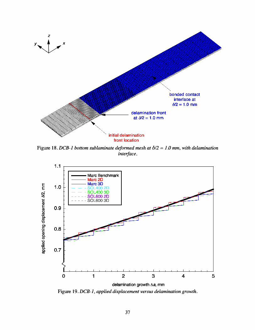
5

Y

front location

Figure 18. DCB-1 bottom sublaminate deformed mesh at δ/2 = 1.0 mm, with delaminationinterface.

1.1

Marc BenchmarkStMarc 2DMarc 3D

• SOL400 2DSOL400 3D

- - - - - SOL600 2D- - - - - SOL600 3D

0.9

0.8

0.7

0 1 2 3 4

delamination growth a, mm

Figure 19. DCB-1, applied displacement versus delamination growth.

1.0

37

Marc Benchmark

Analysis

6

4

53

a

2 a

a

1-2 FT

3-4

a AaAa

5-6

E 0.9E

c

E

0.8COCL

CY) 2ca^

0 0.7a^.Q

CLcU

1 0 1 2

3delamination growth a, mm

Figure 20. Delamination growth behavior.

6

E 5E

a^4

Ea^UNC- 3A

a 20vLD

CL

0 1

increased peakdisplacement \ • •• t

at mesh transition \^ .

i

•000, r

i • Test [46]— — Beam Theory [27]

Marc 2DMarc 3D

- - - - Abaqus 2D [45]- - - - - Abaqus 3D [45]

00 10 20 30 40

50

delamination growth a, mm

Figure 21. DCB-2, applied displacement versus delamination growth.

38

4.5

Marc Benchmark

Marc 3D

4.0

3.5

3.0

0 5 10 15 20 25 30 35 40 45

delamination growth a, mm

Figure 22. SLB, applied displacement versus delamination growth.

z

bonded contactinterface at

y x w = 4.0 mm

delamination frontat w = 4.0 mm

delamination front atfirst (unstable) crackgrowth, w = 3.19 mm

delamination front atinitial sub-critical crack

delamination growth, w = 3.18 mmfront location

Figure 23. SLB bottom sublaminate mesh with delamination front progression.

39

9.0

8.0

E7.0

6.0E

0 5.0CL

Mn

aD4.0

CaD

3.0aD

C 2.0

1.0

00

Marc Benchmark• Marc 2D

Marc 3DI

I

I

I

I

I

I

I

location ofloading pin

.0 10 20 30 40 50

60

delamination growth a, mm

Figure 24. ENF, applied displacement versus delamination growth.

bonded contactz interface at

y x w = 8.0 mm

delamination frontat w = 8.0 mm

delamination front atfirst (unstable) crackgrowth, w = 4.28 mm

initial delaminationfront location

Figure 25. ENF bottom sublaminate mesh with delamination front progression.

40

Y

Figure 26. ENF refined model bottom sublaminate mesh with delamination front progression.

9.0

8.0

BE 7.0

aD6.0

E

0 5.0CL

aD4.0

C

3.0aD

C 2.0

1.0

00

ZMarc Benchmark Static StepDefault Static Step X ZMarc 3DContact Status X

Marc 3D refined Force XI

I

I

I

I

I

I

I

location ofloading pin

.0 10 20 30 40 50

60

delamination growth a, mm

Figure 27. ENF, applied displacement versus delamination length.

41

delaminationinterface -

1.21.

a^ 1.01.

U

O_CO

C 0.81.C

mCLOvm

1.4 0.5 mm 0.75 mm 0.25 mm

1 . 6 elements elements elements

transition tosmaller mesh

transition to prevents growth

larger meshincreases growth

Marc BenchmarkMesh transition

0.6co0.80 1 2 3 4 5 6 7 8 9

Benchmarkdelamination growth a, mm

Mesh transition

0.6 Figure 28. Effect of mesh transition regions, DCB-1 2D.0 1 2 3 4 5 6 7 8

E 1.0N

CN0.9

U

O_Mn

CM

S 0.8

0.7

NO_O

NCLCL

Marc Benchmark—e— Coarse time increments• Fine time increments

0 1 2 3 4 5

delamination growth a, mm

Figure 29. Effect of increment size, DCB-1 2D.

42

REPORT DOCUMENTATION PAGEOForm Approved

MB No. 0704-0188

The public reporting burden for this collection of information is estimated to average 1 hour per response, including the time for reviewing instructions, searching existing data sources,gathering and maintaining the data needed, and completing and reviewing the collection of information. Send comments regarding this burden estimate or any other aspect of thiscollection of information, including suggestions for reducing this burden, to Department of Defense, Washington Headquarters Services, Directorate for Information Operations andReports (0704-0188), 1215 Jefferson Davis Highway, Suite 1204, Arlington, VA 22202-4302. Respondents should be aware that notwithstanding any other provision of law, no personshall be subject to any penalty for failing to comply with a collection of information if it does not display a currently valid OMB control number.PLEASE DO NOT RETURN YOUR FORM TO THE ABOVE ADDRESS.

1. REPORT DATE (DD-MM-YYYY) 2. REPORT TYPE 3. DATES COVERED (From - To)

01-06 - 2010 Contractor Report4. TITLE AND SUBTITLE 5a. CONTRACT NUMBER

Assessment of Static Delamination Propagation Capabilities in CommercialFinite Element Codes Using Benchmark Analysis 5b. GRANT NUMBER

NNL09AA00A5c. PROGRAM ELEMENT NUMBER

6. AUTHOR(S) 5d. PROJECT NUMBER

Orifici, Adrian C.; Krueger, Ronald5e. TASK NUMBER

5f. WORK UNIT NUMBER

814358.02.01.077. PERFORMING ORGANIZATION NAME(S) AND ADDRESS(ES) 8. PERFORMING ORGANIZATION

NASA Langley Research Center National Institute of Aerospace(NIA) REPORT NUMBER

Hampton, VA 23681-2199 100 Exploration WayHampton, VA 23666 NIA Report No. 2010-03

9. SPONSORING/MONITORING AGENCY NAME(S) AND ADDRESS(ES) 10. SPONSOR/MONITOR'S ACRONYM(S)

National Aeronautics and Space Administration NASAWashington, DC 20546-0001

11. SPONSOR/MONITOR'S REPORTNUMBER(S)

NASA/CR-2010-21670912. DISTRIBUTION/AVAILABILITY STATEMENTUnclassified - UnlimitedSubject Category 24Availability: NASA CASI (443) 757-580213. SUPPLEMENTARY NOTES

Langley Technical Monitor: Jonathan B. Ransom

14. ABSTRACT

With capabilities for simulating delamination growth in composite materials becoming available, the need for benchmarking and assessingthese capabilities is critical. In this study, benchmark analyses were performed to assess the delamination propagation simulation capabilitiesof the VCCT implementations in Marc TM and MD NastranTM. Benchmark delamination growth results for Double Cantilever Beam, SingleLeg Bending and End Notched Flexure specimens were generated using a numerical approach. This numerical approach was developedpreviously, and involves comparing results from a series of analyses at different delamination lengths to a single analysis with automaticcrack propagation. Specimens were analyzed with three-dimensional and two-dimensional models, and compared with previous analysesusing Abaqus®. The results demonstrated that the VCCT implementation in Marc TM and MD NastranTM was capable of accuratelyreplicating the benchmark delamination growth results and that the use of the numerical benchmarks offers advantages over benchmarkingusing experimental and analytical results.

15. SUBJECT TERMS

Composites; Delamination propagation; Finite element analysis; Fracture mechanics; Virtual crack closure technique

16. SECURITY CLASSIFICATION OF: 17. LIMITATION OF 18. NUMBER 19a. NAME OF RESPONSIBLE PERSONABSTRACT

PAOFPAGESGES Help Desk email: hel sti.nasa. ovp ( p@ g )a. REPORT b. ABSTRACT c. THIS PAGE

19b. TELEPHONE NUMBER (Include area code)

U U U UU 47 (443) 757-5802Standard Form 298 (Rev. 8-98)Prescribed by ANSI Std. Z39.18