Measurement and Modeling of Rain Intensity and Attenuation for the Design and Evaluation of...
31
Measurement and modeling of rain intensity and attenuation for the design and evaluation of microwave and millimeter-wave communication systems 271 x Measurement and modeling of rain intensity and attenuation for the design and evaluation of microwave and millimeter-wave communication systems Gamantyo Hendrantoro Institut Teknologi Sepuluh Nopember Indonesia Akira Matsushima Kumamoto University Japan 1. Introduction Rain-induced attenuation creates one of the most damaging effects of the atmosphere on the quality of radio communication systems, especially those operating above 10 GHz. Accordingly, methods have been devised to overcome this destructive impact. Adaptive fade mitigation schemes have been proposed to mitigate the rain fade impact in terrestrial communications above 10 GHz (e.g., Sweeney & Bostian, 1999). These schemes mainly deal with the temporal variation of rain attenuation. When such methods as site diversity and multi-hop relaying are to be used, or when the impact of adjacent interfering links is concerned, the spatial variation of rain must also be considered (Hendrantoro et al, 2002; Maruyama et al, 2008; Sakarellos et al, 2009; Panagopoulos et al, 2006). There is also a possibility of employing a joint space-time mitigation technique (Hendrantoro & Indrabayu, 2005). In designing a fade mitigation scheme that is expected to work well within a specified set of criteria, an evaluation technique must be available that is appropriate to test the system performance against rainy channels. Consequently, a model that can emulate the behavior of rain in space and time is desired. This chapter presents results that have thus far been acquired from an integrated research campaign jointly carried out by researchers at Institut Teknologi Sepuluh Nopember, Indonesia and Kumamoto University, Japan. The research is aimed at devising transmission strategies suitable for broadband wireless access in microwave and millimeter-wave bands, especially in tropical regions. With regards to modeling rain rate and attenuation, the project has gone through several phases, which include endeavors to measure the space- time variations of rain intensity and attenuation (Hendrantoro et al, 2006; Mauludiyanto et al, 2007; Hendrantoro et al, 2007b), to appropriately model them (e.g., Yadnya et al, 2008a; 14 www.intechopen.com
-
Upload
independent -
Category
Documents
-
view
5 -
download
0
Transcript of Measurement and Modeling of Rain Intensity and Attenuation for the Design and Evaluation of...
Measurement and modeling of rain intensity and attenuation for the design and evaluation of microwave and millimeter-wave communication systems 271
Measurement and modeling of rain intensity and attenuation for the design and evaluation of microwave and millimeter-wave communication systems
Gamantyo Hendrantoro and Akira Matsushima
x
Measurement and modeling of rain intensity and attenuation for the
design and evaluation of microwave and millimeter-wave communication systems
Gamantyo Hendrantoro
Institut Teknologi Sepuluh Nopember Indonesia
Akira Matsushima Kumamoto University
Japan
1. Introduction
Rain-induced attenuation creates one of the most damaging effects of the atmosphere on the quality of radio communication systems, especially those operating above 10 GHz. Accordingly, methods have been devised to overcome this destructive impact. Adaptive fade mitigation schemes have been proposed to mitigate the rain fade impact in terrestrial communications above 10 GHz (e.g., Sweeney & Bostian, 1999). These schemes mainly deal with the temporal variation of rain attenuation. When such methods as site diversity and multi-hop relaying are to be used, or when the impact of adjacent interfering links is concerned, the spatial variation of rain must also be considered (Hendrantoro et al, 2002; Maruyama et al, 2008; Sakarellos et al, 2009; Panagopoulos et al, 2006). There is also a possibility of employing a joint space-time mitigation technique (Hendrantoro & Indrabayu, 2005). In designing a fade mitigation scheme that is expected to work well within a specified set of criteria, an evaluation technique must be available that is appropriate to test the system performance against rainy channels. Consequently, a model that can emulate the behavior of rain in space and time is desired. This chapter presents results that have thus far been acquired from an integrated research campaign jointly carried out by researchers at Institut Teknologi Sepuluh Nopember, Indonesia and Kumamoto University, Japan. The research is aimed at devising transmission strategies suitable for broadband wireless access in microwave and millimeter-wave bands, especially in tropical regions. With regards to modeling rain rate and attenuation, the project has gone through several phases, which include endeavors to measure the space-time variations of rain intensity and attenuation (Hendrantoro et al, 2006; Mauludiyanto et al, 2007; Hendrantoro et al, 2007b), to appropriately model them (e.g., Yadnya et al, 2008a;
14
www.intechopen.com
Microwave and Millimeter Wave Technologies: Modern UWB antennas and equipment 272
Yadnya et al, 2008b), and finally to apply the resulting model in evaluation of transmission system designs (e.g., Kuswidiastuti et al, 2008). Tropical characteristics of the measured rain events in Indonesia have been the focus of this project, primarily due to the difficulty in implementing rain-resistant systems in microwave and millimeter-wave bands in tropical regions (Salehudin et al, 1999) and secondarily because of the lack of rain attenuation data and models for these regions. The design of millimeter-wave broadband wireless access with short links, as typified by LMDS (local multipoint distribution services), is also a central point in this project, which later governs the choice of space-time measurement method. As such, endeavors reported in this chapter offer multiple contributions:
a. Measurements and analyses of raindrop size distribution, raindrop fall velocity distribution, rain rate and attenuation in maritime tropical regions represented by the areas of Surabaya.
b. Method to estimate specific attenuation of rain from raindrop size distribution models.
c. Stochastic model of rain attenuation that can be adopted to generate rain attenuation samples for use in evaluation of fade mitigation techniques.
We start in the next section with the measurement system, raindrop size distribution modeling, estimation of specific attenuation, and the synthetic storm technique. Afterward, we discuss modeling of rain intensity and attenuation, touching upon space-time distribution and the time series models. Finally, examples of evaluation of communication systems are given, followed by some concluding remarks.
2. Measurement of rain intensity and attenuation
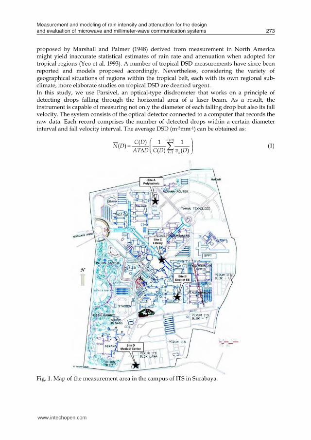
2.1 Spatio-temporal measurement of rain intensity The design of our space-time rain field measurement system is based on several criteria. Firstly, the spatial and temporal scope and resolution of the rain field variation must be taken into account. Another constraint is the available budget and technology. When budget is not a concern, space-time measurement using rain radar can be done, as exemplified by Tan and Goddard (1998) and Hendrantoro and Zawadzki (2003). Radar has its strength in large observation area and feasibility of simulating radio links on radar image. However, due to its weaknesses that include high cost and low time resolution, and due to the relatively small measurement area desired to emulate an LMDS cell, it is decided to employ a network of synchronized rain gauges operated within the campus area of Institut Teknologi Sepuluh Nopember (ITS) in Surabaya, as shown in Fig. 1. The longest distance between rain gauges is about 1.55 km, from site A at the Polytechnic building to site D at the Medical Center. The shortest, about 400 m, is between site B at the Department of Electrical Engineering building and site C at the Library building. The rain gauges, each of tipping-bucket type, are synchronized manually. At site B, an optical-type Parsivel disdrometer is also operated to record the drop size distribution (DSD), as well as a 54-meter radio link at 28 GHz adopted to measure directly rain attenuation.
2.2 Raindrop size distribution measurement and modelling DSD (raindrop size distribution) is a fundamental parameter that directly affects rainfall rate and rain-induced attenuation. The widely used negative exponential model of DSD
proposed by Marshall and Palmer (1948) derived from measurement in North America might yield inaccurate statistical estimates of rain rate and attenuation when adopted for tropical regions (Yeo et al, 1993). A number of tropical DSD measurements have since been reported and models proposed accordingly. Nevertheless, considering the variety of geographical situations of regions within the tropical belt, each with its own regional sub-climate, more elaborate studies on tropical DSD are deemed urgent. In this study, we use Parsivel, an optical-type disdrometer that works on a principle of detecting drops falling through the horizontal area of a laser beam. As a result, the instrument is capable of measuring not only the diameter of each falling drop but also its fall velocity. The system consists of the optical detector connected to a computer that records the raw data. Each record comprises the number of detected drops within a certain diameter interval and fall velocity interval. The average DSD (m-3mm-1) can be obtained as:
)(
1 )(1
)(1)()(
DC
k k DvDCDATDCDN (1)
Fig. 1. Map of the measurement area in the campus of ITS in Surabaya.
www.intechopen.com
Measurement and modeling of rain intensity and attenuation for the design and evaluation of microwave and millimeter-wave communication systems 273
Yadnya et al, 2008b), and finally to apply the resulting model in evaluation of transmission system designs (e.g., Kuswidiastuti et al, 2008). Tropical characteristics of the measured rain events in Indonesia have been the focus of this project, primarily due to the difficulty in implementing rain-resistant systems in microwave and millimeter-wave bands in tropical regions (Salehudin et al, 1999) and secondarily because of the lack of rain attenuation data and models for these regions. The design of millimeter-wave broadband wireless access with short links, as typified by LMDS (local multipoint distribution services), is also a central point in this project, which later governs the choice of space-time measurement method. As such, endeavors reported in this chapter offer multiple contributions:
a. Measurements and analyses of raindrop size distribution, raindrop fall velocity distribution, rain rate and attenuation in maritime tropical regions represented by the areas of Surabaya.
b. Method to estimate specific attenuation of rain from raindrop size distribution models.
c. Stochastic model of rain attenuation that can be adopted to generate rain attenuation samples for use in evaluation of fade mitigation techniques.
We start in the next section with the measurement system, raindrop size distribution modeling, estimation of specific attenuation, and the synthetic storm technique. Afterward, we discuss modeling of rain intensity and attenuation, touching upon space-time distribution and the time series models. Finally, examples of evaluation of communication systems are given, followed by some concluding remarks.
2. Measurement of rain intensity and attenuation
2.1 Spatio-temporal measurement of rain intensity The design of our space-time rain field measurement system is based on several criteria. Firstly, the spatial and temporal scope and resolution of the rain field variation must be taken into account. Another constraint is the available budget and technology. When budget is not a concern, space-time measurement using rain radar can be done, as exemplified by Tan and Goddard (1998) and Hendrantoro and Zawadzki (2003). Radar has its strength in large observation area and feasibility of simulating radio links on radar image. However, due to its weaknesses that include high cost and low time resolution, and due to the relatively small measurement area desired to emulate an LMDS cell, it is decided to employ a network of synchronized rain gauges operated within the campus area of Institut Teknologi Sepuluh Nopember (ITS) in Surabaya, as shown in Fig. 1. The longest distance between rain gauges is about 1.55 km, from site A at the Polytechnic building to site D at the Medical Center. The shortest, about 400 m, is between site B at the Department of Electrical Engineering building and site C at the Library building. The rain gauges, each of tipping-bucket type, are synchronized manually. At site B, an optical-type Parsivel disdrometer is also operated to record the drop size distribution (DSD), as well as a 54-meter radio link at 28 GHz adopted to measure directly rain attenuation.
2.2 Raindrop size distribution measurement and modelling DSD (raindrop size distribution) is a fundamental parameter that directly affects rainfall rate and rain-induced attenuation. The widely used negative exponential model of DSD
proposed by Marshall and Palmer (1948) derived from measurement in North America might yield inaccurate statistical estimates of rain rate and attenuation when adopted for tropical regions (Yeo et al, 1993). A number of tropical DSD measurements have since been reported and models proposed accordingly. Nevertheless, considering the variety of geographical situations of regions within the tropical belt, each with its own regional sub-climate, more elaborate studies on tropical DSD are deemed urgent. In this study, we use Parsivel, an optical-type disdrometer that works on a principle of detecting drops falling through the horizontal area of a laser beam. As a result, the instrument is capable of measuring not only the diameter of each falling drop but also its fall velocity. The system consists of the optical detector connected to a computer that records the raw data. Each record comprises the number of detected drops within a certain diameter interval and fall velocity interval. The average DSD (m-3mm-1) can be obtained as:
)(
1 )(1
)(1)()(
DC
k k DvDCDATDCDN (1)
Fig. 1. Map of the measurement area in the campus of ITS in Surabaya.
www.intechopen.com
Microwave and Millimeter Wave Technologies: Modern UWB antennas and equipment 274
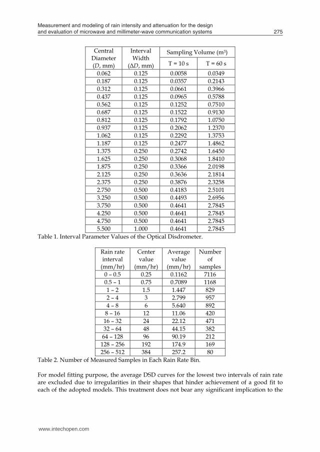
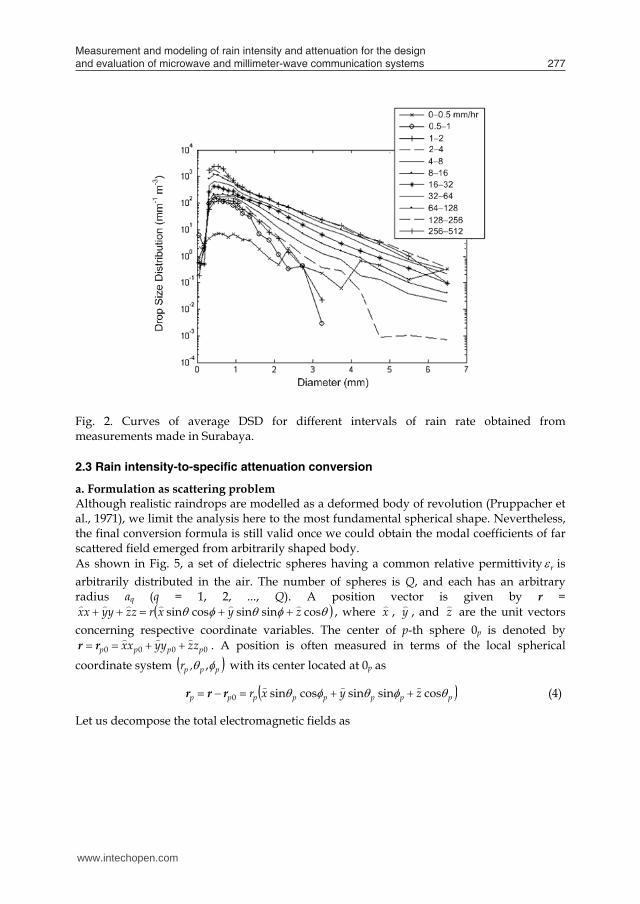
where C(D) denotes the number of drops detected in the diameter interval [D-ΔD/2, D+ΔD/2) given in millimeters, A (m2) the area of the laser beam, T (seconds) the integration time, vk(D) the measured velocity in m/s of the kth drop in the diameter interval [D-ΔD/2, D+ΔD/2), as opposed to a deterministic diameter-dependent velocity model such as the Gunn-Kinzer (Brussaard & Watson, 1995). From (1) it is apparent that the average DSD is a linear function of the average of the inverse of drop fall velocity, rather than the average velocity itself. This can cause discrepancy of attenuation or radar reflectivity estimates from their actual values. In fact, measurements made using a similar instrument in the US reveal discrepancy of the average fall velocity from the theoretical deterministic value (Tokay et al, 2003). The variations of raindrop fall velocity will be discussed later in this section. In our study, DSD measurements are categorized into bins representing disjoint intervals of rainfall rate, 0-0.5, 0.5-1, 1-2, …, 256-512 mm/h. An average DSD and an average rain rate are subsequently computed for each bin. Table 1 summarizes the parameter values for each interval. Although the Parsivel is able to detect objects of larger diameters, only those within the diameter range up to 6 mm, relevant to the maximum diameter of stable raindrops (Brussaard & Watson, 1995), are considered. The sampling volume in the table is calculated by assuming the Gunn-Kinzer fall velocity and using the fact that the laser beam area is 3 cm × 18 cm. Table 2 recapitulates the DSD measurements made in Surabaya for the various bins of rain rate. Fig. 2 presents the average DSD curves for all rain rate bins. Singapore and Surabaya are located in the same region of Southeast Asia and share the same tropical maritime climate. Three models fitted to Singapore DSD reported in the literature are used in this study, two of which are lognormal and gamma fitted to measurements made by Ong et al using a Joss-Waldvogel disdrometer (Timothy et al, 2002). The other is a negative exponential model obtained using the indirect method in which the DSD shape is assumed a priori and it is only the shape parameters that are estimated by fitting the DSD model to measurements of rainfall rate and attenuation (Yeo et al, 1993, Li et al, 1994). The Marshal-Palmer model is also included in the comparison. The DSD evaluation is made for three different values of average rain rate, 11.068, 44.15, and 174 mm/h, representing low, medium, and high intensity, respectively. As shown in Fig. 3 in general the Surabaya curve stays constantly below the Marshall-Palmer. Comparison with the Singapore models show that, except for the gamma model, the higher the rain rate, the larger the difference between the Singapore models and the Surabaya results, with the Surabaya DSD falling below the Singapore results for almost all drop diameters. For lower rain rates, the difference is not large and Surabaya DSD shows larger concentration of drops with larger diameters yet fewer smaller drops. A previous study in North America reported by Hendrantoro and Zawadzki (2003) has found that contribution to attenuation at 30 GHz is dominated by drops of diameters in the 1-3 mm range. This observation suggests that for the same rain rate the induced attenuation at 30 GHz in Surabaya might be lower on average than that in Singapore. It should be stressed herein that all of these disagreements in the detailed shapes of Surabaya DSD from that of either Singapore or Marshall-Palmer might originate from differences in various aspects of the measurement, such as the local climate, the measuring instrument, the number of samples, and the year of measurement. A more in-depth study is required to identify the real causes of the disagreements.
Central Diameter (D, mm)
Interval Width
(ΔD, mm)
Sampling Volume (m3)
T = 10 s T = 60 s 0.062 0.125 0.0058 0.0349 0.187 0.125 0.0357 0.2143 0.312 0.125 0.0661 0.3966 0.437 0.125 0.0965 0.5788 0.562 0.125 0.1252 0.7510 0.687 0.125 0.1522 0.9130 0.812 0.125 0.1792 1.0750 0.937 0.125 0.2062 1.2370 1.062 0.125 0.2292 1.3753 1.187 0.125 0.2477 1.4862 1.375 0.250 0.2742 1.6450 1.625 0.250 0.3068 1.8410 1.875 0.250 0.3366 2.0198 2.125 0.250 0.3636 2.1814 2.375 0.250 0.3876 2.3258 2.750 0.500 0.4183 2.5101 3.250 0.500 0.4493 2.6956 3.750 0.500 0.4641 2.7845 4.250 0.500 0.4641 2.7845 4.750 0.500 0.4641 2.7845 5.500 1.000 0.4641 2.7845
Table 1. Interval Parameter Values of the Optical Disdrometer.
Rain rate interval
(mm/hr)
Center value
(mm/hr)
Average value
(mm/hr)
Number of
samples 0 – 0.5 0.25 0.1162 7116 0.5 – 1 0.75 0.7089 1168 1 – 2 1.5 1.447 829 2 – 4 3 2.799 957 4 – 8 6 5.640 892 8 – 16 12 11.06 420
16 – 32 24 22.12 471 32 – 64 48 44.15 382 64 – 128 96 90.19 212
128 – 256 192 174.9 169 256 – 512 384 257.2 80
Table 2. Number of Measured Samples in Each Rain Rate Bin. For model fitting purpose, the average DSD curves for the lowest two intervals of rain rate are excluded due to irregularities in their shapes that hinder achievement of a good fit to each of the adopted models. This treatment does not bear any significant implication to the
www.intechopen.com
Measurement and modeling of rain intensity and attenuation for the design and evaluation of microwave and millimeter-wave communication systems 275
where C(D) denotes the number of drops detected in the diameter interval [D-ΔD/2, D+ΔD/2) given in millimeters, A (m2) the area of the laser beam, T (seconds) the integration time, vk(D) the measured velocity in m/s of the kth drop in the diameter interval [D-ΔD/2, D+ΔD/2), as opposed to a deterministic diameter-dependent velocity model such as the Gunn-Kinzer (Brussaard & Watson, 1995). From (1) it is apparent that the average DSD is a linear function of the average of the inverse of drop fall velocity, rather than the average velocity itself. This can cause discrepancy of attenuation or radar reflectivity estimates from their actual values. In fact, measurements made using a similar instrument in the US reveal discrepancy of the average fall velocity from the theoretical deterministic value (Tokay et al, 2003). The variations of raindrop fall velocity will be discussed later in this section. In our study, DSD measurements are categorized into bins representing disjoint intervals of rainfall rate, 0-0.5, 0.5-1, 1-2, …, 256-512 mm/h. An average DSD and an average rain rate are subsequently computed for each bin. Table 1 summarizes the parameter values for each interval. Although the Parsivel is able to detect objects of larger diameters, only those within the diameter range up to 6 mm, relevant to the maximum diameter of stable raindrops (Brussaard & Watson, 1995), are considered. The sampling volume in the table is calculated by assuming the Gunn-Kinzer fall velocity and using the fact that the laser beam area is 3 cm × 18 cm. Table 2 recapitulates the DSD measurements made in Surabaya for the various bins of rain rate. Fig. 2 presents the average DSD curves for all rain rate bins. Singapore and Surabaya are located in the same region of Southeast Asia and share the same tropical maritime climate. Three models fitted to Singapore DSD reported in the literature are used in this study, two of which are lognormal and gamma fitted to measurements made by Ong et al using a Joss-Waldvogel disdrometer (Timothy et al, 2002). The other is a negative exponential model obtained using the indirect method in which the DSD shape is assumed a priori and it is only the shape parameters that are estimated by fitting the DSD model to measurements of rainfall rate and attenuation (Yeo et al, 1993, Li et al, 1994). The Marshal-Palmer model is also included in the comparison. The DSD evaluation is made for three different values of average rain rate, 11.068, 44.15, and 174 mm/h, representing low, medium, and high intensity, respectively. As shown in Fig. 3 in general the Surabaya curve stays constantly below the Marshall-Palmer. Comparison with the Singapore models show that, except for the gamma model, the higher the rain rate, the larger the difference between the Singapore models and the Surabaya results, with the Surabaya DSD falling below the Singapore results for almost all drop diameters. For lower rain rates, the difference is not large and Surabaya DSD shows larger concentration of drops with larger diameters yet fewer smaller drops. A previous study in North America reported by Hendrantoro and Zawadzki (2003) has found that contribution to attenuation at 30 GHz is dominated by drops of diameters in the 1-3 mm range. This observation suggests that for the same rain rate the induced attenuation at 30 GHz in Surabaya might be lower on average than that in Singapore. It should be stressed herein that all of these disagreements in the detailed shapes of Surabaya DSD from that of either Singapore or Marshall-Palmer might originate from differences in various aspects of the measurement, such as the local climate, the measuring instrument, the number of samples, and the year of measurement. A more in-depth study is required to identify the real causes of the disagreements.
Central Diameter (D, mm)
Interval Width
(ΔD, mm)
Sampling Volume (m3)
T = 10 s T = 60 s 0.062 0.125 0.0058 0.0349 0.187 0.125 0.0357 0.2143 0.312 0.125 0.0661 0.3966 0.437 0.125 0.0965 0.5788 0.562 0.125 0.1252 0.7510 0.687 0.125 0.1522 0.9130 0.812 0.125 0.1792 1.0750 0.937 0.125 0.2062 1.2370 1.062 0.125 0.2292 1.3753 1.187 0.125 0.2477 1.4862 1.375 0.250 0.2742 1.6450 1.625 0.250 0.3068 1.8410 1.875 0.250 0.3366 2.0198 2.125 0.250 0.3636 2.1814 2.375 0.250 0.3876 2.3258 2.750 0.500 0.4183 2.5101 3.250 0.500 0.4493 2.6956 3.750 0.500 0.4641 2.7845 4.250 0.500 0.4641 2.7845 4.750 0.500 0.4641 2.7845 5.500 1.000 0.4641 2.7845
Table 1. Interval Parameter Values of the Optical Disdrometer.
Rain rate interval
(mm/hr)
Center value
(mm/hr)
Average value
(mm/hr)
Number of
samples 0 – 0.5 0.25 0.1162 7116 0.5 – 1 0.75 0.7089 1168 1 – 2 1.5 1.447 829 2 – 4 3 2.799 957 4 – 8 6 5.640 892 8 – 16 12 11.06 420
16 – 32 24 22.12 471 32 – 64 48 44.15 382 64 – 128 96 90.19 212
128 – 256 192 174.9 169 256 – 512 384 257.2 80
Table 2. Number of Measured Samples in Each Rain Rate Bin. For model fitting purpose, the average DSD curves for the lowest two intervals of rain rate are excluded due to irregularities in their shapes that hinder achievement of a good fit to each of the adopted models. This treatment does not bear any significant implication to the
www.intechopen.com
Microwave and Millimeter Wave Technologies: Modern UWB antennas and equipment 276
design of millimeter-wave communications since rain events of high intensity are of higher importance. The DSD measurements are fitted to a number of theoretical models, namely, the negative exponential, Weibull, and gamma. Among the three, gamma fits worst, and therefore is not discussed further herein. On the other hand, Weibull slightly outdoes the negative exponential and yields the following equation:
DDDN exp629.281
1
(2)
with 056.0212.1 R and 177.0728.0 R . Whereas the negative exponential fit gives:
)415.2(exp1054)( 14.0 DRDN (3)
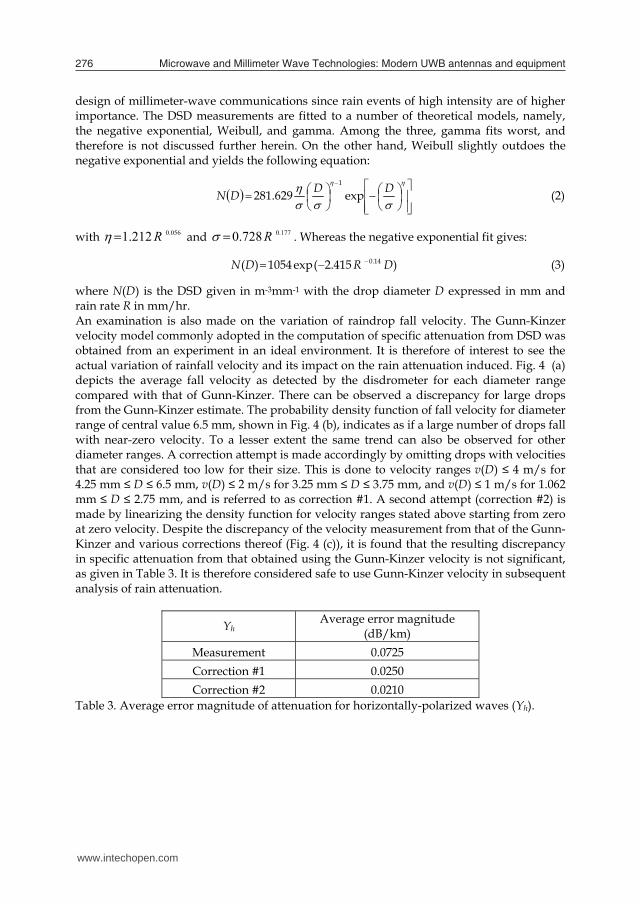
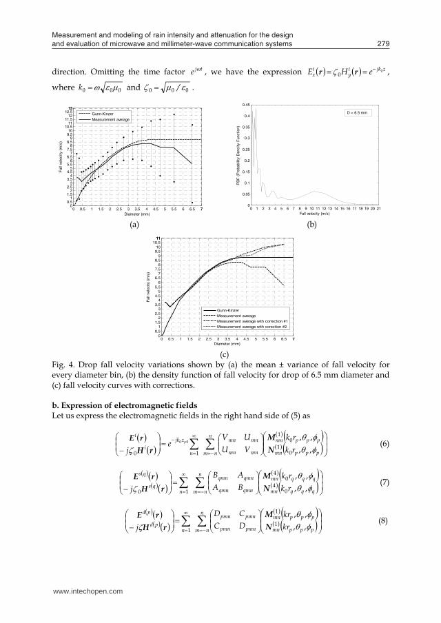
where N(D) is the DSD given in m-3mm-1 with the drop diameter D expressed in mm and rain rate R in mm/hr. An examination is also made on the variation of raindrop fall velocity. The Gunn-Kinzer velocity model commonly adopted in the computation of specific attenuation from DSD was obtained from an experiment in an ideal environment. It is therefore of interest to see the actual variation of rainfall velocity and its impact on the rain attenuation induced. Fig. 4 (a) depicts the average fall velocity as detected by the disdrometer for each diameter range compared with that of Gunn-Kinzer. There can be observed a discrepancy for large drops from the Gunn-Kinzer estimate. The probability density function of fall velocity for diameter range of central value 6.5 mm, shown in Fig. 4 (b), indicates as if a large number of drops fall with near-zero velocity. To a lesser extent the same trend can also be observed for other diameter ranges. A correction attempt is made accordingly by omitting drops with velocities that are considered too low for their size. This is done to velocity ranges v(D) ≤ 4 m/s for 4.25 mm ≤ D ≤ 6.5 mm, v(D) ≤ 2 m/s for 3.25 mm ≤ D ≤ 3.75 mm, and v(D) ≤ 1 m/s for 1.062 mm ≤ D ≤ 2.75 mm, and is referred to as correction #1. A second attempt (correction #2) is made by linearizing the density function for velocity ranges stated above starting from zero at zero velocity. Despite the discrepancy of the velocity measurement from that of the Gunn-Kinzer and various corrections thereof (Fig. 4 (c)), it is found that the resulting discrepancy in specific attenuation from that obtained using the Gunn-Kinzer velocity is not significant, as given in Table 3. It is therefore considered safe to use Gunn-Kinzer velocity in subsequent analysis of rain attenuation.
Yh Average error magnitude
(dB/km) Measurement 0.0725 Correction #1 0.0250 Correction #2 0.0210
Table 3. Average error magnitude of attenuation for horizontally-polarized waves (Yh).
Fig. 2. Curves of average DSD for different intervals of rain rate obtained from measurements made in Surabaya.
2.3 Rain intensity-to-specific attenuation conversion
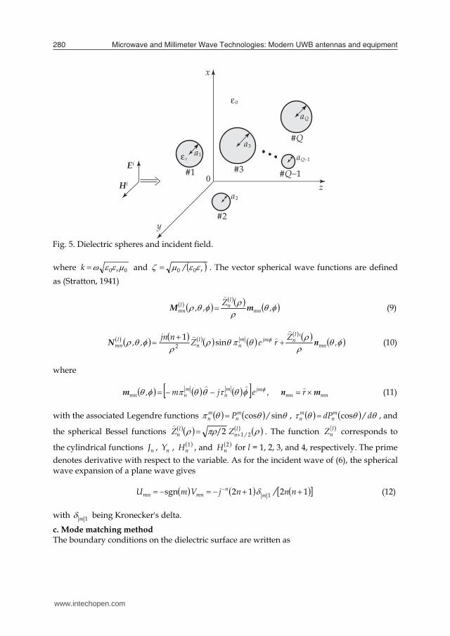
a. Formulation as scattering problem Although realistic raindrops are modelled as a deformed body of revolution (Pruppacher et al., 1971), we limit the analysis here to the most fundamental spherical shape. Nevertheless, the final conversion formula is still valid once we could obtain the modal coefficients of far scattered field emerged from arbitrarily shaped body. As shown in Fig. 5, a set of dielectric spheres having a common relative permittivity r is arbitrarily distributed in the air. The number of spheres is Q, and each has an arbitrary radius aq (q = 1, 2, ..., Q). A position vector is given by r = cos sin sin cos sin zyxrzzyyxx , where x , y , and z are the unit vectors concerning respective coordinate variables. The center of p-th sphere 0p is denoted by
0000 pppp zzyyxx rr . A position is often measured in terms of the local spherical coordinate system ppp ,r , with its center located at 0p as
pppppppp zyxr cos sin sin cos sin 0 rrr (4)
Let us decompose the total electromagnetic fields as
www.intechopen.com
Measurement and modeling of rain intensity and attenuation for the design and evaluation of microwave and millimeter-wave communication systems 277
design of millimeter-wave communications since rain events of high intensity are of higher importance. The DSD measurements are fitted to a number of theoretical models, namely, the negative exponential, Weibull, and gamma. Among the three, gamma fits worst, and therefore is not discussed further herein. On the other hand, Weibull slightly outdoes the negative exponential and yields the following equation:
DDDN exp629.281
1
(2)
with 056.0212.1 R and 177.0728.0 R . Whereas the negative exponential fit gives:
)415.2(exp1054)( 14.0 DRDN (3)
where N(D) is the DSD given in m-3mm-1 with the drop diameter D expressed in mm and rain rate R in mm/hr. An examination is also made on the variation of raindrop fall velocity. The Gunn-Kinzer velocity model commonly adopted in the computation of specific attenuation from DSD was obtained from an experiment in an ideal environment. It is therefore of interest to see the actual variation of rainfall velocity and its impact on the rain attenuation induced. Fig. 4 (a) depicts the average fall velocity as detected by the disdrometer for each diameter range compared with that of Gunn-Kinzer. There can be observed a discrepancy for large drops from the Gunn-Kinzer estimate. The probability density function of fall velocity for diameter range of central value 6.5 mm, shown in Fig. 4 (b), indicates as if a large number of drops fall with near-zero velocity. To a lesser extent the same trend can also be observed for other diameter ranges. A correction attempt is made accordingly by omitting drops with velocities that are considered too low for their size. This is done to velocity ranges v(D) ≤ 4 m/s for 4.25 mm ≤ D ≤ 6.5 mm, v(D) ≤ 2 m/s for 3.25 mm ≤ D ≤ 3.75 mm, and v(D) ≤ 1 m/s for 1.062 mm ≤ D ≤ 2.75 mm, and is referred to as correction #1. A second attempt (correction #2) is made by linearizing the density function for velocity ranges stated above starting from zero at zero velocity. Despite the discrepancy of the velocity measurement from that of the Gunn-Kinzer and various corrections thereof (Fig. 4 (c)), it is found that the resulting discrepancy in specific attenuation from that obtained using the Gunn-Kinzer velocity is not significant, as given in Table 3. It is therefore considered safe to use Gunn-Kinzer velocity in subsequent analysis of rain attenuation.
Yh Average error magnitude
(dB/km) Measurement 0.0725 Correction #1 0.0250 Correction #2 0.0210
Table 3. Average error magnitude of attenuation for horizontally-polarized waves (Yh).
Fig. 2. Curves of average DSD for different intervals of rain rate obtained from measurements made in Surabaya.
2.3 Rain intensity-to-specific attenuation conversion
a. Formulation as scattering problem Although realistic raindrops are modelled as a deformed body of revolution (Pruppacher et al., 1971), we limit the analysis here to the most fundamental spherical shape. Nevertheless, the final conversion formula is still valid once we could obtain the modal coefficients of far scattered field emerged from arbitrarily shaped body. As shown in Fig. 5, a set of dielectric spheres having a common relative permittivity r is arbitrarily distributed in the air. The number of spheres is Q, and each has an arbitrary radius aq (q = 1, 2, ..., Q). A position vector is given by r = cos sin sin cos sin zyxrzzyyxx , where x , y , and z are the unit vectors concerning respective coordinate variables. The center of p-th sphere 0p is denoted by
0000 pppp zzyyxx rr . A position is often measured in terms of the local spherical coordinate system ppp ,r , with its center located at 0p as
pppppppp zyxr cos sin sin cos sin 0 rrr (4)
Let us decompose the total electromagnetic fields as
www.intechopen.com

Microwave and Millimeter Wave Technologies: Modern UWB antennas and equipment 278
) ..., ,2 ,1 :sphereth -(in ,
air) the(in ,,, 1
Qpppdpd
Q
q
qsqsii
HE
HEHEHE (5)
0 1 2 3 4 5 6 7
10-4
10-2
100
102
104
Diameter (mm)
Dro
p S
ize
Dis
tribu
tion
( m-3
mm
-1 )
SurabayaSingapore (Li, 1994)Singapore (Ong, 2001)Singapore (Ong, 1997)Marshall-Palmer
R = 11.068 mm/h
0 1 2 3 4 5 6 7
10-4
10-2
100
102
104
Diameter (mm)
Dro
p S
ize
Dis
tribu
tion
( m-3
mm
-1 )
SurabayaSingapore (Li, 1994)Singapore (Ong, 2001)Singapore (Ong, 1997)Marshall-Palmer
R = 44.15 mm/h
(a) (b)
0 1 2 3 4 5 6 7
10-4
10-2
100
102
104
Diameter (mm)
Dro
p S
ize
Dis
tribu
tion
( m-3
mm
-1 )
SurabayaSingapore (Li, 1994)Singapore (Ong, 2001)Singapore (Ong, 1997)Marshall-Palmer
R = 174.92 mm/h
(c)
Fig. 3. Comparison of drop size distributions measured in Surabaya and models derived from measurements in Singapore for various rain rates: (a) 11.068 mm/h, (b) 44.15 mm/h, and (c) 174.92 mm/h, which for the Surabaya measurement are average values of intervals 8-16, 32-64, and 128-256 mm/h, respectively. where the superscripts i, s(q), and d(p) concern the incident field, the scattered field due to the existence of the sphere #q, and the field inside the sphere #p, respectively. With no loss of generality, we can assume that the incident field is x-polarized and propagates in the +z
direction. Omitting the time factor tje , we have the expression zjkiy
ix eHE 0
0 rr ,
where 000 k and 000 / .
0 0.5 1 1.5 2 2.5 3 3.5 4 4.5 5 5.5 6 6.5 770
0.51
1.52
2.53
3.54
4.55
5.56
6.57
7.58
8.59
9.510
10.511
11.512
12.51313
Diameter (mm)
Fall
velo
city
(m
/s)
Gunn-KinzerMeasurement average
0 1 2 3 4 5 6 7 8 9 10 11 12 13 14 15 16 17 18 19 20 21
0
0.05
0.1
0.15
0.2
0.25
0.3
0.35
0.4
0.45
Fall velocity (m/s)
PD
F (
Pro
babi
lity
Den
city
Fun
ctio
n)
D = 6.5 mm
(a) (b)
0 0.5 1 1.5 2 2.5 3 3.5 4 4.5 5 5.5 6 6.5 770
0.51
1.52
2.53
3.54
4.55
5.56
6.57
7.58
8.59
9.510
10.5111111
Diameter (mm)
Fall
velo
city
(m/s
)
Gunn-KinzerMeasurement averageMeasurement average with correction #1Measurement average with corection #2
(c)
Fig. 4. Drop fall velocity variations shown by (a) the mean ± variance of fall velocity for every diameter bin, (b) the density function of fall velocity for drop of 6.5 mm diameter and (c) fall velocity curves with corrections. b. Expression of electromagnetic fields Let us express the electromagnetic fields in the right hand side of (5) as
pppmn
pppmnn
nm mnmn
mnmn
n
zjki
i
rkrk
VUUV
ej
p
,,,,
01
01
10
00
NM
rHrE
(6)
qqqmn
qqqmnn
nm qmnqmn
qmnqmn
nqs
qs
rkrk
BAAB
j
,,,,
04
04
10 NM
rHrE
(7)
pppmn
pppmnn
nm pmnpmn
pmnpmn
npd
pd
krkr
DCCD
j
,,,,
1
1
1 NM
rHrE
(8)
www.intechopen.com
Measurement and modeling of rain intensity and attenuation for the design and evaluation of microwave and millimeter-wave communication systems 279
) ..., ,2 ,1 :sphereth -(in ,
air) the(in ,,, 1
Qpppdpd
Q
q
qsqsii
HE
HEHEHE (5)
0 1 2 3 4 5 6 7
10-4
10-2
100
102
104
Diameter (mm)
Dro
p S
ize
Dis
tribu
tion
( m-3
mm
-1 )
SurabayaSingapore (Li, 1994)Singapore (Ong, 2001)Singapore (Ong, 1997)Marshall-Palmer
R = 11.068 mm/h
0 1 2 3 4 5 6 7
10-4
10-2
100
102
104
Diameter (mm)
Dro
p S
ize
Dis
tribu
tion
( m-3
mm
-1 )
SurabayaSingapore (Li, 1994)Singapore (Ong, 2001)Singapore (Ong, 1997)Marshall-Palmer
R = 44.15 mm/h
(a) (b)
0 1 2 3 4 5 6 7
10-4
10-2
100
102
104
Diameter (mm)
Dro
p S
ize
Dis
tribu
tion
( m-3
mm
-1 )
SurabayaSingapore (Li, 1994)Singapore (Ong, 2001)Singapore (Ong, 1997)Marshall-Palmer
R = 174.92 mm/h
(c)
Fig. 3. Comparison of drop size distributions measured in Surabaya and models derived from measurements in Singapore for various rain rates: (a) 11.068 mm/h, (b) 44.15 mm/h, and (c) 174.92 mm/h, which for the Surabaya measurement are average values of intervals 8-16, 32-64, and 128-256 mm/h, respectively. where the superscripts i, s(q), and d(p) concern the incident field, the scattered field due to the existence of the sphere #q, and the field inside the sphere #p, respectively. With no loss of generality, we can assume that the incident field is x-polarized and propagates in the +z
direction. Omitting the time factor tje , we have the expression zjkiy
ix eHE 0
0 rr ,
where 000 k and 000 / .
0 0.5 1 1.5 2 2.5 3 3.5 4 4.5 5 5.5 6 6.5 770
0.51
1.52
2.53
3.54
4.55
5.56
6.57
7.58
8.59
9.510
10.511
11.512
12.51313
Diameter (mm)
Fall
velo
city
(m
/s)
Gunn-KinzerMeasurement average
0 1 2 3 4 5 6 7 8 9 10 11 12 13 14 15 16 17 18 19 20 21
0
0.05
0.1
0.15
0.2
0.25
0.3
0.35
0.4
0.45
Fall velocity (m/s)
PD
F (
Pro
babi
lity
Den
city
Fun
ctio
n)
D = 6.5 mm
(a) (b)
0 0.5 1 1.5 2 2.5 3 3.5 4 4.5 5 5.5 6 6.5 770
0.51
1.52
2.53
3.54
4.55
5.56
6.57
7.58
8.59
9.510
10.5111111
Diameter (mm)
Fall
velo
city
(m/s
)
Gunn-KinzerMeasurement averageMeasurement average with correction #1Measurement average with corection #2
(c)
Fig. 4. Drop fall velocity variations shown by (a) the mean ± variance of fall velocity for every diameter bin, (b) the density function of fall velocity for drop of 6.5 mm diameter and (c) fall velocity curves with corrections. b. Expression of electromagnetic fields Let us express the electromagnetic fields in the right hand side of (5) as
pppmn
pppmnn
nm mnmn
mnmn
n
zjki
i
rkrk
VUUV
ej
p
,,,,
01
01
10
00
NM
rHrE
(6)
qqqmn
qqqmnn
nm qmnqmn
qmnqmn
nqs
qs
rkrk
BAAB
j
,,,,
04
04
10 NM
rHrE
(7)
pppmn
pppmnn
nm pmnpmn
pmnpmn
npd
pd
krkr
DCCD
j
,,,,
1
1
1 NM
rHrE
(8)
www.intechopen.com
Microwave and Millimeter Wave Technologies: Modern UWB antennas and equipment 280
x
z
y
0
ε0
Ei
Hi
εr
#1
#2
#3#Q−1
#Q
a2
a3
aQ−1a1
aQ
Fig. 5. Dielectric spheres and incident field. where 00 rk and r/ 00 . The vector spherical wave functions are defined as (Stratton, 1941)
,Z,, mn
lnl
mn mM
(9)
,'ZreZnjn,, mn
lnjmm
nl
nl
mn nN
sin 12 (10)
where
mnmnjmm
nm
nmn r,ejm, mnm (11)
with the associated Legendre functions sincos /Pmn
mn , d/dPm
nmn cos , and
the spherical Bessel functions l/n
ln ZZ 21 /2
. The function lnZ corresponds to
the cylindrical functions nJ , nY , 1nH , and 2
nH for l = 1, 2, 3, and 4, respectively. The prime denotes derivative with respect to the variable. As for the incident wave of (6), the spherical wave expansion of a plane wave gives
12 12 sgn 1 nn/njVmU mn
mnmn (12)
with 1m being Kronecker's delta.
c. Mode matching method The boundary conditions on the dielectric surface are written as
Qpr pp
ar
pdQ
q
qsip
pp
..., ,2 ,1 ;20 ,0 01
rFrFrF (13)
where F stands for E and H. We substitute (6)-(8) into (13) and truncate the infinite series at n = Nq for the q-th sphere (q = 1, 2, …, Q). The values Nq depend on the electrical size of spheres. This leads us to linear equations including Q
q qq NN1
24 unknown coefficients
Aqmn, Bqmn, Cpmn, and Dpmn. As seen from (6)-(8), the origins of observation points are not unified at this stage. In order to shift the origin of qsE and qsH from 0q to 0p, we apply the addition theorem for vector spherical wave functions (Cruzan, 1962)
p
p
pqmnpqmn
pqmnpqmn
qmn
qmn
kk
kkkk
kk
rNrM
rrrr
rNrM
01
01
04
,04
,
04
,04
,
104
04
(14)
where the position ppp ,rk ,0 has been simply written as k0rp. The translation coefficients 4 ,mn and 4 ,mn are the functions of the shift vector 00 qppq rrr . Making use of the
orthogonal properties of the vector spherical wave functions, and eliminating the coefficients pC and pD , we arrive at the set of linear equations
Qp--N
eBVBkBkAB
eAUAkBkAA
p
zjkpp
n
nmpqmnqmnpqmnqmn
N
n
Q
pqp
zjkpp
n
nmpqmnqmnpqmnqmn
N
n
Q
pqp
pq
pq
..., ,2 ,1 ; ..., 1, , ; ..., ,2 ,1
00
00
04
,04
,1 1
04
,04
,1 1
rr
rr
(15)
where
pprpp
pprppp kaJak'Hka'JakH
kaJak'Jka'JakJA
02
02
00
(16)
pprpp
pprppp ka'JakHkaJak'H
ka'JakJkaJak'JB
02
02
00
(17)
Equation (15) includes the same number of relations as that of unknowns, and thereby, is numerically solved. After that, the other coefficients are computed from
pppppppp B/BD,A/ACC D (18)
where
www.intechopen.com
Measurement and modeling of rain intensity and attenuation for the design and evaluation of microwave and millimeter-wave communication systems 281
Fig. 5. Dielectric spheres and incident field. where 00 rk and r/ 00 . The vector spherical wave functions are defined as (Stratton, 1941)
,Z,, mn
lnl
mn mM
(9)
,'ZreZnjn,, mn
lnjmm
nl
nl
mn nN
sin 12 (10)
where
mnmnjmm
nm
nmn r,ejm, mnm (11)
with the associated Legendre functions sincos /Pmn
mn , d/dPm
nmn cos , and
the spherical Bessel functions l/n
ln ZZ 21 /2
. The function lnZ corresponds to
the cylindrical functions nJ , nY , 1nH , and 2
nH for l = 1, 2, 3, and 4, respectively. The prime denotes derivative with respect to the variable. As for the incident wave of (6), the spherical wave expansion of a plane wave gives
12 12 sgn 1 nn/njVmU mn
mnmn (12)
with 1m being Kronecker's delta.
c. Mode matching method The boundary conditions on the dielectric surface are written as
Qpr pp
ar
pdQ
q
qsip
pp
..., ,2 ,1 ;20 ,0 01
rFrFrF (13)
where F stands for E and H. We substitute (6)-(8) into (13) and truncate the infinite series at n = Nq for the q-th sphere (q = 1, 2, …, Q). The values Nq depend on the electrical size of spheres. This leads us to linear equations including Q
q qq NN1
24 unknown coefficients
Aqmn, Bqmn, Cpmn, and Dpmn. As seen from (6)-(8), the origins of observation points are not unified at this stage. In order to shift the origin of qsE and qsH from 0q to 0p, we apply the addition theorem for vector spherical wave functions (Cruzan, 1962)
p
p
pqmnpqmn
pqmnpqmn
qmn
qmn
kk
kkkk
kk
rNrM
rrrr
rNrM
01
01
04
,04
,
04
,04
,
104
04
(14)
where the position ppp ,rk ,0 has been simply written as k0rp. The translation coefficients 4 ,mn and 4 ,mn are the functions of the shift vector 00 qppq rrr . Making use of the
orthogonal properties of the vector spherical wave functions, and eliminating the coefficients pC and pD , we arrive at the set of linear equations
Qp--N
eBVBkBkAB
eAUAkBkAA
p
zjkpp
n
nmpqmnqmnpqmnqmn
N
n
Q
pqp
zjkpp
n
nmpqmnqmnpqmnqmn
N
n
Q
pqp
pq
pq
..., ,2 ,1 ; ..., 1, , ; ..., ,2 ,1
00
00
04
,04
,1 1
04
,04
,1 1
rr
rr
(15)
where
pprpp
pprppp kaJak'Hka'JakH
kaJak'Jka'JakJA
02
02
00
(16)
pprpp
pprppp ka'JakHkaJak'H
ka'JakJkaJak'JB
02
02
00
(17)
Equation (15) includes the same number of relations as that of unknowns, and thereby, is numerically solved. After that, the other coefficients are computed from
pppppppp B/BD,A/ACC D (18)
where
www.intechopen.com
Microwave and Millimeter Wave Technologies: Modern UWB antennas and equipment 282
pprpp
rp kaJak'Hka'JakH
jC
0
20
2 (19)
pprpp
rp ka'JakHkaJak'H
jD
0
20
2 (20)
Equations (16), (17), (19), and (20) are called Mie's coefficients (Harrington, 1961). It should be noted that the terms including the translation coefficients in (15) represent the effect of multiple scattering among spheres. If raindrops are so sparsely distributed that the multiple effect is very weak, the approximate solutions of (15) are directly derived as
0000 B qq zjkqnmnqmn
zjkqnmnqmn eBV,eAUA (21)
d. Scattering and absorption cross sections Employing the large argument approximations qrjkn
qnqn ejrk'HjrkH 010
20
2 and
r/rr qq 0rr in (7), we can write the far scattered field in the form of inhomogeneous spherical waves as
rff
rke
HH
EE rjk
s
s
s
s
,,
00
0
rr
rr
(22)
where the scattering pattern functions are
r/jk
mn
mnn
nmqmnqmn
nN
n
Q
q
e,,
jBAjff
00 ,,
11
rr
mn
(23)
The total scattered power is computed from
dd,f,fk
ddrrPr
*sss
sin 2
1
sinRe21
22
0
2
0200
20
2
0
rHrΕ (24)
where the asterisk denotes complex conjugate. The integrals with respect to and in above are numerically evaluated by the Gauss-Legendre quadrature rule and the trapezoidal formula, respectively. Since the power density of incident field is 021 /W i , the total
scattering cross section is given by siss PW/P 02 . On the other hand, the power absorbed inside the spheres is computed from
Q
*nqnqmnq
*nqnqmn
n
nm
N
nr
qar*qdqd
Q
q
a
ka'JkaJDkaJka'JC
mnnmnnn
jk
ddarP
q
q
1
22
1020
20
2
01
-
! 12! 121Re
sinRe21
rHrΕ
(25)
The absorption cross section is given by aiaa PW/P 02 . The optical theorem or the extinction theorem states that the diffracted field in the forward direction, which is related to 00 ,f , should be attenuated due to the scattering and absorption. This is based on the law of energy conservation. The amount of this attenuation is called the extinction cross section and expressed as
00 Im 12
00Im4
11111
1
120
20
zjkQ
qnqnqnqnq
nN
n
ase
eBBAAjnnk
,fk
(26)
e. Specific rain attenuation Suppose that Q spheres are randomly allocated inside the volume V (m3). By using e (m2) in Eq. (26), the specific rain attenuation is given by V/e (m1). From a practical viewpoint, the unit is often converted via
V/e e 4343log 1010][m [dB/km] 1031 (27)
If we can neglect the multiple scattering among spheres, the approximate cross section
Q
qqnqn
n
e BAnk 11
20
12Re2 (28)
is applied to Eq. (27) with the aid of Eqs. (16) and (17). We will use this formula in the later computations. Let us determine the series of realistic radii aq as a function of rainfall intensity R (mm/h). Each distribution model proposes a function N(a) (m3 mm1), which is a number of raindrops having the radius between a and a + da (mm) per unit volume. Then the integral
][m 30
'da'aNaN~a
(29)
gives a number of raindrops, the radius of which are less than a (mm), per unit volume. The value N~ denotes the total number. When we deal with Q raindrops in the numerical computation, the q-th radius aq (mm) is sampled by the rule
www.intechopen.com
Measurement and modeling of rain intensity and attenuation for the design and evaluation of microwave and millimeter-wave communication systems 283
pprpp
rp kaJak'Hka'JakH
jC
0
20
2 (19)
pprpp
rp ka'JakHkaJak'H
jD
0
20
2 (20)
Equations (16), (17), (19), and (20) are called Mie's coefficients (Harrington, 1961). It should be noted that the terms including the translation coefficients in (15) represent the effect of multiple scattering among spheres. If raindrops are so sparsely distributed that the multiple effect is very weak, the approximate solutions of (15) are directly derived as
0000 B qq zjkqnmnqmn
zjkqnmnqmn eBV,eAUA (21)
d. Scattering and absorption cross sections Employing the large argument approximations qrjkn
qnqn ejrk'HjrkH 010
20
2 and
r/rr qq 0rr in (7), we can write the far scattered field in the form of inhomogeneous spherical waves as
rff
rke
HH
EE rjk
s
s
s
s
,,
00
0
rr
rr
(22)
where the scattering pattern functions are
r/jk
mn
mnn
nmqmnqmn
nN
n
Q
q
e,,
jBAjff
00 ,,
11
rr
mn
(23)
The total scattered power is computed from
dd,f,fk
ddrrPr
*sss
sin 2
1
sinRe21
22
0
2
0200
20
2
0
rHrΕ (24)
where the asterisk denotes complex conjugate. The integrals with respect to and in above are numerically evaluated by the Gauss-Legendre quadrature rule and the trapezoidal formula, respectively. Since the power density of incident field is 021 /W i , the total
scattering cross section is given by siss PW/P 02 . On the other hand, the power absorbed inside the spheres is computed from
Q
*nqnqmnq
*nqnqmn
n
nm
N
nr
qar*qdqd
Q
q
a
ka'JkaJDkaJka'JC
mnnmnnn
jk
ddarP
q
q
1
22
1020
20
2
01
-
! 12! 121Re
sinRe21
rHrΕ
(25)
The absorption cross section is given by aiaa PW/P 02 . The optical theorem or the extinction theorem states that the diffracted field in the forward direction, which is related to 00 ,f , should be attenuated due to the scattering and absorption. This is based on the law of energy conservation. The amount of this attenuation is called the extinction cross section and expressed as
00 Im 12
00Im4
11111
1
120
20
zjkQ
qnqnqnqnq
nN
n
ase
eBBAAjnnk
,fk
(26)
e. Specific rain attenuation Suppose that Q spheres are randomly allocated inside the volume V (m3). By using e (m2) in Eq. (26), the specific rain attenuation is given by V/e (m1). From a practical viewpoint, the unit is often converted via
V/e e 4343log 1010][m [dB/km] 1031 (27)
If we can neglect the multiple scattering among spheres, the approximate cross section
Q
qqnqn
n
e BAnk 11
20
12Re2 (28)
is applied to Eq. (27) with the aid of Eqs. (16) and (17). We will use this formula in the later computations. Let us determine the series of realistic radii aq as a function of rainfall intensity R (mm/h). Each distribution model proposes a function N(a) (m3 mm1), which is a number of raindrops having the radius between a and a + da (mm) per unit volume. Then the integral
][m 30
'da'aNaN~a
(29)
gives a number of raindrops, the radius of which are less than a (mm), per unit volume. The value N~ denotes the total number. When we deal with Q raindrops in the numerical computation, the q-th radius aq (mm) is sampled by the rule
www.intechopen.com
Microwave and Millimeter Wave Technologies: Modern UWB antennas and equipment 284
Q...,,,q
Q/q
N~aN~ q 2 1 21 (30)
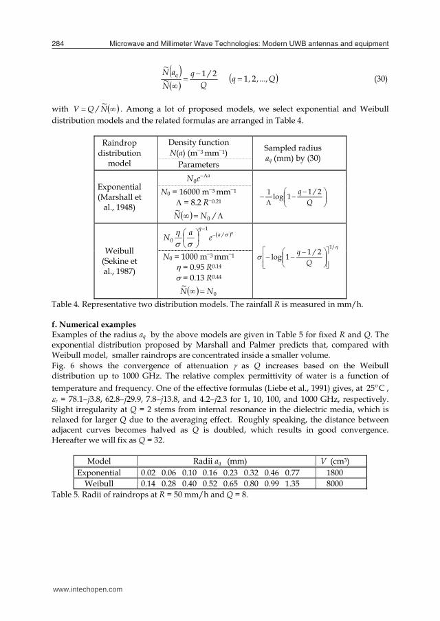
with N~/QV . Among a lot of proposed models, we select exponential and Weibull distribution models and the related formulas are arranged in Table 4.
Raindrop distribution
model
Density function N(a) (m3 mm1) Sampled radius
aq (mm) by (30) Parameters
Exponential (Marshall et
al., 1948)
aeN 0
Q
/q 211log1 N0 = 16000 m3 mm1 = 8.2 R0.21
/NN~ 0
Weibull (Sekine et al., 1987)
/aeaN
1
0
1/
211log
Q/q
N0 = 1000 m3 mm1 = 0.95 R0.14 = 0.13 R0.44
0NN~ Table 4. Representative two distribution models. The rainfall R is measured in mm/h. f. Numerical examples Examples of the radius aq by the above models are given in Table 5 for fixed R and Q. The exponential distribution proposed by Marshall and Palmer predicts that, compared with Weibull model, smaller raindrops are concentrated inside a smaller volume. Fig. 6 shows the convergence of attenuation as Q increases based on the Weibull distribution up to 1000 GHz. The relative complex permittivity of water is a function of temperature and frequency. One of the effective formulas (Liebe et al., 1991) gives, at C25o , r = 78.1j3.8, 62.8j29.9, 7.8j13.8, and 4.2j2.3 for 1, 10, 100, and 1000 GHz, respectively. Slight irregularity at Q = 2 stems from internal resonance in the dielectric media, which is relaxed for larger Q due to the averaging effect. Roughly speaking, the distance between adjacent curves becomes halved as Q is doubled, which results in good convergence. Hereafter we will fix as Q = 32.
Model Radii aq (mm) V (cm3) Exponential 0.02 0.06 0.10 0.16 0.23 0.32 0.46 0.77 1800
Weibull 0.14 0.28 0.40 0.52 0.65 0.80 0.99 1.35 8000 Table 5. Radii of raindrops at R = 50 mm/h and Q = 8.
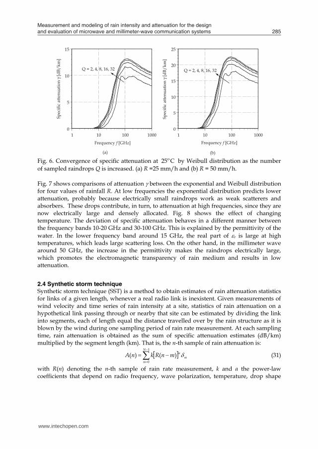
Fig. 6. Convergence of specific attenuation at C25o by Weibull distribution as the number of sampled raindrops Q is increased. (a) R =25 mm/h and (b) R = 50 mm/h. Fig. 7 shows comparisons of attenuation between the exponential and Weibull distribution for four values of rainfall R. At low frequencies the exponential distribution predicts lower attenuation, probably because electrically small raindrops work as weak scatterers and absorbers. These drops contribute, in turn, to attenuation at high frequencies, since they are now electrically large and densely allocated. Fig. 8 shows the effect of changing temperature. The deviation of specific attenuation behaves in a different manner between the frequency bands 10-20 GHz and 30-100 GHz. This is explained by the permittivity of the water. In the lower frequency band around 15 GHz, the real part of r is large at high temperatures, which leads large scattering loss. On the other hand, in the millimeter wave around 50 GHz, the increase in the permittivity makes the raindrops electrically large, which promotes the electromagnetic transparency of rain medium and results in low attenuation.
2.4 Synthetic storm technique Synthetic storm technique (SST) is a method to obtain estimates of rain attenuation statistics for links of a given length, whenever a real radio link is inexistent. Given measurements of wind velocity and time series of rain intensity at a site, statistics of rain attenuation on a hypothetical link passing through or nearby that site can be estimated by dividing the link into segments, each of length equal the distance travelled over by the rain structure as it is blown by the wind during one sampling period of rain rate measurement. At each sampling time, rain attenuation is obtained as the sum of specific attenuation estimates (dB/km) multiplied by the segment length (km). That is, the n-th sample of rain attenuation is:
1
0
)()(N
mmmnRknA (31)
with R(n) denoting the n-th sample of rain rate measurement, k and α the power-law coefficients that depend on radio frequency, wave polarization, temperature, drop shape
www.intechopen.com
Measurement and modeling of rain intensity and attenuation for the design and evaluation of microwave and millimeter-wave communication systems 285
Q...,,,q
Q/q
N~aN~ q 2 1 21 (30)
with N~/QV . Among a lot of proposed models, we select exponential and Weibull distribution models and the related formulas are arranged in Table 4.
Raindrop distribution
model
Density function N(a) (m3 mm1) Sampled radius
aq (mm) by (30) Parameters
Exponential (Marshall et
al., 1948)
aeN 0
Q
/q 211log1 N0 = 16000 m3 mm1 = 8.2 R0.21
/NN~ 0
Weibull (Sekine et al., 1987)
/aeaN
1
0
1/
211log
Q/q
N0 = 1000 m3 mm1 = 0.95 R0.14 = 0.13 R0.44
0NN~ Table 4. Representative two distribution models. The rainfall R is measured in mm/h. f. Numerical examples Examples of the radius aq by the above models are given in Table 5 for fixed R and Q. The exponential distribution proposed by Marshall and Palmer predicts that, compared with Weibull model, smaller raindrops are concentrated inside a smaller volume. Fig. 6 shows the convergence of attenuation as Q increases based on the Weibull distribution up to 1000 GHz. The relative complex permittivity of water is a function of temperature and frequency. One of the effective formulas (Liebe et al., 1991) gives, at C25o , r = 78.1j3.8, 62.8j29.9, 7.8j13.8, and 4.2j2.3 for 1, 10, 100, and 1000 GHz, respectively. Slight irregularity at Q = 2 stems from internal resonance in the dielectric media, which is relaxed for larger Q due to the averaging effect. Roughly speaking, the distance between adjacent curves becomes halved as Q is doubled, which results in good convergence. Hereafter we will fix as Q = 32.
Model Radii aq (mm) V (cm3) Exponential 0.02 0.06 0.10 0.16 0.23 0.32 0.46 0.77 1800
Weibull 0.14 0.28 0.40 0.52 0.65 0.80 0.99 1.35 8000 Table 5. Radii of raindrops at R = 50 mm/h and Q = 8.
Sp
ecif
ic a
tten
uat
ion
γ [
dB
/k
m]
Frequency f [GHz]
(a)
0
5
10
15
1 10 100 1000
0
5
10
15
20
25
1 10 100 1000
Sp
ecif
ic a
tten
uat
ion
γ [
dB
/k
m]
Frequency f [GHz]
(b)
Q = 2, 4, 8, 16, 32 Q = 2, 4, 8, 16, 32
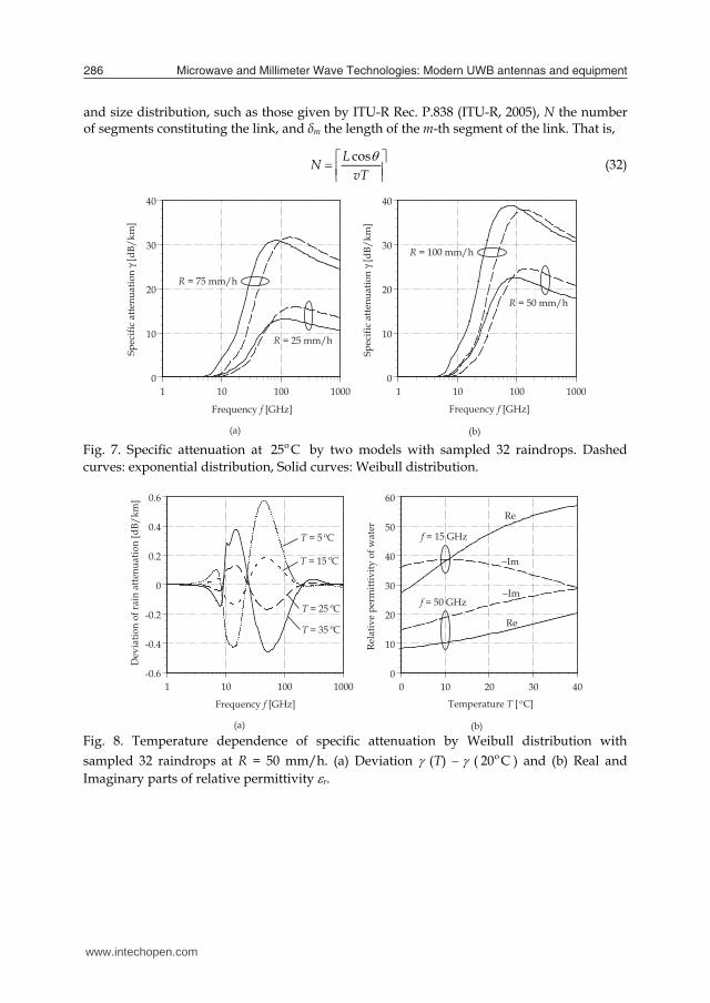
Fig. 6. Convergence of specific attenuation at C25o by Weibull distribution as the number of sampled raindrops Q is increased. (a) R =25 mm/h and (b) R = 50 mm/h. Fig. 7 shows comparisons of attenuation between the exponential and Weibull distribution for four values of rainfall R. At low frequencies the exponential distribution predicts lower attenuation, probably because electrically small raindrops work as weak scatterers and absorbers. These drops contribute, in turn, to attenuation at high frequencies, since they are now electrically large and densely allocated. Fig. 8 shows the effect of changing temperature. The deviation of specific attenuation behaves in a different manner between the frequency bands 10-20 GHz and 30-100 GHz. This is explained by the permittivity of the water. In the lower frequency band around 15 GHz, the real part of r is large at high temperatures, which leads large scattering loss. On the other hand, in the millimeter wave around 50 GHz, the increase in the permittivity makes the raindrops electrically large, which promotes the electromagnetic transparency of rain medium and results in low attenuation.
2.4 Synthetic storm technique Synthetic storm technique (SST) is a method to obtain estimates of rain attenuation statistics for links of a given length, whenever a real radio link is inexistent. Given measurements of wind velocity and time series of rain intensity at a site, statistics of rain attenuation on a hypothetical link passing through or nearby that site can be estimated by dividing the link into segments, each of length equal the distance travelled over by the rain structure as it is blown by the wind during one sampling period of rain rate measurement. At each sampling time, rain attenuation is obtained as the sum of specific attenuation estimates (dB/km) multiplied by the segment length (km). That is, the n-th sample of rain attenuation is:
1
0
)()(N
mmmnRknA (31)
with R(n) denoting the n-th sample of rain rate measurement, k and α the power-law coefficients that depend on radio frequency, wave polarization, temperature, drop shape
www.intechopen.com
Microwave and Millimeter Wave Technologies: Modern UWB antennas and equipment 286
and size distribution, such as those given by ITU-R Rec. P.838 (ITU-R, 2005), N the number of segments constituting the link, and δm the length of the m-th segment of the link. That is,
vT
LN cos (32)
Sp
ecif
ic a
tten
uat
ion
γ [
dB
/k
m]
Frequency f [GHz]
(a)
Sp
ecif
ic a
tten
uat
ion
γ [
dB
/k
m]
Frequency f [GHz]
(b)
0
10
20
30
40
1 10 100 1000
0
10
20
30
40
1 10 100 1000
R = 25 mm/h
R = 75 mm/h
R = 50 mm/h
R = 100 mm/h
Fig. 7. Specific attenuation at C25o by two models with sampled 32 raindrops. Dashed curves: exponential distribution, Solid curves: Weibull distribution.
Dev
iati
on
of
rain
att
enu
atio
n [
dB
/k
m]
Frequency f [GHz]
(a)
Rel
ativ
e p
erm
itti
vit
y o
f w
ater
Temperature T [ C]
(b)
R = 25 mm/h
R = 75 mm/h
-0.6
-0.4
-0.2
0
0.2
0.4
0.6
1 10 100 1000
0
10
20
30
40
50
60
0 10 20 30 40
f = 15 GHz
f = 50 GHz
T = 15 C
T = 5 C
T = 25 C
T = 35 C
Re
Re
−Im
−Im
o
o
o
o
o
Fig. 8. Temperature dependence of specific attenuation by Weibull distribution with sampled 32 raindrops at R = 50 mm/h. (a) Deviation (T) ( C20o ) and (b) Real and Imaginary parts of relative permittivity r.
90 and all
90 and 1cos
)1(
90 and 2,,0cos
mL
NmvTNL
NmvT
m
(33)
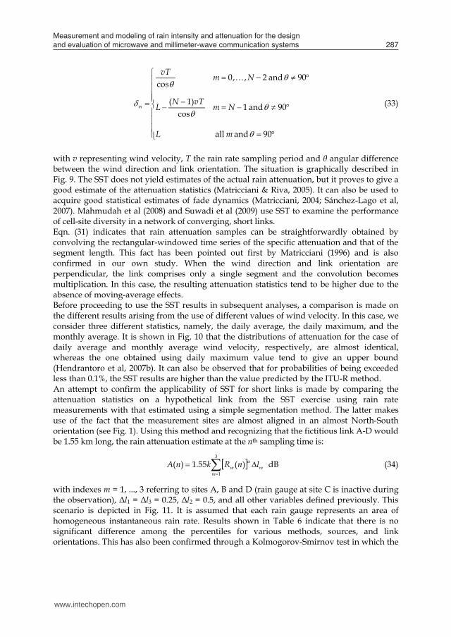
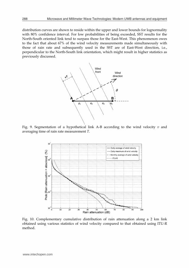
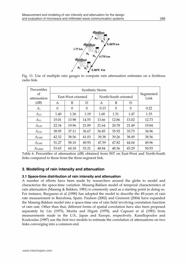
with v representing wind velocity, T the rain rate sampling period and θ angular difference between the wind direction and link orientation. The situation is graphically described in Fig. 9. The SST does not yield estimates of the actual rain attenuation, but it proves to give a good estimate of the attenuation statistics (Matricciani & Riva, 2005). It can also be used to acquire good statistical estimates of fade dynamics (Matricciani, 2004; Sánchez-Lago et al, 2007). Mahmudah et al (2008) and Suwadi et al (2009) use SST to examine the performance of cell-site diversity in a network of converging, short links. Eqn. (31) indicates that rain attenuation samples can be straightforwardly obtained by convolving the rectangular-windowed time series of the specific attenuation and that of the segment length. This fact has been pointed out first by Matricciani (1996) and is also confirmed in our own study. When the wind direction and link orientation are perpendicular, the link comprises only a single segment and the convolution becomes multiplication. In this case, the resulting attenuation statistics tend to be higher due to the absence of moving-average effects. Before proceeding to use the SST results in subsequent analyses, a comparison is made on the different results arising from the use of different values of wind velocity. In this case, we consider three different statistics, namely, the daily average, the daily maximum, and the monthly average. It is shown in Fig. 10 that the distributions of attenuation for the case of daily average and monthly average wind velocity, respectively, are almost identical, whereas the one obtained using daily maximum value tend to give an upper bound (Hendrantoro et al, 2007b). It can also be observed that for probabilities of being exceeded less than 0.1%, the SST results are higher than the value predicted by the ITU-R method. An attempt to confirm the applicability of SST for short links is made by comparing the attenuation statistics on a hypothetical link from the SST exercise using rain rate measurements with that estimated using a simple segmentation method. The latter makes use of the fact that the measurement sites are almost aligned in an almost North-South orientation (see Fig. 1). Using this method and recognizing that the fictitious link A-D would be 1.55 km long, the rain attenuation estimate at the nth sampling time is:
3
1
)(55.1)(m
mm lnRknA dB (34)
with indexes m = 1, ..., 3 referring to sites A, B and D (rain gauge at site C is inactive during the observation), Δl1 = Δl3 = 0.25, Δl2 = 0.5, and all other variables defined previously. This scenario is depicted in Fig. 11. It is assumed that each rain gauge represents an area of homogeneous instantaneous rain rate. Results shown in Table 6 indicate that there is no significant difference among the percentiles for various methods, sources, and link orientations. This has also been confirmed through a Kolmogorov-Smirnov test in which the
www.intechopen.com
Measurement and modeling of rain intensity and attenuation for the design and evaluation of microwave and millimeter-wave communication systems 287
and size distribution, such as those given by ITU-R Rec. P.838 (ITU-R, 2005), N the number of segments constituting the link, and δm the length of the m-th segment of the link. That is,
vT
LN cos (32)
Fig. 7. Specific attenuation at C25o by two models with sampled 32 raindrops. Dashed curves: exponential distribution, Solid curves: Weibull distribution.
Fig. 8. Temperature dependence of specific attenuation by Weibull distribution with sampled 32 raindrops at R = 50 mm/h. (a) Deviation (T) ( C20o ) and (b) Real and Imaginary parts of relative permittivity r.
90 and all
90 and 1cos
)1(
90 and 2,,0cos
mL
NmvTNL
NmvT
m
(33)
with v representing wind velocity, T the rain rate sampling period and θ angular difference between the wind direction and link orientation. The situation is graphically described in Fig. 9. The SST does not yield estimates of the actual rain attenuation, but it proves to give a good estimate of the attenuation statistics (Matricciani & Riva, 2005). It can also be used to acquire good statistical estimates of fade dynamics (Matricciani, 2004; Sánchez-Lago et al, 2007). Mahmudah et al (2008) and Suwadi et al (2009) use SST to examine the performance of cell-site diversity in a network of converging, short links. Eqn. (31) indicates that rain attenuation samples can be straightforwardly obtained by convolving the rectangular-windowed time series of the specific attenuation and that of the segment length. This fact has been pointed out first by Matricciani (1996) and is also confirmed in our own study. When the wind direction and link orientation are perpendicular, the link comprises only a single segment and the convolution becomes multiplication. In this case, the resulting attenuation statistics tend to be higher due to the absence of moving-average effects. Before proceeding to use the SST results in subsequent analyses, a comparison is made on the different results arising from the use of different values of wind velocity. In this case, we consider three different statistics, namely, the daily average, the daily maximum, and the monthly average. It is shown in Fig. 10 that the distributions of attenuation for the case of daily average and monthly average wind velocity, respectively, are almost identical, whereas the one obtained using daily maximum value tend to give an upper bound (Hendrantoro et al, 2007b). It can also be observed that for probabilities of being exceeded less than 0.1%, the SST results are higher than the value predicted by the ITU-R method. An attempt to confirm the applicability of SST for short links is made by comparing the attenuation statistics on a hypothetical link from the SST exercise using rain rate measurements with that estimated using a simple segmentation method. The latter makes use of the fact that the measurement sites are almost aligned in an almost North-South orientation (see Fig. 1). Using this method and recognizing that the fictitious link A-D would be 1.55 km long, the rain attenuation estimate at the nth sampling time is:
3
1
)(55.1)(m
mm lnRknA dB (34)
with indexes m = 1, ..., 3 referring to sites A, B and D (rain gauge at site C is inactive during the observation), Δl1 = Δl3 = 0.25, Δl2 = 0.5, and all other variables defined previously. This scenario is depicted in Fig. 11. It is assumed that each rain gauge represents an area of homogeneous instantaneous rain rate. Results shown in Table 6 indicate that there is no significant difference among the percentiles for various methods, sources, and link orientations. This has also been confirmed through a Kolmogorov-Smirnov test in which the
www.intechopen.com
Microwave and Millimeter Wave Technologies: Modern UWB antennas and equipment 288
distribution curves are shown to reside within the upper and lower bounds for lognormality with 80% confidence interval. For low probabilities of being exceeded, SST results for the North-South oriented link tend to surpass those for the East-West. This phenomenon owes to the fact that about 67% of the wind velocity measurements made simultaneously with those of rain rate and subsequently used in the SST are of East-West direction, i.e., perpendicular to the North-South link orientation, which might result in higher statistics as previously discussed.
Fig. 9. Segmentation of a hypothetical link A-B according to the wind velocity v and averaging time of rain rate measurement T.
Fig. 10. Complementary cumulative distribution of rain attenuation along a 2 km link obtained using various statistics of wind velocity compared to that obtained using ITU-R method.
Fig. 11. Use of multiple rain gauges to compute rain attenuation estimates on a fictitious radio link.
Percentiles of
attenuation (dB)
Synthetic Storm Segmented
Link East-West oriented North-South oriented
A B D A B D A1 0 0 0 0.13 0 0 0.22
A0.5 1.40 1.36 1.19 1.68 1.31 1.47 1.35 A0.1 15.01 13.98 14.55 13.66 12.86 13.02 12.73 A0.05 22.34 19.96 21.89 21.64 20.78 21.49 19.84 A0.01 38.95 37.11 36.67 36.85 35.92 35.73 34.96 A0.005 42.32 38.56 41.03 39.38 39.26 38.49 38.56 A0.001 51.27 58.10 49.93 47.59 47.82 44.04 49.96 A0.0005 53.65 60.18 53.21 48.84 48.36 45.29 50.93
Table 6. Percentiles of attenuation (dB) obtained from SST on East-West and North-South links compared to those from the three-segment link.
3. Modelling of rain intensity and attenuation
3.1 Space-time distribution of rain intensity and attenuation A number of efforts have been made by researchers around the globe to model and characterize the space-time variation. Maseng-Bakken model of temporal characteristics of rain attenuation (Maseng & Bakken, 1981) is commonly used as a starting point in doing so. For instance, Burgueno et al (1990) has adopted the model to describe the 49-years of rain rate measurement in Barcelona, Spain. Paulson (2002) and Gremont (2004) have expanded the Maseng-Bakken model into a space-time one of rain field involving correlation function of rain rate. Other than that, different forms of spatial correlation have also been proposed separately by Lin (1975), Morita and Higuti (1978), and Capsoni et al (1981) from measurements made in the U.S., Japan and Europe, respectively. Kanellopoulos and Koukoulas (1987) use the first two models to estimate the correlation of attenuations on two links converging into a common end.
www.intechopen.com
Measurement and modeling of rain intensity and attenuation for the design and evaluation of microwave and millimeter-wave communication systems 289
distribution curves are shown to reside within the upper and lower bounds for lognormality with 80% confidence interval. For low probabilities of being exceeded, SST results for the North-South oriented link tend to surpass those for the East-West. This phenomenon owes to the fact that about 67% of the wind velocity measurements made simultaneously with those of rain rate and subsequently used in the SST are of East-West direction, i.e., perpendicular to the North-South link orientation, which might result in higher statistics as previously discussed.
Fig. 9. Segmentation of a hypothetical link A-B according to the wind velocity v and averaging time of rain rate measurement T.
Fig. 10. Complementary cumulative distribution of rain attenuation along a 2 km link obtained using various statistics of wind velocity compared to that obtained using ITU-R method.
Fig. 11. Use of multiple rain gauges to compute rain attenuation estimates on a fictitious radio link.
Percentiles of
attenuation (dB)
Synthetic Storm Segmented
Link East-West oriented North-South oriented
A B D A B D A1 0 0 0 0.13 0 0 0.22
A0.5 1.40 1.36 1.19 1.68 1.31 1.47 1.35 A0.1 15.01 13.98 14.55 13.66 12.86 13.02 12.73 A0.05 22.34 19.96 21.89 21.64 20.78 21.49 19.84 A0.01 38.95 37.11 36.67 36.85 35.92 35.73 34.96 A0.005 42.32 38.56 41.03 39.38 39.26 38.49 38.56 A0.001 51.27 58.10 49.93 47.59 47.82 44.04 49.96 A0.0005 53.65 60.18 53.21 48.84 48.36 45.29 50.93
Table 6. Percentiles of attenuation (dB) obtained from SST on East-West and North-South links compared to those from the three-segment link.
3. Modelling of rain intensity and attenuation
3.1 Space-time distribution of rain intensity and attenuation A number of efforts have been made by researchers around the globe to model and characterize the space-time variation. Maseng-Bakken model of temporal characteristics of rain attenuation (Maseng & Bakken, 1981) is commonly used as a starting point in doing so. For instance, Burgueno et al (1990) has adopted the model to describe the 49-years of rain rate measurement in Barcelona, Spain. Paulson (2002) and Gremont (2004) have expanded the Maseng-Bakken model into a space-time one of rain field involving correlation function of rain rate. Other than that, different forms of spatial correlation have also been proposed separately by Lin (1975), Morita and Higuti (1978), and Capsoni et al (1981) from measurements made in the U.S., Japan and Europe, respectively. Kanellopoulos and Koukoulas (1987) use the first two models to estimate the correlation of attenuations on two links converging into a common end.
www.intechopen.com
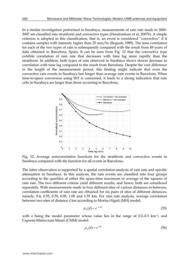
Microwave and Millimeter Wave Technologies: Modern UWB antennas and equipment 290
In a similar investigation performed in Surabaya, measurements of rain rate made in 2006-2007 are classified into stratiform and convective types (Hendrantoro et al, 2007b). A simple criterion is adopted in this classification, that is, an event is considered “convective” if it contains samples with intensity higher than 25 mm/hr (Bogush, 1989). The time correlation for each of the two types of rain is subsequently compared with the result from 49 years of data obtained in Barcelona, Spain. It can be seen from Fig. 12 that the convective type exhibits correlation of rain rate that decreases with time lag more rapidly than the stratiform. In addition, both types of rain observed in Surabaya shows slower decrease in correlation with time lag compared to the result from Barcelona. Despite the vast difference in the length of the measurement period, this finding might indicate that even the convective rain events in Surabaya last longer than average rain events in Barcelona. When time-to-space conversion using SST is concerned, it leads to a strong indication that rain cells in Surabaya are larger than those occurring in Barcelona.
Fig. 12. Average autocorrelation functions for the stratiform and convective events in Surabaya compared with the function for all events in Barcelona. The latter observation is supported by a spatial correlation analysis of rain rate and specific attenuation in Surabaya. In this analysis, the rain events are classified into four groups according to the quartiles of either the space-time maximum or average of the squares of rain rate. The two different criteria yield different results, and hence, both are considered separately. With measurements made in four different sites of various distances in-between, correlation coefficients of rain rate are obtained for six pairs of sites of different distances, namely, 0.4, 0.55, 0.70, 0.95, 1.00 and 1.55 km. For rain rate analysis, average correlation between two sites of distance d km according to Morita-Higuti (MH) model:
dR ed )( (35)
with α being the model parameter whose value lies in the range of 0.2–0.3 km-½, and Capsoni-Matricciani-Mauri (CMM) model:
dR ed )( (36)
with β equal to 0.46 km-1, are used as reference. For the specific attenuation, which is calculated by applying the power-law relation with ITU-R coefficients for 30 GHz horizontally polarized waves (ITU-R, 2005), Lin model is adopted:
22
)(dG
Gd (37)
with G being the characteristic distance that lies in the range of 1.5–3 km. The rain rate and specific attenuation quartiles together with the parameter values of the HM, CMM and Lin models obtained through fitting to (35)–(37) are shown in Tables 7 and 8, while the correlation curves are pictorially depicted in Fig. 13. For the lower quartiles the value of α is in the same range as the MH model, but is generally lower for the greater quartiles. For the CMM model, the values of β are all less than 0.46 obtained in Europe. These findings suggest that rain cells in Surabaya, especially those formed during the heaviest rain events, possess larger dimension than their Japanese and European counterparts. Conclusions that can be drawn from this investigation are manifold. Firstly, it is apparent that categorization of rain events into quartiles based on maximum and mean squared values of rain rate yields different sets of correlation function. It indicates that events with high maximum values do not necessarily possess high mean square values. An extreme exemplary case of such a condition is an event comprising a very long drizzle preceded by a brief high-intensity storm. Secondly, it can be observed that events with high mean square values, i.e., greater than 49.7 (mm/h)2, tend to produce high spatial correlation of rain rates between two sites up to 2 km apart. It suggests that the average size of rain cells having long intense rain is relatively large.
Q Maximum rain rate criterion Mean squared rain rate criterion Range α β Range α β
I Rmax ≤ 32.1 0.25 0.24 R2 ≤ 49.7 0.24 0.23 II 32.1 < Rmax ≤ 61.1 0.21 0.22 49.7 < R2 ≤ 253.5 0.16 0.17 III 61.1 < Rmax ≤ 101.4 0.18 0.19 253.5 < R2 ≤ 730.5 0.15 0.16 IV 101.4 < Rmax 0.073 0.074 730.5 < R2 0.059 0.062
Table 7. HM and CMM model parameter estimation from Surabaya measurements.
Q Maximum specific attenuation criterion Mean squared specific attenuation criterion
Range G Range G I AH,max ≤ 7.11 1.54 AH2 ≤ 1.95 1.56 II 7.11 < AH,max ≤ 12.75 1.72 1.95 < AH2 ≤ 10.38 1.86 III 12.75 < AH,max ≤ 21.76 1.93 10.38 < AH2 ≤ 29.92 1.88 IV 21.76 < AH,max 3.19 29.92 < AH2 3.64
Table 8. Lin model parameter estimation from Surabaya measurements.
www.intechopen.com
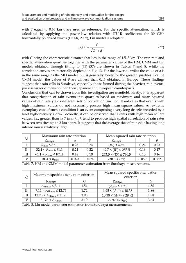
Measurement and modeling of rain intensity and attenuation for the design and evaluation of microwave and millimeter-wave communication systems 291
In a similar investigation performed in Surabaya, measurements of rain rate made in 2006-2007 are classified into stratiform and convective types (Hendrantoro et al, 2007b). A simple criterion is adopted in this classification, that is, an event is considered “convective” if it contains samples with intensity higher than 25 mm/hr (Bogush, 1989). The time correlation for each of the two types of rain is subsequently compared with the result from 49 years of data obtained in Barcelona, Spain. It can be seen from Fig. 12 that the convective type exhibits correlation of rain rate that decreases with time lag more rapidly than the stratiform. In addition, both types of rain observed in Surabaya shows slower decrease in correlation with time lag compared to the result from Barcelona. Despite the vast difference in the length of the measurement period, this finding might indicate that even the convective rain events in Surabaya last longer than average rain events in Barcelona. When time-to-space conversion using SST is concerned, it leads to a strong indication that rain cells in Surabaya are larger than those occurring in Barcelona.
Fig. 12. Average autocorrelation functions for the stratiform and convective events in Surabaya compared with the function for all events in Barcelona. The latter observation is supported by a spatial correlation analysis of rain rate and specific attenuation in Surabaya. In this analysis, the rain events are classified into four groups according to the quartiles of either the space-time maximum or average of the squares of rain rate. The two different criteria yield different results, and hence, both are considered separately. With measurements made in four different sites of various distances in-between, correlation coefficients of rain rate are obtained for six pairs of sites of different distances, namely, 0.4, 0.55, 0.70, 0.95, 1.00 and 1.55 km. For rain rate analysis, average correlation between two sites of distance d km according to Morita-Higuti (MH) model:
dR ed )( (35)
with α being the model parameter whose value lies in the range of 0.2–0.3 km-½, and Capsoni-Matricciani-Mauri (CMM) model:
dR ed )( (36)
with β equal to 0.46 km-1, are used as reference. For the specific attenuation, which is calculated by applying the power-law relation with ITU-R coefficients for 30 GHz horizontally polarized waves (ITU-R, 2005), Lin model is adopted:
22
)(dG
Gd (37)
with G being the characteristic distance that lies in the range of 1.5–3 km. The rain rate and specific attenuation quartiles together with the parameter values of the HM, CMM and Lin models obtained through fitting to (35)–(37) are shown in Tables 7 and 8, while the correlation curves are pictorially depicted in Fig. 13. For the lower quartiles the value of α is in the same range as the MH model, but is generally lower for the greater quartiles. For the CMM model, the values of β are all less than 0.46 obtained in Europe. These findings suggest that rain cells in Surabaya, especially those formed during the heaviest rain events, possess larger dimension than their Japanese and European counterparts. Conclusions that can be drawn from this investigation are manifold. Firstly, it is apparent that categorization of rain events into quartiles based on maximum and mean squared values of rain rate yields different sets of correlation function. It indicates that events with high maximum values do not necessarily possess high mean square values. An extreme exemplary case of such a condition is an event comprising a very long drizzle preceded by a brief high-intensity storm. Secondly, it can be observed that events with high mean square values, i.e., greater than 49.7 (mm/h)2, tend to produce high spatial correlation of rain rates between two sites up to 2 km apart. It suggests that the average size of rain cells having long intense rain is relatively large.
Q Maximum rain rate criterion Mean squared rain rate criterion Range α β Range α β
I Rmax ≤ 32.1 0.25 0.24 R2 ≤ 49.7 0.24 0.23 II 32.1 < Rmax ≤ 61.1 0.21 0.22 49.7 < R2 ≤ 253.5 0.16 0.17 III 61.1 < Rmax ≤ 101.4 0.18 0.19 253.5 < R2 ≤ 730.5 0.15 0.16 IV 101.4 < Rmax 0.073 0.074 730.5 < R2 0.059 0.062
Table 7. HM and CMM model parameter estimation from Surabaya measurements.
Q Maximum specific attenuation criterion Mean squared specific attenuation criterion
Range G Range G I AH,max ≤ 7.11 1.54 AH2 ≤ 1.95 1.56 II 7.11 < AH,max ≤ 12.75 1.72 1.95 < AH2 ≤ 10.38 1.86 III 12.75 < AH,max ≤ 21.76 1.93 10.38 < AH2 ≤ 29.92 1.88 IV 21.76 < AH,max 3.19 29.92 < AH2 3.64
Table 8. Lin model parameter estimation from Surabaya measurements.
www.intechopen.com

Microwave and Millimeter Wave Technologies: Modern UWB antennas and equipment 292
(a)
(b)
Fig. 13. Spatial correlations of (a) rain rate according to MH model and (b) specific attenuation of 30 GHz horizontally polarized waves according to Lin, both obtained by regression with respect to the correlations from measurements for four quartiles of mean squared values.
3.2 ARIMA modeling of rain rate and attenuation The short-term variation of rain attenuation is of great interest to millimeter-wave system designers as it determines the capability of the system required to handle the induced fades. In particular, two parameters are commonly used as a measure of fade dynamics, namely
fade duration and fade slope (van de Kamp & Castanet, 2002). A time series model is sought to demonstrate fade dynamics characteristics that approach those of actual measurements. A number of models have been proposed and tested by various researchers. In stochastic signal processing, it is of interest to obtain an appropriate time series model for stationary random processes. Such models that might be useful and appropriate to describe rain fade dynamics are of the ARMA family. The ARMA model has been proposed for modelling rain attenuation in both single- and multiple-link configuration (Hendrantoro et al, 2006, Yadnya et al, 2008a, 2008b). The underlying assumption is that the rain field is stationary, at least during the rain event under consideration, both in time and space. The temporal stationarity assumption assures that the ARMA model order does not change during the event, whereas the spatial stationarity is necessary for the applicability of the multi-variate version to the case of multiple-link system. The latter is deemed acceptable for a configuration with very short links located nearby, such as the macro-diversity access links of a millimeter-wave cellular system. Considering the statistics of rain cell diameter, which is approximately in the order of 4-5 km (extrapolation of spatial correlation of specific attenuation for the 4th quartile in Fig. 13 (b) up to about 0.5), it is motivating to obtain a more realistic, non-stationary model. Consequently, studies are made on various possible models, including those of ARIMA family. To determine the appropriate ARIMA(p, d, q) model parameters, where p, d and q denote the orders of the AR part, the differencing process and the MA, respectively, firstly the stationarity in both variance and mean of the event is evaluated following Box-Jenkins (Box et al, 1994). The test for stationarity in variance is intended to determine the appropriate transformation required to make the event stationary, if necessary. Whereas the test for stationarity in mean is meant to specify the order of differencing d. Next, the orders of the AR and MA parts are identified and diagnosed for the whiteness and normality of the residual. If necessary, outliers can be detected and discarded to increase the model accuracy as measured by the mean squared error (MSE). The resulting model parameters can be used to generate time series samples of rain attenuation following the characteristics of the particular event upon which the model is developed. To produce a more generic model, a large database of rain events must be used, from which various values of model parameters can be identified and clustered to yield a complete stochastic model. Such a model, for instance, must be capable of determining the statistics of appearance of a given set of model parameter values. Expansion into space-time model can also be made by invoking, for example, the VARIMA (Vector ARIMA) model using simultaneous measurements at several spatially distributed rain gauges (for rain rate) or radio links (for attenuation). An illustration of the ARIMA model application involving a number of rain events is given as follows. During an event, rain attenuation at 28 GHz on the 54 meter link is recorded with one-second sampling period. For verification purposes, attenuation is also estimated from rainfall rate measured during the event by invoking the conversion method outlined in ITU-R Rec. P.838 for vertically polarized radio wave at 30 GHz (ITU-R, 2005). Shown below is the cumulative distribution function (CDF) of rain attenuation estimates on February 10, 2009 obtained through three fashions: direct measurement of attenuation, measurement of rain rate followed by conversion using the ITU-R method and computer generation of time series samples according to the ARIMA modelling result. It is found out that the most appropriate model for this particular event is ARIMA (0, 1, 1). However, for different events, ARIMA model of different orders might result.
www.intechopen.com
Measurement and modeling of rain intensity and attenuation for the design and evaluation of microwave and millimeter-wave communication systems 293
(a)
(b)
Fig. 13. Spatial correlations of (a) rain rate according to MH model and (b) specific attenuation of 30 GHz horizontally polarized waves according to Lin, both obtained by regression with respect to the correlations from measurements for four quartiles of mean squared values.
3.2 ARIMA modeling of rain rate and attenuation The short-term variation of rain attenuation is of great interest to millimeter-wave system designers as it determines the capability of the system required to handle the induced fades. In particular, two parameters are commonly used as a measure of fade dynamics, namely
fade duration and fade slope (van de Kamp & Castanet, 2002). A time series model is sought to demonstrate fade dynamics characteristics that approach those of actual measurements. A number of models have been proposed and tested by various researchers. In stochastic signal processing, it is of interest to obtain an appropriate time series model for stationary random processes. Such models that might be useful and appropriate to describe rain fade dynamics are of the ARMA family. The ARMA model has been proposed for modelling rain attenuation in both single- and multiple-link configuration (Hendrantoro et al, 2006, Yadnya et al, 2008a, 2008b). The underlying assumption is that the rain field is stationary, at least during the rain event under consideration, both in time and space. The temporal stationarity assumption assures that the ARMA model order does not change during the event, whereas the spatial stationarity is necessary for the applicability of the multi-variate version to the case of multiple-link system. The latter is deemed acceptable for a configuration with very short links located nearby, such as the macro-diversity access links of a millimeter-wave cellular system. Considering the statistics of rain cell diameter, which is approximately in the order of 4-5 km (extrapolation of spatial correlation of specific attenuation for the 4th quartile in Fig. 13 (b) up to about 0.5), it is motivating to obtain a more realistic, non-stationary model. Consequently, studies are made on various possible models, including those of ARIMA family. To determine the appropriate ARIMA(p, d, q) model parameters, where p, d and q denote the orders of the AR part, the differencing process and the MA, respectively, firstly the stationarity in both variance and mean of the event is evaluated following Box-Jenkins (Box et al, 1994). The test for stationarity in variance is intended to determine the appropriate transformation required to make the event stationary, if necessary. Whereas the test for stationarity in mean is meant to specify the order of differencing d. Next, the orders of the AR and MA parts are identified and diagnosed for the whiteness and normality of the residual. If necessary, outliers can be detected and discarded to increase the model accuracy as measured by the mean squared error (MSE). The resulting model parameters can be used to generate time series samples of rain attenuation following the characteristics of the particular event upon which the model is developed. To produce a more generic model, a large database of rain events must be used, from which various values of model parameters can be identified and clustered to yield a complete stochastic model. Such a model, for instance, must be capable of determining the statistics of appearance of a given set of model parameter values. Expansion into space-time model can also be made by invoking, for example, the VARIMA (Vector ARIMA) model using simultaneous measurements at several spatially distributed rain gauges (for rain rate) or radio links (for attenuation). An illustration of the ARIMA model application involving a number of rain events is given as follows. During an event, rain attenuation at 28 GHz on the 54 meter link is recorded with one-second sampling period. For verification purposes, attenuation is also estimated from rainfall rate measured during the event by invoking the conversion method outlined in ITU-R Rec. P.838 for vertically polarized radio wave at 30 GHz (ITU-R, 2005). Shown below is the cumulative distribution function (CDF) of rain attenuation estimates on February 10, 2009 obtained through three fashions: direct measurement of attenuation, measurement of rain rate followed by conversion using the ITU-R method and computer generation of time series samples according to the ARIMA modelling result. It is found out that the most appropriate model for this particular event is ARIMA (0, 1, 1). However, for different events, ARIMA model of different orders might result.
www.intechopen.com
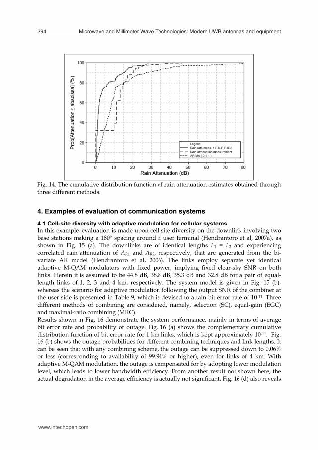
Microwave and Millimeter Wave Technologies: Modern UWB antennas and equipment 294
Fig. 14. The cumulative distribution function of rain attenuation estimates obtained through three different methods.
4. Examples of evaluation of communication systems
4.1 Cell-site diversity with adaptive modulation for cellular systems In this example, evaluation is made upon cell-site diversity on the downlink involving two base stations making a 180° spacing around a user terminal (Hendrantoro et al, 2007a), as shown in Fig. 15 (a). The downlinks are of identical lengths L1 = L2 and experiencing correlated rain attenuation of AR1 and AR2, respectively, that are generated from the bi-variate AR model (Hendrantoro et al, 2006). The links employ separate yet identical adaptive M-QAM modulators with fixed power, implying fixed clear-sky SNR on both links. Herein it is assumed to be 44.8 dB, 38.8 dB, 35.3 dB and 32.8 dB for a pair of equal-length links of 1, 2, 3 and 4 km, respectively. The system model is given in Fig. 15 (b), whereas the scenario for adaptive modulation following the output SNR of the combiner at the user side is presented in Table 9, which is devised to attain bit error rate of 10-11. Three different methods of combining are considered, namely, selection (SC), equal-gain (EGC) and maximal-ratio combining (MRC). Results shown in Fig. 16 demonstrate the system performance, mainly in terms of average bit error rate and probability of outage. Fig. 16 (a) shows the complementary cumulative distribution function of bit error rate for 1 km links, which is kept approximately 10-11. Fig. 16 (b) shows the outage probabilities for different combining techniques and link lengths. It can be seen that with any combining scheme, the outage can be suppressed down to 0.06% or less (corresponding to availability of 99.94% or higher), even for links of 4 km. With adaptive M-QAM modulation, the outage is compensated for by adopting lower modulation level, which leads to lower bandwidth efficiency. From another result not shown here, the actual degradation in the average efficiency is actually not significant. Fig. 16 (d) also reveals
that diversity might only be necessary for user terminals positioned near the border of cells having radius of about 4 km.
(a) (b) Fig. 15. Simulated communication system: (a) physical configuration and (b) system model.
SNR (dB) < 13.6 13.6 – 20.6 20.6 - 26.8 > 26.8 Modulation No Transmission
(M0) 4-QAM (M1=4)
16-QAM (M2=16)
64-QAM (M3=64)
Table 9. Scenario used in adaptive modulation
4.2 Channel capacity of LMDS applying distributed MIMO MIMO (multi-input multi-output) wireless systems with distributed antennas (D-MIMO) has been studied as a way to improve the system capacity (Lioli et al, 2009). Herein we explain the evaluation of the Shannon capacity performance of a 2×2 D-MIMO, with link configuration as used in the previous section, especially in rainy conditions. Fig. 17 shows the improvement in channel capacity due to adoption of D-MIMO. A significant increase in capacity over the SISO case can be realized when the links involved are of equal length, that is, 1 km as in Fig. 17 (a). Lower increases in capacity happen when the other link is longer, as seen in Fig. 17 (b), with positive improvement occurs only when the clear-sky SNR is about 12 dB or larger. However, it can be observed in all cases that the destructive impact of rain on the achieved capacity is not so significant.
5. Concluding remarks
A number of issues have been discussed throughout this chapter. First, raindrop size distribution measurements made in Surabaya have been found to slightly differ from that of the M-P model and those derived from Singapore measurements. Fits to Weibull and gamma have subsequently been made from the Surabaya measurements. It has also been found that large variation also occurs in raindrop fall velocity distribution, deviating from the commonly used Gunn-Kinzer model, but does not significantly change the specific attenuation estimates computed accordingly.
www.intechopen.com
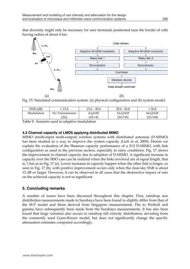
Measurement and modeling of rain intensity and attenuation for the design and evaluation of microwave and millimeter-wave communication systems 295
Fig. 14. The cumulative distribution function of rain attenuation estimates obtained through three different methods.
4. Examples of evaluation of communication systems
4.1 Cell-site diversity with adaptive modulation for cellular systems In this example, evaluation is made upon cell-site diversity on the downlink involving two base stations making a 180° spacing around a user terminal (Hendrantoro et al, 2007a), as shown in Fig. 15 (a). The downlinks are of identical lengths L1 = L2 and experiencing correlated rain attenuation of AR1 and AR2, respectively, that are generated from the bi-variate AR model (Hendrantoro et al, 2006). The links employ separate yet identical adaptive M-QAM modulators with fixed power, implying fixed clear-sky SNR on both links. Herein it is assumed to be 44.8 dB, 38.8 dB, 35.3 dB and 32.8 dB for a pair of equal-length links of 1, 2, 3 and 4 km, respectively. The system model is given in Fig. 15 (b), whereas the scenario for adaptive modulation following the output SNR of the combiner at the user side is presented in Table 9, which is devised to attain bit error rate of 10-11. Three different methods of combining are considered, namely, selection (SC), equal-gain (EGC) and maximal-ratio combining (MRC). Results shown in Fig. 16 demonstrate the system performance, mainly in terms of average bit error rate and probability of outage. Fig. 16 (a) shows the complementary cumulative distribution function of bit error rate for 1 km links, which is kept approximately 10-11. Fig. 16 (b) shows the outage probabilities for different combining techniques and link lengths. It can be seen that with any combining scheme, the outage can be suppressed down to 0.06% or less (corresponding to availability of 99.94% or higher), even for links of 4 km. With adaptive M-QAM modulation, the outage is compensated for by adopting lower modulation level, which leads to lower bandwidth efficiency. From another result not shown here, the actual degradation in the average efficiency is actually not significant. Fig. 16 (d) also reveals
that diversity might only be necessary for user terminals positioned near the border of cells having radius of about 4 km.
(a) (b) Fig. 15. Simulated communication system: (a) physical configuration and (b) system model.
SNR (dB) < 13.6 13.6 – 20.6 20.6 - 26.8 > 26.8 Modulation No Transmission
(M0) 4-QAM (M1=4)
16-QAM (M2=16)
64-QAM (M3=64)
Table 9. Scenario used in adaptive modulation
4.2 Channel capacity of LMDS applying distributed MIMO MIMO (multi-input multi-output) wireless systems with distributed antennas (D-MIMO) has been studied as a way to improve the system capacity (Lioli et al, 2009). Herein we explain the evaluation of the Shannon capacity performance of a 2×2 D-MIMO, with link configuration as used in the previous section, especially in rainy conditions. Fig. 17 shows the improvement in channel capacity due to adoption of D-MIMO. A significant increase in capacity over the SISO case can be realized when the links involved are of equal length, that is, 1 km as in Fig. 17 (a). Lower increases in capacity happen when the other link is longer, as seen in Fig. 17 (b), with positive improvement occurs only when the clear-sky SNR is about 12 dB or larger. However, it can be observed in all cases that the destructive impact of rain on the achieved capacity is not so significant.
5. Concluding remarks
A number of issues have been discussed throughout this chapter. First, raindrop size distribution measurements made in Surabaya have been found to slightly differ from that of the M-P model and those derived from Singapore measurements. Fits to Weibull and gamma have subsequently been made from the Surabaya measurements. It has also been found that large variation also occurs in raindrop fall velocity distribution, deviating from the commonly used Gunn-Kinzer model, but does not significantly change the specific attenuation estimates computed accordingly.
www.intechopen.com
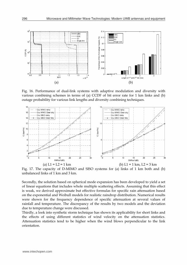
Microwave and Millimeter Wave Technologies: Modern UWB antennas and equipment 296
(a) (b)
Fig. 16. Performance of dual-link systems with adaptive modulation and diversity with various combining schemes in terms of (a) CCDF of bit error rate for 1 km links and (b) outage probability for various link lengths and diversity combining techniques.
(a) L1 = L2 = 1 km (b) L1 = 1 km, L2 = 3 km
Fig. 17. The capacity of D-MIMO and SISO systems for (a) links of 1 km both and (b) unbalanced links of 1 km and 3 km. Secondly, the solution based on spherical mode expansion has been developed to yield a set of linear equations that includes whole multiple scattering effects. Assuming that this effect is weak, we derived approximate but effective formulas for specific rain attenuation based on the exponential and Weibull models for realistic raindrop distribution. Numerical results were shown for the frequency dependence of specific attenuation at several values of rainfall and temperature. The discrepancy of the results by two models and the deviation due to temperature change were discussed. Thirdly, a look into synthetic storm technique has shown its applicability for short links and the effects of using different statistics of wind velocity on the attenuation statistics. Attenuation statistics tend to be higher when the wind blows perpendicular to the link orientation.
Fourthly, an examination of space-time variation shows that on average convective rain events in Surabaya last longer than those in Barcelona. A deeper study into the spatial variation indicates that the spatial correlation depends on the intensity of the rain. Events with high mean squared rain rate tend to produce high spatial correlation between two sites up to 2 km apart, which suggests that the average rain cells having long intense rain are relatively large. ARMA and ARIMA modeling of rain events has also been discussed and given an example. The ARIMA model has been chosen particularly due to its ability to describe the non-stationarity of rain events. Finally, examples have been given on the use of rain model to evaluate the performance of millimeter-wave communication systems under the impact of rain attenuation. The first example involves cell-site diversity with adaptive modulation implemented in cellular systems, while the second concerns LMDS applying distributed MIMO scheme. In particular, average bit error rate, probability of outage and channel capacity are taken as performance indicators.
6. Acknowledgement
Our studies are made possible by a research grant from JICA through the PREDICT-ITS project and a 2009 Hibah Kompetensi grant from the Indonesian Ministry of National Education. We wish to acknowledge the contribution and assistance to the reported work from our colleagues and students: Achmad Mauludiyanto, Suwadi, Muriani, Lince Markis, Haniah Mahmudah, Ari Wijayanti, Made S. Yadnya, Devy Kuswidiastuti, Adelina Hapsari, Kartika Ramadhani, Ninik Dwi Yundariani and Taufiq Ramadhany at Institut Teknologi Sepuluh Nopember, as well as Eko Setijadi and Naoki Tanaka at Kumamoto University.
7. References
Bogush, A. J. (1989) Radar and the Atmosphere, Artech House, ISBN: 0-89006-222-6, Boston. Box, G. E. P.; Jenkins, G. M. & Reinsel, G. C (1994). Time Series Analysis, Prentice-Hall, ISBN-
10: 0130607746. Brussaard, G. & Watson, P. (1995) Atmospheric Modelling and Millimetre-Wave Propagation,
Chapman-Hall, ISBN: 0-412-56230-8, London. Burgueno, A.; Vilar, E. & Puigcerver, M. (1990) Spectral Analysis of 49 Years of Rainfall Rate
and Relation to Fade Dynamics, IEEE Transactions on Communications, Vol. 38, No. 9, September 1990, 1359-1366, ISSN: 0090-6778.
Capsoni, C., Matricciani, E. & Mauri, M. (1981) Radar Derived Statistics of Rain Profile Slant Path, Proceedings of URSI 20th General Assembly, 50-57, Washington, D. C., 1981.
Cruzan, O. R. (1962). Translation addition theorem for spherical vector wave functions, Quarterly of Applied Mathematics, Vol. 20. 33-40, ISSN: 0033569X.
Drufuca, G. (1974) Rain Attenuation Statistics for Frequencies Above 10 GHz from Raingauges Observations, Journal de Recherches Atmospherique, Vol. 8, No. 1-2, 1974, 399–411, ISSN: 0021-7972.
Gremont, B. C. (2004) Spatio-Temporal Rain Attenuation Model for Application to Fade Mitigation Techniques, IEEE Transactions on Antennas and Propagation, Vol. 52, No. 5, May 2004, 1245-1256, ISSN: 0018-926X.
www.intechopen.com
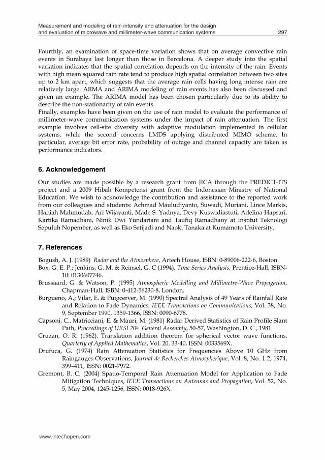
Measurement and modeling of rain intensity and attenuation for the design and evaluation of microwave and millimeter-wave communication systems 297
(a) (b)
Fig. 16. Performance of dual-link systems with adaptive modulation and diversity with various combining schemes in terms of (a) CCDF of bit error rate for 1 km links and (b) outage probability for various link lengths and diversity combining techniques.
(a) L1 = L2 = 1 km (b) L1 = 1 km, L2 = 3 km
Fig. 17. The capacity of D-MIMO and SISO systems for (a) links of 1 km both and (b) unbalanced links of 1 km and 3 km. Secondly, the solution based on spherical mode expansion has been developed to yield a set of linear equations that includes whole multiple scattering effects. Assuming that this effect is weak, we derived approximate but effective formulas for specific rain attenuation based on the exponential and Weibull models for realistic raindrop distribution. Numerical results were shown for the frequency dependence of specific attenuation at several values of rainfall and temperature. The discrepancy of the results by two models and the deviation due to temperature change were discussed. Thirdly, a look into synthetic storm technique has shown its applicability for short links and the effects of using different statistics of wind velocity on the attenuation statistics. Attenuation statistics tend to be higher when the wind blows perpendicular to the link orientation.
Fourthly, an examination of space-time variation shows that on average convective rain events in Surabaya last longer than those in Barcelona. A deeper study into the spatial variation indicates that the spatial correlation depends on the intensity of the rain. Events with high mean squared rain rate tend to produce high spatial correlation between two sites up to 2 km apart, which suggests that the average rain cells having long intense rain are relatively large. ARMA and ARIMA modeling of rain events has also been discussed and given an example. The ARIMA model has been chosen particularly due to its ability to describe the non-stationarity of rain events. Finally, examples have been given on the use of rain model to evaluate the performance of millimeter-wave communication systems under the impact of rain attenuation. The first example involves cell-site diversity with adaptive modulation implemented in cellular systems, while the second concerns LMDS applying distributed MIMO scheme. In particular, average bit error rate, probability of outage and channel capacity are taken as performance indicators.
6. Acknowledgement
Our studies are made possible by a research grant from JICA through the PREDICT-ITS project and a 2009 Hibah Kompetensi grant from the Indonesian Ministry of National Education. We wish to acknowledge the contribution and assistance to the reported work from our colleagues and students: Achmad Mauludiyanto, Suwadi, Muriani, Lince Markis, Haniah Mahmudah, Ari Wijayanti, Made S. Yadnya, Devy Kuswidiastuti, Adelina Hapsari, Kartika Ramadhani, Ninik Dwi Yundariani and Taufiq Ramadhany at Institut Teknologi Sepuluh Nopember, as well as Eko Setijadi and Naoki Tanaka at Kumamoto University.
7. References
Bogush, A. J. (1989) Radar and the Atmosphere, Artech House, ISBN: 0-89006-222-6, Boston. Box, G. E. P.; Jenkins, G. M. & Reinsel, G. C (1994). Time Series Analysis, Prentice-Hall, ISBN-
10: 0130607746. Brussaard, G. & Watson, P. (1995) Atmospheric Modelling and Millimetre-Wave Propagation,
Chapman-Hall, ISBN: 0-412-56230-8, London. Burgueno, A.; Vilar, E. & Puigcerver, M. (1990) Spectral Analysis of 49 Years of Rainfall Rate
and Relation to Fade Dynamics, IEEE Transactions on Communications, Vol. 38, No. 9, September 1990, 1359-1366, ISSN: 0090-6778.
Capsoni, C., Matricciani, E. & Mauri, M. (1981) Radar Derived Statistics of Rain Profile Slant Path, Proceedings of URSI 20th General Assembly, 50-57, Washington, D. C., 1981.
Cruzan, O. R. (1962). Translation addition theorem for spherical vector wave functions, Quarterly of Applied Mathematics, Vol. 20. 33-40, ISSN: 0033569X.
Drufuca, G. (1974) Rain Attenuation Statistics for Frequencies Above 10 GHz from Raingauges Observations, Journal de Recherches Atmospherique, Vol. 8, No. 1-2, 1974, 399–411, ISSN: 0021-7972.
Gremont, B. C. (2004) Spatio-Temporal Rain Attenuation Model for Application to Fade Mitigation Techniques, IEEE Transactions on Antennas and Propagation, Vol. 52, No. 5, May 2004, 1245-1256, ISSN: 0018-926X.
www.intechopen.com
Microwave and Millimeter Wave Technologies: Modern UWB antennas and equipment 298
Harrington, R. F. (1961). Time-Harmonic Electromagnetic Fields, 292-298, McGraw-Hill, ISBN-10: 0070267456, New York
Hendrantoro, G.; Bultitude, R. J. C. & Falconer, D. D. (2002) Use of Cell-Site Diversity in Millimeter-Wave Fixed Cellular Systems to Combat the Effects of Rain Attenuation, IEEE Journal on Selected Areas in Communications, Vol. 20, No. 3, April 2002, 602-614, ISSN: 0733-8716.
Hendrantoro, G. & Zawadzki, I. (2003). Derivation of Parameters of Y-Z Power Relation from Raindrop Size Distribution Measurements and Its Application in the Calculation of Rain Attenuation form Radar Reflectivity Factor Measurements. IEEE Transactions on Antennas and Propagation, Vol. 51, No. 1, January 2003, 12-22, ISSN: 0018-926X.
Hendrantoro, G. & Indrabayu (2005). A Multichannel Autoregressive Model of Rain Attenuation on Multiple Radio Links and Its Application in Assessment of Fade Mitigation Schemes in Fixed Wireless Systems Above 10 GHz, Proceedings of URSI General Assembly, New Delhi, September 2005.
Hendrantoro, G.; Indrabayu; Suryani, T. & Mauludiyanto, A. (2006). A Multivariate Autoregressive Model of Rain Attenuation on Multiple Short Radio Links, IEEE Antennas and Wireless Propagation Letters, Vol. 5, 2006, 54-57, ISSN: 1536-1225.
Hendrantoro, G.; Mauludiyanto, A. & Yundariani, N. D. (2007a), Application of Adaptive QAM Modulation and Diversity Scheme for 30 GHz Cellular Communications under the Impact of Rain Attention in Indonesia (in Indonesian), IPTEK: The Journal for Technology and Science, Vol. 18, No. 3, September 2007, 82-88.
Hendrantoro, G.; Muriani; Cahyono, D.; Mauludiyanto, A. & Matsushima, A. (2007b) Measurement of Time-Varying Rainfall Rate in Surabaya and Estimation of Attenuation Statistics by Synthetic Storm Technique, Proceedings of Korea-Japan Microwave Conference, Okinawa, November 2007.
ITU-R (2005) Specific Attenuation Model for Rain for Use in Prediction Methods, Rec P.838-3, January 2005.
Kanellopoulos, J. D. & Koukoulas, S. G. (1987) Analysis of the Rain Outage Performance of Route Diversity Systems, Radio Science, Vol. 22, No. 4, July-August 1987, 549-565, ISSN: 0048-6604.
Kuswidiastuti, D.; Suwadi & Hendrantoro, G. (2008) LMDS Channel Capacity Enhancement using D-MIMO under the Impact of Rain Attenuation, Proceedings of Indonesian Students Scientific Meeting, Delft, May 2008.
Li, L. W.; Yeo, T. S.; Kooi, P. S. & Leong, M. S. (1994). Comment on Raindrop Size Distribution Model. IEEE Transactions on Antennas and Propagation, Vol. 12, No. 9, Sep. 1994, 1360, ISSN: 0018-926X.
Liebe, H. J.; Hufford, G. A. & Manabe, T. (1991). A Model for the complex permittivity of water at frequencies below 1 THz, International Journal of Infrared and Millimeter Waves, Vol. 12, No. 7, 1991, 659-675, ISSN: 01959271.
Lin, S. H. (1975). A Method for Calculating Rain Attenuation Distribution on Microwave Paths, Bell System Technical Journal, Vol. 54, No. 6, 1975, 1051-1086, ISSN: 00058580.
Liolis, K. P.; Panagopoulos, A. D.; Cottis, P. G. & Rao, B.D. (2009) On the applicability of MIMO principle to 10-66GHz BFWA networks: capacity enhancement through spatial multiplexing and interference reduction through selection diversity, IEEE Transactions on Communications, Vol. 57, No. 2, February 2009, 530–541, ISSN: 0090-6778.
Mahmudah, H.; Wijayanti, A.; Mauludiyanto, A.; Hendrantoro, G. & Matsushima, A. (2008) Evaluation of Millimeter Wave Cell Site Diversity using Synthetic Storm, Proceedings of URSI General Assembly, Chicago, August 2008.
Marshall, J. S. & Palmer, W, M. (1948). The distribution of raindrops with size, Journal of Meteorology, Vol. 5, 1948, 165-166, ISSN: 00959634
Maruyama, T.; Shirato, Y.; Akimoto, M. & Nakatsugawa, M. (2008) Service Area Expansion of Quasi-Millimeter FWA Systems Through Site Diversity Based on Detailed Rainfall Intensity Data, IEEE Transactions on Antennas and Propagation, Vol. 56, No. 10, Oct. 2008, 3285 – 3292, ISSN: 0018-926X.
Maseng, T. & Bakken, P. M. (1981) A Stochastic Dynamic Model of Rain Attenuation, IEEE Transactions on Communications, Vol. COM-29, No. 5, May 1981, 660-669, ISSN: 0090-6778.
Matricciani, E. (1996) Physical-Mathematical Model of the Dynamics of Rain Attenuation Based on Rain Rate Time Series and a Two-Layer Vertical Structure of Precipitation, Radio Science, Vol. 31, No. 2, March-April 1996, 281-295, ISSN: 0048-6604.
Matricciani, E. (2004) Service Oriented Statistics of Interruption Time Due to Rainfall in Earth-Space Communication Systems, IEEE Transactions on Antennas and Propagation, Vol. 52, No. 8, August 2004, 2083-2090, ISSN: 0018-926X.
Matricciani, E. & Riva, C. (2005) The Search for the Most Reliable Long-Term Rain Attenuation CDF of a Slant Path and the Impact on Prediction Models, IEEE Transactions on Antennas and Propagation, Vol. 53, No. 9, September 2005, 3075-3079, ISSN: 0018-926X.
Mauludiyanto, A; Muriani; Markis, L.; Hendrantoro, G. & Matsushima, A. (2007) Preliminary Results from the Study of Raindrop Size Distribution and Rainfall Rate in Indonesia for the Development of Millimetre-Wave Systems in Tropical Regions, Proceedings of International Symposium on Antennas and Propagation, Niigata, 2007.
Morita, K. & Higuti, I. (1976) Prediction Methods for Rain Attenuation Distributions of Micro- and Millimeter Waves, Review of the Electronic Communication Laboratory, Vol. 24, No. 7-8, July-August 1976, 651-668.
Morita, K. & Higuti, I. (1978). Statistical Studies on Rain Attenuation and Site Diversity Effect on Earth to Satellite Links in Microwave and Millimeter Wavebands, Transactions of The IECE of Japan, Vol. E 61, No. 6.
Panagopoulos, A.D.; Skouloudakis, P.V. & Cottis, P.G. (2006) Quality of Service of Broadband Fixed Wireless Access QPSK Channels Interfered by Adjacent Terrestrial Links, IEEE Transactions on Antennas and Propagation, Vol. 54, No. 11, Nov. 2006, 3317 – 3326, ISSN: 0018-926X.
Paulson, K. S. (2002) The Spatial-Temporal Statistics of Rain Rate Random Fields, Radio Science, Vol. 37, No. 5, September 2002, ISSN: 0048-6604.
Pruppacher, H. R. & Pitter, R. L. (1971). A semi-empirical determination of the shape of cloud and rain drops, Journal of the Atmospheric Sciences, Vol. 28, No. 1, 1971, 86-94, ISSN: 00224928
www.intechopen.com
Measurement and modeling of rain intensity and attenuation for the design and evaluation of microwave and millimeter-wave communication systems 299
Harrington, R. F. (1961). Time-Harmonic Electromagnetic Fields, 292-298, McGraw-Hill, ISBN-10: 0070267456, New York
Hendrantoro, G.; Bultitude, R. J. C. & Falconer, D. D. (2002) Use of Cell-Site Diversity in Millimeter-Wave Fixed Cellular Systems to Combat the Effects of Rain Attenuation, IEEE Journal on Selected Areas in Communications, Vol. 20, No. 3, April 2002, 602-614, ISSN: 0733-8716.
Hendrantoro, G. & Zawadzki, I. (2003). Derivation of Parameters of Y-Z Power Relation from Raindrop Size Distribution Measurements and Its Application in the Calculation of Rain Attenuation form Radar Reflectivity Factor Measurements. IEEE Transactions on Antennas and Propagation, Vol. 51, No. 1, January 2003, 12-22, ISSN: 0018-926X.
Hendrantoro, G. & Indrabayu (2005). A Multichannel Autoregressive Model of Rain Attenuation on Multiple Radio Links and Its Application in Assessment of Fade Mitigation Schemes in Fixed Wireless Systems Above 10 GHz, Proceedings of URSI General Assembly, New Delhi, September 2005.
Hendrantoro, G.; Indrabayu; Suryani, T. & Mauludiyanto, A. (2006). A Multivariate Autoregressive Model of Rain Attenuation on Multiple Short Radio Links, IEEE Antennas and Wireless Propagation Letters, Vol. 5, 2006, 54-57, ISSN: 1536-1225.
Hendrantoro, G.; Mauludiyanto, A. & Yundariani, N. D. (2007a), Application of Adaptive QAM Modulation and Diversity Scheme for 30 GHz Cellular Communications under the Impact of Rain Attention in Indonesia (in Indonesian), IPTEK: The Journal for Technology and Science, Vol. 18, No. 3, September 2007, 82-88.
Hendrantoro, G.; Muriani; Cahyono, D.; Mauludiyanto, A. & Matsushima, A. (2007b) Measurement of Time-Varying Rainfall Rate in Surabaya and Estimation of Attenuation Statistics by Synthetic Storm Technique, Proceedings of Korea-Japan Microwave Conference, Okinawa, November 2007.
ITU-R (2005) Specific Attenuation Model for Rain for Use in Prediction Methods, Rec P.838-3, January 2005.
Kanellopoulos, J. D. & Koukoulas, S. G. (1987) Analysis of the Rain Outage Performance of Route Diversity Systems, Radio Science, Vol. 22, No. 4, July-August 1987, 549-565, ISSN: 0048-6604.
Kuswidiastuti, D.; Suwadi & Hendrantoro, G. (2008) LMDS Channel Capacity Enhancement using D-MIMO under the Impact of Rain Attenuation, Proceedings of Indonesian Students Scientific Meeting, Delft, May 2008.
Li, L. W.; Yeo, T. S.; Kooi, P. S. & Leong, M. S. (1994). Comment on Raindrop Size Distribution Model. IEEE Transactions on Antennas and Propagation, Vol. 12, No. 9, Sep. 1994, 1360, ISSN: 0018-926X.
Liebe, H. J.; Hufford, G. A. & Manabe, T. (1991). A Model for the complex permittivity of water at frequencies below 1 THz, International Journal of Infrared and Millimeter Waves, Vol. 12, No. 7, 1991, 659-675, ISSN: 01959271.
Lin, S. H. (1975). A Method for Calculating Rain Attenuation Distribution on Microwave Paths, Bell System Technical Journal, Vol. 54, No. 6, 1975, 1051-1086, ISSN: 00058580.
Liolis, K. P.; Panagopoulos, A. D.; Cottis, P. G. & Rao, B.D. (2009) On the applicability of MIMO principle to 10-66GHz BFWA networks: capacity enhancement through spatial multiplexing and interference reduction through selection diversity, IEEE Transactions on Communications, Vol. 57, No. 2, February 2009, 530–541, ISSN: 0090-6778.
Mahmudah, H.; Wijayanti, A.; Mauludiyanto, A.; Hendrantoro, G. & Matsushima, A. (2008) Evaluation of Millimeter Wave Cell Site Diversity using Synthetic Storm, Proceedings of URSI General Assembly, Chicago, August 2008.
Marshall, J. S. & Palmer, W, M. (1948). The distribution of raindrops with size, Journal of Meteorology, Vol. 5, 1948, 165-166, ISSN: 00959634
Maruyama, T.; Shirato, Y.; Akimoto, M. & Nakatsugawa, M. (2008) Service Area Expansion of Quasi-Millimeter FWA Systems Through Site Diversity Based on Detailed Rainfall Intensity Data, IEEE Transactions on Antennas and Propagation, Vol. 56, No. 10, Oct. 2008, 3285 – 3292, ISSN: 0018-926X.
Maseng, T. & Bakken, P. M. (1981) A Stochastic Dynamic Model of Rain Attenuation, IEEE Transactions on Communications, Vol. COM-29, No. 5, May 1981, 660-669, ISSN: 0090-6778.
Matricciani, E. (1996) Physical-Mathematical Model of the Dynamics of Rain Attenuation Based on Rain Rate Time Series and a Two-Layer Vertical Structure of Precipitation, Radio Science, Vol. 31, No. 2, March-April 1996, 281-295, ISSN: 0048-6604.
Matricciani, E. (2004) Service Oriented Statistics of Interruption Time Due to Rainfall in Earth-Space Communication Systems, IEEE Transactions on Antennas and Propagation, Vol. 52, No. 8, August 2004, 2083-2090, ISSN: 0018-926X.
Matricciani, E. & Riva, C. (2005) The Search for the Most Reliable Long-Term Rain Attenuation CDF of a Slant Path and the Impact on Prediction Models, IEEE Transactions on Antennas and Propagation, Vol. 53, No. 9, September 2005, 3075-3079, ISSN: 0018-926X.
Mauludiyanto, A; Muriani; Markis, L.; Hendrantoro, G. & Matsushima, A. (2007) Preliminary Results from the Study of Raindrop Size Distribution and Rainfall Rate in Indonesia for the Development of Millimetre-Wave Systems in Tropical Regions, Proceedings of International Symposium on Antennas and Propagation, Niigata, 2007.
Morita, K. & Higuti, I. (1976) Prediction Methods for Rain Attenuation Distributions of Micro- and Millimeter Waves, Review of the Electronic Communication Laboratory, Vol. 24, No. 7-8, July-August 1976, 651-668.
Morita, K. & Higuti, I. (1978). Statistical Studies on Rain Attenuation and Site Diversity Effect on Earth to Satellite Links in Microwave and Millimeter Wavebands, Transactions of The IECE of Japan, Vol. E 61, No. 6.
Panagopoulos, A.D.; Skouloudakis, P.V. & Cottis, P.G. (2006) Quality of Service of Broadband Fixed Wireless Access QPSK Channels Interfered by Adjacent Terrestrial Links, IEEE Transactions on Antennas and Propagation, Vol. 54, No. 11, Nov. 2006, 3317 – 3326, ISSN: 0018-926X.
Paulson, K. S. (2002) The Spatial-Temporal Statistics of Rain Rate Random Fields, Radio Science, Vol. 37, No. 5, September 2002, ISSN: 0048-6604.
Pruppacher, H. R. & Pitter, R. L. (1971). A semi-empirical determination of the shape of cloud and rain drops, Journal of the Atmospheric Sciences, Vol. 28, No. 1, 1971, 86-94, ISSN: 00224928
www.intechopen.com
Microwave and Millimeter Wave Technologies: Modern UWB antennas and equipment 300
Sakarellos, V. K.; Skraparlis, D.; Panagopoulos, A. D. & Kanellopoulos, J. D. (2009) Optimum Placement of Radio Relays in Millimeter-Wave Wireless Dual-Hop Networks, IEEE Antennas and Propagation Magazine, Vol. 51, No. 2, April 2009, 190 – 199, ISSN: 1045-9243.
Salehudin, M.; Hanantasena, B. & Wijdeman, L. (1999). Ka-Band Line-of-Sight Radio Propagation Experiment in Surabaya Indonesia. Proceedings of 5th Ka-Band Utilization Confenference, Taormina, 1999.
Sánchez-Lago, I.; Fontán, F. P.; Mariño, P. & Fiebig, U. -C. (2007) Validation of the Synthetic Storm Technique as Part of a Time-Series Generator for Satellite Links, IEEE Antennas and Wireless Propagation Letters, Vol. 6, 2007, 372-375, ISSN: 1536-1225.
Sekine, M.; Chen, C. D. & Musha, T. (1987). Rain attenuation from log-normal and Weibull rain-drop distributions, IEEE Transactions on Antennas and Propagation, Vol. 35, No. 3, March 1987, 358-359, ISSN: 0018926X.
Stratton, J. A. (1941). Electromagnetic Theory, 392-423, McGraw-Hill, ISBN-10: 0070621500, New York.
Suwadi; Hendrantoro, G.; Murdaningtyas, C. D. (2009) Performance of Selection Combining and Adaptive Coded Modulation in Millimeter-Wave Wireless Communication Systems under the Impact of Rain Attenuation in Indonesia (in Indonesian), Proceedings of National Seminar on Electrical Engineering, Informatics and Education, Malang, July 2009.
Sweeney, D. G. & Bostian, C. W. (1999) Implementing Adaptive Power Control as a 30/20-GHz Fade Countermeasure, IEEE Transactions on Antennas and Propagation, Vol. 47, No. 1, January 1999, 40-46, ISSN: 0018-926X.
Tan, J. & Goddard, J. W. F. (1998). Radar-derived area coverage, Proceedings of 8th URSI Commission F Triennial Open Symposium on Wave Propagation and Remote Sensing, Aveiro, Portugal, Sept. 22–25, 1998, 51–54.
Timothy, K. I.; Ong, J. T. & Choo, E. B. L. (2002) Raindrop Size Distribution Using Method of Moments for Terrestrial and Satellite Communication Applications in Singapore. IEEE Transactions on Antennas and Propagation, Vol. 15, No. 10, October 2002, 1420-1424, ISSN: 0018-926X.
Tokay, A.; Wolff, K. R.; Bashor, P. & Dursun, O. K. (2003). On the Measurement Errors of the Joss-Waldvogel Disdrometer. Proceedings of 31st Int. Conf. on Radar Meteorology, Seattle, August 2003.
van de Kamp, M. M. J. L. & Castanet, L. (2002) Fade Dynamics Review, Proceedings of COST 280 1st International Workshop, Malvern, July 2002.
Yadnya, M. S.; Mauludiyanto, A.; Hendrantoro, G. (2008a). ARMA Modeling of Rain Rate in Surabaya (In Indonesian), Proceedings of Seminar on Intelligent Technology and Its Application, Surabaya, May 2008.
Yadnya, M.S.; Mauludiyanto, A.; Hendrantoro, G. (2008b) ARMA Modeling from rain rate Measurement to Simulation Communication Channel Modeling for Millimeter Wave in Surabaya, The 6th Kumamoto University Forum, Surabaya, November 5-6, 2008.
Yeo, T. S.; Kooi, P. S. & Leong, M. S. (1996). A Two-Year Measurement of Rainfall Attenuation of CW Microwaves in Singapore. IEEE Transactions on Antennas and Propagation, Vol. 41, No. 6, June 1993, 709-712, ISSN: 0018-926X.
www.intechopen.com
Microwave and Millimeter Wave Technologies Modern UWBantennas and equipmentEdited by Igor Mini
ISBN 978-953-7619-67-1Hard cover, 488 pagesPublisher InTechPublished online 01, March, 2010Published in print edition March, 2010
InTech EuropeUniversity Campus STeP Ri Slavka Krautzeka 83/A 51000 Rijeka, Croatia Phone: +385 (51) 770 447 Fax: +385 (51) 686 166www.intechopen.com
InTech ChinaUnit 405, Office Block, Hotel Equatorial Shanghai No.65, Yan An Road (West), Shanghai, 200040, China
Phone: +86-21-62489820 Fax: +86-21-62489821
How to referenceIn order to correctly reference this scholarly work, feel free to copy and paste the following:
Gamantyo Hendrantoro, Akira Matsushima (2010). Measurement and Modeling of Rain Intensity andAttenuation for the Design and Evaluation of Microwave and Millimeter-Wave Communication Systems,Microwave and Millimeter Wave Technologies Modern UWB antennas and equipment, Igor Mini (Ed.), ISBN:978-953-7619-67-1, InTech, Available from: http://www.intechopen.com/books/microwave-and-millimeter-wave-technologies-modern-uwb-antennas-and-equipment/measurement-and-modeling-of-rain-intensity-and-attenuation-for-the-design-and-evaluation-of-microwav