
Mathematical Formulation Requirements and Specifications for the Process Models
132
eScholarship provides open access, scholarly publishing services to the University of California and delivers a dynamic research platform to scholars worldwide. Lawrence Berkeley National Laboratory Lawrence Berkeley National Laboratory Title: Mathematical Formulation Requirements and Specifications for the Process Models Author: Steefel, C. Publication Date: 01-03-2011 Publication Info: Lawrence Berkeley National Laboratory Permalink: http://escholarship.org/uc/item/2r6571qn Local Identifier: LBNL Paper LBNL-4085E
-
Upload
independent -
Category
Documents
-
view
1 -
download
0
Transcript of Mathematical Formulation Requirements and Specifications for the Process Models

eScholarship provides open access, scholarly publishingservices to the University of California and delivers a dynamicresearch platform to scholars worldwide.
Lawrence Berkeley National LaboratoryLawrence Berkeley National Laboratory
Title:Mathematical Formulation Requirements and Specifications for the Process Models
Author:Steefel, C.
Publication Date:01-03-2011
Publication Info:Lawrence Berkeley National Laboratory
Permalink:http://escholarship.org/uc/item/2r6571qn
Local Identifier:LBNL Paper LBNL-4085E

ASCEM-HPC-10-01-1
Mathematical Formulation Requirementsand Specifications for the Process Models
November 9, 2010
United States Department of Energy
C. Steefel, LBNL P. Lichtner, LANL J. Bell, LBNL G. Zyvoloski, LANLD. Moulton, LANL T. Wolery, LLNL G. Moridis, LBNL B. Andre, LBNLG. Pau, LBNL D. Bacon, PNNL S. Yabusaki, PNNL L. Zheng, LBNLK. Lipnikov, LANL N. Spycher, LBNL E. Sonnenthal, LBNL J. Davis, LBNLJ. Meza, LBNL
dshawkes
Typewritten Text
LBNL affiliates were partially supported by U.S. DOE and LBNL under Contract No. DE-AC02-05CH11231.
dshawkes
Typewritten Text
LBNL-4085E
dshawkes
Typewritten Text
dshawkes
Typewritten Text
dshawkes
Typewritten Text
dshawkes
Typewritten Text

Process Model Mathematical Formulation Requirements
DISCLAIMER
This work was prepared under an agreement with and funded by the U.S. Government.Neither the U.S. Government or its employees, nor any of its contractors, subcontractors ortheir employees, makes any express or implied:
1. warranty or assumes any legal liability for the accuracy, completeness, or for the useor results of such use of any information, product, or process disclosed; or
2. representation that such use or results of such use would not infringe privately ownedrights; or
3. endorsement or recommendation of any specifically identified commercial product,process, or service.
Any views and opinions of authors expressed in this work do not necessarily state or reflectthose of the United States Government, or its contractors, or subcontractors.
Printed in the United States of America
Prepared forU.S. Department of Energy
2 ascemdoe.org November 9, 2010

Process Model Mathematical Formulation Requirements
Authorization:
Dr. Paul Dixon, Los Alamos National LaboratoryMulti-Lab ASCEM Program Manager
Date
Dr. Juan Meza, Lawrence Berkeley National LaboratoryASCEM Technical Integration Manager
Date
Dr. J. David Moulton, Los Alamos National LaboratoryASCEM Multi-Process HPC Simulator Thrust Lead
Date
Dr. Carl I. Steefel, Lawrence Berkeley National LaboratoryASCEM Multi-Process HPC Simulator Deputy Thrust Lead
Date
Concurrence:
Mark Williamson, ASCEM Program ManagerEM-32 Groundwater & Soil Remediation
Date
Kurt Gerdes, EM-32Office Director for Groundwater & Soil Remediation
Date
3 ascemdoe.org November 9, 2010

Process Model Mathematical Formulation Requirements
Table of Contents
1 Introduction to Process Models Requirements 71.1 ASCEM Overview . . . . . . . . . . . . . . . . . . . . . . . . . . . . . . . . . . 7
1.2 Purpose and Scope of this Document . . . . . . . . . . . . . . . . . . . . . . . . . 7
1.3 Links to Other Thrust Areas . . . . . . . . . . . . . . . . . . . . . . . . . . . . . 8
1.4 Organization and Layout of this Document . . . . . . . . . . . . . . . . . . . . . . 9
1.5 Prioritization and Selection of Process Models . . . . . . . . . . . . . . . . . . . . 9
2 Overview of Process Models 112.1 Continuum Hypothesis . . . . . . . . . . . . . . . . . . . . . . . . . . . . . . . . 11
2.2 Fluid Description . . . . . . . . . . . . . . . . . . . . . . . . . . . . . . . . . . . 11
2.3 Governing Equations . . . . . . . . . . . . . . . . . . . . . . . . . . . . . . . . . 12
2.4 Phase Behavior . . . . . . . . . . . . . . . . . . . . . . . . . . . . . . . . . . . . 14
2.5 Reactive Transport . . . . . . . . . . . . . . . . . . . . . . . . . . . . . . . . . . 16
2.6 Fractured and Highly Heterogeneous Media . . . . . . . . . . . . . . . . . . . . . 19
3 Flow Processes 213.1 Overview . . . . . . . . . . . . . . . . . . . . . . . . . . . . . . . . . . . . . . . 21
3.2 Assumptions and Applicability for Flow Equations . . . . . . . . . . . . . . . . . 21
3.3 General Formulation for Multiphase Flow . . . . . . . . . . . . . . . . . . . . . . 21
3.4 Richards’ Equation . . . . . . . . . . . . . . . . . . . . . . . . . . . . . . . . . . 24
3.5 Single-Phase Flow . . . . . . . . . . . . . . . . . . . . . . . . . . . . . . . . . . 25
3.6 Infiltration . . . . . . . . . . . . . . . . . . . . . . . . . . . . . . . . . . . . . . . 26
3.7 Data Requirements for Flow . . . . . . . . . . . . . . . . . . . . . . . . . . . . . 29
3.8 Reaction-Induced Porosity and Permeability Change . . . . . . . . . . . . . . . . 30
4 Transport Processes 334.1 Overview . . . . . . . . . . . . . . . . . . . . . . . . . . . . . . . . . . . . . . . 33
4.2 Process Model Equations for Transport . . . . . . . . . . . . . . . . . . . . . . . . 33
4.3 Boundary Conditions, Sources and Sinks . . . . . . . . . . . . . . . . . . . . . . . 34
4.4 Advective Transport . . . . . . . . . . . . . . . . . . . . . . . . . . . . . . . . . . 34
4.5 Dispersive Transport . . . . . . . . . . . . . . . . . . . . . . . . . . . . . . . . . 35
4.6 Diffusive Transport . . . . . . . . . . . . . . . . . . . . . . . . . . . . . . . . . . 36
5 Biogeochemical Reaction Processes 425.1 Aqueous Complexation . . . . . . . . . . . . . . . . . . . . . . . . . . . . . . . . 42
4 ascemdoe.org November 9, 2010

Process Model Mathematical Formulation Requirements
5.2 Aqueous Activity Coefficients . . . . . . . . . . . . . . . . . . . . . . . . . . . . 44
5.3 Sorption . . . . . . . . . . . . . . . . . . . . . . . . . . . . . . . . . . . . . . . . 69
5.4 Mineral Precipitation and Dissolution . . . . . . . . . . . . . . . . . . . . . . . . 79
5.5 Microbially-Mediated Reactions . . . . . . . . . . . . . . . . . . . . . . . . . . . 86
6 Colloid Transport Processes 906.1 Overview . . . . . . . . . . . . . . . . . . . . . . . . . . . . . . . . . . . . . . . 90
6.2 Process Model Equations . . . . . . . . . . . . . . . . . . . . . . . . . . . . . . . 96
7 Thermal Processes 1017.1 Overview . . . . . . . . . . . . . . . . . . . . . . . . . . . . . . . . . . . . . . . 101
7.2 Process Model Equations . . . . . . . . . . . . . . . . . . . . . . . . . . . . . . . 101
7.3 Data Needs . . . . . . . . . . . . . . . . . . . . . . . . . . . . . . . . . . . . . . 101
7.4 Boundary Conditions, Sources and Sinks . . . . . . . . . . . . . . . . . . . . . . . 101
7.5 Coupling Considerations . . . . . . . . . . . . . . . . . . . . . . . . . . . . . . . 102
8 Geomechanical Processes 1038.1 Overview . . . . . . . . . . . . . . . . . . . . . . . . . . . . . . . . . . . . . . . 103
8.2 Assumptions and Applicability . . . . . . . . . . . . . . . . . . . . . . . . . . . . 103
8.3 THM Formulation . . . . . . . . . . . . . . . . . . . . . . . . . . . . . . . . . . . 103
8.4 Single-Phase Biot Model . . . . . . . . . . . . . . . . . . . . . . . . . . . . . . . 104
8.5 Boundary Conditions . . . . . . . . . . . . . . . . . . . . . . . . . . . . . . . . . 105
9 Source Terms 1069.1 Cementitious Source Terms . . . . . . . . . . . . . . . . . . . . . . . . . . . . . . 106
9.2 Glass Waste Forms . . . . . . . . . . . . . . . . . . . . . . . . . . . . . . . . . . 106
9.3 High-Level Radioactive Waste Tanks as Source Terms . . . . . . . . . . . . . . . . 111
A Nomenclature 113A.1 Variables . . . . . . . . . . . . . . . . . . . . . . . . . . . . . . . . . . . . . . . 113
5 ascemdoe.org November 9, 2010

Process Model Mathematical Formulation Requirements
List of Tables
1 An initial list of process models proposed for the Phase I demonstration is listedalong with their corresponding subsection. . . . . . . . . . . . . . . . . . . . . . 10
2 Key Pitzer interaction coefficients. . . . . . . . . . . . . . . . . . . . . . . . . . . 55
3 Key Pitzer parameters other than interaction coefficients. . . . . . . . . . . . . . . 56
4 Chebyshev polynomial coefficients for computing J(x) and J ′(x) (Harvie, 1981) . 60
5 List of Latin variables. Unitless variables are indicated by —. . . . . . . . . . . . . 113
6 List of Greek variables. Unitless variables are indicated by —. . . . . . . . . . . . 116
7 List of variables used in the Pitzer, UNIQUAC and NEA SIT models, Section 5.2 . 117
List of Figures
1 Tortuous diffusion paths in porous media (Steefel and Maher, 2009) . . . . . . . . 38
2 Schematic of the TLM model from Goncalves et al. (2007). . . . . . . . . . . . . . 80
3 A conceptual image of the colloid classes I-III is presented along with their origins. 93
4 General schematic of the stages of glass-water reaction . . . . . . . . . . . . . . . 107
6 ascemdoe.org November 9, 2010

Process Model Mathematical Formulation Requirements
1 Introduction to Process Models Requirements
1.1 ASCEM Overview
The Advanced Simulation Capability for Environmental Management (ASCEM) is intended to bea state-of-the-art scientific tool and approach for understanding and predicting contaminant fateand transport in natural and engineered systems. The ASCEM program is aimed at addressing crit-ical EM program needs to better understand and quantify flow and contaminant transport behaviorin complex geological systems. It will also address the long-term performance of engineered com-ponents including cementitious materials in nuclear waste disposal facilities, in order to reduceuncertainties and risks associated with DOE EM’s environmental cleanup and closure activities.Building upon national capabilities developed from decades of Research and Development in sub-surface geosciences, computational and computer science, modeling and applied mathematics, andenvironmental remediation, the ASCEM initiative will develop an integrated, open-source, high-performance computer modeling system for multiphase, multicomponent, multiscale subsurfaceflow and contaminant transport. This integrated modeling system will incorporate capabilities forpredicting releases from various waste forms, identifying exposure pathways and performing dosecalculations, and conducting systematic uncertainty quantification. The ASCEM approach will bedemonstrated on selected sites, and then applied to support the next generation of performanceassessments of nuclear waste disposal and facility decommissioning across the EM complex.
The Multi-Process High Performance Computing (HPC) Simulator is one of three thrust areasin ASCEM. The other two are the Platform and Integrated Toolsets (dubbed the Platform) andSite Applications. The primary objective of the HPC Simulator is to provide a flexible and ex-tensible computational engine to simulate the coupled processes and flow scenarios described bythe conceptual models developed using the ASCEM Platform. The graded and iterative approachto assessments naturally generates a suite of conceptual models that span a range of process com-plexity, potentially coupling hydrological, biogeochemical, geomechanical, and thermal processes.The Platform will use ensembles of these simulations to quantify the associated uncertainty, sen-sitivity, and risk. The Process Models task within the HPC Simulator focuses on the mathematicaldescriptions of the relevant physical processes.
1.2 Purpose and Scope of this Document
At the highest level of the HPC Simulator design is a set of process models that mathematically rep-resent the physical, chemical, and biological phenomena controlling contaminant release into, andtransport in, the subsurface. The objective of this requirements document is to provide a catalogueof process models, along with their detailed mathematical formulation, for potential implemen-tation in the HPC Simulator. This concise mathematical description and accompanying analysis,provides critical information for requirements and design of both the HPC Core Framework (Task1.1.2.2) and the HPC Toolsets (Task 1.1.2.3). This effort will also leverage ongoing efforts else-where in the Department of Energy, including the Cementitious Barrier Project (CBP) funded alsoby Environmental Management through EM-31.
It is important to note that with its focus on mathematical descriptions for a catalogue of process
7 ascemdoe.org November 9, 2010

Process Model Mathematical Formulation Requirements
models, this requirements document is significantly different from a traditional Software Require-ments Specification (SRS) document. Hence, this document does not follow the IEEE Std 830-1998 template, and instead uses a process category based layout that is summarized in Section 1.4.Moreover, this mathematical focus serves multiple audiences:
1. This document provides guidance to the developers engaged in designing and implement-ing the HPC Core Framework and HPC Toolsets. To meet their needs, sufficient detail foreach process model is provided in the form of a background discussion, supporting equa-tions, and references to relevant literature. The process models that are currently targeted forimplementation in the Phase 1 demonstration are listed in Table 1.
2. The document is also intended for “domain scientists” whose primary interest is in the pro-cesses themselves. The presentation is intended to justify the choice of process models andtheir mathematical detail.
3. Finally, the document is also intended for end users engaged in individual site applications.
Over time this document will evolve into a comprehensive graded presentation of models, fromcomplex to simple, under a general mathematical framework for each process category. The pri-oritization and selection of process models from this catalogue for implementation is discussed inSection 1.5. Evolution of the list of processes is inevitable, and the modular design of the HPCSimulator will easily accommodate the addition of new process implementations.
1.3 Links to Other Thrust Areas
The set of requirements detailed in this document have a clear connection to the other two thrustareas in ASCEM. In particular, many of the process model requirements follow from recommen-dations made from end users as captured in the User Suggestions for ASCEM Requirements Doc-uments (Section 5, pp. 18–19) (Seitz et al., 2010). These requirements include the need for mul-tiphase flow and transport, reactive transport, and both groundwater flow. Surface water flow,an important process at some contaminated sites, will be added as needed at a later date, but iscurrently beyond the scope of the present effort. In addition, there is a need for modeling thedegradation of engineered barriers, including, for example, covers, liners, cementitious materialsand waste forms. Other aspects that were deemed desirable include the modeling of radionuclides,source releases, and fractured media. All of these needs have been recognized and addressed insome form within this document.
Similarly, there are several areas where the process models will need to interface with the Platformand Integrated Toolsets Thrust Area. The Platform Thrust Area is tasked with developing thetools necessary to set up the conceptual models. These models represent the subsurface flow andreactive transport processes described in this document and will include 1) the geologic setting orframework, 2) the physical, geochemical, and biological processes and their interactions, and 3)the scenarios to which the models are applied. An end user wishing to perform a simulation willhave to specify features such as the process models, the initial and boundary conditions, and thematerial properties. These features will have to be consistent with and fully integrated with theexisting capabilities of the process models. For example, for each process model that is available,
8 ascemdoe.org November 9, 2010

Process Model Mathematical Formulation Requirements
there will be an associated set of constitutive models from which a user can select. In turn, eachprocess model will have a set of specifications that will dictate the parameter requirements thatare specific to the particular model and associated constitutive relations. Because of these links,there needs to be close ties between the development of the process models and the tools beingdeveloped by the Platform Thrust area so that the final simulation package can be reliable, robust,and easy to use.
1.4 Organization and Layout of this Document
The remainder of the Mathematical Formulation Requirements and Specifcations for the ProcessModels document is organized as follows. It presents an overview of the mathematical frameworkthat is used to model subsurface flow and reactive transport (Section 2). This overview is followedby a series of sections focusing on individual process categories. These include a presentationof Flow Processes in Section 3, Transport Processes in Section 4, Biogeochemical Reaction Pro-cesses in Section 5, Colloid Transport Processes in Section 6, Thermal Processes in Section 7,Geomechanical Processes in Section 8, and Source Terms, in Section 9. Each of these processcategories may present multiple process models. For example, biogeochemistry includes individ-ual process models for sorption, mineral precipitation-dissolution, microbially-mediated reactions,colloid generation, etc. In addition, models of differing fidelity can be accommodated by the HPCcode so, for example, several models for sorption (e.g., classical Kd, multicomponent-multisiteion exchange, non-electrostatic surface complexation, electrostatic surface complexation) are in-cluded.
The difficult question of prioritizing and ultimately selecting process models for implementationin any given year is addressed in the following subsection (Section 1.5). Finally, the notationalconventions and variables are summarized in Section A.1.
1.5 Prioritization and Selection of Process Models
Within each section that focuses on a particular process category (e.g., flow, transport), sub-sections contain the details of specific process models that may be implemented in the HPC Sim-ulator. However, the inclusion of a process model in this document does not guarantee it will beimplemented in the HPC Simulator in the near term. A combination of many factors will be con-sidered in the prioritization of process models and selection for implementation in any given year.For example, these factors include, the relative importance of the process models to various EMsites and the availability of required data for EM sites of interest. These types of information aregathered and organized by the Site Application Thrust. In the first years of the ASCEM project,prioritization must also consider the overhead of initiating development of the supporting HPCCore Framework (i.e., supporting infrastructure), as well as the design and initial development ofthe HPC Toolsets (i.e., the fundamental algorithmic building blocks).
Given these constraints, preliminary discussions involving all three thrusts have led to a list ofproposed process models for the first year’s development and the Phase I demonstration. This listof proposed process models is presented in Table 1.
Finally, it is important to note that the set of process models described in this document is by no
9 ascemdoe.org November 9, 2010

Process Model Mathematical Formulation Requirements
Table 1: An initial list of process models proposed for the Phase I demonstration is listed alongwith their corresponding subsection.
Process Category Process Model Section
Flow Single-phase 3.5Flow Richards 3.4
Transport Non-reactive, single component 4Transport Reactive, multicomponent 4
Biogeochemical Reactions Sorption 5.3Biogeochemical Reactions Precipitation/Dissolution 5.4
means exhaustive. Process models will be added based on the prioritization of specific EM needsduring periodic reviews and updates of this document.
10 ascemdoe.org November 9, 2010

Process Model Mathematical Formulation Requirements
2 Overview of Process Models
There are many formulations of the process models for contaminant transport that one couldpresent. Here we will start with the equations for conservation of mass and energy in the pres-ence of chemical reactions for a multiphase-multicomponent system. This leads to the basic flowequations describing non-isothermal, multiphase, multicomponent flows in heterogeneous porousmedia. A short description of phase behavior follows, which explains the relationship betweenthe composition of the phases and the flow equations. An introduction to some of the chemicalconcepts needed concludes this section.
There are other components describing the physical processes that must be included, includingmore detailed descriptions of transport, chemical processes, transport of colloids, geothermal, me-chanical, and source terms. In addition, within flow there are many processes that must be takeninto account, the major one being infiltration from various sources including surface water, evapo-ration and transpiration. All of these process models are described in greater detail in subsequentchapters.
2.1 Continuum Hypothesis
A rock mass consisting of aggregates of mineral grains and pore spaces or voids is referred to as aporous medium. An actual porous medium is a highly heterogeneous structure containing physicaldiscontinuities marked by the boundaries of pore walls which separate the solid framework fromthe void space. Although it is possible in principle at least, to describe this system at the microscaleof individual pores, such a description rapidly becomes a hopeless task as the size of the systemincreases and many pore volumes become involved. It is therefore necessary to approximate thesystem by a more manageable one. One quantitative description of the transport of fluids and theirinteraction with rocks is based on a mathematical idealization of the real physical system referredto as a continuum. In this theory the actual discrete physical system, consisting of aggregates ofmineral grains, interstitial pore spaces, and fractures, is replaced by a continuous system in whichphysical variables describing the system vary continuously in space. Allowance is made for thepossibility of a discrete set of surfaces across which discontinuous changes in physical propertiesmay occur. In this fictitious representation of the real physical system solids and fluids coexistsimultaneously at each point in space.
2.2 Fluid Description
A material body may be grouped into different regions having homogeneous properties at somescale called phases. A phase may be considered a homogeneous mixture of its constituents. Jumpdiscontinuities in various properties generally occur at the boundaries of phases. For example, arock is considered an aggregate of different minerals each of which constitute a separate phase.For a system in thermodynamic equilibrium a minimal set of independent components are used todescribe the system that may or may not correspond to the actual constituents in the system.
To start, we will denote the porosity of the medium by φ. We assume that the pore space isfiled with one or more phases. The saturation of each phase, sα denotes the fraction of the pore
11 ascemdoe.org November 9, 2010

Process Model Mathematical Formulation Requirements
volume occupied by that phase. The fluids are composed of N chemical components (or lumpedcomponents) that can appear in one or more phases. The components therefore are conservedquantities that need to be tracked potentially across multiple phases. The phases themselves arenot conserved. We denote by nkα the number of moles of component k in phase α per unit porevolume, or, in vector form nα. Thus,
∑αnα ≡ n is the vector of total moles of each component
per unit pore volume in the multiphase fluid system with elements nk. We note that the system canbe analogously defined by the composition of the fluid in terms of mass per unit pore volume, Mkα
or, in vector formMα. We can also define nα =∑
k nkα and Mα =∑
kMkα to be the total molesand mass, respectively, per unit pore volume in phase α. With these definitions the mass density ofphase α is ρα = Mα/sα.
From these basic definitions we can define several other useful ways to characterize the compo-sition of the phases, some of which are typically used in subsurface groundwater systems. Massfractions are defined as
Ykα =Mkα
Mα
, (2.1)
mole fractions are defined asXkα =
nkαnα
, (2.2)
molarity is defined asCkα =
nkαsα
, (2.3)
and molality is defined asmkα =
nkαM0α
, (2.4)
where M0α denotes the mass of solvent in phase α per unit pore volume. Another useful measureof concentration is the mass density ρiα defined as
ρkα =Mkα
sα=
Mα
sα
Mkα
Mα
, (2.5)
= ραYkα = WkCkα , (2.6)
where Wk is the molecular weight of component k. Or a molar density, ρ ′kα, can be defined
ρ ′kα =nkαsα
= ρ ′αXkα. (2.7)
With these definitions,nkα = ρ ′αXkαsα, (2.8)
nk =∑α
ρ ′αXkαsα. (2.9)
2.3 Governing Equations
The flow is governed by the equations of mass, momentum, and energy conservation.
12 ascemdoe.org November 9, 2010

Process Model Mathematical Formulation Requirements
2.3.1 Conservation of Momentum
The conservation of momentum in groundwater systems is typically given by Darcy’s law, whichdescribes the volumetric flow rate, qα, of each phase in terms of the phase pressure, pα by
qα = −kkrαµα
(∇pα − ραg), (2.10)
where k is the permeability (tensor) of the medium, kr,α is the relative permeability, which ex-presses the modification of the flow rate by multiphase effects, µα and ρα are the phase viscosityand density, respectively, and g is the gravitational force. The pressure in each phase is relatedto a reference pressure, p, typically taken to be the least wetting phase by a capillary pressure,pc,α = pα − p, which is a function of saturation.
2.3.2 Conservation of Mass
Molar (or mass) conservation for each component is given by
∂(φn)
∂t+ ∇ ·
∑α
nαsαqα = ∇ ·D +R+Q, (2.11)
or equivalently, making use of (2.3), in notation perhaps more commonly found in groundwaterhydrology
∂(φ∑
α sαCα)
∂t+ ∇ ·
∑α
Cαqα = ∇ ·D +R+Q. (2.12)
We note that the component conservation equation are often written in terms of mole fractions us-ing Eqns. (2.8) and (2.9). Here D are diffusive terms that include multiphase molecular diffusionand dispersion,R are reaction terms andQ are source terms. Both the diffusion / dispersion, reac-tion terms and source terms can be quite complex. Their particular forms are discussed elsewhere.
2.3.3 Conservation of Energy
For non-isothermal systems it is necessary to include the energy conservation in the system ofequations. The overall energy balance must include energy in the solid phase. If we assume thatthe porous medium and the fluids are in thermal equilibrium, the total energy balance is of the form
∂Ht
∂t+ ∇ ·
∑α
qαsαnα
Thα = ∇ ·QT +RH +∂∑
α pαuα∂t
+ ∇ ·∑α
qα ·∇pα, (2.13)
whereHt = (1− φ)ρrHr + φ
∑α
nαThα (2.14)
is the total enthalpy of the system, uα is the internal energy of phase α, hα are the partial molarphase enthalpies, Hr is the enthalpy of the medium and ρr is the density of the medium. Here QT
represents other energy transport processes such as thermal conduction, radiation, or dispersive
13 ascemdoe.org November 9, 2010

Process Model Mathematical Formulation Requirements
heat transfer, andRH represents energy release from reactions and external heating. This representsa form of the energy equation in which the solid and the fluid phases are in thermal equilibrium.If they are not, the fluid and solid portions of the enthalpy become distinct variables and RH willcontain relaxation terms that equilibrate the two temperatures.
In most cases, the term on the right hand side of Eqn. (2.13),
∂∑
α pαuα∂t
+ ∇ ·∑α
qα ·∇pα, (2.15)
can be omitted from the system. Omitting this term implicitly assumes that the change in phasepressures is slow so that these terms can be ignored. It is worth noting that many people for-mulate the energy equation without this term and replace total enthalpy by total internal energy.Formulations based on internal energy make a similar assumption by dropping a term of the form∑
α
pα∇ · qα (2.16)
from the energy equation.
2.4 Phase Behavior
The component conservation equations express the change in total moles of each of the componentdue to advection, diffusion, and chemical reactions. Since components are being transported inphases, it is necessary to know the composition of the phases before we can solve the flow equa-tions. This decomposition is referred to as the phase behavior of the system. For the nonisothermalsystem, the phase behavior is determined by saying that the equilibrium state of the mixture occursat the point of maximum entropy, or equivalently, a minimum of the negative entropy. For isother-mal systems, phase equilibrium occurs at the minimum of the Gibbs free energy. The entropy andGibbs free energy of the phases are derived from the chemical potential µα. These chemical po-tentials are typically specified in terms of an equation of state to model the dependence of pressureon temperature, composition, and specific volume of the phase. For a more detailed discussion see,for example, Michelsen and Mollerup (2004), Brantferger et al. (1991).
The chemical potentials µα are functions of pα, T , and phase composition nα. (Here, we havepreserved the role of capillary pressure in determining the thermodynamic behavior of the system.One simplification is to define the thermodynamics in terms of the reference pressure and retaincapillary pressure effects only in the definition of phase velocities, see Brantferger et al. (1991).)Furthermore the major thermodynamic variables describing each phase can all be expressed interms of the phase’s chemical potential. In particular, the partial molar entropy’s are given by
σα = −(∂µα∂T
)Xα,pα
, (2.17)
whereXα are the mole fractions and the partial molar enthalpies are given by
hα = (µα + Tσα) . (2.18)
14 ascemdoe.org November 9, 2010

Process Model Mathematical Formulation Requirements
Here the phase equilibrium problem is to determine the molar composition of the phases nα giventhe total moles n, pressure p and the total enthalpy Ht. The equilibrium distribution of the com-ponents is given by minimizing the negative entropy of the system. In a general multiphase settingthis becomes
min − S = −∑α
nTασα, (2.19)
subject ton =
∑α
nα, (2.20)
andHt = (1− φ)ρrhr + φ
(∑α
nTαhα
), (2.21)
along with inequality constraints (nα ≥ 0) guaranteeing non-negativity of the compositions andthermal stability of the fluid (nα
T∂hα/∂T > 0). (As noted above, if we do not consider thesolid and the fluids to be in thermal equilibrium then we hold the total fluid enthalpy, Hf =nTl hl + nTv hv, constant rather than the total enthalpy).
Treating this minimization problem, typically referred to as an isenthalpic flash calculation, hasbeen discussed in the literature (see Brantferger (1991); Michelsen and Mollerup (2004); Michelsen(1999)) and will not be discussed in detail here. it is worth noting, however, that the Hessian of thenegative entropy is a rank one perturbation of the Hessian of the Gibbs free energy, which indicatesthat the two functions are closely related.
In addition, at equilibrium the chemical potentials are equal; for example, in a two phase systemswhere the phases are denoted by l and v,
µl(Xl, T, pl) = µv(Xv, T, pv). (2.22)
Here, the chemical potentials are typically specified in terms of mole fractions rather than moles;however, we can use the definition of mole fractions to express them in this form.
In addition to determining the composition of the phases and the temperature, the phase behav-ior also determines the properties of the phases. In particular, given pressure, temperature, andcomponent molar densities, we can compute the volume occupied by the phases. To complete themathematical formulation of the system we require that the sum of the phase volumes match theavailable pore volume according to the relation
1 =∑α
sα(pα, T,nα). (2.23)
This equation constrains the evolution of the component conservation and energy equations. Herewe have implicitly used the capillary pressure to relate the phase pressures to the reference pres-sure. Note that the sα can be expressed in terms of the total moles per pore volume of the phase,given by
nTα = eTnα, (2.24)
where e is a vector of 1’s, divided by a molar density, ρ ′α; thus,
sα =nTαρ ′α. (2.25)
15 ascemdoe.org November 9, 2010

Process Model Mathematical Formulation Requirements
2.5 Reactive Transport
Chemical reactions may take place within a single fluid phase or between different fluid phasesand between solids and fluids. Consider a mixture consisting of various fluid phases designatedby α and solid grains with each solid phase designated by the index m. For convenience it isassumed that the same set of species are present in all fluid phases. Solid-Solid reactions areassumed to be mediated through one or more fluid phase. Reactions within a single fluid phase arereferred to as homogeneous and all other reactions that involve fluid-fluid or fluid-solid reactionsas heterogeneous. Homogeneous reactions can be written in canonical form in terms of a set ofbasis or primary species Ajα as (Lichtner, 1985)∑
i
νjiAjα Aiα , (2.26)
with reaction rate Iiα, stoichiometric reaction coefficients νji and secondary species Aiα. Suchreactions are often fast and their rates may be represented through equilibrium mass action relations(see Section 5.1).
Heterogeneous reactions take the form of reaction of a fluid phase with minerals which can bewritten in canonical form as ∑
j
νjmAjα Mm, (2.27)
for mineral Mm with reaction rate Imα and stoichiometric coefficients νjm. Here it is assumedthat different fluid phases may react with the same minerals in the solid aggregate. These reac-tions are represented as a parallel reaction network with potentially different reaction mechanisms.Since mineral-water reactions tend to be slow, they are generally represented with kinetic rate laws(Steefel and Lasaga, 1994).
In addition, phase transformations between different fluid phases may take place described byreactions of the form
Ajα Ajβ, (2.28)
between phases α and β. If Iαβj denotes the rate of reaction (2.28), then it follows that the rate isantisymmetric in the phases α and β
Iαβj = −Iβαj . (2.29)
For a system of Np phases, there are a total of 2Np − 1 different equilibrium phase combinations.The total number of independent degrees of freedom is independent of the number of phases andequal to NC +1, where NC denotes the number of independent chemical components. All reactionrates are assumed to have units of moles and are converted to mass units by multiplying by theappropriate formula weights Wj , Wi, and Wm associated with the subscripted species.
To develop mass conservation equations for the reacting constituents, phase α is chosen as areference phase with respect to which interphase mass transfer is described according the reactiongiven in Eqn. (2.28). In this treatment it is assumed that phase α refers to the aqueous phase.For a mass-based description and taking into account kinetic mass transfer rates for homogeneousand heterogeneous reactions, Eqns.(2.26) and (2.27), the mass balance equations for each primary
16 ascemdoe.org November 9, 2010

Process Model Mathematical Formulation Requirements
species can be written as
∂
∂t
(φsαρjα
)+ ∇ ·
(φsαρjαvjα
)= −Wj
∑i
νjiIiα
−Wj
∑β 6=α
Iαβj
−Wj
∑m
νjmImα , (2.30)
∂
∂t
(φsβρjβ
)+ ∇ ·
(φsβρjβvjβ
)= −Wj
∑i
νjiIiβ
+WjIαβj
−Wj
∑m
νjmImβ, (2.31)
and for each secondary species as
∂
∂t
(φsαρiα
)+ ∇ ·
(φsαρiαviα
)= WiIiα. (2.32)
Changes in mineral concentrations are described by the equations
∂φm∂t
= V m
∑α
Imα, (2.33)
with molar volume V m and where the sum over α on the right-hand side is over all fluid phases thatreact with the mth mineral. It is assumed that the solid phase is stationary, an assumption whichmust be relaxed in order to incorporate mechanical deformation effects.
In these equations viα denotes the mean velocity of the ith species in phase α. The velocity vα ofeach fluid phase α may be represented by the baryocentric form defined as
vα =1
ρα
∑k
ρkαvkα. (2.34)
The diffusive flux JDkα is defined as
JDkα = ρkα(vkα − vα
), (2.35)
= −ραDα∇Xkα, (2.36)
with the property ∑k
JDkα = 0. (2.37)
Note that for simplicity it is assumed that the diffusion coefficient Dα is species-independent andonly depends on the particular phase α. This assumption is generally not correct and the effectsof a local electric field must be taken into account in a more general treatment involving diffusion
17 ascemdoe.org November 9, 2010

Process Model Mathematical Formulation Requirements
of charged species to maintain local charge balance (Section 4.6). With this definition of diffusiveflux one has
ρkαvkα = ραXkαvα + JDkα. (2.38)
It should be noted that the choice of the baryocentric velocity is arbitrary and other definitions arealso possible. Introducing the Darcy velocity qα for each fluid phase defined as
qα = φsαvα, (2.39)
the flux becomesρkαvkα =
1
φsαραXkαqα + JDkα . (2.40)
Summing Eqns.(2.30)–(2.32) over all species and fluid phases yields the overall mass conservationequation
∂
∂t
(φ∑α
sαρα
)+ ∇ ·
(φ∑α
ραvα
)= 0, (2.41)
where the reaction rate terms disappear through conservation of mass of each chemical reaction∑j
Wjνji = Wi, (2.42)
and ∑j
Wjνjm = Wm. (2.43)
Typically, the molar concentration defined in Eqn.(2.3) is used in place of mass concentration. Inthis case under the assumption of incompressible flow the diffusive flux can be written approxi-mately as
JDkα ' −Dα∇Ckα. (2.44)
which is Fick’s First Law.
2.5.1 Partial Equilibrium
Typically the reaction rates Iiα for secondary species are transport-controlled and may be deter-mined by imposing conditions of local equilibrium through algebraic mass action constraints. Inthis case the rates Iiα can be eliminated by substituting Eqn.(2.32) into Eqns.(2.30) and (2.31).Summing over all fluid phases and assuming molar concentration variables are used this yieldsconservation equations for the primary species given by∑
α
∂
∂t
(φsαΨjα
)+ ∇ ·Ωjα
= −
∑αm
ναjmImα, (2.45)
which may be written alternatively as
∂
∂tφ∑α
sαΨjα + ∇ ·∑α
Ωjα = −∑αm
ναjmImα, (2.46)
18 ascemdoe.org November 9, 2010

Process Model Mathematical Formulation Requirements
where the total concentration Ψjα and flux Ωjα are defined, respectively, by
Ψjα = δααCjα +∑i
νjiCiα, (2.47)
andΩjα = δααJ jα +
∑i
νjiJ iα, (2.48)
where J jα and J iα denote the solute flux for primary and secondary species, respectively.
2.6 Fractured and Highly Heterogeneous Media
Important processes exist at the pore scale that can affect flow and transport at the continuum scale.For example, conceptual models of fracture flow and rock-water chemical interactions have beendeveloped and studied at various scales. Although these models are considered a priority for lateryears, it is important to provide background information that may impact the current requirementsand design documents. Thus, the following discussion presents a high-level overview of conceptualmodels used in fractured and highly heterogeneous media.
2.6.1 Overview
The fact that subsurface flow and transport occurs in an extremely heterogeneous material envi-ronment, which is often hierarchical in nature, has led to the multi-continuum class of models.Broadly speaking, these models separate the subsurface into several distinct materials based onflow and transport properties. For example fractures and clay layers have a permeability valuethat is orders of magnitude different than the surrounding rock or soil. Depending on the appli-cation, the properties of the different continua can be averaged into an “upscaled” property or leftdistinct. Other approaches have been taken to handle heterogeneities and transport occurring atsmall scales. For example, the field of stochastic hydrology attempts to quantify the impact ofsmall-scale permeability heterogeneity by casting the governing equations for hydrologic flow andsolute transport as a function of random variables (Zhang, 2001). When multiple continua remaindistinct, sub-grid-scale processes arise. While this section is concerned with process models andnot numerical grids, we can assume that at almost all grid resolutions, there is need, based onthe discussion above, that several materials and processes will need to be represented in a singlegridblock. For example, fracture widths are often on the order of millimeters while a fine grid ina basin-scale simulation may be on the order of meters. Sub-grid-scale models address this need.These models include common double permeability (DK), double porosity (DP, Barenblatt et al.(1960); Warren and Root (1963)), Multiple interacting continua (MINC, Pruess and Narasimhan(1985)), and Generalized Double Porosity Method (GDPM, Zyvoloski et al. (2008)).
Permeability in soils and rocks can be dominated by fine scale structure such as fractures, macro-pores, and clay layers. Fractures and macropores can be thought of conceptually as globally con-nected flow paths surrounded by material that acts as fluid storage. Similarly, clay layers can pro-vide a contaminant release to a high permeability aquifer through rate-limited diffusion; the doubleporosity conceptualization has been validated by field and laboratory data and under isothermal
19 ascemdoe.org November 9, 2010

Process Model Mathematical Formulation Requirements
conditions. The original development of dual porosity models began with the work of Barenblattet al. (1960) who recognized that in fractured porous media, the fractures provide the primary con-duit for mass transport, whereas the rock matrix could be represented as a fluid storage medium.In such a system the normal mass and energy balance equations can be written for the fracturedomain, and an additional equation is written for the matrix node, which is connected only to itscorresponding fracture node in a numerical model. In this formulation, the matrix is not a con-tinuous medium in which the full mass and energy transport equations are solved. Nevertheless,important fluid and energy storage terms within the matrix blocks can be explicitly included. Asignificant limitation of the dual porosity (DP) concept is that although a matrix node is introducedto capture storage in the medium surrounding each fracture, there is no ability to capture gradientsinto the matrix with a single node. The solution to the original dual porosity models are sometimescalled “quasi-steady” matrix solutions because of this limitation. Pruess and Narasimhan (1985)and Zyvoloski et al. (1997) extended the treatment of the matrix material by introducing a secondmatrix node.
Dual Permeability (DK) methods are like double porosity (DP) methods in that the grid-blockis divided into distinct materials with different properties. Unlike DP methods, the secondarymaterial is not only connected to the primary material, but also to other secondary material. Thismethod is appropriate for non-isothermal and high-capillary pressure models. In these models heatconduction and capillary flow in the secondary (matrix) material is important.
20 ascemdoe.org November 9, 2010

Process Model Mathematical Formulation Requirements
3 Flow Processes
3.1 Overview
In this section the basic flow models for single phase flow, Richards’ equation and for multiphaseflow are discussed, which is then followed by a section on infiltration. At the end of this section,data requirements for flow models are discussed, although this is a potentially very broad topic thatcan only be treated briefly here. Surface water flow and groundwater-surface water interactions willeventually be considered formally, since this is an important effect at many DOE sites, includingOak Ridge. At this stage, however, surface water is treated as a prescribed boundary condition.
3.2 Assumptions and Applicability for Flow Equations
Subsurface flow simulations typically assume that Darcy’s law is valid. As this law gives a re-lationship between velocity and pressure, it essentially replaces the momentum equation. Therehas been much research to support the validity of Darcy’s Law (?). Most references give the ap-plicability of Darcy’s Law to be for laminar flows with Reynolds numbers less that 10 using thepore throat diameter for a soil. There has been some effort to include inertial as well as turbulenceeffects that can occur near the wells.
It is also assumed that thermodynamic equilibrium (mechanical and thermal) exists for each gridblock. Sub-grid scale features will often play a prominent role in multi-fluid simulations. Faultsand fractures will likely be fast paths for contaminant transport and can effectively be treatedwith multiple porosity models. Similarly, rate-limited diffusion from clay inclusions can also bemodeled with a multiple porosity material.
Modeling multiphase flow in liquid-gas systems is essential for many applications ranging fromnuclear waste disposal involving boiling to problems involving a variably saturated zone withoxidation-reduction reactions taking place with consequent consumption of oxygen, for example.The EM complex includes a diversity of hydrologic settings that reflects the variability of geologicand climatic condition in the United States. The Hanford and Oak Ridge (or Savannah River) sitesrepresent end members of these conditions. The Hanford site is very dry with a large vadose zone,a deep water table, and little atmospheric recharge. The Oak Ridge and Savannah River sites havewet conditions that result in a small vadose zone and a very shallow water table. The waste formsand contaminant sources vary from the simple (increased total dissolved solids) to the complex(multi-phase air-water-NAPL at Oak Ridge and Savannah River) to the daunting (mixed NAPLand radioactive waste at Rocky Flats and the Hanford site).
3.3 General Formulation for Multiphase Flow
The model equations that describe the flow of multiple fluid phases in the subsurface are a combi-nation of the continuity equation and Darcy’s law, which replaces the momentum equation.
21 ascemdoe.org November 9, 2010

Process Model Mathematical Formulation Requirements
3.3.1 Component Conservation Equations
For each component, j, we have
∂
∂t
(φ∑α
ραsαYjα
)+ ∇ ·
(∑α
kkrαραYjαµα
∇(pα − ραg)
)= Qj, (3.1)
where k is the absolute permeability of the medium, krα is the relative permeability of phase, ραand sα are the density and saturation of phase α respectively, Yjα is the mass fraction, and Qj isthe net source term for component j.
3.3.2 Relative Permeability and Capillary Pressure
For both Richards’ equation and more general multiphase problems, the model requires represen-tations of relative permeability and capillary pressure. For two-phase systems, relative perme-ability and capillary pressure data are widely available for the more common forms such as vanGenuchten-Mualem and Brooks-Corey.
In Equation (3.1) the individual phase pressures, pα, are related to a reference pressure p by acapillary pressure pcα that depends on saturation,
pcα = pα − p. (3.2)
The capillary pressure is a function of saturation. Below we summarize two of the more commonmodels for relative permeability and capillary pressure.
van Genuchten Capillary Pressure and Relative Permeability Relations. Effective liquid sat-uration described by the van Genuchten (1980) relation is given by
se = [1 + (α|Pc|)n]−m
, (3.3)
where Pc represents the capillary pressure [Pa], and the effective liquid saturation se is definedfurther by
se =sl − srls0l − srl
, (3.4)
where sl denotes liquid saturation, srl denotes the residual saturation, and s0l denotes the maximum
saturation. The constants n and m are generally related by the expressions
m = 1− 1
n, n =
1
1−m. (3.5)
The inverse relation is given by
Pc =1
α
[(se)
−1/m − 1]1/n
. (3.6)
22 ascemdoe.org November 9, 2010

Process Model Mathematical Formulation Requirements
The van Genuchten-Mualem relative permeability for the liquid phase is given by
krl =√se
1−
[1− s1/m
e
]m2
. (3.7)
For the gas phase, the following formulation has been suggested
krg = 1− krl, (3.8)
but a formulation proposed by Luckner et al. (1989) is often preferred and is given by
krg = (1− sekg)1/3[1− s1/m
ekg
]2m
, (3.9)
where sekg is defined in terms of the liquid saturation, sl, and the residual gas saturation, sgr, as
sekg =sl
1− sgr. (3.10)
Brooks-Corey Capillary Pressure and Relative Permeability Relations. Liquid saturation asdescribed by the Brooks and Corey (1964) is given by
se = (α|pc|)−λ , (3.11)
with the inverse relation given by
pc =1
α(se)
−1/λ . (3.12)
Here λ is a fitting parameter.
Brooks and Corey (1964) used the Burdine (1953) theory to derive an expression for the liquidrelative permeability function given by
krl = (se)(2+3λ)/λ
= (α|pc|)−(2+3λ) . (3.13)
For the gas phase, the relative permeability is given by
krg = (1− se)2 [1− s(2+λ)/λe
], (3.14)
Alternatively, both Equation (3.8) and Equation (3.9) have been used to describe the relative per-meability of the gas phase.
Conservation Equations - Energy. For nonisothermal problems this system must be augmentedwith an energy equation. In the case of multi-phase flow, the conservation of energy equation takesa slightly different form from that given in Equation (2.13)
∂
∂t
[(1− φ)ρrur + φ
∑α
ραuαSα
]= ∇ ·
∑α
(kkrαραhα
µα
)∇(pα − ραg)+∇·QT+Qe, (3.15)
where: ρr is the rock density, ur is the internal energy of the rock, uα is the internal energy ofphase α, hα is the enthalpy of phase α, QT represents thermal conduction and radiation, and Qe isa source or sink of energy.
23 ascemdoe.org November 9, 2010

Process Model Mathematical Formulation Requirements
Closure and Constraint Equations. The equations above represent the conservation of watermass, the conservation of the jth non-aqueous component, and the conservation of energy. Theseequations are augmented by the following constraints. The mass fractions (or equivalently, themole fractions) in each phase must sum to 1:∑
j
Yjα = 1. (3.16)
The phase saturations must sum to 1: ∑α
sα = 1. (3.17)
An equation of state is used to specify the phase behavior and to supply additional fluid properties.
3.4 Richards’ Equation
3.4.1 Overview
Richard’s equation is often used to describe single phase flow under partially saturated conditions(i.e., the pores are not occupied exclusively by a single phase). As such, it requires the introductionof a relative permeability and a capillary pressure relations as discussed in Section 3.3.2. Richards’equation is well suited to very large numerical problems (millions of degrees of freedom) becauseit requires only one independent variable per cell. This is accomplished by assuming a static gasphase. There are limitations to this approach. For example, when light or chlorinated hydrocar-bons are present, even in very dilute quantities, the accurate representation of Henry’s partitioninginto the vapor (air) phase can be important. With Richards’ equation, the partitioning can be repre-sented, but the subsequent dilution due to air movement cannot. Another problem that can arise indeeper saline aquifers is the change in water density due to changes in brine concentration. In thiscase, another material balance equation can be introduced and solved in a fully coupled manner(with additional CPU and memory requirements) or the density variation can be obtained in a lesscoupled manner such as explicitly solving the flow and transport independently and calculating thedensity as a function of concentration. This method, while easier, has numerical stability concerns.As noted above, a variable density precludes the use of a head formulation for Richards’ equation.
Assumptions and Applicability. Richards’ equation makes the fundamental assumption thatwe are neglecting the movement of the gas phase. Because of this assumption, using Richards’equation may limit the kinds of transport analysis that can be done. It should also be noted thatRichards’ equation is often highly nonlinear with relative permeability of the liquid (most com-monly water) phase, krl (in turn a function of the liquid saturation, sl) and the liquid pressure,pl(swl).
There are limitations to this approach. For example, when light or chlorinated hydrocarbons arepresent, even in very dilute quantities, the accurate representation of Henry’s partitioning into thevapor (air) phase can be important. With Richards’ equation, the partitioning can be represented,but the subsequent dilution due to air movement cannot. Another problem that can arise in deepersaline aquifers is the change in water density due to changes in brine concentration. In this case,
24 ascemdoe.org November 9, 2010

Process Model Mathematical Formulation Requirements
another material balance equation can be introduced and solved in a fully coupled manner (with ad-ditional CPU and memory requirements) or the density variation can be obtained in a less coupledmanner such as explicitly solving the flow and transport independently and calculating the densityas a function of concentration. This method, while simpler, has numerical stability concerns. Asnoted above, a variable density precludes the use of a head formulation for Richards’ equation.Finally, it is often the case that Richards’ equation is presented in terms of hydraulic head insteadof pressure.
3.4.2 Process Model Equations
Richards’ equation provides the necessary physics to represent the flow of a liquid phase (typicallywater) under partially saturated conditions, with the assumption made that the second phase isinactive. Richards’ equation is derived from the conservation of liquid mass continuity equation:
∂(φ slρl)
∂t= ∇ · (ρlql) +Ql, (3.18)
where ρl is the liquid density, Ql is a source or sink, and ql is the liquid velocity given by Darcy’sLaw. This formulation differs from Equation (3.22) only in adding a relative permeability of theliquid, krl
ql = −kkrlµl
(∇pl − ρlg) , (3.19)
where k is the intrinsic rock or soil permeability, µl is the liquid viscosity, pl is the liquid pressure(or capillary pressure), and g is the acceleration of gravity.
These equations are usually combined to form the traditional form of Richards’ equation:
∂ (φ slρl)
∂t= ∇ ·
[Kkrlρlµl
(∇pl − ρlg)
]+Ql. (3.20)
Typical models of relative permeability as a function of saturation are the van Genuchten-Mualemrelations (Equation (3.7)) and the Brooks-Corey relations (Equation (3.13)).
3.5 Single-Phase Flow
3.5.1 Overview
The most basic case of flow is that of a single phase in a porous medium. Notwithstanding its sim-plicity, it has a wide application to describing subsurface processes. As we described in Section 2,the mathematical treatment is based on Darcy’s Law for momentum balance for flow in a porousmedium.
Assumptions and Applicability. There are many assumptions required for the strict validity ofDarcy’s Law, including incompressible, laminar flow.
25 ascemdoe.org November 9, 2010

Process Model Mathematical Formulation Requirements
3.5.2 Process Model Equations
For single phase flow in porous media under isothermal conditions the general formulation dis-cussed in section 2 reduces to
∂
∂t(φρl) + ∇ · (ρlq) = Q, (3.21)
where ρl denotes the fluid density (sometimes considered to be a function of p), Q represents asource/sink term and q is the Darcy velocity
q = − kµl
(∇p− ρg), (3.22)
In place of this formulation for Darcy’s Law, it is common to see it written in terms of hydraulichead defined as:
h = z +p
ρlg. (3.23)
Use of the hydraulic head as the key variable leads naturally to the use of the hydraulic conductivity,K, defined as
K =kρlg
µl. (3.24)
In the case where the density and viscosity are constant, therefore, it is possible to write Darcy’sLaw as
q = −K∇h. (3.25)
3.6 Infiltration
3.6.1 Overview
The infiltration process models are components of the subsurface fluid migration. Infiltration canbe an important driving force for contaminant transport, especially in the vadose zone. Engineeredsubsurface barrier technology seeks to minimize the infiltration driving force for contaminant mi-gration. There are a number of approaches and models that can be applied to predict infiltrationprocesses. These range from simple storage routing models to the more mechanistic Richards’equation-based models that simulate water flow and heat transport in response to meteorologicalforcing and plant water uptake. Within the complex interaction of physical, hydrologic, and bioticprocesses that control field-scale infiltration at the site of interest, the ideal model should be capa-ble of assessing the impact of infiltration on contaminant transport, as well as supporting barrierdesign and performance assessment.
Predicting infiltration requires consideration of unsaturated flow processes, precipitation, snow ac-cumulation and melting, surface runoff, water storage, evaporation, transpiration, lateral diversionalong sloped layers, and, ultimately, deep percolation (Ward and Gee, 1997; Ward and Keller,2005). All of these processes occur in response to forcing meteorology that leads to temporalvariability in air temperature, relative humidity, wind speed, and barometric pressure and, in themost sophisticated implementations, require the solution of coupled equations for mass and energytransport.
26 ascemdoe.org November 9, 2010

Process Model Mathematical Formulation Requirements
A minimum set of processes for modeling the water budget should include:
P + I = Rover + ∆W +D +GD + E + T, (3.26)
where:
P = precipitation
I = irrigation
Rover = overland flow (run-off and run-on)
D = drainage out of the soil cover (diverted by reduced-permeability layer)
GD = ground water recharge (deep percolation past a reduced-permeability layer)
∆W = change in soil water storage
E = evaporation
T = transpiration.
Evaporation is defined as the process by which liquid water is transformed into a gaseous stateand the subsequent transfer of this vapor to the atmosphere. Transpiration is the loss of waterfrom plants through their stomata to the atmosphere. Plants compensate for transpiration losses bytaking up water from the soil.
Another requirement is that the process models must include a full energy balance (nonisothermal)option for evapotranspiration processes. Water that does not run off the surface must be availablefor evaporation from the soil or plant surfaces, or infiltration into the soil profile. Soil water contentmust depend on the interactions of precipitation, temperature, vegetation, and albedo changes thatvary temporally (e.g., diurnally, seasonally, and episodically). Spatially and temporally variablewater storage and flux must be available for contaminant transport.
3.6.2 Process Model Requirements
Precipitation. The treatment of precipitation must include all natural sources of moisture thatmay reach the surface in the form of rain, snow, sleet, hail, dew, and fog, and must account for pre-cipitation not available for infiltration. This includes precipitation intercepted by the plant canopy,from which it is evaporated or transpired without ever contacting the soil; and sublimation, thedirect conversion of water from the solid phase to the vapor phase. This should also account forthe presence of a snow cover that can delay infiltration, reduce evaporation rates, and in the eventof rapid snowmelt, lead to surface runoff.
Non-Precipitation Surface Recharge (including leaks). Process models should account forsurface recharge sources (e.g., irrigation water used during construction as a dust control agentand post-construction to support the establishment of vegetation; water condensing on plant sur-faces and falling to the ground once the maximum storage depth in the canopy is exceeded, pipeleaks). These sources must also be subject to evaporation from soil and plant surfaces with theremainder becoming available for runoff or infiltration.
27 ascemdoe.org November 9, 2010

Process Model Mathematical Formulation Requirements
Evapotranspiration. Evapotranspiration models should include all the processes that convertwater from the aqueous phase into water in the gaseous phase, i.e., water vapor. This should alsoaccount for evaporation from soil and plant surfaces and plant transpiration and include optionswhere these components vary with soil properties and structure of the plant canopy.
Evaporation. In particular, evaporation models should account for surface wetness controls onevaporation for soil and plant surfaces. This should be done using the concept of potential evap-oration, the amount of water that could be evaporated were it freely available under the energyand atmospheric conditions (i.e., function of surface and air temperatures, insolation, and windspeed) that control water-vapor concentrations immediately above the evaporating surface. Actualevaporation will be calculated as a fraction of potential evaporation that accounts for the wateravailability and humidity differences between the atmosphere and the evaporating surface. Evap-oration from wet vegetated surfaces will depend on the amount of water that has accumulated onthe leaves and stems following precipitation events. The evaporation rate will be determined bythe amount of energy available, i.e., the solar radiation that is intercepted, the relative humidity ofthe air, and the vapor pressure of the air above the evaporating surface. For evaporation to occur,the vapor pressure of the free water in or on plants must be greater than the vapor pressure of waterin the air. Finally, models should be able to account for air flow over the plant surfaces.
Transpiration. Transpiration models need to account for passive transpiration processes con-trolled by the humidity of the atmospheric and the moisture content of the soil. To take advantageof existing databases, use the concept of potential and actual transpiration. The potential transpi-ration rate depends on the leaf area and the evaporative demand of the atmosphere, assuming soilwater is not limiting. The evaporative demand will be a function of incoming solar radiation andits partitioning into sensible and latent heat fluxes, vapor pressure deficit, and wind speed. Actualtranspiration is the water limited transpiration rate, and the ratio between actual and potential tran-spiration is indicative of the extent to which the plant suffers from water stress. Actual transpirationwill be a function of temperature and root water uptake reductions caused by water stress.
3.6.3 Plant Interactions
Root Water Uptake. Account for water uptake by plants from the soil to compensate for tran-spiration losses. Include stomatal opening and closing to control water loss and the capability totake up water held at very high matric potentials.
Canopy Interception. Models should account for precipitation falling on vegetative surfaces,i.e., the plant canopy, that collects on these surfaces. They should also be able to account forintercepted water being absorbed by plant surfaces, evaporated from these surfaces, or eventuallydripped to the ground surface after the interception capacity is exceeded. Include options forspecifying relationships between interception of rainfall and rainfall intensity.
28 ascemdoe.org November 9, 2010

Process Model Mathematical Formulation Requirements
3.7 Data Requirements for Flow
3.7.1 Permeability and Porosity
The most basic properties of the subsurface, which are required for all of the flow models, arepermeability and porosity. Often this data can only be provided by sparsely located well logs andat a spatial scale much finer than the scale of the model. As a consequence, techniques of upscalingare required to fill in the missing data and extrapolate to larger scales.
Permeability estimates are available for a large variety of soils and rocks. When conceptual (andnumerical) models have cells that represent fractures or faults, field tests (pumping and/or tracer)are required to determine effective permeabilities. Porosity data is also available for many rockand soil types.
3.7.2 Relative Permeability and Capillary Pressure.
For both Richards’ equation and more general multiphase problems, the model requires representa-tions of relative permeability and capillary pressure. For two-phase systems, relative permeabilityand capillary pressure data are widely available for the more common forms such as van Genuchtenand Brooks Corey.
When a NAPL phase is present and the likelihood of three phases is significant, much of the rel-ative permeability data available from the soil literature may have only limited applicability andexperiments on at least core size sample will be necessary. Stone (1973) presented a method toestimate three-phase relative permeability that is in common usage in the oil industry. However,when fractures or faults are present, parameters of the relative permeability and capillary pressuremodels are estimated with field data. Relative permeabilities often exhibit strong hysteretic behav-ior. Land’s method (Land, 1968; Spiteri and Juanes, 2006) is one approach for handling hystereticbehavior that is relatively simple to implement and is commonly used in the oil industry.
Some capillary pressure data is available in the database described by Schaap et al. (2001). Capil-lary models derived using surface tension data of pure components (Prausnitz et al., 1977) are usedwhere experimental data is not available.
3.7.3 Fluid Characterization
The model equations must also be augmented with property data for the fluids. In simple prob-lems we require only estimates of density and viscosity for each of the flowing phases. For morecomplex problems in which we are modeling a multicomponent system, additional data is required.
Equation of State. For multicomponent system, equation of state (EOS) data is required for wa-ter and all the NAPL components. Typically these are EOS for pure substances that are combinedfor mixtures. A basic EOS relates density to pressure and temperature. The form for the EOSis typically cubic such as the Soave-Redlich-Kwong (SRK) or the Peng-Robinson (PR) models.Tabular models are also in common use.
29 ascemdoe.org November 9, 2010

Process Model Mathematical Formulation Requirements
Mixture thermodynamics is used to combine pure phase EOS’s for the application. The EPAlists over 80 potential NAPL components (volatile organic compounds or VOCs) that can causegroundwater contamination and has data bases with at least some properties for these contaminants.
Mixture Internal Energy and Enthalpy. These will generally follow the simple additive rulebased of component values and mass fraction. Consideration must be also given to heats of solu-tion.
3.7.4 Boundary Conditions and Initial Conditions
Boundary and initial conditions can take several different forms depending on the application.Dirichlet boundary conditions specify the pressure, temperature, and saturation at the boundary.Neumann conditions specify the flux q at the boundary. Initial conditions may consist of specifyinga constant pressure or variable pressure, temperature, and saturation, for example in the form ofhydrostatic conditions taking into account the change in fluid density.
Typical boundary condition for Richard’s equation consist of infiltration (recharge) and constantor time varying pressure conditions. More sophisticated conditions such at unit gradient, freedrainage, and seepage face are also used.
3.8 Reaction-Induced Porosity and Permeability Change
3.8.1 Porosity Changes
Porosity changes in matrix and fractures are directly tied to the volume changes as a result of min-eral precipitation and dissolution. The molar volumes of minerals created by hydrolysis reactions(i.e., anhydrous phases, such as feldspars, reacting with aqueous fluids to form hydrous mineralssuch as zeolites or clays) are often larger than those of the primary reactant minerals; therefore,constant molar dissolution-precipitation reactions may lead to porosity reductions.
The porosity, φ, of the medium (fracture or matrix) can be calculated from
φ = 1−Nm∑m=1
φm, (3.27)
where Nm is the number of minerals, and φm is the volume fraction of mineral m in the rock (m3
mineral m−3 medium). As the volume fraction of each mineral changes due to mineral reactions,the porosity can be recalculated at each time step.
3.8.2 Fracture Permeability Changes
Fracture permeability changes can be approximated using the porosity change and an assump-tion of plane parallel fractures of uniform aperture (cubic law; Steefel and Lasaga (1994)). The
30 ascemdoe.org November 9, 2010

Process Model Mathematical Formulation Requirements
modified permeability, k, is then given by
k = ki
(φ
φi
)3
, (3.28)
where ki and φi are the initial permeability and porosity, respectively. This law yields zero perme-ability only under the condition of zero fracture porosity.
In most experimental and natural systems, permeability reductions to values near zero occur atporosities significantly greater than zero. This generally is the result of mineral precipitation inthe narrower interconnecting apertures. The hydraulic aperture, as calculated from the fracturespacing and permeability (as determined through air-permeability measurements) assuming a cubiclaw relation, is a closer measure of the smaller apertures in the flow system. Using the hydraulicaperture, a much stronger relationship between permeability and porosity can be developed. Thisrelationship can be approximated as follows:
The initial hydraulic aperture δ0,h (m) is calculated using the following cubic law relation:
δ0,h = [12k0s]13 , (3.29)
where k0 is the initial fracture permeability (m2) and s is the fracture spacing (m). The permeability(k′) resulting from a change in the hydraulic aperture, is given by
k′ =(δ0,h + ∆δ)3
12s, (3.30)
where ∆δ is the aperture change resulting from mineral precipitation/dissolution.
The aperture change resulting from a calculated volume change can be approximated by assumingprecipitation of a uniform layer over the entire geometric surface area of the fracture, assumingalso that this area as well as the fracture spacing remains constant. The actual distribution ofmineral alteration is much more heterogeneous and depends on many processes that are active atscales much smaller than the resolution of the model; however, the combined effect of the initialheterogeneities and localized precipitation processes can only be treated through model sensitivitystudies and experiments.
For a dual permeability model, changes in the fracture porosity are calculated based on the porosityof the fracture medium, so that ∆δ can be approximated by
∆δ =
(φ′fm − φfm,0
)φfm,0
δg. (3.31)
3.8.3 Matrix Permeability Changes
Matrix permeability changes are calculated from changes in porosity using ratios of permeabilitiescalculated from the Carman-Kozeny relation (Bear, 1972a), and ignoring changes in grain size,tortuosity, and specific surface area as follows:
k = ki(1− φi)2
(1− φ)2
(φ
φi
)3
. (3.32)
31 ascemdoe.org November 9, 2010

Process Model Mathematical Formulation Requirements
The simple cubic law (Equation (3.28)) and the Kozeny-Carman (Equation (3.32)) porosity-permeabilityequations may not reflect the complex relationship of porosity and permeability in geologic mediathat depends on an interplay of many factors, such as pore size distribution, pore shapes, and con-nectivity (Verma and Pruess, 1988). Laboratory experiments have shown that modest reductionsin porosity from mineral precipitation can cause large reductions in permeability (Vaughan, 1989).Detailed analysis of a large set of field data also indicated a very strong dependence of permeabil-ity on small porosity changes (Pape et al., 1999). This is explained by the convergent-divergentnature of natural pore channels, where pore throats can become clogged by precipitation whiledisconnected void spaces remain in the pore bodies (Verma and Pruess, 1988). The permeabilityreduction effects depend not only on the overall reduction of porosity, but on the details of the porespace geometry and the distribution of precipitates within the pore space. These may be quite dif-ferent for different media, which makes it difficult to achieve generally applicable predictions. Toevaluate the effects of a more sensitive coupling of permeability to porosity, we also implementedan improved porosity-permeability relationship presented by (Verma and Pruess, 1988).
k
ki=
(φ− φcφi − φc
)n, (3.33)
where φc is the value of “critical” porosity at which permeability goes to zero, and n is a powerlaw exponent. Parameters φc and n are medium-dependent.
3.8.4 Effects of Permeability and Porosity Changes on Capillary Pressures
Permeability and porosity changes will likely result in modifications to the unsaturated flow prop-erties of the rock. Changes to unsaturated flow properties are approximated by modification ofthe calculated capillary pressure (pc) using the Leverett scaling relation (Slider, 1976) to obtain ascaled p′c as follows:
p′c = pc
√kiφ
kφi. (3.34)
32 ascemdoe.org November 9, 2010

Process Model Mathematical Formulation Requirements
4 Transport Processes
4.1 Overview
Transport is arguably the single most important process that needs to be accurately captured inthe Environmental Management modeling tool set. This is of course because the rate of transportdetermines the rate at which contaminants migrate to the biosphere. In what follows, we use”Transport” to refer to the set of physical processes that lead to movement of dissolved and solidcontaminants in the subsurface, treating the chemical and microbiological reactions that can affectthe transport rate through a retardation effect as a separate set of processes. The principal transportprocesses to be considered are advection, dispersion, and molecular diffusion. In addition, weconsider electrochemical migration (Newman and Thomas-Alyea, 2004) as related to moleculardiffusion, although it could be potentially treated as a separate flux at the same level as the others.
4.2 Process Model Equations for Transport
Recall the equation for mass conservation can be written as
∂(φ∑
α[sαCα])
∂t+ ∇ · J adv = ∇ · J disp + ∇ · J diff +
∑i
Qi, (4.1)
where Jadv refers to the advective flux, Jdisp is the dispersive flux, Jdiff is the diffusive flux (oftengrouped with the dispersive flux), and
∑iQi is the summation of the various source terms (which
may include reactions).
Assumptions and Applicability. The principal assumptions associated with the transport pro-cess models derive from the continuum treatment of the porous medium. Pore scale processes,including the resolution of variations in transport rates within individual pores or pore networks(Kang et al., 2006; Li et al., 2008), are generally not resolved, although some capabilities for treat-ing multi-scale effects will be included in the HPC code. In general, it is assumed that within anyone Representative Elementary Volume (REV) corresponding to a grid cell all transport rates arethe same. It will be possible, however, to define overlapping continua with distinct transport rates,as in the case where the fracture network and rock matrix are represented as separate continua.
Coupling Considerations. Transport processes may be tightly coupled to both flow and reactionprocesses. In the case of flow, one important coupling is associated with the transport of chem-ical constituents that affect the density of the solution, which in turn affects flow rates throughbuoyancy.
In the case of chemical reactions, the coupling effect is normally very strong for reactive consti-tutents. Chemical reactions may consume components present in the gaseous phase (e.g., CO2 orO2), thus modifying the size of the phase itself. Or reactions can strongly modify gradients, andthus transport rates, by either consuming or producing various chemical species.
33 ascemdoe.org November 9, 2010

Process Model Mathematical Formulation Requirements
Multiscale Considerations. The multiscale nature of porous media and the transport processesassociated is arguably the most significant and largely unresolved challenge for simulation of fateand transport in subsurface aquifers. Transport actually operates at the pore scale where varia-tions in flow velocity and reaction rates can result in microscopic variability in transport rates.Continuum treatments of transport in porous media cannot resolve such sub-grid variations easily,although various upscaling techniques may be available for capturing the smaller scale behavior.In addition, multi-continuum or hybrid approaches may obviate the need for a formal upscalingprocedure, although there are significant computational difficulties and expense associated withtheir implementation.
4.3 Boundary Conditions, Sources and Sinks
A number of boundary conditions are possible for the diffusive flux, including a Dirichlet (orfirst-type) boundary condition (fixed concentration), a Neuman (or second-type or flux) boundarycondition, and a Cauchy (or third-type) boundary condition.
First-Type or Dirichlet Boundary Condition: A first-type or Dirichlet condition involves specifica-tion of a fixed value (typically) of the concentration, C0, at the boundary location,
y(0) = C0. (4.2)
Second-Type or Neuman Boundary Condition: A second-type or Neuman (or flux) boundary con-dition involves specification of the derivative
∂C
∂x(0) = α, (4.3)
where α is a prescribed value of the concentration gradient.
Third-Type or Robin Boundary Condition: A third-type or Robin boundary condition involves aspecification of the value of the function itself and its derivative, so
αC + β∂C
∂n= γ, (4.4)
where α and β are prescribed values of the function and its derivative, respectively.
4.4 Advective Transport
4.4.1 Overview
The advection process models are components of the subsurface transport capability. Advection isthe process where the bulk fluid motion transports mass and heat. In the simplest conceptualizationof advection, the mass of a component in a fluid parcel simply moves with the velocity of the fluidparcel. This assumes there are no other processes (e.g., diffusion, dispersion, reactions) that canaffect the component concentration in the fluid parcel. There are, however, situations where the ad-vection is modified by attributes of the transported mass and the pore structure. One is the potential
34 ascemdoe.org November 9, 2010

Process Model Mathematical Formulation Requirements
for nonreactive anions to be repulsed by negatively charged solid surfaces into the center of porethroats where the velocity is faster. Another is the advection of inorganic and organic colloids, andmicroorganisms, whose movement can be affected by the geometry of pore throats. In addition tobeing subject to the same physicochemical phenomena as abiotic colloids, microorganisms havebiological processes that can affect advection (e.g., temporal changes in surface properties due tochanges in metabolic state; chemotaxis; predation). We limit the discussion here to advection andexclude the attenuation mechanisms and microbial behaviors that are discussed elsewhere. Thus,advection can be a particulate or a dissolved species moving with the pore-water whose veloc-ity is governed by the flow processes (discussed elsewhere). Continuum models have addressedthese behaviors using bulk parameterizations to characterize the pore-scale controls and control-ling chemical gradients. Sufficiently high concentrations of these advected components can affectthe fluid properties which feedback to the flow processes.
The advection process can be modeled in isolation or as part of a transport process that includesdiffusion, dispersion, and transformation processes, the latter typically represented as sources andsinks. Mathematically, advection is addressed in the divergence of mass fluxes across the surface ofa control volume, ∇·(uc), where the fluxes are the product of concentrations of a given componentand the fluid velocity at the control volume surface.
Numerical difficulties with the accuracy, robustness, and computation efficiency of modeling theadvection of moving steep concentration fronts, especially in complex velocity fields, are wellknown. In some cases, there are constraints on the Peclet and Courant numbers for the usefulapplication of a given technique. Without going into those difficulties and techniques, we specifythe following requirements for the treatment of these issues.
4.4.2 Process Model Equations
Advection involves the translation in space of dissolved or suspended material at the rate of move-ment of the bulk fluid phase. No modification of the shape of a front and no dilution occurswhen transport is purely via advection—a sharp front remains so when undergoing purely advec-tive transport. The advective flux, Jadv, of a dissolved species in porous media can be describedmathematically as
Jadv = φsαvαCi, (4.5)
where φ is the porosity, sα is the saturation of phase α, and vα is the average linear velocity of thephase, and Ci is the concentration of the ith species.
4.5 Dispersive Transport
4.5.1 Overview
Dispersion of a dissolved constituent refers to its spreading along tortuous pathways in a porousmedium caused by mixing effects. Dispersion takes place in the direction of the flow (longitudinal)and normal to the flow (transverse). A conventional Eulerian Fickian representation of dispersion
35 ascemdoe.org November 9, 2010

Process Model Mathematical Formulation Requirements
is assumed, which may be taken as the asymptotic limiting form of the dispersion tensor (Neu-man, 1990). It should be noted that issues related to the scale dependence of dispersion are notconsidered. While this approach is known to have several limitations, such as backward dispersionagainst the direction of flow and scale independence, nevertheless it is still widely used in practicalapplications. Furthermore, it may be the only approach for representing local scale dispersion.
4.5.2 Process Model Equations
The dispersion tensor takes different forms depending on whether the media is isotropic or anisotropic.
Isotropic Media. For an isotropic medium there is no preferred axis of symmetry the dispersiontensorDH has the well-known form (Bear, 1972b)
DH = αTvI + (αL − αT )vv
v, (4.6)
where αL [m] and αT [m] refer to the longitudinal and transverse dispersivity, respectively, v [m/s]denotes the average pore velocity with magnitude v, and I is the identity matrix.
Anisotropic Media. The dispersion tensor for anisotropic media has not received much attention,However, it has been shown that in an axi-symmetric medium with axis of symmetry λs, thedispersion tensor takes the general form (Lichtner et al., 2002)
DH = αHT vI +[αHL − αVT + cos2θ
(αVL − αHL + αVT − αHT
)] vvv
+(αVT − αHT
)v
[λsλs −
cos θ
v(λsv + vλs)
], (4.7)
where αH,VL and αH,VT refer to the longitudinal and transverse dispersivity in the horizontal andvertical directions, and θ denotes the angle between the axis of symmetry and the flow velocity.
4.6 Diffusive Transport
4.6.1 Overview
Molecular diffusion is often indistinguishable from mechanical dispersion as a process operating inporous media, and thus the two are often lumped together to form a hydrodynamic dispersion term.Unlike dispersion, however, there is no effect of flow direction, so the potential difficulties associ-ated with mismatches between flow and grid coordinate direction do not arise. Molecular diffusionis an entropy-producing process in which the random motion of molecules causes spreading orhomogenization of a concentration field. Atomistic representations of molecular diffusion capturethis random motion, but continuum models of the kind considered here typically represent onlythe average behavior of the molecules. It is noteworthy, however, that atomistic and continuummodels for molecular diffusion do agree if sufficiently long time scales with a sufficient number ofmolecules are considered (Bourg et al., 2008).
36 ascemdoe.org November 9, 2010

Process Model Mathematical Formulation Requirements
The principal distinctions in the treatment of molecular diffusion are between those based on Fick’sLaw, which states that the diffusive flux is linearly proportional to the concentration gradient,and multicomponent treatments that take into account the buildup of electrostatic forces as theindividual charged species (ions) attempt to diffuse at their own rate. In addition, a full treatmentof molecular diffusion involves calculating fluxes in terms of gradients in chemical potential ratherthan concentration (Steefel and Maher, 2009).
In addition to the complexities associated with chemical interactions, it is also necessary to accountfor the effects of the porous medium through which diffusion occurs. Corrections to the diffusiveflux are often represented with a tortuosity (see Section 4.6.2 below) based on an upscaled constitu-tive law intended to capture the heterogeneous pore geometries. Since diffusion may be restrictedor eliminated through narrow pore throats, the effective diffusivity for a specific ion may be quitedifferent from its diffusivity in water alone. Capturing the multiscale nature of the pore structureand its effect on molecular diffusion remains a challenge.
4.6.2 Process Model Equations
General Formulation for Molecular Diffusion. The most rigorous and general expression formolecular diffusion is given by
Jdiffj = −∇(Ljiµj), (4.8)
where the Lji are the phenomenological coefficients introduced in the theory of irreversible ther-modynamics (Lasaga, 1998; Onsager, 1931; Prigogine, 1968) and µj is the chemical potential ofthe jth species. Here, the fluxes are linearly related to gradients in the chemical potentials of thesolutes rather than to their concentrations as in Fick’s Law that follows. The phenomenologicalcoefficients, Lji, can be linked back to measurable quantities by making use of the mobility as the“velocity” of a particle acted upon by a force, with the force in this case provided by the chemicalpotential rather than the concentration
Jdiffj = −∇(ujCjµj), (4.9)
where uj is the mobility of the jth ion defined by
uj =Di
RT. (4.10)
Single Species Diffusion (Fick’s Law). Molecular diffusion is usually described in terms ofFick’s First Law, which states that the diffusive flux is proportional to the concentration gradient
J i = −∇ (DiCi) . (4.11)
Di is referred to as the diffusion coefficient and is specific to the chemical component consideredas indicated by the subscript i. Fick’s First Law is a phenomenological theory for diffusion thatrelates diffusion to the “driving force” provided by the concentration gradient, although it can alsobe derived atomistically (Lasaga, 1998). In the case of diffusion in porous media, it is normallynecessary to include a tortuosity correction as well (see discussion below).
37 ascemdoe.org November 9, 2010

Process Model Mathematical Formulation Requirements
Figure 1: Tortuous diffusion paths in porous media (Steefel and Maher, 2009)
Tortuosity. Since water-rock interaction commonly takes place in porous materials, it is impor-tant to account for the effect of tortuosity (Figure 1), which is defined as the ratio of the path lengththe solute would follow in water alone, L, relative to the tortuous path length it would follow inporous media, Le (Bear, 1972b)
TL =(L/Le
)2
. (4.12)
In this definition of tortuosity (sometimes the inverse of Equation (4.12) is used), its value is always< 1 and the effective diffusion coefficient in porous media is obtained by multiplying the tortuosityby the diffusion coefficient for the solute in pure water.
With this formulation, the diffusion coefficient in porous media, D∗i , is given by
D∗i = TLDi. (4.13)
The diffusive flux, then, is given by
Jdiffj = −∇ (φsαDjTLCj) = −∇
(φsαD
∗jCj
). (4.14)
An alternative formulation for the coefficient for molecular diffusion in porous media is given bythe formation factor, Ff , defined as (Bear, 1972b)
Ff =1
φsα
(LeL
)2
=1
φsαTL, (4.15)
in which case the diffusive flux in porous media becomes
Jdiffj = −∇
(Dj
FfCj
). (4.16)
Various approaches for calculating formation factors (and thus, the diffusion coefficient in porousmedium) are in use, with a formulation based on Archie’s Law being the most common for fullysaturated (single phase) systems
Ff =1
aφm, (4.17)
where a is a fitting constant and m is the cementation exponent.
For partially saturated systems, it is common to use the Millington-Quirk formulation (Millingtonand Quirk, 1961; Moldrup et al., 2000; Sumner, Sumner)
D∗i = φ4/3s10/3α Di, (4.18)
where the saturation, sα, can refer to either the gas or the aqueous phase.
38 ascemdoe.org November 9, 2010

Process Model Mathematical Formulation Requirements
Multicomponent Diffusion and Electrochemical Migration. Fick’s First Law is strictly appli-cable only in the case of an infinitely dilute solution with uncharged chemical species. In electro-chemical systems or systems containing charged species, it is also necessary to consider an elec-trochemical migration term. While this could be considered as a separate flux on the same levelas advection and diffusion, this effect is most commonly related to diffusion of charged speciesat different rates. The full expression for the migration of a charged species in an electric field isgiven by Newman and Thomas-Alyea (2004)
Jmigri = −ziuiFCi∇Φ, (4.19)
where zi is the charge of the species, ui is its mobility, F is Faraday’s constant (= 96,487 Coulombs-/equivalent), and Φ is the electrical potential. The mobility refers to the average velocity of aspecies in solution acted upon by a unit force, independent of the origin of the force. The flux ofcharged species in an electric field gives rise to a current, which can be expressed as
i = F∑i
ziJ i, (4.20)
where i is the current density in units of amperes per m2. Expanding Equation (4.20) in terms ofthe migration term (Equation (4.19)) and the diffusive flux (Equation (4.11)), the current densitycan be written as
i = −F 2∇Φ∑i
z2i uiCi − F
∑i
zi∇(DiCi). (4.21)
Where no concentration gradients are present, the current is given by the first term on the righthand side
i = −κe∇Φ, (4.22)
whereκe = F 2
∑i
z2i uiCi, (4.23)
is the conductivity of the solution. Note that using Equation (4.23), it is possible to determine themobility of an ion by measuring the conductivity of a solution. The mobility in turn can be usedto determine the diffusion coefficient for an ion from the Nernst-Einstein equation (Lasaga, 1998;Newman and Thomas-Alyea, 2004)
Di = RTui, (4.24)
where R is the gas constant and T is the temperature on the Kelvin scale. Rearranging Equation(4.21) to obtain an expression for the gradient in the electrical potential
∂Φ
∂x= − i
κe− F
κe
∑i
zi∇(DiCi), (4.25)
it is apparent that even in the absence of an electrical current, i, it is possible to have a gradient inthe electrical potential as a result of concentration gradients of charged species. The second termon the right hand side of Equation (4.25) is known as the diffusion potential, which vanishes when
39 ascemdoe.org November 9, 2010

Process Model Mathematical Formulation Requirements
all of the diffusion coefficients for the charged species are the same. To proceed further, it is usefulto define the fraction of the current carried by a species j (or the transference number)
tj =z2jujCj∑i z
2i uiCi
, (4.26)
which can be used along with the substitution of Equation (4.25) and Equation (4.23) into Equation(4.19) to obtain an expression for the migration flux
Jmigrj =tji
zjF+tjzj
∑i
zi∇(DiCi). (4.27)
This equation (still only strictly applicable to relatively dilute solutions) can be used to describe thecase where an electrical current is present (e.g., an electrochemical cell), although more commonlyin fluid-rock interaction one encounters only the second term. Note that for corrosion problems,the current cannot be neglected to the extent that cathodic and anodic corrosion sites need to beresolved spatially. If the spatial scale of interest is larger than the scales separating the anodic andcathodic sites, an explicit treatment of the electrical current is not needed.
In the absence of a current and advection, the total flux (combining Fickian diffusion and electro-chemical migration) is then given by
J j = −∇(DjCj) +tjzj
∑i
zi∇(DjCj). (4.28)
As noted above, the second term vanishes when all of the diffusion coefficients for the chargedspecies are the same, but since this is in general not the case, this term should normally be retainedalong with the first term. Note also that the effect of electrochemical migration may be importanteven in dilute systems.
In the case where a gradient in chemical potential rather than concentration is used, the migrationflux (compare to Equation (4.27) in the absence of a current) becomes
Jmigrj =tjzj
∑i
zi∇(Diµi). (4.29)
By writing the chemical potential as (Denbigh, 1981)
µj = µ0j +RT ln(γjCj), (4.30)
where γj is the activity coefficient for the species, and differentiating with respect to x, we obtainthe following combined expression for the pure diffusive flux and electrochemical migration bymaking use again of the definition of the ion mobility (Equation (4.10))
J j = −∇(DjCj)−∇(DjCj ln γj) +tjzj
∑i
zi∇(DiCi) +tjzj
∑i
zi∇(Diγi). (4.31)
This more general expression, which reduces to Equation (4.28) where gradients in activity coef-ficients are negligible (for example, for diffusion of a trace species in a strong electrolyte), makesclear that both the diffusive and electrochemical migration fluxes can depend on the activity coeffi-cients for the species. If gradients in one or more activity coefficients are negative, it is possible for“uphill diffusion”, in which a species diffuses up its own concentration gradient, to occur (Lasaga,1998).
40 ascemdoe.org November 9, 2010

Process Model Mathematical Formulation Requirements
4.6.3 Data Needs
For modeling of molecular diffusion in porous media, two kinds of data are needed:
1. Experimental data on the diffusivities of individual ions in aqueous solution;
2. Characterization of the tortuosity of the porous medium under consideration. The tortuos-ity of the medium may be determined by a number of methods, including transport experi-ments involving tracers (Navarre-Sitchler et al., 2009), 2) microscopic imaging of the porousmedium using synchrotron X-ray or related methods (Navarre-Sitchler et al., 2009), or esti-mation based on grain size and mineralogy of the materials. In addition, it may be possibleto determine tortuosity from effective diffusion coefficients determined in field-scale exper-iments.
For the diffusivities of individual ions, there are some compilations in the literature (Lasaga, 1998;Steefel and Maher, 2009). While the diffusivity of individual ions could in theory be calibratedfrom field tests, normally they should be determined independently so that a more accurate deter-mination of the tortuosity can be carried out.
41 ascemdoe.org November 9, 2010

Process Model Mathematical Formulation Requirements
5 Biogeochemical Reaction Processes
A range of biogeochemical reaction processes may be included in the HPC Simulator, includingmulticomponent aqueous complexation, sorption (including simple linear distribution coefficient,or Kd, and more complex multicomponent and multisite surface complexation and ion exchangemodels), mineral dissolution and precipitation, and microbially-mediated reactions.
5.1 Aqueous Complexation
5.1.1 Overview
It is customary to treat the reaction network corresponding to the homogeneous reactions in theaqueous phase as a distinct set of processes taking place within a single aqueous phase (Steefel andMacQuarrie, 1996), although these can also be described within the same more general formalismprovided in Section 2 that includes multiphase reactions. This reaction network is sometimes re-ferred to as aqueous complexation, since it involves reactions between individual dissolved speciesto form complexes.
5.1.2 Process Model Equations
Equilibrium Reactions. If we assume that the various aqueous species are in chemical equilib-rium, it is possible to reduce the number of independent concentrations, that is, the number thatactually need to be solved for. Mathematically, this means that in a system containing Ntot aque-ous species, the number of independent chemical components in the system Nc is reduced fromthe total number of species by the Nx linearly independent chemical reactions between them (forfurther discussion, see Aris (1965); Bowen (1968); Hooyman (1961); Kirkner and Reeves (1988);Lichtner (1985); Reed (1982); Van Zeggeren and Storey (1970). This leads to a natural partition-ing of the system into Nc primary or basis species, designated here as Cj , and the Nx secondaryspecies, referred to asCi (Kirkner and Reeves, 1988; Lichtner, 1985; Reed, 1982). The equilibriumchemical reactions between the primary and secondary species take the form
Ai Nc∑j=1
νijAj (i = 1, ..., Nx), (5.1)
where the Aj and the Ai are the chemical formulas of the primary and secondary species respec-tively and νij is the number of moles of primary species j in one mole of secondary species i. Itshould be noted here that the partitioning between the primary and secondary species is not unique,that is, we can write the chemical reactions in more than one way. The equilibrium reactions pro-vide an algebraic link between the primary and secondary species via the law of mass action foreach reaction
Ci = K−1i γ−1
i
Nc∏j=1
(γjCj)νij (i = 1, ..., Nx), (5.2)
where γj and γi are the activity coefficients for the primary and secondary species respectively,and the Ki are the equilibrium constants of the reaction given in Equation (5.2), written here as the
42 ascemdoe.org November 9, 2010

Process Model Mathematical Formulation Requirements
destruction of one mole of the secondary species. Equation (5.2) implies that the rate of productionof a primary component j due to homogeneous reactions, Raq
j , can be written in terms of the sumof the total rates of production of the secondary species (Kirkner and Reeves, 1988)
Raqj = −
Nx∑i=1
νijIaqi , (5.3)
where Iaqi are the reaction rates of the secondary species in the aqueous phase. Equation (5.3)suggests that one can think of a mineral dissolving, for example, as producing only primary specieswhich then equilibrate instantly with the secondary species in the system. Using Equation (5.3)and neglecting transport for the sake of simplicity here, the rates of the equilibrium reactions canbe eliminated (Steefel and MacQuarrie, 1996)
∂
∂t
[φswρw
(Cj +
Nx∑i=1
νijCi
)]= Rmin
j (j = 1, ..., Nc), (5.4)
where sw and ρw refer to the saturation and mass density of the aqueous phase, respectively. Notethat only the term Rmin
j remains on the right hand side of Equation (5.4) because we have assumedthat they are the only kinetic reactions.
Definition of a Total Concentration. If a total concentration, Ψj , is defined as (Kirkner andReeves, 1988; Lichtner, 1985; Reed, 1982)
Ψj = Cj +Nx∑i=1
νijCi, (5.5)
then the governing differential equations can be written in terms of the total concentrations in thecase where only aqueous (and therefore mobile) species are involved (Kirkner and Reeves, 1988)
∂
∂t(φswρwΨj) + ∇ · [φswρwvwΨj −D∇ (φswρwΨj)] = Rmin
j (j = 1, ..., Nc), (5.6)
where vw is the velocity of the aqueous phase. As pointed out by Reed (1982) and Lichtner (1985),the total concentrations can usually be interpreted in a straightforward fashion as the total elementalconcentrations (e.g., total aluminum in solution), but in the case of H+ and redox species, the totalconcentration has no simple physical meaning and the total concentrations may take on negativevalues. Such quantities, however, do appear occasionally in geochemistry, the best example ofwhich is alkalinity. In fact, the alkalinity (which may take on negative values) is just the negativeof the total H+ concentration where CO2(aq) or H2 CO3 is chosen as the basis species for thecarbonate system.
Note that the total concentration is generally only a useful concept computationally where equilib-rium reactions allow the definition of secondary species described with Equation (5.3). In the casewhere the reactions among aqueous species are described kinetically, then the various aqueouscomplexes cannot be eliminated algebraically and they have to be solved for individually.
43 ascemdoe.org November 9, 2010

Process Model Mathematical Formulation Requirements
Kinetic Aqueous Reactions. If the aqueous phase reactions are not sufficiently fast for a giventime scale of interest that they reach equilibrium, then they must be treated kinetically by solvingan ordinary differential equation. A convenient way to represent the reactions is with a TransitionState Theory (TST) type of rate law (Aagaard and Helgeson, 1982; Lasaga, 1981, 1984)
Iaqj = kaq+
(Qaq
Kaq
)∏ani , (5.7)
where kaq+ is the rate constant for the aqueous reaction, Qaq is the ion activity product , Kaq is thecorresponding equilibrium constant, and ai are the activities of the species affecting the rate farfrom equilibrium raised to the power n.
Alternatively, the reactions can be considered as completely irreversible, in which case there is noback reaction. A good example is radioactive decay. The reactions are assumed to take the form
Iaqj = kaq+
∏ani , (5.8)
and are therefore similar to the TST form except that a dependence on the saturation state is miss-ing.
5.2 Aqueous Activity Coefficients
5.2.1 Overview
This Toolset includes models for thermodynamic activity coefficients in aqueous solutions. Multi-ple models, each with its own set of parameters and limitations, will be provided. In general, thetoolset user must choose one such model to use in a given modeling application. In setting up torun the application, the user must ensure that a matching database with the requisite model-specificparameters is provided to support the run.
A key solution parameter associated with aqueous species activity coefficients is the ionic strength,defined as
I =1
2
∑i
miz2i . (5.9)
Here mi denotes the molal concentration (molality) of the ith solute species and zi denotes itselectrical charge number. Activity coefficients of charged solute species include a functional de-pendence on the ionic strength. The exact nature of this dependence depends on the specific model.
Activity coefficient models can be classified as to the upper limit of ionic strength to which agiven model provides generally satisfactory results. For the most part, there are two kinds of suchmodels. Low ionic strength models are generally usable up to an ionic strength of more or less 1molal. Examples include the Davies equation and the B-dot equation. These models are based onsimple equations and have a relatively small number of associated parameters. High ionic strengthmodels are usable to very high ionic strength (>20 molal). The highest values of ionic strengthnormally seen are limited by the solubilities of highly soluble salts, such as calcium chloride andcalcium nitrate. Examples of high ionic strength models include Pitzer’s equations and ExtendedUNIQUAC. High ionic strength models have more complex equations and require substantially
44 ascemdoe.org November 9, 2010

Process Model Mathematical Formulation Requirements
more parameters than low ionic strength models. They are most likely to be applied to problemsin which the ionic strength is higher than 1 molal. At low ionic strength, it is generally preferableto use a low ionic strength model, because the number of required parameters is smaller. In manyinstances, there will be sufficient supporting data available to support the use of low ionic strengthmodels for large numbers of chemical components and species, but that may not be the case for thehigh ionic strength models. There are activity coefficient models that extend to intermediate ionicstrength (4-6 molal). The NEA SIT model is an example. These models tend to be intermediate inequation complexity and number of required parameters. They have not received much attentionto date in modeling geochemically complex systems.
It is noted that low ionic strength models are sufficient for many EM applications. Hanford tanksand the WIPP site pose notable exceptions, requiring the use of high ionic strength models. Theremay be other instances in which the use of low ionic strength models may be inappropriate.
There are two kinds of activity coefficients that a model should be able to provide. The first is themolal activity coefficient of a solute species (denoted by γi). This is subsequently used to computethe thermodynamic activity of the corresponding species (denoted by ai). The activity of a speciesis obtained by multiplying the molality (molal concentration) of the species (denoted by mi) bythe molal activity coefficient:
ai = miγi. (5.10)
This activity is then used in various equations describing thermodynamic equilibrium and chemicalkinetics.
The second kind of activity coefficient, the rational activity coefficient, pertains to the solvent,water (w). Its activity coefficient is denoted by λw to emphasize that it is different in kind: itis a mole fraction activity coefficient. The thermodynamic activity of water (aw) is obtained bymultiplying the mole fraction of water (Xw) by the activity coefficient of water:
aw = Xwλw. (5.11)
The activity of water is also different in kind from the activity of a solute species (a mole fractionactivity as opposed to a molal activity). In treating the thermodynamics of aqueous electrolytesolutions, the activity of water and the activity of a solute species are almost always treated asdescribed above.
Activity coefficients are generally first calculated in logarithmic form (e.g., ln γi or log γi). Inpractical usage, activity coefficients are used most often used in base-10 logarithmic form, beingconverted from natural logarithm form as necessary. The conversion is illustrated by
log γi =ln γi
ln(10). (5.12)
The conversion factor ln(10) is approximately equal to 2.303, and this value often appears inequations in the literature in place of the exact factor. The approximate value should not be used inthis toolset, as it is insufficiently precise for accurate work. Instead the value should be calculatedusing the same floating-point precision that will be used to calculate activity coefficients. This ismost efficiently done by calculating the value once and then storing it for subsequent use. It is notedthat “log” is somewhat ambiguous, in that the literature contains examples of it being used for both
45 ascemdoe.org November 9, 2010

Process Model Mathematical Formulation Requirements
natural and base-10 logarithms. In the present description given in this section (Section 5.2), it willalways refer to the base-10 logarithm.
Activity coefficient model equations ideally satisfy thermodynamic consistency relations. Thevalue of consistency lies in allowing the possibility of accuracy at higher ionic strengths. Lowionic strength models typically include inconsistent equations, but the numerical consequences ofthe inconsistencies tend to be acceptable in the range of applicability of these models. For elec-trolyte solutions, Wolery (1992b) presents equations and methods for ensuring the developmentof consistent equations and for testing the consistency of existing sets of equations. The easiestmeans of testing for consistency is to use the cross-differentiation rule, which takes the followingforms for solute-solute and solvent-solute pairs:
∂ ln γj∂mi
=∂ ln γi∂mj
, (5.13)
Nkgw
∂ ln aw∂mi
= −1−∑j
mj∂ ln γi∂mj
(5.14)
where i and j denote different solute species and Nkgw is the number of moles of water in a 1 kg
mass (approximately 55.51).
5.2.2 The Debye-Huckel Equations
Activity coefficient model equations for electrolyte solutions generally include some type of Debye-Huckel term to represent the effects of long-range electrical forces. The most common represen-tation is based on the “extended” Debye-Huckel equation, which for the activity coefficient of anionic solute species is given by
log γi = −Aγ,10z2i
( √I
1 + b√I
). (5.15)
HereAγ,10 is the Debye-Huckel “A” parameter for the activity coefficient (hence the subscript “γ”),modified for consistency with the base-10 logarithmic activity coefficient on the left-hand-side ofthe equation (hence the additional subscript, “10”). To assist in avoiding potential confusion, Aγ,10
should have a value of 0.5114 at 25C and 1.013 bar pressure. The parameter “b” is conceptuallythe product of the Debye-Huckel “B” parameter for the activity coefficient (Bγ) and a length thatcorresponds to either the diameter of the ion in question or a characteristic distance of closestapproach to itself or any other ion in solution. Practical models treat this in various ways. Someassign a constant value, typically 1.0, 1.2, or 1.5. Others use the product of Bγ (which has a knowntemperature and pressure dependence) and some sort of length parameter.
The equation for the activity of water corresponding to the extended Debye-Huckel equation is
log aw =1
Nkgw
(−∑
imi
ln(10)+
2
3Aγ,10I
3/2ς(b√I)
). (5.16)
where the summation over molalities spans all solute species (all aqueous species except the sol-vent), and the function ς(x) in Equation (5.16) is given by
ς(x) =3
x3
(1 + x− 1
1 + x− 2 ln(1 + x)
), (5.17)
46 ascemdoe.org November 9, 2010

Process Model Mathematical Formulation Requirements
where x serves the purpose of a generic variable. If the activity coefficient of water is desired, itcan be obtained from the relation
log λw = log aw − log(Xw), (5.18)
where the mole fraction of water is given by
Xw =Nkgw
Nkgw +
∑imi
. (5.19)
The activity of water is closely related to the osmotic coefficient, ϕ:
ϕ = −(
Nkgw∑imi
)ln aw. (5.20)
All forms of the extended Debye-Huckel equation are consistent with the Debye-Huckel LimitingLaw (DHLL):
limI→0
log γi = −Aγ,10z2i
√I . (5.21)
The limiting law is a critical feature describing the behavior of ionic activity coefficients in therange of very low ionic strength. The ionic activity coefficient plunges rapidly from unity as ionicstrength increases from zero. There is no comparable limiting relation for the activity of water, dueto the compositional dependence on both the ionic strength and the sum of solute molalities.
In general, the extended Debye-Huckel equation is not useful for significant practical modeling,as it is accurate only in very dilute aqueous solutions. If only monovalent ions are present, it maybe useful for I < 0.1 molal. In the presence of higher valence ions, the maximum range becomesmore compressed. Most practical models therefore extend the “extended” Debye-Huckel equationby adding additional terms or otherwise adding to the mathematical complexity, in the processintroducing more model parameters.
The activity coefficient models that will be available in this toolset include the Davies equation,the B-dot equation, Pitzer’s equations, Extended UNIQUAC, and NEA-SIT. The models are firstaddressed, followed by the discussion on rescaling the activity coefficients.
5.2.3 The Davies Equation
The Davies (1962) equation is a commonly used at low ionic strength (less than about 1 molal)model. The activity coefficient of an aqueous solute species is given by
log γi = −Aγ,10z2i
( √I
1 +√I− dI
). (5.22)
Here d is a constant, either 0.2 as in EQ3/6 (Wolery, 1992a) or 0.3 as in PHREEQC (Parkhurst andAppelo, 1999). If the “dI” part is dropped, this equation reduces to the extended Debye-Huckelform with b set to unity. It can be shown that the full equation satisfies the solute-solute-form ofthe cross-differentiation rule.
47 ascemdoe.org November 9, 2010

Process Model Mathematical Formulation Requirements
For the activity coefficient of water, the matching equation used in EQ3/6 for the activity of wateris
log aw =1
Nkgw
(−∑
imi
ln(10)+
2
3Aγ,10I
32 ς(√I)− dAγ,10I
2
). (5.23)
where all parameters and the ς(x) function have been previously introduced (See Section 5.2.2).This equation is a corrected version of that given by Wolery (1992a) (Equation 86 in that docu-ment). Here a factor of 2 in the “d” term has been removed, and d substitutes for the originalconstant value of 0.2. This equation is quasi-consistent with the equation for the activity coeffi-cient of a solution species, in the sense that the solvent-solute form of the cross-differentiation ruleis satisfied for the case of a pure solution of a uni-univalent electrolyte, such as sodium chloride. Itdoes not satisfy this rule in the general case.
The equation used by PHREEQC is symbolically equivalent to
aw = 1− 1
Nkgw
∑i
mi. (5.24)
As given by the source (Parkhurst and Appelo, 1999, p. 17), the factor 1/Nkgw is replaced by a con-
stant value of 0.017, which is rather approximate, and the molality is replaced by the mole numberdivided by the number of kg of solvent water (this substitution is exact). This equation is based onignoring the activity coefficient of water and replacing the mole fraction with a limiting approxi-mation of itself. Hence, the activity of water is given in direct form, rather than logarithmically.
For the present toolset, it is recommended that the Davies model be implemented as two options,one (Davies-EQ3/6) consistent with the implementation in EQ3/6, the other (Davies-PHREEQC),with PHREEQC. This will permit direct comparison with both codes.
The Davies equation predicts a unit activity coefficient for electrically neutral solute species. Thisis known to be generally inaccurate, as the activity coefficients of non-polar neutral solutes such asO2(aq) and N2(aq) should increase with ionic strength (the “salting out” effect), while the activitycoefficients of polar species such as CaSO4(aq) and MgSO4(aq) should decrease (“salting-in”).
In practice, the Davies equation is mainly used for low temperatures (near 25C) and near-atmosphericpressures. The Aγ,10 parameter has temperature and pressure dependence. As long as this is ac-counted for, the Davies equation model could be applied in principle at higher temperatures andpressures. However, it needs to be kept in mind that the 0.2 constant was obtained by fitting datato solutions for temperature near 25C and for atmospheric pressure. The accuracy of the model istherefore likely to deteriorate at higher temperatures and pressures.
5.2.4 The B-dot Equation
The B-dot equation of Wolery (1969) is an alternative low ionic strength model. The activitycoefficient of a solute species is given by
log γi = − Aγ,10z2i
√I
1 + aiBγ
√I
+ BI. (5.25)
where ai is the diameter of the ith solute species, Bγ is the Debye-Huckel B parameter for theactivity coefficient, and B is the “B-dot” parameter. Removing the BI term and setting aBγ to
48 ascemdoe.org November 9, 2010

Process Model Mathematical Formulation Requirements
unity, this equation reduces to the Davies equation with the dI term omitted. Comparison with theDavies equation brings up two points. The first is that the B-dot model has more parameters. TheBγ parameter appears, and each solute species has an assigned diameter. The “B-dot” parameteritself is an additional parameter.
It can be shown that the B-dot equation does not satisfy the solute-solute form of the cross-differentiation rule. There is an issue with the first term on the right hand side in that the rulecan only be satisfied if all aqueous ions have the same diameter. There is an issue with the secondterm in that the rule is only satisfied if the charge number squared is the same for all ions, as wouldbe the case for example in a pure sodium chloride solution.
For an electrically neutral species, the B-dot equation reduces to
log γi = BI. (5.26)
As the B parameter is generally assigned a positive value, this would provide for some measureof “salting-out.” By tradition, however, the B-dot equation is not applied to neutral solute species,and it will not be so applied in the present toolset. For non-polar neutral species, the commonpractice is to assign an approximation for the activity coefficient of CO2(aq) in otherwise puresodium chloride solution of the same ionic strength. The approximation used in EQ3/6 (based onS. E. Drummond (1981), and which will be adopted for the present toolset) is
ln γi =
(C + FT +
G
T
)I − (E +HT )
(I
I + 1
). (5.27)
Here T is the absolute temperature and C = -1.0312, F = 0.0012806, G = 255.9, E = 0.4445, andH = -0.001606. Note that the result is presented in terms of the natural logarithm. For a polaraqueous species, the EQ3/6 practice (which will be adopted in the present toolset) is to use
log γi = 0. (5.28)
Because different equations are used for electrically neutral solute species than for ionic species,there is necessarily an additional set of violations of the solute-solute cross-differentiation rule.
For the activity of water, the B-dot model as implemented in EQ3/6 (and recommended for thepresent toolset) is to use the equation
log aw =1
Nkgw
(−∑
imi
ln(10)+
2
3Aγ,10I
32σ(aBγ
√I)− BI2
). (5.29)
All the parameters here have been introduced previously, except for the unsubscripted a, which isconceptually an effective solute species diameter. In practice, this is assigned a constant value of4.0 angstroms.
The above equation for the activity of water is quasi-consistent with the solvent-solute form ofthe cross-differentiation rule. The term containing the effective solute diameter leads to inconsis-tency unless every ionic solute has a matching diameter value. The term containing B leads toinconsistency unless the solution is a pure solution of a uni-univalent electrolyte such as sodiumchloride.
49 ascemdoe.org November 9, 2010

Process Model Mathematical Formulation Requirements
The thermodynamic inconsistencies noted above introduce some level of inaccuracy into the model,tending to negate the improvement that might be expected by introducing more parameters (e.g.,a diameter value specific to each solute species). Thus, for temperature near 25C and near-atmospheric pressure, the B-dot model is probably as good as the Davies equation model.
The B-dot model does have an advantage over the Davies equation model in that it is better pa-rameterized to cover a wide range of temperature and pressure. In addition to Aγ,10, the BγandB parameters are treated as functions of temperature and pressure. The Aγ,10 and Bγ parametershave values derived from pure theory (and models for pure water properties). The B parameter isobtained by fitting to data for pure sodium chloride solutions. The ion size parameters are treatedas constant with respect to temperature and pressure.
In regard to solute species, diameters are only necessary for ionic species. Some means needs tobe provided to specify (as on a supporting thermodynamic data file) whether a neutral species isto be treated as non-polar or polar. All the necessary information could be folded into a diameterarray or equivalent structure, in which the values in the case of neutral species would not be ac-tual diameters, but code values specifying non-polar or polar type. However, a separate flaggingstructure should be utilized, as the variable type can then be something more appropriate (integeror logical) than the floating point necessary for actual diameters. Also, the structure for diameterswould then be free to include diameters for neutral solute species. Although such diameters arenot be used in the B-dot model, they might be usable in other models.
50 ascemdoe.org November 9, 2010

Process Model Mathematical Formulation Requirements
5.2.5 Pitzer’s Equations
At the present time, models of activity coefficients in high ionic strength solutions are most com-monly based on Pitzer’s equations (Pitzer, 1973, 1991). The basic approach is to extend a Debye-Huckel representation of long-range electrical forces with a virial (interaction coefficient) expan-sion, accounting for interactions among solute species pairs and triplets. A characteristic of thePitzer equations is an ionic strength dependence of the pair interaction parameters. Modern formsof the Pitzer equations also include a theoretical accounting of higher-order electrical interactions(Harvie et al., 1984; Pitzer, 1975), which is described in terms of pair interactions for certain kindsof pairs of solute ions. However, the pair and triplet interactions are mainly described by param-eters obtained by fitting to experimental data, as for osmotic coefficients of solutions of singleaqueous electrolytes and pairs of aqueous electrolytes sharing a common ion, and for solubilitiesof various salt minerals.
The Pitzer equations themselves only provide a mathematical framework. That exists in two prin-cipal forms, the original one based on expansion in molalities, and a later one based on expansionin mole fractions (Pitzer and Simonson, 1986). The latter approach solves some problems in theregion in which solutions become so concentrated that solvent water is not abundant relative tosolute species. It is less commonly applied and fitted parameter data are consequently less abun-dant. It is likely to be necessary only in limited circumstances, such as when there is a co-solventsuch as ethanol which can be much more abundant than water or where there is a solution that iseffectively a slightly hydrous molten salt. The mole fraction form might be considered for futureaddition to the toolkit if future applications warrant. At the present time only the molal form willbe addressed for inclusion as an option in the toolkit.
The Pitzer equations are derived using a mathematical approach that, in the absence of mistakes inpartial differentiation, guarantees that the relevant consistency relations are satisfied (see Wolery1992b). Because these equations are a basis for high ionic strength modeling, this consistency is anecessary (but not necessarily sufficient) component to achieving accurate results.
Because the Pitzer approach is based on fitting experimental data, a model per se only followswhen the equations are fit to experimental data. There is some variation in Pitzer-based modelsowing to choices of experimental datasets and dataset weighting. Some variation is associatedwith the exact choice of value for the Debye-Huckel Aφ parameter (which is related to, but notthe same as, the Aγ,10 parameter discussed previously). This occurs because the values of fittedparameters depend on the value of Aφ used in the fitting. A second source of variation comesfrom the assumed set of solute species present. For example, a calcium chloride solution can bemodeled assuming only Ca2+ and Cl−, or with additional species such as CaCl+ or CaCl2(aq).Additional species present additional interaction parameters, and require adjustments to the otherrelevant parameters not involving the additional species (e.g., including CaCl+ requires adjustingthe pair interaction parameters for Ca2+ and Cl− from the values appropriate when not includingthe ion pair). In general, the practice of developing Pitzer models (and other high ionic strengthmodels) has been to minimize the number of species considered. Thus, typical high ionic strengthmodels do not include many of the ion pair and complex species that are often present in low ionicstrength models. A third source of variation is that in some instances the available experimentaldata are insufficient to obtain a unique fitting to the set of relevant fitting parameters. In such cases,some parameters may be arbitrarily assigned a value of zero. This is especially likely when ion
51 ascemdoe.org November 9, 2010

Process Model Mathematical Formulation Requirements
pair and complex species are included in the model. An additional factor in variation has to dowith the description of the temperature dependence of the model parameters, as different more orless arbitrary functions are used for this purpose.
The more extensive Pitzer model databases are divided into two types. Models which only pertainto a temperature of 25C are almost all built using as a core the model of Harvie et al. (1984) for theNa-K-Mg-Ca-H-Cl-SO4-OH-HCO3-CO3-CO2-H2O system at this temperature. The Harvie modelis notable because it provided the first integrated description in the Pitzer framework of activitycoefficients and mineral solubilities for a reasonably large geochemical system. Prior works hadmainly focused on describing measurements of the osmotic coefficient (related to the activity ofwater) in pure liquid systems, or touched on the solubility of minerals in more limited systems. TheHarvie et al. (1984) model is often supplemented with the borate extension of Felmy and Weare(1986). Various extant low temperature databases (including the WIPP thermodynamic database)include other extensions.
Some Pitzer databases extend to higher temperature. Most of these include as a core the modelof Greenber and Moller (1989) for the system Na-K-Ca-Cl-SO4-H2O , which covers the range 0-250C. This work also addresses mineral solubilities. The model of Pabalan and Pitzer (1987)for the system Na-K-Ca-Mg-Cl-SO4-OH-H2O extending to high temperature (˜300C in at leastsome parts) also directly addresses mineral solubilities and is equally notable. Various extant hightemperature Pitzer databases include one or both of these (e.g., the Yucca Mountain Project Pitzerdatabase, a Hanford tanks database), usually supplemented with additional data.
A point to be made is that combining data from different sources may lead to inconsistencies.In constructing and maintaining databases, it may be necessary to at least evaluate if not correctinconsistencies. In some instances, the data must be reformulated to follow a common format,such as a common temperature function or for consistency with say a slightly different value of theAφ parameter.
In general, there is a small inconsistency between low temperature (25C) and high temperaturePitzer databases in that virtually all low temperature work uses the Aφ value of 0.392 originallyused by Harvie et al. (1984) (who incorrectly reported a value of 0.39, see Plummer et al. (1988)or Plummer and Parkhurst (1990)). Temperature functions describing Aφ generally yield a valueclose to 0.391 when evaluated at 25C. It has been shown (Plummer and Parkhurst, 1990; Plummeret al., 1988) that small differences in this parameter can be significant in the computation of mineralsolubilities. The parameter itself appears not only in the Debye-Huckel part of the model equations,but also in the theory-based part describing higher-order electrical interactions.
The Pitzer models addressed here only describe activity coefficients and their temperature depen-dence. It is noted that volumetric property models based on the Pitzer framework (e.g. Kumar,1986; Monnin, 1989) do exist. These models can provide the solution density as a function ofdetailed composition. The data for such models is in principal the same as that required to calcu-late the pressure dependence of the activity coefficients. Similarly, enthalpic properties are alsotreatable within the larger Pitzer framework (cf. Pitzer, 1991). However, there are relatively fewapplications addressing the volumetric and enthalpic properties, and most modeling codes ignorethem or use simplified approximations for a few key necessary items (e.g., estimate the density ofbrine by substituting the density of a sodium chloride solution having the same total dissolved saltcontent).
52 ascemdoe.org November 9, 2010

Process Model Mathematical Formulation Requirements
The ideas behind Pitzer’s equations are relatively simple. The mathematical development (Pitzer,1973, 1991) begins with writing an expression for the excess Gibbs energy. This consists of aDebye-Huckel term and a virial expansion in the mole numbers of solute species that is truncatedat third order. The expansion includes only second and third order terms; first order terms areexcluded because the excess Gibbs energy is an extensive thermodynamic quantity and so mustbe described by a zero-th order homogeneous equation. The expansion includes second and thirdorder virial coefficients (respectively represented by λij and µijk, where i, j, and k each span theset of aqueous solute species). In the general form, a species may be repeated in a pair or tripletsubscripting. There are no virial terms or coefficients involving the solvent, water, because theexcess Gibbs energy must be zero when the solution consists of pure water. Expressions for thesolute activity coefficient and the osmotic coefficient (which is closely related to the activity ofwater, see below) are derived using pertinent partial differentiation (Pitzer, 1973, 1991; Wolery,1992b).
A key aspect of the Pitzer approach is that second order virial coefficients for ionic interactionsare treated as functions of ionic strength. This is responsible for much of the success of the ap-proach compared to prior approaches incorporating virial expansion. A distinguishing feature ofthe Pitzer model is its usage of the Debye-Huckel-osmotic (DHO) model as opposed to the morefamiliar Debye-Huckel-charging (DHC) model, which is incorporated for example in the Davies(1962) equation and the B-dot equation (Wolery, 1969). This substitution probably has little todo with the success of the Pitzer model, but it is a characteristic. Pitzer (1975) modified the orig-inal 1973 model by including a theoretical description of higher order electrostatic effects. Thiswas incorporated in the form of adding a theoretical component to the pair interactions for ionsof the same charge sign but different charge number (e.g., Na+, Ca2+). All modern work withPitzer’s equations includes this modification. The modification includes a representation of theJ(x) and J’(x) functions (see below), which are defined by integral equations and consequently arerepresented by numerical approximations for the sake of rapid, practical calculation. Pitzer (1975)presented some suggested formulas. However, all modern work utilizes the approximation devel-oped by Harvie (1981). The use of older approximations may lead to noticeable inconsistencies.
The actual practical equations for the Pitzer model are fairly complex. Much of the complexityresults from the fact that electroneutrality requires that many of the theoretical virial coefficientsare only observable in certain combinations. These combinations have been effectively definedas the set of practical interaction coefficients, and are mostly represented by additional symbols.The original λij and µijk coefficients only carry through for some species combinations involvingneutral solute species. The various types of practical interaction coefficients give rise to differenttypes of summations in the equations for solute activity coefficients and for the osmotic coefficient(or the activity or activity coefficient of water).
The Pitzer notation deserves some comment, as it may otherwise be confusing. There are severalinstances in which superscript symbols are used as labels, not exponents. Examples include the su-perscript φ in the interaction coefficient Cφ
ca and the pre-superscript E in the interaction coefficient(actually function) Eθcc′ . Although φ is used as a label, it is also used to symbolize the osmoticcoefficient. The usage as label traces to actual and historical ties to equations for or closely relatedto the osmotic coefficient.
The coding of Pitzer’s equations poses its own difficulties. This task is much more difficult than
53 ascemdoe.org November 9, 2010

Process Model Mathematical Formulation Requirements
coding the Davies equation or the B-dot model. One fundamental issue is how to store the relevantdata. Consider a parameter that goes with a cation-anion pair. Should the data be stored in a 2-Dmatrix (cations by anions)? Or should each cation-anion pair for which non-zero data exists betreated as the fundamental entity, and relevant lists be constructed identifying the pair membersand giving the corresponding parameter values? This issue must be addressed multiple times,and there are multiple types of interaction coefficients and associated parameters. The types ofdata are associated with certain summations (singe, double, and triple) in the equations for theactivity coefficients, and the issue of data storage is necessarily tied to the most efficient means ofevaluating the summations. This is not trivial. Also, because of the complexity, it is difficult toavoid errors. Consequently, careful code-to-code validation will be necessary.
The types of Pitzer model data are listed in Tables 2-3. Table 2 summarizes the practical interactioncoefficients. All of these coefficients may potentially be treated as functions of temperature andpressure (see below). The coefficients β(0)
ca , β1ca, β
2ca, C
φca describe cation-anion interactions. β2
ca isonly used for certain cation-anion pairs (as will be noted below). These coefficients are generallyobtained by regressing osmotic coefficient data for binary systems consisting of the solvent waterand a single aqueous electrolyte, such as NaCl. The coefficients Sθcc′ and Sθaa′ respectively de-scribe (in part, see below) the interactions between a cation (c) and a different cation (c’), or ananion (a) and a different anion (a’). These coefficients are most often tabulated omitting the pre-superscript S (for “short range”). The coefficients ψcc′a and ψcc′a respectively describe interactionsamong a cation, a different cation, and an anion, and an anion, a different anion, and a cation. Otherparameters involve neutral solute species (n). The coefficients λnc and λna respectively describeneutal-cation and neutral-anion second order interactions. These represent the curious case of the-oretical λ coefficients that cannot be combined into an equivalent practical interaction coefficient,but which still cannot be determined one in the absence of the other. It is necessary to establishsome convention for their practical use. Harvie et al. (1984) adopted the convention that
λn,H+ = 0. (5.30)
The usual alternative (e.g. Clegg and Brimblecombe, 1990) is
λn,Cl− = 0. (5.31)
Most Pitzer models follow this, but not all. For the present toolkit, the Harvie et al. (1984)convention is preferred. The implementation of such a convention would be in a supporting datafile, not in software. Therefore, the software should be capable of following either convention.
The coefficient σnca describes interactions among a neutral, a cation, and an anion. The coefficientsλnn, µnnn respectively describe second and third order interactions involving a neutral and itself.The coefficients λnn′ , µnnn′ , µn′n′n describe second and third order interactions among a neutral (n)and a different neutral (n’).
Coefficients of the form µnnc and µnna describe third order interactions among a neutral and acation or anion respectively (cf. Clegg and Brimblecombe, 1990). They bear a certain analogy tothe coefficients λnc and λna in that an analogus convention is required. The preferred conventionfor the present toolkit is analogous to that of Harvie et al. (1984) for those λ coefficients:
µn,n,H+ = 0. (5.32)
54 ascemdoe.org November 9, 2010
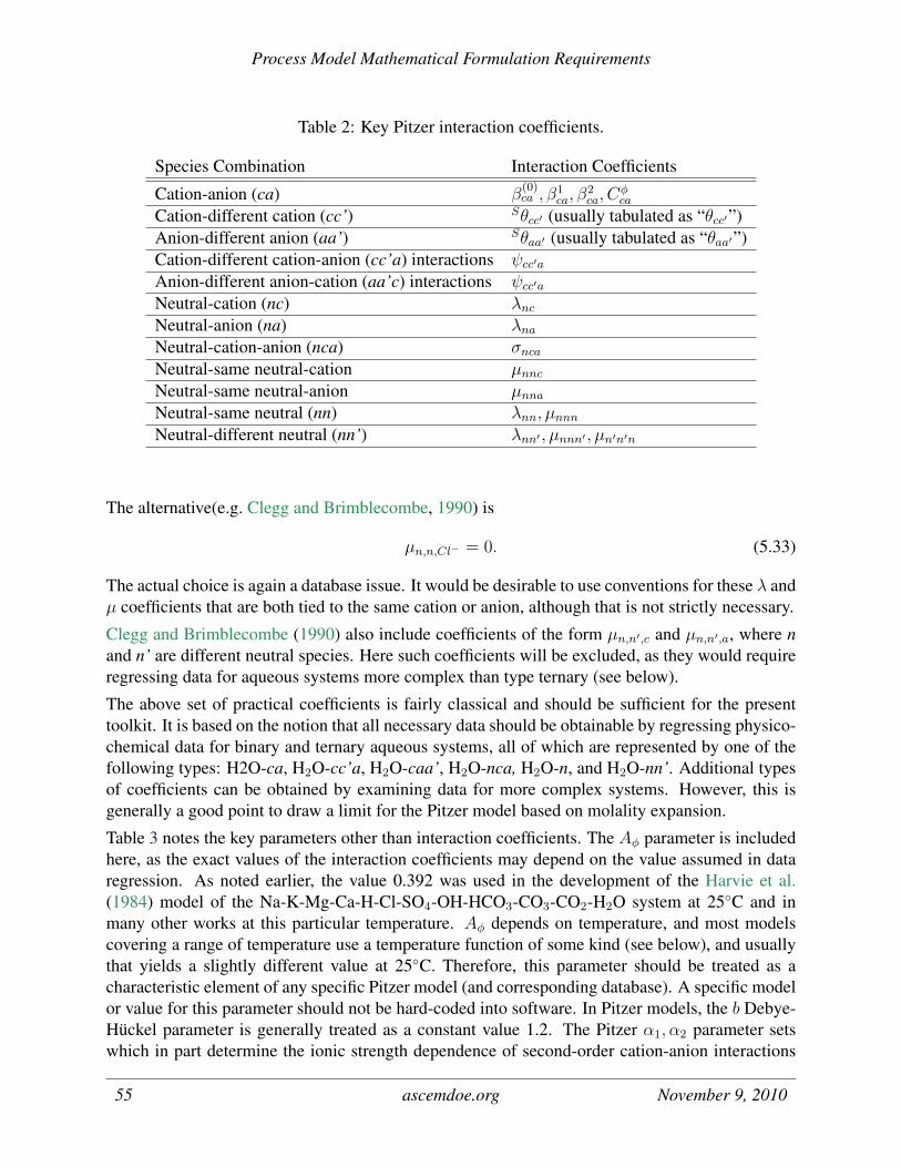
Process Model Mathematical Formulation Requirements
Table 2: Key Pitzer interaction coefficients.
Species Combination Interaction Coefficients
Cation-anion (ca) β(0)ca , β1
ca, β2ca, C
φca
Cation-different cation (cc’) Sθcc′ (usually tabulated as “θcc′”)Anion-different anion (aa’) Sθaa′ (usually tabulated as “θaa′”)Cation-different cation-anion (cc’a) interactions ψcc′aAnion-different anion-cation (aa’c) interactions ψcc′aNeutral-cation (nc) λncNeutral-anion (na) λnaNeutral-cation-anion (nca) σncaNeutral-same neutral-cation µnncNeutral-same neutral-anion µnnaNeutral-same neutral (nn) λnn, µnnnNeutral-different neutral (nn’) λnn′ , µnnn′ , µn′n′n
The alternative(e.g. Clegg and Brimblecombe, 1990) is
µn,n,Cl− = 0. (5.33)
The actual choice is again a database issue. It would be desirable to use conventions for these λ andµ coefficients that are both tied to the same cation or anion, although that is not strictly necessary.
Clegg and Brimblecombe (1990) also include coefficients of the form µn,n′,c and µn,n′,a, where nand n’ are different neutral species. Here such coefficients will be excluded, as they would requireregressing data for aqueous systems more complex than type ternary (see below).
The above set of practical coefficients is fairly classical and should be sufficient for the presenttoolkit. It is based on the notion that all necessary data should be obtainable by regressing physico-chemical data for binary and ternary aqueous systems, all of which are represented by one of thefollowing types: H2O-ca, H2O-cc’a, H2O-caa’, H2O-nca, H2O-n, and H2O-nn’. Additional typesof coefficients can be obtained by examining data for more complex systems. However, this isgenerally a good point to draw a limit for the Pitzer model based on molality expansion.
Table 3 notes the key parameters other than interaction coefficients. The Aφ parameter is includedhere, as the exact values of the interaction coefficients may depend on the value assumed in dataregression. As noted earlier, the value 0.392 was used in the development of the Harvie et al.(1984) model of the Na-K-Mg-Ca-H-Cl-SO4-OH-HCO3-CO3-CO2-H2O system at 25C and inmany other works at this particular temperature. Aφ depends on temperature, and most modelscovering a range of temperature use a temperature function of some kind (see below), and usuallythat yields a slightly different value at 25C. Therefore, this parameter should be treated as acharacteristic element of any specific Pitzer model (and corresponding database). A specific modelor value for this parameter should not be hard-coded into software. In Pitzer models, the b Debye-Huckel parameter is generally treated as a constant value 1.2. The Pitzer α1, α2 parameter setswhich in part determine the ionic strength dependence of second-order cation-anion interactions
55 ascemdoe.org November 9, 2010

Process Model Mathematical Formulation Requirements
Table 3: Key Pitzer parameters other than interaction coefficients.
Parameter Value(s)Aφ 0.392 for the Harvie et al. (1984) model at
25C and most models at that temperature;otherwise a function of temperature and pres-sure.
b Constant value of 1.2 in all significant knownPitzer models.
α1, α2 1.2, 0 for most cation-anion pairs;1.4, 12 for 2:2, 3:3, and 4:4 cation-anion pairsand sometimes other cation-anion pair types.Other values may be used in certain examplesof Pitzer models. Should be treated in thepresent toolkit as potentially unique to eachcation-anion pair.
(see below) are specific to cation-anion pairs. Here α1 is associated with β1ca and α2 is associated
with β2ca. Originally Pitzer (1973) assigned the values 1.2 and 0 (effectively zero, at least) for most
cation-anion pairs, and the value of α2is irrelevant in such instances as β2ca is not used (see below).
The values 1.4, 12 (and usage of β2ca) were recommended for 2:2 (charge of cation: -charge of
anion) pairs, and this was later extended to 3:3, 4:4, etc. Some Pitzer models assign other thanthese traditional values. The safest procedure is to define the values for each cation-anion pair ona supporting data file and use the traditional values (which are charge dependent) as defaults. Thisallows maximum flexibility.
The other key Pitzer parameters are interaction parameters of various types. In the developmentof the theory (Pitzer, 1973), there are second order coefficients (symbolized by λ), and third ordercoefficients, symbolized by µ.
The corresponding key equations for Pitzer’s equations (based on molality expansion) are givenbelow. Here M refers to a cation whose activity coefficient is to be calculated, X to such an anion,and N to such a neutral solute species.
ln γM = z2MF +
∑a
ma[2BMa + ZCMa] +∑c
mc
(2ΘMc +
∑a
maΨMca
)+∑
a′
∑a<a′
mama′ΨMaa′ + |zM |∑c
∑a
mcmaCca +
2∑n
mnλnM +∑n
∑a
mnmaσnMa + 3∑n
m2nµnnM ; (5.34)
56 ascemdoe.org November 9, 2010

Process Model Mathematical Formulation Requirements
ln γX = z2XF +
∑c
mc[2BcX + ZCcX ] +∑a
ma
(2ΘXa +
∑c
mcΨcXa
)+∑
c′
∑c<c′
mcmc′Ψcc′X + |zX |∑c
∑a
mcmaCca +
2∑n
mnλnX +∑n
∑c
mnmcσncX + 3∑n
m2nµnnX ; (5.35)
ln γN = 2∑c
mcλNc + 2∑a
maλNa +∑c
∑a
mcmaσNca +
6∑c
mNmcµNNc + 6∑a
mNmaµNNa +
2∑n6=N
mnλNn +mNλNN + 3∑n
m2nµNnn +
6∑n6=N
mNmnµNNn; (5.36)
(φ− 1)
(∑imi
2
)=
AφI32
1 + b√I
+∑c
∑a
mcma
(Bφca + ZCca
)+
∑c′
∑c<c′
mcmc′
(Θφcc′ +
∑a
maΨcc′a
)+
∑a′
∑a<a′
mama′
(Θφaa′ +
∑c
mcΨcaa′
)+∑
n
∑c
mnmcλnc +∑n
∑a
mnmaλna +∑n′
∑n<n′
mnmn′λnn′ +
1
2
∑n
m2nλnn +
∑n
m3nµnnn + 3
∑n′
∑n<n′
m2nmn′µnnn′ +
3∑n
∑c
m2nµnnc + 3
∑n
∑a
m2n;µnna (5.37)
ln aw = −(∑
imi
Ω
)φ; (5.38)
where
F = −Aφ
( √I
1 + b√I
+2
bln(1 + b
√I)
)+∑c
∑a
mcmaB′
ca,
+∑c′
∑c<c′
mcmc′Θ,cc′ +
∑a′
∑a<a′
mama′Θ,aa′ , (5.39)
57 ascemdoe.org November 9, 2010

Process Model Mathematical Formulation Requirements
Bca = β(0)ca + β(1)
ca g(α1
√I)
+ β(2)ca g
(α2
√I), (5.40)
B′
ca = β(1)ca
g(α1
√I)
I+ β(2)
ca
g(α2
√I)
I, (5.41)
g(x) = 2(1− (1 + x)e−x)
x2, (5.42)
g′(x) = −2
(1−
(1 + x+ x2
2
)e−x)
x2, (5.43)
Bφca = Bca + IB
′
ca
(= β(0)
ca + β(1)ca e
−α1
√I + β(2)
ca e−α2
√I), (5.44)
Z =∑i
mi |zi| , (5.45)
CMX =CφMX
2 |zMzX |12
, (5.46)
Θcc′ = SΘcc′ +EΘcc′ , (5.47)
Θaa′ = SΘaa′ +EΘaa′ , (5.48)
Θ′
cc′ = EΘ′
cc′ , (5.49)
Θ′
aa′ = EΘ′
aa′ , (5.50)
EΘcc′ =(zczc′
4I
)(J(xcc′)−
J(xcc)
2− J(xc′c′)
2
), (5.51)
EΘaa′ =(zaza′
4I
)(J(xaa′)−
J(xaa)
2− J(xa′a′)
2
), (5.52)
EΘ′
cc′ = −EΘcc′
I+(zczc′
8I2
)(xcc′J
′(xcc′)−xccJ
′(xcc)
2− xc′c′J
′(xc′c′)
2
), (5.53)
EΘ′
aa′ = −EΘaa′
I+(zaza′
8I2
)(xaa′J
′(xaa′)−xaaJ
′(xaa)
2− xa′a′J
′(xa′a′)
2
), (5.54)
xij = 6zizjAφ√I (ij can be cc′, cc, c′c′, aa′, aa, or a′a′), (5.55)
Θφcc′ = SΘcc′ +
EΘcc′ + IEΘ′
cc′ , (5.56)
Θφaa′ = SΘaa′ +
EΘaa′ + IEΘ′
aa′ . (5.57)
Harvie (1981) proposed a method of using two Chebyshev polynomial approximations to calculateJ(x) and J ′(x). One polynomial is used for Region I (x = 1) and the other for Region II (x >1).Table 4 contains the requisite coefficients. The equations are as follows:
58 ascemdoe.org November 9, 2010

Process Model Mathematical Formulation Requirements
Region I (x = 1):
z = x5 − 2,dz
dx=
4
5x−
45 ,
bk = zbk+1 − bk+2 + aIk, k = 0, . . . , 20,
dk = bk+1 + zdk+1 − dk+2, k = 0, . . . , 20;
Region II (x > 1):
z =40
9x−
110 − 22
9,
dz
dx= −40
90x−
1110 ,
bk = zbk+1 − bk+2 + aIIk , k = 0, 20,
dk = bk+1 + zdk+1 − dk+2, k = 0, 20.
The final equations are
J(x) =1
4x− 1 +
1
2(b0 − b2) , (5.58)
J ′(x) =1
4+
1
2
dz
dx(d0 − d2) . (5.59)
When temperature dependence is considered, the various Pitzer parameters are generally describedby empirical temperature functions. The recommended temperature function for the present toolkitis
A = a1 + a2
(1
T− 1
Tr
)+ a3 ln
(T
Tr
)+ a4 (T − Tr) + a5
(T 2 − T 2
r
). (5.60)
where A is the parameter to be calculated, a1 − a5 are the associated constants, T is the abso-lute temperature, and Tr is the reference temperature (298.15K). More elaborate forms are notrecommended. Also, it is preferred to use the term in temperature-squared only if the precedinigfour terms are inadequate. More recent work is likely to be consistent with the above form in thefirst four terms, although the terms might be in a different order. It is noted that the eight-termform proposed by Greenber and Moller (1989) is overly complex and contains singularities withrespect to temperature. When data are encountered in such a form, they should be recast into themore reasonable form given above. This has been done for example for the Greenber and Moller(1989) data in the Yucca Mountain Project Pitzer thermodynamic database (see Sandia NationalLaboratories, 2007, Appendix I).
59 ascemdoe.org November 9, 2010

Process Model Mathematical Formulation Requirements
Table 4: Chebyshev polynomial coefficients for computing J(x) and J ′(x) (Harvie, 1981)
k aIk aIIk0 1.92515 40148 14667 0.62802 33205 208521 -0.06007 64777 53119 0.46276 29853 384932 -0.02977 90774 56514 0.15004 46371 878953 -0.00729 94996 90937 -0.02879 60576 049064 0.00038 82606 36404 -0.03655 27459 103115 0.00063 68745 99598 -0.00166 80879 452726 0.00003 65836 01823 0.00651 98403 987447 -0.00004 50369 75204 0.00113 03780 790868 -0.00000 45378 95710 -0.00088 71713 101319 0.00000 29377 06971 -0.00024 21076 41309
10 0.00000 03965 66462 0.00008 72944 5159411 -0.00000 02020 99617 0.00003 46821 2275112 -0.00000 00252 67769 -0.00000 45837 6893813 0.00000 00135 22610 -0.00000 35486 8430614 0.00000 00012 29405 -0.00000 02504 5388015 -0.00000 00008 21969 0.00000 02169 9177916 -0.00000 00000 50847 0.00000 00807 7957017 0.00000 00000 46333 0.00000 00045 5855518 0.00000 00000 01943 -0.00000 00069 4475719 -0.00000 00000 02563 -0.00000 00028 4925720 -0.00000 00000 10991 0.00000 00002 37816
60 ascemdoe.org November 9, 2010

Process Model Mathematical Formulation Requirements
5.2.6 Extended UNIQUAC
The Extended UNIQUAC model is another high ionic strength model. It differs from the Pitzermodel in various ways, but the most striking is the elimination of triplet interaction parameters andthe appearance of a small number of “singlet” parameters in addition to the charge number. Thesedifferences result in a striking reduction in the number of parameters required to model a systemcontaining a large number of solute species. Extended UNIQUAC is fundamentally based on molefractions. Molal activity coefficients for the solute species are therefore derived the mole fractioncounterparts. Also, water (the solvent) is considered in the relevant pair interactions.
There are presently multiple “flavors” of Extended UNIQUAC. The one that will be addressedhere is based on Thomsen (1997, 2005) and various other papers, of which Thomsen is usually aco-author. The reason for this choice is that this particular flavor has been openly developed tocover a wide range of useful components, while others are less extensively developed or are atleast in significant part proprietary. The original model covers the system containing the solutespecies Na+, K+, NH+
4 , H+, Cl−, NO−3 , SO2−4 , HSO−4 , OH−, CO2−
3 , HCO−3 , and S2O2−8 from
25 to about 110C. The number of chemical species treated has been significantly extended insubsequent development. Thomsen (2005) provides the preferred overview of the model, whileThomsen (1997) provides more detail. This model has been incorporated into an as yet unreleasedversion of EQ3/6 (and a corresponding supporting thermodynamic data file exists).
The effectiveness of the Extended UNIQUAC model is comparable to the molality-based Pitzermodel described above. It may have an advantage at smaller mole fractions of water, as it thisis a mole fraction-based model. It is notably weaker at elevated temperature, due to the sim-ple temperature dependence currently applied to the pair interaction parameters, as noted below.That weakness could be easily remedied, however. The Extended UNIQUAC model is becomingincreasing popular since, compared with the Pitzer’s model (in either molality- or mole fraction-based form), it produces comparably good results with fewer parameters that need to be fitted toexperimental data.
The model utilizes the following singlet parameters: ri and qi (“volume” and “surface area” pa-rameters, respectively). These are treated as constant in regard to temperature. The model alsouses the uki pair interaction parameter, which is treated as a function of temperature:
uki = u0ki + utki(T − Tr), (5.61)
where T is the absolute temperature and Tr is the reference temperature (298.15K). Here both kand i span the range of component species, including solvent water. The combination in which kand i are equal is included. For example, the pair combination H2O − H2O is included. The ucoefficients are symmetrical (ukl = ulk). The linear representation of temperature dependence isprobably a limiting factor in regard to the temperature range of the model. A three-parameter formwould likely be required to significantly extend the temperature range.
The ri and qi are used to calculate the following quantities:
φi =xiri∑l xlrl
, (the “volume fraction”); (5.62)
θi =xiqi∑l xlql
, (the “surface area fraction”). (5.63)
61 ascemdoe.org November 9, 2010

Process Model Mathematical Formulation Requirements
In the above equations, l spans all component species (including solvent water). Here x denotesmole fraction. Note that for a solute species, the mole fraction is given by
xi =mi
Ω +∑
jmj
, (5.64)
where j spans only the solute species. For solvent water (w), the mole fraction is given by
xw =Ω
Ω +∑
jmj
. (5.65)
The uki pair interaction parameter is used to calculate
ψki = exp(−uki − uiiT
). (5.66)
Note that symmetry does not apply to this parameter (ψik does not necessarily equal ψki, becauseuii does not necessarily equal ukk).
The Extended UNIQUAC theory first addresses mole fraction (or “rational”) activity coefficients,symbolized here by f (by λ in earlier discussion). These are calculated by first obtaining char-acteristic parts. In UNIQUAC theory, these include the “combinatorial” (C) or entropic part and“residual” (R) or enthalpic part. For the mole fraction activity coefficient these parts are respec-tively given by
ln fCi = ln
(φixi
)+ 1− φi
xi− z
2qi
[ln
(φiθi
)+ 1− φi
θi
], (5.67)
ln fRi = qi
[1− ln
(∑k
θkψki
)−∑k
θkψik∑l θlψlk
], (5.68)
where i spans all component species. Here z in the combinatorial part is the coordination number,assigned a value of 10.
The corresponding infinite dilution terms are obtained by setting xw = 1:
ln f∞,Ci = ln
(rirw
)+ 1− ri
rw− z
2qi
[ln
(riqwrwqi
)+ 1− riqw
rwqi
], (5.69)
ln f∞,Ri = qi [1− lnψwi − ψwi] . (5.70)
These infinite dilution terms are only pertinent to the solute species. They are required to obtainthe mole fraction activity coefficients for solute species for an infinite dilution reference (fi = 1 atinfinite dilution, instead of at xi = 1).
The desired mole fraction activity coefficients are obtained by combining the combinatorial andresidual parts with a Debye-Huckel part, which is based on the Debye-Huckel-charging model .
The activity coefficient of water is then given by
ln fw = ln fCw + ln fRw +1
Ω
(2Aγ,eb3
σ(b√I)
), (5.71)
62 ascemdoe.org November 9, 2010

Process Model Mathematical Formulation Requirements
where b is assigned the familiar value of 1.5. Since fwis the same as λw, the activity of water canbe obtained from
ln aw = lnxw + ln fw. (5.72)
The osmotic coefficient, if desired, can be obtained from the activity of water using the relationgiven in previous sections.
The mole fraction activity coefficient of a solute species is given by
ln fi = −Aγ,ez2i
√I
1 + b√I
+ ln fCi − ln f∞,Ci + ln fRi − ln f∞,Ri . (5.73)
Here Aγ,e = ln (10)Aγ,10. The molal activity coefficient of a solute species can then be obtainedusing
ln γi = ln fi + lnxw. (5.74)
63 ascemdoe.org November 9, 2010

Process Model Mathematical Formulation Requirements
5.2.7 NEA SIT
The NEA SIT model is a “Specfic Interactions Theory” model adopted by the European NuclearEnergy Agency (NEA) for use in its international program to develop thermodynamic data sets formostly radionuclide elements of concern to geologic disposal of high level nuclear waste. The termspecific interactions theory is generically used to describe theories in which the activity coefficientspertinent to aqueous solutions have a general dependence on specific solution composition. Inparticular, it is recognized that the ionic strength is insufficient to fully describe this dependence.Recall that Pitzer’s equations also represent a “specific interaction theory.” Therefore, the presentmodel, often referred to as just “SIT,” will here be referred to as “NEA SIT” to avoid potentialconfusion.
The NEA SIT model was basically adopted to provide activity coefficient corrections to measureddata, so as to yield true equilibrium constants (mostly complexation constants). The model inthe modern context traces to Grenthe et al. (1992), who used it in a study of the thermodynamicproperties of aqueous, solid, and gas uranium-bearing species. The model was described in theirAppendix B, “Ionic strength corrections”. The model has been more recently discussed by Grentheet al. (1997), whose title more appropriately includes “medium effects.” They also introducedsome minor modification in regard to the treatment of neutral aqueous species.
The NEA SIT model has been further developed in other volumes in the NEA “Chemical Thermo-dynamics” series (the uranium volume was the first in the series). Although there has always beena strong focus on species pertinent to radionuclide species, it was recognized from the start thatanalyzing data pertinent to aqueous media would require extending the model to include necessaryspecies that would be part of the media. These “auxiliary data” include extension of the NEA SITmodel to handle pertinent non-radionuclide species.
Although there has been great interest in and usage of the standard state thermodynamic data pro-duced by the NEA project, there has been less implementation of the NEA SIT activity coefficientmodel in pertinent modeling codes and applications. There has thus far been little testing of theability of the NEA SIT model to handle systems of geochemical interest, which would provide astronger test of the adequacy of the model, in particular regard to the adequacy of the auxiliarydata. This situation may be changing, as it has recently been announced that NEA SIT has beenadded as an option to the modeling code PHREEQC.
The origins of the NEA SIT theory basically go back to Guggenheim (1935), although the presentmodel includes some modifications, mostly tracing to Ciavatta (1980). A helpful way to lookat the model is to compare it with Pitzer’s equations. Basically, the equations are like Pitzer’sequations, except that third-order interactions are excluded. NEA SIT uses a form of the Debye-Huckel-charging model instead of Pitzer’s Debye-Huckel-osmotic model for the Debye-Huckel-term. The second order interactions are treated as a function of ionic strength, somewhat similarto the treatment in Pitzer’s equations. This treatment distinguishes the NEA SIT model from theGuggenheim (1935) model, which did not include such ionic strength dependence.
The relevant equations are
log10 γj =−z2
jAγ,10
√I
1 + 1.5√I
+∑k
εjkmk, (5.75)
64 ascemdoe.org November 9, 2010

Process Model Mathematical Formulation Requirements
where εjk is a second-order interaction coefficient. This is treated in the general case as a functionof ionic strength as previously recommended by Ciavatta (1980):
εjk = ε1,jk + ε2,jk log10 I. (5.76)
In many instances, however, it may simply be treated as a constant (e.g., εjk = ε1,jk).
It is assumed (Grenthe et al., 1992, p. 686, Assumption 2) that there are no pair-wise interactionsamong ions of the same charge sign and for uncharged species. More simply put, the only non-zero interactions are for cation-anion combinations. Grenthe et al. (1997) removed the restrictionregarding uncharged species, but appear to have considered only ion-neutral interactions.
There are difficulties with the Ciavatta (1980) representation of the ionic strength dependence ofthe second-order interaction coefficient. The magnitude of the term in log10 I approaches infinityas I approaches zero. Note that
ε′
jk =∂εjk∂I
=ε2,jk
ln(10)I. (5.77)
The derivative becomes singular as I approaches zero Also, although εjk at first seems to be theanalogue of the Pitzer λij (differing by a factor of two, with jk substituting for ij), it really isn’t.This can be seen by comparing the NEA SIT equation for the solute activity coefficient with thatfor Pitzer’s equations. The NEA SIT equation lacks a term containing ε′jkanalogous to the term inλ′
ijappearing in the Pitzer equation (and which is second order in molality). One should therefore
expect that the NEA SIT equation 1) may not satisfy the thermodynamic consistency relations, and2) may be at best only quasi-consistent with a corresponding equation for the activity of water.Grenthe et al. (1997) reviewed similarities and differences between the NEA SIT equations andPitzer’s equations but unfortunately did not address the consistency issue in the former. This issuewill be addressed further later in this section.
The omission of treatment of third-order interactions and the restriction of the treatment of second-order interactions to cation-anion cases only provides for a much simplified model. However, itis likely to also restrict the range of accuracy (as may the suspected consistency problem notedabove). Indeed, the model is only intended for application in a moderate range of ionic strength.Grenthe et al. (1992, p. 685) note that the use of the 1.5 value in the denominator of the Debye-Huckel term was found by Ciavatta (1980) to provide useful fits in the ionic strength range 0.5-3.5mand note its correlation to regressed values of second-order interaction coefficients. The actualapplication of the NEA SIT model in the NEA “Chemical Thermodynamics” series is generallyfor maximum ionic strengths in the 1-2 molal range. In the absence of additional testing, an upperlimit of ionic strength for using this model would appear to be something like 2-4 molal. This issufficient to be useful for many applications, but clearly falls short of what can be done using amodel based on Pitzer’s equations or Extended UNIQUAC.
Grenthe et al. (1992, Table B.1, p. 685) recommend using the values of Helgeson et al. (1981) forthe Aγ,10 parameter, which they simply refer to as A. They note its temperature dependence, but donot recommend a specific means of describing this.
Grenthe et al. (1992) do not present a general equation for the activity of water. Their primaryrecommendation is to calculate the activity of water from the osmotic coefficient, using data tablesfor pure aqueous electrolytes and electrolyte mixtures that correspond to the relevant electrolytemedia. They do suggest (p. 688, equation B.12) a formulation that is specific to a pure electrolyte
65 ascemdoe.org November 9, 2010

Process Model Mathematical Formulation Requirements
solution. This does not specifically address the consistency problem that may arise if the interactioncoefficient is dependent on ionic strength, and the derivative of this coefficient is ignored.
If one tests the activity coefficient equation for self-consistency using the relation
∂ ln γj∂mi
=∂ ln γi∂mj
, (5.78)
one obtains, after making appropriate substitutions and simplification, that the following residualwould have to be satisified: (∑
k
mkε2,jk
)z2i
2=
(∑k
mk′ε2,ik
)z2j
2. (5.79)
This is not likely to be the case unless ions i and j have the same magnitude of charge numberand the two summations happen to be equal. The summations are likely to be equal only underrestricted circumstances. For example, if i and j are both cations and k spans the anions (ignoringneutral species) , then ε2, would have to have the same value for all cation-anion pairs. Otherassumptions about i and j lead to the same result (or similar results if neutral species are con-sidered). This problem vanishes if the total interaction coefficients are treated as constants (e.g.,εjk = ε1,ik, ε2,ik = 0 ).
The following approximation for the activity of water is recommended for the present toolkit whenusing the NEA SIT model:
log aw =1
Ω
(−∑
imi
ln(10)+
2
3Aγ,10I
32σ(1.5
√I)−
∑jk
εjkmjmk
). (5.80)
This is only a quasi-consistent form due to the points noted above.
The NEA SIT model does not seem to have a specific recommended form for the temperaturedependence of the coefficients ε1 and ε2. This is apparently because the model is mainly developedfor 25C. Grenthe et al. (1992) largely avoid the issue. Grenthe et al. (1997) give a detaileddiscussion of thermodynamic properties related to elevated temperature and pressure. However,they give no generally useful form for a practical treatment of the temperature dependence. To usetheir equations, one would need tabulated values of various derivative properties, which are onlyavailable for a relatively small number of species. Therefore, in practice, this model is restricted to25C until someone does further development.
66 ascemdoe.org November 9, 2010

Process Model Mathematical Formulation Requirements
5.2.8 Rescaling Ionic Activity Coefficients
The activity coefficient models described above include descriptions of individual ion activitycoefficients. This is problematic in that ionic activity coefficients and ionic activities are notmeasurable for individual ions. These quantities are measurable only in combinations that cor-respond to electrical neutrality. For activity coefficients, examples of such combinations includelog γH+ + log γCl− and 2 log γH+ + log γSO2−
4; examples for activities are analogous. Molalities of
individual ions are measureable (or quantifiable by inference). Thus, if one could obtain or specifythe activity or activity coefficient of one single ion in an aqueous solution, one could then use thisas a reference to obtain the activities and activity coefficients of all other ions present in the samesolution.
The need to define activity coefficients and activities for individual ionic species is dealt with by theuse of a “splitting” convention. Such a convention is at least somewhat arbitrary, although it may beguided in part by theoretical concerns. One could address the issue by adopting the results of modelequations for single ion activity coefficients. The model equations for these are all in part arbitrary,implicitly including a splitting based on some combination of theoretical notions and pleasing(but not necessarily unique) symmetry. The problem with just using the model equations in theirnative form is that other conventions have been previously adopted into measurement practice,particularly the measurement of pH. For accurate modeling consistent with standard analyticalchemistry practice, it becomes necessary to rescale the results of the model equations presentedabove. This only affects the activity coefficients of ionic species. For most analytical splittingconventions, some expression is specified for the activity coefficient of a reference ion, usuallyCl− or H+.
The most significant analytical splitting conventions for aqueous ions are tied to the definition ofthe pH. Conceptually,
pH = − log aH+ . (5.81)
In order to provide a practical basis for measuring the pH, it is necessary to define the activity ofthe hydrogen ion. The splitting convention used for this purpose then defines a pH scale. Thechoice of pH scale further affects the definition of the redox potential, Eh.
In modern work, the dominant pH scale is the NBS scale, originated by the National Bureau ofStandards, now the National Institute of Standards and Technology. The NBS scale is based on theBates-Guggenhiem equation (Bates, 1964):
log γCl− = − Aγ,10
√I
1 + 1.5√I. (5.82)
This is a simple form of the extended Debye-Huckel equation. It defines the activity coefficientof the chloride ion. It may be surprising that chloride is used as the reference ion rather than thehydrogen ion, which is more closely tied to the pH. What is apparent is that the Bates-Guggenheimequation must give a result that is different from what would be obtained for the chloride ion usingsay the Davies equation or the B-dot equation, or for that matter, from Pitzer’s equations. In therange of low ionic strength (say less than 1 molal), the differences should be numerically small foreach of the three practical models, as they and the Bates-Guggenheim equation all include someform of extended Debye-Huckel model and thus are all consistent with the Debye-Huckel limiting
67 ascemdoe.org November 9, 2010

Process Model Mathematical Formulation Requirements
law. At higher ionic strength, however, the differences can be substantial (the equivalent of severalpH units).
The Bates-Guggenheim equation can be applied whether or not there is any chloride in aqueoussolution, as the equation is sufficient to calculate the specified activity coefficient. The chargenumber of -1 is effectively built into the equation.
The Bates-Guggenheim equation (the NBS pH scale) is effectively built in to the calibration of allmodern means of measuring the pH, whether in pH calibration buffers or pH paper. EQ3/6 forexample by default rescales ionic activity coefficients computed from the models to be consistentwith the NBS pH scale (other options, including no rescaling, may be offered). Rescaling fromone scale (scale “1”) to another (scale “2”) is accomplished using
log γ(2)i = log γ
(1)i +
zizj
(log γ
(2)j − log γ
(1)j
). (5.83)
Here j denotes the reference ion (here Cl−) and i denotes any ion (including the reference ion).In the present context, scale “1” is usually that implied by a model equation and scale “2” is thedesired scale.
An alternative convention is to choose
log γH+ = 0. (5.84)
For the hydrogen ion, this results in
pH = − logmH+ . (5.85)
as the activity and molality of the hydrogen ion are numerically equivalent. The rescaling of ionicactivity coefficients for consistency does not give an analogous result for other ions. EQ3/6 allowsrescaling using this convention as an option, but it has limited utility and it not recommended as ageneral option in the present toolset.
The definition of the pH in terms of molality (“pmH”) is significant independent of rescaling. Thusone has simply
pmH = − logmH+ . (5.86)
In concentrated electrolyte solutions (e.g., WIPP, Hanford tanks), pmH is often more useful forassessing the acidity/basicity of a solution than the NBS pH. The NBS pH cannot be accuratelymeasured in concentrated solutions owing to liquid junction effects with electrodes and interfer-ences with dyes. Also, the Bates-Guggenheim equation (and the NBS pH scale itself) was origi-nally intended for use only at low ionic strength. Bates (1964) suggested application to solutionswith ionic strengths of no greater than 0.1 molal. Since then, however, the scale has been used athigher ionic strengths. This has led to the problem that of two highly concentrated solutions withan NBS pH of say 2, one might be acidic (in the sense that H+ is abundant) and the other not (in thesense that H+ is not abundant). In other words, the common association of pH values with variousdegrees of acidity/basicity (e.g., 7 is neutral) no longer applies.
Still other conventions and scales exist. However, for the present toolset only the following isrequired. First, the default behavior will be to apply rescaling to the NBS scale. Second, the option
68 ascemdoe.org November 9, 2010

Process Model Mathematical Formulation Requirements
will be available to use the basic model results without rescaling. Third, the pmH will be directlycalculated and included in the output. An option to rescale the activity coefficients for consistencywith the log γH+ = 0 convention will not be required.
5.3 Sorption
5.3.1 Overview
Sorption involves the attachment of dissolved and/or colloidal species to mineral or other solidsurfaces. Sorption has the effect of slowing the effective transport rate of a species through porousmedia through its retardation effect. The retardation effect for a species, Rf , is given by (Bouwer,1991)
Rf =VgwVsp
, (5.87)
where Vgw is the velocity of the groundwater and Vsp is the velocity of the species. A variety ofmodels have been used to describe sorption and can be broadly divided into those that describe itas a bulk process versus those that are mineral or solid phase specific. The latter approach involvesthe calculation of bulk sorption from the sum of sorption on individual solid phases, an assumptionreferred to as Component Additivity. Within the class of bulk sorption models, a distinction canbe made between those which assume a finite number of sorption sites (these are referred to asshowing Langmuir type behavior and include the Langmuir isotherm itself and most surface com-plexation and ion exchange models) and those that assume either an infinite sorption capacity or atleast a capacity that is not tightly constrained (these include the linear distribution coefficient andthe nonlinear Freundlich isotherm). Alternatively, one could also distinguish between single com-ponent, non-competitive models (e.g., Langmuir and Freundlich) and multicomponent competitivemodels (surface complexation and ion exchange).
Another possible distinction is between equilibrium and kinetic sorption models. In many cases,the formulations for the equilibrium and kinetic cases differ only insofar as the kinetic case involvesinvolves a thermodynamic driving force (as in the equilibrium case), but modified by a finite rateconstant. In some cases, however, sorption is described as irreversible, which implies that there isno back reaction (desorption).
5.3.2 Process Model Equations
Linear Distribution Coefficients (Kd). A simple approach to describe metal or ionic radionu-clide sorption by a sediment,
Aaq Aads, (5.88)
is to use a constant distribution coefficient, defined by:
Kd =[Aads]
[Aaq], (5.89)
where Kd is the distribution coefficient (L/kg), [Aads] is the sorbed concentration (mol/kg) to thebulk solid phase, and [Aaq] is the total dissolved concentration in groundwater (mol/L) (Davis and
69 ascemdoe.org November 9, 2010

Process Model Mathematical Formulation Requirements
Kent, 1990). One of the key advantages of representing sorption with a distribution coefficient isthat it can be easily incorporated into reactive transport models used for migration predictions.
Equation (5.89) shows that if one assumes that the amount of sorption is proportional to the dis-solved concentration, then there is a linear relationship where the Kd value is the slope. In thissimple case, referred to as a linear isotherm, retardation of a concentration front in simple porousmedia is given by
v
vc= 1 +
ρbnKd, (5.90)
where ρb is the bulk density, n the porosity, v the average linear velocity of the groundwater andvc the velocity of the point on the concentration profile where the concentration is half that of theinput concentration (Freeze and Cherry, 1979). Note that the ratio v/vc here is the retardation factorand represents the retardation of the movement of front relative to the flowing groundwater. Whilethis is a simplified example, it serves to illustrate the key point that theKd value directly influencespredictions of adsorbing metal or radionuclide mobility.
Assumptions and Applicability Sorption is proportional to the dissolved concentration. Theaqueous and adsorbed phases are in equilibrium.
Data Needs Typically Kd values are determined for a particular subsurface material from theslope of a fitted line to the concentration of the sorbed species, Aads, plotted versus the dissolvedconcentration of the same species,Aaq. These data may be derived from laboratory analyses, whereone typically varies the dissolved concentrations systematically, or they may be derived from insitu field data. Since Kd values may be variable, and in particular a function of temperature, pH orthe redox state of the system (see below), it is often necessary to compile them in a lookup tablefor use by a particular computer code.
Langmuir Isotherm. The Langmuir isotherm assumes that the sorption sites, S, on the surfaceof a solid (absorbent) become occupied by an absorbate from the solution, A. Implying a 1:1stoichiometry
S + A SA, (5.91)
where SA is the adsorbed species on the surface. At equilibrium, a standard mass action equationcan be written:
Kads,L =[SA]
[S]A, (5.92)
where the square brackets here refer to the concentration of the species or site, and the curlybrackets refer to the aqueous activity. Using the maximum concentration of surface sites, ST
[ST ] = [S] + [SA], (5.93)
70 ascemdoe.org November 9, 2010

Process Model Mathematical Formulation Requirements
one can write the Langmuir isotherm in its familiar hyperbolic form
[SA] = [ST ]KadsA
1 +KadsA. (5.94)
Assumptions For the following, it is assumed that the surface and aqueous species are in equi-librium.
Data Needs The equilbrium constant, Kads, is typically obtained from experimental data. Itdepends on the specified absorbent and absorbate, and may be a function of temperature. It maybe calculated from:
Kads = exp
(−∆GadsRT
), (5.95)
where ∆G is the change in free energy for the reaction, typically obtained from a database, R isthe gas constant and T is the temperature.
Freundlich. The Freundlich isotherm is another equilibrium model for sorption of absorabte Aonto sorption sites, S.
S + A SA. (5.96)
Represented by the mass action equation:
Kads,F =[SA]
AβF, (5.97)
where the square brackets again refer to the concentration of the species or site, the curly bracketsrefer to the aqueous activity. Kads,F and βF are the Freundlich parameters (e.g. Langmuir, 1997;Stumm, 1992).
Assumptions For the following, it is assumed that the surface and aqueous species are in equi-librium.
Data Needs The Freundlich parameters, Kads,F and n, are generally obtained by fits to exper-imental data for a specific surface and aqueous species. They will generally be obtained from adatabase, and may be represented by a functional form or lookup table.
Multi-site, Multi-component Ion Exchange. An ion exchange reaction can be described via amass action expression with an associated equilibrium constant (Appelo and Postma, 1993; Spositoand Sparks, 1981; Vanselow, 1932). The exchange reaction can be written in generic form as
vAClu(aq) + uBXν(s) uBClν(aq) + vAXu(s), (5.98)
71 ascemdoe.org November 9, 2010

Process Model Mathematical Formulation Requirements
where X refers to the exchange site occupied by the cations Au+ and Bv+. The equilibrium con-stant, Keq, for this reaction can be written as (Vanselow, 1932)
Keq =BClνuAXuν
ACluνBXνu, (5.99)
where the curly braces refer to the thermodynamic activities. Several activity conventions are inwide use. One possibility is the Gaines-Thomas activity convention, which assumes a reactionstoichiometry of the following form (Appelo and Postma, 1993), written here assuming the Cs+ isthe relevant cation of interest
Cs+ + (1/z)MX(i)z CsX(i) + (1/z)M z+, (5.100)
where M is the competing cation (Na+, K+, Ca++), z is its charge, and X(i) refers to the ith typeof exchange site. In the Gaines-Thomas convention, each exchange site, X(i) has a charge of -1.The activities of adsorbed species correspond to the charge equivalent fractions, β(i)M ,
β(i)M =zMq(i)M∑M zMq(i)M
= X(i)M, (5.101)
where zM is the charge of cation M , q(i)M is the concentration of adsorbed cation M in exchangesite i (moles/g), and the curly brackets denote activities. The Gapon activity convention is obtainedby writing the reactions in every case with a single exchanger (Appelo and Postma, 1993). Alter-natively, the Vanselow convention (Vanselow, 1932) describes the exchanger activity with molefractions
β(i)M =q(i)M∑M q(i)M
= X(i)M. (5.102)
The exchange reactions can then be used to write a mass action equation for binary Cs-M exchange:
KM/Cs =β(i)
1/zM Cs+
β(i)CsM z+1/z(5.103)
=X(i)M1/zCs+X(i)CsM z+1/z
. (5.104)
In a single-site ion exchange model, the CEC is equal to the sum of the charge equivalent concen-trations of the adsorbed cations:
CEC =∑M
zMqM , (5.105)
while in a multi-site model, the CEC is the charge summed over all of the cation exchange sites(Cernik et al., 1996; Voegelin et al., 2000)
CEC =∑i
∑M
zMq(i)M . (5.106)
Assumptions For the following, it is assumed that the surface and aqueous species are in equi-librium.
72 ascemdoe.org November 9, 2010

Process Model Mathematical Formulation Requirements
Surface Complexation. An alternative approach that allows a modeler to describe sorption whilesimultaneously considering variable chemical conditions in the subsurface is a surface complexa-tion model (Davis et al., 2004). In this approach, the sorbing sediment surfaces are considered topossess surface functional groups that can form complexes analogous to the formation of aqueouscomplexes in solution. These surface reactions include proton exchange, cation binding and anionbinding via ligand exchange at surface hydroxil sites (represented here asXOH to avoid confusionwith other chemical species). For example, the sorption of a metal could be represented as
XOH +M z+ XOM z+−1 +H+. (5.107)
At equilibrium, the sorption reactions can be described by the mass law equation
Kapp =[XOM z+−1] H+
[XOH] M z+, (5.108)
where Kapp is referred to as the apparent equilibrium constant, because it includes surface chargeeffects and hence is dependent on the extent of surface ionization (Dzombak and Morel, 1990), iis the thermodynamic activity of aqueous species i, and the terms in square brackets represent theconcentration of surface complexes (mol/kg).
Surface complexation differs from the simpler isotherm and ion-exchange models in several impor-tant ways. Surface complexation is based on the electrical double layer (EDL) theory. EDL theoryassumes that the surface charge of a sorbent in contact with solution generates an electrostaticpotential that declines rapidly away from the sorbent surface, creating an electrostatic field. Anadditional energetic term accounting for the work needed for the aqueous species to travel acrossthe surface electric field is required:
∆Gads = ∆Gintr + ∆Gcoul
= ∆Gintr + (∆Gψ=0 −∆Gψ=ψ0)
= ∆Gintr − zFψ0. (5.109)
where ∆Gads is the free energy change of the overall adsorption reaction, ∆Gintr and ∆Gcoul
are the free energy change due to chemical bonding and to the electrostatic work (Coulombicattraction), respectively, z is the charge of the surface species, F the Faraday’s constant (96485C/mol), and ψ0 is the mean surface potential (V ). Since
∆G = −RTlnK, (5.110)
Equation (5.109) can be rewritten as
Kapp = Kint exp
(zFψ0
RT
), (5.111)
where R is the gas constant (8.314 J/mol/K), T is the absolute temperature (K), and Kint is theintrinsic equilibrium constant which does not depend on the surface charge.
73 ascemdoe.org November 9, 2010

Process Model Mathematical Formulation Requirements
Bulk and Mineral Specific Surface Complexation. There are two major approaches for apply-ing the surface complexation concept to soils and sediments: the Component Additivity (CA) andGeneralized Composite (GC) approaches (Davis et al., 1998, 2004). In the CA approach, it is as-sumed that a mineral assemblage is composed of a mixture of one or more reference phases, whosesurface chemical reactions are known from independent studies of each phase (e.g. Arnold et al.,2001; Davis et al., 2004; Landry et al., 2009). Based on a measurement of the relative amounts orsurface areas of each mineral present in the soil or sediment, sorption by the mixture of phases canbe predicted by an equilibrium calculation, without any fitting of experimental data for the mixture.CA model predictions are sometimes made by assuming that one mineral component dominatessorption (Barnett et al., 2002; Davis et al., 2004; Payne et al., 2004; Zhang et al., 2009), allowing astraightforward equilibrium calculation, if the exposed surface area of that mineral component inthe soil or sediment can be quantified.
In the GC approach, the surface of the mineral assemblage is considered too complex to be quan-tified in terms of the contributions of individual phases to sorption and/or that the contribution ofindividual components is not additive. The complexity is caused, in part, by the difficulties inquantifying the electrical field and proportions of surface functional groups at the mineral-waterinterface in the mixture of mineral phases and associated surface coatings. In the GC approach, itis assumed that sorption can be described by mass laws written with “generic” surface functionalgroups, with the stoichiometry and formation constants for each mass law determined by fitting ex-perimental data for the mineral assemblage as a whole (Bond et al., 2008; Davis et al., 2004; Hyunet al., 2009). The GC modeling approach has generally been applied using a non-electrostaticmodel (NEM), which considers surface equilibria strictly as chemical reactions without explicitcorrection for electrostatic attraction or repulsion (Davis et al., 2004; Kent et al., 2000; Yabusakiet al., 2008). In an NEM, the apparent binding constants and stoichiometry of the mass actionequations are derived by fitting the macroscopic dependence of adsorption as a function of pH(Davis et al., 1998). Because of the exclusion of electrical double layer terms, the mass actionequations are not expected to provide accurate representations of the stoichiometry of the reac-tions at the molecular scale, however, the surface reactions can still be coupled with aqueouscomplexation reactions to provide simulations of macroscopic sorption as a function of aqueouschemical conditions.
Although there are differences between the GC and CA approaches, they are very similar withrespect to their scientific basis. The following concepts form the basic tenets of both GC and CAmodelling approaches (Davis et al., 1998):
1. Mineral surfaces are composed of chemical functional groups that can react with dissolvedsolutes to form surface complexes (coordinated complexes or ion pairs) in a manner analo-gous to aqueous complexation reactions in homogeneous solutions.
2. The equilibria of surface complexation and ionization reactions can be described via masslaw equations, either with or without correction factors applied for electrostatic attraction toor repulsion from the surface.
3. The apparent binding constants determined for the mass law equations of surface complex-ation and ionization reactions are semi-empirical parameters related to thermodynamic con-stants via rational activity coefficients for surface species.
74 ascemdoe.org November 9, 2010

Process Model Mathematical Formulation Requirements
Both CA and GC models may:
1. be coupled to the same critically reviewed aqueous thermodynamic data
2. use spectroscopic data to constrain and/or determine surface complex chemical compositionand stoichiometry, and
3. use the same mass laws and surface species.
The differences among the model approaches lie primarily in the manner in which the models arecalibrated and assumptions about various model parameters (in particular, whether the contribu-tions of the various mineral phases to sorption and electrostatic fields can be considered as addi-tive). CA models have almost always been applied using mass laws with electrostatic correctionfactors, while GC models have not usually used these factors.
Experimental and Modeling Issues Associated with SCMs for Soils and Sediments. Com-mon to all applications of surface complexation approaches in soils and sediments is an initialcharacterization with respect to surface area, bulk mineralogy, and clay and organic carbon content.In addition, if the sediment is already contaminated with a metal or radionuclide, a measurementof the labile fraction of the contaminant needs to be determined (Bond et al., 2008; Curtis et al.,2004; Kohler et al., 2004).
In the GC approach, laboratory experiments are conducted with the field site sediments acrossthe range of chemical conditions that are relevant to the scenarios of the physical and temporalmodeling domains. Then, mass law relationships are derived that describe the change in metal orradionuclide sorption with variations in the aqueous chemical conditions (Davis et al., 2004). Totalsurface functional groups are typically estimated from surface area measurements. The number ofsurface site types and surface binding reactions is a practical modeling decision made based on thegoodness-of-fit and the desired number of modeling parameters (Hyun et al., 2009).
In the CA modeling approach, after the sediment mineralogy is known, an estimate of the dis-tribution of mineral surface areas is made. This can be done by simply assuming that the bulkweight abundances of various mineral phases are related to the distribution of functional groups atthe sediment surface. For example, if quartz represents 60% by weight of the sediment, then aninitial estimate could be that 60% of the surface area is represented by the quartz surfaces. Then amodel of metal or radionuclide adsorption on quartz (as a function of chemical conditions relevantto the field site) is chosen from available literature data. Similar models for other minerals in thesediment are also catalogued. In some cases, model parameters may need to be re-derived fromthe original experimental data to develop a dataset that is self-consistent. In particular, this maybe necessary if different electrical double layer models were used in the reference mineral models.Other approaches for estimating the distribution of mineral surface areas may be used, includingchemical extractions and other methods (Davis et al., 1998, 2004). Once the component mineralmodels have been chosen, a predictive calculation of metal or radionuclide sorption for a specificset of chemical conditions can be made.
Possible limitations inherent to the surface complexation approach include poor representationof: a) surface functional groups, b) surface area, c) electrical double layer properties, d) surface
75 ascemdoe.org November 9, 2010

Process Model Mathematical Formulation Requirements
species, e) surface binding constants, and f) competing surface reactions and their electrostaticeffects. These limitations exist for both GC and CA modeling approaches, but the GC approachattempts to resolve some of the issues by using empirical data to overcome unknown factors andunmeasured parameters. For example, consider the representation of surface functional groups:Assume that only silanol, aluminol, ferrinol, and clay mineral edge sites are of importance in aparticular sediment sample. At present it is very difficult or expensive to determine the distribu-tion of mineral surface areas in a mixed mineral assemblage. Extractions, X-ray diffraction, andsurface spectroscopies have been used by various investigators, but each of these methods pro-vides estimates that are difficult to confirm independently. This uncertainty is circumvented in theGC approach by assuming that the distribution of site types is an unknowable quantity, and onlygeneric sites are used. However, this requires that experimental data for the metal or radionuclidesorption on a site-specific sediment sample are collected, whereas in principle at least, additionalcharacterization experiments are not needed for the CA modeling approach.
Quantifying Surface Sites Surface area is an important experimental quantity to be character-ized in all surface complexation approaches. Typically a mixed mineral assemblage is character-ized by BET analysis of nitrogen gas adsorption. Adjustments may need to be made for samplesthat contain high abundances of clay minerals, depending on whether there is evidence of sorptionon the basal planes of clay mineral particles. Many investigators have concluded that surface func-tional groups of the basal planes are unreactive for metal and radionuclide sorption, and thereforethe surface area of the basal planes does not need to be included in most applications. Fortunately,the BET method does not typically measure the surface area of the basal planes. In GC applica-tions, the surface area is typically used in a straightforward manner to quantify the total abundanceof surface sites using a conversion factor. In CA applications, however, the surface area should bedistributed among different functional group types.
Multiple site-types are commonly used in formulating SCMs and approximate the nonlinear isothermscommonly observed for cation adsorption on well-characterized oxide mineral phases (Davis andKent, 1990; Dzombak and Morel, 1990). Postulating multiple site-types is also important for sim-ulating peak tailing observed in experimental studies of U(VI) transport in columns (Kohler et al.,1996). Reactive transport simulations that use multisite adsorption models can also simulate sig-nificant peak tailing in field-scale simulations (Curtis et al., 2006; Kent et al., 2000, 2008, 2007).
Sub-models
1. Non-electrostatic Models: EDL models differ in whether coulombic attraction or repulsionterms are considered in the mass laws of surface reactions. A non-electrostatic EDL meansthat the term
exp(zFψ0
RT) (5.112)
in Equation (5.111) need not be considered. While electrical double layer (EDL) models mayrepresent these terms well for simple systems with single mineral phases, the approaches fortreating these terms in mixed mineral assemblages have not been studied. In ComponentAdditivity (CA) (Davis et al., 1998, 2004) applications to sediments, typically authors as-sume that the EDL properties of pure, clean mineral phases investigated remain the same
76 ascemdoe.org November 9, 2010

Process Model Mathematical Formulation Requirements
in mixed mineral assemblages (Davis et al., 2004). This ignores the likely effects of sur-face contaminants (adsorbed major solutes such as silicate, organic compounds, etc.) andthe overlapping EDL regions of particles that are known to change coulombic terms. InGeneralized Composite (GC) approaches (Davis et al., 1998, 2004), the coulombic attrac-tion or repulsion terms are not included, but are instead built into the semi-empirical modelcalibration of reaction stoichiometries and binding constants to experimental data. That is,whatever EDL forces exist, they are lumped into the model fitting of reactions and bindingconstants. In each case, there is inherent uncertainty in the modeling approach. The errorswithin the GC model may not be that significant because of model calibration to experi-mental data, but the error is only minimized by confining model calculations to chemicalconditions interpolated between those investigated in laboratory experiments. Extrapolationof any non-electrostatic model to uninvestigated chemical conditions is unwise because theEDL forces for those conditions will not necessarily be captured accurately by the modelcalibration. In addition the formation of unknown surface species may not be realized ifcalculations are extrapolated to chemical conditions not investigated at all.
2. Electrostatic models: When the coulombic attraction or repulsion terms is considered asshown in Equation (5.111), the electrostatic models differs also among themselves in howthey conceptualize the structure of the double-layer and describe changes in surface potentialand surface charge from the surface of the sorbent phase to the bulk solution. In the constantcapacity and diffuse-layer models, all adsorbed species are considered specifically adsorbedat the zero plane while the triple layer model can assign adsorbed species to either a zeroplane or more distant plane. The constant capacity and diffuse-layer model are elaborated inthe following sections.
(a) Constant Capacitance The constant capacitance model is a special case of the diffuse-layer model. Both models are based on the assumption that all the species are adsorbedin the same layer and a diffuse layer of counterions constitutes the transition to ho-mogenous solution. Additionally, it is assumed that the surface potentials are small,or the double layer has been compressed (very high ionic strength). However, differ-ently from the diffuse-layer model, the relationship between the surface charge and thepotential is assumed to be linear:
σ = Cψ, (5.113)
where σ is the surface charge, C m−2, ψ is the potential at the surface, V , and C is aconstant capacitance value, C V −1 m−2, to be obtained from fitting experimental data.Equation (5.113) is solved for the potential and substituted into Equation (5.111).
(b) Diffuse Double Layer Model The diffuse layer model has been described in greatdetail by Dzombak and Morel (1990) and was applied to adsorption of metals on ironoxide surfaces. In the diffuse layer model, the solid-water interface is composed oftwo layers: a layer of surface-bound complexes and a diffuse layer of counter ions insolution. The surface charge is calculated from the total surface species adsorbed on
77 ascemdoe.org November 9, 2010

Process Model Mathematical Formulation Requirements
the layer:
σp =F
A
Ns∑k=1
zkyk. (5.114)
Here A is the surface area sorbent per liter solution (m2/L), F is the Faraday constant(96, 480C/mol), zk is the charge of the ion, and yk is the concentration (mol/L) ofsurface bound ions in the Stern Layer. According to the Gouy-Chapman theory, thesurface charge density σp (C/m2) is related to the potential at the surface (volts) by:
σp = (8RTεR ε0 Ce × 103)1/2 sinh
(zFψ0
2RT
), (5.115)
where R is the molar gas constant (8.314 Jmol−1K−1), Ce is the molar electrolyteconcentration (M ), z is the electrolyte charge, T is the absolute temperature (K), εR isthe relative dielectric constant of water (ε = 78.5 at 25C), and ε0 is the permittivity offree space (8.854×10⁻¹² C V −1m−1). Equation (5.115) is only valid for a symmetricalelectrolyte, the anion and cation must have the same charge. Note that C the unit(coulombs or celcius) is not a concentration. Capacitance is not solved for explicitly,but is implicitly accounted for in Equation (5.115). It is common to use the linearizedversion of Equation (5.115) for low values of the potential:
σp = ε ε0κψ0, (5.116)
where 1/κ (m) is the double-layer thickness defined as
1
κ=
(ε ε0RT
2F 2 · 1000 I
)1/2
, (5.117)
where I is the ionic strengthmol L−1. The first term of Equation (5.115), (8RTε ε0Ce×103)1/2, can be rewritten at 25C:
σp = 0.1174 C1/2e sinh
(zFψd2RT
). (5.118)
Therefore, in the diffuse-layer model, the value of the capacitance C relating the surfacecharge and the potential can be calculated based on theoretical considerations insteadof being an experimental fitting parameter.
(c) Triple Layer Model The triple layer model is similar to the double layer model, butdivides the sorbed species into two layers, Figure 2. Strongly sorbed species are locatedclose to the surface, the zero plane, while weakly sorbed species reside in the betaplane, seperated from the surface by the strongly sorbed species and hydration layers(e.g. Langmuir, 1997). Further out from the surface is a diffuse layer and the bulksolution similar to the double layer.The charge balance equation for the triple layer model is
σ0 + σβ + σd = 0, (5.119)
78 ascemdoe.org November 9, 2010

Process Model Mathematical Formulation Requirements
where σ0, σβ and σd are the net surface charges in the zero, beta and diffuse planesrespectively, (C/m2). The net surface charge in the zero plane is given by:
σ0 =F
A
Ns∑k=1
zky0k, (5.120)
where the variables are as defined in Equation (5.114) with the exception of y0k, which
is the concentration (mol/L) bound in the zero plane. Similarly, the net surface chargeof the beta plane is
σβ =F
A
Ns∑k=1
zkyβk , (5.121)
where yβk refers to the ions bound in the beta plane. Note that the composition ofthe diffuse layer is not often calculated explicitly in either Triple Layer Model or theDiffuse Double Layer Model, although a method to do so has been presented by Leroyet al. (2007).The triple layer model assumes constant capacitances between the zero plane and betaplane, C1, and the beta plane and d-plane, C2. These are related to the surface chargesand potentials by:
σ0 = C1 (ψ0 − ψβ) , (5.122)
σβ = C1 (ψβ − ψ0) + C2 (ψβ − ψd) , (5.123)
σd = C2 (ψd − ψβ) . (5.124)
5.3.3 Common Data Needs for Sorption Models
All sorption models will require access to a database of parameter values that are potentially inde-pendent of the specific contaminated site under consideration. For example, the cation exchangecapacity (CEC) of a mineral like smectite or kaolinite can be described with a range of values.However, it is likely that site-specific experimental data will have to be collected and either col-lected in a site-specific database, or serve as the basis of a site-specific lookup table.
5.4 Mineral Precipitation and Dissolution
5.4.1 Overview
Mineral precipitation and dissolution are among the most important processes affecting the trans-port of contaminants in the subsurface. They represent a class of heterogeneous reactions thatrequire a slightly different treatment than do reactions taking place within the same phase. Perhapsmost importantly, a kinetic treatment of mineral reactions requires the inclusion of the interfacial
79 ascemdoe.org November 9, 2010

Process Model Mathematical Formulation Requirements
J. Gonçalvès et al. / Journal of Colloid and Interface Science 316 (2007) 92–99 93
truncation are introduced and then implemented into the electri-cal model by Leroy and Revil [1] in Section 3. The optimizationand the results of such approach are finally presented and dis-cussed.
2. Electrical models
2.1. Diffuse-layer model: Basic equations
The negative surface charge of clay minerals under near-neutral PH conditions (i.e., 7–8) is attributed to isomorphicsubstitutions in the clay minerals lattice and complexation reac-tions at the edge of the particles [1,3]. Ions of opposite charge,referred to as counterions, are attracted to the surfaces of miner-als in order to balance this negative charge and achieve the over-all electroneutrality of the porous medium. As a result of theseinteractions, an electrical potential distribution and related ionsdistribution develops within the interparticle space of clay ma-terials, as depicted in Fig. 1. Two major types of electrical mod-els have been developed over the past century: the double-layermodel (DLM) and the triple-layer model (TLM) [2,8]. The mostwidely used DLM is based on the simple Gouy–Chapman the-ory. In this approach, an atmosphere of counterions, consideredas point charges, the diffuse layer is distributed according to aBoltzmann distribution in the vicinity of the charged surface.The second model (TLM) is based on the Stern–Grahame the-ory, which introduces a more realistic finite size for ions and anadditional compact layer of bound counterions, the Stern layer,between the charged surface and the diffuse layer. These mod-els, first applied to colloidal suspensions and then to compactedclays, have been undergoing almost continuous use and devel-opment for a long time (see [2,4,6,8]; and, e.g., [1,14–17]).
The DLM is based on the resolution of the Poisson–Boltzmann equation in the simple Gouy–Chapman descriptionof the electrical distribution in the pore water, assumed to con-tain N different species. The Poisson equation describes thedistribution of an electrical potential ! (V) in the pore water.For an infinite charged mineral surface, the Poisson equation is
(1)d2!
dx2 = !"
#,
where # is the permittivity (F m!1) of the solution, consideredas a constant (dielectric constant taken to be 80), " is the volu-metric charge density (C m!3), and x is the distance normal tothe charged surface. The volumetric charge density is given by
(2)" = e!
i
$iCi,
where e is the elementary charge (1.6 " 10!19 C), Ci the con-centration of ions i in the pore space, and $i the valence of thision. The Boltzmann distribution gives the concentration of ionsi at distance x from the mineral surface,
(3)Ci(x) = Ci exp"!$ie!(x)
kBT
#,
where Ci is the concentration of species i in the equilibriumsolution (i.e., the solution, eventually fictitious, that would be
Fig. 1. Sketch of the TLM at clay surface from Leroy and Revil [1]. (a) M+represents a metal cation (e.g., Na+) and A! an anion (e.g., Cl!). OHP is theouter Helmoltz plane. The d-plane is assimilated to the shear plane; i.e., !d # % ,where % is the zeta potential arising in electrokinetic phenomena. The &-planeand o-plane are respectively the mean plane in of Stern layer and the surface ofthe clay particle. (b) Sketch of the electrical potential in the cases of truncatedand untruncated diffuse layers.
in thermodynamic equilibrium with the clay, see [1,18,19]),kB is the Boltzmann constant (1.38 " 10!23 J K!1), and T isthe temperature (K). Combining Eqs. (1)–(3), one obtains thePoisson–Boltzmann equation:
(4)d2!
dx2 = !e
#
N!
i=1
$iCi exp"!$ie!
kBT
#.
This equation can be solved for a simple Gouy–Chapman model(no compact layer adjacent to charged surfaces) or in the diffuselayer of a Stern–Grahame model. Equation (4) can be integratedunder two main boundary conditions: an infinitely developeddiffuse layer or interacting (truncated) diffuse layers. In the caseof a diffuse layer developed at infinity the boundary conditionswrite are
(5)d!
dx
$$$$x$%
= 0, !|x$% = !l = 0.
In the case where a truncation occurs at x = r , they are
(6)d!
dx
$$$$x$r
= 0, !|x$r = !l = !r.
Figure 2: Schematic of the TLM model from Goncalves et al. (2007).
80 ascemdoe.org November 9, 2010

Process Model Mathematical Formulation Requirements
area between the phases (water and mineral), or reactive surface area (see Section 5.4.5). The re-active minerals may be considered as pure, in which case their treatment is simplified by the factthat their activity is always = 1, or they may be solid solutions, in which case their activities haveto be determined as in any other solution. Minerals may be assumed to be at equilibrium with theaqueous solution, in which case they can be included in the total concentration in a fashion similarto the way in which equilibrium secondary species are (Equation (5.5)), or they may be treatedkinetically. In most cases, it appears to be sufficient to treat the minerals kinetically, since theequilibrium condition can be regained by using reaction rates that are sufficiently fast relative tothe time scales of interest (Steefel and MacQuarrie, 1996). This approach also offers the advantagethat the minerals can potentially be removed as direct unknowns in the solution procedure withinany one nonlinear iteration cycle and updated only at the end of the time step.
5.4.2 Kinetic Mineral-Water Rate Laws
Following the notation presented in Section 2, the mineral reactions take the form∑j
νjmAjα Mm, (5.125)
for mineralMm with reaction rate Imα and stoichiometric coefficients νjm. The sum of the mineralreaction rates affecting component j in phase α can be written as
Rjα =∑m
νjmImα. (5.126)
In most cases, this will involve water as the fluid phase. Equation (5.126) implies that componentj may be involved in any number of parallel mineral reaction pathways (even within the samephase), with each potentially described by its own rate law. Changes in mineral concentrations aredescribed by the equation
∂φm∂t
= V m
∑α
Imα, (5.127)
with molar volume V m and where the sum over α on the right-hand side is over all fluid phasesthat react with the mth mineral.
We use a kinetic rate law based on the assumption that attachment and detachment of ions frommineral surfaces is the rate–limiting step (i.e., a surface reaction-controlled rate law). It does notmean, however, that one cannot obtain overall transport control on the mineral dissolution or pre-cipitation rate since this depends on the magnitude of the reaction rate relative to the macroscopictransport rates. The rate laws used for mineral precipitation and dissolution are based loosely ontransition state theory (Aagaard and Helgeson, 1982; Lasaga, 1981, 1984)).
TST Type Rate Law. This formulation gives the dependence of the rate on the saturation stateof the solution with respect to a particular mineral as a function of the ion activity product, Qs,defined by
Qm =Nc∏j=1
aνjmj , (5.128)
81 ascemdoe.org November 9, 2010

Process Model Mathematical Formulation Requirements
where the aj are the activities of the primary species used in writing the dissolution reaction forthe mineral and νjm are stoichiometric reaction coefficients. In order to incorporate the strong pHdependence of most mineral dissolution and precipitation reactions far from equilibrium, parallelrate laws are used which are summed to give the overall reaction rate law for a particular mineralin phase α
Imα = −Amα
Nrm∑l=1
kl
(Nc+Nx∏i=1
apili
)[1−
(Qm
Km
)Ml
]nl, (5.129)
where kl is the far from equilibrium dissolution rate constant for the lth parallel reaction, pil is theexponential dependence on species i of the lth parallel reaction (i.e., the reaction order), Km is theequilibrium constant, Nrm is the number of parallel reactions within phase α, and Amα refers tothe surface area of the reacting mineral in contact with phase α (m2 mineral m−3 porous medium).The exponents nl and Ml allow for nonlinear dependencies on the affinity term and are normallytaken from experimental studies. The term
∏Nc+Nxi=1 apili incorporates the effects of various ions in
solution on the far from equilibrium dissolution rate. This is most commonly the solution pH orhydroxyl ion activity but may include other electrolytes as well.
The temperature dependence of the reaction rate constant can be expressed reasonably well viaan Arrhenius equation (Lasaga, 1984). Since many rate constants are reported at 25C, it is moreconvenient to write the rate constant at some temperature as
k = k25 exp
[−Ea
R
(1
T− 1
298.15
)], (5.130)
where Ea is the activation energy, k25 is the rate constant at 25C, R is the gas constant, and T istemperature in the Kelvin scale.
Nonlinear Parallel Mineral Rate Laws. The rate law proposed by Hellmann and Tisserand(2006), based on experimental data for albite, can be used for dissolution of silicate minerals. Onerate law describes far from equilibrium dissolution behavior with a rate constant k2, and one ratelaw describes close to equilibrium behavior (k1):
Imα = Amαk1[1− exp(−m1gm2)] + k2[1− exp(−g)]m3, (5.131)
where g represents |∆Gr|RT
and the fitted parameters m1, m2 and m3 have values of 7.98×10⁻⁵, 3.81and 1.17 (Hellmann and Tisserand, 2006). Here again the assumption is that the phase in question,α, is water. This formulation is consistent with theoretical and experimental considerations whichsuggest that far-from-equilibrium dissolution is characterized by the opening of etch pits and rapidpropagation of step waves, whereas close-to-equilibrium dissolution in the absence of etch pits islocalized to surface defects.
Dissolution Only. The simplest form of a dissolution only rate law would be a completely irre-versible reaction with no back reaction (i.e., no precipitation). However, it may be desirable to havea rate law which slows as equilibrium is approached, even though the back reaction cannot reallybe demonstrated. Such a rate law is likely applicable to the dissolution of albite at low temperature,since dissolution can be demonstrated while precipitation cannot. There is clear evidence in the
82 ascemdoe.org November 9, 2010

Process Model Mathematical Formulation Requirements
case of plagioclase that the rate of dissolution does slow, so it is important to be able to includethis in the code (Maher et al., 2009). Similarly, it was found that kaolinite could not be describedwith a single rate law that was continuous for both dissolution and precipitation (Yang and Steefel,2008). To describe both precipitation and dissolution of kaolinite, therefore, one can use distinctdissolution-only and precipitation-only rate laws.
A rate law for dissolution only could in principle include any number of rate laws having a TST(linear or nonlinear) form, but with the added code (here presented as a linear TST rate with nodependence on dissolved or sorbed species far from equilibrium for the sake of simplicity):
Imα =
−Amα
[1−
(QmKm
)]if Imα < 0,
0 if Imα > 0.(5.132)
Precipitation Only. A precipitation-only rate law takes a similar form to that of dissolution-only
Imα =
Amα
[1−
(QmKm
)]if Imα > 0,
0 if Imα < 0.(5.133)
5.4.3 Assumptions and Applicability for Rate Laws
All of the rate laws described above use reactive surface area as an important parameter (see Sec-tion 5.4.5). This is because most of the rates determined for mineral dissolution and precipitationare based on normalization to physical surface area. Rate laws that consider the actual kind anddensity of reactive sites are possible, but so far are difficult to implement at the field scale.
5.4.4 Data Needs for Rate Laws
Data needs for mineral dissolution and precipitation are considerable and help to explain whythese processes have not always been included in subsurface environmental management codes.In the case of mineral dissolution, it is necessary to know the reactive surface area of the dissolv-ing mineral in contact with the mobile fluid phase. Reactive surface area within immobile zonesmay contribute to the reactivity as well over long time scales via diffusion, so normally must beconsidered as well (see Section 5.4.5).
Reactive surface area is an even more difficult topic in the case of mineral precipitation. Hereseeds may be created by nucleation, the seeds may growth via crystal growth and/or ripeningand agglomeration (Steefel and Van Cappellen, 1990). Some proposed methods for including theevolution of reactive surface area are given in Section 5.4.5.
5.4.5 Reactive Surface Area Evolution
Surface area is a key parameter affecting mineral dissolution and precipitation rates, as well asthe extent of aqueous species (e.g., contaminants) sorption onto mineral surfaces. Accordingly,surface area is one of the variables that appear in mineral dissolution and precipitation rate laws,
83 ascemdoe.org November 9, 2010

Process Model Mathematical Formulation Requirements
Section 5.4, as well as in expressions needed to compute sorption site concentration for surfacecomplexation models, Section 5.3.2. The incorporation and treatment of surface areas into reactivetransport simulations can be broken down into two parts: initial surface areas, Equation (5.134),which can be either directly input into the model if known, or estimated from input geometric dataand Equation (5.138) the actual evolution of surface areas (starting from input or calculated initialvalues) upon mineral dissolution or precipitation.
Initial surface areas can be estimated from laboratory measurements for pure minerals or bulksediments. However, actual “reactive” surface areas in natural systems are largely unknown, andhave been shown to be typically smaller than laboratory measurements by several orders of mag-nitude, and in much closer agreement with geometric mineral surface areas. For this reason, it isnot uncommon to estimate initial reactive surface areas from available geometric data on the sizeand shape of mineral grains in porous media, or from data on fracture coverage (thus spacing) infractured rocks. This can be achieved either internally or externally prior to input, using relativelysimple mathematical expressions that do not require a high level of accuracy given the large vari-ability of this parameter in natural systems. Alternatively, initial surface areas can be calibratedduring the course of reactive transport simulations.
Once initial (reactive) surface areas have been determined, the evolution of these areas upon min-eral reaction needs to be captured in a manner that is consistent with field and experimental ob-servations. For dissolving minerals in water-saturated systems, the evolution of reactive surfacearea can be calculated, as a first approximation, by assuming some proportionality between theamount of mineral present and its surface area. In such case, simple relationships can be devel-oped relating surface area with mineral volume fraction, as shown further below. In unsaturatedsystems, however, the problem is complicated by the fact that reactive surface areas are not onlyfunction of mineral volume fractions, but also potentially of liquid saturation. While water servesas the wetting phase in most cases, and thus in in contact with the solid grains in the medium, atlow saturations the coverage may become discontinuous. In this case, as a first approximation, thereactive surface area in contact with the phase (in the case of water, the ”wetting phase”) can beassumed to be proportional to liquid saturation.
Predicting the evolution of surface area from the onset of, and during, mineral precipitation is lessstraightforward. If a mineral forms on existing surfaces (of the same mineral and/or on surfacesof existing precursors), the surface area can be assumed to evolve with some proportionality to thecurrent volume fraction of the mineral (or precursor mineral(s)). However, if a mineral actuallynucleates from solution, without precursors, a rigorous treatment of nucleation is required (Steefeland Van Cappellen, 1990). Such rigorous treatment, however, is deemed outside the scope ofcurrent model requirements, primarily because input parameters for nucleation models are scarcefor most minerals. Instead, an approximate treatment can be considered, yielding a trend of sur-face area evolution similar to that expected upon nucleation (i.e., initially large surface areas uponnucleation decreasing with growth). This general behavior can be captured by assuming that theinitial (first formed, minimum) amount and grain size of a nucleating mineral is known. Us-ing these two (input) parameters (i.e., minimum/initial volume fraction and grain size), the initialnumber of precipitating mineral grains and their surface area can be easily computed for each min-eral assuming simple grain geometries (e.g., spheres). Upon further precipitation, the evolution ofsurface area can then be computed as a function of mineral grain size, with mineral grains growingwith some proportionality to the amount of mineral precipitation. As such, surface areas initially
84 ascemdoe.org November 9, 2010

Process Model Mathematical Formulation Requirements
decrease with increasing mineral amounts, starting from initially large values at small initial grainsizes. For each mineral, this decrease in surface area with growth can be assumed to continue untilthe surface area reaches some preset (input) value corresponding to the surface area of the “bulk”mineral. At this point, the surface area is assumed to evolve again with some direct proportionalityto volume fraction, as in the case of dissolving minerals.
The general methodology and formulation of the above-described approach are presented furtherbelow. Note that because surface areas evolve relatively slowly in most systems, compared toother parameters such as aqueous concentrations, surface areas can be computed explicitly. Thatis, surface areas computed at the end of a flow/transport/reaction time step can be used as valuesfor computing reactive transport at the next time step.
Reactive Surface Area. The following general relationship can be used to compute reactivesurface areas of minerals as a function of time:
Amα = γm(φmASSm 1000 ρm + Amα
), (5.134)
where Amα is the effective reactive surface area of minerals (m2 mineral per m−3 porous medium),γm is the fraction of the mineral’s surface area that is in contact with the phase (normally water),φm is the volume fraction of the mineral, ASSm is the specific surface area of the mineral (m2/g),ρM is the dry density of the mineral (kg m−3), and the factor of 1000 converts from kg to g. Amα isthe precursor surface area (m2 mineral m−3 medium). The fraction of the mineral surface area, γm,in contact with the phase αmay be estimated from petrographic observations, fitted from field data,or potentially estimated based on as yet unspecified relationship with phase (liquid) saturation.
An alternative expression for computing reactive surface area is given by Steefel and Lasaga (1994)
Amα = γmAmα
(φmφm
), (5.135)
where Amα and φm are the initial surface area and volume fraction of the mineral, respectively.
In the case of secondary minerals that are not initially present and where no precursor mineraloccurs with a non-zero volume fraction, both Eqns. (5.134) and (5.135) can be modified to includea “threshold” mineral volume fraction that is used just for the purposes of calculating reactivesurface area. This mineral mass is considered to be derived from a short-lived nucleation eventthat quickly creates surface area upon which subsequent mineral growth can occur. The thresholdvolume fraction, φnucl, can be incorporated in the following way:
Amα =
γm (φmASSm 1000 ρm) if φm > φnuclm ,
γm (φnuclASSm 1000 ρm) if φm < φnuclm .(5.136)
Such a procedure obviates the need for a more complicated formulation such as that found inSteefel and Van Cappellen (1990).
Another option to be implemented involves a simple geometric method for calculating surface area(Lasaga, 1984). If a simple cubic packing of spherical grains of radius r, is considered, then thecubic arrangement of spheres yields, in a cube of side 4r and volume (4r)3, a total of 8 spheres,
85 ascemdoe.org November 9, 2010

Process Model Mathematical Formulation Requirements
each of radius r, volume 4πr3
3, and area 4πr2. Thus the surface areaAnucl (as the area of the spheres
divided by the volume of the cube) can be computed as
Amα = γm0.5
r, (5.137)
where r is the average grain size of the mineral. A more comprehensive approach involving crystalsize distributions has been proposed by Steefel and Van Cappellen (1990).
Estimation of Reactive Surface Areas for Fractures. In a dual permeability (fracture-matrix)system, the surface area of the fracture in contact with the mobile fluid phase, AF (in units of m2
fracture m−3 medium) is (Steefel and Lasaga, 1994)
AF = ϕF2
δ, (5.138)
where ϕF is the fracture porosity and δ is the fracture aperture. To calculate the amount of mineralsurface area present along the fracture, one can use the volume fraction of the primary dissolvingphase as an estimate of the fraction of the fracture surface made up of that mineral
Amα = ϕFφm2
δ. (5.139)
For precipitation, various schemes are possible. If the assumption is made that mineral precipita-tion can occur anywhere along the fracture surface, then (5.138) can be used without modification.For partially wetted fractures, a correction can be introduced to reduce the reactive surface area:
Amα = ϕFγmφm2
δ, (5.140)
where γm is the fraction of the fracture actually in contact with the reactive phase (normally water).
5.5 Microbially-Mediated Reactions
5.5.1 Overview
Microbially-mediated reactions or reaction networks represent an important class of biogeochem-ical processes that need to be incorporated into environmental management codes (Roden, 2008).Modeling of microbially-mediated processes is still in its infancy at this stage, however, with rela-tively little treatment of the actual metabolic processes of microbial communities, or the interactionof individual microbes making up the community. The revolution associated with the application ofmolecular genetic tools (Banfield et al., 2005), which aims ultimately provide quantitative markersfor explicit metabolic pathways, is as yet still largely qualitative. As a result, the available ap-proaches are limited in the extent to which they can capture the effects of environmental influenceson metabolic rates. This in turn limits the ability to quantify biogeochemical reaction processesaffecting contaminant transport.
As currently implemented in a number of reactive transport codes, microbially-mediated processesare approached from a macroscopic point of view, with the rate of a specific biogeochemical re-action (e.g., Fe(III) reduction) mediated by a microbial community. A number of biogeochemical
86 ascemdoe.org November 9, 2010

Process Model Mathematical Formulation Requirements
models have been proposed that do not take explicit account of the microbial community dynam-ics, with the argument that under many conditions the population will evolve to some steady statevalue where its effects can be folded into the rate constant for the pathway (sometimes referred toas a biomass-implicit approach, e.g., Dale et al. 2006). This may often be the case in subsurfacesystems involving natural attenuation, but is clearly not a good assumption in the case of biostim-ulation experiments where the biomass and its metabolic activity involve over relatively short timescales (Li et al., 2009). In biogeochemical systems where biomass growth or death is important, itis important to be able to track the amount of carbon converted to biomass (anabolic pathways) aswell as the amount of carbon used for respiration (catabolic pathways). As the relative proportionof these pathways change, the reaction stoichiometry must change as well in order to conservemass locally and globally.
5.5.2 Process Model Equations
A variety of kinetic expressions have been used to describe microbially-mediated biogeochemicalreactions, ranging from zeroeth-order kinetic schemes, to first-order schemes, to hyperbolic for-mulations (Michaelis-Menten or “Monod” kinetics). In addition, thermodynamic controls may beimportant as well, since the microbes can make use of only the energy (∆G) that is available fromthe reaction, and perhaps not even as much as that since there is a minimum Gibbs energy neces-sary for maintenance of the ATP cycle (Jin and Bethke, 2005). However, a general formulation fora microbially-mediated reaction can be written (Dale et al., 2006)
Rm = −υmaxB
Υ
∏i
Fi, (5.141)
where Rm is the microbially mediated reaction rate ( mol m−3 s−1), υmax is the maximumrate of substrate utilization (s−1), B is the microbial biomass (cells m3), Υ is the cell yield(cells mol−1
substrate), and Fi are dimensionless scaling functions for factors affecting growth. Analternative model is the non-interacting model (Bader, 1978) assuming that the limiting factors formicrobial growth are independent:
Rm = −υmaxB
ΥminiFi. (5.142)
where min is the minimum of all the possible limiting functions, Fi.
Monod Kinetics. The kinetic factor, FK is given by a standard dual Monod expression
FK =
([CD]
KD + [CD]
)([CA]
KA + [CA]
), (5.143)
where CD and CA refer to the activities of the electron donor and acceptor respectively and KD
and KA are the half-saturation constants for the electron donor and acceptor respectively.
It has been noted that energetically less favorable pathways are inhibited, so the Monod expressionsalso need to include hyperbolic inhibition terms of the form
FK =
([CD]
KD + [CD]
)([CA]
KA + [CA]
)(KI
KI + [CI ]
), (5.144)
87 ascemdoe.org November 9, 2010

Process Model Mathematical Formulation Requirements
where KI is the inhibition constant for a particular pathway by another species (normally an elec-tron acceptor) and CI is the concentration of the inhibiting species for a particular pathway (e.g.,O2 for a nitrate-reducing pathway).
Zeroeth-Order Kinetics. Zeroeth-order kinetics have been used in some cases to describe microbially-mediated reactions.
Rm = υ0, (5.145)
where Rm is the substrate consumption rate and ζ is the rate constant with biomass implictly ac-counted for, moles m−3 s−1. Such formulations, however, do not allow for a decrease in rate aseither equilibrium is approached or as the reactants are depleted, so they are inherently unrealisticand problematic in a numerical context. Monod kinetics do show zeroeth-order kinetics when elec-tron acceptor and donor concentrations are sufficiently high, but the Monod formulations transitionto first-order kinetics as concentrations of the acceptor and/or donor decrease.
First-Order Kinetics. Some classes of microbially-mediated reactions can be described withfirst-order kinetics, with perhaps the oxidation of organic matter being the most common of these.Such first-order biodegration schemes are relatively common in modeling organic matter in marinesediments (Berner, 1977) and in contaminant plumes dominated by organics (Lorah and Olsen,1999). The first-order rate expression can be written (similarly to those for radioactive decay) witha dependence on either the electron donor or acceptor
Rm = υ1C, (5.146)
where υ1 is the first order rate constant for substrate consumption, s−1 with implicit biomass.
Thermodynamic Factor. The thermodynamic driving force, which is assumed to drive the reac-tion in only one direction, is given by (Jin and Bethke, 2005)
FT = max
[0,
(1− exp
(∆Gnet
χRT
))], (5.147)
where ∆GNET is the fraction of the Gibbs energy of catabolism that provides a thermodynamicdrive for the reaction (further defined below), χ is the average stoichiometric coefficient, R isthe gas constant, and T is the absolute temperature. The average stoichiometric coefficient, χ,is equivalent to the number of protons translocated across the cell membrane during catabolismand is assumed equal to 1 in anaerobic metabolism (Jin and Bethke, 2005). As is apparent fromEquations (5.143) and (5.147), both FK and FT are dimensionless and vary from 0 to 1. As pointedout, inclusion of such a thermodynamic term removes the need for kinetic inhibition terms as areoften found in microbial rate models (Dale et al., 2008). A temperature dependence can be addedthrough parameterization of the Gibbs energy (or equilibrium constants) in terms of temperature.
In the formulation of Dale et al. (2008) as adapted from Jin and Bethke (2005), the ∆GNET termis the sum of two Gibbs energy terms of opposite sign
∆GNET = ∆GINSITU + ∆GBQ, (5.148)
88 ascemdoe.org November 9, 2010

Process Model Mathematical Formulation Requirements
where ∆GINSITU is the in situ Gibbs energy yield of the catabolic process and ∆GBQ is thebioenergetic energy quantum (Dale et al., 2006; Hoehler, 2004)
∆GINSITU = ∆G0′ +RT ln [Q] . (5.149)
Here ∆G0′is the standard Gibbs energy of catabolism at the in situ temperature. The minimumbioenergetic energy, ∆GBQ, is the minimum that can be exploited by living cells to synthesizeadenosine tri-phosphate (ATP) and is coupled to the transfer of 3-4 protons across the cellularmembrane.
Biomass Evolution. For microbially-mediated reactions, typically some portion of the organicmatter (in the case of heterotrophs) or CO2 (in the case of autotrophs) is used for cell synthesis(Roden, 2008), with the remaining portion of the electrons are used to generate energy. The fractionof an electrons from the electron donor substrate used for cell synthesis is given by f 0
s , while thatfraction going to generate energy is given by f 0
e (Rittmann and McCarty, 2001). The sum of f 0s
and f 0e is 1. The fraction f 0
s can also be converted into mass units to give a true cellular yield
Υ =f 0s
ne, (5.150)
where ne is the number of electron equivalents in a mole of cells. The growth rate of cells can thenbe written as
dB
dt= Υ
(−dCdt
)− bB, (5.151)
where dBdt
is the net growth rate (mass of cells per unit volume per time) of an active organism B,−dSdt
is the rate of usage of the substrate, b is the decay rate, and Υ is the true yield. Rittmann andMcCarty (2001) have proposed a method for calculating the fraction of electrons going to cellularsynthesis versus energy generation. Their approach should be included in the HPC for the caseswhere the yield must be calculated dynamically.
89 ascemdoe.org November 9, 2010

Process Model Mathematical Formulation Requirements
6 Colloid Transport Processes
6.1 Overview
Colloids are very fine particles (such as clay minerals, metal oxides, viruses, bacteria, and organicmacromolecules) that range in size between 1 and 10,000 nm (McCarthy and Zachara, 1989) andhave high specific surface areas (∼300 m2/g). The generation and mobilization of colloids are con-sidered important issues in contaminant transport, particularly in the transport of radioactive true(intrinsic) colloids (e.g., colloidal Pu(IV) and Pu(V)) and colloid-assisted transport of radioactivespecies (e.g., 239Pu, 237Np, 243Am, and 247Cm from high-level radionuclide wastes, or 137Cs, 90Sr,and 60Co from low-level radioactive wastes; see Meijer (2001) for sorption on pseudocolloids (e.g.,naturally occurring clay colloids).
The DOE EM complex includes a diversity of hydrologic settings that involve transport of colloids.Such transport can be a cause of concern when contaminants (such as radionuclides) have sorbedon these colloids, or the colloids themselves have formed from supersaturation of contaminants. Inthe case of heavy metals and radionuclides, colloids are responsible for significant transport fromthe point of release, which is orders of magnitude larger than what would be expected if solutetransport were the main mechanism of contaminant migration. Such transport has been observedat several locations that are part of the US DOE complex, and which represent a wide spectrum ofgeological and climatic conditions: LANL, INEL, LLNL, PNNL (Hanford site), Savannah River,Rocky Flats, Nevada Test Site etc. Additionally, concerns about colloid transport were significantdrivers behind the analysis involved in the evaluation of the suitability of the Yucca Mountain siteas the location for a proposed High level Nuclear Waster Repository.
The complexity of colloid-related transport necessitates inclusion of all the known processes (asdescribed in the next sections). Therefore, it may be necessary to account for different colloidtypes involved in the transport of a particular species, or for subsets (each representing a rangeof the particle size distributions) of similar types of colloid colloids. In some of the more com-plex problems involving the transport of multidisperse colloids, it is entirely possible that up to 8equations (2 for the main mass components, i.e., gas and water, one for a species of interest (e.g.,PuO2), and up to five components representing distinct ranges of colloidal sizes) may need to besolved simultaneously. If colloidal and contaminant concentrations are low (i.e., unaffecting thewater density), and/or if the flow fields become time-invariant within a relatively short time, it ispossible that the flow and transport equations can be decoupled and solved separately, thus speed-ing up execution. Thus, the code capabilities need to be flexible, accommodating the entire rangefrom very demanding situations necessitating the solution of the fully-coupled strongly-nonlinearproblem, to more easily solved scenarios in which linearization is possible and flow and transportcan be safely decoupled.
It is envisaged that the software describing colloid transport will be accessible by all flow-relatedsoftware developed within the framework of the ASCEM. However, it is expected that two-phaseflow systems (involving the flow of water and air) in saturated-unsaturated geologic media willrepresent the vast majority of the problems to be encountered, i.e., it is not expected that therewill be a need to involve 3-phase flow physics. Additionally, in cases in which the gas phase isnot expected to exhibit significant pressure changes, it is expected that a single flow equation (i.e.,
90 ascemdoe.org November 9, 2010

Process Model Mathematical Formulation Requirements
the Richards’ equation, rather than the two full equations for the air-water system) will suffice todescribe the hydrologic regime that controls colloid transport.
6.1.1 Colloidal Behavior
Radioactive true colloids or radionuclides adsorbed onto pseudocolloids can be transported far-ther than free radioactive elements (McCarthy and Zachara, 1989). The significant migrationof strongly sorbing Pu and Am (more than 30 m), from a low-level nuclear waste site at LosAlamos National Laboratory through unsaturated tuff over a period of approximately 30 years,is attributed to colloid and/or colloid assisted transport, a hypothesis confirmed by laboratory ex-periments (Buddemeier and Hunt, 1988). Using the 240Pu/239Pu isotope ratio to fingerprint thesource of Pu in the water table, Kersting et al. (1999) demonstrated that soluble (ionic) Pu is prac-tically immobile in the subsurface of the Nevada Test Site because of its strong sorption, but canbe transported over significant distances (1.3 km over a 30-year period) in colloidal form.
A complete description of colloid-facilitated radionuclide transport requires consideration of alarge number of processes (EPRI, 1999), including advection, diffusion, colloid generation, colloidstability, colloid-solute-matrix interactions, affinity of colloids for the gas-water interface, colloidfiltration (surface and straining), and kinetically controlled physical-chemical filtration.
6.1.2 Colloid Types and Classes
The analysis in Buck et al. (2003) identifies the following types of colloids (Figure 3), based ontheir origin and characteristics:
1. True (or intrinsic) colloids are generated from a solute when its concentration exceeds itssolubility (Saltelli and Bidoglio, 1984). For example, true Pu(IV) colloids have been pro-duced by the agglomeration of hydrolyzed Pu(IV) ions under acidic conditions (EPRI, 1999).When immature, actinide true colloids display hydrophilic properties, but become hydropho-bic with increasing age.
2. Waste-form colloids are formed from the nucleation of colloids from waste form dissolution,and from spallation of colloid-sized waste from alteration products.
3. Pseudocolloids are all other colloidal particles, i.e., natural colloids that can be inorganic(e.g., clay, iron oxyhydroxides, silica) or organic (microbes and humic acids (Ibaraki andSudicky, 1995). Pseudocolloids become carriers of contaminants (including radionuclides)when the corresponding solutes sorb onto them. (Note that in Buck et al. (2003) only ra-dioactive pseudocolloids are referred to as such, while non-radioactive ones are referred toas seepage/groundwater colloids).
In terms of the mathematical description of their radioactive and transport behavior, these colloidsare classified as follows:
91 ascemdoe.org November 9, 2010

Process Model Mathematical Formulation Requirements
Class I. In this class the entire non-aqueous component of the colloidal particle is radioactive.True colloids and waste-form colloids are Class I colloids (Figure 3). It is not generally knownwhether, in radioactive Class I colloids, decay-induced recoil is sufficiently strong to cause ejectionof daughters and shrinkage of the colloidal particle, whether the colloidal size is maintained butits density is reduced after daughter ejection, or whether the daughters remain trapped within thecolloidal structure. If there is ejection, then either the colloid density or the colloid size decreases(leading to larger diffusion).
Class II. In Class II, only a portion of the colloidal particle (usually a very small one) involvesa contaminant (e.g., is radioactive). This class includes radioactive pseudocolloids (Figure 3), inwhich the actinide is irreversibly sorbed onto the colloid or incorporated into the colloidal structure(e.g., through ion exchange). In this case, the actinide remains confined onto the colloid and doesnot exchange mass with its surroundings (i.e., the liquid phase or adjacent colloids). If the timeof actinide production is the same (a valid approximation, especially in radionuclides with longhalf lives), then the colloidal particle concentration in the liquid (mobile colloids) and solid phases(immobile colloids, filtered or strained), and the radionuclide concentration of each colloid, areindependent of each other and can be computed separately. Radioactive decay does not change thedimensions of Class II colloids because, even in the event of daughter ejection due to recoil, theactinide mass represents a very small portion of the total colloid mass, and the colloidal structure ismaintained. Compared to the transport of Class I colloids of the same size with decaying sources,Class II colloids result in lower radioactivity concentrations (because actinides are a small portionof the total mass), but their relative concentrations (with respect to that at the release points) arethe same.
Class III. Class III includes radioactive pseudocolloids in which actinides are reversibly sorbedonto the underlying natural colloid (Figure 3). As in Class II colloids, only a small portion of thecolloidal particle is radioactive. In this case, the actinide components are not confined onto thecolloid, but can exchange mass with their surroundings (i.e., the liquid phase or adjacent colloids).For the same reasons discussed in Class II colloids, radioactive decay does not change the dimen-sions of Class III colloids. However, determination of the radioactivity concentration is much morecomplex in Class III colloids than in Class I and II colloids (the transport equations of which canbe linearized), because the corresponding equations are nonlinear.
Class IV. A fourth class of colloids, Class IV colloids, includes all nonradioactive colloids andcan belong to any colloid type (true colloids or pseudocolloids).
6.1.3 Colloid Generation and Stability
The formation of mobile colloidal suspensions in the subsurface is attributed to a number of mech-anisms:
1. matrix dissolution caused by changes in pH or redox conditions;
2. supersaturation with respect to the inorganic species;
92 ascemdoe.org November 9, 2010

Process Model Mathematical Formulation Requirements
Figure 3: A conceptual image of the colloid classes I-III is presented along with their origins.
93 ascemdoe.org November 9, 2010

Process Model Mathematical Formulation Requirements
3. disruption of the mineral matrix by large changes in the flow regimes resulting from injec-tion, pumping, or large episodic rainfall infiltrations;
4. release and movement of viruses and bacteria; and
5. formation of micelles from the agglomeration of humic acids (Abdel-Salam and Chrysikopou-los, 1995).
6. Buddemeier and Hunt (1988) indicate that submicrometer colloids can easily be releasedfrom mineral and glass surfaces that are chemically, hydrodynamically, or mechanicallystressed.
Colloid stabilization/destabilization includes steric stabilization by mechanisms such as organiccoating of inorganic colloids, and the effects of pH and ionic strength on coagulation and precip-itation. The stability of colloid suspension is very sensitive to changes in ionic strength (EPRI,1999).
6.1.4 Colloid Deposition
Colloid deposition (physical-chemical filtration) during saturated flow through a porous mediumis commonly assumed to occur in two steps: (1) transport of colloids to matrix surfaces by Brow-nian diffusion, interception, or gravitational sedimentation (i.e., colloid-matrix collision) and (2)attachment of colloids to matrix surfaces. The attachment efficiency (i.e., the fraction of colli-sions resulting in attachment) is strongly influenced by interparticle forces between colloids andmatrix surfaces, such as van der Waals and electric double-layer interactions, steric stabilization,and hydrodynamic forces (Kretzschmar et al., 1995). Kretzschmar et al. (1997) demonstrated thatcolloid deposition generally follows a first-order kinetic-rate law and experimentally determinedthe corresponding collision efficiencies.
6.1.5 Colloid–Contaminant–Matrix Interactions
Colloid attachment to the host rock is strongly dependent on electrostatic interactions. Once at-tached, colloid detachment (declogging) is generally slow to irreversible (Ibaraki and Sudicky,1995). Sorption of radionuclides on colloids is controlled by a range of chemical processes suchas ion exchange, surface complexation, and organic complexation (Ding et al., 2006; EPRI, 1999).
If sorption of radioactive ions onto colloids is assumed to follow an equilibrium isotherm, radionu-clides are stripped very quickly from the colloids when these enter a clean (radionuclide-free) partof the porous medium. This approach was incapable of explaining the long transport distancesobserved in field experiments (Van de Weerd and Leijnse, 1997). In the study, the problem wasaddressed by assuming (a) kinetic sorption of radionuclides onto the humic colloids and (b) ki-netic colloid deposition (Van de Weerd and Leijnse, 1997). The sorption of dissolved ionic Pu(IV)onto hematite, goethite, montmorillonite, and silica colloids in both natural and carbonate-richsynthetic waters was reported to be fast (Meijer, 2001). Under equilibrium conditions, the colloiddistribution coefficient Kd values of Pu(V) was about 100 mL/g for hematite and montmorillonite
94 ascemdoe.org November 9, 2010

Process Model Mathematical Formulation Requirements
colloids. These very large values indicate that iron oxide and clay colloids can significantly en-hance the transport of 239Pu. Very large Kd values of actinide sorption are also confirmed in Bucket al. (2003). The values are so large that they can support an approximation of treating suchradioactive Class III colloids as Class II colloids.
6.1.6 Colloid Straining Filtration
Colloid straining filtration is a physical retardation process. Wan and Tokunaga (1997) distinguishtwo types of straining: conventional straining (if the colloid is larger than the pore throat diameteror the fracture aperture) and film straining (if the colloid is larger than the thickness of the adsorbedwater film coating the grains of the rock).
Wan and Tokunaga (1997) developed a conceptual model to describe colloid transport in unsatu-rated media as a function of water saturation Sw. If the rock Sw exceeds a critical saturation valueSc, colloids move through the system entirely within the aqueous phase. For Sw < Sc, colloids canonly move in the thin film of water that lines the grain boundaries, and colloid transport throughthe water film depends on two parameters: the ratio of the colloid size to the film thickness, andthe flow velocity. Temporal variations in Sw in the subsurface profile and in the infiltration rate canlead to strongly nonlinear colloid mobility in the vicinity of Sc.
McGraw and Kaplan (1997) investigated the effect of colloid size (from 52 to 1900 nm) andSw (from 6 to 100%) on colloid transport through unsaturated media in Hanford sediments. Theyshowed a very strong dependence of filtration on the colloid size under unsaturated conditions. Ata volumetric water content of 6%, (the expected water content in the Hanford vadose zone), colloidremoval increased exponentially with colloid size. The decrease in colloid mobility at low volu-metric water contents was attributed to resistance caused by friction (as the colloids were draggedalong the sand grains). Colloid retardation increased as the ratio between the water film thicknessand colloid diameter decrease.
Straining filtration is determined by the ratio Rd = dg/dp, where dg is the diameter of the grainsof the porous medium and dp is the suspended particle diameter. Based on the experimental dataof Sakthivadivel (1969), Rd = 10 leads to cake filtration, 10 < Rd ≤ 20 corresponds to substantialstraining filtration (permeability reductions by a factor of 7-15 and particles occupying 0.3φ), andRd > 20 results in limited straining (only 2 - 5% of φ occupied by particles, and permeabilityreductions by 10-50%). Herzig et al. (1970) indicated that little straining was expected when Rd
> 12, and calculated that when Rd = 50, only 0.053% of φ would be occupied by particles.
6.1.7 Other Processes
Colloid Diffusion. Colloids diffuse slower than dissolved species because of their larger size.For the largest colloids, diffusion is approximately three orders of magnitude slower than that formolecular species (Nuttall et al., 1991). For example, the diffusion coefficient D0 of a 0.1µmcolloid at 20C is 4.29 × 10⁻¹² m2/sec, while the D0 of Br− is 2.08 × 10⁻⁹ m2/sec (Cussler,1997).
95 ascemdoe.org November 9, 2010

Process Model Mathematical Formulation Requirements
Pore Exclusion. Using mercury porosimetry, Roberts and Lin (1997) determined that the av-erage pore diameters of welded and densely welded tuff samples ranged between 19.7 and 53.1.These extremely small pores are certain to exclude a significant proportion of colloids. It is pos-sible for colloids to accumulate on the fracture walls and thus clog the matrix pores open to thefracture. This can lead to reduction in the matrix permeability and in the colloid diffusion into thematrix. Pore exclusion is not expected to be significant in the fractures, and colloids can travelcover significant distances in the fractures (especially given the limited diffusion into the matrix).
Role of Air-Water Interface. The affinity of colloids for the air-water interface depends on theirhydrophobicity and electrostatic charge. Hydrophilic colloids, such as mineral fragments, have alow affinity for the interface, in contrast to hydrophobic colloids (such as organic colloids andmicrobes). This affinity increases with the positive charge on the colloids (EPRI, 1999). The flowand saturation conditions in the subsurface determine whether this enhances or retards transport.Note that the potential impact of the air-water interfaces on colloid transport has not been quantifiedyet.
6.2 Process Model Equations
6.2.1 General Mass Balance Equation
The conservation of mass for a tracer is given by (Equation (2.12))
∂φ∑
α sαραYi,α∂t
= ∇ · J i +Qi, (6.1)
where Yi mass fraction of tracer i (solute or colloid), φ is the porosity, sα is the saturation ofphase α, ρ is the density of phase α, J i the total mass flux of tracer i and Qi the mass rate of thesource/sink of tracer i.
6.2.2 Accumulation Terms
The total accumulation of tracer i, Yi, (solute or colloid) in a porous or fractured medium (PFM) isgiven by:
Yi =
Yi,α + Yi,Θ + Yi,C when i is a solute;
Yi,α + Yi,ξ when i is a colloid,(6.2)
where Yi,α is the mass fraction in phase α, Yi,Θ is the mass of tracer i adsorbed onto the PFM grainsor surface, Yi,C is the mass of tracer i adsorbed onto pseudocolloidal particles, Yi,ξ is the mass offiltered colloidal tracer i.
Pseudocolloids are clearly differentiated from “true” colloids – i.e., those generated from contami-nants when their concentrations exceed the solubility limit (Saltelli and Bidoglio, 1984) - and theirtransport behavior includes both transport of these colloids, as well as that of solute contaminantssorbed onto them (colloid-assisted transport).
96 ascemdoe.org November 9, 2010

Process Model Mathematical Formulation Requirements
Accumulation of Filtered Colloids. Accumulation of filtered colloids is given by:
Yi,ξ = ρC,iξi, (6.3)
where ρC,i is the density of colloidal tracer i, ξi is the filtered concentration of colloids expressedas the volume of colloids per volume of the PFM.
For equilibrium filtrationξi = KξρYi, (6.4)
where Kξ is a distribution coefficient. Colloid filtration is more accurately described by a linearkinetic model (Corapcioglu et al., 1987), which can take the following form:
∂ξi∂t
= k+Yi − k−ξi, (6.5)
where k+ and k− [s−1] are the kinetic forward and reverse colloid deposition rates (clogging anddeclogging coefficients), respectively, which are specific to each colloid and rock type. The termk− is commonly assumed to be zero (Bowen and Epstein, 1979), but there is insufficient evidenceto support this assumption. An alternative is to set k− equal to a fraction of k+. Because thekinetic coefficient k+ is a linear function of the flow velocity, Equation (6.6), dependence of k− onvelocity appears to be conceptually sound.
From De Marsily (1986) and Ibaraki and Sudicky (1995), the following expression for the k+
coefficient can be derived:k+ = εffvqGB, (6.6)
where εf is the filter coefficient of the porous medium , fv is a velocity adjustment factor, q is theDarcy velocity , and GB is a dynamic blocking function that describes the variation of the porosityand specific surface with ξi (James and Chrysikopoulos, 1999). The factor f (1 ≤ f ≤ 1.5)accounts for the velocity of the colloidal particle flow being larger than that of water (Ibaraki andSudicky, 1995). This larger particle flow results from the relatively large size of the colloids,which tends to concentrate them in the middle of the pores where the water velocity is larger thanthe bulk average velocity. The factor fv tends to increase with decreasing ionic strength, but cannotexceed 1.5 because colloids cannot move faster than the maximum water velocity, which occurs atthe middle of the pores and is equal to 1.5 times the average pore velocity (Ibaraki and Sudicky,1995).
The filter coefficient ε can be computed from Harvey and Garabedian (1991) as
ε = 1.51− φdm
αCηC , (6.7)
where dm is the particle size of the medium grains or the fracture aperture [L], αC is the collisionefficiency factor, ηC is the single collector efficiency that is given by
ηC = 0.9
(kBT
µwdcdmq
)2/3
+ 1.5
(dcdm
)2
+ (ρC,i − ρ)gd2
c
18µwq, (6.8)
where kB is the Boltzmann constant, dc is the colloid diameter [m], T is the absolute temperature,µw is the water viscosity, and all other terms remain as previously defined.
97 ascemdoe.org November 9, 2010

Process Model Mathematical Formulation Requirements
For deep filtration (i.e., in the case of very dilute colloidal suspensions), there is no interactionamong the colloidal particles and no effects on the medium porosity φ and permeability, i.e., φ isconstant, and G = 1. Note that it is possible to have combined filtration, in which two differenttypes of filtration (e.g., equilibrium and kinetic, or two kinetic filtrations with different k+ and k−)occur simultaneously.
Accumulation of Solutes In Colloid-Assisted Transport. The mass of a tracer i sorbed onto aset of pseudocolloids j = 1, . . . , NC is given by:
YΘ,i =
NC∑j=1
(ρC,jξj + ρYj) Θi,j, (6.9)
where Θi,jis the sorbed mass of solute i per unit mass of the pseudocolloid j [kg kg−1 ], andNC is the total number of pseudocolloid species involved in the transport of the solute. The firstterm in the sum inside the parenthesis of Equation (6.9) describes the filtered (deposited) colloidconcentration, and the second the concentration of the suspended colloids in the liquid phase.Note that Equation (6.9) applies to pseudocolloids only (Class III), as opposed to true colloids,onto which contaminants are not considered to sorb.
For equilibrium physical sorption,
Θi =
KdρYi for linear equilibrium sorption,KFρ
βFi for Freundlich equilibrium sorption,
K1ρYi1 +K2ρYi
for Langmuir equilibrium sorption,(6.10)
where Kd [kg−1 m3 ], KF [kg−βF m3βF ], K1 [kg−1 m3 ], and K2 [kg−1 m3] are sorption param-eters specific to each solute and rock type. Of particular interest is the parameter Kd, called thedistribution coefficient, which is the constant slope of the linear equilibrium adsorption isothermof a solute in relation to the medium. If a kinetic isotherm is followed, then sorption is describedby:
dΘi
dt=
kl (KdρYi − δΘΘi) for linear kinetic sorption,
kF
(KF (ρYi)
βF −Θi
)for Freundlich kinetic sorption,
kL
(K1ρYi
1 +K2ρYi−Θi
)for Langmuir kinetic sorption,
(6.11)
where δΘ is a Dirac delta function
δΘ =
1 for reversible linear kinetics physical sorption,0 for irreversible linear kinetic physical sorption,
(6.12)
and kl, kF and kL are the kinetic constants for linear, Freundlich and Langmuir sorption, respec-tively [s−1].
98 ascemdoe.org November 9, 2010

Process Model Mathematical Formulation Requirements
6.2.3 Flux Terms
The flux of tracer i has contributions from advective, diffusive, and dispersive transport processes,and is given by
J i = −φsAρAqYi + φsAρADHi ∇Yi, (6.13)
where q is the Darcy velocity vector of the aqueous phase, and DHi is the dispersion tensor of
tracer i, a second order symmetric tensor with a principal axis aligned with the Darcy flow vector.Omitting the i subscript, the dispersion tensor is described by the equations:
D = DTI +DL −DT
q2qq, (6.14)
DL = φsAτD0 + αLq, (6.15)
DT = φsAτD0 + αT q, (6.16)
where I is the unit vector, τ the tortuosity is coefficient of the pore paths [m m−1]; D0 is themolecular diffusion coefficient of tracer i in water; αL and αT are the longitudinal and transversedispersivities, respectively [m]; q is the Darcy velocity vector and q is the magnitude of the ve-locity. Equations (6.13) through (6.16) apply to solutes, but need the following modifications torender them suitable for colloidal transport. More specifically:
1. The flux JA and the Darcy velocities q are multiplied by the factor φ (see Section 6.2.2).
2. The dispersivities αL and αT are generally different from those for solutes (Ibaraki andSudicky, 1995) and may be a function of the colloidal particle size.
3. The term D0 is the colloidal diffusion coefficient in water [m2 s−1] and is described by theStokes-Einstein equation, according to Bird et al. (1960), as
D0 =kBT
3πµwdp, (6.17)
where kB is the Boltzmann constant (1.38 × 10⁻²³ JK−1 in SI units), T is the absolutewater temperature, µw is the dynamic viscosity of water, and dp is the colloid diameter [m].
4. The fluxes in Equation (6.13) are multiplied by the colloid accessibility factors fc (0 ≤ fc ≤1) at the interface of different media. The fc factor describes the portion of the colloidalconcentration in a medium that is allowed to enter an adjacent medium of different charac-teristics, and quantifies pore-size exclusion (straining).
In the treatment of the general 3-D dispersion tensor, velocities are averaged by using the projectedarea weighting method (Wu et al., 1996), in which a velocity component qj (j ≡ x, y, z) of thevector q is determined by vectorial summation of the components of all local connection vectorsin the same direction, weighted by the projected area in that direction. This approach allows thesolution of the transport problem in irregularly shaped grids, in which the velocities normal to theinterface areas are not aligned with the principal axes.
99 ascemdoe.org November 9, 2010

Process Model Mathematical Formulation Requirements
6.2.4 Data Needs
The flow problem that defines the transport problem has specific data needs that are addressedelsewhere, and will not be further discussed here. Data needs related to the colloid transport prob-lem include the transport properties of (a) the porous/fractured media, (b) of the colloids and (c)of the solutes described in the earlier sections (including colloidal size range, accessibility factors,velocity factors, pore size distribution for straining evaluation, filtration parameters, sorption typeand sorption properties of solute species onto colloids in cases of colloid-assisted solute transport,etc.). It is possible that some of these data needs can be covered from earlier laboratory studies,and from data in the literature. If no previous data exist, the use of analogs and extensive sensitivityanalysis of the system behavior are a reasonable approach.
6.2.5 Boundary Conditions, Sources and Sinks
For colloid transport studies, the needed boundary conditions include (a) those of the hydrologicalsystem and (b) those of the transport problem. The former are addressed by the solution of the flowproblem and will not be further discussed here. The latter are usually quite simple because theyeither describe releases, or indicate lack of contaminants at the outer boundaries (or even inner) ofthe simulated domain. There is significant uncertainty related to source/sink terms, as these are notalways known or well constrained. Lack of sufficiently accurate information on the subject willprobably necessitate significant sensitivity analysis of the impact of sources and sinks on colloidaltransport.
6.2.6 General and Other Considerations
The general analysis presented in the earlier sections is general is scope, and can be applied withoutany limitations if the needed transport data are available. If, as is expected, the colloid-transportcapability will be developed in a flexible manner that will allow user-defined levels of complexity,coupling and non-linearity, then no serious limitations of application are expected. However, it isimportant to note that, for colloid-assisted solute transport, the code will have to be coupled withsolute transport capabilities (probably developed by other entities), or to include its own internalcolloid-assisted transport capability.
Multi-scale Versions. It is expected that multi-scale methods (e.g., multi-porosity, multi-permeability,multiple interacting continua, etc.) will be necessary in some of the studies, especially when de-scribing colloid transport through fractured media. The use of such methods is not expected to poseany fundamental difficulties, as the general colloid transport equations apply without any modifi-cation. However, such applications will necessitate knowledge of potential straining/filtration atthe subdomain interfaces, as well as knowledge of the transport properties and characteristics ofeach subdomain.
100 ascemdoe.org November 9, 2010

Process Model Mathematical Formulation Requirements
7 Thermal Processes
7.1 Overview
Heat flow and thermal conduction is an important aspect of many geochemical systems affectingchemical processes through changes in equilibrium and kinetic rate constants. Non-isothermal con-ditions can also result in buoyancy driven flow resulting in convection cells and causing fingeringphenomena due to differences in density.
7.2 Process Model Equations
One form of the governing equation for energy conservation in a porous medium with porosity φis given by
∂
∂t
[φ∑α
sαραUα + (1− φ)ρrcrT]
+ ∇ ·[∑
α
qαραHα − κ∇T]
= Qe. (7.1)
In this equation T refers to temperature and the subscript α represents a fluid phase with Darcyvelocity qα, density ρa, saturation sα, internal energy Uα, and enthalpy Hα. The coefficient κdenotes the thermal conductivity of the medium and cr and ρr refer to the specific heat and densityof the porous medium. The quantity Qe denotes a source/sink term. Internal energy and enthalpyare related by the equation
Uα = Hα −pαρα. (7.2)
Thermal conductivity if often described by the phenomenological relation given by Somerton et al.(1974)
κ = κdry +√sl(κsat − κdry), (7.3)
where κdry and κsat are dry and fully saturated rock thermal conductivities, and sl denotes thesaturation state of H2O.
7.3 Data Needs
Equations of state for fluid density, internal energy and/or enthalpy are needed in addition to heatcapacity and thermal conductivity of the porous medium. Often the fluid properties for a complexmixture is unknown and the pure phase end member properties are used.
7.4 Boundary Conditions, Sources and Sinks
Boundary conditions may take the form of specified temperature or heat flux including zero tem-perature gradient. Initial conditions include specifying the temperature over the computationaldomain such as a constant value or derived from the geothermal gradient.
101 ascemdoe.org November 9, 2010

Process Model Mathematical Formulation Requirements
7.5 Coupling Considerations
As heat flow is coupled to the Darcy flux, the heat equation itself is coupled to the flow equationas well as reactive transport equations through heat generated by chemical reactions. Converselythe flow and reactive transport equations are coupled to the heat equation through the tempera-ture dependence of fluid properties such as density, viscosity, internal energy and enthalpy, andequilibrium thermodynamic and kinetic rate constants.
102 ascemdoe.org November 9, 2010

Process Model Mathematical Formulation Requirements
8 Geomechanical Processes
8.1 Overview
We define geomechanical models in the broad sense of models that describe coupled processes thatact to deform, or change the mechanical properties of the sediment, soil, or rock. Geomechanicscan play a very important role in the fluid flow of large groundwater basins. Changes in earthstresses, from either natural (e.g. earthquakes) or anthropogenic (e.g. pumping) can affect porosityand permeability in aquifers. Similarly, in some EM applications various processes may causesignificant changes in the stress field of the aquifer. For example, remediation treatments mayinject large volumes of water at temperatures that are significantly different from the backgroundtemperature. In these cases a formal treatment of mechanics models may be required.
In addition to the mathematical/empirical description of geomechanical processes using consti-tutive equations (e.g. Hookes Law), we also can include the underlying mechanistic equationsthat may lead to a specific stress-strain relation. These may include coupled mechanical-chemicalprocesses (e.g., swelling, pressure solution, subcritical crack growth) mediated by transport andstress. It also may include dissolution-precipitation leading to cementation (strengthening) or re-actions leading to weakening (e.g., many silicate to clay weathering reactions).
This broad class of geomechanical models is targeted for development in later years, however,it is important to provide background information that may impact the current requirements anddesign documents. Thus, the following discussion is intended to provide a high-level overview ofconcepts, and to summarize key elements in the mathematical formulation.
8.2 Assumptions and Applicability
While some shallow aquifer applications may require soil plasticity to be considered for slopestability considerations, it is assumed that linear elasticity, Hookes law, will be sufficient for mostEM applications. In addition, the speed of sound for the rock or soil matrix in a typical aquifer willbe much faster than the sound speed in the fluid. Thus the force balance equations that representsubsurface stresses are essentially steady state. Additionally, the velocity of the rock deformationwill be assumed instantaneous relative to the fluid velocity and not considered further.
8.3 THM Formulation
The momentum conservation equation for static geomechanical process is
∇ · σ + ρ g = 0,
where σ is the total stress tensor and g the gravitational acceleration vector. To describe theinteraction between the flow and deformation, the concept of effective stress has been introducedby K.Terzaghi in 1923. This concept was further generalized by Maurice Biot in a number ofpapers (Biot, 1941, 1955, 1973; Biot and Willis, 1957). Extending the Terzaghi’s effective stressto the unsaturated state, we obtain
σ = σ′ − αBp I,
103 ascemdoe.org November 9, 2010

Process Model Mathematical Formulation Requirements
where p is the average pore pressure, σ′ the effective stress tensor, and αB the Biot coefficient.Introducing the displacement vector d, recalling the stress-strain relation, and taking into consid-eration the thermal expansion effect, the effective stress tensor can be written as
σ′ = C : ε−KβTT I, ε =1
2(∇d+ (∇d)T ) ≡ D(d),
whereC is the fourth-order tangential elastic modulus tensor, ε the strain tensor, T the temperature,K the drained bulk modulus of the medium, and βT the volumetric thermal expansion coefficient.
Note that the model for the effective stress can be extended, for example, by incorporating swellingdue to moisture. Collecting the above, the momentum equation becomes
∇ · (C : D(d))−∇(αBp+KβTT ) + ρ g = 0. (8.1)
Thus, the flow equations affect the stresses through the temperature and pressure gradient termsin the above equation. Additional coupling of the flow and force balance equations occurs thoughthe porosity and permeability terms in the flow equations. The displacements d calculated withthe force balance equations are used to calculate volume strains and porosity changes and thesechanges are used to update permeabilities with some conceptual model.
8.4 Single-Phase Biot Model
The Biot model for a single phase flow is derived here under the following assumptions: (a) tem-perature of the reservoir is constant, (b) there is no mass exchange between the rock phase and thefluid phase, (c) the rock is elastic material, and (d) the fluid is incompressible. Two fundamen-tal physical processes are the mass conservation and momentum balance for both fluid and rockphases.
The constitutive equation for the effective stress is
C : ε =EY
1 + νp
(ε+
νp1− 2νp
trace(ε)I
),
where EY is Young’s modulus of elasticity and νp Poisson’s ratio. The governing equation for therock deformation become:
−∇ · [µL(∇d+ (∇d)T )]−∇(λL∇ · d) + ∇(αBp) = 0, (8.2)
where µL and λL are the Lame constants:
λL =EY νp
(1 + νp)(1− 2νp)and µL =
EY2(1 + νp)
.
Note that µL is sometimes called the shear modulus of the rock.
Generally speaking, αB could be a function of the fluid pressure and rock deformation. However,for the simplified model, it is reasonable to assume that αB is the physical constant (Biot, 1941).
104 ascemdoe.org November 9, 2010

Process Model Mathematical Formulation Requirements
To derive the second governing equation, we shall follow (Biot, 1941). It has been shown therethat the fundamental relation describing the increment θ of fluid volume per unit volume of soilmay be written as
θ = α1∇ · d+ α2p,
where α1 measures the ratio of the fluid volume squeezed out to the volume change of the soil ifthe latter is compressed while allowing the fluid to escape and α2 is a measure of the amount offluid which can be forced into the soil under pressure while the volume of the soil is kept constant.
Since the fluid is incompressible, the mass conservation law states that the rate of fluid content inan element of soil must be equal to the volume of fluid entering per second through the surface ofthe element plus a flow rate Q from an external source or sink:
∂θ
∂t= −∇ · q +Q,
or∂(α1divd)
∂t+∂(α2p)
∂t+ ∇ · q = Q.
The fluid flow equations are solved together with the force balance equation (8.2).
8.5 Boundary Conditions
Boundary conditions for the force balance equations consist of fixed displacements d at aquiferboundaries or a variety of stress conditions that replicate known (measured or inferred) earthstresses.
105 ascemdoe.org November 9, 2010

Process Model Mathematical Formulation Requirements
9 Source Terms
9.1 Cementitious Source Terms
Cement waste forms and barriers are among the most important of the source terms that need to beconsidered in a comprehensive Environmental Management simulation tool. Engineered barriersincluding cementitious barriers are used at sites disposing or contaminated with low-level radioac-tive waste to enhance performance of the natural environment with respect to controlling the po-tential spread of contaminants. Drivers for using cementitious barriers include: high radionuclideinventory, radionuclide characteristics (e.g., long half-live, high mobility due to chemical form /speciation, waste matrix properties, shallow water table, and humid climate that provides water forleaching the waste).
The ASCEM integrated modeling and simulation effort will develop several possibilities for deal-ing with the cementitious source terms in the context of the ASCEM modeling and simulationtool:
1. Make use of the simulation tools developed by the Cementitious Barriers Partnership (CBP)to represent the cementitious source terms, including the release of contaminants and thecollateral effects of cement chemistry (e.g., high pH) on groundwater chemistry, or
2. Build on the conceptual models developed by the Cementitious Barriers Partnership to de-velop complementary capabilities using the software tools in the HPC.
With the first option, the understanding is that the code or codes developed by the CementitiousBarriers Partnership will be used as a source term, although possibilities for feedbacks between theprocesses modeled by the ASCEM software (e.g., flow) and those modeled by the CBP code (e.g.,cement degradation) will be limited under this scenario. The Cementitious Barriers Partnershipwill be providing a detailed set of process models and their mathematical formulation for laterversions of this document. Many of the equations for an ASCEM HPC treatment of the cementdegradation and release processes are to be found throughout this document. Subsequent versionsof this document will describe the coupled set of equations that need to be considered.
9.2 Glass Waste Forms
A mathematical formulation for glass waste form corrosion over laboratory and geological periodsof time is under development as part of the Nuclear Energy Advanced Modeling and Simulation(NEAMS) effort within the Department of Energy. The goal of this effort is to develop one or morerate laws for glass corrosion that can be upscaled from the molecular to microscopic continuumto macroscopic continuum scales. The upscaled rate law will be used in the ASCEM HPC code.However, it is useful to discuss some of the key issues and processes associated with glass corrosionand these are presented in the following sections.
106 ascemdoe.org November 9, 2010

Process Model Mathematical Formulation Requirements
9.2.1 Short and Long-Term Corrosion Rates
A large amount of information on the glass–water reaction collected over the past 25 years has beensummarized in the “glass compendium” (Cunnane, 1994) and numerous reviews (Barkatt et al.,1986; Bourcier, 1991, 1994; Bunker et al., 1988; Casey and Bunker, 1990; Hench et al., 1986;Icenhower et al., 2004; McGrail et al., 1997; Strachan and Croak, 2000; Vernaz and Dussossoy,1992; Vernaz et al., 2001; Werme et al., 1990). Based on these reviews, the glass dissolutionreaction can be divided into four regimes or stages (Figure 1) that occur as the reaction proceeds(e.g., Stage I, II, III, and IV).
Figure 4: General schematic of the stages of glass-water reaction
Stage I, commonly referred to as the initial rate, consists of the following processes: upon initialcontact by water, alkali cations are extracted by interdiffusion, which is considered a diffusion-controlled reaction such that hydrogen or hydronium ions from the solution exchange for alkaliions contained in the glass. The process of interdiffusion is followed by two simultaneous re-actions; hydration and dissolution of the glass network. In dilute solutions, the TST-based modelsuccessfully accounts for silicate dissolution in terms of temperature, pH, and reactive surface area.As the concentration of dissolved components increases and the build-up of these components ap-proach the formation of a thermodynamically unstable phase (hydrated surface layer), Stage II isreached.
During Stage II the matrix dissolution rate becomes dependent on the solution saturation state(concentration of elements in solution). Therefore, the process of ion exchange reaches a relativelyconstant rate in accordance with a diffusion-controlled process as a hydrated surface layer (e.g.,gel layer) develops on the surface of the glass over time. The hydrated surface layer forms whenrelatively insoluble glass components (i.e., Al, Fe, and Si) accumulate in the bulk solution andcondense at the glass-water interface. Unlike the rate of ion-exchange, the dissolution rate of the
107 ascemdoe.org November 9, 2010

Process Model Mathematical Formulation Requirements
glass network decreases because of the common ion effect (i.e., as the solution becomes moreconcentrated in glass components). The difference in chemical potential between the glass andaqueous phase decreases, which decreases the dissolution rate. This decrease in the rate of matrixdissolution is partially due to the effect H4SiO4(aq) has on the dissolution rate and the formationof the hydrated surface layer (Abraitis et al., 2000; Pierce et al., 2004). In other words, as theactivity of H4SiO4(aq) increases in the aqueous solution the rate of glass dissolution decreases.It is important to note that in the case of glass, the dissolution rate cannot become zero becausesilicate glasses are thermodynamically unstable in water.
During Stage III the solution becomes saturated and secondary minerals begin to form, the alter-ation phase is often a simple clay mineral, such as a smectite or chlorite. The precipitation kineticsassociated with these phases can be complex, but in general the rate of secondary phase growth in-creases in response to the increase in magnitude of supersaturation (Nagy, 1995; Nagy and Lasaga,1993). Depending on the type of alteration phase, the glass-water reaction can increase from theresidual rate and return to the forward rate (e.g., Stage IV – alteration rate renewal). This type ofbehavior has been observed in accelerated weathering experiments and may be associated with theAl:Fe ratio of the glass formulation (Jantzen et al., 2008).
9.2.2 Glass Passivation
It has been hypothesized that alteration “protective gel” layers are formed during the glass disso-lution that act as a diffusion barrier for the glass constituents, in particular silicon.
In Van Iseghem, Gin, Grambow, McGrail, Strachan, and Wicks (Van Iseghem et al.), the alterationlayer is defined as all glass altered by a dissolution reaction, where three types of sublayers aredistinguished (Figure 2). The diffusion layer is the layer closest to the pristine glass. In this (thin)layer, high diffusion gradients of alkalis, hydrogen and boron exist. Otherwise the composition ofthis layer is similar to the pristine glass Zavoshy et al. (1985). If the solution flows sufficiently slow,the layer closest to the solution contains phases which have precipitated from solution. This layeris called the precipitated layer. The newly formed phases are called secondary phases. The layerbetween the diffusion layer and the precipitated layer is called the gel (layer). Here, the abundanceand ordering of secondary phases increases with distance from the glass (Zavoshy et al., 1985).Most of the secondary phases have nucleated within the layers (Zavoshy et al., 1985) suggesting alocal equilibrium caused by the reaction of the remaining glass components with the pore solution.
A recent paper by Jantzen et al. (2010) reviews the thermodynamic and structural approaches tothe prediction of glass durability. Mechanistic modeling of glass durability including the slowingof the dissolution rate due to affinity and/or surface layer effects was first modeled by Grambowand Muller (2001) and is referred to as the GM2001 model. The GM2001 model combines theeffect of glass hydration by water diffusion with ion exchange and affinity-controlled glass networkcorrosion. The slowing of dissolution due to the effect of a growing surface gel layer is representedby a mass transfer resistance for silica by this layer. At the interface between the glass and the gellayer, a different “gel layer” is assumed to be hydrated glass that allows the diffusion of H2O inand boron and alkali atoms out of the glass. A 2003 modification of the GM2001 model, knownas the GM2003 model (Van Iseghem, Gin, Grambow, McGrail, Strachan, and Wicks, Van Iseghemet al.) treats silica dissolution and silica diffusion through the gel separately from water diffusion
108 ascemdoe.org November 9, 2010

Process Model Mathematical Formulation Requirements
and boundary conditions are specified at the gel/diffusion layer and the gel/solution interfaces.Introducing a boron/alkali diffusion coefficient, the BRAG model describes boron/alkali diffusionin the diffusion layer as well (Aertsens, 2007). Recently, the Glass Reactivity with Allowance forthe Alteration Layer (GRAAL) model (Frugier et al., 2009, 2008) has been proposed, which isdependent on the composition and the passivating nature of the gel layer, called the passivatingreactive interphase (PRI). The GRAAL model considers that water diffusion in the passivatingreaction zone (the gel formed under saturation conditions) is a rate-limiting step in the overallglass dissolution kinetics. Moreover, this passivation zone is a soluble phase whose stability isdirectly dependent on the nature of the secondary phases likely to precipitate and on the solutionrenewal conditions.
An alternate approach to modeling the effect of glass alteration layers has been used at the HanfordSite (Pierce et al., 2004). Alteration products were modeled as a series of amorphous solids. Usingthe boron release data from the PCT experiments with LAWA44 glass, a reaction progress valuewas calculated as a function of test duration.
9.2.3 Radionuclide Release
Before the ILAW can be disposed, DOE must conduct a PA for IDF that describes the long-termimpacts of the disposal facility on public health and environmental resources. One of the inputs tothe PA is estimates of radionuclide release rates from the engineered portion of the disposal facility(source term). These estimates are expected to be based on chemical reactions that occur in thenear-field and are controlled by the dissolution of the vitrified matrix. Therefore to provide cred-ible estimates, a mechanistic understanding of the basic physical and geochemical processes thatcontrol glass dissolution and hence, radionuclide release, must be understood and incorporated intomodels in order to effectively simulate the glass-water reaction over the period of regulatory con-cern (approximately 10 000 years). Neglecting glass composition, the dissolution rate is a functionof temperature, pH, and solution composition of the fluid contacting the glass. The temperatureof the IDF is a known constant, 15C. However, both pH and composition of the fluid contactingthe glass are variables that are affected by flow rate, reactions with other engineered materials,gas-water equilibria, secondary phase precipitation, alkali-ion exchange, and by dissolution of theglass itself. Consequently, glass dissolution rates will vary both in time and as a function of po-sition in the disposal system. There is no physical constant such as a “leach rate” or radionucliderelease rate parameter that can be assigned to the glass waste form in such a dynamic system.
A model based on empirical release behavior of the glass cannot provide feedback regarding theimpacts of design options on the disposal system performance. Therefore, the source-term anal-ysis requires the use of a reactive chemical transport modeling framework that takes into accountthe coupled effects of fluid flow and glass-water reactions on the chemistry of fluids percolat-ing through the disposal facility. The fluid chemistry is coupled with kinetic rate equations thatdescribe the response of the glass corrosion rate to changes in fluid composition in the disposalfacility or repository, all computed as a function of time and space. These kinetic rate equationsassume
1. the dependence of dissolution and precipitation rates on departure from equilibrium arebased on arguments and assumptions of Transition State Theory (TST) and,
109 ascemdoe.org November 9, 2010

Process Model Mathematical Formulation Requirements
2. the driving force for the transformation of unstable to stable silicate materials is governedprincipally by the magnitude of displacement from thermodynamic equilibrium.
To predict the long-term fate of glass in the subsurface over the period of regulatory concern, amathematical model that describes glass reactivity is needed. Over the last few decades, a generalrate equation has been fashioned to describe the dissolution of glass (and more ordered materi-als) into aqueous solution. The overall dissolution equation for glass may be quite complex, forexample:
LAWABP1 + 4.42× 10⁻¹ H+ + 1.89× 10⁻¹ H2O→ 1.36× 10⁻¹ AlO−2+ 1.84× 10⁻¹ B(OH)3(aq) + 1.13× 10⁻² Cl− + 1.82× 10⁻⁴ CrO2−
4
+ 1.46× 10⁻³ F− + 2.16× 10⁻² Fe(OH)3(aq) + 1.54× 10⁻⁷ IO−3+ 3.23× 10⁻² K+ + 8.48× 10⁻³ La3+ + 1.71× 10⁻² Mg2+ + 4.46× 10⁻¹ Na+
+ 7.79× 10⁻⁴ HPO2−4 + 3.52× 10⁻⁸ PuO2(CO3)4−
3 + 8.63× 10⁻⁴ SO2−4
+ 1.77× 10⁻⁸ SeO2−4 + 4.82× 10⁻¹ SiO2(aq) + 6.59× 10⁻⁷ TcO−4
+ 2.15× 10⁻² Ti(OH)4(aq) + 9.81× 10⁻⁷ UO2(OH)2(aq)+ 2.20× 10⁻² Zn2+ + 2.94× 10⁻² Zr(OH)4(aq).
(9.1)However, as described below, the equation is based upon the TST of chemical kinetics, in whichthe overall reaction rate is governed by the slowest elementary reaction. Elementary reactions havesimple stoichiometry and can be combined as an overall reaction. In many cases, the elementaryreactions can only be inferred. As an example of the elementary reaction, consider the dissolutionof SiO2 polymorphs to form silicic acid:
SiO2(s) + 2H2O↔ SiO2 · 2H2O‡ → H4SiO4(aq), (9.2)
in which SiO2 · 2H2O‡ represents an activated complex. Note that the reactants and the activatedcomplex in Equation (9.2) are linked by a double-headed arrow symbolizing a reversible reaction.Equation (9.2) also illustrates that the TST formulation assumes the decay of the activated complexis an irreversible reaction.
Previous studies have established that the corrosion rate of silicate waste glasses is a complex pro-cess that depends strongly on temperature, pH, and the chemical composition of the aqueous solu-tion contacting the glass. When the aqueous solution is dilute, the glass dissolves at a characteristicforward rate that depends only on glass composition, temperature, and solution pH (McGrail et al.,1997). In static systems, or where the rates of mass transport by fluid flow are slow, dissolutionreleases glass components into the aqueous solution, and the concentration of these elements inthe contacting fluid increases. The buildup of these dissolved components leads to slower glasscorrosion rates as the contacting solution becomes more concentrated. As solution concentrationsof dissolved elements continue to increase, solubility limits with respect to secondary phase(s) arereached, and these phases may begin to precipitate. Because silicate glasses are meta-stable solids,thermodynamics dictates that the glass will continue to dissolve or transform into more stable alter-ation phases. The key factor controlling long-term durability of waste glasses is the rate at whichthis processes proceeds.
The rate law that appears to best describe this overall dissolution behavior developed by Aagaard
110 ascemdoe.org November 9, 2010

Process Model Mathematical Formulation Requirements
and Helgeson (1982) and applied to glass by Grambow (1985) is presented as follows:
ri = k+o via
ηH+ exp
(EaRT
)[1−
(Q
Kg
)σ]∏j
aj. (9.3)
The chief virtue of Equation (9.3) is that it can be directly input into reaction-transport codes forpredicting the long-term dissolution behavior of glass. Another benefit of Equation (9.3) is that itis solidly based on the TST of chemical kinetics, in which a series of reaction rates are governed bythe slowest elementary reaction. Therefore, it is simply necessary to ascertain the “rate limiting”step in dissolution, rather than attempt to fully understand all of the possible reactions and kineticpathways that can occur during the reaction of glass with aqueous solution. Because this rate-limiting step is an “elementary reaction,” the stoichiometry of the reaction is typically simple andcan easily be modeled.
In addition, test results with LAWABP1 glass (and most other ILAW glasses) show that it is sus-ceptible to a secondary reaction mechanism, alkali ion exchange, which can have a significantimpact on solution pH. This reaction results in the selective extraction of Na via a reaction
LAWABP1Na + H+ → LAWABP1H + Na+,
where LAWABP1Na represents the unreacted glass containing Na and LAWABP1H represents ahydrated glass where the Na has been replaced with an equimolar amount of hydrogen.
9.3 High-Level Radioactive Waste Tanks as Source Terms
Historical releases of high-level radioactive waste from underground storage tanks at U.S. Depart-ment of Energy (DOE) sites were highly basic and high ionic strength, often with strong chelatingagents present. Source terms for these release will require liquid release rates as well as the com-position and speciation of the in-tank waste. Very few analyses of tank waste were performed;consequently, the compostion of the wastes is typically based on reconstructions of process wastestreams and tank storage procedures. Physical and chemical characterization of tank sludge, solids,and interstitial liquids can be critical to the determination of the liquid components in a tank release.Prediction of the chemical behavior of the tank waste requires high-ionic strength thermodynamicmodels to accurately speciate the chemical components under the relatively extreme electrolyte,radioactivity, and temperature conditions. These predictive thermodynamic models are discussedin the section on Activity Corrections, (see Section 5.2).
In the simplest case, the tank waste source term would be concentrations of chemical speciesreleased at a liquid flow rate. Thermal effects from radiolytic heating could induce temperature-dependent fluid properties, reaction thermodynamics, and equations of state. Near-field analysescould include multiphase flow in the vadose zone immediately surrounding the tank. In the extremecase with self-boiling tanks, a heat pipe effect could set up where liquid water would evaporate,be driven away as water vapor before condensing at distance. The evaporation would result inhypersaline conditions with increasing liquid density and the precipitation of salts, which causepore fluids to move toward the tank and lower the vapor pressure.
111 ascemdoe.org November 9, 2010

Process Model Mathematical Formulation Requirements
In subsequent versions of this document, the complete set of coupled equations for treatment ofthe complex tank source terms will be presented. These conceptual and mathematical models,however, are currently still under development.
112 ascemdoe.org November 9, 2010

Process Model Mathematical Formulation Requirements
A Nomenclature
A.1 Variables
The International System of Units (SI) are used as the basic units in Table 5 and Table 6. Itis recommended that the internal implementation use a single consistent system of units. Anyappropriate units can be used for the input database and output with appropriate conversion factors.Table 2, Table 3 and Table 7 contain additional variables specific to the Pitzer model, Section 5.2.5.
In the text, bold variables, J , indicate vector or tensor quantities, while normal variables, J , indi-cate scalars.
Table 5: List of Latin variables. Unitless variables are indi-cated by —.
Symbol Meaning UnitsA aqueous speciesA Debye-Huckel parameterAm surface area m2 m−3
ai chemical species activity —a diameter of solute species mB biomass concentration cells m−3
B Debye-Huckel parameterBγ Debye-Huckel parameterb Debye-Huckel parameterC capacitance C V −1 m−2
C 4th-order tangential elastic modulus ten-sor
C molar concentration mol L−1
Cp specific heat capacity J K−1
D diffusion coefficient m2 s−1
DH hydrodynamic dispersion coefficient m2 s−1
D drainage m s−1
dc colloid diameter md displacement mEa activation energy J mol−1
E evaporation m s−1
EY Young’s modulus Pae scaled unit vector —F Faraday constant C mol−1
Ff formation factor —f fugacity Pafs cell synthesis fraction —fe energy fraction —
Continued on next page
113 ascemdoe.org November 9, 2010

Process Model Mathematical Formulation Requirements
Table 5 – ContinuedSymbol Meaning Unitsfv velocity adjustment factor —fc colloid accessibility factor —G Gibbs Energy JGB dynamic blocking functionGD ground water recharge m s−1
g gravitational acceleration m s−2
H enthalpy Jh hydraulic head mhα partial molar phase ethalpy J mol−1
I unit vectorI i,j reaction rate mol m−3 s−1
I irrigation m s−1
I identity matrix —I ionic strength mol kg−1
H2O
i current density A m−2
J flux kg m−2 s−1
K hydraulic conductivity m s−1
Keq, Km equilibrium constant —Ki half saturation constant mol kg−1
H2O
Kd distribution coefficient L3 kg−1
k permeability m2
k+ forward rate constant s−1
k− reverse rate constant s−1
kB Boltzmann constant J K−1
Li,j phenomenological coefficientL, Le path length mM mineral species —M mass kg, molM+ competing cationm molalityNc number of components —Np number of phases —n number of moles molP natural precipitation m s−1
p pressure Papc capillary pressure PaQ mass source or sink kg m−3 s−1
QT energy source/sink J m−3 s−1
Q ion activity product —q(i) concentration of adsorbed cation mol g−1
q Darcy flux m3 m−2 s−1 or m s−1
Continued on next page
114 ascemdoe.org November 9, 2010

Process Model Mathematical Formulation Requirements
Table 5 – ContinuedSymbol Meaning UnitsR Gas constant J K−1 mol−1
Rover overland flow m s−1
Rj rate of production of primary species mol m−3 s−1
Rj reaction rate mol m−3 s−1
RH energy source term J m−3 s−1
Rf Retardation effect –r radius mS entropy J K−1
s saturation —∆Lf fracture spacing mT temperature KelvinTt transpiration m s−1
t time stj transference number —U internal energy Ju internal energy Juj species mobility m2 V olt−1 s−1
V volume m3
Vm volume fraction m3 m−3
V molar volume m3 mol−1
v fluid velocity m s−1
W formula or molecular weight kg mol−1
Wst soil water storage m s−1
Xex exchange site mol kg−1H2O
X mole fraction —Y mass fraction —zi species charge
115 ascemdoe.org November 9, 2010

Process Model Mathematical Formulation Requirements
Table 6: List of Greek variables. Unitless variables are indi-cated by —.
Symbol Meaning UnitsαL longitudinal dispersivity mαT transverse dispersivity mαB Biot coefficient −β charge equivalent fractionβF Freundlich exponent —βT volumetric thermal expansion coefficientγ activity coefficient —∆ film thickness mδ aperture mε strain —εR relative dielectric constantεf filter coefficientε0 permittivity of free space C2 J−1 m−1
η viscosity Pa s−1
ηC single collector efficiencyΘ angle radians
Θi,j sorbent per unit mass pseudocolloid kg kg−1κ inverse of double layer thickness m−1
κe electrical conductivityκT thermal conductivity W K−1 m−1
λ phase mobilityλw rational activity coefficient –λL Lame constantλ axis of symmetry —µ dynamic viscosity Pa sµi chemical potential J mol−1
µL Lame constant, shear modulusνij stoichiometric reaction coefficient —νp Poisson’s ratio —ξ filtered concentration of colloids m3 m−3
π mathematical constant —ρ mass density kg m−3
ρ′ molar density mol m−3
σ stress Paσα partial molar entropy J K−1 mol−1
σcd surface charge density C m−2
τ tortuosity —Υ cell yield cells mol−1
substrate
υ rate of substrate utilization s−1
Continued on next page
116 ascemdoe.org November 9, 2010

Process Model Mathematical Formulation Requirements
Table 6 – ContinuedSymbol Meaning Units
Φ electrical potential Volts or J C−1
φ porosity —ϕ osmotic coefficientχ average stoichiometric coefficientΨ total concentration of primary species molalψ surface potential VΩ total flux of primary species mol m−2 s−1
∇ vector differential operator —
Table 7: List of variables used in the Pitzer, UNIQUAC andNEA SIT models, Section 5.2
.
Symbol Meaning Unitsα Pitzer parameterβ Pitzer interaction coefficientε NEA SIT second-order interaction coeffi-
cientθ Pitzer interaction coefficient
UNIQUAC parameterλ Pitzer interaction coefficientµ Pitzer interaction coefficientσ Pitzer interaction coefficientψ UNIQUAC parameter
Pitzer interaction coefficientA Pitzer parameter
Pitzer temperature functiona Pitzer temperature constantsb Pitzer parameterf rational activity coefficient, UNIQUAC —J Pitzer Chebyshev polynomial —q UNIQUAC surface area parameterr UNIQUAC volume parameteru UNIQUAC pair interaction parameterz UNIQUAC coordination number
117 ascemdoe.org November 9, 2010

Process Model Mathematical Formulation Requirements
REFERENCESAagaard, P. and H. Helgeson (1982). Thermodynamic and kinetic constraints on reaction rates
among minerals and aqueous solutions; I, Theoretical considerations. American journal of Sci-ence 282(3), 237.
Abdel-Salam, A. and C. V. Chrysikopoulos (1995). Modeling of colloid and colloid-facilitatedcontaminant transport in a two-dimensional fracture with spatially variable aperture. Transportin porous media 20(3), 197–221.
Abraitis, P., F. Livens, J. Monteith, J. Small, D. Trivedi, D. Vaughan, and R. Wogelius (2000).The kinetics and mechanisms of simulated British Magnox waste glass dissolution as a functionof pH, silicic acid activity and time in low temperature aqueous systems. Applied Geochem-istry 15(9), 1399–1416.
Aertsens, M. (2007). The BRAG and GM2003 models for glass dissolution. Scientific Basis forNuclear Waste Management XXX 985, 117–122.
Appelo, C. and D. Postma (1993). Geochemistry, groundwater, and pollution. Balkema, Rotter-dam.
Aris, R. (1965). Prolegomena to the rational analysis of systems of chemical reactions. Archivefor rational mechanics and analysis 19(2), 81–99.
Arnold, T., T. Zorn, H. Zanker, G. Bernhard, and H. Nitsche (2001). Sorption behavior of U (VI)on phyllite: experiments and modeling. Journal of contaminant hydrology 47(2-4), 219–231.
Bader, F. G. (1978). Analysis of double-substrate limited growth. Biotechnology and Bioengineer-ing 20(2), 183–202.
Banfield, J., G. Tyson, E. Allen, and R. Whitaker (2005). The search for a molecular-level under-standing of the processes that underpin the Earth’s biogeochemical cycles. Reviews in mineral-ogy and geochemistry 59(1), 1.
Barenblatt, G., I. Zheltov, and I. Kochina (1960). Basic Concepts in the Theory of HomogeneousLiquids in Fissured Rocks. J. Appl. Math. Mech 24, 1286–1303.
Barkatt, A., B. Gibson, P. Macedo, C. Montrose, W. Sousanpour, A. Barkatt, M. Boroomand,V. Rogers, and M. Penafiel (1986). Mechanisms of defense waste glass dissolution. NuclearTechnology 73(2), 140–164.
Barnett, M., P. Jardine, and S. Brooks (2002). U (VI) adsorption to heterogeneous subsurfacemedia: Application of a surface complexation model. Environ. Sci. Technol 36(5), 937–942.
Bates, R. G. (1964). Determination of pH. Wiley and sons, New York.
Bear, J. (1972a). Dynamics of fluid in porous media.
Bear, J. (1972b). Dynamics of fluid in porous media.
118 ascemdoe.org November 9, 2010

Process Model Mathematical Formulation Requirements
Berner, R. (1977). Stoichiometric models for nutrient regeneration in anoxic sediments. Limnologyand Oceanography 22(5), 781–786.
Biot, M. (1941). General theory of three-dimensional consolidation. J. Appl. Phys. 12, 155–164.
Biot, M. (1955). Theory of elasticity and consolidation for porous anisotropic solid. J. Appl.Phys. 26, 182–185.
Biot, M. (1973). Nonlinear and semilinear rheology of porous solids. J. Geophy. Res. 73, 4924–4937.
Biot, M. and D. Willis (1957). The elastic coefficients of the theory of consolidation. J. Appl.Mech. 24, 594–601.
Bird, R. B., W. E. Stewart, and E. N. Lightfoot (1960). Transport Phenomena. New York: JohnWiley & Sons.
Bond, D., J. Davis, and J. Zachara (2008). Uranium(VI) release from contaminated vadose zonesediments: Estimation of potential contributions from dissolution and desorption. In M. Barnettand D. Kent (Eds.), Adsorption of metals by geomedia II: variables, mechanisms, and modelapplications, pp. 153. Elsevier Science Ltd.
Bourcier, W. (1991). Overview of chemical modeling of nuclear waste glass dissolution. In Fallmeeting of the Materials Research Society (MRS), Boston, MA (United States), 24 Nov-1 Dec1990.
Bourcier, W. (1994). Critical review of glass performance modeling. Technical report, ANL–94/17,Argonne National Lab., IL (United States).
Bourg, I., G. Sposito, and A. Bourg (2008). Modeling the diffusion of Na+ in compacted water-saturated Na-bentonite as a function of pore water ionic strength. Applied Geochemistry 23(12),3635–3641.
Bouwer, H. (1991). Simple derivation of the retardation equation and application to preferentialflow and macrodispersion. Ground Water 29(1), 41–46.
Bowen, B. D. and N. Epstein (1979). Fine particle deposition in smooth parallel-plate channels.Journal of colloid and interface science 72(1), 81–97.
Bowen, R. M. (1968). On the stoichiometry of chemically reacting materials. Archive for RationalMechanics and Analysis 29(2), 114–124.
Brantferger, K. M. (1991). Development of a thermodynamically consistent, fully implicit, com-positional, equation-of-state, steamflood simulator. Ph. D. thesis, The University of Texas atAustin.
Brantferger, K. M., G. A. Pope, and K. Sepehrnoori (1991). Development of a thermodynamicallyconsistent, fully implicit, equation-of-state, compositional steamflood simulator. SPE 21253,471–480.
119 ascemdoe.org November 9, 2010

Process Model Mathematical Formulation Requirements
Brooks, R. and A. Corey (1964). Hydraulic properties of porous media.
Buck, E., R. Aguilar, S. Alcorn, and J. Cunnane (2003). Waste form and in-drift colloids-associated radionuclide concentrations: Abstraction and summary. Technical Report MDL-EBS-PA-000004 REV 00, Bechtel SAIC Company, Las Vegas, Nevada.
Buddemeier, R. W. and J. R. Hunt (1988). Transport of colloidal contaminants in groundwater:radionuclide migration at the Nevada Test Site. Applied Geochemistry 3(5), 535–548.
Bunker, B., D. Tallant, and T. Headley (1988). Structure of leached sodium borosilicate glass.Physics and Chemistry of Glasses 29(3), 106–20.
Burdine, N. (1953). Relative permeability calculations from pore-size distribution data. Trans.AIME 198(1), 71–78.
Casey, W. and B. Bunker (1990). Leaching of mineral and glass surfaces during dissolution.Reviews in Mineralogy and Geochemistry 23(1), 397.
Cernik, M., M. Borkovec, and J. Westall (1996). Affinity distribution description of competitiveion binding to heterogeneous materials. Langmuir 12(25), 6127–6137.
Clegg, S. L. and P. Brimblecombe (1990). Solubility of Volatile Electrolytes in MulticomponentSolutions with Atmospheric Applications. In Melchoir, D. C. and Bassett, R. L., editors, Chem-ical Modelling of Aqueous Systems II, Volume 416, pp. 58–73. American Chemical Society,Washington D. C.
Corapcioglu, M. Y., N. M. Abboud, and A. Haridas (1987). Governing equations for particletransport in porous media. In J. Bear and M. Y. Corapcioglu (Eds.), Proceedings of the NATOAdvanced Study Institute on Fundamentals of Transport Phenomena in Porous Media”, Newark,Delaware, USA, July 14-23, 1985, pp. 209–342.
Cunnane, J. C. (1994). High-level waste borosilicate glass: A compendium of corrosion charac-teristics.
Curtis, G., J. Davis, and D. Naftz (2006). Simulation of reactive transport of uranium (VI) ingroundwater with variable chemical conditions. Water Resour. Res 42(4).
Curtis, G., P. Fox, M. Kohler, and J. Davis (2004). Comparison of in situ uraniumKd values with alaboratory determined surface complexation model. Applied Geochemistry 19(10), 1643–1653.
Cussler, E. L. (1997). Diffusion: Mass transfer in fluid systems. New York: Cambridge UniversityPress.
Dale, A., P. Regnier, N. Knab, B. Joergensen, and P. Van Cappellen (2008). Anaerobic oxidationof methane (AOM) in marine sediments from the Skagerrak (Denmark): II. Reaction-transportmodeling. Geochimica et Cosmochimica Acta 72(12), 2880–2894.
Dale, A., P. Regnier, and P. Van Cappellen (2006). Bioenergetic controls on anaerobic oxidationof methane (AOM) in coastal marine sediments: A theoretical analysis. American Journal ofScience 306(4), 246.
120 ascemdoe.org November 9, 2010

Process Model Mathematical Formulation Requirements
Davies, C. W. (1962). Ion Association. Butterworths, London.
Davis, J., J. Coston, D. Kent, and C. Fuller (1998). Application of the surface complexationconcept to complex mineral assemblages. Environ. Sci. Technol 32(19), 2820–2828.
Davis, J. and D. Kent (1990). Surface complexation modeling in aqueous geochemistry. In M. F.Hochella and A. F. White (Eds.), Mineral-Water Interface Geochemistry, Volume 23, pp. 177–260. Mineral Soc America.
Davis, J., D. Meece, M. Kohler, and G. Curtis (2004). Approaches to surface complexationmodeling of Uranium (VI) adsorption on aquifer sediments1. Geochimica et CosmochimicaActa 68(18), 3621–3641.
De Marsily, G. (1986). Quantitative Hydrogeology: Groundwater Hydrology for Engineers. SanDiego, California: Academic.
Denbigh, K. (1981). The principles of chemical equilibrium: with applications in chemistry andchemical engineering. Cambridge Univ Pr.
Ding, M., P. W. Reimus, W. Lukens, S. Chipera, and C. Scism (2006). Sorption characteristics ofradionuclides on clays in yucca mountain alluvium. In IHLRWM 2006, April 30 – May 4 2006,Las Vegas, Nevada.
Dzombak, D. and F. Morel (1990). Surface complexation modeling: Hydrous ferric oxide. Wiley-Interscience.
EPRI (1999). Colloids in Saturated and Partially-Saturated Porous Media, Approaches to theTreatment of Colloids in Yucca Mountain Total System Performance Assessment. TechnicalReport EPRI TR-112135, Electric Power Research Institute, Palo Alto, California.
Felmy, A. R. and J. H. Weare (1986). The prediction of borate mineral equilibrium in naturalwaters: Application to searles lake, california. Geochimica et Cosmochimica Acta 50, 2771–2783.
Freeze, R. and J. Cherry (1979). Groundwater. Prentice Hall, Englewood Cliffs, New Jersey.
Frugier, P., T. Chave, S. Gin, and J. Lartigue (2009). Application of the GRAAL model to leachingexperiments with SON68 nuclear glass in initially pure water. Journal of Nuclear Materials.
Frugier, P., S. Gin, Y. Minet, T. Chave, B. Bonin, N. Godon, J. Lartigue, P. Jollivet, A. Ayral,L. De Windt, et al. (2008). SON68 nuclear glass dissolution kinetics: Current state of knowledgeand basis of the new GRAAL model. Journal of Nuclear Materials 380(1-3), 8–21.
Goncalves, J., P. Rousseau-Gueutin, and A. Revil (2007, December). Introducing interacting dif-fuse layers in tlm calculations: A reappraisal of the influence of the pore size on the swellingpressure and the osmotic efficiency of compacted bentonites. Journal of Colloid and InterfaceScience 316(1), 92–99.
Grambow, B. (1985). A general rate equation for nuclear waste glass corrosion. In Mat. Res. Soc.Symp. Proc, Volume 44, pp. 15–27.
121 ascemdoe.org November 9, 2010

Process Model Mathematical Formulation Requirements
Grambow, B. and R. Muller (2001). First-order dissolution rate law and the role of surface layersin glass performance assessment. Journal of Nuclear Materials 298(1-2), 112–124.
Greenber, J. P. and N. Moller (1989). The prediction of mineral solubilities in natural waters: Achemical equilibrium model for the Na-K-Ca-H-Cl-SO4-H2O system to high concentration from0 to 250c. Geochimica et Cosmochimica Acta 53, 2503–2518.
Harvey, R. W. and S. P. Garabedian (1991). Use of colloid filtration theory in modeling movementof bacteria through a contaminated sandy aquifer. Environmental science & technology 25(1),178–185.
Harvie, C. E. (1981). Theoretical Investigations in geochemistry and atom scattering. Ph. D.thesis, University of California, San Diego, CA.
Harvie, C. E., N. Moller, and J. H. Weare (1984). The prediction of mineral solubilities in naturalwaters: the Na-K-Mg-Ca-H-Cl-SO4-OH-HCO3-CO3-CO2-H2O system to high ionic strengthsat 25c. Geochimica et Cosmochimica Acta 48, 723–751.
Hellmann, R. and D. Tisserand (2006). Dissolution kinetics as a function of the Gibbs free energyof reaction: An experimental study based on albite feldspar. Geochimica et CosmochimicaActa 70(2), 364–383.
Hench, L., D. Clark, and A. Harker (1986). Review. Nuclear Waste Solids. J. Mater. Sci. 21(5),1457–1478.
Herzig, J. P., D. M. Leclerc, and P. Goff (1970). Flow of suspensions through porous media:Application to deep filtration. Industrial & Engineering Chemistry 62(5), 8–35.
Hoehler, T. (2004). Biological energy requirements as quantitative boundary conditions for life inthe subsurface. Geobiology 2(4), 205–215.
Hooyman, G. J. (1961). On thermodynamic coupling of chemical reactions. Proceedings of theNational Academy of Sciences of the United States of America 47(8), 1169.
Hyun, S., P. Fox, J. Davis, K. Campbell, K. Hayes, and P. Long (2009). Surface complexationmodeling of U (VI) adsorption by aquifer sediments from a former mill tailings site at Rifle,Colorado. Environmental Science & Technology, 5465–5478.
Ibaraki, M. and E. A. Sudicky (1995). Colloid-facilitated contaminant transport in discretely frac-tured porous media 1. Numerical formulation and sensitivity analysis. Water Resources Re-search 31(12), 2945–2960.
Icenhower, J., S. Samson, A. Luttge, and B. McGrail (2004). Towards a consistent rate law: glasscorrosion kinetics near saturation. Geological Society London Special Publications 236(1), 579.
James, S. C. and C. V. Chrysikopoulos (1999). Transport of polydisperse colloid suspensions in asingle fracture. Water Resources Research 35(3), 707–718.
Jantzen, C., K. Brown, and J. Pickett (2010). Durable Glass for Thousands of Years. InternationalJournal of Applied Glass Science 1(1), 38–62.
122 ascemdoe.org November 9, 2010

Process Model Mathematical Formulation Requirements
Jantzen, C., D. Kaplan, N. Bibler, D. Peeler, and M. John Plodinec (2008). Performance of a buriedradioactive high level waste (HLW) glass after 24 years. Journal of Nuclear Materials 378(3),244–256.
Jin, Q. and C. Bethke (2005). Predicting the rate of microbial respiration in geochemical environ-ments. Geochimica et Cosmochimica Acta 69(5), 1133–1143.
Kang, Q., P. Lichtner, and D. Zhang (2006). Lattice Boltzmann pore-scale model for multicompo-nent reactive transport in porous media. J. Geophys. Res 111.
Kent, D., R. Abrams, J. Davis, J. Coston, and D. LeBlanc (2000). Modeling the influence ofvariable pH on the transport of zinc in a contaminated aquifer using semiempirical surface com-plexation models. Water resources research 36(12), 3411–3425.
Kent, D., J. Davis, J. Joye, and G. Curtis (2008). Influence of variable chemical conditions onEDTA-enhanced transport of metal ions in mildly acidic groundwater. Environmental Pollu-tion 153(1), 44–52.
Kent, D., J. Wilkie, and J. Davis (2007). Modeling the movement of a pH perturbation and itsimpact on adsorbed zinc and phosphate in a wastewater-contaminated aquifer. Water ResourcesResearch 43(7), W07440.
Kersting, A. B., D. W. Efurd, D. L. Finnegan, D. J. Rokop, D. K. Smith, and J. L. Thompson(1999). Migration of plutonium in ground water at the Nevada Test Site. Nature 397(6714),56–59.
Kirkner, D. J. and H. Reeves (1988). Multicomponent mass transport with homogeneous andheterogeneous chemical reactions: The effect of the chemistry on the choice of numerical algo-rithm, part 1. Theory. Water Resources Research 24, 1719–1729.
Kohler, M., G. Curtis, D. Kent, and J. Davis (1996). Experimental investigation and modeling ofuranium (VI) transport under variable chemical conditions. Water Resources Research 32(12),3539–3551.
Kohler, M., G. Curtis, D. Meece, and J. Davis (2004). Methods for estimating adsorbed uranium(VI) and distribution coefficients of contaminated sediments. Environ. Sci. Technol 38(1), 240–247.
Kretzschmar, R., K. Barmettler, D. Grolimund, Y. D. Yan, M. Borkovec, and H. Sticher (1997). Ex-perimental determination of colloid deposition rates and collision efficiencies in natural porousmedia. Water Resources Research 33(5), 1129–1137.
Kretzschmar, R., W. P. Robarge, and A. Amoozegar (1995). Influence of natural organic matter oncolloid transport through saprolite. Water Resources Research 31(3), 435–445.
Kumar, A. (1986). Prediction of densities of concentrated brines by pitzer theory. Journal ofChemical and Engineering Data 31, 19–20.
123 ascemdoe.org November 9, 2010

Process Model Mathematical Formulation Requirements
Land, C. (1968). Calculation of imbibition relative permeability for two-and three-phase flow fromrock properties. Old SPE Journal 8(2), 149–156.
Landry, C., C. Koretsky, T. Lund, M. Schaller, and S. Das (2009). Surface complexation modelingof Co (II) adsorption on mixtures of hydrous ferric oxide, quartz and kaolinite. Geochimica etCosmochimica Acta 73(13), 3723–3737.
Langmuir, D. (1997). Aqueous Environmental Geochemistry. Prentice Hall, New Jersey.
Lasaga, A. (1998). Kinetic theory in the earth sciences. Princeton Univ Pr.
Lasaga, A. C. (1981). Rate laws of chemical reactions. In A. C. Lasaga and R. J. Kirkpatrick(Eds.), Kinetics of Geochemical Processes, Reviews in Mineralogy and Geochemistry, pp. 135–169. Mineral Soc America.
Lasaga, A. C. (1984). Chemical kinetics of water-rock interactions. J. Geophys. Res 89(B6),4009–4025.
Leroy, P., A. Revil, S. Altmann, and C. Tournassat (2007). Modeling the composition of thepore water in a clay-rock geological formation (Callovo-Oxfordian, France). Geochimica etCosmochimica Acta 71(5), 1087–1097.
Li, L., C. Steefel, M. Kowalsky, A. Englert, and S. Hubbard (2009). Effects of physical andgeochemical heterogeneities on mineral transformation and biomass accumulation during bios-timulation experiments at Rifle, Colorado. Journal of Contaminant Hydrology.
Li, L., C. Steefel, and L. Yang (2008). Scale dependence of mineral dissolution rates within singlepores and fractures. Geochimica et Cosmochimica Acta 72(2), 360–377.
Lichtner, P., S. Kelkar, and B. Robinson (2002). New form of dispersion tensor for axisymmetricporous media with implementation in particle tracking. Water Resources Research 38(8), 21–1– 21–16.
Lichtner, P. C. (1985). Continuum model for simultaneous chemical reactions and mass transportin hydrothermal systems. Geochimica et Cosmochimica Acta 49(3), 779–800.
Lorah, M. and L. Olsen (1999). Natural attenuation of chlorinated volatile organic compoundsin a freshwater tidal wetland: Field evidence of anaerobic biodegradation. Water ResourcesResearch 35(12).
Luckner, L., M. Van Genuchten, and D. Nielsen (1989). A consistent set of parametric models forthe two-phase flow of immiscible fluids in the subsurface. Water Resources Research 25(10).
Maher, K., C. Steefel, A. White, and D. Stonestrom (2009). The role of reaction affinity and sec-ondary minerals in regulating chemical weathering rates at the Santa Cruz Soil Chronosequence,California. Geochimica et Cosmochimica Acta 73(10), 2804–2831.
McCarthy, J. F. and J. M. Zachara (1989). Subsurface transport of contaminants. EnvironmentalScience & Technology 23(5), 496–502.
124 ascemdoe.org November 9, 2010

Process Model Mathematical Formulation Requirements
McGrail, B., W. Ebert, A. Bakel, and D. Peeler (1997). Measurement of kinetic rate law parameterson a Na—Ca—Al borosilicate glass for low-activity waste. Journal of Nuclear Materials 249(2-3), 175–189.
McGraw, M. A. and D. I. Kaplan (1997). Colloid suspension stability and transport through unsat-urated porous media. Technical Report PNNL–11565, Pacific Northwest National Laboratory,Richland, Washington.
Meijer, A. (2001). Unsaturated Zone and Saturated Zone Transport Properties (U0100). TechnicalReport AANL-NBS-HS-000019 REV 00 ICN 02, Bechtel SAIC Company, Las Vegas, Nevada.
Michelsen, M. and J. Mollerup (2004). Thermodynamic Models: Fundamentals & ComputationalAspects. Holte, Denmark: Tie-Line Publications.
Michelsen, M. L. (1999). State function based flash specifications. Fluid Phase Equilibria 158,617–626.
Millington, R. and J. Quirk (1961). Permeability of porous solids. Transactions of the FaradaSociety 57, 1200–1207.
Moldrup, P., T. Olesen, P. Schjonning, T. Yamaguchi, and D. Rolston (2000). Predicting the gasdiffusion coefficient in undisturbed soil from soil water characteristics. Soil Science Society ofAmerica Journal 64(1), 94.
Monnin, C. (1989). An ion interaction model for volumetric properties of natural waters: Den-sity of the solution and partial molal volumes of electrolytes to higher concentrations at 25c.Geochimica et Cosmochimica Acta 53, 1177–1188.
Nagy, K. (1995). Dissolution and precipitation kinetics of sheet silicates. Reviews in Mineral-ogy 31, 173–234.
Nagy, K. and A. Lasaga (1993). Simultaneous precipitation kinetics of kaolinite and gibbsite at 80C and pH 3. Geochimica et Cosmochimica Acta 57(17), 4329–4335.
Navarre-Sitchler, A., C. Steefel, L. Yang, L. Tomutsa, and S. Brantley (2009). Evolution of porosityand diffusivity associated with chemical weathering of a basalt clast. Journal of GeophysicalResearch-Earth Surface 114(F2), F02016.
Neuman, S. (1990). Universal scaling of hydraulic conductivities and dispersivities in geologicmedia. Water Resources Research 26(8), 1749–1758.
Newman, J. and K. Thomas-Alyea (2004). Electrochemical systems. Wiley-Interscience.
Nuttall, H. E., R. Jain, and Y. Fertelli (1991). Radiocolloid transport in saturated and unsaturatedfractures. In High Level Radioactive Waste Management, Proceedings of the Second AnnualInternational Conference, Las Vegas, Nevada, April 28-May 3, 1991, La Grange Park, Illinois,pp. 189–196. American Nuclear Society.
Onsager, L. (1931). Reciprocal Relations in Irreversible Processes. I. Physical Review 37(4),405–426.
125 ascemdoe.org November 9, 2010

Process Model Mathematical Formulation Requirements
Pabalan, R. and K. Pitzer (1987). Thermodynamics of concentrated electrolyte mixtures and theprediction of mineral solubilities to high temperatures for mixtures in the system Na-K-Mg-Cl-SO4-OH-H2O. Geochimica et Cosmochimica Acta 51(9), 2429–2443.
Pape, H., C. Clauser, and J. Iffland (1999). Permeability prediction for reservoir sandstones andbasement rocks based on fractal pore space geometry. Geophysics 64(5), 1447–1460.
Payne, T., J. Davis, M. Ochs, M. Olin, and C. Tweed (2004). Uranium adsorption on weatheredschist–intercomparison of modelling approaches. Radiochimica Acta/International journal forchemical aspects of nuclear science and technology 92(9-11/2004), 651–661.
Pierce, E., B. McGrail, E. Rodriguez, H. Schaef, P. Saripalli, R. Serne, K. Krupka, P. Martin,S. Baum, K. Geiszler, et al. (2004). Waste Form Release Data Package for the 2005 IntegratedDisposal Facility Performance Assessment. PNNL-14805, Pacific Northwest National Labora-tory.
Pitzer, K. S. (1973). Thermodynamics of electrolytes - i. theoretical basis and general equations.Journal of Physical Chemistry 77, 268–277.
Pitzer, K. S. (1975). Thermodynamics of electrolytes - v. effects of higher-order electrostatic terms.Journal of Solution Chemistry 4, 249–265.
Pitzer, K. S. (1991). Ion interaction approach: Theory and Data Correlation in activity coefficientsin Electrolyte Solutions. CRC Press, Boca Raton, Florida.
Pitzer, K. S. and J. M. Simonson (1986). Thermodynamis of multicomponent, miscible, ionicsystems: theory and equations. Journal of Physical Chemistry 90, 3005–3009.
Plummer, L. N. and D. L. Parkhurst (1990). Application of the Pitzer Equations to the PHREEQEGeochemical Model. In Melchoir, D. C. and Bassett, R. L., editors, Chemical Modelling ofAqueous Systems II, Volume 416, pp. 58–73. American Chemical Society, Washington D. C.
Plummer, L. N., D. L. Parkhurst, G. W. Fleming, and S. A. Dunkle (1988). A computer programincorporating pitzer’s equations for calculation of geochemical reactions in brines: United statesgeological survey water-resources investigations report. Technical Report 88-4153, USGS.
Prausnitz, J., T. Sherwood, and R. Reid (1977). The properties of gases and liquids. McGraw-HillNew York.
Prigogine, I. (1968). Introduction to Thermodynamics of Irreversible Processes. John Wiley &Sons, Inc.
Pruess, K. and T. Narasimhan (1985). A practical method for modeling fluid and heat flow infractured porous media. Soc. Pet. Eng. J 25(1), 14–26.
Reed, M. H. (1982). Calculation of multicomponent chemical equilibria and reaction processesin systems involving minerals, gases and an aqueous phase. Geochimica et CosmochimicaActa 46(4), 513–528.
126 ascemdoe.org November 9, 2010

Process Model Mathematical Formulation Requirements
Rittmann, B. and P. McCarty (2001). Environmental biotechnology: principles and applications.McGraw-Hill New York.
Roberts, J. J. and W. Lin (1997). Electrical properties of partially saturated Topopah Spring tuff:Water distribution as a function of saturation. Water resources research 33(4), 577–587.
Roden, E. (2008). Microbiological controls on geochemical kinetics. 1: Fundamentals and casestudy on microbial Fe (III) reduction. Kinetics of water-rock interactions. Springer, New York,NY 28, 335–415.
S. E. Drummond, J. (1981). Boiling and mixing of hydrothermal fluids: Chemical effects onmineral precipitation. Ph. D. thesis, The Pennsylvania State University, University Park, Penn-sylvania.
Sakthivadivel, R. (1969). Clogging of a granular porous medium by sediment, Final Report. Tech-nical Report Rep. HEL 15–7, Hydraulic Engineering Laboratory, College of Engineering, Uni-versity of California, Berkeley, California.
Saltelli, A. and G. Bidoglio (1984). Americium filtration in glauconitic sand columns. NUCLEARTECHNOL. 67(2), 245–254.
Schaap, M., F. Leij, and M. van Genuchten (2001). : a computer program for estimating soilhydraulic parameters with hierarchical pedotransfer functions. Journal of Hydrology 251(3-4),163–176.
Seitz, R., M. Freshley, B. Faybishenko, S. Hubbard, D. Watson, R. Roback, J. Blink, and A. Arm-strong (2010). User suggestions for ascem requirements documents. Technical Report SRNL-RP-2010-00856, Savannah River National Laboratory.
Slider, H. (1976). Practical Petroleum Reservoir Engineering Methods, An Energy ConservationScience. Petroleum Publishing Co., Tulsa, OK.
Somerton, W., A. El-Shaarani, and S. Mobarak (1974). High temperature behavior of rocks asso-ciated with geothermal type reservoirs. In SPE California Regional Meeting.
Spiteri, E. and R. Juanes (2006). Impact of relative permeability hysteresis on the numericalsimulation of WAG injection. Journal of Petroleum Science and Engineering 50(2), 115–139.
Sposito, G. and D. Sparks (1981). The thermodynamics of soil solution. Oxford.
Steefel, C. and A. Lasaga (1994). A coupled model for transport of multiple chemical speciesand kinetic precipitation/dissolution reactions with applications to reactive flow in single phasehydrothermal systems. American Journal of Science 294(5), 529–592.
Steefel, C. and K. Maher (2009). Fluid-rock interaction: A reactive transport approach. Reviewsin Mineralogy and Geochemistry 70(1), 485.
Steefel, C. and P. Van Cappellen (1990). A new kinetic approach to modeling water-rock interac-tion: The role of nucleation, precursors, and Ostwald ripening. Geochimica et CosmochimicaActa 54(10), 2657–2677.
127 ascemdoe.org November 9, 2010

Process Model Mathematical Formulation Requirements
Steefel, C. I. and K. T. B. MacQuarrie (1996). Approaches to modeling of reactive transport inporous media. In Reactive Transport in Porous Media, Reviews in Mineralogy and Geochemistry34, pp. 83–125. Mineral Soc America.
Stone, H. (1973). Estimation of three phase relative permeability and residual oil data. J. Pet.Technol 12(4), 52–61.
Strachan, D. and T. Croak (2000). Compositional effects on long-term dissolution of borosilicateglass. Journal of Non-Crystalline Solids 272(1), 22–33.
Stumm, W. (1992). Chemistry of the solid-water interface: processes at the mineral-water andparticle-water interface in natural systems. New York: John Wiley & Sons.
Sumner, M. Handbook of soil science,. 2000.
Thomsen, K. (1997). Aqueous electrolytes: model parameters and process simulation.
Thomsen, K. (2005). Modeling electrolyte solutions with the extended universal quasichemical(UNIQUAC) model. Pure and applied chemistry 77(3), 531–542.
Van de Weerd, H. and A. Leijnse (1997). Assessment of the effect of kinetics on colloid facilitatedradionuclide transport in porous media. Journal of contaminant hydrology 26(1-4), 245–256.
van Genuchten, M. (1980). A closed-form equation for predicting the hydraulic conductivity ofunsaturated soils. Soil Sci. Soc. Am. J 44(5), 892–898.
Van Iseghem, P., S. Gin, B. Grambow, B. McGrail, D. Strachan, and G. Wicks. GLAMOR, ACritical Evaluation of the Dissolution Mechanisms of High Level Waste Glasses in Conditionsof Relevance for Geological Disposal. Final report to the EC, in progress.
Van Zeggeren, F. and S. Storey (1970). The computation of chemical equilibria. Cambridge UnivPr.
Vanselow, A. (1932). Equilibria of the base-exchange reactions of bentonites, permutites, soilcolloids, and zeolites. Soil Science 33(2), 95.
Vaughan, P. (1989). Analysis of permeability reduction during flow of heated, aqueous fluidthrough westerly granite. In C. F. Tsang (Ed.), Coupled processes associated with nuclearwaste repositories, pp. 529–539. Academic Press, New York.
Verma, A. and K. Pruess (1988). Thermohydrological conditions and silica redistribution nearhigh-level nuclear wastes emplaced in saturated geological formations. J. Geophys. Res 93(B2).
Vernaz, E. and J. Dussossoy (1992). Current state of knowledge of nuclear waste glass corrosionmechanisms: the case of R7T7 glass. Applied Geochemistry 7, 13–22.
Vernaz, E., S. Gin, C. Jegou, and I. Ribet (2001). Present understanding of R7T7 glass alterationkinetics and their impact on long-term behavior modeling. Journal of Nuclear Materials 298(1-2), 27–36.
128 ascemdoe.org November 9, 2010

Process Model Mathematical Formulation Requirements
Voegelin, A., V. Vulava, F. Kuhnen, and R. Kretzschmar (2000). Multicomponent transport ofmajor cations predicted from binary adsorption experiments. Journal of contaminant hydrol-ogy 46(3-4), 319–338.
Wan, J. and T. K. Tokunaga (1997). Film straining of colloids in unsaturated porous media: Con-ceptual model and experimental testing. Environmental Science & Technology 31(8), 2413–2420.
Ward, A. L. and G. W. Gee (1997). Performance evaluation of a field-scale surface barrier. Journalof Environmental Quality 26(3), 694.
Ward, A. L. and J. M. Keller (2005). Hydrology and vegetation data package for 200-uw-1 wastesite engineered surface barrier design. Technical Report PNNL-15464, Pacific Northwest Na-tional Laboratory, Richland,WA.
Warren, J. and P. Root (1963). The behavior of naturally fractured reservoirs. Old SPE Jour-nal 3(3), 245–255.
Werme, L., I. Bjorner, G. Bart, H. Zwicky, B. Grambow, W. Lutze, R. Ewing, and C. Magrabi(1990). Chemical corrosion of highly radioactive borosilicate nuclear waste glass under simu-lated repository conditions. Journal of Materials Research 5(5), 1130–46.
Wolery, T. J. (1969). Thermodynamics of hydrothermal systems at elevated temperatures andpressures. American Journal of Science 267, 792–804.
Wolery, T. J. (1992a). EQ3NR, A Computer Program for geochemical aqueous speciation-solubility calculations: Theoretical manual, Users Guide, and Related documentation (Version7.0).
Wolery, T. J. (1992b). On the thermodynamic framework of solutions (with special refernce toaqueous electrolyte solutions. American Journal of Science 290, 296–320.
Wu, Y.-S., C. F. Ahlers, P. Fraser, A. Simmons, and K. Pruess (1996). Software qualificationof selected TOUGH2 modules. Technical Report LBNL–39490, Lawrence Berkeley NationalLaboratory, Berkeley, California.
Yabusaki, S., Y. Fang, and S. Waichler (2008). Building conceptual models of field-scale ura-nium reactive transport in a dynamic vadose zone-aquifer-river system. Water Resources Re-search 44(W12403).
Yang, L. and C. Steefel (2008). Kaolinite dissolution and precipitation kinetics at 22 C and pH 4.Geochimica et Cosmochimica Acta 72(1), 99–116.
Zavoshy, S., P. Chambre, and T. Pigford (1985). Mass transfer in a geologic environment. Pro-ceedings of the Materials Research Society, Scientific Basis for Nuclear Waste ManagementVIII, 311–322.
Zhang, D. (2001). Stochastic Methods for Flow in Porous Media Coping with Uncertainties.Academic Press, London.
129 ascemdoe.org November 9, 2010

Process Model Mathematical Formulation Requirements
Zhang, F., J. Parker, S. Brooks, Y. Kim, G. Tang, P. Jardine, and D. Watson (2009). Comparisonof Approaches to Calibrate a Surface Complexation Model for U (VI) Sorption to WeatheredSaprolite. Transport in Porous Media 78(2), 185–197.
Zyvoloski, G., B. Robinson, Z. Dash, and L. Trease (1997). Summary of the models and methodsfor the FEHM application-a finite-element heat-and mass-transfer code. Technical report, LA-13307-MS, Los Alamos National Lab., NM (US).
Zyvoloski, G., B. Robinson, and H. Viswanathan (2008). Generalized dual porosity: A numer-ical method for representing spatially variable sub-grid scale processes. Advances in WaterResources 31(3), 535–544.
130 ascemdoe.org November 9, 2010

DISCLAIMER This document was prepared as an account of work sponsored by the United States Government. While this document is believed to contain correct information, neither the United States Government nor any agency thereof, nor The Regents of the University of California, nor any of their employees, makes any warranty, express or implied, or assumes any legal responsibility for the accuracy, completeness, or usefulness of any information, apparatus, product, or process disclosed, or represents that its use would not infringe privately owned rights. Reference herein to any specific commercial product, process, or service by its trade name, trademark, manufacturer, or otherwise, does not necessarily constitute or imply its endorsement, recommendation, or favoring by the United States Government or any agency thereof, or The Regents of the University of California. The views and opinions of authors expressed herein do not necessarily state or reflect those of the United States Government or any agency thereof or The Regents of the University of California. Ernest Orlando Lawrence Berkeley National Laboratory is an equal opportunity employer.