MASTER'S THESIS

CFD Modeling of Mud Flow around DrillBit

Johanna Hamne2014

Master of Science in Engineering TechnologyIndustrial Design Engineering

Luleå University of TechnologyDepartment of Business, Administration, Technology and Social Sciences

Acknowledgements

A thank you to

• Carlos Javier Delgado, Lyng Drilling

• Kjell Haugvaldstad, Lyng Drilling

• Balram Panjwani, SINTEF

• Simon Johansson, Luleå University of Technology

• Gunnar Hellström, Luleå University of Technology

• Patrick Johansson, Luleå University of Technology

• Robert Strong, Strong Simulation Consulting LLC

• Are Funderud, Lyng Drilling

• Otto Lundberg

• Ivan Schrooyen, Ulstein Group

for providing help and guidance in the preparation of this master thesis.

About the author, Johanna HamneOriginally from Stockholm, moved after one year at KTH Royal Institute of Technology tocontinue studying up north. At the time of writing in the process of the master thesis of LuleåUniversity of Technology’s five year programme in Industrial Design and Engineering withmaster’s course in Product Design. Has during the course of the studies started to focus moreon mechanical engineering, material science and Computational Fluid Dynamics (CFD).Another recent interest is the study of damages, how different types of damages occur andinitial reasons; also relating to the material micro-structure, different methods of curing anddynamic properties.

Abstract

This project was performed on behalf of SINTEF Materials and Chemistry in close collabora-tion with Lyng Drilling, part of the Schlumberger Group. The scope of the project has been todevelop a method for geometry and setup simplifications on a Computational Fluid Dynamics(CFD) simulation made on a drill bit at work; to see if there is a possibility to implement thistype of simulations as a step in the product development process of drill bits at the company LyngDrilling. This in order to establish the local flow-patterns around the drill bit, that governs amongother things how the cuttings is transported away and the cooling of the drill bit. The drill bitsoften have a pattern of surface erosion, caused by an increased intensity and velocity of the flowat that area. Zones with low flow velocity, stagnation points, can cause problems to the drillingas cuttings and mud can get stuck there subsequently leading to clogging of the drill head andincreased energy required for the overall drilling. The only success on simulating the mud flowaround the drill bit was obtained with transient simulations on a stationary drill bit. A rotatingcase was simulated with dynamic mesh, but simulation time was estimated to exceed 6 months,and this scenario was one of the limitations set initially in the project.No industrial gain can be obtained by implementing CFD-simulations as a step in the product de-velopment process for the design of drill bits at Lyng Drilling. The simulations are far too complexand require a lot of work and simulation time, as well as the parameter assumptions are too many.

Key Words: Computational Fluid Dynamics, Offshore Oil Drilling, PDC Drill Bits, Turbulencemodelling, Drilling fluids, ANSYS Fluent

Contents

1. Introduction 1

2. Background 42.1. Economical aspect . . . . . . . . . . . . . . . . . . . . . . . . . . . . . . . . . . . 42.2. Erosion and flow-related damages on drill bit . . . . . . . . . . . . . . . . . . . . 42.3. Market Identification . . . . . . . . . . . . . . . . . . . . . . . . . . . . . . . . . . 5

2.3.1. Introduction . . . . . . . . . . . . . . . . . . . . . . . . . . . . . . . . . . 52.3.2. Method . . . . . . . . . . . . . . . . . . . . . . . . . . . . . . . . . . . . . 52.3.3. Knowledge of market . . . . . . . . . . . . . . . . . . . . . . . . . . . . . . 62.3.4. Porter’s five forces . . . . . . . . . . . . . . . . . . . . . . . . . . . . . . . 62.3.5. Porter’s generic strategies . . . . . . . . . . . . . . . . . . . . . . . . . . . 82.3.6. SWOT-analysis . . . . . . . . . . . . . . . . . . . . . . . . . . . . . . . . . 92.3.7. Suppliers . . . . . . . . . . . . . . . . . . . . . . . . . . . . . . . . . . . . 102.3.8. Result . . . . . . . . . . . . . . . . . . . . . . . . . . . . . . . . . . . . . . 10

3. Theory 113.1. Introduction . . . . . . . . . . . . . . . . . . . . . . . . . . . . . . . . . . . . . . . 11

3.1.1. Drilling process . . . . . . . . . . . . . . . . . . . . . . . . . . . . . . . . . 113.1.2. Drill bits . . . . . . . . . . . . . . . . . . . . . . . . . . . . . . . . . . . . 123.1.3. Drill fluids . . . . . . . . . . . . . . . . . . . . . . . . . . . . . . . . . . . . 133.1.4. Fluid dynamics . . . . . . . . . . . . . . . . . . . . . . . . . . . . . . . . . 143.1.5. Computational Fluid Dynamics (CFD) . . . . . . . . . . . . . . . . . . . . 16

3.2. Drilling fluids . . . . . . . . . . . . . . . . . . . . . . . . . . . . . . . . . . . . . . 163.3. Grid size and meshing . . . . . . . . . . . . . . . . . . . . . . . . . . . . . . . . . 173.4. Computational Fluid dynamics (CFD) . . . . . . . . . . . . . . . . . . . . . . . . 18

3.4.1. Reynolds-averaged Navier-Stokes Equation (RANS) . . . . . . . . . . . . 183.4.2. Transient Turbulence models . . . . . . . . . . . . . . . . . . . . . . . . . 213.4.3. Direct Numerical Solution (DNS) . . . . . . . . . . . . . . . . . . . . . . . 223.4.4. The method of discretization . . . . . . . . . . . . . . . . . . . . . . . . . 223.4.5. Boundary Conditions (BC) for Turbulent Flows . . . . . . . . . . . . . . . 22

3.5. Flows around moving parts . . . . . . . . . . . . . . . . . . . . . . . . . . . . . . 22

4. Method 244.1. Planning . . . . . . . . . . . . . . . . . . . . . . . . . . . . . . . . . . . . . . . . . 24

4.1.1. Literature study . . . . . . . . . . . . . . . . . . . . . . . . . . . . . . . . 244.2. Concept development . . . . . . . . . . . . . . . . . . . . . . . . . . . . . . . . . . 25

4.2.1. Concept review . . . . . . . . . . . . . . . . . . . . . . . . . . . . . . . . . 264.3. System Level Design . . . . . . . . . . . . . . . . . . . . . . . . . . . . . . . . . . 26

4.3.1. Simulations . . . . . . . . . . . . . . . . . . . . . . . . . . . . . . . . . . . 264.4. Detail Level Design . . . . . . . . . . . . . . . . . . . . . . . . . . . . . . . . . . . 27

5. Results 285.1. Concept Development . . . . . . . . . . . . . . . . . . . . . . . . . . . . . . . . . 28

5.1.1. Visit at Lyng Drilling (Schlumberger), Vanvikan . . . . . . . . . . . . . . 285.1.2. Unstructured Concept Combination Table . . . . . . . . . . . . . . . . . . 295.1.3. One case . . . . . . . . . . . . . . . . . . . . . . . . . . . . . . . . . . . . 305.1.4. Initial assumptions . . . . . . . . . . . . . . . . . . . . . . . . . . . . . . . 315.1.5. Simplified case . . . . . . . . . . . . . . . . . . . . . . . . . . . . . . . . . 315.1.6. The Bore hole . . . . . . . . . . . . . . . . . . . . . . . . . . . . . . . . . . 325.1.7. Concept Screening . . . . . . . . . . . . . . . . . . . . . . . . . . . . . . . 33

5.2. System Level Design . . . . . . . . . . . . . . . . . . . . . . . . . . . . . . . . . . 345.2.1. Meshing of the drill bit . . . . . . . . . . . . . . . . . . . . . . . . . . . . 34

5.2.2. Initial Simulations - First approach . . . . . . . . . . . . . . . . . . . . . . 345.2.3. Secondary Approach . . . . . . . . . . . . . . . . . . . . . . . . . . . . . . 365.2.4. Third Approach . . . . . . . . . . . . . . . . . . . . . . . . . . . . . . . . 365.2.5. Further Development . . . . . . . . . . . . . . . . . . . . . . . . . . . . . . 37

5.3. Detail Level Design . . . . . . . . . . . . . . . . . . . . . . . . . . . . . . . . . . . 375.3.1. Simplifications to the geometry . . . . . . . . . . . . . . . . . . . . . . . . 375.3.2. Mesh generation . . . . . . . . . . . . . . . . . . . . . . . . . . . . . . . . 375.3.3. Simplifications to the setup . . . . . . . . . . . . . . . . . . . . . . . . . . 375.3.4. Creep start . . . . . . . . . . . . . . . . . . . . . . . . . . . . . . . . . . . 375.3.5. Refinements - Finer mesh simulations . . . . . . . . . . . . . . . . . . . . 385.3.6. Dynamic mesh simulation . . . . . . . . . . . . . . . . . . . . . . . . . . . 395.3.7. Ansys CFX . . . . . . . . . . . . . . . . . . . . . . . . . . . . . . . . . . . 39

6. Conclusions 406.1. Geometry . . . . . . . . . . . . . . . . . . . . . . . . . . . . . . . . . . . . . . . . 406.2. Flow and Simulations . . . . . . . . . . . . . . . . . . . . . . . . . . . . . . . . . 406.3. Flow Patterns . . . . . . . . . . . . . . . . . . . . . . . . . . . . . . . . . . . . . . 406.4. Validation . . . . . . . . . . . . . . . . . . . . . . . . . . . . . . . . . . . . . . . . 406.5. Industrial Gain . . . . . . . . . . . . . . . . . . . . . . . . . . . . . . . . . . . . . 40

7. Discussion 427.1. Market Analysis and Background of the problem . . . . . . . . . . . . . . . . . . 427.2. Methodology . . . . . . . . . . . . . . . . . . . . . . . . . . . . . . . . . . . . . . 427.3. Research Questions . . . . . . . . . . . . . . . . . . . . . . . . . . . . . . . . . . . 43

7.3.1. Primary Research Question . . . . . . . . . . . . . . . . . . . . . . . . . . 437.3.2. Guiding Research Questions . . . . . . . . . . . . . . . . . . . . . . . . . . 44

7.4. Simplifications . . . . . . . . . . . . . . . . . . . . . . . . . . . . . . . . . . . . . 45

8. Recommendations and Further Research 46

A. Appendix iA.1. Unstructured Concept Combination Table . . . . . . . . . . . . . . . . . . . . . . iA.2. Simplified case SK-ω, SSTKω and Trans-SST turbulence model . . . . . . . . . . ii

A.2.1. Dynamic Pressure . . . . . . . . . . . . . . . . . . . . . . . . . . . . . . . iiA.2.2. Molecular Viscosity . . . . . . . . . . . . . . . . . . . . . . . . . . . . . . ivA.2.3. Turbulent Reynolds . . . . . . . . . . . . . . . . . . . . . . . . . . . . . . v

A.3. System Level Design . . . . . . . . . . . . . . . . . . . . . . . . . . . . . . . . . . viiA.3.1. Secondary Approach Simulation: Simulation Results . . . . . . . . . . . . vii

A.4. Detail Level Design . . . . . . . . . . . . . . . . . . . . . . . . . . . . . . . . . . . ixA.4.1. Set up for creep start . . . . . . . . . . . . . . . . . . . . . . . . . . . . . ixA.4.2. Mesh refinements . . . . . . . . . . . . . . . . . . . . . . . . . . . . . . . . xi

A.5. Further Development . . . . . . . . . . . . . . . . . . . . . . . . . . . . . . . . . . xiiA.5.1. Simplification to the geometry . . . . . . . . . . . . . . . . . . . . . . . . xiiA.5.2. Transient simulation, creep start of rotation . . . . . . . . . . . . . . . . . xiv

1. Introduction

"CFD Modelling of Mud Flow around Drill Bit" is a Master Thesis project that has been executedat SINTEF Materials and Chemistry in Trondheim, Norway. The project have been conductedin close collaboration with drill bit manufacturer Lyng Drilling, a Schlumberger company. Thethesis have been conducted from February 2014 to September 2014.

The hunt for hydrocarbons forces the drilling companies to more and more remote places anddeeper fields. As the rig-rates for drilling operations keeps increasing, every aspect of the opera-tion that has a possibility for optimization should be researched and regarded.

Background of the Problem The drilling operation’s cost can be measured by rig rate, cost perday. Any delays in the drilling process cause a great impact on the total cost of the operation. Atime-consuming task is to change the drill-bit[1], something that has to be done when changingthe pipe-diameter, or when a drill bit breaks. This has lead to companies not running drillbits as hard as they are intended for, out of caution for breaking the bit. This affects the timeconsumed, and a relation in between some parameters affecting the drilling time can be seen inSection 3.2 Figure 8. The oil drilling industry is a tough branch, and it is important for smallcompanies to have their own niche to be able to compete; regardless of aspects of the market. Amore elaborate background to the problem can be found in Section 2, as this is a very importantaspect of the project.

Statement of the Problem The affect on the overall drill process is not thoroughly investigated.The flow patterns determine how the debris is transported away from the cutted area, how andwhat part of the drill bit is being cooled most efficiently. The pressure drop influences the energyneeded to pump the mud, and when regarding erosion the importance lies within the directionto the surface and flow of the mud. Usually, such CFD simulations are complex, unreliableand requires massive amount of time and computational assets; and is thus not interesting forindustrial applications.The gap in knowledge is whether it is economically viable and informational-wise interesting toinclude fluid dynamics simulations when designing drill bits at Lyng Drilling or a small-scaledrill bit manufacturer.

Purpose of the study The purpose is to find a promising method for simplifying geometry andflow-setup, and still obtain results with useful, valid information. With this information, designchanges can be made and simulated before building the actual design, and subsequently mightdirect or indirect reduce the overall drilling-time.The task is to find a suitable model for simulating the drill bit in motion with mud flowing, andbeing able to validate this by analysing used drill bits regarding flow patterns. Subsequently,simplifications to the geometry and assumptions regarding the flow parameters will be madewith the goal of developing a method for simplifying geometry and flow set-ups. This in orderto find a ’break-even-level’ where the simulations are relatively simple, yet the result will createvaluable information for the industry. If this succeeds, there is an opportunity to further researchthe area and validate for different types of drill bits and subsequently implement as a step in theproduct development process.

Significance of the Study The overall project objective is to get a greater understanding ofthe local flow patterns around the drill bit, and how it affects the overall drilling process. Thepurpose is to obtain valid simulation models that can be used later in the research for evaluatingheat transfer in the drill process, simulate different mud flows with non- Newtonian stress-strainmodels and connect the result with studies of drill bit erosion.If possibility exists to simulate the flow with a reasonable amount of work and time invested;subsequently being able to optimize the flow from given parameters. This could affect the drilling

1

time and furthermore shorten the time required for each drilling operation. In an extent, thiswould save a lot of money for the drilling companies if succeeded.

Primary Research Questions By trying to include all stakeholders point of interest, followingquestion was formulated:Is it economically and technologically viable to include CFD-simulations as a step in the devel-opment process of drill bits at a small-scale bit manufacturer?

Guiding Research Questions By answering following questions, this information can aid insetting up a working simulation and also investigate future potential in the area.

• What trends are there in the Oil-drilling process regarding drilling fluids and drill bits?

• What has research concluded regarding simplifications of CFD-models, what simplificationscan be made and still be useful and accurate enough?

• What turbulence models and boundary conditions are suitable? Is there any research donein the area regarding drilling operations?

• Look at research and models for similar applications from a simulation point of view, solidsthat rotate; adding velocity to the fluid

Research Design Initially, a thorough search for current research in the mentioned areas. Inorder to understand the full situation, a market analysis will be performed, pin-pointing LyngDrillings place in the market segment.This will help creating a clearer view of what demands and possibilities that is affecting thisproject. Choosing promising turbulence-models, approaches, assumptions on flow settings andcreating set-ups will all be affected indirect by the market analysis. These cases will be assessedbased on potential, with further development and refinements on the chosen cases. During thelater part of the development process, focus will be on creating an economically viable model forthe simulation, if possible.

Theoretical Framework Literature that will be reviewed in the study will include relevantbooks, scientific papers, research publications, conference papers and project reports. Also tuto-rials and videos of flow set-ups will aid in developing methods.

Assumptions, Limitations and Scope Since this is a pre-study to a future research-project,obvious limitations exist. There is no budget for experiments, and thus the validation will haveto rely on very loose grounds. The result of the simulations can be regarded as indications, ifthe flow patterns comply between the simulations and reality. Also, this project will only regarda simplified set-up from the beginning, as among other things; multi-phase flow not will be sim-ulated and a correct Non-Newtonian material won’t be programmed.This project will only regard the area around the drill bit; any affects the flow has on the drillstring will not be regarded. Turbulence models chosen will be according to recommendationsfrom the software company; ANSYS Fluent and according to indications after the literature study.Also, a thorough literature study will focus on validation of some different turbulence modelsand their accuracy in certain applications. As a primary approach, only Newtonian fluids willbe simulated, and subsequently will drilling fluids used by the industry be tested if time exists.This will be drilling fluids Lyng Drilling (Schlumberger) uses. Heat transfer and debris particleswill not be simulated in the initial approach, but will also be tested if time exists. Out of alldrill-bits, only fixed cutters will be regarded; no bits with moving parts.

2

Thesis Outline The first chapter presents the introduction to the thesis, aim and limitations.The second chapter presents background of the project, but also a market analysis that furtherexplains the underlying interest.Chapter three contains the theoretical framework, and for giving a better understanding to thereader about the equations that CFD is based on, these will be presented but never used inactual calculations. The chapter starts with an introduction to the different subjects that thisthesis contains.Chapter four describes the method used in the project, and in what way the process has beenadapted to suit this project better.The fifth chapter describes the different results from the development phase.The sixth chapter contains the conclusions drawn from the results in the previous chapter.Chapter seven includes the discussion, reflection of the process and what parts of the projectthat could have been performed with another approach.The eighth and final chapter presents the recommendations to the company and commissioner.

3

2. Background

The hunt for hydrocarbons has forced the oil-drilling companies to more and more remote places,and the depth drilled has increased. Improved drilling technology is increasingly important foreconomically viable production of hydrocarbons, and for the new area of interest; geothermalenergy. For existing fields going towards tail-end production, typically a significant number ofwells need to be drilled, either for production or for pressure support, to keep up the productionrates. Furthermore, new fields are often less accessible than before; resulting in more demandingdrilling processes.An important part of the drilling process is the flow of drilling mud down through the drill stringand drill bit, and up again outside the drill string, transporting heat and cuttings away fromthe drilling zone. Important flow parameters for drill bit design are pressure drop and the flowpatterns around the drill bit. The pressure drop influence the energy needed to pump the mud,and the flow patterns influence how efficiently cuttings are picked up and transported. The flowpatterns around the drill bit is connected to erosion of the drill bit and can subsequently leadingto change in flow patterns, increased resistance due to friction and could contribute to flaking.If a drill bit breaks; the change of a drill bit is a time consuming operation since the whole drillstring of pipes must be raised to the surface.[1]

2.1. Economical aspect

The economical aspect of a drilling operation makes this area of research interesting to exploit,as the drilling rig costs keep increasing. The part of the process that drilling activities aloneis normally between 17-55 days (see section 3.1.1) and if some improvements can be done thatreduces the total time slightly, this would imply a substantial amount of money saved.The improvement could just give more input and information, giving the operators confidenceto run the drill harder. Today it is common that the drill bits is not run according to recom-mendations, instead the bits are run more carefully by reducing depth of cut(DOC) and rpm.This is caused by the worry that the bit will break, since it is a time-consuming task to change it.

2.2. Erosion and flow-related damages on drill bit

Erosion has been reported in the drilling tools used in the oil and gas industry. Both ductileand brittle erosion occurs, and study has been conducted by Arefi et. al. reporting promisingresults for the computational models, although the models had problems predicting the magni-tude of erosion. This study was conducted on a under reamer tool, the part that the drill headis attached to. Erosion of brittle material and ductile material are fundamentally different; thereare different parameters that govern. Amongst the most important ones are velocity of erosiveparticles, angle of impact and type of material. Brittle materials has maximum erosion rate whenunder subject from impact angles close to 90◦. Oppose to brittle materials, erosion of ductilematerials is at maximum at angles about 20-30◦[2]. In an extent, this erosion model could besuitable to apply in this application.When regarding erosion, studies from Ramadan et. al. has shown that erosion rate for three dif-ferent cases with varying particle-size, was at maximum for the medium sized particles (around1 mm in diameter). Both model prediction and experimental results concludes that there is adirect relationship between particle acceleration and particle removal rate (erosion). [3]This can be utilized as a validation method when analyzing simulations, from used drilling headsprovided by Lyng Drilling (Schlumberger).

4

2.3. Market Identification

The market regarding oil drilling on the Norwegian shelf is on a negative trend. Drilling produc-tivity has been falling, and at the same time the drilling expenses has increased. Osmudsen et.al. reflects that oil operations on the Norwegian Continental shelf lately has been characterizedby a shortage of rigs and very high rig rates. In new contracts for high-spec semi rigs, the dayrate increased from 147,500 USD in 2004 to 530,820 USD in 2008. From an economic perspective,the overall time consumption is directly connected to cost and the most time-consuming partis the drilling.[4] This trend means the actors need to focus on developing the process in orderto minimize the time required from finding to completing a well. Although, the forecast is thatthe oil and gas production will reach a new peak in 2022, see figure (1), and in order to exploitthis opportunity to maximum the focus should be on optimizing processes. Of the productionincrease, 50 percent will come from new fields, requiring a substantial amount of drilling.[5] Onestrategy to improve the process, is to develop the drill bits. By improving the design of drill bits,there is a possibility of shortening the drilling time. If it is possible to shorten the overall drilltime, this would greatly reduce the cost for the operation which is mainly determined by time.[1, 4]

2.3.1. Introduction By making a thorough market analysis, the background for this projectcan be better specified, and more importantly what strategy Lyng Drilling should have in theirproduction.

2.3.2. Method The market analysis will be conducted based on the literature, as well assearching the web for oil-drilling companies forecast for coming years. Since this is an industrythat has an enormous economical turnover, there are plenty of forecasts and research availablein that area.The market analysis is the foundation for why this project is implemented.

Porters five forces and generic strategies In order to obtain a greater understanding for theunderlying interest for this study, the method of Pointer’s five forces is performed. This givesinsight in the market and what is driving the market and subsequently the actors’ behaviour.This can be seen in section 2.3.4 and 2.3.5. For a company, there is out of principle three genericstrategies that can be adapted. The choice of strategy has a fundamental impact on design onorganisation. This is valuable; to see in which direction it can be valuable for the company todevelop towards.

SWOT-analysis A SWOT-analysis is used for evaluating for a specific product range, whatstrengths, weaknesses, opportunities and threats that can be identified. This analysis will mainlybe used in this thesis as a reminder of the possibilities and limitations that exists on the markettoday. By gaining awareness of the situation today, both strategic planning and decision makingcan be simplified. The SWOT-analysis can be seen in section 2.3.6.

5

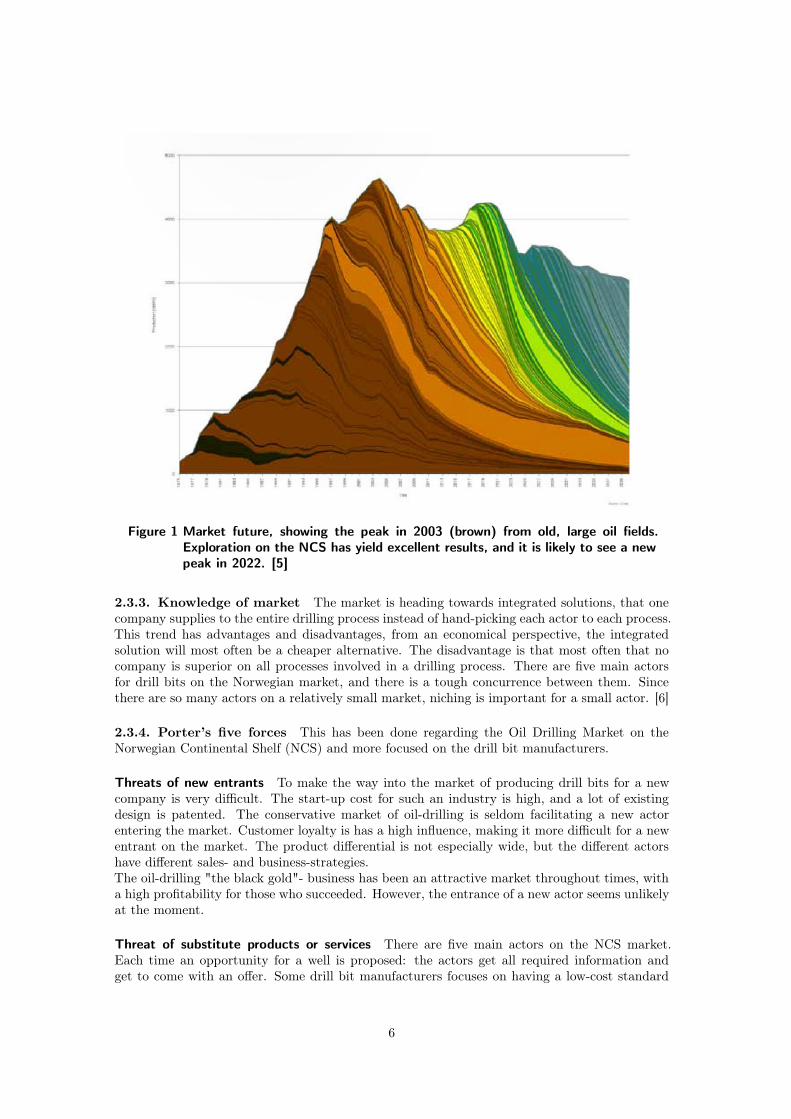
Figure 1 Market future, showing the peak in 2003 (brown) from old, large oil fields.Exploration on the NCS has yield excellent results, and it is likely to see a newpeak in 2022. [5]

2.3.3. Knowledge of market The market is heading towards integrated solutions, that onecompany supplies to the entire drilling process instead of hand-picking each actor to each process.This trend has advantages and disadvantages, from an economical perspective, the integratedsolution will most often be a cheaper alternative. The disadvantage is that most often that nocompany is superior on all processes involved in a drilling process. There are five main actorsfor drill bits on the Norwegian market, and there is a tough concurrence between them. Sincethere are so many actors on a relatively small market, niching is important for a small actor. [6]

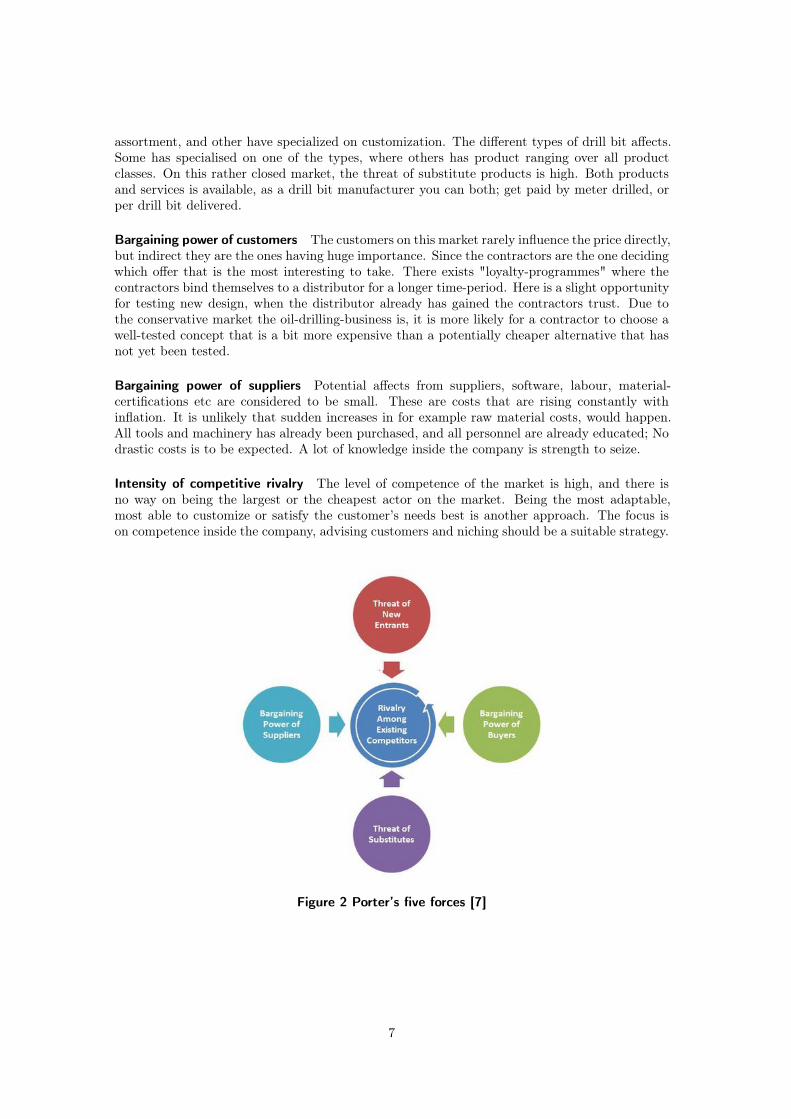
2.3.4. Porter’s five forces This has been done regarding the Oil Drilling Market on theNorwegian Continental Shelf (NCS) and more focused on the drill bit manufacturers.

Threats of new entrants To make the way into the market of producing drill bits for a newcompany is very difficult. The start-up cost for such an industry is high, and a lot of existingdesign is patented. The conservative market of oil-drilling is seldom facilitating a new actorentering the market. Customer loyalty is has a high influence, making it more difficult for a newentrant on the market. The product differential is not especially wide, but the different actorshave different sales- and business-strategies.The oil-drilling "the black gold"- business has been an attractive market throughout times, witha high profitability for those who succeeded. However, the entrance of a new actor seems unlikelyat the moment.

Threat of substitute products or services There are five main actors on the NCS market.Each time an opportunity for a well is proposed: the actors get all required information andget to come with an offer. Some drill bit manufacturers focuses on having a low-cost standard

6

assortment, and other have specialized on customization. The different types of drill bit affects.Some has specialised on one of the types, where others has product ranging over all productclasses. On this rather closed market, the threat of substitute products is high. Both productsand services is available, as a drill bit manufacturer you can both; get paid by meter drilled, orper drill bit delivered.

Bargaining power of customers The customers on this market rarely influence the price directly,but indirect they are the ones having huge importance. Since the contractors are the one decidingwhich offer that is the most interesting to take. There exists "loyalty-programmes" where thecontractors bind themselves to a distributor for a longer time-period. Here is a slight opportunityfor testing new design, when the distributor already has gained the contractors trust. Due tothe conservative market the oil-drilling-business is, it is more likely for a contractor to choose awell-tested concept that is a bit more expensive than a potentially cheaper alternative that hasnot yet been tested.

Bargaining power of suppliers Potential affects from suppliers, software, labour, material-certifications etc are considered to be small. These are costs that are rising constantly withinflation. It is unlikely that sudden increases in for example raw material costs, would happen.All tools and machinery has already been purchased, and all personnel are already educated; Nodrastic costs is to be expected. A lot of knowledge inside the company is strength to seize.

Intensity of competitive rivalry The level of competence of the market is high, and there isno way on being the largest or the cheapest actor on the market. Being the most adaptable,most able to customize or satisfy the customer’s needs best is another approach. The focus ison competence inside the company, advising customers and niching should be a suitable strategy.

Figure 2 Porter’s five forces [7]

7

2.3.5. Porter’s generic strategies After regarding the five forces of the market, one candevelop a strategy for optimizing the company’s potential for success within the market. Theidea is that a company will waste valuable resources if not choosing between either one of thethree strategies; cost leadership, differentiation or focus. Research has showed that companiesin the middle of the box are less likely to be profitable than companies located in the differentends of the box seen in figure 3.The company is active in a small segment of the market, only manufacturing PDC-bits. Also

the manufacturer is a rather small company compared to all other drill bit manufacturers on themarket (2.3.7), and several other parameters affect the fact that it is impossible to be the costleader of the market. One of these parameters to regard is the location of the factory, which isin Norway, implying both high cost for personnel and premises.By following the chart, this company ends up in the "Differentiation Focus" box and would

benefit from finding its own niche on the slim market segment where they act today. To developa product that the customer is willing to pay a higher price for due to the special, unique andinteresting properties that the product offer. This is the strategy that will most likely be asprofitable as possible.

Figure 3 Porter’s generic strategies [8]

8

2.3.6. SWOT-analysis This SWOT-analysis was performed as a reminder of the possibilitiesand the limitations that exists on the market of drilling sub-sea today. Below in table 1 theinternal factors can be seen, and in table 2 external factors can be seen.

Table 1 Internal factors

STRENGTH WEAKNESS

Old "stable" market Finite reserve

High demand Risky and Expensive operations

Many applications Conservative market

Lot of Research and Develop-ment (R&D) on the area

Disliked market, regarded as"dirty"

Table 2 External factors

OPPORTUNITIES THREATS

New Market - Geothermal en-ergy

Environment issues

Many locations left to explore Alternative sources

Still high demand on hydrocar-bons

Unavailable locations

Room for finding niches Many competitors on the market

There is a lot of R&D due to the interest and the amount of money circulating the market ofoil drilling. The weakness of a finite reserve helps increasing the prices and the profit. As themarket is rather conservative, any radical changes is believed to be unwelcome.The threat that exists are mainly environmental; as fossil fuels have a large affect on the ozonelayer. Although, as technology moves forward, the vehicles using fossil fuels are getting more andmore efficient. There is still many locations yet to explore regarding the hunt for hydrocarbons,and also when searching for geothermal energy.

9

2.3.7. Suppliers The market divided after suppliers can be seen below in figure 4. This chartregards the market on NCS, and largest actors on the market is Baker Hughes International andSchlumberger.

• Hughes Christensen (BHI)

• Smith Bits (Schlumberger) (SLB)

• Lyng Drilling (Schlumberger) (SLB)

• Halliburton (HAL)

• National Oilwell Varco (NOV)

• Varel

Lyng Drilling is a small bit- manufacturer recently acquired by Schlumberger. Also deliveringdrill bits to Schumberger is Smith Bits that produces the most of Schlumberger’s drill bits.

Figure 4 Market of drill bits today [9]

2.3.8. Result From the five forces analysis, it has been determined that the threat for a newdrill bit manufacturer to enter the market is relatively low, whereas the threat of a product gettingsubstituted by another is high. At the same time, it is the costumer that has the bargainingpower to choose between offers. The bargaining power of suppliers is regarded low on this market.The strategy Lyng Drilling should apply is the "Differention Focus", i.e. to find their own nichewithin the market segment. Also one should keep in mind that Lyng Drilling is located in Norway,implying high cost for both personnel and premises.

10

3. Theory

This section is divided up in several sections, starting with an introduction to the subject; togive insight in the oil-drilling process, the foundation of CFD and the different types of drill bits.This is to give a better understanding to the equations and approximations already built intothe models in CFD, and also all parameters affecting the simulations.

3.1. Introduction

Being able to successfully drill into the ocean floor has become increasingly more importantduring the last 50 years[10]. Starting in the 19th century the search for hydrocarbons has beenconstantly facing new challenges. In the early history of drilling for oil, the wells were shallowand located on solid ground. Around the 1950’s, the oil drilling started moving from solid groundand into the Gulf of Mexico, where larger amounts of hydrocarbons were found. Ever since, theindustry has gone towards deeper water and new drilling techniques. In later years, the searchfor geothermal energy has opened up a new market for the drilling industry.The challenge is the harsh environment, and the far distance that is to be drilled. Today whatis called ’horizontal drilling’ is common, to have a steerable drilling head in order to extract asingle layer of hydrocarbons from a finding.The various materials that the drill encounters, and along with the fact that this is a heavily price-influenced market makes every possibility to make the entire process more efficient an interestingmatter to investigate. The overall effect that the flow patterns have on the life-span of the drillbit is not thoroughly investigated. The flow of drill mud mainly serves to transport away cuttedmaterial, cool down the drill bit, maintain pressure control and to lubricate the drill operation.[1]

3.1.1. Drilling process Plant and animal remains is constantly being washed out in the oceanin a continuous process. The pressure in the underlying layers will increase as new layers willadd on. When the conditions are right; High pressure, high temperature in combination withlow supply of oxygen; these remains will chemically transform into hydrocarbons. Mainly thepressure affects which types of carbons will be created and all this undergoes in a certain typeof slate (Kimmeridge). The oil and gas will then migrate away from the source rock.When searching for potential fields, exploration vessels is using seismic waves to determine thegeometry of the underlying ocean floor. Test drilling of an exploration well is the only secureway to determine if there are hydrocarbons to be extracted in the area. Several exploration wellsare required to determine the size of the field. [1]After having drilled the exploration wells, the company who claimed the field can begin the

operation. Now it is up for the company to organize with all necessary equipment, personneland all other things for starting the operation.Leaping forward in the process, the flotation rig (or already in place; if working with for examplea jack-up rig. The different types of rig can be seen in figure 5) is being held in place by anchoringto the ocean floor and the lead frame is being placed by the sea floor while monitoring from aRemote Operated Vehicle (ROV). A hole is being drilled, and a permanent lead frame is beingplaced there and subsequently cemented. Later, the Blow Out Preventer (BOP) is mounted ontop of the well-head, to prevent gas of oil to start flowing uncontrolled; in the event of facingunexpected high pressure, too low density of the drilling mud or other unexpected situations.The BOP is replaced after the drilling operation is executed.Standard procedure for the rest of the drilling process is to start out with a large diameter drill,and stepwise change to smaller diameter. Almost the entire length of the well is the type "tube-in-tube", and thus, large amount of pipes in different dimensions is required.For completing the well, production equipment is installed to let the hydrocarbons flow up fromthe well, safety vault is put in place and the liner is perforated. Normal time to consume from

11

Figure 5 Drilling Rig Types, Maersk Drilling [11]

finding (exploration wells already drilled) a well to start production is normally between 35-85days, where the drilling activities alone are around 17-55 days.[1]

3.1.2. Drill bits Today, there are mainly two types of drill bits that dominate the market,with several variations in each category. Depending on the operation, the drill head is carefullychosen. Amongst the Roller cones, there are different types available on the market ranging fromtwo to four cones, but the market is dominated by the design with three cones. Also amongst thefixed cutter bits, different types are available on the market with for example: Natural diamondinserts, diamond impregnated bits, polycrystalline diamond compact (PDC) bit and thermallystable PDC. Regular PDC is dominating this market segment. A new type of drills has recentlypenetrated the market, a hybrid between the two types. This type can be seen below. [12]

Figure 6 3D view of a hybrid Tricone/PDC drill bit, KymeraTMbyHughes Christensen[13]

Figure 7 Top view of a hybrid Tricone/PDC drill bit, KymeraTMbyHughes Christensen[13]

Roller Cone - Tricone Drill bits The basic principle of a tri-cone is three rotating cones facinginwards towards the centre of the drill bit. This type of bit is the most common one, and differentdesigns have been developed since the birth of the roller-cone bit in the beginning of the 20th

12

century. There are large variations between different companies that manufacture the drill bits,but the principle is the same. The cones are equipped with elements for removing material, asseen above (the conical geometry). The materials used vary, common materials for the insertteeth are tungsten carbide and steel. The drill itself rotates, and so does the three cones (seesection 1). The design is varied depending on the rock, and the angle of the cone is increasingas the rock goes from soft to hard. [12, 13]

Fixed Cutter - Polycrystalline Diamond Compact bit This type of drill has inserts consistingof PDC that acts as cutting elements. This drill bit is slightly more expensive, but also morereliable as it does not include moving parts and bearings. This results in a longer service life.The design of the PDC can be seen as the swirling elements of the KymeraTM in the figures 6and 7. PDC bits are well suitable in offshore applications, when drilling in long sections andhigh demand is put on having high rpm. [12]

3.1.3. Drill fluids Drilling fluid is essential during the drilling process. The drilling fluid islead down the drill string to the drill head, and flows up on the outside transporting cuttingsback to the rig. It is essential for the cost of the operation (figure 8) how much and how efficientlythe drilling fluid can transport cuttings away from the drill head. Locally around the drill head,the drilling fluid is also cooling down the drill-head during operation, due to the frictional heatdeveloped in the process. Subsequently, the fluid is also lubricating all moving parts. The fluidis cleansing the drill head as it is being ejected from nozzles between the cutting elements. Asthe drill fluid is flowing around, it picks up the debris that is cutted away in the hole.

Figure 8 Relationship between rig costs and solid content[14], originally from World Oil

Another important for the drilling fluid is to support the drilling string. The drilling stringweighs many tonnes, and through buoyancy some of the load is reduced. The drilling fluid mustalso be able to keep the pressure controlled; the pressure must be high enough to prevent oiland gas to flow up to the surface. If the pressure is too high, the walls of the drilling hole risk

13

to start cracking, and drilling fluid will seep away. The pressure of the drilling fluid is directlyconnected to the density of the fluid.From time to time, the drilling operation must stop due to different reasons. When this

happens, the drilling fluid must have such properties that the cuttings does not sink to thebottom of the well and wedges the drill string.[1]More about the material properties for the different types of drill fluids is found in 3.2.

3.1.4. Fluid dynamics Fluid dynamics, a sub-discipline of fluid mechanics, deals with thenatural science of liquids and gases in motion. Fluid dynamics itself can be divided up in sub-disciplines; among other hydrodynamics, the study of liquids in motion.The foundational axioms of fluid dynamics are based on classical mechanics, but are modified inquantum mechanics and general relativity; conversation of mass, conservation of linear momen-tum and conservation of energy. The three conservation laws are used to solve fluid dynamicsproblems, and the mathematical formulation considers the concept of a control volume(CV). Thecontrol volume is defined as a specified volume in space where a fluid can flow in and out. [15, 16]

• Mass continuity, the conservation of mass, which states that the rate of change inside acontrol volume must be equal to the net rate of fluid flow into the volume. Requires thatmass is neither created, nor destroyed in the control volume.

∂

∂t

˚V

ρdV = −‹

S

ρu · dS (1)

ρ is the fluid density, u is a velocity vector and t is time. The differential form of thecontinuity equation is, by the divergence theorem:

∂ρ

∂t+∇ · (ρu) = 0 (2)

• Conservation of momentum, any change in momentum of fluid within a CV will be dueto the net flow into the volume and the action of external forces on the fluid within thevolume.

∂

∂t

˚V

ρdV = −‹

S

(ρu · dS)u−‹

S

p · dS +

˚V

ρfbodydV + Fsurf (3)

The differential form of same equation:

DuDt

= F− ∇pρ

(4)

• Conservation of energy, the total energy in a given closed system remains constant:

ρDh

Dt=Dp

Dt+∇ · (k∇T ) + Φ (5)

h is enthalpy, k is thermal conductivity of the fluid, T is temperature and Φ is the viscousdissipation function.

Compressible and incompressible flow All fluids are to a certain extent compressible, whichwill subsequently change the density of the fluid. This could also be due to change in temperature.In many situations the changes are small, and thus the fluid could be regarded as incompressibleresulting in:

Dρ

Dt= 0 (6)

14

Being able to neglect compressibility simplifies the governing equations.

Viscous and inviscid flow A problem is regarded as viscous if the fluid friction has significanteffect on the fluid motion. The Reynolds number (Equation 9) is suitable for determining whetherviscous or inviscid equations are appropriate for solving the problem at hand. High Reynoldsnumber indicates the more significant inertial forces compared to the viscous forces. Whendealing with a problem with high Reynolds number and no solid boundaries, viscosity can beneglected. However, when dealing with solid boundaries, the no-slip condition creates a thinregion close to the solid surface (Boundary layer) where the strain rate is large, enhancing theeffect of viscosity and thus generating vortices.

Vorticity The local spinning motion of a fluid near some point (as it would be seen by anobserver travelling along with the fluid at that point) can be described by a pseudo-vector fielddenoted ~w, known as vorticity. The vorticity tells how the velocity vector changes when onemoves by an infinitesimal distance in a direction perpendicular to it. This is described by:

~w = ∇× ~v =( ∂∂x,∂

∂y,∂

∂z

)× (vx, vy, vz) (7)

, where ~v is the velocity field describing the fluid motion.[15, 17]

Steady and unsteady flow A flow is considered steady, when all time derivatives in the flowfield are equal to zero. In other words, the fluid properties do not change over time. This is alsocalled Steady-State solution. Otherwise, the system is called unsteady or transient. Turbulentflows are per definition unsteady and thus have one more dimension to regard than a similarsteady flow.

Laminar and Turbulent flow Turbulence is a flow that is characterized by recirculation, eddies,and apparent randomness. To determine mathematically if a flow is turbulent or laminar, theReynolds number (Equation 9) can be calculated. In general, if Re > 2000 the flow is likelyto be turbulent, and Re < 2000 the flow is likely to be laminar. It is believed that turbulentflows can be described by the Navier-Stokes equation (3.1.4) at moderate Reynolds numbers.For larger and more complex problems one can combine turbulence modelling with Reynolds-averaged Navier- Stokes equations.[18]Also, the properties of the fluid greatly influence its dynamic behaviour. Many fluids behavelinearly: The stress and rate of strain are close to linear. This is true for some fluids, for exampleair and water. Some mixtures have a more complicated so called non-Newtonian stress-strainbehaviour, and many drilling fluids are of that type. This will be more discussed in section 3.2.

Eddies An eddy is the swirling motion of a fluid and the reverse current created when a flowpasses an obstacle. When the fluid passes the obstacle, a space devoid is created on the down-stream side of the obstacle. Fluid behind the obstacle flows into the void creating a swirl of fluidon each edge of the obstacle, followed by a short reverse flow of fluid behind the obstacle flowingupstream, towards the back of the obstacle.[15]The difference between an eddy and a vortex (3.1.4) is depending on context. A vortex is akind of motion of fluid which involves vorticity; meaning that the fluid elements rotate aroundits centre or centre of gravity. Consider a turbulent flow in which separation takes place; dueto the separation, the flow downstream produces what we denote as eddies. Meaning, the fluidelements are already having the vorticity, but in addition these fluid elements are circulatinglocally downstream of the separation point. Eddies are nothing but circulation or spinning offluid elements in circles.[19]

15

Navier-Stokes equation Navier-Stokes equation describes the motion of fluid substances, andthe equations arise from applying Newton’s second law on fluid motion together with assumptionthat the stress in the fluid is the sum of a diffusing viscous term and a pressure term. How the fluidactually moves is determined by the initial and boundary condition, and depending on problem,some terms may be considered to be negligible or zero, thus simplifying the equations. In short,the Navier-Stokes equations are the sum of gravitational force, pressure force and viscous forces,and equal to the mass times acceleration:

~Fgrv + ~Fprs + ~Fvisc = m~a (8)

A complete definition can be found in [20].

Boundary layer A boundary layer is a transitional layer between two distinct regions withdifferent physical properties. When a fluid is flowing around a body, it produces a force thattends to drag the body in the direction of the flow. This drag can be divided up in skin frictionand form drag. The skin friction drag is due to viscous shearing in the region between the surfaceand the layer of fluid immediately above it. This occurs on surfaces long in compared to height.When the fluid flows over the solid surface, the layer next to the surface may become attached toit, known as the ’no slip condition’. The boundary layer thickness is denoted δ and is defined asthe distance from the no slip plane it takes for the fluid to reach 99% of the average velocity u0.Form drag applies to bodies that are tall in comparison to long in the direction of the flow.[21]

3.1.5. Computational Fluid Dynamics (CFD) CFD is a branch of fluid mechanics thatuses algorithms and numerical methods to solve and analyze problems that involve fluid flows(based on the equations in previous section). The basic equations governing fluid motion arecalled Navier-Stokes equation and it governs the motion of a viscous, heat conducting fluid. Sim-plification of the equations comes in various types depending of which effects are insignificant.[16]There are several dimensionless parameters which characterize the relative importance of variouseffects, among other Reynolds number, Mach number and Prandtl number. Reynolds numberis an indicator on turbulent flow. A high Reynolds number tend to be turbulent, and it isdetermined as the ratio between internal force and viscous force.

Re =ρUL

µ(9)

Mach number is the local flow-speed, u, divided by the sound of speed in the medium a:

M =u

a(10)

Prandtl number is the ratio between kinematic viscosity to thermal diffusitivity, and is definedas:

Pr =µCp

k(11)

It can be related to the thickness of the thermal and velocity boundary layers.

3.2. Drilling fluids

Most drilling fluids used in drilling operations sub-sea are usually Non-Newtonian. This is whenthe stress-strain correlation is not linear, and can be described simply as its behaviour is some-times as a solid and sometimes as a fluid. This is of great use in these applications, whenhaving kilometres of drill string and mud, and the operation has to stop for some reason. Theynon-Newtonian fluids have low effective viscosity and high effective yield stress suitable for trans-

16

porting cuttings and hold them in suspension during stationary periods, in order to preventcuttings from sinking down on the drill head and clog the hole.Nouri and Whitelaw [22] performed a study where the difference between the behaviour of aNewtonian and non-Newtonian fluid in an eccentric annulus at a Re of 9200 was tested. Theyconcluded that the flow resistance were almost unaffected at high Re, but increased with morethan 30% with rotation for low Re.

The major functions of drilling fluids are [23, 24]:

• Carry cuttings away from the hole and permit their separation at the surface

• Cool and clean the bit

• Reduce friction between the drill pipe and wellbore or casing

• Maintain stability of the wellbore

• Prevent the inflow of fluids from the wellbore

• Form a thin, low-permeable filter cake

• Be non-damaging to the producing formation

• Be non-hazardous to the environment and personnel.

The most common type of drilling fluids is water based muds. Around 5-10 % uses oil-basedmuds and a small percentage uses air. Usually oil-based muds are used in high-angle holes andduring special conditions. The cost of an oil-based mud is higher and the ROP is slower. [14] Aircan be used in shallow, hard conformations. The water based muds are a mixture of mud andfreshwater, sometimes with added salt. The development today is also towards muds formulatedwith a synthetic base fluid. They have the advantage of oil muds but with the handling anddisposal of a water mud. The chemical types that can be used instead in these muds can befor example esters, ethers, glycols and glycerines. Today, water based muds are the superioralternatives for drilling muds.

3.3. Grid size and meshing

When regarding the mesh of a model, one differs between structured grids that are suitable formore simple geometries and unstructured grids for more complex geometries. The unstructuredgrid implies that the cells are arranged in an arbitrary fashion. When dealing with 3D geometries,tetrahedral, prisms and pyramids are used as elements. Also combinations, for example; use atetrahedral volume mesh in combination with a prism layer as boundary layer closest to thesolid. To evaluate the mesh quality, a number of factors are regarded. Skewness for a triangleor tetrahedra is checked by:

Skewness =Optimal cell size− Cell size

Optimal cell size(12)

, based on the equilateral volume. And when applying a prism or pyramids as a mesh:

Skewness = max

(θmax − 90

90,

90− θmin

90

)(13)

, based on the deviation from a normalized equilateral angle. A common measure of quality isbased on the equiangular skew, and range of skewness goes from 0 to 1, where 0 is the best and1 is the worst, seen in Table 3.

17

Table 3 Skewness

Value ofSkewness

0− 0.25 0.25 −0.50

0.50 −0.80

0.80 −0.95

0.95 −0.99

0.99−1.0

Cell Qual-ity

excellent good acceptable poor sliver degenerate

A poor grid quality can cause slow convergence and inaccurate solutions. The change in sizeshould be gradual, giving a smooth transition in size between elements. Ideally, the maximumchange in cells connected to each other should be less than 20 %. Also the aspect ratio of thelongest edge to the shortest edge of an element is a matter that affects the mesh quality. Theideal aspect ratio is equal to 1 for an equilateral triangle or a square. Regarding orthogonalquality, the worst cells will have an orthogonal quality closer to 0 and the best cells will have anorthogonal quality closer to 1. [26, 27]

3.4. Computational Fluid dynamics (CFD)

Listed below are the different Turbulence models available in ANSYS Fluent 14.5, identifyingtheir different advantages and disadvantages from research conducted with the different models.

3.4.1. Reynolds-averaged Navier-Stokes Equation (RANS) Divided up in Eddy Vis-cosity models (EVM), and Reynolds Stress Models (RSM). The difference between the two ishow the Reynolds Stress term is calculated. Within the EVM’s the assumption that the stressis proportional to the strain, where the strain is being gradients of velocity, is being made. TheEVM’s have a general poor performance where turbulence is highly anisotropic, and where 3Deffects are present. The models have inability to account for extra strain due to streamline curva-ture, rotation and highly skewed flows. Also where the linear algebraic stress-strain relationshipmakes result in non-equilibrium flows, separating and reattaching flows poor.

Zhang and Che made a comparison on flow between cross-corrugated plates for eight different tur-bulence models (LBKE, SKE, RKE, RNGKE, RSM, KW, SST and LES) and experimental data,regarding and discussing velocity, temperature and turbulent viscosity ratio distributions. Whencomparing to available heat transfer and pressure drop experimental data, all models predictscorrect entry effects, practically satisfactory j (Average Colburn factor) values and acceptablef(friction factor) values and all of them capture the major characteristics in the NuL map overthe hole Re range. This test is not including any rotating parts, but interesting result that thevelocity and temperature distributions predicted by the RSM, SST and LES differs a lot fromeach other. [28]

Cebeci-Smith and Baldwin- Lomax model Both models are zero equations EVM where theeddy viscosity is a function of the local boundary layer profile. They are suitable for high-speedflows with thin attached boundary-layers, for example in applications regarding aerospace. Thesemethods are rarely used in recent times.

Spalart-Allmaras(S-A) S-A is the least complex turbulence model, solving one transport equa-tion for a modified eddy viscosity. A model mainly intended for aerodynamic applications withmild separation such as for example supersonic or transonic flows over airfoils. One of the limita-tions with this model is its uncertainty to predict decay of homogeneous, isotropic turbulence.[29]

18

Standard k-ε (SKE) The SKE model is one of the most widely-used engineering turbulencemodels used in the industry, due to its robustness and it is reasonably accurate for many appli-cations. The model is based upon a two-equation approach, and the turbulence energy has itsown transport equation. It bases upon the presumption that there exists an analogy betweenthe action of viscous stresses and the Reynolds stresses of the mean flow. The model solvesa transport equation for k, turbulent kinetic energy and ε, the rate of dissipation of turbulentkinetic energy. The model focuses on the mechanisms that affect the turbulent kinetic energy.The model is well-validated, performs well in confined flows where the Reynolds shear stressis most important. It is known that the model performs poorly for flows with larger pressuregradient, strong separation, rotating flows, high swirling components and large streamline cur-vature. Also the model makes inaccurate predictions of the spreading rate, and has a problemmaking predictions in regions with a large strain rate. SKE and all other models based on theBoussinesq isotropic eddy viscosity assumption will have problems in swirling flows and flowswith large rapid extra strain (highly curved boundary layers and diverging passages) that affectsthe structure of turbulence in a subtle manner. [29, 30]

A study performed by Håkansson et. al. on flow through a high pressure valve concludes thatthe SKE significantly overestimates both turbulent kinetic energy and the mean area averageddissipation of turbulent kinetic energy in the gap region. The two other KE-models tested re-ports good accuracy on gap flow velocity and turbulent kinetic energy. In the outlet none of themodels describes turbulent kinetic energy well. [31]

It is acknowledged that the two-equation SKE are unable to account for the extra strains causedby streamline curvature, recirculation and swirling flow. This has been confirmed from numerousof studies. Problems encountered when applying this method to strongly swirling flows includeinability to predict the correct tangential velocity profile due to strong radial diffusion of mo-mentum, and over-prediction of the shear stresses.[32]

Al-Kayiem et. al. used the SKE to simulate the transport of cuttings in a non-Newtonianfluid. Their approach was to first simulate without particles to study the behaviour of the non-Newtonian pseudo-plastic mud in the annulus. They report a velocity profile in the annular crosssectional area that is flattening around the centre and the velocity gradient near the wall is highin comparison to a Newtonian fluid. There is no reflection about the accuracy of their model,but experimental setup was also evaluated. [33]

Realizable k-ε (RKE) The RKE model has a two equation approach as the SKE, with thedifference that the dissipation rate (η) equation is derived from the mean-square vorticity fluc-tuation. It has proven better in predicting the spreading rate, and is likely to provide superiorperformance in modelling flows involving rotation, boundary layers under strong adverse pressuregradients, separation and recirculation.[29]

The Renormalization Group (RNG) k-ε The constants used in the model are derived ana-lytically using renormalization group theory, instead of empirically obtained experimental data.This model performs better than SKE for more complex shear flows, flows with high strain rates,swirl and separation.[29] In the model, increasing the loss of turbulent kinetic dissipation ratehas reduced turbulent kinetic energy for high strain rates. [31]

Standard k-ω (SKW) The SKW model is based on a two equation approach as well, and ismost widely adopted in the aerospace and turbo machinery communities. The dissipation perunit turbulence kinetic energy, ω. The benefits with this model are the many sub-models andoptions available; compressibility effects, transitional flows and shear- flow corrections. It ismore sensitive to free-steam conditions and has an improved behaviour under adverse pressure

19

gradient compared to any of the k-ε models.[29] In this model the turbulent frequency is used,defined as

ω =ε

k(14)

as the second variable. This results in the length scale

l =

√k

ω(15)

and eddy viscosity

µt =ρk

ω(16)

The SKW model has been considered for swirling and asymmetric flows and has reported goodresults, but the literature is limited and it is unclear for what Re and S this model is limited to.[34]Also has the SKW been used to recreate the study conducted by Nouri and Whitelaw [22], non-Newtonian Transitional Flow in an Eccentric annulus [35]. The rotational Reynolds number fora flow outside a concentric rotating annulus in a confined flow is defined as

Reω =ωRinSav

ν(17)

where ω is the inner cylinder angular velocity and Sav the average gap, Rin is the inner radii andν is the kinematic viscosity. The results from the simulation complies well with test data fromthe study conducted.

Shear Stress Transport k-ω (SSTKW) A blending function to describe a gradual transitionfrom the SKW method near the wall to a high Reynolds-number version of the k-ε model inthe outer portion of the boundary layer is used in this model. The SSTKW contains a modifiedturbulent viscosity formulation to account for the transport effects of the principal turbulent shearstress. This model generally gives accurate prediction of the onset and the size of separation underadverse pressure gradient.[29] It also has the benefits compared to SKE and SKW of limiters; theeddy viscosity is limited to give improved performance in flows with adverse pressure gradientsand wake-regions. Also, the turbulent kinetic energy production is limited to prevent the build-upof turbulence in stagnation regions.[30]

4-Equation v2f The v2f Turbulence model shows promising result for many 3D, low Re, bound-ary layer flows. This model is still an EVM, and same limitations exist. The difference lies withinthe assumption that wall-normal fluctuations are responsible for the near-wall damping of theeddy viscosity, and thus requiring two additional transport equations: One for the wall-normalfluctuations and one for the relaxations function together with k and ε.[29] The turbulent kineticenergy is the same as the SKE, dissipation is notably different.

k-kl-ω Transition Model This EVM focuses on solving transitional flow cases by using a threeadditional transport equation. This method was developed from the k-ω model and has shownreasonable accuracy for transitional flow behaviour. [36]

Shear Stress Transport (SST) Transition model This is a combination of the SKE and SKWmodel, using the SKE away from the wall and SKW near the wall. This in order to try toovercome the shortcomings of the models individually. Turbulent kinetic energy is nearly thesame as for the SKE, while the dissipation includes a cross-diffusion term. The model has testedwell for swirling jet comparisons at high Re(20,000 to 40,000) and weak to intermediate S (0 to0,3). The method has not tested well for strong S(0,89).[34]

20

Reynolds Stress Model A more complex approach is being made; a transport equation forthe Reynolds Stress terms is being made and the stresses are thus allowed to be anisotropic.Trying to solve the weakness amongst the EVM’s, the RSM models uses six equations for thedistinct Reynolds stress components. These are derived by averaging the products of velocityfluctuations and Navier-Stokes equations. Also, a turbulent dissipation rate equation is needed.These models are most suitable for highly anisotropic, 3D-flows where the EVM’s perform poorly.One of the cons with this model is that it is more difficult and costly to converge than the 2equation-models.[29]

A study by Vedantam et. al. investigated an annular centrifugal extractor simulated withdifferent types of CFD-approaches. When comparing RSM to the SKE, they found in the annularregion, more reasonable predictions for the three components of mean velocity, Reynolds stresses,k and ε for this model. [37]

3.4.2. Transient Turbulence models Turbulence models not possible to solve steady-stateis presented below.

The CFD solvers ANSYS use are based on the finite volume method, discreticising the domainto a finite set of control volumes. When dealing with turbulent flows, all flows are dependingon time. In other words, the flow is regarded as transient. When calculating a transient flow,the time step (∆t) size must be set. The order of magnitude of an appropriate time step can beestimated by the following formula [38]

∆t =Typical cell size

Characteristic flow velocity(18)

Scale-Adaptive Simulations (SAS) A model under development that resolves turbulence intransient instabilities, while resolving steady in stable flow regimes. [29]

Large Eddy Simulation A spectrum of turbulent eddies in the Navier-Stokes equations is fil-tered, and the filter is a function of grid size. The eddies smaller than the grid size are removedand modelled by a sub-grid scale model, and the larger eddies are directly solved numerically bythe filtered transient NS equation. The most common types of filters are top-hat or box filter,Gaussian filter and Spectral cut-off. The top-hat filter is used in finite volume implementationsof LES, whereas the following two is preferred in research literature. [29]A study was conducted regarding comparison between experimental measurements and com-

putational models of free surface flow in the mixing cone of an annular centrifugal contractor.Concluded is that LES can compute on a course grid and both qualitatively and quantitativelypredict the actual dynamics of the flow in the mixing zone. When comparing to the experimen-tal values, mean and RMS velocities was captured with much better accuracy by LES modellingthan for either RANS or DES of the same mesh. It appears that using LES with a courser gridcan obtain good results without an increase in computational cost. [37]LES has proven very good for flow systems governed by large turbulent structures that can

be captured with a course mesh. There is a possibility for partly dissatisfying result regardingthe boundary layer region, unless finer mesh is used. Many researchers suggest a hybrid: RANSmethod near wall and LES in the rest of the part. [39] From these suggestions, more modelshave been developed:

Deatached Eddy Simulation (DES) A hybrid model that treats the near wall regions in aRANS manner and the rest of the flow in a LES-manner. There are three different RANS-modelsfor using on the near wall treatment. [29]

21

Synthetic Eddy Method (SEM) Method based on the view of turbulence as superposition ofeddies; SEM is a stochastic algorithm generating instantaneous velocity fluctuations.[40]

3.4.3. Direct Numerical Solution (DNS) DNS is approaches where the 3D unsteadyNavier-Stokes equations are solved numerically by resolving all scales, both in time and space.This has been done successfully for simpler geometries and at modest Reynolds number. Limitedat Re > 4 million, based on Navier-Stokes Equation (3.1.4). Only approximation made is thediscretization made when calculating the NS equation and continuity equation in discrete points.This method is not included in ANSYS Fluent, and will not be regarded. [29]

3.4.4. The method of discretization Most common method when regarding Annular Cen-trifugal Extractors has used ’First order upwind’ or in some cases ’QUICK’. To facilitate duringcomputation, the Pressure-velocity coupling: PISO has shown effect on time required. For theenergy equation PRESTO or standard is common. [37]

3.4.5. Boundary Conditions (BC) for Turbulent Flows When setting up a simulation,some initial conditions is required for the software to set up the problem. A good strategy is tostart out simple, and make the conditions more and more difficult subsequently.

Inlet Starting with the inlet; the surface from where the calculations begin. This can be definedby specifying for example velocity, mass flow, initial temperature, turbulent intensity, pressureetc.

Wall Near a wall, the velocity changes rapidly and by manipulating this; making the velocityand the distance from the wall dimensionless, a wall model(The Universal Law of The Wall) hasbeen created. This wall model contains a viscous sub-layer, buffering layer/ blending region andthen over a certain value a fully turbulent region. The choice of wall modelling strategy liesbetween resolving the viscous sub-layer with a low-Reynolds number turbulence model, or usinga wall function and a high Reynolds turbulence model (SKE, RKE or RNG). One could also beusing Enhanced Wall Treatment Option (GUI) or Scalable Wall Functions (TUI). [29]

Outlet Almost same parameters that can be applied for the inlet is possible to the define hereas well. Also values of for example expected backflow is possible to define.

3.5. Flows around moving parts

For modelling a flow over moving parts, five different approaches can be used. They are dividedup in two groups, Steady state and transient. The transient gives often a more accurate result,but is also a more complex approach that requires more time. First three in the list is Steady-stateand the last two can only be solved as transient. [41]

• Single (Rotating) Reference Frame ModelA problem where walls are moving with the reference frame.[42]

• Multiple Reference Frame Model (MRF)A steady-state approximation in which individual cell zones move at different speed. [43]

• Mixing Plane ModelAlternative to MRF and Sliding mesh model for flow through domains with regions inrelative motion. [44]

22

• Sliding Mesh ModelRegarding unsteady interactions caused by the relative motion of stationary and rotat-ing components. Computationally demanding and accurate model for simulating flows inmultiple moving reference frames. [45]

• Dynamic Mesh ModelModel that can be used for modelling flows where the shape of the domain is changing withtime. [46]

23

4. Method

Initially, a project plan was made to create an understanding of the processes needed for solvingthe problem, including comprehensive literature studies as well as acquisition of knowledge influid mechanics, dynamics and material properties. The time limitations were mapped out, anda GANT-chart was made to allocate resources.Overall, the project was inspired by the product development process described by Ulrich and

Eppinger[47], see figure 9 below. The development process will go through some of the steps.

Figure 9 Steps in the product development process according to Ulrich and Eppinger[47]

The project will go from Planning to the end of Detail Design, and the result will be comparedto a validation method. As this project does not fit into the above development process, thesteps will be adapted to suit the project.

Table 4 The processPlanning Concept System Level Detail Level Testing

Development Design and RefinementAllocate resources Need-finding 3D-modelling Refine geometries Compare erosionCurrent research Lyng Drilling Meshing Refine simulations patternsMarket Analysis Creative methods Combine solutions Better setup Recommend

Part-solutions One approach Final simulation further research

4.1. Planning

According to Ulrich and Eppinger, the different steps of the planning phase are depending onapplication and type of project. When designing a new product, the phase consists of tasks likeassessing new technologies and to consider product platform and architecture. In marketing, toarticulate market opportunity and define market segment is the appropriate approach. Whendealing with research, demonstrating available technologies is done during the planning phase.In this project, a thorough literature study will be performed, searching for available technologies.Subsequently, a market analysis was performed to get a better understanding for this company’schallenges.[47]

4.1.1. Literature study The literature study will be conducted with the aim of exploit cur-rent research in the areas regarding mud flow, non-Newtonian fluid modelling, computationalfluid dynamic simulations of rotating operations, market segment, drill bits, problems arising

24

during drill operations, non-Newtonian drilling fluids and historical exposé of the drilling indus-try.Literature that will be reviewed in the study will include books, scientific papers, research pub-lications, conference papers and project reports. The library of Norwegian University of Scienceand Technology (NTNU) will be used. The search for scientific papers, research publications,conference papers etc. will be conducted with a methodology which will make the study system-atic. First, the title will be read, then abstract and conclusions, and finally the entire article inorder to make the literature study as efficient as possible. The main areas that were put in focusduring the search for current research was:

• Drilling processes

• Turbulence modelling

• CFD of rotating operations

• Drilling fluids and muds

• Simplifications of flow setup

• CFD compared to experimental tests

By looking into the drilling processes and drilling fluids and muds, a better understanding of theproblem can be reached. Looking for research regarding turbulence methods will be the basisfor choosing what methods that can be adequate for these types of simulations. Finding CFD ofrotating operations, can give ideas and tips of how to set up the simulations, and what problemsthat can arise. By regarding the flow set-up this; is a fact that needs to be simplified, as thelimitation of not simulate a multi-phase simulation exists. Ways of simplifying the parametersand still get a valid results will be exploited.

Market Analysis As a part of the background for this project, a thorough market analysis willbe performed. This will give knowledge of the market and also a better understanding of theinterest for Lyng Drilling for this type of research project. See section 2.3 for separate report.

4.2. Concept development

Needs of the target market are identified, and concepts are generated and evaluated. Of theseconcepts, one or more are selected for further development.[47]In this section of the project, different approaches to this problem will be made. Not all will

be full scale approaches to the situation. Some will test a theory that some turbulence modelsare more likely to be more or less accurate in this type of case. This can be used later in therefinement of the model. See section 5.1

Lyng Drilling A visit was made to Lyng Drilling to get a better understanding of their productdevelopment process, limitations and requirements regarding the project. During an earliermeeting with the company, the head of production announced that there existed some used drillbits that can be used for investigating erosion patterns. These erosion patterns are believed tohave potential for validating future simulations. See section 5.1.1.From the visit, a list of requirements will be formulated. As many measurable demands aspossible will be stated.

25

Unstructured Concept Combination Table This is a way to consider combinations of solutionfragments in a systematic way. In this method, tables of solutions to part-problems are created.The concepts generated takes one solution from each table and combines them. [47] The methodConcept Combination Table inspires this creative process, and instead of listing solutions to partproblems, all parameters that affect the situation are listed. Since no experimental data exists,there are many parameters that have to be disregarded. Listing all parameters and getting anoverview of the situation formed a basis for a creative session that resulted in a few concepts andpossible approaches. These are parts of possible approaches, which might be combined or testedalone.

4.2.1. Concept review The best features from the different concepts will be used for furtherdevelopment. To aid this part, the selection will be a discussion with experts in the area.

4.3. System Level Design

In the System Level Design phase of the project, the overall design of the product is developed.Product architecture, decomposition into subsystem and components, initial production plan aretasks normally in this step of the process. [47]In this project, the System Level Design phase will be dominated by testing and evaluatingpotential models. The different approaches from previous section will be combined and tested.

Concept selection The concept with the most potential will be brought to further development.The concepts will be assessed by the parameters’ accuracy, time of simulations and time ofpreparation.

Meshing One of the most important things to regard when setting up a 3D-simulation, is tohave a good mesh to work with. The mesh is generated with tetrahedrons and the meshing toolused was connected to ANSYS Fluent. The 3D-model used was the one created in section 5.1.3,seen in figure 12. To try and improve the quality, two other softwares were tested.

4.3.1. Simulations After having generated a sufficient good quality mesh, the simulationswas set up. The input data of the simulations is presented with the result of the simulations.

First Approach A first approach to the simulations, using rotating wall in order to try andmake the solid boundary move the fluid and at the same time have axial flow from the inlet. Thefluid is set to have a relative velocity to the boundary set to zero.

Secondary Approach Instead of simulating steady-state solutions, decision was made to trytransient simulations. A very coarse mesh was generated to try to avoid long computationaltime. The simulation was run outside the cluster on a regular laptop, as simulations was runningparallel with each other. The transient simulations have a better potential for some types ofsituations. If the transient simulation shows good results, one can run with finer and moreaccurate mesh.

Third Approach Parallel with the transient simulations, a new stationary simulation is run,with aim of making a particle track of the result. Making a particle track out of this might giveuseful information if compared to the erosion patterns. If only regarding flow, the simulationsshould run fine.

26

4.4. Detail Level Design

This step consists of specifying geometry, material, tolerances and plan for production planetc. [47] During the Detail Level Design phase, refinements to the chosen model will be made,improving results and shortening the simulation time if possible. Different meshes will be testedand if necessary also different types of simulations. The models will be extended with moreparameters, for example particles. The non-Newtonian properties of the mud will be added tothe simulation.

27

5. Results

Listed below are the three development phases of the project. During Concept Development,approaches were developed that was brought forward to the next phase. In System Level Design,the different approaches were tested and further developed. The one with most potential wastaken to the next phase. In Detail Level Design, the refinement of the simulations is presented.

5.1. Concept Development

From the literature study, some turbulence models were concluded not to be suitable for simu-lating such a case as drilling implies. There is always the weighing between computational costversus accuracy to regard. The validation method is a difficult problem to solve. There is ageneral saying when dealing with CFD, that if you would like a water-proof validation; build themodel, set up all parameters as in the simulation and measure. That is not possible to do, butLyng drilling has provided both used drill heads, CAD-models and some data for the simulation.

5.1.1. Visit at Lyng Drilling (Schlumberger), Vanvikan The visit at Lyng Drilling wasto get a clearer picture of the company’s product development process and the interest from theindustry’s side. Today, the development process is based on minor changes on current design.A suggestion is made on a design change, strength calculations and dynamic simulations on thesolids are conducted, followed by a prototype manufacturing and testing. The drill bit is testedeither on site or tested in a contracted well.

Figure 10 Marking the flow-patterns, Kjell Haugvaldsson, Lyng Drilling [6]

Used drill bits Lyng Drilling has some used drill bits that has not been recycled, where somehas a more distinct flow pattern than other. This pattern that can be seen on the drill bits aserosion in the top layer of the material. There are multiple types of damages to the drill bits, butit is fairly easy to distinguish erosion from abrasion and thus the cause of damage. This gives

28

the possibility to some extent to validating the simulations, besides looking for convergence andmonitoring points.Together with the chief of production, three drill bits were chosen for a closer analysis of thedrill pattern. These drill bits had all distinctive erosion patterns, and all with slightly differentgeometry. To make the patterns more visible, they were marked before photographing (Figure10). One of the drill bits was close to symmetric on 120 degrees and had a repetitive pattern.This drill bit was chosen, believed to be a bit easier computational-wise to simulate.

One must regard that the flow patterns will change related to the erosion and other damages,but the conclusion was reached that the main flow still can be indicated through the erosionpatterns.

Terms and demands Due to the nature of this pre-study, there are difficulties setting up a strictlist of measurable demands; since no experimental data exists and the method of validation can atbest be regarded as irresolute. During the visit at Lyng, when speaking to the head of production,it was clear that any strict demands are difficult to define.If there is a possibility to conduct these types of simulations and the result could give an indicationof the flow, there is an interest from the industry’s point of view. Since this indication is notfully trusted, it is important that not too much time is spent during preparation and conductingthese simulations. In other words, a valid simulation that takes one month is not of interest forthe industry.

5.1.2. Unstructured Concept Combination Table When brainstorming for ideas for ap-proach, all limitations were written on a white-board, as seen in figure 11. From all theselimitations, a few different approaches were developed. No full concepts were developed, butpartial concepts that could be included, what was desired to include and in what way.

Figure 11 Brainstorming approaches to the problems, unknown parameters and makingapproximations. A larger picture can be found in Appendix A.1, Figure 23

29

5.1.3. One case The model that was pro-vided by Lyng was exported from a different3D-modelling program, and had to be modifiedand repaired to be usable for simulating theflow patterns. The export had generated sliversurfaces and gaps, making the model containonly sheets instead of a full solid model. Thisis a very time-consuming operation, but nec-essary for providing the software with a goodmodel to work with.

Surfaces were re-build to obtain better ge-ometries, infinite corners were fixed and somedistorted surfaces were removed and replaced.The entire model was created with a very finetolerance, which reduces the risk or errors andsimulation problems caused by poor geometry.Some of the data used for the case can be seenin (Table 5). As for the first simulations, thecomplex geometry will be used(see figure 12),but simplifications to the flow properties willbe made, just to try and get a working casethat can subsequently be extended.

Figure 12 Section of the 3D-geometry.The inlet and outlet will be atthe same height, but differentdirections in Z.

Two cases The second idea was to divide the problem in two cases: Simulate the flow fromthe inlet to the nozzles and a second simulation for the outer flow with the result from the firstsimulation as input for the second simulation. See figure 13 and 14. The internal flow would gofrom the blue inlet to the red nozzles and the external flow would go from the red nozzles andup the drill string.

Table 5 Data Drilling operation

Drill bit Drilling mud

Size/height: ∅215.9/52 mm ρ = 1197.85 kg/m3

29/5/12/6 PDC Cutters and trimmers Water - based mud with additives

115− 141 rpm 1700− 2000 l/min

6 x 13/32” Nozzles Temperature at drill bit 38◦C per 1000m

30

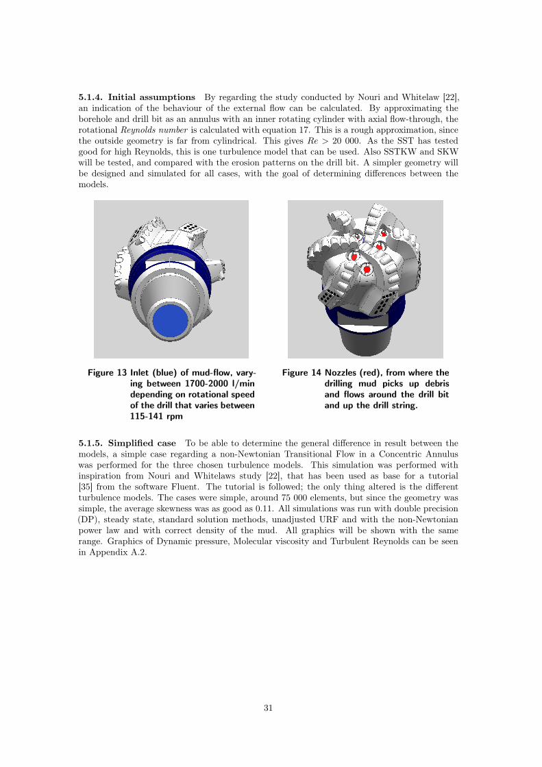
5.1.4. Initial assumptions By regarding the study conducted by Nouri and Whitelaw [22],an indication of the behaviour of the external flow can be calculated. By approximating theborehole and drill bit as an annulus with an inner rotating cylinder with axial flow-through, therotational Reynolds number is calculated with equation 17. This is a rough approximation, sincethe outside geometry is far from cylindrical. This gives Re > 20 000. As the SST has testedgood for high Reynolds, this is one turbulence model that can be used. Also SSTKW and SKWwill be tested, and compared with the erosion patterns on the drill bit. A simpler geometry willbe designed and simulated for all cases, with the goal of determining differences between themodels.

Figure 13 Inlet (blue) of mud-flow, vary-ing between 1700-2000 l/mindepending on rotational speedof the drill that varies between115-141 rpm

Figure 14 Nozzles (red), from where thedrilling mud picks up debrisand flows around the drill bitand up the drill string.

5.1.5. Simplified case To be able to determine the general difference in result between themodels, a simple case regarding a non-Newtonian Transitional Flow in a Concentric Annuluswas performed for the three chosen turbulence models. This simulation was performed withinspiration from Nouri and Whitelaws study [22], that has been used as base for a tutorial[35] from the software Fluent. The tutorial is followed; the only thing altered is the differentturbulence models. The cases were simple, around 75 000 elements, but since the geometry wassimple, the average skewness was as good as 0.11. All simulations was run with double precision(DP), steady state, standard solution methods, unadjusted URF and with the non-Newtonianpower law and with correct density of the mud. All graphics will be shown with the samerange. Graphics of Dynamic pressure, Molecular viscosity and Turbulent Reynolds can be seenin Appendix A.2.

31

• Dynamic Pressure

SSTKW predicts lowest pressure in the narrow-gap region close to the outlet, andTrans-SST the highest

SKW predicts a medium-pressure region "before" the rotating annulus close to theoutlet, seen in figure 15. None of the other models predict this.

• Molecular Viscosity

SSTKW predicts more fluctuations close to the rotating wall than the other two.

Trans-SST predicts higher values in general than the other two.

• Turbulent Reynolds

SKW predicts highest values close to the outlet.

Overall, all models predicts this parameter very similar; although the extreme valuesdiffer.

Figure 15 Dynamic pressure prediction with SKW turbulence model. Medium pressureregion close to the outlet, that none of the other turbulence models included.

5.1.6. The Bore hole When looking at the bore hole at a chosen time in an ideal world,the imprint will look exactly like the teeth rotated one sixth turn, and at the same time moveddownwards the DOC. This pattern was created by extracting the curves from the 3D-modelprovided by Lyng, and then revolving these curves 120◦ creating a sheet intersecting at a numberof places. This imprint was cleaned up and sewn together. This sheet will be used as an outerlimitation for the fluid model, see figure 16.

32

Figure 16 Approximation of the Bore-hole.

5.1.7. Concept Screening A small workshop with supervisor and CFD colleagues was per-formed, where the different alternatives were discussed.

One vs. two cases After discussing pros and cons with the two comparable concepts, conclu-sions were reached that most likely the two-case scenario would create more problems than itwould solve. It would also be difficult to define the velocity in the outer case. Just having onecase is easier to define as only few data exists; and thus explicit input is difficult.

Simplified case From section 5.1.5 and after discussions with CFD-expert Robert Strong [48],following models were chosen for use in the further developed cases: SKW and SSTKW. Thesemodels show reasonable results regarding all parameters and are fairly well known and used inresearch.

Drill hole The decision was reached that the complex imprint created would not be used. In-stead a simpler geometry will be used (see figure 17). The boundary of the fluid can be thoughtof as a bowl being put on top of the drill bit. This will not add to the complexity of the fluidmodel. This geometry can be included in a later state of the simulations.

Chosen concept A case containing both internal and external flow was chosen as the mostsuitable approach. As for the bore-hole, an imaginary bowl will be created and used as boundaryfor the fluid. The simulations will start out using the SKW turbulence model, as this is the mostcommonly known in research.

33

Figure 17 Chosen boundary for the fluid

5.2. System Level Design

In this part of the process, an overall working approach was simulated, where the result can becompared to the flow patterns seen on the used drill bits.

5.2.1. Meshing of the drill bit Meshing was intended to be done in the meshing tool con-nected to Fluent. Unfortunately, this tool does not give an accurate enough mesh that can beused with a good result in the simulations.Instead, two other softwares were tested: ANSYS ICEM and Hexpress. Difficulties were encoun-tered with both these programs, and the end result for the mesh was worse than when using theFluent-connected meshing. As a result, the mesh created will have to be good enough. Otherwisea substantial amount of time will be required for creating a mesh that only might be slightlybetter.The method for the meshing is to create a tetrahedron mesh on all surfaces, with a face sizing onthe surfaces where one could see erosion patterns. The mesh is applied with focus on curvature;there is no gain in adding proximity whilst meshing. This as the small geometrical detail is notof interest, where the focus is on capturing the overall flow motion. The quality of the mesh willbe thoroughly checked, and the goal of average skewness is to be kept as low as possible.This mesh will be saved as a case, and then read into Fluent where the mesh will be changedinto a polyhedron mesh, to reduce the cell number. This will in an extension reduce the timeconsumed for the simulations.

5.2.2. Initial Simulations - First approach The first simulation of the entire drill bit wastested with the SSTKW turbulence model. The fluid used was the properties of water but withthe density of the drilling mud. Data can be seen in Appendix A.3, Table 7, simulation 1. Therotation of the inner wall of the drill bit was set to 140 rpm, and the mass flow of the fluid to40 kg/s. As much data was used from the real case as possible. Steady state was assumed, DP,standard solution methods and default solution controls, under relaxation factors (URF).

Mesh Quality The mesh created has an average skewness of 0, 254 and can be regarded asgood, see Table 3. Although it is suspected that the long time, around 20 minutes, required forgenerating the mesh could indicate complicated areas. The distribution of the mesh skewnesscan be seen below in figure 18. The mesh will later be transformed into polyhedrons, whichreduces the computational time needed.

34

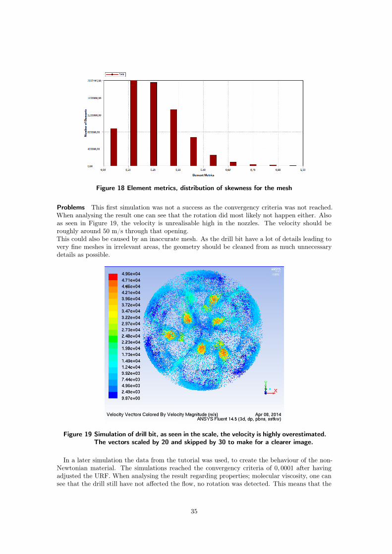
Figure 18 Element metrics, distribution of skewness for the mesh

Problems This first simulation was not a success as the convergency criteria was not reached.When analysing the result one can see that the rotation did most likely not happen either. Alsoas seen in Figure 19, the velocity is unrealisable high in the nozzles. The velocity should beroughly around 50 m/s through that opening.This could also be caused by an inaccurate mesh. As the drill bit have a lot of details leading tovery fine meshes in irrelevant areas, the geometry should be cleaned from as much unnecessarydetails as possible.

Figure 19 Simulation of drill bit, as seen in the scale, the velocity is highly overestimated.The vectors scaled by 20 and skipped by 30 to make for a clearer image.

In a later simulation the data from the tutorial was used, to create the behaviour of the non-Newtonian material. The simulations reached the convergency criteria of 0, 0001 after havingadjusted the URF. When analysing the result regarding properties; molecular viscosity, one cansee that the drill still have not affected the flow, no rotation was detected. This means that the

35

viscosity is less near walls and high in the central parts. Instead, only even distributed turbulentproperties can be seen.To rule out that the velocity in the flow is dominated by the z-component, i.e. that the flow ismainly affected by the mass flow and not the rotation and therefore does not show any rotationalbehaviour, two other simulations were made; one where there is no rotation and one where thereis no flow.

Simulation without flow The simulation without flow seems to have similar, mesh-relatedproblems. The velocity is over-estimated, and the result regarding velocity is not as expected.The main flow is in the range of 0,004-5 m/s, and the maximum value obtained is 235 m/s. Thissolution has been monitored in some points and has stabilized in these points. Data can be seenin Appendix A.3, Table 7, simulation 1.1.

Simulation without rotation A stationary case is simulated, and water with the density of themud is used. The simulation has problems converging, diverging residuals and fluctuating values.Mesh-related problems, wrong assumption regarding steady or transient case could among otherthings cause this. Regarding the mesh, there are a lot of areas that does not affect the generalflow, but have unnecessary many details that can cause unnecessary complex mesh. Data canbe seen in Appendix A.3, Table 7, simulation 1.2.

5.2.3. Secondary Approach After having tried to simulate steady-state with no success, anew approach was needed. Simulating transient cases is a time-consuming option, but in thiscase it might be necessary. Instead of using the original mesh, a very coarse mesh is to begenerated in an initial simulation. Instead of just using convergence criteria for the accuracyof the simulations, monitor points will be included and supervised. When the velocity of thosepoints has started to stabilize to one value the solution can be regarded as converged. A meshwith approximately 178, 000 elements was generated, the most coarse mesh Fluent could generatewithout getting errors, but still too many elements for an easy simulation. The average skewnesswas around 0, 27 and average orthogonal quality around 0, 83, implying a very bad mesh whenalso regarding the max and min values; Fluent gives a warning for low quality. This simulationwas run with the non-Newtonian material model used in section 5.1.5, DP, standard solutionmethods and default solution controls (URF).

This simulation shows promising results seen in Appendix A.3.1, as the velocity is not over-estimated for this simulation. The simulation was made outside the cluster, and was stoppedafter having run for approximately 12 h. If the simulation would have been allowed to run further,convergency criteria would eventually have been reached. Still, this simulation has probably notrotated, as no difference was visible close to the wall for molecular viscosity.Another simulation was run on the cluster where monitor points was put in and monitored forvelocity. The solution showed max velocities of 153 m/s, an unlikely situation. As the maximumvelocity was not in the nozzles, a possible explanation could be mesh-problem. Later on, thenumber of elements can be increased and then one can try to see if one can get approximatelysame frequencies as for the first simulation.

5.2.4. Third Approach Parallel with the transient simulations, the possibility of simulatinga non-rotating case arises. The non-rotating steady-state case should not be as demandingcomputational wise, and the idea is to make particle tracks out of these simulations. Here thereis a possibility to set some of the walls as ’reflecting’ and other surfaces as ’stuck’. The valuein this is to be able to set the outside of the drill bit as ’stuck’ and all the rest of the surfacesto ’reflecting’. This should create a flow pattern for later analysis. If there is a possibility tosee similarities between the flow patterns on the drill bit and the particle tracks simulated, therecould be value in simulating a stationary case in the development process, as these simulationsdoes not require as much computational power.

36

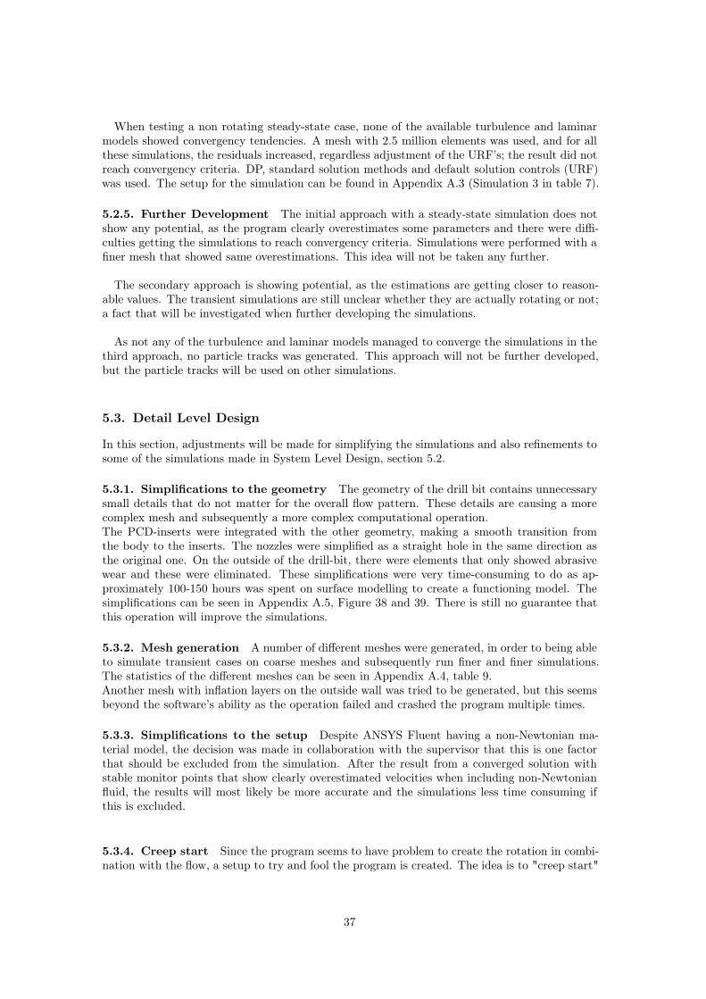
When testing a non rotating steady-state case, none of the available turbulence and laminarmodels showed convergency tendencies. A mesh with 2.5 million elements was used, and for allthese simulations, the residuals increased, regardless adjustment of the URF’s; the result did notreach convergency criteria. DP, standard solution methods and default solution controls (URF)was used. The setup for the simulation can be found in Appendix A.3 (Simulation 3 in table 7).

5.2.5. Further Development The initial approach with a steady-state simulation does notshow any potential, as the program clearly overestimates some parameters and there were diffi-culties getting the simulations to reach convergency criteria. Simulations were performed with afiner mesh that showed same overestimations. This idea will not be taken any further.

The secondary approach is showing potential, as the estimations are getting closer to reason-able values. The transient simulations are still unclear whether they are actually rotating or not;a fact that will be investigated when further developing the simulations.

As not any of the turbulence and laminar models managed to converge the simulations in thethird approach, no particle tracks was generated. This approach will not be further developed,but the particle tracks will be used on other simulations.

5.3. Detail Level Design

In this section, adjustments will be made for simplifying the simulations and also refinements tosome of the simulations made in System Level Design, section 5.2.

5.3.1. Simplifications to the geometry The geometry of the drill bit contains unnecessarysmall details that do not matter for the overall flow pattern. These details are causing a morecomplex mesh and subsequently a more complex computational operation.The PCD-inserts were integrated with the other geometry, making a smooth transition fromthe body to the inserts. The nozzles were simplified as a straight hole in the same direction asthe original one. On the outside of the drill-bit, there were elements that only showed abrasivewear and these were eliminated. These simplifications were very time-consuming to do as ap-proximately 100-150 hours was spent on surface modelling to create a functioning model. Thesimplifications can be seen in Appendix A.5, Figure 38 and 39. There is still no guarantee thatthis operation will improve the simulations.

5.3.2. Mesh generation A number of different meshes were generated, in order to being ableto simulate transient cases on coarse meshes and subsequently run finer and finer simulations.The statistics of the different meshes can be seen in Appendix A.4, table 9.Another mesh with inflation layers on the outside wall was tried to be generated, but this seemsbeyond the software’s ability as the operation failed and crashed the program multiple times.

5.3.3. Simplifications to the setup Despite ANSYS Fluent having a non-Newtonian ma-terial model, the decision was made in collaboration with the supervisor that this is one factorthat should be excluded from the simulation. After the result from a converged solution withstable monitor points that show clearly overestimated velocities when including non-Newtonianfluid, the results will most likely be more accurate and the simulations less time consuming ifthis is excluded.

5.3.4. Creep start Since the program seems to have problem to create the rotation in combi-nation with the flow, a setup to try and fool the program is created. The idea is to "creep start"

37

the simulation, in other words creating a case that is guaranteed to be laminar to begin with.Letting the simulation run for 100 time steps, and then increasing the rotation and flow.This method seems to gain some success, using the SSTKW model, with a low Re-correction[48].This in order to also being able to represent the laminar flow well, and this model has proven toobtain good result in the transition phase.Tendency is shown around flow 0.48 m/s and a rotation of 16 rpm that the simulations arestarting to overestimate the maximum velocity and minimum velocity. The program shows max-imum velocity of 32.25 m/s. When looking at the graphics of the velocity vectors of the nozzles,it is easy to determine that the velocity ranges from 1, 9 − 3, 5 m/s, a result that is reasonable.Graphics can be seen in Appendix A.4.1, Figure 35 .When keeping the flow constant and increasing to 32 rpm the maximum velocity increases to

43.41 m/s, but when regarding the entire flow, it seems likely that this can be due to the coarsemesh, as the velocity vectors show reasonable result, see figure 20.

Figure 20 Velocity vectors seen with limited range, converged after 3648 iterations withcreep start. Setup can be seen in table 8 in Appendix A.4.1

This transient case is run with a very coarse mesh, with a number of elements of around 2 million.The finer mesh is believed not to overestimate the velocities and the average velocity throughthe nozzles will be the same as for these simulations.

5.3.5. Refinements - Finer mesh simulations After getting questionable results from thecreep start simulations, a stationary transient simulation with another mesh was to be tested.The high-quality meshes generated in 5.3.2 is believed to get more accurate result since onlyvery coarse meshes have been tested up to this point in the thesis. A transient but stationarycase is to be set up and run, but when the mesh with approximately 7 million elements is tobe set up on the cluster, the cluster fails unexpectedly. As the script was set on batch whichautomatically closes a simulation after 48 hours, a new try could be made 2 days later. Whenthe cluster had failed with the mesh five times, the conclusion is made that the cluster for somereason has difficulties to handle a complex mesh of that size. This is the mesh generated withinflation layers on only the surfaces exposed to surface erosion.

38

5.3.6. Dynamic mesh simulation After having been unsuccessful to simulate a rotatingcase with MRF, a dynamic mesh simulation was tested. The initial limitation of the project wasnot to do any of these types of simulations, as they are both sensitive to the setup and requiresmassive amount of computational power. A deformable mesh was applied to the fluid, and thewall of the drill to rotate. The rotation was set to 141 rpm, water was used and the velocitythrough the inlet was set to 1.05 m/s. Same timestep was used as in the transient simulations,DP, standard solution methods and default solution controls (URF). After letting the simulationrun over night, no result was visible; not one single iteration had gone through. Weather theprogram had crashed or still running is unclear.

5.3.7. Ansys CFX The change of software was due to the fact that CFX was believed tohave less problems simulating a rotating case, as it is used when simulating among other things;turbines.The difference is that this program is less forgiving regarding mesh quality, i.e. a bad meshwill not be accepted by the program. The correct approach when using this software is to tryand create a flawless mesh in for example ICEM where it is possible to repair separate elementsmanually. Another approach is to import the geometry to the software and use the meshing-toolconnected to CFX. The least time-consuming meshing alternative was chosen.Subsequently, a transient case with rotation was tested. Unfortunately, errors with the simula-tions rose instantly. The errors were never resolved, common fault was checked. It is suspectedthat CFX reacts to the same rotational problems as Fluent ignores to regard. The simulationsdid run problem-free when the rotational velocity was set to zero.

Dynamic mesh Also in CFX, a case with dynamic mesh was created. This was run to see ifthere was a possibility to use for the simulations. For the program to calculate the movementof the mesh, six hours on a standard laptop was needed. The simulation was stopped after ninehours without successfully having done one single iteration.

39

6. Conclusions

Conclusions from the different parts of this project can be seen below.There is no industrial gain performing these types of simulations; the complexity of the simula-tions is too great. The time required is too long and computational power required is too great.No success was achieved in the task of setting up a rotating case.

6.1. Geometry

A lot of effort was put into simplifying the outer geometry of the drill bit. Difficult surfaces werere-built, and some sharp corners were removed. Some of the drill-bit’s features were removed, asthey were suspected not to affect the flow. Inserts were rebuilt into the drill bit, reducing thenumber of faces and complexity of the surfaces. Some of the internal edges were rounded off;something that is believed to make the calculations easier in an area that is out of interest forthis project.The simplifications made to the geometry made a considerable difference in the time needed forgenerating a mesh. With same set-up the meshing time was reduced from around ten minutesto three minutes. Also the statistics for the quality was slightly improved, but no considerabledifference was noticed when regarding the many hours invested in simplifying the geometry. Acomparison can be seen in Appendix A.5 between the two geometries.

6.2. Flow and Simulations

The flow when simulating a stationary case is as expected; the fluid takes the shortest way tothe outlet.The flow through the nozzles is of expected magnitude; estimations made by hand calculations.

Many of the simulations did not reach convergency criteria.

6.3. Flow Patterns

The comparison between the erosion patterns and the particle tracks does not show any similar-ities. As the particle tracks are made from a stationary case, this is to be expected. See figure21 and 22.

6.4. Validation

As no experimental data is available, the degree of validation of the result can be discussed.Although, the residuals is converging down below a value of 1e−6, and the random monitorpoints is stable. The only variable controlled during the simulations is the velocity (flow) and itis also the variable monitored in the points.

6.5. Industrial Gain

As stated in section 1, the chance of any industrial gain today is directly connected to the amountof work and time invested. These simulations show little potential of any industrial gain todayat this bit manufacturer.

40

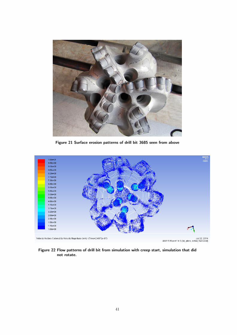
Figure 21 Surface erosion patterns of drill bit 3685 seen from above

Figure 22 Flow patterns of drill bit from simulation with creep start, simulation that didnot rotate.

41

7. Discussion

This project has been conducted at SINTEF Materials and Chemistry during the time period3/2 - 25/4 2014 and 1/7 - 29/8 2014. In total, more time has been spent on this master thesisthan the 800 h planned from the beginning. This is due to many reasons, among other thingsthe decision to perform the type of simulations that already had been mentioned as a limitationof the project. Also testing other softwares’ was outside the limitations of the project.Several unexpected problems has been encountered throughout the project; Initially in theproject, there was no computer available that could handle the software, getting a user onthe cluster was delayed; Two months in to the project, I had still not opened Fluent. Later inthe project, there were problems with not having licenses available.

A reoccurring problem throughout the project has been lack of relevant and updated research.Within such an industry as oil well drilling, many aspects of it are thoroughly researched tooptimize the process and make it more profitable. Lot of money is being invested in R&D everyyear, and many of the larger actors have their own research departments.The problem is that much of the research conducted is company-specific, and never get pub-lished until years later. There is many traces that different types of simulations is being madeon drill bits, but I have been unable to find any further details or results from these. Sameproblem applies when searching for forecasts of the industry, trends and new technology. Thereare extensive forecasts available, but one has to spend thousands of dollars to get hold of thesereports.

7.1. Market Analysis and Background of the problem

The oil drilling industry is a very special and complex industry to understand. In a normalindustry, downtime can be compensated by working overtime, having production running duringweekends, holidays or putting in a night shift. The oil drilling industry is already running twenty-four seven, all year around. It is impossible to retain that profit that was lost during downtime.The delay will be paid back the last day of service for that well.This implies that: The extra cost the delay causes will affect the entire operation and the loss willnot get caught up with. If a drill bit breaks unexpectedly during service and must be changed,the operation will suffer from devastating down-time. Not only must the drill string be taken allthe way to the surface, but also must a fishing tool be taken out to the platform to clean thehole before a new drill-bit can be mounted. During the time this is done, the entire operation isstanding still, and the cost keep ticking away.So if it is possible to come up with a simulation that can give more information about theoperation, direct or indirect resulting in a shorter drilling time; It could be worth investing asubstantial amount of money in it.

7.2. Methodology

This thesis has been inspired by the development process by Ulrich and Eppinger. The majorsteps have been followed, and the steps have been adapted to suit this type of project better.This development process is mostly common in project developing a new product or process, andespecially in mechanical engineering applications, but has a wide range of application also inmarketing, research and finance.From the University’s point of view, it was of interest to use some sort of development process, asthis is a master thesis for the programme Industrial Design and Development. Since Ulrich andEppinger are very adaptable, this process was chosen. Also, it was predicted that this project’sdifferent stages would be suitable for the different steps up to ’Testing and Refinements’. If thisproject had gone according to plan, the development process would have been very suitable for

42

this application as well. But since this project and simulations got stuck in ’System Level Design’-phase, and the expected scenario was to have a working (however slow and rather inaccurate)simulation by then. The plan subsequently was to include more parameters, and also to simulatewith finer meshes and more accurate settings. Also to see if there was a possibility by simplifyingthe geometry to get shorter simulation time.Hindsight, if one would have predicted this outcome of the project; a different developmentprocess would have been chosen, or an overall different scientific method. If this would have beenmade, perhaps the conclusion would have come earlier in the project and the project could havetaken a different direction.

7.3. Research Questions

The research questions are discussed in this section. A discussion regarding the different sourcesof error and a reflection of what could have been done better is as well presented in this section.

7.3.1. Primary Research Question

"Is it economically and technology viable to include CFD-simulations as a step in thedevelopment process of drill bits at a small-scale bit manufacturer?"

This question is not possible to answer, as no simulation of the actual rotational flow was suc-cessfully simulated. If one lets the dynamic mesh and transient simulation run until reachedconvergency criteria, one will have an answer.When testing the previous stated; the simulation would have been extremely long. The time ittook for the software to calculate the movement of the mesh took 6 hours and the simulation wasstopped after 9 hours when not one single iteration had gone through. If one assumes that theiteration would have taken the same amount of time that the calculation of the mesh movement,and having reached convergency in same amount of iterations as the previous transient simula-tion; the simulation would have reached convergency criteria in roughly 7 months.Although, this simulation could have been run on a faster computer which would have shortenedthe time significantly, but on the other hand; The mesh used was only around 200.000 elementsand very coarse and inaccurate. If a good result was to be obtained, the meshes with inflationlayers and good quality would have been better to use, and instead increasing the element countup to 7-10 million. Also, there are many more parameters to regard that this simulation did notinclude at all, adding to the complexity of the simulations. One can debate whether it wouldhave been the correct decision to change primary research question, to weather it is possible ornot to set up such a simulation.

Changes The choice of software was set from the beginning; but after having worked withFluent a lot, I believe that these simulations might have been better suitable for the softwareCFX. CFX has the advantage to be very good at flows with rotating components, but is betterwith steady-state flows; Whereas Fluent is especially good with transient flows. Since this isa case that in an ideal world would be a hybrid between the software’s, the decision betweensoftware’s is not an easy one to address. It seems like CFX has a shorter solution time for similarcases, but requires better quality when it comes to mesh. Another factor putting CFX beforeFluent is that CFX can handle 50% higher number of nodes on the same computer compared toFluent. [49]Personally, I believe a possible working solution would have been to simulate the internal andexternal flow separately as suggested during the concept development phase. By building amodel where the nozzles is flat inlets and a sliding mesh simulation is set up, this might havebeen slightly less computational- wise demanding than the full dynamic mesh simulation. Still,it is not possible to estimate how long time such simulation would take, and how accurate theresults would have been.

43

7.3.2. Guiding Research Questions

What trends are in the Oil-drilling process regarding drilling fluids and drill bits? Regardingdrilling fluids, a lot of R&D is put into developing additives for enhancing certain properties inthe drilling fluid. WBF are still on an upwards trend, accounted for 56% of the market revenuein 2013. The water based fluids also has an estimated compound annual growth rate of 8.8%from 2014 to 2020. The trend in this industry as in many other industries is to have a betterawareness for environmental effects. The challenge is to make the WBF competitive with thedrilling performance of OBF.[50]Basically, two trends in research can be found. As earlier stated, developing additives for WBFfor enhancing performance, but also developing and introducing new compounds into OBF.[51]The research conducted on market forecasts of drilling fluids, is extensive but unfortunatelyunavailable; as the companies conducting the research does not publicly publish these reports.Regarding drill bits, there are several different types on the market. Generally for all types,

new coatings are preventing mud to get stuck as easily is being developed, affecting the processpositively. Also, the development process of drill bits has been time reduced significantly underrecent years. A normal development process from design to finished product is roughly onemonth, but Hughes Christensen managed to design and ship away two bits in only 8 days[52].Implying that this is still a very costly operation with very expensive tooling and raw-materials,but this opens up the possibility for building new designs and testing a bit more.It seems like many of the larger companies have started to include CFD-simulations in theirdevelopment process, but it is unclear whether the simulations are run static or dynamic. Whenregarding the new market of drilling for geothermal energy, the temperature stability comesincreasingly more important. The normal oil well is seldom over 200 ◦C, whereas the geothermalwell can reach 315 ◦C. Even up to 490 ◦C has been measured in a well in Japan.[53]

What turbulence models and boundary conditions are suitable? Any research done in the arearegarding drilling operations? When looking at the different models available, in discussionwith the supervisor and an expert in the area, the decision was reached after having weighedtheir advantages and disadvantages. The SKW is well researched, and better suitable than SKEthat has proven giving bad results for rotating flows. SSTKW is not as well researched as SKW,but shows promising results; and also has an low- Re correction that was suitable when tryingto creep start the simulation.Most research on CFD-simulations in the oil industry has regarded pipe-flow or the circulationaround the drill string further away from the drill bit. Some has researched simulations of theunder-reamer tool, but approximated the geometry in order to get a 2D simulation.

Look at research and models for similar applications from a simulation point of view, solidsthat rotate; adding velocity to the fluid A lot of research is done on turbines or wind turbines,mainly using CFX for those applications. These simulations are common, but fundamentallydifferent from a set-up point of view. In that case, one can easily define the inlet as more orless laminar and assume the flow to get more turbulent after the rotating solid. The inlet andoutlet is far apart, separated by a rotating solid. Whereas in such a case as this, the inlet andoutlet is in the same height in Z, separated by a rotating wall. And the fluid domain is contained,and the gap between the bit and the wall is small. If looking at CFD- simulations done on boatpropellers or helicopter blades, the same limitations exist. These simulations are rotating, butstill have an open domain.

44

7.4. Simplifications

Many simplifications was made to this set up, and even if it did not work, questions are raised ofhow much simplifications one can make? Amongst other things, when letting the fluid in throughthe inlet, it is assumed to be laminar (only has velocity in z). In real life, the fluid is also used torotate the drill bit, by driving a turbine. Meaning; the flow is most likely already fully turbulentwhen it reaches the inlet of the drill bit. To extend the models with multiphase flow is possible,and it is possible to get data from the platform about particle size distribution. How muchextra computational power it requires and how accurate one can reproduce the different sizesand geometries is not something I can estimate. Pressure, temperature, different types of rockthat is being drilled; the simplifications in this types of situations are many. There are erosionmodels available that can be applied on such a case, but whether they are applicable on thistype of model and with these types of programs is not anything I have knowledge of.

45

8. Recommendations and Further Research

The simulations of the flow patterns are an interesting area to research, and should be regardedin the product development process. Knowledge how to optimize the flow to be able to cool thedrill bit more evenly, transport cuttings more efficiently and all other parameters that can beimproved is crucial for the development and can be used as a tool for niching on the market.

Although, these simulations are too difficult to include as a step in the process, as the sim-plifications has to be too many for making the simulations possible to handle for a smaller indus-try. This results in an inaccurate result with low value compared to the time and money invested.

The simulations should be made including multiphase flow, the non-Newtonian fluid used asa written code for CFX or Fluent. This will probably work simulating as a transient case usingdynamic or sliding mesh; using all variations as the drill bit experienced during its operationallife. This is something that can be done as a research project in the future, having access toexperts on CFD and large capacities of computational power.

To make this project as good as possible, it would require experimental data from the operation,and the best case would be to build a model in a controlled environment to test and monitor.

46

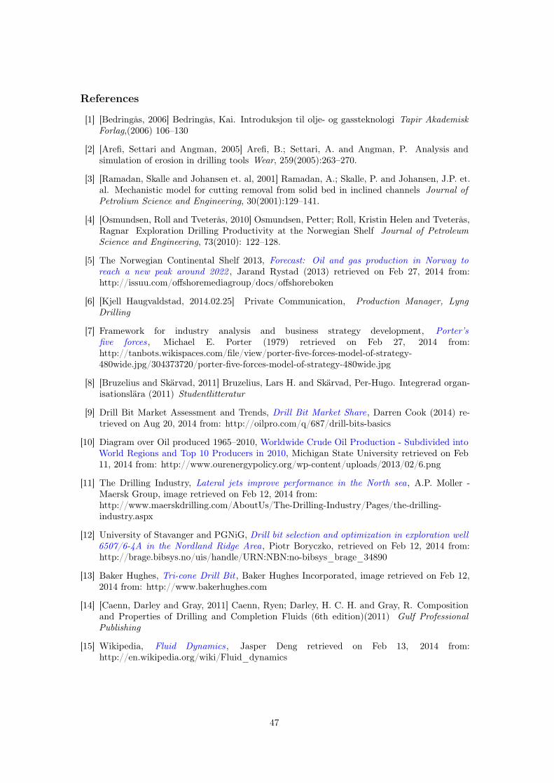
References

[1] [Bedringås, 2006] Bedringås, Kai. Introduksjon til olje- og gassteknologi Tapir AkademiskForlag,(2006) 106–130

[2] [Arefi, Settari and Angman, 2005] Arefi, B.; Settari, A. and Angman, P. Analysis andsimulation of erosion in drilling tools Wear, 259(2005):263–270.

[3] [Ramadan, Skalle and Johansen et. al, 2001] Ramadan, A.; Skalle, P. and Johansen, J.P. et.al. Mechanistic model for cutting removal from solid bed in inclined channels Journal ofPetrolium Science and Engineering, 30(2001):129–141.

[4] [Osmundsen, Roll and Tveterås, 2010] Osmundsen, Petter; Roll, Kristin Helen and Tveterås,Ragnar Exploration Drilling Productivity at the Norwegian Shelf Journal of PetroleumScience and Engineering, 73(2010): 122–128.

[5] The Norwegian Continental Shelf 2013, Forecast: Oil and gas production in Norway toreach a new peak around 2022 , Jarand Rystad (2013) retrieved on Feb 27, 2014 from:http://issuu.com/offshoremediagroup/docs/offshoreboken

[6] [Kjell Haugvaldstad, 2014.02.25] Private Communication, Production Manager, LyngDrilling

[7] Framework for industry analysis and business strategy development, Porter’sfive forces, Michael E. Porter (1979) retrieved on Feb 27, 2014 from:http://tanbots.wikispaces.com/file/view/porter-five-forces-model-of-strategy-480wide.jpg/304373720/porter-five-forces-model-of-strategy-480wide.jpg

[8] [Bruzelius and Skärvad, 2011] Bruzelius, Lars H. and Skärvad, Per-Hugo. Integrerad organ-isationslära (2011) Studentlitteratur

[9] Drill Bit Market Assessment and Trends, Drill Bit Market Share, Darren Cook (2014) re-trieved on Aug 20, 2014 from: http://oilpro.com/q/687/drill-bits-basics

[10] Diagram over Oil produced 1965–2010, Worldwide Crude Oil Production - Subdivided intoWorld Regions and Top 10 Producers in 2010, Michigan State University retrieved on Feb11, 2014 from: http://www.ourenergypolicy.org/wp-content/uploads/2013/02/6.png

[11] The Drilling Industry, Lateral jets improve performance in the North sea, A.P. Moller -Maersk Group, image retrieved on Feb 12, 2014 from:http://www.maerskdrilling.com/AboutUs/The-Drilling-Industry/Pages/the-drilling-industry.aspx

[12] University of Stavanger and PGNiG, Drill bit selection and optimization in exploration well6507/6-4A in the Nordland Ridge Area, Piotr Boryczko, retrieved on Feb 12, 2014 from:http://brage.bibsys.no/uis/handle/URN:NBN:no-bibsys_brage_34890

[13] Baker Hughes, Tri-cone Drill Bit , Baker Hughes Incorporated, image retrieved on Feb 12,2014 from: http://www.bakerhughes.com

[14] [Caenn, Darley and Gray, 2011] Caenn, Ryen; Darley, H. C. H. and Gray, R. Compositionand Properties of Drilling and Completion Fluids (6th edition)(2011) Gulf ProfessionalPublishing

[15] Wikipedia, Fluid Dynamics, Jasper Deng retrieved on Feb 13, 2014 from:http://en.wikipedia.org/wiki/Fluid_dynamics

47

[16] Institute of Applied Mathematics University of Dortmund, Introduction to Com-putational Fluid Dynamics, Dmitri Kuzmin retrieved on Feb 13, 2014 from:http://www.mathematik.uni-dortmund.de/ kuzmin/cfdintro/cfd.html

[17] AccessScience, Vortex , Prof. Sidney Leibovich retrieved on Feb 10, 2014 from:http://www.accessscience.com.proxy.lib.ltu.se//content/vortex/737100

[18] Wikipedia, Reynolds number , Unknown Author retrieved on Oct 14, 2014 from:http://en.wikipedia.org/wiki/Reynolds_number

[19] Researchgate, Vortex or Eddy? , Janamejay Singh retrieved on Feb 13, 2014 from:http://www.researchgate.net/post/What_is_the_difference_between_a_vortex_and_an_eddy2

[20] Academic Resource Center, The Navier-Stokes Equations, Illinois Institute of Technologyretrieved on Feb 13, 2014 from: http://iit.edu/arc/workshops/pdfs/Navier_Stokes.pdf

[21] Fluid Mechanics Tutorial No. 3, Boundary Layer Theory , Freestudy.UK retrieved on Feb13, 2014 from: http://www.freestudy.co.uk/fluid%20mechanics/t3203.pdf

[22] [Nouri and Whitelaw, 1997] Nouri, J. M. and Whitelaw, J. H. Flow of Newtonian and non-Newtonian fluids in an eccentric annulus with rotation of the inner cylinder Int. J. of Heatand Fluid Flow, 18(1997):236–246.

[23] [Chilingarian and Vorapur, 1983] Chilingarian, G. V. and Vorapur, P. (1983). Drilling andDrilling fluids 2nd ed. Elsavier, (1983): 767 pp.

[24] [Darley and Gray, 1988] Darley, H. C. H. and Gray, G. R. Composition and Properties ofDrilling and Completion Fluids 5th ed. Gulf Houston TX, (1988): 630 pp.

[25] [Caenn and Chillingar, 1996] Caenn, Ryen and Chillingar, G. V Drilling fluids: State of theart Journal of Petrolium Science and Engineering, 14(1996): 221–230.

[26] Applied Computational Fluid Dynamics, Lecture 7 - Meshing , André Bakker retrieved onMar 17, 2014 from: http://www.bakker.org/dartmouth06/engs150/07-mesh.pdf

[27] VirginiaTech Educational Material, Mesh Quality , SAS IP Inc retrieved on Apr 23, 2014from: http://www.arc.vt.edu/ansys_help/flu_ug/flu_ug_mesh_quality.html

[28] [Zhang and Che, 2011] Zhang, Lei and Che, Defu. Turbulence models for fluid flow and heattransfer between cross-corrugated plates Numerical Heat Transfer, Part A, 60(2011):410–440.

[29] Introduction to ANSYS FLUENT, Lecture 6: Turbulence Modeling , ANSYS Inc. retrievedon Feb 20, 2014 from: http://imechanica.org/files/fluent_13.0_lecture06-turbulence.pdf

[30] [Versteeg and Malalasekera, 2007] Versteeg, H. K. and Malalasekera, W. An Introduction toComputational Fluid Dynamics The Finite Volume Method (2nd. ed.) Pearson EducationLimited,(2007) 40–113

[31] [Håkansson, Fuchs and Innings et. al., 2012] Håkansson, Anders; Fuchs, Lazlo and Innings,Fredrik et. al. Experimental validation of k-ε RANS-CFD on a high-pressure homogeniservalve Chemical Engineering Science, 71(2012):264–273.

[32] [Murphy, Delfos and Pourquié et. al, 2007] Murphy, S.; Delfos, R and Porquié, M.J.B.Met. al Prediction of strongly swirling flow whitin an axial hydroclone using two commercialCFD codes Chemical Engineering Science, 62(2007):1619–1635.

[33] [Al-Kayiem, Mohd Zaki and Asyraf et. al., 2010] Al-Kayiem, Hussain H.; Mohd Zaki, Nadiaand Asyraf, Muhammad Z. et. al Simulation of the Cuttings Cleaning During the DrillingOperation American Journal of Applied Sciences, 7(6) (2010):800–806.

48

[34] Sandia National Laboratories, Swirling Jets for the Mitigation of Hot Spots and ThermalStratification in the VHTR Lower Plenum, Salvador B. Rodriguez retrieved on Feb 10, 2014from: http://prod.sandia.gov/techlib/access-control.cgi/2011/117474.pdf

[35] Tutourial 8, Non-Newtonian Transitional Flow in an Eccentric Annulus , Fluent Inc. (2007)retrieved on Apr 05, 2014 from: http://cfd.iut.ac.ir/files/annulus.pdf

[36] [Walters and Cokljat, 2008] Walters, Keith W. and Cokljat, Davor A Three-EquationEddy-Viscosity Model for Reynolds-Averaged Navier–Stokes Simulations of TransitionalFlow Journal of Fluids Engineering, 130(2008): 121401—14.

[37] [Vendantam, Wardle and Tamhane et. al., 2012] Vendantam, S. ; Wardle, K.E. and Tamhane,T.V. et. al. CFD Simulation of Annular Centrifugal Extractors International Journal ofChemical Engineering, (2012): ID 759397.

[38] Introduction to ANSYS FLUENT, Lecture 10: Transient Flow Modeling , ANSYSInc. retrieved on Feb 20, 2014 from: http://imechanica.org/files/fluent_13.0_lecture10-transient.pdf

[39] [Wegner, Maltsev and Schneider et. al, 2004] Wegner, B.; Maltsev, A. and Schneider, C. et.al. Assessment of unsteady RANS in predicting swirl... International Journal of Heat andFluid Flow, 25(2004): 528–536.

[40] Computational Fluid Dynamics and Turbulence Mechanics, SyntheticEddy Method , Dominique Laurence retrieved on Sept 26, 2014 from:http://cfd.mace.manchester.ac.uk/twiki/bin/view/Main/SyntheticEddyMethod

[41] Introduction to ANSYS FLUENT, Lecture 9: Advanced Modeling Options, ANSYSInc. retrieved on Feb 20, 2014 from: http://imechanica.org/files/fluent_13.0_lecture09-physics.pdf

[42] ANSYS Fluent , 10.2.3 Single Rotating Reference Frame (SRF)Modeling , Fluent Inc. (2006) retrieved on Sep 12, 2014 from:http://aerojet.engr.ucdavis.edu/fluenthelp/html/ug/node417.htm

[43] ANSYS Fluent , 10.3.1 The Multiple Reference Frame Mode , Fluent Inc. (2006) retrievedon Sep 12, 2014 from: http://aerojet.engr.ucdavis.edu/fluenthelp/html/ug/node419.htm

[44] ANSYS Fluent , 10.3.2 The Mixing Plane Model , Fluent Inc. (2006) retrieved on Sep 12,2014 from: http://aerojet.engr.ucdavis.edu/fluenthelp/html/ug/node420.htm

[45] ANSYS Fluent , 11.2 Sliding Mesh Theory , Fluent Inc. (2006) retrieved on Sep 12, 2014from: http://aerojet.engr.ucdavis.edu/fluenthelp/html/ug/node440.htm

[46] ANSYS Fluent , 11.3 Dynamic Mesh Theory , Fluent Inc. (2006) retrieved on Sep 12, 2014from: http://aerojet.engr.ucdavis.edu/fluenthelp/html/ug/node443.htm

[47] [Ulrich and Eppinger, 2004] Ulrich, Karl T. and Eppinger, Steven D. . Product Design andDevelopment McGraw-Hill(2004)

[48] [Robert Strong, 2014.07.18] Private Communication, Strong Simulation Consulting LLC

[49] CFD online , Comparison of Fluent and CFX for turbomachinery , Post by SijalAhmed Memon (May 27, 2011) retrieved on Sep 26, 2014 from: http://www.cfd-online.com/Forums/cfx/88076-comparison-fluent-cfx-turbomachinery-2.html

[50] Drilling Fluids Market Analysis, Drilling Fluids Market Analysis By Product(OBF, SBF, WBF) By Application (Offshore, Onshore) And Segment ForecastsTo 2020 , Grand View Research (April, 2014) retrieved on Oct 1, 2014 from:http://www.grandviewresearch.com/industry-analysis/drilling-fluids-market-analysis

49

[51] Drilling Fluid Technology, Performances and Environmental Considerations, MohamedKhodja, Malika Khodja-Saber, Jean Paul Canselier, Nathalie Cohaut and Faïza Bergaya(November, 2010) retrieved on Oct 3, 2014 from: http://cdn.intechopen.com/pdfs-wm/12330.pdf

[52] Oil and Gas Journal, Case-specific designs improve drill bit performance,Shelly Cory and Evan Turner (Mars, 2003) retrieved on Oct 3, 2014 from:http://www.ogj.com/articles/print/volume-101/issue-11/drilling-production/case-specific-designs-improve-drill-bit-performance.html

[53] Wall Street Journal, Baker Hughes Drills Deep for High-Stress Bits,Russel Gold (December, 2007) retrieved on Oct 3, 2014 from:http://online.wsj.com/articles/SB10001424052748704825504574580361710978836

50

A. Appendix

A.1. Unstructured Concept Combination Table

When brainstorming for ideas for approach, all limitations were written on a white-board, as seenbelow. From all these limitations, a few different approaches were developed. No full conceptswere developed, but partial concepts that could be included, what was desired to include and inwhat way.

Figure 23 Brainstorming approaches to the problem, over viewing unknown parametersand making approximations

i

A.2. Simplified case SK-ω, SSTKω and Trans-SST turbulence model

Table 6 Ranges of graphicsEccentric Annulus Velocity Dynamic Pressure Turbulent Reynolds Molecular viscosity

[m/s] [Pa] − [kg/m− s]SKW 1.55 - 2.84 1455.2 - 4815.4 10.2 - 100.5 0.0069 - 0.0403SSTKW 1.35 - 2.66 1106.7 - 4237.8 10.2 - 77.0 0.0070 - 0.0402Trans-SST 1.51 - 2.68 1358.6 - 4284.4 9.77 - 81.8 0.0070 - 0.0410Range 1.30 – 2.90 1100 – 4900 9.0 – 110 0.0065 – 0.045

A.2.1. Dynamic Pressure SSTKW predicts least pressure in the narrow-gap region close tothe outlet, and Trans-SST the highest.SKW predicts a medium-pressure region "before" the rotating annulus close to the outlet, seenin figure 24 below. None of the other models predict this.

Figure 24 Dynamic pressure SKW Turbulence model

ii

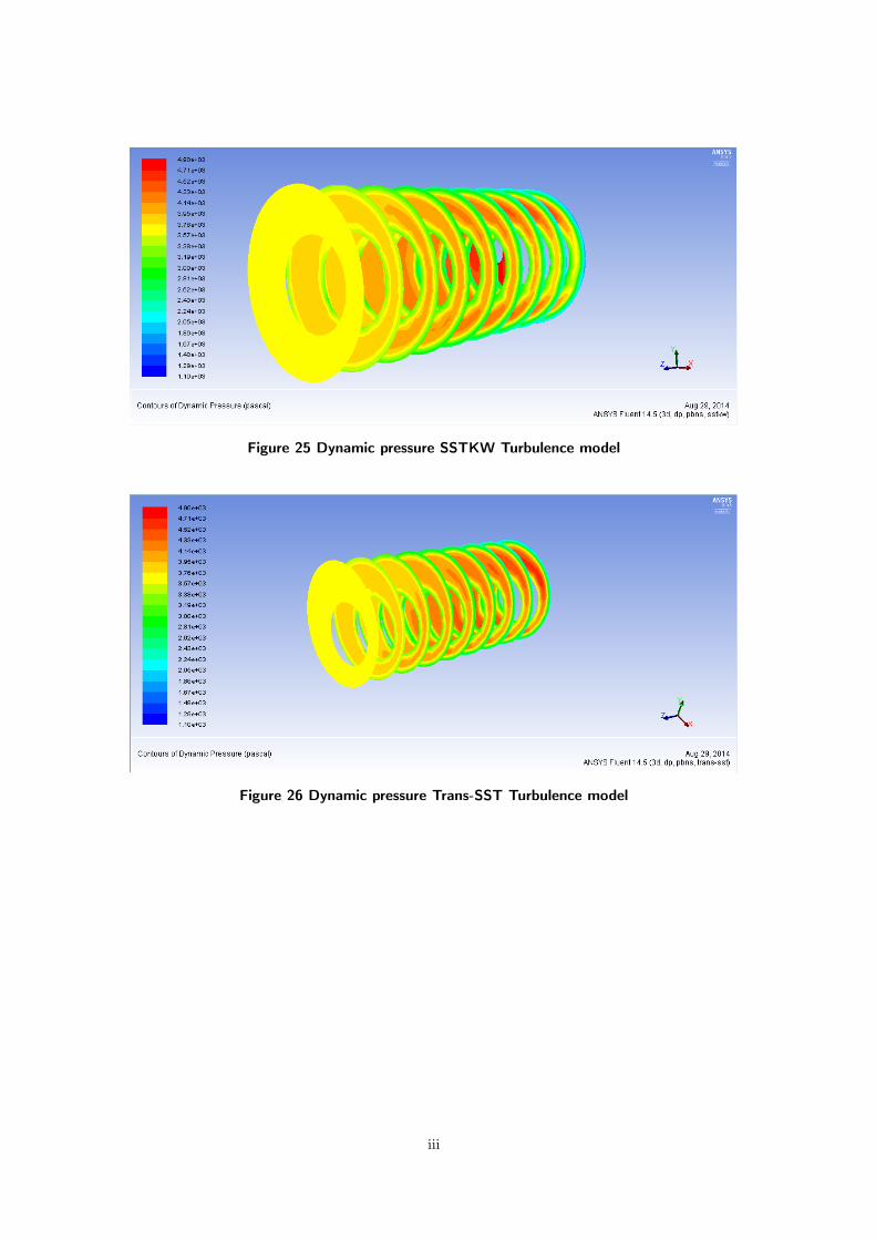
Figure 25 Dynamic pressure SSTKW Turbulence model

Figure 26 Dynamic pressure Trans-SST Turbulence model

iii

A.2.2. Molecular Viscosity SSTKW predicts more fluctuations close to the rotating wallthan the other two.Trans-SST predicts higher values in general than the other two.

Figure 27 Molecular Viscosity SKW Turbulence model

Figure 28 Molecular Viscosity SSTKW Turbulence model

iv

Figure 29 Molecular Viscosity Trans-SST Turbulence model

A.2.3. Turbulent Reynolds SKW predicts highest values close to the outlet.Overall, all models predicts this parameter very similar; although the extreme values differ.

Figure 30 Turbulent Reynolds SKW Turbulence model

v

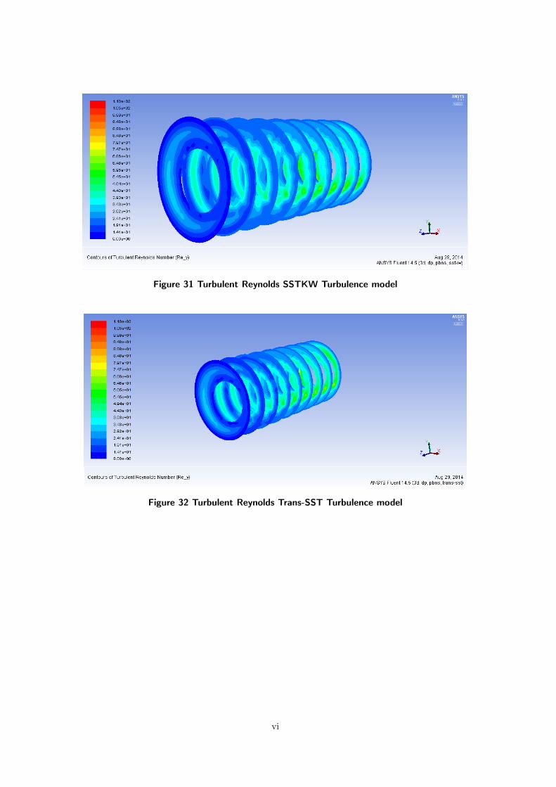
Figure 31 Turbulent Reynolds SSTKW Turbulence model

Figure 32 Turbulent Reynolds Trans-SST Turbulence model

vi

A.3. System Level Design

Abbreviations and elucidation of the table

• Simulations, Approach one to three from referred section.

• Turbulence model used

• Quality, Skewness (Q)

• Number of Elements (El.)

• Mass flow rate kg/s (m)

• Velocity (v)

• Revelations per minute (rpm)

• Material (M)

• Density of the material (ρ)

• Transient (T) or Steady-State(S-S) simulation

• Converged solution, criteria 10−5

Table 7 Simulations in System Level Design-phaseSimulation Model Q El. m v rpm M ρ T / S-S C1 SSTKW 0.254 2.5 milj. 40 - 140 Water 1197.85 S-S N1.1 SSTKW 0.254 2.5 milj. 0 - 140 Water 1197.85 S-S N1.2 SSTKW 0.254 2.5 milj. 40 - 0 Water 1197.85 S-S Y2 SSTKW 0.27 178 k 40 - 140 N.Newt. 1197.85 T "N"3 All 0.254 2.5 milj. 40 - 0 N.Newt. 1197.85 S-S N

The initial approach (Simulation 1, 1.1, 1.2) with a steady-state simulation does not show anypotential, as the program clearly overestimates some parameters. Simulations were performedwith a finer mesh that showed same overestimations.The secondary approach (Simulation 2) is showing potential, as the estimations are getting closerto reasonable values. The transient simulations are still unclear whether they are actually rotat-ing or not; a fact that will be investigated when further developing the simulations.As not any of the turbulence and laminar models managed to converge the simulations in thethird approach (Simulation 3), no particle tracks was generated. This approach will not be fur-ther developed, but the particle tracks will be used on other simulations.

A.3.1. Secondary Approach Simulation: Simulation Results After having tried to sim-ulate steady-state with no success, a new approach is needed. Simulating transient cases is atime-consuming option, but in this case it might be necessary. Instead of using the original mesh,a very coarse mesh is to be generated in an initial simulation. Instead of just using convergencecriteria for the accuracy of the simulations, monitor points will be included and supervised. Whenthe velocity of those points has started to stabilize to one value the solution can be regardedas converged. A mesh with approximately 178, 000 nodes was generated, the most coarse meshfluent could generate without getting errors and still too many elements for an easy simulation.The average skewness was around 0, 27 and average orthogonal quality around 0, 83, implying avery bad mesh when also regarding at the max and min values; Fluent gives a warning for low

vii

quality. This simulation was run with the non-Newtonian material model used in section 5.1.5,DP, standard solution methods and default solution controls (URF).

Figure 33 Scaled residuals for first simulation of transient case.

Figure 34 Scaled vectors for first transient case. Maximum velocity agrees with estima-tion.

viii

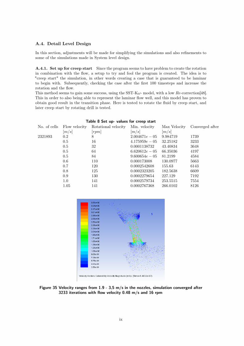
A.4. Detail Level Design

In this section, adjustments will be made for simplifying the simulations and also refinements tosome of the simulations made in System level design.

A.4.1. Set up for creep start Since the program seems to have problem to create the rotationin combination with the flow, a setup to try and fool the program is created. The idea is to"creep start" the simulation, in other words creating a case that is guaranteed to be laminarto begin with. Subsequently, checking the case after the first 100 timesteps and increase therotation and the flow.This method seems to gain some success, using the SST-Kω- model, with a low Re-correction[48].This in order to also being able to represent the laminar flow well, and this model has proven toobtain good result in the transition phase. Here is tested to rotate the fluid by creep start, andlater creep start by rotating drill is tested.

Table 8 Set up- values for creep startNo. of cells Flow velocity Rotational velocity Min. velocity Max Velocity Converged after

[m/s] [rpm] [m/s] [m/s]2321893 0.2 8 2.004671e− 05 9.984719 1739

0.5 16 4.175959e− 05 32.25182 32330.5 32 0.0001138732 43.40834 36480.5 64 6.620612e− 05 66.35036 41970.5 84 9.600654e− 05 81.2199 45840.6 110 0.000173008 130.0977 56630.7 120 0.0002542608 155.63 61430.8 125 0.0002323205 182.5638 66090.9 130 0.0002279654 227.129 71921.0 141 0.0002579734 253.5515 75541.05 141 0.0002767368 266.0102 8126

Figure 35 Velocity ranges from 1.9 - 3,5 m/s in the nozzles, simulation converged after3233 iterations with flow velocity 0.48 m/s and 16 rpm

ix

Figure 36 Particle tracks for creep start simulation, entire fluid has rotated

Figure 37 Turbulent Reynolds Rotating Fluid

x

A.4.2. Mesh refinements These mesh refinements was made to have different quality meshesto test, for the later simulations. When running transient simulations, starting out with a coarsemesh minimizes the calculation time. Subsequently, finer mesh for better result can be used.

Table 9 Mesh statisticsMesh Properties Cells Faces Nodes Max. Min. Inflationname Aspect Orthogonal layers

Ratio Quality

FFF. Coarse (C) 2 321 893 4 477 901 439 279 7.40017e+02 8.70001e-03 NoFFF. 1 C 890 237 1 825 284 171 420 1.5721e+02 5.51120e-02 NoFFF. 2 C/M 2 519 491 5 146 675 475 645 7.08227e+02 1.25881e-02 NoFFF. 3 C/M 2 517 727 5 143 120 475 358 7.08227e+02 1.25881e-02 NoFFF. 4 C/M 2 717 281 5 549 145 512 261 3.74554e+04 2.50153e-04 NoFFF. 5 Medium (M) 7 058 590 14 381 586 1 313 882 1.10549e+04 5.15630e-04 No

xi

A.5. Further Development

A.5.1. Simplification to the geometry Below can be seen a comparison of the geometrycut through before and after the detail simplifications to the geometry.The PCD-inserts were integrated with the other geometry, making a smooth transition from thebody to the inserts. The nozzles were simplified as a straight hole in the same direction as theoriginal one. On the outside of the drill-bit, there were elements that only showed abrasive wearwhen looking at the drill bits, and these were eliminated.

Figure 38 3D Model of the fluid for the initial simulations. Lot of sharp edges andunnecessary details.

xii

Figure 39 3D Model after simplifications made. Lot of detail featuring is gone, and asmany as possible of the sharp edges is rounded off.

xiii

A.5.2. Transient simulation, creep start of rotation Below can be seen graphics of atransient simulation, where the flow was held constant from the beginning, only creep startingthe rotation of the drill bit.

Figure 40 Particle tracks rotating drill MRF; slowly increasing the rotation

Points monitored during the simulations. Rpm has been increased every 100 iterations, some-thing that cannot be seen in the plots below. The conclusion is reached that this creep start didnot solve the problem causing the drill not to rotate.

Figure 41 Surface monitor 1

xiv

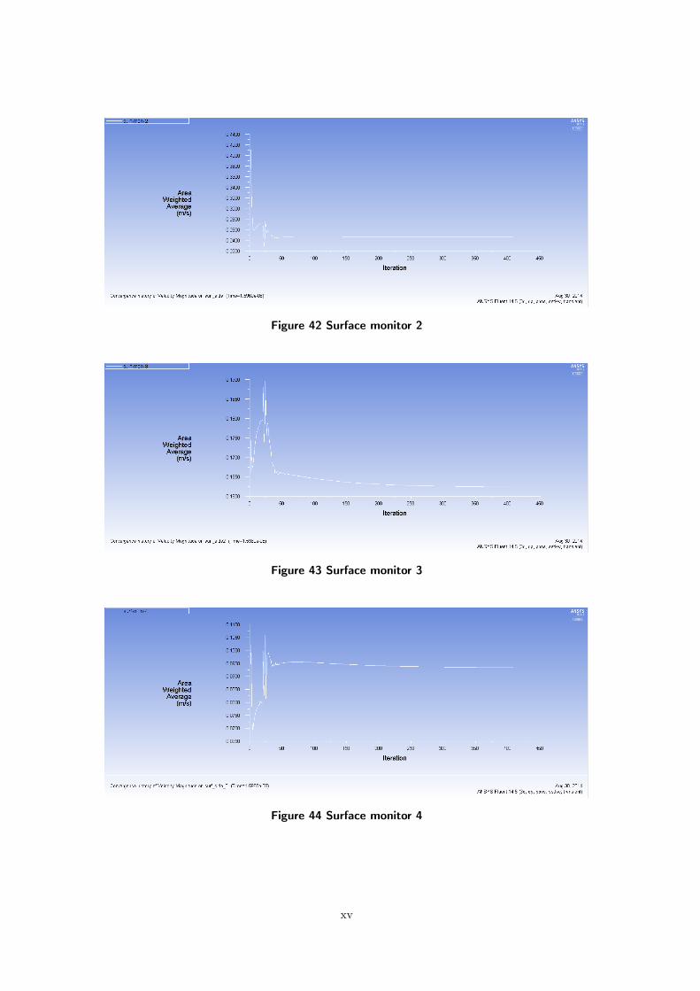
Figure 42 Surface monitor 2

Figure 43 Surface monitor 3

Figure 44 Surface monitor 4

xv