Geographic Information System (GIS) What is GIS? - Connect ...

int j geographical information science 1997 vol 11 no 7 699plusmn 718
Research Article
Mapping urban air pollution using GIS a regression-based approach
DAVID J BRIGGS1 SUSAN COLLINS2 PAUL ELLIOTT3 PAUL FISCHER5 SIMON KINGHAM4 ERIK LEBRET5 KAREL PRYL6 HANS VAN REEUWIJK5 KIRSTY SMALLBONE7
and ANDRE VAN DER VEEN5
1 Nene Centre for Research Nene College Northampton NorthamptonNN2 7AL England UK2 She eld Centre for Geographic Information and Spatial Analysis Universityof She eld She eld S10 2TN England UK3 Department of Epidemiology and Public Health Imperial College MedicalSchool at St Maryrsquos London W2 1PG England UK4 Institute of Environmental and Policy Analysis University of Huddersreg eldHuddersreg eld HD1 1RA England UK5 RIVM 1 Antonievanhoeklaan 3720 BA Bilthoven The Netherlands6 National Institute of Hygiene Warsaw Poland7 Department of Geography University of Brighton Brighton BN2 4ATEngland UK
(Received 8 June 1996 accepted 23 December 1996 )
Abstract As part of the EU-funded SAVIAH project a regression-based meth-odology for mapping tra c-related air pollution was developed within a GISenvironment Mapping was carried out for NO2 in Amsterdam Huddersreg eld andPrague In each centre surveys of NO2 as a marker for tra c-related pollutionwere conducted using passive di usion tubes exposed for four 2-week periods AGIS was also established containing data on monitored air pollution levels roadnetwork tra c volume land cover altitude and other locally determined fea-tures Data from 80 of the monitoring sites were then used to construct a regressionequation on the basis of predictor environmental variables and the resultingequation used to map air pollution across the study area The accuracy of themap was then assessed by comparing predicted pollution levels with monitoredlevels at a range of independent reference sites Results showed that the mapproduced extremely good predictions of monitored pollution levels both forindividual surveys and for the mean annual concentration with r2~0 79plusmn 0 87across 8plusmn 10 reference points though the accuracy of predictions for individualsurvey periods was more variable In Huddersreg eld and Amsterdam further mon-itoring also showed that the pollution map provided reliable estimates of NO2
concentrations in the following year (r2~0 59plusmn 0 86 for n=20)
1 Introduction
Despite the major improvements in air quality seen in many European citiesover the last 30plusmn 40 years the problem of urban air pollution remains Levels oftraditional pollutants such as smoke and sulphur dioxide (SO2 ) have declined as aresult of industrial restructuring technological changes and pollution control butthe rapid growth in road tra c has given rise to new pollutants and new concernsBetween 1970 and 1990 for example passenger car transport in Europe increasedby ca 3 4 per cent per annum and car ownership in East European countries is
1365plusmn 881697 $12acute00 Ntilde 1997 Taylor amp Francis Ltd
D Briggs et al700
currently rising by 7plusmn 12 per cent per year (Stanners and Bordeau 1995) As a resultof these increases emissions of many pollutants are growing in the UK emissionsof nitrogen dioxide (NO2 ) of which 45plusmn 50 per cent is derived from the transportsector rose by 120 per cent between 1970 and 1990 before declining slightly emissionsof volatile organic compounds (VOCs) of which ca 40 per cent derives fromtransport rose by 73 per cent (Department of the Environment 1995) For the futurethese trends seem set to continue In the absence of major shifts in policy a furtherdoubling of both passenger and freight transport in Europe is anticipated by theyear 2010 (Stanners and Bordeau 1995 ) Notwithstanding the e ects of improvementsin engine design and fuel technology this is likely to lead to at least the maintenanceof current emission levels in most West European countries In East Europe wherethe rates of increase are higher emissions may be expected to grow
Against this background there has been heightening concern about the healthe ects of tra c-related pollution Several factors contribute to this concern One isthe simple arithmetic of exposure In Europe for example about 70 per cent of thepopulation is classireg ed as urbanized (UNEP 1993 ) while Flachsbart (1992) estimatesthat between 9 5 and 18 million people spend a considerable part of their workingday at or near roadsides Equally urban areas are estimated to account for themajor proportion of emissions The potential for human exposure to tra c-relatedpollution is therefore large Secondly there is growing evidence from epidemiologicalstudies of a relationship between air pollution and respiratory illness and mortality(eg Schwartz 1993 1994) and of increased levels of respiratory symptoms in peopleliving close to major roads or in areas of high tra c density (eg Edwards et al1994 Ishizaki et al 1987 Weiland et al 1994 Wjst et al 1993) In a study of 1000adults in Oslo NILU (1991 ) also found a positive association between self-reportedsymptoms of cough and chronic bronchitis and modelled levels of air pollution atthe place of residence At the same time there has been an apparent increase inlevels of respiratory illness particularly asthma in vulnerable groups such as childrenand the old (Anderson et al 1994 Burney 1988 Burney et al 1990 Haahtelaet al 1990)
In the light of these concerns there is clearly a need for improved informationon levels of tra c-related air pollution and their potential links to human healthThis information is required for a wide range of purposes to help investigate therelationships involved as inputs to health risk assessment to assist in establishingand monitoring air quality standards and to help evaluate and compare transportpolicies and plans For all these purposes information is needed not only on thetemporal trends in air pollution (as for example provided by data from reg xed-sitemonitoring stations) but also on geographical variations Maps are needed forexample to identify pollution hot-spotsrsquo to dereg ne at-risk groups to show changesin spatial patterns of pollution resulting from policy or other interventions and toprovide improved estimates of exposure for epidemiological studies
Mapping urban air pollution nevertheless faces many problems The complexgeography of emission sources and the equal complexity of dispersion processes inan urban environment mean that levels of air pollution typically vary over extremelyshort distances often no more than a few tens of metres (eg Hewitt 1991) On theother hand data on both emission sources and pollution levels are often sparse Asa result maps of urban air pollution tend to be highly generalized and estimates ofexposure to air pollutants subject to serious misclassireg cation
The development of GIS techniques however o ers considerable potential to
Mapping urban air pollution using GIS 701
improve upon this situation Digital data on urban road networks for example arenow becoming increasingly available providing a valuable data source for pollutionmodelling The spatial analysis and overlay techniques available in GIS also pro-vide powerful tools for pollution mapping This paper describes and evaluates aregression-based approach to air pollution mapping developed as part of theEU-funded SAVIAH (Small Area Variations in Air quality and Health) project Thisstudy was a multi-centre project involving collaborators in London and Huddersreg eld(UK) Bilthoven (Netherlands) Prague (Czech Republic) and Warsaw (Poland )The aim of the study was to develop and validate methods for analysing relationshipsbetween air pollution and health at the small area scale A description of the overallSAVIAH study is given by Elliott et al (1995)
2 Approaches to pollution mapping
Traditionally two general approaches to air pollution mapping can be identireg edspatial interpolation and dispersion modelling (Briggs 1992) The former uses statist-ical or other methods to model the pollution surface based upon measurements atmonitoring sites With the development of GIS and geostatistical techniques in recentyears a wide range of spatial interpolation methods have now become availableBurrough (1986) divides these into global methods (eg trend surface analysis)which reg t a single surface on the basis of the entire data set and local methods (egmoving window methods kriging spline interpolation) in which a series of localestimates are made based on the nearest data points Recently particular attentionhas tended to focus on kriging in its various forms (eg Oliver and Webster 1990Myers 1994) Nevertheless despite a number of studies comparing this with othertechniques (eg Abbass et al 1990 Dubrule 1984 Laslett et al 1987 von Kuilenburget al 1982 Weber and Englund 1992 Knotters et al 1995 ) there is no clear consensusto suggest that any one approach is universally optimal Instead performance of thevarious methods tends to vary depending upon the character of the underlyingspatial variation being modelled and the specireg c characteristics of the data concerned(eg sampling density sampling distribution)
A number of these interpolation methods have found applications in pollutionmapping albeit mainly at a relatively broad regional scale Linear interpolation forexample has been widely used to derive contour maps of pollution surfaces on thebasis of point measurements (eg Archibold and Crisp 1983 Muschett 1981) Krigingin its various forms has been used to map national patterns of NO2 concentrations(Campbell et al 1994 ) acid precipitation (Venkatram 1988 Schaug et al 1993) andozone concentrations (Lefohn et al 1988 Liu et al 1995) and to help designcontinental-scale monitoring networks (Haas 1992) Wartenberg (1993) also reportsthe use of kriging to estimate and map exposures to groundwater pollution andmicrowave radiation Mapping of tra c-related pollution in urban areas howeverpotentially faces far more severe di culties First and foremost is the inherentcomplexity of the pollution surfaces involved Within an urban area emissions mayderive from a large number of intersecting line sources The distance decay ofpollution levels away from these sources is also rapid and greatly a ected by localmeteorological and topographical conditions Marked variations in pollutant levelscan thus occur over distances of less than 100 metres in urban areas (eg Hewitt1991) In contrast the density and distribution of most monitoring networks isgenerally poor The number of stations monitoring pollutants such as NO2 VOCs
D Briggs et al702
and reg ne particulates on a routine basis is generally small and the location of thesestations is often biased towards specireg c pollution environments As a consequencethe existing monitoring networks provide only a limited picture of spatial patternsof urban air pollution potentially biased estimates of trends and poor indicationsof human exposure Even where purpose-designed surveys can be conducted (egusing passive samplers) constraints of time and cost severely limit the samplingdensity which is possible
The main alternative to interpolation is the use of dispersion modelling tech-niques This involves constructing a dynamic model of the dispersion processestaking account of all the main factors which inmacr uence the ultimate pollution concen-tration reg eld It is an approach which has been most widely used in relation to pointsources but several models have also been built for road tra c pollution examplesinclude the CALINE models developed on behalf of the US EPA (Benson 1992 )the CAR model developed in the Netherlands (Eerens et al 1992) the HighwaysAgency Design Manual for Roads and Bridges (DMRB) model and the ADMSmodel (which has been developed from DMRB by Cambridge EnvironmentalResearch Consultants Ltd)
Dispersion modelling has much to commend it as a basis for air pollutionmapping in that it attempts to remacr ect the processes of dispersion and can relativelyeasily be adapted to new pollutants or areas without the need for additional mon-itoring On the other hand it also has a number of important constraints Amongstthe most serious are the relatively severe data demands of most dispersion modelstypically data are required not only on the distribution of the road network butalso tra c volumes and composition tra c speed emission factors for all mainclasses of vehicle street characteristics (eg road width building height or type) andmeteorological conditions (eg wind speed wind direction atmospheric stabilitymixing height) Rarely are these data available for a su ciently dense network oflocations in an urban area with the result that considerable data extrapolation oftenhas to occur Line dispersion models also provide estimates of pollution concentra-tions only within the immediate vicinity of the roadwayETH up to a distance of only35 metres in the CAR model for example and ca 200 metres for the CALINEmodels This means that they do not easily provide information on variations inbackground concentrations at greater distances from major roads In additionunlike spatial interpolation techniques there is as yet little progress either in integrat-ing dispersion models into GIS or coupling the two technologies ( though the ADMSmodel does have a limited interface with GIS)
Against this background there is clearly a need to develop more practicabletechniques of air pollution mapping which can make use of the capability o eredby GIS and extract the maximum amount of information from the di erent datasets which are available within urban areas Regression-mapping o ers particularpotential in this respect This involves using least squares regression techniques togenerate predictive models of the pollution surface based on a combination ofmonitored pollution data and exogenous information The technique is widely usedfor exploratory and explanatory investigations and is also used to help classifyremote sensing imagery Regression methods have only rarely been used howeverfor mapping purposes Examples include the development of a regression-basedmodel of road salt contamination (Mattson and Godfrey 1994) air pollution (Wagner1995) and soil depth (Knotters et al 1995)
Mapping urban air pollution using GIS 703
3 The SAVIAH regression method
31 Pollution monitoringAs part of the SAVIAH study surveys of nitrogen dioxide pollution were carried
out in four study areas Huddersreg eld (UK) Amsterdam (Netherlands) Prague(Czech Republic) and Poznan (Poland ) NO2 was selected as the pollutant of concernboth because it is considered to provide a good marker of tra c-related pollutionand because of its relative ease of measurement using low-cost passive samplingdevices A summary of the study areas and the sampling design is given in table 1because of di erences in sampling regime results from the Poznan study are notreported here
In each area a pilot survey was initially undertaken in June 1993 during whichtwo di erent samplers Palmes tubes and Willems badges were compared (vanReeuwijk et al 1995) and sampling strategies assessed Thereafter three surveys werecarried out in October 1993 FebruaryMarch 1994 and MayJune 1994 On eachof these three occasions Palmes tubes were exposed for a period of two-weeks at areg xed set of 80 core monitoring sites in each study area In each area 40 so-calledvariable sites were also established (ie sites which were moved from one survey toanother) to provide further insight into local patterns of variation and to provideadditional validation of the results In addition a series of 8plusmn 10 reference sites ineach area was monitored continuously on a monthly basis over the study period toprovide independent estimates of the mean annual pollution concentration and toact as reference sites for validation purposes In Huddersreg eld and Amsterdam onlymonitoring was also continued at a limited number of sites over the following yearin order to allow the stability of the pollution surface to be analysed
In each case duplicate samplers were exposed at each site in order to provide ameasure of precision and to give back-up in the case of damage or loss to one tubeDespite these precautions however loss or damage to ca 10 per cent of samplersoccurred resulting in gaps within the full data set For this reason estimates of meanannual pollution at each of the 80 corersquo sites were made using a mixed-e ect modelwith terms for measurement error and site and survey e ects (Lebret et al 1995)Signireg cantly when compared to the measured means at the referencersquo sites thesewere found to provide good estimates of the true mean with an r2 value across allstudy areas of 0 95 (n=28) and a standard error of the estimate of 5 02 mg m Otilde
3 These modelled results were therefore used in all subsequent analysis Mean concen-trations for core sites in Huddersreg eld and Amsterdam are shown in reg gures 1 and 2
32 Development of a regression modelDevelopment and testing of a regression-mapping approach was carried out in
all three centres using ARCINFO version 71 In each centre a GIS was reg rstestablished containing four main sets of data
ETH road tra c (eg road network road type tra c volume)ETH land coverland useETH altitudeETH monitored NO2 concentrations
Additional variables were also added locally as required The variables and datasources used in each centre are summarized in table 2
Due to variations in data availability classireg cation systems (eg of tra c macr owand land use) and local topography it was not felt appropriate to use exactly the
D Briggs et al704
Tab
le1
Su
mm
ary
des
crip
tio
no
fst
ud
yar
eas
and
surv
eyre
sult
s
Co
nce
ntr
atio
n(m
gm
Otilde3)
Su
rvey
Stu
dy
area
Des
crip
tio
nN
o
Dat
eD
evic
e(n
o)
Min
Max
Mea
nS
D
Am
ster
dam
Urb
anar
eaw
ith
bu
syro
ads
1Ju
ne
July
1993
Bad
ges
(80
)12
473
536
412
2b
ord
ered
by
hig
h-r
ise
Tu
bes
(20
)b
lock
sar
eaca
26
km
2
2N
ov
1993
Tu
bes
(80
)39
672
151
86
4p
opu
lati
on15
588
33
Feb
Mar
ch19
94T
ub
es(8
0)
282
682
500
72
(199
2)
4M
ayJ
un
e19
94T
ub
es(8
0)
275
708
413
108
Hu
dd
ersreg
eld
Mix
edu
rban
-ru
ral
area
ar
ea1
Jun
e19
93B
adge
s(8
0)
105
884
282
141
305
km
2a
ltit
ud
era
nge
Tu
bes
(80
)80
plusmn582
mO
D
po
pula
tion
2O
ct
1993
Tu
bes
(20
)27
778
547
610
221
130
03
Feb
19
94T
ub
es(8
0)
95
515
256
95
(199
1)
4M
ay19
94T
ub
es(8
0)
156
694
331
127
Tu
bes
(80
)
Pra
gue
Mix
ture
of
resi
den
tial
1
Jun
eJu
ly19
93B
adge
s(8
0)
56
658
222
139
ind
ust
rial
and
op
ensp
ace
Tu
bes
(20
)ar
eaca
48
km
2
alti
tud
e2
Oct
1993
Tu
bes
(80
)21
965
439
610
2ra
nge
172plusmn
355
mO
D
3F
eb19
94T
ub
es(8
0)
200
577
334
96
po
pula
tion
163
700
(199
1)
4M
ay19
94T
ub
es(8
0)
148
829
367
180
Mapping urban air pollution using GIS 705
Figure 1 Monitoring results mean annual NO2 concentration Huddersreg eld UK
Figure 2 Monitoring results mean annual NO2 concentration Amsterdam TheNetherlands
D Briggs et al706
Table 2 Data sets and sources
Centre Variable Dereg nition Data source
Road network All roads (stored as 10 mHuddersreg eld Aerial photography (1510 k)grid )
Tra c volume Mean 18 hour tra c macr ow Motorways automatic(vehicleshour) for each counts (Department ofroad segment Transport ) A roads
automatic counts (WestYorkshire Highways)manual counts (KirkleesHighways Services)Other roads (estimatesbased on local knowledge)
Land cover Land cover class (20 Aerial photography (1510 k)classes stored as 10 mgrid )
Altitude Metres OD 50 m DTM (YorkshireWater)
NO2 concentration Mean NO2 concentration Field monitoring(by survey period andmodelled annual mean)
Sample height Height of sampler Field measurement(metres) above groundsurface
Site exposure Mean angle to visible Field measurementhorizon at eachmonitoring site
Topographical Mean di erence in GIS-GRID based on DTMexposure altitude between each
pixel and the eightsurrounding pixels
Amsterdam Road network All access roads within City highways authoritythe study area
Road type Classireg cation of road on City highways authoritybasis of populationserved
Distance to road Distance to nearest road GISserving gt25 000people
Land cover Area of built up land Planning mapsNO2 concentration Mean NO2 concentration Field monitoring
(by survey period andmodelled annual mean)
Prague Road network All tra c routes in the Department ofstudy area Development Prague
Municipal AuthorityTra c volume Mean daytime tra c Department of
macr ow (vehicleshour) Development PragueMunicipal Authority
Land cover Land cover class (6 City planning mapsclasses based onbuilding density)
Altitude Height (metres) above Topographic mapssea level
NO2 concentration Mean NO2 concentration Field monitoring(by survey period andmodelled annual mean)
Mapping urban air pollution using GIS 707
same regression procedure in all study areas Instead each centre developed its ownequation subject only to the constraint that (a) it included terms for tra c volumeland cover and topography (b) a similar bu ering approach was used In each centretherefore data on the relevant input variables were reg rst computed for a series ofbands around each monitoring site (to a distance of 300 m) using the GRID routinesin ARCINFO These were then entered into a multiple regression analysis using asthe dependent variable either the monitored NO2 values for a specireg c survey period(to provide a pollution map for that period alone) or the modelled annual meanconcentration (to provide an annual average pollution map) The equation thusgenerated was reg nally used to compute the predicted pollution level at all unmeasuredsites for a reg ne grid of points across the study area and the results mapped
As an example details of the approach used in Huddersreg eld are presented inreg gure 3 In brief the method was as follows
1 GIS development Coverages were compiled in ARCINFO as outlined intable 2
2 Computation of a weighted tra c volume factor (Tvol300) for the 300 metrebu er around each monitoring site Daytime tra c volumes (vehicle kmhour) wereestimated for each 20 m zone around each sample point (to a maximum distance of300 metres) using the FOCALSUM command in ARCINFO Results were thenentered into a multiple regression analysis (in SPSS) against the modelled meanannual NO2 concentrations and di erent combinations of band width comparedThe best-reg t combination (as dereg ned by the r2 value) was selected and weights foreach band determined by examination of the slope coe cients This gave two bandsweighted as follows 0 plusmn 40 m (weight=15) and 40plusmn 300 m (weight=1) These werethus combined into a compound tra c volume factor (equation (1)
T vol300=15Tvol0plusmn 40 + Tvol40plusmn 300 (1 )
3 Computation of a compound land cover factor (Land300 ) for the 300 m bu eraround each monitoring site The area of each land use type (hectares) within each20 m band around each sample point (to a maximum distance of 300 m) was calcu-lated using the FOCALSUM command in ARCINFO Results were then enteredinto a multiple regression analysis (in SPSS) against the residuals from the previousanalysis (step 2) Di erent combinations of land cover and distance were comparedin terms of the r2 value and the best-reg t non-negative combination selected Thisgave a single band (0 plusmn 300 m) comprising two land use types high density housing(HDH0plusmn 300 ) and industry (Ind0plusmn 300 ) Weights were identireg ed by examination of theslope coe cients and a compound land use factor computed in equation (2)
L and300=1 8HDH0plusmn 300+ Ind0plusmn 300 (2 )
4 Stepwise multiple regression analysis was rerun using the two compoundfactors (Tvol300 and L and300 ) together with altitude (variously transformed) topexsitex and sampler height against the modelled mean nitrogen dioxide concentrationsOnly variables signireg cant at the 5 per cent conreg dence level were retained A numberof equations were derived from this procedure all explaining generally similarproportions of variation in the monitored NO2 levels From these regression equa-tion (3) was chosen for further analysis because of its marginally higher r2 valuewhich was 0 607 and because all variables were signireg cant at the 0 05 level
MeanNO2=11 83+ (0 00398Tvol300 )+ (0 268Land300 )
Otilde (0 0355RSAlt )+ (6 777Sampht) (3)
D Briggs et al708
Fig
ure
3T
he
regr
essi
on
map
pin
gm
eth
od
Hu
dd
ersreg
eld
U
K
Mapping urban air pollution using GIS 709
5 This equation was then used to construct a complete air pollution coveragefor the study area by applying the equation on a cell by cell basis to all locations inthe study area
In Prague a broadly similar approach was used In this case however airpollution data were seen to be skewed so the data were log-transformed prior toanalysis In this case also no attempt was made to produce a compound tra cvolume instead separate tra c volume factors were computed for each zone Asingle land cover factor was computed in equation (4) representing the weightedsum of the areas of each land cover type within the bu er zone around the site andequation (5) was thus derived
L and = (areadensity class) (4)
LogMeanNO2=3 48+ (1 17Tvol60 )+ (0 125Tvol120 )
+ (0 000554L and60 ) Otilde (0 00152Alt) (5)
where Tvol60=tra c volume (1000 vehicle km hrOtilde1 ) within 60 m of the site
Tvol120=tra c volume (1000 vehicles km hrOtilde1 ) within 60 plusmn 120 m of the site
L and60=land cover factor within 60 m of the siteAlt=altitude (m)
This equation gave r2=0 72 for the 80 sample points Plotting of the residualsshowed one outlier with a large negative residual When this was removed and theregression analysis rerun the equation (6) was obtained
LogMeanNO2=3 46+ (1 17Tvol60 )+ (0 110Tvol120 )
+ (0 000569L and60 ) Otilde (0 00155Alt) (6)
The r2 value was again 0 72 but the plot of residuals showed a better distributionwith no outliers This equation was therefore used for subsequent analysis
In Amsterdam the lack of data on tra c volume and the essentially macr at natureof the local terrain meant that a di erent approach was used In this case roadsegments were classireg ed into broad types based upon the classireg cation used by thecity Highways Department Three road types were identireg ed as follows
RD1 access road for residential areas with gt25 000 peopleRD2 access road for residential areas with gt5000 and lt25 000 peopleRD3 access road for residential areas with gt1000 and lt5000 people
The length of each road type within a 0plusmn 50 m and 50plusmn 200 m bu er was thencomputed in GRID giving six road variables Distance to the nearest road servinggt25 000 people (RD1) was also included as a variable Land cover was dereg ned asall built up land within 100 m of the site based on planning maps The variablesthus computed were then entered into a stepwise regression model using the modelledmean NO2 concentration as the independent variable The resulting model (withr2=0 62) is given in equation (7)
MeanNO2=41 64+ (0 5832RD150 )+ (0 6190RD250 )
+ (0 0723RD1200 ) Otilde (0 0570RD2200 ) Otilde (0 0348RD3200 )
+ (0 0133RD350 ) Otilde (0 0246Land100 )+ (0 0036DistRD1 ) (7 )
It should be noted that the approach used here di ers from that in the other twocentres in that no attempt was made to derive compound tra c macr ow variables
D Briggs et al710
based on tra c volumes in bu er zones around each site Instead a large numberof individual tra c-related variables were used and allowed to enter the regressionmodel freely The result is a regression equation which is to some extent counter-intuitive in that some variables (eg RD2200 RD3200 and Land100 ) have negativesigns While the model thus optimizes predictions for this data set it is less genericin structure and may not be readily transferable to other areas
4 Validation
Examples of the air pollution maps for Huddersreg eld and Amsterdam are shownin reg gures 4 and 5 As these indicate the maps show considerable local detail andclearly pick out high zones of pollution along the main road network
Validation of the air pollution maps was carried out by comparing the NO2
concentrations predicted from each of the air pollution maps with the measuredconcentrations at the 8plusmn 10 referencersquo sites using simple least squares regression(Note that these sites were not used in the generation of the original regressionequation) Results of the validation are summarized in table 3 and reg gure 6 Becauseof di erences in the number of sample sites available for validation and the di erentstructures of the regression models care is needed in comparing the results Overallhowever it is apparent that the regression method gave extremely good predictionsof the pollution levels at the reference sites (as shown by the r2 values and meandeviations)
In Huddersreg eld for example the regression equation reg tted well to the measuredNO2 concentrations for the 80 sites on which it was based with an r2 value of 0 61Examination of the residuals showed some heterogeneity with a tendency for over-prediction at low concentrations and under-prediction at high concentrations
Figure 4 The regression map mean annual NO2 Huddersreg eld UK
Mapping urban air pollution using GIS 711
Figure 5 The regression map mean annual NO2 Amsterdam The Netherlands
Table 3 Performance of the regression maps r2 and standard error of estimate for referencesites
Standard errorof estimate
Centre Number of sites r2 (mg m Otilde3 )
Huddersreg eld 8 0 82 3 69Prague 10 0 87 4 67Amsterdam 10 0 79 4 45
Residuals showed no spatial correlation however and Moranrsquos I coe cients wereconsistently low (ca 0 08) Although attempts were therefore made to use kriging onthe residuals no improvement in predictions was obtained
Remacr ecting this the r2 values for the referencersquo sites was uniformly high in allcentres (0 79plusmn 0 87) while the standard error of the estimate ranged from 3 5 plusmn 4 7 mgm Otilde
3 (table 3) As reg gure 6 also shows the slope of the relationship between predictedand measured concentrations is close to unity albeit with some tendency to under-predict actual concentrations in Amsterdam and to over-predict in Prague InHuddersreg eld the relationship between measured and predicted concentrations alsotends to be non-linear resulting in some over-prediction at low concentrations
In Huddersreg eld predictions for individual surveys were also tested by rerunningthe regression procedure outlined above using data for surveys 2 to 4 separately(survey 1 was not analysed because of the small number of di usion tubes for whichdata were available) Regression models and r2 values for the individual surveyperiods are shown in table 4 The validity of each of these models was then further
D Briggs et al712
Figure 6 Predicted mean annual concentration from the regression map versus monitoredconcentration (1993plusmn 1994) all centres
tested by comparing the predicted and measured values at the 8 reference and 40variablersquo sites Table 4 includes the resulting r2 values For all three surveys broadlysimilar regression equations are obtained Notably for the last period (4) the r2 forthe regression equation is relatively high (gt0 6) and model coe cients are close tothose derived for the mean annual concentration In the second and third surveysa reduced number of variables enter the equation and the r2 value is lower(0 36plusmn 0 39) All three equations however provide good estimates of concentrationsat the 8 reference sites with r2 values between 0 69 and 0 75 Survey 4 also gives areasonably good prediction of concentrations at the 40 variablersquo sites (r2=0 52)Surveys 2 and 3 however are less strongly predictive of the variable sites with r2
values of 0 26 and 0 35 respectively In part this may remacr ect the distribution of thesevariable sites in these surveys in that they were specireg cally selected to examinevariation in background concentrations and are thus not representative of pollutionconditions across the whole study area Overall however it appears that results ofregression mapping are more variable when applied to individual survey periodsThis should not cause surprise for the tra c data used in the model refer to long-
Mapping urban air pollution using GIS 713
Tab
le4
Reg
ress
ion
equ
atio
nsfo
rin
div
idu
alsu
rvey
per
iod
sH
ud
der
sregel
d
r2
Co
resi
tes
Var
iab
lesi
tes
Co
nti
nu
ou
ssi
tes
Per
iod
Eq
uat
ion
(Su
rvey
mea
nN
O2)
(n=
80)
(n=
40)
(n=
8)
Oct
1993
4072
0+0
0048
7T
vol 3
00+
025
0L
and 3
000
387
025
60
729
Feb
1994
1150
5+0
0032
6T
vol 3
00+
019
7La
nd30
0+4
092S
amph
t0
362
035
00
743
May
1994
701
1+0
0056
6T
vol 3
00+
038
5La
nd30
0+7
674S
amph
t-0
611
052
40
690
005
2RS
alt
D Briggs et al714
term mean macr ows and thus do not take account of short-term variations in tra cconditions nor is any allowance made for variations in weather conditions
As noted earlier in both Huddersreg eld and Amsterdam pollution data were alsoavailable for a subset of 20 sites in the following year (October 1994plusmn September1995) In Huddersreg eld these were measured over 21 consecutive 2-week periods inAmsterdam they were measured during four two-week campaigns Comparing thesemeasured data with the estimated concentrations from the regression map allowedthe temporal stability of the pollution map to be estimated Results are summarizedin reg gures 7 and 8 As can be seen the correlation between the predicted value fromthe map and the mean annual concentration measured in the following year is strongin both centres (r2=0 59 in Huddersreg eld and 0 86 in Amsterdam) In Huddersreg eldhowever the map tends to underpredict actual concentrations in the following yearThis remacr ects the relatively hot summer and still conditions experienced in 1994plusmn 5which contributed to higher than average pollution levels Nevertheless it is apparentthat notwithstanding the short-term variations in air pollution levels whichundoubtedly occur the geography of pollution is relatively stable from year to yearThe air pollution maps derived from the regression method thus have longer-termvalidity On this evidence the pollution maps should provide a basis for estimatinghistoric exposures at least over recent years In the case of health outcomes with arelatively long lag period this has considerable signireg cance for environmental epi-demiology In addition the maps clearly provide a useful framework for designingair pollution monitoring systems and identifying the areas for which individualmonitoring sites can be considered representative
Figure 7 Predicted NO2 concentrations from the regression map versus observed meanannual concentration the following year Huddersreg eld UK
Mapping urban air pollution using GIS 715
Figure 8 Predicted NO2 concentrations from the regression map versus observed meanannual concentration the following year Amsterdam The Netherlands
5 Discussion and conclusions
The results of this study clearly illustrate the complex nature of spatial variationin urban air pollution and conreg rm the marked variation in levels of tra c-relatedpollution which may occur over small distances (lt100 m) At the same time howeverthey also demonstrate that this variation is predictable and can be modelled to ahigh degree of accuracy using information on emission sources and topography
The spatial variations in pollution levels seen in this study have considerableimplications both for air pollution monitoring and management and for environ-mental epidemiology It means for example that pollution data derived from asingle monitoring site cannot normally be considered representative of more than asmall surrounding area This clearly limits the extent to which existing monitoringnetworks ETH based as they are on a small number of reg xed-site monitoring devices ETHcan either provide spatially representative measures of levels of compliance with airpollution legislation or give meaningful warnings of air pollution hazards across anurban environment Equally epidemiological studies based upon only a small numberof monitoring sites are likely to involve considerable misclassireg cation of exposureIn both cases understanding of the geography of pollution within the area of interestis vital Signireg cantly however this study suggests that the long term pattern ofpollution within an urban area may be reliably predicted from a relatively smallnumber of surveys in this case only four two-week surveys provided good predictionsof mean annual concentrations of NO2 The study also suggests that whilst averageconcentrations of NO2 inevitably vary from year to year the spatial pattern ofpollution within an urban area remains broadly stable
The method of GIS-based regression mapping used in this study appears to o er
D Briggs et al716
an e ective method for mapping tra c-related pollutants such as NO2 The mapsproduced here consistently gave good predictions of pollution levels at unsampledpoints As with any empirical approach however regression mapping has its limita-tions It potentially su ers for example from being case- and area-specireg c This isespecially likely to be true when models are developed simply through a process ofstatistical optimization As the results for Amsterdam show in this study the regres-sion equation may then be somewhat counter-intuitive and as such may not bevalid outside the specireg c study area Nevertheless where the regression models aredeveloped from clear underpinning principles as here in Prague and Huddersreg eldit may be expected that the models would be more generally valid Recent studiesto be reported elsewhere do in fact demonstrate that the Huddersreg eld regressionmodel can be applied successfully to other urban areas in the UK The empiricalnature of regression mapping is also part of its strength for unlike formal dispersionmodelling it can be readily adapted to local circumstances and data availability Itthus allows optimal use to be made of the available data In small area studieswhere monitored data are scarce and where the need for high resolution maps isparamount GIS-based regression mapping thus o ers a powerful tool
Acknowledgments
The SAVIAH study was a multi-centre project funded under the EU ThirdFramework Programme It was led by Professor Paul Elliott (Department ofEpidemiology and Public Health Imperial College School of Medicine at St MaryrsquosLondon UK formerly at the London School of Hygiene and Tropical Medicine) andco-principal investigators were Professor David Briggs (Nene Centre for ResearchNene College Northampton UK formerly at the University of Huddersreg eld ) DrErik Lebret (Environmental Epidemiology Unit National Institute of Public Healthand Environmental Protection Bilthoven Netherlands) Dr Pawel Gorynski(National Institute of Hygiene Warsaw Poland ) and Professor Bohimir Kriz(Department of Public Health Charles University Prague) Other members of theproject team were Marco Martuzzi and Chris Grundy (London School of Hygieneand Tropical Medicine London UK) Susan Collins Emma Livesely and KirstySmallbone (University of Huddersreg eld UK) Caroline Ameling Gerda DoornbosArnold Dekker Paul Fischer L Gras Hans van Reeuwijk and Andre van der Veen(National Institute of Public Health and Environmental Protection Bilthoven NL)Henrik Harssema (Wageningen Agricultural University) Bogdan Wojtyniak andIrene Szutowicz (National Institute of Hygiene Warsaw Poland ) Martin Bobakand Hynek Pikhart (National Institute of Public Health Prague CR) and KarelPryl (City Development Authority Prague CR) All members of this team madeinvaluable contributions to all parts of the project and this paper is a product oftheir joint e ort and expertise Thanks are also due to the local authorities andhealth authorities in the four study areas Amsterdam Huddersreg eld Prague andPoznan for their assistance in carrying out this research
References
Abbass T El Jallouli C Albouy Y and D iament M 1990 A comparison of surfacereg tting algorithms for geophysical data Terra Nova 2 467plusmn 75
Anderson H R Butland B K and Strachan D P 1994 Trends in prevalence andseverity of childhood asthma British Medical Journal 308 1600plusmn 4
Archibold O W and Crisp P T 1983 The distribution of airborne metals in the Illawarraregion of New South Wales Australia Applied Geography 3 (4 ) 331plusmn 344
Mapping urban air pollution using GIS 717
Benson P E 1992 A review of the development and application of the CALINE3 andCALINE4 models Atmospheric Environment 26B 379plusmn 90
Briggs D J 1992 Mapping environmental exposure In Geographical and EnvironmentalEpidemiology Methods for Small-area Studies edited by P Elliott J CuzickD English and R Stern (Oxford Oxford University Press) pp 158plusmn 76
Burney P 1988 Asthma deaths in England and Wales 1931plusmn 85 evidence for a true increasein asthma mortality Journal of Epidemiology and Community Health 42 316plusmn 20
Burney P Chinn S and Rona R J 1990 Has the prevalence of asthma increased inchildren Evidence from the national study of health and growth 1973plusmn 86 BritishMedical Journal 300 1306plusmn 10
Burrough P A 1986 Principles of Geographical Information Systems for Land ResourcesAssessment Monographs on soil and resources survey no 12 (Oxford ClarendonPress)
Campbell G W Stedman J R and Stevenson K 1994 A survey of nitrogen dioxideconcentrations in the United Kingdom using di usion tubes Julyplusmn December 1991Atmospheric Environment 28 (3 ) 477plusmn 87
Department of the Environment 1995 Digest of Environmental Statistics No 17 1995London HMSO
Dubrule O 1984 Comparing splines and kriging Computers amp Geosciences 10 327plusmn 38Edwards J Walters S and Griffiths R K 1994 Hospital admissions for asthma in
preschool children relationship to major roads in Birmingham United KingdomArchives of Environmental Health 49 223plusmn 7
Eerens H Sliggers C and van der Hout K 1993 The CAR model the Dutch methodto determine city street air quality Atmospheric Environment 27B 389plusmn 99
Elliott P Briggs D Lebret E Gorynski P and Kriz B 1995 Small area variationsin air quality and health (the SAVIAH study) design and methods (Abstract)Epidemiology 6 S32
Flachsbart P G 1992 Human exposure to motor vehicle air pollution In Motor VehicleAir Pollution Public Health Impact and Control Measures edited by D T Mage andO Zali (Geneva WHO Division of Environment ) pp 85plusmn 113
Haahtela T Lindholm H Bjorkstoen F Koskenvuo K and Laitinen I A 1990Prevalence of asthma in Finnish young men British Medical Journal 301 266plusmn 8
Haas T C 1992 Redesigning continental-scale monitoring networks AtmosphericEnvironment 26A 3323plusmn 33
Hewitt C N 1991 Spatial variations in nitrogen dioxide concentration in an urban areaAtmospheric Environment 25B 429plusmn 34
Ishizaki T Koizumi K Ikemori R Ishiyama Y and Kushibiki E 1987 Studies ofprevalence of Japanese cedar pollinosis among the residents in a densely cultivatedarea Annals of Allergy 58 265plusmn 70
Knotters M Brus D J and Voshaar J H O 1995 A comparison of kriging co-krigingand kriging combined with regression for spatial interpolation of horizon depth withcensored observations Geoderma 67 227plusmn 46
Laslett G M McBratney A B Pahl P J and Hutchinson M F 1987 Comparisonof several prediction methods for soil pH Journal of Soil Science 38 325plusmn 70
Lebret E Briggs D Collins S van Reeuwijk H and Fischer P 1995 Small areavariations in exposure to NO2 (Abstract ) Epidemiology 6 S31
Lefohn A S Knudsen H P and McEvoy L R 1988 The use of kriging to estimatemonthly ozone exposure parameters for the southeastern United States EnvironmentalPollution 53 27plusmn 42
Liu L J S Rossini A and Koutrakis P 1995 Development of cokriging models topredict 1- and 12-hour ozone concentrations in Toronto (Abstract ) Epidemiology6 S69
Mattson M D and Godfrey P J 1994 Identireg cation of road salt contamination usingmultiple regression and GIS Environmental Management 18 767plusmn 73
Muschett F D 1981 Spatial distribution of urban atmospheric particulate concentrationsAnnals of the Association of American Geographers 71 552plusmn 65
Mutius E 1993 Road tra c and adverse e ects on respiratory health in children BritishMedical Journal 307 596plusmn 600
Mapping urban air pollution using GIS718
Myers D E 1994 Spatial interpolation an overview Geoderma 62 17plusmn 28NILU 1991 The health e ects of tra c pollution as measured in the Valerenga area of Oslo
Summary report (Lillestrom Norsk Institut fur Luftforskning )Oliver M A and Webster R 1990 Kriging a method of interpolation for geographical
information systems International Journal of Geographical Information Systems 4313plusmn 32
Schaug J Iversen T and Pedersen U 1993 Comparison of measurements and modelresults for airborne sulphur and nitrogen components with kriging AtmosphericEnvironment 27A 831plusmn 44
Schwartz J 1993 Particulate air pollution and chronic respiratory disease EnvironmentalResearch 62 7plusmn 13
Schwartz J 1994 Air pollution and daily mortality a review and meta-analysisEnvironmental Research 64 36plusmn 52
Stanners D and Bordeau P (editors) 1995 Europersquos Environment The Dobrotilde Acirc s Assessment(Copenhagen European Environment Agency)
UNEP 1993 Environmental Data Report 1993plusmn 94 (Oxford Blackwell )van Kuilenburg J de Gruijter J J Marsman B and Bouma J 1982 Accuracy of
spatial interpolation between point data on moisture supply capacity compared withestimates from mapping units Geoderma 27 311plusmn 25
van Reeuwijk H Lebret E Fischer P H Smallbone K Celko M and Harssema H 1995 Performance of NO2 passive samplers in ambient air in dense networks(Abstract ) Epidemiology 6 S60
Venkatram A 1988 On the use of kriging in spatial analysis of acid precipitation dataAtmospheric Environment 22 1963plusmn 75
Wagner E 1995 Impacts on air pollution in urban areas Environmental Management 18 759plusmn 65
Wartenberg D 1993 Some epidemiologic applications of kriging In Geostatistics Troiarsquo92 Vol 2 (A Soares ed) (New York Kluwer) Quantitative Geology and Statistics5 pp 911plusmn 22
Weber D and Englund E 1992 Evaluation and comparison of spatial interpolatorsMathematical Geology 24 381plusmn 91
Weiland S K Mundt K Ruckmann A and Keil U 1994 Self-reported wheezing andallergic rhinitis in children and tra c density on street of residence AEP 4 243plusmn 7
Wjst M Reitmeir P Dold S Wulff A N icolai T von Loeffelholz-Colberg E Fand von Mutius E 1993 Road tra c and adverse e ects on respiratory health inchildren British Medical Journal 307 596plusmn 600
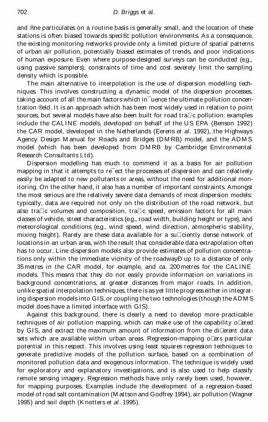
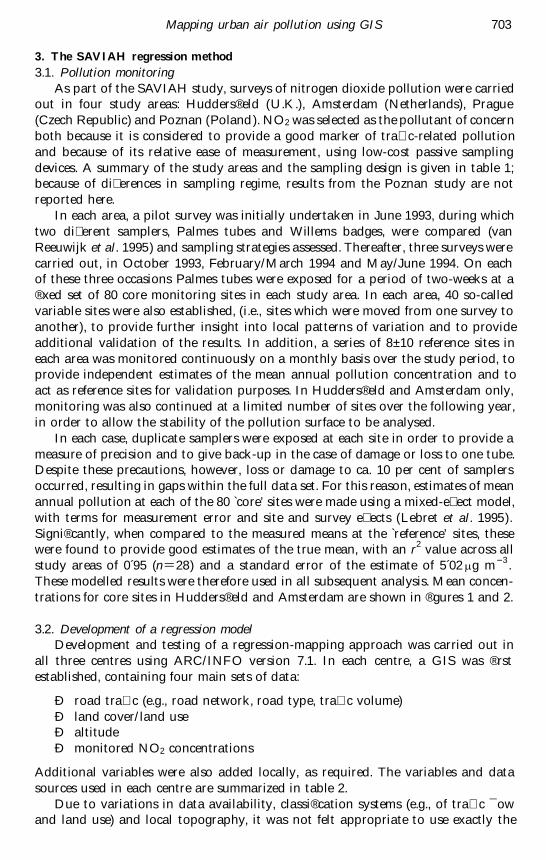
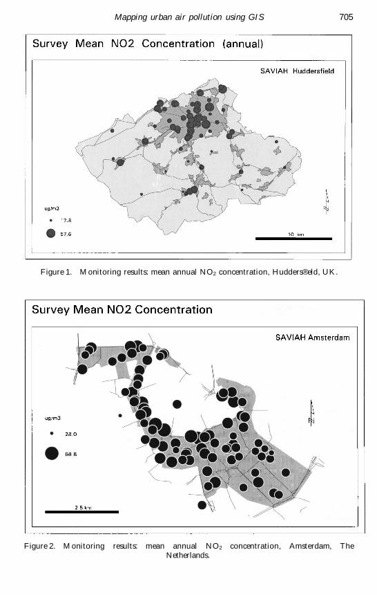
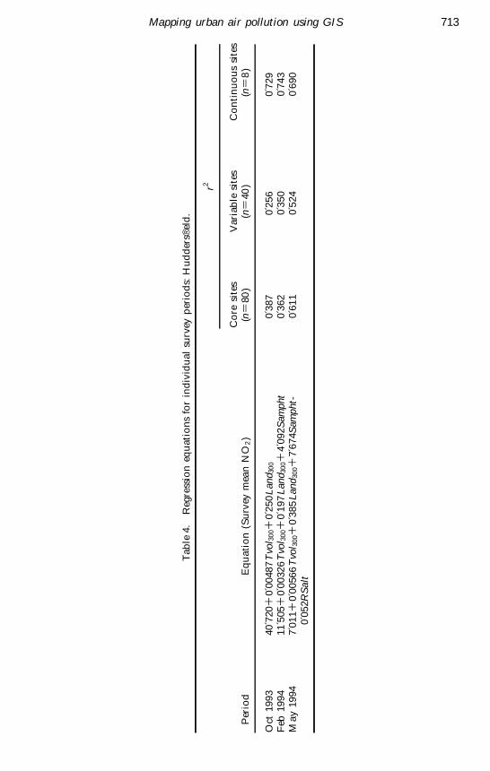
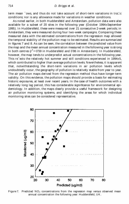
Copyright © 2022 FDOKUMEN