Mapping the Spatial Variability of Plant Diversity in a Tropical Forest: Comparison of Spatial...

Environmental Monitoring and Assessment (2006) 117: 307–334

DOI: 10.1007/s10661-006-0885-z c© Springer 2006

MAPPING THE SPATIAL VARIABILITY OF PLANT DIVERSITYIN A TROPICAL FOREST: COMPARISON OF SPATIAL

INTERPOLATION METHODS

J. LUIS HERNANDEZ-STEFANONI1 and RAUL PONCE-HERNANDEZ1,2,∗1Watershed Ecosystems Graduate Program, Trent University; 2Environmental and Resource Studies

Program, Department of Geography, Trent University, Peterborough, Ontario, Canada(∗author for correspondence, e-mail: [email protected])

(Received 25 March 2004; accepted 1 July 2005)

Abstract. Knowledge of the spatial distribution of plant species is essential to conservation and forest

managers in order to identify high priority areas such as vulnerable species and habitats, and designate

areas for reserves, refuges and other protected areas. A reliable map of the diversity of plant species over

the landscape is an invaluable tool for such purposes. In this study, the number of species, the exponent

Shannon and the reciprocal Simpson indices, calculated from 141 quadrat sites sampled in a tropical

forest were used to compare the performance of several spatial interpolation techniques used to prepare

a map of plant diversity, starting from sample (point) data over the landscape. Means of mapped classes,

inverse distance functions, kriging and co-kriging, both, applied over the entire studied landscape and

also applied within vegetation classes, were the procedures compared. Significant differences in plant

diversity indices between classes demonstrated the usefulness of boundaries between vegetation types,

mapped through satellite image classification, in stratifying the variability of plant diversity over the

landscape. These mapped classes, improved the accuracy of the interpolation methods when they were

used as prior information for stratification of the area. Spatial interpolation by co-kriging performed

among the poorest interpolators due to the poor correlation between the plant diversity variables

and vegetation indices computed by remote sensing and used as covariables. This indicated that the

latter are not suitable covariates of plant diversity indices. Finally, a within-class kriging interpolator

yielded the most accurate estimates of plant diversity values. This interpolator not only provided

the most accurate estimates by accounting for the indices’ intra-class variability, but also provided

additional useful interpretations of the structure of spatial variability of diversity values through the

interpretation of their semi-variograms. This additional role was found very useful in aiding decisions

in conservation planning.

Keywords: biodiversity, co-kriging, geo-statictics, kriging, plant diversity, remote sensing vegetation

indices, tropical forest

1. Introduction

Tropical forests have the highest diversity of plants and animals in the world. Theyare being destroyed by uncontrolled degradation and conversion to other land uses(Wilcox, 1995). The resulting impacts of such degradation are in the form of loss ofbiological diversity, damage to habitats, soil erosion, and disturbances inflicted tothe hydrological and nutrient cycles, among others (Isik et al., 1997). To preserve thebiological diversity of these forests, accurate information about their biodiversity

308 J. L. HERNANDEZ-STEFANONI AND R. PONCE-HERNANDEZ

is required. Developing and using this type of information is, therefore, an essentialpart of conservation programs. For example, the spatial distribution of species over alandscape aids in the identification of high priority areas (Myers et al., 2000; Carroll,1998), which may be used for locating reserves, refuges or other protected areas.

The spatial distribution of species can be estimated through several approaches.One of the most common approaches is to assess species diversity based on theaverage values of computed diversity indices, as obtained from the diversity mea-surements within vegetation or land cover classes. In this method, the mappedclasses are viewed as habitats and the diversity within those classes is assessedthrough field samples. Then, species composition and abundance are both referredto such mapped classes. Researchers and practitioners have used vegetation or landcover classes to analyze the spatial distribution of plant species (Pitkanen, 1998;Nagendra and Gadgil, 1999; Wagner et al., 2000), of animal species (French, 1999;Moreno and Halffter, 2001) or they have considered both, plant and animal species(Fuller et al., 1997). This approach implicitly uses the mean values of classes asspatial interpolators by assigning the average values of the diversity indices mea-sured at different locations to the entire area covered by those classes (Burroughand McDonnell, 1998; Voltz and Webster, 1990).

One of the main concerns of this approach, aside from the simplification ofhaving a single mean value predicting all non-measured points within each class,is that it assumes independence of the samples, i.e. it does not account for spatialdependence and auto-correlation. Yet, species composition is often influenced, atany given location, by the structure of species at surrounding locations, due tocontagious biotic processes such as growth, reproduction, mortality, etc. (Legendre,1993). In such cases, it is reasonable to assume that the values of diversity frompoints closer together are often more similar than those farther apart. Therefore, theassumption of spatial independence of samples is not realistic due to the presenceof spatial autocorrelation (Robertson, 1987; Legendre, 1993).

Geostatistical techniques are useful in providing estimates of sampled attributesat unsampled locations from sparse information (Burrough, 2001). These meth-ods are based on knowledge of the spatial structure of the phenomenon, whichis obtained through spatial autocorrelation or auto-covariance functions, such assemi-variograms. Estimating values between measured points follows the semi-variogram estimation, based on the degree of spatial autocorrelation or covariancefound in the data (Robertson, 1987; Isaak and Srivastava, 1989). Geostatistical tech-niques have been useful for characterizing the spatial distribution and mapping ofsoil properties (Voltz and Webster, 1990; Booker, 2001) and of climatic data (Nalderand Wein, 1998; Prudhomme and Reed, 1999). They have been also applied to eco-logical studies such as in the prediction of forest volume (Wallerman et al., 2002),or the characterization of the spatial structure of vegetation communities (Wallaceet al., 2000).

Furthermore, a number of approaches have been suggested in order to enhancethe accuracy of estimations generated by geostatistical interpolation techniques.

MAPPING THE SPATIAL VARIABILITY OF PLANT DIVERSITY 309

Notably, the incorporation of what is termed as “a-priori information” (Ponce-Hernandez, 1994; Stein, 1992), which involves the use of class boundaries in con-junction with point-data to “guide” the within-class interpolation. In other instances,researchers have used an auxiliary variable, correlated with the variable of inter-est, to lead the estimation process by co-kriging. Such a variable is more intenselysampled than the original variable because it is easier or cheaper to measure, re-ducing the cost of sampling. Co-kriging has been used successfully, for instance,in mapping heavy-metal contaminants in soils (Juang and Lee, 1998) and soilsolute concentrations (Zhang and Yates, 1997). Kriging procedures and their re-quired variography are not, however, without critics. It is argued that the structuralanalysis (variography) may be a rather involved and even a somewhat subjectiveprocess. Consequently, simpler alternatives to kriging, such as the inverse distanceweighting, have been suggested and used as interpolation methods (Kravchenkoand Bullock, 1999). This technique is easier to implement due to the fact that theestimation of values does not require any measure of either spatial autocorrelationor spatial auto-covariance.

In this paper, several spatial interpolation methods were compared in their use-fulness for estimating species diversity and two measures of abundance, Shannonand Simpson indices, of a tropical forest. Such interpolation techniques were exam-ined in order to find an optimal (in the sense of accuracy) interpolating mechanismfor the estimation and mapping of the distribution of diversity values across thelandscape and the production of accurate biodiversity maps. In total four meth-ods: kriging, co-kriging, interpolation based on class boundaries (class means asinterpolator), and inverse distance weighting were tested. Combinations of thesemethods were also examined.

2. Methods

2.1. STUDY AREA AND PLANT DIVERSITY DATA

The study site is a tropical landscape mosaic of 64 km2, located in the southeasternportion of the Yucatan peninsula, Mexico (18◦53′54′′–18◦58′14′′ N latitude and88◦10′04′′– 88◦14′37′′ W longitude). The climate of the area is tropical warm sub-humid with a dry period (i.e., Climate type Aw). The mean annual temperature is26◦ C, the coldest month is January with 23◦ C and the warmest period is betweenJuly and August with 29◦ C. The annual rainfall is between 1000 and 1300 mm,concentrated in a period between June and October, whereas the dry season is fromDecember to April (Cabrera et al., 1982).

Most of the area is covered with tropical sub-deciduous forests in different stagesof succession characterized by age. This forest has 2 or 3 canopy levels consisting oftrees, shrubs and vines 3–25 m high. Indigenous local farmers identified the stagesof succession with Mayan names. “Kanah kax” refers to a forest 20-60 years old;


“kelenche” is used for vegetation between 11 and 19 years of age; “juche” is usedfor plant species between 4 and 10 years of age and “saakab” with plants speciesof 3 years or less. There are also secondary plant associations in the area, including“savanna”, which have few sparse tree species between 3 and 10 m of height and“akalche” (in local Mayan language) consisting of a shrub stratum. Both of thesesecondary plant associations are found in flooded areas or areas with intermittentflooding (Cabrera et al., 1982). The two oldest vegetation classes in the forestsuccession were reclassified as “forest 1”, the two earliest classes were grouped asthe class “forest 2”, and the two classes of secondary associations were grouped intoone class. This reclassification was performed in order to yield sufficient within-class sites to compute a reliable semi-variogram within each, and to fit a model inevery one of the vegetation classes.

Two plant surveys were conducted during two periods, the first between Juneand July of 2000 and the second in July and August of 2001. The surveys werebased on a stratified random sampling design with a total of 141 sampling sites,which were located on the ground using a GPS unit in the six vegetation classes.Each sampling site consisted of two quadrats. One 10 × 10 m quadrat was usedto sample trees and vines higher than 3 m while a 5 × 5 m quadrat was used forsampling all shrubs taller than 1 m. Of the total number of quadrats 67 fell withinforest 1 class, 40 in forest 2 class and 34 in secondary associations (Figure 1). A totalof 16543 sampled individuals were identified to species. In every quadrat, species

Figure 1. Location of the sample units in the study area for the three vegetation classes.


Figure 2. Perspective views of data sets of different plant diversity measures.

richness (i.e., the number of species present in an area) and two measures basedon species frequencies or abundance, including exponent Shannon and reciprocalSimpson indices (Magurran, 1988; Krebs, 1989) were computed. Figure 2 showsthree-dimensional maps of plant diversity indices, as calculated at each quadrat, toprovide information on their spatial distribution.

Small sample plots (0.01 has) were selected because this is the magnitude ofsize in which individuals can interact without expecting substantial variation ingeomorphology, hydrology, soils and climate variables (Palmer et al., 2000) andthus using a uniform support area to make the estimations at unsampled locationsusing autocorrelation functions. However, in order to make an estimation of speciesrichness of tropical forest at community level there is a problem. Species diversityis high but density of any given species is low. Thus, for capturing adequatelythe extreme rarity of most species using small plots, it is necessary to obtain alarge enough number of independent replicate sample plots. This, in order to insurethe accuracy of extrapolative methods used to estimate plant diversity at the land-scape level (Plotking et al., 2000; Clark et al., 1999). In Hernandez-Stefanoni andPonce-Hernandez (2004) species accumulations curves were used to evaluate howrepresentative the sample size was for estimating total species richness in every oneof the vegetation classes as well as in the entire landscape for the studied area.

2.2. LAND COVER MAPPING

A land cover map was generated from Landsat 7 Thematic Mapper (TM) imagery,acquired on April 2000. Every band was already geo-referenced and radiometrically


Figure 3. Land cover map of study area.

corrected. Four classes of forest in different stages of succession, two secondaryassociations, as well as deforested areas, grasslands and cropping areas were identi-fied as the dominant land cover classes, after applying a supervised classification onbands 5 (short-wave infrared: 1.55–1.75 ηm), 4 (near infrared: 0.76–0.90 ηm) and3 (red: 0.63–0.69 ηm). The Maximum Likelihood Algorithm implemented by ERMapperTM 6.1 (Earth Resource Mapping Ltd., 1998) was used as the classificationmethod. The sampling quadrats were used for “ground-truth” assessment of theaccuracy of the classified land cover map, which resulted in an overall accuracy of82.3%. The final land cover map after reclassify the six original vegetation classesinto a 3 new classes is shown in Figure 3.

2.3. VEGETATION INDICES COMPUTED FROM SPECTRAL REFLECTANCE

A relatively large number of multi-spectral band-ratio indices have been designedand applied to ecological studies. Their band combinations have been used tocharacterize and measure different aspects of vegetation canopy (Campbell, 1987).Drawing from this array of published band-ratio indices, several vegetation indiceswere computed to explore their degree of correlation with species richness andtwo measures of abundance, for the purposes of using them as “surrogate” or co-variables in the estimation of plant diversity through a co-kriging procedure.

The vegetation indices computed from spectral reflectance that are examinedin this study are grouped in three categories. The first type consists of indices that


use the differences between the near infrared and the red bands. These include: Ra-tio Vegetation Index (RVI), Normalized Difference Vegetation Index (NDVI) andInfrared Percentage Vegetation Index (IPVI). Such indices are functionally equiv-alent and the difference between them is the range of values that they possess afterthe calculations. These indices are commonly used due to their strong relationshipwith the amount and health of chlorophilically-active vegetation present in an area.However, they are difficult to interpret in areas with low or sparse vegetation cover(Lyon, 1998).

The second category of vegetation indices uses the short-wave and the middle in-frared bands. The Normalized Difference Wetness Index (NDWI) is in this category.NDWI values increase with vegetation water content. So, this index is sensitive tototal amounts of liquid water in the leaves (Gao, 1996). Finally, the so-called GreenVegetation Index (GVI), which is a linear transformation of the six TM bands, wascomputed as part of the third group. GVI projects soil and vegetation informationinto a single plane, and it not only has the ability to readily detect full canopy, butalso to discriminate the mixture of vegetation and soil reflectance as well (Cristand Cicone, 1984). The equations for the computation of each vegetation index aregiven in Table I.

The vegetation indices were calculated from Landsat 7 TM imagery using pro-cedures described as follows. First, digital numbers (DN) were obtained for allspectral bands at the exact location of each of the 141 sampling quadrats. If thequadrats fell onto two or more pixels, the average DN value between such pixels wascalculated. Secondly, another set of pixels (141 in total) was randomly generated toobtain the DN values of all bands. Then, DN values were converted to radiance andtransformed to exo-atmospheric reflectance units, using the equations suggestedby the Landsat 7 Handbook (NASA, 1998). Then, such reflectance values wereused to compute the vegetation indices. So, the resulting data set is a collectionof 141-paired observations of plant diversity values and vegetation indices, which

TABLE I

Equations for the vegetation indices

INDEX FORMULA

RVI RVI = TM4 / TM3

NDVI NDVI = (TM4 −TM3) / (TM4 + TM3)

IPVI IPVI = TM4 / (TM4 + TM3)

NDWI NDWI = (TM5 −TM7) / (TM5 + TM7)

GVI GVI = −0.2848TM1 − 0.2435TM2 − 0.5436TM3

+ 0.7243TM4 + 0.0840TM5 − 0.1800TM7

∗TM3 represents the red band, TM4 is the near infrared band,

TM5 is the short-wave infrared band and TM7 is the middle

infrared band of the landsat 7 Thematic Mapper imagery.


were used to explore the relationships between these variables. In addition to these141 values, an extra equal amount (141 values) of vegetation indices from the addi-tional sampling units were also calculated, yielding a total of 282 samples of suchindices. The vegetation indices were used as “surrogate” variable or co-variableenabling the estimation of species richness and two measures of abundance by theco-kriging procedure.

2.4. INTERPOLATION TECHNIQUES

2.4.1. Estimation Using Class Mean from a Classification Map as InterpolatorThis approach essentially uses the classes as the mechanism for interpolating meanvalues of the attributes within each of the classes to any point or location inside theclass. The model for classification is:

Zi j = μ + vt j + εi j

where Zi j is the value of the plant diversity index at sampling quadrat i within thevegetation type j . The parameter μ is the general mean of the plant diversity index,vt j is the difference between the μ and the mean of class j and εi j is the randomerror. The estimate of Zi j is given by the mean value of the observations within theclass j .

The estimation of species richness and two measures of abundance based on themean values of vegetation classes are underpinned by a number of assumptions.First, the within-class values of plant diversity should be randomly and indepen-dently distributed and not spatially auto-correlated. Secondly, the variance of di-versity data within vegetation classes should be homogeneous. Finally, all changesin plant diversity over space should take place at the mapped class boundaries andin a sharp way (Burrough and Mcdonnell, 1998).

A standard analysis of variance was used to test for significant differences inmean plant diversity values between vegetation types. To provide an indicator ofthe goodness of the classification in partitioning spatial variability of plant diversityvalues, a uniformity index was proposed. This index is essentially a ratio (i.e. therelative variance) of the within-class variance (σ 2

w) to the total sample variance (σ 2t )

subtracted from 1. The uniformity index can be calculated from the equation:

U = 1 − (σ 2

W

/σ 2

T

)Values of uniformity range from 0 to 1, which are easy to convert to percentageof uniformity. When the value of the index is close to 0, the within-class vari-ance is considerable and approximating the total variance, indicating that the classcontribution to partitioning total variability is not useful for discriminating plantdiversity between the vegetation types involved. If the value of the uniformity is


close to 1, the classes are relatively homogeneous and effective for distinguishingplant diversity between vegetation classes.

2.4.2. Inverse Distance WeightingThis is a nearest neighbor interpolation technique. Here, plant diversity values atunvisited sites become the kernel of a local window. Estimates are obtained asa weighted average of the plant diversity values from the neighbouring quadrats,the contribution of which is weighted as an inverse function of the distance to thekernel. The inverse distance equation is expressed as:

Z =n∑

i=1

(1/

dpi∑

1/

dpi

Zi

)

where Z is the estimated plant diversity value (number of species, exponent Shannonor reciprocal Simpson), Zi is the plant diversity value calculated at the quadrat i , dis the distance between the estimated site and the sampling quadrat, p is a analysis-defined power parameter and n represents the number of sampling quadrats usedfor estimation.

The main factor affecting the accuracy of inverse distance interpolator is thevalue of the power parameter p (Isaak and Srivastava, 1989). In this study, we com-pared different estimates of this interpolator using arbitrary integer powers 1, 2 and3. In addition, the size of the neighbourhood and the number of neighbors are alsorelevant to the accuracy of the results. Here, the closest 16 sampling quadrats in a ra-dius of 8 km were used to perform the estimations. The choice of neighborhood sizeis arbitrary, but guided by experience and intuitive knowledge gathered in the field.

2.4.3. KrigingWith the technique called kriging, estimates of plant diversity values at unsam-pled locations are obtained from the information provided by the structures ofspatial variability, as depicted by an auto-covariance function, in this case the semi-variogram of species richness and two measures of abundance. Such structureshelp in defining the size and shape of the neighborhood for interpolation (i.e. sam-pling quadrats that are spatially auto-correlated to the site to be estimated). Thesemi-variogram is computed from:

γ (h) = 1

2n

n∑i=1

(Z (xi ) − Z (xi +h))2

where Z (xi ) is the plant diversity value (number of species, exponent Shannon orreciprocal Simpson) in the quadrat i , Z (xi + h) is the plant diversity value of otherquadrats separated from xi , by a discrete distance h; n represents the number ofpairs of observations separated by h, and γ (h) is the estimated or “experimental”semi-variance value for all pairs at a lag distance h.


Semi-variances were calculated for each possible pair of sampling quadrats, andthe mean values of semi-variances were plotted for increasing distance intervals (h)to produce the experimental semi-variogram. Spherical, gaussian and exponentialmodels were then fitted to experimental semi-variograms using the GS+ software(Robertson, 2000). The fitted models provided the following parameters; the totalvariance, also known as the “sill” variance, which defines the asymptotic value ofsemi-variance with respect to the lag distance. The sill variance is split in two, thevariance due to spatial dependence and the random or “nugget” variance. In turn,the nugget variance reflects both, the spatial variation at shorter distances than theminimum sample spacing and the unexplained variance. The range of influence isthe maximum distance at which plant diversity measures are still spatially dependent(Isaak and Srivastava, 1989; Burrough and Mcdonnell, 1998). The coefficient ofdetermination (r2) resulting from least-squares fitting of models to experimentalsemi-variograms and cross-validation procedures were both used as criteria to selectthe best models in each situation.

Plant diversity estimates were obtained by block kriging using the followingequation:

Z (x0) =n∑

i=1

λi Z (xi )

where λi are the optimal weights selected to minimize the estimation variance(Burrough and Mcdonnell, 1998), Z (xi ) are the observed values of plant diversityand Z (x0) is the optimal and unbiased estimate of plant diversity. Plant diversitymaps were obtained using at least 16 sampling quadrats for each estimation withina maximum radius of 8 km. Neighbourhood characteristics were determined by therange of influence of the semi-variogram.

2.4.4. Co-krigingThe “co-regionalization” (expressed as correlation) between two variables, i.e. thevariable of interest, plant diversity in this case, and another easily obtained andinexpensive variable, can be exploited to advantage for estimation purposes bythe co-kriging technique. In this sense, the advantages of co-kriging are realizedthrough reductions in costs or sampling effort. Considering the lower sampling costsof obtaining computed remote sensing vegetation indices, relative to that of mea-suring plant diversity directly on the ground, makes exploring co-regionalizationa worthwhile undertaking. In this study the computed vegetation indices fromspectral reflectance were employed as auxiliary or surrogate variables. The cross-semivariogram is used to quantify cross-spatial auto-covariance between the origi-nal variable and the covariate, in this case the spectral reflectance vegetation indices.The cross-semivariance is computed through the equation:

γ12(h) = 1

2n

n∑i=1

[Z1(xi + h) − Z1(xi )][Z2(xi + h) − Z2(xi )]


where Z1 is a plant diversity value; Z2 is a given vegetation index; γ12(h) repre-sents the cross-semivariance and h is the distance between both locations x + hand x . Three types of semi-variogram models were fitted to the experimental semi-variograms using the GS+ software. One for the primary variable (i.e., numberof species, exponent Shannon and reciprocal Simpson), another for the auxiliaryvariable (i.e., the reflectance vegetation index in this case), and the other for thecross-variogram of plant diversity and vegetation index. The coefficient of determi-nation (r2) of the fit by least-squares and that of a cross-validation procedure, wereused both as criteria for the selection of the best model to fit the three experimentalsemi-variograms.

Plant diversity estimates were obtained using block co-kriging computed fromthe following expression:

Z (x0) =n∑

i=1

λ1i Z1 (xi ) +m∑

j=1

λ2 j Z2(x j )

where λ1i and λ2 j are the optimal weights selected to minimize the estimationvariance (Isaak and Srivastava, 1989), Z1(xi ) are the plant diversity values at then neighboring locations, Z2(xi ) are the vegetation index values at the m nearbylocations, and Z (x0) represents the estimated plan diversity value. Plant diversityinterpolated maps were obtained using at least 16 sampling locations found withina radius of 8 km.

2.4.5. Estimation by Combined ProceduresSignificant differences among the mean plant diversity values of the different veg-etation classes were expected. If this were true, it would mean that the diversitymap generated from class means as interpolators could explain, to some extent,the variability of plant diversity over the entire area. Consequently, it was deemedappropriate to exploit the variability explained by class means as interpolator andintroduce it as “a priori” information in combination with other interpolation proce-dures. Prior information was used to devise partitions of data sub-sets within eachvegetation class. Then, other interpolation techniques were applied within eachstratum to observe if improvements in accuracy of estimates could be achieved.Thus, estimations of each interpolation method namely inverse distance, krigingand co-kriging within each of the vegetation classes were computed, aiming atachieving better estimates.

2.5. COMPARISON OF INTERPOLATION PROCEDURES

The performance of each interpolation technique alone and in combination, in termsof the accuracy of estimates, was assessed through the deviations of estimates fromthe measured data using a “jack-kniffe” technique for cross-validation. In such aprocedure, sample values are deleted from the data set, one at a time and then


the value in turn is interpolated by performing the interpolation method with theremaining sampling values. This yields a list of estimated values of plant diversitypaired to those computed from measurements within the sampling quadrats (Isaakand Srivastava, 1989).

The comparison of performance between interpolation techniques, in terms ofthe accuracy of estimates, was achieved through the use of four different statistics,namely, the correlation coefficient between measured and estimated plant diversityvalues, the mean error (ME), the mean absolute error (MAE) and the root meansquare error (RMSE). The ME is used for determining the degree of bias in theestimates and it is calculated from:

ME = 1

n

n∑i=1

Z (xi ) − Z (xi )

The MAE provides an absolute measure of the size of the error. MAE is calculatedfrom the following equation:

MAE = 1

n

n∑i=1

|Z (xi ) − Z (xi )|

Finally, the RMSE provides a measure of the error size that it is sensitive to outliers.RMSE values can be calculated from:

RMSE =√√√√1

n

n∑i=1

(Z (xi ) − Z (xi )

)2

The use of these criteria jointly, will provide for a comprehensive performanceevaluation of estimation procedures in order to select the best method for mappingout the spatial variability of biodiversity in the tropical forest of the area studied.

3. Results

3.1. ESTIMATION USING CLASS MEANS FROM A CLASSIFICATION

MAP AS INTERPOLATOR

The difference in plant diversity values between the vegetation classes can be ap-preciated clearly through plotting the histograms of the data. For example, Figure 4shows a histogram of the number of species considering the pooled data (all vege-tation classes) as well as one histogram for each class. The graphs illustrate largedifferences in number of species between the vegetation classes, which suggeststhat a classification model can be effective in explaining the spatial distribution of


Figure 4. Histograms of number of species for the entire area and for each stratum.

number of species over the area. The same behaviour is shown by the other twomeasures of abundance.

The mean number of species of trees, shrubs and vines differs between vegetationclasses (F[2,140] = 311.98, P < 0.00001), with significantly more species in forest1 (33.8) than forest 2 and secondary associations, which have a mean value of 22.08and 4.3 species in 100 m2 respectively (P < 0.0001, Table II). In the same waythe exponent Shannon index and reciprocal Simpson index values differ betweenvegetation types (F[2,140] = 194.5, P < 0.00001; (F[2,140] = 115.38, P < 0.00001

TABLE II

Mean diversity values of trees, shrubs and vines and their standard devia-

tion in three vegetation types

Vegetation Number of Exponent Reciprocal

class species Shannon Simpson

Forest 1 33.79 ± 5.38 20.78 ± 5.09 14.36 ± 4.79

Forest 2 22.08 ± 7.70 12.27 ± 5.21 8.36 ± 4.03

Secundary associations 4.35 ± 1.90 2.31 ± 0.53 1.88 ± 0.38

∗A LDS test was perforfemed for comparing the mean diversity values

among the vegetation types.∗∗There were significant differences between all groups (P < 0.0001).


respectively). Forest 1 has a more even distribution of species and less dominancethan forest 2 class, while the secondary associations are dominated by few species,which is shown with low values of exponent Shannon (2.3) and reciprocal Simpsonindices (1.88). In fact such associations are dominated by only two species: Scleriapterota and Hemotoxylon campechianum (P < 0.0001; Table II).

In terms of the internal uniformity of the mapped classes, calculated as the Uindex, for species richness and the other two measures of abundance mentionedabove, the results also confirm that the vegetation classes had a relatively highinternal uniformity in two of them; number of species (0.816 or about 82%) andexp Shannon index with 0.734 (74%). The results for the reciprocal Simpson indexshow a moderate internal uniformity (0.620). This indicates that the vegetationmap generated from the supervised classification is useful in partitioning the spatialvariability of the number of species, the exponent Shannon index and the reciprocalSimpson index over the study area. The effectiveness of the means of map classesas a spatial interpolator is dependent, to a large extent, on the degree of internaluniformity (U index) of the mapped classes. The encouraging results of the U indexobtained, tend to indicate that class means can be a promising spatial interpolatorfor estimating the three plant diversity parameters over the area studied.

3.2. SEMI-VARIOGRAM MODELS FOR KRIGING

The spatial variation depicted by the semi-variogram models revealed a spatialstructure in each of the plant diversity variables (number of species, exponent Shan-non and reciprocal Simpson) from every one of the three vegetation classes (forest1, forest 2 and secondary associations) and for the combined data (all vegetationclasses), as it is shown in Table III. Spherical, Gaussian and exponential modelswere found to fit well the experimental semi-variograms, and to explain the spatialautocorrelation present in the three plant diversity variables, yielding an r2 rangingfrom 0.63 to 0.97. The structural variance, which determines the variance due tospatial dependence explained by the model and calculated as (total variance–nuggetvariance)/total variance ∗ 100, ranged from 42.1 to 77.1%. This not only suggeststhat there is substantial unexplained variability of plant diversity indices and thatthis may vary considerably over small distances, but also that a moderate to a largefraction of variability is attributable to the nugget variance (Table III).

The relatively “noisy” nature of the spatial variability of plant diversity valuesas reflected in the values of the “nugget” variance (i.e., ranged from 32.9 to 57.9%),may be explained by two factors: the sampling error, which aggregates other types oferrors (i.e., positional error, etc.), and that the spatial dependence of plant diversityindices exists at finer scales than the minimum separation distance in the sample(Figure 5). Comparing the explained structural variance of the semi-variogrammodels for aggregated units (including all vegetation classes in the analysis) againstthose semi-variogram models for every one of the individual classes, it is possible toobserve that such variance holds similar values regardless of the level of aggregation


TABLE III

Parameters and statistics of semi-variogram models describing the spatial variability of number of

species, exponent Shannon and reciprocal Simpson for different vegetation classes

Relative

Variable Nugget Total structural

vegetation class MODEL variance variance Range variance (%) r 2

Number of species

All classes Spherical 78.12 168.30 1765.9 53.6 0.94

Forest 1 Spherical 12.19 26.19 1836.0 53.5 0.97

Forest 2 Gaussian 33.50 67.31 1333.0 50.2 0.97

Secondary associations Spherical 1.05 4.59 1334.0 77.1 0.97

Exponent Shannon

All classes Spherical 35.65 68.19 1542.5 47.7 0.83



Secondary associations Gaussian 0.10 0.21 1530.0 51.0 0.91

Reciprocal Simpson

All classes Exponential 23.87 41.50 1642.0 42.5 0.87

Forest 1 Gaussian 11.91 23.13 1204.0 48.5 0.78

Forest 2 Gaussian 9.49 16.40 1379.0 42.1 0.72

Secondary associations Exponential 0.05 0.18 1986.0 71.2 0.94

of the classes. Moreover, in some cases these values of structural variance show anincrease. For example, reciprocal Simpson index has a structural variance of 42.5%in the semi-variogram model for the unit that include all vegetation types, whilesuch value increased in the individual classes such as mature forest and secondaryassociations (48.5 and 71.2% respectively).

The range of influence showed values between 1204.0 and 2103.2 meters. Thisindicates that one would reasonably expect that the plant diversity values in placesseparated by distances as far as in between 1.2 to 2.1 km are still somewhat related.The moderate variation of this structure suggests that the spatial dependence ofplant diversity values has low differences between vegetation classes (Table III).

3.3. SEMIVARIOGRAM AND CROSS-SEMIVARIOGRAM MODELS

FOR CO-KRIGING

In order to select which of the reflectance-based vegetation indices could be used as acovariate, Pearson correlation coefficients between plant diversity and such indiceswere computed (Table IV). GVI showed the highest correlation coefficients withplant diversity variables when all the vegetation classes are included in the analysis.These coefficients varied from 0.49 to 0.59. In contrast, NDVI showed the best


Figure 5. Experimental and model semi-variograms of number of species, exponent Shannon and

reciprocal Simpson for different vegetation classes.

correlation values inside some vegetation classes, such as forest 2 and secondaryassociations, with values ranging from 0.31 to 0.46. On the other hand, no significantcorrelation was found between plant diversity and vegetation indices for the forest1 class (P > 0.05; Table IV). Although the correlation coefficients between bothplant diversity and vegetation indices were found to vary from moderate to low,GVI was still used as a covariate in the estimations of number of species, exponentShannon and reciprocal Simpson indices, for the unit that combined all vegetationtypes. The NDVI was used as an auxiliary variable for predicting number of speciesin the forest 1 + 2 class (a combination of forest 1 and forest 2 classes) and insecondary associations.

The variograms and cross-semivariogram useful for co-kriging interpolationwere well described by spherical models in most instances, with determinationcoefficients (r2) of the fitted model ranging from 0.83 to 0.97 (Table V). The


TABLE IV

Single correlations between vegetation indices and plant diversity values

Vegetation indicesVariable

vegetation type RVI NDVI IPVI NDWI GVI

Number of species

Forest 1 −0.066 −0.081 −0.081 0.052 0.061

Forest 2 0.408∗ 0.442∗ 0.442∗ 0.231 0.347∗

Forest 1 + 2 0.433∗ 0.455∗ 0.455∗ 0.311∗ 0.409∗

Sec associations 0.436∗ 0.460∗ 0.460∗ 0.372∗ 0.370∗

All vegetation classes 0.526∗ 0.519∗ 0.519∗ 0.434∗ 0.593∗

Exp Shannon

Forest 1 −0.078 −0.088 −0.088 0.109 0.062

Forest 2 0.419∗ 0.435∗ 0.435∗ 0.245 0.342∗

All forest 0.391∗ 0.405∗ 0.405∗ 0.315∗ 0.379∗

Sec associations −0.184 −0.171 −0.171 −0.156 −0.201


Reciprocal Simpson

Forest 1 −0.121 −0.131 −0.131 0.081 0.023

Forest 2 0.359∗ 0.359∗ 0.359∗ 0.210 0.291

Forest 1 + 2 0.303∗ 0.313∗ 0.314∗ 0.268∗ 0.311∗

Sec associations −0.503∗ −0.466∗ −0.466∗ −0.432∗ −0.467∗


∗Correlations are significant at P < 0.05.

structural variance of plant diversity variables ranged from 42.5% to 77.1%, whichincreased in all cases by the cross-variograms with values between 69.5% and99.8%. However, the forest 1 + 2 class was an exception, its structural variance,explained by the combination of number of species and NDVI, was 36.0%. Thus,the values of the nugget variance had a large contribution to total variation withinthe forest 1 + 2 class, which ranged from 0.2 to 68.0%, as it can be appreciatedin the variograms and cross-variograms of number of species in Figure 6. Finally,it could be observed that the spatial dependence for plant diversity variables andcovariates occurs between distances of 1248.0 and 4272.0 meters.

3.4. COMPARISON OF SPATIAL INTERPOLATION PROCEDURES

The results, in terms of the accuracy of estimates (estimation errors), obtained fromthe cross-validation tests by all the different interpolation techniques, are presentedin Table VI. The mean error (ME) is relatively low for all methods, but it is generallythe lowest for the means of classes as an interpolator, and in the combined stratified


TABLE V

Parameters and statistics of semi-variogram models describing the spatial variability of primary

variable (number of species, exponent Shannon and reciprocal Simpson), covariate (GVI and NDVI)

and both variables (cross-variogram) for different vegetation classes

Relative

Vegetation type Nugget Total Structural

variable MODEL variance variance Range variance (%) r 2

All vegetation classes

Number of species Spherical 78.121 168.302 1765.9 53.6 0.94

GVI Spherical 0.0008 0.0013 1248.9 40.3 0.84

Number of species/GVI Spherical 0.084 0.301 2868.0 72.0 0.97

Forest 1 + 2


NDVI Spherical 0.0021 0.0036 1282.9 41.7 0.83

Number of species/NDVI Spherical 0.112 0.176 2910.0 36.0 0.99

Secondary associations


NDVI Spherical 0.0007 0.0019 2793.0 63.4 0.97

Number of species/NDVI Spherical 0.000 0.042 1511.0 99.8 0.95


Exponent Shannon Spherical 35.649 68.188 1542.5 47.7 0.83

GVI Spherical 0.0008 0.0013 1344.5 40.0 0.86

Exponent Shannon/GVI Spherical 0.048 0.181 3048.0 73.5 0.95


Reciprocal Simpson Exponential 23.87 41.50 1642.0 42.5 0.87

GVI Spherical 0.0009 0.0015 3294.8 36.4 0.83

Reciprocal Simpson/GVI Spherical 0.039 0.128 4272.0 69.5 0.92

methods, in that order. These relatively low errors indicate that there may not besystematic under- or overestimation of the plant diversity values. However, there aresome exceptions, one of them is that of number of species when predicted by inversedistance, on the one hand, and co-kriging on the other. When used as interpolators,these resulted in average overestimations of 0.56 and 0.23 respectively. The otherexception is that of the exponent Shannon index while interpolated by an inversedistance procedure, which gave a mean overestimation of 0.22.

The other two measures of error, i.e. MAE and RMSE, showed similar behav-ior for all methods. The highest values of these measures of errors were obtainedwith methods (i.e., kriging, cokriging and inverse distance) applied to the completedataset (i.e., without stratification). Therefore, there is evidence that the accuracyof plant diversity estimations is improved when “a priori” information in the formof stratification (mapped classes) is introduced in combination with other interpola-tion procedures. Now, when examining the performance of interpolation techniques


Figure 6. Experimental and model semi-variograms of number of species and its covariate (GVI and

NDVI) as well as cross-variograms for different vegetation classes.

combined with the stratification, the inverse distance interpolation yielded the high-est error for the three variables (number of species, exponent Shannon and reciprocalSimpson). Indeed, the estimation errors by this technique were even higher thanthose of the estimation based on means of classes (i.e., the classification map). Incontrast, the within-strata kriging procedure (stratified kriging) showed the bestperformance of all methods, in terms of accuracy of estimates, as revealed by thesmallest values of the error measures. For instance, the estimation of number ofspecies had a MAE of 3.92 and a RMSE of 5.23, both values are the lowest errorsof all interpolation procedures (Table VI). Moreover, the correlation coefficientbetween the estimated and measured number of species had the highest value of allinterpolation methods (0.913).

Figure 7 shows three-dimensional maps of number of species for a section ofthe study area. The spatial distribution of number of species was estimated usingkriging, co-kriging, stratified co-kriging (i.e., within the forest 1 + 2 and secondaryassociations classes). Estimations of the spatial distribution of number of specieswere also generated from average values of the class as interpolators, as well asfrom both inverse distance and kriging interpolations within forest 1, forest 2 andthe secondary association classes. The results strongly suggest that the accuracy ofestimates and therefore the accuracy of mapping plant diversity were improved by


TABLE VI

Results of mean error, mean absolute error, root mean square error and correlation coefficients

between measured and estimated plan diversity indices for different interpolation techniques

Interpolation

Variable procedure ME MAE RMSE Corr

Number of species Kriging −0.11 8.85 10.73 0.545

Co-kriging 0.23 9.16 11.55 0.511

Inverse distance-2 0.56 9.49 11.53 0.487

Stratified co-kriging* 0.08 5.54 7.49 0.819

Stratified kriging 0.10 3.92 5.23 0.913

Stratified inv. distance-1 0.04 4.54 6.03 0.887

Classification 0.01 4.39 5.66 0.901

Exponent Shannon Kriging −0.09 6.21 7.40 0.449

Co-kriging 0.11 6.27 7.95 0.423

Inverse distance-2 0.22 6.63 7.89 0.450

Stratified Kriging 0.01 3.06 4.14 0.867

Stratified Inv distance-1 0.04 3.43 4.78 0.836


Reciprocal Simpson Kriging 0.04 4.65 5.58 0.354

Co-kriging −0.02 4.84 6.12 0.357

Inverse distance-1 −0.01 4.97 5.97 0.368

Stratified kriging 0.07 2.80 3.87 0.787

Stratified inv. distance-1 0.05 2.98 4.13 0.765


∗Stratified with two strata; 1,2 power parameters; numbers in bold indicate the best values.

using the stratification (Table VI). Consequently, there are somewhat abrupt changesat the boundaries of the vegetation classes as it is shown in the stratified procedures,in contrast to techniques applied to the complete dataset (i.e. non-stratified) thatshowed gradual changes.

Comparing the maps of the procedures that used three classes for estimatingnumber of species (Figure 7), the inverse distance interpolation produced circularpatterns around the sampling quadrats, which is deemed as an unrealistic char-acterization of the spatial distribution of plant diversity in the field. Furthermore,this technique yielded high discrepancies between the estimated and the measurednumber of species, which makes it an inaccurate interpolator (Table VI). Turning tothe mapped classes as interpolators, one must remember that there is only one valuefor the entire vegetation class; again this is not a realistic characterization of thespatial variability of plant diversity on the ground. In contrast, the map produced bystratified kriging (i.e. kriging within classes) showed relatively smooth contours aswell as the best performance in terms of accuracy of estimations. The final spatial


Figure 7. Comparison of 3D maps for number of species using different interpolation procedures.

distribution maps of number of species, exponent Shannon and reciprocal Simpsonusing stratified kriging are displayed in Figure 8.

It must be remembered that the kriging technique has an intrinsic additionaladvantage over the other interpolation methods. Kriging estimates are unbiasedand with minimum variance. Thus, they are accompanied by a measure of the errorin each predicted value: the estimation variance. This measure of the estimationerror is provided by most of the geostatistical software programs, including GS+.The estimation errors from stratified kriging, for the three plant diversity indices,are displayed as standard deviation maps in Figure 9. These maps incorporate sup-plementary information that can be used in the design of biodiversity conservationplans.


Figure 8. Maps in 3D representation of number of species, exponent Shannon and reciprocal Simpson

using stratified kriging.

4. Discussion

The results obtained from the multiple comparisons of interpolation methods an-alyzed in this study (Table VI) lead to three main sets of conclusions. First, themethods called here “global” in the sense that they were applied over all vegetation


Figure 9. Standard deviation maps of estimates of number of species, exponent Shannon and recip-

rocal Simpson using stratified kriging.

classes, performed the worst having the lowest accuracy of predictions. Second,the interpolation techniques that used the stratification (interpolation within classes)achieved better estimations in the sense of greater accuracy. Finally, of all inter-polation methods used for estimation, the stratified kriging was the most suitablemethod for mapping the spatial distribution of species richness and the other twomeasures of abundance in the study area. Other studies applied to estimate forestvolume (Wallerman et al., 2002) and the spatial distributions of trees (Riemann,1996) have reported similar results, revealing that the estimation is improved whenthe interpolation techniques are applied separately within each class, thus recog-nizing the contribution of partitioning variability of plant diversity indices in termsof vegetation classes.

In this paper, it has been demonstrated that vegetation classes identified onthe ground and mapped through the digital classification of multi-spectral satellite


imagery can explain the spatial variability of plant diversity indices. A standardbetween-subjects ANOVA confirmed a significant reduction of the within-classvariance of plant diversity with respect to their total variance across the landscape.Moreover, species richness and the other two measures of abundance were signif-icantly different between classes (Table II). These large differences in variationamong the mapped classes have important implications for the performance of theinterpolation methods tested in this study. Such differences suggest that when thecomplete dataset is considered over the entire area, there are no stationary means andvariances through out the sampling space, challenging the assumption of stationar-ity over the entire area (Burrough and Mcdonnell, 1998; Isaak and Srivastava, 1989).However, the relative high internal uniformity of the classes suggests that quasi-stationarity within the domain of each class boundary can be safely assumed. Thus,validating the applicability of semi-variograms and within-strata Kriging interpola-tions. There are also discontinuities of the plant diversity values at vegetation-typeboundaries; in other words, the vegetation classes are not in the same categoricallevel of information (Figure 8). Consequently, when the species in distinct habitats(vegetation classes) have a significantly different pattern of spatial distribution, asin this case, the final estimate will be improved if the interpolation procedures areapplied separately within each vegetation class (Burrough and Mcdonnell, 1998;Voltz and Webster, 1990).

The results also reveal that although the inverse distance method has the ad-vantage of relative simplicity and ease of processing, this method is one of theleast accurate, having one of the highest levels of errors among all interpolationprocedures. Similarly, estimation by co-kriging performed rather poorly in termsof accuracy of estimations. The inclusion of vegetation indices, as a co-variable orauxiliary variable, does not reduce the estimation errors. This is due to the poorcorrelation that was shown between the plant diversity variables and potential co-variables (i.e. the calculated spectral reflectance vegetation indices) (Table IV).Ahmed and Marsily (1987) cited by Juang and Lee (1998) pointed out that co-kriging is a better estimating technique than kriging only when the correlationcoefficient between the target and the co-variable is higher than 0.7. Therefore, itis concluded that a better choice of the auxiliary variable or co-variable for thisstudy could have yielded better results. The vegetation indices were not suitableas co-variables for exploiting the advantages of co-kriging procedures. There isno physical model, which can relate directly the feature extraction of vegetationindices to the measures of plant diversity. So, even if better correlation coefficientswere found, resulting in improved accuracy of estimates by co-kriging, it would bedifficult to explain, in physical terms, the nature of such an empirical relationship.

Plant species distribution is affected by many factors including the environmentalconditions created by both biotic and abiotic elements. As a consequence of thedifferent influences of these factors, each species exhibits different patterns ofspatial distribution. These relationships are far too complex to elucidate withoutthe appropriate historical data. Yet, it might be possible to reveal some relationships


between plan diversity values and a given set of environmental variables, such assoil properties, topography, moisture, drainage, and others (Austin, 2002). Onecan speculate on the improvements on the accuracy of estimations that could beachieved, if such variables were incorporated into a co-kriging interpolation scheme,as auxiliary variables. Another line of thought that could be explored further isthe relationships between plant diversity variables and the distribution of particularspecies known as “bioindicator groups” (Noss, 1990). Any of such variables may beused as a co-variate in the co-kriging method; however the data of abiotic variablescan be collected in a quicker and less expensive way (Carroll, 1998).

Comparing both, stratified kriging and classification procedures revealed thatthe former produce more accurate estimations than the latter for the species rich-ness and the other two measures of abundance (Table VI). However, the differencein performance between both procedures is relatively small. Moreover, the semi-variogram analysis required for kriging interpolation provides interpretative valuesbeyond its role in kriging estimation (Rossi et al., 1992). Such information is notproduced and made available by the mapped classes. For example, semi-variogrammodels were able to explain the nature, intensity and extent of the spatial distribu-tion patterns of plant diversity variables varied between vegetation classes. Theyalso showed that such indices are spatially structured from patches that fluctuatedbetween 1.2 and 2.1 km, which corresponds to the “range of influence” parameteron the semi-variogram (Table III). This information can be useful in formulatingand implementing conservation strategies, for instance in identifying areas rich inspecies composition, or those areas that are dominated by a few species, as well aslocating areas where plant diversity is critical (Carroll, 1998). The semi-variogrammodel parameters also indicate the overall plant diversity variance explained byspatial dependence (i.e., auto-covariance or autocorrelation), their lowest valuesvaried from 42.1 to 54.2% in forest 2, while the values for forest 1 fluctuated be-tween 48.5% and 60.1%. The highest values of variability explained by spatialdependence were present in secondary associations (51.1 to 77.1%). This indicatesthat there were autocorrelations at scales lower than 85.15 m, 98.13 m and 41.19m, the separation distance between quadrats in forest 1, forest 2 and secondaryassociations respectively (Table VI).

5. Conclusions

The results demonstrated that stratifying by vegetation classes identified on theground and mapped through satellite imagery, improves the accuracy of severalinterpolation procedures and the resulting maps of species richness and the other twomeasures of abundance. The results also revealed that vegetation indices computedfrom spectral reflectance could not be used as co-variates to estimate plant diversityvalues using co-kriging in the area of this study. This is not to suggest that theycould not be quite successful as co-variates in a different setting, even within tropical


environments. Finally, stratified kriging is an effective method for estimating thespatial distribution of species richness and the other two measures of abundancein the studied landscape mosaic. Not only because this technique yielded the bestcross-validated accuracies among the different methods that were tested, but alsobecause of its great contribution to explaining the spatial distribution of such indicesover the studied landscape.

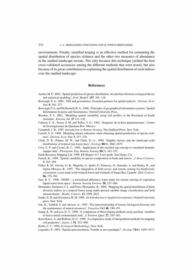
References

Austin, M. P.: 2002, ‘Spatial prediction of species distribution: An interface between ecological theory

and statistical modeling’, Ecol. Modell. 157, 101–118.

Borrough, P. A.: 2001, ‘GIS and geostatistics: Essential partners for spatial analysis’, Environ. Ecol.Stat. 8, 361–377.

Borrough, P. A. and McDonnell, R. A.: 1998, ‘Principles of geographical information systems,’ Spatial

Information Systems and Geostatistics. Oxford University Press.

Brooker, P. I.: 2001, ‘Modeling spatial variability using soil profiles in the Riverland of South

Australia’, Environ. Int. 27 121–126.

Cabrera, C. E., Souza, S. M. and Tellez, V. O.: 1982, ‘Imagenes de la flora quintanaroense’, Centro

de Investigaciones de Quintana Roo. Mexico.

Campbell, J. B.: 1987, Introduction to Remote Sensing, The Guilford Press. New York.

Carroll, S. S.: 1998, ‘Modeling abiotic indicators when obtaining spatial predictions of species rich-

ness’, Environ. Ecol. Stat. 5, 257–276.

Clark, D. B., Palmer, M. W., and Clark, D. A.: 1999, ‘Edaphic factors and the landscape-scale

distributions of tropical rain forest trees’, Ecology 80(8), 2662–2675.

Crist, E. P. and Cicone, R. C.: 1984, ‘Application of the tasseled cap concept to simulated thematic

mapper data’, Photogram. Eng. Remote Sensing 50(3), 343–352.

Earth Resource Mapping Ltd. 1998. ER Mapper 6.1. User guide. San Diego, CA.

French, K.: 1999, ‘Spatial variability in species composition in birds and insects’, J. Insect Conserv.3, 183–189.

Fuller, R. M., Groom, G. B., Mugisha, S., Ipulet, P., Pomeroy, D., Katende, A. and Bailey, R., and

Ogutu-Ohwayo, R.: 1997, ‘The integration of field survey and remote sensing for biodiversity

assessment: a case study in the tropical forest and wetlands of Sango Bay, Uganda’, Biol. Conserv.86, 379–391.

Gao, B. C.: 1996, ‘NDWI – a normalized difference water index for remote sensing of vegetation

liquid water from space’, Remote Sensing Environ. 58, 257–266.

Hernandez-Stefanoni, J. L. and Ponce-Hernandez, R.: 2004, ‘Mapping the spatial distribution of plant

diversity indices in a tropical forest using multi-spectral satellite image classification and field

measurements’, Biodiv. Conserv. 13, 2599–2621.

Isaaks, E. H. and Srivastava, R. M. 1989, An Introduction to Applied Geostatistics, Oxford University

press. New York.

Isik, K., Yaltikik, F. and Akesen, A.: 1997, ‘The interrelationship of forests, biological diversity and

the maintenance of natural resources’, Unasylva FAO 48, 190–191.

Juang, K. W. and Lee, D. Y.: 1998, ‘A comparison of three kriging methods using auxiliary variables

in heavy-metal contaminated soils’, J. Environ. Qual. 27, 355–363.

Kravchenco, A. and Bullock, D. G.: 1999, ‘A comparative study of interpolation methods for mapping

soil properties’, Agron. J. 91, 393–400.

Krebs, C. J.: 1989, Ecological Methodology, New York.

Legendre, P.: 1993, ‘Spatial autocorrelation: Trouble or new paradigm?’, Ecology 74(6), 1659–1673.


Lyon, J. G., Yuan, D., Lunetta, R. S. and Elvidge, C. D.: 1998, ‘A change detection experiment using

vegetation indices’, Photogram. Eng. Remote Sensing 64(2), 143–150.

Magurran, A. E.: 1988, Ecological Diversity and its Measurement. Princeton University Press,

Princeton, NJ.

Moreno, C. E. and Halffter, G.: 2001, ‘Spatial and temporal analysis of α, β, and γ diversities of bats

in a fragmented landscape’, Biodiv. Conserv. 10, 367–382.

Myers, N., Mittermeier, R. A., Mittermeier, C. G., da Fonseca, G. A. B. and Kent, J.: 2000, ‘Biodiversity

hotspots for conservation priorities’, Nature 43(24), 853–858.

Nagendra, H. and Gadgil, M.: 1999, ‘Satellite imagery as a tool for monitoring species diversity: An

assessment’, J. Appl. Ecol. 36, 388–397.

Nalder, I. A. and Wein, R. W. 1998, ‘Spatial interpolation of climatic normals: Test of a new method

in the Canadian boreal forest’, Agricult. For. Meteorol. 92, 211–225.

National Aeronautics and Space Administration. 1998, Landsat 7 science data users

handbook Greenbelt, Maryland, Goddard Space Flight Center, electronic version

http://ltpwww.gsfc.nasa.gov/IAS/handbook/handbook toc.html.

Noss, R. F.: 1990, ‘Indicators for monitoring biodiversity: A hierarchical approach’, Conserv. Biol.4(4), 355–364.

Palmer, M. W., Clark, D. B. and Clark, D. A.: 2000, ‘Is the number of tree species en small tropical

forest plots nonramdom?’, Comm. Ecol. 1(1), 95–101.

Pitkanen, S.: 1998, ‘The use of diversity indices to assess the diversity of vegetation in managed

boreal forest’, For. Ecol. Manage. 112, 121–137.

Plotkin, J. B., Potts, M. D., Yu, D. W., Bunyavejchewin, S., Condit, R., Foster, R., Hubbell, S.,

LaFrankie, J., Manokaran, N., Lee, H. S., Sukumar, R., Nowak, M. A. and Ashton, P. S.: 2000,

‘Predicting species diversity in tropical forests’, Proc. Nat. Ac. Sci. 97(20), 10850–10854.

Ponce-Hernandez, R.: 1994, ‘Improving the representation of soil spatial variability in geographical

information systems: A paradigm shift and its implications’, in: International Society of SoilScience, 1994. 15th World Congress of Soil Science. Volume 6a. Acapulco, Mexico.

Prudhomme, C. and Reed, D. W.: 1999, ‘Mapping extreme rainfall in a mountainous region using

geostatistical techniques: A case study in Scotland’, Int. J. Climatol. 19, 1337–1356.

Riemann, H. R.: 1996, ‘Understanding the spatial distribution of tree species in Pennsylvania’, in:

Mowrer, H. T. (ed), ‘Spatial Accuracy Assessment in Natural Resources and Environmental Sci-

ences’. Second International Symposium. General Technical Report. RM-GTR-277. Fort Collins,

CO. USDA Forest Service, Rocky Mountain Forest and Range Experiment Station, pp. 73–82.

Robertson, G. P.: 1987, ‘Geoestatistics in ecology: Interpolating with known variance’, Ecology 68(3),

744–748.

Robertson, G. P.: 2000, GS+: Geostatistics for Environmental Science. Gamma Design Software.

Plainwell, Michigan.

Rossi, R. E., Mulla, D. J., Journel. A. G., and Franz, E. H.: 1992. ‘Geostatiscal tools for modeling

and interpreting ecological spatial dependence’, Ecol. Monogr. 62, 277–314.

Stein, A.: 1992, ‘The use of prior information in spatial statistics’, in: De Gruijter et al. 1994.

Pedometrics’92. Proceedings of the First Conference of the Working Group on Pedometrics of theInternational Society of Soil Science. Wageningen, The Netherlands.

Voltz, M. and Webster, R.: 1990, ‘A comparison of kriging, cubic splines and classifi-

cation for predicting soil properties from sample information’, J. Soil Sci. 41, 473–

490.

Wagner, H. H., Wildi, O., and Ewald, K. C.: 2000, ‘Additive partitioning of plant species diversity in

an agricultural mosaic landscape’, Landscape Ecol. 15, 219–227.

Wallace, C. S. A. and Watts, J. M. and Yool, S. R. 2000, ‘Characterizing the spatial structure of

vegetation communities in the Mojave desert using geostatistical techniques’, Comp. Geosci. 26,

397–410.


Wallerman, J., Joyce, S., Vencatasawmy, C. P., and Olsson, H.: 2002, ‘Prediction of forest steam

volume using kriging adapted to detect edges’, Can. J. For. Res. 32, 509–518.

Wilcox, B. A.: 1995, ‘Tropical forest resources and biodiversity: The risk of forest loss and degrada-

tion’, Unasylva FAO 46(181).

Zhang, R., Shouse, P., and Yates, S.: 1997, ‘Use of pseudo-crossvariograms and cokriging to improve

estimates of soil solute concentrations’, Soil Sci. Soc. Am. J. 61, 1342–1347.

Mapping the Spatial Variability of Plant Diversity in a Tropical Forest: Comparison of Spatial...

Documents

Transcript of Mapping the Spatial Variability of Plant Diversity in a Tropical Forest: Comparison of Spatial...