AQUATIC MICROBIAL ECOLOGYAquat Microb Ecol

Vol. 30: 185–196, 2003 Published January 7

INTRODUCTION

Plankton are distributed in patches (Cushing 1953,Steele 1978) which can be conceptualised as rare dis-

continuous local regions of high density, sparsely dis-tributed over a larger background of low density. How-ever, the extent and abundance of such patches aredifficult to quantify. Geostatistics is a powerful set oftools that can assess patchiness (Legendre & Fortin1989, Legendre & Legendre 1998). Underlying this

© Inter-Research 2003 · www.int-res.com

*Email: cbulit@cueyatl.uam.mx

Spatial structure of planktonic ciliate patches in atropical coastal lagoon: an application of

geostatistical methods

Celia Bulit1,*, Carlos Díaz-Avalos2, Martha Signoret1, David J. S. Montagnes3

1Departamento El Hombre y su Ambiente, Universidad Autónoma Metropolitana-Xochimilco, Calzada del Hueso 1100, 04960 México DF, México

2Instituto de Investigaciones en Matemáticas Aplicadas y Sistemas, Universidad Nacional Autónoma de México, Apartado Postal 20-726, 01000 México DF, México

3Port Erin Marine Laboratory, School of Biological Sciences, University of Liverpool, Port Erin, Isle of Man, IM9 6JA, British Isles

ABSTRACT: The distribution of ciliates in a Mexican coastal lagoon was studied. The 4 goals were to:examine small-scale (<100 m) patches; indicate how geostatistical techniques can be used to examinethese patches; make inferences concerning ciliate distribution and behaviour in the lagoon using geo-statistical techniques; and assess geostatistics as a method for modelling ciliate distributions. Underly-ing these goals we attempt to make geostatistical techniques accessible to the non-expert. We providean overview of the methodology, references to the geostatistical literature, and use our system as anexample. Ciliates were sampled in a 40 × 40 m grid, divided at 10 m intervals; the grid was further di-vided into subsets, to determine 1 to 10 m scale variation. Between 30 and 35 points were sampled on2 occasions (January and October). Ciliates were preserved with Lugol’s iodine; abundance and spe-cies composition were determined by standard inverted microscopy. The work focused on 4 abundantciliate species. We indicate, using the variographic analysis, that the abundance of 3 of the 4 ciliates isneither randomly nor homogeneously distributed, but exhibits a structured small-scale patchy distrib-ution. We indicate that species-specific patterns of patchiness exist in stratified and in mixed waters,supporting the notion of behavioural niche-separation of planktonic ciliates. Patches of <13, <18, and<77 m were formed by Lohmaniella oviformis, Tintinnopsis sp. and Strombidium sp., respectively. Incontrast, Pleuronema sp. formed patches below the detection limits of the analysis (<1 m). Using geo-statistical techniques, we established variograms and used them to model ciliate distribution and pre-dict ciliate behaviour. Distribution maps were then generated that depicted the shape, distinctness,and gradient of the different patches. After analysing the data, we proposed a working definition of a‘ciliate patch’: regions with abundance above the cut-off of the upper quartile from the kriging pre-diction model. Finally, error-maps were developed, indicating the coefficient of variation of the pre-dicted distributions. We conclude that geostatistical analysis is a powerful tool to examine microzoo-plankton at small-scales, and we support its further application in the field.

KEY WORDS: Microzooplankton patchiness · Variographic analysis · Ordinary kriging · Tintinnopsis ·Lohmaniella · Strombidium · Pleuronema · Mexico

Resale or republication not permitted without written consent of the publisher

Aquat Microb Ecol 30: 185–196, 2003

approach is the expectation that, on average, samplesclose together have values (e.g. of abundance) moresimilar than those further apart. This methodology hasbeen applied to examine the spatial distribution of anumber of aquatic populations in various systems (e.g.Mackas 1984, Legendre & Troussellier 1988, Freire etal. 1992, González-Gurriarán et al. 1993, Pelletier &Parma 1994, Maravelias et al. 1996, Pinel-Alloul et al.1999, Pinca & Huntley 2000, Roa & Tapia 2000, Passy2001, Rueda 2001, Defeo & Rueda 2002), but to ourknowledge, it has not been applied to small-scale dis-tributions of microzooplankton.

Many works that use geostatistics either provide de-tailed methodology or assume expert knowledge on thepart of the reader. While we recognise the existence ofan entire literature devoted strictly to these details (e.g.Isaaks & Srivastava 1989, Cressie 1993, Goovaerts1997, Armstrong 1998, Chilès & Delfiner 1999 and ref-erences therein), with some notable exceptions (Le-gendre & Fortin 1989, Liebhold et al. 1993), there is alack of simple ‘how-to’ instructions on the processes ofgeostatistics, using case-specific examples. Thus, as abasis for our own work, and to encourage other aquaticmicrobial ecologists to apply these techniques, we pro-vide an overview of the methodology, references to theappropriate literature for geostatistical details, and fi-nally use our system as an example. Specifically, we re-frained from complicating this description with jargonand detailed formulae. In taking this approach, we de-viate somewhat from a standard presentation; for clar-ity some specific methods are incorporated into the ‘Re-sults and discussion’ section.

This study has 4 main goals: (1) to examine the small-scale (<100 m) distribution patterns of ciliates in acoastal lagoon; (2) to assess how geostatistical tech-niques can be applied to examine and quantify small-scale patches of plankton; (3) to use these geostatisticaltechniques to make inferences concerning ciliate dis-tribution and behaviour in the lagoon; and (4) to assessthe ability of these techniques to model ciliate distribu-tions in the lagoon.

MATERIALS AND METHODS

General overview of geostatistics. It is simple to cre-ate contour/density maps from grid data (e.g. Fig. 1a,b)using many existing software packages (e.g. Surfer,Golden Software; S-Plus, MathSoft). Such maps pro-vide some information regarding microplankton distri-bution (e.g. Montagnes et al. 1999) but may be inade-quate or misleading as they: (1) use simplistic methodsto create smoothed contours; (2) typically, do not pro-vide a method to interpolate between contours orextrapolate beyond the data set; (3) do not provide

detailed, quantifiable data regarding patch composi-tion; and (4) do not provide an estimate of the errorassociated with predicted values (e.g. of abundance).Geostatistical analysis provides a method of solvingthese problems, by assuming an underlying probabilis-tic model that accounts for the pattern of spatial vari-ability (Cressie 1993, Chilès & Delfiner 1999). Geosta-tistics is based on the concept of random spatialdistributions; in our case, ciliate assemblages areviewed as random patches in space, and the data col-lected are a discrete observation of that distribution.

Here, we offer a simple step-by-step description ofthe basic principles underlying this analysis, and weassume that the variogram is valid over the area cov-ered by the population (i.e. we assume a second orderstationarity hypothesis; see Roa & Tapia 2000).

First, data are collected over a region, ideally, but notnecessarily, forming a regular grid (Fig. 1a). Next,comparisons are made among data (in our case, ciliateabundance) at discrete distances; e.g. over all 1 mintervals (short arrow, Fig. 1a), all √2 m intervals(medium arrow, Fig. 1a), all 2 m intervals (long arrow,Fig. 1a), etc. For each discrete distance (referred to asa lag, h), data-pairs can be plotted on a scattergram toexamine the strength of their association (Fig. 1c). If2 estimates from grid-points have an identical value,then that point will fall on the 45° slope of the scatter-gram, and if they differ substantially, they will fall farfrom this line. An estimate of the variance of these datais then computed for the scattergram at each lag fol-lowing:

(1)

where γ̂ (h) is the estimated variance for any lag (h),z(xi) is a datum-value at any one point, z(xi + h) is adatum value at lag (distance) h from z(xi), and N(h) isthe number of pairs of points separated by h. Ideally, toreduce biases, only lags less than half the maximumlag are used, and all points of the variograms include>30 data pairs (Isaaks & Srivastava 1989).

Each variance value, γ̂ (h), is then plotted against theassociated lag (h) to produce an ‘empirical variogram’(Fig. 1d). Patchy systems typically follow the patternillustrated in Fig. 1d: as distances increase betweensamples, the variance increases until variance remainsconstant regardless of the lag, i.e. 2 samples very closetogether are probably similar; as distance betweensamples increases, they become less similar. Ulti-mately, regardless of distance, there is a constant dis-similarity between samples.

To assess the shape of the empirical variogram, func-tions are fit to the data to provide a ‘model variogram’.There are a number of potential functions (Isaaks &Srivastava 1989, Goovaerts 1997, Armstrong 1998), but

ˆ( ) ( )

( )

γ hN h i

N h

= − +( )[ ]=∑1

22

1

z(x ) z(x hi i

186

Bulit et al.: Spatial structure of planktonic ciliate patches 187

0 10 20 30 40

0

10

20

30

40

0 10 20 30 40

0

10

20

30

40

c

exponential

a

c

dDistance (lag, h)

Var

ianc

e (γ

)

Abundance (xi)

Ab

und

ance

(xi +

h)

distance

dis

tanc

e

sill (c0+c)

nugget (c0)

b

e

f

g

spherical

GaussianStructuralvariance (c)

range (a0)

kriging

Lag

(h)

density map

ˆ γ (h) =

12N(h)

z(xi )− z(xi + h)[ ]2

i =1

N (h)

∑

0

10

20

30

40

0

10

20

30

40

0 10 20 30 40

0 10 20 30 40

Fig. 1. Schematic description of the geostatistical method, using ciliate distribution as an example. Ciliates are collected frompoints, generally forming a grid (a). To assess for patchiness, data can be processed by a simple contour-mapping function, to pro-duce contour (or density) plots (b). If patchiness appears to exist, geostatistical analysis is then applied. First, ciliate abundance atpoints separated by a common distance (lag, h) are calculated; data pairs can then be plotted on a scattergram (c). Next, this illus-tration of similarity is quantified: for a single lag, differences are summed, squared, and divided by twice the number of pairs toyield a variance (γ, equation). This process is repeated for each lag; e.g. the short, medium, and long arrows in (a) are examples ofthe first 3 lags for which γ is calculated. Each of these estimates of γ is then plotted against the lag to produce an empirical vari-ogram (points in d). Then, a model is fit to the variogram data (lines in d); these are used to predict abundance at unsampledpoints and to assess the behaviour of the ciliate (see ‘Results and discussion’ on species). Commonly, exponential, spherical, orGaussian models are fit to the data (thin, medium, thick lines, respectively, in d). There are 3 main components of the variogram:the nugget (c0); the range (a0); and the sill (c0 + c ), composed of the nugget variance (c0) and the structural variance (c) (see ‘Gen-eral overview of geostatistics’). Once models are fit to the variogram, they are used to map ciliate abundance by kriging (see‘Cross-validation and kriging’). Note that each model produces a different predicted distribution (e–g, see ‘General overview of

geostatistics’)

Aquat Microb Ecol 30: 185–196, 2003

the 3 most commonly used are spherical, exponential,and Gaussian functions (Fig. 1d). The spherical func-tion indicates a system where patches are more struc-tured (Fig. 1e); the exponential function indicates thatpatches have fuzzy edges (Fig. 1f); the Gaussian func-tion indicates an extremely continuous distributionwith patches that fade off smoothly (Fig. 1g). Thus, theshape of the function (or model) fit to the variogramalso provides useful information concerning the struc-ture of the system and the behaviour of the organism(ciliates in our case).

The relationship illustrated in Fig. 1d indicates fea-tures of the patchiness: the distance between the small-est scale sampled and where the data become asymp-totic (Fig. 1d: range, a0) indicates the range over whichpatches will be observed; the asymptote (Fig. 1d: sill, c0

+ c) provides an indication of the variability of the data inthe sampling region; and the y-intercept (Fig. 1d). Note,the sill is composed of the structural variance (c) and thenugget (c0). The nugget is an unfortunate term stemmingfrom the geological roots of the methodology rather thanbeing named after a general phenomenon; it indicatesthe difference between 2 samples at an infinitely smalldistance from each other, either due to natural variation,experimental error, or both. These 3 aspects of the datatend to exist for most spatial distributions, but the shapeof the variogram varies depending on how data arespatially distributed.

Furthermore, using a process called kriging (namedafter D. G. Krige, who devised the method), the modelcan then be used to interpolate between samplingpoints on the grid (Fig. 1a) to provide a better predic-tion of distribution (cf. Fig. 1b vs Fig. 1e-g). Finally, themodel can be incorporated into ecosystem models toextrapolate patchiness to larger scales (e.g. rather thaninitiating dynamic models with even or randomly dis-tributed plankton, species-specific patterns of patchi-ness could be imposed). Thus, geostatistical analysisprovides considerable information about a system.

The above description is simple, and the reader isdirected to Isaaks & Srivastava (1989), Cressie (1993),Goovaerts (1997), Armstrong (1998), Chilès & Delfiner(1999) and to the reviews of Legendre & Fortin (1989),Rossi et al. (1992), and Burrough (1995). Below (see‘Results and discussion’) we illustrate the usefulness ofthis method, as applied to the distribution of 4 abun-dant ciliate species in a coastal lagoon. We use thesedata to assess the behaviour of these ciliates and toindicate some of the subtle inferences that can bemade from geostatistical analysis concerning the biol-ogy of ciliates in general.

Sampling design, collection, and enumeration. A40 × 40 m grid, divided at 10 m intervals, was designedfollowing the requirements of the geostatistical analy-sis (Yfantis et al. 1987, Burrough 1995). Ciliate abun-

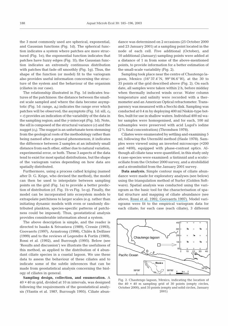
dance was determined on 2 occasions (25 October 2000and 23 January 2001) at a sampling point located in thenode of each cell. Five additional (October), and10 additional (January) sampling points were added ata distance of 1 m from some of the above-mentionedpoints, to provide information for a better estimation ofthe small-scale variability (Fig. 2).

Sampling took place near the centre of Chautengo la-goon, Mexico (16° 37.4’ N, 99° 06.6’ W), at the 30 to35 points of the grid described above (Fig. 2). On eachdate, all samples were taken within 2 h, before middaywhen thermally induced winds occur. Water columntemperature and salinity were recorded with a ther-mometer and an American Optical refractometer. Trans-parency was measured with a Secchi disk. Sampling wasconducted at 0.4 m by deploying 400 ml Niskin-type bot-tles, built for use in shallow waters. Individual 400 ml wa-ter samples were homogenised, and for each, 100 mlsubsamples were preserved with acid Lugol’s iodine(2% final concentration) (Throndsen 1978).

Ciliates were enumerated by settling and examining 5ml, following the Utermöhl method (Hasle 1978). Sam-ples were viewed using an inverted microscope (×200and ×400), equipped with phase-contrast optics. Al-though all ciliate taxa were quantified, in this study only4 case-species were examined: a tintinnid and a scutic-ociliate from the October 2000 survey, and a strobilidiidand a strombidiid from the January 2001 survey.

Data analysis. Simple contour maps of ciliate abun-dance were made for exploratory analyses (see below)using the triangulation method of Surfer (Golden Soft-ware). Spatial analysis was conducted using the vari-ogram as the basic tool for the characterisation of spa-tial structure and mapping of ciliate abundance (seeabove, Rossi et al. 1992, Goovaerts 1997). Model vari-ograms were fit to the empirical variogram data foreach ciliate; for each case (each ciliate), 3 different

188

Fig. 2. Chautengo lagoon, Mexico, indicating the location ofthe 40 × 40 m sampling grid of 30 points (empty circles,October 2000), and 35 points (empty and solid circles, January

2001)

Bulit et al.: Spatial structure of planktonic ciliate patches

models were fit to the variogram according to anapproximate weighted least squares (WLS) procedure,as described in Cressie (1993) (the best fit models areindicated in Fig. 4). Mapping was based on ordinarykriging, an interpolation technique that predicts valuesat unsampled points, using the model variogram(Isaaks & Srivastava 1989). To provide an indication ofthe precision of estimates, the coefficient of variationassociated with each estimate was calculated as theratio of the standard deviation to the mean, both ofwhich are determined by kriging (Isaaks & Srivastava1989). Some further details of the methodology associ-ated with specific conditions are presented below.

RESULTS AND DISCUSSION

Environmental and biological variables

In October, the 1 m water column (i.e. from the surfaceto the sediment) was stratified at ~0.8 m: salinity was16 psu at the surface and 23 psu near the bottom, whiletemperature was uniform, at 30°C throughout thecolumn. The Secchi depth in October was 0.6 m, there-fore, the entire water column was well illuminated,assuming the euphotic zone is 2 to 2.7 times the Secchidepth (Parsons et al. 1977). In January, the 0.8 m watercolumn was mixed: salinity was 30 psu and temperaturewas 29°C; the Secchi depth was 0.3 m. Thus, for eachindividual month (October stratified, January mixedwater), samples taken at 0.4 m across the grid were fromwaters with similar physical conditions.

Taxa for geostatistical analysis

In October, the ciliate community was dominated by atintinnid (Tintinnopsis sp.) and a scuticociliate(Pleuronema sp.), which constituted up to ~70 and 10%of the total ciliate numbers, respectively. Tintinnopsis sp.abundance varied between 21 and 37 cells ml–1, where-as Pleuronema sp. varied between 2 and 7 cells ml–1. InJanuary, Lohmaniella oviformis (5 to 23 cells ml–1) and amedium sized (30 to 50 µm) Strombidium sp. (2 to 14 cellsml–1) were the dominant ciliates, composing up to ~50and 30% of the numbers, respectively. The followingsections are a step-by-step presentation of the analysisconducted to uncover the underlying spatial structure ofthe abundance of these 4 ciliates.

Exploratory data analysis

Before starting the variographic analysis, anexploratory data analysis was performed to assess the

main features of the data and examine for outliers thatmay influence the results of the analysis (Tukey 1977,Cressie 1993). We used several of the exploratory tech-niques but here we present only the contour maps ofthe data.

These maps indicated the overall trends in the abun-dance data (Fig. 3). Local maxima of Tintinnopsis sp.were apparent: 2 distinct peaks of abundance occurredover the background surface (Fig. 3a). The contourmap for Lohmaniella oviformis (Fig. 3b) indicated sev-eral areas of high abundance. The spatial distributionfor Strombidium sp. (Fig. 3c) suggested 3 peaks ofabundance. The contour map for Pleuronema sp. indi-cated higher values in the upper region and a smallpeak near the centre of the grid (Fig. 3d). The contourplots thus suggest that patchiness existed for all 4 spe-cies. However, as stated above, contour maps havelimitations.

Structural analysis

Following the procedure outlined above (see ‘Mate-rials and methods’ and Fig. 1), the next step was to cal-culate variograms for the 4 species (Fig. 4). However apreliminary requirement, not outlined above, was todetermine if the patch structure has a directional com-ponent. For example, Langmuir currents may induceelongated planktonic patches (Parsons et al. 1977), inwhich case, the spatial variability will be higher whenperpendicular to the wind direction and smaller whenparallel to it.

A phenomenon with spatial variability, the same inany direction, is known as isotropy, whereas direction-ality results in anisotropy. Empirical variograms (i.e.variograms presenting lag-data only; e.g. points onFig. 4 a–d) can be used to test for anisotropy (for detailssee Rossi et al. 1992). To assess for anisotropic distribu-tion, empirical variograms for all 4 ciliates were com-puted for vertical and horizontal directions—given ourexperimental design these were the only directionsthat could be assessed. There was no markedanisotropic effect, so the spatial distribution wasassumed to be isotropic. Furthermore, stable condi-tions of weather and water column led us to adopt anomnidirectional variogram. It was thus appropriate touse empirical omnidirectional variograms in the analy-sis. To perform variographic analysis we used 60%(~30 m) of the maximum lag as the active lag distance,as variograms decompose at intervals close to the max-imum (Isaaks & Srivastava 1989). All point of the vari-ograms, except the first one, included >30 data pairs(see Fig. 4).

Variograms are sensitive to extreme data values (po-tential outliers), as differences are squared (Eq. 1). To

189

Aquat Microb Ecol 30: 185–196, 2003

assess for the influence of such values, a further testwas conducted; a ‘robust’ variogram was computedwhich can reduce the effect of outliers, without remov-ing data (Cressie & Hawkins 1980, Maravelias et al.1996). The comparison between the ‘classical’ and the‘robust’ variogram indicated no remarkable differencesin terms of the underlying spatial structure. Thus, thepresence of high values did not affect the detection ofthe patches, and these high values may actually repre-sent the core of patches. Consequently, in subsequentanalyses, classical variograms were used.

The next step for data analysis was to fit models tothe empirical variogram data (i.e. lines on Fig. 4).Using such models we can characterise the spatial

structure of ciliate abundance and estimate abundanceat unsampled points. The fitting of models was con-ducted following the approximate WLS procedure(Cressie 1993). This method gives more weight to thelags with more observations, and with lower empiricalvariogram values, allowing for a better fit of the vari-ogram near the origin, which can be the most impor-tant part of the model. Note: in practice most geostatis-tical packages determine average lags from the data,and thus variograms generally do not present lagsidentical to those measured (cf. Fig. 2 with Fig. 4).

In fitting the omnidirectional variograms, the 3 mod-els illustrated in Fig. 1 were considered, but only2 adequately fit the data (based on the least weighted

190

h

East-West (m) East-West (m)

East-West (m)

Nor

th-S

outh

(m)

Nor

th-S

outh

(m)

Nor

th-S

outh

(m)

Nor

th-S

outh

(m)

b

c

a

d

g

e

j

f i

Contour plots Kriging predictions CV maps

0 10 20 30 400

10

20

30

40

0

10

20

30

40

0

10

20

30

40

0

10

20

30

40

0

10

20

30

40

0

10

20

30

40

0

10

20

30

40

0

10

20

30

40

0

10

20

30

40

0

5

10

15

20

25

30

35

40

0 10 20 30 40 0 10 20 30 40

0 10 20 30 40 0 10 20 30 40 0 10 20 30 40

0 10 20 30 40 0 10 20 30 40 0 10 20 30 40

0 10 20 30 40

Fig. 3. Indications of ciliate patchiness using contour (left),kriging (center), and CV (or error; right) maps for 4 ciliates(from top to bottom: Tintinnopsis sp., Lohmaniella oviformis,Strombidium sp., Pleuronema sp.). On the contour and krig-ing maps, grey areas correspond to water parcels consideredas patches, following Definition 2 (see ‘Assessing patches’).

On the CV maps, grey areas have the highest CV

Bulit et al.: Spatial structure of planktonic ciliate patches

squares, Cressie 1993): a ‘spherical’ model with anugget effect and an ‘exponential’ model, also with anugget effect. These models are given by:

(2)

for the spherical model, and:

(3)

for the exponential model, where c0 is the nugget,c0 + c is the sill and a0 is the range of the variogram(Cressie 1993). These models were fit to the empiricalvariograms using the interactive feature of S-Plus 2000(MathSoft).

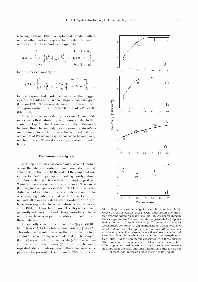
The variograms for Tintinnopsis sp. and Lohmaniellaoviformis both illustrated typical cases, similar to thatshown in Fig. 1d, but there were subtle differencesbetween them. In contrast, the variogram for Strombid-ium sp. failed to reach a sill over the sampled distance,while that of Pleuronema sp. appeared to have alreadyreached the sill. These 4 cases are discussed in detailbelow.

Tintinnopsis sp. (Fig. 4a)

Tintinnopsis sp. was the dominant ciliate in October,when the shallow water column was stratified. Aspherical function best fit the data of the empirical var-iogram for Tintinnopsis sp., suggesting clearly definedstructured ciliate patches within the sampling grid (see‘General overview of geostatistics’ above). The range(Fig. 1d) for this species is ~18 m (Table 1); this is thedistance below which discrete patches might beobserved, e.g. patches could be 1, 10 or 15 m, butunlikely 20 m in size. Patches on the order of 1 to 100 mhave been suggested for other tintinnids (e.g. Stoeckeret al. 1984), but size limitations of such patches havegenerally not been proposed. Using geostatistical tech-niques, we have now provided observational limits ofthese patches.

The spatially structured component (c/(c0 + c) × 100,Fig. 1d) was 74% of the total spatial variation (Table 1).This ratio can be interpreted as the portion of the totalvariance explained by a spatial model. The nugget(Fig. 1d) accounts for the microscale (<1 m) variationsand the measurement error (the difference betweenrepeated ciliate counts made with the same water sam-ple), and it represented the remaining 26% of the vari-

ˆ ( )

exp γ h

h

c ch

ah

=

=

+ − −

≠

0 0

13

00

2

02

for

for

ˆ ( )

γ h

h

c cha

ha

for h a

c c h a

=

=

+

−

< ≤

+ ≥

0 0

32

12

000 0

3

0

0 0

for

for

191

0 5 10 15 20 25 30

0

5

10

15

a5

60

112 104

Distance (m)

Gam

ma

(γ) (

cells

ml–

1 )2

0 5 10 15 20 25 30

0

5

10

15

d

5

60112

104

0 5 10 15 20 25 30

0

5

10

15

b

141

154

82

12

0 5 10 15 20 25 30

0

5

10

15

c

15

70

156141

88

Fig. 4. Empirical variograms (points) and fitted models (lines).Only 60% of the total distance (~30 m), measured in any direc-tion over the sampling space (see Fig. 1a), was represented inthe variograms (see ‘General overview of geostatistics’). Spher-ical models were fit to the data for (a) Tintinnopsis sp. and (b)Lohmaniella oviformis. An exponential model was fit to data for(c) Strombidium sp.. The spatial distribution of (d) Pleuronemasp. was random at the measured scale; therefore a spatial modelcannot explain this variability, and a random model explains it.See Table 1 for the parameters associated with these curves.The number of pairs of points for each lag distance is indicated.Note: in practice most geostatistical packages determine aver-age lags from the data, and thus variograms generally do not

present lags identical to those measured (cf. Fig. 2)

Aquat Microb Ecol 30: 185–196, 2003

ability. The nugget effect thus reflects, in plankton dis-tribution, the existence of ciliate aggregations thatcannot be further resolved by our sampling. Buskey &Stoecker (1988, 1989) have indicated that swimming ofthe tintinnid Favella sp. would allow the ciliate toremain in small-scale patches, and Kils (1993) hasdemonstrated the existence of dense patches on theorder of centimetres. Such patches may produce themicroscale variance of the nugget that we estimatedfor Tintinnopsis sp. The nugget may also representmeasurement error (e.g. variation between subsam-ples); we are presently examining this error-term in aseparate study (Bulit et al. unpubl.). The nugget alsoreflects how tight the patches are (Dalthorp et al.2000); a small nugget indicates a tight patch. There-fore, on the basis of the properties derived from thenugget and range, patches of Tintinnopsis sp. are ofmedium size relative to the sampled grid and tighterthan those of Lohmaniella oviformis and Strombidiumsp. patches (see below).

Lohmaniella oviformis (Fig. 4b)

This small strobilidiid, close in size to the nanoplank-ton, was the dominant ciliate in January, when the wa-ter column was mixed. Like Tintinnopsis sp., a sphericalfunction best fit the data of the empirical variogram forLohmaniella oviformis, although the exponential func-tion provided almost as good a fit (Table 1). The rangefor this species was 13 m, suggesting that patches of thestrobilidiid were slightly smaller than those of Tin-tinnopsis sp. The sill of the L. oviformis model was alsolower than that of Tintinnopsis sp. (Table 1), indicatingless variability in its distribution. These small patchescould result from repeated cell divisions, as small cili-

ates can have generation times on the order of hours inwarm waters (Montagnes 1996), but patches might alsobe due to swimming behaviour (see below).

For Lohmaniella oviformis, the spatially structuredcomponent was 69% of the total spatial variation, withthe nugget representing 31% (Table 1). These resultssuggest a similar structure in patches to that of Tin-tinnopsis sp; possibly, the slightly larger nugget of L.oviformis was due to its lower density (Fig. 3), and thuspotentially a larger measurement error. To date, thereare few studies on L. oviformis. Jonsson (1989) exam-ined the vertical distribution of L. oviformis, indicatinga swimming velocity of 340 µm s–1. In contrast, Jonsson(1989) found T. campanula to have a vertical swim-ming velocity of 260 µm s–1. Furthermore, small, nakedstrobilidiids tend to have a higher tumbling-reorienta-tion rate than larger tintinnids (D.J.S.M. pers. obs.).Thus, although it is small, the ability of L. oviformis toaccumulate in patches by rapid swimming and reori-entation might be considerable, and we speculate thatthis may explain the patches observed in the lagoon.

Strombidium sp. (Fig. 4c)

Strombidium sp. also dominated in January althoughits mean abundance (8.0 ± 3.4 cells ml–1) was lowerthan that of Lohmaniella oviformis. The variogram forthis strombidiid shows that the variance continued toincrease without reaching a sill. This suggests thatpatches tend to be larger than the 40 m sampling grid.Some geostatistical packages provide an option to fit alinear variogram, but this does not allow prediction atunsampled points (e.g. Fig. 1d). Thus, one option is tofit an exponential model to the data, approximating thelinear shape with a range beyond the survey’s maxi-

192

Ciliate Abundance Model Parameters Spatially structured Model statisticsx SD c0 c0 + c a0 component (%) Bias SD2 MSE

(γ, cells ml–1)2 (m) c/(c0 + c ) × 100

Tintinnopsis sp. 27.8 4.0 Spherical 4.5 17.5 17.5 74 –0.22 12.25 12.29*Exponential 6.6 16.8 24.5 61 –0.20 13.10 13.14

Lohmaniella 12.4 4 Spherical 5 16 13 69 0.13 18.14 18.16*oviformis Exponential 2.5 16.5 10 87 0.12 18.31 18.33

Strombidium sp. 8 3.4 Exponential 6 15 25.6 60 0.086 11.08 11.09*Spherical 6 18 70 66 0.081 11.15 11.16

Pleuronema sp. 3.4 1.3 Nugget 14.5 14.5 <1 0

Table 1. Abundance statistics (x: mean; SD: standard deviation, measured as cells ml–1) and parameters of the different variogrammodels for ciliate abundance, determined through cross validation (see ‘Cross-validation and kriging’ for details). The best fit, thelowest according to Cressie (1993), for each ciliate is presented graphically in Fig. 4. See Fig. 1 for a definition of symbols (e.g. c0,

nugget effect; c0 + c, sill; a0, range). Cross-validation results of models and parameters selected to map the predictions of ciliateabundance by ordinary kriging (see ‘Cross-validation and kriging’ for details): Bias, the mean prediction error (estimated – ob-served); SD2: the variance of the error; MSE (mean squared error) = SD2 + bias2. See ‘Results and discussion’ for discussion of the

models. *Lowest MSE

Bulit et al.: Spatial structure of planktonic ciliate patches

mum allowable distance (i.e. 30 m for this study); wefollowed this second option (see Goovaerts 1997). Asthe exponential model approaches its sill asymptoti-cally, the practical range is calculated as 3 × a0, as thedistance at which the model reaches 95% of its sill(Goovaerts 1997, Armstrong 1998). In the case ofStrombidium sp., a0 was 25.6 m; therefore the practicalrange was ~77 m. Thus, if the grid were larger, discretepatches of this ciliate are likely to be have beenobserved. The spatially structured component was60% of the total spatial variation (Table 1).

It is unclear why this ciliate would form large diffusepatches. However, there are many mixotrophic speciesof Strombidium (Stoecker et al. 1989, Bernard & Ras-soulzadegan 1994, Dolan & Pérez 2000); mixotrophsmight form patches larger than exclusively heterotro-phic ciliates, as autotrophy would allow these ciliatesto occupy areas where there are no prey, assumingthat prey are also distributed in patches. Dale & Dahl(1987) suggested that swimming behaviour of strom-bidiid ciliates might cause concentration of organisms.Jonsson (1989) indicated that some species of Strom-bidium have swimming velocities of 450 to 680 µm s–1.Thus, under very calm weather conditions and waterstability like those we found, this speed can be of sig-nificance, and patches of Strombidium might be large.However, the Strombidiidae comprises a diversegroup, and it may be imprudent to generalise based onthe few well-studied taxa.

Pleuronema sp. (Fig. 4d)

This species occurred in October at a lower abun-dance (3.4 ± 1.3 cells ml–1) than Tintinnopsis sp. and itdiffers in distribution from those species discussedabove. It appears from the variogram that a sill wasreached below the minimum sampling distance (1 m).Thus, a pure nugget model was fit to the data (Table 1),which indicates a lack of spatial resolution; i.e. patcheswere not detected. Ideally, we would return to the fieldand sample for this ciliate at a smaller scale. Note thatthis analysis contradicts the observations predicted bya simple contour map (i.e. Fig. 3d). Thus, the applica-tion of geostatistical analysis has allowed a different,and likely more accurate, evaluation of the distributionof this ciliate.

We might predict that the bacterivorous nature ofthis scuticociliate (Fenchel 1987, Dolan & Coats 1991,Ederington et al. 1995) means that it forms patchesaround detrital clumps. Furthermore scuticociliatesappear to be the most abundant ciliates in aggregatesof suspended matter (Artolozaga et al. 2000), and theyhave been associated with detritus (Silver et al. 1984,Sherr et al. 1986). Such clumps would undoubtedly be

microns to millimetres in size, and thus the patcheswould be <<1 m. The samples of Pleuronema sp. thathave high values (13% of the total samples) may,therefore, be chance collection of detrital material withassociated ciliates.

We have shown, using variographic analysis, that for3 of the 4 evaluated ciliates, the abundance is neitherrandomly nor homogeneously distributed, but ratherexhibits a structured small-scale patchy distribution.We have also indicated that simply applying standardcontour fits to the data, using existing packages (see‘General overview of geostatistics’ above) may provideerroneous conclusions regarding patchiness (e.g. Pleu-ronema sp. did not form patches when geostatisticallyanalised). Furthermore, we have indicated that spheri-cal and exponential functions, and not the Gaussianfunction, best model ciliate patches; this suggests tight,rather than diffuse, patches (see Fig. 1). These arepotentially useful observations of patches, and we thussupport the application of these variographic tech-niques to analyze microzooplankton distributions.

Cross-validation and kriging

In the next step of the analysis, we indicate how pre-diction maps are generated and associated with thecoefficients of variation. In this phase, the variogrammodels are used to predict abundance values at un-sampled localities, using a linear prediction methodcalled ordinary kriging (Isaaks & Srivastava 1989,Goovaerts 1997, Armstrong 1998).

In practice, the prediction is computed using onlythose observations inside a selected ‘search radius’.The performance of the best model, search radius, andnumber of points to be used in the kriging system weredetermined through a cross validation procedure. Thisprocedure consists of incrementally removing observa-tions (abundance values) from the data set, one by one,and re-estimating the value of the removed observa-tion using the parameters being validated (Goovaerts1997). Thus, a prediction error (predicted abundance –measured abundance) was generated at each sam-pling location.

The goal of this validation is to select the model andthe search-strategy parameters that give the minimummean squared error (MSE), by making a trade-offbetween bias and variance (see Table 1). The MSE isthe sum of the squared bias (the mean of the error) andthe variance (the spread of the error) of the residuals(Isaaks & Srivastava 1989). The X-valid procedure(Geo-Eas 1.2.1; Englund & Sparks 1991) was used togenerate the residual vectors. Table 1 summarises theresults of crossed validated models and parametersfrom the 2 best models assessed (out of 8 to 10 possible

193

Aquat Microb Ecol 30: 185–196, 2003

models). The models with the lowest MSE (values withasterisks, Table 1) were then used to map the distribu-tions of Tintinnopsis sp., Lohmaniella oviformis, andStrombidium sp. (Fig. 3e–g). These distributions canthen be used to assess patchiness.

Assessing patches

Although many studies describe patches, a ‘patch’ israrely quantifiably defined; we offer 2 definitions andthen assess if either is appropriate. Following our ini-tial argument that patches are rare, relative to a back-ground of lower abundance, a patch might then be de-fined as a region where the ciliate abundance exceedsa cut-off value of the kriging predictions map, such as(1) the median value or (2) the upper quartile value.Below, we use our data to assess these 2 definitions.

The search strategy with the best performance for pre-dicting tintinnid abundance used a circular searchneighbourhood of 12 m and the nearest 10 observations(Table 1). The kriging-abundance predictions for tintin-nids (Fig. 3e) were mapped using the spherical modeland these parameters. The resulting distribution differedfrom that obtained from the contour plot (Fig. 3a). Themodelled distribution produced one extended patch(70% of the total area), following Definition 1. In con-trast, when Definition 2 was applied, 2 small patches ex-isted and represented the 4.4% of the total area (Fig. 3e).Following the initial premise that patches are rare, it ap-pears that Definition 2 is more appropriate for the tintin-nid. Similarly, the prediction map for Lohmaniella ovi-formis was made using a spherical model, a circularsearch neighbourhood of 12 m in radius, and consideredthe 10 nearest points (Table 1). This modelled distribu-tion (Fig. 3f) differed from the contour map (Fig. 3b),where several areas were presumptively considered aspatches, and allowed quantification of the distribution:by Definition 1, patches occupied 52% of the surface,while by Definition 2, patches covered 23% of the totalarea. Again, assuming patches are rare, the second def-inition of a patch seems more appropriate. For Strom-bidium sp., an exponential model was used, a circularsearch neighbourhood of 20 m in radius, and the nearest20 points were considered to make the kriging map(Table 1). The modelled distribution (Fig. 3g) was dis-tinctly different from that of the contour map (Fig. 3c).Following Definition 1, the modelled distribution indi-cated that a portion of a patch occupied 50% of the area,but by Definition 2, there was a tiny part of a patch, lo-cated at coordinates 0, 20, covering only 1% of the area,yet again supporting Definition 2. In contrast to the 3taxa examined above, fitting of a pure nugget model tothe empirical variogram for Pleuronema sp. precludedthe use of kriging (Goovaerts 1997). Therefore, at this

scale, Pleuronema sp. is considered to be randomly dis-tributed, with no distinct patches.

We have thus assessed that in the lagoonal environ-ment, structured ciliate patches exist at a small-scale instratified as well as in mixed waters. Following thepremise that patches are rare (covering <<50% of thesampled area), and using quantitative criteria providedby geostatistics, we have put some limits on the defini-tion of these ciliate patches; they are nearer to beingassociated with the abundance above the density cut-off of the upper quartile range from kriging maps,rather than above the median value. We have alsoindicated a difference in predicted distribution whenkriging is applied to the data, relative to using tradi-tional interpolation methods. This is because the con-tour levels obtained by kriging are dictated by the var-iogram model and are not simply based on isolatedpoints measured over the grid. Furthermore, the mod-els illustrated in Fig. 4 can be used to predict patchi-ness on a larger scale and thus could be used forecosystem models. However, like any estimates thereis error associated with these predictions; the next sec-tion examines this error.

Estimating error of the modelled distribution

The maps for the coefficient of variation (CV) indi-cate the precision of the estimated distribution(Fig. 3h-j). This error term can then be used to assessthe predictable nature of the kriging map, takinginto account the variability of the predictions. TheCV for the predicted distribution of Tintinnopsis sp.varied between 9 and 17% (Fig. 3h); the CV forLohmaniella oviformis ranged from 16 to 43% (Fig.3i); the CV for Strombidium sp., ranged from 25 to74% (Fig. 3j). As the CV was <100% in all cases, wecan conclude that outlying, or erratic, values thataffect the estimated distribution are rare or nonexis-tent (Isaaks & Srivastava 1989). By examining thekriging and the CV maps for all the ciliates, it can beseen that at higher ciliate abundance, the CV formsa homogeneous spatial pattern, increasing towardsthe edges, where fewer points were sampled; this isespecially clear for the case of Tintinnopsis sp. (Fig.3h). However, the CV may also vary inversely withthe predicted abundance, as depicted for L. oviformis(Fig. 3i) and for Strombidium sp. (Fig. 3j). This sug-gests that the uncertainty on the predicted valuesincreases at lower abundance and could be reducedby adding more sampling points in those areas.These estimates of error illustrate the precision ofmodelling distributions and may thus ultimately beused to help assess the predictability of larger scalefood-web models.

194

Bulit et al.: Spatial structure of planktonic ciliate patches

To our knowledge, this study constitutes the firstapplication of geostatistical techniques to model thesmall-scale spatial structure of microplanktonic popu-lations. Our results indicate different species-specificpatterns of patchiness at a small-scale and in differenthydrodynamic conditions, supporting the notion ofbehavioural niche-separation of planktonic ciliates.The size, shape, and distinctness of the patches werecharacterised by the spatial dependence, which weindicate can be summarised by 3 parameters: therange, sill, and nugget. And finally, a working defini-tion of patch was proposed and was used to charac-terise the generated kriging predictions. Thus, geosta-tistical analysis appears to be a powerful tool toexamine microzooplankton at small-scales, and wesupport its further application in the field.

Acknowledgements. This paper forms part of the PhD thesisof C.B. at the University of Liverpool and UniversidadAutónoma Metropolitana-Xochimilco. We thank Dr. AndrésBoltovskoy, Eusebio Cueva, and Héctor Chagoyan for theirassistance during fieldwork. We also thank PROMEP-SEP forsupport in purchasing a microscope. Rubén Roa and FabiánTapia kindly provided the templates for cross validation pro-cedure. Finally, we thank 2 anonymous reviewers for theirconstructive comments.

LITERATURE CITED

Armstrong M (1998) Basic linear geostatistics. Springer-Verlag, Berlin

Artolozaga I, Ayo B, Latatu A, Azúa I, Unanue M, Iriberri J(2000) Spatial distribution of protists in the presence ofmacroaggregates in a marine system. FEMS MicrobiolEcol 33:191–196

Bernard C, Rassoulzadegan F (1994) Seasonal variations ofmixotrophic ciliates in the northwest Mediterranean Sea.Mar Ecol Prog Ser 108(3):295–301

Burrough P (1995) Spatial aspects of ecological data. In: Jong-man R, Ter Braak C, Van Tongeren O (eds) Data analysisin community and landscape ecology. Cambridge Univer-sity Press, Cambridge, p 213–251

Buskey EJ, Stoecker DK (1988) Locomotory patterns of theplanktonic ciliate Favella sp.: adaptations for remainingwithin food patches. Bull Mar Sci 43:783–796

Buskey EJ, Stoecker DK (1989) Behavioral responses of themarine tintinnid Favella sp. to phytoplankton: influence ofchemical, mechanical and photic stimuli. J Exp Mar BiolEcol 132:1–16

Chilès JP, Delfiner P (1999) Geostatistics: modeling spatialuncertainty. Wiley, New York

Cressie NAC (1993) Statistics for spatial data. Wiley, NewYork

Cressie NAC, Hawkins DM (1980) Robust estimation of thevariogram, I. Math Geol 12:115–125

Cushing DH (1953) Studies on plankton populations. J ConsPerm Int Explor Mer 19:1–22

Dale T, Dahl E (1987) Mass occurrence of planktonic oligotri-chous ciliates in a bay in southern Norway. J Plankton Res9:871–879

Dalthorp D, Nyrop J, Villani MG (2000) Foundations of spatialecology: the reification of patches through quantitativedescription of patterns and pattern repetition. EntomolExp Appl 96:119–127

Defeo O, Rueda M (2002) Spatial structure, sampling designand abundance estimates in sandy beach macroinfauna:some warnings and new perspectives. Mar Biol 140:1215–1225

Dolan JR, Coats WD (1991) A study of feeding in predaciousciliates using prey ciliates labeled with fluorescent micros-pheres. J Plankton Res 13:609–627

Dolan JR, Pérez MT (2000) Costs, benefits and characteristicsof mixotrophy in marine oligotrichs. Freshw Biol 45(2):227–238

Ederington MC, McManus GB, Harvey HR (1995) Trophictransfer of fatty acids, sterols, and a triterpenoid alcoholbetween bacteria, a ciliate, and the copepod Acartia tonsa.Limnol Oceanogr 40:860–867

Englund E, Sparks A (1991) GEO-EAS 1.2.1 User’s guide.Environmental Protection Agency, Las Vegas, NV

Fenchel T (1987) Ecology of Protozoa: the biology of free-liv-ing phagotrophic protists. Brock/Springer Series in Con-temporary Bioscience. Science Tech Publishers, Madison,WI

Freire J, González-Gurriarán E, Olaso I (1992) Spatial distrib-ution of Munida intermedia and M. sarsi (Crustacea, Ano-mura) on the Galician continental-shelf (NW Spain): appli-cation of geostatistical analysis. Estuar Coast Shelf Sci 35:637–648

González-Gurriarán E, Freire J, Fernández L (1993) Geosta-tistical analysis of spatial-distribution of Liocarcinus depu-rator, Macropipus tuberculatus and Polybius henslowii(Crustacea, Brachyura) over the Galician continental-shelf(NW Spain). Mar Biol 115:453–461

Goovaerts P (1997) Geostatistics for natural resources evalua-tion. Oxford University Press, New York

Hasle G (1978) The inverted microscope method. In: SourniaA (ed) Phytoplankton manual. UNESCO, Paris, p 88–96

Isaaks EH, Srivastava RM (1989) An introduction to appliedgeostatistics. Oxford University Press, New York

Jonsson PR (1989) Vertical distribution of planktonic cili-ates—an experimental analysis of swimming behaviour.Mar Ecol Prog Ser 52:39–53

Kils U (1993) Formation of micropatches by zooplankton-dri-ven microturbulences. B Mar Sci 53(1):160–169

Legendre P, Fortin MJ (1989) Spatial pattern and ecologicalanalysis. Vegetatio 80:107–138

Legendre P, Legendre L (1998) Numerical ecology. ElsevierScience, Amsterdam

Legendre P, Troussellier M (1988) Aquatic heterotrophic bac-teria: modeling in the presence of spatial autocorrelation.Limnol Oceanogr 33:1055–1067

Liebhold A, Rossi R, Kemp W (1993) Geostatistics and geo-graphic information systems in applied insect ecology.Annu Rev Entomol 38:303–327

Mackas DL (1984) Spatial autocorrelation of plankton com-munity composition in a continental shelf ecosystem. Lim-nol Oceanogr 29:451–471

Maravelias CD, Reid DG, Simmonds EJ, Haralabous J (1996)Spatial analysis and mapping of acoustic survey data inthe presence of high local variability: geostatistical appli-cation to North Sea herring (Clupea harengus). Can J FishAquat Sci 53:1497–1505

Montagnes DJS (1996) Growth responses of planktonic cili-ates in the genera Strobilidium and Strombidium. MarEcol Prog Ser 130:241–254

Montagnes DJS, Poulton AJ, Shammon TM (1999) Mesoscale,

195

Aquat Microb Ecol 30: 185–196, 2003

finescale and microscale distribution of micro- and nano-plankton in the Irish Sea, with emphasis on ciliates andtheir prey. Mar Biol 134:167–179

Parsons T, Takahashi M, Hargrave B (1977) Biological ocea-nographic processes. Pergamon Press, Oxford

Passy SI (2001) Spatial paradigms of lotic diatom distribution:a landscape ecology perspective. J Phycol 37:370–378

Pelletier D, Parma AM (1994) Spatial distribution of Pacifichalibut (Hippoglossus stenolepis): an application of geo-statistics to longline survey data. Can J Fish Aquat Sci 51:1506–1518

Pinca S, Huntley ME (2000) Spatial organization of particlesize composition in an eddy-jet system off California.Deep-Sea Res 47:973–996

Pinel-Alloul B, Guay C, Angeli N, Legendre P, Dutilleul P,Balvay G, Gerdeaux D, Guillard J (1999) Large-scale spa-tial heterogeneity of macrozooplankton in Lake of Gene-va. Can J Fish Aquat Sci 56:1437–1451

Roa R, Tapia F (2000) Cohorts in space: geostatistical map-ping of the age structure of the squat lobster Pleuroncodesmonodon population off central Chile. Mar Ecol Prog Ser196:239–251

Rossi RE, Mulla DJ, Journel AG, Franz EH (1992) Geostatisti-cal tools for modeling and interpreting ecological spatialdependence. Ecol Monogr 62:277–314

Rueda M (2001) Spatial distribution of fish species in a tropi-cal estuarine lagoon: a geostatistical appraisal. Mar EcolProg Ser 222:217–226

Sherr EB, Sherr BF, Fallon RD, Newell SY (1986) Small, alori-cate ciliates as a major component of the marine hetero-trophic nanoplankton. Limnol Oceanogr 31:177–183

Silver MW, Gowing MM, Brownlee DC, Corliss JO (1984) Cil-iated protozoa associated with oceanic sinking detritus.Nature 309:246–248

Steele JH (1978) Spatial pattern in plankton communities.Plenum Press, New York

Stoecker DK, Davis LH, Anderson DM (1984) Fine scale spa-tial correlations between planktonic ciliates and dinofla-gellates. J Plankton Res 6:829–842

Stoecker DK, Taniguchi A, Michaels AE (1989) Abundance ofautotrophic, mixotrophic and heterotrophic planktonic cil-iates in shelf and slope waters. Mar Ecol Prog Ser 50:241–254

Throndsen J (1978) Preservation and storage. In: Sournia A(ed) Phytoplankton manual. UNESCO, Paris, p 69–74

Tukey JW (1977) Exploratory data analysis. Addison-Wesley,Reading, MA

Yfantis E, Flatman GT, Behar JV (1987) Efficiency of krigingestimation for square, triangular and hexagonal grids.Math Geol 19:183–205

196

Editorial responsibility: John Dolan, Villefranche-sur-Mer, France

Submitted: March 22, 2002; Accepted: September 17, 2002Proofs received from author(s): December 16, 2002