ORIGINAL ARTICLE

Spatial interpolation of severely skewed data with several peakvalues by the approach integrating kriging and triangularirregular network interpolation

Chunfa Wu • Jiaping Wu • Yongming Luo •

Haibo Zhang • Ying Teng • Stephen D. DeGloria

Received: 27 October 2009 / Accepted: 1 October 2010 / Published online: 19 October 2010

� Springer-Verlag 2010

Abstract It was not unusual in soil and environmental

studies that the distribution of data is severely skewed with

several high peak values, which causes the difficulty for

Kriging with data transformation to make a satisfied pre-

diction. This paper tested an approach that integrates kri-

ging and triangular irregular network interpolation to make

predictions. A data set consisting of total Copper (Cu)

concentrations of 147 soil samples, with a skewness of 4.64

and several high peak values, from a copper smelting

contaminated site in Zhejiang Province, China. The origi-

nal data were partitioned into two parts. One represented

the holistic spatial variability, followed by lognormal dis-

tribution, and then was interpolated by lognormal ordinary

kriging. The other assumed to show the local variability of

the area that near to high peak values, and triangular

irregular network interpolation was applied. These two

predictions were integrated into one map. This map was

assessed by comparing with rank-order ordinary kriging

and normal score ordinary kriging using another data set

consisting of 54 soil samples of Cu in the same region.

According to the mean error and root mean square error,

the approach integrating lognormal ordinary kriging and

triangular irregular network interpolation could make

improved predictions over rank-order ordinary kriging and

normal score ordinary kriging for the severely skewed data

with several high peak values.

Keywords Skewed data � High peak value �Data transformation � Triangular irregular network �Spatial distribution

Abbreviations

Cu Copper

TIN Triangular irregular network

OK Ordinary kriging

OKRK Rank order ordinary kriging

OKNS Normal score ordinary kriging

OKLG ? TIN Integration of lognormal ordinary kriging

and triangular irregular network

interpolation

LG Logarithmic transform

RK Rank order transformation

RS Normal score transformation

IDW Inverse distance weighted

Cdf Cumulative distribution function

ME Mean error

RMSE Root mean square error

COV Coefficient of variation

Introduction

Soil contamination by heavy metals is serious in China

(Luo et al. 2003; Li 2005; Tan et al. 2006) and some area of

other countries (Bardgett et al. 1994; Loland and Singh

2004). Copper (Cu) is one of the heavy metals most often

C. Wu � Y. Luo (&) � H. Zhang � Y. Teng

Key Laboratory of Soil Environment and Pollution Remediation,

Institute of Soil Science, Chinese Academy of Sciences,

Nanjing 210008, China

e-mail: ymluo@issas.ac.cn

C. Wu � J. Wu

College of Environmental and Resources Sciences,

Zhejiang University, Hangzhou 310029, China

S. D. DeGloria

Department of Crop and Soil Sciences, Cornell University,

Ithaca, NY 14853, USA

123

Environ Earth Sci (2011) 63:1093–1103

DOI 10.1007/s12665-010-0784-z

encountered (Cao and Hu 2000; Lu et al. 2003). Cu con-

tamination not only directly affects soil physical and

chemical properties, and decreases nutrient availability

(Moreno et al. 1997), but also poses a threat to human

health by entering food chains. In order to develop effec-

tive management practices for soil contamination, it is

necessary to know the spatial distribution of pollutants.

Geostatistical methods can provide an unbiased predic-

tion with minimum variance for the content of a given

pollutant (Isaaks and Srivastava 1989; Goovaerts 1997).

Many studies used geostatistics to describe the spatial

distribution of pollutants in contaminated soils (Atteia et al.

1994; Arrouays et al. 1996; Goovaerts 1997; Meuli et al.

1998; Carlon et al. 2001) and assess risk of exceeding

critical threshold value (von Steiger et al. 1996; Barabas

et al. 2001; van Meirvenne and Goovaerts 2001; Cattle

et al. 2002). Geostatistical inferences using kriging tech-

niques are more efficient when data for variables are dis-

tributed normally. However, previous studies showed that

the spatial distributions of pollutants in contaminated soils

varied greatly with a large skewness (Juang and Lee 1998;

Juang et al. 1999). High peak values (i.e., locally extreme

values are surrounded by much smaller values) were often

observed (Hendficks Franssen et al. 1997). Difficulties

caused by severely skewed distributions can often be

alleviated by appropriate transformation of the data. The

most common is the natural logarithmic transform (LG)

(Journel 1980; Saito and Goovaerts 2000), which is best

suited to lognormal data. A second approach is to use a

standardized rank order transformation (RK) prior to kri-

ging, a simple method that is well suited to integrating

many diverse types of data (Journel and Deutsch 1997). A

third approach is normal score transformation (NS) (Go-

ovaerts 1997; Deutsch and Journel 1998), a procedure that

transforms any distribution into a normalized distribution.

To severely skewed data with several high peak values,

data transformations may help correct the skewness, but

not able to alleviate huge smooth effect on high peak

values inherited from interpolation procedures such as

kriging (Wu et al. 2006). These high peak values are

usually surrounded by much smaller values. Smooth effect

induced by interpolation leads to under-estimate large

values and over-estimate small values, thus large errors

occur around high peak values. Although the number of

high peak values is limited, they are very important for

pollution sources detection and pollution approach survey

(Lee and Juang 2003). In general, the high peak values are

simply deleted or replaced as outliers in conventional kri-

ging for soil prosperities (Liu et al. 2004; Zhang and

McGrath 2004; Rawlins et al. 2005; Zhang et al. 2006).

This action will alleviate the smooth effect in kriging, but it

is unacceptable for it conceal the related information of

pollution sources in environmental study. Spatial point-

process analysis (SPPA) is a new method that can alleviate

the smooth effect on high peak values (Walter et al. 2005).

However, this method was not useful for sparsely sampled,

and it was difficult to use it for common environmental and

soil research.

Geostatistical methods quantify the spatial structure of

the contaminant and then make prediction. Triangular

irregular network (TIN) interpolation is one of conven-

tional methods that predict unknown point using the values

of three closest corner points of a triangle. It can eliminate

the smooth effect of high peak values in neighboring area

in interpolation, since the impact scope of individual node

is strictly limited in an area between adjacent nodes.

Therefore, integrating geostatistics and TIN method has the

potential to share their merits and satisfy the need of spatial

interpolation for severely skewed data with several high

peak values. The objectives of this study is to evaluate the

spatial distribution of severely skewed data with several

high peak values predicted by integrating lognormal

ordinary kriging and TIN interpolation, and to compare the

result with those obtained by rank-order ordinary kriging

and normal score ordinary kriging, respectively.

Materials and methods

Descriptions of study area

The study area is located in Fuyang valley, southwest of

Hangzhou City, Zhejiang Province, China with a total land

area of 10.9 km2 (Fig. 1). Its topography is characterized

by hilly mountains in the periphery and plain in the center.

The dominant wind directions are north and northeast.

Many small copper smelting plants were found in study

area in 1980s, which is assumed to be the major source of

heavy metals contaminations in this small area. In recent

years, most smelting plants had been closed for environ-

mental reasons, and eleven smelters are still operating (the

locations are shown in Fig. 4).

Sample collection and analyses

A total of 147 surface (0–20 cm) soil samples for predic-

tion was collected in winter 2003 using a mixed grid

sampling method. In spring 2004, 54 supplementary soil

samples for validation were collected (Fig. 1). The samples

for validation were collected on approximate ‘‘S’’ shaped

(Huang et al. 2006) sampling method with consideration of

the locations of smelting plants and the variability of soil

Cu concentration. The total concentration of Cu was ana-

lyzed using atomic absorption spectroscopy (AAS) (Varian

220AS) after the samples was digested with aqua regia.

The correctness of methodology was checked on the basis

1094 Environ Earth Sci (2011) 63:1093–1103

123

of reference materials IEAE-Soil-7 and CRM 277 (Loska

et al. 2005).

High peak value identification and data split

Outliers are observations presumably come from a differ-

ent distribution than the majority of the data. They can

have a profound influence on the data analysis, often

leading to erroneous conclusions (Schwertman and de Silva

2007). Outliers include extremely large values and small

values. In environmental study, only extremely large val-

ues i.e. high peak values are flagged, but not extremely

small ones. The large values produced by pollution are

what people concern and have major influence on statistics

and spatial prediction. Due to the major influence of out-

liers on most parametric tests, considerable attention has

been devoted to the detection and accommodation of out-

liers (i.e. Andrews 1974; Tukey 1977; Atkinson 1994;

Schwertman et al. 2004, Das and Basudhar 2006).

Tukey (1977) suggested a simple graphical method for

identifying outliers that is based on the box-plot and

involves the construction of ‘‘inner fences’’ and ‘‘outer

fences’’. This method is especially appealing not only in its

simplicity but, more importantly, because it does not use

the extreme potential outliers that can distort the computing

of a measure of spread and lessen the sensitivity to outliers.

In the terminology of Tukey (1977), the fences procedure

uses the estimated interquartile range (IQR), referred to as

the Hspread, which is the difference between values of the

hinges, i.e. sample third and first quartiles. Specifically, the

inner fences, f1 and f3, and outer fences, F1 and F3, are

usually defined as:

f1 ¼ q1 � 1:5Hspread

f3 ¼ q3 þ 1:5Hspread

F1 ¼ q1 � 3:0Hspread

F3 ¼ q3 þ 3:0Hspread

where q1 and q3 are the first and third sample quartiles, and

Hspread = q3 - q1.

Tukey (1977) referred to observations that fall between

the inner and outer fences as ‘‘outside’’ outliers, while

those that fall below the outer fence F1 or above the outer

fence F3 are ‘‘far out’’ outliers. In this study, we used

‘‘outer fences’’ i.e. F3 to identify the high peak values.

When the high peak values were identified from original

data, we split all the original data for prediction into two

parts,i.e. Part A and Part B. High peak values, as one kind

of outliers, are usually presumed to come from a different

distribution than the majority of the data. Part A reflects the

holistic spatial variability, and Part B, the local spatial

variability of the region that nears high peak values. To

common values, Part A equals itself and Part B is zero. To

high peak values, Part A equals the median of all samples

except for the high peak values and Part B equals to itself

minus Part A. Therefore, we divided the original data of all

soil samples for prediction into two new data sets: set A

and set B. The data set A and data set B made up of Part A

and Part B of all soil samples for prediction, respectively.

Data transformation and interpolation methods

The rank order transformation and back-transformation are

carried out as follows (Journel and Deutsch 1997; Juang

et al. 2001):

1. Arrange the n sample in ascending order:

z 1ð Þ � � � � � z rð Þ � � � � � z nð Þ ð1Þ

where the superscript r is the rank of datum z(r) among

all n data, z(r) is the rth order statistic.

2. Calculate the standardized rank y(r) of the sample

yðrÞ ¼ r

nð2Þ

The value of y(r) is between 1/n and 1.

3. Rank order ordinary kriging (OKRK) is performed on

standardized rank order transformed data. Estimated

Fig. 1 Locations of sampling sites and study area

Environ Earth Sci (2011) 63:1093–1103 1095

123

ranks, y� uð Þ, are back-transformed into the original

units for variable Z:

z�ðuÞ ¼ F�1 y� uð Þð Þ ð3Þ

F-1() is the inverse function of the function y (). Most

estimated values for y� uð Þ usually fall between two

adjacent standardized ranks, say r/n and (r ? 1)/n. Under

the circumstances, the corresponding estimates in the

original concentration space z� uð Þ will be between z(r) and

z(r?1). Thus, the value of z� uð Þ is assigned to the mid-point

between z(r) and z(r?1) (Juang et al. 2001):

z� uð Þ ¼ 0:5 z rð Þ þ z rþ1ð Þh i

ð4Þ

If y� uð Þ happens to be r/n, then

z� uð Þ ¼ z rð Þ ð5Þ

On occasion, a value for y� uð Þ estimated by kriging may

fall outside the acceptable range between the minimum of

1/n and the maximum of 1. In this case, we re-assigned any

estimate\1/n to equal 1/n and any estimate[1 to equal 1,

prior to back-transformation.

The normal score transform is carried out as follows

(Deutsch and Journel 1998; Saito and Goovaerts 2000):

1. The n sample data are ranked in descending order:

z nð Þ � � � � � z kð Þ � � � � � z 1ð Þ ð6Þ

where the superscript k is the rank of datum z(k) among

all n data;

2. The sample cumulative frequency of the datum z(k) is

then computed as:

pk ¼ k=n ð7Þ

3. The normal score transform of the z(k) datum is

matched to the pk quantile of the standard normal

cumulative distribution function (cdf):

yðkÞ ¼ G�1 F½z kð Þ�n o

¼ G�1 pk� �

ð8Þ

4. Normal score ordinary kriging (OKNS) is performed on

the normal score transformed data. Estimates of the

standard normal deviate, y� uð Þ, are back-transformed

to original unit:

z � ðuÞ ¼ F�1 G y� uð Þð Þð Þ ð9Þ

where F(z) is the cumulative distribution function (cdf)

of the original data.

Lognormal ordinary kriging is performed on natural log-

transformed data. Back-transformation of kriging result

was carried out by exponentiation (exp (z)), providing a

prediction for total Cu (Cu) concentration expressed in

original concentration units.

TIN interpolation includes three steps. The first step is

triangulation that takes the grid points and triangulates

them using the Delaunay triangulation method (Park et al.

2001). The next step is determines which triangle the

sample point lies within. The last step is linear interpola-

tion. The linear interpolation is done by calculating the

plane equation that fits through the three grid points at the

triangle vertices, then solving for the value using the

coordinates of the sample point and the plane equation.

Based on three corner points, a planar plane can be fitted to

each triangle using the equation:

Z ¼ a�X þ b�Y þ c ð10Þ

where a, b and c are parameters, X and Y is X-coordinate

and Y-coordinate of location, respectively, and Z is the

predicted variable. The value of a, b and c can be solved by

use the three corner points, then variable value for any

unknown location that lies within the triangle can be esti-

mated by the equation (Eq. 10) to interpolate.

Inverse distance weighted (IDW) interpolation is one of

the most commonly used techniques for interpolation of

scatter points (Mueller et al. 2004). IDW is based on the

assumption that the interpolating surface should be influ-

enced most by the nearby points and less by the more

distant points. The interpolating surface is a weighted

average of the scatter points and the weight assigned to

each scatter point diminishes as the distance from the

interpolation point to the scatter point increases.

LG, RK, and NS are the three most common data

transformation methods for severely skewed data. In this

study, OKRK and OKNS methods worked on original data

of all soil samples for prediction before peak value

removal; however, OKLG only worked on the data set A,

and both IDW and TIN only worked on the data set B.

All kriging inferences were made using GSLIB (Deutsch

and Journel 1998), TIN interpolation, relative file con-

version (TIN to grid file, grid to image), and predicted

map integration were conducted using ArcGIS 9.0. The

IDW interpolation was also conducted using ArcGIS 9.0,

and the detail process can be found in ArcGIS Desktop

Help 9.0.

Evaluation of kriging methods

Fifty-four soil samples that were sampled in spring 2004 as

supplement were used for validation. To evaluate the per-

formance of the three spatial methods, descriptive statistics

were used to compare measured concentrations of 54 soil

samples for validation with the predicted ones by the three

interpolation methods. In addition, the mean error (ME),

and root mean square error (RMSE) were calculated. The

ME and RMSE have their standard meanings (Isaaks and

Srivastava 1989):

1096 Environ Earth Sci (2011) 63:1093–1103

123

ME ¼ 1

n

Xn

i¼1

z uið Þ � z� uið Þ½ � ð11Þ

RMSE ¼ffiffiffiffiffiffiffiffiffiffiffiffiffiffiffiffiffiffiffiffiffiffiffiffiffiffiffiffiffiffiffiffiffiffiffiffiffiffiffiffiffiffi1

n

Xn

i¼1

z uið Þ � z� uið Þ½ �2s

ð12Þ

where z(ui) is the measured value of Z at location ui, z� uið Þis the predicted value at the same location. The ME pro-

vides a measure of bias; the RMSE provides a measure of

accuracy.

To consider of the difference of sampling program in

winter 2003 and spring 2004, 20 soil samples were selected

randomly from the 147 soil samples that were collected in

winter 2003 for validation to evaluate the performance of

three spatial methods on the other 127 soil samples for

prediction, and repeated it 10 times. The average ME and

average RMSE of 10 times were calculated for evaluation.

In the ME and RMSE calculation, several samples for

validation were excluded for they were located in the

boundary of study area and outside the borders of corre-

sponding prediction.

Results

Status of soil Cu pollution and high peak values

The Cu concentrations of the 147 samples for prediction

ranged from 4.2 to 3,065.1 mg kg-1 with a mean of

231.5 mg kg-1 (Fig. 2). The Cu concentrations of 54 sam-

ples for validation were in the range of 11.8–2,087.7

mg kg-1, and had a mean concentration of 292.0 mg kg-1.

About 66% of soil samples for prediction (97 samples) and

74% of soil samples for validation (40 samples) had the Cu

concentration exceeding the guide value (50 mg kg-1 for

soil pH value \6.5 and 100 mg kg-1 for pH Cto 6.5)

according to the Chinese Environmental Quality Standard

for Soils (GB 15618-1995) (State Environmental Protection

Administration of China 1995).

The Cu concentrations of about 96% soil samples for

prediction (141 soil samples) were in the range of

4.2–763.8 mg kg-1, and the Cu concentrations of the rest

six samples were as high as 932.9, 1,070.5, 1,737.5,

1,764.8, 2,640.5 and 3,065.1 mg kg-1, respectively. They

are belonging to high peak values according to ‘‘outer

fences’’. The 54 samples for validation also had four very

high peak values using the ‘‘outer fences’’ value of the 147

soil samples for prediction, and they were 961.3, 1,019.3,

1,750.7 and 2,087.4 mg kg-1, respectively.

The original data of 147 soil samples that were collected

in winter 2003 had a severely skewed distribution with a

very large skewness (4.64) and also a very large COV

(175.1%) (Table 1). They did not follow normal distribu-

tion or lognormal distribution according to the

Fig. 2 Histogram of copper concentrations of 147 soil samples in

study area

Table 1 Summary statistics for the original data and transformed data of copper concentrations in soils (mg kg-1)

Original data Transformed data

All Exclusive Substitute RK NS LG

Maximum 3,065.1 763.8 763.8 1.00 2.71 6.64

Minimum 4.2 4.2 4.2 0.00 -2.71 1.42

Mean 231.5 161.8 159.4 0.50 0.00 4.66

Median 106.5 102.1 102.1 0.50 0.00 4.63

SD 405.3 161.6 158.7 0.29 1.00 0.93

COV (%) 175.1 99.8 99.5 58.0 – 20.0

Skewness 4.64 1.79 1.85 0.00 0.00 -0.09

Kurtosis 25.08 2.69 2.98 -1.20 -0.12 0.26

K–S test Non-Normal Non-Normal Non-Normal Normal Normal Normal

SD standard deviation, COV coefficients of variation, All all original data, Exclusive all original data except the six high peak values, Substitutethe original data that high peak values were substituted by the median of the other, K–S test Kolmogorov–Smirnov test at the 0.05 level, RK rank-

order, NS normal score, LG the natural logarithm of the original data that high peak values were substituted by the sample median

Environ Earth Sci (2011) 63:1093–1103 1097

123

Kolmogorov–Smirnov test. The skewness decreased shar-

ply from 4.64 to 1.79 and the coefficient of variation

(COV) also decreased from 175.1 to 99.8% when the six

high peak values were excluded from the original data of

147 soil samples for prediction (Table 1). This indicated

that the high skewness of the original data was in large part

due to the six high peak values.

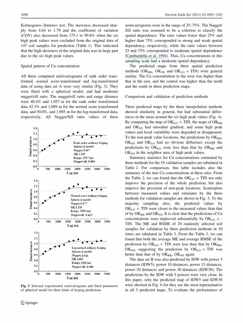
Spatial pattern of Cu concentration

All three computed semivariograms of rank order trans-

formed, normal score-transformed and log-transformed

data of using data set A were very similar (Fig. 3). They

were fitted with a spherical model, and had moderate

nugget/sill ratio. The nugget/sill ratio and range distance

were 40.4% and 1,957 m for the rank order transformed

data 42.3% and 1,989 m for the normal score transformed

data, and 50.0%, and 1,905 m for the log-transformed data,

respectively. All Nugget/Sill ratio values of three

semivariograms were in the range of 25–75%. The Nugget/

Sill ratio was assumed to be a criterion to classify the

spatial dependence. The ratio values lower than 25% and

higher than 75% corresponded to strong and weak spatial

dependency, respectively, while the ratio values between

25 and 75% corresponded to moderate spatial dependence

(Cambardella et al. 1994). Thus, Cu concentrations in this

sampling scale had a moderate spatial dependency.

The predicted maps from three spatial prediction

methods (OKRK, OKNS and OKLG ? TIN) were general

similar. The Cu concentration in the west was higher than

that in the east, and the central was higher than the north

and the south in three prediction maps.

Comparison and validation of prediction methods

Three predicted maps by the three interpolation methods

showed similarity in general, but had substantial differ-

ences in the areas around the six high peak values (Fig. 4).

By comparing the map of OKLG ? TIN, the maps of OKRK

and OKNS had smoother gradient, and some high peak

values and local variability were degraded or disappeared.

To the non-peak value locations, the predictions by OKRK,

OKNS and OKLG had no obvious difference except the

predictions by OKLG were less than that by OKRK and

OKNS in the neighbor area of high peak values.

Summary statistics for Cu concentrations estimated by

three methods for the 54 validation samples are tabulated in

Table 2. For comparison, this table includes also the

summary of the true Cu concentrations at these sites. From

the Table 2, we can found that the OKLG ? TIN not only

improve the precision of the whole prediction, but also

improve the precision of non-peak locations. Scatterplots

between measured values and estimates by the three

methods for validation samples are shown in Fig. 5. To the

majority sampling sites, the predicted values by

OKLG ? TIN were closer to the measured values than that

of by OKRK and OKNS. It is clear that the predictions of Cu

concentrations were improved substantially by OKLG ? -

TIN. The ME and RSME of 20 randomly selected soil

samples for validation by three prediction methods in 10

times are tabulated in Table 3. From the Table 3, we can

found that both the average ME and average RMSE of the

prediction by OKLG ? TIN were less than that by OKRK,

OKNS, suggesting the prediction by OKLG ? TIN was

better than that of by OKRK, OKNS again.

The data set B was also predicted by IDW with power 5

distances (IDW5), power 10 distances, power 15 distances,

power 20 distances and power 30 distances (IDW30). The

predictions by the IDW with 5 powers were very close. In

this paper, only the predicted map of IDW5 and IDW30

were showed in Fig. 6 for they are the most representative

in all 5 predicted maps. To evaluate the performance ofFig. 3 Selected experimental semivariograms and fitted parameters

of spherical model for three kinds of kriging predictions

1098 Environ Earth Sci (2011) 63:1093–1103

123

Fig. 4 The prediction maps of

copper concentration in study

area by rank order ordinary

kriging (OKRK), normal score

ordinary kriging (OKNS) and

integration of lognormal

ordinary kriging (OKLG) and

triangular irregular network

interpolation (TIN), respectively

Table 2 Summary statistics for measured and predicted Cu concentrations (mg kg-1) of 54 (50) soil samples for validation by three prediction

methods

Measured Predicted

True Truea OKRK OKNS OKLG ? TIN OKRKa OKNS

a OKLG ? TINa

Max 2,087.7 840.0 694.8 1,056.0 2,210.0 582.0 755.0 625.1

Min 11.8 11.8 48.3 41.5 41.1 48.3 41.5 41.1

Mean 292.0 199.0 202.0 223.8 298.4 169.1 181.6 184.7

Med 154.5 150.1 138.9 144.3 174.6 138.2 136.4 163.7

SD 396.6 179.3 215.0 228.2 416.7 136.0 164.0 140.9

LQ 73.2 72.1 85.2 86.6 78.7 82.5 85.2 78.2

UQ 347.5 286.66 177.6 210.7 253.7 164.5 172.7 196.8

ME 90.0 68.2 5.1 27.7 16.1 13.2

RMSE 274.7 229.1 89.9 103.2 87.0 83.9

Max maximum, Min minimum, Med median, SD standard deviation, LQ the lower quartile (mg kg-1), UQ the upper quartile (mg kg-1), MEmean errors, RMSE root mean square errors, OKRK rank-order ordinary kriging, OKNS normal score ordinary kriging, OKLG ? TIN combine

lognormal ordinary kriging with triangular irregular network interpolationa Statistical summary for non-peak locations (all samples for validation except the four high peak values)

Environ Earth Sci (2011) 63:1093–1103 1099

123

OKLG ? IDW, the 54 soil samples that were sampled in

spring 2004 were used to validation. The ME and RMSE

was for OKLG ? IDW (5), 14.6, 92.5 mg kg-1; OKL-

G ? IDW (30), 18.3, 112.4 mg kg-1, respectively, sug-

gesting that the IDW (5) was better than IDW (30) for the

data set B prediction. The result also showed that the ME

and RMSE of OKLG ? TIN was lower than that of OKL-

G ? IDW (5) and OKLG ? IDW (30).

Discussion

In environmental study, high peak value as one of outlier is

significant greater than the values of majority samples. The

univariate statistics of Grubbs, Dixon, Walsh, t test, and

range method (mean ± n 9 SD), are quite commonly used

to detect outlying values (Zhang and Selinus 1998), and

these method are also suit for high peak value identifica-

tion. However, the results may have some difference for

they based on different criterions in high peak values

identification. The results of high peak value identification

were also influenced the result of data split directly and

total Cu prediction indirectly.

Locations with high peak values (hot spots) were close

to the smelting furnaces (Fig. 4). The hot spots were

probably due to the atmospheric deposition and scrap

material dumps from copper smelting. Some high peak

values and local variability were degraded or disappeared

in the prediction maps of OKRK and OKNS and the ranges

of OKRK and OKNS were reduced in some degree, in large

part because of the smooth effect inherent in the kriging

and in part because of the effects of back-transformation.

Fig. 5 Measured copper (Cu-measured) concentrations of the 54 soil

samples for validation and their predicted concentrations (Cu-

predicted) by rank order ordinary kriging (a), normal score ordinary

kriging (b) and integration of lognormal ordinary kriging and

triangular irregular network interpolation (c), respectively

Table 3 The mean errors (ME) and root mean square errors (RSME)

of 20 randomly selected soil samples for validation (mg kg-1) by

three prediction methods in 10 times

Seriesa ME RMSE

OKRK OKNS OKLG ?

TIN

OKRK OKNS OKLG ?

TIN

1 (1) 75.2 72.4 63.8 241.3 239.8 224.9

2 (2) 63.1 62.7 54.1 194.8 185.7 161.3

3 (1) 73.5 72.1 62.7 239.4 238.7 219.6

4 (0) 32.7 33.1 19.4 83.6 82.1 57.0

5 (0) 37.6 38.3 22.3 86.3 85.8 58.9

6 (0) 35.2 36.4 20.7 77.4 73.5 41.6

7 (0) 26.3 24.9 15.6 48.2 43.7 28.3

8 (1) 89.2 86.8 83.5 233.5 230.2 228.1

9 (1) 54.4 52.7 47.8 209.2 202.7 195.4

10 (1) 42.3 45.8 48.3 222.8 220.9 215.2

Average 53.0 52.5 43.8 163.7 160.3 143.0

OKRK rank-order ordinary kriging, OKNS normal score ordinary kri-

ging, OKLG ? TIN combine lognormal ordinary kriging with trian-

gular irregular network interpolation, Average the average ME or

RMSE of all 10 timesa 1 (1), 2 (2),…,10 (1), the outside of parentheses is the series number

and the inside of parentheses is the number of high peak values

1100 Environ Earth Sci (2011) 63:1093–1103

123

High peak values are always surrounded by comparatively

lower values. So, the high peak value was decrease sharply

and the values of surrounding area were increase in some

degree for the smooth effect inherent in the kriging pre-

diction. Due to OKLG ? TIN split data into two parts, and

the main part of high peak values were predicted by TIN

interpolation that could avoid smooth effect, this method

could substantially alleviate smooth effect of kriging on

high peak values in prediction although OKLG was still

influenced by smooth effect of kriging The high peak

values were substituted by the median of the remainder

data in logarithm kriging. So, the prediction based on

OKLG ? TIN was not influenced by high peak values.

All summary statistics of the predictions by OKLG ? -

TIN except the median were closest to that of measured

values among the three prediction methods for the 54 val-

idation samples (Table 2). The ME and RMSE of 54 vali-

dation samples that collected in 2004 by OKLG ? TIN were

much less than that by OKRK and OKNS, which demon-

strated that OKLG ? TIN was better than OKRK, OKNS in

the interpolation of severely skewed data with several high

peak values. In general, kriging could provide an unchanged

mean, and all three of the back-transformation methods

used in this study yield a prediction of a median rather than

the mean for each kriged location. So, all the three medians

were close to that of the measured value. In most cases, the

ME and RMSE of 20 randomly selected validation samples

by OKLG ? TIN were also less than that by OKRK and

OKNS. However, the ME and RMSE of 20 randomly

selected validation samples by OKLG ? TIN were closed to

that by OKRK and OKNS when high peak values were

selected for validation. It indicated that the local variability

in the neighborhood of high peak value will be concealed

when it was excluded for prediction data and it could not be

predict based on holistic spatial variability.

There was a distinct difference in the predictions of high

peak values by different interpolation methods (Fig. 4). For

those high peak values, the predicted by OKLG ? TIN were

very close to their measured values, while that by OKRK and

OKNS were far less than their measured ones (Fig. 5). This

demonstrated that OKLG ? TIN could predict the high peak

values successfully, but not by OKRK and OKNS. All eval-

uation indicators of OKLG ? TIN were better than that of

OKRK and OKNS except the maximum and standard devi-

ation when the four high peak values were excluded from

the samples for validation (Table 2). It demonstrated that

the integrated method improved the prediction precision of

other data again. The major reason was the prediction based

on OKLG ? TIN was not influenced by high peak values as

we have mentioned in front text. To the data set B that could

reflect the most importance local variability of hot spots of

soil contaminate i.e. the neighborhood of high peak values

approximately. However, the sampling density in the

neighborhood of high peak value was always too sparse to

know the detail characters of local spatial variability IDW is

based on the assumption that the interpolating surface

should be influenced most by the nearby points and less by

the more distant points. This assumption was always con-

sisting with the fact of pollutions distribution, and IDW was

popular in pollutions spatial prediction of single pollution

source. Whereas, there were several high peak values that

come from different pollution source in contaminated site

and their affect ranges had large difference. IDW with high

power often increase the error in the neighborhood of high

peak values for it make the predicted value decrease shar-

ply, and IDW with low power often increase the error in the

locations of non-peak value for it had wide influence range.

So, it is difficult to choose a fitted power for IDW inter-

polation. Therefore, it was difficult to choose a uniform

appropriate power parameter.

TIN is also one of the most commonly used techniques

for interpolation of scatter points, and the prediction was

only influenced by the values of three nearest known

Fig. 6 The prediction maps of soil copper concentration in study area

based on the data set B by triangular irregular network interpolation

(TIN), inverse distance weighted interpolation with power 5 distances

(IDW5) and power 30 distances (IDW30), respectively

Environ Earth Sci (2011) 63:1093–1103 1101

123

points. Although the effect of TIN interpolation very much

depends on the density of observations TIN maybe not the

best method of conventional interpolation methods for data

set B, and further research should attempt to look for a

more suitable interpolation method for data set B. In this

study, TIN was used for it seldom even to does not smooth

the spatial variation of Cu estimates for the prediction was

only influenced by the values of three nearest known

points, whereas the estimates by other interpolation method

are weighed linear combinations of several sample values,

and hence overestimation of small, and underestimation of

large, values occur.

In this study, to majority samples for validation, the

predicted values based on three methods were close to the

measured value and had no significant difference for they

were not in the neighborhood of high peak values and the

effect of high peak values on their prediction were limited

(Fig. 5). It demonstrates that the prediction precisions of

OKLG, OKRK and OKNS for the same data had no large

difference if the data satisfy their requirements, and the

study of Wu et al. (2006) also demonstrated it. So, it was

unnecessary to compare the spatial prediction by

OKLG ? TIN with these by integration of OKRK and TIN

and by integration of OKNS and TIN, respectively, for the

data set A satisfies lognormal distribution. OKLG ? TIN

was better than the OKRK and OKNS in spatial interpolation

of severely skewed data with several high peak values, in

large part because the data partition improve the suitability

for kriging and alleviate the smooth effect of high peak

values in kriging, and TIN interpolation could describe the

local variability around high peak values. Transformation

and back-transformation may have other effects that are

hard to interpret or may add uncertainty (Armstrong and

Boufassa 1988; Journel and Deutsch 1997; Deutsch and

Journel 1998; Roth 1998; Goovaerts 1999; Jordan et al.

2007). The integrated method of kriging and TIN could

extend the scope of application of kriging interpolation,

and it was suitable for spatial interpolation of severely

skewed data with several high peak values.

High peak values were often presumed to come from a

different distribution than the majority of the survey data in

environmental study, and they often reflect local variabil-

ity. The common survey data were often having a global

variability. It indicated that it is necessary to deal with the

high peak values alone when we spatially interpolate the

environmental survey data with several high peak values.

Spatial interpolation methods can be classified in different

ways and are generally defined based on geometric or

geostatistical properties. Spatial interpolation methods can

generally be classified as local or global, exact or

approximate, and deterministic or stochastic methods.

Local interpolation methods work on a small portion of the

data points while global methods work across the whole

data set (Ali 2004). To this criterion, OKLG is one of global

interpolation methods, and TIN is one of local interpolation

methods for TIN only use three values and kriging usually

use much more samples in the study. Therefore, the inte-

grating kriging and TIN has the potentials to describe both

holistic and local variability of environmental survey data

with several high peak values. OKLG and TIN maybe not

the optimal method for data set A and data set B interpo-

lation, respectively. However, the method of data split and

integrating geostatistics and conventional statistic method

had potential to improve the precision of severely skewed

data with several high peak values.

Summary

In case of severely skewed data with several high peak

values, rank order and normal score transformations could

reduce skewness, but both OKRK and OKNS could not

make satisfied interpolations. The predictions by integrat-

ing OKLG and TIN had a smaller ME and RMSE than that

of OKRK and OKNS. After the high peak values were

substituted by the median of the remaining data set, the

smooth effect could be alleviated sharply by OKLG and

TIN interpolation, which provided more accurate predic-

tions for the areas around the high peak values. This

integrated method has the potentials to apply in other cases

of severely skewed data with several high peak values.

Acknowledgments This research was funded in part by the Science

and technology support program Grant (2007BAC16B06) and the

National Basic Research Priorities Program (973 Program) Grant

(2002CB410810). We appreciate our staffs for soil sample collection

and analysis. We also extend our appreciation to the journal reviewers

and Editor-in-Chief, Dr. LaMoreaux for their valuable suggestions

and constructive criticism.

References

Ali TA (2004) On the selection of an interpolation method for

creating a terrain model (TM) from LIDAR data. In: Proceedings

of the American Congress on Surveying and Mapping (ACSM)

Conference 2004, Nashville, TN, USA

Andrews DF (1974) A robust method for multiple linear regression.

Technometrics 16:523–531

Armstrong M, Boufassa A (1988) Comparing the robustness of

ordinary kriging and lognormal kriging-outlier resistance. Math

Geol 20:447–457

Arrouays D, Mench M, Amans V, Gomez A (1996) Short-range

variability of fallout Pb in a contaminated soil. Can J Soil Sci

76:73–81

Atkinson AC (1994) Fast very robust methods for the detection of

multiple outliers. J Am Stat Assoc 89:1329–1339

Atteia O, Dubois JP, Webster R (1994) Geostatistical analysis of soil

contamination in the Swiss Jura. Environ Pollut 86:315–327

Barabas N, Goovaerts P, Adriaens P (2001) Geostatistical assessment

and validation of uncertainty for three-dimensional dioxin data

1102 Environ Earth Sci (2011) 63:1093–1103

123

from sediments in an estuarine river. Environ Sci Technol

35:3294–3301

Bardgett RD, Speir TW, Ross DJ, Yeates GW, Kettles HA (1994)

Impact of pasture contamination by copper, chromium, and

arsenic timber preservative on soil microbial properties and

nematodes. Biol Fertil Soils 18:71–79

Cambardella CA, Moorman TB, Novak JM, Parkin TB, Karlen DL,

Turco RF, Konopka AE (1994) Field-scale variability of soil

properties in central Iowa soils. Soil Sci Soc Am J 58:1501–1511

Cao ZH, Hu ZY (2000) Copper contamination in paddy soils irrigated

with wastewater. Chemosphere 41:3–6

Carlon C, Critto A, Marcomini A, Nathanail P (2001) Risk based

characterisation of contaminated industrial site using multivar-

iate and geostatistical tools. Environ Pollut 111:417–427

Cattle JA, McBratney AB, Minasny B (2002) Kriging method

evaluation for assessing the spatial distribution of urban soil lead

contamination. J Environ Qual 31:1576–1588

Das SK, Basudhar PK (2006) Comparison study of parameter

estimation techniques for rock failure criterion models. Can

Geotech J 43(7):764–771

Deutsch CV, Journel AG (1998) GSLIB, geostatistical software

library and user’s guide. Oxford University Press, New York

Goovaerts P (1997) Geostatistics for natural resources evaluation.

Oxford University Press, New York

Goovaerts P (1999) Geostatistics in soil science: state-of-the-art and

perspectives. Geoderma 89:1–45

Hendficks Franssen HJWM, van Eijnsbergen AC, Stein A (1997) Use

of spatial prediction techniques and fuzzy classification for

mapping soil pollutants. Geoderma 77:243–262

Huang M, Shu YR, Huang DY, Wu JS, Huang QY (2006) An on-the-

spot sampling and survey method for soil nutrient cycling study

(In Chinese). Chin J Appl Ecol 17(2):205–209

Isaaks EH, Srivastava RM (1989) Applied geostatistics. Oxford

University Press, New York

Jordan C, Zhang CS, Higgins A (2007) Using GIS and statistics to

study influences of geology on probability features of surface soil

geochemistry in Northern Ireland. J Geochem Explor 93:135–152

Journel AG (1980) The lognormal approach to predicting local

distributions of selective mining unit grades. Math Geol

12:285–303

Journel AG, Deutsch CV (1997) Rank order geostatistics: a proposal

for a unique coding and common processing of diverse data. In:

Baafi EY, Schofield NA (eds) Geostatistics Wollongong ‘96.

Kluwer, Dordrecht

Juang KW, Lee DY (1998) A comparison of three kriging methods

using auxiliary variables in heavy-metal contaminated soils.

J Environ Qual 27:355–363

Juang KW, Lee DY, Chen ZS (1999) Geostatistical cross-validation

for additional sampling assessment in heavy-metal contaminated

soils. J Chin Inst Environ Eng 9:89–96

Juang KW, Lee DY, Ellsworth TR (2001) Using rank order

geostatistics for spatial interpolation of highly skewed data in

a heavy-metal contaminated site. J Environ Qual 30:894–903

Lee DY, Juang KW (2003) Use geostatistics to delimit the boundary

of pollution in a contaminated site (In Chinese). Taiwan’s Soil

Groundwater Environ Protect Assoc Newslett 7:2–13

Li GG (2005) The status and development needs of soil environmen-

tal monitoring in China (In Chinese). Environ Monitor Technol

17(1):8–10

Liu FC, Shi XZ, Yu DS, Pan XZ (2004) Mapping soil properties of

the typical area of Taihu Lake Watershed by geostatistics and

geographic information systems––a case study of total nitrogen

in topsoil (In Chinese). Acta Pedol Sin 41(1):20–27

Loland JO, Singh BR (2004) Copper contamination of soil and

vegetation in coffee orchards after long-term use of Cu

fungicides. Nutr Cycl Agroecosyst 69:203–211

Loska K, Wiechula D, Pelczar J (2005) Application of enrichment

factor to assessment of zinc enrichment/depletion in farming

soils. Commun Soil Sci Plant Anal 36:1117–1128

Lu Y, Gong ZT, Zhang GL, Burghardt W (2003) Concentrations and

chemical speciation of Cu, Zn, Pb and Cr of urban soils in

Nanjing, China. Geoderma 115:101–111

Luo Y, Jiang X, Wu L, Song J, Wu S, Lu R, Christie P (2003)

Accumulation and chemical fractionation of Cu in a paddy soil

irrigated with Cu-rich wastewater. Geoderma 115:113–120

Meuli R, Schulin R, Webster R (1998) Experience with the

replication of regional survey of soil pollution. Environ Pollut

101:311–320

Moreno JL, Garcia C, Hernandez T, Ayuso M (1997) Application of

composted sewage sludges contaminated with heavy metals to

an agricultural soil. Soil Sci Plant Nutr 43:565–573

Mueller TG, Pusuluri NB, Mathias KK, Cornelius PL, Barnhisel RI

(2004) Site-specific fertility management: a model for predicting

map quality. Soil Sci Soc Am J 68(6):2031–2041

Park D, Cho H, Kim Y (2001) A TIN compression method using

Delaunay triangulation. Int J Geogr Inform Sci 5(3):255–269

Rawlins BG, Lark RM, O’Donnell KE, Tye AM, Lister TR (2005)

The assessment of point and diffuse metal pollution of soils from

an urban geochemical survey of Sheffield, England. Soil Use

Manag 21(4):353–362

Roth C (1998) Is lognormal kriging suitable for local estimation?

Math Geol 30:999–1009

Saito H, Goovaerts P (2000) Geostatistical interpolation of positively

skewed and censored data in a dioxin-contaminated site. Environ

Sci Technol 34:4228–4235

Schwertman NC, de Silva R (2007) Identifying outliers with

sequential fences. Comput Statist Data Anal 51:3800–3810

Schwertman NC, Owens MA, Adnan R (2004) A simple more general

boxplot method for identifying outliers. Comput Statist Data

Anal 47(1):165–174

State Environmental Protection Administration of China (1995)

Chinese environmental quality standard for soils (GB 15618-

1995). http://www.chinaep.net/hjbiaozhun/hjbz/hjbz017.htm

Tan MZ, Xu FM, Chen J, Zhang XL, Chen JZ (2006) Spatial

prediction of heavy metal pollution for soils in peri-urban

Beijing, China based on fuzzy set theory. Pedosphere 16(5):545–

554

Tukey JW (1977) Exploratory data analysis. Addison-Wesley,

Reading

van Meirvenne M, Goovaerts P (2001) Evaluating the probability of

exceeding a site-specific soil cadmium contamination threshold.Geoderma 102:75–100

von Steiger B, Webster R, Schulin R, Lehmann R (1996) Mapping

heavy metals in polluted soil by disjunctive kriging. Environ

Pollut 94:205–215

Walter C, McBratney AB, Viscarra Rossel RA, Markus JA (2005)

Spatial point-process statistics: concepts and application to the

analysis of lead contamination in urban soil. Environmetrics

16:339–355

Wu J, Norvell WA, Welch RM (2006) Kriging on highly skewed data

for DTPA- extractable soil Zn with auxiliary information for pH

and organic carbon. Geoderma 134:187–199

Zhang CS, McGrath D (2004) Geostatistical and GIS analyses on soil

organic carbon concentrations in grassland of southeastern

Ireland from two different periods. Geoderma 119(3–4):261–275

Zhang CS, Selinus O (1998) Statistics and GIS in environmental

geochemistry––some problems and solutions. J Geochem Explor

64:339–354

Zhang CB, Li ZB, Yao CX, Yin XB, Wu LH, Song J, Teng Y, Luo

YM (2006) Characteristics of spatial variability of soil heavy

metal contents in contaminated sites and their implications for

source identification (In Chinese). Soils 38(5):525–533

Environ Earth Sci (2011) 63:1093–1103 1103

123