Mapping Pre-European Settlement Vegetation Using a Hierarchical Bayesian Model and GIS
19
Mapping Pre-European Settlement Vegetation Using a Hierarchical Bayesian Model and GIS Hong S. He 1,* , Daniel C. Dey 2 , Xiuli Fan 1 , Mevin B. Hooten 3 , John M. Kabrick 2 , Christopher K. Wikle 3 , and Zhaofei Fan 1 1 School of Natural Resources, University of Missouri-Columbia, Columbia, Missouri, USA, 2 US Forest Service, North Central Research Station, Columbia, Missouri, USA, 3 Department of Statistics, University of Missouri-Columbia, Columbia, Missouri, USA * Correspondence contact: 203 ABNR Building, Columbia, MO 65211. Phone (573) 882-7717 Email [email protected] Abstract In the Midwestern United States, the General Land Office (GLO) survey records provide the only reasonably accurate data source of forest composition and tree species distribution at the time of pre-European settlement (circa late 1800 to early 1850). However, GIS and statistic inference methods to map GLO data and reconstruct historical vegetation are needed. In this study, we applied a hierarchical Bayesian approach that combines species and environment relationships and explicit spatial dependence to map GLO data. We showed that the hierarchical Bayesian approach 1) is effective in predicting historical vegetation distribution, 2) is robust at multiple classification levels (species, genus, and functional groups), 3) can be used to derive vegetation patterns at fine scales (e.g. in this study, 120 m) when the corresponding environmental data exist, and 4) is applicable to relatively moderate map sizes (e.g., 792×763 pixels) due to the limitation of computational capacity. Our predictions of historical vegetation from this 1
Transcript of Mapping Pre-European Settlement Vegetation Using a Hierarchical Bayesian Model and GIS

Mapping Pre-European Settlement Vegetation Using a Hierarchical Bayesian Model
and GIS
Hong S. He1,*, Daniel C. Dey2, Xiuli Fan1, Mevin B. Hooten3, John M. Kabrick2,
Christopher K. Wikle3, and Zhaofei Fan1
1 School of Natural Resources, University of Missouri-Columbia, Columbia, Missouri,
USA, 2 US Forest Service, North Central Research Station, Columbia, Missouri, USA, 3
Department of Statistics, University of Missouri-Columbia, Columbia, Missouri, USA
* Correspondence contact: 203 ABNR Building, Columbia, MO 65211.
Phone (573) 882-7717 Email [email protected]
Abstract
In the Midwestern United States, the General Land Office (GLO) survey records provide
the only reasonably accurate data source of forest composition and tree species
distribution at the time of pre-European settlement (circa late 1800 to early 1850).
However, GIS and statistic inference methods to map GLO data and reconstruct historical
vegetation are needed. In this study, we applied a hierarchical Bayesian approach that
combines species and environment relationships and explicit spatial dependence to map
GLO data. We showed that the hierarchical Bayesian approach 1) is effective in
predicting historical vegetation distribution, 2) is robust at multiple classification levels
(species, genus, and functional groups), 3) can be used to derive vegetation patterns at
fine scales (e.g. in this study, 120 m) when the corresponding environmental data exist,
and 4) is applicable to relatively moderate map sizes (e.g., 792×763 pixels) due to the
limitation of computational capacity. Our predictions of historical vegetation from this
1

study provide a quantitative and spatial basis for restoration of natural floodplain
vegetation.
Keywords: GLO, GIS, Bayesian hierarchical model, presettlement vegetation, Missouri
1. Introduction
The General Land Office (GLO) survey conducted from early 18th to mid 19th
century in the Midwestern United States provides a key data source of forest and
environmental conditions of the pre-European settlement period (Bourdo, 1956). Under
the GLO, the public land survey system (PLSS) was developed, in which land was
divided into a grid of square townships, each containing 36 1-square-mile (1.6-square-km)
sections. To conduct the survey, the surveyors walked the section lines, documenting the
land, vegetation, water, and human features along each mile. At each section corner and
the mid-point between section corners (quarter corner) 2 to 4 witness trees were
identified and measured to mark the corner location by the surveyors. Witness tree
species and diameter, as well as the distance and bearing to the corner were recorded in
the surveyor’s notebook. When traversing the section lines, the surveyors also recorded
trees that fell along the section lines (line trees), and trees around survey posts set where
section lines intersected rivers or impenetrable wetlands (meander corners). Since GLO
records are spatially available for a regular square grid of points one mile apart and
quarter corner points at half mile intervals along section lines, a GLO data set can be
easily imported into a geographic information system (GIS) for further spatial analysis
and statistical inference.
Tree count, forest density, species composition, and dominance are the most
important information that can be derived from the witness tree records (e.g., Fralish et
2

al., 1991; Abrams and Ruffner, 1995; Nelson, 1997; Dyer, 2001; Schulte et al., 2002).
Density is estimated from recorded distances to witness trees using established distance-
based sampling methods (Cottam & Curtis, 1956); tree species relative density (%
species composition) is estimated from species counts; and dominance (% basal area) is
calculated from recorded species diameters (He et al., 2000). Despite the survey biases
including surveyor’s preference and exclusion of certain species and age groups (Manies
et al., 2001), GLO data provides the only reasonably accurate data source of forest
composition and tree species distribution prior to the pre-European settlement (Manies
and Mladenoff, 2000). Thus, it is commonly used for assessing forest change and guiding
ecological restoration (Dey et al., 2000; Bolliger et al., 2004; Schulte et al., in press).
Besides the recognized biases, GLO data is limited due to its coarse PLSS
sampling structure. The sparseness of GLO records is a primary limitation of any effort to
map forest types. The square mile section and half mile distance between quarter corner
and section corner is very coarse for a typical ecological restoration task that often ranges
from a few hectares to several townships. Although some methods have been used to map
GLO data to finer scales, they have not been validated (Brown, 1998). Another inherent
limitation of GLO data is that point data alone are insufficient to describe vegetation that
is continuously distributed over the landscape. GIS and statistical inference are needed to
convert point data into more relevant data forms such as grids of finer resolutions and
determine vegetation for places where data were not recorded. The most common
statistical inference methods used to reconstruct historic vegetation by interpolating GLO
data are ISOLINE, kriging or co-kriging embedded in GIS (e.g., Porter, 1998; Brown,
1998; Batek et al., 1999). These methods use the vegetation values of the known data
3

points to interpolate the vegetation values for points that do not have recordings. They
assume the interpolated data are numerical and are spatially continuous, such as elevation.
These methods can be problematic when applied to GLO data that are primarily in the
form of tree count and tree diameter. Also, GLO data are not necessarily spatially
continuous because many factors such as soil, elevation, and competition among other
species often cause the spatial discontinuity of a species distribution. Therefore, the
interpolation methods may ignore the ecological principles underlined by these
environmental factors.
Methods have been proposed for mapping individual species pattern using known
environmental covariates that account for ecological/biotic processes (e.g.,
Zimmermanmn and Kienast 1999, Lichstein et al. 2002). These methods, however, either
lack the consideration of residual spatial dependence inherent in the vegetation
distribution or are limited to small spatial domains (e.g., 10 ha). Hooten et al. (2003)
developed a statistically rigorous method for combining species/environment
relationships and explicit spatial dependence for binary response data. Their method
combines information found within abiotic covariates and spatial dependence that may is
used as a surrogate for various biotic covariates. They were able to provide spatial
predictions for vegetation with known certainty, and map ground flora distribution using
recent vegetation plot data (point) for areas ranging from 265 ha to 530 ha. However,
whether this method can be applied to GLO data and much larger areas with diverse
vegetation and environmental combinations is of interest.
The objective of this study was to apply the hierarchical Bayesian approach to
GLO data and test its applicability in that setting. More specifically, we evaluated if this
4

approach a) can be used to interpolate GLO data to fine spatial resolutions (e.g., 30 m, 60
m, and 120 m), b) can be applied to large landscapes (e.g., 103-106 ha), and c) is robust
at the species, genus or functional plant group levels. The Bayesian hierarchical approach
differs from traditional statistic approaches (e.g., logistic regression) because it can
account for uncertainty in various levels of the model including spatially correlated errors.
We applied this approach by incorporating digital elevation, slope, aspect, soil water
capacity, soil depth, and soil organic matter as covariates in the model.
2. Material and methods
2.1 Study area and data preparation
Our study area encompasses a portion of Missouri River in the Columbia and
Booneville, Missouri, USA (Fig. 1). The size of the study area is about 7,200 ha and
involves 14 counties, and include 19,000 GLO tree data points. The study area has
diverse terrain, soil, and hydrological features and consequently a high diversity of tree
species. Thus, it provides an ideal place for evaluating our statistical approach. The
bottomland of the study area includes the lower Missouri River alluvial plain land type
association to the east and Missouri Grand River alluvial plain and loess woodland/forest
breaks land type associations to the west (Nigh and Schroeder, 2002). The bottomlands
have flood tolerant species such as American elm (Ulmus americana L.), hackberry
(Celtis occidentalis L.), and green ash (Fraxinus pennsylvanica, Marsh.), cottonwood
(Populus deltoids Bart. Ex Marsh.), sycamore (Platanus occidentalis L.), boxelder (Acer
negundo L.) and pin oak (Quercus palustris Muenchh.). The upland of the study area are
dominated by white oak (Quercus alba L.), black oak (Quercus velutina Lam.), and
hickory (Carya spp). There are a total of 19,000 individual GLO tree recorded in the
5

GLO data for the study area, among which white oak is most abundant (30%), followed
by black oak (21%), hickory (11%), elm (8%), hackberry (5%), and ash (2%).
Cottonwood, sycamore, boxelder and pin oak are at 1-2%.
To evaluate the robustness of the statistical approach, we processed the GLO tree
data at three classification levels: individual tree species, genus, and functional groups.
For individual tree species we chose black oak since it was one of the most abundant
upland species. For the genus level classification, we chose bottomland oaks (Quercus
Sp.) that included primarily pin oak, white oak, and red oak. Functional groups were
defined based upon the successional stages for the bottomland tree species and nut-
producing capability for tree species in the whole area. Bottomland tree species were
grouped into a) early successional, including primarily sycamore, cottonwood, and
willow (Salix Sp.), and b) mid and late successional, including elm, boxelder, silver
maple (Acer saccharinum L.) and ash. For the nut-producing functional group tree
species include all oak species, black walnut (Juglans nigra L.), and hickory.
We identified the seven most significant terrain and soil covariates for the
statistical model. They were elevation, slope, aspect, soil water capacity, soil organic
matter, soil depth, and depth to bedrock. These covariates were chosen because 1) they
are the determinants of the availability of basic energy, water, and nutrients influencing
tree species establishment and growth, 2) they were available at the scale of our study,
and 3) they remain relatively consistent from between the time GLO data were surveyed
to the time these data were measured. The terrain data was derived from USGS 7.5
minute DEM at 30-meter resolution. The soil data was derived from the county soil
6

survey (SURGGO) for each of the 14 counties and then merged for the study area. All
data were converted into 30-m, 60-m, and 120-m resolutions.
2.2 Statistical modeling
We adopt the hierarchical Bayesian model implemented in Hooten (2001) and Hooten et
al. (2003) to predict the probability of occurrence for the three vegetative classification
groups mentioned in the previous section. This generalized linear mixed model provides
a method of probabilistically predicting a binary response variable based on several
environmental covariates and residual spatial structure. The hierarchical modeling
framework teamed with an explicitly defined spatial random effect allows us to
incorporate various sources of uncertainty at many levels of the ecological process
(Wikle, 2002; Hooten et al., 2003; Wikle, 2003).
Specifically, using the notation in Hooten et al. (2003), we let Yi represent the
presence/absence of the vegetation group of interest and be defined as:
⎩⎨⎧
≤>
=00
01
i
ii Z
Zifif
Y (1)
Where Zi represents an underlying (latent) continuous process analogous to that derived
by Albert and Chib (1993). In our case, it is composed of a covariate component, Xβ, and
a spatially correlated component, η. Where X is comprised of the covariate data (e.g.,
slope, aspect, elevation, soil depth, and organic matter). The model can then be
summarized in matrix notation:
Z|β, η ~ N(Xβ + η, I), (2)
η ~ N(0, Rη), (3) 2ησ
β ~ N(β0, β∑ ) (4)
7

In this setting, equations (3) and (4) represent our prior distributions for the spatial
random effect and the covariate parameters, respectively. Additionally, an inverse gamma
prior distribution was specified for . The matrix Rη is a spatial correlation matrix
although not directly parameterized. That is, we adopt the same spectral decomposition of
η using Fourier basis functions as in Hooten et al. (2003). Although not detailed here, this
Fourier (and inverse Fourier) transform allow for implementation of this model on very
large spatial domains. For additional details see Wikle (2003) and Royle and Wikle
(2005).
2ησ
Ultimately, our interest lies with the predictions of Yj, where j can exist on some
other set of spatial location than our original data. Perhaps more informative are the
predictions of probability of occurrence (p) at location j. That is, the predictions of
( ) ( )jjjj xpYE ηβ +Φ== ' . In this case Φ represents the probit transform (standard
normal CDF); note that the probit transform behaves similarly to the more common logit
transform used in logistic regression.
Preliminary spatial analysis of the dataset was used to inform the prior for the
spatial random effect. An efficient sampling algorithm similar to that used in Hooten et al.
(2003) was used to sample from the posterior distribution via the full conditionals.
Due to the dimension of the dataset and prediction grid, a repeated hold-out
version of cross-validation (as in Hooten et al., 2003) was not feasible. However, one
benefit of using a rigorous statistical model is that it provides for model-based validation
methods. The ability to create maps of prediction error allows us to visualize the
uncertainty across the spatial domain as well as assess specific areas of high and low
variability. Additionally, we can employ the use of Receiver Operating Characteristic
8

curves (ROC) to evaluate model accuracy and compare against similar but simpler model
specifications. Specifically, a logistic regression model was constructed using the same
response and covariate data to get a baseline from which to compare the hierarchical
model through ROC analysis.
Assessing the sensitivity versus specificity of a model, the ROC curve is a plot of
the true positive rate against the false positive rate based on the predictions. The closer
and curve follows the left-hand and top border of the ROC space, the better the
predictions.
3. Results and Discussion
3.1 Spatial resolution and extent
Analysis of GLO data using the hierarchical Bayesian model at the 30-, 60-, and
120-meter resolution yielded 600,000, 2.4 million, and almost 10 million prediction
locations, respectively. Our current computational capability limited our analysis to the
120 m resolution. At this resolution, the floodplain and islands in the river can be
delineated finer than that of GLO data (~1,600 m) and therefore, allowing GLO data
inference at the finer scale. In addition, the study showed that the model can be applied to
the study area of 7,200 ha, which is much larger than previously reported (265-530 ha).
3.2 Genus and functional group at bottomland
Maps that display information about the posterior distribution based on the prediction
process can be viewed as probabilities of species occurrence. Such values range from 0 to
1 (100% probability of species occurrence). Results show that as a genus group,
bottomland oaks have medium probability (0.4-0.6) of occurring on the northwestern
areas of Missouri River floodplain and other tributaries where floodplains are wide and
9

islands are high in elevation. These areas are flooded less frequently compared to
narrower and lower floodplains from northwest to southeast in the study area. The
prediction shows that the occurrence probability of bottomland oaks decreases to low
(0.2-0.4) in the mid section of the Missouri River and very low (<0.2) in the southwest
section of the river within the study area (Fig. 2).
The predicted distributions for the early and late successional functional group
show a strong association with the physical variations. The early successional group has
medium probability of occurring in the mid to southeastern section of the Missouri River
where the valley is narrow and frequently flooded, while the mid and late successional
group shows medium probability of occurring in the northwestern section of the Missouri
River and small floodplains along other tributaries (Fig. 2). Overall, the predictions for
the bottomland areas reflect the ecological dynamics coinciding with floodplain
hydrological process of erosion and deposition. Species of the early successional group
are adapted to readily establish on recently deposited and exposed alluvium. Mid and late
successional group species typically succeed the early successional group because they
do not need mineral soil for germination and open (full sun) environments to grow to
maturity. Their seed is large enough to permit seedling establishment in leaf litter and
they are more tolerant of shade than the cottonwoods and willows.
3.3 Individual species and functional group at whole study area
Predictions for black oak and the nut-producing group were made for the entire
study area including both bottomlands and uplands. Predictions show a high probability
of black oak occurring on most upland areas and very low probabilities on most
bottomland areas (Fig. 2). This pattern also agrees with ecological and biological
10

characteristics of black oak as a common upland species that is not tolerant of flooding.
The nut-producing functional group contained the most abundant upland tree species in
this area including white oak, black oak, and hickory. The predictions show that this
group has a very high probability of occurrence (0.8-1.0) on most upland areas (Fig. 2).
This pattern agrees with the ecological traits of these nut- producing species (Burns and
Honkala, 1990). Today they are still the most common tree species in the uplands.
3.4 Result Validation
A partial validation of the predicted results was performed by presenting maps of
prediction error in the form of marginal posterior standard deviations for grid cells and by
ROC analysis. Posterior standard deviations for grid cells were derived for all predicted
classes. Overall, they suggested that the predictions have general agreement with the
GLO data records. Low prediction errors were small in places where data were abundant
and relatively high in places where data were sparse (Fig. 2). The ROC analysis
suggested that the statistical method was useful in modeling historical vegetation (Fig. 3).
Figure 3 illustrates that the logistic regression model and the hierarchical model present
with very similar ROC curves, implying that their ability to accurately predict is nearly
the same. Recall however, that the hierarchical model has taken into account many other
sources of uncertainty including an explicit spatial random effect. Although it may not
improve on the prediction in this setting, it is providing us with a more accurate portrail
of the variability in the predictions (Fig. 3).
4. Conclusions
This paper demonstrated how GLO data can be analyzed to reveal the probable
distribution of historical vegetation using a hierarchical Bayesian approach and GIS. We
11

showed that this approach 1) was effective in predicting historical vegetation distribution,
2) was robust at multiple classification levels (species, genus, and functional groups), 3)
can be used to derive vegetation patterns at fine scales (e.g. in this study, 120 m) when
the corresponding environmental data exist, and 4) was applicable to relatively moderate
map sizes (e.g., 792×763 pixels) only because of the limitation of computational capacity.
Our results also indicated that the residual spatial dependence of various vegetation types
was weak at 120 m resolution, which resulted in predictions from the Bayesian
hierarchical approach to be similar to those from the logistic regression model. However,
the strength of the Bayesian hierarchical approach over logistic regression is its ability to
provide a prediction error estimate at each pixel location while accounting for various
sources of uncertainty. Maps of prediction error can be very useful for forest managers
and planners so that they can consider spatially varying uncertainty in their planning
processes.
The predicted probabilities for each vegetation class graphically depict the
relationships between the vegetation and environment. Such predictions are based on a
combination of environmental factors and surrogates for biotic factors, making them a
very complete and robust reflection of species response on a continuous spatial domain.
Such relationships can be easily validated against the existing ecological and biological
knowledge about the predicted vegetation.
The results from this study are useful for guiding ecological restoration efforts.
Floodplain forests reflecting the natural processes of floodplain erosion and deposition,
normally include a wide range of seral communities, however many of the natural seral
communities such as young and mature floodplain forests are now scarce due to
12

harvesting and farming (Bragg and Tatschl 1977; Nelson, 1997). Losses of extensive and
continuous floodplain forest communities to cultivation, or losses of particular seral
stages to the catastrophic, stand replacing disturbances may lead either to the disruption
of the natural occurrence of organisms along the Missouri River or to the destruction of
particular habitats required by certain species. While the debate of how to restore
floodplains continues, quantitative and spatial predictions from this study provide a
firmer basis for identifying appropriate seral stages for ecological restoration of
floodplains.
5. Acknowledgement
Funding support is from U.S. Forest Service North Central Research Station and
University of Missouri GIS Mission Enhancement Program.
6. References
Abrams, M. D., Ruffner, C. M. (1995) Physiographic analysis of witness-tree distribution
(1765-1798) and present forest cover through north central Pennsylvania. Canadian
Journal of Forest Research, 25, 659-668.
Albert, J., Chib, S. (1993) Bayesian analysis of binary and polychotomous response data.
Journal of the American Statistical Association, 88, 669-679.
Batek, M.J., A.J. Rebertus, W.A. Schroeder, T.L. Haithcoat, E. Compas, and R.P.
Guyette. (1999) Reconstruction of early nineteenth century vegetation and fire regimes
in the Missouri Ozarks. Journal of Biogeography, 26, 397-412.
Bolliger, J., Schulte, L. A., Burrows, S. N., Sickley, T. A., Mladenoff, D. J. (2004)
Assessing ecological restoration potentials of Wisconsin (USA) using historical
landscape reconstructions. Restoration Ecology, 12, 124-142.
13

Bragg, T. B., Tatschl, A. K. (1977) Changes in flood-plain vegetation and lands use along
the Missouri River from 1826 to 1972. Environmental Management, 4, 353-348.
Brown, D. G. (1998) Mapping historical forest types in Baraga County Michigan, USA
as fuzzy sets. Plant Ecology, 134, 97-111.
Buordo, E. A. (1956) A review of the General Land Office Survey and of its use in
quantitative studies of former forests. Ecology, 37, 754-768.
Burns, R. M., Honkala, B. H. (1990) Silvics of North America, Vol. 2 Hardwoods.
Agriculture Handbook 654. Washington, D. C. US Department of Agriculture Forest
Service. 877p.
Curtis, J. T. (1959) The vegetation of Wisconsin: an ordination of plant communities, 657
pp. University of Wisconsin Press, Madison, WI, USA.
Dey, D. Burhans, D., Kabrick, J., Root, B., Grabner, J., Gold, M. (2000) The Missouri
River Floodplain: history of oak forests and current restoration efforts. Glade, 3, 2-4.
Dyer, J. M. (2001) Using witness trees to assess forest change in southeastern Ohio.
Canadian Journal of Forest Research, 31, 1708-1718.
Fralish, J. S., Crooks, F. B., Chambers, J. L., & Harty, F. M. (1991) Comparison of
presettlement second-growth and old-growth forest on six site types in the Illinois
Shawnee Hills. American Midland Naturalist, 125, 294-309.
He, H. S., Mladenoff, D. J., Sickley, T., Gutensburgen, G. (2000) GIS interpolation of
witness tree records (1839-1866) of northern Wisconsin. Journal of Biogeography, 27:
1031-1042.
Hooten, M. B. (2001) Modeling the distribution of ground flora on large spatial domains
in the Missouri Ozarks. Master’s thesis, University of Missouri, Columbia, MO, USA.
14

Hooten, M. B., Larsen, D. R., Wikle, C. K. (2003) Predicting the spatial distribution of
ground flora on large domains using a hierarchical Bayesian model. Landscape
Ecology, 18, 487-502.
Lichstein, J. Simmons, T. Shriner, S., Fanzreb, K. (2002) Spatial autocorrelation and
autoregressive models in ecology. Ecological Monographs, 72, 446-463.
Manies, K. L., Mladenoff, D. J. (2000) Testing methods to produce landscape-scale
presentment vegetation maps from the U. S. public land survey records. Landscape
Ecology, 15, 741-754.
Manies, K. L., Mladenoff, d. J., Nordheim, E. V. (2001) Surveyor bias in forest data of
the U. S. General Land Office records for northern Wisconsin. Canadian Journal of
Forest Research 31: 1719-1730.
Nelson, J. C. (1997) Presettlement vegetation patterns along the 5th Principal Meridian,
Missouri territory, 1815. American Midland Naturalist, 137, 79-94.
Nigh, T. a., Schroeder, W. A. (2002) Atlas of Missouri Ecoregions. Missouri Department
of Conservation Publication. 212p.
Porter, S. (1998) Modeling historic woody vegetation in the lower Ozarks of Missouri.
Master’s Thesis. University of Missouri, Columbia, MO, USA.
Royle, J. A., Wikle, C. K. (2005) Efficient statistical mapping of avian count data.
Ecological and Environmental Statistics. To appear.
Schulte, L. A., Mladenoff, D. J., Nordheim, E. V. (2002) Quantitative classification of a
historic northern Wisconsin (USA) landscape: mapping forest at regional scales.
Canadian Journal of Forest Research, 32, 1616-1638.
15

Schulte, L. A., Mladenoff, D. J., Burrows, S. N., Sickley, T. A., Nordheim, E. V. (in
press) Spatial controls of pre-Euroamerican wind and fire disturbance in northern
Wisconsin (USA) forest landscape. Ecosystems.
Wikle, C. K., Berliner, L. M., Cresses, N. (1998) Hierarchical Bayesian space-time
models. Environmental and Ecological Statistics, 5, 117 – 154.
Wikle, C. K. (2002) spatial modeling of count data: a case study in modeling breaeeding
bird survey data on large spatial domains. In: Spatial Cluster Modelling. Chapman and
Hall / CRC. Pp. 199-209.
Wikle, C. K. (2003) Hierachical baysian models for predicting the spread of ecological
processes. Ecology, 84, 1382-1394.
Zimmermann, N., Kienast, F. (1999) Predictive mapping of alpine grasslands in
Switzerland: species versus community approach. Journal of Vegetation Science, 10,
469-482.
16
0 90 180 Miles
N
Figure 1. The study area encompasses a portion of Missouri River in the Columbia and
Booneville region. The size of the study area is about 7,200 ha and involves 14 counties.
There are 9,680,944 prediction locations for 30 m resolution, 2,420,236 for 60 m, and
605,059 for 120 m. There are a total of 19,000 individual GLO trees recorded in the GLO
data for the study area.
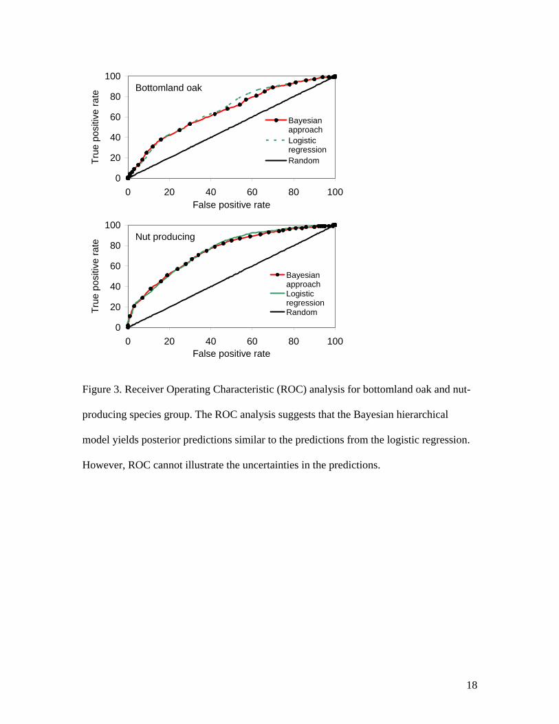
Figure 2. Predicted probabilities for various vegetation types. The prediction maps are
draped on the digital elevation model to show a 3-D perspective. The strength of the
Bayesian hierarchical approach over logistic regression is its ability to provide an error
estimate at each pixel location (last page).
17
18
0
20
40
60
80
100
0 20 40 60 80 100False positive rate
True
pos
itive
rate
BayesianapproachLogisticregressionRandom
Bottomland oak
0
20
40
60
80
100
0 20 40 60 80 100False positive rate
True
pos
itive
rate
BayesianapproachLogisticregressionRandom
Nut producing
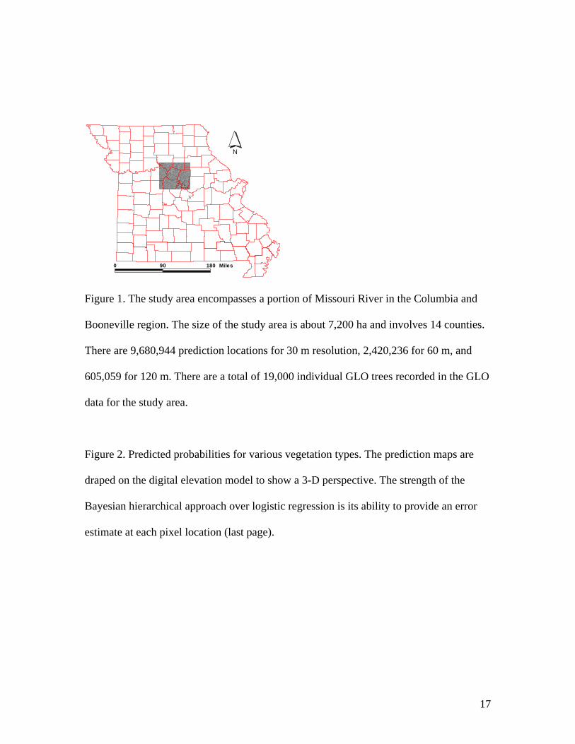
Figure 3. Receiver Operating Characteristic (ROC) analysis for bottomland oak and nut-
producing species group. The ROC analysis suggests that the Bayesian hierarchical
model yields posterior predictions similar to the predictions from the logistic regression.
However, ROC cannot illustrate the uncertainties in the predictions.
19