Macro Models and Household Survey Data: Linkages for Poverty

and Distributional Analysis

Pierre-Richard Agénor* Derek H. C. Chen** Michael Grimm***

Final version: November 6, 2005

Abstract

This paper focuses on approaches to linking macroeconomic models to household income data for poverty and distributional and analysis. Given that linkage methods can influence the resulting poverty and income distribution effects, understanding the benefits and costs of various linkages is important. Simulation exercises do not show fundamentally different results when comparing three approaches: a simple micro-accounting method, an extension of that method to account for changes in employment structure, and the Beta distribution approach. However, potential differences can be very large. We also highlight the extended micro-accounting method as a practical approach to linking macroeconomic models to household income data.

*Hallsworth Professor of International Macroeconomics and Development Economics, University of Manchester, and Centre for Growth and Business Cycle Research. **The Knowledge for Development Program of the World Bank Institute, The World Bank. ***Department of Economics, University of Göttingen, DIW Berlin, and DIAL, Paris. We are grateful to two anonymous referees for helpful comments. The views expressed in this paper do not necessarily represent those of the World Bank.

2

1. Introduction

In recent years renewed efforts have been made (at the World Bank and

elsewhere) to develop new policy tools aimed at better understanding the channels

through which adjustment policies affect the poor and the possible trade-offs that poverty

reduction strategies may entail regarding the sequencing of policy reforms.

One approach consists of using disaggregated computable general equilibrium

(CGE) models that distinguish between several representative household groups (RHG),

according to their education level (skilled and unskilled), their location (rural and urban),

and their sector of employment. In these models, henceforth referred to as “Macro-RHG

models”, the distributional and poverty effects of macroeconomic shocks are generally

based on the association between household-group-specific mean incomes and the state

of poverty. For instance, if the mean income of workers in the rural tradable goods sector

is below the poverty line, all workers in the sector are considered poor. Likewise,

inequality indicators are based only on the distance between group-specific means.

Therefore, within-group heterogeneity (dispersion around group means) is completely

ignored, or in other words, it is assumed that within-group distributions are uniform.

However, a common observation is that the contribution of within-group income

inequality to overall income inequality is much more important than that of between-

group inequality, even if households are disaggregated in relatively small groups. For

example, if Ivorian households are classified in ten groups according to activity sector

and educational attainment of the household head, more than 80 percent of the variance

of household incomes per capita is within groups. Likewise, a similar classification into

ten groups for the Indonesian population leaves 74 percent of the total variance

unexplained.1 Because, by definition and construction, Macro-RHG models do not

account for intra-group heterogeneity, they cannot provide much insight in the analysis of

the impact of government policy or exogenous shocks on income distribution.

1 These estimates are derived from computations by the authors, based on household surveys of

the respective countries.

3

One approach to extend the use of such Macro-RHG models for poverty and

income distribution analysis is to link the macroeconomic model with household survey

data, thereby forming a framework with macro and micro components. The linkage

methodology between the macroeconomic model and survey data clearly determines the

channel(s) and extent to which macroeconomic shocks are transmitted to the micro

component of the framework, which consequently affects the resultant changes in poverty

and income distribution.

There are two broad categories of methodologies for linking macro models to

household surveys. The first transmits the resultant changes in incomes, prices, and

sometimes employment using either ‘accounting methods’ or parametrical methods to

generate changes in the income distribution. These methods use only the minimum of the

observed hetereogeneity in household surveys and do not postulate any behavior for

households when transmitting the changes. In contrast, the second methodology

transmits these changes explicitly via econometrically estimated behavioral equations to

the household survey. Our focus in this paper is on the first category of methods.2

Methods within this category have the advantage that they are rather easy to implement,

which is especially important for developing countries whenever skills and resources are

limited. However, it is important to understand more fully the benefits and costs of these

various linkages within this methodology by comparing the results they produce. To our

knowledge such systematic comparisons have never been made.

This paper addresses this gap in the literature by comparing three commonly used

approaches that belong to the first category of linkage methodologies.3 Knowing the

benefits and costs of these different approaches are pertinent for enabling researchers and

policymakers to choose between them. In addition, understanding the robustness of the

simulated distributional effects is very important given that changes in poverty and

2 For an example of the use of the second methodology, see Robilliard, Bourguignon and

Robinson (2002). 3 For a comparison of the second category of methodologies, see Cogneau and Robilliard (2004).

4

income distribution are the key indicators international donors and policymakers look to

when deciding between different policy options.

Of the three approaches, note that the first two are micro-accounting methods and

are non-parametrical in nature, while the third is purely parametrical. The first approach

was initially proposed by Agénor, Izquierdo and Fofack (2003) and was used

subsequently in the number of other studies. It assumes a stable within-household group

distribution and employment structure. Shocks are introduced by applying changes in

household-group-specific income and consumption to that of each household in the

household income survey. The new poverty and distributional indicators are then

computed on the basis of the “adjusted” post-shock household data. The second

approach is to our knowledge new and extends the first by accounting for changes in the

employment structure predicted by the macro component. This is achieved by modifying

the weight given to each household group in the survey. The third approach uses

estimated income distributions to measure distributional changes.4 It imposes a fixed,

parametrically estimated distribution of income within each household group and

assumes that shocks shift the mean of these distributions without modifying their shape.

Poverty indicators are then computed on the basis of these new distributions. We select

one variant of this approach that uses the Beta distribution to compare with the micro-

accounting methods.

To illustrate and compare these three approaches we use the Mini-IMMPA

macroeconomic framework developed by Agénor (2003) and repeat a pair of experiments

with each approach. The Mini-IMMPA CGE model is based on a four-good production

structure combined with five categories of households, consisting of workers in the rural

sector, the urban informal sector, the urban unskilled formal sector, the urban skilled

formal sector, and the capitalists-rentiers. This framework focuses only on the “real” side

of the economy and provides a very detailed treatment of the labor market, which is

important for comparing the first and second approaches. We use a calibrated prototype

5

version of the model for a “typical” middle-income developing country and link it to

fictitious (but representative) household income and expenditure survey.

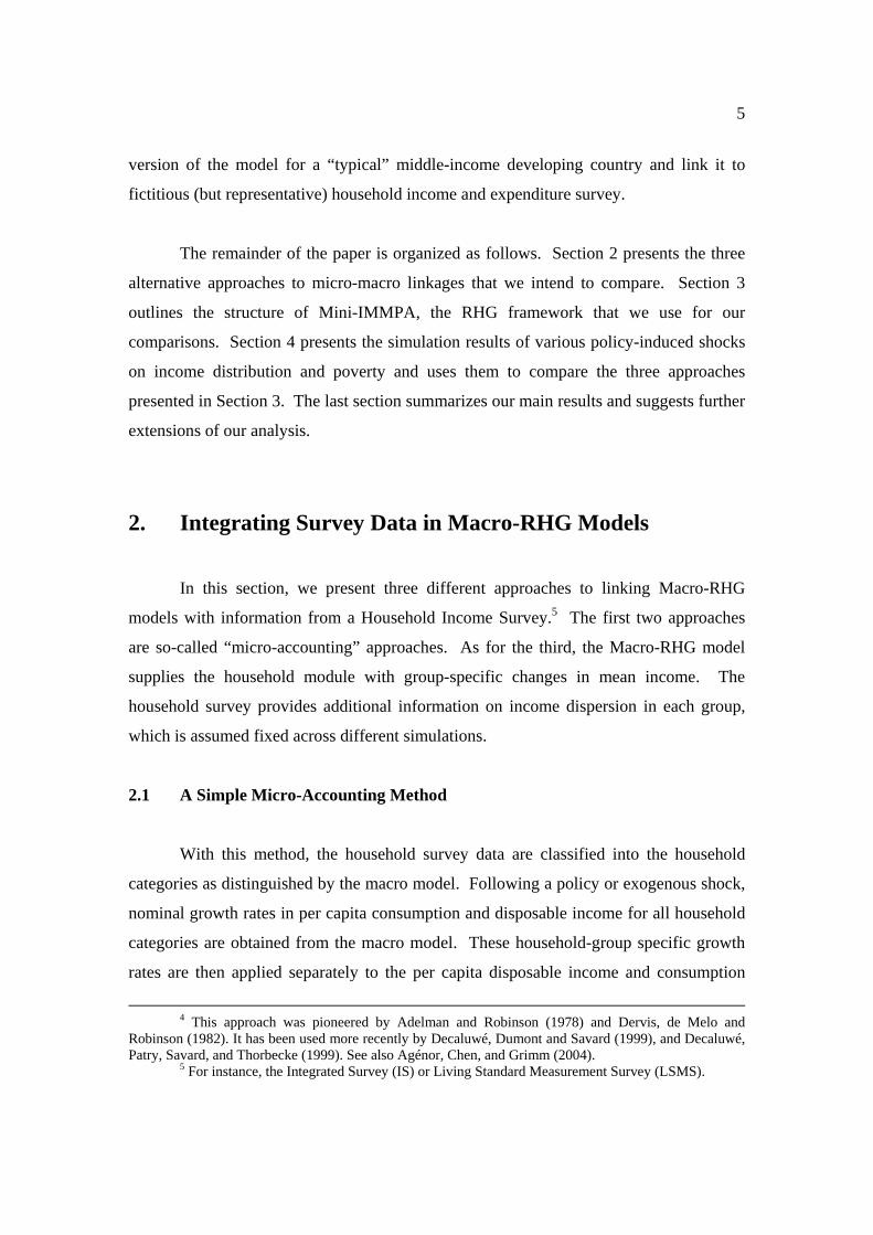
The remainder of the paper is organized as follows. Section 2 presents the three

alternative approaches to micro-macro linkages that we intend to compare. Section 3

outlines the structure of Mini-IMMPA, the RHG framework that we use for our

comparisons. Section 4 presents the simulation results of various policy-induced shocks

on income distribution and poverty and uses them to compare the three approaches

presented in Section 3. The last section summarizes our main results and suggests further

extensions of our analysis.

2. Integrating Survey Data in Macro-RHG Models

In this section, we present three different approaches to linking Macro-RHG

models with information from a Household Income Survey.5 The first two approaches

are so-called “micro-accounting” approaches. As for the third, the Macro-RHG model

supplies the household module with group-specific changes in mean income. The

household survey provides additional information on income dispersion in each group,

which is assumed fixed across different simulations.

2.1 A Simple Micro-Accounting Method

With this method, the household survey data are classified into the household

categories as distinguished by the macro model. Following a policy or exogenous shock,

nominal growth rates in per capita consumption and disposable income for all household

categories are obtained from the macro model. These household-group specific growth

rates are then applied separately to the per capita disposable income and consumption

4 This approach was pioneered by Adelman and Robinson (1978) and Dervis, de Melo and

Robinson (1982). It has been used more recently by Decaluwé, Dumont and Savard (1999), and Decaluwé, Patry, Savard, and Thorbecke (1999). See also Agénor, Chen, and Grimm (2004).

5 For instance, the Integrated Survey (IS) or Living Standard Measurement Survey (LSMS).

6

expenditure of each household in the survey, thereby providing the post-shock levels of

nominal income and consumption. Initial poverty lines are updated using the price

indexes generated by the macro model, to reflect changes in the price of the consumption

basket and purchasing power of income for each group. Poverty and income distribution

indicators are then calculated using the updated survey data and new poverty lines.6

Figure 1 summarizes the procedure.7

[Figure 1 around here]

While appealing from a practical point of view, this approach has two main

shortcomings. The first is that it does not fully account for heterogeneity among agents

within groups. The application of group-specific, instead of household-specific, real

growth rates of consumption or income assumes that the intra-group distribution of

consumption and disposable income remains constant after a shock, which in reality may

not be the case. The second shortcoming is that, given that changes in the employment

structure are ignored, this approach only partially introduces the effects of the

macroeconomic shock to the micro component. When the changes are transmitted to the

household survey, it is thus assumed that each individual remains in his or her initial

sector of activity. Put differently, labor market mobility is assumed to affect poverty and

income distribution only through relative income changes.

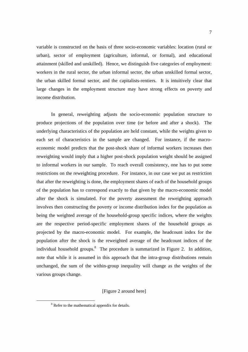
2.2 An Extension with Reweighting Techniques

To account for changes in the employment structure at the micro-component of

the framework, our second approach involves the combination of the micro-accounting

method with reweighting techniques. This approach is to our knowledge new and

original. Note that in the macro-economic model that we use later on, the employment

6 See the Mathematical Appendix to this paper for detailed descriptions regarding the poverty and income distribution indicators used in this paper.

7 Note that this approach to micro-macro linkage is “top-down” by construction, as there are no feedback effects from the household survey to the Macro-RHG model. More specifically, market equilibria are entirely simulated on the macro-side without accounting for any further heterogeneity in behavior within groups.

7

variable is constructed on the basis of three socio-economic variables: location (rural or

urban), sector of employment (agriculture, informal, or formal), and educational

attainment (skilled and unskilled). Hence, we distinguish five categories of employment:

workers in the rural sector, the urban informal sector, the urban unskilled formal sector,

the urban skilled formal sector, and the capitalists-rentiers. It is intuitively clear that

large changes in the employment structure may have strong effects on poverty and

income distribution.

In general, reweighting adjusts the socio-economic population structure to

produce projections of the population over time (or before and after a shock). The

underlying characteristics of the population are held constant, while the weights given to

each set of characteristics in the sample are changed. For instance, if the macro-

economic model predicts that the post-shock share of informal workers increases then

reweighting would imply that a higher post-shock population weight should be assigned

to informal workers in our sample. To reach overall consistency, one has to put some

restrictions on the reweighting procedure. For instance, in our case we put as restriction

that after the reweighting is done, the employment shares of each of the household groups

of the population has to correspond exactly to that given by the macro-economic model

after the shock is simulated. For the poverty assessment the reweighting approach

involves then constructing the poverty or income distribution index for the population as

being the weighted average of the household-group specific indices, where the weights

are the respective period-specific employment shares of the household groups as

projected by the macro-economic model. For example, the headcount index for the

population after the shock is the reweighted average of the headcount indices of the

individual household groups.8 The procedure is summarized in Figure 2. In addition,

note that while it is assumed in this approach that the intra-group distributions remain

unchanged, the sum of the within-group inequality will change as the weights of the

various groups change.

[Figure 2 around here]

8 Refer to the mathematical appendix for details.

8

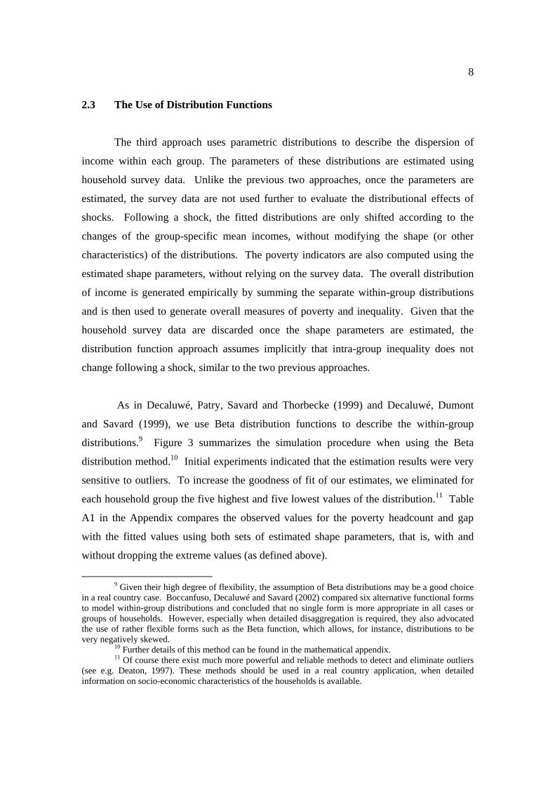
2.3 The Use of Distribution Functions

The third approach uses parametric distributions to describe the dispersion of

income within each group. The parameters of these distributions are estimated using

household survey data. Unlike the previous two approaches, once the parameters are

estimated, the survey data are not used further to evaluate the distributional effects of

shocks. Following a shock, the fitted distributions are only shifted according to the

changes of the group-specific mean incomes, without modifying the shape (or other

characteristics) of the distributions. The poverty indicators are also computed using the

estimated shape parameters, without relying on the survey data. The overall distribution

of income is generated empirically by summing the separate within-group distributions

and is then used to generate overall measures of poverty and inequality. Given that the

household survey data are discarded once the shape parameters are estimated, the

distribution function approach assumes implicitly that intra-group inequality does not

change following a shock, similar to the two previous approaches.

As in Decaluwé, Patry, Savard and Thorbecke (1999) and Decaluwé, Dumont

and Savard (1999), we use Beta distribution functions to describe the within-group

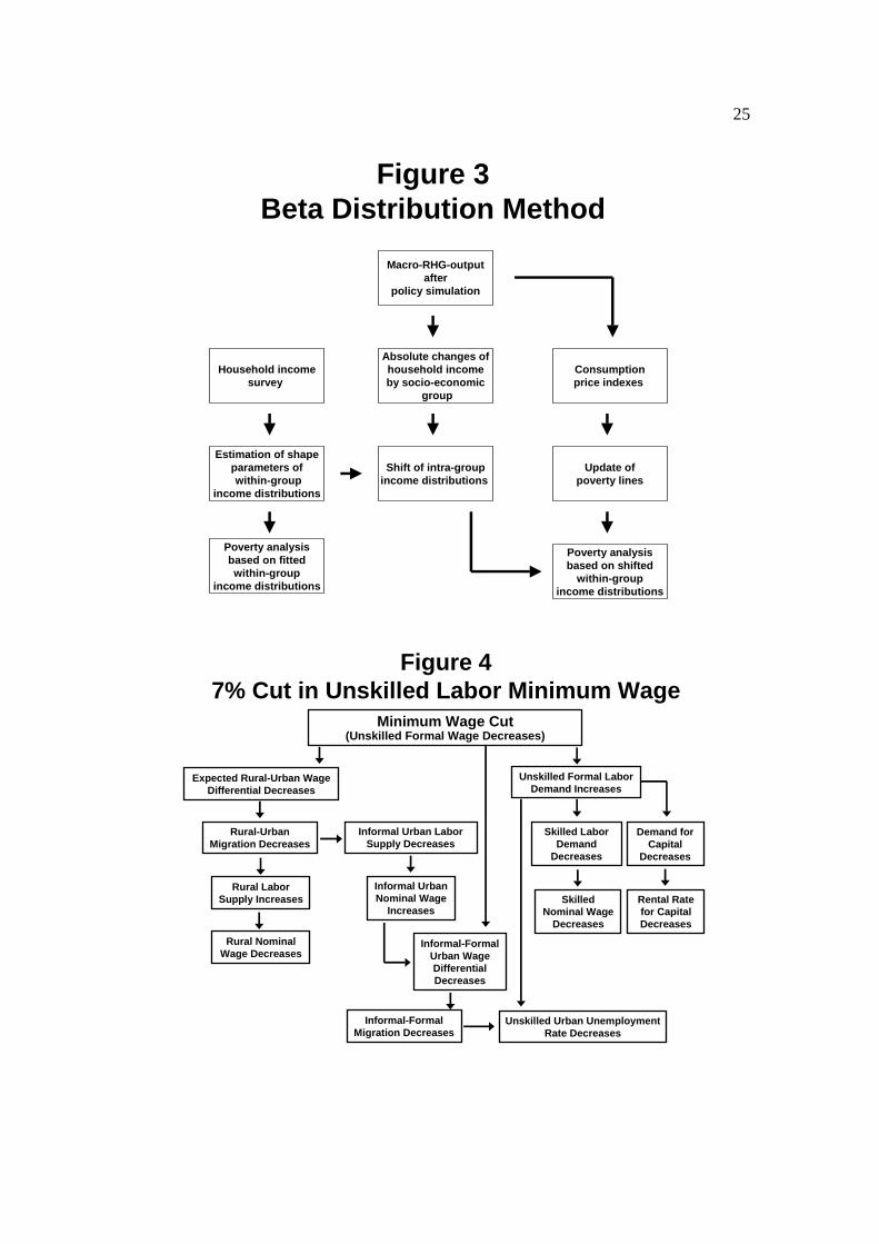
distributions.9 Figure 3 summarizes the simulation procedure when using the Beta

distribution method.10 Initial experiments indicated that the estimation results were very

sensitive to outliers. To increase the goodness of fit of our estimates, we eliminated for

each household group the five highest and five lowest values of the distribution.11 Table

A1 in the Appendix compares the observed values for the poverty headcount and gap

with the fitted values using both sets of estimated shape parameters, that is, with and

without dropping the extreme values (as defined above).

9 Given their high degree of flexibility, the assumption of Beta distributions may be a good choice

in a real country case. Boccanfuso, Decaluwé and Savard (2002) compared six alternative functional forms to model within-group distributions and concluded that no single form is more appropriate in all cases or groups of households. However, especially when detailed disaggregation is required, they also advocated the use of rather flexible forms such as the Beta function, which allows, for instance, distributions to be very negatively skewed.

10 Further details of this method can be found in the mathematical appendix. 11 Of course there exist much more powerful and reliable methods to detect and eliminate outliers

(see e.g. Deaton, 1997). These methods should be used in a real country application, when detailed information on socio-economic characteristics of the households is available.

9

[Figure 3 around here]

From Table A1, it can be seen that if we correct the data for outliers the fit is quite

acceptable for the headcount index, at least for households in the rural sector and

households in the informal urban sector. For instance for those households whose

income comes predominantly from the urban informal sector, the observed poverty

headcount is 43.35%. Using the parametrical approach, we estimate (or “fit”) a poverty

headcount of 51.59% if outliers are not eliminated. If outliers are eliminated, the

estimated poverty headcount is 45.66% and therefore much closer to the “observed”

value. However, for the other three groups, the deviations remain significant. One

explanation for this outcome is that the population size is smaller for these groups, and

thus the estimated shape parameters are less reliable. The poverty gap ratio is much more

difficult to fit. Here the predicted indicators are more than 40 percent above the observed

values. These results show the first limitation of the distribution approach, especially if

sample sizes are small. Further implications will be discussed below.

3. The Macro-RHG Framework

Mini-IMMPA is a simplified version of the Integrated Macroeconomic Model for

Poverty Analysis developed by Agénor, Izquierdo and Fofack (2003), and Agénor,

Fernandes, Haddad, and Jensen (2003). The model is based on a four-good production

structure (rural, urban informal, urban private formal, and urban public formal) combined

with five categories of households. The model focuses only on the “real” side of the

economy and hence its building blocks consist of production, employment, demand,

external trade, sectoral and aggregate prices, income formation, consumption and

savings, private investment, and the public sector. One of many strong points of the

model include its detailed treatment of the labor market,12 which is important for poverty

12 Mini-IMMPA accounts for labor market features such as bilateral wage bargaining, free public

education, employment subsidies, job security provisions and firing costs in the formal sector.

10

analysis, as incomes are strongly connected with the sector of employment in many

developing countries. Households in Mini-IMMPA are defined according to their skills

and their sector of employment. There is one rural household, comprising all workers

employed in the rural sector. In the urban sector there are two types of unskilled

households, those working in the informal sector and those employed in the formal sector

(public and private). The fourth type of households consists of skilled workers employed

in the formal urban economy (in both the private and public sectors). Finally, there are

capitalists-rentiers whose income comes from firms' earnings in the urban private sector.

The model accounts for the migration of workers from the rural sector to the urban

(informal) sector, and the transformation of unskilled labor into skilled labor via a

publicly provided education technology.

The household survey data used in the Mini-IMMPA framework is an artificial

sample consisting of 5,000 observations, where each observation represents one

household and the share of each household category corresponds exactly to that in the

macro model.13 Using a random number generator following a lognormal distribution,

values for disposable income and consumption expenditure were drawn for each

household.14 For simplicity, poverty lines were assumed to remain constant in real terms

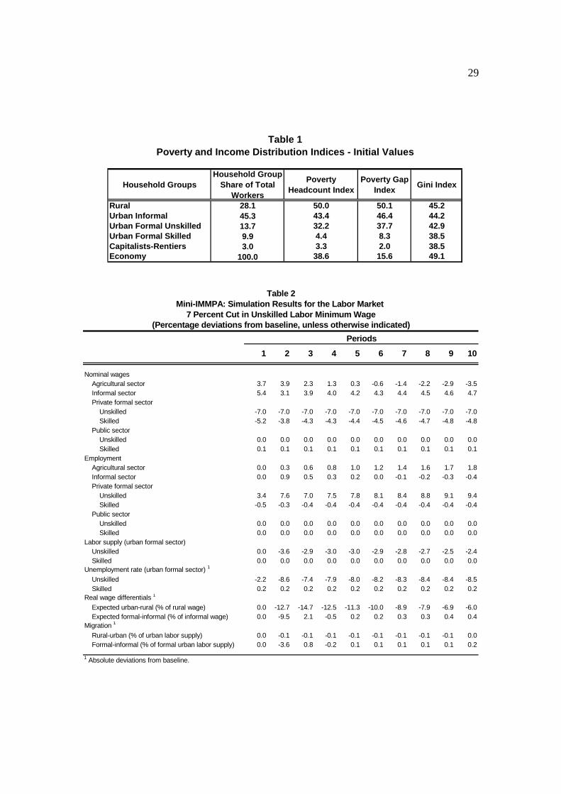
up to the end of the simulation horizon.15 Table 1 provides the initial values of the

poverty and income distribution indices.16

[Insert Table 1 around here]

13 See Table 1 for the initial employment shares. 14 The initial values for average disposable income for each household group were set so as to

equal that of the numerical solution of the macro model. 15 The income poverty line for the rural sector was set such that the percentage of poor households

in the rural sector is 50 percent. The poverty line in urban areas was assumed to be 15 percent higher. Rural and urban poverty lines for consumption expenditure were constructed in similar way.

16 See Agénor (2003, 2004) for a more detailed presentation of the Mini-IMMPA framework.

11

4. Comparing Shocks with Alternative Linkages

To compare the performance of the three alternative approaches to model micro-

macro linkages discussed earlier, the growth, employment and poverty effects of two

types of labor market policies are examined in this section: a cut in the minimum wage

and an increase in the employment subsidy on unskilled labor in the urban formal sector.

Both experiments relate to critical policy issues in developing countries. As an indicator

of living standards, we consider in what follows only disposable household income per

capita.17

4.1 Reduction in the Minimum Wage

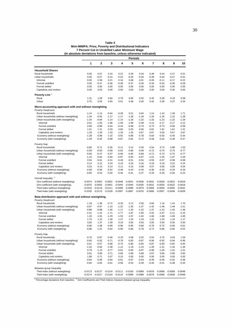
The simulation results associated with a permanent 7 percent reduction in the

minimum wage are illustrated in Tables 2 and 3 for the first 10 periods after the shock.

This time span is referred to below as the “adjustment period”. Table 2 provides data on

the labor market. Table 3 presents data on poverty and distributional indicators, all in

absolute deviations from the baseline solution.18 A more detailed presentation can be

found in Agénor, Chen and Grimm (2004). We first comment on the general results of

this simulation and then compare more specifically the effects on poverty and inequality,

as measured by the three different methods.

[Insert Tables 2 and 3 around here]

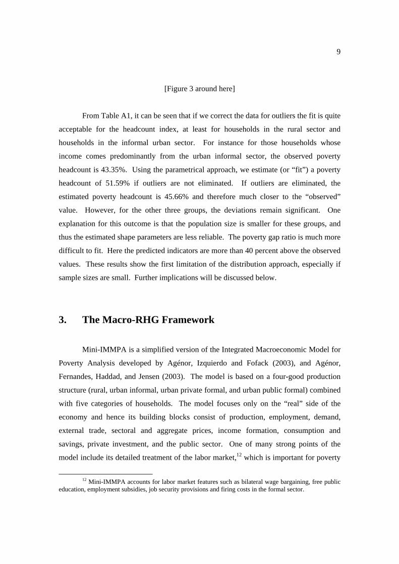
Figure 4 illustrates selected general results of the simulation. The reduction in the

minimum wage on impact results in an increase in the demand for unskilled labor in the

private sector. The number of unemployed unskilled workers in the urban sector

therefore falls, along with the unskilled unemployment rate. Hence, for unskilled

17 In a real country application it may be worthwhile to test the sensitivity of the results to

alternative equivalence scales. 18 The experiment assumes that the government borrows domestically to finance its deficit,

implying therefore an offsetting adjustment in private investment (at the initial level of foreign saving), in order to maintain the aggregate balance between savings and investment.

12

workers in that sector, both measures of poverty indicate an improvement in the longer

run.19 The fall in the minimum wage also leads to a drop in the expected urban unskilled

wage20, and consequently to a reduction in migration flows from rural to urban areas.

This results in a relatively larger supply of rural workers, thus leading to a drop in

nominal wages for rural workers. By the end of the adjustment period, both the

proportion of poor households and the poverty gap in rural areas increases.

[Insert Figure 4 around here]

With the reduction in rural-urban migration flow, labor supply in the informal

sector falls and informal sector wages increases throughout the adjustment period. Both

measures of poverty for the informal sector therefore indicate an improvement in the

longer run. Because the cut in the minimum wage reduces the relative cost of unskilled

labor, demand for both skilled labor and physical capital falls, along with skilled wages

and the rental price of capital. Hence, poverty for skilled workers tends to increase

slightly in both the short and the long run. Similarly, the incidence of poverty for

capitalists and rentiers increases toward the end of the adjustment period. Overall,

poverty increases in rural areas and decreases in urban areas, resulting in a slight decrease

in poverty at the economy-wide level. Changes in the income-based Gini coefficient

indicate that income distribution is affected only modestly by a cut in the minimum wage;

by contrast, the degree of inequality falls by a small amount in the long run.

We now examine the differences concerning changes in poverty and inequality as

measured by the three approaches to micro-macro linkages presented in section 2. As

can be seen from Table 3, using the simple micro-accounting method without

reweighting, the decrease in poverty tends to be larger, compared to the approach that

involves reweighting. Even though the absolute differences between the estimates are

19 However, note that poverty increases on impact. There is therefore a potential short-run trade-

off emerging between unemployment and poverty: although the reduction in the minimum wage lowers open unskilled unemployment in the formal sector, it also increases poverty for that category of households. See Agénor (2004) for a more detailed discussion of unemployment-poverty trade-offs.

20 This is despite the increase in unskilled employment in the private sector in the first period, which raises the probability of finding a job.

13

relatively small, the discrepancies become significant when compared to the small total

reduction in poverty predicted for the initial period.

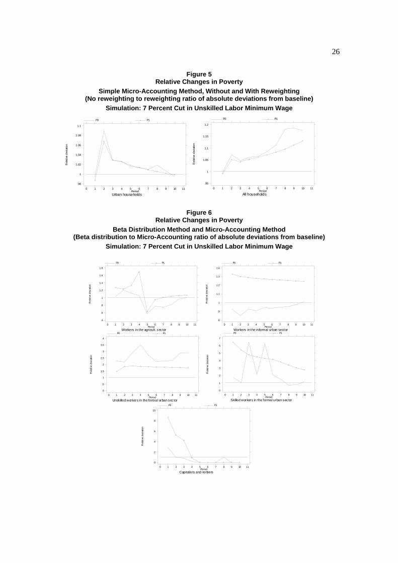
Figure 5 traces the deviations from the baseline results obtained with the simple

micro-accounting method as a ratio to those obtained with reweighting, for both the

headcount and gap measures.21 For both urban households and all households the

decrease in poverty estimated by the non-reweighting approach is larger over the entire

adjustment period. The difference amounts to up to 9 percent for urban households and

nearly up to 20 percent for all households. The discrepancy between the estimates tends

to decrease over the adjustment period for urban households, whereas that for all

households tends to increase. The estimated decrease in inequality also tends to be larger

if changes in the employment structure are not taken into account. Again, in absolute

terms the difference is not large, but given the small change in inequality, the relative

difference is significant.

[Insert Figure 5 around here]

Comparison of the estimated changes from the micro-accounting framework and

the Beta distribution approach show that results from both approaches are consistent in

terms of direction of changes in poverty headcount and gap measures. As with the micro-

accounting approach, reweighting tends to produce small reductions in poverty. We also

note that the Beta distribution approach tends to predict, with a few exceptions, changes

in poverty of larger magnitude, compared to the micro-accounting approach.

Figure 6 shows the differences between the estimated changes from the Beta

distribution approach relative to that of the micro-accounting approach. For workers in

the rural sector, the discrepancy fluctuates between plus-minus 50 percent, but the actual

numbers tend to be lower in the beginning and at the end of the adjustment period. For

21 In Figure 5, positive (negative) values reflect the fact that both approaches predict a change in

poverty in the same (opposite) direction. A value greater than 1 implies that the predicted value from the approach without reweighting is larger than that with reweighting. Similarly, positive values smaller than 1

14

urban informal workers, decreases in the poverty gap using the Beta distribution are

systematically 25 to 30 percent larger, whereas decreases in the headcount measure are

around 10 percent smaller than those obtained with the micro-accounting approach. For

urban formal unskilled workers, changes predicted by the Beta distribution are larger by

100 to 250 percent for the headcount measure and nearly 100 percent for the poverty gap

measure. For skilled workers in the urban sector, the deviations for the poverty gap

measure are up to 6 times the change indicated by the micro-accounting with reweighting

method, but are in general small for the headcount measure. The fact that the beta

distribution approach rather overestimates poverty is not surprising given that it tends to

overestimate poverty already in the base year (see Table A1). This bias then also shows

up when the beta distribution is used to forecast poverty changes.

[Insert Figure 6 around here]

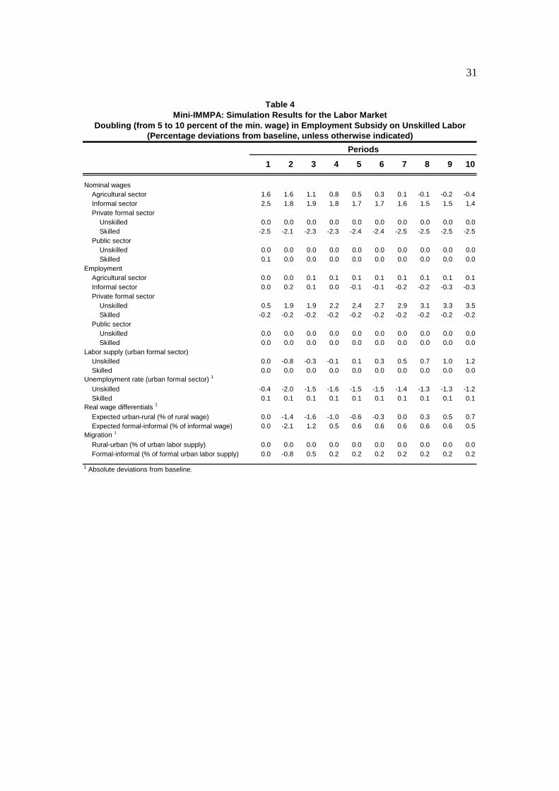
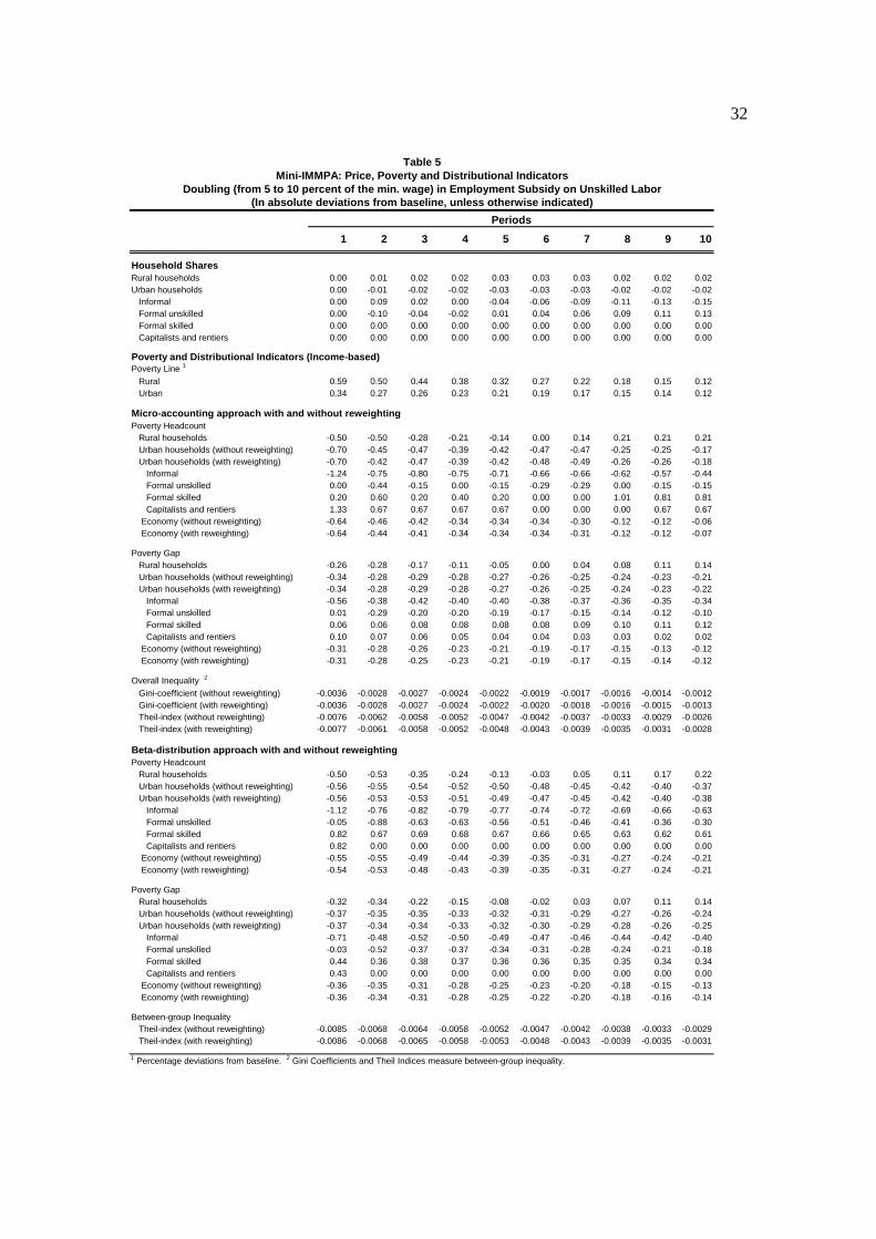
4.2 Increase in Employment Subsidy

The simulation results associated with a permanent, doubling of the nominal

employment subsidy on unskilled labor in the private formal sector (an increase in the

subsidy rate from 5 to 10 percent of the minimum wage) are illustrated in Tables 4 and 5

for the first 10 periods after the shock. This subsidy is assumed to be paid on a per

worker basis.

[Insert Tables 4 and 5 around here]

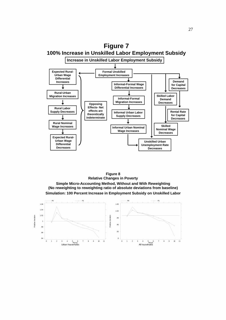
Similar to the effect of a reduction in the minimum wage, an increase in the

employment subsidy reduces the effective cost of unskilled labor (Figure 7). Demand

and thus formal unskilled employment expands, and the unskilled unemployment rate

falls, which results in lower values in the corresponding poverty headcount and gap

indices.

imply smaller changes from the approach without reweighting, and values equal to 1 imply that both approaches predict changes in poverty that are of the same magnitude.

15

[Insert Figure 7 around here]

The increase in formal unskilled employment raises the inflow of workers from

the informal to the formal sector, leading to a corresponding increase in the informal

wage. As a result, poverty in the informal sector decreases throughout the adjustment

period. The reduction in the “effective” cost of unskilled labor leads firms in the private

formal urban sector to substitute away from skilled labor and physical capital, leading to

a reduction in skilled wages and capital rental prices. Consequently, poverty increases for

both of these household groups. Rural-urban migration flows also increases, which in

turn decreases labor supply in the rural sector and rural wages therefore tend to increase.

Rural poverty consequently decreases, at least in the short run. As with the cut in the

minimum wage, inequality in the distribution of disposable income decreases.

In terms of difference in results due to the alternative linkage methods, we see

from Table 5 that the simulated changes in poverty are larger with the simple micro-

accounting method without reweighting, as compared to those obtained with reweighting.

Again, because changes in the employment structure following the shock are small, the

absolute differences are also small, but relatively significant when compared to the

decrease in poverty. Figure 8 illustrates the absolute deviations from the baseline

measured by the simple micro-accounting method without reweighting relative to that

with reweighting. For both poverty indicators, and for urban households and all

households, changes in poverty with the micro accounting approach are larger in the short

run (approximately 5 percent) and smaller in the long run (also by approximately 5

percent). In addition, the method involving no reweighting produces smaller decreases in

inequality, as compared to that with reweighting. The difference between the two

methods are again very small in absolute terms, but large in relative terms.

[Insert Figure 8 around here]

16

Figure 9 illustrates the comparison of the results from the Beta distribution

approach and the micro-accounting framework. The relative changes in poverty were

typically equivalent for both poverty measures. For workers in the rural sector, and

relative to the micro-accounting approach, the Beta distribution approach produces

changes in poverty that are slightly larger at the beginning of the adjustment period,

changes that are large and of the opposite sign in the middle of the adjustment period, and

nearly identical changes towards the end of the adjustment period.

[Insert Figure 9 around here]

For the urban informal sector, the Beta distribution approach simulated changes in

poverty that were consistently larger; for the poverty headcount index in the long run it

was larger by more than 30 percent, and for the poverty gap by 20 to 30 percent

throughout the adjustment period. For unskilled workers in the urban formal sector,

changes in the headcount poverty measure simulated by the Beta distribution are very

volatile, ranging from negative 1000 to positive 300 percent of those obtained with the

micro-accounting methods. The poverty gap measure is somewhat more stable, ranging

from negative 200 to positive 100 percent. For skilled workers in the urban formal

sector, changes in both poverty indicators are more than 2 to 10 times higher, but the

deviations decrease over time. For capitalists and rentiers, the Beta distribution approach

indicates no change in poverty, with either measure of poverty, whereas the reweighting

approach indicates that poverty increased.

In summary, the simulation of both experiments using the three alternative

linkage approaches led to qualitatively similar results: an increase in rural poverty, a

decrease in urban poverty, a decrease in economy-wide poverty measures and an

improvement in the economy-wide income distribution. However, a comparison of

changes in poverty and income distribution measures at a disaggregated level shows that

large differences in outcomes (both quantitative and qualitative) also exist.

17

5. Conclusion

This paper focused on the various approaches to linking macroeconomic models

with representative households to micro household income data. Such linkages between

models and survey data form frameworks that are used to evaluate the distributional and

poverty effects of policy and other exogenous shocks. We compare three linkage

approaches by simulating two exogenous policy shocks with the Mini-IMMPA

framework developed by Agénor (2003), using each approach in turn. The selected

shocks are a cut in the minimum wage and an increase in employment subsidies for

unskilled labor in the formal urban sector. The resulting effects on poverty and income

distributions were then evaluated and compared.

We found that the distributional and poverty effects indicated by the three

approaches are generally similar, especially at the economy-wide level. With all three

approaches, both experiments lead to an increase in rural poverty, a decrease in urban

poverty, a decrease in economy-wide poverty and an improvement in the economy-wide

distribution of income. However, closer comparisons between the simulation results

using the micro-accounting approach with and without reweighting reveal that the latter

produced larger decreases in poverty for aggregated household groups in both

experiments. In addition, we observed some substantial differences in the simulated

changes in poverty at the sectoral level, both in terms of magnitude and the direction of

change, between the micro-accounting and Beta distribution approaches.

From both a conceptual and practical point of view, it is tempting to view the

micro-accounting method combined with reweighting for changes in the employment

structure as constituting the most appealing method among the three, despite the fact that

it has its own shortcomings. The reason is that the simple micro-accounting method

ignores a potentially crucial feature of the economy’s response to shocks (namely,

changes in the composition of employment), whereas the distribution approach relies on

estimated instead of real income distributions, and depends therefore on the quality of the

corresponding estimates of the shape parameters.

18

In the past, a key advantage of the distribution approach was that it enabled

simulations to be conducted without the direct use of the actual household survey data

(beyond the estimation of distributional parameters), thereby making simulations less

computationally intensive. However, given today’s computing power and statistical

software, working directly with actual survey data does not present much of a constraint,

except perhaps for very large household surveys (which are not yet common in

developing countries). Hence, there is usually little need to use the distribution approach

and discard much valuable information contained in household survey data. However,

advocates of this approach also argue that if the sample of households is small, the use of

the estimated distribution ensures smoothness, even if the observed one is not. The

smoothing avoids the possibility that small shifts in the income distribution would lead to

huge changes in the poverty measure, or conversely, that big shifts would lead to very

small changes in the poverty measure. The problem with this argument is that the

estimated distribution parameters are not very reliable if they are estimated over a small

sample of households.22 Therefore the parametric approach runs the risk of producing

biased results, which may have been an important factor for the significant observed

differences in the simulated changes in poverty.

The potential errors associated with the use of the simple micro-accounting

approach without reweighting or the distribution method are obviously more important if

policies with strong effects on the employment structure and the group-specific income

levels are analyzed. For instance, simulations with our model show that if the minimum

wage were reduced by 50 percent, the employment structure would change drastically--

with the share of rural workers decreasing by 50 percent, the share of informal workers

increasing by 25 percent and the share of formal unskilled workers doubling. Poverty

indicators calculated by either method would differ by more than 10 percentage points,

depending on whether these changes in employment structure are taken into account or

not. Although a shock of this magnitude may be viewed as implausibly large, this

22 This issue is illustrated in Table A1. For instance, compare the observed and fitted poverty

measures for the group of skilled workers in the formal urban sector and of capitalists-rentiers.

19

argument is quite general. Indeed, many of the policies that form part of poverty

reduction strategies (such as changes in the composition of public investment) are likely

to generate substantial variations in the composition of employment in the long run.

Even in our own experiments, changes in the employment structure would be a lot bigger

than those we obtained, if migration flows were assumed to respond more rapidly and

significantly to changes in relative wages. One can rightly conclude, therefore, that

failure to account for such changes in employment structure can lead to severely biased

simulation results. At the same time, whether this bias is greater or smaller than other

difficulties typically associated with the use of macroeconomic models for policy

analysis (such as parameter uncertainty) remains open to debate.

The micro-accounting framework with employment reweighting can be extended

to account for changes in other dimensions of the population structure, such as age

structure, household size, or gender—all potentially important considerations when

conducting dynamic analyses. However, this framework also has its shortcomings. The

most obvious one is the assumption of unchanged within-household group distributions.

One possible remedy to account for individual and household heterogeneity is to allow

the intra-group distributions to vary explicitly. This would entail the use of a micro-

simulation model that accounts for labor supply decisions and earnings at the level of the

household, or even, the individual. This methodology differs from the reweighting

approach in that individuals would actually be simulated to shift from one sector to

another using econometrically estimated behavioral functions, instead of merely changing

the weights of household groups. The downside of micro-simulation approach is that it

requires the use of a microeconomic model of income generation, and therefore relatively

powerful statistical software for econometric estimation and simulation. In addition,

good quality detailed data are also necessary, and this increases the difficulty of proper

implementation. In contrast, the micro-accounting framework combined with

reweighting for changes in the employment structure preserves a high degree of user-

friendliness, which may help its eventual adoption by researchers and policy advisers in

developing countries whenever skills and resources are scarce.

20

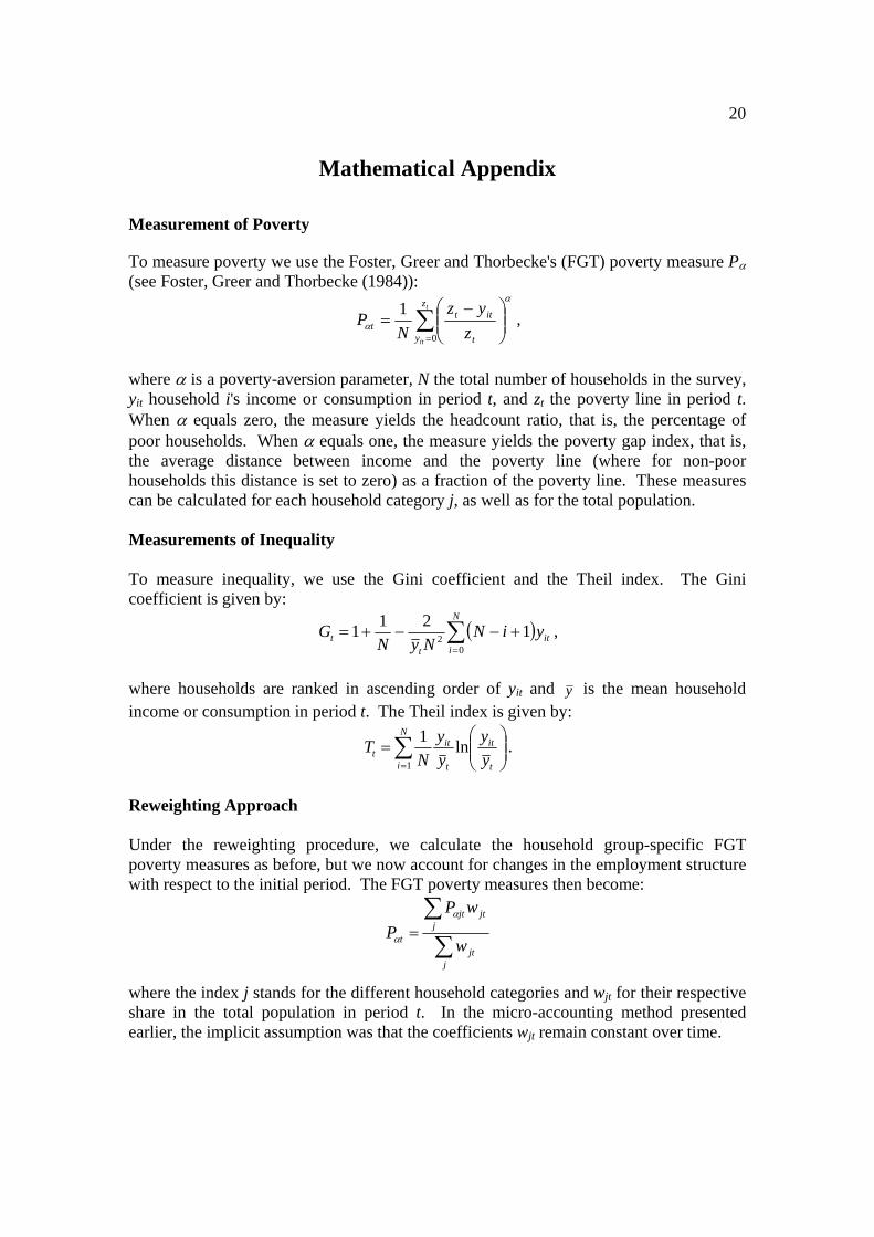
Mathematical Appendix Measurement of Poverty To measure poverty we use the Foster, Greer and Thorbecke's (FGT) poverty measure Pα (see Foster, Greer and Thorbecke (1984)):

∑=

⎟⎟⎠

⎞⎜⎜⎝

⎛ −=

t

it

z

y t

ittt z

yzN

P0

1α

α ,

where α is a poverty-aversion parameter, N the total number of households in the survey, yit household i's income or consumption in period t, and zt the poverty line in period t. When α equals zero, the measure yields the headcount ratio, that is, the percentage of poor households. When α equals one, the measure yields the poverty gap index, that is, the average distance between income and the poverty line (where for non-poor households this distance is set to zero) as a fraction of the poverty line. These measures can be calculated for each household category j, as well as for the total population. Measurements of Inequality To measure inequality, we use the Gini coefficient and the Theil index. The Gini coefficient is given by:

( )∑=

+−−+=N

iit

tt yiN

NyNG

02 1211 ,

where households are ranked in ascending order of yit and y is the mean household income or consumption in period t. The Theil index is given by:

⎟⎟⎠

⎞⎜⎜⎝

⎛= ∑

= t

itN

i t

itt y

yyy

NT ln1

1

.

Reweighting Approach Under the reweighting procedure, we calculate the household group-specific FGT poverty measures as before, but we now account for changes in the employment structure with respect to the initial period. The FGT poverty measures then become:

∑∑

=

jjt

jjtjt

t w

wPP

α

α

where the index j stands for the different household categories and wjt for their respective share in the total population in period t. In the micro-accounting method presented earlier, the implicit assumption was that the coefficients wjt remain constant over time.

21

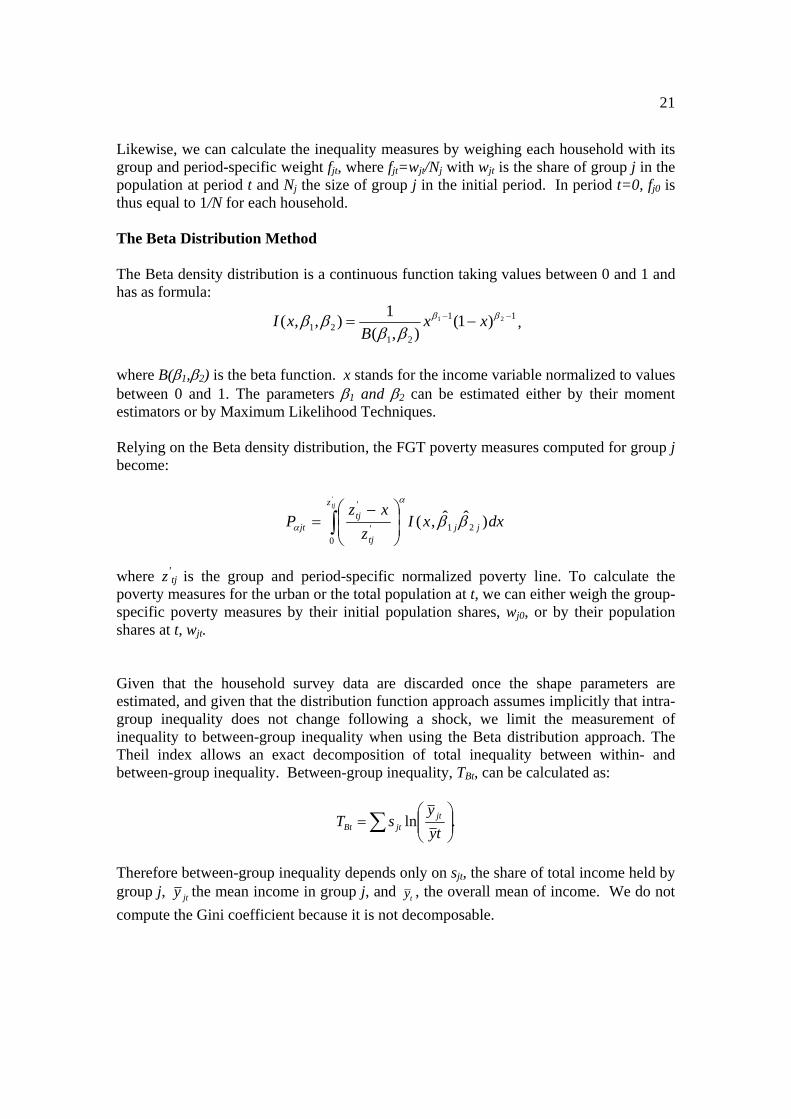
Likewise, we can calculate the inequality measures by weighing each household with its group and period-specific weight fjt, where fjt=wjt/Nj with wjt is the share of group j in the population at period t and Nj the size of group j in the initial period. In period t=0, fj0 is thus equal to 1/N for each household. The Beta Distribution Method The Beta density distribution is a continuous function taking values between 0 and 1 and has as formula:

11

2121

21 )1(),(

1),,( −− −= ββ

ββββ xx

BxI ,

where B(β1,β2) is the beta function. x stands for the income variable normalized to values between 0 and 1. The parameters β1 and β2 can be estimated either by their moment estimators or by Maximum Likelihood Techniques. Relying on the Beta density distribution, the FGT poverty measures computed for group j become:

dxxIz

xzP jj

z

tj

tjjt

tj

)ˆˆ,( 210

'

''

ββα

α ∫ ⎟⎟⎠

⎞⎜⎜⎝

⎛ −=

where z’

tj is the group and period-specific normalized poverty line. To calculate the poverty measures for the urban or the total population at t, we can either weigh the group-specific poverty measures by their initial population shares, wj0, or by their population shares at t, wjt. Given that the household survey data are discarded once the shape parameters are estimated, and given that the distribution function approach assumes implicitly that intra-group inequality does not change following a shock, we limit the measurement of inequality to between-group inequality when using the Beta distribution approach. The Theil index allows an exact decomposition of total inequality between within- and between-group inequality. Between-group inequality, TBt, can be calculated as:

.ln ⎟⎟⎠

⎞⎜⎜⎝

⎛= ∑ ty

ysT jt

jtBt

Therefore between-group inequality depends only on sjt, the share of total income held by group j, jty the mean income in group j, and ty , the overall mean of income. We do not compute the Gini coefficient because it is not decomposable.

22

Assessment of the fit of the Beta Distribution Method

[Insert Table A1 here]

References

Adelman, Irma and Sherman Robinson, Income Distribution Policy in Developing Countries: A case Study of Korea, Stanford University Press (Stanford, Cal.: 1978).

Agénor, Pierre-Richard, “Mini-IMMPA: A Framework for Assessing the Unemployment and

Poverty Effects of Fiscal and Labor Market Reforms,” Policy Research Working Paper No. 3067, the World Bank (May 2003).

------, “Unemployment-Poverty Trade-offs,” in Labor Markets and Institutions, ed. by Jorge

Restrepo and Andrea Tokman, Central Bank of Chile (Santiago: 2004). Agénor, Pierre-Richard, Derek H. C. Chen, and Michael Grimm, “Linking Representative

Household Models with Household Surveys for Poverty Analysis: A Comparison of Alternative Methodologies,” Policy Research Working Paper No. 3343, the World Bank (June 2004).

Agénor, Pierre-Richard, Reynaldo Fernandes, Eduardo Haddad, and Henning Tarp Jensen,

“Analyzing the Impact of Adjustment Policies on the Poor: An IMMPA Framework for Brazil,” unpublished, the World Bank (October 2003).

Agénor, Pierre-Richard, Alejandro Izquierdo, and Hippolyte Fofack, “IMMPA: A Quantitative

Macroeconomic Framework for the Analysis of Poverty Reduction Strategies,” Policy Research Working Paper No. 3092, the World Bank (June 2003).

Boccanfuso, Dorothé, Bernard Decaluwé, and Luc Savard, “Poverty, Income Distribution and

CGE Modeling: Does the Functional Form of Distribution Matter?” unpublished, CREFA, Université de Laval (March 2002).

Bourguignon, Francois, Anne-Sophie Robilliard, and Sherman Robinson, “Representative versus

real households in the macro-economic modeling of inequality,” unpublished, the World Bank (2002). Cogneau, Denis and Anne-Sophie Robilliard, “Poverty Alleviation Policies in Madagascar: a

micro-macro simulation model,” DIAL Working paper DT/2004/11, DIAL, Paris (November 2004). Deaton, Angus, The Analysis of Household Surveys: A Microeconometric Approach to

Development Policy, World Bank Publications. (Washington D.C.: 1997). Decaluwé, Bernard, Jean-Christophe Dumont, and Luc Savard, “Measuring Poverty and Inequality

in a Computable General Equilibrium Model,” Working Paper No. 99-20, Université Laval (September 1999).

Decaluwé, Bernard, A. Patry, Luc Savard, and Eric Thorbecke, “Poverty Analysis within a

General Equilibrium Framework,” Working Paper No. 99-09, African Economic Research Consortium (June 1999).

Dervis, Kemal, Jaime de Melo, and Sherman Robinson, General Equilibrium Models for

Development Policy, Cambridge University Press (Cambridge: 1982).

23

Foster James, Joel Greer, and Erik Thorbecke, “A Class of Decomposable Poverty Measures,” Econometrica, 52 (3, 1984), 761-6.

Robilliard, Anne-Sophie, Francois Bourguignon, and Sherman Robinson, “Crisis and Income

Distribution: A Micro-Macro Model for Indonesia,” unpublished, DIAL Paris and IFPRI, Washington D.C. (2002).

24

Figure 1Simple Micro-accounting Method

Macro-RHG-outputafter

policy simulation

Growth rates ofhousehold incomeby socio-economic

group

Expansion ofhousehold incomesby socio-eco. group

Consumptionprice indexes

Update ofpoverty lines

Income distributionafter policy simulationPoverty analysis after

Income distributionbefore policy simulationPoverty analysis before

Household incomesurvey

Figure 2Reweighting Method

Macro-RHG-outputafter

policy simulation

Growth rates ofhousehold incomeby socio-economic

group

Expansion ofhousehold incomesby socio-eco. group

Consumptionprice indexes

Update ofpoverty lines

Household incomesurvey

Changes inaggregate

employmentstructure

Reweightingprocedure

Income distributionbefore policy simulationPoverty analysis before

Income distributionafter policy simulationPoverty analysis after

25

Figure 3Beta Distribution Method

Macro-RHG-outputafter

policy simulation

Absolute changes ofhousehold incomeby socio-economic

group

Shift of intra-groupincome distributions

Consumptionprice indexes

Update ofpoverty lines

Poverty analysisbased on shifted

within-groupincome distributions

Poverty analysisbased on fittedwithin-group

income distributions

Household incomesurvey

Estimation of shapeparameters ofwithin-group

income distributions

Figure 47% Cut in Unskilled Labor Minimum Wage

Minimum Wage Cut(Unskilled Formal Wage Decreases)

Unskilled Formal Labor Demand Increases

Skilled Labor Demand

Decreases

Demand for Capital

Decreases

Skilled Nominal Wage

Decreases

Rental Rate for Capital Decreases

Unskilled Urban Unemployment Rate Decreases

Expected Rural-Urban Wage Differential Decreases

Rural-Urban Migration Decreases

Rural Labor Supply Increases

Informal Urban Labor Supply Decreases

Informal Urban Nominal Wage

Increases

Informal-Formal Migration Decreases

Informal-Formal Urban Wage Differential Decreases

Rural Nominal Wage Decreases

26

Figure 5 Relative Changes in Poverty

Simple Micro-Accounting Method, Without and With Reweighting (No reweighting to reweighting ratio of absolute deviations from baseline)

Simulation: 7 Percent Cut in Unskilled Labor Minimum Wage

Figure 6

Relative Changes in Poverty Beta Distribution Method and Micro-Accounting Method

(Beta distribution to Micro-Accounting ratio of absolute deviations from baseline) Simulation: 7 Percent Cut in Unskilled Labor Minimum Wage

Rela

tive

devi

atio

n

Urban householdsPeriod

P0 P1

0 1 2 3 4 5 6 7 8 9 10 11

.98

1

1.02

1.04

1.06

1.08

1.1

Rela

tive

devi

atio

nAll households

Period

P0 P1

0 1 2 3 4 5 6 7 8 9 10 11

.95

1

1.05

1.1

1.15

1.2

Rela

tive

devi

atio

n

Workers in the agricult. sectorPeriod

P0 P1

0 1 2 3 4 5 6 7 8 9 10 11

.4

.6

.8

1

1.2

1.4

1.6

1.8

Rela

tive

devi

atio

n

Workers in the informal urban sectorPeriod

P0 P1

0 1 2 3 4 5 6 7 8 9 10 11

.8

.9

1

1.1

1.2

1.3

1.4

Rela

tive

devi

atio

n

Unskilled workers in the formal urban sectorPeriod

P0 P1

0 1 2 3 4 5 6 7 8 9 10 11

0

.5

1

1.5

2

2.5

3

3.5

4

Rela

tive

devi

atio

n

Skilled workers in the formal urban sectorPeriod

P0 P1

0 1 2 3 4 5 6 7 8 9 10 11

0

1

2

3

4

5

6

7

Rela

tive

devi

atio

n

Capitalis ts and rentiersPeriod

P0 P1

0 1 2 3 4 5 6 7 8 9 10 11

0

2

4

6

8

10

27

Figure 8 Relative Changes in Poverty

Simple Micro-Accounting Method, Without and With Reweighting (No reweighting to reweighting ratio of absolute deviations from baseline)

Simulation: 100 Percent Increase in Employment Subsidy on Unskilled Labor

Figure 7100% Increase in Unskilled Labor Employment Subsidy

Increase in Unskilled Labor Employment Subsidy

Skilled Labor Demand

Decreases

Demand for Capital Decreases

Skilled Nominal Wage

Decreases

Rental Rate for Capital Decreases

Unskilled Urban Unemployment Rate

Decreases

Expected Rural-Urban Wage Differential Increases

Rural-Urban Migration Increases

Rural Labor Supply Decreases Informal Urban Labor

Supply Decreases

Informal Urban Nominal Wage Increases

Rural Nominal Wage Increases

Formal Unskilled Employment Increases

Informal-Formal Migration Increases

Expected Rural-Urban Wage Differential Decreases

Opposing Effects- Net effects are

theoretically indeterminate

Informal-Formal Wage Differential Increases

Rela

tive

devi

atio

n

Urban householdsPeriod

P0 P1

0 1 2 3 4 5 6 7 8 9 10 11

.94

.96

.98

1

1.02

1.04

1.06

Rela

tive

devi

atio

n

All householdsPeriod

P0 P1

0 1 2 3 4 5 6 7 8 9 10 11

.9

.93

.96

.99

1.02

1.05

28

Figure 9 Relative Changes in Poverty

Beta Distribution Method and Micro-Accounting Method (Beta distribution to Micro-Accounting ratio of absolute deviations from baseline, in

percent) Simulation: 100 Percent Increase in Employment Subsidy on Unskilled Labor

Rela

tive

devi

atio

n

Workers in the agricult. sectorPeriod

P0 P1

0 1 2 3 4 5 6 7 8 9 10 11

-20

-16

-12

-8

-4

0

4

Rela

tive

devi

atio

nWorkers in the informal urban sector

Period

P0 P1

0 1 2 3 4 5 6 7 8 9 10 11

.5

.7

.9

1.1

1.3

1.5

Rela

tive

devi

atio

n

Unskilled workers in the formal urban sectorPeriod

P0 P1

0 1 2 3 4 5 6 7 8 9 10 11

-10

-8

-6

-4

-2

0

2

4

Rela

tive

devi

atio

n

Skilled workers in the formal urban sectorPeriod

P0 P1

0 1 2 3 4 5 6 7 8 9 10 11

0

2

4

6

8

10

Rela

tive

devi

atio

n

Capitalis ts and rentiersPeriod

P0 P1

0 1 2 3 4 5 6 7 8 9 10 11

0

1

2

3

4

5

29

1 2 3 4 5 6 7 8 9 10

Nominal wages Agricultural sector 3.7 3.9 2.3 1.3 0.3 -0.6 -1.4 -2.2 -2.9 -3.5 Informal sector 5.4 3.1 3.9 4.0 4.2 4.3 4.4 4.5 4.6 4.7 Private formal sector Unskilled -7.0 -7.0 -7.0 -7.0 -7.0 -7.0 -7.0 -7.0 -7.0 -7.0 Skilled -5.2 -3.8 -4.3 -4.3 -4.4 -4.5 -4.6 -4.7 -4.8 -4.8 Public sector Unskilled 0.0 0.0 0.0 0.0 0.0 0.0 0.0 0.0 0.0 0.0 Skilled 0.1 0.1 0.1 0.1 0.1 0.1 0.1 0.1 0.1 0.1Employment Agricultural sector 0.0 0.3 0.6 0.8 1.0 1.2 1.4 1.6 1.7 1.8 Informal sector 0.0 0.9 0.5 0.3 0.2 0.0 -0.1 -0.2 -0.3 -0.4 Private formal sector Unskilled 3.4 7.6 7.0 7.5 7.8 8.1 8.4 8.8 9.1 9.4 Skilled -0.5 -0.3 -0.4 -0.4 -0.4 -0.4 -0.4 -0.4 -0.4 -0.4 Public sector Unskilled 0.0 0.0 0.0 0.0 0.0 0.0 0.0 0.0 0.0 0.0 Skilled 0.0 0.0 0.0 0.0 0.0 0.0 0.0 0.0 0.0 0.0Labor supply (urban formal sector) Unskilled 0.0 -3.6 -2.9 -3.0 -3.0 -2.9 -2.8 -2.7 -2.5 -2.4 Skilled 0.0 0.0 0.0 0.0 0.0 0.0 0.0 0.0 0.0 0.0Unemployment rate (urban formal sector) 1

Unskilled -2.2 -8.6 -7.4 -7.9 -8.0 -8.2 -8.3 -8.4 -8.4 -8.5 Skilled 0.2 0.2 0.2 0.2 0.2 0.2 0.2 0.2 0.2 0.2Real wage differentials 1

Expected urban-rural (% of rural wage) 0.0 -12.7 -14.7 -12.5 -11.3 -10.0 -8.9 -7.9 -6.9 -6.0 Expected formal-informal (% of informal wage) 0.0 -9.5 2.1 -0.5 0.2 0.2 0.3 0.3 0.4 0.4Migration 1

Rural-urban (% of urban labor supply) 0.0 -0.1 -0.1 -0.1 -0.1 -0.1 -0.1 -0.1 -0.1 0.0 Formal-informal (% of formal urban labor supply) 0.0 -3.6 0.8 -0.2 0.1 0.1 0.1 0.1 0.1 0.2

1 Absolute deviations from baseline.

Table 2

7 Percent Cut in Unskilled Labor Minimum Wage(Percentage deviations from baseline, unless otherwise indicated)

Periods

Mini-IMMPA: Simulation Results for the Labor Market

Household GroupsHousehold Group

Share of Total Workers

Poverty Headcount Index

Poverty Gap Index Gini Index

Rural 28.1 50.0 50.1 45.2Urban Informal 45.3 43.4 46.4 44.2Urban Formal Unskilled 13.7 32.2 37.7 42.9Urban Formal Skilled 9.9 4.4 8.3 38.5Capitalists-Rentiers 3.0 3.3 2.0 38.5Economy 100.0 38.6 15.6 49.1

Table 1Poverty and Income Distribution Indices - Initial Values

30

1 2 3 4 5 6 7 8 9 10

Household SharesRural households 0.00 0.07 0.15 0.22 0.29 0.34 0.39 0.44 0.47 0.51Urban households 0.00 -0.07 -0.15 -0.22 -0.29 -0.34 -0.39 -0.44 -0.47 -0.51 Informal 0.00 0.39 0.21 0.16 0.08 0.01 -0.05 -0.11 -0.17 -0.22 Formal unskilled 0.00 -0.47 -0.36 -0.38 -0.37 -0.36 -0.34 -0.32 -0.30 -0.28 Formal skilled 0.00 0.00 0.00 0.00 0.00 0.00 0.00 0.00 0.00 0.00 Capitalists and rentiers 0.00 0.00 0.00 0.00 0.00 0.00 0.00 0.00 0.00 0.00

Poverty Line 1

Rural 1.31 1.09 0.94 0.79 0.65 0.52 0.40 0.28 0.18 0.08 Urban 0.75 0.55 0.55 0.51 0.48 0.45 0.42 0.39 0.37 0.34

Micro-accounting approach with and without reweightingPoverty Headcount Rural households -1.14 -1.14 -0.64 -0.28 0.21 0.64 1.14 1.42 1.49 1.71 Urban households (without reweighting) -1.34 -0.92 -1.17 -1.17 -1.28 -1.34 -1.34 -1.25 -1.22 -1.28 Urban households (with reweighting) -1.34 -0.84 -1.14 -1.14 -1.26 -1.32 -1.32 -1.23 -1.22 -1.29 Informal -2.61 -1.55 -1.86 -1.94 -1.99 -2.08 -2.12 -2.17 -2.17 -2.12 Formal unskilled 0.58 -0.88 -0.44 -0.44 -0.58 -0.73 -0.73 -0.73 -0.58 -0.58 Formal skilled 1.01 1.21 0.20 0.60 0.20 0.60 0.81 1.81 1.61 1.01 Capitalists and rentiers 1.33 1.33 1.33 1.33 1.33 0.67 0.67 0.00 0.67 0.67 Economy (without reweighting) -1.28 -0.98 -1.02 -0.92 -0.86 -0.78 -0.64 -0.50 -0.46 -0.44 Economy (with reweighting) -1.29 -0.92 -0.98 -0.87 -0.81 -0.72 -0.58 -0.42 -0.39 -0.37

Poverty Gap Rural households -0.60 -0.71 -0.35 -0.11 0.12 0.34 0.54 0.72 0.88 1.03 Urban households (without reweighting) -0.59 -0.50 -0.58 -0.62 -0.66 -0.69 -0.72 -0.74 -0.75 -0.77 Urban households (with reweighting) -0.60 -0.47 -0.57 -0.60 -0.65 -0.68 -0.71 -0.73 -0.75 -0.77 Informal -1.15 -0.64 -0.84 -0.87 -0.93 -0.97 -1.01 -1.05 -1.07 -1.09 Formal unskilled 0.54 -0.61 -0.41 -0.49 -0.51 -0.54 -0.55 -0.57 -0.58 -0.58 Formal skilled 0.14 0.12 0.15 0.15 0.16 0.16 0.18 0.19 0.22 0.24 Capitalists and rentiers 0.23 0.14 0.14 0.11 0.10 0.08 0.07 0.06 0.05 0.04 Economy (without reweighting) -0.59 -0.56 -0.52 -0.48 -0.44 -0.40 -0.36 -0.33 -0.29 -0.26 Economy (with reweighting) -0.60 -0.53 -0.50 -0.45 -0.41 -0.37 -0.34 -0.30 -0.26 -0.23

Overall Inequality 2

Gini-coefficient (without reweighting) -0.0074 -0.0053 -0.0052 -0.0046 -0.0041 -0.0036 -0.0031 -0.0026 -0.0022 -0.0018 Gini-coefficient (with reweighting) -0.0075 -0.0053 -0.0051 -0.0045 -0.0040 -0.0035 -0.0031 -0.0026 -0.0022 -0.0018 Theil-index (without reweighting) -0.0153 -0.0116 -0.0111 -0.0099 -0.0089 -0.0079 -0.0069 -0.0059 -0.0050 -0.0041 Theil-index (with reweighting) -0.0155 -0.0113 -0.0109 -0.0097 -0.0087 -0.0076 -0.0066 -0.0057 -0.0048 -0.0039

Beta-distribution approach with and without reweightingPoverty Headcount Rural households -1.18 -1.36 -0.72 -0.30 0.12 0.50 0.84 1.16 1.44 1.70 Urban households (without reweighting) -0.87 -0.97 -1.10 -1.22 -1.30 -1.37 -1.42 -1.46 -1.49 -1.51 Urban households (with reweighting) -0.88 -0.88 -1.05 -1.17 -1.25 -1.32 -1.37 -1.42 -1.45 -1.48 Informal -2.41 -1.31 -1.71 -1.77 -1.87 -1.95 -2.02 -2.07 -2.11 -2.15 Formal unskilled 1.33 -1.91 -1.29 -1.53 -1.57 -1.62 -1.66 -1.68 -1.69 -1.69 Formal skilled 1.70 1.22 1.30 1.27 1.25 1.24 1.22 1.20 1.19 1.17 Capitalists and rentiers 3.82 1.37 1.09 0.19 0.00 0.00 0.00 0.00 0.00 0.00 Economy (without reweighting) -0.96 -1.08 -0.99 -0.96 -0.90 -0.84 -0.78 -0.72 -0.66 -0.61 Economy (with reweighting) -0.96 -1.01 -0.94 -0.90 -0.84 -0.78 -0.72 -0.66 -0.60 -0.54

Poverty Gap Rural households -0.76 -0.87 -0.46 -0.19 0.08 0.32 0.54 0.75 0.93 1.09 Urban households (without reweighting) -0.60 -0.62 -0.71 -0.78 -0.83 -0.87 -0.90 -0.92 -0.94 -0.96 Urban households (with reweighting) -0.61 -0.57 -0.68 -0.74 -0.80 -0.84 -0.87 -0.90 -0.92 -0.94 Informal -1.52 -0.83 -1.08 -1.12 -1.18 -1.23 -1.28 -1.31 -1.34 -1.36 Formal unskilled 0.79 -1.13 -0.77 -0.91 -0.93 -0.97 -0.99 -1.00 -1.01 -1.01 Formal skilled 0.91 0.66 0.71 0.69 0.68 0.68 0.67 0.66 0.66 0.65 Capitalists and rentiers 1.99 0.71 0.57 0.10 0.00 0.00 0.00 0.00 0.00 0.00 Economy (without reweighting) -0.64 -0.69 -0.64 -0.61 -0.57 -0.53 -0.49 -0.45 -0.42 -0.38 Economy (with reweighting) -0.65 -0.65 -0.61 -0.58 -0.54 -0.49 -0.45 -0.41 -0.38 -0.34

Between-group Inequality Theil-index (without reweighting) -0.0173 -0.0127 -0.0124 -0.0111 -0.0100 -0.0089 -0.0078 -0.0068 -0.0058 -0.0048 Theil-index (with reweighting) -0.0174 -0.0127 -0.0124 -0.0110 -0.0099 -0.0088 -0.0078 -0.0068 -0.0058 -0.0048

1 Percentage deviations from baseline. 2 Gini Coefficients and Theil Indices measure between-group inequality.

Periods

Table 3Mini-IMMPA: Price, Poverty and Distributional Indicators

7 Percent Cut in Unskilled Labor Minimum Wage(In absolute deviations from baseline, unless otherwise indicated)

31

1 2 3 4 5 6 7 8 9 10

Nominal wages Agricultural sector 1.6 1.6 1.1 0.8 0.5 0.3 0.1 -0.1 -0.2 -0.4 Informal sector 2.5 1.8 1.9 1.8 1.7 1.7 1.6 1.5 1.5 1.4 Private formal sector Unskilled 0.0 0.0 0.0 0.0 0.0 0.0 0.0 0.0 0.0 0.0 Skilled -2.5 -2.1 -2.3 -2.3 -2.4 -2.4 -2.5 -2.5 -2.5 -2.5 Public sector Unskilled 0.0 0.0 0.0 0.0 0.0 0.0 0.0 0.0 0.0 0.0 Skilled 0.1 0.0 0.0 0.0 0.0 0.0 0.0 0.0 0.0 0.0Employment Agricultural sector 0.0 0.0 0.1 0.1 0.1 0.1 0.1 0.1 0.1 0.1 Informal sector 0.0 0.2 0.1 0.0 -0.1 -0.1 -0.2 -0.2 -0.3 -0.3 Private formal sector Unskilled 0.5 1.9 1.9 2.2 2.4 2.7 2.9 3.1 3.3 3.5 Skilled -0.2 -0.2 -0.2 -0.2 -0.2 -0.2 -0.2 -0.2 -0.2 -0.2 Public sector Unskilled 0.0 0.0 0.0 0.0 0.0 0.0 0.0 0.0 0.0 0.0 Skilled 0.0 0.0 0.0 0.0 0.0 0.0 0.0 0.0 0.0 0.0Labor supply (urban formal sector) Unskilled 0.0 -0.8 -0.3 -0.1 0.1 0.3 0.5 0.7 1.0 1.2 Skilled 0.0 0.0 0.0 0.0 0.0 0.0 0.0 0.0 0.0 0.0Unemployment rate (urban formal sector) 1

Unskilled -0.4 -2.0 -1.5 -1.6 -1.5 -1.5 -1.4 -1.3 -1.3 -1.2 Skilled 0.1 0.1 0.1 0.1 0.1 0.1 0.1 0.1 0.1 0.1Real wage differentials 1

Expected urban-rural (% of rural wage) 0.0 -1.4 -1.6 -1.0 -0.6 -0.3 0.0 0.3 0.5 0.7 Expected formal-informal (% of informal wage) 0.0 -2.1 1.2 0.5 0.6 0.6 0.6 0.6 0.6 0.5Migration 1

Rural-urban (% of urban labor supply) 0.0 0.0 0.0 0.0 0.0 0.0 0.0 0.0 0.0 0.0 Formal-informal (% of formal urban labor supply) 0.0 -0.8 0.5 0.2 0.2 0.2 0.2 0.2 0.2 0.2

1 Absolute deviations from baseline.

Table 4

Doubling (from 5 to 10 percent of the min. wage) in Employment Subsidy on Unskilled Labor(Percentage deviations from baseline, unless otherwise indicated)

Periods

Mini-IMMPA: Simulation Results for the Labor Market

32

1 2 3 4 5 6 7 8 9 10

Household SharesRural households 0.00 0.01 0.02 0.02 0.03 0.03 0.03 0.02 0.02 0.02Urban households 0.00 -0.01 -0.02 -0.02 -0.03 -0.03 -0.03 -0.02 -0.02 -0.02 Informal 0.00 0.09 0.02 0.00 -0.04 -0.06 -0.09 -0.11 -0.13 -0.15 Formal unskilled 0.00 -0.10 -0.04 -0.02 0.01 0.04 0.06 0.09 0.11 0.13 Formal skilled 0.00 0.00 0.00 0.00 0.00 0.00 0.00 0.00 0.00 0.00 Capitalists and rentiers 0.00 0.00 0.00 0.00 0.00 0.00 0.00 0.00 0.00 0.00

Poverty and Distributional Indicators (Income-based)Poverty Line 1

Rural 0.59 0.50 0.44 0.38 0.32 0.27 0.22 0.18 0.15 0.12 Urban 0.34 0.27 0.26 0.23 0.21 0.19 0.17 0.15 0.14 0.12

Micro-accounting approach with and without reweightingPoverty Headcount Rural households -0.50 -0.50 -0.28 -0.21 -0.14 0.00 0.14 0.21 0.21 0.21 Urban households (without reweighting) -0.70 -0.45 -0.47 -0.39 -0.42 -0.47 -0.47 -0.25 -0.25 -0.17 Urban households (with reweighting) -0.70 -0.42 -0.47 -0.39 -0.42 -0.48 -0.49 -0.26 -0.26 -0.18 Informal -1.24 -0.75 -0.80 -0.75 -0.71 -0.66 -0.66 -0.62 -0.57 -0.44 Formal unskilled 0.00 -0.44 -0.15 0.00 -0.15 -0.29 -0.29 0.00 -0.15 -0.15 Formal skilled 0.20 0.60 0.20 0.40 0.20 0.00 0.00 1.01 0.81 0.81 Capitalists and rentiers 1.33 0.67 0.67 0.67 0.67 0.00 0.00 0.00 0.67 0.67 Economy (without reweighting) -0.64 -0.46 -0.42 -0.34 -0.34 -0.34 -0.30 -0.12 -0.12 -0.06 Economy (with reweighting) -0.64 -0.44 -0.41 -0.34 -0.34 -0.34 -0.31 -0.12 -0.12 -0.07

Poverty Gap Rural households -0.26 -0.28 -0.17 -0.11 -0.05 0.00 0.04 0.08 0.11 0.14 Urban households (without reweighting) -0.34 -0.28 -0.29 -0.28 -0.27 -0.26 -0.25 -0.24 -0.23 -0.21 Urban households (with reweighting) -0.34 -0.28 -0.29 -0.28 -0.27 -0.26 -0.25 -0.24 -0.23 -0.22 Informal -0.56 -0.38 -0.42 -0.40 -0.40 -0.38 -0.37 -0.36 -0.35 -0.34 Formal unskilled 0.01 -0.29 -0.20 -0.20 -0.19 -0.17 -0.15 -0.14 -0.12 -0.10 Formal skilled 0.06 0.06 0.08 0.08 0.08 0.08 0.09 0.10 0.11 0.12 Capitalists and rentiers 0.10 0.07 0.06 0.05 0.04 0.04 0.03 0.03 0.02 0.02 Economy (without reweighting) -0.31 -0.28 -0.26 -0.23 -0.21 -0.19 -0.17 -0.15 -0.13 -0.12 Economy (with reweighting) -0.31 -0.28 -0.25 -0.23 -0.21 -0.19 -0.17 -0.15 -0.14 -0.12

Overall Inequality 2

Gini-coefficient (without reweighting) -0.0036 -0.0028 -0.0027 -0.0024 -0.0022 -0.0019 -0.0017 -0.0016 -0.0014 -0.0012 Gini-coefficient (with reweighting) -0.0036 -0.0028 -0.0027 -0.0024 -0.0022 -0.0020 -0.0018 -0.0016 -0.0015 -0.0013 Theil-index (without reweighting) -0.0076 -0.0062 -0.0058 -0.0052 -0.0047 -0.0042 -0.0037 -0.0033 -0.0029 -0.0026 Theil-index (with reweighting) -0.0077 -0.0061 -0.0058 -0.0052 -0.0048 -0.0043 -0.0039 -0.0035 -0.0031 -0.0028

Beta-distribution approach with and without reweightingPoverty Headcount Rural households -0.50 -0.53 -0.35 -0.24 -0.13 -0.03 0.05 0.11 0.17 0.22 Urban households (without reweighting) -0.56 -0.55 -0.54 -0.52 -0.50 -0.48 -0.45 -0.42 -0.40 -0.37 Urban households (with reweighting) -0.56 -0.53 -0.53 -0.51 -0.49 -0.47 -0.45 -0.42 -0.40 -0.38 Informal -1.12 -0.76 -0.82 -0.79 -0.77 -0.74 -0.72 -0.69 -0.66 -0.63 Formal unskilled -0.05 -0.88 -0.63 -0.63 -0.56 -0.51 -0.46 -0.41 -0.36 -0.30 Formal skilled 0.82 0.67 0.69 0.68 0.67 0.66 0.65 0.63 0.62 0.61 Capitalists and rentiers 0.82 0.00 0.00 0.00 0.00 0.00 0.00 0.00 0.00 0.00 Economy (without reweighting) -0.55 -0.55 -0.49 -0.44 -0.39 -0.35 -0.31 -0.27 -0.24 -0.21 Economy (with reweighting) -0.54 -0.53 -0.48 -0.43 -0.39 -0.35 -0.31 -0.27 -0.24 -0.21

Poverty Gap Rural households -0.32 -0.34 -0.22 -0.15 -0.08 -0.02 0.03 0.07 0.11 0.14 Urban households (without reweighting) -0.37 -0.35 -0.35 -0.33 -0.32 -0.31 -0.29 -0.27 -0.26 -0.24 Urban households (with reweighting) -0.37 -0.34 -0.34 -0.33 -0.32 -0.30 -0.29 -0.28 -0.26 -0.25 Informal -0.71 -0.48 -0.52 -0.50 -0.49 -0.47 -0.46 -0.44 -0.42 -0.40 Formal unskilled -0.03 -0.52 -0.37 -0.37 -0.34 -0.31 -0.28 -0.24 -0.21 -0.18 Formal skilled 0.44 0.36 0.38 0.37 0.36 0.36 0.35 0.35 0.34 0.34 Capitalists and rentiers 0.43 0.00 0.00 0.00 0.00 0.00 0.00 0.00 0.00 0.00 Economy (without reweighting) -0.36 -0.35 -0.31 -0.28 -0.25 -0.23 -0.20 -0.18 -0.15 -0.13 Economy (with reweighting) -0.36 -0.34 -0.31 -0.28 -0.25 -0.22 -0.20 -0.18 -0.16 -0.14

Between-group Inequality Theil-index (without reweighting) -0.0085 -0.0068 -0.0064 -0.0058 -0.0052 -0.0047 -0.0042 -0.0038 -0.0033 -0.0029 Theil-index (with reweighting) -0.0086 -0.0068 -0.0065 -0.0058 -0.0053 -0.0048 -0.0043 -0.0039 -0.0035 -0.0031

1 Percentage deviations from baseline. 2 Gini Coefficients and Theil Indices measure between-group inequality.

Periods

Table 5Mini-IMMPA: Price, Poverty and Distributional Indicators

Doubling (from 5 to 10 percent of the min. wage) in Employment Subsidy on Unskilled Labor(In absolute deviations from baseline, unless otherwise indicated)

33

Sectors Observed Fitted (out)

Fitted (no-out) Observed Fitted

(out)Fitted

(no-out)

Rural 50.04 50.90 49.09 20.57 30.90 29.20

Urban Informal 43.35 51.59 45.66 17.41 31.69 26.57Urban Formal

Unskilled 32.16 37.89 36.48 13.03 21.39 20.62

Urban Skilled 4.44 14.88 9.60 1.15 7.50 4.99Capitalist-Rentiers 3.33 4.66 0.00 0.40 2.44 0.00

Gap RatioHeadcount Ratio

Table A1Observed and Fitted Poverty Measures

Using Estimated Shape Parameters of the Beta Distributionincludes outliers (out) and without outliers (no-out)