Macro-Sensitive Portfolio Strategies - MSCI

MSCI Research msci.com © 2013 MSCI Inc. All rights reserved. Please refer to the disclaimer at the end of this document 1 of 27

Market InsightMacro Sensitive Portfolio Strategies

April 2013

Market Insight

Macro‐Sensitive Portfolio Strategies Pricing and Analyzing Macro Risk

Kurt Winkelmann, Raghu Suryanarayanan, Ludger Hentschel, and Katalin Varga

[email protected]

Raghu.Suryanarayanan @msci.com

[email protected]

[email protected]

April 2013

Abstract:

Our previous papers in this series showed that cash flow betas relative to economic growth vary by asset class and

portfolio type. In this paper, we show that assets with higher cash flow betas receive a higher long term return, and

that return is a compensation for the macro risk exposure. We label those holdings risk premium assets. We further

show that long‐term portfolio risk can be attributed to multiple macro factors, such as persistent shocks to real GDP,

and inflation. We show that portfolios that tilt towards risk premium strategies receive a higher return than the

market portfolio when there are positive shocks to economic growth. Finally, we demonstrate that portfolios with

significant exposures to nominal bonds receive an inflation premium; while all portfolios are hurt by increases in

inflation, portfolios with high exposures to nominal bonds are hurt even more.

Why This Matters:

We provide a framework for understanding the sources of macro risk.

We show that some strategies are priced to receive a long‐term premium.

These results are important for macro‐sensitive portfolio choices.



April 2013

Introduction Institutional investors are inherently interested in the impact that shocks to the economy have on the value of their portfolios. In the first paper of this series, we defined macro risk as the risk of persistent shocks to the economy. In the second paper of the series, we showed that asset cash flows vary in their responsiveness to macro shocks; in particular, we showed that the cash flow beta for most assets is close to zero at a short horizon. Over longer horizons, however, many assets have substantial cash flow betas that can differ materially from one another.

In this paper, the third in the series, we discuss how asset markets price exposure to macro risk, and analyze how macro risk affects long term portfolio risk and returns. Because the cash flows of some assets are sensitive to macro shocks, these assets carry macro risk, and that risk should be priced. Basic finance theory (and our intuition) tells us that asset pricing and returns should reflect differences in exposures to risk factors. Thus, assets with higher long‐term cash flow betas should have higher expected long‐run returns. Moreover, portfolios with tilts towards higher long‐term cash flow beta assets should have more exposure to macro risks, and in the long‐run, a higher proportion of their total volatility should be attributable to these macro risks.

Asset prices are linked to asset cash‐flows through the discount function. The discount function that we choose is itself sensitive to macro risks. As our discount function is estimated from bond market data, we are also able to introduce inflation risk as another source of macro risk.

We conclude that different portfolios are likely to show different exposures to macro risk. This naturally leads to the implications of macro risk for portfolio strategy, which we will address in the next paper in this series.

Risk, Uncertainty and Investment Horizon We have shown that the impact of macro shocks is realized over longer time horizons. By contrast, it is very hard to determine, over short horizons, whether a macro shock is permanent or transitory. Thus, an investor who observes a shock to real output must first decide whether it is permanent or transitory and then assess the likely impact on asset cash flows. This tension suggests that investors face uncertainty in determining the long‐run impact of shocks to the economy on their asset cash flows.

This uncertainty that investors face is a different issue than risk. To place the differences in an investment framework: risk can be treated as describing the state of the current investment opportunity set; uncertainty, on the other hand, can be described as the potential for different evolutions of the investment opportunity set. It is the evolution of the investment opportunity set that is affected by persistent shocks to the economy. Aversion to uncertainty is aversion to these persistent shocks.

The asset pricing function resolves this tension between the known structure of the current investment opportunity set and the unknown evolution of the investment opportunity set. We illustrate this point in Figure 1. Specifically, investor preferences are assumed to be governed by risk aversion and uncertainty aversion, with separate parameters for each.1 Separating risk aversion from uncertainty aversion helps investors to evaluate persistent shocks to the economy and how these shocks affect the evolution of the investment opportunity set.

1 The original formulation of these types of investor preferences comes from Kreps and Porteus (1978). They disentangle aversion to risk from aversion to later resolution of uncertainty. Epstein and Zin (1989) specialize to a case where the latter is governed by the elasticity of intertemporal substitution (EIS), which measures an investor’s willingness to save today for more wealth tomorrow. Anderson, Hansen, and Sargent (2001), and Barillas, Hansen and Sargent (2009) show that this distinction between risk aversion and EIS can also be interpreted as a distinction between risk aversion and uncertainty aversion.



April 2013

Figure 1: Uncertainty Aversion.

Introducing uncertainty aversion into investor preferences tells us why an investor would assign different prices to different asset cash flows. An implication of this approach to pricing is that the optimal portfolio structure should vary for investors with different uncertainty aversion parameters. Thus, different uncertainty aversion parameters justify different portfolio strategies. For example, as aversion to uncertainty is the same as aversion to persistent shocks, long horizon investors may be less averse to uncertainty than short horizon investors. As a result, short horizon investors may command a higher premium for portfolios that exhibit a high long‐term cash flow beta. Long horizon investors may consider tilting towards these portfolios to profit from the premiums.

Investor preferences also set the discount rate. As we saw in the first paper in this series, the discount rate is the second key component of the asset pricing function, besides an asset’s cash flows. In the next section, we show how it is possible to calibrate the uncertainty aversion parameter governing the representative investor’s discount rate from the nominal bond markets.

Inflation, Real Growth and Discount Rates We estimate discount functions by observing discount rates in government bond markets; most analysts focus on estimating the parameters of the discount function by using the risk‐free term structure. The principal advantage of the bond data is that they contain no variability in future cash flows. Because macro events do not affect future cash flows of bonds, their effects can only materialize via the pricing of the cash flows. Although some markets have real (inflation‐adjusted) bonds, for the most part the most liquid bond markets are for nominal bonds. For example, the US inflation‐adjusted bond market (the market for TIPS) has only been active since 1997, and it remained highly illiquid until about 2002.2 Because of the wider availability of pricing data, we will use the nominal bond market to estimate discount functions.

Using nominal bonds to estimate a discount function means that we must address the impact of inflation and inflation volatility. As with real output (discussed in our first paper), there has been time variation in both inflation level and the volatility of inflation. Figure 2 illustrates this point. The Figure

2 Even as of March 31st, 2013, the market value of US TIPS was $883 Billion, a small fraction of about 9 percent of the $10.5 trillion nominal US Treasury bonds market.



April 2013

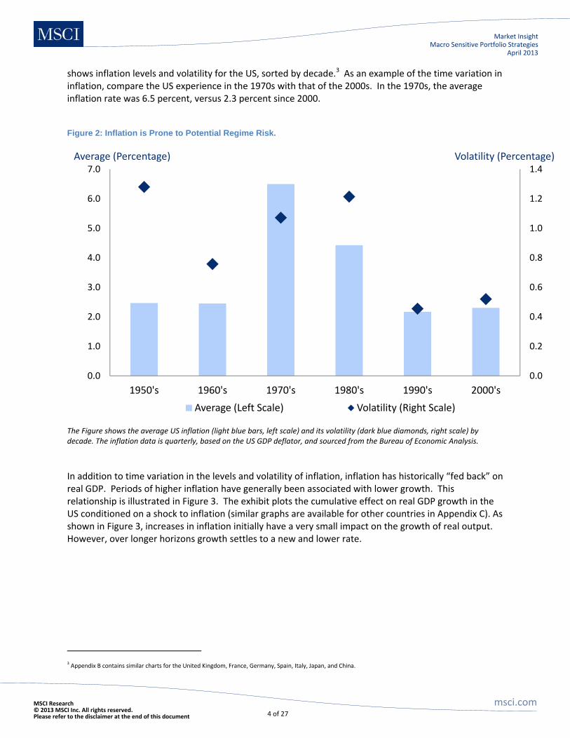
shows inflation levels and volatility for the US, sorted by decade.3 As an example of the time variation in inflation, compare the US experience in the 1970s with that of the 2000s. In the 1970s, the average inflation rate was 6.5 percent, versus 2.3 percent since 2000.

Figure 2: Inflation is Prone to Potential Regime Risk.

The Figure shows the average US inflation (light blue bars, left scale) and its volatility (dark blue diamonds, right scale) by decade. The inflation data is quarterly, based on the US GDP deflator, and sourced from the Bureau of Economic Analysis.

In addition to time variation in the levels and volatility of inflation, inflation has historically “fed back” on real GDP. Periods of higher inflation have generally been associated with lower growth. This relationship is illustrated in Figure 3. The exhibit plots the cumulative effect on real GDP growth in the US conditioned on a shock to inflation (similar graphs are available for other countries in Appendix C). As shown in Figure 3, increases in inflation initially have a very small impact on the growth of real output. However, over longer horizons growth settles to a new and lower rate.

3 Appendix B contains similar charts for the United Kingdom, France, Germany, Spain, Italy, Japan, and China.

0.0

0.2

0.4

0.6

0.8

1.0

1.2

1.4

0.0

1.0

2.0

3.0

4.0

5.0

6.0

7.0

1950's 1960's 1970's 1980's 1990's 2000's

Average (Left Scale) Volatility (Right Scale)

Volatility (Percentage)Average (Percentage)



April 2013

Figure 3: Shocks to Inflation Can Have Persistent Effects on Real Output.

The Figure shows the cumulative impact of a 2 percent persistent long term increase in US inflation on US Real GDP growth. The impulse responses are based on quarterly data for US inflation and real GDP growth from 1950 to 2011.

To calibrate the parameters of risk aversion and uncertainty aversion for investor preferences, we combine data on government bond prices with the historical relationships between inflation and real GDP. We then find discount functions by using current observations on inflation and real GDP (see Appendix A for details). Figure 4 shows an illustration of the calibrated discount function, expressed as a

yield curve. This is an equilibrium discount function that represents how the market discounts expected future cash flows, assuming that markets are in equilibrium.4

4 Appendix D shows the equilibrium yield curves for the United Kingdom, France, Germany, Spain, Italy, Japan. Note that we find a negative inflation premium for Japan, consistent with the data.

‐0.35

‐0.30

‐0.25

‐0.20

‐0.15

‐0.10

‐0.05

0.00

0 4 8 12 16 20 24 28 32 36 40 44 48 52 56 60 64 68 72 76 80

Horizon (Quarters)

Impact (Percentage)



April 2013

Figure 4: Yield Curves Reflect Long Run Macro Risk.

The Figure shows the nominal (solid dark blue) and real (dashed light blue) zero‐coupon yield curve implied by our asset pricing model.

Figure 4 shows real and nominal yield curves, suggesting that when markets are in equilibrium, the real yield curve should be relatively low and inverted. By contrast, the nominal curve is above the real curve and is positively sloped. Thus, nominal bonds are priced to have a yield premium relative to real bonds — this is the inflation premium. Since the differential between real and nominal bond yields increases with maturity, the inflation premium is seen to increase as well.

Since the discount function explicitly incorporates macroeconomic relationships, the impact on risk‐free bond pricing of macroeconomic shocks is straightforward to explore. There are two relevant shocks that are of interest: a shock to real GDP, and a shock to inflation.

Figure 5 shows the impact on 10‐year bond prices of a permanent negative 1.5 percent shock to real GDP growth. The figure shows both short‐ and long‐term effects on real and nominal bond prices, indicating that persistent weakness in the economy produces higher bond prices (lower bond yields) over both short and long term horizons. The impact on pricing is more pronounced at longer horizons. Interestingly, the impact of a negative shock to real GDP is more pronounced on nominal bond prices than real bond prices, regardless of horizon.

0.40

0.60

0.80

1.00

1.20

1.40

1.60

1.80

1 2 3 4 5 6 7 8 9 10

Inflation‐Linked Bonds

Nominal Bonds

Maturity (Years)

Yield (Percentage)



April 2013

Figure 5: Bond Prices Exhibit Positive Sensitivity to Trend Growth Risk.

The Figure shows the cumulative impact of a 1.5 percent permanent decrease in US real GDP growth on the 10 year real and nominal bond prices, both over the short term (one quarter) and the longer term (20 quarters).

The impact on real and nominal 10‐year bond prices of inflation shocks are seen in Figure 6, which shows the impact on bond prices under a positive shock to inflation for both short and long horizons.

0.0

0.2

0.4

0.6

0.8

1.0

1.2

1.4

1.6

Short Term Long Term

Impact (Percentage) on Bond Prices

10‐Year Inflation‐Linked Bond

10‐Year Nominal Bond



April 2013

Figure 6: Bond Prices Reveal a Premium for Inflation Risk.

The Figure shows the cumulative impact of a 2 percent permanent increase in US inflation on the 10 year real and nominal bond prices, both over the short term (one quarter) and the longer term (20 quarters).

For real bonds, positive shocks to inflation have only a minor impact on prices over short horizons. Over longer horizons, though, positive shocks to inflation lead to some modest price appreciation. This effect is observed over longer horizons, where positive inflation shocks lead to lower real economic growth. From Figure 5, lower real growth leads to higher real bond prices. Thus, higher inflation has neutral‐to‐positive effects on real bond prices.

By contrast, higher inflation is unambiguously negative for nominal bond prices, regardless of horizon. In Figure 6, the longer term negative effect on nominal bond prices is more than double the short term (negative) effect. Although the impact of higher inflation means lower real economic growth, the negative effects of higher inflation overwhelm the beneficial effects on nominal bond prices during lower economic growth.

Which effect is more important for bond pricing — shocks to real output or shocks to inflation? Figures 5 and 6 offer a straightforward way to assess this question. In Figure 5, negative shocks to real output lead to increases in bond prices that are no larger than 1.5 percent. By contrast, the inflation shocks of Figure 6 lead to decreases in nominal bond prices that range from 4 percent to over 8 percent. Clearly, the most significant macro risk for nominal bonds is inflation.

‐10

‐8

‐6

‐4

‐2

0

2

4

Short Term Long Term

Impact (Percentage) on Bond Prices

10‐Year Inflation‐Linked Bond

10‐Year Nominal Bond



April 2013

Asset Returns and Uncertainty Aversion The previous section discussed the exposures of real and nominal bond prices to macro risks, concluding that the dominant source of macro risk for nominal bonds is inflation. By contrast, exposures to both inflation and real output shocks are quite similar to each other. The impact of inflation on real bond prices is derived from the feedback from inflation to growth rates in real output.

To assess the impact of macro risk on equity prices and returns, we need to combine the effects of macro risk on discount rates with their effects on asset cash flows. The previous paper in this series discussed the exposure of equity cash flows to persistent shocks to trend growth. That paper concluded that, under persistent shocks to real output, significant variations exist across equity portfolios in the long‐run responses of dividend cash flow growth rates. .

Figure 7 shows the long‐run impact on dividend growth rates under a persistent shock to inflation.5 The chart shows the cumulative effect of inflation on dividend growth rates as estimated from a four‐

variable‐two‐lag Vector Autoregression (VAR) — see Appendix A for more details about the VAR. Inflation has a persistently negative effect on dividend cash flow growth for all portfolios, except the momentum strategy. In particular, increases in inflation have significantly negative effects on cash flow growth for the minimum volatility, materials, and real estate portfolios. Real cash flow growth for the consumer staples portfolio seems to be unaffected by bursts of unanticipated inflation. Figure 7: Inflation Has a Negative Long Run Impact on Equity Cash-Flows.

5 The global recession and financial crisis of 2008 are important events in our sample used to estimate the dividend growth responses of sector and strategy portfolios. In particular, for the MSCI USA Minimum Volatility, Materials, and Real Estate portfolios, the true long‐run response of dividend growth estimated from a much larger sample (with less influence from financial crises) may be less dramatic, than what we show in Figure 7.

‐16

‐14

‐12

‐10

‐8

‐6

‐4

‐2

0

2Impact (%)



April 2013

Perhaps the two most surprising impacts are for the Materials and Real Estate portfolios. Commodities and real estate are commonly considered good investments when anticipating inflation. Exhibit 7, however, shows that equity portfolios in these sectors have strongly negative long‐run cash flow responses to inflation. The principal reason for this is, as we illustrated in Exhibit 3, that a permanent shock to inflation eventually produces a negative impact on real GDP growth. Firms in the Materials and Real Estate sectors are especially sensitive to this decline.

Having examined how real output and inflation shocks impact both the discount rates and cash‐flows, we are now ready to understand how these shocks are priced. Our intuition is that assets with a larger exposure to macro risk should receive a higher return (or a premium). However, since macro risk is only likely to be revealed over longer time horizons, that premium will also be received over longer time horizons. This basic intuition is revealed in Figure 8, which shows the long‐run returns to four specific portfolios (Value, Growth, Small Cap and Large Cap), and compares them to the market portfolio. The returns are calculated using an equilibrium model that assumes that the representative investor holds the market portfolio. The equilibrium model assumes that the preferences of the representative investor reflect both risk aversion and uncertainty aversion. Both of these parameters were estimated using returns data for equities (including the returns to the specific portfolios) and bonds. Furthermore, the parameter estimation included the empirical relationships between equity cash flows, real output, and inflation.

Figure 8: Expected Returns to Equity Portfolios Reflect Macro Risk.

The Figure shows the equilibrium expected returns implied by our asset pricing model for different holding periods, from one quarter to 20 years (80 quarters), for the Value, Growth, Small Cap, Large Cap, and Market portfolios. The uncertainty aversion of the asset pricing model’s representative investor is calibrated to 15, to match the equity market long term average return observed in the data of 7.9 percent.

0

2

4

6

8

10

12

14

0 4 8 12 16 20 24 28 32 36 40 44 48 52 56 60 64 68 72 76 80

Growth Value Small Large Market

Horizon (Quarters)

Holding‐Period Expected Return (Percentage, Annualized)



April 2013

Our analysis of equity cash flows from the previous paper indicated that value and small cap portfolios are more exposed to shocks to real GDP than are growth and large cap portfolios. Furthermore, our analysis suggested that the impact of shocks to real output on these portfolios is only revealed over longer horizons. Thus, we would anticipate that the long‐run return to value and small cap should be higher than the return to large cap and growth. This pattern is illustrated in Figure 8.

The generalization of the pattern in Figure 8 is as follows — any sequence of cash flows that has a low long‐term beta with respect to the real economy should have a low return relative to the market portfolio. Sequences of cash flows with high long‐term betas should have high returns relative to the market. Thus, we should expect defensive industries such as consumer staples to have low returns relative to the market portfolio, and cyclical industries such as financials to have high long‐term returns. Clearly, the same analytic approach can be applied to understanding the return drivers for strategy portfolios, such as a momentum portfolio, or a minimum volatility portfolio.

Macro Shocks and Portfolio Risk Many investors hold multi‐asset class portfolios. To calculate the level of total portfolio risk, investors rely on publicly available data. Often, there is variability in these data both in terms of the length of history, and in terms of the sampling frequency. Consequently, most risk forecasts can be viewed as being consistent with short‐ to intermediate‐term investment horizons.

To use risk models, many practitioners use risk decompositions. These decompositions take the level of total portfolio volatility and attribute it to different sources. Those sources can be asset classes or, if a risk model is used, risk factors. If a risk model is used, then its parameters are estimated with the same data limitations as overall portfolio risk.

The issue facing investors when assessing macro risk is how the impact of macro shocks are revealed only over longer horizons. Accounting for the impact of horizon, the appropriate analysis of macro risk includes stress tests and risk decompositions.

Stress tests are particularly suited to the analysis of macro risk, principally because of the analytic structure that we have used to describe macro risk. More specifically, the impact of a macro shock on portfolio value (and return) can be assessed by combining the impulse responses for asset cash flows with the responses for discount functions. And, since the impulse responses cover multiple periods, the stress test can show the evolution of asset prices and returns, conditioned on a macro shock.

Risk decompositions, on the other hand, are more complicated. The objective of risk decomposition is to attribute a portion of total portfolio volatility to factor exposures. The general assumption with factor models is that individual asset returns can be described in terms of a small set of factors. Portfolio returns are then found by aggregating the exposures of each asset to this smaller set of factors. Portfolio risk is then simply expressed in terms of the aggregate factor exposures and the volatility and correlation of the factor returns.

Three issues make this an even trickier problem for describing macro risk:

1. The exposure of each asset to macro risk varies with horizon.

2. The two principal macro risks are real output and inflation and ‐‐ as we have discussed ‐‐ the evolution of these two factors is described by a dynamic model in which one‐time shocks play out over long horizons.



April 2013

3. The relative importance of each macro factor for a given horizon depends on the interaction between the evolution of cash flows and the evolution of discount factors.

Fortunately, many of these issues can be resolved, to a first approximation, through a linearization of the asset pricing model6.

Table 9, Figure 10 and Figure 11 illustrate the analysis of macro risk through risk decompositions and stress tests, applied to six portfolios (see Appendix E for a description of the six portfolios).

Table 9 starts the analysis by looking at short‐ and long‐term volatility for each portfolio. For each portfolio, and for each horizon, volatility is calculated with both actual returns data and with our macro risk model. Then, volatility is attributed to macro factors.

Standard risk decompositions usually attribute a portion of the variance to each of the factors in the model. The implicit assumption is that the factor exposures are not affected by a shock to the factors. For example, the returns to points on the government bond curve can be attributed to three factors (level, slope and curvature). Exposures to these factors for specific bonds are the coupon and principal payments, allocated to each term structure point. The bond’s volatility is the combination of the payments and the covariance matrix of factor returns.

Macro shocks work differently. The assumption that the factor exposures are unaffected by shocks to the macro factors does not work for equities (as shown in our earlier work). Consequently, the arithmetic of allocating our risk is more complicated than the simple decompositions of the bond example. Conceptually, though, the idea is similar: introduce separate shocks to real GDP and inflation, and trace through their effects on discounts and cash flows. Combining the effects through the asset pricing model produces a total change in value, which can in turn be attributed to the separate macro factors (Appendix A contains details of these calculations).

Turning to the risk decompositions in Table 9, we show that over long horizons macro factors are the dominant source of portfolio risk. Over short horizons, the contribution of macro factors depends on the portfolio holdings; for the three portfolios that are predominantly equity‐oriented, macro factors contribute a small portion to total volatility. That the importance of macro factors only emerges over longer horizons in the risk decompositions for equity‐oriented portfolios should not be surprising‐ the cash flow betas for equity portfolios are quite low at short horizons (as shown in our earlier paper).

The risk (both short‐ and long‐term) in the portfolios with higher bond allocations is driven mostly by macro‐factors, and principally inflation. In fact, for the 100 percent bond portfolio, 70 percent of the long‐term variance is attributed to inflation. Again, this result should not be surprising‐ Figures 5 and 6 illustrated that nominal bond prices are much more significantly affected by shocks to inflation than shocks to real GDP.

Equally interesting is the comparison between the two equity‐oriented portfolios. The portfolio with a tilt to risk premium strategies (value and small cap) has a higher total risk. Because of the tilt to risk premium strategies, the contribution of real GDP shocks is more significant.

6 The analysis of the impact of macro shocks on portfolio risk can also be undertaken without resorting to a linear approximation of asset returns as a function of macro shocks. Following the work of Hansen and Scheinkman (2012), the concept of impulse responses for VARs can be generalized to the non‐linear case. Such extension, however, is beyond the scope of this paper.



April 2013

Table 9: Macro Risk Contributions to Portfolio Volatility Dominate in the Long-Run.

Equity Market

Bonds

60/40 Equity and Bonds

60/40 Equity and Bonds, and Risk Premia Tilt


Equity Market and Risk Premia Tilt

Short Horizon

Historical Total Risk (%) 18.0 5.0 10.4 11.8 5.4 19.5

Model Total Risk (%) 2.3 5.0 2.4 2.8 3.6 3.2

Macro Risk Contribution (%) 0.2 97.4 4.1 2.5 41.6 0.3

Real GDP 0.1 30.1 1.3 0.8 12.7 0.3

Inflation 0.0 67.3 2.8 1.7 28.9 0.0

Long Horizon

Historical Total Risk (%) 15.6 5.6 9.8 10.1 6.3 15.9

Model Total Risk (%) 10.6 5.3 8.0 10.4 6.4 13.1

Macro Risk Contribution (%) 87.9 100.0 92.5 87.8 97.1 84.8

Real GDP 77.8 30.3 70.3 74.7 56.1 78.3

Inflation 10.1 69.7 22.2 13.1 41.0 6.5

The Table contrasts the short term (one‐quarter), and the long‐term (80‐quarter) portfolio volatility and variance contributions from real GDP and inflation for six US portfolios. Appendix E gives the allocations for the six portfolios. We represented the US equity market, treasuries, value and small cap portfolios with, respectively, the MSCI USA Standard Index, the long‐only portfolios sorted by book‐to‐market and size from Kenneth French’s website, and the Citigroup US All Maturity Treasury Index. The short‐term historical volatility is the exponentially weighted standard deviation of portfolio monthly real returns with a 24‐month half‐life, from January 1980 to December 2012. The long‐term historical volatility is the equally weighted standard deviation of portfolio monthly real returns over the same period. The model volatility and variance contributions from real GDP and inflation are derived from our asset pricing model.

The essence of the risk decompositions are confirmed in the stress tests, as shown in Figures 10 and 11. The two figures trace out, respectively, the cumulative impact of positive shocks to real GDP and inflation on the real return for each of the six portfolios.

As evident in Figure 10, all portfolios in our study benefit from a positive shock to real economic growth. Positive shocks to real output are felt at first as increases in the values of nominal bonds. Over time, growth rates of equity cash flows increase, and the shock is translated into increases in equity values; the three blended portfolios nicely illustrate these interactions. Over the first one or two years following a shock, the 30/70 portfolio outperforms the other two blended portfolios. However, from approximately two years on, the performance of the 60/40 portfolio matches that of the 30/70 portfolio. Furthermore, the performance of the 60/40 portfolio that incorporates a tilt to risk‐premium strategies outperforms the other two blended portfolios over time. This relationship highlights the importance of the risk premium portfolio in asset allocation decisions.



April 2013

Figure 10: Macro-Based Scenario Stress Test – Impact of a 1.5% Permanent Increase in Real Output on Portfolio Values.

The Figure shows the impact of a 1.5 percent persistent shock to US real output on the return to six US portfolios. Appendix E gives the allocations for the six portfolios. The sensitivity of portfolio returns to macro shocks are derived from our asset pricing model.

The impact on portfolio value of a permanent increase in inflation is illustrated in Figure 11, which shows how increases in inflation reduce portfolio value over the long run for all six of our example portfolios. It also shows that the impact of inflation is significantly more pronounced for portfolios with large bond allocations. Thus, portfolios with significant allocations to nominal bonds are capturing an inflation premium, and under circumstances of benign or decreasing inflation, these portfolios will perform well. However, the figure makes clear that these portfolios are adversely affected by increases in inflation.

‐2

0

2

4

6

8

10

0 4 8 12 16 20 24 28 32 36 40 44 48 52 56 60 64 68 72 76 80

60/40 Equity Market and Bonds

60/40 Equity Market and Bonds, and Risk Premia Tilt


Equity Market

Bonds


Impact on Portfolio Value (Percentage)

Horizon (Quarters)



April 2013

Figure 11: Macro-Based Scenario Stress Test – Impact of a 2% Permanent Increase in Inflation on Portfolio Values.

The Figure shows the impact of a 2 percent persistent shock to US inflation on the real return to six US portfolios. Appendix E gives the allocations for the six portfolios. The sensitivity of portfolio returns to macro shocks are derived from our asset pricing model.

‐2.5

‐2.0

‐1.5

‐1.0

‐0.5

0.0

0.5

1.0

0 4 8 12 16 20 24 28 32 36 40 44 48 52 56 60 64 68 72 76 80


60/40 Equity Market and Bonds, and Risk Premia Tilt


Equity Market

Bonds


Impact on Portfolio Value (Percentage)

Horizon (Quarters)



April 2013

Conclusion A theme of this series is that macro risk is only revealed over long horizons. In the second paper of this series, we showed that asset cash flows differ in their responses to macro shocks. We argued that these differences must be reflected in asset prices.

In this paper, we showed that the discount function used to price asset cash flows is also sensitive to macro shocks. In particular, we showed that the dominant macro risk in real bond prices is a shock to real output. By contrast, the dominant source of macro risk in nominal bond prices can be shocks to inflation. These effects, combined with the long horizon betas for asset cash flows, can drive asset prices and returns.

The result of combining macro‐sensitive discounts with macro‐sensitive cash flows is that long‐run returns are higher for those assets with higher long‐term betas to the macro‐economy. Moreover, portfolios with tilts towards these assets will have a higher percentage of portfolio risk attributable to macro shocks.

For the most part, our analysis has been done in the context of a representative investor. Our example portfolios hypothesized portfolio weights, but did not discuss the process by which an investor would choose these allocations. Portfolio strategy in the face of macro risk will be the subject of the next paper in this series.



April 2013

Reference

Anderson, Evans, Lars P. Hansen, and Thomas J. Sargent, 2000 “Robustness, Detection, and the Price of Risk.” Working Paper https://files.nyu.edu/ts43/public/research/.svn/.../ahs3.pdf.svn-base

Barrillas, Francisco, Lars P. Hansen, and Thomas J. Sargent, 2009, “Doubts or Variability.” Journal of Economic Theory 144, pp.2388‐2418.

Blanchard, Olivier J., and Danny Quah, 1989, “The Dynamic Effects of Aggregate Demand and Supply Disturbances.” The American Economic Review, Vol. 79, No. 4, pp. 655‐673.

Campbell, John Y., and Tuomo Vuolteenaho, 2004, “Bad Beta, Good Beta.” The American Economic Review, Vol. 94, No. 5, pp. 1249‐1275.

Epstein, Larry, and Stanley Zin, 1989, “Substitution, Risk Aversion and the Temporal Behavior of Consumption and Asset Returns: A Theoretical Perspective.” Econometrica 57, pp. 937‐969.

Kreps, David M., and Evan L. Porteus, 1978. "Temporal Resolution of Uncertainty and Dynamic Choice

Theory," Econometrica, Econometric Society, vol. 46(1), pp 185‐200, January.

Piazzesi, Monika, and Martin Schneider, 2007, “Equilibrium Yield Curves.” NBER Macroeconomics Annual 2006, published in 2007, Cambridge MA: MIT Press pp. 389-442.

Hansen, Lars P., John Heaton and Nan Li, 2008, “Consumption Strikes Back? Measuring Long Run Risk.” Journal of Political Economy 116 (2), pp.260‐302.

Hansen, Lars P., and Jose A. Scheinkman, 2012 “Pricing Growth‐Rate Risk”, Finance and Stochastics 16(1): pp. 1‐15, January, 2012.

Sims, Chris A., 1980a, “Comparison of Interwar and Postwar Business Cycles: Monetarism Reconsidered.” American Economic Review, Vol. 70, pp. 250‐257.

Sims, Chris A., 1980b, “Macroeconomics and Reality.” Econometrica, Vol. 48, pp. 1‐48.

Winkelmann, Kurt, Ludger Hentschel, Raghu Suryanarayanan, and Katalin Varga, 2012, “Macro‐Sensitive Portfolio Strategies: How We Define Macroeconomic Risk.” MSCI Market Insight, November 2012.

Winkelmann, Kurt, Raghu Suryanarayanan, Ludger Hentschel, and Katalin Varga, 2013, “Macro‐Sensitive Portfolio Strategies: Macroeconomic Risk and Asset Cash‐Flows.” MSCI Market Insight, March 2013.



April 2013

Appendix A: Equilibrium Asset Pricing

Asset Prices, Discount Factors and Cash‐Flows Modern asset pricing theory states that the competitive equilibrium value of an asset equals the expected discounted value of current and future asset cash flows, conditional on the current state of the

economy. More precisely, the price of asset tP at time t can be expressed as:

,1

( )t t t j t j tj

P E S D X

(1)

Where:

tX is the “state”, capturing investors’ current expectations of the economy (real GDP growth and

inflation for example).

tD denotes the asset payoff or cash‐flow at time t

,t t jS is the time t discount factor for payoffs realized at time t+j in the future (also known as the

stochastic discount factor). The discount factor reflects a representative investor’s willingness to trade‐off current consumption for future consumption.

In our previous paper (“Macroeconomic Risk and Asset Cash‐Flows”), we showed how the evolution of the state and cash‐flows can be modeled with a VAR (Vector Autoregression). In the next sections, we show how the discount factor and the resulting asset prices relate to the state.

Preferences Set the Discount Factors

Standard Time Additive Expected Utility

Standard time additive expected utility preferences are commonly used in economics and finance. The

time t value of an investor current and future stream of consumption 1( , ,...)t tC C is given by:

11

( , ,...) ( ) ( ( ) )jt t t t t j t

j

V C C u C E u C X

(2)

Where is the constant time discount factor, and ( )u C is the periodic utility, measuring the value of

C units of consumption at any point in time. The periodic utility function u is commonly assumed to be CRRA (Constant Relative Risk Aversion):

1( ) / (1 )u C C , where is the coefficient of relative risk aversion (risk aversion for a

given level of wealth)

Discount Factors

Discount factors measure the willingness of an investor to trade‐off current consumption for future consumption, and captures an investor’s sensitivity to real economic growth risk. Formally, it can be derived from an investor’s preferences as:



April 2013

, 11

/t tt t

t t

V VS

C C

(3)

Epstein‐Zin Recursive Utility

Epstein and Zin introduce a new parameter, the Elasticity of Intertemporal Substitution (EIS), which governs an investor’s willingness to forgo current consumption for a certain level of future consumption, in addition to the standard risk aversion parameter. Formally, they define preferences recursively as:

1 1 1/(1 )1[(1 ) ( ( )) ]t t t tV C R V (4)

Where:

1 1/(1 )1 1( ) ( ( ))t t t tR V E V is the “risk‐sensitive adjustment,” sensitive to future economic

growth risk

is the relative risk aversion parameter

is the EIS

In doing so, they allow investors to be sensitive to persistent shocks to trend economic growth. Indeed, the discount factor implied by the Epstein‐Zin preferences can be expressed as7

1 1, 1

1

( )t t tt t

t t

C R VS

C V

(5)

When the EIS is equal to risk aversion ( ), the Epstein‐Zin utility reduces to the standard

preferences. And the discount factor only depends on current and next period’s consumption. When the EIS is different from risk aversion, however, the discount factor now depends on the entire stream of

current and future consumption, through the risk‐sensitive adjustment term 1 1( ) /t t tR V V .

In particular, an investor can now be averse or tolerant to persistent shocks to trend economic growth, depending on whether risk aversion is strictly greater or lower than the EIS. Anderson, Hansen, and Sargent (2000), and Barrillas, Hansen, and Sargent (2009) reinterpret aversion to persistence in economic growth as aversion to model uncertainty, or uncertainty around the evolution of economic growth in the long run.

We assume that the EIS is equal to 1, and we set to 16 to match an equity market average return of

7.9 percent. Uncertainty aversion is measured by 1 and is equal to 15.

Long Run Risk Model for Real GDP Growth and Inflation In our previous paper (“Macroeconomic Risk and Asset Cash‐Flows”), we modeled the evolution of the state using the long run risk model for real GDP growth, a two‐variable VAR with two lags. The two

variables were the log of real GDP growth 1( )t tg g and the log of GDP to Corporate Profits ratio

t tg cp . We now introduce the log of consumer price inflation (we used the GDP deflator to measure

7 See Epstein and Zin (1989).



April 2013

the consumer price level) as a third variable in the VAR. More precisely, the state tX is now modeled

as:

1 1t x t tX AX u (6)

Where 1

tt

t

YX

Y

and 1[ , , ]t t t t t tY g g g cp

g is the log of real GDP, cp is the log of corporate profits, and is the log of inflation

tu is a 3‐by‐1 vector of macro shocks, assumed to be normally distributed with zero mean and

covariance matrix equal to the identity matrix. We further assume that the residuals are identically and independently distributed over time.

We also add a portfolio’s log of cash‐flow growth as a fourth variable in tY to analyze the sensitivity of

cash‐flows to shocks to both real GDP and inflation.

Following equation (6), the log of real GDP growth and inflation can be expressed as:

1 ,0 1t t g g t g tg g X u (7)

1 ,0 1t t tX u (8)

Where is the long term average trend growth, ,0g is the short term real growth risk, ,0 is the short

term inflation risk, [1,0,0,0,0,0]g , and [0,0,1,0,0,0]

Nominal and Real Bonds Pricing To price assets, we need to derive the equilibrium discount factor for the representative investor in the economy. Hansen, Heaton, and Li (2008) show that the log of the discount factor can be expressed as a linear function of the state:

, 1 , 1 1ln( )t t t t s s t s tS s X u (9)

The parameters in equation (9) closely relate to the parameters governing real GDP growth:

22(1 ) ( )log

2g

s g

, s g , and ,0 ( 1) ( )s g g

where ,0

( ) jg g j

j

and 1,

hg h g A

The equilibrium asset pricing equation (1) together with equation (9), assuming that the shocks tu

normally distributed, can be used to derive the equilibrium yield of inflation‐linked bonds ( ),n

b ty and of

nominal bonds ( )$, ,nb ty , at any time t and for any maturity n. In particular, yields are linear functions of the

state tX :

( ),

1( )n

b t n n ty E B Xn

and ( )$, , $, $,

1( )n

b t n n ty E B Xn

(10)



April 2013

Following (9), rolling bond (log) returns will also be a linear function of the state tX :

( ) ( 1) ( ) ( ) ( ), , 1 , , 1 1( 1)n n n n n

b t t b t b t b b t b tr ny n y X u (11)

( ) ( ) ( 1) ( ) ( ) ( )$, , 1 $, , $, , 1 $, $, $, 1( 1)n n n n n n

b t b t b t b b t b tr ny n y X u (12)

The details of the derivations and the expressions for the coefficients of equations (10), (11) and (12) may be requested on demand.

Equity Portfolio Pricing

The price of an equity portfolio ( ,e tP ) and its return can also be derived from equation (1) in a similar

fashion. For each portfolio, we first derive the dividend growth process:

( )1 1ln /t t d d t d tD D X um d l+ += + + (13)

Where [0,0,0,1,0,0,0,0]d and tX now includes the log of dividend growth. We then derive a

linear approximation for the log of an equity portfolio real return ( , 1e tr ) as:

, 1 ,1

, 1 11

ln( ) ln( 1) ln( )e t e tte t e e t e t

t t t

P PDr X u

D D D

(14)

The details of the derivations and the expressions for the coefficients of equation (14) may be requested on demand.

Long Run Portfolio Returns and Risk Equations (12) and (14) can now be used to decompose the (log of the) long run return to a portfolio of equities and bonds into a transitory and a long run component:

,1 1 Transitory

Long-Run

t t

P P P P tr t u X

(15)

P is the long run impulse response of the portfolio return to macro shocks captured by tu :

P e e b b , where e and b are the weights on equities and bonds,

1

1

je e

j

A

and 1

1

jb b

j

A

are the long run impulse response of the equities

and bonds portfolios.

And P e e b b is the sensitivity of the portfolio return to the transitory state tX ,

where 1( )e e I A and 1( )b b I A are the sensitivities of the equities and

bonds portfolios to the transitory state.

As the macro shocks tu are independently distributed over time, the long‐run component will dominate

the portfolio return’s volatility as time grows. Thus, P is a measure of long run portfolio risk.

Moreover, as we identify the shocks to real GDP and inflation, captured by the elements of tu , to be

uncorrelated, we can readily decompose the long run portfolio variance 2

P into independent

contributions from real GDP and inflation shocks.



April 2013

Appendix B: Inflation is Prone to Potential Regime Risk

Table 12: Average Inflation by Decade.

US Canada UK France Germany Italy Spain Japan China

1950's 2.5 3.2 6.9

1960's 2.5 3.3 4.0 4.1 6.1

1970's 6.5 12.4 8.8 13.1 13.7

1980's 4.4 4.8 6.6 6.6 10.6 9.3 1.7 4.8

1990's 2.2 1.7 3.0 1.4 2.1 4.2 4.3 0.4 7.0

2000's 2.3 2.4 2.2 1.9 0.9 2.3 3.3 ‐1.3 3.9

The Table shows the average inflation by decade, for US, Canada, UK, France, Germany, Italy, Spain, Japan, and China. The inflation data is quarterly, based on the GDP deflator.

Table 13: Volatility of Inflation by Decade.

US Canada UK France Germany Italy Spain Japan China

1950's 1.3 2.6 3.8

1960's 0.8 1.9 1.6 1.5 1.2

1970's 1.1 3.6 1.7 3.5 2.6

1980's 1.2 1.2 2.2 1.8 2.7 1.6 1.0 5.7

1990's 0.5 0.8 1.4 0.5 1.3 2.1 1.6 0.9 8.4

2000's 0.5 2.1 1.1 0.5 0.6 1.1 0.8 0.9 5.3

The Table shows the volatility of inflation by decade, for US, Canada, UK, France, Germany, Italy, Spain, Japan, and China. The inflation data is quarterly, based on the GDP deflator.



April 2013

Appendix C: Shocks to Inflation Have Persistent Effects on Real Output

Figure 14: Impact of a 2 percent Persistent Increase in Inflation on Real GDP.

The Figure shows the impulse response of real GDP to a 2 percent persistent increase in inflation in Canada, UK, France, Germany, Italy, Spain, and Japan.

‐0.5

‐0.4

‐0.3

‐0.2

‐0.1

0.0

0.1

0.2

0.3

0.4

0.5

0 4 8 12 16 20 24 28 32 36 40 44 48 52 56 60 64 68 72 76 80

Canada Japan Spain Italy Germany France UK US

Impact (Percentage)

Horizon (Quarters)



April 2013

Appendix D: Yield Curves Reflect Long Run Macro Risk

Figure 15: Zero-Coupon Nominal Yield Curves Implied by the Asset Pricing Model.

0.00

1.00

2.00

3.00

4.00

5.00

6.00

7.00

1 2 3 4 5 6 7 8 9 10

US UK Canada Germany

France Italy Spain Japan

Maturity (Years)

Yield (Percentage)



April 2013

Figure 16: Zero-Coupon Real Yield Curves Implied by the Asset Pricing Model.

0.00

0.20

0.40

0.60

0.80

1.00

1.20

1.40

1.60

1 2 3 4 5 6 7 8 9 10

US UK Canada Germany

France Italy Spain Japan

Maturity (Years)

Yield (Percentage)



April 2013

Appendix E: Portfolio Allocation

Table 17: Asset allocations for the Six Portfolios.

Equity Market

Bonds 60/40 Equity and Bonds

60/40 Equity and Bonds, and Risk Premia

Tilt



Bonds (%) 0 100 40 40 70 0

Equities* (%) 100 0 60 30 30 50

Small Cap (%) 0 0 0 15 0 25

Value (%) 0 0 0 15 0 25



April 2013

Client Service Information is Available 24 Hours a Day [email protected]

Notice and Disclaimer This document and all of the information contained in it, including without limitation all text, data, graphs, charts (collectively, the “Information”) is the property of MSCI Inc. or its

subsidiaries (collectively, “MSCI”), or MSCI’s licensors, direct or indirect suppliers or any third party involved in making or compiling any Information (collectively, with MSCI, the “Information Providers”) and is provided for informational purposes only. The Information may not be reproduced or redisseminated in whole or in part without prior written permission from MSCI.

The Information may not be used to create derivative works or to verify or correct other data or information. For example (but without limitation), the Information may not be used to create indices, databases, risk models, analytics, software, or in connection with the issuing, offering, sponsoring, managing or marketing of any securities, portfolios, financial products or other investment vehicles utilizing or based on, linked to, tracking or otherwise derived from the Information or any other MSCI data, information, products or services.

The user of the Information assumes the entire risk of any use it may make or permit to be made of the Information. NONE OF THE INFORMATION PROVIDERS MAKES ANY EXPRESS OR IMPLIED WARRANTIES OR REPRESENTATIONS WITH RESPECT TO THE INFORMATION (OR THE RESULTS TO BE OBTAINED BY THE USE THEREOF), AND TO THE MAXIMUM EXTENT PERMITTED BY APPLICABLE LAW, EACH INFORMATION PROVIDER EXPRESSLY DISCLAIMS ALL IMPLIED WARRANTIES (INCLUDING, WITHOUT LIMITATION, ANY IMPLIED WARRANTIES OF ORIGINALITY, ACCURACY, TIMELINESS, NON‐INFRINGEMENT, COMPLETENESS, MERCHANTABILITY AND FITNESS FOR A PARTICULAR PURPOSE) WITH RESPECT TO ANY OF THE INFORMATION.

Without limiting any of the foregoing and to the maximum extent permitted by applicable law, in no event shall any Information Provider have any liability regarding any of the Information for any direct, indirect, special, punitive, consequential (including lost profits) or any other damages even if notified of the possibility of such damages. The foregoing shall not exclude or limit any liability that may not by applicable law be excluded or limited, including without limitation (as applicable), any liability for death or personal injury to the extent that such injury results from the negligence or wilful default of itself, its servants, agents or sub‐contractors.

Information containing any historical information, data or analysis should not be taken as an indication or guarantee of any future performance, analysis, forecast or prediction. Past performance does not guarantee future results.

None of the Information constitutes an offer to sell (or a solicitation of an offer to buy), any security, financial product or other investment vehicle or any trading strategy. You cannot invest in an index.

MSCI’s indirect wholly‐owned subsidiary Institutional Shareholder Services, Inc. (“ISS”) is a Registered Investment Adviser under the Investment Advisers Act of 1940. Except with respect to any applicable products or services from ISS (including applicable products or services from MSCI ESG Research Information, which are provided by ISS), neither MSCI nor any of its products or services recommends, endorses, approves or otherwise expresses any opinion regarding any issuer, securities, financial products or instruments or trading strategies and neither MSCI nor any of its products or services is intended to constitute investment advice or a recommendation to make (or refrain from making) any kind of investment decision and may not be relied on as such.

The MSCI ESG Indices use ratings and other data, analysis and information from MSCI ESG Research. MSCI ESG Research is produced by ISS or its subsidiaries. Issuers mentioned or included in any MSCI ESG Research materials may be a client of MSCI, ISS, or another MSCI subsidiary, or the parent of, or affiliated with, a client of MSCI, ISS, or another MSCI subsidiary, including ISS Corporate Services, Inc., which provides tools and services to issuers. MSCI ESG Research materials, including materials utilized in any MSCI ESG Indices or other products, have not been submitted to, nor received approval from, the United States Securities and Exchange Commission or any other regulatory body.

Any use of or access to products, services or information of MSCI requires a license from MSCI. MSCI, Barra, RiskMetrics, ISS, CFRA, FEA, and other MSCI brands and product names are the trademarks, service marks, or registered trademarks or service marks of MSCI or its subsidiaries in the United States and other jurisdictions. The Global Industry Classification Standard (GICS) was developed by and is the exclusive property of MSCI and Standard & Poor’s. “Global Industry Classification Standard (GICS)” is a service mark of MSCI and Standard & Poor’s.

About MSCI MSCI Inc. is a leading provider of investment decision support tools to investors globally, including asset managers, banks, hedge funds and pension funds. MSCI products and services include indices, portfolio risk and performance analytics, and governance tools.

The company’s flagship product offerings are: the MSCI indices with close to USD 7 trillion estimated to be benchmarked to them on a worldwide basis1; Barra multi‐

asset class factor models, portfolio risk and performance analytics; RiskMetrics multi‐asset class market and credit risk analytics; IPD real estate information, indices and analytics; MSCI ESG (environmental, social and governance) Research screening, analysis and ratings; ISS governance research and outsourced proxy voting and reporting services; FEA valuation models and risk management software for the energy and commodities markets; and CFRA forensic accounting risk research, legal/regulatory risk assessment, and due‐diligence. MSCI is headquartered in New York, with research and commercial offices around the world.

1As of March 31, 2012, as published by eVestment, Lipper and Bloomberg in September 2012. Jan 2013

Americas Europe, Middle East & Africa Asia Pacific

Americas Atlanta Boston Chicago Montreal Monterrey New York San Francisco Sao Paulo Stamford Toronto

1.888.588.4567 (toll free) + 1.404.551.3212 + 1.617.532.0920 + 1.312.675.0545 + 1.514.847.7506 + 52.81.1253.4020 + 1.212.804.3901 + 1.415.836.8800 + 55.11.3706.1360 +1.203.325.5630 + 1.416.628.1007

Cape TownFrankfurt Geneva London Milan Paris

+ 27.21.673.0100+ 49.69.133.859.00 + 41.22.817.9777 + 44.20.7618.2222 + 39.02.5849.0415 0800.91.59.17 (toll free)

China NorthChina South Hong Kong Seoul Singapore Sydney Tokyo

10800.852.1032 (toll free)10800.152.1032 (toll free) + 852.2844.9333 798.8521.3392 (toll free) 800.852.3749 (toll free) + 61.2.9033.9333 + 81.3.5226.8222

Macro-Sensitive Portfolio Strategies - MSCI

Documents

Transcript of Macro-Sensitive Portfolio Strategies - MSCI