Low frequency atmospheric transport and surface flux measurements

Chapter 5

LOW FREQUENCY ATMOSPHERIC TRANSPORTAND SURFACE FLUX MEASUREMENTS

Yadvinder Malhi, Keith McNaughton, Celso Von [email protected]

AbstractWe review the issue of turbulent atmospheric transport of scalars or

momentum on timescales greater than 30 minutes or 1 hour, regions ofthe spectrum of atmospheric motion that are not usually sampled byconventional flux measurement methodologies. We first explore what isknown about the nature and timescales of turbulent transport structuresin the near-surface layers of the atmosphere, and the degree to whichthis transport is controlled or modulated by the timescales of inner layer(shear) transport and outer boundary layer transport. We then presentempirical evidence of the existence of low frequency transport by pre-senting data from two contrasting field studies, a shear-dominated mea-surement set-up in Scotland, and a convection dominated measurementset-up in Brazilian Amazonia. It is clear that low frequency transportcan transport a significant amount of flux in measurement situationssuch as towers over forests in anticyclonic conditions, or in the tropics.Thereafter we explore the quantitative implications of undersamplinglow frequency atmospheric transport. Extending the sampling periodof surface flux measurements is desirable under certain conditions, butis not without complications. We conclude by highlighting some of thedangers of extending sampling periods into the low frequency domain.

1 IntroductionThe micrometeorological technique of eddy covariance aims to mea-

sure the transport of flux via turbulence between the surface and theatmosphere. In practice it samples only a part of the possible spec-trum of atmospheric motion, typically time scales between one secondand one hour. Transport at timescales less than one second are dis-cussed elsewhere in this volume (Chapter 4). For longer timescales an

77

78 HANDBOOK OF MICROMETEOROLOGY

assumption is made of frequency separation — that a spectral gap existsbetween the operational timescales of flux transport, and longer-scale at-mospheric motions. The presumed existence of such a gap is critical formeasured turbulent fluxes, as it provides an upper time limit to measure-ments averaging and rotation periods to separate “locally meaningful”fluxes from background trends and oscillations. However, it is unclearas to whether this gap really exists. The importance of low frequencymotions to energy and carbon balance studies have been highlighted inrecent papers (Mahrt 1998a, 1998b, Sakai et al. 2001, Von Randow etal. 2002, Finnigan et al. 2003).

In this Chapter, we first review what is known about the nature andtimescales of turbulent transport structures in the near-surface layers ofthe atmosphere, and the degree to which this transport is controlled bythe timescales of inner layer (shear) transport and boundary layer trans-port. This chapter covers some of the same territory as Mahrt (1998a),but using the perspective of the new turbulence model of McNaughton(2004b). We focus primarily here on daytime turbulent transport, thedeeper complexities of nighttime transport are discussed in Chapters 10and 8 of this book. We then present empirical evidence of the existenceof low frequency transport by presenting data from two contrasting fieldstudies, a shear dominated measurement set-up in Scotland, and a con-vection dominated measurement set-up in Brazilian Amazonia. There-after we explore the quantitative implications of undersampling low fre-quency atmospheric transport, summarizing an analysis presented byFinnigan et al (2003). We conclude by highlighting some of the dan-gers complications of extending sampling periods into the low frequencydomain. The subject of low frequency transport and how to deal withit enters into the still poorly understood fields of self-organized turbu-lent structures and mesoscale flows, and is clearly an area of ongoingresearch. We begin by reviewing these issues.

2 Turbulence structure, eddy sizes and samplingtimes

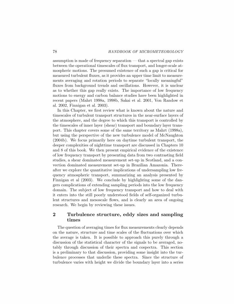
The question of averaging times for flux measurements clearly dependson the nature, structure and time scales of the fluctuations over whichthe average is taken. It is possible to approach this purely through adiscussion of the statistical character of the signals to be averaged, no-tably through discussion of their spectra and cospectra. This sectionis a preliminary to that discussion, providing some insight into the tur-bulence processes that underlie these spectra. Since the structure ofturbulence varies with height we divide the boundary layer into a series

Low frequency atmospheric transport 79

Figure 5.1. Schematic diagram of the location of flux measuring instruments, shownas rectangles on the top of each tower, in relationship to the various layers ofthe boundary layer in both weakly and strongly unstable conditions. Instrumentsmounted a few meters above low vegetation are usually within the surface layer. Thislayer may completely disappear over forests as the outer layer extends downwardsinto the layer directly influenced by the vegetation (up to at least twice forest height).Measurements from a forest tower may often be in the transition or outer layer dur-ing the day. This affects the averaging times needed to make reliable observations ofscalar fluxes.

of layers, the principle ones being the ’outer layer’ or ’mixed layer’ wherelarge convective circulations form during the day, and the ’inner layer’or ’surface layer’ whose characteristics are dominated by shear. Withinthe inner layer is a roughness sublayer where the turbulence is directlyaffected by the surface itself. The inner and outer layers are separatedby a transition layer. This has variously been called an ’interactionlayer’ (McNaughton 2004b), a ’matching layer’ (Mahrt 1998a) or a ’freeconvection layer’ (e.g. Garratt 1992). These different names reflect dif-ferent understandings of what this layer represents. Garratt (1992) seesit as a layer of gradual transition where proposed plume-like structuresthat develop progressively with height in the surface layer finally breakfree of shear effects while not yet being constrained by the top of theboundary layer. Mahrt (1998a) takes a more cautious approach andsimply notes that layered models typically require that properties in theinner and outer layer should be mathematically matched at this height.McNaughton (2004b) describes it as a layer where two fundamentallydifferent kinds of turbulence interact, so turbulence there is fundamen-tally less ordered than in the layers above and below. McNaughton’sideas are based on the few direct observations available, and we baseour discussion on it.

Figure 5.1 shows four of the identifiable structural layers of a convec-tive boundary layer. Above the boundary layer lies the free atmosphere,with an entrainment layer (another interaction layer) between this and


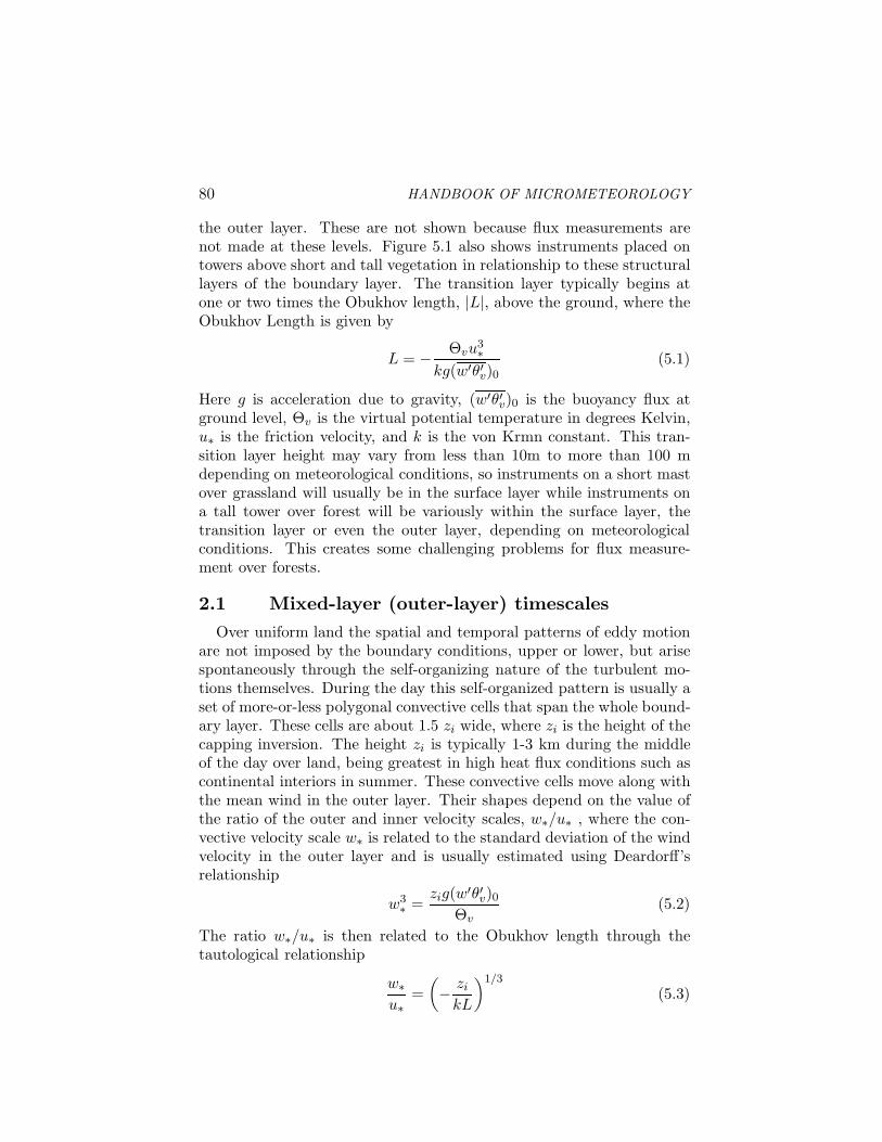
the outer layer. These are not shown because flux measurements arenot made at these levels. Figure 5.1 also shows instruments placed ontowers above short and tall vegetation in relationship to these structurallayers of the boundary layer. The transition layer typically begins atone or two times the Obukhov length, |L|, above the ground, where theObukhov Length is given by

L = − Θvu3∗

kg(w′θ′v)0(5.1)

Here g is acceleration due to gravity, (w′θ′v)0 is the buoyancy flux atground level, Θv is the virtual potential temperature in degrees Kelvin,u∗ is the friction velocity, and k is the von Krmn constant. This tran-sition layer height may vary from less than 10m to more than 100 mdepending on meteorological conditions, so instruments on a short mastover grassland will usually be in the surface layer while instruments ona tall tower over forest will be variously within the surface layer, thetransition layer or even the outer layer, depending on meteorologicalconditions. This creates some challenging problems for flux measure-ment over forests.

2.1 Mixed-layer (outer-layer) timescalesOver uniform land the spatial and temporal patterns of eddy motion

are not imposed by the boundary conditions, upper or lower, but arisespontaneously through the self-organizing nature of the turbulent mo-tions themselves. During the day this self-organized pattern is usually aset of more-or-less polygonal convective cells that span the whole bound-ary layer. These cells are about 1.5 zi wide, where zi is the height of thecapping inversion. The height zi is typically 1-3 km during the middleof the day over land, being greatest in high heat flux conditions such ascontinental interiors in summer. These convective cells move along withthe mean wind in the outer layer. Their shapes depend on the value ofthe ratio of the outer and inner velocity scales, w∗/u∗ , where the con-vective velocity scale w∗ is related to the standard deviation of the windvelocity in the outer layer and is usually estimated using Deardorff’srelationship

w3∗ =

zig(w′θ′v)0Θv

(5.2)

The ratio w∗/u∗ is then related to the Obukhov length through thetautological relationship

w∗u∗

=(− zi

kL

)1/3

(5.3)


When zi/|L| is larger than about 25, the cells form a polygonal patternwith no notable alignment. At smaller values of zi/|L|, when drag onthe ground is more important, the convective cells become elongatedin the direction of the wind and aligned, one with the next, so thatthey form elongated roll structures aligned with the wind. Water vaporcondensing in the updrafts of these structures can form cloud streets(Etling and Brown 1993). These streets, whether made visible by cloudsor not, are quasi-permanent in position and many kilometers long. Fixedsensors in the outer layer may then record steady updrafts (w > 0) orsteady downdrafts (w < 0) over long periods, with obvious consequencesfor the calculation of fluxes. Very often the decrease in zi/|L| reflectsan increases in |L|, so the surface layer grows in thickness to envelopefixed-height sensors above a forest. At zi/|L| ratios less than about5 the boundary layer becomes near-neutral, exhibiting no large-scaleconvective roll structures. We might observe that the combination ofdeeper surface and transition layers leaves no room for outer convectivestructures to develop in such situations.

An important characteristic of the main convective motions in theouter layer is that they carry most of the flux, with lesser amounts car-ried by the smaller eddies created by internal friction and breakdownof these larger eddies. An aircraft equipped with flux sensors must flythrough many tens of large eddies to sample the flux properly, so an ade-quate flight path would be of order 50 km long, more or less depending onprevailing conditions and the accuracy required. Flux sensors mountedon a fixed tower or suspended from a tethered balloon must sample asimilar number of eddies by waiting as they blow past the instruments,so the sample period should be many tens of times zi/Um, where Um

is the mean wind speed in the outer part of the boundary layer. Inlight winds, as often encountered in the tropics or in mid-latitude anti-cyclones, the convective structures may pass very slowly so that a goodsample is obtained only for times long compared with the evolutionarytime scale of the convection cells. Values for this evolutionary time scalehave not been reported, but they may depend strongly on any inhomo-geneities in roughness, surface heat flux or topography that might causeconvective cells to lock into fixed positions on the landscape. Even infavorable conditions it usually takes rather more than an hour to achievea good average in convective conditions, and much longer if the convec-tive cells are aligned with the wind in quasi-permanent rows or lockedonto the landscape. A non-zero mean for vertical velocity may persistfor hours. Kanda et al. (2004) use Large Eddy Simulation (LES) modelsto calculate errors likely to be found in instrumental measurements fromvery tall towers over uniform ground.


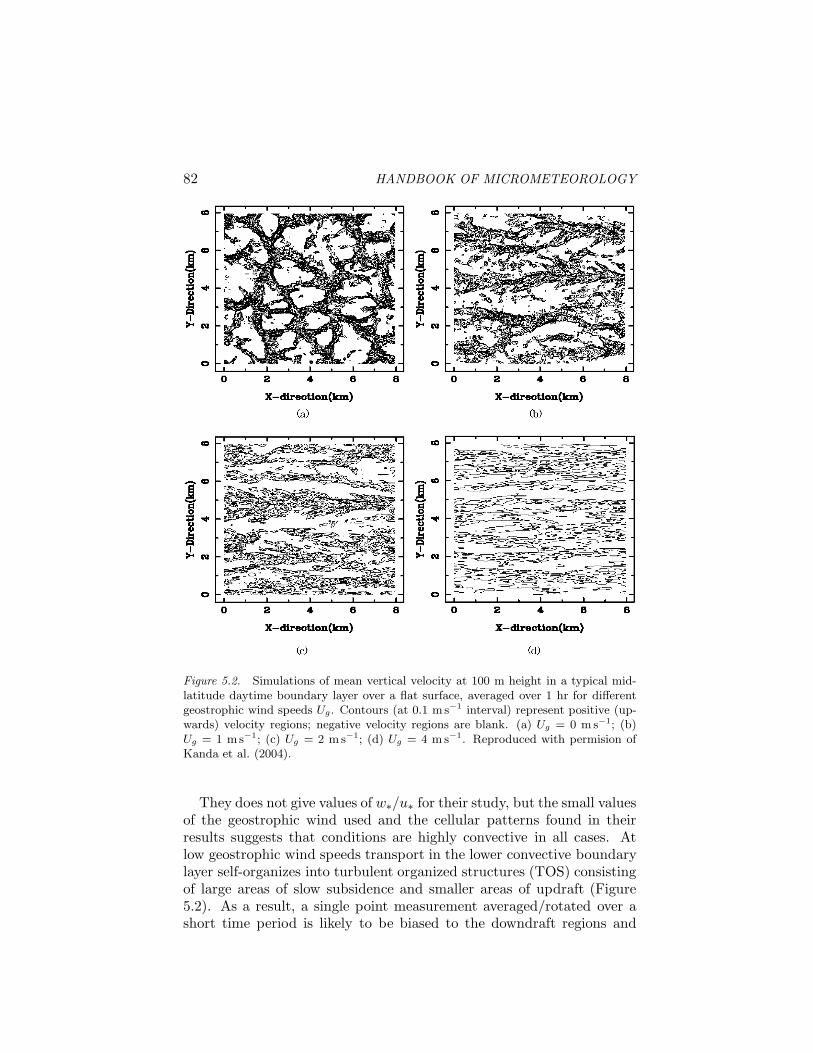
Figure 5.2. Simulations of mean vertical velocity at 100 m height in a typical mid-latitude daytime boundary layer over a flat surface, averaged over 1 hr for differentgeostrophic wind speeds Ug. Contours (at 0.1 m s−1 interval) represent positive (up-wards) velocity regions; negative velocity regions are blank. (a) Ug = 0 m s−1; (b)Ug = 1 ms−1; (c) Ug = 2 m s−1; (d) Ug = 4 m s−1. Reproduced with permision ofKanda et al. (2004).

They does not give values of w∗/u∗ for their study, but the small valuesof the geostrophic wind used and the cellular patterns found in theirresults suggests that conditions are highly convective in all cases. Atlow geostrophic wind speeds transport in the lower convective boundarylayer self-organizes into turbulent organized structures (TOS) consistingof large areas of slow subsidence and smaller areas of updraft (Figure5.2). As a result, a single point measurement averaged/rotated over ashort time period is likely to be biased to the downdraft regions and


Figure 5.3. The probability distribution of the “imbalance” of fluxes measured atany point in the simulation are shown in Figure ??a, for geostrophic wind speed Ug =0 m s−1, height z = 100 m. The two curves represent averaging periods of 1 and 3 hr.Measurements at any point are biased to underestimate surface fluxes. Increasing theaverage period reduces the systematic error in the “imbalance”, but broadens the dis-tribution and hence the random uncertainty in any single measurement. Reproducedwith permision of Kanda et al. (2004).

hence underestimate the local fluxes. Simulated observations at 100 mabove ground display vertical winds that do not average to zero overone-hour periods, with the net upwards or downwards flow typicallyaccounting for half the flux when u∗ = 0.14 m s−1. This “imbalance” isreduced with (i) increasing wind speed which decreases the cross-winddiameter of the TOS and increases the sampling track in any averagingperiod (e. g. at u∗ = 0.3 m s−1, mean flow accounts for about 10%of vertical scalar transport on average over the simulation domain, butwith values for particular points having a standard deviation of about20% about that mean); (ii) lower measurement height increasing theinfluence of shear turbulence. Hence measurement points located abovetall forests, and in particular in low-wind regions such as many tropicaland continental interior sites, are particularly likely to be prone to such ameasurement “imbalance”. In these conditions flux measurements fromsingle point measurements are inherently distorted (Figure 5.3).


2.2 Surface-layer (inner-layer) timescalesNear the ground the flux-carrying eddies have a rather different char-

acter, though what that character is has become the subject of debate.Here we base our discussion on the new model of McNaughton (2004b)in which the turbulence consists of large-scale wedge-like structures thatare aligned with the wind, along with the detached breakdown productsof these. The turbulence is again self-organizing, just like the cellularstructures in the outer layer, but here the preferred structures are up-scale cascades of TEAL (Theodorsen ejection amplifier-like) structures,which ‘compete’ for space so that only the best formed and most pow-erful continue on at each scale. This kind of turbulence is driven bythe shear, so its velocity scale is u∗. Though the value of u∗ changeswith stability it seems that the structure of the shear turbulence doesnot. This property is again like that of the turbulent outer layer wherethe velocity scale of the convective cells varies with stability while thepolygonal structure and the length scale of turbulence does not (at leastwhile w∗/u∗ and zi are held constant). This model is consistent with-indeed it is based on-the spectral observations from Kansas (Kaimal etal. 1972). It contradicts the basic hypothesis of Monin-Obukhov simi-larity on which much of our theory of the surface layer is built. Timewill judge whether the new model is successful, but for the moment itsimplifies our discussion by removing the need to consider the effectsof stability acting within the surface layer, at least when we know u∗directly. Turbulence in the surface layer scales simply on z and u∗.

To get a good sample of the dominant flux-carrying eddies, withwidths about 2z, we must allow a large number of them to pass ourfixed measuring position. A simple estimate is that this should be ahundred times z/u, which is a very few minutes in most cases. Expe-rience tells us that this is a considerable underestimate and there areseveral reasons for this. One is that the flux-carrying coherent struc-tures are not randomly dispersed, so our sample must take account ofthe scale of the aggregates (i. e. whole ramp structures) which are aboutten times longer than our estimate of about 2z (McNaughton 2004a).Another reason is that flux transport is affected by eddies of a greaterrange of sizes here than in the outer layer. In the outer layer there are noeddies much wider than 1.5zi, while in the surface there are eddies of allsizes, right up to those as tall as the surface layer itself, and all of thesetransport at least some momentum and scalars. Our averaging periodmust be long enough to sample not just the dominant eddies but all thesignificant flux-carrying eddies. As suitable averaging period must be at


least several tens of minutes long, perhaps even an hour long for goodresults.

Another factor is the modulating effects of the outer convection on theturbulence in the surface layer. The outer-layer convection constitutes avariable driving of the whole surface layer. A large-scale gust from theouter layer is equally a large cohort of TEAL structures moving alongwith enhanced speed and transmitting an enhanced momentum flux to-wards the ground. The direction, speed and power of the TEAL cascadeswithin the surface layer will therefore all vary with the wind at the topof the surface layer, as will the momentum flux to the ground. Observa-tions of momentum flux from a fixed tower will not represent area meansunless sampled on an outer time scale, not the inner one. We expect pooragreement in hourly observations of u∗ from towers spaced a few hun-dred meters apart in homogeneous terrain. The situation is easier for thescalar fluxes, most of which are more strongly controlled at source ratherthan by the varying wind overhead. For example, photosynthesis is con-trolled by radiation receipt and biochemical and physiological processeswithin the canopy, both of which are insensitive to wind speed. The fluxof water vapor is somewhat sensitive to wind speed, depending on thevalue of the decoupling parameter Ω calculated with values at referenceheight zs (Jarvis and McNaughton 1986), but only for wet canopies is itimportant. Averaging times for source-limited scalar fluxes depend littleon outer time scales. This difference accounts for the reported differentaveraging times required for momentum and scalars in the Kansas ex-periment (Wyngaard 1973). Wyngaard shows the variance of heat fluxmeasurements from one-hour runs to be about 8%, with only small de-pendence on instability (-z/L), while the sensitivity of momentum fluxranged from 10% to about 80% with a strong dependence on instability.Wyngaard used -z/L to measure instability while our discussion suggeststhat -zi/L should be used.

The layered structure discussed above is not relevant when the outerturbulence dies away at night. In the first part of the night we have,typically, a fully-turbulent state where the turbulence is similar thatin the daytime surface layer, but buoyancy now opposes these motionsand saps their energy. Momentum transfer then decreases progressivelythis kind of structure collapses altogether unless the flow is maintainedby strong pressure gradients or katabatic forcing. If not then a varietyof other phenomena may appear, some creating intermittency in theturbulence with time scales up to an hour or more. These processes arenot well described and are discussed in Chapters 9 and 8 of this book.For the weakly stable case flux sampling times can be a little shorterthan in the daytime surface layer.


The roughness sublayer is a subdivision of the surface layer and manyof the above comments apply equally to it. Near canopy top the tur-bulence has many of the characteristics of a mixing layer (Raupach etal. 1996), and the main eddies scale on the canopy dimensions (h − d),where h is tree height and d is the displacement height of the forest windprofile. This structure is not well known, but it is known that spectraand cospectra have more peaked shapes than the standard Kansas forms.Following the methods of McNaughton (2004a) we can therefore surmisethat tendency of these eddies to align into long wedge-like structures isless pronounced than in the surface layer. Good time samples shouldbe easier to obtain in the surface layer, but the length scale used tocalculate these is (h − d) rather than (z − d).

A theme running through the above comments is that eddy flux calcu-lations made on short data runs may not fairly represent true long-termaverages. This is so whether the flux itself varies on a rather long timescale, or whether the statistical sampling of the flux-carrying eddies isinsufficient. In the former case the actual local flux is a poor sample ofthe required area average flux; this cannot be remedied by any analysisbased solely on the data from that interval. In the latter case the localflux during the measurement interval is not in question, but some of thelarger eddies carrying it have been poorly sampled.

3 Empirical evidence of low frequency fluxtransport

3.1 Wavelet spectral analyses of turbulent fluxesin Scotland and Amazonia

To demonstrate the variable contribution of processes occurring ondifferent scales to the surface layer fluxes, in this study we apply a Haarwavelet transform on the turbulent signals measured at two differentsites: a rain forest in south west Amazonia (Rebio Jaru; Von Randowet al. 2002) and a sitka spruce coniferous forest in Scotland (Griffin;Chapter 4). The wavelet transform (WT) is a powerful mathematicalanalysis tool, which permits an evolutionary spectral study of turbulentatmospheric signals (Daubechies 1998; Farge 1992). The wavelet analy-ses were done following a similar methodology as Katul and Parlange(1994) and Von Randow et al. (2002).

After application of the Haar wavelet to the data from the two sites,the scale covariances of vertical wind velocity and scalars were calcu-lated and the partial contribution of each scale to the total covariancewas determined at each record. The results are presented in Figure 5.4(daytime) and Figure 5.5 (nighttime). The x-axes represent the spatial


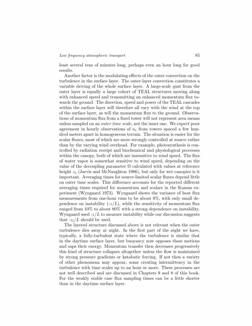
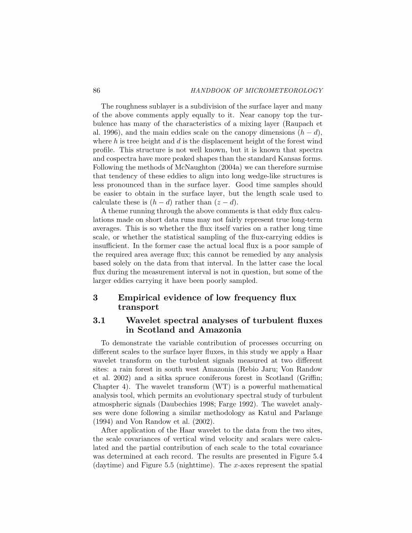
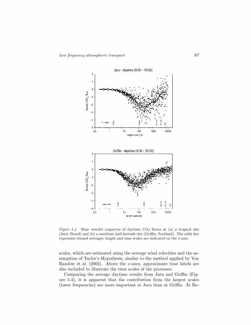
Figure 5.4. Haar wavelet cospectra of daytime CO2 fluxes at (a) a tropical site(Jaru, Brazil) and (b) a maritime mid-latitude site (Griffin, Scotland). The solid linerepresents binned averages; length and time scales are indicated on the x-axis.

scales, which are estimated using the average wind velocities and the as-sumption of Taylor’s Hypothesis, similar to the method applied by VonRandow et al. (2002). Above the x-axes, approximate time labels arealso included to illustrate the time scales of the processes.

Comparing the average daytime results from Jaru and Griffin (Fig-ure 5.4), it is apparent that the contribution from the largest scales(lower frequencies) are more important at Jaru than at Griffin. At Re-


Figure 5.5. Haar wavelet cospectra of nighttime CO2 fluxes at (a) a tropical site(Jaru, Brazil) and (b) a maritime mid-latitude site (Griffin, Scotland). The solid linerepresents binned averages; length and time scales are indicated on the x-axis.

bio Jaru, the peak of contribution to the covariances happens on scalesof 100-500 m (that correspond approximately to scales of 1 to 5 min),while at Griffin scales less that 100 m (usually corresponding to scalesof less than 1 min) dominate the transport of carbon dioxide. One othernoticeable difference between the two sites is that at Jaru the variationfrom the average scale dependence is higher, especially at longer scales(low frequencies). On scales longer than 1 km, the low frequency mo-


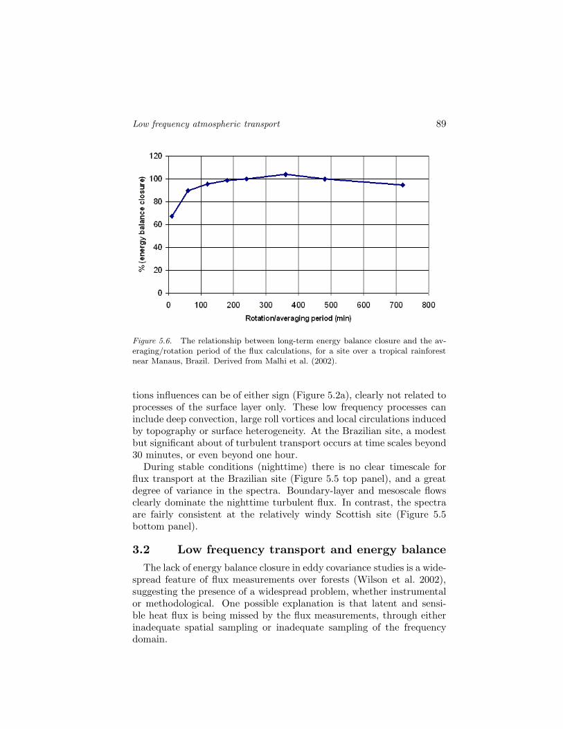
Figure 5.6. The relationship between long-term energy balance closure and the av-eraging/rotation period of the flux calculations, for a site over a tropical rainforestnear Manaus, Brazil. Derived from Malhi et al. (2002).

tions influences can be of either sign (Figure 5.2a), clearly not related toprocesses of the surface layer only. These low frequency processes caninclude deep convection, large roll vortices and local circulations inducedby topography or surface heterogeneity. At the Brazilian site, a modestbut significant about of turbulent transport occurs at time scales beyond30 minutes, or even beyond one hour.

During stable conditions (nighttime) there is no clear timescale forflux transport at the Brazilian site (Figure 5.5 top panel), and a greatdegree of variance in the spectra. Boundary-layer and mesoscale flowsclearly dominate the nighttime turbulent flux. In contrast, the spectraare fairly consistent at the relatively windy Scottish site (Figure 5.5bottom panel).

3.2 Low frequency transport and energy balanceThe lack of energy balance closure in eddy covariance studies is a wide-

spread feature of flux measurements over forests (Wilson et al. 2002),suggesting the presence of a widespread problem, whether instrumentalor methodological. One possible explanation is that latent and sensi-ble heat flux is being missed by the flux measurements, through eitherinadequate spatial sampling or inadequate sampling of the frequencydomain.


Malhi et al. (2002) explored this phenomenon for flux measurementsabove a forest near Manaus in central Amazonia (Figure 5.6). Theyfound that extending the rotation/averaging period of the measurementsfrom 1 hr up to 4 hr improved the energy balance closure to about 100%;increasing the rotation/averaging period further resulting in no furtherincrease in mean fluxes, although variance increased substantially. Thisresult suggests that, for some sites at least, low frequency transport may“solve” the energy balance problem, for ensemble-averaged data at least.The general applicability of this approach remains uncertain, however, asKruijt (pers comm.) and Malhi and Iwata (unpublished data) find thatthe low frequency component at other sites is not sufficient to accountfor all the “missing” flux.

To summarize this section, there is evidence of significant flux trans-port at low frequencies at some measurement sites; in particular sitesin the tropics with tall measurement towers, low mean wind speeds anddeep convective boundary layers. In the next section we examine howundersampling these low frequency fluxes using standard eddy covari-ance analysis can affect measured fluxes.

4 What effect do standard flux calculations haveon low frequency flux terms?

In this section we explore the effect that the coordinate rotation usedin eddy covariance analyses has on calculated fluxes. Finnigan et al.(2003) recently presented a revision of the theory of measurement ofturbulent fluxes in terms of mass balance equations. First they consid-ered an idealized case, where the long-term ensemble-averaged flow ishorizontally homogeneous, the mean wind vector is always confined tothe x − z plane, so that v = 0 and only the inclination of the velocityvector, α = tan−1(w/u) changes from period to period. To transformthe long-term vertical covariance wcLT in any period to short-term ‘ro-tated every period’ coordinates in which w = 0, coordinates are rotatedthrough an angle α given by,

α = tan−1 w ′

< u > +u ′ (5.4)

where <> is the ensemble mean over all periods, w ′ = w− < w >, andu ′ = u− < u >.

Hence, the horizontal and vertical components of the long-term, ensemble-averaged flux vector, denoted by subscript LT , can be expressed in termsof components, denoted by subscript, R, in the ‘rotated-every-period’


coordinate frame as (Finnigan et al. 2003, equation 26)

(uc)R = (uc)LT cos α − (wc)LT sinα

(wc)R = (wc)LT cosα + (uc)LT sinα (5.5)

Even in horizontally homogeneous terrain, the flow field is only hor-izontally homogeneous when averaged over a period much longer thanthat of any significant temporal perturbation to the flow. When theduration of an individual averaging period, T , is comparable to thatof significant atmospheric motions, then in any one period, horizontalflux divergence may be important. Many periods must be averaged toensure the canceling out of transient vertical advection events that in re-ality contribute nothing to the vertical flux because they merely balancesimultaneous but unmeasured transient horizontal advection events. Toensure this averaging is done rigorously, mass balances over any timeperiod must be calculated in a single coordinate system that applies tothe entire period.

What is the precise effect of rotating the vector basis so that w isforced to zero in each period? In particular, what is the effect on themeasured covariance in any one averaging period of rotating coordinatesso that v = w = 0? Dividing the signals into a set of periods of lengthT , block averaging in each period and then subtracting the block averagedvalues w and c is equivalent to high-pass filtering the signal with a boxcarfilter function of width T . This is precisely what is achieved when werotate coordinates each period so that w is forced to zero. In effectwe have thrown away the part of the covariance carried by motions offrequency lower than the (rather leaky) cut-off frequency of the boxcarfilter function.

However, in addition, the coordinate rotation itself distorts the co-variance carried by frequencies higher than the boxcar cut-off by foldinginto (wc)R some of the streamwise and lateral fluxes (wc)LT and (vc)LT ,as we have shown in Equation 5.5 for the case where the low frequencyflow is confined to the x − z plane. A simple algebraic example of thedistortion to be expected is presented in Appendix 2 of Finnigan et al.(2003).

In summary, rotating coordinates every period effectively high-passfilters the signal so that contributions to the covariance from atmosphericmotions of period longer than T are lost but the rotation itself folds someof the (wc)LT and (vc)LT flux into (w′c′)R in an essentially unpredictableway.


5 ComplicationsThe energy balance closure in Figure 5.6 suggests that in some sites

consideration of low frequency transport can improve the flux measure-ments to the point of full energy balance closure. If this were a generalprinciple that could be applied to all sites, then it would appear that theproblem of poor energy balance closure at eddy covariance sites wouldhave been “solved”. However, there are good grounds for skepticismabout the wider applicability of this result.

The problem revolves around whether these low frequency fluxes are“locally meaningful” or represent features of the wider landscape thatare not related to the local surface. Kanda et al. (2004) demonstrated intheir LES model simulation that, although the systematic bias decreasedwhen turbulent fluxes are averaged over longer time periods, the varianceincreases greatly (Figure 5.3). Hence any single measurement period isvulnerable to random advective fluxes, and becomes increasingly difficultto interpret in terms of local surface fluxes.

Another problem arises in complex terrain, or in the presence of fixedpressure fields caused by local inhomogeneities (e. g. land-water inter-faces, or crop-forest mosaics). In this situation, a variation in winddirection can result in a low frequency covariance that has nothing to dowith flux transport (Finnigan et al. 2003). Interestingly, Kanda et al.(2004) showed that moderate inhomogeneity (ca 5%) can actually reducebias by dampening the self-organization of TOS, but greater degrees ofinhomogeneity generate local circulations and enhance the bias.

6 ConclusionsIt is important to consider transport at time scales up to at least

10zi/Um, where Um is the mean wind speed in the outer part of theboundary layer. This corresponds to length scales of about 10-50 km)but in complex topography or variable landscapes, it is tricky to disen-tangle what we want (low frequency CBL turbulent transport) from whatwe do not want (wind direction covariance). There is clearly transportof flux at these low frequencies which can explain the failure of eddy co-variance systems to fully capture fluxes. However, separating the locallymeaningful fluxes from wider-scale advection may prove a challenge.

7 ReferencesDaubechies, I.: 1998, ‘Recent results in wavelet applications’, J. Electronic Imaging,

7, 719-724.

Etling, D., Brown, R. A.: 1993, ‘Roll vortices in the planetary boundary layer: areview’, Bound.-Layer Meteor., 65, 215-248.


Farge, M.: 1992, ‘Wavelet transforms and their applications to turbulence’, AnnualRev. Fluid Mech., 24, 395-457.

Finnigan, J., Clement, R., Malhi, Y., Leuning, R., Cleugh, H. A.: 2003, ‘A re-evaluation of long-term flux measurement techniques. Part I: Averaging andcoordinate rotation’, Bound.-Layer Meteorol., 107, 1-48, 2003.

Garratt, J. R.: 1992, The Atmospheric Boundary Layer. Cambridge UniversityPress, Cambridge, 316 pp.

Jarvis, P. G., McNaughton, K. G.: 1986, ‘Stomatal control of transpiration: scalingup from leaf to region’, Adv. Ecol. Res., 15, 1-49.

Kaimal, J. C., Wyngaard, J. C., Izumi, Y., Cote, O. R.: 1972, ‘Spectral character-istics of surface-layer turbulence’, Quart. J. R. Meteorol. Soc., 98, 563-589.

Kanda, M. Inagaki, A., Letzel, M. O., Raasch, S., Watanabe, T.: 2004, ‘LES studyof the energy imbalance problem with eddy covariance fluxes’, Bound.-LayerMeteorol., 110, 381-404.

Katul, G. G., Parlange, M., B.: 1994, ‘On the active role of temperature in surface-layer turbulence’, J. Atmos. Sci., 51, 2181-2195.

Mahrt, L.: 1998a, ‘Surface fluxes and boundary layer structure’, In: (Eds.) Holtslag,AAM, Duynkerke, PG, Clear and Cloudy Boundary Layers, Royal NetherlandsAcademy of Arts and Sciences, Amsterdam, 113-128.

Mahrt, L.: 1998b, ‘Flux sampling errors for aircraft and towers’, J. Atmos. OceanicTech., 15, 416-429.

Malhi, Y., Pegoraro, E., Nobre, A. D., Pereira, M. G. P., Grace, J., Culf, A. D.,Clement, R.: 2002, ‘Energy and water dynamics of a central Amazonian rainforest’, J. Geophys. Res., 107, Art. No. 8061.

McNaughton, K. G.: 2004a, ‘Attached eddies and production spectra in the at-mospheric logarithmic layer’, Bound.-Layer Meteor., 111, 1-18.

McNaughton, K. G.: 2004b, ‘Turbulence structure of the unstable atmospheric sur-face layer and transition to the outer layer’, Bound.-Layer Meteor. (In press)

Raupach, M. R., Finnigan, J. J., and Brunet, Y.: 1996, ‘Coherent eddies and tur-bulence in vegetation: the mixing layer analogy’, Bound.-Layer Meteor. 78,351-382.

Sakai, R. K., Fitzjarrald, D. R., Moore, K. E.: 2001, ‘Importance of low-frequencycontributions to eddy fluxes observed over rough surfaces’, J. Appl. Meteorol.,40, 2178-2192.

Von Randow, C., Sa, L. D. A., Gannabathula, P. S. S. D., Manzi, A. O., Arlino, P.R. A., Kruijt, B.: 2002, ‘Scale variability of atmospheric surface layer fluxes ofenergy and carbon over a tropical rain forest in southwest Amazonia. I. Diurnalconditions’, J. Geophys. Res., 107, 8062, doi:10.1029/2001JD000379.

Wilson, K., Goldstein, A., Falge, E., Aubinet, M., Baldocchi, D., Berbigier, P.,Bernhofer, C., Ceulemans, R., Dolman, H., Field, C., Grelle, A., Ibrom, A.,Law, B. E., Kowalski, A., Meyers, T., Moncrieff, J., Monson, R., Oechel,W., Tenhunen, J., Valentini, R., Verma, S.: 2002, ‘Energy balance closure atFLUXNET sites’, Agric. For. Meteorol., 113, 223-243.

Wyngaard, J. C.: 1973, ‘On surface-layer turbulence’, In: (Ed.) Haugen, DA,Workshop on Micrometeorology, American Meteorological Society, 101-149.

Low frequency atmospheric transport and surface flux measurements

Documents

Transcript of Low frequency atmospheric transport and surface flux measurements