Application of the band-pass covariance technique to

portable flux measurements over the Tibetan Plateau

Jun Asanuma,1,2 Hirohiko Ishikawa,3 Ichiro Tamagawa,4 Yaoming Ma,5

Taiichi Hayashi,3 Yongqiang Qi,6,7 and Jiemin Wang8

Received 8 January 2005; revised 25 April 2005; accepted 15 June 2005; published 10 September 2005.

[1] Two versions of the band-pass covariance technique were applied to the turbulencedata collected during daytime with a simple and portable measurement system overthe sparse grasslands of the Tibetan Plateau. The coherency spectra between thetemperature and the specific humidity, which is a spectral counterpart of the correlationcoefficient, were used as a dynamic indicator of the energy-containing ranges as well asthat of the sensor attenuation at higher frequencies. The comparison with independentmeasurements by the eddy covariance method showed that the original version of theband-pass covariance technique occasionally fails. This indicates breakdowns of thesimilarity between the temperature and the water vapor, especially in the lowest-frequencyregions. On the other hand, the latent heat flux computed with the advanced versionexhibited adequate agreement with the eddy covariance method. This paper demonstratesthat the current implementation of the advanced version with the embedded self-calibration procedure provides a robust method of frequency extrapolation in scalar fluxmeasurements under unstable conditions.

Citation: Asanuma, J., H. Ishikawa, I. Tamagawa, Y. Ma, T. Hayashi, Y. Qi, and J. Wang (2005), Application of the band-pass

covariance technique to portable flux measurements over the Tibetan Plateau, Water Resour. Res., 41, W09407,

doi:10.1029/2005WR003954.

1. Introduction

[2] Sensors of humidity that are not capable of fullycapturing turbulence fluctuations of water vapor, neverthe-less, can be used for the measurements of the latent heatflux from the Earth’s surface. One possibility is throughthe band-pass covariance technique, or the band-passcovariance method, independently proposed or suggestedby Hicks and McMillen [1988] and Hogstrom et al. [1989].This technique is primarily a spectral extrapolation accom-panied by the eddy covariance technique, and calculates thehigher-frequency component of a scalar flux in question thatwas lost due to the inadequate sensor response. This is donewith a guide of a perfectly measured scalar, usually thesonic temperature. This technique facilitates measurementsof a scalar flux using a portable instrumentation [see, e.g.,Horst and Oncley, 1995; Horst et al., 1997] and a long-termmonitoring of a scalar flux [Watanabe et al., 2000; Yasudaand Watanabe, 2001].

[3] One of the important advantages of the band-passcovariance technique is that, unlike the other flux correctionmethods [e.g., Moore, 1986; see also, Massman and Lee,2002], it does not require a predetermined frequency re-sponse function of the sensor, nor does it necessitateassuming a functional form of the flux cospectra. As it isshown in this paper, however, there has been an ambiguityleft with the band-pass covariance technique and an expla-nation based on an existing theory or an empirical relation-ship is desired. Surely, this has been a factor that hasprevented its potentially wider application, despite strongpotential capability of the band-pass covariance technique.[4] The aims of this study are to investigate the band-pass

covariance technique from the view point of the surfacelayer similarity. Particularly, the similarity theory for thetwo-point statistics in the unstable atmospheric surface layer(ASL) proposed by Kader and Yaglom [1991] will be usedin an effort to give a clear explanation of its physical basisto the technique. Throughout this process, it will be shownthat this technique has, in fact, two different versions, eachwith a different physical background. A plain distinctionbetween these two versions will be made in this paper. Thisdocument, then, proposes an improved algorithm for thetechnique using the coherency spectra as an indicator of thesimilarity between the sonic temperature and the watervapor. The band-pass covariance technique with the newlyproposed scheme is applied to the latent heat flux measure-ments obtained over the sparse grasslands of the TibetanPlateau using a portable flux measurement system calledmobile turbulence measurement system (MTMS). Thereany laboratory calibration results were not expected to beapplicable, and any kind of in situ calibration was virtuallyimpossible. This is the most challenging of the flux mea-

1Nicholas School of the Environment and Earth Sciences, DukeUniversity, Durham, North Carolina, USA.

2On leave from Terrestrial Environment Research Center, TsukubaUniversity, Tsukuba, Japan.

3Disaster Prevention Research Institute, Kyoto, Japan.4River Basin Research Center, Gifu University, Gifu, Japan.5Institute of Tibetan Plateau Research, Chinese Academy of Sciences,

Beijing, China.6Department of Information Science, Kochi University, Kochi, Japan.7Now at China Patent Agent (H.K.) Ltd., Beijing, China.8Cold and Arid Regions Environmental and Engineering Research

Institute, Chinese Academy of Sciences, Lanzhou, China.

Copyright 2005 by the American Geophysical Union.0043-1397/05/2005WR003954

W09407

WATER RESOURCES RESEARCH, VOL. 41, W09407, doi:10.1029/2005WR003954, 2005

1 of 10

surements. Therefore this paper, without using any addi-tional information other than the measured turbulence dataitself, fully utilizes and qualifies the capability of the band-pass covariance technique.

2. Band-Pass Covariance Technique

[5] Here, two major versions of the band-pass covariancetechnique are introduced. For the sake of generality, they arewritten in terms of a scalar, s. Their application to latent heatflux, E = rLew0q0, or the flux of carbon dioxide, Fc = rw0c0,can be readily derived by substituting s with either specifichumidity, q, or carbon dioxide concentration, c, where r isthe air density, and Le the heat of vaporization.

2.1. Extension of Monin-Obukhov Similarityto Cospectra

[6] Cospectra between the vertical velocity componentand the scalar are a projection of the vertical transport of s tothe Fourier domain. Its integration over the entire frequencydomain is the covariance between them.

w0s0 ¼Z 1

0

Sws nð Þdn ð1Þ

where Sws(n) represents the cospectra, z the height above thedisplacement height, u the mean velocity, and n = fz/u thenormalized frequency, in which f is the cyclic frequency.Taylor’s hypothesis is used to normalize the frequency andother ordinary mathematical notations in the surfacehydrology are used in this paper.[7] In a steady and horizontally homogeneous ASL,

Sws(n) can be written by extending Monin-Obukhov simi-larity (MOS) to the Fourier domain, as follows [e.g.,Wyngaard and Cote, 1972; Kader and Yaglom, 1991]

Sws nð Þ= u*js*j� �

¼ Fs n; zð Þ ð2Þ

where u*is the friction velocity, s

*� �w0s0/u

*the scale of

s, Fs the universal function of n and z � z/L, in which L isthe Obukhov length. Within the context of MOS, thesimilarity between scalars, or shortly the scalar similarity, isdefined as an universality of dimensionless moments,independent of the choice of scalars [Hill, 1989; Dias andBrutsaert, 1996]. If this concept can be extended to beapplied to the cospectra, it is assumed that Fs is universal,i.e., independent of the choice of s. This is written for thetemperature, T, and a scalar, s, as follows

FT n; zð Þ ¼ Fs n; zð Þ ð3Þ

A considerable number of experimental evidences for eq. (3)have been presented using themeasurements in ASL [Schmittet al., 1979; Anderson and Verma, 1985; Ohtaki, 1985].[8] Plugging (2) into (3) gives the following relationship,

b nð Þ � SwT nð ÞSws nð Þ ¼ w0T 0

w0s0: ð4Þ

Integrating (4) over a frequency range, X, gives the firstversion of the band-pass covariance technique as follows

w0s0 ¼

ZX

Sws nð ÞdnZX

SwT nð Þdnw0T 0: ð5Þ

Equation (5) can be taken as a spectral extension of theBowen ratio method, and gives an estimate of w0s0 from w0T 0

and the ratio of the cospectra in a limited frequency band.This is a core concept of the original band-pass covariancetechnique proposed by Hicks and McMillen [1988] that waslater also used by Verma et al. [1992] for methane fluxmeasurements. Equation (5) has been used often in themeasurements of trace gases fluxes, such as, ozone [Jacobet al., 1992], carbon dioxide and methane [Fan et al., 1992]and isoprene [Guenther and Hills, 1998] among others.[9] Another application of (5) can also be found in the

measurements of surface heat fluxes [Blanken et al., 1997;Twine et al., 2000], when the eddy covariance measure-ments of the sensible heat flux and the latent heat flux,denoted as HEC and EEC, do not close the surface energybudget equation. In such circumstances, a new value ofH andE that satisfies the energy budget equation is often computedusing the Bowen ratio of the measured fluxes, Bo =HEC/EEC,and the measurements of the other energy budget compo-nents. This procedure implicitly assumes that measurementsof HEC and EEC both suffer from the same spectral attenua-tion, and that their ratio, HEC/EEC, is equal to the actualvalue. Henceforth, this can be considered as an implicitapplication of the original band-pass covariance technique,i.e., equation (5).[10] In should be noted that these practical applications of

(5), whether explicit or implicit, are usually utilized only fora rough estimate of the flux values, while, in some cases,they are used in seeking more accurate estimates of fluxes.

2.2. Advanced Version of Band-PassCovariance Technique

[11] Another, and more advanced, version of the band-pass covariance technique has been suggested independentlyby Hogstrom et al. [1989]. They tried to make a practicalestimate of lost covariance in w0q0 with q measured with wetbulb thermometer over a sparse pine forest. They observedthat the ratio of the cospectra, SwT(n)/Swq(n), remained at aconstant value over a middle frequency range. Then, theyassumed this to be also constant at the higher frequencieswhere true fluctuations of q were not available due to thesensor attenuation. With this assumption, they made a roughestimate of underestimation in w0q0. The same procedure wasalso applied in CO2 flux measurements by Grelle andLindroth [1996].[12] Although the initial intention of Hogstrom et al.

[1989] appears to be limited to a rough estimate designatedto meet practical necessity, their procedure can be used toformulate the advanced version of the band-pass covariancetechnique for the flux of the scalar, s, in general. First, it isassumed that the following equation is valid over a certainfrequency range.

b nð Þ ¼ b0 ¼ const:ð Þ for n1 < n < 1 ð6Þ

where n1 is the lower end of the frequency range, in which(6) is valid, and b0 is the value of the constant of b(n). Withthis assumption, w0s0 can be computed as follows [Yasudaand Watanabe, 2001].

w0s0 ¼Z n2

0

Sws nð Þdnþ 1

b0

Z 1

n2

SwT nð Þdn ð7Þ

2 of 10

W09407 ASANUMA ET AL.: BAND-PASS COVARIANCE TECHNIQUE W09407

where n2 is the upper end of the frequency range in whichunattenuated measurements of Sws(n) are available. Inpractice, b0 can be determined as an average of b(n) overthe frequency range, n1 < n < n2.[13] Equation (7) forms the advanced version of the band-

pass covariance technique. It was used by Horst and Oncley[1995] and Horst et al. [1997] in their algorithm for NCAR(National Center for Atmospheric Research) PAM (PortableAutomated Mesonet) III to compute latent heat flux. Morerecently, Watanabe et al. [2000] utilized (7) with watervapor flux measurements over a deciduous forest where qwas measured by a capacitance hygrometer. They comparedthe results with the eddy covariance measurement and foundan overall satisfying performance of (7), except when w0T 0

was small. Yasuda and Watanabe [2001] applied (7) to CO2

flux measurements with closed path infrared gas analyzerand obtained an adequate comparison with open pathmeasurements.[14] A basic assumption which allows (7) to compute w0s0

is that (6) is valid over a frequency range, n1 < n < 1. Thishas been observed by some investigators: As describedabove, Hogstrom et al. [1989, Table 1] found that b(n)remained at constant values from around the energy-containing range up to the frequency at which the cospectradrops off due to the slow q sensor. Watanabe et al. [2000,Figure 2] also observed that SwT(n)/Swq(n) was roughlyconstant at the ratio, w0T 0/w0q0, around the energy-containingrange.[15] Equation (6) can be derived by extending a surface

similarity argument of Kader and Yaglom [1991], whoapplied the directional similarity of Kader and Yaglom[1990] to spectra and cospectra of the velocity componentsand the temperature in the unstable ASL. The directionalsimilarity assumes that there exist three sublayers in theunstable ASL, namely, (1) the dynamic sublayer (D sub-layer, z �0.04) where the buoyancy does not affect theturbulence field, (2) the dynamic-convective sublayer (DCsublayer, �1.2 ] z ] �0.12) where both the buoyancy andthe shear stress affect the turbulence but in the differentdirections, causing the vertical and horizontal motionsuncoupled with each other, and (3) the convective sublayer(C sublayer, z ] �2) where the shear stress does not play animportant role in generating turbulence. Kader and Yaglom[1991] applied this three-layered structure of ASL tocospectra and spectra and predicted their formulation as afunction of z and n. One of the most notable predictions oftheir results is �1 power decay of the longitudinal velocityspectra in the energy-containing range, and this receivesgrowing attention in the micrometeorological community[see, e.g., Katul and Chu, 1998; McNaughton and Laubach,2000; Hogstrom et al., 2002].[16] The theory for cospectra, SwT(n), by Kader and

Yaglom [1991] can be extended to any scalar, s. In theinertial range (1 ] n ] z/h, where h is Kolmogorov’smicroscale), Kader and Yaglom [1991] invoked �7/3 powerdecay of the cospectra, first suggested by Lumley [1964,1967] and later validated with the ASL data for SwT(n) [e.g.,Kaimal et al., 1972; Wyngaard and Cote, 1972; Katul etal., 1998, 2001; Su et al., 2004] and for Swq(n) and Swc(n)[e.g., Ohtaki, 1985; Anderson and Verma, 1985; Katul etal., 1998, 2001]. See also Warhaft [2000] for recent devel-opments. With Sws(n) n�7/3 and the aforementioned

stability requirements for each of the three sublayers, Kaderand Yaglom [1991] gave predictions of SwT(n), which can berewritten for Sws(n) in general, as follows

Sws nð Þu*js*j

¼

C 1ð Þs � n�7

3 for D sublayerð Þ

f 2ð Þs zð Þ � n�7

3 for DC sublayerð Þ

C 3ð Þs � n�7

3 for C sublayerð Þ

8>>>><>>>>:

ð8Þ

where Cs(1) and Cs

(3) are constants to be determinedexperimentally, and fs

(2)(z) the dimensionless function of z.[17] In the energy-containing range (n < 1), according to

Kader and Yaglom [1991], z is no longer a relevantparameter for the turbulent statistics, and Sws(n) is propor-tional to n�1. With this assumption and the aforementionedthree sublayer structure, Sws(n) is predicted as follows

Sws nð Þu*js*j

¼

D 1ð Þs � n�1 for D sublayerð Þ

D 2ð Þs � n�1 for DC sublayerð Þ

D 3ð Þs � n�1 for C sublayerð Þ

8>>>><>>>>:

ð9Þ

where Ds(1), Ds

(2) and Ds(3) are constants that can be

determined experimentally. Decay with n�1 of thesecospectra was also observed by Katul et al. [1998].[18] Equations (8) and (9) readily yield a simple expres-

sion for b(n) in the inertial and the energy-containing rangesas follows.

b nð Þ s*=T*���

��� ¼fb zð Þ for DC sublayer in the inertial rangeð Þ

const: otherwiseð Þ

8<:

ð10Þ

where fb(z) � fT(z)/fs(z) is a function of z, and the value ofthe constant in the second expression can vary in differentsublayers and in different frequency ranges (the inertial orthe energy-containing range). In each realization of b(n),fb(z) is constant, and therefore equation (10) states thatb(n), as a function of n, takes a constant value in the energy-containing and the inertial ranges, irrespective of thestability. Since these two frequency ranges are almostcontiguous to each other [Kader and Yaglom, 1991], it canbe postulated that b(n) is a constant between the energy-containing and the dissipation frequencies in all stabilityclasses.[19] It should be noted that any form of the scalar

similarity between T and s defined above as the equityof the dimensionless function, was not assumed in thederivation of (10). In fact, if the scalar similarity betweenT and s had been assumed, then all of the constants and thefunctions were identical for T and s, i.e., CT

(i) = Cs(i) (for i = 1,

3), DT(i) = Ds

(i) (for i = 1, 2, 3), and fT(2)(z) = fs

(2)(z), assuggested by Hill [1989]. This would lead to b(n)js*/T*j = 1,that is equivalent to (4). This is not meant in (10) where thevalue of the constancy is left unspecified. The only assump-tion that leads to (10) is that both T and s follow thesimilarity arguments that result in (8) and (9), that is n�7/3

and n�1 dependence of the cospectra, respectively. Decay of

W09407 ASANUMA ET AL.: BAND-PASS COVARIANCE TECHNIQUE

3 of 10

W09407

Sws(n) with n�7/3 in the inertial range can be derived from adimensional argument where Sws(n) is a function of �, n, @s/@z [Lumley, 1967; Wyngaard and Cote, 1972], in which � isthe average dissipation rate of the turbulent kinetic energy.In the energy containing range, a hypothesis that z is not arelevant parameter leads to its proportionality to n�1.Therefore (10) is a consequence of the fact that the both Tand s fluctuations share the same flow characteristicsbetween the production and the dissipation frequencies.[20] It has been shown in this section that the band-pass

covariance technique, in fact, points to the two different fluxcalculation methods, and that they have different physicalbases. The original version formulated as (5) requires that Tand s be similar at all frequencies. This is the Fourierversion of the scalar similarity compliant to MOS. On theother hand, the advanced version, (7), requires that the ratioof the cospectra, b(n), should be constant in the higher-frequency range. This is most likely valid between theproduction and the dissipation frequencies, where well-defined dynamic forcing on the scalar field exists. It isapparent that the former is more strict than the latter. If (7)fails, (5) should also fail, while (7) works even if (5) fails.

3. Mobile Turbulence Measurements OverTibetan Plateau

[21] The data subject to analyses in this study werecollected with MTMS during GAME-Tibet (GEWEX AsiaMonsoon Experiment-Tibet) IOP (Intensive ObservationPeriod) in the summer of 1998. GAME-Tibet is one ofthe regional subprograms of the GAME, and the mainobjective of GAME-Tibet is the better understanding ofthe energy and water cycle over the Tibetan Plateau. Tofulfill this objective, spatially distributed time series ofhydrological and meteorological data were acquired duringits IOP in the region of approximately 150 km � 150 km inthe central Tibetan Plateau. Among all ground-based mea-surements, several measurement systems were used tohighlight the spatial distribution of surface energy compo-nents along the north-south cross section of the centralTibetan Plateau. These measurement systems include twotower-based eddy covariance (EC) systems, two PAM IIIsystems, four AWS (Automated Weather Stations) systems,and MTMS. Those except for MTMS are site-fixed mea-surements placed along the Qinghai-Xizang highway.Several publications have already reported these measure-ment systems and some results from them. These includethose by Tanaka et al. [2001, 2003], Ma et al. [2003], Choiet al. [2004], and Yang et al. [2004].

[22] The roles of MTMS during GAME-Tibet IOP areclosely related to the other flux measurement systems. ECand PAMIII are designed to provide independent measure-ments of the surface energy components. AWS’s measuredT, q, and wind speed at a single level, and the surfaceradiative temperature. Therefore, in order to compute sur-face fluxes out of the data of AWSs, surface roughness forwind speed and temperature need to be determined. MTMSwas planned to provide flux data to calculate these param-eters. Another major role of MTMS is to provide referenceflux data for the cross comparison of the other tower-basedsurface flux measurements. The flux measurement systemsused in GAME-Tibet ’98 IOP were composed of differentsensors and were based on different measurement tech-niques. Therefore a cross comparison between thesesystems is essential to derive spatial distribution of thesurface energy components out of their measurements. Forthis cross comparison, rather than gathering all of themeasurement systems at one place, a method with a portableflux measurement system was adopted in GAME-Tibet. If asingle flux measurement system can collect flux data atall of the flux sites, site-to-site comparisons of the fluxmeasurements are possible using this system as a reference.The second role of MTMS is to serve as a reference for thisindirect cross comparison.[23] MTMS was designated specifically to perform these

two roles over the Tibetan Plateau. It was designed andassembled at the Disaster Prevention Research Institute ofKyoto University. Sensors used in MTMS are tabulated inTable 1. Of them all, the two capacitance-type hygrometers,namely, HumAir (AIR Inc.) and Humicap (Vaisala Inc.),give measurements of specific humidity, q, at a relativelyslower response. Hereafter, subscripts HA and HC, are usedto represent HumAir and Humicap, respectively, when theorigins of the measurements need to be specified. Sincethese sensors are not designed for turbulence measurements,use of the band-pass covariance technique was planned.Both q sensors were mounted in radiation shields. HumAirhas a motored fan for ventilation, whereas Humicap isventilated with the natural wind to minimize the powerconsumption of the system. All of the sensors are mountedon the tripod at about 2 meters above ground, and all of thesystem runs on a shielded battery. Measured data weresampled at 10 Hz and all of the unprocessed data werestored in a custom-made logger. The whole measurementsystem is so simple and light weight that it can be trans-ported in a single sport utility vehicle.[24] Of the measurements collected with MTMS

(Table 2), those measured at the BJ site were used when acomparison with eddy covariance measurements is needed.Detailed information regarding the sites and the measure-ment instruments at the BJ site are available elsewhere [Gaoet al., 2004; Choi et al., 2004]. Briefly, the BJ site is locatedin an open area to the south of the town of Naqu. Theground surface there is almost bare soil during the premon-soon period, while in the middle of the summer monsoon,the land surface is covered with short, sparse grass. Thetopography is almost flat within 10 km from the site.Therefore the site meets a condition for micrometeorolog-ical measurements in the horizontally homogeneous ASL.[25] Measured 10 Hz data were segmented into 30-min

data runs. After linear trends were removed, the Fourier

Table 1. Sensors Used in the Eddy Correlation System at the BJ

Site and Those Used in the Mobile Turbulent Measurement System

Sensors Manufacture and TypeMeasuredVariables

Eddy Correlation System at BJSonic anemometer Campbell Scientific, CSAT-3 u, v, w, TKrypton hygrometer Campbell Scientific, KH-20 q

Mobile Turbulent Measurement SystemSonic anemometer Kaijo, DA-100 u, v, w, TCapacitance hygrometer AIR, HumAir T, RHCapacitance hygrometer Vaisala, Humicap T, RH

4 of 10

W09407 ASANUMA ET AL.: BAND-PASS COVARIANCE TECHNIQUE W09407

transform [Frigo and Johnson, 1998] were applied to thedata. Only the data under the unstable condition, judgedtentatively for this purpose as H > 10 W/m2, were subject tothe analyses.

4. New Implementation of Band-PassCovariance Technique

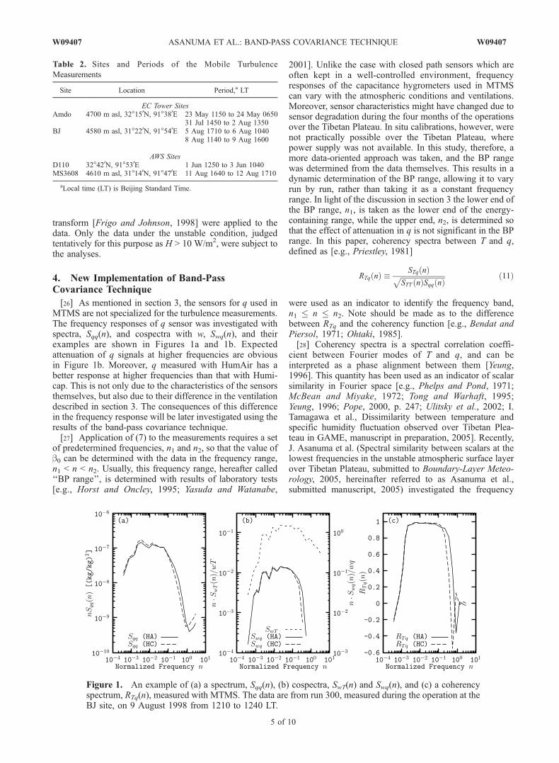
[26] As mentioned in section 3, the sensors for q used inMTMS are not specialized for the turbulence measurements.The frequency responses of q sensor was investigated withspectra, Sqq(n), and cospectra with w, Swq(n), and theirexamples are shown in Figures 1a and 1b. Expectedattenuation of q signals at higher frequencies are obviousin Figure 1b. Moreover, q measured with HumAir has abetter response at higher frequencies than that with Humi-cap. This is not only due to the characteristics of the sensorsthemselves, but also due to their difference in the ventilationdescribed in section 3. The consequences of this differencein the frequency response will be later investigated using theresults of the band-pass covariance technique.[27] Application of (7) to the measurements requires a set

of predetermined frequencies, n1 and n2, so that the value ofb0 can be determined with the data in the frequency range,n1 < n < n2. Usually, this frequency range, hereafter called‘‘BP range’’, is determined with results of laboratory tests[e.g., Horst and Oncley, 1995; Yasuda and Watanabe,

2001]. Unlike the case with closed path sensors which areoften kept in a well-controlled environment, frequencyresponses of the capacitance hygrometers used in MTMScan vary with the atmospheric conditions and ventilations.Moreover, sensor characteristics might have changed due tosensor degradation during the four months of the operationsover the Tibetan Plateau. In situ calibrations, however, werenot practically possible over the Tibetan Plateau, wherepower supply was not available. In this study, therefore, amore data-oriented approach was taken, and the BP rangewas determined from the data themselves. This results in adynamic determination of the BP range, allowing it to varyrun by run, rather than taking it as a constant frequencyrange. In light of the discussion in section 3 the lower end ofthe BP range, n1, is taken as the lower end of the energy-containing range, while the upper end, n2, is determined sothat the effect of attenuation in q is not significant in the BPrange. In this paper, coherency spectra between T and q,defined as [e.g., Priestley, 1981]

RTq nð Þ � STq nð ÞffiffiffiffiffiffiffiffiffiffiffiffiffiffiffiffiffiffiffiffiffiffiffiffiffiSTT nð ÞSqq nð Þ

p ð11Þ

were used as an indicator to identify the frequency band,n1 n n2. Note should be made as to the differencebetween RTq and the coherency function [e.g., Bendat andPiersol, 1971; Ohtaki, 1985].[28] Coherency spectra is a spectral correlation coeffi-

cient between Fourier modes of T and q, and can beinterpreted as a phase alignment between them [Yeung,1996]. This quantity has been used as an indicator of scalarsimilarity in Fourier space [e.g., Phelps and Pond, 1971;McBean and Miyake, 1972; Tong and Warhaft, 1995;Yeung, 1996; Pope, 2000, p. 247; Ulitsky et al., 2002; I.Tamagawa et al., Dissimilarity between temperature andspecific humidity fluctuation observed over Tibetan Plea-teau in GAME, manuscript in preparation, 2005]. Recently,J. Asanuma et al. (Spectral similarity between scalars at thelowest frequencies in the unstable atmospheric surface layerover Tibetan Plateau, submitted to Boundary-Layer Meteo-rology, 2005, hereinafter referred to as Asanuma et al.,submitted manuscript, 2005) investigated the frequency

Table 2. Sites and Periods of the Mobile Turbulence

Measurements

Site Location Period,a LT

EC Tower SitesAmdo 4700 m asl, 32�150N, 91�380E 23 May 1150 to 24 May 0650

31 Jul 1450 to 2 Aug 1350BJ 4580 m asl, 31�220N, 91�540E 5 Aug 1710 to 6 Aug 1040

8 Aug 1140 to 9 Aug 1600

AWS SitesD110 32�420N, 91�530E 1 Jun 1250 to 3 Jun 1040MS3608 4610 m asl, 31�140N, 91�470E 11 Aug 1640 to 12 Aug 1710

aLocal time (LT) is Beijing Standard Time.

Figure 1. An example of (a) a spectrum, Sqq(n), (b) cospectra, SwT(n) and Swq(n), and (c) a coherencyspectrum, RTq(n), measured with MTMS. The data are from run 300, measured during the operation at theBJ site, on 9 August 1998 from 1210 to 1240 LT.

W09407 ASANUMA ET AL.: BAND-PASS COVARIANCE TECHNIQUE

5 of 10

W09407

behavior of RTq(n) with the current data set. By extendingthe similarity arguments of Kader and Yaglom [1991], theyshowed that a procedure similar to the derivation of (10)yields an expression for RTq(n), as follows

RTq nð Þ ¼fR zð Þ for DC sublayer in inertial rangeð Þ

const: otherwiseð Þ

8<: ð12Þ

where fR is a function of z. The value of the constant in thesecond expression may be different in the differentsublayers and in the different frequency ranges (the inertialor the energy-containing range). Asanuma et al. (submittedmanuscript, 2005) also have found that RTq(n) remainsalmost constant within the energy-containing range and that,at its lower end, RTq(n) levels off sharply toward the lowerfrequencies.[29] The frequency, n2, at which the attenuation of q

becomes significant, was also identified with RTq(n). Anexample of RTq(n), shown in Figure 1c, exhibits clear drop-off toward the higher frequencies. Especially, it is clearlyshown that RTq(n) with qHC levels off earlier than that ofqHA. This is consistent with the relatively slower responseof Humicap, shown in spectra and cospectra in Figures 1aand 1b. These indicates the capability of RTq(n) to detectsignal attenuation.[30] With these background, RTq(n) was used to detect the

BP frequency range in this article. For each 30-min run,RTq(n) was calculated from the corresponding spectra andcospectra that were block averaged over frequency bandsequally spaced in the logarithmic frequency. Then, BPrange, n1 < n < n2, was identified as a frequency range thatmeets RTq(n) > Rcr, where the critical value, Rcr, is apredetermined constant. For the value of Rcr, Rcr = 0.9 istentatively chosen, and sensitivity of the results on the valueof Rcr will be investigated later in this paper.[31] The vertical bars in Figure 2 indicate the BP range

identified for all the data analyzed. Note that the verticalaxis in Figure 2 is f = nu/z, and it is not normalized. It isnoticed that BP ranges identified in June are consistentlylower than those of July and August. This can be attributedto the fact that HumAir was not aspirated in June due to ahardware problem. This accidental failure of the hardwarehappens to suggest that RTq(n) successfully detects thesensor response that may vary under the influence ofexternal conditions, in this case, the ventilation.

[32] In order to investigate further the validity of RTq(n)as an indicator of the attenuation in q, a first-order responsefunction was assumed for the response of the capacitancehygrometers used in MTMS as, Swq

m = Swq( f )/(1 + ( f/f0)2).

where the superscript, m, denotes the measured value, f0 thecharacteristic frequency of the sensor at which the measure-ments are the half of the actual value [Horst et al., 1997; seealso Toda et al., 2002]. Then, (6) can be recast as follows

bm fð Þ � SmwT fð Þ=Smwq fð Þ ¼ b0 1þ f =f0ð Þ2h i

: ð13Þ

Using (13), the value of f0 was computed by linearly fittingf 2 against bm( f ), and the calculated values were also plottedin Figure 2. Figure 2 exhibits that f2 = n2u/z determined withRTq(n) closely follows f0 during the course of the seasons.Especially, the difference in the value of f2 between Juneand August was explained plainly by that of f0. This closerelationship between f0 and f2 is also manifested in Figure 3,where most of the data are shown to fall within the range f0/2 < f2 < 2f0. In Figure 3, it is also shown that f0 tends to belarger than f2. These agreements between f0 and f2 stronglysupport the use of RTq(n) as an indicator of the sensorattenuation in q and therefore as an identifier of the higherend of the BP frequency range.[33] It should also be noted that as the definition of

RTq(n) suggests, simple attenuation of q does not solelyreduce the value of RTq(n). The actual cause of the reductionin RTq(n) in the higher frequency is the phase shift betweenT and q fluctuations, accompanied with q attenuation [seeHorst, 2000; Watanabe et al., 2000].[34] The BP range determined in this section will be used

in the application of the band-pass covariance technique, (5)and (7), to the current data set in the next section.

5. Results

[35] By using the BP frequency range identified insection 4 the two versions of the band-pass covariancetechnique, namely equations (5) and (7), were applied tothe measurements. In this section the resulting latent heat

Figure 2. BP frequency range determined with RTq > 0.9for HumAir (the vertical bars). The circles denote f0, thecharacteristic frequency of the q sensor response.

Figure 3. Higher end of BP range, f2, determined as RTq >0.9 plotted against f0, the characteristic frequency of thesensor response. The lines for y = 2x and y = 0.5x are alsoshown.

6 of 10

W09407 ASANUMA ET AL.: BAND-PASS COVARIANCE TECHNIQUE W09407

flux, EBC, was compared with the eddy covariance measure-ments of the tower at the BJ site, EEC, in various aspects.For each of the comparisons, relevant statistics, namely thecorrelation coefficient, r, the slope of the linear regressionline forced through the origin with EBC on abscissa, a, andthe root mean squared error, RMSE, were calculated.

5.1. Sensitivity Analysis to Rcr

[36] In section 4, BP frequency ranges were identified asRTq(n) > Rcr with the tentative value, Rcr = 0.9. Thereforesensitivity of EBC computed with (7) to the value of Rcr wasinvestigated by calculating EBC with different values of Rcr,i.e., Rcr = 0.5, 0.6, 0.7, 0.8 and 0.9. With general shape ofRTq(n) (see Figure 1c), the higher values of Rcr result in thenarrower BP range. Each of the flux values computed fromqHA signals were compared with EEC, and the relevantstatistics were tabulated in Table 3.[37] The first row in Table 3, denoted as ‘‘BC0’’, repre-

sents the latent heat flux computed using the raw covariancew0q0 without any application of the band-pass covariancetechnique. This revealed that about 30% of the latent heatflux was under measured due to the high-frequency atten-uation of the q sensor. The current results show that morethan two thirds of the under measurements were recoveredby the band-pass covariance technique. It is important toemphasize that the current implementation of the band-passcovariance technique does not utilize any external informa-tion other than the measured data.[38] It can be observed that r and RMSE are almost

insensitive to the value of Rcr. A noticeable feature inTable 3 is that the slope, a, slightly yet constantly increaseswith increasing Rcr. In other words, the smaller values of b0in (7) are computed with the narrower BP range associatedwith the higher value of Rcr. This indicates that attenuated qsignals are still contained in the BP range. This is expectedfrom Figure 3, where the higher end of the BP rangeroughly equals to the half-attenuated point, f0.[39] Table 3 suggests that the higher values of Rcr give

superior results. Rcr = 0.9, however, is the highest amongthe practically possible values. A value of Rcr higher than0.9 would not give a frequency range for RTq(n) > Rcr, assuggested by Figure 1c. One possibility to improve thisfurther is to assume the first-order sensor responseexpressed in (13). Applying the data to (13) computes b0[Horst, 1997], which, in turn, can be used in (7) to compute

the latent heat flux. This was tested with the data in the BPrange with Rcr = 0.9. The comparison with EEC gives thestatistics as r = 0.91, a = 1.00(±0.04), RMSE = 47.6 W/m2.The slope, a, has thus been improved, while RMSE hasbeen degraded. By imposing a functional form of the sensorresponse, uncertainty was added to the computed fluxvalues With these considerations, hereafter the thresholdvalue Rcr = 0.9 will be used.

5.2. Comparison Between the Humidity Sensors

[40] Latent heat flux computed by using (7) with the qmeasurements of the two hygrometers, namely, qHA andqHC, are compared in Figure 4. Each of the two panels inFigure 4 shows the latent heat flux from the raw covarian-ces, w0q0, without applying the band-pass covariance tech-nique. Again, these raw covariances are significantlysmaller than EEC and these under measurements werecorrected substantially by the band-pass covariance tech-nique (open circles), with which both of r and the slope, a,are close to unity. This again demonstrates the strongcapability of the band-pass covariance technique in frequencyextrapolations. A comparison between the two panels

Table 3. Statistics Relevant to the Comparison Between the

Tower Eddy Covariance Measurements EEC and the Computations

by the Band-Pass Covariance Techniques EBC (Equation (7)) With

Different Values for Rcra

Rcr nd r a RMSE

BC0 25 0.92 0.71 (±0.03) 71.80.5 25 0.93 0.91 (±0.03) 40.20.6 25 0.93 0.92 (±0.03) 39.50.7 25 0.94 0.92 (±0.03) 37.60.8 25 0.94 0.94 (±0.03) 35.70.9 25 0.94 0.97 (±0.03) 33.2

aHumAir measurements were used. Here nd is the number of the data, r isthe correlation coefficient, a is the slope of the linear regression line forcedthrough the origin, and RMSE is the root-mean-square error in W/m2. BC0in the first column refers to the values computed from the raw covariancesof w0q0 without any application of the band-pass covariance technique.

Figure 4. Comparison between the latent heat fluxmeasured with the eddy correlation systems, EEC, and thatcomputed with equation (7), EBC (open circles). (top)Measurements with HumAir; (bottom) measurements withHumicap. The solid circles are those computed from the rawcovariances plotted against EEC.

W09407 ASANUMA ET AL.: BAND-PASS COVARIANCE TECHNIQUE

7 of 10

W09407

shows slight differences in the performance of the twosensors. HumAir gives a slightly smaller value of RMSEthan does Humicap. This is expected from the betterfrequency response of the former than the latter (Figure 1).A closer look at these figures indicates that the performanceof Humicap is worse when the values of latent heat flux aresmaller. This may be related to the fact that Humicap wasnaturally aspirated.

6. Discussion

[41] The comparison between the two versions of theband-pass covariance technique, namely (5) and (7), canelucidate the validity of the assumptions underlying themethods. This is the main interest of this paper.[42] As discussed earlier in this document, (5) requires

that the dimensionless form of SwT(n) and Swq(n) areequal for the range, 0 < n < 1 (equation (3)), while lessstrict (7) demands that these cospectra have the samefrequency dependency between the energy-containing andthe dissipation frequencies. From the more physical point ofview, (5) assumes that T and q fluctuations are similar toeach other over the entire Fourier space, whereas (7) onlyassumes that these scalar fluctuations share the same flowcharacteristics at their production and during the course ofcascading down to their dissipation. Apparently, (7) is basedon a less strict assumption than the one (5) is based on.[43] The first two rows of Table 4 compare the two

versions of the band-pass covariance technique with allruns analyzed. Although the difference is small, it can beobserved that (5) considerably underestimates the latent heatflux. These differences between the two methods werefurther investigated by following Asanuma et al. (submittedmanuscript, 2005). All of the runs analyzed were catego-rized into two groups using the behavior of RTq(n) at thelower frequencies. One of them are those that reduce thevalue of RTq(n) below 0.5 in the frequency range, 0 < n < n1,and the others are those that do not. The specific threshold,0.5, was chosen so that the two groups have nearly the samepopulation. These two groups are hereafter termed ‘‘lower’’and ‘‘higher correlation’’ runs. For example, the run shownin Figure 1 is categorized into the former. The comparisonstatistics were, again, computed for each of these twogroups, and they were also tabulated in Table 4. Thestatistics shown in Table 4 give a clear distinction betweenthe two versions of the band-pass covariance technique.With the higher correlation runs, both of (5) and (7) works

almost equally well. The value of the slope, a, almost equalsto unity, and RMSE are almost equal to each other. On theother hand, the performance of (5) with the lower-correla-tion runs were worse: RMSE is twice larger and the flux isunderestimated by about 15%. Equation (7), in contrast,remains relatively unchanged even with the lower-correla-tion runs. This illuminates the robustness of (7).[44] These observations can be explained with the find-

ings of Asanuma et al. (submitted manuscript, 2005). Byusing RTq(n) as an indicator, they investigated the similaritybetween T and q in the Fourier domain with the same dataset. By categorizing the analyzed data runs into the twogroups as in this study, they found that the lower-correlationruns have remarkably reduced RTq(n) at the lower frequen-cies, 10�4 < n < 10�3, while the higher-correlation runsmaintain higher values of RTq(n) even at these frequencies.Dissimilarity between T and q occurred at the lowerfrequencies has been also pointed out by Dias et al.[2004]. The fact that the reduced RTq(n) occurs only inthe lower-correlation runs indicates that the dissimilarity isoccasional, and its occurrence is limited in time. Asanumaet al. (submitted manuscript, 2005) argued that the dissim-ilarity between T and q found at the lower frequencies wasassociated with the ‘‘decorrelation events’’ at the scale ofthe atmospheric boundary layer (ABL) height. With theirlonger return period relative to the length of the data run,these events were sensed to be occasional or sporadic. Theyalso mentioned the entrainment at the top of ABL and theconvective cloud activities as possible candidates for thedecorrelation events.[45] If we extend their arguments, the failure of (5) found

in this study can also be associated with these decorrelationevents at the scale of the ABL height. In other words,occasional occurrences of the dissimilarity at the lowerfrequencies caused occasional failures of (5), which relieson the similarity of T and q over whole Fourier domain. Incontrast, equation (7) only relies on the characteristics of thescalar field at the higher frequencies, and remains fairlyintact against these decorrelation events. This points to therobustness of (7), as well as the validity of the fundamentalassumption of (7) expressed as (6).[46] A comment should be made on the consistency of

the current result with the findings in the literature. Someauthors have already presented observational evidences inwhich T and q become dissimilar at the higher frequencies[e.g., Phelps and Pond, 1971; McBean and Miyake, 1972;Katul and Parlange, 1994]. Katul and Parlange [1994], forexample, argued that the active role of T and the relativelypassive role of q in the turbulent field become significant atthe higher frequencies. The current result that (6) is validdoes not contradict this: Since b(n) is the ratio of thecospectra of w and these scalars, the different behavior ofT and q associated with their different roles might befiltered out when the cospectra with w are taken. Thisconcept also characterizes the robustness of the assumptionunderlying (7).

7. Conclusion

[47] The band-pass covariance technique forms a physi-cally sound method for frequency extrapolation in latentheat flux measurements. The term ‘band-pass covariancetechnique,’ in fact, points to two different methods that have

Table 4. Same Statistics as Table 3 but for Those Relevant to the

Comparison Between the Two Versions of the Band-Pass

Covariance, Namely, Equations (5) and (7)

Equation nd r a RMSE

All Runs(5) 25 0.93 0.90 (±0.03) 40.5(7) 25 0.94 0.97 (±0.03) 33.2

Runs With Higher Correlation(5) 12 0.97 0.99 (±0.04) 26.0(7) 12 0.97 1.00 (±0.03) 24.1

Runs With Lower Correlation(5) 13 0.91 0.84 (±0.05) 39.7

8 of 10

W09407 ASANUMA ET AL.: BAND-PASS COVARIANCE TECHNIQUE W09407

a different physical background. Distinctions between thesetwo versions and their different backgrounds are clearlyaddressed in this paper.[48] The original version by Hicks and McMillen [1988]

requires the similarity between the temperature and thespecific humidity, or a scalar in question, over the entireFourier domain, while the other, more advanced, version[Hogstrom et al., 1989] assumes ‘‘similarity’’ between thetwo scalars only at the higher frequencies. The word‘‘similarity’’ for the latter has been used ambiguously, yetnot incorrectly, in the literature. In light of the surfacesimilarity arguments, this paper demonstrates that the as-sumption invoked by the advanced version is different fromthe similarity between scalars in its strict definition. Instead,it relies only on the fact that the two scalars obey the sameflow characteristics at the higher frequencies. The surfacesimilarity arguments also suggest that this is most likely tobe valid during the course of the production, the cascading,and the dissipation of the flux covariance in the turbulencefield. This requirement for the advanced version turns out tobe less strict than that of the original version. Moreover, theflux calculation algorithm, fully described by Watanabe etal. [2000] and Yasuda and Watanabe [2001], has a self-calibration procedure embedded in itself. These facts makethe advanced version more robust and more practical for usein the real atmosphere.[49] The algorithm of the advanced version [Horst and

Oncley, 1995; Horst, 1997; Watanabe et al., 2000; Yasudaand Watanabe, 2001] was further modified and was appliedto the daytime measurements of latent heat flux above thesparse grasslands over the Tibetan Plateau. In the modifiedalgorithm, the energy-containing range was dynamicallyidentified using the coherency spectra between temperatureand specific humidity. The coherency spectra were also usedto detect attenuation in the measured signals of specifichumidity. Though the number of the data is limited, thecomputed latent heat flux values exhibited adequate agree-ment with the eddy covariance measurements, indicatingstrong capability of the current algorithm in frequencyextrapolation under unstable conditions. The applicationof the original version, on the other hand, clearly showedthat it fails when the similarity between temperature andhumidity is not maintained at the lower frequencies.[50] The occasional failures of the original version need

an special attention. Clearly, the current observations inval-idate the frequently invoked ‘‘perfect similarity’’ assump-tion between the temperature and the specific humidity. Useof this erroneous assumption in the flux measurements oftrace gases may cause substantial biases. Instead, directmeasurements of the lower-frequency portions of thesefluxes are recommended for better accuracy. In contrast,the background assumption behind the advanced versionwas shown to be relatively robust.[51] The modified algorithm of the band-pass covariance

technique proposed in this text gives the band-pass limit,once the thresholding value of the coherency spectra ischosen. Therefore the algorithm offer a semiautomaticprocedure of the scalar flux calculation from measurementsof a simple and robust scalar sensor. Hence the algorithmrenders long-term flux measurements, i.e., for months andyears, more feasible. For this to be complete, however,applicability of the band-pass covariance under the stable

stratification need to be investigated, which is beyond thecoverage of this text.[52] Finally, the strong extrapolating capability of the

band-pass covariance technique with the proposed algo-rithm does have a large potential in scalar flux measure-ments. One possibility is to correct attenuated scalar fluxesdue to the separation between the sonic anemometer and thescalar sensor by using a sonic temperature as a guide. Theband-pass covariance technique can be also used as analternative measurements for gap filling [e.g., Falge et al.,2001] of long-term data of water vapor, CO2 and trace gasfluxes with an additional low-cost scalar sensor as a backupin case of failures of the fast response scalar sensor.

[53] Acknowledgments. The authors are grateful to T. Yasunari atNagoya University and T. Koike at Tokyo University, without whose effortsand leadership the GAME-Tibet project could not have been possible.Appreciation is also given to the other participants of the GAME-Tibet fieldcampaigns for their help and cooperation. Invaluable comments fromG. Katul at Duke University, N. Dias at UFPR, Brazil, and T. Watanabeat Forestry and Forest Products Research Institute, Japan, are also appre-ciated. One of the authors (J.A.) is supported, in part, by Ministry ofEducation, Culture, Sport, Science and Technology (MEXT), Japan, througha Grant-in-Aid for Scientific Research (A) (13308027) and (C)(17560450)and Asahi Breweries Foundation through its academic grant.

ReferencesAnderson, D. E., and S. B. Verma (1985), Turbulence spectra of CO2 water-vapor, temperature and wind velocity fluctuations over a crop surface,Boundary Layer Meteorol., 33, 1–14.

Bendat, J. S., and A. G. Piersol (1971), Random Data Analysis and Mea-surement Procedure, Wiley Interscience, Hoboken, N. J.

Blanken, P. D., T. A. Black, P. C. Yang, H. H. Neumann, Z. Nesic,R. Staebler, G. den Hartog, M. D. Novak, and X. Lee (1997), Energybalance and canopy conductance of a boreal aspen forest: Partitioningoverstory and understory components, J. Geophys. Res., 102(D24),28,915–28,927.

Choi, T., J. Kim, H. Lee, J. Hong, J. Asanuma, H. Ishikawa, Z. Gao,J. Wang, and T. Koike (2004), Turbulent exchange of heat, water vaporand momentum over a Tibetan prairie by eddy covariance and flux-variance measurements, J. Geophys. Res., 109(D21), D21106,doi:10.1029/2004JD004767.

Dias, N. L., and W. Brutsaert (1996), Similarity of scalars under stableconditions, Boundary Layer Meteorol., 80, 355–373.

Dias, N., M. Chamecki, A. Kan, and C. Okawa (2004), A study of spectra,structure and correlation functions and their implications for the statio-narity of surface-layer turbulence, Boundary Layer Meteorol., 110(2),165–189.

Falge, E., et al. (2001), Gap filling strategies for defensible annual sums ofnet ecosystem exchange, Agric. For. Meteorol., 107, 43–69.

Fan, S. M., S. C. Wofsy, P. S. Bakwin, D. J. Jacob, S. M. Anderson, P. L.Kebabian, J. B. McManus, C. E. Kolb, and D. R. Fitzjarrald (1992),Micrometeorological measurements of CH4 and CO2 exchange betweenthe atmosphere and sub-arctic tundra, J. Geophys. Res., 97, 16,627–16,643.

Frigo, M., and S. G. Johnson (1998), FFTW: An adaptive software archi-tecture for the FFT, in Proceedings of 1998 IEEE International Confer-ence on Acoustics Speech and Signal Processing, vol. 3, pp. 1381–1384,IEEE Press, Piscataway, N. J.

Gao, Z. Q., N. Chae, J. Kim, J. Y. Hong, T. Choi, and H. Lee (2004),Modeling of surface energy partitioning, surface temperature, and soilwetness in the Tibetan prairie using the Simple Biosphere Model 2(SiB2), J. Geophys. Res., 109, D06102, doi:10.1029/2003JD004089.

Grelle, A., and A. Lindroth (1996), Eddy-correlation system for long-termmonitoring of fluxes of heat, water vapour and CO2, Global ChangeBiol., 2, 297–307.

Guenther, A. B., and A. J. Hills (1998), Eddy covariance measurement ofisoprene fluxes, J. Geophys. Res., 103(D11), 13,145–13,152.

Hicks, B., and McMillen (1988), On the measurement of dry depositionusing indirect sensors and in non-ideal terrain, Boundary Layer Meteorol.,42, 79–94.

Hill, R. (1989), Implications of Monin-Obukhov similarity theory for scalarquantities, J. Atmos. Sci., 46, 2236–2244.

W09407 ASANUMA ET AL.: BAND-PASS COVARIANCE TECHNIQUE

9 of 10

W09407

Hogstrom, U., H. Bergstrom, A. S. Smedman, S. Halldin, and A. Lindroth(1989), Turbulent exchange above a pine forest. 1. Fluxes and gradients,Boundary Layer Meteorol., 49, 197–217.

Hogstrom, U., J. C. R. Hunt, and A. S. Smedman (2002), Theory andmeasurements for turbulence spectra and variances in the atmosphericneutral surface layer, Boundary Layer Meteorol., 103, 101–124.

Horst, T. (1997), A simple formula for attenuation of eddy fluxes measuredwith first-order-response scalar sensors, Boundary Layer Meteorol., 82,219–233.

Horst, T. (2000), On frequency response corrections for eddy covarianceflux measurements, Boundary Layer Meteorol., 94, 517–520.

Horst, T., and S. Oncley (1995), Flux-PAM measurement of scalar fluxesusing cospectral similarity, paper presented at 9th Symposium on Me-teorological Observations and Instrumentation, Am. Meteorol. Soc.,Charlotte, N. C.

Horst, T., S. Oncley, and S. Semmer (1997), Measurement of water vaporfluxes using capacitance RH sensors and cospectral similarity, paperpresented at 12th Symposium on Boundary Layers and Turbulence,Am. Meteorol. Soc., Vancouver, B.C., Canada.

Jacob, D. J., et al. (1992), Deposition of ozone to tundra, J. Geophys. Res.,97, 16,473–16,479.

Kader, B., and A. Yaglom (1990), Mean fields and fluctuation moments inunstably stratified turbulent boundary layer, J. Fluid. Mech., 212, 637–662.

Kader, B., and A. Yaglom (1991), Spectra and correlation functions ofsurface layer atmospheric turbulence in unstable thermal stratification,in Turbulence and Coherent Structures, edited by O. Metais andM. Lesieur, pp. 387–412, Springer, New York.

Kaimal, J., J. C. Wyngaard, Y. Izumi, and O. Cote (1972), Spectral character-istics of surface-layer turbulence, Q. J. R. Meteorol. Soc., 98, 563–589.

Katul, G., and C. R. Chu (1998), A theoretical and experimental investiga-tion of energy-containing scales in the dynamic sublayer of boundary-layer flows, Boundary Layer Meteorol., 86, 279–312.

Katul, G. G., and M. B. Parlange (1994), On the active-role of temperaturein surface-layer turbulence, J. Atmos. Sci., 51, 2181–2195.

Katul, G. G., C. D. Geron, C. I. Hsieh, B. Vidakovic, and A. B. Guenther(1998), Active turbulence and scalar transport near the forest-atmosphereinterface, J. Appl. Meteorol., 37, 1533–1546.

Katul, G., C. T. Lai, K. Schafer, B. Vidakovic, J. Albertson, D. Ellsworth,and R. Oren (2001), Multiscale analysis of vegetation surface fluxes:From seconds to years, Adv. Water Resour., 24, 1119–1132.

Lumley, J. L. (1964), The spectrum of nearly inertial turbulence in a stablystratified fluid, J. Atmos. Sci., 21, 99–102.

Lumley, J. L. (1967), Similarity and the turbulent energy spectrum, Phys.Fluids, 10(4), 855–858.

Ma, Y. M., Z. B. Su, T. Koike, T. D. Yao, H. Ishikawa, K. Ueno, andM. Menenti (2003), On measuring and remote sensing surface energypartitioning over the Tibetan Plateau—From GAME/Tibet to CAMP/Tibet, Phys. Chem. Earth, 28, 63–74.

Massman, W. J., and X. Lee (2002), Eddy covariance flux corrections anduncertainties in long-term studies of carbon and energy exchanges, Agric.For. Meteorol., 113, 121–144.

McBean, G., and M. Miyake (1972), Turbulent transfer mechanisms in theatmospheric surface layer, Q. J. R. Meteorol. Soc., 98, 383–398.

McNaughton, K., and J. Laubach (2000), Power spectra and cospectra forwind and scalars in a disturbed surface layer at the base of an advectiveinversion, Boundary Layer Meteorol., 96, 143–185.

Moore, C. J. (1986), Frequency response corrections for eddy correlationsystems, Boundary Layer Meteorol., 37, 17–35.

Ohtaki, E. (1985), On the similarity in atmospheric fluctuations of carbondioxide, water vapor and temperature over vegetated fields, BoundaryLayer Meteorol., 32, 25–37.

Phelps, G., and S. Pond (1971), Spectra of the temperature and humidityfluctuations and of the fluxes of moisture and sensible heat in the marineboundary layer, J. Atmos. Sci., 28, 918–928.

Pope, S. B. (2000), Turbulent Flows, Cambridge Univ. Press, New York.Priestley, M. B. (1981), Spectral Analysis and Time Series, Elsevier, NewYork.

Schmitt, K., C. Friehe, and C. Gibson (1979), Structure of marine surface-layer turbulence, J. Atmos. Sci., 36(4), 602–618.

Su, H. B., H. P. Schmid, C. S. B. Grimmond, C. S. Vogel, and A. J.Oliphant (2004), Spectral characteristics and correction of long-termeddy-covariance measurements over two mixed hardwood forests innon-flat terrain, Boundary Layer Meteorol., 110, 213–253.

Tanaka, K., H. Ishikawa, T. Hayashi, I. Tamagawa, and Y. Ma (2001),Surface energy budget at Amdo on the Tibetan Plateau using GAME/Tibet/IOP98 data, J. Meteorol. Soc. Jpn., 79(1B), 505–517.

Tanaka, K., I. Tamagawa, H. Ishikawa, Y. Ma, and Z. Hu (2003), Surfaceenergy budget and closure of the eastern Tibetan Plateau during theGAME-Tibet IOP 1998, J. Hydrol., 283(1–4), 169–183.

Toda, M., K. Nishida, N. Ohte, M. Tani, and K. Musiake (2002), Observa-tions of energy fluxes and evapotranspiration over terrestrial complexland covers in the tropical monsoon environment, J. Meteorol. Soc.Jpn., 80, 465–484.

Tong, C. N., and Z. Warhaft (1995), Passive scalar dispersion and mixing ina turbulent jet, J. Fluid. Mech., 292, 1–38.

Twine, T., W. P. Kustas, J. Norman, D. Cook, P. Houser, T. Meyers,J. Prueger, P. Starks, and M. Wesely (2000), Correcting eddy-covarianceflux underestimates over a grassland, Agric. For. Meteorol., 103, 279–300.

Ulitsky, M., L. R. Collins, and T. Vaithianathan (2002), A spectral study ofdifferential diffusion of passive scalars in isotropic turbulence, J. FluidMech., 460, 1–38.

Verma, S. B., F. G. Ullman, D. Billesbach, R. J. Clement, J. Kim, and E. S.Verry (1992), Eddy-correlation measurements of methane flux in a north-ern peatland ecosystem, Boundary Layer Meteorol., 58, 289–304.

Warhaft, Z. (2000), Passive scalars in turbulent flows, Ann. Rev. FluidMech., 32, 203–240.

Watanabe, T., K. Yamanoi, and Y. Yasuda (2000), Testing of the bandpasseddy covariance method for a long-term measurement of water vaporflux over a forest, Boundary Layer Meteorol., 96, 473–491.

Wyngaard, J. C., and O. Cote (1972), Cospectral similarity in the atmo-spheric surface layer, Q. J. R. Meteorol. Soc., 98, 590–603.

Yang, K., T. Koike, H. Ishikawa, and Y. M. Ma (2004), Analysis of thesurface energy budget at a site of GAME/Tibet using a single-sourcemodel, J. Meteorol. Soc. Jpn., 82, 131–153.

Yasuda, Y., and T. Watanabe (2001), Comparative measurements of CO2

flux over a forest using closed-path and open-path CO2 analysis, Bound-ary Layer Meteorol., 100, 191–208.

Yeung, P. K. (1996), Multi-scalar triadic interactions in differential diffu-sion with and without mean scalar gradients, J. Fluid. Mech., 321, 235–278.

����������������������������J. Asanuma, Terrestrial Environment Research Center, Tsukuba

University, 1-1-1Ten-nohdai, Tsukuba, Ibaraki, 305-8577 Japan. (asanuma@suiri.tsukuba.ac.jp)

T. Hayashi and H. Ishikawa, Disaster Prevention Research Institute,Gokasho, Uji, Kyoto 611-0011, Japan.

Y. Ma, Institute of Tibetan Plateau Research, Chinese Academy ofSciences, 18 Shuangqing Road, Haidian District, P.O. Box 2871, Beijing100864, China.

Y. Qi, China Patent Agent (H.K.) Ltd., 27 Jinrong Street, XichengDistrict, Beijing 100032, China.

I. Tamagawa, River Basin Research Center, Gifu University, Yanagido1-1, Gifu, Gifu 501-1193, Japan.

J. Wang, Cold and Arid Regions Environmental and EngineeringResearch Institute, Chinese Academy of Sciences, 260 Donggang WestRoad, Lanzhou, Gansu 730000, China.

10 of 10

W09407 ASANUMA ET AL.: BAND-PASS COVARIANCE TECHNIQUE W09407