Measurements of industrial emissions of alkenes in Texas

using the solar occultation flux method

Johan Mellqvist,1 Jerker Samuelsson,1 John Johansson,1 Claudia Rivera,1 Barry Lefer,2

Sergio Alvarez,3 and John Jolly4

Received 29 December 2008; revised 7 September 2009; accepted 14 September 2009; published 13 March 2010.

[1] Solar occultation flux (SOF) measurements of alkenes have been conducted toidentify and quantify the largest emission sources in the vicinity of Houston and in SETexas during September 2006 as part of the TexAQS 2006 campaign. The measurementshave been compared to emission inventories and have been conducted in parallel withairborne plume studies. The SOF measurements show that the hourly gas emissions fromthe large petrochemical and refining complexes in the Houston Ship Channel area andMount Belvieu during September 2006 corresponded to 1250 ± 180 kg/h of ethene and2140 ± 520 kg/h of propene, with an estimated uncertainty of about 35%. This can becompared to the 2006 emission inventory value for ethene and propene of 145 ± 4 and 181 ±42 kg/h, respectively. On average, for all measurements during the campaign, thediscrepancy factor is 10.2(+8,-5) for ethene and 11.7(+7,-4) for propene. The largestemission source was Mount Belvieu, NE of the Houston Ship Channel, with ethene andpropene emissions corresponding to 440 ± 130 kg/h and 490 ± 190 kg/h, respectively.Large variability of propene was observed from several petrochemical industries, forwhich the largest reported emission sources are flares. The SOF alkene emissions agreewithin 50% with emissions derived from airborne measurements at three different sites.The airborne measurements also provide support to the SOF error budget.

Citation: Mellqvist, J., J. Samuelsson, J. Johansson, C. Rivera, B. Lefer, S. Alvarez, and J. Jolly (2010), Measurements of industrial

emissions of alkenes in Texas using the solar occultation flux method, J. Geophys. Res., 115, D00F17, doi:10.1029/2008JD011682.

1. Introduction

[2] This study investigates fugitive emissions of etheneand propene, two highly reactive volatile organic com-pounds (HRVOCs), from industrial sources in the vicinityof Houston. The objective of the study was to locate thesesources and quantify their VOC emissions. The work is partof the TexAQS 2006 intensive summer campaign, includedin the Second Texas Air Quality Study (TexAQS II), withthe aim of better understanding the formation of troposphericozone in southeastern Texas. Ozone is formed by photo-chemical reactions between VOCs and nitrogen oxides. In aprevious air quality study in 2000 it was noted that theindustries in Texas seem to emit considerably more highlyreactive VOCs than reported and that the emissions areimportant contributors to ozone formation in Texas [Ryersonet al., 2003;Wert et al., 2003]. This was found by conductingairborne measurements downwind of several isolated facili-ties to determine the ratios of HRVOCs to NOx. The results

showed discrepancies between reported and measured val-ues of a factor 20 to 70. Assuming the NOx emissions arebetter known, which seemed to be the case, the discrepancyis primarily due to higher than reported VOC emissions.This approach is indirect as it relies on the assumption thatthe NOx emissions are known and that the HRVOCs andNOx is mixed uniformly in the plume. The latter is notalways the case since the species are released from differentparts of the industries, NOx mostly through stacks andVOCs through fugitive emissions from process equipment.An uncertainty is whether the relatively few measurementdays during which the measurements were conducted arerepresentative of the industries’ baseline emissions.[3] To overcome some of the uncertainties with the

previous emission studies, a direct method to quantifyfugitive emissions has been applied in the TexAQS 2006study, i.e., the solar occultation flux (SOF) method. Itutilizes the Sun as the light source and vertically integratedconcentrations of gas species that absorb in the infraredportion of the solar spectrum are measured from a vehiclethat travels on roads upwind and downwind of the targetsources (0.5 to 3 km distance). The gas fluxes are obtainedby multiplying the mass across the plume with the windspeed. This approach of obtaining the gas flux is similar toother methods used to measure volcanic fluxes of SO2, forinstance scanning passive ultraviolet measurements [Galleet al., 2003], the laser based technique DIAL [Weibring etal., 1998] and DOAS and COSPEC, two mobile techniques

JOURNAL OF GEOPHYSICAL RESEARCH, VOL. 115, D00F17, doi:10.1029/2008JD011682, 2010ClickHere

for

FullArticle

1Radio and Space Science, Chalmers University of Technology,Goteborg, Sweden.

2Department of Geosciences, University of Houston, Houston, Texas,USA.

3Institute for Air Science, Baylor University, Waco, Texas, USA.4Texas Commission on Air Quality, Austin, Texas, USA.

Copyright 2010 by the American Geophysical Union.0148-0227/10/2008JD011682

D00F17 1 of 13

using zenith scattered UV light [Weibring et al., 1998]. TheDIAL technique is also applied for measurement of VOCemissions from industries [Walmsley and O’Connor, 1998].[4] In this paper the 2006 SOF data has been compared to

emission inventories developed by the TCEQ (Texas Com-mission on Environmental Quality) for 2006. The SOF datahas also been compared to emission values estimated fromthe NOAA WP-3D aircraft and the Baylor Piper Aztecairplane, measuring in parallel with the SOF. Furthermore,the airborne data has been used to analyze the verticalmixing of the gas plumes. This is of relevance for theestimation of the measurement uncertainty for the SOFmeasurements. More information can be found in tworecent reports [Mellqvist et al., 2007; 2008]. Simultaneousmeasurements of NO2 and SO2 were also conducted with aUV/visible system and these will be published elsewhere[Rivera et al., 2010] as well as SOF alkane emissionmeasurement (J. Samuelsson, manuscript in preparation,2010).

2. Methods

2.1. Measurement Method

[5] The SOF method is relatively new and was developedfrom research projects involving studies of industrial emis-sions [Mellqvist, 1999] using long path FTIR (FourierTransform Infrared) and solar high-resolution FTIRmeasure-ments of atmospheric species [Mellqvist, 1999; Mellqvist etal., 2002; Galle et al., 1999] within the NDACC network(Network for Detection of Atmospheric CompositionChange, http://www.ndsc.ncep.noaa.gov). The method isbased on the recording of solar broadband infrared (IR)absorption spectra (1.8–14 mm). The spectral retrieval issimilar to that of conventional long path FTIR spectroscopy[Hanst et al., 1982] but due to the long atmospheric pathlength of the solar light the spectra are characterized by strongabsorptions caused by the background atmospheric speciessuch as H2O, CO2 and CH4 and this has to be taken intoaccount in the spectral evaluation. In the infrared region ofthe solar spectrum a large number of species, such asaldehydes, alkanes, ammonia, CO, ethene, ethane oxide,HF, HCl, SO2, propene, terpenes, and vinyl chloride, canbe measured. The method has been used quite extensively inSweden [Kihlman et al., 2005; Kihlman, 2005] for VOCmeasurements of refineries but also for volcanic measure-ments of SO2, HCl and HF [Mellqvist et al., 2005] and COcolumn measurements in megacities [Mellqvist et al., 2004;Foy et al., 2007].[6] The SOF instrument is built into a van and consists of a

custom built solar tracker, transfer optics and a Bruker OPAGFTIR spectrometer with a spectral resolution of 0.5 cm�1,equipped with both an MCT (MercuryCadmiumTelluride)detector, primarily for the 9–14 mm wavelength region, andan InSb (IndiumAntimonide) detector for the 2.5–5.5 mmregion. The Sun tracker is a mirror device that tracks the Sunand reflects the light into the spectrometer. Optical inter-ference filters are used to optimize the signal-to-noise ratio(S/N) of the measurements.[7] The spectral retrieval is conducted by custom soft-

ware (QESOF) [Kihlman, 2005]. Here, calibration spectraare fitted to the measured spectra using nonlinear multivar-iate analysis. Calibration data from the HITRAN database

[Rothman et al., 2005] are used to simulate absorptionspectra for ethene and other interfering atmospheric back-ground species at the actual pressure, temperature andinstrumental resolution of the measurements. The sameapproach is applied for several retrieval codes for high-resolution solar spectroscopy [Rinsland et al., 1991; Griffith,1996]. For propene, high-resolution spectra are obtainedfrom the PNL (Pacific Northwest Laboratory) database[Sharpe et al., 2004] and these are degraded to the spectralresolution of the instrument by convolution with the instru-ment line shape. The uncertainty in the absorption strength ofthe calibration spectra is about 3% for both species.[8] The retrieval of ethene is conducted in the wavelength

region between 945 and 979 cm�1 (10.21–10.58 mm)taking into account the interfering species water and CO2.Propene is retrieved between 900 and 920 cm�1 (10.87–11.11 mm) taking into account interfering absorptions ofethene, ammonia, 1-butene, 1,3-butadiene, CO2 and H2O. Inthe spectral region around 10 mm, warm objects radiate heatwhich creates a thermal background in the absorptionspectrum. To correct for this a thermal background spectrumis recorded at regular intervals by measuring with the solartracker pointed to the cold sky i.e., away from the Sun. Thisbackground spectrum is then subtracted from each recordedsolar spectrum. In the spectral retrieval algorithm, a refer-ence spectrum is chosen from a region of the measurementtransect where it can be assumed that the target gasconcentration is near zero and which corresponds to thelowest column value measured. Instead of calculating thetransmittance by dividing all spectra with the reference,which is the common approach in long path FTIR, thelogarithm of the reference spectrum is fitted to the measuredspectrum together with cross sections of the gas species tobe retrieved which are adapted to the instrumental param-eters, as shown in equation (1) below, which simply is arewriting of the Beer Lambert law. This approach makes itpossible to account for wavelength shifts in the spectra andalso to include several reference spectra in the fit, whichresults in efficient removal of the influence of the upperatmosphere.

ln I vð Þ½ � ¼Xj

Fj � ln I0;j vð Þ� �

�Xi

si vð Þ �Z

conci zð Þ � dz: ð1Þ

Here, I corresponds to the measured light intensity as afunction of frequency n, I0,j corresponds to reference spectrawith fitting factors Fj, si corresponds to cross sections forthe fitted species and the last part of equation (1) is thevertically integrated concentration, i.e., column, to bedetermined.[9] The results of the spectral fitting algorithm for alkanes

have been compared and verified with the results retrievedfrom the nonlinear NLM4 software developed by Griffith[1996]. The agreement between NLM4 and QESOF isgood; it is within a few percent. Verification of the QESOFsoftware has also been conducted for the volcanic speciesHCl and SO2 by comparison with a code developed byBurton et al. [2001] which shows good agreement, also withdifferences of within a few percent [Mellqvist et al., 2005].In Figure 1 solar spectra are shown corresponding tomeasurements downwind and upwind of an industrial

D00F17 MELLQVIST ET AL.: SOF MEASUREMENTS IN TEXAS

2 of 13

D00F17

facility in the Houston Ship Channel (HSC). The measure-ment time of these spectra corresponds to 5 s, which istypical for all measurements presented here. In addition, aspectral fit of ethene, H2O and CO2 to the downwindspectrum is shown, using the upwind spectrum as reference.For this case, a clear absorption signal for ethene is showncorresponding to 35 mg/m2. The retrieval for ethene has avariability (1s) of about 0.5 mg/m2 caused by interferenceeffects and noise due to instrument vibrations and distur-bances while driving. For propene the variability is higher,around 3 mg/m2, due to lower absorption sensitivity andgiven that the chosen spectroscopic retrieval was moresensitive to instrumental noise features.[10] To obtain the gas emission from a target source, SOF

transects, measuring vertically integrated species concen-trations, are conducted along roads oriented crosswind andclose downwind (0.5–3 km) of the target source so that thedetected solar light cuts through the emission plume asillustrated in Figure 2. The gas flux is obtained first byadding the column measurements and hence the integratedmass of the key species across the plume is obtained. Toobtain the flux this value is then multiplied by the massaverage wind speed of the plume, u0mw. The flux calculationis shown in equation (2). Here, x corresponds to the traveldirection, z to the height direction, u0 to the wind speedorthogonal to the travel direction (x), u0mw to the massweighted average wind speed and Hmix to the mixing layerheight. The slant angle of the Sun is compensated for, by

multiplying the concentration with the cosine factor of thesolar zenith angle.

flux ¼Zx2

x1

ZHmix

0

conc zð Þ � u0 zð Þ � dz

0@

1Adx ¼ u0mw

Zx2

x1

column xð Þ;

ð2Þ

where u0mw ¼

RHmixconc zð Þu0 zð Þ�dz

RHmixo

conc zð Þdzand column ¼

RHmix0

conc zð Þ � dz.

[11] The determination of the mass averaged wind speedfor SOF is not straightforward to obtain as winds are usuallycomplex close to the ground and increase with the heightabove a surface. What helps the situation is that themeasurements can only be undertaken in sunny conditions,which is advantageous since it corresponds to unstablemeteorological conditions for which wind gradients aresmoothed out by convection. Under these conditions theindustrial emission plumes mix rather quickly in the verticalgiving a more or less homogeneous distribution of thepollutants versus height through the mixing layer even10 km downwind. In addition to the atmospheric mixing,the plumes from process industries exhibit an initial liftsince they are usually hotter than the surrounding air. Thisassumption of rapid mixing agrees with Doppler LIDARmeasurements conducted from the ship RVRonald H. Brownby NOAA during the TexAQS 2006 [Tucker et al., 2008].

Figure 1. Solar spectra measured outside and inside the emission plume of an industrial plant inarbitrary intensity units. In addition, spectral fits of ethene (upper) obtained using the QESOF spectralretrieval algorithm are shown.

D00F17 MELLQVIST ET AL.: SOF MEASUREMENTS IN TEXAS

3 of 13

D00F17

From these measurements information about mixing heightand the vertical mixing of the atmosphere could beobtained showing typical daytime vertical mixing speedsof ±(0.5–1.5) m/s.[12] In the case of the SOF measurements during TexAQS

2006, the measurements were typically conducted at a plumetransport time of 200 to 500 s downwind of the industries,which, according to the discussion above, means that suffi-cient time has elapsed for the emission plume to mix atheights of up to several hundredmeters above the ground. Forthis reason we have used the average wind over the first200–500 m of the atmosphere as a proxy for the massweighted wind. Several airborne experiments have beenconducted in this study to evaluate the vertical plumemixing and the results are given in section 4.

2.2. Emission Inventories

[13] The measured emissions have been compared tothree different emission inventories (EIs). The first is anemission inventory that has been derived by NOAA (G.Frost, unpublished data, 2006) for the state of Texasincluding emissions of total and selected speciated VOCsand other species from 1858 fixed location pollution sourcesstatewide. The data are based on 2004 annual totals fromTCEQ. The 2004 ethylene, propylene and alkane emissionsfor each point source have been derived from the 2004 totalVOC emissions by assuming the same speciation at thatpoint source as in 1999. This inventory will be referred to asthe 2004 Annual EI.[14] The second emission inventory contains hourly emis-

sion data for 3192 sources for the time period 15 August to15 September 2006 (TCEQ, 2006 Point Source EmissionsInventory, accessed October 2008 at http://www.tceq.state.tx.us/implementation/air/industei/psei/psei.html) (hereinaf-ter TCEQ data set, 2008). During that period, 141 sites ineastern Texas reported their hourly emissions of VOC basedon process flow monitoring (flares, cooling towers) andassumptions about the combustion efficiency of the flare.The sites were selected since they were subject to special

regulation by the TCEQ regarding monitoring and recordkeeping of their HRVOC emissions. While each source inthe 2004 Annual EI corresponds to an entire facility andreports all kinds of emissions from these sources together,this inventory reports each source within a facility and eachemitted species from such a source separately. This inven-tory will be referred to as the 2006 Hourly EI.[15] The third emission inventory contains daily emission

data for 102314 sources for the time period 15 August to 15October 2006 (TCEQ, data set, 2008). The data are dailyaverages of the data in the 2006 Hourly Inventory for thesources and time periods for which that data exist and yearlyemissions from 2006 for the other sources and time periods.This inventory will be referred to as the 2006 Daily EI. Notethat the 2004 Annual EI and the 2006 Daily EI are completein the sense that they cover all known emission sources at thetime while the 2006 Hourly EI is incomplete since it onlycovers 3192 of the 102314 sources in the 2006 Daily EI.

2.3. Airborne Measurements

[16] In this study the SOF measurements have beencompared against airborne ethene measurements by a laserphoto acoustic sensor (LPAS) on the NOAA WP-3D air-plane [de Gouw et al., 2009]. In addition, comparisons havebeen made against airborne measurements taken from aPiper Aztec plane from Baylor University [Alvarez et al.,2007] which carried, among other instruments, a chemilu-minescence instrument (Thermo Electron 42C) equippedwith a molybdenum converter to measure NOy and a RADinstrument (Rapid Alkene Detector/Hills Scientific) to mea-sure the sum response for several alkenes. The RAD isoriginally developed for isoprene measurements [Guentherand Hills, 1998], and it is based on the chemiluminescencereaction between alkenes or isoprene and ozone whichproduces excited formaldehyde emitting light between 450and 500 nm. The RAD is sensitive to ethene, propene,butadiene and isoprene with a detection limit of around 1 ppb.Response factors relative to propene (volume fraction) for theinstrument were measured prior to the campaign yielding

Figure 2. The SOF technique utilizes the absorption of direct solar infrared radiation for retrieval oftotal columns of various species. The total gas flux emerging from an industrial source is obtained byconducting a downwind transect across its plume and then multiplying the integrated concentration by theplume wind speed.

D00F17 MELLQVIST ET AL.: SOF MEASUREMENTS IN TEXAS

4 of 13

D00F17

values of 0.34, 1.39 and 0.92 for ethene, isoprene and 1,3-butadiene, respectively. During the campaign the instru-ment was regularly calibrated with propene from ScottSpecialties, Inc., with an uncertainty of 5%. The RADalkene values used here have been postcorrected using theratio between ethene and propene obtained from the SOFmeasurements.

3. Measurements

[17] During the month of September 2006 SOF measure-ments were conducted with the aim of pinpointing andquantifying the largest industrial emission sources of VOCsand other species. Six days of measurements were con-ducted in the vicinity of petrochemical and refinery con-glomerates in the HSC area (20 km east of Houston), 1 dayin Texas City (50 km SE of Houston), 2 days in Sweeny(90 km SWof Houston) and 1 day in Freeport (85 km southof Houston) and Chocolate Bayou (50 km SSE of Houston).In addition, measurements were conducted at the industrialconglomerate at Bayport, 10 km south of the HSC. Thewind direction was northerly to northwesterly during four ofthe measurement days in the HSC and Mount Belvieu andeasterly the other two. For the other sites the wind was southto southwesterly. On a given day, multiple measurements ofthe emission sources were conducted, if possible bothupwind and downwind of the industrial site to capture theenclosed sources and to eliminate background sources.However, since upwind and downwind measurementsrequires steady state conditions in the solar light and the

wind during several hours, this was only achieved a fewtimes during the campaign for the same day.[18] A SOF transect conducted on 30 August 2006,

measuring columns of ethene across the HSC, is shown inFigure 3. The color-coded circles represent the measuredethene column amounts in mg/m2 at the specific location.The lines attached to the circles are pointing in the upwinddirection. The total column is also shown in the lower partof Figure 3. The known point emissions from the 2006Daily EI in kg/h are shown as yellow circles, with thediameter corresponding to the emission rate. The measuredfluxes in the HSC have been divided into the different sectorsshown in Figure 3. The sectors are named: (1) Allen GenoaRd, (2) Davison Street, (3) Deer Park, (4) Battleground Rd,(5) Miller Cutoff Rd, (6) Sens Rd, and (7) Baytown.[19] Wind measurements were conducted by launching

GPS sondes obtained from Environmental Science Corpo-ration, Boulder. In general three to four soundings wereconducted each measurement day. The risetime of theballoons was typically 5 m/s. In the HSC the soundingswere carried out close to the Lynchburg Ferry crossing, asshown in Figure 3, in Texas City westward of the town andin Freeport, Chocolate Bayou and Sweeny downwind of theindustrial facilities. Wind data was also used from a radarprofiler operated by the Texas Commission of EnvironmentalQuality (TCEQ) within the NOAA profiler network at theLa Porte Airport south of the HSC (directly south of sector 6).During the TexAQS 2006 campaign TCEQ also operated twoSODAR profilers at the Waterworks (middle of sector 1)and the HRM4 (north of sector 3) sites. In addition to the

Figure 3. SOF measurement of ethene columns on 30 August 2006 in the HSC. The lines are pointingupwind. The emission rates of the point sources in the Daily 2006 EI are shown in yellow circles with thediameter corresponding to emission rate. The total column values are also shown at the bottom of theplot. Different sectors are shown into which the results have been divided. The location for the GPSsonde measurements is also shown. The accumulated emission in this transects corresponds to 1100 kg/hof ethene.

D00F17 MELLQVIST ET AL.: SOF MEASUREMENTS IN TEXAS

5 of 13

D00F17

wind profilers TCEQ is operating a network of groundstations with wind measurements at 10 m height, whichhas been used in assessing the wind.[20] Coordinated measurements with two airplanes, a

Piper Aztec from the Baylor University and the NOAAWP-3D, were conducted on several occasions during theproject.[21] The major uncertainty for the SOF measurements lies

in the estimation of the mass weighted wind, which includesboth uncertainties in plume lift and in the wind profile.[22] The plume lift has been discussed in section 2.1, and

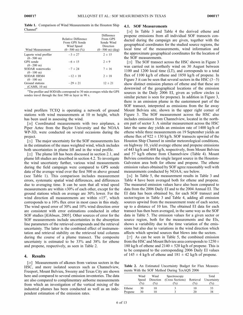
plume lift studies are described in section 4.2. To investigatethe wind uncertainty further, various wind measurementsduring the field campaign were compared to GPS sondedata of the average wind over the first 500 m above ground(see Table 1). This comparison includes measurementerrors, systematic spatial wind differences, and differencesdue to averaging time. It can be seen that all wind speedmeasurements are within ±30% of each other, except for theground stations which on average are 30% lower. For thewind direction all measurements are within ±15�, whichcorresponds to a 10% flux error in most cases in this study.The wind speed error of 30% and 10% wind direction errorare consistent with error estimations conducted in otherSOF studies [Kihlman, 2005]. Other sources of error for theSOF measurements include uncertainties in the absorptionline parameters of the retrieved compounds and the retrievaluncertainty. The latter is the combined effect of instrumen-tation and retrieval stability on the retrieved total columnsduring the course of a plume transect. The compositeuncertainty is estimated to be 33% and 38% for etheneand propene, respectively, as seen in Table 2.

4. Results

[23] Measurements of alkenes from various sectors in theHSC, and more isolated sources such as Channelview,Freeport, Mount Belvieu, Sweeny and Texas City are shownhere and compared to several emission inventories. The dataare also compared to complimentary airborne measurementsfrom which an investigation of the vertical mixing of theindustrial plumes has been conducted as well as an inde-pendent estimation of the emission rates.

4.1. SOF Measurements

[24] In Table 3 and Table 4 the derived ethene andpropene emissions from all individual SOF transects con-ducted during the campaign are given, together with thegeographical coordinates for the studied source regions, thelocal time of the measurements, wind information andthe approximate geographical coordinates for the location ofthe SOF measurements.[25] The SOF transect across the HSC shown in Figure 3

was carried out in northerly wind on 30 August between1100 and 1200 local time (LT), and corresponds to a totalflux of 1100 kg/h of ethene and 1850 kg/h of propene. InFigure 3 it can be seen that several sectors in the HSC (3–5)show distinct emission plumes of ethene and that these aredownwind of the geographical locations of the emissionsources in the Daily 2006 EI, given as yellow circles (asimilar picture is seen for propene). In addition in Figure 3,there is an emission plume in the easternmost part of theSOF transect, interpreted as emissions from the far awayMount Belvieu site, shown in the upper right corner ofFigure 3. The SOF measurement across the HSC alsoincludes emissions from Channelview, located in the north-ern part of sector 3. A similar measurement across the HSClater the same day yields an emission rate of 1400 kg/h ofethene while three measurements on 19 September yields anethene flux of 922 ± 130 kg/h. SOF transects upwind of theHouston Ship Channel in similar meteorological conditions,on highway 10, yield average ethene and propene emissionsof 443 kg/h and 488 kg/h, respectively, from Mount Belvieuand 57 kg/h ethene from Channelview (Table 4). MountBelvieu constitutes the single largest source in the Houston-Galveston area both for ethene and propene. The etheneemission values obtained by SOF agree reasonably well withmeasurements conducted by NOAA; see below.[26] In Table 5, the measurement results in Table 3 and

Table 4 have been averaged both for ethene and propene.The measured emission values have also been compared todata from the 2006 Daily EI and to the 2004 Annual EI. TheEI data has been obtained by, for each SOF transect andsector/region in Table 3 and Table 4, adding all emissionsources upwind from the measurement route of each sector,up to a distance of 10 km. The obtained EI data for eachtransect has then been averaged, in the same way as the SOFdata in Table 5. The emission values for a given sector orsource region, both for the measurements and the EIs,shows a variability due to the time variation of the emis-sions but also due to variations in the wind direction whichaffects which upwind sources that blows into the sectors.[27] As can be seen in Table 5, the combined emission

from the HSC andMount Belvieu area corresponds to 1250 ±180 kg/h of ethene and 2140 ± 520 kg/h of propene. This isto be compared to the corresponding 2006 Daily EI valuesof 145 ± 4 kg/h of ethene and 181 ± 42 kg/h of propene.

Table 1. Comparison of Wind Measurements in the Houston Ship

Channela

Wind Measurement

Relative DifferenceFrom GPS Sonde

Wind Speed(0–500 m) (%)

DifferenceFrom GPSSonde WindDirection

(0–500 m) (deg)

Laporte wind profiler(0–500 m)

�3 ± 27 2 ± 15

GPS sonde(0–200 m)

�6 ± 15 2 ± 9

SODAR waterworks(0–100 m)

�7 ± 24 7 ± 16

SODAR HRM4(0–100 m)

�12 ± 18 2 ± 18

Ground stations(CAMS, 10 m)

�29 ± 21 12 ± 21

aThe profiler and SODARs correspond to 30 min averages while the GPSsondes travel through the first 500 m layer in 90 s.

Table 2. An Estimated Uncertainty Budget for Flux Measure-

ments With the SOF Method During TexAQS 2006

WindSpeed(%)

WindDirection

(%)

Spectroscopy(Cross Sections)

(%)Retrieval

(%)

TotalUncertainty

(%)

Ethene 30 10 3 10 33Propene 30 10 3 20 38

D00F17 MELLQVIST ET AL.: SOF MEASUREMENTS IN TEXAS

6 of 13

D00F17

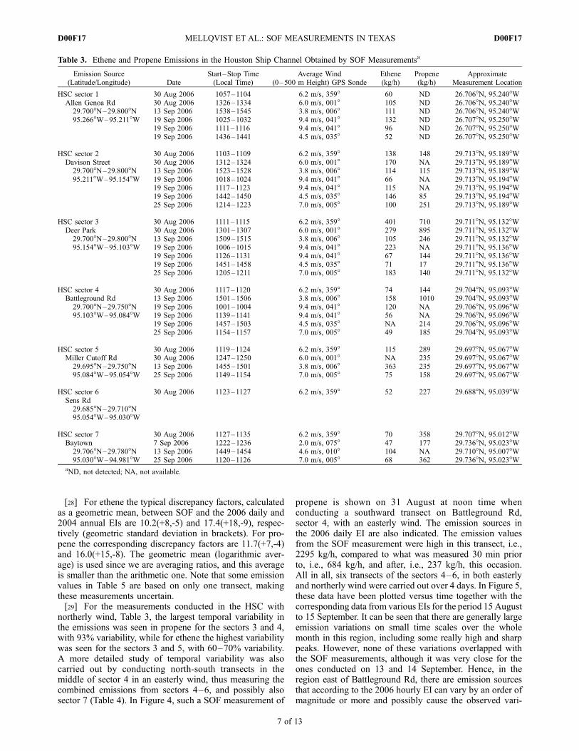
[28] For ethene the typical discrepancy factors, calculatedas a geometric mean, between SOF and the 2006 daily and2004 annual EIs are 10.2(+8,-5) and 17.4(+18,-9), respec-tively (geometric standard deviation in brackets). For pro-pene the corresponding discrepancy factors are 11.7(+7,-4)and 16.0(+15,-8). The geometric mean (logarithmic aver-age) is used since we are averaging ratios, and this averageis smaller than the arithmetic one. Note that some emissionvalues in Table 5 are based on only one transect, makingthese measurements uncertain.[29] For the measurements conducted in the HSC with

northerly wind, Table 3, the largest temporal variability inthe emissions was seen in propene for the sectors 3 and 4,with 93% variability, while for ethene the highest variabilitywas seen for the sectors 3 and 5, with 60–70% variability.A more detailed study of temporal variability was alsocarried out by conducting north-south transects in themiddle of sector 4 in an easterly wind, thus measuring thecombined emissions from sectors 4–6, and possibly alsosector 7 (Table 4). In Figure 4, such a SOF measurement of

propene is shown on 31 August at noon time whenconducting a southward transect on Battleground Rd,sector 4, with an easterly wind. The emission sources inthe 2006 daily EI are also indicated. The emission valuesfrom the SOF measurement were high in this transect, i.e.,2295 kg/h, compared to what was measured 30 min priorto, i.e., 684 kg/h, and after, i.e., 237 kg/h, this occasion.All in all, six transects of the sectors 4–6, in both easterlyand northerly wind were carried out over 4 days. In Figure 5,these data have been plotted versus time together with thecorresponding data from various EIs for the period 15 Augustto 15 September. It can be seen that there are generally largeemission variations on small time scales over the wholemonth in this region, including some really high and sharppeaks. However, none of these variations overlapped withthe SOF measurements, although it was very close for theones conducted on 13 and 14 September. Hence, in theregion east of Battleground Rd, there are emission sourcesthat according to the 2006 hourly EI can vary by an order ofmagnitude or more and possibly cause the observed vari-

Table 3. Ethene and Propene Emissions in the Houston Ship Channel Obtained by SOF Measurementsa

Emission Source(Latitude/Longitude) Date

Start –Stop Time(Local Time)

Average Wind(0–500 m Height) GPS Sonde

Ethene(kg/h)

Propene(kg/h)

ApproximateMeasurement Location

HSC sector 1 30 Aug 2006 1057–1104 6.2 m/s, 359� 60 ND 26.706�N, 95.240�WAllen Genoa Rd 30 Aug 2006 1326–1334 6.0 m/s, 001� 105 ND 26.706�N, 95.240�W29.700�N–29.800�N 13 Sep 2006 1538–1545 3.8 m/s, 006� 111 ND 26.706�N, 95.240�W95.266�W–95.211�W 19 Sep 2006 1025–1032 9.4 m/s, 041� 132 ND 26.707�N, 95.250�W

19 Sep 2006 1111–1116 9.4 m/s, 041� 96 ND 26.707�N, 95.250�W19 Sep 2006 1436–1441 4.5 m/s, 035� 52 ND 26.707�N, 95.250�W

HSC sector 2 30 Aug 2006 1103–1109 6.2 m/s, 359� 138 148 29.713�N, 95.189�WDavison Street 30 Aug 2006 1312–1324 6.0 m/s, 001� 170 NA 29.713�N, 95.189�W29.700�N–29.800�N 13 Sep 2006 1523–1528 3.8 m/s, 006� 114 115 29.713�N, 95.189�W95.211�W–95.154�W 19 Sep 2006 1018–1024 9.4 m/s, 041� 66 NA 29.713�N, 95.194�W

19 Sep 2006 1117–1123 9.4 m/s, 041� 115 NA 29.713�N, 95.194�W19 Sep 2006 1442–1450 4.5 m/s, 035� 146 85 29.713�N, 95.194�W25 Sep 2006 1214–1223 7.0 m/s, 005� 100 251 29.713�N, 95.189�W

HSC sector 3 30 Aug 2006 1111–1115 6.2 m/s, 359� 401 710 29.711�N, 95.132�WDeer Park 30 Aug 2006 1301–1307 6.0 m/s, 001� 279 895 29.711�N, 95.132�W29.700�N–29.800�N 13 Sep 2006 1509–1515 3.8 m/s, 006� 105 246 29.711�N, 95.132�W95.154�W–95.103�W 19 Sep 2006 1006–1015 9.4 m/s, 041� 223 NA 29.711�N, 95.136�W

19 Sep 2006 1126–1131 9.4 m/s, 041� 67 144 29.711�N, 95.136�W19 Sep 2006 1451–1458 4.5 m/s, 035� 71 17 29.711�N, 95.136�W25 Sep 2006 1205–1211 7.0 m/s, 005� 183 140 29.711�N, 95.132�W

HSC sector 4 30 Aug 2006 1117–1120 6.2 m/s, 359� 74 144 29.704�N, 95.093�WBattleground Rd 13 Sep 2006 1501–1506 3.8 m/s, 006� 158 1010 29.704�N, 95.093�W29.700�N–29.750�N 19 Sep 2006 1001–1004 9.4 m/s, 041� 120 NA 29.706�N, 95.096�W95.103�W–95.084�W 19 Sep 2006 1139–1141 9.4 m/s, 041� 56 NA 29.706�N, 95.096�W

19 Sep 2006 1457–1503 4.5 m/s, 035� NA 214 29.706�N, 95.096�W25 Sep 2006 1154–1157 7.0 m/s, 005� 49 185 29.704�N, 95.093�W

HSC sector 5 30 Aug 2006 1119–1124 6.2 m/s, 359� 115 289 29.697�N, 95.067�WMiller Cutoff Rd 30 Aug 2006 1247–1250 6.0 m/s, 001� NA 235 29.697�N, 95.067�W29.695�N–29.750�N 13 Sep 2006 1455–1501 3.8 m/s, 006� 363 235 29.697�N, 95.067�W95.084�W–95.054�W 25 Sep 2006 1149–1154 7.0 m/s, 005� 75 158 29.697�N, 95.067�W

HSC sector 6 30 Aug 2006 1123–1127 6.2 m/s, 359� 52 227 29.688�N, 95.039�WSens Rd29.685�N–29.710�N95.054�W–95.030�W

HSC sector 7 30 Aug 2006 1127–1135 6.2 m/s, 359� 70 358 29.707�N, 95.012�WBaytown 7 Sep 2006 1222–1236 2.0 m/s, 075� 47 177 29.736�N, 95.023�W29.706�N–29.780�N 13 Sep 2006 1449–1454 4.6 m/s, 010� 104 NA 29.710�N, 95.007�W95.030�W–94.981�W 25 Sep 2006 1120–1126 7.0 m/s, 005� 68 362 29.736�N, 95.023�W

aND, not detected; NA, not available.

D00F17 MELLQVIST ET AL.: SOF MEASUREMENTS IN TEXAS

7 of 13

D00F17

ability on 31 August. Even though there are 21 propenesources in this area in the hourly EI, all the large fluctua-tions seen in Figure 5 are dominated by emissions from fourflares, marked with red circles in Figure 4. Noteworthy isthat the high propene flux measured by SOF in Figure 4 waslocated just downwind of these four flares. Similar measure-ments were also conducted in sector 3 with the same type ofresults.[30] In Figure 6, SOF measurements are shown at the

isolated source in Sweeny on 27 September together with2006 daily EI data. The average emission for three measure-ments on this day for ethene and propene corresponds to160 ± 34 kg/h and 127 ± 65 kg/h, respectively. This can becompared to the 2006 Daily EI values of 10 and 8 kg/h forethene and propene, respectively. The GPS wind measure-ment was conducted just north of the facility. Airbornemeasurements were conducted in parallel here to investigatethe plume lift, as described below.

4.2. Complementary Airborne Measurements

[31] Measurements of ethene at Mount Belvieu, sector 8,by the NOAAWP-3D during September of 2006 shows anaverage emission of 520 kg/h with an uncertainty of 50%,based on 10 transects between 13 September and 13October [de Gouw et al., 2009]. This can be compared withthe average SOF value from Table 5 of 443 kg/h with anuncertainty of 35%, based on 6 transects (31 August, 13September and 25 September). The 2006 daily EI shows anemission value of 81 kg/h here. The emissions from theWP-3D were obtained by measuring the mixing ratio ofethene at distances corresponding to 1000–2000 s transporttime of the plume downwind of the industry, at severalflight altitudes. It was then assumed that the gas plume waswell mixed through the whole mixing layer and this made itpossible to calculate gas columns from the measured mixingratio data. These columns, integrated across the plume, werethen converted to a gas flux by multiplication with the windspeed, in a similar fashion to the SOF method.

Table 4. Ethene and Propene Emissions From Various Isolated Sources in Southeast Texas and the Eastern Part of the Houston Ship

Channel Obtained by SOF Measurementsa

Source Region Latitude/Longitude Borders Date Local Time

Average Wind(0–500 m Height)

GPS SondeEthene(kg/h)

Propene(kg/h)

ApproximateMeasurement Location

Bayport 26 Sep 2006 1054–1109 2.3 m/s, 038� 163 ND 29.622�N, 95.096�W29.662�N–29.665�N95.096�W–95.032�W

Channelview 31 Aug 2006 1648–1703 3.0 m/s, 043� 46.268 ND 29.823�N, 95.127�W29.810�N–29.838�N 31 Aug 2006 1757–1813 2.0 m/s, 126� 22.751 ND 29.823�N, 95.127�W95.125�W–95.101�W 19 Sep 2006 1355–1408 6.0 m/s, 032� 60.682 ND 29.770�N, 95.182�W

26 Sep 2006 1515–1529 2.8 m/s, 051� 97.924 ND 29.820�N, 95.127�W

Chocolate Bayou 27 Sep 2006 1027–1049 4.1 m/s, 184� 136 273 29.268�N, 95.190�W29.240�N–29.260�N95.228�W–95.204�W

Freeport 27 Sep 2006 1237–1252 4.0 m/s, 183� 215 ND 29.007�N, 95.397�W28.940�N–29.260�N 27 Sep 2006 1302–1344 4.0 m/s, 183� 325 ND 29.007�N, 95.397�W95.228�W–95.204�W 27 Sep 2006 1417–1425 5.0 m/s, 200� 211 ND 29.007�N, 95.397�W

Mount Belvieu 30 Aug 2006 1132–1142 6.2 m/s, 359� 354 NA 29.719�N, 94.947�W29.820�N–29.883�N 30 Aug 2006 1216–1229 6.0 m/s, 001� 275 NA 29.727�N, 94.909�W94.941�W–94.878�W 19 Sep 2006 1311–1333 6.0 m/s, 032� 331 222 29.810�N, 94.950�W

25 Sep 2006 1456–1524 6.6 m/s, 353� 559 NA 29.820�N, 94.912�W25 Sep 2006 1555–1606 6.6 m/s, 353� 536 646 29.820�N, 94.912�W25 Sep 2006 1643–1701 6.6 m/s, 353� 605 596 29.820�N, 94.912�W

Sweeny 21 Sep 2006 1148–1154 10.0 m/s, 191� 55 NA 29.079�N, 95.750�W29.062�N–29.084�N 21 Sep 2006 1156–1201 10.0 m/s, 191� 174 NA 29.079�N, 95.750�W95.761�W–95.731�W 21 Sep 2006 1445–1502 10.0 m/s, 191� 273 NA 29.079�N, 95.750�W

27 Sep 2006 1616–1622 2.2 m/s, 185� 136 NA 29.079�N, 95.750�W27 Sep 2006 1643–1651 2.2 m/s, 185� 124 79 29.079�N, 95.750�W27 Sep 2006 1708–1716 2.2 m/s, 185� 186 200 29.079�N, 95.750�W27 Sep 2006 1726–1750 2.2 m/s, 185� 192 101 29.079�N, 95.750�W

Texas City 20 Sep 2006 0929–0939 3.8 m/s, 060� 80 ND 29.363�N, 94.947�W29.354�N–29.384�N 20 Sep 2006 1208–1215 3.8 m/s, 060� 72 ND 29.363�N, 94.947�W94.949�W–94.888�W 20 Sep 2006 1228–1235 3.8 m/s, 060� 95 ND 29.363�N, 94.947�W

HSC east 31 Aug 2006 1054–1112 2.3 m/s, 075� 158.82 NA 29.723�N, 95.089�WSector 4–6 31 Aug 2006 1150–1209 2.3 m/s, 075� 254.28 683.61 29.723�N, 95.089�W29.690�N–29.740�N 31 Aug 2006 1219–1234 2.3 m/s, 075� 276.42 2294.6 29.723�N, 95.089�W95.090�W–95.032�W 31 Aug 2006 1252–1310 2.3 m/s, 075� 95.139 237.47 29.723�N, 95.089�W

14 Sep 2006 1435–1500 5.6 m/s, 107� 479.82 1319.8 29.723�N, 95.089�W14 Sep 2006 1537–1603 4.0 m/s, 120� 264.92 NA 29.723�N, 95.089�W14 Sep 2006 1608–1636 4.0 m/s, 120� 437.32 NA 29.723�N, 95.089�W

aND, not detected; NA, not available.

D00F17 MELLQVIST ET AL.: SOF MEASUREMENTS IN TEXAS

8 of 13

D00F17

Table 5. Average Ethene and Propene Emissions Obtained by SOF Measurements and Emission Inventories for September 2006a

Source Region SpeciesSOF 2006(kg/h)

2006 Daily Inventory(kg/h)

2004 Annual Inventory(kg/h)

Number ofMeasurements

HSC sector 1: Ethene 93 ± 28 5.2 ± 1.1 1.5 ± 0.3 6Allen Genoa Rd Propene NDHSC sector 2: Ethene 122 ± 31 12.8 ± 2.4 8.0 ± 1.2 7Davison Street Propene 150 ± 62 8.9 ± 4.3 8.1 ± 0.9 4HSC sector 3: Ethene 190 ± 113 4.7 ± 0.5 3.8 ± 0.6 7Deer Park Propene 359 ± 325 13.0 ± 2.0 8.14 ± 0.9 6HSC sector 4: Ethene 91 ± 41 13.3 ± 0.9 3.6 ± 2.1 5Battleground Rd Propene 388 ± 360 62.6 ± 21.1 20.3 ± 5.9 4HSC sector 5: Ethene 184 ± 127 15.7 ± 6.9 29.6 ± 0.8 3Miller Cutoff Rd Propene 229 ± 47 29.5 ± 36.6 10.7 ± 5.0 4HSC sector 6: Ethene 52 2.8 3.3 1Sens Rd Propene 227 0 0 1HSC sector 7: Ethene 72 ± 21 9.4 ± 1.2 6.5 ± 0.2 4Baytown Propene 300 ± 86 23.7 ± 4.3 35.3 ± 11.3 3Total HSCb Ethene 804 ± 127 64 ± 3.0 56 ± 0.2

Propene 1653 ± 490 138 ± 43 82 ± 11Bayport Ethene 163 22.4 6.8 1

Propene ND 13.2 10.8 1Channelview Ethene 57 ± 27 7.3 ± 0.2 11.8 ± 0.1 4

Propene NDChocolate Bayou Ethene 136 42.1 10.0 1

Propene 273 29.3 24.7 1Freeport Ethene 250 ± 53 39.0 ± 1.9 7.0 ± 10.0 3

Propene NDMount Belvieu Ethene 443 ± 127 81.1 ± 1.8 44.8 ± 0.0 6

Propene 488 ± 189 35.0 ± 3.2 12.2 ± 1.0 3Sweeny Ethene 163 ± 63 10.0 ± 0.2 4.8 ± 0.0 7

Propene 127 ± 53 7.4 ± 0.2 5.1 ± 0.0 3Texas City Ethene 83 ± 9 7.0 ± 0.0 8.6 ± 0.0 3

Propene ND 8.7 ± 0.0 10.7 ± 0.0 3aThe given variability is not the uncertainty but corresponds to the variations of the emissions and variations in which sources blows in to the sectors due

to the wind direction. The sectors in the HSC were measured in northerly wind. ND, not detected.bIncludes Channelview.

Figure 4. SOF measurement of propene columns on 31 August 2006 when conducting a southwardtransect on Battleground Rd. North is to the right. The emission rates of the point sources in the Daily2006 EI in kg/h are shown in yellow circles and the dominant ones are shown in red. The total columnvalues are also shown at the bottom of the plot.

D00F17 MELLQVIST ET AL.: SOF MEASUREMENTS IN TEXAS

9 of 13

D00F17

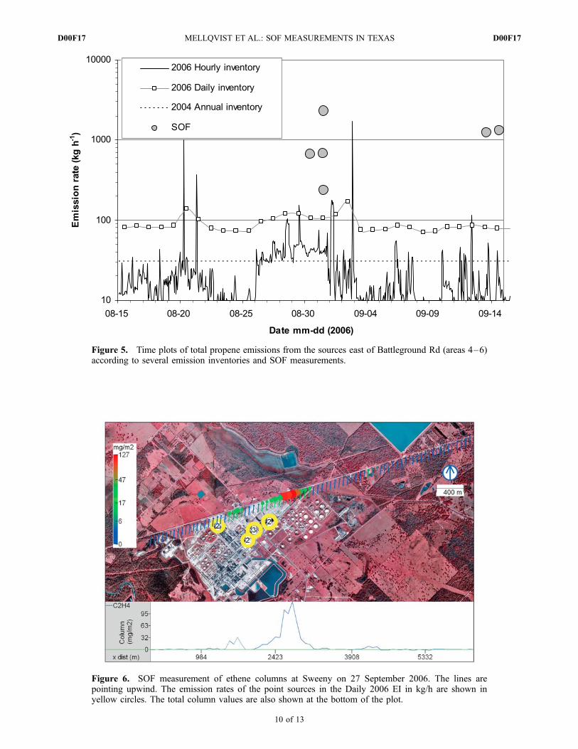
Figure 5. Time plots of total propene emissions from the sources east of Battleground Rd (areas 4–6)according to several emission inventories and SOF measurements.

Figure 6. SOF measurement of ethene columns at Sweeny on 27 September 2006. The lines arepointing upwind. The emission rates of the point sources in the Daily 2006 EI in kg/h are shown inyellow circles. The total column values are also shown at the bottom of the plot.

D00F17 MELLQVIST ET AL.: SOF MEASUREMENTS IN TEXAS

10 of 13

D00F17

[32] The Piper Aztec from Baylor University flew abovethe SOF path on several occasions. On 27 Septembermeasurements were conducted at several heights close tothe industrial facility in Sweeny along the SOF path shownin Figure 6. In Figure 7 the horizontally integrated concen-tration values of alkenes (ppm�m) from the airborne RADinstrument are shown as gray circles, across the plumeversus height. In addition the wind profile measured bythe GPS sounding just north of the facility is shown. TheRAD values have been post corrected by a factor of 1.76 byassuming a number ratio between ethene and propene of 1.9in the plume as measured by the SOF instrument during thesame time and taking into account the response factors ofthe two species. It is estimated that the measurements weretaken at a distance from the source which corresponds to250 s transport time downwind of the plume. It can be seenthat the highest average value is found at 150 m altitude,although there is quite a large variability, and that theaverage value is 50% lower at the higher altitudes up to atleast 600 m. The large variability at the lower altitude isprobably caused by the fact that the plume is ratherturbulent at this height. The 50% lower values at the higheraltitudes are consistent with the fact that the wind speed ishigher above 150 m and that it is diluting the concentrationmore there. It thus seems that the plume is mixed evenly up

to at least 600 m, and this indicates a 2.5 m/s vertical mixingspeed since the plume traveling time is 250 s. This value issurprisingly high, compared to the vertical wind measure-ment of 0.5–1 m/s conducted by the Doppler LIDARalready mentioned in section 2. From the mixing ratio datain Figure 7 a rough mixing ratio profile has been derived bycalculating the average mixing ratio of the lower altitudesand then the average of the upper altitude values and thenassuming zero values above 600 m. Assuming this profile tobe correct it is possible to calculate the true mass weightedwind speed, according to equation (2) which should be usedfor the SOF measurements, and in this case it corresponds to3.3 m/s. This should be compared to the average wind valueover the first 200 m, i.e., 2.2 m/s, applied in the SOFmeasurement and which yields a flux value that is 33%lower than the mass weighted wind speed.[33] Similar measurements to the one in Sweeny were

made by the Baylor Piper Aztec airplane at the nearbyFreeport industrial facility with similar results; the VOCs inthe plume mixed all the way up to 500 m, at a plume traveltime of about 250 s downwind of the source. Measurementswere also conducted at Texas City with a plume rising toabout 300 m, but here it is uncertain how far away thesources were.

Figure 7. Measurement of alkenes with the Baylor Piper Aztec. The horizontally integratedconcentration values across the plume are shown with gray circles. In addition the wind profilemeasured by the GPS sounding and the assumed average alkene profile are shown.

D00F17 MELLQVIST ET AL.: SOF MEASUREMENTS IN TEXAS

11 of 13

D00F17

[34] The flux from the average mixing ratio profile inFigure 7 can be obtained by multiplying the concentrationwith the wind speed at each height in the same manner as inthe SOF approach. An alkene flux of 450 kg/h is obtained,which should be compared with the SOF estimate of thealkene emission for this day of 287 kg/h. It is also possibleto calculate the emissions from the Sweeny facility in anindirect way by calculating the average mass ratio ofalkenes to NOy in the plume from the airborne data andthen multiplying with the reported emission rate of NOx forthe facility [Ryerson et al., 2003]. This assumes that thelatter value is better understood than the alkene emission.Here, an alkene to NOy ratio of 1.4 was obtained by takingthe ratio of the sum of all alkenes from the RAD instrumentand the sum of all NOy, obtained by chemiluminescence.The emission rate of NOx reported for Sweeny in the 2006daily EI is 292 kg/h, and thus this implies that the emissionof alkenes corresponds to 397 kg/h, obtained throughmultiplication with the measured alkene to NOx ratio.[35] Another parallel measurement between SOF and the

Baylor Piper Aztec was conducted at the industrial site inChocolate Bayou. Here the SOF measurements, Table 5show that 368 kg/h of alkenes are being emitted, to becompared to 530 kg/h obtained from the airborne measure-ments using the ratio between alkenes, measured by RADand NOy and the 2006 daily EI value of NOx.

5. Discussion and Conclusion

[36] The results from the campaign that was carried outduring September 2006 in the Houston area, show that theemissions of ethene and propene, obtained by SOF, are onaverage an order of magnitude larger than what is reportedin the 2006 daily EI. The largest single emission source ofHRVOCs in the vicinity of Houston was the Mount Belvieuarea with emissions that are 5 and 12 times higher for etheneand propene, respectively, than reported in the 2006 daily EI.[37] In some sectors in the HSC, large variability in the

alkene emissions, especially propene, was observed down-wind of petrochemical plants. There is poor correlationbetween these measurements and the emission ratesreported in the 2006 hourly EI, but the same plants ingeneral report highly variable flare emissions during Augustand September 2006, which actually dominate their totalemissions of alkenes from time to time.[38] As described in section 2.2 the reported emissions

for flares are based on monitoring of the mass flow to theflares. The hourly emission inventory developed from thisdata assumes a fixed combustion efficiency of 98–99%,corresponding to the permitting guidance for flares. Asshown in this work this current approach does not matchobservations.[39] Even though there is poor correlation between the

measurement and the EI, we believe it is still likely that thevariable and large emissions measured by SOF are causedby flaring, since these were measured just downwind of theflares, i.e., coincide geographically, and due to their largetemporal variation, which is consistent with flaring events.This is consistent with the fact that large alkene emissionsfrom petrochemical flares have been observed in anotherSwedish SOF study [Mellqvist, 2001].

[40] The estimated uncertainty for the SOF measurementsis about 35%, based on the measured variability in the windduring the campaign, i.e., 30%, and assumptions aboutvertical mixing, i.e., that the plume mixes vertically witha speed of 0.5–1 m/s. As discussed in section 2.1 thevertical wind speed is supported by the NOAA DopplerLIDAR measurements. It is further supported by airbornemeasurements by the Baylor Piper Aztec in Sweeny andFreeport, showing that the alkene plume was distributed upto 600 m, even at a plume transport time of 250 s downwindof the plume. It is unlikely that this strong plume raise is alldue to normal vertical mixing due to convection of the air,since this would correspond to a vertical mixing speed ofmore than 2 m/s. It may instead, partly, be caused by initialplume lift due to the fact that air inside the industrial processis hotter than the surrounding air, and this may explain thestrong vertical mixing observed.[41] Airborne and SOF measurements of alkene emis-

sions were compared at three sites. For measurements atMount Belvieu, the NOAA WP-3D shows 17% higheremission values on average than the SOF measurementsduring the campaign, but for a single simultaneous mea-surement on 25 September the NOAAWP-3D shows a 60%higher value. Measurements at Sweeny on 27 September bythe Baylor Piper Aztec show emissions that were 45–55%higher than the SOF measurement. Here two approacheswere used to obtain the flux, either by using the ratio ofalkenes to NOx and then multiplying with the reported NOx

emissions and the other based on using the concentrationand mass profile in Figure 7.[42] Similar measurements at Chocolate Bayou on 27

September show an alkene emission from the airplanewhich is 47% higher than the one obtained by the SOFmethod. Here the airborne emission was obtained throughthe ratio of alkenes to NOy which was then multiplied withthe reported NOx emission. The SOF measurement here israther uncertain since only one transect was conducted.[43] Hence, in general the comparison between SOF and

airborne measurements shows an agreement within 50%.Even though several examples show that the SOF method isconsistently lower this is probably a coincidence and weactually believe that most of the discrepancy is caused byuncertainties in the airborne estimations. For instance theratio method is dependent on accurate NOx emissions in theinventory and assumes good mixing between the NOx andalkenes. This is not entirely true, as already discussed insection 1. The method applied by NOAA [de Gouw et al.,2009] has an estimated uncertainty of 50% and is dependenton full mixing in the mixing layer and that the mixing layerheight is known. Nevertheless, even though there is 17–50% discrepancy between the SOF and airborne methods,this uncertainty has to be put into context with the 900%discrepancy between the SOFmeasurements and the emissioninventories.

[44] Acknowledgments. The SOF measurements and analysis werefunded by Texas Environmental Research Consortium (TERC) underproject H53. Further analysis has also been funded by TCEQ under contract582-5-64594-FY08-06. The authors would like to thank Elisabeth Undenfor assisting with the SOF measurements and Monica Patel and CraigClements for conducting the GPS soundings. We thank TNRIS forproviding digital maps and TCEQ for supplying auto-GC and wind profiler

D00F17 MELLQVIST ET AL.: SOF MEASUREMENTS IN TEXAS

12 of 13

D00F17

data. The Baylor Piper Aztec data was funded by TERC under project H63.We thank Levi Kauffman, Tim Compton, Grazia Zanin, Maxwell Shauck,and Martin Buhr for conducting part of the work with the Piper Aztec, andNoor Gillani is acknowledged for flight planning. Joost de Gouw isacknowledged for providing LPAS data.

ReferencesAlvarez, S., et al. (2007), H-63 Aircraft Measurements in support ofTexAQS II, report, Tex. Environ. Res. Consortium, Houston.

Burton, M. R., C. Oppenheimer, L. A. Horrocks, and P. W. Francis (2001),Diurnal changes in volcanic plume chemistry observed by lunar and solaroccultation spectroscopy, Geophys. Res. Lett., 28, 843–846, doi:10.1029/2000GL008499.

de Gouw, J. A., et al. (2009), Airborne measurements of ethene from in-dustrial sources using laser photo-acoustic spectroscopy, Environ. Sci.Technol., 43, 2437–2442, doi:10.1021/es802701a.

Foy, B., et al. (2007), Modelling constraints on the emission inventory andon vertical dispersion for CO and SO2 in the Mexico City metropolitanarea using solar FTIR and zenith sky UV spectroscopy, Atmos. Chem.Phys., 7, 781–801.

Galle, B., et al. (1999), Ground Based FTIR Measurements of StratosphericTrace Species from Harestua, Norway during Sesame and Comparisonwith a 3-D Model, J. Atmos. Chem., 32(1), 147–164, doi:10.1023/A:1006137924562.

Galle, B., C. Oppenheimer, A. Geyer, A. McGonigle, and M. Edmonds(2003), A miniaturised ultraviolet spectrometer for remote sensing of SO2

fluxes: A new tool for volcano surveillance, J. Volcanol., 119, 241–254,doi:10.1016/S0377-0273(02)00356-6.

Griffith, D. W. T. (1996), Synthetic calibration and quantitative analysis ofgas-phase FT-IR spectra, Appl. Spectrosc., 50(1), 59–70, doi:10.1366/0003702963906627.

Guenther, A. B., and A. J. Hills (1998), Eddy covariance measurement ofisoprene fluxes, J. Geophys. Res., 103(D11), 13,145 – 13,152,doi:10.1029/97JD03283.

Hanst, P. L., et al. (1982), A long path infrared study of Los Angeles smog,Atmos. Environ., 16, 969–981, doi:10.1016/0004-6981(82)90183-4.

Kihlman, M. (2005), Application of solar FTIR spectroscopy for quantify-ing gas emissions, Tech. Rep. 4, Dep. of Radio and Space Sci., ChalmersUniv. of Technol., Gothenburg, Sweden.

Kihlman, M., J. Mellqvist, and J. Samuelsson (2005), Monitoring of VOCemissions from three refineries in Sweden and the Oil Harbour of Gote-borg using the solar occultation flux method, technical report, Dep. ofRadio and Space Sci., Chalmers Univ. of Technol., Gothenburg, Sweden.

Mellqvist, J. (1999), Application of infrared and UV-visible remote sensingtechniques for studying the stratosphere and for estimating anthropogenicemissions, Ph.D. thesis, Chalmers Univ. of Technol., Goteborg, Sweden.

Mellqvist, J. (2001), Flare testing using the SOF method at Borealis poly-ethene in the summer of 2000, report, Chalmers Univ. of Technol.,Gothenburg, Sweden.

Mellqvist, J., B. Galle, T. Blumenstock, F. Hase, D. Yashcov, J. Notholt,B. Sen, J.-F. Blavier, G. C. Toon, and M. P. Chipperfield (2002),Ground-based FTIR observations of chlorine activation and ozone de-pletion inside the Arctic vortex during the winter of 1999/2000,J. Geophys. Res., 107(D20), 8263, doi:10.1029/2001JD001080.

Mellqvist, J., B. Galle, J. Samuelsson, and A. Strandberg (2004), Mobilecolumn measurements of CO in megacities, in Proceedings of The XVIII

Quadrennial Ozone Symposium, edited by C. Zerefos, pp. 612–613, Int.Ozone Comm., Halkidiki, Greece.

Mellqvist, J., et al. (2005), Mobile solar FTIR Measurements of SO2, HCland HF in the gas plumes of active volcanoes, paper presented at 9thGas Workshop, Comm. on the Chem. of Volcanic Gases, Int. Assoc. ofVolcanol. and Chem. of the Earth’s Int., Palermo, Italy.

Mellqvist, J., J. Samuelsson, C. Rivera, B. Lefer, and M. Patel (2007),Measurements of industrial emissions of VOCs, NH3, NO2 and SO2 inTexas using the solar occultation flux method and mobile DOAS, report,Texas Environ. Res. Consortium, Houston.

Mellqvist, J., J. Samuelsson, C. Rivera, B. Lefer, M. Patel, andS. Alvarez (2008), Comparison of solar occultation flux measurements tothe 2006 TCEQ emission inventory and airborne measurements for theTexAQS II, report, Tex. Comm. on Environ. Qual., Austin, Tex.

Rinsland, C. P., R. Zander, and P. Demoulin (1991), Ground-based infraredmeasurements of HNO3 total column abundances: Long-term trend andvariability, J. Geophys. Res., 96(D5), 9379 – 9389, doi:10.1029/91JD00609.

Rivera, C., J. Mellqvist, J. Samuelsson, B. Lefer, S. Alvarez, andM. Patel (2010), Quantification of NO2 and SO2 emissions from theHouston Ship Channel and Texas City industrial areas during the 2006Texas Air Quality Study, J. Geophys. Res., doi:10.1029/2009JD012675,in press.

Rothman, L. S., et al. (2005), HITRAN 2004 molecular spectroscopicdatabase, J. Quant. Spectrosc. Radiat. Transfer, 96, 139 – 204,doi:10.1016/j.jqsrt.2004.10.008.

Ryerson, T. B., et al. (2003), Effect of petrochemical industrial emissions ofreactive alkenes and NOx on tropospheric ozone formation in Houston,Texas, J. Geophys. Res., 108(D8), 4249, doi:10.1029/2002JD003070.

Sharpe, S., et al. (2004), Gas-phase databases for quantitative infraredspectroscopy, Appl. Opt., 58(12), 1452–1461.

Tucker, S., et al. (2008), Doppler lidar estimation of mixing height usingturbulence, shear, and aerosol profiles, J. Atmos. Oceanic Technol., 26(4),673–688, doi:10.1175/2008JTECHA1157.1.

Walmsley, H. L., and S. J. O’Connor (1998), The accuracy and sensitivityof infrared differential absorption lidar measurements of hydrocarbonemissions from process units, Pure Appl. Opt., 7, 907 – 925,doi:10.1088/0963-9659/7/4/024.

Weibring, P., et al. (1998), Monitoring of volcanic sulphur dioxide emissionsusing differential absorption lidar (DIAL), differential optical absorptionspectroscopy (DOAS), and correlation spectroscopy (COSPEC), Appl.Phys. B, 67, 419–426, doi:10.1007/s003400050525.

Wert, B. P., et al. (2003), Signatures of terminal alkene oxidation in airborneformaldehyde measurements during TexAQS 2000, J. Geophys. Res.,108(D3), 4104, doi:10.1029/2002JD002502.

�����������������������S. Alvarez, Institute for Air Science, Baylor University, Waco, TX 76798,

USA.J. Johansson, J. Mellqvist, C. Rivera, and J. Samuelsson, Radio and

Space Science, Chalmers University of Technology, Horsalsvagen 11,SE-41296 Goteborg, Sweden. (johan.mellqvist@chalmers.se)J. Jolly, Texas Commission on Air Quality, PO Box 13087, Austin, TX

78711-3087, USA.B. Lefer, Department of Geosciences, University of Houston, Houston,

4800 Calhoun Rd., Houston, TX 77204, USA.

D00F17 MELLQVIST ET AL.: SOF MEASUREMENTS IN TEXAS

13 of 13

D00F17