�����������������

Citation: Field, R.W.; Wu, J.J.

Permeate Flux in Ultrafiltration

Processes—Understandings and

Misunderstandings. Membranes 2022,

12, 187. https://doi.org/10.3390/

membranes12020187

Academic Editors: Jia Wei Chew

and Cristiana Boi

Received: 28 December 2021

Accepted: 29 January 2022

Published: 5 February 2022

Publisher’s Note: MDPI stays neutral

with regard to jurisdictional claims in

published maps and institutional affil-

iations.

Copyright: © 2022 by the authors.

Licensee MDPI, Basel, Switzerland.

This article is an open access article

distributed under the terms and

conditions of the Creative Commons

Attribution (CC BY) license (https://

creativecommons.org/licenses/by/

4.0/).

membranes

Article

Permeate Flux in Ultrafiltration Processes—Understandingsand MisunderstandingsRobert W. Field 1,2,* and Jun Jie Wu 3,*

1 Faculty of Engineering and Environment, Northumbria University, Newcastle NE1 8ST, UK2 Department of Engineering Science, University of Oxford, Oxford OX1 3PJ, UK3 Department of Engineering, Faculty of Science, Durham University, Durham DH1 3LE, UK* Correspondence: robert.field@northumbria.ac.uk (R.W.F.); junjie.wu@durham.ac.uk (J.J.W.)

Abstract: Concentration polarization refers to the rapid emergence of concentration gradients ata membrane/solution interface resulting from selective transfer through the membrane. It is dis-tinguishable from fouling in at least two ways: (1) the state of the molecules involved (in solutionfor concentration polarization, although no longer in solution for fouling); and (2) by the timescale,normally less than a minute for concentration polarization, although generally at least two or more or-ders of magnitude more for fouling. Thus the phenomenon of flux decline occurring over a timescaleof tens of minutes should not be attributed to concentration polarization establishing itself. Thisdistinction and a number of questions surrounding modelling are addressed and clarified. There aretwo paradigmatic approaches for modelling flux, one uses the overall driving force (in which case al-lowance for osmotic effects are expressed as additional resistances) and the other uses the net drivingforce across the separating layer or fouled separating layer, although often the two are unfortunatelycomingled. In the discussion of flux decline models’ robust approaches for the determination offlux-time relationships, including the integral method of fouling analysis, are discussed and variousconcepts clarified. The final section emphases that for design purposes, pilot plant data are vital.

Keywords: concentration polarization; osmotic model; fouling; modes of fouling; design

1. Introduction

It is our privilege to have received mentorship from and been befriended by Tony overwhat is now an extended period. In the case of one of us, this stretches back to one of hisresearch trips to Europe over three decades ago (RWF), and for the rest of us, to two decadesago when one of us (JJW) was a Tan Chin Tuan academic exchange fellow at NanyangTechnological University. In bearing witness to the fact that his insatiable passion formembrane research is still very much alive, mention is made of his insightful contribution toa very recent paper we co-authored comparing fouling of a thin-film composite membranein reverse osmosis mode with the corresponding behavior in forward osmosis mode [1].This is about 40 years since his first contributions to the Journal of Membrane Scienceand to Desalination, though not his first contributions to membrane science [2,3] Theseearly papers were, respectively, on membrane surface pore characteristics and flux throughultrafiltration membranes, and factors affecting flux in crossflow filtration subjects, whichare of concern herein.

His international recognition is in part due to his prolific published output but also tohis editorship of the Journal of Membrane Science and to his contributions to conferencesboth large and small. The latter category includes the long series of roughly biennial Oxfordworkshops on membranes and water treatment starting with one on critical flux in 2002and including the first UK–Israeli Workshop and Research Event on the Application ofMembrane Technology in Water Treatment and Desalination in 2008, one on Membrane(Bio)Fouling in 2012 and one on Recent Advances in Membrane Science and Technology in

Membranes 2022, 12, 187. https://doi.org/10.3390/membranes12020187 https://www.mdpi.com/journal/membranes

Membranes 2022, 12, 187 2 of 18

2015. At these workshops and when giving plenary lectures he brought great clarity to thevarious concepts under discussion.

As fellow academics, whose formation was also chemical engineering, we note thatwe share similar concerns. At the heart of chemical and process engineering is the designand operation of processes that change the thermodynamic state, composition, morphologyor other characteristic of materials. Thus it is fitting to include a section on the designof membrane systems. Herein we confine ourselves to membrane separations and thusthe concern is with a change in composition with a feed stream being separated into twostreams one that has passed through the membrane and one that has been retained aboveit. Although a number of basic issues are addressed below, all are linked to the ultimateaims of understanding and of improving a separation process, in which a desired degreeof concentration or purification is achieved at a quantifiable rate propelled by a knowndriving force.

The format of this paper is a little unusual and has been designed with the aim ofbringing clarity and insight to a number of areas. The laudably high aim is to achieve asimilar level of clarity to that demonstrated by Tony over the past 40+ years and counting.This is a clarity that is often regrettably missing in the huge proliferation of papers today.Each of the subsequent sub-sections start with a question and these are grouped underone of three principal sections on Fundamentals, Modelling and Design. Some of thesequestions reflect subtleties and some might, by some readers, be seen as basic tutorialquestions. The common thread is that all have arisen from us observing misunderstandingsand over-simplifications in the recent peer-reviewed literature.

2. Fundamentals2.1. Is Concentration Polarisation Distinct from Fouling?

Concentration polarization refers to the emergence of concentration gradients at amembrane/solution interface resulting from selective transfer of some species throughthe membrane. The link between this natural consequence of permselectivity and theattenuation of driving forces across the active layer of the membranes themselves wasexplored in some detail for a range of membrane processes previously [4]. Here it is simplyemphasized, paraphrasing the often-overlooked work of Aimar et al. [5] that foulingand concentration polarization effects are distinguishable by two facts: (1) the state ofthe molecules involved (in solution concentration polarization, although no longer insolution for fouling); and (2) by the timescale, normally less than a minute for concentrationpolarization, although generally at least two or more orders of magnitude for fouling. Theyestablished the timescales through elegant experimentation involving the measurementof optical density. The response curves indicated that the build-up of the concentrationpolarization was achieved within 30 s in all of their experiments, which as they noted is avalue that accords with various theoretical calculations [6]. The experiments just referredto involved bovine serum albumin and for all macromolecules it is readily appreciated thatthere is a clear distinction between the build-up of macromolecules that remain in solutionadjacent to an interface and the build-up of macromolecules no longer in solution that aredeposited at the interface.

Thus to the question posed above, namely; Is concentration polarization distinct fromfouling? The answer to the ultrafiltration of macromolecules must undoubtedly be “yes”.Indeed if researchers are to use the term, ‘concentration polarization’ in a manner consistentwith the IUPAC definition that it refers to the “concentration profile that has a higher levelof solute nearest to the upstream membrane surface compared with the more-or-less well-mixed bulk fluid far from the membrane surface” [7], it is absolutely clear that it hasnothing to do with fouling. This is absolutely consistent with the statement made byresearchers from another laboratory [8] who distinguished between “(i) concentrationpolarization (i.e., accumulation of retained solutes, reversibly and immediately occurring)and (ii) fouling phenomena such as adsorption, pore-blocking and deposition of solidifiedsolutes, a long-term, and more or less irreversible process.”

Membranes 2022, 12, 187 3 of 18

Whilst maintaining a distinction between concentration and fouling, some authorssuch as those who write, “Concentration polarization (CP), produced by the accumulationof solutes on the membrane surface, causes an increased resistance to solvent transportand possibly a change in the separation characteristics of the membrane” [9] clearly createroom for a number of subtle misunderstandings. Firstly there should be no change to theintrinsic separation characteristics of the membrane as the pores have not been blockedor even partially blocked by CP and secondly there is no accumulation of solutes on themembrane surface; CP refers to the mass transfer layer adjacent to the upstream membranesurface and the associated equation includes the thickness of this mass transfer layer: Asshown elsewhere (e.g., [10,11]) the relationship linking the concentrations of the solute inthe bulk (Cb), at the interface with the membrane (Cm) and in the permeate (Cp) is:

Cm =(Cb − Cp

)exp(Pe) + Cp (1)

where Pe is the boundary layer Peclet number and is defined as Jδ/D. J is the volumetricflux through the membrane, δ is the thickness of the mass transfer boundary layer and D isthe diffusivity of the solute. The relationship is shown schematically in Figure 1.

Membranes 2022, 12, 187 3 of 18

immediately occurring) and (ii) fouling phenomena such as adsorption, pore-blocking and deposition of solidified solutes, a long-term, and more or less irreversible process.”

Whilst maintaining a distinction between concentration and fouling, some authors such as those who write, “Concentration polarization (CP), produced by the accumulation of solutes on the membrane surface, causes an increased resistance to solvent transport and possibly a change in the separation characteristics of the membrane” [9] clearly create room for a number of subtle misunderstandings. Firstly there should be no change to the intrinsic separation characteristics of the membrane as the pores have not been blocked or even partially blocked by CP and secondly there is no accumulation of solutes on the membrane surface; CP refers to the mass transfer layer adjacent to the upstream membrane surface and the associated equation includes the thickness of this mass transfer layer: As shown elsewhere (e.g., [10,11]) the relationship linking the concentrations of the solute in the bulk (𝐶 ), at the interface with the membrane (𝐶 ) and in the permeate (𝐶 ) is: 𝐶 = 𝐶 − 𝐶 exp(𝑃𝑒) + 𝐶 (1)

where 𝑃𝑒 is the boundary layer Peclet number and is defined as 𝐽𝛿/𝐷. J is the volumetric flux through the membrane, 𝛿 is the thickness of the mass transfer boundary layer and D is the diffusivity of the solute. The relationship is shown schematically in Figure 1.

Figure 1. Schematic of concentration polarization phenomena in ultrafiltration. Between the bulk feed solution (the region of constant 𝐶𝑏) and the membrane there is the mass transfer boundary layer of thickness 𝛿. Within this region the concentration is said to be polarized.

2.2. Is Concentration Polarisation the Primary Reason for Flux Decline during the Initial Period of Operation?

The quotation from a recent 2021 paper given towards the end of the previous section continues, “CP is considered as a reversible phenomenon and is the primary reason of flux decline during the initial period of operation” [9]. Elsewhere it is not uncommon for authors to mistakenly attribute the flux decline over the first 10–30 min to CP. See for example Qaid et al. [12], who in their discussion of their Figures 4 and 5 in [12] attribute all of the flux decline in the initial 25 min to concentration polarization, and only the much more modest slight decline thereon is attributed to fouling. Whilst CP can lead to a reduction in driving force, as discussed later in Section 2.5, this reduction, will be rapid. Therefore the aforementioned reduction over 25 min has to be attributed, in part, to other causes. The reductions observed by Qaid et al. [12], with their two membranes, during ultrafiltration of orange juice, would not have been due to CP per se. CP leads to higher concentration at the membrane surface as indicated by Equation (1) and this can exacerbate the formation of a fouling layer, although such a fouling layer is not reversible.

We concur with [9] that CP is a reversible phenomenon. Indeed it is suggested that the statement “CP is considered as a reversible phenomenon” be strengthened so as to state that CP is a reversible phenomenon. The answer that we would posit to the question

Figure 1. Schematic of concentration polarization phenomena in ultrafiltration. Between the bulkfeed solution (the region of constant Cb) and the membrane there is the mass transfer boundary layerof thickness δ. Within this region the concentration is said to be polarized.

2.2. Is Concentration Polarisation the Primary Reason for Flux Decline during the Initial Periodof Operation?

The quotation from a recent 2021 paper given towards the end of the previous sectioncontinues, “CP is considered as a reversible phenomenon and is the primary reason offlux decline during the initial period of operation” [9]. Elsewhere it is not uncommonfor authors to mistakenly attribute the flux decline over the first 10–30 min to CP. See forexample Qaid et al. [12], who in their discussion of their Figures 4 and 5 in [12] attributeall of the flux decline in the initial 25 min to concentration polarization, and only themuch more modest slight decline thereon is attributed to fouling. Whilst CP can lead to areduction in driving force, as discussed later in Section 2.5, this reduction, will be rapid.Therefore the aforementioned reduction over 25 min has to be attributed, in part, to othercauses. The reductions observed by Qaid et al. [12], with their two membranes, duringultrafiltration of orange juice, would not have been due to CP per se. CP leads to higherconcentration at the membrane surface as indicated by Equation (1) and this can exacerbatethe formation of a fouling layer, although such a fouling layer is not reversible.

We concur with [9] that CP is a reversible phenomenon. Indeed it is suggested that thestatement “CP is considered as a reversible phenomenon” be strengthened so as to statethat CP is a reversible phenomenon. The answer that we would posit to the question Isconcentration polarisation the primary reason for flux decline during the initial period of operation?is this: if you are referring to an initial period of up to a few minutes then the answer is‘maybe’, however if you are referring to a period beyond that then the principal reason forflux decline will be due to other factors.

Membranes 2022, 12, 187 4 of 18

2.3. Can Gel Theory Explain Flux Decline?

To many, this will seem a strange question as in the twentieth century gel theory wasnever concerned with the time evolution of fouling. However the reason for raising thisquestion will become apparent shortly. Firstly, we rearrange Equation (1) to obtain anexpression for the limiting flux at a surface concentration that is equal to a gel concentrationi.e., Cm = Cgel . If this concentration is fixed (and in the gel-polarisation model it isconsidered fixed) then from Equation (1), one can readily derive Equation (2). Clearly for agiven value of bulk concentration and fixed mass transfer conditions, the flux is predictedto have a unique value, the limiting flux, Jlim, as given by:

Jlim = k. ln(Cgel − Cp

Cb − Cp

); k = D/δ (2)

For cross-flow ultrafiltration the attraction of gel-polarization theory [8] was thatit could explain many experimental results such as (i) flux approximately proportionalto − ln(Cb), (ii) flux approximate proportional to mass transfer coefficient, and (iii) in an agewhen the tendency was to maximize flux and work in the plateau region, a reason for theinsensitivity of flux to applied pressure. However, the assumption that the concentration atthe membrane interface cannot exceed a fixed concentration leads to a peculiar assumptionnamely that “an increase in the applied pressure will then only result in an increased thick-ness in the gel layer, although not in an increase in flux”. That non-gelling macromoleculesalso displayed the same experimental behavior of flux being approximately proportionalto − ln(Cb) and to mass transfer coefficient, k, coupled with the characteristic plateauing offlux at high TMP led to the emergence of other theories as discussed elsewhere [8,13,14].Also gel-polarisation theory could not and cannot explain why for one given solute, the lim-iting concentration determined from a plot of Jlim versus − ln(Cb) as the point where fluxwould go to zero, varies when that solute is filtered in two different filtration-cells [8,15].Also as pointed out by others the supposedly constant value of Cgel . seems to vary duringfiltration [9,16,17].

It will be apparent that the answer to the question, Can gel theory explain flux decline,is, for crossflow, filtration “no”. In a batch system one can envisage an increasing bulkconcentration with a consequential decrease in the mass transfer coefficient and thus forthese reasons a decrease in the flux. However, such a decrease in flux would not be dueto the evolution of a fouling layer (although the two changes could occur side-by-side).The reason for positing the question is that equations in some recent publications (e.g., seeEquation (2) in [9]), are identical to Equation (2) above, except the subscript is omittedfrom the flux term and additionally the accompanying text treats J as a general term thatgives the clear impression that it could be a shorthand for J(t). From those who originatedgel-polarization theory it is clear that the predicted flux is the plateau flux and this shouldalways be made clear.

As the performance of membrane processes are strongly influenced by the accumula-tion of retained solutes at the membrane surface, concentration polarization needs to betaken into account. Thus film theory is highly relevant but the general adoption of theconcept of gel-polarization is not only necessary and is often a distraction. “Film theory” isthe application of Equation (1). Rewriting it as Equation (3) it is simply expressing a linkbetween the bulk concentration, the concentration at the solid-fluid interface and flux.

J = k. ln(

Cm − Cp

Cb − Cp

); k = D/δ (3)

In ultrafiltration the increase in the concentration of macromolecules at the interfacewill increase the osmotic pressure difference across the membrane and lead to viscosityincreases in the boundary layer, which decrease the mass transfer coefficient, principally byincreasing the value of the boundary layer thickness, δ. These factors are explored in thefollowing sections.

Membranes 2022, 12, 187 5 of 18

2.4. Can the Effect of Viscosity upon Mass Transfer Explain a Limiting Flux?

The boundary layer thickness δ is not the value that would be obtained under isovis-cous conditions i.e., conditions where there is no change in viscosity across the boundarylayer and this was shown to be a crucial factor [14]. It might be argued that an exclusivefocus upon viscosity ignores changes in density and diffusivity, however Fane and oth-ers [18] concluded that an examination of physical property data shows: (a) the variationsin density are negligible; and (b) for the systems such as BSA, sucrose and dextran thevariations in viscosity are much larger than those in diffusivity. They posed the question“How does the viscosity variation with concentration affect the level of polarisation?” andin answering this question they noted that a “blow-up” in polarization can occur when thevariation in viscosity with concentration is considered.

So in looking at the concentration dependency of k (= D/δ), it is considered reasonableto relate the reduction in mass transfer coefficient solely to a viscosity ratio. This is notoffered as a general observation on the cause of flux reduction as osmotic pressure changeswill also influence the overall driving force as discussed in the next section. Additionally,for most solutions (but not all) there will the potential of fouling. Nevertheless, the effect ofmacroscopic viscosity upon the velocity profile has been shown to be significant and theviscosity dependency of the mass transfer coefficient can on its own in principle lead to alimiting flux [19]. So the answer to the question posed is ‘yes’. Whilst the viscosity profileis more important than physiochemical phenomena such as changing solute mobilities, anequally important phenomenon is the increase in osmotic pressure at the interface due tothe concentration profile.

2.5. Can the Effect of Osmotic Pressure Explain a Limiting Flux?

Concentration polarization has four main effects [14]: (a) changes in the physico-chemical properties of the fluid within the membrane boundary layer (e.g., viscosity);(b) an enhanced osmotic pressure difference across the membrane that partially offsets theapplied pressure difference; (c) changes in the membrane properties due to membrane-solute interactions (i.e., fouling); and (d) the potential of gelation at sufficiently high surfaceconcentrations of certain macromolecules. Thus osmotic pressure models are intrinsicallylinked to the phenomenon of concentration polarization.

Aimar and Sanchez [20] quantitatively linked effects (a) and (b). They proposeda model to describe the relationship between permeate flux, J, TMP, Cb and crossflowvelocity for a range of fluxes from zero to the limiting value with a limited number ofparameters being obtained from experimental data. Their model, like all other osmoticpressure models, did not predict the slight decrease in flux, which can occur at hightransmembrane pressures. Now for solutions that do not foul or gel at high concentrations(e.g., those of dextran) there is some evidence that at high pressures and low crossflowvelocities the flux decreases slightly with increasing pressure. Later it was confirmed froma theoretical viewpoint that such a decrease can only be caused by concentration increasesin the boundary layer leading to a decrease in the average mass-transfer coefficient [14].These authors also proposed a methodology for the calculation of permeate fluxes as afunction of the transmembrane pressure for the ultrafiltration of ideal solutions, where‘ideal’ indicates the absence of fouling and gelation. The model allows for the influence ofboth osmotic pressure and the variation in viscosity due to concentration polarization. Thusto make predictions knowledge of osmotic pressure and viscosity as a function of soluteconcentration is required. The only membrane parameter that has to be experimentallydetermined is the membrane permeability. The set of equations that need to be solved arethe following pair of equations, one of which (Equations (3)) has already been introduced:

J = k. ln(

Cm − Cp

Cb − Cp

)(3)

J =∆P − ∆π

µpRm(4)

Membranes 2022, 12, 187 6 of 18

where µp is the viscosity of the permeate and Rm is the hydraulic resistance of the mem-brane, ∆P is the TMP across the membrane and ∆π is the osmotic pressure difference acrossthe membrane itself. Often (e.g., as in [9]) this is not made clear. To be precise, the difference∆π = πm − πp where the terms on the righthand side are, respectively, the osmotic pres-sure at the interface on the upstream side and on the permeate side. To calculate the osmoticpressure difference a relationship between osmotic pressure and solute concentration isrequired. For many macromolecular solutions an appropriate expression takes the form ofa virial expansion. Thus,

π = B1C + B2C2 + B3C3 (5)

where B1, B2, and B3 are the osmotic virial coefficients, and C is the concentration of themacromolecular solute (g L−1).

An expression similar to Equation (5) above is required for the viscosity of the feedsolution. Given this information the mass transfer, k can be linked to that which wouldhold for isoviscous conditions. The correction factor adopted in [14] was similar to thatused by others in the field of ultrafiltration [21,22]. The expression for the mass transfercoefficient, k is then given by:

k = k0(µb/µm)z (6)

where k0 is the mass transfer coefficient for isoviscous conditions and the viscosity termsrefer to the viscosity of the bulk solution and to that of the concentrated solution at themembrane surface. The index z will have a value of around 0.14 [14,23].

Thus the osmotic pressure model (preferably with due allowance for the effect ofboundary layer viscosity gradient upon mass transfer) accomplishes everything that thegel-polarization model achieved and more. There is no need to hypothesize a gel layer andthe full range of flux is covered.

2.6. What Is the Flux Paradox?

When filtering colloidal suspensions “puzzlingly high” fluxes can be observed; mem-branologists refer to these as “puzzlingly high” as Equation (3) indicates the flux shoulddecrease with decreasing values of diffusivity, D. Now larger particles have lower valuesof D, as given by calculations of Brownian diffusion, than macromolecules, however theobserved fluxes are higher. Hence, the use of the term ‘paradox’.

One of the first observations of this “colloid flux paradox” can be attributed toCohen et al. [24]. A physical explanation for it can be acquired through balancing surfaceinteraction, diffusion and convection [25]. When compared to other transport phenomena,surface interaction has been shown, for particle size between 10 nanometers and 10 micronsto be responsible for fluxes, which are well above the ones given with other transportphenomena such as diffusion, shear induced diffusion and lateral migration. The potentialimportance of surface interactions is well illustrated elsewhere, see for example Figure3 in [26]. In the absence of significant charge interactions, the dominant mechanism willdepend on the particle size and the tangential shear rate. As noted in [9], “for typical shearrates, Brownian diffusion is important for submicron particles, the inertial lift is importantfor particles larger than approximately 10 microns, and shear-induced diffusion is dominantfor intermediate-sized particles.” The equations relevant to these mechanisms can be foundin [27] and for an overall review see [28]. In terms of the equations given above, one cansay that the back-transport mechanisms will influence the “k” in Equation (3). Membranepermeability does have a direct effect upon the mechanisms governing diffusion, howeverthe link between Equations (3) and (4) is the overall flux and this is determined in partby the transmembrane pressure and the membrane resistance. Predictions for complexmixtures involving colloids are extremely problematic and further comment is left untilSection 4.

Membranes 2022, 12, 187 7 of 18

3. Modelling of Flux Decline3.1. What Is an Appropriate Classification for Flux Decline Models?

A statement such as “Some authors [five references given] have said that the mod-els applied in UF for flux prediction can be grouped into five categories: (i) concentra-tion polarization models; (ii) osmotic pressure models; (iii) resistance-in-series models;(iv) fouling models, based on the classical film theory model; and (v) non-phenomenologicalmodels” [9] will puzzle many. Questions arising ask whether there is an agreed positionin the literature that there are five category of models, and, whether there five distinctcategories. Upon consulting the first of the five references (e.g., [8] which was mentionedin another context above) it is clear that ‘five’ is not an agreed position. That 1990 pa-per actually mentions just three categories almost corresponding to (i) to (iii) howeverinstead of ‘concentration polarization’ they mention ‘gel-polarization’, which as discussedin Section 2.3 (and captured by Equations (2) and (3)) are two related yet distinct concepts.Confusingly, Figure 1 of [9] is inconsistent with the text that was quoted at the beginning ofthe paragraph.

The number of categories should follow from a careful consideration of their un-derlying basis. Now from the discussion in Section 2 it will be clear that concentrationpolarization is part of the foundation of osmotic models. Therefore the separating off ofosmotic models can lead to a false dichotomy. Clearly the creation of a division runs therisk of creating a false understanding that they are not linked. Likewise, the separationof resistance-in-series models from fouling models ignores the fact that a fouling modelbased upon cake formation is a model that has a cake resistance in series with a membraneresistance. Hermia’s seminal paper [29] on constant pressure filtration, which they includein their fourth category, has nothing to do with “classical film theory” and thus the qual-ification of the category “(iv) fouling models” by the addition of the phrase, “based onthe classical film theory model” is not illuminating and instead confuses. An appropriateclassification would distinguish between models that generate expressions for ideal fluxes(i.e., no fouling included) and those that include fouling. With regard to fouling models,there are those models that allow for length of the flow channels (see example in [27])and those that do not [29,30]. In agreeing with [27] that for short times the transient fluxdecline is closely approximated by dead-end batch filtration theory, it is noted that thequalification ‘short’ is important. Thus in accordance with others e.g., [27,30] the steady orquasi-steady flux at longer times will only be appropriately modelled by expressions thatinclude a term that can reflect the steady or quasi steady flux. Thus it is a category mistaketo treat dead-end and crossflow expressions as equivalent (as for example in [31]) and anappropriate taxonomy of UF and MF models should reflect their difference. Logicianswould say that a category mistake has been committed when, once the phenomenon inquestion is properly understood, it becomes clear that the claim being made could notpossibly be true. To us the appropriate number of categories of fouling models is a matterfor debate, however the misunderstanding that one can analyze, without qualification,crossflow experimental data using dead-end models is a category mistake that needs tobe avoided.

3.2. What Is the Appropriate Viscosity in the Resistance-In-Series Model?

Now, we generalize the equation in Section 2.5 to allow for fouling:

J =∆P − ∆π

µpRt; Rt = Rm + R f (7)

where µp is the viscosity of the permeate and Rt is the overall resistance R f is the resistancedue to fouling. It is reiterated that the relevant viscosity is that of the permeate. Often(e.g., [9,31] there is just a reference to “the viscosity of solution” and the viscosity term islabelled simply as µ. When this is coupled with a mention that viscosity increases withsolute concentration, there is the clear impression that the relevant viscosity is that of the

Membranes 2022, 12, 187 8 of 18

feed solution rather than that of the permeate. Indeed, in some papers the viscosity usedin the calculation of resistance (e.g., Equation (15) in [32]) is clearly stated to be that of thefeed, which is erroneous for the following reason. The permeate is passing through themembrane and thus, to be consistent with Darcy’s law the relevant viscosity should be thatof the permeate, as clearly set out by the majority of researchers, e.g., [8,27,33].

3.3. When Is It Appropriate to Include a Concentration Polarisation Resistance Term?

In Equation (7) the driving force was that across the membrane itself, ∆P − ∆π. Analternative to this equation is to relate the flux to the overall driving force between the bulkfluid on one side and bulk fluid on the other side. With this approach one has to ascribe aresistance to the concentration polarization layer, Rcp, and this gives, with inclusion of aseparate fouling resistance term:

J =∆P

µpRt; Rt = Rm + Rcp + R f (8)

As others [34,35] have shown that the expressions in Equations (7) and (8) are ther-modynamically equivalent the answer to the question, When is it appropriate to include aconcentration polarization resistance term is as follows: it is appropriate to include a resistanceto the concentration polarization layer, Rcp in the denominator provided the driving forceis from the bulk feed on one side to the permeate on the other. One can consider that theconcentration boundary layer impedes the flow of the solvent and thus “consumes” partof the overall driving force. If this approach is taken, then Equation (8) is used. A com-mon misunderstanding is to pair the numerator of Equation (7) with the denominator ofEquation (8), however this mistakenly double counts the effect of the boundary layer.

3.4. Is There a Robust Methodology for Fouling Analysis of Crossflow Systems?

The main question is prefaced by another: what is the attraction of dead-end filtrationmodels? A tentative answer to this question might be threefold and reference the attractionof deceptive simplicity, perhaps mention that Equation (9) below is intriguing and finallytouch upon the fact that a straightforward methodology of fouling analysis, with dueallowance for crossflow, has yet to establish itself. As illustrated in Figure 2, crossflowinhibits the build-up of particles and thus the associated mass balances the need to have aremoval term as discussed elsewhere [30,36]. The allowance for crossflow leads to a modestincrease in the complexity of fouling analysis, however it is a necessity to accept thiscomplexity. Even for early times, a check should be made to see whether use of dead-endanalysis is appropriate or not.

Regarding dead-end filtration, Hermia was the first person to give a physical deriva-tion of the so-called intermediate blocking law and to provide a single equation linking thefour blocking filtration laws for porous media [29]. The mechanisms of fouling associatedwith each of these laws are illustrated in Figure 3. They are linked by a single equation:

d2tdV2 = kn

(dtdV

)n(9)

where t is time, V is filtrate volume, n is an index characteristic of a particular mode ofblocking (see Figure 3) and kn is a constant that is dependent upon the mode of blockage.In [9] it is stated that “in the intermediate blocking mechanism (n = 1), the particle sizeof the feed is the same as the membrane pore size; however the membrane pore is notnecessarily plugged by particles”. The second sentence is correct however, as a re-readingof [29] will show, the first sentence of the quote reflects a misunderstanding; no restrictionon the ratio of particle size to pore size was given by Hermia [29] other than the implicitone that the particle size is not less than the pore size.

Membranes 2022, 12, 187 9 of 18Membranes 2022, 12, 187 9 of 18

Figure 2. Main flow types in membrane separations: (a) Dead-end filtration; and (b) Crossflow filtration. Large (red) spheres represent rejected particles, small (green) spheres represent non-rejected particles, and the arrows indicate the feed flow direction. Reproduced with permission from Elsevier.

Regarding dead-end filtration, Hermia was the first person to give a physical derivation of the so-called intermediate blocking law and to provide a single equation linking the four blocking filtration laws for porous media [29]. The mechanisms of fouling associated with each of these laws are illustrated in Figure 3. They are linked by a single equation: = 𝑘 (9)

where t is time, V is filtrate volume, n is an index characteristic of a particular mode of blocking (see Figure 3) and 𝑘 is a constant that is dependent upon the mode of blockage. In [9] it is stated that “in the intermediate blocking mechanism (n = 1), the particle size of the feed is the same as the membrane pore size; however the membrane pore is not necessarily plugged by particles”. The second sentence is correct however, as a re-reading of [29] will show, the first sentence of the quote reflects a misunderstanding; no restriction on the ratio of particle size to pore size was given by Hermia [29] other than the implicit one that the particle size is not less than the pore size.

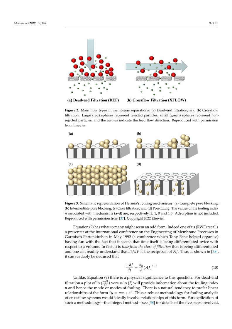
Figure 3. Schematic representation of Hermia’s fouling mechanisms: (a) Complete pore blocking; (b) Intermediate pore blocking; (c) Cake filtration; and (d) Pore filling. The values of the fouling index n associated with mechanisms (a) to (d) are, respectively, 2, 1, 0 and 1.5. Adsorption is not included. Reproduced with permission from [37]. Copyright 2022 Elsevier.

Figure 2. Main flow types in membrane separations: (a) Dead-end filtration; and (b) Crossflowfiltration. Large (red) spheres represent rejected particles, small (green) spheres represent non-rejected particles, and the arrows indicate the feed flow direction. Reproduced with permissionfrom Elsevier.

Membranes 2022, 12, 187 9 of 18

Figure 2. Main flow types in membrane separations: (a) Dead-end filtration; and (b) Crossflow filtration. Large (red) spheres represent rejected particles, small (green) spheres represent non-rejected particles, and the arrows indicate the feed flow direction. Reproduced with permission from Elsevier.

Regarding dead-end filtration, Hermia was the first person to give a physical derivation of the so-called intermediate blocking law and to provide a single equation linking the four blocking filtration laws for porous media [29]. The mechanisms of fouling associated with each of these laws are illustrated in Figure 3. They are linked by a single equation: = 𝑘 (9)

where t is time, V is filtrate volume, n is an index characteristic of a particular mode of blocking (see Figure 3) and 𝑘 is a constant that is dependent upon the mode of blockage. In [9] it is stated that “in the intermediate blocking mechanism (n = 1), the particle size of the feed is the same as the membrane pore size; however the membrane pore is not necessarily plugged by particles”. The second sentence is correct however, as a re-reading of [29] will show, the first sentence of the quote reflects a misunderstanding; no restriction on the ratio of particle size to pore size was given by Hermia [29] other than the implicit one that the particle size is not less than the pore size.

Figure 3. Schematic representation of Hermia’s fouling mechanisms: (a) Complete pore blocking; (b) Intermediate pore blocking; (c) Cake filtration; and (d) Pore filling. The values of the fouling index n associated with mechanisms (a) to (d) are, respectively, 2, 1, 0 and 1.5. Adsorption is not included. Reproduced with permission from [37]. Copyright 2022 Elsevier.

Figure 3. Schematic representation of Hermia’s fouling mechanisms: (a) Complete pore blocking;(b) Intermediate pore blocking; (c) Cake filtration; and (d) Pore filling. The values of the fouling indexn associated with mechanisms (a–d) are, respectively, 2, 1, 0 and 1.5. Adsorption is not included.Reproduced with permission from [37]. Copyright 2022 Elsevier.

Equation (9) has what to many might seem an odd form. Indeed one of us (RWF) recallsa presenter at the international conference on the Engineering of Membrane Processes inGarmisch-Partenkirchen in May 1992 (a conference which Tony Fane helped organise)having fun with the fact that it seems that time itself is being differentiated twice withrespect to a volume. In fact, it is time from the start of filtration that is being differentiatedand one can readily understand that dt/dV is the reciprocal of AJ. Thus as shown in [38],it can readably be deduced that

−dJdt

=kn

A(AJ)3−n (10)

Unlike, Equation (9) there is a physical significance to this question. For dead-endfiltration a plot of ln (−dJ

dt ) versus ln (J) will provide information about the fouling indexn and hence the mode or modes of fouling. There is a natural tendency to prefer linearrelationships of the form “y = mx + c”. Thus a robust methodology for fouling analysisof crossflow systems would ideally involve relationships of this form. For explication ofsuch a methodology—the integral method—see [38] for details of the five steps involved.

Membranes 2022, 12, 187 10 of 18

Here only a few key details are noted. One of the principal advantages of this methodover many others is the avoidance of the need to numerically differentiate data [39,40].Another advantage is that it is a practical method for identifying whether the initial foulingof a membrane is by the same mechanism as the subsequent fouling. Underpinningthis methodology is the crossflow equivalent of Equation (10), which following earlierwork [30,40], has the form:

−dJdt

= Kn J2−n(J − JR) for J > JR (11)

where J is volumetric flux, n is an index characteristic of a particular fouling mechanismand Kn is a constant that is dependent upon the mode of blockage and JR is related to thecross-flow removal from the surface of the membrane. Here as in [38] this term is taken tobe an empirical parameter that reflects removal term.

If there are two consecutive phases of fouling, then the value of JR for the secondphase will be the steady state flux. The value of JR for the first phase can be expected to bedifferent as in the example given in [38]. Basically the reason is that the surface interactionswill be different as for the first phase they involve foulant–membrane interaction and forthe second foulant–cake interaction.

Integration of Equation (11) for each of the four values of n, followed by rearrangement,leads to four different expressions, however each is of the form “y = mx + c” as given inTable 1 where “x” is v/t.

Table 1. Tabulated expressions permitting facile crossflow fouling analysis.

Complete pore blockingwith allowance forcrossflow removal

n = 2 (J0 − J)/t = Knv/t − Kn JR (12a)

Pore filling mechanism (1) n = 1.5(

J0.50 − J0.5)/t = Knv/t − Kn JR (12b)

Intermediate poreblocking with allowance

for crossflow removaln = 1 ln(J0/J)/t = Knv/t − Kn JR (12c)

Cake formation withallowance for

crossflow removaln = 0 (1/J − 1/J0)/t = Knv/t − Kn JR (12d)

(1) For this fouling mechanism, the value of JR is expected to be zero.

The integral method is a practical method for identifying whether the initial fouling ofa membrane is by the same mechanism as the subsequent fouling. Starting with v(t) andJ(t) data, the four expressions (Equation (12a–d)) can be evaluated to establish which arethe most appropriate. It is unlikely that any one equation adequately fits all the data.

The plots are likely to reveal a characteristic break as shown in Figure 4a and as foundwith the data sets checked previously [36,38]. As discussed elsewhere [38] the evaluation ofRt(t) and its derivative with respect to time can illuminate decisions regarding the mode offouling. Here the principal message from Figure 4b is that the rate of change of resistanceis nearly three times greater from 0–25 min as it is from 25–50 min. Once the breakpointhas been identified (here we assume just two phases) the two parts of the J(t) curve areevaluated separately. The main elements of the methodology are detailed elsewhere [38]and are summarized in Figure 4.

The initial plot of overall possibilities in Figure 4a indicates a breakpoint at 4 L/m2

and the existence of a clear breakpoint is confirmed by the resistance–time plot (Figure 4b).Evaluation of the most appropriate mechanism for each phase indicated that the modesn = 2 and n = 0, for the first and second phases, respectively, gave the best fit to the data.The final output is shown in Figure 4d.

Membranes 2022, 12, 187 11 of 18Membranes 2022, 12, 187 12 of 19

(a)

(b)

(c)

0

0.5

1

1.5

2

2.5

3

02468

1012141618

0 5 10 15

fn(J,

n)

V-J*t (L m-2)

n=2n=1.5n=1n=0

10

15

20

25

30

35

40

45

50

0 10 20 30 40 50 60

Resis

tanc

e

Time (minutes)

0

0.2

0.4

0.6

0.8

1

1.2

1.4

0

1

2

3

4

5

6

0 2 4 6 8 10 12 14

fn(J,

n)/t

V/t

n=1

n=0

Linear (n=1)

Linear (n=0)

Figure 4. Cont.

Membranes 2022, 12, 187 12 of 18Membranes 2022, 12, 187 13 of 19

(d)

Figure 4. (a) Initial plot of data to determine overall possibilities; (b) Data used in 𝑅(𝑡) format to check on breakpoint from one mode to the next; (c) Evaluation of most appropriate mechanism for modelling of second phase; (d) final output with data shown in blue.

The initial plot of overall possibilities in Figure 4a indicates a breakpoint at 4 L/m2 and the existence of a clear breakpoint is confirmed by the resistance–time plot (Figure 4b). Evaluation of the most appropriate mechanism for each phase indicated that the modes n = 2 and n = 0, for the first and second phases, respectively, gave the best fit to the data. The final output is shown in Figure 4d.

3.5. Can One Make Permeate Flux Predictions? When reading that “the prediction of permeate flux is critical”, one is intrigued as to

what input parameters will be used to formulate the prediction; how will the feed solution/suspension be characterized, what will characterize the membrane and how will the hydrodynamics be characterized? Papers elsewhere e.g., [9,41] freely use the word ‘prediction’ as if they will be able to make a priori prediction of the permeate flux-time curve. At best such so-called predictions are better described as a posteriori deductions. It is not clear to us that the ARIMA models evaluated elsewhere [41] actually convey much new knowledge as a result of the observations and analysis, whereas it is readily appreciated that the integral method of fouling analysis can illuminate the phases of fouling a posteriori. However neither phenomenological models nor non-phenomenological models can in general be used to make “predictions” as to predict is to say in advance what will happen in experiments.

3.6. What Differences Are Observed in Operation under Constant Flux? All of the above discussion has been concerned with constant pressure filtration. The

other canonical form of filtration is constant flux filtration, in which the transmembrane pressure (TMP) either stays constant (if there is no fouling) or increases. To illustrate the difference, it is useful to examine the following general membrane equation, in which F represents the net driving force and other terms have their normal meaning (see the nomenclature). 𝐽 = 𝐹 𝜇 (𝑅 + 𝑅 )⁄ (13)

Rearrangement and differentiation with respect to time yields: = − (14)

Regarding constant flux operation, the second term on the righthand side is zero. Thus fouling (an increase in 𝑅 ) necessitates an increase in F. Now, historically

Figure 4. (a) Initial plot of data to determine overall possibilities; (b) Data used in R(t) format tocheck on breakpoint from one mode to the next; (c) Evaluation of most appropriate mechanism formodelling of second phase; (d) final output with data shown in blue.

3.5. Can One Make Permeate Flux Predictions?

When reading that “the prediction of permeate flux is critical”, one is intrigued asto what input parameters will be used to formulate the prediction; how will the feedsolution/suspension be characterized, what will characterize the membrane and how willthe hydrodynamics be characterized? Papers elsewhere e.g., [9,41] freely use the word‘prediction’ as if they will be able to make a priori prediction of the permeate flux-time curve.At best such so-called predictions are better described as a posteriori deductions. It is notclear to us that the ARIMA models evaluated elsewhere [41] actually convey much newknowledge as a result of the observations and analysis, whereas it is readily appreciatedthat the integral method of fouling analysis can illuminate the phases of fouling a posteriori.However neither phenomenological models nor non-phenomenological models can ingeneral be used to make “predictions” as to predict is to say in advance what will happenin experiments.

3.6. What Differences Are Observed in Operation under Constant Flux?

All of the above discussion has been concerned with constant pressure filtration.The other canonical form of filtration is constant flux filtration, in which the transmem-brane pressure (TMP) either stays constant (if there is no fouling) or increases. To illus-trate the difference, it is useful to examine the following general membrane equation, inwhich F represents the net driving force and other terms have their normal meaning (seethe nomenclature).

J = F/[µp

(Rm + R f

)](13)

Rearrangement and differentiation with respect to time yields:

dR f

dt=

1µp J

∂F∂t

− Fµp J2

∂J∂t

(14)

Regarding constant flux operation, the second term on the righthand side is zero. Thusfouling (an increase in R f ) necessitates an increase in F. Now, historically experiments onconstant flux filtration have tended to involve dead-end mode despite the frequent use ofconstant flux crossflow filtration membrane operation in practical applications. The firststudy combining experiments and a thorough mathematical analysis for a constant fluxcrossflow filtration report was recent [37]. Therein a model combining intermediate poreblocking and cake filtration gave the best agreement with the experimental data. Below

Membranes 2022, 12, 187 13 of 18

the threshold flux, an intermediate pore blocking model sufficed, however as permeateflux approached and passed a threshold flux, accurate fitting of the data necessitated useof the combined model. The key finding of that paper is that in constant flux crossflowfiltration there can be (at least for some membrane-feed pairs) a finite amount of foulingnecessitating just a finite increase in the operating pressure. To many this may seem counter-intuitive, and if one focusses upon the accumulation of a material as a foulant cake (n = 0mode in Table 1) then it is would be counter-intuitive. However, for other modes it is notnecessarily counter-intuitive. Indeed when intermediate pore blocking is the only mode offouling, constant flux crossflow filtration can initially display positive dR f /dt followed bydR f /dt = 0. A mathematical explanation is given elsewhere [37].

An important caveat with respect to the findings just mentioned is that in that workthe membrane was really tight with respect to the suspended particles and/or the droplets.Thus in-pore fouling was physically impossible. Now for those applications, in whichthe product is recovered in the permeate, there is passage of macromolecules through themembrane, which necessitates very open membranes. Typically these operations are atconstant flux and for these applications there have been no reports of a threshold in thebuild-up of TMP.

The concept of a threshold flux (TF) was first developed ten years ago [42] and it wasintroduced within the context of constant flux filtration in the water industry. Examiningthree sets of pilot plant data it was found there was a modest rate of fouling below a certainflux value (which depended upon the water source) however above this value (whichvaried with the water source) there was a step change in the rate of fouling. The key fluxwas labelled as a threshold flux (TF) to distinguish it from the concept of critical flux thathad been introduced much earlier [30]. The latter is a demarcation of the point belowwhich there is no fouling. When the concept of TF was introduced it separated a region, inwhich the rate of fouling was modest from a region in which the rate of fouling was great,and generally significantly greater. Now in the aforementioned findings [37] regardinga threshold flux in constant flux crossflow filtration, in which the ratio of foulant size tomembrane pore size was large, the interesting phenomenon illustrated in Figure 5, wasobserved. Below TF, as shown in Figure 5a, the required TMP rises to a plateau valueindicating that there is initially a positive dR f /dt however the rate of increase in thefoulant resistance then goes to zero. However above TF, as shown in Figure 5b, there isan initial jump in TMP followed by a steady rate of increase. It has yet to be establishedexperimentally whether this behavior can be reproduced with macromolecules. So whilstthe findings may be irrelevant when the product is macromolecules in the permeate theyare highly relevant to the recovery of water from oily water emulsions and applicationsinvolving concentration of a feed.

Membranes 2022, 12, 187 14 of 18

experimentally whether this behavior can be reproduced with macromolecules. So whilst the findings may be irrelevant when the product is macromolecules in the permeate they are highly relevant to the recovery of water from oily water emulsions and applications involving concentration of a feed.

Figure 5. Constant flux filtration conducted with 200 ppm 0.22 µm latex bead suspension below and above the threshold flux (TF). Influence of filtration time on ΔP at (a) constant flux of 40 LMH (below the TF), and (b) constant flux of 100 LMH (above the TF). Reproduced with permission from Elsevier.

4. Design Is Pilot Plant Evaluation Essential?

Firstly, as noted in a recent paper concerning the microfiltration of skimmed milk, experimental research is essential in the development of any membrane process where the constituents exhibit a “flux paradox” [43]. As they noted, “experimental research on membrane technology is a must to predict proper operating conditions as the gel polarization model underpredicts the flux by 1 to 2 orders of magnitude in colloidal suspensions, hindering the selection of operating conditions that meet the needs of large-scale production”. Furthermore, as they also noted, most of the models that have been proposed as an alternative to the gel polarization model are only valid for laminar flow and/or for some specific particle sizes, however, microfiltration processes in the dairy industry are principally carried out in a turbulent regime [44]. Thus for such fluids membrane models are at best a guide; the process is more complex than, for example, the design of heat exchangers.

More generally the design of membrane processes involves a number of steps and the claim that permeate flux in UF processes can be predicted ab initio by either phenomenological models or non-phenomenological models is a misrepresentation. One can readily agree that several models are useful “to both describe the reduction in flux and to understand different phenomena involved in membrane filtration” [9] however to go further underplays the crucial role of pilot plant data. The basic steps, as seen by co-authors from academe and industry [45], include at least five steps: (i) Initial membrane screening; (ii) For the selected membranes, experimental evaluation at bench scale of flux and selectivity under different process conditions including various TMPs and concentrations, preferably with realistic hydrodynamic conditions; (iii) After the membranes have been evaluated, an initial process layout can be formulated based on data collected from literature, experiments and simulations. A first economic analysis can then be made to establish whether there is an economic case to move to pilot plant assessment; (iv) The evaluation of actual modules at a pilot unit so as to ensure that the results are transferable to larger scale units. Various cross-flow velocities will need to be examined and for the most promising set of conditions a full run with a number of

Figure 5. Constant flux filtration conducted with 200 ppm 0.22 µm latex bead suspension below andabove the threshold flux (TF). Influence of filtration time on ∆P at (a) constant flux of 40 LMH (belowthe TF), and (b) constant flux of 100 LMH (above the TF). Reproduced with permission from Elsevier.

Membranes 2022, 12, 187 14 of 18

4. DesignIs Pilot Plant Evaluation Essential?

Firstly, as noted in a recent paper concerning the microfiltration of skimmed milk,experimental research is essential in the development of any membrane process wherethe constituents exhibit a “flux paradox” [43]. As they noted, “experimental research onmembrane technology is a must to predict proper operating conditions as the gel polariza-tion model underpredicts the flux by 1 to 2 orders of magnitude in colloidal suspensions,hindering the selection of operating conditions that meet the needs of large-scale produc-tion”. Furthermore, as they also noted, most of the models that have been proposed as analternative to the gel polarization model are only valid for laminar flow and/or for somespecific particle sizes, however, microfiltration processes in the dairy industry are princi-pally carried out in a turbulent regime [44]. Thus for such fluids membrane models are atbest a guide; the process is more complex than, for example, the design of heat exchangers.

More generally the design of membrane processes involves a number of steps and theclaim that permeate flux in UF processes can be predicted ab initio by either phenomenolog-ical models or non-phenomenological models is a misrepresentation. One can readily agreethat several models are useful “to both describe the reduction in flux and to understand dif-ferent phenomena involved in membrane filtration” [9] however to go further underplaysthe crucial role of pilot plant data. The basic steps, as seen by co-authors from academeand industry [45], include at least five steps: (i) Initial membrane screening; (ii) For theselected membranes, experimental evaluation at bench scale of flux and selectivity underdifferent process conditions including various TMPs and concentrations, preferably withrealistic hydrodynamic conditions; (iii) After the membranes have been evaluated, an initialprocess layout can be formulated based on data collected from literature, experiments andsimulations. A first economic analysis can then be made to establish whether there is aneconomic case to move to pilot plant assessment; (iv) The evaluation of actual modules ata pilot unit so as to ensure that the results are transferable to larger scale units. Variouscross-flow velocities will need to be examined and for the most promising set of conditionsa full run with a number of operating cycles (including cleaning) should be undertaken;(v) The membrane system will be part of an overall process and the potential for synergiesshould be examined. The work of Krishna Kumar et al. [46] is one example of a food relatedpilot scale study that coupled an experimental study of the effect of selected operatingparameters on flux with cost considerations and the development of models to describe thephenomena observed.

For stage (ii), analysis such as the use of the integral method can aid understandingand help to reduce the number of experiments. Furthermore, understanding the role ofelements of modules such as spacers is important. Here again Tony Fane was involved [47].Stage (iv) may reveal that the hydrodynamic conditions at the pilot scale lead to a poorerperformance than that found at the laboratory scale. Sometimes the mass transfer conditionsat the module scale are noticeably inferior to those that had appertained at the laboratoryscale [48]. As noted previously in the paper, fouling time scales range from minutes tohours, however, as found in practice there is also potentially another timescale of days.This reinforces the need to work at the pilot scale. An important note of detail is that if thefeedstock is recycled during the evaluation period then the amount of key foulant per unitarea of membrane area may be very different from that of the proposed full-scale plant.Consideration needs to be given to foulant load as well as time of operation. Following pilotscale evaluation, a full-scale unit can be simulated and optimized, although extrapolationoutside of the parameter space covered by the pilot tests is to be avoided. There couldbe a role for non-phenomenological models at this stage, however we are not aware ofsuch work.

5. Concluding Remarks

Whilst the definition of concentration polarization (CP) as the rapid emergence ofconcentration gradients at a membrane/solution interface resulting from selective transfer

Membranes 2022, 12, 187 15 of 18

through the membrane will be readily accepted by almost the whole membrane community,there is often a confusion between the effects of CP itself (such as increased osmotic pressureat the interface) and fouling that may arise as a result of the increased concentration at theinterface. CP is distinguishable from fouling in at least two ways: (1) the timescale for theestablishment of the effect; and (2) the state of the molecules involved. Regarding the first,CP will normally be established in less than a minute although fouling can continue overtimescales of varying orders of magnitude. Crucially, CP involves molecules in solutionwhereas fouling by macromolecules involves molecules no longer in solution.

Secondly, care in the definition of terms can often tease out subtleties that are important.There are two paradigmatic approaches for modelling flux, one uses the overall drivingforce (in which case allowance for osmotic effects are expressed as additional resistances)and the other uses the net driving force across the separating layer or fouled separating layer,although often the two are unfortunately comingled. It is wrong to include a resistance tothe concentration polarization layer, Rcp in the denominator of the flux equation, whilstsimultaneously including ∆π in the numerator. One needs to choose whether one isestablishing an equation across the membrane itself, or from the bulk feed on one side tothe permeate on the other.

Whilst various approaches to the categorization of fouling models can be debated, theuse of dead-end models for the analysis of fouling in crossflow systems is to be avoided.The attraction of taking the ‘short-cut’ was identified as the easy way relationships of theform “y = mx + c” can be used. For the analysis of crossflow data the integral method offouling analysis is recommended. In addition to determining, in a clear-cut manner, thepoint at which there is a switch from one mode to another, the robust methodology yieldscharacteristic J(t) equation for each mode that are an excellent fit to the data.

Author Contributions: Conceptualization, R.W.F.; writing—original draft preparation, R.W.F. andJ.J.W.; writing—review and editing, R.W.F. and J.J.W. All authors have read and agreed to thepublished version of the manuscript.

Funding: J.J.W. is grateful to EPSRC and Durham University for an EPSRC Impact AccelerationAccount (IAA) strategic award.

Institutional Review Board Statement: Not applicable.

Informed Consent Statement: Not applicable.

Data Availability Statement: Not applicable.

Acknowledgments: Both authors are grateful to those concerned for securing a full waiver.Figures 2, 3 and 5 are reprinted from Journal of Membrane Science, volume 574 with permissionfrom Elsevier. (Source: Kirschner, A.Y., Cheng, Y.-H., Paul, D.R., Field, R.W., Freeman, B.D. Foulingmechanisms in constant flux crossflow ultrafiltration 65-75, 2019).

Conflicts of Interest: The authors declare no conflict of interest.

Abbreviations and Nomenclature

ARIMA Autoregressive integrated moving averageCP Concentration polarisationln natural logarithmPe Boundary layer Peclet numberTMP Transmembrane PressureUF Ultrafiltration

A area of membraneC concentrationD diffusivityF net driving forceJ or J(t) volumetric flux

Membranes 2022, 12, 187 16 of 18

Kn constant dependent upon the mode of blockage (Equation (11))k boundary layer mass transfer coefficient (= D/δ)kn constant dependent upon the mode of blockage (Equation (9))n index characteristic of a particular mode of blockingRf foulant resistance (m−1)Rm hydraulic resistance of the membrane (m–1)Rt overall resistance (m−1)t timeV filtrate volumev specific volume (= V/A)δ thickness of mass transfer boundary layerµ viscosityµp viscosity of the permeate∆P transmembrane pressure difference∆π osmotic pressure difference across the membrane (= πm − πp)

Subscripts

0 initialb bulkcp concentration polarisationgel gellim limitm upstream membrane surfacep permeateR removal term

References1. Field, R.W.; She, Q.; Siddiqui, F.A.; Fane, A.G. Reverse osmosis and forward osmosis fouling: A comparison. Discov. Chem. Eng.

2021, 1, 6. [CrossRef]2. Fane, A.G.; Fell, C.J.; Waters, A.G. The relationship between membrane surface pore characteristics and flux for ultrafiltration

membranes. J. Membr. Sci. 1981, 9, 245–262. [CrossRef]3. Baker, R.J.; Fane, A.G.; Fell, C.J.; Yoo, B.H. Factors affecting flux in crossflow filtration. Desalination 1985, 53, 81–93. [CrossRef]4. Field, R.W.; Wu, J.J. On boundary layers and the attenuation of driving forces in forward osmosis and other membrane processes.

Desalination 2018, 429, 167–174. [CrossRef]5. Aimar, P.; Howell, J.A.; Clifton, M.J.; Sanchez, V. Concentration polarisation build-up in hollow fibers: A method of measurement

and its modelling in ultrafiltration. J. Membr. Sci. 1991, 59, 81–99. [CrossRef]6. Velicangil, O.; Howell, J.A. Self-cleaning membranes for ultrafiltration. Biotechnol. Bioeng. 1981, 23, 843–854. [CrossRef]7. Koros, W.J.; Ma, Y.H.; Shimidzu, T. Terminology for membranes and membrane processes (IUPAC Recommendations 1996). Pure

Appl. Chem. 1996, 68, 1479–1489. [CrossRef]8. Berg, G.V.D.; Smolders, C. Flux decline in ultrafiltration processes. Desalination 1990, 77, 101–133. [CrossRef]9. Quezada, C.; Estay, H.; Cassano, A.; Troncoso, E.; Ruby-Figueroa, R. Prediction of Permeate Flux in Ultrafiltration Processes:

A Review of Modeling Approaches. Membranes 2021, 11, 368. [CrossRef]10. Zydney, A.L. Stagnant film model for concentration polarization in membrane systems. J. Membr. Sci. 1997, 130, 275–281.

[CrossRef]11. Vasan, S.S.; Field, R.W. On maintaining consistency between the film model and the profile of the concentration polarisation layer.

J. Membr. Sci. 2006, 279, 434–438. [CrossRef]12. Qaid, S.; Zait, M.; El Kacemi, K.; El Midaoui, A.; El Hajjil, H.; Taky, M. Ultrafiltration for clarification of Valencia orange juice:

Comparison of two flat sheet membranes on quality of juice production. J. Mater. Environ. Sci. 2017, 8, 1186–1194.13. Denisov, G.A. Theory of concentration polarization in cross-flow ultrafiltration: Gel-layer model and osmotic-pressure model.

J. Membr. Sci. 1994, 91, 173–187. [CrossRef]14. Field, R.; Aimar, P. Ideal limiting fluxes in ultrafiltration: Comparison of various theoretical relationships. J. Membr. Sci. 1993,

80, 107–115. [CrossRef]15. Porter, M.C. Concentration Polarization with Membrane Ultrafiltration. Prod. RD 1972, 11, 234–248. [CrossRef]16. Wijmans, J.; Nakao, S.; Smolders, C. Flux limitation in ultrafiltration: Osmotic pressure model and gel layer model. J. Membr. Sci.

1984, 20, 115–124. [CrossRef]

Membranes 2022, 12, 187 17 of 18

17. Mondal, S.; Cassano, A.; Conidi, C.; De, S. Modeling of gel layer transport during ultrafiltration of fruit juice with non-Newtonianfluid rheology. Food Bioprod. Process. 2016, 100, 72–84. [CrossRef]

18. Gill, W.N.; Wiley, D.E.; Fell, C.J.; Fane, A.G. Effect of viscosity on concentration polarization in ultrafiltration. AIChE J. 1988,34, 1563–1567. [CrossRef]

19. Aimar, P.; Field, R. Limiting flux in membrane separations: A model based on the viscosity dependency of the mass transfercoefficient. Chem. Eng. Sci. 1992, 47, 579–586. [CrossRef]

20. Aimar, P.; Sanchez, V. A novel approach to transfer-limiting phenomena during ultrafiltration of macromolecules. Ind. Eng. Chem.Fundam. 1986, 25, 789–798. [CrossRef]

21. Kozinski, A.A.; Lightfoot, E.N. Protein ultrafiltration: A general example of boundary layer filtration. AIChE J. 1972, 18, 1030–1040.[CrossRef]

22. Gekas, V.; Ölund, K. Mass transfer in the membrane concentration polarization layer under turbulent cross flow: II. Applicationto the characterization of ultrafiltration membranes. J. Membr. Sci. 1988, 37, 145–163. [CrossRef]

23. Pritchard, M.; Howell, J.A.; Field, R.W. The ultrafiltration of viscous fluids. J. Membr. Sci. 1995, 102, 223–235. [CrossRef]24. Cohen, R.; Probstein, R. Colloidal fouling of reverse osmosis membranes. J. Colloid Interface Sci. 1986, 114, 194–207. [CrossRef]25. Bacchin, P.; Aimar, P.; Sanchez, V. Model for colloidal fouling of membranes. AIChE J. 1995, 41, 368–376. [CrossRef]26. Bacchin, P.; Aimar, P.; Field, R. Critical and sustainable fluxes: Theory, experiments and applications. J. Membr. Sci. 2006,

281, 42–69. [CrossRef]27. Davis, R.H. Modeling of Fouling of Crossflow Microfiltration Membranes. Sep. Purif. Methods 1992, 21, 75–126. [CrossRef]28. Belfort, G.; Davis, R.H.; Zydney, A.L. The behavior of suspensions and macromolecular solutions in crossflow microfiltration.

J. Membr. Sci. 1994, 96, 1–58. [CrossRef]29. Hermia, J. Constant pressure blocking filtration laws—Application to power-law non-Newtonian fluids. Trans. IChemE. 1982,

60, 183–187.30. Field, R.; Wu, D.; Howell, J.; Gupta, B. Critical flux concept for microfiltration fouling. J. Membr. Sci. 1995, 100, 259–272. [CrossRef]31. Razi, B.; Aroujalian, A.; Fathizadeh, M. Modeling of fouling layer deposition in cross-flow microfiltration during tomato juice

clarification. Food Bioprod. Processing 2012, 90, 841–848. [CrossRef]32. Ochando-Pulido, J.M.; Martinez-Ferez, A. Fouling modelling on a reverse osmosis membrane in the purification of pretreated

olive mill wastewater by adapted crossflow blocking mechanisms. J. Membr. Sci. 2017, 544, 108–118. [CrossRef]33. Choi, H.; Zhang, K.; Dionysiou, D.D.; Oerther, D.; Sorial, G.A. Effect of permeate flux and tangential flow on membrane fouling

for wastewater treatment. Sep. Purif. Technol. 2005, 45, 68–78. [CrossRef]34. Wijmans, J.; Nakao, S.; Berg, J.V.D.; Troelstra, F.; Smolders, C. Hydrodynamic resistance of concentration polarization boundary

layers in ultrafiltration. J. Membr. Sci. 1985, 22, 117–135. [CrossRef]35. Ko, M.K.; Pellegrino, J.J. Determination of osmotic pressure and fouling resistance and their effects of performance of ultrafiltration

membranes. J. Membr. Sci. 1992, 74, 141–157. [CrossRef]36. Field, R.W.; Wu, J.J. Modelling of permeability loss in membrane filtration: Re-examination of fundamental fouling equations and

their link to critical flux. Desalination 2011, 283, 68–74. [CrossRef]37. Kirschner, A.Y.; Cheng, Y.H.; Paul, D.R.; Field, R.W.; Freeman, B.D. Fouling mechanisms in constant flux crossflow ultrafiltration.

J. Membr. Sci. 2019, 574, 65–75. [CrossRef]38. Wu, J.J. Improving membrane filtration performance through time series analysis. Discov. Chem. Eng. 2021, 1, 7. [CrossRef]39. Grenier, A.; Meireles, M.; Aimar, P.; Carvin, P. Analysing flux decline in dead-end filtration. Chem. Eng. Res. Des. 2008,

86, 1281–1293. [CrossRef]40. Vela, M.C.; Blanco, S.Á.; García, J.L.; Rodríguez, E.B. Analysis of membrane pore blocking models adapted to crossflow

ultrafiltration in the ultrafiltration of PEG. Chem. Eng. J. 2009, 149, 232–241. [CrossRef]41. Ruby-Figueroa, R.; Saavedra, J.; Bahamonde, N.; Cassano, A. Permeate flux prediction in the ultrafiltration of fruit juices by

ARIMA models. J. Membr. Sci. 2017, 524, 108–116. [CrossRef]42. Field, R.W.; Pearce, G.K. Critical, sustainable and threshold fluxes for membrane filtration with water industry applications. Adv.

Colloid Interface Sci. 2011, 164, 38–44. [CrossRef] [PubMed]43. Astudillo-Castro, C.; Cordova, A.; Oyanedel-Craver, V.; Soto-Maldonado, C.; Valencia, P.; Henriquez, P.; Jimenez-Flores, R.

Prediction of the Limiting Flux and Its Correlation with the Reynolds Number during the Microfiltration of Skim Milk Using anImproved Model. Foods 2020, 9, 1621. [CrossRef] [PubMed]

44. Hurt, E.; Adams, M.; Barbano, D. Microfiltration: Effect of retentate protein concentration on limiting flux and serum proteinremoval with 4-mm-channel ceramic microfiltration membranes. J. Dairy Sci. 2015, 98, 2234–2244. [CrossRef] [PubMed]

45. Field, R.; Lipnizki, F. Membrane Separation Processes: An Overview. In Engineering Aspects of Membrane Separation and Applicationin Food Processing; Field, R.W., Bekassy-Molnar, E., Lipnizki, F., Vatai, G., Eds.; CRC Press: Boca Raton, FL, USA, 2017; Chapter 1;pp. 3–40. [CrossRef]

46. Krishna Kumar, N.; Yea, M.; Cheryan, M.; Kumar, N.K. Ultrafiltration of soy protein concentrate: Performance and modelling ofspiral and tubular polymeric modules. J. Membr. Sci. 2004, 244, 235–242. [CrossRef]

Membranes 2022, 12, 187 18 of 18

47. Da Costa, A.R.; Fane, A.G.; Wiley, D.E. Spacer characterization and pressure drop modelling in spacer-filled channels forultrafiltration. J. Membr. Sci. 1994, 87, 79–98. [CrossRef]

48. Field, R.W.; Siddiqui, F.A.; Ang, P.; Wu, J.J. Analysis of the influence of module construction upon forward osmosis performance.Desalination 2018, 431, 151–156. [CrossRef]