Productivity, Respiration, and Light-Response

Parameters of World Grassland and Agro-Ecosystems

Derived From Flux-Tower Measurements

G. Gilmanov Tagir, V. Allard, D. Baldocchi, Pierre Beziat, Eric Ceschia,

Pierre Cellier, J.F. Soussana

To cite this version:

G. Gilmanov Tagir, V. Allard, D. Baldocchi, Pierre Beziat, Eric Ceschia, et al.. Productivity,Respiration, and Light-Response Parameters of World Grassland and Agro-Ecosystems DerivedFrom Flux-Tower Measurements. Rangeland Ecology and Management, Society for RangeManagement, 2009, pp.1-73. <ird-00411045>

HAL Id: ird-00411045

http://hal.ird.fr/ird-00411045

Submitted on 25 Aug 2009

HAL is a multi-disciplinary open accessarchive for the deposit and dissemination of sci-entific research documents, whether they are pub-lished or not. The documents may come fromteaching and research institutions in France orabroad, or from public or private research centers.

L’archive ouverte pluridisciplinaire HAL, estdestinee au depot et a la diffusion de documentsscientifiques de niveau recherche, publies ou non,emanant des etablissements d’enseignement et derecherche francais ou etrangers, des laboratoirespublics ou prives.

Productivity, Respiration, and Light-Response Parameters of World Grassland and 1

Agro-Ecosystems Derived From Flux-Tower Measurements 2

3

4

Tagir G. Gilmanov1 5

and data contributors2: 6

L. Aires4, K. Akshalov4, V. Allard4, C. Ammann4, M. Aubinet4, M. Aurela4, J. Baker5, D. 7

Baldocchi4, J. Balogh4, M. Balzarolo4, L. Belelli4, Z. Barcza4, C. Bernacchi4, C. 8

Bernhofer4, V.S. Baron5, J. Berringer4, P. Beziat4, D. Billesbach5, J. Bradford3, K. 9

Brehe5, N. Buchmann4, E. Ceschia4, P. Cellier4, Shiping Chen4, D. Cook4, C. Corradi4, R. 10

Coulter4, R. Czerny4, E. Dellwik4, A. Detwyler5, H. Dolman4, M. Dourikov5, W. Dugas3, 11

J. Elbers4, W. Emmerich3, W. Eugster4, D. Fitzjarrald4, L. Flanagan4, A. Frank3, J. 12

Fuhrer4, D. Gianelle4, T. Griffis5, T. Gruenwald4, M. Haferkamp3, Guo Haiquang4, N. 13

Hanan4, R. Harding4, L. Haszpra4, M. Heuer5, J. Heilman4, A. Hensen4, S. Hollinger4, A. 14

Jacobs4, D. Janous4, W. Jans4, D.A. Johnson3, M. Jones4, T. Kato4, G. Katul4, G. Kiely4, 15

W. Kutsch4, G. Lanigan4, T. Laurila5, P. Leahy4, S. Li5, A. Lohila5, V. Magliulo4, A. 16

Manzi4, M. Marek4, R. Matamala4, T. Meyers4,5, P. Mielnick3, A. Miyata4, E. Moors4, J. 17

Morgan3, C. Moureaux4, M. Nasyrov5, J. Olejnik4, J. Olesen4, W. Oechel4, C. Owensby5, 18

D. Papale4, C. Pio4, J. Prueger5, A. Raschi4, C. Rebmann4, M. Reichstein4, H. da Rocha4, 19

N. Rogiers4, N. Saliendra3, M.J. Sanz4, K. Schelde4, R. Scott4, P. Sims3, R.H. Skinner5, H. 20

Soegaard4, J.-F. Soussana4, M. Sutton4, A. Suyker4, T. Svejcar3, M. Torn5, Z. Tuba4, S. 21

Verma4, M. Waterloo4, G. Wohlfahrt4, Bin Zhao4, Guangsheng Zhou4 22

23

2

Authors are 1Associate professor at the Department of Biology and Microbiology, South 1

Dakota State University, Brookings, SAG 304, Box 2207B, SD 57007, USA, and 2

2researchers who contributed their data to the 3USDA-ARS RANGEFLUX data set, 3

4FLUXNET La Thuile data set, or 5WORLDGRASSAGRIFLUX data set. 4

5

Research was supported in part by the Science Applications International Corporation, 6

Subcontract # 4400089887 to Gilmanov Research and Consulting, LLP. 7

8

9

Correspondence: Tagir G. Gilmanov, Department of Biology and Microbiology, South 10

Dakota State University, SAG 305, Box 2207B, Brookings, SD 57006, USA. Email: 11

tagir.gilmanov@sdstate.edu 12

13

14

3

LIST OF SYMBOLS 1

2

Latin symbols 3

Amax – maximum gross photosynthetic assimilation (mg CO2 m-2 s-1) 4

CumNEE – cumulative net ecosystem CO2 exchange (g CO2 m-2) 5

Fc – net CO2 flux (mg CO2 m-2 s-1; g CO2 m-2 d-1) 6

GPP – annual gross primary production (g CO2 m-2 yr-1) 7

kT – coefficient in the exponential equation for respiration temperature dependence (°C)-1 8

L – leaf area index (m2 m-2) 9

Lmax – seasonal maximum leaf area index (m2 m-2) 10

Pd – daytime integral of the net ecosystem CO2 flux (g CO2 m-2 d-1) 11

Pg – gross photosynthetic assimilation (mg CO2 m-2 s-1; g CO2 m-2 d-1) 12

Q – incoming photosynthetically active radiation (µmol CO2 m-2 s-1; mol CO2 m-2 d-1) 13

Qa – absorbed photosynthetically active radiation (µmol CO2 m-2 s-1; mol CO2 m-2 d-1) 14

PCPN – atmospheric precipitation (mm d-1, mm yr-1) 15

rd – daytime ecosystem respiration rate (mg CO2 m-2 s-1) 16

Rd – daytime ecosystem respiration (mg CO2 m-2 s-1; g CO2 m-2 d-1) 17

Re – total ecosystem respiration (mg CO2 m-2 s-1; g CO2 m-2 d-1) 18

RE – annual total ecosystem respiration (g CO2 m-2 yr-1) 19

RH – air relative humidity (%) 20

Rn – nighttime ecosystem respiration (mg CO2 m-2 s-1; g CO2 m-2 d-1) 21

Rnet – net radiation (W m-2; MJ m-2 d-1) 22

r0 – ecosystem respiration rate at temperature Ts = 0 °C (mg CO2 m-2 s-1) 23

4

rn – night-time ecosystem respiration rate (mg CO2 m-2 s-1) 1

Rn – nighttime ecosystem respiration (mg CO2 m-2 s-1; g CO2 m-2 d-1) 2

Rnet – net radiation (W m-2; MJ m-2 d-1) 3

Ta – air temperature (°C) 4

tr – time of sunrise (h) 5

ts – time of sunset (h) 6

Ts – soil temperature (typically, at 5 cm depth) (°C) 7

Vc,max- maximum rate of carboxylation (mg CO2 m-2 s-1) ) 8

Ws – volumetric soil moisture (m3 m-3) 9

10

Greek symbols 11

α - apparent quantum yield of gross photosynthetic assimilation (mmol CO2 mol quanta-12

1) 13

ε, εecol – gross ecological light-use efficiency (mmol CO2 (mol incident quanta)-1) 14

εphys – gross physiological light-use efficiency (mmol CO2 (mol absorbed quanta)-1) 15

λ - latent heat of evaporation (MJ kg-1) 16

θ - convexity (curvature) coefficient of the light-response equation (dimensionless) 17

ρd – diffusion resistance to carbon transport (s m-1) 18

ρx – carboxylation resistance to carbon transport (s m-1) 19

20

21

22

23

24

5

ABSTRACT 1

2

Grasslands and agroecosystems occupy nearly a third of the land surface area, but their 3

quantitative contribution to the global carbon cycle remains uncertain. We used a set of 4

316 site-years of year-round net CO2 exchange (Fc) measurements to quantitatively 5

analyze gross primary productivity, ecosystem respiration, and light-response parameters 6

of extensively and intensively managed grasslands, shrublands/savanna, wetlands, and 7

cropland ecosystems worldwide. Analyzed data set included data from 72 flux-tower sites 8

worldwide partitioned into gross photosynthesis (Pg) and ecosystem respiration (Re) 9

components using the light-response functions method (Gilmanov et al. 2003, Bas. Appl. 10

Ecol. 4:167-183) from the RANGEFLUX and WorldGrassAgriflux data sets 11

supplemented by data from 46 sites partitioned using the temperature-response method 12

(Reichstein et al. 2005, Gl. Change. Biol. 11:1424-1439) from the FLUXNET La Thuile 13

data set. Maximum values of the apparent quantum yield (α = 75 mmol mol-1), 14

photosynthetic capacity (Amax = 3.4 mg CO2 m-2 s-1), maximum daily gross 15

photosynthesis (Pg,max = 116 g CO2 m-2 d-1), and gross ecological light-use efficiency 16

(εecol = 59 mmol mol-1) of intensively managed grasslands and high-productive croplands 17

exceed those for forest ecosystems, indicating high potential of non-forest ecosystems for 18

uptake and sequestration of atmospheric CO2. Maximum values of annual gross primary 19

production (8600 g CO2 m-2 yr-1), total ecosystem respiration (7900 g CO2 m-2 yr-1), and 20

net CO2 exchange (2400 g CO2 m-2 yr-1) for non-forest ecosystems are observed in 21

intensively managed grasslands and high-yield crops, and are comparable or higher than 22

in forest ecosystems (excluding tropical forests). On the average, 80% of the non-forest 23

6

sites were sinks for atmospheric CO2, with mean annual net CO2 uptake 848 g CO2 m-2 1

yr-1 for intensively managed grasslands and 933 g CO2 m-2 yr-1 for croplands. The new 2

flux-tower data indicate the need to revise substantially previous views of grassland and 3

agricultural ecosystems as being predominantly a source of carbon, or having a neutral 4

role, in the regional and continental carbon budgets. 5

6

Key Words: gross primary production, ecosystem respiration, net CO2 flux partitioning, 7

light-response functions method, grasslands, croplands 8

9

10

11

7

INTRODUCTION 1

2

Quantifying the contribution of various ecosystem types in terms of carbon budget and 3

total continental and global exchange of carbon has been recognized as a fundamental 4

task since the very beginning of the carbon cycle science (Rodin and Bazilevich 1968; 5

Whittaker and Likens 1973; Lieth 1975; Rodin et al. 1975; Olson et al. 1983). While 6

generalizations on the role of forest, wetland, and tundra ecosystems in the global carbon 7

budget have been provided recently, resulting in a general consensus on the contribution 8

to the carbon budget of these ecosystem types (Griffiths and Jarvis 2005; Davidson and 9

Janssens 2006; Birdsey et al. 2007; Bridgham et al. 2007; Tarnocai et al, 2007), there is 10

considerably less agreement with respect to grassland and cropland ecosystems. 11

Available estimates of carbon budgets at the country or continental levels 12

typically characterize grasslands as weak sinks, or as approaching a carbon-neutral state, 13

while croplands are considered moderate to strong sources of atmospheric carbon (Smith 14

and Falloon 2005; Conant et al. 2007). It should be emphasized, however, that those 15

assessments are not based on direct measurements of carbon exchange, but rather on 16

indirect measures such as biomass and soil organic matter inventories. As a rule, indirect 17

measures involve lumping agricultural fields, where organic matter is produced, with 18

locations (feedlots, harvest processing plants, ethanol facilities etc.) where harvested 19

biomass is transported and utilized. 20

Although fully justified as initial “zero approximations”, indirect measures are 21

fundamentally inadequate as tools for understanding the precise contributions of different 22

land areas to regional CO2 exchange. In contrast, our objective is to get reliable, 23

8

measurement-based estimates of carbon fluxes into and out of the system at the 1

ecosystem scale provided by tower records. According to some authors, corn fields 2

producing good harvests of grain with no soil organic matter loss due to advanced 3

agronomic management, but considered together with ethanol producing plants where 4

this corn is processed, will be viewed as only a small net sinks for atmospheric carbon 5

(Powlson et al., 2005; Farrell et al. 2006) or even as net carbon sources (Patzek et al., 6

2005). This completely overshadows the fact that the field itself is often a very strong 7

sink for atmospheric CO2 (e.g., Buyanovsky and Wagner, 1998; Hollinger et al. 2005). 8

The last decade has been characterized by an explosive growth in number and 9

duration of observations from nonforest flux tower stations all over the world. Through 10

the La Thuile synthesis process of the FLUXNET network (Baldocchi 2008; Agarwal et 11

al. 2008) and other cooperation initiatives, these observations are now available for 12

comparative analysis and generalization. In this publication we present the first synthesis 13

of results from tower CO2 flux measurements at 118 tower sites representing grassland, 14

cropland, shrubland, savanna and wetland ecosystems of the world-- with the final goal 15

of obtaining measurement-based estimates of their role as net sinks or sources of 16

atmospheric CO2. Such estimates provide a scientific basis for establishing carbon credit 17

market and poverty alleviation projects. 18

19

METHODS 20

Data for this study were provided by the WorldGrassAgriFlux data set (Gilmanov et al. 21

2007b) currently including data from 72 nonforest sites (Table 1, method L) for which 22

original 30-min (or 20-min in some sites) net CO2 flux, Fc, was partitioned into gross 23

9

primary productivity, Pg, and ecosystem respiration, Re, components using light-response 1

function methods (Gilmanov et al. 2003a,b, 2004, 2005, 2006, 2007a). These data were 2

combined with an additional 46 nonforest sites (Table 1, method T) from the FLUXNET 3

La Thuile dataset (Agarwal et al. 2008) that were partitioned into Pg and Re components 4

using temperature-response methods (Reichstein et al. 2005). In most cases, we used 5

daily Pg and Re estimates directly from the La Thuile dataset, though sometimes it was 6

necessary to correct negative values of daily gross primary production that were 7

occasionally generated by the night-time temperature response method (cf. Stoy et al. 8

2006). 9

In total, tower sites included in our analysis represent 316 site-years of 10

measurements during the 1997-2006 period (Table 1). They are grouped into the 11

following categories: extensively managed grasslands (ungrazed or lightly grazed, uncut 12

or cut occasionally), intensively managed grasslands (regularly cut, grazed, fertilized, 13

irrigated, etc.), croplands, shrublands/savannas, and wetlands. The geographic 14

distribution of sites is illustrated in Fig. 1. 15

16

Net Tower Flux (Fc) Partitioning into Photosynthesis (Pg) and Respiration (Re) 17

Analysis of flux tower measurements requires processing algorithms (Lee et al. 2004; 18

Burba and Anderson 2007; Baldocchi 2008a) that describe the net result of interacting 19

ecosystem components that absorb CO2 (mostly, photosynthetic assimilation by 20

autotrophic organisms), and those that release CO2 (metabolic CO2 production, Re, is the 21

major component of CO2 efflux during the growing season). Because photosynthesis and 22

respiration respond rather differently to major environmental drivers (e.g., Thornley and 23

10

Johnson 2000), partitioning of tower-based {Fc} data into photosynthetic assimilation 1

and ecosystem respiration components is recognized as an necessary step in post-2

processing of net flux data for use in predictive modeling of ecosystem carbon cycling 3

(Gilmanov et al. 2003b, 2004, 2005, 2006, 2007a; Reichstein et al. 2005; Stoy et al. 4

2006). 5

Using the ecophysiological sign convention (positive flux from atmosphere to 6

ecosystem), and excluding plants with CAM-type metabolism, the instantaneous gross 7

photosynthesis rate, Pg, used in this study was obtained as a sum of daytime net CO2 8

exchange, Fc, and daytime ecosystem respiration, Rd, minus the rate of change of CO2 9

storage in the atmospheric layer between the soil surface and the CO2 sensor at the tower 10

(Gilmanov et a. 2007). When estimates of the storage term were not available (e.g. for 11

communities with low canopy height and sufficient turbulent transport) the gross 12

productivity was approximated as: 13

14

!

Pg(t) =

Fc(t) + Rd(t), Q(t) > 0,

0, Q(t) = 0.

"

# $

% $

[1] 15

16

where Q(t) is the intensity of photosynthetically active radiation (Gilmanov et al. 2004). 17

18

Because direct measurements of the daytime ecosystem respiration Rd are quite 19

difficult to make, two main approaches of its indirect estimation (leading to the two 20

major methods of net flux partitioning into photosynthesis and respiration components) 21

were used: 22

11

(i) establishing relationship of the night-time respiration: 1

2

!

Rn(t) =

Fc(t), Q(t) = 0

0, Q(t) > 0,

"

# $

% $

[2] 3

4

to environmental drivers affecting it (e.g., soil temperature, Ts) and using these 5

relationships to estimate daytime respiration, Rd. This approach has been widely used for 6

forest-type ecosystems (Goulden et al. 1996) and was used in this study for the first round 7

of network-level aggregation of the raw 30-min data into daily gross primary productivity 8

and ecosystem respiration values (http://www.fluxdata.org/DataInfo/). 9

(ii) obtaining estimates of daytime ecosystem respiration Rd through identification 10

of the respiration term in the ecosystem-scale light-response functions describing 11

relationships of the daytime flux Fc to photon flux density, Q, leaf area index, L, soil 12

temperature, Ts, water content of the soil, Ws, air relative humidity, HR, and other 13

factors. In general, light-response functions include rather complicated analytical or 14

algorithmic expressions (e.g., those suggested by Thornley and Johnson [2000, p. 248-15

249]), taking into account most of the major ecophysiological parameters of 16

photosynthesis (quantum yield α, maximum photosynthesis Amax, convexity of the light 17

response, θ, leaf area index, L). When fully expanded, these expressions can require 18

several lines of printed text. At the other end of the complexity spectrum lie simple Fc(Q) 19

relationships like the ramp function by Blackman (1905), Mitscherlich’s saturated 20

exponent (1909), and the rectangular hyperbola by Tamiya (1951); the latter being a 21

nearly standard approach to light-response fitting at the early stages of flux tower data 22

12

analysis (Ruimy et al. 1995). These simple models are convenient and, in some cases, fit 1

observed data well; however, they share the major drawback of lacking the ability to 2

describe light-response patterns of varying convexity (curvature). 3

Under the widely accepted eco-physiological framework, the convexity of the 4

light-response is represented by the fraction of diffusion resistance to the total (diffusion 5

+ carboxylation) resistance to carbon transport: θ = ρd/(ρd + ρx) (Thornley and Johnson 6

2000). Taking into account the differences in leaf morphology and biochemistry in 7

different plant groups (e.g., C3 vs. C4 photosynthesis types), the ability to describe light-8

response curves of different convexity seems to be a necessary requirement for an 9

adequate light-response function model. Our experience with quantification of the tower-10

based light-response data from a wide range of nonforest ecosystems led us to use the 11

nonrectanglar hyperbolic model (Rabinowich 1951; Thornley and Johnson 2000): 12

13

!

Fc(Q;", Amax,#,rd) =1

2#"Q + Amax $ ("Q + Amax)

2 $ 4"Amax#Q%

& '

(

) * $ rd, 14

[3] 15

where Q denotes photon flux density, α is the quantum yield, Amax maximum gross 16

photosynthesis, θ is the convexity parameter of the light-response curve, and rd is 17

daytime ecosystem respiration rate, for days when solar radiation is the major driver of 18

daytime CO2 exchange. This model provides a powerful and flexible tool to describe 19

light-response at the various nonforest tower sites (Gilmanov et al. 2003a,b, 2004, 2005, 20

2006, 2007a). 21

Under semi-arid and arid conditions, when significant warming of the soil in the 22

afternoon period is observed, the pattern of data points on the light-response plane {Q, 23

13

Fc} is often characterized by a hysteresis-like loop with the morning branch of the light-1

response curve lying above the afternoon branch. In such cases, these light-response 2

patterns were effectively described by the modified nonrectangular hyperbolic model 3

(Gilmanov et al. 2003a): 4

5

!

Fc(Q,Ts;", Amax,#,rd) =1

2#"Q + Amax $ ("Q + Amax)

2 $ 4"Amax#Q%

& '

(

) * $ r0e

kTTs,6

[4] 7

where the daytime respiration term rd of eq. [3] is modified to

!

r0ekTTs to represent an 8

exponential increase of respiration with soil temperature, Ts, and kT and r0 are empirical 9

parameters estimated in the process of fitting eq. [4] to the daytime data 10

{Q(ti),Ts(ti),Fc(ti)}, and ti is time between the sunrise and sunset, tr ≤ ti ≤ ts. For days 11

described by eq. [4], average daytime respiration rate, rd, was calculated as: 12

13

!

rd =r0

ts " tr( )ekTTs(t)dt .

tr

ts# [5] 14

15

Numerical fitting of parameters α, Amax, θ, rd or r0 and kT of equations [3] or [4] was 16

achieved using procedures from the “Global Optimization Package” by Loehle 17

Enterprises (2009) available under the “Mathematica” software system (Wolfram 18

Research 2009). It should be emphasized that to avoid serious errors of light-response 19

parameter estimation resulting from fitting equations to data lumped over several days (as 20

sometimes can be seen in publications on the subject, e.g., Ruimy et al. 1995; Zhang et al. 21

2006; Zhao et al. 2006), only single day datasets {Q(ti),Ts(ti),Fc(ti)} were used in this 22

14

study to identify the light-curves and the light-temperature response surfaces of CO2 1

exchange. 2

It should also be noted that parameters obtained by fitting equations [3] or [4] to 3

flux-tower data sets are ecosystem-scale parameters referring to a ground unit (e.g., per 1 4

m2 ground surface) and should be distinguished from leaf-level light-response parameters 5

used in physiological studies, which correspond to units of leaf area (e.g., AL,max, αL, etc.). 6

Only under special conditions (monoculture with convexity θ = 0), is photosynthetic 7

capacity per unit ground area (Amax) equal to the product of photosynthetic capacity per 8

unit leaf area (AL,max) and the leaf area index (L): Amax = AL,max*L (cf. Thornley and 9

Johnson 2000). 10

For measurement days that allow identification of parameters of models [3] or [4], 11

total daytime respiration, Rd, was calculated as the product of average daytime rate, rd, 12

and the length of the daylight period: 13

14

Rd = rd(ts-tr). [6] 15

16

For days with daytime data inappropriate for light-response analysis, parameters kT and r0 17

were estimated by fitting an exponential equation

!

Fc = r0ekTTs to the nighttime data 18

!

{Ts(ti),Fc(ti)}Q(ti)=0. 19

Eventually, total daily gross primary production, Pg, was obtained as the sum of daytime 20

respiration total Rd and the daytime net flux integral,

!

Pd = Fc(t)dt

tr

ts" : 21

22

15

Pg = Pd + Rd. [7] 1

2

Gap-filling of Pg and Re values for days with missing measurements was achieved 3

using various methods characterized in the recent review by Moffat et al. (2007), with 4

particular emphasis on (i) extrapolation of parameters of light- and temperature-response 5

functions to days with missing flux measurements, calculations of fluxes at the 30-min 6

time scale, and estimation of daily Pg and Re values as integrals of corresponding 30-min 7

estimates; and (ii) nonlinear regressions of daily Pg and Re values from daily aggregated 8

values of predictors such as photosynthetically active radiation, air and soil temperature, 9

soil water content, etc. 10

11

Seasonal Patterns of Parameter Dynamics 12

Numerical estimation of the major light-response parameters on a daily basis, i.e. 13

obtaining the values α, Amax, θ, rd for as many days t as allowed by the quality and 14

quantity of the data, permits evaluation of time-functions α(t), Amax(t), θ(t), rd(t) 15

characterizing seasonal patterns of the dynamics of these parameters. These patterns are 16

revealed most clearly through smoothing of the empirical time series of the parameter 17

estimates. In this study we used one of the simplest and easily interpretable methods – 18

calculation of the mean parameter value and its standard error, e.g., 19

!

" j,s" j{ }, A max,j,sA max,j{ } , etc. for every calendar week, j, of the year of 20

observations (j = 1, …, 52}. Using weekly average values instead of individual daily 21

estimates proved to be most appropriate for comparison between ecosystems and years, 22

16

particularly for such parameters as quantum yield, α, exhibiting large day-to-day 1

variability. 2

3

Seasonal Dynamics and Annual Budgets of GPP, RE, and NEE 4

Estimated values of Pg(t) and Re(t) for the year-round or observation period were 5

integrated over the 365 days (or over the measurement season – when no year-round data 6

were available) to obtain annual (seasonal) totals of gross primary production, GPP, and 7

total ecosystem respiration, RE. Cumulative NEE total to day t, CumNEE(t), was 8

calculated by integrating daily values of Fc(t) = Pg(t)-Re(t). The net ecosystem CO2 9

exchange for years or growing seasons, NEE, was calculated as the difference (GPP–RE). 10

11

Ecosystem-Scale Light-Use Efficiency 12

Comparative physiological studies at the leaf, individual, or population level commonly 13

calculate the light-use efficiency of gross photosynthesis Pg with respect to absorbed 14

photosynthetically active radiation, Qa, resulting in a gross physiological light-use 15

efficiency coefficient (Larcher 1995): 16

17

!

"phys =Pg

Qa, [8] 18

19

where both the photosynthesis Pg and absorbed radiation Qa are expressed in molar units 20

(e.g., it is convenient to measure ε in mmol CO2 per mol quanta). However, in 21

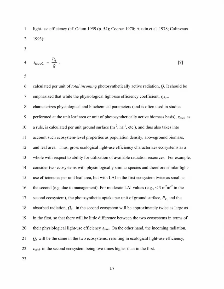
comparative ecological studies it is preferable to use the coefficient of gross ecological 22

17

light-use efficiency (cf. Odum 1959 (p. 54); Cooper 1970; Austin et al. 1978; Colinvaux 1

1993): 2

3

!

"ecol =Pg

Q, [9] 4

5

calculated per unit of total incoming photosynthetically active radiation, Q. It should be 6

emphasized that while the physiological light-use efficiency coefficient, εphys, 7

characterizes physiological and biochemical parameters (and is often used in studies 8

performed at the unit leaf area or unit of photosynthetically active biomass basis), εecol, as 9

a rule, is calculated per unit ground surface (m-2, ha-1, etc.), and thus also takes into 10

account such ecosystem-level properties as population density, aboveground biomass, 11

and leaf area. Thus, gross ecological light-use efficiency characterizes ecosystems as a 12

whole with respect to ability for utilization of available radiation resources. For example, 13

consider two ecosystems with physiologically similar species and therefore similar light-14

use efficiencies per unit leaf area, but with LAI in the first ecosystem twice as small as 15

the second (e.g. due to management). For moderate LAI values (e.g., < 3 m2m-2 in the 16

second ecosystem), the photosynthetic uptake per unit of ground surface, Pg, and the 17

absorbed radiation, Qa, in the second ecosystem will be approximately twice as large as 18

in the first, so that there will be little difference between the two ecosystems in terms of 19

their physiological light-use efficiency εphys. On the other hand, the incoming radiation, 20

Q, will be the same in the two ecosystems, resulting in ecological light-use efficiency, 21

εecol, in the second ecosystem being two times higher than in the first. 22

23

18

RESULTS AND DISCUSSION 1

2

Light-Response Functions and Parameters 3

Within the broad range of climatic conditions and ecosystem types represented in the data 4

set, we observed a variety of patterns of light-response. For comparative purposes, it is 5

convenient to distinguish four major categories differentiated in terms of convexity and 6

presence of the hysteresis-like loop on the light-response scatter diagram {Q, Fc} (Fig. 2). 7

In the latter case, plotting the 3-D scatter diagram of the diurnal dynamics of the 8

measurement data and of the response surface Fc(Q, Ts) (eq. [4]) fitted to them provides a 9

partial explanation the loop on the 2-D {Q, Fc} plot caused by the increase of ecosystem 10

respiration with the increase of temperature in the afternoon hours (Fig. 3). For the cases 11

shown in Figures 2 and 3, numerical estimates and statistical characteristics of parameters 12

in equations [3] and [4] are presented in Tables 2 and 3. 13

Nonrectangular hyperbolic equation [3] and its modification [4] taking into account 14

temperature-dependence of daytime respiration, were found to be good numerical tools to 15

fitting light-responses of nonforest ecosystems for days when photosynthetically active 16

radiation was the dominant factor governing the ecosystem CO2 exchange. It is important 17

to emphasize that the nonrectangular hyperbola provided a close fit to light-response data 18

and provided consistent estimates of the light-response parameters for days when the 19

{Q,Fc} plots showed no saturation with respect to Q and were characterized by convexity 20

parameter θ close to 1 (cf. Fig. 2A). The rectangular hyperbola, Mitscherlich’s equation, 21

and other approximations lacking convexity parameter fitted to data with such a pattern, 22

yield highly biased estimates of the initial slope, plateau, and the intercept parameters. 23

19

Estimates of the apparent quantum efficiency, α, in nonforest ecosystems cover a 1

wide range of values (Fig. 4A), from 5 mmol mol-1 in the desert shrublands of Central 2

Asia (Karrykul) to 75 mmol mol-1 in intensively managed grasslands of the North 3

Atlantic (Cabauw, the Netherlands), with mean value αnonfor = 33.3 mmol mol-1 and 4

standard deviation snonfor = 14.2 mmol mol-1. The lower 10% quantile of the α values in 5

the sample (5-17 mmol mol-1) included extensively managed arid and semiarid grasslands 6

and shrublands (Karrykul, Cottonwood, Karnap, Audubon, Lethbridge, Kherlenbayan, 7

Tojal, and Fort Peck), while the upper 10% quantile (50-75 mmol mol-1) encompassed 8

intensively managed grasslands (Cabauw, Carlow, Neustift, Easter Bush, Oensingen, 9

Lille Valby, Grillenburg, Haller, Rigi-Seebodenalp), extensively managed grasslands 10

under favorable weather conditions (Laqueuille-extensive, Jornada), and intensive 11

agricultural crops (Lonzee). Interestingly, most productive crop sites, characterized by 12

the highest Amax and Pg,max values, did not make it to the upper 10% quantum yield 13

quantile, though they belong to the upper 20% quantum yield quantile. 14

In addition to scatter plots for the pooled data set, understanding relationships 15

between parameters within a particular ecosystem is of interest. Presently, only a subset 16

of extensively managed grasslands shows scatter diagrams with pronounced patterns of 17

co-variation (Fig. 5). 18

In evaluating obtained estimates of the quantum yield, we should first note that 19

our maximum estimate of 75 mmol mol-1 is only two thirds of the theoretical maximum 20

of quantum efficiency of gross photosynthesis estimated by Good and Bell (1980) as 110 21

mmol mol-1. Comparing our nonforest estimates with those reviewed by Ruimy et al. 22

(1995), from which we estimated mean

!

" forest = 37 mmol mol-1 with standard 23

20

deviation sforest = 17 mmol mol-1 (we have excluded data in Ruimy et al. 1995 with α 1

values greater than theoretical maximum of quantum efficiency), one can see that 2

quantum efficiency of nonforest ecosystems is not statistically different from forests. In 3

fact,

!

"max,nonforest estimated for intensively managed Cabauw grassland in The 4

Netherlands (75 mmol mol-1) was numerically higher, but statistically not significantly 5

different from the maximum quantum efficiency determined for the chestnut coppice near 6

Paris, France (

!

"max,forest = 73 mmol mol-1 ) (Mordacq et al 1991). 7

The values of maximum average weekly gross photosynthesis, Amax, for nonforest 8

sites of the world (Fig. 4A) span from 0.2 mg CO2 m-2 s-1 (Fort Peck mixed prairie during 9

a drought year) to 3.4 mg CO2 m-2 s-1 (Mead, irrigated continuous corn), with the lower 10

10% quantile (0.2-0.36 mg CO2 m-2 s-1) including Fort Peck, Dubois, Miles City, 11

Kherlenbayan, Xilinhot, Karrykul, Kubuqi, Burns, and Karnap, and the upper 10% 12

quantile (2-3.4 mg CO2 m-2 s-1) including intensive crops (Mead, Bondville, Lonzee, 13

Ames), intensively managed grasslands (Cabauw, Carlow, Lille Valby), and tallgrass 14

prairies (Shidler, Fort Reno). The mean photosynthetic capacity of nonforest ecosystems, 15

1.2 mg CO2 m-2 s-1 (SD = 0.68 mg CO2 m-2 s-1), lies at the upper end of the mean Amax 16

range for different forest types from eddy covariance estimates, 0.66 mg CO2 m-2 s-1 to 17

1.3 mg CO2 m-2 s-1 (mean = 0.97 mg CO2 m-2 s-1) (Falge et al. 2002; Funk and Lerdau 18

2004). At the same time, the highest Amax value for nonforest ecosystems found in 19

intensive corn cultures of the Midwest of the USA (3.4 mg CO2 m-2 s-1) were 20

substantially higher than Amax = 2.64 mg CO2 m-2 s-1 estimated from data by Jarvis (1994) 21

for a Sitka spruce culture in Scotland. 22

21

The values of daytime ecosystem respiration rate, rd, in all ecosystems remained 1

substantially lower than corresponding Amax values (cf. Fig. 6, left), but also displayed 2

substantial variability among ecosystem types (Fig. 4B), with maximum weekly average 3

rd ranging from 0.04 mg CO2 m-2 s-1 (Burns, drought year) to 0.50 mg CO2 m-2 s-1 4

(Haller, warm and wet year). The lower 10% quantile of maximum weekly rd values 5

included arid and semiarid grasslands and shrublands (Burns, Karnap, Kherlenbayan, 6

Karrykul, Cottonwood, Burns, Dubois, Kubuqi) and tundra (Barrow), while the upper 7

10% quantile of rd distribution was represented by intensively managed grasslands 8

(Haller, Neustift, Cabauw, Carlow, Oensingen, Lille Valby, Easter Bush), intensive crops 9

(Ames, Mead), tallgrass prairies (Shidler, Rannels Ranch), and a semidesert grassland in 10

a year with exceptionally high precipitation (Jornada). 11

The weekly maxima of the coefficient of gross ecological light-use efficiency, ε, 12

resulting from this study were in the range from 3 to 59 mmol mol-1 (mean 22, standard 13

deviation 12.4 mmol mol-1), and, understandably, were lower than the weekly maxima of 14

the apparent quantum yield, α (Fig. 6, right). It is interesting, however, that for some 15

ecosystems, particularly for agricultural C4-crops and tropical grasslands dominated by 16

C4-species, ε values were not considerably lower than α (e.g., see Fig. 6E, 6F and 6H, 17

right). This is a direct result of relatively high values of the convexity coefficient of the 18

light-response curves of C4 species; at the ultimate case of θ = 1, the values of α and ε 19

will become equal, provided input radiation levels remains within the range of linear 20

light-response. 21

On the contrary, in C3-communities characterized by lower convexity values (θ = 22

0 in the extreme case of rectangular hyperbolic light-response), ecological light-use 23

22

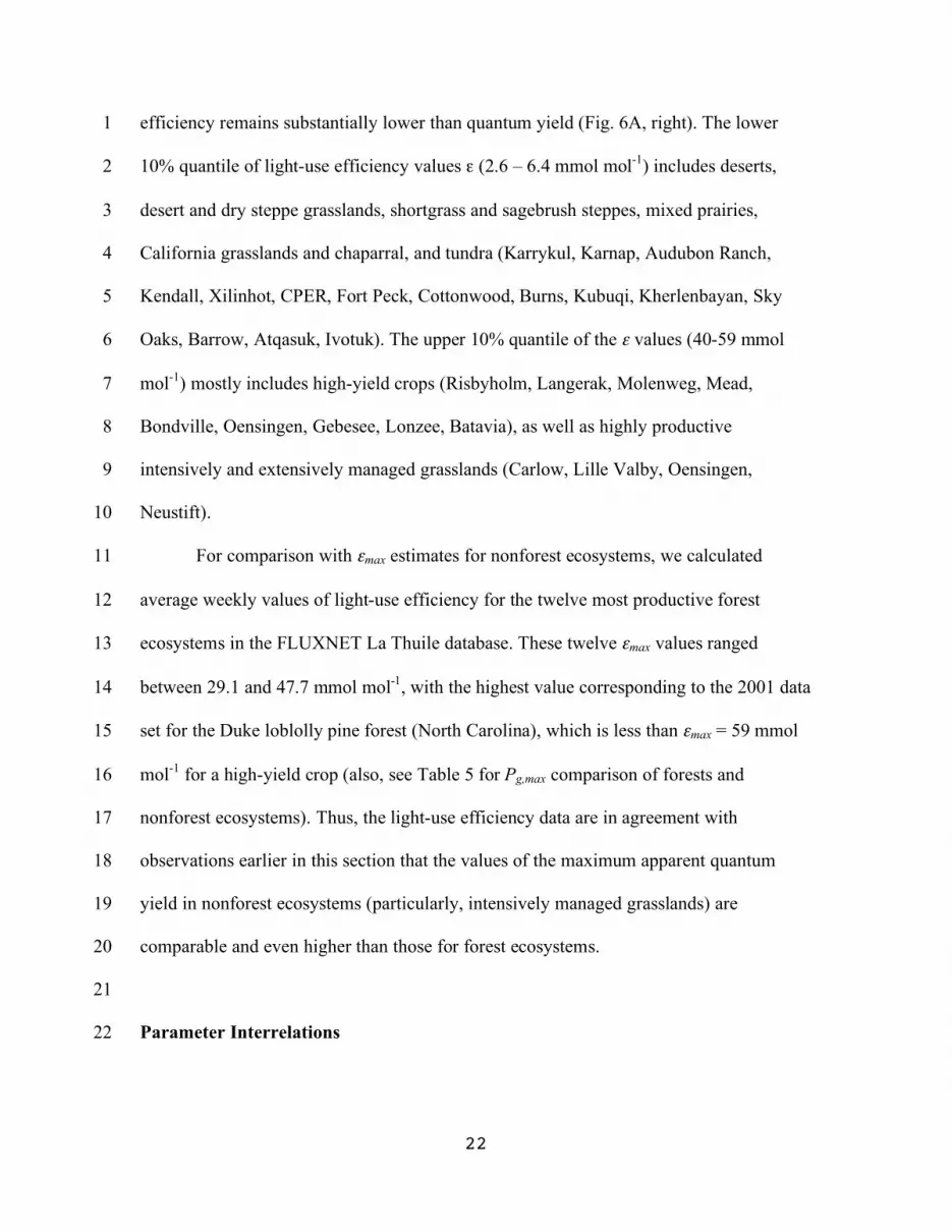
efficiency remains substantially lower than quantum yield (Fig. 6A, right). The lower 1

10% quantile of light-use efficiency values ε (2.6 – 6.4 mmol mol-1) includes deserts, 2

desert and dry steppe grasslands, shortgrass and sagebrush steppes, mixed prairies, 3

California grasslands and chaparral, and tundra (Karrykul, Karnap, Audubon Ranch, 4

Kendall, Xilinhot, CPER, Fort Peck, Cottonwood, Burns, Kubuqi, Kherlenbayan, Sky 5

Oaks, Barrow, Atqasuk, Ivotuk). The upper 10% quantile of the ε values (40-59 mmol 6

mol-1) mostly includes high-yield crops (Risbyholm, Langerak, Molenweg, Mead, 7

Bondville, Oensingen, Gebesee, Lonzee, Batavia), as well as highly productive 8

intensively and extensively managed grasslands (Carlow, Lille Valby, Oensingen, 9

Neustift). 10

For comparison with εmax estimates for nonforest ecosystems, we calculated 11

average weekly values of light-use efficiency for the twelve most productive forest 12

ecosystems in the FLUXNET La Thuile database. These twelve εmax values ranged 13

between 29.1 and 47.7 mmol mol-1, with the highest value corresponding to the 2001 data 14

set for the Duke loblolly pine forest (North Carolina), which is less than εmax = 59 mmol 15

mol-1 for a high-yield crop (also, see Table 5 for Pg,max comparison of forests and 16

nonforest ecosystems). Thus, the light-use efficiency data are in agreement with 17

observations earlier in this section that the values of the maximum apparent quantum 18

yield in nonforest ecosystems (particularly, intensively managed grasslands) are 19

comparable and even higher than those for forest ecosystems. 20

21

Parameter Interrelations 22

23

As expected, numerical values of light-response parameters among different ecosystems 1

did not vary independently of each other, but demonstrated patterns of correlation shown 2

in Figs. 4 and 5. Our results for this extensive data set are in agreement with earlier 3

studies based on smaller subsets of flux-tower data, suggesting that the plateau parameter 4

of gross photosynthesis, Amax, is a good predictor for other light-response parameters, 5

including quantum yield, α, ecosystem respiration rate, rd, and light-use efficiency, ε 6

(Gilmanov et al. 2007a; Owen at al. 2007). Baldocchi and Xu (2005) found that Amax is a 7

good predictor for another photosynthetic parameter, the maximum rate of carboxylation, 8

Vc,max. Nevertheless, while in previous studies mostly linear relationships between Amax 9

and other parameters were identified, the wider range of parameter variations in our data 10

set has revealed a number of distinct nonlinearities. For example, an allometric 11

relationship

!

" = 30.36 Amax( )0.55 with R2 value of 0.55 was obtained for the 12

relationship between apparent quantum yield and maximum photosynthesis (Fig. 4A). 13

The better fit of the allometric (nonlinear) description of the α(Amax) relationship 14

compared with the simple linear model is demonstrated by the fact that the nonlinear 15

model conveys a decrease in α with decreasing Amax as the latter is approaching zero, 16

while the linear model predicts an unrealistic α0 value of ∼15 mmol mol-1 even when Amax 17

→ 0. 18

Daytime ecosystem respiration, rd, also demonstrated an allometric relationship to 19

Amax described as

!

rd = 0.22 Amax( )0.71 characterized by R2 = 0.69 (Fig. 5B). In this 20

case, the linear model also provided a reasonable fit to the data (R2 = 0.67), though its 21

applicability to areas with low Amax values is limited by an unrealistically high intercept 22

of rd0 = 0.09 mg CO2 m-2 s-1 as Amax → 0. From the patterns of data points on Figs. 5C 23

24

and 5D one may see that the relationships between ecological light-use efficiency, 1

maximum daily gross photosynthesis, and Lmax may be approximated by both the linear, 2

and the allometric equations, though the latter provides better description in the lower 3

range of Amax and Lmax. 4

For various reasons, not all flux sites collected data on maximum leaf area (Lmax) 5

and/or maximum aboveground green biomass (Gmax). Nevertheless, with the limited data 6

available (Figs. 5F and 5H) we were able to establish nonlinear allometric (with 7

allometry coefficient < 1) dependence of maximum photosyntyhesis parameters (Amax, 8

Pg,max) and the standard morphometric characteristics such as maximum aboveground 9

biomass, Gmax and maximum leaf area index, Lmax (Figures. 5F and 5H). 10

11

Seasonal Patterns of Parameter Dynamics 12

Because light-response parameters evaluated from flux-tower measurement data sets 13

represent not only physiological characteristics (which also change in time with 14

phenology and environmental conditions) but also the ecosystem-scale attributes like 15

aboveground biomass, leaf area index and others, such parameters exhibit pronounced 16

variation in magnitude during the year. Seasonal changes of these parameters, though 17

specific for particular sites and years, have general patterns that are revealed by time-18

plots of parameter values aggregated at the weekly time step (Fig. 6). Pronounced 19

seasonal dynamics of light-response parameters shown on Fig. 6 in cold and temperate 20

environments is apparently driven by radiation and temperature inputs (Fig. 6, A, D), 21

while under arid conditions it mainly reflects fluctuation of precipitation (Fig. 6 E, F). 22

This climatically driven unimodal pattern of seasonal parameter change was particularly 23

25

pronounced in species-poor ecosystems or monocultures with relatively narrow 1

production period, be that a floodplain meadow in the tundra zone (Fig. 6A) or 2

agricultural crops (Figs. 6G and 6H). In ecosystems with higher species diversity and 3

broader production period (up to year-round production in tropical conditions), the 4

general seasonal pattern of parameter dynamics was compounded by additional 5

fluctuations reflecting different reactions of various species groups (e.g., cool and warm-6

season grasses) to weather variability and management pressure (grazing, mowing) 7

during various parts of the year (Figs. 6 B, C, D). These data may help to explain 8

difficulties experienced by those attempting to simulate year-round dynamics of gross 9

primary productivity and light-response parameters by modification of the hypothetical 10

maximum parameter value by factors-multipliers describing effects of various drivers like 11

radiation, temperature, moisture, etc. (cf. Monteith 1972; Ciais et al. 2001). 12

13

Seasonal Dynamics and Annual Budgets of GPP, RE, and NEE 14

Depending on a number of external (e.g. radiation, temperature, precipitation) and 15

internal ecological factors (e.g. leaf area, phenological state, water and nutrient supply), 16

the functions of gross primary productivity, Pg(t), and total ecosystem respiration, Re(t), 17

demonstrated pronounced temporal dynamics during the year, as exemplified by the 18

measurement-based estimates of Pg(t) and Re(t) presented on Fig. 7. On the other hand, 19

the curve of cumulative net ecosystem exchange, CumNEE(t) showed much smoother 20

behavior, and its value at the end of the year, NEE, provides a summary of ecosystem 21

carbon budget. 22

26

Data from the WorldGrassAgriFlux data set demonstrated a great variety of 1

seasonal patterns of productivity and respiration dynamics, some of the typical curves are 2

illustrated in Fig. 7. There are three major seasonal patterns of the cumulative NEE curve: 3

(i) equilibrium (S-shaped), (ii) permanent accumulation, and (iii) permanent release of 4

carbon. The equilibrium pattern (i) characterizing non-harvested ecosystems with marked 5

seasonality of primary productivity was exemplified by data from a floodplain tundra 6

meadow at Cherskii in the Far North-East of Russia (Fig. 7A). With the period of 7

decomposition activity (May-September) completely encompassing the production period 8

(June-August) and with maximum decomposition lagging behind maximum production, 9

the curve of cumulative NEE assumed a characteristic S-shaped form with the net annual 10

ecosystem CO2 exchange nearly zero. The accumulative pattern (ii) is described by the 11

more or less monotonous accumulation of net ecosystem production in ecosystems with a 12

period of marked domination of production over decomposition processes observed in 13

both grassland (Fig. 7F) and cropland ecosystems (Fig. 7G). The third pattern (iii) – 14

nearly permanent domination of respiratory efflux over assimilatory uptake resulting in 15

significant net loss of carbon from the ecosystem at the end of the year, as exemplified by 16

measurements at the Audubon (AZ) desert grassland on a high carbonate soil (Emmerich 17

2003) (Fig. 7D). These three major patterns were accompanied by a variety of 18

intermediate variants with local maxima and minima of the CumNEE(t) curve reflecting 19

weather fluctuations and harvesting, finally leading to either net uptake (Fig. 7C) or net 20

loss of carbon from the ecosystem (Fig. 7B, 7E and 7H). 21

Year-round integration of the Pg(t), Re(t), and Fc(t) curves provided estimates of 22

annual GPP, RE, and NEE totals for all the site-years in this study. These data stratified 23

27

by major ecosystem groups (extensively and intensively managed grasslands, shrublands 1

and savanna, wetlands, and croplands) are summarized in Table 4. The highest mean 2

gross primary production (5767 g CO2 m-2 yr-1) and ecosystem respiration (4990 g CO2 3

m-2 yr-1) were achieved in intensively managed grasslands. Not surprisingly, the highest 4

mean annual net ecosystem CO2 exchange (933 g CO2 m-2 yr-1) was found in croplands. 5

To supplement these basic statistical characteristics, Fig. 8 shows the distributions of the 6

GPP, RE, and NEE values in the pooled data set of estimates from all site-years in the 7

database. They show that while the GPP and RE values in our sample had a wide range 8

of variation (95 - 8600 g CO2 m-2 yr-1 for gross production and 112 - 7880 g CO2 m-2 yr-1 9

for respiration), with GPP and RE values fairly well distributed over their ranges (Fig. 8A 10

and 8B), the net CO2 exchange values concentrated between -1342 g CO2 m-2 yr-1 and 11

2394 g CO2 m-2 yr-1 had a distinctly unimodal distribution (Fig. 8 C). The average NEE 12

value for our sample of 316 nonforest ecosystems is 485 g CO2 m-2 yr-1 (SD = 696 g CO2 13

m-2 yr-1). Comparing these statistics with the mean (671 g CO2 m-2 yr-1) and standard 14

deviation (988 g CO2 m-2 yr-1) of published NEE values for 506 site-years from flux 15

towers worldwide (Baldocchi 2008b), we did not detect a difference between the two 16

NEE averages at the 1% level of significance. The higher mean NEE value for 17

Baldocchi’s sample is easily explained, taking into account that it contains a number of 18

growing forest sites with high NEE, while the WorldGrassAgriFlux data set includes 19

mostly nonforest sites (with occasional near-climax shrubland and savanna ecosystems). 20

A particularly interesting question, in the context of comparing basic parameters of the 21

carbon cycle, regards identifying maximum rates of photosynthetic CO2 assimilation in 22

various ecosystems. For this purpose, in Table 5 we have compiled the data of the two 23

28

dozen (or maximum available) site-years with maximum values of daily photosynthesis, 1

Pg,max, and annual GPP for our five types of nonforest ecosystems and for the forest sites 2

represented in the most recent FLUXNET database. With respect to the annual GPP, 3

forest ecosystems achieved the highest estimates of photosynthetic CO2 uptake, with 4

maximum GPP = 14339 g CO2 m-2 yr-1 for a tropical forest in French Guyana (Table 5F) 5

compared to maximum GPP = 8600 g CO2 m-2 yr-1 for a tropical grassland in Rondonia, 6

Brazil (Table 5 A). In contrast, maximum daily rates of photosynthetic uptake were 7

recorded not in forests, but in the intensive crops of the Midwestern United States, with 8

Pg,max = 116 g CO2 m-2 d-1 estimated for irrigated corn in a corn-soybean rotation (Mead, 9

NE) in 2001 (Table 5E). These data clearly demonstrate that even in other types of 10

nonforest ecosystems (e.g. shrublands and savanna), in addition to intensive agricultural 11

crops, maximum rates of gross photosynthetic assimilation (50 – 76 g CO2 m-2 d-1) are 12

quite comparable to those in most productive forests (55 – 99 g CO2 m-2 d-1). Apparently, 13

the major reason why annual GPP in forests is typically higher than nonforested 14

ecosystems is the length of production period. In tropical forests, production may 15

encompass the whole year, while in most nonforest ecosystems it is temporally limited by 16

temperature and water availability. 17

Source/Sink Activity of Nonforest Ecosystems 18

The data on annual budgets of production, respiration, and net exchange of nonforest 19

ecosystems obtained in our study allow quantitative consideration of important question 20

about the magnitude and significance of the source or sink activity of various ecosystem 21

types. Since H.T. Odum (1956) (see also Baldocchi 2008b), a convenient way to 22

visualize the net carbon budget of ecosystems for comparative purposes is to construct an 23

29

RE versus GPP scatter diagram and compare the distribution of data points with respect 1

to the 1:1 diagonal. Points below the diagonal correspond to sinks (GPP > RE, NEE >0), 2

while points above the diagonal describe sources of carbon (GPP < RE, NEE < 0). 3

H.T. Odum’s plot for the whole nonforest data set (Fig. 9) demonstrates that for four out 4

of every five site-years, gross production was higher than ecosystem respiration, 5

indicating net ecosystem sink activity. Stratification of the data with respect to ecosystem 6

type (Fig. 10) shows that for all types of nonforest ecosystem in our database there were 7

considerably more years with net CO2 uptake than release. However, years with net 8

source activity occasionally occurred in all ecosystems except wetlands. 9

The distributions of NEE for different ecosystems presented in Fig. 11 provide a more 10

detailed description of the matter. Source-type activity more frequently occurred in 11

extensively managed grasslands, shrublands/savanna, and croplands, than in intensively 12

managed grasslands and wetlands. As a rule, source-type activity was associated with 13

years of drought, excessive grazing and hay mowing, high organic matter content of soils 14

(e.g. grasslands on peat) or high CaCO3 reserves in the soil profile, and transitional 15

successional status of the ecosystem (e.g., grasslands of previously forested soils). For 16

agroecosystems, source activity is often observed in crops with intensive soil preparation 17

and relatively short leaf duration periods (e.g. soybeans). However, it should be 18

emphasized that for all ecosystems examined in our study, carbon sink activity was 19

frequently observed, with the highest net carbon uptakes in intensively managed 20

grasslands and cropland ecosystems (Fig. 11, Table 4). 21

These observations are in obvious contradiction with conclusion of the first State 22

Of the Carbon Cycle Report (SOCCR) (King et al. 2007) and some earlier authors (e.g., 23

30

Reicosky 1997; Smith and Falloon 2005) who emphasized net source or neutral activity 1

of agricultural ecosystems. In this context, it is appropriate to consider the argument by 2

C. Körner (2003) regarding the critical significance of the representativeness of flux 3

tower data sets. Recognizing the relevance of Körner’s arguments to the situation in the 4

early 2000s, it should be emphasized that, at least with regard to nonforested ecosystems, 5

the present set of flux tower sites includes a wide range of climatic conditions and 6

management regimes and, therefore, is much less biased towards highly productive 7

ecosystems. 8

Ecosystem-Scale Production and Respiration in Relation to Major Ecological 9

Factors 10

Relationships of production and decomposition to major ecological factors attracted 11

attention of ecologists and geographers of the 20th century (Weaver 1924; Walter 1939; 12

Budyko and Efimova 1968; Rosenzweig 1968; Lieth 1975) and were later approached 13

under the framework of dynamic global vegetation models (DGVM) and related models 14

(e.g., Woodward et al. 2001; Cramer et al. 2001). Presently, these problems are back in 15

the focus of ecosystem, regional and global ecology, not only because of the recognition 16

of their relevance to global climatic change, but also because today, for the first time, 17

measurement-based quantitative estimates of gross productivity and total ecosystem 18

respiration are readily available through post-processing of net CO2 exchange 19

measurements at flux towers. 20

Besides radiation and temperature, which are already taken into account by the 21

light-temperature-response function method, the next most important factor influencing 22

ecosystem productivity and respiration is water (e.g., Slatyer 1967; Boyer 1982). Though 23

31

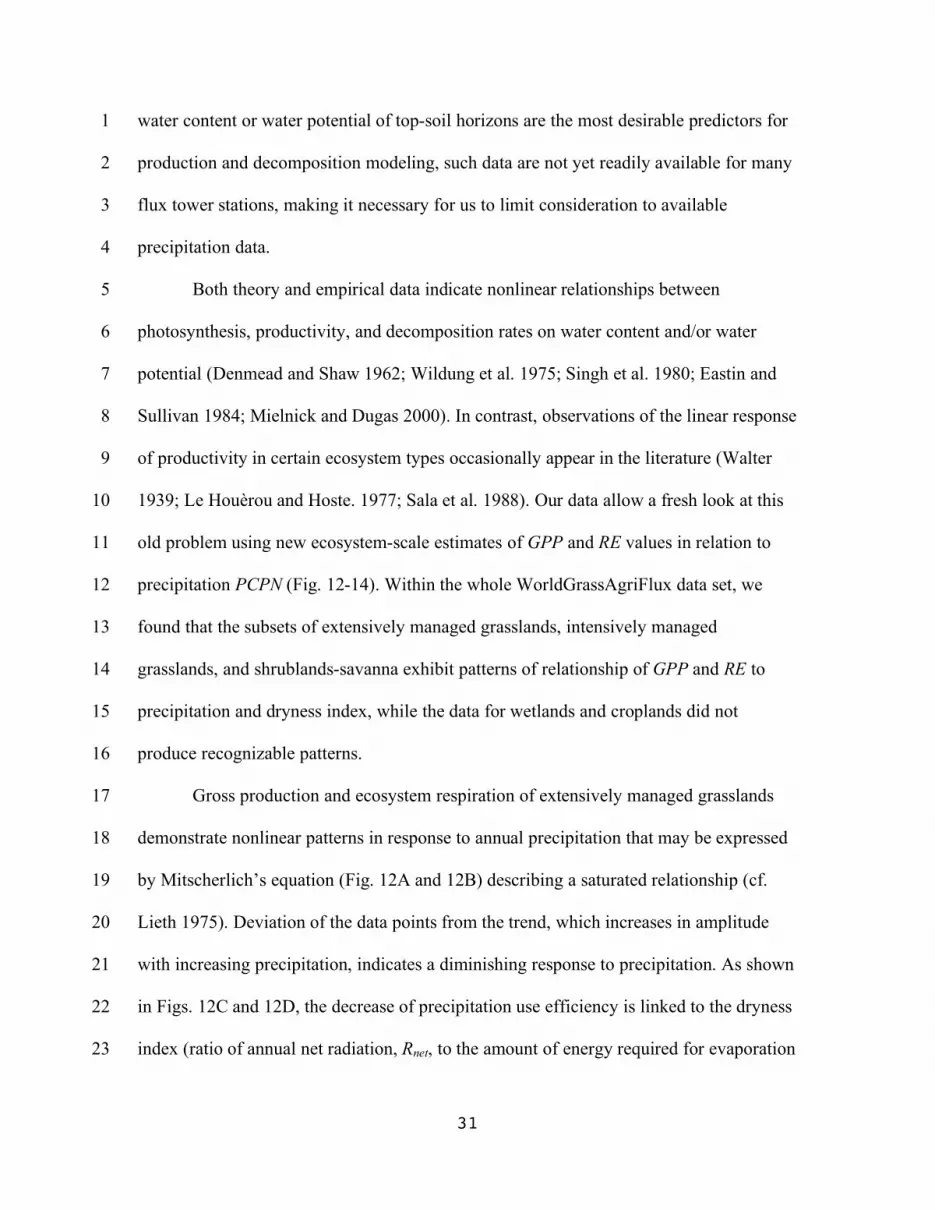
water content or water potential of top-soil horizons are the most desirable predictors for 1

production and decomposition modeling, such data are not yet readily available for many 2

flux tower stations, making it necessary for us to limit consideration to available 3

precipitation data. 4

Both theory and empirical data indicate nonlinear relationships between 5

photosynthesis, productivity, and decomposition rates on water content and/or water 6

potential (Denmead and Shaw 1962; Wildung et al. 1975; Singh et al. 1980; Eastin and 7

Sullivan 1984; Mielnick and Dugas 2000). In contrast, observations of the linear response 8

of productivity in certain ecosystem types occasionally appear in the literature (Walter 9

1939; Le Houèrou and Hoste. 1977; Sala et al. 1988). Our data allow a fresh look at this 10

old problem using new ecosystem-scale estimates of GPP and RE values in relation to 11

precipitation PCPN (Fig. 12-14). Within the whole WorldGrassAgriFlux data set, we 12

found that the subsets of extensively managed grasslands, intensively managed 13

grasslands, and shrublands-savanna exhibit patterns of relationship of GPP and RE to 14

precipitation and dryness index, while the data for wetlands and croplands did not 15

produce recognizable patterns. 16

Gross production and ecosystem respiration of extensively managed grasslands 17

demonstrate nonlinear patterns in response to annual precipitation that may be expressed 18

by Mitscherlich’s equation (Fig. 12A and 12B) describing a saturated relationship (cf. 19

Lieth 1975). Deviation of the data points from the trend, which increases in amplitude 20

with increasing precipitation, indicates a diminishing response to precipitation. As shown 21

in Figs. 12C and 12D, the decrease of precipitation use efficiency is linked to the dryness 22

index (ratio of annual net radiation, Rnet, to the amount of energy required for evaporation 23

32

of precipitation, λ*PCPN, where λ is the latent heat coefficient) (Budyko and Efimova, 1

1968; Long et al. 1991). 2

Intensively managed grasslands, which are typically located in climates with more 3

favorable precipitation and less drought stress, still exhibit responses to precipitation and 4

dryness; this response is especially pronounced for gross primary production (Fig. 13). 5

Shrublands and savanna ecosystems, with their broad range of precipitation and dryness 6

index, demonstrate strong nonlinearity of response to precipitation and dryness for both 7

the assimilation and respiration components of the carbon cycle (Fig. 14). 8

9

10

33

CONCLUSIONS AND IMPLICATIONS 1

2

The light-response parameters of nonforest terrestrial ecosystems have a wide range of 3

variability, from relatively low values of photosynthetic capacity (Amax = 0.2 mg CO2 m-2 4

s-1 in drought-stressed grasslands), quantum yield (α = 5 mmol mol-1 in deserts), daytime 5

ecosystem respiration (rd = 0.04 mg CO2 m-2 s-1 in drought-stressed sagebrush steppe), 6

and gross ecological light-use efficiency (ε = 2.6 mmol mol-1 in sedge and tussock 7

tundras of Alaska), to the highest values ever recorded for terrestrial ecosystems 8

(intensively managed grasslands and agricultural crops: Amax = 3.4 mg CO2 m-2 s-1, α = 9

75 mmol mol-1, rd = 0.50 mg CO2 m-2 s-1, ε = 59 mmol mol-1). Under optimal conditions, 10

gross primary productivity in nonforest terrestrial ecosystems can surpass productivity of 11

forests, with maximum rates of daily gross photosynthetic assimilation, Pg,max, achieving 12

values greater 100 g CO2 m-2 d-1 in intensive agricultural crops (Pg,max = 116 g CO2 m-2 d-13

1), while for forest ecosystems Pg,max values remain below 100 g CO2 m-2 d-1 (FLUXNET 14

data base: www.fluxdata.org). Nevertheless, due to limitation by radiation, temperature, 15

water, and nutrient resources, as well as management practices, maximum values of 16

annual gross photosynthesis (GPP) of nonforest ecosystems estimated from flux-tower 17

measurements remain below 10000 g CO2 m-2 yr-1, while in many types of forests they 18

considerably exceeded this value (with maximum GPP > 14000 calculated for a tropical 19

forest in French Guyana). The annual values of both GPP and RE for extensively and 20

intensively managed grasslands, and shrubland/savanna ecosystems are nonlinearly 21

related to annual precipitation, PCPN, and dryness index, Rnet/(λ*PCPN), indicating the 22

potential sensitivity of these ecosystems to anthropogenic climate change. 23

34

The average annual net CO2 exchange of our sample of 316 NEE values for 1

nonforest ecosystems indicates that on average, nonforest ecosystems act as net sinks for 2

atmospheric CO2, with the highest rates of annual CO2 uptake in agricultural crops (mean 3

NEEcrop = 933 g CO2 m-2 yr-1) and intensively managed grasslands (mean NEEgrassint = 4

848 g CO2 m-2 yr-1). These data, based on continuous long-term flux-tower 5

measurements, confirm that grasslands and agricultural crops play a significant role in the 6

carbon budget and have high carbon sequestration potential (Lal et al. 1998; Follett et al. 7

2001; Follett and Schuman 2005). These findings directly contradict conclusions of 8

earlier authors (e.g., Smith and Faloon 2005; Conant et al. 2007 in SOCCR) about the 9

negative or nearly neutral role agroecosystems play in continental carbon budgets. These 10

earlier studies were based on C-inventory methods and did not utilize flux-tower 11

measurements. Clearly, further analyses are needed to determine the extent to which 12

flux-tower networks and the GIS and remote-sensing methods used to up-scale flux 13

measurements to the regional level are representative, and to support our conclusion 14

about the significant sink role of managed grasslands and intensive agricultural crops in 15

the carbon budget. 16

17

18

35

ACKNOWLEDGEMENTS 1

2

The authors thank managers of the RANGEFLUX data base Patricia Mielnick and the 3

FLUXNET data base Dario Papale, Markus Reichstein, and Deb Agrawal for assistance 4

with updating tower flux data. We also thank Mary Brooke McEachern for help with 5

editing the manuscript of the paper. 6

7

36

LITERATURE CITED 1

2

Agarwal, D., M. Humphrey, C. van Ingen, N. Beekwilder, M. Goode, K. Jackson, M. R. L. 3

Rodriguez, and R. Weber. 2008. FLUXNET snthesis dataset collaboration infrastructure. 4

FluxLetter (The Newsletter of FLUXNET) 1: 5-7. 5

Austin, R. B., G. Kingston, P. C. Longden, and P. A. Donovan. 1978. Gross energy yields and 6

the support energy requirements for the production of sugar from beet and cane: a study 7

of four production areas. Journal of Agricultural Science 91:661-675. 8

Baldocchi, D. 2008a. Advanced topics in biometeorology and micrometeorology. 9

http://nature.berkeley.edu/biometlab/espm228/. 10

Baldocchi, D. 2008b. “Breathing” of the terrestrial biosphere: lessons learned from a global 11

network of carbon dioxide flux measurement systems. Australian Journal of Botany 56: 12

1-26. 13

Baldocchi, D., and L. Xu. 2005. Carbon exchange of deciduous broadleaved forests in temperate 14

and Mediterranean regions. In: H. Griffiths and P. G. Jarvis, editors. The carbon balance 15

of forests. Taylor and Francis, New York, p. 187-215. 16

Birdsey, R. A., J. C. Jenkins, M. Johnston, E. Huber-Sannwald, B. Amero, B. de Jong, J. D. E. 17

Barra, N. R. French, F. Garcia-Oliva, M. Harmon, L. S. Heath, V. J. Jaramillo, K. 18

Johnsen, B. E. Law, E. Martin-Spiotta, O. Masera, R. Neilson, Y. Pan, and K. S. 19

Pregitzer. 2007. North American Forests. in A. W. King, L. Dilling, G. P. Zimmerman, 20

D. M. Fairman, H. R.A., G. Marland, R. A.Z., and T. J. Wilbanks [eds.]. The First State 21

of the Carbon Cycle Report (SOCCR): The North American Carbon Budget and 22

Implications for the Global Carbon Cycle. A Report by the U.S. Climate Change Science 23

37

Program and the Subcommittee on Global Change Research. National Oceanic and 1

Atmospheric Administration, National Climatic Data Center, Asheville, NC, USA, p. 2

117-126. 3

Blackman, F. F. 1905. Optima and limiting factors. Annals of Botany 19: 281-295. 4

Boyer, J.S. 1982. Plant productivity and environment. Science 218:443-448. 5

Bridgham, S. D., J. P. Megonigal, J. K. Keller, N. B. Bliss, and C. Trettin. 2007. Wetlands. In: A. 6

W. King, L. Dilling, G. P. Zimmerman, D. M. Fairman, H. R.A., G. Marland, R. A.Z., 7

and T. J. Wilbanks [eds.]. The First Stata of the Carbon Cycle Report (SOCCR): The 8

North American Carbon Budget and Implications for the Global Carbon Cycle. A Report 9

by the U.S. Climate Change Science Program and the Subcommittee on Global Change 10

Research. National Oceanic and Atmospheric Administration, National Climatic Data 11

Center, Asheville, NC, USA, p. 139-148. 12

Budyko, M. I., and N. A. Efimova. 1968. The use of solar energy by the natural plant cover of 13

the USSR. Botanicheskii Zhurnal 53:1384-1389. 14

Burba, G., and D. Anderson. 2007. Introduction to lthe eddy covariance method. General 15

guidelines, and conventional workflow. LI-COR Biosciences. 16

http://www.licor.com/env/PDF_Files/EddyCovariance_readonly.pdf. 17

Buyanovsky, G. A., and G. H. Wagner. 1998. Changing role of cultivated land in the global 18

carbon cycle. Biology and Fertility of Soils 27:242-245. 19

Ciais, P., P. Friedlingstein, A. Friend, and D. S. Schimel. 2001. Integrating global models of 20

terrestrial primary produuctivity. In: J. Roy, B. Saugier, and H. A. Mooney [eds.] 21

Terrestrial global productivity. Academic Press, San Diego et al., p. 449-478. 22

Colinvaux, P. A. 1993. Ecology 2. Wiley, New York. 23

38

Conant, R. T., K. Paustian, F. Garcia-Oliva, H. H. Janzen, M. J. Jaramillo, D. E. Johnson, and S. 1

N. Kulshreshtha. 2007. Agricultural and grazing lands. In: A. W. King, L. Dilling, G. P. 2

Zimmerman, D. M. Fairman, R. A. Houghton, G. Marland, A. Z. Rose, and T. J. 3

Wilbanks, editors. The first state of the carbon cycle report (SOCCR): The North 4

American carbon budget and implications for the global carbon cycle. A report by the 5

U.S. Climate Change Science Program and the Subcommittee on Global Change 6

Research. National Oceanic and Atmospheric Administration, National Climatic Data 7

Center, Asheville, NC, USA, p. 107-116. 8

Cooper, J. P. 1970. Potential production and energy conversion in temperate and tropical grasses. 9

Herbage Abstracts 40:1-13. 10

Cramer, W., R. J. Olson, S. D. Prince, J. M. O. Scurlock, and 11

members_of_the_Global_Primary_Production_Data_Initiative. 2001. Determining 12

present patterns of global productivity. In: J. Roy, B. Saugier, and H. A. Mooney [eds.]. 13

Terrestrial global productivity. Academic Press, San Diego et al., p. 429-448. 14

Davidson, E. A., and I. A. Janssens. 2006. Temperature sensitivity of soil carbon decomposition 15

and feedbacks to climate change. Nature 440: 165-173. 16

Denmead, O. T., and R. H. Shaw. 1962. Availability of soil water to plants as affected by soil 17

moisture content and meteorological conditions. Agronomy Journal 54: 385-390. 18

Eastin, J. D., and C. Y. Sullivan. 1984. Environmental stress influences on plant persistence, 19

physiology, and production. In: M. B. Tesar [ed.]. Physiological basis of crop growth and 20

development. American Society of Agronomy and Crop Science Society of America, 21

Madison, Wisconsin, p. 201-236. 22

Emmerich, W. E. 2003. Carbon dioxide fluxes in a semiarid environment with high carbonate 23

39

soils. Agricultural and Forest Meeorology 116: 91-102. 1

Falge, E., J. Tenhunen, D. Baldocchi, M. Aubinet, P. Bakwin, P. Berbigier, C. Bernhofer, J. M. 2

Bonnefond, G. Burba, R. Clement, K. J. Davis, J. A. Elbers, M. Falk, A. H. Goldstein, A. 3

Grelle, A. Granier, T. Grünwald, J. Gudmundsson, D. Hollinger, I. A. Janssens, P. 4

Keronen, A. S. Kowalski, G. Katul, B. E. Law, Y. Malhi, T. Meyers, R. K. Monson, E. 5

Moors, J. W. Munger, W. Oechel, K. T. P. U, K. Pilegaard, U. Rannik, C. Rebmann, A. 6

Suyker, H. Thorgeirsson, G. Tirone, A. Turnipseed, K. Wilson, and S. Wofsy. 2002. 7

Phase and amplitude of ecosystem carbon release and uptake potentials as derived from 8

FLUXNET measurements. Agricultural and Forest Meteorology 113:75-95. 9

Farrell, A. E., M. O'Hare, D. M. Kammen, R. J. Plevin, B. T. Turner, and A. D. Jones. 2006. 10

Ethanol can contribute to energy and environmental goals. Science 311:506-508. 11

Follett, R. F., J. M. Kimble, and R. Lal [eds.]. 2001. The potential of U.S. grazing lands to 12

sequester carbon and mitigate the greenhouse effect. Lewis Publishers, Boca Raton, 13

Florida. 14

Follett, R. F., and G. E. Schuman. 2005. Grazing land contributions to carbon sequestration. In: 15

D. A. McGilloway [ed.]. Grassland: a global resource. Wageningen Academic Publishers, 16

Wageningen, p. 265-277. 17

Funk, J. L., and M. T. Lerdau. 2004. Photosynthesis in forest canopies. In: M. D. Lowman and 18

H. B. Rinker[ eds.]. Forest canopies. Elsevier Academic Press, Amsterdam et al., p. 335-19

358. 20

Gilmanov, T. G., A. B. Frank, M. R. Haferkamp, T. P. Meyers, J. A. Morgan, L. L. Tieszen, B. 21

K. Wylie, and L. B. Flanagan. 2005. Integration of CO2 flux and remotely-sensed data for 22

primary production and ecosystem respiration analyses in the Northern Great Plains: 23

40

Potential for quantitative spatial extrapolation. Global Ecology and Biogeography 14: 1

271-292. 2

Gilmanov, T. G., D. A. Johnson, and N. Z. Saliendra. 2003a. Growing season CO2 fluxes in a 3

sagebrush-steppe ecosystem in Idaho: Bowen ratio/energy balance measurements and 4

modeling. Basic and Applied Ecology 4: 167-183. 5

Gilmanov, T. G., D. A. Johnson, N. Z. Saliendra, K. Akshalov, and B. K. Wylie. 2004. Gross 6

primary productivity of the true steppe in Central Asia in relation to NDVI: Scaling-up 7

CO2 fluxes. Environmental Management 39: S492-S508. 8

Gilmanov, T. G., J. F. Soussana, L. Aires, V. Allard, C. Ammann, M. Balzarolo, Z. Barcza, C. 9

Bernhofer, C. L. Campbell, A. Cernusca, A. Cescatti, J. Clifton-Brown, B. O. M. Dirks, 10

S. Dore, W. Eugster, J. Fuhrer, C. Gimeno, T. Gruenwald, L. Haszpra, A. Hensen, A. 11

Ibrom, A. F. G. Jacobs, M. B. Jones, G. Lanigan, T. Laurila, A. Lohila, G.Manca, B. 12

Marcolla, Z. Nagy, K. Pilegaard, K. Pinter, C. Pio, A. Raschi, N. Rogiers, M. J. Sanz, P. 13

Stefani, M. Sutton, Z. Tuba, R. Valentini, M. L. Williams, and G. Wohlfahrt. 2007a. 14

Partitioning European grassland net ecosystem CO2 exchange into gross primary 15

productivity and ecosystem respiration using light response function analysis. 16

Agriculture, Ecosystems and Environment 121: 93-120. 17

Gilmanov, T. G., T. J. Svejcar, D. A. Johnson, R. F. Angell, N. Z. Saliendra, and B. K. Wylie. 18

2006. Long-term dynamics of production, respiration, and net CO2 exchange in two 19

sagebrush-steppe ecosystems. Rangeland Ecology and Management 59: 585-599. 20

Gilmanov, T. G., S. B. Verma, P. L. Sims, T. P. Meyers, J. A. Bradford, G. G. Burba, and A. E. 21

Suyker. 2003b. Gross primary production and light response parameters of four Southern 22

Plains ecosystems estimated using long-term CO2-flux tower measurements - art. no. 23

41

1071. Global Biogeochemical Cycles 17: doi: 10.1029/2002GB002023, 2003. 1

Gilmanov, T. G., and WORLDGRASSAGRIFLUX Data Set Participants. 2007b. Productivity, 2

respiration, CO2 sink potential, and light-response parameters of world grasslands 3

derived from flux-tower data partitioning. Eos Trans. AGU, 88(52), Fall Meet. Suppl., 4

Abstract B32B-03. 5

Good, N. E., and D. H. Bell. 1980. Photosynthesis, plant productivity and crop yield. In: P. S. 6

Carlson, editor. The biology of crop productivity. Academic Press, New York, p. 3-51. 7

Goulden, M. L., J. W. Munger, S.-M. Fan, B. C. Daube, and S. C. Wofsy. 1996. Measurements 8

of carbon sequestration by long-term eddy covariance: methods and critical evaluation of 9

accuracy. Global Change Biology 2: 169-182. 10

Griffiths, H., and P. Jarvis [eds.]. 2005. The carbon balance of forest biomes. Taylor & Francis, 11

New York et al. 12

Hollinger, S. E., C. J. Bernacchi, and T. P. Meyers. 2005. Carbon budget of mature no-till 13

ecosystem in North Central Region of the United States. Agricultural and Forest 14

Meteorology 130: 59-69. 15

Jarvis, P. G. 1994. Capture of carbon dioxide by a coniferous forest. In: J. L. Monteith, R. K. 16

Scott, and M. H. Unsworth [eds.]. Resource capture by crops. Nottingham University 17

Press, Loughborough, Leicestershire, p. 351-374. 18

King, A. W., L. Dilling, G. P. Zimmerman, D. M. Fairman, R. A. Houghton, G. Marland, A. Z. 19

Rose, and T. J. Wilbanks, editors. 2007. The first state of the carbon cycle report 20

(SOCCR): The North American carbon budget and implications for the global carbon 21

cycle. A report by the U.S. Climate Change Science Program and the Subcommittee on 22

Global Change Research. National Oceanic and Atmospheric Administration, National 23

42

Climatic Data Center, Asheville, NC, USA. 1

Körner, C. 2003. Slow in, rapid out – carbon flux studies and Kyoto target. Science 300:1242-2

1243. 3

Lal, R., J. M. Kimble, R. F. Follett, and C. V. Cole [eds]. 1998. The potential of U.S. cropland to 4

sequester carbon and mitigate the greenhouse effect. Ann Arbor Press, Chelsea, MI. 5

Larcher, W. W. 1995. Physiological plant ecology: ecophysiology and stress physiology of 6

functional groups. Springer-Verlag, Berlin ; New York. 7

Le Houèrou, H. N., and C. H. Hoste. 1977. Rangeland production and annual rainfall relations in 8

the Mediterranean basin and in the African Sahelo-Sudanian Zone. Journal of Range 9

Management 30: 181-189. 10

Lee, X., W. Massman, and B. Law [eds]. 2004. Handbook of Micrometeorology: A Guide for 11

Surface Flux Measurement and Analysis. Kluwer Academic Publishers. 12

Lieth, H. 1975. Modeling the primary productivity of the world. In: H. Lieth, R. H. Whittaker 13

[eds.]. Primary Productivity of the Biosphere. Springer-Verlag, New York, p. 237-263. 14

Loehle Enterprises. 2007. Global optimization 6.0. Global nonlinear optimization using 15

Mathematica. Loehle Enterprises, Naperville, Illinois. 16

Long, S. P., M. B. Jones, and M. J. Roberts, eds. 1991. Primary productivity of grass ecosystems 17

of the tropics and sub-tropics. Chapman & Hall, London; New York. 18

Mielnick, P. C., and W. A. Dugas. 2000. Soil CO2 flux in a tallgrass prairie. Soil Biology and 19

Biochemistry 32:221-228. 20

Mitscherlich, E. A. 1909. Das Gesetz des Minimums und das Gesetz des abnehmenden 21

Bodenertrages. Landwirtschaftliches Jahrbuch der Schweiz 38: 537-552. 22

Moffat, A. M., D. Y. Hollinger, A. D. Richardson, A. G. Barr, C. Beckstein, B. H. Braswell, G. 23

43

Churkina, A. R. Desai, E. Falge, J. H. Gove, M. Heimann, D. Hui, A. J. Jarvis, J. Kattge, 1

A. Noormets, V. J. Stauch, D. Papale, and M. Reichstein. 2007. Comprehensive 2

comparison of gap-filling techniques for eddy covariance net carbon fluxes. Agricultural 3

and Forest Meteorology 147: 209-232. 4

Monteith, J. L. 1972. Solar radiation and productivity in tropical ecosystems. Journal of Applied 5

Ecology 9: 747-766. 6

Mordacq, L., J. Ghasghaie, and B. Saugier. 1991. A simple method for measuring the gas 7

exchange of small trees. Functional Ecology 5:572-576. 8

Odum, E. P. 1959. Fundamentals of ecology. Philadelphia. 9

Odum, H. T. 1956. Primary production in flowing waters. Limnology and Oceanography 1:102-10

117. 11

Olson, J. S., J. A. Watts, and L. J. Allison. 1983. Carbon in live vegetation of major world 12

ecosystems (Oak Ridge National Laboratory Technical Report ORNL-5862). 13

Washington, D.C. U.S. Dept. of Energy, Springfield, Va. 14

Owen, K. E., E. Falge, R. Geyer, X. Xiao, P. Stoy, C. Ammann, A. Arain, M. Aubinet, M. 15

Aurela, C. Bernhofer, B. H. Chojnicki, A. Granier, T. Gruenwald, J. Hadley, B. 16

Heinesch, D. Hollinger, A. Knohl, W. Kutsch, A. Lohila, T. Meyers, E. Moors, C. 17

Moureaux, K. Pilegaard, N. Saigusa, S. Verma, T. Vesala, C. Vogel, J. Tenhunen, M. 18

Reichstein, and Q. Wang. 2007. Linking flux network measurements to continental scale 19

simulations: Ecosystem carbon dioxide exchange capacity under non-water-stressed 20

conditions. Global Change Biology 13:734-760. 21

Patzek, T. W., J. Lee, B. Li, J. Padnick, S. A. Yee, S. M. Anti, R. Campos, and K. W. Ha. 2005. 22

Ethanol from corn: Clean renewable fuel for the future, or drain on our resources and 23

44

pockets? Environment, Development and Sustainability 7:319-336. 1

Powlson, D. S., A. B. Riche, and I. Shield. 2005. Biofuels and other approaches for decreasing 2

fossil fuel emissions from agriculture. Annals of Applied Biology 146:193-201. 3

Rabinowich, E. I. 1951. Photosynthesis and related processes. Interscience Publishers, Inc, New 4

York. 5

Reichstein, M., E. Falge, D. Baldocchi, D. Papale, R. Valentini, M. Aubinet, P. Berbigier, C. 6

Bernhofer, N. Buchmann, M. Falk, T. Gilmanov, A. Granier, T. Grünwald, K. 7

Havránková, D. Janous, A. Knohl, T. Laurela, A. Lohila, D. Loustau, G. Matteucci, T. 8

Meyers, F. Miglietta, J.-M. Ourcival, D. Perrin, J. Pumpanen, S. Rambal, E. Rotenberg, 9

M. Sanz, J. Tenhunen, G. Seufert, F. Vaccari, T. Vesala, and D. Yakir. 2005. On the 10

separation of net ecosystem exchange into assimilation and ecosystem respiration: review 11

and improved algorithm. Global Change Bilology 11: 1424-1439. 12

Reicosky, D. C. 1997. Tillage-induced CO2 emission from soil. Nutrient Cycling in 13

Agroecosystems 49:273-285. 14

Rodin, L. E., and N. I. Bazilevich. 1968. Production and mineral cycling in terrestrial vegetation. 15

Oliver and Boyd, Edinburgh. 16

Rodin, L. E., N. I. Bazilevich, and N. N. Rozov. 1975. Productivity of the world's main 17

ecosystems. In: D. E. Reichle, J. F. Franklin, and D. W. Goodall [eds.]. Productivity of 18

the World Ecosystems. Proceedings, Symposium Fifth General Assembly of Special 19

Committee of IBP. National Acad. of Sci., Washington, D.C., p. 13-26. 20

Rosenzweig, M. L. 1968. Net primary production of terrestrial communities: Prediction from 21

climatological data. American Naturalist 102:67-74. 22

Ruimy, A., P. G. Jarvis, and D. D. Baldocchi. 1995. CO2 fluxes over plant canopies and solar 23

45

radiation: a review. Anvances in Ecological Research 26: 1-68. 1

Sala, O. E., W. J. Parton, L. A. Joyce, and W. K. Lauenroth. 1988. Primary production of the 2

central grassland region of the United States. Ecology 69:40-45. 3

Singh, J. S., M. J. Trlica, P. G. Risser, R. E. Redmann, and J. K. Marshall. 1980. Autotrophic 4

subsystem. Pages 59-200. In: A.I. Breymeyer and G. M. Van Dyne [eds.]. Grasslands, 5

systems analysis and man. Cambridge University Press, Cambridge. 6

Slatyer, R. O. 1967. Plant-water relationships. Academic Press, London, New York. 7

Smith, P., and P. Falloon. 2005. Carbon sequestration in European croplands. Pages 47-55 in H. 8

Griffiths and P. G. Jarvis, editors. The carbon balance of forest biomes. Taylor and 9

Francis, New york. 10

Stoy, P. C., J. Y. Juang, K. A. Novick, J. M. Uebelherr, R. Oren, G. G. Katul, and M. B. S. 11

Siqueira. 2006. An evaluation of models for partitioning eddy covariance-measured net 12

ecosystem exchange into photosynthesis and respiration. Agricultural and Forest 13

Meteorology 141: 2-18. 14

Tamiya, H. 1951. Some theoretical notes on the kinetics of algal growth. Botanical Magazine 6: 15

167-173. 16

Tarnocai, C., C.-L. Ping, and J. Kimble. 2007. Carbon cycle in the permafrost region of North 17

America. Pages 127-138 in A. W. King, L. Dilling, G. P. Zimmerman, D. M. Fairman, H. 18

R.A., G. Marland, R. A.Z., and T. J. Wilbanks, eds. The First State of the Carbon Cycle 19

Report (SOCCR): The North American Carbon Budget and Implications for the Global 20

Carbon Cycle. A Report by the U.S. Climate Change Science Program and the 21

Subcommittee on Global Change Research. National Oceanic and Atmospheric 22

Administration, National Climatic Data Center, Asheville, NC, USA. 23

46

Thornley, J. H. M., and I. R. Johnson. 2000. Plant and crop modelling. A mathematical approach 1

to plant and crop physiology. The Blackburn Press, Caldwell, New Jersey. 2

Walter, H. 1939. Grassland, Savanne und Busch der ariden Teile Afrikas in ihrer ökologische 3

Bedingtheit. Jahrbuch fur wissenschaftliche Botanik 87:850-860. 4

Weaver, J. E. 1924. Plant production as a measure of environments. Journal of Ecology 12: 205-5

237. 6

Whittaker, R. H., and G. E. Likens. 1973. Carbon in the biota. In: G. M. Woodwell and E. V. 7

Pecan, eds. Carbon and the biosphere. National Technical Information Service, 8

Springfield, Virginia, p. 281-302. 9

Wildung, R. E., T. R. Garland, and R. L. Buschbom. 1975. The interdependent effects of soil 10

temperature and water content on soil respiration rate and plant root decomposition in 11

arid grassland soils. Soil Biology and Biochemistry 7:373-378. 12

Wolfram Research. 2009. www.wolfram.com. 13

Woodward, F. I., M. R. Lomas, and S. E. Lee. 2001. Predicting the future productivity and 14

distribution of global terrestrial vegetation. In: J. Roy, B. Saugier, and H. A. Mooney 15

[eds.]. Terrestrial global productivity. Academic Press, San Diego et al., p. 521-541. 16

Zhao, L., S. Gu, G. Yu, X. Zhao, Y. Li, S. Xu, and H. Zhou. 2006. Diurnal, seasonal and annual 17

variation in net ecosystem CO2 exchange of an alpine shrubland on Qinghai-Tibetan 18

plateau. Global Change Biology 12: 1940-1953. 19

Zhang, L.-M., Y. Gui-Rui, X.-M. Sun, X.-F. Wen, C.-Y. Ren, Y.-L. Fu, Q.-K. Li, Z.-Q. Li, Y.-F. 20

Liu, D.-X. Guan, and J.-H. Yan. 2006. Seasonal variation of ecosystem apparent quantum 21

yield (α) and maximum photosynthesis rate (Pmax) of different forest ecosystems in 22

China. Agricultural and Forest Meteorology 137: 176-187. 23

24

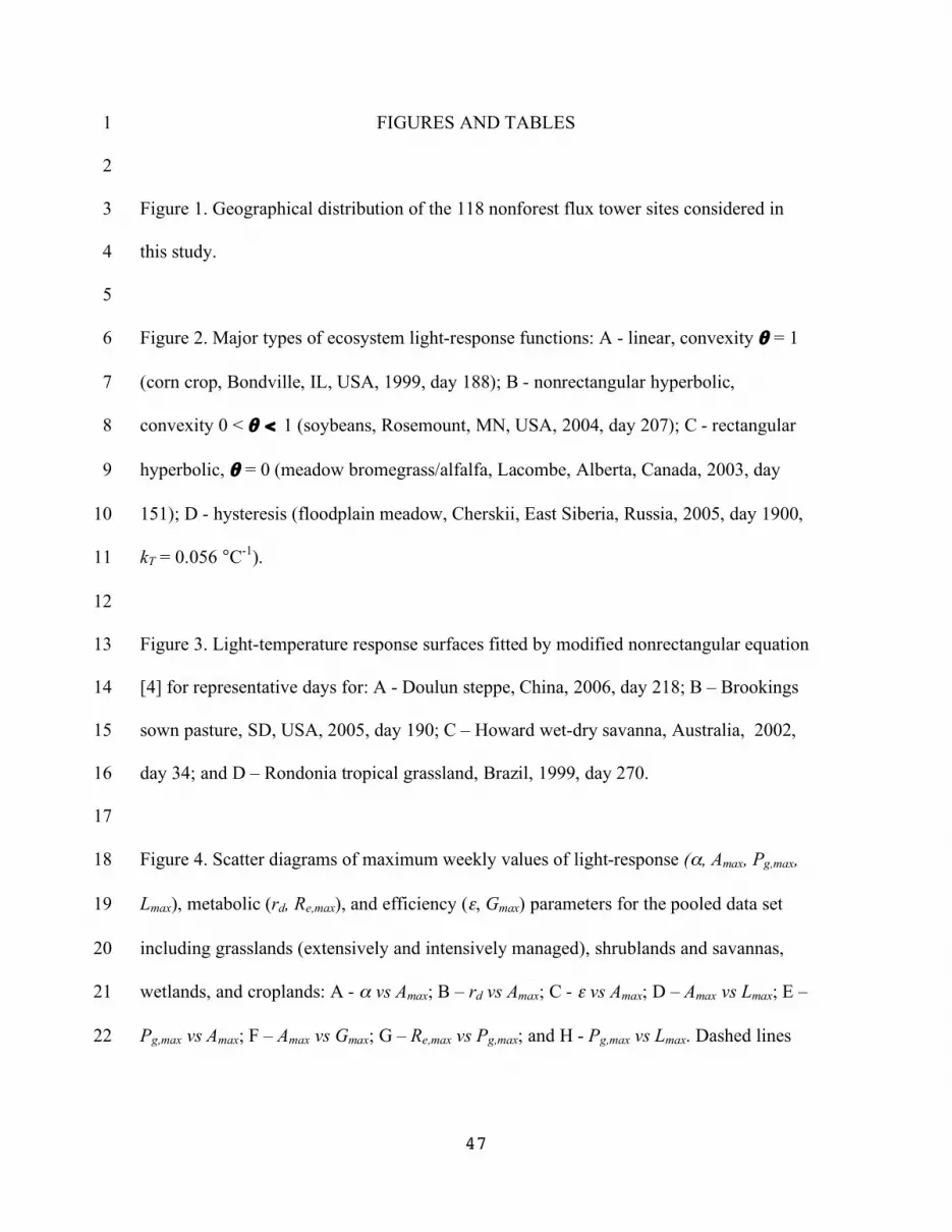
47

FIGURES AND TABLES 1

2

Figure 1. Geographical distribution of the 118 nonforest flux tower sites considered in 3

this study. 4

5

Figure 2. Major types of ecosystem light-response functions: A - linear, convexity θ = 1 6

(corn crop, Bondville, IL, USA, 1999, day 188); B - nonrectangular hyperbolic, 7

convexity 0 < θ < 1 (soybeans, Rosemount, MN, USA, 2004, day 207); C - rectangular 8

hyperbolic, θ = 0 (meadow bromegrass/alfalfa, Lacombe, Alberta, Canada, 2003, day 9

151); D - hysteresis (floodplain meadow, Cherskii, East Siberia, Russia, 2005, day 1900, 10

kT = 0.056 °C-1). 11

12

Figure 3. Light-temperature response surfaces fitted by modified nonrectangular equation 13

[4] for representative days for: A - Doulun steppe, China, 2006, day 218; B – Brookings 14

sown pasture, SD, USA, 2005, day 190; C – Howard wet-dry savanna, Australia, 2002, 15

day 34; and D – Rondonia tropical grassland, Brazil, 1999, day 270. 16

17

Figure 4. Scatter diagrams of maximum weekly values of light-response (α, Amax, Pg,max, 18

Lmax), metabolic (rd, Re,max), and efficiency (ε, Gmax) parameters for the pooled data set 19

including grasslands (extensively and intensively managed), shrublands and savannas, 20

wetlands, and croplands: A - α vs Amax; B – rd vs Amax; C - ε vs Amax; D – Amax vs Lmax; E – 21

Pg,max vs Amax; F – Amax vs Gmax; G – Re,max vs Pg,max; and H - Pg,max vs Lmax. Dashed lines 22

48

describe linear or allometric equations characterizing patterns of co-variation between 1

parameters. 2

3

Figure 5. Scatter diagrams of maximum weekly values of light-response (α, Amax, Pg,max, 4

Lmax), metabolic (rd, Re,max), and efficiency (ε, Gmax) parameters for the extensively 5

managed grasslands data subset: A - α vs Amax; B – rd vs Amax; C - ε vs Amax; D – Amax vs 6

Lmax; E – Pg,max vs Amax; F – Amax vs Gmax; G – Re,max vs Pg,max; and H - Pg,max vs Lmax. 7

Dashed lines describe linear or allometric equations characterizing patterns of co-8

variation between parameters. 9

10

Figure 6. Seasonal dynamics of light-response parameters: maximum photosynthesis, 11

Amax, daytime ecosystem respiration, rd, quantum yield, α, and gross ecological light-use 12

efficiency, ε, in selected nonforest ecosystems: A – floodplain meadow, Cherskii, 2003; 13

B – mixed prairie, Cottonwood, 2006; mixed prairie, Gudmundsen Ranch, 2006; D- 14

tallgrass prairie, Fort Reno, 2005; E – wet-dry savanna, Howard, 2002; F – tropical 15

grassland, Rondonia, 1999; G – sugar beet, Lonzee, 2004; H – corn crop, Bondville, 16

1999. 17

18

Figure 7. Seasonal dynamics and annual budgets of gross primary productivity, Pg(t), 19

total ecosystem respiration, Re(t), and cumulative net ecosystem CO2 exchange, 20

CumNEE(t) for selected nonforest sites and years: A – floodplain meadow, Cherskii, 21

2003; B – sown northern temperate grassland, Jokioinen, 2001-2002; C – temperate 22

grassland, Grillenburg, 2005; D – desert grassland, Audubon Ranch, 2004; E - dry 23

49

savanna, Skukuza, 2002; F – tropical grassland, Rondonia, 1999; G – corn crop, 1

Bondville, 2003; H – soybean crop, Mead, 2002. 2

3

Figure 8. Frequency distributions of gross primary production (A), ecosystem respiration 4

(B), and net ecosystem CO2 exchange (C) estimates in the pooled set site-years from 5

nonforest flux tower sites. 6

7

Figure 9. Scatter plot of RE versus GPP values for the pooled set of site-years from 8

nonforest flux tower stations of the world. The 1:1 diagonal is shown as a dashed line. 9

10

Figure 10. Scatter plots of the RE versus GPP values for various types of nonforest 11

ecosystems: A - extensively managed grasslands; B – intensively managed grasslands; C 12

– shrublands and savanna; D – wetlands; E – croplands. 13

14

Figure 11. Histograms of statistical distributions of the annual net ecosystem CO2 15

exchange values (NEE) in various types of nonforest ecosystems: A - extensively 16

managed grasslands; B – intensively managed grasslands; C – shrublands and savanna; D 17

– wetlands; E – croplands. 18

19

Figure 12. Response of gross primary production, GPP, (A, C) and ecosystem 20

respiration, RE, (B, D) of extensively managed grasslands on the annual precipitation 21

PCPN (A, B) and the dryness index DI = Rnet/(λ*PCPN). The dashed lines indicate 22

nonlinear regressions describing predominant trends. 23

50

1

Figure 13. Response of gross primary production, GPP, (A, C) and ecosystem 2

respiration, RE, (B, D) of intensively managed grasslands on the annual precipitation 3

PCPN (A, B) and the dryness index DI = Rnet/(λ*PCPN). The dashed lines indicate 4

nonlinear regressions describing predominant trends. 5

6

Figure 14. Response of gross primary production, GPP, (A, C) and ecosystem 7

respiration, RE, (B, D) of shrublands and savanna on the annual precipitation PCPN (A, 8

B) and the dryness index DI = Rnet/(λ*PCPN). The dashed lines indicate nonlinear 9

regressions describing predominant trends. 10

11

12

Table 1. Nonforest flux tower sites analyzed in this study. 13

14 Site Latitude Longitude Elevation PCPN Tyear Years Investigator(s) Method*

Croplands Ames, IA, USA, corn 41.720 -93.410 300 814 8.9 2003 J. Prueger L

Auradé, France 43.549 1.108 243 690 13.3 2005 E. Ceschia, P. Beziat T Batavia-agro, IL, USA 41.859 -88.223 227 921 10.5 2005-2006

R. Matamala; D. Cook T

Bondville, IL, USA, corn 40.006 -88.292 300 990 11.3 1997-2005

S. Hollinger; C. Bernacchi, T. Meyers L

Bondville, IL, USA, soybeans 40.006 -88.292 300 990 11.3 1998-2006

S. Hollinger; C. Bernacchi, T. Meyers L

Bondville-companion, IL, USA 40.006 -88.292 219 990 11.3 2005-2006

S. Hollinger; C. Bernacchi T

Borgo Cioffi-crop, Italy 40.524 14.957 20 490 19.0 2004-2006 V. Magliulo T

Carlow, Ireland 52.859 -6.918 59 824 9.4 2004-2006 M. Jones; G. Lanigan L

Doulun, China 42.046 116.280 1350 399 3.3 2005-2006 Shiping Chen L Foulum-crop, Denmark 56.484 9.587 51 712 8.0 2005 J. Olesen; K. Schelde T

Gebesee, Germany 51.100 10.914 162 492 9.6 2004-2006 C. Rebmann, W. Kutsch T

Grignon, France 48.844 1.952 125 600 11.1 2005-2006 P. Cellier T

Haller, PA, USA 48.860 -77.840 352 974 9.7 2003 R.H. Skinner L

51

Klingenberg, Germany 50.893 13.222 480 850 7.0 2004-2006

C. Bernhofer; T. Gruenwald T

Lamasquère, France, irrigated 43.493 1.237 180 690 13.3 2005 E. Ceschia T

Langerak, France 52.004 4.806 -1 786 9.8 2005-2006 E. Moors, J. Elbers, W. Jans T

Lonzee, Belgium 50.552 4.745 165 800 10.0 2004-2006 C. Moureaux, M. Aubinet L

Mase, Japan, paddy field 36.054 140.027 13 1200 13.7 2002-2003 A. Miyata T Mead, NE, USA, corn rainfed 41.180 -96.440 363 887 9.7 2001-2003 S. Verma, A. Suyker L Meadm NE, USA, soybeans rainfed 41.180 -96.440 363 887 9.7 2002-2004 S. Verma, A. Suyker L Mead, maize rotation irrigated 41.165 -96.470 362 887 9.7 2001-2003 S. Verma, A. Suyker T Mead, NE, USA, corn irrigated 41.165 -96.477 361 728 10.1 2001-2004 S. Verma, A. Suyker T Mead, NE, USA, soybeans irrigated 41.165 -96.470 362 728 10.1 2002-2004 S. Verma, A. Suyker T Molenweg, Netherlands 51.650 4.639 1 800 9.8 2005 E. Moors, J. Elbers T Oensingen, Switzerland 47.286 7.734 452 1100 9.0 2005

N. Buchmann; W. Eugster T

Ponca City, OK, USA, winter wheat 36.767 -97.133 310 866 14.8 1997 S. Verma L Risbyholm, Denmark 51.530 12.097 10 575 9.0 2004-2005 H. Soegaard T Rosemount, MN, USA 44.714 -93.090 260 799 6.8 2004-2005 T. Griffis, J. Baker L

Extensively managed grasslands

Alinya, Spain 42.202 1.449 1770 669 13.0 2003-2005 M.J. Sanz L

Amplero, Italy 41.867 13.633 884 1365 10.0 2003-2005 M. Balzarolo L

Atquasuk, AK, USA 70.470 -157.409 N/A 127 NA? 1999-2006 W. Oechel T Audubon Ranch, AZ, USA 31.591 -110.510 985 382 16.0 2002-2006 T. Meyers L

Barrow, AK, USA 71.323 -156.626 1 124 -12.5 1998-2002 W. Oechel T Batavia Prairie, IL, USA 41.841 -88.241 226 921 10.5 2005-2006 R. Matamala L Bily Kriz, Czech Republic 49.495 18.545 855 1200 5.5 2004-2006 M. Marek, R. Czerny T Brookings, SD, USA 44.311 -96.798 495 550 5.8 2004-2006

T. Meyers, T. Gilmanov, M. Heuer L

Bugacpuszta, Hungary 46.800 18.900 100 500 10.8 2003-2006 Z. Tuba, L Canaan Valley, WV, USA 39.063 -79.421 988 900 8.2 2004 T. Meyers L Cheyenne, WY, USA 41.183 -104.900 1910 397 7.2 1997-1998 J. Morgan L Cottonwood, SD, USA 43.950 -101.847 735 447 7.7 2004-2006

T. Meyers, A. Detwyler, K. Brehe L

CPER, CO, USA 40.683 -104.750 1660 332 9.2 2001-2004 J. Morgan L

Doulun, China 42.047 116.284 1350 399 3.3 2006 Shiping Chen L Duke grassland, NC, USA 35.971 -79.090 163 1145 15.5 2001-2005 G. Katul L

Fort Peck, MT, USA 48.308 -105.101 634 310 7.7 2000-2006 T. Meyers L Fort Reno, OK, USA 35.557 -98.017 421 870 14.9 2005

M. Torn, D. Billesbach L

Freeman Ranch, TX, USA 29.930 -98.010 244 959 19.4 2004 J. Heilman L

52

Goodwin Creek, MS, USA 34.250 -89.970 70 1455 15.7 2002-2006 T. Meyers L Grillenburg, Germany 50.951 13.514 400 853 7.2 2004-2006

C. Bernhofer, T. Gruenwald L

Gudmundsen Ranch, NE, USA 42.069 -101.407 1081 560 7.9 2006 D. Billesbach L

Haibei, China 37.617 101.317 3250 561 -1.7 2002-2003 T. Kato T

Ivotuk, Alaska 68.486 -155.750 550 250 -9.0 2004-2006 W. Oechel T

Jornada, NM, USA 32.600 -106.750 1320 272 N/A 2000-2001 W. Dugas, P. Mielnick L

Karnap, Uzbekistan 40.000 65.500 310 237 14.6 2001 M. Nasyrov, N. Saliendra L

Kendall, AZ, USA 31.737 -109.942 1531 356 17.0 1999-2006 W. Emmerich L

Khakasia, Russia 54.773 90.002 430 304 0.5 2002-2004 L. Belelli L

Khakasia-3, Russia 54.705 89.078 N/A N/A N/A 2004 L. Belelli T Kherlenbayan, Mongolia 47.214 108.737 1235 196 1.2 2003 S. Li L

Laqueuille, France 45.643 2.736 1040 1013 8.6 2002-2006 J.-F. Soussana, V. Allard L

Lethbridge, Canada 49.709 -112.940 960 378 6.4 1998-2002 L. Flanagan L Little Washita, OK, USA 34.967 -97.983 335 750 16.3 1997-1998 T. Meyers L

Malga Arpaco, Italy 46.117 11.703 1699 1200 6.3 2003-2004 A. Raschi L

Mandan, ND, USA 46.767 -100.917 518 404 5.0 1999-2001 A. Frank L

Matra, Hungary 47.842 19.726 350 605 10.6 2004-2005 J. Balogh T

Miles City, MT, USA 46.300 -105.967 719 343 7.9 2000-2001 M. Haferkamp L Monte Bondone, Italy 46.016 11.047 1550 1189 5.5 2003-2006 D. Gianelle T Neal Smith, IA, USA 41.558 -93.296 280 826 9.1 2005 J. Prueger L

Neustift, Austria 47.117 11.317 970 850 6.3 2001-2006 G. Wohlfahrt L Oensingen, Switzerland 47.283 7.733 450 1100 9.0 2002-2003

C. Ammann, J. Fuhrer L

Rannels Ranch, KS, USA 39.139 -96.523 324 840 12.9 1998-1999 C. Owensby L Rigi-Seebodenalp, Switzerland 47.058 8.457 1025 1327 7.3 2003

W. Eugster, N. Rogiers L

Rondonia, Brazil -10.762 -62.357 306 1664 23.9 1999 M. Waterloo, A. Manzi L

Santarem, Brazil -3.012 -54.537 N/A N/A N/A 2001-2002 D. Fitzjarrald L

Shidler, OK, USA 36.933 -96.683 356 942 14.8 1997-1999 S. Verma, A. Suyker L

Shortandy, Kazakhstan 51.667 71.000 367 323 1.6 1998-2001

K. Akshalov, N. Saliendra, D. A. Johnson L

Temple, TX, USA 31.100 -97.333 219 878 19.6 1998-1999 W. Dugas, P. Mielnick L

Tojal, Portugal 38.477 -8.025 190 750 15.5 2004-2006 C. Pio, L. Aires L Viara Ranch, CA, USA 38.407 -120.951 129 500 15.9 2001-2006 D. Baldocchi L Walnut River, KS, USA 37.521 -96.855 408 1030 13.1 2002-2004 R. Coulter, D. Cook L Woodward, OK, USA 36.600 -99.583 630 586 14.3 1997-2002 P. Sims, J. Bradford L Xilinhot grazed, China 43.554 116.671 1250 360 2.0 2006 Shiping Chen L Xilinhot-fenced, China 43.546 116.678 1250 360 2.0 2006 Shiping Chen T Xilinhot-typical fenced, China 44.134 116.329 1030 290 2.0 2004-2006 Guangsheng Zhou T

53

Intensively managed grasslands Cabauw- extension. The Netherlands 51.954 4.903 -1 786 9.8 2005 E. Moors, J. Elbers T Cabauw, The Netherlands 51.967 4.917 -1 800 10.0 2003 A. Hensen T Cabauw, The Netherlands 51.971 4.927 -1 786 9.8 2004-2006 E. Moors, J. Elbers T Carlow-grassland, Ireland 52.850 -6.900 50 804 10.1 2003 M. Jones, G. Lanigan L Dripsey-grass, Ireland 51.919 -8.751 187 1450 9.5 2002-2005 G. Kiely, P. Leahy T

Easter Bush, UK 55.867 -3.200 190 890 8.0 2003-2004 M. Sutton L Haarweg, The Netherlands 51.970 5.630 7 760 9.5 2002 A. Jacobs T Haastrect, Netherlands 52.004 4.806 -2 786 9.8 2003 E. Moors T

Haller, PA, USA 40.862 -77.840 352 974 9.7 2003-2005 R.H. Skinner L Hegihátsál, Hungary 46.950 16.650 248 759 8.9 1999 Z. Barcza, L. Haszpra T Horstermeer, Netherlands 52.029 5.068 -2 797 9.8 2004-2006 H. Dolman T

Jokioinen, Finland 60.899 23.514 104 581 3.9 2002 A. Lohila, T. Laurila L

Lacombe, Canada 52.436 -113.808 871 446 2.1 2003 V.S. Baron L

Laqueuille, France 45.643 2.736 1040 1013 8.6 2002-2006 J.-F. Soussana, V. Allard L

Lelystad, The Netherlands 52.500 5.500 0 780 10.0 2004 A. Hensen L Lille Valby, Denmark 55.700 12.117 15 1119 8.5 2004-2006 E. Dellwik L Oensingen, Switzerland 47.283 7.733 450 1100 9.0 2002-2006

C. Ammann; J. Fuhrer L

Shrublands and savanna

Burns, OR, USA 43.483 -119.717 1380 283 7.6 1995-2001 T. Svejcar L

Dubois, ID, USA 44.267 -112.133 1700 302 6.2 1996-2001 N. Saliendra, D.A. Johnson L

Howard Springs, Australia -12.329 131.000 38 1824 25.9 2002-2005 J. Berringer L

Karrykul, Turkmenistan 38.600 58.400 90 148 15.6 1998-2000

M. Dourikov, N. Saliendra, D.A. Johnson L

Kubuqi, China 40.381 108.549 1160 180 7.5 2006 Shiping Chen L Santa Rita, AZ, USA 31.821 -110.866 1120 330 17.6 2004-2006 R. Scott T

Sao Paulo, Brazil -21.619 -47.650 N/A 953 N/A 2001-2002 H. da Rocha T Skukuza, South Africa -24.983 31.600 263 561 21.6 2001-2003 N. Hanan L Sky Oaks, CA, USA, old stand 33.374 -116.623 1394 491 12.2 1997-2006 W. Oechel L Sky Oaks, CA, USA, young stand 33.377 -116.623 1429 491 12.2 1997-2001 W. Oechel T Tonzi Ranch, CA, USA 38.432 -120.966 177 559 15.4 2002-2006 D. Baldocchi T

Wetlands

Cherskii, Russia 68.615 161.339 4 200 -12.5 2003-2004 C. Corradi T CzechWet, Czech Republic 49.025 14.772 420 740 7.2 2006 M. Marek; D. Janous T Dongtan marsh-1, China 31.517 121.961 31 2192 15.7 2005

Bin Zhao; Guo Haiquang T

Dongtan marsh-2, 31.585 121.903 31 2074 15.7 2005 Bin Zhao; Guo T

54

China Haiquang

Dongtan marsh-3, China 31.517 121.972 31 1957 15.5 2005

Bin Zhao; Guo Haiquang T

Kaamanen wetland, Finland 69.141 27.295 155 395 -1.3 2000-2006 T. Laurila; M. Aurela T

PolWet, Poland 52.762 16.309 54 550 8.1 2004 J. Olejnik T

Siikaneva, Finland 61.833 24.193 N/A 713 3.0 2004-2006 M. Aurela T

Tadham Moore, UK 51.207 -2.829 3 750 11.1 2001 R. Harding T

1 * Method on net flux partitioning into photosynthesis and respiration: L – light-response 2

function analysis; T – nighttime temperature dependence. 3

4

5

Table 2. Parameters α, Amax, rd, and θ from the nonrectangular hyperbolic light-response 6

function

!

Fc(Q)=1

2"#Q + Amax $ (#Q + Amax)

2 $4#Amax"Q%

& '

(

) * $rd, for representative 7

days at the Bondville, Rosemount, Lacombe, and Brookings flux tower stations. 8

9

Parameters

Statistical

characteristics

Slope, α

mg CO2 µmol-1

Plateau, Amax

mg CO2 m-2 s-1

Respiration, rd

mg CO2 m-2 s-1

Convexity, θ

dimensionless

A. Corn crop, Bondville, IL, USA, 1999, day 188 R2 = 0.98; SE = 0.158 mg CO2 m-2 s-1

Estimate 0.0014 3.2 0.1936 1.0 Standard Error 0.0001 - 0.0423 0.0012 Student’s t 19.92 - 4.58 84.20 p-level 0.0000 - 0.0000 0.0000

Soybeans, Rosemount, MN, USA, 2004, day 207 R2 = 0.98; SE = 0.045 mg CO2 m-2 s-1

Estimate 0.0009 0.9930 0.2002 0.6947 Standard Error 0.0002 0.1899 0.0221 0.3329 Student’s t 4.77 5.23 9.07 2.09 p-level 0.0000 0.0000 0.0000 0.0243

Sown pasture, Lacombe, Alberta, Canada, 2003, day 151 R2 = 0.94; SE = 0.061 mg CO2 m-2 s-1

55

Estimate 0.0026 0.8321 0.3413 0.0 Standard Error 0.0009 0.0969 0.0273 - Student’s t 2.98 8.58 12.50 - p-level 0.0023 0.0000 0.0000 -

Floodplain meadow, Cherskii, East Siberia, Russia, 2003, day 214 R2 = 0.93; SE = 0.033 mg CO2 m-2 s-1

Estimate 0.0006 0.2987 0.1038 0.9333 Standard Error 0.0001 0.0252 0.090 0.090 Student’s t 5.31 11.85 11.58 10.38 p-level 0.0000 0.0000 0.0000 0.0000

1

2

Table 3. Parameters α, Amax, r0, kT and θ from the modified nonrectangular hyperbolic 3

light-temperature response function 4

!

Fc(Q,Ts) =1

2"#Q + Amax $ (#Q + Amax)

2 $ 4#Amax"Q%

& '

(

) * $ r0e

kTTs , for 5

representative days at Doulun, Brookings, Howard, and Rondonia sites. 6

7 Parameters

Statistical characteristics Slope, α

mg CO2 µmol-1 Plateau, Amax

mg CO2 m-2 s-1 Respiration, r0 mg CO2 m-2 s-1

Temperature coefficient, kT,

(°C)-1

Convexity, θ dimensionless

A. Steppe, Doulun, China, 2006, day 218 R2 = 0.98; SE = 0.037 mg CO2 m-2 s-1

Estimate 0.0009 0.5542 0.0377 0.0671 0.9644 Standard Error 0.00001 0.0241 0.0102 0.0116 0.0408 Student’s t 9.08 22.98 3.68 5.78 23.64 p-level 0.0000 0.0000 0.0003 0.0000 0.0000

B. Sown pasture, Brookings, SD, USA, 2005, day 190 R2 = 0.99; SE = 0.032 mg CO2 m-2 s-1

Estimate 0.0014 1.0867 0.0631 0.0614 0.0000 Standard Error 0.0001 0.0498 0.0141 0.0094 0.0000 Student’s t 13.87 21.81 4.48 6.53 - p-level 0.0000 0.0000 0.0000 0.0000 -

C. Wet-dry savanna, Howard, Australia, 2002, day 34 R2 = 0.97; SE = 0.074 mg CO2 m-2 s-1

Estimate 0.0017 1.147 0.0278 0.0690 0.8376 Standard Error 0.0003 0.1019 0.0167 0.0186 0.1529 Student’s t 5.83 11.25 1.67 3.71 5.48

56

p-level 0.0000 0.0000 0.0522 0.0004 0.0000

D. Tropical grassland, Rondonia, Brazil, 1999, day 270 R2 = 0.97; SE = 0.052 mg CO2 m-2 s-1

Estimate 0.0008 0.8048 0.0339 0.0760 0.9902 Standard Error 0.0001 0.0721 0.0183 0.0217 0.0230 Student’s t 9.38 11.16 1.85 3.50 43.04 p-level 0.0000 0.0000 0.0408 0.0014 0.0000 * Not significantly different from zero 1

2

Table 4. Statistical characteristics of annual gross primary production (GPP), total 3

ecosystem respiration (RE), and net ecosystem exchange (NEE) for major groups within 4

nonforest terrestrial ecosystems. 5

6

Ecosystem group Statistical characteristics

Grasslands extensively managed

Grasslands intensively managed

Shrublands and savanna

Wetlands Croplands

Gross primary production, GPP (g CO2 m-2 yr-1) Number of site-years 179 34 28 48 66 Mean 2708 5767 2949 2328 4521 Standard deviation 1842 1144 1950 1836 1365 Minimum 95 3141 645 749 1376 Maximum 8600 7720 6836 5643 6774

Total ecosystem respiration, RE (g CO2 m-2 yr-1) Number of site-years 169 34 27 18 66 Mean 2535 4990 2537 1824 3588 Standard deviation 1689 1024 1396 1373 909 Minimum 112 3186 756 665 1052 Maximum 7880 7003 5094 4751 5905

Net Ecosystem Exchange, NEE (g CO2 m-2 yr-1) Number of site-years 169 36 27 18 66 Mean 239 848 493 504 933 Standard deviation 521 658 740 719 814 Minimum -1342 -961 -585 -40 -770 Maximum 1762 2934 2254 2226 2382 7

8

Table 5. Maximum values of daytime gross primary productivity, Pg,max, and annual net 9

primary production, GPP, estimated for nonforest and forest flux-tower sites 10

Site Year Pg,max Site Year GPP

57

g CO2 m-2

d-1 g CO2 m-2

yr-1

A. Grasslands extensively managed

Neustift, Austria 2004 76.2 Rondonia, Brazil 1999 8600 Jornada, NM, USA 2000 63.1 Neustift, Austria 2006 7415

Rannels Ranch, KS, USA 1998 60.8 Goodwin Creek, MS, USA 2004 6391

Batavia Prairie Site, IL, USA 2006 59.9 Grillenburg, Germany 2005 6299

Grillenburg, Germany 2005 57.34 Duke grassland, NC, USA 2003 6039

Monte Bondone, Italy 2006 56.9 Laqueuille, France, extensive 2006 5943

Shidler, OK, USA 1999 56.9 Neal Smith, IA, USA 2005 5756

Temple, TX, USA 1999 56.2 Batavia Prairie Site, IL, USA 2006 5435

Oensingen, Switzerland 2003 53.6 Oensingen, Switzerland 2003 5326

Neal Smith, IA, USA 2005 52.7 Laqueuille, France, extensive 2004 5322

Laqueuille, France, extensive 2004 51.7

Rigi-Seebodenalp, Switzerland 2003 5320

Goodwin Creek, MS, USA 2003 51.4 Shidler, OK, USA 1997 5208

B. Grasslands intensively managed Cabauw- extension. The Netherlands 2005 76.3 Oensingen, Switzerland 2004 7720 Easter Bush, UK 2003 63.6 Dripsey-grass, Ireland 2004 7388 Oensingen, Switzerland 2004 63.5 Haastrect, Netherlands 2003 7267 Lille Valby, Denmark 2006 63.4 Lille Valby, Denmark 2004 6873

Haastrect, Netherlands 2003 63.1 Laqueuille, France, intensive 2004 6838

Laqueuille, France, intensive 2006 59.0

Carlow-grassland, Ireland 2003 6807

Carlow-grassland, Ireland 2003 57.9 Easter Bush, UK 2003 6793 Haarweg, The Netherlands 2002 57.5

Cabauw- extension. The Netherlands 2005 6785

Dripsey-grass, Ireland 2003 54.7 Haarweg, The Netherlands 2002 5915

Lacombe, Alberta, Canada 2003 53 Hegihátsál, Hungary 1999 5867 Haller, State College, PA, USA 2004 52.2

Cabauw, The Netherlands 2004 5837

Cabauw, The Netherlands 2004 47.9 Horstermeer, Netherlands 2006 5337

C. Shrubs and savannas

Howard Springs, Australia 2005 54.2 Sao Paulo cerrado, Brazil 2002 6836 Sao Paulo cerrado, Brazil 2002 42.7 Howard Springs, Australia 2002 5874 Tonzi Ranch, California 2005 38.6 Skukuza, South Africa 2001 3947 Skukuza, South Africa 2001 34.6 Tonzi Ranch, CA, USA 2005 3837

58

Tonzi Ranch, California 2003 34.1 Sky Oaks Old stand, CA, USA 1997 2682

Sky Oaks Young stand, CA, USA 1998 22.7

Sky Oaks Young stand, CA, USA 1998 2021

Sky Oaks Old stand, CA, USA 1997 21.0 Skukuza, South Africa 2003 1873 Santa Rita mesquite, AZ, USA 2005 19.8

Santa Rita mesquite, AZ, USA 2005 1125

Kubuqi, shrubland, China 2006 12.8 Kubuqi, shrubland, China 2006 1021

Karrykul, Turkmenistan 2000 7.79 Karrykul, Turkmenistan 2000 769

D. Wetlands

Dongtan marsh-2, China 2005 70.1 Dongtan marsh-2, China 2005 5643 CzechWet, Czech Republic 2006 56.9 CzechWet, Czech Republic 2006 5368 Dongtan marsh-1, China 2005 51.9 Dongtan marsh-1, China 2005 5150 Dongtan marsh-3, China 2005 43.3 Tadham Moore, UK 2001 4767

Tadham Moore, UK 2001 41.1 Dongtan marsh-3, China 2005 3662 PolWet, Poland 2005 41.1 PolWet, Poland 2005 3393 Cherskii, Russia 2003 20.1 Siikaneva, Finland 2005 1359

Kaamanen wetland, Finland 2005 19.8 Kaamanen wetland, Finland 2005 1210

Siikaneva, Finland 2004 19.8 Cherskii, Russia 2003 834

E. Croplands Mead, corn rot. irrigated, NE, USA 2001 116.1 Langerak-crop, France 2005 6774 Mead, maize cont. irrigated, NE, USA 2001 107.8

Mead, rot. corn irrigated, NE, USA 2003 6720

Bondville, corn, IL, USA 1999 99.9 Borgo Cioffi-crop, Italy 2005 6513

Batavia-agro, IL, USA 2006 99.0 Mead, cont. corn irrigated, NE, USA 2001 6437

Bondville, corn, IL, USA 1999 94.1 Borgo Cioffi-crop, Italy 2006 6393

Borgo Cioffi-crop, Italy 2006 93.1 Mead, maize rotation irrigated 2001 6316

Mead, corn rainfed, NE, USA 2003 87.6

Lonzee, Belgium, sugar beet 2005 6313

Langerak-crop, France 2006 87.5 Oensingen-crop, Switzerland 2005 6295

Bondville-companion, IL, USA 2006 83.03

Mead corn rainfed, NE, USA 2001 5834

Grignon-crop, France 2005 81.3 Bondville, corn, IL, USA 1999 5602 Lonzee, winter wheat, Belgium 2005 80.5

Bondville, soybeans, IL, USA 2005 5582

Bondville, soybeans, IL, USA 2005 80.1 Risbyholm, Denmark, crop 2004 5525

F. Forests and plantations Duke Forest Loblolly Pine, NC, USA 2001 99.0 French Guyana 2004 14339 Campbell River, British Columbia, Canada 1998 86.6 Vanuatu - CocoFlux 2002 13057 Hampshire Forest, UK 2004 73.9 Rondonia forest, Brazil 2002 12727 Duke Forest Loblolly Pine 2005 69.0 Palangkaraya, Indonesia 2003 12236

59

Vanuatu - CocoFlux 2003 68.2 Santarem km67 primary forest, Brazil 2003 11703

Duke Forest Hardwood, NC, USA 2003 67.6

Caxiuana Forest-Almeirim, Brasil 2002 11436

French Guyana 2005 64.21 Santarem km67 primary forest, Brazil 2002 11271

Rondonia forest, Brazil 2002 60.8 Loblolly Pine plantation, NC, USA 2006 10173

Campbell River, British Columbia, Canada 2000 60.1

Donaldson Slash Pine Plantation, FL, USA 1999 9249

Loblolly Pine plantation, NC, USA 2006 59.7

Campbell River, British Columbia, Canada 2005 9162

Duke Forest Hardwood, NC, USA 2004 57.5

Duke Forest Loblolly Pine, NC, USA 2002 9067

Donaldson Slash Pine Plantation, FL, USA 1999 54.6

Duke Forest Hardwood, NC, USA 2003 8892

1

2

60

1

Figure 1. 2

3

Figure 2. 4

5

61

1

Figure 3. 2

62

1

Figure 4. 2

63

1

Figure 5. 2

3

64

1

2

3

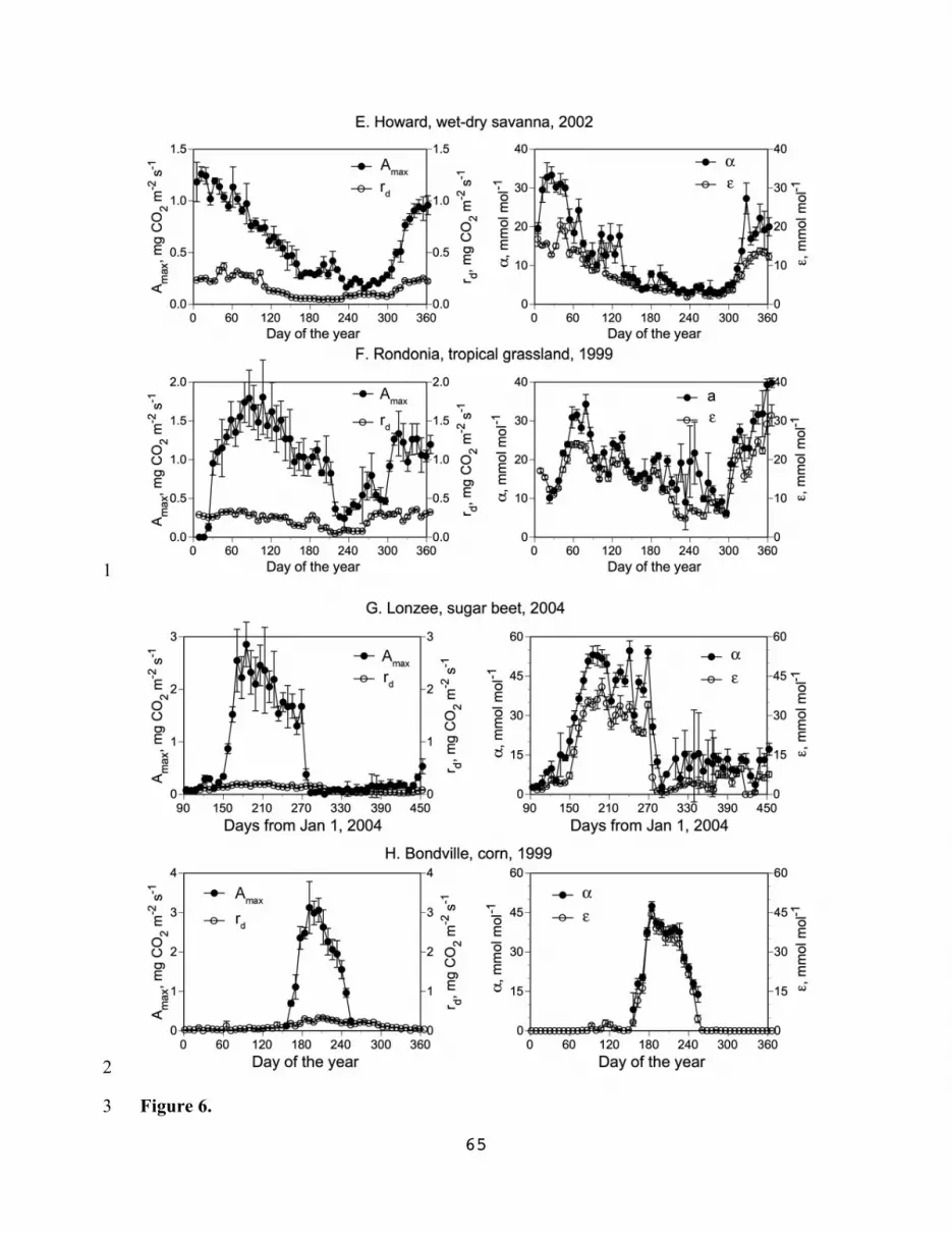
65

1

2

Figure 6. 3

66

1

67

1

Figure 7. 2

68

1

Figure 8. 2

3

69

1

Figure 9. 2

70

1

Figure 10. 2

3

4

5

6

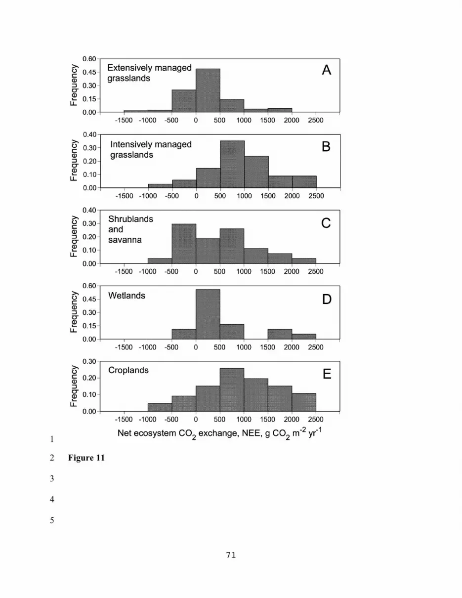
71

1

Figure 11 2

3

4

5

72

1

Figre 12 2

3

4

Figure 13 5

73

1

Figure 14. 2

3