Agriculture, Ecosystems and Environment 101 (2004) 39–51

Scale-dependent controls on ecological functions inagroecosystems of Argentina

E.F. Viglizzoa,b,d,∗, A.J. Pordomingoa,d, M.G. Castroc,F.A. Lértorad, J.N. Bernardosd

a INTA, Centro Regional La Pampa, Av. Spinetto 785, 6300 Santa Rosa, La Pampa, Argentinab CONICET, Centro Regional La Pampa, 6300 Santa Rosa, La Pampa, Argentina

c Secretary of Ecology of La Pampa Province, Av. Luro 700, First Floor, 6300 Santa Rosa, La Pampa, Argentinad Faculty of Natural Sciences, La Pampa University, Av. Uruguay 151, 6300 Santa Rosa, La Pampa, Argentina

Received 16 July 2002; received in revised form 7 March 2003; accepted 19 May 2003

Abstract

Agricultural managers that operate at different levels (plot, farm, landscape, region) need to understand how ecologicalfunctions (energy, nutrients and water flows and cycles) are controlled by scale-dependent factors. Using cross-level datafrom the Argentine pampas, analyzed by simple and multiple regression analysis, we demonstrate that controls differ fromone spatio-temporal level to the other, but they can be altered by humans. In the Argentine pampas, environmental controls(climate, landform, soil quality) seem to have a strong top-down influence on lower levels. But the bottom-up aggregatedeffect of anthropogenic controls seems to scale-up to upper levels and counteract such influence. Thus, the more intense useof land and technology in small units, the larger the up-scaling human influence on ecological functions. We suggest that adiscrimination among farming intensity levels is useful and necessary to understand and predict human controls on ecologicalfunctions across scales.© 2003 Elsevier B.V. All rights reserved.

Keywords:Ecological functions; Scale-dependent controlling factors; Top-down and bottom-up controls; Land use; Technology; Argentineagroecosystems

1. Introduction

To make sound decisions, agronomists, farmers,land managers, and development agents who operateat different levels (plot, farm, agroecosystem, land-scape, region) need to understand the links betweenscale and ecological functions (energy, nutrients andwater flows and cycles) that are critical to agriculture(Freemark, 1995).

∗ Corresponding author. Tel./fax:+54-2954-434-222.E-mail address:evigliz@cpenet.com.ar (E.F. Viglizzo).

The hierarchical approach to analyze ecological sys-tems was introduced nearly one century ago, but itwas only in recent decades that it was properly devel-oped by various authors. The traditional view looksat ecological systems as a vertically arranged hierar-chy (Patee, 1973; Allen and Starr, 1982; Salthe, 1985;O’Neill et al., 1986), in which upper levels often con-trol the lower ones through a so-called hierarchicalcontrol. A more recent approach (Nielsen, 2000) tendsto see the hierarchy as a series of thermodynamicallyembedded or nested systems, in which outer levelscontrol the inner ones by a continuous supply of energyfrom one level to the following (Warren, 1979; Klijn

0167-8809/$ – see front matter © 2003 Elsevier B.V. All rights reserved.doi:10.1016/S0167-8809(03)00229-9

40 E.F. Viglizzo et al. / Agriculture, Ecosystems and Environment 101 (2004) 39–51

and Udo de Haes, 1994; Bailey, 1995). At the sametime, ecologists accept that new properties emerge ateach level that are not present at the rest of the levels.As Odum (1977)stated, the knowledge on propertiesat one level is insufficient to explain the properties atthe next level. This means that the whole picture canonly be completed with specific studies on each levelacross a multi-level hierarchy.

The concepts of level and scale should be differenti-ated. While levels are qualitative, human abstractionsthat are constructed to facilitate the analysis, scalesare concrete spatial and time measures designed toprovide a quantitative focus on cross-level problems(Dumanski et al., 1998).

The strong relationship between hierarchical leveland function has long been recognized in ecology(Holling, 1992). However, due to the increasing needof balancing production and environmental demands,concerns about the ecosystem dynamics across lev-els have increased in recent years (Gardner, 1998).Considering the complex behavior of ecosystems inspace and time (Gustafson, 1998), we need to knowmore about the hierarchical factors and mechanismsthat control ecological functions across different spa-tial and temporal scales (Weston and Ruth, 1997). Thisknowledge is key to guide sound decision-making.

Controls on ecological functions are determinedby both, bio-physical and socio-economic drivers (DeKoning et al., 1999), which vary from one scale toanother (Bergkamp, 1998). While landform, climateand land quality are generally considered strong,large-scale environmental controls (Bailey, 1998),land use and applied technology should be consideredsmall-scale and human-driven controls (Buringh andDudal, 1987). However, asTurner et al. (1995)postu-late, both categories (socio-economic and bio-physicaldrivers) may have both, bottom-up and top-down in-fluences. According toO’Neill et al. (1996), whiletop-down controls result mainly from environmentalfactors that vary across a large geographical area, thebottom-up ones are the result of both, bio-physicaland anthropogenic factors that vary in time, andemerge from small geographical units. Top-downcontrols determine predictable geographic patterns ofenergy, nutrient and water flows and cycles (Wagenet,1998). On the other hand, bottom-up controls seemto be determined by human-driven factors (e.g., cropsallocation, tillage operations, pesticides application,

seasonal fertilization), that can up-scale their effectsto higher levels (Solbrig and Viglizzo, 1999).

The assessment of scale-dependent influences isnot simple in agroecology. Practical problems arisewhen the results from small-scale studies, common intraditional agricultural research, are used to interpretlarge-scale events, and make inference from them(Hobbs, 1998). Given that experiments on lower levels(e.g., the plot, the farm) are usually too small and tooshort to perceive changes that normally occur on up-per levels (the landscape, the ecoregion) through longperiods of time (Carpenter et al., 1995), alternativeapproaches seem to be necessary to focus the problem.

Given that field experimentation involving differentscales is not always possible in ecology, we have to ac-cept that hierarchical studies are useful and necessary.Statistical data and records on land and technologyuse on broad geographic scales should be viewed byresearchers as valuable replacements for cross-scaleexperiments. Furthermore, the complementary useof theoretical, observational, and experimental ap-proaches seems to be essential to build a body ofcross-scale knowledge in agroecology (Hobbs, 1998).

In this work, we analyzed the impact of environ-mental and anthropogenic controls on key ecologicalfunctions (flows and cycles of energy and nutrients)at three different geographic and temporal scales inagroecosystems of the Argentine pampas. At the sametime, we addressed two distinct, though closely re-lated questions: (a) How do environmental and humancontrols affect ecological functions across scales? (b)Can humans increase their control on key ecologicalfunctions? Answers to these questions may help agri-cultural and land managers to make sensible decisionsat each level, minimizing negative impacts on bothupper and lower levels.

2. Methods

2.1. Description of the study region

The Argentine pampas is a wide plain with morethan 52 million ha of lands suitable for cattle rearingand cropping. The area has a relatively short farminghistory. The pampas remained as native grassland un-til the end of 19th century and the beginning of 20thcentury, and then, lands were allocated in varying

E.F. Viglizzo et al. / Agriculture, Ecosystems and Environment 101 (2004) 39–51 41

proportions to cattle and crop production underdryland conditions. The generalized application ofagronomic practices suitable for humid zones causedsevere episodes of soil erosion in semiarid and sub-humid areas during the first half of the 20th century(Cole et al., 1989). An example of this ecologicaldisruption was the pampean “dust bowl” during the1930s and 1940s, similar to the process that the GreatPlains had in North America during the same period(Covas, 1989; Viglizzo et al., 1991; Lal, 1994).

Applied technology varied greatly along the lastcentury. Agricultural systems based on crop–crop andcrop–pasture rotations under grazing conditions havebeen extensively disseminated until the 1980s. Thistraditional rotation scheme tended to disappear duringthe 1990s, when crop and animal production became

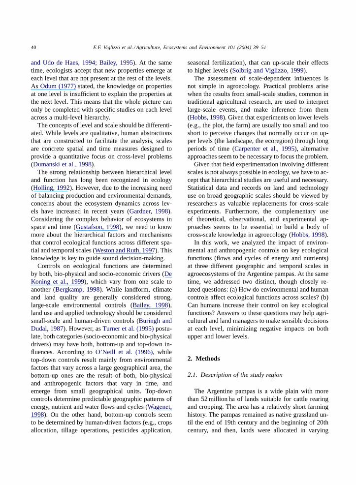
Fig. 1. Location of more relevant ecological areas in the Argentine pampas ecoregion: (1) rolling pampas, (2) subhumid central pampas,(3) semiarid central pampas, (4) southern pampas, (5) Mesopotamian pampas, and (6) flooding pampas. Thin isolines are isohyets (mmper year); thick isolines are mean annual temperature (◦C).

managed as rather independent and highly specializedactivities on the farm. Plow harrow and hand sowingwere very common all over the region, independentlyof soil fragility, until the 1930s and 1940s. In responseto the “dust bowl”, less aggressive conventional tillage(shallow disk) and mechanical sowing predominatedbetween the 1950s and 1970s. The adoption of con-servation tillage and no-till practices has significantlyincreased during the 1980s and 1990s. Although pesti-cides were extensively used since the 1960s, crops andpastures fertilization increased noticeably only duringthe 1990s.

According to rainfall and soil quality patterns, theregion was divided into five ecologically homoge-neous areas (Fig. 1). In this figure, areas 2 and 3are only climatic divisions (subhumid and semiarid,

42 E.F. Viglizzo et al. / Agriculture, Ecosystems and Environment 101 (2004) 39–51

respectively) of the same landscape (the central pam-pas). So, they were considered as a same ecologicalarea for analytical purposes. Briefly, the arable soilsof the pampas have few limitations to crop produc-tion, and the majority is suitable for grazing. Fol-lowing FAOs guidelines for land use (FAO, 1989),well-drained conditions on deep soils that can sup-port land use indefinitely predominate in the so-calledrolling pampas. Organic matter, as well as the nitrogencontents and the granular structure of soils decreasefrom the eastern humid to the western semiarid lands.Most lands are suitable for cultivation in thecentralpampas, although susceptibility to wind erosion im-poses some limitations to crop production. Problemsof salinity, drainage and water erosion limit produc-tion in the marginal lands of theflooding and theMesopotamianpampas (Musto, 1979; Casas, 1998).In spite of the fact that soil depth limits crop produc-tion in areas of thesouthernpampas, most lands are ingeneral suitable for cultivation. Some marginal lands,suitable for cattle production only, can also be foundon the western sector of the region. Unsuitable landsthat cannot support land use on a sustained basis arevery rare in the pampas. In a large part of the region,cattle and crop production activities are combined indifferent proportions according to their susceptibilityto environmental constraints (Viglizzo, 1986). Cattleproduction ranges from steer fattening to cow–calf op-erations on both perennial and annual pastures, and na-tive grasslands (Hall et al., 1992). The rainfall regimevaries in space and time, determining occasional ex-treme conditions of droughts and floods over wide ar-eas (Viglizzo et al., 1997).

2.2. Data sources

Different sources of information have been utilizedin this study: (1) six general agricultural censuses ofyears 1881, 1914, 1937, 1947, 1960, and 1988 thatcomprised the totality of farms scattered in 147 po-litical districts, (2) one national survey for 1996, thatcomprised a sample of farms in different areas, (3) avariety of production and yield statistics regularly pub-lished by the Department of Agriculture of Argentina,and (4) energy, nitrogen (N), and phosphorus (P) con-centration of inputs and outputs as determined by var-ious authors. Data on land use and crop yields wereanalyzed for all districts. Land use was expressed in

terms of the relative area (%) of crops, pastures andnatural grasslands with respect to the total area devotedto farming activities. The analysis was based onlyon predominant (crop and beef production) activities:wheat (Triticum aestivumL.), maize (Zea maysL.),soybean (Glycine maxL. Merr.), and sunflower (He-lianthus annuusL.). Because of the lack of long-termdata, beef production was estimated from equations foreach ecologically homogeneous area (Viglizzo, 1986)that relate stocking rate (available data) to meat pro-duction per hectare.

2.3. Land use, technology and scale analysis

Changes in key ecological functions such as theenergy flow and nutrient dynamics were analyzed inthis study at different spatial and temporal scales.Three scales were considered: (1) the pampas as awhole at the broader scale, (2) five agroecologicalareas at the intermediate scale, (3) 145 political dis-tricts that are part of the five agroecological areas atthe smaller scale. At the broad scale, the control ofecological functions was analyzed in terms of envi-ronmental factors, such as the predominant climate,soil and landform conditions. At the intermediatescale, simple and multiple regression analysis wasused to assess the control of environmental and an-thropogenic factors on the variability of energy andnutrient flows. A similar regression analysis was usedat the smaller district-scale.

Supported by a GIS, different patterns of landand fossil energy use intensity were identifiedthrough software (ArcView) that linked databases andgeo-referenced maps. The density of dots in mapsrepresents the relative allocation of land and the rel-ative use of fossil energy in the five study ecologicalareas. Fossil energy was used to assess changes intechnology application. The annual fossil energy con-sumption (FEC) (MJ ha−1) was an aggregate valuethat resulted from the sum of fossil energy consumed,respectively, by predominant farming activities (fourcrops and beef production). It was estimated byconsidering: (1) the tillage method, (2) the amountof applied pesticides, (3) the level of nitrogen (N)and phosphorus (P) fertilization, and (4) seed of im-proved varieties. Plow harrow and hand sowing wereused until the 1930s and 1940s, conventional tillage(shallow disk) and mechanical sowing predominated

E.F. Viglizzo et al. / Agriculture, Ecosystems and Environment 101 (2004) 39–51 43

between the 1950s and 1970s, and conservation tillageand no-till practices were increased during the 1980sand 1990s. Pesticides were extensively used since the1960s, but crops and pastures fertilization increasedvery quickly only during the 1990s.

2.4. The energy model

An energy model proposed byOdum (1975), basedon basic input–output relationships, was utilized forthe energy analysis. Given that input technologies(e.g., oil for machinery operation, fertilizers, pesti-cides, concentrate feeds, etc.) are normally associatedwith the use of fossil energy, an important assumptionin this work was that the input of fossil energy is agood indicator of technology incorporation. Differentsources (Grossi-Gallegos et al., 1985; Reed et al.,1986; Stout, 1991; Conforti and Giampietro, 1997)were used to estimate the energy values of inputsand outputs. The following energy values expressedin MJ ha−1 per year were used for inputs: (1) aver-age energy consumption in terms of oil equivalentswas estimated at 462, 260, 80 and 323, and for con-ventional, minimum, zero tillage, and agrochemicalapplication, respectively; and (2) energy consumptionwas 418, 20.3, and 277 as pesticides, seeds, and trac-tors and machinery, respectively. Energy values ofoutputs (in MJ kg−1) were estimated at 25.53 for sun-flower, soybean and peanut grains, 16.33 for wheat,maize and sorghum, and 13.36 for bovine meat.

The energy analysis of inputs and outputs was donefor the period 1960–2000 in the five study ecore-gions and the 145 districts. Estimations were made forperennial pastures, summer and winter grain pastures,summer and winter grain crops, and oil-seed crops. Acorrelation analysis was done to evaluate the degreeof association between the output of energy, and thenitrogen and phosphorus output, respectively. If thevalue of the correlation coefficients was high (morethan 90%), the analysis would be focused on the en-ergy factor only.

2.5. The nutrients dynamics

Using a simple mathematical model, a simplifiedinput–output relationship for N and P was estimatedby difference between the main sources of gain andloss. The respective nutrient content (in g kg−1 of

product) of wheat, maize, sorghum, linseed, soybean,sunflower, peanut and meat were 22.9, 16.3, 20.0, 40.8,58.1, 40.8, 51.2 and 27.0, respectively, in terms of N;4.3, 3.5, 3.4, 8.0, 6.8, 7.6, 6.1 and 43.1, respectively,in terms of P (Lloyd et al., 1978; NRC, 1978). In thecase of N, the extraction from soil by crops and cattleproduction was subtracted from literature-based N in-put estimation to the soil by legumes in different eco-logical areas. The following issues have been takeninto account: (a) the area devoted to crop production,(b) the area devoted to leguminous perennial pastures,(c) the N lost by outputs (grain and beef) that wasclosely related to yield and N density in products, and(d) the N fixed by leguminous and the amounts addedby occasional fertilization.

2.6. The analytical model

Previous theoretical studies on the Argentine Pam-pas (Nakama and Sobral, 1987; INTA/UNDP, 1990)were used to assess the environmental control on eco-logical functions at the largest analyzed geographicalscale (the region). They were used to identify differ-ent patterns of potential productivity among the fivestudy agroecological areas. It was only a qualitativeassessment. A so-called productivity index (PI) wasdetermined through the application of a multiplicativemethod (Riquier et al., 1970) that incorporates themain factors affecting land productivity for crop pro-duction. The method includes: (a) climate conditions,(b) drainage capacity, (c) soil depth, (d) soil texture,(e) salt density, (f) alkalinity, (g) organic matter con-centration, (h) exchangeable cation capacity, and (i)soil erodability. Although they all can be consideredenvironmental factors, it must be accepted that someof them have been affected by humans for more than100 years of continuous farming. However, the rela-tive effect of anthropogenic factors at this scale wasvery hard to determine.

Quantitative analytical methods were used, on theother hand, to assess the intermediate scales (fiveecological areas comprising many districts, and 144single districts). Simple and multiple regression anal-ysis were used at those two scales to quantify theeffect of environmental and anthropogenic controlson energy, and indirectly on nitrogen and phosphorusflows. The purpose of this analytical procedure wasto determine the relative weight of environmental and

44 E.F. Viglizzo et al. / Agriculture, Ecosystems and Environment 101 (2004) 39–51

anthropogenic factors to explain the variability of en-ergy output during the period 1960–1996. Long-termchanges in the annual productivity (MJ ha−1 per year)of farming activities were considered an acceptableindicator of human control on ecological functions. Itwas assumed that the increase of productivity alongthe 36-year study period, was mainly explained byhuman influence through the changes that have beenintroduced in land use and technology incorporation.Our analysis included the annual rate (%) of energyproductivity change (EPC), which was the dependentvariable, and the corresponding independent vari-ables of: (a) the average energy productivity (AEP) inMJ ha−1 per year, (b) the annual rate (%) of changein the cultivated area or annual rate (%) of croplandchange (CC), and (c) the annual rate (%) of changein FEC. While the first one (AEP) was consideredan environmental driving factor, the last two (CC andFEC) were both considered human-dependent factors.Thus, the higher the value of determination coeffi-cients (r2), the higher the relative influence of theanalyzed independent variables. A non-assessed inter-action between human factors and climate variabilitywas not discarded. It must be mentioned that therewas no inter-correlation among AEP, CC and FEC.

3. Results

Normally, the output of energy and nutrients areclosely associated (Viglizzo et al., 2001). Looking foran analytical simplification, we explored the correla-tion between the output of energy, and the output ofnitrogen and phosphorus, respectively. Highly signifi-cant (P < 0.01) correlation coefficients for the outputof energy and nitrogen (r = 0.996) and also for en-ergy and phosphorus (r = 0.989), suggested that theanalysis of only one factor (the energy output, in thiscase) would enable us to make a reliable inference onthe other two (the nitrogen and phosphorus output).

3.1. Control on ecological functions at the broaderscale (the whole region)

The energy flow and the nutrients dynamics in thepampas, as a whole region, appear to be strongly de-termined by environmental factors like climate, soilquality and landform.

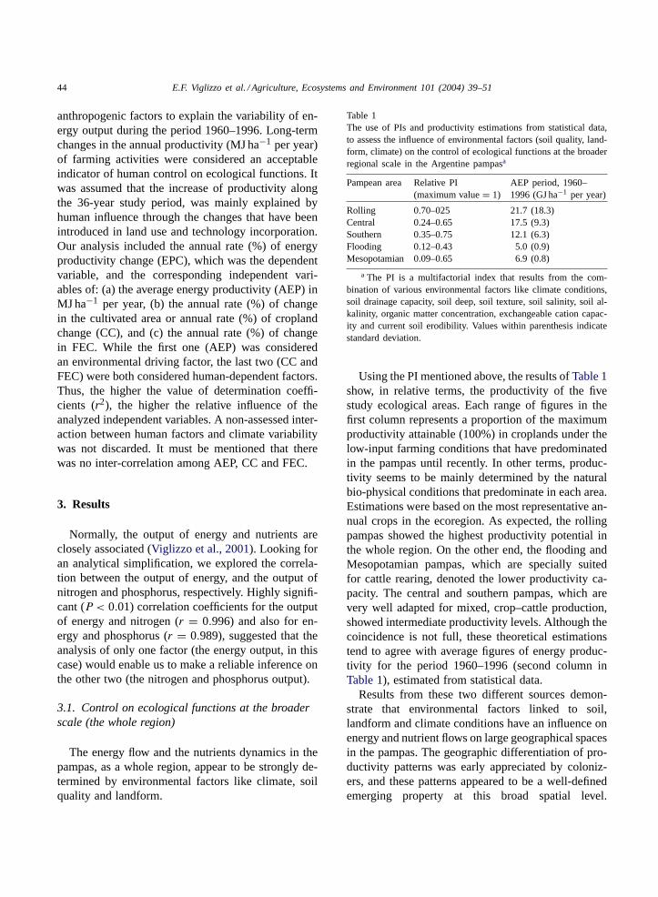
Table 1The use of PIs and productivity estimations from statistical data,to assess the influence of environmental factors (soil quality, land-form, climate) on the control of ecological functions at the broaderregional scale in the Argentine pampasa

Pampean area Relative PI(maximum value= 1)

AEP period, 1960–1996 (GJ ha−1 per year)

Rolling 0.70–025 21.7 (18.3)Central 0.24–0.65 17.5 (9.3)Southern 0.35–0.75 12.1 (6.3)Flooding 0.12–0.43 5.0 (0.9)Mesopotamian 0.09–0.65 6.9 (0.8)

a The PI is a multifactorial index that results from the com-bination of various environmental factors like climate conditions,soil drainage capacity, soil deep, soil texture, soil salinity, soil al-kalinity, organic matter concentration, exchangeable cation capac-ity and current soil erodibility. Values within parenthesis indicatestandard deviation.

Using the PI mentioned above, the results ofTable 1show, in relative terms, the productivity of the fivestudy ecological areas. Each range of figures in thefirst column represents a proportion of the maximumproductivity attainable (100%) in croplands under thelow-input farming conditions that have predominatedin the pampas until recently. In other terms, produc-tivity seems to be mainly determined by the naturalbio-physical conditions that predominate in each area.Estimations were based on the most representative an-nual crops in the ecoregion. As expected, the rollingpampas showed the highest productivity potential inthe whole region. On the other end, the flooding andMesopotamian pampas, which are specially suitedfor cattle rearing, denoted the lower productivity ca-pacity. The central and southern pampas, which arevery well adapted for mixed, crop–cattle production,showed intermediate productivity levels. Although thecoincidence is not full, these theoretical estimationstend to agree with average figures of energy produc-tivity for the period 1960–1996 (second column inTable 1), estimated from statistical data.

Results from these two different sources demon-strate that environmental factors linked to soil,landform and climate conditions have an influence onenergy and nutrient flows on large geographical spacesin the pampas. The geographic differentiation of pro-ductivity patterns was early appreciated by coloniz-ers, and these patterns appeared to be a well-definedemerging property at this broad spatial level.

E.F. Viglizzo et al. / Agriculture, Ecosystems and Environment 101 (2004) 39–51 45

Furthermore, asViglizzo et al. (2001)have demon-strated, the human colonization of the pampas wasclearly driven by environmental factors (land qualityand rainfall regime), which allowed a quick trans-formation of the best endowed natural lands intocroplands.

3.2. Control on ecological functions at intermediatescales (agroecological areas)

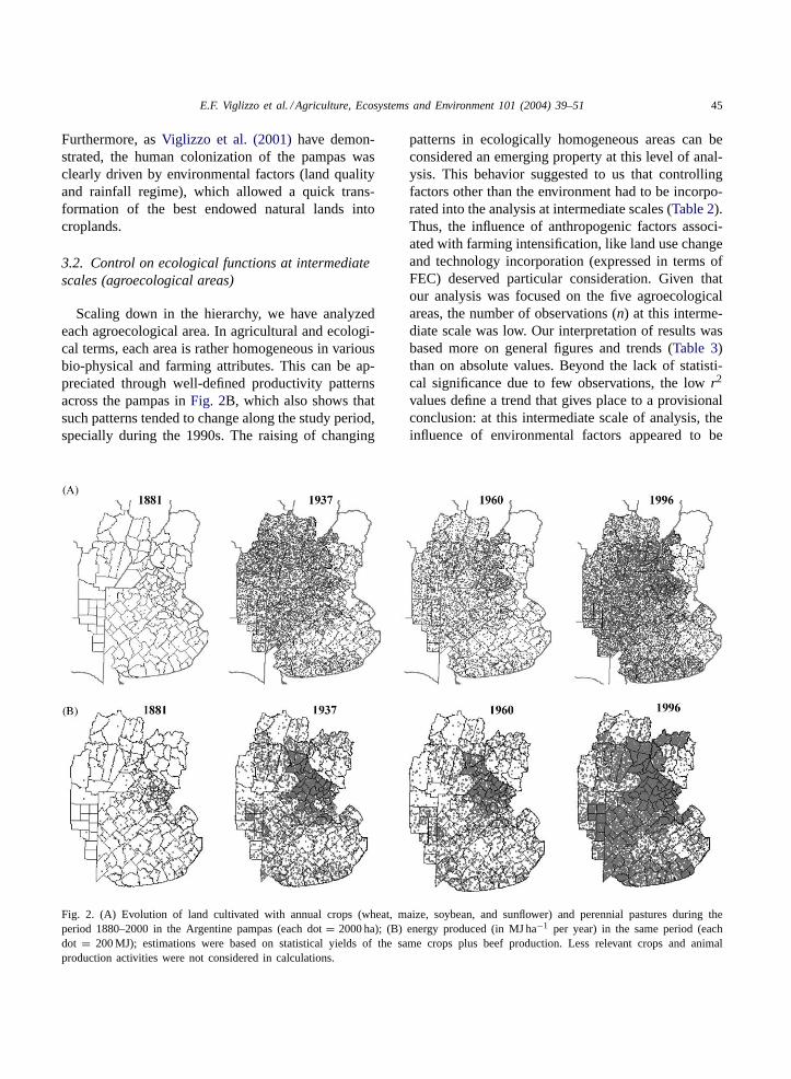
Scaling down in the hierarchy, we have analyzedeach agroecological area. In agricultural and ecologi-cal terms, each area is rather homogeneous in variousbio-physical and farming attributes. This can be ap-preciated through well-defined productivity patternsacross the pampas inFig. 2B, which also shows thatsuch patterns tended to change along the study period,specially during the 1990s. The raising of changing

Fig. 2. (A) Evolution of land cultivated with annual crops (wheat, maize, soybean, and sunflower) and perennial pastures during theperiod 1880–2000 in the Argentine pampas (each dot= 2000 ha); (B) energy produced (in MJ ha−1 per year) in the same period (eachdot = 200 MJ); estimations were based on statistical yields of the same crops plus beef production. Less relevant crops and animalproduction activities were not considered in calculations.

patterns in ecologically homogeneous areas can beconsidered an emerging property at this level of anal-ysis. This behavior suggested to us that controllingfactors other than the environment had to be incorpo-rated into the analysis at intermediate scales (Table 2).Thus, the influence of anthropogenic factors associ-ated with farming intensification, like land use changeand technology incorporation (expressed in terms ofFEC) deserved particular consideration. Given thatour analysis was focused on the five agroecologicalareas, the number of observations (n) at this interme-diate scale was low. Our interpretation of results wasbased more on general figures and trends (Table 3)than on absolute values. Beyond the lack of statisti-cal significance due to few observations, the lowr2

values define a trend that gives place to a provisionalconclusion: at this intermediate scale of analysis, theinfluence of environmental factors appeared to be

46 E.F. Viglizzo et al. / Agriculture, Ecosystems and Environment 101 (2004) 39–51

Table 2AEP, and the average annual rate of change for energy productivity, land allocated to main crops, and FEC during the period 1960–1996in the five study ecological areas of the Argentine pampasa

Pampean area AEP (GJ ha−1 per year) Rate of EPC (% per year) Rate of CC (% per year) Rate of FEC (% per year)

Rolling 21.7 (18.3) 6.9 (0.7) 3.3 (0.9) 5.3 (1.1)Central 17.5 (9.3) 8.1 (5.2) 1.9 (1.7) 3.1 (0.6)Southern 12.1 (6.8) 7.2 (4.4) 1.7 (1.2) 1.7 (3.6)Flooding 5.0 (0.9) 5.8 (5.7) 0.3 (0.6) 3.6 (2.7)Mesopotamian 6.9 (0.8) 9.1 (1.7) 0.0 (1.04) 6.1 (2.4)

a Values within parenthesis indicate standard deviation.

weaker than the influence of the anthropogenic ones.An increasing trend of human factors to increase theircontrol on energy and nutrients flows can be appreci-ated, especially when this trend was assessed throughFEC in a simple regression analysis, and through thecombined effect of FEC and land use (FEC× CC) ina multiple regression analysis.

In other terms, at this intermediate scale, our resultssuggest that humans tended to increase their controlon ecological functions through a more intense use offossil energy or, what is the same, through the incor-poration of more input technology.

3.3. Control on ecological functions at smallerscales (the districts)

This trend of anthropogenic factors to increase theircontrol on the energy and nutrients flows appeared tobe reinforced as we scaled down to even smaller scales.We have selected fifteen political districts spatiallyscattered over the five agroecological areas. They wereevaluated by simple and multiple regression analysisfollowing a similar analytical scheme that we haveused for intermediate scales.

Table 3Results from a simple and multiple regression analysis to assess the influence of environmental and anthropogenic factors on the controlof ecological functions at an intermediate scale (ecological area level) of analysis in the Argentine pampas, during the period 1960–1996a

Factors EPC versus r2 P Inters. AEP CC FEC CC× FEC S.E.

Environmental AEP 0.002 >0.05 7.33 0.071 1.44

Anthropogenic CC 0.037 >0.05 7.68 −0.18 1.41FEC 0.15 >0.05 6.33 0.15 1.33CC × FEC 0.17 >0.05 6.58 −0.14 0.26 1.61

a AEP: average energy productivity (GJ ha−1 per year); EPC: annual rate (%) of change in energy productivity; CC: annual rate (%)of cropland change; FEC: annual rate (%) of change in fossil energy consumption.

Ordering the districts in terms of the annual rate(%) of EPC,Table 4shows the corresponding valuesof: (a) AEP, (b) annual rate (%) of change in the CC,and (c) annual rate (%) of change in FEC. It can be ap-preciated that the higher values of EPC did not agreewith the higher AEP values. The larger increase in en-ergy productivity was not necessarily found in areasof higher potential productivity, as it was expected.This means that environmental forces did not regulateany more changes in the energy flow at this smallerscale. Then, the necessary following step was to as-sess the impact of anthropogenic forces. The resultsfrom the regression analysis are presented inTable 5.While the effect of environmental forces, expressed interms of AEP, was very low (r2 = 0.017; P > 0.05),such controlling effect on energy and nutrients flowsnotably increased when we focused on anthropogenicfactors (CC and FEC). Highly significant determina-tion coefficients were found for CC (r2 = 0.52; P <

0.01) and FEC (r2 = 0.31; P < 0.01) in the simpleregression analysis. Such figures even increased (r2 =0.76; P < 0.01) when a multiple regression analysiswas used to assess the combined effect of CC andFEC. Thus, 76% of the variability in the productive

E.F. Viglizzo et al. / Agriculture, Ecosystems and Environment 101 (2004) 39–51 47

Table 4AEP, and the annual rate of change for energy productivity, land allocated to main crops, and FEC during the period 1960–1996 in 15selected districts scattered across of the five ecological areas in the Argentine pampasa

Local districts Area AEP(GJ ha−1 per year)

Rate of EPC(% per year)

Rate of CC(% per year)

Rate of FEC(% per year)

Maraco Central 13.0 (10.7) 18.6 2.7 5.4Balcarce Southern 11.5 (9.3) 15.0 2.6 11.0Villegas Central 14.6 (11.2) 17.6 4.6 5.6Olavarrıa Flooding 6.6 (5.8) 12.2 0.9 11.3Laprida Southern 6.7 (5.7) 11.5 1.9 9.8Marcos Juarez Rolling 31.8 (16.9) 6.9 3.4 2.3Lamadrid Southern 8.0 (4.8) 6.3 0.3 4.3Pergamino Rolling 37.2 (18.6) 6.0 3.3 4.4Conhelo Central 5.2 (2.9) 5.6 1.3 6.8Rojas Rolling 36.5 (17.3) 5.4 1.7 3.6Gualeguaychu Mesopotamian 2.1 (0.9) 2.9 0.0 2.7Pila Flooding 2.4 (1.0) 2.9 −0.2 7.8Gualeguay Mesopotamian 2.6 (0.8) 2.6 1.4 −5.6Chascomus Flooding 3.1 (0.8) 1.9 0.0 6.0Nogoya Mesopotamian 3.0 (0.5) −0.2 −0.4 0.6

a Values within parenthesis indicate standard deviation.

Table 5Results from a simple and multiple regression analysis to assess the influence of environmental and anthropogenic factors on the controlof ecological functions at the smaller scale (district level) of analysis in the Argentine pampas, during the period 1960–1996a

Factors EPC versus r2 P Inters. AEP CC FEC CC× FEC S.E.

Environmental AEP 0.017 >0.05 6.74 0.071 5.52

Anthropogenic CC 0.52 <0.01 3.36 2.54 3.87FEC 0.31 <0.01 1.81 0.95 4.63CC × FEC 0.76 <0.01 1.35 2.39 0.85 2.83

a AEP: average energy productivity (GJ ha−1 per year); EPC: annual rate (%) of change in energy productivity; CC: annual rate (%)of cropland change; FEC: annual rate (%) of change in FEC.

energy flow (and consequently, N and P flows) couldbe explained by the variability in the two analyzed an-thropogenic (land use and FEC) factors. However, asit can be appreciated inTable 5, land use had a higherexplanatory power than FEC. These results would beindicating that the influence of anthropogenic factorstends to increase, at the expense of the environmentalones, as we move toward smaller scales.

In summary, the increasing human control on eco-logical functions that was already insinuated at inter-mediate scales, was clearly strengthen at the smallerstudy scale. Ideally, this increasing control shouldbe checked at even smaller scales, but we had notenough field data in the pampas to do an equivalentanalysis at the farm- and the plot-level.

4. Discussion

Our interpretation of results from this study isthat the spatial aggregation of human-driven effectsat lower levels can cascade up to upper levels, andcounteract the strong influence of the environment onenergy and nutrients flows at broader scales. Thus, thehigher the geographical expansion of intensificationin the pampas, the greater the substitution of environ-mental by anthropogenic controls.Fig. 2 graphicallyshows that a bottom-up human control of ecologi-cal functions, driven by the expansion of croplandsand increasing fossil energy use, has scaled-up andmodified the natural borders of the ecological areas,particularly in the 1990s when farming became more

48 E.F. Viglizzo et al. / Agriculture, Ecosystems and Environment 101 (2004) 39–51

intensive all over the region. While land use intensityincreases (Fig. 2A), the higher impact of fossil energyuse on energy productivity (Fig. 2B) during the 1990s,has erased the traditional borders that were shapedby the environment under low-input conditions. Thiseffect can even be appreciated in areas of low produc-tivity suitable for cattle production (e.g., the floodingpampas), where technology has allowed the transfor-mation of traditional grazing areas into croplands.

Our results seem to support the theoretical viewof authors that have stated that climate and geomor-phology determine the structure and dynamics ofagroecosystems at the larger and less detailed scales,while human-driven factors dominate at the smallerscales (O’Neill et al., 1986, 1996; Wagenet, 1998;Bailey, 1998). Results from other studies (Veldkampet al., 2001) do not necessarily support this view.Using multiple regression analysis to assess the im-pact of bio-physical and socio-economic factors onyield variability at two spatial levels in Costa Rica,Honduras and Ecuador,Veldkamp et al. (2001)ob-tained contradictory results. Neither bio-physical norsocio-economic factors had completely dominated the

Anthropogenic bottom-up controlsEnvironmental top-down controls

ecoregion

district

ecoregion

district

farm

plot

ecoregion

district

farm

Pre-colonial(before 1880)

Extensive farmingperiod (1880-1960)

Semi-intensive farmingperiod (1960-2000)

Fig. 3. Hypothetical model that represents the relative influence of top-down and bottom-up controls on ecological functions at differentscale in agricultural ecosystems of the Argentine pampas during different historical periods.

yield variability of crops at the two spatial resolutionlevels. Furthermore, the dominance varied greatlyamong countries and crops (coffee, banana, maize,rice and bean). On the other hand,Turner et al. (1995)stated that the modalities of land management tend todominate at the smaller scales, whereas bio-physicaland socio-economic forces dominate across differenttemporal and spatial scales. According to this view,environmental and anthropogenic forces may produceboth, top-down and bottom-up effects. They consid-ered that the hypothesis based on a scale-dependentdichotomy (environmental top-down, and anthro-pogenic bottom-up influences) is too simplistic to bemeaningful.

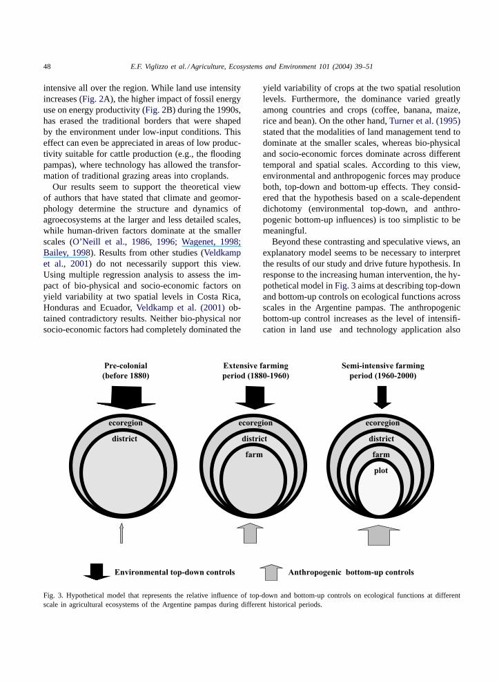
Beyond these contrasting and speculative views, anexplanatory model seems to be necessary to interpretthe results of our study and drive future hypothesis. Inresponse to the increasing human intervention, the hy-pothetical model inFig. 3aims at describing top-downand bottom-up controls on ecological functions acrossscales in the Argentine pampas. The anthropogenicbottom-up control increases as the level of intensifi-cation in land use and technology application also

E.F. Viglizzo et al. / Agriculture, Ecosystems and Environment 101 (2004) 39–51 49

increases in recent times. Thus, we could hypothet-ically assume that the ecological functions had beenentirely controlled by top-down environmental forcesduring the pre-colonial period (before 1880), whenhuman colonization and the corresponding ranchingprocess had not yet begun. Once both processes weretriggered and a typically extensive, low-input farm-ing model was consolidated between 1880 and 1960,bottom-up anthropogenic forces increased in impor-tance and scaled up, counteracting in part the control-ling effects of the environment. Such human-drivencontrol increased quickly during the period of greaterintensification (1960–2000). Starting from the plot-and the farm-level, farmers probably began to influ-ence decisively the fate of energy and nutrients. Thespatial aggregation of such anthropogenic effects inplots and farms in the 1990s, appeared to be strongenough to minimize the influence of natural controlsover large geographical areas.

5. Concluding remarks

The relative weight of environmental and anthro-pogenic controls, as well as their trade-offs acrossscales, are relevant for decision-makers. Our re-sults demonstrate that the environment has a de-cisive top-down control on ecological functions inextensive farming, independent of scale. But thismay change when a human-driven intensificationincreases and overflow over larger scales. Environ-mental forces can be largely neutralized, at the plot-and farm-level, by the intensive application of input-and management-based technologies. However, ourresults suggest that human-driven controls in thepampas are still relatively low. In general, humanshave succeeded in controlling the production-relatedflows (those that directly render economic or socialutility), but has failed in doing the same on flows thatare not of their close interest in the short term. Theincomplete human control over such non-productive(or non-harvesting) flows might well be cause ofcross-scale degradation. For example, over-cropping,over-fertilization, or over-irrigation, can eventuallyproduce a short-term benefit in terms of harvested en-ergy. But in the mid- and long-term, the excess of en-ergy injected into the ecosystem that escapes to humancontrol, may trigger episodes of environmental degra-

dation (desertification, contamination, salinization,etc.).

More technological innovations that could be ap-plied at different scales (from minimum tillage tosatellite monitoring) are necessary to drive the energythat normally escapes to human control. However,effective technology is not equally available at allscales. Modern technology was developed to resolveproblems that occur, predominantly, at the plot- andthe farm-level. But technologies that aim at resolvingproblems on broader scales are rare and scarce. Evennowadays, the conventional small-scale technologyneeds to be perfected if we want to increase the con-trol on non-productive flows. In the meantime, thedevelopment of large-scale technology to increase thecontrol of flows over wide geographic areas and longperiods of time appears to be as necessary as urgent.

The notion of scale-dependent processes must beunderstood by decision-makers. A better cross-scaleunderstanding of environmental and anthropogeniccontrols and trade-offs, seems to be imperative toharmonize production and environmental goals.

Acknowledgements

The authors wish to express their gratitude for thefinancial support of INTA and CONICET of Argentinathat made this work possible. We also want to thankthe Editor and referees of this journal for their helpfulcomments and suggestions.

References

Allen, T.F.H., Starr, T.B., 1982. Hierarchy Perspectives of Eco-logical Complexity. University of Chicago Press, Chicago, IL.

Bailey, R.G., 1995. Description of the Ecoregions of the UnitedStates. Miscellaneous Publication No. 1391. USDA ForestService, Washington, DC.

Bailey, R.G., 1998. Ecoregions: The Ecosystem Geography of theOceans and Continents. Springer, New York.

Bergkamp, G., 1998. The response of hierarchical soil erosionprocesses to land use and land cover change. In: Usó, J.L.,Brebbia, C.A., Power, H. (Eds.), Advances in EcologicalSciences: Ecosystems and Sustainable Development. Comp-utational Mechanics Publications, Southampton, UK.

Buringh, P., Dudal, R., 1987. Agricultural land use in spaceand time. In: Wolman, M.G., Fournier, F.G.A. (Eds.), LandTransformation in Agriculture SCOPE, Wiley, New York.

50 E.F. Viglizzo et al. / Agriculture, Ecosystems and Environment 101 (2004) 39–51

Carpenter, S.R., Chisholm, C.J., Krebs, C.J., Schindler, D.W.,Wright, R.F., 1995. Ecosystems experiments. Science 269, 324–327.

Casas, R.R., 1998. Causas y evidencias de la degradación desuelos en la región pampeana. In: Solbrig, O.T., Vainesman, L.(Eds.), Hacia una Agricultura Productiva y Sustentable en LaPampa. Harvard University, Consejo Profesional de IngenierıaAgronómica (CPIA), Buenos Aires.

Cole, C.V., Stewart, J.W.B., Ojima, D.S., Parton, W.J., Schimel,D.S., 1989. Modelling land use effects of soil organic matterdynamics in the North American Great Plains. In: Clarholm,M., Bergstrom, L. (Eds.), Ecology of Arable Lands. KluwerAcademic Publishers, New York, pp. 89–98.

Conforti, P., Giampietro, M., 1997. Fossil energy use in agriculture:an international comparison. Agric. Ecosyst. Environ. 65, 231–243.

Covas, G., 1989. Evolución del manejo de suelos en la regiónpampeana semiárida. Acta de las Primeras Jornadas de Suelosen Zonas Aridas y Semiáridas, INTA, Santa Rosa, La Pampa,pp. 1–11.

De Koning, G.H.J., Verburg, P.H., Veldkamp, A., Fresco, L.O.,1999. Multi-scale modelling of land use change dynamics inEcuador. Agric. Syst. 61, 77–93.

Dumanski, J., Pettapiece, W.W., McGregor, R.J., 1998. Relevanceof scale dependent approaches for integrating bio-physical andsocio-economic information and development of agroecologicalindicators. Nutr. Cycl. Agroecosyst. 50, 13–22.

FAO, 1989. Guidelines for land use planning. Food AgricultureOrganization of the United Nations, Rome.

Freemark, K., 1995. Assessing the effect of agriculture onterrestrial wildlife: developing a geographical approach for USEPA. Landsc. Urban Plan. 31, 99–115.

Gardner, R.H., 1998. Pattern, process and the analysis of spatialscales. In: Peterson, D.L., Parker, V.T. (Eds.), Ecological Scale:Theory and Applications. Columbia University Press, NewYork.

Grossi-Gallegos, H., Lopardo, R., Atienza, G., Garcıa, M.,1985. Evaluación del aporte energético de origen solar en laRepública Argentina. In: AAPURE (Ed.), Primer CongresoArgentino sobre Uso Racional de la Energıa, Buenos Aires,pp. 1217–1237.

Gustafson, E.J., 1998. Quantifying landscape spatial pattern: whatis the state of the art? Ecosystems 1, 143–156.

Hall, A.J., Rebella, C.M., Ghersa, C.M., Culot, J.Ph., 1992.Field-crop systems of the pampas. In: Pearson, C.J. (Ed.), FieldCrop Ecosystems, Series: Ecosystems of the World. Elsevier,Amsterdam.

Hobbs, R.J., 1998. Managing ecological systems and processes.In: Peterson, D.L., Parker, V.T. (Eds.), Ecological Scale: Theoryand Applications. Columbia University Press, New York.

Holling, C.S., 1992. Cross-scale morphology, geometry anddynamics of ecosystems. Ecol. Monogr. 62, 447–502.

INTA/UNDP, 1990. Atlas de Suelos de la República Argentina(Tomo 1). Ediciones INTA, Buenos Aires.

Klijn, F., Udo de Haes, H.A., 1994. A hierarchical approachto ecosystems and its applications for ecological landclassification. Landsc. Ecol. 9, 89–104.

Lal, R., 1994. Sustainable land use systems and soil resilience.In: Greenland, D.J., Szabolcs, I. (Eds.), Soil Resilience andSustainable Land Use. CAB International, Wallingford, UK.

Lloyd, L.E., McDonald, B.E., Crampton, E.W., 1978. Funda-mentals of Nutrition, 2nd ed. Freeman, San Francisco, CA.

Musto, J.C., 1979. La Degradación de los Suelos en la RepúblicaArgentina. Publication No. 67. CIRN INTA, Castelar, Argentina.

Nakama, V., Sobral, R., 1987. Indices de Productividad: MétodoParamétrico para Evaluación de Tierras. Publication INTA.INTA/UNDP, Castelar, Argentina.

Nielsen, S.N., 2000. Thermodynamics of an ecosystem interpretedas a hierarchy of embedded systems. Ecol. Model. 135, 279–289.

NRC (National Research Council), 1978. Nutrient Requirements ofDomestic Animals. National Academy of Sciences, Washington,DC.

O’Neill, R.V., DeAngelis, D.L., Waide, J.B., Allen, T.F.H., 1986.A Hierarchical Concept of Ecosystems. Princeton UniversityPress, Princeton, NJ.

O’Neill, R.V., Hunsaker, C.T., Timmings, S.P., Jackson, B.L.,Jones, K.B., Riiters, K.H., Wickham, J.D., 1996. Scale problemsin reporting landscape pattern at the regional scale. Landsc.Ecol. 11, 169–180.

Odum, E.P., 1975. Ecology: The Link Between the Natural andSocial Sciences. Holt, Reinhart & Winston, San Francisco.

Odum, E.P., 1977. The emergence of ecology as a new integrativediscipline. Science 195, 1289–1293.

Patee, H.H., 1973. Hierarchy Theory: The Challenge of ComplexSystems. George Braziller, New York.

Reed, W., Shu, G., Hills, F.J., 1986. Energy input and outputanalysis of four field crops in California. J. Agron. Crop Sci.157, 99–104.

Riquier, J., Bramao, D.L., Cornet, J.P., 1970. A New System ofSoil Appraisal in Terms of Actual and Potential Productivity.Mimeo No. AGL:TERS/70/6. FAO, Rome.

Salthe, S.N., 1985. Evolving Hierarchical Systems: Their Structureand Representation. Columbia University Press, New York.

Solbrig, O.T., Viglizzo, E.F., 1999. Sustainable farming in theargentine pampas: history, society, economy and ecology.DRCLAS Paper No. 99/00-1. Harvard University, Cambridge,MA.

Stout, B.A., 1991. Handbook of Energy for World Agriculture.Elsevier, New York.

Turner II, B.L., Skole, D., Sanderson, S., Fisher, G., Fresco,L., Leemans, R., 1995. Land-use and Land-cover Change(Science/Research Plan). IGBP Report No. 35. HDP ReportNo. 7, Stockholm.

Veldkamp, A., Kok, K., De Koning, G.H.J., Schoorl, J.M.,Sonneveld, M.P.W., Verburg, P.H., 2001. Multi-scale systemapproaches in agronomic research at the landscape level. SoilTill. Res. 58, 129–140.

Viglizzo, E.F., 1986. Agroecosystems stability in the Argentinepampas. Agric. Ecosyst. Environ. 16, 1–12.

Viglizzo, E.F., Roberto, Z.E., Brockington, N.R., 1991. Agro-ecosystems’ performance in the semi-arid pampas of Argentinaand their interactions with the environment. Agric. Ecosyst.Environ. 36, 23–36.

E.F. Viglizzo et al. / Agriculture, Ecosystems and Environment 101 (2004) 39–51 51

Viglizzo, E.F., Roberto, Z.E., Lértora, F.A., López Gay, E.,Bernardos, J., 1997. Climate and land-use change in field-cropecosystems of Argentina. Agric. Ecosyst. Environ. 66, 61–70.

Viglizzo, E.F., Lértora, F.A., Pordomingo, A.J., Bernardos, J.N.,Roberto, Z.E., Del Valle, H., 2001. Ecological lessons andapplications from one century of low external-input farmingin the pampas of Argentina. Agric. Ecosyst. Environ. 81, 65–81.

Wagenet, R.J., 1998. Scale issues in agroecological research chains.Nutr. Cycl. Agroecosyst. 50, 23–34.

Warren, C.E., 1979. Toward classification and rationale forwatershed management and stream protection. EnvironmentalProtection Agency No. EPA-600/3-79-059. Corvallis, OR.

Weston, R.F., Ruth, M., 1997. A dynamic, hierarchical approach tounderstanding and managing natural economic systems. Ecol.Econ. 21, 1–17.