Locality Constrained Joint Dynamic Sparse Representation for Local Matching based Face Recognition

RESEARCH ARTICLE

Locality Constrained Joint Dynamic SparseRepresentation for Local Matching BasedFace RecognitionJianzhong Wang1,3, Yugen Yi1,2, Wei Zhou1,4, Yanjiao Shi2, Miao Qi1, Ming Zhang4,Baoxue Zhang2,5*, Jun Kong1,4*

1. College of Computer Science and Information Technology, Northeast Normal University, Changchun,China, 2. School of Mathematics and Statistics, Northeast Normal University, Changchun, China, 3. NationalEngineering Laboratory for Druggable Gene and Protein Screening, Northeast Normal University,Changchun, China, 4. Key Laboratory of Intelligent Information Processing of Jilin Universities, NortheastNormal University, Changchun, China, 5. School of Statistics, Capital University of Economics and Business,Beijing, China

*[email protected] (BZ); [email protected] (JK)

Abstract

Recently, Sparse Representation-based Classification (SRC) has attracted a lot of

attention for its applications to various tasks, especially in biometric techniques

such as face recognition. However, factors such as lighting, expression, pose and

disguise variations in face images will decrease the performances of SRC and most

other face recognition techniques. In order to overcome these limitations, we

propose a robust face recognition method named Locality Constrained Joint

Dynamic Sparse Representation-based Classification (LCJDSRC) in this paper. In

our method, a face image is first partitioned into several smaller sub-images. Then,

these sub-images are sparsely represented using the proposed locality constrained

joint dynamic sparse representation algorithm. Finally, the representation results for

all sub-images are aggregated to obtain the final recognition result. Compared with

other algorithms which process each sub-image of a face image independently, the

proposed algorithm regards the local matching-based face recognition as a multi-

task learning problem. Thus, the latent relationships among the sub-images from

the same face image are taken into account. Meanwhile, the locality information of

the data is also considered in our algorithm. We evaluate our algorithm by

comparing it with other state-of-the-art approaches. Extensive experiments on four

benchmark face databases (ORL, Extended YaleB, AR and LFW) demonstrate the

effectiveness of LCJDSRC.

OPEN ACCESS

Citation: Wang J, Yi Y, Zhou W, Shi Y, Qi M, etal. (2014) Locality Constrained Joint DynamicSparse Representation for Local Matching BasedFace Recognition. PLoS ONE 9(11): e113198.doi:10.1371/journal.pone.0113198

Editor: Oscar Deniz Suarez, Universidad deCastilla-La Mancha, Spain

Received: January 4, 2014

Accepted: October 24, 2014

Published: November 24, 2014

Copyright: � 2014 Wang et al. This is an open-access article distributed under the terms of theCreative Commons Attribution License, whichpermits unrestricted use, distribution, and repro-duction in any medium, provided the original authorand source are credited.

Funding: This work is supported by Fund of JilinProvincial Science & Technology Department(20130206042GX, 20111804), Young scientificresearch fund of Jilin province science andtechnology development project(No. 20130522115JH, 201201070, 201201063)and National Natural Science Foundation of China(No. 11271064, 61403078). The funders had norole in study design, data collection and analysis,decision to publish, or preparation of the manu-script.

Competing Interests: The authors have declaredthat no competing interests exist.

PLOS ONE | DOI:10.1371/journal.pone.0113198 November 24, 2014 1 / 26

http://crossmark.crossref.org/dialog/?doi=10.1371/journal.pone.0113198&domain=pdf

http://creativecommons.org/licenses/by/4.0/

Introduction

In the past two decades, face recognition has become one of the most active and

challenging research topics in pattern recognition and computer vision fields due

to its wide range of applications in biometrics, human-computer interaction,

information security and so on [1, 2]. Although many researchers have proposed

various algorithms for face recognition [1, 2], it is still a challenging problem

[3, 4]. This is because the appearance of real-world face images is always affected

by illumination condition, aging, pose, facial expression and disguise variances.

Moreover, some other problematic factors such as occlusion and noise will also

impair the performances of face recognition algorithms.

Recently, sparse representation (or sparse coding) techniques have drawn wide

interest and been successfully used in signal, image, video processing and

biometric applications [5]. Motivated by sparse representation, a novel face

recognition method named Sparse Representation-based Classification (SRC) [6]

was proposed by Wright et al. In SRC, a query image is first sparsely linear coded

by the original training images, and then the classification is performed by

checking which class leads to the minimal representation residual of the query

image. Since the experimental results in Wright et al.’s pioneer work showed that

the SRC achieved impressive face recognition performance, the research of sparse

representation-based face recognition was largely boosted and lots of algorithms

have been developed. Gao et al. [7] proposed an extension of SRC named kernel

SRC (KSRC), which performed the sparse representation technique in a new high-

dimensional feature space obtained by the kernel trick [8]. Meanwhile, Yang et al.

[9] utilized Gabor features rather than the original facial features in SRC to

improve recognition accuracy. Wang et al. [10] developed a Locality constrained

Linear Coding (LLC) scheme. In LLC, the query image is represented only using

the nearest codewords (or training samples). However, SRC, KSRC and LLC did

not take the structure of the training data into consideration. Thus, their methods

may fail to deal with the data which lie on multiple low-dimensional subspaces in

the high-dimensional ambient space [11, 12]. In order to overcome this

limitation, Elhamifar et al. put forward a structured sparse representation

algorithm in [13]. The main idea of their algorithm is to find a good

representation of the query sample using the minimum number of structure

blocks in the training set. In [14], Wagner et al. proposed a sparse representation-

based method that could deal with face misalignment and illumination variation.

Yang et al. introduced a Robust Sparse Coding model (RSC) in [15]. RSC relaxed

the assumption that the representation residual should follow the Gaussian or

Laplacian distribution in original SRC, and sought for a maximum likelihood

estimator (MLE) solution for the sparse coding problem. Moreover, Deng et al.

[16] proposed another extended SRC (ESRC) method in which they assumed the

intra-class variations of one subject can be approximately represented by a sparse

linear combination of the other subjects. Therefore, ESRC can successfully handle

face recognition with limited training samples per subject. Recently, Mi et al. [17]

presented a novel face recognition method named sparse representation-based

Locality Constrained Joint Dynamic Sparse Representation


classification on k-nearest subspace (SRC-KNS). In SRC-KNS, the distance

between the test image and the subspace of each individual class is first exploited

to determine the k nearest subspaces, and then the SRC is performed on the k

selected classes.

Although the above-mentioned SRC-based methods perform well, their

recognition performances may also be affected by some problematic factors (such

as illumination, expression, disguises and pose) in real-world face images [18].

The main reason is that they utilize the holistic information of the face images for

recognition. Based on the observation that some of the local facial features would

not vary with pose, lighting, facial expression and disguise, some local matching-

based methods which extract facial features from different levels of locality have

been proposed showing more promising results in face recognition tasks [3, 19–

25]. In [6], Wright et al. also incorporated their SRC into the local matching

framework to improve its performance. In their local matching-based SRC

(LMSRC), the query and training face images are first divided into a number of

equally sized sub-images. Then, each sub-image of the query face is represented by

the corresponding sub-images of the training set using SRC, and a final decision is

made by majority voting for classification. However, since LMSRC represented

the sub-images independently, it merely focused on how to sparsely encode each

sub-image of the query face but ignored the latent relationships among the

multiple sub-images from the same face image, which may weaken its recognition

performance [25, 26].

In the local matching-based face recognition framework, each sub-image of a

face can be regarded as a sub-pattern which contains a partial feature of the face

image. Furthermore, different sub-images divided from the same image can reflect

various kinds of information of the query face, and have some latent connections

with each other since they jointly provide the full information of the whole face

image. Therefore, jointly estimating the sparse representation models of latently-

related sub-images from a query face image can be viewed as a ‘‘multi-task

learning’’ problem in which each sub-image is a task [27]. Nowadays, some multi-

task learning-based sparse representation algorithms have been proposed to take

advantage of an object’s different features. Yuan et al. proposed a Multi-task Joint

Sparse Representation-based Classification method (MTJSRC) in [28]. MTJSRC

assumes that the sparse representation coefficients of different features have the

same sparsity pattern. Thus, the ,1,2-norm is utilized in this method to make the

sparse representation coefficients of different features be the same at atom-level.

However, this assumption is too strict to hold in practice. For example, if the

appearance of a face image is affected by large illumination changes, it would be

hard to represent all sub-images of this face properly by the same set of atoms.

Therefore, Zhang et al. proposed a new method named Joint Dynamic Sparse

Representation-based Classification (JDSRC) to deal with this problem [29]. In

their method, a novel concept of joint dynamic sparsity is introduced to represent

the different features of an object by different sets of training samples from the

same class [29]. As a result, the sparse representation coefficients of different

features obtained by JDSRC tend to have the same sparsity pattern at class-level



rather than atom-level. Additionally, another method named Relaxed

Collaborative Representation (RCR) was proposed by Yang et al. [27]. RCR

assumes the sparse representation coefficients with respect to different features

should be alike. Therefore, the sparse representation coefficients of all features

obtained by RCR have the similar sparsity pattern in appearance (i.e. the positions

and values of non-zero elements in different representation coefficient vectors are

similar to each other). Though the experiments in [27–29] showed that the

MTJSRC, JDSRC and RCR algorithms achieved better recognition and

classification performances than SRC, the locality information (i.e. similarity

between the query and training samples) [10] was neglected in all of them.

Therefore, these algorithms may select the training samples which are dissimilar to

the query sub-image for representation and produce unsatisfying recognition

results. In recent studies, since the researchers have shown that exploiting locality

information of data was more essential than sparsity in some cases [30–32], it is

crucial to incorporate the locality information into the multi-task learning-based

sparse representation algorithms.

Inspired by the pioneer work of joint sparse representation and the importance

of data locality, we present a novel multi-task learning-based sparse representation

algorithm called Locality Constrained Joint Dynamic Sparse Representation-based

Classification (LCJDSRC) for local matching-based face recognition. One

important advantage of the proposed algorithm is that it explicitly integrates the

joint sparse representation and the locality constraint into a unified framework.

Therefore, our algorithm not only takes the latent correlations among different

local facial features into account but also considers the similarity between the

query and training samples. Like the existing JDSRC, the sparse representation

coefficients of different sub-images from a face have the same sparsity pattern at

class-level in LCJDSRC. However, since the locality constraint in our algorithm

will magnify the representation coefficients corresponding to the similar samples

of the query sub-image while reducing the dissimilar ones, LCJDSRC tends to

select the nearest neighbors of the query sub-image for representation to improve

its recognition performance. The effectiveness of our algorithm is evaluated by

extensive experiments on four well-known face databases and compared with

other state-of-the-art approaches.

The rest of this paper is organized as follows. The LCJDSRC model is presented

in Section 2. In Section 3, the proposed algorithm and several other methods are

evaluated on the four databases (ORL, Extended YaleB, AR and LFW). Finally, the

conclusions are given in Section 4.


In this section, we first present the outline of the proposed local matching-based

face recognition method. Then, the details of our Locality Constrained Joint

Dynamic Sparse Representation algorithm are discussed. Next, the recognition



criterion of our algorithm is given. Finally, some comparisons between the

proposed algorithm and related work are also analyzed.

Outline

There are four steps in the proposed local matching-based face recognition

algorithm. The first step is to partition the query face image and the face images in

the training set. Generally, there are two different techniques to implement the

partition, i.e., local components and local regions. Local components are areas

occupied by the facial components, such as eyes, nose and mouth, and local

regions are local sub-images centered at designated coordinates of a common

coordinate system. Since some researchers have verified that the local region

partition is to be preferred in local matching-based face recognition [3], we adopt

rectangular regions to partition the images as many other approaches do [20–25].

That is, the query and training face images are divided into several smaller

rectangular sub-images in our algorithm. In the second step, the sub-images of the

query face are sparsely represented by their corresponding sub-images in the

training set using the proposed locality constrained joint dynamic sparse

representation (LCJDSR) algorithm, which not only considers the latent

relationships among the sub-images but also takes the locality information into

account. The third step of our algorithm is to compute the representation residual

of each sub-image using the sparse representation coefficients obtained by

LCJDSR. At last, the total representation residuals of all sub-images from the

query face are aggregated for final recognition. The flow diagram of the proposed

algorithm can be seen in Figure 1.

Locality Constrained Joint Dynamic Sparse Representation Model

Let X~½x1,x2,:::,xN �[Rd|N denote N face images belonging to C persons in the

training set (Nc samples, c~1,2,:::,C are associated to each person), and let the

size of each face image be S1|S2(S1|S2~d). Given a query face image y[RS1|S2 ,

we partition it into M non-overlapping sub-images and then concatenate each

sub-image into a column vector. Thus, y can be represented as y~½y1,y2,:::,yM� inwhich yi[Rdi|1(i~1,2,:::,M) is the vector of the i-th sub-image. Similarly, the face

images in the training set are also partitioned into X1,X2,:::,XM , where

Xi~½xi1,xi

2,:::,xiN �[Rdi|N(i~1,2,:::,M) is the set which contains the i-th sub-image

vectors of all training samples. Here, di is the dimension of the i-th sub-images in

y and Xi.

After partition the query and training face images into non-overlapping sub-

images, our objective is to sparsely represent the sub-images in y using their

corresponding sub-images in the training set. To address this problem, one can

simply apply the standard SRC to each of the M sub-images in y, which can be

written as:

minAmjjym{XmAmjj22zljjAmjj1, m~1,2,:::,M ð1Þ



where Am~½am1 ,am

2 ,:::,amN �

Tis the coefficient vector of the m-th sub-image and

l§0 is a tradeoff parameter. Taking all M sub-images into account, the objective

function of local matching-based SRC is:

minfAmg

XM

m~1

jjym{XmAmjj22zljjAmjj1 ð2Þ

In fact, this strategy is the same as Wright et al.’s [6]. Therefore, as we have

discussed in Section 1, it is far from optimal due to the following reasons. First,

the objective function in Equation (2) neglects the similarity between the query

and the training samples, thus it may select training sub-images which are not

similar to the query face for representation. Second, Equation (2) represents each

sub-image of the query face independently, ignoring the latent relationships

among the sub-images.

In SRC and other related algorithms, the classification result of a query sample

is always determined by the class-wise minimum representation residual [6–7, 9-

10, 13–17], so it is reasonable to believe that selecting training samples similar to

the query image for representation can improve classification and recognition

Figure 1. The diagram of the proposed algorithm. The face images are collected from the Extended YaleB database [36].

doi:10.1371/journal.pone.0113198.g001



[30, 31]. According to the above analysis, a locality adaptor which measures the

similarity between the query and training samples is introduced in this study to

overcome the first shortcoming of Equation (2). The locality adaptor is defined as:

wmj ~ exp (

jjym{xmj jj

2

s), m~1,2,:::,M, j~1,2,:::,N ð3Þ

where sw0 is a parameter which determines the decay rate of the weight

function, ym is the m-th sub-image of the query face and xmj denotes the m-th sub-

image of the j-th training sample. From Equation (3), it is clear that a smaller wmj

indicates that xmj is more similar to the query sub-image ym, and vice versa.

In order to overcome the second problem of Equation (2), a dynamic active set

is adopted in our algorithm. The concept of dynamic active set was first proposed

by Zhang et al. to exploit the correlations (or relationships) among the multiple

observations which describe the same subject during the multi-task learning-based

sparse representation. In [29], a dynamic active set is defined as a set of coefficient

indices belonging to the same class, and a number of dynamic active sets are

jointly activated to sparsely represent the multiple observations. Formally, let

A~½A1,A2,:::,AM� be the matrix containing the sparse representation coefficients

of M sub-images from y, where Am is the coefficient vector of the m-th sub-image.

Then, each dynamic active set (denoted by gs[RM,s~1,2,:::) can be described as a

set of row indices of coefficients whose corresponding samples in the training set

are from the same class. To promote sparsity and allow only a small number of

dynamic active sets to be involved during the joint sparsity representation, a

mixed-norm which applies ,2-norm on each dynamic active set and then ,0-norm

across the ,2-norm is defined as:

jjAjjG~jj(jjAg1 jj2,jjAg2 jj2,:::)jj0 ð4Þ

where

Ags~A(gs)~(A(gs(1),1),A(gs(2),2),::::,A(gs(M),M))T[RM ð5Þ

is the vector formed by the coefficients associated with the s-th dynamic active set

gs, in which gs(m) is the row index of the selected training sample for the m-th

column of A in the s-th dynamic active set. In order to better illustrate the

organization of the dynamic active set, an example is provided in Figure 2. From

Figure 2, we can see that there are two dynamic active sets denoted by g1 and g2 in

this example. Therefore, according to the definition of the dynamic active set, we

can get g1~(1,2,1,1) and g2~(5,6,5,6). Furthermore, according to Equation (5),

the coefficient vectors associated with g1 and g2 are Ag1~(0:5,0:8,0:2,0:6) and

Ag2~(0:8,0:6,0:4,0:9), respectively. For more details about the dynamic active set,

the readers can refer to [29].

Now, by integrating the locality constraint and the joint sparse representation

into a unified framework, we can obtain the objective function of our model as

follow



minA

XM

m~1

jjym{XmAmjj22zljjWm8Amjj22

s:t: jjAjjGƒK

ð6Þ

where l§0 is a parameter to control the tradeoff between the two terms in

Equation (6), [denotes the element-wise multiplication, Wm~½wm1 ,wm

2 ,:::,wmN � is

the locality adaptor vector of the m-th sub-image and K is the sparsity level which

denotes the number of non-zero elements in each Am [6, 29].

In the proposed algorithm, since we want to guarantee that the sub-images of a

query face can be well represented by their corresponding samples in the training

set, the first term in Equation (6) which stands for the representation residual

should be minimized. On the other hand, the second term is referred to as locality

constraint because minimizing this term will magnify the absolute values of

coefficients corresponding to the training samples similar to the query sub-image

and reduce the dissimilar ones. Furthermore, the mix-norm regularization term

jjAjjGƒK combines the cues from all the sub-images coming from the query

image y during the representation process and promotes a joint sparsity pattern

shared at class-level [29].

The optimization stage

Since the regularization term in our proposed model contains the ,0-norm, how

to solve Equation (6) becomes a challenging problem. In this subsection, a greedy

algorithm based on Matching Pursuit (MP) [33] is presented to optimize the

objective function in Equation (6). In our algorithm, we initialize the

representation residual of each query sub-image as Rm0 ~ym(1,2,:::,M) and the

Figure 2. An example of the organization of the dynamic active set. For simplicity, we just take twoclasses as an example and the number of sub-images M is 4. A5[A1,A2,A3,A4] is a coefficient matrix and Ai

(i51,2,3,4) is a column vector of A, the number in each squared block denotes the sparse representationcoefficient and the blank blocks denote zero values.




selected dynamic active sets I0 as empty. Then, the following four steps are

processed in the t-th iteration (t~1,2,:::) until certain conditions are satisfied.

Step 1. Select new candidates based on the current residual.

Based on the current representation residual, some candidate dynamic active

sets are selected. First, the representation coefficients of each query sub-image are

computed by the inner product of the representation residual and its

corresponding training set as:

Amt ~XmT Rm

t{1, m~1,2,:::,M ð7Þ

Then, according to the representation coefficient matrix At~½A1t ,A2

t ,:::,AMt �[

RN|M, L candidate dynamic active sets whose associated coefficients can best

approximate toAtare selected. According to the suggestions in [29] and [34], we

set L52K in this study. This problem can be solved by the following objective

function:

arg minAt[RN|M

jjAt{Atjj

s:t:jjAtjjGƒL

ð8Þ

where At[RN|M is a sparse matrix which only keeps the coefficients associated

with the selected candidate dynamic active sets in At and sets the other coefficients

to be zero. The solution of Equation (8) can be obtained by the Joint Dynamic

Sparsity mapping (JDS mapping) detailed in Figure 3, which gives the dynamic

active sets and associated At based on the input coefficient matrix [29]. In JDS

mapping, one dynamic active set is selected in each of its iteration by four steps.

Firstly, the maximum absolute coefficient for each class and each sub-image is

calculated by Equation (9). Then, these maximum absolute coefficients are

combined across the sub-images for each class as the total response by Equation

(10). Third, one of the dynamic active sets which gives the maximum total

response is selected by Equation (11). At last, the selected dynamic active sets are

added into the matrix It as a row and its associated coefficients in At are assigned

to At by Equation (12) and (13). In order to ensure that the selected dynamic

active set will not be selected again in the following iterations, we also set its

associated coefficients in At to be zero by Equation (14). These four steps are

iterated until the desired number of dynamic active sets is obtained. A simple

example about the organizations of matrices A, I and A in JDS mapping can be

seen in Figure 4.

Step 2. Merge the newly selected candidates with the previously selected sets.

After obtaining the matrix It which contains the L candidate dynamic active sets

selected by Algorithm 1, we merge it with It-1 to update the dynamic active sets:

It~½ITt{1,IT

t �T ð15Þ

Step 3. Estimate the representation coefficients based on the merged set.



Figure 3. The joint dynamic sparsity mapping algorithm.




Let Zm~d(Xm) and Sm~d(diag(Wm)), where diag(N) is the vector diagonali-

zation operator and d(N) is an operator that only keeps the columns whose indices

are included inItwhile setting others to be zero vectors in matrices Xm and

diag(Wm). The representation coefficient of each sub-image can be updated by

Am0t ~(ZmT

ZmzSmTSm){1ZmT

ym, m~1,2,:::,M ð16Þ

More details about the derivation process of Equation (16) can be seen in the in

the supporting information file S1.

Step 4. Prune the merged set to a specified sparsity level based on the newly

estimated representation coefficients.

Based on the representation coefficients A0t~½A10

t ,A20t ,:::,AM0

t � obtained from

Equation (16), the K most representative dynamic active sets are calculated using

JDS mapping. Therefore, the selected dynamic active sets are further updated by

It~I0t ð17Þ

where I0t is the matrix which contains the K most representative dynamic active

sets obtained by JDS mapping. That is, only K dynamic active sets in It are selected

according to A0t and others are pruned away in this step.

Figure 4. An example about the matrix organization in JDS mapping (L52). (a) the input representationcoefficient matrix A; (b) the output matrix I contains two selected candidate dynamic active sets selected byJDS mapping; (c) the output sparse matrix A associated with I.




Step 5. Update the residual.

Firstly, according to the dynamic active sets It obtained by Step4, the

representation coefficient of each sub-image is further obtained by Equation (16).

Then, the representation residual of each sub-image is updated by

Rmt ~XmAm0

t {ym, m~1,2,:::,M ð18Þ

Step 6. Check whether the termination condition is satisfied.

The termination condition of our algorithm can be defined in two alternative

ways. That is, if the predetermined maximum iteration number is reached, or the

difference between the representation residuals in adjacent iterations is smaller

than a preset value, the algorithm will stop. The flowchart of the proposed

optimization algorithm is illustrated in Figure 5.

Recognition criterion

After obtaining the sparse representation matrix A~½A1,A2,:::,AM�, we combine

the residuals of all the sub-images in y and get the identity of the query face as:

identity(y)~ mini

XM

m~1

jjym{Xmi Am

i jj22 ð19Þ

where Xmi is the subset of Xm belonging to the i-th class, and Am

i is the coefficient

vector of Am with respect to the i-th class (i~1,2,:::,C).

Comparisons with other works

In this subsection, the proposed algorithm is compared with other related works

to demonstrate its novelty.

Firstly, the objective function of the proposed algorithm is compared with SRC

[6], LMSRC [6], LLC [10], MTJSRC [28] and JDSRC [29]. Since all these methods

adopt the sparse representation-based scheme to classify the query samples, it is

the regularization on the representation coefficients that makes them different

from each other. Specifically, the objective functions of these methods can be

written as:

minXM

m~1

jjym{XmAmjj22zlw(A) ð20Þ

where ym is the m-th sub-image of the query face, Xm is the m-th sub-images of

all training samples, w(A) is a regularization term over the representation

coefficients A~½A1,A2,:::,AM� and lw0 is a tradeoff parameter. When the

number of sub-patterns M is set to 1, Equation (20) reduces to the holistic

classification algorithm. In this case, if we utilize ,1-norm and jjW8Ajj22 to

regularize the representation coefficients, then Equation (20) becomes the

standard SRC and LLC. When the number of sub-patterns M is larger than 1, if



Figure 5. The flowchart of the proposed optimization algorithm.




the ,1-norm, ,1,2-norm andjjAjjGare employed to regularize the representation

coefficients, Equation (20) naturally becomes LMSRC [6], MTJSRC [28] and

JDSRC [29], respectively. For our algorithm, the regularization w(A) in Equation

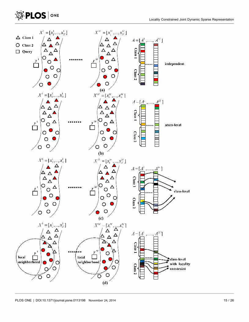
(20) is jjW8Ajj22zjjAjjG. The differences among LMSRC, MTJSRC, JDSRC and

LCJDSRC are illustrated in Figure 6. In this figure, the rectangles denote the sub-

images of a query face belonging to Class 2, and the triangles and circles represent

the training sub-images belonging to Class 1 and Class 2, respectively. From

Figure 6a, it can be seen that, since LMSRC simply utilizes the ,1-norm to

regularize the representation coefficients, the query sub-images are sparsely

represented independently and the representation coefficient vectors (i.e. A1,…,

AM) obtained by LMSRC are very different from one another. In MTJSRC, the

latent relationships of the sub-images from the query face are considered by ,1,2-

norm regularization. Thus, as demonstrated in Figure 6b, if one sub-image of a

training face is selected to represent its corresponding sub-image of the query face,

then the other sub-images of the same training face will also be selected to

represent their corresponding sub-images in y. This leads the representation

coefficient vectors of different query sub-images obtained by MTJSRC to have the

same sparsity pattern at atom-level (i.e. the non-zero elements of different

coefficient vectors are located in the same row). For JDSRC and LCJDSRC, since

both of them take the latent relationships of the query sub-images into account by

employing the mixed-norm of dynamic active set as regularization, the sparse

representation coefficient vectors of different query sub-images obtained by these

two algorithms have the same sparsity pattern at class-level as shown in Figure 6c

and Figure 6d. That is, the non-zero elements in different coefficient vectors

joined by each line (i.e. dynamic active set) are from the same class. Furthermore,

since the locality information is neglected in LMSRC, MTJSRC and JDSRC, we

can find that some distant training samples belonging to Class 1 are selected for

representation by these three algorithms in Figure 6a-c, which may result in

misrecognition. However, this limitation is overcome by the locality constraint in

LCJDSRC. From Figure 6d, it can be seen that by taking the similarity between the

query and training sub-images into consideration, the proposed algorithm tends

to assign non-zero coefficients to similar training samples within the local

neighborhoods of the query sub-images. Therefore, the training sub-images

selected for representation by LCJDSRC are mostly from the same class of the

query images and the recognition performance can be improved.

Then, the differences between the optimization algorithms in our study and

other works are analyzed. Though the optimization algorithm presented in

Section 2.3 looks similar to those in CoSOMP [34] and JDSRC [29], there are two

key different points between them. First, the dynamic active sets in our algorithm

are obtained by Joint Dynamic Sparsity mapping, thus, our algorithm can jointly

represent the sub-images of the query face and make the sparsity of the

representation coefficients for different sub-images be the same at class level,

which is the major difference between our algorithm and CoSOMP. Second, our

algorithm updates the representation coefficients using Equation (16). Therefore,



the similarity between the query and training samples is considered. However,

JDSRC updates the coefficients using standard least squares regression. Thus,

LCJDSRC can achieve better recognition result than the JDSRC algorithm.

Experimental Results and Analysis

In this section, extensive experiments are conducted to verify the effectiveness of

the proposed algorithm on four benchmark face databases including ORL [35],

Extended YaleB [36], AR [37] and LFW [38]. We compare the performance of our

proposed method with four state-of-the-art algorithms, i.e., LMSRC [6], RCR

[27], MTJSRC [28] and JDSRC [29]. For all face images in each database, we first

normalize them in scale and orientation such that eyes are always in the same

position, and then crop the facial areas into the final images for recognition. In

order to prevent overfitting and fairly compare our algorithm with other

algorithms, we randomly split the samples of each database into three disjoint

subsets: a training set used to train different recognition algorithms, a validation

set for optimizing the parameters in each algorithm and a test set used to assess

the recognition performances of various algorithms.

In local matching-based face recognition methods, a face image can be

partitioned into a set of equally or unequally sized sub-images, depending on the

user’s option. However, how to choose the sub-image size which gives optimal

performance is still an open problem. In this work, we will not attempt to deal

with this issue. So without loss of generality, equally sized partitions are adopted

in our study as in many other approaches [19–25].

Experimental results on the ORL database

In this subsection, we apply the proposed algorithm to the ORL face database

which contains 400 face images of 40 individuals, i.e., 10 images per individual.

The images were captured under different lighting conditions, facial expressions

(open or closed eyes, smiling or not smiling) and facial details (glasses or without

glasses). In our experiments, all images are resized to the resolution of

64664 pixels with 256 gray levels for computation efficiency. In this database, 4

and 3 images of each person are randomly selected for the training and validation

sets, and the remaining samples are regarded as the test set. The random sample

selection is repeated 10 times.

In a first experiment, the impacts of the two parameters (K and l) on the

performance of our algorithm under different sub-image sizes are evaluated on

the validation set. Here, the sub-image size is set as 32632, 21632, 16632 and

Figure 6. Comparisons among different algorithms. (a) LMSRC, (b) MTJSRC, (c) JDSRC and (d) LCJDSRC. The training sub-images highlighted in redare those selected to represent the query sub-images. In the sparse representation coefficient vectors, the elements marked as "Class 1" and "Class 2"represent the coefficients corresponding to the training samples belonging to each class; the non-zero elements in the vectors are highlighted in colors.




21616. For the parameters l and K, we tune their values by searching the grid

{0.001, 0.01, 0.05, 0.1, 1, 10, 100, 1000}6{5, 10, 15, 20, 25, 30} (where 6 is the

Cartesian product). From the validation results in Tables S1-S4 in File S1, the

optimal parameter values for which our algorithm gives the best performances for

various sub-image sizes can be easily found. Moreover, two other interesting

points can also be observed. Firstly, when the l value is fixed, a larger K will

deteriorate the performance of our algorithm. The reason for this phenomenon is

that when the sparsity level K is large, more training sub-images from the

incorrect classes are selected to represent the query sample, thus the recognition

rate is reduced. Secondly, we can see that when the sparsity level K is fixed, the

performance of our algorithm improves as the value of l increases when the lvalue is relatively small. However, this trend is not maintained for all K values. For

the cases of K55, 10, 15 and 20, the performance of our algorithm will slightly

decrease after it achieves its top recognition rate. Furthermore, we can find that a

larger l value is more suitable for larger sparsity level. This means that when the

number of training samples selected for representation becomes large, it is

preferable to magnify the coefficients corresponding to training samples similar to

the query sub-image and penalize the dissimilar ones, since similar training

samples are more likely belong to the same class of the query sample. At last, we

can see that given the standard deviation, the differences among the recognition

results of LCJDSRC under a large number of parameter sets are not significant.

This indicates the proposed algorithm is not sensitive to the parameters when they

are set as appropriate values.

In the second experiment, the performance of our algorithm is compared with

other algorithms on the test set. According to the validation results in Tables S1-

S4 in File S1, the parameters K and l in LCJDSRC are set as {K510, l51},

{K510, l51}, {K510, l510} and {K510, l5100} for the sub-image size 32632,

21632, 16632 and 21616, respectively. We also optimized the parameters of the

other algorithms in the same manner as for our algorithm. The average

recognition results of the algorithms under evaluation over ten independent runs

for each experiment can be seen in Table 1. The table shows that LMSRC obtains

the worst recognition result among all algorithms. This is because it processes the

sub-images of the query face independently. The performances of MTJSRC,

JDSRC and RCR are better than LSMRC, since the latent relationships among

sub-images are taken into account. For LCJDSRC, we can see that it outperforms

all other algorithms, which confirms that both data locality and the joint sparse

Table 1. The average recognition rates (%) and the corresponding standard deviations (%) of different algorithms under various sub-image sizes on the testset of the ORL face database.

Size LMSRC MTJSRC RCR JDSRC LCJDSRC

32632 83.25¡1.68 85.41¡2.05 87.91¡2.12 88.42¡1.78 91.92¡1.80

21632 82.00¡1.97 85.00¡2.69 86.58¡2.37 86.75¡3.21 90.50¡2.16

16632 83.41¡2.23 84.66¡2.39 86.75¡2.30 87.00¡2.42 90.67¡2.38

16621 83.08¡2.48 84.75¡2.54 86.41¡1.88 86.66¡1.92 89.00¡1.66

doi:10.1371/journal.pone.0113198.t001



representation are important to improve face recognition performance. Moreover,

the table shows that the recognition performances of all algorithms vary with the

sub-image size. For LMSRC, it achieves the best performance under smaller sub-

image size. Instead, a larger sub-image size is preferable for MTJSRC, RCR,

JDSRC and LCJDSRC. These results show that the proposed algorithm

consistently yields better recognition rates than the other algorithms regardless of

the sub-image sizes.

Finally, in order to further demonstrate the superiority of our algorithm to the

other algorithms, the one-tailed Wilcoxon rank sum test is utilized in this study to

verify whether LCJDSRC performs significantly better than the other algorithms.

In this test, the null hypothesis is that LCJDSRC makes no difference when

compared to the other local matching-based algorithms, and the alternative

hypothesis is that LCJDSRC makes an improvement when compared to the other

algorithms. For example, if we want to compare the performance of our algorithm

with that of LMSRC (LCJDSRC vs. LMSRC), the null and alternative hypotheses

can be defined as H0: MLCJDSRC~MLMSRC and H1:MLCJDSRCwMLMSRC, where

MLCJDSRC and MLMSRC are the medians of the recognition rates obtained by

LCJDSRC and LMSRC. In our experiments, the significance level is set to 1%.

From the test results in Table 2, we can find that the p-values obtained by all

pairwise Wilcoxon rank sum tests are much less than 0.01, which means the null

hypotheses are rejected in all pairwise tests and the proposed algorithm

significantly outperforms the other algorithms.

Experimental results on the Extended YaleB database

In this subsection, the performance of the proposed algorithm is evaluated using

the Extended YaleB face database, which contains 2414 frontal views of face

images from 38 individuals. For each individual, about 64 images were taken

under various laboratory-controlled lighting conditions. In our experiment, all

images are cropped and resized to the resolution of 64664 pixels. We randomly

select 10 images as training set, 20 images as validation set and the remaining

images as test set for each person. This random selection operation is repeated 10

times.

The performances of the proposed algorithm under different parameters values

on the validation set are tested firstly. In this experiment, the sub-image size is set

as 32632 and 21632. Since the number of training samples in this database is

much larger than ORL, we tune the values of K and l by searching the grid {30,

Table 2. The p-values of the pairwise one-tailed Wilcoxon rank sum tests on the test set of the ORL database.

32632 21632 16632 16621

LCJDSRC vs. LMSRC 8.34e-05 8.73e-05 1.78e-04 1.75e-04

LCJDSRC vs. MTJSRC 9.65e-05 4.80e-04 3.04e-04 3.96e-04

LCJDSRC vs. RCR 3.94e-04 1.03e-03 1.68e-03 2.45e-03

LCJDSRC vs. JDSRC 9.90e-04 1.32e-03 2.18e-03 8.02e-03




40, 50, 60, 70, 80, 90}6{0.001, 0.01, 0.05, 0.1, 1, 10, 100, 1000} (where 6 is the

Cartesian product). Tables S5 and S6 in File S1 show the average recognition

results of our algorithm under different parameter values. From these tables, it can

be found that with the increase of sparsity level, the recognition performance of

the proposed algorithm is generally improved. What’s more, we can also observe

that when the value of sparsity level is small, LCJDSRC performs better under

smaller l values, while a relatively larger l is preferred at large sparsity levels.

Finally, LCJDSRC achieves its best recognition results as 98.01% and 98.20%

when the parameters are set to {K580, l5100} and {K580, l510} for the sub-

image size 32632 and 21632, respectively.

Secondly, we assess the performance of LCJDSRC and compare it with LMSRC,

MTJSRC, RCR and JDSRC on the test set. The parameter values for all algorithms

are set according to their optimization results on the validation set. In our

algorithm, the sparsity level and tradeoff parameter are set as {K580, l5100} and

{K580, l510}. From the average recognition rates and standard deviations of

different algorithms obtained by ten independent repetitions of the experiment

reported in Table 3, it can be seen that LCJDSRC outperforms the other

algorithms. Furthermore, we can find that the performances of multi-task

learning-based algorithms (MTJSRC, RCR, JDSRC and LCJDSRC) are all better

than LMSRC. These two observations are consistent with the results obtained on

the ORL database. Besides, the one-tailed Wilcoxon rank sum test is also utilized

to verify whether the performance of the proposed algorithm is significantly better

than the existing algorithms. The p-values of the pairwise one-tailed Wilcoxon

rank sum tests are listed in Table 4. From these results, we can see that our

algorithm significantly outperforms the other algorithms.

Experimental results on the AR database

In this section, we evaluate the performance of our algorithm using the AR

database. This database consists of more than 4000 frontal images from 126

subjects including 70 men and 56 women. For each subject, 26 images were taken

under different conditions, including illumination, expression, and facial

Table 3. The average recognition rates (%) and the corresponding standard deviations (%) of different algorithms under various sub-image sizes on the testset of the Extended YaleB face database.

Size LMSRC MTJSRC RCR JDSRC LCJDSRC

32632 88.51¡1.68 91.13¡1.10 92.89¡1.40 93.35¡1.02 96.67¡1.04

21632 87.30¡1.51 90.73¡1.20 92.55¡1.08 92.41¡1.29 95.48¡0.97


Table 4. The p-values of the pairwise one-tailed Wilcoxon rank sum tests on the test set of the Extended YaleB database.

Size LCJDSRC vs. LMSRC LCJDSRC vs. MTJSRC LCJDSRC vs. RCR LCJDSRC vs. JDSRC

32632 9.08e-05 9.08e-05 1.64e-04 8.98e-05

21632 9.13e-05 9.08e-05 1.22e-04 1.23e-04




occlusion/disguise. In our experiments, we select a subset which contains 50 males

and 50 females from this database. All images are cropped and resized to the

resolution of 64664 pixels.

In the first experiment, 14 images of each individual with only illumination and

expression changes are selected. Among these images, 6 images from each person

are randomly chosen for training, 4 images are used for validation and the

remaining images are utilized for testing. This random selection operation is also

repeated 10 times. Similar to Section 3.2, we first set the sub-image size as 32632

and 21632, and then find the optimal parameter values of the proposed

algorithm using the validation set. From the results in Tables S7 and S8 in File S1,

it can be found that the optimal values of K and l for sub-image size of 32632

and 21632 are {K535, l50.1} and {K530, l50.1}, respectively. Furthermore,

we can also see that the influence of parameter values on the performance of

LCJDSRC is consistent with the observations in Section 3.1 and 3.2. Next, the

recognition results of our algorithm are compared to the other approaches on the

test set. Here, the optimal parameter values in LMSRC, MTJSRC, RCR and JDSRC

are obtained in the same way as for LCJDSRC. The average recognition rates

obtained by 10 independent runs for each experiment in Table 5 shows that our

algorithm outperforms the other algorithms, which is consistent with the

experimental results in Section 3.1 and 3.2. However, we can see that our

algorithm performs better under the smaller sub-image size, which is opposite to

the experimental results on the ORL and Extended YaleB databases. This may

happen because the expression variance in this database is much larger than those

in the ORL and Extended YaleB, thus a smaller sub-image size is preferable to

capture the local facial features which do not vary with the facial expressions.

Finally, the p-values of pairwise one-tailed Wilcoxon rank sum tests in Table 6

show that the recognition performance of the proposed algorithm is significantly

better than the other algorithms.

The second experiment on the AR database is run to test the effectiveness of our

algorithm under severe occlusion conditions. In this experiment, 1400 images

with illumination and expression variations from the database are selected for

Table 5. The average recognition rates (%) and the corresponding standard deviations (%) of different algorithms under various sub-image sizes on the testset of the AR face database.

LMSRC MTJSRC RCR JDSRC LCJDSRC

32632 90.62¡1.35 92.90¡1.75 95.07¡1.21 94.42¡0.63 97.68¡0.51

21632 91.82¡1.33 94.05¡1.56 95.80¡1.08 94.95¡0.87 97.90¡0.70


Table 6. The p-values of the pairwise one-tailed Wilcoxon rank sum tests on the test set of the AR face database.

LCJDSRC vs. LMSRC LCJDSRC vs. MTJSRC LCJDSRC vs. RCR LCJDSRC vs. JDSRC

32632 8.93e-05 8.78e-05 8.88e-05 8.83e-05

21632 8.58e-05 9.82e-05 1.54e-04 8.34e-05




training, 600 images with sunglasses and scarf occlusions are selected for

validation and the other 600 images with sunglasses and scarf occlusions are

utilized for testing. We optimize the parameter values of different algorithms

using the validation set and then compare their recognition performances on the

test set. From the validation results in Tables S9-S12 in the File S1, it is easy to

find the best parameter values for the proposed algorithm. From the comparison

results of various algorithms obtained by ten independent repetitions of the

experiment on the test set in Tables 7 and 8, the following points can be observed.

Firstly, it can be found that when the face images are occluded by the sunglasses,

the recognition performances obtained by all algorithms are relatively low.

However, if the faces are occluded by a scarf, the performances of several

algorithms improve. This happens because the sunglasses occlude the eyebrows

and eyes in the face, which are proved to be the most important components for

face recognition [26]. Secondly, we can see that a smaller sub-image size (21632)

is more suitable for the local matching-based algorithms to deal with the face

image with occlusions. Finally, it can be obviously seen that our algorithm

outperforms the other algorithms. Furthermore, the superiority of our algorithm

can also be proved by the pairwise one-tailed Wilcoxon rank sum test results in

Tables 9–10.

Experimental results on the LFW database

The LFW database [38] is a large scale database which contains 13,233 target face

images of 5,749 different individuals. Since all the samples were taken from the

real world in an unconstrained environment, facial expressions, pose, illumina-

tion, occlusions and alignment are very variable in this database. As suggested in

[39], a subset which contains 1580 face images of 158 individuals from the LFW-a

[40] database is employed in our study. In this subset, each individual has 10

images with the size of 32632 pixel (The mat file can be download from http://

www4.comp.polyu.edu.hk/,cslzhang/code/MPCRC_eccv12_code.zip). In our

experiment, 6 samples of each individual are randomly selected for training.

Table 7. The average recognition rates (%) and the corresponding standard deviations (%) of different algorithms on the test set of the AR face databasewith sunglasses and scarf occlusions (sub-image size 32632).


Sunglasses 64.30¡1.65 70.86¡1.87 73.06¡1.67 79.13¡1.54 81.30¡1.13

Scarf 83.13¡0.89 85.50¡1.05 88.73¡1.09 87.76¡0.78 90.86¡0.84


Table 8. The average recognition rates (%) and the corresponding standard deviations (%) of different algorithms on the test set of the AR face databasewith sunglasses and scarf occlusions (sub-image size 21632).


Sunglasses 83.30¡0.89 86.00¡1.26 89.20¡0.86 90.20¡0.75 92.76¡0.72

Scarf 87.73¡1.06 88.83¡1.34 91.40¡1.26 91.46¡1.11 94.83¡0.61




http://www4.comp.polyu.edu.hk/~cslzhang/code/MPCRC_eccv12_code.zip

http://www4.comp.polyu.edu.hk/~cslzhang/code/MPCRC_eccv12_code.zip

Among the remaining 4 samples, 2 images of each individual are randomly chosen

for validation and the other 2 images are used for testing. This random selection

operation is also repeated 10 times. Here, we equally partition the face images into

four sub-images and the sub-image size is 16616.

Firstly, the performances of the proposed algorithm under various parameter

values are tested on the validation set to find the optimal parameters for our

algorithm. From the validation results in Table S13 in the File S1, we can see that

the influence of the two parameters on the proposed algorithm is similar to those

in Section 3.1-3.3, and the optimal parameter values for which our algorithm gives

the best recognition rate are K550 and l 50.05.

Then, we compare the proposed algorithm with other algorithms on the test

set. From the average recognition rate of each algorithm over ten independent

runs for each experiment in Table 11 and the Wilcoxon rank sum test results in

Table 12, it can be said that, although the recognition performances of all

algorithms on the LFW database are relatively lower than those on the other three

databases, our algorithm is still significantly superior to the other algorithms.

Conclusion and Future Work

In this paper, a novel classification algorithm named Locality Constrained Joint

Dynamic Sparse Representation-based Classification (LCJDSRC) has been

proposed for local matching-based face recognition. Our algorithm combines the

joint sparse representation and locality constraint into a unified framework.

Therefore, not only does it consider the latent relationships among different sub-

images of a face, but also introduces the locality information into the sparse

representation model. Moreover, a greedy algorithm based on Matching Pursuit

(MP) has been presented to optimize the objective function of LCJDSRC.

Extensive experiments have been carried out on four databases including ORL,

Extended YaleB, AR and LFW to demonstrate the effectiveness of our proposed

LCJDSRC approach. The experimental results have shown that LCJDSRC

Table 9. The p-values of the pairwise one-tailed Wilcoxon rank sum tests on the test set of the AR face database with sunglasses and scarf occlusions (sub-image size 32632).


Sunglasses 8.83e-05 8.83e-05 8.93e-05 3.58 e-03

Scarf 8.34e-05 8.58e-05 6.32e-05 8.58e-05


Table 10. The p-values of the pairwise one-tailed Wilcoxon rank sum tests on the test set of the AR face database with sunglasses and scarf occlusions(sub-image size 21632).


Sunglasses 7.78e-05 7.92e-05 7.92e-05 7.92e-05

Scarf 8.25e-05 8.20e-05 9.65e-05 8.39e-05




outperforms several similar methods such as LMSRC, MTJSRC, RCR and JDSRC

on the data sets considered in our tests.

Finally, it should be pointed out that in LCJDSRC, the query sub-images are

represented by the sub-images partitioned from the original training samples,

which may decrease its performance when too few training samples are available.

Thus, one of our future goals is to incorporate our algorithm into the dictionary

learning framework [41, 42] to further improve its flexibility. Besides, since some

researchers have shown that the dimensionality reduction methods are helpful to

the sparse representation-based classification algorithms, how to combine

LCJDSRC with the dimensionality reduction techniques is another interesting

topic for future study.

Supporting Information

File S1. Tables S1-S13 and Text S1. Table S1. The average recognition rates (%)

and the corresponding standard deviations (%) of LCJDSRC under different

parameters on the validation set of the ORL face database (sub-image size is

32632). Table S2. The average recognition rates (%) and the corresponding

standard deviations (%) of LCJDSRC under different parameters on the

validation set of the ORL face database (sub-image size is 21632). Table S3. The

average recognition rates (%) and the corresponding standard deviations (%) of

LCJDSRC under different parameters on the validation set of the ORL face

database (sub-image size is 16632). Table S4. The average recognition rates (%)

and the corresponding standard deviations (%) of LCJDSRC under different

parameters on the validation set of the ORL face database (sub-image size is

16621). Table S5. The average recognition rates (%) and the corresponding

standard deviations (%) of LCJDSRC under different parameters on the

validation set of the Extended YaleB face database (sub-image size is 32632).

Table S6. The average recognition rates (%) and the corresponding standard

deviations (%) of LCJDSRC under different parameters on the validation set of

the Extended YaleB face database (sub-image size is 21632). Table S7. The


LCJDSRC under different parameters on the validation set of the AR face database

Table 11. The average recognition rates (%) and the corresponding standard deviations (%) of different algorithms on the test set of the LFW face database(sub-image size 32632).


32632 35.88¡1.36 42.97¡2.48 44.71¡2.23 45.53¡2.20 49.34¡0.99


Table 12. The p-values of the pairwise one-tailed Wilcoxon rank sum tests on the test set of the LFW face database (sub-image size 32632).


32632 8.93e-05 8.98e-05 8.93e-05 1.04e-04




(sub-image size is 32632). Table S8. The average recognition rates (%) and the

corresponding standard deviations (%) of LCJDSRC under different parameters

on the validation set of the AR face database (sub-image size is 21632). Table S9.

The average recognition rates (%) and the corresponding standard deviations (%)

of LCJDSRC under different parameters on the validation set of the AR face

database with sunglasses occlusion (sub-image size is 32632). Table S10. The



with scarf occlusion (sub-image size is 32632). Table S11. The average

recognition rates (%) and the corresponding standard deviations (%) of


with sunglasses occlusion (sub-image size is 21632). Table S12. The average



with scarf occlusion (sub-image size is 21632). Table S13. The average


LCJDSRC under different parameters on the validation set of the LFW face

database (sub-image size is 32632). Text S1. The derivation process of Equation

(16).

doi:10.1371/journal.pone.0113198.S001 (DOC)

Author Contributions

Conceived and designed the experiments: JZW YGY JK BXZ. Performed the

experiments: YGY WZ YJS MQ MZ. Analyzed the data: JZW YGY JK BXZ. Wrote

the paper: JZW YGY.

References

1. Li SZ, Jain AK (2011) Handbook of face recognition, Springer.

2. Jafri R, Arabnia HR (2009) A survey of face recognition techniques. Information Processing Systems5(2): 41–68.

3. Zou J, Ji Q, Nagy G (2007) A comparative study of local matching approach for face recognition. IEEETransactions on Image Processing 16(10): 2617–2628.

4. Subban R, Mankame DP (2014) Human face recognition biometric techniques: analysis and review.Recent Advances in Intelligent Informatics: 455–463.

5. Ramirez I, Sapiro G (2010) Universal sparse modeling. Technical Report.

6. Wright J, Yang AY, Ganesh A, Sastry SS, Ma Y (2009) Robust face recognition via sparserepresentation. IEEE Transactions on Pattern Analysis and Machine Intelligence 31(2): 210–227.

7. Gao S, Tsang IWH, Chia LT (2010) Kernel sparse representation for image classification and facerecognition. European Conference on Computer Vision: 1–14.

8. Shawe-Taylor J, Cristianini N (2004) Kernel methods for pattern analysis. Cambridge University Press.

9. Yang M, Zhang L (2010) Gabor feature based sparse representation for face recognition with gaborocclusion dictionary. European Conference on Computer Vision: 448–461.

10. Wang J, Yang J, Yu K, Lv F, Huang T, et al. (2010) Locality-constrained linear coding for imageclassification. IEEE Conference on Computer Vision and Pattern Recognition: 3360–3367.



http://www.plosone.org/article/fetchSingleRepresentation.action?uri=info:doi/10.1371/journal.pone.0113198.S001

11. Roweis ST, Saul LK (2000) Nonlinear dimensionality reduction by locally linear embedding. Science290(5500):2323–2326.

12. Tenenbaum JB, De Silva V, Langford JC (2000) A global geometric framework for nonlineardimensionality reduction. Science 290(5500): 2319–2323.

13. Elhamifar E, Vidal R (2011) Robust classification using structured sparse representation. IEEEConference on Computer Vision and Pattern Recognition: 1873–1879.

14. Wagner A, Wright J, Ganesh A, Zhou Z, Mobahi H, et al. (2009) Towards a practical face recognitionsystem: robust registration and illumination by sparse representation. IEEE Conference on ComputerVision and Pattern Recognition: 597–604.

15. Yang M, Zhang L, Yang J, Zhang D (2011) Robust sparse coding for face recognition. IEEE Conferenceon Computer Vision and Pattern Recognition: 625–632.

16. Deng W, Hu J, Guo J (2012) Extended SRC: undersampled face recognition via intraclass variantdictionary. IEEE Transactions on Pattern Analysis and Machine Intelligence 34(9): 1864–1870.

17. Mi JX, Liu JX (2013) Face recognition using sparse representation-based classification on K-nearestsubspace. Plos One 8(3): e59430 doi: 10.1371/journal.pone.0059430.

18. Chen Y, Li Z, Jin Z (2013) Feature extraction based on maximum nearest subspace margin criterion.Neural Processing Letters 37(3): 355–375.

19. Pentland A, Moghaddam B, Starner T (1994) View-based and modular eigenspaces for facerecognition. IEEE Conference on Computer Vision and Pattern Recognition: 84–91.

20. Chen S, Zhu Y (2004) Subpattern-based principle component analysis. Pattern Recognition 37(5):1081–1083.

21. Nanni L, Maio D (2007) Weighted sub-gabor for face recognition. Pattern Recognition Letters 28(4):487–492.

22. Tan K, Chen S (2005) Adaptively weighted sub-pattern PCA for face recognition. Neurocomputing 64:505–511.

23. Kumar KV, Negi A (2008) SubXPCA and a generalized feature partitioning approach to principalcomponent analysis. Pattern Recognition 41(4): 1398–1409.

24. Wang J, Zhang B, Wang S, Qi M, Kong J (2010) An adaptively weighted sub-pattern locality preservingprojection for face recognition. Journal of Network and Computer Applications 33(3): 323–332.

25. Wang J, Ma Z, Zhang B, Qi M, Kong J (2011) A structure-preserved local matching approach for facerecognition. Pattern Recognition Letters 32(3): 494-504.

26. Sinha P, Balas B, Ostrovsky Y, Russell R (2006) Face recognition by humans: nineteen results allcomputer vision researchers should know about. Proceedings of the IEEE 94(11): 1948–1962.

27. Yang M, Zhang D, Wang S (2012) Relaxed collaborative representation for pattern classification. IEEEConference on Computer Vision and Pattern Recognition: 2224–2231.

28. Yuan XT, Yan S (2010) Visual classification with multi-task joint sparse representation. IEEE Conferenceon Computer Vision and Pattern Recognition: 3493–3500.

29. Zhang H, Nasrabadi NM, Zhang Y, Huang TS (2012) Joint dynamic sparse representation for multi-view face recognition. Pattern Recognition 45(4): 1290–1298.

30. Chao YW, Yeh YR, Chen YW, Lee YJ, Wang YCF (2011) Locality-constrained group sparserepresentation for robust face recognition. IEEE International Conference on Image Processing: 761–764.

31. Wei CP, Chao YW, Yeh YR, Wang YCF (2013) Locality-sensitive dictionary learning for sparserepresentation based classification. Pattern Recognition 46(5): 1277–1287.

32. Yu K, Zhang T, Gong Y (2009) Nonlinear learning using local coordinate coding. Advances in NeuralInformation Processing Systems 22: 2223–2231.

33. Mallat SG, Zhang Z (1933) Matching pursuits with time-frequency dictionaries. IEEE Transactions onSignal Processing 41(12): 3397–3415.

34. Duarte MF, Cevher V, Baraniuk RG (2009) Model-based compressive sensing for signal ensembles.Proceedings of the Allerton Conference on Communication, Control, and Computing: 585–600.



35. Samaria FS, Harter AC (1994) Parameterisation of a stochastic model for human face identification.IEEE Workshop on Applications of Computer Vision: 138–142.

36. Georghiades AS, Belhumeur PN, Kriegman D (2001) From few to many: illumination cone models forface recognition under variable lighting and pose. IEEE Transactions on Pattern Analysis and MachineIntelligence 23(6): 643–660.

37. Martinez AM, Benavente R (1998) The AR face database. CVC Technical Report 24.

38. Huang GB, Mattar M, Berg T, Learned-Miller E (2007) Labeled face in the wild: a database for studyingface recognition in unconstrained environments. Technical Report 07–49.

39. Zhu P, Zhang L, Hu Q, Shiu SC (2012) Multi-scale patch based collaborative representation for facerecognition with margin distribution optimization. European Conference on Computer Vision: 822–835.

40. Wolf L, Hassner T, Taigman Y (2009) Similarity scores based on background sample. AsianConference on Computer Vision, 88–89.

41. Tosic I, Frossard P (2011) Dictionary learning. IEEE Signal Processing Magazine 28(2): 27–38.

42. Ramırez I, Sapiro G (2012) An MDL framework for sparse coding and dictionary learning. IEEETransactions on Signal Processing 60(6): 2913–2927.



Locality Constrained Joint Dynamic Sparse Representation for Local Matching based Face Recognition

Documents

Transcript of Locality Constrained Joint Dynamic Sparse Representation for Local Matching based Face Recognition