Effective Automatic Parallelization and Locality Optimization ...
190
Effective Automatic Parallelization and Locality Optimization Using The Polyhedral Model DISSERTATION Presented in Partial Fulfillment of the Requirements for the Degree Doctor of Philosophy in the Graduate School of The Ohio State University By Uday Kumar Reddy Bondhugula, B-Tech, M.S. ***** The Ohio State University 2008 Dissertation Committee P. Sadayappan, Advisor Atanas Rountev Gagan Agrawal J. Ramanujam Approved by Advisor Graduate Program in Computer Science and Engineering
-
Upload
khangminh22 -
Category
Documents
-
view
0 -
download
0
Transcript of Effective Automatic Parallelization and Locality Optimization ...

Effective Automatic Parallelization and
Locality Optimization Using The Polyhedral
Model
DISSERTATION
Presented in Partial Fulfillment of the Requirements for
the Degree Doctor of Philosophy in the
Graduate School of The Ohio State University
By
Uday Kumar Reddy Bondhugula, B-Tech, M.S.
* * * * *
The Ohio State University
2008
Dissertation Committee
P. Sadayappan, Advisor
Atanas Rountev
Gagan Agrawal
J. Ramanujam
Approved by
Advisor
Graduate Program inComputer Science and
Engineering

ABSTRACT
Multicore processors have now become mainstream. The difficulty of programming
these architectures to effectively tap the potential of multiple processing units is well-
known. Among several ways of addressing this issue, one of the very promising and
simultaneously hard approaches is Automatic Parallelization. This approach does not
require any effort on part of the programmer in the process of parallelizing a program.
The Polyhedral model for compiler optimization is a powerful mathematical frame-
work based on parametric linear algebra and integer linear programming. It provides
an abstraction to represent nested loop computation and its data dependences using
integer points in polyhedra. Complex execution-reordering, that can improve perfor-
mance by parallelization as well as locality enhancement, is captured by affine trans-
formations in the polyhedral model. With several recent advances, the polyhedral
model has reached a level of maturity in various aspects – in particular, as a powerful
intermediate representation for performing transformations, and code generation after
transformations. However, an approach to automatically find good transformations
for communication-optimized coarse-grained parallelization together with locality op-
timization has been a key missing link. This dissertation presents a new automatic
transformation framework that solves the above problem. Our approach works by
finding good affine transformations through a powerful and practical linear cost func-
tion that enables efficient tiling and fusion of sequences of arbitrarily nested loops.
ii
This in turn allows simultaneous optimization for coarse-grained parallelism and lo-
cality. Synchronization-free parallelism and pipelined parallelism at various levels can
be extracted. The framework can be targeted to different parallel architectures, like
general-purpose multicores, the Cell processor, GPUs, or embedded multiprocessor
SoCs.
The proposed framework has been implemented into a new end-to-end transfor-
mation tool, PLUTO, that can automatically generate parallel code from regular C
program sections. Experimental results from the implemented system show significant
performance improvement for single core and multicore execution over state-of-the-art
research compiler frameworks as well as the best native production compilers. For
several dense linear algebra kernels, code generated from Pluto beats, by a significant
margin, the same kernels implemented with sequences of calls to highly-tuned libraries
supplied by vendors. The system also allows empirical optimization to be performed
in a much wider context than has been attempted previously. In addition, Pluto can
serve as the parallel code generation backend for several high-level domain-specific
languages.
iii

ACKNOWLEDGMENTS
I am thankful to my adviser, P. Sadayappan, for always being very keen and
enthusiastic to discuss new ideas and provide valuable feedback. He also provided me
a great amount of freedom in the direction I wanted to take and this proved to be
very productive for me. Nasko’s (Atanas Rountev) determination in getting into the
depths of a problem had a very positive influence and was helpful in making some key
progresses in the theory surrounding this dissertation. In addition, I was fortunate to
have Ram’s (J. Ramanujam) advice from time to time that complemented everything
else well. Interaction and discussions with Saday, Nasko, and Ram were very friendly
and entertaining. I would also like to thank Gagan (Prof. Gagan Agrawal) for being
a very helpful and accessible Graduate Studies Committee chair and agreeing to serve
on my dissertation committee at short notice.
Thanks to labmates Muthu Baskaran, Jim Dinan, Tom Henretty, Brian Larkins,
Kamrul, Gaurav Khanna, Sriram Krishnamoorthy, Qingda Lu, and Rajkiran Panu-
ganti for all the interesting conversations during my stay at 474 Dreese Labs: they
will be remembered. I am also thankful to the researchers at the Ohio Supercom-
puter Center, Ananth Devulapalli, Joseph Fernando, and Pete Wyckoff, with whom
I worked during the initial stages of my Ph.D., and they gave me a good start.
Many thanks to Louis-Noel Pouchet and Albert Cohen for hosting a very pleasant
visit at INRIA Saclay. Good friendships have evolved with them and with Nicolas
iv

Vasilache that will last for a long time. I am also thankful to the group of Kathryn
O’Brien at the IBM TJ Watson Research Center at Yorktown Heights – its group
members Alex Eichenberger and Lakshminarayanan Renganarayana, as well as Kevin
O’Brien and Dan Prener for a memorable experience during my internship there, and
a mutually beneficial association.
I have to acknowledge the contributions of the developers of CLooG, LooPo, and
PipLib, without which the theory this dissertation proposes would not have translated
into a complete end-to-end system. In particular, I would like to acknowledge Cedric
Bastoul for having written Cloog, and Martin Griebl and the LooPo team for creating
an excellent polyhedral infrastructure over the years. I just had all the necessary
components to build and complete the missing links. I hope the results presented in
the thesis vindicate the efforts put into these libraries and tools both from a research
and an engineering standpoint.
I conclude by acknowledging my parents who deserve the maximum credit for
this work. My father, Cdr. B. Sudhakar Reddy, and my mother, Nirmala, took
extraordinary interest in my education since my childhood. I am glad their efforts
have been fruitful at every stage of my studies.
v

VITA
Sep 10, 1982 . . . . . . . . . . . . . . . . . . . . . . . . . . . . . . . .Born - India
Jul 2000 – Jul 2004 . . . . . . . . . . . . . . . . . . . . . . . . . Bachelor of TechnologyComputer Science and EngineeringIndian Institute of Technology, Madras
Sep 2004 – Aug 2008 . . . . . . . . . . . . . . . . . . . . . . .Graduate Research AssociateComputer Science and EngineeringThe Ohio State University
Jun 2007 – Sep 2007 . . . . . . . . . . . . . . . . . . . . . . . .Research InternAdvanced Compilation TechnologiesIBM TJ Watson Research Labs,Yorktown Heights, New York
Mar 2008 – Apr 2008 . . . . . . . . . . . . . . . . . . . . . . . Visiting ResearcherALCHEMY teamINRIA Saclay, Ile-de-France
PUBLICATIONS
Uday Bondhugula, A. Hartono, J. Ramanujam, and P. Sadayappan. A PracticalAutomatic Polyhedral Parallelizer and Locality Optimizer. In ACM SIGPLAN Pro-gramming Language Design and Implementation, Jun 2008.
Uday Bondhugula, M. Baskaran, S. Krishnamoorthy, J. Ramanujam, A. Rountev, andP. Sadayappan. Automatic transformations for communication-minimized paralleliza-tion and locality optimization in the polyhedral model. In International Conferenceon Compiler Construction, Apr. 2008.
M. Baskaran, Uday Bondhugula, S. Krishnamoorthy, J. Ramanujam, A. Rountev,and P. Sadayappan. A Compiler Framework for Optimization of Affine Loop Nestsfor GPGPUs. In ACM International Conference on Supercomputing (ICS), June2008.
vi
M. Baskaran, Uday Bondhugula, S. Krishnamoorthy, J. Ramanujam, A. Rountev, andP. Sadayappan. Automatic Data Movement and Computation Mapping for Multi-level Parallel Architectures with Explicitly Managed Memories. In ACM SIGPLANSymposium on Principles and Practice of Parallel Programming, Feb 2008.
Uday Bondhugula, J. Ramanujam, and P. Sadayappan. Automatic mapping of nestedloops to FPGAs. In ACM SIGPLAN Symposium on Principles and Practice ofParallel Programming, Mar 2007.
S. Krishnamoorthy, M. Baskaran, Uday Bondhugula, J. Ramanujam, A. Rountev,and P. Sadayappan. Effective automatic parallelization of stencil computations. InACM SIGPLAN Conference on Programming Language Design and Implementation,Jun 2007.
Uday Bondhugula, A. Devulapalli, J. Dinan, J. Fernando, P. Wyckoff, E. Stahlberg,and P. Sadayappan. Hardware/software integration for FPGA-based all-pairs shortest-paths. In IEEE Field Programmable Custom Computing Machines, Apr 2006.
Uday Bondhugula, A. Devulapalli, J. Fernando, P. Wyckoff, and P. Sadayappan. Par-allel FPGA-based all-pairs shortest-paths in a directed graph. In IEEE InternationalParallel and Distributed Processing Symposium, Apr 2006.
S. Sur, Uday Bondhugula, A. Mamidala, H.-W. Jin, and D. K. Panda. High per-formance RDMA-based all-to-all broadcast for InfiniBand clusters. In 12th IEEEInternational Conference on High Performance Computing, Dec 2005.
FIELDS OF STUDY
Major Field: Computer Science and Engineering
Emphasis: Automatic parallelization, Parallelizing compilers, Polyhedral model
vii

TABLE OF CONTENTS
Page
Abstract . . . . . . . . . . . . . . . . . . . . . . . . . . . . . . . . . . . . . . . ii
Acknowledgments . . . . . . . . . . . . . . . . . . . . . . . . . . . . . . . . . . iv
Vita . . . . . . . . . . . . . . . . . . . . . . . . . . . . . . . . . . . . . . . . . vi
List of Figures . . . . . . . . . . . . . . . . . . . . . . . . . . . . . . . . . . . xii
List of Tables . . . . . . . . . . . . . . . . . . . . . . . . . . . . . . . . . . . . xvii
List of Algorithms . . . . . . . . . . . . . . . . . . . . . . . . . . . . . . . . . xviii
Chapters:
1. Introduction . . . . . . . . . . . . . . . . . . . . . . . . . . . . . . . 1
2. Background . . . . . . . . . . . . . . . . . . . . . . . . . . . . . . . 9
2.1 Hyperplanes and Polyhedra . . . . . . . . . . . . . . . . . . . . . . 102.2 The Polyhedral Model . . . . . . . . . . . . . . . . . . . . . . . . . 142.3 Polyhedral Dependences . . . . . . . . . . . . . . . . . . . . . . . . 16
2.3.1 Dependence polyhedron. . . . . . . . . . . . . . . . . . . . . 172.3.2 Strengths of dependence polyhedra. . . . . . . . . . . . . . . 19
2.4 Polyhedral Transformations . . . . . . . . . . . . . . . . . . . . . . 212.4.1 Why affine transformations? . . . . . . . . . . . . . . . . . . 25
2.5 Putting the Notation Together . . . . . . . . . . . . . . . . . . . . 272.6 Legality and Parallelism . . . . . . . . . . . . . . . . . . . . . . . . 27
viii
3. Automatic transformations . . . . . . . . . . . . . . . . . . . . . . 32
3.1 Schedules, Allocations, and Partitions . . . . . . . . . . . . . . . . 323.2 Limitations of Previous Techniques . . . . . . . . . . . . . . . . . . 33
3.2.1 Scheduling + allocation approaches . . . . . . . . . . . . . . 333.2.2 Existing partitioning-based approaches . . . . . . . . . . . . 36
3.3 Recalling the Notation . . . . . . . . . . . . . . . . . . . . . . . . . 373.4 Problem statement . . . . . . . . . . . . . . . . . . . . . . . . . . . 393.5 Legality of Tiling in the Polyhedral Model . . . . . . . . . . . . . . 393.6 Towards Finding Good Solutions . . . . . . . . . . . . . . . . . . . 443.7 Cost Function . . . . . . . . . . . . . . . . . . . . . . . . . . . . . . 463.8 Cost Function Bounding and Minimization . . . . . . . . . . . . . . 483.9 Iteratively Finding Independent Solutions . . . . . . . . . . . . . . 503.10 Communication and Locality Optimization Unified . . . . . . . . . 53
3.10.1 Space and time in transformed iteration space. . . . . . . . 543.11 Examples . . . . . . . . . . . . . . . . . . . . . . . . . . . . . . . . 54
3.11.1 A step by step example . . . . . . . . . . . . . . . . . . . . 543.11.2 Example 2: Imperfectly nested 1-d Jacobi . . . . . . . . . . 60
3.12 Handling Input Dependences . . . . . . . . . . . . . . . . . . . . . 603.13 Refinements for Cost Function . . . . . . . . . . . . . . . . . . . . 623.14 Loop Fusion . . . . . . . . . . . . . . . . . . . . . . . . . . . . . . . 623.15 Summary . . . . . . . . . . . . . . . . . . . . . . . . . . . . . . . . 633.16 Comparison with Existing Approaches . . . . . . . . . . . . . . . . 653.17 Scope for Extensions . . . . . . . . . . . . . . . . . . . . . . . . . . 70
4. Integrating Loop Fusion: Natural Task . . . . . . . . . . . . . . . 72
4.1 Automatic Fusion . . . . . . . . . . . . . . . . . . . . . . . . . . . 744.1.1 Implications of minimizing δ for fusion . . . . . . . . . . . . 754.1.2 Dependence cutting schemes . . . . . . . . . . . . . . . . . 78
4.2 Correctness and Completeness . . . . . . . . . . . . . . . . . . . . . 794.2.1 Bound on iterative search in Algorithm 2 . . . . . . . . . . 82
4.3 Theoretical Complexity of Computing Transformations . . . . . . . 824.4 Examples . . . . . . . . . . . . . . . . . . . . . . . . . . . . . . . . 84
4.4.1 Sequence of Matrix-Matrix multiplies . . . . . . . . . . . . . 844.4.2 Multiple statement stencils . . . . . . . . . . . . . . . . . . 854.4.3 CCSD (T) . . . . . . . . . . . . . . . . . . . . . . . . . . . . 854.4.4 TCE four-index transform . . . . . . . . . . . . . . . . . . . 88
ix
4.4.5 GEMVER . . . . . . . . . . . . . . . . . . . . . . . . . . . . 894.5 Past Work on Fusion . . . . . . . . . . . . . . . . . . . . . . . . . . 89
5. The PLUTO Parallelization System . . . . . . . . . . . . . . . . . 96
5.1 Overview of PLUTO . . . . . . . . . . . . . . . . . . . . . . . . . . 965.2 Tiled Code Generation under Transformations . . . . . . . . . . . . 99
5.2.1 Syntactic tiling versus tiling scattering functions . . . . . . 1005.2.2 Tiles under a transformation . . . . . . . . . . . . . . . . . 1015.2.3 Pipelined parallel code generation . . . . . . . . . . . . . . . 1075.2.4 Example 1: Imperfectly nested stencil. . . . . . . . . . . . . 1105.2.5 Example 2: LU . . . . . . . . . . . . . . . . . . . . . . . . . 111
5.3 Preventing Code Expansion in Tile Space . . . . . . . . . . . . . . 1125.4 Tilability Detection and Parallelism Detection . . . . . . . . . . . . 113
5.4.1 AST-based versus scattering function-based . . . . . . . . . 1145.4.2 Intricacies in detecting tilable bands . . . . . . . . . . . . . 115
5.5 Setting Tile Sizes . . . . . . . . . . . . . . . . . . . . . . . . . . . . 1175.6 Post-processing Transformations . . . . . . . . . . . . . . . . . . . 121
5.6.1 Unroll-jamming or register tiling . . . . . . . . . . . . . . . 1215.6.2 Intra-tile reordering and aiding auto-vectorization . . . . . . 122
5.7 Related Work on Tiled Code Generation . . . . . . . . . . . . . . . 123
6. Experimental Evaluation . . . . . . . . . . . . . . . . . . . . . . . 125
6.1 Comparing with previous approaches . . . . . . . . . . . . . . . . . 1256.2 Experimental Setup . . . . . . . . . . . . . . . . . . . . . . . . . . 1276.3 Imperfectly nested stencil code . . . . . . . . . . . . . . . . . . . . 1286.4 Finite Difference Time Domain . . . . . . . . . . . . . . . . . . . . 1316.5 LU Decomposition . . . . . . . . . . . . . . . . . . . . . . . . . . . 1356.6 Matrix Vector Transpose . . . . . . . . . . . . . . . . . . . . . . . . 1366.7 3-D Gauss-Seidel successive over-relaxation . . . . . . . . . . . . . 1406.8 DGEMM . . . . . . . . . . . . . . . . . . . . . . . . . . . . . . . . 1416.9 Experiments with Fusion-critical Codes . . . . . . . . . . . . . . . . 143
6.9.1 GEMVER . . . . . . . . . . . . . . . . . . . . . . . . . . . . 1436.9.2 Doitgen . . . . . . . . . . . . . . . . . . . . . . . . . . . . . 147
6.10 Analysis . . . . . . . . . . . . . . . . . . . . . . . . . . . . . . . . . 148
x
7. Conclusions and Future Directions . . . . . . . . . . . . . . . . . 154
Bibliography . . . . . . . . . . . . . . . . . . . . . . . . . . . . . . . . . . . . 160
Index . . . . . . . . . . . . . . . . . . . . . . . . . . . . . . . . . . . . . . . . 170
xi

LIST OF FIGURES
Figure Page
1.1 Clock Frequency of Intel Processors in the past decade . . . . . . . . 2
2.1 Hyperplane and Polyhedron . . . . . . . . . . . . . . . . . . . . . . . 12
2.2 A portion of the GEMVER kernel . . . . . . . . . . . . . . . . . . . . 16
2.3 The data dependence graph . . . . . . . . . . . . . . . . . . . . . . . 16
2.4 Domain for statement S1 from Figure 2.2 . . . . . . . . . . . . . . . . 16
2.5 Flow dependence from A[i][j] of S1 to A[l][k] of S2 and its dependencepolyhedron (Figure courtesy: Loopo display tool) . . . . . . . . . . . 18
2.6 An imperfect loop nest . . . . . . . . . . . . . . . . . . . . . . . . . . 20
2.7 Dependence polyhedron S4(hz[i][j]) → S2(hz[i − 1][j]) . . . . . . . . 20
2.8 Polyhedral transformation: an example . . . . . . . . . . . . . . . . . 23
2.9 Outer parallel loop, i: hyperplane (1,0) . . . . . . . . . . . . . . . . . 29
2.10 Inner parallel loop, j: hyperplane (0,1) . . . . . . . . . . . . . . . . . 29
2.11 Pipelined parallel loop: i or j . . . . . . . . . . . . . . . . . . . . . . 30
3.1 A typical solution with scheduling-allocation . . . . . . . . . . . . . . 36
3.2 A fine-grained affine schedule . . . . . . . . . . . . . . . . . . . . . . 36
3.3 Affine partitioning with no cost function can lead to unsatisfactorysolutions . . . . . . . . . . . . . . . . . . . . . . . . . . . . . . . . . . 37
xii

3.4 A good set of φ’s: (1,0) and (1,1) . . . . . . . . . . . . . . . . . . . . 38
3.5 Tiling an iteration space . . . . . . . . . . . . . . . . . . . . . . . . . 40
3.6 No 2-d tiling possible . . . . . . . . . . . . . . . . . . . . . . . . . . . 42
3.7 A legal and an illegal tile . . . . . . . . . . . . . . . . . . . . . . . . . 42
3.8 1-d Jacobi: perfectly nested . . . . . . . . . . . . . . . . . . . . . . . 43
3.9 1-d Jacobi: imperfectly nested . . . . . . . . . . . . . . . . . . . . . 43
3.10 Communication volume with different valid hyperplanes for 1-d Jacobi:the shaded tiles are to be executed in parallel . . . . . . . . . . . . . 45
3.11 Example: Non-uniform dependences . . . . . . . . . . . . . . . . . . . 55
3.12 Imperfectly nested Jacobi stencil parallelization: N = 106, T = 105 . 61
4.1 Fusion: simple example . . . . . . . . . . . . . . . . . . . . . . . . . . 76
4.2 Lexicographic u.~n + w reduction for fusion . . . . . . . . . . . . . . . 76
4.3 No fusion possible . . . . . . . . . . . . . . . . . . . . . . . . . . . . . 77
4.4 Two matrix vector multiplies . . . . . . . . . . . . . . . . . . . . . . 77
4.5 Sequence of MMs . . . . . . . . . . . . . . . . . . . . . . . . . . . . . 85
4.6 Stencils involving multiple statements . . . . . . . . . . . . . . . . . . 86
4.7 CCSD (T) code . . . . . . . . . . . . . . . . . . . . . . . . . . . . . . 87
4.8 CCSD (T): Pluto transformed code: maximally fused. X and Y havebeen reduced to scalars from 6-dimensional arrays . . . . . . . . . . . 88
4.9 TCE 4-index transform (original specification) . . . . . . . . . . . . . 90
xiii

4.10 Transformed TCE code (tiling and parallelization is not shown): T1,T3 can be contracted to scalars, while T2 and B to a 2-d array and a3-d array respectively . . . . . . . . . . . . . . . . . . . . . . . . . . . 91
4.11 The GEMVER kernel . . . . . . . . . . . . . . . . . . . . . . . . . . . 92
4.12 GEMVER nested loop code . . . . . . . . . . . . . . . . . . . . . . . 93
4.13 GEMVER performance: preview (detailed results in Chapter 6) . . . 93
5.1 The PLUTO source-to-source transformation system . . . . . . . . . 97
5.2 Imperfectly nested Jacobi stencil: tiling . . . . . . . . . . . . . . . . . 105
5.3 Imperfectly nested Jacobi: tiled code (context: N ≥ 4) . . . . . . . . 106
5.4 Tile wavefront along (2,1) . . . . . . . . . . . . . . . . . . . . . . . . 108
5.5 Original (sequential) code . . . . . . . . . . . . . . . . . . . . . . . . 109
5.6 Shared memory parallel code generation example: a coarse-grained tileschedule . . . . . . . . . . . . . . . . . . . . . . . . . . . . . . . . . . 109
5.7 LU decomposition (non-pivoting) form . . . . . . . . . . . . . . . . . 110
5.8 Doitgen (original code) . . . . . . . . . . . . . . . . . . . . . . . . . . 115
5.9 Doitgen tiled code (register tiling and vector pragmas not shown) . . 118
5.10 Doitgen performance on an Intel Core 2 Quad: preview . . . . . . . . 119
6.1 Imperfectly nested 1-d Jacobi stencil: all codes compiled with ICC . . 129
6.2 Imperfectly nested 1-d Jacobi stencil: all codes compiled with GCC . 130
6.3 1-d Jacobi: L1 tiling: N = 105, T = 104 (note the log scale on y-axis) 132
6.4 2-d Finite Difference Time Domain: original code and the statement-wise transformation . . . . . . . . . . . . . . . . . . . . . . . . . . . . 133
xiv
6.5 2-d FDTD . . . . . . . . . . . . . . . . . . . . . . . . . . . . . . . . . 134
6.6 2-D FDTD on a 8-way SMP Power5 . . . . . . . . . . . . . . . . . . . 135
6.7 LU decomposition (non-pivoting) form . . . . . . . . . . . . . . . . . 136
6.8 LU decomposition parallelized code (register tiling, L2 tiling, and vec-tor pragmas not shown); context: N ≥ 2 . . . . . . . . . . . . . . . . 137
6.9 LU performance . . . . . . . . . . . . . . . . . . . . . . . . . . . . . . 138
6.10 Matrix vector transpose . . . . . . . . . . . . . . . . . . . . . . . . . 139
6.11 MVT performance on a quad core: N=8000 . . . . . . . . . . . . . . 140
6.12 3-d Seidel code (original) and transformation . . . . . . . . . . . . . . 141
6.13 3-D Gauss Seidel on Intel Q6600: Nx = Ny = 2000; T=1000 . . . . . 142
6.14 3-D Gauss Seidel on a Power5 SMP: Nx = Ny = 2000; T=1000 . . . . 142
6.15 DGEMM perf: Pluto vs. Hand-tuned . . . . . . . . . . . . . . . . . . 144
6.16 GEMVER (high-level specification) . . . . . . . . . . . . . . . . . . . 145
6.17 Nested loops for GEMVER . . . . . . . . . . . . . . . . . . . . . . . 145
6.18 GEMVER on Opteron . . . . . . . . . . . . . . . . . . . . . . . . . . 146
6.19 GEMVER on Intel Core 2 Quad . . . . . . . . . . . . . . . . . . . . . 146
6.20 GEMVER on AMD Phenom x4 9850 . . . . . . . . . . . . . . . . . . 147
6.21 Doitgen . . . . . . . . . . . . . . . . . . . . . . . . . . . . . . . . . . 148
6.22 Doitgen tiled code (register tiling and vector pragmas not shown) . . 149
6.23 Doitgen on an Intel Core 2 Quad . . . . . . . . . . . . . . . . . . . . 150
xv
6.24 Doitgen on AMD Phenom x4 . . . . . . . . . . . . . . . . . . . . . . 151
xvi

LIST OF TABLES
Table Page
4.1 Time to compute transformations as of Pluto version 0.3.1 on an In-tel Core2 Quad Q6600 . . . . . . . . . . . . . . . . . . . . . . . . . . 84
5.1 Performance sensitivity of L1-tiled imperfectly nested stencil code withCloog options: N = 106, T = 1000, tile dimensions: 2048 × 2048 . . . 113
xvii

LIST OF ALGORITHMS
1 Pluto automatic transformation algorithm . . . . . . . . . . . . . . . 64
2 Pluto algorithm – fusion . . . . . . . . . . . . . . . . . . . . . . . . . 80
3 Tiling for multiple statements under transformations . . . . . . . . . 102
4 Code generation for tiled pipelined parallelism . . . . . . . . . . . . 107
xviii

CHAPTER 1
INTRODUCTION
Current trends in microarchitecture are towards larger number of processing ele-
ments on a single chip. Till the early 2000s, increasing the clock frequency of micro-
processors gave most software a performance boost without any additional effort on
part of the programmers, or much effort on part of compiler or language designers.
However, due to power dissipation issues, it is now no longer possible to increase clock
frequencies the same way it had been (Figure 1.1). Increasing the number of cores
on the chip has currently become the way to use the ever increasing number of tran-
sistors available, while keeping power dissipation in control. Multi-core processors
appear in all realms of computing – high performance supercomputers built out of
commodity processors, accelerators like the Cell processor and general-purpose GPUs
and multi-core desktops. Besides mainstream and high-end computing, the realm of
embedding computing cannot be overlooked. Multiprocessor System-on-Chip (MP-
SoCs) are ubiquitous in the embedding computing domain for multimedia and image
processing.
1

1. Introduction
0
0.5
1
1.5
2
2.5
3
3.5
4
4.5
1994 1996 1998 2000 2002 2004 2006 2008
Clo
ck f
requ
ency
(G
Hz)
Year
CPU Frequency -- Intel Processors
Figure 1.1: Clock Frequency of Intel Processors in the past decade
End of the ILP era. Dynamic out-of-order execution, superscalar processing,
multiple way instruction issuing, hardware dynamic branch prediction and specu-
lative execution, non-blocking caches, were all techniques to increase instruction-level
parallelism (ILP), and thus improve performance for “free”, i.e., transparent to pro-
grammers and without much assistance from compilers or programming languages.
Compilers were taken for “granted” and programmers would mainly expect correct
code generated for them. In general, compiler optimizations have had a narrow audi-
ence [Rob01]. Most of the credit for improved performance would go to the architec-
ture, or to the language designer for higher productivity. However, currently, efforts
to obtain more ILP have reached a dead-end with no more ILP left to be extracted.
This is mainly because ILP works well within a window of instructions of bounded
length. Extracting a much more coarser granularity of parallelism, thread-level par-
2

1. Introduction
allelism, requires looking across instructions that are possibly thousands or millions
of instructions away in the dynamic length of a program. The information that they
can be executed in parallel is obviously something that hardware does not have, or is
at least not feasible to be done by hardware alone at runtime. Analyses and trans-
formation that can achieve the above can only be performed at a high level – by a
software system like the language translator or a Compiler.
Computers with multiple processors have a very long history. Special-purpose par-
allel computers like massively parallel processors (MPPs), systolic arrays, or vector
supercomputers were the dominant form of computers or supercomputers up till the
early 1990s. However, all of these architectures slowly disappeared with the arrival
of single-threaded superscalar microprocessors. These microprocessors continuously
delivered ever increasing performance without requiring any advanced parallel com-
piler technology. As mentioned before, this was due to techniques to obtain more and
more ILP and increasing clock speed keeping up with Moore’s law. Even a majority
of the supercomputers today are built out of commodity superscalar processors [top].
Hence, due to the absence of parallelism in the mainstream for the past decade and a
half, parallel compiler and programming technology stagnated. However, with paral-
lelism and multi-core processors becoming mainstream, there is renewed interest and
urgency in supporting parallel programming at various levels – languages, compilers,
libraries, debuggers, and runtime systems. It is clear that hardware architects no
longer have a solution by themselves.
3
1. Introduction
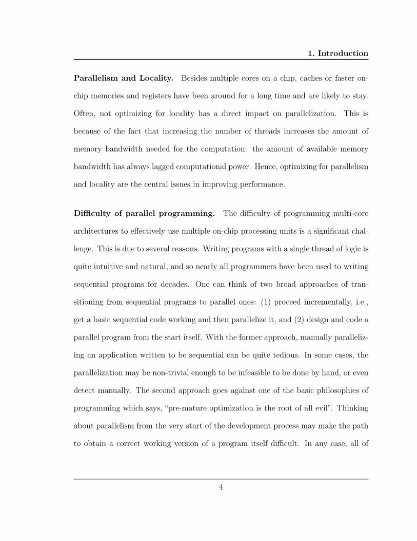
Parallelism and Locality. Besides multiple cores on a chip, caches or faster on-
chip memories and registers have been around for a long time and are likely to stay.
Often, not optimizing for locality has a direct impact on parallelization. This is
because of the fact that increasing the number of threads increases the amount of
memory bandwidth needed for the computation: the amount of available memory
bandwidth has always lagged computational power. Hence, optimizing for parallelism
and locality are the central issues in improving performance.
Difficulty of parallel programming. The difficulty of programming multi-core
architectures to effectively use multiple on-chip processing units is a significant chal-
lenge. This is due to several reasons. Writing programs with a single thread of logic is
quite intuitive and natural, and so nearly all programmers have been used to writing
sequential programs for decades. One can think of two broad approaches of tran-
sitioning from sequential programs to parallel ones: (1) proceed incrementally, i.e.,
get a basic sequential code working and then parallelize it, and (2) design and code a
parallel program from the start itself. With the former approach, manually paralleliz-
ing an application written to be sequential can be quite tedious. In some cases, the
parallelization may be non-trivial enough to be infeasible to be done by hand, or even
detect manually. The second approach goes against one of the basic philosophies of
programming which says, “pre-mature optimization is the root of all evil”. Thinking
about parallelism from the very start of the development process may make the path
to obtain a correct working version of a program itself difficult. In any case, all of
4
1. Introduction
the manual techniques are often not productive for the programmer due to the need
to synchronize access to data shared by threads.
Automatic Parallelization. Among several approaches to address the parallel
programming problem, one that is very promising but simultaneously very challenging
is Automatic Parallelization. Automatic Parallelization is the process of automatically
converting a sequential program to a version that can directly run on multiple pro-
cessing elements without altering the semantics of the program. This process requires
no effort on part of the programmer in parallelization and is therefore very attractive.
Automatic parallelization is typically performed in a compiler, at a high level where
most of the information needed is available. The output of an auto-parallelizer is a
race-free deterministic program that obtains the same results as the original sequen-
tial program. This dissertation deals with compile-time automatic parallelization and
primarily targets shared memory parallel architectures for which auto-parallelization
is significantly easier. A common feature of all of the multicore architectures we have
named so far is that they all have shared memory at one level or the other.
The Polyhedral Model. Many compute-intensive applications often spend most
of their execution time in nested loops. This is particularly common in scientific
and engineering applications. The Polyhedral Model provides a powerful abstraction
to reason about transformations on such loop nests by viewing a dynamic instance
(iteration) of each statement as an integer point in a well-defined space called the
statement’s polyhedron. With such a representation for each statement and a precise
5
1. Introduction
characterization of inter and intra-statement dependences, it is possible to reason
about the correctness of complex loop transformations in a completely mathematical
setting relying on machinery from Linear Algebra and Integer Linear Programming.
The transformations finally reflect in the generated code as reordered execution with
improved cache locality and/or loops that have been parallelized. The polyhedral
model is readily applicable to loop nests in which the data access functions and
loop bounds are affine functions (linear function with a constant) of the enclosing
loop variables and parameters. While a precise characterization of data dependences
is feasible for programs with static control structure and affine references and loop-
bounds, codes with non-affine array access functions or code with dynamic control can
also be handled, but primarily with conservative assumptions on some dependences.
The task of program optimization (often for parallelism and locality) in the poly-
hedral model may be viewed in terms of three phases: (1) static dependence analysis
of the input program, (2) transformations in the polyhedral abstraction, and (3)
generation of code for the transformed program. Significant advances were made
in the past decade on dependence analysis [Fea91, Fea88, Pug92] and code genera-
tion [AI91, KPR95, GLW98] in the polyhedral model, but the approaches suffered
from scalability challenges. Recent advances in dependence analysis and more impor-
tantly in code generation [QRW00, Bas04a, VBGC06, VBC06] have solved many of
these problems resulting in the polyhedral techniques being applied to code represen-
tative of real applications like the spec2000fp benchmarks [CGP+05, GVB+06]. These
advances have also made the polyhedral model practical in production compiler con-
texts [PCB+06] as a flexible and powerful representation to compose and apply trans-
6

1. Introduction
formations. However, current state-of-the-art polyhedral implementations still apply
transformations manually and significant time is spent by an expert to determine the
best set of transformations that lead to improved performance [CGP+05, GVB+06].
Regarding the middle step, an important open issue is that of the choice of transfor-
mations from the huge space of valid transforms. Existing automatic transformation
frameworks [LL98, LCL99, LLL01, AMP01, Gri04] have one or more drawbacks or
restrictions in finding good transformations. All of them lack a practical and scalable
cost model for effective coarse-grained parallel execution and locality as is used with
manually developed parallel applications.
This dissertation describes a new approach to address this problem of automati-
cally finding good transformations to simultaneously optimize for coarse-grained par-
allelism and locality. Our approach is driven by a powerful and practical linear cost
function that goes beyond just maximizing the number of degrees of parallelism or
minimizing the order of synchronization. The cost function allows finding good ways
to tile and fuse across multiple statements coming from sequences of arbitrarily nested
loops. The entire framework has been implemented into a tool, PLUTO, that can
automatically generate OpenMP parallel code from regular C program sections. In
this process, we also describe techniques to generate efficient tiled and parallel code,
along with a number of other optimizations to achieve high performance on modern
multicore architectures.
Experimental results from the implemented system show very high speedups for lo-
cal and parallel execution on multicores over state-of-the-art research compiler frame-
works as well as the best native production compilers. For several linear algebra
7

1. Introduction
kernels, code generated from Pluto beats, by a significant margin, the same kernels
implemented with sequences of calls to hand-tuned BLAS libraries supplied by ven-
dors. The system also leaves a lot of scope for further improvement in performance.
Thanks to the mathematical abstraction provided by the polyhedral model, Pluto
can also serve as the backend for parallel code generation with new domain-specific
frontends.
The rest of this dissertation is organized as follows. Chapter 2 provides the math-
ematical background for the polyhedral model. Chapter 3 describes our automatic
transformation framework. Chapter 4 is devoted to explaining how loop fusion is nat-
urally handled in an integrated manner in our framework. Chapter 5 describes the
implemented Pluto system along with details on parallel and tiled code generation
and complementary post-processing. Chapter 6 provides an experimental evaluation
of the framework. Conclusions and directions for future research are finally presented
in Chapter 7. Most of the content in Chapters 3 and 5, and some results from Chap-
ter 6 have been published in [BBK+08c] and [BHRS08].
8

CHAPTER 2
BACKGROUND
In this chapter, we present a overview of the polyhedral model, and introduce
notation used throughout the dissertation. The mathematical background on Linear
Algebra and Linear Programming required for understanding the theory presented in
this dissertation is fully covered in this section. However, a few fundamental concepts
and definitions relating to cones, polyhedra, and linear inequalities that have been
omitted and can be found in [Wil93] and [Sch86]. Detailed background on traditional
loop transformations can be found in [Wol95, Ban93]. Overall, I expect the reader
to find the mathematical background presented here self-contained. Other sources on
background for the polyhedral model are [Bas04b, Gri04].
All row vectors will be typeset in bold lowercase, while regular vectors are typeset
with an overhead arrow. The set of all real numbers, the set of rational numbers, and
the set of integers are represented by R, Q, and Z, respectively.
9
2.1. Hyperplanes and Polyhedra
2.1 Hyperplanes and Polyhedra
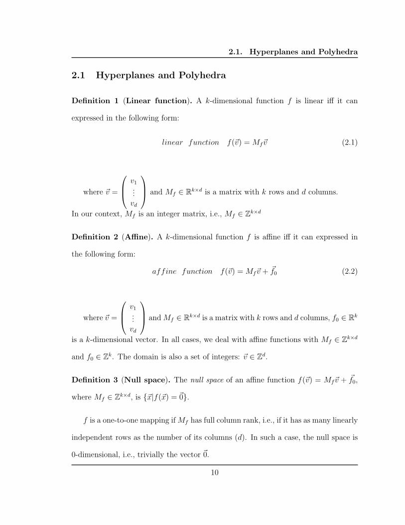
Definition 1 (Linear function). A k-dimensional function f is linear iff it can
expressed in the following form:
linear function f(~v) = Mf~v (2.1)
where ~v =
v1
...vd
and Mf ∈ Rk×d is a matrix with k rows and d columns.
In our context, Mf is an integer matrix, i.e., Mf ∈ Zk×d
Definition 2 (Affine). A k-dimensional function f is affine iff it can expressed in
the following form:
affine function f(~v) = Mf~v + ~f0 (2.2)
where ~v =
v1
...vd
and Mf ∈ Rk×d is a matrix with k rows and d columns, f0 ∈ Rk
is a k-dimensional vector. In all cases, we deal with affine functions with Mf ∈ Zk×d
and f0 ∈ Zk. The domain is also a set of integers: ~v ∈ Zd.
Definition 3 (Null space). The null space of an affine function f(~v) = Mf~v + ~f0,
where Mf ∈ Zk×d, is {~x|f(~x) = ~0}.
f is a one-to-one mapping if Mf has full column rank, i.e., if it has as many linearly
independent rows as the number of its columns (d). In such a case, the null space is
0-dimensional, i.e., trivially the vector ~0.
10

2.1. Hyperplanes and Polyhedra
Definition 4 (Affine spaces). A set of vectors is an affine space iff it is closed under
affine combination, i.e., if ~x, ~y are in the space, all points lying on the line joining ~x
and ~y belong to the space.
A line in a vector space of any dimensionality is a one-dimensional affine space.
In 3-d space, any 2-d plane is an example of a 2-d affine sub-space. Note that ‘affine
function’ as defined in (2.2) should not be confused with ‘affine combination’, though
several researchers use the term affine combination in place of an affine function.
Definition 5 (Affine hyperplane). An affine hyperplane is an n − 1 dimensional
affine sub-space of an n dimensional space.
In our context, the set of all vectors v ∈ Zn such that h.~v = k, for k ∈ Z, forms
an affine hyperplane. The set of parallel hyperplane instances correspond to different
values of k with the row vector h normal to the hyperplane. Two vectors ~v1 and ~v2
lie in the same hyperplane if h.~v1 = h.~v2. An affine hyperplane can also be viewed
as a one-dimensional affine function that maps an n-dimensional space onto a one-
dimensional space, or partitions an n-dimensional space into n− 1 dimensional slices.
Hence, as a function, it can be written as:
φ(~v) = h.~v + c (2.3)
Figure 2.1(a) shows a hyperplane geometrically. Throughout the dissertation, the
hyperplane is often referred to by the row vector, h, the vector normal to the hy-
perplane. A hyperplane h.~v = k divides the space into two half-spaces, the positive
half-space, h.~v ≥ k, and a negative half-space, h.~v ≤ k. Each half-space is an affine
inequality.
11

2.1. Hyperplanes and Polyhedra
φ(~x) =k
φ(~x) ≤ k
φ φ(~x) ≥ k
(a) An affine hyperplane
for (i = 0; i < N; i++)
for (k = 0; k < N; k++)
for (i = 0; i < N; i++)
S1
S2
for (j = 0; j < N; j++)
S1
for (j = 0; j < N; j++)S2
(b) Polyhedra (courtesy: Loopo display tool)
Figure 2.1: Hyperplane and Polyhedron
Definition 6 (Polyhedron, Polytope). A polyhedron is an intersection of a finite
number of half-spaces. A polytope is a bounded polyhedron.
Each of the half-spaces provides a face to the polyhedron. Hence, the set of
affine inequalities, each representing a face, can be used to compactly represent the
polyhedron. If there are m inequalities, the set of all vectors ~x ∈ Rn such that
A~x +~b ≥ 0, where A ∈ Rm×n is a constant real matrix and ~b is a constant real vector
is a real polyhedron. A polyhedron also has an alternate dual representation in terms
of vertices, rays, and lines, and algorithms like the Chernikova algorithm [LeV92] exist
to move from the face representation to the vertex one. Polylib [pol] and PPL [BHZ]
are two libraries that provide a range of functions to perform various operations on
polyhedra and use the dual representation internally.
12
2.1. Hyperplanes and Polyhedra
In our context, we are always interested in the integer points inside a polyhedron
since loop iterators typically have integer data types and traverse an integer space.
So, we always mean to ~x ∈ Zn, A~x +~b ≥ 0. The matrix A and vector b for problems
we will deal with also comprise only integers, i.e., A ∈ Zm×n, ~b ∈ Zn.
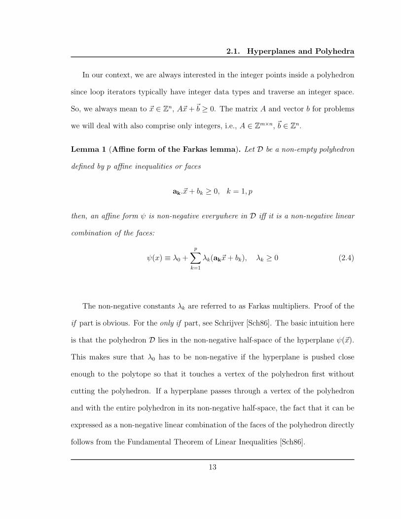
Lemma 1 (Affine form of the Farkas lemma). Let D be a non-empty polyhedron
defined by p affine inequalities or faces
ak.~x + bk ≥ 0, k = 1, p
then, an affine form ψ is non-negative everywhere in D iff it is a non-negative linear
combination of the faces:
ψ(x) ≡ λ0 +
p∑
k=1
λk(ak~x + bk), λk ≥ 0 (2.4)
The non-negative constants λk are referred to as Farkas multipliers. Proof of the
if part is obvious. For the only if part, see Schrijver [Sch86]. The basic intuition here
is that the polyhedron D lies in the non-negative half-space of the hyperplane ψ(~x).
This makes sure that λ0 has to be non-negative if the hyperplane is pushed close
enough to the polytope so that it touches a vertex of the polyhedron first without
cutting the polyhedron. If a hyperplane passes through a vertex of the polyhedron
and with the entire polyhedron in its non-negative half-space, the fact that it can be
expressed as a non-negative linear combination of the faces of the polyhedron directly
follows from the Fundamental Theorem of Linear Inequalities [Sch86].
13

2.2. The Polyhedral Model
Definition 7 (Perfect loop nest, Imperfect loop nest). A set of nested loops
is called a perfect loop nest iff all statements appearing in the nest appear inside the
body of the innermost loop. Otherwise, the loop nest is called an imperfect loop nest.
Figure 2.6 shows an imperfect loop nest.
Definition 8 (Affine loop nest). Affine loop nests are sequences of imperfectly
nested loops with loop bounds and array accesses that are affine functions of outer
loop variables and program parameters.
Program parameters or structure parameters are symbolic constants that appear
in loop bounds or access functions. They very often represent the problem size. N is
a program parameter in Figure 2.1(b), while in Figure 2.2, N and β are the program
parameters.
2.2 The Polyhedral Model
The Polyhedral Model is a geometrical as well as a linear algebraic framework for
capturing the execution of a program in a compact form for analysis and transforma-
tion. The compact representation is primarily of the dynamic instances of statements
of a program surrounded by loops in a program, the dependences between such state-
ments, and transformations.
Definition 9 (Iteration vector). The iteration vector of a statement is the vector
consisting of values of the indices of all loops surrounding the statement.
14
2.2. The Polyhedral Model
Let S be a statement of a program. The iteration vector is denoted by ~iS. An
iteration vector represents a dynamic instance of a statement appearing in loop nest
that may be nested perfectly or imperfectly.
Definition 10 (Domain, Index set). The set of all iteration vectors for a given
statement is the domain or the index set of the statement.
A program comprises a sequence of statements, each statement surrounded by
loops in a given order. We denote the domain of a statement S by DS. When the
loop bounds and data accesses are affine functions of outer loop indices and other
program parameters, and all conditionals are statically predictable, the domain of ev-
ery statement is a polyhedron as defined in Def. 6. Again, conditionals that are affine
functions of outer loop indices and program parameters are statically predictable.
Affine loop nests with static control are also called static control programs or regular
programs. These programs are readily accepted in the polyhedral model. Several of
the restrictions for the polyhedral model can be overcome with tricks or conservative
assumptions while still making all analysis and transformation meaningful. How-
ever, many pose a challenging problem requiring extensions to the model. Techniques
developed and implemented in this thesis apply to all programs for which a polyhe-
dral representation can be extracted. All codes used for experimental evaluation are
regular programs with static control.
Each dynamic instance of a statement S, in a program, is identified by its itera-
tion vector ~iS which contains values for the indices of the loops surrounding S, from
outermost to innermost. A statement S is associated with a polytope DS of dimen-
15

2.3. Polyhedral Dependences
for ( i=0; i<N; i++)for (j=0; j<N; j++)
S1: A[i , j ] = A[i,j]+u1[i]*v1[j ] + u2[i]*v2[j ];
for (k=0; k<N; k++)for ( l=0; l<N; l++)
S2: x[k] = x[k]+beta*A[l,k]*y[l ];
Figure 2.2: A portion of the GEMVER kernel
S1
RAWWAW
RAW
S2
WAR
Figure 2.3: The data depen-dence graph
i ≥ 0
j ≥ 0
−i + N − 1 ≥ 0
−j + N − 1 ≥ 0
DS1 :
1 0 0 00 1 0 0−1 0 1 −10 −1 1 −1
i
j
N
1
≥ 0
Figure 2.4: Domain for statement S1 from Figure 2.2
sionality mS. Each point in the polytope is an mS-dimensional iteration vector, and
the polytope is characterized by a set of bounding hyperplanes. This is true when
the loop bounds are linear combinations (with a constant) of outer loop indices and
program parameters (typically, symbolic constants representing the problem size).
2.3 Polyhedral Dependences
Dependences. Two iterations are said to be dependent if they access the same
memory location and one of them is a write. A true dependence exists if the source
16
2.3. Polyhedral Dependences
iteration’s access is a write and the target’s is a read. These dependences are also
called read-after-write or RAW dependences, or flow dependences. Similarly, if a
write precedes a read to the same location, the dependence is called a WAR depen-
dence or an anti-dependence. WAW dependences are also called output dependences.
Read-after-read or RAR dependences are not actually dependences, but they still
could be important in characterizing reuse. RAR dependences are also called input
dependences.
Dependences are an important concept while studying execution reordering since
a reordering will only be legal if does not violate the dependences, i.e., one is allowed
to change the order in which operations are performed as long as the transformed
program has the same execution order with respect to the dependent iterations.
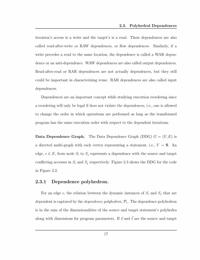
Data Dependence Graph. The Data Dependence Graph (DDG) G = (V,E) is
a directed multi-graph with each vertex representing a statement, i.e., V = S. An
edge, e ∈ E, from node Si to Sj represents a dependence with the source and target
conflicting accesses in Si and Sj respectively. Figure 2.3 shows the DDG for the code
in Figure 2.2.
2.3.1 Dependence polyhedron.
For an edge e, the relation between the dynamic instances of Si and Sj that are
dependent is captured by the dependence polyhedron, Pe. The dependence polyhedron
is in the sum of the dimensionalities of the source and target statement’s polyhedra
along with dimensions for program parameters. If ~s and ~t are the source and target
17

2.3. Polyhedral Dependences
i
j
l
k
S1
S2
1 0 0 0 0 00 −1 0 0 1 −10 0 1 0 0 00 0 0 −1 1 −11 0 0 −1 0 00 1 −1 0 0 0
i
j
k
l
N
1
≥
=
000000
Figure 2.5: Flow dependence from A[i][j] of S1 to A[l][k] of S2 and its dependencepolyhedron (Figure courtesy: Loopo display tool)
iterations that are dependent, we can express:
〈~s,~t〉 ∈ Pe ⇐⇒ ~s ∈ DSi ,~t ∈ DSj are dependent through edge e ∈ E (2.5)
The ability to capture the exact conditions on when a dependence exists through
linear equalities and inequalities rests on the fact that there exists a affine relation
between the iterations and the accessed data for regular programs. Equalities can be
replaced by two inequalities (‘≥ 0’ and ‘≤ 0’) and everything can be converted to
inequalities in the ≥ 0 form, i.e., the polyhedron can be expressed as the intersection
of a finite number of non-negative half-spaces. Let the ith inequality after conversion
to such a form be denoted by P ie. For the code shown in Figure 2.2, consider the
dependence between the write at A[i][j] from S1 and the read A[l][k] in S2. The
dependence polyhedron for this edge is shown in Figure 2.5.
In the next chapter, we see that the dependence polyhedra is the most important
structure around which the problem of finding legal and good transformations centers.
18
2.3. Polyhedral Dependences
In particular, the Farkas lemma (Sec. 2.1) is applied for the dependence polyhedron.
A minor point to note here is that the dependence polyhedra we see are often integral
polyhedra, i.e., polyhedra that have integer vertices. Hence, the application of Farkas
lemma for it is exact and not conservative. Even when the dependence polyhedron
is not integral, i.e., when its integer hull is a proper subset of the polyhedron, the
difference between applying it to the integer hull and the entire polyhedron is highly
unlikely to matter in practice. If need be, one can construct the integer hull of the
polyhedron and apply the Farkas lemma on it.
2.3.2 Strengths of dependence polyhedra.
The dependence polyhedra are a very general and accurate representation of
instance-wise dependences which subsume several traditional notions like distance
vectors (also called uniform dependences), dependence levels, and direction vectors.
Though a similar notion of exact dependences was presented by Feautrier [Fea91] for
value-based array dataflow analysis, this notion of dependence polyhedra has only
been sharpened in the past few years by researchers [CGP+05, VBGC06, PBCV07]
and is not restricted to programs in single assignment form nor does it require con-
version to single-assignment form. Dependence abstractions like direction vectors or
distance vectors are tied to a particular syntactic nesting unlike dependence polyhedra
which is more abstract and captures the relation between integer points of polyhedra.
One could obtain weaker dependence representations from a dependence polyhedra.
19

2.3. Polyhedral Dependences
for (t=0; t<tmax; t++) {for (j=0; j<ny; j++)
ey [0][ j ] = t;for ( i=1; i<nx; i++)
for (j=0; j<ny; j++)ey[ i ][ j ] = ey[i ][ j ] − 0.5*(hz[i ][ j]−hz[i−1][j ]);
for ( i=0; i<nx; i++)for (j=1; j<ny; j++)
ex[ i ][ j ] = ex[i ][ j ] − 0.5*(hz[i ][ j]−hz[i ][ j−1]);for ( i=0; i<nx; i++)
for (j=0; j<ny; j++)hz[ i ][ j]=hz[i [ j ] −
0.7*(ex[ i ][ j+1]−ex[i][ j]+ey[i+1][j]−ey[i ][ j ]);}
Figure 2.6: An imperfect loop nest
0 ≤ t ≤ T − 1
0 ≤ t′ ≤ T − 1
0 ≤ i ≤ N − 1
0 ≤ j ≤ N − 1
0 ≤ i′ ≤ N − 1
0 ≤ j′ ≤ N − 1
t = t′ − 1
i = i′ − 1
j = j′
Figure 2.7: Dependencepolyhedron S4(hz[i][j]) →S2(hz[i − 1][j])
Another example. For the code shown in Figure 2.6, consider the flow dependence
between S4 and S2 from the write at hz[i][j] to the read at hz[i-1][j] (later time steps).
Let ~s ∈ DS4, ~t ∈ DS2, ~s = (t, i, j), ~t = (t′, i′, j′); then, Pe for this edge is shown in
Figure 2.7.
Uniform and Non-uniform dependences. Uniform dependences traditionally
make sense for a statement in perfectly nested loop nest or two statements which
are in the same perfectly nested loop body. In such cases a uniform dependence
is a dependence where the source and target iteration in question are a constant
vector distance apart. Such a dependence is also called a constant dependence and
represented as a distance vector [Wol95].
20

2.4. Polyhedral Transformations
For detailed information on polyhedral dependence analysis and a good survey of
older techniques in the literature including non-polyhedral ones, the reader can refer
to [VBGC06].
2.4 Polyhedral Transformations
A one-dimensional affine transform for statement S is an affine function defined by:
φS(~i) =(cS1 cS
2 . . . cSmS
) (~iS
)+ cS
0 (2.6)
=(cS1 cS
2 . . . cSmS
cS0
)(
~iS1
)
where c0, c1, c2, . . . , cmS∈ Z, ~i ∈ ZmS Hence, a one-dimensional affine transform
for each statement can be interpreted as a partitioning hyperplane with normal
(c1, . . . , cmS). A multi-dimensional affine transformation can be represented as a se-
quence of such φ’s for each statement. We use a superscript to denote the hyperplane
for each level. φkS represents the hyperplane at level k for statement S. If 1 ≤ k ≤ d,
all the φkS can be represented by a single d-dimensional affine function TS as was
defined in 2.2.
TS~iS = MS
~iS + ~tS (2.7)
where MS ∈ Zd×mS , ~tS ∈ Zd.
TS(~i) =
φ1S(~i)
φ2S(~i)...
φdS(~i)
=
cS11 cS
12 . . . cS1mS
cS21 cS
22 . . . cS2mS
......
......
cSd1
cSd2
. . . cSdmS
~iS +
cS10
cS20
...cSd0
(2.8)
21
2.4. Polyhedral Transformations
Scalar dimensions. The dimensionality of TS, d, may be greater than mS as some
rows in TS serve the purpose of representing partially fused or unfused dimensions at
a level. Such a row (c1, . . . , cmS) = 0, and a particular constant for c0. All statements
with the same c0 value are fused at that level and the unfused sets are placed in the
increasing order of their c0s. We call such a level a scalar dimension. Hence, a level
is a scalar dimension if the φ’s for all statements at that level are constant functions.
Figure 2.8 shows a sequence of matrix-matrix multiplies and how a transformation
captures a legal fusion: the transformation fuses ji of S1 with jk of S2, and φ3 is a
scalar dimension.
Complete scanning order. The number of rows in MS for each statements should
be the same (d) to map all iterations to a global space of dimensionality d. To provide
a complete scanning order for each statement, the number of linearly independent φS’s
for a statement should be the same as the dimensionality of the statement, mS, i.e.,
TS should have full column rank. Note that it is always possible to represent any
transformed code (any nesting) with at most 2m∗S + 1 rows, where m∗
S = maxS∈S mS.
Composition of simpler transformations. Multi-dimensional affine functions
capture a sequence of simpler transformations that include permutation, skewing,
reversal, fusion, fission (distribution), relative shifting, and tiling for fixed tile sizes.
Note that tiling cannot be readily expressed as an affine function on the original
iterators (~iS), but can be once supernodes are introduced into the domain increasing
its dimensionality: this is covered in detail in a general context in Chapter 5.
22

2.4. Polyhedral Transformations
for ( i=0; i<n; i++) {for (j=0; j<n; j++) {
for (k=0; k<n; k++) {S1: C[i , j ] = C[i,j ] + A[i,k] * B[k,j ];}
}}for ( i=0; i<n; i++) {
for (j=0; j<n; j++) {for (k=0; k<n; k++) {S2: D[i , j ] = D[i,j ] + E[i,k] * C[k,j ];}
}}
Original code
for (t0=0;t0<=N−1;t0++) {for (t1=0;t1<=N−1;t1++) {
for (t3=0;t3<=N−1;t3++) {C[t1,t0]=A[t1,t3]*B[t3,t0]+C[t1,t0 ];
}for (t3=0;t3<=N−1;t3++) {
D[t3,t0]=E[t3,t1]*C[t1,t0]+D[t3,t0 ];}
}}
Transformed code
TS1(~iS1
) =
0 1 01 0 00 0 00 0 1
i
j
k
+
0000
TS2(~iS2
) =
0 1 00 0 10 0 01 0 0
i
j
k
+
0010
i.e.,
φ1S1
= j φ1S2
= j
φ2S1
= i φ2S2
= k
φ3S1
= 0 φ3S2
= 1φ4
S1= k φ4
S2= i
Figure 2.8: Polyhedral transformation: an example
23
2.4. Polyhedral Transformations
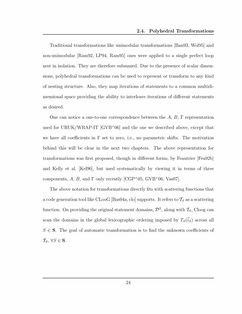
Traditional transformations like unimodular transformations [Ban93, Wol95] and
non-unimodular [Ram92, LP94, Ram95] ones were applied to a single perfect loop
nest in isolation. They are therefore subsumed. Due to the presence of scalar dimen-
sions, polyhedral transformations can be used to represent or transform to any kind
of nesting structure. Also, they map iterations of statements to a common multidi-
mensional space providing the ability to interleave iterations of different statements
as desired.
One can notice a one-to-one correspondence between the A, B, Γ representation
used for URUK/WRAP-IT [GVB+06] and the one we described above, except that
we have all coefficients in Γ set to zero, i.e., no parametric shifts. The motivation
behind this will be clear in the next two chapters. The above representation for
transformations was first proposed, though in different forms, by Feautrier [Fea92b]
and Kelly et al. [Kel96], but used systematically by viewing it in terms of three
components, A, B, and Γ only recently [CGP+05, GVB+06, Vas07].
The above notation for transformations directly fits with scattering functions that
a code generation tool like CLooG [Bas04a, clo] supports. It refers to TS as a scattering
function. On providing the original statement domains, DS, along with TS, Cloog can
scan the domains in the global lexicographic ordering imposed by TS(~iS) across all
S ∈ S. The goal of automatic transformation is to find the unknown coefficients of
TS, ∀S ∈ S.
24

2.4. Polyhedral Transformations
2.4.1 Why affine transformations?
Definition 11 (Convex combination). A convex combination of vectors, ~x1, ~x2, . . . , ~xn,
is of the form λ1 ~x1 + λ2x2 + · · · + λn ~xn, where λ1, λ2, . . . , λn ≥ 0 and∑n
i=1λi = 1.
Informally, a convex combination of two points always lies on the line segment
joining the two points. In the general case, a convex combination of any number of
points lies inside the convex hull of those points.
The primary reason affine transformations are of interest is that affine transforma-
tions are the most general class of transformations that preserve the collinearity and
convexity of points in space. An affine transformation transforms a polyhedron into
another polyhedron and one stays in the polyhedral abstraction for further analyses
and most importantly for code generation. Code generation is relatively easier and
so has been studied extensively for affine transformations. We now quickly show that
if DS is convex, its image under the affine function TS is also convex. Let the image
be:
T (DS) ={~z | ~z = TS(~x), ~x ∈ DS
}
Consider the convex combination of any two points, TS(~x) and TS(~y), of T (DS):
λ1TS(~x) + λ2TS(~y), λ1 + λ2 = 1, λ1 ≥ 0, λ2 ≥ 0
Now,
λ1TS(~x) + λ2TS(~y) = λ1MS(~x) + λ1~tS + λ2MS(~y) + λ2
~tS
= MS(λ1~x + λ2~y) + ~tS, (∵ λ1 + λ2 = 1)
= TS(λ1~x + λ2~y) (2.9)
25

2.4. Polyhedral Transformations
Since DS is convex, λ1~x + λ2~y ∈ DS. Hence, from (2.9), we have:
λ1TS(~x) + λ2TS(~y) ∈ T (DS)
⇒ T (DS) is convex
If MS (the linear part of TS) has full column rank, i.e., the rank of MS is same as
the number of columns, TS is a one-to-one mapping from DS to T (DS). A point to
note when looking at integer spaces instead of rational or real spaces is that not every
point in T (DS) has an integer pre-image in DS, for example, transformations that are
non-unimodular may create sparse integer polyhedra. This is not a problem since a
code generator like Cloog can scan such sparse polyhedra by inserting modulos, and
techniques for removal of modulos also exist [Vas07]. Hence, no restrictions need be
imposed on the affine function TS. Such sparse polyhedra also correspond to code with
non-unit strides. However, these can be represented with an additional dimension as
long as the stride is a constant like {0 ≤ i ≤ n − 1, i = 2k} for i going from 0 to
n − 1 with stride two. However, if one is interested, a more direct representation for
integer points in a polyhedron can be used [S.P00, GR07]. The term Z-polyhedron
is associated with such a representation which is the image of a rational polyhedron
under an affine integer lattice. Closure properties with such a representation under
various operations including affine image and pre-image have been proved [GR07].
26
2.5. Putting the Notation Together
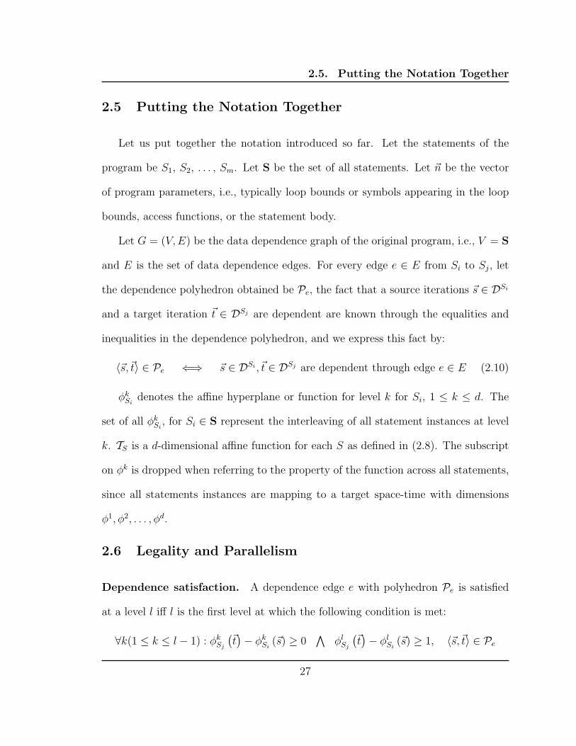
2.5 Putting the Notation Together
Let us put together the notation introduced so far. Let the statements of the
program be S1, S2, . . . , Sm. Let S be the set of all statements. Let ~n be the vector
of program parameters, i.e., typically loop bounds or symbols appearing in the loop
bounds, access functions, or the statement body.
Let G = (V,E) be the data dependence graph of the original program, i.e., V = S
and E is the set of data dependence edges. For every edge e ∈ E from Si to Sj, let
the dependence polyhedron obtained be Pe, the fact that a source iterations ~s ∈ DSi
and a target iteration ~t ∈ DSj are dependent are known through the equalities and
inequalities in the dependence polyhedron, and we express this fact by:
〈~s,~t〉 ∈ Pe ⇐⇒ ~s ∈ DSi ,~t ∈ DSj are dependent through edge e ∈ E (2.10)
φkSi
denotes the affine hyperplane or function for level k for Si, 1 ≤ k ≤ d. The
set of all φkSi
, for Si ∈ S represent the interleaving of all statement instances at level
k. TS is a d-dimensional affine function for each S as defined in (2.8). The subscript
on φk is dropped when referring to the property of the function across all statements,
since all statements instances are mapping to a target space-time with dimensions
φ1, φ2, . . . , φd.
2.6 Legality and Parallelism
Dependence satisfaction. A dependence edge e with polyhedron Pe is satisfied
at a level l iff l is the first level at which the following condition is met:
∀k(1 ≤ k ≤ l − 1) : φkSj
(~t)− φk
Si(~s) ≥ 0
∧φl
Sj
(~t)− φl
Si(~s) ≥ 1, 〈~s,~t〉 ∈ Pe
27
2.6. Legality and Parallelism
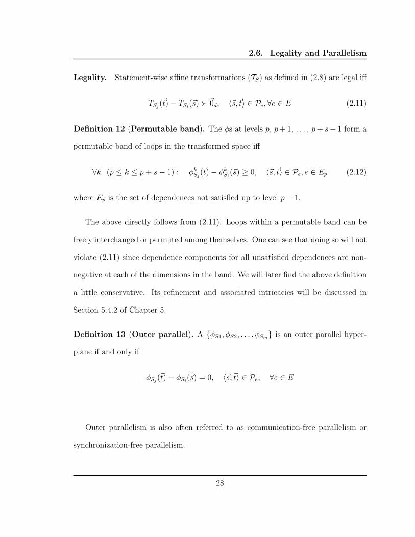
Legality. Statement-wise affine transformations (TS) as defined in (2.8) are legal iff
TSj(~t) − TSi
(~s) ≻ ~0d, 〈~s,~t〉 ∈ Pe,∀e ∈ E (2.11)
Definition 12 (Permutable band). The φs at levels p, p + 1, . . . , p + s− 1 form a
permutable band of loops in the transformed space iff
∀k (p ≤ k ≤ p + s − 1) : φkSj
(~t) − φkSi
(~s) ≥ 0, 〈~s,~t〉 ∈ Pe, e ∈ Ep (2.12)
where Ep is the set of dependences not satisfied up to level p − 1.
The above directly follows from (2.11). Loops within a permutable band can be
freely interchanged or permuted among themselves. One can see that doing so will not
violate (2.11) since dependence components for all unsatisfied dependences are non-
negative at each of the dimensions in the band. We will later find the above definition
a little conservative. Its refinement and associated intricacies will be discussed in
Section 5.4.2 of Chapter 5.
Definition 13 (Outer parallel). A {φS1, φS2, . . . , φSm} is an outer parallel hyper-
plane if and only if
φSj(~t) − φSi
(~s) = 0, 〈~s,~t〉 ∈ Pe, ∀e ∈ E
Outer parallelism is also often referred to as communication-free parallelism or
synchronization-free parallelism.
28

2.6. Legality and Parallelism
for ( i=0; i<N; i++) {for (j=0; j<N; j++) {
a[ i ][ j ] = a[i ][ j−1] + 1;}
}
j
i
N
N b b b b b
b b b b b
b b b b b
b b b b b
b b b b b
0 1 2 3
1
2
3
Figure 2.9: Outer parallel loop, i: hy-perplane (1,0)
for ( i=0; i<N; i++) {for (j=0; j<N; j++) {
a[ i ][ j ] = a[i−1][N−1−j] + 1;}
}
j
i
N
N b b b b b
b b b b b
b b b b b
b b b b b
b b b b b
0 1 2 3
1
2
3
Figure 2.10: Inner parallel loop, j: hy-perplane (0,1)
Definition 14 (Inner parallel). A {φkS1, φ
kS2, . . . , φ
kSm
} is an inner parallel hyper-
plane if and only if φkSi
(~t) − φkSi
(~s) = 0, for every 〈~s,~t〉 ∈ Pe, e ∈ Ek, where Ek is the
set of dependences not satisfied up to level k − 1.
It is illegal to move an inner parallel loop in the outer direction since the depen-
dences satisfied at loops it has been moved across may be violated at the new position
of the moved loop. However, it is always legal to move an inner parallel loop further
inside.
Outer and inner parallelism is often referred to as doall parallelism. However, note
that inner parallelism requires synchronization every iteration outer to the loop.
29

2.6. Legality and Parallelism
for ( i=0; i<N; i++) {for (j=0; j<N; j++) {
a[ i ][ j ] = a[i ][ j−1] + a[i−1][j ];}
}j
i
N
N b b b b b
b b b b b
b b b b b
b b b b b
b b b b b
0 1 2 3
1
2
3
Figure 2.11: Pipelined parallel loop: i or j
Pipelined parallelism. Two or more loops may have dependences that have de-
pendence components along each of them can still be executed in parallel if one of
them can be delayed with respect to the other by a fixed amount. If dependence
components are non-negative along each of the dimensions in question, one just needs
a delay of one. Figure 2.11 shows a code with dependences along both i and j. How-
ever, say along i, successive iterations can start with a delay of one and continue
executing iterations for j’s in sequence. Similarly, if there are n independent dimen-
sions, at most n − 1 of them can be pipelined while iterations along at least one will
be executed in sequence. Pipelined parallelism is also often referred to as doacross
parallelism. We will formalize conditions for this in a very general setting in Chap-
ter 3 since it is goes together with tiling. Code generation for pipelined parallelism is
discussed in Chapter 5.
Space-time mapping. Once properties of each row of TS are known, some of
them can be marked as space, i.e., a dimension along which iterations are executed
by different processors, while others can be marked as time, i.e., a dimension that is
30
2.6. Legality and Parallelism
executed sequentially by a single processor. Hence, TS specifies a complete space-time
mapping for S. Each of the d dimensions is either space or time. Since MS is of full
column rank, when an iteration executes and where it executes, is known. However,
in reality, post-processing can be done to TS before such a mapping is achieved.
31

CHAPTER 3
Automatic Transformations for Parallelism and Locality
The three major phases of an optimizer for parallelism and locality are:
1. Static analysis: Computing affine dependences for an input source program
2. Automatic transformation: Computing the transformations automatically
3. Code generation: Generating the new nested loop code under the computed
transformations
As explained in Chapter 1, the first and last steps are currently quite stable,
while no scalable and practical approach exists for the middle step that works for
all polyhedral input or for input that the first and last steps are known to be quite
advanced for. This chapter deals with the theory for the key middle step: automatic
transformation, which is often considered synonymous with automatic parallelization.
3.1 Schedules, Allocations, and Partitions
Hyperplanes can be interpreted as schedules, allocations, or partitions, or any
other term a researcher may define based on the properties it satisfies. Saying that a
32

3.2. Limitations of Previous Techniques
hyperplane is one of them implies a particular property that the new loop will satisfy
in the transformed space. Based on the properties the hyperplanes will satisfy at
various levels, certain further transformations like tiling, unroll-jamming, or marking
it parallel, can be performed. Typically, scheduling-based works [Fea92a, Fea92b,
DR96, Gri04] obtains the new set of hyperplanes as schedules and allocations, while
Lim and Lam [LL98] find them as space and time partitions.
3.2 Limitations of Previous Techniques
In this section, we briefly describe the limitations of existing polyhedral transfor-
mation frameworks in the literature. Automatic parallelization efforts in the poly-
hedral model broadly fall into two classes: (1) scheduling/allocation-based, and (2)
partitioning-based. The works of Feautrier [Fea92a, Fea92b] and Griebl [Gri04] (to
some extent) fall into the former class, while Lim and Lam’s approach [LL98, LCL99,
LLL01] falls into the second class.
3.2.1 Scheduling + allocation approaches
Schedules specify when iterations execute. A schedule can assign a time point
for every iteration, and a code generator can generate code that will scan them in
the specified order. Schedules in our context are assumed to be affine functions since
code generation in such cases has been studied extensively. Hence, serial order or
sequentiality is implicit in a schedule. For a complete coverage of scheduling for
automatic parallelization, the reader is referred to the book of Darte et al. [DRV00].
33
3.2. Limitations of Previous Techniques
Briefly, a set of scheduling hyperplanes satisfy all dependences.
θSj(~t) − θSi
(~s) ≥ 1, 〈~s,~t〉 ∈ Pe
Several such θ with a given order specify a multi-dimensional schedule. Allocations
specify where iterations execute. An allocation is implicitly parallel. It can always be
coarsened, i.e., a group of iterations mapped to a particular processor since everything
that is scheduled at a time point are independent of each other. With scheduling-
allocation techniques, good schedules with the minimum number of dimensions are
first found [Fea92a, Fea92b], and then allocations are found [Fea94, DR96, GFG05].
If communication costs were to be zero or negligible when compared with compu-
tation and there were to be no memory hierarchy, clearly, just using optimal or near
optimal affine schedules would be the solution. This is obviously not the case with
any modern parallel computer architecture. Hence, reducing communication overhead
and improving locality across the memory hierarchy through tiling is needed. For the
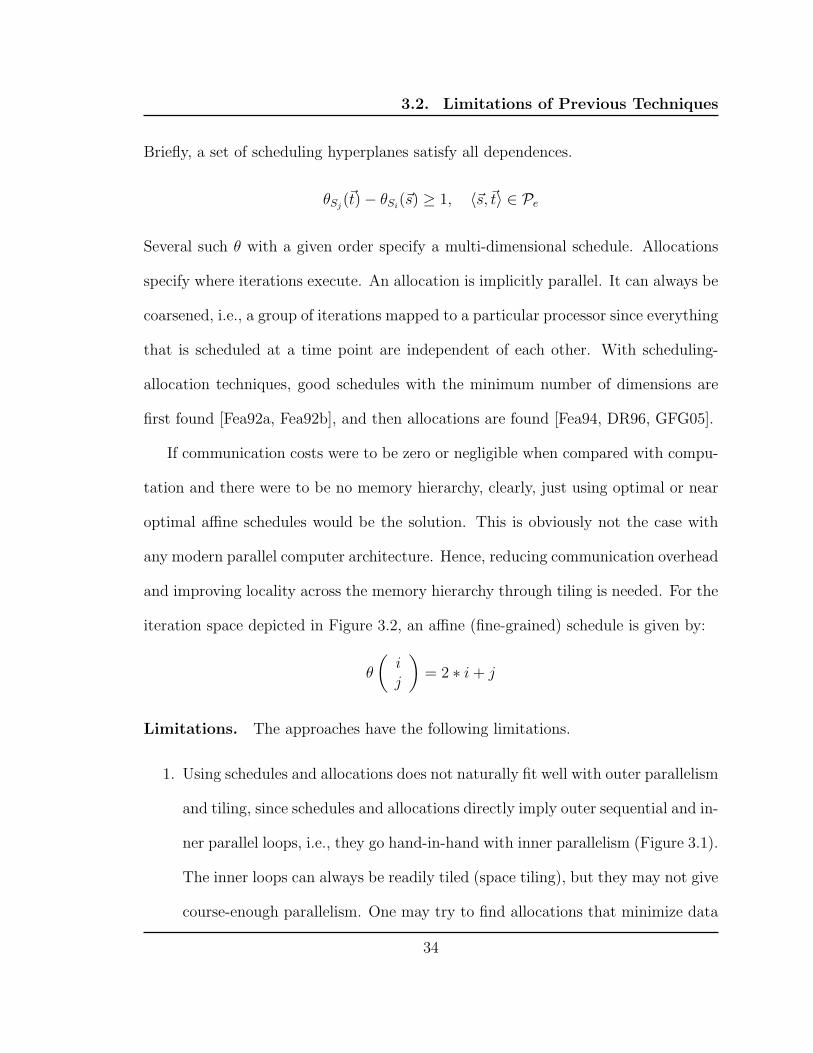
iteration space depicted in Figure 3.2, an affine (fine-grained) schedule is given by:
θ
(i
j
)
= 2 ∗ i + j
Limitations. The approaches have the following limitations.
1. Using schedules and allocations does not naturally fit well with outer parallelism
and tiling, since schedules and allocations directly imply outer sequential and in-
ner parallel loops, i.e., they go hand-in-hand with inner parallelism (Figure 3.1).
The inner loops can always be readily tiled (space tiling), but they may not give
course-enough parallelism. One may try to find allocations that minimize data
34

3.2. Limitations of Previous Techniques
movement, however, it may still require a high order of synchronization, or too
frequent synchronization.
2. They can go against locality even if the schedule gives a course granularity of
parallelism, since reuse will often be across the outer loops (dependences satis-
fied at outer levels) and no tiling can be done across those without modifying
the allocations. This in turn may kill all benefits of parallelization due to lim-
ited memory bandwidth. Inability to tile along the scheduling dimensions would
also affect register reuse when register tiling is done.
3. Using schedules and allocations typically leads to schedules with minimum num-
ber of schedule dimensions and maximum number of parallel loops. This misses
solutions that correspond to higher dimensional schedules. These missed sched-
ules might be sub-optimal with the typical schedule selection criteria, but still
perform better due to better tiling and coarse-grained parallelization. The
downsides of this cannot be undone.
One may try to “fix” the above problems by finding allocations with a certain
property that will allow tiling along the scheduling dimensions too [GFG05, Gri04],
but it has other undesired effects – sometimes unable to find the natural solution
primarily due to the third reason listed above. All of these will be clearer to the
reader through this chapter.
35

3.2. Limitations of Previous Techniques
for (t1=0; i<N; i++) {for (t2=0; i<N; i++) {
forall (p1=0; i<N; i++) {forall (p2=0; i<N; i++) {
S1}
}<barrier>;
}}
Figure 3.1: A typical solution with scheduling-allocation
(2,1)
Figure 3.2: A fine-grained affine schedule
3.2.2 Existing partitioning-based approaches
A partitioning based approach would just use the code generator as a way to scan
the iteration space in another order and later on mark loops as parallel or sequential, or
stripmine and interchange loops at a later point. We gave an detailed background on
affine hyperplanes as partitions in Section 2.4. A key limitation of existing techniques
in this class is the absence of a way to find good partitions. Criteria based on finding
36

3.3. Recalling the Notation
those that maximize the number of degrees of parallelism and minimize the order
of synchronization are not sufficient to enable good parallelization. One could for
example obtain the partitioning shown in Figure 3.3 which is:
φ1(i, j) = i
φ2(i, j) = i + 3j
Figure 3.3: Affine partitioning with no cost function can lead to unsatisfactory solu-tions
However, a desirable affine partitioning here is given by the following and shown
in Figure 3.4.
φ1(i, j) = i
φ2(i, j) = i + j
3.3 Recalling the Notation
Let us recall the notation introduced in the previous chapter in Section 2.4 and
Section 2.5 before we introduce the new transformation framework. The statements of
37

3.3. Recalling the Notation
Figure 3.4: A good set of φ’s: (1,0) and (1,1)
the program are S1, S2, . . . , Sn. The dimensionality of Si is mSi. S = {S1, S2, . . . , Sn}.
~n is the vector of program parameters, i.e., typically loop bounds or symbols that
appear in loop bounds, access functions, or the statement body.
Let G = (V,E) be the data dependence graph for the original program, i.e., V = S
and E is set of data dependence edges. For every edge e ∈ E from Si to Sj, Pe is
the dependence polyhedron. The fact that a source iterations ~s ∈ Si and a target
iteration ~t ∈ Sj are dependent are known through the equalities and inequalities in
the dependence polyhedron, and this is expressed as:
〈~s,~t〉 ∈ Pe ⇐⇒ ~s ∈ DSi ,~t ∈ DSj are dependent through edge e ∈ E (3.1)
All inequalities and equalities in Pe can be written as inequalities in the ≥ 0 form.
Let the LHS of each such inequality be denoted by P ie, 1 ≤ i ≤ me.
φkSi
denotes the affine hyperplane for level k for Si. The set of all φkSi
, for Si ∈ S
represent the interleaving of all statement instances at level k. We drop the superscript
from the coefficients when a single statement is in question.
φSi=
(
c1 c2 . . . cmSi
) (~iSi
)+ c0 (3.2)
38

3.4. Problem statement
c0, c1, c2, . . . , cmSi∈ Z, ~i ∈ ZmSi
The subscript on φk is dropped when referring to the property of the function across
all statements, since all statements instances are mapping to a target space-time with
dimensions φ1, φ2, . . . , φd. TS is a d-dimensional affine function capturing the complete
space-time transformation for statement S:
TS~iS = MS
~iS + ~tS
All row vectors are typeset in bold, while normal vectors are typeset with an
overhead arrow. ≻,≺ denote lexicographic comparisons. ≤,≥, <,> in the context of
vectors apply component-wise.
3.4 Problem statement
The goal of automatic transformation is to find the unknown coefficients of TS,
∀S ∈ S. In other words, the φ’s for all statements at each level are the unknown
we wish to find. In addition, the rows that correspond to processor space and that
correspond to sequential time should also be determined.
3.5 Legality of Tiling in the Polyhedral Model
Loop tiling [IT88, WL91b, Xue00] is a key transformation in optimizing for paral-
lelism and data locality. There has been a considerable amount of research into these
two transformations. Tiling has been studied from two perspectives – data locality
optimization and parallelization. Tiling for locality requires grouping points in an
iteration space into smaller blocks (tiles) allowing reuse in multiple directions when
39
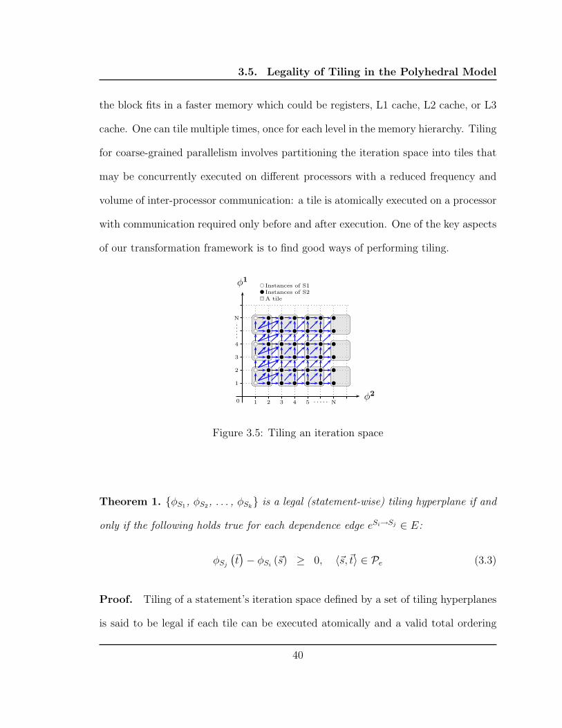
3.5. Legality of Tiling in the Polyhedral Model
the block fits in a faster memory which could be registers, L1 cache, L2 cache, or L3
cache. One can tile multiple times, once for each level in the memory hierarchy. Tiling
for coarse-grained parallelism involves partitioning the iteration space into tiles that
may be concurrently executed on different processors with a reduced frequency and
volume of inter-processor communication: a tile is atomically executed on a processor
with communication required only before and after execution. One of the key aspects
of our transformation framework is to find good ways of performing tiling.
φ2
φ1
N
N
bc
bc
bc
bc
bc
bc b b b b b b
b b b b b b
b b b b b b
b b b b b b
b b b b b b
b b b b b b
bc Instances of S1b Instances of S2rs A tile
0 1 2 3 4 5
1
2
3
4
Figure 3.5: Tiling an iteration space
Theorem 1. {φS1, φS2
, . . . , φSk} is a legal (statement-wise) tiling hyperplane if and
only if the following holds true for each dependence edge eSi→Sj ∈ E:
φSj
(~t)− φSi
(~s) ≥ 0, 〈~s,~t〉 ∈ Pe (3.3)
Proof. Tiling of a statement’s iteration space defined by a set of tiling hyperplanes
is said to be legal if each tile can be executed atomically and a valid total ordering
40

3.5. Legality of Tiling in the Polyhedral Model
of the tiles can be constructed. This implies that there exists no two tiles such that
they both influence each other. Let {φ1S1
, φ1S2
, . . . , φ1Sk}, {φ2
S1, φ2
S2, . . . , φ2
Sk} be
two statement-wise 1-d affine transforms that satisfy (3.3). Consider a tile formed
by aggregating a group of hyperplane instances along φ1 and φ2. Due to (3.3), for
any dynamic dependence, the target iteration is mapped to the same hyperplane or
a greater hyperplane than the source, i.e., the set of all iterations that are outside
of the tile and are influenced by it always lie in the forward direction along one of
the independent tiling dimensions (φ1 and φ2 in this case). Similarly, all iterations
outside of a tile influencing it are either in that tile or in the backward direction
along one or more of the hyperplanes. The above argument holds true for both
intra- and inter-statement dependences. For inter-statement dependences, this leads
to an interleaved execution of tiles of iteration spaces of each statement when code
is generated from these mappings. Hence, {φ1S1
, φ1S2
, . . . , φ1Sk}, {φ2
S1, φ2
S2, . . . , φ2
Sk}
represent rectangularly tilable loops in the transformed space. If such a tile is executed
on a processor, communication would be needed only before and after its execution.
From the point of view of locality, if such a tile is executed with the associated data
fitting in a faster memory, reuse is exploited in multiple directions.2
The above condition was well-known for the case of a single-statement perfectly
nested loops from the work of Irigoin and Triolet [IT88] (as“hT .R ≥ 0”). The above is
a generalization for multiple iteration spaces with possibly different dimensionalities
and with affine dependences, coming from code that could be nested arbitrarily.
41
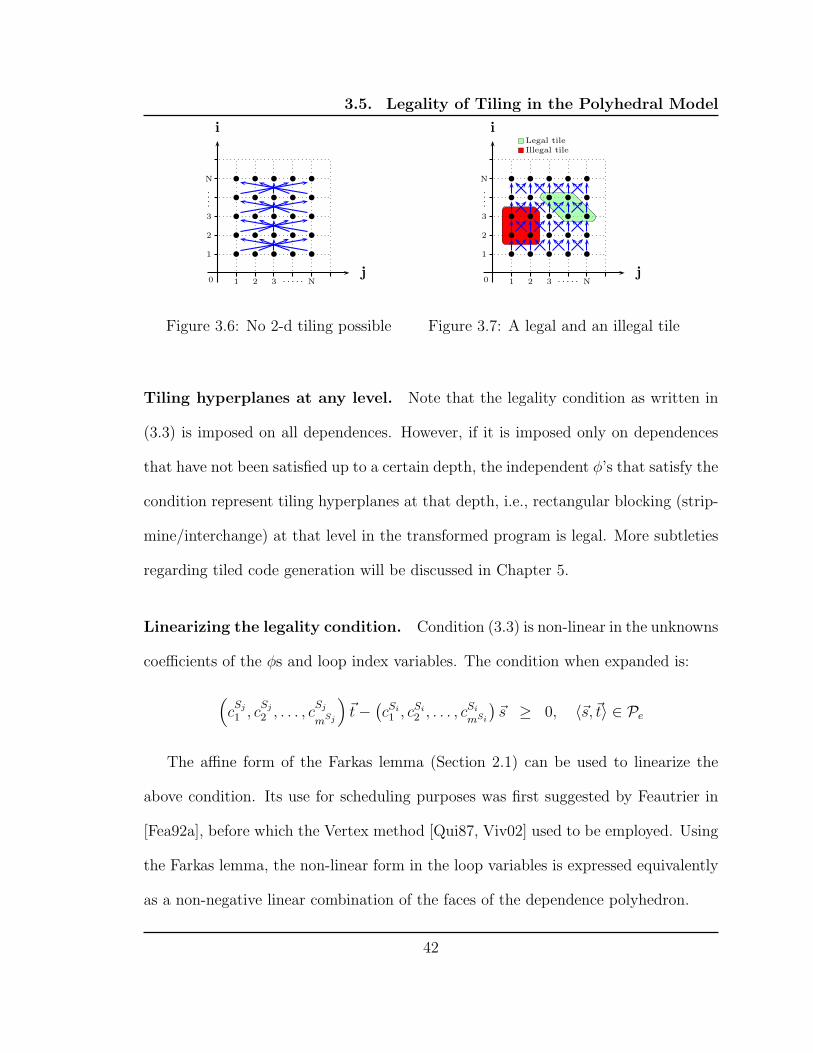
3.5. Legality of Tiling in the Polyhedral Model
j
i
N
N b b b b b
b b b b b
b b b b b
b b b b b
b b b b b
0 1 2 3
1
2
3
Figure 3.6: No 2-d tiling possible
j
i
N
N
b b b b b
b b b b b
b b b b b
b b b b b
b b b b b
rs Legal tilers Illegal tile
0 1 2 3
1
2
3
Figure 3.7: A legal and an illegal tile
Tiling hyperplanes at any level. Note that the legality condition as written in
(3.3) is imposed on all dependences. However, if it is imposed only on dependences
that have not been satisfied up to a certain depth, the independent φ’s that satisfy the
condition represent tiling hyperplanes at that depth, i.e., rectangular blocking (strip-
mine/interchange) at that level in the transformed program is legal. More subtleties
regarding tiled code generation will be discussed in Chapter 5.
Linearizing the legality condition. Condition (3.3) is non-linear in the unknowns
coefficients of the φs and loop index variables. The condition when expanded is:
(
cSj
1 , cSj
2 , . . . , cSj
mSj
)
~t −(cSi
1 , cSi
2 , . . . , cSi
mSi
)~s ≥ 0, 〈~s,~t〉 ∈ Pe
The affine form of the Farkas lemma (Section 2.1) can be used to linearize the
above condition. Its use for scheduling purposes was first suggested by Feautrier in
[Fea92a], before which the Vertex method [Qui87, Viv02] used to be employed. Using
the Farkas lemma, the non-linear form in the loop variables is expressed equivalently
as a non-negative linear combination of the faces of the dependence polyhedron.
42

3.6. Towards Finding Good Solutions
for (t=0; t<T; t++) {for ( i=2; i<N−1; i++) {
a[t , i ] = 0.333*(a[t−1,i] + a[t−1,i−1]+ a[t−1,i+1]);
}}
Figure 3.8: 1-d Jacobi: perfectly nested
for (t = 1; t<T; t++)for ( i=2; i<N−1; i++)
S1: b[ i ] = 0.333*(a[i−1]+a[i]+a[i+1]);}for{i=2; i<N−1; i++}
S2: a[ i ] = b[i ];}
}
Figure 3.9: 1-d Jacobi: imperfectlynested
(
cSj
1 , cSj
2 , . . . , cSj
mSj
)
~t −(cSi
1 , cSi
2 , . . . , cSi
mSi
)~s ≥ 0, 〈~s,~t〉 ∈ Pe
⇐⇒
(
cSj
1 , cSj
2 , . . . cSj
mSj
)
~t −(cSi
1 , cSi
2 , . . . cSi
mSi
)~s ≡ λe0 +
me∑
k=1
λekPke , λek ≥ 0
Once this is done, the coefficients of the loop variables on the LHS and the RHS
are equated to get conditions free free of the original loop variables. Application of
the Farkas Lemma is done on a per-dependence basis, and the resulting constraints
linear in the coefficients of the φs are aggregated. All Farkas multipliers can be
eliminated dependence-wise, some by Gaussian elimination and the rest by Fourier-
Motzkin elimination [Ban93, Sch86]. Subsequently, the Farkas lemma has been used
to linearize the legality constraint by nearly all polyhedral approaches in the litera-
ture [LL98, AMP01, CGP+05, PBCV07].
43
3.6. Towards Finding Good Solutions
3.6 Towards Finding Good Solutions
Consider the perfectly-nested version of 1-d Jacobi shown in Figure 3.8 as an
example. This discussion also applies to the imperfectly nested version, but for con-
venience we first look at the single-statement perfectly nested one. The code has
three uniform dependences, (1,0), (1,1) and (1,-1) when represented as distance vec-
tors. We first describe solutions obtained by existing state of the art approaches -
Lim and Lam’s affine partitioning [LL98, LCL99] and Griebl’s space and time tiling
with Forward Communication-only placement [Gri04]. Lim and Lam define legal
time partitions which have the same property of tiling hyperplanes we described in
the previous section. Their algorithm obtains affine partitions that minimize the or-
der of communication while maximizing the degree of parallelism. Using the validity
constraint in Eqn 3.3, we obtain the constraints:
(ct, ci)
(10
)
≥ 0; (ct, ci)
(11
)
≥ 0; (ct, ci)
(1−1
)
≥ 0
i.e.,
ct ≥ 0
ci + cj ≥ 0
ci − cj ≥ 0
There are infinitely many valid solutions with the same order complexity of syn-
chronization, but with different communication volumes that may impact perfor-
mance. Although it may seem that the volume may not effect performance con-
sidering the fact that communication startup time on modern interconnects domi-
44

3.6. Towards Finding Good Solutions
i
t
(1,0) (2,1)
i i
t
(1,1)(1,0) (1,1)
(1,0)
P1 P2P0
P3P1
P1
P0
P2 P2 P2P1 P1P1
P0P0
space space
i
t
(1,0) (2,1)
i i
t P1
P0
P3
(1,1)(1,0) (1,1)
(1,0)
space
P1 P2P0
spacetime
of communication
spacetime
of communication of communicationThree linesTwo lines ofOne line
t
time
P2
P2
Figure 3.10: Communication volume with different valid hyperplanes for 1-d Jacobi:the shaded tiles are to be executed in parallel
nates, for higher dimensional problems like n-d Jacobi, the ratio of communication
to computation increases, proportional to tile size raised to n− 1. Existing works on
tiling [SD90, RS92, Xue97] can find good or near communication-optimal tile shapes
for perfectly nested loops with constant dependences, but cannot handle arbitrarily
nested loops. For 1-d Jacobi, all solutions within the cone formed by the vectors (1, 1)
and (1,−1) are valid tiling hyperplanes. For the imperfectly nested version of 1-d Ja-
cobi, the valid cone has extremals (2, 1) and (2,−1). Lim et al.’s algorithm [LL98]
finds two valid independent solutions without optimizing for any particular criterion.
In particular, the solutions found by their algorithm (Algorithm A in [LL98]) are
(2,−1) and (3,−1) which are clearly not the best tiling hyperplanes to minimize
communication volume, though they do maximize the degree of parallelism and min-
imize the order of synchronization to O(N): in this case any valid hyperplane has
O(N) synchronization. Figure 3.10 shows that the required communication increases
45

3.7. Cost Function
as the hyperplane gets more and more oblique. For a hyperplane with normal (k, 1),
one would need (k + 1) ∗ T values from the neighboring tile.
Using Griebl’s technique [GFG05, Gri04], if coarser granularity of parallelism is
desired with schedules, the forward communication-only (FCO) constraint finds an
allocation satisfying the constraint that all dependences have non-negative affine com-
ponents along it, i.e., communication will be in the forward direction. Due to this,
both the schedule and allocation dimensions become one permutable band of loops
that can be tiled. Hence, tiling along the scheduling dimensions, called time tiling
is enabled. For the code in question, we first find that only space tiling is enabled
with the affine schedule being θ(t, i) = t. With a forward-communication only (FCO)
placement along (1,1), time tiling is enabled that can aggregate iterations into 2-d
tiles decreasing the frequency of communication. However, note that communication
in the processor space occurs along (1,1), i.e., two lines of the array are required.
However, using (1,0) and (1,1) as tiling hyperplanes with (1,0) as space and (1,1) as
inner time and a tile space schedule of (2,1) leads to only one line of communication
along (1,0). The approach we will present will find such a solution. We now define a
cost metric for an affine transform that captures reuse distance and communication
volume.
3.7 Cost Function
Consider the affine form δ defined as follows.
δe(~s,~t) = φSj(~t) − φSi
(~s), 〈~s,~t〉 ∈ Pe (3.4)
46

3.7. Cost Function
The affine function, δe(~s,~t), holds much significance. This function is also the number
of hyperplanes the dependence e traverses along the hyperplane normal. It gives us a
measure of the reuse distance if the hyperplane is used as time, i.e., if the hyperplanes
are executed sequentially. Also, this function is a rough measure of communication
volume if the hyperplane is used to generate tiles for parallelization and used as a
processor space dimension. An upper bound on this function would mean that the
number of hyperplanes that would be communicated as a result of the dependence
at the tile boundaries would not exceed this bound. We are particularly interested
if this function can be reduced to a constant amount or zero by choosing a suitable
direction for φ: if this is possible, then that particular dependence leads to a constant
or no communication for this hyperplane. Note that each δe is an affine function of
the loop indices. The challenge is to use this function to obtain a suitable objective
for optimization in a linear setting.
The constraints obtained from Eqn 3.3 above only represent validity (permutabil-
ity). We discuss below problems encountered when one tries to apply a performance
factor to find a good tile shape out of the several possibilities.
As explained in the previous sub-section, the Farkas lemma has been used to
eliminate loop variables from constraints by getting equivalent linear inequalities.
However, an attempt to minimize δe ends up in an objective function involving both
loop variables and hyperplane coefficients. For example, φ(~t) − φ(~s) could be c1i +
(c2−c3)j, where 1 ≤ i ≤ N ∧1 ≤ j ≤ N ∧ i ≤ j. One could possibly end up with such
a form when one or more of the dependences are not uniform, making it infeasible to
construct an objective function involving only the unknown coefficients of φ’s.
47
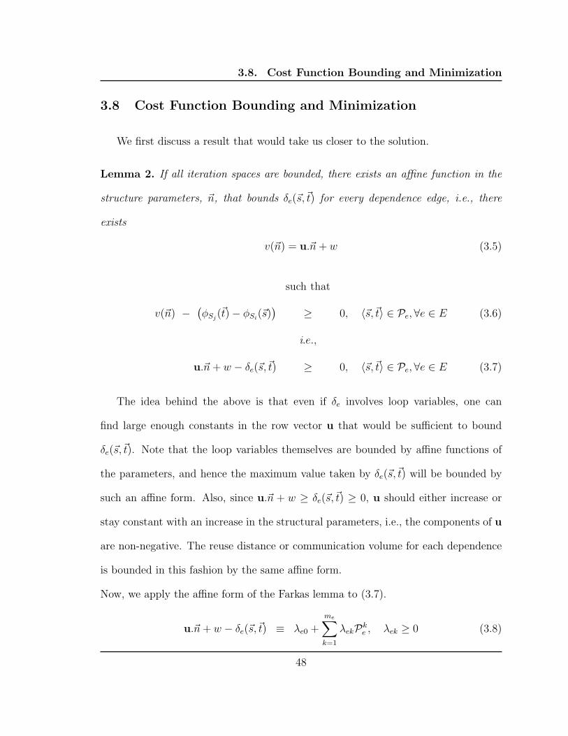
3.8. Cost Function Bounding and Minimization
3.8 Cost Function Bounding and Minimization
We first discuss a result that would take us closer to the solution.
Lemma 2. If all iteration spaces are bounded, there exists an affine function in the
structure parameters, ~n, that bounds δe(~s,~t) for every dependence edge, i.e., there
exists
v(~n) = u.~n + w (3.5)
such that
v(~n) −(φSj
(~t) − φSi(~s)
)≥ 0, 〈~s,~t〉 ∈ Pe,∀e ∈ E (3.6)
i.e.,
u.~n + w − δe(~s,~t) ≥ 0, 〈~s,~t〉 ∈ Pe,∀e ∈ E (3.7)
The idea behind the above is that even if δe involves loop variables, one can
find large enough constants in the row vector u that would be sufficient to bound
δe(~s,~t). Note that the loop variables themselves are bounded by affine functions of
the parameters, and hence the maximum value taken by δe(~s,~t) will be bounded by
such an affine form. Also, since u.~n + w ≥ δe(~s,~t) ≥ 0, u should either increase or
stay constant with an increase in the structural parameters, i.e., the components of u
are non-negative. The reuse distance or communication volume for each dependence
is bounded in this fashion by the same affine form.
Now, we apply the affine form of the Farkas lemma to (3.7).
u.~n + w − δe(~s,~t) ≡ λe0 +me∑
k=1
λekPke , λek ≥ 0 (3.8)
48
3.8. Cost Function Bounding and Minimization
The above is an identity and the coefficients of each of the loop indices in ~i and
parameters in ~n on the left and right hand side can be gathered and equated. We now
get linear inequalities entirely in coefficients of the affine mappings for all statements,
components of row vector u, and w. The above inequalities can be at once be solved
by finding a lexicographic minimal solution with u and w in the leading position,
and the other variables following in any order, i.e., if u = (u1, u2, . . . , uk), then our
objective function is:
minimize≺ (u1, u2, . . . , uk, w, . . . , ci, . . . ) (3.9)
Finding the lexicographic minimal solution is within the reach of the simplex algo-
rithm and can be handled by the PIP software [Fea88]. Since the structural param-
eters are quite large, we first want to minimize their coefficients. We do not lose the
optimal solution since an optimal solution would have the smallest possible values
for u’s. Though the zero vector is always a trivial solution with the above objective
function, it is avoided through constraints described in the next section.
The solution gives a hyperplane for each statement. Note that the application of
the Farkas lemma to (3.7) is not required in all cases. When a dependence is uniform,
the corresponding δe(~s,~t) is independent of any loop variables, and application of the
Farkas lemma is not required. In such cases, we just have δe ≤ w.
49

3.9. Iteratively Finding Independent Solutions
Avoiding the zero vector
Avoiding the zero solution statement-wise poses a challenge. In particular, to
avoid the zero vector we need:
(cS1 , cS
2 , . . . , cSmS
) 6= ~0, for each S ∈ S (3.10)
The above constraint cannot be expressed as a single convex space in the cS’s even for
a single statement. For multiple statements, the number of possibilities get multiplied.
The above difficulties can be solved at once by only looking for non-negative trans-
formation coefficients. Then, the zero solution can be avoided with the constraint of
∑mS
i=1cSi ≥ 1, for each S ∈ S.
Making the above practical choice leads to the exclusion of solutions that involve
loop reversals or combination of reversals with other transformations. In practice, we
do not find this to be a concern at all. The current implementation of Pluto [Plu] is
with this choice, and scales well without any evident loss of good transformations for
codes evaluated.
3.9 Iteratively Finding Independent Solutions
Solving the ILP formulation in the previous section gives us a single solution
to the coefficients of the best mappings for each statement. We need at least as
many independent solutions as the dimensionality of the polytope associated with
each statement. Hence, once a solution is found, we augment the ILP formulation
with new constraints and obtain the next solution; the new constraints ensure linear
independence with solutions already found. Let the rows of HS represent the solutions
50

3.9. Iteratively Finding Independent Solutions
found so far for a statement S. Then, the sub-space orthogonal to HS [Pen55, LP94,
BRS07] is given by:
H⊥
S = I − HTS
(HSHT
S
)−1HS (3.11)
Note that H⊥S .HS
T = 0, i.e., the rows of HS are orthogonal to those of H⊥S . Assume
that H⊥S has been freed of any unnecessary rows so that it forms a spanning basis for
the null space of HS. Let h∗S be the next row (linear portion of the hyperplane) to be
found for statement S. Let H i⊥
S be a row of H⊥S . Then, any one of the inequalities
given by: ∀i, H i⊥
S .~h∗S > 0, H i⊥
S .~h∗S < 0 gives the necessary constraint to be added for
statement S to ensure that h∗S has a non-zero component in the sub-space orthogonal
to HS and thus be linearly independent to HS. This leads to a non-convex space,
and ideally, all cases have to be tried and the best among those kept. When the
number of statements is large, this leads to a combinatorial explosion. In such cases,
we restrict ourselves to the sub-space of the orthogonal space where all the constraints
are positive, i.e., the following constraints are added to the ILP formulation for linear
independence:
∀i,H i⊥
S .h∗S ≥ 0 ∧
∑
i
H i⊥
S h∗
S ≥ 1 (3.12)
Example. For example, let us say there is one statement and that the first hyper-
plane found for it is (1, 0, 0), i.e., (ci, cj, ck) = (1, 0, 0).
HS = (1, 0, 0) H⊥
S =
0 0 00 1 00 0 1
i.e.,
H1⊥
S = (0, 1, 0) H2⊥
S = (0, 0, 1)
51

3.9. Iteratively Finding Independent Solutions
So, for linear independence we need to have:
cj 6= 0∨
ck 6= 0
i.e.,
cj ≥ 1∨
cj ≤ −1∨
ck ≥ 1∨
ck ≤ −1
Just forcing a positive component in the positive orthant will give a single convex
space for linear independence:
cj ≥ 0 ∧ ck ≥ 0 ∧ cj + ck ≥ 1
Note that when only the positive orthant is considered, the constraints for linear
independence for all statements form a single convex space.
The mappings found are independent on a per-statement basis. When there are
statements with different dimensionalities, the number of such independent mappings
found for each statement is equal to its domain dimensionality. Hence, no more linear
independence constraints need be added for statements for which enough independent
solutions have been found – the rest of the rows get automatically filled with zeros
or linearly dependent rows. The number of rows in the transformation matrix (MS)
is the same for each statement, consistent with our definition of TS. The depth of
the deepest loop nest in the transformed code is the same as that of the source
loop nest. Overall, a hierarchy of fully permutable bands (Def 12) is found, and a
lower level in the hierarchy will not be obtained unless ILP constraints corresponding
to dependences that have been satisfied by the parent permutable band have been
removed.
52

3.10. Communication and Locality Optimization Unified
3.10 Communication and Locality Optimization Unified
From the algorithm described above, both synchronization-free and pipelined
parallelism is found. Note that the best possible solution to Eqn. (3.9) is with
(u = 0, w = 0) and this happens when we find a hyperplane that has no dependence
components along its normal, which is a fully parallel loop requiring no synchroniza-
tion if it is at the outer level, i.e., it is outer parallel. It could be an inner parallel
loop if some dependences were removed previously and so a synchronization is re-
quired after the loop is executed in parallel. Thus, in each of the steps that we find a
new independent hyperplane, we end up first finding all synchronization-free hyper-
planes; these are followed by a set of fully permutable hyperplanes that are tilable and
pipelined parallel requiring constant boundary communication (u = 0, w > 0) w.r.t
the tile sizes. In the worst case, we have a hyperplane with u > 0, w ≥ 0 resulting in
long communication from non-constant dependences. It is important to note that the
latter are pushed to the innermost level. By bringing in the notion of communication
volume and its minimization, all degrees of parallelism are found in the order of their
preference.
From the point of view of data locality, note that the hyperplanes that are used
to scan the tile space are same as the ones that scan points in a tile. Hence, data
locality is optimized from two angles: (1) cache misses at tile boundaries are mini-
mized for local execution (as cache misses at local tile boundaries are equivalent to
communication along processor tile boundaries); (2) by reducing reuse distances, we
are increasing the size of local tiles that would fit in cache. The former is due to
53
3.11. Examples
selection of good tile shapes and the latter by the right permutation of hyperplanes
that is implicit in the order in which we find hyperplanes.
3.10.1 Space and time in transformed iteration space.
By minimizing δe(~s,~t) as we find hyperplanes from outermost to innermost, we
push dependence satisfaction to inner loops and also ensure that no loops have neg-
ative dependences components so that all target loops can be blocked. Once this is
done, if the outer loops are used as space (how many ever desired, say k), and the
rest are used as time (note that at least one time loop is required unless all loops
are synchronization-free parallel), communication in the processor space is optimized
as the outer space loops are the k best ones. All loops can be tiled resulting in
coarse-grained parallelism as well as better reuse within a tile. Hence, the same set
of hyperplanes are used to scan points in a tile. When space loops have dependences,
a transformation may be necessary in the outer tile space loops to get a schedule of
tiles to generate parallel code: this will be described in Chapter 5.
3.11 Examples
3.11.1 A step by step example
Figure 3.11 shows an example from the literature [DV97] with affine non-constant
dependences. We exclude the constant c0 from the transformation function as we
have a single statement. Dependence analysis produces the following dependence
54

3.11. Examples
polyhedra:
flow : a[i′, j′] → a[i, j − 1] Pe1: i′ = i, j′ = j − 1, 2 ≤ j ≤ N, 1 ≤ i ≤ N
flow : a[i′, j′] → a[j, i] Pe2: i′ = j, j′ = i, 2 ≤ j ≤ N, 1 ≤ i ≤ N, i − j ≥ 1
anti : a[j′, i′] → a[i, j] Pe3: j′ = i, i′ = j, 2 ≤ j ≤ N, 1 ≤ i ≤ N, i − j ≥ 1
for ( i=0; i<N; i++) {for (j=1; j<N; j++) {
a[ i , j ] = a[j , i]+a[i , j−1]}
}
P0 P3
P3 P4P2
P3
j
iP1
P0 P1
P1 P2
P2
P2
P4
P5
spacetime
Figure 3.11: Example: Non-uniform dependences
Note that the equalities in the dependence polyhedra can be readily used to elim-
inate variables from the constraints. In this case, u = (u1) since we have only one
parameter N .
Dependence 1: Tiling legality constraint (3.3) gives:
(ci, cj)
(i
j
)
− (ci, cj)
(i′
j′
)
≥ 0, 〈i, j, i′, j′〉 ∈ Pe1
⇒ cii + cjj − cii − cj(j − 1) ≥ 0
⇒ cj ≥ 0
55

3.11. Examples
Since this is a uniform dependence, the volume bounding constraint gives:
(ci, cj)
(i
j
)
− (ci, cj)
(i′
j′
)
≤ w, 〈i, j, i′, j′〉 ∈ Pe1
⇒ w − cj ≥ 0
Dependence 2: This is not a uniform dependence and hence the application of
Farkas Lemma for legality and bounding constraints cannot be avoided. The tiling
legality condition is given by:
(cii + cjj) − (cij + cji) ≥ 0, 2 ≤ j ≤ N, 1 ≤ i ≤ N, i − j ≥ 1
Applying Farkas lemma, we have:
(ci − cj)i + (cj − ci)j
≡ λ0 + λ1(N − i) + λ2(N − j)
+λ3(i − j − 1) + λ4(i − 1) + λ5(j − 2) (3.13)
λ1, λ2, λ3, λ4, λ5 ≥ 0
LHS and RHS coefficients for i, j, N and the constants are equated in (3.13) and the
Farkas multipliers are eliminated through Fourier-Motzkin (FM) variable elimination,
56

3.11. Examples
i.e., by equating coefficients on each side, we first obtain:
ci − cj = λ3 + λ4 − λ1
cj − ci = λ5 − λ3 − λ2
λ0 − λ3 − λ4 − 2λ5 = 0
λ1 + λ2 = 0
λ1 ≥ 0
λ2 ≥ 0
λ3 ≥ 0
λ4 ≥ 0
λ5 ≥ 0
The reader may verify that eliminating the λ’s through Gaussian elimination and
FM yields:
ci − cj ≥ 0
Volume bounding constraint:
u1N + w − (cij + cji − cii − cjj) ≥ 0, (i, j) ∈ Pe2
Application of Farkas lemma in a similar way as above and elimination of the multi-
pliers yields:
u1 ≥ 0
u1 − ci + cj ≥ 0 (3.14)
3u1 + w − ci + cj ≥ 0
57

3.11. Examples
Dependence 3: Due to symmetry with respect to i and j, the third dependence
does not give anything more than the second one.
Avoiding the zero solution: As discussed in Section 3.8, the zero solution is
avoided with
ci + cj ≥ 1
Finding the transformation. Aggregating legality and volume bounding con-
straints for all dependences, we obtain:
cj ≥ 0
w − cj ≥ 0
ci − cj ≥ 0
u1 ≥ 0
u1 − ci + cj ≥ 0 (3.15)
3u1 + w − ci + cj ≥ 0
ci + cj ≥ 1
minimize≺ (u1, w, ci, cj)
The lexicographic minimal solution for the vector (u1, w, ci, cj) = (0, 1, 1, 1). The zero
vector is a trivial solution and is avoided with ci + cj ≥ 1. Hence, we get ci = cj = 1.
Note that ci = 1 and cj = 0 is not obtained even though it is a valid tiling hyperplane
as it involves more communication: it requires u1 to be positive.
58

3.11. Examples
The next solution is forced to have a positive component in the subspace orthog-
onal to (1, 1) given by (3.11) as:
HS = (1, 1)
H⊥
S = I − HS(HSHTS )−1HT
S =
(1
2
−1
2−1
2
1
2
)
We first normalize the rows of H⊥S , then rows that are all zero and negations
of previous rows are discarded (the second row in this case) since they do not give
anything new in terms of linear independence, and ultimately we are just left with
(1,-1). We thus have ci − cj ≥ 1. With the trade-off discussed in Sec. 3.9, we just add
ci − cj ≥ 1 for linear independence.
Adding ci − cj ≥ 1 to (3.15), the lexicographic minimal solution is (1, 0, 1, 0), i.e.,
u1 = 1, w = 0, ci = 1, cj = 0 (u1 = 0 is no longer possible). Hence, (1, 1) and (1, 0)
are the best tiling hyperplanes. The transformation is given by:
TS
(i
j
)
=
(1 11 0
) (i
j
)
(1,1) is used as space with one line of communication between processors, and the
hyperplane (1,0) is used as time in a tile. The outer tile schedule is (2,1), obtained
by the addition of (1,1) and (1,0): this is described in more detailed in Chapter 5 in
Section 5.2.3.
This transformation is in contrast to other approaches based on schedules which
obtain a schedule and then the rest of the transformation matrix. Feautrier’s greedy
heuristic gives the schedule θ(i, j) = 2i + j − 3 which satisfies all dependences. How-
ever, using this as either space or time does not lead to communication or locality
optimization. The (2,1) hyperplane has non-constant communication along it. In
59

3.12. Handling Input Dependences
fact, the only hyperplane that has constant communication along it is (1,1). This
is the best hyperplane to be used as a space loop if the nest is to be parallelized,
and is the first solution that our algorithm finds. The (1,0) hyperplane is used as
time leading to a solution with one degree of pipelined parallelism with one line per
tile of near-neighbor communication along (1,1) as shown in Figure 3.11.1. Hence,
a good schedule that tries to satisfy all dependences (or as many as possible) is not
necessarily a good loop for the transformed iteration space.
3.11.2 Example 2: Imperfectly nested 1-d Jacobi
For the code in Figure 3.9, our algorithm obtains:
TS1
(t
i
)
=
1 02 10 0
(t
i
)
TS2
(t′
j
)
==
1 02 10 0
(t′
j
)
+
011
The resulting transformation is equivalent to a constant shift of one for S2 relative to
S1, fusion and skewing the i loop with respect to the t loop by a factor of two. The
(1,0) hyperplane has the least communication: no dependence crosses more than one
hyperplane instance along it.
3.12 Handling Input Dependences
Input dependences need to be considered for optimization in many cases as reuse
can be exploited by minimizing them. Clearly, legality (ordering between dependent
RAR iterations) need not be preserved. We thus do not add legality constraints
(3.3) for such dependences, but consider them for the bounding objective function
60

3.12. Handling Input Dependences
0
2
4
6
8
10
1 2 3 4
GFL
OPs
Number of cores
PlutoAffine partitioning (max degree parallelism)
Scheduling-based (FCO time tiling)icc -parallel -fast
Figure 3.12: Imperfectly nested Jacobi stencil parallelization: N = 106, T = 105
(3.7). Since input dependences can be allowed to have negative components in the
transformed space, they need to be bounded from both above and below. If Pe is a
dependence polyhedron corresponding to an input (RAR) dependence, we have the
constraints:
∣∣φSj
(~t)− φSi
(~s)∣∣ ≤ u.~n + w, 〈~s,~t〉 ∈ Pe
i.e.,
φSj
(~t)− φSi
(~s) ≤ u.~n + w∧
φSi(~s) − φSj
(~t)≤ u.~n + w, 〈~s,~t〉 ∈ Pe
61

3.13. Refinements for Cost Function
3.13 Refinements for Cost Function
The metric we presented here can be refined while keeping the problem within ILP.
The motivation behind taking a max is to avoid multiple counting of the same set of
points that need to be communicated for different dependences. This happens when
all dependences originate from the same data space and the same order volume of
communication is required for each of them. Using the sum of max’es on a per-array
basis is a more accurate metric. Also, even for a single array, sets of points with very
less overlap or no overlap may have to be communicated for different dependences.
Also, different dependences may have source dependence polytopes of different di-
mensionalities. Note that the image of the source dependence polytope under the
data access function associated with the dependence gives the actual set of points to
be communicated. Hence, just using the communication rate (number of hyperplanes
on the tile boundary) as the metric may not be accurate enough. This can be taken
care of by having different bounding functions for dependences with different orders of
communication, and using the bound coefficients for dependences with higher orders
of communication as the leading coefficients while finding the lexicographic minimal
solution. Hence, the metric can be tuned while keeping the problem linear.
3.14 Loop Fusion
We just give a brief overview here as Chapter 4 is devoted to discussion on how
fusion is naturally handled with our scheme. Solving for hyperplanes for multiple
statements leads to a schedule for each statement such that all statements in question
62

3.15. Summary
are finely interleaved: this is indeed fusion. In some cases, it might be enabled in
combination with other transformations like permutation or shifts. It is important to
leave the structure parameter ~n out of our hyperplane form in (2.7) for the above to
hold true. Leaving the parameter out allows us to control the fusion choices. Hence,
a common tiling hyperplane also represents a fused loop, and reuse distances between
components that are weakly connected can be reduced with our cost function. The
set of valid independent hyperplanes that can be iteratively found from our algorithm
for multiple statements (at a given depth) is the maximum number of loops that can
be fused at that depth. This generalization of fusion is same as the one proposed in
[CGP+05, GVB+06] however we are able to automatically enable it in conjunction
with other transformations. All of this is the subject of Chapter 4.
3.15 Summary
The algorithm is summarized below. Our approach can be viewed as transforming
to a tree of permutable loop nests sets/bands - each node of the tree is a good
permutable loop nest set. Step 12 of the repeat-until block in Algorithm 1 finds
such a band of permutable loops. If all loops are tilable, there is just one node
containing all the loops that are permutable. On the other extreme, if no loops are
tilable, each node of the tree has just one loop and so no tiling is possible. At least
two hyperplanes should be found at any level without dependence removal to enable
tiling. Dependences from previously found solutions are thus not removed unless
they have to be (Step 17): to allow the next permutable band to be found, and so
on. Hence, partially tilable or untilable input is all handled. Loops in each node of
63

3.15. Summary
Algorithm 1 Pluto automatic transformation algorithm
INPUT Data Dependence graph G = (V,E) with dependence polyhedra, Pe, ∀e ∈ E
1: Smax: statement with maximum domain dimensionality2: for each dependence e ∈ E which is from Si to Sj do3: Build legality constraints: apply Farkas Lemma on φSj
(~t) − φSi(~s) ≥ 0, under
〈~s,~t〉 ∈ Pe, and eliminate all Farkas multipliers4: Build bounding function constraints: apply Farkas Lemma to u.~n+w−(φSj
(~t)−
φSi(~s)) ≥ 0 under 〈~s,~t〉 ∈ Pe, and eliminate all Farkas multipliers
5: Aggregate constraints from both into Ce(i)6: end for7: repeat8: C = ∅9: for each dependence edge e ∈ E do
10: C ← C ∪ Ce(i)11: end for12: Compute lexicographic minimal solution with u′s coefficients in the leading
position followed by w; iteratively find independent solutions to C with linearindependence constraints (3.12) added after each solution is found
13: if no solutions were found then14: Remove dependences between two strongly-connected components in the
GDG and insert a scalar dimension in the transformation functions of thestatements (Chapter 4)
15: end if16: Compute Ec: dependences satisfied by solutions of Step 12/1417: E ← E − Ec; reform the data dependence graph G = (V,E)18: Compute H⊥
Smax: the null space of TSmax
19: until H⊥Smax
= 0 and E = ∅OUTPUT The transformation function TS for each statement
64
3.16. Comparison with Existing Approaches
the target tree can be stripmined/interchanged when there are at least two of them
in it; however, it is illegal to move a stripmined loop across different levels in the
tree. There are some intricacies involved here when moving across scalar dimensions:
they will be fully described in Chapter 5. When compared to earlier approaches that
found maximal sets of permutable loop nests [WL91a, DSV97, LCL99], ours is with
an optimization criterion (3.9) that goes beyond maximum degrees of parallelism.
Also, [WL91a, DSV97] were applicable to only perfect loop nests.
The theoretical complexity of the algorithm will be discussed in the next chapter
after the notion of fusion is sharpened.
3.16 Comparison with Existing Approaches
Tiling and cost functions. Iteration space tiling [IT88, RS92, Xue00, WL91b] is
a standard approach for aggregating a set of loop iterations into tiles, with each tile
being executed atomically. It is well known that it can improve register reuse, improve
locality and minimize communication. Researchers have considered the problem of
selecting tile shape and size to minimize communication, improve locality or mini-
mize finish time [ABRY03, BDRR94, HS02, HCF97, HCF99, RS92, SD90, Xue97].
However, these studies were restricted to very simple codes – like single perfectly
nested loop nests with uniform dependences and/or sometimes loop nests of a par-
ticular depth. To the best of our knowledge, these works have not been extended to
more general cases and the cost functions proposed therein not been implemented to
allow a direct comparison for those restricted cases. Our work is in the direction of
a practical cost function that works for the general case (any polyhedral program or
65
3.16. Comparison with Existing Approaches
one that can be approximated into it) as opposed to a more sophisticated function
for restricted input. With such a function, we are able to keep the problem linear,
and since sparse ILP formulations that result here are solved very quickly, we are at
a sweet-spot between cost-function sophistication and scalability to real-world pro-
grams. Note that our function does not capture tile size optimization, but the results
to be presented in Chapter 6 show that decoupling optimization of tile shapes and
sizes is a practical and very effective approach.
Ahmed et al. Ahmed et al. [AMP00, AMP01] proposed a framework to optimize
imperfectly nested loops for locality. The approach determines the embedding for each
statement into a product space, which is then considered for locality optimization
through another transformation matrix. Their framework was among the first to
address tiling of imperfectly nested loops. However, the heuristic used for minimizing
reuse distances is not scalable as described. The reuse distances in the target space for
some dependences are set to zero (or a constant) with the goal of obtaining solutions
to the embedding function and transformation matrix coefficients. However, there is
no concrete procedure to determine the choice of the dependences and the number
(which is crucial), and how a new choice is made when no feasible solution is found.
Moreover, setting some reuse classes to zero (or a constant) need not completely
determine the embedding function or transformation matrix coefficients. Some reuse
distances may not be reducible to a constant while some may be. Exploring all
possibilities here leads to a combinatorial explosion even for simple imperfect loop
nests. Hence, a test-and-set approach for minimizing reuse distances is unlikely to
66

3.16. Comparison with Existing Approaches
succeed for general affine dependences. With several recent polyhedral approaches, no
special embedding or sinking (conversion of an imperfect loop nest to a perfect one)
is needed; the original nesting of the code can be discarded once polyhedral domains
and dependences have been extracted. The transformation functions finally specify
the space-time mapping into a common space that Cloog efficiently scans.
Some specialized works [SL99, YKA04] also exist on tiling a restricted class of
imperfectly nested loops for locality. These works are subsumed by approaches em-
ploying the polyhedral model. This is without any additional evident complexity in
dependence analysis, transformation computation, or code generation with the poly-
hedral tools for the input those tools handle.
Iteration space slicing [PR97, PR00] and transitive closure are techniques that
potentially go beyond affine transformations, i.e., they can partition iteration spaces
in a way that is not readily expressible with affine transformations. However, existing
slicing techniques [PR00, PR97] do not provide a solution to the key decision prob-
lems of – which array to slice and the dimension along which to slice. Besides, the
practicality of slicing for coarse-grained parallelization or computation of transitive
closure has not yet been demonstrated even for simple affine loop nests.
Loop parallelization has been studied extensively. The reader is referred to the
survey of Boulet et al. [BDSV98] for a detailed summary of earlier parallelization
algorithms – these restricted the input loop forms, like to perfect loop nests and/or
were based on weaker dependence abstractions than exact polyhedral dependences.
These include Lamport’s seminal hyperplane method [Lam74], Allen and Kennedy’s
algorithm [AK87] based on dependence levels, Wolf and Lam [WL91a], and Darte et
67
3.16. Comparison with Existing Approaches
al. [DV97, DSV97]. Automatic parallelization efforts in the polyhedral model broadly
fall into two classes: (1) scheduling/allocation-based [Fea92a, Fea92b, Fea94, DR96,
Gri04] and (2) partitioning-based [LL98, LCL99, LLL01]. We now compare with
previous approaches from both classes.
Pure scheduling-based approaches are geared towards finding minimum latency
schedules or maximum fine-grained parallelism, as opposed to tilability for coarse-
grained parallelization with minimized communication and improved locality. Clearly,
on most modern parallel architectures, at least one level of coarse-grained parallelism
is desired as communication/synchronization costs matter, and so is improving local-
ity. Several works are based on such schedules [BF03, Gri04, CGP+05, PBCV07,
PBCC08].
Griebl et al. Griebl [Gri04] presents an integrated framework for optimizing local-
ity and coarse-grained parallelism with space and time tiling, by enabling time tiling
as a post-processing step after a schedule is found. When schedules are used, the
inner parallel (space) loops can be readily tiled. In addition, if coarser granularity of
parallelism is desired, Griebl’s forward communication-only (FCO) constraint finds
an allocation satisfying the constraint that all dependences have non-negative affine
components along it, i.e., communication will be in the forward direction. Due to
this, both the schedule and allocation dimensions become one permutable band of
loops that can be tiled. Hence, tiling along the scheduling dimensions (time tiling)
is enabled. As shown in this chapter from a theoretical standpoint (Section 3.2.1),
fixing schedules as loops does not naturally fit well with tiling. It also adds additional
68

3.16. Comparison with Existing Approaches
complexity to code generation. Results presented in Chapter 6 also confirm these
downsides which cannot be undone regardless of how allocations are computed.
Lim and Lam. Lim and Lam’s approach [LL98, LCL99] was the first to take a par-
titioning view with affine functions. They proposed a framework that identifies outer
parallel loops (communication-free space partitions) and permutable loops (time par-
titions) with the goal of maximizing the degree of parallelism and minimizing the order
of synchronization. They employ the same machinery to tile for locality and array
contraction [LLL01]. There are infinitely many affine transformations that maximize
the degree of parallelism and they significantly differ in performance. Whenever there
exist no communication-free partitions, their algorithm finds maximally independent
solutions to time partitioning constraints without a cost metric to pick good ones. As
shown in this chapter, without a cost function, solutions obtained even for simple in-
put may be unsatisfactory with respect to communication cost and locality. It is also
not clear how linear independence is ensured between permutable bands belonging
to different levels in the hierarchy. Lastly, their algorithm cannot enable non-trivial
fusion across sequences of loop nests that fall in different strongly-connected compo-
nents having a producer-consumer relationship: this is discussed and compared in the
next chapter.
Our approach is closer to the latter class of partitioning-based approaches. How-
ever, to the best of our knowledge, it is the first to explicitly model good ways of
tiling in the transformation framework with an objective function that is applicable
to any polyhedral program. Codes which cannot be tiled or only partially tiled are
69

3.17. Scope for Extensions
all handled, and traditional transformations are captured. Loop fusion in conjunc-
tion with all other transformations is also captured and this is described in the next
chapter.
Semi-automatic and iterative techniques. In addition to model-based approaches,
semi-automatic and search-based transformation frameworks in the polyhedral model
also exist [KP93, KP95, CGP+05, GVB+06, PBCV07, PBCC08]. Cohen et al. [CGP+05]
and Girbal et al. [GVB+06] proposed and developed a powerful framework (URUK
WRAP-IT) to compose and apply sequences of transformations semi-automatically.
Transformations are applied automatically, but specified manually by an expert.
A limitation of the recent iterative polyhedral compilation approaches [PBCV07,
PBCC08] is that the constructed search space does not include tiling and its inte-
gration poses a non-trivial challenge. Though our system now is fully model-driven,
empirical iterative optimization would be beneficial on complementary aspects, such
as determination of optimal tile sizes and unroll factors, and in other cases when in-
teractions with the underlying hardware and native compiler cannot be well-captured.
3.17 Scope for Extensions
Besides the refinements suggested in Section 3.13, the process for constructing
the linearly independent sub-space can be made more comprehensive. This might
be possible by adding additional decision variables. In addition, the framework can
be made to find negative coefficients for the φ′s – we avoided this to avoid the zero
vector solution easily and since the additional benefit of considering negative values
70

3.17. Scope for Extensions
is not worth the complexity they bring in. For all the codes tried so far with the
implemented system, these practical choices have not caused a problem. The ILP
formulations on hyperplane coefficients appear to be very sparse and can benefit from
special techniques to solve them much faster [Fea06].
Index set splitting. The transformation our algorithm computes for a statement
applies to the entire domain of the statement as was extracted from the input pro-
gram. Griebl et al. [GFL00] proposed a method to split the original iteration domains
based on dependences before space-time mappings are computed. After such a pre-
processing phase, a parallelizer may be able to find better mappings with the split
domains. Such a dependence-driven index set splitting technique is complementary
to our algorithm and could enhance the transformations computed.
Acknowledgments
I would like to acknowledge the anonymous reviewers of our papers published
at the International Conference on Compiler Construction 2008, and the ACM SIG-
PLAN Conference on Programming Languages Design and Implementation 2008 for
several constructive comments on this framework. I would also like to acknowl-
edge Nicolas Vasilache, Alex Eichenberger, and Lakshminarayanan Renganarayana
for some discussion and feedback from time to time.
71
CHAPTER 4
Integrating Loop Fusion: Natural Task
In this chapter, we describe how loop fusion is naturally captured in our trans-
formation framework and how finding legal and reasonably good fusion structures is
automatically enabled.
Loop fusion involves merging a sequence of two or more loops into a fused loop
structure with multiple statements in the loop body. Sequences of producer/consumer
loops are commonly encountered in applications, where a nested loop statement pro-
duces an array that is consumed in a subsequent loop nest. In this context, fusion can
greatly reduce the number of cache misses when the arrays are large - instead of first
writing all elements of the array in the producer loop (forcing capacity misses in the
cache) and then reading them in the consumer loop (incurring cache misses), fusion
allows the production and consumption of elements of the array to be interleaved,
thereby reducing the number of cache misses. Figure 4.4 shows an example. For
parallel execution, fusion can also reduce the number of synchronizations. Hence, an
automatic transformation framework should be able to find good ways of fusion in
conjunction with other transformations.
72

4. Integrating Loop Fusion: Natural Task
Loop fusion has mainly been studied in an isolated manner by the compiler op-
timization community [KM93, MS97, SM97, DH99]. Following are the limitations of
previous works.
1. Only fusion legality in isolation with other transformations
2. Usually studied fusion with shifts only
3. Simpler dependence models were employed that miss complex fusions that can
provide better performance or reduce storage requirement
Often, more complex sequence of transformations are needed that include fusion
as one of the transformations. For example, one could permute and shift to enable
fusion, and then tile (partially) fused structures. The ability of enumerate fusion
structures is also useful.
Fusion strongly interacts with tiling and parallelization. Maximal fusion often
kills parallelism, no fusion gives maximal parallelism but can lead to lesser storage
optimization or lower cache reuse. Due to complex interactions with other transfor-
mations, fusion needs to be studied in an integrated way in a compiler framework for
automatic parallelization. For example, it is common for fusion to be legal with some
loop shifts. In many scientific codes, fusion is legal after specific permutations. In
several of those cases, multiple choices exist and not all of them may be amenable to
good parallelization.
It is possible to reason about fusion and drive it completely in the polyhedral
model. Traditional literature on loop fusion states that one can distribute two loop
73
4.1. Automatic Fusion
nests that were originally fused if there are no “back edges”, i.e., no dependences from
the second statement to the first. Similarly, one can fuse if it does not add back edges.
These legality conditions are already captured with the standard legality constraints
in our ILP formulation on the transformation coefficients. Note that we consider all
dependences including dependences between SCCs.
Researchers have successfully represented fusion structures through affine trans-
formations: Feautrier [Fea92b], Kelly et al. [KP95, Kel96], Cohen et al and Girbal et
al [CGP+05, GVB+06]. However, there is no framework to automatically find such
transformations representing good fusions. Our framework can automatically enable
good fusion in conjunction with all other transformations. We present three differ-
ent fusion algorithms that capture the interesting fusion choices in most cases with
medium-sized loop nests.
4.1 Automatic Fusion
Let us recall again the structure of our transformation. φS for a statement was
defined as:
φS(~i) =(cS1 cS
2 . . . cSmS
).~iS + 0.~n + cS
0
where ~iS is the iterators surrounding the statement in the original program and ~n
is the vector of program parameters. φ does not have any coefficients for the pro-
gram parameters ~n. Also, note that trivial solutions are avoided (Sec. 3.8) through:
∑mS
i=1cSi ≥ 1 for each statement. Recall also the definition of a scalar dimension,
where φkSi
is a constant function for each Si, i.e.,(cS1 cS
2 . . . cSmS
)= 0.
74

4.1. Automatic Fusion
Solving for hyperplanes for multiple statements leads to a schedule for each state-
ment such that all statements in question are finely interleaved: this is indeed fusion.
The fine interleaving is due to the fact that φ does not have coefficients for the pro-
gram parameters (typically loop bounds). Hence, a common tiling hyperplane also
represents a fused loop, and reuse distances between components that are weakly
connected can be reduced with our cost function. The set of valid independent hy-
perplanes that can be iteratively found from our algorithm for multiple statements
(at a given depth) is the maximum number of loops that can be fused at that depth.
4.1.1 Implications of minimizing δ for fusion
Recall from (3.9) that φSj(~t) − φSi
(~s) is bounded by u.~n + w and minimized
iteratively level after level.
One can see that the dependence distance is minimized from (1,0,0) to (0,0,1)
after transformation and this is lexicographically the minimum. It is obtained since
solutions are found iteratively that minimize the dependence distances each level and
thus lexicographically minimize the vector of maximum dependence components.
Now, we discuss how the case of non-existence of a fused loop is handled concretely.
The code in Figure 4.3 is one example.
A program’s data dependence graph (DDG) can always be viewed as a DAG of
strongly connected components (SCCs). Let SCC(i) be the ith one in the topological
sort of the DAG of SCCs.
75

4.1. Automatic Fusion
for ( i=1; i<N−2; i++) {A[i ] = 0.33*(In[i−1]+In[i]+In[i+1]);
}for ( i=2; i<N−3; i++) {
Out[i] = 0.33*(A[i−1]+A[i]+A[i+1]);}
(a) original code
for (t0=1;t0<=min(2,N−3);t0++) {A[t0] = 0.33*(In[1+t0]+In[t0]+In[t0−1]);
}for (t0=3;t0<=N−3;t0++) {
A[t0] = 0.33*(In[1+t0]+In[t0]+In[t0−1]);Out[t0−1] = 0.33*(A[1+t0−1]+A[t0−1]+
A[t0−1 −1]);}
(b) Fused code
Figure 4.1: Fusion: simple example
Original Transformedφ1
S1 = 0, φ1S2 = 1 φ1
S1 = i, φ1S2 = i + 1
φ2S1 = i, φ2
S2 = i φ2S1 = 0, φ2
S2 = 1
Level min≺(u, w)Original Transformed
Level 0 1 0Level 1 0 1
Figure 4.2: Lexicographic u.~n + w reduction for fusion
Definition 15 (Cutting dependences). Two adjacent nodes in the DAG, SCC(i)
and SCC(i + 1), are considered cut at a level m iff φmSi
= α, ∀Si ∈ SCC(k), k ≤ i,
and φmSj
= α + 1, ∀Sj ∈ SCC(k), j > k, where α is an integer constant.
Consider the sequence of two matrix-vector multiplies in Figure 4.1.1. Applying
our algorithm on it first gives us only one solution: φ1S1 = i, φ1
S2 = l. This implies
fusion of the i loop of S1 and the j loop of S2. Putting the linear independence
constraint now, we do not obtain any more solutions. As per our algorithm, we now
remove the dependences satisfied by the φ1s, and this still does not yield a solution as
the loops cannot be fused further. Now, if a scalar dimension is inserted, with φ2S1
= 0,
and φ2S2
= 1, it will satisfy any remaining (unsatisfied) dependences between S1 and
S2. This is a cut between S1 and S2 which are SCCs in the DDG by themselves. After
76

4.1. Automatic Fusion
for ( i=0; i<N; i++) {s = s + b[i]*c[ i ]
}for ( i=0; i<N; i++) {
c[ i ] = s + a[i ];}
Figure 4.3: No fusion possible
the dependences are cut, φ3S1
= j, and φ3S2
= l can be found. The remaining unfused
loops are thus placed one after the other as shown in Figure 4.1.1. This generalization
of fusion is same as the one proposed in [CGP+05, GVB+06].
for ( i=0; i<N; i++)for (j=0; j<N; j++)
S1: x[ i ] = x[i]+a[i , j ]*y[ j ];
for (k=0; k<N; k++)for ( l=0; l<N; l++)
S2: y[k] = y[k] + a[k,l ]*x[ l ];
for ( i=0; i<N; i++) {for (j=0; j<N; j++) {
S1: x[ i ] = x[i]+a[i , j ]*y[ j ];}for (k=0; k<N; k++) {
S2: y[k] = y[k]+a[k,i]*x[ i ];}
}
Figure 4.4: Two matrix vector multiplies
Now, consider a sequence of three matrix vector multiplies such as
y = Ax; z = By; w = Cz
Together, these three loop nests do not have a common surrounding loop. How-
ever, it is possible to fuse the first two or the last two. When our algorithm is run
77

4.1. Automatic Fusion
on all three components, no solutions are found. However, a solution is found if de-
pendences between either the first and second MVs or the second and third MVs is
cut.
4.1.2 Dependence cutting schemes
The notion of cutting dependences between SCCs exposes the choice of fusion
structures. The algorithm as described is geared towards maximal fusion, i.e., depen-
dences are cut at the deepest level (as a last resort). However, it does not restrict how
the following decision is made – which dependences between SCCs to cut when fused
loops are not found (Step 14)?. Aggressive fusion may be detrimental to parallelism
and increases the running time of the transformation framework in the presence of a
large number of statements, while separating all SCCs may give up reuse. To capture
most of the interesting cases, we use three different fusion schemes:
1. nofuse: Whenever no more common loops are found, all SCCs in the DDG are
completely separated out through a scalar dimension, i.e., dependences between
all SCCs are cut
2. smartfuse: Dependences between SCCs are cut based on the order of reuse of
the maximum dimensionality array in an SCC, i.e., SCCs with the same order
of reuse are grouped together. If solutions are still not found, SCCs with the
same order of reuse are separated based on the maximum dimensionality across
all statement domains in an SCC. This scheme ultimately falls back to nofuse
if the above does not succeed in finding any fusable loops.
78
4.2. Correctness and Completeness
3. maxfuse: Dependences are cut very conservatively, between exactly two SCCs
at a time. The scheme falls back to smartfuse and ultimately to nofuse in the
presence of no fusion at all.
Our notion of a cut is equivalent to introducing a parametric shift to separate
loops. Loop shifting was used for parallelization and fusion with a simplified repre-
sentation of dependences and transformations by Darte et al. [DH99, DH00]. Shifting
was used for correcting illegal loop transformations by Vasilache et al. [VCP07]. Ex-
ample 4.4.4 explains how more sophisticated transformations can be enabled than
with techniques based purely on loop shifting.
The smartfuse and maxfuse heuristics have a tendency to introduce a large number
of scalar dimensions with many of them being redundant, i.e., a continuous set of
them can be collapsed into just one scalar dimension and polyhedral operations on
such dimensions anyway are trivial. Thanks to code generation optimizations in Cloog
that remove such scalar dimensions [VBC06].
4.2 Correctness and Completeness
We now show that the above terminates successfully with a legal transformation.
Theorem 2. A transformation is always found by Algorithm 2
Proof. We show that the termination condition (Step 21) of Algorithm 2 is always
reached. Firstly, every strongly-connected component of the dependence graph has
at least one common surrounding loop, if the input comes from a valid computation.
79
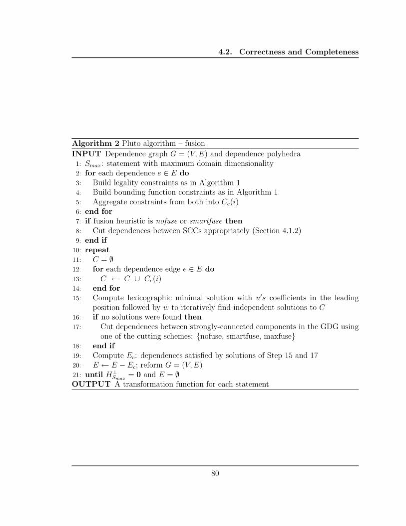
4.2. Correctness and Completeness
Algorithm 2 Pluto algorithm – fusion
INPUT Dependence graph G = (V,E) and dependence polyhedra1: Smax: statement with maximum domain dimensionality2: for each dependence e ∈ E do3: Build legality constraints as in Algorithm 14: Build bounding function constraints as in Algorithm 15: Aggregate constraints from both into Ce(i)6: end for7: if fusion heuristic is nofuse or smartfuse then8: Cut dependences between SCCs appropriately (Section 4.1.2)9: end if
10: repeat11: C = ∅12: for each dependence edge e ∈ E do13: C ← C ∪ Ce(i)14: end for15: Compute lexicographic minimal solution with u′s coefficients in the leading
position followed by w to iteratively find independent solutions to C
16: if no solutions were found then17: Cut dependences between strongly-connected components in the GDG using
one of the cutting schemes: {nofuse, smartfuse, maxfuse}18: end if19: Compute Ec: dependences satisfied by solutions of Step 15 and 1720: E ← E − Ec; reform G = (V,E)21: until H⊥
Smax= 0 and E = ∅
OUTPUT A transformation function for each statement
80

4.2. Correctness and Completeness
Hence, Step 15 is guaranteed to find at least one solution when all dependences be-
tween strongly-connected components have eventually been cut (iteratively in Step 17
whenever solutions are not found). Hence, enough linearly independent solutions are
found for each statement such that H⊥S eventually becomes 0mS×mS
for every S ∈ V ,
i.e., HS becomes full-ranked for each statement. Now, we show that the condition
E = ∅ is also eventually satisfied. Let us consider the two groups of dependences:
(1) self-edges (or intra-statement dependences), and (2) inter-statement dependences.
Since HS becomes full-ranked and does not have a null space, all dependent iterations
comprising a self-edge are satisfied at one level or the other (since φ(~t) − φ(~s) ≥ 0
stays in the formulation till satisfaction). Now, consider an inter-statement depen-
dence from Si to Sj. If at Step 17, the dependences between Si and Sj were cut,
all unsatisfied dependences between Si and Sj will immediately be satisfied at the
scalar dimension introduced in the transformation matrices (since φSjis set to one
and φSito zero). However, if Si and Sj belong to the same strongly-connected com-
ponent, then a solution will be found at Step 15, and eventually they will belong to
separate strongly-connected components and dependences between them will be cut
(if not satisfied). Hence, both intra and inter-statement dependences are eventually
satisfied, and the condition E = ∅ is met.2
Theorem 3. The transformation found by Algorithm 2 is always legal.
Proof. Given the proof for Theorem 2, the proof for legality is straightforward.
Since we keep φ(~t) − φ(~s) ≥ 0 in the formulation till satisfaction, no dependence
is violated. The termination condition for the repeat-until block (Step 21) thus en-
81

4.3. Theoretical Complexity of Computing Transformations
sures that all dependences are satisfied. Hence, the transformations found are always
legal.2
4.2.1 Bound on iterative search in Algorithm 2
Each iteration of the repeat-until block in Algorithm 2 incurs a call to PIP. The
number of times this block executes depends on how dependences across strongly-
connected components are handled in Step 17. Consider one extreme case when all
dependences between any two strongly-connected components are cut whenever no
solutions are found (nofuse): then, the number of PIP calls required is 2d+1 at worst,
where d is the depth of the statement with maximum dimensionality. This is because,
in the worst case, exactly one solution is found at Step 15, and the rest of the d times
dependences between all SCCs are cut (both happen in an alternating fashion); the
last iteration of the block adds a scalar dimension that specifies the ordering of the
statements in the innermost loop(s). Now, consider the other extreme case, when
dependences are cut very conservatively between SCCs; in the worst case, this would
increase the number of iterations of the block by the number of dependences in the
program.
4.3 Theoretical Complexity of Computing Transformations
Integer Linear Programming is known to be NP-hard. The PIP solver employed
here uses the dual-simplex algorithm with Gomory’s cutting plane method [Sch86] to
obtain the best integer solution. The Simplex algorithm is known to have an average-
case complexity of O(n3) and is very efficient in practice, even though its worst case
82
4.3. Theoretical Complexity of Computing Transformations
complexity is exponential. In particular, it is important to note that the ILP formu-
lations that result out of affine scheduling or partitioning in the polyhedral model are
very simple and sparse, and are quickly solved. The following are the key input sizes.
n: Sum of the dimensionalities of the domains of all statements|E|: Number of dependences (edges in the DDG)m: Depth of the statement with maximum domain dimensionality
Our algorithms needs Θ(m) to Θ(|E|) number of calls to PIP depending on the fu-
sion heuristic. Assuming smartfuse, the theoretical complexity is typically O(n3 ∗m).
This does not yet include the complexity of building the legality and cost function
constraints which is a one-time process proportional to the number of dependences.
Elimination of the Farkas multipliers is done dependence-wise, and therefore on sys-
tems with dimensionality proportional to nesting depth. Usually, Fourier-Motzkin
elimination on these systems leads to a reduction in the number of inequalities, hence,
its super-exponential theoretical complexity is of little importance for our problems.
The complexity involved in building the constraints can be written as O(|E| ∗ m3),
since Θ(m) Farkas multipliers are to be eliminated from systems with Θ(m ∗ d) con-
straints. When dependences edges are omitted, the formulation need not be rebuilt,
but constraints pertaining to the omitted dependences need to be just discarded.
Overall, the average-case complexity appears to be O(n3 ∗ m + |E| ∗ m3).
Table 4.3 shows the time taken compute transformations for several kernels.
83

4.4. Examples
Code Number of Number of Number of Computationstatements loops dependences time
2-d Jacobi 2 6 20 0.033sHaar 1-d 3 5 12 0.018s
LU 2 5 10 0.011sTCE 4-index 4 20 15 0.095s2-d FDTD 4 11 37 0.061s
Swim 57 109 633 2.8s
Table 4.1: Time to compute transformations as of Pluto version 0.3.1 on an In-tel Core2 Quad Q6600
4.4 Examples
We now give several examples to show non-trivial fusion structures are achieved
from our framework. The transformed code for all of these examples have automati-
cally been generated from Pluto with either the maxfuse or smartfuse heuristic.
4.4.1 Sequence of Matrix-Matrix multiplies
For the sequence of matrix-matrix multiplies in Figure 4.5, each of the original
loop nests can be parallelized, but a synchronization is needed after the first loop nest
is executed. The transformed loop nest has one outer parallel loop (c1), but reuse is
improved as each element of matrix C is consumed immediately after it is produced.
C can be contracted to a single scalar. This transformation is non-trivial and cannot
be obtained from existing frameworks.
84
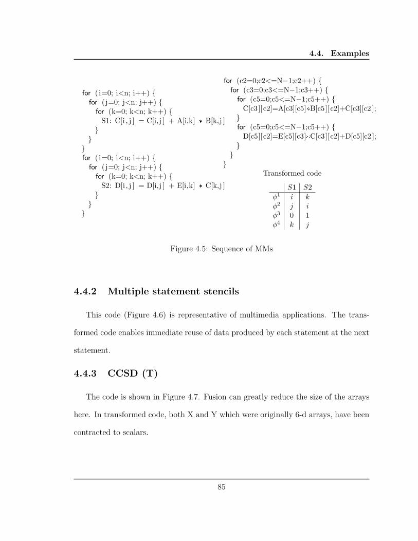
4.4. Examples
for ( i=0; i<n; i++) {for (j=0; j<n; j++) {
for (k=0; k<n; k++) {S1: C[i , j ] = C[i,j ] + A[i,k] * B[k,j ]
}}
}for ( i=0; i<n; i++) {
for (j=0; j<n; j++) {for (k=0; k<n; k++) {
S2: D[i , j ] = D[i,j ] + E[i,k] * C[k,j ]}
}}
for (c2=0;c2<=N−1;c2++) {for (c3=0;c3<=N−1;c3++) {
for (c5=0;c5<=N−1;c5++) {C[c3][c2]=A[c3][c5]*B[c5][c2]+C[c3][c2 ];
}for (c5=0;c5<=N−1;c5++) {
D[c5][c2]=E[c5][c3]*C[c3][c2]+D[c5][c2 ];}
}}
Transformed code
S1 S2
φ1 i k
φ2 j i
φ3 0 1φ4 k j
Figure 4.5: Sequence of MMs
4.4.2 Multiple statement stencils
This code (Figure 4.6) is representative of multimedia applications. The trans-
formed code enables immediate reuse of data produced by each statement at the next
statement.
4.4.3 CCSD (T)
The code is shown in Figure 4.7. Fusion can greatly reduce the size of the arrays
here. In transformed code, both X and Y which were originally 6-d arrays, have been
contracted to scalars.
85
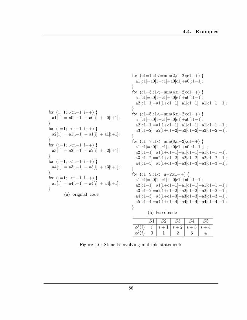
4.4. Examples
for ( i=1; i<n−1; i++) {a1[ i ] = a0[i−1] + a0[i] + a0[i+1];
}for ( i=1; i<n−1; i++) {
a2[ i ] = a1[i−1] + a1[i] + a1[i+1];}for ( i=1; i<n−1; i++) {
a3[ i ] = a2[i−1] + a2[i] + a2[i+1];}for ( i=1; i<n−1; i++) {
a4[ i ] = a3[i−1] + a3[i] + a3[i+1];}for ( i=1; i<n−1; i++) {
a5[ i ] = a4[i−1] + a4[i] + a4[i+1];}
(a) original code
for (c1=1;c1<=min(2,n−2);c1++) {a1[c1]=a0[1+c1]+a0[c1]+a0[c1−1];
}for (c1=3;c1<=min(4,n−2);c1++) {
a1[c1]=a0[1+c1]+a0[c1]+a0[c1−1];a2[c1−1]=a1[1+c1−1]+a1[c1−1]+a1[c1−1 −1];
}for (c1=5;c1<=min(6,n−2);c1++) {
a1[c1]=a0[1+c1]+a0[c1]+a0[c1−1];a2[c1−1]=a1[1+c1−1]+a1[c1−1]+a1[c1−1 −1];a3[c1−2]=a2[1+c1−2]+a2[c1−2]+a2[c1−2 −1];
}for (c1=7;c1<=min(8,n−2);c1++) {
a1[c1]=a0[1+c1]+a0[c1]+a0[c1−1];} ;a2[c1−1]=a1[1+c1−1]+a1[c1−1]+a1[c1−1 −1];a3[c1−2]=a2[1+c1−2]+a2[c1−2]+a2[c1−2 −1];a4[c1−3]=a3[1+c1−3]+a3[c1−3]+a3[c1−3 −1];
}for (c1=9;c1<=n−2;c1++) {
a1[c1]=a0[1+c1]+a0[c1]+a0[c1−1];a2[c1−1]=a1[1+c1−1]+a1[c1−1]+a1[c1−1 −1];a3[c1−2]=a2[1+c1−2]+a2[c1−2]+a2[c1−2 −1];a4[c1−3]=a3[1+c1−3]+a3[c1−3]+a3[c1−3 −1];a5[c1−4]=a4[1+c1−4]+a4[c1−4]+a4[c1−4 −1];
}(b) Fused code
S1 S2 S3 S4 S5φ1(i) i i + 1 i + 2 i + 3 i + 4φ2(i) 0 1 2 3 4
Figure 4.6: Stencils involving multiple statements
86

4.4. Examples
e1 = 0;e2 = 0;
for (a=0;a<V;a++)for (b=0;b<V;b++)
for (c=0;c<V;c++)for (e=0;e<V;e++)
for ( i=0;i<O;i++)for (j=0;j<O;j++)
for (k=0;k<O;k++)for (m=0;m<O;m++)
X[a][b ][ c ][ i ][ j ][ k] = X[a][b][c ][ i ][ j ][ k] +T2[a][b ][k ][m]*O1[c][m][i ][ j ] + T2[c][e ][ i ][ j ]*O2[a][b ][ e ][ k ];
for (a=0;a<V;a++)for (b=0;b<V;b++)
for (c=0;c<V;c++)for ( i=0;i<O;i++)
for (j=0;j<O;j++)for (k=0;k<O;k++)
Y[a][b ][ c ][ i ][ j ][ k] = T1[c][k]*O3[a][b ][ i ][ j ];
for a, b, c, i , j , ke1 = e1 + X[a][b][c ][ i ][ j ][ k]*X[a][b ][ c ][ i ][ j ][ k ];
for a, b, c, i , j , ke2 = e2+ X[a][b ][ c ][ i ][ j ][ k]*Y[a][b ][ c ][ i ][ j ][ k ];
Figure 4.7: CCSD (T) code
87

4.4. Examples
for (c1=0; c1<=V−1; c1++) {for (c2=0; c2<=V−1; c2++) {
for (c3=0; c3<=V−1; c3++) {for (c4=0; c4<=O−1; c4++) {
for (c5=0; c5<=O−1; c5++) {for (c6=0; c6<=O−1; c6++) {
Y = T1[c3][c6]*O3[c1][c2 ][ c4 ][ c5 ];for (c8=0; c8<=V−1; c8++) {
for (c9=0; c9<=O−1; c9++) {X = X + T2[c3][c8][c4][c5]*O2[c1][c2 ][ c8 ][ c6] +
T2[c1][c2 ][ c6 ][ c9]*O1[c3][c9 ][ c4 ][ c5 ];}
}e1 = e1 + X*X;e2 = e2 + X*Y;
}}
}}
}}
Figure 4.8: CCSD (T): Pluto transformed code: maximally fused. X and Y have beenreduced to scalars from 6-dimensional arrays
4.4.4 TCE four-index transform
This is a sequence of four loop nests, each of depth five (Figure 4.9), occurring
in Tensor Contraction Expressions that appear in computational quantum chemistry
problems [CS90]. Our tool transforms the code as shown in Figure 4.10, where the
producing/consuming distances between the loops have been reduced. One of the
dimensions of arrays T1, T3 can now be contracted. There are other maximal fusion
structures that can be enumerated, but we do not show them due to space constraints.
88

4.5. Past Work on Fusion
It is extremely tedious to reason about the legality of such a transformation manually.
With a semi-automatic framework accompanied with loop shifting to automatically
correct transformations [VCP07], such a transformation cannot be found unless the
expert has applied the right permutation on each loop nest before fusing them. In this
case, correction purely by shifting after straightforward fusion will introduce shifts at
the outer levels itself, giving up reuse opportunity.
4.4.5 GEMVER
The GEMVER kernel is a combination of outer products and matrix vector prod-
ucts. It is used for householder bidiagonalization. The BLAS version of the GEMVER
kernel from Siek et al. [SKJ08] along with the linear algebraic specification is shown
in Figure 4.11. A, B are matrices, while x, y, w, u1, v1, u2, v2 are vectors and α,
β, γ are scalars. The nested loop code is in Figure 4.12. Permuting and fusing the
first two loop nests is the key. Figure 4.13 shows the performance comparison. More
detailed results will be presented in Chapter 6.
4.5 Past Work on Fusion
Traditional works on loop fusion [KM93, MS97, SM97, QK06] are restricted in
their ability to find complex fusion structures. This is mainly due to the lack of a pow-
erful representation for dependences and transformations. Hence, the non-polyhedral
approaches typically study fusion in an manner isolated with other transformations.
This is the case for several kernels discussed in Section 4.4 and for which results will
be presented in Chapter 6.
89
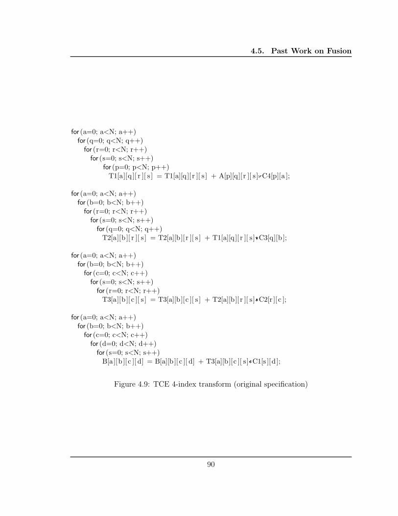
4.5. Past Work on Fusion
for (a=0; a<N; a++)for (q=0; q<N; q++)
for (r=0; r<N; r++)for (s=0; s<N; s++)
for (p=0; p<N; p++)T1[a][q ][ r ][ s ] = T1[a][q][ r ][ s ] + A[p][q][ r ][ s]*C4[p][a ];
for (a=0; a<N; a++)for (b=0; b<N; b++)
for (r=0; r<N; r++)for (s=0; s<N; s++)
for (q=0; q<N; q++)T2[a][b ][ r ][ s ] = T2[a][b][ r ][ s ] + T1[a][q][ r ][ s]*C3[q][b ];
for (a=0; a<N; a++)for (b=0; b<N; b++)
for (c=0; c<N; c++)for (s=0; s<N; s++)
for (r=0; r<N; r++)T3[a][b ][ c ][ s ] = T3[a][b][c ][ s ] + T2[a][b][ r ][ s]*C2[r ][ c ];
for (a=0; a<N; a++)for (b=0; b<N; b++)
for (c=0; c<N; c++)for (d=0; d<N; d++)
for (s=0; s<N; s++)B[a][b ][ c ][ d] = B[a][b ][ c ][ d] + T3[a][b][c ][ s]*C1[s ][d ];
Figure 4.9: TCE 4-index transform (original specification)
90
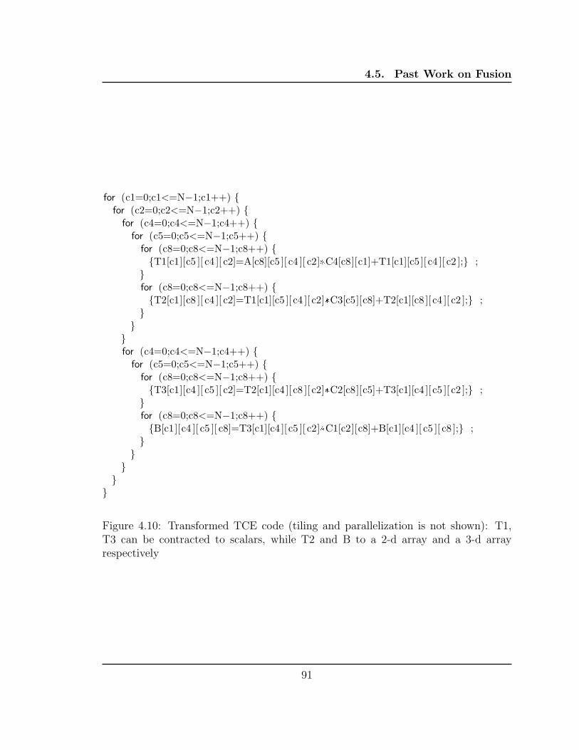
4.5. Past Work on Fusion
for (c1=0;c1<=N−1;c1++) {for (c2=0;c2<=N−1;c2++) {
for (c4=0;c4<=N−1;c4++) {for (c5=0;c5<=N−1;c5++) {
for (c8=0;c8<=N−1;c8++) {{T1[c1][c5 ][ c4 ][ c2]=A[c8][c5 ][ c4 ][ c2]*C4[c8][c1]+T1[c1][c5 ][ c4 ][ c2 ];} ;
}for (c8=0;c8<=N−1;c8++) {{T2[c1][c8 ][ c4 ][ c2]=T1[c1][c5 ][ c4 ][ c2]*C3[c5][c8]+T2[c1][c8 ][ c4 ][ c2 ];} ;
}}
}for (c4=0;c4<=N−1;c4++) {
for (c5=0;c5<=N−1;c5++) {for (c8=0;c8<=N−1;c8++) {{T3[c1][c4 ][ c5 ][ c2]=T2[c1][c4 ][ c8 ][ c2]*C2[c8][c5]+T3[c1][c4 ][ c5 ][ c2 ];} ;
}for (c8=0;c8<=N−1;c8++) {{B[c1][c4 ][ c5 ][ c8]=T3[c1][c4 ][ c5 ][ c2]*C1[c2][c8]+B[c1][c4 ][ c5 ][ c8 ];} ;
}}
}}
}
Figure 4.10: Transformed TCE code (tiling and parallelization is not shown): T1,T3 can be contracted to scalars, while T2 and B to a 2-d array and a 3-d arrayrespectively
91
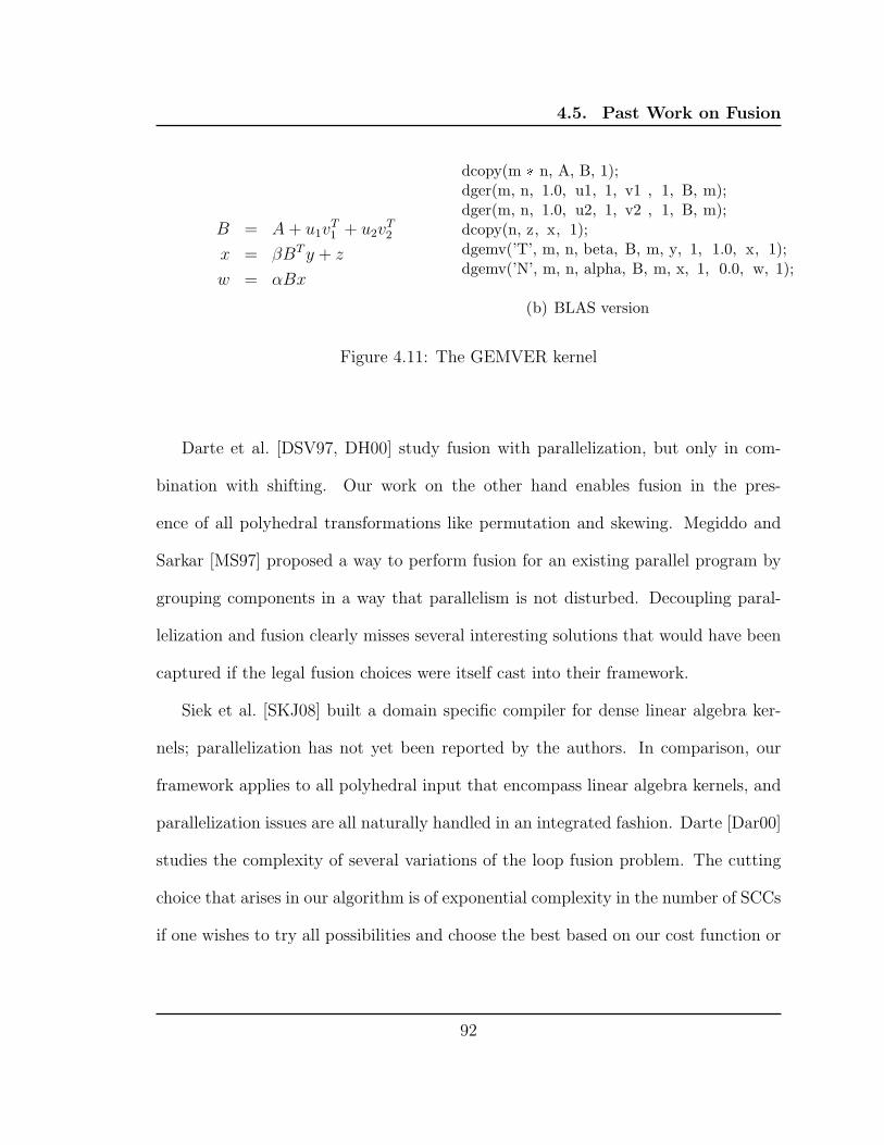
4.5. Past Work on Fusion
B = A + u1vT1 + u2v
T2
x = βBT y + z
w = αBx
dcopy(m * n, A, B, 1);dger(m, n, 1.0, u1, 1, v1 , 1, B, m);dger(m, n, 1.0, u2, 1, v2 , 1, B, m);dcopy(n, z, x, 1);dgemv(’T’, m, n, beta, B, m, y, 1, 1.0, x, 1);dgemv(’N’, m, n, alpha, B, m, x, 1, 0.0, w, 1);
(b) BLAS version
Figure 4.11: The GEMVER kernel
Darte et al. [DSV97, DH00] study fusion with parallelization, but only in com-
bination with shifting. Our work on the other hand enables fusion in the pres-
ence of all polyhedral transformations like permutation and skewing. Megiddo and
Sarkar [MS97] proposed a way to perform fusion for an existing parallel program by
grouping components in a way that parallelism is not disturbed. Decoupling paral-
lelization and fusion clearly misses several interesting solutions that would have been
captured if the legal fusion choices were itself cast into their framework.
Siek et al. [SKJ08] built a domain specific compiler for dense linear algebra ker-
nels; parallelization has not yet been reported by the authors. In comparison, our
framework applies to all polyhedral input that encompass linear algebra kernels, and
parallelization issues are all naturally handled in an integrated fashion. Darte [Dar00]
studies the complexity of several variations of the loop fusion problem. The cutting
choice that arises in our algorithm is of exponential complexity in the number of SCCs
if one wishes to try all possibilities and choose the best based on our cost function or
92

4.5. Past Work on Fusion
for ( i=0; i<N; i++)for (j=0; j<N; j++)
B[i ][ j ] = A[i][ j ] + u1[i]*v1[j ] + u2[i]*v2[j ];
for ( i=0; i<N; i++)for (j=0; j<N; j++)
x[ i ] = x[i ] + beta* B[j][ i ]*y[ j ];
for ( i=0; i<N; i++)x[ i ] = x[i ] + z[i ];
for ( i=0; i<N; i++)for (j=0; j<N; j++)
w[i ] = w[i] + alpha* B[i][ j ]*x[ j ];
Figure 4.12: GEMVER nested loop code
0
0.5
1
1.5
2
2.5
500 1K 2K 4K 8K
GFL
OPs
Problem size
GEMVER on Phenom x4 9850 (2.5 GHz)
Pluto (--smartfuse)Pluto --nofuse
ACML 4.1.0ICC -fast
Figure 4.13: GEMVER performance: preview (detailed results in Chapter 6)
93
4.5. Past Work on Fusion
any other cost model. None of our heuristics explore all possible choices, but just the
ones that seem to be interesting.
Affine scheduling-based approaches are geared towards finding minimum latency
schedules or maximum fine-grained parallelism. However, a schedule specifying maxi-
mum parallelism need not finely interleave operations of different statements. Hence,
works based on such schedules [BF03, Gri04] do not readily enable fusion.
Lim et al.’s [LCL99] affine partitioning algorithm, like our algorithm, would al-
low maximal fusion within an SCC. However, their algorithm does not enumerate or
present a choice of fusion structures across SCCs as they treat each SCC indepen-
dently. Some treatment of optimizing across two neighboring SCCs exists [LCL99]
using constraints for near-neighbor communication, but the approach as presented is
a test-and-set approach and is not automatable in general. Also, whether it is within
an SCC or across SCCs, the choice of the partitions would have the same downsides as
those described in Section 3.16 whenever communication-free partitions do not exist.
For the same reasons, their framework for array contraction [LLL01] though may be
successful in contracting arrays whenever it independent partitions can be found, it
cannot be employed when storage along an array dimension can be shrunk to a small
constant. Due to minimization of δ(~s,~t), our algorithm can enable that.
Ahmed et al. [AMP01] proposed a framework to tile imperfectly nested loops for
locality. Their embedding functions can also capture fusion. However, limitations
of their reuse distance minimization heuristic discussed in detail in Section 3.16 will
have a direct impact on the ability to find good fusions. Also, there is no procedure
to expose fusion structure choices, as is possible with our cutting schemes.
94

4.5. Past Work on Fusion
The URUK/WRAP-IT framework [CGP+05, GVB+06] can be used to manually
specify fusion and its legality can be checked. With the automatic correction scheme
proposed by Vasilache et al. [VCP07], any illegal fusion can be corrected by intro-
ducing shifts, at multiple levels if needed. However, this cannot enable, for eg., a
permute and fuse, unless the expert specifying the transformation provides the right
permutation to start with.
In this chapter, we proposed three different fusion heuristics that cover the diver-
sity in choice of available fusion structures for loop nest sequences of medium size.
Detailed experimental results are presented in Chapter 6. Overall, to the best of
our knowledge, ours is the first work to treat fusion in an integrated manner in a
transformation framework for automatic parallelization.
95
CHAPTER 5
The PLUTO Parallelization System
In this chapter, we first provide an overview of the new end-to-end parallelization
system that we developed. Then, issues involved in generation of actual tiled and par-
allel code are discussed. Lastly, some complementary post-processing transformations
are discussed.
5.1 Overview of PLUTO
The transformation framework described in Chapter 3 and Chapter 4 has been
implemented into a tool, PLUTO [Plu]. Figure 5.1 shows the entire tool-chain. We
used the scanner, parser and dependence tester from the LooPo project [loo]. We
used PipLib 1.3.6 [pip, Fea88] as the ILP solver to find lexicographic minimal solu-
tion for 3.9. Note that the parametric functionality of PIP is not utilized, so any ILP
solver can be used here. Cloog 0.14.1 [clo] was used for code generation. The trans-
formation framework takes as input, polyhedral domains and dependence polyhedra
from LooPo’s dependence tester, computes transformations and provides it to Cloog.
Compilable OpenMP parallel code is finally output after some post-processing on the
Cloog code.
96

5.1
.O
verv
iew
ofP
LU
TO
gcc/icc/xlc
Dependencepolyhedra
parallel)
sequences
Compilable
framework
transformationPluto
processingSyn. post
target codeUpdated domains
Statement−wiseaffine
Nested loop
(OpenMPand transformations
transformations
tester
LooPo
+dependence
scanner/parser tilespecifier
PolyhedralCLooG
Figu
re5.1:
The
PLU
TO
source-to-sou
rcetran
sformation
system
97

5.1. Overview of PLUTO
LooPo’s dependence tester can provide flow, anti, output, and input dependences.
However, if techniques to remove false dependences are applied, our framework can
work with those reduced set of dependences too. The removal of transitively covered
dependences is desired but not necessary, and techniques for the same exist [VBGC06,
Vas07]. LooPo’s tester employs the PIP library [Fea88] to test for the existence of an
integer solution to a system of linear equalities and inequalities. In addition, it can also
compute the last conflicting access for a given dependence that is expressed through
an affine function called the h-transformation, which gives the last source iteration
as a function of the target iteration, i.e., ~s = he(~t). The equalities representing the
h-transformation are included in the dependence polyhedron. The h-transformation
is meaningful for all but the anti-dependences (Chapter 5.2.2 of [Gri04]). For RAW
and WAW dependences, providing the h-transformation can be viewed as freeing
transitive dependences from a given dependence polyhedron.
A brief description of CLooG. The affine functions, φ or TS, are called scattering
functions in the specification of Cloog. Cloog [clo, Bas04a] can scan a union of poly-
hedra, and optionally, under a new global lexicographic ordering specified as through
scattering functions. Scattering functions are specified statement-wise, and the legal-
ity of scanning the polyhedron with these dimensions in the particular order should
be guaranteed by the specifier – an automatic transformation system in our case.
The code generator does not have any information on the dependences and hence, in
the absence of any scattering functions would scan the union of the statement poly-
hedra in the global lexicographic order of the original iterators (statement instances
98

5.2. Tiled Code Generation under Transformations
are interleaved). Cloog uses Quillere separation [QRW00] with several improvements
made by Bastoul [Bas04a]. Its operations are based on PolyLib [Wil93, pol], which
in turn uses the Chernikova algorithm [LeV92]) to move between the vertex form of
a polyhedron and its face form [Wil93]. The Chernikova algorithm is guaranteed to
give an irredundant set of linear inequalities from the vertex form. The code gener-
ated is more efficient than that by older code generators based on Fourier-Motzkin
variable elimination like Omega Codegen [KPR95] or LooPo’s internal code genera-
tor [GLW98, Gri04]). Also, code generation time and memory utilization are much
lower [Bas04a] besides making it feasible for cases it was earlier thought not to be.
Such a powerful and efficient code generator is essential in conjunction with the trans-
formation framework we developed. When tiling is expressed with the transformations
we compute, generating code is a challenging task. In particular, Cloog’s ability to
optimize control for user-desired levels (-f/-l options) – trading code size with condi-
tional depth control make code generation feasible in the presence of a large number
of statements or under complex transformations for coarse-grained parallelization.
5.2 Tiled Code Generation under Transformations
In this section, we describe how tiled code is generated from transformations found
by the algorithm in the previous chapter. This is an important step in generation of
high performance code.
99
5.2. Tiled Code Generation under Transformations
5.2.1 Syntactic tiling versus tiling scattering functions
Before proceeding further, we differentiate between using the term ‘tiling’ for, (1)
modeling and enabling tiling through a transformation framework (as was described
in the previous chapter), (2) final generation of tiled code from the hyperplanes found.
Both are generally referred to as tiling. Our approach models tiling in the transfor-
mation framework by finding affine transformations that make rectangular tiling in
the transformed space legal. The hyperplanes found are the new basis for the loops
in the transformed space and have special properties that have been detected when
the transformation is found – e.g. being parallel, sequential or belonging to a band
of loops that can now be rectangularly tiled. Hence, the transformation framework
guarantees legality of rectangular tiling in the new space. The final generation of
tiled loops can be done in two ways broadly, (1) directly through the polyhedral code
generator itself in one pass itself, or (2) as a post-pass on the abstract syntax tree
generated after applying the transformation. Each has its merits and both can be
combined too.
For transformations that possibly lead to imperfectly nested code, tiling the scat-
tering functions is a natural way to get tiled code in one pass through the code gen-
erator. Consider the code in Figure 5.2.2(a) for example. If code is generated by just
applying the transformation first, we get code shown in Figure 5.2.2(b). Even though
the transformation framework obtained two tiling hyperplanes, the transformed code
in Figure 5.2.2(b) has no 2-d perfectly nested kernel, and tiling it syntactically is
illegal (fully distributing the two statements is also legal). The legality of syntactic
100

5.2. Tiled Code Generation under Transformations
tiling or unroll/jam (for register tiling) of such loops cannot be reasoned about in the
target AST easily since we are typically out of the polyhedral model once we obtain
the loop nests. We describe in the next section how tiled code can be obtained in
one pass through the code generator by just updating the domains and scattering
functions without knowing anything about the AST. For example, for the code in
Figure 5.2.2(a), 2-d tiled code generated would be as shown in Figure 5.3.
5.2.2 Tiles under a transformation
Our approach to tiling is to specify a modified higher dimensional domain and
specify transformations for what would be the tile space loops in the transformed
space. Consider a very simple example: a two-dimensional loop nest with original
iterators: i and j. Let the transformation found be c1 = i, and c2 = i + j, with c1,
c2 constituting a permutable band; hence, they can be blocked leading to 2-d tiles.
We would like to obtain target code that is tiled rectangularly along c1 and c2. The
domain supplied to the code generator is a higher dimensional domain with the tile
shape constraints like that proposed by Ancourt and Irigoin [AI91]; but the scatterings
are duplicated for the tile space too. ‘T’ subscript is used to denote the corresponding
tile space iterator. The tile space and intra tile loop scattering functions are specified
101

5.2. Tiled Code Generation under Transformations
as follows. The new domain is given by:
0 ≤ i ≤ N − 1
0 ≤ j ≤ N − 1
0 ≤ i − 32iT ≤ 31
0 ≤ (i + j) − 32(iT + jT ) ≤ 31
The scattering function is given by: (c1T , c2T , c3T , c1, c2, c3) = (iT , iT + jT , i, i + j)
Algorithm 3 Tiling for multiple statements under transformations
INPUT Hyperplanes (statement-wise) belonging to a tilable band of width k:φi
S, φi+1
S , . . . , φi+k−1
S ; original domains: DS; tile sizes: τi, τi+1, . . . , τi+k−1
1: /* Update the domains */2: for each statement S do3: for each φ
jS = f j(~iS) + f0 do
4: Increase the domain (DS) dimensionality by creating supernodes for all orig-inal iterators that appear in φ
jS
5: Let the supernode iterators be ~iT6: Add the following two constraints to DS:
τj ∗ f j(~iTS) ≤ f j(~iS) + f
j0
f j(~iS) + fj0 ≤ τj ∗ f j(~iTS
) + τj − 17: end for8: end for9: /* Update the transformation functions */
10: for each statement S do11: Add k new rows to the transformation of S at level i
12: Add as many columns as the number of supernodes added to DS in Step 413: for each φ
jS = f j(~iS) + f
j0 , j = i, . . . , i + k − 1 do
14: Create a supernode: φjTS
= f j(~iTS)
15: end for16: end forOUTPUT Updated domains (DS) and transformations
102
5.2. Tiled Code Generation under Transformations
The higher-dimensional tile space loops are referred to as supernodes in the de-
scription. iT , jT are supernodes in the original domain, while c1T , c2T are supernodes
in the transformed space. We will refer to the latter as scattering supernodes. With
this, we formally state the algorithm to update the domains and transformations
(Algorithm 3).
Theorem 4. The set of scattering supernodes, φiTS
, φi+1
TS, . . . , φi+k−1
TSobtained from
Algorithm 3 satisfy the tiling legality condition (3.3)
Since, φjS, i ≤ j ≤ i + k − 1 satisfy (3.3) and since the supernodes step through
an aggregation of parallel hyperplane instances, dependences have non-negative com-
ponents along the scattering supernode dimensions too. This holds true for both
intra and inter-statement dependences. {φjTS1
, φjTS2
, . . . , φjTSn
} thus represent a com-
mon supernode dimension in the transformed space with the same property as that
of {φjS1
, φjS2
, . . . , φjSn}. 2
Figure 5.2.2 shows tiles for imperfectly nested 1-d Jacobi. Note that tiling it
requires shifting S2 by one and skewing the space loops by a factor of two with
respect to time, as opposed to skewing by a factor of one that is required for the
single-assignment perfectly nested variant in Figure 5.2.2(a). The update statement
causes the increase in skewing factor. Figure 5.3 shows the tiled code. One can
notice a 2-d perfectly nested hotspot in the code which corresponds to the so-called
full tiles shown in Figure 5.2.2. Such a perfectly nested hotspot gets separated out
from the imperfectly nested code. Further optimizations like register tiling can be
performed on this portion of the code syntactically. Alternatively, separation of such
103

5.2. Tiled Code Generation under Transformations
a full tile can also be accomplished with much more compact code by modifying the
code generator itself [KRSR07].
Example: 3-d tiles for LU The transformation obtained for the LU decomposi-
tion code shown in Figure 5.7 is:
TS1
c1
c2
c3
=
1 00 11 0
(k
j
)
TS2
c1
c2
c3
=
1 0 00 0 10 1 0
k
i
j
Hyperplanes c1, c2 and c3 are identified as belonging to one tilable band. The
domains are specified as:
S1 S20 ≤ k ≤ N − 1 0 ≤ k ≤ N − 1
k + 1 ≤ j ≤ N − 1 k + 1 ≤ i ≤ N − 1k + 1 ≤ j ≤ N − 1
0 ≤ k − 32kT ≤ 31 0 ≤ k − 32kT ≤ 310 ≤ j − 32jT ≤ 31 0 ≤ i − 32iT ≤ 31
0 ≤ j − 32jT ≤ 31
The scattering functions for S1 and S2 are given by:
TS1 : (c1T , c2T , c3T , c1, c2, c3) = (kT , jT , kT , k, j, k)
TS2 : (c1T , c2T , c3T , c1, c2, c3) = (kT , jT , iT , k, j, i)
The tiled code after applying the parallelization technique described in the next sub-
section is shown in the next chapter (Figure 6.8).
Tiling multiple times. The same tiling hyperplanes can be used to tile multiple
times (due to Theorem 4), for registers, L1, L2 caches, and for parallelism, and the
legality of the same is guaranteed by the transformation framework. The scattering
functions are duplicated for each such level as it was done for one level. Such a
104

5.2. Tiled Code Generation under Transformations
for (t=0; t<T; t++) {for ( i=2; i<N−1; i++) {
b[ i ] = 0.333*(a[i−1] + a[i] + a[i+1]);}for (j=2; j<N−1; j++){
a[ j ] = b[j ];}
}
(a) Original code
for (c1=0;c1<=T−1;c1++) {b[2]=0.333*(a[1+2]+a[2]+a[2 −1]);for (c2=2*c1+3;c2<=2*c1+N−2;c2++) {
b[−2*c1+c2] = 0.333*(a[1+−2*c1+c2]+a[−2*c1+c2]+a[−2*c1+c2−1]);
a[−2*c1+c2−1]=b[−2*c1+c2−1];}a[N−2]=b[N−2];
}
(b) Transformed (before tiled code generation)context N >= 5
Ts1
(t
i
)
=
1 02 10 0
(t
i
)
Ts2
(t
j
)
==
1 02 10 0
(t
j
)
+
011
φ2
φ1
N+2*T+1
T φ3 b b b b b b b b b b b b
b b b b b b b b b b b b
b b b b b b b b b b b b
b b b b b b b b b b b b
b b b b b b b b b b b b
b b b b b b b b b b b bbc bc bc bc bc bc bc bc bc bc bc bc
bc bc bc bc bc bc bc bc bc bc bc bc
bc bc bc bc bc bc bc bc bc bc bc bc
bc bc bc bc bc bc bc bc bc bc bc bc
bc bc bc bc bc bc bc bc bc bc bc bc
bc bc bc bc bc bc bc bc bc bc bc bc
b Instances of S1bc Instances of S2rs A tile
0 1 2 3 4 5 6 7 8 9 10 11 12 13 14 15 16 17 18 19 20 21
1
2
3
4
Indexing base changed to (1,1) for convenient display
(c) Tiles in the transformed space
Figure 5.2: Imperfectly nested Jacobi stencil: tiling
105
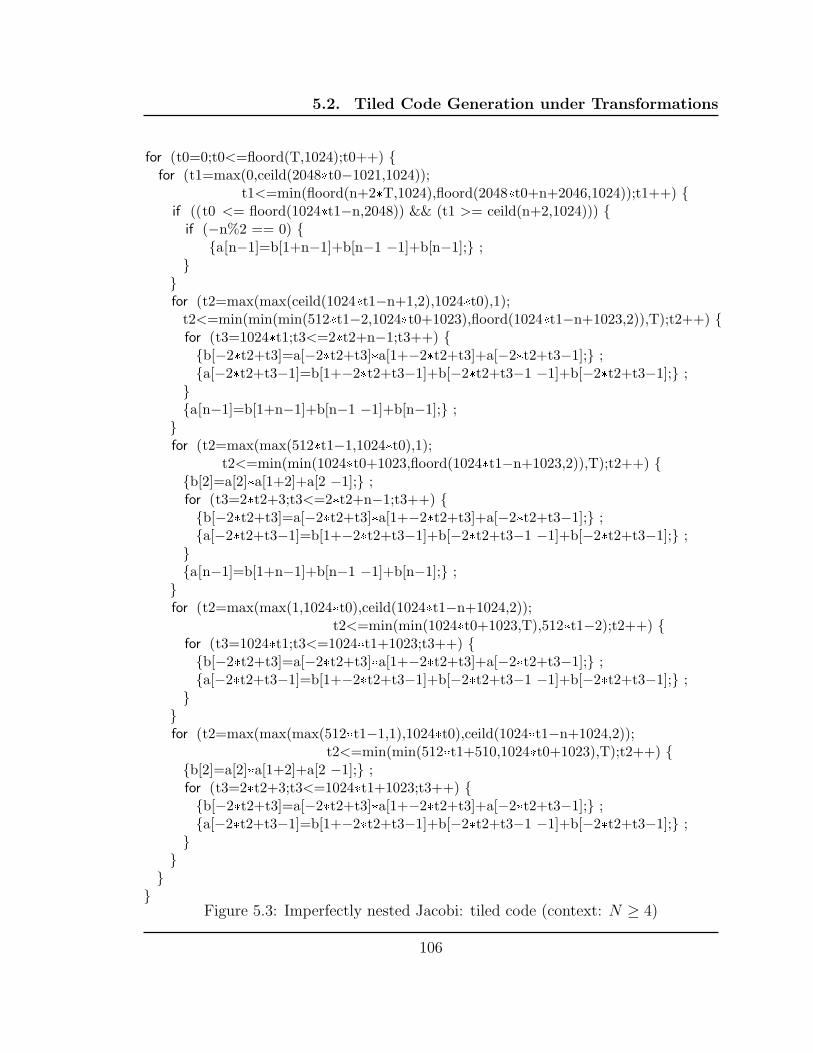
5.2. Tiled Code Generation under Transformations
for (t0=0;t0<=floord(T,1024);t0++) {for (t1=max(0,ceild(2048*t0−1021,1024));
t1<=min(floord(n+2*T,1024),floord(2048*t0+n+2046,1024));t1++) {if ((t0 <= floord(1024*t1−n,2048)) && (t1 >= ceild(n+2,1024))) {
if (−n%2 == 0) {{a[n−1]=b[1+n−1]+b[n−1 −1]+b[n−1];} ;
}}for (t2=max(max(ceild(1024*t1−n+1,2),1024*t0),1);
t2<=min(min(min(512*t1−2,1024*t0+1023),floord(1024*t1−n+1023,2)),T);t2++) {for (t3=1024*t1;t3<=2*t2+n−1;t3++) {{b[−2*t2+t3]=a[−2*t2+t3]*a[1+−2*t2+t3]+a[−2*t2+t3−1];} ;{a[−2*t2+t3−1]=b[1+−2*t2+t3−1]+b[−2*t2+t3−1 −1]+b[−2*t2+t3−1];} ;
}{a[n−1]=b[1+n−1]+b[n−1 −1]+b[n−1];} ;
}for (t2=max(max(512*t1−1,1024*t0),1);
t2<=min(min(1024*t0+1023,floord(1024*t1−n+1023,2)),T);t2++) {{b[2]=a[2]*a[1+2]+a[2 −1];} ;for (t3=2*t2+3;t3<=2*t2+n−1;t3++) {{b[−2*t2+t3]=a[−2*t2+t3]*a[1+−2*t2+t3]+a[−2*t2+t3−1];} ;{a[−2*t2+t3−1]=b[1+−2*t2+t3−1]+b[−2*t2+t3−1 −1]+b[−2*t2+t3−1];} ;
}{a[n−1]=b[1+n−1]+b[n−1 −1]+b[n−1];} ;
}for (t2=max(max(1,1024*t0),ceild(1024*t1−n+1024,2));
t2<=min(min(1024*t0+1023,T),512*t1−2);t2++) {for (t3=1024*t1;t3<=1024*t1+1023;t3++) {{b[−2*t2+t3]=a[−2*t2+t3]*a[1+−2*t2+t3]+a[−2*t2+t3−1];} ;{a[−2*t2+t3−1]=b[1+−2*t2+t3−1]+b[−2*t2+t3−1 −1]+b[−2*t2+t3−1];} ;
}}for (t2=max(max(max(512*t1−1,1),1024*t0),ceild(1024*t1−n+1024,2));
t2<=min(min(512*t1+510,1024*t0+1023),T);t2++) {{b[2]=a[2]*a[1+2]+a[2 −1];} ;for (t3=2*t2+3;t3<=1024*t1+1023;t3++) {{b[−2*t2+t3]=a[−2*t2+t3]*a[1+−2*t2+t3]+a[−2*t2+t3−1];} ;{a[−2*t2+t3−1]=b[1+−2*t2+t3−1]+b[−2*t2+t3−1 −1]+b[−2*t2+t3−1];} ;
}}
}}
Figure 5.3: Imperfectly nested Jacobi: tiled code (context: N ≥ 4)
106

5.2. Tiled Code Generation under Transformations
guarantee is available even when syntactic tiling is to be done as a post-pass on a
perfectly nest band in the target AST.
5.2.3 Pipelined parallel code generation
Once the algorithm in Sec. 5.2.2 is applied, outer parallel or inner parallel loops
can be readily marked parallel (for example with OpenMP pragmas). However, unlike
scheduling-based approaches, since we find tiling hyperplanes and the outer ones are
used as space, one or more of the space loops may have dependences along them.
Tiles created from an outermost band of tiling hyperplanes are to be scheduled ap-
propriately.
Algorithm 4 Code generation for tiled pipelined parallelism
INPUT Given that Algorithm 3 has been applied, a set of k (statement-wise) su-pernodes in the transformed space belonging to a tilable band: φ1
TS, φ2
TS, . . . , φk
TS
1: To extract m (< k) degrees of pipelined parallelism:2: /* Update transformation functions */3: for each statement S do4: Perform the following unimodular transformation on only the scattering su-
pernodes: φ1T → φ1
T + φ2T + · · · + φm+1
T
5: Mark φ2T , φ3
T , . . . , φm+1
T as parallel6: Leave φ1
T , φm+2
T , . . . , φkT as sequential
7: end forOUTPUT Updated transformation functions and scatterings
Treating pipelined parallelism as inner parallelism: For pipelined parallel
codes, our approach to generate coarse-grained (tiled) shared memory parallel code
is as described in Figure 4. Once the technique described in the previous section is
107
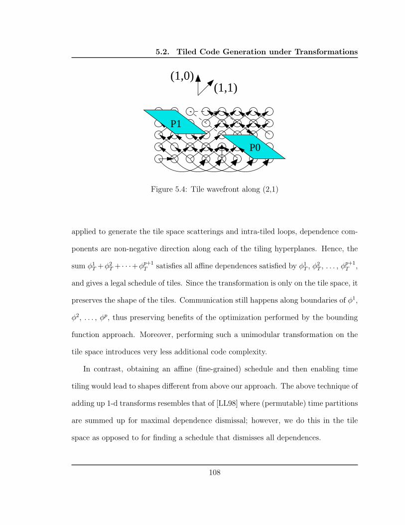
5.2. Tiled Code Generation under Transformations
P1
P0
(1,1)(1,0)
Figure 5.4: Tile wavefront along (2,1)
applied to generate the tile space scatterings and intra-tiled loops, dependence com-
ponents are non-negative direction along each of the tiling hyperplanes. Hence, the
sum φ1T +φ2
T + · · ·+φp+1
T satisfies all affine dependences satisfied by φ1T , φ2
T , . . . , φp+1
T ,
and gives a legal schedule of tiles. Since the transformation is only on the tile space, it
preserves the shape of the tiles. Communication still happens along boundaries of φ1,
φ2, . . . , φp, thus preserving benefits of the optimization performed by the bounding
function approach. Moreover, performing such a unimodular transformation on the
tile space introduces very less additional code complexity.
In contrast, obtaining an affine (fine-grained) schedule and then enabling time
tiling would lead to shapes different from above our approach. The above technique of
adding up 1-d transforms resembles that of [LL98] where (permutable) time partitions
are summed up for maximal dependence dismissal; however, we do this in the tile
space as opposed to for finding a schedule that dismisses all dependences.
108
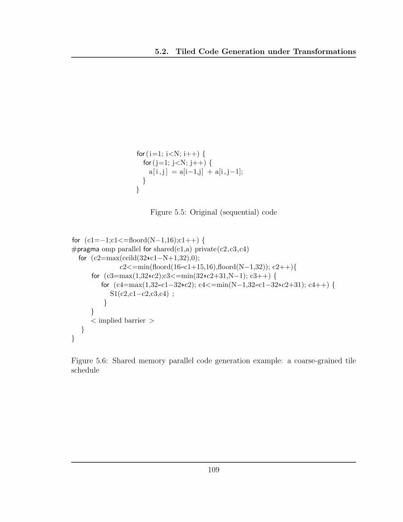
5.2. Tiled Code Generation under Transformations
for ( i=1; i<N; i++) {for (j=1; j<N; j++) {
a[ i , j ] = a[i−1,j] + a[i , j−1];}
}
Figure 5.5: Original (sequential) code
for (c1=−1;c1<=floord(N−1,16);c1++) {#pragma omp parallel for shared(c1,a) private(c2,c3,c4)
for (c2=max(ceild(32*c1−N+1,32),0);c2<=min(floord(16*c1+15,16),floord(N−1,32)); c2++){
for (c3=max(1,32*c2);c3<=min(32*c2+31,N−1); c3++) {for (c4=max(1,32*c1−32*c2); c4<=min(N−1,32*c1−32*c2+31); c4++) {
S1(c2,c1−c2,c3,c4) ;}
}< implied barrier >
}}
Figure 5.6: Shared memory parallel code generation example: a coarse-grained tileschedule
109
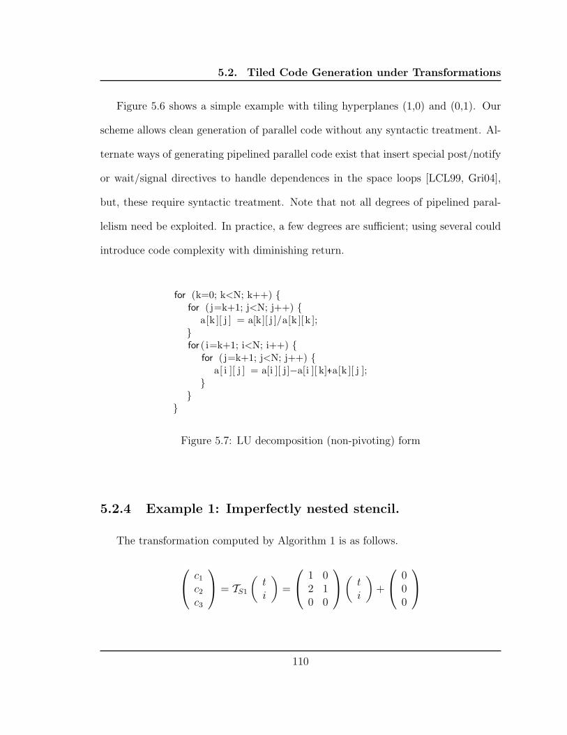
5.2. Tiled Code Generation under Transformations
Figure 5.6 shows a simple example with tiling hyperplanes (1,0) and (0,1). Our
scheme allows clean generation of parallel code without any syntactic treatment. Al-
ternate ways of generating pipelined parallel code exist that insert special post/notify
or wait/signal directives to handle dependences in the space loops [LCL99, Gri04],
but, these require syntactic treatment. Note that not all degrees of pipelined paral-
lelism need be exploited. In practice, a few degrees are sufficient; using several could
introduce code complexity with diminishing return.
for (k=0; k<N; k++) {for (j=k+1; j<N; j++) {
a[k ][ j ] = a[k][ j ]/a[k ][ k ];}for ( i=k+1; i<N; i++) {
for (j=k+1; j<N; j++) {a[ i ][ j ] = a[i ][ j]−a[i ][ k]*a[k ][ j ];
}}
}
Figure 5.7: LU decomposition (non-pivoting) form
5.2.4 Example 1: Imperfectly nested stencil.
The transformation computed by Algorithm 1 is as follows.
c1
c2
c3
= TS1
(t
i
)
=
1 02 10 0
(t
i
)
+
000
110

5.2. Tiled Code Generation under Transformations
c1
c2
c3
= TS2
(t
j
)
=
1 02 10 0
(t
j
)
+
011
The transformation is updated to the following for generation of locally tiled code.
TS1
tTiTt
i
1
=
1 0 0 0 02 1 0 0 00 0 1 0 00 0 2 1 00 0 0 0 0
tTiTt
i
1
TS2
tTjT
t
j
1
=
1 0 0 0 02 1 0 0 00 0 1 0 00 0 2 1 10 0 0 0 1
tTjT
t
j
1
After applying Algorithm 4, the transformation for generation of parallelized and
locally tiled code will be the following with the second hyperplane marked parallel.
TS1 :
tTiTt
i
1
=
3 1 0 0 02 1 0 0 00 0 1 0 00 0 2 1 00 0 0 0 0
tTiTt
i
1
TS2 :
tTjT
t
j
1
=
3 1 0 0 02 1 0 0 00 0 1 0 00 0 2 1 10 0 0 0 1
tTjT
t
j
1
(5.1)
5.2.5 Example 2: LU
For the LU decomposition code in Fig. 5.7, we show how the transformations are
updated to obtain one degree or two degrees of pipelined parallelism. The trans-
formations for S1 and S2 after the tiling for 1-d pipelined parallelism is expressed
111

5.3. Preventing Code Expansion in Tile Space
are:
TS1 :
c1
c2
c3
c4
c5
c6
=
1 1 0 00 1 0 01 0 0 00 0 1 00 0 0 10 0 1 0
kT
jT
k
j
TS2 :
c1
c2
c3
c4
c5
c6
=
1 0 1 0 0 00 0 1 0 0 00 1 0 0 0 00 0 0 1 0 00 0 0 0 0 10 0 0 0 1 0
kT
iTjT
k
i
j
The loop c2 is marked OpenMP parallel. If one wishes to extract two degrees of
pipelined parallelism, the transformation would be the following, with loops c2 and
c3 are marked OpenMP parallel.
TS1 :
c1
c2
c3
c4
c5
c6
=
2 1 0 00 1 0 01 0 0 00 0 1 00 0 0 10 0 1 0
kT
jT
k
j
TS2 :
c1
c2
c3
c4
c5
c6
=
1 1 1 0 0 00 0 1 0 0 00 1 0 0 0 00 0 0 1 0 00 0 0 0 0 10 0 0 0 1 0
kT
iTjT
k
i
j
5.3 Preventing Code Expansion in Tile Space
The overhead of floor and ceil operations as well as conditionals in the tile-space
loops (at the outer levels) is insignificant. Hence, we would like to have compact code
112

5.4. Tilability Detection and Parallelism Detection
at the outer level while allowing code expansion in the intra-tile loops to decrease
control complexity. This improves performance while keeping the code size under
control.
Using the default options with tiling specified as described leads to significant
code expansion since the transformed space we are tiling is a shifted and skewed
space. Preventing any code expansion at all leads to an if condition in the innermost
loop, resulting in very low performance. However, optimizing only the intra-tile loops
for control is very effective. It also avoids large numbers in the intermediate operations
performed by code generators, that could possibly lead to PolyLib exceptions for large
tile sizes or deep loop nest tiling. Table 5.1 shows the sensitivity in performance for
the code in Figure 5.2.2.
Cloog options Code size Codegen Execution Improvement(lines) time time over ‘icc -fast’
Full code expansion 2226 1.84s 2.57s 2.7xOnly intra-tile expansion 40 0.04s 1.6s 4.3x
No code expansion 15 0.01s 17.6s 0.39x
Table 5.1: Performance sensitivity of L1-tiled imperfectly nested stencil code withCloog options: N = 106, T = 1000, tile dimensions: 2048 × 2048
5.4 Tilability Detection and Parallelism Detection
Our algorithm naturally transforms to hierarchy of tilable loop nest sets. The
outermost band can be taken and used for coarse-grained parallelization using the
scheme proposed in Sec. 5.2.3.
113
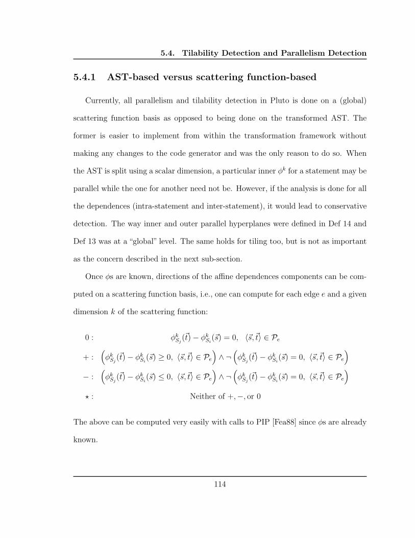
5.4. Tilability Detection and Parallelism Detection
5.4.1 AST-based versus scattering function-based
Currently, all parallelism and tilability detection in Pluto is done on a (global)
scattering function basis as opposed to being done on the transformed AST. The
former is easier to implement from within the transformation framework without
making any changes to the code generator and was the only reason to do so. When
the AST is split using a scalar dimension, a particular inner φk for a statement may be
parallel while the one for another need not be. However, if the analysis is done for all
the dependences (intra-statement and inter-statement), it would lead to conservative
detection. The way inner and outer parallel hyperplanes were defined in Def 14 and
Def 13 was at a “global” level. The same holds for tiling too, but is not as important
as the concern described in the next sub-section.
Once φs are known, directions of the affine dependences components can be com-
puted on a scattering function basis, i.e., one can compute for each edge e and a given
dimension k of the scattering function:
0 : φkSj
(~t) − φkSi
(~s) = 0, 〈~s,~t〉 ∈ Pe
+ :(
φkSj
(~t) − φkSi
(~s) ≥ 0, 〈~s,~t〉 ∈ Pe
)
∧ ¬(
φkSj
(~t) − φkSi
(~s) = 0, 〈~s,~t〉 ∈ Pe
)
− :(
φkSj
(~t) − φkSi
(~s) ≤ 0, 〈~s,~t〉 ∈ Pe
)
∧ ¬(
φkSj
(~t) − φkSi
(~s) = 0, 〈~s,~t〉 ∈ Pe
)
⋆ : Neither of +,−, or 0
The above can be computed very easily with calls to PIP [Fea88] since φs are already
known.
114
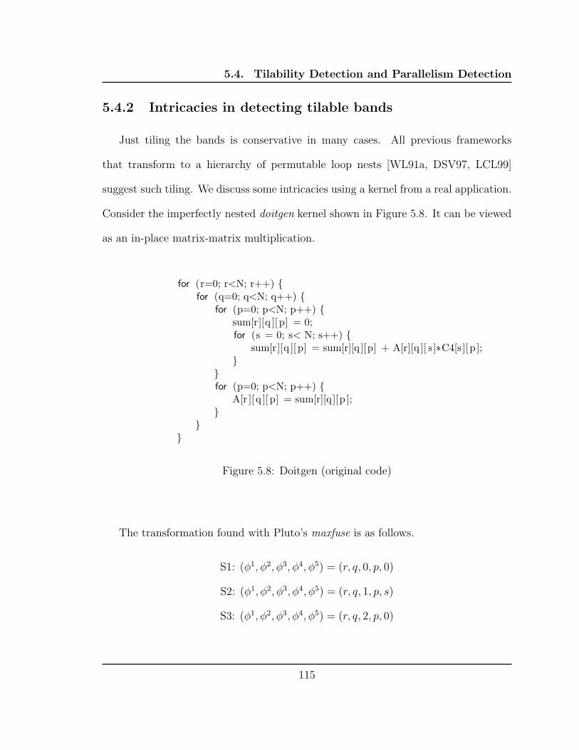
5.4. Tilability Detection and Parallelism Detection
5.4.2 Intricacies in detecting tilable bands
Just tiling the bands is conservative in many cases. All previous frameworks
that transform to a hierarchy of permutable loop nests [WL91a, DSV97, LCL99]
suggest such tiling. We discuss some intricacies using a kernel from a real application.
Consider the imperfectly nested doitgen kernel shown in Figure 5.8. It can be viewed
as an in-place matrix-matrix multiplication.
for (r=0; r<N; r++) {for (q=0; q<N; q++) {
for (p=0; p<N; p++) {sum[r][q ][ p] = 0;for (s = 0; s< N; s++) {
sum[r][q ][ p] = sum[r][q][p] + A[r][q ][ s]*C4[s ][p ];}
}for (p=0; p<N; p++) {
A[r ][ q ][ p] = sum[r][q][p ];}
}}
Figure 5.8: Doitgen (original code)
The transformation found with Pluto’s maxfuse is as follows.
S1: (φ1, φ2, φ3, φ4, φ5) = (r, q, 0, p, 0)
S2: (φ1, φ2, φ3, φ4, φ5) = (r, q, 1, p, s)
S3: (φ1, φ2, φ3, φ4, φ5) = (r, q, 2, p, 0)
115

5.4. Tilability Detection and Parallelism Detection
The direction vectors based on the affine dependence components can now be
written as:
Dependence Affine component directionS1 → S2 (0, 0, +, 0, +)S2 → S2 (0, 0, 0, 0, +)S1 → S3 (0, 0, +, 0, 0)S2 → S3 (0, 0, +, 0,−)S2 → S2 (0, 0, 0, 0, +)S2 → S3 (0, 0, +,−,−)S1 → S2 (0, 0, +, 0, +)S2 → S2 (0, 0, 0, 0, +)
Standard tiling based on identifying hierarchies of tilable bands would treat (φ1,φ2)
as one band and (φ4,φ5) as another. Note that φ3 is a scalar dimension. So the tiled
space for S2 would be given by:
(rT , qT , r, q, 1, pT, sT, p, s)
The above does not create true 4-d tiles for S2. However, the surprising good tiling
here is given by:
S1: (rT , qT , 0, pT , 0, r, q, p, 0)S2: (rT , qT , 1, pT , sT , r, q, p, s)S3: (rT , qT , 2, pT , 0, r, q, p, 0)
Here, it is legal to move the two outer loops all the way inside since the dependences
that have negative components on c4 and c5 are satisfied at the scalar dimension
c3. Hence, we have an additional consideration of ignoring negative directions for
dependences that have been satisfied at a scalar dimension, since the scalar dimension
can be preserved at the third level even in the tiled code. This “trick” is very useful in
tiling several codes that would otherwise come out as untilable or not tilable with any
good benefit. Pluto’s detection can take care of the above. The tiled code is shown in
116
5.5. Setting Tile Sizes
Figure 5.9. Figure 5.10 compares the performance of the transformed code with the
version written with BLAS calls. More detailed performance results are presented in
Chapter 6.
It would also be useful to note that the following tiling would be illegal as some
values of A will been overwritten before they are finished using.
S1: (rT, qT, 0, pT, 0, r, q, 0, p, 0)S2: (rT, qT, 0, pT, sT, r, q, 1, p, s)S3: (rT, qT, 0, pT, 0, r, q, 2, p, 0)
In this case, the scalar dimension has no longer been preserved and has been consid-
ered as part of the tilable band violating the inter-statement dependences between
S2 and S3.
5.5 Setting Tile Sizes
With our approach, tile sizes can be set in a decoupled manner as the shapes have
been captured with TS. Pluto currently uses very rough thumb rules based on array
dimensionalities to set tile sizes. In addition, custom tile sizes can be forced by the
user easily through a separate file. By decoupling tile shape and size optimization,
not only is the transformation framework’s objective function kept linear, but also is
the possibility of employing stronger cost models to determine tile sizes for locality
opened. Techniques to efficiently count integer points in parametrized polytopes exist:
[VSB+07] is the state-of-the-art approach that employs Barvinok’s rational functions
for this purpose and has been implemented into a library. It is straightforward to
obtain the polyhedra corresponding to the points in the data space that are touched
by a tile [BBK+08b]. Once this is done and the cache sizes are known, [VSB+07]
117
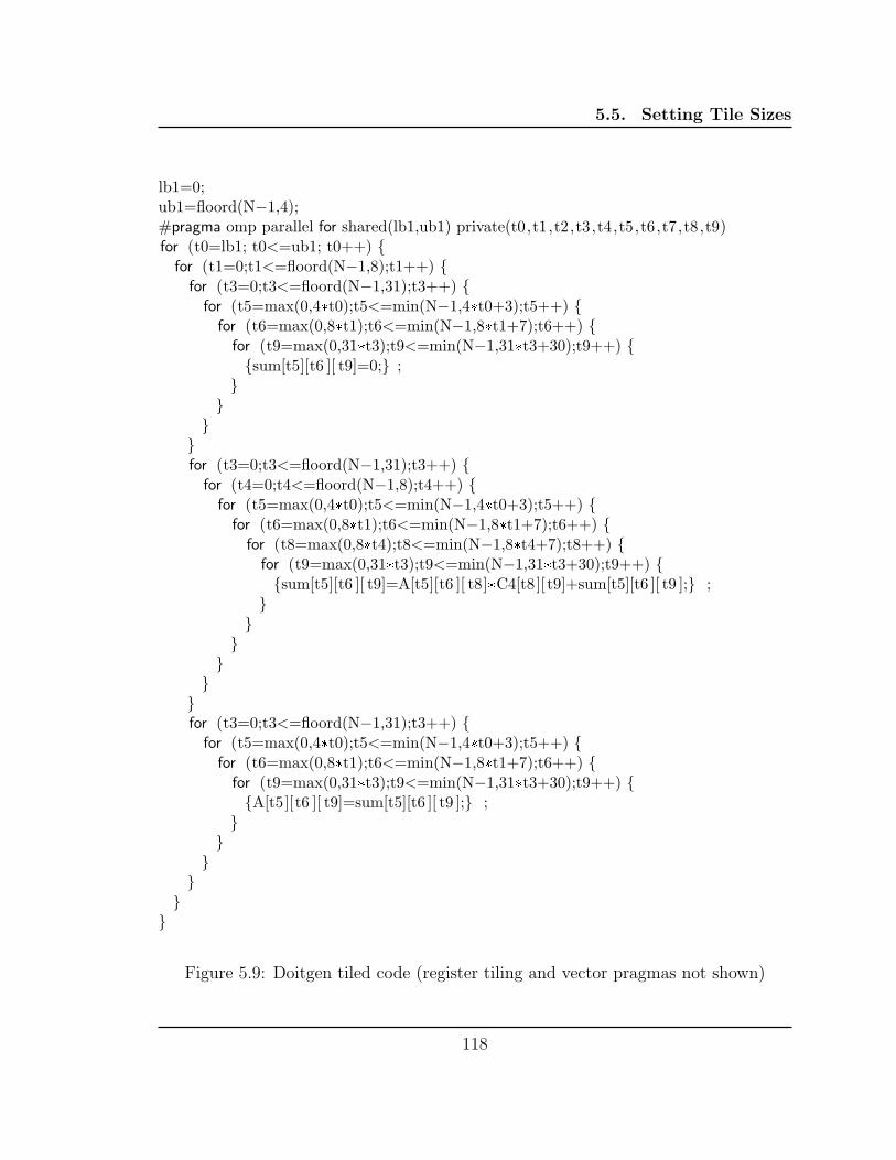
5.5. Setting Tile Sizes
lb1=0;ub1=floord(N−1,4);#pragma omp parallel for shared(lb1,ub1) private(t0,t1,t2,t3,t4,t5,t6,t7,t8,t9)for (t0=lb1; t0<=ub1; t0++) {
for (t1=0;t1<=floord(N−1,8);t1++) {for (t3=0;t3<=floord(N−1,31);t3++) {
for (t5=max(0,4*t0);t5<=min(N−1,4*t0+3);t5++) {for (t6=max(0,8*t1);t6<=min(N−1,8*t1+7);t6++) {
for (t9=max(0,31*t3);t9<=min(N−1,31*t3+30);t9++) {{sum[t5][t6 ][ t9]=0;} ;
}}
}}for (t3=0;t3<=floord(N−1,31);t3++) {
for (t4=0;t4<=floord(N−1,8);t4++) {for (t5=max(0,4*t0);t5<=min(N−1,4*t0+3);t5++) {
for (t6=max(0,8*t1);t6<=min(N−1,8*t1+7);t6++) {for (t8=max(0,8*t4);t8<=min(N−1,8*t4+7);t8++) {
for (t9=max(0,31*t3);t9<=min(N−1,31*t3+30);t9++) {{sum[t5][t6 ][ t9]=A[t5][t6 ][ t8]*C4[t8][ t9]+sum[t5][t6 ][ t9 ];} ;
}}
}}
}}for (t3=0;t3<=floord(N−1,31);t3++) {
for (t5=max(0,4*t0);t5<=min(N−1,4*t0+3);t5++) {for (t6=max(0,8*t1);t6<=min(N−1,8*t1+7);t6++) {
for (t9=max(0,31*t3);t9<=min(N−1,31*t3+30);t9++) {{A[t5][t6 ][ t9]=sum[t5][t6 ][ t9 ];} ;
}}
}}
}}
Figure 5.9: Doitgen tiled code (register tiling and vector pragmas not shown)
118

5.5. Setting Tile Sizes
0
1
2
3
4
5
10 15 20 25 31
GF
LOP
s
Problem size
doitgen perf on Intel Core2 Q6600
Pluto (--maxfuse)Pluto --nofuse/--smartfuse
ICC -fastIntel MKL (dgemv)
(a) Single core
0
2
4
6
8
10
1 2 3 4
GF
LOP
s
Cores
doitgen parallel perf (N=25) Intel Core2 Quad Q6600 (2.4 GHz)
Pluto --maxfusePluto --nofuse/--smartfuse
doitgen (Intel MKL dgemm)doitgen (Intel MKL dgemv)
ICC -parallel -fast
(b) Parallel: N = 25
Figure 5.10: Doitgen performance on an Intel Core 2 Quad: preview
119
5.5. Setting Tile Sizes
may be used to deduce tile sizes. We intend to explore the effectiveness of such an
approach.
Tile sizes for parallelism. The OpenMP“parallel for”directive(s) typically achieves
block distribution of iterations of tile space loops among processor cores. Hence,
whenever there is outer parallelism or pure inner parallelism, there is no special
need to compute another set of tile sizes for parallelism, unless one wants to sched-
ule tiles in a block cyclic manner. However, just performing block distribution
is better for inter-tile reuse. Execution on each core is a sequence of L2 tiles or
L1 tiles if no L2 tiling is done. However, whenever no synchronization-free paral-
lelism exists, tile sizes for parallelism affect pipelined startup cost, load balance, and
the number of synchronizations. There is a trade-off between the former two and
the latter. This problem has been studied extensively, but for very restrictive in-
put [ABRY03, BDRR94, HS02, HCF97, HCF99, SD90]. Clearly, the right tile sizes
here are a function of the problem size and the number of processors, and leaving tile
sizes as parameters in the final generated code is necessary for any scheme to succeed.
The approach we described in this chapter is for fixed tile sizes, and extension to
parametric ones [RKRS07] is needed. Meanwhile, just setting conservative L2 tile
sizes or not performing L2 tiling for smaller problem sizes seems to be a reasonable
approach in practice. This avoids load imbalance and possibly incurs higher number
of synchronizations than the optimal solution. This is however not likely to be a big
issue since coarse-enough parallelism has already been achieved making it a case of
diminishing return. Given the large size of L2 caches on current processors, for small
120
5.6. Post-processing Transformations
problem sizes, L2 tiling should be disabled with Pluto to prevent load imbalance.
This can also be easily automated by generating multiple versions of code conditional
on structure parameter sizes.
5.6 Post-processing Transformations
We have integrated an annotation-driven system, Orio [ori, NHG07], to perform
syntactic transformations on the code generated from Cloog as a post-processing.
These include register tiling, unrolling, and unroll-jamming. The choice of loops to
perform these transformations on is specified by Pluto’s core transformation mod-
ule, and hence legality is guaranteed. The tool Orio itself has no information on
dependences.
5.6.1 Unroll-jamming or register tiling
Trivially, the innermost loop can always be unrolled since doing so does not change
the execution order. A loop can be unrolled and jammed iff it can be made the inner-
most loop, i.e., if it can be stripmined and the point loop can be made the innermost
one. Now, a hyperplane can be made the innermost loop if all the dependences it
satisfies have non-negative components on the inner hyperplanes. One can see that
unroll-jamming a particular loop can affect the unroll-jamming at inner levels. To
avoid all of these pathologies and to come up with a clean condition, we simply focus
on consecutive sets of loops. Unroll-jamming a consecutive set of loops is the same
as register tiling, since it can be viewed as tiling and unrolling the intra-tile loops.
121

5.6. Post-processing Transformations
Hence, the legality of tiling a band of loops is same as the legality of unroll-jamming
them. The following conditions seem to be adequate and powerful:
1. A parallel loop at any level (inner parallel or outer parallel) can always be
unroll-jammed
2. The innermost band of permutable loops can always be unroll-jammed
Recall that our cost function pushes hyperplanes carrying higher reuse to inner levels.
This goes well with register tiling the innermost band of permutable loops when there
are multiple bands in the hierarchy. Orio [ori, NHG07] can perform syntactic unrolling
or unroll-jamming of specified loops, rectangular or non-rectangular, and Pluto uses
it for that purpose on the output of Cloog. The syntactic register tiling accomplished
by Orio is same in effect when compared to [KRSR07, JLF02], although code from
the scheme of Kim et al.[KRSR07] will be more compact. We chose to use Orio as
it is annotation-driven and can be readily integrated with Pluto without the need to
modify Cloog.
5.6.2 Intra-tile reordering and aiding auto-vectorization
Due to the nature of our algorithm, even within a local tile (L1) that is executed
sequentially, the intra-tile loops that are actually parallel do not end up being outer
in the tile (Sec. 3.10): this goes against vectorization of the transformed source for
which we rely on the native compiler. However, we know that it is always legal
to move a parallel loop inside (Def 14). As a consequence, a parallel loop at any
level can be stripmined, the corresponding point loop moved innermost and left for
122
5.7. Related Work on Tiled Code Generation
auto-vectorization by the native compiler. Pluto generated code is complex enough
to hinder a native compiler’s dependence analysis leading to assumed vector depen-
dences. So, with ICC for example, we use the ignore vector dependence pragma
(ivdep) [Int] to mark the loop for vectorization.
In the current implementation of Pluto, a loop that is moved in and marked for
vectorization as described above is not unrolled for two reasons: (1) we find that it
interferes with its vectorization by the compiler (for eg. with Intel’s C compiler),
and (2) the loop is parallel and so the only possible reuse along it is due to input
dependences. Hence, for a code like matrix-matrix multiplication in the standard ijk
form, where i and j are parallel, and ijk is one tilable band, we obtain:
After tiling: (iT , jT , kT , i, j, k)
After inner movement for vectorization: (iT , jT , kT , i, k︸︷︷︸
8×8
, j).
Then, register tiling is done for i and k while j will be auto-vectorized by the compiler.
Similar reordering is possible to improve spatial locality that is not considered
by our cost function due to the latter being fully dependence-driven. Characterizing
spatial locality for affine accesses is easy and well known [WL91b]. Note that the tile
shapes or the schedule in the tile space is not altered by such post-processing.
5.7 Related Work on Tiled Code Generation
Code generation under multiple affine mappings was first addressed by Kelly et
al. [KPR95]. Significant advances relying on new algorithms and mathematical ma-
chinery were made by Quillere et al. [QRW00] and by Bastoul [Bas04a], resulting in
a powerful open-source code generator, Cloog [clo]. Our tiled code generation scheme
123
5.7. Related Work on Tiled Code Generation
uses Ancourt and Irigoin’s [AI91] classic approach to specify domains with fixed tile
sizes and shape information, but combines it with Cloog’s support for scattering
functions to allow generation of tiled code for multiple domains under the computed
transformations.
Goumas et al. [GAK02] reported an alternate tiled code generation scheme to
Ancourt and Irigoin’s [AI91]) to address the inefficiency involved in using Fourier-
Motzkin elimination – however, this is no longer an issue as the state-of-the-art uses
efficient algorithms [QRW00, Bas04a] based on PolyLib [Wil93, pol].
Techniques for parametric tiled code generation [RKRS07, KRSR07] were recently
proposed for single statement domains for which rectangular tiling is valid. These
techniques complement our system very well and we intend to explore their integra-
tion. There are two clear benefits in the context of our system. Firstly, empirical
tuning can be done much faster since code need not be generated each time for a
particular set of tile sizes. Secondly, big numbers in the intermediate computations
of Cloog can be avoided. When large tile sizes are used with multiple levels of tiling,
the numbers can sometimes grow big enough to cross 64-bit boundaries.
Regarding generation of pipelined parallel code, existing techniques [LCL99, Gri04]
insert or propose the use of special post/notify or wait/signal directives to handle
dependences in the space loops. Our scheme does not require any additional syn-
chronization primitives or any syntactic treatment. This is achieved by transforming
the tile space to translate pipelined parallelism into doall parallelism. Hence, only
OpenMP pragmas are sufficient with our scheme.
124

CHAPTER 6
EXPERIMENTAL EVALUATION
This chapter presents the experimental evaluation of the Pluto automatic paral-
lelization system, the design to implementation of which were described in the previ-
ous three chapters. The performance for several kernels is compared to the existing
state-of-the-art from the research literature as well as to that of best native compilers
and highly tuned vendor-supplied libraries where applicable.
6.1 Comparing with previous approaches
Several previous papers on automatic parallelization have presented experimen-
tal results. However, significant jumps were made in the process of going from the
compiler framework to evaluation. A direct comparison is difficult since the im-
plementations of those approaches (with the exception of Griebl’s) is not available;
further most previously presented studies did not use an end-to-end automatic im-
plementation, but performed manual code generation based on solutions generated
by a transformation framework, or by picking solutions from a large space of solu-
tions characterized. In addition, a common missing link in the chain was the lack of
125
6.1. Comparing with previous approaches
a powerful and efficient code generator like Cloog, which has only recently become
available.
In assessing the effectiveness of our system, we compare performance of the gen-
erated code with that generated by production compilers, as well as undertaking a
best-effort fair comparison with previously presented approaches from the research
community. The comparison with other approaches from the literature is in some
cases infeasible because there is insufficient information for us to reconstruct a com-
plete transformation (e.g. [AMP01]). For others [LL98, LCL99, LLL01], a complete
description of the algorithm allows us to manually construct the transformation; but
since we do not have access to an implementation that can be run to determine the
transformation matrices, we have not attempted an exhaustive comparison for all the
cases.
The current state-of-the-art with respect to optimizing code has been semi-automatic
approaches that require an expert to manually guide transformations. As for scheduling-
based approaches, the LooPo system [loo] includes implementations of various poly-
hedral scheduling techniques including Feautrier’s multi-dimensional time scheduler
which can be coupled with Griebl’s space and FCO time tiling techniques. We
thus provide comparison for some number of cases with the state of the art – (1)
Griebl’s approach that uses Feautrier’s schedules along with Forward-Communication-
Only allocations to enable time tiling [Gri04], and (2) Lim-Lam’s affine partition-
ing [LL98, LCL99, LLL01]. For both of these previous approaches, the input code
was run through our system and the transformations were forced to be what those
126

6.2. Experimental Setup
approaches would have generated. Hence, these techniques get all benefits of Cloog
and our fixed tile size code generation scheme.
6.2 Experimental Setup
Three different processor architectures are used for the results in this section.
1. Intel Core 2 Quad Q6600 quad-core CPU clocked at 2.4 GHz (1066 MHz
FSB) with a 32 KB L1 D cache, 8MB of L2 cache (4 MB shared per core pair),
and 2 GB of DDR2-667 RAM, and running Linux kernel version 2.6.22 (x86-64)
2. AMD Opteron 2218 dual-core CPUs (2-way SMP) clocked at 2.6 GHz with
a 64 KB L1 cache and 1 MB L2 cache, running Linux kernel version 2.6.18
(x86-64)
3. AMD Phenom x4 9850 quad-core clocked at 2.5 GHz with a 64 KB L1 data
cache, 512 KB private L2 cache per core, and a 2 MB shared L3 cache, running
Linux kernel version 2.6.25 (x86-64)
ICC 10.0, Intel’s C compiler, is used to compile the base codes as well as the source-
to-source transformed codes; it was run with ‘-fast’ (-openmp for parallelized code);
the ‘-fast’ option turns on -O3, -ipo, -static, -no-prec-div on x86-64 processors – these
options also enable auto-vectorization in icc. Whenever gcc is used, it is GCC 4.1.1
with options “-O3” (-fopenmp for parallelized code). The OpenMP implementation
of icc supports nested parallelism – this is needed for exploiting multiple degrees of
pipelined parallelism when they exist. For easier presentation and analysis, local tiling
for most codes is done for the L1 cache, with equal tile sizes used along all dimensions;
127

6.3. Imperfectly nested stencil code
they were set empirically (without any comprehensive search) and agreed with the
cache size quite well. In all cases, the optimized code for our framework was obtained
automatically in a turn-key fashion from the input source code. When comparing with
approaches of Lim/Lam and Griebl, the same tile sizes were used for each approach
and they appeared to be good ones. The OpenMP “parallel for” directive(s) achieves
the distribution of the blocks of tile space loop(s) among processor cores. Hence,
execution on each core is a sequence of L1 or L2 tiles. Analysis is more detailed for
the first example which is simpler.
6.3 Imperfectly nested stencil code
The original code, code optimized by our system without tiling, and optimized
tiled code were shown in Figure 5.2.2. The performance of the optimized codes are
shown in Figure 6.3. Speedup’s ranging from 4x to 7x are obtained for single core
execution due to locality enhancement. The parallel speedups are compared with
Lim/Lam’s technique (Algorithm A in [LL98]) which finds (2,-1), (3,-1) as the max-
imally independent time partitions. These do minimize the order of synchronization
and maximize the degree of parallelism (O(N)), but any legal independent time par-
titions would have one degree of pipeline parallelism.
With scheduling-based techniques, the schedules found by LooPo’s Feautrier sched-
uler are 2t and 2t+1 for S1 and S2, respectively (note that this does not imply fusion).
An FCO allocation here is given by 2t + i, and this enables time tiling. Just space
tiling in this case does not expose sufficient parallelism granularity and an inner space
parallelized code has very poor performance. This is the case with icc’s auto paral-
128
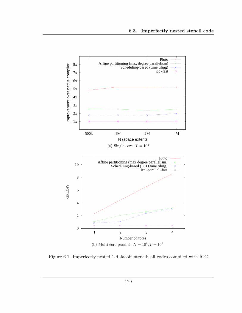
6.3. Imperfectly nested stencil code
1x
2x
3x
4x
5x
6x
7x
8x
500k 1M 2M 4M
Impr
ovem
ent o
ver
nativ
e co
mpi
ler
N (space extent)
PlutoAffine partitioning (max degree parallelism)
Scheduling-based (time tiling)icc -fast
(a) Single core: T = 104
0
2
4
6
8
10
1 2 3 4
GFL
OPs
Number of cores
PlutoAffine partitioning (max degree parallelism)
Scheduling-based (FCO time tiling)icc -parallel -fast
(b) Multi-core parallel: N = 106, T = 105
Figure 6.1: Imperfectly nested 1-d Jacobi stencil: all codes compiled with ICC
129

6.3. Imperfectly nested stencil code
1x
2x
3x
4x
5x
6x
7x
8x
500000 1M 2M 4M
Spe
edup
ove
r G
CC
-O
3
N (space extent)
PlutoLim/Lam
Scheduling-based (time tiling)gcc -O3
(a) Single core (with gcc): T = 104
0
2
4
6
8
10
1 2 3 4
GFL
OPs
Number of cores
Pluto (tiled parallel)Lim/Lam affine partitioning
Scheduling-based (FCO time tiling)gcc -O3
(b) Multi-core parallel (with gcc): N = 106, T = 105
Figure 6.2: Imperfectly nested 1-d Jacobi stencil: all codes compiled with GCC
130

6.4. Finite Difference Time Domain
lelizer; hence, we just show the sequential run time for icc in this case. Figure 6.3
shows L1 cache misses with each approach for a problem size that completely fits in
the L2 cache. Though Griebl’s technique incurs considerably lesser cache misses than
Lim-Lam’s, the schedule introduces non-unimodularity leading to modulo comparison
in inner loops; it is possible to remove the modulo through an advanced technique
using non-unit strides [Vas07] that Cloog does not implement yet. Our code incurs
two times lesser number of cache misses than Griebl’s and nearly 50 times lesser cache
misses than Lim/Lam’s scheme. Note that both Lim-Lam’s and our transformation
in this case are unimodular and hence have the same number of points in a tile for a
given tile size. Comparison with gcc is provided in Figure 6.2(b) (gcc used to compile
all codes) to demonstrate that the relative benefits of our source-to-source system will
be available when used in conjunction with any sequential compiler.
6.4 Finite Difference Time Domain electromagnetic kernel
FDTD code is as shown in Figure 6.4. ex, ey represent electric fields in x and
y directions, while hz is the magnetic field. The code has four statements - three
of them 3-d and one 2-d and are nested imperfectly. Our transformation framework
finds three tiling hyperplanes (all in one band - fully permutable). The transformation
represent a combination of shifting, fusion and time skewing. Parallel performance
results shown are for nx = ny = 2000 and tmax = 500. L1 and L2 tile sizes were
set automatically using rough thumb rules based on dimensionality of arrays involved
and vectorization considerations. Results are shown in Figure 6.5. With polyhedral
scheduling-based techniques, the outer loop is identified as the sequential schedule
131
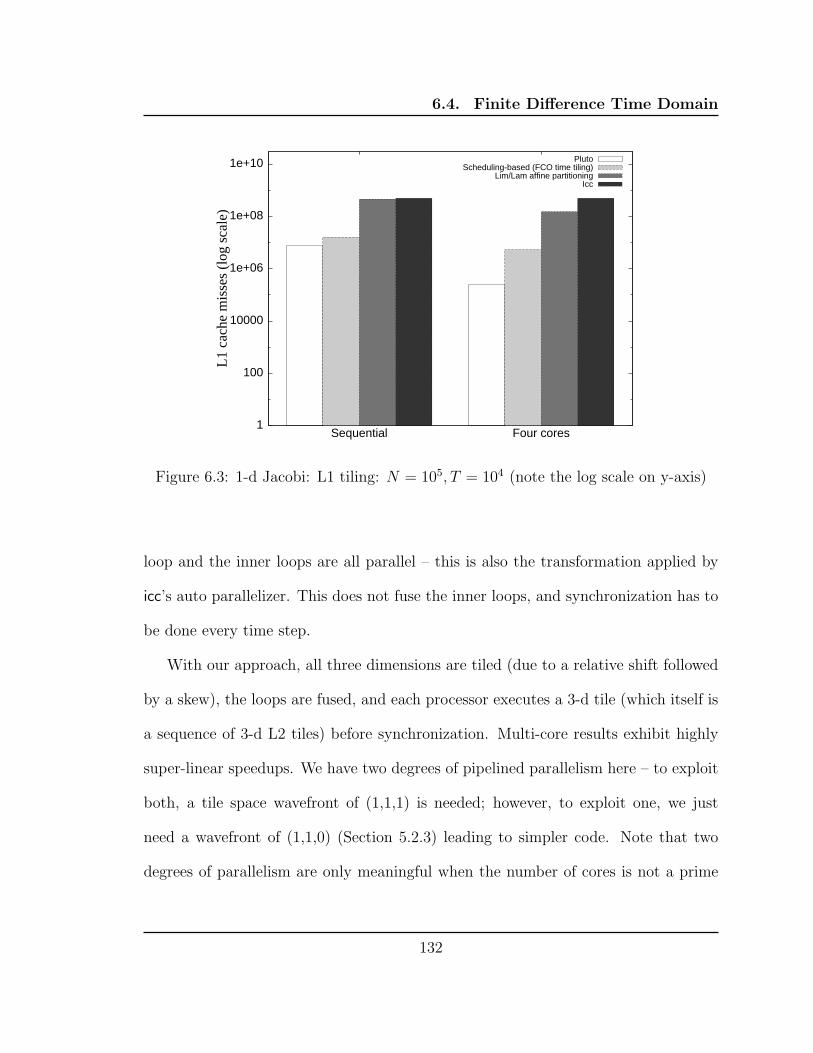
6.4. Finite Difference Time Domain
1
100
10000
1e+06
1e+08
1e+10
Sequential Four cores
L1
cach
e m
isse
s (l
og s
cale
)
PlutoScheduling-based (FCO time tiling)
Lim/Lam affine partitioningIcc
Figure 6.3: 1-d Jacobi: L1 tiling: N = 105, T = 104 (note the log scale on y-axis)
loop and the inner loops are all parallel – this is also the transformation applied by
icc’s auto parallelizer. This does not fuse the inner loops, and synchronization has to
be done every time step.
With our approach, all three dimensions are tiled (due to a relative shift followed
by a skew), the loops are fused, and each processor executes a 3-d tile (which itself is
a sequence of 3-d L2 tiles) before synchronization. Multi-core results exhibit highly
super-linear speedups. We have two degrees of pipelined parallelism here – to exploit
both, a tile space wavefront of (1,1,1) is needed; however, to exploit one, we just
need a wavefront of (1,1,0) (Section 5.2.3) leading to simpler code. Note that two
degrees of parallelism are only meaningful when the number of cores is not a prime
132
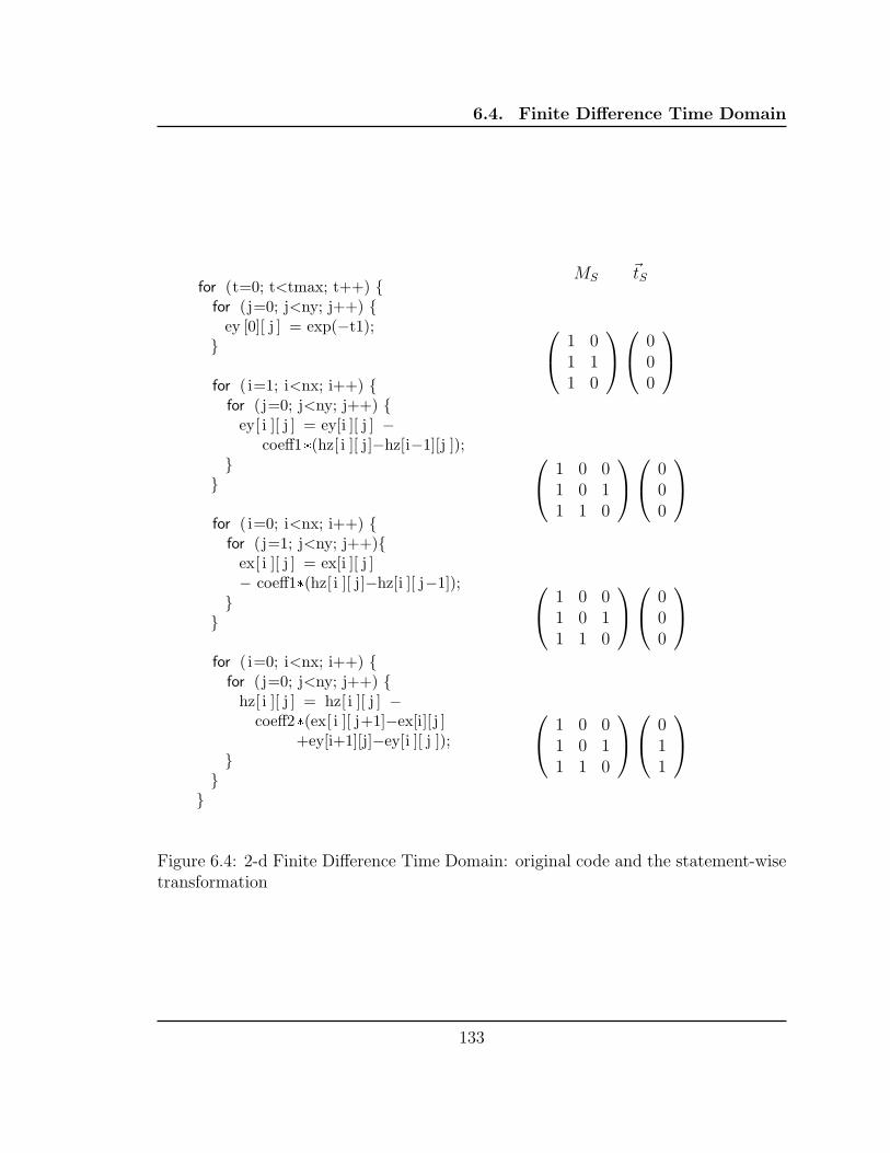
6.4. Finite Difference Time Domain
for (t=0; t<tmax; t++) {for (j=0; j<ny; j++) {
ey [0][ j ] = exp(−t1);}
for ( i=1; i<nx; i++) {for (j=0; j<ny; j++) {
ey[ i ][ j ] = ey[i ][ j ] −coeff1*(hz[ i ][ j]−hz[i−1][j ]);
}}
for ( i=0; i<nx; i++) {for (j=1; j<ny; j++){
ex[ i ][ j ] = ex[i ][ j ]− coeff1*(hz[ i ][ j]−hz[i ][ j−1]);
}}
for ( i=0; i<nx; i++) {for (j=0; j<ny; j++) {
hz[ i ][ j ] = hz[ i ][ j ] −coeff2*(ex[ i ][ j+1]−ex[i][ j ]
+ey[i+1][j]−ey[i ][ j ]);}
}}
MS~tS
1 01 11 0
000
1 0 01 0 11 1 0
000
1 0 01 0 11 1 0
000
1 0 01 0 11 1 0
011
Figure 6.4: 2-d Finite Difference Time Domain: original code and the statement-wisetransformation
133
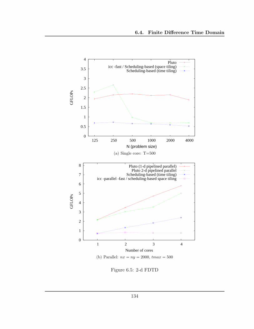
6.4. Finite Difference Time Domain
0
0.5
1
1.5
2
2.5
3
3.5
4
125 250 500 1000 2000 4000
GFL
OPs
N (problem size)
Plutoicc -fast / Scheduling-based (space tiling)
Scheduling-based (time tiling)
(a) Single core: T=500
0
1
2
3
4
5
6
7
8
1 2 3 4
GFL
OPs
Number of cores
Pluto (1-d pipelined parallel)Pluto 2-d pipelined parallel
Scheduling-based (time tiling)icc -parallel -fast / scheduling-based space tiling
(b) Parallel: nx = ny = 2000, tmax = 500
Figure 6.5: 2-d FDTD
134

6.5. LU Decomposition
0
1
2
3
4
5
6
7
8
1 2 4 8 16
GFL
OPs
Number of cores
2-d FDTD on a Power5 (8-way SMP)
PlutoXLC (current)
Figure 6.6: 2-D FDTD on a 8-way SMP Power5
number. The slight drop in performance for N = 4000 for the sequential case is due
to sub-optimal L2 cache tile sizes.
6.5 LU Decomposition
Three tiling hyperplanes are found – all belonging to a single band of permutable
loops. The first statement though lower-dimensional is naturally sunk into a a 3-
dimensional fully permutable space. Thus, there are two degrees of pipelined paral-
lelism. Exploiting both degrees of pipelined parallelism requires a tile wavefront of
(1,1,1) while exploiting only one requires (1,1,0). The code for the latter is likely to be
less complex, however, has a lesser computation to communication ratio. Performance
results on the quad core machine are shown in Figure 6.9. The GFLOPs is computed
135
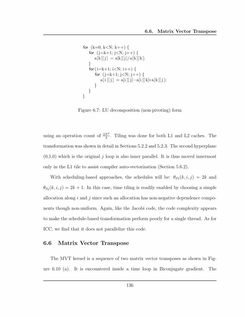
6.6. Matrix Vector Transpose
for (k=0; k<N; k++) {for (j=k+1; j<N; j++) {
a[k ][ j ] = a[k][ j ]/a[k ][ k ];}for ( i=k+1; i<N; i++) {
for (j=k+1; j<N; j++) {a[ i ][ j ] = a[i ][ j]−a[i ][ k]*a[k ][ j ];
}}
}
Figure 6.7: LU decomposition (non-pivoting) form
using an operation count of 2N3
3. Tiling was done for both L1 and L2 caches. The
transformation was shown in detail in Sections 5.2.2 and 5.2.3. The second hyperplane
(0,1,0) which is the original j loop is also inner parallel. It is thus moved innermost
only in the L1 tile to assist compiler auto-vectorization (Section 5.6.2).
With scheduling-based approaches, the schedules will be: θS1(k, i, j) = 2k and
θS2(k, i, j) = 2k + 1. In this case, time tiling is readily enabled by choosing a simple
allocation along i and j since such an allocation has non-negative dependence compo-
nents though non-uniform. Again, like the Jacobi code, the code complexity appears
to make the schedule-based transformation perform poorly for a single thread. As for
ICC, we find that it does not parallelize this code.
6.6 Matrix Vector Transpose
The MVT kernel is a sequence of two matrix vector transposes as shown in Fig-
ure 6.10 (a). It is encountered inside a time loop in Biconjugate gradient. The
136

6.6. Matrix Vector Transpose
for (t0=−1;t0<=floord(9*N−17,128);t0++) {lb1=max(max(ceild(8*t0−63,72),0),ceild(16*t0−N+2,16));ub1=min(floord(N−1,128),floord(16*t0+15,16));
#pragma omp parallel for shared(t0,lb1,ub1) private(t1,t2,t3,t4,t5)for (t1=lb1; t1<=ub1; t1++) {
for (t2=max(ceild(8*t0−8*t1−105,120),ceild(8*t0−8*t1−7,8));t2<=floord(N−1,16);t2++) {
if (t0 == t1+t2) {for (t3=max(0,16*t2);t3<=min(min(16*t2+14,N−2),128*t1+126);t3++) {
for (t5=max(t3+1,128*t1);t5<=min(N−1,128*t1+127);t5++) {a[t3 ][ t5]=a[t3 ][ t5]/a[t3 ][ t3 ];
}for (t4=t3+1;t4<=min(16*t2+15,N−1);t4++) {
for (t5=max(t3+1,128*t1);t5<=min(N−1,128*t1+127);t5++) {a[t4 ][ t5]=a[t4 ][ t5]−a[t4 ][ t3]*a[t3 ][ t5 ];
}}
}}for (t3=max(0,16*t0−16*t1);
t3<=min(min(16*t2−1,16*t0−16*t1+15),128*t1+126);t3++) {for (t4=16*t2;t4<=min(N−1,16*t2+15);t4++) {
for (t5=max(128*t1,t3+1);t5<=min(N−1,128*t1+127);t5++) {a[t4 ][ t5]=a[t4 ][ t5]−a[t4 ][ t3]*a[t3 ][ t5 ];
}}
}if ((−t0 == −t1−t2) &&
(t0 <= min(floord(16*t1+N−17,16),floord(144*t1+111,16)))) {for (t5=max(16*t0−16*t1+16,128*t1);t5<=min(N−1,128*t1+127);t5++) {
a[16*t0−16*t1+15][t5]=a[16*t0−16*t1+15][t5]/a[16*t0−16*t1+15][16*t0−16*t1+15];
}}
}}
}
Figure 6.8: LU decomposition parallelized code (register tiling, L2 tiling, and vectorpragmas not shown); context: N ≥ 2
137
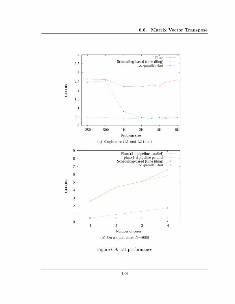
6.6. Matrix Vector Transpose
0
0.5
1
1.5
2
2.5
3
3.5
4
250 500 1K 2K 4K 8K
GFL
OPs
Problem size
PlutoScheduling-based (time tiling)
icc -parallel -fast
(a) Single core (L1 and L2 tiled)
0
1
2
3
4
5
6
7
8
9
1 2 3 4
GFL
OPs
Number of cores
Pluto (2-d pipeline parallel)pluto 1-d pipeline parallel
Scheduling-based (time tiling)icc -parallel -fast
(b) On a quad core: N=8000
Figure 6.9: LU performance
138

6.6. Matrix Vector Transpose
for ( i=0; i<N; i++) {for (j=0; j<N; j++) {
x1[ i ] = x1[i] + a[i ][ j ]*y1[j ];}
}
for ( i=0; i<N; i++) {for (j=0; j<N; j++) {
x2[ i ] = x2[i] + a[j ][ i ]*y2[j ];}
}(a) Original code
for (t0=0;t0<=N−1;t0++) {for (t1=0;t1<=N−1;t1++) {
x1[t0] = x1[t0] + a[t0 ][ t1]*y1[t1 ];x2[t1] = x2[t1] + a[t0 ][ t1]*y2[t0 ];
}}
(b) Transformed
TS1:
(t0t1
)
=
(1 00 1
)(i
j
)
TS2 :
(t0t1
)
=
(0 11 0
) (i
j
)
Figure 6.10: Matrix vector transpose
only inter-statement dependence is a non-uniform read/input on matrix A. The cost
function bounding (3.7) leads to minimization of this dependence distance by fusion
of the first MV with the permuted version of the second MV. As a result, the δe
for this dependence becomes 0 for both t0 and t1). This however leads to loss of
synchronization-free parallelism, since, in the fused form, each loop satisfies a de-
pendence. However, since these dependences have non-negative components, parallel
code can be generated corresponding to one degree of pipelined parallelism.
Existing techniques, even if they consider input dependences, cannot automatically
fuse the first MV with the permuted version of the second MV. Note that each of
the matrix vector multiplies is one strongly connected component. Hence, previous
approaches are only able to extract synchronization-free parallelism from each of the
139

6.7. 3-D Gauss-Seidel successive over-relaxation
0
0.5
1
1.5
2
2.5
1 2 3 4
GFL
OPs
Number of cores
Pluto (1-d pipelined parallel, fused ij/ji)Scheduling-based, Lim-Lam
fused (ij/ij), i parallelgcc -O3 (4.1.2)
Figure 6.11: MVT performance on a quad core: N=8000
MVs separately with a barrier between the two, giving up reuse on array A. Figure 6.11
shows the results for a problem size N = 8000. Note that both the optimized versions
were tiled for the L1 cache. Fusion of ij with ij does not exploit reuse on matrix A,
whereas the code that our tool comes up with performs best – it fuses ij with ji, tiles
it and exploits a degree of pipelined parallelism.
6.7 3-D Gauss-Seidel successive over-relaxation
The Gauss-Seidel computation (Figure 6.12) allows tiling of all three dimensions
after skewing. The transformation our tool obtains skews the first space dimension
by a factor of one with respect to time, while the second one by a factor of two
with time and one with respect to the previous space dimension. The transformation
140

6.8. DGEMM
for (t=0; t<=T−1; t++) {for ( i=1; i<=N−2; i++) {
for (j=1; j<=N−2; j++) {a[ i ][ j ] = (a[i−1][j−1] + a[i−1][j ] + a[i−1][j+1]
+ a[i ][ j−1] + a[i ][ j ] + a[i ][ j+1]+ a[i+1][j−1] + a[i+1][j ] + a[i+1][j+1])/9.0;
}}
}
MS =
1 0 01 1 02 1 1
Figure 6.12: 3-d Seidel code (original) and transformation
is also shown in Figure 6.12. Two degrees of pipelined parallelism can be extracted
subsequently after creating 3-d tiles. Figure 6.13 shows the performance improvement
achieved with 2-d pipelined parallel space as well as 1-d: the latter is better in practice
mainly due to simpler code. Again, icc is unable to parallelize this code. The GFLOPs
performance is on the lower side since unroll-jamming of non-rectangular loops is not
yet supported. Also, this code is not readily vectorized since none of intra-tile loops
are fully parallel.
6.8 DGEMM
We now compare the Pluto generated code for DGEMM with several highly-tuned
libraries. The purpose of this comparison is to see how far Pluto code is from the
machine peak and the factors responsible for this gap. Figure 6.15 shows that the
Pluto code is within 1.5 to 2x of vendor-supplied BLAS. The difference appears to be
mainly due to the performance left on the table by the auto-vectorization performed
141

6.8. DGEMM
0
0.5
1
1.5
2
2.5
3
3.5
4
4.5
1 2 3 4
GFL
OPs
Number of cores
Pluto (1-d pipeline parallel)Pluto (2-d pipeline parallel)
icc -parallel -fast
Figure 6.13: 3-D Gauss Seidel on Intel Q6600: Nx = Ny = 2000; T=1000
0
0.5
1
1.5
2
2.5
3
3.5
4
1 2 4 8 16
GFL
OPs
Number of cores
3-d Gauss Seidel
PlutoXLC (current)
Figure 6.14: 3-D Gauss Seidel on a Power5 SMP: Nx = Ny = 2000; T=1000
142

6.9. Experiments with Fusion-critical Codes
on transformed Pluto code by ICC. Merging this gap is the subject on one of the
threads of future work discussed briefly in the next chapter.
6.9 Experiments with Fusion-critical Codes
We now show the benefits of the techniques proposed in Chapter 4 by evaluating
codes for which performing loop fusion in conjunction with other transformations
is important. Some comparisons include a version of the benchmark written with
vendor supplied libraries. On the Intel Core 2 machine, we used the Intel Math Kernel
Library (MKL) 10.0 that includes a multithreaded implementation of the Basic Linear
Algebra Software (BLAS) routines highly optimized for Intel processors. Similarly,
for the AMD machines, the AMD Core Math Library (ACML) version 4.1 was used.
6.9.1 GEMVER
The GEMVER kernel is a combination of outer products and matrix vector prod-
ucts. It is used for householder bidiagonalization. The BLAS version of the GEMVER
kernel from Siek et al. [SKJ08] along with the linear algebraic specification is shown
in Figure 6.16. The nested loop code is in Figure 6.17. Permuting and fusing the
first two loop nests is the key optimization to reduce cache misses. Pluto’s fusion
algorithm is able to cut between the second and third statement, and the third and
fourth statement. The fused code is automatically tiled for caches and registers too.
The parallel loop inside the L1 tile is made the innermost for vectorization as de-
scribed in Section 5.6.2. Figures 6.9.1, 6.18, and 6.20 show performance results on
three different architectures. The performance is relatively lower on the Opteron as
143

6.9. Experiments with Fusion-critical Codes
0
2
4
6
8
10
12
32 64 128 256 512 1024 2048 4k
GF
LOP
s
Matrix size (M=N=K)
DGEMM perf - Intel Core 2 Quad Q6600 - one core
PlutoICC -fast
ATLAS 3.8.0 (selected MM)ATLAS 3.8.0 generated MM
Intel MKL 9.1NetLib BLAS 3.1 FC7
Absolute machine peak
(a) Single core
0
5
10
15
20
25
30
35
1 2 3 4
GF
LOP
s
Number of cores
DGEMM perf - Intel Core 2 Quad Q6600
PlutoICC -fast
ATLAS 3.8.0 (kSelMM)ATLAS 3.8.0 kGenMM
Intel MKL 9.1NetLib BLAS 3.1 FC7
Goto BLAS 1.23
(b) Parallel: M = N = K = 2048
Figure 6.15: DGEMM perf: Pluto vs. Hand-tuned
144
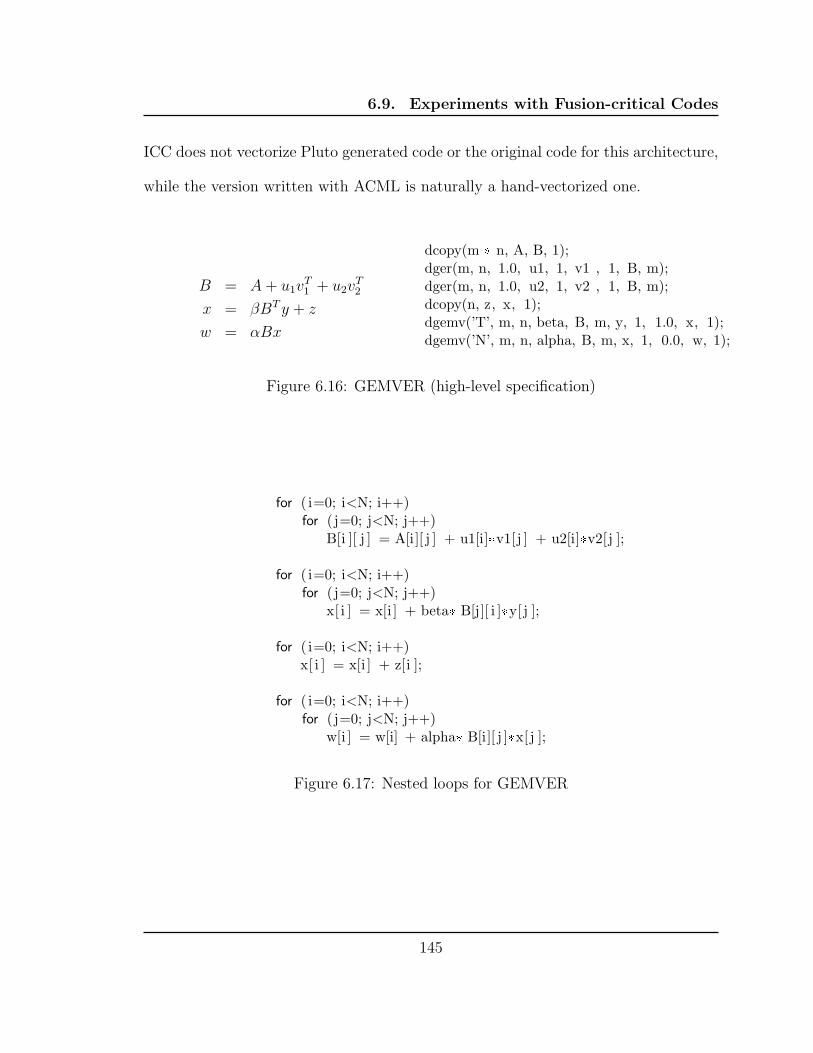
6.9. Experiments with Fusion-critical Codes
ICC does not vectorize Pluto generated code or the original code for this architecture,
while the version written with ACML is naturally a hand-vectorized one.
B = A + u1vT1 + u2v
T2
x = βBT y + z
w = αBx
dcopy(m * n, A, B, 1);dger(m, n, 1.0, u1, 1, v1 , 1, B, m);dger(m, n, 1.0, u2, 1, v2 , 1, B, m);dcopy(n, z, x, 1);dgemv(’T’, m, n, beta, B, m, y, 1, 1.0, x, 1);dgemv(’N’, m, n, alpha, B, m, x, 1, 0.0, w, 1);
Figure 6.16: GEMVER (high-level specification)
for ( i=0; i<N; i++)for (j=0; j<N; j++)
B[i ][ j ] = A[i][ j ] + u1[i]*v1[j ] + u2[i]*v2[j ];
for ( i=0; i<N; i++)for (j=0; j<N; j++)
x[ i ] = x[i ] + beta* B[j][ i ]*y[ j ];
for ( i=0; i<N; i++)x[ i ] = x[i ] + z[i ];
for ( i=0; i<N; i++)for (j=0; j<N; j++)
w[i ] = w[i] + alpha* B[i][ j ]*x[ j ];
Figure 6.17: Nested loops for GEMVER
145

6.9. Experiments with Fusion-critical Codes
0
0.2
0.4
0.6
0.8
1
1.2
1.4
1.6
75 150 250 500 1K 2K 4K 8K
GFL
OPs
Problem size
GEMVER on Opteron 2218 (2.6 GHz)
Pluto (--smartfuse)Pluto --nofuse
ACML 4.1.0ICC -fast
Figure 6.18: GEMVER on Opteron
0
0.5
1
1.5
2
2.5
3
3.5
4
4.5
75 125 250 500 1K 2K 4K 8K
GFL
OPs
Problem size
GEMVER on Intel Core2 Q6600 (2.4 GHz)
Pluto (--smartfuse)Pluto --nofuse
ICC -fastMKL 10.1
Figure 6.19: GEMVER on Intel Core 2 Quad
146

6.9. Experiments with Fusion-critical Codes
0
0.5
1
1.5
2
2.5
500 1K 2K 4K 8K
GFL
OPs
Problem size
GEMVER on Phenom x4 9850 (2.5 GHz)
Pluto (--smartfuse)Pluto --nofuse
ACML 4.1.0ICC -fast
Figure 6.20: GEMVER on AMD Phenom x4 9850
6.9.2 Doitgen
The Doitgen kernel is part of MADNESS [mad], a scientific simulation frame-
work in many dimensions using adaptive multiresolution methods in multiwavelet
bases [mad]. The computation is quite similar to matrix-matrix multiplication and
is shown in Figure 6.21. The kernel is special in that it involves small problem sizes
and is called repeatedly from higher level routines. Figure 6.23 and Figure 6.24
show significantly higher performance with Pluto over the same kernel written with
BLAS library calls. Register tiling of the imperfect loop nest is responsible for most
of the improvement here for the smaller problem sizes. The tiled code is shown in
Figure 6.22. Creating 4-d tiles for this code involves an intricacy described in Sec-
147

6.10. Analysis
tion 5.4.2. Previous approaches [WL91a, LCL99, AMP01] that just tile every band
of permutable loops in a hierarchy will be unable to create 4-d tiles for the second
statement.
for (r=0; r<N; r++) {for (q=0; q<N; q++) {
for (p=0; p<N; p++) {sum[r][q ][ p] = 0;for (s = 0; s< N; s++) {
sum[r][q ][ p] = sum[r][q][p] + A[r][q ][ s]*C4[s ][p ];}
}for (p=0; p<N; p++) {
A[r ][ q ][ p] = sum[r][q][p ];}
}}
Figure 6.21: Doitgen
6.10 Analysis
All the above experiments show very high speedups with our approach, both for
single thread and multicore parallel execution. The performance improvement is very
significant over production compilers as well as state-of-the-art from the research
community. Speedup ranging from 2x to 5x are obtained over previous automatic
transformation approaches in most cases, while an order of 10x improvement is ob-
tained over native production compilers. Linear to super-linear speedups are seen for
almost all compute-intensive kernels considered here due to optimization for locality
148

6.10. Analysis
lb1=0;ub1=floord(N−1,4);#pragma omp parallel for shared(lb1,ub1) private(t0,t1,t2,t3,t4,t5,t6,t7,t8,t9)for (t0=lb1; t0<=ub1; t0++) {
for (t1=0;t1<=floord(N−1,8);t1++) {for (t3=0;t3<=floord(N−1,31);t3++) {
for (t5=max(0,4*t0);t5<=min(N−1,4*t0+3);t5++) {for (t6=max(0,8*t1);t6<=min(N−1,8*t1+7);t6++) {
for (t9=max(0,31*t3);t9<=min(N−1,31*t3+30);t9++) {{sum[t5][t6 ][ t9]=0;} ;
}}
}}for (t3=0;t3<=floord(N−1,31);t3++) {
for (t4=0;t4<=floord(N−1,8);t4++) {for (t5=max(0,4*t0);t5<=min(N−1,4*t0+3);t5++) {
for (t6=max(0,8*t1);t6<=min(N−1,8*t1+7);t6++) {for (t8=max(0,8*t4);t8<=min(N−1,8*t4+7);t8++) {
for (t9=max(0,31*t3);t9<=min(N−1,31*t3+30);t9++) {{sum[t5][t6 ][ t9]=A[t5][t6 ][ t8]*C4[t8][ t9]+sum[t5][t6 ][ t9 ];} ;
}}
}}
}}for (t3=0;t3<=floord(N−1,31);t3++) {
for (t5=max(0,4*t0);t5<=min(N−1,4*t0+3);t5++) {for (t6=max(0,8*t1);t6<=min(N−1,8*t1+7);t6++) {
for (t9=max(0,31*t3);t9<=min(N−1,31*t3+30);t9++) {{A[t5][t6 ][ t9]=sum[t5][t6 ][ t9 ];} ;
}}
}}
}}
Figure 6.22: Doitgen tiled code (register tiling and vector pragmas not shown)
149

6.10. Analysis
0
1
2
3
4
5
10 15 20 25 31
GF
LOP
s
Problem size
doitgen perf on Intel Core2 Q6600
Pluto (--maxfuse)Pluto --nofuse/--smartfuse
ICC -fastIntel MKL (dgemv)
(a) Single core
0
2
4
6
8
10
1 2 3 4
GF
LOP
s
Cores
doitgen parallel perf (N=25) Intel Core2 Quad Q6600 (2.4 GHz)
Pluto --maxfusePluto --nofuse/--smartfuse
doitgen (Intel MKL dgemm)doitgen (Intel MKL dgemv)
ICC -parallel -fast
(b) Parallel: N = 25
Figure 6.23: Doitgen on an Intel Core 2 Quad
150
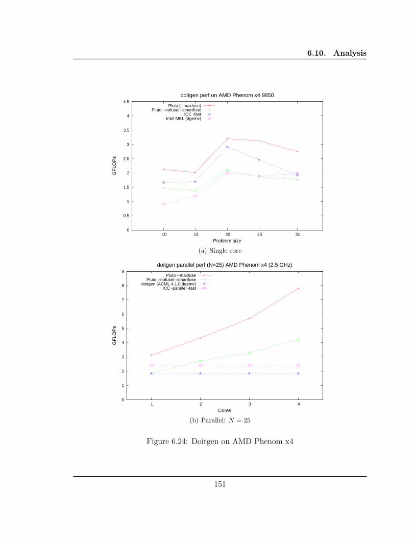
6.10. Analysis
0
0.5
1
1.5
2
2.5
3
3.5
4
4.5
10 15 20 25 31
GF
LOP
s
Problem size
doitgen perf on AMD Phenom x4 9850
Pluto (--maxfuse)Pluto --nofuse/--smartfuse
ICC -fastIntel MKL (dgemv)
(a) Single core
0
1
2
3
4
5
6
7
8
9
1 2 3 4
GF
LOP
s
Cores
doitgen parallel perf (N=25) AMD Phenom x4 (2.5 GHz)
Pluto --maxfusePluto --nofuse/--smartfuse
doitgen (ACML 4.1.0 dgemv)ICC -parallel -fast
(b) Parallel: N = 25
Figure 6.24: Doitgen on AMD Phenom x4
151
6.10. Analysis
as well as parallelism. To the best of our knowledge, such speedup’s have not been
reported by any automatic compiler framework as general as ours.
Hand-parallelization of many of the examples we considered here is extremely
tedious and not feasible in some cases, especially when time skewed code has to be
pipelined parallelized; this coupled by the fact that the code has to be tiled for at
least for one level of local cache, and a 2-d pipelined parallel schedule of 3-d tiles
is to be obtained makes manual optimization very complex. The performance of
the optimized stencil codes through our system is already in the range of that of
hand optimized versions reported in [KDW+06]. Also, for many of the codes, a
simple parallelization strategy of exploiting inner parallelism and leaving the outer
loop sequential (i.e., no time tiling) hardly yields any parallel speedup (Figure 6.5(b),
Figure 6.1(b)). Scheduling-based approaches that do not perform time tiling, or
production compilers’ auto-parallelizers perform such parallelization.
As mentioned before, tile sizes were not optimized through any extensive search or
a model. Also, Orio does not yet support unroll-jamming for non-rectangular iteration
spaces: this impacted the performance for LU and Gauss-Seidel. Using models for
tile size selection, with some amount of empirical search, in a manner decoupled
with the pure model-driven scheme presented is a reasonable approach to take this
performance higher. For simpler codes like matrix-matrix multiplication, this latter
phase of optimization, though very simple and straightforward when compared to the
rest of our system, brings most of the benefits.
As for fusion for long sequences, it is almost clear that finding the highest perform-
ing parallel code taking into account fusion, tiling, and storage optimization needs
152

6.10. Analysis
some kind of iterative techniques. However, finding reasonably good fusion structures
for loop nests with up to a handful of statements can be achieved purely through
models and heuristics. Interactions with the hardware (mainly prefetching) create
more complications and the best transformation is often architecture-specific. Pres-
ence or the lack of explicit copying also has an impact. Hence, a study of fusion has
to be revisited once automatic explicit copying is implemented into Pluto.
153
CHAPTER 7
CONCLUSIONS AND FUTURE DIRECTIONS
In this dissertation, we presented the theory, design, and implementation of an
automatic polyhedral program optimization system that can optimize sequences of
arbitrarily-nested loops simultaneously for coarse-grained parallelism and locality.
The framework has been fully implemented into a tool, Pluto, to generate OpenMP
parallel code from regular C program sections automatically. Experimental results
show significantly higher performance for single core and parallel execution on multi-
cores, when compared with production compilers as well as state-of-the-art research
approaches. In many cases, the parallelization performed through Pluto is infeasible
to obtain by hand. A beta release of the Pluto system including all codes used for
experimental evaluation in this dissertation are available at [Plu].
Past studies on loop fusion were done in an isolated fashion not integrated with
other transformations for parallelization and locality optimization. We showed how
our approach can come up with non-trivial fusions and presented three different fusion
algorithms that cover the interesting cases. For several linear algebra kernels, code
generated from Pluto beats, by a significant margin, the same kernel implemented
154

7. Conclusions and Future Directions
with a sequence of calls to BLAS routines linked with hand-tuned vendor supplied
libraries.
Domain-specific frontends. The transformation system built here is not just ap-
plicable to C or Fortran code, but to any input language from which polyhedral com-
putation domains can be extracted and analyzed. Since our entire transformation
framework works in the polyhedral abstraction, only the frontend and the depen-
dence tester needs to be adapted to accept a new language. It could be applied for
example to very high-level languages or domain-specific languages to generate high-
performance parallel code. Designing new domain-specific frontends for Pluto can be
done easily. Corequations [cor] already is one such high-level language using which
computation can be specified through equations – a natural way to represent compu-
tations for many scientific calculations. Pluto can directly benefit such languages by
serving as their backend optimizer.
Iterative compilation and auto-tuning. The Pluto system leaves a lot of flex-
ibility for future optimization, through iterative and empirical approaches. For very
long sequences of loop nests, it appears clear that iterative compilation is needed to
find the best fusion structure, mainly because the best choice for the fusion structure
along with all other transformations and optimizations appears to be complex to be
captured in a model. Integration of polyhedral iterative [PBCV07, PBCC08] and our
pure model-driven approach is thus promising. Orthogonally, tuning parameters such
as tile sizes and unroll factors, for which we currently do not have a sophisticated
155

7. Conclusions and Future Directions
model is a necessity. The Orio auto-tuner [ori, NHG07] recently developed at the
Argonne National Labs already provides a solution by providing auto-tuning capabil-
ities on top of Pluto as one of its features. Model-driven empirical optimization and
automatic tuning approaches (e.g., ATLAS [WD98, WPD00]) have been shown to be
very effective in optimizing single-processor execution for some regular kernels like
matrix-matrix multiplication [WPD00, YLR+03]. There is interest in developing ef-
fective empirical tuning approaches for arbitrary input kernels. Pluto can enable such
model-driven or guided empirical search to be applied to arbitrary affine programs,
in the context of both sequential and parallel execution.
Memory optimization. The integration of false dependence removal techniques [Fea91,
PW92, MAL93, TP94, BCC98, KS98] and subsequent memory optimization after
transformation is a useful component of an optimizer for imperative languages. Pro-
grammers typically tend to use the same storage for each iteration of a loop intro-
ducing a number of false dependences that hinder parallelization. Removing all false
dependences can cause a storage bloat, and hence the need to optimize storage after
parallelization. These techniques have been studied well [RW97, SCFS98, CDRV97,
Coh99, TVSA01, DSV05, QR00, ABD07]. Storage optimization techniques that are
schedule dependent like that of Alias et al. [ABD07] are the natural solution to opti-
mize storage after Pluto determines the transformation. No existing system integrates
such storage optimization techniques into an automatic parallelizer yet.
156

7. Conclusions and Future Directions
More real-world applications. The application of polyhedral techniques to true
real-world programs is still a significant challenge mainly due to the lack of techniques
to handle irregular and non-affine programs, procedures, and dynamic control. Mak-
ing interprocedural dependence analysis work in conjunction with polyhedral static
analysis is now interesting to explore given that all the links have been put together
for optimization of regular codes. Availability of a robust full-fledged frontend to
extract polyhedra is a necessary step. There are currently efforts to bring the poly-
hedral model to production compilers like GCC [PCB+06]. The availability of such
infrastructure is crucial for further progress. In addition, hybrid static-cum-dynamic
approaches are promising to explore. [RPR07], for example, uses dynamic techniques
to aid static analysis to enable parallelization that cannot be performed statically
alone. However, such techniques have not been studied in conjunction with the poly-
hedral model.
Vector intrinsics. For most kernels evaluated in Chapter 6, there is a significant
amount of performance that is left unexploited, even though Pluto generated code
provides high speedup. Figure 6.15 gives some indication. The quality of auto-
vectorization performed by the compiler on the polyhedral transformed code appears
to be one primary reason for this gap. Usage of vector intrinsics and automatically
mapping polyhedral computation to vector intrinsics is a very challenging problem.
This is even more crucial with several architectures employing wider vector architec-
tures on the horizon [avx]. Spiral [spi, PMJ+05] is one domain-specific project that
157
7. Conclusions and Future Directions
employs such vector intrinsics to generate highly optimized implementations of digital
signal processing algorithms.
More target architectures. The framework presented in this dissertation is ap-
plicable to any parallel architecture as long as at least one degree of coarse-grained
parallelism is desired: this is the case with almost all modern parallel computers.
Some works have used Pluto to map programs to GPGPUs [BBK+08a] with addi-
tional optimizations like explicit copying for scratchpad memories [BBK+08b] as well
as considerations to avoid bank conflicts for SIMD threads. Similarly, the Cell proces-
sor, and embedded multiprocessor chips are also good targets. In addition to shared
memory architectures, techniques presented are in a form that would also distributed
memory automatic parallelization to be addressed incrementally: the incremental step
being the efficient generation of message passing code.
Concluding remarks. The Polyhedral model is about two decades old now. With
a practical and scalable approach for automatic transformation, all the missing links
have been put together for end-to-end automatic parallelization of input that the
polyhedral model can readily handle – affine loop nests with static control. There
are several codes that fall into this category, parallelization and optimization for
which will benefit a large number of users: [CS90, mad] are just two examples. One
can now conclude that polyhedral techniques are very effective for these domains
and are the best way to obtain the highest performance parallel code with no effort
on part of the programmer. The possibility of extension to more general code is
158

7. Conclusions and Future Directions
now feasible and interesting to be tried. Thanks to the mathematical abstraction,
the techniques can be applied to new languages or domain-specific languages. The
problem of auto-parallelization has always been considered a mountain, but mountains
can be approximated by polyhedra.
159

BIBLIOGRAPHY
[ABD07] Christophe Alias, Fabrice Baray, and Alain Darte. Bee+Cl@k: an im-plementation of lattice-based array contraction in the source-to-sourcetranslator Rose. In Languages Compilers and Tools for Embedded Sys-tems, pages 73–82, 2007.
[ABRY03] Rumen Andonov, Stefan Balev, Sanjay Rajopadhye, and Nicola Yanev.Optimal semi-oblique tiling. IEEE Trans. Par. and Dist. Sys., 14(9):944–960, 2003.
[AI91] Corinne Ancourt and Francois Irigoin. Scanning polyhedra with do loops.In ACM SIGPLAN Symposium on Principles and Practice of ParallelProgramming, pages 39–50, 1991.
[AK87] Randy Allen and Ken Kennedy. Automatic translation of Fortran pro-grams to vector form. ACM Trans. on Programming Languages andSystems, 9(4):491–542, 1987.
[AMP00] N. Ahmed, N. Mateev, and K. Pingali. Tiling imperfectly-nested loopnests. In Proc. Supercomputing, 2000.
[AMP01] N. Ahmed, Nikolay Mateev, and Keshav Pingali. Synthesizing transfor-mations for locality enhancement of imperfectly-nested loops. Intl. J. ofParallel Programming, 29(5), October 2001.
[avx] Intel Advanced Vector Extensions (AVX).http://softwareprojects.intel.com/avx/.
[Ban93] Utpal K. Banerjee. Loop Transformations for Restructuring Compilers:The Foundations. Kluwer Academic Publishers, Norwell, MA, USA, 1993.
[Bas04a] Cedric Bastoul. Code generation in the polyhedral model is easier thanyou think. In IEEE Intl. Conf. on Parallel Architectures and CompilationTechniques, pages 7–16, September 2004.
[Bas04b] Cedric Bastoul. Improving Data Locality in Static Control Programs.PhD thesis, University Paris 6, Pierre et Marie Curie, France, December2004.
160
BIBLIOGRAPHY
[BBK+08a] M. Baskaran, Uday Bondhugula, Sriram Krishnamoorthy, J. Ramanu-jam, A. Rountev, and P. Sadayappan. A Compiler Framework for Op-timization of Affine Loop Nests for GPGPUs. In ACM Intl. Conferenceon Supercomputing (ICS), June 2008.
[BBK+08b] M. Baskaran, Uday Bondhugula, Sriram Krishnamoorthy, J. Ramanu-jam, A. Rountev, and P. Sadayappan. Automatic Data Movement andComputation Mapping for Multi-level Parallel Architectures with Explic-itly Managed Memories. In ACM SIGPLAN Symposium on Principlesand Practice of Parallel Programming, February 2008.
[BBK+08c] Uday Bondhugula, Muthu Baskaran, Sriram Krishnamoorthy, J. Ra-manujam, A. Rountev, and P. Sadayappan. Automatic transformationsfor communication-minimized parallelization and locality optimization inthe polyhedral model. In Intl. Conf. on Compiler Construction (ETAPSCC), April 2008.
[BCC98] Denis Barthou, Albert Cohen, and Jean-Francois Collard. Maximal staticexpansion. In ACM SIGPLAN Symposium on Principles of ProgrammingLanguages, pages 98–106, 1998.
[BDRR94] Pierre Boulet, Alain Darte, Tanguy Risset, and Yves Robert. (Pen)-ultimate tiling? Integration, the VLSI Journal, 17(1):33–51, 1994.
[BDSV98] Pierre Boulet, Alain Darte, Georges-Andre Silber, and Frederic Vivien.Loop parallelization algorithms: From parallelism extraction to code gen-eration. Parallel Computing, 24(3–4):421–444, 1998.
[BF03] Cedric Bastoul and P. Feautrier. Improving data locality by chunking.In Intl. Conf. on Compiler Construction (ETAPS CC), pages 320–335,Warsaw, Apr. 2003.
[BHRS08] Uday Bondhugula, Albert Hartono, J. Ramanujam, and P. Sadayappan.A practical automatic polyhedral program optimization system. In ACMSIGPLAN Conference on Programming Language Design and Implemen-tation (PLDI), June 2008.
[BHZ] Roberto Bagnara, Patricia Hill, and Enea Zaffanella. PPL: The ParmaPolyhedra Library. http://www.cs.unipr.it/ppl/.
[BRS07] Uday Bondhugula, J. Ramanujam, and P. Sadayappan. Automatic map-ping of nested loops to FPGAs. In ACM SIGPLAN Symposium on Prin-ciples and Practice of Parallel Programming, March 2007.
161

BIBLIOGRAPHY
[CDRV97] Pierre-Yves Calland, Alain Darte, Yves Robert, and Frederic Vivien.Plugging anti and output dependence removal techniques into loop par-allelization algorithm. Parallel Computing, 23(1-2):251–266, 1997.
[CGP+05] Albert Cohen, Sylvain Girbal, David Parello, M. Sigler, Olivier Temam,and Nicolas Vasilache. Facilitating the search for compositions of programtransformations. In ACM Intl. Conf. on Supercomputing, pages 151–160,June 2005.
[clo] CLooG: The Chunky Loop Generator. http://www.cloog.org.
[Coh99] Albert Cohen. Parallelization via constrained storage mapping optimiza-tion. Lecture Notes in Computer Science, 16(15):83–94, 1999.
[cor] COREquations. http://www.corequations.com.
[CS90] Lawrence A. Covick and Kenneth M. Sando. Four-index transformationon distributed-memory parallel computers. Journal of ComputationalChemistry, pages 1151 – 1159, November 1990.
[Dar00] Alain Darte. On the complexity of loop fusion. Parallel Computing,26(9):1175–1193, 2000.
[DH99] Alain Darte and Guillaume Huard. Loop shifting for loop compaction.In LCPC ’99: Proc. of the Intl. Workshop on Languages and Compilersfor Parallel Computing, pages 415–431, 1999.
[DH00] Alain Darte and Guillaume Huard. Loop shifting for loop parallelization.Technical Report RR2000-22, ENS Lyon, May 2000.
[DR96] Michele Dion and Yves Robert. Mapping affine loop nests. ParallelComputing, 22(10):1373–1397, 1996.
[DRV00] Alain Darte, Yves Robert, and Frederic Vivien. Scheduling and Auto-matic Parallelization. Birkhauser Boston, 2000.
[DSV97] Alain Darte, Georges-Andre Silber, and Frederic Vivien. Combining re-timing and scheduling techniques for loop parallelization and loop tiling.Parallel Processing Letters, 7(4):379–392, 1997.
[DSV05] Alain Darte, Robert Schreiber, and Gilles Villard. Lattice-based memoryallocation. IEEE Transactions on Computers, 54(10):1242–1257, 2005.
162
BIBLIOGRAPHY
[DV97] Alain Darte and Frederic Vivien. Optimal fine and medium grain par-allelism detection in polyhedral reduced dependence graphs. Intl. J. ofParallel Programming, 25(6):447–496, December 1997.
[Fea88] P. Feautrier. Parametric integer programming. RAIRO Recherche Opera-tionnelle, 22(3):243–268, 1988.
[Fea91] P. Feautrier. Dataflow analysis of scalar and array references. Intl. J. ofParallel Programming, 20(1):23–53, Feb. 1991.
[Fea92a] P. Feautrier. Some efficient solutions to the affine scheduling problem: I.one-dimensional time. Intl. J. of Parallel Programming, 21(5):313–348,1992.
[Fea92b] P. Feautrier. Some efficient solutions to the affine scheduling prob-lem. part II. multidimensional time. Intl. J. of Parallel Programming,21(6):389–420, 1992.
[Fea94] P. Feautrier. Toward automatic distribution. Parallel Processing Letters,4:233–244, 1994.
[Fea06] P. Feautrier. Scalable and structured scheduling. Intl. J. of ParallelProgramming, 34(5):459–487, 2006.
[GAK02] G. Goumas, M. Athanasaki, and N. Koziris. Code Generation Methodsfor Tiling Transformations. J. of Information Science and Engineering,18(5):667–691, Sep. 2002.
[GFG05] Martin Griebl, Paul Feautrier, and Armin Großlinger. Forward commu-nication only placements and their use for parallel program construction.In Languages and Compilers for Parallel Computing, LCPC’02., pages16–30. Springer-Verlag, 2005.
[GFL00] Martin Griebl, Paul Feautrier, and Christian Lengauer. Index set split-ting. International Journal of Parallel Programming, 28(6):607–631,2000.
[GLW98] Martin Griebl, Christian Lengauer, and S. Wetzel. Code generation inthe polytope model. In IEEE Intl. Conf. on Parallel Architectures andCompilation Techniques, pages 106–111, 1998.
[GR07] Gautam Gupta and Sanjay Rajopadhye. The z-polyhedral model. InProc. of the ACM SIGPLAN symposium on Principles and Practice ofParallel Programming, pages 237–248, 2007.
163

BIBLIOGRAPHY
[Gri04] Martin Griebl. Automatic Parallelization of Loop Programs for Dis-tributed Memory Architectures. University of Passau, 2004. Habilitationthesis.
[GVB+06] Sylvain Girbal, Nicolas Vasilache, Cedric Bastoul, Albert Cohen, DavidParello, Marc Sigler, and Olivier Temam. Semi-automatic compositionof loop transformations. Intl. J. of Parallel Programming, 34(3):261–317,June 2006.
[HCF97] K. Hogstedt, Larry Carter, and Jeanne Ferrante. Determining the idletime of a tiling. In ACM SIGPLAN symposium on Principles of Pro-gramming Languages, pages 160–173, 1997.
[HCF99] K. Hogstedt, Larry Carter, and Jeanne Ferrante. Selecting tile shapefor minimal execution time. In Symposium on Parallel Algorithms andArchitectures, pages 201–211, 1999.
[HS02] Edin Hodzic and Weijia Shang. On time optimal supernode shape. IEEETrans. on Parallel and Distributed Systems, 13(12):1220–1233, 2002.
[Int] Intel C Compiler Manuals. Intel C/C++ Optimizing Applications. Doc-ument Number: 315890-002US.
[IT88] F. Irigoin and R. Triolet. Supernode partitioning. In ACM SIGPLANPrinciples of Programming Languages, pages 319–329, 1988.
[JLF02] Marta Jimenez, Jose M. Llaberıa, and Agustın Fernandez. Register tilingin nonrectangular iteration spaces. ACM Trans. Program. Lang. Syst.,24(4):409–453, 2002.
[KDW+06] S. Kamil, Kaushik Datta, Samuel Williams, Leonid Oliker, John Shalf,and Katherine Yellick. Implicit and explicit optimization for stencil com-putations. In ACM SIGPLAN workshop on Memory Systems Perofmanceand Correctness, 2006.
[Kel96] W. Kelly. Optimization within a unified transformation framework. Tech-nical Report CS-TR-3725, 1996.
[KM93] K. Kennedy and K. McKinley. Maximizing loop parallelism and im-proving data locality via loop fusion and distribution. In Languages andCompilers for Parallel Computing, pages 301–320, 1993.
164
BIBLIOGRAPHY
[KP93] W. Kelly and W. Pugh. Determining schedules based on performance es-timation. Technical Report UMIACS-TR-9367, University of Maryland,College Park, December 1993.
[KP95] W. Kelly and W. Pugh. A unifying framework for iteration reorderingtransformations. Technical Report CS-TR-3430, Dept. of Computer Sci-ence, University of Maryland, College Park, 1995.
[KPR95] W. Kelly, W. Pugh, and E. Rosser. Code generation for multiple map-pings. In Intl. Symp. on the frontiers of massively parallel computation,pages 332–341, Feb. 1995.
[KRSR07] Daegon Kim, Lakshminarayanan Renganarayanan, Michelle Strout, andSanjay Rajopadhye. Multi-level tiling: ‘m’ for the price of one. In Super-computing, 2007.
[KS98] Kathleen Knobe and Vivek Sarkar. Array ssa form and its use in par-allelization. In Proc. of the ACM SIGPLAN-SIGACT symposium onPrinciples of programming languages, pages 107–120, 1998.
[Lam74] Leslie Lamport. The parallel execution of do loops. Communications ofthe ACM, 17(2):83–93, 1974.
[LCL99] A. Lim, Gerald I. Cheong, and Monica S. Lam. An affine partitioningalgorithm to maximize parallelism and minimize communication. In ACMIntl. Conf. on Supercomputing, pages 228–237, 1999.
[LeV92] H. LeVerge. A note on Chernikova’s algorithm. Technical Report Re-search report 635, IRISA, February 1992.
[LL98] A. Lim and Monica S. Lam. Maximizing parallelism and minimizingsynchronization with affine partitions. Parallel Computing, 24(3-4):445–475, 1998.
[LLL01] A. Lim, S. Liao, and M. Lam. Blocking and array contraction acrossarbitrarily nested loops using affine partitioning. In ACM SIGPLANSymposium on Principles and Practice of Parallel Programming, pages103–112, 2001.
[loo] The LooPo Project - Loop parallelization in the polytope model.http://www.fmi.uni-passau.de/loopo.
165
BIBLIOGRAPHY
[LP94] Wei Li and Keshav Pingali. A singular loop transformation frame-work based on non-singular matrices. Intl. J. of Parallel Programming,22(2):183–205, 1994.
[mad] Madness: Multiresolution adaptive numerical scientific simulation.http://www.csm.ornl.gov/ccsg/html/projects/madness.html.
[MAL93] D. E. Maydan, Saman P. Amarasinghe, and Monica S. Lam. Array-data flow analysis and its use in array privatization. In Proc. of the ACMSIGPLAN-SIGACT symposium on Principles of programming languages,pages 2–15, 1993.
[MS97] Nimrod Megiddo and Vivek Sarkar. Optimal weighted loop fusion forparallel programs. In Symposium on Parallel Algorithms and Architec-tures, pages 282–291, 1997.
[NHG07] Boyana Norris, Albert Hartono, and William Gropp. Annotations forperformance and productivity. 2007. Preprint ANL/MCS-P1392-0107.
[ori] Orio. https://trac.mcs.anl.gov/projects/performance/wiki/Orio.
[PBCC08] L-N Pouchet, Cedric Bastoul, John Cavazos, and Albert Cohen. Iterativeoptimization in the polyhedral model: Part II, multidimensional time. InACM SIGPLAN PLDI, Tucson, Arizona, June 2008.
[PBCV07] L.-N. Pouchet, C. Bastoul, A. Cohen, and N. Vasilache. Iterative op-timization in the polyhedral model: Part I, one-dimensional time. InInternational Symposium on Code Generation and Optimization, March2007.
[PCB+06] Sebastian Pop, Albert Cohen, Cedric Bastoul, Sylvain Girbal, P. Jou-velot, G.-A. Silber, and N. Vasilache. GRAPHITE: Loop optimizationsbased on the polyhedral model for GCC. In Proc. of the 4th GCC De-velopper’s Summit, Ottawa, Canada, June 2006.
[Pen55] Roger Penrose. A generalized inverse for matrices. Proceedings of theCambridge Philosophical Society, 51:406–413, 1955.
[pip] PIP: The Parametric Integer Programming Library.http://www.piplib.org.
[Plu] PLUTO: A polyhedral automatic parallelizer and locality optimizer formulticores. http://pluto-compiler.sourceforge.net.
166

BIBLIOGRAPHY
[PMJ+05] Markus Puschel, Jose M. F. Moura, Jeremy Johnson, David Padua,Manuela Veloso, Bryan Singer, Jianxin Xiong, Franz Franchetti, AcaGacic, Yevgen Voronenko, Kang Chen, Robert W. Johnson, and NicholasRizzolo. SPIRAL: Code generation for DSP transforms. Proceedingsof the IEEE, special issue on “Program Generation, Optimization, andAdaptation”, 93(2):232– 275, 2005.
[pol] PolyLib - A library of polyhedral functions.http://icps.u-strasbg.fr/polylib/.
[PR97] W. Pugh and Evan Rosser. Iteration space slicing and its applicationto communication optimization. In Intl. Conference on Supercomputing,pages 221–228, 1997.
[PR00] W. Pugh and Evan Rosser. Iteration space slicing for locality. In Pro-ceedings of the Workshop on Languages and Compilers for Parallel Com-puting, pages 164–184, London, UK, 2000. Springer-Verlag.
[Pug92] W. Pugh. The omega test: a fast and practical integer programmingalgorithm for dependence analysis. Communications of the ACM, 8:102–114, August 1992.
[PW92] W. Pugh and David Wonnacott. Eliminating false data dependencesusing the omega test. In Proceedings of the ACM SIGPLAN conferenceon Programming Language Design and Implementation, pages 140–151,1992.
[QK06] Apan Qasem and Ken Kennedy. Profitable loop fusion and tiling usingmodel-driven empirical search. In Proc. ACM Intl. Conf. on Supercom-puting, pages 249–258, 2006.
[QR00] Fabien Quillere and Sanjay Rajopadhye. Optimizing memory usage inthe polyhedral model. ACM Trans. Program. Lang. Syst., 22(5):773–815,2000.
[QRW00] Fabien Quillere, Sanjay V. Rajopadhye, and Doran Wilde. Generation ofefficient nested loops from polyhedra. Intl. J. of Parallel Programming,28(5):469–498, 2000.
[Qui87] Patrice Quinton. The systematic design of systolic arrays. In CentreNational de Recherche Scientifique on Automata networks in computerscience: theory and applications, pages 229–260, Princeton, NJ, USA,1987. Princeton University Press.
167

BIBLIOGRAPHY
[Ram92] J. Ramanujam. Non-unimodular transformations of nested loops. InSupercomputing, pages 214–223, 1992.
[Ram95] J. Ramanujam. Beyond unimodular transformations. Journal of Super-computing, 9(4):365–389, 1995.
[RKRS07] L. Renganarayana, DaeGon Kim, Sanjay Rajopadhye, and Michelle MillsStrout. Parameterized tiled loops for free. In ACM SIGPLAN symposiumon Programming Languages Design and Implementation, pages 405–414,2007.
[Rob01] Arch D. Robison. Impact of economics on compiler optimization. In JGI’01: Proceedings of the 2001 joint ACM-ISCOPE conference on JavaGrande, pages 1–10, 2001.
[RPR07] Silvius Rus, Maikel Pennings, and Lawrence Rauchwerger. Sensitivityanalysis for automatic parallelization on multi-cores. In Proc. of the 21stIntl. Conference on Supercomputing, pages 263–273, 2007.
[RS92] J. Ramanujam and P. Sadayappan. Tiling multidimensional iterationspaces for multicomputers. Journal of Parallel and Distributed Comput-ing, 16(2):108–230, 1992.
[RW97] S. Rajopadhye and D. Wilde. Memory reuse analysis in the polyhedralmodel. Parallel Processing Letters, 7(2):207–215, June 1997.
[SCFS98] M. Strout, Larry Carter, Jeanne Ferrante, and Beth Simon. Schedule-independent storage mapping for loops. In Proc. of the Intl. Conferenceon Architectural Support for Programming Languages and Operating Sys-tems, pages 24–33, October 3–7, 1998.
[Sch86] Alexander Schrijver. Theory of Linear and Integer Programming. JohnWiley & Sons, 1986.
[SD90] R. Schreiber and J. Dongarra. Automatic blocking of nested loops. Tech-nical report, University of Tennessee, Knoxville, TN, August 1990.
[SKJ08] Jeremy G. Siek, Ian Karlin, and E. R. Jessup. Build to order linearalgebra kernels. In IPDPS: HIPS-POHLL workshop, April 2008.
[SL99] Yonghong Song and Zhiyuan Li. New tiling techniques to improve cachetemporal locality. In ACM SIGPLAN symposium on Programming Lan-guages Design and Implementation, pages 215–228, 1999.
168

BIBLIOGRAPHY
[SM97] S. Singhai and K. McKinley. A Parameterized Loop Fusion Algorithmfor Improving Parallelism and Cache Locality. The Computer Journal,40(6):340–355, 1997.
[S.P00] S.P.K. Nookala and Tanguy Risset. A library for Z-polyhedral opera-tions. Technical Report PI 1330, IRISA, Rennes, France, 2000.
[spi] SPIRAL: Software/Hardware Generation for DSP Algorithms.http://www.spiral.net.
[top] The top 500 supercomputers. http://www.top500.org.
[TP94] Peng Tu and David A. Padua. Automatic array privatization. In Intl.Workshop on Languages and Compilers for Parallel Computing, pages500–521, 1994.
[TVSA01] William Thies, Frederic Vivien, Jeffrey Sheldon, and Saman P. Ama-rasinghe. A unified framework for schedule and storage optimization.In ACM SIGPLAN symposium on Programming Languages Design andImplementation, pages 232–242, 2001.
[Vas07] Nicolas Vasilache. Scalable Program Optimization Techniques in thePolyhedral Model. PhD thesis, Universite de Paris-Sud, INRIA Futurs,September 2007.
[VBC06] Nicolas Vasilache, Cedric Bastoul, and Albert Cohen. Polyhedral codegeneration in the real world. In Intl. Conf. on Compiler Construction(ETAPS CC), pages 185–201, March 2006.
[VBGC06] Nicolas Vasilache, Cedric Bastoul, Sylvain Girbal, and Albert Cohen.Violated dependence analysis. In ACM Intl. Conf. on Supercomputing,June 2006.
[VCP07] Nicolas Vasilache, Albert Cohen, and Louis-Noel Pouchet. Automaticcorrection of loop transformations. In IEEE Intl. Conf. on Parallel Ar-chitectures and Compilation Techniques, 2007.
[Viv02] Frederic Vivien. On the optimality of feautrier’s scheduling algorithm. InProceedings of the 8th Intl. Euro-Par Conference on Parallel Processing,pages 299–308, London, UK, 2002. Springer-Verlag.
169

BIBLIOGRAPHY
[VSB+07] Sven Verdoolaege, Rachid Seghir, Kristof Beyls, Vincent Loechner, andMaurice Bruynooghe. Counting integer points in parametric polytopesusing Barvinok’s rational functions. Algorithmica, 48(1):37–66, June2007.
[WD98] R. Whaley and J. Dongarra. Automatically Tuned Linear Algebra Soft-ware (ATLAS). In Proc. Supercomputing ’98, 1998.
[Wil93] D. K. Wilde. A library for doing polyhedral operations. Technical ReportRR-2157, IRISA, 1993.
[WL91a] M. Wolf and M. S. Lam. A loop transformation theory and an algorithmto maximize parallelism. IEEE Trans. Parallel Distrib. Syst., 2(4):452–471, 1991.
[WL91b] M. Wolf and Monica S. Lam. A data locality optimizing algorithm. InACM SIGPLAN symposium on Programming Languages Design and Im-plementation, pages 30–44, 1991.
[Wol95] Michael Wolfe. High Performance Compilers for Parallel Computing.Addison-Wesley Longman Publishing Co., Inc., Boston, MA, USA, 1995.
[WPD00] R. Whaley, A. Petitet, and J. Dongarra. Automated Empirical Optimiza-tions of Software and the ATLAS Project. Parallel Computing, 2000.
[Xue97] Jingling Xue. Communication-minimal tiling of uniform dependenceloops. Journal of Parallel and Distributed Computing, 42(1):42–59, 1997.
[Xue00] Jingling Xue. Loop tiling for parallelism. Kluwer Academic Publishers,Norwell, MA, USA, 2000.
[YKA04] Qing Yi, Ken Kennedy, and Vikram Adve. Transforming complex loopnests for locality. J. of Supercomputing, 27(3):219–264, 2004.
[YLR+03] Kamen Yotov, Xiaoming Li, Gang Ren, Michael Cibulskis, Gerald De-Jong, Maria Garzaran, David A. Padua, Keshav Pingali, Paul Stodghill,and Peng Wu. A comparison of empirical and model-driven optimization.In ACM SIGPLAN symposium on Programming Languages Design andImplementation, pages 63–76, 2003.
170

Index
affine, 10affine combination, 11affine function, 10affine hyperplane, 11affine loop nest, 14affine schedule, 33affine space, 11affine transformation, 21allocation, 34anti dependence, 17automatic parallelization, 5
Cloog, 98communication-free parallelism, 28convex combination, 25
data dependence graph, 17ddg, 17dependence, 16dependence cutting, 75dependence polyhedron, 17dependence satisfaction, 27doacross parallelism, 29doall parallelism, 29domain, 15
Farkas lemma (affine form), 13Farkas multipliers, 13FCO, 46flow dependence, 17forward communication-only, 46fusion, 72
h-transformation, 98half-space, 11hyperplane, 11
imperfect loop nest, 14index set, 15inner parallel, 28input dependence, 17iteration vector, 14
linear, 10linear function, 10linear independence, 50loop fusion, 72loop tiling, 39
maxfuse, 79
nofuse, 78non-uniform dependence, 20null space, 10
orthogonal subspace, 51outer parallel, 28output dependence, 17
permutable band, 28pipelined parallelism, 29PLUTO, 96polyhedral model, 14polyhedron, 12polytope, 12program parameters, 14
register tiling, 121regular program, 15
scalar dimension, 22scattering function, 24, 98scattering supernodes, 103schedule, 33
171
INDEX
smartfuse, 78space tiling, 34space time mapping, 30static control programs, 15structure parameters, 14supernode, 103synchronization-free parallelism, 28
tiling, 39time tiling, 46transformation matrix, 21
uniform dependence, 20unroll and jam, 121unrolling, 121
z-polyhedra, 26
172