Defining locality as a problem difficulty measure in genetic programming

Noname manuscript No.

(will be inserted by the editor)

Defining Locality as a Problem Difficulty Measure in

Genetic Programming

Edgar Galvan-Lopez · James McDermott ·

Michael O’Neill · Anthony Brabazon

Received: date / Accepted: date

Abstract A mapping is local if it preserves neighbourhood. In Evolutionary Com-

putation, locality is generally described as the property that neighbouring genotypes

correspond to neighbouring phenotypes. A representation has high locality if most

genotypic neighbours are mapped to phenotypic neighbours. Locality is seen as a key

element in performing effective evolutionary search. It is believed that a representation

that has high locality will perform better in evolutionary search and the contrary is

true for a representation that has low locality. When locality was introduced, it was the

genotype-phenotype mapping in bitstring-based Genetic Algorithms which was of in-

terest; more recently, it has also been used to study the same mapping in Grammatical

Evolution. To our knowledge, there are few explicit studies of locality in Genetic Pro-

gramming (GP). The goal of this paper is to shed some light on locality in GP and use

it as an indicator of problem difficulty. Strictly speaking, in GP the genotype and the

phenotype are not distinct. We attempt to extend the standard quantitative definition

of genotype-phenotype locality to the genotype-fitness mapping by considering three

possible definitions. We consider the effects of these definitions in both continuous- and

discrete-valued fitness functions. We compare three different GP representations (two

of them induced by using different function sets and the other using a slightly different

GP encoding) and six different mutation operators. Results indicate that one definition

of locality is better in predicting performance.

Keywords Locality · Genotype-Phenotype mapping · Genotype-Fitness mapping ·

Problem Hardness · Genetic Programming

1 Introduction

The concept of a fitness landscape [69] has dominated the way geneticists think about

biological evolution and has been adopted within the Evolutionary Computation (EC)

Edgar Galvan-Lopez, James McDermott, Michael O’Neill and Anthony BrabazonNatural Computing Research & Applications Group, University College Dublin, IrelandTel.: +353-17-165332Fax: +353-17-165396E-mail: {edgar.galvan, james.m.mcdermott, m.oneill, anthony.brabazon}@ucd.ie

2

community and many others as a way to visualise evolution dynamics. Over the years,

researchers have defined fitness landscapes in slightly different ways (e.g., [30], [36]

and [62]). All of them have in common the use of three main elements: search space x,

neighbourhood mapping χ and fitness function f . More formally, a fitness landscape, as

specified in [58], is normally defined as a triplet (x, χ, f): (a) a set x of configurations,

(b) a notion χ of neighbourhood, distance or accessibility on x, and finally, (c) a fitness

function f .

How an algorithm explores and exploits a landscape is a key element of evolution-

ary search. Rothlauf [53,56] has described and analysed the importance of locality in

performing effective evolutionary search of landscapes. In EC, locality refers to how

well neighbouring genotypes correspond to neighbouring phenotypes, and is useful as

an indicator of problem difficulty. Similarly, the principle of strong causality states

that for successful search, a small change in genotype should result in a small change

in fitness [2]. In other words, the design process of an algorithm should be guided by

the locality principle [50].

In his research, Rothlauf distinguished two forms of locality, low and high. A repre-

sentation has high locality if most neighbouring genotypes correspond to neighbouring

phenotypes, that is small genotypic changes result in small phenotypic changes. On

the other hand, a representation has low locality if many neighbouring genotypes do

not correspond to neighbouring phenotypes. It is demonstrated that a representation

of high locality is necessary for efficient evolutionary search. No threshold between low

and high locality is established in Rothlauf’s work, nor indeed in ours. Instead, we

study locality as a relative concept: higher locality is assumed to lead to improved per-

formance. In Section 2 we give quantitative definitions of locality allowing the relative

locality of different representations and operators to be compared. Also, in Section 2,

we re-label these two concepts with the goal to avoid misinterpretations.

In his original studies, Rothlauf used GAs with bitstrings to conduct his experi-

ments [52] (and more recently he further used the idea of locality to study Grammatical

Evolution at the genotype level [56]). To our knowledge, there are few explicit studies

on locality using the typical Genetic Programming (GP) [33,46] representation (i.e.,

tree-like structures).

The goal of this paper then is to shed some light on the degree of locality present

in GP. That is,

– We extend the notion of genotype-phenotype locality to the genotype-fitness case.

For this purpose we treat two individuals as neighbours in the genotype space if

they are separated by a single mutation operation.

– We consider three different definitions of locality to study which of them gives the

best difficulty prediction,

– We consider a mutation based GP (six different mutation operators), without

crossover,

– We use three different encodings on five different problems and compare the results

against the three definitions of locality, and

– Finally, we use three different distance measures to study genotypic step-size.

This paper is organised as follows. In the following section, a more detailed de-

scription on locality will be provided. Section 3 presents previous work on performance

prediction. Section 4 presents the experimental setup used to conduct our experiments.

In Section 5 we present and discuss our findings. Finally, in Section 6 we draw some

conclusions and in Section 7 we outlined future work.

3

2 Locality

Understanding how well neighbouring genotypes correspond to neighbouring pheno-

types is a key element in understanding evolutionary search [52,56]. In the abstract

sense, a mapping has locality if neighbourhood is preserved under that mapping1. In

EC this generally refers to the mapping from genotype to phenotype. This is a topic

worthy of study because if neighbourhood is not preserved, then the algorithm’s at-

tempts to exploit the information provided by an individual’s fitness will be misled

when the individual’s neighbours turn out to be very different.

Rothlauf gives a quantitative definition of locality: “the locality dm of a represen-

tation can be defined as

dm =∑

dg(x,y)=dg

min

|dp(x, y)− dpmin|

where dp(x, y) is the phenotypic distance between the phenotypes x and y, dg(x, y) is

the genotypic distance between the corresponding genotypes, and dpmin resp. dgmin is

the minimum distance between two (neighbouring) phenotypes, resp. genotypes” [52,

p. 77; notation changed slightly]. Locality is thus seen as a continuous property rather

than a binary one. The point of this definition is that it provides a single quantity

which gives an indication of the behaviour of the genotype-phenotype mapping and

can be compared between different representations.

It should be noticed that while Rothlauf gives a quantitative definition of locality,

as expressed above (dm), this, in fact measures phenotypic divergence. Once a value is

obtained by this measure, then we can talk about high and low locality. In particular,

key definitions such as high and low locality. Although Rothlauf does not provide

a threshold value to distinguish high and low locality, nevertheless it is possible to

make relative comparisons between representations. As mentioned in Section 1, it is

important to avoid confusion on the definitions used in this paper. So, we have decided

to re-label these two terms. That is, when the phenotypic divergence dm is low, we are

in presence of locality (Routhlauf originally called it high-locality). On the other hand,

when the phenotypic divergence dm is high, we are in the presence of “non-locality”

(originally called low-locality [52]).

Rothlauf claims that a representation that has locality will be more efficient at

evolutionary search. If a representation has locality (i.e., neighbouring genotypes cor-

respond to neighbouring phenotypes) then performance is good.

This, however, changes when a representation has non-locality. To explain how

non-locality affects evolution, Rothlauf considered problems in three categories, taken

from the work presented in [30]. These are:

– easy, in which fitness increases as the global optimum approaches,

– difficult, for which there is no correlation between fitness and distance and,

– misleading, in which fitness tends to increase with the distance from the global

optimum.

It should be noticed that Rothlauf used these three categories only to highlight the

implications of the type of locality on these scenarios. To this end, Rothlauf described

the following three scenarios with different types of locality.

1 The term locality has also been used in an unrelated context, to refer to the quasi-geographical distribution of an EC population [8].

4

If a given problem lies in the first category (i.e., easy), a non-locality representation

will change this situation by making it more difficult and now, the problem will lie in the

second category. This is because non-locality introduces randomness to the search. This

can be explained by the fact that representations with non-locality lead to uncorrelated

fitness landscapes, so it is difficult for heuristics to extract information.

If a problem lies in the second category, a non-locality representation does not

change the difficulty of the problem. There are representations that can convert a

problem from difficult (class two) to easy (class one). However, it is non-trivial to

construct such a representation.

Finally, if the problem lies in the third category, a representation with non-locality

will transform it so that the problem will lie in the second category. That is, the problem

is less difficult because the search has become more random. This is a mirror image of

a problem lying in the first category and using a representation that has non-locality.

According to Rothlauf [52, Page 73] “Previous work has indicated that high local-

ity of a representation is necessary for efficient evolutionary search [55,25,24,23,54]

However, it is unclear as to how the locality of a representation influences problem

difficulty, and if high locality representations always aid evolutionary search.”. In this

study, as mentioned previously, we want to corroborate this by using locality as a tool

for prediction of performance. Before doing so, it is necessary to extend the typical

definition of locality from the genotype-phenotype to the genotype-fitness mapping.

This extension is presented in the following section.

2.1 Extending the Definition of Locality to the Genotype-Fitness Mapping

To use locality as a measure of problem difficulty in GP, it is necessary to extend

the standard definition of genotype-phenotype locality given by Rothlauf [52] to the

genotype-fitness mapping. Some GP variants have distinct genotypes and phenotypes,

for example Cartesian GP [40], linear GP [3], and others. The genotype must be trans-

formed to produce the program proper. The case of standard, tree-structured GP is

different, because the genotype is the program proper. Depending on one’s viewpoint,

one might say that the genetic operators work directly on the phenotype, that the

genotype-phenotype mapping is the identity map, or simply that no phenotype exists.

In this work, we have adopted the traditional GP system, where there is no explicit

genotype-phenotype mapping, so we can say that there are no explicit phenotypes dis-

tinct from genotypes. It is common therefore to study instead the behaviour of the

mapping from genotype to fitness [34], and we take this approach here. We will also

regard two individuals as neighbours in the genotype space if they are separated by a

single mutation. That is, a mutation operator defines the neighbourhood of individuals

in the genotype space, adhering to the Jones principle [30] that each operator induces

its own landscape.

We begin by considering again the standard definition of locality. It can be char-

acterised as “the sum of surplus distances”, where a surplus distance is the actual

phenotypic distance between genotypic neighbours less what that distance “should

have been”. Note in particular Rothlauf’s treatment of neutrality. Where genotypic

neighbours turn out to lead to the same phenotype, the phenotypic minimum distance

dmin is added to the sum dm. This is the same quantity that is added when neigh-

bouring genotypes diverge slightly (for bitstring phenotypes with Hamming distance).

In other words synonymous redundancy (redundancy of genotypic neighbours) has the

5

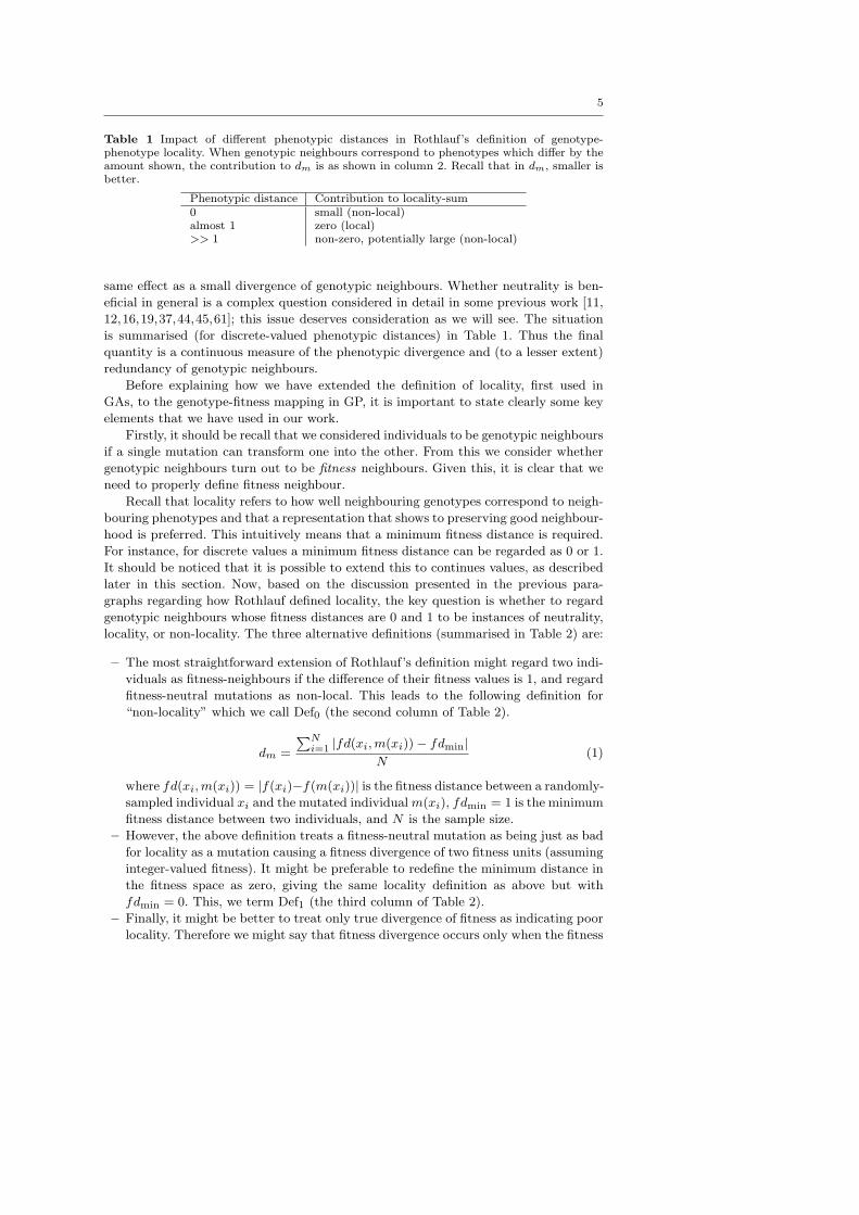
Table 1 Impact of different phenotypic distances in Rothlauf’s definition of genotype-phenotype locality. When genotypic neighbours correspond to phenotypes which differ by theamount shown, the contribution to dm is as shown in column 2. Recall that in dm, smaller isbetter.

Phenotypic distance Contribution to locality-sum0 small (non-local)almost 1 zero (local)>> 1 non-zero, potentially large (non-local)

same effect as a small divergence of genotypic neighbours. Whether neutrality is ben-

eficial in general is a complex question considered in detail in some previous work [11,

12,16,19,37,44,45,61]; this issue deserves consideration as we will see. The situation

is summarised (for discrete-valued phenotypic distances) in Table 1. Thus the final

quantity is a continuous measure of the phenotypic divergence and (to a lesser extent)

redundancy of genotypic neighbours.

Before explaining how we have extended the definition of locality, first used in

GAs, to the genotype-fitness mapping in GP, it is important to state clearly some key

elements that we have used in our work.

Firstly, it should be recall that we considered individuals to be genotypic neighbours

if a single mutation can transform one into the other. From this we consider whether

genotypic neighbours turn out to be fitness neighbours. Given this, it is clear that we

need to properly define fitness neighbour.

Recall that locality refers to how well neighbouring genotypes correspond to neigh-

bouring phenotypes and that a representation that shows to preserving good neighbour-

hood is preferred. This intuitively means that a minimum fitness distance is required.

For instance, for discrete values a minimum fitness distance can be regarded as 0 or 1.

It should be noticed that it is possible to extend this to continues values, as described

later in this section. Now, based on the discussion presented in the previous para-

graphs regarding how Rothlauf defined locality, the key question is whether to regard

genotypic neighbours whose fitness distances are 0 and 1 to be instances of neutrality,

locality, or non-locality. The three alternative definitions (summarised in Table 2) are:

– The most straightforward extension of Rothlauf’s definition might regard two indi-

viduals as fitness-neighbours if the difference of their fitness values is 1, and regard

fitness-neutral mutations as non-local. This leads to the following definition for

“non-locality” which we call Def0 (the second column of Table 2).

dm =

∑Ni=1 |fd(xi,m(xi))− fdmin|

N(1)

where fd(xi,m(xi)) = |f(xi)−f(m(xi))| is the fitness distance between a randomly-

sampled individual xi and the mutated individualm(xi), fdmin = 1 is the minimum

fitness distance between two individuals, and N is the sample size.

– However, the above definition treats a fitness-neutral mutation as being just as bad

for locality as a mutation causing a fitness divergence of two fitness units (assuming

integer-valued fitness). It might be preferable to redefine the minimum distance in

the fitness space as zero, giving the same locality definition as above but with

fdmin = 0. This, we term Def1 (the third column of Table 2).

– Finally, it might be better to treat only true divergence of fitness as indicating poor

locality. Therefore we might say that fitness divergence occurs only when the fitness

6

Table 2 Descriptive summary of the contribution to dm made by mutations falling into threeclasses (fd = 0, fd = 1, and fd > 1), for each of three possible definitions of locality. Discretecase.

Definition Def0 Def1 Def2Phenotypic distance Contributionfd = 0 local non-local localfd = 1 non-local (small) local localfd > 1 non-local (large) non-local non-local

distance between the pair of individuals is 2 or greater: otherwise the individuals are

regarded as neighbours in the fitness space. This leads to the following definition,

which we will call Def2 (the final column of Table 2).

dm =

∑Ni=1:fd(xi,m(xi))≥2 fd(xi,m(xi))

N(2)

Since we have no a priori reason to decide which of these three is the best definition

of genotype-fitness locality, we will decide the issue by relating the values produced by

each with performance achieved on extensive EC runs.

2.2 Generalisation of Genotype-Fitness Locality to Continuous-Valued Fitness

Several aspects of Rothlauf’s definition and the extensions to it given above assume

that phenotypic and fitness distances are discrete-valued. In particular, it is assumed

that a minimum distance exists. For GP problems of continuous-valued fitness, such as

many symbolic regression problems, it is necessary to generalise the above definitions.

– Under the first definition (Def0), the quantity being calculated is simply the mean

fitness distance. This idea carries over directly to the continuous case.

– Under the second definition (Def1), the idea is that mutations should create fitness

distances of 1: lesser fitness distances are non-local, as are greater ones. In the

continuous case we set up bounds, α and β, and say that mutations should create

fitness distances α < fd < β. When fd < α, we add α − fd to dm, penalising an

overly-neutral mutation; when fd > β, we add fd − β to dm, penalising a highly

non-local mutation. Each of these conditions reflects a similar action in the discrete

case.

– Under the third definition (Def2), both neutral and small non-zero fitness distances

are regarded as local; only large fitness distances contribute to dm. Thus, in the

continuous case, only when fd > β do we add a quantity (fd−β) to dm, penalising

mutations of relatively large fitness distances.

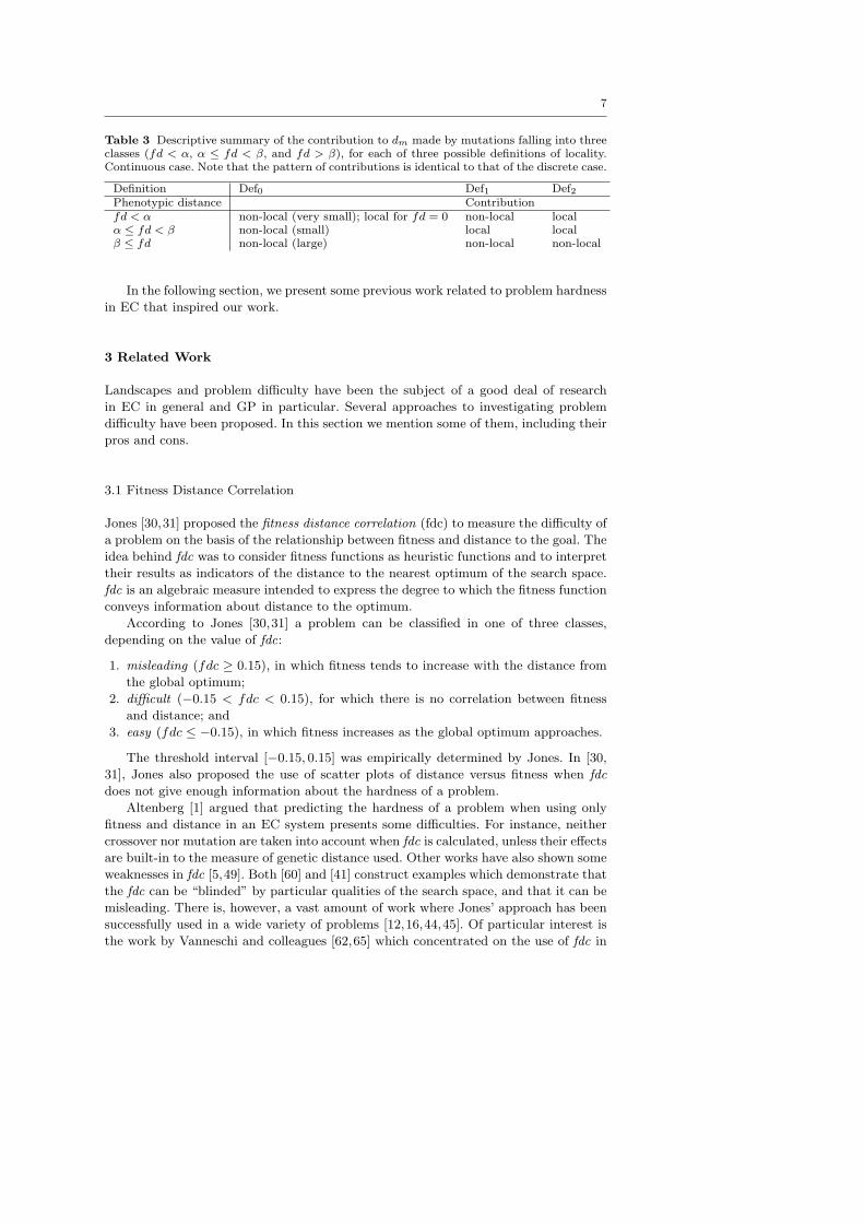
Table 3 preserves the same pattern of contributions to dm for continuous-valued

fitness as held for discrete-valued fitness, and gives new, generalised definitions based

on the idea of two threshold values. α is a small value: mutations which alter fitness

by less than α are regarded as essentially fitness-neutral. β is larger: mutations which

alter fitness by more than β are regarded as quite non-local. So, Table 3 generalises

Table 2.

As stated in Section 2, Rothlauf’s definition of locality is small for well-behaved

mappings (locality), and large for badly-behaved mappings (non-locality). This prop-

erty is inherited by our modifications to the definition.

7

Table 3 Descriptive summary of the contribution to dm made by mutations falling into threeclasses (fd < α, α ≤ fd < β, and fd > β), for each of three possible definitions of locality.Continuous case. Note that the pattern of contributions is identical to that of the discrete case.

Definition Def0 Def1 Def2Phenotypic distance Contributionfd < α non-local (very small); local for fd = 0 non-local localα ≤ fd < β non-local (small) local localβ ≤ fd non-local (large) non-local non-local

In the following section, we present some previous work related to problem hardness

in EC that inspired our work.

3 Related Work

Landscapes and problem difficulty have been the subject of a good deal of research

in EC in general and GP in particular. Several approaches to investigating problem

difficulty have been proposed. In this section we mention some of them, including their

pros and cons.

3.1 Fitness Distance Correlation

Jones [30,31] proposed the fitness distance correlation (fdc) to measure the difficulty of

a problem on the basis of the relationship between fitness and distance to the goal. The

idea behind fdc was to consider fitness functions as heuristic functions and to interpret

their results as indicators of the distance to the nearest optimum of the search space.

fdc is an algebraic measure intended to express the degree to which the fitness function

conveys information about distance to the optimum.

According to Jones [30,31] a problem can be classified in one of three classes,

depending on the value of fdc:

1. misleading (fdc ≥ 0.15), in which fitness tends to increase with the distance from

the global optimum;

2. difficult (−0.15 < fdc < 0.15), for which there is no correlation between fitness

and distance; and

3. easy (fdc ≤ −0.15), in which fitness increases as the global optimum approaches.

The threshold interval [−0.15, 0.15] was empirically determined by Jones. In [30,

31], Jones also proposed the use of scatter plots of distance versus fitness when fdc

does not give enough information about the hardness of a problem.

Altenberg [1] argued that predicting the hardness of a problem when using only

fitness and distance in an EC system presents some difficulties. For instance, neither

crossover nor mutation are taken into account when fdc is calculated, unless their effects

are built-in to the measure of genetic distance used. Other works have also shown some

weaknesses in fdc [5,49]. Both [60] and [41] construct examples which demonstrate that

the fdc can be “blinded” by particular qualities of the search space, and that it can be

misleading. There is, however, a vast amount of work where Jones’ approach has been

successfully used in a wide variety of problems [12,16,44,45]. Of particular interest is

the work by Vanneschi and colleagues [62,65] which concentrated on the use of fdc in

8

the context of GP. Recent works using fdc on GP include [11,12]. This is particularly

interesting because it has been shown that fdc can be applied using tree-like structures

providing a suitable tree distance definition.

3.2 Fitness Clouds and Negative Slope Coefficient

Later work by Vanneschi and colleagues attempted to address weaknesses of the fdc

with new approaches. Fitness clouds plots the relationship between the individuals’

fitness values in a sample and the fitness of (a sample of) their neighbours. The negative

slope coefficient [64,66] can be calculated even without knowing the optima’s genotypes

and it does not (explicitly) use any distance. In [62,64], the authors reported good

results on some GP benchmark problems. Successively in [63] these results have been

extended to some real-like applications. Then in [47] the authors gave a formal model

of the fitness proportional negative slope coefficient and a more rigorous justification

of it. Finally, in [67], the authors pointed out the limitations of this approach.

3.3 Other Landscape Measures

Several other approaches to studying landscapes and problem difficulty have also been

proposed, generally in a non-GP context, including: other measures of landscape cor-

relation [68], autocorrelation [39]; epistasis, which measures the degree of interaction

between genes and is a component of deception [20,21,41]; monotonicity, which is

similar to fdc in that it measures how often fitness improves despite distance to the

optimum increasing [41]; and distance distortion which relates overall distance in the

genotype and phenotype spaces [52]. All of these measures are to some extent related.

3.4 Further Comments on Locality

Routhlauf [52] was, perhaps, one of the first researchers that formally introduced the

concept of locality in Evolutionary Computation systems. However, it is fair to say

that other researchers [10,39] have also studied this concept motivated by the same

idea: small changes at the genotype level should correspond to small changes at the

phenotype level to have locality (originally referred as “high locality” in Routhlauf’s

work [52]).

Similarly, the principle of strong causality [50] states that for successful search, a

small change in genotype should result in a small change in fitness [2,51]. In other

words, the design process of an algorithm should be guided by the locality principle.

4 Experimental Setup

For our analysis, we have used five well-known problems for GP: the Even-n-Parity

(n = {3, 4}) problem (problems that require the combination of several XOR functions,

and are difficult if no bias favorable to their induction is added in any part of the

algorithm), the Artificial Ant Problem [33] (which has been shown to have multimodal

9

Table 4 Function sets used on the Even-n-Parity Problem (n = {3, 4}), the Artificial AntProblem and Symbolic Regression Problems (F1 = x4,+x3 + x2 + x, F2 = 2sin(x)cos(y)).FE3∗ , FA3∗ and FS6∗ refer to the Uniform GP (read text).

Problem Function Sets

FE3 = {AND,OR,NOT}Even-n-Parity FE4 = {AND,OR,NAND,NOR}

FE3∗ = {AND,OR,NOT2}FA3 = {IF, P2, P3}

Artificial Ant FA4 = {IF, P2, P3, P4}FA3∗ = {IF3, P23, P3}FS6 = {+,−, ∗,%, Sin, Cos}

Symbolic Regression FS4 = {+,−, ∗,%}FS6∗ = {+,−, ∗,%, Sin2, Cos2}

deceptive features [36, Chapter 9]) and Real-Valued Symbolic Regression problems

(with target functions: F1 = x4 + x3 + x2 + x and F2 = 2sin(x)cos(y)).

The first and second problems are Boolean Even-n-Parity problems (n = {3, 4})

where the goal is to evolve a function that returns true if an even number of the inputs

evaluate to true, and false otherwise. The maximum fitness for this type of problem is

2n. The terminal set is the set of inputs. In the next section we further describe and

explain two function sets used in this type of problem to study the locality present.

The third problem, the Artificial Ant Problem [33, pp. 147–155], consists of finding

a program that can successfully navigate an artificial ant along a path of 89 pellets of

food on a 32 x 32 toroidal grid. When the ant encounters a food pellet, its (raw) fitness

increases by one, to a maximum of 89. The problem is in itself challenging for many

reasons. The ant must eat all the food pellets (normally in 600 steps) scattered along

a twisted track that has single, double and triple gaps along it. The terminal set used

for this problem is T = {Move,Right, Left}. The function sets used in this problem

are explained in the following section.

The fourth and fifth problem are real-valued symbolic regression problems. The

goal of this type of problem is to find a program whose output is equal to the values of

functions. In this case we used functions F1 = x4+x3+x2+x and F2 = 2sin(x)2cos(y).

Thus, the fitness of an individual in the population reflects how close the output of

an individual comes to the target (F1, F2). It is common to define the fitness as

the sum of absolute errors measured at different values of the independent variable

x, in this case in the range [-1.0,1.0]. In this study we have measured the errors for

x ∈ {−1.0,−0.9,−0.8 · · · 0.8, 0.9, 1.0}. We have defined an arbitrary threshold of 0.01

to indicate that an individual with a fitness less than the threshold is regarded as a

correct solution, i.e. a “hit”. Different threshold values produce different results when

comparing the number of hits.

Note that in all five problems, fitness is maximised.

To study locality we need to have alternative representations with differing locality

and (presumably) differing performance. Therefore, we will use contrasts in encoding

(three encodings: standard GP, alternative function set and a slightly modified encod-

ing) and in operators (six different mutation operators). The idea here is that each

encoding will give a different value for locality and different performance, allowing us

to compare the predictions of relative performance made by locality with results of

evolutionary runs.

10

4.1 Alternative Function Sets

As mentioned previously, we expect to find different performance when using different

function sets. This will allow us to compare the performance predictions made by

locality with actual performance. So, for each of the problems used, we propose to use

an alternative function set.

Let us start with the Even-n-Parity problem. The terminal set used for this problem

is the set of inputs, often called T = {D0, D1, · · · , Dn−1}. The standard function set is

FE3 = {NOT,OR,AND} and we propose an alternative function set for comparison:

FE4 = {AND,OR,NAND,NOR}.

For the Artificial Ant problem, the terminal set used is T = {Move,Right, Left}.

The standard function set is FA3 = {If, P2, P3} (see [33] for a full description). In

order to have alternative encodings (with again, as we will see, different performance

and locality characteristics), we now propose an alternative function set. This is FA4 =

{If, P2, P3, P4}. The only difference is the addition of an extra sequencing function,

P4, which runs each of its four subtree arguments in order.

For the last type of problem, Symbolic Regression, the terminal set is defined

by the variables used in the function (e.g., T = {x}). The standard function set

FS6 = {+,−, ∗,%, Sin, Cos}, and we propose an alternative function set for com-

parison purposes: FS4 = {+,−, ∗,%}.

4.2 Uniform GP

In our previous work [13,14], we have studied contrasts between GP encodings induced

by using alternative function sets. However, in GP contrasts also exist between different

encodings, including linear GP [42], graph-based GP [18], and more. In order to include

in our study the distinction between encodings, we use a contrast between standard

tree-structured GP and a slightly different GP encoding called Uniform GP [17].

Uniform GP, called uniform because all internal nodes are of the same arity, is an

encoding defined by adding ‘dummy’ arguments (i.e., terminals/subtrees) to internal

nodes whose arity is lower than the maximum arity defined in the function set. These

are called dummy arguments because they are not executed when the individual is

evaluated. For this to happen, it is necessary to use special functions that indicate the

use of dummy arguments (these special functions can be seen as flags that indicate

that the subtree beneath these type of functions will not be executed). Thus, dummy

arguments can be seen only in trees that allow those special functions.

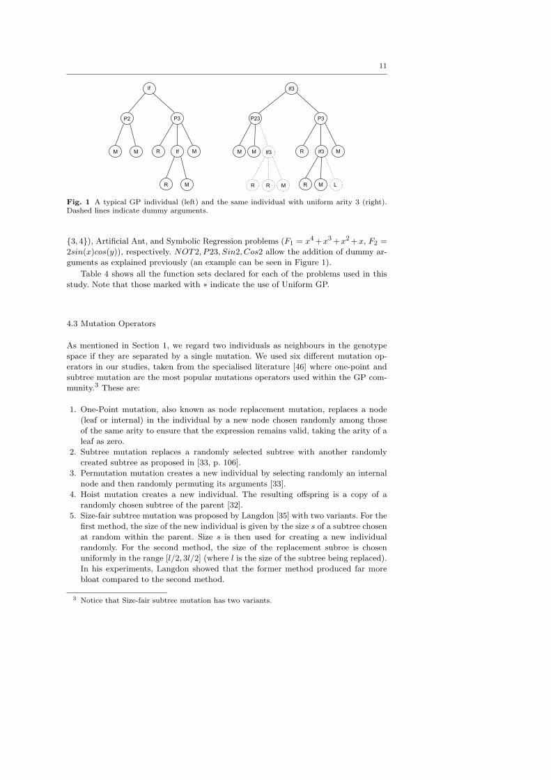
For a better understanding of how this representation works, let us present an

example. Suppose that one is dealing with the traditional Artificial Ant Problem. That

is, the function set is formed by F = {If, P2, P3} where the arities of each function

are 2, 2 and 3, respectively. This function set has a maximum arity of 3. A typical GP

individual is shown in Figure 1 (left) and a corresponding individual using Uniform

GP is shown on the right of Figure 1.2 Please, refer to [17] for a detailed explanation.

To use this representation in our five problems, we defined three func-

tion sets: FE3∗ = {AND,OR,NOT2}, FA3∗ = {If3, P23, P3} and FS6∗ =

{+,−, ∗,%, Sin2, Cos2} (where % is protected division), for the Even-n-Parity (n =

2 Notice that this type of encoding is distinct only when the arities defined in the functionset are of different values. So, if arities are all the same, Uniform GP reduces to standard GP.

11

If

P2 P3

M M R If M

R M

If3

P23 P3

M M R If3 M

R M L

If3

R R M

Fig. 1 A typical GP individual (left) and the same individual with uniform arity 3 (right).Dashed lines indicate dummy arguments.

{3, 4}), Artificial Ant, and Symbolic Regression problems (F1 = x4+x3+x2+x, F2 =

2sin(x)cos(y)), respectively. NOT2, P23, Sin2, Cos2 allow the addition of dummy ar-

guments as explained previously (an example can be seen in Figure 1).

Table 4 shows all the function sets declared for each of the problems used in this

study. Note that those marked with ∗ indicate the use of Uniform GP.

4.3 Mutation Operators

As mentioned in Section 1, we regard two individuals as neighbours in the genotype

space if they are separated by a single mutation. We used six different mutation op-

erators in our studies, taken from the specialised literature [46] where one-point and

subtree mutation are the most popular mutations operators used within the GP com-

munity.3 These are:

1. One-Point mutation, also known as node replacement mutation, replaces a node

(leaf or internal) in the individual by a new node chosen randomly among those

of the same arity to ensure that the expression remains valid, taking the arity of a

leaf as zero.

2. Subtree mutation replaces a randomly selected subtree with another randomly

created subtree as proposed in [33, p. 106].

3. Permutation mutation creates a new individual by selecting randomly an internal

node and then randomly permuting its arguments [33].

4. Hoist mutation creates a new individual. The resulting offspring is a copy of a

randomly chosen subtree of the parent [32].

5. Size-fair subtree mutation was proposed by Langdon [35] with two variants. For the

first method, the size of the new individual is given by the size s of a subtree chosen

at random within the parent. Size s is then used for creating a new individual

randomly. For the second method, the size of the replacement subree is chosen

uniformly in the range [l/2, 3l/2] (where l is the size of the subtree being replaced).

In his experiments, Langdon showed that the former method produced far more

bloat compared to the second method.

3 Notice that Size-fair subtree mutation has two variants.

12

Table 5 Parameters used to conduct our experiments. Notice that we used different combi-nations of population sizes along with number of generations.

Selection Tournament (size 7)Initial Population Ramped half and half (depth 3 to 8)Population size 200, 250, 500Generations 125, 100, 50 (25,000 divided by population size)Runs 100Mutations One Point, Subtree, Permutation, Hoist

Size-Fair & Size-Fair RangeMutation rate One single mutation per individualTermination Maximum number of generations

4.4 Sampling and Parameters

To have sufficient statistical data, we created 1,250,000 individuals for each of the

six mutation operators described previously. These samplings were created using the

traditional ramped half-and-half initialisation method described in [33] using depths

= [3, 8]. By using this method, we guarantee that we will use trees of different sizes

and shapes.

4.4.1 Comments on the Sampling Method

This sampling method is only one possibility among many. Another approach that can

be considered is to balance the number of bad individuals (low fitness values) against

good individuals (fitter individuals) by creating a sample for each of the individuals that

will be inserted in the final sampling. That is, one could take the approach of sampling

individuals, take the fitter value(s) and add those into the final sampling, and repeating

this process until the final sampling has been completed. Another approach that one

can use is generating the same number of individuals for each of the fitness values that

can be created, as shown in our previous work [15]. There are some restrictions with

this approach. For instance, one should know in advance all the possible values that

the fitness could take. Also, the generation of individuals with high fitness is very hard

to achieve. Other approaches might be possible and each of these will definitely give

different results.

We decided to start with one the simplest possible approaches to generate a sam-

pling. In future work, we would like to explore the implications of using different

sampling methods.

4.5 Studying Locality

To study and examine the locality present, for each data point in the sample data,

we created an offspring via each mutation operator described earlier, as in our locality

definitions (Section 2).

To compare the predictions made by locality, we performed runs using the parame-

ters shown in Table 5 and using the function sets explained previously and summarised

in Table 4. In particular, note that mutation-only GP was used. This is because in typi-

cal EC scenarios including crossover, mutation is relegated to a “background operator”

[27]. In such an algorithm, the true neighbourhood of individuals is largely determined

13

by their mutual accessibility under crossover, rather than mutation, and so the typical,

mutation-based definition of locality used here would be misleading.

In the following section we present and describe the results on locality using the

described parameters.

5 Results

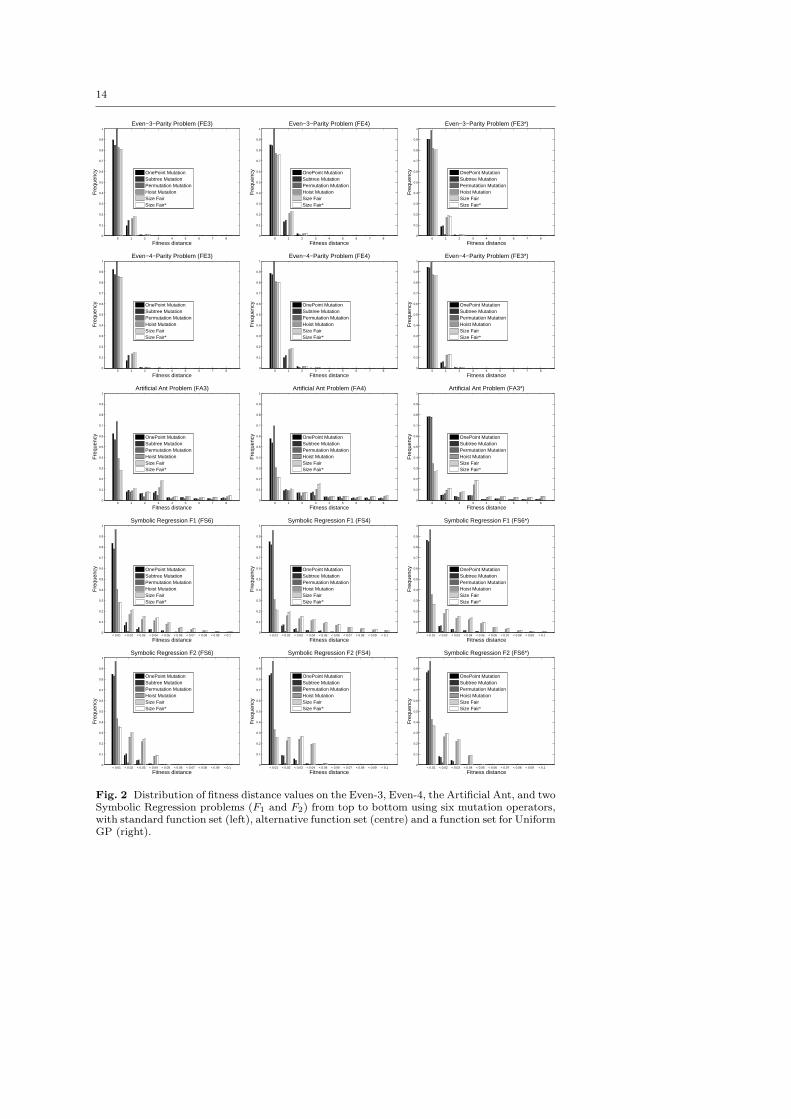
5.1 Fitness Distance Distributions

Let us start our analysis by taking a look at the distributions of fitness distances (fd)

induced by the six mutation operators explained in Section 4. In particular, we will

focus our attention on fd = {0, 1} for discrete values (i.e., Even-n-Parity and Artificial

Ant). This situation, however, changes for continuous values which is the case for the

Symbolic Regression problem. Here, as explained in Section 2, it is necessary to set

thresholds (denoted with α and β). So, we analyse the frequency of fitness distance

grouped into bins (fd < α, α < fd < β). Figure 2 shows the frequency of each possible

fd between parent-offspring, for the five problems used in this study (introduced in

Section 4) and three function sets (see Table 4) for each problem.

For the first and second problem, Even-n-Parity (n = {3, 4}) problems, we can see

on the fitness distance distribution (first and second row of Figure 2) that regardless of

the encoding used a high number of mutations are fitness neutral (i.e., fd = 0). There

are, however, some variations worth mentioning. For instance, FE3 and FE3∗ (see

Table 4 for a description of them) produce the largest number of neutral mutations for

all six mutation operators used4 compared with FE4. If we further analyse this fitness

neutrality in each of the function sets, we can see that one-point mutation produces

the largest number of neutral (fd = 0) mutations compared to the other mutation

operators (excluding permutation mutation for this particular problem for the reasons

explained previously). On the other hand, we can see that FE4 produces the largest

number of (fd = 1) mutations compared to FE3 and FE3∗ .

For the third problem, the Artificial Ant, fitness differences of up to 89 are possible,

but larger values are rare and their frequency decreases roughly linearly. Therefore, we

have omitted values above 8 to make the important values easier to visualise (see

middle of Figure 2). Again, we can see that regardless of the encoding used, a high

number of mutations are fitness neutral, where the largest number of occurrences of

fd = 0 is when using the encoding FA3∗ and subtree mutation. For the case of fd = 1,

the situation is less clear. Here, using any of the three encodings (i.e., FA3, FA4, FA3∗)

seems to produce more or less the same number of occurrences.

For the last two problems, Symbolic Regression (F1 and F2) functions, it is no

longer possible to use the same approach as before because of the nature of the problem

(continuous-valued fitness). So, as mentioned previously, we analyse the frequency of

fitness distances grouped into bins. For this particular problem and for the threshold

values that we have used for our studies, it is not clear what encoding (induced by FS6,

FS4 and FS6∗) produces the largest number of occurrences for fd < α and α < fd < β.

In the following section we further discuss this and clarify the type of locality present

in this problem.

4 Notice that when using the permutation mutation operator and using FE3 and FE4 onthe Even-n-Parity problem, the fd is always 0 because all of the operators in these functionsets are symmetric.

14

0 1 2 3 4 5 6 7 80

0.1

0.2

0.3

0.4

0.5

0.6

0.7

0.8

0.9

1Even−3−Parity Problem (FE3)

Fitness distance

Fre

quen

cy

OnePoint MutationSubtree MutationPermutation MutationHoist MutationSize FairSize Fair*

0 1 2 3 4 5 6 7 80

0.1

0.2

0.3

0.4

0.5

0.6

0.7

0.8

0.9


Fitness distance

Fre

quen

cy


0 1 2 3 4 5 6 7 80

0.1

0.2

0.3

0.4

0.5

0.6

0.7

0.8

0.9

1Even−3−Parity Problem (FE3*)

Fitness distance

Fre

quen

cy


0 1 2 3 4 5 6 7 80

0.1

0.2

0.3

0.4

0.5

0.6

0.7

0.8

0.9


Fitness distance

Fre

quen

cy


0 1 2 3 4 5 6 7 80

0.1

0.2

0.3

0.4

0.5

0.6

0.7

0.8

0.9


Fitness distance

Fre

quen

cy


0 1 2 3 4 5 6 7 80

0.1

0.2

0.3

0.4

0.5

0.6

0.7

0.8

0.9

1Even−4−Parity Problem (FE3*)

Fitness distance

Fre

quen

cy


0 1 2 3 4 5 6 7 80

0.1

0.2

0.3

0.4

0.5

0.6

0.7

0.8

0.9

1Artificial Ant Problem (FA3)

Fitness distance

Fre

quen

cy


0 1 2 3 4 5 6 7 80

0.1

0.2

0.3

0.4

0.5

0.6

0.7

0.8

0.9

1Artificial Ant Problem (FA4)

Fitness distance

Fre

quen

cy


0 1 2 3 4 5 6 7 80

0.1

0.2

0.3

0.4

0.5

0.6

0.7

0.8

0.9

1Artificial Ant Problem (FA3*)

Fitness distance

Fre

quen

cy


< 0.01 < 0.02 < 0.03 < 0.04 < 0.05 < 0.06 < 0.07 < 0.08 < 0.09 < 0.10

0.1

0.2

0.3

0.4

0.5

0.6

0.7

0.8

0.9

1Symbolic Regression F1 (FS6)

Fitness distance

Fre

quen

cy


< 0.01 < 0.02 < 0.03 < 0.04 < 0.05 < 0.06 < 0.07 < 0.08 < 0.09 < 0.10

0.1

0.2

0.3

0.4

0.5

0.6

0.7

0.8

0.9


Fitness distance

Fre

quen

cy


< 0.01 < 0.02 < 0.03 < 0.04 < 0.05 < 0.06 < 0.07 < 0.08 < 0.09 < 0.10

0.1

0.2

0.3

0.4

0.5

0.6

0.7

0.8

0.9

1Symbolic Regression F1 (FS6*)

Fitness distance

Fre

quen

cy


< 0.01 < 0.02 < 0.03 < 0.04 < 0.05 < 0.06 < 0.07 < 0.08 < 0.09 < 0.10

0.1

0.2

0.3

0.4

0.5

0.6

0.7

0.8

0.9


Fitness distance

Fre

quen

cy


< 0.01 < 0.02 < 0.03 < 0.04 < 0.05 < 0.06 < 0.07 < 0.08 < 0.09 < 0.10

0.1

0.2

0.3

0.4

0.5

0.6

0.7

0.8

0.9


Fitness distance

Fre

quen

cy


< 0.01 < 0.02 < 0.03 < 0.04 < 0.05 < 0.06 < 0.07 < 0.08 < 0.09 < 0.10

0.1

0.2

0.3

0.4

0.5

0.6

0.7

0.8

0.9

1Symbolic Regression F2 (FS6*)

Fitness distance

Fre

quen

cy


Fig. 2 Distribution of fitness distance values on the Even-3, Even-4, the Artificial Ant, and twoSymbolic Regression problems (F1 and F2) from top to bottom using six mutation operators,with standard function set (left), alternative function set (centre) and a function set for UniformGP (right).

15

Finally, it should be noticed that Uniform GP (introduced in Section 4) was orig-

inally proposed to add neutrality in the search space, as explained in [17]. So, we can

see that in almost all cases, this type of encoding produced a larger number of neutral

mutations compared to the other two alternative function sets (see third column of

Figure 2).

It is clear that while fitness distance distributions can give us an idea of the type of

locality induced by each mutation operator and encoding, the plots shown in Figure 2

cannot really tell us which operator and encoding gives the best locality. Thus, to better

understand this, one should really take a look at the quantitative measures introduced

formally in Section 2. This will be discussed in the next section.

5.2 Quantitative Measures and Performance

As mentioned previously (see Section 2), Rothlauf [52] distinguished two forms of

locality: high and low locality. In a nutshell, Rothlauf claimed that a representation

with high locality is more likely to perform effective evolutionary search compared to a

representation with low locality. However, his numerical definition, and the extensions

we have proposed for it, give smaller values for higher locality. To avoid confusion, as

we mentioned previously, we refer to high and low locality as locality and non-locality,

respectively.

We have seen in the previous paragraphs an overall picture of the fitness distance

distributions induced by different encodings on the five problems analysed in this paper.

As mentioned previously, to better understand the effects of locality on performance,

a quantitative analysis is necessary. To achieve this, we performed extensive empirical

experimentation (100 ∗ 45 ∗ 6 runs in total)5. Details of the parameters used to con-

duct our runs are shown in Table 5. Because of the dimensions of all the information

gathered during our experiments (details of these results can be seen in Appendix A

from Table 9 to 18), we have decided to process this information to help the reader to

better understand our findings.

Let us start with the number of correct predictions of locality on performance

on the five problems and six different mutation operators used in this study. This is

shown in Table 6. Using the data shown from Tables 9 to 18, this table was built by

comparing the best locality (recall that the lower the value for locality, the better)

versus performance (measured in terms of best average fitness per run) over three

different settings (i.e., different population sizes and number of generations). Thus, a

perfect prediction will be 3, where the representation with the best locality value under

a particular definition turns out to give the best performance over all three population

size/number of generations settings. We have grouped the three definitions (denoted

by Def0, Def1 and Def2 – see caption of Table 6 for a description of them) for each of

the five problems used in this study.

So, let us focus our attention on the Even-3-Parity problem. The results shown in

Table 6 indicate that Def0 was able to correctly predict 2 (out of 3) when using Hoist,

Size Fair mutation and its variant. Def1 was able to correctly predict performance when

using One-Point and Subtree mutation on the three different settings (i.e., population

sizes and number of generations) and was able to predict performance only once when

5 100 independent runs, 45 different settings (i.e., three different combinations of populationsizes and number of generations, five different problems and three different function sets foreach of the five problems - 3 ∗ 5 ∗ 3), and 6 different mutation operators.

16

Table 6 Number of correct predictions of good locality on performance (measured as meanbest fitness over 100 runs), for the Even-n-Parity (n = {3, 4}), Artificial Ant and two SymbolicRegression problems (F1, F2) and using six different mutation operators. The three differentdefinitions of locality are denoted by Def0, Def1 and Def2. Table 2 shows the locality definitionsfor discrete-valued fitness (e.g., Even-n-Parity and Artificial Ant). Table 3 shows the localitydefinitions for continuous-values fitness (e.g., Symbolic Regression).

One Subtree Permut. Hoist Size Size TotalPoint Fair Fair*

Even-3-ParityDef0 0 0 - 2 2 2 6Def1 3 3 - 1 1 1 9

Def2 0 0 - 0 0 0 0

Even-4-ParityDef0 1 1 - 1 0 1 4Def1 1 1 - 3 3 3 11

Def2 0 1 - 0 0 0 1

Artificial AntDef0 0 0 3 0 3 3 9Def1 0 0 3 0 3 3 9Def2 0 0 3 0 3 3 9

Symbolic Regression F1

Def0 2 2 0 0 0 0 4Def1 0 0 0 3 3 3 9

Def2 2 2 0 0 0 0 4


Def0 1 1 2 1 1 0 6Def1 3 1 2 1 1 1 9

Def2 1 1 1 1 1 1 6

using Hoist, Size Fair mutation and its variant. On the other hand, Def2 was unable

to predict performance of any of the mutation operators used for the Even-3-Parity

problem. When we focus our attention on the overall prediction versus performance

for each of the definitions of locality (shown at the bottom of Table 6), we can see that

the definition of locality that most frequently predicted performance correctly on the

Even-3-Parity problem is Def1 with 9 correct predictions. It is important to mention

that the lack of values for the Permutation operator for this particular problem is due

to the nature of both the operator and the problem in itself. That is, recalling how

the permutation operator works (described in detail in Section 4), we can see that this

operator will not have any impact after being applied to an individual because the

binary operators AND and OR are insensitive to the ordering of their arguments.

The same trend can be observed for the second problem, the Even-4-Parity. That

is, Def1 was able to predict correctly 11 out of 15 (recall that a perfect prediction

is 3 for each mutation operator – in this particular case only 5 mutation operators

because permutation cannot be applied for this problem as explained in the previous

paragraph). For Def0 and Def2 the overall prediction was 4 and 1, respectively. This

agrees with the results on the Even-3-Parity problem, as described previously.

Now, let us turn our attention to the third problem, the Artificial Ant problem.

Here, the three definitions of locality (formally introduced and described in Section 2)

show the same behaviour, so none of the definitions is better or worse than the others.

For the fourth problem Symbolic Regression problem F1, definitions Def0 and Def2correctly predicted the performance in 2 out of 3 cases for One-Point and Subtree

17

Table 7 Number of correct predictions of all locality values on performance (measured asmean best fitness over 100 runs), for the Even-n-Parity (n = {3, 4}), Artificial Ant and twoSymbolic Regression problems (F1, F2). The three different definitions of locality are denotedby Def0, Def1 and Def2. Table 2 shows the locality definitions for discrete-valued fitness (e.g.,Even-n-Parity and Artificial Ant). Table 3 shows the locality definitions for continuous-valuesfitness (e.g., Symbolic Regression). FE3, FA3, FS6 uses standard GP, FE4, FA4, FS4 uses an al-ternative function set and FE3∗ , FA3∗ , FS6∗ uses Uniform GP for the Even-n-Parity, ArtificialAnt and Symbolic Regression problems, respectively.

FE3, FA3, FS6 FE4, FA4, FS4 FE3∗ , FA3∗ , FS6∗ Total

Even-3-ParityDef0 7 0 2 9Def1 3 9 3 15

Def2 3 0 3 6

Even-4-ParityDef0 8 2 0 10Def1 5 7 11 23

Def2 6 2 1 9

Artificial AntDef0 7 12 9 28Def1 7 12 9 28Def2 7 12 9 28


Def0 6 4 12 22Def1 10 16 12 38

Def2 5 0 4 9


Def0 3 3 7 13Def1 10 2 4 16

Def2 4 2 5 11

mutation. On the other hand, Def1 had a perfect prediction on performance for Hoist,

Size Fair mutation and its variant. Again, when we focus our attention on the overall

prediction versus performance for each of the definitions on locality, we can clearly see

that the definition of locality that most frequently correctly predicted performance is

α < fdmin < β (denoted by Def1) with 9 correct predictions.

Finally, for the last problem (Symbolic Regression problem F2), we continue see-

ing the same trend. That is, Def1 gives the best prediction with 9, compared to the

predictions done by Def0 and Def2 with 6 for these two definitions.

So far, we have examined how many of the “best” locality made a good prediction.

In other words, locality should correspond with the best performance (measured in

terms of the average of the best fitness per generation). As mentioned previously, we

have condensed this information in Table 6 (details can be found from Table 9 to 18

shown in Appendix A) and, as discussed in the previous paragraphs, we can clearly see

that overall, the best definition of locality in terms of performance prediction is when

using Def1 (see Section 2 for a formal definition of it).

Of course, there are other ways to interpret all the data gathered during our ex-

periments (shown in Tables 9 - 18). So, to corroborate these initial findings, we have

analysed all locality values (shown in Tables 9, 11, 13, 15 and 17) and compared their

values against performance (shown in Tables 10, 12, 14, 16 and 18) over all the six

mutation operators used in this study (see Section 4 for a description of each of them).

We have condensed this information in a way to highlight what definition of locality

18

Table 8 Correlation values.

Problem Def. Even-3 Even-4 Artificial Ant F1 F2

Def0 -0.16 (×) 0.11 (×) -0.73 (X) -0.34 (×) -0.36 (×)Def1 0.19 (×) 0.13 (×) -0.74 (X) 0.47 (X) 0.34 (X)Def2 0.01 (×) -0.02 (×) -0.74 (X) 0.05 (×) 0.11 (×)

is the best focusing on function sets used for each problem and the three definitions of

locality used in this study. This data is shown in Table 7.

As mentioned before, we have obtained this data (Table 7) by comparing each value

of locality versus performance. To better understand this, let us focus our attention

on the Even-3-Parity problem (predictions made by locality are shown in Table 9 and

performance is shown in Table 10).

We have obtained this data by comparing each prediction made by locality versus

performance, focusing our attention on each of the definition of locality and each of

the function sets used. For instance, let us focus our attention on the predictions done

by Def0 on the Even-3-Parity (shown in Table 9), using One-Point mutation and FE3.

We can see that the quantitative measure is 0.1125 and the other two values for FE4

and FE3∗ are 0.1727 and 0.1059, respectively. This means, that the best locality is

when using FE3∗ (recall that the lower the value of locality, the better). The locality

value for FE3 is the second best, which means that performance when using One-Point

mutation and FE3 should be the second best performance, regardless of the population

size and number of generations used. When we check this, we can observe that in none

of the cases, this was true. We continue doing the same for the rest of the mutation

operators. At the end, we sum all the values (it is clear that we can have up to 18

correct predictions). Finally, to summarise these values we count the number of correct

predictions for all the function sets (per row for each of the problems used). These

values are shown in the last row of Table 7.

This data (Table 7) simply confirms our previous findings, the best definition of lo-

cality (three definition formally introduced in Section 2) on the five problems examined

in this paper is Def1.

5.2.1 Correlating Quantitative Measures and Performance

We can perform another form of analysis on the same data (Tables 9 to 18), again

relating the results of evolutionary runs with those of locality calculations. Here, we

calculate the correlation between the mean best fitness values achieved on the various

problems, using the various encodings and operators, and the corresponding locality

values. If locality values are functioning as predictors of performance, then a corre-

lation between the two should exist. For each problem and each locality-definition,

then, we arrange all locality values by function set and mutation. We do the same for

performance values, with all population size/number of generations settings grouped

together. We then calculate the Pearson’s correlation between these two data-sets.

The results are shown in Table 8. For the Even-n-Parity problems, all three defini-

tions of locality are shown to give values uncorrelated with fitness values (correlations

are not statistically significant, p > 0.05. Therefore, none of our definitions of locality

makes useful predictions on these problems.

In the case of the Artificial Ant, all three definitions of locality are shown to give

values which are strongly negatively correlated (p < 0.0001) with performance. That is,

19

lower (better) values of locality are associated with higher (better) performance. Thus,

all three definitions are making good predictions. This matches with our initial findings

shown in Tables 6 and 7. Also, this is evidence in favour of locality as a measure of

problem difficulty, though no new evidence is found in favour of one definition over the

others on this problem.

Finally, in the case of the Symbolic Regression problems, lower values of fitness

are better, so a positive correlation indicates good predictions. Def1 gives a good re-

sult (high positive correlation, p < 0.001); Def0 gives a misleading result (a negative

correlation), and Def2’s correlation does not give us information. Thus, we find some

evidence in favour of Def1. This agrees with the results reported in Tables 6 and 7.

5.3 Genotypic and Fitness Distance Distributions

In previous sections we have seen that each mutation operator leads to a characteristic

distribution of fitness distances for each problem and each encoding: indeed, it is these

distributions which are intended to be summarised by our locality measures. We now

give a partial explanation of how the differences between these distributions arise.

Recall that our definition of genetic neighbourhood is based on mutation operators:

two individuals are neighbours if one can be transformed into the other by a single

mutation. Simply, the fitness distance between neighbours arises partly from the effect

of the operator (how different are the individuals in genetic space?) and partly from

the effect of the genotype-fitness mapping (to what extent does the mapping allow

similar individuals to diverge?). Studying the first of these two effects is the goal of

this section.

Previous work has studied “the amount of variation generated in the genotype” by

an operator application, and the effect of this variation on phenotypic variation [28].

This concept is here termed the genotypic step-size. It can be quantified by applying a

distance function to the original and mutated individual [28].

In many EC applications, it is useful to choose a distance function which is coherent

with the operator, i.e. that reflects the “remoteness” of individuals via applications of

an operator. Distances have been described which reflect the number of operator appli-

cations required to produce one individual from another [43,65,6,62] or the probability

of producing one individual from another in a single step [26].

Such an approach turns out not to be useful for the current experiment. If a geno-

typic distance coherent with the operator is used to measure genotypic step-size, then

by definition every pair of neighbours (which differ by a single operator application)

will turn out to be at a minimum distance from each other. If we try to compare the

genotypic step-sizes of two different operators, for each using a distance coherent with

the operator, we will discover that every operator gives pairs of neighbours which are

always at the minimum distance from the original, and so we will get a “null” result:

every operator achieves the same genotypic step-size.

Instead, it is necessary to distinguish between the ideas of “remoteness” and “dis-

similarity”. Dissimilarity is a general-purpose concept, unrelated to the process of trans-

forming individuals using operators. In the next section we therefore introduce three

general-purpose ways to quantify dissimilarity of GP trees. No claim is made that these

three are the “best” ways to quantify dissimilarity. However, by using three different

and general-purpose functions, and showing that they do not contradict each other,

20

arguments concerning the size of the change caused by different mutation operators

can be convincingly supported.

5.3.1 Tree Distance Measures for GP

There are at least three natural approaches to comparing tree structures, based respec-

tively on minimal editing operations (tree-edit distance), alignment of similar structures

(tree-alignment distance) and normalised compression distance. Each of these has been

studied extensively outside the field of EC [4,57,59,29], and used by EC researchers

also [7,22,43,9,65,6,60]. We describe them in more detail next.

Tree-Edit Distance

Tree-edit distance is integer-valued and reflective of a very intuitive notion of the

distance between a pair of trees, based on the number of edits required to transform one

into the other. Three types of edits are allowed: insertion, deletion, and substitution.

This distance measure was studied outside EC, with algorithms given by [57,59]. It

was proposed for use in GP by [43], and is notable partly because it is closely aligned

with a mutation operator defined in the same paper.

Tree-Alignment Distance

Tree-alignment distance is a good general-purpose, continuous-valued measure

which reflects the fact that the roots of syntactic trees tend to be more important

than their lower levels. This measure, proposed for use in GP by Vanneschi and col-

leagues [65,6,60,62], is based on that proposed by [29] via [9].

Formally, the distance between trees T1 and T2 with roots R1 and R2, respectively,

is defined as follows:

dist(T1, T2, k) = d(R1, R2) + k

m∑

i=1

dist(childi(R1), childi(R2),k

2) (3)

where: d(R1, R2) = (|c(R1) − c(R2)|)z and childi(Y ) is the ith of the m possible

children of a node Y , if i < m, or the empty tree otherwise. Note that c evaluated on

the root of an empty tree is 0 by convention. The parameter k is used to give different

weights to nodes belonging to different levels in the tree and z ∈ N is a parameter of the

distance. The depth-weighting is well-motivated, in that GP trees’ roots tend to be more

important than their lowest levels. Code for this calculation is available in Galvan’s

Ph.D. thesis [11]. This distance is notable partly because, for k = 1 (i.e. without

depth-weighting) and for a particular function/terminal set (the Royal Tree set [48]),

the distance is coherent with a specially-constructed pair of mutation operators. The

configuration we use in this paper does use depth-weighting, and we are not using the

Royal Tree function/terminal set, and so our tree-alignment distance is not coherent

with any operator. As demonstrated by Vanneschi and colleagues, it is still useful as a

general-purpose distance function.

Normalised Compression Distance

The so-called “universal similarity metric” is a theoretical measure of similarity

between any two data structures (for example strings), defined in terms of Kolmogorov

21

complexity [38]. This is defined as the length of the shortest program which creates the

given string. Informally, two strings are very similar if the Kolmogorov complexity of

their concatenation is close to the complexity of just one of them. This idea was made

practical by [4]: they approximated the (uncomputable) Kolmogorov complexity of a

string by the length of its compressed version, as calculated by off-the-shelf compression

software. The “normalised compression distance” or NCD is defined as follows:

d(x, y) =C(xy)−min(C(x), C(y))

max(C(x), C(y))

where x and y are two strings, xy is their concatenation, and the function C gives the

length of the compressed version of its argument.

The NCD has been used as a distance measure for trees in fields other than EC

[4] and has been used for linear structures within EC [22], and GP has been used

to approximate Kolmogorov complexity [7]. However, to the authors’ knowledge the

NCD has not yet been used to measure distance between GP trees. It can be applied

to trees simply by encoding them as strings in prefix format. For fixed node arities,

this encoding is injective, i.e. distinct trees will give distinct prefix strings. It has the

advantage that a single mutation in a large tree will lead to a smaller distance than

a single mutation in a small tree. On the other hand, mutations near the root have

the same weight as deeper ones. It shares this disadvantage with, for example, tree

edit distance. Such distances are general-purpose, in that they are intended for general

trees, not only the syntactic trees as used in standard GP.

5.3.2 Analysis on Fitness Distance and Tree Distance Measures

In Figures 3–5 we present the most representative results on the distribution of fitness

distances and three measures (presented in the previous paragraphs) of genotypic dis-

tances between individuals which are separated in genetic space by a single mutation.

To save space we present only a small selection of results from the various problems

and encodings.

Consider first the Artificial Ant problem. Figure 3 shows the fitness and genotypic

distance distributions created by the various operators for the FA4 encoding. Although

all mutation operators can create very large outliers in fitness distance, it is clear that

the normal range of fitness distances created by the Hoist, Size-Fair, and Size-Fair

Range mutations is larger than that of the other operators, One-Point, Subtree, and

Permutation. A similar pattern holds in the three measures of genetic distance in the

same figure. If anything, the difference between operators is stronger in genetic distance

than in fitness distance: this shows that although genotypic step-size is a factor in the

fitness distance distributions summarised by the three definitions of locality, it is not

the only factor. The discrepancy between genotypic step-size distributions and fitness

distance distributions is caused by the behaviour of the genotype-fitness mapping.

Similar remarks apply to the Symbolic Regression problem, as illustrated in Fig-

ure 4, where we consider only the FS6 encoding. Again we see relatively larger values

for fitness distance, created by the Hoist, Size-Fair, and Size-Fair Range mutations,

being reflected in the three genetic distance measures. Note that Subtree mutation

is also shown here to also create larger distances than Permutation, and again this

is partly reflected in the genetic distances. However, again, genetic distances are not

perfect reflections of fitness distances. Genotypic step-size only partially explains the

22

OnePoint Subtree Hoist Permutation SizeFair SFRange

010

2030

4050

60

Fitn

ess

Dis

tanc

e


020

0040

0060

0080

0010

000

1200

0

Edi

t Dis

tanc

e


020

0040

0060

0080

0010

000

1200

0

Alig

nmen

t Dis

tanc

e


0.0

0.2

0.4

0.6

0.8

1.0

NC

D

Fig. 3 Fitness distance (top left) and the three distances used in our studies: edit, tree-alignment and normalised compression distance shown in the top right, bottom left and bottomright, respectively. Problem used: Artificial Ant using FA4 = {IF, PROG2, PROG3, PROG4}.


0.0

0.1

0.2

0.3

0.4

Fitn

ess

Dis

tanc

e


050

100

150

200

250

300

350

Edi

t Dis

tanc

e


050

100

150

200

250

300

350

Alig

nmen

t Dis

tanc

e


0.0

0.2

0.4

0.6

0.8

NC

D

Fig. 4 Fitness distance (top left) and the three distances used in our studies: edit, tree-alignment and normalised compression distance shown in the top right, bottom left and bottomright, respectively. Problem used: Symbolic Regression F1 using FS6 = {+,−, ∗,%, Sin, Cos}.

23


0.0

0.2

0.4

0.6

0.8

1.0

Fitn

ess

Dis

tanc

e


010

020

030

040

050

0

Edi

t Dis

tanc

e


010

020

030

040

050

0

Alig

nmen

t Dis

tanc

e


0.0

0.2

0.4

0.6

0.8

1.0

NC

D

Fig. 5 Fitness distance (top left) and the three distances used in our studies: edit, tree-alignment and normalised compression distance shown in the top right, bottom left and bottomright, respectively. Problem used: Symbolic Regression F1 using FS4 = {+,−, ∗,%}.

distribution of fitness distance. The discrepancy between genotypic step-size and fitness

distance is caused by the behaviour of the genotype-fitness mapping.

Contrast this finally with Figure 5, again showing the Symbolic Regression problem,

this time with the FS4 encoding. Similar patterns in the distances created by the

mutations are seen again. The difference is that often much larger outliers are created

with the FS4 encoding than FS6. This is notable in both fitness distances and genetic

distances. It may that the greater likelihood of mutations involving the discontinuous

protected division operator causes this effect.

6 Conclusions

It has been argued that locality is a key element in performing effective evolutionary

search of landscapes [53]. According to Rothlauf [53], a representation that has high

locality is necessary for efficient evolutionary search. The opposite is true when a

representation has low locality. To avoid confusion on these terms, we have referred

them as locality and non-locality, respectively.

In this work, we have extended the original genotype-phenotype definition of local-

ity (formally introduced and explained in Section 2) to the genotype-fitness mapping,

considering three different scenarios of fitness neighbourhood.

24

For this purpose, we have used five problems that include discrete- and continuous-

valued ones (both necessary for the understanding of locality in EC). We used three

different encodings (two of them induced by the use of alternative function sets and

the other by modifying slightly the GP encoding as explained in Section 4) for each of

theses problems and analysed the locality present under each encoding.

From the five problems that we have analysed, and using the three different defini-

tions of neighbourhood denoted by Def0, Def1 and Def2 (see Sections 2.1 and 2.2), we

have seen that the correct prediction was obtained more often when neighbourhood was

defined with Def1 which correspond to the definition given by Rothlauf in his original

genotype-phenotype mapping studies using bitstrings [53].

To test these quantitative measures of locality, we performed 100 independent runs

for all three different encodings, 6 different operators, and three different combinations

of population sizes and number of generations. In almost all of them, we have confirmed

the prediction made by locality. It is, however, fair to say that none of the locality

definitions presented in Section 2 was able to predict performance all the time (e.g.,

different mutation operators, population sizes, generations and more). One can argue

that for any performance prediction approach, there is always a counter example, as

shown in various works (e.g., [30,67]).

7 Future Work

We have made an effort to shed some light on locality in Genetic Programming. For

this purpose, we started our analysis by using by using only mutations. This has helped

us to better understand how locality influences evolutionary search. A natural step to

take from here is by considering the use of crossover.

Also, to compare the predictions made by locality against performance, we used

one of the most popular sampling methods by considering the use of the ramped half-

and-half method. As mentioned previously, this approach has some limitations, so it

would be interesting to explore other sampling methods (some of them were detailed

in Section 4).

Acknowledgments

This research is based upon works supported by Science Foundation Ireland under

Grant No. 08/IN.1/I1868 and by the Irish Research Council for Science, Engineer-

ing and Technology under the Empower scheme. The authors would like to thank the

anonymous reviewers for their valuable comments. Leonardo Vanneschi is particularly

thanked for his helpful suggestions and for his encouragement to further continue de-

veloping this research.

A Appendix

Tables 9, 11, 13, 15 and 17 show the results on locality and Tables 10, 12, 14, 16 and 18show the performance (measured in terms of average of the best fitness values over all runs)for the Even-3, Even-4, Artificial Ant and two Symbolic Regression problems (F1 and F2),respectively.

25

Table 9 Locality on the Even-3-Parity Problem using three function sets (FE3 ={AND,OR,NOT}, FE4 = {AND,OR,NAND,NOR} and FE3∗ = {AND,OR,NOT2}),six mutations, and three locality definitions. Lower is better.

Mutation fdmin = 0 fdmin = 1 Cond.(fdmin = 1)Operators FE3 FE4 FE3∗ FE3 FE4 FE3∗ FE3 FE4 FE3∗

One Point 0.1125 0.1727 0.1059 0.9057 0.8699 0.9145 0.0091 0.0213 0.0102Subtree 0.1599 0.1638 0.1026 0.8562 0.8541 0.9064 0.0081 0.0089 0.0045

Permutation 0 0 0.0154 1 1 0.9859 0 0 0.0006Hoist 0.1902 0.2497 0.1932 0.8376 0.7936 0.8304 0.0139 0.0217 0.0118

Size Fair 0.2046 0.2710 0.2063 0.8173 0.7707 0.8150 0.0109 0.0209 0.0106Size Fair* 0.1993 0.2641 0.2017 0.8207 0.7742 0.8179 0.0100 0.0191 0.0098

Table 10 Performance (measured in terms of average of the best fitness values over all runs)of a Mutation-Based GP on the Even-3-Parity Problem. Numbers within parentheses indicatenumber of runs able to find the global optimum. Higher is better. Values out of 16.

Mutation P = 500, G = 50 P = 250, G = 100 P = 200, G = 125Operators FE3 FE4 FE3∗ FE3 FE4 FE3∗ FE3 FE4 FE3∗

OnePoint 6.97 7.77 7.51 6.99 7.87 7.13 6.52 7.75 7.00(81) (64) (88) (28) (81) (18)

Subtree 7.41 7.76 7.63 7.28 7.85 7.15 6.86 7.66 7.09(42) (80) (69) (30) (86) (29) (1) (79) (21)

Permutation 5.94 4.95 5.88 5.94 4.95 4.98 4.95 5.94 5.41Hoist 6.00 5.15 5.03 6.00 5.06 5.00 5.16 6.00 4.00Size Fair 6.00 5.03 5.00 5.99 5.03 5.00 4.98 6.00 4.98Size Fair* 6.00 5.03 5.00 5.99 5.02 5.00 4.99 6.00 5.00

References

1. L. Altenberg. Fitness Distance Correlation Analysis: An Instructive Counterexample. InT. Back, editor, Proceedings of the Seventh International Conference on Genetic Algo-rithms, pages 57–64, San Francisco, CA, USA, 1997. Morgan Kaufmann.

2. H. Beyer and H. Schwefel. Evolution strategies–A comprehensive introduction. NaturalComputing, 1(1):3–52, 2002.

3. M. Brameier and W. Banzhaf. Linear genetic programming. Springer-Verlag New YorkInc, 2006.

4. R. Cilibrasi and P. M. B. Vitanyi. Clustering by compression. IEEE Transactions onInformation theory, 51(4):1523–1545, 2005.

5. M. Clergue and P. Collard. GA-Hard Functions Built by Combination of Trap Func-tions. In D. B. Fogel, M. A. El-Sharkawi, X. Yao, G. Greenwood, H. Iba, P. Marrow, andM. Schackleton, editors, CEC 2002: Proceedings of the 2002 Congress on EvolutionaryComputation, pages 249–254. IEEE Press, 2002.

6. M. Clergue, P. Collard, M. Tomassini, and L. Vanneschi. Fitness Distance Correlationand Problem Difficulty for Genetic Programming. In W. B. Langdon, E. Cantu-Paz, K. E.Mathias, R. Roy, D. Davis, R. Poli, K. Balakrishnan, V. Honavar, G. Rudolph, J. Wegener,L. Bull, M. A. Potter, A. C. Schultz, J. F. Miller, E. K. Burke, and N. Jonoska, editors,Proceedings of the Genetic and Evolutionary Computation Conference, GECCO 2002,pages 724–732, New York, 9-13 July 2002. Morgan Kaufmann Publishers.

7. I. De Falco, A. Iazzetta, E. Tarantino, A. Della Cioppa, and G. Trautteur. A Kolmogorovcomplexity based genetic programming tool for string compression. In Proceedings of theGenetic and Evolutionary Computation Conference (GECCO-2000), 2000.

8. P. D’haeseleer and J. Bluming. Effects of locality in individual and population evolution.In K. E. Kinnear, editor, Advances in Genetic Programming, pages 177–198. MIT Press,1994.

9. A. Ekart and S. Z. Nemeth. A metric for genetic programs and fitness sharing. In EuroGP,number 1802 in Lecture Notes in Computer Science, pages 259–270. Springer, 2000.

10. D. B. Fogel and A. Ghozeil. Using fitness distributions to design more efficient evolutionarycomputations, 1996.

26

Table 11 Locality on the Even-4-Parity Problem using three function sets (FE3 ={AND,OR,NOT}, FE4 = {AND,OR,NAND,NOR} and FE3∗ = {AND,OR,NOT2}),six mutations, and three locality definitions. Lower is better.

Mutation fdmin = 0 fdmin = 1 Cond.(fdmin = 1)Operators FE3 FE4 FE3∗ FE3 FE4 FE3∗ FE3 FE4 FE3∗


Permutation 0 0 0.0109 1 1 0.9900 0 0 0.0005Hoist 0.1526 0.2121 0.1365 0.8686 0.8304 0.8801 0.0106 0.0213 0.0083


Table 12 Performance (measured in terms of average of the best fitness values over all runs)of a Mutation-Based GP on the Even-4-Parity Problem. Numbers within parentheses indicatenumber of runs able to find the global optimum. Higher is better. Values out of 32.

Mutation P = 500, G = 50 P = 250, G = 100 P = 200, G = 125Operators FE3 FE4 FE3∗ FE3 FE4 FE3∗ FE3 FE4 FE3∗

OnePoint 11.89 14.35 12.16 11.35 13.66 11.66 10.88 13.40 11.29(29) (25) (17)

Subtree 12.43 14.12 12.35 12.59 13.18 11.65 12.23 13.28 11.03(15) (11) (9)


11. E. Galvan-Lopez. An Analysis of the Effects of Neutrality on Problem Hardness for Evolu-tionary Algorithms. PhD thesis, School of Computer Science and Electronic Engineering,University of Essex, United Kingdom, 2009.

12. E. Galvan-Lopez, S. Dignum, and R. Poli. The Effects of Constant Neutrality on Perfor-mance and Problem Hardness in GP. In M. O’Neill, L. Vanneschi, S. Gustafson, A. I. E.Alcazar, I. D. Falco, A. D. Cioppa, and E. Tarantino, editors, EuroGP 2008 - 11th Euro-pean Conference on Genetic Programming, volume 4971 of LNCS, pages 312–324, Napoli,Italy, 26–28 Mar. 2008. Springer.

13. E. Galvan-Lopez, J. McDermott, M. O’Neill, and A. Brabazon. Defining locality in geneticprogramming to predict performance. In CEC 2010: Proceedings of the 12th AnnualCongress on Evolutionary Computation, Barcelona, Spain, July 2010. IEEC Press.

14. E. Galvan-Lopez, J. McDermott, M. O’Neill, and A. Brabazon. Towards an understandingof locality in genetic programming. In GECCO 2010: Proceedings of the 12th AnnualConference on Genetic and Evolutionary Computation, Portland, Oregon, USA, July 2010.ACM Press.

15. E. Galvan-Lopez, M. O’Neill, and A. Brabazon. Towards understanding the effects oflocality in gp. In Artificial Intelligence, 2009. MICAI 2009. Eighth Mexican InternationalConference on, pages 9 –14, 2009.

16. E. Galvan-Lopez and R. Poli. Some Steps Towards Understanding How Neutrality AffectsEvolutionary Search. In T. P. Runarsson, H.-G. Beyer, E. Burke, J. J. Merelo-Guervos,L. D. Whitley, and X. Yao, editors, Parallel Problem Solving from Nature (PPSN IX).9th International Conference, volume 4193 of LNCS, pages 778–787, Reykjavik, Iceland,9-13 Sept. 2006. Springer-Verlag.

17. E. Galvan-Lopez and R. Poli. An empirical investigation of how degree neutrality affectsgp search. In A. H. Aguirre, R. M. Borja, and C. A. R. Garcia, editors, MICAI, volume5845 of Lecture Notes in Computer Science, pages 728–739. Springer, 2009.

18. E. Galvan Lopez, R. Poli, and C. A. Coello Coello. Reusing Code in Genetic Programming.In M. Keijzer, U.-M. O’Reilly, S. Lucas, E. Costa, and T. Soule, editors, Genetic Program-ming 7th European Conference, EuroGP 2004, Proceedings, volume 3003 of LNCS, pages359–368, Coimbra, Portugal, 5-7 Apr. 2004. Springer-Verlag.

19. E. Galvan-Lopez, R. Poli, A. Kattan, M. O’Neill, and A. Brabazon. Neutrality in evolu-tionary algorithms ... what do we know? Evolving Systems, 2011.

27

Table 13 Locality on the Artificial Ant Problem using three function sets(FA3 = {IF, PROG2, PROG3}, FA4 = {IF, PROG2, PROG3, PROG4} andFA3∗ = {IF3, PROG23, PROG3}), six mutations, and three locality definitions.Lower is better.

Mutation fdmin = 0 fdmin = 1 Cond.(fdmin = 1)Operators FA3 FA4 FA3∗ FA3 FA4 FA3∗ FA3 FA4 FA3∗


Permutation 1.1468 1.2881 0.9440 1.6234 1.6808 1.5020 0.8851 0.9844 0.7229Hoist 4.0950 4.7628 4.2617 3.8720 4.7628 3.9515 3.4835 4.4549 3.6066


Table 14 Performance (measured in terms of average of the best fitness values over all runs)of a Mutation-Based GP on the Artificial Ant Problem. Number within parentheses indicatenumber of runs able to find the global optimum. Higher is better. Values out of 89.

Mutation P = 500, G = 50 P = 250, G = 100 P = 200, G = 125Operators FA3 FA4 FA3∗ FA3 FA4 FA3∗ FA3 FA4 FA3∗

OnePoint 51.24 47.36 48.63 51.74 45.35 42.08 50.85 44.22 50.69(3) (1)

Subtree 60.54 53.60 57.76 60.14 55.09 54.25 61.63 55.27 53.28(6) (1) (5) (4) (1) (6) (2) (5)


20. D. E. Goldberg. Construction of High-Order Deceptive Functions Using Low-Order WalshCoefficients. Ann. Math. Artif. Intell., 5(1):35–47, 1992.

21. D. E. Goldberg, K. Deb, and J. Horn. Massive Multimodality, Deception, and GeneticAlgorithms. In R. Manner and B. Manderick, editors, PPSN II: Proceedings of the 2ndInternational Conference on Parallel Problem Solving from Nature, pages 37–48, Amster-dam, 1992. Elsevier Science Publishers, B. V.

22. F. J. Gomez. Sustaining diversity using behavioral information distance. In Proceedingsof the 11th Annual conference on Genetic and evolutionary computation, pages 113–120,Montreal, Canada, 2009. ACM.

23. J. Gottlieb, B. A. Julstrom, G. R. Raidl, and F. Rothlauf. Prufer numbers: A poor repre-sentation of spanning trees for evolutionary search. In S. Spector, E. Wu, B. Voigt, Gen,Sen, Dorigo, Pezeshk, Garzon, and Burke, editors, Proceedings of the Genetic and Evo-lutionary Computation Conference (GECCO 2001), pages 343–350. Morgan Kaufmann,2001.

24. J. Gottlieb and G. R. Raidl. The effects of locality on the dynamics of decoder-based evolu-tionary search. In Proceedings of the Genetic and Evolutionary Computation Conference2000.

25. J. Gottlieb and G. R. Raidl. Characterizing locality in decoder-based EAs for the multi-dimensional knapsack problem. In AE ’99: Selected Papers from the 4th European Con-ference on Artificial Evolution, pages 38–52, London, UK, 2000. Springer-Verlag.

26. S. Gustafson and L. Vanneschi. Crossover-Based Tree Distance in Genetic Programming.IEEE Transactions on Evolutionary Computation, 12(4):506–524, 2008.

27. J. H. Holland. Adaptation in Natural and Artificial Systems. University of Michigan Press,Ann Arbor, 1975.

28. C. Igel and K. Chellapilla. Investigating the influence of depth and degree of genotypicchange on fitness in genetic programming. 1999.

29. T. Jiang, L. Wang, and K. Zhang. Alignment of trees – an alternative to tree edit.Theoretical Computer Science, 143(1):137–148, 1995.

30. T. Jones. Evolutionary Algorithms, Fitness Landscapes and Search. PhD thesis, Universityof New Mexico, Albuquerque, 1995.

28

Table 15 Locality on the Symbolic Regression Problem F1 using three function sets FS6 ={+,−, ∗,%, Sin, Cos}, FS4 = {+,−, ∗,%}, FS6∗ = {+,−, ∗,%, Sin2, Cos2}, six mutations,and three locality definitions. Lower is better.

Mutation fdmin = 0 fdmin = α Cond.(fdmin = 1)Operators FS6 FS4 FS6∗ FS6 FS4 FS6∗ FS6 FS4 FS6∗

One Point 0.0052 0.0051 0.0041 0.0078 0.0082 0.0083 5.82e-05 0.0001 5.28e-05Subtree 0.0068 0.0061 0.0046 0.0071 0.0079 0.0091 7.54e-05 0.0002 4.88e-05

Permutation 0.0014 0.0016 0.0013 0.0094 0.0094 0.0029 1.92e-05 3.25e-05 8.51e-06Hoist 0.0213 0.0290 0.0232 0.0034 0.0027 0.0029 9.73e-05 0.0002 8.47e-05


Table 16 Performance (measured in terms of average of the best fitness values over all runs)of a Mutation-Based GP on the Symbolic Regression Problem F1. Numbers within parenthesesindicate number of runs able to find the global optimum. FS6 = {+,−, ∗,%, Sin, Cos}, FS4 ={+,−, ∗,%}, FS6∗ = {+,−, ∗,%, Sin2, Cos2}. Higher is better.

Mutation P = 500, G = 50 P = 250, G = 100 P = 200, G = 125Operators FS6 FS4 FS6∗ FS6 FS4 FS6∗ FS6 FS4 FS6∗

OnePoint .2063 .3180 .6751 .1959 .2686 .4633 .1930 .2726 .1916(6)

Subtree .5209 .6310 .7112 .3873 .4619 .6720 .3323 .3830 .2770(18) (46) (4) (7)) (22) (23) (6) (10) (1)

Permutation .1909 .2677 .1909 .1909 .2677 .2045 .1909 .2663 .1909Hoist .1909 .2677 .2567 .1909 .2677 .2045 .1909 .2670 .1909Size Fair .1935 .2681 .1919 .1921 .2677 .2056 .1901 .2669 .1913Size Fair* .1919 .2677 .1939 .1919 .2681 .2045 .1901 .2661 .1938

31. T. Jones and S. Forrest. Fitness Distance Correlation as a Measure of Problem Difficultyfor Genetic Algorithms. In L. J. Eshelman, editor, Proceedings of the 6th InternationalConference on Genetic Algorithms, pages 184–192, San Francisco, CA, USA, 1995. MorganKaufmann Publishers.

32. K. E. Kinnear, Jr. Fitness landscapes and difficulty in genetic programming. In Proceedingsof the 1994 IEEE World Conference on Computational Intelligence, volume 1, pages 142–147, Orlando, Florida, USA, 27-29 June 1994. IEEE Press.

33. J. R. Koza. Genetic Programming: On the Programming of Computers by Means ofNatural Selection. The MIT Press, Cambridge, Massachusetts, 1992.

34. W. Langdon and R. Poli. Why ants are hard. In J. R. Koza, editor, Proceedings of theThird Annual Conference on Genetic Programming, pages 193–201. Morgan Kaufmann,Madison, USA, 1998.

35. W. B. Langdon. The evolution of size in variable length representations. In 1998 IEEEInternational Conference on Evolutionary Computation, pages 633–638. IEEE Press, 1998.

36. W. B. Langdon and R. Poli. Foundations of Genetic Programming. Springer, Berlin, 2002.

37. P. K. Lehre and P. C. Haddow. Phenotypic Complexity and Local Variations in NeutralDegree. BioSystems, 87(2-3):233–42, 2006.

38. M. Li and P. Vitanyi. An introduction to Kolmogorov complexity and its applications.Springer Verlag, 1997.

39. B. Manderick, M. K. de Weger, and P. Spiessens. The genetic algorithm and the structureof the fitness landscape. In R. K. Belew and L. B. Booker, editors, ICGA, pages 143–150.Morgan Kaufmann, 1991.

40. J. F. Miller and P. Thomson. Cartesian genetic programming. In EuroGP, pages 121–132.Springer, 2000.

41. B. Naudts and L. Kallel. A comparison of predictive measures of problem difficulty inevolutionary algorithms. IEEE Transactions on Evolutionary Computation, 4(1):1–15,April 2000.

42. P. Nordin. Evolutionary Program Induction of Binary Machine Code and its Applications.PhD thesis, der Universitat Dortmund am Fachereich Informatik, 1997.

29

Table 17 Locality on the Symbolic Regression Problem F2 using three function sets FS6 ={+,−, ∗,%, Sin, Cos}, FS4 = {+,−, ∗,%}, FS6∗ = {+,−, ∗,%, Sin2, Cos2}, six mutations,and three locality definitions. Lower is better.

Mutation fdmin = 0 fdmin = α Cond.(fdmin = 1)Operators FS6 FS4 FS6∗ FS6 FS4 FS6∗ FS6 FS4 FS6∗

One Point 0.0046 0.0045 0.0037 0.0071 0.0072 0.0077 1.27e-05 1.38e-05 3.87e-05Subtree 0.0048 0.0040 0.0032 0.0070 0.0075 0.0080 4.91e-05 1.54e-05 3.88e-05

Permutation 0.0009 0.0008 0.0009 0.0093 0.0094 0.0094 5.96e-06 2.33e-05 1.18e-05Hoist 0.0139 0.0175 0.0141 0.0029 0.0023 0.0027 4.63e-05 1.34e-05 5.01e-05

Size Fair 0.0160 0.0193 0.0156 0.0019 0.0014 0.0019 7.17e-05 2.77e-05 6.81e-05Size Fair* 0.0160 0.0195 0.0157 0.0019 0.0013 0.0019 5.36e-05 3.64e-05 6.25e-05

Table 18 Performance (measured in terms of average of the best fitness values over all runs)of a Mutation-Based GP on the Symbolic Regression Problem F2. Numbers within parenthesesindicate number of runs able to find the global optimum. FS6 = {+,−, ∗,%, Sin, Cos}, FS4 ={+,−, ∗,%}, FS6∗ = {+,−, ∗,%, Sin2, Cos2}. Higher is better.

Mutation P = 500, G = 50 P = 250, G = 100 P = 200, G = 125Operators FS6 FS4 FS6∗ FS6 FS4 FS6∗ FS6 FS4 FS6∗

OnePoint 0.2052 .01715 0.2654 0.1508 0.1304 0.7412 0.1391 0.1296 0.2078(28) (67)

Subtree .3207 .1806 .4374 .4844 .1322 .4454 .4676 .1319 .3007(9) (21) (30) (28) (28) (7)

Permutation .1298 .1085 .1298 0.0719 .0634 .1298 .0713 .0634 .0632Hoist .1298 .1139 .1376 .0623 .0748 .1353 .0624 .0707 .0622Size Fair .1364 .1153 .1340 .0914 .0749 .1342 .0780 .0792 .0695Size Fair* .1340 .1150 .1342 .0720 .0820 .1295 .0720 .0790 .0682

43. U.-M. O’Reilly. Using a distance metric on genetic programs to understand genetic oper-ators. In IEEE International Conference on Systems, Man, and Cybernetics: Computa-tional Cybernetics and Simulation, volume 5, 1997.

44. R. Poli and E. Galvan-Lopez. On The Effects of Bit-Wise Neutrality on Fitness Dis-tance Correlation, Phenotypic Mutation Rates and Problem Hardness. In C. R. Stephens,M. Toussaint, D. Whitley, and P. Stadler, editors, Foundations of Genetic Algorithms IX,Lecture Notes in Computer Science, pages 138–164, Mexico city, Mexico, 8-11 Jan. 2007.Springer-Verlag.

45. R. Poli and E. Galvan-Lopez. The Effects of Constant and Bit-Wise Neutrality on Hard-ness, Fitness Distance Correlation and Phenotypic Mutation Rataes. IEEE Transactionson Evolutionary Computation, 2011.

46. R. Poli, W. B. Langdon, and N. F. McPhee. A field guide to genetic programming. Pub-lished via http://lulu.com and freely available at http://www.gp-field-guide.org.uk,2008. (With contributions by J. R. Koza).

47. R. Poli and L. Vanneschi. Fitness-proportional negative slope coefficient as a hardnessmeasure for genetic algorithms. In Proceedings of the 9th annual conference on Geneticand evolutionary computation, GECCO ’07, pages 1335–1342, New York, NY, USA, 2007.ACM.

48. B. Punch, D. Zongker, and E. Godman. The Royal Tree Problem, A Benchmark for Singleand Multi-population Genetic Programming. In P. Angeline and K. Kinnear, editors,Advances in Genetic Programming 2, pages 299–316, Cambridge, MA, 1996. The MITPress.

49. R. J. Quick, V. J. Rayward-Smith, and G. D. Smith. Fitness Distance Correlation andRidge Functions. In Proceedings of the 5th International Conference on Parallel ProblemSolving from Nature, pages 77–86, London, UK, 1998. Springer-Verlag.

50. I. Rechenberg. Evolutionsstrategie 94, volume 1 of Werkstatt Bionik und Evolutionstech-nik. Frommann-Holzboog, Stuttgart, 1994.

51. S. Ronald. Robust encodings in genetic algorithms. In Z. Michalewicz, K. Deb, M. Schmidt,and T. Stidsen, editors, Evolutionary Algorithms in Engineering Applications, pages 29–44. Springer, 1997.

30

52. F. Rothlauf. Representations for Genetic and Evolutionary Algorithms. Physica-Verlag,2nd edition, 2006.

53. F. Rothlauf and D. Goldberg. Redundant Representations in Evolutionary Algorithms.Evolutionary Computation, 11(4):381–415, 2003.

54. F. Rothlauf and D. E. Goldberg. Pruefer numbers and genetic algorithms: A lesson howthe low locality of an encoding can harm the performance of GAs. Technical Report3/2000, Bayreuth, 2000.

55. F. Rothlauf and E. Goldberg, David. Tree network design with genetic algorithms - aninvestigation in the locality of the pruefernumber encoding. Technical Report 6/1999,Bayreuth, 1999.

56. F. Rothlauf and M. Oetzel. On the locality of grammatical evolution. In P. Collet,M. Tomassini, M. Ebner, S. Gustafson, and A. Ekart, editors, Proceedings of the 9th Eu-ropean Conference on Genetic Programming, volume 3905 of Lecture Notes in ComputerScience, pages 320–330, Budapest, Hungary, 10 - 12 Apr. 2006. Springer.

57. D. Shasha and K. Zhang. Fast Parallel Algorithms for the Unit Cost Editing DistanceBetween Trees. In SPAA ’89: Proceedings of the First Annual ACM Symposium onParallel Algorithms and Architectures, pages 117–126, New York, NY, USA, 1989. ACM.

58. P. F. Stadler and C. R. Stephens. Landscapes and effective fitness. Comments Theori.Biol., (8):389–431, 2002.

59. M. Tacker, P. F. Stadler, E. G. Bornberg-Bauer, I. L. Hofacker, and P. Schuster. AlgorithmIndepedent Properties of RNA Secondary Structure Predictions. European BiophysicsJournal, 25(2):115–130, 1996.

60. M. Tomassini, L. Vanneschi, P. Collard, and M. Clergue. A study of fitness distancecorrelation as a difficulty measure in genetic programming. Evolutionary Computation,13(2):213–239, 2005.

61. M. Toussaint and C. Igel. Neutrality: A necessity for self-adaptation. In Proceedings ofthe IEEE Congress on Evolutionary Computation (CEC 2002), pages 1354–1359, 2002.

62. L. Vanneschi. Theory and Practice for Efficient Genetic Programming. PhD thesis,Faculty of Science, University of Lausanne, Switzerland, 2004.

63. L. Vanneschi. Investigating problem hardness of real life applications. In R. et al., editor,Genetic Programming Theory and Practive V, chapter 7, pages 107–124. Springer US,2007.

64. L. Vanneschi, M. Clergue, P. Collard, M. Tomassini, and S. Verel. Fitness clouds andproblem hardness in genetic programming. In EuroGP, LNCS, pages 690–701. Springer,2004.

65. L. Vanneschi, M. Tomassini, P. Collard, and M. Clergue. Fitness distance correlation instructural mutation genetic programming. In EuroGP, Lecture notes in computer science,pages 455–464. Springer, 2003.

66. L. Vanneschi, M. Tomassini, P. Collard, S. Verel, Y. Pirola, and G. Mauri. A comprehensiveview of fitness landscapes with neutrality and fitness clouds. In Proceedings of EuroGP2007, volume 4445 of LNCS, pages 241–250. Springer, 2007.

67. L. Vanneschi, A. Valsecchi, and R. Poli. Limitations of the fitness-proportional negativeslope coefficient as a difficulty measure. In GECCO ’09: Proceedings of the 11th Annualconference on Genetic and evolutionary computation, pages 1877–1878, New York, NY,USA, 2009. ACM.

68. E. Weinberger. Correlated and uncorrelated fitness landscapes and how to tell the differ-ence. Biological Cybernetics, 63(5):325–336, 1990.

69. S. Wright. The Roles of Mutation, Inbreeding, Crossbreeding and Selection in Evolution. InD. F. Jones, editor, Proceedings of the Sixth International Congress on Genetics, volume 1,pages 356–366, 1932.

Defining locality as a problem difficulty measure in genetic programming

Documents

Transcript of Defining locality as a problem difficulty measure in genetic programming