Locality-Sensitive Hashing for Chi2 Distance

IEEE TRANSACTIONS ON PATTERN ANALYSIS AND MACHINE INTELLIGENCE, VOL. XXXX, NO. XXX, JUNE 2010 1

Locality-Sensitive Hashing for Chi2 DistanceDavid Gorisse, Matthieu Cord, and Frederic Precioso

Abstract —In the past ten years, new powerful algorithms based on efficient data structures have been proposed to solve the problemof Nearest Neighbors search (or Approximate Nearest Neighbors search). If the Euclidean Locality Sensitive Hashing algorithm whichprovides approximate nearest neighbors in a Euclidean space with sub-linear complexity is probably the most popular, the Euclideanmetric does not always provide as accurate and as relevant results when considering similarity measure as the Earth-Mover Distanceand χ2-distance. In this paper, we present a new LSH scheme adapted to χ2-distance for approximate nearest neighbors search inhigh-dimensional spaces. We define the specific hashing functions, we prove their local-sensitivity and compare, through experiments,our method with the Euclidean Locality Sensitive Hashing algorithm in the context of image retrieval on real image databases. Theresults prove the relevance of such a new LSH scheme either providing far better accuracy in the context of image retrieval thanEuclidean scheme for an equivalent speed, or providing an equivalent accuracy but with a high gain in terms of processing speed.

Index Terms —Sublinear Algorithm, Approximate Nearest Neighbors, Locality Sensitive Hashing, χ2-distance, image retrieval

✦

1 INTRODUCTION

In the recent years, the development of effective methodsto retrieve images in large databases (more than 100 000images) has seen a growing interest both in computervision and data mining research communities.

Commonly, “Image Similarity Search” refers to theproblem of retrieving, from a database, all images shar-ing perceptual characteristics with a query image q.Describing explicitly these perceptual characteristics re-quires:

• to extract relevant visual features to represent per-ceptual image characteristics,

• to define a (dis)-similarity function between thetwo image representations in order to evaluate theoriginal perceptual similarity of these two images.

Let us notice that these two processes are not indepen-dent but related to the proper matching between distanceand visual features. When discriminating histograms forinstance, some (dis)-similarity functions, or distances, aremore accurate than the L2 distance [1]–[3].

The most simple approach to perform “Image Simi-larity Search” is then to compute the similarity functionbetween the query image q and all database imagesin order to find the k best images. In Content BasedImage Retrieval (CBIR), more sophisticated systems, likeinteractive search [4], have been considered in orderto perform semantic similarity search and to reducethe semantic gap. However, as the complexity of suchapproaches grows linearly with the size of the database,this problem is intractable when considering the sizes of

• D. Gorisse is with ETIS, CNRS/ENSEA/UCP, Fr. and Yakaz, Fr.E-mail: [email protected]

• F. Precioso is with ETIS, CNRS/ENSEA/UCP, Fr. and I3S-UMR6070-UNS CNRSE-mail: [email protected]

• M. Cord is with LIP6, UPMC-Sorbonne Universites, France.E-mail: [email protected]

current databases. Facing the huge increase of databasesizes, a third issue must be considered: the design ofa data structure allowing to quickly identify similarimages.

The type of index structure depends directly on whatvisual features (descriptors) are considered to describethe images. Indeed, in the context of copy detection ornear duplicate search, images are described with sparsevectors, as it is the case for Bag-of-Word descriptionapproaches (BoW), inverted files are then an optimalsolution. Indeed, this index structure allows fast exactsearch fully exploiting vector sparsity.

However, in the context of semantic search, whenimages are described with dense vectors as for instancecolor histograms [1], [4], all known techniques to solvethe similarity search problem fall prey to ”the curse ofdimensionality” [5].

Indeed, exact search methods, as kd-tree approaches,are only possible for small size description vectors [6].Approximate Nearest Neighbors algorithms (ANN) haveshown to be interesting approaches to overcome theissue of dimensionality by drastically improving thesearch speed while maintaining good precision [6].

The effectiveness of such approximate similaritysearch methods are classically evaluated using two cri-teria:

• efficiency: speedup factor between exact and ap-proximate search,

• accuracy: fraction of the k nearest images retrievedby exact search which are also retrieved by approx-imate search.

Several approximate search algorithms have been pro-posed like VA-files, Best-Bin-First, Space Filling Curves,K-means (see [7] and references therein), NV Tree [8].One of the most popular ANN algorithms is the Eu-clidean Locality Sensitive Hashing (E2LSH) proposedby Datar et al. [9]. The authors proved their schemeto integrate into the theoretical framework provided by


[10], based on hashing functions with a strong “local-sensitivity” in order to retrieve nearest neighbors ina Euclidean space with a complexity sub-linear in theamount of data. The LSH Scheme has been successfullyused in several multimedia applications [11], [12].

Several families of hash functions have recently beenproposed to improve the performance of E2LSH [13].However, all of them are only designed for the L2

distance while the Earth-Mover Distance (EMD) andthe χ2-distance (refer to 3.1 for the definition of the χ2

distance considered in this article) proved to often lead tobetter results than using the Euclidean metric for imageand video retrieval task [1]–[3], especially when globaldescriptors such as color histograms are used to describethe images.

Indyk and Thaper [14] have proposed to embed theEMD metric into the L2 norm, then to use the orig-inal LSH scheme to find the nearest neighbor in theEuclidean space. They thereby obtain an approximatenearest neighbor search algorithm for the EMD metric.To compare different ANN schemes in the same metricspace, the intuitive approach is to compare the set ofk-Nearest-Neighbors (k-NN) retrieved from a query forboth scheme with the exact k-NN (in this specific metricspace) of the same query, as in the work of Muja andLowe [15] in Euclidean space for instance. Such anevaluation remains valid for comparing ANN schemesfor two different metrics when one of the metric can beembedded into the other (as with EMD embedded intoL2).

In this paper, we design a new LSH scheme forthe χ2-distance that we call χ2-LSH. To the best ofour knowledge, the χ2-distance cannot be embeddedinto the L2 distance since the χ2-distance between twovectors intrinsically normalizes the two histogram intra-component variances. We thus directly introduce the χ2

distance into the definition of the hash function familyfor LSH. Then, the main issue, when comparing the χ2-LSH and E2LSH schemes, is that the same query willnot provide comparable k-NN sets. We thus considersemantic search to compare the two hashing schemes.

Some works have been focused on designing adaptivedata-driven hashing schemes to avoid partitioning inlow-density regions [16], [17]. However, our objectiveis not to obtain a non-uniform tiling of the space butto create a hashing local sensitive within the meaningof the Chi2 distance (two feature vectors, similar withinthe meaning of the χ2-distance, fall into the same bucketwhile two dissimilar feature vectors do not).

In this paper, we design a complete χ2-LSH scheme,then present its extension to Multi-Probe LSH (MPLSH)[18] which allows to reduce the memory usage whilepreserving, in the speedup/approximation scheme, thebetter accuracy of the χ2-based similarity over the L2-based similarity. Our method retrieves thereby data sim-ilar to a given query with a higher search accuracythan L2 distance approaches and with a complexity sub-linear in the amount of data. In one of our recent works,

we have encompassed this χ2 similarity search schemein a learning framework in order to design a scalableclassification system, based on the fast approximation ofGaussian-χ2 kernel and compliant with active learningstrategies [19].

With the detailed description of χ2-LSH scheme, wealso provide theoretical proofs of both validity andlocality-sensitive properties [10] of our hash functions.

We first evaluate the accuracy and the efficiency ofour ANN search algorithm (χ2-LSH vs. linear search)providing extensive experiments for several databases.We then focus on evaluating our method in a CBIRframework, with semantic similarity search experimentsfor color and texture based features.

2 LOCALITY SENSITIVE HASHING

In this section we present an overview of the LSHscheme. The intuition behind LSH is to use hash func-tions to map points into buckets, such that nearby objectsare more likely to map into the same buckets than objectsthat are farther away. A similarity search consists infinding the bucket B the query q hashes into, selectingcandidates, i.e., objects in B, and ranking the candidatesaccording to their exact distance to q.

2.1 Background

LSH was first introduced by Indyk and Motwani in [10]for the Hamming metric. They defined the requirementson hash function families to be considered as locality-sensitive (Locality-Sensitive Hashing functions). Let S bethe domain of the objects and D the distance measurebetween objects.

Definition D1: A function family H = {h : S → U} iscalled (r1, r2, p1, p2)-sensitive, with r1 < r2 and p1 > p2,for D if for any p, q ∈ S

• if D(q, p) ≤ r1 then PH[h(q) = h(p)] ≥ p1,• if D(q, p) > r2 then PH[h(q) = h(p)] ≤ p2.

Intuitively, the definition states that nearby objects(those within distance r1) are more likely to collide(p1 > p2) than objects that are far apart (those with adistance greater than r2).

To decrease the probability of false detection p2, sev-eral functions are concatenated: for a given integer M ,let us define a new function family G = {g :→ UM}such that g(p) = (h1(p), . . . , hM (p)), where hi ∈ H. Asa result, the probability of good detection p1 decreasestoo. To compensate the decrease in p1, several functionsg are used. For a given integer L, choose g1, . . . , gL fromG, independently and uniformly at random, each onedefining a new hash table, in order to get L hash tables.

2.2 Euclidean metric hashing

Datar et al. [9] proposed a method to build a LSH familyfor the Euclidean metric, named E2LSH.

Their hashing function works on tuples of randomprojections of the form: ha,b(p) =

⌊

a.p+bW

⌋

where W spec-ifies a bin width, a is a random vector whose each entryis chosen independently from a Gaussian distribution, b


is a real number picked up uniformly in the range [0,W ]representing an offset.

Each projection splits the space by a random set ofparallel hyperplanes; the hash function indicates in whatslice of each hyperplane the vector has fallen.

The main drawback of this approach is a computa-tional limitation since each hash table must be stored inmain memory. Moreover, a large number of hash tablesis required to reach high accuracy.

2.3 Multi-Probe LSH

Lv et al. in [18] proposed a new indexing scheme for theL2 metric called Multi-Probe LSH (MPLSH) that over-comes this drawback. MPLSH is based on the E2LSHprinciple. Indeed, this approach also uses hash functionto map points into buckets and the pre-process (hashtable construction) is therefore identical. However, theexploration stage is quite different: instead of exploringonly one bucket by hash table, success probabilities arecomputed for several buckets and buckets which aremost likely to contain relevant data are examined. Giventhe property of locality sensitive hashing, we know thatif an object is close to a query object but does not hashinto the same bucket, it is likely to be in a neighboringbucket. The authors defined a hash perturbation vector∆ = (δ1, . . . , δM ) where δi ∈ {−1, 0, 1}. For a query q anda hash function g(x) = (h1(x), . . . , hM (x)), the successprobabilities for g(q) + ∆ are computed and the T mostlikely buckets of each hash tables are visited. As a result,the authors reduce the number of hash tables by a factorof 14 to 18 for similar search accuracy and query timeas E2LSH.

3 χ2-LSH HASHING

In this section we detail how we adapt the algorithm ofE2LSH then MPLSH to the χ2 distance.

3.1 Basics

Definition D2: For any 2 d-sized vectors x and y withstrictly positive components, the χ2-distance between x

and y is defined as χ2(x,y) =√

∑di=1

(xi−yi)2

xi+yi.1

As mentioned previously, the χ2-distance is more ap-propriate than the L2 distance to compare histograms.We thus want to work with the χ2 distance keepingthe same efficiency as Datar’s E2LSH algorithm. There-fore, we map all the points into a space of smallerdimension and cluster this sub-space. The clusterizationmust ensure that the probability for two points to fallinto the same bucket (a cluster cell) is higher whenthe distance between these two points is smaller thanwhen this distance is greater than a certain threshold.In our case, the sub-space is the line la. This line isobtained by projecting all points on a random vectora where each entry is chosen independently from a

1. The χ2-distance is a weighted standardized Euclidean distancethereby a true metric [20]. Furthermore, even if there is not a firmconsensus on the definition of this distance, all our developments stillhold for a definition without the square-root by substituting W to W 2

in all equations.

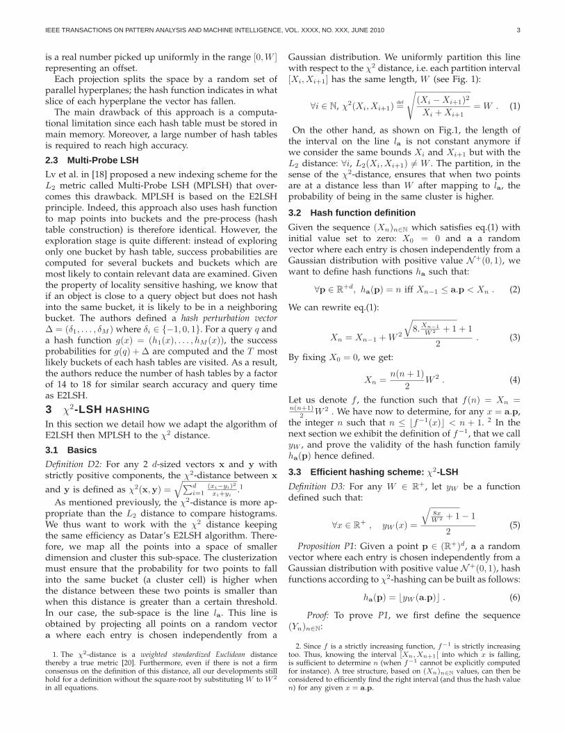
Gaussian distribution. We uniformly partition this linewith respect to the χ2 distance, i.e. each partition interval[Xi,Xi+1] has the same length, W (see Fig. 1):

∀i ∈ N, χ2(Xi,Xi+1)def=

√

(Xi − Xi+1)2

Xi + Xi+1= W . (1)

On the other hand, as shown on Fig.1, the length ofthe interval on the line la is not constant anymore ifwe consider the same bounds Xi and Xi+1 but with theL2 distance: ∀i, L2(Xi,Xi+1) 6= W . The partition, in thesense of the χ2-distance, ensures that when two pointsare at a distance less than W after mapping to la, theprobability of being in the same cluster is higher.

3.2 Hash function definition

Given the sequence (Xn)n∈N which satisfies eq.(1) withinitial value set to zero: X0 = 0 and a a randomvector where each entry is chosen independently from aGaussian distribution with positive value N+(0, 1), wewant to define hash functions ha such that:

∀p ∈ R+d, ha(p) = n iff Xn−1 ≤ a.p < Xn . (2)

We can rewrite eq.(1):

Xn = Xn−1 + W 2

√

8.Xn−1

W 2 + 1 + 1

2. (3)

By fixing X0 = 0, we get:

Xn =n(n + 1)

2W 2 . (4)

Let us denote f , the function such that f(n) = Xn =n(n+1)

2 W 2 . We have now to determine, for any x = a.p,the integer n such that n ≤ ⌊f−1(x)⌋ < n + 1. 2 In thenext section we exhibit the definition of f−1, that we callyW , and prove the validity of the hash function familyha(p) hence defined.

3.3 Efficient hashing scheme: χ2-LSH

Definition D3: For any W ∈ R+, let yW be a function

defined such that:

∀x ∈ R+ , yW (x) =

√

8xW 2 + 1 − 1

2(5)

Proposition P1: Given a point p ∈ (R+)d, a a randomvector where each entry is chosen independently from aGaussian distribution with positive value N+(0, 1), hashfunctions according to χ2-hashing can be built as follows:

ha(p) = ⌊yW (a.p)⌋ . (6)

Proof: To prove P1, we first define the sequence(Yn)n∈N:

2. Since f is a strictly increasing function, f−1 is strictly increasingtoo. Thus, knowing the interval [Xn, Xn+1[ into which x is falling,is sufficient to determine n (when f−1 cannot be explicitly computedfor instance). A tree structure, based on (Xn)n∈N values, can then beconsidered to efficiently find the right interval (and thus the hash valuen) for any given x = a.p.


Fig. 1. χ2 and L2 space tilings. 4500 image feature vectors have been randomly selected from the COREL database.Space grids for 2 features components with respect to χ2 (in red) and to L2 (in blue) distances are reported. Pointsfalling into the same bucket in χ2 hashing scheme may fall into seperate buckets in L2 hashing scheme.

Yn = yW (Xn) :

√

8 Xn

W 2 + 1 − 1

2. (7)

We prove that for all n ∈ N, (Hn) : Yn = n by inductionon n.Since by definition Y0 = 0, then (H0) is true.Rewriting eq.(7) as Y 2

n + Yn = 2 Xn

W 2 and combining thiswith eq.(1), we get:

Y 2n + Yn = 2

Xn−1

W 2+ 1 +

√

8Xn−1

W 2+ 1 . (8)

Let us now assume that (Hn−1) true, i.e. Yn−1 = n − 1.From eq.(7) we deduce that: 2Xn−1

W 2 = n(n − 1).Introducing this result in eq.(8), we then get:Yn(Yn + 1) = n(n + 1) .

The only positive solution of this equation is Yn = n.

We thus show that the hash function defined in eq.(6)satisfies:

∀p′ ∈ (R+)d s.t. Xn = a.p′, ha(p′) = ⌊yW (Xn)⌋ = n .

(9)

It is then straightforward, using the strict monotonyof yW , to see that:

∀p ∈ (R+)d s.t. Xn ≤ a.p < Xn+1, ha,b(p) = n .

(10)This completes the proof of proposition P1.

To avoid boundary effects, we introduce, as in [9], anoffset in the hash functions, i.e. a real number b pickedrandomly following the uniform distribution U([0, 1[):

ha,b(p) = ⌊yW (a.p) + b⌋ . (11)

Since all points are shifted by b, the previous construc-tion of the hash functions holds by setting X0 = b.Let H be the family of such hash functions.

3.4 χ2-LSH: a locality sensitive function

We now demonstrate that the original LSH scheme(Definition D1) still holds for this family H.

Theorem 1 (χ2-LSH sensitivity): The χ2 hash functionfamily H, defined in eq.(11), is (r1, r2, p1, p2)-sensitivewhen input vectors get positive components.

Proof: Let us define P as the probability of the hashfunctions to be locality-sensitive:

P = PH[ha,b(q) = ha,b(p)]

= Pa,b

[

∃n, n 6 yW (a.p) + b < n + 1,n 6 yW (a.q) + b < n + 1

]

For all a, as defined in the previous section, we canconsider either a.p ≤ a.q or a.p ≥ a.q without loss ofgenerality. For the sake of demonstration clarity, let usconsider a.p ≤ a.q. a and b are independent and bothadmit density probabilities p(a), p(b). Then P may becomputed using marginalization over b with the follow-ing integral bounds. From the 2 previous inequalities wehave: n 6 yW (a.p) + b 6 yW (a.q) + b < n + 1, so thatbounds on b are:

n − yW (a.p) 6 b < n + 1 − yW (a.q) (12)

and we also have:

0 6 yW (a.q) − yW (a.p) 6 1 (13)

Integrating on the random variable b leads to:

∫ n+1−yW (a.q)

n−yW (a.p)

db = 1 − (yW (a.q) − yW (a.p)) (14)

P may then be rewrited as:

P = Pa [0 6 1− (yW (a.q)− yW (a.p)) 6 1] (15)

Combining the relation between hash function ha,b andinterval bounds Xn in the sense of χ2 hashing of eq.(2)with the expression eq.(4),


we can then rewrite,

P = Pa

[

0 6 1 −1

(n + 1)W 2a(p − q) 6 1

]

(16)

Following the reasonning in [9], we use the 2-stabledistribution property: for two vectors p and q, a randomvariable a where each entry is drawn from a 2-stabledistribution, a.(q − p) is distributed as cX where c =‖p − q‖L2

and X is a random variable drawn from a2-stable distribution. It follows that:

P = p(c) =

∫ (n+1)W 2

0

1

cf(

t

c)(1 −

t

(n + 1)W 2)dt , (17)

where f(t) denotes the probability density function ofthe absolute value of the 2-stable distribution.

Let us define c′ = χ2(p,q). Since pi and qi ∈ R+

and since on (R+)d × (R+)d, the scalar product betweenthe gradients of the χ2-distance and the L2-distanceis always positive: the two distances vary similarly.Therefore, p decreases monotonically with respect to c,and p decreases also monotonically with respect to c′.Reminding that r1 < r2, if we set p1 = p(r1) andp2 = p(r2), then p2 < p1. This concludes the proof ofTheorem 1: Our H family is (r1, r2, p1, p2)-sensitive.

3.5 Multi-probe hashing scheme: χ2-MPLSH

To adapt the multi-probe scheme to the χ2-metric wehave to compute the success probability of finding avector p that is close to q after it has been perturbedby a hash perturbation vector, as presented in section 2.3Pr [g(p) = g(q) + ∆]. As all coordinates hi in the hashfunctions g are independent, we have:

Pr [g(p) = g(q) + ∆] =

M∏

i=1

Pr [hi(p) = hi(q) + δi] (18)

Note that each hash function hi first maps q to a lineand divides the line into slots of length W . We remindthat the length of a slot, according to the χ2-metric, is W ,i.e., the χ2-distance between two consecutive bounds Xi

and Xi+1 is equal to W . Each slot is numbered and thehash value is the number of the slot q falls into. A pointp close to q is likely to fall in the same slot as q but theprobability it falls in one of the adjacent slots hi(q) − 1or hi(q) + 1 is high too. In fact, the closer q to the rightboundary Xi+1, the higher the success probability thatp falls into hi(q) + 1. Thus, the position of q in the slotallows to compute the success probability of hi(q) + δi.For δ ∈ {−1,+1}, let xi(δ) be the distance of q fromthe boundary between hi(q) and hi(q) + δ, then xi(δ) =|ki(q) − hi(q) − δ| with ki(q) = y(a.p) + b.

As, in [18], we then estimate the probability that p fallsinto the slot hi(q) + δ by:

Pr [hi(p) = hi(q) + δ] ≈ e−Cxi(δ)2

(19)

where C is a constant depending on the data.Introducing the eq.(19) in eq.(18), we deduce the score

representing the likelihood of finding a point close to q

in the bucket defined by ∆: score(∆) =∑M

i=1 xi(δi)2. The

smaller the score, the higher the probability of finding apoint in the bucket perturbed by ∆.

For each query, we compute all possible perturbedvectors ∆ and use their scores to select the T bucketslikely to hold a nearest neighbor.

4 EFFICIENCY AND ACCURACY ANALYSIS

In this section, we present the empirical performanceevaluation of our hash function. We first evaluate theefficiency for different accuracy values of the χ2-LSHscheme. Next, we assess the memory factor gain by theχ2-MPLSH scheme.

4.1 Experimental Setup

No consensus among the community is currentlyachieved on a standardized experimental setup forthe evaluation of high-dimensional indexing methods.Therefore, among the main challenges for researchersfocusing on this topic, we should point out the choiceof databases, of queries, and of ground truth. Thoughearly works tried to use synthetic data, following auniform random distribution, it is now usually acceptedthat this is an unrealistic context of evaluation. Recentworks are usually assessed on real data. We performedevaluation of our scheme on the 158,929 keyframes ofTrecvid 2009 database. Each keyframe is represented bya high dimensional histogram of 128 bins obtained bythe concatenation of 2 histograms, one of 64 chrominancefrom CIE L*a*b and one of 64 textures from Gabor filters.

To assess the influence of the size of the database, wehave built 3 datasets, one of 43,616 images correspondingto Trecvid 2007 database, called DB1, a second of 86,077images corresponding to Trecvid 2008 database, calledDB2, and the whole database corresponding to Trecvid2009, called DB3. For each dataset, we created an evalu-ation benchmark by randomly picking 25,000 images asquery images.

The ground truth is built by brute force search of eachquery image’s exact k Nearest Neighbors, using the χ2

distance and not including the query image itself. Theground truth is used both to compute the speedup factorand to estimate the approximation of χ2-LSH. In ourexperiments, we set k = 20.

Performance is evaluated on two aspects: accuracy(the capability of the method to return the correct resultsusing precision metric) and efficiency (the capability ofthe method to use as few resources as possible us-ing speed up ratio with respect to brute force search).Therefore, this measure does not depend neither on themachine nor on the operating system.

4.2 Speedup factor: exact search vs χ2-LSH

We ran two sets of experiments to assess the speedupperformance of χ2-LSH: we evaluate the impact of boththe LSH parameters and the size of the dataset.

Three parameters impact the performance of the LSHalgorithm: the number of hash tables (L), the numberof projections per hash value (M ) and the size of the


search window (W ). The first set of experiments allowsus to study the influence of the two last parameters(M and W ). We used the first parameter L to controlthe trade-off between accuracy and efficiency. Firstly,

Fig. 2. Influence of W : curves for 4 values of W , M fixedto 26 and 6 different values of L

to study the influence of W , we fix M to 26 and wemake W and L vary. Fig. 2 reports the evaluation onDB3 of the influence of the two parameters W andL. For each pair of parameters, the efficiency and theaccuracy are computed. W spans the range from 125 to160 and L from 25 to 150. We observe that for a sameL, increasing the value of W decreases the speedup.Indeed, as we increase the value of W , we increase thenumber of false positives per hash tables, i.e. points thatare not near neighbors but hash into the same bucket.As a result, the number of candidates to visit increases.However, at the same time the precision increases too.Indeed, the number of false negatives, i.e. points that arenear neighbors but do not hash into the same bucket,decreases.

As we can see in the Fig. 2, W = 140 gives thebest trade-off between false negatives and false positives.Secondly, to study the influence of M , we hold fixed the

Fig. 3. Influence of M : curves for 3 values of M , W fixedto 140 and 6 different values of Lparameter W to 140 and we make M and L vary. Fig. 3reports the evaluation on DB3 of the influence of the two

other parameters M and L. For each pair of parameters,the efficiency and the accuracy are computed. M spansthe range from 24 to 28, and L from 25 to 150. Wenotice that for a same L, increasing the value of M

increases the speedup. Indeed, as we increase the valueof M , we decrease the number of false positives perhash tables. As a result, the number of candidates tovisit decreases. However, at the same time the precisiondecreases too. Indeed, the number of false negativesincreases. To keep low the probability of false negatives,we have to increase the number of tables L. However, ittakes more time to compute two tables rather than onetable. Therefore a good trade-off is to be found betweenthe number of candidates to check and the computationtime for hashing. This explains why we obtain betterperformance for M = 26 than for M = 28.

To sum up, W = 140 < with M = 26 are consideredas default parameters because they give a good trade-offbetween accuracy and efficiency.

Fig. 4. query time vs number of images for DB1, DB2 andDB3 and different Average Precision rates

The second set of experiments aims at evaluating thecomplexity of the search, according to the database sizein order to prove the sub-linearity of our algorithmcomplexity, and the stability of the method with respectto W parameter value. In Fig. 4, we evaluate the searchtime for the 3 datasets and for Average Precision (AP) of80%, 85%, 90% and 95%. M and L are respectively setto 26 and 115. As we can see in Fig. 4, the brute forcesearch is indeed linear: DB3 is 3.64 times higher thanDB1 and the search time for DB3 is 3.67 times slowerthan for DB1 (respectively 233 and 63 msecs).

For our χ2-LSH scheme, the search time is of courseconnected to the target AP. We can notice that for anAP of 85%, our χ2-LSH scheme provides a very goodtrade-off between AP and query time which is the sameas for an AP rate of 80%. For an accuracy of 85%, thequery time is only 1.98 times higher for DB3 than for DB1(respectively 13.44 and 6.77 msecs), which illustrates thesub-linear complexity of our scheme. Our χ2-LSH is


Average Precision 0.8 0.85 0.9 0.95

WDB1 142 149 161 188DB2 132 144 155 176DB3 128 140 150 169

TABLE 1

then 9.37 times faster for the database of 44K images(DB1) and becomes 17.35 times faster for the database of160K images (DB3), than the exhaustive search. It followsthat the efficiency of our fast scheme increases with thesize of the database for an AP of 85%. This remainstrue for an AP of 90% but the gain over exhaustivesearch decreases since our χ2-LSH is 4.92 times fasterfor DB1 and becomes 9.07 times faster for DB3 than theexhaustive search. For the highest AP rate of 95%, thegain over the exhaustive search is almost linear with again of about 3.5 times faster for the 3 databases.

The value of the parameter W is directly connectedto both the target value for the AP and the size of thedatabase. In the following table (Tab.1), we present thevariations of W during the previous experiment. Thevalue of W is set to 142, 132 and 128, respectively forDB1, DB2 and DB3, to maintain an AP of 80%. These W

values evolve, with the target AP, homogeneously forthe 3 databases. One can also see that, as expected, thelarger the database, the more dense the feature space is,and thus the smaller the LSH bin width W is. Of course,in order to reach an AP of 95%, our scheme has to beless approximating and thus the value of W increasesto account for feature vectors farther away from thequery, considering hence more of the feature space. Thistable illustrates also the stability of W with respect toboth the increase of the size of the database and theincrease of AP. Indeed, we can notice that whateverthe rate for the target AP is, W decreases within arange of less than 15 to get adapted to the databasesize. Equivalently, whatever the size of the databaseconsidered, W increases within a range of less than 40to get adapted to the increase of the AP rate.

4.3 Memory usage: χ2-LSH vs χ2-MPLSH

In this part, we assess the improvement of χ2-MPLSH onχ2-LSH in terms of space requirements and effectivenessfor various accuracy values on the DB3 dataset.

First, we evaluate the accuracy according to the effi-ciency of χ2-MPLSH to ensure that χ2-MPLSH is ableto reach the same precision as χ2-LSH with few hashtables, thus less memory usage. Results are reported inFig. 5. In this experiment, we set W = 140 and M = 26and we make the parameter L span the range from 2 to 6and the parameter T from 25 to 150. To reach a precisionbetween 0.8 and 0.9 (see Fig. 5), only 6 hash tables arenecessary for χ2-MPLSH against between 75 and 150 forχ2-LSH (see Fig. 3). Moreover, only 4 tables are requiredfor a precision between 0.6 and 0.8.

On Tab.2 and Tab.3, we compare memory usage for χ2-LSH and χ2-MPLSH. By using the second scheme, thememory requirement falls down from Gb to hundredsof Mb.

Fig. 5. χ2-MPLSH, influence of L: curves for 3 values ofL, W and M fixed to 26 and 140 and 6 values for T

L 25 50 75 100 125 150Mem. χ2-LSH (Gb) 1.00 1.65 2.24 2.86 3.47 4.09

TABLE 2L 2 4 6

Mem. χ2-MPLSH (Mb) 445 527 546

TABLE 3

Secondly, we evaluate the effectiveness of χ2-MPLSH.We use χ2-LSH has a baseline setting W = 140 andM = 26 and we make L vary from 25 to 150 to changethe accuracy. As shown in Fig. 6, choosing the sameparameters W = 140 and M = 26 for χ2-MPLSH as forχ2-LSH and L = 6 is not optimal. Indeed, for a similaraccuracy, the χ2-MPLSH does not reach same speedupfactor. However, with W = 130, M = 24 and L = 6,χ2-MPLSH reaches the same efficiency as χ2-LSH foran accuracy between 0.72 and 0.9. Furthermore, withW = 120, M = 24 and L = 4, χ2-MPLSH reaches thesame efficiency as χ2-LSH for an accuracy between 0.55and 0.76. It is worth noting that for accuracy between0.65 and 0.8, χ2-MPLSH with W = 120, M = 24 andL = 6 reaches higher efficiency than χ2-LSH.

Finally, χ2-MPLSH achieves the same performance asχ2-LSH with little memory requirements: for instance, ifwe consider W = 120, L = 4, M = 24 for χ2-MPLSH, thememory usage gain is about 8 with the χ2-LSH defaultscheme. Considering that the system is installed on arecent computer with 32 Gb of RAM, the system dealswith a 10 Million image dataset.

5 SEARCH QUALITY FOR χ2 VS L2

The aim of this experiment is to compare the searchquality of the two methods: MPLSH and χ2-MPLSHfor different parametrizations. To compare the searchquality, we consider a context of supervised classificationof image database.

5.1 Experimental protocol

We do not perform evaluation on near copy detectiondatabase (like INRIA Holidays used in [7]) because, asaforementioned, for this task BoW and inverted file areoptimal solutions. Moreover, we do not use SIFT descrip-tors because they are designed for the L2-distance.


(a) accuracy between 0.9 and 0.7 (b) accuracy between 0.8 and 0.5

Fig. 6. χ2-MPLSH: speedup vs precision for several parameters

Unlike the copy detection tasks, we are rather inter-ested in CBIR and interactive CBIR tasks that aim toretrieve semantic classes [2], [4], [21]. In this context,color and texture descriptors are widely used.

Let {pi}1,n be the n image indexes of the database. Atraining set is expressed as A = {(pi, yi)i=1,n|yi 6= 0},where yi = c if the image pi belongs to the class c.

Since we are interested in comparing L2- and χ2-distances, we use simple classification rule based on [5]:

fc(p) =∑

Nj(p)∈k-NN(p)

(K(p, Nj(p))|yj = c) (20)

where Nj(p) is the jth neighbor point of p in A, k thenumber of nearest neighbors considered and K(p,q) =

1 − d(p,q)R

with R a search radius and d(p,q) the L2 orthe χ2 distance between p and q. We set k = 20.

As [1], [14], we perform evaluation of our scheme onthe well-known COREL database. The dataset containsc = 154 classes of 99 images per class or n = 15246images. Each image p is represented by a 128-dimensionvector obtained by concatenating 2 histograms, one of64 chrominances value from CIE L*a*b and one of 64textures from Gabor filters.

As in PASCAL Challenges, we use the Mean AveragePrecision (MAP) to assess the classification: To computethe MAP of a class c, each image belonging to this class issuccessively removed from the training set and used asquery image (leave-one-out strategy). A Precision scoreis computed for each query, then averaged (AP) on thewhole class c. The MAP is then computed by averagingthe AP of each class.

5.2 Quality assessment

In this part, we evaluate the classification as explainedin the previous experimental protocol section with fournearest neighbor methods: E2LIN, χ2-LIN for linear scanusing respectively the L2- and χ2- distance, MPLSH

and χ2-MPLSH. Fig. 7 shows the AP in function ofspeedup factors. As in [18], we have experimented withdifferent parameter values for the LSH methods andpicked the ones that provide best performance. We setW = 110000, M = 20, L = 6 for MPLSH and W = 115,

M = 22, L = 6 for χ2-MPLSH. Let us notice thatthe bin width parameter W is squared in our χ2-LSH11 and not in Datar’s E2LSH algorithm [9]. Thus, W

parameter values are comparable (differing from a factorof less than 3). To modify both accuracy and efficiency,T varies from 10 to 150. Linear scanning searches allow

Fig. 7. Average Precision vs speedupus to compute the speedup factor and to estimate theapproximation of LSH. We thus confirm that χ2 reachesbetter accuracy than L2. The AP is 0.36 for L2 and 0.47for χ2 or a gain of 30.56%.

We reduce the approximation of search quality from10 to 5% (compared with linear scan) by making theparameter T spanning the range from 150 to 10. Forall these parametrizations, χ2-MPLSH is at least 28%more accurate than MPLSH for the same efficiency: fora speedup factor of 44, the precision of MPLSH is 0.32and the precision of χ2-MPLSH is 0.41.

6 CONCLUSIONIn this paper, we have introduced a new LSH schemefitted to the χ2-distance for approximate nearest neigh-bor search in high-dimensional spaces. Our method out-performs the original E2LSH algorithm in the context ofimage and video retrieval when data are represented byhistograms. This approach makes the most of LSH effi-ciency since it does not require any embedding process.The experiments we lead showed the relevance of sucha new LSH scheme in the context of image retrieval.


ACKNOWLEDGMENTS

We sincerely thank A. Andoni for providing us withthe package E2LSH [?]. We are grateful to the reviewerswhose valuable comments helped greatly improve thepaper.

REFERENCES

[1] O. Chapelle, P. Haffner, and V. Vapnik, “Support vector machinesfor histogram-based image classification,” IEEE trans. NeuralNetworks, pp. 1055–1064, 1999.

[2] P. Gosselin, M. Cord, and S. Philipp-Foliguet, “Combining visualdictionary, kernel-based similarity and learning strategy for imagecategory retrieval,” CVIU, vol. 110, no. 3, pp. 403–417, 2008.

[3] Y. Rubner, C. Tomasi, and L. Guibas, “The earth mover’s distanceas a metric for image retrieval,” Int. J. Comput. Vision, vol. 40,no. 2, pp. 99–121, 2000.

[4] A. Smeulders, M. Worring, S. Santini, A. Gupta, and R. Jain,“Content-based image retrieval at the end of the early years,”IEEE Trans. Pattern Anal. Mach. Intell, pp. 1349–1380, 2000.

[5] T. Hastie, R. Tibshirani, and J. Friedman, The Elements ofStatistical Learning. Springer, 2009.

[6] H. Samet, Found. of multidim. metric data struct. MK, 2006.[7] H. Jegou, M. Douze, and C. Schmid, “Product quantization for

nearest neighbor search,” IEEE Transactions on Pattern Analysis& Machine Intelligence, vol. 33, no. 1, pp. 117–128, jan 2011.

[8] H. Lejsek, F. Asmundsson, B. Jonsson, and L. Amsaleg, “NV-Tree:An efficient disk-based index for approximate search in very largehigh-dimensional collections,” IEEE Trans. Pattern Anal. Mach.Intell., vol. 31, no. 5, pp. 869–883, 2009.

[9] M. Datar, N. Immorlica, P. Indyk, and V. Mirrokni, “Locality-sensitive hashing scheme based on p-stable distributions,” inSOCG. ACM, 2004, pp. 253–262.

[10] P. Indyk and R. Motwani, “Approximate nearest neighbors: to-wards removing the curse of dimensionality,” in STOC. ACM,1998, pp. 604–613.

[11] Y. Ke, R. Sukthankar, and L. Huston, “Efficient near-duplicatedetection and sub-image retrieval,” in Multimedia. ACM, 2004,pp. 869–876.

[12] D. Gorisse, M. Cord, F. Precioso, and S. Philipp-Foliguet, “FastApproximate Kernel-Based Similarity Search for Image RetrievalTask,” in ICPR. IAPR, 2008, pp. 1873–1876.

[13] A. Andoni and P. Indyk, “Near-optimal hashing algorithms forapproximate nearest neighbor in high dimensions,” in FOCS.IEEE, 2006, pp. 459–468.

[14] P. Indyk and N. Thaper, “Fast image retrieval via embeddings,”in Int. Workshop SC Theories of Vision, 2003.

[15] M. Muja and D. G. Lowe, “Fast approximate nearest neighborswith automatic algorithm configuration,” in VISSAPP, 2009.

[16] B. Georgescu, I. Shimshoni, and P. Meer, “Mean shift basedclustering in high dimensions: A texture classification example,”in International Conference on Computer Vision, 2003.

[17] Y. Weiss, A. Torralba, and R. Fergus, “Spectral hashng,” in NIPS,2008.

[18] Q. Lv, W. Josephson, Z. Wang, M. Charikar, and K. Li, “Multi-probe lsh: Efficient indexing for high-dimensional similaritysearch,” 2007, pp. 950–961.

[19] D. Gorisse, M. Cord, and F. Precioso, “Scalable active learningstrategy for object category retrieval,” in ICIP. IEEE, 2010.

[20] M. Greenacre, Correspondence Analysis in Practice, SecondEdition. Chapman & HallCRC, 2007, iSBN 1-584-88616-1.

[21] E. Chang, S. Tong, K. Goh, and C. Chang, “Support vectormachine concept-dependent active learning for image retrieval,”IEEE Trans. on Multimedia, vol. 2, 2005.

David Gorisse is now a research engineer at Yakaz. Hereceived an M.Sc. in electrical engineering and telecommuni-cations by ISEN, France, in 2006 and an M.Sc. degrees in com-puter science from the University of Cergy-Pontoise, France, in2007. He obtained his PhD degree in Image Processing in 2011from the University of Cergy-Pontoise as member of ETIS jointLaboratory of CNRS/ENSEA/Univ Cergy-Pontoise, France.

Matthieu Cord is Professor of Image Processing at theComputer Science Department, University of UPMC PARIS6 since 2006. He received the PhD degree in 1998 from theUniversity of Cergy, France. In 1999, he was post-doc at theKatholieke Universiteit Leuven, Belgium, and he joined theImage Indexing team of the ETIS lab., France. In 2009, he isnominated at the IUF (French Research Institute) for 5 years.His current research interests include Computer Vision, Pat-tern Recognition, Information Retrieval, Machine Learning forMultimedia Processing, especially interactive learning imageand video retrieval systems. He has published over 100 papersand is involved in several International research projects andnetworks.

Frederic Precioso is Professor at I3S laboratory, University ofNice-Sophia Antipolis since 2011. He has a PhD in Signal andImage Processing, obtained from Univeristy of Nice-SophiaAntipolis,France, in 2004. After a year as Marie-Curie Fellowat CERTH-Informatics and Telematics Institute, (Thessaloniki,Greece), where he worked on semantic methods for objectextraction and retrieval, he has become Associate professor atENSEA since 2005. He used to work on video and image seg-mentation, active contours and his current main research topicsconcern video object detection and classification, content-basedvideo indexing and retrieval systems, scalability of such sys-tems.

Locality-Sensitive Hashing for Chi2 Distance

Documents

Transcript of Locality-Sensitive Hashing for Chi2 Distance