arX

iv:h

ep-t

h/00

0218

5v1

22

Feb

2000

Berlin Sfb288 Preprinthep-th/0002185

Large and small Density Approximations tothe thermodynamic Bethe Ansatz

A. Fring and C. Korff

Institut fur Theoretische Physik, Freie Universitat Berlin

Arnimallee 14, D-14195 Berlin, Germany

Abstract

We provide analytical solutions to the thermodynamic Bethe ansatzequations in the large and small density approximations. We extendresults previously obtained for leading order behaviour of the scalingfunction of affine Toda field theories related to simply laced Lie alge-bras to the non-simply laced case. The comparison with semi-classicalmethods shows perfect agreement for the simply laced case. We derivethe Y-systems for affine Toda field theories with real coupling constantand employ them to improve the large density approximations. Wetest the quality of our analysis explicitly for the Sinh-Gordon model

and the (G(1)2 ,D

(3)4 )-affine Toda field theory.

PACS numbers: 11.10Kk, 11.55.Ds, 05.70Jk, 05.30.-d, 64.60.Fr

Fring@physik.fu-berlin.deKorff@physik.fu-berlin.de

1 Introduction

In the context of 1+1-dimensional integrable quantum field theories numer-ous methods have been developed to compute various quantities in an exactmanner, that is non-perturbative in the coupling constant. Sometimes it iseven possible to perform the related computations analytically. Often theevaluation within one particular approach lacks information, typically a con-stant, which might be supplied by an entirely different method. Ideally onewould like to achieve a situation in which each approach is self-consistent.

An example for the situation just outlined is given for instance in the form-factor program [1], which allows in principle to compute correlation functions.The lowest non-vanishing form-factor is not fixed within this approach andis typically obtained from elsewhere. For instance the vacuum expectationvalue of the energy-momentum tensor can be extracted from the thermody-namic Bethe ansatz (TBA) [2]. Alternatively, one can compute correlationfunctions by perturbing around the conformal field theory [3]. Also in thisapproach one appeals to the thermodynamic Bethe ansatz for the vacuumexpectation value of the energy-momentum tensor and to the Bethe ansatz[4] for the relation between the coupling constant and the masses. The lattercorrespondence is also needed in an approach initiated recently in [5, 6, 7],where it was observed that the ultraviolet asymptotic behaviour for manytheories may be well approximated by zero-mode dynamics. The consider-ations in [5] exploit the knowledge of an exact reflection amplitude, whichon one hand results from certain manipulation on the three-point functionof the underlying ultraviolet conformal field theory and on the other handhas a semi-classical counterpart in the related quantum mechanical problem.The question why this approach allows to compute scaling functions with ahigh accuracy is still to be settled [8].

The computation of scaling functions by means of the TBA does con-ceptually not require any additional input from other methods. However,up-to-now it is only possible to tackle the problem numerically due to thenonlinear nature of the central equation involved. Several attempts havebeen made to formulate analytical approximations. This is desirable for var-ious reasons, one being that the numerical effort becomes quite considerablefor some models with increasing particle species content. A further reason isof course that analytical expressions allow to study further the deeper struc-tures of the theories. For instance for affine Toda field theories (ATFT) [9]related to simply laced Lie algebras some analytical expressions have been

1

provided [10, 11, 12]. In the approximation method of [10, 11, 12] a constantwas left undetermined, which can be fixed in the same spirit as outlined forthe other methods in the preceding paragraph, namely by appealing to an-other approach. Contrary to the claim in [6], we demonstrate in the presentmanuscript that it is possible to fix the constant in this way without ap-proximating higher order terms. Extending the analysis of [11, 12] also tothe non-simply laced case in the present manuscript, we will demonstratein addition that the constant may also be well approximated from withinthe TBA-analysis. Furthermore, we give simple analytical expressions forimproved approximations in the large and small density regime.

Our manuscript is organized as follows: In section 2 we provide largeand small density approximations for the solutions of the TBA-equations. Insection 3 we assemble the necessary data for ATFT needed to extend ourprevious analysis to the non-simply laced case. We derive universal TBA-equations and Y-systems for all ATFT and show how they may be utilizedto improve on the analytical approximations. We derive the related scalingfunction. We test the quality of the various approximations for the explicitexample of the Sinh-Gordon model and the (G

(1)2 , D

(3)4 )-ATFT. We state our

conclusions in section 4.

2 Large and small density approximations

2.1 The TBA

The object of investigation of the TBA is a multiparticle system containingn different particle species with masses mi (1 ≤ i ≤ n) whose dynamicalinteraction is described by a factorizable diagonal scattering matrix Sij(θ),which is a function of the rapidity difference θ. We assume the statisti-cal interaction to be of fermionic type∗. Adopting the notation of [12] thethermodynamic Bethe Ansatz equations [2], which characterize the thermo-dynamic equilibrium of such a system, are the n coupled nonlinear integralequations

rmi cosh θ + ln(eLi(θ) − 1

)=

n∑

j=1

(ϕij ∗ Lj

)(θ) . (1)

∗In order to keep the discussion as simple as possible we do not treat general statisticshere as for instance Haldane type [13]. Generalizations of our arguments in this sense arestraightforward.

2

Here the scaling parameter r is given by the inverse temperature times amass scale. The convolution of two functions is abbreviated as usual by(f ∗ g)(θ) := 1/2π

∫dθ′ f(θ − θ′)g(θ′). The TBA kernel reads

ϕij(θ) := −id

dθln Sij(θ). (2)

The functions Li, which are to be determined as solutions of the TBA equa-tions (1), are related to the particle densities ρi

r and the densities of availablestates ρi

h as Li = ln(1+ρir/ρ

ih), such that for physical reasons Li ≥ 0. Keeping

this definition in mind, we speak of the large density regime when Li > ln 2and of the small density regime when Li < ln 2. It is sometimes useful toexpress matters in terms the pseudo-energies εi(θ) := − ln[exp(Li(θ)) − 1)].

Having solved the TBA-equations (1) for the L–functions one is in prin-ciple in the position to evaluate the scaling function

c(r) =6r

π2

n∑

i=1

mi

∞∫

0

dθLi(θ) cosh θ (3)

which can be interpreted as off-critical effective central charge belonging tothe conformal field theory obtained in the ultraviolet limit, i.e. r → 0. It isour goal in this manuscript to approximate this function in a simple analyticalway to high accuracy.

2.2 Approximative analytical Solutions

In general it is possible to solve the TBA-equations numerically, where theconvergence of the iterative procedure is guaranteed by means of the Banachfixed point theorem [12]. However, the numerical problem becomes quitecomplex when one increases the number of particle species. For this reason,and more important because one would like to gain a deeper structural in-sight into the solutions of (1), it is desirable to obtain analytical solutions tothe TBA-equations. Due to the nonlinear nature of (1) only few analyticalsolutions are known. Nonetheless, one may obtain approximated analyticalsolutions when r tends to zero. For large Li, i.e. for large particle densities, itwas shown in [10, 11, 12] that the integral equation (1) may be turned into aset of differential equations of infinite order. Under certain natural assump-tions, which are however not satisfied universally for all models, one may

3

approximate these equations by second order differential equations, whosesolutions are given by

L0i (θ) = ln

(cos2 (βiθ)

2β2i ηi

)for |θ| ≤ arccos(βi

√2ηi)

βi

. (4)

The restriction on the range of the rapidity stems from the physical require-ment Li ≥ 0. The n constants ηi =

∑j η

(2)ij are determined by a power series

expansion of the TBA kernel

ϕij(t) :=

∫ ∞

−∞

dθ ϕij(θ)eitθ = 2π

∞∑

n=0

(−i)nη(n)ij tn . (5)

The dependence on the scaling parameter r enters through the quantity

βi =π

2(δi − ln(r/2)). (6)

Here the βi, δi are constants of integration. There is a very crude lowerbound we can put immediately on δi. From the fact that L0

i (0) ≥ ln 2, wededuce δi > 1/π/

√ηi + ln(r/2). For particular models we will provide below

a rigorous argument which establishes that in fact they do not depend onthe particle type, such that we may replace βi → β and δi → δ. We willalso show that they can be fixed by appealing to the semi-classical approachin [5, 7]. In addition, we provide an argument which determines them ap-proximately from within the TBA analysis by matching the large and smalldensity regimes. Since the constant turns out to be model dependent, wewill report on it in detail below when we discuss concrete theories.

The restriction on the range for the rapidities in (4), for which the largedensity approximation L0

i (θ) ceases to be valid, makes it desirable to developalso an approximation for small densities. For extremely small densities wenaturally expect that the solution will tend to the one for a free theory.Solving (1) for vanishing kernel yields the well-known solution

Lfi (θ) = ln

(1 + e−rmi cosh θ

). (7)

Ideally we would like to have expressions for both regions which match atsome distinct rapidity value, say θm

i , to be specified below. Since L0i (θ) and

Lfi (θ) become relatively poor approximations in the transition region between

large and small densities, we seek for improved analytical expressions. This

4

is easily achieved by expanding (1) around the “zero order” small densityapproximations. In this case we obtain the integral representation

Lsi (θ) = exp

(−rmi cosh θ +

∑n

j=1(ϕij ∗ Lf

j )(θ))

. (8)

For vanishing ϕij we may check for consistency and observe that the functionsLs(θ) become the first term of the expansion in (7). One could try to proceedsimilarly for the large density regime and develop around L0

i instead of Lfi .

However, there is an immediate problem resulting from the restriction onthe range of rapidities for the validity of L0

i , which makes it problematic tocompute the convolution. We shall therefore proceed in a different mannerfor the large density regime and employ Y-systems for this purpose.

In many cases the TBA-equations may be expressed equivalently as aset of functional relations referred to as Y -systems in the literature [14].Introducing the quantities Yi = exp(−εi), the determining equations canalways be cast into the general form

Yi(θ + iπµ)Yi(θ − iπµ) = exp(gi(θ)) (9)

with µ being some real number and gi(θ) being a function whose preciseform depends on the particular model. We can formally solve the equationby Fourier transformations

Yi(θ) = exp [(gi ∗ γi)(θ)] , γi(θ) = [2µ cosh(θ/2/µ)]1/2 (10)

i.e. substituting (10) into the l.h.s. of (9) yields exp(gi(θ)). Of course thisidentification is not completely compelling and we could have chosen also adifferent combination of Y ’s. However, in order to be able to evaluate thegi(θ) we require a concrete functional input for the function Yi(θ) in form ofan approximated function. Choosing here the large density approximationL0 makes the choice for gi(θ) with hindsight somewhat canonical, since othercombinations lead generally to non-physical answers.

We replace now inside the defining relation of gi(θ) the Y ’s by Yi (θ) →exp(L0

i (θ)) − 1. Analogously to the approximating approach in [10, 11, 12],we can replace the convolution by an infinite series of differentials

εi(θ) = −(gi ∗ γi)(θ) = −∞∑

m=0

ν(m)i

dm

dθm gi(θ) , (11)

5

where the ν’s are defined by the power series expansion

∞∫

−∞

dθγi(θ) eitθ = 2π∞∑

m=0

(−i)mν(m)i tm = π

∞∑

m=0

E2m

(2m)!(πηi)

2m t2m . (12)

The Em denote the Euler numbers, which enter through the expansion 1/ cosh x =∑∞

m=0 x2mE2m/(2m)!. In accordance with the assumptions of our previousapproximations for the solutions of the TBA-equations in the large densityapproximation, we can neglect all higher order derivatives of the L0

i (θ). Thuswe only keep the zeroth order in (11). From (12) we read off the coefficient

ν(0)i = 1/2, such that we obtain a simply expression for an improved large

density approximation

Lli(θ) = ln[1 + Y l

i (θ)] = ln[1 + exp(gi(θ)/2)] . (13)

In principle we could proceed similarly for the small density approximationand replace now Yi (θ) → exp(Ls

i (θ))−1 in the defining relations for the gi’s.However, in this situation we can not neglect the higher order derivatives ofthe Ls

i such that we have to keep the convolution in (11) and end up withan integral representation instead. We now wish to match Ls

i and Lli in the

transition region between the small and large density approximations at somedistinct value of the rapidity, say θm

i . We select this point to be the valuewhen the function fi(θ) = (6/π2)rmiLi(θ) cosh θ, which is proportional tothe free energy density for a particular particle species, has its maximum inthe small density approximation

d

dθf s

i (θ)

∣∣∣∣θm

i

= 0 . (14)

In regard to the quantity we wish to compute, the scaling function (3), thisis the point in which we would like to have the highest degree of agreementbetween the exact and approximated solution, since this will optimize theoutcome for c(r). Having specified the θm

i , the matching condition providesa simple rational to fix the constant δi

Lli(θ

mi ) = Ls

i (θmi ) ⇒ δm

i . (15)

Clearly, in general we can not solve these equations analytically, but it isa trivial numerical problem which is by no means comparable with the one of

6

solving (1). Needless to say that the outcome of (15) is not to be consideredas exact, but as our examples below demonstrate it will lead to rather goodapproximations. One of the reasons why this procedure is successful is thatLs

i (θmi ) is still very close to the precise solution, despite the fact that is at its

worst in comparison with the remaining rapidity range.Combining the improved large and small density approximation we have

the following approximated analytical L-functions for the entire range of therapidity

Lai (θ) =

{Ll

i(θ) for |θ| ≤ θmi

Lsi (θ) for |θ| > θm

i

, (16)

such that the scaling function becomes well approximated by

c(r) ≃n∑

i=1

∞∫

0

dθfai (θ) . (17)

To develop matters further and report on the quality of L0, Lf , Ls, Ll wehave to specify a particular theory at this point.

3 Affine Toda field theory

Affine Toda field theories [9] form a well studied class of relativistic inte-grable quantum field theories in 1+1 space-time dimensions. To each ofthese field theories a pair of affine Lie algebras (X

(1)n ,X(ℓ)) [15] is associated

whose structure allows universal statements concerning its properties, likethe S-matrix, the mass spectrum, the fusing rules, etc. Here X(ℓ) denotes atwisted affine Lie algebra w.r.t. a Dynkin diagram automorphism of order ℓ.Both algebras are chosen to be dual to each other, i.e. X(ℓ) is obtained fromthe non-twisted algebra X

(1)n of rank n by exchanging roots and co-roots. For

X(1)n simply-laced both algebras coincide, i.e. X

(1)n

∼= X(ℓ), ℓ = 1, which isreflected in the quantum theory by a strong-weak self-duality in the couplingconstant. Moreover, the mass spectrum renormalises by an overall factorand the poles of the S-matrix in the physical sheet do not depend on thecoupling constant. For non-simply laced Lie algebras these features cease tobe valid. The quantum masses are now coupling dependent and flow betweenthe classical masses associated with X

(1)n and X(ℓ) in the weak and strong

coupling limit, respectively. Consequently, the physical poles of the S-matrixshift depending on the coupling and the strong-weak self-duality is broken.

7

3.1 The universal S-matrix

Remarkably, despite these structural differences the S-matrix of ATFT canbe cast into a universal form covering the simply-laced as well as the non-simply laced case [16, 17]. For our purposes the formulation in form of anintegral representation is most useful

Sij(θ) = exp

∫ ∞

0

dt

tφij(t) sinh

tθ

iπ, (18)

φij(t) = 8 sinh(tϑh) sinh(tjϑHt)([K]q(t)q(t)

)−1

ij. (19)

Denoting a q-deformed integer n as common by [n]q = (qn − q−n)/(q1 − q−1),we introduced here a “doubly q-deformed” version of the Cartan matrix K[16, 18, 17] of the non-twisted Lie algebra

[Kij]qq = (qq ti + q−1q−ti)δij − [Iij ]q (20)

for the generic deformation parameters q, q. The incidence matrix Iij =

2δij −Kij of the X(1)n related Dynkin diagram is symmetrized by the integers

ti, i.e. Iijtj = Ijiti. With αi being a simple root we fix the length of thelong roots to be 2 and choose the convention ti = ℓα2

i /2. Inside the integralrepresentation (18) we take

q(t) = etϑh, q(t) = etϑH , with ϑh :=2 − B

2h, ϑH :=

B

2H(21)

for the deformation parameters, where 0 ≤ B ≤ 2 is the effective couplingconstant. We further need the Coxeter numbers h, h and the dual Coxeternumbers h∨, h∨ of X

(1)n and X(ℓ), respectively, as well as the ℓ-th Coxeter

number H = ℓh of X(ℓ). Complete tables of these quantities for individualalgebras may be found in [15].The incidence matrix satisfies the relation [16, 17]

n∑

j=1

[ Iij]q(iπ) mj = 2 cosh(θh + tiθH) mi , (22)

which will turn out to be crucial for the arguments below. We introducedhere the imaginary angles θh = iπϑh and θH = iπϑH .

8

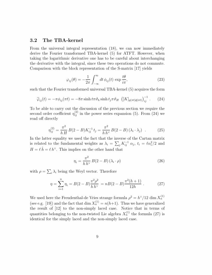
3.2 The TBA-kernel

From the universal integral representation (18), we can now immediatelyderive the Fourier transformed TBA-kernel (5) for ATFT. However, whentaking the logarithmic derivative one has to be careful about interchangingthe derivative with the integral, since these two operations do not commute.Comparison with the block representation of the S-matrix [17] yields

ϕij(θ) = − 1

2π

∫ ∞

−∞

dt φij(t) exptθ

iπ, (23)

such that the Fourier transformed universal TBA-kernel (5) acquires the form

ϕij(t) = −πφij(πt) = −8π sinh tπϑh sinh tjπϑH

([K]q(πt)q(πt)

)−1

ij. (24)

To be able to carry out the discussion of the previous section we require thesecond order coefficient η

(2)ij in the power series expansion (5). From (24) we

read off directly

η(2)ij =

π2

h HB(2 − B)K−1

ij tj =π2

h h∨B(2 − B) (λi · λj) . (25)

In the latter equality we used the fact that the inverse of the Cartan matrixis related to the fundamental weights as λi =

∑j K−1

ij αj , ti = ℓα2i /2 and

H = ℓ h = ℓ h∨. This implies on the other hand that

ηi =π2

h h∨B(2 − B) (λi · ρ) (26)

with ρ =∑

i λi being the Weyl vector. Therefore

η =

n∑

i=1

ηi = B(2 − B)π2ρ2

h h∨= nB(2 − B)

π2(h + 1)

12h. (27)

We used here the Freudenthal-de Vries strange formula ρ2 = h∨/12 dim X(1)n

(see e.g. [19]) and the fact that dim X(1)n = n(h+1). Thus we have generalized

the result of [12] to the non-simply laced case. Notice that in terms of

quantities belonging to the non-twisted Lie algebra X(1)n the formula (27) is

identical for the simply laced and the non-simply laced case.

9

3.3 Universal TBA equations and Y-systems

In analogy to the discussion for simply-laced Lie algebras [12], the universalexpression for the kernel (24) can be exploited in order to derive universalTBA-equations for all ATFT, which may be expressed equivalently as a setof functional relations referred to as Y -systems. Fourier transforming (1) ina suitable manner and invoking the convolution theorem we can manipulatethe TBA equations by using the expression (24). After Fourier transformingback we obtain

εi +n∑

j=1

∆ij ∗ Lj =n∑

j=1

Γij ∗ (εj + Lj) . (28)

The universal TBA kernels ∆ and Γ are then given by

γi(θ) =(2(ϑh + tiϑH) cosh θ

2(ϑh+tiϑH)

)−1

, (29)

Γij(θ) =

Iij∑

k=1

γi(θ + i(2k − 1 − Iij)θH), (30)

∆ij(θ) = [γi(θ + (θh − tiθH)) + γi(θ − (θh − tiθH))] δij . (31)

The key point here is that the entire mass dependence, which enters throughthe on-shell energies mi cosh θ, has dropped out completely from the equa-tions due to the identity (22). Noting further that

[ Iij]q(iπ) mj cosh θ =

Iij∑

k=1

mj cosh [θ + (2k − 1 − Iij)θH ] , (32)

we have assembled all ingredients to derive functional relations for the quan-tities Yi = exp(−εi). For this purpose we may either shift the TBA equationsappropriately in the complex rapidity plane or use again Fourier transforma-tions, see [12]

Yi (θ+θh + tiθH) Yi (θ − θh − tiθH) = [1+Yi(θ+θh−tiθH)][1+Yi(θ−θh+tiθH)]

n∏j=1

Iij∏k=1

[1+Y −1

j (θ+(2k−1−Iij)θH)]. (33)

These equations are of the general form (9) and specify concretely the quanti-ties µ and gi(θ). We recover various particular cases from (33). In case the as-sociated Lie algebra is simply-laced, we have θh +tiθH → iπ/h, θh−tiθH →

10

iπ/h(1−B) and Iij → 0, 1, such that we recover the relations derived in [12].As stated therein we obtain the system for minimal ATFT [14] by taking thelimit B → i∞.

The concrete formula for the approximated solution of the Y-systems inthe large density regime, as defined in (13), reads

Y li (θ) = cos(2θβi)+cos(2(θh−tiθH)βi)

4ηiβ2

i

n∏

j=1

Iij∏

m=1

(1 − 2ηjβ2

j

cos2(βj(θ+(2m−1−Iij )θH)

) 1

2

. (34)

Exploiting possible periodicities of the functional equations (33) they maybe utilized in the process of obtaining approximated analytical solutions [20].As we demonstrated they can also be employed to improve on approximatedanalytical solution in the large density regime. In the following subsection wesupply a further application and use them to put constraints on the constantof integration δi in (6).

3.4 The constants of integration β and δ

There are various constraints we can put on the constants βi and δi on generalgrounds, e.g. the lower bound already mentioned. Having the numerical dataat hand we can use them to approximate the constant. In [12] this was doneby matching L0 with the numerical data at θ = 0 and a simple analyticalapproximation was provided δnum = ln[B(2 − B)21+B(2−B)]. Of course theidea is to become entirely independent of the numerical analysis. For thisreason the argument which led to (15) was given.

When we consider a concrete theory like ATFT, we can exploit its partic-ular structure and put additional constraints on the constants from generalproperties. For instance, when we restrict ourselves to the simply laced case itis obvious to demand that the constants respect also the strong-weak duality,i.e. βi(B) = βi(2 − B) and δi(B) = δi(2 − B).

Finally we present a brief argument which establishes that the constantsβi are in fact independent of the particle type i. We replace for this purposein the functional relations (33) the Y-functions by Y h

i (θ)) and consider theequation at θ = 0, such that

cosh2[πβi(ϑh + tiϑH)] − 2β2i ηi

cosh2[πβi(ϑh + tiϑH)]=

n∏

j=1

Iij∏

m=1

(cosh2[πβi(2m−1−Iij)ϑH ]−2β2

i ηi)12

cosh[πβi(2m−1−Iij )ϑH ].

(35)

11

Keeping in mind that βi is a very small quantity in the ultraviolet regime,we expand (35) up to second order in βi, which yields after cancellation

4tiϑhϑH =α2

i

2

B(2 − B)

hh∨=

∑

j=1

Kij

β2j

β2i

ηj

π=

B(2 − B)

hh∨

∑

j=1

Kij

β2j

β2i

(λj · ρ) .

(36)We substituted here the expression (26) for the constants ηj in the last equal-

ity. Using once more the relation λi =∑

j K−1ij αj, we can evaluate the inner

product such that (36) reduces to

α2i =

n∑

j=1

n∑

k=1

Kij

β2j

β2i

K−1jk α2

k . (37)

Clearly this equation is satisfied if all the βi are identical. From the unique-ness of the solution of the TBA-equations follows then immediately that wecan always take βi → β. Since the uniqueness is only rigorously established[12] for some of the cases we are treating here, it is reassuring that we canobtain the same result also directly from (37). From the fact that the βi arereal numbers and all entries of the inverse Cartan matrix are positive followsthat β2

i = β2j for all i and j. The ambiguity in the sign is irrelevant for the

use in L(θ).

3.5 The Scaling Functions

In [12] it was proven that the leading order behaviour of the scaling functionis given by

c(r) ≃ n − 3η

(δ − ln(r/2))2= n

(1 − π2B(2 − B)(h + 1)

4h(δ − ln(r/2))2

). (38)

From our arguments in section 3.2, which led to the general expression forthe constant η in form of (27), follows that in fact this expression holds for all

affine Toda field theories related to a dual pair of simple affine Lie algebras(X

(1)n ,X(ℓ)). However, strong-weak duality is only guaranteed for ℓ = 1.Restricting ourselves to the simply laced case, we can view the results

of [5, 6, 7] obtained by means of a semi-classical treatment for the scalingfunction as complementary to the one obtained from the TBA-analysis andcompare directly with the expression (38). Translating the quantities in

12

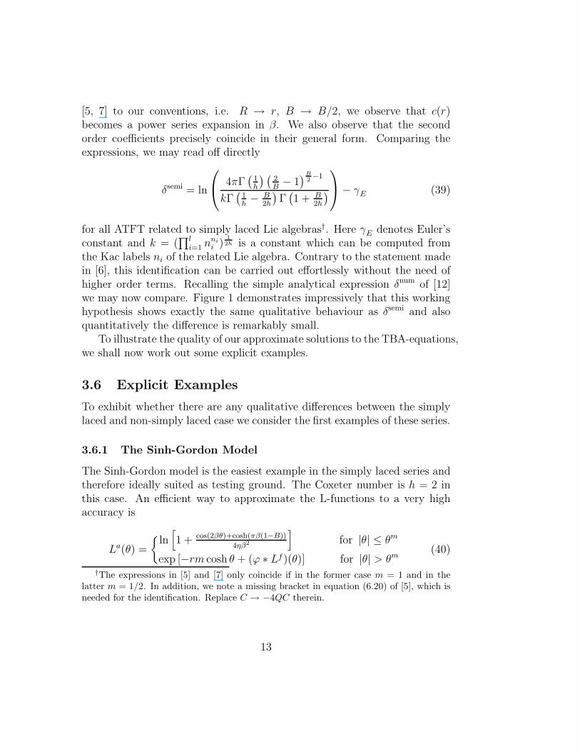
[5, 7] to our conventions, i.e. R → r, B → B/2, we observe that c(r)becomes a power series expansion in β. We also observe that the secondorder coefficients precisely coincide in their general form. Comparing theexpressions, we may read off directly

δsemi = ln

4πΓ(

1h

) (2B− 1

)B2−1

kΓ(

1h− B

2h

)Γ

(1 + B

2h

)

− γE (39)

for all ATFT related to simply laced Lie algebras†. Here γE denotes Euler’sconstant and k = (

∏li=1 nni

i )1

2h is a constant which can be computed fromthe Kac labels ni of the related Lie algebra. Contrary to the statement madein [6], this identification can be carried out effortlessly without the need ofhigher order terms. Recalling the simple analytical expression δnum of [12]we may now compare. Figure 1 demonstrates impressively that this workinghypothesis shows exactly the same qualitative behaviour as δsemi and alsoquantitatively the difference is remarkably small.

To illustrate the quality of our approximate solutions to the TBA-equations,we shall now work out some explicit examples.

3.6 Explicit Examples

To exhibit whether there are any qualitative differences between the simplylaced and non-simply laced case we consider the first examples of these series.

3.6.1 The Sinh-Gordon Model

The Sinh-Gordon model is the easiest example in the simply laced series andtherefore ideally suited as testing ground. The Coxeter number is h = 2 inthis case. An efficient way to approximate the L-functions to a very highaccuracy is

La(θ) =

{ln

[1 + cos(2βθ)+cosh(πβ(1−B))

4ηβ2

]for |θ| ≤ θm

exp [−rm cosh θ + (ϕ ∗ Lf )(θ)] for |θ| > θm(40)

†The expressions in [5] and [7] only coincide if in the former case m = 1 and in thelatter m = 1/2. In addition, we note a missing bracket in equation (6.20) of [5], which isneeded for the identification. Replace C → −4QC therein.

13

with

ϕ(θ) =4 sin(πB/2) cosh θ

cosh 2θ − cos πB, η =

π2B(2 − B)

8. (41)

0,0 0,5 1,0 1,5 2,0-2,0

-1,5

-1,0

-0,5

0,0

0,5

1,0

1,5

B

δ(B)

δnum

δsemi

Figure 1: Numerically fitted constant δnum versus the constant from the semi-

classical approach for the Sinh-Gordon model δsemi.

The determining equation for the matching point reads

sinh θm − rm/2 sinh(2θm) + cosh(θm)(ϕ′ ∗ Lf )(θm) = 0 . (42)

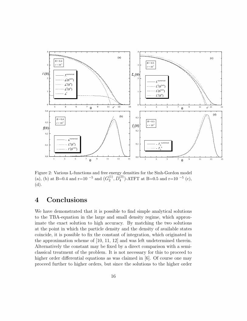
For instance for B = 0.4 this equation yields θm = 11.9999 such that thematching condition (15) gives δm = 0.4913. Figure 2(a) shows that thelarge and small density approximation L0 and Lf may be improved in afairly easy way. In view of the simplicity of the expression La the agreementwith the numerical solution is quite remarkable. Figure 2(a) also illustratesthat when using the constant δsemi instead of δm the agreement with thenumerical solutions appears slightly better for small rapidities. When weemploy δnum instead of δsemi the difference between the two approximated

14

solutions is beyond resolution. However, as may be deduced from Figure2(b), with regard to the computation of the scaling function the differencebetween using δm instead of δsemi is almost negligible. Whereas in the formercase the resulting value for the scaling function is slightly below the correctvalue, it is slightly above by almost the same amount in the latter case. Moreon the approximation of the scaling function in form of (38) may be foundin [12].

3.6.2 (G(1)2 , D

(3)4 )-ATFT

In this case we have h = 6 and H = 12 for the related Coxeter numbers. Thetwo masses are m1 = m sin(π(1/6−B/24)) and m2 = m sin(π(1/3−B/12)).The L-functions are well approximated by

La1(θ) =

{ln[1 +

cos(2βθ)+cosh(πβ( 1

3−B

4))

4η1β2

√1 − 2η2β2

cos2(βθ)] for |θ| ≤ θm

1

exp[−rm1 cosh θ + (ϕ11 ∗ Lf1 + ϕ12 ∗ Lf

2)(θ)] for |θ| > θm1

La2(θ) =

{ln[1 +cos(2βθ)+cosh(πβ( 1

3− 5B

24))

4η2β2

1∏k=−1

√1 − 2η1β2

cos2(β(θ+ kB12

))] for |θ| ≤ θm

2

exp[−rm2 cosh θ + (ϕ21 ∗ Lf1 + ϕ22 ∗ Lf

2)(θ)] for |θ| > θm2

,

with ϕ given by (23) and

η1 =5π2B(2 − B)

72, η2 =

π2B(2 − B)

8, η =

7π2B(2 − B)

36. (43)

Using now the numerical data L1(0) = 4.2524 and L2(0) = 3.67144 as bench-marks, we compute by matching them with La

1(0) and La2(0) the constant

to δ = 1.1397 in both cases. This confirms our general result of section 3.4.Evaluating the equations (15) and (14) we obtain for B = 0.5 the matchingvalues for the rapidities θm

1 = 12.744 and θm2 = 12.278 such that δm

1 = 1.9539and δm

2 = 1.5572. Figure 2(c) and 2(d) show a good agreement with thenumerical outcome.

The approximated analytical expression for the scaling function reads

c(r) ≃ 2 − 7 π2B(2 − B)

12(δ − ln(r/2))2. (44)

This expressions differs from the one quoted in [12], since in there the signof some scattering matrices at zero rapidity was chosen differently.

15

1 3 5 7 9 11 13 150

1

2

3

4

B = 0.4

r = 10-5

(a)

θm

θ

/�θ� /numerical

/l(δsemi)

/a(δm)

/0(δm)

/f

1 3 5 7 9 11 13 150

1

2

3

4

θm

B = 0.5

r = 10-5

Lnumerical

L0(δnum)

Ll(δnum)

La(δm)

(c)

θ

/��θ�

1 3 5 7 9 11 13 150,0

0,1

0,2

0,3

0,4

B = 0.4

r = 10-5

(b)

f2(θ)

θ

f(θ)

L /numerical

L /a(δm)

L /O(δsemi)

1 3 5 7 9 11 13 150,0

0,1

0,2

0,3

B = 0.5

r = 10-5

L /2

numerical

L /2

a

(d)

θ

Figure 2: Various L-functions and free energy densities for the Sinh-Gordon model

(a), (b) at B=0.4 and r=10 −5 and (G(1)2 , D

(3)4 )-ATFT at B=0.5 and r=10 −5 (c),

(d).

4 Conclusions

We have demonstrated that it is possible to find simple analytical solutionsto the TBA-equation in the large and small density regime, which approx-imate the exact solution to high accuracy. By matching the two solutionsat the point in which the particle density and the density of available statescoincide, it is possible to fix the constant of integration, which originated inthe approximation scheme of [10, 11, 12] and was left undetermined therein.Alternatively the constant may be fixed by a direct comparison with a semi-classical treatment of the problem. It is not necessary for this to proceed tohigher order differential equations as was claimed in [6]. Of course one mayproceed further to higher orders, but since the solutions to the higher order

16

differential equations may only be obtained approximately one does not gainany further structural insight and moreover one has lost the virtue of thefirst order approximation, its simplicity.

We derived the Y-systems for all ATFT and besides demonstrating howthey can be utilized to improve on the large density approximations we alsoshowed how they can be used to put constraints on the constant of integra-tion.

We have proven that the expression (38) for the scaling function is of ageneral nature, i.e. valid for all ATFT. It is desirable to extend the semi-classical analysis [7] also to the non-simply laced case. This would allow toread off the constant δ also in that case.

Acknowledgments: The authors are grateful to the Deutsche Forschungs-gemeinschaft (Sfb288) for financial support. We acknowledge constructiveconversations with B.J. Schulz at the early stage of this work and are grate-ful to V.A. Fateev for kind comments.

References

[1] P. Weisz, Phys. Lett. B67 (1977) 179;

M. Karowski and P. Weisz, Nucl. Phys. B139 (1978) 445.

[2] Al.B. Zamolodchikov, Nucl. Phys. B342 (1990) 695;

T.R. Klassen and E. Melzer, Nucl. Phys. B338 (1990) 485; B350 (1991)

635.

[3] Al.B. Zamolodchikov, Nucl. Phys. B348 (1991) 619.

[4] V.A. Fateev, Phys. Lett. B324 (1994) 45;

Al.B. Zamolodchikov, Int. J. Mod. Phys. A10 (1995) 1125.

[5] A.B. Zamolodchikov and Al.B. Zamolodchikov, Nucl. Phys. B477 (1996)

577.

[6] C. Ahn, C. Kim and C. Rim, Nucl. Phys. B556 (1999) 505.

17

[7] C. Ahn, V.A. Fateev, C. Kim, C. Rim and B. Yang, Reflection Amplitudes of

ADE Toda Theories and Thermodynamic Bethe Ansatz, hep-th/9907072.

[8] Al.B. Zamolodchikov, 4-th Bologna Workshop on CFT and Integrable Models,

(Bologna, 1999).

[9] A.V. Mikhailov, M.A. Olshanetsky and A.M. Perelomov, Commun. Math.

Phys. 79 (1981) 473;

G. Wilson, Ergod. Th. Dyn. Syst. 1 (1981) 361;

D.I. Olive and N. Turok, Nucl. Phys. B257 [FS14] (1985) 277.

[10] Al.B. Zamolodchikov, “Resonance Factorized Scattering and Roaming Tra-

jectories”, Preprint ENS-LPS-335 (1991).

[11] M.J. Martins, Nucl. Phys. B394 (1993) 339.

[12] A. Fring, C. Korff and B.J. Schulz, Nucl. Phys. B549 (1999) 579.

[13] A. Bytsko and A. Fring, Nucl. Phys. B532 (1998) 588.

[14] Al.B. Zamolodchikov, Phys. Lett. B253 (1991) 391.

[15] V.G. Kac, “Infinite Dimensional Lie Algebras” (CUP, Cambridge, 1990).

[16] T. Oota, Nucl. Phys. B504 (1997) 738.

[17] A. Fring, C. Korff and B.J. Schulz, Nucl. Phys. B567 (2000) 409.

[18] E. Frenkel and N. Reshetikhin, Deformations of W-algebras associated to

simple Lie algebras, q-alg/9708006 v2.

[19] P. Goddard and D.I. Olive, Int. J. Mod. Phys. A1 (1986) 303.

[20] Al.B. Zamolodchikov, Nucl. Phys. B358 (1991) 497; Nucl. Phys. B358

(1991) 524; Nucl. Phys. B366 (1991) 122.

18