A STUDY OF THE EFFECTS OF STATETRANSITION MATRIX APPROXIMATIONS

Janet A. May

Goddard Space Flight Center

ABSTRACT

This paper investigates the effects of using an approximate state transition matrix in orbit estima-

tion. The approximate state transition matrix results when higher order geopotential terms in theequations of motion are ignored in the formation of the variational equations. Two methods of

orbit estimation were considered: the differential correction procedure (DC) and the extendedKalman filter (EKF). The system used for the study was the Research & Development version of

the Goddard Trajectory Determination System (R&D GTDS). The effects of the approximation

were analyzed on a number of orbits. These include orbits of various inclinations and semimajor

axes. Other parameters studied include geopotential models and DC arc length.

29

introduction

Tilestate transitionmatrix plays an importantrole in orbit

determination. It relatesperturbationsin the state at time t to

perturbationsin the state at epoch. Rice (4) suggeststhat divergence

in orbit estimationmethodsmight be linked to the use of an approximate

state transitionmatrix. The objectiveof this projectis to study the

effects of approximatingvariationalequationson orbit estimBtion

methods.

We startwith the equationof state:

which represents n-nonlinear simultaneous equations. An initial state

vectorX(to)=X 0 is associated with (I), file state transition matrix is

described by the matrix differential equation

g

where B(t_)=Iand Fx(X,t)is a matrix of partial derivationsof F(X,t)

evaluatedalong a particulartrajectorysatisfyingequation (1).

The force model, F(X,t),used for this study includesperturbations

involvingonly gravitationalharmonics;other perturbations,such as drag,

low thrust,etc., have been ignored. Specifically,the force functionlooks

like

•_=zK,o (3)

30

withf(X,t)being the point mass gravitationalforce causedby the central

body, __._ _ 9_ _JG_ the perturbationdue to the nonspherlcltyof the

central body. The transcendentalfunctionsg_(X,t)are extremelycomplex

for i 7]3. Based on this force model,equation (2) has the form

Due to the complexityof gt(X,t),the terms g_x(X,t)become very cumbersome.+

The questionthis study addressescan now be stated as: What is the effect

on orbit determinationmethods when M is strictlyless than N even though

the resultingmatrix Fx(X,t) is still to be evaluatedalong a trajectory

satisfyingequation (3)? The main objectivefor settingM(N in (4) is a

reduced cost in time and space in programmingand evaluatingthese equations.

Relationshipto Orbit Estimation

Orbit estimationis the processof solvingfor the values of a set of

parameters from the observationalmodel which will minimizethe difference

between a computedand an observedtrajectory. The ResearchVersion of the

Goddard TrajectoryDeterminationSystem (R&D GTDS) uses two methodsof orbit

estimation: A classicalweighted least squaresestimator (differentialcorrection

procedure)and a sequentialestimator (Kalmanfilter).

The observationalmodel is a nonlinearregressionfunctionof the

state and time:

(.-C): C+'CX,+.)+r,

+ Baker in Astrodynamics: Applications& AdvancedTopics devotesAppendixEto "Partial Derivativesof Total Acceleration."

31

where n denotes random noise. The system is mxl, m being the number of

observations. When least squares estimation is considered, the value of X

which minimizes the weighted sum of the squares of the observational

residuals is sought. The function to be minimized is called the loss

function. It has the form:

(6)

The initial estimate of the state is XO. Equation (6) will be minimized

_ (__-0 Since <_when _ _->_ will be nonlinear, Q(X) is first linearized

by expanding G(X,t) in a truncated Taylor's series about XO. The linearized

problem is now solved and the nonlinear problem is solved recursively vla a

Newton-Raphson iterative scheme to give the minimum difference between computed

and observed trajectories. This briefly describes the differential correction

process where a "batch" of m observations are processed simultaneously. The

state transition matrix is utilized in" the linearization of G(X,t).

The sequential estimator, or filter, handles the problem from a continuous

process point of view. Rather than handling the data in batches as in

differential correction, the filter processes new data immediately upon

collection to yield an improved estimate of the state.

In this approach, observations from times t O and tk are used to determine

an estimate of the state residual from a reference trajectory X(tk) and a

covariance matrix Pk. An observation from time tk+ 1 is added to this set.

Values of the estimated state at tk+ I, X(tk+l), and the covariance matrix at

tk+l, Pk+l, are to be found. The filter used for this study is the Extended

Kalman Filter (EKF) as programmed in R&DGTDS. The EKF corrects the reference

trajectory to the most recent state estimate, which reduces the nonlinearities

32

of the original system and is desirable in real-time solution. In the EKF,

the covariance matrix is propagated via the state transition matrix.

S.tudy Results

This study has attempted to address the question of approximate state

transition matrices by initially investigating a parameter, R, formulated byI

, r,

Rice (4). Mr. Rice defines a single parameter to monitor the state transition

matrix. He presents a statisticalJargumen.t to show that the-_luani;ity ,.

I_: _ , where is an element of the transition matrix {_, can beI /

/ 5z/

interpreted as a 1_asure of "error growth rate." Rice_'glves P(t)=(_P(O)_ T

as a propagation formula for the covariance matrix, where .L

' } is commonly used asand states that the square root of the trace of Pit

a statistical measure of position errors. Hence,

/

The signature of R suggested using the GTDSestimators with several parameters

to be varied. These included arc length, geopotential modeling of state

and var.iational equations, inclination and eccentricity. Being observed

were the signature of R, the convergence/divergenceof the estimat'or, and

the rate of convergence. ,/

As a starting point, three cases discussed in Mr. Rice's paper were

compared. Case one used a force model based solely on the point mass force

for both the .state a_nd state transition matrices, which will be>denoted (Jo,Jo)'.• /

Case two included the "d2" harmonic term in both the equations of state and

the variational equations, denoted (J2,J2), whileca_e three included the J2

33

harmonic term in the eo,uations of state but only the point mass model in the

variational equations, (J2,Jo). The comparison of these three cases was

based on a parameter of the state transition matrix and behavior (in terms of

convergence/divergence) of the two estimators in R&DGTDSdiscussed above.

The first orbit considered was a circular (e:O.O), equatorial (i=O.O °)

orbit with semi-major axis a=6550.524 kin; this orbit will be referred to as

SATORBI. The EPHENERISGENERATION(EPHEM)PROGRAMwa._used in the calculation

of the quantity R. EPHEMis used to compute an ephemeris from a given set

of initial conditions and, optionally, will compute the elements of the

state transition matrix by numerically integrating the variational equations

(Eq(4)). Using this option, the quantity R can be printed at any dcsired

interval. The first results obtained printed the value of R every 5 minutes

for the above--mentioned orbit with the modeling of cases I, 2, and 3. Over

48 hours, little difference was observed between the corresponding values of

!q_o _L,o,o ,_o/' ; ,

I

°o I t I! II I ,

cJ :.,_ I

I

tl i

_oucs

GRAPHI

34

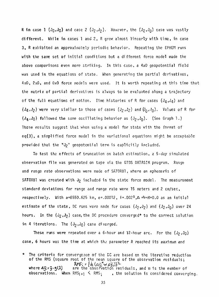
R in case 1 (Jo,Jo) and case 2 (J2,J2). Ho,vever, the (J2,Jo) case was vastly

different. While in cases I and 2, R grew almost linearly with time, in case

3, R exhibited an approximately periodic behavior. Repeating the EPHEMruns

with the same set of initial conditions but a different force model made the

above comparisons even more striking. In this case, a 4xO geopotential field

was used in the equations of state. When generating the partial derivatives,

4xO, 2xO, and OxO force models were used. It is worth repeating at this time that

the matrix of partial derivatives is always to be evaluated along a trajectory

of the full equations of motion. Time histories of R for cases (J4,J4) and

(J4,J2) were very similar to those of cases (J2,J2) and (Jo,Jo). Values of R for

(J4,Jo) followed the same oscillating behavior as (J2,Jo). (See Graph I.)

These results suggest that when using a model for state with the format of

eq(3), a simplified force model in the variational equations might be acceptable

provided that the "J2" geopotential term is explicitly included.

To test the effects of truncation on batch estimation, a 5-day simulated

observation file was generated on tape via the GTDSDATASIMprogram. Range

and range rate observations were made of SATORBI,where an ephemeris of

SATORBIwas created with J2 included in the state force model. The measurement

standard deviations for range and range rate were 15 meters and 2 cm/sec,

respectively. With a=6550.625 km, e=.O0012, i=.O02O,_:_=N=O.O as an initial

estimate of the state, DC runs were made for cases (J2,J2) and (J2,Jo) over 24

hours. In the (J2,J2) case, the DC procedure converged* to the correct solution

in 4 iterations. The (J2,Jo) case diverged.

These runs were repeated over a 6-hour and 12-hour arc. For the (J2,Jo)

case, 6 hours was the time at which the parameter R reached its maximumand

* The criteria for converge:_ce of the DC are based on the iterative reductionof the RMS(square root of the r_an square of the observation residuals;

where _;--_-_(R) are the observation residuals, and m is the number ofobservations. When RMSi+1 _ RMS_ , the solution is considered converging.

35

hence the time at which R started to decrease in value. In other words,

for the initial 6 hours, R is monotonically increasing _Jhich more accurately

reflects the "error growth rate" expected in the state transition matrix.

The period of SATORBI was about 90 minutes, so that a 6-hour arc covers about

4 orbits. When the DC program was used with (J2,Jo) to correct over the 6-hour

arc, it converged in 9 iterations; the 12-hour correction diverged. In other

words, a short term (where 4xP, P being the period of the orbit, might be a

guideline for shoFt term) cort'ection might be possible with a point-mass

force n_del for the variaticnal equations with a loss of speed in convergence.

It has been demonstrated that using an approximate state transition

matrix can be a detriment to the differential correction process. A logical

question at this point might be "how much, if any; of an approximation to the

variational equations can be tolerated by the DC?" The behavior of the parameter

R when (J4,J4), (J4:J2) end (J_.,Jo) epherlerides are compared hints that a

truncation is pez_ss±ble, provided J2 is explicitly included in the va'_iational

equations. To test this hypothesis, simulated observations were made ;,;itiL

SATORBI elements using a 5x5 geopotential field in the equations of motion.

Five DC runs were made with Jo, J2, J33, J_, and j5 models for the variational

equations and the same initial estimate of the state as mentioned above. The

DC pro qrams converged in 4 iterations for cases (J_,J_), (j_,d4)and (J_,J_).

Convergence wa_ achieved in 5 iteratior_s for the (J_,J2) case. (J_,Jo) diverged.

Table 1 lists RMS values for the last two iterations of these cases as an

indication of how little is lost when a truncati(;n from j5 to J2 for the

variational equations is used./

5 3 5,a ),Iteration # (J_,J_) (j_,j4) (j5,j3) (05/

3 I.1273519 l.0687897 l.7389176 2.1896022 ,

4 .99626079 .99626079 .99631702 .99647488

5 .99626083

TABLE l

36

The above runs were all made with a 24-hour arc. The (J_,jO)DC case did

convergein 9 iterationswhen used for the short (6 hour) term correction.

By lookingat a typical term of the matrix of partialderivatives,it becomesM i

clear that the.J2 term dominatesthe term i=_2_=_ikgikx(X,t) . FromBaker,

the followingterm is the term added to the 2-body partial derivativewhen

forming for i=2,3 and K=O:

To begin with, the term J2 is three orders of magnitudelargerthan Ji, i_ 3.

Also, Ji is divided by ri, rapidlydecreasingthe relativemagnitudeof each Ji

term for i increasing. In other words, the term J2 will reflectthe vast

majorityof theperturbation due to the asphericityof the earth. Hence, itN _"K_ tC

is not at all surprisingthat the terms._Z_ i_i can be truncatedwhen forming

the partialderivativeswithout Jeopardizingconvergencein the DC.

Other orbits were used to test (he relationshipbetween inclinationand

behaviorof the DC in the (J2,Jo)case. SATORB2had initialelementsa=6550.524km,

e=.O, i=30o, _=m=M=O. A DC programwas run for a 24-hour arc with an initial

estimateof the state as a=6550.624km, e=.O0012,i=30.002oand _=m =M=O.

Again, the (J2,J2)case convergedin four iterationsand (J2,OO)diverged.

Again, using SATORB2elementswith 5x5 geopotentialfield in the equationsof

motion, a (J ,J2) DC run over 24 hours will convergein six iterations. These

results supportthe suggestionthat an approximatestate transitionmatrix might

be acceptableprovidedthe J2 potentialterm is included.

Severalmore inclinationswere tried: I=60o,i=90o, _=98o, i=120o. At

this point, differentresultswere achieved. The initialorbitalelements

used are listed in Table 2. Simulatedobservationswere made for each orbit.

37

a e i _n. _) M

SATORB3 6550.524 0 60o 0 0 0

SATORB4 6550.524 0 90o 0 0 0

SATORB5 6550.524 0 980 0 0 0

SATORB6 6550.524 0 120o 0 0 0

TABLE2

For the initial estimate of the state in each DC run, the same error

was added to the orbital elements: I00 meters added to the semi-major axis,

eccentricity was increased to .000]2, .002o added to the inclination and no

error added to.o_,_ and M. Rapid convergence occured for all (J2,J2) DC

runs. With computed observations based on an ephemeris of SATORB3,the

(J2,Jo) DC run showed a definite trend toward convergence. After 12 iterations,

the current state was given as a=6550.257, e~O(-6), i=60.00003 °, _+_+M)=720 °.

DC runs based on simulated observations of SATORB4,SATORB5,and SATORB6were

also converging in the (J2,Jo) case, though at a slower rate than SAIORB3.

The results are summarized in 'Fable 3.

Value of State

No. ofIterations a e i

SATORB4 20 6550.534 .4578xi0-4 89.99754

SATORB5 27 6550.525 .2398xi0 "5 98.00005

SATORB6 24 6550.252 .6327xi0 "6 120.0

TABLE3

38

Table 4 comparesthe RMS value for variousiterationsfor SATORB3,4,

5, and 6 (J2,Jo). This serves as a monitor for the ratesof convergence.

RMS Values (J2'Jo)

Iteration # SATORB3 SATORB4 SATORB5 SATORB6

I 2084.7695 226I.6206 1766.1576 2307.2376

6 74.458092 I175.0753 742.93831 103.57066

12 57.808147 521.06515 260.84572 I12.82074

TABLE 4

As one might expect, since cos_T_r=Icos_I and sin-_'__= sin_K

the RMS values are most similar for i=60° and i=120°, (SATORB3and SATORB6).

In these two cases, the first 12 iterationsalternatedbetween convergingand

diverging,with large decreasesof RMS value in convergentiterations.

(This accountsfor RMSI2)RMS6 in SATORB6.)

In order to examine the sensitivityto inclination,it is helpful to

look at first order perturbations. In Methodsof Orbit Determination,Escobal

devotes a chapter to "SecularPerturbations,"where the term secular describes

variations"associatedwith a steady nonscillatory,continuousdrift of an

element from the adoptedepoch value."* He representsthe perturbingpotential

as A_=I-V where _" is the potentialdue to an asphericalearth and V is the

potentialof a sphericalearth. He segregatesfrom A those terms which

will contributesecular variationsin the elementsand arrivesat

where K2m=n2a3. Note that this is a first order expressionin J2 and for the

sake of this analysis,the Ji, i_/ 3, terms have been neglected. Littleis lost

* Escobal,P.R., 1965, p. 362.

39

by neglecting Ji, i_ 3 as the J3 term is approximately I0 orders of magnitude

smaller than the J2 term and the relative magnitude of Ji and J2 beconms even

more drastic for i7 3. Expression (7) is then averaged over one revolution,

resulting in:

(8)

Using this as the perturbing function due to J2, it is easy to see that the

secular effect of J2 is eliminated in the equations of motion when i=54.7 o

(since I/3-I/2 sin 2 54.7°=0). In other words, at this specific inclination,

the satellite, in a secular sense, perceives the earth as approximately (i.e.,

to first order J2) spherical.

With the aid of the above model for the perturbing function, Escobal

develops the following equations representing the gradual drift of the classical

elements from their adopted epoch values. Note that only-EL_ and M experience

this drift and a, e and i are taken to be constant. (It might be worthwhile to

state again that this is only a first order secular perturbation theory.)

Anomalistic m_an motion:

Mean Anomaly:

Longitude of the ascending Node:

Argument of Perigee:

4O

Between these critical inclinations of 54.7o and 125.3 o , the rate of the

secular variations of the elements is smaller than outside of this region.

This accounts for convergence in the DC procedure with (J2,Jo) modeling

for orbits with inclinations between 54o and 125o .

To conclude the differential correction section of this study, two more

orbits were considered. These orbits were elliptical with a greater

semi-major axis. Simulated observations were made of these orbits. The

initial states are given in Table 5.

a e i 4) I M

SATORB7 7278. 360 .1 0 0 0

SATORB8 9357. 89143 .3 0 0 0

TABLE5

A larger value for a will decrease the effect of J2 which is readily seen in

equation (8). However, the effect of J2 is not absent from these two orbits

and the graph of the parameter R with (J2,JO) modeling suggests that the DC

procedure will have trouble converging over a 24 hour arc, which it indeed does.

But the period of SATORB7and 8 is increased to 103 minutes arld 150 minutes,

respectively. Because of its period, it is not surprising that SATORB8converges

in II iterations over a 12-hour span with the (J2,Jo) modeling. With SATORB7,

P=I03 minutes so that 7 hours (_4xP) should be a reasonable time arc in the

(J2,Jo) DC. Whena 6-hour arc is used, the (J2,JO) DC converges to SATORB7

elements in iI iterations with rapidly decreasing RMSvalues. With a 12-hour

arc, convergence was still not achieved after 30 iterations.

The results obtained using the FILTER as an orbit estimator are more

difficult to examine than the results from the DC. As input to the FILTER

program, the user supplies an initial estimate of the state along with an

41

initial estimate of the covariance matrix.* The a priori covariance

matrix contains the state standard deviation and correlations, hence

points the filter in the right direction•

For this study, the observational residuals were used to monitor

filter performance, with decreasing residuals within a pass and modestly

larger residuals appearing after a data gap indicating convergence. The

arc length used in the filter portion of this study was 18 hours.

Whentesting the effect of approximating the state transition matrix

in the filter, only the SATORBIorbit was used. With i=O.Oo and e=O.O,

this orbit is particularly susceptible to perturbations due to the earth's

J2 nonsphericity. As will be demonstrated below, the filter has an added

dimension of sensitivity, that being the a priori covariance matrix. Because

of this and tirne constraints,_the use of the filter was restricted to this

orbi t.

The first offset imposed en the state was the same as that used for

the DC:_a=lOOm,_e=.OOOl2,ai=.O02O,_ =_=M=O.O. With this offset,

the cartesian elements at t O are x=6549.8379 km, y=z=O.O km, x=O km/sec,

y=7.801531422 km/sec and z=-.0002723 km/sec. At t O, the true cartesian elementso

are x=6550.524 km, y=z=O.O km, x=z=O.O km/sec and y=7.8006548 km/sec. Four

different a priori covariance matrices were tried in the filter with this

initial state estimate. All four covariance matrices were diagonal, implying

there was no correlation among the errors in the state estimate• The first

covariance matrix exactly reflected the errors in the state:

The DC procedure has an a priori covariance matrix default value ofinfinite magnitude so that its inverse is the null matrix. In the DCprocedure it is this inverse which is an additive term to the loss function(eq(6)); however, it has been omitted in eq(6) as it is the null matrix.

42

0-" x=.68 km,_"y=O_z=.l x 10-4 km,C-k=.l x 10-4 km/sec,O'_=.87 x 10-3 km/sec

and (T-_:,27 x 10-3 km/sec.

The results obtained for (J2,J2) and (J2,Jo) were very similar, both cases

converging. Table 6 below lists, for the last 6 passes, the largest

residual in meters within a pass for both cases:

Pass Number

(02,00 ) max IO-CI 23 2120 - 291 21 19 31

(J2,02) max IO-CI 31 _43 22 27 21 30

TABLE6

These results change greatly when a different a priori covariance

matrix is used. With _=d-y=.l km,d-z=.Ol km andd_=d_:o_=.l x I0 -4 km/sec,

the (J2,Jo) case failed to converge. This covariance matrix fails to

recognize the error in the y component,ay=.O0087 km/sec, so that the actual error

in y is 87 times larger than is reflected in the standard deviation associated

with it: d-_=.l x 10-4 km/sec. The largest residual in the last 6 passes is

listed below. Note that the (J2,J2) case fares much better than (J2,Jo) and

is considered converging.

Pass Number

19 20 I 211 22 I 23 24 , o maxlOC,(J2,J2) max IO-CI 35 72 illll 521 8 I 45 81

TABLE7

If the standard deviation of _ is increased to_y=.O0004 so that _y is

approximately 20 tin_s larger than is reflected in the standard deviation,

43

the (J2,Jo} case responds a little better. However, it is not considered

converging. The residuals during the first 9 hours suggestthe filter

has a ha_dle on the correct state. The next 9 hours shows increasing

residualsas the filter drifts away from the possiblesteadystate.

Lastly,the standard deviationof y was increasedagain to(Ty=.00015or 5 times

smallerthan the error on y. Here the (J2,J0)case did as well as the

(J2,J2)case. Table 8 summarizesthe results for 0-_=.0004and

6-#=.00015,with IFx=O-y=.l,(I-z=.Ol,O-_=_-_=.lx 10-4.

Pass Number

19 20 21 22! 23 1 24

I(FD =.00004 km/sec I I

, (J2,J0)max _0-C_ 190 226 230 220 i 242 1_ 227

Io-ct 2a 39 22 2s i , 41

i ,c'_ =.000}5 km/sec

i

(J2,J0) ma,x lO-Cl 32 23 3l 33 I 29 ! 47

(02,02) max IO-C_k 28 37 23 28 '1 '14 38

TABLE8

Although these results are far from conclusive,some inferencescan

be drawn from them. It has been demonstratedthat for this case the filter

responds_,ellwith an approximatestate transitionmatrix providedthe a

priori covariancematrix reflectsthe state errors within five standarddeviations.

The test cases used for this study suggestthat when the error is between20

and 90 ti_es larger than the standarddeviation,the (J2,Jo)case fails,yet

44

the (J2,J2)case is able to reach a steady state solution. This suggests

that when the a priori covariancematrix is consideredan accurateindicatio_

of the state error, truncatedvariationalequationsmight not harm the per-

formanceof the filter. On the other hand, when the initialcovariancematrix

somewhatinaccuratelyreflectsthe state error, the full partialderivatives

are needed to help steer the filtertoward steady state. (The term "somewhat"

is used here as a precaution;a totallyinaccuratea prioricovariancematrix

can easily cause a (J2,J2)filter case to diverge.) This sensitivityto the

initial covariancematrix makes it difficultto draw conclusionsregarding

the filter'sperformanceas a functionof the state transitionmatrix.

Conclusions

This paper has attemptedto evaluatethe effectsof an approximate

state transitionmatrix on the differentialcorrectionprocedureand the

filter procedureas used for orbit estimation. The I)Cresults fall into

four categories: the effectsdue to (1) extent of the approximation,

(2) orbitalinclination,(3) length of time arc, and (4) orbital

eccentricity. Coincidingwith these categoriesis the behaviorof the

parameter_, C_¢_I_J _(_3_;_'. R can be used to "predict" convergence/divergence

in the DC and its behavior suggested these four categories as meaningful

avenues to investigate. Whenusing a force model for the state which

includes the jm harmonic term, it has been shown that it is a safe practice

to approximate the variational equations provided that the J2 term is

included. When this approximation is made, the DC process will still

converge as it would with the full variational equations with only a

45

negligible loss of speed. A total truncation of the harmonic terms in

the variational equations will, in general, cause divergence in the DC.

One e>'ception to this is orbits with inclinations between 54.7 o and 125.3 °

In this range of inclination, the effect of the nonsphericity of the earth

is minimized. Here (J2,Jo) DC cases will converge but so slowly that

the truncation might, in pr.actice, be undesirable

The oscillatory signature of R when the most drastic truncation is

made suggests the possibility of short term differential corrections. The

maximum value of R tends to occur after four periods of the orbit. Hence an

arc length of four times the orbital period becomes a reasonable guideline

for short term corrections. In this arc length, convergence is achieved but

speed of convergence again becomes the trade-off for the truncation. As the

orbital period lengthens with greater semi-major axis, so does the time

arc over which the (J2,Jo) case converges in the DC procedure.

Wl.., the Filter as an estimator, l.ess conclusive results are found.

Tl_e effect of a truncation in the variational equations on filter perfo_'ntance

was highly cor._elated to the initial covariance matrix. When the a priori

covariance matrix was a good indication (within 5 standard deviations) of

the actual error imposed on the state, little difference was seen in the convergent

behavior of the filter for the (J2,J2) and (J2,Jo) cases. However, when the

accuracy of the a priori covariance matrix is relaxed, the (J2,Jo) case showed

divergence in the cases tested. Furthermore, when the accuracy of the a priori

covariance matrix is completely lost, neither the (J2,Jo) nor the (J2,J2) case

will converge.

46

The results obtained in the filter section of this paper leave another

set of questions open. It was assumed tl_at using the low altitude, circular

equatorial orbit where the perturbatiorls due to the nonsphericity of the earth

are most pronounced would be a good orbit to test the effects of truncated

variational equations in the filter. This appear.s to be a valid assumption

in view of the analysis mentioned above based on equations (7) and (8).

However, other sets of orbital elements could be tested iri order to help

determine the limits of accuracy needed in the a priori covariance matrix

when using an approximate state transition matrix. Also, this study was

restricted to variations inO-_ . Certainly many other variations could be

tested, although this starts to drift away from the original intent of the

study. Also, is there a level of state noise which might be used to help

compensate for the use of an approximate stmLe transition matrix?

In general, this study could be expanded to rlenpotentiai accelerations

such as drag and solar radiation pressure. What, then, would be the effect

of including a nonpotential acceleration in the equations of motion but

excluding it in the variational equations?

Lastly, the stability properties of the state transition matrix is

a question of interest. Does the solution to the variational equations

exhibit one type of stability for the (J2,J2) modeling which is different

from (J2,JO) modeling?

Although many questions remain open, it is hoped that this study

sheds some light on the appropriateness of state transition matrix

approxi mati ons.

4?

REf.ERENCF.I.

I. Baker', R.M.L., M.L., Astrgdy.namics A!;j)'licati(ms and Advanced To_ics,Academic Press, New York, 1967.

2. Escobal, P.R., Methods of Orbit Peteri_:!.!!?ti_ozL, Wiley_ New York, 1965.

3. Kaula, W.M., Theory of Satellite Geo(c._.y, Blaisdell Publishing Company,Toronto, 1966.

4. Rice, D.R., "An Investigation inLo the Effects of Using SimplifiedForce Models in the Coml)uLation of SL_.i:e Transition liatrices," presentedat AIAA 5th Aerospace Sciences _,ieetin!;, IIev_ York, January, 1967.

48