Linear Algebra and its Applications 430 (2009) 483–503

Available online at www.sciencedirect.com

www.elsevier.com/locate/laa

Spectra of generalized Bethe trees attached to a path�

Oscar Rojo∗, Luis MedinaDepartamento de Matemáticas, Universidad Católica del Norte, Antofagasta, Chile

Received 29 May 2008; accepted 12 August 2008Available online 21 September 2008

Submitted by R.A. Brualdi

Abstract

A generalized Bethe tree is a rooted tree in which vertices at the same distance from the root have thesame degree. Let Pm be a path of m vertices. Let {Bi : 1 � i � m} be a set of generalized Bethe trees.Let Pm{Bi : 1 � i � m} be the tree obtained from Pm and the trees B1,B2, . . . ,Bm by identifying theroot vertex of Bi with the ith vertex of Pm. We give a complete characterization of the eigenvalues of theLaplacian and adjacency matrices of Pm{Bi : 1 � i � m}. In particular, we characterize their spectral radiiand the algebraic conectivity. Moreover, we derive results concerning their multiplicities. Finally, we applythe results to the case B1 = B2 = · · · = Bm.© 2008 Elsevier Inc. All rights reserved.

AMS classification: 5C50; 15A48

Keywords: Tree; Bethe tree; Generalized Bethe tree; Laplacian matrix; Adjacency matrix; Algebraic connectivity

1. Introduction

Let G be a simple undirected graph on n vertices. The Laplacian matrix of G is the n × n

matrix L(G) = D(G) − A(G) where A(G) is the adjacency and D(G) is the diagonal matrix ofvertex degrees. It is easy to see that L(G) is singular and positive semidefinite. Fiedler [1] provedthat G is a connected graph if and only if the second smallest eigenvalue of L(G) is positive. Thiseigenvalue is called the algebraic connectivity of G and it is denoted by a(G).

� Work supported by Project Fondecyt 1070537 and Project Mecesup UCN0202, Chile.∗ Corresponding author.

E-mail address: orojo@ucn.cl (O. Rojo).

0024-3795/$ - see front matter ( 2008 Elsevier Inc. All rights reserved.doi:10.1016/j.laa.2008.08.009

484 O. Rojo, L. Medina / Linear Algebra and its Applications 430 (2009) 483–503

A bipartite graph is a graph whose vertices can be divided into two disjoint sets U and V suchthat every edge connects a vertex in U to one in V . A tree is a connected acyclic graph. Everytree is a bipartite graph.

Let B(G) = D(G) + A(G).

Lemma 1 [3]. If G is a bipartite graph then B(G) and L(G) are unitarily similar.

A generalized Bethe tree is a rooted tree in which vertices at the same distance from the roothave the same degree. Throughout this paper {Bi : 1 � i � m} is a set of generalized Bethetrees.

In [5], we give a complete characterization of the spectra of the Laplacian and adjacencymatrices of a tree obtained from the union of the trees Bi joined at their respective root vertices.Let Pm be a path of m vertices. In this paper, we study the tree Pm{Bi : 1 � i � m} obtainedfrom Pm and B1,B2, . . . ,Bm by identifying the root vertex of Bi with the ith vertex of Pm. Forbrevity, we writePm{Bi} instead ofPm{Bi : 1 � i � m}. We obtain a complete characterizationof the eigenvalues of the Laplacian and adjacency matrices of Pm{Bi} together with resultsconcerning their multiplicities. In particular, we characterize the spectral radii and the algebraicconectivity.

From Lemma 1, it follows that L(Pm{Bi}) and B(Pm{Bi}) have the same eigenvalues. Thenwe consider B(Pm{Bi}) instead of L(Pm{Bi}).

For j = 1, 2, 3, . . . , ki, let di,ki−j+1 and ni,ki−j+1 be the degree of the vertices and the numberof them at the level j of Bi . Observe that ni,ki

= 1 and ni,ki−1 = di,ki. We have

ni,ki−j = (di,ki−j+1 − 1)ni,ki−j+1, 2 � j � ki − 1 (1)

The total number of vertices in Pm{Bi} is n = ∑mi=1

∑ki−1j=1 ni,j + m.

We introduce the following additional notation.|A| is the determinant of A.0 and I are the all zeros matrix and the identity matrix of the appropiate order, respectively.Ir is the identity matrix of order r × r .er is the all ones column vector of dimension r .For 1 � i � m and 1 � j � ki − 2, mi,j = ni,j

ni,j+1and Ci,j is the block diagonal matrix defined

by

Ci,j = diag{emi,j, emi,j

, . . . , emi,j} (2)

with ni,j+1 diagonal. The order of Ci,j is ni,j × ni,j+1.

For 1 � i � m, let si = ∑ki−2j=1 ni,j and Ei be the matrix of order si × m defined by

Ei(p, q) ={

1 if q = i and si + 1 � p � si + ni,ki−1,

0 elsewhere.(3)

We label the vertices of Pm{Bi} as follows:1. Using the labels 1, 2, . . . ,

∑k1−1j=1 n1,j , we label the vertices of B1 from the bottom to level

2 and, at each level, from the left to the right.2. Using the labels

∑k1−1j=1 n1,j + 1, . . . ,

∑k1−1j=1 n1,j +∑k2−1

j=1 n2,j , we label the vertices ofB2 from the bottom to level 2 and, at each level, from the left to the right.

3. We continue labelling the vertices of B3,B4, . . . ,Bm, in this order, from the bottom tolevel 2 and, at each level, from the left to the right.

O. Rojo, L. Medina / Linear Algebra and its Applications 430 (2009) 483–503 485

4. Finally, using the labels n − m + 1, n − m + 2, . . . , n, we label the vertices of Pm fromthe left to the right.

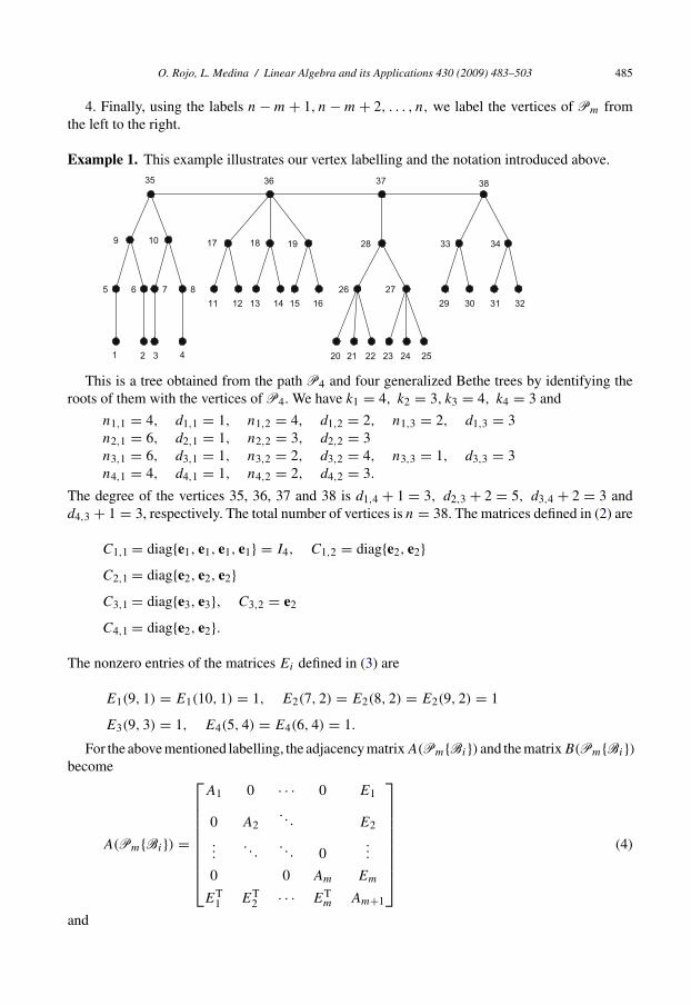
Example 1. This example illustrates our vertex labelling and the notation introduced above.

1 2 3 4

5 6 7 8

9 10

11 12 1413 15 16

17 18 19

20 21 22 23 24 25

26 27

28

29 30 31 32

33 34

35 36 37 38

This is a tree obtained from the path P4 and four generalized Bethe trees by identifying theroots of them with the vertices of P4. We have k1 = 4, k2 = 3, k3 = 4, k4 = 3 and

n1,1 = 4, d1,1 = 1, n1,2 = 4, d1,2 = 2, n1,3 = 2, d1,3 = 3n2,1 = 6, d2,1 = 1, n2,2 = 3, d2,2 = 3n3,1 = 6, d3,1 = 1, n3,2 = 2, d3,2 = 4, n3,3 = 1, d3,3 = 3n4,1 = 4, d4,1 = 1, n4,2 = 2, d4,2 = 3.

The degree of the vertices 35, 36, 37 and 38 is d1,4 + 1 = 3, d2,3 + 2 = 5, d3,4 + 2 = 3 andd4,3 + 1 = 3, respectively. The total number of vertices is n = 38. The matrices defined in (2) are

C1,1 = diag{e1, e1, e1, e1} = I4, C1,2 = diag{e2, e2}C2,1 = diag{e2, e2, e2}C3,1 = diag{e3, e3}, C3,2 = e2

C4,1 = diag{e2, e2}.

The nonzero entries of the matrices Ei defined in (3) are

E1(9, 1) = E1(10, 1) = 1, E2(7, 2) = E2(8, 2) = E2(9, 2) = 1

E3(9, 3) = 1, E4(5, 4) = E4(6, 4) = 1.

For the abovementioned labelling, the adjacencymatrixA(Pm{Bi}) and thematrixB(Pm{Bi})become

A(Pm{Bi}) =

⎡⎢⎢⎢⎢⎢⎢⎢⎢⎣

A1 0 · · · 0 E1

0 A2. . . E2

.... . .

. . . 0...

0 0 Am Em

ET1 ET

2 · · · ETm Am+1

⎤⎥⎥⎥⎥⎥⎥⎥⎥⎦(4)

and

486 O. Rojo, L. Medina / Linear Algebra and its Applications 430 (2009) 483–503

B(Pm(Bi )) =

⎡⎢⎢⎢⎢⎢⎢⎢⎢⎣

B1 0 · · · 0 E1

0 B2. . . E2

.... . .

. . . 0...

0 0 Bm Em

ET1 ET

2 · · · ETm Bm+1

⎤⎥⎥⎥⎥⎥⎥⎥⎥⎦, (5)

where, for i = 1, 2, . . . , m, the matrices Ai and Bi are the following block tridiagonalmatrices:

Ai =

⎡⎢⎢⎢⎢⎢⎢⎢⎢⎣

0 Ci,1

CTi,1 0 Ci,2

CTi,2

. . .. . .

. . .. . . Ci,ki−2

CTi,ki−2 0

⎤⎥⎥⎥⎥⎥⎥⎥⎥⎦, (6)

Bi =

⎡⎢⎢⎢⎢⎢⎢⎢⎢⎣

Ini,1 Ci,1

CTi,1 di,2Ini,2 Ci,2

CTi,2

. . .. . .

. . .. . . Ci,ki−2

CTi,ki−2 di,ki−1Ii,nki−1

⎤⎥⎥⎥⎥⎥⎥⎥⎥⎦(7)

and

Am+1 =

⎡⎢⎢⎢⎢⎢⎢⎢⎢⎣

0 1

1 0 1

1. . .

. . .

. . .. . . 1

1 0

⎤⎥⎥⎥⎥⎥⎥⎥⎥⎦, (8)

Bm+1 =

⎡⎢⎢⎢⎢⎢⎢⎢⎢⎣

d1,k1 + 1 1

1 d2,k2 + 2 1

1. . .

. . .

. . . dm−1,km−1 + 2 1

1 dm,km + 1

⎤⎥⎥⎥⎥⎥⎥⎥⎥⎦(9)

both of order m × m.

O. Rojo, L. Medina / Linear Algebra and its Applications 430 (2009) 483–503 487

2. Preliminaries

Lemma 2. Let

X =

⎡⎢⎢⎢⎢⎢⎢⎣

X1 0 · · · 0 −E1

0 X2. . . −E2

.... . .

. . . 0...

0 0 Xm −Em

−ET1 −ET

2 · · · −ETm Xm+1

⎤⎥⎥⎥⎥⎥⎥⎦ ,

where, for i = 1, 2, . . . , m, Xi is the block tridiagonal matrix

Xi =

⎡⎢⎢⎢⎢⎢⎢⎣

αi,1Ini,1 −Ci,1

−CTi,1 αi,2Ini ,2 −Ci,2

−CTi,2

. . .. . .

. . .. . . −Ci,ki−2

−CTi,ki−2 αi,ki−1Ii,nki−1

⎤⎥⎥⎥⎥⎥⎥⎦and

Xm+1 =

⎡⎢⎢⎢⎢⎢⎢⎣

α1 −1−1 α2 −1

−1. . .

. . .. . .

. . . −1−1 αm

⎤⎥⎥⎥⎥⎥⎥⎦ .

For i = 1, 2, . . . , m, let

βi,1 = αi,1,

βi,j = αi,j − ni,j−1

ni,j

1

βi,j−1, j = 2, 3, . . . , ki − 1,

βi = αi − ni,ki−11

βi,ki−1.

If βi,j /= 0 for all i = 1, 2, . . . , m and all j = 1, 2, . . . , ki − 1 then

|X| =⎛⎝ m∏

i=1

ki−1∏j=1

βni,j

i,j

⎞⎠ |Ym+1|, (10)

where

Ym+1 =

⎡⎢⎢⎢⎢⎢⎢⎣

β1 −1−1 β2 −1

−1. . .

. . .. . .

. . . −1−1 βm

⎤⎥⎥⎥⎥⎥⎥⎦ . (11)

488 O. Rojo, L. Medina / Linear Algebra and its Applications 430 (2009) 483–503

Proof. Suppose β1,j /= 0 for all j = 1, 2, . . . , k1 − 1. After some steps of the Gaussian elim-ination procedure, without row interchanges, we reduce X to the intermediate matrix givenbelow:⎡⎢⎢⎢⎢⎢⎢⎣

R1 0 · · · 0 −E1

0 X2. . . −E2

.... . .

. . . 0...

0 0 Xm −Em

0 −ET2 · · · −ET

2 X(1)m+1

⎤⎥⎥⎥⎥⎥⎥⎦ ,

where R1 is the upper triangular matrix

R1 =

⎡⎢⎢⎢⎢⎣β1,1In1,1 C1,1

β1,2In1,2

. . .

. . . C1,k1−2β1,k1−1In1,k1−1

⎤⎥⎥⎥⎥⎦and X

(1)m+1 is the tridiagonal matrix

X(1)m+1 =

⎡⎢⎢⎢⎢⎢⎢⎣

β1 −1−1 α2 −1

−1. . .

. . .. . .

. . . −1−1 αm

⎤⎥⎥⎥⎥⎥⎥⎦ .

Suppose, in addition, βi,j /= 0 for all i = 2, 3, . . . , m and all j = 1, 2, . . . , ki − 1. We continuethe Gaussian elimination procedure to finally obtain the upper triangular matrix⎡⎢⎢⎢⎢⎢⎢⎣

R1 0 · · · 0 −E1

0 R2. . . −E2

.... . .

. . . 0...

0 0 Rm −Em

0 0 · · · 0 Ym+1

⎤⎥⎥⎥⎥⎥⎥⎦ ,

where, for i = 2, 3, . . . , m,

Ri =

⎡⎢⎢⎢⎢⎣βi,1Ini,1 −Ci,1

βi,2Ini,2

. . .

. . . −Ci,ki−2βi,ki−1Ini,ki−1

⎤⎥⎥⎥⎥⎦and Ym+1 is as in (11). Thus, (10) is proved. �

From now on, we denote by A the submatrix obtained from A by deleting its last row and itslast column and, for i = 1, 2, . . . , m − 1, by Fi the matrix of order ki × ki+1 whose are 0 exceptfor the entry Fi(ki, ki+1) = 1.

O. Rojo, L. Medina / Linear Algebra and its Applications 430 (2009) 483–503 489

Lemma 3. Let

Mm =

⎡⎢⎢⎢⎢⎢⎣T1 −F1

−F T2 T2 −F2

−F T2

. . .. . .

Tm−1 −Fm−1

· · · −F Tm−1 Tm

⎤⎥⎥⎥⎥⎥⎦ ,

where Ti is a matrix of order ki × ki . Let

Dm =

∣∣∣∣∣∣∣∣∣∣∣∣

|T1| |T1||T2| |T2| |T2|

|T3| . . .. . .

. . . |Tm−1| |Tm−1||Tm| |Tm|

∣∣∣∣∣∣∣∣∣∣∣∣.

Then

|M2| = |D2| (12)

and, for all m,

|Mm| = |Dm|. (13)

Proof. By induction on m. Clearly |M1| = |D1|. We may write

M2 =[

T1 −F1

−F T1 T2

]=

⎡⎢⎢⎣T1 p 0 0qT T1 (k1, k1) 0 −10 0 T2 r0 −1 sT T2(k2, k2)

⎤⎥⎥⎦ ,

where p, q, r, s are clear from the context and 0 is the all zeros vector of the appropiate order. Weknow that the determinant function is linear transformation on each column (row). We apply thisproperty on the last column of M2 to obtain

|M2| =

∣∣∣∣∣∣∣∣T1 p 0 0qT T1(k1, k1) 0 00 0 T2 r0 −1 sT T2(k2, k2)

∣∣∣∣∣∣∣∣+∣∣∣∣∣∣∣∣T1 p 0 0qT T1(k1, k1) 0 −10 0 T2 00 −1 sT 0

∣∣∣∣∣∣∣∣= |T1||T2| − (−1)2k1+k2

∣∣∣∣∣∣T1 p 00 0 T2

0 −1 sT

∣∣∣∣∣∣ = |T1||T2| − (−1)k2 |T1|∣∣∣∣ 0 T2

−1 sT

∣∣∣∣= |T1||T2| + (−1)k2(−1)k2+1|T1||T2| = |T1||T2| − |T1||T2|.

Thus (12) is proved. Observe that (12) is (13) for m = 2. Let m � 2. Suppose that (13) is true forall integer less or equal to m. We have

Mm+1 =[

Mm −Km

−KTm Tm+1

],

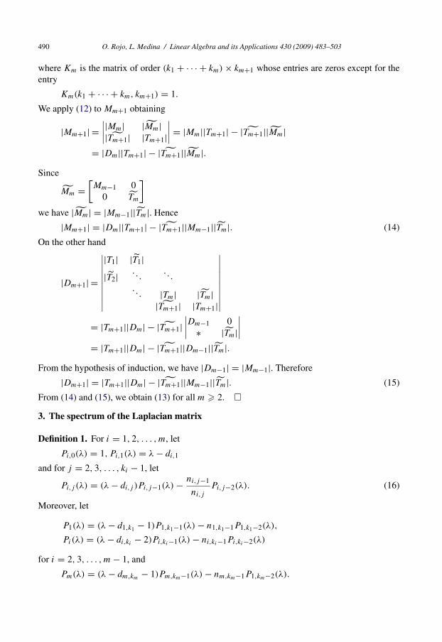
490 O. Rojo, L. Medina / Linear Algebra and its Applications 430 (2009) 483–503

where Km is the matrix of order (k1 + · · · + km) × km+1 whose entries are zeros except for theentry

Km(k1 + · · · + km, km+1) = 1.

We apply (12) to Mm+1 obtaining

|Mm+1| =∣∣∣∣|Mm| |Mm||Tm+1| |Tm+1|

∣∣∣∣ = |Mm||Tm+1| − |Tm+1||Mm|= |Dm||Tm+1| − |Tm+1||Mm|.

Since

Mm =[Mm−1 0

0 Tm

]we have |Mm| = |Mm−1||Tm|. Hence

|Mm+1| = |Dm||Tm+1| − |Tm+1||Mm−1||Tm|. (14)

On the other hand

|Dm+1| =

∣∣∣∣∣∣∣∣∣∣|T1| |T1||T2| . . .

. . .. . . |Tm| |Tm|

|Tm+1| |Tm+1|

∣∣∣∣∣∣∣∣∣∣= |Tm+1||Dm| − |Tm+1|

∣∣∣∣Dm−1 0∗ |Tm|

∣∣∣∣= |Tm+1||Dm| − |Tm+1||Dm−1||Tm|.

From the hypothesis of induction, we have |Dm−1| = |Mm−1|. Therefore

|Dm+1| = |Tm+1||Dm| − |Tm+1||Mm−1||Tm|. (15)

From (14) and (15), we obtain (13) for all m � 2. �

3. The spectrum of the Laplacian matrix

Definition 1. For i = 1, 2, . . . , m, let

Pi,0(λ) = 1, Pi,1(λ) = λ − di,1

and for j = 2, 3, . . . , ki − 1, let

Pi,j (λ) = (λ − di,j )Pi,j−1(λ) − ni,j−1

ni,j

Pi,j−2(λ). (16)

Moreover, let

P1(λ) = (λ − d1,k1 − 1)P1,k1−1(λ) − n1,k1−1P1,k1−2(λ),

Pi(λ) = (λ − di,ki− 2)Pi,ki−1(λ) − ni,ki−1Pi,ki−2(λ)

for i = 2, 3, . . . , m − 1, and

Pm(λ) = (λ − dm,km − 1)Pm,km−1(λ) − nm,km−1P1,km−2(λ).

O. Rojo, L. Medina / Linear Algebra and its Applications 430 (2009) 483–503 491

For i = 1, 2, . . . , m, let

�i = {j : 1 � j � ni,ki−1 : ni,j > ni,j+1}.

Theorem 1. We have

(a)

|λI − L(Pm{Bi})| = P(λ)

m∏i=1

∏j∈�i

Pni,j −ni,j+1i,j (λ) (17)

where

P(λ) =

∣∣∣∣∣∣∣∣∣∣P1(λ) P1,k1−1(λ)

P2,k2−1(λ). . .

. . .. . .

. . . Pm−1,km−1−1(λ)

Pm,km−1(λ) Pm(λ)

∣∣∣∣∣∣∣∣∣∣(b) The set of eigenvalues of L(Pm{Bi}) is

σ(L(Pm{Bi})) = (∪mi=1 ∪j∈�i

{λ : Pi,j (λ) = 0}) ∪ {λ : P(λ) = 0}.

Proof. (a) We consider B(Pm{Bi}) instead of L(Pm{Bi}). We know that B(Pm{Bi}) is givenby (5), (7) and (9). We apply Lemma 2 to the matrix X = λI − B(Pm{Bi}). For this matrix

αi,j = λ − di,j (1 � i � m, 1 � j � ki − 1)

α1 = λ − d1,k1

αi = λ − di,ki− 2 (2 � i � m − 1)

αm = λ − dm,km − 1.

Let βi,j , βi be as in Lemma 2. We first suppose that λ ∈ R is such that Pi,j (λ) /= 0 for all i =1, 2, . . . , m and for all j = 1, 2, . . . , ki − 1. For brevity, we write Pi,j (λ) = Pi,j and P(λ) = P .We have

βi,1 = λ − di,1 = Pi,1

Pi,0/= 0,

βi,2 = (λ − di,2) − ni,1

ni,2

1

βi,1= (λ − di,2) − ni,1

ni,2

Pi,0

Pi,1,

=(λ − di,2)Pi,1 − ni,1

ni,2Pi,0

Pi,1= Pi,2

Pi,1/= 0,

...

βi,ki−1 = (λ − di,ki−1) − nki−2

nki−1

1

βi,ki−2= (λ − di,ki−1) − ni,ki−2

ni,ki−1

Pi,ki−3

Pi,ki−2

=(λ − di,ki−1)Pi,ki−2 − nki−2

ni,ki−1Pi,ki−3

Pi,ki−2= Pi,ki−1

Pi,ki−2/= 0.

492 O. Rojo, L. Medina / Linear Algebra and its Applications 430 (2009) 483–503

Moreover

β1 = (λ − d1,k1 − 1) − n1,k1−11

β1,k1−1

= (λ − d1,k1 − 1) − n1,k1−1P1,k1−2

P1,k1−1

= (λ − d1,k1 − 1)P1,k1−1 − n1,k1−1P1,k1−2

P1,k1−1= P1

P1,k1−1,

βm = (λ − dm,km − 1) − nm,km−11

βm,k1−1= (λ − dm,km − 1) − nm,km−1

Pm,km−2

Pm,km−1

= (λ − dm,km − 1)Pm,km−1 − nm,km−1Pm,km−2

Pm,km−1= Pm

Pm,km−1

and for i = 2, . . . , m − 1

βi = (λ − di,ki− 2) − ni,ki−1

1

βi,ki−1= (λ − di,ki

− 2) − ni,ki−1Pi,ki−2

Pi,ki−1

= (λ − di,ki− 2)Pi,ki−1 − ni,ki−1Pi,ki−2

Pi,ki−1= Pi

Pi,ki−1.

From (10)

det(λI − B(Pm{Bi})) =⎛⎝ m∏

i=1

ki−1∏j=1

βni,j

i,j

⎞⎠ |Cm+1|

=(

m∏i=1

Pni,1i,1

Pni,1i,0

Pni,2i,2

Pni,2i,1

Pni,3i,3

Pni,3i,2

· · · Pni,ki−2

i,ki−2

Pni,ki−2

i,ki−3

Pni,ki−1

i,ki−1

Pni,ki−1

i,ki−2

)|Cm+1|

=(

m∏i=1

Pni,1−ni,2i,1 P

ni,2−ni,3i,2 · · · P ni,ki−2−ni,ki−1

i,ki−2 Pni,ki−1

i,ki−1

)|Cm+1|

where

|Cm+1| =

∣∣∣∣∣∣∣∣∣∣∣∣∣∣

P1P1,k1−1

−1

−1 P2P2,k2−1

−1

−1. . .

. . .. . .

. . . −1−1 Pm

Pm,km−1

∣∣∣∣∣∣∣∣∣∣∣∣∣∣= 1∏m

i=1 Pi,ki−1

∣∣∣∣∣∣∣∣∣∣P1 P1,k1−1

P2,k2−1 P2. . .

. . .. . . Pm−1,km−1−1

Pm,km−1 Pm

∣∣∣∣∣∣∣∣∣∣.

O. Rojo, L. Medina / Linear Algebra and its Applications 430 (2009) 483–503 493

Hence

|λI − L(Pm{Bi})| = P(λ)

m∏i=1

ni,ki−1∏j=1

Pni,j −ni,j+1i,j

= P(λ)

m∏i=1

∏j∈�i

Pni,j −ni,j+1i,j (λ).

Thus (17) is proved for all λ ∈ R such that Pi,j (λ) /= 0, for all i = 1, 2, . . . , m and for all j =1, 2, . . . , ki − 1. Now, we consider λ0 ∈ R such that Pl,s(λ0) = 0 for some 1 � l � m and for1 � s � kl − 1. Since the zeros of any nonzero polynomial are isolated, there exists a neighbor-hood N(λ0) of λ0 such that Pi,j (λ) /= 0 for all λ ∈ N(λ0) − {λ0} and for all i = 1, 2, . . . , m andfor all j = 1, 2, . . . , ki − 1. Hence

|λI − B(Pm{Bi})| = P(λ)

m∏i=1

∏j∈�i

Pni,j −ni,j+1i,j (λ)

for all λ ∈ N(λ0) − {λ0}. By continuity, taking the limit as λ tends to λ0 we obtain

|λ0I − B(Pm{Bi})| = P(λ0)

m∏i=1

∏j∈�i

Pni,j −ni,j+1i,j (λ0).

Therefore (17) holds for all λ ∈ R.(b) It is an immediate consequence of part (a). �

Definition 2. For i = 1, 2, 3, . . . , m, let

Ti =

⎡⎢⎢⎢⎢⎢⎣di,1

√di,2 − 1√

di,2 − 1 di,2. . .

√di,ki−1 − 1√

di,ki−1 − 1 di,ki−1√

di,ki√di,ki

di,ki+ c

⎤⎥⎥⎥⎥⎥⎦of order ki × ki , where c = 2 for i = 2, 3, . . . , m − 1 and c = 1 for i = 1 and i = m. More-over, for i = 1, 2, . . . , m and for j = 1, 2, 3, . . . , ki − 1, let Ti,j be the j × j leading principalsubmatrix of Ti .

Lemma 4. For i = 1, 2, . . . , m and for j = 1, 2, . . . , ki − 1, we have

|λI − Ti,j | = Pi,j (λ). (18)

Moreover,

|λI − Ti | = Pi(λ) (19)

for i = 2, 3, . . . , m − 1, and

|λI − T1| = P1(λ), (20)

|λI − Tm| = Pm(λ).

494 O. Rojo, L. Medina / Linear Algebra and its Applications 430 (2009) 483–503

Proof. It is well known [7, page 229] that the characteristic polynomials, Qj , of the j × j leadingprincipal submatrix of the k × k symmetric tridiagonal matrix⎡⎢⎢⎢⎢⎢⎢⎣

c1 b1b1 c2 b2

. . .. . .

. . .. . . ck−1 bk−1

bk−1 ck

⎤⎥⎥⎥⎥⎥⎥⎦satisfy the three-term recursion formula

Qj(λ) = (λ − cj )Qj−1(λ) − b2j−1Qj−2(λ) (21)

with

Q0(λ) = 1 and Q1(λ) = λ − c1.

We recall that, for i = 1, 2, . . . , m and for j = 1, 2, . . . , ki , the polynomials Pi,j are defined

by the recursion formula (16). Let 1 � i � m be fixed. From (1),√

ni,j

ni,j+1= √

di,j+1 − 1 for

j = 1, 2, . . . , ki − 2. For the matrix Ti,ki−1, we have cj = di,j for j = 1, 2, . . . , ki − 1 and

bj = √di,j+1 − 1 =

√ni,j

ni,j+1for j = 1, 2, . . . , ki − 2. Replacing in the recursion formula (21),

we get the polynomials Pi,j , j = 1, 2, . . . , ki − 1. Thus (18) is proved. The proof for (19) and(20) are similar. �

Lemma 5. Let r = ∑mi=1 ki . Let G be the symmetric matrix of order r × r defined by

G =

⎡⎢⎢⎢⎢⎣T1 F1

F T1 T2

. . .. . .

. . . Fm−1

F Tm−1 Tm

⎤⎥⎥⎥⎥⎦ .

Then

|λI − G| = P(λ).

Proof. We apply Lemma 3 to λI − G to obtain that

|λI − G| =

∣∣∣∣∣∣∣∣∣∣∣

|λI − T1| | ˜λI − T1|| ˜λI − T2| |λI − T2| | ˜λI − T2|

. . .. . .

. . .| ˜λI − Tm−1| |λI − Tm−1| | ˜λI − Tm−1|

| ˜λI − Tm| |λI − Tm|

∣∣∣∣∣∣∣∣∣∣∣.

We observe that ˜λI − Ti = λI − Ti,ki−1. We now use Lemma 4 to obtain

O. Rojo, L. Medina / Linear Algebra and its Applications 430 (2009) 483–503 495

|λI − G| =

∣∣∣∣∣∣∣∣∣∣∣

P1(λ) P1,k1−1(λ)P2,k2−1(λ) P2(λ) P2,k2−1(λ)

P3,k3−1(λ). . .

. . .. . .

. . . Pm−1,km−1−1(λ)Pm,km−1(λ) Pm(λ)

∣∣∣∣∣∣∣∣∣∣∣= P(λ).

The proof is complete. �

Theorem 2. (a)

σ(L(Pm{Bi})) = (∪mi=1 ∪j∈�i

σ (Ti,j )) ∪ σ(G).

(b) The multiplicity of each eigenvalue of the matrix Ti,j , as an eigenvalue of L(Pm{Bi}), isat least (ni,j − ni,j+1) for j ∈ �i .

(c) The matrix G is singular.

Proof. It is known that the eigenvalues of a symmetric tridiagonal matrix with nonzero codiagonalentries are simple [2]. This fact and Theorem 1, Lemma 4 and Lemma 5 imply (a) and (b). Onecan easily check that |Ti,j | = 1 for 1 � i � m and 1 � j � ki − 1. This fact and part (a) implythat 0 is an eigenvalue of G. �

Example 2. Let P4{Bi : i = 1, 2, 3, 4} be the tree in Example 1. For this tree

T1 =

⎡⎢⎢⎣1 11 2

√2√

2 3√

2√2 3

⎤⎥⎥⎦ , T2 =⎡⎣ 1

√2√

2 3√

3√3 5

⎤⎦

T3 =

⎡⎢⎢⎣1

√3√

3 4√

2√2 3 1

1 3

⎤⎥⎥⎦ , T4 =⎡⎣ 1

√2√

2 3√

2√2 3

⎤⎦ .

We have�1 = {2, 3}, �2 = {1, 2}, �3 = {1, 2}, �4 = {1, 2}.

From Theorem 2, the eigenvalues of L(Pm{Bi}) are those ofT1,2, T1,3, T2,1, T2,2, T3,1, T3,2, T4,1, T4,2 and G,

where

G =

⎡⎢⎢⎣T1 F1

F T1 T2 F2

F T2 T3 F3

F T3 T4

⎤⎥⎥⎦ .

Let ρ(A) be the spectral radius of a matrix A.

Lemma 6 [8]. If A is a irreducible nonnegative matrix and B is any principal submatrix of A

then ρ(B) < ρ(A).

496 O. Rojo, L. Medina / Linear Algebra and its Applications 430 (2009) 483–503

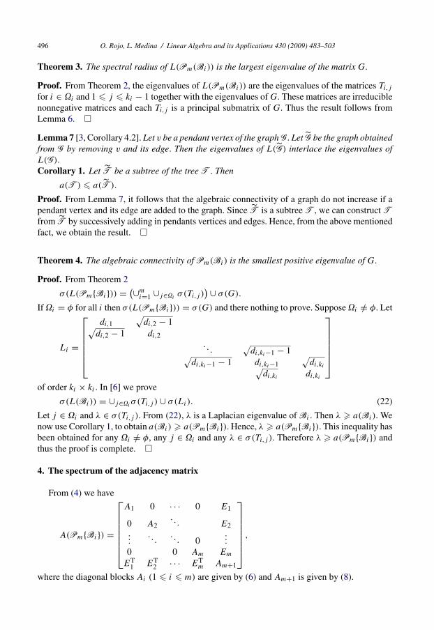
Theorem 3. The spectral radius of L(Pm(Bi )) is the largest eigenvalue of the matrix G.

Proof. From Theorem 2, the eigenvalues of L(Pm(Bi )) are the eigenvalues of the matrices Ti,j

for i ∈ �i and 1 � j � ki − 1 together with the eigenvalues of G. These matrices are irreduciblenonnegative matrices and each Ti,j is a principal submatrix of G. Thus the result follows fromLemma 6. �

Lemma 7 [3, Corollary 4.2]. Let v be a pendant vertex of the graphG. Let G be the graph obtainedfrom G by removing v and its edge. Then the eigenvalues of L(G) interlace the eigenvalues ofL(G).

Corollary 1. Let T be a subtree of the tree T. Then

a(T) � a(T).

Proof. From Lemma 7, it follows that the algebraic connectivity of a graph do not increase if apendant vertex and its edge are added to the graph. Since T is a subtree T, we can construct Tfrom T by successively adding in pendants vertices and edges. Hence, from the above mentionedfact, we obtain the result. �

Theorem 4. The algebraic connectivity of Pm(Bi ) is the smallest positive eigenvalue of G.

Proof. From Theorem 2

σ(L(Pm{Bi})) = (∪mi=1 ∪j∈�i

σ (Ti,j )) ∪ σ(G).

If �i = φ for all i then σ(L(Pm{Bi})) = σ(G) and there nothing to prove. Suppose �i /= φ. Let

Li =

⎡⎢⎢⎢⎢⎢⎣di,1

√di,2 − 1√

di,2 − 1 di,2. . .

√di,ki−1 − 1√

di,ki−1 − 1 di,ki−1√

di,ki√di,ki

di,ki

⎤⎥⎥⎥⎥⎥⎦of order ki × ki . In [6] we prove

σ(L(Bi )) = ∪j∈�iσ (Ti,j ) ∪ σ(Li). (22)

Let j ∈ �i and λ ∈ σ(Ti,j ). From (22), λ is a Laplacian eigenvalue of Bi . Then λ � a(Bi ). Wenow use Corollary 1, to obtain a(Bi ) � a(Pm{Bi}). Hence, λ � a(Pm{Bi}). This inequality hasbeen obtained for any �i /= φ, any j ∈ �i and any λ ∈ σ(Ti,j ). Therefore λ � a(Pm{Bi}) andthus the proof is complete. �

4. The spectrum of the adjacency matrix

From (4) we have

A(Pm{Bi}) =

⎡⎢⎢⎢⎢⎢⎢⎣

A1 0 · · · 0 E1

0 A2. . . E2

.... . .

. . . 0...

0 0 Am Em

ET1 ET

2 · · · ETm Am+1

⎤⎥⎥⎥⎥⎥⎥⎦ ,

where the diagonal blocks Ai (1 � i � m) are given by (6) and Am+1 is given by (8).

O. Rojo, L. Medina / Linear Algebra and its Applications 430 (2009) 483–503 497

We may apply Lemma 2 to X = λI − A(Pm{Bi}). For this matrix αi,j = λ for 1 � i � m

and 1 � j � ki − 1, and αi = λ for 1 � i � m.

Definition 3. For i = 1, 2, . . . , m, let

Qi,0(λ) = 1, Qi,1(λ) = λ

and for j = 2, 3, . . . , ki − 1, let

Qi,j (λ) = λQi,j−1(λ) − ni,j−1

ni,j

Qi,j−2(λ).

Moreover, let

Qi(λ) = λQi,ki−1(λ) − ni,ki−1Qi,ki−2(λ)

for i = 1, 2, . . . , m.

Theorem 5. We have(a)

|λI − A(Pm{Bi})| = Q(λ)

m∏i=1

∏j∈�i

Qni,j −ni,j+1i,j (λ).

(b)

σ(A(Pm{Bi})) = (∪mi=1 ∪j∈�i

{λ : Qi,j (λ) = 0}) ∪ {λ : Q(λ) = 0},where

Q(λ) =

∣∣∣∣∣∣∣∣∣∣∣∣

Q1(λ) Q1,k1−1(λ)

Q2,k2−1(λ) Q2(λ) Q2,k2−1(λ)

Q3,k3−1(λ). . .

. . .. . .

. . . Qm−1,km−1−1(λ)

Qm,km−1(λ) Qm(λ)

∣∣∣∣∣∣∣∣∣∣∣∣.

Proof. Similar to the proof of Theorem 1. �

Definition 4. For i = 1, 2, 3, . . . , m, let

Si =

⎡⎢⎢⎢⎢⎢⎢⎣

0√

di,2 − 1√di,2 − 1 0

. . .. . .

. . .√

di,ki−1 − 1√di,ki−1 − 1 0

√di,ki√

di,ki0

⎤⎥⎥⎥⎥⎥⎥⎦of order ki × ki . Moreover, for i = 1, 2, . . . m and for j = 1, 2, 3, . . . , ki − 1, let Si,j be the j × j

leading principal submatrix of Si .

Lemma 8. For i = 1, 2, . . . , m and for j = 1, 2, . . . , ki − 1, we have

|λI − Si,j | = Qi,j (λ).

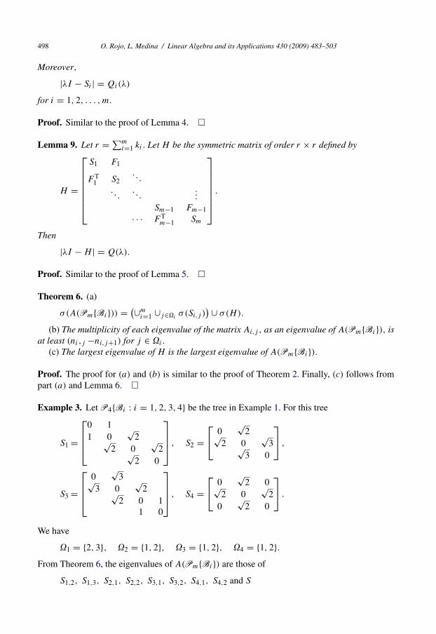
498 O. Rojo, L. Medina / Linear Algebra and its Applications 430 (2009) 483–503

Moreover,

|λI − Si | = Qi(λ)

for i = 1, 2, . . . , m.

Proof. Similar to the proof of Lemma 4. �

Lemma 9. Let r = ∑mi=1 ki . Let H be the symmetric matrix of order r × r defined by

H =

⎡⎢⎢⎢⎢⎢⎢⎣

S1 F1

F T1 S2

. . .. . .

. . ....

Sm−1 Fm−1

· · · F Tm−1 Sm

⎤⎥⎥⎥⎥⎥⎥⎦ .

Then

|λI − H | = Q(λ).

Proof. Similar to the proof of Lemma 5. �

Theorem 6. (a)

σ(A(Pm{Bi})) = (∪mi=1 ∪j∈�i

σ (Si,j )) ∪ σ(H).

(b) The multiplicity of each eigenvalue of the matrix Ai,j , as an eigenvalue of A(Pm{Bi}), isat least (ni,j −ni,j+1) for j ∈ �i .

(c) The largest eigenvalue of H is the largest eigenvalue of A(Pm{Bi}).

Proof. The proof for (a) and (b) is similar to the proof of Theorem 2. Finally, (c) follows frompart (a) and Lemma 6. �

Example 3. Let P4{Bi : i = 1, 2, 3, 4} be the tree in Example 1. For this tree

S1 =

⎡⎢⎢⎣0 11 0

√2√

2 0√

2√2 0

⎤⎥⎥⎦ , S2 =⎡⎣ 0

√2√

2 0√

3√3 0

⎤⎦ ,

S3 =

⎡⎢⎢⎣0

√3√

3 0√

2√2 0 1

1 0

⎤⎥⎥⎦ , S4 =⎡⎣ 0

√2 0√

2 0√

20

√2 0

⎤⎦ .

We have

�1 = {2, 3}, �2 = {1, 2}, �3 = {1, 2}, �4 = {1, 2}.From Theorem 6, the eigenvalues of A(Pm{Bi}) are those of

S1,2, S1,3, S2,1, S2,2, S3,1, S3,2, S4,1, S4,2 and S

O. Rojo, L. Medina / Linear Algebra and its Applications 430 (2009) 483–503 499

where

S =

⎡⎢⎢⎣S1 F1

F T1 S2 F2

F T2 S3 F3

F T3 S4

⎤⎥⎥⎦ .

5. Copies of a generalized Bethe tree attached to a path

In this section, we assume B1 = B2 = · · · = Bm = B, where B is a generalized Bethe of k

levels in which the numbers dk−j+1 and nk−j+1 are the degree of the vertices and the number ofthem at level j . Then

k1 = k2 = · · · = km = k,

�1 = · · · = �m = � = {j : 1 � j � k − 1, nj+1 > nj

},

F1 = F2 = · · · = Fm = F,

where F is a k × k matrix whose entries are 0 except F(k, k) = 1,

T2 = T3 = · · · = Tm−1 = T + F,

where

T = T1 = Tm =

⎡⎢⎢⎢⎢⎢⎣d1

√d2 − 1√

d2 − 1 d2. . .

√dk−1 − 1√

dk−1 − 1 dk−1√

dk√dk dk + 1

⎤⎥⎥⎥⎥⎥⎦and for i = 1, 2, . . . , m, j = 1, 2, . . . , k − 1,

Ti,j =

⎡⎢⎢⎢⎢⎢⎣d1

√d2 − 1√

d2 − 1 d2. . .

√dk−1 − 1√

dk−1 − 1 dj−1√

dj − 1√dj − 1 dj

⎤⎥⎥⎥⎥⎥⎦ .

Definition 5. For s = 1, . . . , m, let

L(s) =

⎡⎢⎢⎢⎢⎢⎢⎢⎢⎣

1√

d2 − 1√d2 − 1 d2

√d3 − 1

√d3 − 1 d3

. . .. . .

. . .√

dk−1 − 1√dk−1 − 1 dk−1

√dk√

dk dk + 2 + 2 cos πsm

⎤⎥⎥⎥⎥⎥⎥⎥⎥⎦of order k × k and, j = 1, 2, . . . , k − 1, let Lj the j × j leading principal submatrix of L(s).

500 O. Rojo, L. Medina / Linear Algebra and its Applications 430 (2009) 483–503

We recall that the Kronecker product [9] of two matrices A = (ai,j ) and B = (bi,j ) of sizesm × m and n × n, respectively, is defined to be the (mn) × (mn) matrix A ⊗ B = (ai,jB). Formatrices A, B, C and D of appropiate sizes

(A ⊗ B)(C ⊗ D) = (AC ⊗ BD).

We write Pm{B} instead of Pm{Bi}.

Theorem 7. The set of eigenvalues of L(Pm{B}) is

σ(L(Pm{B})) = (∪j∈�σ(Lj )) ∪ (∪m

s=1σ(L(s))).

Proof. From Theorem 2, we have

σ(L(Pm{B})) = (∪mi=1 ∪j∈�i

σ (Ti,j )) ∪ σ(G)

We observe that Lj = Ti,j . Then

σ(L(Pm{B})) = ∪j∈�σ(Lj ) ∪ σ(G).

It remains to prove that σ(G) = ∪ms=1σ(L(s)). We have

L(m) =

⎡⎢⎢⎢⎢⎢⎢⎢⎢⎣

1√

d2 − 1√d2 − 1 d2

√d3 − 1

√d3 − 1 d3

. . .. . .

. . .√

dk−1 − 1√dk−1 − 1 dk−1

√dk√

dk dk

⎤⎥⎥⎥⎥⎥⎥⎥⎥⎦.

For brevity, let L = L(m). Then L(s) = L + 2 + 2 cos πsm

F and T = L + F . Hence

G =

⎡⎢⎢⎢⎢⎢⎢⎣

T F

F T + F F

F. . .

. . .. . . T + F F

F T

⎤⎥⎥⎥⎥⎥⎥⎦ =

⎡⎢⎢⎢⎢⎢⎢⎣

L + F F

F L + 2F F

F. . .

. . .. . . L + 2F F

F L

⎤⎥⎥⎥⎥⎥⎥⎦ .

We may write

G = Im ⊗ L + Cm ⊗ F,

where

Cm =

⎡⎢⎢⎢⎢⎢⎢⎢⎣

1 1

1 2. . .

. . .. . .

. . .. . . 2 1

1 1

⎤⎥⎥⎥⎥⎥⎥⎥⎦of order m × m. The eigenvalues of Cm are known [4]. They are γs = 2 + 2 cos πs

m, 1 � s � m.

O. Rojo, L. Medina / Linear Algebra and its Applications 430 (2009) 483–503 501

Let

V = [v1 v2 · · · vm−1 vm

]be a orthogonal matrix whose columns v1, v2, . . . , vm are eigenvectors corresponding to theeigenvalues γ1, γ2, .., γs . Therefore

(V ⊗ Ik)G(V T ⊗ Ik) = (V ⊗ Ik)(Im ⊗ L + Cm ⊗ F)(V T ⊗ Ik)

= Im ⊗ L + (V CmV T) ⊗ F.

We have

(V CmV T) ⊗ F =

⎡⎢⎢⎢⎢⎣γ1

γ2

γm−1γm

⎤⎥⎥⎥⎥⎦⊗ F

=

⎡⎢⎢⎢⎢⎢⎣γ1F

γ2F

. . .γm−1F

γmF

⎤⎥⎥⎥⎥⎥⎦ .

Therefore

(V ⊗ Ik)G(V T ⊗ Ik) =

⎡⎢⎢⎢⎢⎢⎣L + γ1F

L + γ2F

. . .L + γm−1F

L + γmF

⎤⎥⎥⎥⎥⎥⎦

=

⎡⎢⎢⎢⎢⎢⎣L(1)

L (2)

. . .L (m − 1)

L (m)

⎤⎥⎥⎥⎥⎥⎦ .

Since G and (V ⊗ Ik)G(V T ⊗ Ik) are similar matrices, we conclude that

σ(G) = ∪ms=1σ(L(s)).

This completes the proof. �

Corollary 2. The largest eigenvalue of L(1) is the spectral radius of L(Pr (B)).

Proof. FromTheorem3, the spectral radius ofL(Pr (B)) is the largest eigenvalue in∪ms=1σ(L(s)).

That is

ρ(L(Pr (B))) = max{ρ(L(s) : s = 1, 2, . . . , m)}.We have

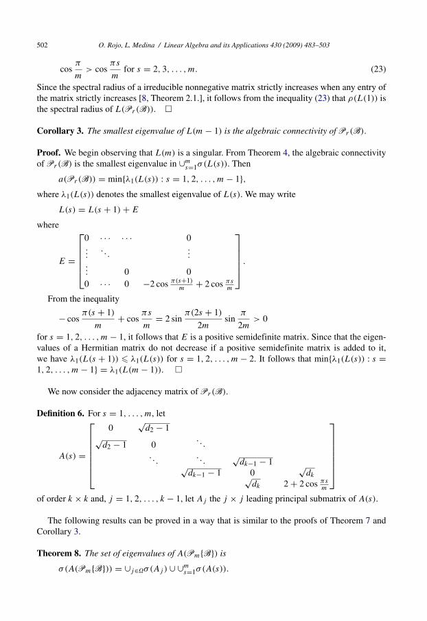
502 O. Rojo, L. Medina / Linear Algebra and its Applications 430 (2009) 483–503

cosπ

m> cos

πs

mfor s = 2, 3, . . . , m. (23)

Since the spectral radius of a irreducible nonnegative matrix strictly increases when any entry ofthe matrix strictly increases [8, Theorem 2.1.], it follows from the inequality (23) that ρ(L(1)) isthe spectral radius of L(Pr (B)). �

Corollary 3. The smallest eigenvalue of L(m − 1) is the algebraic connectivity of Pr (B).

Proof. We begin observing that L(m) is a singular. From Theorem 4, the algebraic connectivityof Pr (B) is the smallest eigenvalue in ∪m

s=1σ(L(s)). Then

a(Pr (B)) = min{λ1(L(s)) : s = 1, 2, . . . , m − 1},where λ1(L(s)) denotes the smallest eigenvalue of L(s). We may write

L(s) = L(s + 1) + E

where

E =

⎡⎢⎢⎢⎢⎣0 · · · · · · 0...

. . ....

... 0 00 · · · 0 −2 cos π(s+1)

m+ 2 cos πs

m

⎤⎥⎥⎥⎥⎦ .

From the inequality

− cosπ(s + 1)

m+ cos

πs

m= 2 sin

π(2s + 1)

2msin

π

2m> 0

for s = 1, 2, . . . , m − 1, it follows that E is a positive semidefinite matrix. Since that the eigen-values of a Hermitian matrix do not decrease if a positive semidefinite matrix is added to it,we have λ1(L(s + 1)) � λ1(L(s)) for s = 1, 2, . . . , m − 2. It follows that min{λ1(L(s)) : s =1, 2, . . . , m − 1} = λ1(L(m − 1)). �

We now consider the adjacency matrix of Pr (B).

Definition 6. For s = 1, . . . , m, let

A(s) =

⎡⎢⎢⎢⎢⎢⎢⎣

0√

d2 − 1√

d2 − 1 0. . .

. . .. . .

√dk−1 − 1√

dk−1 − 1 0√

dk√dk 2 + 2 cos πs

m

⎤⎥⎥⎥⎥⎥⎥⎦of order k × k and, j = 1, 2, . . . , k − 1, let Aj the j × j leading principal submatrix of A(s).

The following results can be proved in a way that is similar to the proofs of Theorem 7 andCorollary 3.

Theorem 8. The set of eigenvalues of A(Pm{B}) is

σ(A(Pm{B})) = ∪j∈�σ(Aj ) ∪ ∪ms=1σ(A(s)).

O. Rojo, L. Medina / Linear Algebra and its Applications 430 (2009) 483–503 503

Corollary 4. The largest eigenvalue of A(1) is the spectral radius of A(Pr (B)).

Acknowledgement

The authors wish to thank the referee for the comments which led to an improved version ofthe paper.

References

[1] M. Fiedler, Algebraic connectivity of graphs, Czechoslovak Math. J. 23 (1973) 298–305.[2] G.H. Golub, C.F. Van Loan, Matrix Computations, second ed., Johns Hopkins University Press, Baltimore, 1989.[3] R. Grone, R. Merris, V.S. Sunder, The Laplacian spectrum of a graph, SIAM Matrix Anal. Appl. 11 (12) (1990)

218–238.[4] S. Kouachi, Eigenvalues and eigenvectors of tridiagonal matrices, Electron. J. Linear Algebra 15 (2006) 115–133.[5] O. Rojo, Spectra of weighted generalized Bethe trees joined at the root, Linear Algebra Appl. 428 (2008) 2961–2979.[6] O. Rojo, R. Soto, The spectra of the adjacency matrix and Laplacian matrix for some balanced trees, Linear Algebra

Appl. 403 (2005) 97–117.[7] L.N. Trefethen, D. Bau III, Numerical linear algebra, Society for Industrial and Applied Mathematics (1997).[8] R.S. Varga, Matrix Iterative Analysis, Prentice-Hall Inc., 1965.[9] F. Zhang, Matrix Theory, Springer, 1999.