arX

iv:h

ep-t

h/05

0402

9v2

9 J

un 2

005

Preprint typeset in JHEP style. - HYPER VERSION SPhT-T05/037, hep-th/0504029

Mixed correlation functions in the 2-matrix

model, and the Bethe Ansatz

B. Eynard, N. Orantin

Service de Physique Theorique de Saclay, CEA/DSM/SPhT,

Unite de Recherche associee au CNRS (URA D2306), CEA Saclay,

F-91191 Gif-sur-Yvette Cedex, France.

E-mail: eynard@spht.saclay.cea.fr, orantin@spht.saclay.cea.fr

Abstract: Using loop equation technics, we compute all mixed traces correlation

functions of the 2-matrix model to large N leading order. The solution turns out

to be a sort of Bethe Ansatz, i.e. all correlation functions can be decomposed on

products of 2-point functions. We also find that, when the correlation functions are

written collectively as a matrix, the loop equations are equivalent to commutation

relations.

Keywords: Matrix Models, Differential and Algebraic Geometry, Bethe Ansatz.

Contents

1. Introduction 2

2. The 2-matrix model, definitions and loop equations 3

2.1 Partition function 3

2.2 Enumeration of discrete surfaces 4

2.3 Enumeration of discrete surfaces with boundaries 5

2.4 Master loop equation and algebraic curve 5

2.5 Correlation functions, definitions 6

2.6 Loop equations 8

2.7 Recursive determination of the correlation functions 9

3. A Bethe Ansatz-like formula for correlation functions 9

4. Amplitudes of permutations 11

4.1 Some definitions: planar permutations 11

4.2 Face amplitudes 12

4.3 The amplitudes Cσ 13

4.4 Examples 14

4.5 Properties of Cσ 16

4.6 Computation of the rational functions F (k)(x1, y1, . . . , xk, yk) 19

4.7 Proof of the main theorem 23

5. Matrix form of correlation functions 26

5.1 Properties of the Ckσ ’s. 28

5.2 Some commutation properties 29

5.3 Examples: k = 2. 31

6. Application: Gaussian case 31

7. Conclusion 32

Appendix A Practical computation of fσ 34

1

1. Introduction

Formal random matrix models have been used for their interpretation as combinato-

rial generating functions for discretized surfaces [4,5,24]. The hermitean one-matrix

model counts surfaces made of polygons of only one color, whereas the hermitean

two–matrix model counts surfaces made of polygons of two colors. In that respect,

the 2-matrix model is more appropriate for the purpose of studying surfaces with

non-uniform boundary conditions. At the continuum limit, the 2-matrix model gives

access to “boundary operators” in conformal field theory [21].

Generating functions for surfaces with boundaries are obtained as random matrix

expectation values. The expectation value of a product of l traces is the generating

function for surfaces with l boundaries, the total power of matrices in each trace

being the length of the corresponding boundary. If each trace contains only one type

of matrix (different traces may contain different types of matrices), the expectation

value is the generating function counting surfaces with uniform boundary conditions.

Those non-mixed expectation values have been computed for finite n since the work

of [16, 25] and refined by [1].

Mixed correlation functions have been considered as a difficult problem for a

long time and progress have been obtained only recently [2, 15]. Indeed, non-mixed

expectation values can easily be written in terms of eigenvalues only (since the trace

of a matrix is clearly related to its eigenvalues), whereas mixed correlation functions

cannot (TrMk1 Mk′

2 cannot be written in terms of eigenvalues of M1 and M2).

The large N limit of the generating function of the bicolored disc (i.e. one

boundary, two colors, i.e. < TrMk1 Mk′

2 >) has been known since [11, 12, 19]. The

large N limit of the generating function of the 4-colored disc (i.e. one boundary,

4 colors, i.e. < TrMk1 Mk′

2 Mk′′

1 Mk′′′

2 >) has been known since [8]. The all order

expansion of correlation functions for the 1-matrix model has been obtained by a

Feynman-graph representation in [9] and the generalization to non-mixed correlation

functions of the 2-matrix model has been obtained in [10].

Recently, the method of integration over the unitary group of [15] has allowed to

compute, for finite N , all mixed correlation functions of the 2-matrix model in terms

of orthogonal polynomials.

The question of computing mixed correlation functions in the large N limit is

addressed in the present article.

The answer is (not so) surprisingly related to classical results in integrable statis-

tical models, i.e. the Bethe Ansatz. It has been known for a long time that random

matrix models are integrable in some sense (Toda, KP, KdV, isomonodromic sys-

tems,...), but the relationship with Yang-Baxter equations and Bethe Ansatz was

rather indirect. The result presented in this article should give some new insight in

that direction. We find that the k-point functions can be expressed as the product

of 2-point function, which is the underlying idea of the Bethe Ansatz.

2

Outline of the article:

- section 1 is an introduction,

- in section 2, we set definitions of the model and correlation functions, and we

write the relevant loop equations,

- in section 3, we introduce a Bethe Ansatz-like formula, and prove it in section 4,

- in section 5, we solve the problem under a matrix form,

- section 6 is dedicated to the special Gaussian case.

2. The 2-matrix model, definitions and loop equations

2.1 Partition function

We are interested in the formal matrix integral:

Z :=∫

H2N

dM1 dM2 e−N Tr [V1(M1)+V2(M2)+M1M2] (2-1)

where M1 and M2 are N×N hermitean matrices and dM1 (resp. dM2) is the product

of Lebesgue measures of all independent real components of M1 (resp. M2). V1(x)

and V2(y) are complex polynomials of degree d1 + 1 and d2 + 1, called “potentials”.

The formal matrix integral is defined as a formal power series in the coefficients of

the potentials (see [5]), computed by the usual Feynman method: consider a local

extremum of e−N Tr [V1(M1)+V2(M2)+M1M2], and expand the non quadratic part as a

power series and, for each term of the series, perform the Gaussian integration with

the quadratic part. This method does not care about the convergence of the integral,

or of the series, it makes sense only order by order and it is in that sense that it can

be interpreted as the generating function of discrete surfaces. All quantities in that

model have a well defined 1/N2 expansion [27].

The extrema of V1(x) + V2(y) + xy are such that:

V ′1(x) = −y , V ′

2(y) = −x (2-2)

there are d1d2 solutions (indeed V ′2(−V ′

1(x)) = −x), which we note (xI , yI),

I = 1, . . . , d1d2. The extrema of Tr[V1(M1)+V2(M2)+M1M2] can be chosen diagonal

(up to a unitary transformation), with xI ’s and yI ’s on the diagonal:

M1 = diag(

n1 times︷ ︸︸ ︷x1, . . . , x1,

n2 times︷ ︸︸ ︷x2, . . . , x2, . . . ,

nd1d2times

︷ ︸︸ ︷xd1d2 , . . . , xd1d2)

M2 = diag(

n1 times︷ ︸︸ ︷y1, . . . , y1,

n2 times︷ ︸︸ ︷y2, . . . , y2, . . . ,

nd1d2times

︷ ︸︸ ︷yd1d2

, . . . , yd1d2) (2-3)

The extremum around which we perform the expansion is thus characterized by a

set of filling fractions:

ǫI =nI

N,

d1d2∑

I=1

ǫI = 1 (2-4)

3

To summarize, let us say that the formal matrix integral is defined for given

potentials and filling fractions.

The “one-cut” case is the one where one of the filling fractions is 1, and all the

others vanish. This is the case where the Feynman expansion is performed in the

vicinity of only one extremum.

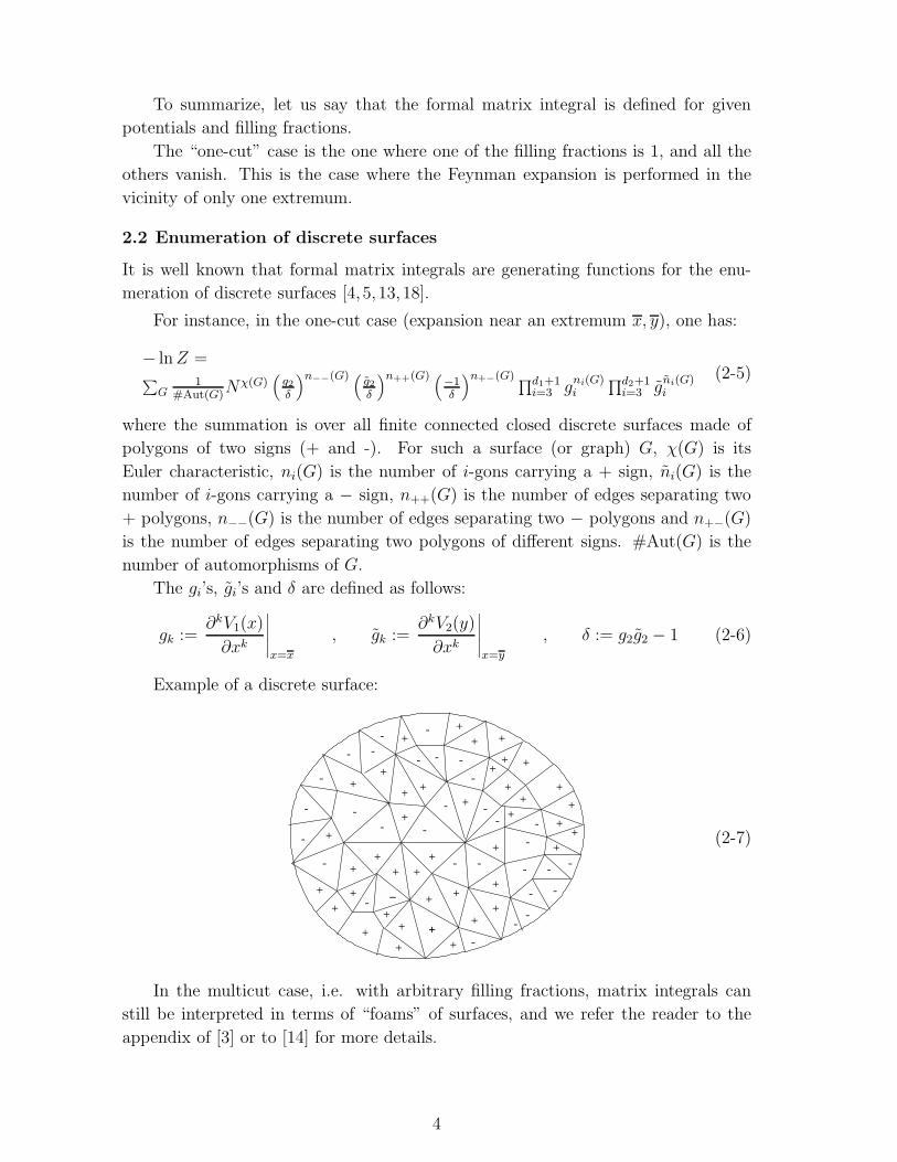
2.2 Enumeration of discrete surfaces

It is well known that formal matrix integrals are generating functions for the enu-

meration of discrete surfaces [4, 5, 13, 18].

For instance, in the one-cut case (expansion near an extremum x, y), one has:

− ln Z =∑

G1

#Aut(G)Nχ(G)

(g2

δ

)n−−(G) ( g2

δ

)n++(G) (−1δ

)n+−(G)∏d1+1i=3 g

ni(G)i

∏d2+1i=3 g

ni(G)i

(2-5)

where the summation is over all finite connected closed discrete surfaces made of

polygons of two signs (+ and -). For such a surface (or graph) G, χ(G) is its

Euler characteristic, ni(G) is the number of i-gons carrying a + sign, ni(G) is the

number of i-gons carrying a − sign, n++(G) is the number of edges separating two

+ polygons, n−−(G) is the number of edges separating two − polygons and n+−(G)

is the number of edges separating two polygons of different signs. #Aut(G) is the

number of automorphisms of G.

The gi’s, gi’s and δ are defined as follows:

gk :=∂kV1(x)

∂xk

∣∣∣∣∣x=x

, gk :=∂kV2(y)

∂xk

∣∣∣∣∣x=y

, δ := g2g2 − 1 (2-6)

Example of a discrete surface:

-

-

-

+++

++

+

++

+

+

++

+

++

-

+

+

++ +

+

+

+

+

++

-

--

-

-

--

-

++

++

+

+

+

+

++

-

---

-

-

+

+

+

- - -

----

---

-- - -

-

+

+

++

(2-7)

In the multicut case, i.e. with arbitrary filling fractions, matrix integrals can

still be interpreted in terms of “foams” of surfaces, and we refer the reader to the

appendix of [3] or to [14] for more details.

4

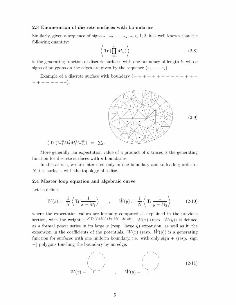
2.3 Enumeration of discrete surfaces with boundaries

Similarly, given a sequence of signs s1, s2, . . . , sk, si ∈ 1, 2, it is well known that the

following quantity: ⟨Tr (

k∏

i=1

Msi)

⟩(2-8)

is the generating function of discrete surfaces with one boundary of length k, whose

signs of polygons on the edges are given by the sequence (s1, . . . , sk).

Example of a discrete surface with boundary (+ + + + + + − − − − − + + +

+ + −−−−−−):

〈Tr (M61 M5

2 M51 M6

2 )〉 =∑

G

-

-

-

+++

++

+

++

+

+

++

+

++

-

+

+

++ +

+

+

+

+

++

-

--

-

-

--

-

++

++

+

+

+

+

++

-

---

-

-

+

+

+

- - -

----

---

-- - -

-

+

+

++

(2-9)

More generally, an expectation value of a product of n traces is the generating

function for discrete surfaces with n boundaries.

In this article, we are interested only in one boundary and to leading order in

N , i.e. surfaces with the topology of a disc.

2.4 Master loop equation and algebraic curve

Let us define:

W (x) :=1

N

⟨Tr

1

x − M1

⟩, W (y) :=

1

N

⟨Tr

1

y − M2

⟩(2-10)

where the expectation values are formally computed as explained in the previous

section, with the weight e−N Tr [V1(M1)+V2(M2)+M1M2]. W (x) (resp. W (y)) is defined

as a formal power series in its large x (resp. large y) expansion, as well as in the

expansion in the coefficients of the potentials. W (x) (resp. W (y)) is a generating

function for surfaces with one uniform boundary, i.e. with only sign + (resp. sign

−) polygons touching the boundary by an edge:

W (x) = + , W (y) = −

(2-11)

5

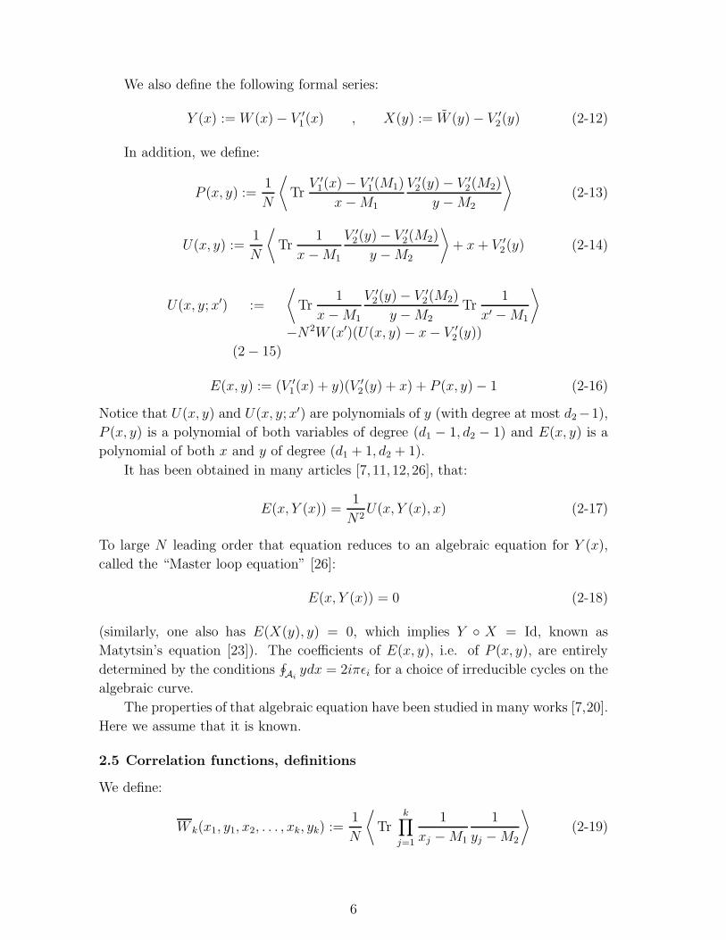
We also define the following formal series:

Y (x) := W (x) − V ′1(x) , X(y) := W (y) − V ′

2(y) (2-12)

In addition, we define:

P (x, y) :=1

N

⟨Tr

V ′1(x) − V ′

1(M1)

x − M1

V ′2(y) − V ′

2(M2)

y − M2

⟩(2-13)

U(x, y) :=1

N

⟨Tr

1

x − M1

V ′2(y) − V ′

2(M2)

y − M2

⟩+ x + V ′

2(y) (2-14)

U(x, y; x′) :=

⟨Tr

1

x − M1

V ′2(y) − V ′

2(M2)

y − M2

Tr1

x′ − M1

⟩

−N2W (x′)(U(x, y) − x − V ′2(y))

(2 − 15)

E(x, y) := (V ′1(x) + y)(V ′

2(y) + x) + P (x, y) − 1 (2-16)

Notice that U(x, y) and U(x, y; x′) are polynomials of y (with degree at most d2−1),

P (x, y) is a polynomial of both variables of degree (d1 − 1, d2 − 1) and E(x, y) is a

polynomial of both x and y of degree (d1 + 1, d2 + 1).

It has been obtained in many articles [7, 11, 12, 26], that:

E(x, Y (x)) =1

N2U(x, Y (x), x) (2-17)

To large N leading order that equation reduces to an algebraic equation for Y (x),

called the “Master loop equation” [26]:

E(x, Y (x)) = 0 (2-18)

(similarly, one also has E(X(y), y) = 0, which implies Y ◦ X = Id, known as

Matytsin’s equation [23]). The coefficients of E(x, y), i.e. of P (x, y), are entirely

determined by the conditions∮Ai

ydx = 2iπǫi for a choice of irreducible cycles on the

algebraic curve.

The properties of that algebraic equation have been studied in many works [7,20].

Here we assume that it is known.

2.5 Correlation functions, definitions

We define:

W k(x1, y1, x2, . . . , xk, yk) :=1

N

⟨Tr

k∏

j=1

1

xj − M1

1

yj − M2

⟩(2-19)

6

Uk(x1, y1, x2, . . . , xk, yk)

:= Polyk

V ′2(yk) W k(x1, y1, x2, . . . , xk, yk)

=1

N

⟨Tr

1

x1 − M1

1

y1 − M2. . .

1

xk − M1

V ′2(yk) − V ′

2(M2)

yk − M2

⟩

(2 − 20)

P k(x1, y1, x2, . . . , xk, yk)

:= Polx1

Polyk

V ′1(x1) V ′

2(yk) W k(x1, y1, x2, . . . , xk, yk)

=1

N

⟨Tr

V ′1(x1) − V ′

1(M1)

x1 − M1

1

y1 − M2. . .

1

xk − M1

V ′2(yk) − V ′

2(M2)

yk − M2

⟩

(2 − 21)

Ak(x1, y1, x2, . . . , xk) :=1

N

⟨Tr

1

x1 − M1

1

y1 − M2

. . .1

xk − M1

V ′2(M2)

⟩(2-22)

where Polx f(x) denotes the polynomial part at infinity of f(x) (i.e. the positive

part in the Laurent series for x near infinity).

The functions W k are generating functions for discrete discs with all possible

boundary conditions. One can recover any generating function of type eq. (2-8) by

expanding into powers of the xi’s and yi’s.

For convenience, we prefer to consider the following functions:

Wk(x1, y1, x2, . . . , xk, yk) := W k(x1, y1, x2, . . . , xk, yk) + δk,1 (2-23)

Uk(x1, y1, x2, . . . , xk, yk) := Uk(x1, y1, x2, . . . , xk, yk) + δk,1(V′2(yk) + xk) (2-24)

and for k > 1:

Pk(x1, y1, x2, . . . , xk, yk) := P k(x1, y1, x2, . . . , xk, yk) + Wk−1(x2, . . . , xk, y1) (2-25)

For the smallest values of k, those expectation values can be found in the liter-

ature to large N leading order:

• it was found in [7, 11, 12]:

W1(x, y) =E(x, y)

(x − X(y))(y − Y (x)), U1(x, y) =

E(x, y)

(y − Y (x))(2-26)

• it was found in the appendix C of [8] (there is a change of sign, because the

action in [8] was e −N tr (V1(M1)+V2(M2)−M1M2)):

W2(x1, y1, x2, y2) =W1(x1, y1)W1(x2, y2) − W1(x1, y2)W1(x2, y1)

(x1 − x2)(y1 − y2)(2-27)

• For finite N , it was found in [2], and with notations explained in [2]:

W1(x, y) = det

(1N + ΠN−1

1

x − Q

1

y − P tΠN−1

)(2-28)

7

• For finite N , it was found in [15] how to compute any mixed correlation function

in terms of determinants involving biorthogonal polynomials, with a formula very

similar to eq. (2-28).

Here, we shall find a formula for all Wk’s in the large N limit.

2.6 Loop equations

Loop equations are nothing but Schwinger–Dyson equations. They are obtained by

writing that an integral is invariant under a change of variable, or alternatively by

writing that the integral of a total derivative vanishes.

The loop equation method is well known and explained in many works [7, 26].

Here, we write for each change of variable the corresponding loop equation (we use

a presentation similar to that of [7]).

In all what follows we consider k > 1.

• the change of variable: δM2 = 1x1−M1

1y1−M2

. . . 1xk−M1

implies:

Ak(x1, . . . , xk) =k−1∑

j=1

W j(x1, . . . , yj) W k−j(xk, yj, . . . , yk−1)

+x1W k−1(x1, y1, . . . , yk−1) − xkW k−1(xk, y1, . . . , yk−1)

x1 − xk

=k−1∑

j=1

Wj(x1, . . . , yj) Wk−j(xk, yj, . . . , yk−1)

−Wk−1(xk, y1, . . . , yk−1)

+xkWk−1(x1, y1, . . . , yk−1) − Wk−1(xk, y1, . . . , yk−1)

x1 − xk(2 − 29)

• the change of variable: δM1 = 1x1−M1

1y1−M2

. . . 1xk−M1

V ′

2(yk)−V ′

2 (M2)

yk−M2implies:

(Y (x1) − yk) Uk(x1, . . . , yk)

=∑k

j=2Wj−1(x1,y1,...,yj−1)−Wj−1(xj ,y1,...,yj−1)

x1−xjUk−j+1(xj , yj, . . . , xk, yk)

+V ′2(yk)

Wk−1(x1,y1,...,yk−1)−Wk−1(xk,y1,x2,...,yk−1)x1−xk

+Ak(x1, . . . , xk) − P k(x1, y1, x2, . . . , xk, yk)

=∑k

j=2Wj−1(x1,y1,...,yj−1)−Wj−1(xj ,y1,...,yj−1)

x1−xjUk−j+1(xj , yj, . . . , xk, yk)

+∑k−1

j=1 Wj(x1, . . . , yj) Wk−j(xk, yj, . . . , yk−1)

−Pk(x1, y1, x2, . . . , xk, yk)

(2-30)

where we have used the loop equation eq. (2-29) for Ak(x1, . . . , xk).

• the change of variable: δM2 = 1x1−M1

1y1−M2

. . . 1xk−M1

1yk−M2

implies:

(X(yk) − x1) W k(x1, y1, x2, . . . , xk, yk)

8

=k−1∑

j=1

Wk−j(xj+1, . . . , yk) − Wk−j(xj+1, . . . , xk, yj)

yk − yjWj(x1, . . . , yj)

−Uk(x1, . . . , yk)

(2 − 31)

2.7 Recursive determination of the correlation functions

Theorem 2.1 The system of equations eq. (2-30) and eq. (2-31) for all k has a

unique solution.

In other words, if we can find some functions Wk, Uk, Pk which obey eq. (2-30)

and eq. (2-31) for all k, then they are the correlation functions we are seeking.

proof:

W1, U1 and P1 have already been computed in the literature.

Assume that we have computed Wj , Uj , Pj for all j < k. Let us show that

eq. (2-30) and eq. (2-31) determine uniquely Wk, Uk and Pk.

Let X(α)(yk), α = 0, . . . , d1 be the d1 + 1 solutions for x of E(x, yk) = 0. For

every α = 0, . . . , d1 one has:

Y (X(α)(yk)) = yk (2-32)

At x1 = X(α)(yk), eq. (2-30) reads:

Pk(X(α)(yk), y1, x2, . . . , xk, yk)

=∑k

j=2Wj−1(X(α)(yk),y1,...,yj−1)−Wj−1(xj ,y1,x2,...,yj−1)

X(α)(yk)−xjUk−j+1(xj , yj, . . . , xk, yk)

+∑k−1

j=1 Wj(X(α)(yk), . . . , yj) Wk−j(xk, yj, . . . , yk−1)

(2-33)

where all the quantities in the RHS are known from the recursion hypothesis. We

thus know the value of Pk for d1 + 1 values of x1. Since Pk is a polynomial in x1 of

degree at most d1 − 1, we can determine Pk by the interpolation formula:

(x1 − X(yk))Pk(x1, . . . , yk)

E(x1, yk)

=d2∑

α=1

(X(α)(yk) − X(yk)) Pk(X(α)(yk), . . . , yk)

(x1 − X(α)(yk)) Ex(X(α)(yk), yk)(2 − 34)

where Xk = X(yk) denotes X(0)(yk). Once Pk is known, eq. (2-30) allows to compute

Uk, and eq. (2-31) allows to compute Wk. •

3. A Bethe Ansatz-like formula for correlation functions

Thus, the loop equations determine Wk uniquely, i.e., if we can find Wk, Uk =

PolykV ′

2(yk)Wk and Pk = Wk−1 + Polx1 V ′1(x1)Uk which satisfy eq. (2-31),eq. (2-30),

9

it means that we have the right solution. We can thus make an Ansatz for Wk, and

check that it satisfies the loop equations above.

Our Ansatz is similar to the Bethe Ansatz [17]:

Wk(x1, y1, . . . , xk, yk) =∑

σ∈Σk

C(k)σ (x1, y1, . . . , xk, yk)

k∏

i=1

W1(xi, yσ(i)) (3-1)

where the coefficients Cσ are rational fractions of the xi’s and yi’s, with at most

simple poles at coinciding points, and independent of the potentials.

We call eq. (3-1) a Bethe Ansatz-like formula, because it is very similar to the

solution initially found by Bethe for the 1-dimensional spin chain, and then for the

δ-interacting bosons.

If we assume that eq. (3-1) satisfies eq. (2-31), we can in particular take the

residue of eq. (2-31) at yk → Y (xl) for some l. That implies the following relationship

among the coefficients C(k)σ ’s:

(xσ−1(k) − x1) C(k)σ (x1, y1, . . . , xk, yk)

=k−1∑

j=1

∑

τ∈Σ(1,...,j)

∑

ρ∈Σ(j+1,...,k)

δσ,τρ

C(j)τ (x1, . . . , yj)C

(k−j)ρ (xj+1, . . . , yk)

yk − yj

(3 − 2)

Beside, since Wk is the expectation value of a trace, the C(k)σ ’s must be cyclically

invariant:

C(k)σ (x1, y1, x2, y2, . . . , xk, yk) = C(k)

σ (x2, y2, . . . , xk, yk, x1, y1) (3-3)

and, since Wk should have no poles at coinciding points yk = yj one should have:

Resy′

k→yj

C(k)σ (x1, y1, x2, y2, . . . , xk, y

′k)dy′

k = Resy′

k→yj

C(k)(k,j)◦σ(x1, y1, x2, y2, . . . , xk, y

′k)dy′

k

(3-4)

With C(1) = 1, it is clear that the set of equations eq. (3-2), eq. (3-3), eq. (3-4), have

at most a unique solution. We prove in the next section that the solution exists, and

thus, eq. (3-2), eq. (3-3), eq. (3-4) determine C(k)σ uniquely. The C(k)

σ ’s are explicitly

computed in section 4.

Then in section 4.7, we prove that:

Theorem 3.1 If the C(k)σ ’s are rational functions defined by eq. (3-2), eq. (3-3),

eq. (3-4), then the functions Wk’s defined by the RHS of eq. (3-1), the functions

Uk(x1, . . . , yk) := Pol(V ′2(yk))Wk(x1, . . . , yk), and the functions Pk(x1, . . . , yk) :=

Pol(V ′1(x1))Uk(x1, . . . , yk) + Wk−1(x2, . . . , xk, y1), satisfy eq. (2-31) and eq. (2-30).

As a corollary, using theorem 2.1, we have:

10

Theorem 3.2

Wk(x1, y1, . . . , xk, yk) =∑

σ∈Σk

C(k)σ (x1, y1, . . . , xk, yk)

k∏

i=1

W1(xi, yσ(i))

(3-5)

The derivation of theorem 3.1 is quite technical and is presented in section 4.7.

4. Amplitudes of permutations

In this section, we compute the amplitudes C(k)σ explicitly.

Eq. (3-2), eq. (3-3), eq. (3-4) and initial condition C(1)(x1, y1) = 1 clearly define

at most a unique function C(k)σ (x1, . . . , yk). In this section, we build the solution

explicitly, and then, we prove that the function we have constructed indeed satisfies

eq. (3-2), eq. (3-3), eq. (3-4).

Below we prove that eq. (3-2) implies that C(k)σ vanishes for non planar permuta-

tions (see Definition 4.1 below) and, for planar permutations, C(k)σ is the product of

C(k)Id corresponding to faces. We are thus led to introduce the following definitions:

4.1 Some definitions: planar permutations

Let S be the shift permutation:

S := shift = (1, 2, . . . , k − 1, k) , i.e. S(i) = i + 1 (4-1)

Definition 4.1 A permutation σ ∈ Σk is called planar if

ncycles(σ) + ncycles(Sσ) = k + 1 (4-2)

where ncycles(σ) is the number of irreducible cycles composing the permutation σ.

Let Σk ⊂ Σk be the set of planar permutations of rank k.

Eq. (4-2) is equivalent to saying that if one draws the points x1, y1, . . . , xk, yk

on a circle, and draws a line between each pair (xj , yσ(j)), the lines don’t intersect.

The cycles of σ and the cycles of Sσ correspond to the faces (i.e. the connected

components) of that partition of the disc.

Each planar permutation can also be represented as an arch system, and thus, the

number of possible planar permutations is given by the Catalan number Cat (k):

Card(Σk) = Cat (k) =2k!

k! (k + 1)!(4-3)

11

σ(1)σ(1)σ

x y

yk

x1

2x2

kx

y

1y

σ (k)x

σ

x

σ

(1)

S

S

-cycle

-cycle

-1

(4-4)

Example of a planar permutation and its faces.

4.2 Face amplitudes

Definition 4.2 For any k ≥ 1, we define a rational function of x1, . . . , yk:

F (k)(x1, y1, x2, . . . , xk, yk) (4-5)

by the recursion formula:

F (1)(x1, y1) := 1

F (k)(x1, y1, . . . , xk, yk) :=k−1∑

j=1

F (j)(x1, y1, . . . , xj , yj)F(k−j)(xj+1, yj+1, . . . , xk, yk)

(xk − x1)(yk − yj)

(4 − 6)

Lemma 4.1 For any k ≥ 1 :

F (k)(x1, y1, . . . , xk, yk) = O(y1−kk ) (4-7)

when yk → ∞.

proof:

Let us prove it by induction on k. It is true for k=1. Let k be larger or equal to 2

and assume that this is true for all F (j) with j < k. Then eq. (4-6) straightforwardly

gives the same behaviour for F (k). •

Lemma 4.2 F (k) has cyclic invariance, i.e.

F (k)(x2, y2, . . . , xk, yk, x1, y1) = F (k)(x1, y1, . . . , xk, yk) (4-8)

proof:

12

We prove it by recursion. It is clearly true for k = 1 and k = 2 since

F (2)(x1, y1, x2, y2) = 1(x2−x1)(y2−y1)

. For k ≥ 3, assume that it is true for all F (j) with

j < k. One has:

F (k)(x2, y2, . . . , xk, yk, x1, y1)

=k∑

j=2

F (j−1)(x2, . . . , xj, yj)F(k+1−j)(xj+1, yj+1, . . . , xk, yk, x1, y1)

(x1 − x2)(y1 − yj)

=k∑

j=2

F (j−1)(x2, . . . , xj, yj)F(k+1−j)(x1, y1, xj+1, yj+1, . . . , xk, yk)

(x1 − x2)(y1 − yj)

=k∑

j=2

F (j−1)(x2, . . . , xj, yj)

(x1 − x2)(y1 − yj)k−1∑

l=j+1

F (l+1−j)(x1, y1, xj+1, yj+1, . . . , xl, yl)F(k−l)(xl+1, yl+1, . . . , xk, yk)

(xk − x1)(yk − yl)

+k∑

j=2

F (j−1)(x2, . . . , xj , yj)

(x1 − x2)(y1 − yj)

F (1)(x1, y1)F(k−j)(xj+1, yj+1, . . . , xk, yk)

(xk − x1)(yk − y1)

=k−1∑

l=3

F (k−l)(xl+1, yl+1, . . . , xk, yk)

(xk − x1)(yk − yl)l∑

j=2

F (j−1)(x2, . . . , xj, yj)F(l+1−j)(xj+1, yj+1, . . . , xl, yl, x1, y1)

(x1 − x2)(y1 − yj)

=k−1∑

l=3

F (k−l)(xl+1, yl+1, . . . , xk, yk)F(l)(x2, . . . , xl, yl, x1, y1)

(xk − x1)(yk − yl)

=k−1∑

l=3

F (l)(x1, y1, x2, . . . , xl, yl)F(k−l)(xl+1, yl+1, . . . , xk, yk)

(xk − x1)(yk − yl)

= F (k)(x1, y1, . . . , xk, yk)

(4 − 9)

•

Lemma 4.3 For k ≥ 2, F (k) has simple poles in yk:

F (k)(x1, y1, . . . , xk, yk) =k−1∑

l=1

1

yk − ylRes

y′

k→yl

F (k)(x1, y1, . . . , xk, y′k)dy′

k (4-10)

proof:

It is clearly true for k = 2. We prove it by induction on k. Assume that it is

true up to k − 1. Using the recursion hypothesis, one can see that each term in the

RHS of eq. (4-6) has at most a simple pole at yk = yl and one can write eq. (4-10)

with the use of Lemma 4.1. Thus the recursion hypothesis is true for k. •

4.3 The amplitudes Cσ

Definition 4.3 Then, for any k ≥ 1, and for any permutation σ ∈ Σk, we define

C(k)σ (x1, y1, x2, . . . , xk, yk) a rational function of x1, . . . , yk, by:

13

• C(k)σ (x1, y1, x2, . . . , xk, yk) := 0 if σ is not planar, and

• if σ is planar, we decompose σ and Sσ into their product of cycles:

σ = σ1σ2 . . . σl , Sσ = σ1σ2 . . . σl (4-11)

such that:

σj = (ij,1, ij,2, . . . , ij,lj) , σ(ij,m) = ij,m+1 (4-12)

σj = (ij,1, ij,2, . . . , ij,lj) , σ(ij,m) = ij,m+1 − 1 (4-13)

C(k)σ (x1, y1, x2, . . . , xk, yk) :=

l∏

j=1

F (lj)(xij,1, yij,2

, xij,2, yij,3

, . . . , xij,lj, yij,1

)

l∏

j=1

F (lj)(xij,1, yij,2−1, xij,2

, . . . , yij,lj

−1, xij,lj

, yij,1−1)

(4 − 14)

i.e. C(k)σ is the product of F ’s of each connected component of the disc partitioned by

σ.

4.4 Examples

In particular with σ = Id, we have:

C(k)Id (x1, y1, x2, . . . , xk, yk) = F (k)(x1, y1, x2, y2, . . . , xk, yk) (4-15)

and with σ = S−1:

C(k)S−1(x1, y1, x2, . . . , xk, yk) = F (k)(xk, yk−1, xk−1, . . . , y1, x1, yk) (4-16)

An example with k = 12

Let us consider an example of σ ∈ Σ12 defined as follow: σ(1) = 3, σ(2) = 1,

σ(3) = 2, σ(4) = 7, σ(5) = 6, σ(6) = 5, σ(7) = 4, σ(8) = 8, σ(9) = 11, σ(10) = 10,

σ(11) = 12 and σ(12) = 9:

σ = (1, 3, 2)(4, 7)(5, 6)(8)(9, 12, 11)(10)

Sσ = (1, 4, 8, 9)(2)(3)(5, 7)(6)(10, 11)(12) (4-17)

14

The corresponding arch system is:

x

y

3

y3 x4 y

12

x1

y

2x2

4

x10

y10

x11

y11

x12

5

8y 99

x5

y

x6

y6

x7

y7

x8

yx

1y

3

σ5

σ

∼

6

σ1

1

σ

2σ

4σ

σ

∼

σ

6

∼σ

7σ

5

∼σ4

∼

3

∼σ

2

∼σ

(4-18)

where dark faces (resp. white faces) correspond to the cycles of σ (resp. Sσ). For

that permutation C(12)σ is worth:

F (3)(x1, y3, x3, y2, x2, y1)F(2)(x5, y6, x6, y5)F

(3)(x9, y12, x12, y11, x11, y9)

×F (2)(x4, y7, x7, y4)F(4)(x1, y3, x4, y7, x8, y8, x9, y12)F

(2)(x5, y6, x7, y4)

×F (2)(x10, y10, x11, y9)

(4-19)

Example k ≤ 3

C(1) = 1 (4-20)

C(2)Id =

1

(x2 − x1)(y2 − y1)(4-21)

C(2)(12) =

1

(x2 − x1)(y1 − y2)(4-22)

C(3)Id =

1

(x1 − x3)

(1

y3 − y1

1

(x2 − x3)(y3 − y2)+

1

y3 − y2

1

(x1 − x2)(y2 − y1)

)(4-23)

C(3)(1)(23) =

1

(x1 − x2)

1

y3 − y1

1

(x2 − x3)(y2 − y3)(4-24)

C(3)(12)(3) =

1

(x1 − x3)

1

y3 − y2

1

(x1 − x2)(y1 − y2)(4-25)

C(3)(123) =

1

(x1 − x2)(x2 − x3)(y1 − y2)

1

y3 − y1+

1

(x1 − x3)(x1 − x2)(y2 − y1)

1

y3 − y2

(4-26)

C(3)(13)(2) = −

1

y3 − y1

1

(x1 − x3)(x2 − x3)(y1 − y2)(4-27)

C(3)(132) = 0 (4-28)

15

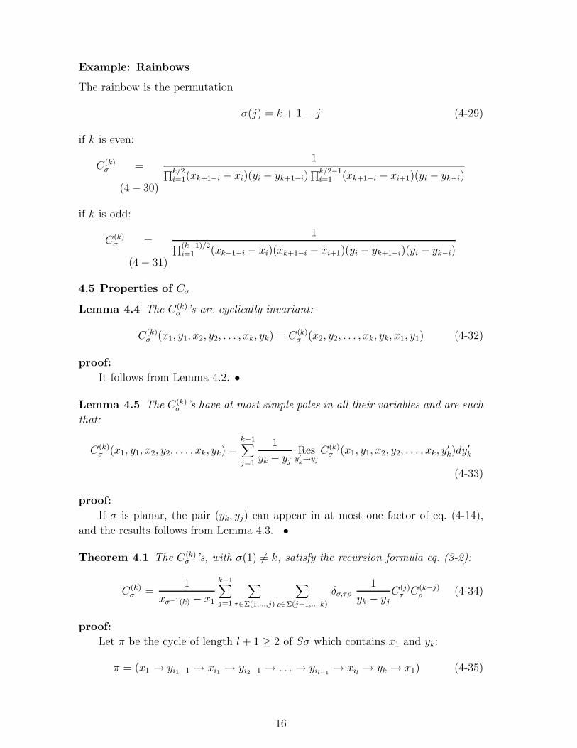
Example: Rainbows

The rainbow is the permutation

σ(j) = k + 1 − j (4-29)

if k is even:

C(k)σ =

1∏k/2

i=1(xk+1−i − xi)(yi − yk+1−i)∏k/2−1

i=1 (xk+1−i − xi+1)(yi − yk−i)(4 − 30)

if k is odd:

C(k)σ =

1∏(k−1)/2

i=1 (xk+1−i − xi)(xk+1−i − xi+1)(yi − yk+1−i)(yi − yk−i)(4 − 31)

4.5 Properties of Cσ

Lemma 4.4 The C(k)σ ’s are cyclically invariant:

C(k)σ (x1, y1, x2, y2, . . . , xk, yk) = C(k)

σ (x2, y2, . . . , xk, yk, x1, y1) (4-32)

proof:

It follows from Lemma 4.2. •

Lemma 4.5 The C(k)σ ’s have at most simple poles in all their variables and are such

that:

C(k)σ (x1, y1, x2, y2, . . . , xk, yk) =

k−1∑

j=1

1

yk − yjRes

y′

k→yj

C(k)σ (x1, y1, x2, y2, . . . , xk, y

′k)dy′

k

(4-33)

proof:

If σ is planar, the pair (yk, yj) can appear in at most one factor of eq. (4-14),

and the results follows from Lemma 4.3. •

Theorem 4.1 The C(k)σ ’s, with σ(1) 6= k, satisfy the recursion formula eq. (3-2):

C(k)σ =

1

xσ−1(k) − x1

k−1∑

j=1

∑

τ∈Σ(1,...,j)

∑

ρ∈Σ(j+1,...,k)

δσ,τρ1

yk − yjC(j)

τ C(k−j)ρ (4-34)

proof:

Let π be the cycle of length l + 1 ≥ 2 of Sσ which contains x1 and yk:

π = (x1 → yi1−1 → xi1 → yi2−1 → . . . → yil−1→ xil → yk → x1) (4-35)

16

ij+1 := σ(ij) + 1 , i0 := 1 (4-36)

Planarity implies that:

i0 < i1 < i2 < . . . < il (4-37)

Since σ is planar, there exists a unique way of factorizing σ as:

σ =l∏

j=0

σj , σj ∈ Σ(ij , . . . , ij+1 − 1) (4-38)

From the definition of C(k)σ we have:

C(k)σ = F (l+1)(x1, yi1−1, xi1 , yi2−1, . . . , yil−1, xil, yk)

∏

j

C(ij+1−ij)σj

(xij , . . . , yij+1−1)

(4-39)

and using eq. (4-6), we have:

C(k)σ = F (l+1)(x1, yi1−1, xi1 , yi2−1, . . . , yil−1, xil, yk)

∏j C

(ij+1−ij)σj (xij , . . . , yij+1−1)

=∑l

m=1

F (m)(x1,yi1−1,xi1,...,xim−1

,yim−1)F (l+1−m)(xim ,yim+1−1,xim+1,...,xil

,yk)

(xil−x1)(yk−yim−1)∏

j C(ij+1−ij)σj (xij , . . . , yij+1−1)

(4-40)

notice that il = σ−1(k), and note:

τm :=m−1∏

j=1

σj , ρm :=l∏

j=m

σj (4-41)

We have:

τm ∈ Σ(1, . . . , im − 1) , ρm ∈ Σ(im, . . . , k) (4-42)

Eq. (4-39) gives:

C(k)σ =

1

xσ−1(k) − x1

l∑

m=1

1

yk − yim−1C(im)

τmC(k−im)

ρm(4-43)

It is clear, from the planarity condition that if there exists some j and τ and ρ, such

that:

σ = τρ , τ ∈ Σ(1, . . . , j) , ρ ∈ Σ(j + 1, . . . , k) (4-44)

then, one must have j = im, τ = τm and ρ = ρm for some m. •

Lemma 4.6 For any transposition (k, j) (with k 6= j), we have:

Resy′

k→yj

C(k)σ (x1, y1, x2, y2, . . . , xk, y

′k)dy′

k = − Resy′

k→yj

C(k)(k,j)◦σ(x1, y1, x2, y2, . . . , xk, y

′k)dy′

k

(4-45)

17

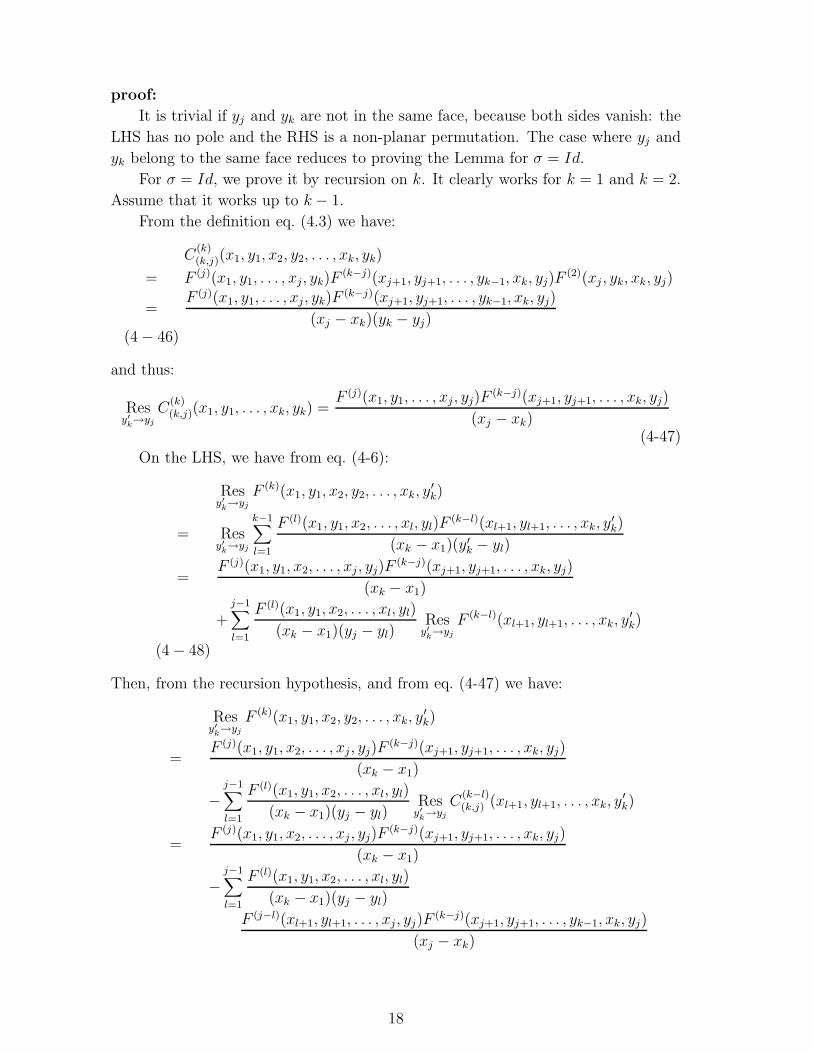
proof:

It is trivial if yj and yk are not in the same face, because both sides vanish: the

LHS has no pole and the RHS is a non-planar permutation. The case where yj and

yk belong to the same face reduces to proving the Lemma for σ = Id.

For σ = Id, we prove it by recursion on k. It clearly works for k = 1 and k = 2.

Assume that it works up to k − 1.

From the definition eq. (4.3) we have:

C(k)(k,j)(x1, y1, x2, y2, . . . , xk, yk)

= F (j)(x1, y1, . . . , xj, yk)F(k−j)(xj+1, yj+1, . . . , yk−1, xk, yj)F

(2)(xj , yk, xk, yj)

=F (j)(x1, y1, . . . , xj, yk)F

(k−j)(xj+1, yj+1, . . . , yk−1, xk, yj)

(xj − xk)(yk − yj)(4 − 46)

and thus:

Resy′

k→yj

C(k)(k,j)(x1, y1, . . . , xk, yk) =

F (j)(x1, y1, . . . , xj , yj)F(k−j)(xj+1, yj+1, . . . , xk, yj)

(xj − xk)(4-47)

On the LHS, we have from eq. (4-6):

Resy′

k→yj

F (k)(x1, y1, x2, y2, . . . , xk, y′k)

= Resy′

k→yj

k−1∑

l=1

F (l)(x1, y1, x2, . . . , xl, yl)F(k−l)(xl+1, yl+1, . . . , xk, y

′k)

(xk − x1)(y′k − yl)

=F (j)(x1, y1, x2, . . . , xj , yj)F

(k−j)(xj+1, yj+1, . . . , xk, yj)

(xk − x1)

+j−1∑

l=1

F (l)(x1, y1, x2, . . . , xl, yl)

(xk − x1)(yj − yl)Res

y′

k→yj

F (k−l)(xl+1, yl+1, . . . , xk, y′k)

(4 − 48)

Then, from the recursion hypothesis, and from eq. (4-47) we have:

Resy′

k→yj

F (k)(x1, y1, x2, y2, . . . , xk, y′k)

=F (j)(x1, y1, x2, . . . , xj , yj)F

(k−j)(xj+1, yj+1, . . . , xk, yj)

(xk − x1)

−j−1∑

l=1

F (l)(x1, y1, x2, . . . , xl, yl)

(xk − x1)(yj − yl)Res

y′

k→yj

C(k−l)(k,j) (xl+1, yl+1, . . . , xk, y

′k)

=F (j)(x1, y1, x2, . . . , xj , yj)F

(k−j)(xj+1, yj+1, . . . , xk, yj)

(xk − x1)

−j−1∑

l=1

F (l)(x1, y1, x2, . . . , xl, yl)

(xk − x1)(yj − yl)

F (j−l)(xl+1, yl+1, . . . , xj, yj)F(k−j)(xj+1, yj+1, . . . , yk−1, xk, yj)

(xj − xk)

18

(4 − 49)

In the last line, we use again eq. (4-6) and get:

Resy′

k→yj

F (k)(x1, y1, x2, y2, . . . , xk, y′k)

=F (j)(x1, y1, x2, . . . , xj , yj)F

(k−j)(xj+1, yj+1, . . . , xk, yj)

(xk − x1)

−(xj − x1)F (j)(x1, y1, x2, . . . , xj , yj)

(xk − x1)

F (k−j)(xj+1, yj+1, . . . , yk−1, xk, yj)

(xj − xk)(4 − 50)

One can then see that the sum of eq. (4-47) and eq. (4-50) vanishes, and the recursion

hypothesis is proven for k. •

Lemma 4.7

∀ k > 1 ,∑

σ∈Σk

C(k)σ (x1, y1, x2, y2, . . . , xk, yk) = 0 (4-51)

proof:

This expression is a rational function of all its variables. Consider the poles at

yk = yj, and write τ = (k, j). One can split the symmetric group Σk into its two

conjugacy classes wrt the subgroup generated by τ : Σk = [Id]⊕ [τ ]. In other words:∑

σ∈Σk

Cσ(x1, y1, x2, y2, . . . , xk, yk)

=∑

σ∈Σk/τ

Cσ(x1, y1, x2, y2, . . . , xk, yk) + Cτσ(x1, y1, x2, y2, . . . , xk, yk)

(4 − 52)

From Lemma 4.6, the terms in the RHS have no pole at yk = yj. Similarly, using

cyclicity and doing the same for the x’s, we prove the lemma. •

The Lemmas we have just proven, are sufficient to prove the main theorem 3.2.

This is done in section 4.7.

4.6 Computation of the rational functions F (k)(x1, y1, . . . , xk, yk)

Although the exact computation of the F (k)’s is not necessary for proving theorem

3.2, we do it for completeness. In this section we give an explicit (and non-recursive)

formula for the F (k)’s.

A practical way of computing these formulas is described in Appendix A.

Definition 4.4 To every permutation σ ∈ Σk−1, we associate a weight fσ computed

as follows:

fσ =l∏

n=1

ln∏

j=2

gin,1,in,j ,in,j+1

l∏

n=2

ln∏

j=2

gin,j ,in,1,σ(in,j )

l1∏

j=1

gi1,j ,k,σ(i1,j)(4-53)

19

where gi,h,j is defined as follows:

gi,h,j :=1

xh − xi

1

yh − yj(4-54)

and σ and Sσ are decomposed into their product of cycles as in Definition 4.3.

Theorem 4.2 F (k)(x1, y1, . . . , xk, yk) is obtained as the sum of the weights fσ’s over

all σ ∈ Σk−1:

F (k)(x1, y1, . . . , xk, yk) =∑

σ∈Σk−1

fσ (4-55)

proof:

First of all, let us interpret diagrammatically the recursion relation eq. (4-6)

defining the F’s:

g1,k,j=j=1

k-1

Σk

xj

x

yj

yj-1

j-1x

x

2

1

x2y

1y

y

k

xj-1

y

yk-1

k-1x

xj+1

j+2xj+2y

j+1

ky

kx

j-1

k-1

j

j+1xk-1

x

x1

y1

2x2y

y

x

yj+1

yj

y

(4-56)

Actually, this recursion relation is nothing else but a rule for cutting a graph

along the dashed line into two smaller ones. The weight of a graph is then obtained

as the sum over all the possible ways of cutting it in two.

Notice that F (k) is the sum of Cat (k − 1) different terms.

Let us now explicit this bijection with the graphs with k − 1 arches. In order

to compute one of the terms composing F (k), one has to cut it with the help of the

recursion relation until one obtains only graphs with one arch. That is to say that

one cuts it k− 1 times along non intersecting lines (corresponding to the dashed one

in the recursion relation). If one draws these cutting lines on the circle, one obtains

a graph with k−1 arches dual of the original one. Thus every way of cutting a graph

with k − 1 arches is associated to a planar permutation σ ∈ Σ(i . . . k − 1). Let us

now prove that the term obtained by this cutting is equal to fσ.

For the sake of simplicity, one denotes the identity graph of (xj , yj, . . . , xk, yk)

by circle (j, j + 1, . . . , k). In these conditions, the recursion relation reads:

(1, 2, . . . , k) =k−1∑

j=1

g1,k,j(1, . . . , j)(j + 1, . . . , k) (4-57)

Let σ be a permutation of (1, . . . , k − 1). Cut it along the line going from the

boundary (x1, yk) to (yσ(1), xSσ(1)). It results from this operation the factor g1,k,σ(1)

20

and the circles (1, . . . , σ(1)) and (Sσ(1), . . . , k):

(1, . . . , k) →σ g1,k,σ(1)(1, . . . , σ(1))(Sσ(1), . . . , k) (4-58)

Then cutting the circle (Sσ(1), . . . , k) along (yk, xSσ(1)) → (yσSσ(1), xSσSσ(1))

gives:

(Sσ(1), . . . , k) →σ gSσ(1),k,σSσ(1)(Sσ(1), . . . , σSσ(1))(SσSσ(1), . . . , k) (4-59)

One pursues this procedure step by step by always cutting the circle containing

k. Using the former notations, this reads:

(1, . . . , k) →σl1∏

j=1

gi1,j ,k,σ(i1,j)(i1,j , . . . , σ(i1,j)) (4-60)

So one has computed the weight associated to the first Sσ - cycle. The remain-

ing circles correspond to σ-cycles. Let us compute their weight by considering for

example (i1,1, . . . , σ(i1,1)) = (i1,1, . . . , i1,2).

The cut along the line (xi1,1 , yi1,2) → (yi1,3, xS(i1,1)) gives:

(i1,1, . . . , i1,2) →σ gi1,1,i1,2,i1,3(i1,1, . . . , i1,3)(S(i1,3), . . . , i1,2) (4-61)

Keeping on cutting the circle containing i1,1 at every step gives:

(i1,1, . . . , i1,2) →σ

l1∏

j=2

gi1,1,i1,j ,i1,j+1(S(i1,j+1), . . . , i1,j) (4-62)

One can notice that the remaining circles in the RHS correspond to cycles of

Sσ whose contribution has not been taken into account yet. One can then compute

their values by following a procedure similar to the one used for the first Sσ-cycle.

One can then recursively cut the circles so that one finally obtains only circles

containing only one element. This recursion is performed by alternatively processing

on σ-cycles and Sσ-cycles.

Thus, one straightforwardly finds:

(1, . . . , k) →σl∏

n=1

ln∏

j=2

gin,1,in,j ,in,j+1

l∏

n=2

ln∏

j=2

gin,j ,in,1,σ(in,j )

l1∏

j=1

gi1,j ,k,σ(i1,j)= fσ (4-63)

And then:

F (k) =∑

σ∈Σk−1

fσ (4-64)

•

21

Example: Let us compute the weight associated to the permutation σ ∈ Σ12

introduced earlier. Starting from the circle (1, . . . , 13), one will proceed step by step

the following cutting:

6x5

y

5x

4y

4x

3y

3x2

y2x1

y1x

13y

y

13x

12y

12x

11x

10y

10x

9y

9x

8y

8x7

y 7x6

11y

(4-65)

The first step consists in cutting along the σ1 cycle. The dashed lines show where

one cuts the circles. Note that one do not represent the circles of unite length. The

associated weight is g1,13,3 g4,13,7 g8,13,8 g9,13,12.

The second step consists in cutting along the remaining σ cycles. One associates

the weight g1,3,2 g1,2,1 × g4,7,4 × g9,12,11 g9,11,9 to this step.

The weights associated to the two last cuttings are g5,7,6 × g10,11,10 and g5,6,5.

y13

x3

y3

x4

y11

y10

x5

x

y6

x7

y7

y5

y

x10

y10

x11

x12

y12

x13

x5

x6

y6

y5

9

4

x5

y5

x6y

6x7y

7x8

y8

x9

y

6

3

2

y7

4 y4

x5

y5

x6

y6

7

x

x

y

y11

y1

x2 y2

x1

y1

x1

x

y2

x3

11

12x

11y

11x

10y

10xy

12

99 yx

x

10x

(4-66)

Finally, the weight of this planar permutation is then:

fσ = g1,13,3 g4,13,7 g8,13,8 g9,13,12 g1,3,2 g1,2,1 g4,7,4 g9,12,11 g9,11,9 g5,7,6 g10,11,10 g5,6,5

(4-67)

22

4.7 Proof of the main theorem

We now prove that the function W defined by the RHS of eq. (3-1) and the functions

U and P defined in theorem 3.1 satisfy the system of equations eq. (2-30) and eq. (2-

31).

Proof of theorem 3.1:

Using eq. (4-33), one has:

Uk(x1, . . . , yk) = Polyk

V ′2(yk) Wk(x1, y1, . . . , xk, yk)

= Polyk

V ′2(yk)

∑

σ∈Σk

C(k)σ (x1, y1, . . . , xk, yk)

k∏

i=1

W1(xi, yσ(i))

=∑

σ∈Σk

∑

j 6=k

Resy′

k→yj

C(k)σ (x1, y1, . . . , xk, y

′k)dy′

k

k−1∏

i=1

W1(xσ−1(i), yi)

Polyk

V ′2(yk)W1(xσ−1(k), yk)

yk − yj

=∑

σ∈Σk

∑

j 6=k

Resy′

k→yj

C(k)σ (x1, y1, . . . , xk, y

′k)dy′

k

k−1∏

i=1

W1(xσ−1(i), yi)

Polyk

(W (yk) − X(yk))W1(xσ−1(k), yk)

yk − yj

= −∑

σ∈Σk

∑

j 6=k

Resy′

k→yj

C(k)σ (x1, y1, . . . , xk, y

′k)dy′

k

k−1∏

i=1

W1(xσ−1(i), yi)

Polyk

X(yk)W1(xσ−1(k), yk)

yk − yj

=∑

σ∈Σk

∑

j 6=k

Resy′

k→yj

C(k)σ (x1, y1, . . . , xk, y

′k)dy′

k

k−1∏

i=1

W1(xσ−1(i), yi)

Polyk

(xσ−1(k) − X(yk))W1(xσ−1(k), yk) − (xσ−1(k) − X(yj))W1(xσ−1(k), yj)

yk − yj

=∑

σ∈Σk

∑

j 6=k

Resy′

k→yj

C(k)σ (x1, y1, . . . , xk, y

′k)dy′

k

k−1∏

i=1

W1(xσ−1(i), yi)

(xσ−1(k) − X(yk))W1(xσ−1(k), yk) − (xσ−1(k) − X(yj))W1(xσ−1(k), yj)

yk − yj

(4 − 68)

Indeed, using eq. (2-26), one sees that the last expression is a polynomial in yk:

(xσ−1(k) − X(yk))W1(xσ−1(k), yk) − (xσ−1(k) − X(yj))W1(xσ−1(k), yj)

yk − yj

=

E(xσ−1(k),yk)

yk−Y (xσ−1(k))

−E(x

σ−1(k),yj)

yj−Y (xσ−1(k))

yk − yj

(4 − 69)

23

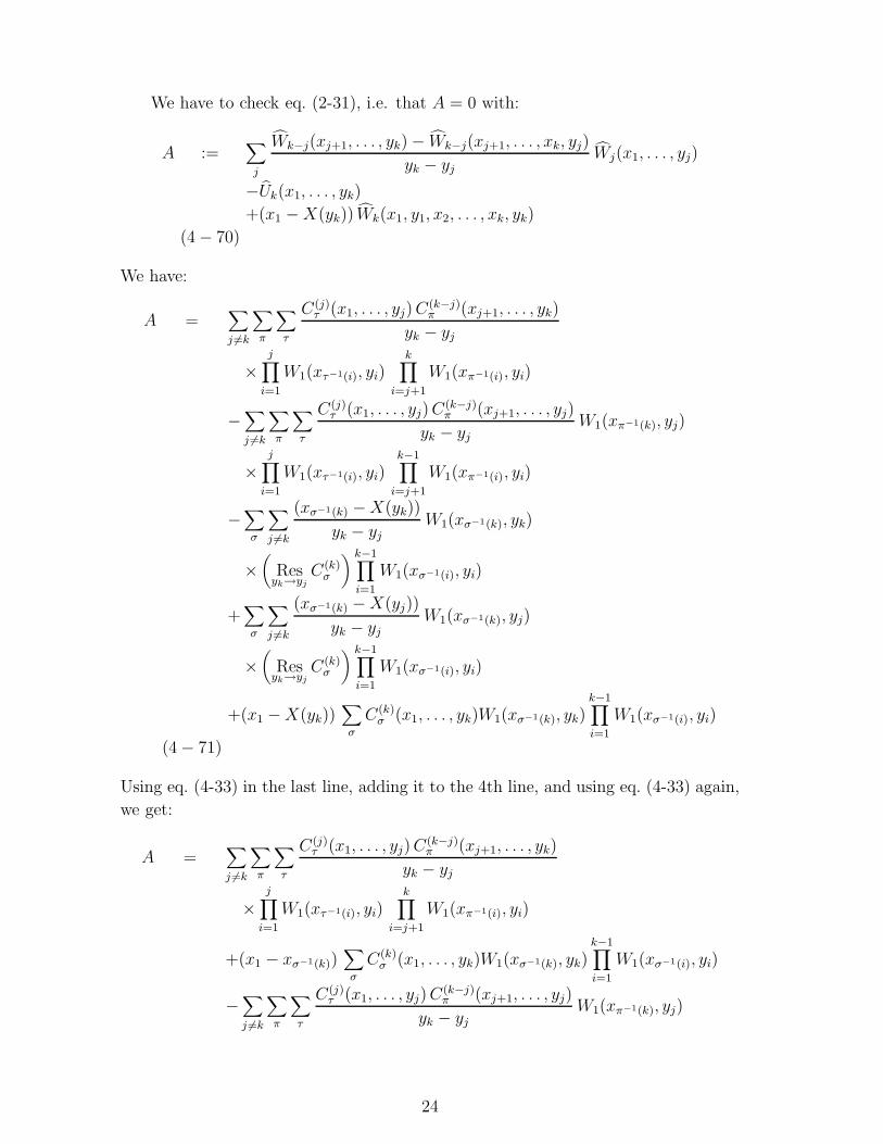
We have to check eq. (2-31), i.e. that A = 0 with:

A :=∑

j

Wk−j(xj+1, . . . , yk) − Wk−j(xj+1, . . . , xk, yj)

yk − yjWj(x1, . . . , yj)

−Uk(x1, . . . , yk)

+(x1 − X(yk)) Wk(x1, y1, x2, . . . , xk, yk)

(4 − 70)

We have:

A =∑

j 6=k

∑

π

∑

τ

C(j)τ (x1, . . . , yj) C(k−j)

π (xj+1, . . . , yk)

yk − yj

×j∏

i=1

W1(xτ−1(i), yi)k∏

i=j+1

W1(xπ−1(i), yi)

−∑

j 6=k

∑

π

∑

τ

C(j)τ (x1, . . . , yj) C(k−j)

π (xj+1, . . . , yj)

yk − yjW1(xπ−1(k), yj)

×j∏

i=1

W1(xτ−1(i), yi)k−1∏

i=j+1

W1(xπ−1(i), yi)

−∑

σ

∑

j 6=k

(xσ−1(k) − X(yk))

yk − yjW1(xσ−1(k), yk)

×(

Resyk→yj

C(k)σ

) k−1∏

i=1

W1(xσ−1(i), yi)

+∑

σ

∑

j 6=k

(xσ−1(k) − X(yj))

yk − yj

W1(xσ−1(k), yj)

×(

Resyk→yj

C(k)σ

) k−1∏

i=1

W1(xσ−1(i), yi)

+(x1 − X(yk))∑

σ

C(k)σ (x1, . . . , yk)W1(xσ−1(k), yk)

k−1∏

i=1

W1(xσ−1(i), yi)

(4 − 71)

Using eq. (4-33) in the last line, adding it to the 4th line, and using eq. (4-33) again,

we get:

A =∑

j 6=k

∑

π

∑

τ

C(j)τ (x1, . . . , yj) C(k−j)

π (xj+1, . . . , yk)

yk − yj

×j∏

i=1

W1(xτ−1(i), yi)k∏

i=j+1

W1(xπ−1(i), yi)

+(x1 − xσ−1(k))∑

σ

C(k)σ (x1, . . . , yk)W1(xσ−1(k), yk)

k−1∏

i=1

W1(xσ−1(i), yi)

−∑

j 6=k

∑

π

∑

τ

C(j)τ (x1, . . . , yj) C(k−j)

π (xj+1, . . . , yj)

yk − yj

W1(xπ−1(k), yj)

24

j∏

i=1

W1(xτ−1(i), yi)k−1∏

i=j+1

W1(xπ−1(i), yi)

+∑

σ

∑

j 6=k

(xσ−1(k) − X(yj))

yk − yj

W1(xσ−1(k), yj)

×(

Resyk→yj

C(k)σ

) k−1∏

i=1

W1(xσ−1(i), yi)

(4 − 72)

Using eq. (3-2) in the second line, exactly cancels the first line, and thus we get:

A = −∑

j 6=k

∑

π

∑

τ

C(j)τ (x1, . . . , yj) C(k−j)

π (xj+1, . . . , yj)

yk − yj

W1(xπ−1(k), yj)

j∏

i=1

W1(xτ−1(i), yi)k−1∏

i=j+1

W1(xπ−1(i), yi)

+∑

σ

∑

j 6=k

(xσ−1(k) − X(yj))

yk − yj

W1(xσ−1(k), yj)

×(

Resyk→yj

C(k)σ

) k−1∏

i=1

W1(xσ−1(i), yi)

(4 − 73)

which is a rational fraction in yk with poles at yk = yj for some j. From Lemma 4.6,

A as defined in eq. (4-70) cannot have poles at yk = yj, thus A = 0.

Now, we have to check eq. (2-30) Using eq. (4-33), one has:

Pk(x1, . . . , yk) − Wk−1(x2, . . . , xk, y1)

= Polx1

V ′1(x1) Uk(x1, y1, . . . , xk, yk)

= Polx1

Y (x1)∑

σ∈Σk

∑

j 6=k

Resy′

k→yj

C(k)σ

k−1∏

i=1

W1(xσ−1(i), yi)

U1(xσ−1(k), yk) − U1(xσ−1(k), yj)

yk − yj

= Polx1

Y (x1)∑

σ∈Σk , σ(1)=k

∑

j 6=k

Resy′

k→yj

C(k)σ

k−1∏

i=1

W1(xσ−1(i), yi)

U1(x1, yk) − U1(x1, yj)

yk − yj

+ Polx1

Y (x1)∑

σ∈Σk , σ(1)6=k

∑

j 6=k

Resy′

k→yj

C(k)σ W1(x1, yσ(1))

∏

i6=k,σ(1)

W1(xσ−1(i), yi)

U1(xσ−1(k), yk) − U1(xσ−1(k), yj)

yk − yj

= −∑

σ∈Σk , σ(1)=k

∑

j 6=k

∑

l 6=1

Resx1→xl

Resy′

k→yj

C(k)σ

k−1∏

i=1

W1(xσ−1(i), yi)

25

E(x1, yk) − E(x1, yj) − E(xl, yk) + E(xl, yj)

(x1 − xl)(yk − yj)

+∑

σ∈Σk , σ(1)6=k

∑

j 6=k

∑

l 6=1

Resx1→xl

Resy′

k→yj

C(k)σ

∏

i6=k,σ(1)

W1(xσ−1(i), yi)

(yσ(1) − Y (x1))W1(x1, yσ(1)) − (yσ(1) − Y (xl))W1(xl, yσ(1))

x1 − xlU1(xσ−1(k), yk) − U1(xσ−1(k), yj)

yk − yj

(4 − 74)

In order to satisfy eq. (2-30), we must prove that B = 0, where:

B :=k∑

l=2

Wl−1(x1, y1, . . . , yl−1) − Wl−1(xl, y1, x2, . . . , yl−1)

x1 − xl

×Uk−l+1(xl, yl, . . . , xk, yk)

+k−1∑

l=1

Wl(x1, . . . , yl) Wk−l(xk, yl, . . . , yk−1)

−Pk(x1, y1, x2, . . . , xk, yk)

−(Y (x1) − yk) Uk(x1, . . . , yk)

(4 − 75)

One does it in a way very similar to the previous one, i.e. first prove, using

eq. (3-2), that B is a rational fraction of x1, with poles at x1 = xl. But B can have

no pole at x1 = xl, so,B = 0.

•

5. Matrix form of correlation functions

So far, we have computed mixed correlation functions with only one trace, i.e. the

generating function of connected discrete surfaces with one boundary. In this section,

we generalize this theory to the computation of generating functions of non-connected

discrete surfaces with any number of boundaries. In order to derive those correlation

functions, a matrix approach of the problem, similar to the one developed in [15], is

used.

Definition 5.1 Let k be a positive integer. Let π and π’ be two permutations of Σk

and decompose π′−1π into the product of its irreducible cycles:

π′−1π = P1P2 . . . Pn (5-1)

Each cycle Pi of π′−1π, of length pi, is denoted :

Pm = (im,1 →π jm,1 ;

π′−1

im,2 →π jm,2 ;

π′−1

. . . ;π′−1

im,pm→π jm,pm

;π′−1

im,1)

(5-2)

26

For any (x1, y1, x2, y2, . . . , xk, yk) ∈ C, we define :

Wkπ,π′(x1, y1, . . . , xk, yk) :=

⟨n∏

m=1

δpm,1 +

1

NTr

pm∏

j=1

1

(M1 − xim,j)(M2 − yjm,j

)

⟩

(5-3)

which is a k! × k! matrix.

Let us now generalize the notion of planarity of a permutation.

Definition 5.2 Let k be a positive integer. Let π and π’ be two permutations of Σk.

A permutation σ ∈ Σk is said to be planar wrt (π, π′) if

ncycles(π−1σ) + ncycles(π

′−1σ) = k + ncycles(π′−1π) (5-4)

Let Σ(π,π′)k ⊂ Σk be the set of permutations planar wrt (π, π′).

Graphically, if one draws the sets of points (xi1,1 , yj1,1, xi1,2 , yj1,2, . . . , xi1,p1, yj1,p1

),

(xi2,1 , yj2,1, xi2,2 , yj2,2, . . . , xi2,p2, yj2,p2

), . . . , (xip,1 , yjp,1, xip,2 , yjp,2, . . . , xin,pn, yjn,pn

) on

n circles and link each pair (xj , yσ(j)) by a line, these lines do not intersect nor go

from one circle to another.

Remark 5.1 One can straightforwardly see two properties of these sets:

• This relation of planarity wrt to (π, π′) is symmetric in π and π′, that is to say:

Σ(π,π′)k = Σ

(π′,π)k (5-5)

• The planarity defined in eq. (4.1) corresponds to π = Id and π′ = S−1:

Σk = Σ(Id,S−1)k (5-6)

Directly from these definitions and the preceding results comes the following

theorem computing any generating function of discrete surface with boundaries.

Theorem 5.1

Wkπ,π′(x1, y1, x2, y2, . . . , xk, yk) =

∑

σ

Ckσ,π,π′(x1, y1, . . . , xk, yk)

k∏

i=1

W1(xi, yσ(i))

(5-7)

where Ckσ is the k! × k!-matrix defined by:

• Ckσ,π,π′(x1, y1, x2, y2, . . . , xk, yk) := 0 if σ is not planar wrt (π, π′);

27

• if σ is planar wrt (π, π′) :

Ckσ,π,π′(x1, y1, . . . , xk, yk) :=a∏

m=1

F (am)(xrm,1 , yσ(rm,1), xrm,2 , yσ(rm,2), . . . , xrm,am, yσ(rm,am ))

×a∏

m=1

F (am)(xrm,1 , yσ(rm,1), xrm,2 , yσ(rm,2), . . . , xrm,am, yσ(rm,am ))

(5 − 8)

with the decompositions of π−1σ and π′−1σ into their products of cycles:

π−1σ = π1π2 . . . πa , π′−1σ = π1π2 . . . πa (5-9)

such that:

πm = (rm,1, rm,2, . . . , rm,am) , πm = (rm,1, rm,2, . . . , rm,am

) (5-10)

Remark 5.2 From the definition, one can see that σ(rm,am) = π(rm, 1) and σ(rm,am) =

π′(rm, 1) for any m.

5.1 Properties of the Ckσ ’s.

Lemma 5.1 The matrices Ckσ are symmetric.

proof:

It comes directly from the definition. •

Lemma 5.2∑

σ

Ckσ = Id (5-11)

proof:

One has:

Wkπ,π′(x1, y1, x2, y2, . . . , xk, yk) =

∑

σ

Ckσ,π,π′

k∏

i=1

W1(xi, yσ(i)) (5-12)

Let us shift all the x’s by a translation a and send a → ∞, i.e. replace all the

xi’s by xi + a. In the LHS, only the δ-terms of Definition 5.1 survive in the limit

a → ∞, and thus the LHS tends towards the identity matrix. In the RHS, notice

that W1(xi + a, yσ(i)) → 1. And Ckσ , which depends only on the differences between

xi’s, is independent of a. •

28

5.2 Some commutation properties

Definition 5.3 Let Mk(~x, ~y, ξ, η) be the k! × k! matrix defined by:

Mk(~x, ~y, ξ, η)π,π′ :=∏

i

(δπ(i),π′(i) +1

(ξ − xi)(η − yπ(i))) (5-13)

Let A(k)(x1, y1, . . . , xk, yk) be the k! × k! matrix defined by:

A(k)π,π(x1, y1, . . . , xk, yk) :=

∑i xiyπ(i)

A(k)π,π′(x1, y1, . . . , xk, yk) := 1 if ππ′−1 = transposition

A(k)π,π′(x1, y1, . . . , xk, yk) := 0 otherwise

(5-14)

Theorem 5.2

∀σ, ξ, η , [Mk(~x, ~y, ξ, η), Ckσ(~x, ~y)] = 0

(5-15)

and

∀ξ, η , [Mk(~x, ~y, ξ, η),Wk(~x, ~y)] = 0(5-16)

proof:

Let us define:

M(~x, ~y, ξ, η) := M(N~x, ~y, Nξ, η) (5-17)

and

Wkπ,π′(x1, y1, . . . , xk, yk) :=

⟨n∏

m=1

δpm,1 + Tr

pm∏

j=1

1

N

1

(M1 − xim,j)(M2 − yjm,j

)

⟩

(5-18)

It was proven in [15] that:

[Mk(~x, ~y, ξ, η), Wk(~x, ~y)] = 0 (5-19)

Now, in the large N limit, the factorization property [5] < Tr Tr >∼< Tr ><

Tr >, implies:

Wkπ,π′(x1, y1, x2, y2, . . . , xk, yk)

∼ Nncycles(π′−1π)−k

n∏

m=1

Wpm(xim,1 , yπ(im,1), . . . , xim,pm

, xπ(im,pm ))

∼ Nncycles(π′−1π)−kWk

π,π′(x1, y1, x2, y2, . . . , xk, yk)

(5 − 20)

and using theorem 5.1, we have:

Wkπ,π′(x1, y1, x2, y2, . . . , xk, yk)

29

∼ Nncycles(π′−1π)−k

∑

σ

Ckσ,π,π′(x1, y1, x2, y2, . . . , xk, yk)

k∏

i=1

W1(xi, yσ(i)) (5-21)

Notice that

Ckσ,π,π′(x1, y1, x2, y2, . . . , xk, yk)

= Nk−ncycles(π−1σ)+k−ncycles(π

′−1σ)Ckσ,π,π′(Nx1, y1, Nx2, y2, . . . , Nxk, yk)

= Nk−ncycles(π′−1π)Ck

σ,π,π′(Nx1, y1, Nx2, y2, . . . , Nxk, yk)

(5 − 22)

Thus:

Wkπ,π′(x1, y1, x2, y2, . . . , xk, yk)

∼∑

σ

Ckσ,π,π′(Nx1, y1, Nx2, y2, . . . , Nxk, yk)

k∏

i=1

W1(xi, yσ(i)) (5-23)

Then, from [15], we have:

0 =∑

σ

[Mk(N~x, ~y, Nξ, η), Ck

σ(Nx1, y1, . . . , Nxk, yk)] k∏

i=1

W1(xi, yσ(i)) (5-24)

In particular, choose a permutation σ, and take the limit where yi → Y (xσ−1(i)), you

get in that limit:

0 =[Mk(N~x, ~Y (xσ−1), Nξ, η), Ck

σ(Nx1, Y (xσ−1(1)), . . . , Nxk, Y (xσ−1(k)))]

(5-25)

Since this equation holds for any potentials V1 and V2, it holds for any function

Y (x), and thus the Y (xi)’s can be chosen independentely of the xi’s, and thus, for

any y1, . . . , yk, we have:

0 =[Mk(N~x, ~y, Nξ, η), Ck

σ(Nx1, y1, . . . , Nxk, yk)]

(5-26)

Since it holds for any xi’s and ξ, it also holds for xi/N and ξ/N . •

Corollary 5.1

∀σ , [A(k)(~x, ~y), Ckσ(~x, ~y)] = 0 (5-27)

proof:

The corollary is obtained by taking the large ξ and η limit of theorem 5.2 (see

Appendix of [15]). •

30

5.3 Examples: k = 2.

W(2) =

(W11W22

W11W22−W12W21

(x1−x2)(y1−y2)W11W22−W12W21

(x1−x2)(y1−y2)W12W21

)(5-28)

where Wij = W1(xi, yj).

C2Id =

(1 1

(x1−x2)(y1−y2)1

(x1−x2)(y1−y2)0

)(5-29)

C2(12) =

(0 1

(x1−x2)(y2−y1)1

(x1−x2)(y2−y1)1

)= 1 − C2

Id

(5-30)

6. Application: Gaussian case

There is an example of special interest, in particular for its applications to string

theory in the BMN limit [22], it is the Gaussian-complex matrix model case, V1 =

V2 = 0. In that case one has E(x, y) = xy − 1, and thus:

W1(x, y) =xy

xy − 1(6-1)

The loop equation defining recursively the Wk’s can be written:

(x1yk − 1)Wk(x1, y1, . . . , xk, yk) =

x1

∑

j

Wj−1(xj , y1, . . . , yj−1) − Wj−1(x1, y1, . . . , yj−1)

x1 − xj

×Wk−j+1(xj , yj, . . . , xk, yk)

(6 − 2)

Its solution is then:

Wk(x1, y1, . . . , xk, yk) =∑

σ∈Σk

C(k)σ (x1, y1, . . . , xk, yk)

k∏

i=1

xiyσ(i)

xiyσ(i) − 1(6-3)

From the loop equation, one can see that Wk(x1, y1, . . . , xk, yk) may have poles

only when xi → y−1j for any i and j. Because the Cσ’s are rational functions of all

their variables and because Wk has no singularity when xi = xj or yi = yj, one can

write:

Wk(x1, y1, . . . , xk, yk) =Nk(x1, y1, x2, y2, . . . , xk, yk)∏

i,j(xiyj − 1)(6-4)

where Nk(x1, y1, x2, y2, . . . , xk, yk) is a polynomial in all its variables.

31

Moreover, the loop equation taken for the values xk = 0 or yk = 0 shows that

Wk(x1, y1, . . . , 0, yk) = Wk(x1, y1, . . . , xk, 0) = 0. Using the cyclicity property of

Wk(x1, y1, . . . , xk, yk), one can claim that it vanishes whenever one of its arguments

is equal to 0. One can thus factorize the polynomial Nk(x1, y1, x2, y2, . . . , xk, yk) as

follows:

Wk(x1, y1, . . . , xk, yk) =Qk(x1, y1, x2, y2, . . . , xk, yk)

∏i xiyi∏

i,j(xiyj − 1)(6-5)

where Qk(x1, y1, . . . , xk, yk) is a polynomial of degree k−2 with integer coefficient in

all its variables.

Notice that Qk(x1, y1, . . . , y−1σ(i), yi, . . . , xk, yk) = 0 if σ is not planar.

As an example, we have:

• for k = 2:

W2(x1, y1, x2, y2) =x1x2y1y2∏

i,j(xiyj − 1), Q2(x1, y1, x2, y2) = 1 (6-6)

• for k = 3:

W3(x1, y1, x2, y2, x3, y3) = (2 −∑

i

xiyi+1 + x1x2x3y1y2y3)x1x2x3y1y2y3∏

i,j(xiyj − 1)(6-7)

and

Q3(x1, y1, x2, y2, x3, y3) = (2 − x1y2 − x2y3 − x3y1 + x1x2x3y1y2y3) (6-8)

7. Conclusion

In this article, we have computed the generating functions of discs with all possible

boundary conditions, i.e. the large N limit of all correlation functions of the formal

2-matrix model. We have found that the 2k point correlation function can be written

like the Bethe Ansatz for the δ-interacting bosons, i.e. a sum over permutations of

product of 2-point functions. That formula is universal, it is independent of the

potentials.

An even more powerful approach consists in gathering all possible 2k point corre-

lation functions in a k!×k! matrix Wk. We have found that this matrix Wk satisfies

commutation relations with a family of matrices Mk which depend on two spectral

parameters, and are related to the representations of U(n) [15]. We claim that the

theorem 5.2 is almost equivalent to the loop equations, and allows to determine Wk.

It remains to understand how all these matrices and coefficients Cσ are related

to usual formulations of integrability, i.e. how to write these in terms of Yang Baxter

equations. For instance, the similarity with equations found in Razumov-Stroganov

conjecture’s proof [6] is to be understood.

32

One could also hope to find a direct proof of theorem 3.2, without having to

solve the loop equations. In other words, we have found that the 2k-point function

can be written only in terms of W1, while, in the derivation, we use the one point

functions Y (x) and X(y) although they don’t appear in the final result.

The next step, is to be able to compute the 1/N2 expansion of those correlation

functions, as well as the large N limit of connected correlation functions. We are

already working that out, by mixing the approach presented in the present article

and the Feynman graph approach of [9] generalized to the 2-matrix model in [10].

Another prospect is to go to the critical limit, i.e. where we describe generating

functions for continuous surfaces with conformal invariance, and interpret this as

boundary conformal field theory [21].

Acknowledgements

The authors want to thank M. Bauer, M. Bergere, F. David, P. Di Francesco, J.B.

Zuber for stimulating discussions. This work was partly supported by the european

network Enigma (MRTN-CT-2004-5652).

33

Appendix A Practical computation of fσ

In this appendix, we build a set of trees in bijection with Σk and use it in order to

compute practicaly the weights fσ defined in Definition 4.4.

Definition A.1 Let Tk be the set of trees defined as follows: A tree T belongs to

T ∈ Tk, and is called a k-planar tree if and only if:

• its root is labelled k + 1;

• it is composed of k+1 vertices, labeled by [1, . . . , k + 1];

• it has k edges which can be either upgoing or downgoing;

• its vertices have valence 1, 2 or 3, and are of one of the following eight possi-

bilities, in which the point m denotes the origin of the branch containing i:

– two trivalent vertices :

m

ij+1<m

ji

j+1

j>m

m

(1-1)

– four bivalent vertices :

m

ii+1<m

,

m

ii-1>m

(1-2)

m

i<m

m-1 i>m

m+1m(1-3)

– two monovalent vertices corresponding to the leaves of the tree:

i<m

m

m

i>m(1-4)

Remark A.1 Those trees are often called planar binary skeleton trees.

Remark A.2 One can see that the first edge is necessarily upgoing, and its extremity is

necessarily 1.

1

k+1

(1-5)

Theorem A.1 There is a bijection between Tk and the set of planar permutations

Σk:

34

proof:

We build explicitly this bijection between Σk−1 and Tk−1.

Consider a planar permutation σ ∈ Σk−1. Planarity means that σ defines a

partition of the disc into faces of two kinds. Let us say that faces which correspond

to cycles of Sσ are colored in white, faces which correspond to cycles of σ are colored

in black.

Decompose σ and Sσ into products of irreducible cycles:

σ = σ1σ2 . . . σl , Sσ = σ1σ2 . . . σl (1-6)

and we assume that σ1 and σ1 contain x1.

Because of planarity, we can define a distance of faces (i.e. cycles) to the face

σ1, as the number of edges one has to cross for going from a face σi or σi to σ1, and

call it D(σi) or D(σi).

We also define the “origin” of a face, noted m(σi) or m(σi), as follows: If the

face is σ1, we define m(σ1) = k, otherwise, because of planarity, there is only one

neighbouring face which is at smaller distance of σ1. Because of planarity, those two

faces share at most one x, and the origin is defined as the label of that x.

Thus, each face has a color, white or black, a distance D, and an origin m.

Now, to every face we associate a branch as follows:

• to a white face, σj , i.e. a cycle of Sσ, noted

σj = (ij,1, ij,2, . . . , ij,lj) , ij,1 = m(σj) , σ(ij,n) = ij,n+1 − 1 (1-7)

we associate the upgoing branch ij,1 → ij,2 → . . . → ij,lj

j,l

j,l-1

j

~

j~

j,1

j,3

~i

~ij,2

~i

~i~i (1-8)

(if lj = 1, the sequence contains only one vertex ij,1 = m(σj) and no edge).

• to a black face, σj , i.e. a cycle of σ, noted

σj = (ij,1, ij,2, . . . , ij,lj) , ij,1 = m(σj) , σ(ij,n) = ij,n+1 (1-9)

we associate the downgoing branch ij,1 → ij,2 → . . . → ij,lj

j

jij,l

j,l-1i

ij,2ij,3

ij,1

(1-10)

35

(if lj = 1, the sequence contains only one vertex ij,1 = m(σj) and no edge).

• to the first face σ1,

σ1 = (i1,1, i1,2, . . . , i1,l1) , i1,1 = 1 , σ(i1,n) = i1,n+1 − 1 (1-11)

we associate the upgoing branch k → i1,1 → i1,2 → . . . → i1,l1

k

1,2

1,1

1~1,l

~i

1~

1,l-1~i

~i~i

(1-12)

By definition of the origin m of a face at distance D, the origin of a branch is

necessarily a vertex on a branch at distance D − 1, and from planarity, it cannot be

a vertex on any other branch. Thus, there is a unique way to attach all branches to

their origin, and we obtain a tree, which belongs to Tk−1.

Inverse bijection:

On the other hand, let us consider a k − 1-tree. One can build a permutation

σ ∈ Σk−1 as follows: the image of an element of (1, . . . , k − 1) is :

• its descendant along a downgoing propagator if it exists;

• the origin of the downgoing branch to which it belongs in the other cases.

Because of the form of the vertices, the upgoing branches are necessarily the

cycles of Sσ. And since the branches form a tree, it implies that two faces touch one

another through zero or one edge. Thus the permutation σ is planar.

It is easy to see that this application is the inverse of the preceding one. •

Example:

Let us carry out explicitly step by step this building for the permutation σ ∈ Σ12

introduced earlier. Notice that it is enrooted in 12 + 1 = 13.

8

9

2

3

7

5

6

4

13

1

σ

σ σ

σ σ

σ

21

3 5

1

4

∼

∼11

13

1

4

8

9

2

3

7

5

6

12

5

13

1

4

8

9

2

3

13

1

13

1

4

8

9

13

1

4

8

9

2

3

7

13

1

4

8

9

2

3

7

(1-13)

36

Considering the last non trivial cycle σ6 = (10, 11), one obtains finally the tree

corresponding to (4-18):

13

1

4

8

9

2

3

7

5

6

12

11

10

(1-14)

Corollary A.1 #Tk = Cat (k) , where Cat (k) is the k’th Catalan number.

From now, one can see how to simply compute the weight fσ associated to a

permutation σ.

Consider a planar permutation σ ∈ Σk and its representation under the form of

a tree T ∈ #Tk. Associate a weight to every edge of the tree as follows:

• To every downgoing edgein,j

in,j+1

of a cycle σn of σ, one associates the weight

gin,1,in,j+1,in,j+2;

• To every upgoing edgei

i

n,j+1

~

~

n,jof a cycle σn of Sσ, one associates the weight

gin,j+1 ,in,1,σ(in,j+1).

Then, the fσ is the product of all the weights of edges composing T .

References

[1] M. Bergere, ”Biorthogonal Polynomials for Potentials of two Variables and External

Sources at the Denominator”, hep-th/0404126, SPhT-T04/042.

[2] M. Bertola, B. Eynard, “Mixed Correlation Functions of the Two-Matrix Model”, J.

Phys. A36 (2003) 7733-7750, hep-th/0303161.

[3] G. Bonnet, F. David, B. Eynard, “Breakdown of universality in multi-cut matrix

models”, J.Phys. A 33 6739-6768 (2000).

[4] E. Brezin, C. Itzykson, G. Parisi, and J. Zuber, Comm. Math. Phys. 59, 35 (1978).

[5] P. Di Francesco, P. Ginsparg, J. Zinn-Justin, “2D Gravity and Random Matrices”,

Phys. Rep. 254, 1 (1995).

[6] Di Francesco P., Zinn-Justin P., “Around the Razumov-Stroganov conjecture: proof

of a multi-parameter sum rule”, Electr. J. Combin. 12, R6 (2005)

37

[7] B. Eynard, “Master loop equations, free energy and correlations for the chain of

matrices”, JHEP11(2003)018, hep-th/0309036, ccsd-00000572.

[8] B. Eynard, “Large N expansion of the 2-matrix model”, JHEP 01 (2003) 051, hep-

th/0210047.

[9] B. Eynard, “Topological expansion for the 1-hermitian matrix model correlation func-

tions”, JHEPJHEP/024A/0904, hep-th/0407261.

[10] B. Eynard, N. Orantin, “A residue formula for correlation functions for the hermitian

2-matrix model”, in preparation.

[11] B. Eynard, “Eigenvalue distribution of large random matrices, from one matrix to

several coupled matrices” Nucl. Phys. B506, 633 (1997), cond-mat/9707005.

[12] B. Eynard, “Correlation functions of eigenvalues of multi-matrix models, and the

limit of a time dependent matrix”, J. Phys. A: Math. Gen. 31, 8081 (1998), cond-

mat/9801075.

[13] B. Eynard “An introduction to random matrices”, lectures given at Saclay, October

2000, notes available at http://www-spht.cea.fr/articles/t01/014/.

[14] B. Eynard “Polynomes biorthogonaux, probleme de Riemann–Hilbert et geometrie

algebrique”, Habilitation a diriger les recherches, universite Paris VII, (2005).

[15] B. Eynard, A. Prats-Ferrer, “2-matrix versus complex matrix model, integrals over the

unitary group as triangular integrals”, preprint SPHT T05/011, preprint UB-ECM-PF

05/03, hep-th/0502041.

[16] B. Eynard, M.L. Mehta, “Matrices coupled in a chain: eigenvalue correlations”, J.

Phys. A: Math. Gen. 31, 4449 (1998), cond-mat/9710230.

[17] M. Gaudin, “La Fonction d’Onde de Bethe”, Collection du Commissariat a l’Energie

Atomique: Serie, Editor: Masson, (1983).

[18] V.A. Kazakov, “Ising model on a dynamical planar random lattice: exact solution”,

Phys Lett. A119, 140-144 (1986).

[19] V. Kazakov, I. Kostov, ”Loop gas model for open strings”, Nucl. Phys. B386 (1992)

520.

[20] V.A. Kazakov, A. Marshakov, ”Complex Curve of the Two Matrix Model and its

Tau-function”, J.Phys. A36 (2003) 3107-3136, hep-th/0211236.

[21] I. K. Kostov, “Boundary Correlators in 2D Quantum Gravity: Liouville versus Dis-

crete Approach”, Nucl.Phys. B658 (2003) 397-416, hep-th/0212194.

[22] C. Kristjansen, J. Plefka, G. W. Semenoff, M. Staudacher, “A New Double-Scaling

Limit of N=4 Super Yang-Mills Theory and PP-Wave Strings”, Nucl.Phys. B643

(2002) 3-30, hep-th/0205033.

38

[23] A. Matytsin, “on the large N limit of the Itzykson Zuber Integral”, Nucl. Phys. B411,

805 (1994), hep-th/9306077.

[24] M.L. Mehta, Random Matrices,2nd edition, (Academic Press, New York, 1991).

[25] M.L. Mehta, ”A method of integration over matrix variables”, Comm. Math. Phys.

79 (1981) 327-340.

[26] M. Staudacher, “ Combinatorial solution of the 2-matrix model”, Phys. Lett. B305

(1993) 332-338.

[27] G. ’t Hooft, “ A planar digram theory for strong interactions”, Nucl. Phys. B72, 461

(1974).

39