Spectral Hermite Approximations for the Actively Mode-Locked Laser

81

0885-7474/01/0600-0081/0 © 2001 Plenum Publishing Corporation

Journal of Scientific Computing, Vol. 16, No. 2, June 2001 (© 2001)

Spectral Hermite Approximations for the ActivelyMode-Locked Laser

Kelly Black1 and John B. Geddes2

1 Visiting the Department of Mathematics and Statistics, Utah State University. E-mail:[email protected] of Mathematics and Statistics, University of New Hampshire. E-mail: [email protected]

Received March 23, 2001; accepted May 2, 2001

An approximation technique for the governing equations for the mode-lockedlaser is examined. The technique centers on a transformation of the governingequations in which the resulting equations closely resemble the Hermite equation.The approximation of the system is constructed through a linear combination ofHermite polynomials resulting in a Hermite-spectral method. The rate of decayof the resulting modes is examined for a simplified problem and difficulties inshowing the stability of the method are also discussed. Numerical comparisonswith a finite difference scheme are also presented.

KEY WORDS: Hermite polynomials; mode-locked laser; spectral method.

1. INTRODUCTION

It could be argued that the laser is second only to the silicon chip inimportance in today’s technological market-place. It is at the heart ofnumerous consumer devices, from CD-players to laser pointers, and it isfueling the rate at which we increase our digital communication speeds viaoptical networks [16]. The need for stable, controllable, pulsed-lasers hasnever been higher, and this demand continues to drive research into eitherthe improvement of current devices or the invention of new ones [9].

While the laser in the market-place today could be one of many varieties,the underlying description of these lasers is fairly ubiquitous [15]. A lasergenerally consists of a gain medium, which coverts energy into a coherentstream of photons via stimulated emission, a cavity which allows for the

buildup of radiation by continuously re-circulating the energy through thegain medium, and some sort of pump source to provide the necessary inputenergy. It is important to recall that lasers are very poor energy converters,with efficiency’s in the range of 0.01–2%. They make up for this, however,by producing ‘‘light’’ that can be very monochromatic, highly coherent,and controllable.

A classic example of a laser consists of a solid-state material, NeodyniumYttrium Aluminum Garnet (Nd:YAG), placed between a set of mirrors. Itis pumped by a flash-lamp which floods the Nd:YAG rod with photons.Some of this energy excites the electrons in the rod and permits them tomake a transition from their current electronic state to one with higherenergy. As the electrons decay from this excited state to a state of lowerenergy, they emit the energy difference as a photon. This process canhappen spontaneously, and is known as spontaneous emission, or can bestimulated by the presence of a photon with the same energy, so-calledstimulated emission. The photons emitted by the rod are corralled along thelaser axis with the aid of the end-mirrors, and these photons stimulatefurther emission as they pass through the rod again and again. In this waythe laser acts as an amplifier and once the gain achieved by the stimulatedemission process exceeds any cavity losses (e.g., energy transformed intoheat in the rod), the laser turns on. Some radiation is allowed to escapefrom the cavity by using partially transmitting mirrors, and thus we arriveat Light Amplification by Stimulated Emission of Radiation.

The simple laser described above would emit radiation throughout alarge number of modes, and the output from such a laser would be a con-tinuous-wave (cw) source, i.e., the average intensity of light would be con-stant over long periods of time. In order to achieve pulsed-operation, someform of additional ‘‘control’’ must be used. In an actively mode-lockedlaser, the losses are modulated in time with a period which nearly matchesthe round-trip time of the laser (the time it takes light to travel from mirrorM1 to mirror M2 and back). This results, in the ideal case, in a perfecttrain of pulses with a repetition rate equal to the round-trip time of thelaser cavity. In a typical application, the laser pulse-width may be measuredin pico-seconds, while the round-trip time may be in the nano-second range(corresponding to a 50 cm cavity).

Achieving a perfect train of pulses is rather difficult experimentally.In fact, many actively mode-locked lasers are very sensitive to perturbations,which seriously degrades both the quality and the dependability of the laserlight. Recent research suggests that an actively mode-locked laser mightprovide an excellent vehicle for the study of ‘‘turbulence’’ in optics. Kaertneret al. [12] have shown theoretically that the non-orthogonality of the basiclaser modes can result in large transient gain for noise perturbations, which

82 Black and Geddes

may be enough to destabilize such a laser and result in ‘‘turbulent’’ beha-viour. While these authors do not discuss the details of their numericalmethod, the importance of using a stable, accurate numerical schemecannot be underestimated, especially given the apparent sensitivity of thesystem to perturbations. We have elsewhere undertaken a detailed study ofthe dynamics of the actively mode-locked laser [7] and many of our resultshave been confirmed with careful numerical solutions of the governingpartial differential equation. In this paper we propose and analyze anumerical method for the actively mode-locked laser based on a spectralapproximation using Hermite–Gaussian basis functions.

2. NUMERICAL METHODS

As we will discuss later, the governing equations for the actively mode-locked laser consist of a partial differential equation for the amplitude ofthe laser-pulse A, and an ordinary differential equation for the laser gain g.The equation for A takes the form of an initial-boundary-value problem onan infinite domain with Dirichlet boundary conditions. The gain equationtakes the form of an ordinary differential equation driven by the energy inthe pulse. While we consider a variety of numerical methods, includingfinite-difference schemes, we analyze in detail a spectral approximationusing Hermite basis functions. This basis is motivated by the equilibriumsolutions to the pulse amplitude equation, as discussed in Section 3.1.

The body of work for spectral approximations on infinite domains isnot as extensive as for approximations on finite domains. Several authorshave investigated spectral methods using Laguerre polynomials and poly-nomial approximations with respect to the Laguerre weight in the innerproduct. In particular Maday, Pernaud-Thomas, and Vandevan have founderror bounds for approximations using Laguerre polynomials with respect toan inner product using the Laguerre weight [13]. Coulaud, Funaro andKavian have examined the special case of elliptic problems with zero bound-aries at infinity [4]. Finally, Funaro has examined approximations usingLaguerre polynomials in more detail [6].

The use of Laguerre polynomials for constructing approximationsusing spectral element methods has also received attention. The approachallows for a combination of semi-inifinite domains to be pieced together toform an infinite domain. Collocation type approaches have been examinedby both Mavriplis [14] as well as Karageorghis and Phillips [11].

There have been relatively few methods proposed using Hermitepolynomials. Weideman and Cloot have proposed methods using aHermite basis [18]. Weideman has also examined the properties of theresulting linear systems [17]. Error estimates for an inner product given by

Spectral Hermite Approximations for the Actively Mode-Locked Laser 83

the Hermite weight have been examined by Guo [8] including an examplefor an approximation to Burger’s equation on an infinite line.

It should be noted that problems with these approaches have beendiscussed by Boyd [2]. Problems which have solutions that do notapproach zero fast enough do not exhibit spectral accuracy. He insteadproposed a method in which the infinite line is mapped to a finite line anda spectral method be implemented on the new domain. One drawback tothe approach is that solutions with an infinite number of waves cannotbe resolved. The method has also been adapted for spectral elements byBlack [1].

The primary method examined here is a spectral approximation basedon Gaussian-Hermite polynomials. We will first provide and discuss thegoverning system of equations for the mode-locked laser. We will alsobriefly discuss the stability of the system. The method for transforming theequations to a form that is similar to the Hermite equation will then begiven, and we will then concentrate on numerical approximations of thesystem based on Hermite expansions.

3. GOVERNING EQUATIONS

The governing equations for the actively mode-locked laser can bederived in a rigorous manner based on a master-equation approach [5].Such an approach follows the laser pulse as it propagates around the cavityand the equations are therefore set in a traveling frame of reference. Theequations read [12]

TM“A(T, t)“T

=1D “2

“t2+C

“

“t+(g(T)−l−mt2)2 A(T, t), (1)

dg(T)dT

=a− yg(T)−bg(T) F.

−.|A(T, t)|2 dt. (2)

We expect the pulses to have a pulse-width much shorter than the round-trip time of the cavity and we therefore consider the evolution of thecomplex pulse envelope A(T, t) on two distinct time-scales. (Recall that thefrequency of light in the infra-red is on the order of 1015 Hz—the laserpulse is in fact the envelope of the basic oscillation.) The time T is sampledon the time-scale of the cavity round-trip time TR (nano-seconds) and thetime t resolves the resulting pulse shape (pico-seconds).

The evolution equation (1) for the pulse envelope includes a number ofrelevant physical effects. The pulse experiences both gain, g(T), and loss,D“tt −l−mt2, as it propagates in the cavity. The parameter l represents the

84 Black and Geddes

fixed cavity losses which are frequency-independent, while D represents thecurvature of the intracavity losses in the frequency domain which limits thebandwidth of the laser. The parameter m is proportional to the depth ofthe loss modulation introduced by the loss-modulator with modulatorperiod TM. While the losses are actually modulated periodically, the modu-lation depth is relatively large so that radiation can only build-up duringthe time of low intracavity loss, which is much shorter than the modulatorperiod. In that case, the cosine modulation is approximated by a parabolaso that m actually represents the curvature of the loss modulation at thepoint of minimum loss. In addition, the loss modulation period (TM) is notperfectly matched to the round-trip time (TR) and this detuning is capturedby C=TM −TR.

There would be no lasing action without the presence of a gain medium,the dynamics of which are captured in Eq. (2). The gain in the cavity, g(T),depends on the amount of energy driving the laser, the rate at which the gainmedium can radiate the laser photons, and the number of photons present inthe cavity. The parameter a accounts for the rate of energy gain due topumping, while y represents the gain relaxation rate. The number of photonsin the cavity at any given time T is measured by the pulse energy,> |A(T, t)|2 dt. Since radiation can only build-up in the vicinity of theminimum loss point we are justified in allowing t to range from −. to +..The pulse energy in the cavity is therefore given by >.−. |A(T, t)|2 dt. In addi-tion, our search for pulse-like solutions to Eq. (1) require us to satisfyvanishing boundary conditions for the pulse amplitude, i.e.,

limtQ ±.

A(T, t)=0. (3)

Finally, the real parameter C may be positive or negative, while the otherreal parameters D, l, m, a, y, and b are all positive. A general treatment ofthe actively mode-locked laser would require both D and m to be complexin order to account for dispersion and phase modulation [5]. This case,however, is beyond the scope of our present treatment, and will be thesubject of future investigation. In the absence of complex parameters thephase of A remains fixed under the evolution described by Eq. (1). We cantherefore take A to be real without loss of generality, and we will sub-sequently drop any reference to the complex nature of A.

3.1. Steady-State Solutions

Before addressing the accuracy and stability of any numerical schemeused to solve Eqs. (1) and (2) subject to boundary conditions (3), we will


consider the steady-state or equilibrium solutions. This will shed light onthe types of solutions we expect to obtain, and will in fact be a motivatingreason for our Hermite–Gaussian basis.

The equilibrium solution for the gain can be obtained by settingdg/dT=0 in Eq. (2) which results in the steady-state gain

g=a

y+b >.−. A2(T, t) dt(4)

On the other hand, the steady-state gain equation also determines the pulseenergy as

F.

−.A2(T, t) dt=

a− ygbg

(5)

The threshold for lasing operation is therefore given by a \ yg as this willlead to non-negative energy in the cavity.

The pulse-shape can be determined by setting “A/“T=0 in Eq. (1)and solving the resulting ordinary differential equation

1D “2

“t2+C

“

“t+(g−l−mt2)2 A(t)=0 (6)

subject to the boundary conditions (3). This equation can be transformedinto the usual Hermite equation by looking for a solution in the form of

A(t)=f(t) exp 1− (t−a)2

2s22 (7)

where a and s are free parameters. Note that such a solution would corre-spond to a pulse located at t=a with width s. Replacing ansatz (7) intoEq. (6) results in

0=Dftt+1Cs2−2D(t−a)

s22 ft

+1g−l−mt2+D(t−a)2−Ds2−Cs2(t−a)

s42 f (8)

Choosing a=−s2C/2D and s2=`D/m further reduces the equation to

Dftt −2`mD tft+1g−l−`mD−C2

4D2 f=0 (9)

86 Black and Geddes

Transforming the variable t by t Q su finally results in

fuu −2ufu+1

`mD1g−l−`mD−

C2

4D2 f=0 (10)

This is precisely the Hermite equation if

1

`mD1g−l−`mD−

C2

4D2=2n; n=0, 1, 2,..., (11)

which must be true in order to satisfy the boundary conditions. In otherwords, a nontrivial solution exists for the pulse amplitude f if the steady-state gain is determined by

gn=l+2`mD (D2+n+12); n=0, 1, 2,..., (12)

where D is a normalised detuning given by D=sC/`8 D. If this is the casethen Eq. (10) is the Hermite equation with the usual Hermite polynomialsHn(u) as solutions. Each value of the gain described by Eq. (12) thereforecorresponds to a Hermite–Gaussian mode of the form

An(t)=Hn1 ts2 exp 1− (t+`2 sD)2

2s22 . (13)

As the ground-mode (n=0) is the mode which requires the lowest value ofthe gain we would expect it to dominate, at least close to lasing threshold. Thebasic lasing solution is therefore a Gaussian pulse located at t=−`2 sD.If the modulator period matches the round-trip period perfectly, i.e., D=0,then the pulse is centered at t=0 which corresponds to the minimum losspoint. If, on the other hand, there is any slight detuning, i.e., D ] 0, thenthe pulse will be shifted away from the minimum loss point by an amountproportional to the detuning. This implies that there is a window either infront of or behind the pulse which sees less loss than the pulse itself. Thisresults in the pulse being remarkably sensitive to perurbations located inthis growth window as detailed in [7, 12].

4. SPECTRAL HERMITE APPROXIMATION

We have seen that the equilibrium solutions of the governing equationfor the pulse amplitude are Hermite–Gaussian functions. The Hermitepolynomial is centered at t=0 while the Gaussian is centered at t=a, anoffset that is proportional to the detuning C. Analytical and numerical


results [12, 7] suggest that much of the interesting dynamics take placeas the detuning is increased beyond a critical value, which roughly corre-sponds to D=4. Furthermore, it can also be shown that perturbationslocated at t=−a experience tremendous growth (on the order of exp(2D2))as they sweep across the domain before coming to equilibrium at t=a. Theuse of the Hermite–Gaussians as a basis for a spectral method is thereforevery appealing.

4.1. Transformations of the Governing Equation

The governing equations, (1) and (2), can be transformed into a systemwhose pulse-shaping operator closely resembles the Hermite equation. Thisis essentially a repeat of our transformation to find the equilibrium solu-tions but we include it here for clarity. The first step is to substitute

A(T, t)=e−12 (

t− ts)2A(T, t), (14)

into the governing equation, where t and s are free parameters. Equation (1)can then be reduced to

AT(T, t)−g(T) A(T, t)=5D(t− t)2−Ds2−Cs2(t− t)s4

−l−mt26 A(T, t)

+5Cs2−2D(t− t)s26 At(T, t)+DAtt(T, t). (15)

Choosing t=−s2C/2D and s2=`D/m further reduces the equation to

AT(T, t)−g(T) A(T, t)=DAtt(T, t)−2`mD tAt(T, t) (16)

−5l+`mD+C2

4D6 A(T, t). (17)

Transforming the variables t and T by t Q st, and T Q s`mD

, reduces thesystem to

As(s, t)− g(s) A(s, t)=Att(s, t)−2tAt(s, t)−MA(s, t), (18)

gŒ(s)=a− yg(s)− bg(s) F.

−.A2(T, t) dt, (19)

88 Black and Geddes

where the following substitutions have been made:

M=1+l

`mD+

C2

4D`mD, (20)

g(s)=g(s)

`mD, (21)

a=a

mD, (22)

y=y

`mD, (23)

b=b

`mD. (24)

(Note that both M and b are real, positive numbers.)The right-hand-side of Eq. (18) is responsible for shaping the pulse and

is similar to the standard Hermite equation. This leads us to construct anapproximation based on a Hermite expansion. One difficulty arises in cal-culating the integral in Eq. (19). Substituting the pulse solution (14) into thisintegral results in a shifted Gaussian as a weighting function.We would like toconstruct an orthogonal basis, but the Hermite polynomials are not orthogo-nal with respect to this weight unless they are also shifted. Furthermore, theintegral calculation can be simplified to an order N operation if the basis thatis used is orthogonal. We will require that the expansion be based on shiftedHermite polynomials due to the shift in the exponential weight in Eq. (14).

4.2. Energy Calculation

An approximation to Eqs. (18) and (19) is constructed using anexpansion based on shifted Hermite polynomials. The reason for shiftingthe polynomials is to simplify the calculation of the norm, ||A(T, · )||2. Inparticular, we must calculate

||A(T, · )||2=F.

−.A2(T, t) dt. (25)

Based on our substitutions, this norm becomes

F.

−.A2(T, t) e−(

t− ts)2 dt=F

.

−.A2(s, t) e−(t− t/s)

2s dt. (26)


Based solely on Eq. (18) the natural basis would be the Hermite poly-nomials. Such a choice would greatly complicate the calculation of thenorm in Eq. (19). Here we will examine a basis formed from the shiftedHermite polynomials,

AN(s, t)=CN

n=0an(s) Hn(t− t/s), (27)

where Hn is the Hermite polynomial of degree n.The resulting basis functions are orthogonal with respect to the weight

in Eq. (26). The calculation of the square of the norm at any point, s, issimply a matter of summing the squares of the coefficients, an(s). The costof this approach is that we are no longer making use of the eigen-functionsto Eq. (18). However, each of the eigen-functions are polynomials of finitedegree. Since the basis functions are also polynomials of finite degree theeigen functions can be recovered from finite linear combinations of thebasis functions.

Before examining the resulting discretization we will first provide abrief introduction to the Hermite polynomials. Once done, we will examinethe behavior of the Fourier coefficients for a simpler linear problem.Finally, we will describe the numerical approximation itself.

4.3. Hermite Polynomials

Some of the properties of Hermite polynomials are briefly introduced.The Hermite polynomials satisfy the differential equation

H'

n (t)−2tH −

n(t)+2nHn(t)=0, (28)

where n is a non-negative integer and Hn(t) is a polynomial of degree n.This equation can be written in the form of a Sturm–Liousville equation

ddt

(H −

n(t) e−t2)+2nHn(t) e−t

2=0. (29)

The Hermite polynomials are thus orthogonal with respect to the innerproduct,

F.

−.Hn(t) Hm(t) e−t

2dt=dmn2mm!`p . (30)

The Hermite polynomials also satisfy the following recurrence relation-ships:

90 Black and Geddes

ddt

Hn(t)=2nHn−1(t),

Hn+1(t)=2tHn(t)−2nHn−1(t).

(31)

Because our approximation will consist of shifted Hermite polyno-mials the inner product we will use is

Ou(s, · ), v(s, · )Pw=F.

−.u(s, t) v(s, t) e−(t−t/s)

2dt. (32)

This inner product then defines an energy,

||u(s, · )||2w=Ou(s, · ), u(s, · )Pw. (33)

Moreover, the inner product also defines the H1w Sobolev norm

||u(s, · )||2H1w=F

.

−.(u(s, t))2 e−(t− t/s)

2dt

+F.

−.

1 ““t

u(s, t)22

e−(t−t/s)2dt. (34)

The space we will work in is the set of functions square integral withrespect to this norm. We will also impose the following boundary conditions

limtQ ±.

u(s, t) e−(t−t/s)2=0. (35)

4.4. Approximation

The approximation of Eq. (18) is given by

AN(s, t)=CN

n=0an(s) Hn(t− t/s). (36)

Focusing on Eq. (18), the discretization is estabilished using a Galerkinapproach

O(AN)s −g(s) AN, Hm( · − t/s)Pw

=O−MAN −2t(AN)t+(AN)tt, Hm( · − t/s)Pw, (37)

for m=0,..., N.


The basis functions are orthogonal with respect to the inner productand the equation reduces to

am(s)− g(s) am(s)=−Mam(s)+CN

n=0an(s) F

.

−.(H'

n (t−t/s)−2tH −

n(t−t/s))

×Hm(t− t/s) e−(t−t/s)2dt. (38)

The domain of the integral can be shifted to give

am(s)− g(s) am(s)

=−Mam(s)+CN

n=0an(s) F

.

−.(H'

n (t)−2(t+t/s) H −

n(t)) Hm(t) e−t2dt,(39)

or

am(s)− g(s) am(s)

=−Mam(s)+CN

n=0an(s) F

.

−.(H'

n (t)−2tH −

n(t)) Hm(t) e−t2dt

−2ts

CN

n=0an(s) F

.

−.H −

n(t) Hm(t) e−t2dt. (40)

The first integral is the Hermite differential equation (28) and can besimplified. The second integral can be simplified using Eq. (31). Takingadvantage of the orthogonality relationship the equation reduces to

am(s)− g(s) am(s)=−(M+2m) am(s)−ts

(4(m+1)) am+1(s), (41)

for m=0,..., N where aN+1=0. Note that this equation results in an upper-triangular matrix when an implicit time stepping scheme is used, and thesystem can be easily inverted. Specific examples are examined in Section 5.

4.5. Rate of Decay for the Fourier Coefficients

Convergence estimates for norms with respect to the weight e−t2have

been examined by Guo [8]. One of the difficulties with this norm, however, isthat large errors far from the origin are discounted through the extremeexponential decay of the weighting function. For example, the differencebetween the approximation and the true solution can grow at an extremely

92 Black and Geddes

large rate but the norm of the difference could be small due to the extremedecay of the weight function.

Another approach is to examine the rate of decay of the Fourier coef-ficients. The behavior of the Fourier modes has been examined for generalSturm–Liousville systems in [3, pp. 281–284] and [10, pp. 130 and 137].The equations in the current situation, however, do not represent aSturm–Liousville system due to the shift.

We have found surprisingly little attention given to Hermite approxi-mations in the literature. Most notably the numerical aspects of the resultinglinear systems have been examined by Weideman and Cloot [18] and byWeideman [17]. However, a detailed analysis on the convergence proper-ties have not been examined. In this situation, we do not have a Sturm–Liousville system and a different approach is necessary.

Because of the difficulties we will examine the solution for a differentproblem, a steady state equation. In particular we will focus on theapproximation of the Hermite equation using a shifted basis. The non-homogeneous Hermite equation that is examined is

f(t)=−Mu(t)−2tuŒ(t)+uœ(t), (42)

where M is a positive parameter. In the current implementation we are alsoconcerned about the use of a shifted basis,

uN(t)=CN

n=0anHn(t−b). (43)

Before examining the coeficients for the expansion, we will need thefollowing intermediate result:

Lemma 4.1. The function

f(x)=ax 5 n+mn+m−x6 (l+1)

(44)

has a minimum at x=0 over the domain 0 [ x [ m when 0 < a < 1, l > 1,and n > −(l+1)

ln(a) .

Proof. The derivative of f(x) is

fŒ(x)=f(x) 5ln(a)+ l+1n+m−x6 . (45)


Note that f(x) > 0 for all x, and the second term is less than zero

ln(a)+l+1

n+m−x< 0. (46)

when n > −(l+1)ln(a) . Under these conditions the function, f(x), is decreasing

over the interval 0 < x < m so the maximum is found at x=0. i

Here we will assume that the shift, b, is non-zero. Just like in Eq. (41)the nonhomogeneous equation, Eq. (42), can be reduced to a recurrancerelationship between the Fourier coefficients,

fn=−(M+2n) an −4b(n+1) an+1. (47)

The coefficients fn are the Fourier coefficients for the Hermite expansionof f(t). We will begin at some n where the long term behavior of theFourier coefficients begin to manifest itself. The Fourier coefficients after ncan be written in terms of an and the coefficients of f(t),

an+m= Cm−1

j=0

31 14b2 j (−1) j

fn+m−j

n+m−j+1Dj

k=1

M+2(n+m−k)2(n+m−k+1)

4

+(−1)m 1 14b2m an D

m−1

k=0

M+2(n+m−k)2(n+m−k+1)

. (48)

We will first focus on the terms withing the products in Eq. (48). Theindividual terms within the product are given by

M+2(n+m−k)2(n+m−k+1)

=1+M−2

2(n+m−k+1). (49)

The largest that this term can get for k from 0 to m is when k=m and wewill define cn so that

1+cn=1+M−2n+1

. (50)

With this definition, the right hand side of Eq. (48) can be bounded togive

|an+m | < Cm−1

j=0

: 14b: j (1+cn) j

|fn+m−j |n+m−j

+: 14b:m (1+cn)m |an |. (51)

94 Black and Geddes

First, to insure that the Fourier coefficients decay to zero it is necessarythat

0 < : 14b: (1+cn) < 1. (52)

In order to evaluate whether or not the sum decays to zero some kindof assumptions must be made on the how fast the coefficients for theforcing function, f(t), decay. We will examine two situations. First we willshow that if the coefficients fl decay algebraically, O(1/N l), then theFourier coefficients for the approximation also decay to zero in the sameway. We will then examine what happend if the coefficients decay expo-nentially. Here, our bound cannot be used to show exponential decay, butthe coefficients do decay to zero faster than any power of N.

4.5.1. Algebraic Convergence

Here we will assume that the coefficients for the forcing function, fn,experience algebraic decay. After the first n terms the Fourier coefficientsare bounded by

fn+m [K

(n+m) l, (53)

where both l and K are positive constants. With this bound the sum inEq. (51) can be bounded by

|an+m | < Cm−1

j=0

: 14b: j (1+cn) j

K(n+m−j) (l+1)+:

14b:m (1+cn)m |an |,

=K

(n+m)(l+1) Cm−1

j=0

: 14b: j (1+cn) j 1

n+m(n+m−j)2 (l+1)

+: 14b:m (1+cn)m |an |. (54)

Each of the terms within the sum are consistent with Lemma 4.1, andbased on the lemma a further bound can be found by

|an+m | <Km

(n+m)(l+1)+:14b:m (1+cn)m |an |. (55)

From this result we find that the coefficients an+m decay like O(1/m l).


4.5.2. Spectral Convergence

The second situation that is examined is if the coefficients for theforcing function exhibit exponential decay,

fn+m [ Kam, (56)

where K is a positive constant and 0 < a < 1. With this assumption thefollowing bound can be found

|an+m | < Cm−1

j=0

: 14b: j (1+cn) j

Kam−j

n+m−j+: 1

4b:m (1+cn)m |an |,

=Kam Cm−1

j=0

1n+m−j

+: 14b:m (1+cn)m |an |, (57)

where a=max(a, | 14b | (1+cn)). The sum can be further bounded by

|an+m | < Kam ln 1n+m+1n+22+: 1

4b:m (1+cn)m |an |. (58)

In this situation our bound on the coefficient, an+m, indicated fast conver-gence to zero. It is of the order O(am ln(m)), but it is not exponentialdecay.

4.5.3. Numerical Considerations

The bound on the shift given in Eq. (52) is a counter-intuitive bound.The bound is a lower bound on the shift,

b >1+cn

4. (59)

There is a lower bound on the size of the shift. The contradiction is thatwhen the shift in the original equation is zero, the analysis is greatlysimplified and is similar to the standard Sturm–Liousville approach givenin [3, pp. 281–284] and [10, pp. 130 and 137].

Another consideration is that calculations based on Hermite polynomialsare numerically difficult in practice. To overcome the stability problemsin calculating the polynomials, our implementation makes use of scaledHermite polynomials, Hn(t). The polynomials are scaled so that the new

96 Black and Geddes

polynomials are orthonormal. The scaling factor is found using Eq. (30),and the new polynomials are

Hn(t)=1

`2nn!`pHn(t). (60)

With this scaling the new system of polynomials are orthonormal. Asdiscussed in Section 4.2 the process of finding the energy calculationremains simple. The system given by Eq. (41) is transformed into

am(s)=−g(s) am(s)−(M+2m) am(s)−ts`8(m+1) am+1(s), (61)

g(s)=a−yg(s)−bsg(s) CN

n=0a2n(s), (62)

for m=0,..., N, where aN+1=0.

4.6. Notes on Stability

Demonstrating the stability of the numerical approximation, Eqs. (18)and (19), has represented some difficulties. Here we will examine severaldifferent aspects of the numerical scheme. The first approach examined isbased on establishing that the numerical operator is both coercive andcontinuous. We will show that the pulse-shaping operator is coercive butmay not be continuous. The result from establishing the bounds on theparameters to retain a coercive operator is interesting because it also resultsin a lower bound on the shift.

The second approach that is examined here is to develop a bound onthe growth of some positive quantity fully describing the system. Unfortu-nately we are only able to establish a constant bound on the rate of growthand then only for a very narrow range of parameters.

The examinationof stabilitywill focus on the operators given byEqs. (18)and (19). It is sufficient to concentrate on those operators for the standardH1

w norm because the associated integrals are exact when restricted on apolynomial space of finite degree. For example, our expansion is based ona Hermite polynomial expansion so the linear operators in Eq. (61) remainthe same, and the energy calculation in Eq. (61) is exact for the finitespace.


First we will show that the operator is coercive with respect to aH1w norm.

The inner product that we will choose must be is modified. We will restrictthe solution space to H1

w ×C[0,.), where a function is represented by

u(t, s)=5A(t, s)g(s)6 . (63)

The inner product can then be defined by

75A(t, s)g(s)6 , 5B(t, s)

h(s)68

S=OA, BPw+g(s) h(s). (64)

The energy norm we will associate with the space is

>5A(t, s)g(s)6>2

E=||A||2H1

w+g2(s). (65)

Equations (18) and (19) can then be expressed as

u+Lu=50a6 , (66)

where

L 5A(t, s)g(s)6=5(M−g(s)) A(t, s)+2tAt(t, s)− Att(t, s)

yg(s)+bg(s) ||A||2w6 . (67)

From these definitions we have that

7L 5A(t, s)g(s)6 , 5A(t, s)

g(s)68

S

=(M−g(s)) ||A||2w −F.

−.(Att−2tA) Ae−(t−b)

2dt

+yg2(s)+bsg2(s) ||A||2w,

=(M−g(s)) ||A||2w −F.

−.(Ate−(t−b)

2)t A dt+2b F

.

−.AtAe−(t−b)

2dt

+yg2(t)+bsg2(s) ||A||2w. (68)

98 Black and Geddes

The first integral simplifies to the expression

7L5A(t, s)g(s)6 , 5A(t, s)

g(s)68

S

=(M−g(s)) ||A||2w+F.

−.(2bAtA+A2

t) e−(t−b)2dt+yg2(t)+bsg2(s) ||A||2w,

=(bsg2(s)− g(s)+M−b2) ||A||2w

+F.

−.(b2A2+2bAtA+A2

t) e−(t−b)2+yg2(s),

=(bsg2(s)− g(s)+M−b2) ||A||2w+b2 ||A||2w+2bOA, AtPw+||At ||2w+yg

2(s).(69)

A bound must be defined for the first term which can be accomplishedby requiring that

bsg2(s)− g(s)+M−b2 \ E, (70)

for some fixed E > 0. We then get the requirement that

b2 \ M−1

4bs− E. (71)

With this bound the relationship satisfies the inequality

7L 5A(t, s)g(s)6 , 5A(t, s)

g(s)68

S

\ (E+b2) ||A||2w+2bOA, AtPw+||At ||2w+yg

2(s),

\ (E+b2) ||A||2w −2 |b| ||A||w ||At ||w+||At ||2w+yg

2(s). (72)

The operator is coercive if the bound

(E+b2) ||A||2w −2 |b| ||A||w ||At ||w+||At ||2w \ C(||A||2w+||At ||

2w) (73)

can be established for some positive constant C.


This is equivalent to finding a postive constant, C, so that

(E+b2−C) ||A||2w −2 |b| ||A||w ||At ||w+(1−C) ||At ||2w \ 0. (74)

To simplify the expression let l=b2+E−1 and m=1−C to give

(l+m) ||A||2w −2 |b| ||A||w ||At ||w+m ||At ||2w \ 0. (75)

The goal now is to show that a positive value of m < 1 can be found thatsatisfies the inequality.

Factoring a value of m from the inequality we get that

1 lm+12 ||A||2w −2

|b|m

||A||w ||At ||w+||At ||2w \ 0. (76)

Extrema for a positive m for the expression on the left occurs only if

m=−l+`l2+4b2

2. (77)

For values of b that insure 0 < m < 1 the operator is coercive. This equiva-lent to the requirement that E be chosen to be greater than one. In order forthe operator to be coercive we have the constraint that the shift satisfy theinequality in Eq. (71) for E > 1. Again, the requirement on the shift is alower bound.

Note that based on the definitions in Section 4.1 and specifically forM in Eq. (20) and the shift, Eq. (71) reduces to

= Dm

C2

4D2 \ 1+l

`mD+

C2

4D`mD−`mD

4b−1. (78)

The relationship can be simplified to

mD4b

\ l. (79)

The difficulty in demonstrating the stability of the method is that theoperator may not be continuous. As a demonstration we will focus on theenergy norm defined and ask if there is a constant, K, that satisfies

:75A(t, s)g(s)6 , 5B(t, s)

h(s)68

S

:2 [ K >5A(t, s)g(s)6>2

E

>5B(t, s)h(s)6>2

E. (80)

100 Black and Geddes

The inequality can be expressed as

:75A(t, s)g(s)6 , 5B(t, s)

h(s)68

S

:2

[ |(M−g(s)) ||A||w ||B||w+||At ||w ||Bt ||w+2 |b| ||At ||w ||B||w

+yg(s) h(s)+bsg(s) h(s) ||A||2w |2. (81)

Choosing B=0 and h(s)=g(s) the inequality becomes

:75A(t, s)g(s)6 , 5 0

g(s)68

S

:2 [ |yg2(s)+bsg2(s) ||A||2w |2. (82)

The resulting ||A||4w term cannot be bounded by the ||A||2H1wnorm.

We can also examine another approach to the problem. Here weexamine how a bound can be established on the growth of the numericalapproximation. This is accomplished by reducing Eqs. (18) and (19) into asystem of ODE’s. First, multiplying Eq. (18) by A(s, t) and Eq. (19) byg(s) we get

A(s, t) As(s, t)=g(s) A2(s, t)−MA2(s, t)+A(s, t)(Att(s, t)−2tAt(s, t)),

g(s) gŒ(s)=ag(s)− yg2(s)− bg2(s) ||A||2w. (83)

The first equation can be integrated over the infinite line with respectto the weight e−(t−b)

2to give

12

dds

||A||2w=g(s) ||A||2w −M ||A||2w

+F.

−.A(s, t)(Att(s, t)−2tAt(s, t)) e−(t−b)

2dt,

=g(s) ||A||2w −M ||A||2w

+F.

−.A(s, t+b)(Att(s, t+b)−2(t+b) At(s, t+b)) e−t

2dt,

=g(s) ||A||2w −M ||A||2w

+F.

−.A(s, t+b)(At(s, t+b) e−t

2)t dt

−F.

−.2At(s, t+b) A(s, t+b) e−t

2dt. (84)


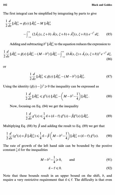
The first integral can be simplified by integrating by parts to give

12

dds

||A||2w=g(s) ||A||2w −M ||A||2w

−F.

−.(2At(s, t+b) A(s, t+b)+A2

t(s, t+b)) e−t2dt. (85)

Adding and subtracting b2 ||A||2w to the equation reduces the expression to

12

dds

||A||2w=g(s) ||A||2w −(M−b2) ||A||2w −F.

−.(bA(s, t)+At(s, t+b))2 e−t

2dt,(86)

or

12

dds

||A||2w [ g(s) ||A||2w −(M−b2) ||A||2w. (87)

Using the identity (g(s)− 12)

2 \ 0 the inequality can be expressed as

12

dds

||A||2w [ g2(s) ||A||2w −1M−b2−142 ||A||2w . (88)

Now, focusing on Eq. (84) we get the inequality

12

dds

g2(s) [14a+(a− y) g2(s)− bg2(s) ||A||2w. (89)

Multiplying Eq. (88) by b and adding the result to Eq. (89) we get that

12

dds

(g2(s)+b ||A||2w) [14a− b 1M−b2−

142 ||A||2w+(a− y) g2(s). (90)

The rate of growth of the left hand side can be bounded by the postiveconstant 1

4 a for the inequalities

M−b2−14\ 0, and (91)

a− y [ 0. (92)

Note that these bounds result in an upper bound on the shift, b, andrequire a very restrictive requirement that a [ y. The difficulty is that even


if these strict requirements are met, the bound on the growth demonstratesat most linear growth in the energy defined above.

5. RESULTS

We now present our results using two different approximations to thepulse-shaping operator of the governing equations (18) and (19). The firstapproximation is the spectral Hermite method discussed in the previoussection, while the second approximation is a finite difference method.

The finite difference scheme is implemented by mapping the infiniteline through the transformation

t=tan(h), (93)

where the parameter h is between − p2 and p

2 . A centered, second orderscheme is used for the second derivative term. Both a centered differenceand a first order, upwinding scheme is examined for the first derivativeterm.

For each pulse-shaping approximation four different temporal discre-tizations are examined. All of the temporal discretizations make use of asecond order Adams–Moulton scheme for the linear terms. The schemesdiffer, however, in the way in which the nonlinear terms are integrated:

Fully Implicit. The non-linear terms are integrated in time using asecond order Adams–Moulton scheme. At each time step the future valueis approximated using Newton–Raphson iterations on the resulting system.For example, the Hermite discretization (61) becomes

am(s+gs)−am(s)=gs2

(g(s+gs) am(s+gs)+g(s) am(s))

−(M+2m)gs2

(am(s+gs)+am(s))

−ts`8(m+1)

gs2

(am+1(s+gs)+am+1(s)),

g(s+gs)− g(s)=ags− ygs2

(g(s+gs)+g(s))

−bsgs21 g(s+gs) C

N

n=0a2n(s+gs)+g(s) C

N

n=0a2n(s)2 .(94)


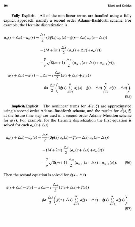
Fully Explicit. All of the non-linear terms are handled using a fullyexplicit approach, namely a second order Adams–Bashforth scheme. Forexample, the Hermite discretization is


(3g(s) am(s)− g(s−gs) am(s−gs))

−(M+2m)gs2

(am(s+gs)+am(s))

−ts`8(m+1)

gs2

(am+1(s+gs)+am+1(s)),

g(s+gs)− g(s)=ags− ygs2

(g(s+gs)+g(s))

−bsgs213g(s) C

N

n=0a2n(s)− g(s−gs) C

N

n=0a2n(s−gs)2.

(95)

Implicit/Explicit. The nonlinear terms for A(s, t) are approximatedusing a second order Adams–Bashforth scheme, and the results for A(s, t)at the future time step are used in a second order Adams–Moutlon schemefor g(s). For example, for the Hermite discretization the first equation issolved for each am(s+gs)



−(M+2m)gs2

(am(s+gs)+am(s))

−ts`8(m+1)

gs2

(am+1(s+gs)+am+1(s)). (96)

Then the second equation is solved for g(s+gs)

g(s+gs)− g(s)=ags−ygs2

(g(s+gs)+g(s))

−bsgs21 g(s+gs) C

N

n=0a2n(s+gs)+g(s) C

N

n=0a2n(s)2 .

(97)


Predictor-Corrector. The non-linear terms are integrated using apredictor-corrector method. In the first part of the scheme an approxima-tion for A(s, t) is calculated for the future time step. This value forA(s+gs, t) is then used to approximate g(s+gs) using an implicitmethod. The final step is to use the approximation for g(s+gs) using animplicit scheme to construct an updated approximation for A(s+gs, t).For example, for the Hermite discretization the first equation is solved foreach am(s+gs)



−(M+2m)gs2

(am(s+gs)+am(s))

−ts`8(m+1)

gs2

(am+1(s+gs)+am+1(s)). (98)

Then the second equation is solved for g(s+gs)

g(s+gs)− g(s)=ags−ygs2

(g(s+gs)+g(s))

−bsgs21 g(s+gs) C

N

n=0a2n(s+gs)+g(s) C

N

n=0a2n(s)2 .

(99)

Finally, this result for g(s+gs) is used to find the approximation for eacham(s+gs)


(g(s+gs) am(s+gs)+g(s) am(s))

−(M+2m)gs2

(am(s+gs)+am(s))

−ts`8(m+1)

gs2

(am+1(s+gs)+am+1(s)). (100)

5.1. Comparison of Numerical TrialsIn order to make comparisons between the numerical trials a simple

initial condition was chosen to aid in the comparison. A single ‘‘pulse’’located at t=t was chosen,

A(0, t)=e−(t− ts)2. (101)


With these initial conditions, the function A(T, t) consists of a single pulsethat evolves in time and eventually becomes centered at t=−t. Theadvantage of this choice is that a system of ordinary differential equationscan be found to describe the evolution of the single pulse [7].

With this initial condition the single pulse can be written as a functionof slow-time T as

A(T, t)=A(T) e−(t− t(T)s(T) )

2. (102)

Substituting this into Eq. (1) reduces the unknowns into the followingsystem of ordinary differential equations:

ddT

(s2(T))=2D−2ms4(T), (103)

ddT

t(T)=−C−2mt(T) s2(T), (104)

ddT

(A2(T))=2 1g(T)−mt2(T)−Ds2(T)2 A2(T), (105)

ddT

g(T)=a− yg(T)−`p bs(T) g(T) A2(T). (106)

Note that the first two equations, Eqs. (103) and (104), can be solvedanalytically. The result is a system of two ODE’s given by Eqs. (105) and(106).

The numerical approximation to the original system is compared tothe results of the approximation to this system of ODE’s. In finding anapproximation to Eqs. (105) and (106) we experienced some difficulties.Our first approach to approximating the system was to simply use theroutines available in MATLAB. A plot of the results for the gain for astraightforward application of the available methods is shown in Fig. 1.The results for the gain using the routines for a restricted time step,gT < 0.0005, and including the Jacobian of the system are shown inFig. 2.

The MATLAB routines appeared to converge to one of three differentsolutions. We also examined the solution using our own codes using a fifthorder Runga–Kutta–Fehlberg method, a fourth order Runga–Kutta method,and a second order implicit code. (An analytic solution to the implicitsystem of nonlinear equations can be found.) The codes that did not makeuse of a varying time step provided the most consistent results. Moreover,


Fig. 1. Comparison of results approximating the system of ODE’s using the availableMATLAB routines.

Fig. 2. Comparison of results approximating the system of ODE’s using the availableMATLAB routines and restricting the maximum time step.


the implicit code converged the closest to the true steady state of all thecodes. For this reason, all of the comparisons are made with respect to theimplicit code using a time step of 10−6.

The values of the parameters that were used for the comparisons were

m=1.0

C=8`2

D=1.0

a=8.0

y=0.01

b=1.0

gT=0.0001

(107)

5.2. Nonlinear, Fully Implicit Scheme

The fully implicit, nonlinear time stepping scheme makes use of a secondorder implicit scheme. At each time step the solution to the non-linear systemof equations, Eq. (61), is approximated usingNewton iterations.

At each time step a non-linear system must be approximated. Here weuse Newton steps until the residual for the system is below 10−10. As acomparison the same time stepping scheme is used for a finite differencescheme where the infinite interval is mapped to the finite interval, [− p

2 ,p2],

using the tangent function. For the finite difference approximation theintegral of A2(T, t) is approximated using a Simpsons Rule quadrature.

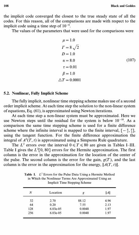
The L2 errors over the interval 0 [ T [ 80 are given in Tables I–III.Table I gives the L2[0, 80] errors for the Hermite approximation. The firstcolumn is the error in the approximation for the location of the center ofthe pulse. The second column is the error for the gain, g(T), and the lastcolumn is the error in the approximation for the energy, ||A(T, t)||.

Table I. L2 Errors for the Pulse Data Using a Hermite Methodin Which the Nonlinear Terms Are Approximated Using an

Implicit Time Stepping Scheme

N Location g ||A||

32 2.70 88.12 4.9664 0.20 7.55 2.13128 6.03e-05 0.0048 1.97256 6.03e-05 0.0048 1.97


Table II. L2 Errors for the Pulse Data Using a Finite DifferenceMethod in Which the Nonlinear Terms Are Approximated Using

an Implicit Time Stepping Scheme. The First Derivative IsApproximated Using a Centered Difference Scheme

N g ||A||

32 251.44 6.6964 174.23 5.65128 55.61 5.07256 15.07 2.49512 3.98 2.01

Tables II and III provide the errors for the finite difference schemes.The errors in Table II are for a finite difference scheme in which the firstderivative term is approximated using an upwinding scheme. The errors inTable III are for a finite difference scheme in which the first derivative isapproximated using a centered difference scheme.

A plot of the errors of the gain, g(T), for all of the fully non-linearschemes is given in Fig. 3. A greater number of discretizations has beenused for the plot than is given in the tables. The Hermite approximationconverges quickly while the finite difference schemes converge as O(N) andO(N2) for the first and second order schemes.

As an example of the difficulties encountered, Figs. 4 through 11 aregiven. Each figure represents the gain found from a given approximation.The first figures, 4 and 5, compares the approximation using a polynomialdegree of 32 with the approximation to the system of ordinary differentialequations.

The wave is not resolved leading to an innacurate approximation.Even though all of the Hermite schemes track the location of the pulse

Table III. L2 Errors for the Pulse Data Using a Finite DifferenceMethod in Which the Nonlinear Terms Are Approximated Using

an Implicit Time Stepping Scheme. The First Derivative IsApproximated Using an Upwinding Scheme

N g ||A||

32 316.29 8.3764 256.00 6.89128 161.31 5.46256 81.81 5.05512 62.75 5.16


Fig. 3. Comparison between the Hermite and finite difference approximations using thefully nonlinear, implicit scheme.

Fig. 4. Comparison between the Hermite and ODE approximations for the gain. Thirty twomodes are used for the approximation.


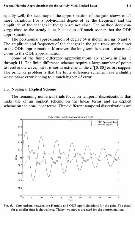
equally well, the accuracy of the approximation of the gain shows muchmore variation. For a polynomial degree of 32 the frequency and theamplitude of the changes in the gain are not close. The method does con-verge close to the steady state, but it dies off much sooner that the ODEapproximation.

The polynomial approximation of degree 64 is shown in Figs. 6 and 7.The amplitude and frequency of the changes in the gain track much closerto the ODE approximation. Moreover, the long term behavior is also muchcloser to the ODE approximation.

Some of the finite difference approximations are shown in Figs. 8through 11. The finite difference schemes require a large number of pointsto resolve the wave, but it is not as extreme as the L2[0, 80] errors suggest.The principle problem is that the finite difference schemes have a slightlyworse phase error leading to a much higher L2 error.

5.3. Nonlinear Explicit Scheme

The remaining numerical trials focus on temporal discretizations thatmake use of an implicit scheme on the linear terms and an explicitscheme on the non-linear terms. Three different temporal discretizations are

Fig. 5. Comparison between the Hermite and ODE approximations for the gain. The detailfor a smaller time is shown here. Thirty two modes are used for the approximation.


Fig. 6. Comparison between the Hermite and ODE approximations for the gain.

Fig. 7. Comparison between the Hermite and ODE approximations for the gain. The detailfor a smaller time is shown here.


Fig. 8. Comparison between the finite difference and ODE approximations for the gain. Thediscretization uses 256 points.

Fig. 9. Comparison between the finite difference and ODE approximations for the gain. Thediscretization uses 256 points. The detail for a smaller time is shown here.


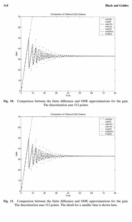
Fig. 10. Comparison between the finite difference and ODE approximations for the gain.The discretization uses 512 points.

Fig. 11. Comparison between the finite difference and ODE approximations for the gain.The discretization uses 512 points. The detail for a smaller time is shown here.


Table IV. L2 Errors for the Pulse Data Using a HermiteMethod in Which the Nonlinear Terms Are Approximated Using

a Fully Explicit Time Stepping Scheme

N Location g ||A||

32 2.84 88.12 4.9664 1.94 7.55 2.13128 6.10e-05 0.0033 1.97256 6.10e-05 0.0033 1.97512 6.10e-05 0.0033 1.97

examined. The first is a method in which the nonlinear terms in the ampli-tude equation are approximated using an explicit method, and the equationfor the gain makes use of an implicit scheme for the nonlinear terms. Thesecond is a fully explicit method where all of the non-linear terms areapproximated using an explicit method. Finally, a predictor/correctormethod is used in the third discretization.

Results are given for numerical trials using the Hermite approxima-tions. Each of the methods failed for the finite difference approximations.For each method both the centered difference and the upwinding schemewas used in the approximation. The time step that was used was reducedto 10−6. Reducing the time step allowed for a longer time before the codediverged, but all of the approximations diverged before the time t=80. Thenumber of grid points was also increased to 2048 with the smallest timestep, but all of the approximations diverged.

The L2[0, 80] for the Hermite approximations are given in Tables IV–VI.Each method returned nearly identical errors for the pulse location. The fully

Table V. L2 Errors for the Pulse Data Using a Hermite Methodin Which the Nonlinear Terms Are Approximated Using a FullyExplicit Time Stepping Scheme for the Amplitude and an Implicit

Scheme for the Gain

N Location g ||A||

32 6.03e-05 88.12 4.9664 6.03e-05 7.56 2.13128 6.03e-05 0.0050 1.97256 6.02e-05 0.0050 1.97512 6.02e-05 0.0050 1.97


Table VI. L2 Errors for the Pulse Data Using a HermiteMethod in Which the Nonlinear Terms Are Approximated Using

a Predictor/Corrector Scheme

N Location g ||A||

32 217.50 100.16 5.4164 19.90 44.29 5.37128 31.28 45.24 5.42256 31.29 45.24 5.42512 31.29 45.24 5.42

explicit method returned the smallest errors for the gain, but the predictor/corrector method returned errors that were consistantly large. A comparisonof the errors is given in the plot in Fig. 12.

Some example plots of the approximations for the gain for the explicitschemes are shown in Figs. 13 through 15. Examples of the fully explicitschemes are shown in Figs. 13 and 14. An Example of the predictor/correctormethod is shown in Fig. 15.

Each of the explicit approximations returned approximations for thegain that matched the amplitude for the changes in the gain. The difference

Fig. 12. Comparison between the different time stepping methods for the Hermite polyno-mials approxmations.


Fig. 13. Hermite approximation using a polynomial degree of 128 and the non-linear termsare approximated using a fully explicit time scheme.

Fig. 14. Hermite approximation using a polynomial degree of 128 and the non-linear termsare approximated using a fully explicit scheme. A detailed view is shown here.


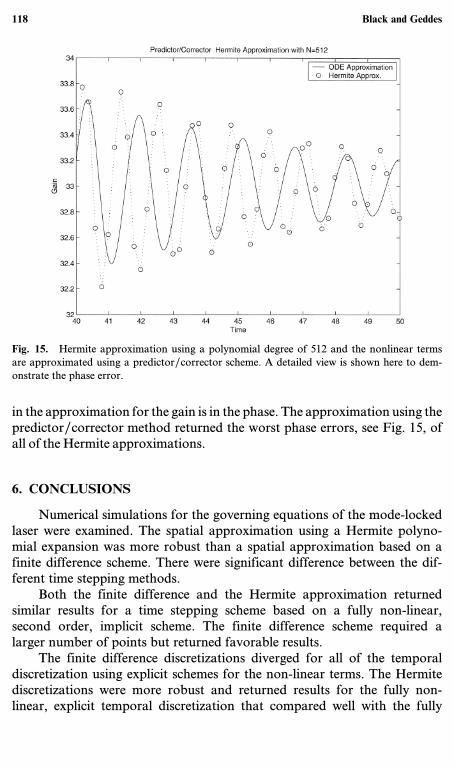
Fig. 15. Hermite approximation using a polynomial degree of 512 and the nonlinear termsare approximated using a predictor/corrector scheme. A detailed view is shown here to dem-onstrate the phase error.

in the approximation for the gain is in the phase. The approximation using thepredictor/corrector method returned the worst phase errors, see Fig. 15, ofall of the Hermite approximations.

6. CONCLUSIONS

Numerical simulations for the governing equations of the mode-lockedlaser were examined. The spatial approximation using a Hermite polyno-mial expansion was more robust than a spatial approximation based on afinite difference scheme. There were significant difference between the dif-ferent time stepping methods.

Both the finite difference and the Hermite approximation returnedsimilar results for a time stepping scheme based on a fully non-linear,second order, implicit scheme. The finite difference scheme required alarger number of points but returned favorable results.

The finite difference discretizations diverged for all of the temporaldiscretization using explicit schemes for the non-linear terms. The Hermitediscretizations were more robust and returned results for the fully non-linear, explicit temporal discretization that compared well with the fully


implicit approach. The predictor/corrector method, however, returnedsignificant phase errors.

ACKNOWLEDGMENTS

The authors would like to thank many people who played importantroles in the work detailed in this paper. First, we would like to thank DavidGottlieb for his guidance, patience and support. We would like to thankWillie Firth for his insights into the mathematical model. We would like tothank Jan Hesthaven for his insights and aid in finding other references.Finally, we would like to thank Matthew Beauregard who did all of theinitial legwork and a good deal of coding.

REFERENCES

1. Black, K. (1998). Spectral elements on infinite domains. SIAM J. Sci. Comput. 19,1667–1681 (electronic).

2. Boyd, J. (1987). Orthogonal rational functions on a semi-infinite interval. J. Comput.Phys. 70, 63–68.

3. Canuto, C., Hussaini, M. Y., Quarteroni, A., and Zang, T. A. (1988). Spectral Methods inFluid Dynamics, Springer-Verlag, New York.

4. Coulaud, O., Funaro, D., and Kavian, O. (1990). Laguerre spectral approximations ofelliptic problems in exterior domains. Comput. Methods Appl. Mech. Engrg. 80, 451–458.

5. Dunlop, A. M., Firth, W. J., and Wright, E. M. (2000). Time-domain master equation forpulse evolution and laser mode-locking. Optical and Quantum Electronics 32, 1131–1146.

6. D. Funaro (October 1989). Computational Aspects of Pseudospectral Laguerre Approxi-mations, Tech. Report NAS1-18605, ICASE, NASA Langley Research Center, HamptonVA 23665-5225.

7. J. B. Geddes and W. J. Firth (2001). Pulse Dynamics in a Mode-Locked Laser, submittedto Physical Review A.

8. B.-Y. Guo (1999). Error estimation of Hermite spectral method for nonlinear partialdifferential equations.Math. Comp. 68, 1067–1078.

9. J. M. Hopkins and W. Sibbett (2000). Ultrashort-pulse lasers: Big payoffs in a flash. Sci.Amer. 283, 72–79.

10. A. J. Jerri (1998). The Gibbs Phenomenon in Fourier Analysis, Splines and WaveletApproximations, Kluwer Academic Publishers, Dordrecht.

11. A. Karageorghis and T. N. Phillips (1987). Spectral collocation methods for Stokes flowin contraction geometries and unbounded domains. J. Comput. Phys. 80, 314–330.

12. F. X. Kartner, D. M. Zumbuhl, and N. Matuschek (1999). Turbulence in mode-lockedlasers. Phys. Rev. Lett. 82, 4428–4431.

13. Y. Maday, B. Pernaud-Thomas, and H. Vandeven (1985). Reappraisal of Laguerre typespectral methods. Rech. Aérospat. 1985, 353–375.

14. C.Mavriplis (1989). Laguerre polynomials for infinite-domain spectral elements. J. Comput.Phys. 80, 480–488.

15. A. E. Siegman (1986). Lasers, University Science Books, Mill Valley, California.


16. G. Stix (2001). The triumph of the light. Sci. Amer. 284, 80–87.17. J. A. C. Weideman (1992). The eigenvalues of Hermite and rational spectral differentia-

tion matrices. Numer. Math. 61, 409–432.18. J. A. C. Weideman and A. Cloot (1990). Spectral methods and mappings for evolution

equations on the infinite line. Comput. Methods Appl. Mech. Engrg. 80, 467–481. Spectraland high order methods for partial differential equations (Como, 1989).


Spectral Hermite Approximations for the Actively Mode-Locked Laser

Documents

Transcript of Spectral Hermite Approximations for the Actively Mode-Locked Laser