Stress-Strain Behavior for Actively Confined Concrete Using
234
Stress-Strain Behavior for Actively Confined Concrete Using Shape Memory Alloy Wires THESIS Presented in Partial Fulfillment of the Requirements for the Degree Master of Science in the Graduate School of The Ohio State University By Gordon Ray Zuboski, B.S. Graduate Program in Civil Engineering The Ohio State University 2013 Thesis Committee: Shive K. Chaturvedi, Advisor Halil Sezen Ethan Kubatko
-
Upload
khangminh22 -
Category
Documents
-
view
0 -
download
0
Transcript of Stress-Strain Behavior for Actively Confined Concrete Using

Stress-Strain Behavior for Actively Confined Concrete Using
Shape Memory Alloy Wires
THESIS
Presented in Partial Fulfillment of the Requirements for the Degree Master of Science in
the Graduate School of The Ohio State University
By
Gordon Ray Zuboski, B.S.
Graduate Program in Civil Engineering
The Ohio State University
2013
Thesis Committee:
Shive K. Chaturvedi, Advisor
Halil Sezen
Ethan Kubatko

Copyright by
Gordon Ray Zuboski
2013

ii
Abstract
Within this work a new and innovative method using shape memory allow (SMA)
wires to actively confine concrete members is discussed and further researched in great
detail. This new confinement method utilizes a constant confining pressure that is a
direct result to the SMA material being able to recover large inelastic strains with the
application of heat. Due to the extraordinary behavior that these SMAs display, this
confining method is classified as “active confinement”, which has been proven to be
superior in almost every way to the ordinary passive confinement method that is almost
exclusively used throughout the world.
In an attempt to fully understand this confinement method, great detail was spent
on accurately formulating the stress-strain relationship of confined concrete members
under certain varied parameters. To achieve this goal Mander et al. (1988)’s passive
unified stress-strain model was modified for application with SMA wires, and multiple
equations were incorporated within the model for comparison purposes to analytically
correlate the stress-strain relationship of the actively confined concrete.
Once multiple analytical formulations are shown and discussed, a medium scale
experiment was undertaken, where the compressive stress-strain relationship of 15 SMA
confined concrete cylinders was obtained. With this experimental data, the confining
effectiveness of the model was verified and the most accurate formulation was concluded
to be from equations by the Xiao et al. (2010).
This research highlights that SMAs have an endless amount of possible
applications, and due to the drastic reduction in price that has occurred in the past and
which is expected to continue to occur in the future, structural engineers need to be aware
of these alloys and continue to find innovative methods that utilizes their extraordinary
behavior. With this in mind, the confining method described within this work could do

iii
just that and eventually become the predominant structural confining method in the not so
distant future, due to the superior stress-strain relationship shown.

iv
Acknowledgements
This research project would not have been possible without the support of many
individuals. I would especially like to express gratitude to Advisor and Professor Shive
Chaturvedi, and Professor Halil Sezen for their ongoing insight, support, and invaluable
guidance throughout this project, and Professor Ethan Kubatko for severing on my thesis
committee. I would also like to acknowledge the assistance and encouragement given by
my family (Carol, David, and Whitney Zuboski) and friends (Kyle Straight, Seth Mielke,
and Ryan Hahnlen) throughout this seemingly never-ending work.

v
Vita
May 2005………………………………….Shadyside High School
June 2010………………………………….B.S. Civil Engineering, Ohio State University
April 2013…………………………………M.S. Civil Engineering, Ohio State University
Fields of Study
Major Field: Civil Engineering

vi
Table of Contents
Abstract ............................................................................................................................... ii
Acknowledgements ............................................................................................................ iv
Vita .......................................................................................................................................v
List of Tables ..................................................................................................................... xi
List of Figures .................................................................................................................. xiii
Chapter 1: Introduction & Background Information ..........................................................1
1.1 Introduction ............................................................................................................. 1
1.2 Stress-Strain Curves for Concrete Members ........................................................... 2
1.3 Importance of Ductility ........................................................................................... 5
1.4 Structural Confinement ........................................................................................... 7
1.5 Structural Confining Approaches ........................................................................... 9
1.5.1 Passive Confinement ......................................................................................... 9
1.5.1.1 Compressive Stress-Strain Behavior of Passively Confined Concrete ..... 10
1.5.2 Active Confinement ........................................................................................ 13
1.5.2.1 Compressive Stress-Strain Behavior of Actively Confined Concrete ...... 14
1.5.3 Important Distinctions between Active and Passive Confinement ................. 16
1.5.3.1 Stress-Strain Behavior .............................................................................. 16
1.5.3.2 Stress-Volumetric Strain Behavior ........................................................... 16
1.6 Objectives and Scope ............................................................................................ 18
1.7 Project Summary ................................................................................................... 20
Chapter 2: Shape Memory Alloys.....................................................................................22
2.1 Shape Memory Alloy Introduction ....................................................................... 22
2.1.1 Shape Memory Behavior ................................................................................ 23

vii
2.1.2 SMA Transformation Temperatures ............................................................... 26
2.1.3 SMA Mechanical Properties ........................................................................... 30
2.1.4 Free or Constrained Recovery ........................................................................ 31
2.1.5 Prestrain Losses .............................................................................................. 32
2.2 SMA Active Confinement Application Procedure for Concrete Specimens ........ 33
2.3 SMA Classifications ............................................................................................. 34
2.3.1 SMA Hysteresis Loop ..................................................................................... 36
Chapter 3: Literature Review ............................................................................................38
3.1 Relevant Research Dealing with Stress-Strain Modeling of Confined Concrete . 38
3.2 Relevant Research Dealing with Shape Memory Alloy Confinement ................. 40
3.2.1 SMA Confinement Essential Findings............................................................ 44
3.2.2 Critiques of Past Findings ............................................................................... 45
Chapter 4: Analytical Models and Their Assessment toward SMA Confined Concrete
Columns .............................................................................................................................47
4.1 Mander’s Model Introduction ............................................................................... 47
4.2 Mander et al. (1988) Stress-Strain Model ............................................................. 47
4.2.1 Required Modifications of Mander’s Model for SMA Confinement ............. 49
4.2.2 Andrawes et al. (2010) SMA Adapted Model ................................................ 50
4.3 Analytical SMA Confined Stress-Strain Relationships ........................................ 51
4.3.1 Stress-Strain Relationship Using Mander et al. Modified Model for SMA
Confinement .................................................................................................... 51
4.4 Recently Developed Analytical Equations for Active Confinement .................... 57
4.4.1 Peak Stress Equation Using Mohr-Coulomb Failure Criterion ...................... 57
4.4.2 Axial Strain at Peak Stress Equation .............................................................. 62
4.4.3 Active-Confinement Model for all Concrete Strengths .................................. 64
4.5 Stress-Strain Relationship Formulated from Various Active Confinement Models
............................................................................................................................. 68

viii
4.5.1 Analytical Assessments .................................................................................. 73
Chapter 5: Experimental Testing Program for Correlations with the SMA Confined
Models................................................................................................................................75
5.1 Introduction ........................................................................................................... 75
5.2 Experimental Objective ........................................................................................ 75
5.3 Experimental Procedure ........................................................................................ 76
5.4 Experimental Testing Materials ............................................................................ 77
5.4.1 SMA Material (Flexinol) Introduction............................................................ 78
5.4.2 Flexinol Recovery Stress ................................................................................ 80
5.4.3 Flexinol Recovery Stress at Varying Levels of Strain .................................... 85
5.4.4 Flexinol Mechanical Properties ...................................................................... 86
5.4.5 Concrete Mix Proportions and the Cylindrical Specimens ............................. 86
5.5 SMA Wire Attachment Method ............................................................................ 88
5.6 Testing Equipment ................................................................................................ 93
5.6.1 Compressive Load Frame ............................................................................... 93
5.6.2 Flexinol Electrical Guidelines and Required Power Supply ........................... 95
5.7 Experimental Obstacles ........................................................................................ 97
Chapter 6: Experimental Results from SMA Confined Concrete ....................................104
6.1 Introduction ......................................................................................................... 104
6.2 Concrete Batch #1 ............................................................................................... 106
6.2.1 Unconfined Concrete Specimens .................................................................. 106
6.2.2 Confined Concrete Specimens ...................................................................... 108
6.2.2.1 SMA Confined 1/3rd
Inch Pitch Specimens ............................................ 109
6.2.2.2 SMA Confined 1/5th
Inch Pitch Specimens ............................................ 115
6.3 Concrete Batch #2 ............................................................................................... 118
6.3.1 Unconfined Concrete Specimens .................................................................. 118
6.3.2 Confined Concrete Specimens ...................................................................... 120
6.3.2.1 SMA Confined 1/3rd
inch Pitch Specimens ............................................ 120

ix
6.3.2.2 SMA Confined 1/5th
inch Pitch Specimens ............................................ 123
6.4 Concrete Batch #3 ............................................................................................... 126
6.4.1 Unconfined Concrete Specimens .................................................................. 126
6.4.2 Confined Concrete Specimens ...................................................................... 127
6.4.2.1 SMA Confined 1/3rd
inch Pitch Specimens ............................................ 127
6.4.2.2 SMA Confined 1/5th
inch Pitch Specimens ............................................ 130
6.5 Experimental Results Summary .......................................................................... 133
6.5.1 Concrete Batch #1 ......................................................................................... 133
6.5.2 Concrete Batch #2 ......................................................................................... 135
6.5.3 Concrete Batch #3 ......................................................................................... 136
6.6 Concluding Remarks ........................................................................................... 137
6.6.1 Experimental Correlations ............................................................................ 138
Chapter 7: Numerical Example to Show the Effect of SMA Confinement .....................139
7.1 Numerical Example Introduction ........................................................................ 139
7.2 Given Information ............................................................................................... 139
7.3 Numerical Results ............................................................................................... 141
Chapter 8: Conclusions and Suggestions for Future Research ........................................147
8.1 Overall Conclusions ............................................................................................ 147
8.2 Future Research .................................................................................................. 147
References ........................................................................................................................149
Appendix A: Mander’s Model ........................................................................................152
A.1 Mander’s et al. (1988) Stress-Strain Model ....................................................... 152
A.2 Ultimate Concrete Compressive Strain .............................................................. 156
Appendix B: Notations ...................................................................................................160
B.1 Notations ............................................................................................................ 160
Appendix C: Experimental Correlations with SMA Confinement Models .....................162
C.1 Concrete Batch #1 .............................................................................................. 162

x
C.1.1 SMA Confined 1/3rd
inch Pitch Specimens.................................................. 162
C.1.2 SMA Confined 1/5th
inch Pitch Specimens .................................................. 169
C.2 Concrete Batch #2 .............................................................................................. 171
C.2.1 SMA Confined 1/3rd
inch Pitch Specimens.................................................. 172
C.2.2 SMA Confined 1/5th
inch Pitch Specimens .................................................. 174
C.3 Concrete Batch #3 .............................................................................................. 176
C.3.1 SMA Confined 1/3rd
inch Pitch Specimens.................................................. 176
C.3.2 SMA Confined 1/5th
inch Pitch Specimens .................................................. 178
C.4 RMSD Values Obtained ..................................................................................... 180
C.5 Concluding Remarks .......................................................................................... 181
C.5.1 Assessment of the Confinement Model and Experimental Correlations ..... 181
Appendix D: Matlab Codes .............................................................................................184
D.1 Code for Unconfined Concrete Stress-Strain Relationship................................ 184
D.2 Code for Steel Stress-Strain Relationship .......................................................... 185
D.3 Typical Code Displaying the Formulated Stress-Strain Relationship of SMA
Confined Concrete for All Models .................................................................... 185
D.4 Typical Code Displaying the Results from the Numerical Example Predicting the
Stress-Strain and Load vs. Displacement for the 12 inch Spaced SMA Column
........................................................................................................................... 194
Appendix E: As Measured Stress-Strain Plots.................................................................200

xi
List of Tables
Table 2.1. Mechanical Properties of Ni-Ti Alloys under Tension (Manach and Favier
1997; Otsuka and Wayman 1999; Rejzner et al. 2002; & DesRoches et al.
2004) ............................................................................................................... 30
Table 4.1. Values of the Experimentally Determined Constant k1, for Varying
Confinement Levels. ....................................................................................... 59
Table 4.2. Equations for Compressive Strength (Peak Stress) of Confined Concrete ...... 61
Table 4.3. Equations for Axial Strain at Peak Stress of Actively Confined Concrete ...... 64
Table 5.1. Mechanical Properties of Flexinol SMA Wire Listing Both Expected Results
from the Manufactures and Experimentally Verified Results. ....................... 86
Table 5.2. Concrete Mix Proportions Used, Displaying the Amounts in Percentages,
Along with the Average Compressive Strength Values Obtained for Each of
the Three Batches. ........................................................................................... 87
Table 5.3. Concrete Specimen Test Matrix, Displaying Total Number of Specimens
Tested and Corresponding Confining Level ................................................... 88
Table 5.4. Flexinol Electrical Wire Guidelines ................................................................ 96
Table 6.1. Stress-Strain Values from Concrete Batch #1 1/3rd
inch Pitch SMA Confined
Cylinders ....................................................................................................... 113
Table 6.2. Stress-Strain Values from Concrete Batch #1 1/5th
inch Pitch SMA Confined
Cylinders ....................................................................................................... 117
Table 6.3. Stress-Strain Values from Concrete Batch #2 1/3rd
inch Pitch SMA Confined
Cylinders ....................................................................................................... 122
Table 6.4. Stress-Strain Values from Concrete Batch #2 1/5th
inch Pitch SMA Confined
Cylinders ....................................................................................................... 125
Table 6.5. Stress-Strain Values from Concrete Batch #3 1/3rd
inch Pitch SMA Confined
Cylinders ....................................................................................................... 129
Table 6.6. Stress-Strain Values from Concrete Batch #3 1/5th
inch Pitch SMA Confined
Cylinders ....................................................................................................... 132
Table 6.7. Experimental Obtained Data from the Specimens of Concrete Batch #1 ...... 135
Table 6.8. Experimental Obtained Data from the Specimens of Concrete Batch #2 ...... 136

xii
Table 6.9. Experimental Obtained Data from the Specimens of Concrete Batch #3 ...... 137
Table 7.1. Mechanical Properties of Longitudinal Steel (Ordinary) Used in Example .. 140
Table 7.2. Mechanical Properties of Transvers SMA Spiral Used in Example .............. 140
Table 7.3. Stress versus Strain Values and Percent Increases from Figure 7.2. ............. 143
Table 7.4. Load versus Displacement Values and Percent Increases from Figure 7.3. .. 146
Table C.1. Summary of RMSD Values Obtained ........................................................... 181

xiii
List of Figures
Figure 1.1. Stress-Strain Relationship for Typical Unconfined Concrete (4000 psi Max
Compressive Strength) .................................................................................... 4
Figure 1.2. Typical Energy Dissipated for A.) Brittle Failure. B.) Ductile Failure ............ 6
Figure 1.3. Stress versus Radial and Axial Strain for both Confined and Unconfined
Concrete Cylinders. (Andrawes et al. 2010) .................................................. 7
Figure 1.4. Schematic of Stress-Strain Curves of Passively Confined Concrete Specimens
(Moghaddam et al. 2010) .............................................................................. 11
Figure 1.5. Conventional Passive Confinement and Active Confinement before Axial
Loads are Applied (Shin and Andrawes 2009) .............................................. 13
Figure 1.6. Schematic of Stress-Strain Curves of Actively Confined Concrete Specimens
(Moghaddam et al. 2010) .............................................................................. 15
Figure 1.7. Schematics of the Cross Section of Confined Concrete Before Loading (A &
B) and Stress versus Volumetric Strain Curves of Unconfined, Passively, and
Actively Confined Concrete (C). (Shin and Andrawes 2009) ....................... 18
Figure 2.1. Schematic Illustration of Change in Crystalline Structure between Austenite,
Martensite (Twinned), and Deformed (Detwinned) Martensite States With
Respect to Temperature (Borden 1990) ........................................................ 25
Figure 2.2. Physical Representation of a SMA Spring, Showing All Possible Phase
Changes Due to Temperature and Deformation. ........................................... 26
Figure 2.3. Typical SMA (A) Thermal Hysteresis. (B) Thermo-Mechanical Behavior
(Shin and Andrawes 2009) ............................................................................ 28
Figure 2.4. Typical SMA Stress versus Temperature Phase Diagram. ............................. 29
Figure 2.5. Schematic of Concrete Samples Confined with Shape Memory Alloy Wire.
(A) Confined Element Displaying Active Pressure, (B) SMA Confinement
Representation before Heating, and (C) SMA Confinement Representation
after Heating. (Shin and Andrawes 2009) ..................................................... 34
Figure 2.6 Location of the Hysteresis Loop Relative to Ambient Temperature for (A)
Type 1 SMA (B) Type 2 SMA (C) Type 3 SMA .......................................... 36

xiv
Figure 4.1. Stress-Strain Relationship Formulated for Various SMA Spacing
Configurations Using Mander’s Original Model Modified for Active
Confinement (4000 psi Confined Concrete with SMA Recovery Stress of
116,000 psi) ................................................................................................... 53
Figure 4.2. Stress-Strain Relationship Formulated for Various SMA Recovery Stresses
Using Mander’s Original Model Modified for Active Confinement (4000 psi
Confined Concrete with 1/3rd
inch SMA Pitch) ............................................ 54
Figure 4.3. Stress-Strain Relationship Formulated for Various Concrete Strengths Using
Mander’s Original Model Modified for Active Confinement (SMA Recovery
Stress of 116000 psi with 1/3rd
inch SMA Pitch) .......................................... 56
Figure 4.4. Percent Compressive Strength Increase Using Mander’s Model for Various
Unconfined Concrete Strengths Due to SMA Confinement (SMA Recovery
Stress of 116000 psi with 1/3rd
inch SMA Pitch) .......................................... 56
Figure 4.5. Approximate Values for the Constant k1 Using Mohr-Coulomb Failure
Criterion Based on the Confinement Level (Results from Dahl (1992b),
Ansari and Li (1998), and Candappa et al. (2001)) ....................................... 60
Figure 4.6. Axial Strain at Peak Stress versus Level of Confinement (Candappa et al.
2001) .............................................................................................................. 63
Figure 4.7. Peak Axial Stress of Actively Confined Concrete (Xiao et al. 2010) ............ 66
Figure 4.8. Axial Strain at Peak Axial Stress of Actively Confined Concrete (Xiao et al.
2010) .............................................................................................................. 67
Figure 4.9. Lightly Confined Stress-Strain Relationship Formulate from Various
Investigators (4000 psi Unconfined Concrete Strength, 116 ksi SMA
Recovery Stress, 1/3rd
inch Pitch) ................................................................. 69
Figure 4.10. Lightly Confined Stress-Strain Relationships Formulated by Various
Investigators (4000 psi Unconfined Concrete Strength, 116 ksi SMA
Recovery Stress, 1/5th
inch Pitch) ................................................................. 71
Figure 4.11. Lightly Confined Stress-Strain Relationships Formulated by Mander, Xiao,
and Moghaddam (4000 psi Unconfined Concrete Strength, 116 ksi SMA
Recovery Stress, 1/3rd
inch Pitch) ................................................................. 72
Figure 4.12. Lightly Confined Stress-Strain Relationship Formulated for Mander, Xiao,
and Moghaddam (4000 psi Unconfined Concrete Strength, 116 ksi SMA
Recovery Stress, 1/5th
inch Pitch) ................................................................. 72
Figure 5.1. Temperature versus Strain (%) for Flexinol SMA Wire (Low and High
Temperature Alloys) (Dynalloy, Inc. Makers of Dynamic Alloys) .............. 80
Figure 5.2. Flexinol Constrained Recovery Stress (Test #1), Plotting Temperature (°F)
versus Force (Lbs). ........................................................................................ 82
Figure 5.3. Flexinol Constrained Recovery Stress (Test #1) Plotting Temperature (°F)
versus Stress (MPa). ...................................................................................... 82

xv
Figure 5.4. Flexinol Constrained Recovery Stress (Test #2), Plotting Temperature (°F)
versus Force (Lbs.). ....................................................................................... 83
Figure 5.5. Flexinol Constrained Recovery Stress (Test #2), Plotting Temperature (°F)
versus Stress (MPa). ...................................................................................... 84
Figure 5.6. U-Clamp Attachment Method ........................................................................ 90 Figure 5.7. Nut and Bolt Attachment Method .................................................................. 91
Figure 5.8. Tapcon Concrete Anchor Attachment Method ............................................... 92
Figure 5.9. General Experimental Layout and Equipment Layout Used Within This
Experiment ................................................................................................... 94
Figure 5.10. 1 inch LVDT and Lever Arm Used for Displacement Measurements ......... 95
Figure 5.11. Mastech 250 Volt 12A Variable Transformer Used to Heat Flexinol SMA
Wire ............................................................................................................. 97
Figure 5.12. Visual Depiction of Concrete Anchor Screws and Metal End Cap Interaction
................................................................................................................... 101
Figure 5.13. Metal Ends Caps (Original and Altered) Used During the Experiments ... 101
Figure 5.14. Typical SMA Confined Concrete Cylinder Ready for Compressive Testing.
................................................................................................................... 102
Figure 5.15. Concrete Anchor Screw and Typical Length of Extra Flexinol Wire Used for
Connection Purposes.................................................................................. 103
Figure 5.16. Power Supply/Flexinol SMA Wire Electrical Connections After Detaching
Occurrence ................................................................................................. 103
Figure 6.1. Recorded (As Measured) Stress versus Strain for the First Unconfined
Anchored Cylinder in Concrete Batch #1. ................................................. 105
Figure 6.2. Stress versus Strain for the First Unconfined Anchored Cylinder in Concrete
Batch #1. Plot Adjusted by Shifting the Curve 0.0032 towards the Origin.
................................................................................................................... 106
Figure 6.3. Stress versus Strain Results for Both Unconfined and Unconfined Anchored
Concrete Cylinders and the Resulting Average Relationship, from Concrete
Batch #1. .................................................................................................... 108
Figure 6.4. Experimental and Approximated Stress versus Strain Relationship for
1/3rd
inch Pitch SMA (Recovery Stress 800MPa), Confined Cylinder #1,
from Concrete Batch #1 (Compressive Strength 3068 psi) (Plot Adjusted
towards the Origin by 0.0016). .................................................................. 110
Figure 6.5. Experimental and Approximated Stress versus Strain Relationship for
1/3rd
inch Pitch SMA (Recovery Stress 800MPa), Confined Cylinder #2,
from Concrete Batch #1 (Compressive Strength 3068 psi) (Plot Adjusted
towards the Origin by 0.00277). ................................................................ 111

xvi
Figure 6.6. Experimental and Approximated Stress versus Strain Relationship for
1/3rd
inch Pitch SMA (Recovery Stress 800MPa), Confined Cylinder #3,
from Concrete Batch #1 (Compressive Strength 3068 psi) (Plot Adjusted
towards the Origin by 0.0016). .................................................................. 112
Figure 6.7. Experimental and Approximated Average (Cylinders 1-3) Stress versus
Strain Relationship for 1/3rd
inch Pitch SMA (Recovery Stress 800MPa),
Confined Cylinders from Concrete Batch #1 (Compressive Strength 3068
psi).............................................................................................................. 113
Figure 6.8. Experimental Average Stress versus Strain Relationship for Unconfined
Concrete and 1/3rd
inch Pitch SMA (Recovery Stress 800MPa), Confined
Cylinders from Concrete Batch #1 (Compressive Strength 3068 psi). ...... 115
Figure 6.9. Experimental and Approximated Average (Cylinders 1 and 2) Stress versus
Strain Relationship for 1/5th
inch Pitch SMA (Recovery Stress 800MPa),
Confined Cylinders from Concrete Batch #1 (Compressive Strength 3068
psi).............................................................................................................. 117
Figure 6.10. Experimental Average Stress versus Strain Relationship for Unconfined
Concrete and 1/5th
inch Pitch SMA (Recovery Stress 800MPa), Confined
Cylinders from Concrete Batch #1 (Compressive Strength 3068 psi). ...... 118
Figure 6.11. Stress versus Strain Results for Both Unconfined and Unconfined Anchored
Concrete Cylinders and the Resulting Average Relationship, from Concrete
Batch #2. .................................................................................................... 120
Figure 6.12. Experimental and Approximated Average (Cylinders 1-3) Stress versus
Strain Relationship for 1/3rd
inch Pitch SMA (Recovery Stress 800MPa),
Confined Cylinders from Concrete Batch #2 (Compressive Strength 4563
psi).............................................................................................................. 122
Figure 6.13. Experimental Average Stress versus Strain Relationship for Unconfined
Concrete and 1/3rd
inch Pitch SMA (Recovery Stress 800MPa), Confined
Cylinders from Concrete Batch #2 (Compressive Strength 4563 psi). ...... 123
Figure 6.14. Experimental and Approximated Average (Cylinders 1 & 2) Stress versus
Strain Relationship for 1/5th
inch Pitch SMA (Recovery Stress 800MPa),
Confined Cylinders from Concrete Batch #2 (Compressive Strength 4563
psi). ........................................................................................................... 125
Figure 6.15. Experimental Average Stress versus Strain Relationship for Unconfined
Concrete and 1/5th
inch Pitch SMA (Recovery Stress 800MPa), Confined
Cylinders from Concrete Batch #2 (Compressive Strength 4563 psi). .... 126
Figure 6.16. Stress versus Strain Results for Both Unconfined and Unconfined Anchored
Concrete Cylinders and the Resulting Average Relationship, from Concrete
Batch #3. ................................................................................................... 127

xvii
Figure 6.17. Experimental and Approximated Average (Cylinders 1-3) Stress versus
Strain Relationship for 1/3rd
inch Pitch SMA (Recovery Stress 800MPa),
Confined Cylinders from Concrete Batch #3 (Compressive Strength 3693
psi). ........................................................................................................... 129
Figure 6.18. Experimental Average Stress versus Strain Relationship for Unconfined
Concrete and 1/3rd
inch Pitch SMA (Recovery Stress 800MPa), Confined
Cylinders from Concrete Batch #3 (Compressive Strength 3693 psi). .... 130
Figure 6.19. Experimental and Approximated Average (Cylinders 1 & 2) Stress versus
Strain Relationship for 1/5th
inch Pitch SMA (Recovery Stress 800MPa),
Confined Cylinders from Concrete Batch #3 (Compressive Strength 3693
psi). ........................................................................................................... 132
Figure 6.20. Experimental Average Stress versus Strain Relationship for Unconfined
Concrete and 1/5th
inch Pitch SMA (Recovery Stress 800MPa), Confined
Cylinders from Concrete Batch #3 (Compressive Strength 3693 psi). .... 133
Figure 6.21. Experimental Average Stress versus Strain Relationships for the
Unconfined, 1/3rd
inch Pitch SMA Confined, and 1/5th
inch Pitch SMA
(Recovery Stress 800MPa), Confined Cylinders for Concrete Batch #1. 134
Figure 6.22. Experimental Average Stress versus Strain Relationships for the
Unconfined, 1/3rd
inch Pitch SMA Confined, and 1/5th
inch Pitch SMA
(Recovery Stress 800MPa), Confined Cylinders for Concrete Batch #2. 136
Figure 6.23. Experimental Average Stress versus Strain Relationships for the
Unconfined, 1/3rd
inch .............................................................................. 137
Figure 7.1. Stress-Strain Relationship for the Longitudinal Steel Based on the Given
Information from the Numerical Example. ................................................. 141
Figure 7.2. Stress versus Strain Relationship for Varying Degrees of Transverse
Reinforcement ............................................................................................. 143
Figure 7.3. Load versus Displacement Relationship for Varying Degrees of Transverse
Reinforcement ............................................................................................. 144
Figure 7.4. Enhanced Load versus Displacement Relationship for Varying Degrees of
Transverse Reinforcement ........................................................................... 144
Figure A.1. Effectively Confined Core for Circular Hoop Reinforcement (Mander et al.
1988) ............................................................................................................ 154
Figure A.2. Stress-Strain Model Proposed For Monotonic Loading of Confined and
Unconfined Concrete by Mander et al. (1988) ............................................ 157
Figure C.1. Stress versus Strain Relationships, Formulated by Select Models and the
Experimentally Determined Descending Average for 1/3rd
inch Pitch SMA
(Recovery Stress 800MPa), Confined Batch #1 Concrete Cylinders. ......... 163

xviii
Figure C.2. Stress versus Strain Relationships, Based on the Model by Mander et al.
(1988) and the Experimentally Determined Adjusted Descending Average for
1/3rd
inch Pitch SMA (Recovery Stress 800MPa), Confined Batch #1
Concrete Cylinders. ..................................................................................... 167
Figure C.3. Stress versus Strain Relationships, Based on the Model by Xiao et al. (2010)
and the Experimentally Determined Adjusted Descending Average for 1/3rd
inch Pitch SMA (Recovery Stress 800MPa), Confined Batch #1 Concrete
Cylinders...................................................................................................... 168
Figure C.4. Stress versus Strain Relationships, Based on the Model by Moghaddam et al.
(2010) and the Experimentally Determined Adjusted Descending Average for
1/3rd
inch Pitch SMA (Recovery Stress 800MPa), Confined Batch #1
Concrete Cylinders. ..................................................................................... 169
Figure C.5. Stress versus Strain Relationship Formulated by Select Models for 1/5th
inch
Pitch SMA (Recovery Stress 800MPa), Confined Batch #1 Concrete
Cylinders...................................................................................................... 170
Figure C.6. Stress versus Strain Relationships, Formulated by Select Models and the
Experimentally Determined Descending Average for 1/3rd
inch Pitch SMA
(Recovery Stress 800MPa), Confined Batch #2 Concrete Cylinders. ......... 172
Figure C.7. Stress versus Strain Relationships, Formulated by Select Models and the
Experimentally Determined Descending Average for 1/5th
inch Pitch SMA
(Recovery Stress 800MPa), Confined Batch #2 Concrete Cylinders. ......... 175
Figure C.8. Stress versus Strain Relationships, Formulated by Select Models and the
Adjusted Experimentally Determined Descending Average for 1/3rd
inch
Pitch SMA (Recovery Stress 800MPa), Confined Batch #3 Concrete
Cylinders...................................................................................................... 177
Figure C.9. Stress versus Strain Relationships, Formulated by Select Models and the
Adjusted Experimentally Determined Descending Average for 1/5th
inch
Pitch SMA (Recovery Stress 800MPa), Confined Batch #3 Concrete
Cylinders...................................................................................................... 179
Figure E.1. Recorded Stress versus Strain for the First Unconfined Cylinder in Concrete
Batch #1. ...................................................................................................... 200
Figure E.2. Recorded Stress versus Strain for the Second Unconfined Cylinder in
Concrete Batch #1. ...................................................................................... 201
Figure E.3. Recorded Stress versus Strain for the First Unconfined Anchored Cylinder in
Concrete Batch #1. ...................................................................................... 201
Figure E.4. Recorded Stress versus Strain for the Second Unconfined Anchored Cylinder
in Concrete Batch #1. .................................................................................. 202
Figure E.5. Recorded Stress versus Strain for the First 1/3rd
inch Pitch SMA Confined
Cylinder in Concrete Batch #1. ................................................................... 202

xix
Figure E.6. Recorded Stress versus Strain for the Second 1/3rd
inch Pitch SMA Confined
Cylinder in Concrete Batch #1. ................................................................... 203
Figure E.7. Recorded Stress versus Strain for the Third 1/3rd
inch Pitch SMA Confined
Cylinder in Concrete Batch #1. ................................................................... 203
Figure E.8. Recorded Stress versus Strain for the First 1/5th
inch Pitch SMA Confined
Cylinder in Concrete Batch #1. ................................................................... 204
Figure E.9. Recorded Stress versus Strain for the Second 1/5th
inch Pitch SMA Confined
Cylinder in Concrete Batch #1. .................................................................. 204
Figure E.10. Recorded Stress versus Strain for the First Unconfined Cylinder in Concrete
Batch #2. .................................................................................................... 205
Figure E.11. Recorded Stress versus Strain for the Second Unconfined Cylinder in
Concrete Batch #2. ..................................................................................... 205
Figure E.12. Recorded Stress versus Strain for the First Unconfined Anchored Cylinder
in Concrete Batch #2. ............................................................................... 206
Figure E.13. Recorded Stress versus Strain for the Second Unconfined Anchored
Cylinder in Concrete Batch #2. ................................................................ 206
Figure E.14. Recorded Stress versus Strain for the First 1/3rd
inch Pitch SMA Confined
Cylinder in Concrete Batch #2. ................................................................ 207
Figure E.15. Recorded Stress versus Strain for the Second 1/3rd
inch Pitch SMA
Confined Cylinder in Concrete Batch #2. ................................................ 207
Figure E.16. Recorded Stress versus Strain for the Third 1/3rd
inch Pitch SMA Confined
Cylinder in Concrete Batch #2. ................................................................ 208
Figure E.17. Recorded Stress versus Strain for the First 1/5th
inch Pitch SMA Confined
Cylinder in Concrete Batch #2. ................................................................ 208
Figure E.18. Recorded Stress versus Strain for the Second 1/5th
inch Pitch SMA
Confined Cylinder in Concrete Batch #2. ................................................ 209
Figure E.19. Recorded Stress versus Strain for the First Unconfined Cylinder in Concrete
Batch #3. ................................................................................................... 209
Figure E.20. Recorded Stress versus Strain for the Second Unconfined Cylinder in
Concrete Batch #3. ................................................................................... 210
Figure E.21. Recorded Stress versus Strain for the First Unconfined Anchored Cylinder
in Concrete Batch #3. ............................................................................... 210
Figure E.22. Recorded Stress versus Strain for the Second Unconfined Anchored
Cylinder in Concrete Batch #3. ................................................................ 211
Figure E.23. Recorded Stress versus Strain for the First 1/3rd
inch Pitch SMA Confined
Cylinder in Concrete Batch #3. ................................................................ 211
Figure E.24. Recorded Stress versus Strain for the Second 1/3rd
inch Pitch SMA
Confined Cylinder in Concrete Batch #3. ................................................ 212

xx
Figure E.25. Recorded Stress versus Strain for the Third 1/3rd
inch Pitch SMA Confined
Cylinder in Concrete Batch #3. ................................................................ 212
Figure E.26. Recorded Stress versus Strain for the First 1/5th
inch Pitch SMA Confined
Cylinder in Concrete Batch #3. ................................................................ 213
Figure E.27. Recorded Stress versus Strain for the Second 1/5th
inch Pitch SMA
Confined Cylinder in Concrete Batch #3. ................................................ 213

1
Chapter 1: Introduction & Background Information
1.1 Introduction
The potential high recovery stress associated with shape memory alloy (SMA)
wires, can make them a very useful material for application of active confinement on
concrete structural members. The active confining pressure that results from the SMA
confinement has been proven superior to the conventional passive confinement method
that is widely used throughout the world and much easier to apply then many other active
confinement methods that often require large mechanical devices to apply post-tension
forces. However, active confinement of concrete members using prestressed SMA wires
is a relatively new concept within the structural engineering community and the amount
of experimental research is extremely limited, severely restricting the possibility for real
world applications. It should also be noted, that the research that does currently exist for
this topic has generally been focused on validating the confining potential under optimum
scenarios. While these early results have been very promising in proving the
effectiveness of SMAs for confining applications, very little research if any, has been
conducted on situations that would be representative of real world applications. These
tests, representing the so called real world applications, will be the next step in the overall
process and will be required to demonstrate the confinement potential under lower and
more cost effective confinement ratios.
Within this work, multiple topics dealing with confinement of concrete members
will be discussed, such as: the overall importance of structural confinement, the
difference between active and passive confinement in both general application and the
resulting stress-strain relationships, a detailed introduction for SMAs describing all
necessary background information and their confining potential, and a detail description
of Mander’s et al. (1988) confinement model along with some results from other
2
important models recently developed for active confinement situations. With this
background information, the stress-strain relationship for SMA actively confined
concrete specimens were analytically evaluated and used to show the possible variations
that can occur depending on various parameters. These parameters include: the spacing of
the confining material (confinement ratio), the recovery stress of the SMA wire used, the
unconfined concrete strength, and the applicable equations that are used to describe the
confined concrete stress-strain behavior.
With all of the analytical formulations characterized and analyzed, the actively
confined stress-strain relationships were then experimentally tested in an attempt to
verify, and/or readjust the characteristic relations (if needed) to be as accurate as possible.
With the experimentally verified stress-strain relationships, the results were then used to
describe the stress-strain behavior of full scale SMA actively confined reinforced
concrete members. This was done in an attempt to further aid the understanding and
development for real world applications of SMA confined concrete members.
1.2 Stress-Strain Curves for Concrete Members
The relationship between the stress and strain that a particular material displays is
known as that material’s stress-strain curve. This curve is unique for each material and is
found by recording the amount of strain or deformation at distinct intervals of stress, with
respect to the original specimen’s cross-sectional area and length. These curves reveal
important properties of the material such as the modulus of elasticity (E), yield stress (in
metallic materials), ultimate strength, and ultimate strain, but more importantly is the
fundamental information required for advanced engineering applications, such as
moment-curvature analysis which gives an indication of the available flexural strength
and ductility.
With concrete being a brittle material its ductility is severely lower than that of
steel, however it still exhibits considerable deformation before failure. To obtain an
approximation of the complete deformation potential, a displacement or strain controlled
compressive test is preferred as opposed to a load control method. With the strain
controlled method the concrete specimen is compressed at a constant displacement rate;
meaning that the overall displacement will remain fairly constant but the stress applied

3
will vary throughout the loading procedure. If the compressive stress applied to the
concrete member is done with a load control rate, the specimen will fail shortly after the
peak stress value is reached and display only the ascending portion of the stress-strain
relationship of the concrete specimen leaving out important information detailing the
post-peak relationship.
A typical stress-strain relationship for an unconfined concrete member (4000 psi
concrete) is shown in Figure 1.1 below. From this typical relationship it can be seen that
with the application of compressive force, the stress will increase with an initial linear
portion that exist up to about 30-40% of the ultimate load. This will be followed by a
non-linear portion where large strains will occur for small increments of stress until the
peak stress is reached. The non-linearity portion of this curve is primarily due to cracks
forming within the concrete. These cracks start with the formation of microcracks at the
paste-aggregate interface, followed by cracking within the cement paste matrix with
increasing stresses, until the cracks eventually increase in size and severity. This causes a
network of large cracks to develop, continually reducing the load carrying capacity until
the peak stress of the member is reached.

4
Figure 1.1. Stress-Strain Relationship for Typical Unconfined Concrete (4000 psi Max
Compressive Strength)
Due to the fact that concrete displays a behavior known as “strain-softening”,
which indicates a reduction in stress beyond the peak value with an increase in the strain.
Obtaining the complete stress-strain relationship is difficult, but it is often necessary
because an understanding of the complete (ascending and descending) stress-strain
behavior of concrete is essential for accurate constitutive modeling (approximation of the
response of a certain material to external forces). It should also be noted that the
ascending portion of the axial stress-strain curve provides key material parameters such
as the Young’s modulus, while the descending or softening portion gives an indication of
the ductility of the concrete (Attard and Setunge 1996). For unconfined concrete the
descending portion of the stress-strain curve is often approximated simply with a
decreasing linear line until the ultimate compressive strain value of 0.004 (inch/inch) or a
larger value is reached and the unconfined specimen is assumed to be completely crushed
and unable to support further loads.

5
1.3 Importance of Ductility
The ability of a member to deform under stress is known as ductility and it is a
very important quality within structural engineering. Past research has shown that
ductility is comparable to strength in the overall importance of structures and should be
incorporated within both individual components and the entire structural configuration.
The main goal for most structural design is to achieve a strong yet ductile
structure. A structure meeting the overall strength and ductility requirements assures that
the capacity of the structure is greater than the overall demand and allows the members to
deform plastically, yet still carry the load. This permits overloaded parts of the structure
to yield (plastically deform) but still redistribute stress without experiencing failure. The
concept of ductility is significant because it prevents progressive and disproportionate
collapses by ensuring that moment redistribution can occur if localized failure arises.
Achieving ductility is partly a matter of design and partly a matter of detailing.
Therefore, over the years most structural codes have been designed to assure a level of
useful ductility by strict detailing procedures.
The most important design consideration for ductility within reinforced concrete
columns is the provision of sufficient transverse reinforcement in the form of spirals or
circular hoops, or rectangular arrangements of steel; depending on the shape of the
original columns. This transverse reinforcement is essential in order to confine the
compressed concrete, prevent buckling of the longitudinal bars, and prevent shear failure
of the structural member.
It is well known that ductile materials exhibit large strains and yielding (when
dealing with most metals such as steel) before the specimen ruptures. On the contrary,
brittle materials fail suddenly and without much warning at much lower strains. Thus,
ductile structures are naturally more desirable because they provide considerable warning
through visual damage before a structure would ultimately fail, as opposed to brittle
structures whose sudden failure is the main reason most seismic related deaths occur.
Ductility is advantageous under static loading but is clearly crucial to the
structural response under dynamic loading, because it is directly linked with energy
absorption capability. The energy absorbed is simply the area under a force versus

6
displacement curve or the area under a stress-strain curve (per unit volume). Figure 1.2
shows a sample stress-strain curve with the same peak stress and the potential energy
dissipated (hatched area) for either a brittle or ductile failure mode. By comparing the
potential energy dissipated in this figure, it is easily observed how ductility can be
comparable to overall strength, since ductile materials are capable of absorbing much
larger quantities of energy before ultimate failure occurs.
Figure 1.2. Typical Energy Dissipated for A.) Brittle Failure. B.) Ductile Failure
The stress-strain curves of brittle and ductile specimens shown in Figure 1.2 A
and B respectively, also display how these types of structures would behave during a
dynamic event such as an earthquake. From the example shown in Figure 1.2A it can be
easily observed that brittle structures only slightly deform before ultimate failure,
therefore most of its energy dissipation potential is directly related to the specimen’s peak
stress value. Thus, brittle structures will show either very little or no damage at all during
a seismic event, or experience a complete collapse with little or no warning. However,
from Figure 1.2B it is obvious that ductile structures can deform significantly before
ultimate failure, with most of the specimens energy dissipation potential existing after
peak stress has been reached. Thus, highly ductile structures will frequently display lots
of damage in a seismic event but the structure will still remain standing, greatly reducing
potential casualties. Therefore, it is essential to remember that during dynamic loading
such as seismic events, a strong but brittle structure is usually less desirable than a
slightly weaker structure with adequate ductility.

7
1.4 Structural Confinement
Structural Confinement is utilized for the enhancement of the strength and
ductility of a member/structure giving added restraint against loads such as dead or live
loads, seismic, explosive, impact, or severe weather loads. Besides the major benefits of
increasing strength and ductility, confinement of concrete also increases the overall
stiffness; while decreasing the extent of micro-cracking and therefore crack propagation.
Figure 1.3 shows the drastic difference that confinement can make for a typical concrete
specimen. In this example the confined specimen had a 15% and 310% increase in the
compressive strength and ultimate strain, respectively compared to the unconfined
specimen. While it is important to remember that the benefits of concrete confinement
could either increase or decrease as they are directly related to the type and overall
amount of confining material that is used, this example clearly shows the potential
benefits that can be expected from concrete confinement.
Figure 1.3. Stress versus Radial and Axial Strain for both Confined and Unconfined
Concrete Cylinders. (Andrawes et al. 2010)
With respect to concrete, this confinement is often obtained initially (during
construction) from internal sources such as transverse hoops or spirals often made of
steel, or externally after construction is completed, with the addition of materials such as

8
jackets or wraps to the outside of the member and are often made of steel or carbon fiber
reinforced polymers (CFRP).
While the overall stress-strain behavior displayed for either internal or external
reinforcement is very similar in nature, this work will focus more on the retrofitting of
members or the addition of confining materials after construction has been completed.
Additional confining material may be required due to multiple reasons. Some of the
main reasons include: an increase in service load above initial design requirements,
simple reduction in strength due to material deterioration over time, changes within
structural codes making the confining material already internally applied insufficient and
unsafe for the current updated code, or simply to repair structural damages that may have
occurred.
It should be noted that recently many structures built prior to 1970 have required
added confinement of members because they have been deemed to display inadequate
lateral strength and stiffness, as well as inadequate ductility from simple deterioration
and/or damage of the structure. Many reinforced concrete members designed in this
period often have inadequate shear capacity due to lack of transverse steel and
confinement, inadequately lapped longitudinal steel, and premature termination of
longitudinal steel.
The revision of newer and stricter building codes from this time frame has often
played a major role in the use of concrete confinement. It was determined that older
codes lacked adequate seismic resistance; therefore, the ductility of the members was
often unacceptable and needed upgraded. Since added confinement greatly increases the
strength and ductility, many members in seismic areas have required added external
confinement to either help repair seismic damage that has already occurred or to
preemptively protect from the possibility of future damage.
The increased structural use of high-strength concrete (HSC) and high strength
lightweight aggregate (HS-LWA) concrete throughout the last few decades has also
greatly increased the need for structural confinement. It is widely accepted that the
potential benefits of a structural member are dependent on the strength to weight ratio of
a member. These stronger and lighter options offer many structural benefits such as
decreasing the overall weight and dimensions of the members, resulting in increased

9
usable floor space along with the span and live load capacity of the structure. Recent cost
analysis studies have also shown that the incurred savings due to the increased benefits
are significantly greater than the added cost of the higher quality concrete, which has
made the use of HSC and HS-LWA concrete very prominent in the civil engineering
industry, presumably assuring an overall increasing trend in the foreseeable future.
However, with concrete and most other materials, an increase in overall strength
is accompanied by a decrease in the materials ductility (increased brittleness). This often
limits their use in certain structures and or location such as in potentially seismic areas.
To overcome this decreased ductility and brittle failures of HSC and HSLWAC members,
the aforementioned benefits from added structural confinement is often required.
1.5 Structural Confining Approaches
Every possible structural confining method that exists will fall under one of two
fundamental confining approaches; either passive or active confinement. The distinction
between these two broad confining approaches is directly related to how the confining
pressure is applied to the structural member. Each approach, when applied correctly, will
significantly and beneficially increase the overall behavior of structural members, but
major differences within the stress-strain curves will exist depending on the approach
used.
1.5.1 Passive Confinement
Passive confinement is the first possible approach used for structural confinement
and this method is by far the more common of the two approaches used to enhance the
strength and ductility capacity of vulnerable members. Passive confinement of concrete
is often applied with external steel jackets, but can also be applied with the application of
other materials such as wraps made of fiber reinforced polymer (FRP). With this
conventional method, the confining pressure applied is directly dependent on the lateral
expansion of the concrete due to the axial load applied (attributed to Poisson’s effect) and
the stress strain relationship of the confining material that was used (Richart et al. 1929).
In other words, with the passively confined method higher values of lateral strain
of the concrete will directly result in higher confining pressures from the externally

10
applied material until the ultimate strain of the material is reached or the concrete
crushes. Due to the fact that the confinement pressure is directly related to the concrete
expansion, it should be noted that if the applied axial load upon a member is nonexistent
or relatively small, the confining pressure from the external confining material will
initially be negligible, and therefore will not have any effect on the load deformation
behavior of the member. Only once the applied axial load is sufficiently increased
causing the member to decrease in length (in the direction of the applied axial force) and
increase in length in the lateral direction due to lateral expansion of the concrete, will the
confining material begin to apply any beneficial confinement for the member. As this
lateral concrete expansion continues to increase due to greater axial loads, the
confinement pressure applied by the confining material will also increase until the
material begins to yield and the ultimate failure of the confining material is reached.
The major disadvantage with this method being a direct function of the concrete
expansion would be that in order for this technique to be fully engaged and the confining
material to be fully utilized, the concrete has to have already experienced at least some
sort of damage (cracking). It should also be noted that lateral expansion of concrete
under an axial compressive load has been known to decrease with an increase in concrete
strength. Therefore, this dramatically reduces the effectiveness of passive confinement
when higher strength concrete is used. This decrease in lateral expansion with higher
strength concrete is another drawback for this approach, as it causes a direct increase in
the amount of confining material that will be required for a particular level of ductility to
be reached in a HSC member as opposed to a member consisting of lower strength
concrete (Ahmad and Shah 1985).
1.5.1.1 Compressive Stress-Strain Behavior of Passively Confined Concrete
To fully understand how passive confinement is actually applied to structural
members, it helps to look at the stress-strain curves that passive confinement typically
produces. Figure 1.4 below has been provided for this purpose, as it shows the typical
stress-strain representation for a concrete member passively confined with steel hoops
with varying levels of confinement. It should be noted that this confinement example,

11
representing a concrete member being passively confined with steel is by far the most
common real world confinement method used.
Figure 1.4. Schematic of Stress-Strain Curves of Passively Confined Concrete Specimens
(Moghaddam et al. 2010)
From Figure 1.4, it can be seen that passively confined concrete shows a
negligible stiffness reduction until a stress level of about 0.7-0.8 of the unconfined
concrete strength ( f ’co). This result is expected, due to the understanding that during this
initial portion the confined member has not exhibited enough lateral deformation to
interact with the confining material. If the load and therefore stress on the member is
increased to the end of this initial portion, the location noted as the critical point (Ɛcr, fcr)
will eventually be reached. This location denotes that the rate of propagation of major
cracks has become significant, and most investigators have been known to describe the
stress at this region as the critical stress (fcr) (Chen 1994). Once the critical stress has
been reached, the stiffness of the member will start to decrease due to the continued
development of cracks within the member and will begin to rapidly decrease as the stress-
strain curve continues towards the second key point known as the yield point (Ɛcc, fcc). At
the so called yield point, the start of significant irreversible dilation in the concrete (due
to the combined effect of cracks and plasticity) finally activates the external passive

12
confinement. Up until this location, the amount of strain and corresponding deformations
in the concrete member were too small for the confinement level to have any noticeable
effect on the confined member. This left the steel confining material simply sitting on the
outside of the member not contributing in any beneficial way. At this point, it’s
important to clarify that when concrete fails (once suitable forces are applied), it actually
crushes and crumbles and therefore doesn’t yield like ordinary metallic materials. With
this in mind, the term yielding or yield point could be confusing when describing
concrete, but was simply used as a general term to describe that permanent deformations
have occurred.
It should be noted that this so called yield point, shown on Figure 1.4, would
approximately correspond to the peak stress location of an unconfined concrete member,
and the stress-strain curve would then be followed by a sharply decreasing linear line
until ultimate failure eventually occurred (refer back to Figure 1.1 for a clearer
representation). However, since we are now talking about confined concrete this yield
point doesn’t mean that the concrete member has failed; it does however represent the
fact that the confining material is now the only mechanism maintaining the concrete from
failure. It should be noted, that only after this yield point has been reached, the effect of
the passive confinement finally starts to become apparent. From Figure 1.4 it can be seen
that once this yield point location has been reached, the stress-strain curve shows a linear
trend with a slope that is strongly influenced by the confinement level applied. This
slope will be negative for low levels of confinement, but can also become positive if the
confinement level is increased sufficiently high. The linear trend continues until the
rupture of the confinement material is reached at the ultimate point (Ɛult, fult), followed by
the curve sharply decreasing with a negative slope equivalent to the post-peak slope of
unconfined concrete. It should be mentioned that if the confining material was metallic,
the material would eventually yield before the ultimate rupture location is reached; giving
this linear line a decreasing nonlinear portion (this yielding behavior of the confining
material is not shown for overall simplicity).
13
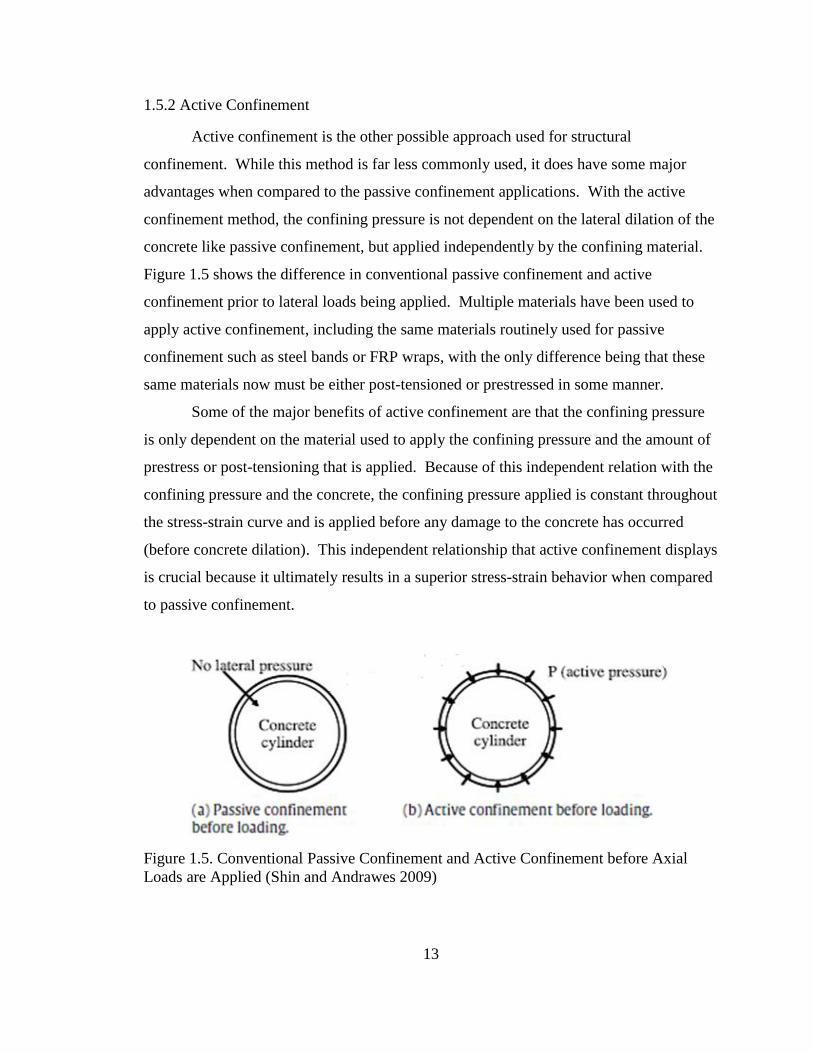
1.5.2 Active Confinement
Active confinement is the other possible approach used for structural
confinement. While this method is far less commonly used, it does have some major
advantages when compared to the passive confinement applications. With the active
confinement method, the confining pressure is not dependent on the lateral dilation of the
concrete like passive confinement, but applied independently by the confining material.
Figure 1.5 shows the difference in conventional passive confinement and active
confinement prior to lateral loads being applied. Multiple materials have been used to
apply active confinement, including the same materials routinely used for passive
confinement such as steel bands or FRP wraps, with the only difference being that these
same materials now must be either post-tensioned or prestressed in some manner.
Some of the major benefits of active confinement are that the confining pressure
is only dependent on the material used to apply the confining pressure and the amount of
prestress or post-tensioning that is applied. Because of this independent relation with the
confining pressure and the concrete, the confining pressure applied is constant throughout
the stress-strain curve and is applied before any damage to the concrete has occurred
(before concrete dilation). This independent relationship that active confinement displays
is crucial because it ultimately results in a superior stress-strain behavior when compared
to passive confinement.
Figure 1.5. Conventional Passive Confinement and Active Confinement before Axial
Loads are Applied (Shin and Andrawes 2009)

14
1.5.2.1 Compressive Stress-Strain Behavior of Actively Confined Concrete
Figure 1.6 shows the typical stress-strain model for actively confined concrete
with varying level of confinements. This stress-strain model for actively confined
concrete is noticeably harder to predict than the stress-strain model for passively confined
concrete because the level of confinement affects the model throughout the entire stress-
strain curve unlike the passively confined method where the confinement level only
greatly affects the model after the yield point has been reached.
Actively confined concrete, like passively confined concrete, starts from the
origin with an initial slope equal to the modulus of elasticity of concrete (Ec) and doesn’t
show a negligible stiffness reduction until the critical point (Ɛcr, fcr) is reached. However,
unlike the passive confinement method the location of this point varies greatly. The
critical stress (fcr) of actively confined concrete is almost always estimated as a constant
percent of the yield stress (fcc), and can best be assumed to be approximately 85% of the
yield stress (Moghaddam et al. 2010). This yield stress value for active confinement
however can be significantly increased by increasing the amount of confinement applied,
as opposed to the behavior of passively confined concrete whose critical stress location
cannot be altered by any level of confinement.
After this point has been reached, the rate of propagation of major cracks again
becomes significant within the member causing the stiffness to again be rapidly
decreased until the location of the next key point, known as the yield point (Ɛcc, fcc), is
reached. The locations of the yield point again signifies the start of significant
irreversible dilation in the concrete (due to the combined effects of cracking and
plasticity), however, with the active confinement application the location of this yield
point can vary greatly depending on the level of confinement that was applied to the
members.
After the yield point, the confining material is the only thing maintaining the
yielded concrete, just like with the passively confined method. However, the post
yielding slopes for actively confined concrete are almost always negative and at best
cannot be much greater than zero (slightly positive). This expected negative post
yielding slope is due to the fact that the confining material stiffness has now been

15
reduced to at most the strain hardening stiffness. This noticeable behavior is due to the
fact that the confining material itself must yield at the exact time as the concrete member;
opposed to the post-yield slope for passively confined concrete that can take large
positive values due to the material still possibly behaving elastically after the concrete
yield point (Ɛcc, fcc) is reached. The linear trend of the post yielding slope continues until
the rupture of the confinement material is reached at the ultimate point (Ɛult, fult), and then
the curve again sharply decreases with a negative slope equivalent to the post-peak slope
of unconfined concrete.
With the knowledge displayed above, the complete stress-strain curve that passes
through the origin, critical point, yield point, and has an initial slope at origin of Ec and
final slope at yield point equal to the post-yield slope can be obtained with the use of a
forth order polynomial. However, for engineering purposes a second order polynomial
can accurately approximate the pre-yield branch of the curve by neglecting the initial
slope at origin of Ec and final slope at yield point equal to the post-yield slope.
Figure 1.6. Schematic of Stress-Strain Curves of Actively Confined Concrete Specimens
(Moghaddam et al. 2010)

16
1.5.3 Important Distinctions between Active and Passive Confinement
1.5.3.1 Stress-Strain Behavior
By comparing Figures 1.4 and 1.6, Moghaddam et al (2010) discovered the
following important distinctions between the stress-strain behavior of active and passive
external confinement:
The critical stress (fcr) of actively confined concrete is almost always a
constant percent of the yield stress (fcc), and this value can be significantly
increased by increasing the amount of confinement, as opposed to the
behavior of passively confined concrete which does not alter the critical stress.
The confining material of passively confined concrete yields after the concrete
yield point (Ɛcc, fcc), while material of actively confined specimens always
yield just at the yield point of the material, implying optimum utilization of
the material in concrete confinement.
The post yielding slopes for actively confined concrete can’t be much greater
than zero, because the confining materials stiffness vanishes to (at most) the
strain hardening stiffness, while the post-yield slope for passively confined
concrete can take large positive values due to the material still possibly
behaving elastically after the concrete yield point (Ɛcc, fcc) has been reached.
For identical confinement layouts, the actively confined concrete specimens
will show higher strength and less ultimate strain in comparison with
passively confined concrete.
The key factor attributing to the active confinement method superiority is the
delay in the damage sustained by the concrete as a result of early application
of the confinement pressure; in the case of passive confinement, the concrete
would have to deform laterally (i.e., dilate) and be damaged to some extent for
the confining pressure to be fully activated.
1.5.3.2 Stress-Volumetric Strain Behavior
To view the benefits of active confinement displayed in another way, Figure 1.7c
shows the stress versus volumetric strain (ratio of change in volume due to deformation

17
to original volume) of unconfined, actively confined, and passively confined concrete.
On this plot the stress is plotted on the y-axis and the volumetric strain is shown on the
x-axis, with volumetric compaction being signified by being on the right side of the
centerline and volumetric expansion being signified by being on the left side of the
centerline.
From this plot it can be seen that with the continual increase in stress the
unconfined concrete specimen first experiences volumetric compaction in the elastic
region (right portion of the graph), until it eventually crosses the centerline and starts
expanding rapidly in the plastic region (left portion of the graph) due to deformations and
crack propagation until reaching the ultimate failure of the member. Similar to
unconfined concrete, the volume of passively confined concrete members under axial
stress begins by reducing in the elastic region, until it eventually starts expanding rapidly
in the plastic region. However, the passive confinement and resulting confining pressure
helps in delaying the point where the concrete starts expanding volumetrically, and
therefore allows for increased stresses to be reached and also delays the ultimate failure
of the member. In the active confinement case, the confining pressure which is applied to
prestress the concrete element laterally, prior to loading, exerts an initial volumetric strain
Ɛvo due to compaction of the confined member. In order to overcome the effect of this
initial volumetric strain, larger axial strains and stresses are required, thus resulting in the
failure point of the concrete to become further delayed compared to the passively
confined concrete (Shin and Andrawes 2010).

18
Figure 1.7. Schematics of the Cross Section of Confined Concrete Before Loading (A &
B) and Stress versus Volumetric Strain Curves of Unconfined, Passively, and Actively
Confined Concrete (C). (Shin and Andrawes 2009)
1.6 Objectives and Scope
With a general understanding of the superior stress-strain behavior displayed by
active confinement now obtained, a new and innovative method to confine concrete
specimens will be discussed and further investigated within this thesis. This confining
method utilizes shape memory alloy (SMA) wires to provide the constant confining
pressure that is essential for active confinement.
Within this thesis all relative information with regards to SMAs and the confining
potential will be further investigated in great detail, and the following overall primary
objectives have been selected:
1. Critical review of literature and assessment of analytical models
a. A critical review of literature is discussed for assessing the suitability of
various models toward their applicability to shape memory alloy (SMA)
induced confinement of concrete cylinders.
b. Computational procedures for a chosen SMA confined concrete
cylindrical specimen are adopted to make the assessment meaningful for
addressing primarily two required goals: enhancement of peak stress, and
post-peak stress-strain response, that is necessary to estimate the increase
in the ductility of concrete columns.

19
2. Development of an experimental program
This program deals with the following aspects:
a. Mechanical characterization of the selected SMA wire that was used as the
confining mechanism.
b. Selecting concrete mix designs, to achieve a variation in the compressive
strength of concrete.
c. Development of appropriate procedures required to wrap the SMA wire
around the concrete cylinders.
d. Carrying out the appropriate loading tests for the concrete cylinders, (both
unwrapped and wrapped) to determine their stress-strain response until
ultimate failure occurred.
3. Experimental/analytical correlations
a. To assess the usefulness of the SMA confinement model toward achieving
the expected increase in the ductility of the specimens beyond peak stress.
b. To make some correlations with the appropriate models with regard to the
descending portion of the stress-strain response. These correlations will
be limited toward the overall trends that are displayed rather than the
numerical values obtained.
c. To carry out these correlations for assessment of the applicability of the
best models toward analyzing the enhancement of peak stress and
ductility, if any.
d. To assess the accuracy of the post-peak stress-strain response.
4. Numerical assessment of the practical usefulness of the SMA confinement
method to achieve enhanced ductility of full scale reinforced concrete
columns.
The scope of this work is limited to exclude:
Steel reinforced concrete cylinders
Dynamic loading effects
Development of new models that may correlate better with the experimental
data

20
This work is also limited due to the relatively smaller number of specimens
that could ultimately be tested. This was primarily due to the lack of
resources available to buy the expensive SMA wires, but also due to the load
testing machine and data acquisition system not being ideal.
1.7 Project Summary
This work entails detailed information describing the main differences between
active and passive confinement, especially discussing how the confining pressure is
ultimately applied and the resulting stress-strain behavior of concrete members confined
under each method. With a full understanding of each approach, the overall superiority
of the active confinement method becomes widely apparent, and it’s easily understood
why the active confinement method appears to be the future of concrete confinement.
One method that appears realistically feasible to actively confine concrete
members involves the use of shape memory allow wires and an innovative technique that
utilizes the recovery stresses that these alloys can generate. These SMAs will therefore
be discussed throughout this work in full detail, with a main focus existing on the
potential beneficial use of SMAs for structural confinement.
Mander et al. (1988) unified passive stress-strain model is then described in detail
and modified for the active confinement application that shape memory alloys wires will
provide. Due to relatively difficult nature of formulating the stress-strain behavior that
occurs with active confinement applications, multiple active confinement equations are
then incorporated within this model to display the wide range of assessed behavior that
may occur under certain varied parameters.
Once multiple analytical formulations are displayed and discussed, a medium
scale experimental procedure was undertaken. The main objectives of this experiment
were to verify the confining effectiveness that this SMA confining method provided
under certain scenarios, and ultimately determine which author’s formulations appeared
to be the most accurate when compared to the experimentally obtained data.
After a conclusion has been made on which authors model most accurately
formulates the stress-strain behavior of SMA confined concrete, the results were then

21
used within a numerical example to predict the behavior of a full scale concrete column
with ordinary longitudinal steel and transverse SMA wires.

22
Chapter 2: Shape Memory Alloys
2.1 Shape Memory Alloy Introduction
Shape memory alloys (SMAs) are a very unique group of metallic alloys that are
capable of recovering apparent permanent strains when they are heated above a certain
temperature, due to a reversible phase change that occurs within the atomic structure of
the alloy. With these amazing alloys, a temporary deformed shape can be virtually held
forever until the right stimulus (mainly temperature) is applied to trigger a shape recovery
and return the alloy back to the original undeformed shape. Due to this reversible
process, SMAs have an endless amount of possible applications and appear to be one of
the main materials of the future.
These extraordinary alloys were first discovered in the early 1930s, although they
didn’t start to attract real attention for engineering applications until 1971 when
significant recoverable strain was observed in a Ni-Ti alloy at the Naval Ordnance
Laboratories (USA). Currently, three major types of SMA compositions exist: nickel
titanium based (Ni-Ti), copper based (Cu-Al-Ni and Cu-Zn-Al), and iron based (Fe-Mn-
Si, Fe-Ni-C and Fe-Ni-Co-Ti). The nickel titanium based alloys are by far the most
common due to their superior mechanical behavior, and if price is not a major concern,
they are always the best choice. The copper based alloys are the second most common
type, and have also seen some real world applications. These alloys, while being cheaper
than the Ni-Ti based alloys, also display inferior mechanical properties and therefore the
importance of cost and function must be weighed when choosing between the two. The
iron based alloys have only been used seldom for actual applications, as they are still
mostly in the research and development stage. These alloys are expected to be heavily
used in the future as they are predicted to be even cheaper than the copper based alloys

23
and only a fraction of the cost of current Ni-Ti based alloys that are used today, greatly
reducing the overall cost for any application.
SMAs have already been used for multiple applications within the biomedical
field (eyeglasses, dental wires, and reinforcement for arteries and veins), and aerospace
industries (fixed wing and rotary-wing components) in the past. Recently, they have also
started to attract a lot of attention in other engineering fields due to the price decrease that
has occurred over the past 10 to 15 years. This price decrease which is mainly due to
enhanced manufacturing processes over this time frame is expected to continue within the
future and should drastically decrease due to the eventual increase in both copper and
iron based alloys, which has made previously large scale applications now realistically
possible. Like almost all other science and engineering fields, structural engineers have
also taken notice to the potential benefits and now reasonable cost that SMAs may
provide, which has led to multiple applications now being further researched, if not
already implemented. One such potential structural application that SMAs may provide
is for the active confinement of concrete members, which will be discussed in great detail
within this chapter and throughout the paper.
2.1.1 Shape Memory Behavior
Shape memory alloys (SMAs) are a class of metals known for their unique
thermomechanical characteristic which gives the alloy the ability to return to their
predetermined undeformed shape, after undergoing large inelastic deformations. These
alloys achieve this by either displaying a superelastic behavior, which allows the alloy to
recover deformations with the removal of the applied stress (like a rubber band), or a
shape-memory behavior, which enables the alloy to recover deformations with the
application of heat.
Contrary to plastically deforming metals, the nonlinear deformation of SMAs is
metallurgically reversible due to a realignment of the alloy’s structure that occurs at the
atomic level. This atomic realignment that occurs within in SMAs is a two-way
transformation (forward and reverse) between two stable atomic phases: a high
temperature austenitic phase and a low temperature martensitic phase. In addition, the
low temperature martensitic phase can be in one of two forms: twinned (undeformed) or

24
detwinned (deformed) if sufficient force is applied. All three of the possible SMA phases
along with the general path SMAs follow is shown in Figure 2.1. These phases are
directly related to the molecular alignment of the alloy with the martensitic structure
being the low energy molecular formation (natural atomic state) and the austenitic
structure being the high energy formation. These phases or molecular formations of the
alloy will therefore change with the application of energy and can be either stress or
temperature induced.
As can be seen from this figure, the original twinned martensitic phase of the
alloy is basically the natural (low energy) atomic structure of the alloy, and this structure
will be preferably displayed, unless acted upon by either force or temperature. If a
suitable force is applied, the alloy will start to transform from the twinned to detwinned
martensitic phases, which has up to 24 martensitic variants until the completely
detwinned martensitic phase is reached. The austenitic phase however, only has one
single atomic structure, which is fundamental for SMAs to display the shape memory
effect (SME) and recover any preliminary deformations that have occurred. Basically,
no matter what phase the martensitic alloy is in (either twinned or any possible variation
of the detwinned alloy), if the alloy is heated to a high enough temperature the alloy will
always revert back to this predetermined austenitic crystalline structure. This basically
allows the alloy to reset back to the twinned martensitic phase when the alloy’s
temperatures are cooled low enough.

25
Figure 2.1. Schematic Illustration of Change in Crystalline Structure between Austenite,
Martensite (Twinned), and Deformed (Detwinned) Martensite States With Respect to
Temperature (Borden 1990)
In other words, for the SME to be shown in SMAs, a quasi-plastic deformation is
induced in the martensitic form, transferring the alloy from twinned to a detwinned
molecular structure. The deformation can then be recovered by raising the temperature
and changing the molecular structure again, this time from the detwinned (deformed)
martensitic phase to austenitic phase. If the heat source is removed and the temperature
is cooled low enough the alloy will change once again, this time from the austenitic form
back to the original (twinned) martensitic structure, while in the process recovering all
previous deformations and allowing the process to be restarted all over again if needed.
A great way to comprehend the physical behavior of SMAs, based on the alloys
phase and temperature, is to visually depict a simple spring made of a typical SMA
material. This representation is shown in the Figure 2.2. From this figure all possible
phase transformations are portrayed, by either increasing or decreasing the temperature,
or by deforming the SMA with the addition of an adequate mass. As can be seen from
this representation when starting with a spring in the martensitic twinned phase (left hand
side of the figure), the addition and eventual removal of heat, will transform the alloy to
the austenite phase and then back into the martensitic twinned phase, with no physical
movement occurring within the spring. If however a sufficient mass is applied, the

26
martensitic twinned spring will become detwinned, causing the spring to stretch out and
increase in length. From this martensitic detwinned phase, if sufficient heat is applied the
alloy will transform to the austenitic phase. During this transformation the alloy will
recover all deformations within the spring, assuming that the mass of the object and the
recovery stress of the alloy permit this to occur. If the heat is removed and the alloy is
allowed to cool back down, the alloy will then transform back to the martensitic
detwinned phase due to the fact that the mass is still attached to the spring. However, if
this mass is removed and the spring is reheated, the alloy will transform back into the
austenitic phase recovering all deformations due to the previously attached mass. With
no mass attached, and with the removal of heat, the alloy will again transform back to the
twinned martensitic form of the alloy.
Figure 2.2. Physical Representation of a SMA Spring, Showing All Possible Phase
Changes Due to Temperature and Deformation.
2.1.2 SMA Transformation Temperatures
As noted above, the amount of martensite or the martensitic fraction of a SMA
will change with respect to temperature. Knowing this martensitic fraction from 0-100%
(where zero percent is a completely austenitic alloy) is crucial, because this fraction will

27
result in different stress-strain behavior and mechanical properties for the alloy. As
depicted in Figure 2.3A, there are four transformation temperatures which locations vary
based on material properties (especially the alloys composition) and are known as the
martensite finish (Mf), martensite start (Ms), austenite start (As), and austenite finish (Af).
If the material is in the low temperature martensite phase (100% martensite) and
heat is applied, the material will begin the transformation to austenite once the
temperature corresponding to the As location has been reached, and will become entirely
austenitic after reaching the Af temperature of that alloy (0% martensite). Likewise, if the
material is in the high temperature austenite phase (0% martensite) and the material is
cooled, the material will begin the transformation to martensite at the temperature
corresponding to the Ms location and will become entirely martensitic once the Mf
temperature has been reached (100% martensite).
The phase of the material (martensitic or austenitic) is very important because it
will determine the behavior of the alloy. For example, when the alloy is in its low
temperature martensitic phase, the SMA will behave plastically and quasi-permanent
deformations will exist after a sufficient stress has been applied and removed
(Figure 2.3B). However, if the alloy is in the high temperature austenite phase, the SMA
will behave elastically (just like a rubber band) and deformations will be recovered with
the removal of stress (superelasticity). The stress strain behavior is shown graphically in
Figure 2.3B for both the martensitic and austenitic phases of the alloy, along with an
approximation for the transformation region between phases.

28
Figure 2.3. Typical SMA (A) Thermal Hysteresis. (B) Thermo-Mechanical Behavior
(Shin and Andrawes 2009)
While the most common method used to transform the phase in SMAs is with the
application of heat, as explained above, it’s important to not overlook the fact that this
phase transformation can also occur with pure mechanical loading if the material is in the
austenitic phase. It is well known now that the transformation temperatures associated
with SMAs are not constant values, but actually increase approximately linear with
applications of stress. Figure 2.4 displays the typical plot of stress versus temperature for
SMAs. From this plot it can be seen how the typical transformation temperature
locations vary based upon the level of applied stress, and the linear relationship that
ultimately results.

29
Figure 2.4. Typical SMA Stress versus Temperature Phase Diagram.
As an example, from this figure it can be seen that if the SMA is in the twinned
martensitic form, the increased application of stress will only transform the alloy to the
detwinned structure until it eventually begins to deform due to permanent (non-
recoverable) plastic deformation. This result is fairly straight forward and besides the
switch from twinned to detwinned, this behavior is just like any other metallic material
under tension. However, major problems may arise if the SMA is in the austenitic phase
and stress is applied while the temperature is held constant. As it can be seen from
Figure 2.4, if a SMA wire is under little or no stress while in the austenitic form, special
care needs to be taken to make sure that the alloy doesn’t transform back into the
detwinned martensitic phase. Due to the estimated slopes of the transformation
temperatures and the typical yield point of SMAs, this stress induced transformation will
most likely only happen near the point of plastic deformation. However, it is important
to note that if a SMA is in the austenitic phase and stressed in tension until ultimate
rupture, the temperature will most likely need to be increased once yielding has occurred
or the SMA will switch its phase back to the detwinned martensitic phase of the alloy.
This stress versus temperature relationship is key for actual SMA use, especially
if the consumer has purchased a non-deformed SMA and is planning to prestrain the
SMA material themselves, as the SMA can be guaranteed to have higher transformation
temperatures then reported by the manufacturer.

30
2.1.3 SMA Mechanical Properties
The mechanical properties under tension, compression, shear, and torsion can
vary widely with SMAs. This possible large variation in SMA properties is not only due
to variations in chemical composition, which are practically endless, but also due to the
thermomechanical processing and original heat treatment of the alloy from the
manufacture, and of course the atomic arrangement of the alloy at the time of testing
(either twinned or detwinned martensite, or austenite).
With these inherently large variations within SMAs, often only ranges or at best
approximate values for the mechanical properties can be assumed. Experimental testing
to obtain the mechanical properties can also be difficult, due to the sensitive nature of
SMAs. Even samples from the same batch may slightly vary in properties such as; elastic
modulus, yield stress, or recovery stress. To get some approximate values for the
mechanical properties of SMAs, various SMAs in the form of wires and bars of varying
diameters have been tested by a number of investigators over the years. A sample of
some of these results and some of their results are summarized in Table 2.1. It should be
noted that the table below is specifically for the Ni-Ti based alloys under tension only.
As explained earlier, the Ni-Ti based alloys have been known to display far superior
mechanical behavior and therefore should be taken as the top end potential for SMAs.
Property Phase Range
Young’s Modulus,
(GPa)
Austenite 30-98
Martensite 21-52
Yield Strength,
(MPa)
Austenite 100-800
Martensite 50-300
Ultimate Strength,
(MPa)
Austenite 800-1500
Martensite 700-2000
Elongation at failure,
u (%)
Austenite 15-20
Martensite 20-60
Table 2.1. Mechanical Properties of Ni-Ti Alloys under Tension (Manach and Favier
1997; Otsuka and Wayman 1999; Rejzner et al. 2002; & DesRoches et al. 2004)

31
As seen from Table 2.1, the values for each mechanical property can vary widely
for both phases. However, general conclusions can still be made off of the trends shown.
From this data it appears that the austenitic phase shows superior mechanical behavior
when compared to the martensitic phase. This however was expected based upon the
knowledge for the stress-strain relationship of SMAs shown earlier within this chapter.
For example, with the knowledge that the martensitic phase by nature will deform
relatively easy and the austenitic phase will try to recover deformation or fight strain
when stress is applied (like a contracting rubber band), it makes sense that the austenitic
phase would have a higher range for Young’s modulus (stiffer) and have a lower
elongation at failure range. The yield strength is also much higher for the austenitic
phase since it yields like normal metals as opposed to the martensitic phase, which in a
sense, is yielding from the initial switch from twinned to detwinned starts to occur. The
values for the ultimate strength at each phase were slightly surprising as it appears the
martensitic phase may have a slightly higher ultimate strength capacity; although the
overall range of the two phases were still relatively similar overall.
2.1.4 Free or Constrained Recovery
Two different types of deformation recovery can occur with SMAs, which are
classified as either free or constrained. With free recovery there is no physical restraint
on the movement of the alloy as it transforms from the deformed martensite phase into
the austenite phase, therefore the element can freely return to its original undeformed
shape at zero stress. However, in the case of constrained recovery the change in the
crystalline structure from martensitic to austenitic state still takes place by altering the
temperature, although the physical movement of the alloy is prevented. Since the shape
recovery is prevented (strained martensite to unstrained austenite), stress which is a
function of final strain (that is, unresolved recovery or contact strain) is generated.
The SME phenomenon under constrained recovery is capable of large recovery
stresses up to 900 MPa being realistically possible (Janke et al. 2005). This recovery
stress does however depend on multiple factors; such as the material composition,
manufacturing procedure, and the amount of prestrain applied. The max recovery stress
(largest amount of stress the SMA is capable of recovering) occurs at temperatures above

32
the Af location and has been known to increase linearly with the amount of prestrain.
This linear relationship generally holds true up until a strain of approximately 8%, which
is usually agreed to be the max strain allowed for SMAs or the potential for
nonrecoverable plastic deformation exists which will reduce the recoverable stress of the
wire significantly (Tautzenberger 1990). Once the heating source is removed and the
temperature is lowered back to room temperature (alloy still austenitic), the recovery
stress of the SMA will drop slightly from the max recovery stress associated with the
wire, to what is called the residual stress. This residual stress is the remaining recovery
stress that occurs once the wire has been transformed into the austenitic phase, but cooled
down to ambient temperatures. This residual stress is the actual stress that defines the
potential of the SMA wire in real world applications. Just like the max recovery stress,
the residual stress is dependent on multiple factors and will vary for each alloy but has
been approximated as 80% of the maximum recovery stress (Shin and Andrawes 2009).
2.1.5 Prestrain Losses
With post-tensioned or prestressed materials, like the SMAs to be used within
active confinement, the amount of prestrain loss is a major issue that needs to be
accounted for accurately. The residual prestrain, after all losses have occurred is
extremely important because it’s the value that will determine the effective amount of
confining pressure that is actually applied to the specimens. When dealing with SMA
confinement, prestrain losses can come from multiple sources. These include: geometric
imperfections of the spiral (bends or kinks), wire slippage that could occur at the splicing
connections or anchor points after the shape recovery of the wire has been activated, and
most likely from the simplest form where slack develops between the wire and the
confined specimen greatly reducing the confinement potential of the SMAs.
While it should be stressed that the amount of prestrain loss will vary with each
application method, Shin and Andrawes (2009 and 2011) attempted to quantify this value
for their active confinement procedure by accurately measuring the average value
obtained from two extensometers that were attached to the SMA spiral on opposite sides
of the concrete specimens. In their particular setups, the prestrain losses increased
consistently after activation of the wire, until reaching a constant max value of 0.67%

33
(2009) and 0.97% (2011) prestrain loss. Obtaining these approximate losses is significant
because of the knowledge that the recovery stress increases linear with increasing
prestrain. Therefore, the predicted recovery stress to be applied to the concrete specimen
can then be adjusted due to the estimated prestrain losses, based on the slope assuming at
least two recovery stress values are known for that specific SMA wire at different
prestrained value.
2.2 SMA Active Confinement Application Procedure for Concrete Specimens
For the application of active confinement using SMA wires on concrete
specimens, the SMA wire is first prestrained usually within 5-8%. Any higher and the
potential for nonrecoverable plastic deformation can reduce the recoverable stress of the
wire significantly. Next the prestrained wire is wrapped around the concrete member
often in the form of a continuous spiral, although individual hoops are also possible
(Figure 2.5B). The SMA spiral is then heated above the alloys Af temperature to activate
its shape recovery (Figure 2.5C). However, since the spirals are fully constrained at the
ends often by clamps and throughout the length of the wire by the surface of the concrete
specimen, a large recovery stress (hoop stress) is developed in the spiral creating a large
confining pressure on the wrapped specimen (Figure 2.5A).

34
Figure 2.5. Schematic of Concrete Samples Confined with Shape Memory Alloy Wire.
(A) Confined Element Displaying Active Pressure, (B) SMA Confinement
Representation before Heating, and (C) SMA Confinement Representation after Heating.
(Shin and Andrawes 2009)
2.3 SMA Classifications
It should be noted that not every SMA type is suitable for this active confinement
application. SMAs are classified as type 1, 2, or 3 depending on the relative position of
the thermal hysteresis loop (distance from Ms to As) and the location of ambient
temperature (Figure 2.6). Type 1 SMAs and type 2 SMAs have the thermal hysteresis
loop located completely below and above ambient temperature respectively, while type 3
SMAs are classified as having ambient temperature within their thermal hysteresis loop.
Type 3 SMAs (Figure 2.6C) are almost always required for civil application
because the material can be deformed (prestrained) often by the manufacturer, stored
virtually forever on the shelf, and applied when needed at ambient temperature in the
martensitic phase without experiencing shape recovery. The material can then be
triggered/activated by applying a heat source to the alloy (either by temperature or
electricity), transforming the alloy into the austenitic phase. The heat source can then be
removed after activation, allowing the SMA to cool and return to ambient temperature,
while still remaining in the stressed austenitic phase resulting in usable residual stress for
confinement.

35
Type 1 SMAs (Figure 2.6A) cannot be used for this application, due to the fact
that the four transformation temperatures are too low relative to ambient temperatures,
making it nearly impossible to apply the SMA wire to the concrete member in the
martensitic prestrained state. With this type of SMA the material is in the austenitic
phase at room temperature, causing them to display the superelastic effect, not the desired
shape memory effect that is needed for the described application.
Type 2 SMAs (Figure 2.6B) are also not practical for real world applications of
active confinement because the four transformation temperatures are too high relative to
ambient temperatures. With this type of SMA, the wire can be safely deformed and
applied to the concrete specimen in the martensitic phase without problems, but would
require a unrealistic constant heat source to be applied throughout the life span of the
alloy, to transform the wire into the austenitic phase and trigger the desired shape
memory effect. With this type of SMA, once the heat source was removed and the wire
was allowed to cool back down to ambient temperature the alloy would transform back
into the martensitic phase, resulting in the loss of all recovery stresses, even with the
alloy being physically restrained.

36
Figure 2.6 Location of the Hysteresis Loop Relative to Ambient Temperature for (A)
Type 1 SMA (B) Type 2 SMA (C) Type 3 SMA
2.3.1 SMA Hysteresis Loop
While the type of SMA is very important, the size of the thermal hysteresis loop is
also another obstacle that must be considered for correct active confinement application,
as this determines the environment in which a SMA may be used in real engineering
application.

37
It is well know that SMAs are very sensitive and even a 1% difference in the
alloys composition can greatly alter the locations of the transformation temperatures and
relative size of the hysteresis loop. For instance, the hysteresis gap can narrow or widen
considerably, with just a small amount of copper (Cu) or niobium (Nb) respectively in the
same nickel-titanium (Ni-Ti) based SMA. At first, the sensitive nature of SMAs seems to
be a major disadvantage. However, this should be looked at positively as it gives the
material tremendous flexibility allowing the user the ability to customize the materials to
their exact specifications.
Most civil applications have utilized the NiTiNb alloy because it is classified as a
type 3 SMA and has a very wide hysteresis range. This alloy’s favorable characteristics
makes it suitable for the wide temperature variations possible in the industry (-5 to
110°F), without the threat of unwanted phase transformations due to seasonal
temperature changes.
However, with that being said, the experimental investigation that will be further
discussed within the upcoming chapters of this work incorporated a type 2 Ni-Ti SMA
with an equal composition of both elements. This SMA was ultimately selected due to
the fact that this composition is by far the most common of all SMAs and therefore was
the one of the cheapest possible selections that could be adequately used within this
work. Any and all other required mechanical properties or details about the SMA
selected, will be further discussed in Chapter 5.
Chapter 3 of this experimental investigation discusses the pertinent literature
reviews related to this topic. This chapter and literature review are separated in two main
sections, with the first section detailing the most useful theoretical constitutive models of
confined concrete cylinders, and the second section detailing previous research obtained
on SMAs used for active confinement.

38
Chapter 3: Literature Review
3.1 Relevant Research Dealing with Stress-Strain Modeling of Confined Concrete
Mander et al. (1988) proposed a theoretical stress-strain model for concrete
subjected to uniaxial compressive loading confined by transverse reinforcement. With
this theoretical model a single equation is used for the stress-strain response. The model
allows for cyclic loading and includes the effect of strain rate. The influence of various
types of confinement is taken into account by defining an effective lateral confining
stress, which is dependent on the configuration of the transverse and longitudinal
reinforcement.
The model utilizes an energy balance approach to predict the longitudinal
compressive strain in the concrete corresponding to first fracture of the transverse
reinforcement by equating the strain energy capacity of the transverse reinforcement to
the strain energy stored in the concrete as a result of the confinement.
The analytical stress-strain model for confined concrete suggested three important
conclusions. First, for a particular transverse reinforcement configuration the effective
confining stresses in the x and y directions can be calculated from the transverse
reinforcement and a confinement effectiveness coefficient (ke) which defines the
effectively confined concrete core area by taking into account the arching action that
occurs between the transverse hoops and between the longitudinal bars. Second, the form
of the stress-strain curve for confined concrete can be expressed in terms of a simple
uniaxial relation suggested by Popovics (1973) and only requires three control parameters
(peak stress of confined concrete (f’cc), strain at the peak concrete stress (Ɛcc), and
modulus of elasticity of concrete (Ec)). Third, with the energy balance approach, when
the work done exceeds the available strain energy of the transverse steel, then hoop

39
fracture occurs and the section can be considered to have reached its ultimate
deformation.
Xiao et al. (2010) presented on their finding through modeling of the stress-strain
behavior of actively confined high-strength concrete (HSC) from a database with 51
actively confined concrete cylinder specimens from Attard and Setunge (1996), Imram
and Pantazopolou (1996), Lu and Hsu (2006), Candappa et al. (2001), and Tan and Sun
(2004). The unconfined concrete strengths of the database ranges from 51.8 to 126 MPa,
while the confinement ratio, which is defined as the ratio of the confining pressure to the
unconfined concrete strength, ranges from 0.01 to 0.84. The new active-confinement
model developed, worked well for both HSC and normal strength concrete (NSC) and
was shown to outperform past models that generally would underestimate the
stress-strain curves because of an underestimated peak axial stress.
Moghaddam et al. (2010) proposed an analytical model to predict the compressive
stress-strain curve of strapped concrete with post-tensioned yielding metal strips as a
function of the confinement level. The critical, yield, and ultimate points were
determined and the full stress-strain curve was then obtained by passing through these
key locations with a good degree of accuracy. The model was calibrated based on
experimental data of 72 cylindrical and prismatic specimens by the authors and 41
specimens used by Frangou and Pilakoutas (1996). The specimens covered several
parameters such as volumetric ratio, yield strength, and ultimate strain of the confining
material, and the strength, shape, and size of the concrete specimens.
Lokuge et al. (2005) presented an approach in predicting the stress-strain
relationship of high strength concrete (HSC) subjected to active lateral confinement. The
proposed model formulation was based on the experimental results reported by Candappa
(2000), which included 24 cylindrical specimens using four grades of concrete (40, 60,
75, and 100 MPa) and three confining pressures (4, 8, and 12 MPa) as test variables.
The analytical results from the proposed model indicated that when confined concrete is
stressed, initially it contracts (reducing in volume), after a certain stress, it starts to
expand (increasing in volume). At the time of peak axial stress, the volume of concrete is
back to its original unloaded volume. That is, the volumetric strain was observed to be

40
back at zero at peak axial stress. This suggests that the magnitude of lateral strain at peak
axial stress is half of the corresponding axial strain magnitude.
3.2 Relevant Research Dealing with Shape Memory Alloy Confinement
Krstulovic-Opara and Thiedeman (2000) investigated the use of self-stressing
composites for active confinement of concrete members with the goal of maximizing
member strength and ductility for both normal strength and high-strength lightweight
concrete (HS-LWC), with the main focus being on HS-LWC. Within this work the
authors embedded SMAs as muscular fibers in cementitous composites to develop self-
inducing prestressing composites. This work used a type 3 Ni-Ti SMA wire and focused
on two different types of confinement: confinement with SMAs only; and confinement
with a combination of SMAs and slurry infiltrated fiber mat concrete (SIMCON) with
each being tested for retrofit and new construction applications.
The obtained data indicated that an increase in confinement, increased crack
stability, material compaction, and corresponding stress throughout the test and at
ultimate strength. Brittle behavior of NSC was prevented, while an already ductile
response of HS-LWA fiber reinforced concrete (FRC) was further improved. Active
confinement was more effective than passive confinement in restraining cracking and
improving crack stability. Thus, active confinement resulted in a higher increase in the
parameters previously listed. Furthermore, for the same level and type of confining
stress, the increase in ultimate strength was typically higher for HS-LWA FRC than for
NSC specimens. The investigation also indicated that a combination of adding fibers and
using active confinement leads to a large increase in strength and ductility of HS-LWA
concrete, and could thus permit their use in seismic-resistant design.
Choi et al. (2008) examined the ability of two 1.0 mm diameter SMA wires shape
memory alloy wires to confine a total of 6 concrete cylinders. The first SMA (Ti-49.7Ni)
remained in the martensitic phase at room temperature, and the second SMA wire (Ti-
50.3Ni) remained in the austenitic form at room temperature. The martensitic wire
utilized the shape memory effect and was prestrained before being wrapped around a
concrete cylinder as opposed to the austenitic shape memory wire which utilized a

41
superelastic behavior, and was prestrained as they were wrapped around the concrete
cylinder.
Based upon the results from this experimental work, the authors concluded that
the two types of SMA wire jackets performed similar and both types of SMAs were
capable of inducing active confinement and therefore can be used to increase the failure
strain and the energy dissipation capacity of the concrete cylinder. The results obtained in
this work were then compared with a constitutive model of concrete confined by steel
jackets and lateral reinforcement by Li et al. (2005a, 2005b) to conduct a parametric
study to understand how the amount of SMA wires can significantly improve the strength
and the difference in using steel jackets compared to SMA jackets.
Shin and Andrawes (2009) completed a study that focused on investigating the
feasibility of using spirals made of NiTiNb SMA to apply active confining pressure on
concrete members. Three types of experimental tests were conducted. First, thermo-
mechanical tests were performed on 2.0 mm diameter SMA wires to determine their
recovery stresses. Second, several mechanical splicing connections were examined in
tension to determine their adequacy in splicing the SMA wires to develop the total length
of continuous wire needed. Third, uniaxial compression tests of SMA, SMA-glass fiber
reinforced polymers (GFRP), and GFRP wrapped concrete cylinders were conducted and
the results were compared.
Thermo-mechanical tests revealed that the recovery stress of the SMA wires
varied linearly with the amount of prestrain, and the average residual recovery stress is
approximately 80% of the maximum recovery stress. Splicing connections tests were
conducted on three types of connections including sleeves, U-clamps, and welded
connections. These tests revealed that using multiple U-clamps provided the best results
as long as the average capacity of the number of U-clamps used was greater than the
expected maximum recovery stress of the spiral.
Using the lateral confining pressure as the base for comparison, it was found that
applying the same confining pressure from either passive or active confinement methods,
produced significantly different concrete behavior (see Sections 1.5 through 1.5.3.2). For
example, applying confining pressure of 1.0 MPa using SMA spirals and GFRP wraps
resulted in an increase in the concrete strength and ultimate strain of approximately 1.2

42
and 10 times, respectively, when the SMA was compared to the GFRP application.
Furthermore, the hybrid SMA-GFRP confinement technique exhibited a superior
performance to the conventional passive confinement technique using GFRP. This
increased performance is due to the small amount of SMAs used in the hybrid specimens
that delayed the rupture of the GFRP sheets as well as the entire specimen, in addition to
maintaining up to 60% of the concrete peak strength until failure.
This study suggested that SMA spirals could be used solely or as a supplementary
confining technique along with FRP composite wraps. The addition of the SMAs could
result in a significant reduction in the amount of FRP material needed to achieve a certain
level of ductility, which could result in a dramatic reduction in the cost of future
structural retrofitting and rehabilitation projects. The authors felt it was worth noting that
due to the small number of specimens tested in this study, that the conclusions should not
be generalized and that more research is needed.
Choi et al. (2010) assessed the confining effectiveness of shape memory alloy
(SMA) wire jackets for concrete, and compared the performance to that of steel jackets.
For this study 1.0 mm diameter shape memory alloy wires of Ni-Ti-Nb (Ni47.4-Ti37.86-
Nb14.69 %wt.) and Ni-Ti (Ni53.85-Ti46.15 %wt.) at varying prestresses (up to 7%) were
used to confine a total of four concrete specimens (two with each type of SMA). This
study used data from both types of SMA wires, and suggested through regression analysis
that the confining effectiveness (k1) of a SMA jacket for concrete equaled 4.33. This
estimated value of confining effectiveness for SMAs was higher than the suggested 4.1
value for steel by Richart et al. (1928), and the suggested 2.0 value for FRP materials by
Lam and Teng (2002). The authors noted that SMA properties vary with components and
the manufacturing process and, thus, more data from various SMA wires should be used
for a more general determination of the confining effectiveness of SMA wire jackets.
Andrawes et al. (2010) explored the feasibility of using Ni-Ti SMA spirals for
seismic retrofitting of reinforced concrete bridge columns both experimentally and
analytically. The experimental results of SMA spirals and CFRP wraps of varying but
equal confinement levels were used to develop a model, displaying the method’s ability
at improving the behavior of reinforced concrete columns under cyclic and seismic
loadings.

43
The analytical results demonstrated a considerable advantage for the actively
confined column using SMAs compared to the passively confined column using CFRP.
Under seismic excitations, damage to the concrete core and longitudinal steel were
decreased; while the strength, effective stiffness (indication of the amount of damage),
and column residual drifts (governs functionality) were all increased with the use of SMA
spirals compared to the CFRP wraps. The superiority of the proposed technique is
primarily attributed to the early increase in concrete strength associated with using active
confinement, which delays the damage experienced by both concrete and steel.
In the paper by Andrawes et al. (2010), the authors used Mander et al. model to
compare formulated stress-strain relationships with some initial experimental results.
However, in this paper the authors used the original equations suggested by Mander et al.
that were designed for passive confinement, and did not investigate any other potential
equations to accurately predict the stress-strain relationship of the SMA confined
specimens. The use of Mander’s original equations was however deemed appropriate for
these comparisons due to the large amount of SMA material (ρs) that was used, as the
authors mainly researched the ultimate potential of SMA confinement, and not what
would be representative in real world situations. As shown in Figure 1.6, this increased
confining ratio (ρs) ultimately allowed the tested specimens to reduce the severity of the
sharply decreasing post-peak relationship that typically occurs in actively confined
concrete specimens.
Shin and Andrawes (2011) examined experimentally the effectiveness in
enhancing the flexural ductility of vulnerable reinforced concrete columns by testing four
reduced-scale (1/3-scale) reinforced concrete single-cantilever columns, representative of
bridge columns. The quasi-static cyclic behavior of the as built column was compared
with that of a column retrofitted by using actively confined NiTiNb 2.0 mm diameter
SMA spirals, passively confined GFRP wraps, and a hybrid (passive plus active)
confined approach using SMA spirals and GFRP jacket simultaneously; all designed to
have the same confinement pressure. The hybrid approach was sought in this study as a
more economical approach for applying active confinement because the amount of SMAs
will be reduced significantly compared to the case with only SMA spirals.

44
To assess the overall performance of each retrofitting technique, the strength,
displacement ductility (ratio of the drifts at the ultimate and yielding points), and
hysteretic energy (area enclosed within the force-displacement curves until the ultimate
point was reached) were compared for each method. The results showed that the SMA
and SMA/GFRP columns exhibited a slight increase in strength and a significant increase
in flexural ductility and ultimate drift capacity compared with the as-built column,
whereas the GFRP column showed only a moderate enhancement in ductility and drift
capacity.
Applying active confinement using SMA spirals significantly enhanced the ability
of the columns to dissipate energy compared with the passive confinement applied by
only using GFRP wraps. It was also noted by the authors that when assessing the damage
of the four tested columns, during and after testing, revealed that the damage to the SMA
and SMA/GFRP columns was far less than that sustained by the GFRP column.
3.2.1 SMA Confinement Essential Findings
Active confinement was more effective than passive confinement in
restraining cracking and improving crack stability. Thus, active confinement
resulted in a higher increase in crack stability and corresponding stress
throughout the test and at ultimate strength.
Applying the same confining pressure from either passive or active methods,
produced significantly different concrete behavior with regard to the location
of the peak stress and the slope/curvature of the post-peak relationship.
Studies suggested that SMA spirals could be used solely or as a
supplementary confining technique.
Analytical results demonstrated a considerable advantage for the actively
confined columns using SMAs compared to the passively confined columns
using CFRP. The superiority of the proposed technique is primarily attributed
to the early increase in concrete strength associated with using active
confinement, which delays the damage experienced by both concrete and the
confining material.

45
Applying active confinement using SMA spirals significantly enhanced the
ability of the columns to dissipate energy compared with the passive
confinement applied by only using GFRP wraps.
It was also noted that when assessing the damage of the confined columns,
during and after testing, revealed that the damage to the SMA confined
columns was far less than that sustained by the passively confined GFRP
column.
3.2.2 Critiques of Past Findings
The work done by Andrawes (2010 and 2011) and Choi (2008, 2009, and
2010) used very high amounts of SMA transverse confining material, in an
attempt to prove the overall feasibility of the SMA confinement method.
However, these authors did not investigate SMA confinement under lower and
much cheaper confining ratios that would be more representative to real world
confinement situations.
None of the previously mentioned research truly investigated which
formulations actually provide the most accurate stress-strain representation of
SMA confined concrete. Under the previously mentioned work, high levels
confining ratios allowed the use of Mander’s passive equations to be
incorporated into the formulation of the stress-strain representation, but when
lower confining ratios are used the behavior is expected to change greatly and
these equations are expected not to be adequate. Therefore, it is still critical to
determine which of the many active confinement models can most accurately
predict the stress-strain behavior of SMA confined concrete members.
The previously mentioned work was very exploratory in nature, and therefore
the authors were only able to test a limited number of confined specimens
(usually around 3 or 4). Due to the lower number of specimens tested, the
data obtained appears to be incomplete and at least somewhat inconclusive
overall. It also appears obvious the both the reliability and repeatability of
this confinement method still needs to be further investigated on a much larger
scale.

46
While Andrawes (2010) did attempt to formulate the stress-strain behavior of
SMA confined specimens with the use of Mander’s unified stress-strain
model, Mander’s passive confinement equations were used within this portion
as the results were only used for preliminary investigations. This formulation
was only lightly discussed in general, and due to the low number of specimens
tested the data obtained still needs to be verified and further investigated
under different confining scenarios.
The type of material used within the previous SMA confinement research has
been very limited in general, and therefore more data with different SMA
wires are still required in an attempt to accurately formulate the confining
effectiveness of a wide range of SMA wires.

47
Chapter 4: Analytical Models and Their Assessment toward SMA Confined Concrete
Columns
4.1 Mander’s Model Introduction
In 1988 Mander et al. proposed a unified stress-strain model (continuous function
for both ascending and descending branches) based on equations from Popovics (1973).
Mander’s model was designed for passively confined concrete members and is applicable
to both circular and rectangular shaped transverse reinforcement. This model has been
widely accepted throughout the structural engineering community for both its accuracy
and relative simplicity in evaluating the stress-strain relationship of confined concrete
members.
Due to the fact that Mander’s model will be used as a base for the stress-strain
prediction of actively confined concrete members, the entire model will be described in
detail within Appendix A, and the main equations will be briefly discussed within this
chapter. It should be noted that only circular reinforcement will be described within this
work and the reader should refer to Mander’s et al. (1988) work for further clarification
on rectangular shaped transverse reinforcement.
4.2 Mander et al. (1988) Stress-Strain Model
Within Mander’s model, the main equation which determines the relationship
between axial compressive stress (fc) and axial strain (Ɛc) is given by the following axial
stress-strain equation which was originally proposed by Popovics (1973):
(4.2.1)

48
where f ’cc = compressive strength (peak stress) of confined concrete and will be
defined later, Ɛc = longitudinal compressive concrete strain, and Ɛcc = the
strain at maximum concrete stress (f ’cc) and can be found with the
following equation from experimental work by Gerstle et al. (1979) which
was based on a simple relationship proposed by Richart et al. (1928):
(4.2.2)
where f ’co and Ɛco, equals the unconfined concrete strength and the
corresponding strain, respectively. Generally, Ɛco = 0.002 can be assumed
based on the results from Richart et al. (1928), and is used within
Mander’s et al. model for unconfined concrete.
The effective lateral confining pressure is defined with the following equation:
(4.2.3)
where fyh= yield strength of the transverse reinforcement, and ρs = the ratio of the
volume of transverse confining steel to the volume of the confined
concrete core
The confined compressive strength (f ’cc) can now be calculated using the
effective lateral pressure (f ’l) and the unconfined concrete compressive strength (f’co).
To develop this equation Mander et al. used the “five-parameter” multiaxial failure
surface equation given by William and Warnke failure criterion (1975):
(4.2.4)

49
With the value of the confined compressive strength (f ’cc) now known, the entire
stress strain curve can be calculated using Equation 4.2.1 with varying longitudinal
compressive concrete strain values up to the ultimate concrete compressive strain (Ɛcu),
which is calculated based on the amount and type of transverse confining material used
with a strain energy balance approach
By equating the ultimate strain energy capacity of the confining reinforcement per
unit volume of concrete core (Ush) to the difference in area between the confined (Ucc)
and the unconfined (Uco) concrete stress-strain curves, plus additional energy required to
maintain yield in the longitudinal steel in compression (Usc), the longitudinal concrete
compressive strain corresponding to hoop fracture can be calculated, with the following
equation:
(4.2.5)
4.2.1 Required Modifications of Mander’s Model for SMA Confinement
With Mander et al. (1988) model, the critical strain for the confined concrete (Ɛcc)
was already taken from experimental work on actively confined concrete specimens by
Gerstle et al. (1979), and therefore already corresponds to a constant confinement
pressure that exists within active confinement applications. As a result, the value of Ɛcc
shown within Equation 4.2.2 does not require modification. However, it should be noted
that multiple investigators have attempted to find (Ɛcc) for active confinement with more
precise equations and these results will be further discussed later within this chapter.
The confined compressive concrete strength (f 'cc), is determined through the use
of the unconfined concrete compressive strength (f ’co) and the effective lateral confining
pressure (f 'l) at the yielding of the transverse reinforcement which signifies a passively
confined approach. The expression given by Mander et al. for the value of the effective
lateral confining stress (f ’l) is given in Equation 4.2.3 and will require modification for
active confinement applications with the use of prestressed SMA wires. It is also
important to note that the left hand side of the simplified Equation 4.2.5 used for
predicting the ultimate concrete strain ( cu) will also have to be adjusted, since that

50
portion of the equation was originally designed for steel transverse confinement as
opposed to the SMA material that will be used.
4.2.2 Andrawes et al. (2010) SMA Adapted Model
The analytical stress-strain model developed by Mander et al. (1988) for concrete
with lateral steel reinforcement was extended and used to describe the effect of active
confinement provided by exterior SMA reinforcement by Andrawes et al. (2010). Within
Mander’s model the effective lateral confining stress on concrete from transverse
reinforcement is only used within Equation 4.2.4, while solving for the peak stress of the
confined concrete (f ‘cc). At this location a constant confinement pressure was assumed
to be equal to the yield strength of the transverse reinforcement because the
corresponding strain level was assumed to be high enough to cause the steel lateral
reinforcement to yield.
With the addition by Andrawes et al. (2010), the constant confinement pressure
was taken as the lateral pressure exerted on the cylinder due to the recovery stress of the
SMA wire. The lateral confining pressure ( could then be calculated by considering
the equilibrium of the resulting SMA forces, shape of the column, and the spacing of the
transverse reinforcements with the following equation:
(4.2.2.1)
where Asma = cross-sectional area of the SMA wire, fsma = recovery stress in the
SMA wire, d = diameter of the specimen confined, and s = spiral pitch
The spacing between the SMA wires still results in a reduced confining pressure, which
according to the model by Mander et al. requires the calculation of a modified (effective)
lateral confining pressure (f ’l) which then equals Equation 4.2.2.2:

51
(4.2.2.2)
Once (f ’l) has been calculated for active confinement with prestressed SMA wires, the
rest of Mander et al. (1988) model can remain unchanged until the value of the ultimate
concrete compressive strain (Ɛcu) has been reached.
The location of Ɛcu on the stress-strain curve for actively confined concrete using
SMA wire will be greatly influenced by the ultimate strength and the fracture strain of
SMA material. As previously mentioned in Chapter 2, these critical values will vary
greatly depending on the overall composition and the state of the SMA (Martensitic or
Austenitic), and therefore will have to be evaluated on a case by case basis.
4.3 Analytical SMA Confined Stress-Strain Relationships
To get a better idea of the potential stress-strain relationship and overall benefit of
SMA confined concrete members, Mander’s et al. (1988) proposed unified stress-strain
model, that was modified for active confinement as described in detail within the
previous sections, was implemented within the computer program Matlab. With the use
of Matlab, multiple stress-strain relationships were evaluated for 4x8 inch actively
confined concrete cylinder specimens. The stress-strain relationships were formulated
based on a number of criteria, such as: the spacing of the transverse SMA wires, the
recovery stress of the SMA wire, and the compressive strength on the unconfined
concrete. It should be noted that changing the spacing of the wire changed the values for
ρs (the ratio of the volume of transverse confining material to the volume of confined
concrete core) and would essentially be the same as using different diameter SMA wire.
4.3.1 Stress-Strain Relationship Using Mander et al. Modified Model for SMA
Confinement
The stress-strain relationships have been generated using Matlab, and the
following geometrical and material parameters are used.

52
Unconfined Concrete Information
Unconfined concrete strength (f ‘co) = 4000 psi (unless given within plot)
Strain at max stress f ‘co of unconfined concrete (Ɛco) = 0.002
Max strain of unconfined concrete (Ɛcu “unconfined”) = 0.04
Sample Column Dimensions
Circular Column
Height = 8 inches
Diameter = 4 inches
Shape Memory Alloy Specifications
Wire diameter = 0.02 inches (0.5 mm)
Recovery stress of SMA = 116,000 psi (800 MPa)
Ultimate tensile Strength = 150,000 psi (1034 MPa)
Fracture Strain = 0.15
For these formulated plots the mechanical properties of the SMA material used
would be considered conservative (refer back to Section 2.1.3), as the idea of this section
was to show a realistic representation of SMAs confining behavior, not their ultimate
potential. Therefore it should be noted that the values for the ultimate tensile strength,
fracture strain, and especially the SMA diameter can be increased, which would give
even better confinement benefits.
The calculated stress-strain relationship for various SMA transverse spacing
configurations using Mander et al. (1988) modified model for active confinement is
shown in Figure 4.1. From this plot one can clearly notice the expected improvements in
both the compressive strength and overall ductility of the confined concrete members as
the SMA spacing is decreased (increasing ρs). The peak compressive strength of the
members increased from the unconfined concrete strength of 4000 psi to over 4500 psi,
and the ductility of the members increased from approximately 0.004 to 0.0125 when the
spacing was at the smallest value with a 1/5th
inch pitch. While the increase in peak
compressive strength from the SMA confinement is valuable, the main benefit from
confinement is often the increase in ductility, which is very significant.

53
Figure 4.1. Stress-Strain Relationship Formulated for Various SMA Spacing
Configurations Using Mander’s Original Model Modified for Active Confinement
(4000 psi Confined Concrete with SMA Recovery Stress of 116,000 psi)
In Figure 4.2 the formulated stress-strain relationship for various SMA recovery
stresses using Mander’s original model, modified for active confinement, are shown.
From these curves, one can again see the expected improvements in the compressive
strength of the concrete over the unconfined concrete strength from 4000 psi to nearly
4500 psi, as the SMA recovery stress was increased. However, from these plots an
interesting and slightly counterintuitive behavior can be noticed with regard to the
ultimate strain values. As one can see from the plots the overall ductility of the confined
concrete members actually decreased as the recovery stress of the SMA was increased.
For example the ultimate strain of the 25,000 psi SMA was nearly 0.014, while the
ultimate strain of the 125,000 psi SMA was only around 0.0095, giving a decrease of
approximately 32% for the ultimate strain.

54
Figure 4.2. Stress-Strain Relationship Formulated for Various SMA Recovery Stresses
Using Mander’s Original Model Modified for Active Confinement (4000 psi Confined
Concrete with 1/3rd
inch SMA Pitch)
This unexpected result occurred because increasing the SMA recovery stress
didn’t affect the value ρs (as it stayed constant throughout Figure 4.2), it did however,
increase the overall strength of the confined concrete. As the increase in strength became
more pronounced, the potential energy that the SMA confining material could dissipate
(area under the curve) was simply reached earlier.
In Figure 4.3 the formulated stress-strain relationship for various concrete
strengths using Mander’s original model modified for active confinement are shown.
From these plots, any trend displaying the effect the SMA confinement had on the
unconfined concrete strength is actually fairly hard to see. Therefore, the actual data itself
had to be examined closer. From the individual data points it was noted that the
evaluated increase of compressive strength at peak stress (f ’cc) was similar throughout all
unconfined concrete strengths, ranging from an approximate increase of 360.5 psi in the
3000 psi concrete to a max increase of 368.6 psi in the 8000 psi concrete. The fact that
these increases in compressive strength were so eerily similar seems to point to one of
two conclusions. The first is that perhaps the unconfined concrete strength has little

55
effect on compressive strength at peak stress (f ’cc), and the second is, that perhaps a
slight weakness exists in Mander’s et al. models ability to decipher differences between
the evaluated compressive strength at peak stress (f ’cc) and the unconfined concrete
strength used. Either way, it appears that this behavior should ultimately be investigated
further, in an attempt to better understand these results.
While these values are surprisingly similar to one another, an overall expected
trend does start to emerge if one looks at the increase in compressive strength as a percent
difference to its corresponding unconfined concrete strength. These percent increases in
compressive strength are shown in Figure 4.4. From this plot it can be seen that the 3000
psi unconfined concrete has an evaluated strength increase of approximately 12%, while
the 8000 psi unconfined concrete only has an evaluated strength increase of around 4.6%.
From this overall trend, it can be concluded that increasing the concrete strength
decreases the overall confinement’s effectiveness when using Mander’s model, which
makes sense due to the fact that the lateral confining stress remaining constant
throughout.

56
Figure 4.3. Stress-Strain Relationship Formulated for Various Concrete Strengths Using
Mander’s Original Model Modified for Active Confinement (SMA Recovery Stress of
116000 psi with 1/3rd
inch SMA Pitch)
Figure 4.4. Percent Compressive Strength Increase Using Mander’s Model for Various
Unconfined Concrete Strengths Due to SMA Confinement (SMA Recovery Stress of
116000 psi with 1/3rd
inch SMA Pitch)
0
2
4
6
8
10
12
14
2000 3000 4000 5000 6000 7000 8000 9000
Pe
rce
nt
Incr
eas
e
Unconfined Compressive Strength (Psi)

57
4.4 Recently Developed Analytical Equations for Active Confinement
The performance of an active confinement model greatly depends on its accuracy
in evaluating the peak axial stress, the axial strain at peak stress, and the main axial
stress-axial strain equation. The equations used to predict these values are often derived
from actual experimentation, and can vary greatly. Within this chapter one of the main
methods used to develop these predictive equations, the Mohr-Coulomb failure criterion,
will be discussed in detail; along with the resulting equations that some investigators
have previously developed with this method.
4.4.1 Peak Stress Equation Using Mohr-Coulomb Failure Criterion
The Mohr-Coulomb theory is a mathematical model describing the response of
brittle materials, such as concrete, to shear stress as well as normal stress. Generally the
theory applies to materials for which the compressive strength far exceeds the tensile
strength, making it ideal for concrete.
The Mohr-Coulomb failure criterion is the classical failure criterion used in many
applications to determine failure load as well as the angle of fracture of a displacement
fracture. This theory assumes one of two different failure modes: the sliding failure,
which occurs when a shear force produces a failure parallel to the direction of the force
(either with or without an angle of fracture) causing the displacements to move parallel to
the rupture surface; or the separation failure which causes the displacements to move
perpendicular to the rupture surface. The separation failure method often occurs when
tensile forces are applied. Therefore, the sliding failure will almost assuredly be the
failure method expected when dealing with confined concrete and will be our major focus
throughout this chapter.
This theory is still used extensively with most investigators, due to the overall
simplistic nature and relative accuracy that exist with this method. The Mohr-Coulomb
theory in its basic form for sliding failure is usually written as shown in Equation 4.4.1.1
that follows:
(4.4.1.1)

58
where: σ1 = f ’cc = peak axial stress; f ‘c = f ‘co = uniaxial strength (f ‘c > 0);
σ3 = f ’l = lateral confining pressure (σ3 > 0); and k1 = a constant
determined experimentally that is a function of the concrete mix and the
lateral pressure applied and can be found from Equation 4.4.1.2.
(4.4.1.2)
Where: = internal-friction angle of concrete defined in degrees (angle measured
between the normal force and the resultant force that is attained when
failure just occurs in response to shearing stress)
For confined concrete, Equation 4.4.1.1 is often normalized with respect to the
uniaxial strength as:
(4.4.1.3)
Or similarly:
(4.4.1.4)
The constant k1 can only be found using triaxial testing and is often assumed to be
equal to 4 because normal strength unconfined concrete will generally fail with an
internal friction angle ( ) of 37°. While assuming k1= 4 is suitable for unconfined
concrete, it should be noted that this value will vary depending on the level of
confinement within the experiment. The level of confinement is often described as the
ratio of the lateral confining pressure and the compressive strength of unconfined
concrete (f ’l / f ’co), and is represented by the far right portion of Equation 4.4.1.4.

59
To get a better idea of just how much the confinement level can affect the value of
this constant, multiple authors have investigated this topic. Some of the most notable
results are listed below along with their general trends discovered for this constant. Dahl
(1992) found that using the assumed value of k1=4 often resulted in over predicting the
peak stresses once the level of confinement (f ’l / f ’co) exceeded 0.5. Ansari and Li
(1998), then studied the results of k1 during high levels of confinement (up to 1.0) and
from their research found the best fit value of k1 could be as low as 2.6. Most recently
Candappa et al. (2001) discovered a value of k1 = 5.3 gave the best peak stress values for
relatively low confinement levels (f ’l / f ’co < 0.2), when he studied past results from Dahl
(1992), Xie et al. (1995) and Attard and Setunge (1996). The results from these authors
are listed in Table 4.1 and the approximated trend is shown in Figure 4.5. From Figure
4.5, it’s easy to see that the constant k1 clearly increases as the confinement ratio is
decreased.
Author Confinement Level
(fl/f ’co) k1 Value
Internal
Friction
Angle
Candappa et al.
(2001) <0.2 5.3 ≈47°
Dahl (1992b) >0.5 <4.0
Ansari and Li
(1998) Up to 1.0
low as
2.6 ≈26°
Table 4.1. Values of the Experimentally Determined Constant k1, for Varying
Confinement Levels.

60
Figure 4.5. Approximate Values for the Constant k1 Using Mohr-Coulomb Failure
Criterion Based on the Confinement Level (Results from Dahl (1992b), Ansari and Li
(1998), and Candappa et al. (2001))
With the inherent variability that exists for the experimentally verified constant k1,
it’s easy to understand that predicting the peak compressive strength of confined concrete
may never be exact, and often the best case scenario is to simply find an accurate
approximation that covers most situations. Listed below in Table 4.2, are some of the
more notable equations for the compressive strength (peak stress) for actively confined
concrete. Special attention should be paid to the values and variability of k1 that was used
within each model’s equations, as certain conclusions can potentially be made dealing
with the confinement ratio used within their testing procedure. It should also be noted
that it appears that Attard and Setunge (1996) and Moghaddam et al. (2010) did not use
the Mohr-Coulomb Failure Criterion, but were still included for completeness.
y = 0.0476x2 - 0.6725x + 2.4269
0
0.2
0.4
0.6
0.8
1
1.2
2.5 3 3.5 4 4.5 5 5.5
Co
nfi
ne
me
nt
Rat
io
Constant k1

61
Investigators Compressive Strength (peak stress) of
Confined Concrete Equations
Richart et al. (1928)
(4.4.1.5)
Balmer (1949)
(4.4.1.6)
Attard and Setunge (1996)
(4.4.1.7)
with
(4.4.1.8)
Candappa et al. (2001)
(4.4.1.9)
Lu and Hsu (2006)
(4.4.1.10)
Jiang and Teng (2007)
(4.4.1.11)
Moghaddam et al. (2010)
(4.4.1.12)
Table 4.2. Equations for Compressive Strength (Peak Stress) of Confined Concrete

62
4.4.2 Axial Strain at Peak Stress Equation
Now that the method and equations used to find the value for the peak
compressive stress of actively confined concrete has been discussed, the next step
involves developing an equation that will accurately locate the corresponding axial strain.
Early investigators discovered that, just like the general Equation 4.4.1.1 used to predict
the value for peak stress, a simple relationship can be used to determine axial strain at
peak stress. This general relationship is given as follows:
(4.4.2.1)
where: f ‘c = f ‘co = uniaxial strength (f ‘c > 0); σ3 = fl = lateral confining pressure
(σ3 > 0) ; Ɛcu = Ɛco = axial strain at peak stress in uniaxial compression;
Ɛ1u= Ɛcc= axial strain at peak stress in triaxial compression and k2 =
coefficient that is a function of the concrete mix and the lateral pressure,
which can be approximated from the slope when the ratio (Ɛcc/ Ɛco) is
plotted versus the ratio of (fl / f ‘co).
Or, similarly:
(4.4.2. 2)
Just like with Equation 4.4.1.4 and the constant k1, the most important thing with
this simple relationship is to determine an accurate value for the constant k2. It’s
important to note, that again, a fairly easy method does exist due to the fact that the axial
strain at peak stress (Ɛcc) has been discovered to increase linearly with the level of
confinement, regardless of the uniaxial strength of the concrete. This is important
because with this knowledge, the constant k2 can be approximated by calculating the
slope from plots of (Ɛcc/Ɛco) versus (fl / f ‘co). An example of this linear relationship and
the value derived from the plot is shown in Figure 4.6 (Candappa 2001).

63
Figure 4.6. Axial Strain at Peak Stress versus Level of Confinement (Candappa et al.
2001)
From Figure 4.6 it can be seen that the value for the constant k2 can easily be
calculated by simply using the slope intercept equation (y=m(x) + b), once the data is
plotted in the correct manner. With this method the y-intercept (b) is often set = 1, and
then the slope (m or k2) can be determined from the plot of experimental data points. Or
in other words, the equation takes the form as “y=k2(x) +1” and constant k2 can be found
with Equation 4.4.2.3.
(4.4.2.3)
Essentially, this constant (k2) determines the amount the failure strain will
increase, depending on the level of confinement applied. As a numerical representation,
it can be seen that providing a level of confinement of 0.1 will result in the failure strain
increasing by threefold, based upon k2 ≈20, as shown in Figure 4.6.
While this constant can be easily approximated due to the linear relationship that
exists, it still can only be determined from experimentally obtained data, and therefore a
certain amount of variability will exist. Listed below in Table 4.3 are some notable

64
equations to predict the axial strain at peak stress for active confinement, which include
the values, derived for the constant k2:
Investigator Axial Strain at Peak Stress Equation
Richart et al. (1928)
(4.4.2. 4)
Attard and Setunge (1996)
(4.4.2. 5)
Candappa et al. (2001)
(4.4.2. 6)
Lu and Hsu (2006)
(4.4.2. 7)
Jiang and Teng (2007)
(4.4.2. 8)
Moghaddam et al. (2010)
(4.4.2.9)
Table 4.3. Equations for Axial Strain at Peak Stress of Actively Confined Concrete
4.4.3 Active-Confinement Model for all Concrete Strengths
The equations listed above in Tables 4.2 and 4. 3 are very useful in predicting the
peak stress and the corresponding strain for concrete. However, each of these equations’
accuracy is limited by the strength of the unconfined concrete to be used. Basically,
these equations were strictly intended for use with either normal strength concrete (NSC)

65
or high strength concrete (HSC), but cannot cover the full range of concrete strengths
available without often decreasing the accuracy.
With this limitation in mind, Xiao et al. (2010) attempted to develop a unified
active-confinement model applicable to both HSC (compressive strength above 50 MPa
or 7250 psi) and NSC. To derive this model, the authors assembled a large database that
included the results of 51 actively confined concrete cylinder specimens from Attard and
Setunge (1996), Imram and Pantazopoulou (1996), Lu and Hsu (2006), Candappa et al.
(2001), and Tan and Sun (2004). The unconfined concrete strength of the specimens
ranged from 7500-18275 psi (51.8 to 126 MPa), while the confinement ratio ranged from
0.01 to 0.84.
From regression analysis of the specimen database, Xiao et al. (2010) developed
the following peak axial stress equations for only HSC which is shown in
Equation 4.4.3.1 and a unified equation for both NSC and HSC, which is shown in
Equation 4.4.3.2:
(4.4.3.1)
(4.4.3.2)
Similar regression analysis of the test results of the actively confined specimens
led to the following equations for axial strain at peak stress equations for only HSC
(Equation 4.4.3.3) and a unified equation for both NSC and HSC (Equation 4.4.3.4):
(4.4.3.3)

66
(4.4.3.4)
The authors used a root-mean-square deviation (RMSD) to measure the
differences between the values evaluated by their model and the values actually observed
experimentally. From these results the authors found that the curves formulated by the
proposed equations gave results that were in close agreement with the experimental
curves, and shown to be considerably better than that of corresponding equations in
existing models, including the one used in the model of Jiang and Teng (2007)
(Equation 4.4.1.10 and 4.4.2.7). The results for the peak axial stresses and axial strain at
peak stress are shown in Figures 4.7 and 4.8, respectively. From these figures, which
display the results from Equations 4.4.3.1 through 4.4.3.4, Xiao et al. concluded that the
behavior of actively confined NSC is very similar to that of actively confined HSC,
which is a very important conclusion but will require further research to be verified.
Figure 4.7. Peak Axial Stress of Actively Confined Concrete (Xiao et al. 2010)

67
Figure 4.8. Axial Strain at Peak Axial Stress of Actively Confined Concrete (Xiao et al.
2010)
Special notice should be paid to the equations developed from Xiao et al.
(Equations 4.4.3.1 through 4.4.3.4) as the authors have introduced exponents to the
confinement ratio, which can tell us information about both the peak stress and
corresponding strain values, but also about the general trend in regards to the confining
ratio overall.
From Equations 4.4.3.1 and 4.4.3.2, it can be seen that the authors have included
an exponential number (0.79 or 0.8) to the confinement ratio when predicting the peak
stress. This exponential value produces slightly counter intuitive results to the peak stress
value as it actually gives better than previously expected values, due to the fact that the
confining ratio is also a value smaller than 1. This additional exponential value also
gives an intriguing trend when comparing the normalized peak stress versus the
confinement ratio (Figure 4.6), as it predicts above average normalized peak stress values
for low confinement ratios, and below average normalized peak stress values for
relatively higher confinement ratios.
From Equations 4.4.3.3 and 4.4.3.4 it can be seen that the authors have also
included an exponential number (1.1 or 1.06) to the confinement ratio when predicting

68
the strain at the peak stress. This exponential value produces lower than previously
expected strain at peak stress results, again due to the fact that the confining ratio is
smaller than 1. This additional exponential value also gives an intriguing trend when
comparing the normalized axial strain at peak stress versus the confinement ratio
(Figure 4.7), as it predicts slightly lower failure strains than previously expected during
low confinement levels, and slightly higher failure strains during higher confinement
levels.
4.5 Stress-Strain Relationship Formulated from Various Active Confinement Models
From the previous sections within this chapter, it is obvious that multiple
researchers have attempted to accurately predict the values for the peak stress and the
corresponding strain of actively confined concrete in attempts to ultimately determine the
complete stress-strain relationships. Therefore, the question that now needs to be asked
is: how much of a difference do these equations actually make?
To hopefully answer this question, within this section some of these equations
will be used to predict the stress-strain relationship of some typical SMA confined
concrete examples. The computer program Matlab was implemented to display these
stress-strain curves for 4x8 inch actively confined concrete specimens with the
geometrical and material parameters previously given in Section 4.3.1. It’s again
important to note that the properties selected are fairly conservative as the idea of this
portion was to again show a realistic representation of their confining behavior, not their
ultimate potential.
The first stress-strain relationship is shown in Figure 4.9 and would be considered
very lightly confined with a SMA pitch of 1/3rd
inch (ρs =0.000967). From even this
lightly confined scenario, the overall differences within each models formulated
relationship can be viewed. It appears, at this low confinement level, that the ascending
branch from all of the models is just about identical up until a compressive stress of
around 3500 psi or approximately 85% of the unconfined concrete strength, and only
after this portion do any noticeable differences exist. Some variation does exist with the
peak stress value as it varies from a low of 4196 psi by Jiang and Teng, to a high value of
4421 by Xiao et al. A general trend also appears to exist when comparing the peak stress

69
value and the date the equations were derived. As it appears that the older equations
seem to predict lower peak stress values as opposed to the newer equations.
The real variation exists within the descending branch of the stress-strain curve,
where even for this low confinement example a relatively large amount of variation can
be seen. First it’s important to notice how Mander et al. curve is by far the highest when
looking strictly at the descending branch. This response appears to be due to the fact that
their equation is based on the passive confinement method, in which at the peak stress
location the confining material may not have or only slightly began to yield, as opposed
to active confinement where the confining material, by definition, must have already
yielded for it to be in the post-peak region (refer to Sections 1.5.1 and 1.5.2).
Figure 4.9. Lightly Confined Stress-Strain Relationship Formulate from Various
Investigators (4000 psi Unconfined Concrete Strength, 116 ksi SMA Recovery Stress,
1/3rd
inch Pitch)
The second stress-strain relationship is shown in Figure 4.10 and would also be
considered lightly confined, although with a slightly higher value of ρs =0.0016, due to
the SMA spacing being reduced to 1/5th
an inch pitch. Again from this confined scenario
overall differences within each models formulated relationship can be viewed, although

70
this time they are even more pronounced then within Figure 4.9. From this plot, it can
again be seen that all models are generally very similar, with their ascending branch up
until the unconfined concrete stress level of 4000 psi. Some variation occurs when
looking at the peak stress value, as it again appears that the newer equations generally
predict a higher value relative to the old equations. When comparing the strain at peak
stress, it’s important to notice the general shift towards the left as it varies from a low of
0.0023 by Moghaddam et al., and a high of 0.0036 by Mander et al. This shift towards
the left is expected and important because it signifies a major difference between active
and passive confinement.
The real variation, as expected, again exists within the descending branch of the
stress-strain curve, where yet again a relatively large amount of variation can be seen.
Mander’s curve is again by far the highest when looking strictly at the descending
branch, and follows the same reasoning as was explained for Figure 4.9. The curve by
Moghaddam et al. shows a very steep drop within its descending curve, which signifies a
significant reduction in the confinement due to yielding of the SMA material. The
ultimate strains also greatly vary within this plot from a low value of 0.00125 from
Mander’s, to a high of approximately 0.03 from Moghaddam. This large discrepancy is
due to the much higher post peak region shown by Mander’s curve, causing the energy
dissipation capacity to be reached much sooner, as opposed to curve formulated by
Moghaddam.

71
Figure 4.10. Lightly Confined Stress-Strain Relationships Formulated by Various
Investigators (4000 psi Unconfined Concrete Strength, 116 ksi SMA Recovery Stress,
1/5th
inch Pitch)
While the results are purely analytical at this point, the correlations by Xiao et al.
(2010) and Moghaddam et al. (2010) appear to give the best overall results. These curves
along with the one formulated by Mander et al., have been plotted again without the other
models for viewing ease, and can be seen in Figures 4.11 and 4.12. With both of these
models the location of the peak stress is shifted more towards the left when compared to
Mander’s model, which is to be expected with active confinement due to the constant
lateral pressure that is applied independent of axial stresses. These equations also predict
lower stress values throughout the descending branch due to an expected yielding of the
confining material. This lower trend allows these equations to also predict a higher
ultimate strain value due to the fact that it takes longer to reach the SMA energy
dissipating capacity as opposed to Mander’s.

72
Figure 4.11. Lightly Confined Stress-Strain Relationships Formulated by Mander, Xiao,
and Moghaddam (4000 psi Unconfined Concrete Strength, 116 ksi SMA Recovery
Stress, 1/3rd
inch Pitch)
Figure 4.12. Lightly Confined Stress-Strain Relationship Formulated for Mander, Xiao,
and Moghaddam (4000 psi Unconfined Concrete Strength, 116 ksi SMA Recovery
Stress, 1/5th
inch Pitch)

73
4.5.1 Analytical Assessments
The ascending branch of the stress-strain relationship evaluated using all the
models is generally very similar, until approximately 85% of the unconfined
concrete compressive strength is reached.
When looking at the peak stress values, it appears that the equations by Xiao
and Moghaddam generally assess a slightly larger increase in peak strength.
When comparing the strain at peak stress, it’s important to notice the general
shift toward the origin throughout the formulations. This shift towards the
origin is expected and it is important because it signifies a major difference
between active and passive confinement, where the peak stress occurs at a
larger strain value for passive confinement leading to increased damage
(cracking) within the concrete.
When looking at the descending portion of the curves, it appears that the
equations by Xiao, Jiang and Teng, and Moghaddam generally assess a much
lower overall stress-strain behavior.
This lower descending trend allows those equations to also assess a higher
ultimate strain value, which is due to the fact that it then takes more
deformations (strain) to reach the SMA energy dissipating capacity.
Based upon these analytical observations, it appears that a great deal of
uncertainty still exists within the stress-strain relationship of actively confined concrete
members, even under a relativity low amount of transverse confinement. It also appears
that past models generally underestimated the benefits that active confinement may
actually provide, due to the general trends that appear to exist within the estimation of
both the value and location of the peak stress, and the general slope/curvature of the
descending curve. With that being said, it does appear that the models by Xiao et al. and
Moghaddam et al. may be the most accurate in formulating the stress-strain response of
SMA actively confined concrete, although at this point in the investigation this is purely
speculation.
74
With these analytical observations in mind, it appeared that further experimental
investigation is required in an attempt to verify which model is the most accurate and
should ultimately be used to formulate the stress-strain relationship of SMA confined
concrete members. This experimental investigation will be greatly detailed and discussed
in Chapters 5, 6, and Appendix C, and as mentioned earlier the models by Xiao,
Moghaddam and Mander will be the main focus for experimental correlations.

75
Chapter 5: Experimental Testing Program for Correlations with the SMA Confined
Models
5.1 Introduction
As one can very clearly see from Figures 4.9 through 4.12, the various models do
significantly differ from each other in their predictions, especially in the domain of the
descending stress-strain behavior. Not only were variations within the model clearly
evident, but they also were found to be greatly dependent on the degree of confinement
provided by the SMA, as they appear to be amplified with increased confining levels.
With this in mind, the experimental study that follows becomes even more important, as
it hopefully will provide more insight into the actual stress-strain behavior of SMA
confined concrete under various levels of SMA confinement.
5.2 Experimental Objective
The main experimental objective was to obtain actual stress-strain relationships of
SMA confined concrete specimens, and validate their overall confining potential. This
information can then be used, in an attempt to determine which actively confined
predictive equations (shown earlier within Chapter 4) most accurately predicts the
descending stress-strain behavior of SMA confined concrete. Once the accuracy of the
model was validated, the information could also then be used to verify the effectiveness
of the newly modified active confinement model with regards to the increases in both
ductility and peak stress.
The experimental portion of this research also incorporated four secondary goals,
which included:
1. To assess how well the energy balance approach used within the model,
correlates with the ultimate strain location of SMA confined concrete
specimens.

76
2. To assess how well certain parameters, such as the amount of confining
material (transverse confining ratio) and the unconfined concrete strength
affect the stress-strain behavior.
3. To assess, which method is the most suitable to actually attach the SMA wire
to the concrete specimens.
4. To investigate the overall accuracy of the stress-strain curves for SMA
confined concrete, once the most appropriate method of attaching the SMA to
the concrete specimen was selected.
With these secondary goals, it should be understood however, that due to the large
amount of variability that exists with prestrained SMAs, it would be nearly impossible to
test all confining possibilities, and therefore only certain instrumented specimens could
be tested by keeping various variables manageable.
5.3 Experimental Procedure
To achieve the main experimental objective,
Axial compression tests were conducted on multiple SMA confined concrete
cylinders with varying degrees of concrete compressive strength and SMA
confining material. From these axial compression tests, the stress versus
strain relationship was calculated from the gathered force and displacement
data, for each specimen tested.
Once all data was obtained, the results were compared with the unconfined
(control) specimens, to determine the approximate increase in overall strength
and ductility that the SMA confinement scenario provided.
To determine the confining potential of SMAs, it was deemed important to
vary the confining ratio provided from the SMA confinement, and therefore
cylinders were either tested with a SMA spacing of either 1/3rd
inch pitch (ρs
=0.000967) or 1/5th
inch pitch (ρs =0.0016).
It was also important to vary the concrete compressive strength used within
the cylinders. To obtain this, the concrete used for the compressive tests were
from one of three batches, each with a different compressive strength value.

77
These values were designed and anticipated to cover a fairly wide range of
strengths.
From each concrete batch, certain cylinders that were not to be confined
would be tested as control specimens, and would be used to determine the
average 28 day compressive strength, and the stress versus strain relationship
of the unconfined concrete.
The cylinders that were not designated as control cylinders would be confined
with varying amounts of SMA material, and these stress-strain curves would
ultimately be compared with the unconfined control cylinders, to determine
the increase in both strength and ductility that the SMA confinement provided.
5.4 Experimental Testing Materials
Within this section the materials used for conducting the experiments are
described in detail. The materials to be discussed include all relevant information
obtained from experimental testing or directly from the manufacturer regarding the
concrete and SMA material used, such as:
Recovery stress - defines the amount of stress and overall active confinement
capability that the SMA may provide to the concrete specimen.
Transformation temperatures - defines when the SMA transforms to the
Austenitic stage and then attempts to recover the previously applied strain
deformations.
Stress versus strain behavior under tension - determines the ultimate tensile
strength and fracture strain of the SMA, which are directly required by the
energy balance approach to calculate the predicted ultimate strain of the
confined concrete specimen.
SMA attachment method - required to tightly secure the SMA wire to the
outside of the concrete cylinder and causing a fixed recovery boundary
condition, so the SMA can apply a recovery stress to the concrete as it
attempts to recover strain (deformation).

78
Once the SMA wire selected for experiments has been described in detail, general
information about the concrete including specimen quantities and mix proportions used
are discussed.
5.4.1 SMA Material (Flexinol) Introduction
The SMA wire that was used within the study to actively confine the concrete
cylinders is known as Flexinol, and was partially donated by the company Dynalloy, Inc.
Makers of Dynamic Alloys. These Flexinol wires were prestrained by the manufacture
and are primarily used for actuator purposes, as they contract in length they create a force
when they are activated. Due to this primary function, these SMA wires by design, work
great for repetitive contractions, but they may also work perfectly for the constant
constrained recovery that is required for active confinement applications.
These Flexinol SMA wires are round with a cross section diameter of 0.5 mm
(0.020 inch) and are nickel-titanium based, with almost an exact 50/50 mixture. This
Flexinol SMA wire is a type 2 SMA and therefore will require constant heating to
maintain the wire in the Austenitic phase (Figure 2.6), allowing the SMAs to achieve the
desired recovery stress necessary for confinement purposes. This wire was ultimately
selected based on cost, as type 2 SMA are almost always the cheapest classification. As
stated previously in Chapter 2, one would ideally want to use a type 3 SMA wire for this
type of confinement application, as a type 2 SMA naturally has some slightly greater
material limitations. The main issue with this type of wire will be due to the fact that the
recovery stress displayed by the SMA, will greatly depend on the exact temperature
during the time of testing, and therefore variations in the recovery stress are expected to
occur in the range of 5-10% of the max possible recovery stress throughout. While this is
obviously not an ideal behavior, this SMA can still be suitable for the relevant nature of
this experiment.
With this in mind, the mechanical properties of the SMA in the high temperature
austenitic phase are of the primary concern, as all active confinement will occur during
this phase. It should be mentioned though, that since the SMA wires will be tested until
the ultimate rupture point, the possibility does exist and is actually expected for the SMA
wire to transform back into the martensitic phase towards the very end of the compressive

79
testing (Figure 2.4). While this transformation is important to understand, by the time it
actually occurs the wires will have almost assuredly, plastically deformed so severely that
the wire will be assumed to no longer be capable of still displaying a recovery stress,
making the transformation back to martensite inconsequential.
Flexinol SMA wires comes with the possibility for two transformation
temperatures, a low temperature alloy that will transform to austenite above 158°F (70°C)
and a high temperature alloy that will transform to austenite above 194°F (90°C). The
plots of temperature versus percent strain, for both the low and high temperature alloys
are shown in Figure 5.1 and this data was taken directly from the Flexinol technical
characteristic sheet off of the Dynalloy, Inc. website. For this experiment, the high
temperature 194°F (90°C) alloy was used. From Figure 5.1, it can be seen that with the
high temperature Flexinol wire, the atomic structure transforms from Martensite to
Austenite causing the contraction in length that is expected to begin at a temperature of
roughly 194°F (90°C) and should be completed at a temperature of approximately 248°F
(120°C). This contraction force can be significant and when the SMA recovery is
constrained, the Flexinol wire is capable of exerting the necessary large recovery stress
that is required for active confinement.

80
Figure 5.1. Temperature versus Strain (%) for Flexinol SMA Wire (Low and High
Temperature Alloys) (Dynalloy, Inc. Makers of Dynamic Alloys)
As it can be seen from Figure 5.1, the Flexinol wires were already prestrained by
the manufactures (Dynalloy Inc.) and are designed to contract approximately 4-5% when
heated into the high temperature Austenitic phase. This manufactured prestrain was a
key factor in the selection of Flexinol, because it permitted that all of the SMA wires
used within the experiment were uniformly prestrained throughout. This reasonable
assumption will give the SMA equal recovery stresses and transformation temperatures
that are given directly within the technical characteristic sheet from the company. If the
prestraining was done manually, which was the other option, the possibility would have
existed for non-uniform recovery stresses and the transformation temperatures would
have to have been experimentally verified, which would have added unnecessary
variability throughout the experiment.
5.4.2 Flexinol Recovery Stress
The most important characteristic of Flexinol that needed to be verified was the
amount of recovery stress that the SMA, could actually provide during a constrained
recovery situation. Since Flexinol was ultimately designed to be used for actuator

81
purposes and repeat small contractions, most of the recovery stress information from the
manufacture was only given as conservative limits to be followed ensuring repetitive
motion without damaging the SMA. Therefore, only general guidelines for the total
recovery stress of Flexinol could be found from either the manufacturer or the technical
characteristic sheet, making it apparent that the recovery stress value was going to have
to be experimentally verified.
For this verification, simple plots of temperature (°F) versus force (lbs) were
obtained for multiple small two inch samples of the as-shipped prestrained wire by
conducting appropriate experiments. The temperature was increased by controlling the
amount of current applied through the SMA with a portable power supply (Joule heating).
The results from the first temperature versus force test are shown below in Figure 5.2,
and by simply dividing the force by the area of the wire (0.02 inch or 0.5 mm diameter),
the corresponding temperature versus stress (MPa) plot is shown in Figure 5.3. From
Figure 5.2 it can be seen that the force generated by the wire reached a high of nearly
35.5 lbs, when the heat source was ultimately reduced after a temperature of roughly
270°F was reached. It should be noted that the maximum temperature reached,
approximately 270°F, was selected because it corresponded to a value of 2.0 amps (1.4
volts) for the sample, and while reaching higher temperatures could have resulted in a
slightly greater recovery force the test was stopped for fear of damaging the wire. The
maximum contraction force recorded of 35.5 lbs. corresponds to a stress of roughly
779 MPa and is shown in Figure 5.3, along with the rest of the temperature versus stress
values. On both of these plots the blue upward pointing arrows that are shown, designate
the general heating trend that that occurred first, followed by the decrease temperature
behavior which is shown by the red downward pointing arrow.

82
Figure 5.2. Flexinol Constrained Recovery Stress (Test #1), Plotting Temperature (°F)
versus Force (Lbs).
Figure 5.3. Flexinol Constrained Recovery Stress (Test #1) Plotting Temperature (°F)
versus Stress (MPa).
0
50
100
150
200
250
300
0 5 10 15 20 25 30 35 40
Tem
per
atu
re (
°F)
Force (lbs)
Heating
Cooling
0
50
100
150
200
250
300
0 100 200 300 400 500 600 700 800 900
Tem
per
atu
re (
°F)
Stress (MPa)
Heating
Cooling

83
The recovery stress was tested again in the exact same method, because the
Flexinol wire was delivered in two separate batches, and it was deemed critical to verify
that both batches would give comparable recovery stress values during the experiment.
The results from the second temperature versus force test are shown in Figure 5.4, and
the corresponding temperature versus stress (MPa) plot is shown in Figure 5.5. From
these plots it can be seen that the constrained SMA wire behaved very similar as the first
test, although this time the max force recorded was slightly less reaching a value of 34.3
lbs. This maximum force value again corresponded to roughly 2.0 amps, causing a
maximum temperature of 250°F when the heat source was again reduced.
Figure 5.4. Flexinol Constrained Recovery Stress (Test #2), Plotting Temperature (°F)
versus Force (Lbs.).
0
50
100
150
200
250
300
0 5 10 15 20 25 30 35 40
Tem
per
atu
re (
°F)
Force (lbs.)
Heating
Cooling

84
Figure 5.5. Flexinol Constrained Recovery Stress (Test #2), Plotting Temperature (°F)
versus Stress (MPa).
From both of the experimental tests (Figures 5.2 and 5.4) it was interesting to note
that the Flexinol alloy didn’t have a very well defined transformation region from the low
temperature martensite phase to the high temperature austenite phase. Before these tests
were conducted the Flexinol SMA was expected to behave as is shown in Figure 5.1,
where very little force would be generated until the austenite transformation temperature
was ultimately reached, at a temperature greater than roughly 194°F (90°C). This idea
was originally expected to be very similar to how water changes phases with the addition
of heat, where the temperature will remain fairly constant during phase changes (solid →
liquid → gas) until the phase has completely transformed. However this wasn’t the case,
as can be seen from these experimental tests that the Flexinol alloy actually increased in
recovery stress pretty much linearly throughout the tests.
After further examination of these plots, it seems that perhaps the Flexinol SMA
is acting as small individual portions or particles instead of one uniformly mixed alloy,
where certain areas can be transformed to austenite, while other areas can still be
martensitic even at the same temperatures. This response may be due to poor material
0
50
100
150
200
250
300
0 100 200 300 400 500 600 700 800
Tem
per
atu
re (
°F)
Stress (MPa)
Heating
Cooling

85
characteristics or simply testing errors where the temperature was increased too fast for
the transformations to be completed throughout the SMA. Either way this result should
have very little effect on the active confinement application as long as the temperature of
the SMA is assured to be high enough for the austenitic transformation to completely
occur (≥ 250 °F). It’s also important to note, that while the results were not identical, it
still appears to be reasonable to assume that both batches of Flexinol are very similar and
any slight difference that may occur between the two are negligible, in regard to the
expected amount of recovery stress.
5.4.3 Flexinol Recovery Stress at Varying Levels of Strain
The maximum recovery stress, which will be discussed in detail in the following
section, is crucial for active confinement application, as this value determines the
ultimate confining potential of SMA in question. However, obtaining the recovery stress
for SMA wires at varying strain levels is also very important, because it’s the best way to
predict the actual recovery stress after prestress losses have occurred (Section 2.1.5).
Typically, with a type 3 SMA, once the wire is sufficiently heated to activate the
material, the recovery stress applied to the specimen would equal the peak recovery stress
based on the amount of prestrain, minus a certain value due to prestrain losses. These
prestrain losses can be measured with strain gauges or other precise equipment, but is
often approximated to be in the range of less than one percent. The amount of prestrain
can then be used to recalculate the current recovery stress, due to the fact that this stress
has been ascertained to increase or decrease linearly with the amount of prestrain.
However, as stated earlier, with the experiment utilizing a type 2 SMA, the
recovery stress of the wire is directly dependent on the temperature during the
experiment, thus the prestrain loss becomes much harder to determine (Section 5.4.1).
Due to this slight material limitation that this wire classification presents, no prestrain
loss will be included into the expected recovery stress. While a zero prestress loss
actually occurring during the proposed experiments is unlikely, this assumption is still
justifiable because the focus is more on the behavioral trends instead of precise numerical
results.

86
5.4.4 Flexinol Mechanical Properties
The mechanical properties of Flexinol are summarized in Table 5.1, and are
labeled as either the expected values (from the manufactures) or experimentally obtained
values for both the martensitic and austenitic phases.
Property Phase Expected Experimental
Transformation
Temperature
Martensitic 158°F (70°C) ≈150-200°F
Austenitic 194°F (90°C) ≈ >200°F
Recovery Stress Martensitic N.A. N.A.
Austenitic N.A. ≈116ksi (800 MPa)
Ultimate
Strength,
Martensitic 170 ksi (1172 MPa) N.A.
Austenitic 170 ksi (1172 MPa) N.A.
Elongation at
failure, u
Martensitic N.A. N.A.
Austenitic 17.5% N.A.
Table 5.1. Mechanical Properties of Flexinol SMA Wire Listing Both Expected Results
from the Manufactures and Experimentally Verified Results.
5.4.5 Concrete Mix Proportions and the Cylindrical Specimens
The concrete specimens that were used for this experiment were cast in 4 inch
diameter 8 inch tall single-use plastic molds. The material used for the concrete
specimens included Cemex type 1 Portland cement, Quikrete mason sand (No. 1952-49),
and Quikrete all-purpose gravel (No. 1151). The sand and gravel was oven dried at
104C (219F) for at least 24 hours to assure that the aggregate contained no water in the
pores or on the surface. The maximum size of the gravel used for the coarse aggregate
was 3/8 inch (10 mm). The specimens were removed from the plastic molds after 24
hours and put into room temperature water baths to be continuously and uniformly moist
cured for 28 days.
For this experiment three different concrete strengths were created for the
specimens, by varying the overall percent of the cement and fine aggregate of the mix
designs. No additives were used in any of the concrete mixes. The three different batches
were used to assess the effect of the plain concrete strength on the behavior of confined
specimens, and were designed to give a slight range of different concrete strengths. The

87
concrete mix designs listed by overall percentage of each ingredient, water/cement ratio,
and the measured slump from each batch are presented in Table 5.2. The average
compressive strength for each batch is also shown within the table giving the average 28
day compressive strength after water curing.
The total number of specimens tested from each concrete batch along with the
amount of SMA spacing applied for confinement is also shown in Table 5.3. It should be
noted that the concrete specimens were not tested in the cured moist condition, but in an
air dried state as it took a few days to apply the SMA confinement to each batch.
Batch #
(Average
28 Day
Strength)
Cement Coarse
Aggregate
Fine
Aggregate Water
Water/Cement
Ratio
Slump
(inch)
Batch #1
(3068 psi) 18.22% 37.23% 35.06% 9.50% 0.52 2.9
Batch #2
(4563 psi) 23.75% 36.67% 29.62% 9.97% 0.42 1.1
Batch #3
(3693 psi) 25.36% 35.11% 29.26% 10.27% 0.40 2.2
Table 5.2. Concrete Mix Proportions Used, Displaying the Amounts in Percentages,
Along with the Average Compressive Strength Values Obtained for Each of the Three
Batches.

88
Control Specimens2 Confined Specimens
2
Concrete
Batch
(Strength)
Unconfined
Unconfined w/
Concrete
Anchor
1/3rd
inch
SMA Pitch
1/5th inch
SMA Pitch
Batch #1
(3068 psi)1
2 2 3 2
Batch #2
(4563 psi) 1
2 2 3 2
Batch #3
(3693 psi) 1
2 2 3 2
1 Average 28 day compressive strength values of control cylinders
2 All concrete specimens are 4 inch diameter 8 inch tall
Table 5.3. Concrete Specimen Test Matrix, Displaying Total Number of Specimens
Tested and Corresponding Confining Level
5.5 SMA Wire Attachment Method
A key portion and a major obstacle of actively confining concrete members with
SMA wire, is finding a suitable method to attach the SMA wire to the concrete specimen.
The method that is ultimately selected must reduce or completely eliminate the potential
of slack developing between the SMA wire and the outside of the cylinder which would
reduce or completely negate the effect of the recovery stress, while still being reliable,
repeatable, and nondestructive to the concrete. For this reason multiple methods and
connections were researched and eventually tried, in an attempt to discover which
method would work best for these specimens.
For each attachment method attempted and described below, the SMA wire was
purposely stopped 0.75 inches short of the end of the concrete cylinders being confined.
Therefore, each SMA confined cylinder roughly only confined 6.5 of the possible 8 inch
height of concrete. This 0.75 inch buffer was intentionally included due to fear of the
SMA wire attachment method getting in the way of the compressive load frame during
the actual testing procedure. While this extra buffer did leave roughly 1.5 inches of
unconfined concrete per each confined cylinder, its effect was assumed to be negligible to
the overall stress-strain relationship, and is not included within the actual calculations.

89
The first method attempted to attach the wire to the cylinder, involved the use of
U-clamps at the top and bottom of the cylinders in a nondestructive manner. With this
method the idea was to basically attach the SMA wire to the cylinder by using the tension
forces of the SMA wire, as it was tightly wrapped around the cylinders and eventually
clamped at its ends. For this method to work the end of a continuous length of SMA wire
must be tightly wrapped around the cylinder creating a complete loop of SMA wire. After
this has been achieved, a u-clamp would then be used to attach the SMA wire from the
completed loop to the rest of the SMA wire used to confine the length of the cylinder.
With this method the tension force within the SMA wire is basically holding itself
securely to the concrete cylinder, and therefore no damage is done to the actual cylinder.
This method is visually depicted in Figure 5.6 and overall gave unfavorable results.
The problem with this method was that it was just too hard to tighten the nuts,
locking the SMA tightly within the u-clamp, while still retaining enough tension within
the wire to keep the SMA tightly wrapped around the concrete cylinder. It also appeared
that some slippage was occurring within the SMA wire and the u-clamps, due to the small
diameter size of the SMA wire, and the design of the u-clamps themselves.

90
Figure 5.6. U-Clamp Attachment Method
The second method attempted, involved the use of simple nuts and bolts, to hold
the SMA securely against the concrete cylinders. Again this method similar to the first,
attempted to basically hold itself together from the tension in the SMA wire in a
nondestructive manner. For this method to work the end of the SMA was first attached to
the bolt, by wrapping the SMA around the bolt and tightly securing the wire with a nut.
Once this was completed, the SMA was then wrapped completely around the cylinder
and then again attached to the bolt in the same manner, by wrapping the SMA around the
bolt and again securing the wire with another nut. This method is visually shown in
Figure 5.7.

91
Figure 5.7. Nut and Bolt Attachment Method
Overall, this method worked better than the u-clamps and was successful in
attaching one section of the cylinder, either top or bottom (whichever side was attempted
first). The problem with this method occurred when excess slack would often develop
between the SMA and the concrete cylinder while trying to repeat the process at the
opposite end of the cylinder. With this method the wire itself could be securely attached
to the nut and bolt apparatus, but the wire would often contain too much slack at the
opposite end and begin to slide down the concrete cylinder. This method worked better
than the U-clamp attachments since the wire was held very tightly and did not slip within
the nut and bolt apparatus, but it was eventually determined to be too difficult to
accurately repeat.
After the first two nondestructive methods gave unfavorable results, and
consistently allowed for too much slack, it was obvious that some type of physical anchor
point needed to exist within the concrete cylinders themselves. Therefore, the third
method incorporated the use of actual screws embedded within the concrete cylinders,
giving the SMA wires a location to be physically attached. For these anchor points, a

92
3/16th
x 1-1/4 inch Tapcon concrete anchor screw with a hex washer head was used.
These anchor screws required predrilling 5/32 inch diameter holes 1-1/2 inches deep into
the concrete at approximately 3/4 inches from both ends of the concrete cylinders. With
this method the SMA wire was wrapped around the concrete anchor points as they were
roughly 90% screwed into the concrete, and then securely tightened the rest of the way,
holding the SMA wire firmly in place. Figure 5.8 displays this method along with general
representation of the location of the anchor bolts.
Figure 5.8. Tapcon Concrete Anchor Attachment Method
The anchor screw attachment shown in Figure 5.8 was ultimately selected as the
best method to secure the SMA wire to the concrete cylinders, and was used in all
experimental testing. This method tightly held the SMA wire to the concrete cylinders,
with little to no slack being visible while still being the most reliable, repeatable, and by
far the easiest of the three described methods.
The only concern of using this method was of the potentially weakening or
cracking the concrete, due to predrilling the holes or physically inserting the anchor
screws into the ends of the cylinders. It should be noted however, that a similar anchor

93
screws attachment method was also used by Choi et al. (2008) who used anchor screws
roughly the same size, with a diameter of 5 mm (0.2 inches) and a length of 20 mm
(0.79 inches). From the experimental data obtained during Choi et al. (2008) research,
comparing the peak stress and stress-strain relationship of both anchored and plain
concrete, it was concluded that anchoring into the concrete with such small anchor screws
did not influence the behavior of the concrete cylinders. Nevertheless, it was still viewed
necessary to again experimentally verify that the anchor screw method used did not
noticeably alter the behavior of plain concrete in a negative manner, potentially negating
some of the benefits of the SMA confinement. To verify this result, some of the
unconfined concrete control specimens, were also compressively tested with the concrete
anchor screw embedded within. The results from these tests will be shown and further
discussed later in this thesis.
5.6 Testing Equipment
Within this section the equipment used within the actual experimental testing is
described in detail. The equipment to be discussed, includes all relevant information
regarding heating the SMA wire and the compressive load frame used.
5.6.1 Compressive Load Frame
To experimentally test the concrete cylinders in compression and obtain the
stress-strain relationship of the concrete specimens, a recently calibrated Durham Geo-
Enterprises CM-415 model concrete load frame was used. Attached to the CM-415
compressive load frame were two Durham Geo E-405 smart digital indicators (single
channel digital readouts), used to measure the compressive load applied by the machine
(kips), and the overall displacement of the cylinders with an attached one inch linear
variable displacement transducer (LVDT). The machine was located in the civil
engineering materials laboratory at The Ohio State University, and had a maximum
compressive load capacity of 500 kips. Figure 5.9 depicts the general layout and
equipment used throughout this experiment. Figure 5.10 displays the LVDT and lever-
arm used for the displacement measurements.

94
Figure 5.9. General Experimental Layout and Equipment Layout Used Within This
Experiment

95
Figure 5.10. 1 inch LVDT and Lever Arm Used for Displacement Measurements
5.6.2 Flexinol Electrical Guidelines and Required Power Supply
Do to the nature of the compressive testing that needed to be completed; it was
obvious that the easiest way to heat and activate the SMA was with joule heating through
the use of an electrical power supply. Flexinol has a high resistance compared to copper
and most other metallic materials, but is still conductive enough to easily carry current.
The same conventional electrical rules apply for Flexinol, except that the resistance of the
SMA actually goes down as it is heated and contracts. This result is partially due to the
shortened wire, and partially due to the fact that the wire gets slightly thicker as it
shortens. It’s also important to note that it makes no difference if either alternating or
direct current is used for heating purposes.
With this information in mind, heating with the use of a power supply is fairly
simple and only requires two key parameters to determine the strength of the power
supply required. These required parameters are the resistance of the SMA in Ohms per
unit length, which is based on the diameter of the wire, and the largest total length of wire
that will require heating.

96
The required electrical guidelines for the Flexinol wire used with this experiment
were taken directly from the technical characteristic sheet provided by the manufacturer
and are shown in Table 5.4. From this table it can be seen that the resistance for a
0.02 inch (0.5 mm) Flexinol wire is roughly 0.11 ohms/inch, and approximately 4 amps
will heat the wire sufficiently enough to contract the wire in 1 second. It should also be
noted that based upon the SMA confinement spacing’s for the cylinders of 1/3rd
inch
pitch and 1/5th
inch pitch, it was easily determined that the largest amount of SMA wire
was approximately 36 ft, for the 1/5th
inch pitched SMA confined cylinders.
With both of these key parameters now known, it was possible to calculate that
roughly 150 volts would be required from the power supply if a slightly lower current of
3000 mA was used. To obtain this required amount of voltage a Mastech 250 volt 12A
variable transformer was used, which is shown in Figure 5.11.
Diameter Size
inches (mm)
Resistance
ohms/inch (ohms/meter)
Approx. Current for
1 Sec Contraction
mA
0.020 (0.51) 0.11 (4.3) 4000
*Data from Dynalloy, Inc. Makers of Dynamic Alloys
Table 5.4. Flexinol Electrical Wire Guidelines

97
Figure 5.11. Mastech 250 Volt 12A Variable Transformer Used to Heat Flexinol SMA
Wire
5.7 Experimental Obstacles
This experimental investigation, like all experiments had its fair share of
obstacles, some expected and some unforeseen, that needed to be resolved for this project
to even be undertaken. While most of these obstacles were minor, they still required
quick and creative resolutions, and that were ultimately both practical and inexpensive.
Some of the obstacles that had to be overcome during this experimental investigation
included:
1. During the compressive cylinder tests, metal end caps are required to be
applied to the top and bottom of the concrete cylinders, to assure that the load
applied is evenly distributed throughout the end of the cylinders during the
tests. These metal end caps are designed to fit snuggly on a certain size of
concrete cylinders. Due to this snug fit the hexagonal tips of the concrete
anchor screws would often stick out too far, causing the end caps to not fit
correctly onto the ends of the cylinders.
98
To remedy this problem the ends of the concrete anchor screws were
required to be shaved off with a metal file, until the end caps could fit
correctly. The proximity of the metal end caps used and the concrete anchor
screws after the end was filed down, is shown in Figure 5.12.
2. Due to the limited amount of space between the inside of the metal end
cap and the outside of the concrete cylinders, extra care had to be taken to
avoid direct contact of the metal end caps with either the concrete anchor
screws or the Flexinol SMA wire during the heating of the SMA wire. This
unwanted metal-metal contact was greatly increasing the resistance of the
SMA confined cylinders and essentially causing the 250 volt power supply to
be unable to sufficiently heat the Flexinol SMA wire.
To remedy this problem, all metal surface of the end caps, except for the
bottom inside portion, was covered with a layer of electrical tape. The bottom
inside portion, was the only area in direct contact with the ends of the concrete
cylinders, and therefore was specifically left uncovered for fear of altering the
displacement measurements due to the layer of electrical tape. The metal end
caps used in this experiment before and after altering can be viewed in
Figure 5.13, and a typical SMA confined cylinder ready for testing can be
viewed in Figure 5.14.
3. With the Flexinol SMA wire being classified as a type 2 SMA, it was
required to heat the SMA material above 194°F (90°C) in order transform the
SMA wire into the high temperature austenitic phase required for active
confinement. To achieve the necessary increase in heat in the SMA wire
during testing, an electrical power supply was deemed the best option, as this
method was able to be easily measured and controlled throughout the tests, in
a reliable and accurate method, while also assuring a uniform temperature
throughout.
During the compressive test though, it was observed that the Flexinol
SMA wire could not handle the application of electrical current, and the
physical act of yielding that occurred in the Flexinol wire due to the expansion
of the concrete at the same time.

99
In almost every test, shortly after the peak stress of the concrete cylinder
was reached, on the descending portion of the stress-strain curve as the
concrete cylinder started to noticeably crush and forcing the SMA wire to
severely yield, the connection between the ends of the SMA wire and power
supply would violently spark and detach from each other, with a sudden
blowout. This blowout and physical detaching of the connections was
unexpected and an apparently undocumented occurrence of SMAs, and would
often happen to both connections simultaneously (though not always). This
sudden blowout would consistently leave a length of about 1 inch of SMA
wire still attached to the power supply connection. Interestingly enough, this
blowout always occurred at the very end of the SMA wire directly where the
power supply was attached, at a location past the concrete anchor screws.
Due to this blowout occurring after the location of the concrete anchor screws,
this meant that the portion of Flexinol wire that eventually sparked and
detached should have been under no stress, as this portion of wire was only
included to easily connect the power supply. Therefore, this portion of the
SMA wire should have been under no stress throughout the entire
compressive test, and would appear to be unaffected by the rest of the
Flexional wire yielding. Pictures displaying the extra length of Flexinol wire
used to attach the power supply, and the resulting outcome from the power
supply/Flexinol wire connection detachment, can be viewed in Figure 5.15
and 5.16.
In an attempt to remedy this problem, multiple electrical connections were
tried throughout the experiment to assure that this behavior was due to a
limitation in the Flexinol wire and not due to the connection used. However,
the same blowout behavior appeared to occur in relatively the same location
no matter what connection was used. Once, the electrical connections used in
the experiment were determined to make no difference, the only conclusion
possible at this time is that with this experimental application, the Flexinol
wire simply could not handle the application of electrical current while
simultaneously yielding, due to the limitations of the Flexinol wire material

100
alone. It is however, important to note that this sudden blowout in the
connection is not fully understood, and will require further investigation to
better understand this unexpected behavior, as it has not been reported in
previous literature.
Due to this conclusion, the rate of loading during the compressive tests
had to be increased to a relatively high value of 0.250 inch/min. Increasing
the rate of loading was necessary due to that fact that once the power supply
and SMA wire connection detached the temperature of the wire would begin
to drop causing the Flexinol wire to transform back into the Martensitic phase
if enough time was allowed to pass. Since, temperatures above 194°F are
required for the austenitic behavior to be displayed, increasing the rate of
loading allowed for the test to be completed fast enough, allowing most of the
tests to reach ultimate failure or at least very close to it before the temperature
in the wire dropped too low switching the alloy back into the martensitic
phase.
While this behavior was unexpected, this result should only marginally
affect the stress-strain behavior, due to the fact once the specimens tested
reached their peak strength and began to display its post-peak curve, the
Flexinol wire would have already begun to severely yield, causing the
recovery stress of the SMA wire, to either be greatly reduced or completely
eliminated.

101
Figure 5.12. Visual Depiction of Concrete Anchor Screws and Metal End Cap Interaction
Figure 5.13. Metal Ends Caps (Original and Altered) Used During the Experiments

102
Figure 5.14. Typical SMA Confined Concrete Cylinder Ready for Compressive Testing.

103
Figure 5.15. Concrete Anchor Screw and Typical Length of Extra Flexinol Wire Used for
Connection Purposes
Figure 5.16. Power Supply/Flexinol SMA Wire Electrical Connections After Detaching
Occurrence

104
Chapter 6: Experimental Results from SMA Confined Concrete
6.1 Introduction
To determine the confining potential of SMAs, the accuracy of the active
confinement models discussed in Chapter 4, and to determine which models best
described the post-peak behavior of SMA confined concrete specimens in Chapter 5, an
experimental investigation was undertaken. As previously discussed, all experimental
data obtained from this investigation will be susceptible to some natural limitations due
to: (i) inherent concrete material non-homogeneity and variation of the mechanical
properties (ii) sensitivity of testing equipment and testing procedures. It is well known
that the behavior of concrete can greatly vary within similar sets of specimens primarily
due to the progressive cracking that occurs during the loading process until ultimate
failure eventually occurs. Therefore, the emphasis of this experimental investigation was
placed on discovering the overall behavioral trends rather than on the numerical values
obtained.
At this point it should be mentioned that all information regarding the accuracy of
analytical model with respect to the experimentally obtained descending curve is
contained in Appendix C and the actual (as measured) stress-strain relationship for each
specimen tested can be viewed in Appendix E. Each of the stress-strain relationships
shown from the experiment undertaken in this chapter, have been slightly adjusted due to
unavoidable machine errors that occurred in the strain measurement at the start of each
specimen tested. This initial strain error that occurred in each test was due to errors in the
displacement measurements from non-uniform contact with the top and bottom platen of
the compressive load frame and the concrete cylinder, at the start of each test. However,
it’s important to note that this type of error is not unusual with this type of experimental
work and specifically with the type of load frame that was used.

105
To eliminate this machine error, a linear trendline was approximated and pushed
backward until a zero stress value was ultimately reached, based on the elastic
deformation that was eventually shown after sufficient contact was made. With this
newly approximated elastic relationship (with the initial machine error removed), the
complete stress-strain representation was then able to be adjusted towards the y-axis,
until the origin and the zero stress representation over lapped. A visual representation of
this required adjustment is shown in Figures 6.1 and 6.2, which show a typical as
measured stress-strain curve with the described initial error, and the stress-strain
relationship after the plots were adjusted.
Figure 6.1. Recorded (As Measured) Stress versus Strain for the First Unconfined
Anchored Cylinder in Concrete Batch #1.

106
Figure 6.2. Stress versus Strain for the First Unconfined Anchored Cylinder in Concrete
Batch #1. Plot Adjusted by Shifting the Curve 0.0032 towards the Origin.
6.2 Concrete Batch #1
The concrete mix proportions and specimen test matrix used within this
experimental investigation were previously shown in Tables 5.2 and 5.3, respectively.
6.2.1 Unconfined Concrete Specimens
For each of the three concrete batches tested it was necessary to determine the
unconfined peak strength of the concrete cylinders that were to be confined. This peak
strength information was directly required for two main reasons: the first was for input
into the active confined models that were discussed in Chapter 4, and the second, was for
comparison purposes with the SMA confined cylinders in an attempt to discover the
overall benefits that the SMA confinement may provide.
To determine the peak unconfined concrete strength of each concrete batch, two
cylinders were tested under compression until ultimate failure occurred. During this
initial testing phase, where the unconfined peak stress was being determined, it was also
deemed important to verify that the addition of the concrete anchor screws didn’t alter the
stress-strain behavior, or noticeably damage the concrete specimens. This verification
about the concrete anchor screws was essential, because if the concrete anchor screws

107
used within the experiment were to damage or severely alter the stress-strain relationship
of the unconfined cylinders, it would be nearly impossible to determine the actual
benefits the SMA confinement actually provided.
The stress versus strain results from concrete batch #1, for two unconfined
cylinders and two unconfined anchored cylinders are shown in Figure 6.3. Multiple
cylinders were tested for each category due to the variation in the behavior that naturally
exists within concrete. From the results shown in this plot, it can be seen that the concrete
anchor screws appeared to have no noticeable negative effects, on either the peak
concrete strength or the overall stress-strain relationship of the concrete specimens for the
first concrete batch, as the two cylinders tested with the anchor screws embedded actually
performed better than the unconfined control cylinders. However, it’s important to note
that although in this test the cylinders with the concrete anchor screws performed better
than the unaltered control cylinders, this performance is assumed to be due to simple
variation of the material properties that exists within concrete and not directly related to
the concrete anchor screws. Nevertheless, this behavior will also be monitored in the
other two concrete batches to see if this overall trend continues.
With this newly obtained information about the addition of the concrete anchor
screws having a negligible effect on the concrete specimens, it was then possible to
determine from this data that the average peak compressive strength of the four cylinders
(two unconfined and two unconfined with anchor screws) was approximately equal to
3068 psi, and this value would be taken as the expected compressive strength of the 1st
concrete batch. The average stress-strain relationship of the four cylinders is also shown
in Figure 6.3, and can now be taken as the most likely stress-strain representation for the
unconfined concrete cylinders from this concrete batch.

108
Figure 6.3. Stress versus Strain Results for Both Unconfined and Unconfined Anchored
Concrete Cylinders and the Resulting Average Relationship, from Concrete Batch #1.
6.2.2 Confined Concrete Specimens
For each SMA confined concrete cylinder the experimentally obtained
stress-strain relationships after the required plot adjustment occurred are shown in this
chapter. Alongside these actual stress-strain relationships are approximated polynomial
trendlines that were required to accurately represent the stress-strain representations in
equation form. These derived equations allowed the experimental stress or strain to be
determined at any location throughout the curve which than can be compared adequately
with the data from the appropriate model. These approximated trendline were often
found from a 6th
degree polynomial and obtained directly from Matlab. To make the
approximated polynomial trendlines as accurate as possible to the actual recorded stress-
strain relationship, each trendline was broken into two connecting sections, consisting of
an ascending and descending (pre-peak and post-peak) portion of the stress-strain
relationship.
In an attempt to numerically determine the accuracy of the approximated trendline
with the experimental data, the coefficient of determination (R2) value, was determined
for each confined cylinder. The R2 value is often used in statistics to describe how well a

109
regression line fits a set of data, and was deemed the best possible way to numerically
prove the accuracy of the overall trendline representation. With this statistical method a
R2 value near 1.0 indicates that the regression line fits the data very well, while a R
2 value
closer to 0.0 indicates that the regression line does not fit the data accurately. The R2
values were determined from either Microsoft Excel or Matlab due to the large number of
data points that existed.
6.2.2.1 SMA Confined 1/3rd
Inch Pitch Specimens
The experimental results from the Flexinol SMA confined concrete specimens
with 1/3rd
inch SMA pitch and concrete batch #1 (unconfined compressive strength
3068 psi) are presented in this section. Figures 6.4 through 6.6, display the results from
the three 1/3rd
inch pitch SMA confined specimens.
As can be seen in Figure 6.4, the first specimen had a peak stress of
approximately 3723 psi and a corresponding strain at peak stress equal to 0.0045. This
specimen also had an ultimate stress of 1125 psi at failure, with an ultimate strain of
0.0228. This specimen showed a very sharply decreasing behavior directly after the peak
location was reached and continued to decrease throughout the post peak region until the
ultimate failure occurred.

110
Figure 6.4. Experimental and Approximated Stress versus Strain Relationship for
1/3rd
inch Pitch SMA (Recovery Stress 800MPa), Confined Cylinder #1, from Concrete
Batch #1 (Compressive Strength 3068 psi) (Plot Adjusted towards the Origin by 0.0016).
The stress-strain curve shown in Figure 6.5 is from the second 1/3rd
inch pitch
SMA confined specimen from concrete batch #1. From this figure it can be seen that this
specimen had a peak stress of approximately 3919 psi and a corresponding strain at peak
stress equal to 0.0072. This specimen also had an ultimate stress at failure of 2292 psi,
with an ultimate strain of 0.0243. This specimen again showed a very sharply decreasing
behavior immediately after the peak stress was reached, but eventually leveled out and
maintained the same stress level of approximately 2300 psi until ultimate failure was
reached. The behavior shown in this test was slightly unexpected, as the cylinder was
able to maintain it compressive strength so close to failure. This constant level of
available compressive strength towards the end of the stress-stress relationship must be at
least somewhat attributed to the concrete alone, as it has already been determined that the
SMA confining material must have already yielded, greatly reducing its confining
potential.

111
Figure 6.5. Experimental and Approximated Stress versus Strain Relationship for
1/3rd
inch Pitch SMA (Recovery Stress 800MPa), Confined Cylinder #2, from Concrete
Batch #1 (Compressive Strength 3068 psi) (Plot Adjusted towards the Origin by
0.00277).
Figure 6.6 shows the stress versus strain relationship for the third 1/3rd
inch pitch
SMA confined specimen from concrete batch #1, and it can be seen that this specimen
had a peak stress of approximately 3671 psi and a corresponding strain at peak stress
equal to 0.0071. This specimen also had an ultimate stress at failure of 2846 psi, with an
ultimate strain of 0.01994. This specimen showed an unexpected post peak behavior as
the stress-strain relationship only dropped slightly, around 1000 psi, after the peak stress
was reached. After this initial drop occurred the stress-strain relationship remained fairly
constant with only minor fluctuations occurring until the ultimate failure was eventually
reached. This behavior, with a fairly constant post-peak, is more representative to what
would be expected from a typical passively confined specimen, and can really only be
described by the inherent variability within concrete as it reaches ultimate failure.

112
Figure 6.6. Experimental and Approximated Stress versus Strain Relationship for
1/3rd
inch Pitch SMA (Recovery Stress 800MPa), Confined Cylinder #3, from Concrete
Batch #1 (Compressive Strength 3068 psi) (Plot Adjusted towards the Origin by 0.0016).
The average stress-strain relationship from the three cylinders is shown in
Figure 6.7 and the corresponding stress-strain values for the critical locations are shown
in Table 6.1. From this average curve, it’s now possible to visualize the most likely
stress-strain behavior for the 1/3rd
inch pitch SMA confined concrete cylinders, which
then can be compared with that of the unconfined cases in an attempt to understand the
potential benefit that the SMA confining wire actually had on the concrete specimens.

113
Figure 6.7. Experimental and Approximated Average (Cylinders 1-3) Stress versus
Strain Relationship for 1/3rd
inch Pitch SMA (Recovery Stress 800MPa), Confined
Cylinders from Concrete Batch #1 (Compressive Strength 3068 psi).
Peak Stress (psi) Strain at Peak
Stress (inch/inch)
Ultimate Stress
(psi)
Ultimate Strain
(inch/inch)
Cylinder 1 3723 0.0045 1125 0.0228
Cylinder 2 3919 0.0072 2292 0.0243
Cylinder 3 3671 0.0071 2846 0.01994
Average 3699 0.0062 2300 0.0217
Table 6.1. Stress-Strain Values from Concrete Batch #1 1/3rd
inch Pitch SMA Confined
Cylinders
As can be seen from Figure 6.7, the average 1/3rd
inch pitch SMA curve from
concrete batch #1 increased fairly linearly until approximately 3000 psi where a
noticeable nonlinear curve develops until the peak stress was reached. Once the peak
stress was reached, the stress-strain representation sharply decreased until a strain value
of approximately 0.01 was obtained, which led to a much more subtle decreasing nature
until the ultimate failure eventually occurred, at an approximate stress value of 2300 psi
and ultimate strain value of 0.0217.

114
For comparison purposes the average stress-strain relationships of the unconfined
concrete cylinders from Figure 6.3 and the average 1/3rd
inch pitch SMA confined
cylinders from the figure above are shown in Figure 6.8. From this figure the large
increase in ductility due to the SMA confinement can easily be noticed, along with a
slight increase in compressive strength. From this representation, it appears that the
addition of SMA confinement increased the ultimate strain from approximately 0.0052
that occurred in the unconfined cylinders to approximately 0.0217, or an increase of
around 317%. The peak stress also appears to have increased from approximately
3068 psi that occurred in the unconfined cylinders to approximately 3699 psi, or an
increase of around 20.5%. It is however important to keep in mind that due to the
material nonhomogeneity of concrete, the peak stress and ultimate strain values can
greatly vary throughout the tested specimens and therefore these increases should not be
taken as definite value, only as a possible behavioral trend that will need to be further
investigated before any definitive conclusions can be drawn.

115
Figure 6.8. Experimental Average Stress versus Strain Relationship for Unconfined
Concrete and 1/3rd
inch Pitch SMA (Recovery Stress 800MPa), Confined Cylinders from
Concrete Batch #1 (Compressive Strength 3068 psi).
6.2.2.2 SMA Confined 1/5th
Inch Pitch Specimens
Shown below are the experimental results from the Flexinol SMA confined
concrete specimens with 1/5th
inch pitch SMA spacing for concrete batch #1 (unconfined
compressive strength 3068 psi). The only difference within the 1/3rd
and 1/5th
inch pitch
confined specimens is that due to restrictions in the amount of Flexinol SMA wire that
was available, only two cylinders were able to be confined per concrete batch to
determine the average representation. It is important to note that the exact same process
that was undertaken in Section 6.2.2.1 for the 1/3rd
inch pitch SMA confined specimens
was also carried out for the specimens within this classification (and all other remaining
specimens tested throughout this experimental investigation), although the amount of
data shown was slightly altered for viewing ease. Within this section the stress-strain
relationship from the two 1/5th
inch pitch SMA confined concrete cylinders is shown in

116
Figure 6.9, and the corresponding stress-strain values for the critical locations are shown
in Table 6.2.
When looking strictly at the behavior of the descending curves in Figure 6.9, it
appears that the first specimen crushed in a slightly odd manner with only a relatively
small decrease in stress after the peak location, and then remained mostly constant or
slightly decreasing, until the ultimate failure eventually occurred. When looking at the
descending portion of the second specimen tested, it’s important to notice the sharp
decrease that occurred directly after the peak stress location was reached. After this
sharp decrease, the stress-strain relationship slightly increased as the specimen completed
its second stage of crushing. Once this second crushing stage was completed, the
specimen remained constant until ultimate failure eventually occurred.
From this plot and corresponding values just discussed, it should be noted that the
peak stress obtained of 3857 psi is very similar to the peak stress values recorded from
the 1/3rd
inch pitch SMA confined cylinders. This result, while being hard to confirm due
to only two confined specimens being tested, does seem to point to the fact that with this
amount of SMA wire, the increased confinement level appears to have a small effect on
the peak strength of the confined specimens. It’s also reassuring that the strain at
ultimate failure is higher than each of the 1/3rd
inch pitch SMA confined cylinders
described previously, as this behavior was expected due to the increase in confining
material.
The average stress-strain relationship from cylinders 1 and 2 is also shown in
Figure 6.9, and from this representation it’s now possible to visualize the most likely
stress-strain behavior for the post peak region for 1/5th
inch pitch SMA confined concrete
cylinders with an unconfined concrete compressive strength of 3068 psi.

117
Figure 6.9. Experimental and Approximated Average (Cylinders 1 and 2) Stress versus
Strain Relationship for 1/5th
inch Pitch SMA (Recovery Stress 800MPa), Confined
Cylinders from Concrete Batch #1 (Compressive Strength 3068 psi).
Peak Stress (psi) Strain at Peak
Stress (inch/inch)
Ultimate Stress
(psi)
Ultimate Strain
(inch/inch)
Cylinder 1 3857 0.0057 2411 0.0308
Cylinder 2 4479 0.0065 2512 0.03357
Average 4192 0.0062 2425 0.0322
Table 6.2. Stress-Strain Values from Concrete Batch #1 1/5th
inch Pitch SMA Confined
Cylinders
The average stress-strain relationships of the unconfined concrete cylinders and
the 1/5th
inch Pitch SMA confined cylinders are shown in Figure 6.10. From this figure
the large increase in ductility due to the SMA confinement can again easily be viewed,
along with the increase in compressive strength. From this representation, the addition of
the SMA confinement increased the ultimate strain from approximately 0.0052 that
occurred in the unconfined cylinders to approximately 0.0323, or an increase of around
521%. The peak stress also appears to have increased from approximately 3068 psi that

118
occurred in the unconfined cylinders to approximately 4173 psi, or an increase of around
36.0%.
Figure 6.10. Experimental Average Stress versus Strain Relationship for Unconfined
Concrete and 1/5th
inch Pitch SMA (Recovery Stress 800MPa), Confined Cylinders from
Concrete Batch #1 (Compressive Strength 3068 psi).
6.3 Concrete Batch #2
At this point, the exact same process discussed for the 1st concrete batch, is
discussed for concrete cylinders with a different concrete mix design and compressive
strength. Table 5.2 provides the mix proportions used for this batch.
6.3.1 Unconfined Concrete Specimens
The stress versus strain results from concrete batch #2 for two unconfined
cylinders and two unconfined anchored cylinders are shown in Figure 6.11. Multiple
cylinders were again tested for each category due to the random behavior that naturally
exists within concrete. From the results shown in this plot, it can be seen that the concrete

119
anchor screws appeared to again have no noticeable negative effects, on either the peak
concrete strength or the overall stress-strain relationship of the concrete specimens for the
second concrete batch. It’s important to note that oddly enough, the two unconfined
anchored cylinders again had slightly higher peak strengths when compared to the
unconfined control specimens. This behavior at this point in time is still assumed to be
due to the inherent variability in concrete, as it would appear unlikely that the addition of
the concrete anchor screws would be enough to increase the peak strength of the
specimens.
With the same assumption about the addition of the concrete anchor screws
having a negligible effect on the concrete specimens, it was then possible to determine
from this data that the average peak compressive strength of the four cylinders (two
unconfined and two unconfined with anchor screws) was approximately equal to 4563
psi. The average stress-strain representation of the four cylinders is also shown in
Figure 6.11, and can now be taken as the most likely representation for the unconfined
concrete cylinders from this concrete batch.

120
Figure 6.11. Stress versus Strain Results for Both Unconfined and Unconfined Anchored
Concrete Cylinders and the Resulting Average Relationship, from Concrete Batch #2.
6.3.2 Confined Concrete Specimens
Shown below are the experimental results from the Flexinol SMA confined
concrete specimens with 1/3rd
and 1/5th
inch SMA pitch for concrete batch #2
(unconfined compressive strength 4563 psi).
6.3.2.1 SMA Confined 1/3rd
inch Pitch Specimens
The stress-strain relationship from the three 1/3rd
inch pitch SMA confined
concrete cylinders, and the corresponding average relationship is shown in Figure 6.12.
The critical stress-strain values for each of the stress-strain representations are also
summarized in Table 6.3.
It’s important to note that an error did occur during the testing of the first
specimen within this batch and the data for the complete descending curve was unable to
be recorded for this cylinder. As a result of this error the descending curve and ultimate
strain recorded, was much lower than the results obtained for the other two specimens
with the same 1/3rd
inch pitch SMA confinement, but would have been expected to be

121
similar if the data was able to be recorded throughout the tests entirety. Without the
entire descending curve it’s difficult to determine any real behavior trends that occurred
from this cylinder, besides noting the sharp decrease that occurred directly after the peak
stress was reached.
The second specimen displayed a very narrow peak on its stress-strain curve as it
somewhat oddly reached peak stress and drastically decreased in a very rapid manner.
After this peak was reached, the stress-strain relationship then continued to decrease
moderately until ultimate failure eventually occurred. While the third specimen showed a
very sharply decreasing behavior directly after the peak stress was reached, but
eventually leveled out as most of the cylinders tested have done, and eventually
maintained the same stress level of approximately 2300 psi until ultimate failure
occurred.
The average stress-strain relationship from cylinders 1 through 3 is also shown in
Figure 6.12, and from this average curve it’s now possible to visualize the most likely
stress-strain behavior for the post peak region for the 1/3rd
inch pitch SMA confined
concrete cylinders with an unconfined concrete compressive strength of 4563 psi. At this
point it should be noted that each of the three 1/3rd
inch pitch SMA confined cylinders in
concrete batch #2, all had a slightly lower peak compressive strength than the average
unconfined compressive strength of 4563 psi that was determined earlier. This result is
most likely simply due to randomly selecting one or two unconfined cylinders with
slightly above average peak strengths. With this possible statistical anomaly in mind, it’s
important to note that the compressive strength of this batch for the predictive model
(Appendix C) was still taken as 4563 psi, even though a slightly lower number near 4000
psi is probably more representative of the compressive strength of this concrete batch.

122
Figure 6.12. Experimental and Approximated Average (Cylinders 1-3) Stress versus
Strain Relationship for 1/3rd
inch Pitch SMA (Recovery Stress 800MPa), Confined
Cylinders from Concrete Batch #2 (Compressive Strength 4563 psi).
Peak Stress (psi) Strain at Peak
Stress (inch/inch)
Ultimate Stress
(psi)
Ultimate Strain
(inch/inch)
Cylinder 1 4238 0.0077 N.A. N.A.
Cylinder 2 4078 0.006279 2163 0.02376
Cylinder 3 3883 0.0038 2371 0.0254
Average 4039 0.0059 2138 0.0247
Table 6.3. Stress-Strain Values from Concrete Batch #2 1/3rd
inch Pitch SMA Confined
Cylinders
The average stress-strain relationship of the unconfined concrete cylinders and the
1/3rd
inch pitch SMA confined cylinders is shown in Figure 6.13. From this plot the
unlikely scenario discussed before dealing with the average peak stress can be viewed.
The unconfined cylinders actually had a slightly higher average peak stress of 4563 psi,
than the average peak stress of the 1/3rd
inch pitch SMA confined cylinders, which only
averaged 4039 psi, or a decrease in peak stress of 11.5%. This unexpected and unlikely
result, again demonstrates the large variability that often exists within the compressive

123
stress of concrete, and can only be described as a statistical anomaly and not a behavioral
trend that is expected to continue. What is important from this plot is to again notice the
large increase in ductility that occurred due to the SMA confinement. From this
representation the addition of SMA confinement increased the ultimate strain from
approximately 0.0072 that occurred in the unconfined cylinders, to approximately 0.0247,
or an increase of around 243%.
Figure 6.13. Experimental Average Stress versus Strain Relationship for Unconfined
Concrete and 1/3rd
inch Pitch SMA (Recovery Stress 800MPa), Confined Cylinders from
Concrete Batch #2 (Compressive Strength 4563 psi).
6.3.2.2 SMA Confined 1/5th
inch Pitch Specimens
Shown below are the experimental results from the Flexinol SMA confined
concrete specimens with 1/5th
inch SMA pitch for concrete batch #2 (unconfined
compressive strength 4563 psi). The stress-strain relationship from the two 1/5th
inch
pitch confined cylinders is shown in Figure 6.14, and the corresponding stress-strain
values for the critical locations are summarized in Table 6.4.

124
From Figure 6.14 it can be seen that the peak stress values obtained for both
cylinders appears to be slightly lower than what would be expected due to the additional
SMA confinement of concrete specimens with an unconfined compressive strength of
4563 psi. This result appears to further agree with the idea that the unconfined concrete
strength used within the model of 4563 psi is at least slightly high.
When looking strictly at the behavior of the descending curves, a sharp decrease
in available compressive strength occurred directly after the peak stress was reached for
both specimens. After this sharp decrease occurs, it again appears that the concrete tries
to maintain its available compressive strength although this time at a strongly reduced
level now in the range of approximately 3000 psi until ultimate failure occurs due to the
eventual rupture of the SMA confining material. It’s also important to not overlook the
fact that the ultimate strain for this cylinder was very similar to the values obtained for
the 1/3rd
inch pitch SMA confined specimens previously discussed for this batch. This
result is noteworthy because it would seem to point towards a slightly earlier failure than
would be expected, as the ultimate strain for this cylinder should be at least slightly larger
due to the extra SMA confining material that was used.
Based upon these experimentally obtained plots for the two 1/5th
inch pitch SMA
confined cylinders, the average stress-strain relationship was able to be determined,
which is also shown in Figure 6.14. From this average curve, it was now again possible
to visualize the most likely stress-strain behavior for the post peak region for 1/5th
inch
pitch SMA confined concrete cylinders with an unconfined concrete compressive
strength of 4563 psi.

125
Figure 6.14. Experimental and Approximated Average (Cylinders 1 & 2) Stress versus
Strain Relationship for 1/5th
inch Pitch SMA (Recovery Stress 800MPa), Confined
Cylinders from Concrete Batch #2 (Compressive Strength 4563 psi).
Peak Stress (psi) Strain at Peak
Stress (inch/inch)
Ultimate Stress
(psi)
Ultimate Strain
(inch/inch)
Cylinder 1 4821 0.0069 2637 0.0255
Cylinder 2 4780 0.0044 2204 0.02289
Average 4835 0.0056 2324 0.0242
Table 6.4. Stress-Strain Values from Concrete Batch #2 1/5th
inch Pitch SMA Confined
Cylinders
The average stress-strain relationship of the unconfined concrete cylinders and the
1/5th
inch Pitch SMA confined cylinders are shown in Figure 6.15. From this figure the
large increase in ductility due to the SMA confinement can again easily be viewed, along
with a slight increase in compressive strength. From this representation the addition of
SMA confinement increased the ultimate strain from approximately 0.0072 that occurred
in the unconfined cylinders to approximately 0.0242, or an increase of around 236.1%.
The peak stress also appears to have increased from approximately 4563 psi that occurred
in the unconfined cylinders to approximately 4835 psi, or an increase of around 5.96%.
This increase in peak stress is much smaller than the increase that occurred when

126
comparing the specimens from concrete batch #1, and as previously discussed is most
likely due to the apparently higher than expected peak stress values recorded for the
unconfined cylinders in this concrete batch.
Figure 6.15. Experimental Average Stress versus Strain Relationship for Unconfined
Concrete and 1/5th
inch Pitch SMA (Recovery Stress 800MPa), Confined Cylinders from
Concrete Batch #2 (Compressive Strength 4563 psi).
6.4 Concrete Batch #3
6.4.1 Unconfined Concrete Specimens
The stress versus strain results from concrete batch #3 (refer to Table 5.2 for mix
proportions) for two unconfined cylinders and two unconfined anchored cylinders are
shown below in Figure 6.16. From the results shown in this plot, it can again be seen that
the concrete anchor screws appeared to again have no noticeable negative effects, on
either the peak concrete strength or the overall stress-strain relationship of the concrete
specimens for the third concrete batch. With the same assumption about the addition of
the concrete anchor screws having a negligible effect on the concrete specimens, it was
then possible to determine that the average peak compressive strength of the four
cylinders (two unconfined and two unconfined with anchor screws) was approximately

127
equal to 3693 psi. The average stress-strain representation of the four cylinders is also
shown in Figure 6.16, and can now be taken as the most likely representation for the
unconfined concrete cylinders from this concrete batch.
Figure 6.16. Stress versus Strain Results for Both Unconfined and Unconfined Anchored
Concrete Cylinders and the Resulting Average Relationship, from Concrete Batch #3.
6.4.2 Confined Concrete Specimens
Shown below are the experimental results from the Flexinol SMA confined
concrete specimens with 1/3rd
and 1/5th
inch SMA pitch for concrete batch #3
(unconfined compressive strength 3693 psi). The stress-strain relationship from the three
confined cylinders is shown in Figure 6.17, and the corresponding stress-strain values for
the critical locations are shown in Table 6.5.
6.4.2.1 SMA Confined 1/3rd
inch Pitch Specimens
The first 1/3rd
inch pitch SMA confined specimen from concrete batch #3 clearly
displayed the crushing and crumbling affect that has been shown multiple times before,
as this cylinder broke in two easily defined phases. The first crushing phase occurred
right after the peak stress was reached and the second crushing phase occurred at a strain

128
in the range of 0.015-0.023. During this second crushing phase the stress-strain
relationship actually slightly regained some its available strength before its eventual
ultimate failure occurred.
The second 1/3rd
inch pitch SMA confined specimen from concrete batch #3 also
again crushed in two distinct regions, but displayed a slightly odd behavior as the
specimen was almost able to completely recover its peak available stress, by reaching a
value of 3120 psi at a corresponding strain value of 0.0164. After this secondary peak
was reached the stress-strain curve again sharply decreased until the ultimately failure
occurred at a stress of 2031 psi and a corresponding strain value of 0.02338.
The third and final 1/3rd
inch pitch SMA confined specimen from concrete batch
#3, had a noticeable higher peak stress than the other cylinders tested in this group with a
value of approximately 4735 psi. This specimen crushed almost ideally, as it crushed in
very small sections giving the post-peak region a very smooth decreasing curvature
throughout. Due to the crushing behavior that occurred during this test, this specimen
sharply decreased after the peak was reached and eventually leveled out as most of the
cylinders tested have done, until a stress value of approximately 2300 psi was reached
and ultimate failure occurred.
Just like within the previous sections, the data obtained from these three stress-
strain relationships were used to determine the average experimental stress-strain
relationship for this batch. This average stress-strain relationship is also shown in
Figure 6.17. From this average curve, it’s now possible to visualize the most likely
stress-strain behavior for the post peak region for 1/3rd
inch pitch SMA confined concrete
cylinders with an unconfined concrete compressive strength of 3693 psi.

129
Figure 6.17. Experimental and Approximated Average (Cylinders 1-3) Stress versus
Strain Relationship for 1/3rd
inch Pitch SMA (Recovery Stress 800MPa), Confined
Cylinders from Concrete Batch #3 (Compressive Strength 3693 psi).
Peak Stress (psi) Strain at Peak
Stress (inch/inch)
Ultimate Stress
(psi)
Ultimate Strain
(inch/inch)
Cylinder 1 3811 0.0042 1842 0.02794
Cylinder 2 3739 0.0038 2031 0.02338
Cylinder 3 4735 0.0062 2087 0.0265
Average 4109 0.0048 2070 0.0257
Table 6.5. Stress-Strain Values from Concrete Batch #3 1/3rd
inch Pitch SMA Confined
Cylinders
For comparison purposes the average stress-strain relationships of the unconfined
concrete cylinders and the 1/3rd
inch pitch SMA confined cylinders are shown in the
following Figure 6.18. From this figure the large increase in ductility due to the SMA
confinement can easily be viewed, along with a slight increase in compressive strength.
From this representation the addition of SMA confinement increased the ultimate strain
from approximately 0.009 that occurred in the unconfined cylinders to approximately
0.0257, or an increase of around 185.6% in ultimate strain. The peak stress also appears

130
to have increased from approximately 3693 psi that occurred in the unconfined cylinders
to approximately 4109 psi, or an increase of 11.3%.
Figure 6.18. Experimental Average Stress versus Strain Relationship for Unconfined
Concrete and 1/3rd
inch Pitch SMA (Recovery Stress 800MPa), Confined Cylinders from
Concrete Batch #3 (Compressive Strength 3693 psi).
6.4.2.2 SMA Confined 1/5th
inch Pitch Specimens
Shown below are the experimental results from the Flexinol SMA confined
concrete specimens with 1/5th
inch SMA pitch for concrete batch #3 (unconfined
compressive strength 3693 psi). The stress-strain relationships from two confined
cylinders are shown in Figure 6.19, and the corresponding stress-strain values for the
critical locations are shown in Table 6.6.
From the stress-strain relationship of the first 1/5th
inch pitch SMA confined
concrete cylinder it can be seen that this specimen had a peak stress of 4221 psi and a
corresponding strain of 0.0043. This specimen also had a stress at ultimate failure of
2567 psi with a corresponding strain of 0.02043. From this plot, it can be seen that the
peak stress value reached for this cylinder fits very closely to what would be expected
with an unconfined compressive strength of 3693 psi that was determined previously.

131
It’s also important to not overlook the fact that the ultimate strain for this cylinder was
lower than expected based upon the values obtained for the 1/3rd
inch pitch SMA
confined specimens previously discussed for this batch. This result is noteworthy
because it would seem to point towards a slightly earlier failure than would be expected,
as the ultimate strain for this cylinder should be at least slightly larger than the 1/3rd
inch
pitch SMA confined cylinders due to the extra SMA confining material that was used.
When looking strictly at the behavior of the descending curve, this specimen
displayed a rather shallow descending slope throughout its post peak region. This result,
which was fairly unexpected, is most likely due to the specimen being crushed in two
distinct regions: a relatively minor initial failure that occurred at the peak location, and a
secondary failure that occurred shortly thereafter. The relative weakness of the initial
failure and the fact that the second crushing location occurred so close to the peak
location, most likely directly resulted in the relatively shallow slope and curvature shown
in this figure causing the specimen to not display the sharply decreasing behavior that has
been expected.
From the stress-strain relationship for the second 1/5th
inch pitch SMA confined
concrete cylinder it can be seen that this specimen had a peak stress of 5557 psi and a
corresponding stress of 0.0062. This specimen also had a stress at ultimate failure of
2328 psi with a corresponding strain of 0.02658. When again looking strictly at the
behavior of the descending curve, this cylinder crushed in an almost ideal manner with
many small stages of crushing occurring that gave the descending stress-strain portion a
relatively smooth curvature. The same general trend that has been discussed many times
before also occurred, where the specimen showed a sharp decrease directly after the peak
stress location was reached, followed by an eventual leveling out or slightly decreasing
stress-strain relationship towards the end of the curve, until the ultimate failure of the
confined cylinder was reached.
With the data obtained from the two specimens tested in this batch, the average
experimental stress-strain results was also able to then calculated, and is shown below in
fig 6.19. From this descending average curve, it’s now again possible to visualize the
most likely stress-strain behavior for the post peak region for the 1/5th
inch pitch SMA

132
confined concrete cylinders with an unconfined concrete compressive strength of
3693 psi.
Figure 6.19. Experimental and Approximated Average (Cylinders 1 & 2) Stress versus
Strain Relationship for 1/5th
inch Pitch SMA (Recovery Stress 800MPa), Confined
Cylinders from Concrete Batch #3 (Compressive Strength 3693 psi).
Peak Stress (psi) Strain at Peak
Stress (inch/inch)
Ultimate Stress
(psi)
Ultimate Strain
(inch/inch)
Cylinder 1 4211 0.0043 2567 0.02043
Cylinder 2 5557 0.062 2328 0.02658
Average 4894 0.0053 2416 0.0235
Table 6.6. Stress-Strain Values from Concrete Batch #3 1/5th
inch Pitch SMA Confined
Cylinders
The average stress-strain relationship of the unconfined concrete cylinders and the
1/5th
inch pitch SMA confined cylinders are shown in Figure 6.20. From this figure the
large increase in ductility due to the SMA confinement can again easily be viewed, along
with a fairly large increase in compressive strength. From this representation, the
addition of SMA confinement increased the ultimate strain from approximately 0.009 that

133
occurred in the unconfined cylinders, to approximately 0.0235, or an increase of around
161.1%. The peak stress also appears to have increased from approximately 3693 psi that
occurred in the unconfined cylinders to approximately 4894 psi, or an increase of around
32.5%. This increase in peak stress is fairly large when comparing the results from either
of the two previously discussed concrete batches.
Figure 6.20. Experimental Average Stress versus Strain Relationship for Unconfined
Concrete and 1/5th
inch Pitch SMA (Recovery Stress 800MPa), Confined Cylinders from
Concrete Batch #3 (Compressive Strength 3693 psi).
6.5 Experimental Results Summary
6.5.1 Concrete Batch #1
Figure 6.21 shows the experimental average results of the unconfined, 1/3rd
, and
1/5th
inch pitch SMA confined cylinders tested for the first concrete batch. From this plot
the benefits of SMA confinement for concrete members are easily visible, and it’s
apparent that the SMA confinement strongly influences the level of ductility as the
ultimate strain location increased as expected for each classification. For example, the
average unconfined ultimate strain value was approximately 0.0052, and the 1/3rd
and

134
1/5th
inch pitch SMA confined average cylinders had ultimate strains of 0.0217and
0.0323, respectively. This figure also clearly displays the slight increase in the peak
stress that the SMA confinement provided. For example, the average unconfined peak
stress was equal to 3068 psi, and the 1/3rd
and 1/5th
inch pitch SMA confined average
cylinders had a peak stress of 3699 psi and 4192 psi, respectively. These values are
summarized in Table 6.7, along with the percent increase in both ultimate strain and peak
stress that the confinement provided.
Figure 6.21. Experimental Average Stress versus Strain Relationships for the
Unconfined, 1/3rd
inch Pitch SMA Confined, and 1/5th
inch Pitch SMA (Recovery Stress
800MPa), Confined Cylinders for Concrete Batch #1.

135
Confinement Level Peak Stress
(psi)
Peak Stress
Increase Ultimate Strain
Ultimate Strain
Increase
Unconfined Avg. 3068 N.A. 0.0052 N.A.
1/3rd
inch Pitch
SMA Avg. 3699 20.5% 0.0217 317.3%
1/5th inch Pitch
SMA Avg. 4173 36.0% 0.0323 521.2%
Table 6.7. Experimental Obtained Data from the Specimens of Concrete Batch #1
6.5.2 Concrete Batch #2
Figure 6.22 shows the experimental average results of the unconfined, 1/3rd
, and
1/5th
inch pitch SMA confined cylinders tested for the second concrete batch. From this
plot the benefits of SMA confinement are again easily visible, and it’s apparent that the
SMA confinement strongly influenced the level of ductility as the ultimate strain location
greatly increased from both levels of confinement when compared to the unconfined
average. With the specimens from this concrete batch it again appears that increasing the
level of confinement also at least slightly increased the peak strength of the cylinders,
even though the measured unconfined average value of 4563 psi seems to have been
slightly higher than expected. The values obtained for both peak stress and ultimate
strain for each confinement level are summarized in Table 6.8, along with the percent
increases that the confinement provided.

136
Figure 6.22. Experimental Average Stress versus Strain Relationships for the
Unconfined, 1/3rd
inch Pitch SMA Confined, and 1/5th
inch Pitch SMA (Recovery Stress
800MPa), Confined Cylinders for Concrete Batch #2.
Confinement Level Peak Stress
(psi)
Peak Stress
Increase Ultimate Strain
Ultimate Strain
Increase
Unconfined Avg. 4563 N.A. 0.0072 N.A.
1/3rd
inch Pitch
SMA Avg. 4039 -11.5% 0.0247 243.1%
1/5th inch Pitch
SMA Avg. 4835 5.9% 0.0242 236.1%
Table 6.8. Experimental Obtained Data from the Specimens of Concrete Batch #2
6.5.3 Concrete Batch #3
Figure 6.23 shows the experimental average results of the unconfined, 1/3rd
, and
1/5th
inch pitch SMA confined cylinders tested for the third concrete batch. From this
plot, the benefits of SMA confinement are once again easily visible, as the SMA
confinement again strongly influenced the level of ductility. The values obtained for both
peak stress and ultimate strain for each confinement level are summarized in Table 6.9,
along with the percent increases that the confinement provided.

137
Figure 6.23. Experimental Average Stress versus Strain Relationships for the
Unconfined, 1/3rd
inch Pitch SMA Confined, and 1/5th
inch Pitch SMA (Recovery Stress
800MPa), Confined Cylinders for Concrete Batch #3.
Confinement Level Peak Stress
(psi)
Peak Stress
Increase Ultimate Strain
Ultimate Strain
Increase
Unconfined Avg. 3693 N.A. 0.009 N.A.
1/3rd
inch Pitch
SMA Avg. 4109 11.3% 0.0257 185.6%
1/5th inch Pitch
SMA Avg. 4894 32.5% 0.0235 161.1%
Table 6.9. Experimental Obtained Data from the Specimens of Concrete Batch #3
6.6 Concluding Remarks
The following conclusions can be drawn from the data obtained directly from the
experimental investigation. When reading these conclusions it’s important to remember
that due to the material and experimental limitations, only some significant trends can be
identified. With this in mind, these conclusions are generally based on the overall
behavior that tends to be prevalent throughout the experimental work, and obviously
more research is needed to arrive at some appropriate numerically driven assessments.

138
6.6.1 Experimental Correlations
1. It appears that the concrete anchor screws were very effective in attaching the
SMA wire to the concrete cylinders as no noticeable slippage in the SMA
confining wire appeared to occur during testing, and the ultimate failure of
each SMA confined cylinder occurred within an acceptable range.
2. The addition of a relatively small amount of SMA wire (ρs =0.000967 or
0.0016) appears to be very effective at increasing the ductility of the concrete
specimens. It appears that an increase in the ultimate strain of approximately
150-500% can realistically be expected.
3. Increasing the SMA confining material, for the 1/5th
inch pitch cylinders
resulted in increased average peak strength in all three concrete batches, when
compared to the 1/3rd
inch pitch confined cylinders. However, the ultimate
strain value was not affected in any significant way, due to the overall
increased stress-strain relationship that resulted throughout the curve.
4. Any correlations between the unconfined concrete strength used and the
resulting increase in ductility are inconclusive at this point.

139
Chapter 7: Numerical Example to Show the Effect of SMA Confinement
7.1 Numerical Example Introduction
A numerical example was chosen to determine the resulting stress versus strain
and axial load versus displacement relationships, for a typical real world SMA actively
confined reinforced concrete column. To solve this numerical example, the stress-strain
relationship predicted for confined concrete by Xiao et al. (2010) will be used, as his
model was concluded to provide the most accurate representation for SMA confined
concrete (Appendix C).
7.2 Given Information
For this numerical example, consider a circular column that is 10ft high with a
1.5ft diameter. This column has been designed with eight ordinary No. 9 longitudinal
steel bars, but is being actively confined with a 0.375 inch diameter continuous SMA
spiral for the transverse reinforcement. This column has a clear cover of 1.5 inches and
the unconfined concrete has a peak stress of fc’=4000 psi and ultimate strain of
cu=0.004. The mechanical properties for the longitudinal (ordinary) steel and the SMA
spiral used within this example are shown in Tables 7.1 and 7.2, respectively, and were
chosen due to the fact that these mechanical properties would be considered typical as
they closely represent what would most likely be used in a real world situation.

140
Modulus of Elasticity (E) 29000 ksi
Yield Stress (fy) 60 ksi
Ultimate Stress (fu) 100 ksi
Yield Strain ( y) 0.00207
Strain Hardening ( sh ) 0.010
Yield Plateau (SH%) 0 (Flat)
Strain at Max Stress ( su) 0.08
Rupture Strain ( rupture ) 0.12
Table 7.1. Mechanical Properties of Longitudinal Steel (Ordinary) Used in Example
Diameter 0.375 inches
Ultimate Strength (fuSMA) 170 ksi
Fracture Strain ( ruptureSMA) 0.0175
Recovery Stress (fSMA) 800 MPa
(116,000 psi).
Table 7.2. Mechanical Properties of Transvers SMA Spiral Used in Example
Due to the fact, that varying the amount of transverse confining material by
altering the pitch/spacing throughout the column will greatly influence the overall
behavior, this numerical example will be solved for four different scenarios. These four
individual scenarios include:
1. A control case with no ties or transverse material (for comparison purposes
only)
2. Then three other scenarios by varying the pitch/spacing of the transverse SMA
material throughout the column height with values of:
a. 18 inches
b. 12 inches
c. 4 inches.
Based upon these four different scenarios the SMA material in these
configurations will give the column Ρs (volume of SMA/volume of confined concrete)
values of 0, 0.0013, 0.002, and 0.006, respectively. It’s also important to mention that
the 18 and 12 inch spaced scenarios, would be representative to an ordinary non-seismic
column design, while the 4 inch spaced scenario represents a column strictly designed for
high seismic activity.

141
7.3 Numerical Results
Based upon the mechanical properties listed above, the stress-strain relationship
for the longitudinal steel that will be used within each numerical configuration can be
viewed in Figure 7.1.
Figure 7.1. Stress-Strain Relationship for the Longitudinal Steel Based on the Given
Information from the Numerical Example.
The stress-strain relationships of the confined portion for each of the four
configurations are shown in Figure 7.2. From these plots the importance of the transverse
ties and the potential benefit from the SMA materiel are clearly evident, as drastic
differences can easily be seen in the peak stress, ultimate strain, and the slope/curvature
in the post-peak behavior, even though the same predictive stress-strain equation by Xiao
et al. was used for each scenario (Equations 4.4.3.2 and 4.4.3.4). Based upon this plot, it
can be seen that for typical levels of SMA transverse material (18 and 12 inches) the
increase in peak stress is only marginal when compared to the unconfined scenario of
4000 psi, as each case predicted a peak stress of 4346 psi and 4596 psi respectively.
However, even with this relatively small amount of transverse SMA, the large increase in
ductility is still very apparent, as the 18 inch, and 12 inch spaced SMA gave ultimate

142
strain values of 0.0243 and 0.0365 respectively compared to the unconfined scenario of
0.004. For both of these two cases, the increase in ductility can still be directly attributed
to the additional transverse SMA material, although it’s important to note that at these
wider spaced scenarios (lower values of Ρs), the amount of transverse confining material
is still too small to avoid a very narrow peak, due to the sharply decreasing
slope/curvature that occurs in the stress-strain relationship once the peak stress location
has been reached.
When looking at the scenario with the 4 inch spaced SMA spiral, which would
most likely occur for a column designed in a highly seismic area, the potential benefit
that the SMA material provides becomes even more predominant. With this large
amount of transverse SMA, the peak stress and ultimate strain reached values of 5790 psi,
and 0.0542 respectively, but the post-peak stress-strain relationship also now decreased at
a much slower rate. Due to this lower post-peak slope that occurs within this scenario,
it’s important to also notice the much larger stress levels that remain until ultimate failure
eventually occurs.
The values obtained from the stress-strain relationships are shown in Figure 7.2
for both the peak stress and ultimate strain, are also summarized in Table 7.3 along with
the percent increase in both these values, when compared with the unconfined scenario
with no transverse SMA material.

143
Figure 7.2. Stress versus Strain Relationship for Varying Degrees of Transverse
Reinforcement
Transverse
Pitch/Spacing Peak Stress Percent Increase Ultimate Strain
Percent
Increase
Unconfined
(No SMA) 4000 psi N.A. 0.004 N.A.
18 inches 4346 psi 8.7% 0.0243 507.5%
12 inches 4596 psi 14.9% 0.0365 812.5%
4 inches 5790 psi 44.8% 0.0542 1255%
Table 7.3. Stress versus Strain Values and Percent Increases from Figure 7.2.
With the stress-strain relationships of both the longitudinal steel and the confined
concrete both known; the axial load versus displacement of the entire column can now be
determined. The load versus displacement plots for each scenario is shown below in
Figure 7.3, and for viewing ease, an enhanced plot showing the locations of the yielding
of the longitudinal steel, and the spalling off of the unconfined concrete is shown in
Figure 7.4. From these figures, the benefits due to the SMA confinement can again be
easily noticed, especially when compared to the unconfined column.

144
Figure 7.3. Load versus Displacement Relationship for Varying Degrees of Transverse
Reinforcement
Figure 7.4. Enhanced Load versus Displacement Relationship for Varying Degrees of
Transverse Reinforcement

145
The unconfined concrete column with no SMA transverse material has a similar
axial load capacity to both the 18 and 12 inch pitch scenarios, although it was slightly
smaller with a peak load value of 1.482e6 lbs., but differs after this location. As with this
scenario, once the axial load capacity is surpassed the longitudinal steel within the
column begins to yield and the response curve sharply decreases until a strain of 0.004, or
a displacement of 0.48 inches is reached and the column completely fails as the concrete
crushes. With this column having no columns ties and therefore no confined concrete,
the response is extremely brittle and therefore very dangerous.
The 18 and 12 inch spaced response curves are fairly similar in both shape and
axial capacity, with the later response curve having a slightly higher axial load capacity
after the longitudinal steel begins to yield and a more ductile response due to the slightly
closer spaced transverse SMA. The 18 inch spaced scenario had a peak axial load of
1.543e6lbs, while the 12 inch spaced scenario had a slightly higher peak axial load of
1.571e6lbs due to the slightly higher peak stress value that was shown in Figure 7.2.
Once the longitudinal steel began to yield, both response curves decreased with regards to
the axial load, with a constant slope until spalling of the cover concrete occurred at a
strain of 0.004 and a displacement of 0.48 inches was reached. After the clear cover
spalled off, the available axial load sharply dropped while the response curves for both
scenarios continued to decrease until eventually leveling off and ultimately failing at
values of 2.92 and 4.38 inches, respectively for each scenario.
As expected, the 4 inch pitch SMA column, gave the best results overall. With
this response, the axial load capacity at the time of the longitudinal steel first yield is
about 1.641e6 lbs, and even continued to increase slightly to a peak axial load value of
1.653e6 lbs even though the longitudinal steel had begun to yield. At an axial load of
1.587e6 lbs a strain of 0.004 corresponding to a displacement of 0.48 inches was reached
and the concrete cover again spalled off, but due to the close spacing of the transverse
SMA the axial load capacity only dropped down to 1.45e6 lbs. After this drop occurred,
it’s important to notice that the column was then able to maintain most of its axial load
capacity. As this response curve only slightly decreased until the ultimate failure of the
column occurred at a value of 1.137e6 lbs, which corresponded to a displacement of
6.51 inches.

146
A summary of the axial load versus displacement data is given in Table 7.4,
where the peak axial load, ultimate displacement, and the percent increases of both values
can be viewed.
Transverse
Pitch/Spacing Peak Load (Lbs.) Percent Increase
Peak
Displacement
(inch)
Percent
Increase
Unconfined
(No SMA) 1.482e6 N.A. 0.48 N.A.
18 inches 1.543e6 4.1% 2.92 508.3%
12 inches 1.571e6 6.0% 4.38 812.5%
4 inches 1.653e6 11.5% 6.51 1256.3%
Table 7.4. Load versus Displacement Values and Percent Increases from Figure 7.3.

147
Chapter 8: Conclusions and Suggestions for Future Research
8.1 Overall Conclusions
Multiple analytically and experimentally conclusions have been included and
discussed within this project (Sections 6.6.1 and C.5.1). With this in mind, the
conclusions on the active confinement of concrete members with SMAs are as follows:
1. The stress-strain response obtained under active confinement is significantly
better than the response obtained under conventional passive confinement.
This superior response is due to the fact that the active confinement method
applies confining pressure independent of the lateral expansion of concrete,
and therefore optimally utilizes the transverse confining mechanism.
2. Under constrained recovery situations, SMAs are very capable of developing
large recovery stresses that can effectively be utilized to actively confine
concrete members.
3. The SMA active confinement method has shown the ability to significantly
increase the ductility and energy dissipation capacity of concrete members.
4. Due to the large variability that may exist within the post-peak stress-strain
relationship of SMA actively confined concrete, the energy balance approach
was determined to be the most suitable method to predict the ultimate strain
location.
5. Xiao et al. (2010) peak stress and axial strain at peak stress equations, when
incorporated into Mander et al. unified stress-strain model, have been
observed to provide the most accurate stress-strain relationship for SMA
actively confined concrete members. These equations (4.4.3.2 and 4.4.3.4)
are the most accurate in predicting the sharply decreasing slope/curvature that
occurs in the post-peak stress-strain relationship, and the ultimate strain
location.
8.2 Future Research
More extensive experimental research investigations are needed before accurate
assessments of SMAs and their use in enhancing the required ductility of reinforced
concrete columns can be made. These investigations must first continue the essential

148
steps of varying the main parameters required for compressive testing of SMA confined
concrete specimens, such as:
Number of specimens tested
Strength and size of the cylinders
Amount of confining material
Level of recovery stress applied
Overall composition of the SMA
However, multiple more detailed items for future research have also been listed
below, but it’s important to note that with this topic still in its infancy, this is only a small
portion of topics that will eventually need to be further investigated, and they are as
follows:
1. Determine what effect, the unconfined concrete strength has on the overall
stress-strain behavior, and verify that the equations by Xiao et al. (2010) can
effectively predict the relationship for all unconfined concrete compressive
strengths
2. Understand and approximate the amount of prestrain loss that occurs during
confinement applications.
3. Large scale tests on real world columns.
4. Better understanding of the recovery stress that the SMA may still provide
throughout the post-peak descending portion of the stress-strain relationship.
5. The concrete anchor screw method will need to be researched in greater detail
in an attempt to better understand the resulting connection for application
purposes.
6. SMA confined concrete members will need to be tested under dynamic loads.
7. Further research will be required comparing the behavior of SMA confined
concrete, and other confinement methods, such as fiber reinforced polymers
(FRPs).

149
References
Andrawes, B., Shin, M. and Wierschem, N. (2010) "Active Confinement of
Reinforced Concrete Bridge Columns Using Shape Memory Alloys." Journal of Bridge
Engineering 15.1: 81-89.
Ansari, F., and Q. Li. (1998)."High-strength Concrete Subjected to Triaxial
Compression." ACI Materials Journal 95, no. 6
Attard, M.M., and S. Setunge. (1996) "Stress-strain Relationship of Confined and
Unconfined Concrete." ACI Materials Journal 93.5: 432-42.
Balmer, G. G. (1949). Shearing strength of concrete under high triaxial stress –
computation of Mohr’s envelope as a curve. Structural Research Laboratory Report SP-
23, Bureau of Reclamation, Research and Geology Division, Denver, Colorado.
Braga, F., R. Gigliotti, and M. Laterza. (2006) "Analytical Stress–Strain
Relationship for Concrete Confined by Steel Stirrups and/or FRP Jackets." Journal of
Structural Engineering 132.9: 1402-416.
Candappa, D. C., J. G. Sanjayan, and S. Setunge. (2001) "Complete Triaxial
Stress-Strain Curves of High-Strength Concrete." Journal of Materials in Civil
Engineering 13.3 : 209-15.
Candappa, D.P., S. Setunge, and J.G. Sanjayan. (1999) "Stress versus Strain
Relationship of High Strength Concrete under High Lateral Confinement." Cement and
Concrete Research 29 : 1977-982.
Choi, E., Chung, Y.S., Choi, J.H., Kim, H.T., and Lee, H. (2010) "The Confining
Effectiveness of NiTiNb and NiTi SMA Wire Jackets for Concrete." Smart Materials and
Structures 19.3
Choi, E., K.T. Yang, G.H. Tae, T.H. Nam, and Y.S. Chung. (2009) "Seismic
Retrofit for RC Columns by NiTi and NiTiNb SMA Wires.".
Choi, E., Nam, T.H., Cho, S.C., Chung, Y.S., and Park T. (2008) "The Behavior
of Concrete Cylinders Confined by Shape Memory Alloy Wires." Smart Materials and
Structures 17.6.

150
Imran, I. and Pantazopoulou, S. J. (1996). Experimental study of plain concrete
under triaxial stress. ACI Materials Journal, 93(6):589–601.
Jiang, T., and J. Teng. (2007) "Analysis-oriented Stress–strain Models for FRP–
confined Concrete." Engineering Structures 29.11: 2968-986.
Janke, L., C. Czaderski, M. Motavalli, and J. Ruth. "Applications of Shape
Memory Alloys in Civil Engineering Structures—Overview, Limits and New Ideas."
Materials and Structures 38.5 (2005): 578-92.
Krstulovic-Opara, N., and Thiedeman, P.D. (2000) "Active Confinement of
Concrete Members with Self-Stressing Composites." ACI Materials Journal 97.3: 297-
308.
Lokuge, W.P., J. G. Sanjayan, and S. Setunge. (2005) "Stress–Strain Model for
Laterally Confined Concrete." Journal of Materials in Civil Engineering 17.6: 607-16.
Lu, X., & Hsu, C. (2006). Behavior of high strength concrete with and without
steel fiber reinforcement in triaxial compression. Cement and Concrete Research, 36(9),
1679-1685. doi: 10.1016/j.cemconres.2006.05.021
Mander, J. B., M. J. N. Priestley, and R. Park. (1988) "Theoretical Stress-Strain
Model for Confined Concrete." Journal of Structural Engineering 114.8: 1804-826.
Moghaddam, H., M. Samadi, K. Pilakoutas, and S. Mohebbi. (2010) "Axial
Compressive Behavior of Concrete Actively Confined by Metal Strips; Part A:
Experimental Study." Materials and Structures 43.10: 1369-381.
Moghaddam, H., S. Mohebbi, and M. Samadi. (2009) "Experimental and
Analytical Investigation of Concrete Confined by External Pre-stressed Strips." Concrete
Repair, Rehabilitation and Retrofitting II: 1041-046.
Moghaddam, H., Samad, M., and Pilakoutas, K. (2010) "Compressive Behavior
of Concrete Actively Confined by Metal Strips, Part B: Analysis." Materials and
Structures 43.10: 1383-396.
Park, J., E. Choi, K. Park, and H.T. Kim. (2011) "Comparing the Cyclic Behavior
of Concrete Cylinders Confined by Shape Memory Alloy Wire or Steel Jackets." Smart
Materials and Structures 20.9.
Richart, F. E., Brandtzaeg, A., and Brown, R. L. (1928). A study of the failure of
concrete under combined compressive stresses. Technical Report Bulletin No. 185,
Engineering Experiment Station, University of Illinois, Urbana.

151
Shin, M., and Andrawes B. (2011) “Lateral Cyclic Behavior of Reinforced
Concrete Columns Retrofitted with Shape Memory Spirals and FRP Wraps." Journal of
Structural Engineering ASCE 137.11: 1282-290.
Shin, M., and Andrawes, B. (2010) "Experimental Investigation of Actively
Confined Concrete Using Shape Memory Alloys." Engineering Structures 32.3: 656-64.
Xiao, Q. G., J. G. Teng, and T. Yu. (2010) "Behavior and Modeling of Confined
High-Strength Concrete." Journal of Composites for Construction 14.3: 249-59.

152
Appendix A: Mander’s Model
A.1 Mander’s et al. (1988) Stress-Strain Model
Within Mander’s model, the main equation which determines the relationship
between axial compressive stress (fc) and axial strain (Ɛc) is given by the following axial
stress-strain equation which was originally proposed by Popovics (1973):
(A.1.1)
where f ’cc = compressive strength (peak stress) of confined concrete and will be
defined later, Ɛc = longitudinal compressive concrete strain, and Ɛcc = the
strain at maximum concrete stress (f ’cc) and can be found with the
following equation from experimental work by Gerstle et al. (1979) which
was based on a simple relationship proposed by Richart et al. (1928):
(A.1.2)
where f ’co and Ɛco, equals the unconfined concrete strength and the
corresponding strain, respectively. Generally, Ɛco = 0.002 can be assumed
based on the results from Richart et al. (1928), and is used within
Mander’s et al. model for unconfined concrete.
The value of (r) in Equation A.1.1 can be calculated with Equation A.1.3 and the use of
Equation A.1.4:

153
(A.1.3)
psi
(A.1.4)
where Ec = tangent modulus of elasticity of the concrete, and Esec = secant
modulus of confined concrete at peak stress, and can be found using the
following equation:
(A.1.5)
An approach similar to the one used by Sheikh and Uzumeri (1980) was adopted
to determine the effective lateral confining pressure on the concrete section. The
maximum transverse pressure from the confining steel can only be exerted effectively on
the part of the concrete core where the confining stress has fully developed due to arching
action that is assumed to occur between the levels of transverse circular hoop
reinforcement. The area of ineffectively confined concrete will be largest midway
between the levels of the transverse reinforcement, and the area of effectively confined
concrete core (Ae ) will be the smallest. Figure A.1 below, visually shows this effective
lateral confining pressure effect for a circular confined section.

154
Figure A.1. Effectively Confined Core for Circular Hoop Reinforcement (Mander et al.
1988)
The area of the confined concrete is the area of the concrete within the center
lines of the perimeter spiral or hoop, Acc. Since Ae < Acc, the effective lateral confining
pressure is defined with the following equation:
(A.1.6)
where fyh= yield strength of the transverse reinforcement, and ρs = the ratio of the
volume of transverse confining steel to the volume of confined concrete
core, which can be calculated from:

155
(A.1.7)
where Asp= area of transverse reinforcement bar, ds= diameter of spiral between
bar centers, and s= center to center spacing of pitch of spiral or circular
hoop. ke = confinement effectiveness coefficient which in general equals:
(A.1.8)
The coefficient ke reflects the geometrical effectiveness of the longitudinal and
transverse reinforcement in confining the concrete and depends on the shape of the
section and arrangement of the transverse reinforcement. With this in mind, Equation
A.1.8 simplifies for circular hoops (A.1.9), and circular spirals (A.1.10) respectively to
become:
(A.1.9)
(A.1.10)
where ’ = the clear vertical spacing between spiral or hoop bars, and ρcc = ratio
of area of longitudinal reinforcement to area of core of section

156
At this point the confined compressive strength (f ’cc) can now be calculated using
the effective lateral pressure (f ’l) and the unconfined concrete compressive strength (f’co).
To develop this equation Mander et al. used the “five-parameter” multiaxial failure
surface equation given by William and Warnke failure criterion (1975):
(A.1.11)
A.2 Ultimate Concrete Compressive Strain
With the value of the confined compressive strength (f ’cc) now known, the entire
stress strain curve can be calculated using Equation A.1.1 with varying longitudinal
compressive concrete strain values up to the ultimate concrete compressive strain (Ɛcu),
which still needs to be evaluated. Scott et al. (1982) proposed that the ultimate concrete
compressive strain be defined as the longitudinal strain at which the first hoop fracture
occurs, since that strain can be regarded as the end of the useful region of the stress-strain
curve for the confined concrete core.
Using Scott et al (1982) ultimate concrete compressive strain concept, which has
been widely accepted by almost all confinement models, Mander et al. (1984) proposed a
rational method for predicting the longitudinal concrete compressive strain at first hoop
fracture based on an energy balance approach. With this approach, the additional
ductility available from concrete confinement is due to the energy stored in the transverse
reinforcement. As discussed earlier, the area under stress-strain curve represents the total
strain energy per unit volume required to “fail” the concrete. Therefore, the increase in
strain energy at failure resulting from the confinement (shown as the shaded area in
Figure A.2) can only be provided by the strain energy capacity of the confining material
as it yields in tension due to the lateral expansion of the concrete.

157
Figure A.2. Stress-Strain Model Proposed For Monotonic Loading of Confined and
Unconfined Concrete by Mander et al. (1988)
By equating the ultimate strain energy capacity of the confining reinforcement per
unit volume of concrete core (Ush) to the difference in area between the confined (Ucc)
and the unconfined (Uco) concrete stress-strain curves, plus additional energy required to
maintain yield in the longitudinal steel in compression (Usc), the longitudinal concrete
compressive strain corresponding to hoop fracture can be calculated, with the following
equation:
(A.1.12)
Equation A.1.12 can then be expanded further and written as:
(A.1.13)

158
where ρs = the ratio of the volume of transverse confining steel to the volume of
confined concrete core; Acc = area of concrete core; fs and s = stress and
strain in transverse reinforcement; sf = fracture strain of transverse
reinforcement; fc and c = longitudinal compressive stress and strain in
concrete; cu = ultimate concrete compressive strain; Ρcc = ratio of
volume of longitudinal reinforcement to volume of concrete core; fsl =
stress in longitudinal reinforcement; and sp = spalling (chipping or
flaking) strain of unconfined concrete.
The Equation A.1.13 was then simplified with results from experimental data
obtained from research by Mander et al. (1984) on varying diameters and grades of steel.
The data from this research suggested that the first term on the left–hand side of
Equation A.1.13 shown below as Equation A.1.14, which designates the total area under
the stress-strain curve for the transverse reinforcement up to the fracture strain ( sf ) is
effectively independent of bar size or yield strength, and may be taken (within ±10%) as
(1 MPa=145 psi)
(A.1.14)
where Usf = the area beneath the stress-strain curve from zero load to fracture of
the transverse confining material.
It is important to note that for the steel tested by Mander et al. (1984) the fracture strain
ranged between 0.24 and 0.29.
The last term in Equation A.1.13 represents the area under the stress strain curve
for unconfined concrete. This required unconfined concrete area designated from the
stress-strain curve has been greatly studied by multiple investigators who tested
numerous plan concrete specimens throughout the past century, and may be accurately
approximated as
(1 MPa=145 psi)
(A.1.15)

159
Therefore, Equation A.1.13 may be written as follows
(A.1.16)
The ultimate strain of confined concrete can now be evaluated using
Equation A.1.16 along with the results for the longitudinal concrete stress (fc) from
Equation A.1.1 and the stress in the longitudinal steel reinforcement (fsl) as a
function of longitudinal strain.

160
Appendix B: Notations
B.1 Notations
The following symbols are use in this thesis:
Acc = area of core within center lines of perimeter spiral or hoops
excluding area of longitudinal steel; Ae = area of effectively confined core concrete; Asma = cross-sectional area of SMA wire; Asp = area of spiral bar; d = diameter of the cylinder; ds = diameter of spiral; Ec = modulus of elasticity of concrete;
Ei = experimental value; Esec = secant modulus of confined concrete at peak stress; fc = longitudinal concrete stress; f ’cc = compressive strength (peak stress) of confined concrete; f ’co = compressive strength of unconfined concrete; fl = lateral confining stress on concrete from transverse reinforcement; f ’l = effective lateral confining stress;
fs = stress in the transverse reinforcement; fsl = stress in longitudinal reinforcement; fsma = recovery stress of the SMA wire; fy = yield stress; fyh = yield strength of transverse reinforcement;
fu = ultimate rupture stress; ke = confinement effectiveness coefficient;
n = number of data points;
Pi = predicted value;
s = spiral spacing or pitch; ’ = clear spacing between spiral or hoop bars;
Ucc = strain energy stored by confined concrete per unit volume; Uco = strain energy stored by unconfined concrete per unit volume; Usc = strain energy stored by longitudinal Usf = area beneath stress-strain curve from zero load to fracture;

161
Ush = strain energy capacity of transverse confining material per unit volume of concrete core;
c = longitudinal concrete strain; cc = strain at maximum concrete stress f ’cc ; co = strain at maximum stress f ’co of unconfined concrete;
cu = ultimate concrete compressive strain, defined as strain at first hoop
fracture;
s = strain in the transverse reinforcement; sf = fracture strain of the transverse reinforcement; sh = strain at the onset of strain hardening; sp = spalling strain of unconfined concrete; su = strain at maximum stress; rupture = strain at rupture; Ρcc = ratio of volume of longitudinal reinforcement to the volume of the
concrete core of the section; and
Ρs = ratio of volume of transverse confining material to volume of
confined concrete core.

162
Appendix C: Experimental Correlations with SMA Confinement Models
C.1 Concrete Batch #1
The descending average curves that are displayed within this section were directly
taken from the experimentally obtained data that was previously displayed in section
6.2.2.1 and 6.2.2.2.
C.1.1 SMA Confined 1/3rd
inch Pitch Specimens
Using the peak stress information for the unconfined concrete cylinders of concrete batch
#1 (3068 psi), the stress-strain relationship was then able to be determined for three
selected models (Mander, Xiao, and Moghaddam) in an attempt to compare the assessed
post-peak behavior, with the experimentally determined average results. The plot
displaying the formulated results and the descending average curve is shown in Figure
C.1.

163
Figure C.1. Stress versus Strain Relationships, Formulated by Select Models and the
Experimentally Determined Descending Average for 1/3rd
inch Pitch SMA (Recovery
Stress 800MPa), Confined Batch #1 Concrete Cylinders.
From Figure C.1, it can be seen that based on the data obtained from this batch of
cylinders the active confinement model was fairly accurate in predicting the increase in
both peak strength and ductility due to the SMA confinement. First off, from this plot it
can be seen that the peak strength of the descending average is fairly similar to the max
stress assessed by the three models shown. While this result is encouraging, comparing
the peak stress of the experimental results and the analytical model was never a key goal
of this experiment, due to the fact that for any solid conclusions to be made in regards to
the increase in peak strength would require more specimens to be tested, as this value can
greatly vary throughout cylinders from even the same batch. For example, with the
experimental results that were obtained it’s very possible that the average strength of the
three SMA confined specimens was simply slightly higher than the 3068 psi compressive
strength shown in the unconfined tested specimens discussed earlier, skewing the results.
In regards to increase to the overall length of the descending curve or increase in
ductility, it also appears that the energy balanced approach used within the active
confinement model was also fairly accurate, as the results again appear comfortably

164
within an acceptable range. However, it’s important to note that a direct comparisons of
the experimentally obtained and analytically predicated ultimate strain values is very
difficult to attain, due to the energy balanced approach taking into account the area below
the stress-strain representation, to determine the ultimate failure location.
Due to the discrepancy in overall location between the formulated results from
the active confinement model and the average descending curve from the experimental
testing, reaching any solid conclusions about which models equations best formulated the
descending curve with the results as they are shown in Figure C.1 would be difficult at
best, and most likely ineffective in general. With that being said, important information
about the behavior of the descending curve can still be reached by simply readjusting the
peak location of the experimentally determined average descending branch to align with
the peak stress location of each of the three formulated stress-strain relationships. With
the experimentally determined average curve correctly lined up at the peak locations of
each of the three possible formulated stress-strain relationships selected, the overall
behavior of the descending branch could then easily be compared, and the differences can
be numerical quantified. At this point, it is very important to mention that physically
adjusting the peak location of the descending average will not alter in any way either the
slope or the curvature of the experimentally determined average stress-strain curve and
therefore will not alter any possible conclusion that may eventually be made from these
results.
Once the peak location of the experimentally determined descending average has
been adjusted to align with the analytically formulated peaks, it would then be possible to
visually compare and numerically quantify the stress-strain relations. To numerically
quantify the stress-strain relationships of the curves and compare the accuracy of the
proposed stress-strain models with the experimentally determined results, a root-mean-
square-deviation (RMSD) was applied to each curve. The RMSD method was used
because it is a good measure of accuracy and is frequently used to measure the difference
between predicted values by a model or an estimator and the values actually observed.
The RMSD method was used to get a single measure of predictive power for the
descending stress-strain relationship, and is defined by Equation C.1 that follows. With
the RMSD method a smaller value implies a more accurate representation, and each

165
RMSD value relating the two descending stress-strain relationships is shown within the
following figures.
(C.1)
Where Ei=experimental value; Pi=predicted value; and n=number of data points.
While this RMSD method will be helpful in determining the best representation
for SMA confined concrete specimens, this method also has three major limitations that
need to be kept in mind. These limitations include:
1. Due to the energy balance approach being used to determine the ultimate
strain location, the length of the descending curve that is able to be compared
will always be the smallest for Mander’s model. This behavior is due to the
fact that Mander’s model always formulates the highest post peak stress-strain
behavior of all the models and therefore the area under the stress-strain
relationship (energy absorbed) will be greater for this model at any particular
level of strain causing an earlier predicted ultimate failure. With this same
reasoning in mind, the opposite will also be true for Moghaddam’s model,
where this model will always predict the largest ultimate strain values due to
the fact that it always formulates the lowest post peak stress-strain
relationship, and therefore will take a higher ultimate strain value in order for
the energy capacity of the SMA material to be exceeded. Due to these
reoccurring behavior trends, the length of the descending curve (number of
values) formulated by Mander’s model, will determine the amount of values
that are used to determine the RMSD value for the other models. This is
important to note and essentially required for comparison purposes, since
naturally the formulations appear to have a much more difficult time assessing
the stress-strain representation further away from the peak stress location.

166
2. This method doesn’t take into account whether the models being compared
overestimates or underestimates the experimental results. Due to the
conservative approach that is often required in structural engineering, ideally
this method would penalize models that overestimate the stress-strain
representation and possibly give a false sense of security for the structural
response of the confined member.
3. This method computes the whole region that is being compared to a single
value, and therefore doesn’t take into account where within the stress-strain
curve the prediction is accurate. In an ideal situation the stress-strain
representation at lower strain values, would be weighed stronger than the
prediction at larger strain values, as the lower strain values are much more
likely to be reached in real world situations.
As shown in Figure C.2, when Mander’s analytical model and the experimental
descending curves are aligned so the peak stress locations occur at the same location,
Mander et al. prediction was fairly accurate, although it’s important to note that this
prediction overestimated the stress-strain representation throughout the curve. This result
was expected as Mander et al. original model uses predictive equations designed for
passive confinement and therefore should over predict the post peak region being
compared for the actively confined SMA specimens due to not accounting for the
yielding of the confining material directly after the peak location is reached. Mander’s
equations also underestimated the ultimate strain of the SMA confined specimens by
predicting a value of 0.0143 which was approximately 30% less than the 0.0186 value
experimentally obtained. When numerically comparing Mander’s model with the
experimental results, a RMSD value of 356 was obtained, which corresponded to the
second most accurate prediction in this category.

167
Figure C.2. Stress versus Strain Relationships, Based on the Model by Mander et al.
(1988) and the Experimentally Determined Adjusted Descending Average for 1/3rd
inch
Pitch SMA (Recovery Stress 800MPa), Confined Batch #1 Concrete Cylinders.
In Figure C.3, the experimentally obtained descending average is compared with
the Xiao’s analytical model. This predictive relationship from Xiao et al. was the most
accurate in predicting the descending curve and had a RMSD value of the 320. From this
figure it can easily be noticed that Xiao’s equations were fairly accurate in predicting the
descending stress-strain relationship directly after the peak location was reached,
although this prediction did underestimate the stress-strain curve as it got closer to the
ultimate strain location, which did increase the RMSD value. When comparing the
ultimate strain location and overall increase in ductility, Xiao prediction was very
accurate as it formulated an ultimate strain value of approximately 0.0186, which resulted
in only a 3% overestimation of the experimental value of 0.018.

168
Figure C.3. Stress versus Strain Relationships, Based on the Model by Xiao et al. (2010)
and the Experimentally Determined Adjusted Descending Average for 1/3rd
inch Pitch
SMA (Recovery Stress 800MPa), Confined Batch #1 Concrete Cylinders.
Shown in Figure C.4 are the experimentally obtained descending average curve
and the relationship based on Moghaddam et al. analytical model. Moghaddam equations
assessed the sharpest post-peak decrease and the lowest stress-strain relationship of the
three models. When comparing the descending average and the predictive relationship, it
can be seen that the equations used by Moghaddam are very accurate directly after the
peak stress is reached as it almost matches the experimental results exactly. However,
it’s important to note that this model severely underestimated the stress-strain
representation towards the ultimate failure location once higher strain values were
reached. Moghaddam’s model also greatly overestimated the location of the ultimate
strain by formulating an ultimate strain value of approximately 0.0257, which resulted in
a 31% overestimation of the experimental value of 0.0177. This large overestimation is
due to the fact that the descending curve formulated by Moghaddam displays such a
sharply decreasing behavior throughout the curve, and therefore takes longer to fail based
upon the smaller amount of area below the stress-strain curve. This ultimate strain
location formulated, appears to signify that perhaps for Moghaddam’s equations to be

169
useful, an ultimate strain location will need to be estimated by some other method as the
energy balanced approach will almost always predict an unreasonably large ultimate
strain value. Moghaddam et al. equations obtained a RSMD value of 526 which was
highest of the three models.
Figure C.4. Stress versus Strain Relationships, Based on the Model by Moghaddam et al.
(2010) and the Experimentally Determined Adjusted Descending Average for 1/3rd
inch
Pitch SMA (Recovery Stress 800MPa), Confined Batch #1 Concrete Cylinders.
C.1.2 SMA Confined 1/5th
inch Pitch Specimens
Just like before using the peak stress information for the unconfined concrete
cylinders of concrete batch #1 (3068 psi), the formulated stress-strain relationship was
then able to be determined for three selected models (Mander, Xiao, and Moghaddam) in
an attempt to compare the formulated post-peak behavior with the experimentally
determined average results. The plot displaying the formulated results from the model
and the descending average curve (once it was again adjusted to align with the peak
theoretical results) is shown in Figure C.5.
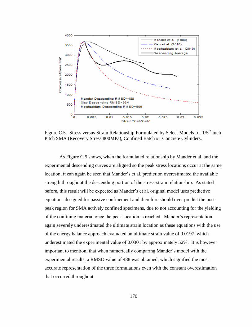
170
Figure C.5. Stress versus Strain Relationship Formulated by Select Models for 1/5th
inch
Pitch SMA (Recovery Stress 800MPa), Confined Batch #1 Concrete Cylinders.
As Figure C.5 shows, when the formulated relationship by Mander et al. and the
experimental descending curves are aligned so the peak stress locations occur at the same
location, it can again be seen that Mander’s et al. prediction overestimated the available
strength throughout the descending portion of the stress-strain relationship. As stated
before, this result will be expected as Mander’s et al. original model uses predictive
equations designed for passive confinement and therefore should over predict the post
peak region for SMA actively confined specimens, due to not accounting for the yielding
of the confining material once the peak location is reached. Mander’s representation
again severely underestimated the ultimate strain location as these equations with the use
of the energy balance approach evaluated an ultimate strain value of 0.0197, which
underestimated the experimental value of 0.0301 by approximately 52%. It is however
important to mention, that when numerically comparing Mander’s model with the
experimental results, a RMSD value of 488 was obtained, which signified the most
accurate representation of the three formulations even with the constant overestimation
that occurred throughout.

171
The predictive relationship from Xiao et al. was the second most accurate in
predicting the descending curve and had a RMSD value of 534. From this figure, it can
be seen that equations from Xiao do a fairly accurate job at predicting the sharp decrease
directly after the peak stress is reached, although it does slightly over estimate this
portion. It can also be seen, that just like with the 1/3rd
inch pitch SMA confined
specimens this stress-strain relationship begins to overestimate the available strength as it
approaches the ultimate failure location. When looking strictly at the increase in ductility
and ultimate strain location, Xiao formulations with the energy balance approach was
again accurate, as it evaluated an ultimate strain value of 0.0273, which only
underestimated the experimental results of 0.029 by approximately 6%.
As typical, Moghaddam et al. assessed the steepest descending curve and the
lowest post-peak stress-strain relationship of the three formulations. This relationship did
a really good job predicting the initial decrease that occurs after the peak stress was
reached. However, in the model by Moghaddam, the estimated relationship again
basically follows this initial decrease until the ultimate strain value is reached, which
differs greatly from the experimental descending average that tends to eventually level
out as the concrete cylinder crushes. Due to this difference in relationships, it appears
that Moghaddam’s prediction will continually underestimate the available compressive
strength towards the last 2/3rds
of the stress-strain curve. Moghaddam’s representation
was stopped at a strain value of 0.035, as this prediction with the energy balance
approach predicts unrealistically high ultimate strain values, and therefore no ultimate
strain comparison will be made. Moghaddam et al. equations obtained a RMSD value of
900 even with the accurate early representation due to the fact that towards the end of the
prediction this model was so far off from the experimental results.
C.2 Concrete Batch #2
The descending average curves that are displayed within this section were directly
taken from the experimentally obtained data that was previously displayed in section
6.3.2.1 and 6.3.2.2.

172
C.2.1 SMA Confined 1/3rd
inch Pitch Specimens
Using the peak stress information for the unconfined concrete cylinders of
concrete batch #2 (4563 psi), the formulated stress-strain relationship was then again able
to be determined for the three selected models (Mander, Xiao, and Moghaddam) in an
attempt to compare the formulated post-peak behavior with the experimentally
determined average results. The plot displaying the formulated results and the
experimentally determined descending average curve after it was adjusted to align with
theoretical peaks is shown in Figure C.6.
Figure C.6. Stress versus Strain Relationships, Formulated by Select Models and the
Experimentally Determined Descending Average for 1/3rd
inch Pitch SMA (Recovery
Stress 800MPa), Confined Batch #2 Concrete Cylinders.
From the stress-strain plots shown in Figure C.6 it appears that all of the
predictive relationships are much steeper and do not match when compared to the
experimental average. This slightly inaccurate performance is most likely due to the odd
occurrence of the unconfined cylinders having an average peak stress higher than the
average 1/3rd
inch pitch SMA confined cylinder, which goes directly against all
expectations and obtained results thus far. Like stated earlier from the three 1/3rd
inch

173
pitch SMA confined cylinders, it would appear that the compressive strength is lower
than the earlier determined value of 4563 psi, and more likely should be closer to
4000 psi or even slightly less. Due to this difference in measured peak strengths from the
unconfined and 1/3rd
inch pitch SMA confined cylinders, the formulated peak strengths
are all about 1000 psi higher, due to the slight increase in peak strength that the original
confinement model estimates. However, for completeness purposes the same procedure
of adjusting the descending curve to align with the formulated peak stress and calculating
a RMSD value carried-out in the previous sections will still be continued, although the
data obtained within this portion should probably be taken lightly.
When comparing relationship formulated by Mander et al. and the experimental
descending curve, once it was aligned so the peak stresses occurred at the same location,
it can again be seen that this time Mander’s et al. prediction was very accurate in
predicting the descending curve. Although, it’s important to mention that the prediction
by Mander usually has the shallowest decreasing slope of the three models, and the likely
erroneous and slightly higher unconfined concrete strength inputted into the model,
would appear to both work towards improving this prediction while decreasing the
accuracy of the other two. Nevertheless, with this scenario, Mander’s prediction had a
RMSD value of only 274, although it again slightly overestimated the relationship
directly after the peak stress location and underestimated the curve towards the ultimate
failure. While this prediction was very accurate in the portion of the prediction shown, it
again did a fairly poor job of predicting the ultimate strain location, as the value of
0.0106 that was evaluated by the model, underestimated the experimental result of 0.0216
by approximately 104%.
For this scenario, the predictive relationship from Xiao et al. obtained a very large
RMSD value of 1046. Xiao’s formulated relationship severely underestimated the
experimentally obtained average, almost completely throughout the prediction. This
much larger than normal RMSD value is again in all probability due to the apparently
erroneous unconfined concrete strength used within the model. With that said, it again
appears that Xiao prediction again did a fairly good job when visually comparing the
length of the descending curve, although the ultimate strain value appears to be slightly
off due to the sharply decreasing curve that was formulated. With this in mind, Xiao

174
assessed an ultimate strain value of 0.0162, which underestimated the experimentally
obtained ultimate strain value of 0.0211 by 30.2%.
Moghaddam et al. again formulated the lowest post-peak stress-strain relationship
of the three models. When comparing the experiential descending average with this
prediction it can be seen the Moghaddam again strongly underestimates the stress-strain
relationship of the entire region compared. While this underestimating behavior has been
shown in all of his formulations, this behavior appears much more severe due to the
perceived unconfined concrete strength error, giving this prediction another high RMSD
value of 1332. Moghaddam’s model also again overestimated the location of the ultimate
strain by assessing an ultimate strain value of approximately 0.0282, which resulted in a
26% overestimation of the experimental value of 0.0209.
C.2.2 SMA Confined 1/5th
inch Pitch Specimens
Just like before using the peak stress information for the unconfined concrete
cylinders of concrete batch #2 (4563 psi), the formulated stress-strain relationship was
then able to be determined for three selected models (Mander, Xiao, and Moghaddam) in
an attempt to compare the post-peak behavior with the experimentally determined
average results. The plot displaying the formulated results and the adjusted descending
average curve is shown in Figure C.7.

175
Figure C.7. Stress versus Strain Relationships, Formulated by Select Models and the
Experimentally Determined Descending Average for 1/5th
inch Pitch SMA (Recovery
Stress 800MPa), Confined Batch #2 Concrete Cylinders.
From the relationships shown in Figure C.7, it can again be seen that Mander et
al. prediction overestimates the stress-strain relationship when compared to the
experimentally obtained descending average directly after the peak location is reached,
but was able to very accurately predict the relationship towards the end of the prediction.
For this scenario the stress-strain relationship formulated by Mander et al. obtained a
RMSD value of 511, due to the inaccurate ability to account for the confining material
yielding directly at the peak location. This representation, once again also did a fairly
poor job at predicting the ultimate failure location, as the value of 0.0151 that was
assessed by the model, underestimated the experimental result of 0.0217 by
approximately 44%.
The predictive relationship from Xiao for this scenario obtained a RMSD value of
1016. Xiao’s formulated relationship was fairly accurate initially in predicting the
immediate decrease that occurred near the peak location, it did again however severely
underestimated the stress-strain relationship towards the ultimate strain location. Xiao
prediction of the ultimate failure location, which is often the best, was slightly off in this

176
case with an ultimate strain value of 0.0283 being assessed, or approximately 25% larger
than the experimental value obtained of 0.0211.
Again Moghaddam’s equations accurately formulated the relationship directly
after the peak stress was reached, but it again severely underestimates the available
strength towards the end of the region being compared. Due to this severe
underestimation that occurred within the last 2/3rds of this prediction, Moghaddam et al.
equations again obtained the highest and therefore least accurate prediction with a RMSD
value of 1518.
C.3 Concrete Batch #3
The descending average curves that are displayed within this section were directly
taken from the experimentally obtained data that was previously displayed in section
6.4.2.1 and 6.4.2.2.
C.3.1 SMA Confined 1/3rd
inch Pitch Specimens
Using the peak stress information for the unconfined concrete cylinders of
concrete batch #3 (3693 psi), the formulated stress-strain relationship was then able to be
determined for three selected models (Mander, Xiao, and Moghaddam) in an attempt to
compare the formulated post-peak behavior with the experimentally determined average
results. The plot displaying the formulated results and the adjusted descending average
curve is shown in Figure C.8.

177
Figure C.8. Stress versus Strain Relationships, Formulated by Select Models and the
Adjusted Experimentally Determined Descending Average for 1/3rd
inch Pitch SMA
(Recovery Stress 800MPa), Confined Batch #3 Concrete Cylinders.
From Figure C.8 it can again be seen that Mander’s et al. prediction overestimates
the stress-strain relationship when compared to the experimentally obtained descending
average throughout the entire region being compared. However, for this scenario the
stress-strain relationship formulated by Mander et al. obtained a RMSD value of 364,
which corresponded to the most accurate prediction. This prediction by Mander, once
again shows the severe underestimation of the ultimate strain location, as the Mander
equations with the use of the energy balanced approach assessed an ultimate strain value
of 0.0125, which underestimated the experimental result of 0.0246 by approximately
96.8%.
The predictive relationship by Xiao et al. was the second most accurate of the
three models with a RMSD value of 398, which was only slightly higher than the RSMD
value previously determined from Mander’s representation. While the RSMD value is
higher in this comparison, it’s important to note that this equation was very accurate in
predicting the initial post-peak relationship and almost perfectly matched the initial slope
of the decreasing curvature.

178
While this prediction was initially extremely accurate, this method again
underestimated the stress-strain relationship the closer it got to the ultimate failure
location. While this method eventually became less accurate towards the end of the
prediction, it should be noted that it again did a fairly accurate job in predicting the
ultimate failure location by assessing a value of 0.0171, which underestimated the
experimental result of 0.0241 by approximately 40.9%.
Moghaddam et al. model again did a decent job in predicting the relationship
directly after the peak stress was reached, but it again severely underestimates the
available strength towards the end of the region being compared. Due to the severe
underestimation that occurs with this prediction towards the end of region being
compared, Moghaddam’s model again obtained the highest and therefore least accurate
prediction with a RMSD value of 632. This prediction was however very accurate in
predicting the ultimate strain location with an assessed value of 0.0249, which only
overestimated the experimentally obtained result of 0.0237, or by 4.8%.
C.3.2 SMA Confined 1/5th
inch Pitch Specimens
Just like in the previous sections, using the peak stress information for the
unconfined concrete cylinders of concrete batch #3 (3693 psi), the formulated stress-
strain relationship was then able to be determined for three selected models (Mander,
Xiao, and Moghaddam) in an attempt to compare the formulated post-peak behavior with
the experimentally determined average results. The plot displaying the formulated results
and the adjusted descending average curve is shown in Figure C.9.

179
Figure C.9. Stress versus Strain Relationships, Formulated by Select Models and the
Adjusted Experimentally Determined Descending Average for 1/5th
inch Pitch SMA
(Recovery Stress 800MPa), Confined Batch #3 Concrete Cylinders.
From Figure C.9 it can again be seen that Mander’s et al. prediction overestimates
the stress-strain relationship when compared to the experimentally obtained descending
average throughout the entire region being compared. Mander’s equations, again does a
poor job accounting for the sharp decrease in available strength that occurs directly after
the peak location is reached. This prediction was however, fairly accurate at predicting
the ultimate strain location with an assessed value of 0.0174, underestimating the
experimental obtained value of 0.022 by only 26.4%. For this scenario the stress-strain
relationship formulated by Mander et al. obtained a RMSD value of 587, which
corresponded to the second lowest RMSD value.
The predictive relationship from Xiao et al. for this scenario was the most
accurate of the three models with a RMSD value slightly better than the curve formulated
by Mander et al. with a corresponding value of 310. Xiao’s model was accurate
throughout the relationship, although towards the end of the region being compared, this
relationship did slightly underestimate the available strength of the confined specimens.
This prediction also did a suitable job in predicting the ultimate strain location by

180
overestimating the experimental value of 0.021 by 20.8% with a value of 0.0265 being
assessed.
Moghaddam et al. model again severely underestimated the available strength
towards the end of the region being compared, and again obtained the highest and
therefore least accurate prediction, with a RMSD value of 833. This model with the use
of the energy balanced approach, once again severely overestimated the ultimate strain
location as well, and therefore was forced to be stopped at a strain value of 0.0035, with
no ultimate strain comparison able to be made.
C.4 RMSD Values Obtained
As with any situation utilizing the RMSD statistical method, there is no real way
to assign a level of accuracy to a single obtained value, and therefore the values obtained
are best used to show accuracy when compared to other results from similar situations.
With that being said, Table C.1 below summarized the RMSD values calculated after
comparing the experimental averages with each of the three models formulated post peak
relationship from each concrete batch/scenario tested within this experimental
investigation.
From Table C.1, it’s easy to see that the models formulated by both Mander and
Xiao were the most accurate, giving low and very similar RMSD values throughout,
especially when remembering that an error is perceived to have occurred within concrete
batch #2. However, it is important to restate, that the RMSD values obtained was just
one of the multiple methods used to determine the most accurate stress-strain relationship
for SMA confined concrete specimens, and this method does has some major limitations
that were previously discussed in Section C.1.1. With this in mind, the RMSD values can
really only be used to numerically display how inaccurate the model formulated by
Moghaddam was, as this model received the highest values throughout this work.

181
Concrete Batch #1 Concrete Batch #2 Concrete Batch #3
Model 1/3rd
1/5th 1/3
rd 1/5
th 1/3
rd 1/5
th
Mander et al. 356 488 274 511 364 587
Xiao et al. 320 534 1046 1016 398 310
Moghaddam
et al. 526 900 1332 1518 632 833
Table C.1. Summary of RMSD Values Obtained
C.5 Concluding Remarks
The following conclusions can be drawn from the experimental investigation and
assessment of the analytical models with regard to their correlations with the
experimental data. When reading these conclusions it’s again important to remember that
due to the material and experimental limitations, only some significant trends can be
identified. With this in mind, these conclusions are generally based on the overall
behavior that tends to be prevalent throughout the experimental work, and obviously
more research is needed to arrive at some appropriate numerically driven assessments.
C.5.1 Assessment of the Confinement Model and Experimental Correlations
1. The active confinement model used in this thesis appears to be reasonable in
predicting the stress-strain relationship of SMA confined specimens, as long
as four key parameters are known:
a. Unconfined concrete strength.
b. SMA ultimate tensile strength.
c. SMA fracture strain.
d. Ratio of the volume of transverse SMA to the volume of the confined
concrete core.
2. The energy balanced approach used within the active confinement model does
a fairly accurate job in predicting the ultimate strain location of the SMA
confined concrete cylinders. However, due to the fact that this method only
takes into account the area under the stress-strain relationship, the equation

182
that is ultimately used to predict this relationship will greatly affect this
location.
3. Moghaddam’s Model:
a. Often accurately matched the initial decrease in the stress-strain
relationship that occurred directly after the peak location was reached,
but severely underestimated the post-peak stress-strain behavior
thereafter.
b. This prediction could be very accurate if the concrete specimens would
fail ideally, but due to the unpredictable crushing nature of concrete,
the experimental stress-strain relationships were often drastically
different from an ideal situation.
c. The least accurate of the three models compared.
4. Mander’s Model:
a) Consistently overestimated the stress-strain relationship throughout the
post-peak region, due to the fact that this model does not take into
account the yielding of the SMA confining material.
b) The energy balance approach often severely underestimated the
ultimate strain location of the SMA confined specimens.
c) The descending portion of this stress-strain formulation was often less
accurate towards the peak stress location, and more accurate towards
the ultimate strain region due to the slope and curvature that this model
assessed.

183
5. Xiao’s Model:
a) Often accurately matched the initial descending curve in the stress-
strain relationship that directly occurred after the peak location was
reached.
b) Although it did tend to underestimate the available strength towards
the ultimate strain location this method was at least correctly on the
conservative side.
c) With the use of the energy balance approach this formulation was
consistently the most accurate in predicting the ultimate strain
location.
6. Based upon the assessment of the analytical models with the data obtained
from the experimental investigation, the model by Xiao et al. was the most
accurate model investigated, and may be used to accurately express the stress-
strain relationship of SMA confined concrete.

184
Appendix D: Matlab Codes
D.1 Code for Unconfined Concrete Stress-Strain Relationship
function [fc]=ConcreteCode(epc)
% fc' =compressive strength of concrete =4000psi % epcu =max usable compressive strain for concrete =0.004 % epco =strain at fc' (max concrete stress) =0.002 % for unconfined concrete % epcc =strain at fc' (max concrete stress) =0.002 % for confined concrete
fcprime=4000; epcu=0.004; epco=0.002; epcc=0.002;
Ec=57000*((fcprime)^.5); Esec=fcprime/epco; r=Ec/(Ec-Esec); ep50u=(3+0.002*fcprime)/(fcprime-1000);
x1=epco; y1=fcprime; x2=ep50u; y2=0.5*fcprime;
Slope=(y2-y1)/(x2-x1); yint=fcprime-Slope*epco;
% epc=-epc;
if epc <= epco && epc>0 fc=((fcprime*r*(epc/epcc))/(r-1+((epc/epcc)^r)));
elseif epc<=epcu && epc>0 fc=Slope*epc+yint; else fc=0; end
end

185
D.2 Code for Steel Stress-Strain Relationship
function [fs]=SteelCode(ep)
% Es =modulus of elasticity of Steel % fy =yeild strength of steel % eps =strain of steel % epsy =strain at the yield point % epsrup =strain at rupture of steel
%Units are PSI Es=29000000; fy=60000; fu=100000;
epsy=0.00207; epsh=0.010; epsu=0.08; epsrup=0.12;
SHpercent=0; NegStrain=0; if ep<0 NegStrain=1; ep=-ep; %A Marker being used to avoid errors if Negative Strain %values are inputed into the function end fsh=fy+(epsh-epsy)*SHpercent*Es;
if ep>epsrup; fs=0;
elseif ep<=epsy; fs=Es*ep; elseif ep<=epsh && ep>=epsy fs=fy+SHpercent*Es*(ep-epsy); else fs=fu-(fu-fsh)*(((epsu-ep)/(epsu-epsh))^2); end
if NegStrain==1 fs=-fs; %Switches Negative stress value from Negative %Strain to Positive end end
D.3 Typical Code Displaying the Formulated Stress-Strain Relationship of SMA
Confined Concrete for All Models
close all clear all clc

186
tic
%Unconfined Concrete Stress in PSI fc_prime=[4000]; %Max unconfined concrete stress fco_prime=fc_prime; epco=0.002; %Strain at max stress of unconfined concrete epcu_unconfined=0.004; %Going to need to use a different variable
for this value and the value of the confined concrete
%Column Information h=8; %Height (inches) d=4; %diameter (inches) ColumnArea=pi*((d/2)^2); %Area of Column (Inches)^2
%SMA information fSMA=116000; %(PSI) (800MPa) diamSMA=0.02 ; %(inch) areaSMA=pi*((diamSMA/2)^2); %(Inch)^2 ds=d+(diamSMA/2)+(diamSMA/2); %diameter of spiral between bar centers (inch)
tieDiam=0; %This portion has no column ties
%SMA information Used for calculating the Ultimate Strain Capacity Ult_ten_Str_SMA=150000; %Ultimate Tensile Strength of SMA USed (Psi) Fracture_strain_SMA=0.15; %Fracture Strain of The transverse SMA
%Unconfined Concrete %This portion finds the stress-strain curve for unconfined concrete
which %is used for solving an energy balance equation, that is required to
find %the ultimate strain of the confined concrete w=1; for epc=0:0.0001:epcu_unconfined; allepc(w)=epc; fc_unconfined=ConcreteCode(epc); allfc_unconfined(w)=fc_unconfined;
UnconfinedConcrete_load=fc_unconfined*ColumnArea; allUnConLoad(w)=UnconfinedConcrete_load;
dispUncon=epc*h; alldispUnCon(w)=dispUncon;
w=w+1; end
Xint_Unconfined=allepc; Yint_Unconfined=allfc_unconfined;
Unconfined_concrete_energy=trapz(Xint_Unconfined ,Yint_Unconfined); %The unconfined concrete energy capacity based on Manders et al.
equations

187
for q=1:1:6; loops_per_inch=5;
s=(1/loops_per_inch)-(diamSMA/2); %s=center line spaceing between ties (inches)
s_prime=s-diamSMA; %clear distance between ties (inch)
roecc=0; %roecc=ratio of area of longitudinal reinforcement to area of core
of section %The core samples have no longitudinal reinforcement and therefore
equals 0
Acc=((pi/4)*((ds)^2)*(1-roecc)); %in^2 ke=(1-((s_prime)/(2*ds)))/(1-roecc);
roe_s=(4*areaSMA)/(ds*s); %ratio of the volume of transverse
confining steel to the volume of confined concrete core allroe_s(q)=roe_s; %Unitless
%epcu_confined=epcu_unconfined+0.14*(roe_s)*(fSMA/fc_prime); %The other possible equation for ultimate strain epcu_confined=0.04; %experimental value used from solving manders
equations
fl=(2*areaSMA*fSMA)/(d*s);
fl_prime=ke*fl;
i=1; for ep=0:0.00025:epcu_confined;
num(q)=i;
allep(q,i)=ep;
if q==1 %Using Manders (1988) Equations fcc_prime=fco_prime*(-
1.254+(2.254*(1+((7.94*fl_prime)/(fco_prime)))^(0.5))-
(2*(fl_prime/fco_prime))); epcc=epco*(1+5*((fcc_prime(q)/fco_prime)-1));
elseif q==2 %Using Richarts (1928) Equations fcc_prime=fco_prime*(1+4.1*(fl_prime/fco_prime)); epcc=(1+20.5*(fl_prime/fco_prime))*epco;
elseif q==3 %Using Candappa (2001) Equations

188
fcc_prime=fco_prime*(1+5.3*(fl_prime/fco_prime)); epcc=(1+20*(fl_prime/fco_prime))*epco;
elseif q==4 %Using Jiang and Teng (2007) Equations fcc_prime=fco_prime*(1+3.5*(fl_prime/fco_prime)); epcc=(1+17.5*((fl_prime/fco_prime)^1.2))*epco;
elseif q==5 %Using Xiaos 2010 Equations NSC and HSC fcc_prime=(1+3.24*((fl_prime/fc_prime)^0.8))*fco_prime; epcc=(1+17.4*((fl_prime/fco_prime)^1.06))*epco;
else %Using Moghaddam 2010 Equations fcc_prime=fco_prime*(1+8*(fl_prime/fco_prime)-
4*((fl_prime/fco_prime)^1.2)); epcc=epco*((fcc_prime/fco_prime)^1.1);
end
x=ep/epcc; allx(q,i)=x; Ec=57000*((fco_prime)^(0.5)); Esec=fcc_prime/epcc; r=Ec/(Ec-Esec);
fc=(fcc_prime*x*r)/(r-1+(x^r)); allfc(q,i)=fc;
i=i+1; end
%This portion is separating the stress and strain values apart from %each curve based upon the spacing value to be used in calculating
the %energy capactiy (area under the curves)
%USH=Ultimate Strain Energy Capacity of the confining %reinforcement per unit volume of concrete core %Ush will vary for each SMA spacing category because it changes the %value of roe_s for each
if q==1 %Manders Xint_Confined_Mander=allep(1,:); Yint_Confined_Mander=allfc(1,:);
Ush_Mander=Ult_ten_Str_SMA*Fracture_strain_SMA*roe_s;
elseif q==2 %Richart Xint_Confined_Richart=allep(2,:); Yint_Confined_Richart=allfc(2,:);

189
Ush_Richart=Ult_ten_Str_SMA*Fracture_strain_SMA*roe_s;
elseif q==3 %Candappa Xint_Confined_Candappa=allep(3,:); Yint_Confined_Candappa=allfc(3,:);
Ush_Candappa=Ult_ten_Str_SMA*Fracture_strain_SMA*roe_s;
elseif q==4 %Jiang and Teng Xint_Confined_Jiang_and_Teng=allep(4,:); Yint_Confined_Jiang_and_Teng=allfc(4,:);
Ush_Jiang_and_Teng=Ult_ten_Str_SMA*Fracture_strain_SMA*roe_s;
elseif q==5 %Xiao Xint_Confined_Xiao=allep(5,:); Yint_Confined_Xiao=allfc(5,:);
Ush_Xiao=Ult_ten_Str_SMA*Fracture_strain_SMA*roe_s;
else %Moghaddam Xint_Confined_Moghaddam=allep(6,:); Yint_Confined_Moghaddam=allfc(6,:);
Ush_Moghaddam=Ult_ten_Str_SMA*Fracture_strain_SMA*roe_s;
end end
%For all sections below %Confined Concrete Portion %For this setup there is no longitudinal steel or unconfined %concrete therefore only the confined concrete portion is %contributing to the stress-strain relationship
%P_column=ConfinedConcrete_load+UnconfinedConcrete_Load+Steel_Load %However, for this setup there is no unconfined concrete or %longitudinal steel therefore they both equal zero and all load is %from the ConfinedConcrete only
%Manders 1988 Equations. for z=2:1:numel(Xint_Confined_Mander);
Confined_Concrete_Energy_Mander=trapz(Xint_Confined_Mander(1:z)
,Yint_Confined_Mander(1:z)); %Approx Energy Capacity for a curve that is Extended delibertly long %pass a realistic ultimate strain value
if Confined_Concrete_Energy_Mander <=
Ush_Mander+Unconfined_concrete_energy %Finds when the Energy capacity of the 1inch SMA spaced
stress-strain curve is greater than the combined

190
%energy from the transverse confining SMA and the energy
from %your typical unconfined concrete energy.
epcu_confined_Mander=Xint_Confined_Mander(z); %Once the Ultimate Strain value has been reach this line %assigns that value to the stress-strain curve zz=z;
allep_Mander_until_Ult_Strain=Xint_Confined_Mander(1:zz); allfc_Mander_Until_Ult_Strain=Yint_Confined_Mander(1:zz); %stops the stress and strain values at the ultimate strain
location
ConfinedConcrete_load_Mander=allfc_Mander_Until_Ult_Strain*ColumnArea; P_column_Mander=ConfinedConcrete_load_Mander;
disp_Mander=allep_Mander_until_Ult_Strain*h; end
end
%Richart 1928 Equations. for v=2:1:numel(Xint_Confined_Richart);
Confined_Concrete_Energy_Richart=trapz(Xint_Confined_Richart(1:v)
,Yint_Confined_Richart(1:v)); %Approx Energy Capacity for a curve that is Extended delibertly long %pass a realistic ultimate strain value
if Confined_Concrete_Energy_Richart <=
Ush_Richart+Unconfined_concrete_energy %Finds when the Energy capacity of 1_2inch stress-strain
curve is greater than the combined %energy from the transverse confining SMA and the energy
from %your typical unconfined concrete energy.
epcu_confined_Richart=Xint_Confined_Richart(v); %Once the Ultimate Strain value has been reach this line %assigns that value to the stress-strain curve vv=v;
allep_Richart_Until_Ult_Strain=Xint_Confined_Richart(1:vv); allfc_Richart_Until_Ult_Strain=Yint_Confined_Richart(1:vv); %stops the stress and strain values at the ultimate strain
location
ConfinedConcrete_load_Richart=allfc_Richart_Until_Ult_Strain*ColumnArea
;

191
P_column_Richart=ConfinedConcrete_load_Richart;
disp_Richart=allep_Richart_Until_Ult_Strain*h;
end end
%Candappa. for b=2:1:numel(Xint_Confined_Candappa);
Confined_Concrete_Energy_Candappa=trapz(Xint_Confined_Candappa(1:b)
,Yint_Confined_Candappa(1:b)); %Approx Energy Capacity for a curve that is Extended delibertly long %pass a realistic ultimate strain value
if Confined_Concrete_Energy_Candappa <=
Ush_Candappa+Unconfined_concrete_energy %Finds when the Energy capacity of 1_3rdinch stress-strain
curve is greater than the combined %energy from the transverse confining SMA and the energy
from %your typical unconfined concrete energy.
epcu_confined_Candappa=Xint_Confined_Candappa(b); %Once the Ultimate Strain value has been reach this line %assigns that value to the stress-strain curve bb=b;
allep_Candappa_Until_Ult_Strain=Xint_Confined_Candappa(1:bb);
allfc_Candappa_Until_Ult_Strain=Yint_Confined_Candappa(1:bb); %stops the stress and strain values at the ultimate strain
location
ConfinedConcrete_load_Candappa=
allfc_Candappa_Until_Ult_Strain*ColumnArea; P_column_Candappa=ConfinedConcrete_load_Candappa;
disp_Candappa=allep_Candappa_Until_Ult_Strain*h; end end
%Jiang and Teng. for e=2:1:numel(Xint_Confined_Jiang_and_Teng);
Confined_Concrete_Energy_Jiang_and_Teng=trapz(Xint_Confined_Jiang_and_T
eng(1:e),Yint_Confined_Jiang_and_Teng(1:e)); %Approx Energy Capacity for a curve that is Extended delibertly long %pass a realistic ultimate strain value

192
if Confined_Concrete_Energy_Jiang_and_Teng <=
Ush_Jiang_and_Teng+Unconfined_concrete_energy %Finds when the Energy capacity of 1_4thinch stress-strain
curve is greater than the combined %energy from the transverse confining SMA and the energy
from %your typical unconfined concrete energy.
epcu_confined_Jiang_and_Teng=Xint_Confined_Jiang_and_Teng(e); %Once the Ultimate Strain value has been reach this line %assigns that value to the stress-strain curve ee=e;
allep_Jiang_and_Teng_Until_Ult_Strain=Xint_Confined_Jiang_and_Teng(1:ee
);
allfc_Jiang_and_Teng_Until_Ult_Strain=Yint_Confined_Jiang_and_Teng(1:ee
); %stops the stress and strain values at the ultimate strain
location
ConfinedConcrete_load_Jiang_and_Teng=allfc_Jiang_and_Teng_Until_Ult_Str
ain*ColumnArea;
P_column_Jiang_and_Teng=ConfinedConcrete_load_Jiang_and_Teng;
disp_Jiang_and_Teng=allep_Jiang_and_Teng_Until_Ult_Strain*h; end end
%Xiao. for p=2:1:numel(Xint_Confined_Xiao);
Confined_Concrete_Energy_Xiao=trapz(Xint_Confined_Xiao(1:p)
,Yint_Confined_Xiao(1:p)); %Approx Energy Capacity for a curve that is Extended delibertly long %pass a realistic ultimate strain value
if Confined_Concrete_Energy_Xiao <=
Ush_Xiao+Unconfined_concrete_energy %Finds when the Energy capacity of 1_5thinch stress-strain
curve is greater than the combined %energy from the transverse confining SMA and the energy
from %your typical unconfined concrete energy.
epcu_confined_Xiao=Xint_Confined_Xiao(p); %Once the Ultimate Strain value has been reach this line %assigns that value to the stress-strain curve pp=p;

193
allep_Xiao_Until_Ult_Strain=Xint_Confined_Xiao(1:pp); allfc_Xiao_Until_Ult_Strain=Yint_Confined_Xiao(1:pp); %stops the stress and strain values at the ultimate strain
location
ConfinedConcrete_load_Xiao=allfc_Xiao_Until_Ult_Strain*ColumnArea; P_column_Xiao=ConfinedConcrete_load_Xiao;
disp_Xiao=allep_Xiao_Until_Ult_Strain*h; end end
%Moghaddam. for u=2:1:numel(Xint_Confined_Moghaddam);
Confined_Concrete_Energy_Moghaddam=trapz(Xint_Confined_Moghaddam(1:u)
,Yint_Confined_Moghaddam(1:u)); %Approx Energy Capacity for a curve that is Extended delibertly long %pass a realistic ultimate strain value
if Confined_Concrete_Energy_Moghaddam <=
Ush_Moghaddam+Unconfined_concrete_energy %Finds when the Energy capacity of 1_5thinch stress-strain
curve is greater than the combined %energy from the transverse confining SMA and the energy
from %your typical unconfined concrete energy.
epcu_confined_Moghaddam=Xint_Confined_Moghaddam(u); %Once the Ultimate Strain value has been reach this line %assigns that value to the stress-strain curve uu=u;
allep_Moghaddam_Until_Ult_Strain=Xint_Confined_Moghaddam(1:uu);
allfc_Moghaddam_Until_Ult_Strain=Yint_Confined_Moghaddam(1:uu); %stops the stress and strain values at the ultimate strain
location
ConfinedConcrete_load_Moghaddam=allfc_Moghaddam_Until_Ult_Strain*Column
Area; P_column_Moghaddam=ConfinedConcrete_load_Moghaddam;
disp_Moghaddam=allep_Moghaddam_Until_Ult_Strain*h; end end
plot (allep_Mander_until_Ult_Strain, allfc_Mander_Until_Ult_Strain,'k',
allep_Richart_Until_Ult_Strain, allfc_Richart_Until_Ult_Strain,'g--',
allep_Candappa_Until_Ult_Strain, allfc_Candappa_Until_Ult_Strain, 'm:',

194
allep_Jiang_and_Teng_Until_Ult_Strain,
allfc_Jiang_and_Teng_Until_Ult_Strain,'r-.',
allep_Xiao_Until_Ult_Strain, allfc_Xiao_Until_Ult_Strain,'b*',
allep_Moghaddam_Until_Ult_Strain,
allfc_Moghaddam_Until_Ult_Strain,'cd'); legend('Mander et al. (1988)', 'Richart et al (1928)', 'Candappa et al.
(2001)', 'Jiang and Teng (2007)', 'Xiao et al. (2010)', 'Moghaddam et
al. (2010)') title(char(' Stress vs. Strain','(4000 Psi Concrete,
SMA=50000 Psi, 1/3in Spacing)')) xlabel('Strain "inch/inch"') ylabel('Compressive Stress "Psi"')
figure
plot (disp_Mander, ConfinedConcrete_load_Mander, 'k', disp_Richart,
ConfinedConcrete_load_Richart, 'g--', disp_Candappa,
ConfinedConcrete_load_Candappa, 'm:', disp_Jiang_and_Teng,
ConfinedConcrete_load_Jiang_and_Teng, 'r-.', disp_Xiao,
ConfinedConcrete_load_Xiao, 'b*' , disp_Moghaddam,
ConfinedConcrete_load_Moghaddam, 'cd') legend('Mander et al. (1988)', 'Richart et al (1928)', 'Candappa et al.
(2001)', 'Jiang and Teng (2007)', 'Xiao et al. (2010)', 'Moghaddam et
al. (2010)') title(char(' Axial Load vs. Displacement','(4000 Psi Concrete,
SMA=50000 Psi 1/3in Spacing)')) xlabel('Axial Displacement (inch)') ylabel('Axial Load (Lbs)')
toc
D.4 Typical Code Displaying the Results from the Numerical Example Predicting the
Stress-Strain and Load vs. Displacement for the 12 inch Spaced SMA Column
close all clear all clc
tic
%SMA information fSMA=116000; %(PSI) (800MPa) diamSMA=.5 ; %(inch) areaSMA=pi*((diamSMA/2)^2); %(Inch)^2
%SMA information Used for calculating the Ultimate Strain Capacity Ult_ten_Str_SMA=170000; %Ultimate Tensile Strength of SMA USed (Psi) Fracture_strain_SMA=0.175; %Fracture Strain of The transverse SMA
%Circular Column Information h=120; %Height (inches)

195
d=18; %diameter (inches) ColumnArea=pi*((d/2)^2); %Area of Column (Inches)^2
ds=d+(diamSMA/2)+(diamSMA/2); %diameter of spiral between bar centers (inch)
cc=1.5; %clear cover inches ConfinedColumnArea=pi*(((d-(2*cc)-diamSMA)/2)^2);
%8 No. 9 longitudinal bars NumLongBars=8; %Number of longitudinal bars ast9=1.00; %Area of a number 9 bar diam9=1.128; %Diam of a number 9 bar astlong=NumLongBars*ast9; %Area of Longitudinal Steel
%Unconfined Concrete Stress in PSI fc_prime=[4000]; %Max unconfined concrete stress fco_prime=fc_prime; epco=0.002; %Strain at max stress of unconfined concrete epcu_unconfined=0.004; %Ultimate Strain for unconfined concrete
%Unconfined Concrete %This portion finds the stress-strain curve for unconfined concrete
which %is used for solving an energy balance equation, that is required to
find %the ultimate strain of the confined concrete w=1; for epc=0:0.0001:epcu_unconfined; allepc(w)=epc; fc_unconfined=ConcreteCode(epc); allfc_unconfined(w)=fc_unconfined;
w=w+1; end
Xint_Unconfined=allepc; Yint_Unconfined=allfc_unconfined;
Unconfined_concrete_energy=trapz(Xint_Unconfined ,Yint_Unconfined); %The unconfined concrete energy capacity based on Manders et al.
equations
%This portion is for SMA confined concrete Specimens that %has only Transverse SMA confining material and incorporates
information %from the unconfiend concrete strength listed directly above for q=2; s=12; %center to center spaceing between ties (inches)
s_prime=s-diamSMA; %clear distance between ties (inch) ac=pi*(((d-(2*cc)-diamSMA)/2)^2); %roecc

196
roecc=astlong/(ac);%area of longitudinal reinforcement/area of core
of
acc=((pi/4)*((ds)^2)*(1-roecc)); %in^2 ke=(1-((s_prime)/(2*ds)))/(1-roecc);
roe_s=(4*areaSMA)/(ds*s); %ratio of the volume of transverse
confining %steel to the volume of confined concrete core (Unitless)
fl=(2*areaSMA*fSMA)/(d*s); fl_prime=ke*fl;
i=1; epcu_confined=0.3; %unrealistically high value used to cover all relatisic examples for ep=0:0.0001:epcu_confined; num=i; allep(q,i)=ep;
%Using Xiaos 2010 Equations NSC and HSC fcc_prime=(1+3.24*((fl_prime/fc_prime)^0.8))*fco_prime; epcc=(1+17.4*((fl_prime/fco_prime)^1.06))*epco;
x=ep/epcc; allx(q,i)=x; Ec=57000*((fco_prime)^(0.5)); Esec=fcc_prime/epcc; r=Ec/(Ec-Esec);
fc=(fcc_prime*x*r)/(r-1+(x^r)); allfc(q,i)=fc;
i=i+1; end %USH=Ultimate Strain Energy Capacity of the confining %reinforcement per unit volume of concrete core
%Xiao Xint_Confined_Xiao=allep(2,:); Yint_Confined_Xiao=allfc(2,:);
Ush_Xiao=Ult_ten_Str_SMA*Fracture_strain_SMA*roe_s; end
%This portion below finds the ultimate strain location based on the
energy %blance approach using the stress-strain raltionship predicted by
Xiao's %relationship for p=2:1:numel(Xint_Confined_Xiao); allp=(1:p);

197
Confined_Concrete_Energy_Xiao=trapz(Xint_Confined_Xiao(1:p)
,Yint_Confined_Xiao(1:p)); %Approx Energy Capacity for a curve that is Extended delibertly long %pass a realistic ultimate strain value
if Confined_Concrete_Energy_Xiao <=
Ush_Xiao+Unconfined_concrete_energy
%Finds when the Energy capacity of the stress-strain curve %is greater than the combined energy from the transverse confining SMA %and the energy from your typical unconfined concrete energy.
epcu_confined_energy=Xint_Confined_Xiao(p); %Once the Ultimate Strain value has been reach this line %assigns that value to the stress-strain curve pp=p;
allep_Xiao_Until_Ult_Strain_Energy=Xint_Confined_Xiao(1:pp);
allfc_Xiao_Until_Ult_Strain_Energy=Yint_Confined_Xiao(1:pp); %stops the stress & strain values at ultimate strain
location end end
%this portion finds the untilmate strain value using a conditional
ultimate %strain value corresponding to 20% of the peak stress value calculated,
as %any value higher should be considered unrealistic for m=2:1:numel(Xint_Confined_Xiao); allm=(1:m); Stop=fcc_prime*0.2;
if Yint_Confined_Xiao(m) >= Stop && Xint_Confined_Xiao(m) >=
0.02 mm=m;
epcu_confined_percent=Xint_Confined_Xiao(mm); %Once the Ultimate Strain value has been reach this line %assigns that value to the stress-strain curve
allep_Xiao_Until_Ult_Strain_Percent=Xint_Confined_Xiao(1:mm);
allfc_Xiao_Until_Ult_Strain_Percent=Yint_Confined_Xiao(1:mm); %stops the stress &strain values at ultimate strain
location end end
%This selects the smaller ultimate strain value from either the energy

198
%balance approach or based on the conditional percented of the peak
stress if epcu_confined_percent < epcu_confined_energy
epcu_confined_Xiao = epcu_confined_percent; allep_Xiao_Until_Ult_Strain = allep_Xiao_Until_Ult_Strain_Percent; allfc_Xiao_Until_Ult_Strain = allfc_Xiao_Until_Ult_Strain_Percent;
else epcu_confined_Xiao = epcu_confined_energy; allep_Xiao_Until_Ult_Strain = allep_Xiao_Until_Ult_Strain_Energy; allfc_Xiao_Until_Ult_Strain = allfc_Xiao_Until_Ult_Strain_Energy; end
%Now that the ultimate strain value has been obtained we can find the
load %vs displacement plot for the column with 1.5inch clear cover
(unconfined %concrete), longitudinal steel, and the confined SMA core
%Load carried by the Confined Concrete Portion allConfinedConcrete_load=allfc_Xiao_Until_Ult_Strain*ConfinedColumnArea
;
ww=1; for ep2=0:0.0001:epcu_confined_Xiao; allep2(ww)=ep2;
%Steel Portion fsteel=SteelCode2(ep2); allfsteel(ww)=fsteel;
Steel_load=fsteel*astlong; allSteel_load(ww)=Steel_load;
%Unconfined Concrete portion clearcoverarea=(ColumnArea-ConfinedColumnArea);
funcon=ConcreteCode2(ep2); allfuncon(ww)=funcon;
Uncon_load=funcon*clearcoverarea; allUnConfinedConcrete_load(ww)=Uncon_load;
ww=ww+1; end
P_column_Xiao=allConfinedConcrete_load+allUnConfinedConcrete_load+allSt
eel_load; disp=allep_Xiao_Until_Ult_Strain*h; %Total Displacement of the Column
plot (allep_Xiao_Until_Ult_Strain, allfc_Xiao_Until_Ult_Strain,'b--');

199
legend('12inch Spacing') title('Confined Concrete Stress vs. Strain Relationship') xlabel('Strain "inch/inch"') ylabel('Compressive Stress "Psi"') % axis([0, 0.05, 0 ,6000])
figure plot(allep_Xiao_Until_Ult_Strain, allfsteel) title('Stress vs. Strain Relationship Typical Steel') xlabel('Strain "inch/inch"') ylabel('Compressive Stress "Psi"')
figure
plot(disp, P_column_Xiao) legend('12inch Spacing') title('Axial Load vs. Axial Displacement of Column') xlabel('Displacement (Inch)') ylabel('Axial Load (Lbs)')
toc

200
Appendix E: As Measured Stress-Strain Plots
Figure E.1. Recorded Stress versus Strain for the First Unconfined Cylinder in Concrete
Batch #1.

201
Figure E.2. Recorded Stress versus Strain for the Second Unconfined Cylinder in
Concrete Batch #1.
Figure E.3. Recorded Stress versus Strain for the First Unconfined Anchored Cylinder in
Concrete Batch #1.

202
Figure E.4. Recorded Stress versus Strain for the Second Unconfined Anchored Cylinder
in Concrete Batch #1.
Figure E.5. Recorded Stress versus Strain for the First 1/3rd
inch Pitch SMA Confined
Cylinder in Concrete Batch #1.
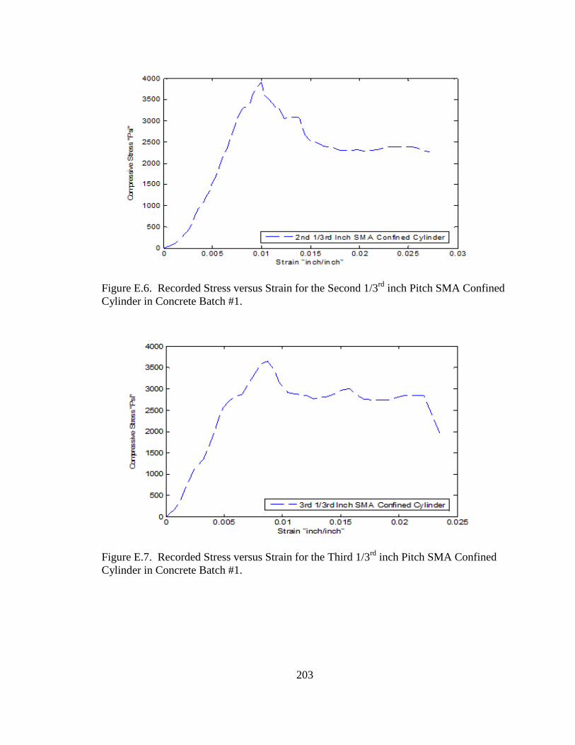
203
Figure E.6. Recorded Stress versus Strain for the Second 1/3rd
inch Pitch SMA Confined
Cylinder in Concrete Batch #1.
Figure E.7. Recorded Stress versus Strain for the Third 1/3rd
inch Pitch SMA Confined
Cylinder in Concrete Batch #1.

204
Figure E.8. Recorded Stress versus Strain for the First 1/5th
inch Pitch SMA Confined
Cylinder in Concrete Batch #1.
Figure E.9. Recorded Stress versus Strain for the Second 1/5th
inch Pitch SMA Confined
Cylinder in Concrete Batch #1.

205
Figure E.10. Recorded Stress versus Strain for the First Unconfined Cylinder in Concrete
Batch #2.
Figure E.11. Recorded Stress versus Strain for the Second Unconfined Cylinder in
Concrete Batch #2.

206
Figure E.12. Recorded Stress versus Strain for the First Unconfined Anchored Cylinder
in Concrete Batch #2.
Figure E.13. Recorded Stress versus Strain for the Second Unconfined Anchored
Cylinder in Concrete Batch #2.

207
Figure E.14. Recorded Stress versus Strain for the First 1/3rd
inch Pitch SMA Confined
Cylinder in Concrete Batch #2.
Figure E.15. Recorded Stress versus Strain for the Second 1/3rd
inch Pitch SMA
Confined Cylinder in Concrete Batch #2.

208
Figure E.16. Recorded Stress versus Strain for the Third 1/3rd
inch Pitch SMA Confined
Cylinder in Concrete Batch #2.
Figure E.17. Recorded Stress versus Strain for the First 1/5th
inch Pitch SMA Confined
Cylinder in Concrete Batch #2.

209
Figure E.18. Recorded Stress versus Strain for the Second 1/5th
inch Pitch SMA
Confined Cylinder in Concrete Batch #2.
Figure E.19. Recorded Stress versus Strain for the First Unconfined Cylinder in Concrete
Batch #3.

210
Figure E.20. Recorded Stress versus Strain for the Second Unconfined Cylinder in
Concrete Batch #3.
Figure E.21. Recorded Stress versus Strain for the First Unconfined Anchored Cylinder
in Concrete Batch #3.

211
Figure E.22. Recorded Stress versus Strain for the Second Unconfined Anchored
Cylinder in Concrete Batch #3.
Figure E.23. Recorded Stress versus Strain for the First 1/3rd
inch Pitch SMA Confined
Cylinder in Concrete Batch #3.

212
Figure E.24. Recorded Stress versus Strain for the Second 1/3rd
inch Pitch SMA
Confined Cylinder in Concrete Batch #3.
Figure E.25. Recorded Stress versus Strain for the Third 1/3rd
inch Pitch SMA Confined
Cylinder in Concrete Batch #3.
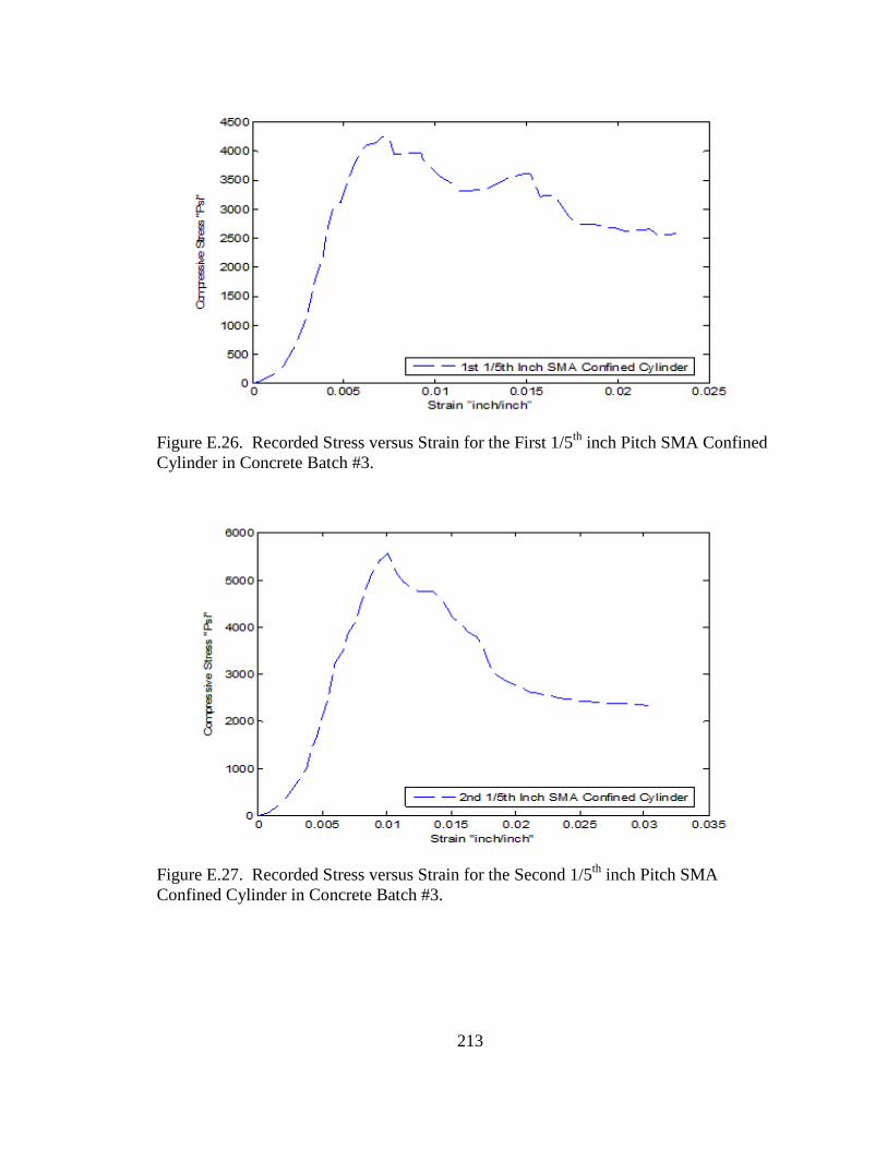
213
Figure E.26. Recorded Stress versus Strain for the First 1/5th
inch Pitch SMA Confined
Cylinder in Concrete Batch #3.
Figure E.27. Recorded Stress versus Strain for the Second 1/5th
inch Pitch SMA
Confined Cylinder in Concrete Batch #3.