Actively Transfer Domain Knowledge

Xiaoxiao Shi1, Wei Fan2, Jiangtao Ren1 ⋆

1. Department of Computer ScienceSun Yat-sen University, Guangzhou, China

{isshxx, issrjt}@mail.sysu.edu.cn,2. IBM T.J.Watson Research, USA

weifan@us.ibm.com

Abstract. When labeled examples are not readily available, active learn-ing and transfer learning are separate efforts to obtain labeled examplesfor inductive learning. Active learning asks domain experts to label asmall set of examples, but there is a cost incurred for each answer.While transfer learning could borrow labeled examples from a differ-ent domain without incurring any labeling cost, there is no guaranteethat the transferred examples will actually help improve the learningaccuracy. To solve both problems, we propose a framework to activelytransfer the knowledge across domains, and the key intuition is to usethe knowledge transferred from other domain as often as possible to helplearn the current domain, and query experts only when necessary. Todo so, labeled examples from the other domain (out-of-domain) are ex-amined on the basis of their likelihood to correctly label the examplesof the current domain (in-domain). When this likelihood is low, theseout-of-domain examples will not be used to label the in-domain exam-ple, but domain experts are consulted to provide class label. We derivea sampling error bound and a querying bound to demonstrate that theproposed method can effectively mitigate risk of domain difference bytransferring domain knowledge only when they are useful, and query do-main experts only when necessary. Experimental studies have employedsynthetic datasets and two types of real world datasets, including re-mote sensing and text classification problems. The proposed method iscompared with previously proposed transfer learning and active learningmethods. Across all comparisons, the proposed approach can evidentlyoutperform the transfer learning model in classification accuracy givendifferent out-of-domain datasets. For example, upon the remote sens-ing dataset, the proposed approach achieves an accuracy around 94.5%,while the comparable transfer learning model drops to less than 89% inmost cases. The software and datasets are available from the authors.

1 Introduction

Supervised learning methods require sufficient labeled examples in order to con-struct accurate models. However, in real world applications, one may easily en-

⋆ The author is supported by the National Natural Science Foundation of China underGrant No. 60703110

(a) Transfer learning (b) Active learning (c) Actively transfer

Fig. 1. Different models to resolve label deficiency

counter those situations in which labeled examples are deficient, such as datastreams, biological sequence annotation or web searching, etc. To alleviate thisproblem, two separate approaches, transfer learning and active learning, havebeen proposed and studied. Transfer learning mainly focuses on how to utilizethe data from a related domain called out-of-domain, to help learn the currentdomain called in-domain, as depicted in Fig 1(a). It can be quite effective whenthe out-of-domain dataset is very similar to the in-domain dataset. As a differ-ent solution, active learning does not gain knowledge from other domains, butmainly focuses on selecting a small set of essential in-domain instances for whichit requests labels from the domain experts, as depicted in Fig 1(b). However,both transfer learning and active learning have some practical constraints. Fortransfer learning, if the knowledge from the out-of-domain is essentially differentfrom the in-domain, the learning accuracy might be reduced, and this is calledthe “domain difference risk”. For active learning, the obvious issue is the costassociated with the answer from domain experts.

Our Method To mitigate domain difference risk and reduce labeling cost, we pro-pose a framework that can actively transfer the knowledge from out-of-domain toin-domain, as depicted in Fig 1(c). Intuitively, in daily life, we normally first tryto use our related knowledge in learning, but if the related knowledge is unableto guide, we turn to teachers. For example, when learning a foreign language,one normally associates it with the mother tongue. This transfer is easy between,for example, Spanish and Portuguese. But it is not so obvious between Chineseand English. In this situation, one normally pays a teacher instead of pickingup himself. The proposed framework is based on these intuitions. We first selectan instance that is supposed to be essential to construct an inductive modelfrom the new or in-domain dataset, and then a transfer classifier, trained withlabeled data from in-domain and out-of-domain dataset, is used to predict thisunlabeled in-domain example. According to defined transfer confidence measure,this instance is either directly labeled by the transfer classifier or labeled by thedomain experts if needed. In order to guarantee the performance when “import-ing” out-of-domain knowledge, the proposed transfer classifier is bounded to beno worse than an instance-based ensemble method in error rate (Section 3 andTheorem 1).

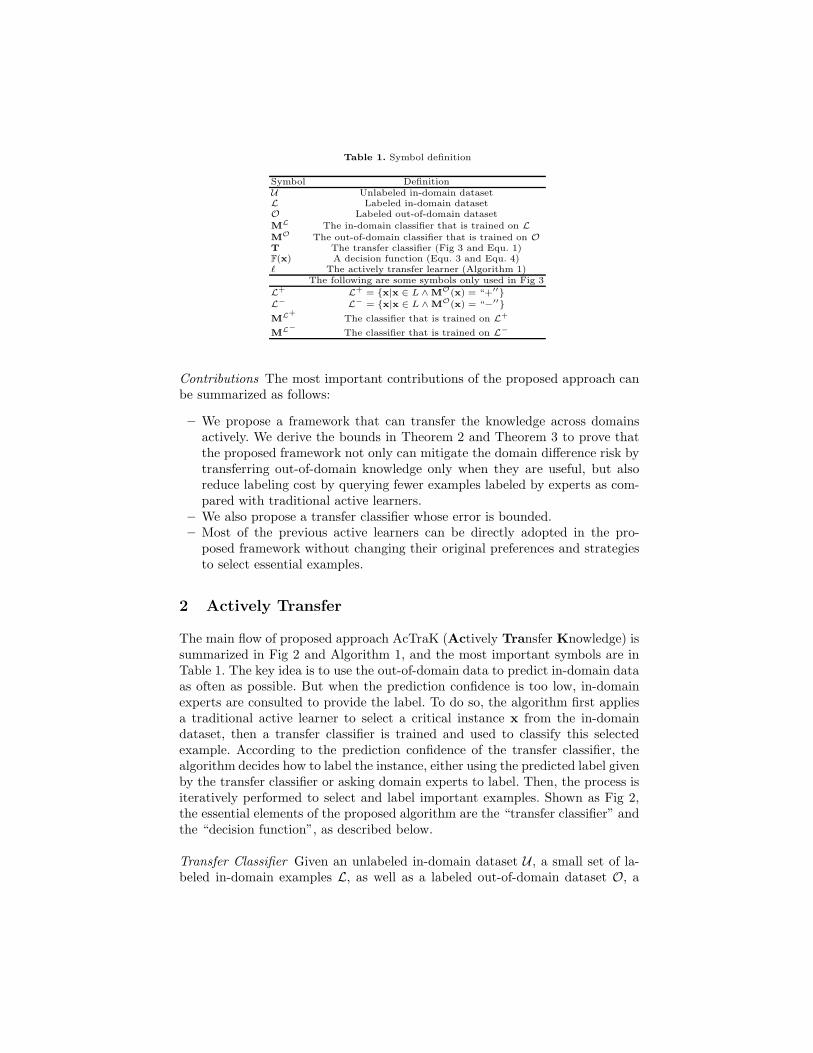
Table 1. Symbol definition

Symbol DefinitionU Unlabeled in-domain datasetL Labeled in-domain datasetO Labeled out-of-domain dataset

ML The in-domain classifier that is trained on L

MO The out-of-domain classifier that is trained on O

T The transfer classifier (Fig 3 and Equ. 1)F(x) A decision function (Equ. 3 and Equ. 4)ℓ The actively transfer learner (Algorithm 1)

The following are some symbols only used in Fig 3

L+ L+ = {x|x ∈ L ∧ MO(x) = “+′′}

L− L− = {x|x ∈ L ∧ MO(x) = “−′′}

ML+

The classifier that is trained on L+

ML−

The classifier that is trained on L−

Contributions The most important contributions of the proposed approach canbe summarized as follows:

– We propose a framework that can transfer the knowledge across domainsactively. We derive the bounds in Theorem 2 and Theorem 3 to prove thatthe proposed framework not only can mitigate the domain difference risk bytransferring out-of-domain knowledge only when they are useful, but alsoreduce labeling cost by querying fewer examples labeled by experts as com-pared with traditional active learners.

– We also propose a transfer classifier whose error is bounded.– Most of the previous active learners can be directly adopted in the pro-

posed framework without changing their original preferences and strategiesto select essential examples.

2 Actively Transfer

The main flow of proposed approach AcTraK (Actively Transfer Knowledge) issummarized in Fig 2 and Algorithm 1, and the most important symbols are inTable 1. The key idea is to use the out-of-domain data to predict in-domain dataas often as possible. But when the prediction confidence is too low, in-domainexperts are consulted to provide the label. To do so, the algorithm first appliesa traditional active learner to select a critical instance x from the in-domaindataset, then a transfer classifier is trained and used to classify this selectedexample. According to the prediction confidence of the transfer classifier, thealgorithm decides how to label the instance, either using the predicted label givenby the transfer classifier or asking domain experts to label. Then, the process isiteratively performed to select and label important examples. Shown as Fig 2,the essential elements of the proposed algorithm are the “transfer classifier” andthe “decision function”, as described below.

Transfer Classifier Given an unlabeled in-domain dataset U , a small set of la-beled in-domain examples L, as well as a labeled out-of-domain dataset O, a

Input: Unlabeled in-domain dataset: U ;Labeled in-domain dataset: L;Labeled out-of-domain dataset: O;Maximum number of exampleslabeled by experts: N.

Output: The actively transfer learner: ℓ

Initial the number of examples that have1

been labeled by experts: n← 0;repeat2

x← select an instance from U by a3

traditional active learner;Train the transfer classifier T (Fig 3);4

Predict x by T(x) (Fig 3 and Equ. 1);5

Calculate the decision function F(x)6

(Details in Equ. 3 and Equ. 4);if F(x) = 0 then7

y ← label by T(x);8

else9

y ← label by the experts;10

n← n + 1;11

end12

L ← L ∪ {(x, y)};13

until n≥N14

Train the learner ℓ with L15

Return the learner ℓ.16

Algorithm 1: Framework Fig. 2. Algorithm flow

transfer classifier is constructed from both O and L to classify unlabeled ex-amples in U . In previous work on transfer learning, out-of-domain dataset O isassumed to share similar distributions with in-domain dataset U ∪ L ([3][16]).Thus, exploring the similarities and exploiting them is expected to improve ac-curacy. However, it is unclear on how to formally determine whether the out-of-domain dataset shares sufficient similarity with the in-domain dataset, andhow to guarantee transfer learning improves accuracy. Thus, in this paper, wepropose a transfer learning model whose expected error is bounded.

Intuitively, if one uses the knowledge in out-of-domain dataset O to makeprediction for an in-domain example x, and then double check the predictedlabel with an in-domain classifier to see if the prediction is the same, it is morelikely that the predicted label is correct. Before discussing in detail, we definesome common notations. Let MO denote the out-of-domain classifier trainedon the out-of-domain dataset O. Also, let Lt denote a set of labeled data fromin-domain, but they are labeled as yt by the out-of-domain classifier MO (yt isthe label of the tth class). Formally, Lt = {x|x ∈ L ∧ MO(x) = yt}. Note thatthe true labels of examples in Lt are not necessarily yt, but they just happen tobe labeled as class yt by the out-of-domain classifier. We illustrate the transferclassifier for a binary-class problem in Fig 3. There are two classes, “+” and “-”,

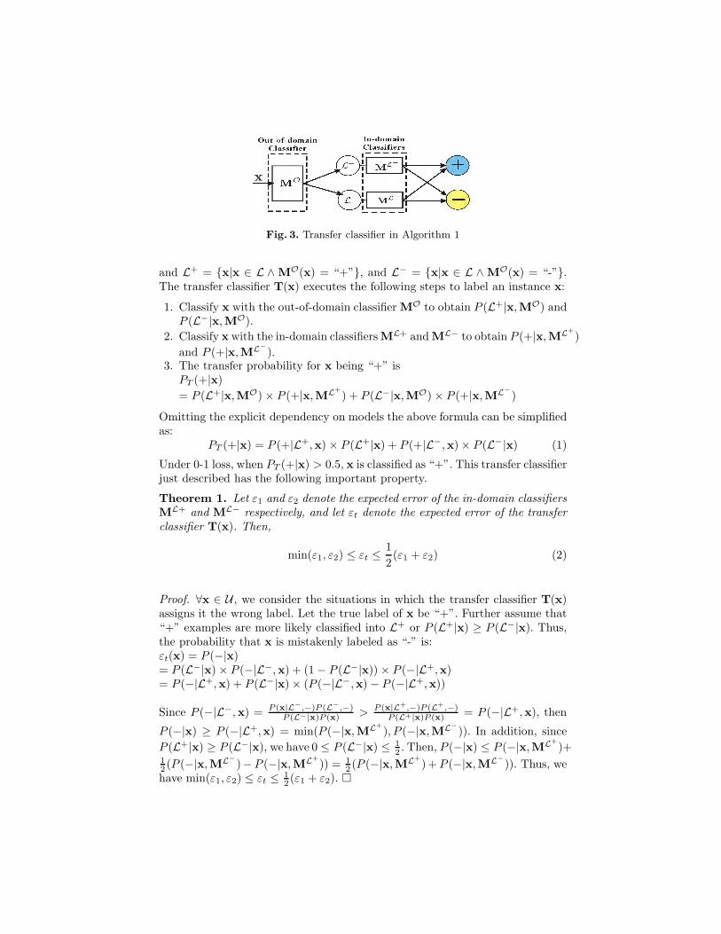
Fig. 3. Transfer classifier in Algorithm 1

and L+ = {x|x ∈ L ∧ MO(x) = “+”}, and L− = {x|x ∈ L ∧ MO(x) = “-”}.The transfer classifier T(x) executes the following steps to label an instance x:

1. Classify x with the out-of-domain classifier MO to obtain P (L+|x,MO) andP (L−|x,MO).

2. Classify x with the in-domain classifiers ML+ and ML− to obtain P (+|x,ML+

)

and P (+|x,ML−

).3. The transfer probability for x being “+” is

PT (+|x)

= P (L+|x,MO) × P (+|x,ML+

) + P (L−|x,MO) × P (+|x,ML−

)

Omitting the explicit dependency on models the above formula can be simplifiedas:

PT (+|x) = P (+|L+,x) × P (L+|x) + P (+|L−,x) × P (L−|x) (1)

Under 0-1 loss, when PT (+|x) > 0.5, x is classified as “+”. This transfer classifierjust described has the following important property.

Theorem 1. Let ε1 and ε2 denote the expected error of the in-domain classifiersML+ and ML− respectively, and let εt denote the expected error of the transferclassifier T(x). Then,

min(ε1, ε2) ≤ εt ≤1

2(ε1 + ε2) (2)

Proof. ∀x ∈ U , we consider the situations in which the transfer classifier T(x)assigns it the wrong label. Let the true label of x be “+”. Further assume that“+” examples are more likely classified into L+ or P (L+|x) ≥ P (L−|x). Thus,the probability that x is mistakenly labeled as “-” is:εt(x) = P (−|x)= P (L−|x) × P (−|L−,x) + (1 − P (L−|x)) × P (−|L+,x)= P (−|L+,x) + P (L−|x) × (P (−|L−,x) − P (−|L+,x))

Since P (−|L−,x) = P (x|L−,−)P (L−,−)P (L−|x)P (x) >

P (x|L+,−)P (L+,−)P (L+|x)P (x) = P (−|L+,x), then

P (−|x) ≥ P (−|L+,x) = min(P (−|x,ML+

), P (−|x,ML−

)). In addition, since

P (L+|x) ≥ P (L−|x), we have 0 ≤ P (L−|x) ≤ 12 . Then, P (−|x) ≤ P (−|x,ML+

)+12 (P (−|x,ML−

)−P (−|x,ML+

)) = 12 (P (−|x,ML+

) + P (−|x,ML−

)). Thus, wehave min(ε1, ε2) ≤ εt ≤

12 (ε1 + ε2). �

Hence, Theorem 1 indicates that if the out-of-domain knowledge is similar tothe current domain, or P (L−|x) is small, the model obtains the expected errorclose to εt = min(ε1, ε2). When the out-of-domain knowledge is different, theexpected error is bounded by 1

2 (ε1 + ε2). In other words, in the worst case, theperformance of the transfer classifier is no worse than the average performancesof the two in-domain classifiers ML+

and ML−

.

Decision Function After the transfer classifier T(x) predicts the selected exam-ple x, a decision function F(x) is calculated and further decides how to label theexample. In the following situations, one should query the experts for the classlabel in case of mislabeling.

– When the transfer classifier assigns x with a class label that is different fromthat given by an in-domain classifier.

– When the transfer classifier’s classification is low in confidence.– When the size of the labeled in-domain dataset L is very small.

Recall that ML is the in-domain classifier trained on labeled in-domain datasetL. According to the above considerations, we design a “querying indicator” func-tion θ(x) to reflect the necessity to query experts.

θ(x) =(

1 + α(x))−1

α(x) =(

1 − [[ML(x) 6= T(x)]])

·PT (T(x) = y|x) · exp(−1

|L|)

(3)

where [[π]] = 1 if π is true. And PT (T(x) = y|x) is the transfer probabilitygiven by the transfer classifier T(x). Thus, 0 ≤ α(x) ≤ 1 and it reflects theconfidence that the transfer classifier has correctly labeled the example x: itincreases with the transfer probability PT (T(x) = y|x), and α(x) = 0 if the twoclassifiers ML(x) and T(x) have assigned different labels to x. Hence, the largerof α(x), the less we need to query the experts to label the example. Formally, the“querying indicator” function θ(x) requires θ(x) ∝ α(x)−1. Moreover, becausemislabeling of the first few selected examples can exert significant negative effect

on accuracy, we further set θ(x) =(

1+α(x))−1

so as to guarantee the possibility

(necessity) to query experts is greater than 50%. In other words, labeling by theexperts is the priority and we trust the label given by the transfer classifier onlywhen its confidence reflected by α(x) is very high. Thus, the proposed algorithmasks the experts to label the example with probability θ(x). Accordingly, withthe value of θ(x), we randomly generate a real number R within 0 to 1, and thenthe decision function F(x) is defined as

F(x) =

{

0 if R > θ(x)

1 otherwise(4)

According to Eq. 4, if the randomly selected real number R > θ(x), F(x) = 0,and it means Algorithm 1 labels the example by the transfer classifier; otherwise,the example is labeled by the domain experts. In other words, AcTraK labelsthe example x by transfer classifier with probability 1 − θ(x).

2.1 Formal Analysis of AcTraK

We have proposed the approach AcTraK to transfer knowledge across domainsactively. Now, we formally derive its sampling error bound to demonstrate itsability to mitigate domain difference risk, which guarantees that out-of-domainexamples are transferred to label in-domain data only when they are useful.Additionally, we prove its querying bound to validate the claim that AcTraKcan reduce labeling cost by querying fewer examples labeled by experts by anybased level active learner incorporated into the framework.

Theorem 2. In the algorithm AcTraK (Algorithm 1), let εt denote the ex-pected error of the transfer classifier, and let N denote the maximum number ofexamples labeled by experts, then the sampling error ε for AcTraK satisfies

ε ≤ε2

t

1 + (1 − εt) × exp(−|N |−1)(5)

Proof. The proof for Theorem 2 is straightforward. According to the transferclassifier T(x) and the decision function F(x) described above, AcTraK makeswrong decision only when both the transfer classifier T(x) and the in-domainclassifier ML agree on the wrong label. And in this case, AcTraK has probability1− θ(x) to trust the classification result given by T(x), where θ(x) is defined inEq. 3. Thus, the sampling error for AcTraK can be written as ε ≤ (εt)

2(1−θ(x)).Moreover, in this situation, θ(x) = 1

1+(1−εt)e− 1

|L|≥ 1

1+(1−εt)e− 1

N

. Thus, ε ≤

ε2t (1 − θ(x)) ≤

ε2t×(1−εt)×exp(−|N |−1)

1+(1−εt)×exp(−|N |−1) ≤ε2

t

1+(1−εt)×exp(−|N |−1) . �

Theorem 3. In the algorithm AcTraK (Algorithm 1), let εt and εi denote theexpected error of the transfer classifier and in-domain classifier respectively. Andlet α = εt + εi. Then for an in-domain instance, the probability that AcTraK

queries the label from the experts (with cost) satisfies:

P [Query] ≤ α +1 − α

1 + (1 − εt) × exp(− 1|N | )

(6)

Proof. According to the labeling-decision function F(x), AcTraK will query theexperts to label the instance when T(x) and ML hold different predictions onthe classification result. Even when the two classifiers agree on the result, itstill has probability θ(x) to query the experts. Thus, P [Query] = εi(1 − εt) +εt(1 − εi) + [εtεi + (1 − εt)(1 − εi)]θ(x) = θ(x) + (εt + εi − 2εtεi)(1 − θ(x)) ≤α + (1 − α)θ(x) ≤ α + 1−α

1+(1−εt)×exp(− 1|N|

). �

From Theorem 2, we can find that the sampling error of the proposed approach

AcTraK is bounded by O(ε2

t

1−εt), where εt is the expected error of the transfer

classifier, and εt is also bounded according to Theorem 1. Thus, the proposed

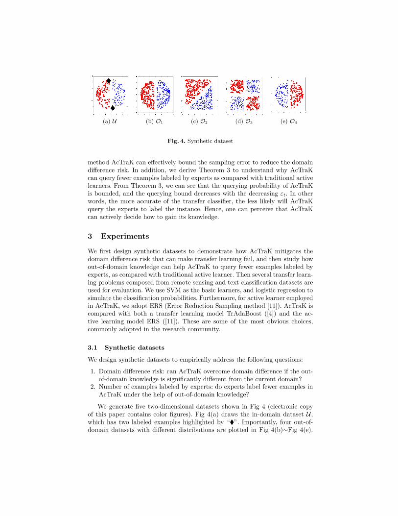
(a) U (b) O1 (c) O2 (d) O3 (e) O4

Fig. 4. Synthetic dataset

method AcTraK can effectively bound the sampling error to reduce the domaindifference risk. In addition, we derive Theorem 3 to understand why AcTraKcan query fewer examples labeled by experts as compared with traditional activelearners. From Theorem 3, we can see that the querying probability of AcTraKis bounded, and the querying bound decreases with the decreasing εt. In otherwords, the more accurate of the transfer classifier, the less likely will AcTraKquery the experts to label the instance. Hence, one can perceive that AcTraKcan actively decide how to gain its knowledge.

3 Experiments

We first design synthetic datasets to demonstrate how AcTraK mitigates thedomain difference risk that can make transfer learning fail, and then study howout-of-domain knowledge can help AcTraK to query fewer examples labeled byexperts, as compared with traditional active learner. Then several transfer learn-ing problems composed from remote sensing and text classification datasets areused for evaluation. We use SVM as the basic learners, and logistic regression tosimulate the classification probabilities. Furthermore, for active learner employedin AcTraK, we adopt ERS (Error Reduction Sampling method [11]). AcTraK iscompared with both a transfer learning model TrAdaBoost ([4]) and the ac-tive learning model ERS ([11]). These are some of the most obvious choices,commonly adopted in the research community.

3.1 Synthetic datasets

We design synthetic datasets to empirically address the following questions:

1. Domain difference risk: can AcTraK overcome domain difference if the out-of-domain knowledge is significantly different from the current domain?

2. Number of examples labeled by experts: do experts label fewer examples inAcTraK under the help of out-of-domain knowledge?

We generate five two-dimensional datasets shown in Fig 4 (electronic copyof this paper contains color figures). Fig 4(a) draws the in-domain dataset U ,which has two labeled examples highlighted by “�”. Importantly, four out-of-domain datasets with different distributions are plotted in Fig 4(b)∼Fig 4(e).

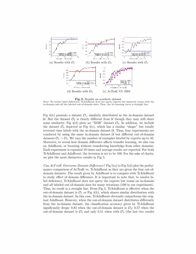
(a) Results with O1 (b) Results with O2 (c) Results with O3

(d) Results with O4 (e) AcTraK VS. ERS

Fig. 5. Results on synthetic datasetNote: To resolve label deficiency, TrAdaBoost does not query experts but passively trains with thein-domain and all the labeled out-of-domain data. Thus, the its learning curve is straight line.

Fig 4(b) presents a dataset O1, similarly distributed as the in-domain datasetU . But the dataset O2 is clearly different from U though they may still sharesome similarity. Fig 4(d) plots an “XOR” dataset O3. In addition, we includethe dataset O4 depicted as Fig 4(e), which has a similar “shape” but totallyreversed class labels with the in-domain dataset U . Thus, four experiments areconduced by using the same in-domain dataset U but different out-of-domaindatasets O1 ∼ O4. We vary the number of examples labeled by experts up to 50.Moreover, to reveal how domain difference affects transfer learning, we also runon AdaBoost, or boosting without transferring knowledge from other domains.Each experiment is repeated 10 times and average results are reported. For bothTrAdaBoost and AdaBoost, the iteration is set to be 100. For the sake of clarity,we plot the most distinctive results in Fig 5.

Can AcTraK Overcome Domain Difference? Fig 5(a) to Fig 5(d) plot the perfor-mance comparison of AcTraK vs. TrAdaBoost as they are given the four out-of-domain datasets. The result given by AdaBoost is to compare with TrAdaBoostto study effect of domain difference. It is important to note that, to resolve la-bel deficiency, TrAdaBoost does not query the experts but trains on in-domainand all labeled out-of-domain data for many iterations (100 in our experiment).Thus, its result is a straight line. From Fig 5, TrAdaBoost is effective when theout-of-domain dataset is O1 or Fig 4(b), which shares similar distribution withthe in-domain dataset. In this case, TrAdaBoost obviously outperforms the orig-inal AdaBoost. However, when the out-of-domain dataset distributes differentlyfrom the in-domain dataset, the classification accuracy given by TrAdaBoostsignificantly drops: 0.82 when the out-of-domain dataset is O2; 0.57 when theout-of-domain dataset is O3 and only 0.51 when with O4 (the last two results

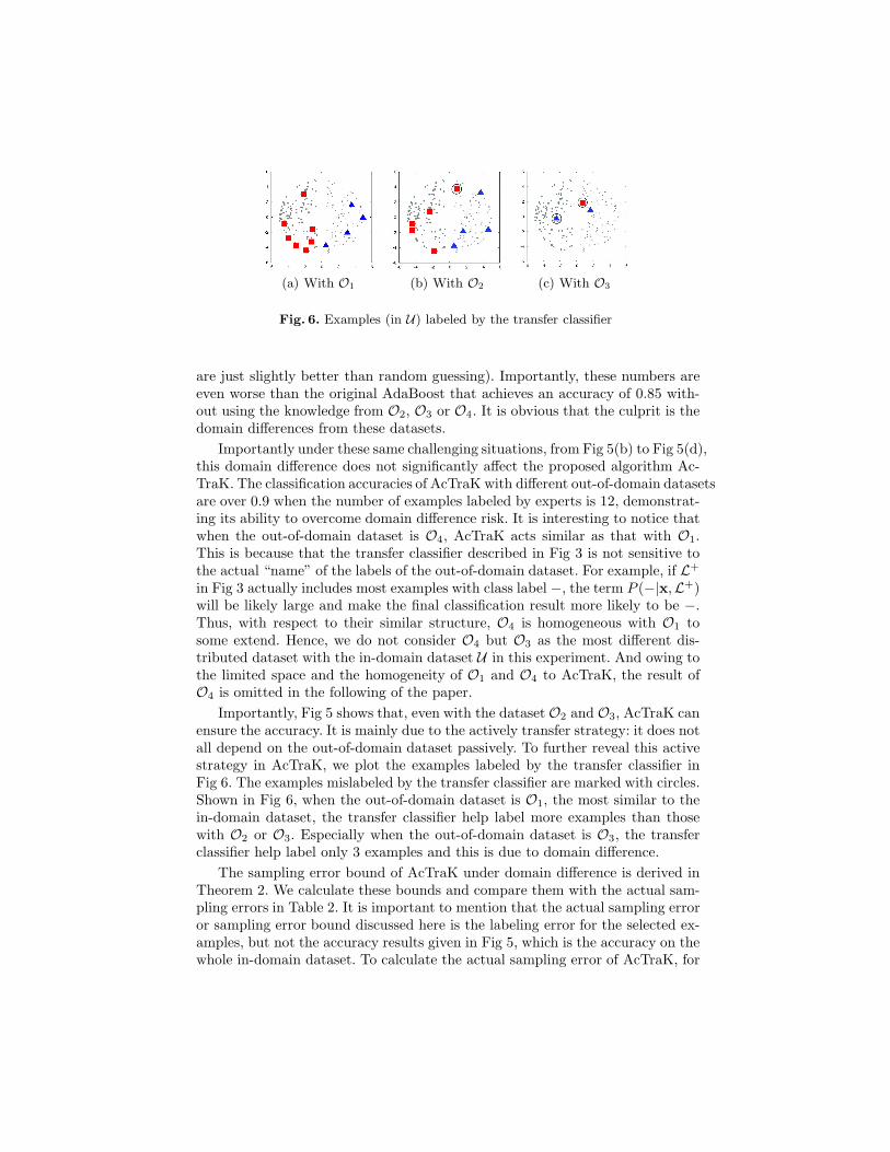
(a) With O1 (b) With O2 (c) With O3

Fig. 6. Examples (in U) labeled by the transfer classifier

are just slightly better than random guessing). Importantly, these numbers areeven worse than the original AdaBoost that achieves an accuracy of 0.85 with-out using the knowledge from O2, O3 or O4. It is obvious that the culprit is thedomain differences from these datasets.

Importantly under these same challenging situations, from Fig 5(b) to Fig 5(d),this domain difference does not significantly affect the proposed algorithm Ac-TraK. The classification accuracies of AcTraK with different out-of-domain datasetsare over 0.9 when the number of examples labeled by experts is 12, demonstrat-ing its ability to overcome domain difference risk. It is interesting to notice thatwhen the out-of-domain dataset is O4, AcTraK acts similar as that with O1.This is because that the transfer classifier described in Fig 3 is not sensitive tothe actual “name” of the labels of the out-of-domain dataset. For example, if L+

in Fig 3 actually includes most examples with class label −, the term P (−|x,L+)will be likely large and make the final classification result more likely to be −.Thus, with respect to their similar structure, O4 is homogeneous with O1 tosome extend. Hence, we do not consider O4 but O3 as the most different dis-tributed dataset with the in-domain dataset U in this experiment. And owing tothe limited space and the homogeneity of O1 and O4 to AcTraK, the result ofO4 is omitted in the following of the paper.

Importantly, Fig 5 shows that, even with the dataset O2 and O3, AcTraK canensure the accuracy. It is mainly due to the actively transfer strategy: it does notall depend on the out-of-domain dataset passively. To further reveal this activestrategy in AcTraK, we plot the examples labeled by the transfer classifier inFig 6. The examples mislabeled by the transfer classifier are marked with circles.Shown in Fig 6, when the out-of-domain dataset is O1, the most similar to thein-domain dataset, the transfer classifier help label more examples than thosewith O2 or O3. Especially when the out-of-domain dataset is O3, the transferclassifier help label only 3 examples and this is due to domain difference.

The sampling error bound of AcTraK under domain difference is derived inTheorem 2. We calculate these bounds and compare them with the actual sam-pling errors in Table 2. It is important to mention that the actual sampling erroror sampling error bound discussed here is the labeling error for the selected ex-amples, but not the accuracy results given in Fig 5, which is the accuracy on thewhole in-domain dataset. To calculate the actual sampling error of AcTraK, for

Table 2. Sampling error bound and querying bound on synthetic dataset

Datasets Error of T(x) Sampling error Sampling error bound Querying rate Querying boundO1 0.00 0.000 0.000 71.43% 75.25%O2 0.18 0.017 0.017 84.75% 85.45%O3 0.34 0.037 0.070 94.34% 93.72%

example, when the out-of-domain dataset is O2, there are a total of 9 exampleslabeled by the transfer classifier with one mislabeled, as depicted in Fig 6(b).Thus, the actual sampling error of AcTraK is 1

50+9 = 0.017, and we compare itwith the bound calculated according to Theorem 2. The results are summarizedin Table 2. The sampling error bound given in Theorem 2 is obviously tight forthe synthetic dataset. Moreover, it is evident that AcTraK can effectively reducesampling error. For instance, when the true error of the transfer classifier T(x)is 0.34 with the dataset O3, AcTraK bounds its sampling error as 0.07 and getsthe actual error 0.04. Thus, it can be concluded that AcTraK can effectivelyresolve domain difference by bounding the sampling error shown as Theorem 2.

Do Experts Label Fewer Examples in AcTraK? In the proposed approach Ac-TraK, knowledge transferred from other domain is used to help label the exam-ples. In other words, it saves the number of examples to ask the experts. Thus,compared with traditional active learner, AcTraK is expected to reduce thenumber of examples labeled by experts, thus to reduce labeling cost. We presentFig 5(e) to demonstrate this claim by comparing AcTraK with the traditionalactive learner ERS. It is important to note that the original ERS only works onthe in-domain dataset. Thus, there is only one result plotted for ERS in Fig 5(e)but three for AcTraK with different out-of-domain datasets. From Fig 5(e), wecan see that in most cases, “AcTraK-O1” and “AcTraK-O2” can evidently out-perform ERS by reaching the same accuracy but with fewer examples labeledby experts. And this is because that some of the examples have been labeled bythe transfer classifier under the help of the out-of-domain datasets. Additionally,the out-of-domain dataset O1 seems more helpful than O2 to AcTraK, due tothe similar distribution between O1 and the in-domain dataset.

When we use the XOR dataset O3 to be the out-of-domain dataset, thelearning curve of AcTraK overlaps with that of ERS depicted as Fig 5(e). Itimplies that the transfer learning process is unable to help label examples in thiscase, and both AcTraK and ERS select the same examples and label them all byexperts. Depicted as Fig 4(a) and Fig 4(d), the distribution of O3 is significantlydifferent from the in-domain dataset U , and thus AcTraK judiciously drops theknowledge transferred from O3 but queries the experts instead in order to avoidmislabeling. This is formally discussed in Theorem 3, in which we have shownthat the bound of the probability to query experts increases when the transferclassifier can not confidently label the examples. We also calculate these queryingbounds and the actual querying rates in Table 2. The querying bound givenin Theorem 3 is tight. Moreover, we can clearly see that AcTraK queries theexperts with probability 94% when the out-of-domain dataset is O3. It explainswhy AcTraK can not outperform ERS with O3 in Fig 5(e): the transfer classifier

has too little chance (1 − 94% = 6%) to label the examples. Additionally, thequerying bound of O1 is less than that of O2. In other words, AcTraK may labelmore examples by the transfer classifier when the out-of-domain dataset is O1.It explains why O1 is more helpful than O2 to AcTraK in Fig 5(e).

3.2 Real World Dataset

Fig. 7. IEA

We use two sets of real world datasets, remote sensingproblem as well as text classification problem, to empiri-cally evaluate the proposed method. But we first employan evaluation metric to compare two active learners. Onemainly cares about the performance with the increasingnumber of examples labeled by experts, shown by thelearning curves of A1 and A2 in Fig 7. A superior ac-tive learner is supposed to gain a higher accuracy underthe same number of queried examples, or reach the sameclassification accuracy with fewer labeled examples. Thisis shown by n1 vs. n2 in Fig 7. Thus, the superiority ofA1 compared with A2 can be reflected by the area sur-rounded by the two learning curves, highlighted by dottedlines in Fig 7. In order to qualify this difference, we em-ploy an evaluation metric IEA(*) (Integral Evaluation on Accuracy), and applyit to evaluate the proposed method in the following experiments.

Definition 1. Given a classifier M, two active learners A1 and A2, let A(n)denote the classification accuracy of M trained on the dataset selected by theactive learner A when the number of examples labeled by experts is n. Then,

IEA(A1,A2, ν) =

ν∫

0

(A1(n) −A2(n))dn =

ν∑

n=0

(A1(n) −A2(n))∆n (7)

Remote Sensing Problem The remote sensing problem is based on data collectedfrom real landmines1. In this problem, there are a total of 29 sets of data, col-lected from different landmine fields. Each data is represented as a 9-dimensionalfeature vector extracted from radar images, and the class label is true mine orfalse mine. Since each of the 29 datasets are collected from different regions thatmay have different types of ground surface conditions, these datasets are con-sidered to be dominated by different distributions. According to [17], datasets1 to 10 are collected at foliated regions while datasets 20 to 24 are collectedfrom regions that are bare earth or desert. Then, we combine the datasets 1 to5 as the unlabeled in-domain dataset, while the datasets 20 to 24 as the labeledout-of-domain dataset respectively. Furthermore, we also combine datasets 6 to10 as another out-of-domain dataset that is assumed to have a very similar dis-tribution with the in-domain dataset. We conduct the experiment 10 times and

1 http://www.ee.duke.edu/∼lcarin/LandmineData.zip

Table 3. Accuracy comparisons on remote sensing (landmine) dataset

Out-of-domain Dataset SVM TrAdaBoost(100 iterations) AcTraK IEA(AcTraK, ERS, 100)Dataset 20 57% 89.76% 94.49% +0.101Dataset 21 57% 86.04% 94.48% +0.108Dataset 22 57% 90.5% 94.49% +0.103Dataset 23 57% 88.42% 94.49% +0.123Dataset 24 57% 90.7% 94.49% +0.12

Dataset 6-10 57% 94.76% 94.49% +0.134Note: The results of AcTraK under the 4th column is when only one example is labeled by experts.

randomly select two examples (one with label “true” while the other with label“false”) as the initial training set each time. The experiment results are averagedand summarized in Table 3.

The first 5 rows of Table 3 show that AcTraK outperforms TrAdaBoost whenthe in-domain dataset is not so similar to the out-of-domain dataset (Dataset 20to Dataset 24). Moreover, AcTraK also outperforms the active learner ERS inall cases. When the in-domain dataset is similar with the out-of-domain dataset(Dataset 6-10), AcTraK achieves the highest gain on ERS, demonstrating domaintransfer can improve learning and reduce number of examples labeled by experts.

Text Classification Problem Another set of experiment on text classificationproblem uses the 20 Newsgroups. It contains approximately 20,000 newsgroupdocuments, partitioned across 20 different newsgroups. We generate 6 cross-domain learning tasks. 20 Newsgroups has a two-level hierarchy so that eachlearning task involves a top category classification problem but the training andtest data are drawn from different sub categories. For example, the goal is to dis-tinguish documents from two top newsgroup categories: rec and talk. So a train-ing set involves documents from “rec.autos”, and “talk.politics.misc” whereasthe test set includes sub-categories “rec.sport.baseball” “talk.religions.misc”, etc.The strategy is to split the sub-categories among the training and the test setsso that the distributions of the two sets are similar but not exactly the same.The tasks are generated in the same way as in [4] and more details can be foundthere. Similar to other experiments, each of the in-domain datasets has only2 randomly selected labeled examples, one positive and another negative. Re-ported results in Table 4 are averaged over 10 runs. The results of the first twodatasets are also plotted in Fig 8.

It is important to note that the classification results of AcTraK shown inFig 4 is when the number of examples labeled by experts is 250. It is relativelysmall in size since each dataset in our experiment has 3500 to 3965 unlabeleddocuments ([4]). As summarized in Table 4, TrAdaBoost can increase the learn-ing accuracy in some cases, such as with the dataset “comp vs. talk”. However,one can hardly guarantee that the exclusive use of transfer learning is enough tolearn the current task. For example, when the dataset is “comp vs. sci”, TrAd-aBoost does not increase the accuracy significantly. But the proposed algorithmAcTraK can achieve an accuracy 78% compared with 57.3% given by TrAd-aBoost. It implies the efficiency of AcTraK to actively gain its knowledge both

(a) rec vs. talk (b) rec vs. sci

Fig. 8. Comparisons with ERS on 20 Newsgroups dataset

Table 4. Accuracy comparisons on 20 Newsgroups dataset

Dataset SVM TrAdaBoost(100 iterations) AcTraK IEA(AcTraK, ERS, 250)rec vs. talk 60.2% 72.3% 75.4% +0.91rec vs. sci 59.1% 67.4% 70.6% +1.83

comp vs. talk 53.6% 74.4% 80.9% +0.21comp vs. sci 52.7% 57.3% 78.0% +0.88comp vs. rec 49.1% 77.2% 82.1% +0.35sci vs. talk 57.6% 71.3% 75.1% +0.84

from transfer learning and domain experts, while TrAdaBoost adopts the passivestrategy to thoroughly depend on transfer learning. In addition, from Table 4and Fig 8, we find that AcTraK can effectively reduce the number of exampleslabeled by experts as compared with ERS. For example, upon the dataset “recvs. talk”, to reach the accuracy 70%, AcTraK is with 160 examples labeled byexperts while ERS needs over 230 such examples.

4 Related Work

Transfer learning utilizes the knowledge from other domain(s) to help learn thecurrent domain so as to resolve label deficiency. One of the main issues in thisarea is how to resolve the different data distributions. One general approachproposed to solve the problem with different data distributions is based on in-stance weighting (e.g., [2][4][5][10][7]). The motivation of these methods are to“emphasize” those “similar” and discriminated instances. Another line of worktries to change the representation of the observation x by projecting them intoanother space in which the projected instances from different domains are similarto each other (e.g., [1][12]). Most of the previous work assume that the knowl-edge transferred from other domain(s) can finally help the learning. However,this assumption can be easily violated in practice. The knowledge transferredfrom other domains may reduce the learning accuracy due to implicit domaindifferences. We call it the domain difference risk, and we effectively solve theproblem by actively transfer the knowledge across domains to help the learningonly when they are useful.

Active learning is another way to solve label deficiency. It mainly focuses oncarefully selecting a few additional examples for which it requests labels, so asto increase the learning accuracy. Thus, different active learners use different

selection criteria. For example, uncertainty sampling (e.g., [9][18]) selects theexample on which the current learner has lower certainty; Query-by-Committee(e.g., [6][13]) selects examples that cause maximum disagreement amongst anensemble of hypotheses, etc. There are also some other topics proposed in recentyears to resolve different problems in active learning, such as the incorporationof ensemble methods (e.g., [8]), the incorporation of model selection (e.g., [15]),etc. It is important to mention that the examples selected by the previous activelearners are more or less uncertain to be labeled directly by the in-domain clas-sifier. Then in this paper, we use the knowledge transferred from other domainto help label these selected examples, so as to reduce labeling cost.

5 Conclusion

We propose a new framework to actively transfer the knowledge from other do-main to help label the instances from the current domain. To do so, we first selectan essential example and then apply a transfer classifier to label it. But if theclassification given by the transfer classifier is of low confidence, we ask domainexperts instead to label the example. We develop Theorem 2 to demonstratethat this strategy can effectively resolve domain difference risk by transferringdomain knowledge only when they are useful. Furthermore, we also derive Theo-rem 3 to prove that the proposed framework can reduce labeling cost by queryingfewer examples labeled by experts, as compared with traditional active learn-ers. In addition, we also propose a new transfer learning model adopted in theframework, and this transfer learning model is bounded to be no worse than aninstance-based ensemble method in error rate, proven in Theorem 1. There areat least two important advantages of the proposed approach. First, it effectivelysolves the domain difference risk problem that can easily make transfer learningfail. Second, most of previous active learning models can be directly adopted inthe framework to reduce the number of examples labeled by experts.

We design a few synthetic datasets to study how the proposed framework re-solves domain difference and reduce the number of examples labeled by experts.The proposed sampling error bound in Theorem 2 and querying bound in Theo-rem 3 are also empirically demonstrated to be tight bounds in this experiment.Furthermore, two categories of real world datasets, including remote sensing andtext classification datasets have been used to generate several transfer learningproblems. Experiment shows that the proposed method can significantly out-perform the comparable transfer learning model by resolving domain difference.For example, with one of the text classification datasets, the proposed methodachieves an accuracy 78.0%, while the comparable transfer learning model dropsto 57.3%, due to domain difference. Moreover, the proposed method can alsoeffectively reduce labeling cost by querying fewer examples labeled by expertsas compared with the traditional active learner. For instance, in an experimenton the text classification problem, the comparable active learner requires over230 examples labeled by experts to gain the accuracy 70%, while the proposedmethod is with at most 160 such examples to reach the same accuracy.

References

1. Ben-David, S., Blitzer, J., Crammer, K., and Pereira, F.: Analysis of representa-tions for domain adaptation. In: Proc. of NIPS’06 (2007)

2. Bickel, S., Bruckner, M., and Scheffer, T.: Discriminative learning for differingtraining and test distributions. In: Proc. of ICML’07 (2007)

3. Daume III, H. and Marcu, D.: Domain adaptation for statistical classifiers. Journalof Artificial Intelligence Research 26, 101–126 (2006)

4. Dai, W., Yang, Q., Xue, G., and Yu, Y.: Boosting for transfer learning. In: Proc.of ICML’07 (2007)

5. Fan, W., and Davidson, I.: On Sample Selection Bias and Its Efficient Correctionvia Model Averaging and Unlabeled Examples. In: Proc. of SDM’07 (2007)

6. Freund, Y., Seung, H., Shamir, E., Tishby, N.: Selective sampling using the QueryBy Committee algorithm. Machine Learning Journal, 28, 133–168 (1997)

7. Huang, J., Smola, A. J., Gretton, A., Borgwardt, K. M., and Scholkopf, B.: Cor-recting sample selection bias by unlabeled data. In: Proc. of NIPS’06 (2007)

8. Korner, C. and Wrobel, S.: Multi-class Ensemble-Based Active Learning. In: Proc.of ECML’06 (2006)

9. Lewis, D. and Gale, W.: A sequential algorithm for training text classifiers. In:Proc. of SIGIR’94 (1994)

10. Ren, J., Shi, X., Fan, W. and Yu, P.:Type-Independent Correction of Sample Se-lection Bias via Structural Discovery and Re-balancing. In: Proc. of SDM’08(2008)

11. Roy, N. and McCallum, A.: Toward optimal active learning through samplingestimation of error reduction. In: Proc. of ICML’01 (2001)

12. Satpal, S. and Sarawagi, S.: Domain adaptation of conditional probability modelsvia feature subsetting. In: Proc. of PKDD’07 (2007)

13. Senung, H.S., Opper, M., Sompolinsky, H.: Query by committee. In: Proc. 5thAnnual ACM Workshop on Computational Learning Theory (1992)

14. Shimodaira, H.: Inproving predictive inference under covariate shift by weightingthe log-likehood function. Journal of Statistical Planning and Inference, 90, 227–244 (2000)

15. Sugiyama, M. and Rubens, N.: Active Learning with Model Selection in LinearRegression. In: Proc. of SDM’08 (2008)

16. Xing, D., Dai, W., Xue, G., and Yu, Y.: Bridged refinement for transfer learning.In: Proc. of PKDD’07 (2007)

17. Xue, Y., Liao, X., Carin, L., and Krishnapuram, B.: Multi-task learning for clas-sification with dirichlet process priors. Journal of Machine Learning Research 8,35–63 (2007)

18. Xu, Z., Y, K., Tresp, V., Xu, X., Wang, J.: Representative sampling for textclassification using support vector machines. In: Proc. of ECIR’03 (2003)