
Frequency-Domain Signal Analysis
353
585 Signal Analysis: Time, Frequency, Scale, and Structure, by Ronald L. Allen and Duncan W. Mills ISBN: 0-471-23441-9 Copyright © 2004 by Institute of Electrical and Electronics Engineers, Inc. CHAPTER 9 Frequency-Domain Signal Analysis Frequency-domain signal analysis covers a wide variety of techniques involving the Fourier transformation of the signal. The signal’s frequency domain representation is then manipulated, decomposed, segmented, classified, and interpreted. One cen- tral idea is that of a filter: a linear, translation-invariant system that allows one band of frequencies to appear in the output and suppresses the others. Where signal ele- ments of interest occupy a restricted spectrum, filters invariably enter into the early processing of candidate signals. In other ways—often purely theoretical— frequency-domain analysis is important. For example, in this chapter we substanti- ate the methods of matched filtering and scale-space decomposition, and the Fourier transform plays a crucial role. The main tools for frequency-domain analysis are of course the discrete signal transforms: the discrete-time Fourier transform (DTFT); its generalization, the z- transform; and especially the discrete Fourier transform (DFT). Many of the intro- ductory applications proceed from Chapter 1 examples. There are extensions of techniques already broached in Chapters 4 and 6. Modern spectral analysis applica- tions have a digital computer at their heart, and they rely on the either the DFT or one of its many fast versions. Some signal filtering applications use infinite impulse response (IIR) filtering methods, implemented using feedback, as discussed in Chapter 2. The DTFT is convenient for obtaining a theoretical understanding of how such filters suppress and enhance signal frequencies. We often begin with an analog filter and convert it to a discrete filter. Thus, we shall have occasion to use the continuous-domain Fourier transform. We also briefly explain how the Laplace transform, a generalization of the Fourier transform, can be used in certain analog filter constructions. The z-transform figures prominently in this conversion process. We are generally working with complex-valued signals, but the thresholding, seg- mentation, and structural decomposition methods that Chapter 4 developed for time- domain signal analyis are just as useful in the frequency domain. For example, to find the spectral region where a source signal contains significant energy, we thresh- old the signal’s magnitude or squared magnitude (power) spectrum. We know that thresholding is often improved by filtering the data, so we are inclined to filter the frequency-domain magnitudes too. This leads directly to the technique of windowing
-
Upload
khangminh22 -
Category
Documents
-
view
0 -
download
0
Transcript of Frequency-Domain Signal Analysis

585
Signal Analysis: Time, Frequency, Scale, and Structure, by Ronald L. Allen and Duncan W. MillsISBN: 0-471-23441-9 Copyright © 2004 by Institute of Electrical and Electronics Engineers, Inc.
CHAPTER 9
Frequency-Domain Signal Analysis
Frequency-domain signal analysis covers a wide variety of techniques involving theFourier transformation of the signal. The signal’s frequency domain representationis then manipulated, decomposed, segmented, classified, and interpreted. One cen-tral idea is that of a filter: a linear, translation-invariant system that allows one bandof frequencies to appear in the output and suppresses the others. Where signal ele-ments of interest occupy a restricted spectrum, filters invariably enter into the earlyprocessing of candidate signals. In other ways—often purely theoretical—frequency-domain analysis is important. For example, in this chapter we substanti-ate the methods of matched filtering and scale-space decomposition, and the Fouriertransform plays a crucial role.
The main tools for frequency-domain analysis are of course the discrete signaltransforms: the discrete-time Fourier transform (DTFT); its generalization, the z-transform; and especially the discrete Fourier transform (DFT). Many of the intro-ductory applications proceed from Chapter 1 examples. There are extensions oftechniques already broached in Chapters 4 and 6. Modern spectral analysis applica-tions have a digital computer at their heart, and they rely on the either the DFT orone of its many fast versions. Some signal filtering applications use infinite impulseresponse (IIR) filtering methods, implemented using feedback, as discussed inChapter 2. The DTFT is convenient for obtaining a theoretical understanding ofhow such filters suppress and enhance signal frequencies. We often begin with ananalog filter and convert it to a discrete filter. Thus, we shall have occasion to usethe continuous-domain Fourier transform. We also briefly explain how the Laplacetransform, a generalization of the Fourier transform, can be used in certain analogfilter constructions. The z-transform figures prominently in this conversion process.
We are generally working with complex-valued signals, but the thresholding, seg-mentation, and structural decomposition methods that Chapter 4 developed for time-domain signal analyis are just as useful in the frequency domain. For example, tofind the spectral region where a source signal contains significant energy, we thresh-old the signal’s magnitude or squared magnitude (power) spectrum. We know thatthresholding is often improved by filtering the data, so we are inclined to filter thefrequency-domain magnitudes too. This leads directly to the technique of windowing

586 FREQUENCY-DOMAIN SIGNAL ANALYSIS
time-domain signal slices before Fourier transformation. The meaning of the analyt-ical results can be quite different, of course; but as long as we understand the trans-form relation clearly and capture that in the application design, then the time-domainand frequency-domain procedures are remarkably similar. In some applications, theresults of this analysis convey the signal content. For other tasks, an inverse transfor-mation back to the time domain is required. In any case, the principal tools are theFourier transform and its inverse, in both their analog and discrete formulations.
Our theoretical resources include Chapters 5, 7, and 8. This chapter introducessome further theory, appropriate to the particular applications upon which we focus.Specific applications include tone detection, speech recognition and enhancement,and chirp analysis. Some of these experiments show that the Fourier transform isprecisely the tool we need to make the application work. Further reflection revealsproblems in applying the Fourier transforms. This motivates a search for frequencytransforms that incorporate a time-domain element: time-frequency and time-scaletransforms, which are topics for the final three chapters.
Fourier-domain techniques also offer many insights into our earlier material.Scale space and random signals are considered once more, this time from the van-tage point of the new frequency-domain methods. The last two sections detail theconstruction of special filters for frequency analysis and possible structures for theirapplication. Later chapters will draw the link between this approach to signal pro-cessing and the notion of a multiresolution analysis of the L2 Hilbert space.
References on Fourier transforms include Refs. 1–5. Popular signal processingtexts that introduce Fourier methods and construct filters from the theory are Refs.6–10. An older book that concludes its thorough coverage of signal theory withdetailed application studies in speech and radar signal analysis is Ref. 11.
Notation. The present discussion covers both analog and discrete filters. We usethe following notations for clarity:
(i) Analog filters: The impulse response is h(t), the radial Fourier transform isH(Ω), and the Laplace transform is HL(s); in some contexts, we insert thesubscript a: ha(t), Ha(Ω), and HL,a(s).
(ii) Discrete filters: The impulse response is h(n), or any FORTRAN-likeinteger independent variable such as h(i), h(k), or h(m); the discrete timeFourier transform is H(ω); and the discrete Fourier transform is H(k).
(iii) We continue to use j2 = −1.
9.1 NARROWBAND SIGNAL ANALYSIS
The most basic frequency-domain analysis task involves detecting and interpretingmore or less isolated periodic components of signals. For some signals, or at leastfor some part of their domain, a few oscillatory components contain the bulk of theenergy. It is such narrowband signals—sinusoids (tones) and dual-tones, mainly,but we could also allow complex-valued exponentials into this category—that we

NARROWBAND SIGNAL ANALYSIS 587
begin our study of Fourier transform applications. We distinguish narrowband sig-nals from wideband signals, where the energy is spread over many frequencies. Asignal that contains sharp edges, for example, will generally have frequency-domainenergy dispersed across a wide spectral range.
Although basic, a tone detection application leads to important practical con-cepts: noise removal, filtering, phase delay, group delay, and windowing. Filters arefrequency-selective linear translation invariant systems. Filtering a signal canchange the time location of frequency components. For instance, a filter might retarda sinusoidal pulse and the signal envelope itself, depending on their frequency.These time lags define the phase and group delay, respectively. Knowing them iscrucial for application designs that must compensate for filter delays. Finally, weoften need to analyze signals in chunks, but so doing invariably corrupts the signalspectrum. Only by looking at the signal through a well-constructed window can wemitigate this effect. This concept leads directly to the modern theory of the win-dowed Fourier transform (Chapter 10) and eventually to wavelets (Chapter 11).
Theory from earlier chapters now becomes practice. For designing filters, weemploy the discrete-time Fourier transform (DTFT). For implementing filters on acomputer, we use the discrete Fourier transform (DFT) or one of its fast Fouriertransform (FFT) schemes. Some infinite impulse response filter implementationsare particularly powerful, and we visualize their possible recursive implementationon a computer through the z-transform (Chapter 8). We definitely do not need thecontinuous-domain Fourier transform (FT), right? Quite wrong: We can obtain verygood discrete filters by first designing an analog filter and then converting it into adiscrete filter. It is perhaps a surprising fact, but this is the preferred method for con-structing high-performance discrete filters. We even use the Fourier series (FS);after a bit of contemplation, we realize that the FS converts an analog L2[0, 2π] sig-nal into a discrete l2 signal—just like the inverse DTFT. Indeed, as mathematicalobjects, they are one and the same.
9.1.1 Single Oscillatory Component: Sinusoidal Signals
Let the real-valued signal x(n) contain a single oscillatory component and perhapssome corrupting noise. We have seen such examples already in the first chapter—x(n) is the Wolf sunspot count, for instance. Now, in earlier chapters, introductoryapplications explored the discrete Fourier transform as a tool for detecting suchperiodicities. The source signal’s oscillatory component manifests itself as an iso-lated cluster of large magnitude spectral values. We can usually segment the fre-quency components with a simple threshold around the maximum value; this is astraightforward application of the DFT.
A tone is a time-domain region of a signal that consists of only a few sinusoidalcomponents. Briefly, detection steps are as follows:
(i) Select signal regions that may contain tones.
(ii) For noise removal and frequency selection, processing the signal throughvarious filters may benefit the analysis steps that follow.

588 FREQUENCY-DOMAIN SIGNAL ANALYSIS
(iii) Fourier transform the signal over such regions.
(iv) For each such region, examine the spectrum for large concentrations of sig-nal energy in a few frequency coefficients.
(v) Optionally, once a possible tone has been identified through frequency-domain analysis, return to the time domain to more precisely localize the tone.
The discrete signal sometimes arises from sampling an analog signal xa(t): x(n) =xa(nT), where T > 0 is the sampling period. But perhaps—as in the case of sunspotestimates—the signal is naturally discrete. If we take select a window of signal val-ues, 0 ≤ n < N, we can compute the DFT over these N samples:
. (9.1)
In (9.1), X(0) represents the direct current (DC), or constant, or zero frequency com-ponent. The signal average over the interval [0, N − 1] is X(0)/N, and it representszero cycles per sample (hertz) in the transform. If x(n) is real, then X(k) = X(N − k)for all 1 ≤ k ≤ N − 1. The transform is invertible:
. (9.2)
Equations (9.1) and (9.2) are the analysis and synthesis equations, respectively, forthe DFT. If xa(t) = cos(2πt/NT) is a real-valued analog sinusoid with frequency(NT)−1 hertz, then upon sampling it becomes x(n) = xa(nT) = cos(2πn/N). We canexpand 2x(n) = [exp(2πjn/N) + exp(2πjn(N − 1)/N)], which is a synthesis equation(9.2) for the sinusoid. Thus, the smallest frequency represented by the transformcoefficients, the frequency resolution of the DFT, is (NT)−1. This means that energyfrom source signal periodicities appears in the transform coefficients in at least twodifferent places. If N is even, then the highest frequency represented by the trans-form values is 1/(2T) = (NT)−1 × (N/2) hertz. If N is odd, then the two middle coeffi-cients share the Nyquist frequency energy.
This section explains the basic methods for applying the discrete Fourier trans-form (DFT) and discrete-time Fourier transform (DTFT) for detecting oscillatorycomponents of signals. Strictly speaking, the DFT applies to periodic signals andthe DTFT to aperiodic signals.
9.1.2 Application: Digital Telephony DTMF
Let us consider the problem of recognizing multiple oscillatory components in asource signal. If the source contains multiple periodic components, then the trans-form exhibits multiple clusters of large values. To spot significant oscillatory signalfeatures, we might invoke the more powerful threshold selection methods coveredin Chapter 4, applying them to the magnitude spectrum instead of the signal
X k( ) x n( )e
2πjkn–N
------------------
n 0=
N 1–
∑=
x n( ) 1N---- X k( )e
2πjknN
---------------
k 0=
N 1–
∑=

NARROWBAND SIGNAL ANALYSIS 589
amplitude values. Thresholding the magnitude spectrum does work, but it does nottake us very far.
This is the limitation of peak finding in the magnitude spectrum: These magni-tudes represent frequencies over the entire time domain of the source signal. Ifoscillations at different times have the same frequency, or those that occur at thesame time overlap with others of different wavelengths, then this potentially crucialinformation for signal understanding is lost in the Fourier transformation. Manyapplications involve signals with localized frequency components. What compli-cates such applications is getting the Fourier transform—an inherently global trans-formation—to work for us in a time localized fashion.
This application—however humble—inspires three general approaches for iden-tifying and localizing signal frequency components:
• Preliminary time-domain analysis, arriving at a segmentation of the signal’svalues, and subsequent frequency-domain analysis on the segments of promise(Section 9.1.2.2);
• An important tool—the time-frequency map or plane—which generallydecomposes the signal into pieces defined by the time interval over which theyoccur and the frequencies over which their oscillatory components range (Sec-tion 9.1.2.3);
• Another significant tool—the filter bank—which directs the signal values intoa parallel array of frequency selective linear, translation-invariant (LTI) sys-tems (filters) and analyzes the outputs jointly (Section 9.1.2.4).
It will become clear that these three alternatives couple their time- and frequency-domain analyses ever more closely. Thus, in the first case, algorithms finish thetime-domain segmentation and hand the results over to spectral analysis. Using thesecond alternative’s time-frequency plane, in contrast, we decompose the signal intopieces that represent a particular time interval and a particular frequency span. Theanalyses within the two domains, instead of working in strict cascade, operatesimultaneously, albeit through restricted time and frequency windows. Finally, in afilter bank, the signal’s values are streamed into the filters in parallel, and applica-tion logic interprets the output of the filters. Since this can occur with each signalsample, the output of the intepretive logic can be associated with the particular timeinstant at which the frequency-domain logic makes a decision. So the filter bank, atleast as we sketch it here, comprises a very intimate merging of both time- andfrequency-domain signal analysis.
9.1.2.1 Dual-Tone Pulses in Noise. Let us review the discrete dual-tonemultifrequency (DTMF) pulses that modern digital telephone systems use for sig-naling [12]. Table 9.1 shows the standard pairs.
True DTMF decoders—such as in actual use at telephone company centraloffices—must stop decoding DTMF pulses when there is speech on the line. One fre-quency-domain trait that allows an application to detect the presence of human voices

590 FREQUENCY-DOMAIN SIGNAL ANALYSIS
voices is that speech contains second and third harmonics [13], which the DTMFtones by design do not [12]. For example, a vowel sound could contain significantenergy at 300 Hz, 600 Hz, and 900 Hz. An upcoming speech analysis applicationconfirms this. But note in Table 9.1 that the second harmonic of the low tone at697 Hz (that would be approximately 1.4 kHz) lies equidistant from the high tonesat 1336 Hz and 1477 Hz. Later in this chapter, we will consider mixed speech andDTMF tones and see how to discriminate between control tones and voice. For now,let us return to the basic tone detection problem.
Suppose we represent a DTMF telephony pulse by a sum of two sinusoids cho-sen from the above table enclosed within a Gaussian envelope. If we sample such ananalog signal at Fs = 8192 Hz, then the sampling period is T = 8192−1 s.
Let us briefly cover the synthesis of the dual-tone multifrequency signal used inthis example.
The analog sinusoidal signals for a “5” and “9” tone are, respectively,
, (9.3a)
, (9.3b)
where F5,a = 770, F5,b = 1336, F9,a = 852, and F5,b = 1477 as in Table 9.1. We needto window these infinite duration signals with Gaussians that—effectively—die tozero outside a small time interval. We take the window width L = 50 ms, let σ = L/2,and use the window functions
, (9.4a)
, (9.4b)
where t5 = 0.125 s and t9 = 0.375 s are the centers of the “5” and “9” pulse windows,respectively. Let x(t) = s5(t)g5(t) + s9(t)g9(t) + n(t), where n(t) is a noise term.
TABLE 9.1. DTMF Frequency Pairsa
High (Hz):
Low (Hz):
1209 1336 1477 1633
697 1 2 3 A770 4 5 6 B852 7 8 9 C941 * 0 # D
aThe letter tones are generally reserved for the telephone company’s signaling, testing,and diagnostic uses.
s5 t( ) 2πtF5 a,( )sin 2πtF5 b,( )sin+=
s9 t( ) 2πtF9 a,( )sin 2πtF9 b,( )sin+=
g5 t( ) e
t t5–( )2
2σ2-------------------–
=
g9 t( ) e
t t9–( )2
2σ2-------------------–
=

NARROWBAND SIGNAL ANALYSIS 591
The noise term n(t) could be genuine noise arduously derived from a real system,such as a radioactive source or galactic background radiation. Or it could be pseudo-random noise conveniently synthesized on a digital computer.1 In order to controlthe noise values for the experiments in this section, let us make noise by assumingsome realistic distribution functions and using some standard algorithms for thesynthesis.
A variety of methods exist for synthesizing noise. For example, an early algorithmfor generating a uniform random variable [14] called the congruential generator is
, (9.5)
where A is the multiplier, M is the modulus, and the iteration typically starts with achoice for x(0), the seed value. The method produces values in the range [0, M − 1)and works better for large M. For uniform noise on [0, 1) divide (9.5) by M.
A better algorithm is the linear congruential generator:
, (9.6)
where C is the increment. If C = 0, then (9.6) reduces to (9.5). The following valuesmake the congruential method work well [15]: A = 16,807; M = 231 − 1; and C = 0.For the linear congruential iteration, nice choices are A = 8,121; M = 134,456; andC = 28,411 [16].
There is a standard algorithm for generating pseudo-random normally (Gauss-ian) distributed sequences [17]. Let x1(n) and x2(n) be two uniformly distributedrandom variables on (0, 1) and define
, (9.7a)
. (9.7b)
Then y1(n) and y2(n) are zero-mean normally distributed random variables. Refer-ences on random number generation include Refs. 18 and 19.
The chapter exercises invite readers to change signal to noise ratios and explorethe impact on detection algorithms.
We begin with an analysis of the DTMF signal using the discrete Fourier trans-form on the entire time interval of N = 4096 points. Let x(n) = xa(nT) be the dis-cretized input, where T = 8192−1s, xa(t) is the real-world analog representation, andn = 0, 1, ..., N − 1 = 4095. Figure 9.1 (second from top) shows the magnitude of theDFT coefficients (9.1). Even though the presence of DTMF tones in the signal isclear, we cannot be sure when the tones occurred. For example, we detect two lowtones, 770 and 852 Hz, and we can see two high tones, 1336 and 1477 Hz, but thisglobal frequency-domain representation does not reveal whether their presence
1“Anyone who considers arithmetical methods of producing random digits is, of course, in a state of sin”(John von Neumann). And having repeated the maxim that everyone else quotes at this point, let us alsoconfess that “Wise men make proverbs, but fools repeat them” (Samuel Palmer).
x n( ) Ax n 1–( )[ ] mod M( )=
x n( ) Ax n 1–( ) C+[ ] mod M( )=
y1 n( ) 2πx2 n( )( ) 2 x1 n( )( )ln–cos=
y2 n( ) 2πx2 n( )( )sin 2 x1 n( )( )ln–=

592 FREQUENCY-DOMAIN SIGNAL ANALYSIS
indicates that the time-domain signal contains a “5” pulse, a “9” pulse, a “6” pulse,an “8” pulse, or some invalid combination of tones.
The DFT efficiently detects signal periodicity. Adding a considerable amount ofnoise to the pure tone signals used above demonstrates this, as can be seen in thelower two panels of Figure 9.1. Should the application need to ascertain the mereexistence of a periodity, obscuring noise is no problem; there is just a question ofseeing the spike in |X(k)|. But it does become a problem when we need to find the
0 0.05 0.1 0.15 0.2 0.25 0.3 0.35 0.4 0.45 0.5-2
-1
0
1
2
Two dual tone pulses: xa(t); |X(k)|; y
a(t) = x
a(t)+noise, σ = 1.0; and |Y(k)|
0 500 1000 1500 2000 2500 3000 3500 4000 45000
100
200
300
0 0.05 0.1 0.15 0.2 0.25 0.3 0.35 0.4 0.45 0.5-4
-2
0
2
4
0 500 1000 1500 2000 2500 3000 3500 4000 45000
100
200
300
400
Fig. 9.1. DTMF numbers “5” and “9” tones (top). Sampling produces x(n) = xa(nT), whereT = 8192−1 s. Discrete Fourier transformation gives |X(k)| (second). Adding noise of zeromean, normal distribution, and standard deviation σ = 1 effectively buries the signal (third).Yet the characteristic peaks remain in the magnitude spectrum of the noisy signal (bottom).

NARROWBAND SIGNAL ANALYSIS 593
time-domain extent of the tone—when one tone occurs earlier than another. Indeed,high noise levels can confound as simple an application as DTMF detection.
9.1.2.2 Preliminary Time-Domain Segmentation. A straightforward ap-proach is to preface frequency-domain interpretation with time-domain segmenta-tion. Chapter 4’s diverse thresholding methods, for example, can decide whether apiece of time-domain signal x(n) merits Fourier analysis. For dual-tone detection,the appropriate steps are as follows:
(i) Segment the time-domain signal x(n) into background regions and possibleDTMF tone regions.
(ii) Compute the DFT of x(n) on possible tone segments.
(iii) Apply the DTMF specifications and check for proper tone combinations inthe candidate regions.
Time-domain signal segmentation methods are familiar from Chapter 4. If we knowthe background noise levels beforehand, we can assume a fixed threshold Tx. Ofcourse, the source x(n) is oscillatory, so we need to threshold against |x(n)| andmerge nearby regions where |x(n)| ≥ Tx. Median filtering may help to remove narrowgaps and small splinters at the edge of high magnitude regions. If we know theprobability of DTMF tones, then a parametric method such as the Chow andKaneko algorithm [20] may be useful. However, if x(n) contains other oscillatorysounds, such as speech, or the tones vary in length and temporal separation, then anonparametric algorithm such as Otsu’s [21] or Kittler and Illingworth’s [22] maywork better. In any case, the first step is to produce a preliminary time-domainsegmentation into possible tone signal versus noise (Figure 9.2).
Nevertheless, segmentation by Otsu’s method fails to provide two complete can-didate pulse regions for noise levels only slightly higher than considered in Figure9.2. It is possible to apply a split and merge procedure to fragmented regions, suchas considered in the exercises. However, these repairs themselves fail for high levelsof noise such as we considered in the previous section.
Since the high level of noise is the immediate source of our time-domain seg-mentation woes, let us try to reduce the noise. Preliminary noise removal filteringcomes to mind. Thus, we can apply some frequency-selective signal processing tothe input DTMF signal before attempting the partition of the source into meaningsignal and background noise regions.
Let us try a moving average filter. The motivation is that the zero mean noiselocally wiggles around more than the sinusoidal pulses that comprise the DTMFinformation. So we anticipate that filter averaging ought to cancel out the noise butleave the sinusoidal DTMF pulses largely intact.
The moving average filter of order N > 0 is h = Hδ, where
(9.8)h n( )1N---- if 0 n N 1,–≤ ≤
0 if otherwise,
=

594 FREQUENCY-DOMAIN SIGNAL ANALYSIS
and N > 0 is the order of the filter. Let x(n) be the pure DTMF signal and let us addnormally distributed noise of mean µx = 0 and standard deviation σx = 0.8 (Figure 9.3).
Why the time domain does not seem to aid the segmentation process is evidentfrom examining the various frequency-domain representations. Figure 9.3 shows thespectral effect of filtering this signal with moving average filters of orders 3, 7, and21. We can see that the smallest order is beneficial in terms of aiding a time-domain
0 500 1000 1500 2000 2500 3000 3500 4000 45000
1
2
3
n
Noisy pulses (σ = .1); median filtered (5), normalized, Otsu segmentation; |X(k)| early; |X(k)| late
0 500 1000 1500 2000 2500 3000 3500 4000 45000
50
100
n
0 500 1000 1500 2000 2500 3000 3500 4000 45000
100
200
300
Frequency (Hz)
0 500 1000 1500 2000 2500 3000 3500 4000 45000
100
200
300
Frequency (Hz)
|X(k
)|, l
ate
segm
ent
|X(k
)|, e
arly
seg
men
tM
edia
n fil
ter,
nor
mal
ize
|X(n
)|
Fig. 9.2. Magnitudes of DTMF “5” and “9” tones within noise of zero mean, normal distri-bution, and moderate σ = 0.1 standard deviation. The second panel shows time-domain seg-mentation via the Otsu algorithm. Here, the magnitude spectra are median-filtered andnormalized to a maximum of 100% before histogram construction and segmentation. Thehorizontal line is the Otsu threshold. The vertical lines are boundaries of the likely pulseregions. The lower panels show the magnitude spectra of DFTs on the two candidate regions.Note that the spikes correspond well to “5” and “9” dual-tone frequencies.

NARROWBAND SIGNAL ANALYSIS 595
segmentation, but only slightly so. The higher-order filters are—if anything—ahindrance.
We can see that the moving average filter magnitude spectrum consists of aseries of slowly decaying humps (Figure 9.4). Frequencies between the humps aresuppressed, and in some cases the frequency buckets that correspond to our DTMFpulses are attenuated by the filter. The filter will pass and suppress frequencies inaccordance with the DFT convolution theorem: Y(k) = H(k)X(k).
This explains in part why the moving average filter failed to clarify the signalfor time-domain segmentation. Although it is intuitive and easy, its frequency
0 0.05 0.1 0.15 0.2 0.25 0.3 0.35 0.4 0.45 0.5-2
-1
0
1
2Time domain: x(n); with noise; and moving average filtered with N = 3, 7, 21
0 0.05 0.1 0.15 0.2 0.25 0.3 0.35 0.4 0.45 0.5-5
0
5
0 0.05 0.1 0.15 0.2 0.25 0.3 0.35 0.4 0.45 0.5-5
0
5
0 0.05 0.1 0.15 0.2 0.25 0.3 0.35 0.4 0.45 0.5-2
-1
0
1
2
0 0.05 0.1 0.15 0.2 0.25 0.3 0.35 0.4 0.45 0.5-1
-0.5
0
0.5
1
Fig. 9.3. Time-domain plots of the pure DTMF signal (top) and with Gaussian noise added,µx = 0 and σx = 0.8 (second from top). The next three panels show y = h*x, with H a movingaverage filter of order N = 3, N = 7, and N = 21.

596 FREQUENCY-DOMAIN SIGNAL ANALYSIS
suppression capabilities do not focus well for narrowband tones. We seem to findourselves designing a raw signal that the moving average filter can improve. Laterin this chapter, we shall discover better filters and learn how to build them in accordwith the requirements of an application.
In fact, the second method, which applies the time-frequency map to the dual-tone signals, offers some help with the high noise problem.
9.1.2.3 Analysis in the Time-Frequency Plane. A time-frequency map is atwo-dimensional array of signal frequencies plotted on one axis and their time loca-tion plotted on the other axis. This is a useful tool for signal interpretation problems
0 500 1000 1500 2000 2500 3000 3500 4000 45000
100
200
300Frequency domain: X(k); with noise; and moving average filtered with N = 3, 7, 21
0 500 1000 1500 2000 2500 3000 3500 4000 45000
200
400
0 500 1000 1500 2000 2500 3000 3500 4000 45000
100
200
300
0 500 1000 1500 2000 2500 3000 3500 4000 45000
50
100
150
0 500 1000 1500 2000 2500 3000 3500 4000 45000
50
100
150
Fig. 9.4. Frequency-domain plots of the magnitude spectrum |X(k)| of DTMF signal x(n)(top); with Gaussian noise added, µx = 0 and σx = 0.8 (b); and the final three panels are|Y(k)| = |H(k)||X(k)|, with H of order N = 3, N = 7, and N = 21.

NARROWBAND SIGNAL ANALYSIS 597
where the preliminary segmentation is problematic or when there is scant a prioriinformation on frequency ranges and their expected time spans. To decompose asignal into a time-frequency plane representation, we chop up its time domain intointervals of equal size and perform a Fourier analysis on each piece.
Let us explain the new tool using the DTMF application as an example. Applica-tion necessity drives much of the design of time-frequency maps. A method appro-priate for the DTMF detection problem is as follows.
(i) Select a fixed window width, say N = 256. This corresponds to a frequencyresolution of 32 Hz at Fs = 8192 Hz and a time-domain width of 31 ms.
(ii) This DFT length supports efficient calculation of the transform: the FastFourier Transform (FFT) algorithm (Chapter 7). Since we may have quite afew time windows, Candidate segments that are too small can be paddedwith zeros at the end to make, say, 256 points.
(iii) We can cover longer segments with 256-point windows, overlapping them ifnecessary.
(iv) We have to run the FFT computation over a whole set of time-domain win-dows; hence it may be crucial to use a fast transform and limit overlapping.
(v) A genuine DTMF application must account for proper pulse time width (23ms, minimum, for decoding), frequency (within 3.5% of specification), andenergy ratio (DTMF tone energy must exceed that of other frequenciespresent by 30 dB).
(vi) Once the application checks these details, it can then invoke the logicimplied by Table 9.1 and make a final tone decision.
Let us form an array of dual tone energies plotted against time window location(Figure 9.5) and thereby interpret the signal. Sixteen disjoint 256-point windowscover the signal’s time domain. Over each window, we compute the FFT. For eachof 16 DTMF tones, we calculate the frequency-domain signal energy in the tone fre-quency range, the energy outside the tone frequency range, and the ratio of the twoenergies in dB.
Recall that there are two formulas for expressing a gain or ratio RdB betweensignals Y1 and Y2 in decibels (dB). We use either magnitude or power (which isproportional to energy, the magnitude squared):
, (9.9)
where Mi and Pi are the magnitude and power, respectively, of signal Yi. For eachtime window we set y(n) = x(n) restricted to the window. Let Y(k) be the 256-point-FFT of y(n) over the window. Then, for each DTMF tone frequency range in Figure9.5, we take P1 to be the sum of squared magnitudes of the transform values that liewithin the tone frequency range, considering only discrete frequency values 0 ≤ k <128 that lie below the Nyquist value. We set P2 to be the sum of squared magnitudesthat remain; these represent other tones or noise. For example, for DTMF dual tone
RdB 20M1
M2-------
10
log 10P1
P2------
10
log= =

598 FREQUENCY-DOMAIN SIGNAL ANALYSIS
“9,” the energy lies in Y(k) coefficients 26 ≤ k ≤ 27 (which represent frequencies f(Hz) of 26 × 32 = 832 ≤ f ≤ 864, for the lower tone) and in 45 ≤ k ≤ 47 (which repre-sent frequencies 1440 ≤ f ≤ 1504 = 47 × 32) for the upper tone. Thus, we construct a16 × 16 array of power ratios, DTMF versus non-DTMF.
Note that the joint frequency and time domain computations involve a tradeoffbetween frequency resolution and time resolution. When we attempt to refine thetime location of a tone segment, we use a lower-order DFT, and the frequency reso-lution (NT)−1 suffers. Since the sampling rate has been fixed at 8 kHz, on the otherhand, improving the frequency resolution—that is, making (NT)−1 smaller—requires a DFT over a larger set of signal samples and thus more imprecision intemporal location.
Let us consider the effect of noise on the time-frequency plane analysis. We haveobserved that preliminary time domain segmentation works well under benign noise.Heavier noise demands some additional time domain segmentation effort. Noisewhose variation approaches the magnitude of the tone oscillations causes problems forsegmentation, even though the Fourier analysis can still reveal the underlying tones.
The noisy signal in Figure 9.1 resists segmentation via the Otsu algorithm, forexample. Without a time domain segmentation, we can try using small time domainwindows and computing an array of coarse frequency resolution magnitude spectra,
0
5
10
15
20
-30
-25
-20
-15
-10
-5
0
5
Time windows, 31 ms
DTMF detection on x(n): pulses in noise
DTMF hex value 0-9, A-D, *, #
Fig. 9.5. A time-frequency array showing DTMF detection on a noisy x(n). The DTMF “5”and “9” tones appear as tall blocks, representing high ratios of DTMF tone power to overallsignal power (dB). Note, however, that the tones are just barely detectable, by a thresholdabove 0 dB.

NARROWBAND SIGNAL ANALYSIS 599
such as in Figure 9.5. The problem is that the noisiness of the signal can obscure thetone peaks in the time-frequency array. Let us apply a moving average filter to thesignal prior to time-frequency decomposition (Figure 9.6).
The moving average filter’s poor performance is not so surprising. We havealready empirically shown that its effectiveness is limited by our lack of controlover the lobes that appear in its magnitude spectrum (Figure 9.4). We apparentlyrequire a filter that passes precisely the range of our DTMF signals, say from 600 to1700 Hz, and stops the rest. Such a bandpass filter cuts down signal componentswhose frequencies lie outside the DTMF band.
We can construct such a filter H by specifying its frequency domain H(k) asbeing unity over the discrete DTMF frequencies and zero otherwise. Let fLO =600 Hz, fHI = 1700 Hz, the sampling rate Fs = 8192 Hz, and suppose N = 256 is theDFT order. The sampling interval is T = Fs
−1, so that the frequency resolution isfres = 1/(N × T). The Nyquist rate is fmax = (N/2) × fres = Fs/2 = 4096 Hz. Hence, letus define kLO = (N/2) × (fLO/fmax) and kHI = (N/2) × (fHI/fmax). An ideal bandpassfilter for this Fourier order is given by
(9.10)
0
5
10
15
20
-30
-25
-20
-15
-10
-5
0
5
Time windows, 31 ms
DTMF detection on y(n), moving average filtered (N = 3) x(n)
DTMF hex value 0-9, A-D, *, #
Fig. 9.6. A time-frequency array showing DTMF detection on a very noisy x(n) subject to amoving average noise removal filter. The plot shows the ratio between frequency-domainDTMF power (dB) and non-DTMF power. The time location of the tones is clear, but thefrequency discrimination shows little improvement.
H k( )1 if kLO k kHI≤ ≤ ,
1 if N k– HI k N k– LO≤ ≤ ,
0 if otherwise.
=

600 FREQUENCY-DOMAIN SIGNAL ANALYSIS
Then we find
. (9.11)
This creates an N-point finite impulse response (FIR) filter (Figure 9.7). Except forthe DC term n = 0, h(n) is symmetric about n = 128.
We can filter the noisy x(n) in either of two ways:
(i) Set up the filter as a difference equation, for example, using the Direct FormII architecture that we will cover later. This method is appropriate for on-line processing of the signal data.
(ii) Translate the filter g(n) = h(n − 128) and perform the convolution y(n) =(g*x)(n). This method is suitable for off-line applications, where all of thesignal data is available and the noncausal filter g(n) can be applied to it.
The results of the filtering are shown in the two lower panels of Figure 9.7. Note thatthe difference equation implementation produces a significant delay in the output
h n( ) 1N---- H k( )e
2πjknN
---------------
k 0=
N 1–
∑=
0 0.05 0.1 0.15 0.2 0.25 0.3 0.35 0.4 0.45 0.5-5
0
5Noisy signal (σ = .7), band-pass filter, difference equation band-pass filtered signal, and y = h*x
0 20 40 60 80 100 120 140-0.5
0
0.5
0 0.05 0.1 0.15 0.2 0.25 0.3 0.35 0.4 0.45 0.5-5
0
5
0 0.05 0.1 0.15 0.2 0.25 0.3 0.35 0.4 0.45 0.5-5
0
5
Fig. 9.7. Noisy signal x(n), σ = 0.7 (top). Bandpass filter h(n) for 0 ≤ n ≤ N/2 (second fromtop). Alternative filtering results (lower panels).

NARROWBAND SIGNAL ANALYSIS 601
signal. Figure 9.8 shows the frequency-domain magnitude spectra of X(k), H(k), andY(k), where y(n) = (Hx)(n).
An analysis of the noisy DTMF signal using a time-frequency map is shown inFigure 9.9. Note that the bandpass filter raises the peaks in the time-frequencyplane, which potentially helps with detection under severe noise. The drawback isthat a few false positive frequency markers appear as well. Why does the bandpassfilter not do a clearly superior job compared to the simple moving average filter andanalysis without prefiltering? Unfortunately, this bandpass filter is still forgiving toall noise in its pass band—that is, from 600 to 1700 Hz. For example, when the sig-nal of interest is a DTMF “1” dual-tone (697 Hz and 1209 Hz), filtering with theabove H will allow noise from 1.25 to 1.7 kHz into the output.
So bandpass filtering is a promising idea, but cleaning all DTMF tones with asingle bandpass filter gives only modest results.
9.1.2.4 Filter Bank Decomposition and Analysis. A third approach todual-tone detection employs a frequency selective filter for each tone in the DTMFensemble. Constructing, implementing, and applying so many filters seems oner-ous, but the humble results in the previous two sections encourage alternatives. Theappropriate frequency domain tool for this approach is called a filter bank. Indeed,this is the conventional approach for DTMF detection, which often calls for onlineimplementation and real-time detection [12].
0 500 1000 1500 2000 2500 3000 3500 4000 45000
100
200
300Discrete spectra of x(n), bandpass filter h(n), and y(n) = (h*x)(n)
0 500 1000 1500 2000 2500 3000 3500 4000 45000
0.5
1
1.5
0 500 1000 1500 2000 2500 3000 3500 4000 45000
100
200
300
400
(c)
|Y(k
)|(b
) |H
(k)|
(a)
|X(k
)|
Fig. 9.8. Magnitude spectra from the bandpass filtering operation.

602 FREQUENCY-DOMAIN SIGNAL ANALYSIS
Filter banks have been carefully studied by signal processing researchers forapplications involving compression and efficient signal transmission. More recentlythey have been subject to intense scrutiny because, when combined with subsam-pling operations, they are related to the theory of wavelets [23–25]. We will con-sider these ideas at the end of the chapter and follow up on them in the last twochapters especially. However, for now, our purposes are elementary.
We just want to assemble an array of filters whose parallel output might beread out to interpret a signal containing digital telephony dual-tones. Such simplefilter banks are suitable for analysis applications where the input signal fre-quency ranges are generally known in advance, but the time at which they mightoccur is not known. If the several filters in the bank are implemented as causalfilters, h(n) = 0 for n < 0, then the filter bank can process data as it arrives in realtime.
To build a filter bank for the DTMF application, we set up bandpass filters withunit gain passbands centered about the eight (four low and four high) tones of Table9.1. Each bandpass filter is designed exactly as in (9.10), except that the frequencyrange is narrowed to within 3.5% of the tone center frequencies. All filters have thesame passband width, and the order of the DFT is N = 200 samples (Figure 9.10).
The result of filtering the input signal x(n), which contains DTMF tones “5” and“9” as well as normally distributed noise of zero mean and standard deviation σ =0.8, is shown in Figure 9.11.
0
5
10
15
20
-25
-20
-15
-10
-5
0
5
Time windows, 31 ms
DTMF detection on y(n), band-pass filtered
DTMF hex value 0-9, A-D, *, #
Fig. 9.9. Time-frequency map: A DTMF signal after bandpass filtering.

NARROWBAND SIGNAL ANALYSIS 603
To complete the application, one could calculate the energy in a certain windowof the last M samples. The dual-tone standard calls for 23 ms for decoding, so at thesampling rate of the example application, M = 188. If the energy exceeds a thresh-old, then the tone is detected. A valid combination of tones, one low tone and onehigh tone, constitutes a dual-tone detection.
The main problem with the filter bank as we have developed it is the delayimposed by the bandpass filters. The shifting of pulses after filtering must be com-pensated for in the later analysis stages, if there is a need to know exactly when thetones occurred. For example, do we know that the tones are delayed the sameamount? If so, then the detection logic will be correct, albeit a little late, dependingon the length of the filters. But if different frequencies are delayed differnetamounts, then we either need to uniformize the delay or compensate for it on afilter-by-filter basis.
0 500 1000 1500 2000 2500 3000 3500 4000 45000
200
400Frequency domain: X(k) and magnitude spectra of eight band-pass filters
0 500 1000 1500 2000 2500 3000 3500 4000 45000
1
2
0 500 1000 1500 2000 2500 3000 3500 4000 45000
1
2
0 500 1000 1500 2000 2500 3000 3500 4000 45000
1
2
0 500 1000 1500 2000 2500 3000 3500 4000 45000
1
2
0 500 1000 1500 2000 2500 3000 3500 4000 45000
1
2
0 500 1000 1500 2000 2500 3000 3500 4000 45000
1
2
0 500 1000 1500 2000 2500 3000 3500 4000 45000
1
2
0 500 1000 1500 2000 2500 3000 3500 4000 45000
1
2
Fig. 9.10. Magnitude spectra of pure DTMF tones “5” and “9” (top) and bank of eightbandpass filters.

604 FREQUENCY-DOMAIN SIGNAL ANALYSIS
9.1.3 Filter Frequency Response
When input signals contain oscillatory components that are hidden within noise, thediscrete Fourier transform reveals the periodicity as high magnitude spikes in themagnitude spectrum. Even when the signal is so immersed in noise that the time-domain representation refuses to betray the presence of sinusoidal components, thissignal transformation is still effective. Though its power is evident for this purpose,the DFT nonetheless loses the time location of oscillations. And for this some time-domain analysis remains. But the noise obscures the time-domain location andextent of the oscillations. This can be a crucial factor in interpreting the signal. Bynoise removal filtering, however, we can improve visibility into the time-domainand better know the places where the periodicity hides. All of this suggests a theo-retical study of the effect of filters on periodic trends in signals.
0 500 1000 1500 2000 2500 3000 3500 4000 4500-5
0
5Filter bank: noisy input x(n) and eight band-pass filtered outputs
0 500 1000 1500 2000 2500 3000 3500 4000 4500-2
0
2
0 500 1000 1500 2000 2500 3000 3500 4000 4500-2
0
2
0 500 1000 1500 2000 2500 3000 3500 4000 4500-2
0
2
0 500 1000 1500 2000 2500 3000 3500 4000 4500-2
0
2
0 500 1000 1500 2000 2500 3000 3500 4000 4500-2
0
2
0 500 1000 1500 2000 2500 3000 3500 4000 4500-2
0
2
0 500 1000 1500 2000 2500 3000 3500 4000 4500-2
0
2
0 500 1000
1633
Hz
1477
Hz
1336
Hz
1209
Hz
941
Hz
852
Hz
770
Hz
697
Hz
1500 2000 2500 3000 3500 4000 4500-2
0
2
Fig. 9.11. Filter bank output, causally implemented. Note the large delay between the cen-ter of the input and output pulses. This is a consequence of the length of the filter, N = 200,and the causal implementation.

NARROWBAND SIGNAL ANALYSIS 605
Consider an exponential signal x(n) input into a linear, translation-invariant sys-tem H, producing output y(n): y = Hx. If δ(n) is the discrete impulse and h = Hδ isthe impulse response of H, then y(n) = (x ∗ h)(n) is the convolution of x(n) and h(n):
. (9.12)
Suppose x(n) = e jωn is the discrete exponential signal with radial frequency ω radi-ans per sample. Then
, (9.13)
where H(ω) is the frequency response of h(n). An exponential input to an LTI sys-tem produces an exponential output of the same frequency, except amplified (orattenuated) by the factor H(ω). This basic Chapter 7 result tells us that LTI systemspass exponential signals directly from input to output, multiplied by a complex con-stant which depends on the signal frequency.
9.1.4 Delay
We have observed empirically that noise removal filtering—and by implication,convolutional filtering in general—imposes a delay on input signals. This sectionexplains the theory of two types of signal delay caused by filtering: phase delay andgroup delay.
9.1.4.1 Phase Delay. Suppose x(n) is a discrete signal and y = Hx is a linear,translation-invariant (LTI) discrete system. If x(n) = exp(jωn) is a pure, complex-valued exponential signal, then y(n) = H(ω)exp(jωn) = H(ω)x(n), where H(ω) is thediscrete-time Fourier transform (DTFT) of h(n) = (Hδ)(n).
Consider a sinusoidal input signal x(n) = cos(nω) = [e jωn + e−jωn]/2. Then
(9.14)
But
. (9.15)
If we set θ(ω) = Arg(H(ω)), then
(9.16)
y n( ) x∗h( ) n( ) x k( )h n k–( )k ∞–=
∞
∑ h k( )x n k–( )k ∞–=
∞
∑= = =
y n( ) h k( )ejω n k–( )
k ∞–=
∞
∑ ejωn
h k( )ejωk
k ∞–=
∞
∑ ejωn
H ω( )= = =
y n( ) H ω( )ejωn
2------------------------- H ω–( )e
j– ωn
2------------------------------+ H ω( )e
jωn
2------------------------- H ω( )e
jωn
2-------------------------+
2Real H ω( )ejωn
2------------------------- Real H ω( )e
jωn[ ].
= =
= =
Real H ω( )ejωn[ ] H ω( ) Arg H ω( )( )e
jωn[ ]cos=
y n( ) Real H ω( )ejωn[ ] H ω( ) ωn θ ω( )+[ ]cos H ω( ) ω n θ ω( )
ω------------+
.cos= = =

606 FREQUENCY-DOMAIN SIGNAL ANALYSIS
So if the input x(n) to H is a sinusoid, then the output y(n) is a sinusoid too. Signalsx(n) and y(n) have the same frequency, but y(n) is scaled by |H(ω)| and phase shiftedby TH = −θ(ω)/ω, which is called the phase delay of H [26].
If we apply a moving average filter of length N = 101 to the noisy DTMF pulses(), then the phase delay imposed by the filter is clearly evident (Figure 9.12).
So sinusoids too, subject to a complex scaling, pass directly through LTI systems.This helps explain the clarity with which the sinusoidal pulses of the DTMF applica-tion appear in the frequency domain. Also, we now have a tool, namely the phasedelay, TH = −θ(ω)/ω in (9.16) for comparing the delays induced by various filters.
9.1.4.2 Group Delay. Another type of filter delay occurs when source signalscontain sinusoids of nearby frequencies that form an envelope. The superposition ofthe two sinusoids
x(n) = cos(ω1n) + cos(ω2n), (9.17)
with ω1 ≈ ω2, creates a long-term oscillation, called a beat. This holds as long as thefilter H does not suppress the individual sinusoids; this means that ω1 and ω2 are inthe passband of H.
By trigonometry, we can write x(n) as a product of cosine functions, one ofwhich gives the envelope, of frequency ω1 − ω2, and the other is a sinusoid whosefrequency is the mean. Thus,
, (9.18)
0 0.05 0.1 0.15 0.2 0.25 0.3 0.35 0.4 0.45 0.5-2
-1.5
-1
-0.5
0
0.5
1
1.5
2Noisy DTMF pulses x (black), filtered y = h*x (white)
Fig. 9.12. Filter phase delay. Noisy DTMF pulses x (black), filtered y = h*x (white).
x n( ) 2 nω1 ω2–( )
2------------------------
nω1 ω2+( )
2------------------------
coscos=

NARROWBAND SIGNAL ANALYSIS 607
which explains the amplitude modulated oscillation of Figure 9.13. Now impose afilter y(n) = (h*x)(n), with h = Hδ. Using (9.16) and (9.17) we have
(9.19)
where θ(ω) = Arg(H(ω)). Assume ω1 ≈ ω2 and that these lie in the passband of H,which is to say |H(ω1)| ≈ |H(ω2)| ≠ 0. Thus,
. (9.20)
From trigonometry once again,
(9.21)
Rearranging the cosine arguments gives
(9.22)
Fig. 9.13. Signal envelope formed by two sinusoids of approximately the same frequency.
y n( ) H ω1( ) ω1n θ ω1( )+( )cos H ω2( ) ω2n θ ω2( )+( ),cos+=
y n( ) H ω1( ) ω1n θ ω1( )+( )cos ω2n θ ω2( )+( )cos+ =
y n( ) 2 H ω1( )ω1n θ ω1( ) ω2n– θ ω2( )–+
2--------------------------------------------------------------------
·
cos
ω1n θ ω1( ) ω2n θ ω2( )+ + +
2---------------------------------------------------------------------
cos
.
=
y n( ) 2 H ω1( )ω1 ω2–
2----------------- n
θ ω1( ) θ ω2( )–
ω1 ω2–------------------------------------+
cos
·ω1 ω2+
2------------------- n
θ ω1( ) θ ω2( )+
ω1 ω2+------------------------------------+
cos
,
=

608 FREQUENCY-DOMAIN SIGNAL ANALYSIS
where the first cosine defines the envelope of y(n). This envelope is delayed by a
factor . As ω1 → ω2, this delay factor becomes a derivative, which
is called the group delay of the filter H: TG = −dθ/dω [11].
9.1.4.3 Implications. Applications that require significant signal filtering mustconsider the phase and group delay inherent in the system. In our own humbleDTMF example above, we noted the phase delay caused by the filter bank. In manyscientific and engineering applications, delay considerations affect the actual choiceof filters. We shall see later that certain types of finite impulse response (FIR) filtershave linear phase, so that their group delay is constant. Such filters support signalprocessing without distortion, an important consideration in communicationssystems [27].
9.2 FREQUENCY AND PHASE ESTIMATION
The dual-tone multifrequency (DTMF) detection problem in the previous sectionrequired Fourier transformation of local signal slices in order to find coded tones.With many slices and many frequency bins, we built time-frequency maps. Andthus, we were able to ascertain the presence of signal frequency components overthe time span of the signal slice by thresholding for large-magnitude Fourier-domain values. In this section, we study the effectiveness of such techniques. Ourmethods will be limited and introductory, only a small part of the broad andinvolved theory of spectral estimation. In what appear to be obviously correct andquite straightforward approaches to the problem, we shall see that there are somesurprising limitations.
This section introduces an important tool: window functions. These are specialanalog or discrete signals that are used to weight a local signal slice. This technique,called windowing, helps to suppress artifacts caused by Fourier transformation on asegment of time-domain signal values. Thus, windowing improves the estimation oflocal signal frequencies. The signal slice itself is called a window or a region ofinterest. Sometimes window functions are loosely called “windows” as well. Theideas are easy, and in context the terms are usually clear. In Chapter 10, we consideranalog window functions as an instrument with which to generalize the Fouriertransform. Here, we pursue signal analysis applications, computerized implementa-tion, and our emphasis is consequently on discrete windowing.
The DTMF tutorial application did not weight the signal values before perform-ing the discrete Fourier transform (DFT). The results were satisfactory, but we shallsee later that applying a window function to the values produces a cleaner, easier toanalyze time-frequency map. Moreover, we shall see that the window functions andthe windowing method provide a straightforward method for designing discretefinite impulse response (FIR) filters.
In the present context, we can hardly to do justice to the vast research andengineering literature on spectral estimation [28–31].
θ ω1( ) θ ω2( )–
ω1 ω2–-------------------------------------–

FREQUENCY AND PHASE ESTIMATION 609
9.2.1 Windowing
Let us experiment with a simple discrete sinusoid x(n) and the task of computing itsdiscrete Fourier transform (DFT) on a window—that is, over a restricted set of val-ues. Three problematic cases emerge:
(i) Alignment of the DFT samples with the signal’s spectrally significant portion;
(ii) Signal features that appear to an initial interpretation as frequency charac-teristics, but in fact arise from wholly different reasons—for example, thepresence of an edge;
(iii) Proper sizing of the DFT for the samples.
The first two points affect one another.
9.2.1.1 Alignment and Edges. Let us consider a sinusoidal pulse and its fre-quency analysis on slices of varying alignments with the pulse event (Figure 9.14).
Windowing involves weighting the samples from the signal slice by windowfunction values before computing the spectrum. We might speculate that Fouriermagnitude spectra would be better represented by weighting the central values more
0 0.1 0.2 0.3 0.4 0.5 0.6 0.7 0.8 0.9 1-3
-2
-1
0
1
2
3Sinusoidal pulse in square envelope with noise
0 50 100 150 200 250 300 350 400 450 5000
20
40
60
80
100
120
Frequency (Hz)
(b)
|X(k
)| (
a) x
(n)
Fig. 9.14. Sinusoidal pulse in square envelope (75 Hz, 200 samples wide, T = .001 s) in mod-erate noise (top) and its magnitude spectrum (bottom).

610 FREQUENCY-DOMAIN SIGNAL ANALYSIS
than the peripheral values with a time slice from an input signal x(n). The nextexperiment (Figure 9.15) shows the result of computing magnitude spectra forsquare and for triangular-weighted window functions.
The main effect of misalignment of the DFT window with the signal oscillationsis a blurring of the magnitude spectrum spike. Improving the alignment—clearly—produces a more distinct spike, and invoking a weighting function (a triangular win-dow) in this case offers only modest improvement.
In many applications, preliminary time-domain segmentation helps avoid thisproblem. Applications can detect signal edges early and use them to align spectralanalysis windows. Sometimes edge detection can be based on signal level changes,but in other cases what constitutes an edge is a change in frequency content.
9.2.1.2 Window Size. Now we turn to another anticipated difficulty. Supposethat the signal slice for DFT computation aligns with the oscillation-bearing part ofthe signal, but the order of the Fourier transformation is a poor choice for the under-lying frequency component. We know that a DFT of order N on data x(n) sampled atFs = 1/T Hz will have frequency resolution (NT)−1 and cover discrete frequencies(NT)−1, 2(NT)−1, ..., (2T)−1 as long as x(n) is real-valued. Adding a pure sinusoid of
0 50 100 150 200
(c) O
ffset
n =
400
(b) O
ffset
n =
350
(a) O
ffset
n =
300
250 300 350 400 450 5000
50
100Square (above) and triangular (below, less noisy) weighting
0 50 100 150 200 250 300 350 400 450 5000
50
100
0 50 100 150 200 250 300 350 400 450 5000
50
100
Frequency (Hz)
Fig. 9.15. Square pulse magnitude spectra, same DFT order (N = 200) at three different off-sets: n = 300, n = 350, and n = 400 (full alignment).

FREQUENCY AND PHASE ESTIMATION 611
one these frequencies—say ωk = k(NT)−1, for 1 ≤ k ≤ N/2—to x(n) will alter onlyX(k) and X(N − k) [32]. Superimposing onto x(n) a sinusoid of frequency ω ≠ ωk, forany 1 ≤ k ≤ N/2, will perturb all of the X(k). The difference caused by adding thesinusoid diminishes in magnitude like 1/|ω − ωk| as |ω − ωk| increases (exercise).
9.2.2 Windowing Methods
Windows are weighting functions that attenuate signals at their discontinuities.When we cut out a piece of a signal and use it to compute its DFT, this effectivelyperiodicizes the signal. The problem is that the signal’s early values might differgreatly from the later values in the excised portion. So the effective periodic signalhas a huge discontinuity, and this creates large spectral components that are due tothe time slicing rather than the trend of the original signal.
The remedy is to suppress the signal slice at its boundaries with a window func-tion. Window functions also serve as a tool for constructing FIR filters. There are avariety of window functions [7–9, 26, 33]:
• The rectangular window takes raw signal values without shaping them.
• The Bartlett2 or triangular window weights them linearly away from the center.
• The Hann3 window, sometimes called a “Hanning” window, is a modifiedcosine weighting function.
• The Hamming4 window is also a modified cosine window.
• The Blackman5 window is another modified cosine window.
• The Kaiser6 window uses a Bessel function for shaping the signal slice.
It seems that throughout our experimentation in Section 9.1, we employed therectangular window. For comparison, Table 9.2 lists the window functions. Note
that the window domains of Table 9.2 are convenient for applications
not needing causal filters, such as off-line signal analysis tasks. It is also the formthat we will use for the analog windows in the next chapter. Since the windows arezero outside this interval, as linear, translation-invariant system impulse responses,the window functions are all weighted moving average filters. They remove highfrequencies and preserve low frequencies when convolved with other discretesignals.
2After M. S. Bartlett, who used this window to estimate spectra as early as 1950.3Austrian meteorologist Julius von Hann introduced this window. At some point, perhaps due toconfusion with Hamming’s similar window or to the use of the term “hann” for the cosine windowingtechnique in general (as in Ref. 32), the name “Hanning” seems to have stuck.4Richard.W. Hamming (1915–1998) used this window for improved signal spectral analysis, but theAmerican mathematician is more widely known for having invented error correcting codes (The BellSystem Technical Journal, April 1950).5After Hamming’s collaborator at Bell Telephone Laboratories, Ralph B. Blackman (1904–).6Introduced by J. F. Kaiser of Bell Laboratories in 1974.
n N 1–2
-------------≤

612 FREQUENCY-DOMAIN SIGNAL ANALYSIS
aThe table defines the windows as centered about n = 0. Outside the specified ranges, the windows arezero. It is straightforward to shift them so that they are causal [7]. The Kaiser window is defined in termsof the zeroth-order Bessel7 function of the first kind (9.23) and a parameter α given below (9.24).
The summation
(9.23)
defines the Bessel function. There is a standard formula [33] for the Kaiser windowparameter α. To ensure a Kaiser window whose Fourier transform suppresses high-frequency components to more than −∆ dB, set
(9.24)
TABLE 9.2. Window Functions for N > 0 Samplesa
Name Definition
Rectangular
Bartlett (triangular)
Hann
Hamming
Blackman
Kaiser
7Professor of astronomy, mathematician, and lifelong director of the Königsberg Observatory, FriedrichWilhelm Bessel (1784–1846) devised the functions bearing his name for analyzing the motions of threebodies under mutual gravitation.
w n( ) 1 if n N 1–2
-------------≤
0 otherwise
=
w n( ) 1 2 nN 1–-------------– if n N 1–
2-------------≤=
w n( ) 12--- 1 2πn
N 1–-------------cos– if n N 1–
2-------------≤=
w n( ) 0.54 0.46– 2πnN 1–-------------cos if n N 1–
2-------------≤=
w n( ) 0.42 0.5+ 2πnN 1–-------------cos 0.08 4πn
N 1–-------------cos+ if n N 1–
2-------------≤=
w n( )
I0 α 1 2nN 1–-------------
2–
I0 α( )-------------------------------------------------= if n N 1–
2-------------≤
I0 t( ) 1 1n!----- t
2---
n 2
n 1=
∞
∑+=
α0.1102 ∆ 8.7–( ) if ∆ 50,>
0.5842 ∆ 21–( )0.40.07886 ∆ 21–( )+ if 50 ∆ 21,≥ ≥
0 if 21 ∆.>
=

FREQUENCY AND PHASE ESTIMATION 613
9.2.3 Power Spectrum Estimation
The Fourier transform magnitude spectrum has some important drawbacks. Ourintroductory digital telephony control tones application showed that—under moder-ate noise—measuring the contributions of frequency components by the relativemagnitude of Fourier transform coefficients is effective.
To understand how this comes about, we have to consider signal noise in a math-ematically tractable form.
9.2.3.1 Power Spectral Density. Let x be a discrete random signal; that is,x = xn: n ∈ Z is a family or ensemble of random variables (Chapter 1). This is anabstract formulation. What it means is that if a signal x(n) has a random nature, thenwe do not know exactly what value it may take at any particular time instant n ∈ Z.But we at least know that the values x(n) might assume at n = k, for example, aregiven by a random variable, namely xk ∈ x. So by a random signal, we understand asignal that is random at all of its measured time instants; it is indeed an ensemble ofrandom variables.
But that is not to say that we know nothing about the random signal x. Associ-ated with each random variable r = xn ∈ x for some n ∈ Z is a probability distribu-tion function Fr and a probability density function fr such that Fr(s) = P(r ≤ s), theprobability that r does not exceed s ∈ R. Moreover,
, (9.25)
which is to say that . To the skeptically inclined individual, theseare almost incredible conditions, but they do approximate naturally occurring ran-dom signals fairly well. In any case, we need them for the theoretical development.
The distribution and density functions allow us to describe random variableswith averages. If r = xn ∈ x again, then we define its mean
(9.26)
and standard deviation σr, the square root of the variance: .Generalizing for two random variables, u = xn and v = xm in x, we assume a joint
distribution function Fu,v(s, t) = P(u ≤ s and v ≤ t) and joint density function
. If E[uv] = E[u]E[v], then random variables u and v areuncorrelated or linearly independent.
Power spectrum estimation studies how signal power distributes among frequen-cies. For finite-energy deterministic signals x(t), the power of x(t) in the (unsigned)band 0 < Ω0 < Ω1 < ∞ comes from integrating |X(Ω)|2 over [−Ω1, −Ω0] ∪ [Ω0, Ω1].
Fr s( ) fr t( ) td∞–
s
∫=
s∂∂ Fr s( ) fr s( )=
µr tfr t( ) td∞–
∞
∫ E r[ ]= =
σr2
E r2[ ] µr
2–=
s t∂
2
∂∂ Fu v, s t,( ) fu v, s t,( )=

614 FREQUENCY-DOMAIN SIGNAL ANALYSIS
But for random signals, the mathematical analysis depends on a special class of sig-nals x(t) that obey the following two conditions:
(i) E[x(t)] does not depend on the process variable t ∈ R.
(ii) E[x(t)x(t + τ)] is a function of τ and does not depend on t ∈ R.
Such signals are called wide-sense stationary (WSS) [34]. We define the autocorre-lation for a WSS random signal x(t) to be rxx(τ) = E[x(t)x(t + τ)]. It is easy to showthat E[x(t)x(s)] = rxx(t − s) and that rxx(τ) is an even signal. A special type of WSSrandom signal x(t) has an autocorrelation function that is an impulse: rxx(τ) = Aδ(t)for some constant A ∈ R. This means that signal values are completely uncorrelatedwith their neighbors. Such random signals are called white noise processes; we shallexplain this colorful terminology in a moment.
In order to study the spectrum of a noisy signal, we have to limit its time-domain extent. So for L > 0 let us define the localization of random signal x(t)to [−L, L]:
(9.27)
so that
. (9.28)
The energy of xL is by Parseval’s identity.
The approximate energy of xL in a narrow signed frequency band, ∆(Ω) = Ω1 − Ω0,
is thus |XL(Ω)|2∆(Ω). Since frequency is the reciprocal of time, |XL(Ω)|2/(2L) hasunits of energy, which is the product of power and time, or power divided byfrequency. Therefore, we may define the power spectral density (PSD) for xL(t) to
be . This is a random variable, and its expectation is . It is
tempting to define the PSD of x(t) as the large time window [−L, L] limit of suchexpectations:
. (9.29)
But some caution is in order. We need to know that the limit (9.29) exists. A famousresult shows that the desired limit operation is valid and moreover provides a way to
xL t( ) x t( ) if L t L≤ ≤– ,
0 if otherwise.
=
XL Ω( ) xL t( )ejΩt–
td∞–
∞
∫ x t( )ejΩt–
tdL–
L
∫= =
xL 22 1
2π------ XL 2
2 12π------ XL Ω( ) 2 Ωd
∞–∞
∫= =
XL Ω( ) 2
2L---------------------- E
XL Ω( ) 2
2L----------------------
XPSD Ω( ) EXL Ω( ) 2
2L---------------------
L ∞→lim=

FREQUENCY AND PHASE ESTIMATION 615
compute it. The Wiener8–Khinchin9 theorem, says that if x(t) is a real-valued, WSSrandom signal with autocorrelation rxx(t) ∈ L1(R), then
. (9.30)
While the exact values of a random signal are not known, it is a reasonableassumption that the autocorrelation of the signal is available. Indeed, the autocorre-lation will tend to resemble a narrow pulse when local signal values x(t + τ) corre-late poorly with a particular x(t), and it will look like a broad pulse when x(t + τ) asa trend repeats x(t). In any case, for τ large, rxx(τ) diminishes, and we can oftenassume a mathematically tractable model for the autocorrelation. For example, frombasic physical considerations, we can derive a model for the thermal noise across aresistor in an electric circuit. A purely theoretical example is the aforementionedwhite noise process. The Wiener–Khinchin theorem implies that the white noiseprocess rxx(τ) = Aδ(t) has XPSD(Ω) = A, for A ∈ R. Thus, its frequency spectrum isflat; it contains all “colors,” as it were, and is therefore “white.” It turns out thatwhite noise models the thermal noise across a resistor and that its autocorrelationscales according to the absolute temperature of the circuit elements.
Similar ideas work for discrete random signals. If x(n) ∈ l2 is a discrete deter-ministic signal with DTFT X(ω), then integrating |X(ω)|2 over [−ω1, −ω0] ∪ [ω0,ω1] gives the power in the band 0 < ω0 < ω1 < π. A wide-sense stationary (WSS)discrete random signal satisfies the following:
(i) E[x(n)] does not depend on the process variable n ∈ Z.
(ii) E[x(n)x(n + ν)] is a function of ν and does not depend on n ∈ Z.
The autocorrelation for a WSS random signal x(n) is rxx(ν) = E[x(n)x(n + ν)].Again, E[x(n)x(m)] = rxx(n − m) and rxx(ν) is symmetric about ν = 0. Toward ana-lyzing the power spectrum, for L > 0 we define
(9.31)
8First-generation American mathematician Norbert Wiener (1894–1964) finished the doctoral programat Harvard at age 18, concentrating on philosophy of mathematics and logic. In the tradition of Plato, thegreat English scholar Bertrand Russell hoped to improve Wiener’s philosophical insights by having himstudy more mathematics. But later encounters with G. H. Hardy, D. Hilbert, and E. G. H. Landau nudgedthe prodigy toward mathematical analysis. After some peregrination, Wiener took a ground-floor job as amathematics instructor at the Massachussetts Institute of Technology. He eventually arose to full Profes-sor, contributed substantially to statistical communication and control theory, and remained at MIT forthe rest of his career. 9Soviet mathematician Aleksandr Yakovlevich Khinchin (1894–1959) established much of the early the-ory of stationary stochastic processes. The author of some 150 papers, he took a mathematics professor-ship at Moscow State University in 1927. He was a patron of the arts and theater. Election to the SovietAcademy of Sciences (1939) recognized Khinchin’s contributions to ranging from probability, numbertheory, information theory, statistical physics, and quantum mechanics.
XPSD Ω( ) Rxx Ω( ) rxx t( )ejΩt–
td∞–
∞
∫= =
xL n( ) x n( ) if L n L≤ ≤– ,
0 if otherwise.
=

616 FREQUENCY-DOMAIN SIGNAL ANALYSIS
The Fourier spectrum of the localized random signal is
. (9.32)
We define the PSD for xL(n) to be
. (9.33)
There is a discrete version of the Wiener–Khinchin theorem. If x(n) is a real-valued,WSS random signal with an absolutely summable autocorrelation function rxx(n),then
. (9.34)
Thus, for both analog and discrete random variables we are justified in defining thepower spectral density, and it can be computed as long as the associated autocorre-lation function is respectively L1 or l1. The exercises outline the proofs of both theanalog and discrete Wiener–Khinchin theorems.
9.2.3.2 Periodogram. Now we consider approximating the power spectral den-sity. The oldest and most straightforward approach is to compute the discrete timeFourier transform on a local time window [−L, L] of sampled data points x(n). Thus,we have
. (9.35)
Generally, we would take ω = 2πk/T for −L ≤ k ≤ L and compute (9.35) on a discreteset of frequencies. After all, although we used the discrete Fourier transform magni-tude spectrum in the application examples of Section 9.1, we could have equallywell used the squared magnitude spectrum. Also, due to the periodicity of the dis-crete Fourier transforms, we could equally well shift the local window of x(n) val-ues. In practice, a window of width 2M is chosen to enable a fast Fourier transformcomputation. In any event, (9.35) is a statistical estimator for the random variableXPSD(ω). The question before us is how well—for a particular frequency of interest,−π < ω ≤ π—the estimate of |X(ω)|2 over N = 2L + 1 samples of noisy x(n) comparesto the actual power at that frequency.
Briefly, the problem with the estimated power spectrum is twofold:
(i) As the number of samples is increased, the mean of the estimate does notapproach the actual mean; it is a biased estimator.
(ii) As the number of samples is increased, the variance of the estimate does notapproach zero; it is an inconsistent estimator.
XL ω( ) x n( )ejωn–
n L–=
L
∑ xL n( )ejωn–
n ∞–=
∞
∑= =
XPSD ω( ) EXL ω( ) 2
2L 1+---------------------
L ∞→lim=
XPSD ω( ) Rxx ω( ) rxx n( )ejωn–
n ∞–=
∞
∑= =
XL PSD, ω( ) 12L 1+---------------- XL ω( ) 2 1
2L 1+---------------- x n( )e
jωn–
n L–=
L
∑2
= =
XPSD ω( )

FREQUENCY AND PHASE ESTIMATION 617
Signal processing [7] and spectrum estimation [29–31] texts explain this theory.Unfortunately, the development would drag us away from our signal analysis focus.We would instead like to emphasize that the problems of the periodogram as an esti-mator of the PSD can be addressed by applying the window functions we developedearlier in this section along with some straightforward averaging techniques.
9.2.3.3 Periodogram Improvement. Fortunately, there are some easy waysto improve the periodogram estimate of (9.35). We cover some classicmethods that use no model of the signal, its spectrum, or its autocorrelation. Thesenonparametric techniques include:
• Bartlett’s method smoothes the time-domain data by breaking the interval intosmaller, equally sized segments and averaging the periodograms computed foreach segment [35].
• Welch’s algorithm smoothes the time-domain data by breaking the intervalinto smaller, equally sized segments, applying a window function to each seg-ment, and allowing the windows to overlap [36].
• Another technique, due to Blackman and Tukey [37], relies directly on theWiener–Khinchin theorem’s identification of the PSD with the Fourier trans-form of the autocorrelation function.
Bartlett’s method divides a set of N = K × M data points of x(n) into K subwindowsof length M. Thus, the signal values on subwindow k are xk(m) = x(kM + m), where0 ≤ k ≤ K − 1 and 0 ≤ m ≤ M − 1. For each such subwindow we set
, (9.36a)
and then average them all to get the estimate over [0, N − 1]:
(9.36b)
The Welch algorithm improves upon the Bartlett method by
(i) Allowing the subwindows to overlap.
(ii) Applying a window function to the individual PSD estimates on the subwin-dows. The window function can be any of those described in Table 9.2.
The steps in the Blackman–Tukey algorithm are as follows:
(i) From a body of measured noisy signal data, the autocorrelation function forthe random process is estimated.
(ii) One of the typical window functions—for example, the Hann window—isapplied to the autocorrelation estimate.
(iii) The discrete Fourier transform is applied to windowed autocorrelationvalues.
XL PSD, ω( )
Xk PSD, ω( ) 1M----- xk m( )e
jωm–
m 0=
M 1–
∑2
=
XN PSD, ω( ) 1K---- Xk PSD, ω( ),
k 0=
K 1–
∑=

618 FREQUENCY-DOMAIN SIGNAL ANALYSIS
Another class of periodogram improvement algorithms—called parametricmethods—make a model for the noisy signal data. The idea is to assume that thesignal arises from a linear system excited by white noise. The exercises cover theconcept of noisy inputs to linear systems.
9.2.4 Application: Interferometry
An application that involves the precise estimation of signal frequency and phase isinterferometry, which is based on the wave nature of electromagnetic radiation [38].In interferometry, an input optical signal contains light combined from two differentsources—for example, reflected from two different surfaces. If the original sourceof both reflecting beams is coherent (that is, the light waves are in phase with oneanother, such as from a laser), then the resulting interferogram will contain peaksand valleys of intensity, depending on the path distance of the component lightwaves. Of course, moving one reflecting surface by a wavelength amount producesthe same light combination, and so the intensity only indicates relative changes inposition between the two reflecting surfaces.
The technique enables us to measure minute differences in distance. Peaks in theinterferogram correspond to when the peak of one sinusoidal wave matches up withthe peak of the other. This is the length of the wave; and in the case of light, thisvalue is quite small, from about 400 nm (violet) to 700 nm (red). Thus, optical inter-ferometry is used in precision measurement and manufacture, such as semiconduc-tor integrated circuit fabrication.
We consider a semiconductor manufacturing and control application of interfer-ometry involving chemical mechanical planarization (CMP) of silicon wafers [39].CMP has become an important process for ensuring the planarity of the wafer sur-face. A high degree of flatness eliminates flaws in later deposition steps. Moreimportantly for modern integrated circuit manufacture, CMP is used for selectivelyremoving thin layers of material on wafers that do not etch well in plasmas, such ascopper.
Evident in the signal trace (Figure 9.16) at the top are:
(i) The long-term undulations in reflected intensity due to the combination ofbeams reflected from the surface and Si/SiO2 interface;
(ii) Short-term vibrations around f = 0.1 Hz;
(iii) At the end of the trace, a change in process conditions causing wild instabil-ity of the sensor’s measured reflectance.
Our interferometric interest is to isolate these three trends. The wavelength of the long-term oscillation, on the order of 0.0085 Hz, will be used to estimate the silicon oxideremoval rate (Figure 9.17). The short-term 0.1 Hz oscillation can be removed with anotch filter in order to enhance the estimation of the removal rate. Also, with the short-term oscillation removed by a notch filter, it becomes possible to design a simple algo-rithm to compute the phase of the long-term reflectance oscillation and use this

FREQUENCY AND PHASE ESTIMATION 619
0 100 200 300 400 500 600 7000.2
0.3
0.4
0.5
0.6
0.7
t = time (s)
Interferometry data, N = 725 samples, T = 1/Fs = .845s
0 0.1 0.2 0.3 0.4 0.5 0.6 0.70
50
100
150
200
Frequency f (Hz)
|X(f
)|2
X(t
)
Fig. 9.16. Reflectance data from a CMP removal process on a silicon wafer with a surfacesilicon dioxide film. The upper panel contains the signal trace and the lower panel containsthe magnitude spectrum.
Fig. 9.17. Periodograms of several windows applied to the interferometic data from CMPprocessing of a silicon wafer. Top four periodograms: Square, Bartlett, Hann, and Hammingwindows applied to signal before periodogram calculation. The bottom four plots show theefficacy of various Kaiser window parameters. The vertical line marks the frequency of theinterference fringes.

620 FREQUENCY-DOMAIN SIGNAL ANALYSIS
as a measurement of the amount of top-level film removed. Finally, we are inter-ested in detecting the signal instability at the end of the trace, which is an indicationthat the oxide has begun to disappear from the wafer, exposing the silicon substrate.This represents polish endpoint.
Let us also investigate one of the spectrogram improvement methods—in thiscase Welch’s method with windows overlapped 50% and a variety of window func-tions applied before computing the local periodograms. The results are shown inFigure 9.18.
As a practical matter, some goal-directed information needs to be invoked in thisexample. A peak detector needs to be provided with a limited range in hertz for itssearch. Once the periodicity of the interferogram fringes is determined from theperiodogram algorithm, it is possible to calculate the phase of individual pointsalong the fringe trace. To do this, we would perform a discrete Fourier transform ofthe proper window size according to the wavelength of the long-term undulations.For the above sampling interval T = 0.8451 s, this would be N = 140 samples. Thephase of points along the interference fringe trace could be computed by the com-plex argument of the first DFT coefficient, for example.
9.3 DISCRETE FILTER DESIGN AND IMPLEMENTATION
Discrete filters are suitable for computer implementation, and signal analysis appli-cations depend on them directly. This section reviews some elements of filter the-ory, the z-transform, and ideal filters. It also covers the more practical aspects such
Fig. 9.18. Welch’s method for periodogram computation.

DISCRETE FILTER DESIGN AND IMPLEMENTATION 621
as (a) filter approximation and (b) the steps in designing a discrete filter, and itexplains basic methods on how to implement discrete filters.
The principal tools for filter design are the discrete Fourier transform (DFT), thediscrete-time Fourier transform (DTFT), and the z-transform. One important designmethod is to derive a discrete filter from an analog filter. So we shall also use the con-tinuous-domain Fourier transform as well as introduce briefly the Laplace transform.The Fourier transform properties allow us to convert one type of filter into another,considerably simplifying the mechanics of filter construction. For example, we gen-erally design a low-pass filter and then convert it into the required bandpass filter.
9.3.1 Ideal Filters
Some applications, such as in the dual-tone multifrequency application above,require fine separation in the frequency domain. Some periodicities we need to passthrough for further analysis, such as the DTMF, range from 697 to 1633 Hz. Others,such as high-frequency background noise and low-frequency interference, we preferto suppress. Offline applications can Fourier transform large time-slices of data andselect spectral components according to the frequency resolution of the transform.Online applications, though, must achieve frequency selection as data enters thesystem, in real time, and then pass the output to interpretation algorithms. Here thefilters have to be causal and efficiently implemented. Since no high-resolutionFourier transform of the input data is possible in this situation, it becomes all themore important to design filters that distinguish between nearby frequencies.
9.3.1.1 Low Pass. We can eliminate all frequencies above the range of interestto an application by processing input signals through an ideal low-pass filter H. It iseasy to describe such a filter using the discrete-time Fourier transform H(ω):
(9.37)
where ωc is the cutoff frequency of the filter. This filter’s perfect cutoff is idealfor separating one frequency from another. The only caveat is that a sufficientlyhigh sampling rate must be chosen so that ωc is close to the frequency of a discretecomponent.
The inverse DTFT serves as a tool for building discrete filters from such fre-quency-domain descriptions. The impulse response of the ideal low-pass system(Figure 9.19) is
. (9.38)
Using the inverse DTFT to generate a filter impulse response from description of itsideal frequency-domain representation is elegant and straightforward, but the result-ing filters are often—and most particularly in the present case—quite impractical.
H ω( ) 1 if ω ωc≤ ,
0 if otherwise,
=
h n( ) 12π------ H ω( )e
jωn ωdπ–
π
∫1
2π------ e
jωn ωdωc–
ωc
∫ωcn( )sin
πn----------------------= = =

622 FREQUENCY-DOMAIN SIGNAL ANALYSIS
The problems with h(n) as given by (9.38) are as follows:
(i) It is an infinite impulse response (IIR) filter.
(ii) This means that it cannot be implemented by a straightforward convolutionin applications.
(iii) Some IIR filters permit a recursive computation for their implementation,but in this case h(n) ≠ 0 for arbitrarily large magnitude n < 0, so it is in factunrealizable for applications.
(iv) The filter is not causal, so its realization requires future signal values andcannot work on real-time data streams.
(v) The filter is not stable, since its impulse response is not absolutely summa-ble (Chapter 2).
But these problems are not catastrophic. We can truncate h(n) so that it is supportedwithin some reasonable interval [−N, N], say. This is often satisfactory for applica-tions where the raw signals contain high-frequency background noise. The perfectfrequency-domain characteristic is lost (Figure 9.19b). We will see how to over-come these problems in a moment.
Next, however, let us look at ideal filters of other types and see how to build themout of low-pass filters.
9.3.1.2 Other Filters. Applications require filters with varying frequency-domain characteristics. For example, the DTMF application of Section 9.1 uses alow-pass filter, a simple moving averager, to suppress background noise. In the filteroutput, this highlights the relatively pure dual tones and improves thresholdingresults. But an online version of the same application would need filters that selectfrequency ranges and reject oscillations below and above certain bands. Here we arespeaking of a bandpass filter, and we have noted that an array of them in paralleloperation can pass filtered signals to the application logic for tone classification.
-4 -3 -2 -1 0 1 2 3 4
0
0.5
(a) H
(ω)
(b) H
(n)
1
-50 -40 -30 -20 -10 0 10 20 30 40 50-0.2
0
0.2
0.4
0.6
n
ω
Fig. 9.19. Ideal low-pass filter in the frequency-domain (a) and truncation of impulseresponse in the time-domain (b).

DISCRETE FILTER DESIGN AND IMPLEMENTATION 623
The mechanics of converting a lowpass filter into one of an alternative fre-quency-domain behavior are fortunately quite straightforward. We require only afew DTFT properties (Chapter 7).
From a low-pass filter h(n) = (Hδ)(n), it is easy to make a high-pass filter f(n) =(Fδ)(n). An all-pass filter is the discrete impulse δ(n) or one of its shifted versionsδ(n − n0). We subtract f(n) = δ(n) − h(n) for a high-pass filter f(n) = (Gδ)(n).
Two elementary methods exist for building a bandpass filter F. One way to dothis, starting from a low-pass filter H with cutoff ωc, is to use the frequency shiftingproperty of the DTFT. If we set , then . F isthus a bandpass filter with lower cutoff ωL and upper cutoff ωH = ωL + ωc. Theblemish on this otherwise elegant modification of h(n) is the fact that f(n) becomes acomplex-valued discrete signal. A second basic technique is to combine a low-passfilter H, with cutoff ωc, and a high-pass filter G, with cutoffs ωL and ωH. Typically,we get G itself by subtracting h(n) from an all-pass system’s impulse response. Ifour filters satisfy ωc > ωL, then the system composition F(n) = G(H(n)) will passprecisely the frequencies that lie in the passband overlap. We know that f = Fδ =g*h, the convolution of g(n) and h(n). So, if both g(n) and h(n) are real-valued, thenf(n) ∈ R too. By the convolution theorem for discrete linear, translation-invariantsystems, the DTFT of f(n) is F(ω) = H(ω)G(ω). So, if H and G are ideal, then F willbe a perfect bandpass filter with lower cutoff ωL and upper cutoff ωc.
We form band-reject or notch filters by subtracting a bandpass filter from an all-pass filter.
9.3.2 Design Using Window Functions
A useful discrete FIR filter design method uses the windowing concept from Sec-tion 9.2. This is a straightforward way to improve truncated perfect low-pass filters(Section 9.3.1.1). Again, let ωc be the cutoff frequency so that h(n) is given by
(9.39)
as shown in Figure 9.20(a).Let w(n) be a window function, for example the Hann window, of Table 9.2. Set
g(n) = h(n)w(n) as in Figure 9.20c. Using signal multiplication in the time domain isequivalent to convolution in the frequency domain:
(9.40)
Since discrete time Fourier transform of w(n) has the shape of a weighted averagingfunction in the frequency domain, convolving it with H(ω) effectively smoothesthe spectrum of h(n). This blends away the Gibbs phenomenon ripples caused bythe truncation of the perfect low-pass filter Figure 9.20b. The result is a magnitudespectrum almost completely devoid of the problematic ringing Figure 9.20d.
f n( ) ejωLn
h n( )= F ω( ) H ω ωL–( )=
h n( ) 12π------ e
jωn ωdωc–
ωc
∫N n N≤ ≤–
ωcn( )sin
πn----------------------
N n N≤ ≤–= =
G ω( ) F h n( )w n( )[ ] 12π------ H θ( )W θ ω–( ) θ.d
π–
π
∫= =

624 FREQUENCY-DOMAIN SIGNAL ANALYSIS
9.3.3 Approximation
This section covers the approximation of ideal filters, the initial step among filterdesign tasks.
9.3.3.1 Design Criteria. Ideal filters are impossible to implement on a digitalcomputer, but a filter that comes close to ideal performance is usually adequate for asignal processing and analysis application. Let us look at the magnitude spectrum ofa typical discrete filter—in this case a third-order low-pass elliptic filter, which wewill study in Section 9.5. A plot of the magnitude response illustrates design criteria(Figure 9.21).
Referring to Figure 9.21, we assume that the filter H has been normalized so thatit has at most unit gain.
• The passband is the region in which the filter in which the magnitude response isnear unity. For a low-pass filter, this is an interval around the origin: ω ∈ [0, ωp).
• The stopband is the region in which H(ω) is near zero: ω ∈ (ωs, π] for the low-pass filter in the figure.
• Between the passband and the stopband lies the transition band: ω ∈ [ωp, ωs].
0 5 10 15 20-0.1
0
0.1
0.2
0.3(a) Truncated impulse response
n
h(n)
-4 -2 0 2 40
0.5
1
1.5
ω
0 5 10 15 20-0.1
0
0.1
0.2
0.3
(c) Hann windowed: g(n) = h(n)w(n)
n
g(n)
-4 -2 0 2 40
0.5
1
1.5 (d) Magnitude spectrum, ω = π/4c
(b) Magnitude spectrum, ω = π/4c
ω
|G(ω
)||H
(ω)|
Fig. 9.20. FIR filter design using Hann window. Formerly perfect, but now truncatedimpulse response h(n) (a). Vertical lines in the magnitude spectrum plot (b) mark the cutofffrequency. Panel (c) shows g(n) = h(n)w(n), where w(n) is a Hann window function havingthe same support as h(n). The final panel (d) shows |G(ω)| with the Gibbs phenomenon ring-ing virtually eliminated.

DISCRETE FILTER DESIGN AND IMPLEMENTATION 625
• The cutoff frequency ωc is a transition band value that is somewhat arbitrary,depending on the particular filter, but represents the frequency at which filtersuppression begins. For our low-pass example, ωp ≤ ωc ≤ ωs.
• Passband ripple measures the variation of |H(ω)| within the passband. We typ-ically specify a maximum value δ > 0, such that |H(ω) − 1| ≤ δ for ω ∈ [0, ωp).An equivalent, and sometimes convenient, mode of specification is to expresstolerances in decibels (dB). Thus, −∆ ≤ 20log10|H(ω)| ≤ ∆, for some ∆ > 0.
• Stopband ripple measures the variation of |H(ω)| within the stopband: There isa λ > 0, such that |H(ω)| ≤ λ for ω ∈ (ωs, π]. Equivalently, in decibels:20log10|H(ω)| ≤ Λ, for some Λ < 0.
• Sharpness indicates how narrow the transition band is. Applications thatrequire fine frequency discrimination use filters with correspondingly sharptransition bands. One measure of sharpness is the average slope of |H(ω)|in the transition band. Another way to specify sharpness is to stipulate a deri-vative at a representative transition band value, such as ωc or (ωp + ωs)/2.
The design criteria for other filters are similar. Thus, in a high-pass filter, thepassband is at the upper end of the spectrum: ωp ≤ ω ≤ π. In a bandpass filter, thereare two stop bands (in the neighborhoods of 0 and π), and there is a single passband.Likewise, the notch filter has two outer passbands and a single inner stopband.
0 0.5 1 1.5 2 2.5 3 3.50
0.1
0.2
0.3
0.4
0.5
0.6
0.7
0.8
0.9
1
p
-
Passband Stopband
Tra
nsiti
on b
and
ω
ω
ω
δ
-λ
s
|H(ω
)|
Fig. 9.21. Design characteristics of a low-pass filter (third-order low-pass elliptic), showingthe positive frequencies 0 ≤ ω ≤ π.

626 FREQUENCY-DOMAIN SIGNAL ANALYSIS
9.3.3.2 Design Steps. In signal analysis, our design steps for discrete filtersare as follows:
(i) Determine the type (low-pass, high-pass, bandpass, or band-reject) of filterG appropriate to the application.
(ii) Select a low-pass filter that approximates an ideal filter’s frequency-domaincharacteristics.
(iii) Design a suitable low-pass filter h(n) = (Hδ)(n).
(iv) Convert the low-pass filter H to the application filter g(n) = (Gδ)(n) usingFourier transform properties, ensuring that the approximation constraints onG are not compromised by the conversion.
(v) For an online application, maintain causality.
(vi) For IIR filters, maintain stability.
(vii) Achieve an efficient computer implementation.
It is sometimes feasible to design G directly, skipping the low-pass starter filter Hand conversion. Once the filter type and approximation questions have beenresolved in accord with application constraints—points (i) and (ii), above—the nextstep is to design a low-pass filter. The z-transform is the basic tool for working outthese remaining design steps.
9.3.4 Z-Transform Design Techniques
We recall from the previous chapter that the z-transform X(z) of a discrete signalx(n) is given by
, (9.41)
where z ∈ C. We recognize that if z = ejω, then (9.41) is the discrete-time Fouriertransform of x(n). Evaluating the z-transform on the complex unit circle, |z| = 1, pro-duces the DTFT. To avoid confusion, we may occasionally use the function nota-tions (Z h)(z) or Hz(z) for the z-transform and continue to use H(ω) for the DTFT.The z-transform came to signal processing from control theory in the early 1960s[40]. It is a staple topic of discrete signal processing books (for example, Refs. 7–11), and there are specialized texts covering the z-transform [41, 42].
The sum (9.41) converges absolutely on annular regions of the extended complexplane C+ = C ∪ ∞, called the region of convergence, ROCX. The z-transformexpression X(z) for a signal is not unique; one must also specify ROCX. Boththe causal signal x(n) = anu(n) and the anti-causal signal y(n) = −anu(−n − 1), forexample, have the same z−transforms: X(z) = Y(z) = z/(z − a). The difference is thatROCX = z ∈ C: |a| < |z| while ROCY = z ∈ C: |z| < |a|.
A theoretical subtlety on the region of convergence concerns square-summa-ble signals. We know that discrete signals h ∈ l2 have DTFTs, but it is possible
X z( ) x n( )zn–
n ∞–=
∞
∑=

DISCRETE FILTER DESIGN AND IMPLEMENTATION 627
that h ∉ l1. In fact, the discrete Hilbert space l2 is isomorphic to the continuousHilbert space L2[−π, π], understanding that x, y ∈ L2[−π, π] are considered identi-cal if they are equal except on a set of Lebesgue measure zero (Chapter 3). Thus,such signals h(n) possess a discrete-time Fourier transform, even though ROCHdoes not include the unit circle |z| = 1.
9.3.4.1 System Function, Stability, Causality. If H is a discrete linear,translation-invariant system, such as we might use for filtering a signal, then the z-transform H(z) of its impulse response h = Hδ is called the system or transfer func-tion of H. The convolution theorem for the z-transform tells us that if y = Hx = h*x,then Y(z) = H(z)X(z), where X(z) is the z-transform of input x(n), Y(z) is the z-trans-form of output y(n), and H(z) is the system function.
Recall that a discrete LTI system H is stable if and only if the impulse responseh = Hδ is absolutely summable: h ∈ l1. But if H is stable, then h(n) has a DTFTH(ω). Since H(ω) = HZ(ejω), ROCH evidently contains the unit circle, |z| = 1. Theconverse is also true: If HZ(z) converges absolutely on a region that contains the unitcircle, then H is stable (exercise).
A signal x(n) is right-sided means that x(n) = 0 for n < N ∈ Z. In this case, its z-transform X(z) (9.41) contains at most a finite number of positive powers of z, andROCX is the exterior of a circle. If N ≥ 0, then ∞ ∈ ROCX, and x(n) is causal; that is,x(n) = 0 for n < 0. Similarly, if x(n) = 0 for n > N ∈ Z, then we say that x(n) is a left-sided sequence. The ROC of a left-sided signal is the interior of a circle, omittingperhaps the origin z = 0.
An LTI system H is causal if its impulse response h = Hδ is causal: h(n) = 0 forn ≤ 0. Thus, h(n) is right-sided, and ROCX is the exterior of a circle. If H is causaland y = Hx, then
; (9.42)
y(n) can be computed without using future values of the input signal.
9.3.4.2 Systems Governed by Difference Equations. A wide variety ofdiscrete systems are defined by a difference equation:
. (9.43)
Note that (9.43) allows us to compute a new output y(n) if we know the previous Noutput values, the previous M input values, and the current input value. Thus, forreal-time applications, signal filtering prior to frequency domain analysis is oftenimplemented using filters governed by a difference equation. Offline applications,of course, do not worry about this detail, and they commonly employ noncausalfilters.
y n( ) h k( )x n k–( )k 0=
∞
∑=
y n( ) aky n k–( )k 1=
N
∑+ bmx n m–( )m 0=
M
∑=

628 FREQUENCY-DOMAIN SIGNAL ANALYSIS
If an LTI system H is governed by a difference equation, then its transfer func-tion is rational. That is, H(z) = P(z−1)/Q(z−1), where P and Q are complex polynomi-als. We can see this by taking the z-transform of both sides of (9.43):
. (9.44)
Consequently,
. (9.45)
This becomes a rational function in z−1 by computing,
(9.46)
Although the system function is given by the z-transform convolution theorem as arational function in the complex variable z, it is often easier to work in terms of thevariable z−1, which is the z-transform of a unit delay.
9.3.4.3 Poles and Zeros Analysis. Let us continue to consider an LTI sys-tem H, defined by a difference equation. The rational system function H(z) = Y(z)/X(z) = P(z−1)/Q(z−1) may also be characterized by its poles and zeros. The poles arethe zeros of Q(z−1), and—assuming that common factors are removed from H(z)—the zeros of P(z−1) are those of H(z) too.
To find the poles and zeros, we must factor P(z−1) and Q(z−1) into products oflinear terms. The fundamental theorem of algebra guarantees that every complexpolynomial factors into linear terms, unique except for their order. Many readersknow theorem, but if we recount some complex variable theory from Chapter 1, anargument of Liouville10 proves it fairly easily.
We may assume that some polynomial P(z) has been reduced to its lowest termsand that it still has degree exceeding unity. If P(c) = 0 for some c ∈ C, then (z − c)evenly divides P(z), so we must have P(z) ≠ 0 for all z ∈ C. This means that thereciprocal function R(z) = 1/P(z) is defined for all z ∈ C. But then R(z) is every-where differentiable, since its denominator is differentiable and has no zeros.Further as |z| gets large, |R(z)| gets small. So R(z) is bounded and everywhere differ-entiable. But, by Liouville’s theorem, a bounded, everywhere differentiable (ana-lytic) function is constant (exercise). This means R(z) is a constant, and we have a
10French mathematician Joseph Liouville (1809–1882) authored some 400 papers on number theory,integral equations, and differential geometry.
Y z( ) akY z( )zk–
k 1=
N
∑+ bmX z( )zm–
m 0=
M
∑=
Y z( ) 1 akzk–
k 1=
N
∑+ X z( ) bmzm–
m 0=
M
∑=
Y z( )X z( )-----------
bmzm–
m 0=
M
∑
1 akzk–
k 1=
N
∑+
-------------------------------------- H z( ).= =

DISCRETE FILTER DESIGN AND IMPLEMENTATION 629
contradiction. It must be the case that we can always extract another root from acomplex polynomial of degree two or more.
Now consider the case of a discrete causal LTI system H whose transfer functionH(z) is a rational function. Since H is causal, h(n) is right-sided: h(n) = 0 for n < 0.ROCH is the exterior of a circle. Since H(z) is rational, its denominator is a complexpolynomial Q(z−1). The only values z ∈ C for which H(z) does not exist are thezeros of Q(z−1), which are the poles of H(z). The number of poles is finite; it is atmost the degree of Q(z−1). Hence, there is a pole of largest modulus |p|, whereQ(p) = 0. Finally, we conclude that ROCH consists of the exterior of the circledefined by |z| = |p|. If all the poles of H(z) are contained within the complex unitcircle |z| =1, then ROCH contains the unit circle, and H is a stable system.
How a signal processing application implements a discrete filter on a digital com-puter depends on the support of its impulse response: finite (FIR) or infinite (IIR).
A simple convolution calculation suffices for an FIR filter. If y = Hx, and h = Hδ,then the filtered output y(n) can be calculated from the input x(n) via a convolutionoperation:
. (9.47)
Finite impulse response filters are particularly easy to implement. The weightingfunction h(k) is the impulse response of the linear, translation invariant discretefilter. The application must store at least N − M + 1 values for this calculation.
The system function for an FIR filter is given by
, (9.48)
where we have written hk = h(k). Since H(z) has no denominator polynomial, it is anall-zero filter. Thus, another way to characterize FIR and IIR filters is as follows:
• The system function for an FIR filter is an all-zero rational function of z−1.
• The system function for an IIR filter has at least one pole.
FIR filters tolerate transient inputs. A transient in past x(n) values eventually fallsoutside the window [M, N] over which the sum is computed in (9.47), so an FIR fil-ter’s output is never permanently affected by input spikes.
FIR filters behave well. They are clearly stable; that is, a bounded output signalresults from filtering a bounded input signal. If x(n) represents time sampled datawith a transient, then eventually the effect of the transient on the output y = Hx willdisappear.
This means that the delay of a sinusoid at the output is proportional to its fre-quency. This can be important for processing and analysis applications where it isimportant that tones not be scrambled by the filter. A preliminary filter for a speechrecognition system, for example, should not turn a simple spoken word into a gruntfollowed by a squeak. Later we shall see that some FIR filters have linear phase.
y n( ) h k( )x n k–( )k M=
N
∑=
Y z( )X z( )----------- hkz
k–
k M=
N
∑ H z( )= =

630 FREQUENCY-DOMAIN SIGNAL ANALYSIS
Examples of FIR filters that are implemented as in (9.47) include moving aver-age filters and weighted averaging filters. We explored moving average filters fornoise reduction in the dual tone multifrequency detection application. There also weconsidered windowing the signal in order to obtain a time localized snapshot of itsspectral characteristics.
The convolution calculation for an IIR filter is impossible to directly implement.However, a large, powerful, efficient, and therefore imporant class of IIR filtersadmits recursive implemenatation. Recursive filters save prior output values andcombine them with current and past input values to produce a current output value.That is, these filters obey a difference equation (Chapters 2 and 8) of the form
(9.49)
9.3.4.4 Implementation. Recursive implementation can be very efficient. Infact, certain IIR filters, defined by a difference equation, require fewer computationsthan equally powerful FIR filters. Moreover, these filters have almost linear phase.
To see schematically how we might implement a filter defined by a differenceequation on a digital computer, let us consider the system defined by (9.49). We cansee that if the blocks symbolized by z−1 store a value for a unit time, then the equationis implemented by the Direct Form I architecture [8] shown in Figure 9.22, where
. (9.50)
y n( ) aky n k–( )k 1=
N
∑+ bmx n m–( ).m 0=
M
∑=
y n( ) bmx n m–( ) aky n k–( )k 1=
N
∑–m 0=
M
∑ v n( ) aky n k–( )k 1=
N
∑–= =
x(n)
b0z-1
x(n-1)
z-1 b1
b2
bM
x(n-2)
x(n-M)
z-1
... ...
v(n)
...
-aN
z-1
y(n)
...
-a1
-a2
z-1
z-1
y(n-1)
y(n-2)
y(n-N)
Fig. 9.22. Direct Form I implementation of a recursive system, governed by a differenceequation.
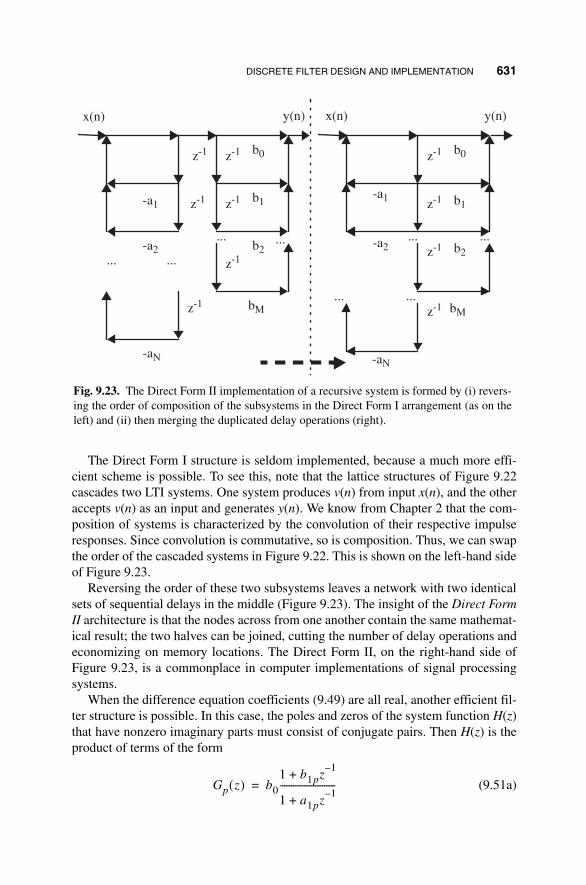
DISCRETE FILTER DESIGN AND IMPLEMENTATION 631
The Direct Form I structure is seldom implemented, because a much more effi-cient scheme is possible. To see this, note that the lattice structures of Figure 9.22cascades two LTI systems. One system produces v(n) from input x(n), and the otheraccepts v(n) as an input and generates y(n). We know from Chapter 2 that the com-position of systems is characterized by the convolution of their respective impulseresponses. Since convolution is commutative, so is composition. Thus, we can swapthe order of the cascaded systems in Figure 9.22. This is shown on the left-hand sideof Figure 9.23.
Reversing the order of these two subsystems leaves a network with two identicalsets of sequential delays in the middle (Figure 9.23). The insight of the Direct FormII architecture is that the nodes across from one another contain the same mathemat-ical result; the two halves can be joined, cutting the number of delay operations andeconomizing on memory locations. The Direct Form II, on the right-hand side ofFigure 9.23, is a commonplace in computer implementations of signal processingsystems.
When the difference equation coefficients (9.49) are all real, another efficient fil-ter structure is possible. In this case, the poles and zeros of the system function H(z)that have nonzero imaginary parts must consist of conjugate pairs. Then H(z) is theproduct of terms of the form
(9.51a)
b0z-1
z-1 b1
b2
bM
z-1
... ...
x(n)
...
-aN
z-1
...
-a1
-a2
z-1
z-1 b0z-1
z-1 b1
b2
bM
z-1... ...
y(n)
...z-1
y(n)x(n)
-a1
-a2
-aN
...
Fig. 9.23. The Direct Form II implementation of a recursive system is formed by (i) revers-ing the order of composition of the subsystems in the Direct Form I arrangement (as on theleft) and (ii) then merging the duplicated delay operations (right).
Gp z( ) b0
1 b1pz1–
+
1 a1pz1–
+-------------------------=

632 FREQUENCY-DOMAIN SIGNAL ANALYSIS
and
, (9.51b)
where all of the coefficients are real. Some coefficients may be zero to account forunequal numbers of poles and zeros. Terms of the form (9.51a) are called first-ordersections. Terms of the form (9.51b) are called second-order sections. We mayimplement each first- or second-order section as a Direct Form I or Direct Form IInetwork. When we serialize all of them to implement H(z), we have the cascadearchitecture for a system defined by a difference equation. Strategies exist for pair-ing poles and zeros in the cascade architecture so as to minimize round-off error infinite precision arithmetic [11].
9.3.5 Low-Pass Filter Design
This section covers several methods for designing discrete low-pass filters. Themechanics of converting an approximate low-pass filter to one of the other types(high-pass, bandpass, or band-reject) are the same as for ideal filters. This sectionalso covers two particularly important procedures for converting continuous domainto discrete filters: the impulse invariance technique and the bilinear transformation.
We have already constructed and applied several ad hoc discrete filters. Oneobvious method is to use a frequency-domain mask:
(i) Fourier transform the signal. Thus, from x(n), we find X(k) according to theDFT analysis equation (9.1).
(ii) Mark out all but the frequencies of interest to the application. In otherwords, the application determines a binary mask H(k) ∈ 0, 1 and we setY(k) = H(k)X(k). Note that this is equivalent to convolving y(n) = (h*x)(n),where h(n) is the inverse DFT of H(k).
(iii) Analyze the result Y(k) by thresholding, segmentation, and classification pro-cedures in the spirit of ordinary time-domain analysis (Chapter 4); or, alter-natively, inverse transform Y(k) to continue time-domain analysis on y(n).
(iv) Finally, interpret the signal.
There are advantages and disadvantages to the obvious approach. It offers per-fect control of the filtering, assuming that the sampling rate is high enough. Also, itallows the application designer to work in both domains: time and frequency. Thiscould be pertinent. But one drawback is that it is only feasible for offline applica-tions. Where decisions about the signal must be made while the data arrive, thisstrategy does not work very well. Even for offline applications, the method couldbe expensive; the discrete Fourier transform requires a lot of arithmetical opera-tions, and if the data do not naturally come in fast transform-sized chunks, this pre-sents another problem of data windowing and interpretation across the windowboundaries.
Kq z( )1 b1qz
1–b2qz
2–+ +
1 a1qz1–
a2qz2–
+ +------------------------------------------------=

DISCRETE FILTER DESIGN AND IMPLEMENTATION 633
Another method is to construct low-pass filters intuitively, using weighted aver-ages or recursive, sample-and-hold algorithms. Although it chagrins a signal theo-rist, probably most of the filters used in analysis applications are of this type. Suchadhoc filters are useful for salt-and-pepper noise removal, blending away transients,and preparing signals for derivative or edge finding operations. One can investigatethe spectral characteristics of such filters using the discrete Fourier transform, suchas we carried out in Section 9.1.
9.3.5.1 Impulse Invariance. It is possible to begin with an analog low-passfilter and convert it to a discrete filter. Often, the useful characteristics for an appli-cation are known from their analog frequency-domain description. An example isthe Gaussian; it is analytically attractive, it decays quickly, and filtering with widerkernels does not create additional time domain structure, as shown by scale-spacetheory (Chapter 4).
The impulse invariance technique is as follows:
(i) From the application, a specification of the filter’s continuous-domain Fou-rier transform Ha(Ω) is generated.
(ii) The inverse Fourier transform is applied to find ha(t), the impulse responseof the analog filter.
(iii) The analog impulse respose is sampled h(n) = ha(nT), where T > 0 is thesampling interval.
Now, impulse invariance is simple and commonly invoked in signal analysis appli-cations. One question, however, is whether the discrete sampling in step (iii) aboveundoes the frequency-domain behavior that motivated the analog filter’s selection inthe first place.
The sampling theorem (Chapter 7) answers this question. We can write H(ω), thediscrete-time Fourier transform of h(n), in terms of Ha(Ω), the analog Fourier trans-form of ha(t):
. (9.52)
We recognize the form of (9.52). The DTFT of h(n) consists of a superposition ofscaled (amplified by T −1) versions of Ha, shifted by 2π/T and dilated by T.
Note also that if |Ha(Ω)| ≈ 1 for |Ω| ≈ 0 in (9.52), then H(ω) will provide a gain ofapproximately 1/T. With the sampling rate close to 1 Hz, the effect will be neglig-ble. However, if T is small—that is, the sampling rate is high—then the discrete fil-ter will have a very high gain. For this reason, it is customary to set h(n) = Tha(nT)[7, 40].
9.3.5.2 Sampling Rational Analog Filters. An important discrete filterdesign method is to sample an analog filter whose Fourier transform is a rational
H ω( ) 1T--- Ha
jT--- ω 2kπ+[ ]
k ∞–=
∞
∑=

634 FREQUENCY-DOMAIN SIGNAL ANALYSIS
function. It turns out that the impulse invariance method applied to such an analogfilter produces a discrete filter governed by a difference equation. Such analog fil-ters are well-known from analog filter theory, and we will develop several of themlater. This becomes a very powerful method for designing discrete filters with excel-lent design characteristics and efficient computer implementations.
Suppose that an analog low-pass filter Ha has impulse response ha(t). Let theradial Fourier transform of ha(t) be a quotient of polynomials in Ω:
. (9.53)
We can find ha(t) using a partial fractions expansion of Ha(Ω). This can be a messymanual computation, but it works just like partial fraction expansions for rational z-transforms. These are the steps to expand Ha(Ω) in partial fractions [10]:
(i) Normalize the fraction so that the denominator Q(Ω) has a leading coeffi-cient of unity.
(ii) Since Ha is low-pass, as |Ω| → ∞, it must also be the case that |Ha(Ω)| → 0;the degree of Q(Ω) must exceed the degree of P(Ω):
. (9.54)
(iii) Factor the denominator Q(Ω) into its roots, ωm, 1 ≤ m ≤ M,
, (9.55)
where we assume for now that the Ωm are distinct. Possibly Q(Ω) has aform that allows us to easily derive its roots. In other cases, a computationalmethod of root finding, such as the Traub–Jenkins algorithm may beemployed [43].
(iv) Then Ha(Ω) has a partial fractions expansion of the form:
, (9.56)
where cm, 1 ≤ m ≤ M, are constants.
(v) To find cm, 1 ≤ m ≤ M, note that—having assumed that the denominator’sroots Ωm are distinct—we see
. (9.57)
Ha Ω( ) ha t( )ejΩt–
td∞–
∞
∫P Ω( )Q Ω( )--------------= =
Ha Ω( ) P Ω( )Q Ω( )--------------
pM 1– ΩM 1–pM 2– ΩM 2– … p0+ + +
ΩMqM 1– ΩM 1– … q0+ + +
--------------------------------------------------------------------------------------------= =
Q Ω( ) Ω Ωm–( )m 1=
M
∏=
Ha Ω( )cm
Ω Ωm–------------------
m 1=
M
∑=
cm Ω Ωm–( )Ha Ω( )[ ]Ω Ωm=
=

DISCRETE FILTER DESIGN AND IMPLEMENTATION 635
The partial fraction expansion enables us to write out the impulse response ha(t)of the analog low-pass filter Ha. Indeed, the inverse radial Fourier transform of
is , where u(t) is the unit step signal. This transformation is
valid so long as the imaginary part of Ωm is positive: Imag(Ωm) > 0. By Fourier trans-form linearity, we have
. (9.58)
Now we can discretize the filter by the impulse invariance technique, for instance.Let T > 0 be the sampling interval. Then,
. (9.59)
Taking the z-transform of (9.59) gives
. (9.60)
The important points about this derivation are as follows:
• Note that (9.60) is already in the form of a partial fractions expansion.
• It has in fact the same partial fractions expansion coefficients as given by(9.56) except for the factor of j ∈ C.
• The poles of H(z) are at exp(jTΩm) for m = 1, 2, ..., M.
• The pole at exp(jTΩm) will be inside the unit circle if and only if Real(jTΩm) <0 and thus if and only if Imag(Ωm) > 0.
• If we consider H(z) to be the z-transform of a causal filter, then Imag(Ωm) > 0for all m = 1, 2, ..., M implies that the region of convergence will be z ∈ C:|z| > a, for some 1 > a > 0, and the discrete filter H will therefore be stable.
• All of the partial fractions (9.60) are of the form , which is
the z-transform of the LTI system governed by the difference equation.
• Finally, if the sampling rate 1/T differs substantially from unity, then wechoose
(9.61)
in accord with (9.52) and the remarks thereafter.
cmΩ Ωm–------------------- jcme
jΩmtu t( )
ha t( ) ju t( ) cmejΩmt
m 1=
M
∑=
h n( ) ha nT( ) ju n( ) cmejΩmnT
m 1=
M
∑= =
H z( ) j cmZ u n( )ejΩmnT[ ] z( )
m 1=
M
∑jcm
1 ejTΩmz
1––
-------------------------------m 1=
M
∑= =
C
1 Az1–
–--------------------- Cz
z A–------------=
y n( ) Ay n 1–( ) Cx n( )+=
H z( ) Tjcm
1 ejTΩmz
1––
-------------------------------m 1=
M
∑=

636 FREQUENCY-DOMAIN SIGNAL ANALYSIS
Now let us turn to the special case of (9.55) where the denominator Q(Ω) has multi-ple roots. Suppose the root Ω1 has multiplicity R and the remaining Ωm, 2 ≤ m ≤ M,are distinct. Then Ha(Ω) has a partial fractions expansion of the form
. (9.62)
where c1,r, 1 ≤ r ≤ R, and cm, 2 ≤ m ≤ M, are constants. The formula for calculatingthe c1,r is as follows:
. (9.63)
If there are several multiple roots, then we follow the above procedure, insertingsupplemental terms in the partial fractions expansion (9.62) and computing thecoefficients with repeated derivatives (9.63).
Notice again that if the analog Ha(Ω) has at least one pole, then so will thez-transform (9.61), and the discrete filter will be IIR.
9.3.5.3 Laplace Transform Techniques. Analog filters and discrete filterdesigns from them are usually approached using the Laplace transform [6–11].Readers are probably familiar with this tool from continuous-domain systems the-ory. The Laplace transform plays the same role in analog systems theory that the z-trasnform plays in discrete system theory. Let us briefly review how the transform isused with analog filters whose Fourier transform is a rational function. Specializedtexts include Refs. 44 and 45.
The Laplace transform XL(s) of the analog signal x(t) is defined by
, (9.64)
where s ∈ C. If H is an LTI system, then the Laplace transform HL(s) of its impulseresponse, h = Hδ , is also called the system or transfer function of H.
Note that if x(t) has a Fourier transform X(Ω), then XL(jΩ) = X(Ω). The Fouriertransform is the Laplace transform evaluated on the imaginary axis of the complexplane. If s = σ + jω, where σ ∈ R, then XL(s) is the Fourier transform of x(t)e−σt.Transform convergence depends on the relation of x(t) to the exponential factorexp(−σt), and it does not depend on the imaginary part of s = σ + jω. Hence, theLaplace transform converges on vertical strips in the complex plane.
A couple of basic examples show that the Laplace transform must be associatedwith a region of convergence (ROC). If x(t) = e−Atu(t), then XL(s) = 1/(s + a) and theROCX = s ∈ C: Real(s) > −a. If y(t) = −e−Atu(−t), then YL(s) = 1/(s + a) and the
Ha Ω( )c1 r,
Ω Ω1–( )r------------------------
cm
Ω Ωm–------------------
m 2=
M
∑+r 1=
R
∑=
c1 r,
ΩR r–
R r–
d
d Ω Ω1–( )RHa Ω( )
Ω Ω1=
R r–( )!---------------------------------------------------------------------------------------=
XL s( ) x t( )est–
td∞–
∞
∫=

DISCRETE FILTER DESIGN AND IMPLEMENTATION 637
ROCY = s ∈ C: Real(s) < −a. Recall that an analog LTI system H is stable if andonly if the impulse response h = Hδ is absolutely integrable: h ∈ L1. But this meansh(t) has a Fourier transform H(Ω). Since H(Ω) = HL(jΩ), ROCH must contain theimaginary axis.
Now suppose x(t) is right-sided: x(t) = 0 for t < a ∈ R. If ROCX contains the ver-tical line Real(s) = b ∈ R, then ROCX contains s ∈ C : Real(s) ≥ Real(b). This isfairly easy to see, because, for such s ∈ C, exp(-Real(s)t) ≤ exp(-Real(b)t) for t > 0and the transform integral (9.64) will still exist. The ROC of a right-sided signal is aright half-plane. Similarly, if x(t) is left-sided (x(t) = 0 for t > a ∈ R), then ROCX isa left half-plane. Now consider the case of a causal LTI system H whose transferfunction HL(s) is a rational function. Since H is causal, h(t) = 0 for t < 0. In otherwords, h(t) is right-sided, and ROCH is a right half-plane. Since HL(s) is rational, itsdenominator is a complex polynomial Q(s). The only values s ∈ C for which HL(s)does not exist are the zeros of Q(s), which are the rational function’s poles. As thereare only a finite number of poles of HL(s), ROCH must be the half-plane to the rightof the zero of Q(s) with the largest real part.
We invert the Laplace transform using much the same methods as z-transforminversion. Rational functions XL(s) can be decomposed into a partial-fractions rep-resentation and the linearity propert applied to elementary transforms to arrive atx(t). Table 9.3 lists basic Laplace transform properties.
Let us turn now to the use of the Laplace transform in designing discrete filtersfrom rational analog filters [7]. Let the Laplace transform of ha(t) be a quotient ofcomplex polynomials
(9.65)
TABLE 9.3. Summary of Laplace Transform Properties
Signal Expression Laplace Transform or Property
x(t)
z(t) = ax(t) + by(t) aXL(ω) + bYL(ω)(Linearity, ROCX ∩ ROCY ⊆ ROCZ)
y(t) = x(t − a) e-saXL(s)(Time shift, ROCX = ROCY)
y(t) = x(t)exp(at) XL(s − a)(Frequency shift, modulation, ROCY = s: s − a ∈ ROCX)
y(t) = x(at), a ≠ 0
(Scaling, dilation, ROCY = s: s/a ∈ ROCX)
y(t) = (x * h)(t) F(s)H(s)(Convolution, ROCX ∩ ROCH ⊆ ROCY)
HL s( ) ha t( )est–
td∞–
∞
∫P s( )Q s( )-----------= =
XL s( ) x t( )est–
td∞–
∞
∫=
1a-----XLL
sa---

638 FREQUENCY-DOMAIN SIGNAL ANALYSIS
and let its partial fractions expansion be
, (9.66)
where dm, 1 ≤ m ≤ M, are constants, and the poles sm are distinct. Laplace transformlinearity and inversion of the summands in (9.66) implies
. (9.67)
Impulse invariance applies exactly as above. We set
, (9.68)
and the z-transform of h(n) is
. (9.69)
Notice that if dm = jcm and sm = jΩm, then the two expressions for H(z), (9.69) and(9.60), are identical. The conditions for stability and causality are similar too. Froma Fourier transform perspective, we need the poles of the rational function
to have positive imaginary parts. From the Laplace transform
standpoint, however, we require the poles of to have negative real
parts. Of course, if Ω0 is a pole of Ha(Ω), then jΩ0 is a pole of HL(s).
9.3.5.4 Bilinear Transformation. The bilinear transformation obtains a dis-crete filter from the frequency domain representation of an analog filter by directlymapping the analog frequency values to discrete frequency values. What sort ofoperation performs such a mapping? Note that analog frequencies can be arbitrarilylarge, −∞ < Ω < +∞, whereas discrete frequencies are limited to a 2π-wide interval:−π < ω ≤ π. So we seek a function that maps the real line to the circumference of acircle. The arctangent, tan−1, maps R to the interval (−π/2, π/2). Let T be the sam-pling interval. Then the following relation maps continuous to discrete frequencyvalues:
. (9.70)
Observe that as Ω → ±∞, the maximum analog frequency values, then ω → ±π,respectively, the maximum discrete frequency values.
HL s( )dm
s sm–--------------
m 1=
M
∑=
ha t( ) u t( ) dmesmt
m 1=
M
∑=
h n( ) ha nT( ) u n( ) dmesmnT
m 1=
M
∑= =
H z( ) dmZ u n( )edmnT
[ ] z( )m 1=
M
∑dm
1 eTsmz
1––
---------------------------m 1=
M
∑= =
Ha Ω( ) P Ω( )Q Ω( )--------------=
HL s( ) P s( )Q s( )-----------=
ω 2 ΩT2
-------- 1–
tan=

DISCRETE FILTER DESIGN AND IMPLEMENTATION 639
Suppose that Ha(Ω) is an analog lowpass filter with cutoff frequency Ωc. Thenthe bilinear transformation (9.70) allows us to define a discrete low-pass filter asfollows:
. (9.71)
The cutoff frequency for H(ω) is .
How does the scaling factor T come to appear in (9.70)? One practical reason isthat for small frequencies, T controls the rate of change of ω with respect to Ω: dω/
dΩ ≈ T. Some authors (e.g., Ref. 46) set to ensure that for low
frequencies ω ≈ Ω.. Another way of justifying the frequency mapping (9.70) is toconsider the relation between poles of rational analog filters and the discrete filtersobtained from them. If s = sm is a pole of the Laplace transform HL(s) of a filter(9.66), then corresponding to it is a pole z = exp(smT) of the z-transform H(z) (9.69).This suggests a mapping from the Laplace s-plane to the z-plane: z = esT. Thus,
, (9.72)
where we approximate the quotient on the right in (9.72) using the first two Taylorseries terms for the exponential function. This implies
, (9.73)
which relates the Laplace transform variable to the z-transform variable. To relatecontinuous and discrete frequency responses, we use z = ejω and s = jΩ in (9.73),treating it as an equality. After a little algebra, (9.70) results (exercise).
9.3.6 Frequency Transformations
There are convenient mappings of the independent variable of a filter’s systemfunction that convert a low-pass filter to a high-pass, bandpass, bandstop, or evenanother low-pass filter [7, 11, 33, 47].
9.3.6.1 Analog. Consider an analog low-pass filter with Laplace transformHL(s) and cutoff frequency Ωc = 1. The transformations are as follows:
(i) Let φ(s) = s/ΩH. Then HL(φ(s)) is a low-pass filter with cutoff frequency ΩH.
(ii) Let φ(s) = ΩH/s. Then HL(φ(s)) is a high-pass filter with cutoff frequency ΩH.
H ω( ) Ha2T--- ω
2----
tan =
ωc 2ΩcT
2-----------
1–
tan=
ω 2T--- ΩT
2--------
1–tan=
z esT e
s T 2⁄( )
es– T 2⁄( )
-------------------1 sT
2---+
1 sT2---–
---------------≈ 2 sT+2 sT–---------------= = =
s 2T--- z 1–
z 1+-----------
≈

640 FREQUENCY-DOMAIN SIGNAL ANALYSIS
(iii) Let . Then HL(φ(s)) is a bandpass filter with lower
cutoff frequency ΩL and upper cutoff frequency ΩH.
(iv) Let . Then HL(φ(s)) is a bandstop filter with lower
cutoff frequency ΩL and upper cutoff frequency ΩH.
9.3.6.2 Discrete. Consider a discrete low-pass filter with z-transform H(z) andcutoff frequency ωc. The transformations are as follows:
(i) Let . If we set , then
H(φ(z)) is a low-pass filter with cutoff frequency ωH.
(ii) Let . If , then
H(φ(z)) is a high-pass filter with cutoff frequency ωH.
(iii) Let . If ,
, , and ,
then H(φ(z)) is a bandpass filter with upper cutoff frequency ωH and lowercutoff frequency ωL.
(iv) Let . If ,
, , and ,
then H(φ(z)) is a bandstop filter with upper cutoff frequency ωH and lowercutoff frequency ωL.
Example (Low-Pass to High-Pass). Suppose that ωc = π/4 and ωH = 3π/4 in (ii)
above. Then and H(φ(z)) = H(−z).
9.3.7 Linear Phase
It is possible to construct causal finite impulse response filters with linear phase.Where the analysis steps in an application depend on linear phase during signal
φ s( )s
2 ΩLΩH+
s ΩH ΩL–( )------------------------------=
φ s( )s ΩH ΩL–( )
s2 ΩLΩH+
------------------------------=
φ z1–( ) z
1– α–
1 αz1–
–----------------------= α
ωc ωH–
2---------------------
sinωc ωH+
2----------------------
sin⁄=
φ z1–( ) z
1– α+
1 αz1–
+----------------------–= α
ωc ωH+
2----------------------
cos–ωc ωH–
2---------------------
cos⁄=
φ z1–( ) z
2–2αβz
1–– γ+
γz2–
2αβz1–
– 1+-----------------------------------------------–= α
ωH ωL+
2----------------------
cosωH ωL–
2----------------------
cos⁄=
κωH ωL–
2----------------------
ωc2
------- tancot= β κ κ 1+( )⁄= γ κ 1–( ) κ 1+( )⁄=
φ z1–( ) z
2–2αβz
1–– γ+
γz2–
2αβz1–
– 1+-----------------------------------------------= α
ωH ωL+
2----------------------
cosωH ωL–
2----------------------
cos⁄=
κωH ωL–
2----------------------
tanωc2
------- tan= β 1 κ 1+( )⁄= γ 1 κ–( ) κ 1+( )⁄=
α π 2⁄( )cosπ 4⁄–( )cos
---------------------------– 0= =

DISCRETE FILTER DESIGN AND IMPLEMENTATION 641
processing steps, this can be factor in favor of using finite impulse response (FIR) fil-ters. Note that it is possible to have infinite impulse response (IIR) filters with linearphase. For example, if h = Hδ and h(n) is symmetric about n = 0, then H will havezero phase. However, we are interested in filters that are practically implementable,and therefore we require right-sided impuse responses: h(n) = 0 for n < N for some N.
9.3.7.1 FIR Characterization. Let H be a linear, translation invariant system,let h(n) be its impulse response, and let H(ω) be its discrete time Fourier transform.If H(ω) = ejφ(ω)HR(ω), with φ(ω) a linear function of ω, and HR(ω) ∈ R, then we sayH has linear phase.
The theoretical result we are going to prove is as follows. If H is a discrete causalFIR filter with impulse response h = Hδ such that h(n) = 0 for n > N − 1, then H haslinear phase if and only if for some c ∈ C, with |c| = 1, h(n) = ch*(N − 1 − n), whereh* is the complex conjugate of h.
To begin, let us assume that H is causal, FIR, and has linear phase. Let H(ω) =ejφ(ω)HR(ω), with φ(ω) = a + bω, for some a, b ∈ R, and HR(ω) ∈ R. Assume thatSupport(h) = [0, N − 1] with N > 0, so that h(0) ≠ 0 and h(N − 1) ≠ 0. Let AH(ω) bethe amplitude function for H(ω) the DTFT of h(n): . Then
, (9.74)
(9.75)
Note that H(ω) and its complex conjugate H*(ω) are both 2π−periodic; we musthave 2b = K ∈ Z on the right-hand side of (9.75). Let c = e2ja and g(n) = h*(−n), sothat G(ω) = H*(ω). Then the discrete signal s(n) = cg(n + K) has DTFT S(ω) =cejKωG(ω) = cejKωH*(ω) = H(ω). Because the DTFT is invertible, we must haveh(n) = s(n) = cg(n + K) = ch*(−K − n). We know that for n < 0, h(n) = h*(n) = 0.Also, if n > −K, we have ch*(−K − n) = h(n) = 0. Thus, −K = N−1 because that is theupper limit of the support of h(n), and so h(n) = ch*(N − 1 − n), as claimed.
Conversely, suppose Support(h) = [0, N − 1] and h(n) = ch*(N − 1 − n) for somec ∈ C with |c| = 1. Applying the DTFT properties gives H(ω) = ce−j(N − 1)ωH*(ω).Let c = ejθ. If , then . Putting thesetogether, we have
, (9.76)
and thus for some K ∈ Z,
. (9.77)
Clearly, φ(ω) is a linear function of ω, and we are done.
H ω( ) ejφ ω( )
AH ω( )=
H ω( ) h n( )ejωn–
∞–
∞
∑ h n( )ejωn–
n 0=
N 1–
∑= =
H ω( ) ej 2a 2bω φ ω( )–+[ ]
AH ω( ) e2ja
e2jbω
ej– φ ω( )
AH ω( ) e2ja
e2jbω
H* ω( ).= = =
H ω( ) ejφ ω( )AH ω( )= H* ω( ) e j– φ ω( )AH ω( )=
ejφ ω( )
ejθ
ej– φ ω( )
ej N 1–( )ω–
=
φ ω( ) 1 N–( )ω2
---------------------- θ2--- πK+ +=

642 FREQUENCY-DOMAIN SIGNAL ANALYSIS
9.3.7.2 Linear Phase Filter Classes. For real-valued filters h = Hδ, whereh(n) has support [0, N − 1], with N > 0, there are four categories of linear phase fil-ters. We showed that a finite impulse response filter H has linear phase if and only iffor some c ∈ C, |c| = 1, h(n) = ch*(N − 1 − n). If h(n) ∈ R, then c = 1, −1.
We can thus put the filter into one of four classes (Figure 9.24):
(i) c = 1 and N = 2M + 1 is odd.
(ii) c = 1 and N = 2M is even.
(iii) c = −1 and N = 2M + 1 is odd.
(iv) c = −1 and N = 2M is even.
9.3.7.3 Examples. We review two cases where the need for linear phase moti-vates the specific use of FIR filters: electroencephalogram (EEG) interpretation andseismogram intrpretation.
The first chapter explained the multichannel EEG [48], a biomedical signal that isoften employed in studying brain functions and diagnosing injuries and illnesses.Electrodes attached to the scalp record the minute voltages produced by the interac-tions of large numbers of neurons. The signals are often quite noisy, and successiveaveraging is often employed to improve the quality of EEG traces. In studying audi-tory potentials—EEG traces of the part of the brain that is involved in the front-endprocessing of auditory nerve impulses—linear filtering has been investigated inorder to improve upon successive averaging, the efficacy of which diminishes after alarge number of sampling epochs. Frequencies above 2 kHz are removed by lowpassfiltering, since they cannot be due to neuronal changes, which take place on the order
0 2 4 6
0
0.5
1
0 2 4 6
0
0.5
1
0 2
(iii)
(iv)
(ii)
(i)
4 6
-1
-0.5
0
0.5
1
0 2 4 6
-1
-0.5
0
0.5
1
Fig. 9.24. Four classes of linear phase FIR filters.

WIDEBAND SIGNAL ANALYSIS 643
of 1 ms. The remaining noise is usually at low frequencies, DC to about 150 Hz [49].The most popular filtering methods for such an application use IIR filters derivedfrom difference equations (Section 9.3.4.2), since they are efficient and generallyhave better sharpness than FIR filters. But the nonlinear phase response of the causalIIR filters distorts the EEG trace, making linear phase FIR filtering preferable [49].
In seismic processing, the signals are generally quite noisy, composed of manyfrequency components, which are filtered by their propagation through the earth.These different sinusoidal pulses arrive at the sensing unit—the seismometer—atdifferent times [50], a kind of phase delay. Perhaps the most basic task of earth-quake seismology is to estimate the arrival time of an event, so that different seis-mometer stations can compare seismograms and locate the epicenter. Against thebackground noise of minor earth movements, impacts from construction equipment,and vehicle traffic vibrations, the seismic station determines the edge of a signifi-cant transient. At what time this transient occurs for a seismic station depends onthe group delay of Mother Earth acting as a filter. Thus, for automated seismograminterpretation, a signal processing filter that introduces a nonlinear phase delay intothe system might distort the signal and cause an error in pinpointing the onset timeof a seismic shock. In order to facilitate the comparison of arrival times among dif-ferent stations with different equipment, it is essential that their diverse noiseremoval filters not introduce any frequency dependent delays at all. The filteringrequirement is even more stringent; successful analysis of the seismogram usuallydemands zero phase filtering [51].
9.4 WIDEBAND SIGNAL ANALYSIS
This section considers signals that contain diverse spectral components. These sig-nals include chirps, which consist of rising or falling tones; transient signals, suchas seismic pulses; signals with sharp edges; and irregularly shaped signals, such asimage object boundaries. Our earlier methods of periodicity detection are successfulonly with much simpler waveforms.
9.4.1 Chirp Detection
A chirp is a signal segment where the frequency rises or falls over time. Strictlyspeaking, of course, a chirp is not a narrowband signal. But locally, at least, the sig-nal energy is contained in a narrow spectral range. If this is indeed the case, then thetask of chirp analysis becomes based upon a series of pure tone detection problemswhere the detected tones regulary rise or fall. This section considers the case wherelocally, at least, a signal contains mainly one frequency component, but that thefrequency itself is changing over time.
9.4.1.1 Synthetic Chirps. Section 6.5 presented the theory of signal modula-tion, which is the theoretical foundation of chirp signal analysis. Let us first consider

644 FREQUENCY-DOMAIN SIGNAL ANALYSIS
chirp signals for which the change in frequency over time is fairly simple—linear,for instance. Thus, we have as shown in Figure 9.25.
From its time-domain plot Figure 9.25a, it is hard to understand the signal. Themagnitude spectrum Figure 9.25b shows that a concentrated range of tones ispresent, in the range from 30 to 50 kHz, amidst some moderate background noise.But the time evolution of these frequencies and therefore the structure of the signal-itself remains unclear. We compute a sequence of 32-point discrete Fourier trans-forms over the time span of the signal. Overlapping the windows by eight sampleshelps smooth the time-frequency representation. The resulting map, shown inFigure 9.25c, reveals a linear chirp beginning at about 50 kHz and decreasing in fre-quency in a linear fashion down to about 30 kHz.
As long as its frequency content is, over a certain time interval, basically a tone,a chirp signal can be analyzed using tone detection techiques and a state machine.
ω t( ) tω1 ω0+=
Fig. 9.25. Synthetic chirp with noise added (a). Panel (b) shows the magnitude spectrum. Atime-frequency map (c) shows how the frequencies change over time. Surface maps (d) areuseful aids for visualizing signal structure.

WIDEBAND SIGNAL ANALYSIS 645
Local discrete Fourier transforms carry out the frequency analysis, and somestraightforward intepretive logic carry out the chirp discrimination. We can surmisethe following steps:
(i) An order N for the number of samples for discrete Fourier transformation(DFT) is selected, depending on the sampling rate of the source signal andthe range of frequencies expected in the chirp signal.
(ii) A DFT window overlap is selected.
(iii) DFT computations are conducted on the source signal within overlappingwindows as chosen in (i) and (ii).
(iv) Where a relatively pure tone in the expected frequency range is found usinglocal Fourier analysis, the state machine enters a tone detected state.
(v) Step (iv) is carried out again, and if there is a tone in the acceptable spectralrange, then the tone is checked for purity, and the machine enters a state ofincreasing or decreasing tone frequency.
(vi) Continued local frequency analysis extends the time-domain support of thetone, breaks out of the tone detected state based on an invalid frequencyresponse, or decides that the tone has the proper quality and range to con-tinue the chirp defined in the current machine state.
(vii) This process continues until the chirp ends or the input signal is exhausted.
The main difficulties with this analysis is that it requires—for the most part—offlinedata analysis. That is, the DFT windows are applied around a time center value in anoncausal fashion. This could be an expensive operation, and for real-time process-ing, it may be impossible. One alternative might be to employ a bank of causal fil-ters and seek significant outputs from the banks tuned to increasing or decreasingfrequency bands. To achieve this, however, we need to devise filtering methods thatare causal and sufficently efficient for online implementation.
9.4.1.2 Biological Signals: Bat Echolocation Chirp. Now let us study theecholocation chirp recorded from a large brown bat (Eptesicus fuscus).11 The sam-pling period is T = 7 µs, and there are N = 400 samples in the data set. The time-domain signal oscillates and rises in amplitude, but the plotted values evince fewother clues as to its structure (Figure 9.26a). The magnitude spectrum explains a lit-tle more. There are frequencies between 20 kHz and 50 kHz, centered more or lessstrongly around a spectral peak at some 35 kHz. The spectrum appears to be bimo-dal (Figure 9.26b). From a Fourier domain perspective, we cannot tell whether themodes are frequency components that appear at certain times, one after the other, orwhether they substantially overlap and the bimodality is an artifact of relativelyweaker middle frequencies.
11This data set is available from the signal processing information base (SPIB): http://spib.rice.edu/spib.html. The authors wish to thank Curtis Condon, Ken White, and Al Fengof the Beckman Center at the University of Illinois for the bat data and for permission to use it in thisbook.

646 FREQUENCY-DOMAIN SIGNAL ANALYSIS
Our knowledge of the echolocation pulse’s content changes dramatically whenwe develop the time-frequency map (Figure 9.27).
We use a boxcar window of width N = 128 to generate the local spectral values,overlapping successvie windows by M = 120 samples. This reveals three descendingchirps (Figure 9.27a) and shows that the time-frequency plot is at least tri-modal.The bar-shaped artifacts most visible in the lower frequencies appear to correlatewith window alignment. We try a Hann window function of length N and overlap Mto improve the local frequency estimates, as shown in Figure 9.27b. This reduces thetime-frequency artifacts, as one might expect. However, Hann windowing has theadded benefit of resolving the time-frequency mode of highest initial frequency intotwo chirps; the echolocation pulse in fact contains four modes.
9.4.2 Speech Analysis
Let us now consider some low-level speech signal analysis problems. There is, to besure, a large research literature on natural language processing from initial filteringmethods, detection of utterances in noise, phoneme recognition, word recognition,contextual analysis, and artificial intelligence techniques for computerized speechunderstanding [13, 52–54].
0 0.5 1 1.5 2 2.5 3x 10⁻³
-0.3
-0.2
-0.1
0
0.1
0.2
t (seconds)
(a) Large Brown Bat echolocation trace
0 10 20 30 40 50 60 70 800
0.5
1
1.5
2
2.5
3
3.5
f (kHz)
(b) Magnitude spectrum
|X(f)
| x
(t)
Fig. 9.26. Large brown bat echolocation pulse time-domian (a) and frequency-domain (b).

WIDEBAND SIGNAL ANALYSIS 647
9.4.2.1 Formant Detection. Formants are relatively high-energy, tone-likecomponents within a spoken word. They appear in the speech spectrum as isolatedpeaks. Consider, for example, a digitized voice fragment, consisting of a singleword (Figure 9.28).
It is possible to discover formants using peak detection in the Fourier magnitudespectrum. The vowel phoneme /a/ in Figure 9.28c exhibits three strong peaks atapproximately 300 Hz, 600 Hz, and 900 Hz. Such harmonics are characteristic ofsounds produced in a tube, with a source at one end and open at the other. Thiscrudely models the vocal tract, with the vocal cords at one end and the open mouthat the other. The vowel phoneme /i/ in in Figure 9.28e shows three resonant compo-nents as well as significant energy in many higher frequencies. Parts of the speechsignal that do not contain high-energy tones, such as the /k/ in Figure 9.28b, cannothave formant structures.
Another formant detection task is to identify a pitch or fundamental harmonicfrequency among the significant tones. This is the frequency of vibration of thevocal cords. In real speech recognition systems, this frequency must be identifiedand tracked, as it varies with the utterance as well as with the gender and emotional
Fig. 9.27. The time-frequency map of the large brown bat echolocation pulse evidently hasthree components (a), each a descending chirp. Instead of a 128-point square window, panel(b) employs a 128-point Hann window to generate the local frequency information.

648 FREQUENCY-DOMAIN SIGNAL ANALYSIS
state of the speaker. Some goal-directed information applies here. Pitch ranges fromabout 60 Hz to 300 Hz in adult males and up to 600 Hz in adult females.
A third formant detection task is to compare the center frequencies of signifi-cant tones. If such peaks represent formants, they must be integral multiples of thepitch frequency. Thus, in addition to ordinary peak finding, a formant detection
0 1000 2000 3000 4000 5000 6000 7000-1
0
1x 10⁴ sFemale voice: "...calling...", F = 8192 Hz
0 500 1000 1500 2000 2500 3000 3500 40000
1
2x 10⁵
/ k /
0 500 1000 1500 2000 2500 3000 3500 40000
1
2x 10⁵
/ a /
0 500 1000 1500 2000 2500 3000 3500 40000
1
2x 10⁵
/ l /
0 500 1000 1500 2000 2500 3000 3500 40000
1
2x 10⁵
/ i /
0 500
(f)
(e)
(d)
(c)
(b)
(a)
1000 1500 2000 2500 3000 3500 40000
1
2x 10⁵
/ ng /
Fig. 9.28. Digitized voice (a) of a woman: “...calling....” Vertical lines mark the approximatelocations of five phonemes. Panels (b)–(f) show the magnitude spectra for phonemes /k/, /a/,/l/, /i/, and /ng/.

WIDEBAND SIGNAL ANALYSIS 649
algorithm must include an assessment of the relative energy contributed by reso-nant frequencies.
9.4.2.2 Voice and Unvoiced Speech Determination. Speech sounds canbe divided into voiced and unvoiced sounds, according to whether the vocal cordsvibrate or do not vibrate, respectively (Figure 9.29). Unvoiced sounds split roughlyinto two categories: fricatives, such as /s/ or /f/, and aspirates, such as /k/.
9.4.2.3 Endpoint Detection. An important early speech analysis stepinvolves automatic discrimination between background noise and speech signals.This segmentation procedure is important for automated compilation of speechdatabases and for detecting word boundaries in speech recognition systems.A fairly old but reliable method uses local energy and zero crossing rate parametersto isolate speech [55]. From a background noise sample, upper- and lower-energyparameters Eu and El, respectively, and a zero crossing threshold Zc are determined.The algorithm refines the boundaries of a speech fragment in three stages asfollows:
(i) The initial energy-based segmentation, say speech exists within [Mu, Nu], isgiven by where local signal energy exceeds Eu.
(ii) The refined energy-based segmentation widens this interval to [Ml, Nl] bysearching outside [Mu, Nu] for the points where energy diminishes to El.
Fig. 9.29. Mixed-domain analysis of “calling” speech fragment. Using N = 256 point Hannwindows for local frequency estimations centered K = 32 samples apart along the time axisproduces the above time-frequency map. In many cases, voiced versus unvoiced speech seg-ments can be found using the time-frequency map.

650 FREQUENCY-DOMAIN SIGNAL ANALYSIS
(iii) Finally, a measure of local signal frequency—the zero crossing rate—ischecked outside of [Ml, Nl]. If the rate exceeds Zc three or more times in the250-ms intervals on either side of [Ml, Nl], then the speech fragment bound-aries grow again to [Mz, Nz], where [Mu, Nu] ⊆ [Ml, Nl] ⊆ [Mz, Nz].
Noise versus speech discrimination problems continue to attract experimentalresearchers [56, 57].
9.4.3 Problematic Examples
Let us mention a couple of signal analysis problem domains where Fouriertransform-based interpretation techniques begin to break down.
Seismic signals contain oscillations, but these oscillations are of unusually shorttime domain and are interspersed with transient artifacts that often thwart analysis.The Fourier transform is adequate for long-term periodic signal trends, but its effi-ciency as a signal descriptor diminishes with the duration of the oscillations. Geo-physicists resorted to the short-time or windowed Fourier transform, which wecover in the next chapter, with some success. This theory constructs a time- andfrequency-domain transform using the Fourier transform and the windowing tech-niques of Section 9.2. However, transient components are still problematic. Finally,efforts to get around the difficulties of windowed Fourier methods let to the devel-opment of the wavelet transform, which is the subject of Chapter 11.
Another problem area for Fourier methods is shape analysis. It seems that objectshapes, however they might be described mathematically, are comprised of parts.One-dimensional methods, such as we develop here, can be applied to objectboundaries, and we attempt such applications in the last chapter. There are Fouriertransform-based approaches:
(i) An early method, called Fourier descriptors, approximates image objectboundaries with varying numbers of Fourier series components.
(ii) Another method, the Fourier–Mellin transform, incorporates a temporalparameter into the transform.
These strategies work, but when the bounded object resolves into separate parts, theoverall analytic techniques collapse. As a result, automated object recognition sys-tems tend to retreat into structural methods of pattern recognition and cordon off,perhaps giving up on frequency-domain interpretation.
9.5 ANALOG FILTERS
Although our present goal is discrete time signal analysis and the frequency selec-tive systems that support it, we have ample reasons for developing a respectable the-ory of analog filtering.
(i) While signal analysis is computerized interpretation of signals and thereforeassumes a digital implementation, it relies upon discrete theory.

ANALOG FILTERS 651
(ii) However, our ultimate source signals come from analog world.
(iii) We need to filter incoming analog so as to remove high frequencies that wouldotherwise cause aliasing during sampling, according to the Nyquist criterion.
(iv) We may be able to implement cheaper analog filters.
(v) A lot of discrete filter designs are based on analog filters.
(vi) We have shown that it is easy to derive discrete filters from analog ver-sions—and especially if the analog filters have a rational transfer function.
(vii) Thus, if we develop a sound theory of analog filters, then we shall have acorrespondingly sound theory of discrete filters.
(viii) Analog filters are historically prior.
(ix) The analog theory of continuous theory involves continuous sinusoidal sig-nals, and hence the analog Fourier transform is a convenient theoretical tool.Anyway, this is consonant with our analog-first treatment of the frequencytransforms.
Just as the contiuous Fourier transform is the natural setting for studying signalfrequency, so the class of continuous domain, or analog, filters constitute the rightbeginning place for our study of frequency-domain signal analysis. Signal analysisusually takes place on a digital computer, but the frequency-selective algorithmsthat operate on digital signal representations often derive from continuous-domainfilters. That is one reason for studying analog filters. But even before signals aredigitized and fed to the computer, the signal digitization must often be filtered byanalog means so that aliasing (Chapter 7) is minimized. This section presents somebasic analog filters, introduces their characterisitic descriptors, and outlines themechanics of converting one filter into another.
Conventional analog filter designs begin by examining the frequency-domainbehavior X(ω) or the s-domain behavior XL(s) of analog signals x(t). System theorytexts covering analog filter theory and the Laplace transform include Refs. 6, 58,and 59. Texts that concentrate on the subsequent conversion to discrete time pro-cessing are [7–11, 26].
Classical electronics studies networks of electrical components—resistors,capacitors, and inductors—which implement the analog filtering operation in hard-ware. Circuit design texts cover the electronic circuit designs [60–63]. More mod-ern electrical and computer engineering texts cover the design of hardware fordigital filtering [64]. For signal analysis using digital computers, we need digital fil-ters that selectively enhance and suppress signal frequency components of interestto the application. We derive the digital filters from their analog equivalents usingsome classic methods.
9.5.1 Introduction
A filter is a frequency-selective linear, translation-invariant system. Analog filteringtakes place by virtue of the convolution property: Y(Ω) = H(Ω)X(Ω). So, if |H(Ω)| issmall for values of Ω where it is desirable to suppress frequencies in the input x(t)

652 FREQUENCY-DOMAIN SIGNAL ANALYSIS
and |H(Ω)| is near unity where it is desirable to preserve frequencies in x(t), thenconvolution with h(t), y(t) = (h*x)(t) performs the requisite frequency selectionoperation. To describe system filtering we specify the magnitude spectrum, |H(Ω)|,or, equivalently, |H(Ω)|2. We are mainly interested in real-valued filters: h(t) ∈ R.Since H(−Ω) = H*(Ω) in this case and since |H(Ω)| = |H*(Ω)|, the filters herein haveboth positive and negative frequency components. Thus, the magnitude spectra aresymmetric about the frequency-domain origin, Ω = 0.
This section explains how to construct bandpass and high-pass filters from low-pass filters. The discussion begins with the Gaussian; its Fourier transform is alsoGaussian, so it is a natural choice for a low-pass filter. Filter constructions dependon the Fourier transform properties from Chapter 5.
The analog convolution operation is once again denoted by the * operator: y =x*h. We define
. (9.78)
Section 6.4.1 introduced ideal analog filter types. One filter missing there is thenotch or band-reject filter. It is a like a reverse bandpass, and it suppresses ratherthan preserves a range of frequencies.
9.5.2 Basic Low-Pass Filters
Since we can move easily from low-pass filters to any of the other three basictypes—high-pass, bandpass, or band-reject—let us consider some examples.
9.5.2.1 Perfect. The ideal low-pass filter completely removes all frequencieshigher than some given frequency and preserves the rest without amplifying orattenuating them. This is the familiar analog moving average or boxcar filter.
9.5.2.2 Gaussian. The Gaussian
(9.79)
with mean µ and standard deviation σ has Fourier transform
. (9.80)
Its magnitude spectrum is also a Gaussian, centered at Ω = 0. Thus, g(t) is the impulseresponse of an analog low-pass filter. If x(t) is an analog signal and y = Gx = (g * x)(t)is the convolution with the Gaussian (9.79), then Y(Ω) = X(Ω)G(Ω), where G(Ω) =(Fg)(Ω) is given by (9.80). Gaussians decay rapidly, faster than the inverse of any
y t( ) x∗h( ) t( ) x s( )h t s–( ) sd∞–
∞
∫= =
gµ σ, t( ) 1
σ 2π--------------e
t µ–( )2
2σ2------------------–
g t( )= =
G Ω( ) g t( )ejΩt–
t σ2Ω2
2------------- jΩµ+–
exp=d∞–
∞
∫=

ANALOG FILTERS 653
polynomial. Thus, the Fourier transform of the system response Y(Ω) = (Fy)(Ω) willcontain the x(t) frequency components near Ω = 0, but they will be suppressed by theproduct with the Gaussian G(Ω). This idea is basic to all low-pass filtering.
Now we also gain a deeper understanding of scale space analysis, introduced inChapter 4. Recall that we showed that smoothing signals by ever broader Gaussiankernels had the unique property that no structure was created in the process. Weunderstand signal structure to be determined by the concavity regions within thesignal. Now (9.80) shows that the wider kernels are actually low-pass filters withsmaller passbands. That is, the wider kernels progressively remove the high-frequency components, leaving relatively lower frequency undulations, and—moreimportantly—not creating additional changes in signal curvature.
A particularly important area of signal analysis is the detection, classification,and recognition of signal features that vary according to the size of their features—according to their scale, for instance.
9.5.2.3 Rational Functions. We can find other examples based on rationalfunctions. For example, suppose H(Ω) = (1 + Ω2)−1. The inverse Fourier transform is
(9.81)
which is easy to see from the forward radial transform F (exp(−a|t|)) = 2a/(a + Ω2).Evidently, convolution with h(t) performs a weighted averaging on input signaldata. In signal analysis applications, the pulse h(t) is often called a Lorentzian, andit is used to find peaks, valleys, and transients in general by the method of templatematching.
9.5.2.4 Better Low-Pass Filters. It turns out that very good filters can bebuilt by pursuing the idea of rational functions introduced in the previous example.The important features of such filters are as follows:
• They have superior cutoffs—sharper and more like perfect low-pass filters.
• Upon discrete conversion, they will be causal.
• They are stable.
• They have efficient implementations, relying on difference equations.
For signal analysis applications involving real-time data, such as in speech rec-ognition or industrial control applications, causality is important. Of course, manysignal analysis applications do not involve real-time data; that is, they are offlineapplications, and so causal systems are less critical. Nonetheless, very good filterscan be developed for data whose discrete values are only known for the presentand past.
h t( ) 12π------ H Ω( )e
jΩt Ω et–
2---------,=d
∞–
∞
∫=

654 FREQUENCY-DOMAIN SIGNAL ANALYSIS
9.5.3 Butterworth
Butterworth12 filters have maximally flat pass and stop bands. Thus, the filterdesigner that values, above all else, reduced pass- and stop-band ripple inclinestoward this filter.
9.5.3.1 Conditions for Optimally Flat Filters. We describe these filters viatheir frequency-domain representation. Their Fourier transforms are based on ratio-nal functions—quotients of continuous domain polynomials. The Butterworth filterspecializes the rational function by looking at the Taylor series representations of itsnumerator and denominator.
Indeed, we have already constructed lowpass filters out of rational functions. Theidea is to look at analog filters h = Hδ, such that their Fourier transform power spec-tra |H(Ω)|2 are rational functions B(Ω)/A(Ω), where A(Ω) and B(Ω) are polynomi-als. We impose conditions on the rational functions so that we achieve our designcriteria: passband performance, stopband performance, cutoff frequency, allowableripple, and required transition band sharpness. Significantly, for signal analysis ondigital computers, when the power spectrum of an analog filter is a rational func-tion, then it can be used to derive a discrete filter.
A simple but useful fact is that if h(t) ∈ R, then the squared magnitude spectrum|H(Ω)|2 is an even function of Ω. To see this, note that Fourier transform symmetryproperties imply H(−Ω) = H*(Ω). So |H(Ω)|2 = H(Ω)H*(Ω) = H(Ω)H(−Ω). But then|H(−Ω)|2 = H(−Ω)H*(−Ω) = H(−Ω)H(Ω) too.
We thus consider P(Ω) = |H(Ω)|2 = B(Ω)/A(Ω), such that P(Ω) is symmetricabout Ω = 0. This means A(Ω) and B(Ω) are polynomials in Ω2 (exercise). Thus,
, (9.82a)
, (9.82b)
with a0 = b0. We may assume that a0 = b0 = 1. A low-pass filter implies |H(Ω)| → 0as |Ω| → ∞, so N > M. For the filter stopband to be maximally flat as Ω → ∞, themaximal number of numerator terms in (9.82b) should be zero. Thus, b2 = b4 = ⋅⋅⋅ =b2M = 0, and we see
. (9.83)
Butterworth criteria also require the filter’s passband to be maximally flat at Ω = 0,which entails a2 = a4 = ⋅⋅⋅ = a2n−2 = 0. We define the cutoff frequency Ωc of the
12After S. Butterworth, a British engineer who first analyzed this response profile [“On the theory of fil-ter amplifiers,” Wireless Engineer, vol. 7, pp. 536–554, 1930]. V. D. Landon later described this same fil-ter as maximally flat [Cascade amplifiers with maximal flatness, RCA Review, vol. 5, pp. 347–362, 1941].
A Ω( ) a0 a2Ω2a4Ω4… a2NΩ2N
+ + +=
B Ω( ) b0 b2Ω2b4Ω4… b2MΩ2M
+ + +=
P Ω( ) H Ω( ) 2 1A Ω( )------------- 1
1 a2Ω2a4Ω4… a2NΩ2N
+ + +---------------------------------------------------------------------------= = =

ANALOG FILTERS 655
Butterworth filter by (Ωc)−2n = a2n. Thus, the Butterworth filter of order N > 0 is
defined by its Fourier transform H(ω) (Figure 9.30):
; (9.84)
an important next step in practical implementation is to decide which square roots tochoose for H(Ω) in (9.84). Note that H(Ωc) = 2−1/2 ≈ 0.707, for any filter order.
It is possible to invert the Butterworth filter Fourier transform H(Ω), truncate theimpulse response h(t), and then sample the result. As we have observed, this wouldinduce some errors due to aliasing into the final filtering result. The filter designermight reduce these errors by preserving a large number of discrete samples. But thisnecessitates a time-consuming convolution operation. It turns out, however, thatbecause a Butterworth filter has a rational Fourier transform, an efficient discreteimplementation is possible using difference equations.
Now let us turn to the approximation problem for the Butterworth filter. The pro-cedure differs depending on how the designer performs conversion from the analogto discrete filter form: impulse invariance or bilinear transformation.
9.5.3.2 Butterworth Approximation: Impulse Invariance. Given boundson how far the filter’s magnitude spectrum can stray from the ideal passband and
-500 -400 -300 -200 -100 0 100 200 300 400 500-0.2
0
0.2
0.4
H(ω
)
0.6
0.8
1
1.2
Butterworth filters, |H(ω)|2: ωc = 100Hz; n = 4, 8, 16
ω (Hz)
Fig. 9.30. Analog Butterworth filters for a few orders.
H Ω( ) 1
1 ΩΩc------
2N+
----------------------------=

656 FREQUENCY-DOMAIN SIGNAL ANALYSIS
stopband, the Butterworth filter approximation finds two parameters: the filter orderN > 0 and the radial cutoff frequency Ωc in (9.84). Suppose that we require a dis-crete low-pass Butterworth filter with unit DC gain: |H(ω)| = 1 for ω = 0, whereH(ω) is the DTMF of the filter impulse response h(n). We assume that the samplingfrequency is high enough so that aliasing of Ha(Ω), the filter’s (radial) Fourier trans-form, is not an issue. This allows us to use the analog filter’s magnitude response inthe design approximation.
Suppose that the passband is |Ω| < Ωp and the application requires that |Ha(Ω)| iswithin δ > 0 of unity. Suppose the stopband begins at Ωs > Ωp, and we need |Ha(Ω)|to be within λ > 0 of zero. The Butterworth magnitude response is monotone; it suf-fices to consider the dual constraints:
(9.85a)
(9.85b)
Filter designers often prefer approximation by differences in decibels. Thus, we saythe passband magnitude (dB) is greater than a small negative value (∆) and the stop-band magnitude (dB) is less than a large negative value (Λ):
(9.86a)
(9.86b)
The above constraints reduce to
(9.87a)
(9.87b)
but (9.85a) and (9.85b) give similar relations too. Let so thatsolving for Ωc gives
. (9.88)
H Ωp( ) 1
1Ωp
Ωc-------
2N+
---------------------------- 1 δ 1,≈–≥=
H Ωs( ) 1
1Ωs
Ωc------
2N+
---------------------------- λ 0.≈≤=
0 10 H Ωp( ) 210
∆,≥log>
10 H Ωs( ) 210
log Λ 0.<≤
1Ωp
Ωc-------
2N+ R∆≤ 10
∆10------–
1,≈=
1Ωs
Ωc------
2N+ RΛ≥ 10
Λ10------–
>> 1,=
RR∆ 1–( )log
RΛ 1–( )log------------------------------=
ΩclogR Ωslog Ωplog–
R 1–----------------------------------------=

ANALOG FILTERS 657
At this point, the filter designer makes choices. We can use (9.87a) to find theButterworth filter order
, (9.89)
which will generally not be a whole number. Designers usually round the orderupward, taking the Butterworth order N to be the integral ceiling of ν in (9.89)—theinteger greater than ν, or Ceil(ν). Using equality in either (9.87a) or (9.87b), thecutoff frequency must be recomputed. For instance, setting
(9.90)
establishes a new cutoff frequency based on the upwardly rounded order and thepassband constraint. The resulting low-pass Butterworth filter satisfies the passbandcondition determined by Ωc,N and improves upon the stopband condition. This is agood approach for low sampling rates, when the aliasing caused by filter conversionusing impulse invariance is a concern [7].
Alternatively, tight application timing contraints might force the designer to rounddown and choose a smaller N, the floor of ν in (9.89). Perhaps N = Floor(ν) ≈ ν, ordeviation from the passband and stopband specifications is acceptable. The designermight also opt for a cutoff frequency that favors an exactly met stopband. Assumingthat the filter order is rounded upward, the filter then meets a more stringent passbandspecification. The cost of this option is that it does not counteract the aliasing arisingfrom impulse invariance. The exercises explore these design alternatives.
We determine the ωp and ωs (radians/sample) from the sampling rate Fs = 1/Tand the application’s specified analog passband and stopband frequencies (Hz).
Example (DTMF Passband and Stopband Calculations). Suppose we require alowpass filter that removes high-frequency noise for the dual-tone multifrequencyapplication of Section 9.1. Let the digital sampling rate be Fs = 8192 Hz. Then dis-crete frequency ω = ±π corresponds to the Nyquist frequency of Fs/2 = 4096 Hz.DTMF tones range up to 1633 Hz. Thus, the lowpass filter bands could be specifiedby setting ωp = (1633/4096) × π ≈ 0.3989π, and, depending upon the desired filtersharpness, ωs = (1800/4096) × π ≈ 0.4395π.
Example (Butterworth impulse invariance approximation). We require a low-pass filter with a passband within 1 dB of unity up to ωp = π/4 and at least 5 dBbelow unity beyond ωs = π/3. Assume the sampling interval is T = 1. Thus, werequire ∆ = −1, and Λ = −5. The approximation steps above give R∆ = 1.2589, RΛ =3.1623, and R = −1.7522. The exact cutoff frequency for this example is Ωc =0.9433, but we elect to round ν = 3.6888 upward to N = 4. Revising the cutofffrequency, we find Ωc,N = 0.9299.
νR∆ 1–( )log
2Ωp
Ωc-------
log
----------------------------=
Ωc N,Ωp
R∆ 1–2N
------------------------=

658 FREQUENCY-DOMAIN SIGNAL ANALYSIS
9.5.3.3 Poles and Zeros Analysis. Let us continue the design of the Butter-worth low-pass filter of order N > 0 by factoring the denominator of the squaredmagnitude response. Indeed, many analog filters satisfy
. (9.91)
PH(Ω) has 2N poles in the complex plane. Let the roots of the denominator in (9.91)be Ω1, Ω2, ..., Ω2N. In the case of the Butterworth squared magnitude, the roots lieon a circle of radius Ωc in the complex plane. They are in fact the order-2N roots ofunity scaled by the cutoff frequency Ωc. All we have to do to find H(Ω) that satisfies(9.91) is to select one pole from each pair Ωi, −Ωi ⊂ Ω1, Ω2, ..., Ω2N. But ajudicious root selection allows us to construct a causal discrete filter governed by adifference equation and therefore having an efficient computer implementation. Wecan obtain a discrete difference equation from an analog filter that has a rationalFourier transform H(Ω) only if its poles have positive imaginary parts (Section9.2.5.5). (Equivalently, if we are working with the Laplace transform, because
, this means that the poles of HL(s) must have negative real
parts.) With causality and difference equation implementation in mind, we retainthose roots, Ω1, Ω2, ..., ΩN, such that
. (9.92)
with Imag(Ωi) > 0.Let the partial fractions expansion of (9.92) be
, (9.93)
where ci, 1 ≤ i ≤ N, are constants. The results of Section 9.2.5.5 give the correspond-ing discrete filter’s transfer function:
, (9.94)
where T is the sampling interval. We generally compute ωp and ωs using the sam-pling interval, as explained in the previous section. Then, we derive the order Nand the cutoff frequency Ωc from the Butterworth approximation. The poles andzeros analysis gives a Butterworth filter of order N with cutoff frequency Ωc, nomatter what sampling interval we choose; it is conventient to assume T = 1. It isusually necessary to scale the coefficients of the discrete filter’s impulse responsefor unit DC gain. Let us see how this works by following through on the previousexample.
PH Ω( ) H Ω( ) 2 1
1 ΩΩc------
2N+
---------------------------- H Ω( )H Ω–( )= = =
H Ω( ) HL s( )s jΩ=
=
H Ω( ) 1Ω Ω1–( ) Ω Ω2–( )… Ω ΩN–( )
----------------------------------------------------------------------------=
H Ω( )ci
Ω Ωi–----------------
i 1=
N
∑=
H z( ) Tjci
1 ejTΩiz
1––
-----------------------------i 1=
N
∑=

ANALOG FILTERS 659
Example (Butterworth impulse invariance design, N = 4). Suppose we require alowpass filter with order N = 4 and cutoff frequency Ωc = 0.9299, as in the previousexample. Figure 9.31 shows the eight roots of the Butterworth squared magnitudefunction denominator. To find H(Ω), we select poles having a positive imaginarypart. This selection corresponds to the poles of HL(s) whose real parts are negative,because if Ω0 is a pole of H(Ω), then HL(jΩ0) is a pole of HL(s) (Table 9.4).
TABLE 9.4. Pole Selection in Butterworth Filter Design, N = 4, Ωc = 0.9299
Poles of |H(Ω)|2Fourier-Selected
Poles Poles of |HL(s)|2Laplace-Selected
Poles
−0.8591 + 0.3559j−0.8591 − 0.3559j
−0.8591 + 0.3559j −0.3559 − 0.8591j 0.3559 − 0.8591j
−0.3559 − 0.8591j
−0.3559 + 0.8591j−0.3559 − 0.8591j
−0.3559 + 0.8591j −0.8591 − 0.3559j 0.8591 − 0.3559j
−0.8591 − 0.3559j
0.3559 + 0.8591j0.3559 − 0.8591j
0.3559 + 0.8591j −0.8591 + 0.3559j 0.8591 + 0.3559j
−0.8591 + 0.3559j
0.8591 + 0.3559j0.8591 − 0.3559j
0.8591 + 0.3559j −0.3559 + 0.8591j 0.3559 + 0.8591j
−0.3559 + 0.8591j
-1 -0.5 0 0.5 1
-1
-0.8
-0.6
-0.4
-0.2
0
0.2
0.4
0.6
0.8
1
Real part
Imag
inar
y pa
rt
Butterworth filter, N = 4, poles of |H(ω)|2
Fig. 9.31. Butterworth filter, N = 4, eight poles of |H(Ω)|2.

660 FREQUENCY-DOMAIN SIGNAL ANALYSIS
Thus, performing the partial fractions calculations for H(z) gives
(9.95)
where T is the sampling interval. Writing H(z) as a quotient of polynomials in z−1,we see that (9.46) becomes
(9.96)
Now, finally, we can implement (9.95) with a cascade architecture and (9.96) with aDirect Form II. We can compute the impulse response h(n) as in Figure 9.32 byfeeding a discrete impulse through either of the difference equation architectures orby using (9.68).
H z( ) T j 0.2379 + 0.5745j–( )
1 ejT 0.8591+0.3559– j( )
z1–
–-------------------------------------------------------------- j 1.3869 0.5745j–( )
1 ejT 0.3559– 0.8591j+( )
z1–
–------------------------------------------------------------------
j 1.3869– 0.5745j–( )
1 ejT 0.3559 + 0.8591j( )
z1–
–-------------------------------------------------------------- j 0.2379 + 0.5745j( )
1 ejT 0.8591 0.3559j+( )
z1–
–--------------------------------------------------------------
+
+ +
=
bmzm–
m 0=
M
∑
1 akzk–
k 1=
N
∑+
-------------------------------------- 0.0873z1–
0.1837z2–
0.0260z3–
+ +
1 -1.7091( )z1–
1.3967z2–
-0.5538( )z3–
0.0880z4–
+ + + +--------------------------------------------------------------------------------------------------------------------------------------------.=
0 5 10 15 20 25 30 35-0.1
0
0.1
0.2
0.3
0.4
0.5
0.6h(n), Butterworth, N = 4
0 0.5 1 1.5 2
ω2.5 3 3.5
0
0.2
0.4
0.6
0.8
1
1.2
1.4
|H(ω
)|
Fig. 9.32. Impulse response h(n) of Butterworth low-pass filter, N = 4, Ωc = 0.9299 (top),and magnitude response (bottom) |H(ω)|. Note that H(0) ≈ 1.3386, so for unit DC gain, wescale h(n) by (1.3386)−1.

ANALOG FILTERS 661
9.5.3.4 Butterworth Approximation: Bilinear Transformation. This sec-tion considers the Butterworth low-pass filter approximation using the bilineartransformation. The crucial difference in finding the filter order N and the cutoff
frequency Ωc is the frequency mapping Here, H(ω) is the
DTMF of the desired discrete low-pass filter, T > 0 is the sampling interval, andHa(Ω) is an analog Butterworth low-pass filter whose order N and cutoff frequencyΩc remain to be found.
Let us suppose specifications on the passband and stopband similar to those withwhich we began the impulse invariance approximation. Thus,
(9.97a)
, (9.97b)
where ωp is the discrete passband frequency, ωs > ωp is the stopband frequency, andΛ < ∆ < 0. Applying the Butterworth filter condition as before, we calculate
(9.98a)
(9.98b)
We treat these as equalities and solve for the filter order:
(9.99)
where, in general, ν is not an integer. Typically, we round ν upward: N = Ceil(ν).We can use equality in either (9.98a) or (9.98b) to find Ωc. An advantage of bilineartransformation over impulse invariance is that there is no stopband aliasing. Thus,computing Ωc in terms of ωs gives
. (9.100)
H ω( ) Ha2T--- ω
2----
tan .=
0 10 H ωp( ) 210
log> 10 Ha2T---
ωp
2------
tan 2
10log ∆,≥=
10 H ωs( ) 210
log 10 Ha2T---
ωs
2------
tan 2
10log Λ 0<≤=
2TΩc----------
ωp
2------
tan2N
10
∆10------–
1–≤ R∆ 1,–=
2TΩc----------
ωs
2------
tan2N
10
Λ10------–
1–≥ RΛ 1.–=
ν
R∆ 1–
RΛ 1–----------------
log
2ωp 2⁄( )tan
ωs 2⁄( )tan--------------------------
log
--------------------------------------------=
Ωc
2 ωs 2⁄( )tan
T----------------------------- RΛ 1–( )
12N-------–
=

662 FREQUENCY-DOMAIN SIGNAL ANALYSIS
Example (Butterworth Bilinear Transformation Approximation). Suppose werequire the same low-pass filter: ωp = π/4, ωs = π/3, ∆ = −1, and Λ = −5. Again,R∆ = 1.2589, RΛ = 3.1623, but we calculate ν = 3.1957 and choose N = 4. Theexact analog cutoff frequency with T = 1 is Ωc = 1.048589, corresponding to adiscrete filter cutoff of ωc = 0.965788. Note that as ν nears its integral floor—inthis case ν ≈ 3—it might be feasible to round to the lower integral order. Thiscould be useful when computing time is a consideration and some cushion existsfor passband and stopband specifications.
Having derived the filter order N and the analog cutoff frequency Ωc, the rest ofthe bilinear filter design steps are the same as for impulse invariance.
Example (Butterworth Bilinear Transformation Design, N = 4). For the low-passfilter with order N = 4 and cutoff frequency ωc = 0.9658, as in the previous example,
the analog cutoff frequency is Ωc = 1.0486, since . Of the eight
poles of (9.101)
we select those having a positive imaginary part for Ha(Ω). The poles of the Laplacetransform HL,a(s) will thus have negative real parts (Table 9.5).
Thus, using the chosen poles (Table 9.5) the rational Laplace transform is
. (9.102)
Substituting the bilinear transform relation with T = 1 into (9.102)gives the discrete transfer function,
. (9.103)
TABLE 9.5. Pole Selection in Butterworth Filter Design Using Bilinear Transformation, N = 4, Ωc = 0.9658.
|Ha(Ω)|2 PolesFourier Poles
Selected |HL,a(s)|2 PolesLaplace Poles
Selected
−0.9688 + 0.4013j−0.9688 − 0.4013j
−0.9688 + 0.4013j −0.4013 − 0.9688j 0.4013 − 0.9688j
−0.4013 − 0.9688j
−0.4013 + 0.9688j−0.4013 − 0.9688j
−0.4013 + 0.9688j −0.9688 − 0.4013j 0.9688 − 0.4013j
−0.9688 − 0.4013j
0.4013 + 0.9688j0.4013 − 0.9688j
0.4013 + 0.9688j −0.9688 + 0.4013j 0.9688 + 0.4013j
−0.9688 + 0.4013j
0.9688 + 0.4013j0.9688 − 0.4013j
0.9688 + 0.4013j −0.4013 + 0.9688j 0.4013 + 0.9688j
−0.4013 + 0.9688j
Ωc2T---
ωc2
------- tan=
Ha Ω( ) 2 1
1 ΩΩc------
2N+
---------------------------- Ha Ω( )aH Ω–( ),= =
H s( ) 1
s4
2.7401s3
3.7541s2
3.0128s 1.2090+ + + +-------------------------------------------------------------------------------------------------------------=
s 2T--- z 1–
z 1+-----------
=
H z( ) 0.0166z4
0.0665z3
0.0997z2
0.0665z 0.0166+ + + +
z4
1.5116z3
– 1.2169z2
0.4549z2
0.0711+–+--------------------------------------------------------------------------------------------------------------------------------=

ANALOG FILTERS 663
The partial fraction expansion of H(z) = B(z)/A(z) is
(9.104)
The filter has a difference equation implementation (9.49), from which the impulseresponse follows (Figure 9.33b).
Note that it is possible to skip the approximation step, instead stipulating a dis-crete cutoff frequency ωc and guessing a filter order N > 0. After computing theassociated analog cutoff Ωc, the above poles and zeros analysis follows. This stepproduces an impulse response h(n), from which one can derive a Fourier magnituderesponse |H(ω)|. Should the passband or stopband not meet the anticipated
B z( )A z( )----------- 0.3048 + 0.1885j–
1 0.4326 + 0.5780j( )z1–
–--------------------------------------------------------------- 0.3048– 0.1885j–
1 0.4326 0.5780j–( )z1–
–--------------------------------------------------------------
0.1962 1.2480j–
1 0.3232 0.1789j+( )z1–
–--------------------------------------------------------------- 0.1962 + 1.2480j
1 0.3232 0.1789j–( )z1–
–-------------------------------------------------------------- 0.2337
+
+ + +
=
-1 -0.5 0 0.5 1
-1
-0.5
0
0.5
1
Real part
(a) Butterworth filter, N = 4, poles of |Ha(Ω)|2
0 10 20 30 40-0.1
0
0.1
0.2
0.3(b) Impulse response, bilinear transformation
n
ω ω0 1 2 3 4
0
0.2
0.4
0.6
0.8
1(c) Magnitude response
0 1 2 3 40
1
2
3
4
5(d) Delays
GroupPhase
|H(ω
)|Im
agin
ary
part
h(n)
Sam
ples
del
ayed
Fig. 9.33. Butterworth filter design, bilinear transformation. Pole locations for analogsquared magnitude response (a). Impulse response h(n) of Butterworth low-pass filter, N = 4,ωc = 0.9658 (b) and (c) magnitude response |H(ω)|. Note that H(0) ≈ 0.8271, so for unit DCgain, we scale h(n) by (0.8271)−1 ≈ 1.2090. Panel (d) shows the phase and group delay forthis filter.

664 FREQUENCY-DOMAIN SIGNAL ANALYSIS
constraints, the filter order is incremented and trial-and-error goes on. This is a gooduse case for a computerized filter design package.
Consider the group and phase delays of the above Butterworth low-pass filter. IfH(ω) = ejφ(ω)HR(ω) is a filter’s DTFT, where HR(ω) ∈ R, and φ(ω) is its phaseresponse, then its group delay is −dφ(ω)/dω. Since FIR filters enjoy linear phase(Section 9.3.6), their group delay is constant. Butterworth filters are IIR, sothe group delay varies. In fact, Figure 9.33d illustrates that this system’s groupdelay can change as much as four samples over the discrete frequency domain.
9.5.4 Chebyshev
Suppose a signal analysis application needs a low-pass filter with an especiallysharp cutoff frequency, but tolerates some passband ripple. The Butterworth condi-tion began by hypothesizing flatness in both the pass- and stopbands, so we need torelax one of these constraints. The first type of Chebyshev13 filter approximationachieves a sharper transition than the Butterworth, but it does so at the cost of allow-ing passband ripple. On the other hand, the stopband is flat, and the designer caneasily reduce the ripple to any positive value.
9.5.4.1 Chebyshev Polynomials and Equiripple Conditions. For the fil-ter stopband to be maximally flat as Ω → ∞, any (rational) analog low-pass filterwill have a squared Fourier magnitude response with a constant numerator (9.83). Ifwe hope to improve upon the Butterworth filter’s sharpness, we have to relax theButterworth contraints. By the logic of the argument for maximally flat filters inSection 9.5.3.1, we must allow more a2k to be nonzero. Let ε2T(Ω) = A(Ω) − 1 bethe nonconstant part of the denominator in (9.83), where ε > 0 is a parameter con-trolling the passband ripple height. A low-pass filter with unity gain requires adenominator near unity when Ω = 0, so let us stipulate that |T(Ω)| ≤ 1 for |Ω| ≤ 1.Then a suitable ε can always make ε2T(Ω) small for Ω near zero. Since T(Ω) is stilla polynomial, its magnitude will get arbitrarily large as |Ω| → ∞, and so away fromthe origin, P(Ω) → 0. Are there such polynomials?
Indeed approximation theory provides us with precisely such polynomials. Weset T(Ω) = TN(Ω), where TN(Ω) is the Chebyshev polynomial of order N ≥ 0 [43,65]. These are defined recursively as follows: , , and
. (9.105)
The Chebyshev polynomials have nice properties, which are explored in the exer-cises and exploited by our filter designs. It can be shown that
, (9.106a)
13In addition to his work on orthogonal functions, Russian mathematician Pafnuty Lvovich Chebyshev(1821−1894) proved Bertrand’s conjecture: For n > 3, there is at least one prime number between n and2n − 2.
T0 Ω( ) 1= T1 Ω( ) Ω=
TN 1+ Ω( ) 2ΩTN Ω( ) TN 1– Ω( )–=
TN Ω( ) N Ω( )1–cos( )cos=

ANALOG FILTERS 665
so that indeed |TN(Ω)| ≤ 1 for |Ω| ≤ 1. Furthermore, the polynomials are orthogonalon [−1, 1]. Chebyshev polynomials are also given for |Ω| > 1 by the relation
, (9.106b)
as shown in Ref. 65 (see Figure 9.34).Importantly for the filter approximation problem:
• If 1 ≤ N and Ω ∈ [−1, 1], then TN(Ω) oscillates between −1 and +1.
• TN(Ω) always achieves the minimum of −1 and the maximum of +1 on [−1, 1](for this reason it is called the equal ripple approximation).
• TN(1) = 1 for all N.
• For |Ω| > 1, TN(Ω) is strictly increasing or strictly decreasing.
Thus, the Chebyshev squared magnitude response is defined by
. (9.107)
TN Ω( ) N Ω( )1–cosh( )cosh=
-2 -1 0 1 2-10
-5
0
5
10
15
20
25(a) Chebyshev polynomials, N = 2, 3, 4
-1 -0.5 0 0.5 1
-1
-0.5
0
0.5
1
Real part
(b) Roots of |Ha(Ω)|2
0 10 20 30 40-0.5
0
0.5
1
1.5(c) Impulse response
h(n)
|H(ω
)|Im
agin
ary
part
NT
(Ω
)
n ω
Ω
0 1 2 3 40
1
2
3
4
5(d) Discrete magnitude spectrum
Fig. 9.34. Chebyshev polynomials for a few orders (a). Roots of the Fourier squared magni-tude response for a third-order low-pass filter (b). Corresponding discrete impulse response(c) and magnitude spectrum (d).
Ha Ω( ) 2 1A Ω( )------------- 1
1 ε2TN
2Ω Ωc⁄( )+
------------------------------------------= =

666 FREQUENCY-DOMAIN SIGNAL ANALYSIS
9.5.4.2 Impulse Invariance Approximation. For the Chebyshev low-passfilter approximation using the impulse invariance transformation, we are given adiscrete passband frequency ωp, a stopband frequency ωs, an allowable passbandripple, and a required stopband attenuation value. We seek the analog cutoff fre-quency Ωc, the filter order N, and the ripple parameter ε (9.107).
The Chebyshev polynomials’ properties simplify the approximation. |TN(Ω/Ωc)|is strictly increasing for Ω > Ωc, so we can set Ωc = ωp. If the passband constraint is
, for some ∆ < 0 as in (9.86a), then the maximum departure
from unity will occur for some −Ωc ≤ Ω ≤ Ωc. Thus, we need .Here our design assumes that ripple is defined by the passband peak-to-valley dif-ference. But some treatments assume that the ripple is half of this value—how farthe passband magnitude strays from its mean [26]. So readers should be aware ofthe differences this assumption can make in the final design specifications. Finally,
suppose the stopband specification (9.86b) is , for some Λ <
0, and the sampling rate is sufficiently high so that in the stopband, |ω| > ωs,
. (9.108)
Thus, we seek N > 0 such that
. (9.109)
We solve (9.109) as an equality for N,
, (9.110)
and round upward to the nearest integer.
Example (Chebyshev Impulse Invariance Approximation). Suppose we try theChebyshev approximation on a filter with the same specifications as in the Butter-worth impulse invariance design (Section 9.5.3.2). We need a passband within 1 dBof unity for ω < ωp = π/4. This means ∆ = −1, Ωc = π/4, and ε = 0.5088. We need astopband that is 5 dB or more below unity for ω > ωs = π/3. We have Λ = −5, and(9.110) gives N = 2.1662, which we round up to N = 3. Thus, the Chebyshevapproximation gives a third-order IIR filter, whereas the Butterworth approximationneeded a fourth-order system—a benefit from allowing passband ripple.
10 H ωp( ) 210
∆≥log
ε 10∆ 10⁄–
1–≥
10 H ωs( ) 210
log Λ≤
H ω( ) 2Ha Ω( ) 2≈ 1
1 εTN Ω Ωc⁄( )[ ]2+
-----------------------------------------------=
Ha ωs( ) 210 1 εTN ωs Ωc⁄( )[ ]2
+[ ]1–
10log Λ≤=
N
10Λ 10⁄–
1–ε
---------------------------------
1–
cosh
ωs
Ωc------
cosh
-------------------------------------------------------=
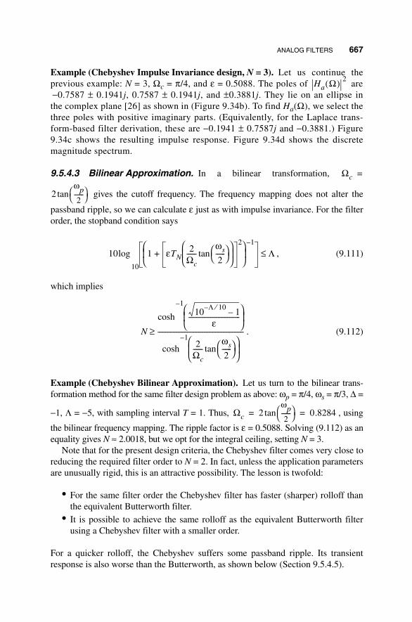
ANALOG FILTERS 667
Example (Chebyshev Impulse Invariance design, N = 3). Let us continue theprevious example: N = 3, Ωc = π/4, and ε = 0.5088. The poles of are−0.7587 ± 0.1941j, 0.7587 ± 0.1941j, and ±0.3881j. They lie on an ellipse inthe complex plane [26] as shown in (Figure 9.34b). To find Ha(Ω), we select thethree poles with positive imaginary parts. (Equivalently, for the Laplace trans-form-based filter derivation, these are −0.1941 ± 0.7587j and −0.3881.) Figure9.34c shows the resulting impulse response. Figure 9.34d shows the discretemagnitude spectrum.
9.5.4.3 Bilinear Approximation. In a bilinear transformation,
gives the cutoff frequency. The frequency mapping does not alter the
passband ripple, so we can calculate ε just as with impulse invariance. For the filterorder, the stopband condition says
, (9.111)
which implies
. (9.112)
Example (Chebyshev Bilinear Approximation). Let us turn to the bilinear trans-formation method for the same filter design problem as above: ωp = π/4, ωs = π/3, ∆ =
−1, Λ = −5, with sampling interval T = 1. Thus, , using
the bilinear frequency mapping. The ripple factor is ε = 0.5088. Solving (9.112) as anequality gives N ≈ 2.0018, but we opt for the integral ceiling, setting N = 3.
Note that for the present design criteria, the Chebyshev filter comes very close toreducing the required filter order to N = 2. In fact, unless the application parametersare unusually rigid, this is an attractive possibility. The lesson is twofold:
• For the same filter order the Chebyshev filter has faster (sharper) rolloff thanthe equivalent Butterworth filter.
• It is possible to achieve the same rolloff as the equivalent Butterworth filterusing a Chebyshev filter with a smaller order.
For a quicker rolloff, the Chebyshev suffers some passband ripple. Its transientresponse is also worse than the Butterworth, as shown below (Section 9.5.4.5).
Ha Ω( ) 2
Ωc =
2ωp2
------- tan
10 1 εTN2
Ωc------
ωs
2------
tan 2
+ 1–
10
log Λ≤
N
10Λ 10⁄–
1–ε
---------------------------------
1–
cosh
2Ωc------
ωs
2------
tan 1–
cosh
-------------------------------------------------------≥
Ωc 2ωp2
------- tan 0.8284= =

668 FREQUENCY-DOMAIN SIGNAL ANALYSIS
Example (Chebyshev Bilinear Design, N = 3). Let us continue the above approx-imation: N =3, ε = 0.5088, and Ωc = 0.8284. The poles of are −0.8003 ±0.2047j, 0.8003 ± 0.2047j, and ±0.4094j (Figure 9.35a). The Laplace transform polesof choice are therefore −0.2047 ± 0.8003j and −0.4094. The analog system function is
. (9.113)
Inserting the bilinear map with T = 1 into (9.113) gives
. (9.114)
H(z) has partial fractions expansion
(9.115)
Figure 9.35 shows the impulse (b) and magnitude responses (c).
Ha Ω( ) 2
HL a, s( ) 1
s3
0.8188s2
0.8499s 0.2793+ + +----------------------------------------------------------------------------------=
s 2T--- z 1–
z 1+-----------
=
H z( ) 0.0754z3
0.2263z2
0.2263z 0.0754+ + +
z3
1.8664z2
– 1.4986z 0.4637–+---------------------------------------------------------------------------------------------------=
B z( )A z( )----------- 0.6458 – 0.1170j–
1 0.6031 + 0.5819j( )z1–
–--------------------------------------------------------------- 0.6458 + 0.1170j–
1 0.6031 – 0.5819j( )z1–
–--------------------------------------------------------------
1.5297
1 0.6602( )z1–
–-------------------------------------- 0.1627.–
+
+
=
-1 -0.5 0 0.5 1
-1
-0.5
0
0.5
1
Real part
ω ω
(a) Poles of |Ha (Ω)| 2
0 10 20 30 40-0.5
0
0.5
1
1.5(b) Impulse response
n
0 1 2 3 40
1
2
3
4(c) Discrete magnitude spectrum
0 1 2 3 40
1
2
3
4
5
6
7(d) Delays
GroupPhase
|H(ω
)|Im
agin
ary
part
h(n)
Sam
ples
del
ayed
Fig. 9.35. Chebyshev low-pass filter, bilinear transformation. Pole locations (a), unnormal-ized discrete impulse response (b), magnitude response (c) and phase and group delay (d).

ANALOG FILTERS 669
9.5.4.4 Phase and Group Delay of IIR Filters. Let us compare the groupdelay of Butterworth and Chebyshev filters. Figure 9.35d shows that the groupdelay of the Chebyshev filter can be as much as six samples for ω ∈ [0, π]—worsethan the equivalent Butterworth design Figure 9.33d. This is one thing the Cheby-shev filter gives up in order to improve its rolloff performance.
9.5.4.5 Application: Transient Response Comparison. The Chebyshevfilter’s better rolloff, compared to the maximally flat filter, also costs it sometransient response performance. To see this, let us consider a basic transient filter-ing application. Observe first that the Chebyshev filter exhibits a sharper rolloffFigure 9.36a.
We apply the Butterworth and Chebyshev low-pass filters (N = 3) developed inprevious sections to the transient Figure 9.36b. The Chebyshev filter produces alonger delay and the ringing induced by the step edge persists for a longer timeinterval than with the Butterworth. On the other hand, the pulse’s later sloped edgeprovokes only a little bad behavior from the Chebyshev filter Figure 9.36c.
0 10 20 30 40 50 60 70 80 90 100
0
0.5
1
n
ω(b) Transient signal
0 10 20 30 40 50 60 70 80 90 100
0
0.5
1
n
y(n)
x(n)
|H(ω
)|
(c) Butterworth and Chebyshev lowpass filter responses
0 0.5 1 1.5 2 2.5 3 3.50
0.5
1(a) Butterworth and Chebyshev discrete magnitude spectra
Fig. 9.36. Butterworth and Chebyshev comparison. Magnitude spectra (a), transient signal(b), and Butterworth and Chebyshev responses (c).

670 FREQUENCY-DOMAIN SIGNAL ANALYSIS
The following points should be taken into consideration when choosing theChebyshev over the Butterworth filter for a signal analysis application:
• For less computational overhead with the same frequency discrimination per-formance, prefer the Chebyshev.
• If the frequencies in the filter passband will be further characterized by theirrelative strength, then the ripple in the Chebyshev becomes a detriment.
• If the application does not further analyze passband frequencies and is con-cerned with their mere presence or absence (such as in the DTMF applicationin Section 9.1) then the Chebyshev should be better.
• This is moreover the case when the application needs to segment relativelyclose bands of spectral information and sharp rolloff becomes a priority.
• Finally, if the time location of edges is important, and the application needs acrisp response from a crisp input edge to satisfactorily identify and locate thetransition, then the Butterworth filter is superior.
9.5.5 Inverse Chebyshev
The inverse Chebyshev filter provides a flat passband and an equiripple stopband.This filter is also called the Chebyshev Type II filter.
9.5.5.1 Stopband Equiripple Conditions. The specification of the filter’ssquared magnitude response is based on the Chebyshev filter of Section 9.5.4 [26,65]. The steps (Figure 9.37a) are as follows.
(i) We begin with the Chebyshev squared magnitude response function
, (9.116)
where TN(Ω) is the order-N Chebyshev polynomial.
(ii) Subtract this response from unity, 1 − P(Ω), to form the squared magnituderesponse of a high-pass filter having a flat passband and equiripple in thestopband.
(iii) Reverse the frequency axis to find Q(Ω) = 1 − P(Ω−1):
, (9.117)
which is the squared magnitude response of a low-pass filter. It has a maxi-mally flat passband and puts the Chebyshev equiripple characteristic in thestopband.
Ha Ω( ) 2 1
1 ε2TN
2Ω Ωc⁄( )+
------------------------------------------ P Ω( )= =
Q Ω( ) 1 1
1 ε2TN
2Ωc Ω⁄( )+
------------------------------------------–ε2
TN2
Ωc Ω⁄( )
1 ε2TN
2Ωc Ω⁄( )+
------------------------------------------= =

ANALOG FILTERS 671
Note that Q(Ω) is a rational function in Ω−1, but we can write it equivalently as arational function of Ω. The poles of Q(Ω) are the reciprocals of the poles of P(Ω)(exercise).
9.5.5.2 Impulse Invariance Approximation. Consider the impulse invari-ance approximation for the inverse Chebyshev low-pass filter. Suppose the discretepassband frequency is ωp, the stopband frequency is ωs, the passband is within ∆ <0 (dB) of unity, and the stopband ripple (dB) does not exceed Λ < ∆ < 0. We needthe analog stopband frequency Ωc, the filter order N, and the ripple parameter ε(9.117).
As remarked above, the parameter Ωc in (9.117) specifies the analog stopband.So, although for an ordinary Chebyshev filter we took Ωc = ωp, now we set Ωc = ωs.The stopband condition is 10log10Q(Ω) ≤ Λ for Ω ≥ Ωc. But as long as Ω ≥ Ωc we
have Ωc/Ω ≤ 1 and so . Hence, we can determine thestopband ripple factor ε from the stopband condition with Ω = Ωc: 10log10Q(Ωc) ≤Λ. Using the elementary Chebyshev polynomial property, TN(1) = 1 for all N ≥ 0,this reduces to
. (9.118)
0 1 2 3Ω Ω
4 50
0.1
0.2
0.3
0.4
0.5
Q(Ω
)
Q(Ω
)
0.6
0.7
0.8
0.9
1(a) Ωc = π/3, ε = .25, N = 3 (a) Ωc = π/3, ε = .25, N = 4
0 1 2 3 4 50
0.1
0.2
0.3
0.4
0.5
0.6
0.7
0.8
0.9
1
Fig. 9.37. Conversion from a Chebyshev to a third-order Inverse Chebyshev squared magni-tude response function (a). The dotted traces are intermediate steps. The vertical line is Ωcfrom (9.117) and represents the stopband frequency. For comparison, panel (b) shows an N =4 squared magnitude response.
1 ε2TN
2Ωc Ω⁄( )+ 1 ε2
+≤
ε 10Λ 10⁄
1 10Λ 10⁄
–--------------------------≤

672 FREQUENCY-DOMAIN SIGNAL ANALYSIS
Observe that the ripple parameter does not depend on the filter order. Typically, wesolve (9.118) as an equality to obtain ε.
The passband condition gives the analog filter order. If the discrete samplingrate is high enough, this means that for Ω < ωp < ωs = Ωc we can assume10log10Q(Ω) ≥ ∆. for Ω < ωp. Q(Ω) is strictly increasing as Ω → 0. Thus, we knowthat the passband condition applied to Ω = ωp is a worst case. The usual algebraboils this down to
. (9.119)
The familiar steps of taking (9.119) as an equality, solving for N, and roundingupward give the filter order.
Example (Inverse Chebyshev, Impulse Invariance, N = 3). We require a low-pass filter with a passband within 1 dB of unity up to ωp = π/4 and at least 5 dBbelow unity beyond ωs = π/3. Again, we see ∆ = −1 and Λ = −5 and assume T =1. As above, we set Ωc = ωs = π/3. From (9.118) we find ε = 0.680055. Solving(9.119) as an equality produces N = 2.1662. This value we round up to N = 3. Since
, it must be the case that
, (9.120)
where we have expressed Q(Ω) in positive powers of Ω (Figure 9.38a).
9.5.5.3 Poles and Zeros Analysis. Unlike the others we have already con-sidered, this filter has finite zeros in the extended complex plane. For Ha(Ω) weselect the poles of Q(Ω) which have positive imaginary parts. In general, among thezeros of a squared magnitude response function, we select one each of the numera-tor’s conjugate roots.
Example (Inverse Chebyshev, Impulse Invariance, N = 3). Let us continue withthe poles and zeros analysis of the previous example, for which the squaredmagnitude response is given by (9.117). The poles of Q(Ω) are ±2.5848j, −1.0581±0.2477j, and 1.0581 ±0.2477j. The selected Laplace transform poles are thus−2.5848, −0.2477 −1.0581j, and −0.2477 + 1.0581j. The zeros of Q(Ω) are −1.1885 ±0.1276j and 1.1885 ± 0.1276j. They all have the same magnitude, so we can chooseLaplace transform zeros to be −0.1276 − 1.1885j, and −0.1276 + 1.1885j. The polesand zeros plot for Q(Ω) is shown in Figure 9.38b.
NΩc
ωp------
1–coshcosh TN
Ωc
ωp------
1ε--- 10
∆ 10⁄
1 10∆ 10⁄
–--------------------------≥=
T32 θ( ) 16θ6
24θ4– 9θ2
+=
Q Ω( )16Ωc
624Ωc
4Ω2– 9Ωc
2Ω4+
16Ωc6
24Ωc4Ω2
– 9Ωc2Ω4 Ω6
ε2-------+ +
--------------------------------------------------------------------------------------=

ANALOG FILTERS 673
As a quotient of polynomials in z−1, the discrete system function H(z) is thusgiven by
. (9.121)
Figure 9.38(c) shows the impulse response. Note that it consists of an impulseand some low magnitude correction terms.
The magnitude response Figure 9.38d shows the effect of the rather loose stop-band ripple constraint for this example. The filter sharpness is adequate, as can beseen from the bounds in the figure. However, there are high frequencies present inthe analog filter, because of the allowed stopband ripple. Because of impulse invari-ance sampling, aliasing occurs and the derived discrete magnitude response does
0 1 2 3 4 50
0.2
0.4
0.6
0.8
1
-2 0 2
-2
-1
0
1
2
Real part
2 2
0 10 20 30 40-0.5
0
0.5
1
1.5(c) Normalized impulse response, inverse Chebyshev, N = 3
n ω
Ω
0 1 2 3 40
0.5
1
1.5
2
2.5(d) Normalized magnitude response
(a) Ωc = π/3, ε = 0.680055, N = 3 (b) Q (Ω): zeros (o) and poles (x)
|H(ω
)|Im
agin
ary
part
Q(Ω
)h(
n)
Fig. 9.38. The squared magnitude response Q(Ω) for an N = 3 analog filter approximatedusing the impulse invariance method (a). Associated poles and zeros (b), extracted discreteimpulse response (c), and magnitude response (d). In panel (d), vertical lines mark the dis-crete passband and stopband, π/4 and π/3, respectively. The horizontal lines are the levelcriteria associated with the ∆ and Λ parameters.
bmzm–
m 0=
M
∑
1 akzk–
k 1=
N
∑+
-------------------------------------- 1 0.7624z1–
– 0.6826z2–
+
1 –0.8412( )z1–
0.6671z2–
–0.0460( )z3–
+ + +---------------------------------------------------------------------------------------------------------------=

674 FREQUENCY-DOMAIN SIGNAL ANALYSIS
not satisfy the required stopband criterion. It might appear that increasing the sam-pling rate should reduce the aliasing. But unfortunately this causes the cutoff fre-quency of the analog filter to increase as well [7]. The best choice is to adjust thedesign parameters so as to meet the discrete filter’s stopband criterion. The filterorder may be increased, the ripple parameter may be reduced, or the bilinearapproximation may be worthwhile.
9.5.5.4 Bilinear Approximation. Let us consider the bilinear approximationfor the inverse Chebyshev low-pass filter. Suppose the discrete passband frequencyis ωp, the stopband frequency is ωs, the passband is within ∆ < 0 (dB) of unity, andthe stopband ripple (dB) does not exceed Λ < ∆ < 0. We need the analog stopbandfrequency Ωc, the filter order N, and the ripple parameter ε (9.117) in order to spec-ify the analog filter.
We know from our study of the inverse Chebyshev squared magnitude resonsethat the Ωc parameter governs the analog stopband frequency. Thus,
using the bilinear transformation. The passband and stopband conditions
on the desired discrete filter are
, (9.122a)
for ω < ωp, and
, (9.122b)
for ω > ωs, where Q(Ω) is the analog squared magnitude response (9.117). By Che-byshev polynomial properties, Q(Ω) achieves its stopband maximum at the analog
stopband value Ω = Ωc. From (9.122b) we have , as in the impulse
invariance approximation (9.118). We assume an equality to compute the ripple
parameter. In the passband constraint (9.122a) we use as a
worst case. This entails
. (9.123)
Changing this relation to an equality, solving for N, and rounding to the integralceiling gives the filter order.
Example (Inverse Chebyshev, Bilinear Approximation, N = 3). For a low-passfilter with a passband within 1 dB of unity for ω < ωp = π/4 and at least 5 dB ofattenuation for ω > ωs = π/3, we again have ∆ = −1, Λ = −5. Let T = 1 be the sample
Ωc =
2T---
ωs2
------ tan
0 10 H ω( ) 210log> 10 Q 2
T--- ω
2----
tan 2
10log ∆≥=
10 H ω( ) 210log 10 Q 2
T--- ω
2----
tan 2
10log Λ 0<≤=
ε 10Λ 10⁄
1 10Λ 10⁄
–-----------------------------≤
Ω Ωp2T---
ωp2
------- tan= =
TN Ωc Ωp⁄( ) N Ωc Ωp⁄( )cosh[ ]1–cosh 1
ε--- 10
Λ 10⁄
1 10Λ 10⁄
–--------------------------≥=

ANALOG FILTERS 675
distance. We find Ωc = 2tan(ωs /2) ≈ 1.154701 and Ωp ≈ 2tan(ωp /2) ≈ 0.8284.Again, from (9.118) we get ε = 0.680055. Solving (9.123) as an equality producesN = 2.0018, and although we are breathtakingly close to a second order filter, weprudently round up to N = 3. The three estimates, Ωc, ε, and N, give the squaredmagnitude response Q(Ω) (Figure 9.39a).
9.5.5.5 Poles and Zeros Analysis. Among the poles of Q(Ω), we selectthose having positive imaginary parts to form Ha(Ω). After bilinear transformation,this filter too has finite zeros in the extended complex plane.
Example (Inverse Chebyshev, Bilinear Transformation, N = 3). Let us wrap upthe previous example. In the squared magnitude response (9.117). The poles ofQ(Ω) are ±2.8657j, −1.1817 ± 0.2550j, and 1.1817 ± 0.2550j. The good Laplacetransform poles are thus −2.8657, −0.2550 − 1.1817j, and −0.2550 + 1.1817j. The
0 1 2 3 4 50
0.2
0.4
0.6
0.8
1
1.2
-2 0 2-3
-2
-1
0
1
2
3
Real part
(b) Q(Ω): zeros (o) and poles (x)
2 2
0 10 20 30 40-0.2
-0.1
0
0.1
0.2
0.3
0.4
0.5(c) Normalized impulse response, inverse Chebyshev, N = 3
n ω
Ω
0 1 2 3 40
0.2
0.4
0.6
0.8
1
1.2(d) Normalized magnitude response
(a) Ω c = 1.154701, ε = 0.680055, N = 3
|H(ω
)|
Q(ω
)h(
n)
Imag
inar
y pa
rt
Fig. 9.39. The squared magnitude response Q(Ω) for an N = 3 analog filter approximatedusing the bilinear transformation method (a). Panel (b) shows the associated poles and zeros.Note that the zeros are second order. In (c), after normalization, is the impulse response.Finally, there is the normalized magnitude response (d). In panel (d), vertical lines mark thediscrete passband and stopband, Ωp and Ωc, respectively. The horizontal lines are the levelcriteria associated with the ∆ and Λ parameters.

676 FREQUENCY-DOMAIN SIGNAL ANALYSIS
zeros of Q(Ω) are ±1.3333 and each has order two. The Laplace transform zerosmust be ±1.3333j. Figure 9.39b shows the poles and zeros plot for Q(Ω). Thus,
. (9.124)
Applying the bilinear map with T = 1 to (9.124) gives
. (9.125)
The z-transform H(z) has partial fractions expansion
(9.126)
Feeding a discrete impulse δ(n) through the difference equation implementation for(9.126) gives the unnormalized impulse response. This we scale (Figure 9.39c) by afactor of (0.4245)−1 so that the magnitude response has unit DC value, as shown inFigure 9.39d.
9.5.6 Elliptic Filters
The fourth common transfer function—the elliptical, or Cauer14 (1958), filter—hasripple in both the passband and stopband, nonlinear phase response, and the fastestrolloff from passband to stopband for a given IIR filter order [26, 66, 67].
The squared magnitude response function for the elliptic or Cauer filter14 is
, (9.127)
where R(Ω) = U(Ω)/V(Ω) is a rational function, ε > 0 is a parameter, R(0) = 0, andthe Degree(U) > Degree(V).
The rational function approximations (9.127) for the elliptic filter response arederived from the analytic properties of the Jacobi elliptic functions, which areencountered in the study of nonlinear oscillations. This oscillatory behavior givesrise to the passband and stopband ripple associated with the elliptic filter transferfunction. Under certain conditions, the elliptic functions are qualitatively similar to
14German circuit theorist Wilhelm Cauer (1900–1945) invented and patented elliptic filters in the mid-1930s. While on his way to his office to get some papers, Cauer was arrested and executed by troops tak-ing control of Berlin at the end of World War II. A short note on Cauer’s life and accomplishments isgiven by A. Fettweis, Fifty years since Wilhelm Cauer’s death, IEEE Transactions on Circuits and Sys-tems—I: Fundamental Theory and Applications, vol. 42, no. 4, pp. 193–194, April 1995.
HL a, s( ) s2
1.7778+
s3
3.3757s2
2.9228s 4.1881+ + +----------------------------------------------------------------------------------=
s 2T--- z 1–( ) z 1+( )⁄[ ]=
H z( ) 0.1832z3
0.0423z2
0.0423z 0.1832+ + +
z3
0.6054z2
– 0.5459z 0.1219+ +---------------------------------------------------------------------------------------------------=
H z( ) 0.0821– 0.0082j–
1 0.3917 + 0.7293j( )z1–
–--------------------------------------------------------------- 0.0821 + 0.0082j–
1 0.3917 0.7293j–( )z1–
–--------------------------------------------------------------
1– .1551
1 0.1779–( )z1–
–----------------------------------------- 1.5026
+
+ + B z( )A z( )-----------.
=
=
Ha Ω( ) 2 1
1 ε2R
2Ω( )+
------------------------------- B Ω( )A Ω( )-------------= =

ANALOG FILTERS 677
the trigonometric sine and cosine. But they have advanced general features which,when properly manipulated, give rise to better rolloff characteristics—for a givenfilter order—than the Chebyshev filter. Since the reader may have only minimalexposure to the elliptic functions, we will describe the analytical background forCauer’s elliptic filter prescription prior to developing the rational function approxi-mations implied by (9.127).
9.5.6.1 Elliptic Functions and Integrals. Just as the Chebyshev filter res-ponse had an analytic description in terms of the circular functions (e.g., (9.106a)),the general elliptic filter response,
(9.128)
can be described in terms of a class of analytic functions known as the Jacobi ellip-tic sine, designated , where the parameter 0 ≤ m < 1 is the modulus, and
is the argument, which may be complex-valued. The Cauer design callsfor a function of the form
(9.129)
where the argument consists of a factor f; a constant additve offset c—both of whichcan be specified to give the desired filter response; and a variable z that is theinverse of a Jacobi elliptic sine,
. (9.130)
The Jacobi15 elliptic sine of modulus m is defined by
(9.131)
The argument u is described by the elliptic integral of the first kind:
, (9.132)
where the modulus is restricted to the interval 0 ≤ m < 1. The function φ(u, m) theinverse of the u(φ, m), for fixed modulus m, and when we refer to a specific valuewe denote φ as the amplitude of the elliptic integral [33]. For the special case ofamplitude , the elliptic integral of the first kind is a function only of themodulus and reduces to the complete elliptic integral of the first kind (Figure 9.40),
. (9.133)
15Carl Gustav Jacobi (1804–1851), along with Gauss and Legendre, contributed to the early theory.
Ha Ω( ) 2 1
1 ε2RN
2Ω( )+
----------------------------------,=
sn z m,( )z u jv+≡
RN Ω( ) sn f z c m,+⋅( ),=
z sn1– Ω Ωc⁄ m,( )=
sn z m,( ) φ z m,( )( ).sin=
u φ m,( ) 1
1 m2 θ2
sin–( )-------------------------------------- θd
0
φ
∫=
φ π 2⁄=
K m( ) 1
1 m2 θ2
sin–( )-------------------------------------- θd
0
π 2⁄
∫=

678 FREQUENCY-DOMAIN SIGNAL ANALYSIS
The complement to this integral is defined
(9.134)
where (We follow the usual convention and denote the complementby a prime, but emphasize that it has nothing to do with differentiation.) From(9.134) it is obvious that
(9.135)
and we will use these interchangeably.In the real-valued interval , the Jacobi elliptic sine is qualitatively sim-
ilar to a sine wave: It is real-valued, restricted in amplitude to the interval ,and exhibits oscillations which qualitatively resemble a pure sinusoid, as illustratedin Figure 9.41. As this illustration suggests, is one-fourth of a full period ofthe elliptic sine. For this reason it is also known as the real quarter period.
The Jacobi elliptic sine exhibits a richness that surpasses the simpler pure sinu-soid. The most important new property is double periodicity,
(9.136)
where r and s are arbitrary integers. In Figure 9.42 and Figure 9.43 we illustrate theelliptic sine along other important intervals of the complex plane.
The validity of the Cauer’s construction of the elliptic filter response is depen-dent upon the value of the Jacobi elliptic sine at several strategic points in the com-plex plane. For convenience, these points are listed in table Table 9.6. This tableapplies to both even- and odd-order elliptic filters.
3
0.2 0.4 0.6 0.8 1
4
5
6
Fig. 9.40. The complete elliptic integral as a function of the modulus m. It is real-valued,but becomes singular as .m ∞→
K′ m( ) 1
1 m12 θ2
sin–( )----------------------------------------- θ,d
0
π 2⁄
∫=
m1 1 m.–=
K m1( ) K′ m( )=
x 0 ∞[ , ]∈1– 1[ , ]
K m( )
sn z r 4K s 4K′⋅+⋅+ m( , ) sn z m( , ),=

ANALOG FILTERS 679
The foregoing illustrations were selected because they will aid in the under-standing of Cauer’s design of the elliptic filter response. Note that along these cho-sen intervals, is real-valued, although the argument itself may acquirenonzero real and imaginary parts. Although excursions from the intervals selectedhere may result in generally complex values for , Cauer’s design conve-niently limits us to these intervals in which the elliptic sine remains real-valued.With suitable manipulation of the free constants and in (9.129), we can ensurecontinuity of the response at the transition points between the pass- and stopbands.The third column in Table 9.6 gives the points in the frequency plane at which theconditions in the first two columns are applied. These issues are considered in thenext section.
1
−1
1
−0.5
0.5
2 3 4 5 6 7
Fig. 9.41. The Jacobi elliptic sine on the interval . The case is shown.
sn x m,( ) x 0 4K[ , ]∈m 0.5=
0.25 0.5
1.3
1.4
1.2
1.1
0.75 1 1.25 1.5 1.75
Fig. 9.42. The Jacobi elliptic sine on the interval . The case is shown.
sn K jy+ m,( ) y 0 4K[ , ]∈m 0.5=
sn z m;( )
sn z m;( )
f c

680 FREQUENCY-DOMAIN SIGNAL ANALYSIS
9.5.6.2 Elliptic Filter Response. For the elliptic low-pass filter approxima-tion using the impulse invariance transformation, we are given a discrete passbandfrequency Ωp, a stopband frequency Ωs, an allowable passband ripple, and a requiredstopband attenuation value. We seek the filter order N and the ripple parameter ε. Asin the case of the Chebyshev response, it is not possible to specify a specific set ofparameters that are identically satisfied by a low-pass elliptic filterresponse, but an allowable upper bound on the passband ripple and a lower bound onthe stopband attenuation can be achieved, with both pass- and stopbands exhibitinga flat response.
The design of an elliptic filter response involves the specification of parameters m,p, and integer N such that these specific acceptable bounds can be achieved. At the sametime, the filter response must be continuous at and while also sat-isfying acceptable bounds at and in the limit . Continuity can beachieved by proper specification of the constants and (see (9.129)), while theproper bounds arise naturally from the behavior of the elliptic sine. The following rela-tions are imposed by the design process and hold for arbitrary positive integer N. First,
(9.137)
TABLE 9.6. The Argument and the associated value of the Jacobi Elliptic Sine as the Frequency Traverses the Passband, Transition Band, and stopband of a Cauer Elliptic Filtera
z
0 0 0
1
aThe integer is even, the integers and are odd.
1
−1
1
−0.5
0.5
2 3 4 5 6 7
Fig. 9.43. The Jacobi elliptic sine on the interval , shown for.
sn x 4jK′+ m( , ) x 0 4K[ , ]∈m 0.5=
Ωp Ωs N ε, , ,
Ω Ωp= Ω Ωs=Ω 0= Ω ∞→
f c
m Ωp2 Ωs
2⁄=
zΩ
sn z m;( ) Ω
βK m )( ) ΩpβK m( ) j± γK′ m( ) m
1 2⁄– ΩsαK m( ) j± γK′ m( ) ∞ ∞
α β γ

ANALOG FILTERS 681
which ensures that , as required by the elliptic sine. Second, we define
(9.138)
The second equality in (9.138) is imposed (it is not an identity) and gives the flat-ness condition,
(9.139)
Since parameter m is specified by the filter rolloff in (9.137), and the order N of thefilter is typically specified in advance, relation (9.139) amounts to a default specifi-cation of the unknown parameter . We note that (9.139) must be satisfied to giveidentically flat pass- and stopband ripple. In practice, deviations from an integerlead to good flatness provided they are small, and we will find it necessary tofinesse the pass- and stopband ripple levels and to achieve something closeto (9.139).
The value of remaining unknown, namely the additive offset depends onwhether the filter is of odd or even order. We will now consider these cases in turn.For odd filter order N, the design process will result in a filter response having thefollowing general characteristics at selected critical frequencies:
(9.140)
(9.141)
(9.142)
(9.143)
For filters of an even order N, the DC value of the response will be
(9.144)
but the other three points are the same as given in (9.141)–(9.143). In an actualdesign problem, the real-valued parameters and will specified according tothe desired acceptable ripple and will be adjusted so as to leave the ripple withinspecified bounds while also providing a flat response in the pass- and stopbands.
Remark. Readers consulting further references on elliptic filter design may encoun-ter alternative design procedures which result in a filter response with asymptotic
m 0 1[ , ]∈
f N K p( )K m( )-------------≡
K p1( )K m1( )----------------.=
N K m( )K p( )-------------
K p1( )K m1( )----------------.=
p
a1 a2
c,
H Ω Ωp⁄( ) 2
H 0( ) 21,=
H 1( ) 2 1
1 a12
+---------------,=
H Ωs Ωp⁄( ) 2 1
1 a22
+---------------,=
H ∞( ) 20.→
H 0( ) 2 1
1 a12
+---------------=
a1 a2

682 FREQUENCY-DOMAIN SIGNAL ANALYSIS
behavior which deviates from that specified in (9.140) and (9.143), especially whenconsulting prepackaged tables or routines. Unless otherwise noted, we confine our-selves to the limits defined here.
Case of N Odd. For an elliptic filter of odd order we stipulate
(9.145)
Consider the conditions at the stopband , as laid out in Table 9.6. Expres-sing (9.29), we have
(9.146)
where we have also used expression (9.135). After straightforward algebra thisreduces to
(9.147)
Similarly, the passband edge at leads to
(9.148)
Substitution of (9.147) and (9.148) into the expression for the filter characteristicsleads to the relations,
(9.149)
and
(9.150)
Combining these lead to expressions for and the parameter in terms of thepass- and stopband ripple:
(9.151)
(9.152)
Remark. In the design of an elliptic characteristic for specified and , theessential relations are (9.139), (9.151), and (9.152). A successful design will involvejuggling of and (within acceptable bounds) such that from (9.152) willlead to close agreement with the flatness criterion (9.139). This can be done graphi-cally utilizing packaged math routines, as we will do in the following example.
c 0.=
Ω Ωs=
RN Ωs Ωp⁄( ) sn N K p( )K m( )-------------
K m( ) jK m1( )+( )⋅ m, ,=
RN Ωs Ωp⁄( ) sn NK p( ) jK p1( )+ p,( ) 1 p⁄ .= =
Ω Ωp=
RN 1( ) sn NK p( ) p,( ) 1.= =
H Ωs Ωp⁄( ) 2 1
1 εp---
+
------------------ 1
1 a22
+---------------= =
H 1( ) 2 11 ε+------------ 1
1 a12
+---------------.= =
ε p
ε a12,=
pa1
2
a22
-----.=
Ωp Ωs
a1 a2 p

ANALOG FILTERS 683
Example (Cauer Elliptic Filter, N = 3). Consider a specification calling for thedesign of an N = 3 elliptic filter with , , a maximum passbandripple of −2.0 dB, and a stopband ripple not exceeding −25.0 dB. As a first pass, onecan barely make the ripple tolerances by setting and ,which lead to
(9.153)
(9.154)
However, the “integer” is given by
(9.155)
The effect of the deviation from the ideal value of 3 is to cause a departure fromflatness, which is particularly notable in the stopband, as illustrated in Figure 9.44.
The problem can be alleviated by reducing the passband ripple such that and
(9.156)
which is close to the ideal target of 3. The reduction in passband ripple required toachieve this exceeds 1 dB, since
(9.157)
Ωp 0.9= Ωs 1.39=
a1 0.763= a2 17.9=
10 1 1 a12
+( )⁄[ ]log⋅ 1.99253,–=
10 1 1 a22
+( )⁄[ ]log⋅ 25.0706.–=
NK p1( )K m1( )---------------- K m( )
K p( )-------------⋅ 2.68387,= =
−0.001
0.001
1.5 2.5 3.53 4
0.002
0.003
0.004
Fig. 9.44. Detail of the stopband response when the integer flatness condition is not met.Note that the characteristic becomes negative in a small region of the spectrum.
a1 0.445=
NK p1( )K m1( )---------------- K m( )
K p( )-------------⋅ 3.00271,= =
10 1 1 a12
+( )⁄[ ]log⋅ 0.784659.–=

684 FREQUENCY-DOMAIN SIGNAL ANALYSIS
However, the result is the desired flat elliptic filter response representing (9.128), asshown in Figure 9.45.
Remark. In practice, deviations from the integer ideal have the greatest effect onthe stopband response. This includes the flatness, as noted, but even small devia-tions can induce a small imaginary part to . When setting up a plot, it is use-ful to specify the real part to eliminate the small but unwanted imaginarycomponent.
Case of N Even. For an elliptic filter of even order we apply a nonzero offset to theargument,
(9.158)
At the passband edge it is easy to show, since is an odd number,
(9.159)
Likewise, at the stopband edge,
(9.160)
The effect of the nonzero offset (9.158) is to give edge conditions (9.159) and(9.160) identical to their counterparts in the odd-order case. The offset will have theeffect of changing the elliptic filter response at zero frequency, but otherwise theeven order characteristic resembles that of the odd-order case. These pointsare illustrated in the following example.
0.5
0.8
1
0.6
0.4
0.2
1 1.5 2
Fig. 9.45. The N = 3 elliptic filter response after the parameters have been adjusted to obtainpass- and stopband flatness.
N
H Ω( )
c K p( ).=
Ω Ωp= N 1+
RN 1( ) sn N 1+( )K p( ) p,( ) 1.= =
RN Ωs Ωp⁄( ) sn N 1+( )K p( ) iK p1( )+ p,( ) 1 p⁄ .= =

ANALOG FILTERS 685
Example (Cauer Elliptic Filter, N = 4). Consider the specifications laid out in theexample for N = 3, but suppose we require faster rolloff by specifying .By increasing the order of the filter to 4, and setting and , weobtain
(9.161)
(9.162)
and
(9.163)
which leads to a nominally flat response shown in Figure 9.46. Note that by increas-ing the order of the filter we have achieved the desired faster rolloff and brought thestopband ripple under the specification by more than 1.5 dB.
Remark. Note that the even-order elliptic response has the low-frequency limit,
(9.164)
This outcome is the legacy of the nonzero offset specified in (9.158): At ,the argument of the Jacobi elliptic sine is no longer zero, as it was in the odd-orderconstruction.
9.5.7 Application: Optimal Filters
Finally, let us consider the problem of designing a filter that conditions a signal sothat later processing preserves just the desired features of the input. To be more pre-cise, suppose that an analog signal x(t) contains an original trend s(t) and an
Ωs 1.12=a1 0.39= a2 23.9=
10 1 1 a12
+( )⁄[ ]log⋅ 0.614902,–=
10 1 1 a22
+( )⁄[ ]log⋅ 27.5756,–=
NK p1( )K m1( )---------------- K m( )
K p( )-------------⋅ 4.01417,= =
0.25 0.5
0.4
0.6
0.8
1
0.2
0.75 1 1.25 1.5
Fig. 9.46. The N = 4 elliptic filter response. The result is flat in the pass- and stopbands.
H 0( ) 2 1
1 a12
+--------------- 0.86798.= =
Ω 0=

686 FREQUENCY-DOMAIN SIGNAL ANALYSIS
unknown corrupting noise component n(t): x(t) = s(t) + n(t). The signal x(t) passesthrough a linear, translation-invariant system H, y(t) = (Hx)(t). Assume all signalsare real-valued. We seek the best H with real impulse response h(t) so that (x*h)(t) isoptimally close to s(t).
Frequency-domain methods provide a solution: the optimal or Wiener16 filter[68]. Arguing informally, let us use the L2 norm as a measure of how close y(t) is tos(t). For an optimal noise removal filter, then, we seek to minimize
, (9.165)
where we have used Parseval’s result and the convolution theorem for the radialFourier transform (Chapter 5). The integrand on the right-hand side of (9.165) is
(9.166)
The noise n(t) is random, so it is uncorrelated with s(t), and integrating productsinvolving their respective Fourier transforms gives zero:
, (9.167)
To find the minimum of , we must minimize the integral in (9.167). Thus, wemust minimize its integrand, and—arguing informally—the criterion for this is thatthe function has zero derivative. Taking the derivative
with respect to H gives Setting and solvinggives
, (9.168)
which is the Fourier transform of the optimal or Wiener filter for removing noisefrom the signal x(t).
9.6 SPECIALIZED FREQUENCY-DOMAIN TECHNIQUES
This section introduces and applies some signal analysis methods arising fromFourier transform theory.
16Although it had been developed in 1942, Wiener’s optimal filter was made public only in 1949, whenthe first edition of Ref. 68 was published. The theory had remained classified during World War II,because of its application to radar.
y s–2 1
2π------ Y S–
2 12π------ S ω( ) S ω( )H ω( )– H ω( )N ω( )–
2 ωd∞–
∞
∫= =
S ω( )S ω( ) 1 H ω( )–[ ] 1 H ω( )–[ ] H ω( )N ω( ) 1 H ω( )–[ ]S ω( )–
H ω( )N ω( ) 1 H ω( )–[ ]S ω( )– N ω( )N ω( )H ω( )H ω( ).+
y s–2 1
2π------ S ω( ) 2
1 H ω( )–2
H ω( )N ω( ) 2–( ) ωd
∞–
∞
∫=
y s–2
f H( ) S2
1 H–2
HN2
–=
H∂∂f H S
2N
2+[ ] S
2.–=
H∂∂f 0=
H S2
S2
N2
+------------------------=

SPECIALIZED FREQUENCY-DOMAIN TECHNIQUES 687
9.6.1 Chirp-z Transform Application
In many applications, the frequencies of interest within candidate signals are knownin advance of their processing. Such a priori information can simplify the design ofthe analysis system. For instance, instead of computing a broad range of spectralvalues using the discrete Fourier transform, the engineer may elect to compute onlya small portion of the spectrum, namely that part that might contain useful signalinformation. One way to focus in on a spectral interval without computing largenumbers of useless coefficients is the use the chirp-z transform (CZT), introducedin the previous chapter (Section 8.3.1).
Let us first recall the basic ideas of the CZT. The CZT computes z-transform ona spiral contour in the complex plane [11]. It is determined by two parameters: Aand W—the spiral starting point and arc step, respectively. Via an example, weshall see how to apply it to zoom in on DFT frequency components. As in Chapter8, we take the notation of Rabiner and Gold [11]. Suppose that A = A0exp(2πjθ0);W = W0exp(2πjφ0); M, N are positive natural numbers; x(n) = 0 outside [0, N − 1];and zk = AW −k for 0 ≤ k < M. The chirp z-transform of x(n) with respect to A andW is
. (9.169)
The exercises of Chapter 8 explained that the CZT reduces to the DFT of order Nwhen A = 1, M = N, and W = exp(−2πj/Ν).
Let us return to the speech fragment considered earlier, “calling” in a femalevoice. The fundamental frequency range of the /a/ phoneme for a woman is fromabout Flo = 100 Hz to Fhi = 400 Hz. We would like to design a CZT detector for thisspectral range and apply it to the digitized speech sample. From a manual segmenta-tion of the speech sample in question (Figure 9.28), we know that the /a/ phonemeoccurs from samples n = 800 to n = 1200. It also degrades off into the /l/ soundimmediately following.
To set up the CZT for this formant detection application, we set the sliding disjointwindows to consist of N = 400 samples. The sampling frequency Fs = 8192 Hz. Also,
(9.170a)
. (9.170b)
Applying the algorithms of Chapter 8, we find the first six detection windows(Figure 9.47).
XA W, k( ) x n( )zkn–
n 0=
N 1–
∑ x n( )An–W
nk
n 0=
N 1–
∑= =
A2πjFlo
Fs----------------- ,exp=
W 2πjFhi Flo–
NFs----------------------
–exp=

688 FREQUENCY-DOMAIN SIGNAL ANALYSIS
9.6.2 Hilbert Transform
The Hilbert transform17 is a powerful technique that can be used to:
(i) Find the envelope of a signal.
(ii) Find the instantaneous phase of a signal.
17David Hilbert originated the idea in his papers on integral equations, reprinted in the book Grundzugeeiner allgemeinen Theorie der linearen Integralgleichungen, Leipzig and Berlin: Teubner, 1912.
100 150 200 250 300 350 4000
0.5
1
100 150 200 250 300 350 400
0
0.5
1
100 150 200 250 300 350 4000
0.5
1
100 150 200 250 300 350 4000
0.5
1
100 150 200 250 300 350 4000
0.5
1
100 150 200 250 300 350 4000
0.5
1
[200
1, 2
400]
[160
1, 2
000]
[120
1, 1
600]
[801
, 120
0][4
01, 8
00]
[1, 4
00]
Frequency (Hz)
Fig. 9.47. Fundamental frequency detector for the /a/ phoneme based on the chirp-z trans-form. A lone peak rises in the third window, which concurs with a manual segmentation ofthe speech sample.

SPECIALIZED FREQUENCY-DOMAIN TECHNIQUES 689
(iii) Find the instantaneous frequency of a signal.
(iv) Suppress one of the sidebands in order to create a single sideband (SSB)modulation of a signal.
The Hilbert transform has rich theory and many interesting properties [7, 69, 70].We shall skim the theoretical material and show how the transform works in anotherspeech analysis application.
9.6.2.1 Definition and Properties. There are analog and discrete Hilberttransforms. The analog Hilbert transform of a signal x(t) is defined to be
. (9.171)
The integral, due to the singularity of its integrand at t = s, must be interpreted in aspecial way in order to make sense. The standard way to define the integral is by theCauchy principal value [71]:
, (9.172)
which is valid as long as the limit of the sum of the two partial integrals exists. Theprincipal value is written with a PV before the integral sign to signify that a special,augmented form of the Lebesgue integral is supposed. Note that the individual lim-its of the integrals inside the square brackets of (9.172) may not exist. It is in generalnot permissable to move the limit operation inside the brackets when using theprincipal value of the integral.
Example (Square Pulse). Consider the signal x(t) = u(t + 1) − u(t − 1). The func-tion h(t) = t−1 defies integration on [−1, 1], because of the singularity at the origin.But using the Cauchy principal value, we can still compute xH(0):
. (9.173)
Consequently, we can interpret the transform integral as a special kind of convolu-tion. Let us investigate how the Hilbert transform system affects an analog signal.Let h(t) = (πt)−1. Then xH(t) = (x*h)(t). The generalized Fourier transform of h(t) is
(9.174)
xH t( ) 1π--- x s( )
t s–---------- sd
∞–
∞
∫ Hx( ) t( )= =
PV x s( )t s–---------- sd
∞–
∞
∫x s( )t s–---------- sd
ε
∞
∫x s( )t s–---------- sd
∞–
ε–
∫+ε 0
+→lim=
xH 0( ) PV x s( )0 s–----------- sd
∞–
∞
∫1s--- sd
ε
1
∫1s--- sd
1–
ε–
∫+ε 0
+→lim– 0= = =
H Ω( ) 1πt-----e
jΩt–td
∞–
∞
∫ j Ω( )sgn–j– for Ω 0,>
0 for Ω= 0,
j for Ω 0,<
= = =

690 FREQUENCY-DOMAIN SIGNAL ANALYSIS
The duality principle of the Fourier transform explains (9.174). If x(t) has radialFourier transform y(Ω), then y(t) will have Fourier transform 2πx(−Ω). FromChapter 6, we know that the Fourier transform of (j/2)sgn(t) is Ω−1. Hence by dual-ity, t−1 transforms to (j/2)(2π)sgn(−Ω), and (9.174) follows.
The Hilbert transform system x(t) → xH(t) is also called a 90° phase shift orquadrature filter [50]. To see why, we look at the system’s frequency-domain effect.The Fourier transform of xH(t) is XH(Ω) = X(Ω)H(Ω) = −jX(Ω)sgn(Ω). This opera-tion multiplies positive spectral components by the factor −j = exp(−jπ/2) and nega-tive spectral components by j = exp(jπ/2). These correspond to phase shifts of −π/2and π/2, respectively. Thus, the Hilbert transform converts sines to cosines and viceversa. Let us examine at these basic transformations.
Example (Sinusoids). Consider x(t) = cos(Ω0t) and y(t) = sin(Ω0t). The general-ized Fourier transforms of x(t) and y(t) are X(Ω) = π[δ(Ω − Ω0) + δ(Ω + Ω0)] andY(Ω) = (π/j)[δ(Ω − Ω0) − δ(Ω + Ω0)]. Note that δ(Ω − Ω0) is a positive frequencyimpulse, whereas δ(Ω + Ω0) lives across the origin, in Ω < 0 land. The Fouriertransform of xH(t) is XH(Ω) = F(xH)(Ω) = −jπsgn(Ω)[δ(Ω − Ω0) + δ(Ω + Ω0)]. Butthis is (π/j)[δ(Ω − Ω0)] − (π/j)[δ(Ω + Ω0)] = Y(Ω). Evidently, xH(t) = y(t). As anexercise, we leave the other relation yH(t) = −x(t) to the reader.
Typically, then, we compute the Hilbert transform of a signal x(t) by examiningthe frequency domain product X(Ω)H(Ω). This is usually much simpler than evalu-ating the Cauchy principal value integral (9.172), although the results can becounter-intuitive. The generalized Fourier transform of the signal x(t) = 1 is theDirac 2πδ(Ω), for instance. Multiplication by −jsgn(Ω) therefore gives zero.
We summarize analog Hilbert transform properties in Table 9.7 and leave the der-ivations as exercises. Note that if X(0) = 0, then the inverse transform is H −1 = −H.Also, many algebraic properties of the Fourier transform carry through to the Hilberttransform.
9.6.2.2 Discretization. Moving toward computer applications, let us now con-sider how to define a discrete Hilbert transform. Again, the frequency-domainbehavior is the key; we seek a discrete 90 phase shift system. Such a system wouldturn each cosine component cos(ωn) in a signal x(n) into a sin(ωn) term and eachsin(ωn) into a −cos(ωn).
First, we consider the case of aperiodic discrete signals x(n). The appropriate 90phase shift system should have a frequency response H(ω) given by
(9.175)H ω( ) h n( )ejωn–
n ∞–=
∞
∑ j ω( )sgn–j– for ω 0,>
0 for ω = 0,
j for ω 0.<
= = =

SPECIALIZED FREQUENCY-DOMAIN TECHNIQUES 691
The inverse DTFT computation gives
(9.176)
So the above discrete Hilbert transform system is neither causal nor FIR. Now let usconsider a discrete x(n) with period N > 0.
Let X(k) be the DFT of a real-valued signal x(n) defined on [0, N − 1]. So corre-sponding to each positive discrete frequency k ∈ [1, N/2) there is a negative fre-quency N − k ∈ (N/2, N − 1]. The DFT coefficients X(0) and X(N/2)—correspondingthe DC and Nyquist frequency values—are both real. Mimicking the analog Hilberttransform, let us therefore define the system function of the discrete Hilbert trans-form to be
(9.177)
We claim this works. For if x(n) = Acos(2πk0n/N), then its representation in terms ofthe inverse DFT is x(n) = (A/2)exp[2πjk0n/N] + (A/2)exp[2πj(N − k0)n/N]. That is,
TABLE 9.7. Some Analog Hilbert Transform Properties
Signal Expression Hilbert Transform or Property
x(t)
(Analysis equation)
xH (t) (HxH)(t) = −x(Inverse, synthesis equation)
ax(t) + by(t) axH (t) + byH (t)(Linearity)
dx/dt dxH /dt(Derivative)
x ∈ L2(R) Orthogonality
x ∈ L2(R) Energy conservation
xH t( ) 1π---PV x s( )
t s–---------- sd
∞–
∞
∫ Hx( ) t( )= =
x xH,⟨ ⟩ x t( )xH t( ) td∞–
∞
∫ 0= =
x 2 xH 2=
h n( ) 12π------ H ω( )e
jωn ωdπ–
π
∫j
2π------ e
jωn ω j–2π------ e
jωn ωd0
π
∫+dπ–
0
∫0 if n is even,
2nπ------ if n is odd.
= = =
H k( )
0 if k = 0,
j– if 1 k N2----,<≤
0 if k = N/2,
j if N2---- k N 1.–≤<
=

692 FREQUENCY-DOMAIN SIGNAL ANALYSIS
X(k) = (A/2)δ(k − k0) + (A/2)δ(k − (N − k0)). Multiplying by H(k) gives X(k)H(k) =(−jA/2)δ(k − k0) + (jA/2)δ(k − (N − k0)). Applying the inverse DFT, this becomesy(n) = (−jA/2)exp[2πjk0n/N] + (jA/2)exp[2πj(N − k0)n/N] = Asin(2πk0n/N). Soy(n) = xH(n), as claimed. Similarly, discrete Hilbert transformation of Asin(2πk0n/N) gives −Acos(2πk0n/N).
Note that the Hilbert transform xH(n) of a discrete signal x(n) on [0, N − 1] losesthe energy of both the DC term and the Nyquist frequency term. To find the impulseresponse of the discrete Hilbert transform system, we calculate the inverse DFT of(9.177) to get h(n). This allows us to implement discrete Hilbert transforms on adigital computer. However, the value of Hilbert transform applications revolvesaround the related concept of the analytic signal, which the next section covers.
9.6.2.3 Analytic Signal. Given an analog signal x(t) and its Hilbert transformxH(t), the associated analytic signal [72, 73] is
. (9.178a)
Although replacing a real-valued with a complex-valued signal may make thingsseem needlessly complicated, it does allow us to define the following related—andquite valuable—concepts. The signal envelope is
. (9.178b)
Thus, we can write the analytic signal as
, (9.178c)
where the instantaneous phase φ(t) is
. (9.178d)
In the first chapter, we argued that the derivative of the phase with respect to time isa reasonable way to define the instantaneous radial frequency. Hence, we set
. (9.178e)
We may also define discrete versions of these notions. Notice that the signal enve-lope for a sinusoid is precisely its amplitude. Thus, the definition of signal envelope(9.178b) gives us a definition that applies to aperiodic signals, but reduces to whatwe should expect for the case of sinusoids. The imaginary part of the analytic signal(9.178a) fills in the gaps, as it were, left in the signal by its fine scale oscillations(Figure 9.48).
In many ways, the analytic signal is more important than the Hilbert transformitself. It is possible to show that the analytic signal satisfies the Cauchy–Riemann
xA t( ) x t( ) jxH t( )+=
xA t( ) x2
t( ) xH2
t( )+=
xA t( ) xA t( ) ejφ t( )
=
φ t( )xH t( )x t( )
-------------1–
tan=
ω t( )td
d φ t( )=

SPECIALIZED FREQUENCY-DOMAIN TECHNIQUES 693
equations , so that it can be extended to an analytic function of a complex variablex(z) [71, 74]. The next section contains an example of envelope computation on aspeech signal.
9.6.2.4 Application: Envelope Detection. An important early task inspeech analysis is to segment the input signal into regions containing utterances andthose holding only background noise. The utterance portions can be further brokenup into separate words, although this is by no means a simple task. One tool ineither segmentation procedure is the signal envelope. Here, as an example, we com-pute the envelope of the speech signal considered earlier, namely, the “calling” clip.
0 0.1 0.2 0.3 0.4 0.5 0.6 0.7 0.8 0.9 1-1
-0.5
0
0.5
1
t (sec)
0 50 100 150 200 250 300 350 400 450 5000
100
200
300
400
f (Hz)
0 0.1 0.2 0.3 0.4 0.5 0.6 0.7 0.8 0.9 10
0.5
1
1.5
t (sec)
Env
elop
ex(
n) =
x(.
001t
)|X
(f)|
Fig. 9.48. Signal x(t) contains a unit amplitude 30-Hz sinusoid that has been attenuated inthe first and last 250 ms of its domain (top). Magnitude spectrum (middle panel). Signalenvelope (bottom).

694 FREQUENCY-DOMAIN SIGNAL ANALYSIS
Working on the first 2000 speech samples (Figure 9.49a), we can compute the Hil-bert transform, analytic signal, and envelope (Figure 9.49b). The problem is that theenvelope remains rather jagged and therefore problematic for segmentation purposes.
One way to improve the envelope is to apply low-pass filter. In Figure 9.49c wecreated a third order Chebyshev Type II low-pass filter with stopband attenuation of20 dB. The speech sampling rate is 8 kHz for this example, so the Nyquist rate is4 kHz, and the cutoff frequency for the low-pass filter is 200 Hz.
In general, envelope detection problems can be improved with such smoothingfilters. Even simple sample-and-hold filters with H(z) = z/(z − a) may prove ade-quate for envelope amelioration.
Signal analysis applications requiring instantaneous phase or frequency computa-tions—such as interferometry, for instance—may demand more refined filtering. Atypical strategy is to use filters based on fitting methods, such as the Savitzky–Golayfilters to the raw signal envelope before computing the phase and its derivative.
9.6.3 Perfect Reconstruction Filter Banks
In this chapter’s first section we considered simple signal analysis problems usingan array of filters selective of different frequency ranges. By examining the energyoutputs of the separate filters, the frequency content according to time location ofsignals could be ascertained. This section investigates filter banks more deeply, and,
0 200 400 600 800 1000 1200 1400 1600 1800 2000-1000
-500
0
500
0 200 400 600 800 1000 1200 1400 1600 1800 20000
200
400
600
0 200 400 600 800 1000 1200 1400 1600 1800 20000
100
200(c)
(b)
(a)
300
400
Fig. 9.49. Speech signal (a), its envelope (b), and its filtered envelope (c).

SPECIALIZED FREQUENCY-DOMAIN TECHNIQUES 695
in particular, takes up the problem of reconstructing the original signal from its sep-arately filtered versions.
Why should this matter? There are two basic reasons:
• If a signal can be broken down into separate components and perfectly (orapproximately) reconstructed, then this provides a basis for an efficient signaltransmission and compression technology.
• There is also the possibility of constructing signal libraries for detection andinterpretation purposes that support a coarse-to-fine recognition methodologybut provide a compact library of signal prototypes.
One more involved reason is that a perfect reconstruction filter bank is closelyrelated to a type of time-scale transform, the orthogonal wavelet transformation,which we shall cover in Chapter 11.
9.6.3.1 Laplacian Pyramid. An early and innovative approach combining sig-nal scale and frequency-domain analysis is the Laplacian pyramid decomposition.Constructing hierarchical image decompositions was employed by Ref. 75 in theirdevelopment of the Laplacian pyramid. They approached the problem of managingthe sheer volume of information in a pixel image by making two points: First, thegray-scale pixel values are highly correlated in natural scenes; second, it is possibleto decompose the original image into both a coarse representation which containsthe gross features of the image and a difference image which contains sufficientinformation to reconstruct the original image from the coarse representation. Theirobjective was to remove the correlations that typically exist between neighboringpixels in natural scenes. This is a primary goal of image compression.
Burt and Adelson used a discrete filter, which in certain instances closelyresembles a Gaussian, to derive the coarse images. The filtered representations aresubsampled at twice the unit distance of the previous image to obtain new levelsin the pyramid. The authors call this the Gaussian pyramid. This process for one-dimensional signals, passes the original signal at resolution level 0, f(n), given bythe digitizer, to the first coarser level of the Gaussian pyramid. The filter coeffi-cients, w(n), are chosen to have an approximately Gaussian shape by Burt andAdelson, although the technical conditions the authors impose on the w(n) allowsome quite different filters to arise [75].
To extract a difference signal from two successive layers of the Gaussian pyra-mid, Burt and Adelson began by inserting zeros between the values of the coarsepyramid level. This is necessary because the coarser level contains pixels whose unitof size is twice that of the finer level. The addition of zero elements causes extrahigh frequency components to be added to the signal when this up-sampling opera-tion is performed. This requires a second smoothing operation. The new smoothedsignal, the values of which are now taken at unit intervals, can be subtracted fromthe original signal. Figure 9.50 illustrates these operations on the signals. The coarseimages are obtained by Gaussian-like filtering and the difference images are

696 FREQUENCY-DOMAIN SIGNAL ANALYSIS
obtained by subtracting such filtered representations. Since the difference of twoGaussians so closely resembles the Laplacian of a Gaussian operation studied byMarr [77], Burt and Adelson called their construction the Laplacian pyramid.
The signal operations of Figure 9.50 may be repeated. Successive differencesignals are produced together with a final coarse, or approximate, signal. TheLaplacian pyramid, then, consists of D0, D-1, D-2, ..., D−J, A−J. As is evident from thesimple decomposition procedure shown in Figure 9.50, the finer resolution layers ofthe pyramid may be recovered from the appropriate difference and coarse signals.
When a one-dimensional signal with N samples is hierarchically analyzed with aLaplacian pyramid, the number of coefficients required increases to approximately2N. This is evident from the diagram (Figure 9.50).
The Laplacian pyramid provides a scale-based signal recognition strategy.Notice that quasi-Gaussian filters of identical shape applied at differing scales andbasic arithmetic operations between the levels of the pyramid to decompose and
−
Difference signal obtained(N values)
Smooth out newly addedhigh frequency components
Up sample by adding zerosbetween coarse signal values
W
1
A−1 fA0 f
D0 f
2
1
Smooth
Signal difference
Original signal(N values)
Coarser signal(N/2 values)Subsample
2W
Fig. 9.50. Signal processing diagram of the Laplacian pyramid decomposition.
+
Difference signal(N values)
signal sum
Smooth newly added highfrequency components
A−1 f
A0 fD0 f
1
Original signal(N values)
Coarser signal(N/2 values)
Upsample
2 W
Fig. 9.51. Laplacian pyramid reconstruction of signal.

SPECIALIZED FREQUENCY-DOMAIN TECHNIQUES 697
reconstruct the original image. The computational strategies of the Laplacian pyra-mid have been implemented in a series of special-purpose vision machines [76].
9.6.3.2 Exact Reconstruction Filter Banks. There is a type of pyramiddecomposition that allows perfect signal reconstruction but does not increase theamount of data required for storing the decomposition components. Of course, thisis an ideal feature for signal compression applications. But it can also be applied forprogressive signal transmission as well as for coarse-to-fine recognition applica-tions. Here we introduce the theory. We shall have occasion to refer back to it whenwe cover wavelet transforms in the last two chapters.
Consider a real-valued signal a0(n). The decomposition and reconstructionscheme resembles the Laplacian pyramid’s signal flow (Figure 9.52). For thepresent and the sequel (Chapter 11, in particular) it is useful to set up the followingnotations. Given the filter impulse responses h(n) and g(n), we set h(n) = h(−n) andg(n) = g(−n) to be their reflections in time. Observe that H(ω) = H*(ω).
Also, we have a1(n) = (a0*h)(2n), which is the original signal convolved withh(−n) and subsampled. Similarly, we have d1(n) = (a0*g)(2n). Typically, we shallselect h(n) to be a low-pass filter and g(n) to be a high-pass filter. In terms of theclassic paper [78], a1(n) and d1(n) are the first-level approximate and detail signals,respectively, in the decomposition of source signal a0(n). Furthermore, we obtaina1′(n) by upsampling a1(n) and then b1′(n) by filtering with h′(n). Similarly, c1′(n)comes from filtering d1′(n) with g′(n), where d1′(n) is an upsampled version ofd1(n). Finally, a0′(n) = (a1′ * h′)(n) + (d1′ * g′)(n). We seek conditions that willguarantee a0(n) = a0′(n).
Let us note some properties of the upsampling and downsampling operations.First, let x(n) be a discrete signal and y(n) = x(2n). Then
. (9.179)
h(-n)
g(-n)
a0(n)
2
2
b1(n)
c1(n)
2
2
a1(n)
d1(n)
h’(n)
g’(n)
b’1(n)
c’1(n)
a’1(n)
d’1(n)
+ a’0(n)
Fig. 9.52. Decomposition and reconstruction signal paths. With the proper choice of filters,the original signal can be recovered and yet its decomposition does not increase the amountof data to be stored.
Y 2ω( ) x 2n( )e2jnω–
n ∞–=
∞
∑ X ω( ) X ω π+( )+2
------------------------------------------= =

698 FREQUENCY-DOMAIN SIGNAL ANALYSIS
The second term on the right in (9.179) is called the folding or aliasing term. This iswhat wrecks the desired exact reconstruction. Next, if y(n) comes from x(n) byupsampling and inserting zeros,
(9.180)
then Y(ω) = X(2ω). We leave the straightforward proofs as exercises.The next result is due to Ref. 79.
Theorem. Let h(n) and g(n) be real-valued impulse responses for discrete filters.Then the decomposition and reconstruction filter bank (Figure 9.52) performs per-fect reconstruction if and only if
(i) and
(ii) .
Proof: Referring to Figure 9.52, let us calculate the frequency response of thereconstructed signal a0′(n). We know that B1(ω) = A0(ω)H(ω) and C1(ω) =A0(ω)G(ω). Thus,
(9.181a)
and similarly,
. (9.181b)
On the reconstruction side of the diagram, we have
. (9.182)
Substituting (9.181a) and (9.181b) into (9.182) and simplifying leads to
(9.183)
Inspecting (9.183), we see that the only way that A0′(ω) can equal A0(ω) is if thenonaliased term is doubled, and the aliased term is zero. These are precisely theconditions (i) and (ii) of the theorem’s statement.
The theorem gives a necessary and sufficient condition on the reconstruction fil-ters h′(n) and g′(n) so that the decomposition scheme provides exact reconstruction.
y n( ) x m( ) if n 2m,=
0 if otherwise.
=
H∗ ω π+( )H′ ω( ) G∗ ω π+( )G′ ω( )+ 0=
H∗ ω( )H′ ω( ) G∗ ω( )G′ ω( )+ 2=
2A1 2ω( ) B1 ω( ) B1 ω π+( )+ A0 ω( )H ω( ) A0 ω π+( )H ω π+( )+
A0 ω( )H∗ ω( ) A+ 0 ω π+( )H∗ ω π+( )= =
=
2D1 2ω( ) A0 ω( )G∗ ω( ) A0 ω π+( )G∗ ω π+( )+=
A0′ ω( ) B1′ ω( ) C1′ ω( )+ A1 2ω( )H′ ω( ) D1 2ω( )G′ ω( )+= =
A0′ ω( ) 12---A
0ω( ) H∗ ω( )H′ ω( ) G∗ ω( )G′ ω( )+[ ]
12---A0 ω π+( ) H∗ ω( π+ )H′ ω( ) G∗ ω π )+( G′ω+[ ].+
=

SPECIALIZED FREQUENCY-DOMAIN TECHNIQUES 699
Theorem. Let h(n) and g(n) be as in the previous theorem. Then the decompositionand reconstruction scheme (Figure 9.52) performs perfect reconstruction only if
. (9.184)
Proof: After taking complex conjugates, we may write the result of the previoustheorem
(iii) and
(iv) .
Let us rewrite these relations in matrix form as follows:
. (9.185)
If the determinant is nonzero, (9.185) can be solved,
, (9.186)
where ∆(ω) = H(ω)G(ω + π) − G(ω)H(ω + π). Note too that ∆(ω + π) = −∆(ω).From (9.186) we get
, (9.187)
implying
(9.188)
Using the complex conjugate of (9.188) with (ii) of the previous theorem gives(9.184) above.
Corollary. Under the theorem’s assumptions,
. (9.189)
Proof: Exercise.
Definition (Quadrature Mirror Filters). If the decomposition filter is the same asthe reconstruction filter h(n) = h′(n), then it is called a quadrature mirror filter(QMF) or conjugate mirror filter (CMF).
Corollary. If h(n) is QMF, then
. (9.190)
Proof: From (9.184).
H∗ ω( )H′ ω( ) H∗ ω π+( )H′ ω π+( )+ 2=
H ω π+( )H′∗ ω( ) G ω π+( )G′∗ ω( )+ 0=H ω( )H′∗ ω( ) G ω( )G′∗ ω( )+ 2=
H ω( ) G ω( )H ω π+( ) G ω π+( )
H′∗ ω( )G′∗ ω( )
2
0=
H′∗ ω( )G′∗ ω( )
2∆ ω( )------------- G ω π+( )
H– ω π+( )=
H′∗ ω π+( ) 2G ω 2π+( )∆ ω π+( )
------------------------------ 2– G ω( )∆ ω( )
--------------------= =
G ω( )G′∗ ω( ) ∆ ω( )H′∗ ω π+( )2–
----------------------------------------- 2–( )H ω π+( )∆ ω( )
---------------------------------- H′∗ ω π+( )H ω π+( ).= =
G∗ ω( )G′ ω( ) G∗ ω π+( )G′ ω π+( )+ 2=
H ω( ) 2H ω π+( ) 2
+ 2=

700 FREQUENCY-DOMAIN SIGNAL ANALYSIS
9.7 SUMMARY
This chapter explored a variety of frequency domain signal analysis applications,developed several related tools, explained how to construct and implement filtersfor frequency selective input processing, and studied the theoretical issues that arosein the course of experimentation.
We can divide analysis applications according to whether the source signals arebasically narrowband or wideband:
(i) Narrowband signals are interpretable—at least locally—via pulse detectionin the Fourier magnitude spectrum.
(ii) Wideband signals, on the other hand, demand more complicated proce-dures, multicomponent, and shape-based techniques.
For narrow band signals we developed three basic approaches:
(i) Time-domain segmentation, based on the histogram for example, prior tofrequency-domain analysis.
(ii) Local windowing using a short (say N = 256) DFT in many locations, thusforming a time-frequency map.
(iii) The filter bank.
Either of the first two methods work well under moderate noise. Under heavy noise,or faced with real-time processing and interpretation constraints, a bank of carefullycrafted filters, operating in parallel and equipped with decision logic at their output,can provide satisfactory results.
We significantly extended filter bank theory at the end of the chapter. We showedthat subsampling combined with low- and high-pass filtering can be used to decom-pose signals for analysis. Moreover, under certain conditions on the filters, the filterbank supports an exact reconstruction algorithm using upsampling and filtering. Wewill revisit these ideas in Chapters 11 and 12, showing that there is a link betweenfilter banks and the theory of orthogonal wavelets—a time-scale signal analysistechnique.
The concepts of phase and group delay arose in frequency-domain signal analy-sis applications where discrete filters were necessary. Applications that filter incom-ing signals for noise removal, frequency selection, or signal shaping and thenanalyze the output must take into account the delay characteristics of the filter. Weobserved the phase delay of sinusoidal tones in the DTMF filter bank application,for example. Other applications involve group delay, such as speech analysis andedge detection.
Many applications require that the filters provide linear, or nearly linear, phase.In communication systems, for example, the information is carried on the envelopeand the carrier has a constant frequency. Thus, nonlinear phase delay could wellstretch and compress the frequencies in the signal so that the distortions render thesignal unintelligible. Important aspects of seismic signal processing are to properly

REFERENCES 701
measure the time delays between different signal components. Thus, linear phase iscrucial when filtering; and for this reason, finite impulse response (FIR) filters,which we proved to have linear phase, are preferred.
REFERENCES
1. J. S. Walker, Fourier Analysis, New York: Oxford University Press, 1988.
2. G. B. Folland, Fourier Analysis and Its Applications, Pacific Grove, CA: Wadsworth andBrooks/Cole, 1992.
3. R. E. Edwards, Fourier Series: A Modern Introduction, vol. I, New York: Holt, Rinehartand Winston, 1967.
4. T. W. Körner, Fourier Analysis, Cambridge: Cambridge University Press, 1988.
5. D. C. Champeney, A Handbook of Fourier Theorems, Cambridge: Cambridge UniversityPress, 1987.
6. H. Baher, Analog and Digital Signal Processing, New York: Wiley, 1990.
7. A. V. Oppenheim and R. W. Schafer, Discrete-Time Signal Processing, Englewood Cliffs,NJ: Prentice-Hall, 1989.
8. J. G. Proakis and D. G. Manolakis, Digital Signal Processing: Principles, Algorithms,and Applications, 2nd ed., New York: Macmillan, 1992.
9. R. A. Roberts and C. T. Mullis, Digital Signal Processing, Reading, MA: Addison-Wesley, 1987.
10. A. V. Oppenheim, A. S. Willsky, and S. H. Nawab, Signals and Systems, 2nd ed., UpperSaddle River, NJ: Prentice-Hall, 1997.
11. L. R. Rabiner and B. Gold, Theory and Application of Digital Signal Processing, Engle-wood Cliffs, NJ: Prentice-Hall, 1975.
12. P. Mock, Add DTMF generation and decoding to DSP-µP designs, Electronic DesignNews, March 21, 1985; also in K.-S. Lin, ed., Digital Signal Processing Applications withthe TMS320 Family, vol. 1, Dallas: Texas Instruments, 1989.
13. J. L. Flanagan, Speech Analysis, Synthesis, and Perception, 2nd ed., New York: Springer-Verlag, 1972.
14. D. H. Lehmer, Mathematical methods in large-scale computing units, Proceeding of the2nd Symposium on Large-Scale Digital Calculating Machines, Harvard University Press,pp. 141–146, 1951.
15. S. K. Park and K. W. Miller, Random number generators: Good ones are hard to find,Communications of the ACM, vol. 31, no. 10, pp. 1192–1201, 1988.
16. W. H. Press, B. P. Flannery, S. A. Teukolsky, and W. T. Vetterling, Numerical Recipes inC, Cambridge: Cambridge University Press, 1988.
17. G. E. Box and M. E. Muller, A note on the generation of random normal deviates, Annalsof Mathematical Statistics, vol. 29, pp. 610–611, 1958.
18. D. E. Knuth, Seminumerical Algorithms, 2nd ed., Reading, MA: Addison-Wesley, 1981.
19. L. Devroye, Non-Uniform Random Variate Generation, New York: Springer-Verlag,1986.
20. C. K. Chow and T. Kaneko, Automatic boundary detection of the left ventricle fromcineangiograms, Computers and Biomedical Research, vol. 5, pp. 388–410, 1972.

702 FREQUENCY-DOMAIN SIGNAL ANALYSIS
21. N. Otsu, A threshold selection method from gray-level histograms, IEEE Transactions onSystems, Man, and Cybernetics, vol. SMC-9, no. 1, pp. 62–66, January 1979.
22. J. Kittler and J. Illingworth, On threshold selection using clustering criteria, IEEE Trans-actions on Systems, Man, and Cybernetics, vol. SMC-15, pp. 652–655, 1985.
23. R. E. Crochiere and L. R. Rabiner, Multirate Digital Signal Processing, EnglewoodCliffs, NJ: Prentice-Hall, 1983.
24.A. N. Akansu and R. A. Haddad, Multiresolution Signal Decomposition: Transforms, Sub-band, and Wavelets, Boston: Academic, 1992.
25. M. Vetterli and J. Kovacevic, Wavelets and Subband Coding, Upper Saddle River, NJ:Prentice-Hall, 1995.
26. T. W. Parks and C. S. Burrus, Dignal Filter Design, New York: Wiley, 1987.
27. L. W. Couch II, Digital and Analog Communication Systems, 4th ed., Upper SaddleRiver, NJ: Prentice-Hall, 1993.
28. R. B. Blackman and J. W. Tukey, The Measurement of Power Spectra, New York: Dover,1958.
29. S. M. Kay, Modern Spectral Estimation: Theory and Application, Englewood Cliffs, NJ:Prentice-Hall, 1988.
30. L. L. Scharf, Statistical Signal Processing: Detection, Estimation, and Time Series Analy-sis, Reading, MA: Addison-Wesley, 1991.
31. D. G. Childers, ed., Modern Spectral Analysis, New York: IEEE Press, 1978.
32. C. Bingham, M. D. Godfrey, and J. W. Tukey, Modern techniques of power spectrum esti-mation, IEEE Transactions on Audio and Electroacoustics, vol. AU-15, pp. 56–66, June1967. Also in Refs. 31, pp. 6–16.
33. A. Antoniou, Digital Filters: Analysis and Design, New York, McGraw-Hill, 1979.
34. A. Papoulis, Probability, Random Variables, and Stochastic Processes, 2nd ed., NewYork: McGraw-Hill, 1984.
35. M. S. Bartlett, Smoothing periodograms from time series with continuous spectra, Nature(London), vol. 161, pp. 686–687, 1948.
36. P. D. Welch, The use of fast Fourier transform for the estimation of power spectra: Amethod based on time averaging over short, modified periodograms, IEEE Transactionson Audio and Electroacoustics, vol. AU-15, no. 2, pp. 70–73, 1967. Also in Refs. 31, p.17–20.
37. R. B. Blackman and J. W. Tukey, Measurement of Power Spectra from the Point of Viewof Communications Engineering, New York: Dover, 1959.
38. D. Malacara, Optical Shop Testing, New York: Wiley-Interscience, 1992.
39. J. M. Steigerwald, S. P. Murarka, and R. J. Gutmann, Chemical Mechanical Planarizationof Microelectronic Materials, New York: Wiley, 1997
40. J. F. Kaiser, Design methods for sampled data filters, Proceedings of the 1st AllertonConference on Circuit and System Theory, pp. 221–236, 1963. Also in L. R. Rabiner andC. M. Rader, eds., Dignal Signal Processing, New York: IEEE Press, 1972.
41. E. I. Jury, Theory and Applications of the Z-Transform Method, Malabar, FL: Krieger,1982.
42. R. Vich, Z Transform Theory and Applications, Boston: D. Reidel, 1987.
43. A. Ralston and P. Rabinowitz, A First Course in Numerical Analysis, New York:McGraw-Hill, 1978.

REFERENCES 703
44. R. Beals, Advanced Mathematical Analysis, New York: Springer-Verlag, 1983.
45. E. D. Rainville, The Laplace Transform: An Introduction, New York: Macmillan, 1963.
46. F. J. Taylor, Digital Filter Design Handbook, New York: Marcel Dekker, 1983.
47. A. G. Constantinides, Spectral transformations for digital filters, Proceedings of the IEE,vol. 117, no. 8, pp. 1585–1590, August 1970.
48. M. Akay, Biomedical Signal Processing, San Diego, CA: Academic Press, 1994.
49. M. Granzow, H. Riedel, and B. Kollmeier, Linear phase filtering of early auditory evokedpotentials, in A. Schick and M. Klatte, eds., Seventh Oldenburg Symposium on Psycho-logical Acoustics, pp. 39–48, 1997.
50. J. F. Claerbout, Fundamentals of Geophysical Data Processing with Applications toPetroleum Prospecting, New York: McGraw-Hill, 1976.
51. F. Scherbaum, Of Poles and Zeros: Fundamentals of Digital Seismology, Dordrecht, TheNetherlands: Kluwer, 1996.
52. T. Parsons, Voice and Speech Processing, New York: McGraw-Hill, 1987.
53. F. J. Owens, Signal Processing of Speech, New York: McGraw-Hill, 1993.
54. L. Rabiner and B.-H. Juang, Fundamentals of Speech Recognition, Englewood Cliffs, NJ:Prentice-Hall, 1993.
55. L. R. Rabiner and M. R. Sambur, An algorithm for determining the endpoints of isolatedutterances, Bell System Technical Journal, vol. 54, no. 2, pp. 297–315, 1975.
56. L. Lamel et al., An improved endpoint detector for isolated word recognition, IEEE Trans-actions on Acoustics, Speech, and Signal Processing, vol. 29, pp. 777–785, Aug. 1981.
57. J. Junqua et al., A robust algorithm for word boundary detection in the presence of noise,IEEE Transactions on Speech and Audio Processing, vol. 2, no. 3, pp. 406–412, July 1994.
58. R. E. Ziemer, W. H. Tranter, and D. R. Fannin, Signals and Systems: Continuous and Dis-crete, 3rd ed., New York: Macmillan, 1993.
59. L. B. Jackson, Signals, Systems, and Transforms, Reading, MA: Addison-Wesley, 1991.
60. E. A. Guillemin, Synthesis of Passive Networks, New York: Wiley, 1957.
61. J. E. Storer, Passive Network Synthesis, New York: McGraw-Hill, 1957.
62. M. E. Van Valkenburg, Analog Filter Design, New York: Holt, Rinehart and Winston,1982.
63. L. Weinberg, Network Analysis and Synthesis, Huntington, NY: Kreiger, 1975.
64. V. K. Madiseti, VLSI Digital Signal Processors, Piscataway, NJ: IEEE Press, 1995.
65. R. W. Daniels, Approximation Methods for Electronic Filter Design, New York:McGraw-Hill, 1974.
66. W. Cauer, Synthesis of Linear Communication Networks, vols. I and II, New York:McGraw-Hill, 1958.
67. D. A. Calahan, Modern Network Synthesis, vol. 1, New York: Hayden, 1964.
68. N. Wiener, Extrapolation, Interpolation, and Smoothing of Stationary Time Series, NewYork: Technology Press of MIT and Wiley, 1957.
69. R. N. Bracewell, The Fourier Transform and Its Applications, New York: McGraw-Hill,1978.
70. S. L. Hahn, Hilbert Transforms in Signal Processing, Norwood, MA: Artech House,1996.
71. L. V. Ahlfors, Complex Analysis, 2nd ed., New York: McGraw-Hill, 1966.

704 FREQUENCY-DOMAIN SIGNAL ANALYSIS
72. S. L. Marple, Computing the discrete-time “analytic signal” via FFT, IEEE Transactionson Signal Processing, vol. 47, no. 9, pp. 2600–2603, September 1999.
73. D. Gabor, Theory of communication, Journal of the IEE, vol. 93, pp. 429–457, 1946.
74. L. Cohen, Time-Frequency Analysis, Englewood Cliffs, NJ: Prentice-Hall, 1995.
75. P. J. Burt and E. H. Adelson, The Laplacian pyramid as a compact image code, IEEETransactions on Communication, vol. 31, no. 4, pp. 532–540, April 1983.
76. P. J. Burt, Smart sensing within a pyramid vision machine, Proceedings of the IEEE, vol.76, no, 8, pp. 1006–1015, August 1988.
77. D. Marr, Vision, New York: W. H. Freeman, 1982.
78. S. Mallat, A theory for multiresolution signal decomposition: The wavelet representation,IEEE Transactions on Pattern Analysis and Machine Intelligence, vol. 11, no. 7, pp. 674–693, July 1989.
79. M. Vetterli, Filter banks allowing perfect reconstruction, Signal Processing, vol. 10, no.3, pp. 219–244, April 1986.
PROBLEMS
1. Suppose an analog signal is sampled x(n) = xa(nT), where T is the samplingperiod. A discrete Fourier transform of order N follows: X(k) = (Fx)(k). Find thefrequency resolution, the Nyquist frequency, and the highest frequency repre-sented by the DFT coefficients:
(a) N = 80, T = 0.02;
(b) N = 10, sampling frequency F = 1 kHz;
(c) N = 21, T = 1;
(d) N = 256, sampling frequency = 8192 Hz.
2. Which of the following finite impulse response (FIR) filters have linear phase?zero phase?
(a) x(n) = u(n + 2) − u(n − 2), where u(n) is the discrete unit step signal.
(b) y(n) = u(n + 2) − u(n − 3).
(c) v(n) = (−1)nx(n).
(d) w(n) = (−1)ny(n).
(e) Can an IIR filter have linear phase?
3. Provide sketches of all four types of linear phase filters H with h(n) ∈ R [26].
4. Let rxx(τ) = E[x(t)x(t + τ)] be the autocorrelation for a wide-sense stationary(WSS) analog random signal x(t). Prove:
(a) E[x(t)x(s)] = rxx(t − s).
(b) rxx(τ) = rxx(−τ).
(c) If x = Ay for some constant A, find ryy(τ).
(d) State and the corresponding properties for the autocorrelation rss(κ) =E[s(n)s(n + κ)] of a discrete WSS random signal s(n).

PROBLEMS 705
5. Suppose data from a noisy signal is collected for two seconds at a sampling rateof 8 kHz.
(a) If a periodogram is calculated for the entire data set, what is its frequencyresolution? What is the Nyquist frequency?
(b) Suppose that Bartlett’s method is tried for the purpose of improving theperiodogram. The data is partitioned into sixteen disjoint windows. Nowwhat is the frequency resolution? What is the Nyquist frequency?
(c) It is decided to try Welch’s method using windows of a larger size than inpart (b), but to overlap them by fifty percent. How many windows areneeded to cut the frequency resolution in half? Sketch your window layout.
6. Let H be a discrete LTI system, let H(z) be its system function, and let ROCH bethe region of convergence of H(z).
(a) Show that if H is stable (if the input x(n) is bounded, then the output y(n) =(Hx)(n) is also bounded), then this implies that ROCH contains the unit cir-cle |z| = 1 of the complex plane.
(b) Suppose that z ∈ C: |z| = 1⊂ ROCH. Show that H is stable.
(c) Given: an example of a discrete signal h(n) that has a discrete-time Fouriertransform H(ω), but ROCH does not include the unit circle. Under this cir-cumstance, can the system y = Hx = h*x be causal, anti-causal, or both?
7. Let H be a discrete LTI system, h(n) its impulse response, H(z) its transfer func-tion, and ROCH the region of convergence of H(z).
(a) Show that if H is stable, then ROCH contains the unit circle |z| = 1.
(b) Show the converse: If ROCH ⊃ z ∈ C: |z| = 1, then H is stable.
8. Let x(n) be a discrete signal, X(z) its z-transform, and ROCX the region of con-vergence.
(a) Show that x(n) is right-sided implies that ROCX is the exterior of a circle inthe complex plane.
(b) More particularly, if x(n) is causal, show that ∞ ∈ ROCX.
(c) If x(n) is left-sided, show that ROCX is the interior of a circle and may ormay not include 0.
(d) Give a condition on a left-sided signal x(n) so that 0 ∈ ROCX.
(e) Give a characterization in terms of ROCH for causal, stable LTI systems y =Hx.
9. Let x(t) have Fourier transform X(Ω) and Laplace transform XL(s).
(a) Show that XL(jΩ) = X(Ω), for Ω ∈ R.
(b) Let s = Σ + jΩ, where Σ ∈ R. Show that XL(s) is the Fourier transform ofx(t)e−Σt.
(c) Show that Laplace transform convergence does not depend on the imagi-nary part of s = Σ + jΩ.
(d) Conclude that XL(s) converges on vertical strips in the complex plane.

706 FREQUENCY-DOMAIN SIGNAL ANALYSIS
10. Let x(t) = exp(−a|t|) be the Lorentzian function, where a > 0.
(a) Show that X(Ω) = 2a/(a + Ω2).
(b) Sketch x(t) for a = 1, 2, 3.
(c) Explain how convolution with x(t) performs a weighted averaging of inputsignal data.
11. Suppose we map the Laplace s-plane to the z-plane via z = esT, where we shallassume equality in (9.72).
(a) Show that this implies , the bilinear relation between the
Laplace and z-transformations.
(b) Let z = ejω and s = jΩ in (a) and derive the bilinear mapping (9.70).
12. Derive the Laplace transform properties given in Table 9.3.
13. Let TN(Ω) be the Chebyshev polynomial of order N ≥ 0.
(a) Show that TN(1) = 1 for all N.
(b) Show TN(Ω) is even if N is odd, and TN(Ω) is odd if N is even.
(c) Show all the zeros of TN(Ω) lie on the open interval (−1, 1).
(d) Show that on [−1, 1].
14. Let P(Ω) and Q(Ω) be the squared magnitude response for the Chebyshev andinverse Chebyshev low-pass filters, respectively.
(a) Show that the poles of Q(Ω) are the reciprocals of the poles of P(Ω).
(b) Find P(Ω) for IIR filters of order 2 and 3.
(c) Find Q(Ω) for IIR filters of order 2 and 3.
(d) Under what conditions is Q(Ω) an all-pass filter? Explain.
(e) Find the zeros of Q(Ω).
(f) Show that the zeros of Q(Ω) do not depend on the stopband ripple function.
15. Compute the Hilbert transform xH(t) for the following signals:
(a) x(t) = cos(2πt).
(b) x(t) = sin(−3πt).
(c) x(t) = cos(5πt) + 2sin(2πt).
(d) x(t) = δ(t), the Dirac delta.
(e) x(t) = C0, a constant signal.
(f) x(t) = u(t), the unit step signal.
(g) x(t) = u(t + 1) − u(t − 1).
16. Let x(t) = cos(Ω0t) and y(t) = sin(Ω0t).
(a) Show that yH(t) = −x(t), where yH(t) is the Hilbert transform of y(t).
(b) Compute the analytic signal xA(t).
(c) Compute the signal envelope for x(t).
(d) Compute the instantaneous phase φ(t).
(e) Compute the instantaneous frequency ω(t).
s 2T--- z 1–
z 1+-----------
=
TN Ω( ) 1≤

PROBLEMS 707
17. Show that the Hilbert transform is linear: If x(t) and y(t) are analog signals andz(t) = Ax(t) + By(t), then zH(t) = AxH(t) + ByH(t).
18. Let x(n) be discrete with period N > 0. Show that the discrete Hilbert transfor-mation of Asin(2πk0n/N) is −Acos(2πk0n/N).
19. Suppose the discrete filter H has impulse responses h(n). Suppose h(n) = h(−n)and let H(ω) be its DTFT.
(a) Show that H(ω) = H*(ω), the complex conjugate of H(ω).
(b) Let y(n) = x(2n). Show that Y(2ω) = [X(ω) + X(ω + π)]/2.
(c) Let y(n) = x(n/2). Show that Y(ω) = X(2ω).
20. Let h(n) and g(n) be discrete filters that provide an exact reconstruction schemeas in Figure 9.52. Show that .
Advanced problems and projects:
21. This problem outlines a proof of the Wiener–Khinchin theorem for discrete ran-dom signals. Assume the notation from Section 9.2.3.1.
(a) First show that
, (9.191)
where XL(ω) is the local discrete time Fourier transform of real-valued WSSrandom signal x(n), and we assume that the autocorrelation function rxx(ν) isabsolutely summable: rxx(ν) ∈ l1.
(b) Apply the expectation operator to both sides of (9.191) to get
(9.192)
(c) Divide by 2L + 1 and take limits on both sides of (9.192). From the absolutesummability of rxx(ν), argue that the equal limits of the double summationcan be replaced with independent limits to get
(9.193)
G∗ ω( )G′ ω( ) G∗ ω π+( )G′ ω π+( )+ 2=
x n( )x m( )ejω n m–( )–
m L–=
L
∑n L–=
L
∑ XL ω( ) 2=
E XL ω( ) 2[ ] E x n( )x m( )[ ]ejω n m–( )–
m L–=
L
∑n L–=
L
∑
rxx n m–( )ejω n m–( )–
.m L–=
L
∑n L–=
L
∑
=
=
12L 1+----------------E XL ω( ) 2[ ]
L ∞→lim 1
2L 1+----------------
L ∞→lim rxx n m–( )e
jω n m–( )–
m L–=
L
∑n L–=
L
∑
12L 1+----------------
L ∞→lim rxx n m–( )e
jω n m–( )–.
m K–=
K
∑K ∞→lim
n L–=
L
∑
=
=

708 FREQUENCY-DOMAIN SIGNAL ANALYSIS
(d) Conclude as follows:
(9.194)
22. This problem outlines a proof of the Wiener–Khinchin theorem (9.30) for WSSanalog random signals x(t). Assume the notation from Section 9.2.3.1.
(a) By interchanging the order of integration, show that
(9.195)
where XL(ω) is the local radial Fourier transform of x(t).
(b) Use the results of probability theory: E[ax + by] = aE[x] + bE[y] andrxx(t − s) = E[x(s)x(t)]. Show that the expectation operation may bemoved inside the integral in (9.195) and therefore that
. (9.196)
(c) Let u = t − s for a change of integration variable in (9.196) and show that
the iterated integral becomes .
(d) Put the above expressions together and take limits to get
. (9.197)
(e) Show that the integrand on the right-hand side of (9.197) is bounded by|rxx(u)| so that Lebesgue’s dominated convergence theorem (Chapter 3)applies.
(f) Since the the limit and integration operations can be interchanged, show
, (9.198)
where Rxx(ω) is the radial Fourier transform of rxx(t).
23. Consider a linear system y = Hx, where the WSS random signal x(t) is the inputand y(t) is the corresponding output. Let rxx(τ) = E[x(t)x(t + τ)] and ryy(τ) =E[y(t)y(t + τ)].
(a) Show that the cross correlation .
XPSD ω( ) 12L 1+----------------
L ∞→lim Rxx ω( )
n L–=
L
∑
2L 1+2L 1+----------------
L ∞→lim Rxx ω( ) Rxx ω( ).
=
= =
E xL t( )xL s( )ejω t s–( )–
sd td∞–
∞
∫∞–
∞
∫ E XL ω( ) 2[ ],=
E xL t( )xL s( )ejω t s–( )–[ ] sd td
∞–
∞
∫∞–
∞
∫ rxx t s–( )ejω t s–( )–
sd tdL–
L
∫L–
L
∫=
rxx u( )ejωu–
2L u–[ ] ud2L–
2L∫
12L------E XL ω( ) 2[ ]
L ∞→lim rxx u( )e
jωu– 2L u–2L
------------------ ud2L–
2L
∫L ∞→lim=
XPSD ω( ) rxx u( )ejωu– 2L u–
2L------------------
L ∞→lim
ud∞–
∞
∫ Rxx ω( )= =
rxy τ( ) rxx τ( ) * h τ–( )=

PROBLEMS 709
(b) Show that .
(c) Show that , where H(Ω) is the radialFourier transform of h(t).
24. Suppose that real-valued discrete signal x(n) is sampled at Fs = 1/T Hz. Weselect a window of N > 0 values and compute the DFT of order N. Thus, theDFT X(k) has frequency resolution (NT)−1 and its coefficients represent dis-crete frequencies (NT)−1, 2(NT)−1, ..., (2T)−1.
(a) Show that adding a pure sinusoid of one these frequencies—say ωk = kFs/N, for 1 ≤ k ≤ N/2—to x(n) will alter only X(k) and X(N − k).
(b) Verify experimentally using that y(n) = x(n) + cos(2πnk/N) a sinusoid offrequency ω ≠ ωk, for any 1 ≤ k ≤ N/2, will perturb all of the X(k).
(c) Show that the difference caused by adding the sinusoid diminishes in mag-nitude like 1/|ω − ωk| as |ω − ωk| increases [32].
25. This problem motivates use of the sampling interval T in the bilinear transfor-mation (9.70). The derivation closely follows [33]. Consider the analog integra-tor system with impulse response
(9.199)
(a) Let y = Hx, so that y(t) = (h*x)(t) and show that for 0 < a < b,
. (9.200)
(b) Argue that as ,
. (9.201)
(c) Let a = nT −T and b = nT so that (9.201) becomes a discrete integrator andshow that
. (9.202)
(d) Show that the discrete integrator has z-transform
. (9.203)
(e) Show that the Laplace transform of the analog integrator is H(s) = s−1.
(f) Argue that an analog system defined by a difference equation (9.65) can beimplemented using adders, amplifiers, and integrators.
ryy τ( ) rxy τ( ) * h τ( )=
YPSD Ω( ) XPSD Ω( ) H Ω( ) 2=
h t( ) 0 if t 0,<1 if t 0.≥
=
y b( ) y a( )– x t( ) tda
b
∫=
a b→
y b( ) y a( )– b a–2
------------ x a( ) x b( )+[ ]≈
Y z( ) z1–Y z( )– T
2--- z
1–X z( ) X z( )+[ ]=
H z( ) T2--- z 1+( )
z 1–( )----------------=

710 FREQUENCY-DOMAIN SIGNAL ANALYSIS
(g) Replace every analog element by its corresponding discrete element andconclude that the discrete transfer function corresponding to (9.65) is givenby
. (9.204)
26. Prove Liouville’s theorem, which we used to justify the fundamental theorem ofalgebra. Let |f(z)| ≤ B on C be everywhere differentiable, or analytic.
(a) Show that the Cauchy Residue Theorem (Chapter 1) implies
, (9.205)
where C is a large circular contour centered about z ∈ C.
(b) Show that
. (9.206)
(c) If C has radius R > 0, show that
. (9.207)
(d) Since the radius of C may be arbitrarily large, conclude that f ′(z) = 0 andf(z) ≡ constant.
27. Suppose a rational function P(Ω) = B(Ω)/A(Ω) is even: P(Ω) = P(−Ω) for allΩ ∈ R. Show that A(Ω) and B(Ω) have no terms of odd degree.
28. Consider the analog Lorentzian signal h(t) with rational (radial) Fourier trans-form. H(Ω) = (1 + Ω2)−1.
(a) Show that h(t) is given by
. (9.208)
(b) Using synthetic signals, evaluate the performace of h(t) as a peak, valley,and transient detector.
(c) Evaluate the signal analysis performance of h(t) for detecting the same sig-nal features in the presence of synthetic additive noise.
(d) Identify suitable real data sets and report on the Lorentzian’s capabilitiesfor detecting these same features.
29. Develop software for a Butterworth filter design tool.
(a) Given a discrete cutoff frequency ωc and filter order N > 0, compute theanalog cutoff Ωc.
s 2T--- z 1–( )
z 1+( )----------------=
f z( ) 12πj-------- f s( )
s z–---------- ds
C∫°=
f ′ z( ) 12πj-------- f s( )
s z–( )2------------------ ds
C∫°=
f ′ z( ) BR---≤
h t( ) 12π------ H Ω( )e
jΩt Ω et–
2---------=d
∞–
∞
∫=

PROBLEMS 711
(b) Find the above poles of the analog squared Fourier magnitude responsefunction.
(c) Select poles in order to ensure a stable filter.
(d) Derive the discrete impulse response h(n).
(e) Compute the discrete magnitude response |H(ω)|.
(f) Compute the margin by which the filter H passes or fails the passband andstopband constraints.
(g) Provide an approximation feature that computes the filter order given ωc aswell as passband and stopband criteria.

712
Signal Analysis: Time, Frequency, Scale, and Structure, by Ronald L. Allen and Duncan W. MillsISBN: 0-471-23441-9 Copyright © 2004 by Institute of Electrical and Electronics Engineers, Inc.
CHAPTER 10
Time-Frequency Signal Transforms
Time-frequency signal transforms combine traditional Fourier transform signalspectrum information with a time location variable. There results a two-dimensionaltransformed signal having an independent frequency variable and an independenttime variable. Such a signal operation consititutes the first example of a mixed-domain signal transform.
Earlier discussions, many applications, and indeed our entire theoreticalapproach considered signal analysis strategies based upon time, frequency, or scale.Time-domain methods are adequate for tasks such as edge detection, elementarysegmentation, correlation-based shape recognition, and some texture analysis prob-lems. But in many situations, the inherent periodicity within signal regions pushesus toward a decomposition of the signal according to its frequency content.
Frequency—or spectral—analysis enters the picture as a tool for discovering asignal’s sinusoidal behavior. But this is an inherently global approach. Standardspectral analysis methods, which the Fourier transform in both its analog and dis-crete guises completely typifies, suffer signal interpretation difficulties when oscil-lations of interest exist only within a limited signal region. As we discovered in theprevious chapter, windowing the signal improves local spectral estimates.
Another approach takes a standard signal shape element, shrinks or expands itinto a library of local signal forms, and then considers how well different regions ofthe signal match one or another such local prototypes. This is an analysis based onsignal scale. The first chapter provided tutorial sketches of all three approaches.Later chapters built up theoretical tools, demonstrated their applications, anddiscovered some limitations. So far we have worked out much theory and manyapplications involving time- and frequency-domain techniques, but we have notformalized the notion of a scale-based analysis.
We now have a sufficient theoretical foundation and practical motivation toexplore combined methods. The idea is to mix time-domain methods with either thefrequency- or the scale-domain approach. Both combinations provide avenues forstructural signal decomposition. The theory is rich and powerful. It has developedrapidly in the last few years. We elect to start with the methods that are most intui-tive and, in fact, historically prior: the time-frequency transform techniques.

GABOR TRANSFORMS 713
The Fourier transform is the fundamental tool for frequency-domain signal ana-lysis. It does allow us to solve some problems that confound time-domain tech-niques. The mapping X(ω) = F [x(t)] lays out the frequency content of a signal x(t),albeit in complex values, and its large magnitude |X(ω)| indicates the presence of astrong sinusoidal component of frequency ω radians per second in x(t). We can con-struct filters and assemble them into filter banks in order to search for spectral com-ponents in frequency ranges of interest. All such strategies stem from theconvolution theorem, which identifies time-domain convolution—and hence linear,time-invariant processing—with frequency-domain multiplication. The caveat isthat standard Fourier techniques depend on a knowledge of the entire time-domainextent of a signal. Even the filter bank highlights ranges of frequencies that existedin the signal for all time: past, present, and future.
But many signals have salient periodic features only over limited time intervals.Although a global analysis is theoretically possible, it may not be practical or effi-cient. Consider, for example, an orchestra that must play a two-hour symphony, andlet us fancy that the composer employs a Fourier transform music style that assignseach instrument just one tone for the entire duration of the performance. The super-position of the various tones, each constantly emitted for two hours by the musi-cians, does indeed produce the composer’s envisioned piece. Of course, theorchestra has but a finite number of musicians, so what is in effect here is really aFourier series music synthesis. The conductor’s job is greatly simplified, perhapsreducing to a few minor pre-concert modifications to the chosen tones. Concert hallowners could well be drawn to encourage such an artform; it would allow them tohire low-paid, unskilled musicians and cut the conductor’s hours. The problem ofcourse is that it would be nearly impossible to get the right tonal mix to compose aFourier symphony. A few hertz too far in this or that direction generates not a sym-phony but a cacophany instead. Localizing the tones works much better. The com-poser uses a local frequency synthesis, assigning tones to moments in time; themusicians—they must be artists of supreme skill and dedication—read the musicalnotation and effect the appropriate, time-limited tones; and the conductor orches-trates the entire ensemble, settting the tempo and issuing direction as the perfor-mance proceeds. The composition of the signal in terms of time-localized tones isfar easier to understand, communicate, replicate, and modify.1
10.1 GABOR TRANSFORMS
The previous chapter studied the strategy of time-limiting, or windowing, a signalbefore calculating its spectrum. This technique—of which there are many variants—furnishes better estimates of the signal’s spectrum, because it restricts the signal
1Interestingly enough, there is a musical composition style that combines long-term tones to producedesired harmonies: “spectral music.” Its resonances evolve slowly, retain a distinctly synthetic character,and thereby differ greatly from traditional 12-tone music. French composer Gérard Grisey (1946–1998),winner of the Rome prize, pioneered this form.

714 TIME-FREQUENCY SIGNAL TRANSFORMS
values to those over which the relevant oscillatory signal features should appear. Thespectrogram of the signal x(t) relative to the window function w(t) is the squaredmagnitude of the Fourier transform of the product s(t) = x(t)w(t): |F [s(t)]|2 =|F [x(t)w(t)]|2 ≥ 0. Applications can therefore compare or threshold spectrogram val-ues in order to decide whether one frequency is more significant than another orwhether an individual frequency is significant, respectively. With the spectrogram, ofcourse, the application design may need to search through possible time locations aswell as through possible frequency ranges when seeking local spectral components.That is, Fourier applications tend to be one-dimensional, in contrast to short-timeFourier applications, which are inherently two-dimensional in nature.
We first explore the basic ideas of the transform, working with its original analogformulation. Section 10.1.2 develops the idea of the time-frequency plane. The Gabortransform partitions the (t, ω)-plane into equally sized regions, which Gabor dubbed“logons,” from the ancient Greek word logos, meaning word or account. Logons arenow generally called time-frequency windows or atoms. These time-frequency cellscontain the signal’s local frequency information, and their derivation provides astructural interpretation. Time-frequency windows with smaller t-dimensions pro-vide higher signal time resolution, and those with tighter ω-dimensions have bettersignal frequency resolution. So small time-frequency cells are good, but we willeventually discover that a lower limit on cell size exists.
We generalize the Gabor transform further in Section 10.2 to include generalwindow functions. It is proven, however, that among the many short-time Fouriertechniques, the Gabor transform has smallest time-frequency windows. A Gaussianwindow, therefore, provides a joint time and frequency resolution superior to allother window functions: Hanning, Hamming, Kaiser, Bartlett, and so on. Finally,we derive the discretization of the Gabor transform in Section 10.3.
The Gabor transform uses a Gaussian window to create a window of time fromwhich the spectrum of the local signal values are computed. Gaussian signals pos-sess a magic property: Their Fourier transform is also a Gaussian. And this factimparts an utterly elegant mathematical development to the study of the transform.But elegance is not the only reason for starting our study of short-time Fouriermethods with the Gabor transform. In a sense that we will make precise momen-tarily, the Gabor transform is in fact the optimal short-time Fourier transform.
Carefully note that the width of the Gaussian window, as measured by its vari-ance, is fixed throughout the transformation. Allowing it to vary has proven usefulin many applications, but doing so undermines the essence of the transform as atime-frequency tool. It could indeed be argued that varying the window widthmakes it more like a time-scale transform. The location of the time-domain window,on the other hand, does change and becomes a variable of the two-dimensional,complex valued, Gabor transform function.
After Gabor’s original paper [1], occasional research contributions related toGabor transforms appeared sporadically in the scientific and engineering literatureover the next 30 years. Interest in mixed-domain transforms accelerated with the dis-covery of the wavelet transform in the mid-1980s. There are now a variety of tutorialarticles [2–4] on time-frequency transforms. Books devoted to Gabor analysis and

GABOR TRANSFORMS 715
the broader category of time-frequency transforms include Refs. 5–9. Their intro-ductory chapters and those concentrating on the short-time Fourier transforms—ofwhich the Gabor transform, by using a Gaussian window, is a particular case—arethe most accessible. Treatments of time-scale transforms, or wavelets, often containmaterial introducing time-frequency transforms; we have found the material in Refs.10–13 to be particularly useful.
10.1.1 Introduction
The Gabor transform picks a particular time-limiting window—the Gaussian—andgeneralizes the windowed spectrum computation into a full signal transform. Thegoal is to capture both the frequency components of a signal and their time localityin the transform equation. Of course, a Gaussian window is not truly finite in extent;its decay is so fast, however, that as a practical computation matter it serves the pur-pose of localizing signal values. Finite windows are possible with species [14–18].
Definition (Gabor Transform). Let g(t) be some Gaussian of zero mean:
, (10.1)
where A, B > 0. If x(t) ∈ L2(R) is an analog signal, then its Gabor transform, writtenXg(µ, ω), is the radial Fourier transform of the product x(t)g(t − µ):
. (10.2)
We will occasionally use the “fancy G ” notation for the Gabor transform: Xg(µ, ω) =Gg[x(t)](µ, ω). The windowing function g(t) in (10.1) remains fixed for the trans-form. If its parameters are understood—for instance, it may be the Gaussian of zeromean and standard deviation σ > 0—then we may drop the subscript g for the win-dowing function.
No reader can have overlooked the fact that we define the Gabor transform forL2(R) signals. Analog Fourier analysis (Chapter 5) shows that square-integrablesignals have Fourier transforms which are also in L2(R). Thus, if x(t) ∈ L2(R)and g(t) is a Gaussian, then x(t)g(t − µ) ∈ L2(R) also, and the Fourier transformintegral (10.2) therefore exists. Now for each µ, F [x(t)g(t − µ)](ω) ∈ L2(R), andthis will therefore enable us to find a Gabor inverse transform, or synthesisformula.
It is possible to specify a particular normalization for the Gaussian window usedin the Gabor transform. For example, we might choose ||g(t)||1 = 1 or ||g(t)||2 = 1,where || ⋅ ||p is the norm in the Banach space Lp(R) of Chapter 3. Gaussian signalsbelong to both spaces. Either choice makes some Gabor transform properties look
g t( ) AeBt–
2
=
Xg µ ω,( ) x t( )e
t µ–( )2
2σ2------------------–
ejωt–
td∞–
∞
∫=

716 TIME-FREQUENCY SIGNAL TRANSFORMS
nice but not others. We generally normalize the window with respect to the L1(R)norm, so that our windowing functions are zero-mean Gaussians of standard devia-tion σ > 0, g0,σ(t):
. (10.3)
The exercises explore how these alternative Gabor transform normalizations affectvarious transform properties.
Observe that the Gabor transform, unlike the analog Fourier transform, is a func-tion of two variables. There is a time-domain variable µ, which is the center or meanof the window function, and a frequency-domain variable, ω. Since a time-domainvariable—namely the location of the window’s center, µ—is a parameter of thetransform, the inverse Gabor transform involves a two-dimensional, or iterated inte-gral. Figure 10.1 shows the Gabor transform scheme.
It is also possible to vary the width of the window, which is determined by σ, thestandard deviation of the Gaussian. However, this changes the fundamental analy-tical nature of the transform operation, and our theory endeavors to avoid this. If σchanges while ω remains fixed, then the effect of the transform is to find oscillatorycomponents of radial frequency ω over signal regions of varying width. But this isthe defining characteristic of a scale-based signal analysis. The size of the prototypesignal changes. When ω and σ both vary, we lapse into a hybrid scale and frequencyapproach. This does aid some applications. But our present purpose is to reveal thestrengths and weaknesses of pure time-frequency methods, and therefore we fix σfor each particular Gabor transform formulation.
Xg µ ω,( ) 1
σ 2π-------------- x t( )e
t µ–( )2
2σ2------------------–
ejωt–
td∞–
∞
∫=
FT
FT
FT
FT
Freq
uenc
y
Time
x(t)
Fig. 10.1. The Gabor transform finds the spectral content of x(t) within a Gaussian windowg(t − µ). The two-dimensional transform function takes parameters µ, the window’s center,and ω, the frequency of the exponential exp(jωt).

GABOR TRANSFORMS 717
10.1.2 Interpretations
There are several fruitful ways to interpret the resulting Gabor transform:
• The most immediate way to visualize Xg(µ, ω) is to see it as the Fourier transformof the windowed—and therefore essentially time-limited—signal x(t)g(t − µ).
• Secondly, in resonance with our physical concept of the Fourier transform, wecan think of Xg(µ, ω) as an inner product relation that measures the similarityof x(t) to the pulse g(t)exp( jωt), a Gabor elementary function (GEF).
• Parseval’s theorem provides yet a third interpretation: an inner product mea-sure of the similarity of the Fourier transforms of x(t) and g(t)exp( jωt).
• Finally, the Fourier transform’s convolution theorem shows that the Gabortransform is a filtering operation on X(ω), the Fourier transform of x(t).
So the idea of windowing a signal x(t) with a Gaussian and making the locationof the window a parameter of the transform richly interconnects concepts in signalspaces and transforms. In fact, we encounter two more interpretations of this many-faceted transform later in the chapter! But these first four carry us a long ways, solet us further investigate them.
The most immediate observation is that the Gaussian function g(t) windows sig-nal values of x(t) in a neighborhood of around the point t = µ. This springs right outof the definiton. The windowing effect suppresses oscillatory components of x(t)distant from t = µ. The Gabor transform of x(t), Xg(µ, ω), is thus the frequency con-tent of x(t) in this Gaussian-trimmed region.
Another perspective on the Gabor transform follows, if we recall that the productg(t)exp(jωt) in the integrand (10.2) is the complex conjugate of a Gabor elemen-tary function,2 introduced in Chapter 1. Thus, if x(t) ∈ L2(R), then for each ω ∈ R,the Gabor transform integral is an inner product: ⟨x(t), g(t − µ)exp( jωt)⟩. Or, if theGaussian has zero mean and standard deviation σ > 0, then Xg(µ, ω) = ⟨x(t),gµ,σ(t)exp(jωt)⟩. Beginning with elementary vector spaces, through abstract innerproduct spaces, and finally with Hilbert spaces, the inner product relation continuesto serve as our yardstick for establishing signal similarity. Hence, the Gabor trans-form Xg(µ, ω) measures the similarity between x(t) and the Gabor elementary func-tion g(t − µ)exp(jωt)—an important idea which leads directly to the next point andfigures prominently in the sequel.
Our third view of the Gabor transform follows from applying Parseval’s formulato inner product relation:
(10.4)
2Gabor actually used the Hertz formulation of the Fourier transform in his landmark 1946 paper. Heapplied the results to human hearing, observing that, up to about 1 kHz and independent of pulse width,we can distinguish some 50% of audible GEFs. Above that frequency, our sense rapidly deteriorates;Gabor concluded that cheaper means of transmission—although perhaps hampered by a poorer fre-quency, response—might replace more faithful and expensive systems [19].
x t( ) g t µ–( )ejωt,⟨ ⟩ 1
2π------ X θ( ) F g t( )e
jωt[ ],⟨ ⟩ Xg µ ω,( ).==

718 TIME-FREQUENCY SIGNAL TRANSFORMS
Note that we are fixing ω so that the Gabor elementary function g(t)exp(jωt) is apure function of t. The dummy variable for F [x(t)](θ) = X(θ) in (10.4) changes fromthe usual ω to avoid a conflict. Thus, the Gabor transform is a (scaled) similaritymeasure between the Fourier transforms of x(t) and the GEF g(t − µ)exp( jωt).
The convolution theorem for the radial Fourier transform provides a fourthinsight into the Gabor transform. Convolution in time is equivalent to multiplicationin frequency. And, reversing the transform direction, convolution in frequencycorresponds to termwise multiplication in time. Therefore, if y(t) = g(t)exp( jωt), itfollows that
(10.5)
Gabor transforming a signal x(t) is the same as filtering X(θ) with the Fourier trans-form of the Gabor elementary function y(t) = g(t − µ)exp( jωt).
These several interpretations lead us to further study the Gaussian, the GEFs,inner products, and convolution operations in both the time and frequency domains.
10.1.3 Gabor Elementary Functions
By now, Gabor elementary functions y(t) = g(t − µ)exp( jωt) are quite familiar. Weintroduced them as early as Chapter 1, noted their applicability to spectral analysisof signal texture in Chapter 4, and considered them as amplitude-modulated sinuso-idal carrier signals in Chapter 5. They have other names, too: Gabor atoms or win-dowed Fourier atoms. Now we have seen that y(t) is a signal model—or prototype—to which the Gabor transform compares x(t). This section continues our investiga-tion of these important signal prototypes.
In the time domain, y(t) = g(t)exp( jωt) is a complex exponential that is ampli-tude modulated by a Gaussian g(t). The Gaussian envelope—let us say it has meanµ and standard deviation σ—gµ,σ(t) amplitude modulates the real and imaginaryparts of exp(jωt). From a communications theory standpoint, the latter are sinusoi-dal carrier signals. The real part of y(t) is cos(ωt)-modulated by gµ,σ(t); hence,Real[gµ,σ(t)exp(jωt)] is even. And its imaginary part is sin(ωt) inside the same enve-lope, making Imag[gµ,σ(t)exp(jωt)] an odd signal. The GEFs exhibit more or lessoscillations as the frequency of the exponential carrier signal increases or decreases,respectively, under a modulating Gaussian pulse of constant width. This changes theshape of the model signal as in Figure 10.2.
Altering the spread of the Gaussian envelope (given by its width parameter σ)while leaving ω constant also produces prototype signals of different shapes. Thelarge sinusoidal oscillations persist over a wider time-domain region (Figure 10.3).This behavior typifies time-scale analysis methods, which depend upon comparingsource signals with models of variable time-domain extent, but similar shape.Unless we tie the frequency ω to the Gaussian’s standard deviation σ, then theGabor elementary functions will exhibit different basic shapes as σ changes. This
Xg µ ω,( ) x t( ) g t µ–( )ejωt,⟨ ⟩= 1
2π------ X*Y( ) θ( ) 1
2π------ X ζ( )Y θ ζ–( ) ζ.d
∞–
∞
∫==

GABOR TRANSFORMS 719
(a)
−5 −4 −3 −2 −1 0 1 2 3 4 5−1
−0.8
−0.6
−0.4
−0.2
0
0.2
0.4
0.6
0.8
1
Time t
Rea
l par
t
(b)
−5 −4 −2−3 −1 0 1 2 3 4 5−1
−0.8
−0.6
−0.4
−0.2
0
0.2
0.4
0.6
0.8
1
Time t
Imag
par
t
Fig. 10.2. Gabor elementary functions. The cosine term (a) represents the real part of aGEF and is an even signal. The sine term represents the imaginary part and is an odd signal(b). Panels (c) and (d) show the effect of frequency doubling.

720 TIME-FREQUENCY SIGNAL TRANSFORMS
technique is often called the adaptive Gabor transform. But a bona fide time-frequency transform should be able to reveal all frequencies within a local signalregion; we cannot mathematically link ω and σ. Consequently, to preserve the time-frequency nature of the Gabor transform and short-time Fourier tools in general, weavoid flexible windows. Time-scale transforms (Chapter 11) use dilation to
(c)
−5 −4 −3 −2 −1 0 1 2 3 4 5−1
−0.8
−0.6
−0.4
−0.2
0
0.2
0.4
0.6
0.8
1Doubled frequency
Time t
Rea
l par
t
(d)
−5 −4 −3 −2 −1 0 1 2 3 4 5−1
−0.8
−0.6
−0.4
−0.2
0
0.2
0.4
0.6
0.8
1Doubled frequency
Time t
Imag
par
t
Fig. 10.2 (Continued)

GABOR TRANSFORMS 721
(a)
−10 −8 −6 −4 −2 0 2 4 6 8 10−1
−0.8
−0.6
−0.4
−0.2
0
0.2
0.4
0.6
0.8
1
Time t
Rea
l par
tR
eal p
art
(b)
−10 −8 −6 −4 −2 0 2 4 6 8 10−1
−0.8
−0.6
−0.4
−0.2
0
0.2
0.4
0.6
0.8
1
Time t
Fig. 10.3. Window size variation. With the radial frequency ω fixed, the shape of a Gaborelementary function signal (a) changes as the window expands (b).

722 TIME-FREQUENCY SIGNAL TRANSFORMS
maintain a basic shape while changing the size of a prototype signal. This chapter’sexercises preview this idea.
Now let us consider the frequency-domain representation of Gabor elementaryfunctions. The formula for the Fourier transform of y(t) = gµ,σ(t)exp(jω0t) derivesfrom the radial Fourier transform’s properties (Chapter 5).
Proposition (Fourier Transform of Gabor Elementary Function). Let σ > 0and suppose g(t) = gµ,σ(t) is the Gaussian with mean µ and standard deviation σ. Lety(t) = g(t)exp( jω0t) be a Gabor elementary function with envelope g(t) and radialfrequency ω0. Then
(10.6)
Proof: In Chapter 5 we calculated the radial Fourier transform of the Gaussian;there results a Gaussian once more: F [exp(−t2)](ω) = π1/2exp(−ω2/4). The Fouriertransform properties allow us to write out the Fourier transform for g(t) = gµ,σ(t):
(10.7)
whose magnitude |G(ω)| is a Gaussian centered at ω = 0. Applying the generalizedFourier transform handles the exponential factor: F [exp( jω0t)](ω) = δ(ω − ω0). Atermwise multiplication y(t) = x1(t)x2(t) in time has Fourier transform Y(ω) =X1(ω)*X2(ω)/(2π). This implies F [g(t)exp( jω0t)] = G(ω)*δ(ω − ω0)/(2π), the con-volution of a Gaussian with a shifted Dirac delta. Making θ the integration variablefor continuous-domain convolution, we compute:
(10.8)
We use the Sifting Property of the Dirac delta in (10.8), the last expression of whichis precisely the value (10.6).
Remarks. In (10.8) observe that |Y(ω)| is a scaled (amplified or attenuated) Gaussianpulse centered at ω = ω0 in the frequency domain (Figure 10.4). To find the Fouriertransform of Real[y(t)], we write cos(ω0t) = [exp( jω0t) + exp(−jω0t)]/2. Its spectrumis a pair of impulses at |ω| = ω0; hence, a convolution like (10.8) produces a sum oftwo Gaussians. A similar procedure (exercises) works for the imaginary part ofexp( jω0t) and gives us the Fourier transform of Imag[ y(t)].
Simple experiments demonstrate that for the Gabor elementary function a recip-rocal relationship apparently exists between time- and frequency-domain windowwidths (Figure 10.4). Further elucidation requires us to formalize the concept ofwindow width, which is a topic covered in Section 10.2.4.
Y ω( ) 12π------ σ2
2------ ω ω0–( )2
– j ω ω0–( )µ+ .exp=
G ω( ) = g t( )ejωt–
t σ2ω2
2------------- jωµ+–
exp=d∞–
∞
∫
Y ω( ) F g t( )ejω0t
[ ] 12π------ δ θ ω0–( )e
σ2 ω θ–( )2j ω θ–( )µ+[ ]– θd
∞–
∞
∫
12π------e
σ2 ω ω0–( )2j ω ω0–( )µ+( )–
.
= =
=

GABOR TRANSFORMS 723
10.1.4 Inversion
Recalling that all of the analog and discrete versions of the Fourier transformof Chapters 5 and 7 have inverse relations, let us consider the same problem forthe Gabor transform. Suppose we transform with respect to a Gaussian window
(a)
0 20 40 60 80 100 120 140 160 180 2000
2
4
6
8
10
12
14
n
x(t) = 25 Hz pulse; sigma = .05; X = DFT of x(nT)
(b)
0 20 40 60 80 100 120 140 160 180 2000
5
10
15
20
25
30
35
40
45
50
n
x(t) = 25 Hz pulse; sigma = .2; X = DFT of x(nT)
|X|
|X|
Fig. 10.4. Fourier transform of a Gabor elementary function. A narrow time-domain signal,y(t) = gµ,σ(t)exp( jω0t), has a wide magnitude spectrum (a). As the time-domain width of theGaussian envelope grows, the frequency-domain window width shrinks (b).

724 TIME-FREQUENCY SIGNAL TRANSFORMS
g(t) = gµ,σ(t). We call the forward transform relation, X(ω) = F [x(t)], the analysisequation, and we call the inverse Fourier transform relation, x(t) = F -1[X(ω)], thesynthesis equation. Of course, Xg(µ, ω) is the radial Fourier transform of the win-dowed signal x(t)gµ,σ(t), so its synthesis equation produces not x(t), but x(t)gµ,s(t)back again. How can we get x(t) from Xg(µ, ω)? Because Xg(µ, ω) is a function of twovariables, we can integrate a second time, letting the Gaussian’s location µ vary andusing it as an integration variable.
We divide our efforts according to whether the Gabor transform of x(t) is integra-ble. As with the Fourier transform development in Chapter 5, if Xg(µ, ω) ∈ L1(R),then we can freely interchange integration limits. If we assume x(t) ∈ L2(R) andnothing more, then a limiting argument is once again necessary.
10.1.4.1 Assuming Transform Integrability. The following lemma is adirect consequence of our choice of gµ,σ(t) for the Gabor transform windowing sig-nal. It shows that, for each µ, the Gabor transform Xg(µ, ω) represents a local pieceof F [x(t)]. Independent variable ω corresponds to the spectral frequency, and µ rep-resents the spectral fragment’s time location. Indeed, when we integrate all of thesepieces together (10.9), the result is the full signal spectrum X(ω).
Lemma. Suppose x(t) ∈ L2(R); µ, σ ∈ R, σ > 0; g(t) = gµ,σ(t) is the Gaussian win-dow with mean µ and standard deviation σ; and let Xg(µ, ω) ∈ L1(R) be the Gabortransform of x(t). Then,
(10.9)
Proof: Let us expand the integrand in (10.9):
(10.10a)
Fubini’s theorem [11, 12] states that if an iterated integral’s integrand is absolutelyintegrable, then it is identical to the double integral, and the order of iteration isirrelevant. The interchange of limits (10.10a) is possible by applying Fubini’stheorem, which is possible because the integrand is absolutely integrable. The innerintegrand is unity, since ||g||1 = 1. Consequently,
. (10.10b)
Now we can prove an initial inverse Gabor transform relationship for the situationwhere Xg(µ, ω) is integrable.
X ω( ) Xg µ σ,( ) µ.d∞–
∞
∫=
Xg µ σ,( ) µd∞–
∞
∫ x s( )g s( )ejωs–
sd∞–
∞
∫
µ x s( )ejωs–
gµ σ, s( ) µd∞–
∞
∫
s.d∞–
∞
∫=d∞–
∞
∫=
Xg µ σ,( ) µd∞–
∞
∫ x s( )ejωs–
s X ω( )=d∞–
∞
∫=

GABOR TRANSFORMS 725
Theorem (Inverse Gabor Transform or Synthesis Equation). Suppose σ > 0;x(t) ∈ L2(R); g(t) = gµ,σ(t) is the Gaussian window with mean µ and standard devia-tion σ; and let Xg(µ, ω) ∈ L1(R) be the Gabor transform of x(t). Then,
. (10.11)
Proof: Using the definition of the Gabor transform for x(t), we have
. (10.12)
We use the assumption that Xg(µ, ω) ∈ L1(R) to infer Xg(µ, ω)exp( jωt) ∈ L1(R) aswell; Fubini’s theorem then implies (10.12). Using the lemma to evaluate the paren-thesized integral on the right-hand side of (10.12) gives
(10.13)
as desired.
The next result is a time-frequency version of Plancherel’s theorem. It shows thatthe Gabor transform preserves signal energy. We do not have a perfect proportion,since the equation depends on the L2(R) norm of the window function.
We interpose a lemma that shows how to compute the Fourier transform of aGabor transform.
Lemma (Fourier Transform of Gabor Transform). Suppose σ > 0; x(t) ∈ L2(R);g(t) = gµ,σ(t) is the Gaussian window with mean µ and standard deviation σ; andlet Xg(µ, ω) ∈ L1(R) be the Gabor transform of x(t). Then, for each ω ∈ R we canFourier transform the signal Xg(µ, ω), viewing it as a function of µ. So,
, (10.14)
where G(θ) is the radial Fourier transform of g(t).
Proof: Expanding Xg(µ, ω) in the integrand (10.14) gives
(10.15)
x t( ) 12π------ Xg µ ω,( )e
jωt ωd∞–
∞
∫
µd∞–
∞
∫=
12π------ Xg µ ω,( )e
jωt ωd∞–
∞
∫
µ 12π------ e
jωtXg µ ω,( ) µd
∞–
∞
∫
ωd∞–
∞
∫=d∞–
∞
∫
12π------ e
jωtXg µ ω,( ) µd
∞–
∞
∫
ω 12π------ e
jωtX ω( ) ω x t( )=d
∞–
∞
∫=d∞–
∞
∫
Xg µ ω,( )ejµθ– µ 1
2π------X ω θ+( )G θ( )=d
∞–
∞
∫1
2π------X ω θ+( )e
θ2σ2
2------------–
=
x t( )g t( )ejωt–
td∞–
∞
∫ ejµθ– µ x t( )g0,σ t µ–( )e
jωt–td
∞–
∞
∫
ejµθ– µ
x t( )g0,σ t µ–( )ejωt–
ejωµ
td∞–
∞
∫
ejµθ–
ejωµ– µ.d
∞–
∞
∫=
d∞–
∞
∫=d∞–
∞
∫

726 TIME-FREQUENCY SIGNAL TRANSFORMS
The algebraic manipulations in (10.15) aim to change the expression’s form into aconvolution of x(t) with the Gabor elementary function y(s) = g0,σ(s)exp( jωs).Because g0,σ(t − µ) = g0,σ(µ − t),
(10.16)
which exposes a convolution integral, (x * y)(µ). But now the outer integral in isevidently a radial Fourier transform; invoking the convolution theorem,
(10.17)
Now, X(ω + θ) is the Fourier transform of x(t) evaluated at ω + θ, as the lemmarequires. Y(φ) = F [y(s)](φ) = F [ g0,σ(s)exp( jωs)](φ) is the Fourier transform ofa Gabor elementary function. In (10.8) we found Y(φ) = (2π)−1F [g0,σ(s)](φ − ω).If µ = 0, then F [ gµ,σ(s)](φ) = exp(−σ2φ2/2). So Y(ω + θ) = (2π)−1F [g0,σ(s)]([ω + θ] − ω) = (2π)−1[g0,σ(s)](θ). Finally,
(10.18)
and the proof is complete.
10.1.4.2 Two-Dimensional Hilbert Spaces in Brief. Our next result is thetime-frequency version of the Plancherel formula. Now, this theorem depends onthe two-dimensional L2(R) norm. “You are so unaccustomed to speak in images,”Adeimantus ironically remarks to Socrates in the Republic,3 and we too havebeen—intentionally—so unaccustomed! The L2(R) norm applies to analog images,and up until now we have been deliberately partial to one-dimensional signal theory.Nonetheless, time-frequency methods, and mixed-domain techniques in general,often transgress into multidimensional or image analysis. This is to be expected,since the transforms do encode both time and frequency information as independentvariables in the transformed signal. The theoretical extensions are gratefullystraightforward. In fact, L2(R × R) is a Hilbert space also, and its theoretical devel-opment follows from our one-dimensional endeavors in Chapter 3. We do not needto spend a lot of time developing that multidimensional theory here; nevertheless,the concepts of the L2(R2) space and its norm are worth reviewing.
3Republic, vol. II, B. Jowett, translator, Oxford: Clarendon Press, 1964.
x t( )g t( )ejωt–
td∞–
∞
∫ ejµθ– µ x t( )g0,σ µ t–( )e
jω µ t–( )td
∞–
∞
∫ ejµθ–
ejωµ– µ
x∗y( ) µ( )ejµ θ ω+( )– µ,d
∞–
∞
∫=
d∞–
∞
∫=d∞–
∞
∫
x t( )g t( )ejωt–
td∞–
∞
∫ ejµθ– µ x * y( ) µ( )e
jµ θ ω+( )– µ
X ω θ+( )Y ω θ+( ).=
d∞–
∞
∫=d∞–
∞
∫
X ω θ+( )Y ω θ+( ) X ω θ+( )F g0,σ t( )ejωt[ ] ω θ+( ) X ω θ+( )
2π----------------------e
σ2θ2
2------------–
,==

GABOR TRANSFORMS 727
Definition (L2(R2)). A two-dimensional signal x(s, t) is square-integrable or hasfinite energy if
(10.19)
We denote the set of all such signals by L2(R2) or L2(R × R). If x(s, t) ∈ L2(R2),then
(10.20)
is its L2(R2) norm. If the context is clear, then we omit the subscripted L2(R2) in(10.20). If x(s, t) and y(s, t) are in L2(R2), then we define their inner product by
. (10.21)
In a clear context, we drop the subscript and write (10.21) as ⟨x, y⟩. The exercisesfurther cover the ideas of two-dimensional signal spaces.
Theorem (Gabor Transform Plancherel’s). Suppose σ > 0; x(t) ∈ L2(R); g(t) =gµ,σ(t) is the Gaussian with mean µ and standard deviation σ; and let Xg(µ, ω) ∈ L1(R)be the Gabor transform of x(t). Then
. (10.22)
Proof: Fubini’s theorem applies to the double integral that defines the L2(R2)norm:
(10.23)
Since the inner integral is a function of the time domain variable µ, we can Fouriertransform its integrand with respect to µ. An application of the Fourier transformPlancherel formula is then feasible:
. (10.24)
x s t,( ) 2sd td
∞–
∞–
∫∞–
∞
∫ ∞.<
x s t,( ) 2sd td
∞–
∞–
∫∞–
∞
∫
12---
x2 L
2Rd
2( ),=
x y,⟨ ⟩L
2R
2( )x s t,( )y s t,( ) sd td
∞–
∞–
∫∞–
∞
∫=
x 2 2πXg µ ω,( )
2 L2
R2( ),
g 2----------------------------------------------=
Xg µ ω,( ) 2
2 L2
R2( ),
Xg µ ω,( ) 2 µd ω Xg µ ω,( ) 2 µd∞–
∞
∫ ω.d∞–
∞
∫=d∞–
∞
∫∞–
∞
∫=
Xg µ ω,( ) 22 L
2R
2( ),1
2π------ F Xg µ ω,( )[ ] θ( ) 2 θd
∞–
∞
∫ ωd∞–
∞
∫=

728 TIME-FREQUENCY SIGNAL TRANSFORMS
Let H(θ) = F [g0,σ(t)](θ), so that by the Lemma we find
(10.25)
To evaluate the iterated integral (10.25), we swap the order of integration and usePlancherel two more times. The last expression above becomes
(10.26)
10.1.4.3 For General Square-Integrable Signals. This section developsthe Plancherel and inverse results for square-integrable signals, dropping theassumption of integrability on the Gabor transform. We begin with a form of theParseval theorem.
Theorem (Gabor Transform Parseval’s). Suppose σ > 0; x(t), y(t) ∈ L2(R); g(t) =gµ,σ(t) is the Gaussian window with mean µ and standard deviation σ; and let Xg(µ,ω) and Yg(µ, ω) be the Gabor transforms of x(t) and y(t), respectively. Then
(10.27)
Proof: For fixed µ, we can apply the Parseval theorem to find
, (10.28)
where F −1 is the inverse radial Fourier transform. Since the inverse Fourier trans-form of the Gabor transform Xg(µ, ω) is the windowed signal x(t)gµ,σ(t), we con-tinue (10.28) as follows:
. (10.29)
Xg µ ω,( ) 22 L
2R
2( ),1
2π------ 1
2π------X ω θ+( )H θ( )
2θd
∞–
∞
∫ ω
12π------ 1
2π( )2-------------- X ω θ+( ) 2
H θ( ) 2 θd∞–
∞
∫ ω.d∞–
∞
∫=
d∞–
∞
∫=
Xg µ ω,( ) 22 L
2R
2( ),1
2π------ H θ( ) 2
2π------------------ X ω θ+( ) 2
2π---------------------------- ωd
∞–
∞
∫ θ
x 22
2π--------- H θ( )2
2π------------------ θ
x 22
2π--------- g0 σ, 2
2.=d
∞–
∞
∫=
d∞–
∞
∫=
2π g 22
x y,⟨ ⟩ Xg µ ω,( )Yg µ ω,( ) ωd µ Xg Yg,⟨ ⟩L
2R
2( ).=d
∞–
∞
∫∞–
∞
∫=
Xg µ ω,( )Yg µ ω,( ) ωd 2π F1–Xg µ ω,( )F 1–
Yg µ ω,( ) ωd∞–
∞
∫=∞–
∞
∫
2π x t( )gµ σ, t( )y t( )gµ σ, t( ) td 2π x t( )y t( )g2
µ σ, t( ) td∞–
∞
∫=∞–
∞
∫

GABOR TRANSFORMS 729
Integrating (10.29) with respect to µ produces
(10.30)
Fubini’s theorem and the Schwarz inequality (applied to the inner integral on the topright-hand side of (10.30), which is itself an inner product) allow us to interchangethe integration order.
The next result shows how to retrieve the original signal x(t) ∈ L2(R) from itsGabor transform Xg(µ, ω). This is the Gabor transform inverse relation, but it hasother names, too. It is sometimes called the resolution of the identity or simply thesynthesis equation for the Gabor transform.
Theorem (Inverse Gabor Transform). Suppose σ > 0; x(t) ∈ L2(R); g(t) = gµ,σ(t)is the Gaussian window with mean µ and standard deviation σ; and let Xg(µ, ω) bethe Gabor transform of x(t). Then for all s ∈ R, if x(t) is continuous at s, then
. (10.31)
Proof: Consider a family of Gaussians ha,s(t), where s > 0. As s → 0, they approxi-mate a delta function, and, informally, from the sifting property we expect that
(10.32)
when x(t) is continuous at t = a. If we set y(t) = ha,s(t), then we can apply the priorPlancherel theorem to obtain
. (10.33)
We calculate the limit
(10.34)
Xg µ ω,( )Yg µ ω,( ) ωd µ 2π x t( )y t( )g2
µ σ, t( ) td µ
2π x t( )y t( ) g2
µ σ, t( ) µd t
2π gµ σ, 22
x y,⟨ ⟩ .=
d∞–
∞
∫∞–
∞
∫=
d∞–
∞
∫∞–
∞
∫=d∞–
∞
∫∞–
∞
∫
x a( ) 1
2π g 22( )
---------------------- Xg µ ω,( )gµ σ, a( )ejωa ωd µd
∞–
∞
∫=
x t( ) ha s, t( ),⟨ ⟩s 0→lim x a( )=
x ha s,,⟨ ⟩ 1
2π g 22
----------------- Xg µ ω,( ) ha s, t( )gµ σ, t( )ejωt–
td∞–
∞
∫ ωd µd∞–
∞
∫∞–
∞
∫=
ha s, t( )gµ σ, t( )ejωt–
td∞–
∞
∫s 0→lim ha s, t( )gµ σ, t( )e
jωttd
∞–
∞
∫s 0→lim
ha s, t( )s 0→lim gµ σ, t( )e
jωtt
δ t a–( )gµ σ, t( )ejωt
t gµ σ, a( )ejωa
.=d∞–
∞
∫=
d∞–
∞
∫=
=

730 TIME-FREQUENCY SIGNAL TRANSFORMS
Taking the same limit s → 0 on both sides of (10.33) and interchanging limit andintegration operations gives
. (10.35)
10.1.5 Applications
Let us pause the theoretical development for a moment to explore two basic Gabortransform applications: a linear chirp and a pulsed tone. These illustrate the use andbehavior of the transform on practical signals. Studying the transform coefficientsas dependent on the width of the transform window function will also lead us toimportant ideas about the relation between the transform’s time and frequencyresolutions.
10.1.5.1 Linear Chirp. This section discusses the Gabor transform for a linearchirp signal. A linear chirp is a sinusoidal function of a squared time variable At2,where A is constant. Thus, as |t| increases, the signal oscillations bunch up. Signalfrequency varies with time in a linear fashion, and we anticipate that the Gabortransform will expose this behavior.
Let us consider the analog signal
(10.36)
The Gabor transform of xa(t) is
. (10.37)
We need to decide upon an appropriate value for the spread of the Gaussian, whichis given by its standard deviation σ. Also, (Xa)g is a two-dimensional function, so weseek an image representation of the Gabor transform for a range of values, µ and ω.
We apply Section 7.1.2’s ideas for approximating an analog transform with dis-crete samples. Recall that the discrete Fourier series (DFS) coefficients
, (10.38)
where 0 ≤ k ≤ N − 1, are a trapezoidal rule approximation to the Fourier series integralusing the intervals [0, T/N], [T/N, 2T/N], . . . , [(N − 1)T/N, T]. Recall as well from
x ha s,,⟨ ⟩s 0→lim 1
2π g 22
----------------- Xg µ ω,( )gµ σ, a( )ejωa ωd µ x a( )=d
∞–
∞
∫∞–
∞
∫=
Xa t( ) At2( ),cos t 0 L,[ ]∈
0 otherwise.
=
G xa t( )[ ] µ ω,( ) Xa( )g
µ ω,( ) xa t( )gµ σ, t( )ejωt–
td0
L
∫= =
c k( ) 1N---- x n( )e
2πjnk–N
------------------
n 0=
N 1–
∑=

GABOR TRANSFORMS 731
Chapter 7 that if x(n) has discrete Fourier transform (DFT) coefficients X(k) and DFScoefficients c(k) on [0, N − 1], then X(k) = Nc(k). Since we have to perform a discretetransform on N samples over an array of points, we choose that N = 2m, for some m,so that the efficient fast Fourier transform (FFT) algorithm applies. We transform thewindowed signal xa(t)gµ,σ(t) sampled at t = 0, T/N, 2T/N, . . . , (N − 1)T/N. Finally,
Fig. 10.5. Gabor transform of linear chirp, windowing with a Gaussian of σ = 16. Thefrequency of xa(t) = cos(At2) rises from 0 to 250 Hz over a 1–s time interval. Its magnitudespectrum X(k) is shown in panel (a). Note the apparent presence of frequencies between 0and 250 Hz, but that the time of a particular frequency is lost by the discrete Fourier trans-form (DFT). The Gabor transform reveals the time evolution of frequencies in x(t), as shownin panel (b). Time values are shown along the bottom over the interval [0, 1], which repre-sents samples n from 0 to 255. Image intensities represent Gabor magnitude spectral values|G [xa](µ, ω)|; darker values indicate larger magnitudes.

732 TIME-FREQUENCY SIGNAL TRANSFORMS
we select σ = 16 as the standard deviation of the Gaussian window function for thetransform (Figure 10.5).
What effect does the decision σ = 16 play for the transform? If σ increases, thenthe band of large transform coefficients shrinks. And decreasing the width of thetransform’s window function causes the sloping region of large magnitude coeffi-cients to expand.
Carefully note in Figure 10.6 that broadening the time-domain window functionsnarrows the region of large magnitude values in the transformed signal. Indeed areciprocal relation is manifest. This is an important characteristic. The next sectionfurther explores the link between time- and frequency-domain resolution underGabor signal transformation.
Fig. 10.6. Window width effects in the Gabor transform of a linear chirp. Windowing with aGaussian of σ = 4 is shown in panel (a). Panel (b) shows the case of σ = 64.

GABOR TRANSFORMS 733
10.1.5.2 Pulsed Tone. Now suppose that we begin with a time-domain pulse:
(10.39)
We shall suppose that the pulse frequency is 50 Hz and consider different time-domain durations of xa(t), which are governed by stretching the Gaussian envelope,exp(−Bt2). (Figures 10.7 and 10.8).
(a)
x(t)
x(k)
0 200 400 600 800 1000 1200−1
−0.8
−0.6
−0.4
−0.2
0
0.2
0.4
0.6
0.8
1
Time t (ms)
(b)
0 100 200 300 400 500 600 700 800 900 10000
20
40
60
80
100
120
140
Magnitude of DFT of x(t)
k
Fig. 10.7. Time-frequency localization tradeoff for a pulse tone. (a) The 50-Hz tone pulserising and decaying in a 600-ms interval about t = 0.5 s. (b) Its Fourier spectrum shows thefrequencies present but provides no time information. (c) The Gabor transform.
xa t( ) Bt2
–( ) At( ).cosexp=

734 TIME-FREQUENCY SIGNAL TRANSFORMS
This elementary experiment reveals that as the time-domain locality of the pulseincreases, the frequency-domain locality decreases. In other words, it seems that as wegain a better knowledge of the time span a signal’s frequencies occupy, then we loseknowledge of the specific frequencies it contains. This points to a fundamental tradeoff
Fig. 10.7 (Continued)
(a)
0 200 400 600 800 1000 1200−1
−0.8
−0.6
−0.4
−0.2
0
0.2
0.4
0.6
0.8
1
Time t (ms)
X(t
)
Fig. 10.8. Time-frequency localization tradeoff for a pulse tone. Panel (a) shows the 50-Hztone pulse rising and decaying in a 300-ms interval about t = 0.5 s; (b) the more tightlylocalized pulse has a Gabor transform that is correspondingly dispersed.

GABOR TRANSFORMS 735
in time-frequency analysis. It is also closely related to the Heisenberg UncertaintlyPrinciple, which we touched upon in our treatment of frequency-domain analysis.
10.1.6 Properties
Table 10.1 summarizes properties of the Gabor transformation, some of which areleft as exercises.
TABLE 10.1. Gabor Transform Propertiesa
Signal Expression Gabor Transform or Property
x(t) Xg(µ, ω)
ax(t) + by(t) aXg(µ, ω) + bYg(µ, ω)
x(t − a) e−jωaXg(µ − a, ω)
x(t)exp(jθt) Xg(µ, ω − θ)
Plancherel’s theorem
Parseval’s theorem
Inverse, resolution of the identity, or synthesis equation
aIn the table, x(t) is square-integrable, and g(t) is a Gaussian of mean µ and standard deviation σ.
Fig. 10.8 (Continued)
x 2 2π
Xg µ ω,( )2 L
2R
2( ),g 2
---------------------------------------------------=
x y,⟨ ⟩ 1
2π g 22
----------------- Xg Yg,⟨ ⟩=
x t( ) 1
2π g 22( )
---------------------- Xg µ ω,( )gµ σ, t( )ejωt ωd µd
∞–
∞
∫=

736 TIME-FREQUENCY SIGNAL TRANSFORMS
10.2 SHORT-TIME FOURIER TRANSFORMS
A short-time Fourier transform (STFT) generalizes the Gabor transform by allow-ing a general window function. For the supporting mathematics to work, the theoryrequires constraints on the window functions. These we will elaborate in a moment.Once these theoretical details are taken care of, though, the general transformenjoys many of the same properties as the Gabor transform.
One might well ask whether a window shape other than the Gaussian can providea better time-frequency transform. The answer is affirmative, but qualified. If thewindow shape matches the shape of signal regions to be analyzed, then an alterna-tive window function offers somewhat better numerical results in signal detectionapplications. Thus, choosing the window to have roughly the same shape as the sig-nals to be analyzed improves detection performance. These benefits are usuallyslight, however.
We know from the experiments with pulses and chirps at the end of the previoussection that there is a tradeoff between time and frequency localization when usingthe Gabor transform. How does the selection of a transform window affect thisbehavior? It turns out that there is a hard lower limit on the joint time-frequencyresolution of windowed Fourier transforms. Constricting the time-domain windowso as to sharpen the time domain resolution results in a proportionately broader,more imprecise frequency-domain localization. This is a fundamental limitation onwindowed Fourier methods. Its practical import is that signals with both low andhigh frequencies or with abrupt transients are difficult to analyze with this trans-form family. In fact, this limitation—which is a manifestation of the famousHeisenberg Uncertainty Principle—stimulated the search for alternative mixeddomain transforms and was an impetus behind the discovery of the wavelettransform (Chapter 11).
Among all possible window functions, there is one signal in particular that showsthe best performance in this regard: the Gaussian. Thus, the Gabor transform is theshort-time Fourier transform with the best joint time-frequency resolution. Sodespite the benefits a special window may have, the Gabor transform prevails in allbut certain specialized STFT-based signal analysis applications.
10.2.1 Window Functions
This section specifies those functions that may serve as the basis for a windowedtransform. We formally define window functions and the resulting general windowtransform. We also develop some window function properties. This leads to a crite-rion for measuring joint time-frequency resolution. We prove the uncertainty princi-ple, and the optimality of the Gabor transform follows as a corollary.
We should note right away that exponential signals modulated by window func-tions will play the role of structuring elements for signal analysis purposes. Theshort-time Fourier transform applies this structuring element at different time loca-tions to obtain a set of time-ordered snapshots of the signal at a given frequency.When we later discretize the STFT, this idea will become clearer.

SHORT-TIME FOURIER TRANSFORMS 737
Definition (Window Function). If x(t) ∈ L2(R), ||x(t)||2 ≠ 0, and tx(t) ∈ L2(R), thenx(t) is called a window function.
So, x(t) is a window function when its squared magnitude, |x(t)|2, has a secondorder moment. This technical condition is necessary for many of the properties ofthe windowed transform. Of course, the familiar functions we have used to improvesignal spectra in Chapter 9 satisfy this definition.
Example (Gaussian). The Gaussian g(t) = Aexp(−Bt2), where A ≠ 0 and B > 0, is awindow function. The Gaussian has moments of all orders, as we can check byintegrating by parts:
(10.40)
The Fourier transform of a Gaussian is still a Gaussian, and therefore G(ω) is awindow function in the frequency domain too. But many window functions haveFourier transforms that are not window functions by our definition.
Example (Square Pulse). The square pulse of width 2T > 0, w(t) = u(t + T) − u(t −T), is a window function. Indeed any non-trivial compactly supported L2(R) signalis a window function. The Fourier transform of w(t), W(ω) = 2Tsinc(Tω), decayslike ω−1 in the frequency domain. Thus, ωW(ω) = 2sin(Tω) ∉ L2(R). So a windowfunction does not necessarily have a Fourier transform that is a window function aswell. Indeed, this occurs rarely, as the next result shows.
Lemma (Integrability). If x(t) is a windowing function, then x(t) ∈ L1(R).
Proof: (A Schwarz Inequality exercise).
Proposition. If x(t) is a discontinuous window function, then X(ω) cannot also be awindow function.
Proof: If X(ω) is a window function, then it is absolutely integrable by the lemma,and its inverse Fourier transform F −1[X(ω)] = x(t) is continuous. But this is acontradiciton.
So constructing double pane windows requires some care. To do so we must find win-dow functions that are continuous, decay quickly, and have Fourier transforms whichare continuous with fast decay. Later, we will define the concept of the center and sizeof a window function. These definitions will lead to the uncertainty principle and the
tg t( ) 2t A t
2e
2Bt2
–t Ate
2Bt2
–
4B–--------------------
∞–
∞A
4B-------
e2Bt
2–
td∞–
∞
∫+
A4B-------
e2Bt
2–
t.d∞–
∞
∫=
=d∞–
∞
∫=d∞–
∞
∫

738 TIME-FREQUENCY SIGNAL TRANSFORMS
result that, among the short-time Fourier transforms, the Gabor transform alonepossesses a window function with optimal time- and frequency-domain resolution.
10.2.2 Transforming with a General Window
It is not hard to generalize the Gabor transform to work with a general window, nowthat we have introduced the moment condition that a window function must satisfy.We will define the windowed transform for window functions and make the addi-tional assuption that the Fourier transform of the window is also a window functionfor some of the properties. Drawing inspiration from the Gabor transform formal-izations, we can easily draft a definition for a general windowed transform.
Definition (Short-Time Fourier Transform). Let w(t) be a window function andx(t) ∈ L2(R). The short-time Fourier transform (STFT) with respect to w(t), writtenXw(µ, ω), is the radial Fourier transform of the product x(t)w(t − µ):
. (10.41)
The STFT is also known as the windowed Fourier transform. There is a “fancy W”notation for the short-time Fourier transform: Xw(µ, ω) = (Ww)[x(t)](µ, ω).
Remarks. The windowing function w(t) in (10.41) remains fixed for the transform,as does the Gaussian in a Gabor transform. Indeed, our definition generalizes theGabor transform: If w(t) is a Gaussian, then the short-time Fourier transform withrespect to w(t) of x(t) is precisely the Gabor transform of x(t) using the Gaussianw(t). We do not demand that the Fourier transform (F w)(ω) = W(ω) must also be awindow function; when we turn to study time-frequency localization using thetransform, however, we make this qualification.
10.2.2.1 Standard Windows. We can define an STFT for any of thewindowing functions used to improve local spectra estimates in Chapter 9.We recall that windowing a signal x(t) with a tapered window function reduces thesize of Gibbs phenomenon sidelobes. Table 10.2 summarizes possible standardanalog windows: rectangle, Bartlett (triangle), Hamming, Hanning, and Blackmanfunctions.
Each of the standard window functions above has a discontinuity in a time-domain derivative of some order. We can develop the STFT using B-splines, how-ever, and achieve smooth time-domain derivatives of arbitrarily high orders.
10.2.2.2 B-spline Windows. Another window function appropriate for theSTFT involves B-splines, which we introduced in Section 3.2.5. Splines are popularin applied mathematics [14], computer graphics [15], and signal processing andanalysis [16–18]. We recall the definition.
Xw µ ω,( ) x t( )w t µ–( )ejωt–
td∞–
∞
∫=

SHORT-TIME FOURIER TRANSFORMS 739
Definition (B-spline). The B-spline of order zero is
(10.42)
and higher-order B-splines are found by successive convolution:
. (10.43)
TABLE 10.2. Short-Time Fourier Transform Window Functionsa
Name Definition
Rectangle
Bartlett (triangle)
Hanning (von Hann)
Hamming
Blackman
aAdjust parameter a > 0 for a window width appropirate to the signal features of interest. Adjust para-meter b > 0 in order to normalize the window function.
w t( ) b if t a≤( )0 otherwise.
=
w t( )
ba---t b+ if a– t 0, ≤ ≤
ba---– t b+ if 0 t a,≤ ≤
0 otherwise.
=
w t( ) b 2 πt2a------
cos if t a≤
0 otherwise.
=
w t( ) 0.54b 0.46b+ πta-----
cos if t a≤
0 otherwise.
=
w t( ) 0.42b 0.5b+ πta-----
cos 0.08b 2πta
-------- cos+ if t a≤
0 otherwise.
=
β0 t( )
1 if 12---– t 1
2---< <
12--- if t 1
2---=
0 if otherwise.
=
βn t( )β0 t( )∗β0 t( )∗…β0 t( )
n + 1 times
=

740 TIME-FREQUENCY SIGNAL TRANSFORMS
The B-splines are clearly window functions; βn(t) has compact support. Now let usexamine the Fourier transform of βn(t). Let Βn(ω) = F (βn)(ω). The Fourier trans-form convolution theorem implies
(10.44)
So the denominator of (10.44) is ωn+1; in case n ≥ 1, we see ωΒn(ω) ∈ L2(R), sothat Βn(ω) is indeed a window function.
In Section 10.2.4 we formulate, refine, and quantify the concept of the a win-dowed Fourier transform’s time-frequency localization. A crucial precondition forfrequency-domain locality is that the window function’s Fourier transform mustalso be a window function. Note that both the Gabor transform and the B-splinewindowed STFT enjoy this condition. Before addressing the idea of joint localiza-tion, however, let us cover some STFT properties.
10.2.3 Properties
Many of the properties of the Gabor transform carry over directly to the short-timeFourier transform. Like the specialized Gabor transform, the STFT obeys basicproperties of linearity, time shift, and frequency shift. We state and leave asexercises the STFT Plancherel, Parseval, and inverse results.
Theorem (Short-Time Fourier Transform Parseval’s). Suppose x(t), y(t) ∈ L2(R);w(t) is a window function; and let Xw(µ, ω) and Yw(µ, ω) be the STFTs of x(t) and y(t),respectively, based on windowing with w(t). Then
. (10.45)
Proof: Similar to Gabor transform (exercise).
Theorem (Short-Time Fourier Transform Plancherel’s). Suppose σ > 0; x(t) ∈L2(R); w(t) is a window function; and let Xw(µ, ω) be the STFT of x(t). Then
. (10.46)
Proof: Exercise.
Bn ω( )
ω2----
sin
ω2----
-----------------
n 1+
.=
2π w 22
x y,⟨ ⟩ Xw µ ω,( )Yw µ ω,( ) ωd µ Xw Yw,⟨ ⟩L
2R
2( )=d
∞–
∞
∫∞–
∞
∫=
x 2 2πXg µ ω,( )
2 L2
R2( ),
g 2----------------------------------------------=
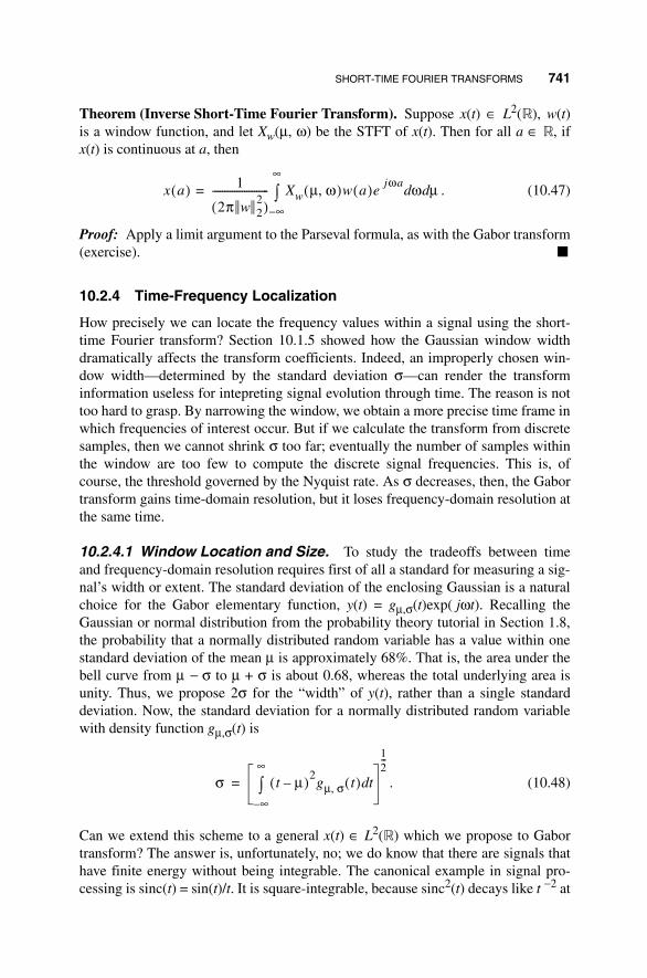
SHORT-TIME FOURIER TRANSFORMS 741
Theorem (Inverse Short-Time Fourier Transform). Suppose x(t) ∈ L2(R), w(t)is a window function, and let Xw(µ, ω) be the STFT of x(t). Then for all a ∈ R, ifx(t) is continuous at a, then
. (10.47)
Proof: Apply a limit argument to the Parseval formula, as with the Gabor transform(exercise).
10.2.4 Time-Frequency Localization
How precisely we can locate the frequency values within a signal using the short-time Fourier transform? Section 10.1.5 showed how the Gaussian window widthdramatically affects the transform coefficients. Indeed, an improperly chosen win-dow width—determined by the standard deviation σ—can render the transforminformation useless for intepreting signal evolution through time. The reason is nottoo hard to grasp. By narrowing the window, we obtain a more precise time frame inwhich frequencies of interest occur. But if we calculate the transform from discretesamples, then we cannot shrink σ too far; eventually the number of samples withinthe window are too few to compute the discrete signal frequencies. This is, ofcourse, the threshold governed by the Nyquist rate. As σ decreases, then, the Gabortransform gains time-domain resolution, but it loses frequency-domain resolution atthe same time.
10.2.4.1 Window Location and Size. To study the tradeoffs between timeand frequency-domain resolution requires first of all a standard for measuring a sig-nal’s width or extent. The standard deviation of the enclosing Gaussian is a naturalchoice for the Gabor elementary function, y(t) = gµ,σ(t)exp( jωt). Recalling theGaussian or normal distribution from the probability theory tutorial in Section 1.8,the probability that a normally distributed random variable has a value within onestandard deviation of the mean µ is approximately 68%. That is, the area under thebell curve from µ − σ to µ + σ is about 0.68, whereas the total underlying area isunity. Thus, we propose 2σ for the “width” of y(t), rather than a single standarddeviation. Now, the standard deviation for a normally distributed random variablewith density function gµ,σ(t) is
. (10.48)
Can we extend this scheme to a general x(t) ∈ L2(R) which we propose to Gabortransform? The answer is, unfortunately, no; we do know that there are signals thathave finite energy without being integrable. The canonical example in signal pro-cessing is sinc(t) = sin(t)/t. It is square-integrable, because sinc2(t) decays like t −2 at
x a( ) 1
2π w 22( )
----------------------- Xw µ ω,( )w a( )ejωa ωd µd
∞–
∞
∫=
σ t µ–( )2gµ σ, t( ) td
∞–
∞
∫
12---
=

742 TIME-FREQUENCY SIGNAL TRANSFORMS
infinity. However, sinc(t) ∉ L1(R), because, for instance, its Fourier transform is asquare pulse, which is not continuous. Another problem is that the second momentintegral (10.48) must also be valid. The following definition accounts for both diffi-culties, but we need a preliminary lemma.
Lemma. If x(t) is a window function, then t1/2x(t) ∈ L2(R).
Proof: This turns out to be a consequence—through the Schwarz inequality—ofthe square integrability of x(t) and tx(t). We leave this as an exercise.
Definition (Center and Radius). If x(t) is a window function, then the center Cxand the radius ρx for x(t) are given by
(10.49a)
and
, (10.49b)
respectively. The diameter or width of a windowing function x(t) is ∆x = 2ρx.
Remark. The lemma assures us that the integral (10.49a) exists.The more highly concentrated a signal x(t) is about its center Cx, the smaller is its
radius ρx. Let us consider a few examples of window functions before stating someof their basic properties.
Examples (Window Functions). Any Gaussian, g(t) = Aexp(−Bt2) is a windowfunction as we already showed. All of the standard window functions of Table 10.2are also window functions. The B-spline functions βn(t) are also window functions,and, for n ≥ 1, Βn(ω) is a window function.
Now let us work out a few basic properties of window center and radius.
Lemma (Window Translation and Modulation). Suppose x(t) is a window func-tion and y(t) = x(t + t0). Then:
(a) Cy = Cx − t0.
(b) If X = F x and Y = Fy are the Fourier transforms of x and y, respectively, andX and Y are window functions, then CX = CY.
(c) ρy = ρx.
(d) If y(t) = exp(−jCXt)x(t + Cx) and X = Fx and Y = Fy are window functions,then Cy = CY = 0 and ρy = ρx.
Cx1
x 22
--------- t x t( ) 2td
∞–
∞
∫=
ρx1
x 22
--------- t Cx–( )2x t( ) 2
td∞–
∞
∫
12---
=

SHORT-TIME FOURIER TRANSFORMS 743
Proof: By the Shifting and Modulation Properties of the Fourier transform(exercises).
Lemma (Radius of Derivative). Suppose x(t) ∈ L2(R) and is differentiable. Ifx′(t) ∉ L2(R), then ρX = ∞.
Proof: Use Parseval’s theorem for the radial Fourier transform and the formula forF [x′(t)](ω). (exercise).
10.2.4.2 Uncertainty Principle. The next theorem is the classic HeisenbergUncertainty Principle4 for the Fourier transform [20, 21]. The theorem says as a sig-nal becomes more concentrated about its time-domain center, it becomes more dis-persed about its frequency domain center. Recent tutorials on the UncertaintyPrinciple include [22, 23].
Theorem (Heisenberg Uncertainty). Suppose x(t) ∈ L2(R), X(ω) = F [x](ω) is theradial Fourier transform of x(t). Then .
Proof: We prove the Uncertainty Principle in two steps:
• First, for the happy circumstance that x(t) obeys a special limit condition atinfinity:
; (10.50)
this condition does not necessarily hold for a square-integrable signal, ofcourse; we could have x(t) > ε > 0 on some set S of measure zero, for example.
• Then, for the general case by writing x(t) as a limit of such continuous, piece-wise smooth signals.
Note that we may assume that x(t) is a window function; otherwise, ρx = ∞, so thatρxρX ≥ 1/2. We assume X(ω) is a window function as well, since otherwise ρX = ∞with the same consequence. In either exceptional case, we are done. The WindowTranslation and Modulation Lemma allows the further simplifying assumption thatCx = CX = 0. Therefore,
(10.51)
4Werner Heisenberg (1901−1976) discovered that the probable location of a particle trades off against itsprobable momentum. In 1927, Heisenberg showed that ∆p∆x ≥ 2h, where ∆p represents the width of aparticle’s momentum distribution, ∆x is the width of its position distribution, and h is Planck’s constant[W. Heisenberg, Physical Properties of the Quantum Theory, New York: Dover, 1949].
ρxρX12---≥
tt ∞→lim x t( ) 0=
ρx2ρFx
2 1
x 22
--------- t2
x t( ) 2td
∞–
∞
∫1
X 22
---------- ω2X ω( ) 2 ωd
∞–
∞
∫
1
X 22
x 22
--------------------- tx t( ) 2td
∞–
∞
∫ ωX ω( ) 2 ωd∞–
∞
∫ .=
=

744 TIME-FREQUENCY SIGNAL TRANSFORMS
Using Plancherel’s theorem and the radial Fourier transform derivative formulagives
(10.52)
That is,
. (10.53)
Invoking the Schwarz inequality, , on (10.53) gives
(10.54)
and, continuing our algebraic duties, we find that
(10.55)
Now, we claim the following:
. (10.56)
The trick behind the strange looking (10.56) is integration by parts on the innerproduct integral:
(10.57)
Note that we have invoked (10.50) to conclude that t|x(t)|2 → 0 as |t| → ∞. Separat-ing the bottom of (10.57) into two integrals gives
. (10.58)
ρx2ρFx
2 x 24–
2π------------ tx t( ) 2
td∞–
∞
∫ F x′ t( )[ ] ω( ) 2 ωd∞–
∞
∫
x 24–
2π------------ tx t( ) 2
2F x′ t( )[ ] ω( ) 2
2.=
=
x 24ρx
2ρFx2 1
2π------ tx t( ) 2
2x′ t( ) 2
22π tx t( ) 2
2x′ t( ) 2
2==
x 2 y 2 xy 1≥
x 24ρx
2ρFx2
tx t( )x′ t( )≥ 12
tx t( ) x′ t( ) td∞–
∞
∫2
= tx t( ) x′ t( ) td∞–
∞
∫2
=
x 24ρx
2ρFx2
tx t( )x′ t( ) td∞–
∞
∫2
x′ t( ) tx t( ),⟨ ⟩ 2Re x′ t( ) tx t( ),⟨ ⟩( )2≥( ).=≥
Re x′ t( ) tx t( ),⟨ ⟩( ) 12---– x t( ) 2
t 12--- x t( ) 2
–=d∞–
∞
∫=
tx t( )x′ t( ) t tx t( )x t( ) ∞–
∞x t( ) tx′ t( ) x t( )+[ ] t
0 x t( ) tx′ t( ) x t( )+[ ] t.d∞–
∞
∫–=
d∞–
∞
∫–=d∞–
∞
∫
tx t( )x′ t( ) t x t( ) 2t tx t( )x′ t( ) td
∞–
∞
∫–d∞–
∞
∫–=d∞–
∞
∫

SHORT-TIME FOURIER TRANSFORMS 745
After rearrangment, the claim (10.56) easily follows. We insert the result into theinequality (10.55), thereby finding
(10.59)
and hence .
Let us proceed to the second step in the proof: removing the limit assumption(10.50) on the finite energy signal x(t). We write x(t) as the limit of a sequence ofsignals in the Schwarz space S of infinitely continuously differentiable, rapidlydecreasing signals [21]:
. (10.60)
We introduced the Schwarz space in Chapter 3 and know it to be dense in bothL2(R) and L1(R). Since for all x ∈ S, we have t|x(t)|2 → 0 as |t| → ∞, we have
(10.61)
Because xn ∈ S, which decreases faster than any polynomial, the integrands in(10.61) are absolutely integrable and we may interchange the integration and limitoperations. Schwarz space elements are also continuous, so the first limit on theright-hand side of (10.61) is still zero. Thus,
. (10.62)
But these limits are precisely (10.57).
The above proof follows Weyl’s derivation [24], which he published in 1931.5
Thus, every windowed Fourier transform has a lower limit on its joint time-frequency resolution. If we work with a transform based on a window function w(t)whose Fourier transform W(ω) is also a window function, then it makes sense todefine the time-frequency resolution as the product ρwρW. If we use a standard win-dow function—a Hamming window, for example—whose Fourier transform is notitself a window function, then ρW is infinite. The Uncertainty Principle tells us thatthis is a hard lower bound: ρwρW ≥ 1/2. As a practical consequence, smaller time-domain window sizes result in proportionally large frequency- domain window
5The interests of Hilbert’s student, Hermann Weyl (1885−1955), ranged from quantum mechanics tonumber theory. He showed, for instance, that given an irrational number r, the fractional parts of r, 2r, 3r, ...,etc., lie uniformly distributed on the interval (0, 1).
x 24ρx
2ρFx2 x 2
4
4---------≥
ρxρX12---≥
x t( ) xnn ∞→lim t( )=
txn t( )xn′ t( ) t tn ∞→lim xn t( )xn t( )
∞–
∞xn t( ) txn′ t( ) xn t( )+[ ] td
∞–
∞
∫n ∞→lim–=d
∞–
∞
∫n ∞→lim .
tn ∞→lim xn t( )xn′ t( ) t x
n ∞→lim t( ) txn′ t( ) xn t( )+[ ] td
∞–
∞
∫–=d∞–
∞
∫

746 TIME-FREQUENCY SIGNAL TRANSFORMS
sizes. As we attempt to better locate a signal oscillation, we suffer a correspondingloss of accuracy in estimating the precise frequency of the oscillation.
There are window functions that achieve the lower bound on time-frequencylocalization given by the Heisenberg Uncertainty Principle. The next section showsthat the optimally localizing window is none other than the Gaussian.
10.2.4.3 Optimally Localized Signals. The Gabor transform is the short-time Fourier transform with the smallest time-frequency resolution. We identifytime-frequency resolution with the joint product of the time-domain and frequency-domain radius: . To derive this optimality claim, we review the UncertaintyPrinciple’s proof. Our scrutiny shows that inequality arises with its use of theSchwarz inequality [21].
Corollary (Optimal Time-Frequency Locality). We have if and only
if for some a ∈ C and b ≥ 0.
Proof: We recall that always, and equality occurs if and only ifx = cy for some constant c ∈ C. In the context of the proof, then, optimally smalltime-frequency locality coincides with the condition . Are there anyL2(R) signals satisfying the above differential equation? It is a basic first-order dif-ferential equation, but before we note the solution, let us address two problems:
• Since the Uncertainty Principle deals with square-integrable signals x(t), weunderstand this equality as occurring almost everywhere; that is, we require
except on some set of measure zero.
• Furthermore, the proof depends on the fact that we can represent a generalx(t) ∈ L2(R) as the limit of a sequence , where xn(t) ∈ S, the
Schwarz space of infinitely continuously differentiable, rapidly decreasing sig-nals. We must therefore show that for any x(t) satisfying the differential equation,which is an L2(R) limit of xn(t) ∈ S, that
. (10.63)
In the convenient Schwarz space, the second point is straightforward. Indeed, werecall that in Lebesgue integration theory means
(10.64)
almost everywhere. We have , and the xn(t) ∈ Sare infinitely continuously differentiable; thus,
. (10.65)
ρxρX
ρxρX12---=
x t( ) ae bt2
–=
x 2 y 2 xy 1≥
x′ t( ) ctx t( )=
x′ t( ) ctx t( )=
x t( ) xnn ∞→lim t( )=
x′ t( ) xnn ∞→lim ′ t( )=
x t( ) y′ t( )=
y t( ) x s( ) s y 0( )+d0
t
∫=
x t( ) x 0( )– xn t( ) xn 0( )–[ ]n ∞→lim=
x t( ) x 0( )– xn′ s( ) sd0
t
∫n ∞→lim x′ s( ) sd
0
t
∫= =

DISCRETIZATION 747
To solve the differential equation, note that , whereby
. (10.66)
If we let b = |c|2, then the solutions to this second-order differential equation are
of the form , where a ∈ C is a constant.
Example (STFT based on a B-Spline Window). Suppose we use a B-spline func-tion β(t) = βn(t), where n ≥ 1, to define a short-time Fourier transform. We knowthat ωΒn(ω) ∈ L2(R), so that Βn(ω) is indeed a window function. The UncertaintyPrinciple applies. The Gaussian is not a B-spline, however, and we know thereforethat ρβρB > 1/2.
10.3 DISCRETIZATION
The short-time Fourier transform can also be discretized. There are two possibleapproaches:
• To compose discrete sums from values of a discrete signal x(n), which is cov-ered in Section 10.3.1.
• To sample the ordinary analog STFT analysis equation of an analog signalxa(t)—the far more interesting and challenging problem—introduced inSection 10.3.2 and further explored in the sequel.
The second approach is our main emphasis. Its successful development leads to anew structural decomposition of finite- energy analog signals. It was also a focus ofGabor’s original paper 1, a preoccupation of a number of later signal analysts, andthe wellspring of much of our later insight into the nature of mixed-domain signalinterpretation. We shall in fact pursue this idea for the remainder of this chapter.
10.3.1 Transforming Discrete Signals
Working with discrete signals, we can forumulate a purely discrete theory of win-dowed Fourier transforms. The results are not difficult to develop, and it turns outthat they follow directly from discrete Fourier theorems. We are thus content toexplicate only the discrete STFT synthesis and energy conservation equations.
We begin with a discrete signal x(n) having period N > 0, x(n) = x(n + N). Alter-natively, we may select N samples s(n): 0 ≤ n < N from an arbitrary discrete signals(n) and consider the periodic extension x(n) = s(n mod N). We require the discrete win-dow function to be nonzero and have the same period as the signal to be transformed.
Definition (Discrete Short-Time Fourier Transform). Let x(n) and w(n) be dis-crete signals of period N > 0. Further suppose w(n) is real and not identically zero
t1–x′ t( ) cx t( )=
t1–x′ t( ) ′ cx t( ) ′ cx′ t( ) cctx t( ) c
2tx t( )====
x t( ) ae bt2
–=

748 TIME-FREQUENCY SIGNAL TRANSFORMS
on [0, N − 1]. Then the discrete short-time Fourier transform (or discrete windowedfourier transform) of x(n) with respect to w(n) is
. (10.67)
The signal w(n) is called the windowing function for the transform.
Definition (Discrete Gabor Elementary Function). Let w(n) be a discrete signalof period N > 0, with w(n) is not identically zero on [0, N − 1]. Then the discrete Gaborelementary function or discrete Gabor atom of discrete frequency k ∈ [0, N− 1]and location m ∈ [0, N − 1] is wm,k(n) = w(n − m)exp(2πjkn/N).
As with its analog world counterpart, the discrete STFT can be viewed in severalways. In particular, we may think of (10.67) as giving
• For each m ∈ [0, N − 1], the discrete Fourier transform (DFT) of x(n)w(n − m);
• For each k ∈ [0, N − 1], the inner product on [0, N − 1] of x(n) with the discreteGEF wm,k(n).
The following theorem gives the synthesis equation for the discrete STFT.
Theorem (Inverse Discrete STFT). Let x(n) and be a discrete signal with period N >0; let Xw(m, k) be its discrete STFT with respect to the windowing function w(n); and,finally, let ||w||2 be the l2-norm of w(n) restricted to the interval [0, N − 1]: ||w||2 =[w2(0) + w2(1) + · · · + w2(N − 1)]1/2. Then,
. (10.68)
Proof: Substituting the definition of Xw(m, k) into the double summation on theright-hand side of (10.68) gives
. (10.69)
Rearrangment of the sums produces
. (10.70)
Xw m k,( ) x n( )w n m–( )e2πjk n
N----–
n 0=
N 1–
∑=
x n( ) 1
N w 22
--------------- Xw m k,( )w n m–( )e2πjk n
N----
k 0=
N 1–
∑m 0=
N 1–
∑=
x p( )w p m–( )e2– πjk p
N----
p 0=
N 1–
∑ w n m–( )e2πjk n
N----
k 0=
N 1–
∑m 0=
N 1–
∑
x p( ) w p m–( )w n m–( ) e2πjk n p–( )
N----------------
k 0=
N 1–
∑m 0=
N 1–
∑p 0=
N 1–
∑

DISCRETIZATION 749
Reciting what has become a familiar and fun argument, we note that the final sum inis zero unless n = p, in which case it is N. Therefore the entire triple summation issimply
, (10.71)
and the theorem follows.
Theorem (Discrete STFT Parseval’s). Let x(n) and be a discrete signal withperiod N > 0; let Xw(m, k) be its discrete STFT with respect to the windowingfunction w(n); and, finally, let ||w||2 be as in the previous theorem. Then,
. (10.72)
Proof: Let us expand the double summation on the right-hand side of (10.72):
. (10.73)
Interchanging the sums we find that (10.73) becomes
. (10.74)
The final bracketed sum is either N or 0, depending on whether p = q or not, respec-tively. Since only the case p = q contributes to the sum, we let n = p = q and reducethe double summation on the left-hand side of (10.74) to a single sum over n:
. (10.75)
Finally we see
, (10.76)
using the periodicity of w(n).
10.3.2 Sampling the Short-Time Fourier Transform
Now let us turn to the deeper question of what happens we attempt to sample theSTFT. We select a time-domain sampling interval T > 0 and a frequency-domain
Nx n( ) w n m–( )w n m–( )m 0=
N 1–
∑ Nx n( ) w 22
=
x n( ) 2
n 0=
N 1–
∑ 1
N w 22
--------------- Xw m k,( ) 2
k 0=
N 1–
∑m 0=
N 1–
∑=
x p( )w p m–( )e2πjk
pN----–
p 0=
N 1–
∑ x q( )w q m–( )e2πjk
qN----
q 0=
N 1–
∑k 0=
N 1–
∑m 0=
N 1–
∑
x p( )x q( ) w p m–( )w q m–( )m 0=
N 1–
∑ e2πjk q p–( )
N----------------
k 0=
N 1–
∑q 0=
N 1–
∑p 0=
N 1–
∑
N x n( )x n( ) w n m–( )w n m–( )m 0=
N 1–
∑n 0=
N 1–
∑
N w 22
x n( )x n( )n 0=
N 1–
∑ Xw m k,( ) 2
k 0=
N 1–
∑m 0=
N 1–
∑=

750 TIME-FREQUENCY SIGNAL TRANSFORMS
sampling interval Ω > 0. These remain fixed for the discrete transform, and acomplex-valued function on pairs of integers results. It might appear that ourendeavors here will not differ radically in method and results from the work we didearlier in discretizing the Fourier transform. Quite the opposite turns out to be thecase: Discretization of the windowed Fourier transform opens the door to a wealthof intriguing problems in signal analysis.
For one thing, discretizing the transform provides us with a ready breakdown of thesignal into time localized frequency components, or time-frequency atoms. Eachatom represents a spot in time. Each atom represents a possible frequency component.And—depending on the nature of our atomic signal building blocks—there is a wayto measure the quantity of that frequency resident in the signal in the vicinity a discretetime instant. This is a structural decomposition of the signal. Chapters 4 and 9explored time- and frequency- domain signal analysis, respectively. Among their les-sons is the usefulness of a structural decomposition of the signal for purposes of clas-sification, recognition, and interpretation. Time-frequency transforms benefit signalanalysis by providing an elegant, formal mathematical theory as well as a relationaldescription of the signal.
Discretization places Gabor’s original problem on the agenda [1]. He proposedto model communication signals using families of discretely indexed signal ele-ments, which he called logons, but which nowadays are known by various othermonikers—Gabor elementary functions, Gabor atoms, windowed Fourier atoms,and so on. Can families of the form exp(2πjnt)g(t − m): m, n ∈ Z provide anorthonormal basis for L2(R) signals? Their optimal joint time-frequency localiza-tion does recommend them, but neither Gabor nor any other signal analyst fordecades after his suggestive 1946 paper could substantiate in theory what seemed sotantalizing for practice.
It was a negative answer to Gabor’s insightful proposal that began to emerge inthe 1980s, a decade marking a watershed of results in time-frequency and time-scale signal analysis. The rest of the chapter elaborates some of these apparentlydiscouraging results for short-time Fourier methods. The next chapter suggests analternative approach, motivated in part our understanding of the limitations inherentin atomic time-frequency signal decompositions. Chapter 11 does show that trans-formations that rely on signal scale instead—the wavelet transform in particular—may avoid the weaknesses of short-time Fourier techniques.
Definition (Discretized Short-Time Fourier Transform). Suppose that Xw(µ, ω)is the STFT of x(t) ∈ L2(R) with respect to the window function w(t). Given T > 0and Ω > 0, the discretized short-time Fourier transform is
. (10.77)
If distinguishing between the discrete and analog transform signals becomes a prob-lem, then we can append a subscript a to the analog form, as in (10.77). Note that
Xw m n,( ) Xw( )a
mΩ nT,( )= x t( )w t mT–( )ejnΩt–
td∞–
∞
∫=

DISCRETIZATION 751
we are using the first discrete independent variable of Xw(m, n) as the time indexand are using the second variable as the frequency index.
10.3.3 Extracting Signal Structure
If we can find a sufficiently strong mathematical representation, then discretizedshort-time Fourier transforms provide an attractive means of describing signal struc-ture. We have already covered the broad qualifications for such a represenation. Itmust be able to represent any candidate signal, for otherwise some inputs will avoidour decomposition method. The representation must also be stable, which, informally,means that changing the signal a little bit only perturbs the representation a little bit.
So, the question is, Can windowed Fourier atoms of the form
, (10.78)
where T > 0 and TΩ = 2π, serve as a complete signal representation? The two prac-tical alternatives are that the family wm,n(t): m, n ∈ Z constitutes either
• An orthonormal basis or
• A frame.
It is hoped that we can discover wm,n(t): m, n ∈ Z that make up an orthonormalbasis. Then every square-integrable signal x(t) has a expansion in terms of Fouriercoefficients, easily calcuated as the inner products of x(t) with the wm,n(t):
(10.79)
If we fail to find such a basis, then computing the expansion coefficients (10.79)becomes problematic. Lack of a basis encumbers our signal analysis too. While wemight be able to decompose a candidate signal x(t) into a linear combination ofatoms, x(t) = Σcm,nwm,n(t), we do not necessarily know the uniqueness of the expan-sion coefficients cm,n for representing x(t). So the utility of the expansion coeffi-cients as indicators of some signal component’s presence or the lack thereof is verymuch compromised.
Should a basis not be available, we could search for a frame representation ofL2(R) signals using the Gabor atoms (10.118). After all, we know from Chapter 3that frame coefficients can characterize the source signal x(t), and they supportnumerically stable reconstructions. This may be a good redoubt.
10.3.3.1 Discrete Time-Frequency Plane. Toward building a structural inter-pretation of a signal, we can place the expansion coefficients cm,n into an array. Thus,for a fixed frequency nΩ, the rows of the array, cm,n: m ∈ Z, indicate the relativeweight of frequency nΩ inside signal x(t) at all time instants mT. Similarly, the columnsrecord the frequencies at a given time instant. Refer to Figure 10.9.
wm n, t( ) ejnΩt
w t mT–( )=
x t( ) x t( ) wm n, t( ),⟨ ⟩wm n, t( ).m n Z∈,
∑=

752 TIME-FREQUENCY SIGNAL TRANSFORMS
Notice that upon discretizing the STFT we have a mathmatical signal transform thatresolves a signal into finite regions of the time-frequency plane. The Fourier series ofChapter 5, in contrast, can only furnish time-frequency regions of infinite time- domainextent. When we covered discrete Fourier theory in Chapter 7, we studied the samplingtheorem by which a band-limited analog signal can be reconstructed from sufficientlydense discrete samples. The sampling theorem too implies a partition of the time-frequency plane, except that its regions have an infinite frequency-domain extent. TheSTFT therefore marks a theoretical advance within our signal analytic understanding.
As a relational structure, this partition of the time-frequency plane is quite sim-ple. Each region has the same size as its neighbors. We can, however, adjust the sizeof the regions to be smaller or larger in time or frequency by dilating our windowingfunction. The Uncertainty Principle imposes the constraint that the area of the STFTregions be no smaller than that given by the Gabor transform. Signal analysis appli-cations based on STFT methods generally search the corresponding time-frequencymesh in order to understand signal content.
Let us consider some examples of how the time-frequency decomposition struc-ture presents itself in applications.
Figure 10.10 illustrates a time-frequency mesh that contains a linear chirp andwhat is apparently a tone. Chirp signal energy concentration is fairly constant and can
T 2T 3T
Ω
2Ω
t
w
Fig. 10.9. Discretized STFT coefficients arranged in a rectangular grid.

DISCRETIZATION 753
be tracked as a rising line over time. Tone signal energy concentration remains at afixed frequency. Clicks or pops are characterized by a narrow time-domain extent andan extended, more or less uniform distribution of signal energy over a wide range offrequencies—a vertical linear structure. A sinusoidal tone is a horizontal linear struc-ture. These ideas are only schematic, but they convey some of the signal varieties thatare amenable to time-frequency analysis.
Let us now consider a speech analysis application. We have considered speechsignal interpretation already in Chapters 4 and 9. In fact, in Chapter 9 we saw thatmany speech recognition systems have been developed using the basic technique ofwindowing the Fourier transform. If x(t) is a speech signal, for example, then look-ing for a large percentage of signal energy in a pair of frequencies might indicate thepresence of a vowel phoneme. Or, a broad dispersion of signal energy in a range ofhigh frequencies could mark a velar fricative. Time-frequency signal decompositionoffers a complete picture of the speech waveform. Figure 10.11 shows a contourdiagram of the energies in a speech fragment.
ω
µ
Fig. 10.10. Schematic representation of a signal with two components: a linear chirp and anisolated tone.
Fig. 10.11. The time-frequency decomposition of the word “Gabor.” Lines indicate signalenergy contours. Note that the two syllables can be segmented in time according to the dis-tribution of signal energy along the frequency axis.

754 TIME-FREQUENCY SIGNAL TRANSFORMS
10.3.3.2 Identifying Significant Local Frequency Components. Manyof the filtering, enhancement, and thresholding techniques we applied in time-domain signal analysis can help us find localized signal frequency components. Forinstance, we might use a threshold to indicate a significant frequency component.Furthermore, we might calculate the total amount of energy among all time-frequency cells at a certain time instant and count the number that contain say amajority of the energy. Such quantities can be assembled into feature vectors, forexample. All of the methods we employed in Chapter 4 for thresholding signalsapply equally well to thresholding values in the two-dimensional time-frequencyplane. Indeed, this is an elementary instance of image analysis, and with it, ourwork in interpreting signal content begins to take advantage of techniques in imageprocessing and computer vision.
10.3.4 A Fundamental Limitation
We have observed that the windowed Fourier transform provides an elegant and nat-ural description of signal structure—a two-dimensional array, easily searched alongtime or frequency axes. With other decomposition techniques, especially thoserevolving around signal scale, structures may assume the form of a tree or some moregeneral graph. Traversing graph structures consumes computer time. So even thoughour derived structures may be far simpler than the time-domain signal, we are stillconcerned to make the graphs sparse and conclude our exhaustive search as quicklyas possible. Hence the problem before us is, How large can we choose the time andfrequency sampling intervals, T and Ω, so that we still build a family of windowedFourier atoms that provide an orthonormal basis or exact frame structure?
10.3.4.1 Nyquist Density. Our question directly concerns the power of short-time Fourier transforms for signal interpretation. Gabor studied the case TΩ = 2π,suggesting that the Fourier expansion coefficients could be used to encode a signalfor efficient transmission. Note too that for this case the time-domain samplinginterval is T = 2π/Ω . If a signal x(t) has bandwidth Ω , then its highest frequencycomponent is Ω/2 radians per second, or Fmax = (Ω/2)/(2π) = Ω /(4π) hertz. By theShannon–Nyquist sampling theorem, it can be reconstructed from discrete samplestaken at intervals sampled at a rate not less than F = T −1 = 2Fmax = Ω/(2π) hertz.We offer the formal definition.
Definition (Time-Frequency, Nyquist Densities). Let x(t) have bandwidth Ωand be sampled at intervals T > 0. Then we define its time-frequency density tobe (TΩ)−1. The Nyquist density is (2π)−1.
In other words, Gabor’s concern was to set the time- and frequency-domainsampling intervals so that TΩ = 2π—that is, to sample at the Nyquist density. Thisis equivalent to time sampling at the largest interval allowable, by the samplingtheorem, for analog signal reconstruction from discrete samples. Gabor proposedfamilies of windowed Fourier atoms, separated from one another at the Nyquist

DISCRETIZATION 755
limit T = 2πΩ−1. Our problem is to characterize Gabor’s proposal for each of thethree cases:
(i) TΩ < 2π, when the sampling interval is less than the Nyquist frequency or,equivalently, when the time-frequency density exceeds the Nyquist density.
(ii) TΩ = 2π, the original proposal of Gabor.
(iii) TΩ > 2π.
10.3.4.2 Too Sparse: TΩ > 2π. Gabor’s proposal to represent signals usingsums of windowed Fourier atoms does not in fact succeed for the sparse case, TΩ >2π. This case occurs when the time- domain sampling interval exceeds the maximumallowable for reconstructing an analog signal of bandwidth Ω by its discrete samplesat times mT, m ∈ Z. That is, families of Gabor atoms wm,n(t) = exp( jnΩ)w(t − mT):m, n ∈ Z cannot be a frame when (TΩ)−1 is less than the Nyquist density.
Using the Zak transform, introduced in Chapter 8, this result can be shown forthe case where (2π)−1TΩ is rational and exceeds unity. We will only consider a farsimpler case: Ω = 2π and T = 2. We recount the following results from Ref. 12.
Lemma. Let w(t) ∈ L2(R); wm,n(t) = ejnΩtw(t − mT), for m, n ∈ Z; Ω = 2π; and T = 2.Then there is an x(t) ∈ L2(R) such that ||x||2 ≠ 0 and ⟨x(t), wm,n(t)⟩ = 0 for all m, n ∈ Z.
Proof: Let t ∈ [0, 1) and define
, (10.80)
where k ∈ Z. It is easily shown (exercise) that
(i) x ∈ L2(R).
(ii) ||x||2 = ||w||2.
(iii) ||x||2 ≠ 0.
We contend that ⟨x(t), wm,n(t)⟩.= 0 for all m, n ∈ Z. Breaking up the inner productintegral reveals
(10.81)
But inserting (10.80), we observe that
. (10.82)
x t k+( ) 1–( )kw t k– 1–( )=
x t( ) wm n, t( ),⟨ ⟩ x t( )ejnΩt
w t 2m–( ) t
ej– nΩt
x t k+( )w k t 2m–+( ) tdk ∞–=
∞
∑0
1
∫=
d∞–
∞
∫=
x t k+( )w k t 2m–+( ) 1–( )kw t k– 1–( )w t k 2m–+( )
k ∞–=
∞
∑=k ∞–=
∞
∑

756 TIME-FREQUENCY SIGNAL TRANSFORMS
On the right-hand side of (10.82) consider a summand,
, (10.83a)
for some k ∈ Z. Let i = 2m − k − 1 and compare the term
. (10.83b)
The trick is that
, (10.84)
which is the additive inverse of (10.83a). The upshot is that every summand in is com-plemented by its additive inverse also inside the summation; the sum is preciselyzero! All inner products (10.81) are zero, and we have constructed a nontrivial x(t) inthe orthogonal complement of wm,n(t): m, n ∈ Z.
Now we can prove the theorem. Recall that a frame generalizes the notion of anorthogonal basis, yet provides stable signal reconstruction and complete signal rep-resentation. We introduced frame theory in Section 3.3.4.
Theorem. Let w(t) ∈ L2(R); wm,n(t) = e jnΩtw(t − mT), for m, n ∈ Z; Ω = 2π; andT = 2. Then wm,n(t): m, n ∈ Z cannot be a frame.
Proof: Let x(t) be given by the lemma: nontrivial and orthogonal to all of thewm,n(t). If the wm,n(t): m, n ∈ Z were a frame, then by the definition of frame,there exist A > 0 and B > 0 such that
(10.85)
for all y(t) ∈ L2(R). The frame condition must hold for the lemma’s x(t) as well, butsince ⟨x(t), wm,n(t)⟩ = 0 for all m, n ∈ Z , we have a contradiction.
Remark. So there are no frames of windowed Fourier atoms, wm,n(t) = ejnΩtw(t − mT),when the frequency- and time-domain sampling intervals are Ω = 2π; and T = 2,respectively. This is perhaps not too surprising a result, given the Shannon–Nyquistsampling theorem.
We have shown our result for only a particular instance, Ω = 2π and T = 2, of thecase TΩ > 2π. An interesting, but somewhat technical, Zak transform applicationextends this same argument whenever TΩ > 2π and TΩ is a rational multiple of 2π[25]. Using advanced mathematical methods well beyond our present scope, it hasbeen shown that whenever the time-frequency sampling is too sparse—whethereither T and Ω are rational or irrational—then there are no frames of windowedFourier atoms [26].
1–( )kw t k– 1–( )w t k 2m–+( )
1–( )iw t i– m–( )w t i 2m–+( )
1–( )iw t i– m–( )w t i 2m–+( ) 1–( ) k– 1–
w t 2m– k+( )w t k– 1–( )=
A y2
y wn,⟨ ⟩ 2
m n, ∞–=
∞
∑ B y≤ ≤

DISCRETIZATION 757
10.3.5 Frames of Windowed Fourier Atoms
Now let us consider another possibility: TΩ < 2π. This is the dense time-frequencysampling case. Now, from a classic construction [27], it can be shown that we canbuild frames from windowed Fourier atoms when TΩ < 2π. Here, we adapt the pre-sentation in Ref. 12 to our own notation and show that collections of Gabor atomswm,n(t) = exp( jnΩ)w(t − mT): m, n ∈ Z can be a frame when (TΩ)−1 exceeds theNyquist density, (2π)−1.
Theorem. Let w(t) ∈ L2(R); let wm,n(t) = e jnΩtw(t − mT), for m, n ∈ Z; TΩ < 2π;and suppose that [−π/Ω, π/Ω] ⊃ Support(w). Then for any x(t) ∈ L2(R),
. (10.86)
Proof: Let us expand the sum on the left-hand side of (10.86) as sums over 2π/Ω-wide intervals:
(10.87)
Notice that the integral in (10.87) is a constant multiple of a Fourier series coefficient.The functions are an orthonormal basis for the Hilbert space
H = L2[0, 2π/Ω], and we know therefore that for any square-
integrable y(t) in H. (This is in fact a Parseval result for H, and its roots extend backto our very early algebraic result from abstract Banach spaces—Bessel’s inequal-ity.) Thus, for each m ∈ Z we are able to replace the sum over n ∈ Z in (10.87) withthe square of the L2[0, 2π/Ω] norm of the sum in the integrand:
.
(10.88)
Next, observe that for any m all of the summands over k inside the integral are zeroexcept for possibly one. This is due to the choice of support for the window functionw(t). The right-hand side of simplifies, and we see
(10.89)
x wm n,,⟨ ⟩ 2 2πΩ------ x t( ) 2
w t kT–( ) 2
k ∞–=
∞
∑
td∞–
∞
∫=m n, ∞–=
∞
∑
x wm n,,⟨ ⟩ 2e
jnΩtx t 2πk
Ω---------+
w t 2πkΩ
--------- mT–+
k ∞–=
∞
∑0
2πΩ------
∫
2
dt.m n, ∞–=
∞
∑=m n, ∞–=
∞
∑
Ω2π------ejnΩt en t( )=
y 22
y en,⟨ ⟩ 2
n∑=
x wm n,,⟨ ⟩ 2 2πΩ------ x t 2πk
Ω---------+
w t 2πkΩ
--------- mT–+
k ∞–=
∞
∑2
td0
2πΩ------
∫m ∞–=
∞
∑=m n, ∞–=
∞
∑
x wm n,,⟨ ⟩ 2 2πΩ------ x t 2πk
Ω---------+
w t 2πkΩ
--------- mT–+
2t.d
0
2πΩ------
∫m k, ∞–=
∞
∑=m n, ∞–=
∞
∑

758 TIME-FREQUENCY SIGNAL TRANSFORMS
We can now reassemble the separate finite integrals to one over the entire real line:
. (10.90)
The term in parentheses inside the integral (10.90) is crucial. If we can show thatthere are constants A, B > 0 such that A bounds this term below and B bounds thisterm above, then we will have found frame bounds and shown that the windowedFourier atoms wm,n(t) = exp( jnΩ)w(t − mT): m, n ∈ Z do comprise a frame. Thefollowing corollary imposes a reasonable technical condition on the window func-tion w(t) [27], namely that the window function be continuous and positive on someinterval about t = 0.
Corollary. Let w(t) ∈ L2(R) be as in the theorem. Further suppose that w(t) is con-tinuous and that there are ε > 0 and 1 > δ > 0 such that |w(t)| > ε on I = [− δπ/Ω, δπ/Ω]. Then wm,n(t) = ejnΩtw(t − mT): m, n ∈ Z are a frame.
. (10.91)
Proof: Since
(10.92)
by the theorem, we seek positive constants α and β such that and for all t. Then we have
, (10.93)
so that A = (2πα)/Ω and B = (2πβ)/Ω constitute lower and upper frame bounds,respectively, for wm,n(t). By the assumption that w(t) exceeds ε > 0 on the propersubinterval I, we can set α = inf|w(t)|2: t ∈ I. Since α is the greatest lower boundof |w(t)|2 on I, and |w(t)| > ε on I, we know α ≥ ε > 0. The lower frame condition fol-lows easily with bound A = (2πα)/Ω. To find the upper frame bound, we note thatbecause the support of w(t) is contained within the interval [−π/Ω, π/Ω], only afinite number K of terms in the sum will be nonzero. Since w(t) iscontinuous and supported on [−π/Ω, π/Ω], we may let M be its least upper bound;that is, M = ||w||∞. We can then set β = sup : t ∈ R ≤ KM, and withB = (2πβ)/Ω we can verify the upper frame bound property.
x wm n,,⟨ ⟩ 2
m n, ∞–=
∞
∑ 2πΩ------ x t( ) 2
w t kT–( ) 2
k ∞–=
∞
∑
td∞–
∞
∫=
x wm n,,⟨ ⟩ 2 2πΩ------ x t( ) 2
w t kT–( ) 2
k ∞–=
∞
∑
td∞–
∞
∫=m n, ∞–=
∞
∑
x wm n,,⟨ ⟩ 2 2πΩ------ x t( ) 2
w t kT–( ) 2
k ∞–=
∞
∑
t,d∞–
∞
∫=m n, ∞–=
∞
∑
α Σ w t kT–( ) 2<Σ w t kT–( ) 2 β<
2παΩ
---------- x t( ) 2td
∞–
∞
∫ x wm n,,⟨ ⟩ 2 2πβΩ
---------- x t( ) 2td
∞–
∞
∫=m n, ∞–=
∞
∑≤
Σ w t kT–( ) 2
Σ w t kT–( ) 2

DISCRETIZATION 759
Remarks. Recall from our general discussion of frames in Section 3.3.4 that theframe reconstruction algorithm is more efficient when the frame is tight. We can seein the theorem that finding w(t) so that is constant does provide uswith a tight frame: A = B = 2π(ΩT)−1. In fact, it is fairly straightforward to concoctwindow functions w(t) so that this expression is constant. Moreover, the construc-tion method gives windows with compact support arbitrarily good smoothness. Werefer the reader to the literature for details [12, 25, 27].
The result of the theorem (10.86) can be used to find examples of windowedFourier frames from special window functions.
Example. Suppose w(t) = (1 + t2)−1. Then w(t) is bounded and absolutely integra-ble. If T > 0, then has an upper and lower bound. One can show(exercise) that wm,n(t) = ejnΩtw(t − mT): m, n ∈ Z are a frame if we take Ω to besufficiently small.
Example. Now let w(t) = gµ,σ(t), the Gaussian with mean µ and standard deviationσ. Again, is bounded above and below when T > 0, and we can usethe theorem’s criterion for showing that Gabor frames exist for a sufficiently smallfrequency sampling interval.
Before summarizing our results in pursuit of Gabor’s problem, let us note animportant necessary condition of windowed Fourier frames [12].
Theorem. Suppose w(t) ∈ L2(R); Ω, T > 0; and wm,n(t) = ejnΩtw(t − mT): m, n ∈Z constitute a frame with lower and upper bounds A and B, respectively. Then
. (10.94)
Proof: Exercise.
10.3.6 Status of Gabor’s Problem
We can briefly summarize the status of our search for frames of windowed Fourieratoms. There are three cases, which depend on the time- and frequency-domainsampling intervals, T and Ω, respectively. Our present understanding is as follows:
(i) When TΩ < 2π the time-frequency density is higher than the Nyquist density,and we have just constructed frames of windowed Fourier atoms in this case.
(ii) When TΩ = 2π the atom are at Nyquist density exactly; this is the alterna-tive proposed by Gabor, and our analysis of it is not yet complete.
(iii) Finally, when TΩ > 2π we have noted that windowed Fourier frames do notexist in this situation; we proved a simple instance, and the research litera-ture—portions of which rely on advanced analysis—completely covers theremaining cases.
Σ w t kT–( ) 2
Σ w t kT–( ) 2
Σ gµ σ, t kT–( ) 2
A 2πΩT-------- w 2
2B≤ ≤

760 TIME-FREQUENCY SIGNAL TRANSFORMS
We will in fact devote a considerable portion of the remainder of this chapter toGabor’s dividing line case. The applicability of the short-time Fourier transform(STFT) when time-frequency localization is of paramount importance hangs on thisquestion. This question also vexed signal processing investigators for a number ofyears; we are especially interested in fully understanding the impact of windowedFourier transform discretization when TΩ = 2π.
Before turning to this question, however, let us consider another approach totime-frequency signal decompositions.
10.4 QUADRATIC TIME-FREQUENCY TRANSFORMS
There are classes of time-frequency transforms that do not depend on a windowingfunction. Instead, the transform relation emerges out of the properties of the ana-lyzed signal. The signal x(t) enters the transform integral as a quadratic rather thanas linear term, as it does in the windowed Fourier transform. This transform familyis therefore generally known as the quadratic time-frequency transformations. Itsprincipal members are the Wigner–Ville transform (WVT) and the closely relatedambiguity function.
Now, transforming without a window function appears to be quite advantageous,since the resulting procedure eliminates the effect window selection imposes on thetransform’s behavior. The short-time Fourier transform mixes spectral properties ofthe analyzed signal x(t) together with those of the window function w(t). Blindlyperusing coefficients, we do not know whether their large magnitude results fromsignal or window properties. On the other hand, we do not often blindly processtransform coefficients. Rather, the window function is typically chosen to isolatesignal features of expected frequency content and time- domain extent; in the moretypical application then, choosing a window function may well be the best first step.
Although avoiding window effects may recommend quadratic transforms, thereare some more important considerations. We shall explore three significant proper-ties of these transforms. This transform family:
• More precisely resolves certain standard cases of time-varying frequenciesthan does the STFT;
• Enjoys special properties called marginal conditions that allow them to act asdistribution functions for a signal’s spectral content;
• Has the significant drawback that transformed signals exhibit certain artifactscalled cross-terms that hamper higher-level interpretation.
This is in fact a very rich transform family. An entire book could be written aboutthese transforms, and many treatments devote considerable space to these trans-forms [2, 6, 9]. By our brief sketch we hope that the reader will acquire a more bal-anced opinion of the windowed Fourier transforms and an interest in furtherexploring the theory and application of quadratic transforms.

QUADRATIC TIME-FREQUENCY TRANSFORMS 761
10.4.1 Spectrogram
We can base a quadratic time-frequency transform on the STFT. This is in fact justthe spectrogram, which we define as follows.
Definition (Spectrogram). Let x(t) ∈ L2(R) and let w(t) be a window function.The spectrogram with respect to w(t), written XS,w(µ, ω), is
, (10.95)
where Xw(µ, ω), is the STFT of x(t) with respect to w(t).
Thus, the spectrogram of x(t) is the squared magnitude of the STFT of x(t) withrespect to w(t). The spectrogram is thus a natural generalization of the windowedFourier methods we have been comfortable in using. However, despite the moreintuitive feel, spectrograms are far from being the most popular quadratic time-frequency transforms. For one thing, XS,w relies on a window function. But it alsohas some other undesirable traits that have motivated signal theorists to search outother transform techniques. Among these better transforms is the the classic trans-form of Wigner and Ville which we introduce next; we shall assess the merits of thespectrogram in this context.
10.4.2 Wigner–Ville Distribution
The Wigner–Ville distribution (WVD) is the oldest time-frequency transform andthe preeminent quadratic signal representation. In fact it dates to the early 1930swhen E. Wigner 6 applied it in quantum mechanics [28]. The communicationtheorist J. Ville7 introduced the transform to the signal processing community some16 years later [29].
The transform has been widely studied for signal analysis applications [30, 31]. Ithas also found use as an important tool in computer vision [32]. The WVD has somedistinct advantages over the more intuitive spectrogram. But it is not without its faults.
One difficulty in applying the WVD is the presence of so-called cross- or inter-ference terms among the transform coefficients. Indeed, many research efforts intime-frequency theory have concentrated on avoiding or ameliorating the effects ofcross-terms when using this type of tool. This problem is covered in the Section 10.4.3.
10.4.2.1 Definition and Motivation. The Wigner–Ville distribution takes theFourier transform of a product of the signal with its complex conjugate. Thus, itresembles the computation of the power spectral density.
6The Hungarian chemical engineer Eugene P. Wigner (1902–1996) immigrated to the United States toteach mathematics at Princeton University in 1930. He received the Nobel prize in 1963 for discoveriesin atomic and elementary particle research.7French communication researcher J. Ville developed the same transform as Wigner, but for the purposesof clarifying the concept of instantaneous frequency.
XS w, µ ω,( ) X µ ω,( ) 2x t( )w t µ–( )e
jωt–td
∞–
∞
∫2
==

762 TIME-FREQUENCY SIGNAL TRANSFORMS
Definition (Wigner–Ville Distribution). If x(t) ∈ L2(R) is an analog signal, thenits Wigner–Ville distribution, written XWV(µ, ω), is the radial Fourier transform ofthe product x(µ + t/2)x*(µ − t/2):
. (10.96)
x(s)
-a a
t
s-a a
2a
-2a
t
s-a a
t
s-a a
2a
-2a
t
-a a
2a
-2a
s
x(s+0xt/2) x(s-t/2)
Fig. 10.12. Illustrating the support of x(s + t/2)x*(s − t/2) in the (s, t) plane. Panel (a) showsthe support of x(s). We move to two dimensions in Panel (b), but show the support of thedegenerate function x(s + 0 × (t/2)). The support of x(s − t/2) is the parallelpiped region (c)and the product x(s + t/2)x*(s − t/2) has support mainly within the diamond (d).
XWV µ ω,( ) x µ t2---+
x µ t2---–
ejωt–
td∞–
∞
∫=

QUADRATIC TIME-FREQUENCY TRANSFORMS 763
Remark. We observe that the integral (10.96) is well-defined. It is the Fourier trans-form of x(µ + t/2)x*(µ − t/2), which must be absolutely integrable. This followsbecause both factors are in L2(R), and the Schwarz inequality ensures that ||x(µ +t/2)||2 ||x*(µ − t/2)||2 ≥ ||x(µ + t/2)x*(µ − t/2)||1. Of course, L1(R) signals have Fou-rier transforms.
No window function appears in the definition (10.96), but there is an easy way tounderstand how folding the source signal x(t) over on itself accomplishes therequired time localization. Imagining that a signal’s support lies mainly within theinterval [−a, a], the local region implied by the WVD transform is a diamond, asshown in Figure 10.12.
10.4.2.2 Properties. The properties of this transform are quite remarkable. Tobegin with, we can show that the Wigner–Ville distribution is real-valued.
Proposition (Real-Valued). Let x(t) ∈ L2(R) and XWV (µ, ω) be its WVD. ThenXWV (µ, ω) ∈ R.
Proof: We calculate the complex conjugate of (10.96) and make the change of inte-gration variable s = − t.
. (10.97)
Because X*WV(µ, ω) = XWV(µ, ω), it must be real.
Already we see that the WVD’s properties are quite unlike those of the Fouriertransform or its time-limited versions. However, the time- and frequency-domainshifting properties are familiar, as the next proposition shows. Symmetry propertiesare covered in the exercises.
Proposition (Time and Frequency Shift). Let x(t) ∈ L2(R) and XWV(µ, ω) be itsWVD. Then
(a) If s(t) = x(t − a), then SWV(µ, ω) = XWV(µ − a, ω).
(b) If y(t) = ejθtx(t), then YWV(µ, ω) = XWV(µ, ω− θ).
Proof: Exercise.
The double product of x(t) terms in the WVD integral, which is the “quadratic” fac-tor, spoils the transform’s linearity. This is easy to see for the scaling property of thelinearity. We let y(t) = ax(t), where a is a constant. Then YWV(µ, ω) = |a|2XWV(µ, ω).
XWV µ ω,( ) x µ t2---+
x µ t2---–
ejωt
t
x µ s2---–
x µ s2---+
ej– ωs
s XWV µ ω,( )=d∞
∞–
∫–=
d∞–
∞
∫=

764 TIME-FREQUENCY SIGNAL TRANSFORMS
Superposition also fails for the WVD. We use an auxiliary transform as part of theargument.
Definition (Cross Wigner–Ville Distribution). If x(t), y(t) ∈ L2(R) are analog sig-nals, then the Cross Wigner–Ville Distribution, written XWV,y(µ, ω), is the radialFourier transform of the product x(µ + t/2)y*(µ − t/2):
. (10.98)
One can easily show that XWV,y(µ, ω) is the complex conjugate of YWV,x(µ, ω).If we set s(t) = x(t) + y(t), then SWV(µ, ω) = XWV(µ, ω) + YWV(µ, ω) +2Real[XWV,y(µ, ω)].
Thus, both component properties of linearity fail for the WVD. The failure ofsuperposition is the more serious deficiency. This defect causes artifacts, calledcross-terms, in the WVD transform coefficients. The presence of cross-terms leadsto difficulties of automatic interpretation, and removing them by various alternativetransformations has been a major research goal of the last several years.
The next theorem reveals an interesting symmetry between time and frequencydomain representations for the WVD. Besides having an eerie similarity to theinverse Fourier relation, it is also useful in calculations involving the WVD.
Theorem (Frequency-Domain Representation). Let x(t) ∈ L2(R), let X(ω) be itsFourier transform, and XWV(µ, ω) be its WVD. Then
. (10.99)
Proof: The key idea is to write XWV(µ, ω) as an inner product,
, (10.100)
splitting the exponential between its two terms. We can then apply Parseval’stheorem:
(10.101)
XWV y, µ ω,( ) x µ t2---+
y µ t2---–
ejωt–
td∞–
∞
∫=
XWV µ ω,( ) 12π------ X ω θ
2---+
X ω θ2---–
ejθµ θd
∞–
∞
∫=
XWV µ ω,( ) x µ t2---+
e
jωt–2
-----------
x µ t2---–
e
jωt2
--------
,=
XWV µ ω,( ) 12π------ Fx µ t
2---+
e
jωt–2
-----------
Fx µ t2---–
e
jωt2
--------
,
12π------ 2X ω 2φ+( )e
jµ ω 2φ+( )2X ω 2– φ( )e
jµ ω 2– φ( ),⟨ ⟩ .=
=

QUADRATIC TIME-FREQUENCY TRANSFORMS 765
The final inner product in (10.101) simplifies to the integral
, (10.102)
whereupon the substitution θ = 4φ gives (10.99).
Corollary (Fourier Transform of WVD). Let x(t) ∈ L2(R), let X(ω) be its Fouriertransform, and XWV(µ, ω) be its WVD. Then, with ω fixed and viewing XWV(µ, ω)as a signal with independent time variable µ, we have
. (10.103)
Proof: Apply the theorem to the WVD term in the integral (exercise).
Table 10.3 summarizes WVD properties. Some of the table’s properties are leftas exercises.
10.4.2.3 Examples. Let us look at some WVD calculations on standard exam-ple signals. These examples are revealing, because they show how the WVDimproves upon the frequency resolving capability of the STFT.
TABLE 10.3. Wigner–Ville Distribution Propertiesa
Signal Expression WVD or Property
x(t) XWV(µ, ω)ax(t) |a|2XWV(µ, ω)x(t) + y(t) XWV(µ, ω) + YWV(µ, ω) +
2Real[XWV,y(µ, ω)]x(t − a) XWV(µ − a, ω)x(t)exp( jθt) XWV(µ, ω − θ)x(t)exp( jθt2) XWV(µ, ω − 2θµ)x(t/a), with a > 0 aXWV(µ/a, aω)
Frequency-domain representation
Fourier transform of WVD
aIn this table, x(t ) and y(t) are square-integrable.
XWV µ ω,( ) 42π------ X ω 2φ+( )X ω 2– φ( )e
4jφµ φd∞–
∞
∫=
F XWV µ ω,( )[ ] θ( ) XWV µ ω,( )ejµθ– µd
∞–
∞
∫ X ω θ2---+
X ω θ2---–
= =
Xwv µ ω,( ) 12π------ X ω θ
2---+
X ω θ2---–
ejθµ θd
∞–
∞
∫=
Xwv µ ω,( )ejµθ– µd
∞–
∞
∫ X ω θ2---+
X ω θ2---–
=

766 TIME-FREQUENCY SIGNAL TRANSFORMS
Example (Dirac). Let x(t) = δ(t − a). Then XWV(µ, ω) = δ(µ − a). To verify thisformula, we utilize the Frequency-Domain Representation Theorem. Then.
(10.104)
The interesting aspect of this example is that the WVD maps an impulse to animpulse. The time-frequency representation that the WVD provides is just as tempo-rally localized as the original time-domain signal. In the (µ, ω) plane, realm of theWVD, the signal δ(µ − a) is a Dirac knife edge, infinitely high and infinitely narrow,parallel to the ω-axis and passing through the point µ = a. This stands in stark contrastto the STFT. The windowed Fourier transformation of the same Dirac impulse x(t) =δ(t − a) is Xw(µ, ω) = w(a − µ)e− jωa, an exponential modulated by the transform win-dow w(t) situated over the point µ = a.
Example (Sinusoid). Let x(t) = e jat. Then XWV(µ, ω) = (2π)−1δ(ω − a). This canbe shown using the WVD properties (Table 10.3) or by direct computation as above.
Example (Gaussian Pulse). Now let g(t) = gα,σ(t), the Gaussian of mean α andstandard deviation σ. Then
. (10.105)
Notice in this example that the WVD of a Gaussian pulse is always positive. Theonly signals x(t) for which XWV(µ, ω) is positive are linear chirps, exp( jbt2 + jat),modulated by a Gaussian envelope Ref. [7].
Example (Square Pulse). Let s(t) = u(t + 1) − u(t − 1), the square pulse supportedon the interval [− 1, 1]. Then
. (10.106)
Thus, although the WVD is real-valued, its values can be negative.
These examples illustrate the trade offs between the windowed Fourier trans-forms and the WVD. There are still other time-frequency transforms, of course;Ref. 33 compares the frequency resolution efficiencies of several of them.
10.4.2.4 Densities and Marginals. Now we turn to an important featureof the Wigner–Ville distribution, a set of properties that distinguish it from the
XWV µ ω,( ) 12π------ e
j ω θ2---+
a–
ej ω θ
2---–
a
ejθµ θ 1
2π------ e
j µ a–( ) θ δ µ a–( ).=d∞–
∞
∫=d∞–
∞
∫=
GWV µ ω,( ) eσω( )2
–
2π3 2⁄ σ------------------e
µ α–σ
------------- 2
–
=
SWV µ ω,( ) 2s µ( )ω
-------------- 2ω 1 µ–( )( )sin=

QUADRATIC TIME-FREQUENCY TRANSFORMS 767
short-time Fourier transform, namely its density function-like character. What doesthis mean? In the case of the Fourier transform, we have been content to use frac-tions of signal energy as an indication that a frequency range is significant within asignal x(t). Thus, the energy of x(t) is Ex:
. (10.107)
We may normalize x(t) or X(ω) so that the have unit energy, or we may elect to usethe normalized radial Fourier transform and equate time and frequency-domainenergies. The exercises explore the use of the Hertz Fourier transform for quantify-ing energy distributions in both time and frequency-domains. In any case then, likea probability density function, the fraction of signal energy between ω0 and ω1 isgiven by
, (10.108)
where we have normalized so that
Now, we are interested in transform representations of signals that have both atime- and a frequency-domain independent variable. Our question is whether suchtransforms can have joint density function behavior as well. For this to be the case,we should require that the signal transform assumes non-negative values and obeycertain marginal integral conditions.
Definition (Marginals). The time-frequency transform P(µ, ω) of x(t) ∈ L2(R)obeys the marginal conditions if
, (10.109a)
, (10.109b)
, (10.109c)
where X(ω) is the radial Fourier transform of x(t).
(These conditions are somewhat imperfect, due to the scaling factor in (10.109b).We can escape the scaling by using a Hertz Fourier transform. All we really requireis that the marginal integral with respect to one variable be proportional to the signal
Ex2
x t( ) 2t x 2
2=d
∞–
∞
∫= 12π------ X ω( ) 2 ω
X 22
2π----------=d
∞–
∞
∫=
Ex2 ω0 ω1,[ ] X ω( ) 2 ωd
ω0
ω1
∫=
X ω( ) 2 ω 1.=d∞–
∞∫
P µ ω,( ) 0≥
12π------ P µ ω,( ) ωd
∞–
∞
∫ x t( ) 2=
P µ ω,( ) µd∞–
∞
∫ X ω( ) 2=

768 TIME-FREQUENCY SIGNAL TRANSFORMS
energy with respect to the other variable; see the exercises.) The idea behind thedefinition is that P(µ, ω) represents a relative amount of the signal per unit time andper unit frequency. Summing the distribution over frequency values should producea relative amount of signal per unit time. Finally, summing over time should pro-duce a signal strength per unit frequency.
The interpretation of the WVD as a kind of probability density function seems togain steam from the fact that its values are real; we have already seen from theexample of the square pulse, however, that the values can be negative. In contrast,the spectrogram, because it is a squared norm, is always non-negative. However, theWVD does satisfy marginal conditions, which the spectrogram does not.
Theorem (Marginals). Let x(t) ∈ L2(R), let X(ω) be its Fourier transform, and letXWV(µ, ω) be its WVD. Then
, (10.110a)
. (10.110b)
Proof: We can directly evaluate the integral (10.110a) as follows:
. (10.111)
Interchanging the order of integration on the right-hand side of (10.111) gives
(10.112)
We leave the second marginal as an exercise.
Thus, we have shown that the WVD obeys a marginal condition akin to that of ajoint probability density function. It is possible to show that employing a Hertz for-mulation of the WVD produces perfect marginal conditions for the transform.Unfortunately, the spectrogram fails the marginals, precisely because of the windowfunction (exercises).
XWV µ ω,( ) ωd∞–
∞
∫ 2π x µ( ) 2=
XWV µ ω,( ) µd∞–
∞
∫ X ω( ) 2=
XWV µ ω,( ) ωd∞–
∞
∫ x µ t2---+
x µ t2---–
ejωt–
td ωd∞–
∞
∫∞–
∞
∫=
x µ t2---+
x µ t2---–
ejωt–
∞–
∞
∫ ω tdd∞–
∞
∫ 2π x µ t2---+
x µ t2---–
δ t( ) ω t
2πx µ t2---+
x µ t2---–
t 0=
2πx µ( )x µ( ) 2π x µ( ) 2.==
=
dd∞–
∞
∫=

QUADRATIC TIME-FREQUENCY TRANSFORMS 769
10.4.3 Ambiguity Function
Another quadratic time-frequency signal representation is the ambiguity function.Its formulation is much like the WVD, except that it swaps the time and integrationvariables in the defining Fourier integral.
Definition (Ambiguity Function). If x(t) ∈ L2(R) is an analog signal, then itsambiguity function, written XAF(µ, ω), is the radial Fourier transform of the productx(t + µ/2)x*(t − µ/2):
(10.113)
The following result relates the ambiguity function to the WVD.
Theorem (Ambiguity Function Characterization). Let x(t) ∈ L2(R) be an analogsignal, XAF(µ, ω) its ambiguity function, and XWV(µ, ω) its Wigner–Ville distribu-tion. Then,
(10.114)
Proof: Let us evaluate the integral on the right-hand side of (10.114) by splitting upthe exponential into two one-dimensional Fourier transforms. Then the corollary tothe Frequency-Domain Representation Theorem [(10.103) applies.
(10.115)
Writing the integral on the right-hand side of (10.115) as an inner product andinvoking Parseval’s formula, we find
(10.116)
But the last integral above is XAF(µ, ω).
Remark. Notice that the ambiguity function characterization (10.114) shows thatXAF(µ, ω) is the two-dimensional Fourier transform of XWV(µ, ω).
10.4.4 Cross-Term Problems
While the WVD does have several advantages over the spectrogram—among themsuperior frequency-domain resolution, satisfaction of the marginals, and indepen-dence of a windowing function—it does have the misfortune of interference terms.
XAF µ ω,( ) x t µ2---+
x t µ2---–
ejωt–
t.d∞–
∞
∫=
XAF µ ω,( ) XWV ν θ,( )ej νω µθ+( )– νd θ.d
∞–
∞
∫∞–
∞
∫=
XWV ν θ,( )ej νω µθ+( )– νd θd
∞–
∞
∫∞–
∞
∫ X ω θ2---+
X ω θ2---–
ejµθ–
θ.d∞–
∞
∫=
X ω θ2---+
X ω θ2---–
ejµθ–
θd∞–
∞
∫ x t µ2---+
x t µ2---–
ejωt–
t.d∞–
∞
∫=

770 TIME-FREQUENCY SIGNAL TRANSFORMS
The cross-terms represent time-frequency domain energy in locations where it is notpresent in the original signal (Figure 10.13).
Cross-terms in WVD coefficients are, generally speaking, oscillatory in nature.As such, their effect on applications can be mitigated if not removed by filtering inthe (µ, ω) plane. The quid pro quo is some loss of frequency resolution [9]. Theprincipal approach to removing these oscillatory components is through frequencydomain filtering. Thus, one manipulates the Fourier transform of XWV(µ, ω)—theambiguity function XAF(µ, ω). Several such methods are compared in Ref. 34. Mod-ification of the ambiguity plane image, a two-dimensional undertaking, is outsideour present scope, however.
Although they are in general tolerable, WVD interferences can be extreme insome cases. For example, for each pair of energy concentrations in the time-fre-quency plane, a possible cross-term region is created. Thus, if there are N significanttemporal-spectral components of x(t), then XWV(µ, ω) will have inter-ference term regions. This combinatorial explosion presents nasty problems forhigher-level interpretation algorithms. Furthermore, by the algebraic nature of theirorigin, cross-term amplitudes can conceivably be double the magnitudes of theirsource pair of time-frequency energy modes. So how then can a high-level algo-rithm distinguish meaningful events from meaningless interferences?
10.4.5 Kernel Construction Method
Many of the latest time-frequency signal analysis research efforts have revolvedaround the problem of finding density-like distributions that obey the marginal con-ditions, but avoid cross-term effects.
The principal strategy is to introduce a third term into the defining transformintegral [35].
Fig. 10.13. An example of the presence of cross-terms in the WVD. The original signal is achirp, first rising in frequency and then falling. High-energy coefficients appear beneath themain arc of energy in the transform plane, yet the time-domain signal contains no suchtones. Higher-level interpretation routines are beset with the problem of separating suchartifacts from genuine features of the signal’s time evolution.
N N 1–( )×

THE BALIAN–LOW THEOREM 771
Definition (Kernel-Based or Cohen’s Class of Transforms). If x(t) ∈ L2(R) is ananalog signal, then its Cohen Class Transform with respect to K, written XK (µ, ω), is
. (10.117)
The kernel term can be thought of as smoothing the interferences. It is also possibleto show that almost all time-frequency transforms, assuming a suitable choice of thekernel function, belong to the Cohen Class [7, 9].
Why resort to such triple integrals for basic one-dimensional signal representa-tion? The spectrogram does not obey the marginals, so signal theorists sought asolution amongst transforms such as the WVD. Hope for a quadratic transform,however, was dashed by Wigner’s theorem [36]. This result states that a quadratictime-frequency transform cannot obey the marginal conditions (10.109a)–(10.109c). Pursuing these very interesting ideas would require quite a bit of multidi-mensional transform development and take us far afield, however.
We return to the STFT family to answer conclusively the question Gabor posed:Can a critically sampled set of windowed Fourier atoms fully support representationand analysis?
10.5 THE BALIAN–LOW THEOREM
This section concludes the chapter by proving a famous result in time-frequencytransform theory: the Balian–Low theorem. The theorem applies to the entire classof time-frequency (or windowed-Fourier) transforms. Balian–Low answers a ques-tion posed by discretizing the short-time Fourier transform: Can windowed Fourieratoms of the form
, (10.118)
where T > 0 and TΩ = 2π serve as a complete signal representation? We desire goodtime and frequency localization; we stipulate, therefore, that both w(t) and its Fou-rier transform W(ω) are window functions. The two practical alternatives are thatwm,n(t): m, n ∈ Z constitutes either
• An orthonormal basis or
• A frame.
It is hoped that we can discover wm,n(t): m, n ∈ Z that make up an orthonormalbasis. Then every square-integrable signal x(t) has a expansion in terms of Fouriercoefficients, easily calcuated as the inner products of x(t) with the wm,n(t):
(10.119)
XK µ ω,( ) K θ t,( )ejθ s µ–( )
x s t2---+
x s t2---–
ejωt–
td sd θd∞–
∞
∫∞–
∞
∫∞–
∞
∫=
wm n, t( ) ejnΩt
w t mT–( )=
x t( ) x t( ) wm n, t( ),⟨ ⟩wm n, t( ).m n Z∈,
∑=

772 TIME-FREQUENCY SIGNAL TRANSFORMS
If we fail to find such a basis, then computing the expansion coefficients (10.119)becomes problematic. Lack of a basis encumbers our signal analysis too. While wemight be able to decompose a candidate signal x(t) into a linear combination ofatoms, x(t) = Σcm,nwm,n(t), we do not necessarily know the uniqueness of the expan-sion coefficients cm,n for representing x(t). So the utility of the expansion coeffi-cients as indicators of some signal component’s presence or the lack thereof is verymuch compromised.
Should a basis not be available, we could search for a frame representation ofL2(R) signals using the Gabor atoms (10.118). After all, frame coefficients cancharacterize the source signal x(t), and they support numerically stable reconstruc-tions. This may be a good redoubt.
In either case, orthonormal basis or frame, we can build a structural interpreta-tion of finite-energy signals x(t). The Balian–Low theorem dashes our hopes—bothof them. We cover the theorem for the easier-to-prove case of orthonormal bases,first. Then we turn to Balian–Low’s rejection of frames. To prove that no suchframes exist, we need a special tool, namely the Zak transform. Frames were cov-ered in Section 3.3.5, and the Zak transform was introduced at the end of Chapter 8.
10.5.1 Orthonormal Basis Decomposition
The Balian–Low theorem answers Gabor’s original problem of finding well-local-ized signal representations using time-frequency atoms [25, 37–40]. It is also a neg-ative result, for it shows the impossibility of finding well-localized, orthonormaldecompositions based on windowed Fourier atoms when TΩ = 2π.
We begin with a lemma. It is simple, but it allows us to reduce the proof of the the-orem for all possible samplings TΩ = 2π, to the specific case of T = 1 and Ω = 2π.
Lemma. If T > 0, then the map H(x(t)) = T1/2x(Tt) is unitary on L2(R); that is,
(i) H is onto;
(ii) H preserves inner products, ⟨Hx, Hy⟩ = ⟨x, y⟩.
Proof: For (i), let y ∈ L2(R) and choose x(t) = T− 1/2y(t/T). Then (Hx)(t) = y(t). For(ii) we change variables, s = Tt, in the inner product integral:
(10.120)
This completes the proof.
Now we can prove the result of Balian and Low for the orthonormal basissituation.
Hx Hy,⟨ ⟩ Hx( ) t( ) Hy( ) t( ) t T x Tt( )y Tt( ) t T x s( )y s( )T
-------------------- s x y,⟨ ⟩=d∞–
∞
∫=d∞–
∞
∫=d∞–
∞
∫=

THE BALIAN–LOW THEOREM 773
Theorem (Balian–Low for Orthonormal Bases). Let TΩ = 2π, let w(t) ∈ L2(R),and let the collection of windowed Fourier atoms wm,n(t): m, n ∈ Z be given by(10.118). If wm,n(t): m, n ∈ Z is an orthonormal basis for L2(R), then either
(i) w(t) is not a window function:
, or (10.121)
(ii) W(ω) is not a window function:
. (10.122)
Proof: It is sufficient to prove the theorem for the special case T = 1 and Ω = 2π.We know from the lemma that the scaling map H(x(t)) = T1/2x(Tt) is unitary onL2(R). If we examine its effect on atoms, we find
(10.123)
The map H takes basis elements wm, n(t) with time and frequency sampling intervalsT and Ω, respectively, to basis elements with corresponding sampling intervals 1and 2π. So it suffices to prove the theorem for this special case—that is, for theimage of the set wm,n(t): m, n ∈ Z under H.
We note that the derivative w′(t) ∈ L2(R) if and only if W(ω) is a window func-tion. We can check this relationship of differentiation to the window condition onW(ω) as follows:
. (10.124)
Let us assume that both w(t) and W(ω) are window functions. From (10.124) this isequivalent to assuming that tw(t) and w′(t) are square-integrable. Our goal is toshow that this leads to a contradiction.
From the assumption, we can calculate the pair of inner products ⟨tw(t), − jw′(t)⟩and ⟨− jw′(t), tw(t)⟩. Since wm,n(t): m, n ∈ Z is an orthonormal basis for L2(R),we can expand both inner products as follows:
(10.125a)
t2
w t( ) 2t tw t( ) 2
2 ∞==d∞–
∞
∫
ω2W ω( ) 2 ω ωW ω( ) 2
2 ∞==d∞–
∞
∫
H wm n, t( )( ) Twm n, Tt( ) TejnΩTt
w Tt mT–( )
e2πjnt
Tw T t m–( )( ) e2πjnt
Hw( ) t m–( ).=
= =
=
w′ t( ) 22 1
2π------ Fw′ 2
2 12π------ jωW ω( ) 2 ωd
∞–
∞
∫1
2π------ ω2
W ω( )2
ωd∞–
∞
∫= = =
tw t( ) jw′ t( )–,⟨ ⟩ tw t( ) wm n, t( ),⟨ ⟩ wm n, t( ) jw′ t( )–,⟨ ⟩ ,m n Z∈,
∑=

774 TIME-FREQUENCY SIGNAL TRANSFORMS
and
(10.125b)
Let us attend to the first inner product in the summations of (10.125a). We compute
(10.126)
where s = t − m. Since w-m,-n(t) = exp(−2πjnt)w(t + m), we can write the final inte-gral in (10.126) as a sum,
(10.127)
The final term in (10.127) is zero. It is clearly so if m = 0, and if m ≠ 0, then it ism⟨w−m,−n(t), w(t)⟩. But by the orthogonality of the wm, n(t), of which w0,0(t) =w(t), we get ⟨w−m,−n(t), w(t)⟩ = 0. Thus,
(10.128)
Now we can rewrite the inner product (10.125a) like this:
(10.129)
Let us now divert our attention to the second inner product expansion (10.125b). Wetry the same strategy, expand the first inner product in the summation, and use theorthogonality of the wm,n(t) to simplify.
(10.130)
Integration by parts gives
(10.131)
jw′ t( )– tw t( ),⟨ ⟩ jw′ t( )– wm n, t( ),⟨ ⟩ wm n, t( ) tw t( ),⟨ ⟩ .m n Z∈,
∑=
tw t( ) wm n, t( ),⟨ ⟩ tw t( )e2πjnt
w t m–( ) t
s m+( )w s m+( )e2– πjns
w s( ) s,d∞–
∞
∫=
d∞–
∞
∫=
tw t( ) wm n, t( ),⟨ ⟩ sw s m+( )e2– πjns
w s( ) sd∞–
∞
∫ m w m n–,– s( )w s( ) s.d∞–
∞
∫+=
tw t( ) wm n, t( ),⟨ ⟩ sw s m+( )e2– πjns
w s( ) s w m– n–, s( ) sw s( ),⟨ ⟩ .=d∞–
∞
∫=
tw t( ) jw′ t( )–,⟨ ⟩ w m– n–, t( ) tw t( ),⟨ ⟩ wm n, t( ) jw′ t( )–,⟨ ⟩ .m n Z∈,
∑=
jw′ t( )– wm n, t( ),⟨ ⟩ j w′ t( )e2– πjnt
w t m–( ) t.d∞–
∞
∫–=
j jw′ t( )– wm n, t( ),⟨ ⟩ w t( )w t m–( )e2– πjnt
∞–
∞I1 m n,( )– I2 m n,( ),+=

THE BALIAN–LOW THEOREM 775
where I1(m, n) and I2(m, n) are the integrals
(10.132a)
and
. (10.132b)
Since w(t) ∈ L2(R), the first term on the right-hand side of (10.131) must be zero.The second integral (10.132b) is zero also. To see this, note that
. (10.133)
But the final term in (10.133) is zero; either n = 0 or byorthogonality of the wm,n(t). Thus,
. (10.134)
Letting s = t− m to change integration variables in (10.134) gives
(10.135)
Thanks to this last result (10.135) we can rewrite the inner product (10.125b) asfollows:
. (10.136)
Reversing the order of summation in (10.136) produces
. (10.137)
This is nothing else but the summation in (10.129); in other words, we have shownthat tw(t) and − jw′(t) commute under the inner product relation:
⟨tw(t), −jw′(t)⟩ = ⟨−jw′(t), tw(t)⟩. (10.138)
I1 m n,( ) e2– πjnt
w t( )w′ t m–( ) td( )∞–
∞
∫–=
I2 m n,( ) 2πjn e2– πjnt
w t( )w t m–( ) td( )∞–
∞
∫=
I2 m n,( ) 2πjn w t( )w t m–( )ej2πnt
t 2πn w t( ) wm n–, t( ),⟨ ⟩=d∞–
∞
∫=
w t( ) wm n–, t( ),⟨ ⟩ 0=
jw′ t( )– wm n, t( ),⟨ ⟩ jI1 m n,( ) j w t( )e2πjnt–
w′ t m–( ) td∞–
∞
∫= =
jw′ t( )– wm n, t( ),⟨ ⟩ w s m+( )e2πjnt–
jw′ s( )–[ ] s w m– n–, t( ) jw′ t( )–,⟨ ⟩ .=d∞–
∞
∫=
jw′ t( )– tw t( ),⟨ ⟩ w m– n–, t( ) jw′ t( )–,⟨ ⟩ wm n, t( ) tw t( ),⟨ ⟩m n Z∈,
∑=
jw′ t( )– tw t( ),⟨ ⟩ wm n, t( ) jw′ t( )–,⟨ ⟩ w m– n–, t( ) tw t( ),⟨ ⟩m n Z∈,
∑=

776 TIME-FREQUENCY SIGNAL TRANSFORMS
Contradiction looms. Indeed, computing the integral on the left-hand side of(10.138), we can integrate by parts to find
(10.139)
Again, |w(t)|2 → 0 as t → ∞, because w(t) ∈ L2(R). This means
(10.140)
Of course, ||w|| = ||w0,0|| = 1 by orthogonality of wm,n, and this contradicts(10.138).
To illustrate the Balian–Low theorem, we consider two examples of orthonormalbases for L2(R).
Example (Fourier Basis). For the first example, we try w(t) = u(t) − u(t − 1), whereu(t) is the unit step signal, as the window function. Then the family wm,n(t) =exp(2πjnt)w(t − m): m, n ∈ Z is an orthonormal basis for L2(R). In fact, for any fixedm0 ∈ Z, we can represent a general signal x(t) restricted to [m0, m0 + 1] by its Fourierseries. And the collection of all such Fourier series suffices to construct x(t). Orthog-onality follows, of course, from the orthogonality of the exponentials on unit intervals.What does Balian–Low say? Either w(t) or its Fourier transform W(ω) must not be awindow function. Indeed the Fourier transform of w(t) is a sinc function, its Fouriertransform decays like ω− 1, and ||ωW(ω)||2 = ∞. So although w(t) is well-localized intime, it is poorly localized in frequency.
Example (Shannon Basis). This example takes the other extreme. We now letw(t) = sinc(πt) = (πt)−1sin(πt). Then, once again, wm,n(t) = exp(2πjnt)w(t − m): m,n ∈ Z is an orthonormal basis for L2(R). Although the Fourier transform of thissignal is a window function, a square pulse, we now find tw(t) ∉ L2(R).
We might yet hope to find an exact frame representation, having shown nowthat no orthonomal basis of Gabor elementary functions, or more general win-dowed Fourier atoms, can exist of the case of TΩ = 2π. Orthonormality is, afterall, an extremely strict constraint. And we understand that exact frames can sup-port complete and stable signal representation for analysis purposes. Unfortu-nately, the looser requirement—that the windowed Fourier decomposition setshould form an exact frame—is also impossible. The next section covers this moreinvolved proof.
tw t( ) jw′ t( )–[ ] t jtw t( )w t( ) ∞–
∞j w t( ) w t( ) tw′ t( )+ t.d
∞–
∞
∫–=d∞–
∞
∫
j tw t( ) jw′ t( )–,⟨ ⟩ w t( )w t( ) td∞–
∞
∫ tw t( )w′ t( ) t w 22 jw′ t( )– w t( ),⟨ ⟩ .+=d
∞–
∞
∫–=

THE BALIAN–LOW THEOREM 777
10.5.2 Frame Decomposition
The most elegant and accesible proof of the Balian–Low theorem for frames reliesuses the notion of a signal’s Zak transform.
10.5.2.1 Zak Transform Preliminaries. Recall from Chapter 8 that the Zaktransform maps an analog signal x(t) to a two-dimensional function having indepen-dent variables in both time and frequency. In this sense, it resembles the Gabortransform; however, it looks through no window function, and, much like thediscrete-time Fourier transform, it is the limit of an infinite sum involving discretesamples of x(t). With parameter a = 1, we define
. (10.141)
The Zak transform’s properties make it a particularly effective tool for studyingframes based on windowed Fourier atoms. Reviews concerning the Zak transform,frames, and windowed Fourier expansions include Refs. 41 and 42.
The Zak transform is a unitary map from L2(R) to L2(S), where S is the unitsquare [0, 1] × [0, 1]. The set of two-dimensional exponentials em,n(t) =exp(2πjmt)exp(2πjnt): m, n ∈ Z is a basis for L2(S). Because of this unitary map,the Zak transform converts questions about frames in L2(R) into questions aboutframes in L2(S), where the answers are generally easier to find. The next propositionshows that Zak transforming a Gabor atom is equivalent to a modulation operation.
Proposition (Modulation). Let w(t) ∈ L2(R); let wm, n(t) = exp(2πjnt)w(t − m) form, n ∈ Z; and let Z: L2(R) → L2(S) be the Zak transform, where S is the unit square[0, 1] × [0, 1]. Then
. (10.142)
Proof: We compute
(10.143)
and find
(10.144)
as required.
Zx( ) s ω,( ) x s k–( )e2πjωk
k ∞–=
∞
∑=
Zwm n,( ) s ω,( ) e2πjns
e2πjωm–
Zw( ) s ω,( )=
Zwm n,( ) s ω,( ) e2πjωk
e2πjns
e2– πjnk
w s k– m–( )
e2πjns
e2πjωk
w s k– m–( )k ∞–=
∞
∑=
k ∞–=
∞
∑=
Zwm n,( ) s ω,( ) e2πjns
e2– πjωm
e2πjω k m+( )
w s k m+( )–( )
Zw( ) s ω,( )e2πjns
e2– πjωm
=
k ∞–=
∞
∑=

778 TIME-FREQUENCY SIGNAL TRANSFORMS
Proposition (Norms). If w(t) ∈ L2(R); wm,n(t) = exp(2πjnt)w(t − m) for m, n ∈ Z;and Z: L2(R) → L2(S) is the Zak transform, where S is the unit square [0, 1] × [0, 1],then
. (10.145)
Proof: From the transform’s unitary property and the previous proposition, the sumin (10.145) expands as follows:
(10.146)
The two-dimensional exponentials are an orthonormal basis for L2(S). Hence, theBessel relation for Hilbert spaces implies that the final sum in is in fact
(10.147)
as desired.
The theorem below uses the ideas on Lebesgue measure and integration fromChapter 3.
Theorem (Bounds). Let w(t) ∈ L2(R) and suppose wm,n(t) = e2πjntw(t − m): m,n ∈ Z is a frame, with lower and upper bounds A and B, respectively. Then foralmost all s and ω we have
. (10.148)
Proof: The frame property implies
(10.149)
for any x(t) ∈ L2(R). By the previous proposition,
(10.150)
x wm n,,⟨ ⟩ 2Zx( ) s ω,( ) Zw( ) s ω,( ) 2
=m n Z∈,
∑
x wm n,,⟨ ⟩ 2Zx Zwm n,,⟨ ⟩ 2
e2– πjns
e2πjωm
Zx( ) s ω,( ) Zw( ) s ω,( ) sd ωd0
1
∫0
1
∫2
.m n Z∈,
∑=
m n Z∈,∑=
m n Z∈,∑
x wm n,,⟨ ⟩ 2Zx( ) s ω,( ) 2
Zw( ) s ω,( ) 2sd ω.d
0
1
∫0
1
∫=m n Z∈,
∑
A Zw( ) s ω,( ) 2B≤ ≤
0 A x2
x wm n,,⟨ ⟩ 2
m n Z∈,∑≤< B x
2 ∞<≤
0 A x2
Zx( ) s ω,( ) 2Zw( ) s ω,( ) 2
sd ωd0
1
∫0
1
∫≤< B x2 ∞<≤

THE BALIAN–LOW THEOREM 779
must hold for all finite energy x(t) as well. We argue that this entails
. (10.151)
To see this, let us suppose that, for example, |(Zw)(s, ω)|2 < A on some subset with positive measure: µ(R) > 0. Let v(s, ω) be the characteristic function on
S and set y = Z −1v; since Z is unitary, ||y(t)||2 = ||v(s, ω)||2 = µ(R). Consequently,
(10.152)
Now, because v(s, ω) = 1 on and v(s, ω) = 0 otherwise, this last integralbecomes
(10.153)
Together, (10.152) and (10.153) produce a contradiction. By a similar argument, sodoes the assumption B < |(Zw)(s, ω)|2. Showing this last step is left as an exercise,which finishes the proof.
The next two propositions characterize time- and frequency-domain window func-tions as having differentiable derivatives of their Zak transforms.
Lemma (Window Function). If x(t) ∈ L2(R), and x(t) is a window function, then
. (10.154)
Proof: Applying the Zak transform (10.141) to y(t) = tx(t), this is straightforward:
. (10.155)
0 A Zw( ) s ω,( ) 2sd ωd
0
1
∫0
1
∫≤< B ∞<≤
R S⊆
Aµ R( ) A y2
= Zy( ) s ω,( ) 2Zw( ) s ω,( ) 2
sd ω
v s ω,( ) 2Zw( ) s ω,( ) 2
sd ω.d0
1
∫0
1
∫=
d0
1
∫0
1
∫<
R S⊆
v s ω,( ) 2Zw( ) s ω,( ) 2
sd ω Zw( ) s ω,( ) 2sd ω A sd ω Aµ R( ).=d∫
R∫<d∫
R∫=d
0
1
∫0
1
∫
Z tx t( )( ) s ω,( ) s Zx( ) s ω,( ) j2π------
ω∂∂ Zx( ) s ω,( )+=
Zy( ) s ω,( ) s k–( )x s k–( )e2πjωk
s x s k–( )e2πjωk
kx s k–( )e2πjωk
k ∞–=
∞
∑–k ∞–=
∞
∑=
k ∞–=
∞
∑=

780 TIME-FREQUENCY SIGNAL TRANSFORMS
The first summation on the bottom of (10.155) is s(Zx)(s, ω). Partial differentiationof (Zx)(s, ω) with respect to ω gives
, (10.156)
and algebraic manipulation accounts for the second summation in (10.155).
Proposition (Window Function Characterization). Let x(t) ∈ L2(R) and Z be theZak transform Z: L2(R) → L2(S), where S is the unit square [0, 1] × [0, 1]. Then x(t)is a window function if and only if
. (10.157)
Proof: If x(t) is a window function, then the Window Function Lemma applies and(10.154) holds. Since s(Zx)(s, ω) ∈ L2(R), necessarily (10.157) holds. Conversely,suppose (10.157). Because both of the final two sums in (10.155) are in L2(S), so istheir sum. Following equalities backwards in (10.155), we thereby find that
. (10.158)
But (10.158) is none other than the Zak transform expansion for tx(t). Thus, x(t) is awindow function.
Lemma (Derivative). If x(t), x′(t) ∈ L2(R), then
. (10.159)
Proof: By differentiating the Zak transform sum (exercise).
Proposition (Derivative Characterization). Let x(t) ∈ L2(R), let X(ω) be itsradial Fourier transform, and let Z be the Zak transform Z: L2(R) → L2(S), where Sis the unit square [0, 1] × [0, 1]. Then X(ω) is a window function if and only if
. (10.160)
Proof: The Fourier transform of x′(t) is jωX(ω), so x′(t) ∈ L2(R) if and only ifωX(ω) ∈ L2(R); that is, X(ω) is a window function. Invoking the Derivative Lemmacompletes the proof (exercise).
The proof of the general Balian–Low theorem for frames uses the above Zaktransform properties. The bounds theorem, however, implies a weaker version of thetheorem, recapitulated from Ref. 13, where it is attributed to Yves Meyer.
ω∂∂ Zx( ) s ω,( ) 2πjke
2πjkωx s k–( )
k ∞–=
∞
∑=
ω∂∂ Zx( ) s ω,( ) L
2S[ ]∈
s k–( )x s k–( )e2πjωk
k ∞–=
∞
∑ L2
S( )∈
Z x′ t( )( ) s ω,( )s∂
∂ Zx( ) s ω,( )=
s∂∂ Zx( ) s ω,( ) L
2S[ ]∈

THE BALIAN–LOW THEOREM 781
Theorem (Meyer). Let w: R → R be continuous and suppose there are ε > 0 andC > 0 such that
. (10.161)
Then wm,n(t) = e2πjntw(t − m): m, n ∈ Z cannot be a frame.
Proof: Since |w(t)| is dominated by C(1 + |t|)− 1− ε, its Zak transform sum con-verges. Moreover, it must converge to a continuous function in L2(S), where S is theunit square [0, 1] × [0, 1]. For the sake of contradiction, now suppose that wm,n(t) =e2πjntw(t − m): m, n ∈ Z constitute an L2(R) frame with lower and upper bounds Aand B, respectively. Since w(t) has a Zak transform, the bounds theorem (10.148)entails 0 < A ≤ |(Zw)(s, ω)| for almost all (s, ω) ∈ S. But (Zw)(s, ω) is continuous,and therefore |(Zw)(s, ω)| ≠ 0 for all (s, ω) ∈ S.
The trick is to define, for each s ∈ [0, 1], the curve, ζs: [0, 1] → C:
. (10.162)
Note that ζ0(ω) = 1. Since (Zw)(s + 1, ω) = e2πjω(Zw)(s, ω), it follows as well thatζ1(ω) = e2πjω for all ω ∈ [0, 1]. But we cannot continuously map the horizontal linesegment defined by ζ0(ω) to the unit circle defined by ζ1(ω) unless at some r ∈ (0, 1)and some ω0 ∈ [0, 1] we have ζr(ω0) = 0. But then (Zw)(r, ω0) = 0, which contradictsthe fact that (Zw)(s, ω) ≠ 0 for all (s, ω) ∈ S. Indeed, wm,n(t): m, n ∈ Z cannot bea frame.
The next section proves the general Balian–Low theorem. We have alreadyshown the result for orthonormal bases and for frames deriving from continuouswindow functions with a sufficient decay rate. In the general theorem, the windowfunction assumption is much weaker: the windowing function w(t) of wm,n(t): m,n ∈ Z need only have finite energy.
10.5.2.2 General Balian–Low Theorem. The idea of a frame generalizes thenotion of an orthonormal basis. We introduced frames along with the theory ofHilbert spaces of analog signals in Section 3.3.4. Signal analysis using atomic sig-nal models is possible with frames in the sense that such a decomposition:
• Uniquely represents candidate signals;
• Reconstructs a candidate signal in a numerically stable way from its decompo-sition coefficients.
Frame theory has classic beginnings—Ref. 43–45, for example—and numerousrecent texts and papers cover its relationship to mixed-domain signal analysis [27,42, 46].
w t( ) C
1 t+( )1 ε+----------------------------≤
ζs ω( ) Zw( ) s ω,( )Zw( ) 0 ω,( )
----------------------------=

782 TIME-FREQUENCY SIGNAL TRANSFORMS
We begin with two lemmas on applying the Zak transform to dual frame ele-ments. Recall from basic frame theory (Section 3.3.4.3) that if F = fn(t): m, n ∈ Zis a frame in a Hilbert space H, then the associated frame operator T : H → l2(Z) isdefined by
. (10.163)
Frame operator T is linear; it is bounded; and, in particular, if B is the upper framebound, then||T (x)||2 ≤ B||x||2. Associated to T is the operator S: l2(Z) → H definedfor y(n) ∈ l2(Z) by
. (10.164)
In fact, we showed that S is the Hilbert space adjoint operator of T: S = T *. Thecomposition T *T happens to be an invertible map T *T : L2(R) → L2(R) given by
. (10.165)
We can thus define the dual frame to F by applying the inverse of T *T to frameelements:
. (10.166)
The dual frame idea is key in signal analysis applications. If the dual frameelements are given by , then we have a reconstruction formulafor x(t) from both frame and dual frame elements:
(10.167a)
and
. (10.167b)
If x(t), y(t) ∈ H, then these formulas imply
(10.168a)
T x( ) n( ) x fn,⟨ ⟩=
S y( ) y n( )fnn ∞–=
∞
∑=
T *T( ) x( ) x fn,⟨ ⟩ fnn ∞–=
∞
∑=
F T *T( ) 1–fn( )
n Z∈=
fn T *T( ) 1– fn=
x t( ) x t( ) fn t( ),⟨ ⟩ fn t( )n ∞–=
∞
∑=
x t( ) x t( ) fn t( ),⟨ ⟩ fn t( )n ∞–=
∞
∑=
x t( ) y t( ),⟨ ⟩ x t( ) fn t( ),⟨ ⟩ fn t( ) y t( ),⟨ ⟩n ∞–=
∞
∑=

THE BALIAN–LOW THEOREM 783
and
. (10.168b)
Our theory now combines frame and Zak transform concepts. We are also exploit-ing several different Hilbert spaces: L2(R), L2([0, 1] × [0, 1]), and l2(Z). Note thatalthough we have formulated these properties for frame elements indexed by a sin-gle integral variable, we can specify a one-to-one correspondence between integersand their pairs, k ↔ (m, n). Our families of windowed Fourier atoms wm,n(t): m,n ∈ Z are doubly indexed, and we thus rewrite (10.163) through (10.166) accord-ingly. The next lemma shows the relationship between the Zak transform and theframe operator.
Lemma. Let w(t) ∈ L2(R); let F = wm,n(t) = exp(2πjnt)w(t − m): m, n ∈ Z be aframe; let T be the associated frame operator; and let Z: L2(R) → L2(S) be the Zaktransform, where S is the unit square [0, 1] × [0, 1]. If x ∈ L2(R) and Zx = y ∈ L2(S),then [Z(T *T )Z− 1]y = |Zw|2y.
Proof: We have [Z(T *T )Z−1]y = [Z(T *T )]x. Since (T *T )x = Σ⟨x, wm, n⟩wm, n,we have
(10.169)
But
∑⟨Zx, Zwm,n⟩Zwm,n = ∑⟨y, e2πjnse−2πjωmZw⟩e2πjnse−2πjωmZw, (10.170)
by the Modulation Proposition in the previous section. Manipulating the inner prod-uct on the right-hand side of (10.170) gives
∑⟨Zx, Zwm,n⟩Zwm,n = ∑⟨yZwZw, e2πjnse−2πjωm⟩e2πjnse−2πjωm. (10.171)
Now, ZwZw = |Zw|2, and since the two-dimensional exponentials e2πjnse−2πjωm arean orthonormal basis for L2(S), the last expression is precisely |Zw|2y.
Lemma (Dual Frame). Let w(t) ∈ L2(R), let F = wm,n(t) = e2πjntw(t − m): m, n ∈Z be a frame, and let T be the frame operator on F. Further, let
(10.172)
be the dual frame elements for F and Z: L2(R) → L2(S) be the Zak transform, whereS is the unit square [0, 1] × [0, 1]. Then
x t( ) y t( ),⟨ ⟩ x t( ) fn t( ),⟨ ⟩ fn t( ) y t( ),⟨ ⟩n ∞–=
∞
∑=
Z T *T( )Z1–[ ]y x wm n,,⟨ ⟩Zwm n, Zx Zwm n,,⟨ ⟩Zwm n .,
m n Z∈,∑=
m n Z∈,∑=
wm n, T *T( ) 1–wm n,=

784 TIME-FREQUENCY SIGNAL TRANSFORMS
. (10.173)
Proof: By the previous lemma, if Zwm,n = y ∈ L2(S), then [Z(T *T )Z− 1]y = |Zw|2y.By definition of the dual frame, . Fiddling with operatorsshows
.
(10.174)
The Bounds Theorem justifies division by |Zw|2 in (10.174), and (10.173) followsfrom the Modulation Proposition.
These tools allow us to extend the Balian–Low theorem to frames.
Theorem (Balian–Low for Frames). Let TΩ = 2π, w(t) ∈ L2(R), and let W = Fwbe the Fourier transform of w. If the collection of windowed Fourier atoms F =wm,n(t) = eΩjntw(t − mT): m, n ∈ Z is a frame, then—once again—either
(i) w(t) is not a window function:
, or (10.175)
(ii) W(ω) is not a window function:
. (10.176)
Proof: By a scaling argument, such as we used in proving the theorem fororthonormal bases in Section 10.6.1, it suffices to prove the theorem for T = 1 andΩ = 2π. Let us suppose that both tw(t) and ωW(ω) are square-integrable and seek acontradiction.
Let Z : L2(R) → L2(S) be the Zak transform, where S = [0, 1] × [0, 1], and, where T is the frame operator for F. We claim that
(10.177a)
and
. (10.177b)
Zwm n,( ) s ω,( )Zwm n,( ) s ω,( )
Zw( ) s ω,( ) 2------------------------------------ e
2πjnse
2πjωm–
Zw( ) s ω,( )-----------------------------------= =
wm n, T *T( ) 1– wm n,=
Zwm n, Z T *T( ) 1–wm n, Z T *T( ) 1–
Z1–y Zw
2y Zw
2Zwm n,====
t2
w t( ) 2t tw t( ) 2
2 ∞==d∞–
∞
∫
ω2W ω( ) 2 ω ωW ω( ) 2
2 ∞==d∞–
∞
∫
w T *T( ) 1– w=
tw t( ) L2∈ R( )
tdd w t( ) L
2∈ R( )

THE BALIAN–LOW THEOREM 785
Indeed, from the assumption that tw(t) ∈ L2(R), the Window Function Characteriza-tion Proposition (10.157) implies . Likewise, supposingωW(ω) ∈ L2(R) gives via the Derivative CharacterizationProposition. But extracting derivatives is straightforward using the Dual FrameLemma (10.173) with m = n = 0. Thus, wm,n(t) = w(t), and we calculate
(10.178a)
and
.
(10.178b)
Denominators are nonzero almost everywhere in (10.178a) and (10.178b) by theBounds Theorem on the Zak transform. That is, the expressions on the right-hand sidesof (10.178a) and (10.178b) are in L2(S). Hence the partial derivatives
and are in L2(S). Hence and by theWindow Function and Derivative Characterization Propositions, respectively.
Now—working toward a contradiction along the same lines we used for the caseof orthonormal bases—we claim that
(10.179)
To justify the claim, we apply the unitary Zak transform to the inner products of(10.179) and use (10.173) once more:
(10.180)
Consequently,
, (10.181)
ω∂∂ Zw( ) s ω,( ) L
2S[ ]∈
s∂∂ Zw( ) s ω,( ) L
2S[ ]∈
s∂∂ Zw( ) s ω,( )
s∂∂ Zw( ) s ω,( )
Zw( ) s ω,( ) 2---------------------------------
s∂∂ 1
Zw( ) s ω,( )--------------------------- s∂
∂ Zw( ) s ω,( )–
Zw( ) s ω,( )2------------------------------------== =
ω∂∂ Zw( ) s ω,( )
ω∂∂ Zw( ) s ω,( )
Zw( ) s ω,( ) 2---------------------------------
ω∂∂ 1
Zw( ) s ω,( )--------------------------- s∂
∂ Zw( ) s ω,( )–
Zw( ) s ω,( )2------------------------------------== =
s∂∂ Zw( ) s ω,( )
ω∂∂ Zw( ) s ω,( ) tw t( ) L
2∈ R( ) w′˜ t( ) L2∈ R( )
w wm n,,⟨ ⟩ w wm n,,⟨ ⟩ 1 if m n 0==
0 otherwise.
==
w wm n,,⟨ ⟩ Zw Zwm n,,⟨ ⟩ Zw( ) s ω,( ) Zwm n,( ) s ω,( ) sd ω
Zw( ) s ω,( )e2– πjns
e2πjωm
Zw( ) s ω,( )----------------------------------- sd ω.d
0
1
∫0
1
∫=
d0
1
∫0
1
∫= =
w wm n,,⟨ ⟩ e2– πjns
e2πjωm
sd ωd0
1
∫0
1
∫=

786 TIME-FREQUENCY SIGNAL TRANSFORMS
which will be unity when m = n = 0 and zero otherwise by the orthogonality of thedual exponentials on the unit square. Showing the same result for is leftas an exercise.
Our next claim is that
. (10.182)
Recalling the reconstruction formula for frames (10.167a) and (10.167b), we write
(10.183)
and work on inner products within the sum. We compute the first by expanding theinner product integral and using (10.179) (exercise):
. (10.184)
The second inner product in the sum of (10.183) involves integration by parts, andhere the proof has much of the uncertainty principle’s flavor.
. (10.185)
It follows, upon integrating by parts, that
(10.186)
The first term on the right-hand side of (10.186) is zero. The inner product in thethird term, , is zero unless m = n = 0, as we proved above,and, thanks to the 2πjn factor, the entire term is necessarily zero. Changing the inte-gration variable in the remaining term produces
.(10.187)
Substituting (10.184) and (10.187) into (10.183) and reversing the summation, wediscover
(10.188)
w wm n,,⟨ ⟩
tw t( ) w′ t( ),⟨ ⟩ w′ t( ) tw t( ),⟨ ⟩–=
tw t( ) w′ t( ),⟨ ⟩ tw t( ) wm n, t( ),⟨ ⟩ wm n, t( ) w′ t( ),⟨ ⟩m n, ∞–=
∞
∑=
tw t( ) wm n, t( ),⟨ ⟩ w m– n–, t( ) tw t( ),⟨ ⟩=
wm n, t( ) w′ t( ),⟨ ⟩ e2πjnt
w t m–( )w′ t( ) td∞–
∞
∫=
wm n, t( ) w′ t( ),⟨ ⟩ e2πjnt
w t m–( )w t( ) ∞–
∞e
2πjntw′ t m–( )w t( ) t
2πjne2πjnt
w t m–( )w t( ) t.d∞–
∞
∫–
d∞–
∞
∫–=
2πjn wm n, t( ) w t( ),⟨ ⟩
wm n, t( ) w′ t( ),⟨ ⟩ e2πjnt
w′ t m–( )w t( ) t w′ t( ) w m– n–, t( ),⟨ ⟩–=d∞–
∞
∫–=
tw t( ) w′ t( ),⟨ ⟩ w′ t( ) wm n, t( ),⟨ ⟩ wm n, t( ) tw t( ),⟨ ⟩ w′ t( ) tw t( ),⟨ ⟩ .–=m n, ∞–=
∞
∑–=

SUMMARY 787
Is this last equality plausible? We claim that it is not, that it leads to a contradiction,and that, therefore, our assumption that w(t) and W(ω) are both window functions isfalse. To verify this final claim, let us work the integration by parts on the innerproduct on the left-hand side of (10.188):
.
(10.189)
The integrals on the right-hand side of (10.189) are inner products, so that
. (10.190)
But we know by (10.188) and by (10.179). This exposes the contradiction and finishes the proof.
Remark. Integration by parts for x, y ∈ L2(R), , generally pre-supposes that x′y, xy′ ∈ L1(R). Using a limit argument, however, we can make onlythe additional assumptions that the derivatives x′ and y′ are square-integrable [12,13]. We can specify xn → x and yn → y, where xn and yn are Schwarz space ele-ments, for example.
10.5.3 Avoiding the Balian–Low Trap
Let us add a final footnote to the saga of Gabor’s problem. It is possible to escapethe negative conclusion of the Balian–Low theorem only by giving up on some ofits suppositions. One of these suppositions is the exponential term in the windowedFourier atoms. This is something that probably seems quite natural given all thework we have done with signal transforms with the complex exponential at theirheart. The idea is to extract orthonormal bases with good time-frequency localiza-tion by using sines and cosines instead [12].
10.6 SUMMARY
The Gabor transform is the most accessible mixed-domain transform tool. It is arepresentative of a broader class of short-time (or windowed) Fourier transforms(STFT). These transforms invoke a tiling of the time-frequency plane with regionsof equal size. The Gabor transform tiles have the minimal area. Tilings of the time-frequency plane are a powerful technique for discovering signal structure, and,developing wavelet theory in the next chapter, we will explore the concept further.In point of fact, equally sized tiles can be a difficulty when analyzing signals thatcontain feature of different extents and transients; the wavelet transform has time-frequency tiles of varying size, and it was first developed as a transient-capablealternative to the Gabor transform.
tw t( ) w′ t( ),⟨ ⟩ tw t( )w′ t( ) td∞–
∞
∫ w t( )w t( ) td∞–
∞
∫– w′ t( )tw t( ) td∞–
∞
∫–= =
tw t( ) w′ t( ),⟨ ⟩ w t( ) w t( ),⟨ ⟩– w′ t( ) tw t( ),⟨ ⟩–=
tw t( ) w′ t( ),⟨ ⟩ w′ t( ) tw t( ),⟨ ⟩–= w t( ) w t( ),⟨ ⟩ 1=
x′y∫ xy xy′∫–=

788 TIME-FREQUENCY SIGNAL TRANSFORMS
Thus, there are some practical and theoretical limitations to the Gabor transformand the STFT in general:
• The size of the signal structures that must be analyzed becomes problematicwhen the time-domain window has already been fixed for the transformanalysis.
• Computationally, the method does not support frames based on windowedFourier atoms unless the time-frequency density is sufficiently dense.
Natural and synthetic signals have time-limited frequency components. One ofthe important observations from Chapter 9’s study of frequency-domain signal anal-ysis is that standard Fourier transform tools sometimes do a poor job of identifyingthese localized oscillations. Our principal approach was to trim the source signalx(t) with a symmetric, decaying window function. This technique time-limits, orwindows, a signal before calculating its spectrum. There are many variants, depend-ing on the window’s shape. Windowing furnishes better estimates of a signal’s spec-trum, because it restricts the signal values to those over which the relevantoscillatory waveform features should appear.
The short-time Fourier transform extends this idea of signal windowing to a fulltransform. It lays out the frequency content of a signal according to the time that theoscillatory components appear. Discretized, the windowed Fourier transform pre-sents a complete structural description of a signal. In Chapters 4 and 9, such con-structions were at best ad hoc. Now we can produce a full graphical representationof signal frequency components and the time of their occurrence. Moreover, a richmathematical theory supports the application of this structural tool.
Of the many feasible window shapes upon which we can found a time-limitedFourier transformation, the one which uses a Gaussian window is the Gabor trans-form. It is the most natural of the various STFTs, and we introduced it to lead off thechapter. The Gabor transform’s Gaussian window function has optimal time andfrequency locality—a result of the classic Heisenberg Uncertainty Principle.
Applications generally use the squared norm of the transformed signal, calledthe spectrogram. We discovered, moreover, that spectrogram performance is sat-isfactory for many signal analysis tasks. In particular, it has seen wide and largelysuccessful application in speech recognition. It has been the basis for many appli-cations that need time-limited descriptions of signal spectra. The spectrogram ofthe signal x(t) relative to the window function w(t) is the squared magnitude ofthe Fourier transform of the product: |F [s(t)]|2 = |F [x(t)w(t)]|2. This is a non-negative real value. Applications can therefore compare or threshold spectrogramvalues in order to decide whether one frequency is more significant than anotheror whether an individual frequency is significant, respectively. With the spec-trogram, of course, the application design may need to search through possibletime locations as well as through possible frequency ranges when seeking localspectral components. That is, Fourier applications tend to be one-dimensional, incontrast to short-time Fourier applications, which are inherently two-dimensionalin nature.

SUMMARY 789
Virtuous in their locality, short-time Fourier transform methods improve uponthe necessarily global Fourier transform, but they are not without their problems.The previous chapter found the spectrogram adequate for many important signalanalysis tasks. It can perform poorly, however, when signals contain sharply varyingfrequencies, such as chirps, transients, or unconstrained frequency modulation. Thisbehavior is mitigated in the short-time Fourier transform, but not completelyremoved. There is still the problem of selecting a window for the transformoperation. And there is the fundamental limitation for discrete methods that theBalian-Low theorem enforces. Since their critically sampled collections cannot beframes, and hence cannot provide stable signal reconstruction, we are led to hopethat the signal universe is made up of more than just windowed Fourier atoms.
10.6.1 Historical Notes
A recent history of time-frequency analysis by one of the principal contributors tothe discipline, L. Cohen, is Ref. 47. It includes an extensive bibliography.
The original time-frequency signal analysis technique is the Wigner–Villedistribution. E. Wigner proposed it for application to quantum mechanics [28]. J.Ville used it to explicate the notion of instantaneous frequency for communicationtheory purposes [29]. The WVD does not rely on a separate window function forgenerating the transform, using instead a bilinear term involving the original signal.This independence from window selection is at once its strength and weakness. TheWVD and its more modern variants have been widely studied and are quite power-ful; under certain conditions these transforms are optimal detectors for frequency-modulated signals [48]. It has been used as the cornerstone of a complete approachto biological and computer vision, for example [32].
The WVD has come under critical scrutiny because of the problematic cross-terms that the transform produces [7]. Some conferences have witnessed spiriteddebates over this transform’s strengths and weaknesses. There are a variety ofapproaches for reducing cross-term effects, and a number of researchers werealready investigating them in the early 1980s. The main line of attack was given byP. Flandrin in 1984 [49].
The general theory of quadratic kernel-based transforms is due to L. Cohen [35].He introduced the Cohen class of distributions for applications in quantum mechan-ics—an area that has stimulated many original contributions to time-frequencysignal theory. Later, Wigner published the result that quadratic time-frequencyrepresentations, such as his namesake distribution, cannot be simultaneously non-negative and obey the Marginal Conditions.
The Gabor transform is the most easily accessible time-frequency transform, andthis is due to the analytic tractability of the Gaussian window function. Gabor’s1946 paper studied sets of signal atoms—Gabor elementary functions—withoptimal joint resolution in the time and frequency domains. Gabor applied thetheory to acoustics [19] and communication theory [1]. Gabor’s conjecture—thatoptimally localized time-frequency atoms of spatial and spectral sampling intervalssatisfying TΩ = 2π could be a foundation for signal analysis—was seriously

790 TIME-FREQUENCY SIGNAL TRANSFORMS
undermined by the Balian–Low theorem. Such windowed Fourier atoms cannotcomprise a frame; their signal reconstruction behavior is therefore unstable. Never-theless, Gabor methods remain the mostly widely applied time-frequency transform.
Researchers in diverse areas—communications theory, speech recognition, seis-mic signal interpretation, image analysis, and vision research—have had a keeninterest in the Gabor transform for many years. One surprise, in fact, issued frominvestigations into the behavior of neurons in the visual cortex of animals. Researchshowed that individual neurons respond to certain visual stimuli in ways that resem-ble the shapes of the real and imaginary parts of GEFs. Chapter 12 outlines thesediscoveries and provide references to the literature.
We now know from frame theory, largely developed by I. Daubechies and hercoworkers [12, 25, 27] that frames of windowed Fourier atoms are possible for suf-ficiently dense time-frequency samplings. For many years, investigators ponderedhow to expand a signal with elementary functions based on a particular windowfunction, such as the Gaussian. Sparse samplings preclude windowed Fourierframes, and at the Nyquist density they are only possible given poor time-frequencylocalization. Therefore, decomposing signals with windowed Fourier atoms was amajor problem. The first solution was in fact given many years after Gabor’s paper,by M. Bastianns [50, 51] using the Zak transform. Another strategy for findingexpansion coefficients relied upon a neural network for their approximation [52].Only recently have efficient algorithms for calculating the decomposition coeffi-cients been disclosed [53].
The correct proof of the Balian–Low theorem eluded researchers for a number ofyears. The result was given independently by Balian [37] and Low [38]. Theirproofs both contained the same technical gap, which was corrected several yearslater for the specific case of orthonormal bases [39] and later extended to frames[25, 40]. It is a hard-won result. Further research in this area produced aworkaround for the Balian–Low theorem: Use sinusoids instead of exponentials forthe atomic decomposition! Some examples of this approach are [54, 55].
10.6.2 Resources
Readers will find the following resources handy for working with time-frequencytransforms:
• The Matlab and Mathematica commercial software packages, which we haveused to generate many of the figures.
• The Time-Frequency ToolBox (TFTB), available over the web from CNRS inFrance; this public-domain software package, based on Matlab, contains avariety of tools for performing STFT, WVD, and other time-frequency signaltransforms. We have used it for replicating the WVD analysis of the speechsample “Gabor.”
• The small, but very educational, demonstration tool bundled with the treatise[8], the Joint Time-Frequency Analysis (JTFA) package. We have used JTFAto illustrate a number of STFT and WVD concepts in this chapter.

REFERENCES 791
10.6.3 Looking Forward
Time-frequency transforms are problematic in certain applications, especially thosewith transients or local frequency information that defies any a priori demarcationof its frequency- and time-domain boundaries. Quadratic methods have better spec-tral resolution, but interference terms are sometimes hard to overcome. Finally, theBalian–Low theorem enforces a fundamental limitation on the joint time-frequencyresolution capability of the windowed Fourier transforms.
This situation led to the discovery of another mixed-domain signal analysis tool—the wavelet transform, one of the great discoveries of mathematical analysis in thetwentieth century. As we have already indicated, the wavelet transform uses a signalscale variable instead of a frequency variable in its tranform relation. This renders itbetter able to handle transient signal behavior, without completely giving up fre-quency selectivity. Readers seeking a popular introduction to wavelet theory, a reviewof the basic equations, and fascinating historical background will find Ref. 56 useful.A more mathematical treatment focusing on applications is Ref. 57. The next chapterintroduces wavelets, and the final chapter covers both time-frequency and time-scaleapplications.
REFERENCES
1. D3. Gabor, Theory of communication, Journal of the Institute of Electrical Engineers,vol. 93, pp. 429–457, 1946.
2. F. Hlawatsch and G. F. Boudreaux-Bartels, Linear and quadratic time-frequency signalrepresentations, IEEE SP Magazine, pp. 21–67, April 1992.
3. L. Cohen, Introduction: A primer on time-frequency analysis, in Time-Frequency SignalAnalysis, B. Boashash, ed., Melbourne: Longman Cheshire, pp. 3–42, 1992.
4. S. Qian and D. Chen, Joint time-frequency analysis, IEEE Signal Processing Magazine,pp. 52–67, March 1999.
5. H. G. Feichtinger and T. Strohmer, eds., Gabor Analysis and Algorithms: Theory andApplications, Boston: Birkhäuser, 1998.
6. B. Boashash, ed., Time-Frequency Signal Analysis, Melbourne: Longman Cheshire, 1992.
7. L. Cohen, Time-Frequency Analysis, Englewood Cliffs, NJ: Prentice-Hall, 1995.
8. S. Qian and D. Chen, Joint Time-Frequency Analysis: Methods and Applications,Englewood Cliffs, NJ: Prentice-Hall, 1996.
9. P. Flandrin, Time-Frequency/ Time-Scale Analysis, San Diego, CA: Academic Press, 1999.
10. C. K. Chui, An Introduction to Wavelets, San Diego, CA: Academic Press, 1992.
11. S. Mallat, A Wavelet Tour of Signal Processing, San Diego, CA: Academic Press, 1998.
12. I. Daubechies, Ten Lectures on Wavelets, Philadelphia: Society for Industrial and AppliedMathematics, 1992.
13. E. Hernandez and G. Weiss, A First Course on Wavelets, Boca Raton, FL: CRC Press,1996.
14. J. H. Ahlberg, E. N. Nilson, and J. L. Walsh, The Theory of Splines and Their Applica-tions, New York: Academic Press, 1967.

792 TIME-FREQUENCY SIGNAL TRANSFORMS
15. R. H. Bartels, J. C. Beatty, and B. A. Barsky, Splines for Use in Computer Graphics, LosAltos, CA: Morgan Kaufmann, 1987.
16. M. Unser, A. Aldroubi, and M. Eden, B-spline signal processing: Part I—theory, IEEETransactions on Signal Processing, vol. 41, no. 2, pp. 821–833, February 1993.
17. M. Unser, A. Aldroubi, and M. Eden, B-spline signal processing: Part II— efficientdesign and applications, IEEE Transactions on Signal Processing, vol. 41, no. 2, pp. 834–848, February 1993.
18. M. Unser, Splines: A perfect fit for signal and image processing, IEEE Signal ProcessingMagazine, vol. 16, no. 6, pp. 22–38, November 1999.
19. D. Gabor, Acoustical quanta and the theory of hearing, Nature, vol. 159, no. 4044,pp. 591–594, May 1947.
20. G. B. Folland, Fourier Analysis and Its Applications, Pacific Grove, CA: Wadsworth,1992.
21. H. Dym and H. P. McKean, Fourier Series and Integrals, New York: Academic, 1972.
22. J. J. Benedetto, Uncertainty principle inequalities and spectrum estimation, in RecentAdvances in Fourier Analysis and Its Applications, J. S. Byrnes and J. F. Byrnes, eds.,Dordrecht: Kluwer, pp. 143–182, 1990.
23. G. B. Folland and A. Sitaram, The uncertainty principle: A mathematical survey, Journalof Fourier Analysis and Applications, vol. 3, pp. 207–238, 1997.
24. H. Weyl, The Theory of Groups and Quantum Mechanics, New York: Dutton, 1931; also,New York: Dover, 1950.
25. I. Daubechies, The wavelet transform, time-frequency localization and signal analysis,IEEE Transactions on Information Theory, vol. 36, no. 5, pp. 961–1005, September 1990.
26. M. A. Rieffel, Von Neumann algebras associated with pairs of lattices in Lie groups,Mathematische Annalen, vol. 257, pp. 403–418, 1981.
27. I. Daubechies, A. Grossmann, and Y. Meyer, Painless nonorthogonal expansions, Journalof Mathematical Physics, vol. 27, no. 5, pp. 1271–1283, May 1986.
28. E. Wigner, On the quantum correction for thermodynamic equilibrium, Physical Review,vol. 40, pp. 749–759, 1932.
29. J. Ville, Théorie et applications de la notion de signal analytique, Cables et Transmission,vol. 2A, pp. 61–74, 1948.
30. F. Hlawatsch and P. Flandrin, The interference structure of the Wigner distribution andrelated time-frequency signal representations, in The Wigner Distribution—Theory andApplications in Signal Processing, W. F. G. Mecklenbrauker, ed., Amsterdam: Elsevier,1993.
31. T. A. C. M. Claasen and W. F. G. Mecklenbrauker, The Wigner distribution—a tool fortime-frequency signal analysis; part I: Continuous-time signals, Philips Journal ofResearch, vol. 35, no. 3, pp. 217–250, 1980.
32. H. Wechsler, Computational Vision, San Diego, CA: Academic Press, 1990.
33. B. Boashash, Time-frequency signal analysis, in S. Haykin, ed., Advances in SpectrumEstimation, Prentice-Hall, 1990.
34. F. Hlawatsch, T. G. Manickam, R. L. Urbanke, and W. Jones, Smoothed pseudo-Wignerdistribution, Choi–Williams distribution, and cone-kernel representation: ambiguity-domain analysis and experimental comparison, Signal Processing, vol. 43, pp. 149–168,1995.

REFERENCES 793
35. L. Cohen, Generalized phase-space distribution functions, Journal of Mathematical Phys-ics, vol. 7. pp. 781–786, 1966.
36. E. Wigner, Quantum-mechanical distribution functions revisited, in Perspectives inQuantum Theory, W. Yourgrau and A. van der Merwe, eds., New York: Dover, 1971.
37. R. Balian, Un principe d’incertitude fort en theorie du signal ou en mecanique quantique,C.R. Acad. Sci. Paris, vol. 292, series 2, pp. 1357–1362, 1981.
38. F. Low, Complete sets of wave packets, in A Passion for Physics—Essays in Honor ofGeoffrey Chew, C. DeTar, ed., Singapore: World Scientific, pp. 17–22, 1985.
39. G. Battle, Heisenberg proof of the Balian–Low theorem, Letters on MathematicalPhysics, vol. 15, pp. 175–177, 1988.
40. I. Daubechies and A. J. E. M. Jannsen, Two theorems on lattice expansions, IEEE Trans-actions on Information Theory, vol. 39, no. 1, pp. 3–6, January 1993.
41. A. J. E. M. Janssen, The Zak transform: A signal transform for sampled time-continuoussignals, Philips Journal of Research, vol. 43, no. 1, pp. 23–69, 1988.
42. C. E. Heil and D. F. Walnut, Continuous and discrete wavelet transforms, SIAM Review,vol. 31, pp. 628–666, December 1989.
43. B. Sz-Nagy, Expansion theorems of Paley–Wiener type, Duke Mathematical Journal,vol. 14, pp. 975–978, 1947.
44. R. J. Duffin and A. C. Schaeffer, A class of nonharmonic Fourier series, Transactions ofthe American Mathematical Society, vol. 72, pp. 341–366, 1952.
45. R. M. Young, An Introduction to Nonharmonic Fourier Series, New York: AcademicPress, 1980.
46. Y. Meyer, Wavelets and Operators, Cambridge: Cambridge University Press, 1992.
47. L. Cohen, Time-frequency analysis, in L. Atlas and P. Duhamel, Recent developments inthe core of digital signal processing, IEEE Signal Processing Magazine, vol. 16, no. 1,pp. 22–28, January 1999.
48. B. Barkat and B. Boashash, Adaptive window in the PWVD for IF estimation of FM sig-nals in additive Gaussian noise, Proceedings of the ICASSP, vol. 3, pp. 1317–1320, 1999.
49. P. Flandrin, Some features of time-frequency representations of multi-component signals,IEEE International Conference on Acoustics, Speech and Signal Processing, ICASSP-84,San Diego, CA, pp. 41.B.4.1– 41B.4.4, 1984.
50. M. Bastiaans, Gabor’s expansion of a signal into gaussian elementary signals, OpticalEngineering, vol. 20, no. 4, pp. 594–598, July 1981.
51. M. Bastiaans, On the sliding-window representation in digital signal processing, IEEETransactions on Acoustics, Speech, and Signal Processing, vol. ASSP-33, pp. 868–873,August 1985.
52. J. Daugman, Complete discrete 2-D Gabor transforms by neural networks for image ana-lysis and compression, IEEE Transactions on Acoustics, Speech, and Signal Processing,vol. 36, July 1988.
53. J. Yao, Complete Gabor transformation for signal representation, IEEE Transactions onImage Processing, vol. 2, no. 2, pp. 152–159, April 1993.
54. I. Daubechies, A simple Wilson orthonormal basis with exponential decay, SIAM Journalof Mathematical Analysis, vol. 22, pp. 554–572, 1991.
55. H. Malvar, Lapped transforms for efficient transform/subband coding, IEEE Transactionson Acoustics, Speech, and Signal Processing, vol. 38, pp. 969–978, 1990.

794 TIME-FREQUENCY SIGNAL TRANSFORMS
56. B. B. Hubbard, The World According to Wavelets, Wellesley, MA: A. K. Peters, 1996.
57. Y. Meyer, Wavelets: Algorithms and Applications, Philadelphia: SIAM, 1993.
PROBLEMS
1. Suppose that µ, σ ∈ R, σ > 0; and g(t) = gµ,σ(t) is the Gaussian signal withmean µ and standard deviation σ. Find the Gabor transform with respect tog0,4(t) of the following signals:
(a) x(t) = exp(6πjt)
(b) y(t) = exp(−5πjt)
(c) z(t) = x(t) + y(t)
(d) exp(jω0t)
(e) sin(6πt)
(f) cos(5πt)
2. Using the notation of the first problem, find the Gabor transform with respect tog0,1(t) of the following signals:
(a) x(t) = δ(t), the Dirac delta
(b) y(t) = δ(t − 5)
(c) s(t) = x(t) + y(t)
(d) z(t) = δ(t− r), where r ∈ R
3. Using the notation of the first problem, find the Gabor transform with respect tog0,1(t) of the following signals:
(a) x(t) = g2,4(t)
(b) y(t) = g2,4(t)exp(6πjt)
(c) z(t) = g−2,4(t)cos(6πt)
(d) s(t) = g−2,4(t)sin(6πt)
4. Let x(t) = exp( jΩt2) be a linear chirp signal and g(t) = g0,σ(t) be the zero-meanGaussian with standard deviation σ > 0.
(a) Find the Gabor transform Xg(µ, ω) of x(t).
(b) Show that the frequency at which |Xg(µ, ω)| reaches a maximum value forµ = T is Ωmax = 2TΩ.
(c) Let φ(t) = Ωt2, so that φ(t) is the phase of the signal x(t); show that the insta-neous frequency of x(t), dφ/dt evaluated at t = T, is precisely Ωmax of part (b).
5. Suppose that x(t) is an analog signal; µ, σ ∈ R, σ > 0; and g(t) = gµ,σ(t) is theGaussian signal with mean µ and standard deviation σ. Show the following:
(a) g(t) ∈ L2(R).
(b) If x(t) ∈ L2(R), then x(t)g(t) ∈ L2(R) and the Gabor transform of x(t),Xg(µ, ω) exists.

PROBLEMS 795
(c) Show that if x(t) ∈ L2(R), then its Gabor transform with respect to the win-dow function g(t) is the inner product of x(t) and the Gabor elementaryfunction g(t)exp( jωt).
(d) Find the norm of g(t) in L2(R): ||g(t)||2.
6. With the notation of Problem 1, show the following:
(a) If x(t) ∈ L1(R), then x(t)g(t) ∈ L1(R) also.
(b) If x(t) ∈ L1(R), then Xg(µ, ω) exists.
(c) Find an upper bound for ||Xg(µ, ω) ||1, the L1(R) norm of Xg(µ, ω).
7. Let y(t) = g(t)exp( jω0t), using the notation of Problem 1.
(a) Write the sinusoidal signal, sin(ω0t), as a sum of exponentials and sketch itsspectrum using Dirac delta functions.
(b) Using the Sifting Property of the Dirac delta, calculate Y(ω).
(c) Sketch the magnitude spectrum |Y(ω)| and the phase spectrum arg[Y(ω)].
8. If w(t) is a window function and v(t) = w(t + t0). Define the center Cw and radiusof ρw of w(t) by
, (10.191)
. (10.192)
(a) Show that v(t) is a window function also.
(b) Show Cv = Cw − t0.
(c) If W = Fw and V = Fv are the Fourier transforms of w and v, respectively,and W and V are window functions, then CW = CV.
(d) ρv = ρw .
(e) If x(t) = exp(− jCWt)w(t + Cw), then Cx = CX = 0 and ρx = ρw .
9. Let w(t) be a window function. Show the following:
(a) s(t) = (1 + |t|)− 1 ∈ L2(R).
(b) v(t) = (1 + |t|)w(t) ∈ L2(R).
(c) Use the Schwarz inequality for analog Hilbert spaces (Chapter 3) and theprevious two results to show that w(t) ∈ L1(R).
(d) Again using the Schwarz inequality, show that t1/ 2w(t) ∈ L2(R).
10. This problem explores how our definitons of center and radius accord with themean and standard deviation of a Gaussian pulse.
(a) Calculate the center and radius of g(t) = gµ,σ(t), the Gaussian with mean µand standard deviation σ. For instance, for ρx we find
Cw1
w 22
----------- t w t( ) 2td
∞–
∞
∫=
ρw1
w 22
----------- t Cw–( )2w t( ) 2
td∞–
∞
∫
12---
=

796 TIME-FREQUENCY SIGNAL TRANSFORMS
. (10.193)
(b) Calculate the center and radius of the other standard window functions: therectangular, triangular, Hanning, Hamming, and Blackman windows.
(c) Calculate the center and radius of the B-spline windows, βn(t).
11. Let w(t) ∈ L2(R) and define the signal x(t) by
, (10.194)
where t ∈ [0, 1) and k ∈ Z. Show the following:
(a) x ∈ L2(R)
(b) ||x||2 = ||w||2(c) ||x||2 ≠ 0
12. Let x(t) ∈ L2(R), and x′(t) ∉ L2(R). Show that ρX = ∞. [Hint: Use Parseval’stheorem for the radial Fourier transform and the formula for F [x′(t)](ω).]
13. Consider the two-dimensional L2(R 2) signals x(s, t), or images, that satisfy
. (10.195)
(a) Show that L2(R 2) is a vector space: it is closed under sums and scalar mul-tiplication, and each element has an additive inverse.
(b) What is the zero element of L2(R 2)? Is it unique? Explain how to rectifythis difficulty by establishing equivalence classes of images [x] = y ∈L2(R 2): x(s, t) = y(s, t) for almost all (s, t) ∈ R2. Define vector addition ofequivalence classes by [x] + [y] = [z], where z = x + y. Define scalar multi-plication analogously. Show that this definition makes sense.
(c) Define a norm on L2(R 2) by
. (10.196)
Show that ||x|| in (10.196) is indeed a norm: ||x|| > 0, unless x(t) is zeroalmost everywhere; ||ax|| = |a|⋅||x||; and ||x|| + ||y|| ≥ ||x + y||.
(d) Show that L2(R 2) with norm (10.196) is a Banach space; that is, everyCauchy sequence of finite-energy images converges to a finite energyimage.
t g t( ) 2t t
σ22π
-------------e
t µ–( )2
σ2------------------–
td∞–
∞
∫=d∞–
∞
∫
x t k+( ) 1–( )kw t k– 1–( )=
x s t,( ) 2sd td
∞–
∞–
∫∞–
∞
∫ ∞<
x s t,( ) 2sd td
∞–
∞–
∫∞–
∞
∫
12---
x2 L
2R
2( ),=

PROBLEMS 797
(e) If x(s, t) and y(s, t) are in L2(R 2), then we define their inner product by
. (10.197)
Show that ⟨x, y⟩ is an inner product space: ⟨x + y, z⟩ = ⟨x, y⟩ + ⟨x, z⟩; ⟨ax, y⟩ =a⟨x, y⟩; ⟨x, x⟩ ≥ 0; ⟨x, x⟩ = 0 if and only if x(t) = 0 almost everywhere; and⟨x, y⟩ = ;
(f) Show that L2(R 2) is a Hilbert space.
14. Prove the Parseval theorem for the short-time Fourier transform. Suppose x(t),y(t) ∈ L2(R); suppose w(t) is a window function; and let Xw(µ, ω) and Yw(µ, ω)be the STFTs of x(t) and y(t), respectively, based on windowing with w(t). Then
. (10.198)
15. Prove the Plancherel formula for the short-time Fourier transform. Let x(t) ∈L2(R), let w(t) be a window function, and let Xw(µ, ω) be the STFT of x(t).Then
. (10.199)
16. Prove the inversion formula for the short-time Fourier transform. Supposex(t) ∈ L2(R), suppose w(t) is a window function, and let Xw(µ, ω) be the STFTof x(t). Then for all a ∈ R, if x(t) is continuous at a, then
. (10.200)
17. Provide an example of a signal x(t) ∈ L2(R) that fails to satisfy the special con-dition we assumed in the first part of the Uncertainty Principle’s proof:
; (10.201)
[Hint: Define x(t) so that x(n) = ε > 0 on the integers Z.]
18. Restate and prove the Uncertainty Principle for the Hertz Fourier transform:
. (10.202)
x y,⟨ ⟩L
2R
2( )x s t,( )y s t,( ) sd td
∞–
∞–
∫∞–
∞
∫=
y x,⟨ ⟩
2π w 22
x y,⟨ ⟩ Xw µ ω,( )Yw µ ω,( ) ωd µ Xw Yw,⟨ ⟩L
2R
2( )=d
∞–
∞
∫∞–
∞
∫=
x 2 2πXg µ ω,( )
2 L2
R2( ),
g 2---------------------------------------------=
x a( ) 1
2π w 22( )
----------------------- Xw µ ω,( )w a( )ejωa ωd µd
∞–
∞
∫=
tt ∞→lim x t( ) 0=
X ω( ) x t( )e2πjωt–
td∞–
∞
∫=

798 TIME-FREQUENCY SIGNAL TRANSFORMS
19. Let us derive a one-dimensional form of Heisenberg’s Uncertainty Principle.Following the quantum mechanical viewpoint, we assume that the position andmomentum describe the state of an electron, and a probability density function|φ(x)|2 governs its position. The probability that the particle is on the closed realinterval a ≤ x ≤ b is
, (10.203)
where we must have ||φ(x)||2 = 1 so that φ is indeed a density. Define a momen-tum state function ψ(ω) as follows:
, (10.204)
where Φ(ω) is the radial Fourier transform of φ(x), and h is a constant(Planck’s).
(a) Show that ||ψ(ω)||2 = 1, so that ψ is a density also.
(b) Let ∆φ = 2ρφ and ∆ψ = 2ρψ be the diameters of φ and ψ, respectively, whereρ is the radius (10.192). Show that ∆φ∆ψ ≥ 2h.
20. Suppose we are interested in time-frequency localization and thus require ashort-time Fourier transform based on a window function w(t) such that W(ω) isalso a window function.
(a) Which of the standard window functions, if any, in Table 10.2 supports thisrequirement?
(b) Show that a Gaussian works.
(c) Show that any B-spline βn(t) of order n ≥ 1 works too.
21. This problem explores the idea of changing the window width normalizationfor the Gabor transform. We defined the Gabor transform for an arbitrary Gaus-sian window g0,σ(t) of zero mean and arbitrary standard deviation σ > 0:
. (10.205)
(a) Suppose we are Gabor transforming with a window function g(t) with ||g(t)||1 =1, where || ⋅ ||1 is the norm in the Banach space of absolutely integrable signalsL1(R). What form do the following Gabor tranform properties take in this case:the inverse theorem, the Plancherel theorem, and the Parseval theorem?
(b) Suppose instead that we have used a Gaussian g(t) with ||g(t)||2 = 1. Nowwhat form do these same properties take?
22. Try to prove the bounds theorem for windowed Fourier frames without resort-ing to Zak transform results. Let w(t) ∈ L2(R) and its windowed Fourier
φ x( ) 2xd
a
b
∫
ψ ω( )Φ ω
h----
2πh--------------=
Xg µ ω,( ) 1
σ 2π-------------- x t( )e
t µ–( )2
2σ2------------------–
ejωt–
td∞–
∞
∫=

PROBLEMS 799
atoms wm,n(t) = ejnΩtw(t − mT): m, n ∈ Z, constitute a frame. Show that
, where A and B are the lower and upper frame bounds, respec-
tively.
23. Suppose we select the following window function: w(t) = (1 + t 2)− 1.
(a) Show that w(t) is bounded (in L∞(R)) and absolutely integrable (in L1(R)).
(b) Let T > 0 be the time-domain sampling interval for discretizing the STFTwith respect to w(t). Show that has an upper and lower bound.
(c) Show that we can find a frequency-domain sampling interval Ω > 0 such thatwm,n(t) = ejnΩtw(t − mT): m, n ∈ Z are a frame. How small must Ω be?
(d) Repeat the above steps for the Gaussian window w(t) = gµ,σ(t), the Gauss-ian with mean µ, and standard deviation σ.
24. Let x(t) ∈ L2(R) and XWV(µ, ω) be its Wigner–Ville distribution. Show thefollowing:
(a) If s(t) = x(t − a), then SWV(µ, ω) = XWV(µ− a, ω).
(b) If y(t) = ejθtx(t), then YWV(µ, ω) = XWV(µ, ω − θ).
(c) If y(t) = ax(t), then YWV(µ, ω) = |a|2XWV(µ, ω).
(d) If y(t) = x(t/a) and a > 0, then YWV(µ, ω) = aXWV(µ/a, aω).
(e) If y(t) = exp(jθt2)x(t), then YWV(µ, ω) = XWV(µ, ω − 2θµ).
25. Let x(t) ∈ L2(R), X(ω) be its Fourier transform, and XWV(µ, ω) be its WVD.Show the following symmetry properties:
(a) If x(t) is real-valued and XWV(µ, ω) = XWV(µ, − ω), then X(ω) is even:X(ω) = X(− ω).
(b) If XWV(− µ, ω) = XWV(µ, ω) and X(ω) is real-valued, then x(t) is even.
26. Let x(t) ∈ L2(R), w(t) be a window function, and let XS,w(µ, ω) be the spectro-gram of x(t) with respect to w(t). Develop a table of properties for XS,w(µ, ω)analogous to Table 10.3.
27. Let x(t) and y(t) be finite energy analog signals and let XWV,y(µ, ω) be the crossWigner –Ville distribution of x(t) with respect to y:
(10.206)
(a) Show that [XWV,y(µ, ω)]* = YWV,x(µ, ω).
(b) If s(t) = x(t) + y(t), show then that SWV(µ, ω) = XWV(µ, ω) + YWV(µ, ω) +2Real[XWV,y(µ, ω)].
(c) What is the relation between the cross Wigner–Ville distribution and theshort-time Fourier transform?
28. Suppose x(t) = ejat. Show that XWV(µ, ω) = (2π)−1δ(ω − a).
29. Let g(t) = gα,σ(t), the Gaussian of mean α and standard deviation σ > 0. Showthat
A 2πΩT-------- w 2
2B≤ ≤
Σ w t kT–( ) 2
XWV y, µ ω,( ) x µ t2---+
y µ t2---–
ejωt–
t.d∞–
∞
∫=

800 TIME-FREQUENCY SIGNAL TRANSFORMS
(10.207)
30. Let s(t) = u(t + 1) − u(t − 1). Show that
. (10.208)
31. Let x(t) ∈ L2(R), let X(ω) be its Fourier transform, and let XWV(µ, ω) be itsWVD. As a function of µ, show that XWV(µ, ω) has the following Fourier trans-form:
. (10.209)
32. Complete the proof of the bounds theorem for windowed Fourier frames. Letw(t) ∈ L2(R) and suppose wm,n(t) = e2πjntw(t − m): m, n ∈ Z is a frame, withlower and upper bounds A and B, respectively. Then for almost all s and ω wehave , where Zw is the Zak transform (parameter a = 1) of w:
. (10.210)
33. Prove the Zak transform derivative lemma: if x(t), x′(t) ∈ L2(R), then
(10.211)
Justify interchanging the summation and differentiation operations when differ-entiating the Zak transform sum with respect to s.
34. Complete the proof of the Zak transform derivative characterization. Let x(t) ∈L2(R); X(ω) = F [x(t)] be its Fourier transform; and Z be the Zak transform Z:L2(R) → L2(S ), where S is the unit square [0, 1] × [0, 1]. Then the following areequivalent:
(a) X(ω) is a window function.
(b) x′(t) ∈ L2(R).
(c) .
35. Letw(t)∈L2(R);F = wm,n(t) = eΩjntw(t−mT): m,n∈Z be a frame; let Z:L2(R) →L2(S) be the Zak transform, where S = [0, 1] × [0, 1]; and let
, where T is the frame operator for F. If k ∈ Z, show that
(a) Translations by k and the operator S commute:
XWV µ ω,( ) eσω( )2
–
2π3 2⁄ σ------------------e
µ α–σ
------------- 2
–
.=
SWV µ ω,( ) 2s µ( )ω
-------------- 2ω 1 µ–( )( )sin=
F XWV µ ω,( )[ ] θ( ) XWV µ ω,( )ejµθ– µd
∞–
∞
∫ X ω θ2---+
X ω θ2---–
= =
Zw( ) s ω,( ) 2B≤
Zx( ) s ω,( ) x s k–( )e2πjωk
k ∞–=
∞
∑=
Z x′ t( )( ) s ω,( ) ∂∂s----- Zx( ) s ω,( ).=
s∂∂ Zx( ) s ω,( ) L
2S[ ]∈
w T *T( ) 1–w S
1–w= =

PROBLEMS 801
. (10.212)
(b) Modulations are also commutative under S transformation:
. (10.213)
(c) .
(d)
(e) Show that
. (10.214)
by expanding the inner product integral.
36. Develop an experiment with either real or synthetic data showing that animproperly chosen STFT window width can render the transform informationuseless for intepreting signal evolution through time.
37. Develop an experiment with either real or synthetic data showing the presenceof cross-terms in the WVD of a signal. Consider the analysis of a linear chirpsignal. Devise an algorithm to estimate the rate of change in frequency overtime. How do the WVD’s cross terms affect this algorithm? Suppose that aquadratic chirp is given, and explore the same issues.
38. Obtain or generate signals have significant transient phenomena in addition tolocalized frequency components. Develop experiments comparing the STFTand the WVD for the purposes of analyzing such signals.
39. Define the following Hertz version of the spectrogram:
. (10.215)
(a) Show that
(10.216)
(b) Also show
(10.217)
(c) Show that the Hertz spectrogram does not satisfy the either the time orfrequency marginal conditions.
(d) Define a Hertz version of the WVD.
(e) Show that the Hertz WVD satisfies the ideal Marginal Conditions.
Sw( ) t k–( ) S w t k–( )( )=
e2πjkt
Sw t( )( ) S e2πjkt
w t( )( )=
T *T( ) 1–w( )m n, T *T( ) 1–
wm n,( )=
w wm n,,⟨ ⟩ 1 if m n 0,==
0 otherwise.
=
tw t( ) wm n, t( ),⟨ ⟩ w m– n–, t( ) tw t( ),⟨ ⟩=
XS w, µ f,( ) x t( )w t µ–( )e2πjft–
td∞–
∞
∫2
=
XS w,∞–
∞
∫ µ f,( )df s t( )w t µ–( ) 2t.d
∞–
∞
∫=
XS w,∞–
∞
∫ µ f,( )dµ X u( )W u f–( ) 2u.d
∞–
∞
∫=

802
Signal Analysis: Time, Frequency, Scale, and Structure, by Ronald L. Allen and Duncan W. MillsISBN: 0-471-23441-9 Copyright © 2004 by Institute of Electrical and Electronics Engineers, Inc.
CHAPTER 11
Time-Scale Signal Transforms
Petroleum seismologists discovered the modern form of the continuous wavelettransform in the mid-1980s. For some time, researchers had been using time-frequency transforms—such as the Gabor transform and its broader family of short-time Fourier transforms—for analyzing signals containing localized frequencycomponents. Speech and seismic waveforms are representative examples.Windowed Fourier analysis becomes problematic, however, when the structure ofthe signal involves transients of varying scale. Then the short-time tools behavemore like the global Fourier transform, and their approximations converge poorly.One idea put forward to improve decomposition convergence was to replace the fre-quency variable with a scale parameter in the transform relation. The basis functionsfor this new method were shifted and dilated versions of each other. So they lookedlike little waves: wavelets.
This research caught the eye of mathematicians who found that the new tech-nique held a wealth of special properties. It could be discretized. Wavelets wereclose kin to theoretical tools used in the study of singular integral operators (mathe-matical physics), the frame signal decomposition structure (harmonic analysis),quadrature mirror filters (communication theory), and the scale space representation(signal and image analysis). And against the intuition of all theoreticians of thetime, there were found orthonormal bases for the L2 Hilbert space that consisted ofsmooth, rapidly decaying, similarly shaped elements: orthonormal wavelets.
This chapter develops both continuous and discrete scale-based transforms. Thetopics include the continuous wavelet transform; further development of the idea offrames, which we covered in Chapters 3 and 10; the concept of multiresolutionanalysis; orthogonal wavelets; discrete wavelet transforms; and, finally, the con-struction of multiresolution analyses and orthogonal wavelets. Wavelet decomposi-tion furnishes an alternative approach for describing signal structure.
There is a rich research literature on wavelet transforms, including a history ofthe discipline [1] and many excellent introductory treatments [2–12].

CONTINUOUS WAVELET TRANSFORMS 803
11.1 SIGNAL SCALE
In a variety of signal analysis applications we have taken note of the problems thatarise due to the scale of signal features. The idea is that of the extent of recognizableportions of the signal or the width of regions of interest within the signal may vary overtime. The scale of signal features affects the behavior of such signal analysis elementsas edge detectors, shape detectors, and local frequency identification algorithms.
From several standpoints we have attempted to interpret signals, and from eachof them we had to deal with the issue of scale in a rather informal manner. Forinstance, in Chapter 4 we pursued time domain techniques for understanding sig-nals. Scale issues affect edge and peak detection, obviously, and even the decisionabout how wide noise removal filters should be must take into account the size ofobjects sought within the signal. In Chapter 9 we designed filters to find periodici-ties within signals. But when such oscillatory components are localized—and sothey often are in natural signals—then the extent of the oscillatory phenomenonaffects the outcome of the analysis.
The dilation of a function has the same basic shape. For scale-based signal anal-ysis we generally use translations and dilations or scalings of a basic signal ψ(t):
(11.1)
In the next section, we shall show, following Grossmann and Morlet [13], that dila-tions (variations in parameter a) and translations (variations in b) support a decom-position of a general function ψ(t).
In the previous chapter we covered time-frequency transforms, which combinetime and frequency information in the transformed signal. These time-frequencytransforms achieve local frequency estimation, but the windowed Fourier trans-forms suffer from a fixed window size. It turns out, as a consequence, that they donot effectively handle signals with transients and components whose pitch changesrapidly. Making the time-domain window more localized (narrower) makes thefrequency-domain window less localized (wider) and vice versa. Time-scale trans-forms can deal with these last problems; indeed we can mark this insight by petro-leum geologists as the grand opening of modern wavelet theory. But time-scaletransforms too have deficiencies. One such is the lack of translation-invariance. Thefinal chapter explores some signal analysis applications and examines the tradeoffsbetween pure time-domain, time-frequency, and time-scale methods.
11.2 CONTINUOUS WAVELET TRANSFORMS
This section presents the continuous wavelet transform. The wavelet representationfor one-dimensional signals was developed by Grossmann and Morlet to overcomethe deficiencies of the Gabor transform for seismic applications [13]. Wavelets arespecial functions whose translations and dilations can be used for expansions of
ψa b, t( ) 1
a-------ψ t b–
a----------
.=

804 TIME-SCALE SIGNAL TRANSFORMS
square-integrable functions. In the discussion of the fixed window size implicit inthe Gabor representation in Section 2.4, it was noted that the Gabor representationis burdened by the problem of high-magnitude, high-frequency coefficients that isso typical of the Fourier transform.
11.2.1 An Unlikely Discovery
Seismic signals contain many irregular and isolated transients (Figure 11.1). Thedrawback of the Fourier transform is that it represents signal frequencies as presentfor all time, when in many situations, and in seismic signal interpretation in particu-lar, the frequencies are localized. The Gabor transform and its more general variant,the short-time Fourier transform (STFT), provide local frequency analysis. One fea-ture of the short-time transforms is that the window size remain fixed. This isacceptable as long as the signal frequency bursts are confined to regions approxi-mating the size of the transform window.
However, in seismic applications, even the STFT becomes problematic. Theproblem is that seismic signals have many transients, and Grossmann and Morletfound the windowed Fourier algorithms to be numerically unstable. That is, a slightchange in the input seismic trace results in a quite pronounced change in the decom-position coefficients. Grossmann and Morlet identified the fixed window size ascontributing to the difficulty. Their solution was to keep the same basic filter shape,but to shrink its time-domain extent. That is, they resorted to a transform based onsignal scale.
11.2.2 Basic Theory
This section introduces the fundamental ideas behind continuous-domain wavelettransforms.
11.2.2.1 Definition and Motivation. Let us begin with a formal definition ofa wavelet. The idea is rather recent, and this special signal type passes through thescientific and engineering literature by means of a variety of monikers.
Fig. 11.1. Typical seismic section.

CONTINUOUS WAVELET TRANSFORMS 805
Definition (Analyzing Wavelet). The square-integrable signal ψ(t) is an analyzingwavelet if it satisfies the admissibility condition
(11.2)
where Ψ(ω) is the radial Fourier transform of ψ(t). The quantity in (11.2) is calledthe admissibility factor. Other names for analyzing wavelets are basic wavelet,continuous wavelet, admissible wavelet, and mother wavelet. In some analyses it isconvenient to normalize the analyzing wavelet,
(11.3)
but normalization is not a necessary condition for generating useful time-scaletransforms or performing the inverse wavelet transform.
The admissibility condition makes possible the inversion relation for the trans-form. There are some further consequences, however: Wavelets are bandpass filterswith a quick frequency cutoff characteristic and have zero mean in the timedomain.
The wavelet transform is a time-scale transform that uses a scaled and translatedversion of the analyzing wavelet in a Hilbert space inner product to convert one-dimensional time-varying signals to a two-dimensional scale and translations space:
Definition (Wavelet Transform). Let
(11.4)
Let be square-integrable. The wavelet transform of is defined as the innerproduct
(11.5)
The wavelet transform is a mapping from the one-dimensional time domain to atwo-dimensional space consisting of a scale and a translation (Figure 11.2).
An inverse wavelet transform synthesizes from the two-dimensional (a, b):
Definition (Inverse Wavelet Transform). The inverse wavelet transform is thetwo-dimensional integral,
(11.6)
CψΨ ω( ) 2
ω------------------- ωd
∞–
∞
∫= ∞,<
ψ t( ) ψ t( ),⟨ ⟩ 1,=
ψa b, t( ) 1
a----------ψ t b–
a----------
=
f t( ) f t( )
Fψ a b,( ) W= f t( )[ ] a b,( ) f t( )ψa b, t( ) td∞–
∞
∫ f t( ) ψa b, t( ),( ).≡=
a bf t( ) W f t( )[ ]
f t( ) 1Cψ------- W f t( )[ ] a b,( )ψ t( ) µ,d
∞–
∞
∫∞–
∞
∫=

806 TIME-SCALE SIGNAL TRANSFORMS
where
(11.7)
and
(11.8)
Remarks. The definition of a wavelet is fundamentally quite simple, consistingof a time criterion (square integrability) and a frequency criterion expressed bythe admissibility condition. Some references include normalization in the defini-tion of a wavelet, but we emphasize that unit energy is an option, not a neces-sity. At the present level of development, (11.6) suggests that the admissibilitycondition (11.2) allows the inverse wavelet transform to be carried out. On cur-sory inspection the admissibility condition would suggest that the spectrum of ananalyzing wavelet should decay rapidly for large , and since wavelets aredefined to be square-integrable, this is automatically fulfilled. On the other hand,the presence of in the denominator of (11.8) imposes two further require-ments on the time domain behavior of the analyzing wavelet. One is obvious, theother is a bit more subtle, but both are relatively easy to satisfy, as the followingdiscussion demonstrates.
Proposition. Let ψ(t) be an analyzing wavelet as previously defined. Then theadmissibility criterion is satisfied if
Fig. 11.2. Example of continuous wavelet transform of a noisy sine wave.
dµ dadb
a2
-------------=
CψΨ ω( ) 2
ω------------------- ω.d
∞–
∞
∫=
ω
ω

CONTINUOUS WAVELET TRANSFORMS 807
(i) the analyzing wavelet is of zero mean, that is,
(11.9)
and
(ii)
(11.10)
Proof: The first condition is obvious: We require Ψ(0) = 0 to ensure that the inte-grand in (11.2) remains finite at ω = 0. Equation (11.9) simply restates this in termsof the Fourier transform,
(11.11)
The significance of the second criterion is best demonstrated by dividing the realline into three segments and examining the integral (11.8),
(11.12)
Our primary interest is the integral over the interval . According tothe moment theorem developed in Chapter 5, if , then the firstderivative of exists and is bounded. Designate the maximum value of thisderivative in the interval :
(11.13)
According to the mean value theorem of differential calculus, if a function isbounded and continuous on an interval , then
(11.14)
Designating , (11.14) implies
(11.15)
for . This bound is actually tighter than implied by (11.15). Since, the relevant interval is effectively halved so that
(11.16)
ψ t( ) td∞–
∞
∫ 0,=
tψ t( ) L1
R( ).∈
ψ t( )ejωt–
td∞–
∞
∫ω 0→lim ψ t( ) td
∞–
∞
∫ 0.= =
CψΨ ω( ) 2
ω------------------- ωd
∞–
1–
∫Ψ ω( ) 2
ω------------------- ωd
1–
1
∫Ψ ω( ) 2
ω------------------- ω.d
1
∞
∫+ +=
t 1 1,–[ ]∈tψ t( ) L1
R( )∈Ψ ω( )
ω 1≤
ωdd Ψ ω( ) M.≤
g ω( )a b,[ ]
g ω( ) ωda
b
∫ M b a–( ).≤
ωdd Ψ ω( ) g ω( )=
Ψ ω( ) M 2 ω⋅≤
ω 1≤Ψ 0( ) 0=
Ψ ω( ) M ω .⋅≤

808 TIME-SCALE SIGNAL TRANSFORMS
Returning to the admissibility condition, we now have
(11.17)
thus bounding one portion of the admissibility condition. The remaining twointegrals along their respective semi-infinite intervals are easily handled. Since
over , it follows that
(11.18)
This is bounded by virtue of the Fourier transform. In summary, the overallproposition is proved by virtue of (11.11), (11.17), and (11.18).
Remark. The conditions (11.9) and (11.10) are not difficult to satisfy. The first cri-terion,
(11.19)
implies that a wavelet must oscillate about the time axis—it puts the wave into awavelet. The stipulation can be met if (for example)
and has compact support. By definition, this would imply that anyfunction with zero mean is a wavelet.
Proposition (Fourier Representation of Wavelet Transform). Let f(t) ∈ L2(R).Then for a given scale the wavelet transform is proportional to a Fourier transforminto the space of translations:
(11.20)
where
(11.21)
By definition and by Parseval’s relation, it readily follows that
(11.22)
However,
(11.23)
Ψ ω( ) 2
ω------------------- ωd
1–
1
∫ M2 ω ωd
1–
1
∫ M,≤ ≤
Ψ ω( ) 2
ω-------------------- 0≥ ω 1≤
Ψ ω( ) 2
ω------------------- ωd
∞–
1–
∫Ψ ω( ) 2
ω------------------- ωd
1
∞
∫+ Ψ ω( ) 2
ω------------------- ωd
∞–
∞
∫ Ψ ω( ) 2 ω.d∞–
∞
∫<≤
L2
ψ t( ) td∞–
∞
∫ 0=
tψ t( ) L1 Rd( )∈ψ t( ) L1 R( )∈
ψ t( ) L1 R( ) L2 R( )∩∈
a,
W f t( )[ ] a b,( ) 1
2π----------F F γ( )[ ] b–( ),=
F γ( ) a F f t( )[ ] γ( ) F ψ t( )[ ] aγ( ).⋅ ⋅=
W f t( )[ ] a b,( ) f t( ) ψa b, t( ),⟨ ⟩ 1
2π---------- F f t( )[ ] γ( ) F ψa b, t( )[ ] γ( ),⟨ ⟩ .= =
F ψa b, t( )[ ] γ( ) ejγb
F ψa 0, t( )[ ] γ( ) ejγb
a F ψ t( )[ ] γa( )= =

CONTINUOUS WAVELET TRANSFORMS 809
so that (11.22) can be expressed in the desired form,
(11.24)
and the proposition is proven.
This intermediate result is useful for establishing the more important Parsevalrelation for the wavelet transform.
Theorem (Wavelet Transform Parseval Relations). Let and g(t) ∈L2(R), and let be the admissibility coefficient as previously defined. Then
(11.25)
Proof: Let be d efined as in (11.21) and define
(11.26)
Then according to the previous proposition,
(11.27)
Using the Parseval relation to convert the b-space Fourier transforms back to space, the above integral takes the form
(11.28)
where .
The integrals over and can be separated so that (11.28) becomes
(11.29)
Applying Parseval’s relation to the second of these integrals gives a time-domaininner product:
(11.30)
W f t( )[ ] a b,( ) 1
2π---------- a F f t( )[ ] γ( ) F ψa b, t( )[ ] γ( ) e
jγb–⋅ ⋅ ⋅ γd∞–
∞
∫=
f t( ) L2
R( )∈Cψ
W f t( )[ ] a b,( )W g t( )[ ] a b,( ) µd∞–
∞
∫∞–
∞
∫ Cψ f t( ) g t( ),⟨ ⟩ .=
F γ( )
G γ( ) a F g t( )[ ] γ( ) F ψ t( )[ ] aγ( ).⋅ ⋅≡
W f t( )[ ] a b,( )W g t( )[ ] a b,( ) µd∞–
∞
∫∞–
∞
∫
1
2π----------F F γ( )[ ] b–( ) 1
2π----------F G γ( )[ ] b–( ) µd
∞–
∞
∫∞–
∞
∫=
γ
1
2π---------- F f t( )[ ] γ( )F g t( )[ ] γ( ) F ψ t( )[ ] aγ( ) 2⋅ γd α,d
∞–
∞
∫∞–
∞
∫
dα daa
------≡
a γ
1
2π---------- F ψ t( )[ ] aγ( ) 2
∞–
∞
∫ dα F f t( )[ ] γ( )F g t( )[ ] γ( ) γ.d∞–
∞
∫
2π f t( ) g t( ),⟨ ⟩ .

810 TIME-SCALE SIGNAL TRANSFORMS
The substitution of variables into the first integral implies sothat (11.29) takes the desired form,
(11.31)
completing the proof.
Theorem (Inverse Wavelet Transform). Let be square-integrable. The syn-thesis problem for the continuous wavelet transform takes the form
(11.32)
Proof: This inversion formula follows directly from the Parseval relation (11.25),which can be written
(11.33)
This can be rearranged in the more suggestive form:
(11.34)
Since is an arbitrary function in , (11.34) implies (11.25), and the prop-osition is proven.
Remark. Note that the wavelet is not conjugated when taking the inversetransform (11.25), in contrast to the forward wavelet transform (11.5).
Since , we must obtain Ψ(ω) → 0 as ω → ∞; hence y(t) is aband-pass filter. The details are left as an exercise.
11.2.2.2 Algebraic Properties. As in the case of the Fourier transform, oper-ations such as scaling, translation, and linear combination can be applied to boththe analyzing wavelet and the signal waveform. The proofs are straightforward,some are given explicitly in the text, and others are left as exercises. In thefollowing discussion, we assume all signals are square-integrable.
Let us first cover operations on the analyzing wavelet.
Proposition. Let be complex constants and are wavelets. If wedefine then
(11.35)
ω aγ= daa
------ dωω
-------=
Cψ f t( ) g t( ),⟨ ⟩ ,
f t( )
f t( ) 1Cψ------- W f t( )[ ] a b,( )ψa b, t( ) µ.d
∞–
∞
∫∞–
∞
∫=
W f t( )[ ] a b,( ) g t( )ψa b, t( ) td∞–
∞∫ µd
∞–
∞
∫∞–
∞
∫ Cψ f t( ) g t( ),⟨ ⟩ .=
W f t( )[ ] a b,( )ψa b, t( ) µd∞–
∞
∫∞–
∞
∫ g t( ) td∞–
∞
∫ Cψ f t( ) g t( ),⟨ ⟩ .=
g t( ) L2
R( )
ψa b, t( )
Ψ ω( ) L2
R( )∈
α β, ψ t( ) φ t( ),θ t( ) αψ t( ) βφ t( ),+=
Wθ f t( )[ ] a b,( ) αWψ f t( )[ ] a b,( ) βWφ f t( )[ ] a b,( ).+=

CONTINUOUS WAVELET TRANSFORMS 811
Proof: Follows trivially from the linearity of the integral (exercise).
Proposition (Translation of Analyzing Wavelet). Let be a real constant and be a wavelet. If we define , then
(11.36)
Proof: By definition,
(11.37)
which proves the theorem.
Proposition (Scaling of Analyzing Wavelet). Let and be a wavelet. If then
(11.38)
Proof: Exercise.
Now let us turn to signal operations and the resulting wavelet transformations.
Proposition (Linearity). Let be complex constants. If we define =, then
(11.39)
Proof: The proof is straightforward and left as an exercise. Note the similarity to,and subtle difference between, this case and the similar operation on the analyzingwavelet.
Proposition (Translation). Let be a real constant. Then
(11.40)
Proof: Exercise.
Proposition (Scaling of Signal). Let . Then
(11.41)
γψ t( ) θ t( ) ψ t γ–( )=
Wθ f t( )[ ] a b,( ) Wψ f t( )[ ] a b γa+,( ).=
Wθ f t( )[ ] a b,( ) f t( ) 1
a----------ψ t b–
a---------- γ–
td∞–
∞
∫ f t( ) 1
a----------ψ t b γa+( )–
a---------------------------
t,d∞–
∞
∫= =
η 0> ψ t( )θ t( ) 1
η---ψ t
η---
,=
Wθ f t( )[ ] a b,( ) 1
η-------Wψ f t( )[ ] aη b,( ).=
α β, θ t( )αψ t( ) βφ t( )+
Wθ αf t( ) βg t( )+[ ] a b,( ) αWψ f t( )[ ] a b,( ) βWφ f t( )[ ] a b,( ).+=
γ
W f t γ–( )[ ] a b,( ) W f t( )[ ] a b γ–,( ).=
η 0>
W 1η---f 1
η---
a b,( ) 1
η-------W f t( )[ ] a
η--- b
η---,
.=

812 TIME-SCALE SIGNAL TRANSFORMS
Proof: By change of variables , it follows that
(11.42)
Since
(11.43)
the desired relation (11.41) follows.
11.2.2.3 Synthesis with Positive Scale. One final set of properties followswhen we restrict the dilation parameter to positive values.
Practical signal analysis and synthesis algorithms benefit from the elimination ofredundant data. We now demonstrate a condition under which the reconstruction(11.32) (and by inference, the forward wavelet transform) requires only positive val-ues of the dilation. We show that this condition is met by all real-valued wavelets,which comprise the vast majority of continuous and discrete wavelets.
Proposition (Positive Dilation Values). If
(11.44)
then (note the limit on the domain of )
(11.45)
where
(11.46)
Proof: First, note
(11.47)
The overall proof is best carried out by reconsidering the steps leading up to theParseval relation (11.25). Note that if (11.44) holds, the two auxiliary functions,
(11.48)
τ t η⁄=
W 1η---f 1
η---
a b,( ) f τ( ) 1
a----------ψ ητ b–
a---------------
τd∞–
∞
∫ f τ( ) 1
a----------ψ τ b η⁄( )–
a η⁄( )------------------------
τ.d∞–
∞
∫= =
W f t( )[ ] aη--- b
η---,
f τ( ) ηa
------ψ τ b η⁄( )–a η⁄( )
------------------------ τd
∞–
∞
∫=
a
Ψ ω( ) 2
ω------------------- ωd
0
∞
∫Ψ ω( ) 2
ω------------------- ω,d
∞–
0
∫=
a
f t( ) 1Cψ------- W f t( )[ ] a b,( )ψa b, t( ) µ,d
∞–
∞
∫0
∞
∫=
CψΨ ω( ) 2
ω------------------- ωd
0
∞
∫Ψ ω( ) 2
ω------------------- ω.d
∞–
0
∫= =
Ψ ω( ) 2
ω------------------- ωd
∞–
∞
∫ 2 Ψ ω( ) 2
ω------------------- ωd
0
∞
∫ 2 Ψ ω( ) 2
ω------------------- ω.d
∞–
0
∫= =
G γ( ) a F g t( )[ ] γ( ) F ψ t( )[ ] aγ( )⋅ ⋅≡

CONTINUOUS WAVELET TRANSFORMS 813
and
(11.49)
display the necessary symmetry in so that (11.27) can be reformulated as an inte-gral over positive dilations only:
(11.50)
The factors of 2 cancel and, starting from (11.50), it is straightforward to reproducethe wavelet inversion formula, leading to the desired result (11.45).
This proposition is of more than passing interest, as indicated by our next obser-vation.
Theorem (Real Wavelets). If is a real-valued function, then (11.44) is satis-fied.
Proof: This is easily established from the Fourier transform of ,
(11.51)
If , then
(11.52)
From here is easy to establish condition (11.44), since
(11.53)
With a simple substitution of variables , this can be rearranged to thedesired result,
(11.54)
Remarks. Note how the condition (11.52) is explicitly used to establish the firstequality in (11.54). Also, the importance of this theorem lies in the implication thatall real-valued wavelets can lead to reconstruction on the half-plane .
F γ( ) a F f t( )[ ] γ( ) F ψ t( )[ ] aγ( ),⋅ ⋅≡
a
2 W f t( )[ ] a b,( )W g t( )[ ] a b,( ) µd∞–
∞
∫0
∞
∫ 2 Ψ ω( ) 2
ω------------------- ωd
0
∞
∫
f t( ) g t( ),⟨ ⟩ .=
ψ t( )
ψ t( )
Ψ ω( ) ψ t( )ejωt–
t.d∞–
∞
∫=
ψ t( ) R∈
Ψ ω–( ) ψ t( )ejωt
td∞–
∞
∫ Ψ ω( ).= =
Ψ ω( ) 2
ω------------------- ωd
∞–
0
∫Ψ ω( ) 2
ω------------------- ω.d
0
∞–
∫–=
η ω–=
Ψ ω( ) 2
ω------------------- ωd
0
∞–
∫– Ψ γ( ) 2
γ------------------ γd
∞
0
∫– Ψ γ( ) 2
γ------------------ γ.d
0
∞
∫= =
a 0 ∞,[ ]∈

814 TIME-SCALE SIGNAL TRANSFORMS
Note that some authors define synthesis to occur over this restricted domain, butthey are often tacitly restricting the discussion to real-valued , which form theoverwhelming majority of practical wavelets. Selected complex-valued wavelets (tobe considered later) may also satisfy (11.45) with a suitable redefinition of , butwhenever complex-valued wavelets are under consideration, the reader shouldexercise caution when performing reconstruction.
Table 11.1 summarizes our results so far.
11.2.2.4 Wavelets by Convolution. Convolution is a smoothing operationwhich preserves any existing localized properties of the functions involved. It issimple to show that under certain reasonable conditions, wavelets generate otherwavelets through the convolution operation.
Theorem (Wavelets Through Convolution). If is a wavelet and then
(11.55)
is a wavelet.
Proof: We first need to establish that . This can be carried out in the timedomain, but it is simpler to consider the frequency domain where
(11.56)
TABLE 11.1. Wavelet Transform Propertiesa
Signal Expression Wavelet Transform or Property
Dilation and translation of ψ(t)
Admissibility factor
f(t)
Fourier transform representation
Inverse
aIn the table, ψ(t) is square-integrable.
ψ t( )
Cψ
ψ t( ) λ t( ) L1,∈
φ ψ*λ≡
φ L2∈
F φ t( )[ ] ω( ) Ψ ω( )Λ ω( ).=
ψa b, t( ) 1
a----------ψ t b–
a----------
=
CψΨ ω( ) 2
ω------------------- ωd
∞–
∞
∫=
W f t( )[ ] a b,( ) f t( )ψa b, t( ) td∞–
∞
∫=
W f t( )[ ] a b,( ) 1
2π----------F F γ( )[ ] b–( )=
f t( ) 1Cψ-------- W f t( )[ ] a b,( )ψ t( )dadb
a2
-------------
∞–
∞
∫∞–
∞
∫=
θ t( ) αψ t( ) βφ t( )+= Wθ f t( )[ ] αWψ f t( )[ ] βWφ f t( )[ ]+=

CONTINUOUS WAVELET TRANSFORMS 815
It is easy to establish that this spectrum is . While we cannot assert that isintegrable, it is certainly bounded and
(11.57)
which proves . The inverse Fourier transform maps to sothat
(11.58)
The admissibility condition on follows in a similar manner:
(11.59)
Conditions (11.58) and (11.59) establish that is a wavelet.
Now let us turn to some examples of analyzing wavelets.
11.2.3 Examples
Continuous analyzing wavelets are atomic functions with imposed oscillations. Forexample, we have seen that the Gaussian time-scale atom is not a wavelet, but oper-ating on a Gaussian by taking one or more derivatives can impose the necessarywaviness to ensure that the zero-mean condition (11.19) is satisfied.
11.2.3.1 First derivative of a Gaussian. Let us first consider the analyzingwavelet. A bona fide wavelet is created by applying the first derivative to aGaussian,
(11.60)
The normalization constant can be determined by solving a straightforwardGaussian integral,
(11.61)
which leads to
(11.62)
L2 Λ ω( )
Ψ ω( )Λ ω( ) 2 ωd∞–
∞
∫ Ψ ω( ) 2 Λ ω( ) 2 ωd∞–
∞
∫ Λ ω( ) max2 Ψ ω( ) 2 ωd
∞–
∞
∫ ∞,< <=
F φ t( )[ ] ω( ) L2∈ L
2L
2
φ t( ) L2.∈
φ t( )
Φ ω( ) 2
ω------------------- ωd
∞–
∞
∫Ψ ω( ) 2
ω------------------- Λ ω( ) 2 ωd
∞–
∞
∫ Λ ω( ) max2 Ψ ω( ) 2
ω------------------- ωd
∞–
∞
∫ ∞.< <=
φ t( )
ψ t( ) A0 tdd– e
t2
–⋅ 2A0tet2
–.= =
A0
ψ t( ) 2td
∞–
∞
∫ 4A02
t2e
2t2
–td
∞–
∞
∫ 1,≡=
A0 2 π⁄4 .=

816 TIME-SCALE SIGNAL TRANSFORMS
The normalization verifies that is in fact square-integrable and by inspection,due to the odd symmetry of (11.60), the zero-mean condition
(11.63)
is assured. Next, we check the admissibility criteria. The Fourier domain is easily handled
by applying the time differentiation property,
(11.64)
Then for
(11.65)
and for positive frequencies
. (11.66)
The coefficient (11.8) takes the form
(11.67)
These integrals defined along the half-line can be evaluated by noting that each inte-grand can be represented as a derivative, so (11.67) now reads
(11.68)
so
(11.69)
Remark. Note that (11.54) holds for this real-valued analyzing wavelet, asexpected. If reconstruction uses only positive values of scale (as per (11.45)), then
(11.70)
should be used in place of (11.69).
ψ t( )
ψ t( ) td∞–
∞
∫ 0=
F ψ t( )[ ] ω( ) jωAo πeω2
4⁄–.=
ω 0<ψ ω( ) 2
ω------------------- Ao
2πωeω2
2⁄––=
ψ ω( ) 2
ω------------------- Ao
2πωeω2
2⁄–=
Cψ A– o2π ωe
ω22⁄– ωd
∞–
0
∫ Ao2π ωe
ω22⁄– ω.d
0
∞
∫+=
Cψ Ao2π
ωdd e
ω22⁄– ω Ao
2– π
ωdd e
ω22⁄– ωd
0
∞
∫d∞–
0
∫=
Cψ 2πA02.=
Cψ πA02
=

CONTINUOUS WAVELET TRANSFORMS 817
Example (Gaussian Transient). We will generate and discuss the wavelet trans-form of a Gaussian pulse
(11.71)
where is a positive factor. The analyzing wavelet (11.60) with an applied scale and translation reads
(11.72)
and the wavelet transform integral breaks down conveniently,
(11.73)
where
(11.74)
and the integrals
(11.75)
and
(11.76)
are evaluated using standard Gaussian integration. The result
(11.77)
is a two-dimensional function of scale and translation shown in Figure 11.3.
f t( ) eαt
2–
,=
α ab
ψ t b–a
---------- 2A0e
b2
a2⁄– t b–
a----------
e
t2
2bt–
a2
------------------
–
⋅=
W f t( )[ ] a b,( ) 1
a------- f t( )ψ t b–
a----------
td∞–
∞
∫ C a b,( ) I1 bI2–[ ],= =
C a b,( )2A0
a a----------e
b2
a2⁄–
=
I1 teα 1 a
2⁄( )+( )t2
– 2b a2⁄( )t+
td∞–
∞
∫≡ a π
a2α 1+
----------------------- b
a2α 1+
------------------- e
b2
a2
----- 1
a2α 1+
-------------------
=
I2 eα 1 a
2⁄( )+( )t2
– 2b a2⁄( )t+
td∞–
∞
∫≡ a π
a2α 1+
-----------------------e
b2
a2
----- 1
a2α 1+
-------------------
=
W f t( )[ ] a b,( ) a2bα α–
a a2α 1+( )
-------------------------------e
b2
a2
----- 1
a2α 1+
-------------------
=

818 TIME-SCALE SIGNAL TRANSFORMS
Example (Rectangular Pulse). Consider a rectangular pulse of width analyzedby the same wavelet as above. The wavelet transform again takes the form
(11.78)
where as before
(11.79)
The integrals now read
(11.80)
and
. (11.81)
The central feature of each integral is the exponential
(11.82)
D
Fig. 11.3. Wavelet transform of Gaussian pulse.
W f t( )[ ] a b,( ) 1
a------- f t( )ψ t b–
a----------
td∞–
∞
∫ C a b,( ) I1 bI2–[ ],= =
C a b,( )2A0
a a----------e
b2
a2⁄–.=
I1 te1 a
2⁄( )t2
– 2b a2⁄( )t+
tdD 2⁄–
D 2⁄
∫≡
I2 e1 a
2⁄( )t2
– 2b a2⁄( )t+
tdD 2⁄–
D 2⁄
∫≡
ef a( ) t
2g b( )t+[ ]–
,

CONTINUOUS WAVELET TRANSFORMS 819
where and . With proper manipulation, (11.81) and(11.82) can be handled analytically. It is a simple matter to complete the square onthe argument of the above exponential, transforming it:
(11.83)
where . If we let and make a substitution of vari-ables, then
(11.84)
where the limits and . This convenientlybreaks into two terms,
(11.85)
Now so
(11.86)
With similar operations, it is easy to show
(11.87)
11.2.3.2 Second Derivative of a Gaussian (“Mexican Hat”). Taking a fur-ther derivative provides an analyzing wavelet
(11.88)
It is readily shown that
(11.89)
f a( ) 1 a2⁄≡ g a( ) 2b
2– a
2⁄≡
f a( )t2
g b( )t+ f a( )t2
g b( )t x+ +( ) x,–→
x 14---g
2b( )
f a( )--------------= y f a( )t 1
2--- g b( )
f a( )--------------+≡
I11
f a( )-------------- y 1
2--- g b( )
f a( )--------------–
ey
2–
ex 1
f a( )--------------⋅ y,d
L1
L2
∫→
L1d f a( )–
2-------------------- 1
2--- g b( )
f a( )--------------+≡ L2
d f a( )2
----------------- 12--- g b( )
f a( )--------------+≡
I1e
x
f a( )--------- ye
y2
–yd
L1
L2
∫12--- g b( )
f a( )-------------- e
y2
–yd
L1
L2
∫– .=
yey
2– 1
2---–
yd
d ey
2–
=
I1e
x
f a( )--------- 1
2---–
eL2
2
eL1
2
– 1
2--- g b( )
f a( )-------------- erf L2( ) erf L1( )+[ ]– .=
I2e
x
f a( )-------------- erf L2( ) erf L1( )+[ ].=
ψ t( ) B0t2
d
det2
–⋅ 2– B0 1 2t
2–[ ]e
t2
–.= =
ψ t( ) 2td
∞–
∞
∫ 3B02 π
2---,=

820 TIME-SCALE SIGNAL TRANSFORMS
so the normalization constant is
(11.90)
This wavelet is shown in Figure 11.4. It has an even symmetry, but equal area aboveand below the axis, so that (11.9) is satisfied.1 These details are left as an exercise.
In the Fourier domain, the Mexican hat provides a spectrum
(11.91)
and the admissibility coefficient is
. (11.92)
Example (Gaussian Transient). Consider the Mexican hat applied to the Gaussiantransient of (11.71). The scaled and translated analyzing wavelet is easily found:
, (11.93)
where(11.94)
(11.95)
1It might resemble a traditional Mexican sombrero in cross section—hence the name.
−10 −5
−2
−1
−1.5
−0.5
0.5
5 10
Fig. 11.4. Mexican hat wavelet.
B01
3------- 2 π⁄4 .=
F ψ t( )[ ] ω( ) B0ω2 πe
ω2
4------–
,–=
Cψψ ω( ) 2
ω------------------- ωd
∞–
∞
∫≡ 23--- 2π=
ψ t b–a
---------- d0 d1t d2t
2+–[ ]e
b2
a2
-----–
e
t2
2bt–
a2
------------------
–
=
d0 2– B0 1 2b2
a2
-----– ,=
d1
8B0
a2
---------,=

FRAMES 821
and
(11.96)
It is left as an exercise to show that the wavelet transform takes the form
(11.97)
with
(11.98)
and as in (11.75), and
(11.99)
11.3 FRAMES
It is much easier to construct frames based upon wavelets than upon the short-timeFourier transform. Building computer applications requires us to work with discreterather than continuous signal representations. One requirement for signal analysis isthat our discrete representation be capable of representing any signal; this is a com-pleteness or spanning condition. If we also ask that our discrete representation alsobe numerically stable—that is, a small change in a signal results in a small changein its decomposition coefficients—then we must use a frame representation.
As a generalization of orthonormal bases, Chapter 3 introduced frames. Weremember that F = fn: n ∈ Z from a Hilbert space H is a frame if there are A, B ∈R such that A > 0, B > 0, and for all x ∈ H,
(11.100)
The frame F is tight if its lower and upper bounds—A and B, respectively—areequal. Any frame F ⊂ H spans H. A frame F is exact if, when an element is removedfrom it, it ceases to be a frame. If F is orthonormal, then F is tight; in fact, A = B = 1,and F is exact.
d2
4B0
a2
---------.=
W f t( )[ ] a b,( ) eb
2a
2⁄–
a----------------- d0I0 d1I1 d2I2+–[ ]=
I0 eα 1 a
2⁄( )+( )t2
– 2b a2⁄( )t+
td∞–
∞
∫≡ a π
a2α 1+
-----------------------e
b2
a2
----- 1
a2α 1+
-------------------
=
I1
I2 t2e
α 1 a2⁄( )+( )t
2– 2b a
2⁄( )t+td
∞–
∞
∫≡
a π
a2α 1+
----------------------- a2
2 a2α 1+( )
---------------------------
14 b
2a
2⁄( )
a2α 1+
-----------------------+
e
b2
a2
----- 1
a2α 1+
-------------------
.=
A x2
x fn,⟨ ⟩ 2
n ∞–=
∞
∑ B x2.≤ ≤

822 TIME-SCALE SIGNAL TRANSFORMS
Recall from Chapter 10 that the Balian–Low theorem imposes strict constraintson the time- and frequency-domain sampling intervals for a frame of windowedFourier atoms. The time- and frequency-domain sampling intervals, T and Ω,respectively are critical:
(i) If TΩ < 2π, then the time-frequency density (TΩ)−1 exceeds the Nyquistdensity (2π)−1, and frames of windowed Fourier atoms are possible.
(ii) If TΩ > 2π, then we are sampling below the Nyquist density and there areno windowed Fourier frames.
(iii) If we sample at precisely the Nyquist density, TΩ = 2π, and F = wm,n(t) =eΩjntw(t − mT): m, n ∈ Z is a frame, then either w(t) or its Fourier trans-form W(ω) is not well-localized (i.e., not a window function).
In this section we shall see that the wavelet transform is not so restrictive; onecan find wavelets ψ(t) that allow tight frames aslong as Ω ≠ 0, 1 and T ≠ 0 [14, 15].
11.3.1 Discretization
The wavelet discretization procedure is analogous to discretization of time-frequency transforms. Instead of applying a time and frequency increment, we use atime and scale increment on a signal model. The signal model is an admissiblewavelet ψ(t).
We have noted that the continuous wavelet transform is an inner product. It mea-sures similarity of x(t) and as follows:
(11.101)
where a, b ∈ R. The wavelet ψ(t) must satisfy the admissibility condition (11.2).For simplicity, let us consider only the case a > 0 and assume ψ(t) ∈ R. The innerproduct (11.101) measures the similarity of x(t) and a−1/2ψa,b(t), which is a dilatedversion of ψ(t), shifted so that it centers at time t = b.
Suppose we are searching a candidate signal for a prototype shape ψ(t). This is atypical signal analysis problem. Perhaps the shape ψ(t) resembles the signal tracewe are trying to detect, or it maybe it responds significantly to some feature—suchas an edge—that we can use in a structural description to identify the candidate. Ifwe know the exact location and time-domain extent, we can fix a, b ∈ R andperform the inner product computation. If x(t) happens to be a scalar multiple (anattenuated or amplified replica) of ψa,b(t), then the Schwarz inequality
|⟨x(t), ψa,b(t)⟩| ≤ ||x|| ||ψa,b|| (11.102)
ψa b, t( ) 1
a-------ψ t b–
a----------
=
Xψ a b,( ) x ψa b,, x t( )ψa b, t( ) t ,d∞–
∞
∫==

FRAMES 823
will be an equality. Thus, we threshold the inner product (11.102) as a percentage of||x|| × ||ψa,b|| to obtain a measure of the match between prototype and candidatesignals.
One the other hand, if we do not know the location and time extent—and this isthe more common and daunting signal recognition problem—then the task of per-forming many inner products in (11.102) becomes a computational burden. Wecan correlate ψa,b(t) with local values of x(t), say restricted to [b − c, b + c], forsome c > 0. But then our inner product varies with the L2 norm of x(t) restricted to[b − c, b + c]. This is conventional normalized cross-correlation, where we dividethe inner product by the norm of the candidate signal in a region of interest. Never-theless, there is in principle a continuous range of scale factors, offsets, and (per-haps) window widths—a, b, and c, respectively. To make the analysis practical, wemust choose a discrete set of locations and signal prototype sizes against which wecompare the candidate waveform.
Let us start discretization with scale increment a0 > 0. Our discussion closelyfollows [3]. Dyadic decomposition remains the most common. In this case a0 = 2,and we have dilation steps ψ(t/2), ψ(t), ψ(2t), ψ(4t), and so on. These signal modelsare, respectively, twice as large, exactly the same, half as large, and one quarter aslarge in time-domain extent as the root scale element ψ(t). If we let a = a0
m, thenψ(ta0
−m) is a0m times wider than ψ(t).
Now let us decide how to discretize the time domain. A moment’s thought showsthat we cannot just take b = nb0 for some b0 > 0 and n ∈ Z. Note that if a0 = 2, thensignal prototypes at the scale a = a0
1 have the shape of ψ(t/2) and occupy twice thetime-domain extent as at unit scale a = 1. Thus, we should cover the time-domainwith step increments that are twice as far apart as at unit scale. That way, the time-domain coverage and overlap between prototypes at unit and double scale is propor-tional. Similarly, if a = a0
−1, then models at this scale look like ψ(2t) and take onlyhalf the time-domain width as at unit scale. We could repeat this logic at quadrupleand quarter scales, but the point is that time-domain steps for scale a = a0
m shouldbe in increments of the product b0a0
m. For wavelet transform discretization, weemploy wavelet atoms of the form
(11.103)
Note that—in accord with other established notations [3, 10]—we use the first dis-crete index for the scale variable and use the second for the time variable.
As with the short-time Fourier transform, discretization implies a structuraldescription of a signal. Windowed Fourier transforms produce a tiling of the time-frequency plane by signal atoms that occupy equally sized regions. In contrast,time-scale discretizations, as with wavelets, tile the plane with regions of varyingsize. Signal atoms tuned to higher frequencies have a more restricted time-domainsupport (Figure 11.5).
ψm n, t( ) a0
m2----–
ψt nb0a0
m–
a0m
-----------------------
a0
m2----–
ψ a0m–
t nb0–( ).= =

824 TIME-SCALE SIGNAL TRANSFORMS
11.3.2 Conditions on Wavelet Frames
In order for a discretization based on translations and dilations to constitute a frame,certain necessary conditions must obtain. We quote the following theorem.
Theorem (Necessity of Admissible Wavelet). Suppose ψ(t) ∈ L2(R), a0 > 0, and
(11.104)
constitutes a frame with lower and upper bounds A and B, respectively. Then
(11.105a)
and
, (11.105b)
where Ψ(ω) is the (radial) Fourier transform of ψ(t).
Proof: Due to Daubechies [3, 15].
Remark. Interestingly, for a family of translates and dilates to be a frame, ψ(t)must be admissible. One might think that the admissibility condition (11.2) is a
−10 −5
−4
−2
2
4
5 10
Fig. 11.5. Tiling of the time-frequency plane by a discretized wavelet transform.
F ψm n, t( ) a0
m2----–
ψ a0m–
t nb0–( ) m n, Z∈=
=
Ab0 a0ln Ψ ω( ) 2
ω------------------- ωd
0
∞
∫ Bb0 a0ln≤ ≤
Ab0 a0ln Ψ ω( ) 2
ω------------------- ωd
0
∞
∫ Bb0 a0ln≤ ≤

FRAMES 825
technicality, concocted just to make the wavelet transform inversion work. We seenow that it is essential for signal analysis using families of scaled, translatedatoms—that is, for wavelet frames.
11.3.3 Constructing Wavelet Frames
This section covers one method for constructing tight wavelet frames [3, 14, 15].Let v(t) be real-valued, k times continuously differentiable, and approximate theunit step as follows:
(11.106)
An example (Figure 11.6) of v ∈ C1 is the following
(11.107)
Now let a0 > 1 and b0 > 0. We will specify two square-integrable signals, ψ+(t) andψ+(t), by their normalized radial Fourier transforms, Ψ+(ω) and Ψ−(ω), respectively.
Let , define
v t( ) 0 if t 0,≤1 if t 1.≥
=
v t( )
0 if t 0,≤
πt2-----
2sin if t 0 1,≤ ≤
1 if t 1.≥
=
L 2π b0 a02
1–( )[ ] 1–=
−2 −1 1
0.2
0.4
0.6
0.8
1
v(t)
2t
Fig. 11.6. Continuously differentiable approximation to the unit step.

826 TIME-SCALE SIGNAL TRANSFORMS
−4 −2 2
(a)
0.2
0.4
0.6
0.8
1.2
1
4 6 8 10
Fig. 11.7. Fourier transforms of atoms used for a tight frame based on translation and dila-tion: (a) Ψ+(ω) and (b) Ψ−(ω).
(b)
−4−6−8−10 −2 2
0.2
0.4
0.6
0.8
1.2
1
4
(11.108)Ψ+ ω( ) a0ln( )12---–
0 if ω L≤ or ω La02,≥
π2---v ω L–
L a0 1–( )-----------------------
sin if L ω La0,≤ ≤
π2---v
ω La0–
La0 a0 1–( )-----------------------------
cos if La0 ω La0
2≤ ≤
=

FRAMES 827
and set Ψ−(ω) = Ψ+(−ω). Then—as Figure 11.7 illustrates for the choices a0 = 2, b0 =1, and v(t) given by (11.107)—Ψ+(ω) is finitely supported on .
The special construction (11.108) guarantees
(11.109)
To see this, note that the sequence a0m | m ∈ Z decreases toward zero as m → −∞
and increases toward ∞ as m → ∞. If ω > 0, then there must be exactly one m ∈ Z
such that ωa0m ∈ [L, La0], the interval of the sin() term in (11.108). Then the next
summand’s argument ωa0m+1 falls in the interval supporting the cos() term, [La0,
La02]. The consequence is that exactly two summands from (11.109) are non-zero:
one sin() term for ωa0m and one cos() term for ωa0
m+1. The sum of their squares isunity justifying (11.109).
We turn to the frame condition. If x(t) ∈ L2(R) and X(ω) is its normalized radialFourier transform, , then following Ref. 3we find
(11.110)
Our strategy has been to break down the integral over R in (11.110) into aninfinite sum of integrals over a finite interval. Note that we have used the fact thatthe normalized radial Fourier transform is an isometry: ⟨x, y⟩ = ⟨ X, Y ⟩. By resort-ing to the normalized frequency transform, we economize on 2π factors. Werecall from basic Hilbert space theory that en(t) = (Ω/2π)1/2exp(jnΩt) | n ∈ Z is
L La02,[ ]
Ψ+a0
mω( )2
m ∞–=
∞
∑1a0( )ln
---------------- if 0 ω,<
0 if ω 0.≤
=
X ω( ) 2π( ) 1 2⁄( )– x t( ) jωt–( )exp td∫=
x ψ+m n,,⟨ ⟩
2
m n, ∞–=
∞
∑
X Ψ+m n,,⟨ ⟩
2
m n, ∞–=
∞
∑
a0m
ejωnb0a0
m
X ω( )Ψ+a0
mω( ) ωd∞–
∞
∫2
m n, ∞–=
∞
∑
a0m
X ω( )Ψ+a0
mω( )ejωnb0a0
m
ωd
k2πΩ------
k 1+( )2πΩ------
∫k∑
2
.n∑
m∑
=
=
=

828 TIME-SCALE SIGNAL TRANSFORMS
an orthonormal basis for the Hilbert space H = L2[0, 2π/Ω]. Thus, by Chapter 2’sabstract version of the Pythagorean theorem, ||x||2
2 = Σn|⟨x, en⟩|2. Above, we setΩ = b0a0
m, break up the integral over R into sections 2π/Ω wide, and interchangesummation and integral. With the substitution , (11.110) continuesas follows:
(11.111)
where Y(θ) is the summation in the integrand at the top of (11.111). Having dis-posed of one summation, we now backtrack, writing the ||Y||2
2 term (which is theL2 norm over H) as an integral, first as a sum over a finite interval, and then as overall of R:
(11.112)
A similar argument—with a little analytical discomfort but still no pain—gives
(11.113)
where ψ−(t) has normalized Fourier transform Ψ−(ω). Now we claim that F =ψm,n
+(t) ∪ ψm,n−(t) is a frame. Indeed, (11.110) through (11.112) and (11.113)
imply
(11.114)
we see that (11.114) is a tight frame with bounds .
ω θ 2π kΩ----+=
a0m
ejθnΩ
Xk∑ θ 2πk
Ω---------+
Ψ+a0
mθ 2πkb0
---------+ θd
0
2πΩ------
∫
2
n∑
m∑
a0m
ejθnΩ
Y θ( ) θd0
2πΩ------
∫
2
n∑
m∑ a0
m2πΩ------ Y 2
2,
m∑= =
a0m2π
Ω------ Y 2
2 2πb0------ Y θ( )Y θ( ) θd
0
2πΩ------
∫m∑=
m∑
2πb0------ X ω( ) 2 Ψ+
a0mω( )
2ωd
∞–
∞
∫m∑ 2π
b0 a0ln----------------- X ω( ) 2 ω.d
0
∞
∫= =
x ψ−m n,,⟨ ⟩
2
m n, ∞–=
∞
∑ 12πb0 a0ln------------------------ X ω( ) 2 ω,d
∞–
0
∫m∑=
x ψεm n,,⟨ ⟩
2
m n, ∞–=
ε +, –=
∞
∑ 2πb0 a0ln----------------- X ω( ) 2 ω 2π
b0 a0ln----------------- x t( ) 2
t;d∞–
∞
∫=d∞–
∞
∫=
2πb0 a0ln-----------------

FRAMES 829
This construction—albeit clearly contrived—shows how readily we can con-struct frames for signal analysis based on translations and dilations. We can actuallyloosen the provisions a0 > 1 and b0 > 0 by reviewing the argument. We see that pos-itive and negative integer powers of a0 were used to justify (11.109). Hence, as longas 0 < a0 and a0 ≠ 1, the same argument applies (exercise).
Now, it turns out that this frame is not a particularly stellar choice for signalanalysis [3]. For one thing, its frame elements do not consist entirely of transla-tions and dilations of a single element; rather, there are two prototype patternsfrom which the others derive. Worse, however, is the fact that the elements inour special tight frame have poor time-domain decay. Their spectrum has finitesupport. The consequence is that inner products will have nonzero responseseven when the analyzing frame elements are offset some distance away fromthe candidate signals. The exercises invite the reader to explore these ideasfurther.
11.3.4 Better Localization
We can construct frames based on translations and dilations of a Gaussian root sig-nal. Such frames offer satisfactory time-domain decay. The drawback, however, isthat the precise explication of the frame condition is not as elegant as in the previoussection’s special construction. There is a sufficient condition for wavelet frames [3],which, despite its ponderous formulation, allows one to estimate frame bounds forψ(t) having good time and frequency-domain decay.
11.3.4.1 Sufficient Conditions for Wavelet Frames. Let us state some theo-rems due to Daubechies [3].
Theorem (Sufficiency). Suppose ψ(t) ∈ L2(R), a0 > 1, Ψ(ω) is the (radial) Fouriertransform of ψ(t), and
(11.115)
Further assume that
(11.116a)
(11.116b)
β s( ) sup1 ω a0≤ ≤
Ψ a0mω( ) Ψ a0
mω s+( )m ∞–=
∞
∑
.=
inf1 ω a0≤ ≤
Ψ a0mω( )
2
m ∞–=
∞
∑
0;>
sup1 ω a0≤ ≤
Ψ a0mω( )
2
m ∞–=
∞
∑
∞;<

830 TIME-SCALE SIGNAL TRANSFORMS
and, for some ε > 0, β(s) decays as fast as (1 + |s|)−1 − ε. Then there is B0 > 0 suchthat for any b0 < B0, is a frame.
Corollary (Bounds). With the theorem’s assumptions and notation, let
(11.117)
and suppose b0 < B0. Then has lower and upper framebounds, A and B, respectively:
(11.118a)
and
(11.118b)
Proofs: Again due to Daubechies [3, 15].
Remark. These technical conditions will be met, for example, if ψ(t) obeys the fol-lowing:
• Its time- and frequency-domain decay rates are not too slow.
• Its spectrum is zero for ω = 0: .
The conditions do imply that ψ(t) is admissible (11.2). Moreover, under thesemild constraints, there will be many combinations of scale and time steps for whichF comprises a frame [3].
11.3.4.2 Example: Mexican Hat. Let us consider the Mexican hat function,introduced in Section 11.2.3.2 (Figure 11.4). This signal is the second derivative ofthe Gaussian: ψ(t) = exp(−t2/2). Normalizing, ||ψ||2 = 1, gives
(11.119)
Table 11.2 repeats some estimates for the lower and upper frame bounds, A and B,respectively, for frames based on translations and dilations of the Mexican hat [3].
F ψm n, t( ) a0m 2⁄( )– ψ a0
m–t nb0–( )= m n, Z∈=
C β 2πkb0
--------- β 2πk
b0---------–
12---
,
k ∞–=
k 0≠
∞
∑=
F ψm n, t( ) m n, Z∈ =
A 1b0----- inf
1 ω a0≤ ≤Ψ a0
mω( )2
m ∞–=
∞
∑
C–=
B 1b0----- sup
1 ω a0≤ ≤Ψ a0
mω( )2
m ∞–=
∞
∑
C+ .=
Ψ 0( ) ψ t( ) td∫ 0= =
ψ t( ) 2π14---–
3------------ 1 t
2–( ) t
2
2----–
.exp=

FRAMES 831
Notice that as the time domain increment b0 increases, then frame lower bound Adecreases much faster toward zero; we might interpret this as indicating that thereare finite energy signals that are more and more orthogonal to the frame elements.Decreasing the scale domain increment , k = 1, 2, 3, 4, etc., mitigates thistendency.
TABLE 11.2. Lower and Upper Bound Estimates for Frames Based on the Mexican Hat
b0 A B a = 21
0.25 13.091 14.1830.50 6.546 7.0920.75 4.364 4.7281.0 3.223 3.5961.25 2.001 3.4541.50 0.325 4.2211.75 — — No frame
b0 A B a = 21/2
0.25 27.273 27.278 Nearly exact0.50 13.673 13.6760.75 9.091 9.0931.0 6.768 6.8701.25 4.834 6.0771.50 2.609 6.4831.75 0.517 7.276
b0 A B a = 21/3
0.25 40.914 40.914 Nearly exact0.50 20.457 20.4570.75 13.638 13.6381.0 10.178 10.2791.25 7.530 8.8351.50 4.629 9.0091.75 1.747 9.942
b0 A B a = 21/4
0.25 55.552 55.552 Nearly exact0.50 27.276 27.2760.75 18.184 18.1841.0 13.586 13.6901.25 10.205 11.6161.50 6.594 11.5901.75 2.928 12.659
a a01 k⁄
=

832 TIME-SCALE SIGNAL TRANSFORMS
What time- and scale-domain increments make the best choices? To answer thisquestion, we recall the formula for reconstructing a signal x(t) from frame elements(Section 3.3.4). Let ψk(t): k ∈ Z enumerate the doubly indexed frame F of trans-lations and dilations of y(t), F = ψm,n(t). Then,
(11.120)
where S = T*T; T is the frame operator, and T* is the frame
operator adjoint, , where s(k) ∈ l2(Z). Now by the FrameCharacterization Theorem of Section 3.3.4.3, we can write the frame condition as
, where I is the identity operator on L2(R). Suppose that the lower and upper frame bounds are almost equal, a condition that
several of the alternatives in Table 11.2 allow [3]. As B → Α, ε = B/A − 1 → 0, andthe operator S = T*T is close to a midpoint operator between AI and BI: .Thus, , and (11.120) becomes
(11.121)
Equation (11.121) is a simple, approximate reconstruction formula for x(t) that isvalid when the frame F is almost exact. Thus, choosing time and scale dilation fac-tors that provide an almost exact frame facilitates reconstruction of x(t) from itsframe coefficients.
The next section develops wavelet theory that provides not just frames, butorthonormal bases for finite energy signals based on translations and dilations of asingle prototype signal.
11.4 MULTIRESOLUTION ANALYSIS AND ORTHOGONAL WAVELETS
After the publication of Grossmann and Morlet’s paper in 1984, wavelet methodsattracted researchers—including the present authors—from a broad range ofscientific and engineering disciplines.2 The new scale-based transform posed analternative to short-time Fourier techniques for seismic applications [13, 16]. Itfacilitated the construction of frames (Section 11.3), which are necessary for numer-ically stable signal modeling [14, 15]. Wavelets were used for analyzing soundwaves [17] and adapted to multiscale edge detection [18]. Academic meetings wereexciting. It was still unclear how powerful this tool could become.
2“Such a portentous and mysterious monster roused all my curiosity” (Melville).
x x S1– ψk,⟨ ⟩ψk
k∑ x ψk,⟨ ⟩S
1– ψk,k∑= =
TF x( ) k( ) x ψk,⟨ ⟩ ;=
T * s( ) s k( )ψkk ∞–=∞∑=
AI S BI≤ ≤
S A B+2
-------------I≈S
1– 2A B+-------------I≈
x x S1– ψk,⟨ ⟩ψk
k∑= 2
A B+------------- x ψk,⟨ ⟩ψk.
k∑≈

MULTIRESOLUTION ANALYSIS AND ORTHOGONAL WAVELETS 833
The wavelet transform was but one of several mixed domain signal transformsknown in the mid-1980s. Among the others were time-frequency techniques such asthe short-time Fourier transform and the Wigner distribution (Chapter 10). Waveletanalysis, in contrast, represents a scale-based transform.
Recall that if we set , then the wavelet transform
(11.122)
measures the similarity of x(t) and the scaled, shifted wavelet ψa,b(t). This makes ita multiscale shape detection technique.
Because Grossmann and Morlet’s wavelets are also bandpass filters, the conv-olution (11.122) effects a frequency selection from the source signal x(t). Assumingthat ψ(t) ∈ L2(R) is an analyzing wavelet and Ψ(ω) is its radial Fourier transform,the inverse wavelet transform is given by
, (11.123)
where Cψ is the admissibility factor, . Thus, the transform
(11.122) characterizes the signal x(t) and can be the basis for signal comparisons,matching, and interpretation.
To accomplish wavelet-based signal analysis on a computer requires, of course,that the transform be discretized. For example, we might study transform coeffi-cients of the form xw(m,n) = Xw(m∆, nT) = ⟨x(t),ψm∆,nT(t)⟩. This leads to the con-struction of wavelet frames, which support signal characterization and numericallystable representation. These benefits would be all the stronger if a wavelet framecould be somehow refined into an orthonormal basis.
Nonetheless, it was the intuition of pioneering researchers that—just as they hadshown for windowed Fourier expansions—a Balian–Low type of result would holdfor wavelets, precluding orthonormal bases. As exciting as the developments of the1980s had been, the prospects for well-localized short-time Fourier bases appearedquite bleak. The critical time-frequency sampling density, TΩ = 2π, does not permitframes let alone orthogonal windowed Fourier bases, unless either the windowingfunction w(t) or its Fourier transform W(ω) fails to be well-localized: ||tw(t)||2 = ∞or ||ωW(ω)||2 = ∞ (Section 10.5.1). Anticipating equally negative results for the newscale-based transforms too, Meyer [19] tried to prove a version of Balian–Low forwavelets. To his own and everyone else’s surprise, he failed and instead found anorthonormal wavelet basis!
Meyer’s basis [4,19] proceeds from a wavelet ψ(t) whose normalized Fouriertransform is given by
ψa b, t( ) 1
a-------ψ t b–
a----------
=
Xw a b,( ) x ψa b,,⟨ ⟩ x t( )ψa b, t( ) td∞–
∞
∫==
x t( ) 1CΨ-------- Xw a b,( )
ψa b, t( )
a2
------------------ bd ad∞–
∞
∫0
∞
∫=
CψΨ ω( ) 2
ω-------------------- ωd∞–
∞∫= ∞<

834 TIME-SCALE SIGNAL TRANSFORMS
(11.124)
In (11.124) υ(t) is a Ck signal, where v(t) ≈ u(t), except on (0, 1). It specializes thev(t) used earlier; the extra proviso is v(t) + v(1 − t) = 1. Figure 11.8 shows Meyer’swavelet ψ(t) = F −1[Ψ(ω)]](t).
Ψ ω( )
e
jω2
------
2π---------- π
2---υ 3 ω
2π---------- 1–
for sin 2π3
------ ω 4π3
------,≤ ≤
e
jω2
------
2π---------- π
2---υ 3 ω
2π---------- 1–
for cos 4π3
------ ω 8π3
------,≤ ≤
0 otherwise.
=
−10 −5 5
0.1
(a)
0.2
0.3
0.4
10
−10 −5 5
(b)
10
−1
−0.5
0.5
1.5
1
2
Fig. 11.8. Its normalized Fourier transform (a) and the Meyer wavelet (b). Its translationsand dilations form an orthonormal basis for L2 signals.
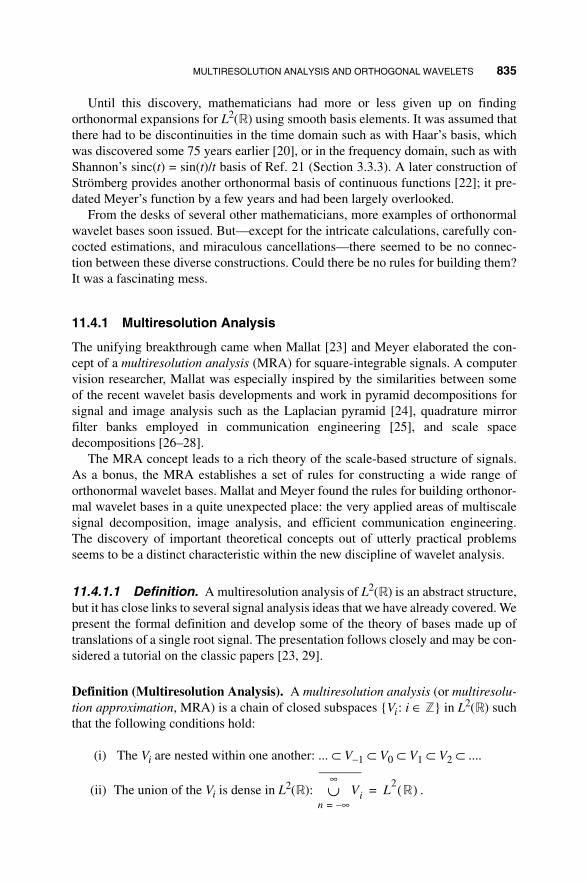
MULTIRESOLUTION ANALYSIS AND ORTHOGONAL WAVELETS 835
Until this discovery, mathematicians had more or less given up on findingorthonormal expansions for L2(R) using smooth basis elements. It was assumed thatthere had to be discontinuities in the time domain such as with Haar’s basis, whichwas discovered some 75 years earlier [20], or in the frequency domain, such as withShannon’s sinc(t) = sin(t)/t basis of Ref. 21 (Section 3.3.3). A later construction ofStrömberg provides another orthonormal basis of continuous functions [22]; it pre-dated Meyer’s function by a few years and had been largely overlooked.
From the desks of several other mathematicians, more examples of orthonormalwavelet bases soon issued. But—except for the intricate calculations, carefully con-cocted estimations, and miraculous cancellations—there seemed to be no connec-tion between these diverse constructions. Could there be no rules for building them?It was a fascinating mess.
11.4.1 Multiresolution Analysis
The unifying breakthrough came when Mallat [23] and Meyer elaborated the con-cept of a multiresolution analysis (MRA) for square-integrable signals. A computervision researcher, Mallat was especially inspired by the similarities between someof the recent wavelet basis developments and work in pyramid decompositions forsignal and image analysis such as the Laplacian pyramid [24], quadrature mirrorfilter banks employed in communication engineering [25], and scale spacedecompositions [26–28].
The MRA concept leads to a rich theory of the scale-based structure of signals.As a bonus, the MRA establishes a set of rules for constructing a wide range oforthonormal wavelet bases. Mallat and Meyer found the rules for building orthonor-mal wavelet bases in a quite unexpected place: the very applied areas of multiscalesignal decomposition, image analysis, and efficient communication engineering.The discovery of important theoretical concepts out of utterly practical problemsseems to be a distinct characteristic within the new discipline of wavelet analysis.
11.4.1.1 Definition. A multiresolution analysis of L2(R) is an abstract structure,but it has close links to several signal analysis ideas that we have already covered. Wepresent the formal definition and develop some of the theory of bases made up oftranslations of a single root signal. The presentation follows closely and may be con-sidered a tutorial on the classic papers [23, 29].
Definition (Multiresolution Analysis). A multiresolution analysis (or multiresolu-tion approximation, MRA) is a chain of closed subspaces Vi: i ∈ Z in L2(R) suchthat the following conditions hold:
(i) The Vi are nested within one another: ... ⊂ V−1 ⊂ V0 ⊂ V1 ⊂ V2 ⊂ ....
(ii) The union of the Vi is dense in L2(R): .Vin ∞–=
∞∪ L
2R( )=

836 TIME-SCALE SIGNAL TRANSFORMS
(iii) The intersection of the Vi is the signal of zero norm (zero almost every-
where), which we write .
(iv) Elements of the spaces are dyadically scaled (more precisely, dilated) ver-sions of one another: x(t) ∈ Vi ⇔ x(2t) ∈ Vi+1.
(v) For any x(t) ∈ V0 and any k ∈ Z, x(t − k) ∈ V0.
(vi) There is an isomorphism from V0 onto the Hilbert space of square-summa-ble discrete signals I: V0 → l2 such that for any k ∈ Z, if I(x(t)) = s(n) ∈ l2,then I(x(t − k)) = s(n − k).
Remark. We give the classic definition and notation for the MRA [23]. It hasbecome common to index the Vi in the other direction: Vi ⊃ Vi+1. So readers mustpay close attention to an author’s Vi indexing.
Nowadays, many treatments (for instance, Refs. 3, 8, and 9) replace (vi) with therequirement that V0 has an orthonormal basis of translates of a single finite-energysignal: φ(t − n) | n ∈ Z. This works. But so early on, it also seems incredible; weprefer to proceed from the apparently weaker criterion. In Section 11.4.2 we dem-onstrate that there is indeed a special function in V0, called a scaling function,whose translates comprise an orthonormal basis of V0.
Finally, note that by an isomorphism in (vi) we mean only a bounded, one-to-one, linear map, with a bounded inverse. Some mathematics texts, for example [30],define the term to mean also ⟨Ix, Iy⟩ = ⟨x, y⟩, which implies an isometry; this we donot assume herein. The last MRA property (vi) is very strong, though. The isomor-phism is a bounded linear map: There is an M such that ||Ix|| ≤ M||x|| for all x ∈ V0.For linear maps this is equivalent to continuity. Range(I) is all of l2. If it were anisometry, then we would be easily able to show that V0 has a scaling function; butwith our weaker assumption, this requires quite a bit more work.
11.4.1.2 Examples. Although it is rich with mathematical conditions, whichmight appear difficult to satisfy, we can offer some fairly straightforward instances ofmultiresolution analyses. Here are three examples where the root spaces consist of:
• Step functions;
• Piecewise linear functions;
• Cubic splines.
Note that the root spaces in these examples contain increasingly smooth signals.
Example (Step Functions). It is easiest to begin with a root space V0 comprised ofstep functions and define the spaces of non-unit scale by dilation of V0 elements.Let u(t) be the analog unit step signal and set V0 = x(t) ∈ L2(R) | for all n ∈ Z, thereis a cn ∈ R such that x(t) = cn[u(t − n) − u(t − n − 1)] for t ∈ (n, n+1). So elementsof V0 are constant on the open unit intervals (n, n+1). The boundary values of the
Vii ∞–=
∞∩ 0=

MULTIRESOLUTION ANALYSIS AND ORTHOGONAL WAVELETS 837
signals do not matter, since Z is a countable set and thus has Lebesgue measurezero. We define Vi = y(t) ∈ L2(R) | for some x(t) ∈ V0, y(t) = x(2it). Thus, Vi sig-nals are constant on intervals (n2−i, (n+1)2−i), where n ∈ Z. Let us show that eachof the MRA properties holds.
(i) Signals that are constant on (n2−i, (n+1)2−i) for all n ∈ Z will also be con-stant on subintervals (n2−i−1, (n+1)2−i−1), so the first property holds.
(ii) From Chapter 3, we know that the step functions are dense in L2(R); sincearbitrarily narrow steps are contained in Vi for i sufficiently large, we knowthat the Vi are dense in L2(R).
(iii) For a nonzero signal to be in all of the Vi, it would have to have arbitrarilywide steps, so the intersection property must be satisfied.
(iv) This is how we define the Vi for i ≠ 0.
(v) Integral translates of signals in V0 are obviously in V0, since an integraltranslate is still constant on unit intervals.
(vi) If x(t) ∈ V0, and x(t) = cn(u(t − n) − u(t − n − 1)] for t ∈ (n, n+1), then we setI(x(t)) = s(n), where s(n) = cn for all n ∈ Z; then I(x(t − k)) = s(n − k), and Iis an isomorphism. This is left as an exercise.
This MRA is the orthonormal basis of Haar in modern guise [20]. For analyzingblocky signals, this simple MRA is appropriate (Figure 11.9a). But when studyingsmoother signals, decompositions on the Haar set require quite a few coefficients in
−1 0 1 2 3 4 5 6 7 80
0.2
0.4
0.6
0.8
1
1.2
1.4
1.6
1.8
2
t
(a)
x(t)
Fig. 11.9. Typical elements of an MRA built by step functions (a), piecewise linear func-tions (b), and cubic splines (c).

838 TIME-SCALE SIGNAL TRANSFORMS
order to smooth out the discontinuities present in the basis elements. So the approx-imations are often quite inefficient.
Example (Piecewise Linear Functions). Let us refine the multiscale structure sothat it employs piecewise continuous signals. MRAs using such functions are better
−1 0 1 2 3 4 5 6 7 80
0.2
0.4
0.6
0.8
1
1.2
1.4
1.6
1.8
2
t(b)
y(t)
−1 0 1 2 3 4 5 6 7 8−0.5
0
0.5
1
1.5
2
t(c)
z(t)
Fig. 11.9 (Continued)

MULTIRESOLUTION ANALYSIS AND ORTHOGONAL WAVELETS 839
for signal analysis purposes when we have to interpret signals that do not containabrupt jumps in value (Figure 11.9b). Let us define V0 to be the L2(R) continuousfunctions that are piecewise linear on integral intervals [n, n+1]. We define theremaining spaces via the MRA’s dilation property (iv): x(t) ∈ Vi ⇔ x(2t) ∈ Vi+1.The six MRA properties are clear, except perhaps for density (ii) and the isomor-phism (vi). Note, however, that a piecewise continuous x(t) ∈ V0 is determineduniquely by its values on integers. We define I(x(t)) = s(n), where s(n) = x(n) for alln ∈ Z. We can approximate a step function to arbitrary precision with piecewise lin-ear functions, and the step functions are dense in L2(R), so the second MRA prop-erty holds. Strömberg [22] elaborated this MRA’s theory.
Example (Cubic Splines). A more interesting example relies on cubic splines.Here, the root space V0 consists of all functions that are twice continuously differ-entiable and equal to a cubic polynomial on integral intervals [n, n+1]. Again,dilation defines the other Vi : x(t) ∈ Vi ⇔ x(2t) ∈ Vi + 1. Numerical analysis texts,(e.g., Ref. 31, show that a continuous function can be approximated to any preci-sion with a cubic spline, so the Vi are dense in L2(R).
As we continue to develop MRA theory, we shall return to these examples.
11.4.1.3 Links to Signal Analysis Legacy. Before expounding more theory,let us reflect on how the multiresolution analysis concept echoes many ideas fromprevious multiscale signal analysis techniques. In fact, stripped of their mathematicalformalism, several of the multiresolution analysis properties (i)–(vi) have conceptualprecedents in prior multiscale representations. Others embody ideas that were onlyimplicit in the intuitive constructs of earlier methods of interpretation.
For example, the nested sequence of subspaces in (i) embodies the concept of therepresentations becoming ever finer in resolution. The inclusion property indicatesthat every coarse representation of a signal may also be considered to be a fine reso-lution version of some other waveform that has an even coarser shape. The sub-spaces are closed; each Vi contains the limit of its convergent function sequences.Coarse resolution representations are useful because:
• Using them can reduce the time required for pattern searches, such as in ele-mentary edge and feature detection applications [32–34].
• Some signal features appear only at certain scales [35].
We need closure to guarantee that given a finite-energy signal x(t) and an approxi-mation error, there is some Vi that approximates x(t) to within the tolerance.
What does the union property (ii) mean? If one looks in a sufficiently fine resolu-tion space, then there is a finite energy signal that is arbitrarily close to any givensignal. Vi signals are only approximations of real signals, but we can choose them tobe very good approximations. Notice that (i) and (ii) encapsulate the intuitive notionof earlier researchers that scale is critical for structural decompositions of signals.

840 TIME-SCALE SIGNAL TRANSFORMS
To interpret a signal we have to determine either the specific time extents of signalshapes, or we must search for shapes across all scales. This insight is the motivationbehind scale space analysis [26–28], which we first considered in Chapter 4.
The intersection property (iii) tells us that, from a scale-based signal analysisstandpoint, any meaningful signal must be visible to the MRA at some scale. Thatis, if a signal is composed of structures that have such a fine scale that it must appearin all the subspaces, then this signal must be the almost everywhere zero signal.
The next property concern resolution. Next, if a function is in space Vi, then itsdilation by a factor of 2 is in the next higher resolution space Vi+1. Furthermore, itsdilation by a factor of 1/2 is in the lower resolution space Vi−1. Thus, the implica-tion of (iv) is that one ascends and descends in resolution by means of dilations,such as in the classic Laplacian pyramid construction [24].
The subspace V0 contains signals that resolve features to the unit of measure.Signals in V0 may be translated by integral amounts, and we are assured that theresult remains in the root space (v).
Lastly, discrete samples characterize the MRA functions that model the signals.Property (vi) formalizes this by requiring an isomorphism between V0 and thesquare-summable sequences of real numbers. This discretization has the furtherproperty that the discrete representations of functions are translated when the func-tion is translated. Without this invariance, the discrete samples associated with awaveform x(t) in V0 might change with the translation of x(t) by integral steps. Forthe lower resolution spaces Vi, i < 0, translation invariance does not hold. It willbecome apparent in applications that the overall situation for translation invarianceis far from satisfactory; indeed, it is problematic.
11.4.1.4 Bases of Translates: Theory. Our first theoretical result on MRAscomes right out of the sixth criterion. It shows that the root space V0 has a basis,consisting of integral translates of a single square-integrable signal. Multiresolutionanalysis exploits the special properties of such bases.
Proposition (Basis). If Vi | i ∈ Z is an MRA in L2(R), then there is e(t) ∈ V0such that e(t − k) | k ∈ Z is a basis for V0.
Proof: Let δ(n − k) be the discrete delta signal delayed by k ∈ Z. δ(n − k) | k ∈ Zis an orthonormal basis for l2. Let I: V0 → l2 be the isomorphism of MRA property(vi). Since I is onto, we may set ek(t) = I−1(δ(n − k)). Then ek(t) | k ∈ Z is a basisfor V0. However, I(e0(t)) = δ(n), so that the translation-invariance provision of (vi)also implies I(e(t − k)) = δ(n − k), whence ek(t) = e(t − k).
The proposition guarantees a basis that is useful for those pattern matching appli-cations where we expect candidate signals containing the shape of the root element.The basis elements comprise our model or prototype signals. For computationalpurposes, we prefer such bases to be orthonormal, since that simplifies expansioncoefficient computations. But, again, orthogonality requires more work. Let usexplore some of the theory of such bases.

MULTIRESOLUTION ANALYSIS AND ORTHOGONAL WAVELETS 841
Definition (Riesz Basis). E = en | n ∈ Z is an unconditional or Riesz basis in aHilbert space H if
(i) E spans H: For any x ∈ H, there is s ∈ l2 such that
. (11.125a)
(ii) There are 0 < A ≤ B < ∞ such that for any s ∈ l2,
. (11.125b)
The constants A and B are called the lower and upper Riesz basis bounds, respectively.
Notice how (11.125b) cross-couples the norms of H and l2. An orthonormal basisis also a Riesz basis. Note too that the lower bound condition in (11.125b) impliesthat a Riesz basis is linearly independent (exercises). The next result shows thatproperty (vi) of an MRA is equivalent to V0 having a Riesz basis.
Theorem (Riesz Basis Characterization). E = ek | k ∈ Z is a Riesz basis in aHilbert space H if and only if:
(i) There is an isomorphism I from H onto l2 such that I(ek) = δ(n − k), whereδ(n) is the discrete delta.
(ii) I−1 is bounded.
Proof: Let E = ek | k ∈ Z be a Riesz basis in H. Since for any x ∈ H, there is s ∈l2 such that (11.125a) holds, we may set Ix = s. This map is well-defined by the lin-ear independence of E; that is, for each x, the coefficient sequence s(n) is unique.The linearity follows from the properties of the square-summable sequences, andclearly I(ek) = δ(n − k). The map is also onto, because any s ∈ l2 defines an elementof H as in (11.125a). This sum converges in H by the upper bound inequality in(11.125b). The boundedness of I follows as well: ||Ix|| = ||s|| ≤ A−1||x||. The inverseJ = I−1 exists because I is one-to-one and onto (a bijection). ||Js|| = ||x|| = ||Σs(k)ek|| ≤B||s|| by (11.125b), so J is bounded too.
Conversely, let I: H → l2 be an isomorphism obeying (i) and (ii). Let x ∈ H.We need to show that x is in the closure of Span(E). Let Ix = s ∈ l2. In general, itdoes not necessarily follow that if an isomorphism is bounded, then its inverseis bounded. However, we are assuming J = I −1 is bounded, so it is also continuous[30]. Thus,
(11.126)
x s n( )enn ∞–=
∞
∑=
A s s n( )enn ∞–=
∞
∑ B s≤ ≤
J s k( )δ n k–( )k N–=
N
∑
N ∞→lim s k( )J δ n k–( )( ) s k( )ek,
k ∞–=
∞
∑=k ∞–=
∞
∑=

842 TIME-SCALE SIGNAL TRANSFORMS
and x is a limit of elements in Span(E). Let ||I|| = A−1 and ||J|| = B. Then A and B arethe lower and upper Riesz bounds for E (11.125b).
Corollary. Property (vi) of an MRA is equivalent to V0 having a Riesz basis oftranslates.
Proof: Since the isomorphism I in (vi) has a bounded inverse and I is onto, we mayfind ek(t) such that I(ek(t)) = δ(n − k), where δ(n) is the discrete delta signal. Thetheorem tells us that ek(t) | k ∈ Z is a Riesz basis. The translation invariance forV0 implies that ek(t) = e(t − k).
The conditions (11.125a) and (11.125b) for a Riesz basis resemble the criterionfor a frame, which we studied in Chapters 3 and 10. Indeed, the following corollaryshows that a Riesz basis is a frame. Of course, the converse is not true; a Riesz basismust be linearly independent, while frames can be overcomplete.
Corollary (Frame). If E = ek | k ∈ Z is a Riesz basis in a Hilbert space H, then Eis a frame.
Proof: Let let I : H → l2 be the isomorphism promised in the Riesz basis character-ization: I(ek) = δ(n − k). Let I* be the Hilbert space adjoint operator for I. We intro-duced the adjoint operator in Chapter 3 and therein applied it to the study of frames(Section 3.3.4). The adjoint cross-couples the inner product relations of H and l2 sothat if s(n) is square-summable, then ⟨Ix, s⟩ = ⟨x, I*s⟩. Note that I*: l2 → H is an iso-morphism, bounded, and in fact ||I*|| = ||I||. For example, to show I* is one-to-one,let I*v = I*w for some v(n), w(n) ∈ l2. Then for any h ∈ H, ⟨h, I*v⟩ = ⟨h, I*w⟩. Butthis implies ⟨Ih, v⟩ = ⟨Ιh, w⟩. Since I is onto and h is arbitrary, Ih could be any finite-energy discrete signal. In other words, ⟨s, v⟩ = ⟨s, w⟩ for all s ∈ l2. But this meansv = w too. We leave the remaining I* details as exercises.
Now, let fk = I*(δ(n − k)). Since δ(n − k) = (I*)−1(fk) and ((I*)−1)−1 = I* isbounded, the proposition says that F =fk | k ∈ Z is a Riesz basis in H. If x ∈ H, thenby (11.125a) there is s ∈ l2 such that . We see that ⟨x, ek⟩ = s(k)by calculating ⟨ fi, ek⟩ = ⟨I*(δ(n − i)), ek⟩ = ⟨δ(n − i), I(ek)⟩ = ⟨δ(n − i), δ(n − k)⟩. So
(11.127)
Since I* and (I*)−1 are bounded and x = I*s, we have
(11.128)
which is precisely a frame condition on E.
x s k( )fkk ∞–=∞∑=
x ek,⟨ ⟩ 2
k ∞–=
∞
∑ s k( ) 2
k ∞–=
∞
∑ s 22.= =
x2
I∗ 2------------ x ek,⟨ ⟩ 2
k ∞–=
∞
∑≤ s k( ) 2
k ∞–=
∞
∑ x2
I∗( ) 1– 2,≤=

MULTIRESOLUTION ANALYSIS AND ORTHOGONAL WAVELETS 843
Theorem (Orthonormal Translates). Let φ(t) ∈ L2(R) and Φ(ω) = F [φ(t)](ω) beits (radial) Fourier transform. The family F = φ(t − k) | k ∈ Z is orthonormal ifand only if
(11.129)
for almost all ω ∈ R.
Proof: An interesting application of Fourier transform properties makes this proofwork. Let us define ak = ⟨φ(t), φ(t − k)⟩. Note that—by a simple change of variablein the inner product integral—F is orthonormal if and only if ak is zero when k ≠ 0and unity when k = 0. We calculate
(11.130)
by the Parseval and shift properties. The right-hand integrand in is |Φ(ω)|2ejkω. Webreak up the integral into 2π-wide pieces, invoke the exponential’s periodicity, andswap the order of summation and integration to get
(11.131)
We move the sum into the integral, since Φ = Fφ ∈ L2(R), so that |Φ(ω)|2 ∈ L1(R).Let us define
(11.132)
Now observe
(11.133)
so that PΦ(ω) is finite for almost all ω ∈ R. This allows us to interchange summa-tion and integration with the Lebesgue integral (Chapter 3) in (11.131). We can saymore about PΦ(ω): It is 2π-periodic, and the right-hand side of (11.131) is preciselythe expression for its Fourier series coefficient, which is ak. Within the inner prod-uct there hides nothing less than a Fourier series analysis equation for the specialperiodic function PΦ(ω)! We use this periodization argument a lot.
Φ ω 2πk+( ) 2
k ∞–=
∞
∑ 1=
ak φ t( ) φ t k–( ),⟨ ⟩ 12π------ Φ ω( ) Φ ω( )e
j– kω,⟨ ⟩ 12π------ Φ ω( )Φ ω( )e
jkω ω.d∞–
∞
∫= = =
ak1
2π------ Φ ω 2πn+( ) 2
ejkω ωd
0
2π
∫n ∞–=
∞
∑ 12π------ e
jkω Φ ω 2πn+( )n ∞–=
∞
∑2
ω.d0
2π
∫= =
PΦ ω( ) Φ ω 2πn+( )n ∞–=
∞
∑2.=
Φ ω 2πn+( )n ∞–=
∞
∑2
ωd0
2π
∫ PΦ ω( ) ωd0
2π
∫ Φ ω( ) 2 ωd∞–
∞
∫ Φ ω( ) 22,= = =

844 TIME-SCALE SIGNAL TRANSFORMS
Let us check our claim that PΦ(ω) = 1 almost everywhere if and only if the fam-ily of translates F is orthonormal. First, if PΦ(ω) = 1, then (11.131) becomes
(11.134)
The integral in (11.134) is 2π if k = 0 and zero if k ≠ 0. So F = φ(t − k) must beorthonormal. Conversely, suppose F is orthonormal so that ak = 1 if k = 0 and ak = 0if k ≠ 0. Because (11.131) gives the Fourier series coefficients for the 2π-periodicfunction PΦ(ω), we know that PΦ(ω) has all zero Fourier series coefficients exceptfor its DC term, which is one. In other words,
(11.135)
The following corollary shows that when the translates of φ(t) are orthonormal, thenits spectrum, as given by the support of Φ(ω), cannot be too narrow [8]. Scalingfunctions cannot have simple frequency components. This result uses the Lebesguemeasure of a set, an idea introduced in Section 3.4.1.
Corollary (Spectral Support). Let φ(t) ∈ L2(R), Φ(ω) = F [φ(t)](ω) be its (radial)Fourier transform, let Support(Φ) = ω ∈ R | Φ(ω) ≠ 0, and let µ(A) be the Lebesguemeasure of a measurable set A. If the family F = φ(t − k) | k ∈ Z is orthonormal, thenµ(Support(Φ)) ≥ 2π. Under these assumptions, moreover, µ(Support(Φ)) = 2π if andonly if |Φ(ω)| = χA, for some Lebesgue measurable A ⊂ R with µ(A) = 2π.
Proof: Since ||φ||2 = 1, we know ||Φ||2 = (2π)1/2, by Plancherel’s formula. The theo-rem then implies |Φ(ω)| ≤ 1 for almost all ω ∈ R. Consequently,
(11.136)
Now suppose (11.136) is an equality, but 0 < |Φ(ω)| < 1 on some set B ⊂ R withµ(B) > 0. Then
(11.137)
and
(11.138)
ak1
2π------ e
jkω ωd0
2π
∫ φ t( ) φ t k–( ),⟨ ⟩ .= =
PΦ ω( ) akejkω
k ∞–=
∞
∑ 1e0
1.= = =
µ Support Φ( )( ) 1 ωdSupport Φ( )
∫ Φ ω( ) 2 ωd∞–
∞
∫ 2π.=≥=
Φ ω( ) 2 ωdB∫ 1 ωd
B∫ µ B( )=<
Φ 22
2π Φ ω( ) 2 ωdSupport Φ( )
∫ µ Support Φ( )\B( ) µ B( )+<
µ Support Φ( )( ) 2π
= =
= =

MULTIRESOLUTION ANALYSIS AND ORTHOGONAL WAVELETS 845
a contradiction. Conversely, assume F is orthonormal and |Φ(ω)| = χA, for someLebesgue measurable A ⊂ R with µ(A) = 2π. Then we quickly see that
(11.139)
Here is a second characterization of unconditional bases. In the next section, we usethis result to find the scaling function for an MRA. We begin with a lemma [9].
Lemma. Suppose φ(t) ∈ L2(R), Φ(ω) = F [φ(t)](ω) is its (radial) Fourier transform,F = φ(t − k) | k ∈ Z, and we define PΦ(ω) as above (11.132). If s ∈ l2, then
(11.140)
where S(ω) is the discrete-time Fourier transform of s(k).
Proof: Let us consider a linear combination of the φ(t − k), ,where s ∈ l2. Using the above periodization technique, we compute
(11.141)
By assumption, s(k) is square-summable. Hence its discrete-time Fourier transformexists (Chapter 7), and we may pass to the double summation limit in (11.141).Indeed, as p, q → ∞, the last integrand in (11.141) becomes |S(ω)|2PΦ(ω), whereS(ω) is the DTFT of s(k).
Theorem (Riesz Translates Basis Characterization). Suppose φ(t) ∈ L2(R), Φ(ω) =F [φ(t)](ω) is its (radial) Fourier transform, F = φ(t − k) | k ∈ Z, 0 < A ≤ B < ∞, andwe define PΦ(ω) as above (11.132). Then the following are equivalent:
(i) F is a Riesz basis with lower and upper bounds and , respectively.
(ii) A ≤ PΦ(ω) ≤ B for almost all ω ∈ R.
Proof: Suppose (ii), and let s ∈ l2. Then A|S(ω)|2 ≤ |S(ω)|2PΦ(ω) ≤ B|S(ω)|2 < ∞almost everywhere, too, where S(ω) is the DTFT of s(k). Integrating on [0, 2π], wesee
. (11.142)
µ A( ) µ Support Φ( )( ) Φ 22
2= π.= =
s k( )φ t k–( )k ∞–=
∞
∑2
2 12π------ S ω( ) 2
PΦ ω( ) ω,d0
2π
∫=
s k( )φ t k–( )k p=q∑
s k( )φ t k–( )k p=
q
∑2
2 12π------ s k( )e
jkω– Φ ω( )k p=
q
∑2
2
12π------ s k( )e
jkω–
k p=
q
∑2
Φ ω( ) 2 ωd∞–
∞
∫1
2π------ s k( )e
jkω–
k p=
q
∑2PΦ ω( ) ωd
0
2π
∫
=
= =
A B
A2π------ S ω( ) 2 ωd
0
2π
∫1
2π------ S ω( ) 2
PΦ ω( ) ωd0
2π
∫B
2π------ S ω( ) 2 ωd
0
2π
∫≤ ≤

846 TIME-SCALE SIGNAL TRANSFORMS
We know that 2π||s||2 = ||S||2, and so the lemma implies
(11.143)
this is precisely the Riesz basis condition for lower and upper bounds and ,respectively.
Now let us assume (i) and try to show A ≤ PΦ(ω) almost everywhere on [0, 2π].Following [9], we set QΦ,a = ω ∈ [0, 2π]: PΦ(ω) < a. If the Lebesgue measure ofQΦ,a, µ(QΦ,a), is zero for almost all a ∈ R, then PΦ(ω) diverges almost everywhere,and, in particular, A ≤ PΦ(ω). We can thus suppose that there is some a ∈ R suchthat µ(QΦ,a) > 0. Let χa be the characteristic function on QΦ,a:
(11.144)
By the theory of Lebesgue measure, if a set is measurable, then so is its characteris-tic function. This entitles us to compute the inverse discrete-time Fourier transformof χa(ω):
(11.145)
where xa ∈ l2. From (i) and the lemma we see
(11.146)
By our choice of QΦ,a, PΦ(ω) < a for ω ∈ QΦ,a, and (11.146) entails
(11.147)
But ||xa||2 = (2π)−1||χa||2 = (2π)−1µ(QΦ,a), and, by (11.147), A ≤ a. This gives us acontradiction by the following observation. If A ≤ PΦ(ω) almost everywhere on[0, 2π], then we are done. Otherwise, there must be some such thatµ(U) > 0 and PΦ(ω) < A. But then there must also be some a > 0 such thatPΦ(ω) < a < A and µ(QΦ,a) > 0. But our argument above has just proven that A ≤a, a contradiction.
A s 22
s k( )φ t k–( )k ∞–=
∞
∑2
2B s 2
2;≤ ≤
A B
χa ω( )1 if ω QΦ a, ,∈
0 if ω QΦ a, .∉
=
xa n( ) 12π------ χa ω( )e
jωn ω,d0
2π
∫=
A xa 22
xa k( )φ t k–( )k ∞–=
∞
∑2
2≤ 1
2π------ χa ω( ) 2
PΦ ω( ) ωd0
2π
∫
12π------ χa ω( )PΦ ω( ) ωd
0
2π
∫1
2π------ PΦ ω( ) ω.d
Qa
∫
=
= =
A xa 22 a
2π------µ QΦ a,( ).≤
U R⊆

MULTIRESOLUTION ANALYSIS AND ORTHOGONAL WAVELETS 847
Let us continue to assume (i) and try to show PΦ(ω) ≤ B for almost all ω ∈ [0,2π]. Define PΦ,a = ω ∈ [0, 2π]: PΦ(ω) > a. Much like before, if µ(PΦ,a) = 0almost everywhere, then PΦ(ω) = 0 for almost all ω ∈ [0, 2π], and thus PΦ(ω) ≤ B.Assume that some a > 0 gives µ(PΦ,a) > 0. Now the argument parallels the one justgiven and is left as an exercise [9]. For an alternative proof, see [8].
11.4.2 Scaling Function
From our study of bases of translates and Riesz expansions, we can show that everymultiresolution analysis V = Vi has a special scaling function, whose translatesform an orthonormal basis for V0. The MRA structure is appropriately named; thescaling function property further implies that signals in every Vi look like combina-tions of dilated versions of V0 elements.
11.4.2.1 Existence. In the following result, the equalities in (11.148a) and(11.148b) are assumed to hold almost everywhere.
Proposition (Spanning Translates). If x(t), y(t) ∈ L2(R), X(ω) and Y(ω) are theirrespective radial Fourier transforms, and s(k) ∈ l2, then the following are equivalent:
(11.148a)
(11.148b)
where S(ω) is the discrete-time Fourier transform of s(k).
Proof: Now, assuming (11.148b), we have
(11.149)
Hence,
(11.150)
To show the converse, we work backwards through the equalities in (11.150) to thefront of (11.149), a Fourier transform synthesis equation for y(t). We must have(11.148b) except on a set of Lebesgue measure zero.
y t( ) s k( )x t k–( ),k ∞–=
∞
∑=
Y ω( ) S ω( )X ω( ),=
y t( ) 12π------ S ω( )X ω( )e
jωt ωd∞–
∞
∫1
2π------ s k( )e
jkω–
k ∞–=
∞
∑
X ω( )ejωt ω.d
∞–
∞
∫= =
y t( ) s k( )k ∞–=
∞
∑ 12π------ X ω( )e
jω t k–( ) ωd∞–
∞
∫ s k( )x t k–( ).k ∞–=
∞
∑= =

848 TIME-SCALE SIGNAL TRANSFORMS
This section’s main result comes from the classic source papers on wavelets andmultiresolution analysis [23, 29].
Theorem (Scaling Function). If Vi: i ∈ Z is an MRA, then there is some φ(t) ∈V0 such that φ(t − k): k ∈ Z is an orthonormal basis of V0.
Proof: By the Riesz Basis Characterization (Section 11.4.1.3), there is some g(t) ∈V0 such that F = g(t − k) | k ∈ Z is a Riesz basis for V0. Let us say it has lower andupper bounds and , respectively. The Riesz Translates Basis Characteriza-tion implies
(11.151)
for almost all ω ∈ R, where G(ω) is the (radial) Fourier transform of g(t). Note thatthe sum in (11.151) is the 2π-periodic function PG(ω), defined in (11.132). TheRiesz bounds on PG(ω) allow us to define (almost everywhere) the L2(R) function
(11.152)
Φ(ω) is the Fourier transform of φ(t) ∈ L2(R), and our claim is that φ(t) works. Theprevious proposition implies . Since V0 is closed, φ(t) ∈ V0,and so φ(t − k) ∈ V0, by MRA property (v). Equation (11.152) works both ways, andwe see that F = g(t − k) | k ∈ Z—which is dense in V0—is in the closure of φ(t −k | k ∈ Z. Thus, It remains to show that the φ(t − k) areorthonormal. We calculate
(11.153)
By the Orthonormal Translates criterion (11.129), φ(t − k | k ∈ Z is an orthonor-mal set.
Corollary. Let Vi: i ∈ Z be an MRA, and φ(t) ∈ V0 be given by the theorem.Then, 2i/2φ(2it − k): k ∈ Z is an orthonormal basis of Vi.
Proof: By properties (iv) and (v) of the MRA, the scaled versions of an orthonor-mal basis for V0 will constitute an orthonormal basis for Vi.
Definition (Scaling Function). Let V = Vi: i ∈ Z be an MRA and φ(t) ∈ V0 suchthat φ(t − k): k ∈ Z is an orthonormal basis of V0. Then φ(t), known from thetheorem, is called a scaling function of the MRA.
A B
A G ω 2πk+( )k ∞–=
∞
∑2
B≤ ≤
Φ ω( ) G ω( )PG ω( )
--------------------.=
φ t( ) Span g t k–( ) ∈
Span φ t k–( ) V0.=
Φ ω 2πk+( )k ∞–=
∞
∑2
G ω 2πk+( )PG ω 2πk+( )
------------------------------------k ∞–=
∞
∑2
G ω 2πk+( )PG ω( )
--------------------------------2
k ∞–=
∞
∑ 1.= = =

MULTIRESOLUTION ANALYSIS AND ORTHOGONAL WAVELETS 849
Any translate φ(t − k) of a scaling function φ(t) is still a scaling function. Thenext corollary [9] characterizes scaling functions for an MRA.
Corollary (Uniqueness). Let V = Vi: i ∈ Z be an MRA and φ(t) ∈ V0 be the scal-ing function found in the proof. Then θ(t) ∈ V0 is a scaling function for V if andonly if there is a 2π-periodic function P(ω) such that
(i) Θ(ω) = P(ω)Φ(ω);
(ii) |P(ω)| = 1 almost everywhere on [0, 2π].
Proof: Exercise.
11.4.2.2 Examples. Let us look at some examples of scaling functions for thethree multiresolution analyses that we know.
Example (Step Functions). The scaling function for the Haar MRA, for which V0consists of constant functions on unit intervals (n, n −1), is just the unit square pulseφ(t) = u(t) − u(t − 1).
Example (Piecewise Continuous Functions). Finding this scaling function is notso direct. The continuity of V0 elements forces us to reflect on how a possible scal-ing function φ(t) might be orthogonal to its translates φ(t − k). It is clear that φ(t)cannot be finitely supported. For then we could take the last interval (n, n+1) to theright over which φ(t) is nonzero, the last interval (m, m+1) proceeding to the leftover which φ(t) is nonzero, and compute the inner product ⟨φ(t), φ(t − (n − m))⟩. Asimple check of cases shows that it is never zero. Evidently, φ(t) ≠ 0 on (n, n+1) forarbitrarily large |n|, and the inner products ⟨φ(t), φ(t − k)⟩ involve an infinite numberof terms.
But rather than stipulating from the start that V0 must have a scaling function, wehave elected to define our MRAs using the apparently weaker isomorphism condition(vi). The existence of this isomorphism I: V0 → l2, which commutes with translationsby integral amounts, is equivalent to V0 having a Riesz basis. This facilitates our studyof the Strömberg MRA. If we can find a Riesz basis F = g(t − k) | k ∈ Z for V0, thenthe Scaling Function Theorem (11.152) readily gives the Fourier transform Φ(ω) ofφ(t). Let g(t) ∈ V0 be the simple triangular pulse with g(0) = 1, g(t) = t+1 on (−1, 0),g(t) = 1− t on (0, 1), and g(t) = 0 otherwise. Then x(t) = Σakg(t − k) is piecewise linear,continuous, and x(k) = ak for all k ∈ Z. We can define the isomorphism I by (Ix)(k) =ak. This map commutes with integer translations. The Riesz Basis Characterizationimplies that g(t − k) | k ∈ Z is a Riesz basis. In fact, g(t) = I−1(δ(n)), where I is theisomorphism from V0 to l2, and δ(n) is the discrete delta signal. We compute
(11.154)G ω( ) g t( )ejωt–
td∞–
∞
∫
ω2----
sin
ω2----
-----------------
2
sinc2 ω
2----
.= = =

850 TIME-SCALE SIGNAL TRANSFORMS
Define
(11.155)
We define the utility the function Σn(ω) as follows:
(11.156)
Though it tests our competence in differential calculus, it is possible [23] to developclosed form expressions for the Σn(ω), beginning with the standard summation [36]:
(11.157)
Twice differentiating (11.157) gives
(11.158)
Finally,
(11.159)
Taking the inverse Fourier transform gives φ(t) (Figure 11.10). Notice from its mag-nitude spectrum that φ(t) is an analog low-pass filter.
Φ ω( ) G ω( )PG ω( )
--------------------sinc
2 ω2----
sinc4 ω 2πk+
2--------------------
k ∞–=
∞
∑
---------------------------------------------------------
sinc2 ω
2----
4sin2 ω( ) ω 2πk+( ) 4–
k ∞–=
∞
∑
-----------------------------------------------------------------------.= = =
Σn ω( ) ω 2πk+( ) n–.
k ∞–=
∞
∑=
Σ2 ω( ) ω 2πk+( ) 2–
k ∞–=
∞
∑ 14--- ω
2----
2–.sin= =
ω2
2
d
d Σ2 ω( ) 6 ω 2πk+( ) 4–
k ∞–=
∞
∑ 6Σ4 ω( ) 14--- ω
2----
2 ω2----
18--- ω
2----
4.csc+
2csccot= = =
Φ ω( ) G ω( )PG ω( )
-------------------- 6
ω2 14--- ω
2----
2 ω2----
18--- ω
2----
4csc+
2csccot
---------------------------------------------------------------------------------------.= =
−0.2−4 −2 2 4
0.2
0.4
0.6
0.8
1
1.2
Fig. 11.10. Scaling function for the MRA consisting of continuous piecewise signals.

MULTIRESOLUTION ANALYSIS AND ORTHOGONAL WAVELETS 851
Example (Spline Functions). The procedure for finding this scaling function issimilar to the one we use for the piecewise continuous MRA. The root space V0contains the L2(R) signals that are continuously differentiable and equal to cubicpolynomials on each interval [n, n +1], where n ∈ Z [37, 38]. To find a scalingfunction we need to find a Riesz basis. Let g(t) ∈ V0 be the cubic spline that satis-fies g(0) = 1 and g(n) = 0 otherwise. This is a rounded tent function. Then x(t) =Σakg(t − k) is a cubic spline on intervals [n, n+1], continuously differentiable, andx(k) = ak for all k ∈ Z. Once again we set (Ix)(k) = ak and invoke the Riesz BasisCharacterization toward showing g(t − k) | k ∈ Z to be a Riesz basis. We computethe radial Fourier transform of g(t):
(11.160)
We can derive a cubic spline scaling function by the standard formula (11.152):
(11.161)
where Σn(ω) is given by (11.156). Again, we can compute the Σn(ω) by takingsuccessive derivatives—six actually—of Σ2(ω). With either resolute patience or asymbolic computation software package, we calculate
(11.162)
Consequently,
(11.163)
and
(11.164)
So once again, we find a scaling function using frequency-domain analysis. The keyrelationship is (11.152). Inverse Fourier transformation gives φ(t) (Figure 11.11). Forthe cubic spline MRA too, the scaling function is a low-pass filter. In comparison tothe MRA for piecewise linear signals, observe the flatter reject band of Φ(ω) for thespline MRA.
G ω( ) 1 23--- ω
2----
2sin–
1–sinc ω
2----
4.=
Φ ω( ) G ω( )PG ω( )
--------------------Σ8 ω( )[ ]
12---–
ω4-------------------------,==
ω6
6
d
d Σ2 ω( ) 14--- ω
2----
6 ω2----
2 578
------ ω2----
4 ω2----
4
454------ ω
2----
2 ω2----
1716------ ω
2----
.8
csc+6
csccot+
csccot+csccot=
Σ8 ω( ) 15040------------
ω6
6
d
d Σ2 ω( )( )=
Φ ω( ) 1
ω4 Σ8 ω( )--------------------------.=

852 TIME-SCALE SIGNAL TRANSFORMS
11.4.3 Discrete Low-Pass Filter
The scaling function is not the only special function connected with the multiresolu-tion analysis structure. This section shows that for every MRA of finite energy sig-nals we can find a special discrete filter [10, 23, 29]. This filter will prove usefulwhen we discretize our theory and use it in signal analysis applications. In fact, weshall show that it is a low-pass filter. Mathematically thorough introductions to thismaterial include [8, 9].
Suppose V = Vi : i ∈ Z is an MRA and φ(t) ∈ V0 is its scaling function. Becauseφ(t/2) ∈ V−1 ⊂ V0 and since integral translates of φ(t) span V0, we see that
(11.165)
where the sequence hn | n ∈ Z is square-summable. Hilbert space theory tells usthat
(11.166)
These observations lead to the following definition.
Definition (Associated Filter). The φ(t) be the scaling function of an MRA,V =Vi : i ∈ Z. If Hφ is the discrete filter with impulse response hφ(n) = hn, where hn isgiven by (11.166), then Hφ is called the associated filter to V (and to φ(t)).
As we develop the properties of the discrete filter associated to an MRA, weshall see that it is indeed a low-pass filter. When there is no ambiguity, we dropthe subscript: H = Hφ. The following proposition gives a formula for the discrete-time Fourier transform H(ω) of the associated filter [23].
−0.2−4 −2 2 4
0.2
0.4
0.6
0.8
1
Fig. 11.11. Scaling function for the MRA consisting of cubic splines.
12---φ t
2---
hnφ t n–( ),n ∞–=
∞
∑=
hn12---φ t
2---
φ t n–( ), .=

MULTIRESOLUTION ANALYSIS AND ORTHOGONAL WAVELETS 853
Proposition. Let φ(t) be the scaling function of an MRA,V = Vi : i ∈ Z; let Φ(ω)be its Fourier transform; and let H be the associated discrete filter with impulseresponse, h(n) = hn, given by (11.166). Then,
(11.167)
where H(ω) is the DTFT of h(n): H(ω) = ∑nh(n)e−jωn.
Proof: Apply the radial Fourier transform to both sides of (11.165).
Remark. The relation shows that H(ω) has a low-pass filter characteristic (Figure11.12). The dilation Φ(2ω) looks just like Φ(ω), except that it is contracted withrespect to the independent frequency-domain variable ω by a factor of two. Therelation (11.167) shows that a multiplication by H(ω) accomplishes this, and the
Φ 2ω( ) Φ ω( )H ω( ),=
−3 −2 −1 1(a)
(b)
0.2
0.4
0.6
0.8
1
2 3
−3 −2 −1 1
0.2
0.4
0.6
0.8
1
2 3
Fig. 11.12. Associated low-pass filters for the MRAs consisting of piecewise linear functions(a) and cubic splines (b). Note the better cutoff behavior of the filter based on cubic splineapproximations.

854 TIME-SCALE SIGNAL TRANSFORMS
only this can be the case, intuitively, is that H(ω) is approximately unity around theDC value ω = 0, and it falls off to essentially zero halfway through the passband ofthe spectrum of Φ(ω). This is not a rigorous argument, but it can be made so byassuming some decay constraints on the scaling function φ(t) [23, 29].
Proposition. Let φ(t) be the scaling function of an MRA,V = Vi : i ∈ Z; Φ(ω) itsFourier transform; h(n) the associated discrete low-pass filter (11.166), and H(ω) itsDTFT. Then,
(11.168)
for almost all ω ∈ R.
Proof: By the Orthonormal Translates Theorem, .Inserting (11.167) into this identity gives
(11.169)
almost everywhere. Next, we split left-hand side of (11.169) into a sum over evenintegers and odd integers:
(11.170)
where we have used H(ω) = H(ω + 2π). The Orthonormal Translates Theorem tellsus that the infinite sums in (11.170) are unity, and (11.168) follows.
Remarks. Discrete filters satisfying (11.168) are conjugate filters, familiar fromChapter 9. Conjugate filters are used to filter a signal in such a way that it can be sub-sampled and exactly reconstructed later. The Laplacian pyramid technique providesdecomposition by filtering and subsampling as well as exact reconstruction [24]. Var-ious efficient signal compression and transmission techniques rely on this idea [25,39, 40]. What is particularly striking about the MRA structure is that quite disparatesignal theoretic techniques such as scale space analysis [26–28], orthogonal bases,and pyramid decompositions all meet together in one place.
The following results [8] link the low-pass filter H of an MRA, V = Vi : i ∈ Z,with the low-resolution subspace V−1 ⊂ V0 ∈ V.
Lemma. Let φ(t) be the scaling function of an MRA, let Φ(ω) be its Fourier trans-form, and let C(ω) ∈ L2[0, 2π] be 2π-periodic. Then C(ω)Φ(ω) ∈ L2(R).
H ω( ) 2H ω π+( ) 2
+ 1,=
Φ 2ω 2πk+( ) 2
k ∞–=∞∑ 1=
Φ ω πk+( ) 2H ω πk+( ) 2
k ∞–=
∞
∑ 1=
H ω( ) 2 Φ ω 2πk+( ) 2
k ∞–=
∞
∑ H ω π+( ) 2 Φ ω 2πk π+ +( ) 2
k ∞–=
∞
∑+ 1,=

MULTIRESOLUTION ANALYSIS AND ORTHOGONAL WAVELETS 855
Proof: We compute
(11.171)
where we have invoked C(ω) = C(ω + 2π). Interchanging summation and integra-tion in (11.171), and again using we get
(11.172)
Proposition (V0 Characterization). Let V = Vi : i ∈ Z be an MRA, let φ(t) be itsscaling function, and let Φ = F (φ) be its (radial) Fourier transform. Then the rootspace V0 ∈ V contains precisely those x(t) ∈ L2(R) such that X(ω) = C(ω)Φ(ω)for some 2π-periodic C(ω) ∈ L2[0, 2π], where X(ω) = F (x).
Proof: Let x(t) ∈ V0. Then x(t) = Σckφ(t − k) for some c(k) = ck, where c ∈ l2. Wecompute X(ω) as follows:
(11.173)
Now suppose X(ω) = C(ω)Φ(ω) for some 2π-periodic C(ω) ∈ L2[0, 2π]. By thelemma, X(ω) ∈ L2(R), and we can write C(ω) = Σcke
−jωk, where c(k) is the inverseDTFT of C(ω). Whence the computation (11.173) shows that x(t) is in the closure ofthe span of φ(t − k) | k ∈ Z; so x ∈ V0.
Corollary. With the same notation, define the operator T: V0 → L2[0, 2π] by Tx =C, where C(ω) is the 2π-periodic function with X(ω) = C(ω)Φ(ω) guaranteed by theproposition. Then:
Φ ω( ) 2C ω( ) 2 ωd
∞–
∞
∫ Φ ω 2πn+( ) 2C ω 2πn+( ) 2 ω
Φ ω 2πn+( ) 2C ω( ) 2 ω,d
0
2π
∫n ∞–=
∞
∑=
d0
2π
∫n ∞–=
∞
∑=
Φ ω 2πn+( ) 2∑ 1,=
Φ ω( ) 2C ω( ) 2 ωd
∞–
∞
∫ Φ ω 2πn+( )n ∞–=
∞
∑2
C ω( ) 2 ω
C ω( ) 2 ω C2
2 L2
0 2π,[ ], .=d0
2π
∫=
d0
2π
∫=
x t( )ejωt–
td∞–
∞
∫ ckφk ∞–=
∞
∑ t k–( )ejωt–
t ckk ∞–=
∞
∑ φ t k–( )ejωt–
t
ckejωk–
k ∞–=
∞
∑ φ t( )ejωt–
t C ω( )Φ ω( ).=d∞–
∞
∫=
d∞–
∞
∫=d∞–
∞
∫=

856 TIME-SCALE SIGNAL TRANSFORMS
(i) T is linear.
(ii) If x ∈ V0, then .
(iii) If x, y ∈ V0, C = Tx, and D = Ty, then
Proof: Linearity (i) is left as an exercise. For (ii), let x(t) ∈ V0, so that X(ω) =C(ω)Φ(ω). Then, the Plancherel’s formula for L2(R) and (11.172) entail
(11.174)
From (11.174) and the polarization identity [8, 30] for inner product spaces (Chap-
ter 2), , (iii) follows.
Definition (Canonical Linear Map on V0). The linear map Tx = C, where C(ω) isthe 2π-periodic function with X(ω) = C(ω)Φ(ω) guaranteed by the corollary, iscalled the canonical map from V0 to L2[0, 2π].
Proposition (V−1 Characterization). Let V = Vi : i ∈ Z be an MRA, let φ(t) beits scaling function, Φ = F (φ), and let H = Hφ the associated low-pass filter. Thenthe first low resolution subspace V−1 ∈ V contains precisely those x(t) ∈ L2(R) suchthat X(ω) = C(2ω)H(ω)Φ(ω) for some 2π-periodic C(ω) ∈ L2[0, 2π], where X(ω) =F (x).
Proof: Let x(t) ∈ V−1, so that 2x(2t) ∈ V0. Then 2x(2t) = Σckφ(t − k) for some ck =c(k) ∈ l2. Thus,
(11.175)
Taking Fourier transforms again [8]:
(11.176)
where we have made the substitution s = t/2 − k, and C(ω) is the DTFT of c(k).From (11.167), Φ(2ω) = H(ω)Φ(ω); thus, X(ω) = C(2ω)H(ω)Φ(ω). For the con-verse, let X(ω) = C(2ω)H(ω)Φ(ω) for some 2π-periodic C(ω) ∈ L2[0, 2π]. SinceC(2ω)H(ω) is still 2π-periodic, the Lemma applies, and X(ω) ∈ L2(R). Finally,(11.176) reverses to show x(t) ∈ V0.
2π x 22
C22 L
20 2π,[ ],=
2π x y,⟨ ⟩L
2R( )
C D,⟨ ⟩L
20 2π,[ ]
.=
X2
2 L2 R( ), Φ ω( ) 2
C ω( ) 2 ωd∞–
∞
∫= C22 L
20 2π,[ ], 2π x
22 L
2R( ), .==
4 x y,⟨ ⟩ x y+2
x y–2
– j x jy+2
j x jy–2
–+=
2x t( ) c k( )φ t2--- k–
.k ∞–=
∞
∑=
2X ω( ) 2 ckk ∞–=
∞
∑ φ s( )ejω 2s 2k+( )–
sd∞–
∞
∫
2 ckk ∞–=
∞
∑ e2jωk– φ s( )e
j 2ω( )s–sd
∞–
∞
∫ 2C 2ω( )Φ 2ω( ),
=
= =

MULTIRESOLUTION ANALYSIS AND ORTHOGONAL WAVELETS 857
It is possible to generalize this result (exercise). The next section explains amathematical surprise that arises from MRA theory.
11.4.4 Orthonormal Wavelet
Besides the scaling function and the associated discrete low-pass filter, a thirdspecial function accompanies any multiresolution approximation of L2(R): theorthonormal wavelet [23, 29]. Our presentation has been guided by the mathemati-cally complete introductions [8, 9].
Definition (Orthonormal Wavelet). Let ψ(t) ∈ L2(R). If its dilations and transla-tions 2n/2ψ(2nt − m): m, n ∈ Z are an orthogonal basis of L2(R), then ψ is anorthogonal wavelet. If ||ψ|| = 1, then ψ is an orthonormal wavelet.
At the beginning of this chapter we considered an extension of the Fourier trans-form based on scale and location as transform parameters. The transform inversionrequired a special signal, the admissible wavelet, in order to succeed, and we foundthat admissible wavelets had to be analog band-pass filters. Now, for MRAs it turnsout that the special associated orthogonal wavelet too is a band-pass filter. To dis-cover how it is that an MRA supports this extraordinary function, we examine theorthogonal complements of the component spaces Vi of the multiresolution analysisV = Vi : i ∈ Z.
11.4.4.1 Existence. Consider first V−1 ⊂ V0. From Hilbert space theory (Chap-ters 2 and 3), we know that every element of V0 can be written uniquely as a sumx = v + w, where v ∈ V−1 and w ⊥ v. The set of all such w ∈ V0 constitute a Hilbertsubspace of V0; let us denote it by W−1. We say that V0 is the direct sum of V−1 andW−1: V0 = V−1 ⊕ W−1. In general, every Vi+1 is the direct sum of Vi and Wi, whereWi is the orthogonal complement of Vi in Vi+1. We know already that the Vi haveorthonormal bases made up of translations and dilations of the scaling function φ(t).We can also find an orthonormal basis of Wi by the Gram–Schmidt orthonormaliza-tion procedure, of course [31]. But this does not imply that the basis elements aretranslates of one another, and it exposes no relation between the basis elements sofound and the rest of the MRA structure. We want a more enlightening theory.
Lemma (First W−1 Characterization). Let V = Vi: i ∈ Z be an MRA; let φ(t) beits scaling function; let Φ = F (φ) be the (radial) Fourier transform of φ(t); let H = Hφbe the associated low-pass filter; and let Tx = C be the canonical linear map from V0to L2[0, 2π]. Then x(t) ∈ W−1 ⊂ V0 if and only if
(11.177)
for almost all ω ∈ [0, 2π].
Proof: Let y(t) ∈ V−1 and let Ty = D. Then by the V−1 characterization, Y(ω) =A(2ω)H(ω)Φ(ω) for some 2π-periodic A ∈ L2[0, 2π]. So D(ω) = A(2ω)H(ω) almost
C ω( )H ω( ) C ω π+( )H ω π+( )+ 0=

858 TIME-SCALE SIGNAL TRANSFORMS
everywhere on [0, 2π]. By the corollary to the V0 characterization, ⟨x, y⟩ = ⟨C, D⟩.Thus, x(t) ∈ W−1 if and only if ⟨C(ω), A(2ω)H(ω)⟩ = 0, for almost all ω ∈ [0, 2π].Writing out the inner product integral [8], we see that this is further equivalent to
(11.178)
for almost all ω ∈ [0, 2π]. Since y(t) is any element of V−1, the A(2ω) in the integrandon the right-hand side of (11.178) is an arbitrary π-periodic signal; evidently, x(t) ∈W−1 if and only if the π-periodic factor almost everywhere on [0, π]. Finally, by the 2π-periodicity of C(ω) and H(ω), thissame expression must be almost everywhere zero on [0, 2π].
Lemma (Second W−1 Characterization). Let V = Vi: i ∈ Z be an MRA, let φ(t)be its scaling function, let Φ = F(φ) be the Fourier transform of φ, let H = Hφ be theassociated low-pass filter, and let Tx = C be the canonical map from V0 to L2[0, 2π].Then, x(t) ∈ W−1 if and only if X(ω) = e−jωS(2ω) Φ(ω) for some 2π-peri-odic S(ω) ∈ L2[0, 2π].
Proof: Resorting to some linear algebra tricks, we formulate the previous lemma’scriterion as a determinant. Thus, x(t) ∈ W−1 is equivalent to
(11.179)
for almost all ω ∈ [0, 2π]. This means that the columns of the matrix (11.179) arelinearly dependent—that is, they are proportional via a 2π-periodic function R(ω):
(11.180)
for just as many ω ∈ [0, 2π]. Now substitute ω + π for ω in (11.180) to see
(11.181)
whence . Further putting ω + π for ω in (11.181) gives. Evidently, for almost all ω ∈ [0, 2π].
Hence we have shown that x(t) ∈ W−1 if and only if X(ω) = C(ω)Φ(ω), where
C0
2π
∫ ω( )A 2ω( )H ω( ) dω A 2ω( )0
π
∫ C ω( )H ω( ) C ω π+( )H ω π+( )+[ ] dω 0= =
C ω( )H ω( ) C ω π+( )H ω π+( )+ 0=
H ω π+( )
det H ω π+( ) C ω( )
H– ω( ) C ω π+( )0=
C ω( )C ω π+( )
R ω( ) H ω π+( )
H– ω( )=
C ω π+( )C ω( )
R ω π+( ) H ω( )
H– ω π+( )=
C ω( ) R– ω π+( )H ω π+( )=C ω( ) R ω( )H ω π+( )= R ω( ) R– ω π+( )=

MULTIRESOLUTION ANALYSIS AND ORTHOGONAL WAVELETS 859
C(ω) = R(ω) for some 2π-periodic R(ω) ∈ L2[0, 2π] with R(ω) = −R(ω +π). We define S(ω) = exp(jω/2)R(ω/2). Then S(ω + 2π) = S(ω) almost everywhere, and
(11.182)
Lemma (W0 Characterization). Let V = Vi : i ∈ Z be an MRA, φ(t) its scalingfunction, Φ = F(φ) the Fourier transform of φ, H = Hφ the associated low-pass filter,and Tx = C the canonical map from V0 to L2[0, 2π]. Then, x(t) ∈ W0 if and only ifX(2ω) = e−jωS(2ω) Φ(ω) for some 2π-periodic S(ω) ∈ L2[0, 2π].
Proof: We note that x(t) ∈ W0 if and only if ⟨x(t), v(t)⟩ = 0 for all v(t) ∈ V0, whichis equivalent to ⟨x(t/2), v(t/2)⟩ = 0. But any f(t) ∈ V−1 is of the form v(t/2), so this isalso equivalent to x(t/2) ⊥ V−1; in other words, y(t) = x(t/2) ∈ W−1. The previouslemma says Y(ω) = e−jωS(2ω) Φ(ω) for some 2π-periodic S(ω) ∈ L2[0,2π]. But Y(ω) = 2X(2ω).
The main result of this section—very probably the main result of this chapter,likely the main result of this book, and arguably the main result of Fourier analysisin the latter half of the twentieth century—is expressed in the following theoremand its corollary [23, 29].
Theorem (Orthonormal Basis of W0). Suppose V = Vi: i ∈ Z is an MRA, φ(t)its scaling function, Φ = F (φ) the Fourier transform of φ, and H = Hφ is the associ-ated low-pass filter. If ψ(t) is the finite energy signal whose Fourier transform isgiven by
Ψ(2ω) = e−jω Φ(ω), (11.183)
then ψ(t − k) | k ∈ Z is an orthonormal basis for W0.
Proof: We know that the W0 characterization lemma entails ψ(t) ∈ W0. (In fact,ψ(t) represents the very straightforward case where the lemma’s S(ω) = 1 almosteverywhere on [0, 2π].) Let x(t) ∈ W0. Let us show that a linear combination oftranslates of ψ(t) is arbitrarily close to x(t). The previous lemma says that X(2ω) =e−jωS(2ω) Φ(ω) for some 2π-periodic S(ω) ∈ L2[0, 2π]. Thus, X(ω) =S(ω)Ψ(ω), almost everywhere on [0, 2π]. But we know this condition already fromthe Spanning Translates Proposition of Section 11.4.2.1: It means that
(11.184)
where s(n) is the inverse discrete-time Fourier transform of S(ω). Verily, the closureof ψ(t − k) | k ∈ Z is all of W0.
H ω π+( )
X ω( ) C ω( )Φ ω( ) R ω( )H ω π+( )Φ ω( ) ej– ω
S 2ω( )H ω π+( )Φ ω( ).= = =
H ω π+( )
H ω π+( )
H ω π+( )
H ω π+( )
x t( ) s n( )ψ t n–( ),n ∞–=
∞
∑=

860 TIME-SCALE SIGNAL TRANSFORMS
What about orthonormality? If we attempt to apply the Orthonormal Translatescriterion (11.129), then we have
.
(11.185)
By the orthonormality of φ(t − k), we have
.
(11.186)
By the 2π-periodicity of H(ω), this becomes
(11.187)
and by Orthonormal Translates applied to the Φ summations on the bottom of(11.187), we get
(11.188)
But this last expression is unity by (11.168), and thus ψ(t − k) | k ∈ Z is orthonormal.
Corollary (Existence of Orthonormal Wavelet). With the theorem’s assumptionsand notation, let ψ(t) ∈ L2(R) be defined as above. Then the dilations and transla-tions 2n/2ψ(2nt − m): m, n ∈ Z are an orthonormal basis of L2(R), and so ψ is anorthonormal wavelet [8–10].
Proof: Since V1 = V0 ⊕ W0, dilations of x(t) ∈ W0 by 2i are in Wi: x(2it) ∈ Wi. Infact, 2i/2ψ(2it − m): m ∈ Z is an orthonormal basis for Wi. But, Vi+1 = Vi ⊕ Wi, so
Ψ ω 2kπ+( ) 2
k ∞–=
∞
∑ Φ ω2---- kπ+
2H ω
2---- k 1+( )π+
2
k ∞–=
∞
∑
Φ ω2---- 2kπ+
2H ω
2---- 2kπ π+ +
2
k ∞–=
∞
∑
Φ ω2---- 2kπ π+ +
2H ω
2---- 2kπ 2+ π+
2
k ∞–=
∞
∑+
=
=
Ψ ω 2kπ+( ) 2
k ∞–=
∞
∑ Φ ω2---- kπ+
2H ω
2---- k 1+( )π+
2
k ∞–=
∞
∑
Φ ω2---- 2kπ+
2H ω
2---- 2kπ π+ +
2
k ∞–=
∞
∑
Φ ω2---- 2kπ π+ +
2H ω
2---- 2kπ 2+ π+
2
k ∞–=
∞
∑+
=
=
Ψ ω 2kπ+( ) 2
k ∞–=
∞
∑ H ω2---- π+
2Φ ω
2---- 2kπ+
2
k ∞–=
∞
∑
H ω2----
2Φ ω
2---- 2kπ π+ +
2
k ∞–=
∞
∑+
=
Ψ ω 2kπ+( ) 2
k ∞–=
∞
∑ H ω2---- π+
2H ω
2----
2.+=

MULTIRESOLUTION ANALYSIS AND ORTHOGONAL WAVELETS 861
Bi+1 = 2n/2ψ(2nt − m): n < i+1 and m ∈ Z is an orthonormal set inside Vi+1. By the intersection property (iii) of the MRA, though, Bi+1 must be dense in
Vi+1. By the MRA union property (ii), ; L2(R) must be theHilbert space direct sum of the Wi:
(11.189)
The wavelet ψ(t) that we have found is essentially unique. The exercises outline anargument that any other W0 function that is an orthogonal wavelet for square-integrable signals must have a Fourier transform that differs from the formula(11.183) by a factor that is unity almost everywhere on [0, 2π].
11.4.4.2 Examples. Let us show some examples of orthonormal wavelets fromthe multiresolution analyses of square-integrable signals that we already know.
Example (Step Functions). In the Haar MRA [20], the root space V0 consists ofconstant functions on unit intervals (n, n −1), and so φ(t) = u(t) − u(t − 1). We com-pute its Fourier transform by
(11.190)
and the relation gives the associated low-pass filter:
(11.191)
From , we calculate
(11.192)
But (11.192) is the radial Fourier transform of the function
(11.193)
so ψ(t) above is the orthogonal wavelet for the step function MRA.
Vii ∞–=
∞∩ 0;=
Vin ∞–=
∞∪ L2
R( )=
∞Wi⊕
i ∞–=
L2
R( ).=
Φ ω( ) φ t( )ejωt–
td∞–
∞
∫ e
jω2
------– ω 2⁄( )sinω 2⁄
-----------------------= =
Φ 2ω( ) Φ ω( )H ω( )=
H ω( ) e
jω2
------–
ω 2⁄( ).cos=
Ψ ω( ) ejω–
H ω π+( )Φ ω( )=
Ψ ω( ) je–
jω2
------ ω 4⁄( )2sin
ω 4⁄--------------------------.=
ψ t( )
1– if 1 t 12---,<≤–
1 if 12--- t 0,<≤–
0 if otherwise.
=

862 TIME-SCALE SIGNAL TRANSFORMS
Example (Piecewise Continuous Functions). We found the scaling function forthe Strömberg [22] MRA in Section 11.4.2.2 and the associated low-pass filter inSection 11.4.3. The expression Ψ(2ω) = ejω Φ(ω) as well as (11.159) and(11.167) give us the Fourier transform for the piecewise continuous MRA’s wavelet.Then, we can compute ψ(t) via the inverse transform (Figure 11.13).
Example (Spline Functions). In the third MRA we have studied, the root spaceV0 contains continuously differentiable, finite-energy signals that are cubic poly-nomials on unit intervals [n, n+1]. This MRA was developed by Lemarié[37] and Battle [38]. The same strategy works once more. We know the scalingfunction’s Fourier transform Φ(ω) from (11.164). The discrete-time Fouriertransform for the associated low-pass filter is the ratio H(ω) = Φ(2ω)/Φ(ω).Hence, we find Ψ(ω), and inverse transforming gives the orthogonal wavelet(Figure 11.14).
H ω + π( )
−1.5
−4 −2 2
(a)
(b)
4−0.5
0.5
1.5
1
−1
−40 −20 20 40
0.2
0.4
0.6
0.8
1
Fig. 11.13. For the Strömberg MRA: The orthogonal wavelet, (a) which we compute from amessy, but exact expression for its Fourier transform (b).

SUMMARY 863
The next chapter provides various examples of mixed domain signal analysis. Inparticular, it covers the use of the multiresolution analysis structure for combiningtime- and scale-domain analysis of signals that arise in typical applications.
11.5 SUMMARY
For signal analysis, both the continuous wavelet transform and the multiresolutionanalysis that leads to orthogonal wavelets are attractive and feasible. This chaptercovered the signal analytic essentials of wavelet theory. The continuous transformfinds more applications in signal understanding, as long as basic facts about inputsignals—location, scale, spectrum—are known beforehand. The orthogonal trans-forms, based on multiresolution analysis, tend to find more use in compression. Weshall see in the last chapter that there are efficient algorithms for decomposition
42
(a)
(b)
−2
−1
−1.5
−0.5
0.5
1.5
1
−4
−20 −10 10 20
0.2
0.4
0.6
0.8
1
Fig. 11.14. For the cubic spline MRA of Lemarié and Battle: The orthogonal wavelet (a)and its Fourier transform (b).

864 TIME-SCALE SIGNAL TRANSFORMS
using MRAs that lend themselves to efficient signal description, compression, aswell as pattern recognition applications.
We omitted the proof of the theorem on the necessity of admissibility for framesbased on translation and dilation (Section 11.3.2). The proof itself is somewhattechnical, and, besides, in compensation, we later showed that an elegant construc-tion, the MRA, leads to orthogonal wavelets from which efficient algorithms andstraightforward frame constructions proceed.
There are three special functions that arise from an MRA, V = Vi: i ∈ Z:
• The scaling function φ(t) whose translates form an orthonormal basis for theroot space V0;
• The associated low-pass filter Hφ;
• And, finally, the orthonormal wavelet ψ(t) whose translations and dilationsconstitute and orthonormal basis for finite-energy signals.
Some conditions in the definition we give for an MRA are consequences of theothers. For example, the third criterion in Section 11.4.1.1—that only the zero sig-nal should appear in all Vi—follows from the rest. This and other interdependencieswere only noted some years later [8, 41].
We provided only a few examples of MRAs, but these suffice for introductorysignal analysis applications. Important extensions include compactly supportedwavelets [3], approximation theory using wavelets [2], and multidimensional signalanalysis using wavelets [10, 23].
Let us remark about how wavelets can be used in image processing and analysis.The principal focus of this book notwithstanding, we should also note that our MRAdefinition extends from one-dimensional functions (signals) to two-dimensionalfunctions (images). Indeed there are MRA structures for the n-dimensional Hilbertspace L2(Rn). The technique is identical to that used to extend the Gaussian andLaplacian pyramid constructions to images [24].
We just repeat the definition of Section 11.4.1.1 for functions of two variables,x(s, t) ∈ L2(R2), denoting the subspace chain V2,n. We can then derive a two-dimen-sional scaling function φ(s, t) as before (exercise). The most common approach,however, is to use a tensor product of one-dimensional MRAs to get an MRA forL2(R2): V2,n = V1,n ⊗ V1,n, where Vn: n ∈ Z is an MRA in L2(R). Then, there is ascaling function for the two-dimensional MRA of L2(R2): Φ(x, y) = φ(x)φ(y). Whilethere is a single scaling function for the two-dimensional case, there are now threewavelets: Ψ1(x, y) = φ(x)ψ(y), sensitive to high vertical frequencies; Ψ2(x, y) =ψ(x)φ(y), horizontal; Ψ3(x, y) = ψ(x)ψ(y), diagonal or corners.
This gives an orientation selective decomposition, especially suitable for imageswith large x- and y-direction edge components. A number of applications involvesuch images: inspection of manufactured materials, remote sensing applications,and seismic signal processing among others.
For a history of wavelets, see Ref. [1]. References 10 and 42 list softwareresources and toolkits for signal analysis using wavelets.

REFERENCES 865
REFERENCES
1. B. B. Hubbard, The World According to Wavelets, Wellesley, MA: A. K. Peters, 1996.
2. C. Chui, Introduction to Wavelets, San Diego, CA: Academic, 1992.
3. I. Daubechies, Ten Lectures on Wavelets, Philadelphia: SIAM, 1992.
4. Y. Meyer, Wavelets: Algorithms and Applications, Philadelphia: SIAM, 1993.
5. T. H. Koornwinder, ed., Wavelets: An Elementary Treatment of Theory and Applications,Singapore: World Scientific, 1993.
6. G. Kaiser, A Friendly Guide to Wavelets, Boston: Birkhauser, 1994.
7. M. Holschneider, Wavelets: An Analysis Tool, Oxford: Oxford University Press, 1995.
8. E. Hernandez and G. Weiss, A First Course on Wavelets, Boca Raton, FL: CRC Press,1996.
9. P. Wojtaszczyk, A Mathematical Introduction to Wavelets, Cambridge: Cambridge Uni-versity Press, 1997.
10. S. Mallat, A Wavelet Tour of Signal Processing, San Diego, CA: Academic, 1998.
11. H. L. Resnikoff and R. O. Wells, Jr., Wavelet Analysis: The Scalable Structure of Informa-tion, New York: Springer-Verlag, 1998.
12. C. Blatter, Wavelets: A Primer, Natick, MA: A. K. Peters, 1999.
13. A. Grossmann and J. Morlet, Decompositions of Hardy functions into square integrablewavelets of constant shape, SIAM Journal of Mathematical Analysis, vol. 15, pp. 723–736,1984.
14. I. Daubechies, A. Grossmann, and Y. Meyer, Painless non-orthogonal expansions, Jour-nal of Mathematical Physics, vol. 27, pp. 1271–1283, 1986.
15. I. Daubechies, The wavelet transform, time-frequency localization and signal analysis,IEEE Transactions on Information Theory, vol. 36, no. 5, pp. 961–1005, September1990.
16. P. Goupillaud, A. Grossmann, and J. P. Morlet, Cycle-octave and related transforms inseismic signal analysis, Geoexploration, vol. 23, pp. 85–102, 1984.
17. R. Kronland-Martinet, J. P. Morlet, and A. Grossmann, Analysis of sound patternsthrough wavelet transforms, International Journal of Pattern Recognition and ArtificialIntelligence, vol. 1, no. 2, pp. 97–126, 1987.
18. A. Grossmann, Wavelet transforms and edge detection, in Stochastic Processes in Physicsand Engineering, S. Albeverio et al., ed., Dordrecht, Holland: D. Reidel Publishing Com-pany, pp. 149–157, 1988.
19. Y. Meyer, Principe d’incertitude, bases hilbertiennes et algèbres d’opérateurs, SéminaireBourbaki, no. 662, 1985–1986.
20. A. Haar, Zur theorie der orthogonalen Functionensysteme, Mathematische Annalen,vol. 69, pp. 331–371, 1910.
21. C. E. Shannon, Communication in the presence of noise, Proceedings of the Institute ofRadio Engineers, vol. 37, pp. 10–21, 1949.
22. J.-O. Strömberg, A modified Franklin system and higher order spline systems on Rn asunconditional bases for Hardy spaces, in Proceedings of the Conference in Honor ofAntoni Zygmund, vol. II, W. Becker, A. P. Calderon, R. Fefferman, and P. W. Jones, eds.,New York: Wadsworth, pp. 475–493, 1981.

866 TIME-SCALE SIGNAL TRANSFORMS
23. S. Mallat, “A theory for multiresolution signal decomposition: The wavelet representa-tion,” IEEE Transactions on Pattern Analysis and Machine Intelligence, pp. 674–693,July 1989.
24. P. J. Burt and E. H. Adelson, The Laplacian pyramid as a compact image code, IEEETransactions on Communications, vol. COM-31, no. 4, pp. 532–540, April 1983.
25. R. E. Crochiere and L. R. Rabiner, Multirate Digital Signal Processing, EnglewoodCliffs, NJ: Prentice-Hall, 1983.
26. A. P. Witkin, Scale-space filtering, Proceedings of the 8th International Joint Conferenceon Artificial Intelligence, Karlsruhe, W. Germany, 1983. Also in From Pixels to Predi-cates, A. P. Pentland, ed., Norwood, NJ: Ablex, 1986.
27. J. J. Koenderink, The structure of images, Biological Cybernetics, vol. 50, pp. 363–370,1984.
28. T. Lindeberg, Scale space for discrete signals, IEEE Transactions on Pattern Analysis andMachine Intelligence, vol. 12, no. 3, pp. 234–254, March 1990.
29. S. G. Mallat, Multiresolution approximations and wavelet orthonormal bases of L2(Rn),Transactions of the American Mathematical Society, vol. 315, no. 1, pp. 69–87, Septem-ber 1989.
30. E. Kreyszig, Introductory Functional Analysis with Applications, New York: John Wiley& Sons, 1989.
31. J. Stoer and R. Bulirsch, Introduction to Numerical Analysis, 2nd ed., New York:Springer-Verlag, 1992.
32. A. Rosenfeld and M. Thurston, Edge and curve detection for visual scene analysis, IEEETransactions on Computers, vol. 20, no. 5, pp. 562–569, May 1971.
33. S. Tanimoto and T. Pavlidis, A hierarchical data structure for picture processing, Com-puter Graphics and Image Processing, vol. 4, no. 2, pp. 104–119, June 1975.
34. R. Y. Wong and E. L. Hall, Sequential hierarchical scene matching, IEEE Transactions onComputers, vol. C-27, no. 4, pp. 359–366, April 1978.
35. D. Marr, Vision, New York: W. H. Freeman and Company, 1982.
36. I. S. Gradshteyn and I. M. Ryzhik, Table of Integrals, Series, and Products, Orlando, FL:Academic, 1980.
37. P.-G. Lemarié, Ondelettes à localisation exponentielle, Journal de Mathématiques Pureset Appliquées, vol. 67, pp. 227–236, 1988.
38. G. Battle, A block spin construction of ondelettes. Part 1: Lemarié functions, Communi-cations in Mathematical Physics, vol. 110, pp. 601–615, 1987.
39. P. P. Vaidyanathan, Multirate digital filters, filter banks, polyphase networks, and applica-tions: A tutorial, Proceedings of the IEEE, vol. 78, pp. 56–93, January 1990.
40. O. Rioul and M. Vetterli, Wavelets and signal processing, IEEE SP Magazine, pp. 14–38,October 1991.
41. W. R. Madych, Some elementary properties of multiresolution analyses of L2(Rn), inWavelets: A Tutorial in Theory and Applications, C. K. Chui, ed., Boston: Academic,pp. 259–294, 1992.
42. A. Bruce, D. Donoho, and H. Y. Gao, Wavelet analysis, IEEE Spectrum, pp. 26–35,October 1996.

PROBLEMS 867
PROBLEMS
1. Let ψ(t) be an analyzing wavelet.
(a) Show that Ψ(0) = 0.
(b) Also,
(c) Show that ψ(t) is a bandpass filter.
2. Provide an example of a bandpass filter that is not an analyzing wavelet.
3. Let V = Vi: i ∈ Z be a multiresolution analysis of L2(R) signals; let φ(t) be thescaling function for V; let Φ(ω) be the (radial) Fourier transform of φ(t); and letH be the associated discrete filter with impulse response, h(n) = hn, given by(11.166). Show in detail that , where H(ω) is the DTFTof h(n).
4. Let and be (analyzing) wavelets. If ,then show
(11.194)
5. Let , let be a wavelet, and let . Show that
(11.195)
6. Let and define . Show that
(11.196)
7. If , then show
(11.197)
8. Let m, n ∈ Z; a0, b0 > 0; and suppose that
. (11.198)
(a) Find the radial Fourier transform Ψm,n(ω) of ψm,n(t).
(b) Defining Ψ−(ω) = Ψ+(−ω), where Ψ+(ω) is given by (11.108), and usingthe arguments of Section 11.3, show that
ψ t( ) td∞–
∞∫ 0.=
Φ 2ω( ) Φ ω( )H ω( )=
α β, C∈ ψ t( ) φ t( ), θ t( ) αψ t( ) βφ t( )+=
Wθ f t( )[ ] a b,( ) αWψ f t( )[ ] a b,( ) βWφ f t( )[ ] a b,( ).+=
η 0> ψ t( ) θ t( ) 1η---ψ t
η---
=
Wθ f t( )[ ] a b,( ) 1
η-------Wψ f t( )[ ] aη b,( ).=
α β, C∈ θ t( ) αψ t( ) βφ t( )+=
Wθ αf t( ) βg t( )+[ ] a b,( ) αWψ f t( )[ ] a b,( ) βWφ f t( )[ ] a b,( )+=
γ R∈
W f t γ–( )[ ] a b,( ) W f t( )[ ] a b γ–,( ).=
ψm n, t( ) a0
m2----–
ψt nb0a0
m–
a0m
-----------------------
a0
m2----–
ψ a0m–
t nb0–( )= =

868 TIME-SCALE SIGNAL TRANSFORMS
(11.199)
where ψ−(t) is the inverse (radial) Fourier transform of Ψ−(ω).
9. Let H be a Hilbert space.
(a) Show that an orthonormal basis in H is also a Riesz basis with unit bounds.
(b) Show that a Riesz basis is linearly independent.
(c) Give an example of a frame in L2(R) that is not a Riesz basis.
10. Let V = Vi be the Haar MRA which we defined in Section 11.4.1.1. Signals inVi are constant on intervals (n2−i, (n+1)2−i), where n ∈ Z. If x(t) ∈ V0, andx(t) = cn[u(t − n) − u(t − n − 1)] for t ∈ [n, n+1), then we set I(x(t)) = s(n),where s(n) = cn for all n ∈ Z.
(a) Show that I is an isomorphism, a bounded linear operator that is one-to-oneand onto.
(b) Show that if I(x) = s(n) and k ∈ Z, then I(x(t − k)) = s(n − k).
(c) Is I an isometry? Explain.
(d) Are the elements of V0 compactly supported? Explain.
11. Let W0 be the continuous L2(R) signals that are piecewise linear on [n, n+1],n ∈ Z. Define x(t) ∈ Wi ⇔ x(2t) ∈ Wi+1.
(a) Verify MRA properties (i), (iii)–(v) for W = Wi.
(b) Let V = Vi be the Haar MRA of the previous problem. Assuming that stepfunctions are dense in L2(R), argue likewise for W by showing that givenv(t) ∈ V0, then some w(t) ∈ W is arbitrarily close to v(t). Moral: An approx-imation of an approximation is still an approximation.
(c) Let w ∈ W0 and set Iw = s, where s(n) = w(n). Show that I is an isomor-phism.
12. Let l∞(Z) be the normed linear space of bounded sequences, with ||x|| =sup|x(n)|: n ∈ Z. Define an operator Tx = y as follows: y(n) = x(n)(|n|+1)−1.Show that
(a) T is linear.
(b) T is one-to-one.
(c) T is onto.
(d) T is bounded.
(e) T −1 is not bounded [30].
13. Let I: H → K be a bounded Hilbert space isomorphism and let I* be the Hilbertspace adjoint of I.
(a) Show that ||I*|| = ||I|| [30].
(b) Supposing that I is onto, show that I* is an isomorphism.
x ψ−m n,,⟨ ⟩
2
m n, ∞–=
∞
∑ 12πb0 a0ln------------------------ X ω( ) 2 ω,d
∞–
0
∫m∑=

PROBLEMS 869
(c) Show that if E = ek | k ∈ Z is a Riesz basis in H, then there is F = fk | k ∈Z such that F is a Riesz basis and [9]
(11.200)
14. Let φ(t) ∈ L2(R), let Φ(ω) = F [φ(t)](ω) be its radial Fourier transform,let s ∈ l2, S(ω) be its discrete-time Fourier transform, and set
Show that
(a) ;
(b)
15. This problem uses the concept of Lebesgue measure. Let P(ω) be defined asabove. Define Pa = ω ∈ [0, 2π] : P(ω) > a and Qa = ω ∈ [0, 2π]: P(ω) < a.Referring to Ref. 9, show that:
(a) If the Lebesgue measure of Pa, µ(Pa), is zero for almost all a ∈ R, thenP(ω) = 0 almost everywhere. Hint: Suppose not, so that P(ω) > 0 on .Then , where n > 0 is a natural number. What is µ(P1/n)?Apply the Lebesgue measure to the countable union.
(b) Similarly, if µ(Qa) = 0 for almost all a ∈ R, then P(ω) = ∞ almost every-where.
16. Complete the proof of the second Riesz basis characterization theorem [9].Suppose φ(t) ∈ L2(R), Φ(ω) = F [φ(t)](ω) is its Fourier transform, F = φ(t − k) |k ∈ Z, 0 < A ≤ B < ∞, , and F is a Riesz basis withlower and upper bounds and , respectively. Show that P(ω) ≤ B foralmost all ω ∈ R.
(a) Define Pa = ω ∈ [0, 2π]: P(ω) > a. Show that if µ(Pa) = 0 almost every-where, then P(ω) = 0 for almost all ω ∈ [0, 2π], and P(ω) ≤ B. Hint: Con-sider the case a = 1/(n+1) for n ∈ N.
(b) Hence, assume that for some a > 0, µ(Pa) > 0. Let χa be the characteristicfunction on Pa and xa(n) be the inverse discrete-time Fourier transform ofχa(ω). Show ||xa||2 = (2π)−1µ(Pa).
(c) Show ||Σxa(k)φ(t − k)||2 ≥ a||xa||2.
(d) Show B ≥ a.
(e) Conclude that, unless B ≥ Σ|Φ(ω + 2πk)|2 almost everywhere on [0, 2π], acontradiction arises.
em fn,⟨ ⟩ 1 if m n,=
0 if m n.≠
=
P ω( ) =Φ ω 2πn+( )
n ∞–=∞∑ 2.
s k( )Φ t k–( )k ∞–=
∞∑ L
2R( )∈
s k( )φ t k–( )k ∞–=
∞
∑2
2 12π------ S ω( ) 2
P ω( ) ω.d0
2π
∫=
U R⊆U P1 n⁄∪=
P ω( ) Σ Φ ω 2πn+( ) 2=A B

870 TIME-SCALE SIGNAL TRANSFORMS
17. This problem uses Lebesgue measure, but is straightforward. Suppose φ(t) ∈L2(R), Φ(ω) = F [φ(t)](ω) is its (radial) Fourier transform, and F = φ(t − k) |k ∈ Z is an orthonormal set.
(a) Show that ||Φ||2 = (2π)1/2.
(b) Show that |Φ(ω)| ≤ 1 for almost all ω ∈ R.
18. This problem studies Strömberg MRA [9, 22], wherein V0 consists of continu-ous signals that are linear on integral segments [n, n+1].
(a) Let φ(t) be a scaling function for V = Vi. Prove that φ(t) cannot be finitelysupported. Assume that it is finitely supported and derive a contradiction asfollows. Take the last interval (n, n+1) to the right over which φ(t) is non-zero, take the last interval (m, m+1) proceeding to the left over which φ(t) isnonzero, and compute the inner product ⟨φ(t), φ(t − (n − m))⟩.
(b) Enumerate all of the cases for the inner product, and show that it is neverzero.
(c) Show that φ(t) ≠ 0 on (n, n+1) for arbitrarily large |n|.
(d) Conclude that the inner products ⟨φ(t), φ(t − k)⟩ involve an infinite numberof terms.
19. Show that the scaling function for an MRA is essentially unique. More pre-cisely, let V = Vi: i ∈ Z be an MRA and let φ(t) ∈ V0 be its scaling function.Show that θ(t) ∈ V0 is a scaling function for V if and only if there is a 2π-periodic function P(ω) such that Θ(ω) = P(ω)Φ(ω) and |P(ω)| = 1 almost every-where on [0, 2π].
20. Let V = Vi: i ∈ Z be an MRA, φ(t) its scaling function, Φ = F(φ), and H = Hφthe associated low-pass filter. State and prove a generalization of the V−1 Char-acterization of Section 11.4.3 for any VN ⊂ V0, where N < 0.
21. With the same notation as in the previous problem, define the operator T: V0 →L2[0, 2π] by Tx = C, where C(ω) is the 2π-periodic function with X(ω) =C(ω)Φ(ω) guaranteed by the V0 characterization (Section 11.4.3).
(a) Show that T is linear: T(x + y) = Tx + Ty and T(ax) = aTx for a ∈ C.
(b) If c(n) ∈ l2 is the inverse DTFT of C(ω) = Tx, show that ||c|| = ||x||.
(c) Show that T is a bounded linear map.
22. This problem uses Lebesgue measure to show that the orthogonal wavelet foran MRA is essentially unique [8]. Suppose V = Vi: i ∈ Z is an MRA, φ(t)is its scaling function, Φ = F(φ) is the Fourier transform of φ, and H = Hφ isthe associated low-pass filter. Let ψ(t) ∈ W0 be an orthogonal wavelet forL2(R).
(a) Show that there is a 2π-periodic v(ω) ∈ L2[0, 2π] such that
Ψ(2ω) = v(2ω)e−jω Φ(ω). (11.201)H ω + π( )

PROBLEMS 871
(b) Show that
(11.202)
(c) Summing over even and odd integers separately, show that the final expres-sion above becomes
(11.203)
(d) Prove that
(11.204)
for almost all ω ∈ [0, 2π].
(e) Conclude that the Fourier transform of ψ(t) has the form
(11.205)
where v(ω) is measurable, and has period 2π, and v(ω) = 1 almost every-where on [0, 2π].
23. Show that to get an orthonormal basis for W0 an alternative definition for theFourier transform of ψ(t) is
(11.206)
Show that with this change of the exponent’s sign ψ(t − k) | k ∈ Z is still anorthonormal basis for W0.
The following problems involve some extension of concepts in the text, mayrequire some exploration of the research literature, and are generally more difficultthan the preceding exercises.
24. Expand the construction of tight wavelet frames in Section 11.3.3 to include thecase 0 < a0 < 1. Show that (11.109) continues to hold.
25. Investigate the application of frames of translations and dilations as constructedin Section 11.3.3. Assume that a0 = 2 and b0 = 1.
Ψ ω 2πk+( ) 2
k ∞–=
∞
∑ 1 v ω( ) 2H ω
2---- πk π+ +
2Φ ω
2---- πk+
2.
k ∞–=
∞
∑= =
v ω( ) 2H ω
2---- π+
2Φ ω
2---- 2πk+
2H ω
2----
2Φ ω
2---- 2πk π+ +
2
k ∞–=
∞
∑+k ∞–=
∞
∑
.
1 v ω( ) 2H ω
2---- π+
2H ω
2----
2+
v ω( ) 2= =
Ψ 2ω( ) v 2ω( )ej– ω
H ω π+( )Φ ω( ),=
Ψ 2ω( ) ejω
H ω π+( )Φ ω( ).=

872 TIME-SCALE SIGNAL TRANSFORMS
(a) Using a mathematical software package such as Mathematica or Matlab,or by developing your own Fourier transform software in a high-levelprogramming language, find the inverse Fourier transforms for Ψ+(ω)and Ψ−(ω).
(b) As Daubechies remarks [3], this frame is not well-localized, and thisbecomes a problem for certain signal analysis tasks. By experiments ofyour own design, justify this claim.
(c) Continue your critique of this frame by considering the fact that it consistsof translations and dilations of two distinct root elements, ψ+(t) and ψ−(t).In particular, explore the consequences of the definition Ψ−(ω) = Ψ+(−ω).What difficulties does this impose on signal analysis applications? Developexperiments that justify your contention.
(d) Develop experiments using translations and dilations of the Mexican hatwavelet and compare the performance to the frame in part (c) based onψ+(t) and ψ−(t).
26. Extend the idea of a multiresolution analysis to L2(R2).
(a) Reformulate the definition of Section 11.4.1.1 for functions of two vari-ables, x(s, t) ∈ L2(R2).
(b) Let V2,k: k ∈ Z be an MRA for L2(R2). Show that there is a uniqueimage φ(s, t) such that 2kφ(2ks − n, 2kt − m): m, n ∈ Z constitutes anorthonormal basis for V2,k.

873
Signal Analysis: Time, Frequency, Scale, and Structure, by Ronald L. Allen and Duncan W. MillsISBN: 0-471-23441-9 Copyright © 2004 by Institute of Electrical and Electronics Engineers, Inc.
CHAPTER 12
Mixed-Domain Signal Analysis
This final chapter explains the methods for using time-frequency or time-scaletransforms to segment, classify, and interpret signals. The previous two chaptersintroduced these mixed-domain transforms and their application to elementary anal-ysis tasks. The short-time Fourier (or Gabor) transform (Chapter 10) and the wave-let transform (Chapter 11) are the main tools for the applications we discuss. Theapplications explain their practical and efficient use, spotlight their strengths andweaknesses, and contrast them with pure time- and frequency-domain techniques.
This chapter covers three methods that, together with the local frequency or scaleinformation given by the transforms, are capable of elucidating signal structure:
• A type of structured neural network, which we call the pattern recognition net-work;
• The hidden Markov model (HMM), which has become very popular forspeech, text, and biological sequence analysis;
• The matching pursuit, a Hilbert space search technique for efficient signaldescription using a dictionary of signal models.
In place of a summary, there is an afterword to the entire book.
12.1 WAVELET METHODS FOR SIGNAL STRUCTURE
This section follows up on the theoretical work of the previous chapter. There wediscovered a special tool for describing multiscale signal structure, the multiresolu-tion analysis (MRA) of finite-energy signals. Now we want to explain how, workingwithin the framework of a chosen MRA, we can:
(i) Develop a discrete version of the wavelet transform.
(ii) Show how an efficient algorithm for signal decomposition arises from theMRA of finite-energy signals.

874 MIXED-DOMAIN SIGNAL ANALYSIS
(iii) Link this result to the perfect reconstruction filter banks covered in Chapter 9.
(iv) And, finally, show how to employ these methods for analyzing signal shapeacross many scales.
12.1.1 Discrete Wavelet Transform
Let us assume that we have selected a multiresolution analysis of square-integrableanalog signals. Section 11.4 introduced this theory. To recapitulate, an MRA [1] is achain of subspaces Vi: i ∈ Z in L2(R) such that:
(i) The Vi are closed and nested: ... ⊂ V−1 ⊂ V0 ⊂ V1 ⊂ V2 ⊂ ....
(ii) Their union is dense in L2(R):
(iii) The only signal common to all the Vi is the signal that is zero almost every-where: .
(iv) Dilation by a factor of two links the closed subspaces: x(t) ∈ Vi ⇔ x(2t) ∈Vi+1.
(v) The root space V0 is closed under integral translation: If x(t) ∈ V0 and k ∈Z, then x(t − k) ∈ V0.
(vi) There is a bounded, one-to-one, linear map, with a bounded inverse I: V0 →l2 that commutes with integral translation: If k ∈ Z, and I(x(t)) = s(n) ∈ l2,then I(x(t − k)) = s(n − k).
Property (vi) is equivalent to the existence of a Riesz basis within V0 (Section11.4.1.4). The previous chapter provided examples of MRAs: step functions, piece-wise linear functions, and cubic spline functions. Most importantly, associated withan MRA Vi: i ∈ Z are three special signals:
(i) An analog scaling function, φ (t) ∈ V0, such that φ (t − k): k ∈ Z is anorthonormal basis of V0.
(ii) A discrete associated lowpass filter Hφ with impulse response, h(n) = hn,given by , where φ (t) is the scaling function in (i).
(iii) An analog orthogonal wavelet ψ(t), defined by its Fourier transform as fol-lows: Ψ(2ω ) = e−jω Φ(ω), where φ(t) is the scaling function of(i), Φ = F (φ) is the Fourier transform of φ, and H = Hφ is the associatedlow-pass filter of (ii).
To make the MRA signal decomposition discrete, we assume that the analog sourcesignals reside in root space x(t) ∈ V0 and that we sample them at unit distance to getx(n). The scaling function is a lowpass filter, and its expanding dilations—for exam-ple, φ(t/2), φ(t/4), φ(t/8), and so on—have successively narrower passbands. Filter-ing x(t) by these dyadic dilations of φ (t) produces approximate versions of x(t)
Vin ∞–=
∞∪ L
2R( ).=
nVii ∞–=
∞∩ 0=
hn12---φ t
2---( ) φ t n–( ),⟨ ⟩=
H ω π+( )

WAVELET METHODS FOR SIGNAL STRUCTURE 875
which are increasingly smooth. Next, since some high frequency detail has beenremoved from x(t) by the filtering, we may select samples that are further apart.For example, after the convolution x * φ(t/4) removes noise and sharp transitionsfrom x(t), sampling occurs on quadruple unit intervals. This idea comes from theLaplacian pyramid decomposition, covered at the end of Chapter 9 [2].
Let us formalize these ideas for the case of the MRA. Following the notationof Ref. 1, let be the scaled dilation of x(t) by factor a. Typically,a = 2i for i ∈ Z. Then the discrete approximate representation of signal x(t) atresolution 2i is
. (12.1a)
On the other hand, the orthogonal wavelet ψ(t) is a bandpass filter. Its dilation byvarious dyadic factors results in filters with narrower passbands and lower center fre-quencies. Thus, we define the discrete detail representation of x(t) at resolution 2i:
. (12.1b)
Although (12.1a) and (12.1b) discretize the decomposition of a square-integrablesignal x(t), it remains to see how to compute the various analog convolutions thatare required.
12.1.2 Wavelet Pyramid Decomposition
The discrete orthogonal wavelet representation or wavelet pyramid decompositionconsists of the following filtered and coarsely sampled discrete signals:
. (12.2)
Notice in (12.2) that only the pyramid maintains all of the detail signals, up to thedecomposition level −J, but only the coarsest approximate representation of x(t).Let us turn our attention to the convolution operations needed to derive this specialstructural description.
12.1.2.1 Coarse Signal Structure: The Approximate Signal. We concen-trate on deriving the coarse signal approximation, in the pyramid decomposi-tion (12.2). The next section explains how to derive the detailed structuraldescriptions.
Again, let be a multiresolution analysis of L2(R), be its scaling
function, and be its orthonormal wavelet (Section 11.4.4). We define to be the reflection of h(n), the impulse response of the associated
xa t( ) ax at( )=
Aidx( ) n( ) x t( ) * φ
2i t–( )( ) 2
i–n( )=
Didx( ) n( ) x t( ) * ψ
2i t–( )( ) 2
i–n( )=
A J–d
x D J–d
x D J– 1+d
x … D 1–d
x, , , ,
A J–d
x
Vi i z∈
φ V0∈ψ V1∈
h n( ) h n–( )=

876 MIXED-DOMAIN SIGNAL ANALYSIS
low-pass filter H = Hφ . (Since a scaling function φ is known for the MRA, we dropthe subscript.)
We rewrite the convolution (12.1a) as an inner product:
, (12.3)
Now let p > 0 and i be integers, let , and let Hp be the discrete filter withimpulse response hp:
. (12.4)
Note that h1(n) = h(n), the impulse response of the quadrature mirror filter associ-ated to the multiresolution analysis Vi.
Then we claim that the decomposition for the discrete approximate representa-tion of signal x(n) at level i is given in terms of the approximate representation ofx(n) at level i + p by
. (12.5)
This means that we can get completely rid of the analog convolutions throughwhich we originally defined the pyramid. Indeed, if we take p = 1 in (12.5), theneach approximate level of representation comes from convolution with fol-lowed by dyadic subsampling. This continues recursively for p levels to produce theapproximate signal structure of x(n) at level i from the approximate representationat level i + p.
To show how this works, we consider the expansion of Vi signals on the orthogonal
basis elements of Vi + p. For any i, the signals span .
Indeed, an orthonormal basis of Vi + p is . Con-sequently,
. (12.6)
With a change of variables , the inner product in (12.6) is
. (12.7)
Aidx( ) n( ) 2
ix t( ) φ 2
it n–( ),⟨ ⟩=
x L2
R( )∈
hp n( ) 2p– φ 2
p–t( ) φ t n–( ),⟨ ⟩ φ
2p– t( ) φ t n–( ),⟨ ⟩= =
Aidx( ) n( ) hp
˜ 2pn k–( ) Ai p+
dx( ) k( )
k ∞–=
∞
∑=
hp˜ n( )
φ2it 2 i– n– n z∈ Vi Vi p+⊂
2 i p+( ) 2⁄– φ2i p+ t 2 i– p– n–( )n z∈
φ 2it n–( ) 2
i p+ φ 2is n–( ) φ 2
i p+s k–( ),⟨ ⟩φ 2
i p+t k–( )
k ∞–=
∞
∑=
s 2i– p–
t 2pn+( )=
φ 2is n–( )φ 2
i p+s k–( ) sd
∞–
∞
∫ 2i p–– φ 2
p–t( )φ t 2
pn k–+( ) td
∞–
∞
∫
2i p–– φ 2
p–s( )φ s k 2
pn–( )–( ) sd
∞–
∞
∫
=
=

WAVELET METHODS FOR SIGNAL STRUCTURE 877
Putting (12.6) back into (12.7), it follows that
(12.8)
From the definition of the impulse response hp (12.4), we get
. (12.9)
But the inner products in (12.9) are in fact the discrete representations of signal x(t)at levels i and i + p. So (12.5) follows directly.
Let us find the impulse response of the discrete filter Hp. Since is a basis for V0,
. (12.10)
Taking radial Fourier transforms on both sides of (12.10) and simplifying,
. (12.11)
The discrete-time Fourier transform of the filter Hp is
, (12.12)
where is the radial Fourier transforms of scaling function φ (t). Applying theinverse discrete time Fourier transform to (12.12), gives hp(n) (Figure 12.1).
Figure 12.2 shows the Hp(ω ). (12.18) lists filter values for the cubic splineMRA. Note that the hp(n) are even.
To extract a coarse approximation of a signal’s structure using a given MRA,then, the steps are:
(i) Select a resolution step factor p > 0.
(ii) Compute the impulse response hp(n) of the filter with discrete time Fouriertransform given by (12.12).
x t( ) φ 2it n–( ),⟨ ⟩ φ 2
p–s( )φ s k 2
pn–( )–( ) s x t( ) φ 2
i p+t k–( ),⟨ ⟩ .d
∞–
∞
∫k ∞–=
∞
∑=
x t( ) φ 2it n–( ),⟨ ⟩ 2
php 2
pn k–( ) x t( ) φ 2
i p+t k–( ),⟨ ⟩
k ∞–=
∞
∑=
φ t k–( ) k Z∈
φ 2p–t( ) φ 2
p–s( ) φ s k–( ),⟨ ⟩φ t k–( )
k ∞–=
∞
∑=
Φ 2pω( ) hp k( ) φ t k–( )e
jω t–td
∞–
∞
∫k ∞–=
∞
∑ Hp ω( )Φ ω( )= =
Hp ω( ) Φ 2pω( )
Φ 2ω( )-------------------=
Φ ω( )

878 MIXED-DOMAIN SIGNAL ANALYSIS
(iii) Compute the convolution (12.5) on 2p-wide intervals to get a coarse approx-
imation from .
(iv) Employ one of Chapter 4’s thresholding methods to the magnitude of thedecomposition coefficients, identifying large and small coefficients withsignificant signal features and background noise, respectively.
–15 –10 –5 0 5 10 15–0.2
0
0.2
0.4
0.6
h1(n
)
–15 –10 –5 0 5 10 15–0.1
0
0.1
0.2
0.3
h2(n
)
–15 –10 –5 0 5 10 15–0.05
0
0.05
0.1
0.15
h3(n
)
–15 –10 –5 0 5 10 15–0.02
0
0.02
0.04
0.06
0.08
h4(n
)
n
Fig. 12.1. Discrete filter impulse response signals h1, h2, h3, and h4 for the cubic splineMRA.
Aidx( ) n( ) Ai p+
dx( ) n( )

WAVELET METHODS FOR SIGNAL STRUCTURE 879
12.1.2.2 Fine Signal Structure: The Detail Signal. A similar derivationgives the signal details at various resolutions. Let Gp be the discrete filter withimpulse response gp,
, (12.13)
and note again that (12.1b) expresses an inner product:
. (12.14)
–4 –3 –2 –1 0 1 2 3 40
0.5
1
1.5
|H1(ω
)|
Using impulse responses from Table 12-1; truncation causes passband ripple
–4 –3 –2 –1 0 1 2 3 40
0.5
1
1.5
|H2(ω
)|
–4 –3 –2 –1 0 1 2 3 40
0.5
1
1.5
|H3(ω
)|
–4 –3 –2 –1 0 1 2 3 40
0.5
1
1.5
|H4(ω
)|
ω
Fig. 12.2. Discrete-time Fourier transforms H1, H2, H3, and H4 of h1, h2, h3, and h4 for thecubic spline MRA.
gp n( ) 2p– ψ 2
p–t( ) φ t n–( ),⟨ ⟩=
Didx( ) n( ) 2
ix t( ) ψ 2
it n–( ),⟨ ⟩=

880 MIXED-DOMAIN SIGNAL ANALYSIS
We claim that , the detail signal at level i, is given in terms of the approx-imate signal at level i + p by
. (12.15)
To verify this, let Oi be the orthogonal complement of Vi inside Vi + 1:
and . The shifted, dilated orthogonal wavelets
span . Since is
an orthonormal basis of Vi + p,
. (12.16)
–15 –10 –5 0 5 10 15–0.5
0
0.5
1
g1(n
)
–15 –10 –5 0 5 10 15–0.5
0
0.5
g2(n
)
–15 –10 –5 0 5 10 15–0.2
0
0.2
g3(n
)
–15 –10 –5 0 5 10 15–0.1
0
0.1
g4(n
)
n
Fig. 12.3. Discrete filter impulse respone signals g1, g2, g3, and g4 for the cubic splineMRA.
Didx( ) n( )
Didx( ) n( ) gp 2
pn k–( ) Ai p+
dx( ) k( )
k ∞–=
∞
∑=
Vi ⊥ OiVi 1+ Vi Oi⊕=
ψ2it 2 i– n– n Z∈ Oi Vi p+⊂ 2i p+( ) 2⁄– φ2
i p+ (t 2i– p–
n)– n Z∈
ψ 2it n–( ) 2
i p+ ψ 2is n–( ) φ 2
i p+s k–( ),⟨ ⟩φ 2
i p+t k–( )
k ∞–=
∞
∑=

WAVELET METHODS FOR SIGNAL STRUCTURE 881
Then, following the argument about approximate signals from the previous section(exercise) gives
, (12.17)
and, consequently,
. (12.18)
–4 –3 –2 –1 0 1 2 3 40
0.5
1
1.5
|G1(ω
)|
Using impulse responses from Table 12-1; too few samples to show G4 stopband
–4 –3 –2 –1 0 1 2 3 40
0.5
1
1.5
|G2(ω
)|
–4 –3 –2 –1 0 1 2 3 40
0.5
1
1.5
|G3(ω
)|
–4 –3 –2 –1 0 1 2 3 40
0.2
0.4
0.6
0.8
|G4(ω
)|
ω
Fig. 12.4. Discrete-time Fourier transforms G1, G2, G3, and G4 of g1, g2, g3, and g4 for thecubic spline MRA.
x t( ) ψ 2it n–( ),⟨ ⟩ 2
pgp 2
pn k–( ) x t( ) φ 2
i p+t k–( ),⟨ ⟩
k ∞–=
∞
∑=
Didx( ) n( ) gp 2
pn k–( ) Ai p+
dx( ) k( )
k ∞–=
∞
∑=

882 MIXED-DOMAIN SIGNAL ANALYSIS
Seeking the impulse response of the filter Gp, we expand on , anorthongormal basis for V0:
. (12.19)
Fourier transformation of (12.19) produces
. (12.20)
Filters for generating the detail structure of signals via the orthogonal wavelet decom-position are shown in Table 12.1(12.18). We set ,so it is not shown. Observe that gp(n) is symmetric about 2p−1.
12.1.2.3 Quadrature Mirror Filters. We have shown that discrete filters, Hpand Gp, with impulse responses hp and gp, respectively, are all that we need for thewavelet pyramid decomposition (12.2). Since we know the Fourier transforms ofthe wavelet and scaling function, we can compute these impulse responses from theinverse discrete-time Fourier transforms of (12.12) and (12.20). Figure 12.5 showshow the pyramid decomposition occurs by successive filtering and subsamplingoperations.
From Chapter 11’s theoretical development, we know that the discrete low-passfilter H(ω) associated to an MRA satisfies . Within anamplification factor, this is precisely the perfect reconstruction criterion of Chapter9. In fact, is a quadrature mirror filter. We can decompose the signal using
TABLE 12.1. Cubic Spline MRA Orthogonal Wavelet Pyramid Filters
n h1(n) h2(n) h3(n) h4(n) g2(n) g3(n) g4(n)
0 0.542 0.272 0.136 0.068 −0.189 −0.095 −0.0481 0.307 0.237 0.131 0.067 0.099 −0.035 −0.0352 −0.035 0.153 0.118 0.066 0.312 0.049 −0.0183 −0.078 0.057 0.099 0.063 0.099 0.125 0.0034 0.023 −0.019 0.077 0.059 −0.189 0.157 0.0255 0.030 −0.047 0.052 0.055 −0.161 0.125 0.0456 −0.012 −0.039 0.028 0.050 0.005 0.049 0.0627 −0.013 −0.013 0.007 0.044 0.054 −0.035 0.0748 0.006 0.012 −0.009 0.038 0.027 −0.095 0.0799 0.006 0.020 −0.019 0.032 0.018 −0.107 0.074
10 −0.003 0.015 −0.024 0.026 0.017 −0.080 0.06211 −0.003 0.004 −0.023 0.020 0.000 −0.037 0.04512 0.002 −0.006 −0.019 0.014 −0.018 0.003 0.02513 0.001 −0.009 −0.013 0.009 −0.016 0.023 0.00314 −0.001 −0.006 −0.006 0.004 −0.004 0.027 −0.01815 −0.001 −0.001 0.000 −0.001 0.003 0.021 −0.035
φ t k–( ) k Z∈
ψ 2p–t( ) ψ 2
p–s( ) φ s k–( ),⟨ ⟩φ t k–( )
k ∞–=
∞
∑=
Gp ω( ) Ψ 2pω( )
Φ 2ω( )--------------------=
g n( ) g1 n( ) 1–( )1 n– h 1 n–( )= =
H ω( ) 2H ω π+( ) 2
+ 1=
2h n( )

WAVELET METHODS FOR SIGNAL STRUCTURE 883
this scaled filter, or we can slightly modify the perfect reconstruction schemeof Chapter 9 by supplying an additional amplification factor upon reconstruction[1, 3].
Consider the QMF pyramid decomposition in Figure 12.5. Let be the reflection of h(n) and
(12.21)
be the z-transform of . Subsampling by two followed by filtering is thesame discrete system as filtering followed by subsampling [4] (exercise).Applying the same idea to , note that we can directly obtain level −2 coeffi-cients by filtering with and and subsampling by four. Wecan compute the impulse response of the filter with transfer function by convolving with the filter obtained by putting a zero between every value.
12.1.3 Application: Multiresolution Shape Recognition
This section shows how to use the orthogonal wavelet pyramid decomposition torecognize signal patterns at varying scales. This is one type of pattern recognitionapplication [5]. We seek a known signal pattern, the model, in a sample signalthat—perhaps along with background shapes and noise—contains a dilated versionof the model. Moreover, if our pattern comparison algorithm gives localized infor-mation, we can attempt to register the time-domain position of the model as well.Registration is the process of finding the position of a prototype, or model, signalwithin a candidate, or sample, signal. For these tasks, signal analysts have reliedupon multiple resolution methods for the following reasons.
1
Level0
Level–1
Level–2
Level–3
11
11
11
11g(–n)
g(–n)
11h(–n)
h(–n)
g(–n)
h(–n)
detail signal
approximatesignal
Fig. 12.5. Signal decomposition using the orthogonal wavelet pyramid.
h n( ) h n–( )=
H z( ) h n( )zn–
n ∞–=
∞
∑=
h n( ) H z( )H z
2( )g n( )
H z( )H z2( ) H z( )G z
2( )H z( )H z
2( )h n( ) h n( )

884 MIXED-DOMAIN SIGNAL ANALYSIS
• If the comparisons between the model and sample proceed pointwise, then thenumber of computations may become prohibitive—an especially acute prob-lem in multiple dimensions (image analysis, computer vision, video analysis).Hierarchical structures that analyze signals at several resolutions can makethe number of computations tractable [6]. Comparisons at coarse scales areiteratively improved in transition to fine scales.
• Coarse representations of signal structure can isolate significant features thatare apparent only at certain resolutions [7–9].
When applying pyramid techniques to register a prototype object in a candidate sig-nal, we first decompose both the model pattern and the sample. At the coarsest scaleof decomposition, the algorithm compares the model and sample at all possible rela-tive positions. The decomposition coefficients should not change as the model’s offsetinto the sample varies. For otherwise, the decomposition would need to be recom-puted for each location; computation time then increases drastically. The model’scoefficients will not change if the decomposition procedure is translation-invariant.Of course, the coefficients could change in some simple way that is comparativelyinexpensive to compute. Eventually, this produces a set of suffiently good—or,feasible—comparison locations between prototype and candidate. The search contin-ues at the next higher resolution with—hopefully—a greatly confined set of feasibleregistrations. The best acceptable match at the finest scale gives the final result.
We apply the multiresolution analysis (MRA) of L2(R) to the multiscale shaperecognition problem [1]. Once a particular MRA is chosen, it leads to simple, com-pact, and efficient pyramid decompositions using quadrature mirror filter (QMF)banks (Figure 12.5). The algorithms do not increase the amount of memory spacerequired for storing the representations, yet exactly reconstruct the original signal.
We note that the MRA concept extends to two (or more) dimensions for imageanalysis. In this case, the separable two-dimensional pyramid decomposition distin-guishes between horizontal and vertical spatial frequencies, which is useful for tex-ture and image analysis in artificial environments [1]. Supplementary orientationtunings are possible too [10].
Orthogonal wavelet pyramids suffer from the following difficulties in registra-tion and matching applications:
(i) A registration problem is that the lower resolution coefficients do not trans-late as the original signal is shifted; in fact, the decomposition coefficientschange drastically (Figure 12.6). This greatly complicates the tasks ofmatching and registration and has inspired research into alternative repre-sentations that support pattern matching [11].
(ii) A second registration difficulty arises from the orthogonality of the repre-sentation, a consequence of its derivation from an MRA of L2(R ). A regis-tration between prototype and candidate at one resolution may not indicateany correlation between them at a finer scale. Whether this second difficultyappears depends on the nature of the signals acquired by the processing

WAVELET METHODS FOR SIGNAL STRUCTURE 885
system. Below, we describe an algorithm for coarse-to-fine tracking of reg-istrations in orthogonal wavelet pyramids. The exercises suggest a compari-son using the Laplacian pyramid [2] representation with the sameregistration algorithm. We report some earlier results here [5].
(iii) A problem in multiscale matching is the dyadic dilation factor between pyr-amid levels. If the modeled object does not happen to be a dyadically scaledversion of the candidate’s pattern, then it is possible to overlook a match.
Fig. 12.6. Decomposing a prototype square pulse one resolution level using the orthogonalwavelet pyramid decomposition (a). The same pulse, shifted by a unit distance, representsthe candidate. Its first coarse representation is shown in (b). This confounds the basic pyra-mid registration algorithm when it uses raw detail signals. The best registration position ofcandidate with respect to prototype is to align the left edge of one with the right edge of theother. On the other hand, the registration algorithm succeeds when using the magnitudes tomeasure of local energy.

886 MIXED-DOMAIN SIGNAL ANALYSIS
In matching applications, we seek instances of model patterns in an acquiredsignal. Suppose that prototypes are decomposed and stored in a phoneme recog-nition system, for example. The large number of prototypes needs a compactrepresentation for the model pyramids to trim memory requirements. Applyingorthogonal wavelets for such recognition systems is attractive and is a motivationfor trying to circumvent the translation of coefficients problem. It is desirableto quickly reject candidate patterns that are not represented by any model.Decomposition of a full pyramid for a candidate pattern is costly when, forinstance, only the coefficients at the fourth level of decomposition (1/16 of the totalvalues) are used for comparison with prototypes. If the pattern is accepted, then thetime constructing a full pyramid is not lost. It helps obtain a precise registration.But if the pattern is rejected, a full pyramid is built for a candidate even though atiny fraction of the coefficients find use. One need not derive all pyramid levels, insequence from finest to coarsest scale of representation, in order to reject or ten-tatively accept a candidate pattern. We derived formulas for filters that allow us todirectly compute coarse pyramid levels in the orthogonal wavelet representation inSections 12.1.2.1.2.
We use the well-known cubic spline MRA for registration experiments [12]. IfVi : i ∈ Z is the MRA, then the root space V0 is all finite-energy continuouslydifferentiable functions that are cubic polynomials on intervals [k, k+1]. We studiedthis example of an MRA in Section 11.4. It has a particularly suitable scalingfunction φ(t) ∈ V0 for signal analysis, with exponential decay in the timedomain and polynomial decay of ω−4 in the frequency domain. We recall thatthe associated discrete low-pass filter is . We set
, which is a discrete high-pass filter.The registration algorithm begins with a set of feasible points, where sufficient
correlation exists between the candidate and prototype signals, at the coarsest levelof representation. Feasible points at finer scales are found, furnishing feasible pathsup the pyramid. In order for a feasible point to continue a feasible path from a lowerlevel, it must be close to a previous, coarser registration value. The best completefeasible path to the finest level of representation gives the registration between can-didate and prototype patterns.
The algorithm uses the limited shift-invariance in the orthogonal wavelet pyra-mid representation. The coefficients of the wavelet representation at level l < 0translate by amount k when the original signal is translated by amount k2−l. Thesteps are:
(i) The candidate signal is decomposed with the wavelet pyramid (Figure12.5).
(ii) The minimum of the registration cost function m over all registrations r,
, (12.22)
h n( ) 12---φ t
2---( ) φ t n–( ),⟨ ⟩=
g n( ) 1–( )1 n–h 1 n–( )=
m r l,( ) Xl c, i( ) Xl p, i r–( )–[ ]2
i∑=

WAVELET METHODS FOR SIGNAL STRUCTURE 887
is computed for level l = −L. Xl,c is the candidate signal decomposition atlevel l, Xl,p is prototype signal decomposition at level l, and i varies overcandidate signal values. Let r−L be a registration at which the minimumoccurs, and call the minimum M−L = m(r−L, −L). We pad arrays with zeroswhen endpoints overlap.
(iii) All registrations s such that m(s, −L) ≤ Tm(r−L, −L), where T > 1 is athreshold, are the feasible points at level −L. Call this set of registrationsFR−L, the starting points of feasible paths up the pyramid levels.
(iv) Steps (ii) and (iii) repeat at higher levels −L + k, 1≤ k < L.
(v) We prune the feasible point sets at the higher levels to retain only feasiblepoints that continue, within an offset tolerance factor, a feasible path com-ing from a lower level. Thus, only if m(s, −k+1) ≤ TM−k+1and t − τ ≤ s ≤ t + τ for some t in FR−k and offset tolerance τ.
(vi) Finally, if at level −1 no full feasible path has been found, then registrationfailed. If at least one feasible path is found, the best is selected as the finalregistration. In a local neighborhood of the best registration found at level−1, the original prototype signal and original candidate signal are exam-ined for the best correspondence value.
(vii) To extend the algorithm to matching, where the scale of the candidateobject is unknown, then we allow feasible paths to start and stop at inter-mediate levels.
(viii) For matching applications based on coarse signal structure, it is useful togenerate low-resolution pyramid levels directly rather than iteratively. Thewide filters we developed above (Table 12.1(12.18)) allow us to jumpmany scales, quickly compare, and tentatively accept or reject candidatesignals. This saves the time and memory cost of performing full pyramiddecompositions. (12.18) Table 12.1 gives sample coefficients for hp(n) andgp(n). We use filters g1(n) = g(n), g2(n), ..., gp(n), and hp(n) for an orthogo-nal wavelet pyramid to level −p.
For experimentation, we register sections of the Australian coastline. Digitized, itcontains 1090 points for the experiments herein. The scale-space representation hasbeen studied in similar experiments [13]. Beginning from a reference zero position,we plot the outline of the Australian coast (Figure 12.7) as ordered pairs (x(t), y(t)),where t is the distance along the coastline to the reference position.
To find derivatives, we approximate x(t) and y(t) to a quadratic using Lagrange’sinterpolation formula. A signed curvature function [14],
, (12.23)
gives the coastline curvature at (x(t), y(t)) (cf. Figure 12.8a). Prototype signal κ (t) isdecomposed using the orthogonal wavelet decomposition (Figure 12.9a). The
s FR k– 1+∈
κ t( ) x′y′′ y′x′′–( )
x′( )2y'( )2
+[ ]3 2⁄
------------------------------------------=

888 MIXED-DOMAIN SIGNAL ANALYSIS
candidate signals for the experiments are partial curvature maps of coastal sections,for example the Gulf of Carpentaria (Figure 12.8b, Figure 12.9b).
The registration algorithm generates feasible paths through the pyramid (Figure12.10). Thresholds T and τ depend on the application. For the boundary matchingshown here, T = 1.2, and τ in Step (v) was chosen to be 2k+1 at level −k. If the valueof T is too small, the registration can fail at the coarsest level; the r−L is incorrect,and the neighborhood of the correct registration holds no feasible point. When τ istoo large, the number of feasible paths to check increases, slowing the coarse-to-fine
Gulf of Carpentaria
Reference Point
Coastal boundary point:
(x, y) = (x(2.41), y(2.41)) = (-1
(x, y) = (0, 0) = reference point
∆t = 1.0
∆t = 1.41
Cape YorkPeninsula
Fig. 12.7. Curvature maps of sections of coastline such as the Gulf of Carpentaria and theCape York Peninsula are registered within an entire boundary curvature map of Australia.The independent variable of the curvature map is the arc-length distance from the referencepoint.

WAVELET METHODS FOR SIGNAL STRUCTURE 889
algorithm. If τ is too small, initially correct feasible paths terminate at coarse reso-lutions. It turns out that this holds for both the Laplacian- and wavelet-basedregistration schemes [5]. The exercises suggest a comparison of these methodsalong with the piecewise continuous MRA [15].
Table 12.2 shows experimental results in registering continental boundaries.Over all but the lowest resolution level we rely on the detail signal magnitudes ofthe candidate and prototype signals. For the coarsest comparisons of structure, theapproximate signals are used for matching. We add noise to the candidate curvaturemaps in some experiments. Note that the mean-square signal-to-noise ratio (SNR)employed here is . Experiments reported in Ref. 5 wereperformed in which the signals Xl,c and Xl,p in (12.22) were taken to be either theapproximate signal, the detail signal, or the absolute value of the detail signal coef-ficients. The outcome is problematic registration with the raw detail signals, but sat-isfacory convergence if Xl,c and Xl,p are approximate signals [5]. This is notunexpected, as the algorithm then compares successively low-pass filtered signals.The approximate signals are always used at the coarsest level (here, level −4) togenerate the initial list of feasible points FR−4. The feasible paths are robust whenthe candidate has large support, but smaller candidates of nearly straight coastlinecan fail to correctly register [5].
Fig. 12.8. Curvature maps. (a) Partial curvature map of Australian coastline. (b) Curvaturemap of Gulf of Carpentaria. The correct registration is evident.
SNR s2
t( )∑ N2
t( )∑⁄=

890 MIXED-DOMAIN SIGNAL ANALYSIS
Fig. 12.9. Beginning registration of Gulf of Carpentaria at level −4. (a) Australian coastlinecurvature at resolution 1/16. (b) Gulf of Carpentaria curvature at resolution 1/16. Feasiblepoints are not so evident.
Fig. 12.10. Registering Gulf segment against Australia boundary: two feasible paths, bothending at the correct registration offset of 251, are found.

WAVELET METHODS FOR SIGNAL STRUCTURE 891
Now, consider the Laplacian pyramid. It analyzes N-point signals into approx-imately 2N coefficients and images into 4N/3 coefficients. Correlation between lev-els causes the larger pyramid sizes. Since the orthogonal wavelet and Laplacianpyramid representations are computationally quite alike [1], it is natural to studythe registration algorithm using the Laplacian pyramid decomposition. For theseexperiments, we implemented the Laplacian pyramid using the approximatelyGaussian [2] low-pass filter 0.05, 0.25, 0.4, 0.25, 0.05. We find that raw dif-ference signals of the pyramid (not their magnitudes) suffice for good registration.Figure 12.11 shows the result of the experiment of Figure 12.10 using the Lapla-cian pyramid decomposition.
Table 12.3 shows the results of the Laplacian-based registration algorithm on thesame battery of experiments for which we used orthogonal wavelets.
To summarize the results, registering curvature maps with wavelet pyramids pro-duces many more feasible points and paths. However, some Laplacian pyramid runsproduce many feasible points too. Both methods are robust in the presence of noise,although the Laplacian pyramid suffers from very large feasible point counts atcoarse resolutions. It turns out that candidate signals with small support often makethe wavelet registration fail, whereas the Laplacian pyramid algorithm withstandsthese same small structures [5]. Overall, the Laplacian pyramid decomposition issomewhat better, since the correlation between levels stabilizes the coarse-to-finetracking.
It appears that these results do not depend substantially on the type of MRA—and hence the discrete pyramid decomposition filters—chosen for deriving thecoarse resolution signal structures. Both the Haar [16] and the Daubechies [17]compactly supported wavelets were used in similar registration experiments [18].
TABLE 12.2. Orthogonal Wavelet Pyramid Algorithm Performance
Run CandidateCorrect Offset
MatchMeasure
Pyramid Levels
Feasible Points Success
1.0W 128 point segment of Gulf of Carpentaria
250 Detail signal magnitude
4 19 Yes
1.1W Same as 1.0W, except shifted
251 Same 4 90 Yes
2.0W Same as 1.0W, except uniform noise with mean-square SNR of 10.0 added to candidate signal
250 Same 4 87 Yes
2.1W Same as 2.0W, except shifted
251 Same 4 111 Yes
2.2W Same as 2.1W, except shifted
252 Same 4 79 Yes

892 MIXED-DOMAIN SIGNAL ANALYSIS
These researchers concluded that as long as two or more samples support the signalstructure of interest, the approximate signal structures suffice for coarse-to-finematching and registration. The same authors advise caution with the pyramid’sdetail signals. Neither method—Haar or Daubechies wavelet pyramids—signifi-cantly outperformed the other, although the Haar structures were slightly betterwhen using detail signals [18].
TABLE 12.3. Laplacian Pyramid Algorithm Performance
Run CandidateCorrect Offset
Match Measure
Pyramid Levels
Feasible Points Success
1.0L 128-point segment of Gulf of Carpentaria
250 Detail signal 4 17 Yes
1.1L Same as 1.0L, except shifted
251 Same 4 7 Yes
2.0L Same as 1.0L, except uniform noise with SNR = 10.0 added to candidate
250 Same 4 954 Yes
2.1L Same as 2.0L, except shifted
251 Same 4 1090 Yes
2.2L Same as 2.1L, except shifted
252 Same 4 942 Yes
Fig. 12.11. Registering Gulf segment against Australia boundary using the Laplacianpyramid decomposition. Again, two feasible paths arise. The correct registration is foundvery quickly, at level −1, where the unit distance of the difference signal is the same as theoriginal curvature maps.

MIXED-DOMAIN SIGNAL PROCESSING 893
12.2 MIXED-DOMAIN SIGNAL PROCESSING
Mixed-domain signal transformations provide some new insights into signal pro-cessing tasks. Although this section concerns applications that refine rather thaninterpret a signal, we observe that these steps are often important ancillary featureof a signal analysis application. Here, we confine our remarks to three areas:
• Compression;
• Filter methods and filter banks;
• Enhancement.
Compression is necessary for constructing large signal databases, such as a model-based recognition system might employ. Filtering is important at the front end of ananalysis application. Enhancement can essential for building signal prototypes. Infact, although it is a purely signal-in, signal-out technology, compression is perhapsthe most important commercial application of the orthogonal wavelet transform. Wehasten to add that a very large research literature continues to flourish in all of theseareas; our present assessment by no means constitutes the final word.
Good compression methods currently employ either the discrete cosine trans-form (DCT) or orthogonal wavelet transform coding. The idea is that the transformcoefficients are statistically far simpler than the original signals or images, andtherefore the transformed data can be described with fewer numerical values. Ofcourse, the orthogonality of the wavelet transform and the efficient, perfect recon-struction filter banks that it provides promote its use in compression. After com-pression, a handful of transform coefficients nonlinearly encode complex signal andimage patterns. Perfect reconstruction is, in principle, possible. Even with lossycompression, ratios of one-bit compressed versus one-byte (8-bit) original signalgives excellent reconstruction. When more decomposition coefficients are discardedin compressing the signal and there remains only a single bit versus 4 bytes ofsource signal, the reconstruction is still fairly good for human perception.
Digital sound, image, and video databases are huge. Whether they support a signalanalysis system or not, compression is essential for economy of storage, retrieval, andtransmission. The earliest wavelet compression methods were based on the orthogonalwavelet pyramid decomposition (12.2), shown in Figure 12.5 [1]. New compressionmethods—some of which provide compression ratios of two orders of magnitude—based on wavelet transforms have been reported in the research literature [19–22].The basic idea is that many detail coefficients carry no useful signal information andcan be set to zero without appreciably affecting the result of the pyramid reconstruc-tion algorithm. There are many variations, but typically the steps are as follows:
(i) Select a multiresoluton analysis and a final level of pyramid decomposition−L, where L > 0.
(ii) Decompose the signal x(n) into its pyramid decomposition (12.2), produc-ing detail coefficients for levels and approximate coefficientsfor level .
L– l 1–≤ ≤l L–=

894 MIXED-DOMAIN SIGNAL ANALYSIS
(iii) Apply a threshold to the fine structure signals ,so that small magnitude coefficients are set to zero. This is typically a hardthreshold: If s(t) is a signal, then its hard threshold by T > 0 is given by
(12.24)
(iv) Apply a standard compression technique to the small coarse-resolutiontrend signal . Examples include the Karhunen–Loeve compression[23] or—for images, especially—the Joint Photographic Experts Group(JPEG) standard algorithm [24], which derives from the discrete cosinetransform (DCT) [25].
(v) Apply an entropy coding technique, such as simple run-length encoding[26] to the detail signals.
(vi) Decode the compressed pyramid levels from (iv) and (v) and reconstruct theoriginal signal (with some loss, principally due to the thresholding operations)using the exact reconstruction afforded by the MRA’s quadrature mirror filters;
(vii) A conservative guideline for hard threshold selection is
, (12.25)
where is the variance of x(n) at level l = 0 and N is the number of samples.
Compression ratios of about 25:1 on natural images are possible with the abovemethod. The extension of the orthogonal wavelet pyramid decomposition to twodimensions (images) is necessary for this technique [1], but is unfortunately beyondour present scope. However, Figure 12.12 gives the idea. As with signals, the detail
D L–d
x D L– 1+d
x … D 1–d
x, , ,
sT h, t( ) s t( ) if s t( ) T,>0 if s t( ) T.≤
=
A L–d
x
T σ 2 N( )logN
-----------------=
σ2
Fig. 12.12. Orthogonal wavelet image compression decomposes the original into four uncor-related subimages. The trend image C1 is analogous to the one-dimensional approximatesignal. The three detail images contain the direction-sensitive fluctuations of the image C0.These include vertical details, horizontal details, and diagonal (corner) details. The imagepyramid decomposition applies the same algorithm to each coarse structure trend image, C1,C2, and so on. This produces more detail images and a final trend image, C3 above.

MIXED-DOMAIN SIGNAL PROCESSING 895
images tend to have simple statistics. They can be modeled, quantized, and individ-ually compressed to impressive ratios. The decomposition allows the algorithmdesigner to tune the vertical, horizontal, and diagonal quantizations so that thedirection-sensitive human viusal system perceives minimum distortion in the recon-structed image [1, 27].
More recent approaches to signal compression are as follows:
• Malvar “wavelets” are in fact a time-frequency signal decomposition [28].They are an alternative to the time-scale decomposition using wavelet pyra-mids. This time-frequency compression technique breaks down an image intoa sequence of sinusoidally textured atoms, with adjustable leading and trailingborders. The overall size of the atoms is also tunable. Lastly, as we notedbriefly in Chapter 10, as an atomic signal decomposition that uses sinusoidsinstead of complex exponentials may avoid the limitation of the Balian–Lowtheorem. This flexibility allows Malvar wavelet compression schemes to beatothers when tested in constrained problem domains, such as fingerprint images[29].
• Wavelet packets are functions of the form , where m, n, andk are integers and n > 0 [30,31]. Wn extends only over a finite interval [0, N],and it contains the root frequency of its family of atoms. The decompositionscheme is similar to the orthogonal wavelet pyramid, except that the detail sig-nal structures are also composed at every level. Image decomposition uses ten-sor products of the translations and dilations of the Wn. A distinct advantage ofwavelet packets over Malvar wavelets is that each set of atoms is generated bytranslation, dilation, and modulation of a single function. This simplifies theconstruction of algorithms and special-purpose compression hardware. Wave-let packets offer excellent compression ratios, in the realm of 100:1 [19].
• Structural approaches to wavelet-based image compression take a two-stageapproach. This scheme first extracts edges across several scales. It thenencodes the texture representing the difference between the original and thereconstruction from edge information. Combining the texture-coded errorimage with the edge-coded image gives a perceptually acceptable rendition ofthe original [20]. Closely related to transform signal compression are mixed-domain processing techniques for noise removal and enhancement.
12.2.1 Filtering Methods
Wavelet decompositions provide for methods that remove background noise from asignal but preserve its sharp edges. This can be especially valuable in signal analysisapplications where it is necessary to identify local shapes, for example, that may becorrupted by noise, but still obtain a precice registration [29]. We recall from Chap-ter 9 that low-pass and bandpass filters removed high-frequency components fromsignals, but as a rule, these convolutional systems blur the edges as well. Once again,there are many alternatives for wavelet-based noise removal. The typical approachfollows the compression algorithm, with a twist at the thresholding step [32–34]:
2m 2⁄
Wn 2m
t k–( )

896 MIXED-DOMAIN SIGNAL ANALYSIS
(i) Select an MRA and final level of decomposition −L, where L > 0.
(ii) Decompose x(n) according to (12.2).
(iii) Retain the coarse structure approximate coefficients at l = −L, but apply asoft threshold to : If s(t) is a signal, then its softthreshold by T > 0 is given by
(12.26)
Soft thresholding results in a continuous signal (Figure 12.13).
(iv) Reconstruct the original signal.
(v) Soft threshold selection is either heuristic, based on the hard thresholdselection (12.25), or extracted via the Stein unbiased risk estimate (SURE)[33, 35].
D L–d x D L– 1+
d x … D 1–d x, , ,
sT s, t( ) s t( )[ ] s t( ) T–( )sgn if s t( ) T,>0 if s t( ) T.≤
=
0 0.1 0.2 0.3 0.4 0.5 0.6 0.7 0.8 0.9 1–1
–0.5
0
0.5
1
x(t)
y is x with soft threshold T = .2 applied
0 0.1 0.2 0.3 0.4 0.5 0.6 0.7 0.8 0.9 1–1
–0.5
0
0.5
1
y(t)
t
Fig. 12.13. Soft thresholding a sinusoidal signal.

MIXED-DOMAIN SIGNAL PROCESSING 897
Figure 12.14 provides an example.
12.2.2 Enhancement Techniques
Let us consider a third processing technique using wavelet transforms. Many signalacquistion and imaging systems use photon detectors, such as the popular charge-coupled device (CCD) or the sensitive photomultiplier tube (PMT), as their datasource. Examples are spectrometers used to control plasma etchers in the semicon-ductor manufacturing industry, an application we considered in Chapter 4; astro-nomical instruments; remote sensing devices; and photo-optical sensors in general.
CCDs now have become the digital image acquistion device of choice [36]. Acharge well corresponds to a single pixel. They are small, holding perhaps 800 elec-trons per micron2 (µ, 10−6m). This is called the well capacity, Wc. Factors affectingCCD sensor performance include the following:
0 0.5 1 1.5 2 2.5–10
–5
0
5
10
x(t)
Sinusoid with DC steps, after Donoho and Johnstone
0 0.5 1 1.5 2 2.5–15
–10
–5
0
5
10
Noi
sy
0 0.5 1 1.5 2 2.5–10
–5
0
5
10
De
-no
ise
d
Fig. 12.14. Noise removal filtering using wavelets, soft thresholding, and the SURE thresh-old selection.

898 MIXED-DOMAIN SIGNAL ANALYSIS
• Wells have finite capactiy, so if exposure time is too long, electrons spill overto adjacent wells, causing blooming of the image (bright blurry spots).
• There are three noise sources. These are due to thermal effects, Nθ, (also calleddark current); the quantum nature of light, Nφ; and logic noise during readout, Nρ.
• Total noise within the image at a pixel is therefore N = Nφ+ Nθ + Nρ .
• Dynamic range of the well is defined as (capacity)/(readout noise level) = Wc/Nρ .
• Thermal effects may be mitigated by cooling the sensor; typically, 6 degrees Cwarmer means twice as much thermal noise; in other words,
, (12.27)
where T is the temperature in degrees Celsius, Kθ is a constant, and iθ is thedark current.
• Readout noise rate increases with readout frequency.
• Light flux striking sensor obeys a Poisson distribution, where α is the parame-ter of the distribution:
. (12.28)
• The mean of a Poisson distributed random variable is µ = α and its standarddeviation is σ = α1/2 in (12.28).
Of the diverse image noise sources, the most troublesome is quantum noise, Nφ,which arises from the discrete nature of light quanta detection. Its magnitudechanges with the light intensity and is thus image-dependent. Toward eliminatingthis pernicious source of noise in photon imaging systems—so-called photonnoise—Nowak and Baraniuk [37] have applied an adaptive filtering method, basedon the wavelet pyramid decomposition.
We have already observed that in some applications, wavelet pyramids furnish anespecially convenient and powerful tool for suppressing noise in signals and images.The decomposition of a signal into a pyramid allows us to design algorithms thateliminate apparent noise in certain frequency bands by simply attenuating (or evenzeroing) the coefficients in the suspect pyramid level. When the signal is recon-structed from the modified pyramid, troublesome noise is then absent. Better com-pression ratios are also obtained, without significant loss in perceptual signal quality.
In Ref. 37, the idea is to adjust pyramid level intensities according to the energyin other parts of the representation. For example, we might decompose to twocoarse levels of representation, then attenuate the detail coefficients selectively,where the approximate signals have large magnitudes. Detail signals correspondingto regions where the approximate signal is weak remain the same or are amplified.Then, we reconstruct the profile using the pyramid scheme. A number of the com-putational experiments in Ref. 37 markedly improve faint, low-constrast medical
Nθ t( ) Kθ2
T6---
td
t0
t
∫=
pI k( ) eα– αk
k!------ Prob I k=( )= =

MIXED-DOMAIN SIGNAL PROCESSING 899
and astronomical images. There is also a promise of better histogramming, edgedetection, and higher-level image interpretation results. Figure 12.15 and Figure12.16 show an application of this technique to raster lines from a scanning electronmicroscope (SEM) image.
0 500 1000 1500 2000 25000
500
1000
1500
2000
2500
3000
3500
4000
4500SEM profile
nm
Fig. 12.15. Example of scanning electron microscope profile of lines on a test wafer. Noisemagnitudes are roughly equal on tops of the high-magnitude lines and at the bottoms of thelow-magnitude spaces between them.
Fig. 12.16. After enhancement using the method of Nowak and Baraniuk. Note that noiseon the wafer lines (lower trace) is reduced, whereas the details on the low magnitude spaces(upper trace) tends to be preserved.

900 MIXED-DOMAIN SIGNAL ANALYSIS
12.3 BIOPHYSICAL APPLICATIONS
There was a surge of interest in these time-frequency and time-scale transforms in themid-1980s. Psychophysicists noticed that Gabor elementary signals (Chapter 10)could model some aspects of the brain’s visual processing. In particular, the receptivefields of adjacent neurons in the visual cortex seem to have profiles that resemble thereal and imaginary parts of the Gabor elementary function. A controversy ensued,and researchers—electrical engineers, computer scientists, physiologists, and psy-chologists—armed with the techniques of mixed-domain signal decomposition con-tinue to investigate and debate the mechanisms of animal visual perception [38, 39].
12.3.1 David Marr’s Program
Signal concavity remains an important concept in analysis applications. Years ago, thepsychologist Attneave [40] noted that a scattering of simple curves suffices to conveythe idea of a complex shape, for instance, a cat. Later, computer vision researchersdeveloped the idea of assemblages of simple, oriented edges into complete theoriesof low-level image understanding [41, 42]. Perhaps the most influential among themwas Marr, who conjectured that understanding a scene depends upon the extractionof edge information over a range of visual resolutions [7]. Marr challenged computervision researchers to find processing and analysis paradigms within biological visionand apply them to machine vision. Researchers investigated concavity and convexitydescriptions as well as finding their boundaries at multiple scales. Thus, we mightresolve an image into an intricately patterned structure at a fine scale, but coarserepresentation reveals just a butterfly wing. Marr speculated, but could not prove, thatmultiscale edges could uniquely describe signals and images. This would imply thatthe ultimate structural description of a signal would consist of its edge maps acrossall scales.
Two important early outcomes from Marr’s program were scale space theory[8, 9, 43, 44] and optimal multiscale edge detectors [45–48] (Chapter 4). These the-oretical results and the practical success of edge-based analysis and description ofsignal structure, bolstered Marr’s conjecture. But wavelets weighed in as well. Mal-lat tried to use wavelet transform zerocrossings [49] as a multiscale structural signalcharacterization, and showed how the technique could be used for stereometry, butthe method suffered from instability. Mallat and Zhong [50] changed strategies andshowed that finding wavelet transform maxima across scales was equivalent to theCanny edge detector [45]. Then both Berman and Baras [51] and Meyer [29] foundcounterexamples to Marr’s conjecture. In fact, Meyer’s example gives a waveletand a collection of sinusoidal sums that have the same zero crossings whenconvolved with the wavelet.
12.3.2 Psychophysics
Among the research efforts Marr's work inspired are comparisons between biologi-cal and computer vision. Such comparisons tend to support the notion that the

BIOPHYSICAL APPLICATIONS 901
particular computer vision innovation being considered is more than an ad-hoc tech-nological trick. When the biological analogies are clear, in fact, it is plausible thatthe technology is taking advantage of some fundamental physical properties ofobjects in the world and their possible understanding from irradiance patterns.
While most physiological studies of the visual brain have concentrated on catsand monkeys as experimental subjects [52], the evidence shows many similaritiesbetween the function of the cat's visual cortex and that of the monkey. It is thereforereasonable to assume—and the psychophysical studies done on human subjectssupport this—that the human visual system implements these same principles ofcortical organization. Visual information arrives through the retina, and then passesdown the optic nerve to the lateral geniculate nucleus (LGN), from which it isrelayed to the visual part of the brain, variously known as V1, area 17, the striatecortex, or the primary visual cortex. Some two or three dozen separate visual areasof the brain have been identified according to their visual function [52].
Light impinging on the retina directly stimulates V1 neurons, as well as someother cortical areas. The area of the retina upon which a pattern of irradiance maystimulate a neuron is called the neuron's receptive field (RF). In their pioneeringwork, Hubel and Wiesel [53] differentiated between simple cortical neurons andcomplex cortical neurons. A simple cell tends to assume one of two states, “on” or“off,” according to whether special light patterns were directed within its RF. Com-plex cells, on the other hand, do not exhibit this binary behavior, are prone to havelarger RFs than the simple cells, and can be stimulated over a much broader RF area[53]. Studying the cat’s visual cortex the researchers further demonstrated that boththe simple and complex cells within area V1 have a very high orientation selectivity.Monitoring the responses of cells while slits of light at various angles were flashedonto the RFs of the neurons demonstrated this. Interestingly, such orientationspecificity is not shown in the retinal area of the eye or in the LGN, but only appearswhen the visual information finally reaches the cortex [53]. Campbell and Robson[54] confirmed this property for human subjects through a series of pyschophysicalexperiments.
Campbell and Kulikowski [55] and Blakemore and Campbell [56] describedanother property showing independent vision channels to exist. These channelshave an orientation selectivity in addition to the spatial frequency selectivity. Theorientation selectivity exhibited by the independent channels is not well accountedfor either in Marr's system [7] or in the Laplacian pyramid algorithms [2]. However,orientation selectivity as well as spatial frequency tuning is a feature of the channelsin the two-dimensional wavelet multiresolution representation [1] as shown inFigure 12.12.
Originally, researchers in the animal vision physiology thought that cortical cellswere feature detectors, activated by the presence of a dot, bar, edge, or corner.Orban [52] emphasizes that it is now clear that cortical cells are actually filters andnot feature detectors. It is also now possible to identify some visual cortical areaswith the animal's behavior. For cats, nearly all neurons of cortical areas 17 (V1), 18,and 19 are orientation-sensitive bandpass filters covering all orientations [52]. Cellsin area 17 have the smallest orientation bandwidth and show strong preference for

902 MIXED-DOMAIN SIGNAL ANALYSIS
horizontal and vertical directions. They are therefore most useful for observingstationary objects. The situation in area 19 is less clear. These cells have largereceptive fields, broad orientation tuning, and little motion sensitivity. Area 18 cellshave very large RFs, are sensitive only to low spatial frequencies, maintain a highorientation bandwidth, and have some velocity sensitivity. These cells worktogether to provide the animal with motion analysis [52].
To obtain an RF profile for a cortical cell, Jones and Palmer [57, 58] and Jones,Stepnoski, and Palmer [59] plotted neuron firing rate—the cell activation level—against the position of a spot of light within a small 16 × 16 grid. According to thewidely held view that the simple cells are filters of varying orientation and spatialfrequency sensitivity, it should be possible to model the impulse response of thesimple cell filter by mapping firing rate versus stimulus position in the RF. In fact,these researchers were able to obtain plots of the spatial and spectral structure ofsimple RFs in cats. Figure 12.17 and Figure 12.18 are based on cross sections ofcontour plots of typical cat simple receptive fields provided in Ref. 57.
degrees
excitation
–3 –2
–2
2
4
2 31–1
Fig. 12.17. RF profile of cortical simple cell #1316 of Ref. 57, odd symmetry.
degrees–2
–2
–1–1
3
2
1
1 2
4
5excitation
Fig. 12.18. RF profile of cortical simple cell #0219 of Ref. 57, even symmetry.

BIOPHYSICAL APPLICATIONS 903
Many cortical simple cells have either an odd or even symmetry. Cells withodd symmetry, such as in Figure 12.17, have areas of excitation and inhibition onopposite sides of the RF center. On the other hand, those cells with even symmetry,such as in Figure 12.18, have a central excitory (or inhibitory) region that is sur-rounded by an inhibitory (or excitory) areas. The two basic types are illustrated inthe above figures. In Figure 12.17 and Figure 12.18 the regions of positive excita-tion represent RF areas where responses to bright stimuli were obtained. Theregions of negative excitation represent RF positions in which the response wasfound to correlate with dark stimuli. All of their excitation frequency measurementswere made by microelectrodes inserted into cortical area 17.
Not long after the profiles of cortical neuron receptive fields became morewidely understood, Marcelja [60] showed that the RF profiles were strikingly simi-lar to the graphs of Gabor elementary functions (GEF). Marcelja’s paper focusedthe attention of the computer and biological vision research communities onto thepotential applications of these functions in vision research. We recall from Chapter10 that a GEF is a sinusoid multiplied by a Gaussian. Gabor [61] showed that thesefunctions are optimally localized in the time and frequency domains. The product oftheir spatial extent and bandwidth is minimal. Further, the functions form a com-plete mathematical set [62] for expansions of other signals.
When we choose the parameters appropriately and graph the GEF’s real andimaginary parts separately, the functions resemble the RF profiles of corticalneurons. More remarkably, Pollen and Ronner [63] discovered that adjacent simplecells are often tuned to similar spatial frequencies, and have similar orientationselectivities, but appear to have phase difference of 90 degrees. That is, it appearsthat the cosine (even) and sine (odd) components of the GEFs are implemented inthe visual cortex by pairs of adjacent simple cells [63]. Not surprisingly, thesediscoveries in physiological and psychophysical research aroused intense new inter-est in the study and application of the Gabor functions for computational vision.
Daugman [64] extended Gabor's results [61] to the case of two-dimensions,showing that the resulting two-dimensional elliptical Gaussians were optimallylocalized in the spatial and spatial frequency domains. Daugman suggested that fil-ters based on the elliptical Gaussians modulated by sinusoids represent a necessaryevolutionary compromise for a biological vision system with incompatible high-level goals. The organism must find both spatial information and spatial frequencyinformation from its visual space. The way to accomplish this is to implement in thevisual cortex the transform that has the best joint specificity in the spatial and fre-quency domains. This transform is the Gabor transform [65]. Further, the corre-spondence remains between the shapes of these two-dimensional Gabor functionsand the cortical RFs considered as two-dimensional filters. Thus, by basing them-selves on the GEFs as models, vision physiologists are evidently equipped with aformalism that explains the properties of orientation selectivity, spatial frequencyselectivity, and the empirically observed quadrature relationship for pairs of corticalsimple cells.
Does the visual cortex implement some kind of Gabor transform? The physio-logical experiments on animals and the psychophysical experiments on humans

904 MIXED-DOMAIN SIGNAL ANALYSIS
seem to overwhelmingly support the view that the simple RFs are filters selective toorientation and frequency. Further, the spatial structure of the simple RFs closelyresembles the GEFs. It is no wonder that the Gabor representation, with its optimallocalization properties, was seized upon as a candidate model for the functioning ofthe visual cortex. Mallat questions the choice of the Gabor transform as a model forcortical functions, however [1]. He points out that the simple cells of the visualcortex do not have impulse responses which contain more cycles when the tuningis for a higher frequency. This would be the case if the cells were organized inthe form of the logons of the Gabor representation. Instead, Mallat argues, thesimple cells have larger RFs when the frequency tuning is lower and smaller RFswhen the frequency tuning is correspondingly higher.
The experimental evidence is not completely clear on this issue however. Thequestion at hand is whether simple cells with high-frequency tuning exhibit morecycles within their fields than cells selective of lower spatial frequencies. This isequivalent to saying that the bandwidth in octaves varies with the particular spatialfrequency preferred by a cortical simple cell. Pollen and Ronner stress that a varietyof bandwidths are typically associated with cells of a given frequency tuning [63].
Nevertheless, the correlations between preferred spatial frequency and band-width tend not to support the contention that a full Gabor transform, with its specificrequirement of increased cycles in RFs with higher frequency tunings, is imple-mented in the visual cortex. A model counterposed to the Gabor model of corticalarchitecture, wherein the RF sizes vary inversely with the frequency tuning of thesimple cells, is presented by Kulikowski, Marcelja, and Bishop [39].
Finally, some more recent studies of the visual cortex support the viewpoint thatthe receptive field sizes vary inversely with preferred spatial frequency. This wouldbe the case if the visual cortex implements a kind of time-scale transform. A case inpoint is Anderson and Burr's investigations of human motion detection neurons inthe visual cortex [66]. The authors discover a regular decrease in RF size as theobserved preferred frequency tuning of these cells increases. The RF size was foundto progressively diminish from as high as 7 degrees at low spatial frequencies to 2minutes of arc for cells with the highest preferred frequencies.
As Gabor—and perhaps wavelet—transforms have proven useful in modelingaspects of the human visual system, so have they found applications in studying theauditory system. One can think of the cochlea as a bandpass filter bank (Chapter 9).From measurements of sound sensitivity above 800 Hz, it then turns out that thefilter impulse responses are approximately dilations of one another [67]. Thus,cochlear sound processing roughly implements a wavelet transform.
12.4 DISCOVERING SIGNAL STRUCTURE
Time-frequency and time-scale transforms provide alternative tools for local signaldescription. The local descriptions can be merged and split, according to applicationdesign, resulting in a structural description of a signal. The motivation for this isthat the physical processes that produced the signal changed over time and that the

DISCOVERING SIGNAL STRUCTURE 905
structure of the signal, properly extracted, provides a means for identifying andunderstanding the the mechanism that generated it. Structures may be simple time-ordered chains of descriptors. When there are long-term and short-term variations inthe signal’s generation, then it may be effective to build a hierarchical graphstructure for describing the data.
12.4.1 Edge Detection
Let us examine how well the windowed Fourier and wavelet transforms can supportbasic edge detection signal analysis tasks. Signal edges represent abrupt changes insignal intensity and are a typical initial step to segmenting the signal.
12.4.1.1 Time-Frequency Strategies. A simple sawtooth edge experimentdemonstrates that the windowed Fourier transform is a problematic edge detector.
The Gabor transform responses indicate local frequencies, and there are indeedhigh frequency components in the neighborhood of signal edges (Figure 12.19).Locality is poor, however. Shrinking the time width of the Gabor elementary func-tions provides better resolution. The problem is that this essentially destroys thenature of the transform. Using different window widths makes it more resemble thewavelet transform. Perhaps the most effective application for the short-time Fouriertransforms is to indirectly detect edges by locating regions of distinct texture.Indeed, the windowed Fourier transforms are very effective for this purpose, and anumber of research efforts have successfully applied them for texture segmentation[68–70]. The filter banks and time-frequency maps of Chapter 9 provide startingpoints for the spectral analysis of signal texture. The edges between differently tex-tured regions are inferred as part of the higher-level interpretation steps.
12.4.1.2 Time-Scale Strategies. Better suited to edge detection are the time-scale transforms. Not only does the wavelet transform provide for narrowing thetime-domain support of the analyzing wavelet, allowing it to zoom in on signaldiscontinuities, there are two theoretical results that support wavelet-based edgedetection:
(i) For certain continuous wavelet transforms, finding maximal response isidentical to applying the optimal Canny edge detector [45].
(ii) The decay of the wavelet transform maxima across scales determines thelocal regularity of the analyzed signal.
However, we also now know that edge-based descriptions of signal structure are notthe final answer:
(iii) Marr’s conjecture is false [29, 51].
Yet, structural description by edges and extrema (ridge edges) remains a powerfultool for understanding signals. Both continuous and discrete wavelet transforms areclosely related. For example, a wavelet transform can be built around spline wavelets

906 MIXED-DOMAIN SIGNAL ANALYSIS
that mimic the optimal derivative of Gaussian [48]. The multiresolution decomposi-tion of the signal supports a multiscale edge detector [50]. This is useful for discrim-inating background noise from substantive signal features according to perceptualcriteria [71]. The discrete high-pass filters gp(n) given in Figure 12.3 and Figure 12.4function as edge detectors for the orthogonal wavelet pyramid (Figure 12.5).
Let us turn to the continuous wavelet transform. Suppose is aGaussian of zero mean. Set . Then is a wavelet because it haszero mean, is integrable, and has finite energy. Let be the scaleddilation of x(t) by factor a. Typically, a = 2i for i ∈ Z, with i < 0 in our notation [1].
Fig. 12.19. A sawtooth edge (top); real and imaginary Gabor transform coefficient magni-tudes (middle); and convolution of the discrete high-pass filter associated with the cubicspline orthogonal wavelet representation.
g t( ) Ae Bt–2
=ψ t( )
tdd g t( )= ψ t( )
xa t( ) ax at( )=

DISCOVERING SIGNAL STRUCTURE 907
Then, changing notations from Chapter 11 slightly, the wavelet transform of ananalog signal x is
(12.29)
at time instant t. Consequently,
.
(12.30)
So where is large, the version of x, smoothed to resolution 2−i, is changing
rapidly [72].
Let us recount the result (ii) above [72]. Suppose x(t) is a signal defined in aneighborhood of t0, , and there is a constant c such that for all t in aninterval about t0, we have
. (12.31)
Then x(t) is Lipschitz1 α at t = t0. The Lipschitz regularity of x(t) at t = t0 is the leastupper bound of all α such that (12.31) holds. If there is an and an openinterval such that (12.31) holds for all , then the signal x(t) is uniformlyLipschitz α on . In other words, x(t) is uniformly Lipschitz if it is as tame as anexponential function in some region.
Now suppose we have a continuous wavelet ψ(t) that decays at infinity as and a square-integrable signal x(t). Then it can be shown [73] that x(t) is
uniformly Lipschitz α on if and only if there is a c > 0 such that for all
. (12.32)
The decay of wavelet transform maxima over many resolutions is essentially a studyof the degree of singularity of the original signal. An extensive study of continuouswavelet transformation as a characterization of regularity is Ref. 74.
12.4.1.3 Application: The Electrocardiogram. Biomedical technology hasinvestigated almost every avenue of signal analysis in order to improveelectrocardiogram (ECG) interpretation. Researchers have experimented with time-domain, frequency domain, time-frequency domain, and now time-scale domainmethods [75, 76]. Chapter 1 introduced ECG signal processing and analysis.
1Analyst Rudolf Lipschitz (1832–1903) was professor at the University of Bonn.
W i– x( ) t( ) ψ2
i– * x( ) t( )=
W i– x( ) t( ) ψ2
i– * x( ) t( ) 2i–
sdd g 2
i–s( ) * x
t( ) 2i–
tdd g
2i– * x( ) t( )= = =
W i– x
0 α 1≤ ≤
x t( ) x t0( )– c t t0–α≤
0 α 1≤ ≤t a b,( )∈
a b,( )
1 1 t2+( )⁄a b,( )
t a b,( )∈
W i– x( ) t( ) c2iα≤

908 MIXED-DOMAIN SIGNAL ANALYSIS
Frequency-domain methods are effective for many important tasks in computer-ized electrocardiography, such as convolutional noise removal and band rejection ofnoise from (50 or 60 Hz, for example) alternating current power sources [77]. Edgesand transients in the ECG are crucial to interpreting abnormalities. In order to preservethese features, yet remove noise, research has turned to mixed-domain filtering tech-niques, such as we covered in Section 12.2 [78]. Compression techniques using wave-let transforms are also known [79]. The most important task in automated ECGanalysis is QRS complex detection [80], essentially a ridge edge detection problem.The foundation of these application is the characterization of signal regularity bywavelet transform maxima across scales [74]. Algorithms for QRS detection andtime-scale decomposition of ECGs using the orthogonal wavelet decomposition areshown in Ref. 81. The continuous wavelet transform is studied for QRS characteriza-tion in Ref. 82. The wavelet transform is effective in revealing abnormalities, such asthe ventricular late potential (VLP) [83]. For example, in Ref. 84 a synthetic VLP isintroduced into the ECG. The late potential is difficult to discern in the time-domaintrace. However, wavelet transformation reveals that the defect is as an enlargement inthe time-domain support of the QRS complex at certain scales.
12.4.2 Local Frequency Detection
Both the short-time Fourier and wavelet transforms perform local frequency detec-tion. The STFT or Gabor transform relies on time-frequency cells of fixed size(Chapter 10). The wavelet transform adapts the time domain extent according to thefrequency tuning (Chapter 11).
12.4.2.1 Mixed-Domain Strategies. The fixed window width of the short-time Fourier transform is useful when the range of frequencies in the analyzedsignal is known to remain within fixed bounds (Figure 12.20). An example of this isin texture analysis, where the local frequencies of the signal pattern are expectedwithin given spectral ranges. Small defects in the texture are not readily detected,but the time-frequency map displays the overall local pattern quite well.
On the other hand, the wavelet pyramid decomposition tends to mimic the coarsestructure of the signal in the approximate coefficients and provides a range ofhighpass filters sensitive to local textures in the detail coefficients (Figure 12.21).
Finally, the continuous wavelet transform clearly shows the scale of the underly-ing pattern features in its amplitude (Figure 12.22).
12.4.2.2 Application: Echo Cancellation. One application of wavelet trans-form-based filter banks has been to improve echo canceller performance. Chapter 2(Section 2.4.4) explained the need for echo cancellation in digital telephony. Theecho arises from an impedance mismatch in the four-wire to two-wire hybrid trans-former. This causes an echo, audible to the far-end listener, to pass into the speechsignal from the near-end speaker. The classical time-domain approach for reducingthe echo is to remove the echo by an adaptive convolutional filter [85]. One problemis getting the canceller to converge quickly to an accurate echo model when the

DISCOVERING SIGNAL STRUCTURE 909
echo path length varies. This can happen in digital telephony, and it is a problem inother applications, such as acoustic echo cancellers employed in teleconferencingsystems. Both conventional quadrature mirror filter bank decompositions [86] andwavelet packet decompositions [87] have been used to replace the adaptive time-domain convolution in the classical echo canceller.
12.4.2.3 Application: Seismic Signal Interpretation. The continuous wave-let transform arose out of problematic attempts to use time-frequency methods inseismic data analysis [88]. Both the continuous wavelet transform and the discreteorthogonal pyramid decomposition are applicable to seismic signal interpretation.Early applications used the wavelet transform to improve visualization and interpre-tation of seismic sections [88–90].
Fig. 12.20. A Gabor transform applied to a sinusoidal chirp signal embedded in noise.

910 MIXED-DOMAIN SIGNAL ANALYSIS
Both the continuous and orthogonal wavelet transforms have been applied toseismic signal analysis. In Ref. 91, for example, researchers recommend the Morletwavelet (12.33) for removing correlated ground roll noise from seismic explorationdata sets.
(12.33)
Fig. 12.21. An orthogonal wavelet transform applied to a sinusoidal chirp signal embeddedin noise. Decomposition to five levels using the Haar wavelets.
ψ t( ) e
t2
2----–
ω0t( ).cos=

DISCOVERING SIGNAL STRUCTURE 911
The authors perform the continuous transformation by convolving the wavelet ψ(t)with the raw data, exclude the bands containing the ground roll noise, and recon-struct the signal using the inverse transform.
In Ref. 92 the wavelet pyramid transform is considered for analyzing arrivaltimes estimation in seismic traces. The researchers conclude that preliminary de-noising is essential. The wavelet-based filtering preserves high-frequency compo-nents necessary for finding the boundaries between oscillatory components.
Fig. 12.22. A continuous wavelet transform applied to a sinusoidal chirp signal embedded innoise. Decomposition over 50 scale values using the Morlet wavelet.

912 MIXED-DOMAIN SIGNAL ANALYSIS
12.4.2.4 Application: Phoneme Recognition. The mixed-domain transformsoffer different structural decomposition tools for the speech analyst. In Chapter 9, weconsidered two types of algorithm for localized frequency analysis: the filter bank andthe time-frequency map. The wavelet pyramid decomposition (Figure 12.5) furnishesa filter bank scheme where the outputs are independent of one another and perfectreconstruction of the original signal is possible. In addition, both discrete time-fre-quency and time-scale transforms support a time-frequency map methodology. Thedifference between the two is that the time-frequency cells of the Gabor transform, forexample, have a fixed time-domain extent (Chapter 10). The wavelet transform cellsvary their time spans; cells tuned to higher frequencies have narrower time domain sup-port. Local-frequency estimation, as a preliminary step for recognizing phonemes,remains an active area of research.
It is difficult to design a pitch detector that adapts to both high and low speechfrequencies while maintaining adequate noise immunity [93–95]. Recently, thedyadic continuous wavelet transform, given by
, (12.34a)
where
, (12.34b)
has finite energy, and a = 2i for some integer i, has been applied to this prob-lem [96]. One advantage is that the the analysis then corresponds to the apparenttime-scale operation of the human auditory system [67]. Surprisingly, the research-ers report that only a few scales a = 2i are necessary for accurate detection [96].Compared to conventional time- and frequency-domain methods, the dyadic wave-let pitch detector:
(i) Is robust to nonstationary signals within its analysis window;
(ii) Works on a wide range of pitch signals, such as from male and female speakers;
(iii) Can detect the beginning of the voiced segment of the speech sample, mak-ing it the possible basis for a pitch detection algorithm that operates syn-chronously with the pitch bearing event;
(iv) Is superior within low frequencies to pitch determination by the time-domain autocorrelation method [95];
(v) Is superior within high frequencies to the frequency-domain cepstrummethod [97].
12.4.3 Texture Analysis
Until recently, texture has been a persistently problematic area for signal and imageanalysis. Although the human subject readily distinguishes visual textures, it has
Fψ a b,( ) W= x t( )[ ] a b,( ) x t( )ψa b, t( ) td∞–
∞
∫ x t( ) ψa b, t( ),⟨ ⟩≡=
ψa b, t( ) 1
a----------ψ t b–
a----------
=
x t( )

PATTERN RECOGNITION NETWORKS 913
hitherto not been possible to classify them with computerized algorithms, let aloneprovide theoretical models for synthesizing visually realistic textures.
12.4.3.1 Mixed-Domain Strategies. Some promising early applications ofthe wavelet transform were to texture analysis [98]. An important contribution totexture analysis and synthesis has come from applying overcomplete wavelet pyra-mids to the problem [99]. A variety of statistics on the transform coefficients areused to characterize textures. Deletion of certain groups of statistical parametersand subsequent flawed reconstruction of the original image demonstrates that thenecessity of the chosen statistics.
12.4.3.2 Application: Defect Detection and Classification. It is possibleto apply the statistics of overcomplete pyramids to the problem of texture flawdetection. This application is important in manufacturing defect detection systems,for example. The algorithm of Ref. 99 is capable of synthesizing textures thatappear to lie in between two others and offers the promise of a statistical divergencemeasure for textures. Defects in local regions can be detected by developing thestatistical parameters from a prototype sample and and comparing them to statisticsextracted from candidate textures.
12.5 PATTERN RECOGNITION NETWORKS
This section explains pattern recognition methods that are useful for analyzingsignals that have been decomposed through mixed doman transforms.
12.5.1 Coarse-to-Fine Methods
Pattern recognition where the time-domain size of the recognized signal structuresare unknown present a variety of problems for the algorithm designer. In particular,the shape recognition computations can require more time than is available in real-time. We have already reviewed a variety of multiresolution methods for this purpose:
• Multiscale signal edge operators [45–48];
• Time-scale representations such as the wavelet multiresolution analysis [1]and the Laplacian pyramid decomposition [2];
• Scale-space smoothing with a range of kernel sizes [5].
Such decompositions demand large numbers of floating-point multiplications andadditions. However, online process control and speech recognition software mustkeep a real-time pace and make a recognition decision with a fraction of a second.Sometimes, cost constrains the type of processor. One way to stay within the para-digms provided by time-scale signal analysis, yet achieve a real-time recognitiontime is to employ the classic Haar wavelet approximation [16–18] (Figure 12.23).How to do this is described in process control applications [100, 101].

914 MIXED-DOMAIN SIGNAL ANALYSIS
It is possible to approximate signals by decomposing them into steps or to modelthem using the signal envelopes [101]. Figure 12.24 shows an example of an end-point signal from the optical emission monitoring application in [101].
The idea behind using the Haar MRA for signal pattern recognition is that thereis a simple relation between certain coarse and fine resolution patterns that allowsthe application to economize on matching.
Fig. 12.23. The Haar MRA wavelet and scaling function. Translations and dilations of thewavelet form an orthonormal basis for all finite-energy signals, so the Haar representationcan accommodate any signal shape. The scaling function can be used to develop step func-tion approximations to signal shapes. The Fourier characteristics of these approximations arenot as attractive as other decompositions, such as smooth spline functions. However, withthis technique it is possible to implement a real-time signal decomposition with small indus-trial control computers.
Fig. 12.24. Two methods to find Haar approximations for signal regions: projection to themean (top) and the Haar envelope (bottom). In this figure, the shapes represent optical emis-sion endpoint traces selected by users.

PATTERN RECOGNITION NETWORKS 915
12.5.2 Pattern Recognition Networks
A pattern recognition network is a set of pattern detector elements or neurons tunedto different resolutions and different signal shapes [101].
Network training creates multiple resolution models of the signal shapes whichare stored inside the neurons. The multiple resolution matching provides noiseimmunity during recognition, although linear and nonlinear smoothing operationshelp to clean acquired signals. To trim the number of pattern detectors in thenetwork, the finest resolutions necessary for the model time and dynamic rangedivisions can be estimated as follows [101].
Given an input data file x(n) with N values, one computes the discrete Fouriertransform:
. (12.35)
Then, the non-DC coefficients representing the bulk of the signal’s energy areselected: . This selection is based on anenergy percentage threshold. Then the signal detectors only need enough time-domain resolution so as to capture the shape of a single cycle of wavelength NT/kcseconds, where T is the real-time application sampling rate. The length of a signalshape model, together with this minimum resolution value, determines the maxi-mum length in samples of the discrete patterns stored in the detector elements.
The scheme of Ref. 101 also limits the dynamic range of signal models. Againusing heuristic thresholds, typically modified by the application user, the amount ofnoise in the signal models is estimated. Then using a DFT approach again, the nece-sary dynamic range resolution in the step-shaped signal models is found. The resultis a rectangular array of pattern detectors, from the lowest time resolution to thehighest and from the lowest dynamic range division to the highest.
The projection of an acquired signal onto the step functions of the Haarrepresentation are the coarse resolution representations used as models for patterndetection. Each “neuron” is a step function pattern detector. Before the network runson real data, the patterns are checked against previously acquired data sets. One cri-terion is stability—how long a signal pattern persists in the data stream. Anothercriterion is the tendency to make false detections in the input data. Any neurons thatfail to meet these criteria are disabled and not used by the network on real data.
The neurons of the network are interconnected with enabling and disabling links.When a coarse resolution node does not detect its established block shape pattern, itmay disable certain finer resolution nodes. An example is shown in Figure 12.25.
At run time, the network presents the current and past signal data to each neuron.Each node computes the step pattern according to its particular resolutions. It com-pares the candidate pattern to its training pattern. When a node shows no match,higher-resolution nodes whose time or range resolutions are multiples of the non-matching unit cannot possibly activate and are disabled (Figure 12.25). When anode actually finds its pattern, all nodes of lesser resolution are disabled. Thenetwork continues to seek a more precise registration of the signal pattern. Any
X k( ) x n( )e2π jnk–
n 0=
N 1–
∑=
k 1 2 … kc N 1– N 2– … N kc–, , , , , , ,=

916 MIXED-DOMAIN SIGNAL ANALYSIS
enabled neuron that detects its own pattern can activate the output node to indicate arecognition success.
This is the key idea behind using the Haar step functions to model and comparesignals. With a faster computer or freedom from the real-time processing require-ment, other multiresolution approximations can be used. Of course, in this situation,the relation between detectors of different resolutions is not so easy to characterizeand remains a potential problem for the algorithm design.
12.5.3 Neural Networks
Neural networks are an alternative to the structured design of the pattern recognitionnetwork above. Both supervised and unsupervised neural networks have been inten-sively studied in the last 20 years. An advantage of neural networks is that theirtraining can be conditioned by training data, learning, as it were, the salient patternspresent in the raw data [102]. The problem is that large amounts of data aresometimes necessary to train such networks. An example of applying neuralnetworks to semiconductor process control is Ref. 103.
12.5.4 Application: Process Control
In semiconductor integrated circuit fabrication, plasma etch processes selectivelyremove materials from silicon wafers in a reactor [104]. The chemical species in the
EP called
All nodes seekingpatterns of a lowerresolution are disabled
t6r4t6r4 t5r4t5r4
t5r3t5r3
t5r2t5r2
Deactivated
No match
Fig. 12.25. Some interconnections of EP pattern detectors [101]. Node names indicate thetime-domain and dynamic range resolutions of the Haar decomposition step functions thatapproximate the EP region. When a node shows no match, certain higher-resolution nodescannot possibly activate and are disabled (left). When a node detects its pattern, the networkdisables all nodes of lesser resolution while it seeks a more precise registration of the signalshape. There is a single output node. Any enabled neuron that detects its own pattern canactivate the output node to signal the detection of the prototype pattern.

SIGNAL MODELING AND MATCHING 917
reaction emit characteristic wavelengths of light. It is typical to employ amonochromator and digitizer pass the light intensity signal to computer softwarealgorithms to monitor and control the etch progress. When the target layerdisappears, process endpoint occurs; the control computer extinguishes the plasma.For signal analysis, the problem is that process endpoints vary from wafer to waferover a run. Both traditional neural networks [103] and the structured pattern recog-nition network [100, 101] have been used for this application. Extensive testing isreported in Ref. 101.
12.6 SIGNAL MODELING AND MATCHING
This final section mentions methods for extracting signal structure that have beenparticularly popular in conjunction with time-frequency and time-scale transforms.
12.6.1 Hidden Markov Models
The hidden Markov model (HMM) is a stochastic state machine that is especiallyuseful for sequential analysis of data. Thus, it has been applied widely in speechrecognition [105], handwriting recognition [106], and biological sequence analysis[107].
SNN BEP
EEPNormalization of monochromatoroutput for dynamic range of analogto digital converter
Fig. 12.26. Plasma etch optical emission trace from Ref. 101. The user acquires a sampletrace and must indicate the points at which valid data begin (SNN), the endpoint is beginning(BEP), and the endpoint event is over (EEP). A Haar model can be made out of the data fortraining a pattern recognition network.

918 MIXED-DOMAIN SIGNAL ANALYSIS
12.6.2 Matching Pursuit
The matching pursuit is a greedy, iterative algorithm [108]. In Ref. 109 the method isapplied with overcomplete dictionaries of damped sinusoids. The method typicallyuses an overcomplete dictionary for numerical stability. It improves upon traditionaltechniques such as least squares, singular value decomposition, and orthonormalbasis decompositions—for example, the orthogonal wavelet pyramid [1].
12.6.3 Applications
Two of the most important applications of hidden Markov models have been inspeech recognition and biological sequence analysis.
12.6.3.1 Speech Analysis. Speech recognition applications are described inthe classic tutorial [105].
12.6.3.2 Protein Analysis. A tutorial on protein analysis is Ref. 110.
12.7 AFTERWORD
There is no doubt that mixed-domain signal transforms, combining both time andeither frequency or scale information, have altered the signal processing landscape.It is almost impossible today to browse an academic journal in the discipline and notfind a contribution that concentrates on the theoretical or practical implications ofthese techniques. This text introduces the new methods into the mainstream of sig-nal processing education.
Some of the trends we identified when contemplating the task of writing thisbook have become clearer and stronger. It is still true that learning windowedFourier and wavelet transforms has its mathematical challenges. The entire signalprocessing research community has embraced the underlying mathematical tools—especially Hilbert space theory—even though they may entail a steep learningcurve. Here we have developed the mathematics incrementally and colored it withterminology, notations, and concepts directly relevant to signal theory. This mightrelieve some anxiety and make the climb less daunting. Also, the selection of algo-rithms and applications in signal analysis not only reflects the modern mathemati-cal slant but also emphasizes signal understanding as opposed to pure processing.We think that this too is timely, as more and more automated signal recognitiontechnologies have intruded into our lives.
Of the new mixed-domain transforms, probably the most surprises came fromorthogonal wavelets. These functions captivated researchers in so many areas.Today, however, the associated signal decomposition seem to be retreating into com-pression applications, with its analysis powers having been tested and found lackingfor pattern recognition. But it does offer insights into texture characterization. Onthe other hand, the continuous wavelet transform rises up to be the better tool for

REFERENCES 919
transient signals. The exponential short-time Fourier methods cannot be sparse andcomplete, as we now know, but this has not prevented them from becoming the toolof choice in a number of early processing applications. The time-frequency andtime-scale tools are just alternative ways to break a signal into pieces and sort themout into a structural description. Beyond that, their importance is that they highlightthe special global nature of the wellspring of them all—Fourier’s transform.
REFERENCES
1. S. Mallat, A theory for multiresolution signal decomposition: The wavelet representa-tion, IEEE Transactions on Pattern Analysis and Machine Intelligence, pp. 674–693,July 1989.
2. P. J. Burt and E. H. Adelson, The Laplacian pyramid as a compact image code, IEEETransactions on Communication, vol. 31, no. 4, pp. 532–540, April 1983.
3. S. Mallat, A Wavelet Tour of Signal Processing, San Diego, CA: Academic Press, 1998.
4. O. Rioul and M. Vetterli, Wavelets and signal processing, IEEE SP Magazine, pp. 14–38, October 1991.
5. R. L. Allen, F. A. Kamangar, and E. M. Stokely, Laplacian and orthogonal waveletpyramid decomposition in coarse-to-fine registration, IEEE Transactions on SignalProcessing, vol. 41, no. 12, pp. 3536-3543, December 1993.
6. R. Y. Wong and E. L. Hall, Sequential hierarchical scene matching, IEEE Transactionson Computers, vol. C-27, no. 4, pp. 359–366, April 1978.
7. D. Marr, Vision, New York: W. H. Freeman, 1982.
8. T. Lindeberg, Scale-Space Theory in Computer Vision, Hingham, MA: Kluwer, 1994.
9. B. ter Haar Romeny, L. Florack, J. Koenderink, M. Viergever, eds., Scale-Space Theoryin Computer Vision (Proceedings, First International Conference, Scale-Space ‘97,Utrecht, The Netherlands), Berlin: Springer-Verlag, 1997.
10. R. H. Bamberger and M. J. T. Smith, A filter bank for the directional decomposition ofimages: Theory and design, IEEE Transactions on Signal Processing, vol. 40, no. 4,pp. 882–893, April 1992.
11. E. P. Simoncelli, W. T. Freeman, E. H. Adelson, and D. J. Heeger, Shiftable multiscaletransforms, IEEE Transactions on Information Theory, vol. 38, no. 2, pp. 587–607,March 1992.
12. P.-G. Lemarié, Ondelettes à localisation exponentielle, Journal de Mathématiques Pureset Appliquées, vol. 67, pp. 227–236, 1988.
13. F. Mokhtarian and A. Mackworth, Scale-based description and recognition of planarcurves and two-dimensional shapes, IEEE Transactions on Pattern Analysis andMachine Intelligence, vol. PAMI-8, no. 1, pp. 34–43, January 1986.
14. M. P. do Carmo, Differential Geometry of Curves and Surfaces, Englewood Cliffs, NJ:Prentice-Hall, 1976.
15. J.-O. Strömberg, A modified Franklin system and higher order spline systems on Rn asunconditional bases for Hardy spaces, in W. Becker, A. P. Calderon, R. Fefferman, andP.W. Jones, eds., Proceedings of the Conference in Honor of Antoni Zygmund, vol. II,New York: Wadsworth, pp. 475–493, 1981.

920 MIXED-DOMAIN SIGNAL ANALYSIS
16. A. Haar, Zur theorie der orthogonalen Functionensysteme, Mathematische Annalen,vol. 69, pp. 331–371, 1910.
17. I. Daubechies, Ten Lectures on Wavelets, Philadelphia: SIAM, 1992.
18. H. S. Stone, J. Le Moigne, and M. McGuire, The translation sensitivity of wavelet-based registration, IEEE Transactions on Pattern Analysis and Machine Intelligence,vol. 21, no. 10, pp. 1074–1081, October 1999.
19. M. Antonini, M. Barlaud, I. Daubechies, and P. Mathieu, Image coding using vectorquantization in the wavelet transform domain, Proceedings of the IEEE Conference onAcoustics, Speech, and Signal Processing, pp. 2297–2300, April 1990.
20. S. G. Mallat and J. Froment, Second generation compact image coding with wavelets, inC. K. Chui, ed., Wavelets: A Tutorial in Theory and Applications, San Diego, CA:Academic Press, 1992.
21. D. Sinha, and A. H. Tewfik, Low bit rate transparent audio compression using adaptedwavelets, IEEE Transactions on Signal Processing, vol. 41, no. 12, pp. 3463–3479,December 1993.
22. M. Vetterli and J. Kovacevic, Wavelets and Subband Coding, Upper Saddle River, NJ:Prentice-Hall, 1995.
23. A. Rosenfeld and A. C. Kak, Digital Picture Processing, San Diego, CA: AcademicPress, 1982.
24. G. K. Wallace, The JPEG still picture compression standard, Communications of theACM, vol. 34, no. 4, pp. 31–44, April 1991.
25. N. Ahmed, T. Natarajan, and K. R. Rao, Discrete cosine transform, IEEE Transactionson Computers, vol. C-23, no. 1, pp. 90–93, January 1974.
26. A. Gersho and A. M. Gray, Vector Quantization and Signal Compression, Boston:Kluwer, 1992.
27. F. W. C. Campbell and J. J. Kulikowski, Orientation selectivity of the human visualsystem, Journal of Physiology, vol. 197, pp. 437–441, 1966.
28. H. Malvar, Lapped transforms for efficient transform/subband coding, IEEE Transac-tions on Acoustics, Speech, and Signal Processing, vol. 38, no. 6, pp. 969–978, June1990.
29. Y. Meyer: Wavelets: Algorithms and Applications, Philadelphia: Society for Industrialand Applied Mathematics, 1993.
30. R. R. Coifman, Y. Meyer, and V. Wickerhauser, Wavelet analysis and signal processing,in M. B. Ruskai, et al., eds., Wavelets and Their Applications, Boston: Jones andBartlett, pp. 153–178, 1992.
31. R. R. Coifman, Y. Meyer, and V. Wickerhauser, Size properties of wavelet-packets, inM. B. Ruskai et al., eds., Wavelets and Their Applications, Boston: Jones and Bartlett,pp. 453–470, 1992.
32. D. L. Donoho and I. M. Johnstone, Ideal spatial adaptation by wavelet shrinkage,Biometrika, vol. 81, pp. 425–455, 1994.
33. D. L. Donoho, De-noising by soft-thresholding, IEEE Transactions on InformationTheory, vol. 41, no. 3, pp. 613–627, March 1995.
34. D. L. Donoho, I. M. Johnstone, G. Kerkyacharian, and D. Picard, Density estimation bywavelet thresholding, Annals of Statistics, vol. 24, pp. 508–539, 1996.

REFERENCES 921
35. C. M. Stein, Estimation of the mean of a multivariate normal distribution, Annals ofStatistics, vol. 9, pp. 1135–1151, 1981.
36. K. R. Castleman, Digital Image Processing, Upper Saddle River, NJ: Prentice-Hall, 1996.
37. Nowak and Baraniuk, Wavelet-domain filtering for photon imaging systems, IEEETrans. IP, pp. 666–678, May 1999.
38. D. A. Pollen and S. F. Ronner, Visual cortical neurons as localized spatial frequencyfilters, IEEE Transactions on Systems, Man, and Cybernetics, vol. SMC–13, no. 5,pp. 907–916, September–October 1983.
39. J. J. Kulikowski, S. Marcelja, and P. O. Bishop, Theory of spatial position and spatialfrequency relations in the receptive fields of simple cells in the visual cortex, BiologicalCybernetics, vol. 43, pp. 187–198, 1982.
40. F. Attneave, Some informational aspects of visual perception, Psychological Review,vol. 61, pp. 183–193, 1954.
41. H. Asada and M. Brady, The curvature primal sketch, IEEE Transactions on PatternAnalysis and Machine Intelligence, vol. PAMI-8, no. 1, pp. 2–14, January 1986.
42. I. Biedermann, Human image understanding: Recent research and a theory, ComputerVision, Graphics, and Image Processing, vol. 32, pp. 29–73, 1985.
43. A. P. Witkin, Scale-space filtering, Proceedings of the 8th International Joint Confer-ence on Artificial Intelligence, Karlsruhe, W. Germany, 1983. See also A. P. Witkin,Scale-space filtering, in From Pixels to Predicates, A. P. Pentland, ed., Norwood, NJ:Ablex, 1986.
44. T. Lindeberg, Scale space for discrete signals, IEEE Transactions on Pattern Analysisand Machine Intelligence, vol. 12, no. 3, pp. 234–254, March 1990.
45. J. Canny, A computational approach to edge detection, IEEE Transactions on PatternAnalysis and Machine Intelligence, vol. PAMI-8, no. 6, pp. 679–698, November 1986.
46. H. D. Tagare and R. J. P. deFigueiredo, On the localization performance measure andoptimal edge detection, IEEE Transactions on Pattern Analysis and Machine Intelli-gence, vol. 12, no. 12, pp. 1186–1190, 1990.
47. R. J. Qian and T. S. Huang, Optimal edge detection in two-dimensional images, IEEETransactions on Image Processing, vol. 5, no. 7, pp. 1215–1220, 1996.
48. M. Gökmen and A. K. Jain, λτ-space representation of images and generalized edgedetector, IEEE Transactions on Pattern Analysis and Machine Intelligence, vol. 19,no. 6, pp. 545–563, June 1997.
49. S. Mallat, Zero-crossings of a wavelet transform, IEEE Transactions on InformationTheory, vol. 37, no. 4, pp. 1019–1033, July 1991.
50. S. Mallat and S. Zhong, Characterization of signals from multiscale edges, IEEE Trans-actions on Pattern Analysis and Machine Intelligence, vol. 14, no. 7, pp. 710–732,July 1992.
51. Z. Berman and J. S. Baras, Properties of the multiscale maxima and sero-crossingsrepresentations, IEEE Transactions on Signal Processing, vol. 41, no. 12, pp. 3216–3231, 1993.
52. G. A. Orban, Neuronal Operations of the Visual Cortex, Berlin: Springer-Verlag, 1984.
53. D. H. Hubel and T. N. Wiesel, Receptive fields, binocular interaction and functionalarchitecture in the cat's visual cortex, Journal of Physiology, vol. 160, pp. 106–154,1962.

922 MIXED-DOMAIN SIGNAL ANALYSIS
54. F. W. C. Campbell and J. Robson, Application of Fourier snalysis to the visibility ofgratings, Journal of Physiology, vol. 197, pp. 551–566, 1968.
55. F. W. C. Campbell and J. J. Kulikowski, Orientation selectivity of the human visualsystem, Journal of Physiology, vol. 195, pp. 437–441, 1966.
56. C. Blakemore and F. W. C. Campbell, On the existence in the human visual system ofneurons selectively sensitive to the orientation and size of retinal images, Journal ofPhysiology, vol. 203, pp. 237–260, 1969.
57. J. P. Jones and L. A. Palmer, The two-dimensional spatial structure of simple receptivefields in cat striate cortex, Journal of Neurophysiology, vol. 58, pp. 1187–1211, 1987.
58. J. P. Jones and L. A. Palmer, An evaluation of the two-dimensional Gabor filter modelof simple receptive fields in cat striate cortex, Journal of Neurophysiology, vol. 58,pp. 1233–1258, 1987.
59. J. P. Jones, A. Stepnoski, and L. A. Palmer, The two-dimensional spectral structure ofsimple receptive fields in cat striate cortex, Journal of Neurophysiology, vol. 58,pp. 1212–1232, 1987.
60. S. Marcelja, Mathematical description of the responses of simple cortical cells, Journalof the Optical Society of America, vol. 70, pp. 1297–1300, 1980.
61. D. Gabor, Theory of communication, Journal of the Institute of Electrical Engineers,vol. 93, pp. 429–459, 1946.
62. M. Porat and Y. Y. Zeevi, The generalized Gabor scheme of image representation inbiological and machine vision, IEEE Transactions on Pattern Analysis and MachineIntelligence, vol. 10, no. 4, pp. 452–468, July 1988.
63. D. A. Pollen and S. F. Ronner, Visual cortical neurons as localized spatial frequencyfilters, IEEE Transactions on Systems, Man, and Cybernetics, vol. SMC-13, no. 5,pp. 907–916, September/October 1983.
64. J. G. Daugman, Uncertainty relation for resolution in space, spatial frequency, andorientation optimized by two-dimensional visual cortical filters, Journal of the OpticalSociety of America A, vol. 2, no. 7, pp. 1160–1169, July 1985.
65. J. G. Daugman, Spatial visual channels in the Fourier plane, Vision Research, vol. 24,no. 9, pp. 891–910, 1984.
66. S. J. Anderson and D. C. Burr, Receptive field size of human motion detection units,Vision Research, vol. 27, no. 4, pp. 621–635, 1987.
67. X. Yang, K. Wang, and S.A. Shamma, Auditory representation of acoustic signals, IEEETransactions on Information Theory, vol. 38, no. 2, pp. 824–839, March 1992.
68. M. R. Turner, Texture discrimination by Gabor functions, Biological Cybernetics,vol. 55, pp. 71–82, 1986.
69. A. C. Bovik, M. Clark, and W. S. Geisler, Multichannel texture analysis using localizedspatial filters, IEEE Transactions on Pattern Analysis and Machine Intelligence, vol. 12,no. 1, pp. 55–73, January 1990.
70. T. Weldon and W. E. Higgins, Designing multiple Gabor filters for multitexture imagesegmentation, Optical Engineering, vol. 38, no. 9, pp. 1478–1489, September 1999.
71. J. Lu, J. B. Weaver, D. M. Healy, Jr., and Y. Xu, Noise reduction with a multiscale edgerepresentation and perceptual criteria, Proceedings of the IEEE-SP InternationalSymposium on Time-Frequency and Time-Scale Analysis, Victoria, BC, Canada,pp. 555–558, October 4–6, 1992.

REFERENCES 923
72. S. Mallat and S. Zhong, Wavelet transform maxima and multiscale edges, in M. B.Ruskai, et al., eds., Wavelets and Their Applications, Boston: Jones and Bartlett,pp. 67–104, 1992.
73. M. Holschneider, Wavelets: An Analysis Tool, New York: Oxford University Press,1995.
74. S. Mallat and W. L. Hwang, Singularity detection and processing with wavelets, IEEETransactions on Information Theory, vol. 38, no. 2, pp. 617–643, March 1992.
75. M. Akay, ed., Time-Frequency and Wavelets in Biomedical Signal Processing, NewYork: Wiley-IEEE Press, 1997.
76. M. Unser and A. Aldroubi, A review of wavelets in biomedical applications, Proceed-ings of the IEEE, vol. 84, no. 4, pp. 626–638, April 1996.
77. J. R. Cox, Jr., F. M. Nolle, and R. M. Arthur, Digital analysis of electroencephalogram,the blood pressure wave, and the electrocardiogram, Proceedings of the IEEE, vol. 60,pp. 1137–1164, 1972.
78. P. E. Tikkanen, Nonlinear wavelet and wavelet packet denoising of electrocardiogramsignal, Biological Cybernetics, vol. 80, no. 4, pp. 259–267, April 1999.
79. B. A. Rajoub, An efficient coding algorithm for the compression of ECG signals usingthe wavelet transform, IEEE Transactions on Biomedical Engineering, vol. 49, no. 4,pp. 255–362, April 2002.
80. B.-U. Kohler, C. Hennig, and R. Orglmeister, The principles of software QRS detection,IEEE Engineering in Medicine and Biology Magazine, vol. 21, no. 1, pp. 42–57,January/February 2002.
81. C. Li, C. Zheng, and C. Tai, Detection of ECG characteristic points using wavelet trans-forms, IEEE Transactions on Biomedical Engineering, vol. 42, no. 1, pp. 21–28,January 1995.
82. S. Kadambe, R. Murray, and G. F. Boudreaux-Bartels, Wavelet transformbasedQRS complex detector, IEEE Transactions on Biomedical Engineering, vol. 46, no. 7,pp. 838–848, July 1999.
83. L. Khadra, M. Matalgah, B. El_Asir, and S. Mawagdeh, Representation of ECG-latepotentials in the time frequency plane, Journal of Medical Engineering and Technology,vol. 17, no. 6, pp. 228–231, 1993.
84. F. B. Tuteur, Wavelet transformations in signal detection, in Wavelets: Time-FrequencyMethods and Phase Space, J. M. Combes, A. Grossmann, and P. Tchamitchian, eds.,2nd ed., Berlin: Springer-Verlag, pp. 132–138, 1990.
85. K. Murano, S. Unagami, and F. Amano, Echo cancellation and applications, IEEECommunications Magazine, vol. 28, no. 1, pp. 49–55, January 1990.
86. A. Gilloire and M. Vetterli, Adaptive filtering in sub-bands with critical sampling:Analysis, experiments and applications to acoustic echo cancellation, IEEE Transac-tions on Signal Processing, vol. 40, no. 8, pp. 1862–1875, August 1992.
87. O. Tanrikulu, B. Baykal, A. G. Constantinides, and J. A. Chambers, Residual echo sig-nal in critically sampled subband acoustic echo cancellers based on IIR and FIR filterbanks, IEEE Transactions on Signal Processing, vol. 45, no. 4, pp. 901–912, April1997.
88. A. Grossmann and J. Morlet, Decomposition of Hardy functions into iquare Integrablewavelets of constant shape, SIAM Journal of Mathematical Analysis, vol. 15, pp. 723–736, July 1984.

924 MIXED-DOMAIN SIGNAL ANALYSIS
89. P. Goupillaud, A. Grossmann, and J. Morlet, Cycle-octave and related transforms inseismic signal analysis, Geoexploration, vol. 23, pp. 85–102, 1984–1985.
90. J. L. Larsonneur and J. Morlet, Wavelets and seismic interpretation, in J. M. Combes,A. Grossmann, and P. Tchamitchian, eds., Wavelets: Time-Frequency Methods andPhase Space, 2nd ed., Berlin: Springer-Verlag, pp. 126–131, 1990.
91. X.-G. Miao and W. M. Moon, Application of wavelet transform in reflection seismicdata analysis, Geosciences Journal, vol. 3, no. 3, pp. 171–179, September 1999.
92. G. Olmo and L. Lo Presti, Applications of the wavelet transform for seismic activitymonitoring, in Wavelets: Theory, Applications, and Applications, C. K. Chui, L. Monte-fusco, and L. Puccio, eds., San Diego, CA: Academic Press, pp. 561–572, 1994.
93. M. Cooke, S. Beet, and M. Crawford, eds., Visual Representations of Speech Signals,Chichester: Wiley, 1993.
94. T. Parsons, Voice and Speech Processing, New York: McGraw-Hill, 1987.
95. W. Hess, Pitch Determination of Speech Signals: Algorithms and Devices, New York:Springer-Verlag, 1983.
96. S. Kadambe and G. F. Boudreaux-Bartels, Application of the wavelet transform forpitch detection of speech signals, IEEE Transactions on Information Theory, vol. 38,no. 2, pp. 917–924, March 1992.
97. A. M. Noll, Cepstrum pitch determination, Journal of the Acoustical Society of Amer-ica, vol. 41, pp. 293–309, February 1967.
98. T. Chang and C.-C. J. Kuo, Texture analysis and classification with tree-structuredwavelet transform, IEEE Transactions on Image Processing, vol. 2, no. 4, pp. 429–441,October 1993.
99. J. Portilla and E. P. Simoncelli, A parametric texture model based on joint statistics ofcomplex wavelet coefficients, International Journal of Computer Vision, vol. 40, no. 1,pp. 49–71, October 2000.
100. R. L. Allen, R. Moore, and M. Whelan, Multiresolution pattern detector networks forcontrolling plasma etch reactors, Process, Equipment, and Materials Control in Inte-grated Circuit Manufacturing, Proceedings SPIE 2637, pp. 19–30, 1995.
101. R. L. Allen, R. Moore, and M. Whelan, Application of neural networks to plasma etchendpoint detection, Journal of Vacuum Science and Technology (B), pp. 498–503,January–February 1996.
102. J. Hertz, A. Krogh, and R. G. Palmer, Introduction to the Theory of Neural Computa-tion, Redwood City, CA: Addison-Wesley, 1991.
103. E. A. Rietman, R. C. Frye, E. R. Lory, and T. R. Harry, Active neural network control ofwafer attributes in a plasma etch process, Journal of Vacuum Science and Technology,vol. 11, p. 1314, 1993.
104. D. M. Manos and G. K. Herb, Plasma etching technology—An overview, in D. M.Manos and D. L. Flamm, eds., Plasma Etching: An Introduction, Boston: AcademicPress, 1989.
105. L. R. Rabiner, A tutorial on hidden Markov models and selected applications in speechrecognition, Proceedings of the IEEE, vol. 77, no. 2, pp. 257–286, February 1989.
106. N. Arica and F. T. Yarman-Vural, Optical character recognition for cursive handwriting,IEEE Transactions on Pattern Analysis and Machine Intelligence, vol. 24, no. 6,pp. 801–813, June 2002.

PROBLEMS 925
107. R. Durbin, S. Eddy, A. Krogh, and G. Mitchison, Biological Sequence Analysis,Cambridge: Cambridge University Press, 1998.
108. S. Mallat and S. Zhang, Matching pursuits with time-frequency dictionaries, IEEETransactions on Signal Processing, pp. 3397–3415, December 1993.
109. M. M. Goodwin and M. Vetterli, Matching pursuit and atomic signal models based onrecursive filter banks, IEEE Transactions on Signal Processing, pp. 1890–1902, July1999.
110. R. Karchin, Hidden Markov Models and Protein Sequence Analysis, Honors Thesis,Computer Engineering Department, University of California, Santa Cruz, June 1998.
PROBLEMS
1. Using material from Chapters 9 and 11, suppose we are given a multiresolutionanalysis of finite-energy signals.
(a) Show that the discrete lowpass filter H(ω) associated to the MRA satisfies;
(b) Let and .Show that, indeed, is the inverse discrete-time Fourier transform ofG(ω).
(c) Show that .
(d) Using the perfect reconstruction criterion of Chapter 9, show that is a quadrature mirror filter (QMF).
(e) Sketch a reconstruction diagram using and for the reconstruc-tion of the original signal decomposed on the pyramid [1].
2. In the QMF pyramid decomposition (Figure 12.5), let be thereflection of h(n) and be its z-transform. Similarly, let and be the transfer function of the filter with impulse response .
(a) Show that subsampling a signal x(n) by two followed by filtering isthe same discrete system as filtering followed by subsampling [4].
(b) Applying the same idea to , prove filtering with and and subsampling by four produces the level −2 approximate
and detail coefficients, respectively.
(c) Show that we can compute the impulse response of the filter with transferfunction by convolving with the filter obtained by put-ting a zero between every value.
(d) State and prove a property similar to (c) for .
(e) State and prove properties for level l = −L, where L > 0, that generalizethese results.
3. Suppose p > 0 and define the filter Gp as in (12.13). Let Oi be the orthogonalcomplement of Vi inside Vi+1: and .
(a) Show (12.16).
H ω( ) 2H ω π+( ) 2
+ 1=
g n( ) g1 n( ) 1–( )1 n–h 1 n–( )= = G ω( ) e
jω–H ω π+( )=
g n( )
H ω( ) 2G ω( ) 2
+ 1=
2h n( )
h n( ) g n( )
h n( ) h n–( )=H z( ) g n( ) g n–( )=
G z( ) g n( )H z( )
H z2( )
g n( ) H z( )H z2( )
H z( )G z2( )
H z( )H z2( ) h n( )
h n( )H z( )G z
2( )
Vi⊥Oi Vi 1+ Vi Oi⊕=

926 MIXED-DOMAIN SIGNAL ANALYSIS
(b) Show (12.17).
(c) Show (12.18).
(d) Since is an orthongormal basis for V0, explain the expan-sion (12.19).
(e) By Fourier transformation of (12.19), show that .
4. Suppose that y(n) = x(n − 2) and both signal x(n) and y(n) are decomposedusing the orthogonal wavelet pyramid.
(a) How do the first-level L = −1 coefficients for y(n) differ from the first-levelcoefficients for x(n)?
(b) Generalize this result to delays that are higher powers of 2.
5. Show by simple convolutions on discrete steps and ridge edges that discretehighpass filters gp(n) given in Figure 12.3 and Figure 12.4 function as edgedetectors for the orthogonal wavelet pyramid.
6. Suppose is a Gaussian of zero mean and .
(a) Show that is a wavelet.
(b) Let be the scaled dilation of x(t) by factor a = 2−i for i ∈Z, with i > 0. Define the wavelet transform .Show that
. (12.36)
(c) Explain the significance of being large.
(d) Explain the significance of large when a is large. What if a issmall?
7. Suppose x(t) is discontinuous at t = t0. Show that its Libschitz regularity at t0 iszero.
Advanced problems and projects.
8. Implement the multiscale matching and registration algorithm of Section12.1.3.
(a) Use the cubic spline MRA as described in the text.
(b) Use the Laplacian pyramid.
(c) Use the MRA based on piecewise continuous functions.
(d) Develop matching and registration expreriments using object boundaries orsignal envelopes.
(e) Compare the performance of the above algorithms based on your chosenapplications.
(f) Explore the effect of target shape support in the candidate signal data.
φ t k–( ) k Z∈
Gp ω( ) Ψ 2pω( )
Φ 2ω( )--------------------=
g t( ) AeBt–
2
= ψ t( )td
d g t( )=
ψ t( )xa t( ) ax at( )=
W i– x( ) t( ) ψa * x( ) t( )=
W i– x( ) t( ) atd
d ga * x( ) t( )=
W i– x
W i– x

PROBLEMS 927
9. Derive the impulse responses for the hp(n) and gp(n) for the case where theMRA is
(a) Based on the Haar functions;
(b) The Stromberg MRA.
10. Compare linear and nonlinear filtering of the electrocardiogram to the waveletde-noising algorithms.
(a) Obtain and plot an ECG trace (for example, from the signal processinginformation base; see Section 1.9.2.2).
(b) Develop algorithms based on wavelet noise removal as in Section 12.2.1.Compare hard and soft thresholding methods.
(c) Compare your results in (b) to algorithms based on edge-preservingnonlinear filters, such as the median filter.
(d) Compare your results in (b) and (c) to algorithms based on linear filters,such as the Butterworth, Chebyshev, and elliptic filters of Chapter 9.
(e) Consider the requirements of real-time processing and analysis. Reevaluateyour comparisons with this in mind.
11. Compare discrete and continuous wavelet transforms for QRS complexdetection [81, 82].
(a) Using your data set from the previous problem, apply a nonlinear filter toremove impulse noise and a convolutional bandpass filter to further smooththe signal.
(b) Decompose the filtered ECG signal using one of the discrete waveletpyramid decompositions discussed in the text (the cubic spline multiresolu-tion analysis, for instance). Describe the evolution of the QRS complexesacross multiple scales [81]. Develop a threshold-based QRS detector andassess its usefulness with regard to changing scale and QRS pulse offsetwithin the filtered data.
(c) Select a scale for decomposition based on a continuous wavelet transform[82]. Compare this method of analysis to the discrete decomposition in (b).
(d) Consider differentiating the smoothed ECG signals to accentuate the QRSpeak within the ECG. Does this improve either the discrete or continuousalgorithms?
(e) Consider squaring the signal after smoothing to accentuate the QRS com-plex. Does this offer any improvement? Explain.
(f) Do soft or hard thresholding with wavelet de-noising help in detecting theQRS complexes?
(g) Synthesize some defects in the QRS pulse, such as ventricular latepotentials, and explore how well the two kinds of wavelet transformperform in detecting this anomaly.


INDEX
929
Signal Analysis: Time, Frequency, Scale, and Structure, by Ronald L. Allen and Duncan W. MillsISBN: 0-471-23441-9 Copyright © 2004 by Institute of Electrical and Electronics Engineers, Inc.
AAbel’s function 256Absolutely integrable 66, 182Absolutely summable Signal 65Accumulator 177Adjoint
frame operator 220Hilbert operator 210
Admissibility condition 805Algebra 80
σ− (sigma-) 80, 227Algebraic signals 25Almost everywhere 231Ambiguity function 769Amplitude 51
modulation (AM) 52, 469spectrum 463
Analogconvolution 176-177filter 650Gaussian 29signal 1, 21-22signal edge 334sinusoid 51system 174
Analog-to-digital converter (ADC) 41Analytic 71
signal 692Analyzing wavelet 805Angle modulation 471Antisymmetric 63Approximate signal 875-876Approximating identity 253-256Approximation, ideal filter 624Arc 75Associated filter, multiresolution
analysis 852Atomic force microscope (AFM) 336Attneave 24Australia 887
Autocorrelation 176, 615-616Axiom of Choice 164-165
BBalian-Low theorem 771-787
frames 784orthonormal basis 773-776
Banach space 147-148, 198construction 201-205completion 203-205
Bandlimited 538Bandpass filter 465, 599-601Bandwidth, 3-db 464Basis 154, 163
orthonormal 211-215of translates 840
Bat 645Bayes 82
classifier 346decision rule 348theorem 82, 91
Bell, A. 93Bessel 612
function 475, 611-612inequality 156-157
Biased estimator 616Bilinear transformation 638Binomial distribution 87biological and computer vision 900Borel set 229Boundary curvature 368Bounded 65, 182
linear operator 197B-spline 189, 739
window 738Butterfly 68Butterworth, S. 654
filter 654-655
CC+, extended complex plane 555, 626

930 INDEX
C++ 507-508Canny edge detector 335-336Canonical linear map, multiresolution
analysis 856Cantor, G. 163Cardano, G. 81Cardinality 163Carleson’s theorem 529Carrier frequency 52Cat 24, 69Cauchy
integral 76-77principal value 689residue 78sequence 148, 198
Cauchy-Riemann equations 73Cauchy-Schwarz inequality 146, 151Cauer, W. 676Cauer filter 676-680. See also elliptic filterCausal 627
system 122, 183Cepstral coefficient 345Chain rule 72Charge-coupled device (CCD)
897Chebyshev, P. 664Chebyshev
polynomial 664-665Type I filter 664Type II filter 670
Chemical mechanical planarization (CMP) 618Chirp
detection 643linear 730-732
Chirp z-transform (CZT) 573, 687algorithm 574-575
City block metric 142Classification 283-284, 346Closed set 65, 148Closing 326Cohen, L. 789Cohen class transform 771, 789Comfort noise 79Compact 65
support 65, 190Complete 154, 158Complete elliptic integral 677-678Completion 203Complex
integration 75-78Lebesgue measure 230-231numbers (C) 70-valued signal 22, 35
Component (channel) signal 9
Compression 894Concavity 37, 354Conditional probability 81Congruential generator 591
linear 591Conjugate
exponents 143-144mirror filter 699
Contextual analysis 61Continuous
mean 89operator 197random variable 88variance 90wavelet transform 803
Contour 75integral 76, 566
Convolution 115, 176discrete 498of distributions 250-252properties 131-132, 184-185theorem 129, 182, 428, 460
Co-occurence matrix 305-307texture descriptors 307
Countable 163Covering, open 230Cross Wigner-Ville distribution 764Cross-correlation 114, 176Cross-terms (interference- ) 761, 769-770Cubic spline 46-50, 839, 851, 862Curvature 354Curve 75Cut-off frequency 625
DDC (direct current) 405
waveform 442Delay 605, 669
group 606-608phase 605
Delta, see also Diracanalog 179discrete 39
Dense 154Density Function 85
Wigner-Ville 766Derivative 71, 241, 332
of Gaussian operator 330Descartes, R. 140Detail signal 879-880Deterministic signal 78Difference equation 130, 571-572,
627-628Difference of boxes (DOB) filter 329

INDEX 931
Differentiable 71Digital
signal 1, 35signal processor (DSP) 7, 507, 509
Dilation 323-325, 803Dirac, P. 33Dirac
comb 452-454delta 33-35, 241, 247-249, 443delta, properties 186-188
Direct current (DC) 405, 442Direct
form I 630form II 631sum 160
Dirichlet, P. 392, 526Dirichlet kernel 392, 526Discrete
algebraic signal 37convolution 498-499cosine transform (DCT) 894delta (impulse) 39density function 86Fourier series (DFS) 495-497Fourier transform (DFT) 155-156,
482-484inverse (IDFT) 485-487properties 497-501
mean 88random variable (RV) 85-86rational function 37signal 1, 35
edge 334frequency 51, 55-56
sinusoid 38system 109, 111unit step 40variance 88
Discrete-time Fourier transform (DTFT)510-515, 555
existence 514-515inverse (IDTFT) 517-519for lp 528and linear, translation-invariant systems 534properties 529-534
Discriminant function 350-351Distribution 84, 241-253
defined 242equivalent 243as limit 252properties 244-246
Dog 308Dolphin 52Doppler 53
Dual-tone multi-frequency (DTMF) 281-282, 588-604
table of pairs 590
EEcho canceller 133-136, 908-909Echolocation 645Edge
analog and discrete 334detection 326-338, 905-908
Canny 336maximal response 336
Eigenfunction 534-535Eigenvector 534Electrocardiogram (ECG, EKG) 12-16,
907-908Electroencephalogram (EEG) 8-9, 643Elliptic
filter 676-685integral 677
complete 677-678sine 678-680
Endpoint detection 330, 344, 649Engine knock detection 344-345Enhancement 314
wavelet-based 897Envelope 692
detection 693Equiripple condition 664-665, 670Equivalence
class 202relation 202
Equivalent distributions 243Erosion 325-326Estimator 616Even and Odd Signals 59Even 63-64Event 81Exact frame 218Expectation 88-89Exponential
distribution 89signal 26, 38, 212, 448
anti-causal 557causal 556
Extended complex plane (C+) 555
FFast Fourier transform (FFT) 2, 501
decimation-in-frequency 505-507decimation-in-time 502-505implementation 507-510
Fatou, P. 237

932 INDEX
Fatou’s lemma 237-238Feature extraction 342-346Feature 279Feller, W. 81Fermat, P. 140Filter 314-322, 460, 462-463.
analog 651approximation 624-626bank 589, 601-604
exact reconstruction 697perfect reconstruction 694-695
Butterworth 654Cauer (elliptic) 676Chebyshev type I 664Chebyshev type II (inverse) 670design
analog 650-685bilinear transformation 638discrete 620-643impulse invariance 633Laplace transform 636-638low-pass 632-639, 652sampling analog 633-636window 623-624
elliptic (Cauer) 676frequency transformations 639-640ideal 465-466, 621inverse Chebyshev 670low-pass 621-622, 653median 322morphological 322nonlinear 321-326optimal 316, 685quadrature mirror (QMF) 699wavelet-based 895
Finite energy 66, 138Finite impulse response (FIR) 629, 641-642Finitely supported 64Finitely supported signals 60Fischer, E. 166Formant 54, 757formants 50Fourier, J. 384Fourier
series (FS) 2, 166, 385-387convergence 391, 394partial 388properties 389trigonometric 397-399
transform (FT) 403discrete, see Discrete Fourier transformdiscrete-time, see Discrete-time Fourier
transformexistence 409
generalized, see Generalized Fourier transform
Hertz 405inverse (IFT) 408for L2(R) 424-429normalized 405properties 411-421properties table 421radial 404short-time, see Short-time Fourier transformtable 407windowed, see Short-time Fourier transform
Fractal 69Frame 216-225, 777
bounds 218, 821dual 222, 782exact 821operator 219-223, 782
adjoint 220, 782tight 821wavelet 821-832windowed Fourier 756-759
Frequency 38, 51domain 20, 56
signal analysis 585estimation 608instantaneous 473-474modulation (FM) 52response 535, 604-605transformations (filter) 639-640
Fubini, G. 240Fubini’s theorem 240Functional 241Fundamental period 51
GGabor, D. 30, 717
problem 759Gabor
elementary function 30-31, 718-722, 903transform (GT) 713-735, 903-904
adaptive 720inverse (IGT) 723-725, 729properties 735
Galileo Galilei 58Gauss, K. 29, 501Gaussian 29, 39, 353, 361, 367, 416, 467-468,
652, 737, 815-817, 819filtering 695-696smoothing 357
Generalized Fourier transform 440-443inverse 443properties 444-451
Geothermal gradient 17-18

INDEX 933
Gestalt psychology 301Gibbs, J. 394, 523Gibbs phenomenon 186, 394, 523-528Gram-Schmidt orthogonalization 162Grisey, G. 713Group delay 606
HHaar, A. 213Haar basis 213-215, 837Hamming distance classifier 346Hartmann, N. 22Heat diffusion equation 28, 365Heine-Borel theorem 65, 190Heisenberg, W. 743Heisenberg uncertainty principle 743Hertz, H. 51, 93Hidden Markov model (HMM) 873, 917High-definition television (HDTV) 3Hilbert, D. 150, 688Hilbert
adjoint operator 210space 150, 158-168
separable 164, 206-210two-dimensional 726-727
transform 688associated analytic signal 692discrete 690properties 689-691
Histogram 289-292Hölder inequality 145, 191Hubble 54
IIdeal filter 465-466, 621Image 10, 726, 894Impulse
invariance 633response 128, 181, 605
finite (FIR) 629infinite (IIR) 133, 629
Independent event 82Infinite impulse response (IIR) 133, 629Inner product 205
space 149-153, 205-206Instantaneous
frequency 52, 473-474, 692phase 692radial frequency 692
Interference-term (cross-) 761, 769-770Interferometry 618-620Interpolation 42-50Inverse
Chebyshev filter (Type II) 670
discrete Fourier transform (IDFT) 485-487discrete-time Fourier transform (IDTFT)
517-519Fourier transform (IFT) 408Gabor transform (IGT) 729short-time (windowed) Fourier transform 741wavelet transform (IWT) 810
Isometry 210, 429-431Isomorphism 210
JJacobi, C. 677Jacobi elliptic sine 677Joint
density 90, 613normal 90
distribution function 613Julesz’s thesis 306-307
KKhinchin, A. 615Knot 45Kolmogorov, A. 81Kotelnikov, V. 94Kronecker, L. 385Kronecker delta 385
Ll1 65L1 66l2 66L1 66lp 137
137Lp 191, 193, 205, 239
191Labeling 279Lagrange, J. 45Lagrange
interpolation 45-46multipliers 316
Laplace, P. 27Laplace
identity 27transform 636
properties 637Laplacian pyramid 695-697, 891-892Laurent series 72, 557-558Lebesgue, H. 260Lebesgue
dominated convergence theorem 238integral 225, 232-240measurable set 229measure 229-230
l∞
L∞

934 INDEX
lim inf 237, 558lim sup 237, 558Linear
congruential generator 591interpolation 45operator 197
bounded 197-198norm 197
phase 640system 177, 459translation-invariant (LTI) 128, 178
Liouville, J. 628Lipschitz, R. 907Lipschitz regularity 907Locality
frequency 546time 546
Localizationrandom signal 614time-frequency 741, 746, 754
Logon 714Loma Prieta earthquake 5-6Lorentzian 653
MMalvar wavelet 895Marconi, G. 93Marginals 767-768Marr, D. 24, 337, 352Marr’s program 900Matched filter 341Matching pursuit 873, 918Mathematics, most important function 73Maxwell, J. 28, 93Maxwell’s equations 28Mean 88, 89, 613Measurable function 227Measure 226-228Median Filter 15, 322Melville, H. 832Metric space 141-142Mexican hat 819-820Minimum distance classifier 346Minkowski inequality 146, 192Mixed-domain signal transform 712Mixed-domain signal analysis 873Modulation 114, 461, 468-469
amplitude 52, 469angle 471-472frequency 52, 537phase 52
Morphological filter 322-326Morse, S. 93 91Motorola 56001 DSP 507, 509
Moving averagefilter 15, 593-595system 178
Multichannel 9Multidimensional 10Multiresolution analysis (MRA) 835-842, 873
associated discrete low-pass filter 852canonical map 856orthonormal wavelet 857scaling function 847
Multivariate distribution 90
NNearest-neighbor clustering 288Noise 589Nonmeasurable set 231-232Norm
inner product 151operator 197
Normalized cross-correlation 338-341Normed linear space 142-143, 195-198Numerical instability 224nverse Hertz Fourier Transform 466Nyquist, H. 2Nyquist
density 754rate 542
OOdd 63-64Open
set 65, 148covering 230
Opening 326Operator
adjoint 210continuous 197ordering 210
Optimal filter 316-321, 685Orthogonal 153
wavelet 857representation 875
Orthonormal 153basis 163translates theorem 843wavelet 857-861
existence 860
PParallelogram law 152, 205Parseval’s theorem 428, 500, 533, 565
Gabor transform 728short-time Fourier transform 740wavelet transform 809
Pascal, B. 81

INDEX 935
Pattern 279detection 338-351
structural 342statistical 346-351
recognition 873, 913-917Periodic 51Period, fundamental 51Periodogram 616, 619
improvement 617Phase 51
delay 605estimation 608factor (WN) 490modulation 52
Phone 60Phoneme 60, 285, 313, 912
classification 83Piecewise linear function 838, 849Pixel 10Plancherel’s theorem 428
Gabor transform 727short-time Fourier transform 740
Planck, M. 22Plasma etching 330Poisson, S.-D. 88Poisson distribution 88, 898Polarization identity 206Pole 77, 628Polynomial signal 24, 37Positive operator 210Power
series 72, 557set 163spectral density (PSD) 613-614
Primary (P) wave 5Probability 79-81
density function 613distribution function 613measure 80space 81
Projection 160-161Prony model 345
QQRS complex 13-15Quadratic time-frequency transform 760-771Quadrature mirror filter (QMF) 699, 882Quantization error 41
RRademacher, H. 154Rademacher signal 154Radius of convergence 559
Randomsignal 78, 91variable 84, 613
Rapidlydecreasing 208descending 242
Rational function 25, 37, 653Receptive field (RF) 900-904Reconstruction from samples 540-541Region
of convergence (ROC) 626merging 286-288splitting 286-288
Registration 279Remote sensing 10Republic, Plato’s 726Residue 78Richter, C. 303Richter scale 303Riemann, G. 225Riemann
integral 225-226-Lebesgue lemma 258, 413
Riesz, F. 166Riesz
basis 841bound 841of translates 845
-Fischer theorem 166-167representation theorem 209
Ripple 625Rosenfeld, A. 274
Sσ-algebra 80, 227Sample space 80-81Sampling 40, 116
frequency 40interval 40theorem 538-542
Sawtooth signal 33, 400-403Scale 67, 354, 803-804
domain 21space 351-368
decomposition 360kernel conditions 357
Scaling function 847-852Scanning electron microscope (SEM) 899Schwartz, L. 260Schwarz
inequality 192space 208-209
Secondary (S) wave 5Segmentation 14, 277-278, 589

936 INDEX
Seismicdata analysis 909section 804
Seismogram 5, 643Shannon, C. 2Shannon
function 465-Nyquist interpolation 544
Shape 354recognition 883
Sharpness 625Short-time (windowed) Fourier transform (STFT)
736-747discretized 747-760inverse (ISTFT) 741properties 740-741sampling 749
Sifting property 40Signal
analysisnarrow-band 586-608wide-band 643-650
envelope 692-to-noise ratio 335periodic 51
Signum 33, 446Sinc function 215Sinusoid 25, 38, 213, 587-588Slowly increasing 243Sobolev, S. 260Spectrum estimation 608, 613-617Speech 60-62, 912
analysis 646-650endpoint 649formants 647pitch 647
envelope 693-694segmentation 283voiced and unvoiced 283, 649
Spline 46-50, 188-190. See also Cubic splineB- 189, 739natural 49
Spline Function 993Splintering, QRS complex 15Stable 138, 182, 627Standard deviation 88, 90, 613Step function 836, 849, 861Structural analysis 18-20, 314Structure 751, 904Sunspot 57, 493Surface
profilometer 302wave 5
Symmetry 63System function 563, 627
TTaylor, B. 25Taylor series 25-26Tempered distribution 243Test function 242Texture 300-314
analysis, mixed-domain 912-913segmentation 301-314
spectral methods 308statistical 301structural 314
Thresholding 117, 119, 176, 288-300hard 894information theoretic 297-298nonparametric 294-297parametric 292-294soft 896
Tight frame 218Time domain 10
signal analysis 273Time-frequency
(Nyquist) density 754plane 589, 596-601, 751-753transform 712
quadratic 760-771kernel-based 770-771
Time-scale transform 802Tone 733-735
detection 587Top surface 324Transfer (system) function 563, 627Transient response 669-670Translate of a set 323Translation-invariant 127, 177
UUmbra 324Unbiased estimator 319Uncertainty principle 545-547, 743-746Uncertainty principle 620, 855Unconditional basis, see Riesz basisUncorrelated 613Uncountable set 163Uniform convergence 186Uniformly continuous 194Unit step 32, 40Unvoiced 61, 283
VVariance 613Vector space 140-141

INDEX 937
Ville, J. 761, 789Voiced 61, 283Voxel 10
WWavelet 802
analyzing 805frames 824-832Haar 214Malvar 895orthonormal 802packet 895pyramid decomposition 875transform (WT) 803-821
continuous 803-805discrete 874discretization 822-824inverse (IWT) 805orthonormal 802properties 810-815properties, table 814
Waviness 308Weyl, H. 745Whale 52, 832White
Gaussian noise 335noise process 614
Wide sense stationary (WSS) 614-615Wiener, N. 615, 686Wiener
filter 686-Khinchin theorem 615-616
Wigner, E. 761, 789Wigner-Ville distribution (WVD) 760-766
cross 764densities and marginals 766-769interference- (cross-) term 761, 769-770properties 763-766
WindowBartlett 611Blackman 611-612b-spline 738-740function 609-612, 736-737
center and radius 742diameter 742table 739
Hamming 611-612Hann 611-612, 624Kaiser 611-612rectangular 611
Windowed Fourier transform, seeShort-time Fourier transform
Wolf, J. 58Wolf sunspot number 58, 493
ZZak transform (ZT) 575-577,
777-781isomorphism 576-577properties 576
Zero 77, 628Zero-crossing 356-359, 900Zorn, M. 165Zorn’s lemma 165z-Transform 554-560
existence 557-560filter design 626-632inverse 566-571
contour integration 566-567Laurent series 567-568partial fractions 570table lookup 569-571
one-sided 556properties 561-565region of convergence (ROC) 555
table 569