ORIGINAL ARTICLE

Frequency-domain reconstruction of signals in electricalbioimpedance spectroscopy

Aleksander S. Paterno • Rodrigo A. Stiz •

Pedro Bertemes-Filho

Received: 5 February 2009 / Accepted: 5 September 2009 / Published online: 10 October 2009

� International Federation for Medical and Biological Engineering 2009

Abstract The use of an amplitude/phase retrieval algo-

rithm in electrical bioimpedance spectroscopy (EIS) that

allows a new technique to reconstruct the impedance

spectrum in the frequency-domain is reported. To the

authors’ knowledge this is the first time the proposed

algorithm has been used to calculate the modulus or phase

of a bioimpedance in EIS from one of these two experi-

mentally obtained parameters. The algorithmic technique is

demonstrated in EIS, when wide-bandwidth amplifiers,

phase-detectors, and high speed converters determine

spectra over frequencies up to 500 kHz at isolated points in

the frequency interval. Simulated data from bioimpedance

models (Cole and 2R1C circuit impedance functions) and

experimental data from a known electrical impedance are

used to show the applicability and limitations of the tech-

nique with a phase retrieval and a modulus retrieval algo-

rithm. Results comparing this technique with the Kramers–

Kronig technique that retrieves the imaginary part of an

impedance from its real part are also discussed.

Keywords Bioimpedance � Phase/modulus retrieval �Dielectric spectroscopy

1 Introduction

Electrical bioimpedance spectroscopy (EIS) is becoming an

important tool in biomedical engineering, being used in the

evaluation and the characterization of biological tissues in

medical diagnosis and in the reconstruction of images in

electrical impedance tomography [3, 13]. One example

application would be the use of multi-frequency bioim-

pedance spectroscopy to assess skin cancers and other

cutaneous lesions [1]. EIS allows the measurement of an

unknown transfer impedance across a predetermined fre-

quency interval from which one can infer the analyzed tissue

characteristics. In a typical sweeping EIS system, the sample

tissue or cell suspension to be characterized is excited by a

constant amplitude sine voltage or current and then the

impedance is calculated at each frequency after the other

parameter, current, or voltage is read. The obtained signal

can be demodulated by a matched filter technique that

produces signals proportional to the reactive and real part of

the bioimpedance at the specific frequency. This technique

is called digital synchronous demodulation (DSD) and uses

a matched filter equivalent to the structure used in the

detection of communication signals [13]. The spectra are

determined either by obtaining the impedance real and

imaginary parts, or by directly obtaining its modulus and

phase. If one decides to determine modulus and phase via

Fourier Transform techniques, analog precision amplifiers

and phase detectors provide signals proportional to modulus

and phase at each frequency, and the EIS frequency range

may cover intervals between 100 Hz and 10 MHz.

The use of the Kramers–Kronig causality relations to

obtain the imaginary part from the real part of a causal

spectrum has also been considered in EIS for the analysis

of biological tissues [26]. In this study, the use of phase/

modulus retrieval algorithms is proposed to calculate the

missing part of an electrical bioimpedance spectrum. The

algorithm differs from the Hilbert transform used in the

Kramers–Kronig technique because it is based on proper-

ties of the discrete Fourier transform and it is an iterative

A. S. Paterno (&) � R. A. Stiz � P. Bertemes-Filho

Department of Electrical Engineering, Santa Catarina State

University, Campus Universitario Prof. Avelino Marcante s/n,

89223-100 Joinville, Brazil

e-mail: dee2asp@joinville.udesc.br

123

Med Biol Eng Comput (2009) 47:1093–1102

DOI 10.1007/s11517-009-0533-1

algorithm, while the direct reconstruction method provided

by the Hilbert transform requires a numerical integration

over the frequency interval of the available data. The

conditions to be satisfied by the phase/modulus retrieval

algorithm are more restrictive than in the Kramers–Kronig

technique. With a direct or iterative algorithm to retrieve

phase or modulus, the phase-detectors or the precision

instrumentation amplifiers may be obviated in the EIS

system, and the use of the algorithm depends on the nature

of the bioimpedance spectrum, since the data must satisfy

the technique constraints. For reconstruction, a version of

the algorithm [12] is proposed as an alternative technique

to determine the transfer impedance in an EIS system from

partial acquired information.

In some EIS systems, the current signal used in the

sample excitation is band-limited, because the output

impedance of the current source and the open-loop gain of

its amplifiers are low, especially at high frequencies [2].

Some of these characteristics may be avoided by also using

digital signal processing techniques to eliminate the elec-

tronic circuitry with frequency limitations such as insuffi-

cient sampling rate or operation bandwidth. The

instrumentation necessary for modulus detection in this

case requires mostly high-speed analog-to-digital convert-

ers following high-precision instrumentation amplifiers. In

the case of phase detection circuits, a high-precision analog

multiplier is commonly used, providing a DC signal pro-

portional to the phase of its input. Such multipliers require

a reference, namely, the excitation source signal. At pres-

ent, integrated phase-gain detector circuits are usually

designed for operation in radio frequency (RF) and inter-

mediate frequency (IF) [27], and not for impedance char-

acterization in the EIS frequency range. Other integrated

circuits which provide modulus and phase of a signal also

have a frequency response in the operation frequency

interval for EIS systems, having a cut-off at around

100 kHz in the frequency response [21]. A software solu-

tion would provide an alternative to the use of such phase

or modulus detectors. With this system configuration,

phase/modulus retrieval algorithms may be used to obtain

the phase or modulus of an impedance, considering that

one of these sets of values has been electronically obtained

and the resulting data satisfies the conditions to use the

algorithm.

In the following sections, the algorithm is analyzed with

input data characterized by noisy impedance functions used

in EIS systems and typical bioimpedance spectra to test the

applicability of the technique. Experimental data obtained

with a complete EIS system applied to a known electrical

impedance are used to illustrate the algorithm performance

in a practical case. Such data were obtained from one

channel of a system developed by the authors for multi-

channel EIS, where another version of the algorithm for

multi-dimensional data sets could well be used, following

the same principle explained here.

2 Methodology

2.1 Impedance simulation

The simulation of an impedance was performed in order to

produce an impedance spectrum that may be used as a

representation of bioimpedance data used in EIS systems.

The 2R1C circuit in parallel version as applied to biolog-

ical tissue or cell suspensions is a circuit where a resis-

tance, R, is in parallel with a series circuit formed by a

resistance, S, and a capacitance, C. For a modeled tissue,

the extracellular fluid is associated with R, the intracellular

fluid, with a resistance S, and the cell membrane capaci-

tance, with C [10]. The 2R1C impedance for lung tissue

was simulated using parameters found in the literature for

R = 99.5 X, S = 23.8 X, and C = 9.86 nF [15]. The Cole

impedance function [4], which is usually used to fit

experimental bioimpedance data, is simulated to evaluate

the behavior of the algorithm. The function of the Cole

impedance for the frequency dependence of tissue or cell

suspension is then represented by [10]

ZColeðxÞ ¼ R1 þR� R1

1þ ðjxs0Það1Þ

where R? = RS/(R ? S) is the resistance at very high

frequencies, j is the imaginary unit, a describes a Cole-type

distribution of relaxation times and for many tissues and

interfaces is a value in the interval 0.7 \ a\ 0.9 [14], and

s0 is the characteristic relaxation time.

For the 2R1C circuit impedance function, the procedure to

simulate it results from obtaining the Laplace transform

impedance, Z(s), and mapping the impedance zeros and

poles into the z-domain by using the matched-z variable

transformation [17]. The system function in the z-domain,

Z(z), can be obtained with a MATLAB built-in function. The

minimum-phase condition may be verified during this pro-

cedure. With another variable transformation, z = ejx, one

obtains the Discrete Fourier Transform (DFT) polar repre-

sentation of the impedance, ZðxkÞ ¼ ZðxkÞj jejhk ; where

xk ¼ 2pkN are the N normalized frequency points with k = 0,

1, …, N - 1. The impedance Fourier Transform is depicted

in Fig. 1, where x = 2pf is a function of the continuous

frequency, f. The DFT data points are complex values which

form the input to the algorithm and in a practical case may be

partially obtained with electronic circuits, either by acquir-

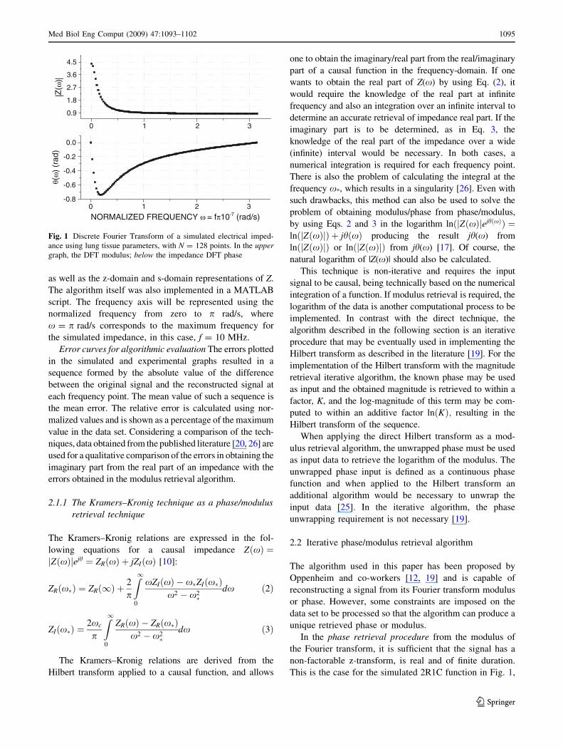
ing the phase hk or modulus ZðxkÞj j:The simulated samples of modulus that serve as input to

the algorithm are all in the frequency-domain at discrete

frequencies and were calculated using a MATLAB script,

1094 Med Biol Eng Comput (2009) 47:1093–1102

123

as well as the z-domain and s-domain representations of Z.

The algorithm itself was also implemented in a MATLAB

script. The frequency axis will be represented using the

normalized frequency from zero to p rad/s, where

x = p rad/s corresponds to the maximum frequency for

the simulated impedance, in this case, f = 10 MHz.

Error curves for algorithmic evaluation The errors plotted

in the simulated and experimental graphs resulted in a

sequence formed by the absolute value of the difference

between the original signal and the reconstructed signal at

each frequency point. The mean value of such a sequence is

the mean error. The relative error is calculated using nor-

malized values and is shown as a percentage of the maximum

value in the data set. Considering a comparison of the tech-

niques, data obtained from the published literature [20, 26] are

used for a qualitative comparison of the errors in obtaining the

imaginary part from the real part of an impedance with the

errors obtained in the modulus retrieval algorithm.

2.1.1 The Kramers–Kronig technique as a phase/modulus

retrieval technique

The Kramers–Kronig relations are expressed in the fol-

lowing equations for a causal impedance ZðxÞ ¼jZðxÞjejh ¼ ZRðxÞ þ jZIðxÞ [10]:

ZRðx�Þ ¼ ZRð1Þ þ2

p

Z1

0

xZIðxÞ � x�ZIðx�Þx2 � x2

�dx ð2Þ

ZIðx�Þ ¼2xc

p

Z1

0

ZRðxÞ � ZRðx�Þx2 � x2

�dx ð3Þ

The Kramers–Kronig relations are derived from the

Hilbert transform applied to a causal function, and allows

one to obtain the imaginary/real part from the real/imaginary

part of a causal function in the frequency-domain. If one

wants to obtain the real part of Z(x) by using Eq. (2), it

would require the knowledge of the real part at infinite

frequency and also an integration over an infinite interval to

determine an accurate retrieval of impedance real part. If the

imaginary part is to be determined, as in Eq. 3, the

knowledge of the real part of the impedance over a wide

(infinite) interval would be necessary. In both cases, a

numerical integration is required for each frequency point.

There is also the problem of calculating the integral at the

frequency x*, which results in a singularity [26]. Even with

such drawbacks, this method can also be used to solve the

problem of obtaining modulus/phase from phase/modulus,

by using Eqs. 2 and 3 in the logarithm lnðjZðxÞjejhðxÞÞ ¼lnðjZðxÞjÞ þ jhðxÞ producing the result jh(x) from

lnðjZðxÞjÞ or lnðjZðxÞjÞ from jh(x) [17]. Of course, the

natural logarithm of |Z(x)| should also be calculated.

This technique is non-iterative and requires the input

signal to be causal, being technically based on the numerical

integration of a function. If modulus retrieval is required, the

logarithm of the data is another computational process to be

implemented. In contrast with the direct technique, the

algorithm described in the following section is an iterative

procedure that may be eventually used in implementing the

Hilbert transform as described in the literature [19]. For the

implementation of the Hilbert transform with the magnitude

retrieval iterative algorithm, the known phase may be used

as input and the obtained magnitude is retrieved to within a

factor, K, and the log-magnitude of this term may be com-

puted to within an additive factor lnðKÞ; resulting in the

Hilbert transform of the sequence.

When applying the direct Hilbert transform as a mod-

ulus retrieval algorithm, the unwrapped phase must be used

as input data to retrieve the logarithm of the modulus. The

unwrapped phase input is defined as a continuous phase

function and when applied to the Hilbert transform an

additional algorithm would be necessary to unwrap the

input data [25]. In the iterative algorithm, the phase

unwrapping requirement is not necessary [19].

2.2 Iterative phase/modulus retrieval algorithm

The algorithm used in this paper has been proposed by

Oppenheim and co-workers [12, 19] and is capable of

reconstructing a signal from its Fourier transform modulus

or phase. However, some constraints are imposed on the

data set to be processed so that the algorithm can produce a

unique retrieved phase or modulus.

In the phase retrieval procedure from the modulus of

the Fourier transform, it is sufficient that the signal has a

non-factorable z-transform, is real and of finite duration.

This is the case for the simulated 2R1C function in Fig. 1,

0 1 2 3

0.9

1.8

2.7

3.6

4.5|Z

(ω)|

0 1 2 3-0.8

-0.6

-0.4

-0.2

0.0

θ(ω

) (r

ad)

NORMALIZED FREQUENCY ω = fπ10-7 (rad/s)

Fig. 1 Discrete Fourier Transform of a simulated electrical imped-

ance using lung tissue parameters, with N = 128 points. In the uppergraph, the DFT modulus; below the impedance DFT phase

Med Biol Eng Comput (2009) 47:1093–1102 1095

123

but impedances used in EIS may not satisfy these con-

straints. As a consequence, for a single data set of modulus

points, there may be more than one corresponding phase

data set, and phase reconstruction will not be unique.

In Fig. 1, it can be observed that the impedance spec-

trum plot is a minimum-phase spectrum of N = 128 points.

As a consequence, the system function of the impedance,

Z(z), has neither zeros on the unit circle nor in conjugate

reciprocal pairs. In addition, it is stable and causal [19] and

all these characteristics are related to the constraints on the

data set for the application of the iterative modulus

retrieval algorithm in the spectrum, so that the calculated

spectrum is unique [12, 16]. Another consequence of the

algorithm use is that the modulus will be reconstructed to

within a scale factor. To obtain such a factor, when pro-

viding experimental phase data sets to retrieve modulus via

software, the algorithm must be previously calibrated.

Since the goal here is to demonstrate the validity of the

technique, the reconstructed spectra can be presented in a

normalized form for comparison purposes between the

reconstructed and the original spectrum.

The ZCole(x) function in Eq. 1 is not a rational function

of polynomials in jx, therefore it is necessary to simulate

the impedance with different a values in the interval (0, 1)

and use the algorithm to reconstruct modulus or phase data

from partial information to find out if the algorithm con-

verges to a unique and correct reconstructed data set. The

conditions to use the algorithm will not be directly tested

with a Cole-type impedance. Considering the analysis

found in the literature for another reconstruction method

using the Kramers–Kronig relations [26], for comparison

purposes, the modulus retrieval algorithm dependence on

the characteristic relaxation constant is evaluated. Different

characteristic relaxation constants are used in Eq. 1 to show

the error performance of the algorithm with respect to

impedance function average relaxation constant, s0.

2.3 Simulation of the fractional order Cole-type

functions

Since many tissues or cell suspensions cannot be modeled

by the ideal Debye-type single relaxation (pole) function,

an impedance function in terms of a distribution function of

relaxation times may be used to evaluate if this structure

(Cole function) is usable with the phase/modulus algo-

rithm. Fuoss and Kirkwood [8] extended the Debye theory

from which a relation can be obtained between the distri-

bution function, G(s) and a transfer function, Z(s), using

ZðsÞ ¼R1

0

GðsÞ1þssds: With this relation between Z(s) and

G(s), the function containing the fractional order term,

ðss0Þa; in the Cole-type impedance function would then be

represented by the following integral of the distribution

function G(s), as originally developed by Cole and Cole [5]

for a dielectric model [5]

ZfracðsÞ ¼R� R1

1þ ðss0Þa¼ ðR� R1Þ

Z1

0

GðsÞ1þ ss

ds ð4Þ

where the function G(s) is the distribution function for the

Cole model and is given by a modified form of the

distribution function as used to obtain the Cole–Cole

function [5]:

GðsÞ ¼ 1

2psin ð1� aÞp½ �

cosh a logð ss0Þ

h i� cos ð1� aÞp½ �

24

35: ð5Þ

It must be recalled that the Cole–Cole function containing

the fractional order term, ðss0Þ1�ainstead of the ðss0Þa; was

originally used in a model for dielectrics [5]. The complete

model developed by Cole and Cole consists of an equation,

an equivalent circuit and a complex impedance circular arc

locus. The Cole–Cole function in Eq. 6 is an empirical

formula that represents the complex dielectric constant of a

large class of liquids and dielectrics [5].

��ðxÞ ¼ �1 þ�0 � �1

1þ ðjxs0Þ1�a ð6Þ

where ��ðxÞ is the complex dielectric permittivity as a

function of frequency x, �0; and �1 are the dielectric

permittivity at x = 0 and at infinite frequency, respec-

tively, and s0 is the generalized relaxation time. The Cole–

Cole function was first obtained by the Cole brothers when

they also introduced the distribution function correspond-

ing to Eq. 6.

For the use of the phase/modulus retrieval algorithm in

ZCole(s) the independent term corresponding to the resis-

tance, R?, causes the frequency dependent function to

satisfy neither the phase nor the modulus retrieval algo-

rithm conditions. However, if the resistance at high fre-

quencies is equal to or even approximately zero, only the

fractional order term Zfrac(s) may be used as input to the

algorithm producing lower errors for a specific interval of

a. In the limit, when a & 0, Zfrac(s) becomes a pure

resistance having minimum phase. For values of a in the

interval (0, 1), the modulus retrieval algorithm is capable of

producing a limited error, and this is going to be demon-

strated in a simulation for different s0 and a.

When the experimental data are initially unknown, it is

not possible to conclude that the algorithm will provide the

desired spectrum and satisfy the algorithm constraints. One

possible solution would be to experimentally determine a

spectrum from a standardized material, and test if this

spectrum satisfies the algorithm constraints. The test could

be implemented, for example, by using an algorithm to

decide if the samples form a minimum-phase sequence.

1096 Med Biol Eng Comput (2009) 47:1093–1102

123

The Schur–Cohn algorithm applied to the sequence in the

time-domain can determine if it has all its zeros inside the

unit circle [18]. For experimental data having a Cole-type

impedance function, if R? = 0, for any s0, or a [ (0, 1),

the phase/modulus retrieval algorithm is not able to retrieve

a unique correct phase or modulus.

There is another method to evaluate if data obtained from

a Cole-type function satisfy the algorithm constraints. This

would be done by sampling the distribution function G(s) in

Eq. 4, and numerically calculating the resulting sum of first-

order processes, and their poles and constants, to obtain the

Cole impedance in a rational form over a limited frequency

interval, in a method called singularity decomposition [23].

ZCole(s) could be represented in this case by a finite sum-

mation of partial fractions having single-poles, that could

produce an approximation to ZCole(x) with a high degree of

accuracy [11]. After this procedure, the approximating

function could be subject to the Schur–Cohn algorithm to

detect if it satisfies the algorithm constraints.

2.4 Algorithm description

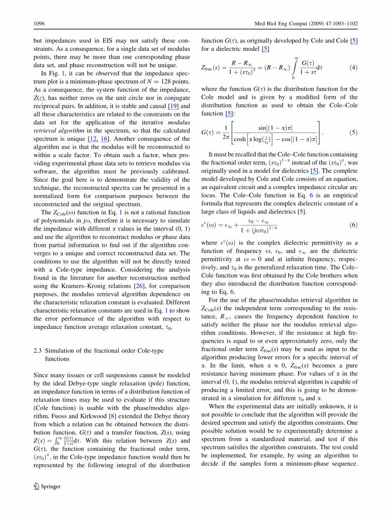
The algorithm is based on the flowchart in Fig. 2. The first

block represents the initialization procedure, where the

modulus in the phase retrieval algorithm can be provided by

electronic means or by simulating the samples, as in this

section. A vector containing the N modulus samples equally

spaced in frequency is saved in YORðkÞj j and a vector that

contains the estimated phase samples is initialized with

random values. The initial impedance Fourier transform

spectrum is a vector represented by the N values, YORðkÞ ¼YORðkÞj jejhest : In the following block, the real part of an

M-point inverse Fast-Fourier transform (IFFT) algorithm is

used to produce a sequence in the time-domain. An M-point

IFFT is used, where the constraint M C 2N guarantees the

algorithm convergence in the determination of the spec-

trum. Only the real part of the M-point IFFT is used because

signal is real in the time-domain [24], and a real signal has

an even Fourier transform modulus, allowing only N sam-

ples to represent the bioimpedance spectrum. In the mod-

ulus retrieval flowchart, phase must be exchanged for

modulus and vice-versa. The fourth block imposes causality

and a finite length constraint on the time-domain sequence,

setting to zero the samples yest(n) that do not belong to the

set Saest ¼ yestð0Þ; . . .; yestðN � 1Þf g: Causality and finite

length are necessary constraints on the sequence to which

one applies the phase-retrieval algorithm. The M-point FFT

of the set Saest produces the first estimate of the impedance

spectrum. This whole process is repeated until the root-

mean square value of the difference between two consec-

utive estimated vectors is less than the loop stopping

parameter value, e. The loop stopping parameter was set

equal to � = 10-6, which is a lower value than the neces-

sary resolution in the modulus or phase values in EIS sys-

tems. The length of input sequences to the algorithm is a

power of 2, since the iterative solution to the problem is

based on the use of uniformly spaced samples [24] and the

Fast-Fourier Transform (FFT) radix-2 algorithm.

2.5 Validation of the algorithm with a known electrical

impedance

In order to validate the algorithm with a practical application,

a multi-channel EIS system developed at the laboratory of

electronic instrumentation at the Santa Catarina State Uni-

versity was used to measure a known transfer impedance

spectrum from an RC circuit. In this case, a circuit formed by

a resistance, R = 1000.35 X in parallel with a capacitance,

C = 1 nF, was used and the modulus retrieval algorithm was

implemented using the acquired phase as the input data. In

the experiment conducted, 28 samples of the spectrum were

acquired with the implemented EIS system and linear

interpolation was used to enlarge the sequence to N = 64

points. Since the circuit is a first-order system, it was con-

sidered that, to demonstrate the applicability of the algorithm

in this case, a linear interpolation was a reasonable choice to

enlarge the sequence size of this spectrum. As a conse-

quence, some of the error produced in the modulus recon-

struction is due to this procedure.

2.5.1 EIS system for the experimental procedure

The hardware used in the experiment is based on an EIS

technique consisting of injecting a current into a load by two

electrodes, measuring its potential by two other electrodes

yest(n)=0

y (n)est

M-pointIFFT

Y (k)=|Y (k)|eOR OR

j (k)est

M-pointFFT

Y (k)=|Y (k)|eest+1 est

j est (k)

|Y (k)| |Y (k)|est OR

Y (k)=|Y (k)|eest+1 OR

j est (k)

simulatedmagnitude

Y| (k)|OR

(k) (k)est random

(k) (k)<-est est+1

Fig. 2 Flowchart representing the processing steps in the phase-

retrieval algorithm for the EIS system

Med Biol Eng Comput (2009) 47:1093–1102 1097

123

and then calculating the transfer impedance. In this circuit,

both phase and modulus are acquired from the load, even

though the purpose of the algorithm is to demonstrate that

one of such acquisition modules may become unnecessary

if the algorithm is applicable. The complete diagram of the

EIS system is shown in Fig. 3. The output of the Voltage-

Controlled-Current-Source (VCCS) is a multi-frequency

sinusoidal current with a constant amplitude of 1 mA.

Injecting current and measured potential are both multi-

plexed into eight output channels. The voltage measure-

ments are done by the Instrumentation Amplifier (IA). The

multi-frequency sine-wave signal (OSC) is generated by a

Direct Digital Synthesizer (DDS). A phase detector circuit

was built to identify the phase shift of the system and then to

supply an output DC voltage proportional to the phase

across the load (RC circuit). The modulus and phase of the

load are both sampled by the kit’s analog-to-digital con-

verters. A graphical interface was developed with MAT-

LAB for acquisition data control by a RS-232 link.

Although the modulus and phase of the load are electroni-

cally obtained, one of the parameters can be used to

experimentally validate the technique by comparing the

estimated and measured values.

3 Results

White gaussian noise was added to the simulated modulus

spectrum of the 2R1C circuit impedance function, causing

the modulus-to-noise ratio (SNR) to be 30, 50, and 80 dB.

In the upper plot of Fig. 4, the phase retrieved by the

algorithm for three different SNR is shown; in the graph

below, the absolute error between the original noiseless

phase and the estimated phase curves are depicted as a

function of the normalized frequency. The error curve for

the phase associated with the noiseless modulus shows the

intrinsic error in the reconstruction without any distortion

caused by noise in the process. Additional noisy simulated

modulus spectra were used to evaluate how many iterations

would be necessary to provide the required estimate. The

number of iterations and the error between the original

simulated signal and the final estimated phase are depicted

in two graphs in Fig. 5 as a function of the SNR, for

sequences of lengths N = 32, 64, 128, 256, 512, 1024.

Fig. 3 EIS system complete diagram for multi-channel evaluation of

electrical bioimpedances

-0.8

-0.4

0.0

0.0 0.7 1.4 2.1 2.8 3.5

0

8

16

RELATIVE ESTIMATION ERROR FOR MNR=30dB RELATIVE ESTIMATION ERROR FOR MNR=50dB RELATIVE ESTIMATION ERROR FOR MNR=80dB

θ (r

ad

)

ORIGINAL SIMULATED PHASE ESTIMATED PHASE WITH MNR=30dB ESTIMATED PHASE WITH MNR=50dB ETIMATED PHASE WITH MNR=80dB

NORMALIZED FREQUENCY (rad/s)

ER

RO

R (

%P

HA

SE)

Fig. 4 In the upper graph, simulated and estimated phase spectrum

under different modulus-to-noise ratios, 30, 50 and 80 dB. Below, the

absolute error as a function of normalized frequency for the depicted

phase

15 30 45 60

05

1015202530

1224364860728496

108

ME

AN

PH

AS

E E

RR

OR

(%

of m

axim

um p

hase

)

SNR (dB)

NU

MB

ER

OF

ITE

RA

TIO

NS

N=32 samples N=64 samples N=128 samples N=256 samples N=512 samples N=1024 samples

Fig. 5 In the upper graph, the necessary number of iterations for the

algorithm to reach e\ 10-6 as a function of SNR and for different

sequence lengths, N = 32, 64, 128, 256, 512,1024; below, the error in

the reconstruction of phase as a function of the SNR and sequence

length, N

1098 Med Biol Eng Comput (2009) 47:1093–1102

123

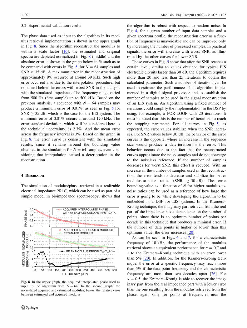
3.1 Cole-type impedance results

A Cole-type function Zfrac is simulated with with a varying

from 0.1 to 1. The Cole impedance function was simulated

with characteristic frequencies Fc = 1/s0 for Fc = 10 kHz,

100 kHz, 1 MHz, and 10 MHz. The frequency interval

used in the Cole function simulation varied from 0 to

Fext = 10 MHz. The phase from the simulated Zfrac(x) was

used as input to the the modulus retrieval algorithm. The

algorithm used N = 128 samples equally spaced in the

frequency-domain. The mean error in the modulus recon-

struction is calculated by the absolute value of the differ-

ence between normalized simulated and reconstructed

modulus represented in % and is shown in Fig. 6. The

curves in Fig. 6 are the same for different Fext and Fc, if the

distance Fext - Fc is kept constant. The resulting distances

in the simulation are 3, 2, and 1 decades and Fext = Fc.

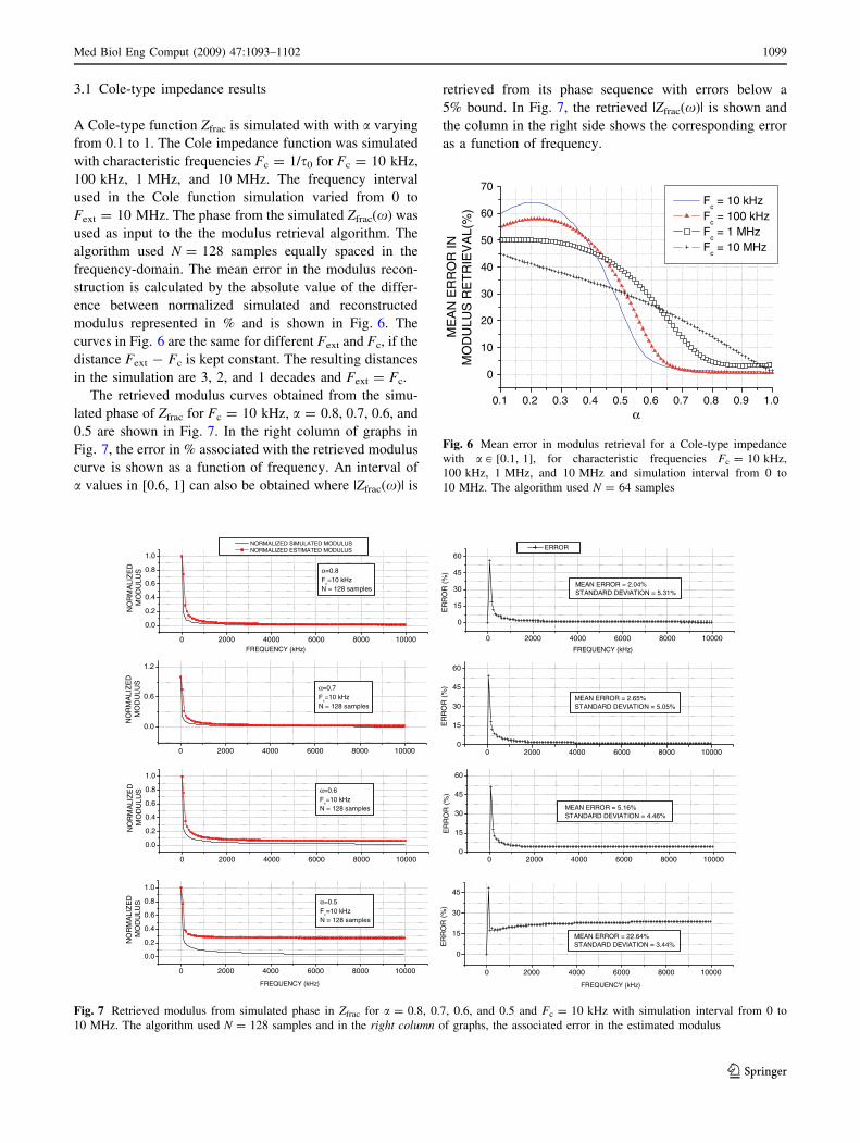
The retrieved modulus curves obtained from the simu-

lated phase of Zfrac for Fc = 10 kHz, a = 0.8, 0.7, 0.6, and

0.5 are shown in Fig. 7. In the right column of graphs in

Fig. 7, the error in % associated with the retrieved modulus

curve is shown as a function of frequency. An interval of

a values in [0.6, 1] can also be obtained where |Zfrac(x)| is

retrieved from its phase sequence with errors below a

5% bound. In Fig. 7, the retrieved |Zfrac(x)| is shown and

the column in the right side shows the corresponding error

as a function of frequency.

0.1 0.2 0.3 0.4 0.5 0.6 0.7 0.8 0.9 1.0

0

10

20

30

40

50

60

70 F

c = 10 kHz

Fc = 100 kHz

Fc = 1 MHz

Fc = 10 MHz

ME

AN

ER

RO

R IN

MO

DU

LUS

RE

TR

IEV

AL(

%)

α

Fig. 6 Mean error in modulus retrieval for a Cole-type impedance

with a [ [0.1, 1], for characteristic frequencies Fc = 10 kHz,

100 kHz, 1 MHz, and 10 MHz and simulation interval from 0 to

10 MHz. The algorithm used N = 64 samples

0 2000 4000 6000 8000 10000

0.0

0.6

1.2

0 2000 4000 6000 8000 100000

15

30

45

60

0 2000 4000 6000 8000 10000

0.0

0.2

0.4

0.6

0.8

1.0

0 2000 4000 6000 8000 10000

0

15

30

45

0 2000 4000 6000 8000 10000

0.0

0.2

0.4

0.6

0.8

1.0

0 2000 4000 6000 8000 100000

15

30

45

60

0 2000 4000 6000 8000 10000

0.0

0.2

0.4

0.6

0.8

1.0

0 2000 4000 6000 8000 10000

0

15

30

45

60

α=0.7 F

c=10 kHz

N = 128 samples

NORMALIZED SIMULATED MODULUS NORMALIZED ESTIMATED MODULUS

NO

RM

ALI

ZE

D

MO

DU

LUS

MEAN ERROR = 2.65%STANDARD DEVIATION = 5.05%

ERROR

ER

RO

R (

%)

α=0.5 F

c=10 kHz

N = 128 samples

NO

RM

ALI

ZE

D

MO

DU

LUS

MEAN ERROR = 22.64%STANDARD DEVIATION = 3.44%E

RR

OR

(%

)

α=0.6F

c=10 kHz

N = 128 samples

NO

RM

ALI

ZE

D

MO

DU

LUS

MEAN ERROR = 5.16%STANDARD DEVIATION = 4.46%

ER

RO

R (

%)

α=0.8 F

c=10 kHz

N = 128 samples

NO

RM

ALI

ZE

D

MO

DU

LUS

FREQUENCY (kHz) FREQUENCY (kHz)

FREQUENCY (kHz)

MEAN ERROR = 2.04%STANDARD DEVIATION = 5.31%

FREQUENCY (kHz)

ER

RO

R (

%)

Fig. 7 Retrieved modulus from simulated phase in Zfrac for a = 0.8, 0.7, 0.6, and 0.5 and Fc = 10 kHz with simulation interval from 0 to

10 MHz. The algorithm used N = 128 samples and in the right column of graphs, the associated error in the estimated modulus

Med Biol Eng Comput (2009) 47:1093–1102 1099

123

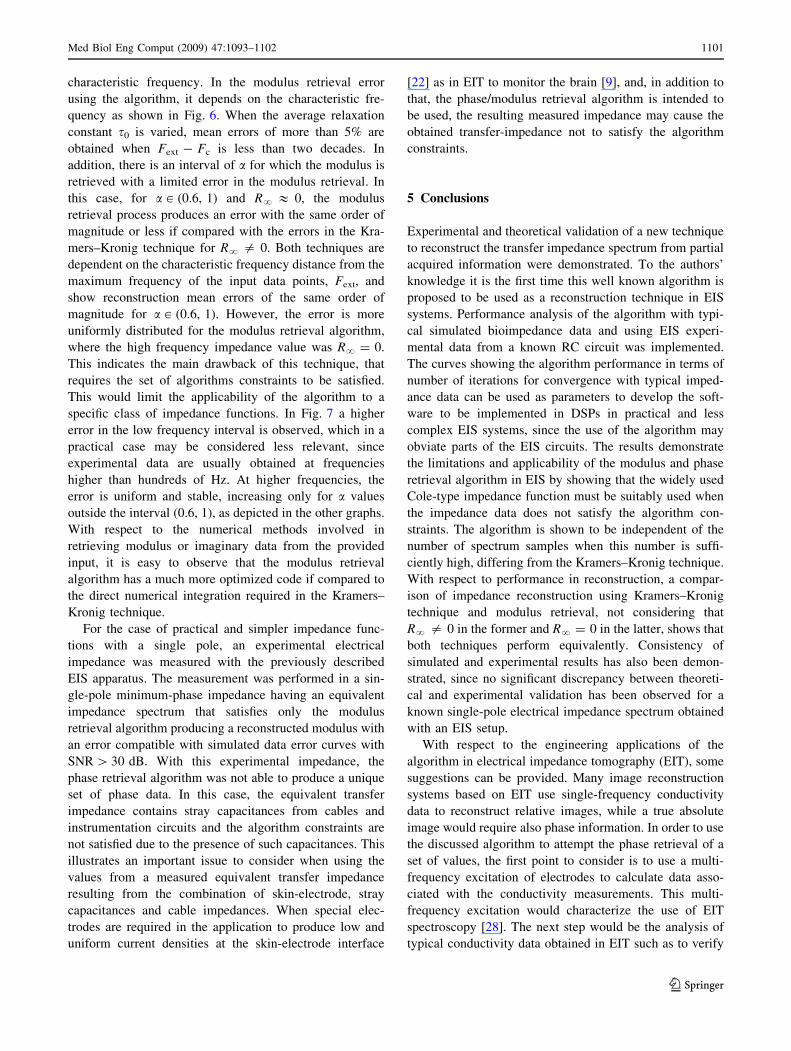
3.2 Experimental validation results

The phase data used as input to the algorithm in its mod-

ulus retrieval implementation is shown in the upper graph

in Fig. 8. Since the algorithm reconstruct the modulus to

within a scale factor [16], the estimated and original

spectra are depicted normalized in Fig. 8 (middle) and the

absolute error is shown in the graph below in % such as to

be compared with errors in Fig. 5, for N = 64 samples and

SNR C 35 dB. A maximum error in the reconstruction of

approximately 9% occurred at around 39 kHz. Such high

error occurred also due to the interpolation procedure, but

remained below the errors with worst SNR in the analysis

with the simulated impedance. The frequency range varied

from 500 Hz (first sample) up to 500 kHz. Based on the

previous analysis, a sequence with N = 64 samples may

produce a minimum error of 0.01%, as seen in Fig. 5 for

SNR C 35 dB, which is the case for the EIS system. The

minimum error of 0.01% occurs at around 170 kHz. The

error standard deviation, which will be considered here as

the technique uncertainty, is 2.3%. And the mean error

across the frequency interval is 3%. Based on the graph in

Fig. 8, the error curve is consistent with the simulated

results, since it remains around the bounding value

obtained in the simulation for N = 64 samples, even con-

sidering that interpolation caused a deterioration in the

reconstruction.

4 Discussion

The simulation of modulus/phase retrieval in a realizable

electrical impedance 2R1C, which can be used as part of a

simple model in bioimpedance spectroscopy, shows that

the algorithm is robust with respect to random noise. In

Fig. 4, for a given number of input data samples and a

given spectrum profile, the reconstruction error as a func-

tion of frequency is unavoidable and can be improved only

by increasing the number of processed samples. In practical

signals, the error will increase with worst SNR, as illus-

trated by the other curves for lower SNR.

Those curves in Fig. 5 show that after the SNR reaches a

certain level, similar to values obtained for typical EIS

electronic circuits larger than 30 dB, the algorithm requires

more than 20 and less than 25 iterations to obtain the

calculated parameter. Such a number of iterations can be

used to estimate the performance of an algorithm imple-

mented in a digital signal processor and to establish the

number of samples to be used in the signal reconstruction

of an EIS system. An algorithm using a fixed number of

iterations could simplify the implementation in the DSP by

using, for example, a FOR-LOOP with 20 iterations. It

must be noted that this is the number of iterations to reach

the stopping parameter. For all curves in Fig. 5, as

expected, the error values stabilize when the SNR increa-

ses. For SNR values below 30 dB, the behavior of the error

curves is the opposite, where an increase in the sequence

size would produce a deterioration in the error. This

behavior occurs due to the fact that the reconstructed

curves approximate the noisy samples and do not converge

to the noiseless reference. If the number of samples

decreases for worst SNR, this effect is reduced. With an

increase in the number of samples used in the reconstruc-

tion, the error tends to decrease and stabilize for better

modulus-to-noise ratios (SNR C 30 dB). The error

bounding value as a function of N for higher modulus-to-

noise ratios can be used as a reference of how large the

error is going to be while developing the algorithm to be

embedded in a DSP for EIS systems. In the Kramers–

Kronig technique, the imaginary part retrieval from the real

part of the impedance has a dependence on the number of

points, since there is an optimum number of points per

decade in this technique that produces a minimal error. If

the number of data points is higher or lower than this

optimum value, the error increases [20].

As can be seen in Figs. 6 and 7, for a characteristic

frequency of 10 kHz, the performance of the modulus

retrieval shows an equivalent performance for a = 0.7 and

1 to the Kramers–Kronig technique with an error lower

than 5% [20]. In addition, for the Kramers–Kronig tech-

nique, the error at a specific frequency may reach more

than 5% if the data point frequency and the characteristic

frequency are more than two decades apart [26]. For

a = 0.5, the Kramers–Kronig is able to recover the imag-

inary part from the real impedance part with a lower error

than the one resulting from the modulus retrieved from the

phase, again only for points at frequencies near the

0.3

0.6

0.9

-1.2

-0.8

-0.4

0.0

0 50 100 150 200 250 300 350 400 450 500 5500

5

10

ACQUIRED INTERPOLATED MODULUS ESTIMATED MODULUS

NO

RM

ALI

ZE

D

MO

DU

LUS

PH

AS

E (

rad)

ACQUIRED INTERPOLATED PHASE WITH 64 SAMPLES USED AS INPUT DATA

ME AN MODULUS ERROR |YOR-Yest| (%)

MO

DU

LUS

ER

RO

R (

%)

FREQUENCY (kHz)

Fig. 8 In the upper graph, the acquired interpolated phase used as

input to the algorithm with N = 64; In the second graph, the

normalized acquired and estimated modulus; below, the relative error

between estimated and acquired modulus

1100 Med Biol Eng Comput (2009) 47:1093–1102

123

characteristic frequency. In the modulus retrieval error

using the algorithm, it depends on the characteristic fre-

quency as shown in Fig. 6. When the average relaxation

constant s0 is varied, mean errors of more than 5% are

obtained when Fext - Fc is less than two decades. In

addition, there is an interval of a for which the modulus is

retrieved with a limited error in the modulus retrieval. In

this case, for a [ (0.6, 1) and R? & 0, the modulus

retrieval process produces an error with the same order of

magnitude or less if compared with the errors in the Kra-

mers–Kronig technique for R? = 0. Both techniques are

dependent on the characteristic frequency distance from the

maximum frequency of the input data points, Fext, and

show reconstruction mean errors of the same order of

magnitude for a [ (0.6, 1). However, the error is more

uniformly distributed for the modulus retrieval algorithm,

where the high frequency impedance value was R? = 0.

This indicates the main drawback of this technique, that

requires the set of algorithms constraints to be satisfied.

This would limit the applicability of the algorithm to a

specific class of impedance functions. In Fig. 7 a higher

error in the low frequency interval is observed, which in a

practical case may be considered less relevant, since

experimental data are usually obtained at frequencies

higher than hundreds of Hz. At higher frequencies, the

error is uniform and stable, increasing only for a values

outside the interval (0.6, 1), as depicted in the other graphs.

With respect to the numerical methods involved in

retrieving modulus or imaginary data from the provided

input, it is easy to observe that the modulus retrieval

algorithm has a much more optimized code if compared to

the direct numerical integration required in the Kramers–

Kronig technique.

For the case of practical and simpler impedance func-

tions with a single pole, an experimental electrical

impedance was measured with the previously described

EIS apparatus. The measurement was performed in a sin-

gle-pole minimum-phase impedance having an equivalent

impedance spectrum that satisfies only the modulus

retrieval algorithm producing a reconstructed modulus with

an error compatible with simulated data error curves with

SNR [ 30 dB. With this experimental impedance, the

phase retrieval algorithm was not able to produce a unique

set of phase data. In this case, the equivalent transfer

impedance contains stray capacitances from cables and

instrumentation circuits and the algorithm constraints are

not satisfied due to the presence of such capacitances. This

illustrates an important issue to consider when using the

values from a measured equivalent transfer impedance

resulting from the combination of skin-electrode, stray

capacitances and cable impedances. When special elec-

trodes are required in the application to produce low and

uniform current densities at the skin-electrode interface

[22] as in EIT to monitor the brain [9], and, in addition to

that, the phase/modulus retrieval algorithm is intended to

be used, the resulting measured impedance may cause the

obtained transfer-impedance not to satisfy the algorithm

constraints.

5 Conclusions

Experimental and theoretical validation of a new technique

to reconstruct the transfer impedance spectrum from partial

acquired information were demonstrated. To the authors’

knowledge it is the first time this well known algorithm is

proposed to be used as a reconstruction technique in EIS

systems. Performance analysis of the algorithm with typi-

cal simulated bioimpedance data and using EIS experi-

mental data from a known RC circuit was implemented.

The curves showing the algorithm performance in terms of

number of iterations for convergence with typical imped-

ance data can be used as parameters to develop the soft-

ware to be implemented in DSPs in practical and less

complex EIS systems, since the use of the algorithm may

obviate parts of the EIS circuits. The results demonstrate

the limitations and applicability of the modulus and phase

retrieval algorithm in EIS by showing that the widely used

Cole-type impedance function must be suitably used when

the impedance data does not satisfy the algorithm con-

straints. The algorithm is shown to be independent of the

number of spectrum samples when this number is suffi-

ciently high, differing from the Kramers–Kronig technique.

With respect to performance in reconstruction, a compar-

ison of impedance reconstruction using Kramers–Kronig

technique and modulus retrieval, not considering that

R? = 0 in the former and R? = 0 in the latter, shows that

both techniques perform equivalently. Consistency of

simulated and experimental results has also been demon-

strated, since no significant discrepancy between theoreti-

cal and experimental validation has been observed for a

known single-pole electrical impedance spectrum obtained

with an EIS setup.

With respect to the engineering applications of the

algorithm in electrical impedance tomography (EIT), some

suggestions can be provided. Many image reconstruction

systems based on EIT use single-frequency conductivity

data to reconstruct relative images, while a true absolute

image would require also phase information. In order to use

the discussed algorithm to attempt the phase retrieval of a

set of values, the first point to consider is to use a multi-

frequency excitation of electrodes to calculate data asso-

ciated with the conductivity measurements. This multi-

frequency excitation would characterize the use of EIT

spectroscopy [28]. The next step would be the analysis of

typical conductivity data obtained in EIT such as to verify

Med Biol Eng Comput (2009) 47:1093–1102 1101

123

if the obtained data satisfy the algorithm constraints. For

validation purposes of this application, at least one set of

data from the phase and magnitude (or the imaginary and

real part) of conductivity should be obtained. In the case of

difference EIT, the conductivity change and its corre-

sponding phase would be calculated. In general, the algo-

rithm may be employed in the retrieval of the phase from

the estimated difference conductivities in EIT in each

reconstructed frame. Given that the proposed algorithm is

computationally optimized being based on Fast-Fourier

transform algorithms, and the use of the algorithm in the

data set is permissible, the first potential use of the algo-

rithm in difference EIT reconstruction techniques, as, for

example, in the technique described in [6], could be the

application of phase-retrieval in the conductivity change

data.

As a work to be developed in the future remains the

analysis of the characterization of biological tissues data

under the standpoint of a minimum-phase sequence, and

also how skin-electrode, stray capacitances and cable

impedances may influence the algorithm response. The

results shown in this work have been obtained mainly by

simulation, and demonstrate that the reconstruction may

work with irrational functions, even considering that the

algorithm was originally developed for rational functions.

Experimental data based on the systematic analysis of

biological tissue in other EIS and EIT systems will also be

analyzed in a future work.

References

1. Aberg P, Nicander I, Hansson J, Geladi P, Holmgren U, Ollmar S

(2004) Skin cancer identification using multifrequency electrical

impedance—a potential screening tool. IEEE Trans Biomed Eng

51:2097–2102

2. Bertemes-Filho P (2002) Tissue characterisation using an

Impedance Spectroscopy Probe. PhD Thesis, The University of

Sheffield, UK

3. Brown BH (2003) Electrical impedance tomography (EIE): a

review. J Med Eng Technol 3:97–108

4. Cole KS (1940) Permeability and impermeability of cell mem-

branes for ions. In: Proceedings of the Cold Spring Harbor

Symposia, vol 8, pp 110–122

5. Cole KS, Cole RH (1941) Dispersion and absorption in dielec-

trics: I Alternating current characteristics. J Chem Phys 9:97–108

6. Dai T, Soleimani M, Adler A (2008) EIT image reconstruction

with four dimensional regularization. Med Biol Eng Comput

46(9):889–999

7. Debye P (1929–Reprint:1965) Polar molecules. Dover Publica-

tions, New York

8. Fuoss R, Kirkwood JG (1941) Electrical properties of solids.

VIII. Dipole moments in polyvinyl chloride-diphenyl systems.

J Am Chem Soc 63(2):385–394

9. Gilad O, Horesh L, Holder DS (2007) Design of electrodes and

current limits for low frequency electrical impedance tomography

of the brain. Med Biol Eng Comput 45(7):621–633

10. Grimnes S, Martinsen OG (2008) Bioimpedance and bioelec-

tricity: basics, 2nd edn. Academic Press, London

11. Haschka M, Krebs V (2007) Advances in fractional calculus the-

oretical developments and applications in physics and engineering,

chap. A direct approximation of fractional cole-cole systems by

ordinary first-order processes. Springer, Netherlands, pp 257–270

12. Hayes M, Lin JS, Oppenheim AV (1980) Signal reconstruction

from phase or magnitude. IEEE Trans Acoust Speech ASSP

28:672–680

13. Holder DS (2004) Electrical impedance tomography: methods,

history and applications, 1st edn. Taylor and Francis, New York

14. McAdams ET, Jossinet J (1996) Problems in equivalent circuit

modelling of the electrical properties of biological tissues. Bio-

electrochem Bioenerg 40:147–152

15. Nebuya S, Noshiro M, Brown BH, Smallwood RH, Milnes P

(2002) Accuracy of an optically isolated tetra-polar impedance

measurement system. Med Biol Eng Comput 40:647–650

16. Oppenheim AV, Lin JS, Curtis S (1983) Signal synthesis and

reconstruction from partial Fourier domain information. J Opt

Soc Am 73:1413–1420

17. Proakis JG, Manolakis DK (1996) Discrete-time signal process-

ing, 3rd edn. Prentice-Hall, Boston, pp 617–681

18. Proakis JG, Manolakis DK (1996) Discrete-time signal process-

ing, 3rd edn. Prentice-Hall, Boston, pp 213–215

19. Quartieri T, Oppenheim AV (1981) Iterative techniques for

minimum phase signal reconstruction from phase or magnitude.

IEEE Trans Acoust Speech ASSP 29:1187–1193

20. Riu PJ, Lapaz C (1999) Practical limits of the Kramers-Kronig

relationships applied to experimental bioimpedance data. Ann

NY Acad Sci 873:374–380

21. Seoane F, Ferreira J, Sanchez JJ, Bragos R (2008) An analog

front-end enables electrical impedance spectroscopy system on-

chip for biomedical applications. Physiol Meas 29:267–278

22. Suesserman MF, Spelman FA, Rubinstein JT (1991) In vitro mea-

surement and characterization of current density profiles produced by

non-recessed, simple-recessed, and radially varying recessed stim-

ulating electrodes. IEEE Trans Biomed Eng 38(5):401–408

23. Sun H, Charef A, Tsao Y, Onaral B (1992) Analysis of polari-

zation dynamics by singularity decomposition method. Ann

Biomed Eng 20:321–335

24. Tom VT, Quartieri T, Hayes MH, McClellan JH (1981) Con-

vergence of iterative nonexpansive signal reconstruction algo-

rithms. IEEE Trans Acoust Speech ASSP 29:1052–1058

25. Tribolet J (1977) A new phase unwrapping algorithm. IEEE

Trans Acoust Speech ASSP-25:170–177

26. Waterworth AR (2000) Data analysis techniques of measured

biological impedance. PhD Thesis, The University of Sheffield, UK

27. Yang Y, Wang J (2005) A Design of bioimpedance spectrometer

for early detection of pressure ulcer. In: Proceedings of the IEEE

engineering in medicine and biology 27th annual conference.

Shanghai, China, pp 6602–6604

28. Yerworth RJ, Bayford RH, Brown B, Milnes PM, Conway M,

Holder DS (2003) Electrical impedance tomography spectros-

copy (EITS) for human head imaging. Physiol Meas 24:477–489

1102 Med Biol Eng Comput (2009) 47:1093–1102

123