arX

iv:c

s/06

0203

1v1

[cs

.AI]

8 F

eb 2

006

Journal of Ma hine Learning Resear h () Submitted ; PublishedClassifying Signals With Lo al Classi�ersWit Jaku zun jaku zun�mini.pw.edu.plFa ulty of Mathemati s and Information S ien eWarsaw University of Te hnologyPl. Polite hniki 100-661 Warsaw, POLANDEditor: Abstra tThis paper deals with the problem of lassifying signals. The new method for building so alled lo al lassi�ers and lo al features is presented. The method is a ombination of thelifting s heme and the support ve tor ma hines. Its main aim is to produ e e�e tive andyet omprehensible lassi�ers that would help in understanding pro esses hidden behind lassi�ed signals. To illustrate the method we present the results obtained on an arti� ialand a real dataset.Keywords: lo al feature, lo al lassi�er, lifting s heme, support ve tor ma hines, signalanalysis1. Introdu tionMany lassi� ation algorithms su h as arti� ial neural networks indu e lassi�ers whi h havegood a ura y but do not give an insight into the real pro ess whi h is hidden behind theproblem. Although predi tions are made with high pre ision su h lassi�ers do not answerthe question \Why?". Even algorithms su h as de ision trees or rule indu ers very oftenprodu e enormous lassi�ers. Their analysis is almost intra table by the human mind. It iseven worse when these algorithms are used for problems of signal lassi� ation. In pra ti egood a ura y without an explanation of the lassi� ation pro ess is useless.In this arti le we des ribe an approa h whi h an help in building lassi�ers whi hare not only very a urate but also omprehensible. The method is based on the idea ofthe lifting s heme (Sweldens, 1998). The lifting s heme is used for al ulating expansion oeÆ ients of analysed signals using biorthogonal wavelet bases. The biggest advantageof this method is that it uses only spatial domain in ontrast to the lassi al approa h(Daube hies, 1992) in whi h the frequen y domain is used. As originally lifting s heme didnot give us enough freedom in in orporating adaptation we used its modi�ed version alledupdate-�rst (Claypoole et al., 1998).Assume we a t in spa e R

N spanned by a biorthogonal base {φi}ni=1 and {φi}

ni=1. Ve tors

{φi}ni=1 and {φi}

ni=1 are biorthogonal in the sense that

⟨

φi, φj

⟩

= δijwhere δij = 1 if i = j and 0 otherwise. © Wit Jaku zun.

Wit Jaku zunEa h ve tor x ∈ RN an be expressed in the following way

x =n∑

i=1

αiφi (1)where αi =⟨

φi, x⟩ are expansion oeÆ ients. Very important feature of ve tors {φi}

ni=1is that they an be nonzero only for several indi es. It implies that for al ulating ⟨φi, x⟩only a part of the ve tor x is needed. This feature is alled lo ality.The aim of the method presented in this arti le is to �nd su h an expansion (1) byimpli itly onstru ting biorthogonal base {(φi, φi)}

ni=1, that oeÆ ients αi =

⟨

φi, x⟩ are asdis riminative as possible for lassi�ed signals.More spe i� ally we assume that a training set X = {(xi, yi) : xi ∈ R

n, yi ∈ {−1,+1}}li=1is given. For ea h base ve tor φj we get a ve tor of expansion oeÆ ients αj ∈ R

l

αj(i) =⟨

φj, xi

⟩For ea h su h ve tor we an �nd a number bj ∈ R alled bias for whi hsgn(αj(i) + bj) = yifor as many indi es i ∈ {1, 2, . . . , l} as possible.For al ulating expansion oeÆ ients we used the idea of support ve tor ma hines (SVM)introdu ed by Vapnik (1998)1. SVM proved to be one of the best lassi�er indu ers. Com-bining the power of SVM and the lo ality feature of the designed base we were able to build lassi�ers with a very good lassi� ation a ura y and whi h are also easily interpreted.We present experiments obtained for an arti� ial datasets and a real dataset. The arti� ialdatasets allowed us to verify our method and to better understand its features. Experiments ondu ted on the real dataset proofed usefulness of the method for real appli ations.2. Outline of the paperThe paper is divided into two main parts and the appendix. The �rst part is devotedto a des ription of the method and onsists of three subparts. First we present a generaloutline of the method next we introdu e some notation that will be used in next part thatgives detailed des ription of the method. The �rst part of the paper we end with a shortsummary of the presented method. In the se ond part of the paper we present a results ofthe experiments ondu ted both on the arti� ial and the real dataset. In the appendix weshow how to eÆ iently solve optimisation problems that arise in the method.3. Method des riptionIn this se tion we will des ribe the new method for designing dis riminative biorthogonalbases for signal lassi� ation. In fa t we will be omputing only expansion oeÆ ients of1. More pre isely, we used PSVM a variant of SVM alled proximal support ve tor ma hines(Fung and Mangasarian, 2001). 2

Classifying signals With Lo al Classifierssome impli itly de�ned dis riminative biorthogonal base. The method is a ombinationof update-�rst version of the lifting s heme (Claypoole et al., 1998) and proximal supportve tor ma hines (Fung and Mangasarian, 2001).3.1 Outline of the methodThe method is based on the Lifting S heme that is very general and easily modi�ed methodfor omputing expansion oeÆ ients of analysed signal with respe t to biorthogonal base.The method is iterative and ea h iteration is divided into three steps• SPLIT - Signal is splitted into two subsignals ontaining even and odd indi es.• UPDATE - Coarse approximation of analysed signal is omputed from subsignals.• PREDICT - Wavelet oeÆ ients are al ulated using oarse approximation andsubsignal ontaining even indi ies. Those oeÆ ients are simply inner produ ts be-tween a weight ve tor and small part of oarse approximation and even subsignal. Weused proximal support ve tor Ma hines (Fung and Mangasarian, 2001) to al ulatethe weight ve tor. As PSVM is the pro edure for generating lassi�ers we de ided to all obtained expansion oeÆ ients dis riminative wavelet oeÆ ients.Coarse approximation is used as an input for next iteration. As the oarse approximation istwi e shorter than original signal the number of iterations is bounded from above by ln(N)where N is the length of the analysed signal.3.2 NotationAssume we are given a training set X

X ={

(xi, yi) ∈ RN×{−1,+1} : i = 1, . . . , l

}where N = 2n for some n ∈ N. Ve tors xi are sampled versions of signals we want toanalyse and yi ∈ {−1,+1} are labels.Having set X we reate two matri esA =

xT1...

xTl

∈ R

l×NandY =

y1 . . .yl

Let I = {i1, . . . , ik} be a set of integer numbers (indi es). We will use the following short-hand notation for a essing indi es I of a ve tor x ∈ RN .

x(I) = (x(i1), . . . ,x(ik))3

Wit Jaku zunWe will also use a spe ial notation for a essing odd and even indi es of a ve tor x ∈ RN

xo = (x(1),x(3), . . . ,x(N − 1)) for odd indi esxe = (x(2),x(4), . . . ,x(N)) for even indi esFinally we will use the following symbols for spe ial ve tors

e =

1...1

ande1 =

10...0

The dimensionality of the ve tors e and e1 will be lear from the ontext.3.3 Three main stepsAs we have mentioned before the method we propose is iterative and ea h iteration step2 onsists of three substeps.3.3.1 First substep - SplitMatrix A is splitted into matri es Ao (odd olumns) and Ae (even olumns)Ao =

xoT1...

xoTl

∈ R

l×N/2andAe =

xeT1...

xeTl

∈ R

l×N/23.3.2 Se ond substep - UpdateHaving matri es Ao ∈ Rl×N/2 and Ae ∈ R

l×N/2 we reate matrix C ∈ Rl×N/2

C =1

2(Ao + Ae) =

cT1...

cTl

This matrix will be alled oarse approximation of matrix A.2. We also use a name de omposition level for iteration step.4

Classifying signals With Lo al Classifiers3.3.3 Third substep - Predi tIn the last step we al ulate dis riminative wavelet oeÆ ients. For ea h olumn k of matrixAe (k = 1, 2, . . . , N/2) we reate matrix A

k ∈ Rl×Lk+1 where Lk ∈ N is an even numberand a parameter of the method.3

Ak =

xe1(k) −ck1... ...

xel(k) −ckl

where cki = ci(Ik) and Ik is a set of indi es sele ted in the following way

• If 1 ≤ k < Lk

2then Ik = {1, 2, . . . , Lk}

• If Lk

2≤ k < N

2− Lk

2then Ik = {k − Lk

2+ 1, . . . , k + Lk

2}

• If N2− Lk

2≤ k ≤ N

2then Ik = {N

2− Lk + 1, . . . , N

2}At this point our method an be splitted into two variants: regularised and non-regularised.

• regularised variant: This variant uses PSVM approa h to �nd the optimal weightve tor wk ∈ R

Lk+1. A ording to Fung and Mangasarian (2001) optimal wk is thesolution of the following optimisation problem

minwk,γk,ξk

1

2‖wk‖2

2 +1

2γ2

k +νk

2‖ξk‖

22 (2)subje t to onstraints

Y(Akw

k − γke) + ξk = e (3)where ξk is the error ve tor and νk ≥ 0.• non-regularised variant: Similarly as in regularised variant the optimal weightve tor w

k ∈ RLk is given by solving the following optimisation problem

minwk,γk,ξk

1

2‖wk‖2

2 +1

2γ2

k +νk

2‖ξk‖

22 (4)subje t to onstraints

Y

(

Ak

(

1

wk

)

− γke

)

+ ξk = e (5)where ξk is the error ve tor and νk ≥ 0. The only di�eren e to the previous variantis that dimensionality of wk is Lk instead of Lk + 1 and xei(k) is multiplied by one.In this variant we an also add some extra onstraints su h that in ase of polynomialsignals (up to some degree pk) we will get wavelet oeÆ ients equal to zero. These onstraints an be written in the following way

Bkw

k = e1 (6)3. In presented experiments we assumed that Lk = L for some onstant L ∈ N.5

Wit Jaku zunwhere e1 ∈ Rpk and B

k onsists of the �rst pk rows of the Vandermonde matrix forsome knots t1, t2, . . . , tLk. For more details on how to sele t knots we refer reader to(Claypoole et al., 1998) and (Fern�andez et al., 1996).The additional onstraints ould be useful if analysed signals are superposition of poly-nomial and some other possibly interesting omponent. They imply that polynomialpart of the analysed signal is eliminated and thus interesting omponent will play abigger role in onstru ting dis riminative wavelets oeÆ ients. Also onstru ted basewill have similar properties to the standard wavelet base. In the appendix the reader an �nd information on how to eÆ iently solve this extended optimisation problem.We have not used this variant in our experiments but present it for ompletenessreasons.Having optimal weight ve tor w

k we an al ulate ve tor dk ∈ R

l of dis riminativewavelet oeÆ ients using the following equations• regularised variant

dk(i) =

⟨

wk,

(

xei(k)

−cki

)⟩

i = 1, 2, . . . , l

• non-regularised variantd

k(i) = xei(k) −⟨

wk, ck

i

⟩

i = 1, 2, . . . , lwhere 〈·, ·〉 is a standard inner produ t.In a result we obtain a matrix D ∈ Rl×N/2

D =(

d1 · · · d

N/2)3.4 Iteration stepThe whole algorithm an be written in the following form

• Let M be the number of iterations (de omposition levels).• Let A0=A

• For m = 1, . . . ,M do{ Cal ulate Cm ∈ Rl× N

2m and Dm ∈ Rl× N

2m by applying three steps des ribed inthe previous se tion to the matrix Am−1.{ Set Am = Cm.The output of the algorithm will be a set of matri es CM ,D1, . . . ,DM . On the basis ofthese matri es we reate the new training setXnew =

{

(xnewi , yi) ∈ R

N×{−1,+1} : i = 1, . . . , l} (7)where new examples are reated by merging rows of matri es CM ,D1, . . . ,DM .6

Classifying signals With Lo al Classifiers3.5 Method summaryWe introdu ed the method that maps the set of signals X into a new set of signals Xnew.In the presented setting this map is a linear and invertible fun tion f : RN → R

N

f(x) = (cTM ,dT

1 , . . . ,dTM )where

cM ∈ RN

2M

dM ∈ RN

2M...d2 ∈ R

N

4

d1 ∈ RN

2are al ulated by the method. With in reasing m more and more samples from the originalsignal is used to al ulate expansion oeÆ ients. For example if we set Lk ≡ L for all kthen to al ulate ve tor dk L2m samples of the original signal will be used.Here we present two most important features of the method

• Motivation for the method is that only a small part of the signals is important in lassi� ation pro ess. The method tries to identify this important part adaptively.• Exploiting natural parallelism ( al ulating d

k is ompletely independent for ea h k)and Sherman-Morrison-Woodbury formula (Gene H. Golub, 1996) the method anbe implemented very eÆ iently. In the appendix A we show how to properly solveoptimisation problems that appears in our method.4. Appli ationsThis se tion ontains des ription of possible appli ations of the proposed method. It isdivided into two parts. In the �rst part we present an illustrative example of analysingarti� ial signals with the proposed method. In the se ond part we present the results forthe real dataset.4.1 Arti� ial datasetsHere we present results obtained on arti� ial datasets: Waveform and Shape.4.1.1 Dataset des riptionWaveform is a three lass arti� ial dataset (Breiman, 1998). For our experiments we useda slightly modi�ed version (Saito, 1994). Three lasses of signals were generated using the7

Wit Jaku zunfollowing formulasx1(i) = uh1(i) + (1 − u)h2(i) + ǫ(i) lass 1 (8)x2(i) = uh1(i) + (1 − u)h3(i) + ǫ(i) lass 2 (9)x3(i) = uh2(i) + (1 − u)h3(i) + ǫ(i) lass 3 (10)(11)where i = 1, 2, . . . , 32, u is a uniform random variable on the interval (0, 1), ǫ(i) is a standardnormal variable and

h1(i) = max(6 − |i − 7|, 0)

h2(i) = h1(i − 8)

h3(i) = h1(i − 4)4.1.2 Analysis-4

-2

0

2

4

6

8

0 5 10 15 20 25 30 35

-4

-2

0

2

4

6

8

10

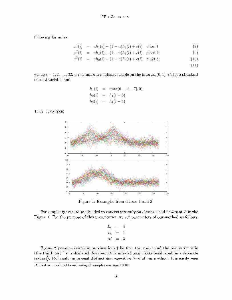
0 5 10 15 20 25 30 35Figure 1: Examples from lasses 1 and 2For simpli ity reasons we de ided to on entrate only on lasses 1 and 2 presented in theFigure 1. For the purpose of this presentation we set parameters of our method as followsLk = 4

νk = 1

M = 3Figure 2 presents oarse approximations (the �rst two rows) and the test error ratio(the third row) 4 of al ulated dis riminative wavelet oeÆ ients (evaluated on a separatetest set). Ea h olumn present distin t de omposition level of our method. It is easily seen4. Test error ratio obtained using all samples was equal 0.10.8

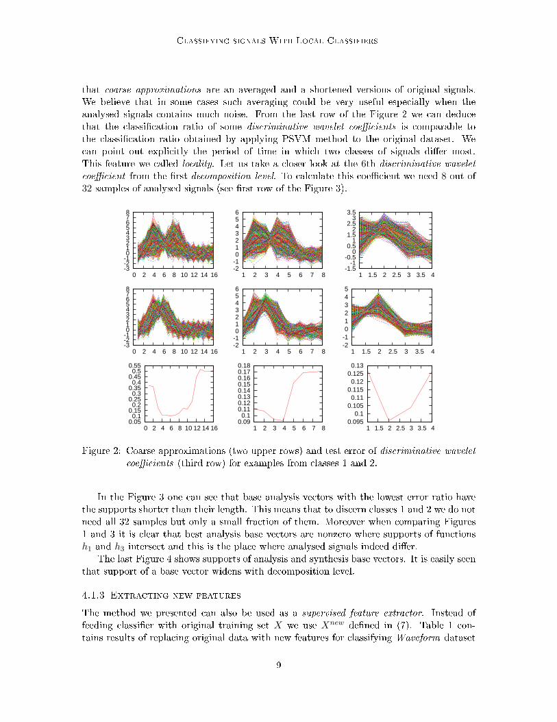
Classifying signals With Lo al Classifiersthat oarse approximations are an averaged and a shortened versions of original signals.We believe that in some ases su h averaging ould be very useful espe ially when theanalysed signals ontains mu h noise. From the last row of the Figure 2 we an dedu ethat the lassi� ation ratio of some dis riminative wavelet oeÆ ients is omparable tothe lassi� ation ratio obtained by applying PSVM method to the original dataset. We an point out expli itly the period of time in whi h two lasses of signals di�er most.This feature we alled lo ality. Let us take a loser look at the 6th dis riminative wavelet oeÆ ient from the �rst de omposition level. To al ulate this oeÆ ient we need 8 out of32 samples of analysed signals (see �rst row of the Figure 3).

-3-2-1 0 1 2 3 4 5 6 7 8

0 2 4 6 8 10 12 14 16

-3-2-1 0 1 2 3 4 5 6 7 8

0 2 4 6 8 10 12 14 16

0.05 0.1

0.15 0.2

0.25 0.3

0.35 0.4

0.45 0.5

0.55

0 2 4 6 8 10 12 14 16

-2-1 0 1 2 3 4 5 6

1 2 3 4 5 6 7 8

-2-1 0 1 2 3 4 5 6

1 2 3 4 5 6 7 8

0.09 0.1

0.11 0.12 0.13 0.14 0.15 0.16 0.17 0.18

1 2 3 4 5 6 7 8

-1.5-1

-0.5 0

0.5 1

1.5 2

2.5 3

3.5

1 1.5 2 2.5 3 3.5 4

-2-1 0 1 2 3 4 5

1 1.5 2 2.5 3 3.5 4

0.095 0.1

0.105 0.11

0.115 0.12

0.125 0.13

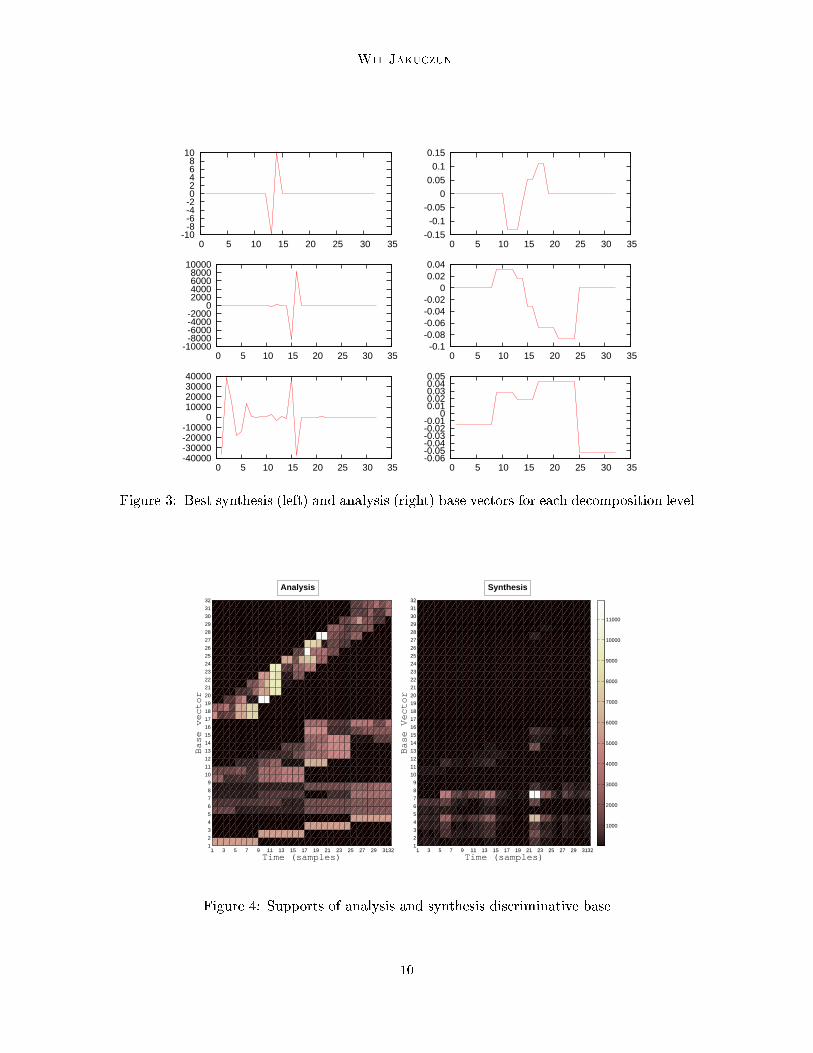
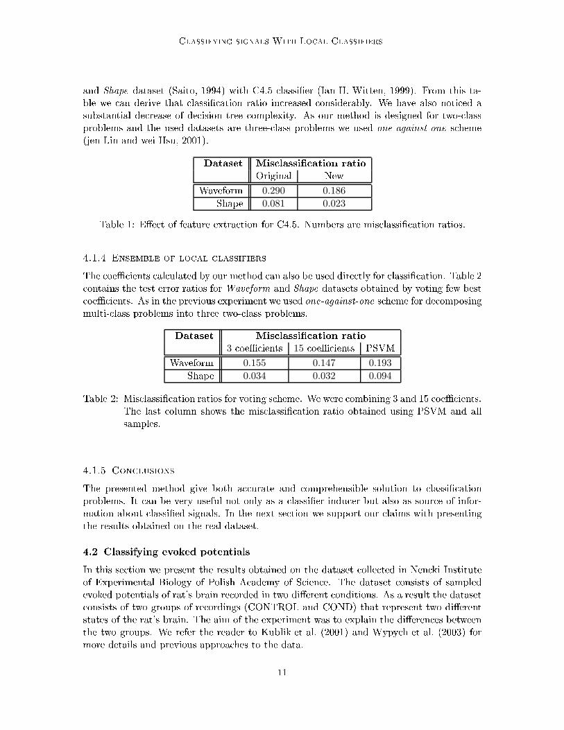
1 1.5 2 2.5 3 3.5 4Figure 2: Coarse approximations (two upper rows) and test error of dis riminative wavelet oeÆ ients (third row) for examples from lasses 1 and 2.In the Figure 3 one an see that base analysis ve tors with the lowest error ratio havethe supports shorter than their length. This means that to dis ern lasses 1 and 2 we do notneed all 32 samples but only a small fra tion of them. Moreover when omparing Figures1 and 3 it is lear that best analysis base ve tors are nonzero where supports of fun tionsh1 and h3 interse t and this is the pla e where analysed signals indeed di�er.The last Figure 4 shows supports of analysis and synthesis base ve tors. It is easily seenthat support of a base ve tor widens with de omposition level.4.1.3 Extra ting new featuresThe method we presented an also be used as a supervised feature extra tor. Instead offeeding lassi�er with original training set X we use Xnew de�ned in (7). Table 1 on-tains results of repla ing original data with new features for lassifying Waveform dataset9

Wit Jaku zun-10-8-6-4-2 0 2 4 6 8

10

0 5 10 15 20 25 30 35-0.15

-0.1

-0.05

0

0.05

0.1

0.15

0 5 10 15 20 25 30 35

-10000-8000-6000-4000-2000

0 2000 4000 6000 8000

10000

0 5 10 15 20 25 30 35-0.1

-0.08-0.06-0.04-0.02

0 0.02 0.04

0 5 10 15 20 25 30 35

-40000-30000-20000-10000

0 10000 20000 30000 40000

0 5 10 15 20 25 30 35-0.06-0.05-0.04-0.03-0.02-0.01

0 0.01 0.02 0.03 0.04 0.05

0 5 10 15 20 25 30 35Figure 3: Best synthesis (left) and analysis (right) base ve tors for ea h de omposition level

1 3 5 7 9 11 13 15 17 19 21 23 25 27 29 31321

2

3

4

5

6

7

8

9

10

11

12

13

14

15

16

17

18

19

20

21

22

23

24

25

26

27

28

29

30

31

32

Time (samples)

Base vector

1 3 5 7 9 11 13 15 17 19 21 23 25 27 29 31321

2

3

4

5

6

7

8

9

10

11

12

13

14

15

16

17

18

19

20

21

22

23

24

25

26

27

28

29

30

31

32

Time (samples)

Base Vector

1000

2000

3000

4000

5000

6000

7000

8000

9000

10000

11000

Analysis Synthesis

Figure 4: Supports of analysis and synthesis dis riminative base10

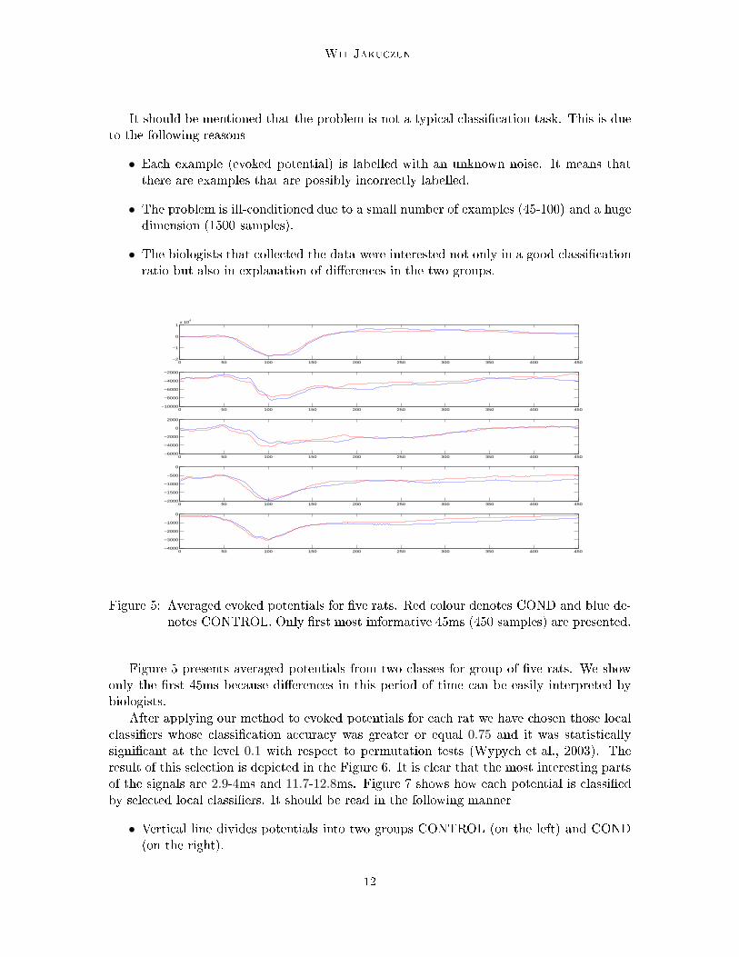
Classifying signals With Lo al Classifiersand Shape dataset (Saito, 1994) with C4.5 lassi�er (Ian H. Witten, 1999). From this ta-ble we an derive that lassi� ation ratio in reased onsiderably. We have also noti ed asubstantial de rease of de ision tree omplexity. As our method is designed for two- lassproblems and the used datasets are three- lass problems we used one-against-one s heme(jen Lin and wei Hsu, 2001).Dataset Mis lassi� ation ratioOriginal NewWaveform 0.290 0.186Shape 0.081 0.023Table 1: E�e t of feature extra tion for C4.5. Numbers are mis lassi� ation ratios.4.1.4 Ensemble of lo al lassifiersThe oeÆ ients al ulated by our method an also be used dire tly for lassi� ation. Table 2 ontains the test error ratios for Waveform and Shape datasets obtained by voting few best oeÆ ients. As in the previous experiment we used one-against-one s heme for de omposingmulti- lass problems into three two- lass problems.Dataset Mis lassi� ation ratio3 oeÆ ients 15 oeÆ ients PSVMWaveform 0.155 0.147 0.193Shape 0.034 0.032 0.094Table 2: Mis lassi� ation ratios for voting s heme. We were ombining 3 and 15 oeÆ ients.The last olumn shows the mis lassi� ation ratio obtained using PSVM and allsamples.4.1.5 Con lusionsThe presented method give both a urate and omprehensible solution to lassi� ationproblems. It an be very useful not only as a lassi�er indu er but also as sour e of infor-mation about lassi�ed signals. In the next se tion we support our laims with presentingthe results obtained on the real dataset.4.2 Classifying evoked potentialsIn this se tion we present the results obtained on the dataset olle ted in Nen ki Instituteof Experimental Biology of Polish A ademy of S ien e. The dataset onsists of sampledevoked potentials of rat's brain re orded in two di�erent onditions. As a result the dataset onsists of two groups of re ordings (CONTROL and COND) that represent two di�erentstates of the rat's brain. The aim of the experiment was to explain the di�eren es betweenthe two groups. We refer the reader to Kublik et al. (2001) and Wypy h et al. (2003) formore details and previous approa hes to the data.11

Wit Jaku zunIt should be mentioned that the problem is not a typi al lassi� ation task. This is dueto the following reasons• Ea h example (evoked potential) is labelled with an unknown noise. It means thatthere are examples that are possibly in orre tly labelled.• The problem is ill- onditioned due to a small number of examples (45-100) and a hugedimension (1500 samples).• The biologists that olle ted the data were interested not only in a good lassi� ationratio but also in explanation of di�eren es in the two groups.

0 50 100 150 200 250 300 350 400 450−2

−1

0

1x 10

4

0 50 100 150 200 250 300 350 400 450−10000

−8000

−6000

−4000

−2000

0 50 100 150 200 250 300 350 400 450−6000

−4000

−2000

0

2000

0 50 100 150 200 250 300 350 400 450−2000

−1500

−1000

−500

0

0 50 100 150 200 250 300 350 400 450−4000

−3000

−2000

−1000

0

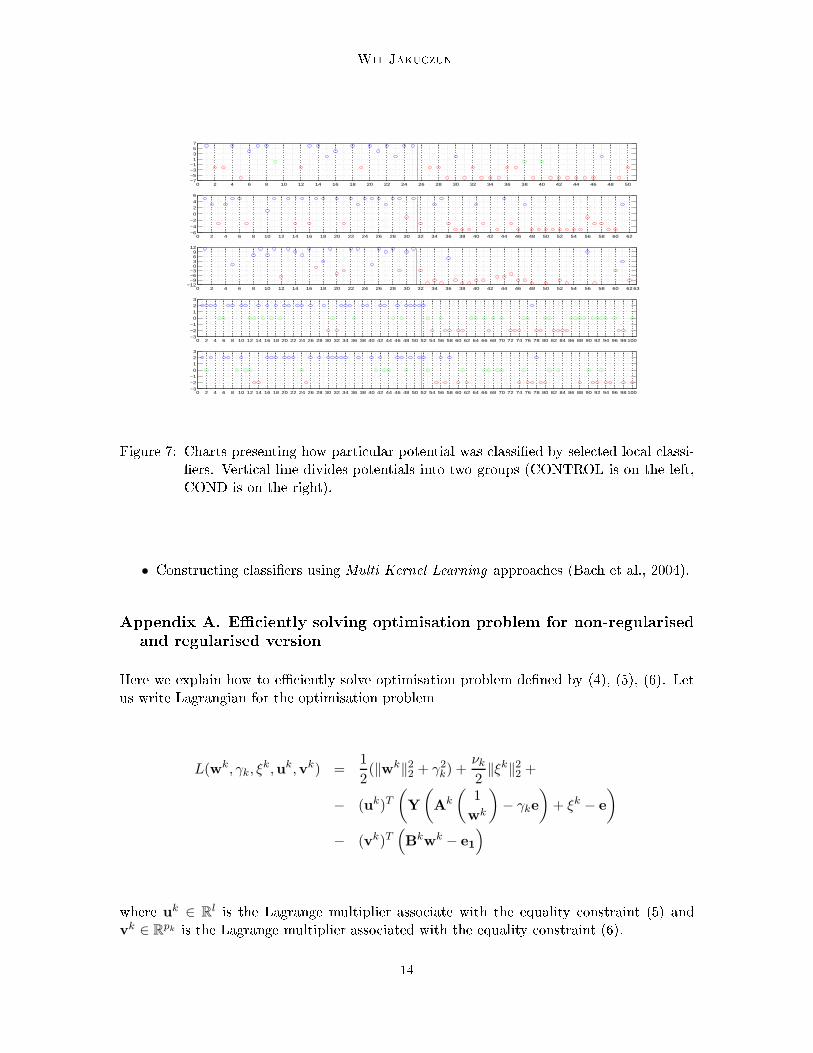
Figure 5: Averaged evoked potentials for �ve rats. Red olour denotes COND and blue de-notes CONTROL. Only �rst most informative 45ms (450 samples) are presented.Figure 5 presents averaged potentials from two lasses for group of �ve rats. We showonly the �rst 45ms be ause di�eren es in this period of time an be easily interpreted bybiologists.After applying our method to evoked potentials for ea h rat we have hosen those lo al lassi�ers whose lassi� ation a ura y was greater or equal 0.75 and it was statisti allysigni� ant at the level 0.1 with respe t to permutation tests (Wypy h et al., 2003). Theresult of this sele tion is depi ted in the Figure 6. It is lear that the most interesting partsof the signals are 2.9-4ms and 11.7-12.8ms. Figure 7 shows how ea h potential is lassi�edby sele ted lo al lassi�ers. It should be read in the following manner• Verti al line divides potentials into two groups CONTROL (on the left) and COND(on the right). 12

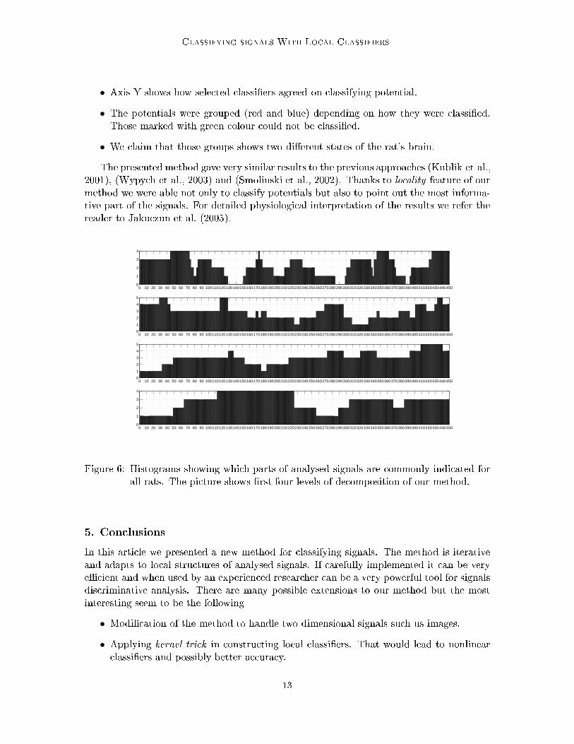
Classifying signals With Lo al Classifiers• Axis Y shows how sele ted lassi�ers agreed on lassifying potential.• The potentials were grouped (red and blue) depending on how they were lassi�ed.Those marked with green olour ould not be lassi�ed.• We laim that those groups shows two di�erent states of the rat's brain.The presented method gave very similar results to the previous approa hes (Kublik et al.,2001), (Wypy h et al., 2003) and (Smolinski et al., 2002). Thanks to lo ality feature of ourmethod we were able not only to lassify potentials but also to point out the most informa-tive part of the signals. For detailed physiologi al interpretation of the results we refer thereader to Jaku zun et al. (2005).

0 10 20 30 40 50 60 70 80 90 1001101201301401501601701801902002102202302402502602702802903003103203303403503603703803904004104204304404500

1

2

3

4

0 10 20 30 40 50 60 70 80 90 1001101201301401501601701801902002102202302402502602702802903003103203303403503603703803904004104204304404500

1

2

3

4

5

0 10 20 30 40 50 60 70 80 90 1001101201301401501601701801902002102202302402502602702802903003103203303403503603703803904004104204304404500

1

2

3

4

5

0 10 20 30 40 50 60 70 80 90 1001101201301401501601701801902002102202302402502602702802903003103203303403503603703803904004104204304404500

1

2

3

4

Figure 6: Histograms showing whi h parts of analysed signals are ommonly indi ated forall rats. The pi ture shows �rst four levels of de omposition of our method.5. Con lusionsIn this arti le we presented a new method for lassifying signals. The method is iterativeand adapts to lo al stru tures of analysed signals. If arefully implemented it an be veryeÆ ient and when used by an experien ed resear her an be a very powerful tool for signalsdis riminative analysis. There are many possible extensions to our method but the mostinteresting seem to be the following• Modi� ation of the method to handle two dimensional signals su h us images.• Applying kernel tri k in onstru ting lo al lassi�ers. That would lead to nonlinear lassi�ers and possibly better a ura y.13

Wit Jaku zun0 2 4 6 8 10 12 14 16 18 20 22 24 26 28 30 32 34 36 38 40 42 44 46 48 50

−7−5−3−1

1357

0 2 4 6 8 10 12 14 16 18 20 22 24 26 28 30 32 34 36 38 40 42 44 46 48 50 52 54 56 58 60 62−6

−4

−2

0

2

4

6

0 2 4 6 8 10 12 14 16 18 20 22 24 26 28 30 32 34 36 38 40 42 44 46 48 50 52 54 56 58 60 62 63−12

−9−6−3

0369

12

0 2 4 6 8 10 12 14 16 18 20 22 24 26 28 30 32 34 36 38 40 42 44 46 48 50 52 54 56 58 60 62 64 66 68 70 72 74 76 78 80 82 84 86 88 90 92 94 96 98 100−3

−2

−1

0

1

2

3

0 2 4 6 8 10 12 14 16 18 20 22 24 26 28 30 32 34 36 38 40 42 44 46 48 50 52 54 56 58 60 62 64 66 68 70 72 74 76 78 80 82 84 86 88 90 92 94 96 98 100−3

−2

−1

0

1

2

3

Figure 7: Charts presenting how parti ular potential was lassi�ed by sele ted lo al lassi-�ers. Verti al line divides potentials into two groups (CONTROL is on the left,COND is on the right).• Constru ting lassi�ers using Multi Kernel Learning approa hes (Ba h et al., 2004).Appendix A. EÆ iently solving optimisation problem for non-regularisedand regularised versionHere we explain how to eÆ iently solve optimisation problem de�ned by (4), (5), (6). Letus write Lagrangian for the optimisation problem

L(wk, γk, ξk,uk,vk) =

1

2(‖wk‖2

2 + γ2k) +

νk

2‖ξk‖2

2 +

− (uk)T(

Y

(

Ak

(

1

wk

)

− γke

)

+ ξk − e

)

− (vk)T(

Bkw

k − e1

)

where uk ∈ R

l is the Lagrange multiplier asso iate with the equality onstraint (5) andv

k ∈ Rpk is the Lagrange multiplier asso iated with the equality onstraint (6).14

Classifying signals With Lo al ClassifiersSettings the gradients of L to zero we get the following optimality onditionsw

k = ( ˜Ak)T Yu

k − (Bk)T vk (12)

γk = −eTYu

k (13)ξk =

1

νku

k (14)Y

(

Ak + ˜

A

kw

k − γke

)

+ ξk = e (15)B

kw

k = e1 (16)where Ak =

(

Ak ˜A

k)Substituting (12) into (16) we get

vk =

[

Bk(

Bk)T]−1

(

Bk

(

˜A

k)T

Yuk − e

) (17)Substituting (12), (13), (14) and (17) into (15) we getY

{

˜A

k(

˜A

k)T

Yuk − ˜

A

k (

Bk)T[

Bk(

Bk)T]−1

(

Bk

(

˜A

k)T

Yuk − e

)}

+1

νku

k = e−YAk(18)Simplifying (18) we get

Y

{

˜A

k(

˜A

k)T

− ˜A

k(

Bk)T[

Bk(

Bk)T]−1

Bk

(

˜A

k)T}

Yuk + 1

νk uk =

= e − YAk − ˜

A

k(

Bk)T[

Bk(

Bk)T]−1

e

(19)Let matrix Hk1 be de�ned as

Hk1 = Y

[

˜A

k| − ˜

A

k (

Bk)T (

Ck)T] (20)and matrix H

k2 be de�ned as

Hk2 = Y

[

˜A

k| ˜A

k (

Bk)T (

Ck)T] (21)where

[

Bk(

Bk)T]−1

=(

Ck)T

CkRewriting equation (19) we obtain that

(

1

νkI + H1 (H2)

T

)

uk = e − YA

k − ˜A

k (

Bk)T[

Bk(

Bk)T]−1

e (22)15

Wit Jaku zunSetting ve tor bk = e − YA

k − ˜A

k(

Bk)T[

Bk(

Bk)T]−1

e we get that ve tor uk is givenby the following set of equations

(

1

νkI + H1 (H2)

T

)

uk = b

k (23)Solving above set of equations is very expensive as the number of equations is equal tonumber of training examples l whi h an be large. Using the Sherman-Morrison-Woodburyformula (Gene H. Golub, 1996) we an al ulate uk as follows

uk = νk

(

I − H1

(

1

νkI + (H1)

TH2

)−1

(H2)T

)

bk (24)It should be stressed that using equation (24) for omputing uk is mu h less expensive thanusing equation (23) be ause the dimensions of matrix

1

νkI + (H1)

TH2are equal to Lk + pk ×Lk + pk whi h is independent of the number of training of examples.Similarly to nonregularised variant presented above we an use the same te hniquesto solve optimisation problem (2) and (3). For more details see (Fung and Mangasarian,2001).Referen esFran is R. Ba h, Gert R. G. Lan kriet, and Mi hael I. Jordan. Multiple kernel learning, oni duality, and the smo algorithm. In ICML '04: Pro eedings of the twenty-�rstinternational onferen e on Ma hine learning, New York, NY, USA, 2004. ACM Press.ISBN 1-58113-828-5. doi: http://doi.a m.org/10.1145/1015330.1015424.L. Breiman. Ar ing lassi�ers. 1998. URL http:// iteseer.ist.psu.edu/breiman98ar ing.html.R. Claypoole, R. Baraniuk, and R. Nowak. Adaptive wavelet transforms via lifting. 1998.URL http:// iteseer.ist.psu.edu/ laypoole98adaptive.html.Ingrid Daube hies. Ten Le tures on Wavelets. SIAM, 1992.G. Fern�andez, S. Periaswamy, and Wim Sweldens. LIFTPACK: A software pa kage forwavelet transforms using lifting. In M. Unser, A. Aldroubi, and A. F. Laine, editors,Wavelet Appli ations in Signal and Image Pro essing IV, pages 396{408. Pro . SPIE 2825,1996.Glenn Fung and O. L. Mangasarian. Proximal support ve tor ma hine lassi-�ers. In Knowledge Dis overy and Data Mining, pages 77{86, 2001. URL iteseer.ist.psu.edu/515368.html.Charles F. Van Loan Gene H. Golub. Matrix Computations. The Johns Hopkins UniversityPress, 1996. 16

Classifying signals With Lo al ClassifiersEibe Frank Ian H. Witten. Data Mining: Pra ti al Ma hine Learning Tools and Te hniqueswith Java Implementations. Morgan Kaufmann, 1999.W. Jaku zun, A. Wróbel, D. Wój ik, and E. Kublik. Classifying evoked potentials withlo al lassi�ers. (in preparation), 2005.Chih jen Lin and Chih wei Hsu. A omparison of methodsfor multi- lass support ve tor ma hines, June 07 2001. URLhttp:// iteseer.ist.psu.edu/537288.html;http://www. sie.ntu.edu.tw/~ jlin/papers/multisvm.ps.gz.E. Kublik, P. Musiaª, and A. Wróbel. Identi� ation of prin ipal omponents in orti alevoked potentials by brief sufa e ooling. Clini al Neuropshysiology, 2001.Naoki Saito. Lo al Feature Extra tion and Its Appli ation Usinga Library of Bases. PhD thesis, Yale University, 1994. URLhttp://www.math.u davis.edu/~saito/publi ations/saito_phd.html.Tomasz G. Smolinski, Grzegorz M. Boratyn, Mariofanna Milanova, Ja ek M. Zurada,and Andrzej Wrobel. Evolutionary algorithms and rough sets-based hybrid approa hto lassi� atory de omposition of orti al evoked potentials. In James J. Alpigini,James F. Peters, Andrzej Skowron, and Ning Zhong, editors, Rough Sets and CurrentTrends in Computing, Third International Conferen e, RSCTC 2002, number 2475 inLe ture Notes in Arti� ial Intelligen e, pages 621{628. Springer-Verlag, 2002. URL iteseer. sail.mit.edu/smolinski02evolutionary.html.Wim Sweldens. The lifting s heme: A onstru tion of se ond generationwavelets. SIAM Journal on Mathemati al Analysis, 29(2):511{546, 1998. URLhttp:// iteseer.ist.psu.edu/sweldens98lifting.html.Vladimir Vapnik. Statisti al Learning Theory. John Wiley & Sons, 1998.M. Wypy h, E. Kublik, P. Wojdyªªo, and A. Wróbel. Sorting fun tional lasses of evokedpotentials by wavelets. Neuroinformati , 2003.

17