
Robust Speech Watermarking Procedure in the Time-Frequency Domain
Upload
khangminh22Category
view
1download
0
T-4269
A FREQUENCY DOMAIN APPROACH
TO DRILLSTRING JARRING ANALYSIS
Alfred William Eustes III
by

ii
T-4269
A thesis submitted to the Faculty and Board of Trustees of the
Colorado School of Mines in partial fulfillment of the requirements for the
degree of Doctorate of Philosophy (Petroleum Engineering).
Golden, Colorado
Date ____________________
Signed: __________________________
Approved:________________________
Golden, Colorado
Date ____________________
__________________________Dr. Craig W. Van KirkProfessor and Head,Department ofPetroleum Engineering
Dr. Bill J. MitchellThesis Advisor
Alfred William Eustes III
iii
T-4269
ABSTRACT
In drilling, a time and money consuming operation called fishing often
occurs. One method to extract a stuck drill string from the hole is to hit the string
with a force impulse. This is called jarring. Before this dissertation, the math-
ematics necessary to predict the magnitude and duration of the forces generated
in jarring had not been developed to the point of functional use. This disserta-
tion examines a new mathematical approach to understanding the forces of
jarring and presents a jarring model that can be implemented in the field.
Current mathematical models of jarring use either wave tracking or finite
element analysis with time and space being the independent variables. These
methods require the use of sophisticated computers with significant central
processing power and memory and take an extraordinary amount of time to
compute. These methods are not suitable for field use.
The jarring model presented in this dissertation is a finite element ap-
proach that uses frequency and space as the independent variables. This ap-
proach is called spectral analysis. The advantages of this method are that
element sizes are not limited nor are time step sizes critical as they are in previ-
ous jarring models.
The spectral analysis method developed in this dissertation is
computationally faster and more accurate than any jarring model presented to
date. This accuracy has shown some interesting effects that could not be seen
iv
T-4269
in all previous models. For example, wave reflections from damping alone can
be seen. This will be called the damping reflection effect. Also, any number of
reflections and transmissions can be incorporated into the model. Previous
models could not incorporate multiple reflections with their accumulated effects
on the hammer and anvil. In addition, some models do not consider the effect of
the anvil movement. The spectral analysis method shows that the anvil move-
ment can be a significant factor in determining the primary impact magnitude.
Finally, the impact force is assumed to be a square wave. Although this as-
sumption is used for this dissertation, the spectral analysis method is not limited
to square waves but can use any wave function.
The program is written using the commercial software package called
MathCad, version 6.0 Plus. The model includes elements for drill pipe, heavy
weight drill pipe, and drill collars. An accelerator can be incorporated and mod-
elled into the string. The jar is modeled with a user preset trigger load and a
hammer and anvil. The stuck section of the drill string can be modeled as either
a long section or a fixed point. Hole deviation effects can be included by varying
the element size and associated damping.
T-4269
v
TABLE OF CONTENTS
INTRODUCTION .................................................................................................. 1Rig Downtime ............................................................................................ 1Fishing Costs............................................................................................. 2Jarring ....................................................................................................... 3Organization of Dissertation ...................................................................... 4
Chapter 1—Fishing Operations ........................................................... 4Chapter 2—Literature Review.............................................................. 4Chapter 3—Time and Frequency Domains .......................................... 4Chapter 4—Deriving the Spectral Element .......................................... 5Chapter 5—The Use of Spectral Analysis in Wave Propagation ......... 5Chapter 6—The New Jarring Model .................................................... 5Chapter 7—Jarring Analysis Cases ..................................................... 6Conclusions and Recommendations .................................................... 6
CHAPTER 1, FISHING OPERATIONS ................................................................ 7Stuck Drill String Problems........................................................................ 9
Differential Pressure Sticking ............................................................... 9Undergauge Hole Sticking ................................................................. 11Sloughing Hole Sticking ..................................................................... 12Key Seat Sticking ............................................................................... 13Sand Sticking and Mud Sticking ........................................................ 13Inadequate Hole Cleaning Sticking .................................................... 14Cemented Sticking ............................................................................. 14Blowout Sticking ................................................................................. 15Mechanical Sticking ........................................................................... 15
Packers ......................................................................................... 15Multiple Strings ............................................................................. 16Crooked Pipe ................................................................................ 16Junk in the Hole ............................................................................ 16
Fishing ..................................................................................................... 17Locating Stuck Point .......................................................................... 17
Stretch Calculations...................................................................... 17Freepoint Tool ............................................................................... 18
Backoff the String ............................................................................... 19Run in the Jars ................................................................................... 19
T-4269
vi
Jarring ..................................................................................................... 20Types of Jars ...................................................................................... 20
Hydraulic ....................................................................................... 21Mechanical ................................................................................... 22
Accelerator ......................................................................................... 23Bumper Sub ....................................................................................... 23
CHAPTER 2, LITERATURE REVIEW ............................................................... 24Summary of Past Work ............................................................................ 24Drillstring Dynamics During Jarring Operations ...................................... 25Transient Dynamic Analysis of the Drillstring Under Jarring Operations by the FEM .......................................................... 30A Study of How Heavy Weight Drill Pipe Affects Jarring Operations ...... 33Computerized Drilling Jar Placement ...................................................... 34A Practical Approach to Jarring Analysis ................................................ 39Loads on Drillpipe During Jarring Operations ......................................... 44
CHAPTER 3, TIME AND FREQUENCY DOMAINS ........................................... 48Wave Theory ........................................................................................... 51
Types of Waves ................................................................................. 52Natural Frequencies........................................................................... 54Wave Relationships ........................................................................... 56
Time Domain versus Frequency Domain ................................................ 59Converting from Time Domains to Frequency Domains ......................... 61
The Fourier Transform ....................................................................... 61The Continuous Fourier Transform .................................................... 62The Discrete Fourier Transform ......................................................... 64The Fast Fourier Transform ............................................................... 65
Problems with Digital Signal Processing ................................................. 67Nyquist Frequency ............................................................................. 67Aliasing .............................................................................................. 68Windowing ......................................................................................... 70Leakage ............................................................................................. 70Noise .................................................................................................. 74Digitizing (Picket Fence Effect) .......................................................... 74
CHAPTER 4, DERIVING THE SPECTRAL ELEMENT ...................................... 76Static Forces ........................................................................................... 80
Gravity ................................................................................................ 80Overpull Force ................................................................................... 81
T-4269
vii
Dynamic Forces....................................................................................... 81Strain .................................................................................................. 81Damping ............................................................................................. 82
Hysteretic Damping ...................................................................... 82Viscous Damping .......................................................................... 84Coulomb Damping ........................................................................ 86Equivalent Viscous Damping ........................................................ 87
General Derivation of the Axial Equation of Motion ................................ 88General Solution for the Axial Equation of Motion .................................. 89The Spectral Solution .............................................................................. 91Finite Element Method ............................................................................ 92A General Axial Two-Noded Spectral Element ........................................ 93Derivation of the Axial One-Noded Semi-Infinite Spectral Element ........ 97Globally Assembling the Spectral Elements............................................ 98
Applying the Boundary Conditions ..................................................... 99Solving the Assembled System ........................................................ 100Post-Processing ............................................................................... 101Between the Nodes .......................................................................... 101
Spectral Analysis Procedure ................................................................. 102Limitations of the Method ...................................................................... 102
Knowledge of the Input .................................................................... 102Windows and Wave Migration ......................................................... 103Nonlinearity ...................................................................................... 105
CHAPTER 5, THE USE OF SPECTRAL ANALYSIS IN WAVE PROPAGATION.......................................................................... 106
Wave Reflections from Various Geometric Boundaries......................... 106Spectral Analysis Example Set-Up ........................................................ 110Calculations for the Examples ............................................................... 113Example One—A Wave Interacting with a Fixed Boundary .................. 117Example Two—A Wave Interacting with a Free Boundary .................... 120Example Three —A Wave Propagating from a Small to a Large Area .. 124Example Four—A Wave Propagating from a Large to a Small Area ..... 128Example Five—A Wave Propagating in Various Areas ......................... 132
CHAPTER 6, THE NEW JARRING MODEL .................................................... 135The Spectral Analysis Jarring Model ..................................................... 135The Jarring Process .............................................................................. 138
Pre-Stretch ....................................................................................... 138Free Contraction .............................................................................. 140

T-4269
viii
Impact .............................................................................................. 143Post-Impact ...................................................................................... 144
Example Calculations ............................................................................ 146Pre-Stretch ....................................................................................... 147Free Contraction .............................................................................. 148Impact .............................................................................................. 150Post-Impact ...................................................................................... 152
CHAPTER 7, JARRING ANALYSIS CASES .................................................... 153Mathcad ................................................................................................. 153Jarring Examples ................................................................................... 154
Case One: Drill Collars and Drill Pipe.............................................. 155Case Two: Drill Collars and Drill Pipe with an Accelerator .............. 164Case Three: Drill Collars, Heavy Weight Drill Pipe, and Drill Pipe .. 170Case Four: Drill Collars, Heavy Weight Drill Pipe, Drill Pipe, and an Accelerator ...................................................................... 174Case Five: Drill Collars, Heavy Weight Drill Pipe, Drill Pipe, and an Accelerator with a Rigid Stuck Point .............................. 177
CONCLUSIONS AND RECOMMENDATIONS ................................................. 187Other Areas of Research ....................................................................... 188
Vibration Analysis ............................................................................ 189Impact Study .................................................................................... 189
More Work to Do ................................................................................... 190Jarring Impact .................................................................................. 190Coulomb Damping ........................................................................... 191Torsional Waves............................................................................... 192Lateral Waves .................................................................................. 192Tool Joints ........................................................................................ 192Stabilizers ........................................................................................ 193Curved Boreholes ............................................................................ 193
REFERENCES CITED ..................................................................................... 194
SELECTED BIBLIOGRAPHY ........................................................................... 198
APPENDIX A, MATHCAD EXAMPLE ............................................................... 219

ix
T-4269
There are a number of people and organizations I wish to acknowledge
and thank. If not for their encouragement and support, this dissertation would
not have been possible.
At the Colorado School of Mines:
Prof. Bill Mitchell, advisor
Prof. Craig Van Kirk
Prof. Ramona Graves
Prof. Robert Thompson
Prof. Michael Pavelich
Prof. Vaughn Griffiths
Prof. Hans-Peter Huttlemaier
Mr. Mark Miller
Mr. Michael Stoner
Mr. Kurt Nordlander
With Cougar Tools Company of Canada
Ray LaBonti
With the Yucca Mountain Site Characterization Project
The United States Department of Energy
Mr. Roy Long
ACKNOWLEDGEMENTS

x
T-4269
Scientific Applications International Corporation
Mr. Eddie Wright
Raytheon Services
Reynolds Electrical and Engineering Company
TRW
With the Hanford Engineering Works
Westinghouse Corporation
Mr. Jim McCormick
Water Development Corporation
With the Eustes Household
Ms. Susan Eustes

xi
T-4269
DEDICATION
This dissertation is dedicated to my wife, Susan, for her commitment
and understanding. She has supported me for my entire eight years of post
graduate school at the University of Colorado and at the Colorado School of
Mines. It has been a long and winding road. She deserves a Ph. T. (Put Him
Through).
T-4269 1
INTRODUCTION
Minimizing rig downtime is critical to drilling an economical well. Any
tasks auxiliary to the actual drilling process slow rig production time and in-
crease operational costs. Having a tool stuck in a hole is a major contributor to
downtime on today’s drilling rigs, yet the mathematics necessary to fully under-
stand the jarring process used to “unstick” the tool have not been developed to
the point of field implementation. Thus jarring is often a hit or miss operation. A
practical mathematical model that accurately predicts the forces of jarring would
minimize the time and costs associated with retrieving lost tools. This disserta-
tion presents such a model and its derivation.
Rig Downtime
No engineer plans to part drill strings or lose drilling tools in the hole.
This, as with most unscheduled events, results in downtime. As defined by
Amoco, “an unscheduled event is any occurrence which causes a time delay in
the progression of planned operations” (Kadaster et al. 1993).
All planned operations can be considered progression toward completing
a well (e.g. running planned casing strings, well evaluation, actual drilling). After
problems strike (e.g. equipment failure, parting of drill string, wellbore collapse,
tools stuck in the hole), no progress is being made toward the completion of the
well. These problems cause downtime. Fishing—the process used to retrieve a
T-4269 2
lost tool or tools (the “fish”) downhole—is a frustrating, expensive and often
prolonged downtime.
Fishing Costs
Any type of downtime is expensive. In the Norwegian North Sea, it is not
unusual to see costs associated with drilling to be $200,000 per day per rig
(Anderson and Lembourn 1994). According to the previous reference, from 1985
to 1991, 18 percent of exploratory rig time was spent in downtime. This in-
cludes: equipment repair (4.0 percent), fishing (3.9 percent), waiting (3.2 per-
cent), other problems (3.2 percent), well control (2.8 percent), and lost circula-
tion (0.9 percent). In 1990 and 1991, Amoco (Kadaster et al. 1993) found that
15 percent of the time spent on drilling operations was downtime. Of that down-
time, 16 percent of the time can be attributed to stuck drill string (which was their
number one problem).
Using the previous paragraph’s example, in the Norwegian North Sea, an
average of $7,800 per day is spent on fishing. This is $2.85 million per year per
rig. For an average of 11 rigs per year for the six year study period, the total
cost for fishing in the Norwegian North Sea must have been approximately $188
million!
In a recent Oil and Gas Journal article (Watson and Smith 1994), anec-
dotal evidence shows that the cost of stuck drill string operations (which can be
considered a subset of fishing operations) varied widely. One operator reported
$37 million spent in downtime from stuck drill string from 1987 to 1991. Another
indicated that his company’s costs approached that number in one year alone. A
T-4269 3
third operator said its company’s worldwide stuck drill string costs were $100
million, $40 million of which was in the company’s Gulf of Mexico operations.
These examples demonstrate the economic necessity to minimize fishing
costs. Even minimal savings per each fishing operation can result in significant
overall savings in drilling operations.
Jarring
Jarring is the method used to extract the fish from the hole by hitting the
string with a force impulse. This involves a transient wave. The physics needed
to predict the amplitude and duration of the forces generated during jarring are
intricate and not fully refined. Considerable computer resources are required to
solve the multiple equations associated with the forces of jarring; resources
which until recently have not been readily available to researchers.
Current jarring analysis involves either the wave tracking method or the
finite element method. The independent variables in both methods are space
and time. This means that both methods are firmly rooted in the time domain.
While this is perhaps a more intuitive approach, there are other ways to look at
the problem.
One such way is to look at the sinusoidal components of a wave. As
shown by the mathematician J. B. Fourier, in his now commonly accepted Fou-
rier transform, all real time functions can be thought of as being made up of an
infinite series of sinusoidal components. Each sinusoidal component has an
amplitude, a phase, and a frequency associated with it. The Fourier transform,
specifically the fast Fourier transform (FFT), is used to find the sinusoidal com-
T-4269 4
ponents from time domain functions. The collection of sinusoidal components
make up the frequency domain.
The spectral analysis method described in this dissertation combines the
best of the current approaches to jarring analysis within the frequency domain.
Organization of Dissertation
This dissertation first presents an overview of fishing operations and
moves to an explanation of the model developed to predict the jarring process.
Chapter 1—Fishing Operations
This chapter discusses drill string components, the different methods of
sticking a drill string in the borehole, typical fishing operation techniques and the
mechanics of jarring. This discussion includes a description of the types of jars
and other tools used in jarring strings.
Chapter 2—Literature Review
This review includes three papers on the wave tracking method of analy-
sis. There is also a review of a finite element method jarring analysis, and there
are reviews of two papers that describe jarring operational techniques.
Chapter 3—Time and Frequency Domains
The current jarring analysis methods are discussed in this chapter. Then
wave theory and relationships are described. The differences between the time
T-4269 5
and frequency domains are shown. Finally, the techniques used to convert from
the time domain to the frequency domain (such as the fast Fourier transform)
and problems inherent in these techniques are explained.
Chapter 4—Deriving the Spectral Element
This chapter sets forth the details of spectral analysis. It starts with a
general description of spectral analysis. Then the static and dynamic forces on
a drill string during jarring are shown. Using the dynamic forces, an axial equa-
tion of motion for a drill string under jarring conditions is derived and solved.
From there, the spectral solution is derived using a finite element model com-
posed of an axial two-noded spectral element and an axial one-noded semi-
infinite spectral element. The elements are then globally assembled into one
structure, the drill string. A linear algebraic solution for the globally assembled
structure is made and post-processing is shown. The general procedure and the
limitations of spectral analysis are described.
Chapter 5—The Use of Spectral Analysis in Wave Propagation
This chapter presents five models that validate the spectral analysis
method.
Chapter 6—The New Jarring Model
This chapter presents the spectral analysis-based model of jarring. A
generic drill string model is described and each phase of the jarring process is
presented.
T-4269 6
Chapter 7—Jarring Analysis Cases
This chapter presents cases of jarring under various conditions. Cases
include the use of drill collars and drill pipe with and without heavy weight drill
pipe and with and without an accelerator. Finally, a comparison of the fre-
quency-domain model with a time-domain finite element model demonstrates the
superior results of the spectral analysis method derived in this dissertation.
Conclusions and Recommendations
This chapter summarizes the impact of the spectral analysis jarring pro-
gram. A discussion of future research plans and capabilities of the program are
included.
T-4269 7
CHAPTER 1
FISHING OPERATIONS
This chapter discusses drill string components, the different methods of
sticking a drill string in the borehole, typical fishing operation techniques and the
mechanics of jarring. This discussion includes a description of the types of jars
and other tools used in jarring strings.
In the drilling industry, fishing operations are not pleasant outings by a
lake or river. They involve sleepless nights, exhausting days, much time, and a
lot of money. It is up to the rig personnel, primarily the drilling engineer involved,
to expeditiously remedy the fishing situation as economically as possible, or
determine that the best course of action is to abandon the hole.
Fishing is a term coined by the drillers of the cable tool era. After a cable
line broke, the drillers would put a hook on the end of the remaining line and try
to “catch” the lost line. Being the innovators that these drillers were, they often
devised unique and clever methods of recovering items that were lost in the
hole. Many of these items, such as wireline spears and wireline jars (now called
bumper subs) still exist and are used daily.
There are many techniques and procedures for fishing, and the drilling
engineer must determine the appropriate method for retrieving a lost or stuck
item, usually referred to as the “fish.” For example, wireline fishing is consider-
ably different from fishing with drill pipe. The fish itself may dictate the proce-
T-4269 8
dures. A fish may be free or stuck. If the fish is stuck, jarring or washover op-
erations may be needed. This dissertation covers only fishing with the use of
jars. The reader is referred to other references for information on more tech-
niques and procedures (Kemp 1990) (NL McCullough 1978) (Tri-State Oil Tool
Industries, Inc. n.d.).
Jarring is simply the process of impacting the fish with a large force im-
pulse. This is not unlike hitting a stuck item with a hammer. For example, if a
mechanic finds a cotter pin stuck in its hole, the first thing usually done is to hit
the pin with a hammer. The reaction is a longitudinal wave running back and
forth in the pin. The longitudinal wave causes the particles of the pin to move as
the wave passes through the particles. This, in turn, causes motion along the
side of the pin and the hole in which the pin is stuck. If the forces are large
enough to overcome the friction loads at the interface of the pin and hole, the pin
will move. With enough hammer blows, the pin eventually comes loose.
The same phenomenon is true using jarring to fish for stuck tools. In this
case, the hammer is called a jar. The jar is placed in the drill string in a position
to apply a hammer blow to the fish. With each hammer blow, the potential en-
ergy in the fish is changed from kinetic energy to strain. Eventually the fish will
come loose. The bad news is that this may take days or weeks. At some point,
it is more economical to abandon the hole and drill a new one.
Although the process of jarring is generally understood, the fine points are
not. How much force does the jar impact give a fish? And, how long does this
force last? Where is the jar positioned within the drill string to maximize the
chance of successfully freeing the fish? How does damping affect the jarring
process? The petroleum industry has invested much time and resources search-
T-4269 9
ing for answers to these questions. Thus far, the answers have been less than
useful: either the answer is reasonably accurate, but takes too much time and
computer resources to find; or, the answer is quick, but not very accurate. The
new method presented in this dissertation, called spectral analysis, is both quick
and accurate. Before getting to the process of spectral analysis, though, there is
the question of how drilling tools get stuck in the first place.
Stuck Drill String Problems
There are more ways to get stuck in a hole than there are words to de-
scribe the emotions of the driller after this happens. Just about any item that
goes in a hole—including drill pipe, drill collars, casing, and tubing—can get
stuck. This section reviews the most common methods of getting stuck, in both
open hole and cased hole. (Note: not every case described requires the use of
a jar.)
Differential Pressure Sticking
Differential pressure sticking, often called differential sticking, is very
prevalent in the drilling industry. Most of the fishing operations in the Gulf of
Mexico are caused by differential sticking. Basically, the string is stuck against
the side of the well because of a large pressure differential between the fluid in
the borehole and the formation.
Differential sticking occurs only across a permeable formation. The
higher the permeability, the higher the probability of differential sticking. As the
mud (made up of insoluble plate-like solids and a fluid phase to carry the solids)
moves across the permeable zone, it has a tendency to lose the fluid phase to
T-4269 10
the permeable formation. This leaves the solids to plate on the side of the bore-
hole. This nearly impermeable filter cake can grow to be thick. Meanwhile, if the
hydrostatic pressure of the mud at the permeable zone is much higher than the
formation pressure in the permeable zone, there will be a pressure gradient
toward the formation across the borehole wall. If, by chance, the drill pipe or
collars are laying in the filter cake, a hydraulic seal can form. Now the pressure
gradient is across the string. Because filter cake has a high friction coefficient,
the force required to pull the string tangentially across the filter cake is high. In
many cases, the rig is not powerful enough to pull the string or the string is not
strong enough to handle the load.
Differential sticking is usually the case if the drill string cannot be moved
up or down or rotated, yet circulation can be maintained. This is after being
stationary across a permeable zone.
An equation used in the petroleum industry for differential sticking is as
follows
F A PTANGENTIAL NORMAL= µ (1.1)
where
A =hydraulically sealed area
µ =coefficient of friction
PNORMAL = pressure differential between wellbore and formation
FTANGENTIAL = drag force needed to move up or down the hole

T-4269 11
Unsticking requires the reduction of the normal force, the coefficient of
friction of the filter cake, the hydraulically sealed area, or a combination of any of
the previous methods. The sooner these methods can be applied, the greater
the chance of success.
One method used to unstick the string is to spot a lightweight fluid with a
filter cake destroying chemical and then jar on the string. This fluid reduces the
pressure differential, the coefficient of friction of the filter cake, and the hydraulic
seal area. An example of this would be to spot an oil-based fluid across the
stuck point. Another method is to blow nitrogen past the stuck point. This as-
sumes that there are no potential kick zones above and below the stuck point.
Well control can be lost in these cases.
Undergauge Hole Sticking
An undergauge hole is any hole that has a smaller diameter than the bit
that drilled that section of hole. One potential cause of an undergauge condition
is drilling a high clay content plastic shale with a fresh water mud. If an oil-
based mud is used, a plastic salt formation can “flow” into the wellbore. If the
wellbore fluid has a hydrostatic pressure less than the formation pressure, the
shale or salt will slowly ooze into the wellbore. It is a slow process, but one that
can stick drilling tools of the unwary.
An undergauge hole can also occur after a drill bit is worn smaller as it
drills through an abrasive formation. In this case, the hole is undergauge be-
T-4269 12
cause the bit drilled it that way. If a new bit is run, it can jam into the
undergauge section of the hole and become stuck. This is often called tapered
hole sticking.
The presence of a thick filter cake, described in “Stuck Drill String Prob-
lems, Differential Pressure Sticking” above, can also cause an undergauge hole.
The filter cake can become so thick that tools can not drag through it. The filter
cake shows as a drag load on the weight indicator.
Sloughing Hole Sticking
Sloughing hole sticking occurs after the hole wall sloughs off. For ex-
ample, a water sensitive shale that has been invaded by water will swell and
break. If circulation is stopped, the broken pieces will collect around the drill
string and eventually pack the drill string in place.
Shales under high formation pressure can slough as well. In this case,
the formation pressure is greater than the wellbore hydrostatic pressure. Be-
cause the shale has a very low permeability, no flow is observed. The rock,
having a high pressure differential toward the wellbore, shears off the hole wall.
This can be seen as large cuttings on the shale shaker screen. Sometimes, the
borehole curvature can be seen on the cuttings, a classic sign of entering a high
pressure zone. If too much sloughing occurs or the wellbore is not cleaned
properly, the drill string can become stuck. More than likely, circulation will
cease and no movement will be possible.
T-4269 13
Steeply dipping and fractured formations also can slough into the hole.
Drilling in overthrust belts are notorious for this problem. Also, if there are cavi-
ties in the wellbore, cuttings can collect there. After the circulation stops, the
cuttings in the cavities may fall back into the hole.
Key Seat Sticking
In a deviated hole or after ledges are present, the drill pipe can wear a
slot into the borehole wall. This slot, called a keyseat, is basically the same
diameter of the drill pipe. While the drill string is being pulled, the drill collars or
bit will try to run through the keyseat. As the diameter of this keyseat is smaller
than the drill collars or bit, these tools become wedged in the keyseat. Circula-
tion can be maintained in this situation. Of course, the usual action of the driller
upon seeing the string start to stick is to pull harder. This exasperates the situa-
tion, sticking the string even harder. Key-seat sticking usually occurs while
moving the drill string up the hole during a trip.
Sand Sticking and Mud Sticking
Sand sticking and mud sticking are similar. The sand particles or the
solids in the mud can settle out of suspension. If there is little or no circulation,
the rain of particles settles around the string, sticking the string in place.
Sand sticking usually occurs in cased holes although it can occur in open
holes. In cased holes, a leak can develop in the casing allowing sand particles
to flow into the well. The sand particles will then fall down and eventually either
pile up on a packer or some other restriction in the hole.
T-4269 14
Mud sticking is similar. For whatever reason, the solids that make up part
of the mud can settle out of suspension. Solids can be barite particles or cut-
tings. In a high temperature well, the mud can lose the fluid phase (filtrate)
leaving the solids packed around the string. In addition, sometimes contamina-
tion, such as acids or salts, can alter the mud properties. This can lead to the
loss of suspension properties of the mud.
Inadequate Hole Cleaning Sticking
Inadequate hole cleaning sticking occurs after the flow rate of the circula-
tion fluid slows to the point that the solids’ carrying capacity of circulation fluid
has been exceeded by the force of gravity. If the fluid is not viscous enough or
flowing fast enough, the drag forces on the solids are less than the gravity
forces. This means that the solids flow down the hole, instead of up and out of
the hole. The hole fills up with solids that build up around the string, eventually
sticking the string.
This flowrate can slow down for a number of reasons, including: (i) the
driller may not be running the pumps fast enough; (ii) there could be a hole
enlargement in the drill string that slows the flowrate (e.g. a washout); or, (iii) the
amount of solids may become overwhelming as a result of sloughing shales,
unconsolidated formations, or lost circulation.
Cemented Sticking
Cemented sticking can occur if the cement that is being circulated goes
somewhere other than where it was intended. For example, if a cement plug was

T-4269 15
being spotted and the cement flowed higher up the string than anticipated, the
cement could set before the string could be pulled out of the cement. The string
is stuck. If the cement is not too thick, the string could be jarred loose, other-
wise, a washover operation is needed.
The cause of cement sticking can be attributed to a number of factors: (i)
mechanical failures, i.e. string leaks, (ii) human error; i.e., miscalculating a
displacement or losing track of cement being used to remedy a blowout or lost
circulation zone, or (iii) oversized holes.
Blowout Sticking
During an uncontrolled flow of fluid from a well, called a blowout, solids
and materials such as drill pipe protector rubbers can flow with the fluids and
become lodged against the string. The forces of the blowout then wedge the
solids and materials against the string. Also, these solids and materials can
bridge across the hole.
Mechanical Sticking
This is a “catch all” sticking problem. Any drilling and completion tool can
get mechanically stuck.
Packers
Sometimes, the slips on a packer can become wedged so tightly against
the casing, that they can not come free. In addition, retrieving failures can hap-
pen. In these cases, sometimes a high force-short duration force pulse can
knock the packer loose.
T-4269 16
Multiple Strings
Multiple strings can jam in a hole. The two, three, or even four strings in
the hole can rotate around each other as they are being run into the hole. It is
very difficult to retrieve intertwined strings.
Crooked Pipe
If a drill string is dropped in a mud-filled hole, the string can become
permanently bent. This bend can wedge the string against the side of the hole,
making it difficult to retrieve. If a string is dropped in an air-drilled hole, there is
no hope of recovery.
Junk in the Hole
Junk in the hole is a description for small pieces of man-made materials
that either are dropped down the hole or fall off a downhole tool. Examples of
items dropped down the hole include: drill collar safety clamps, wrenches, and
drill string tools being made in the rotary table. Items that can fall off of
downhole tools include slips off of packers, rubber drill pipe protectors, and
(especially prevalent) cones off of roller cone bits. This debris can either fall to
the bottom of the hole or can wedge against the side of the drill string. If the
debris wedges the string in the hole, then jarring could possibly knock it loose.
T-4269 17
Fishing
This section will cover a typical fishing operation where the string is stuck
in an open hole. This operation involves first determining where the string is
stuck in the hole, then determining the procedure needed to unstick the string.
Locating Stuck Point
There are a couple of techniques that can be used to determine the loca-
tion at which the string is stuck (the “stuck point”). They involve either stretching
the string with a known load or running a special wireline tool. The best method
depends on the time available and the accuracy needed.
Stretch Calculations
A stretch calculation is the quick method of determining the stuck point.
This test assumes that the same type of string is connected from the surface to
the fish. To run this test, the string is pulled to a given tension on the weight
indicator and a mark is made on the string opposite the rotary table top. Then
more tension is pulled on the string and another mark is made on the string
opposite the rotary table. There should be some distance between the two
marks. That distance is proportional to the load pulled and the length of the
string that is free if buckles have been removed.
The equation that describes this is as follows
LE LW
FFREE = ∆(1.2)

T-4269 18
where
E = modulus of elasticity
∆L = distance between the two marks
W = weight per foot of the string
F = tension force difference at the two marked points
L FREE
= free length of string (distance to the stuck point)
While this method is fast, it is not particularly accurate. It can get the
answer to within two or three joints. If the string is to be backed-off, the answer
must be closer. In addition, if there is more than one type of pipe in the string,
the calculations become more complicated. Also, if the hole is deviated or
doglegged, the drag from the string rubbing against the hole wall may preclude
any stretching of the string below that point.
Freepoint Tool
The freepoint tool is far more accurate than the stretch method; however,
it requires that a wireline tool be run inside the drill string. The freepoint tool has
a set of strain gages and spring loaded drag blocks or electromagnets that rub
against the inside of the string. As the tool is run into the string, the string has
torsion or tension applied. The degree of pipe movement that results from the
application of the torsion or tension is transmitted to the surface through the
wireline. After the tool is below the stuck point, no movement of the string will be
detected.
T-4269 19
Backoff the String
After the stuck point has been found, the method of recovery must be
determined. Often, the string is broken just above the stuck point and a jarring
string is run into the hole. The backoff procedure, as this is called, involves
unscrewing or cutting the string above the stuck point. Unscrewing the string is
the preferred method as it leaves the string intact. Breaking the string involves
explosive, chemical, or mechanical cutting of the metal.
To unscrew a string that is stuck, a string shot is run into the hole. A
string shot is a small explosive. The tool joint that is to be unscrewed is found
using a collar locator. Then the string shot is run into the middle of the inside of
the tool joint. The driller then applies torque and tension to the string. The
amount of torque should be sufficient to unscrew the string after the shot, but not
before. The string shot is exploded. The torque in the string should unscrew the
string at the explosion point. It is similar to hammering a reluctant screw. If all
goes well, which it often does not, the string should come loose at that point.
The string is then pulled out of the hole leaving the fish stuck in the hole.
Run in the Jars
With the drill string out of the hole, the fishing tools are made up. A
fishing string with a jar is often called a jarring string. A typical jarring string will
consist of an overshot or screw-in sub, drill collars, a jar, more drill collars,
maybe an accelerator, more drill collars, maybe a bumper sub, and drill pipe.
The makeup of jarring strings varies considerably and depends on the fish and
the amount of jarring force needed. There are no hard and fast rules concerning
how to make up a jarring string.

T-4269 20
The makeup of this jarring string is really the basis for all the various
jarring analysis programs in the world. As mentioned in the Introduction, current
analysis is either too slow or too inaccurate. This dissertation’s goal is to find a
faster and more accurate method for the field people to determine how to make
up the jarring string. The amount of impulse, force, and energy developed and
applied by the jar to the string is highly dependent upon the make up the jarring
string.
Jarring
This section covers the downhole tools that are specific to jarring strings.
Types of Jars
The original type of jars used in cable tool drilling consisted of two links of
steel attached to the cable. The links would be loose while attached to the fish.
Then the driller would pull on the cable causing the two links to crash together.
This applied a jolt to the fish.
Today there are two types of jars. They are either fishing jars or drilling
jars. Fishing jars are used in fishing strings. They are built somewhat lighter
than drilling jars and are more easily adjusted from the surface. In addition, they
are designed to generate a larger impact than the typical drilling jar. Drilling jars
are part of the drill string. They are placed in the drill string to be ready for
immediate use in case the drill string gets stuck. The two types of jars operate
on either a hydraulic or mechanical principle. Most jars can operate either down
or up but are really designed to impart a larger impact force up rather than down.
T-4269 21
The jar is designed to impart a force impulse into the fish. This is accom-
plished in the following manner. The string is stretched putting strain energy into
the string above and below the jar. The amount of tension put into the string
greater than the weight of the string above the jar is called the overpull. At some
predetermined load value, the jar is triggered. The top and bottom parts of the
jar disconnect from each other and are free to travel up for the top part (called
the hammer) and down for the bottom part (called the anvil). Both parts of the
string contract at what is known as the free contraction velocity and build kinetic
energy. Eventually, after the anvil and hammer have traveled a certain distance
(called the stroke), the hammer and anvil impact. Most of the kinetic energy is
converted back into strain energy which then propagates up and down the string.
Some of this energy will propagate to the stuck point and hopefully jar the fish
loose. The amount of force, energy, impulse, etc. depends upon the initial strain
energy, stroke length, and wave propagation characteristics of the jarring string.
Hydraulic
Hydraulic jars are often called oil jars. This is because a hydraulic fluid or
light oil is used in the jar. In the cocked position, the jar has a tight fitting piston
(the hammer) inside of a cylinder. There is fluid in a chamber above the piston.
As the string is pulled in tension, the piston tries to move up but the fluid above
cannot bypass the piston. The fluid increases in pressure and slowly bypasses
the piston through a bypass hole or channel. At some point as the piston slowly
travels up the cylinder, the tight fitting clearance opens up to a very loose clear-
ance and the fluid can easily bypass the piston. The jar has triggered. The

T-4269 22
sudden reduction in pressure above the piston allows the piston to freely travel
up the cylinder until it impacts the anvil. After impact and after the strain waves
have died, the jar is reset by slowly recompressing the jar in order that the piston
is shoved back into the tight fitting cylinder. This can take a few minutes.
The big advantage of an hydraulic jar is that the impact intensity can be
varied from the surface by changing the overpull in the string prior to triggering
the jar. However, heat and recocking too fast can destroy the seals in the hy-
draulic jar. If the seals leak, the jar has failed and a trip is necessary. Hydraulic
fishing jars are built somewhat lighter than hydraulic drilling jars.
Some jars can be triggered to impact upward and downward. The upward
impact is called an “up hit”. This is the usual operational direction of most jars.
However, in some cases, such as unsticking a keyseated string, the jar should
be fired downward. This is called a “down hit.” Most jars do not work as well
downward as they do upward.
Mechanical
Mechanical jars trigger differently from hydraulic jars. The triggering
mechanism can be a set of rollers or a spring detent that is set at a given load
for triggering. The given load is set at the surface prior to running in the hole.
Once in the hole, most mechanical jars cannot be reset to a different triggering
load. A few mechanical jars allow for very limited trigger load changes by using
torque from the string to reset the trigger load. These kinds of jars can be re-
cocked up to three times per minute as opposed to the two to three minutes for
the hydraulic jars. Mechanical jars tend to be more rugged than their hydraulic
counterparts and are used more often in drilling strings.
T-4269 23
Accelerator
An accelerator is often called a booster jar or an intensifier. It is a device
run in the jarring string somewhere above the jar. It is full of a compressible fluid
that acts like a spring. The accelerator can act as a shock absorber for the rest
of the jarring string under the impact of the jar, but its main purpose is to inten-
sify the impact force.
The force of the jar impact is directly related to the velocities of the ham-
mer and anvil. The accelerator acts to increase the velocity of the hammer by
reflecting the free contraction waves sooner than it would have without the accel-
erator. The position of the accelerator in the jarring string is critical to the suc-
cess of this intensification. It allows for a shorter duration and higher force
impact.
Bumper Sub
A bumper sub is used to impart a downward impact into a jarring string. It
is a mechanical slip joint. The impact occurs because the string is allowed to fall
over the length of the slip joint. After the string travels the distance of the slip
joint, it stops with an impact.
By maintaining the load such that the slip joint is within its stroke, only the
load below the bumper sub is the string. Also, if an overshot or a spear is
grappled onto a fish, it takes a downward blow to free the grapples.

T-4269 24
CHAPTER 2
LITERATURE REVIEW
This chapter is a review of six major petroleum-oriented papers on jarring.
This review will include three papers on the wave tracking method of analysis.
There is also a review of a finite element method jarring analysis. And there are
reviews of two papers that describe jarring operational techniques.
Summary of Past Work
The six papers discussed advance the technology of jarring and the
authors are to be commended. The areas which are not totally and comprehen-
sively addressed by these past authors and which are addressed in this disserta-
tion are the following:
1. Calculational speed and computational accuracy
2. Damping effects on wave propagation including wave reflection
from damping
3. Multiple wave reflections and transmissions and their effects on
jarring
4. Anvil movement
5. Iimpact wave form
T-4269 25
Drillstring Dynamics During Jarring Operations
The paper Drillstring Dynamics During Jarring Operations was published
in the November 1979 edition of the Journal of Petroleum Technology. It was
written by Marcus Skeem, Morton Friedman, and Bruce Walker and was pre-
sented at the 53rd SPE Fall Convention in Houston, Texas in 1978 as SPE
paper 7521 (Skeem et al. 1979).
This paper is the first in the United States to apply an analytical approach
to determining the dynamic loads on drill strings under jarring operations. (Some
work was done in Russia by A. Fershter, B. Bleikh, and S. Sheinbaum in 1977.)
The analysis is performed to determine the best location in the drill string for the
jar by studying the stress history at the stuck point. This approach uses a closed
form stress wave tracking method under which routine analytical techniques
(Kolsky 1963) track the stress waves’ propagation and reflections and refrac-
tions.
The authors model the drill string as a one-dimensional, piecewise con-
stant elastic medium with large length to diameter ratios. The string is broken
into three simple sections: the drill pipe, the drill collars above the jar, and the
drill collars below the jar. This implies that lateral and bending loads and associ-
ated stresses are not considered. No other components, such as heavy weight
drill pipe or stabilizers, are considered. In addition, in this analysis, the authors
consider only the free contraction of the string above the jar and ignore all forms
of damping.
The study is broken into two parts, pre-impact jarring and post-impact
jarring. During pre-impact, the jar is assumed to have just triggered. The string
T-4269 26
above the jar (the hammer section) is in free contraction while the string below
the jar (the anvil section) is stationary. The end in the jar (the hammer) then
accelerates with the return of each reflection off of the drill pipe of the original
stress wave. This acceleration continues to increase the velocity of the hammer
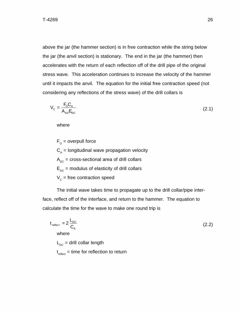
until it impacts the anvil. The equation for the initial free contraction speed (not
considering any reflections of the stress wave) of the drill collars is
VF C
A ECO A
DC DC
= (2.1)
where
FO = overpull force
CA = longitudinal wave propagation velocity
ADC = cross-sectional area of drill collars
EDC
= modulus of elasticity of drill collars
VC = free contraction speed
The initial wave takes time to propagate up to the drill collar/pipe inter-
face, reflect off of the interface, and return to the hammer. The equation to
calculate the time for the wave to make one round trip is
tLCreflec t
DC
A
= 2 (2.2)
where
LDC = drill collar length
treflect = time for reflection to return
T-4269 27
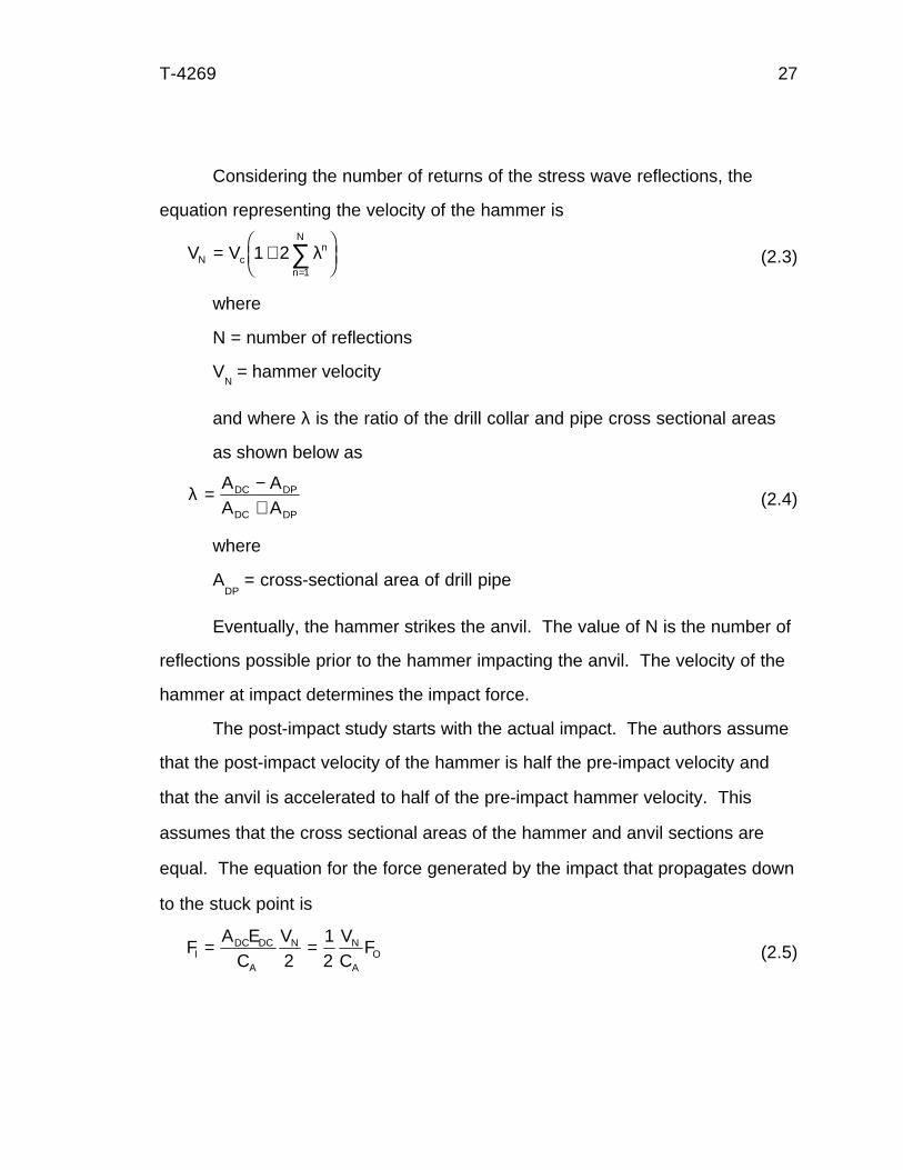
Considering the number of returns of the stress wave reflections, the
equation representing the velocity of the hammer is
V VN cn
n
N
= +FHG
IKJ=
∑1 21
λ (2.3)
where
N = number of reflections
VN = hammer velocity
and where λ is the ratio of the drill collar and pipe cross sectional areas
as shown below as
λ = −+
A AA A
DC DP
DC DP(2.4)
where
ADP
= cross-sectional area of drill pipe
Eventually, the hammer strikes the anvil. The value of N is the number of
reflections possible prior to the hammer impacting the anvil. The velocity of the
hammer at impact determines the impact force.
The post-impact study starts with the actual impact. The authors assume
that the post-impact velocity of the hammer is half the pre-impact velocity and
that the anvil is accelerated to half of the pre-impact hammer velocity. This
assumes that the cross sectional areas of the hammer and anvil sections are
equal. The equation for the force generated by the impact that propagates down
to the stuck point is
FA E
CV V
CFI
DC DC
A
N N
AO= =
212 (2.5)
T-4269 28
where
FI = impact force
The authors also point out that part of this wave also propagates up the
drill string, reflects off of the drill collar/pipe interface, and eventually superim-
poses its force to the stuck point. To describe the stress history at the stuck
point, the authors track each separate contribution of each original and reflected
wave and use linear superposition at any given point in time. However, as the
authors note that after about three reflections, any further contributions by the
residual wave reflections are practically nil.
As the authors state, the peak force derived during the impact is not a
good measure of the jar’s effectiveness. If the stuck point is truly a mathematical
point, then a peak force greater than the sticking force would immediately free
the pipe. No time would be considered. However, the stuck point is actually an
area of some length. As field experience proves, it takes time and repeated
jarring to break a string loose.
In addition, the authors state this method only approximates the forces. In
the model, the forces are changed discontinuously whereas in reality, the forces
are continuous. The impulse function is introduced as
I F T F dtT
( , ) (t)= z (2.6)
where
F(t) = impact force function with respect to time
T = duration of impact
I(F,T) = impulse function
T-4269 29
Using this equation, an average force is determined as follows
FI F t
TAVG =,b g
(2.7)
where
FAVG = average force over impulse duration
To make the model more valid, the authors assume that the drill pipe did
not have any reflections occur inside it. That means the drill pipe is longer than
1,500 feet. Even though there actually are reflections from inside the drill pipe,
the reflections do not return to the drill collars until long after the useful part of
the jarring wave has decayed. Also, it is assumed that the jar was not placed
within a joint of the drill collar/pipe interface.
An important point that the authors make is that the slip force is an as-
sumed value of force needed to initiate and maintain motion at the stuck point.
This force has to be greater than the overpull force (otherwise the string would
move!). The string at the stuck point moves with a slip velocity of
VF F C
A ESS A
DC DC
=−b g
(2.8)
where
F = impact force
FS = force needed to overcome sticking
VS = slip velocity
T-4269 30
The distance traveled by the string at the stuck point is the product of the
slip velocity and the time of the impulse. This distance traveled is very small and
would not be seen at the surface. A real concern is the fact that the slip force is
rarely known.
The results of this analysis show that moving the jar further up the drill
collars results in a higher impact force but at a shorter duration than jars lower in
the string. However, the impulse increases with the jars set lower in the string.
The optimum location of the jar depends upon the nature of the sticking force.
Although this is a valuable paper, there are too many simplifying assump-
tions for this method to be useful. With so few parts of the drill string actually
considered, this method does not work for the complex strings typically used.
Friction is totally ignored. In addition, the stuck point is modeled as a fixed point.
Finally, it is not correct to assume that the drill string below the jar is stationary.
Transient Dynamic Analysis of the Drillstring Under
Jarring Operations by the FEM
The next major paper on jarring analysis, Transient Dynamic Analysis of
the Drillstring Under Jarring Operations by the FEM, was written by M. Kalsi, J.
Wang, and U. Chandra. It was published in the March 1987 SPE Drilling Engi-
neering edition and was presented at the SPE/IADC Drilling Conference in New
Orleans, Louisiana in 1985 as SPE paper 13466 (Kalsi 1987).
In this paper, the authors approach the problem of drill string jarring
analysis from a different viewpoint. Rather than track individual waves, the
authors use the finite element method (FEM) which allows the user to include
T-4269 31
complex strings and various forms of damping. With this method, the force,
displacement, velocity, and acceleration histories anywhere along the string are
available.
A nonlinear transient dynamic analysis is performed using the commer-
cially available FEM software package, ANSYS™, to analyze a typical drill
string. The authors compare a uniform collar string to a string with drill collars,
accelerator, heavy weight drill pipe, and drill pipe.
This analysis requires three types of elements: 1-D spar, gap, and
spring-damper. A 1-D spar element, capable of only axial loads, is used for drill
collars and pipe. The cross sectional area is constant across this element. The
jar is modeled as a gap element with one side of the gap being the hammer and
the other, the anvil. The gap size corresponds to the jar stroke length. The
spring-damper elements connect the string to the hole wall. The spring values
are set to zero to simulate wall friction. Spring damper elements are also used
to model the stuck point as they have the characteristic of a linear relationship of
force and displacement until a threshold force is reached. At that point, the force
stays constant regardless of the displacement.
A total of 174 elements and 188 nodes are used. The time step is 0.0002
seconds for 0.14 seconds duration. The model is run in two steps. The first step
applies the overpull. The second part models the free contraction, impact, and
post-impact phases.
The model shows many interesting effects not seen in the previous paper.
The accelerator acts as an almost free end. This is the main reflection point for
the upwardly propagating waves. But there is a slight departure of the wave
arrival times for the anvil. The authors attribute this to the fact that the stuck
T-4269 32
point is not modeled as a fixed point, but rather as a stiff spring. The velocity of
the hammer is somewhat lower than predicted by theory, too. This can be attrib-
uted to the almost free end of the accelerator. It is not a true free end. In addi-
tion, the hammer is slightly decelerating between wave reflections. This is
attributed to wall damping.
The impact shows that the anvil motion is important. A stationary anvil
assumption can lead to a ±30 percent error in the predicted impact force. There-
fore, the authors show the need to model a moving anvil.
The authors also find that acceleration values are numerically very sensi-
tive to the time step chosen. Reducing the time step requires a large computa-
tional and storage effort. Acceleration loads are important to know for the design
of downhole measurement while drilling (MWD) tools. The authors demonstrate
that the velocity changes are not as sensitive to time step selection; therefore,
design values can be determined using changes in velocity rather than calcu-
lated values of accelerations.
While this is a very good model, there are two major drawbacks. The first
is that the FEM can be a very powerful technique; but, it is not easy to use. It
takes training and good engineering skills. The second problem is that it takes a
very long time to run one analysis. Depending upon the computer and the com-
plexity of the drill string, it can take from 15 minutes to six hours for one run.
This makes optimization very time consuming. This is unacceptably long for
typical field usage.

T-4269 33
A Study of How Heavy Weight Drill Pipe Affects Jarring Operations
This paper, A Study of How Heavy-Weight Drillpipe Affects Jarring Opera-
tions, was written by M. Lerma. It was presented at the 60th SPE Fall Confer-
ence in Las Vegas, Nevada in 1985 (Lerma 1985).
The author uses the wave tracking method developed by Markus Skeem
(Skeem et al. 1979). He increases the capability of that model by incorporating
a more complex drill string and he includes the effect of heavy weight drill pipe.
The author considers two examples, one with 356 feet of drill collars above the
jar and one with 960 feet of heavy weight drill pipe above the jars. No attempt
was made to put drill collars and heavy weight drill pipe together in the same drill
string.
The author runs two cases: (1) with drill collars above the jar, and (2) with
heavy weight drill pipe above the jar. The weight above the jars is the same in
both cases. The author points out that initially the jarring hammer has a higher
velocity in heavy weight drill pipe than in drill collars. He states that this is
because the heavy weight drill pipe is more elastic than drill collars. The author
also notes that drill collars (in his example) are accelerating faster than the
heavy weight drill pipe (because of more reflections in the drill collar example).
Still, the author adds, the hammer in the heavy weight drill pipe case would have
the higher momentum because the hammer would strike the anvil at a higher
velocity.
The author points out that friction causes a significant change in the
results. According to the author, running jars in heavy weight drill pipe reduces
peak force by 50 percent; but increases impulse by 40 percent as compared to
T-4269 34
jars in drill collars. However, if friction is incorporated into both cases (by chang-
ing the end boundary conditions, which is not an accurate method to take friction
into account) at the stuck point, there is a reduction of peak force by 50 percent,
reduction in impulse of 50 percent, and a reduction in displacement by 65 per-
cent.
The author includes a description of the model’s limitations: damping is
not considered; the impact of the hammer and anvil do not consider
inelasticities; energy absorption of the drilling mud (a form of damping) is not
calculated; stretch in the lower drill collar section is ignored; and, some bottom
hole assembly items are not considered. The author concludes that a more
complex model is needed.
Computerized Drilling Jar Placement
The paper, Computerized Drilling Jar Placement, was written by W.E.
Askew. It was presented at the 1986 IADC/SPE Conference in Dallas, Texas as
SPE paper 14746 (Askew 1986).
This paper describes a proprietary jarring program written for Anadrill
Schlumberger. The program uses the finite element method to determine opti-
mum drilling jar performance. In this case, optimum performance means the
largest jarring force at the stuck point. This paper does not go into the details of
their model, but rather describes typical results of the model. These results are
broken into three parts: jar placement recommendation, trip setting recommenda-
tion, and bottom hole assembly design information.

T-4269 35
Their jar placement recommendation meets the following five criteria:
1. The jar location has to be more than 60 feet from a stabi-
lizer or cross sectional area change.
This recommendation is made because the concentration of
bending stresses near a stabilizer or cross sectional area change
tend to be high. Since jars tend to be less stiff than other drill
string components of the same diameter, the jar flexes. The flexing
coupled with rotation while drilling can lead to jar failure as the
parts inside of jar wear out from flexing.
2. Depending upon hole inclination, there is a maximum
weight that can be slacked off above a jar while drilling.
Current recommendations are that a jar used in a drill string
should be run in tension. This is thought to keep bending stresses
to a minimum. In some holes, especially directional drilled holes,
the jar can not be run in the tension section of the string. In those
cases, there is a maximum compression load that can be run in the
jar. For holes from 0° to 10° inclination, a maximum compression
load of 10,000 lbf can be used. For every 10° more in inclination,
another 5,000 lbf can be added.
3. There is a minimum 5,000 lbf needed to trip the jar.
Because of hydrostatic and hydrodynamic pressure loads, a
jar has a tendency to be pumped into the cocked position. This is
T-4269 36
sometimes called the extension force. If the weight slacked off
above the jar is about the same as the extension force, the jar’s
interior parts are floating in a neutral position. This can cause the
jar to cock. Then vibrations from drilling can cause wear to the
cocking mechanism. Having a minimum load for the tripping
mechanism minimizes this possibility. This problem usually does
not arise in typical drilling operations.
4. A maximum stiffness ratio of 3.0 at the jar is required.
The stiffness ratio is the ratio of the section moduli of
the two different sections. This is often called the section modulus
ratio (SMR). The section modulus is the polar moment of inertia
divided by the section outside diameter (Mitchell 1995). If one
section has a modulus of 6 and another section has a modulus of
2, the stiffness ratio would be 3. If the ratio were higher, a very stiff
section of pipe would be next to a limber section of pipe. This
would cause the limber member to flex far more than it would for a
smaller ratio. This, in turn, would lead to fatigue failure in the
limber pipe section.
Drilling jars are not as stiff as drill collars. For a jar of
the same outside diameter as the drill collar, the stiffness ratio is
usually 3, which is satisfactory. If a jar is sandwiched between two
very stiff sections, the jar is likely to have a higher than 3 stiffness
ratio, leading to eventual jar failure.
T-4269 37
5. A minimum of 5,000 lbf weight must be available above
the jar.
This is the authors’ recommendation for the “proper” amount
of weight (the authors actually meant mass) above the drill collar
for a sufficient amount of mass as the jar impacts up and down.
This jarring program can determine the location of the jar within the string
using these five recommendations. It starts checking every 30 feet beginning at
the bit. Only those locations meeting the recommendations are then considered
for the second part of the program, trip setting recommendation.
This first part of the program determines the trip setting load value (the
overpull) needed to trigger the jar. This load must not be greater than the
strength of the string. Usually the lowest string strength is in the drill pipe sec-
tion. Operating the jars with a triggering load near but not exceeding the drill
pipe strength will give the peak jarring force capable for that particular string.
The model in this paper shows that the peak force and impulse increase propor-
tionally with an increase in the jar triggering load.
In addition, the location of the jar within the string dictates the available
triggering load. The higher the jar is in the string, the higher the up triggering
load can be set. This is because there is more tensile force available higher in
the string. The program chooses a “proper” up hit setting as follows
F F F F FUP SETTING MAXIMU M SAFETY UP STRING ABOVE JAR DRAG_ _ _ _= − − − (2.9)
where
FMAXIMUM
= maximum overpull force (includes string weight)
FSAFETY_UP
= a safety factor force
T-4269 38
FSTRING_ABOVE_JAR
= bouyed string weight above the jar
FDRAG
= drag force
FUP_SETTING
= recommended up hit setting
Drag is usually assigned a value of 10 percent of the string weight above
the jars. A safety load, used for operator uncertainty, of 10,000 to 20,000 lbf is
usually considered good.
For a down hit, the equation is
F F f f
FDOWN SETTING BHA ABOVE JAR DRAG BOUYANCY
SAFETY DOWN
_ _ _
_
( ) cos= +
+
1 αb g(2.10)
where
fDRAG
= drag factor (fraction of string weight)
FBHA_ABOVE_JAR
= bottom hole assembly weight above the jar
fBOUYANCY
= bouyancy factor
α = inclination angle
FSAFETY_DOWN
=a safety factor force
FDOWN_SETTING
= recommended down hit setting
The drag factor is usually assigned a value of 10 percent. The safety
load of 20,000 lbf is considered minimal.
With the jar high in the string, there is more tension available for a high up
hit load; but, the down hit load is lessened because there is less weight bottom
hole assembly above the jar. Conversely, the lower the jar is in the string, the
more down-hit load is available at the expense of the up hit load. However, if the
up hit load is set low, the weight of the bottom hole assembly below the jar may
be enough the trigger the jar.
T-4269 39
The third part of the program provides potentially helpful bottom hole
assembly information. This part determines if the current bottom hole assembly
is adequate given the calculations of the previous two parts of the program. This
part also calculates the jar operating loads.
Although this paper does not have any model mathematics, it is useful in
determining the operating parameters and characteristics of the jarring process.
Other than that, it is an advertisement for Anadrill Schlumberger.
A Practical Approach to Jarring Analysis
The next paper, A Practical Approach to Jarring Analysis, was written by
Jaw-Kuang Wang, Monmohan S. Kalsi, René A Chapelle, and Thomas R.
Beasley. It was published in the March 1990 edition of the SPE Drilling Engi-
neering . The paper was originally given in the 1987 IADC/SPE Conference in
New Orleans as SPE paper 16155 (Wang et al. 1990).
This paper picks up where Skeem et al. ends. It is a jarring analysis that
is based on a closed form stress wave tracking method. The authors took
Skeem’s work further by incorporating heavy weight drill pipe and including the
stretch in the string below the jars (the anvil section).
As the authors point out, the FEM method is a good method for analytical
and research engineers. However, for the person on the rig, the FEM method is
not a solution. FEM requires large computational resources, long solution times,
and engineering expertise to perform and interpret the analysis. It can take a
thousand time steps to do one typical analysis. Since each time step requires an
iterative solution, an inordinate amount of time is needed. The author’s solution
is to use the stress wave method and call it “good enough.”
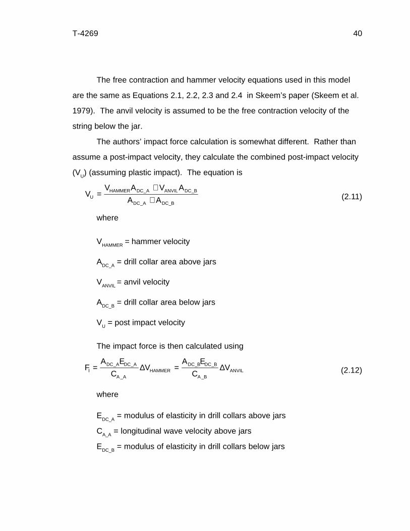
T-4269 40
The free contraction and hammer velocity equations used in this model
are the same as Equations 2.1, 2.2, 2.3 and 2.4 in Skeem’s paper (Skeem et al.
1979). The anvil velocity is assumed to be the free contraction velocity of the
string below the jar.
The authors’ impact force calculation is somewhat different. Rather than
assume a post-impact velocity, they calculate the combined post-impact velocity
(VU) (assuming plastic impact). The equation is
VV A V A
A AUHAMMER DC A ANVIL DC B
DC A DC B
=+
+_ _
_ _(2.11)
where
VHAMMER = hammer velocity
ADC_A = drill collar area above jars
VANVIL
= anvil velocity
ADC_B = drill collar area below jars
VU = post impact velocity
The impact force is then calculated using
FA E
CV
A E
CVI
DC A DC A
A AHAMMER
DC B DC B
A BANVIL= =_ _
_
_ _
_
∆ ∆ (2.12)
where
EDC_A
= modulus of elasticity in drill collars above jars
CA_A = longitudinal wave velocity above jars
EDC_B = modulus of elasticity in drill collars below jars
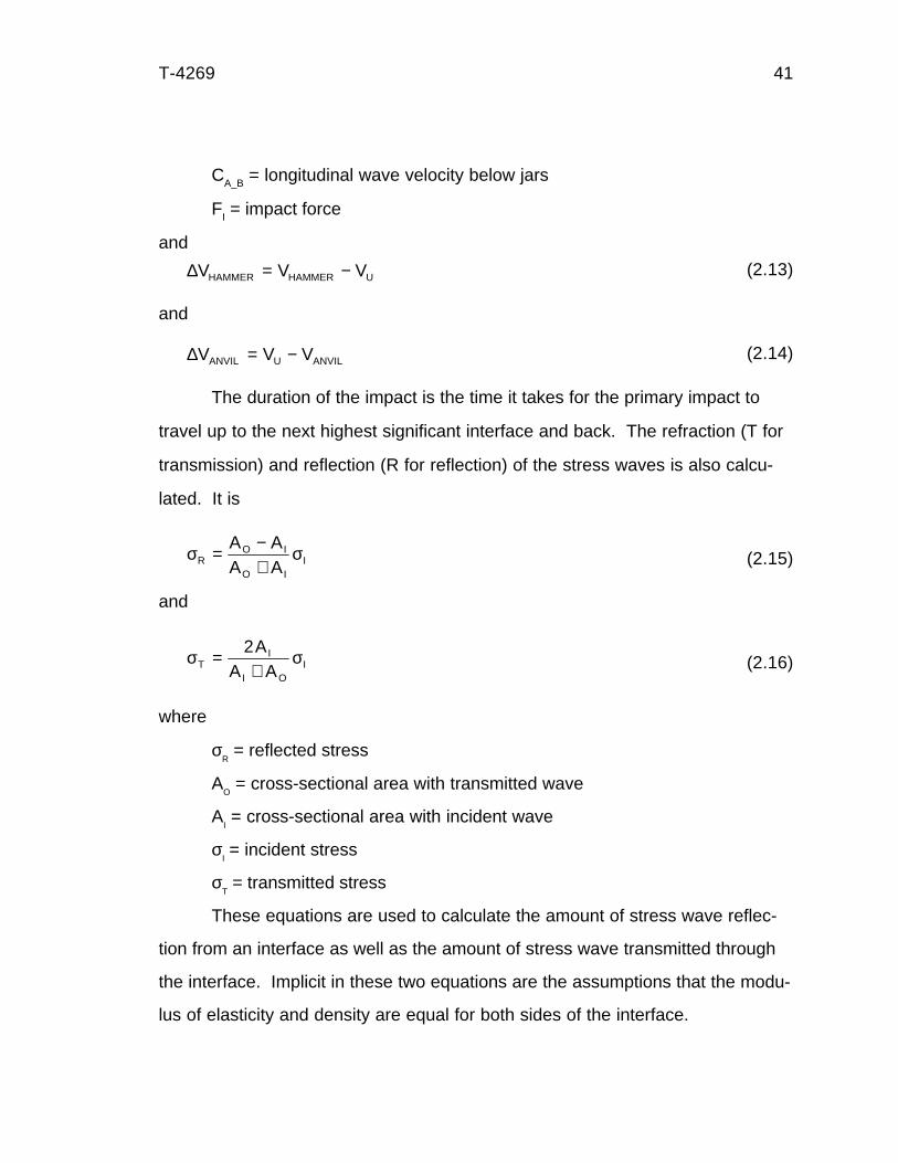
T-4269 41
CA_B = longitudinal wave velocity below jars
FI = impact force
and
∆V V VHAMMER HAMMER U= − (2.13)
and
∆V V VANVIL U ANVIL= − (2.14)
The duration of the impact is the time it takes for the primary impact to
travel up to the next highest significant interface and back. The refraction (T for
transmission) and reflection (R for reflection) of the stress waves is also calcu-
lated. It is
σ σRO I
O II
A AA A
= −+ (2.15)
and
σ σTI
I OI
AA A
=+
2(2.16)
where
σR = reflected stress
AO = cross-sectional area with transmitted wave
AI = cross-sectional area with incident wave
σI = incident stress
σT = transmitted stress
These equations are used to calculate the amount of stress wave reflec-
tion from an interface as well as the amount of stress wave transmitted through
the interface. Implicit in these two equations are the assumptions that the modu-
lus of elasticity and density are equal for both sides of the interface.
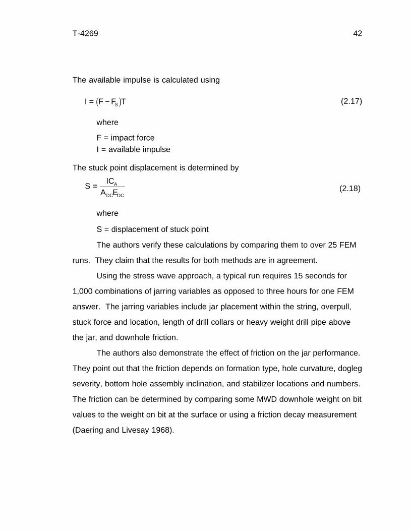
T-4269 42
The available impulse is calculated using
I F F TS= −b g (2.17)
where
F = impact forceI = available impulse
The stuck point displacement is determined by
SIC
A EA
DC DC
= (2.18)
where
S = displacement of stuck point
The authors verify these calculations by comparing them to over 25 FEM
runs. They claim that the results for both methods are in agreement.
Using the stress wave approach, a typical run requires 15 seconds for
1,000 combinations of jarring variables as opposed to three hours for one FEM
answer. The jarring variables include jar placement within the string, overpull,
stuck force and location, length of drill collars or heavy weight drill pipe above
the jar, and downhole friction.
The authors also demonstrate the effect of friction on the jar performance.
They point out that the friction depends on formation type, hole curvature, dogleg
severity, bottom hole assembly inclination, and stabilizer locations and numbers.
The friction can be determined by comparing some MWD downhole weight on bit
values to the weight on bit at the surface or using a friction decay measurement
(Daering and Livesay 1968).
T-4269 43
The authors take friction into account by slowing the hammer between
reflections. The percentage loss in velocity is assumed to be proportional to the
ratio of the interface areas, bottom hole assembly length above the jar, and to
the square root of the jar stroke as shown in
′ = −FHG
IKJ
V V KA
AL JN N
DC A
DC BDC A1 1
0 5_
__
.b g (2.19)
where:
K1 = experimentally derived drag constant
LDC_A = length of drill collars above jar
J = jar stroke length
The friction for the anvil section is
′ = − ′V V K tC C 1 20 5b ge j.
(2.20)
where
K2 = experimentally derived drag constant
′VC = drag modified anvil velocity
For a high impact, the hammer should be traveling as fast as possible.
For every reflection, the hammer velocity increases; however, the magnitude of
the increase in hammer velocity decreases for every reflection. To get many
reflections, the section of drill collars above the jar should be relatively short.
According to the authors, the jar stroke is not as important under these condi-
tions. In long drill collar sections above the jar, the jar stroke length is more
important. The jar stroke must be long enough to allow the hammer to acceler-
ate fully.
′VN = drag modified hammer velocity
′t = time from trigger to impact

T-4269 44
The authors compare a straight drill collar bottom hole assembly to a
bottom hole assembly with drill collars and heavy weight drill pipe. The results
show that for the straight drill collar bottom hole assembly, there is only one
maximum impulse location for the jar. In the case of the heavy weight drill pipe
bottom hole assembly, there are two maximum impulse locations for the jar. This
is because of the complexities of the stress wave propagation with drill collars
and heavy weight drill pipe. In this case, it could be that a jar is set in a location
that corresponds to the minimum between the two peaks of impulse. If that
should happen, the jars will not be working at optimum performance.
Loads on Drillpipe During Jarring Operations
The latest paper on jarring available at the time of this dissertation, Loads
on Drillpipe During Jarring Operations, was written by Thor V. Aarrestad and Åge
Kyllingstad. It was published in SPE Drilling and Completion in December
1994. It was originally presented in the 1992 SPE European Petroleum Confer-
ence in Cannes, France. This paper uses the closed form stress wave tracking
method (Aarrestad and Kyllingstad 1994).
In some wells, especially deviated wells, the drill pipe at the surface is
near its rated tensile capacity. There is some concern that the stresses from
jarring may exceed the tensile capacity of the drill pipe and cause a failure. In
this paper, the authors show that the drill string loads in the drill pipe during
jarring operations are not significant.
The jarring process is broken into five phases. The first phase is loading,
the storing of strain energy in the string. This can take a few seconds to a

T-4269 45
minute for some hydraulic jars. The next phase is acceleration which occurs
after the jar triggers but before the hammer and anvil impact. The strain energy
stored in the pipe is converted to kinetic energy. The third phase is impact. This
phase is short, lasting 10 to 50 milliseconds. The fourth phase is post-impact
where the stress waves are propagating. The fifth and final phase is recocking
the jar in order to be able to start the jarring cycle over.
The analysis in this paper makes the following five assumptions:
1. The stuck string can be divided into four sections: the fish
(the string under the jar), the jarring mass (the bottom hole
assembly above the jar), a heavy weight drill pipe section (if
needed), and the drill pipe section. Note that accelerators
were not considered.
2. The drill pipe section is so long that no reflections from the
surface will be seen during the acceleration, impact, and
post-impact phases.
3. Jar release is instantaneous. There is no transition time
between the loading and acceleration phases. This release
from the static pull to zero force represents a negative force
wave travelling up the string.
4. Internal and external friction forces are ignored. The au-
thors make this simplifying assumption by regarding friction
forces as static and not dynamic.
5. Residual vibrations in the fish section at impact time are
ignored.

T-4269 46
The equations used by the authors are the same as in Skeem 1979 pa-
per, Drillstring Dynamics During Jarring Operations (Skeem et al. 1979). The
force ratio of overpull force to impact force transmitted to the drill pipe is
Φ = + −−
+
η1 21
1r rr
CP CPn
CPn (2.21)
where
Φ = ratio of impact force to overpull force
η =+
A
A ADC B
DC B DC A
_
_ _(2.22)
rA A
A ACPDC A DP
DC A DP
=−+
_
_(2.23)
If Φ is less than one, then the force on the drill pipe during jarring opera-
tions will be less than the overpull load. Examples in the paper show that if the
number of reflections is four or more, Φ will be less than one.
The addition of heavy weight drill pipe complicates the system because of
the multitude of reflections that need to be tracked. In this case,
Φ ≈+ +
η4A A
A A A AHWDP DC A
DC A HWDP DP HWDP
_
_d ib g (2.24)
where
AHWDP = cross-sectional area of heavy weight drill pipe
The values of Φ are slightly greater than in the straight drill collar case.
The transmission of stress waves into the drill pipe is more efficient with a ta-
pered string. This reduces the magnitude of the wave being reflected back to
the hammer. Because of this, the authors state that a heavy weight drill pipe
section reduces the effectiveness of the jar.

T-4269 47
Because of an accident on a test drilling rig in Norway, a 4,000 foot drill
string with a jar was stuck in the hole. The research engineers measured the
forces on the kelly while jarring. One important result showed that the assump-
tion that jar release is instantaneous is not valid. (Although in the paper, the
authors claim it is assumption 4, further discussion indicates that they really
meant assumption 3.) There is aproximately a 100 millisecond time from jar
trigger to full release. This implies that the sharp stair step look to the hammer
velocity plots are not truly valid. This also indicates that the discontinuity of
force inherent in stress wave analysis procedures are not descriptive of reality.
The waves measured on the kelly are much broader than expected. A
sharp wave was expected; instead, the wave appears dispersed over time. This
may be because stress waves tend to disperse as a result of the many cross
sectional area changes inside the jar. The stress wave must propagate through
these changes prior to coming out of the jar and propagating through the rest of
the string. This weakens the stress wave. In addition, the wave disperses
because of friction. The high frequency components of the wave tend to dampen
more than the low frequency components. Also, the tool joints on the drill pipe
act to dampen the axial component of the stress wave.
T-4269 48
CHAPTER 3
TIME AND FREQUENCY DOMAINS
The current jarring analysis methods are discussed in this chapter. Then
wave theory and relationships are described. The differences between the time
and frequency domains are shown. Finally, the techniques used to convert from
the time domain to the frequency domain (such as the fast Fourier transform)
and problems inherent in these techniques are explained.
The mathematical analysis of jarring traditionally has been firmly rooted in
the time domain with the two independent variables being time and space (a
location). Thus, the analysis is performed at a single point in time on a single
location within the string.
One form of time domain analysis is stress wave tracking, which is a
closed form partial differential method, It has the advantages of being exact and
solvable at any location and time without regard to any previous solutions. How-
ever, these types of solutions can be difficult (if not impossible) to solve. The
analysis is restricted to constant geometric and material properties. For ex-
ample, there is no single solution for changes in a cross-sectional area. Finally,
only linear functions can be considered. As will be seen, dry sliding friction,
called Coulomb damping, is nonlinear and cannot be solved in a linear only
fashion.
T-4269 49
The other time domain method is the finite element method. This is a
technique which simplifies complex problems. It involves breaking a structure
into a finite number of pieces called elements. For a specific analysis, a simpli-
fied equation is developed for each element. For example, if an axial displace-
ment for a given force is desired, then a simplified equation is derived for that
type of analysis. If all the elements are similar, then the same type of equation
can be used. Once all the elements are mathematically described and boundary
conditions are prescribed, then all the equations for each element are simulta-
neously solved with a linear algebraic approach.
The finite element method can incorporate multiple geometric and mate-
rial properties. Nonlinear functions can also be incorporated through iteration
methods. However, since a simplified equation describes the element, the
results are only approximate. In addition, a complex structure requires large
computational resources. The computer requirements include a fast central
processing unit (CPU), a large amount of random access memory (RAM), a large
storage disk, and a lot of time. The method also requires that the user have
training and knowledge of how to input the data as well as interpret the results.
The degree of approximation depends upon many factors. In wave propa-
gation problems, a limitation of this approximation method is evident. A string of
pipe has a continuous distribution of mass, but the finite element method re-
quires that the mass be lumped at the ends (called nodes) of the elements.
This is similar to a series of springs connected to points of mass. If the analysis
was done at the atomic level, this approach would work well; however, it is virtu-
ally impossible to model every atom in a section of pipe.

T-4269 50
A rule of thumb in finite element method solution techniques is to use 20
elements over a wavelength (ANSYS, Inc. 1992). A 1,000 Hertz wave (not
uncommon is jarring analysis) would have a wavelength in steel of 16.84 feet.
This means that an element should not have a length greater than 0.84 feet.
A popular finite element method for wave propagation problems is as
follows. The structure to be analyzed is built with various multiple elements.
Initial conditions at a given time point are then imposed. The equations making
up the structure are solved. This solution becomes the initial values for the next
step in time, which is solved and so on. Time marches on.
The size of the step in time is critical to the solution of the wave propaga-
tion problem. The step size (time duration) must be small enough for the finite
element method wave propagation algorithm to be stable. If the time step is too
large, the algorithm will not be stable and will not converge to an answer.
In addition, the time step must be small for wave tracking. This means
that for a given element length, if the time step is larger than the time it takes for
a wave to propagate across the element, then the wave literally passes through
the element without being seen! Another rule of thumb in finite element method
solution techniques is to use a time step of aproximately 1.5 times the amount of
time for a wave to propagate through an element (ANSYS, Inc. 1992). A time
step for wave propagation in a one foot steel element would be 84 microseconds
at the longest. This is 11,909 steps per second. A longer element would have a
larger time step. A 20 foot element would have a maximum time step of 1,680
microseconds or 595 steps per second.
As previously noted, longer elements do not model the continuous mass
of the string very well. An increasing number of elements are needed to accu-

T-4269 51
rately model the wave propagation. This means that each element must be
smaller which, in turn, requires the time step be smaller. More time steps are
required. More elements need to be solved simultaneously over many time
steps. The more accuracy needed, the more elements and time steps required.
This can rapidly get out of hand.
For example, a wave in steel travels 3,450 feet in 0.2048 seconds. If the
1,000 Hertz example is used, then at 0.84 feet per element, 4,107 elements
would be required. A 0.84 foot element requires a time step of 74.8 microsec-
onds. For 0.2048 seconds, 2,738 time steps are needed. That means that
4,107 equations must be simultaneously solved 2,738 times. This is 11,244,966
calculations! This takes time and out on the drilling rig, no one will be waiting for
the answer. There must be a better method. There is, but some preliminary
work must be done first.
This is not to say that all time based finite element methods will not work.
There are some implicit methods of time domain based finite element methods
that can treat mass as a continium. In those situations, element length may not
need to be as critical as in the time domain explicit methods. In addition, time
step sizing may not be a critical issue. This is an area that needs more investi-
gation.
Wave Theory
After an external force is impressed on a body, a real world elastic body
does not instantly react over its entire length. The point immediately under the
external force reacts first, then the section just under that point reacts to the
previous section’s reaction, and so on. This transfer of reactions travels at a
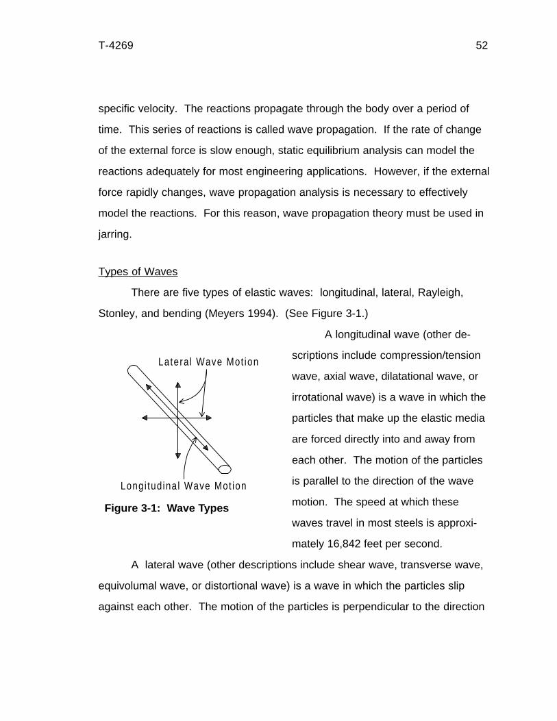
T-4269 52
specific velocity. The reactions propagate through the body over a period of
time. This series of reactions is called wave propagation. If the rate of change
of the external force is slow enough, static equilibrium analysis can model the
reactions adequately for most engineering applications. However, if the external
force rapidly changes, wave propagation analysis is necessary to effectively
model the reactions. For this reason, wave propagation theory must be used in
jarring.
Types of Waves
There are five types of elastic waves: longitudinal, lateral, Rayleigh,
Stonley, and bending (Meyers 1994). (See Figure 3-1.)
A longitudinal wave (other de-
scriptions include compression/tension
wave, axial wave, dilatational wave, or
irrotational wave) is a wave in which the
particles that make up the elastic media
are forced directly into and away from
each other. The motion of the particles
is parallel to the direction of the wave
motion. The speed at which these
waves travel in most steels is approxi-
mately 16,842 feet per second.
A lateral wave (other descriptions include shear wave, transverse wave,
equivolumal wave, or distortional wave) is a wave in which the particles slip
against each other. The motion of the particles is perpendicular to the direction
Longi tud inal Wave Mot ion
Latera l Wave Mot ion
Figure 3-1: Wave Types
T-4269 53
of the wave motion. Because slipping uses more energy, lateral waves are
slower. The speed at which these waves travel in steel is approximately 10,428
feet per second. A rapidly changing torsional force on a section of pipe will
cause a lateral wave to propagate from the point of application to all other parts
of the pipe. All other waves are made up of either longitudinal or lateral waves.
A Rayleigh wave is a surface wave that travels along the surface of a
solid elastic media. The particle motion is elliptical and is analogous to a buoy
reacting to an ocean wave. It is a special form of a wave. These waves are
slower than lateral waves and move approximately 9,656 feet per second in
steel.
A Stoneley wave is a wave that travels along an interface. With two
different types of solids joined together, any wave crossing that boundary will
induce a wave traveling along the interfacial boundary. With many layers of
media, a Love wave occurs (as in wave propagation through the Earth).
A bending wave is also called a flexural wave. It is a wave that travels as
a bend in a bar or plate. Both longitudinal and lateral components are present in
this type of wave. Rotary shears and moments of inertia complicate the analysis
of this type of wave.
In jarring analysis in drill strings, the most logical wave to analyze is the
longitudinal wave. Since the jar acts mainly in the longitudinal direction, the
analysis of the jarring procedure can be one-dimensional. Although waves other
than longitudinal are present to some degree, they generally do not warrant
inclusion in the first pass of jarring analysis. It should be noted, however, that in
curved boreholes, a bending wave is induced by the motion of the string during
jarring. Since the bending wave is a mixture of the longitudinal and lateral

T-4269 54
waves, the analysis required is considerably more complex and is not a part of
this dissertation. The authors of the six papers discussed in Chapter 2 have not
included waves of types other than longitudinal. Furthermore, the surface type
of waves in drill strings are not significant. Surface waves are more important in
semi-infinite media than in long narrow rods like pipe.
Natural Frequencies
Everything has a frequency at which it would vibrate if it was given the
energy to vibrate and was left alone. This is called a natural frequency. For
instance, the human body has a natural frequency of around five cycles per
second. All drill strings have a natural frequency. This frequency depends on
the drill string material and the geometry of the drill string. The material deter-
mines the speed of a wave in the material. The geometry determines how waves
are reflected and refracted.
During wave propagation, the wave will eventually reach an end of the
material. Some of the wave will reflect back to the source of the wave. If the
reflection reaches the source at the same time a new wave is generated, the two
waves will add together and be synchronized in phase. Later, those two waves’
reflections will return to the source at the same time the next new wave is gener-
ated. All three waves will add. This continues for as long as waves are gener-
ated. The wave will increase in amplitude, theoretically to infinity. This is called
resonance. The frequency at which resonance occurs is the natural frequency
or an integer multiple of that frequency (called a harmonic). If this wave rein-
forcement is allowed to continue, eventually the system will either self destruct or
fatigue to failure.
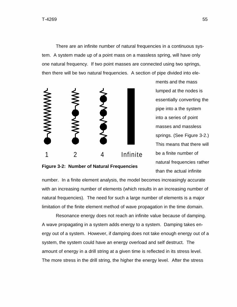
T-4269 55
There are an infinite number of natural frequencies in a continuous sys-
tem. A system made up of a point mass on a massless spring, will have only
one natural frequency. If two point masses are connected using two springs,
then there will be two natural frequencies. A section of pipe divided into ele-
ments and the mass
lumped at the nodes is
essentially converting the
pipe into a the system
into a series of point
masses and massless
springs. (See Figure 3-2.)
This means that there will
be a finite number of
natural frequencies rather
than the actual infinite
number. In a finite element analysis, the model becomes increasingly accurate
with an increasing number of elements (which results in an increasing number of
natural frequencies). The need for such a large number of elements is a major
limitation of the finite element method of wave propagation in the time domain.
Resonance energy does not reach an infinite value because of damping.
A wave propagating in a system adds energy to a system. Damping takes en-
ergy out of a system. However, if damping does not take enough energy out of a
system, the system could have an energy overload and self destruct. The
amount of energy in a drill string at a given time is reflected in its stress level.
The more stress in the drill string, the higher the energy level. After the stress
1 2 4 Infinite
Figure 3-2: Number of Natural Frequencies
T-4269 56
reaches a value greater than the yield strength of the drill string, failure is immi-
nent. If the stress is greater than the ultimate strength of the drill string, failure is
immediate.
Wave Relationships
There are some basic wave relationships that must be defined. These will
be referred to in the coming chapters.
The amplitude of a wave is the difference between the maximum and
minimum values of a sinusoidally varying quantity. The crest of a wave is its
maximum amplitude. The trough of a wave is its minimum amplitude. The wave
period (T) is the length of time is takes a wave to travel as measured from crest
to crest. The wave length (λ) is the distance covered by one wave period (Harris
1988).
The wave frequency (f ) is the inverse of the wave period. It is the number
of crests that occur in a given time unit. This is also called a cyclic frequency.
An angular (sometimes called circular) frequency (ω) is a frequency measured in
radians per unit time. The angular frequency is cyclic frequency times 2π (Harris
1988).
The phase angle (abbreviated to “phase”) of a wave (φ) is the fraction of
the distance the wave has traveled relative to an arbitrary reference. The point
at which the various waves cross the average amplitude line do not coincide
unless the phase is zero. The phase is negative if the crossing occurs before
the reference wave crossing. The phase is positive if the crossing occurs after
the reference wave crossing.
T-4269 57
The velocity of a given point on a sinusoidal wave is defined by the phase
angle from the average amplitude crossing to that given point. This is called the
phase velocity (c).
The wave number (k) is the ratio of the wave length to 2π (Achenbach
1993). If this ratio is a real number, the wave will have a constant phase velocity
for all of its components and will retain its shape. This is called a non-dispersing
wave. If the wave number is complex, then the wave components will have
differing phase velocities. The wave will not retain its shape and will disperse
over time. This is called a dispersing wave. All waves encountered in macro-
scopic reality are dispersing to some extent.
The group speed (cg) is different than the phase velocity. Since any wave
is comprised of a group of sinusoidal components, the response of the group is
important. The interaction of all the wave components in terms of wave number,
amplitude, and frequency results in the appearance of a carrier wave of some
wave number, amplitude, and frequency. This carrier wave is modulated by
group waves that propagate at group speeds. In a non-dispersing wave, the
group speeds are the same as the phase velocity of the wave components.
In a dispersing wave, these group speeds can be different. If the group
speeds are greater than the phase velocities, it will appear that a carrier wave
will originate at the back of the wave and propagate forward until it reaches the
front of the wave. At that point, it vanishes and reappears at the back of the
wave again. If the group speeds are less than the phase velocities, it will appear
that a carrier wave will originate at the front of the wave and propagate back-
wards until it reaches the back of the wave. At that point, it vanishes and reap-
pears at the front of the wave again. This can be visualized by using a caterpil-
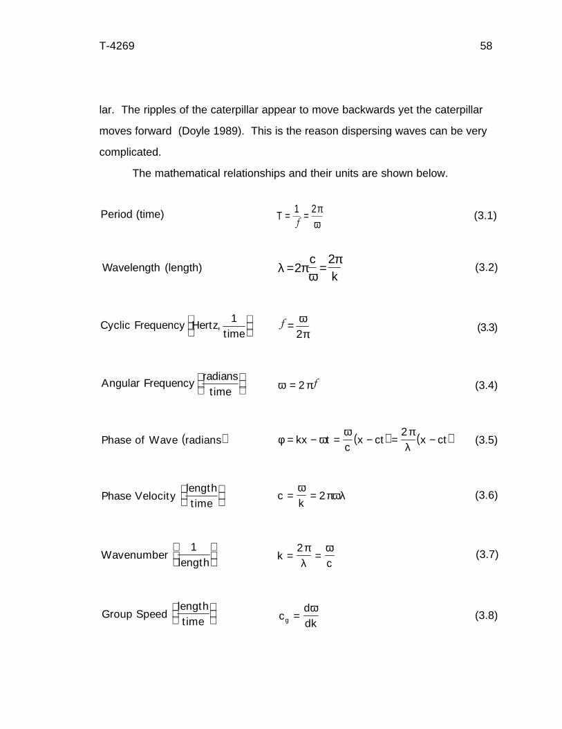
T-4269 58
lar. The ripples of the caterpillar appear to move backwards yet the caterpillar
moves forward (Doyle 1989). This is the reason dispersing waves can be very
complicated.
The mathematical relationships and their units are shown below.
Wavelength (length) λ πω
π= =2
2ck
(3.2)
T = =1 2f
πω
Period (time) (3.1)
f = ωπ2
(3.3)Cyclic Frequency Hertztime
,1
Angular Frequencyradians
time
ω π= 2 f
( )Phase of Wave radians ( ) ( )φ ωω π
λ= − = − = −kx t
cx ct x ct
2
Phase Velocity lengtht ime
c
k= =
ωπωλ2
Wavenumber 1
length
k
c= =
2πλ
ω
(3.4)
Group Speed lengtht ime
c
ddkg =ω
(3.5)
(3.6)
(3.7)
(3.8)
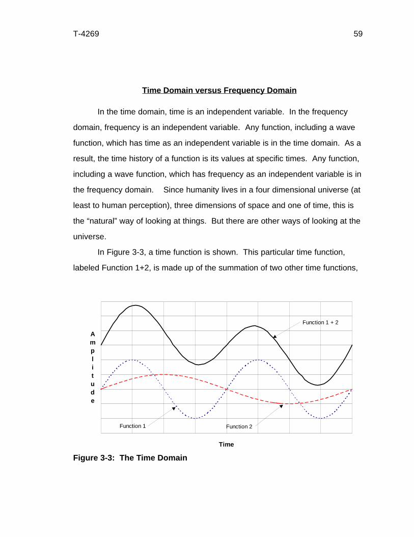
T-4269 59
Time Domain versus Frequency Domain
In the time domain, time is an independent variable. In the frequency
domain, frequency is an independent variable. Any function, including a wave
function, which has time as an independent variable is in the time domain. As a
result, the time history of a function is its values at specific times. Any function,
including a wave function, which has frequency as an independent variable is in
the frequency domain. Since humanity lives in a four dimensional universe (at
least to human perception), three dimensions of space and one of time, this is
the “natural” way of looking at things. But there are other ways of looking at the
universe.
In Figure 3-3, a time function is shown. This particular time function,
labeled Function 1+2, is made up of the summation of two other time functions,
Figure 3-3: The Time Domain
0.0
0.5
1.0
1.5
2.0
2.5
3.0
3.5
4.0
4.5
0.0 0.5 1.0 1.5 2.0 2.5 3.0 3.5 4.0
Time
Amplitude
Function 1 + 2
Function 1 Function 2
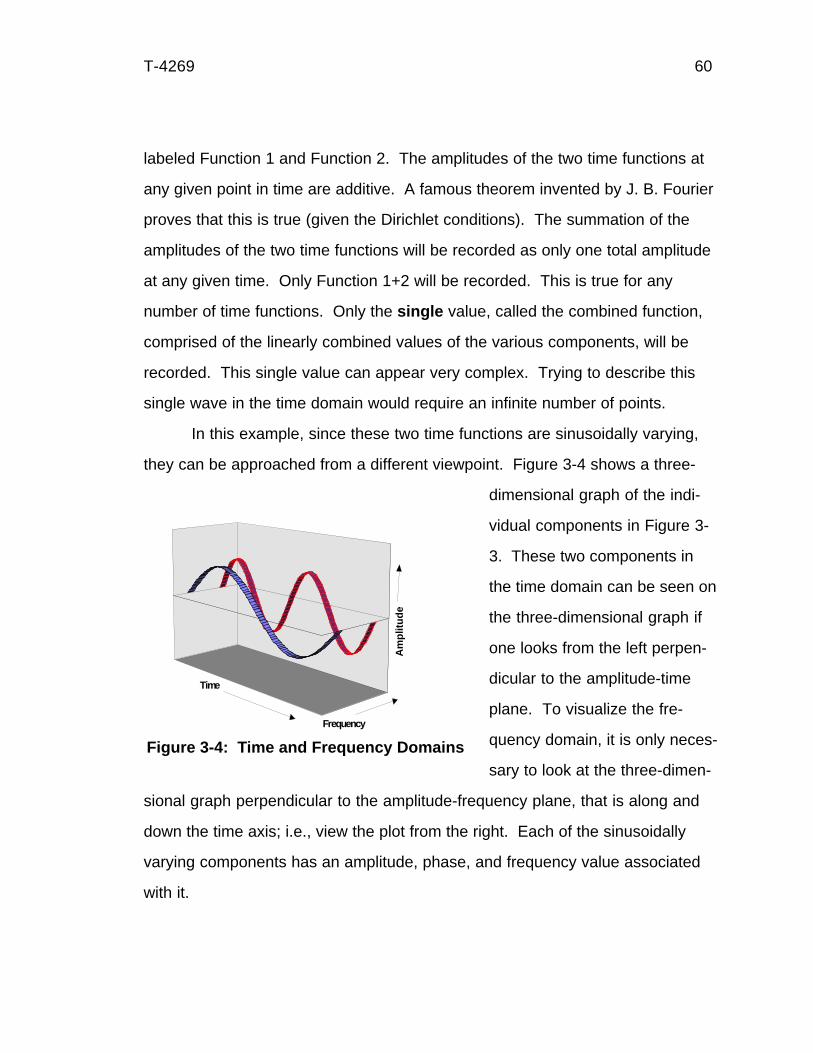
T-4269 60
labeled Function 1 and Function 2. The amplitudes of the two time functions at
any given point in time are additive. A famous theorem invented by J. B. Fourier
proves that this is true (given the Dirichlet conditions). The summation of the
amplitudes of the two time functions will be recorded as only one total amplitude
at any given time. Only Function 1+2 will be recorded. This is true for any
number of time functions. Only the single value, called the combined function,
comprised of the linearly combined values of the various components, will be
recorded. This single value can appear very complex. Trying to describe this
single wave in the time domain would require an infinite number of points.
In this example, since these two time functions are sinusoidally varying,
they can be approached from a different viewpoint. Figure 3-4 shows a three-
dimensional graph of the indi-
vidual components in Figure 3-
3. These two components in
the time domain can be seen on
the three-dimensional graph if
one looks from the left perpen-
dicular to the amplitude-time
plane. To visualize the fre-
quency domain, it is only neces-
sary to look at the three-dimen-
sional graph perpendicular to the amplitude-frequency plane, that is along and
down the time axis; i.e., view the plot from the right. Each of the sinusoidally
varying components has an amplitude, phase, and frequency value associated
with it.
Figure 3-4: Time and Frequency Domains
00.4
0.8
1.2
1.6
2S1
S2
-2.000
0.000
2.000
Am
plitu
de
Time
Frequency
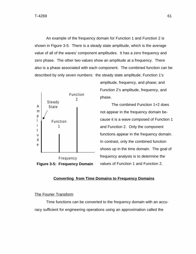
T-4269 61
An example of the frequency domain for Function 1 and Function 2 is
shown in Figure 3-5. There is a steady state amplitude, which is the average
value of all of the waves’ component amplitudes. It has a zero frequency and
zero phase. The other two values show an amplitude at a frequency. There
also is a phase associated with each component. The combined function can be
described by only seven numbers: the steady state amplitude; Function 1’s
amplitude, frequency, and phase; and
Function 2’s amplitude, frequency, and
phase.
The combined Function 1+2 does
not appear in the frequency domain be-
cause it is a wave composed of Function 1
and Function 2. Only the component
functions appear in the frequency domain.
In contrast, only the combined function
shows up in the time domain. The goal of
frequency analysis is to determine the
values of Function 1 and Function 2.
Converting from Time Domains to Frequency Domains
The Fourier Transform
Time functions can be converted to the frequency domain with an accu-
racy sufficient for engineering operations using an approximation called the
Frequency
Amplitude
Funct ion2
Funct ion1
SteadyState
Figure 3-5: Frequency Domain

T-4269 62
discrete Fourier transform. This method assumes the Dirichlet conditions are
met for a given time function. Since all time domain functions are continuous in
time (that is, they are analog in nature), the time domain function must be
sampled at given increment of time. This leads to problems that will be dis-
cussed later. Since the advent of computers, the processing of time domain
functions to the frequency domain has been made much easier. A method that
is quick and especially suited for computers is the fast Fourier transform (FFT).
The FFT is the base of most computer based methods to transform time domain
data to the frequency domain. The transformation of frequency domain functions
to time domain functions are also possible through an inverse FFT.
The Continuous Fourier Transform
Jean B. Fourier proved in 1822 that most functions can be described as
consisting of an infinite series of sinusoidal waves. The process involves using
a Fourier integral (Doyle 1989). This is called the continuous Fourier transform
(CFT).
The conditions for using a Fourier integral are referred to as Dirichlet
conditions. The time function must be integrable in any given period, have a
finite number of discontinuities (if any), and contain a finite number of maxima
and minima during any period. Also, the function must have started at minus
infinite time and end at plus infinite time. All functions that occur in reality meet
these conditions.
The equations that describe the transform are
C F t e dti tω ωb g b g=−∞
∞ −z (3.9)
T-4269 63
and its inverse is
F t C e di tb g b g=−∞
∞z12π
ω ωω (3.10)
where
F(t) = time domain function
t = time
C(ω) = frequency domain function
Using the Fourier integral allows the user to transform a time domain
function into a frequency domain function. This is the method used to find the
amplitude, frequency, and phase of the components of a given wave. The plot of
C(ω) versus ω (the angular frequency) is called a frequency spectrum. In gen-
eral, the values of C(ω) are complex.
C a ibωb g = + = Reiφ (3.11)
The amplitude, R, is found by taking the absolute value of C(ω)
R a b= +2 2 (3.12)
And the phase, φ, is found
φ = FHG
IKJa
ab
tan (3.13)
The solution of a Fourier integral for any given function of time can be
difficult to determine. The Fourier series is a method that can be applied to any
given function, provided it meets the Dirichlet conditions.
In a Fourier series, an arbitrary function can be described as an infinite
summation of coefficients multiplied by a sinusoidal value. The summation of all
the sinusoids is the original function. This is shown is Equation 3-14
T-4269 64
F t a a ntT
b ntTn n
n
b g = + FHG
IKJ + F
HGIKJ
LNM
OQP=
∞
∑12
2 201
cos sinπ π (3.14)
where
a F t ntT
dtn
T= F
HGIKJz2
20π
πb gcos (3.15)
and
b F t ntT
dtn
T= F
HGIKJz2
20π
πb gsin (3.16)
A more compact method of showing the Fourier series using complex notation is
F tT
C eni t
n
nb g b g==−∞
∞
∑1 ω ω(3.17)
where
ω πn
nT
= 2 (3.18)
The Discrete Fourier Transform
The Fourier integral may be discretized so that a given function can be
sampled over time. A time function is discretized into N equal segments. Each
segment is ∆T wide, where ∆T is the time step. It is the time duration of interest,
often called the period (T), divided by the number of segments (N) of that time
duration. This implies that the function is periodic with a period of T. The ampli-
tude of the segment is F(tm), which is the average of the amplitude over ∆T for a
given point in time, tm, where m is an incremental counter.
T-4269 65
The equations for the discrete Fourier transform (DFT) are
C T F t en m
i nmN
n
N
ωπ
b g b g=−
=
−
∑∆2
0
1
(3.19)
And its inverse
F tT
C em n
i nmN
n
N
b g b g==
−
∑1 2
0
1
ωπ
(3.20)
By discretizing the function, the section that was discretized is forced into
a periodicity. If a greater number of points, n, are used than there are segments,
N, the exponential function simply repeats itself. For example, if N is 8, then at
n = 9, 11, and 17, the function is evaluated the same as at n = 1, 3, and 1 (Doyle
1989). Periodicity is enforced by the discretization process.
The CFT of a non-perioditic function can be considered to be a DFT of a
periodic function with an infinite period. The DFT of a periodic function breaks
the function into a finite number of frequencies. It is like a CFT of a periodic
function. It is the period of the sample that determines how numerically close the
DFT and CFT are.
The Fast Fourier Transform
The fast Fourier transform (FFT) is a computer algorithm for implementing
the DFT. The number of calculations in the DFT involves
C N= 2 2 (3.21)
where
C = number of calculations
N = number of samples
T-4269 66
This equation normally would take a very long time to calculate. Because
of the repetitive nature of the exponential equations underlying the DFT, an
algorithm of the DFT, the FFT, is incredibly efficient (Cooley and Tukey 1965).
With N samples, the integral counters, n and m, which in binary form can
be only 0 or 1, can be written as
m m m m mMM= + + + + −
−0 1 21
12 4 2L (3.22)
and
n n n n nMM= + + + + −
−0 1 21
12 4 2L (3.23)
That means that the DFT looks like
C T f t en mnnn
iN
m m m n n n
M
MM
NNω
π
b g b g e je j=−
−−
−−
===
− + + + +
∑∑∑∆ LL L
110
0 11
1 0 11
1
0
1
0
1
0
1 22 2 2 2
(3.24)
If, for example, M = 3, N = 8, then the CFT looks like
C T f t en mnnn
im m m n n n
ωπ
b g b g b gb g=
===
− + + + +
∑∑∑∆210
0 1 2 0 1 2
0
1
0
1
0
1 28
2 4 2 4
(3.25)
Using the exponential term, expanding it, and collecting the terms, the
equation is
e e e ei
m n m n m ni
m ni
n m mi
n m m m− + + − − + − + +2
88 2
28
428
2 228
2 41 2 2 2 2 1 0 2 1 1 0 0 0 1 2π π π πb g b g b gc h b gc h (3.26)
The first term of this equation is always equal to one. The following terms
can be evaluated sequentially according to the summations in Equation 3-20.
T-4269 67
Each sequence is used in the subsequent sequence in a bootstrap func-
tion. In addition, the first term in each sequence always is equal to one. The
function also evaluates as the complex conjugates after half the number of
samples have been processed (assuming a real only time function) (Clough and
Penzien 1975).
In this case, the number of calculations is
C N N= 32 2log (3.27)
For N = 8, the reduction of calculations is by a factor of 3.56. At N = 1,024, the
calculations are reduced by a factor of 136.5. For N = 4,096, the reduction is by
a factor of 455.1 (Doyle 1989). The FFT has revolutionized the frequency analy-
sis business. This is called digital signal processing.
For future reference, the “ $ “ symbol will be used to designate anything
that is in the frequency domain. The term “signal” in digital signal processing is
defined as the time history of a time domain function.
Problems with Digital Signal Processing
Because the FFT, via the CFT, forces periodicity onto a function, prob-
lems can arise.
Nyquist Frequency
There is a maximum value of frequency that can be determined for a
given sample rate. The sample rate is the number of samples taken over a given
T-4269 68
time period. That maximum frequency value is called the Nyquist frequency. It
is one-half of the sampling frequency. The sampling frequency is given as
fSAMPLE T= 1
∆(3.28)
The Nyquist frequency is
fNYQUIST T= 1
2∆(3.29)
In an FFT analysis, the signal evaluates as the complex conjugates after
half the number of samples have been processed (assuming a real only time
signal). Therefore, frequencies which are one-half or less of the sampling
frequency can be identified.
The Nyquist sampling theory states that the sampling rate must be at least
twice the frequency of the highest identifiable frequency component in the
sampled signal. If the sampling rate is 60 samples per second, then the highest
frequency component that can be identified is 30 cycles per second (cps). If
there are frequency components above the Nyquist frequency, then aliasing
occurs.
Aliasing
Aliasing is a high frequency wave masquerading as a low frequency
wave. In western movies, the wagon wheels often appear to be running back-
wards. This is aliasing. A movie is a sequence of pictures run at 24 frames per
second. Since all the spokes look alike, the sampling process, “filming,” is
catching the spokes in a frame just prior to their reaching the position of the
spokes in the previous frame. Thus, the wheel appears to be running backward.

T-4269 69
Figure 3-6 shows aliasing. The same high frequency time signal is shown
in both figures. In Figure 3-6a, the time signal is being sampled at a frequency
which is slightly less than the signal’s frequency. This is shown by the equally
spaced boxes. If, as shown in Figure 3-6b, the amplitudes at each sampled
location are connected, a low frequency wave appears.
If there are frequency components above the Nyquist frequency, because
of the mathematics of the CFT, the amplitudes of the frequencies above the
Nyquist frequency are “folded back” onto the lower frequency components.
Aliasing appears as frequency components that add amplitude to frequencies
that are below the Nyquist frequency. There is no method to separate an actual
amplitude from an aliased amplitude, therefore, it is impossible to differentiate an
actual frequency component from an aliased high frequency component.
Figure 3-6: Aliasing
ba
T-4269 70
The best way to minimize aliasing is to sample at a higher rate. Aliasing
also may be reduced by filtering out nonessential high frequency components
(anti-aliasing filters). If it is important to keep the high frequency components, a
higher sampling rate is the only way to reduce aliasing.
Windowing
The assumption of the Dirichlet conditions and the sampling process can
give problems. One of the Dirichlet conditions is the assumption that the time
the signal exists is from minus to plus infinity . All time signals that are based in
reality have a beginning and an end. They are not infinite in time, therefore a
window is used to simulate infinite time.
This is accomplished by looking at a signal through a “window” in time.
One cannot see beyond the sides of the windows. Instead, the assumption is
that the signal simply repeats in window sized time chunks to plus and minus
infinity. In Figure 3-7a, the actual time signal is shown. The signal is non-zero
only once. However, in Figure 3-7b, the DFT mathematically sees the actual
time signal as an infinite series of the windowed part of the signal. All the other
windowed signals, except for the one real signal, are virtual signals. Since the
math requires an infinitely repeating sample, a signal is sampled and then as-
sumed it repeats over and over based on the size of the window. Window size is
based on the time step and the number of samples.
Leakage
If the endpoints at the edge of the windowed signal do not match, then a
discontinuity is introduced. A jump appears to occur, which in reality, does not
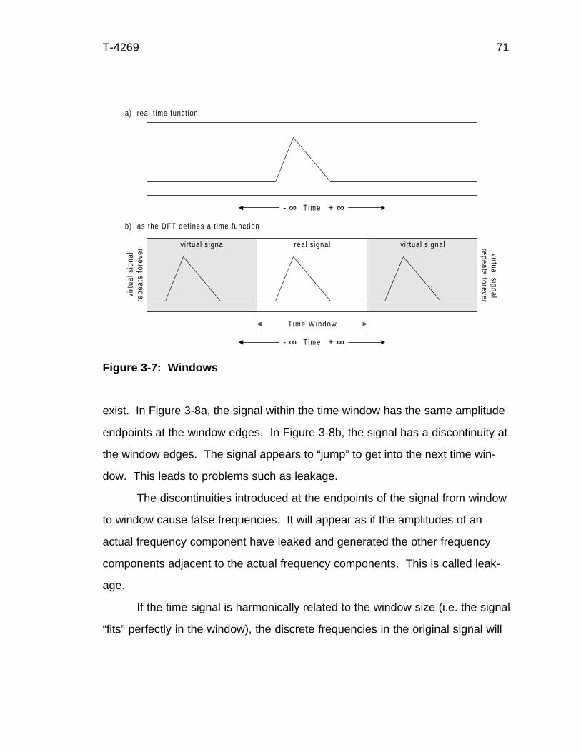
T-4269 71
exist. In Figure 3-8a, the signal within the time window has the same amplitude
endpoints at the window edges. In Figure 3-8b, the signal has a discontinuity at
the window edges. The signal appears to “jump” to get into the next time win-
dow. This leads to problems such as leakage.
The discontinuities introduced at the endpoints of the signal from window
to window cause false frequencies. It will appear as if the amplitudes of an
actual frequency component have leaked and generated the other frequency
components adjacent to the actual frequency components. This is called leak-
age.
If the time signal is harmonically related to the window size (i.e. the signal
“fits” perfectly in the window), the discrete frequencies in the original signal will
Figure 3-7: Windows
b) as the DFT def ines a t ime funct ion
a) real t ime funct ion
virtual signalreal signalvirtual signal
virt
ual s
igna
lre
peat
s fo
reve
r virtual signalrepeats forever
T ime- ∞ + ∞
Time- ∞ + ∞
T ime Window
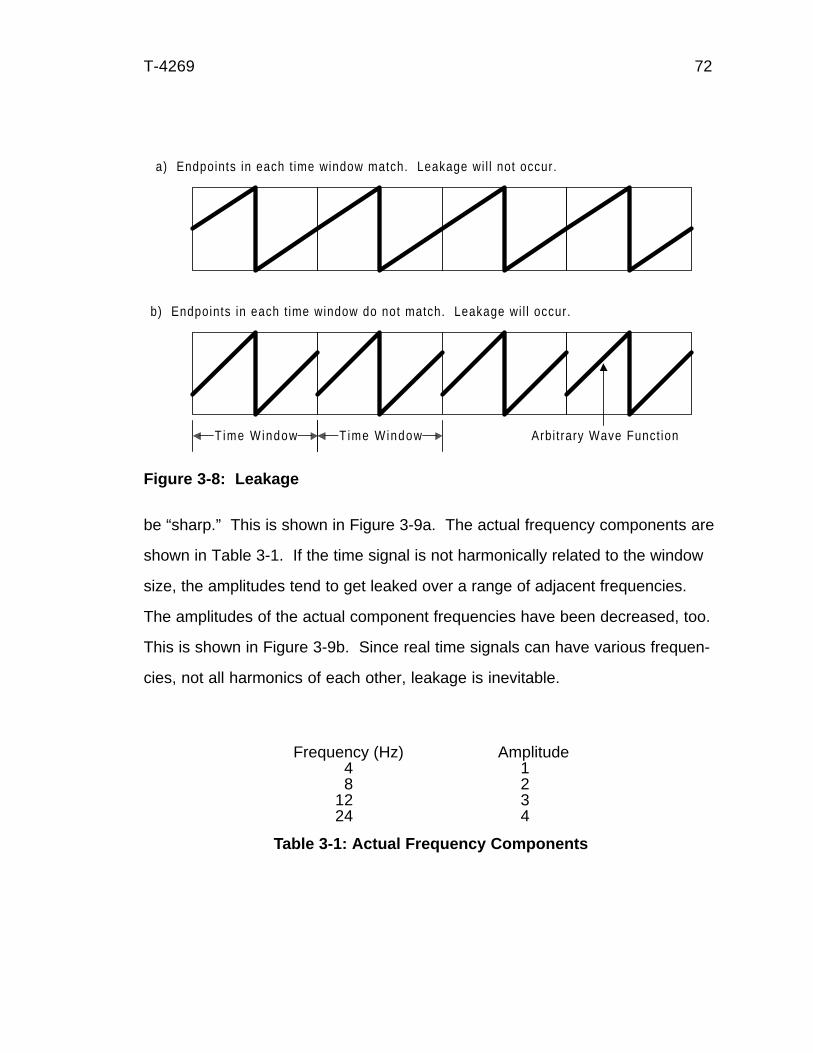
T-4269 72
be “sharp.” This is shown in Figure 3-9a. The actual frequency components are
shown in Table 3-1. If the time signal is not harmonically related to the window
size, the amplitudes tend to get leaked over a range of adjacent frequencies.
The amplitudes of the actual component frequencies have been decreased, too.
This is shown in Figure 3-9b. Since real time signals can have various frequen-
cies, not all harmonics of each other, leakage is inevitable.
Frequency (Hz) Amplitude 4 1 8 212 324 4
Table 3-1: Actual Frequency Components
a) Endpoints in each t ime window match. Leakage wi l l not occur.
b) Endpoints in each t ime window do not match. Leakage wi l l occur.
Arbi t rary Wave Funct ionT ime WindowTime Window
Figure 3-8: Leakage
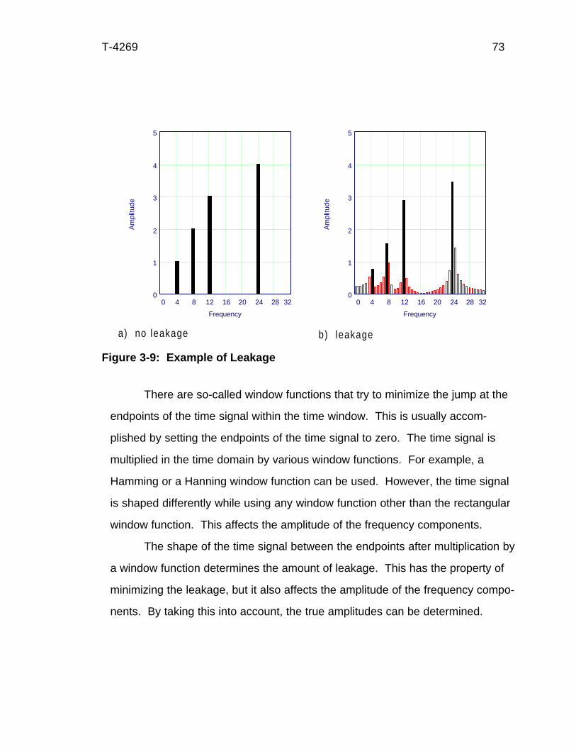
T-4269 73
There are so-called window functions that try to minimize the jump at the
endpoints of the time signal within the time window. This is usually accom-
plished by setting the endpoints of the time signal to zero. The time signal is
multiplied in the time domain by various window functions. For example, a
Hamming or a Hanning window function can be used. However, the time signal
is shaped differently while using any window function other than the rectangular
window function. This affects the amplitude of the frequency components.
The shape of the time signal between the endpoints after multiplication by
a window function determines the amount of leakage. This has the property of
minimizing the leakage, but it also affects the amplitude of the frequency compo-
nents. By taking this into account, the true amplitudes can be determined.
a) no leakage b) leakage
0 4 8 12 16 20 24 28 320
1
2
3
4
5
Frequency
Am
plitu
de
0 4 8 12 16 20 24 28 320
1
2
3
4
5
Frequency
Am
plitu
de
Figure 3-9: Example of Leakage

T-4269 74
Noise
During actual data collection for digital signal processing, noise—small
inexplicable signals generated by the data gathering process—will occur. Noise
in the time domain transforms into noise in the frequency domain. Noise, which
is attendant in all data, is reduced with the filtering process. The filtering pro-
cess assumes small amplitudes of frequency are noise and excludes them from
the presentation of the data. Filtering improves the appearance of the plotted
data but detail is lost.
Noise due to the data gathering process can occur because of time jitter
or quantizing error. Time amplitude variation occurs with improper triggering of
the acquisition gate by the signal processing equipment. The signal must reach
some predefined amplitude before measuring starts. If this gate is triggered at
slightly different levels, then the signal appears to have a jitter to it. Signal
averaging helps reduce this problem.
Quantizing error occurs because of the sampling process. If the signal
amplitude happens to be in between two digital values, the processor must pick
one of the digital values. If the signal continues to run between two digital val-
ues, the processor might pick one, then the other value. This is because of the
rounding process and is part of the processing. This can show as a high fre-
quency component that does not really exist.
Digitizing (Picket Fence Effect)
Another problem in data gathering has to do with taking analog data and
converting it to digital data. In the Figure 3-10, two identical analog functions
are shown sampled at the same interval step. Only the starting points are differ-
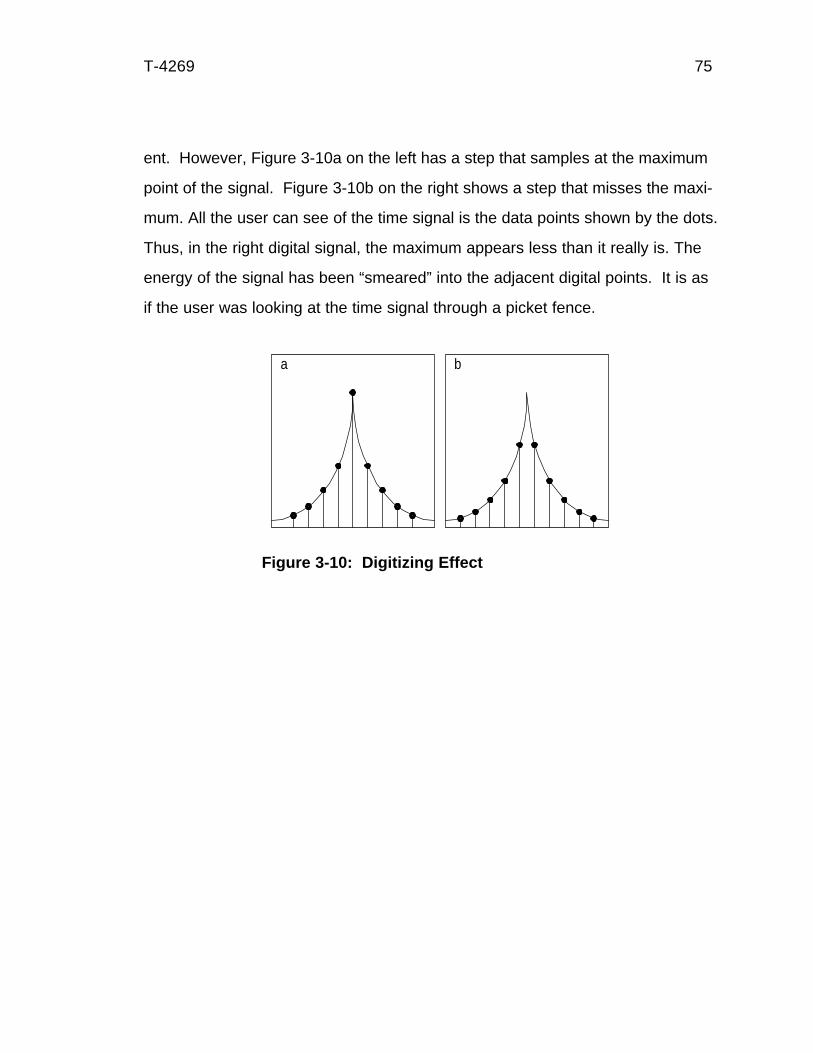
T-4269 75
Figure 3-10: Digitizing Effect
a b
ent. However, Figure 3-10a on the left has a step that samples at the maximum
point of the signal. Figure 3-10b on the right shows a step that misses the maxi-
mum. All the user can see of the time signal is the data points shown by the dots.
Thus, in the right digital signal, the maximum appears less than it really is. The
energy of the signal has been “smeared” into the adjacent digital points. It is as
if the user was looking at the time signal through a picket fence.

T-4269 76
CHAPTER 4
DERIVING THE SPECTRAL ELEMENT
This chapter sets forth the details of spectral analysis. It starts with a
general description of spectral analysis. Then the static and dynamic forces on
a drill string during jarring are shown. Using the dynamic forces, an axial equa-
tion of motion for a drill string under jarring conditions is derived and solved.
From there, the spectral solution is derived using a finite element model com-
posed of an axial two-noded spectral element and an axial one-noded semi-
infinite spectral element. The elements are then globally assembled into one
structure, the drill string. A linear algebraic solution for the globally assembled
structure is made and post-processing is shown. The general procedure and the
limitations of spectral analysis are described.
Stress wave tracking and finite element analysis are the two current
jarring models. Both methods, rooted in the time domain, have limitations.
Wave tracking analysis is a closed form partial differential model. It has
the advantage of being exact and can be solved at any location and time without
regard to any previous solutions. The disadvantage, on the other hand, is that
these types of solutions can be difficult (if not impossible) to solve. The analysis
is also restricted to linear conditions (i.e., constant geometric and material prop-
erties).
T-4269 77
Using iteration methods, the finite element method incorporates multiple
geometric and material properties and nonlinear functions. This method requires
large computational resources not generally available in the field. More impor-
tantly, the results only approximate the mass distribution of a drill string and
there are algorithm stability problems with the time step choices.
The semi-analytic finite element method, set forth in this dissertation,
combines wave tracking analysis with the finite element method. The semi-
analytic finite element method uses the actual equations of motion rather than an
approximation of the equations between nodes of motion. The equations of
motion in the frequency domain are derived from the sinusoidally varying compo-
nents of the equations of motion in the time domain.
This is accomplished by using the FFT. Then, a series of forced fre-
quency responses based on the results of the decomposed force values can be
analyzed. After the analysis, the resulting displacement functions can be in-
verted back into their calculated time displacement functions. This process also
can work in reverse; i.e., starting with a time displacement function and returning
with the time force function.
A sinusoidal input will cause a sinusoidal output. (Another way of looking
at this is that a harmonic excitation generates a harmonic response.) The output
or response will have the same frequency, but not necessarily the same ampli-
tude or phase. This is called a forced frequency response. Equation 4-1 shows
a sinusoidally varying force, P. This, with the appropriate calculations depen-
dent on the type of analysis, gives a sinusoidally varying displacement, U.
P pe ue Ui t i t= ⇒ =ω ω (4.1)

T-4269 78
where
ω = angular frequency
t = time
p = sinusoidal force amplitude
u = sinusoidal displacement amplitude
Remember that Euler’s formula is
Re cos sini R iθ θ θ= +b g b gc h (4.2)
where
θ = angular frequency
R = amplitude
The p and u in equation 4.1 are the amplitudes of the sinusoidal waves and
correspond to the R in equation 4.2. The forced frequency response can apply
to any number of frequencies and they can be added together through linear
algebra. This is shown in equation 4.3
P
P
P
p
p
p
e
u
u
u
e
U
U
Un n
i t
n
i t
n
1
2
1
2
1
2
1
2
M M M M
R
S||
T||
U
V||
W||
=
R
S||
T||
U
V||
W||
⇒
R
S||
T||
U
V||
W||
=
R
S||
T||
U
V||
W||
ω ω
(4.3)
This is where the frequency domain gets involved. The conversion from the time
domain to the frequency domain involves the exponential function
ei tω (4.4)
The values in equation 4.3 are a set of linear equations multiplied by this same
exponential function. The Fourier transform turns time based data into fre-
T-4269 79
quency based data. The inverse Fourier transform reverses the process. It
transforms frequency based data into time based data. In the frequency do-
main, equation 4.3 would looks like equation 4.5
P p e u e Un ni t
ni t
nn n= ⇒ =$ $ω ω (4.5)
At first, this process may not appear to be much of an advantage over any
strictly time domain processes. If anything, more steps appear to be needed.
However, the process of determining the frequency equations for the forced
function response analysis involves taking a second order partial differential
equation (PDE) and converting it to a second order ordinary differential equation
(ODE). ODE’s are easier to solve than PDE’s. In addition, the shape function
used to determine the finite element equations continuously describes the mass
distribution. There is no need to determine a maximum element size. It can be
as large as geometry or material permits. Finally, the FFT process that deter-
mines the frequency spectrum is computationally very efficient.
In this dissertation, assumptions have been made. One such assumption
is that there are no transverse waves. All of the waves generated by the jarring
impact are assumed to be planar longitudinal stress waves traveling in the axial
direction. It is also assumed that there is no reduction or enlargement in the
area affected by the wave from the Poisson’s effect.
These assumptions are reasonable because of the fact that the majority of
the jarring waves are generated in the axial direction for most straight hole
situations. Torsional and bending waves are not significant because, in straight
holes, the method used to generate the forces is an impact in the axial direction.
There are a number of forces acting on the drill string. They can be
broken into static and dynamic forces.
T-4269 80
Static Forces
Static forces are those that do not significantly change within the time
frame of the jarring process. This includes such forces as gravity and overpull.
In the context of jarring analysis, both the static and dynamic forces can be
analyzed separately. The stresses from the static forces can be linearly added
to the dynamic forces. For example, even though there might be two equal
dynamic force stress waves propagating outward from a jar, the actual stresses
in the drill string will reflect the stress from the dynamic forces plus the stress
from the static forces.
Axial stress is real tension divided by the cross-sectional area of the drill
string (Mitchell 1995). Tension causes two marks on a drill string to separate.
Compression causes two marks on a drill string to converge. To analyze static
stress, it is important to ascertain all of static forces acting on a section of the
drill string. Since this dissertation is limited to the one dimensional axial case,
only those stresses that directly affect axial stress will be considered. This is a
uniaxial load case.
Static axial stress is calculated by dividing the tension or compression by
the cross-sectional area of the drill string.
Gravity
Part of the axial stress at a given point in the drill string is based on grav-
ity and the fluids in which it is immersed. The fluids have a density which deter-
mines the hydrostatic pressure and possibly an additional pressure from the
T-4269 81
surface. The force from the fluids must have a pressure area to act over. Be-
cause this is a one dimensional case, only areas perpendicular to the axial
direction need be considered. The drill string also has weight.
Overpull Force
The overpull force is the force necessary to trigger the jars. It is a force at
the trigger mechanism in the jars. As such, this force is the determining factor
for all of the static stresses in the drill string at the time the jar triggers. Since
this force vanishes as the jar is triggered, it acts as a negative stress wave after
the jar triggers and before the jar impact. The force at the top of the stuck point
is determined by taking the overpull force and subtracting the weight of the drill
string below the jars and above the top of the stuck point.
Dynamic Forces
Dynamic forces are those that significantly change within the time frame
of the jarring process. That includes such forces which arise from strain
changes and damping.
Strain
Changes in strain occur because a wave of stress is being propagated.
An assumption is made that the wave propagation stress remains in the linear
portion of the stress-strain curve. This allows for the use of Hooke’s Law which
is
σ ∂∂
= Eux
(4.6)
T-4269 82
where
E = modulus of elasticity
σ = stress
u = displacement
x = location
Since stress is a force acting over a cross-sectional area, then the forces
from strain can be determined as
F AEux
= ∂∂
(4.7)
where
A = cross-sectional area
F = force
This is a very important equation to remember for jarring analysis.
Damping
Damping is the dissipation of energy over time or distance (Harris 88). If
damping, or friction, did not occur, vibrations could race out of control, leading to
structural failure. Energy from vibrations would simply build until there is too
much energy for the structure to sustain. Most of the time, the dissipated energy
from the vibration is converted into heat. In the borehole, three distinctive types
of damping occur. They are hysteretic, viscous, and Coulomb damping.
Hysteretic Damping
Another name for hysteretic damping is structural damping. This is the
type of damping that arises from internal friction within a structure. A wave
moves through a material because the atomic structure is reacting to an applied

T-4269 83
force. As the atoms of the structure move, energy is lost from the interaction of
these atoms with their neighboring atoms. Hysteretic damping is the energy
wasted as atoms move relative to each other.
If a material had a perfectly linear stress-strain relationship, hysteretic
damping would not occur. But in reality, there is no such thing as a perfectly
linear stress-strain curve. As a material is stressed and relieved, two curves on
the stress-strain diagram will develop. The center area between the two curves
represents the energy lost to internal friction. This hysteresis loop is the source
of the name for this type of damping. The gray shaded areas in Figure 4-1 show
various values for hysteretic damping. Note that in Figure 4-1a, the loop is very
small. However, because high frequency vibrations can cause this loop to be
repeated many, many times over a given time period, the actual energy dissi-
pated can be large (Kolski 1963).
The value of hysteretic damping is highly dependent on a number of
factors. One factor is the condition of the material (i.e., chemical composition,
STRESS
STRAIN0 STRAIN STRAIN
a b c
Figure 4-1: Examples of Hysteretic Damping
T-4269 84
inhomogeneities, and property changes due to thermal and stress histories).
Another factor is the state of internal stress from initial and subsequent thermal
and stress histories. Also, the type and variation of stress—axial, torsional,
shear, and/or bending— will affect the hysteretic damping value.
A way of looking at hysteretic damping force is to set it proportional to the
particle velocity divided by the wave frequency. This is shown in equation 4.8
(Doyle 1991)
Fh u
tH =ω
∂∂
(4.8)
where
h = hysteretic damping factor
FH = hysteretic damping force
If this is converted into the frequency domain, the hysteretic damping is
proportional to the spectral displacement but is in the imaginary plane. This is
shown in equation 4.9 (Doyle 1991)
$ $F ihuH = (4.9)
In this manner, a form of hysteretic damping can be included in the jarring
model. Unfortunately, h is difficult to determine.
Viscous Damping
Any time the damping force is proportional to the velocity of the particles,
it is called viscous damping. This is shown as follows
FutD = γ ∂
∂(4.10)

T-4269 85
where
γ = damping coefficient
FD = viscous damping force
One way viscous damping arises in jarring analysis is from the interaction
of a solid and liquid at their interface. This occurs along the sides of the drill
string where the steel contacts the liquid mud.
A method of determining the viscous damping involves noting the decre-
ment of acceleration over one vibration cycle (Dareing and Livesay 1968). An
impulse is impressed on the drill string producing a wave. While the wave is
decaying, the acceleration is measured and recorded over multiple times at one
location on the string. It is necessary that the two recordings to be compared are
at the same phase (i.e. crest to crest). The time (T) between the two recordings
is also noted. These values are used in equation 4.11 to compute the value of
the damping coefficient γ. Unfortunately, this method gives the total damping
and does not distinguish between viscous and Coulomb damping
γ = 22
1
2
AEc T
AAA
ln (4.11)
where
cA = axial wave propagation speed
T-4269 86
Coulomb Damping
Coulomb damping is the friction that occurs from two dry surfaces sliding
over each other. The Coulomb damping force is a constant value that is inde-
pendent of particle velocity and displacement, but dependent on the friction
factor, µ, and the force normal to the friction surface. This value is shown as
follows
F FF N= µ (4.12)
where
µ = friction factor
FN = normal force
FF = Coulomb friction force
This force is always of the opposite sign from the particle velocity. This
means that as the particle velocity changes signs, there is a complete reversal of
the damping force. It is this discontinuity that makes this a nonlinear damping
force. This is shown in as follows
Fut
FF N= FHG
IKJsgn
∂∂
µ (4.13)
where
sgn = sign of term in parenthesis
This nonlinearity makes a closed form solution to an equation of motion
virtually impossible.

T-4269 87
Equivalent Viscous Damping
One potential way to include Coulomb damping in a linear manner, is to
determine an equivalent viscous damping system such that the energy dissi-
pated over a given cycle is the same as for a given Coulomb damping system
(Jacobson 1930). For a constant friction force, the equivalent viscous damping
coefficient is
CFXEQ
F= 4π ω
(4.14)
where
CEQ = equivalent viscous damping coefficient
X is the maximum displacement for a given frequency and is
XP c k m F k m c F
c k m
F F
=+ − − −L
NMOQP −
+ −
$ 2 2 2 2 2
22 2 2
12 2
2 2 2 2
16 4ω ωπ
ωπ
ω
ω ω
c h{ } c h
c h(4.15)
where
k = spring constant
m = mass
c = viscous damping coefficient
According to Jacobson, equation 4.14 does not tend to be accurate if the
ω value is not near a resonant value. Unfortunately, too many variables are
unknown to make this work very well.
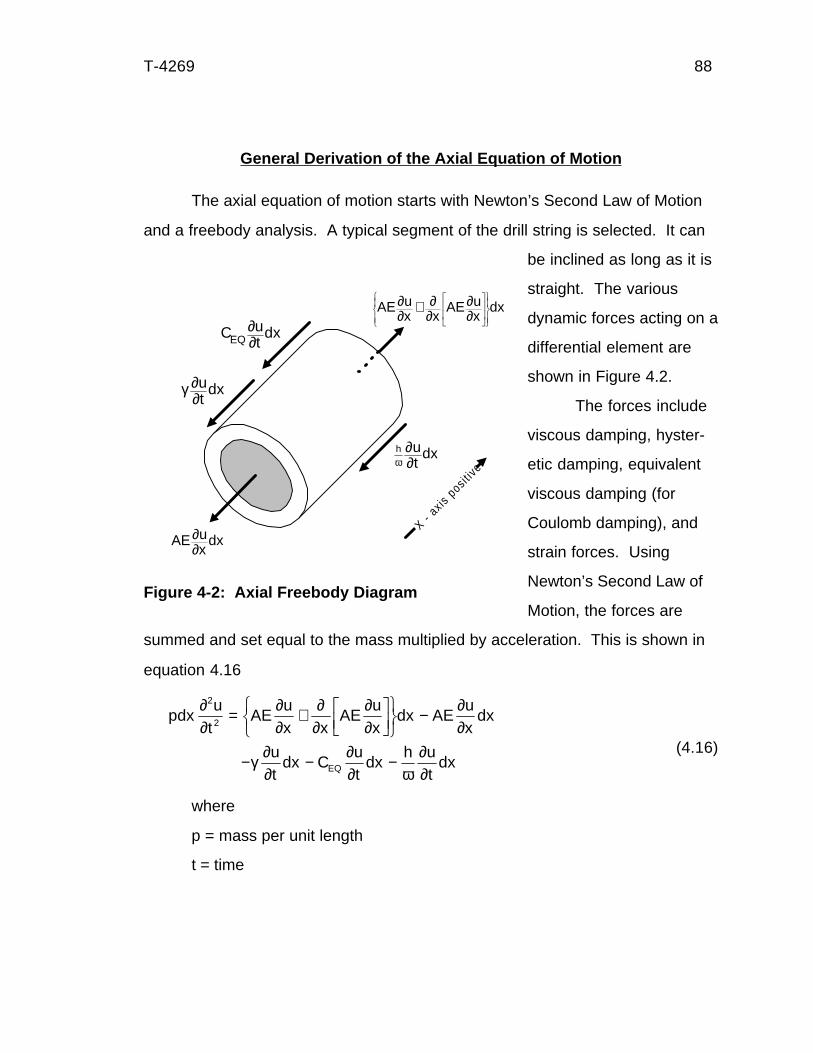
T-4269 88
General Derivation of the Axial Equation of Motion
The axial equation of motion starts with Newton’s Second Law of Motion
and a freebody analysis. A typical segment of the drill string is selected. It can
be inclined as long as it is
straight. The various
dynamic forces acting on a
differential element are
shown in Figure 4.2.
The forces include
viscous damping, hyster-
etic damping, equivalent
viscous damping (for
Coulomb damping), and
strain forces. Using
Newton’s Second Law of
Motion, the forces are
summed and set equal to the mass multiplied by acceleration. This is shown in
equation 4.16
pdxu
tAE
ux x
AEux
dx AEux
dx
ut
dx Cut
dxh u
tdxEQ
∂∂
∂∂
∂∂
∂∂
∂∂
γ ∂∂
∂∂ ω
∂∂
2
2 = + LNM
OQP
RSTUVW
−
− − −(4.16)
where
p = mass per unit length
t = time
C ut
dxEQ∂∂
γ ∂∂ut
dx
AE ux x
AE ux
dx∂∂
∂∂
∂∂
+L
NMM
O
QPP
RS|T|
UV|W|
AE ux
dx∂∂
X - axis p
osit ive
h ut
dxω
∂∂
Figure 4-2: Axial Freebody Diagram

T-4269 89
x = location on the string
Simplifying this equation and assuming a constant area and modulus of
elasticity yields
pdxu
tAE
ux
dxut
dx Cut
dxh u
tdxEQ
∂∂
∂∂
γ ∂∂
∂∂ ω
∂∂
2
2
2
2= − − − (4.17)
Canceling the differential distance dx and collecting like terms gives
pu
tAE
ux
Ch u
tEQ
∂∂
∂∂
γω
∂∂
2
2
2
2= − + +FHG
IKJ (4.18)
This is the axial equation of motion for the differential element. The next step is
to find a solution for it.
General Solution for the Axial Equation of Motion
This equation is amenable to solution by way of the separation of vari-
ables method. This is shown as
U x t X x T t,b g b g b g= (4.19)
where
U(x,t) = solution in time and space
X(x) = function of space only
T(t) = function of time only
If the following assumption is made concerning the time function
T t ei tb g = ω (4.20)
Then the solution looks like
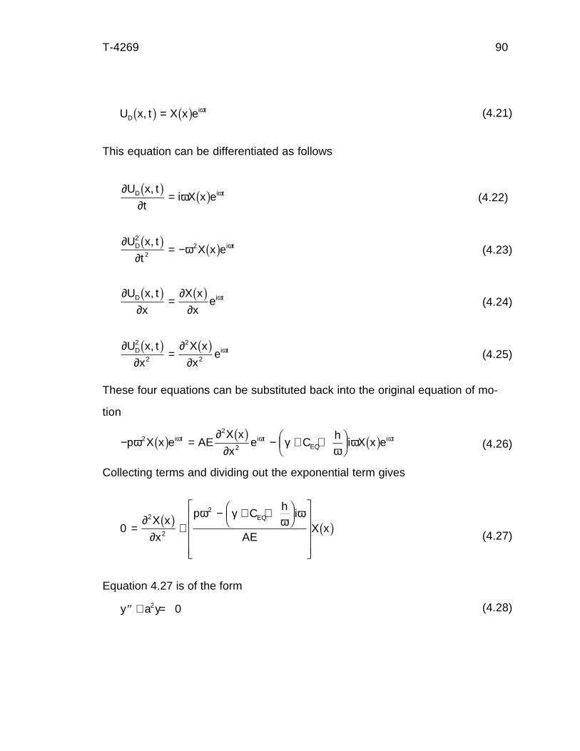
T-4269 90
U x t X x eDi t,b g b g= ω (4.21)
This equation can be differentiated as follows
∂∂
ω ωU x t
ti X x eD i t,b g b g= (4.22)
∂∂
ω ωU x t
tX x eD i t
2
22,b g b g= − (4.23)
∂∂
∂∂
ωU x t
x
X x
xeD i t,b g b g= (4.24)
∂∂
∂∂
ωU x t
x
X x
xeD i t
2
2
2
2
,b g b g= (4.25)
These four equations can be substituted back into the original equation of mo-
tion
− = − + +FHG
IKJp X x e AE
X x
xe C
hi X x ei t i t
EQi tω
∂∂
γω
ωω ω ω22
2b g b g b g (4.26)
Collecting terms and dividing out the exponential term gives
02
2
2
= +− + +FHG
IKJ
L
N
MMMM
O
Q
PPPP
∂∂
ω γω
ωX x
x
p Ch
i
AEX x
EQb g b g(4.27)
Equation 4.27 is of the form
′′ + =y a y2 0 (4.28)
T-4269 91
The standard solution of this equation is
X x e eikx ikxb g = +−A B (4.29)
where
A and B = constants of integration
The constants of integration are determined by the boundary conditions.
k is a collection of the constants and is equal to
kp C
hi
AE
EQ
=− + +FHG
IKJω γ
ωω2
(4.30)
Therefore, the total dynamic solution is
U x t e e eDikx ikx i t,b g = +−A B ω (4.31)
The Spectral Solution
The next step is to convert the previous solution into the frequency do-
main. In Chapter 3, the Fourier analysis of a time function was discussed. In
equation 3.17, it was shown that a Fourier solution in complex terms was
F tT
C eni t
n
nb g b g==−∞
∞
∑1 ω ω(3.17)
Looking at equation 4.31, similarities between the two equations can be seen.
One can say that for a given location in space that the Fourier coefficients are
1T
C e enikx ikx
n
ωb g = +−
=−∞
∞
∑ A B (4.32)
Therefore, the equation to determine the frequency domain solution at a given
point on the drill string is
$u x e eikx ikxb g = +−A B (4.33)
T-4269 92
where
û(x) = displacement spectrum
Finite Element Method
The previous discussion centered on a closed form solution to the dy-
namic axial equation of motion for a finite element. Now that will be applied to
the finite element method.
The basic procedure for applying the finite element method is as follows.
1) The structure is divided into logical elements. How this
is accomplished is dependent upon the method used to formulate
the element properties. Current time-based domain methods
require a large number of elements to model the mass distribution
in a lumped manner for wave propagation problems. In the fre-
quency domain, this is not needed. The mathematics model the
mass continuously rather than in a lumped manner. The only
element division needed is for differences in geometric and mate-
rial properties (i.e. changing from drill collars to drill pipe).
2) Formulate the element properties. This formulation
involves using a shape function. This function is the “simplified”
equation discussed earlier. In the frequency domain, this equation
need not be simplified; it is exact. This is why this method is often
called a semi-analytical finite element method. It is also why the
mass distribution is modeled continuously.
3) Each of the elements is then assembled into a global
system. The elements are added together at their endpoints
T-4269 93
(called nodes) using linear algebra. This is accomplished in the
model developed in this dissertation because this is a one-dimen-
sional model. Although adding more dimensions complicates the
procedure, it is primarily a bookkeeping problem (assuming the
stiffness matrices are derived correctly).
4) The external boundary conditions are added to the global
system. This is addressed in the next chapter.
5) Solve the system of element equations. This is a simul-
taneous solution using linear algebraic techniques. This gives the
displacement values at the nodes.
6) Back substitute the displacement nodal values into the
shape function equations to return displacement values to the
element level.
7) Assess the results.
After dividing the structure into elements, the shape function for a spectral
finite element is
$u x e eikx ik x Lb g b g= +− −A B (4.34)
where
L = element length
Note that the second term has the element length built into it. The û(x) is
called the spectral displacement.
A General Axial Two-Noded Spectral Element
A general axial two-noded spectral element is shown in Figure 4-3.
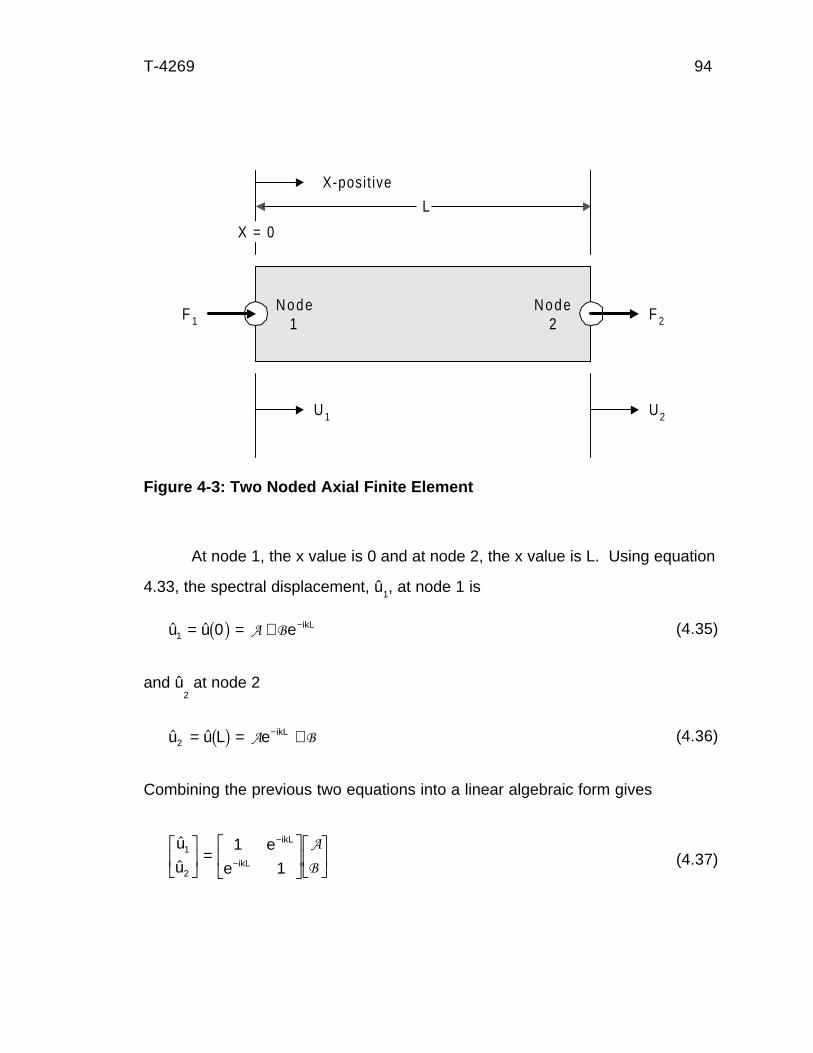
T-4269 94
At node 1, the x value is 0 and at node 2, the x value is L. Using equation
4.33, the spectral displacement, û1, at node 1 is
$ $u u e ikL1 0= = + −b g A B (4.35)
and û2 at node 2
$ $u u L e ikL2 = = +−b g A B (4.36)
Combining the previous two equations into a linear algebraic form gives
$
$
u
ue
e
ikL
ikL
1
2
1
1
LNM
OQP
=LNM
OQPLNM
OQP
−
−
A
B (4.37)
L
F 2F 1
U 1 U2
X-posit ive
X = 0
Node1
Node2
Figure 4-3: Two Noded Axial Finite Element
T-4269 95
Solving for A and B gives
A
B
LNM
OQP
=−
−−LNM
OQPLNM
OQP−
−
−
11
1
12
1
2e
e
e
u
ui kL
ikL
ikL
$
$ (4.38)
Now, remembering equation 4.7, the shape function is differentiated with respect
to x
∂∂$u x
xik e eikx ik x Lb g e jb g= − +− −A B (4.39)
and multiplied by cross-sectional area, A, and modulus of elasticity, E, to get the
force equation
$F x ikAE e eikx ik x Lb g e jb g= +− −A B (4.40)
Using this equation, the nodal forces are determined
$ $F F ikAE e ikL1 0= = − − + −b g c hA B (4.41)
and
$ $F F L ikAE e ikL2 = = − +−b g c hA B (4.42)
to get
$
$F
FikAE
e
e
ikL
ikL1
2
1
1
LNM
OQP
=−
−LNM
OQPLNM
OQP
−
−
A
B (4.43)
T-4269 96
Substituting back into equation 4-43 with 4-38 gives
$
$
$
$
F
FikAE
e
e e
e
e
u
u
ikL
ikL ikL
ikL
ikL1
22
1
2
1
1
11
1
1
LNM
OQP
=−
−LNM
OQP −
−−LNM
OQPLNM
OQP
−
− −
−
− (4.44)
after algebraic manipulation, the finite element equation is
$
$
$
$
F
F
ikAEe
e e
e e
u
uikL
ikL ikL
ikL ikL1
22
2
2
1
21
1 2
2 1
LNM
OQP
=−
+ −− +
LNM
OQPLNM
OQP−
− −
− − (4.45)
This equation is in the form of
F Ku= (4.46)
The K in the above equation is called the stiffness matrix. It is
KikAE
e
e e
e eikL
ikL ikL
ikL ikL=
−+ −
− +LNM
OQP−
− −
− −1
1 2
2 12
2
2 (4.47)
Some items of note concerning the above equation. First, the k in the
equation is based on the damping factors, mass distribution, and most impor-
tantly, the frequency. (See equation 4.30.) This means that this finite element
equation works for one frequency at a time. This is not a problem as the FFT of
a force gives a frequency and an associated force for that frequency.
Also to be noted is that the modulus of elasticity and the cross-sectional
area for the elements are constant. The structure must be divided wherever a
change in geometry or material occur. Note that the division is not for the pur-
pose of lumping the mass.
T-4269 97
Derivation of the Axial One-Noded Semi-Infinite Spectral Element
Because these equations are written in the frequency domain, a semi-
infinite element is now possible. This element is unusual in that it has only one
active node. The other end which is at an infinite distance has no effect on the
model. This has the advantage of conducting and dissipating all of the energy
away from the area of interest with no returning energy.
A semi-infinite element is placed where a reflection of a wave from the far
end can not take an active role within the time frame of analysis. For example, if
a wave reflection takes 2 seconds to return to the original location and the time
of interest is 0.5 seconds, it does not really matter if the reflection shows up in 2
seconds or 2,000,000 seconds. It has no effect on the analysis. In essence, the
element is infinitely long.
To derive this element, a value of infinity is used for L
$
$
$
$
F
F
ikAEe
e e
e e
u
uik
ik ik
ik ik1
22
2
2
1
21
1 2
2 1
LNM
OQP
=−
+ −− +
LNM
OQPLNM
OQP− ∞
− ∞ − ∞
− ∞ − ∞ (4.48)
This reduces the equation to
$
$
$
$
F
FikAE
u
u1
2
1
2
1 0
0 1
LNM
OQP
=LNM
OQPLNM
OQP (4.49)
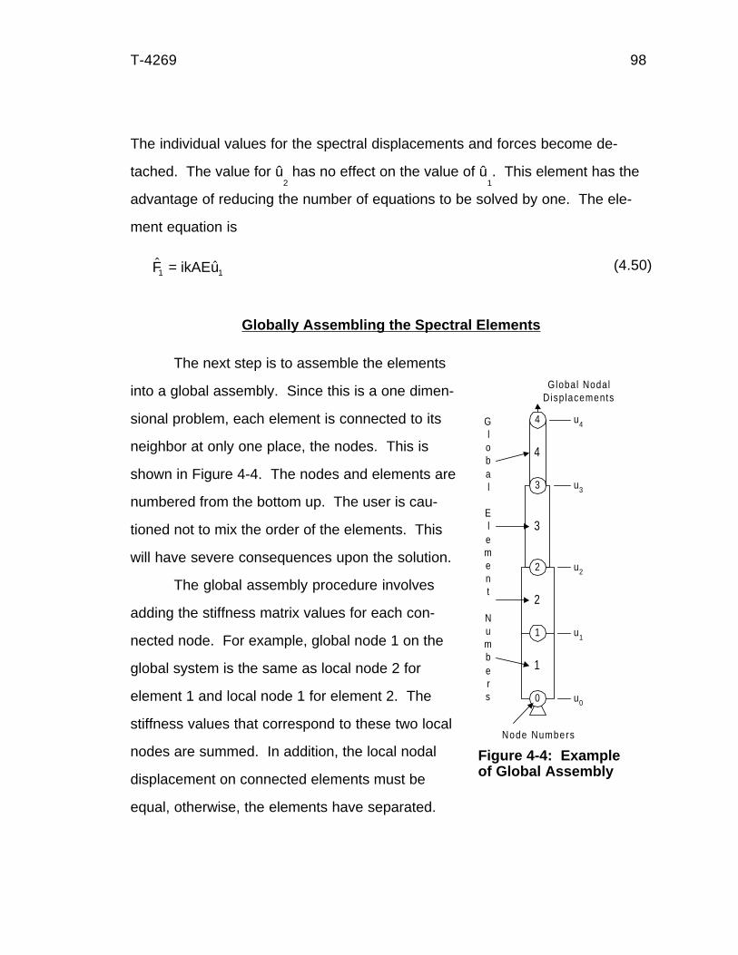
T-4269 98
The individual values for the spectral displacements and forces become de-
tached. The value for û2 has no effect on the value of û
1. This element has the
advantage of reducing the number of equations to be solved by one. The ele-
ment equation is
$ $F ikAEu1 1= (4.50)
Globally Assembling the Spectral Elements
The next step is to assemble the elements
into a global assembly. Since this is a one dimen-
sional problem, each element is connected to its
neighbor at only one place, the nodes. This is
shown in Figure 4-4. The nodes and elements are
numbered from the bottom up. The user is cau-
tioned not to mix the order of the elements. This
will have severe consequences upon the solution.
The global assembly procedure involves
adding the stiffness matrix values for each con-
nected node. For example, global node 1 on the
global system is the same as local node 2 for
element 1 and local node 1 for element 2. The
stiffness values that correspond to these two local
nodes are summed. In addition, the local nodal
displacement on connected elements must be
equal, otherwise, the elements have separated.
Global NodalDisp lacements
Global
Element
Numbers
u3
u2
u1
u4
u0
4
3
2
1
0
1
2
3
4
Node Numbers
Figure 4-4: Exampleof Global Assembly
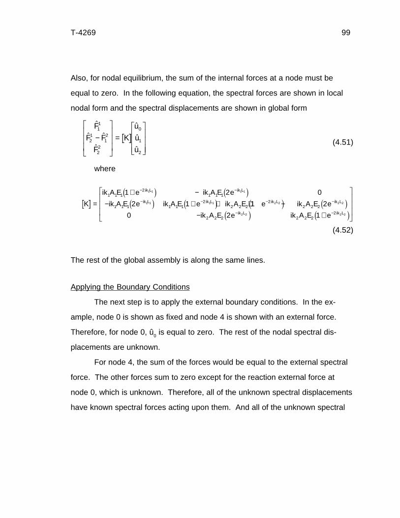
T-4269 99
Also, for nodal equilibrium, the sum of the internal forces at a node must be
equal to zero. In the following equation, the spectral forces are shown in local
nodal form and the spectral displacements are shown in global form
$
$ $
$
$
$
$
F
F F
F
K
u
u
u
11
21
12
22
0
1
2
−
L
N
MMM
O
Q
PPP
=L
NMMM
O
QPPP (4.51)
where
K
ik A E e ik A E e
ik A E e ik A E e ik A E e ik A E e
ik A E e ik A E e
ik L ik L
ik L ik L ik L ik L
ik L ik L
=+ −
− + + + −− +
L
N
MMM
O
Q
PPP
− −
− − − −
− −
1 1 12
1 1 1
1 1 1 1 1 12
2 2 22
2 2 2
2 2 2 2 2 22
1 2 0
2 1 1 2
0 2 1
1 1 1 1
1 1 1 1 2 2 2 2
2 2 2 2
c h c hc h c h c h c h
c h c h(4.52)
The rest of the global assembly is along the same lines.
Applying the Boundary Conditions
The next step is to apply the external boundary conditions. In the ex-
ample, node 0 is shown as fixed and node 4 is shown with an external force.
Therefore, for node 0, û0 is equal to zero. The rest of the nodal spectral dis-
placements are unknown.
For node 4, the sum of the forces would be equal to the external spectral
force. The other forces sum to zero except for the reaction external force at
node 0, which is unknown. Therefore, all of the unknown spectral displacements
have known spectral forces acting upon them. And all of the unknown spectral
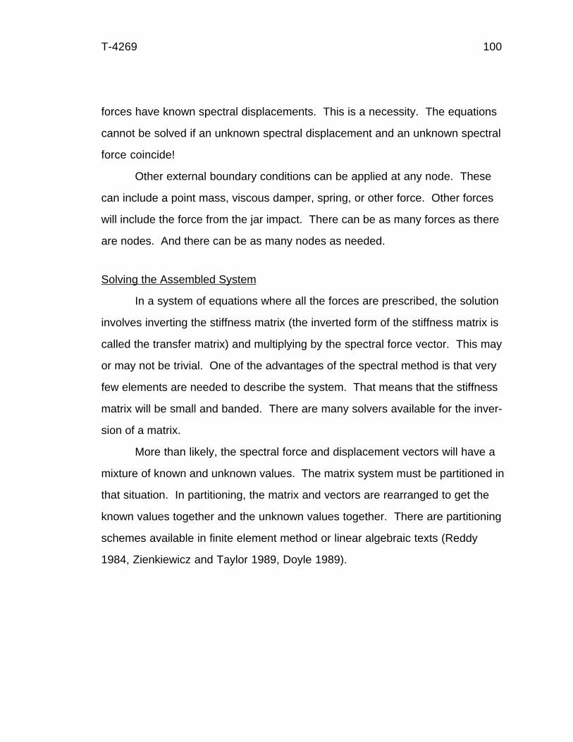
T-4269 100
forces have known spectral displacements. This is a necessity. The equations
cannot be solved if an unknown spectral displacement and an unknown spectral
force coincide!
Other external boundary conditions can be applied at any node. These
can include a point mass, viscous damper, spring, or other force. Other forces
will include the force from the jar impact. There can be as many forces as there
are nodes. And there can be as many nodes as needed.
Solving the Assembled System
In a system of equations where all the forces are prescribed, the solution
involves inverting the stiffness matrix (the inverted form of the stiffness matrix is
called the transfer matrix) and multiplying by the spectral force vector. This may
or may not be trivial. One of the advantages of the spectral method is that very
few elements are needed to describe the system. That means that the stiffness
matrix will be small and banded. There are many solvers available for the inver-
sion of a matrix.
More than likely, the spectral force and displacement vectors will have a
mixture of known and unknown values. The matrix system must be partitioned in
that situation. In partitioning, the matrix and vectors are rearranged to get the
known values together and the unknown values together. There are partitioning
schemes available in finite element method or linear algebraic texts (Reddy
1984, Zienkiewicz and Taylor 1989, Doyle 1989).
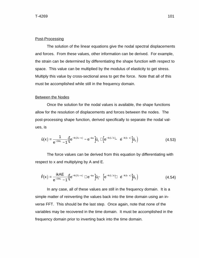
T-4269 101
Post-Processing
The solution of the linear equations give the nodal spectral displacements
and forces. From these values, other information can be derived. For example,
the strain can be determined by differentiating the shape function with respect to
space. This value can be multiplied by the modulus of elasticity to get stress.
Multiply this value by cross-sectional area to get the force. Note that all of this
must be accomplished while still in the frequency domain.
Between the Nodes
Once the solution for the nodal values is available, the shape functions
allow for the resolution of displacements and forces between the nodes. The
post-processing shape function, derived specifically to separate the nodal val-
ues, is
$ $ $u xe
e e u e e uikLik L x ikx ik L x ik L xb g e jb g b g b g=
−− + −−
− − − − + − −112
21 2 (4.53)
The force values can be derived from this equation by differentiating with
respect to x and multiplying by A and E.
$ $ $F xikAE
ee e u e e uikL
ik L x ikx ik L x ik L xb g e jb g b g b g=−
+ − +−− − − − + − −
22
1 21(4.54)
In any case, all of these values are still in the frequency domain. It is a
simple matter of reinverting the values back into the time domain using an in-
verse FFT. This should be the last step. Once again, note that none of the
variables may be recovered in the time domain. It must be accomplished in the
frequency domain prior to inverting back into the time domain.
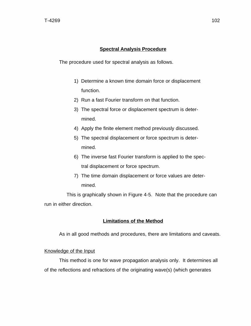
T-4269 102
Spectral Analysis Procedure
The procedure used for spectral analysis as follows.
1) Determine a known time domain force or displacement
function.
2) Run a fast Fourier transform on that function.
3) The spectral force or displacement spectrum is deter-
mined.
4) Apply the finite element method previously discussed.
5) The spectral displacement or force spectrum is deter-
mined.
6) The inverse fast Fourier transform is applied to the spec-
tral displacement or force spectrum.
7) The time domain displacement or force values are deter-
mined.
This is graphically shown in Figure 4-5. Note that the procedure can
run in either direction.
Limitations of the Method
As in all good methods and procedures, there are limitations and caveats.
Knowledge of the Input
This method is one for wave propagation analysis only. It determines all
of the reflections and refractions of the originating wave(s) (which generates
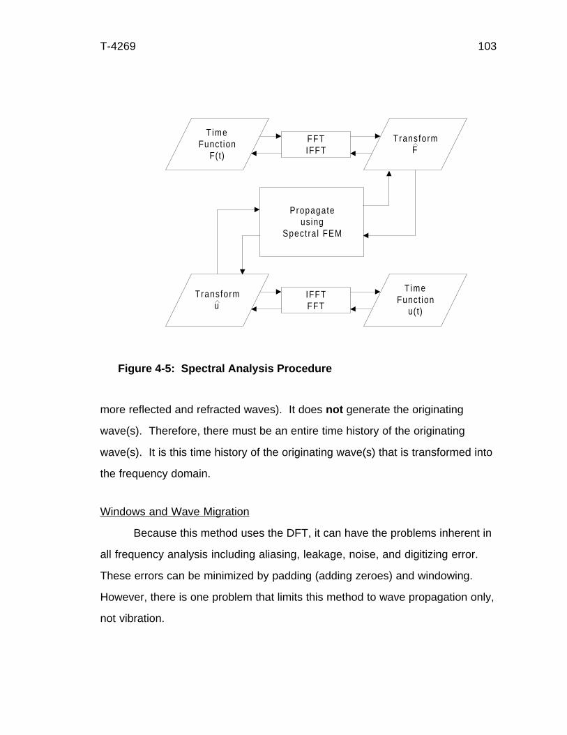
T-4269 103
more reflected and refracted waves). It does not generate the originating
wave(s). Therefore, there must be an entire time history of the originating
wave(s). It is this time history of the originating wave(s) that is transformed into
the frequency domain.
Windows and Wave Migration
Because this method uses the DFT, it can have the problems inherent in
all frequency analysis including aliasing, leakage, noise, and digitizing error.
These errors can be minimized by padding (adding zeroes) and windowing.
However, there is one problem that limits this method to wave propagation only,
not vibration.
TimeFunct ion
F(t)
TransformF
Transformu
TimeFunct ion
u(t)
Propagateusing
Spectra l FEM
FFTIFFT
IFFTFFT
Figure 4-5: Spectral Analysis Procedure

T-4269 104
The frequency methods all assume a periodic function, even if the func-
tion is not periodic. Since infinity is a very long time, this limitation has been
built into the mathematics of frequency analysis. The problem arises after a
wave has completely propagated across a time window. Since this wave is
assumed periodic, a virtual wave will appear on the other side of the time win-
dow. This virtual wave is from the neighboring window. It will ride on top of the
original time function.
Figure 4-6 shows an example of this phenomena. Since the spectral
analysis is location specific, a time window represents what happened in time at
a specific location. The wave is not being followed. Rather, it is as if one was
sitting watching traffic go by. In the figure, this is a triangular wave going by a
specific location. It is being reflected back and forth while it is decaying.
In Figure 4-6a, the wave is decaying before the window is traversed. In
Figure 4-6b, the time window is of shorter duration. Since this is the same wave
as in Figure 4-6a, the wave is not decaying before it migrates through the shorter
time window. Part of the wave is appearing in the next window. This wave is
labeled as the “wrap-around wave” and is the virtual wave. The reconstructed
time window looks quite different than the actual conditions. Extreme care must
be taken to insure this migration does not occur. It will significantly affect the
results of an analysis!
Therefore, it is critical to have the wave decay to practically zero before
the time window closes. This is accomplished by either dumping the energy
using damping or a semi-infinite element (remember it conducts energy out of a
system) or by using a very long window.

T-4269 105
Nonlinearity
Finally, since the time signal is built into the frequency analysis, there can
be no control of time once inside the frequency domain. This means that nonlin-
ear effects, such as free contraction to impact conditions, cannot not be directly
analyzed. As will be seen in the next chapter, this analysis can be made, but it
must be separated. In addition, Coulomb damping cannot be directly addressed.
T ime Window T ime Window T ime Window
real signalswrap-around s ignal
Figure 4-6: Wave Propagation into Windows
T-4269 106
CHAPTER 5
THE USE OF SPECTRAL ANALYSIS
IN WAVE PROPAGATION
This chapter presents five models that validate the spectral analysis
method. The first example will show the effect of a wave interacting with a fixed
end point (a wall). The second example will show the effect of a wave interact-
ing with a free end point. The third and fourth examples will show how changes
in cross-sectional areas affect the wave propagation through the interface. The
last example will show how multiple cross-sectional areas affect wave propaga-
tion.
Wave Reflections from Various Geometric Boundaries
For future developments and confidence in the model presented in this
dissertation, it is required that a corollary model be developed which contains
wave propagation and wave interaction with geometric discontinuities. What
happens as a wave meets a fixed or free boundary condition? Also, what hap-
pens to a wave as it encounters a cross-sectional area change?
A fixed end is one in which there can be no displacement. According to
wave theory, during a wave encounter with a fixed end, the stress at that end will
double during the passage of the wave. This effect can be looked at as if the
incident stress wave encounters an identical stress wave coming out of the fixed

T-4269 107
end. The two waves, one
incident and one virtual, will
interact and exchange
places. This is shown in
Figure 5-1. The boxes in the
figure represent the ampli-
tude of either stress or veloc-
ity. Above the line is positive
and below the line is nega-
tive. A reflection of a stress
wave will simply bounce
back with the same sign. A
compression wave will reflect
as a compression wave and
a tension wave will reflect as
a tension wave.
At a fixed end, because the displacement is equal to zero, the particle
velocity will be zero. It is as if the wave encounters a virtual wave with velocity
of the opposite sign. The waves will interact and cancel each other during the
encounter. The wave particle velocity amplitude will be inverted during a reflec-
tion from a fixed end.
A free end is defined as a traction free end. The stress at the free end is
always equal to zero. A free end will cause the opposite effects on stress and
particle velocity as the effects on a fixed end. This is shown in Figure 5-2.
*
S t ress Velocity
Figure 5-1: Fixed End Boundary Conditions

T-4269 108
In this case, the incident
stress wave encounters a
virtual wave with stress with
the opposite sign. The
incident and virtual waves
interact and exchange
places. They cancel each
other during the encounter
and the virtual wave ex-
changes places with the
incident wave to become
the outgoing wave. A
compression wave encoun-
tering a free end will reflect
as a tension wave. A
tension wave will reflect as
a compression wave.
At a free end, because a displacement must occur, the virtual wave will
have particle velocities of the same sign. The incident and virtual waves will
interact and reinforce each other during the encounter. The wave particle veloc-
ity values will double during an encounter with a free end and will reflect with the
same sign.
Stress Veloci ty
Figure 5-2: Free End Boundary Conditions
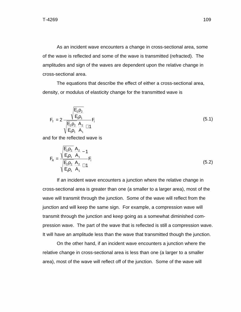
T-4269 109
As an incident wave encounters a change in cross-sectional area, some
of the wave is reflected and some of the wave is transmitted (refracted). The
amplitudes and sign of the waves are dependent upon the relative change in
cross-sectional area.
The equations that describe the effect of either a cross-sectional area,
density, or modulus of elasticity change for the transmitted wave is
F
EE
EE
AA
FT I=+
21
2 2
1 1
2 2
1 1
2
1
ρρ
ρρ
(5.1)
and for the reflected wave is
F
EE
AA
EE
AA
FR I=−
+
2 2
1 1
2
1
2 2
1 1
2
1
1
1
ρρρρ
(5.2)
If an incident wave encounters a junction where the relative change in
cross-sectional area is greater than one (a smaller to a larger area), most of the
wave will transmit through the junction. Some of the wave will reflect from the
junction and will keep the same sign. For example, a compression wave will
transmit through the junction and keep going as a somewhat diminished com-
pression wave. The part of the wave that is reflected is still a compression wave.
It will have an amplitude less than the wave that transmitted though the junction.
On the other hand, if an incident wave encounters a junction where the
relative change in cross-sectional area is less than one (a larger to a smaller
area), most of the wave will reflect off of the junction. Some of the wave will

T-4269 110
transmit through the junction and will keep the same sign. For example, a com-
pression wave will transmit through the junction and keep going as a diminished
compression wave. The reflected part of the wave is a tension wave. The abso-
lute amplitude of the tension wave will be greater than the compression wave
that is transmitted through the junction.
Spectral Analysis Example Set-Up
It is important to keep the node number-
ing in order. The scheme for the examples is
shown in Figure 5-3. There are four nodes:
0, 1, 2, and 3. Node 3 is not shown because
it is an infinite distance away. The nodes are
broken into two halves. This is done be-
cause the forces on one side of a node are
not always equal to the forces on the other
side of the node, although the overall nodal
forces balance. This occurs because there
could be an external force at that node or
changes in material or geometric properties.
The nodes’ halves have been labeled
with the node number and the side of the
node on which it is located. For example, a
force at the top side of node 1 would be
labeled Force1T.Figure 5-3: Example Nodeand Element Numbering
ELEM
2
Node 0
ELEM
0
ELEM
1
Node 1B
Node 0T
Node 2B
Node 2T
Node 1T
Node 2
Node 1
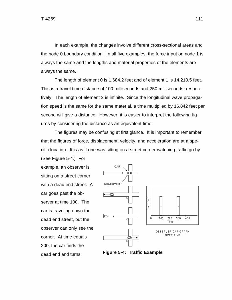
T-4269 111
In each example, the changes involve different cross-sectional areas and
the node 0 boundary condition. In all five examples, the force input on node 1 is
always the same and the lengths and material properties of the elements are
always the same.
The length of element 0 is 1,684.2 feet and of element 1 is 14,210.5 feet.
This is a travel time distance of 100 milliseconds and 250 milliseconds, respec-
tively. The length of element 2 is infinite. Since the longitudinal wave propaga-
tion speed is the same for the same material, a time multiplied by 16,842 feet per
second will give a distance. However, it is easier to interpret the following fig-
ures by considering the distance as an equivalent time.
The figures may be confusing at first glance. It is important to remember
that the figures of force, displacement, velocity, and acceleration are at a spe-
cific location. It is as if one was sitting on a street corner watching traffic go by.
(See Figure 5-4.) For
example, an observer is
sitting on a street corner
with a dead end street. A
car goes past the ob-
server at time 100. The
car is traveling down the
dead end street, but the
observer can only see the
corner. At time equals
200, the car finds the
dead end and turns
0 100 200 300 400Time
1 1
CARS
O B S E R V E R
C A R
OBSERVER CAR GRAPHOVER T IME
Figure 5-4: Traffic Example
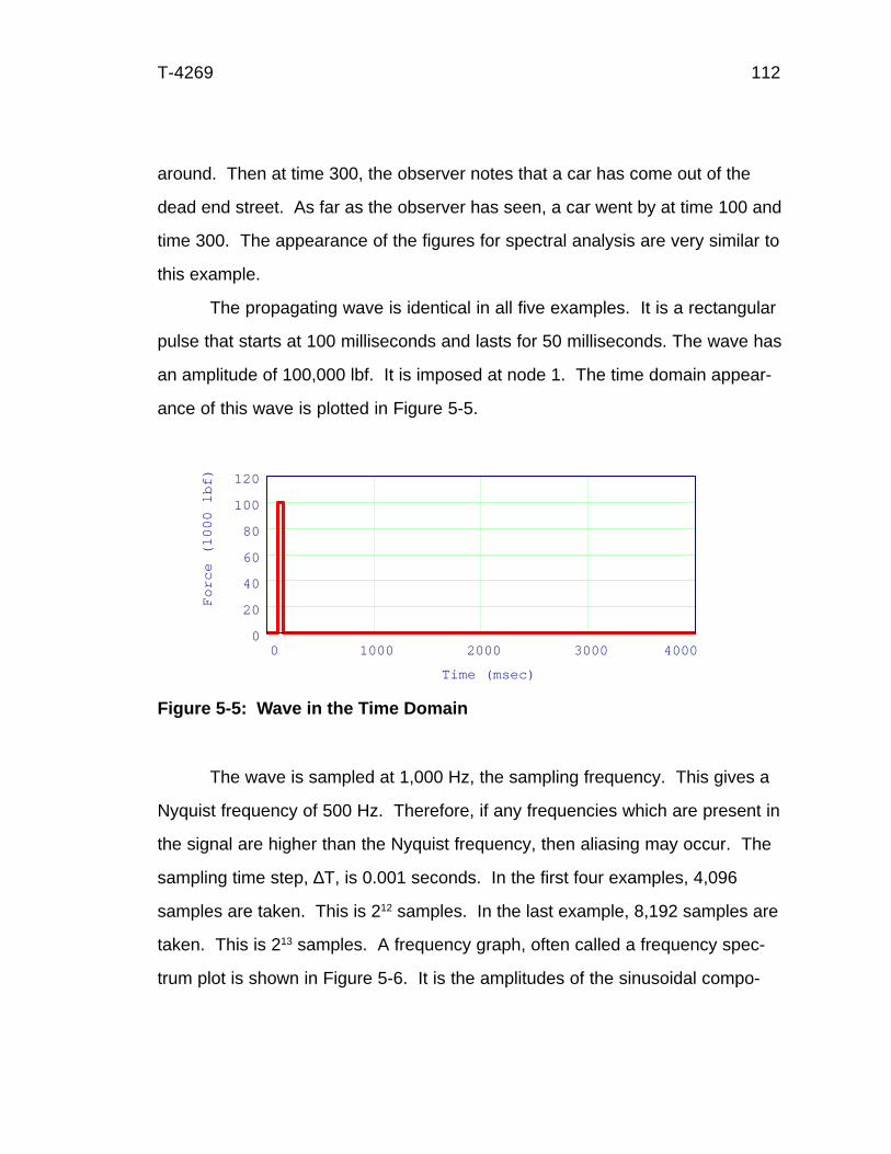
T-4269 112
around. Then at time 300, the observer notes that a car has come out of the
dead end street. As far as the observer has seen, a car went by at time 100 and
time 300. The appearance of the figures for spectral analysis are very similar to
this example.
The propagating wave is identical in all five examples. It is a rectangular
pulse that starts at 100 milliseconds and lasts for 50 milliseconds. The wave has
an amplitude of 100,000 lbf. It is imposed at node 1. The time domain appear-
ance of this wave is plotted in Figure 5-5.
The wave is sampled at 1,000 Hz, the sampling frequency. This gives a
Nyquist frequency of 500 Hz. Therefore, if any frequencies which are present in
the signal are higher than the Nyquist frequency, then aliasing may occur. The
sampling time step, ∆T, is 0.001 seconds. In the first four examples, 4,096
samples are taken. This is 212 samples. In the last example, 8,192 samples are
taken. This is 213 samples. A frequency graph, often called a frequency spec-
trum plot is shown in Figure 5-6. It is the amplitudes of the sinusoidal compo-
Figure 5-5: Wave in the Time Domain
0 1000 2000 3000 40000
20
40
60
80
100
120
Time (msec)
Fo
rce
(1
00
0 lb
f)
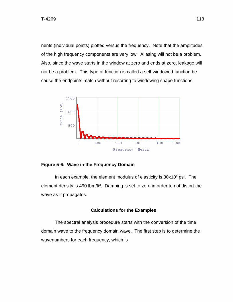
T-4269 113
nents (individual points) plotted versus the frequency. Note that the amplitudes
of the high frequency components are very low. Aliasing will not be a problem.
Also, since the wave starts in the window at zero and ends at zero, leakage will
not be a problem. This type of function is called a self-windowed function be-
cause the endpoints match without resorting to windowing shape functions.
In each example, the element modulus of elasticity is 30x106 psi. The
element density is 490 lbm/ft3. Damping is set to zero in order to not distort the
wave as it propagates.
Calculations for the Examples
The spectral analysis procedure starts with the conversion of the time
domain wave to the frequency domain wave. The first step is to determine the
wavenumbers for each frequency, which is
Figure 5-6: Wave in the Frequency Domain
0 100 200 300 400 500
500
1000
1500
Frequency (Hertz)
Fo
rce
(lb
f)

T-4269 114
$kc
iAE
= +ω ωγ2
2
(5.3)
With these values, the stiffness matrix elements can be determined for
each element. For the on diagonal values
$$
$
$K
ikAE
eeD ikL
ikL=−
+−
−
11
2
2e j (5.4)
For the off diagonal values
$$
$
$K
ikAE
eeOD ikL
ikL=−
−−
−
12
2 e j (5.5)
These values are true for the non-infinite elements. For the semi-infinite ele-
ment, the stiffness matrix values for the on diagonal value is
$ $K ikAEDSI = ( 5.6)
and for the off diagonal value
$KODSI = 0 ( 5.7)
The entire stiffness matrix is assembled for the global solution. In the
fixed boundary examples, since the U0 value is known to be zero for all time and
frequencies, a reduced stiffness matrix can be used. In addition, because the
off-diagonal values of the semi-infinite element are zero, the stiffness matrix can
be reduced further. The solution for the spectral displacements are
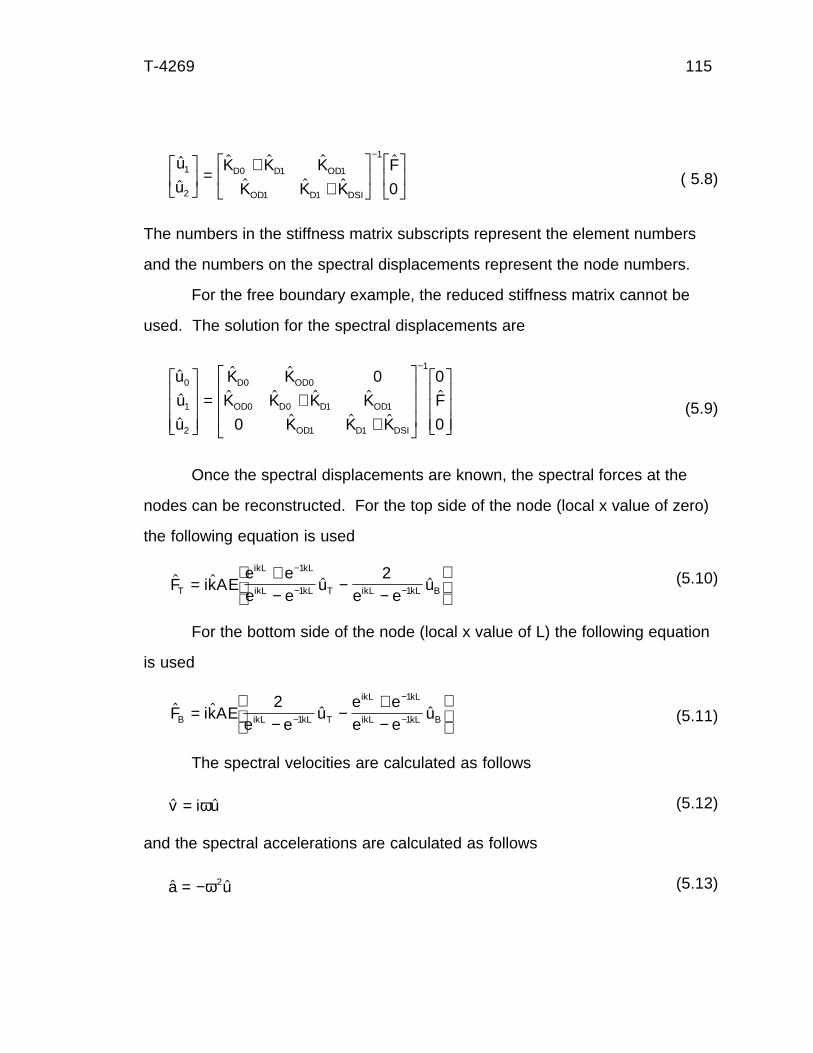
T-4269 115
$
$
$ $ $
$ $ $
$u
uK K K
K K K
FD D OD
OD D DSI
1
2
0 1 1
1 1
1
0
LNM
OQP
= ++
LNM
OQP
LNMOQP
−
( 5.8)
The numbers in the stiffness matrix subscripts represent the element numbers
and the numbers on the spectral displacements represent the node numbers.
For the free boundary example, the reduced stiffness matrix cannot be
used. The solution for the spectral displacements are
$
$
$
$ $
$ $ $ $
$ $ $
$u
u
u
K K
K K K K
K K K
FD OD
OD D D OD
OD D DSI
0
1
2
0 0
0 0 1 1
1 1
10
0
0
0
L
NMMM
O
QPPP
= ++
L
N
MMM
O
Q
PPP
L
NMMM
O
QPPP
−
(5.9)
Once the spectral displacements are known, the spectral forces at the
nodes can be reconstructed. For the top side of the node (local x value of zero)
the following equation is used
(5.10)
For the bottom side of the node (local x value of L) the following equation
is used
(5.11)
The spectral velocities are calculated as follows
$ $v i u= ω (5.12)
and the spectral accelerations are calculated as follows
$ $a u= −ω2 (5.13)
$ $ $ $F ikAEe ee e
ue e
uT
ikL kL
ikL kL T ikL kL B=+−
−−
−
− −
1
1 1
2
$ $ $ $F ikAEe e
ue ee e
uB ikL kL T
ikL kL
ikL kL B=−
−+−
−
−
−
21
1
1
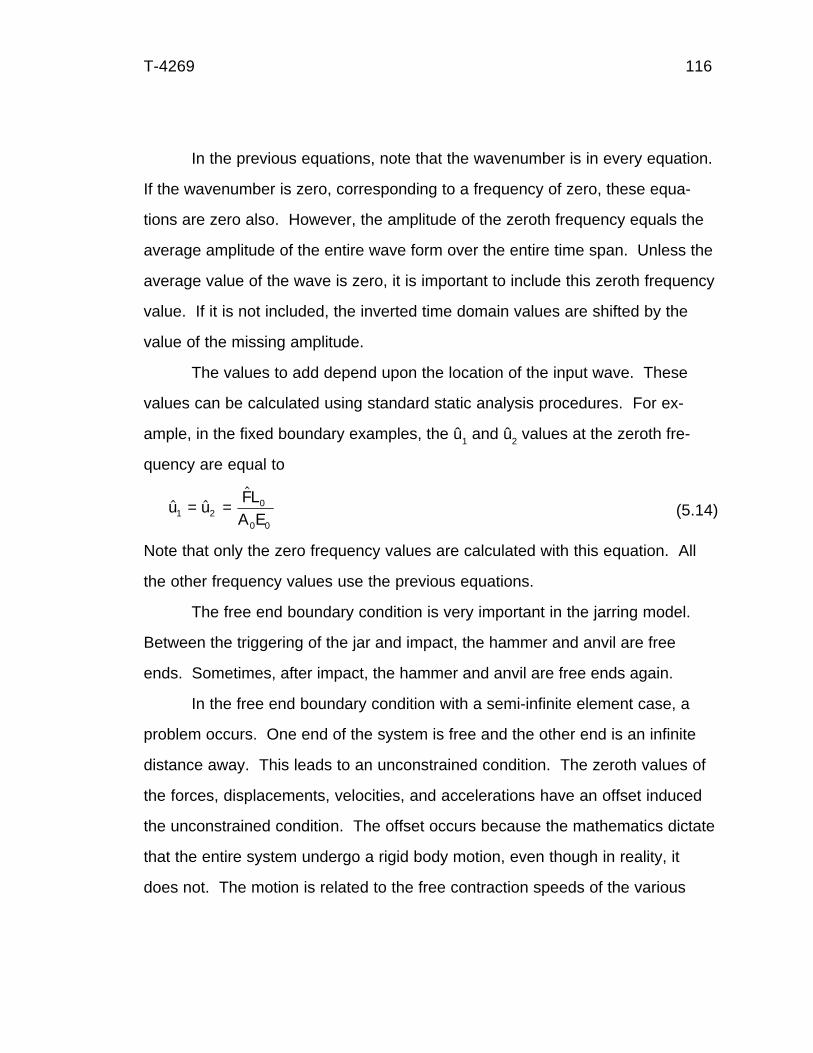
T-4269 116
In the previous equations, note that the wavenumber is in every equation.
If the wavenumber is zero, corresponding to a frequency of zero, these equa-
tions are zero also. However, the amplitude of the zeroth frequency equals the
average amplitude of the entire wave form over the entire time span. Unless the
average value of the wave is zero, it is important to include this zeroth frequency
value. If it is not included, the inverted time domain values are shifted by the
value of the missing amplitude.
The values to add depend upon the location of the input wave. These
values can be calculated using standard static analysis procedures. For ex-
ample, in the fixed boundary examples, the û1 and û2 values at the zeroth fre-
quency are equal to
$ $$
u uFLA E1 2
0
0 0
= = (5.14)
Note that only the zero frequency values are calculated with this equation. All
the other frequency values use the previous equations.
The free end boundary condition is very important in the jarring model.
Between the triggering of the jar and impact, the hammer and anvil are free
ends. Sometimes, after impact, the hammer and anvil are free ends again.
In the free end boundary condition with a semi-infinite element case, a
problem occurs. One end of the system is free and the other end is an infinite
distance away. This leads to an unconstrained condition. The zeroth values of
the forces, displacements, velocities, and accelerations have an offset induced
the unconstrained condition. The offset occurs because the mathematics dictate
that the entire system undergo a rigid body motion, even though in reality, it
does not. The motion is related to the free contraction speeds of the various
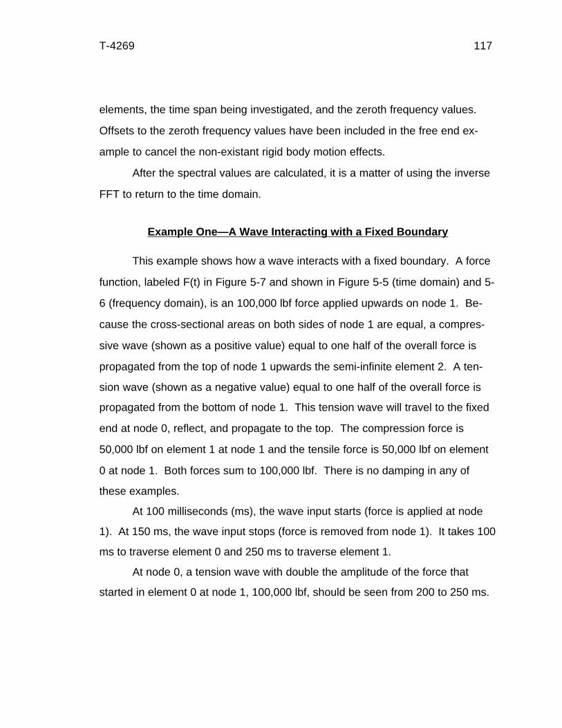
T-4269 117
elements, the time span being investigated, and the zeroth frequency values.
Offsets to the zeroth frequency values have been included in the free end ex-
ample to cancel the non-existant rigid body motion effects.
After the spectral values are calculated, it is a matter of using the inverse
FFT to return to the time domain.
Example One—A Wave Interacting with a Fixed Boundary
This example shows how a wave interacts with a fixed boundary. A force
function, labeled F(t) in Figure 5-7 and shown in Figure 5-5 (time domain) and 5-
6 (frequency domain), is an 100,000 lbf force applied upwards on node 1. Be-
cause the cross-sectional areas on both sides of node 1 are equal, a compres-
sive wave (shown as a positive value) equal to one half of the overall force is
propagated from the top of node 1 upwards the semi-infinite element 2. A ten-
sion wave (shown as a negative value) equal to one half of the overall force is
propagated from the bottom of node 1. This tension wave will travel to the fixed
end at node 0, reflect, and propagate to the top. The compression force is
50,000 lbf on element 1 at node 1 and the tensile force is 50,000 lbf on element
0 at node 1. Both forces sum to 100,000 lbf. There is no damping in any of
these examples.
At 100 milliseconds (ms), the wave input starts (force is applied at node
1). At 150 ms, the wave input stops (force is removed from node 1). It takes 100
ms to traverse element 0 and 250 ms to traverse element 1.
At node 0, a tension wave with double the amplitude of the force that
started in element 0 at node 1, 100,000 lbf, should be seen from 200 to 250 ms.
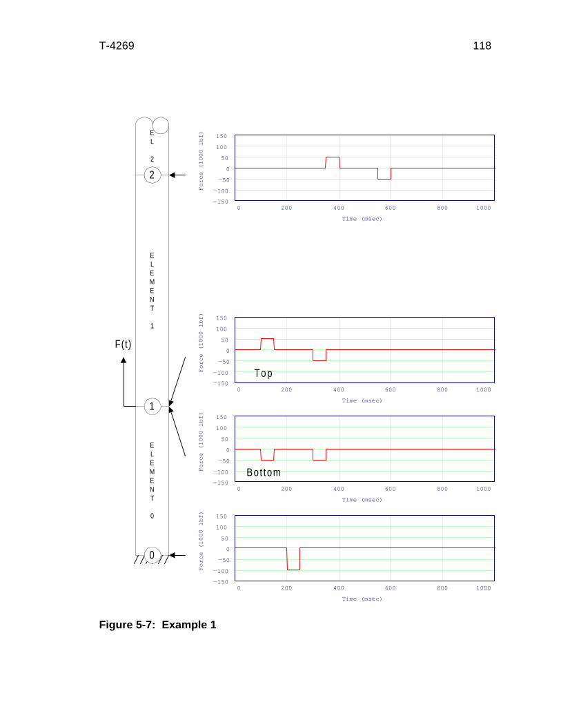
T-4269 118
Figure 5-7: Example 1
0 200 400 600 800 1000150
100
50
0
50
100
150
Time (msec)
Fo
rce
(1
00
0 lb
f)
0 200 400 600 800 1000150
100
50
0
50
100
150
Time (msec)
Fo
rce
(1
00
0 lb
f)
0 200 400 600 800 1000150
100
50
0
50
100
150
Time (msec)
Fo
rce
(1
00
0 lb
f)0 200 400 600 800 1000
150
100
50
0
50
100
150
Time (msec)
Fo
rce
(1
00
0 lb
f)
Top
Bot tom
ELEMENT
0
ELEMENT
1
EL
2
1
2
0
F(t)

T-4269 119
Figure 5-8: Example 1—Displacements
0 200 400 600 800 10002
0
2
4
Node 0Node 1Node 2
Time (msec)
Dis
pla
cem
ent (in)
Figure 5-9: Example 1—Velocities
0 200 400 600 800 1000
5
0
5
Node 1Node 2
Time (msec)
Ve
loci
ty (
fee
t p
er
seco
n
T-4269 120
This is the initial wave starting at 100 ms plus the transit time of 100 ms. Be-
cause there are no reflections from anywhere else in the string, there should be
no more waves appearing at node 0.
At node 1, the initial wave should be seen at 100 to 150 ms. On the top
side of node 1, a compression wave of 50,000 lbf should be seen. On the bot-
tom side of node 1, there should be a tension wave of one-half the overall ampli-
tude of the wave, 50,000 lbf. On both sides of the node, at 300 ms (the start at
100 ms plus a round trip to the fixed end of 200 ms ), another 50 ms wave of
50,000 lbf should be seen. This is the reflected wave from the fixed end (node
0).
The same waves travel through the bottom and top sides of Node 2. Both
sides should be identical because there is no original wave input at this node.
The waves traveling through this node are the same waves that traveled through
the top side of node 1, 250 ms earlier. There should be a 50,000 lbf compres-
sive wave at 350 ms and a 50,000 lbf tension wave at 550 ms (100 ms plus 200
ms plus 250 ms).
The displacement and velocity histories of nodes 0, 1, and 2 are shown in
Figure 5-8 and Figure 5-9. The displacement and velocity at node 0 are zero for
all time. This is the fixed boundary and is modelled correctly. The displacement
is nonzero until both the compressive and tension wave passes through the
node. Nodes 1 and 2 show the displacements as the wave passes through. The
velocities are nonzero only while the wave is traveling through the node.
Example Two—A Wave Interacting with a Free Boundary
This example shows how a wave interacts with a free boundary. All of the
conditions in Example 2 are the same as in Example 1 except that the boundary
T-4269 121
at node 0 is a free boundary. (See Figure 5-10.) The same 100,000 lbf 50 ms
wave starts at node 1 at 100 ms. A 50,000 lbf compressive wave is propagated
from the top of node 1 and a 50,000 lbf tension wave is propagated from the
bottom of node 1. This tension wave will travel to the free end, reflect and invert
into a compressive wave, and propagate to the top. The timing on all the waves
are the same as in Example 1. The force from the wave at node 0 should be
zero for all times. This is the definition of a traction free end.
The wave at 100 ms is the same as in Example 1, the wave at 300 ms is
inverted from Example 1. This is the expected inverted tension wave reflected
as a compression wave from the free end.
As in all of these examples, the bottom and top sides of node 2 react to
the same waves.
The displacements shown in Figure 5-11 and velocities shown in Figure
5-12 have the previously mentioned rigid body motion removed. The displace-
ments show a permanent change of location. There were two compressive
waves rather than a tensile and compressive wave. In Example 1, the compres-
sive wave traveled through first and then the tensile wave traveled through
canceling the displacements. In this example, the two compression waves
doubled the displacement.
The rigid body motion is removed because it is an artificial construct of
the wave theory where semi-infinite elements are involved. This rigid body
motion is the free contraction speed of the particular element. This gives a zero
velocity to the nodes except while the wave is travelling through the nodes. The
velocity at node 0 is double the velocities at the other two nodes. This is a free
end effect and is modelled correctly.

T-4269 122
Figure 5-10: Example 2
0 200 400 600 800 1000150
100
50
0
50
100
150
Time (msec)
Fo
rce
(1
00
0 lb
f)
0 200 400 600 800 1000150
100
50
0
50
100
150
Time (msec)
Fo
rce
(1
00
0 lb
f)
0 200 400 600 800 1000150
100
50
0
50
100
150
Time (msec)
Fo
rce
(1
00
0 lb
f)0 200 400 600 800 1000
150
100
50
0
50
100
150
Time (msec)
Fo
rce
(1
00
0 lb
f)
Top
Bot tom
ELEMENT
0
ELEMENT
1
EL
2
1
2
0
F(t)

T-4269 123
0 200 400 600 800 10004
2
0
2
4
Node 0Node 1Node 2
Time (msec)
Dis
pla
cem
en
t (i
n)
Figure 5-11: Example 2—Displacements
0 200 400 600 800 1000
0
5
10
Node 0Node 1Node 2
Time (msec)
Ve
loci
ty (
fee
t p
er
seco
nd
)
Figure 5-12: Example 2—Velocities
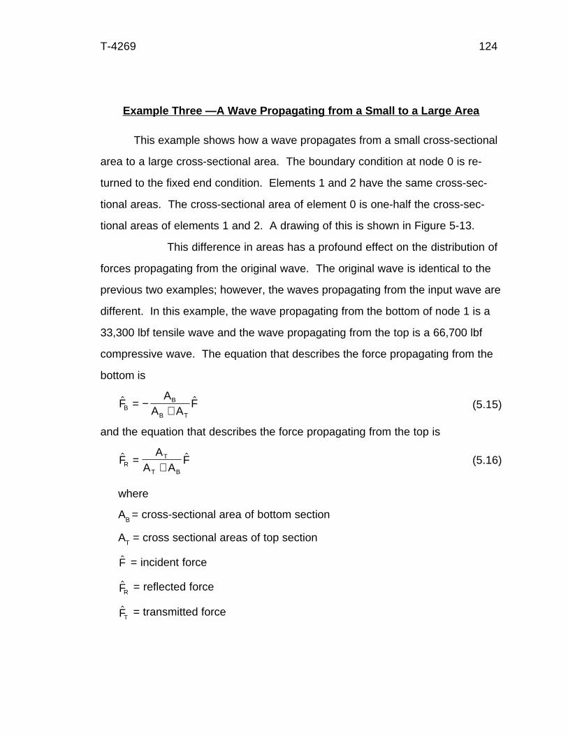
T-4269 124
Example Three —A Wave Propagating from a Small to a Large Area
This example shows how a wave propagates from a small cross-sectional
area to a large cross-sectional area. The boundary condition at node 0 is re-
turned to the fixed end condition. Elements 1 and 2 have the same cross-sec-
tional areas. The cross-sectional area of element 0 is one-half the cross-sec-
tional areas of elements 1 and 2. A drawing of this is shown in Figure 5-13.
This difference in areas has a profound effect on the distribution of
forces propagating from the original wave. The original wave is identical to the
previous two examples; however, the waves propagating from the input wave are
different. In this example, the wave propagating from the bottom of node 1 is a
33,300 lbf tensile wave and the wave propagating from the top is a 66,700 lbf
compressive wave. The equation that describes the force propagating from the
bottom is
$ $FA
A AFR
T
T B
=+
$ $FA
A AFB
B
B T
= −+ (5.15)
and the equation that describes the force propagating from the top is
where
AB
= cross-sectional area of bottom section
AT = cross sectional areas of top section
$F = incident force
$FR = reflected force
$FT = transmitted force
(5.16)

T-4269 125
Figure 5-13: Example 3
0 200 400 600 800 1000150
100
50
0
50
100
150
Time (msec)
Fo
rce
(1
00
0 lb
f)
0 200 400 600 800 1000150
100
50
0
50
100
150
Time (msec)
Fo
rce
(1
00
0 lb
f)
0 200 400 600 800 1000150
100
50
0
50
100
150
Time (msec)
Fo
rce
(1
00
0 lb
f)0 200 400 600 800 1000
150
100
50
0
50
100
150
Time (msec)
Fo
rce
(1
00
0 lb
f)
Top
Bot tom
ELEMENT
0
ELEMENT
1
EL
2
1
2
0
F(t)

T-4269 126
The force time history for node 0 will show a doubling of the 33,300 lbf
tensile wave at time 200 ms. The wave will reflect off of the fixed end with the
same sign, therefore, a 33,300 lbf tensile wave will propagate to the top after
reflection. In this example, unlike the previous two, there will be more reflections
from the change in geometric properties at node 1. Some of the wave will trans-
mit through the junction, and some will reflect off of the junction. These calcula-
tions are shown in equations 5.1 and 5.2.
For each reflection at the junction, a smaller amplitude tensile wave will
propagate back to the fixed end, reflect off of the fixed end, and return to the
junction as the diminished tensile wave. The wave eventually decays with every
reflection at the junction. This is the advantage of the semi-infinite element. The
waves will not return to set up a resonance or other complications.
At node 0, the reflection from the junction is always in the same sign. A
tensile wave reflects as a tensile wave and a compressive wave reflects as a
compression wave. As a wave travels from a smaller to a larger cross-sectional
area, the junction acts as a fixed end, as far as the sign of the wave is con-
cerned.
Node 1 shows a difference in the bottom and top sides only for the origi-
nating wave. There is a 66,700 lbf compressive wave propagating to the top and
a 33,300 lbf tensile wave propagating to the bottom. The tensile wave reflects
off of the fixed end and returns to the junction. The wave then reflects back and
forth between the fixed end and the junction, slowly diminishing.
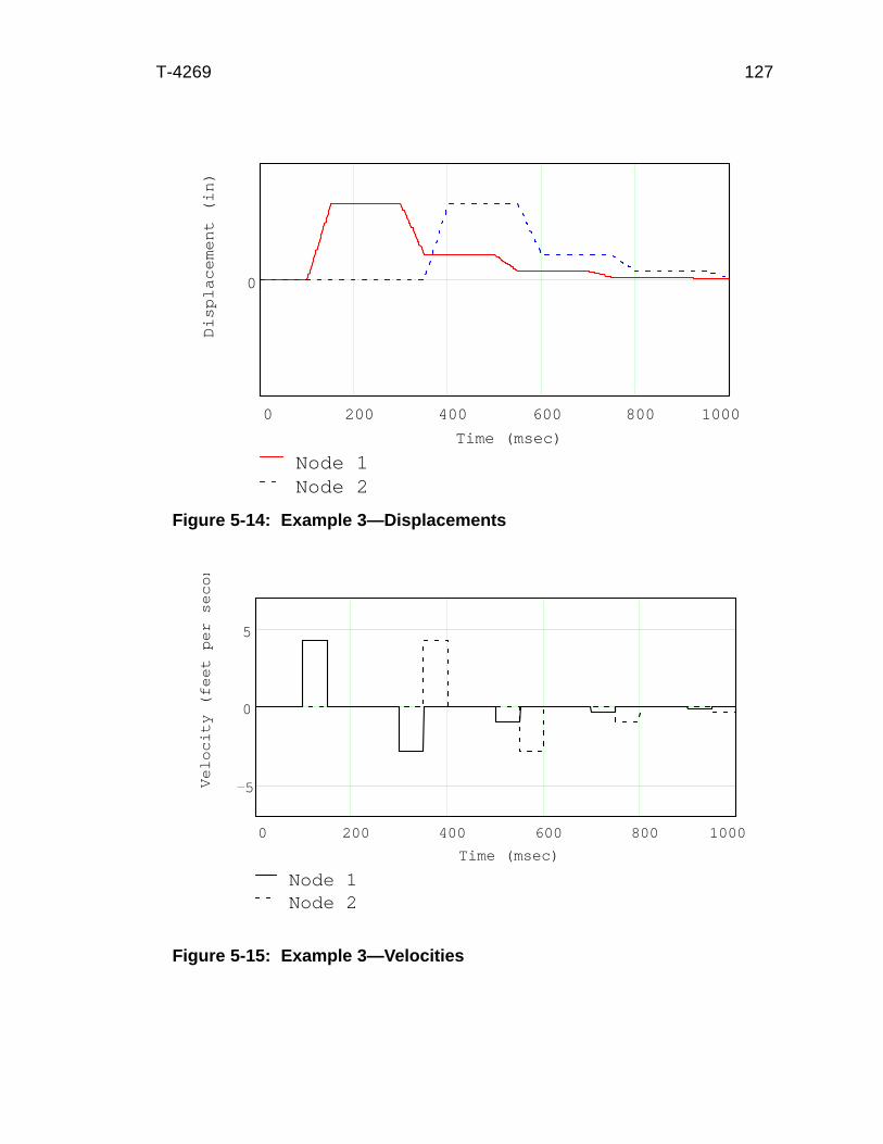
T-4269 127
Figure 5-14: Example 3—Displacements
0 200 400 600 800 1000
0
Node 1Node 2
Time (msec)
Dis
pla
cem
ent (in)
Figure 5-15: Example 3—Velocities
0 200 400 600 800 1000
5
0
5
Node 1Node 2
Time (msec)
Velo
city
(fe
et per
seco
n

T-4269 128
At the bottom side of node 1, after the originating wave, the wave force
values are the same, 44,400 lbf tensile, on both sides of the node. Yet at node
0, a 22,200 lbf tensile is seen as the second wave. It would seem that a 22,200
lbf tensile wave should appear on the bottom side of the node. There is a inter-
esting effect occurring during a wave transmittal through a junction. The wave at
the node acts the same on both sides of the junction. This is correct as the
forces on both sides of the node were summed to zero. However, since this
junction is acting like a fixed end, the incident force amplitude plus the reflected
force amplitude is the force on the bottom side of the node. This is equal to the
force amplitude on the top side of the node. This has a duration of exactly one-
half the length of the wave. Afterwards, the wave propagating from the bottom is
the expected 22,200 lbf tensile wave. The wave propagating from the top is the
44,400 lbf tensile wave.
Node 2 shows the waves from node 1 shifted in time by the value neces-
sary to traverse element 1, which is 250 ms.
The displacements, shown in Figure 5-14, show the effect of the waves’
reflections. Because this example has a fixed end boundary condition, the
displacements will return to zero. The velocities in Figure 5-15 are nonzero
during wave transit through the node. This is the same as in all the fixed end
boundary condition examples.
Example Four—A Wave Propagating from a Large to a Small Area
This example shows how a wave propagates from a large cross-sectional
area to a small cross-sectional area. This example ( shown in Figure 5-16), the

T-4269 129
0 200 400 600 800 1000150
100
50
0
50
100
150
Time (msec)
Fo
rce
(1
00
0 lb
f)
0 200 400 600 800 1000150
100
50
0
50
100
150
Time (msec)
Fo
rce
(1
00
0 lb
f)
0 200 400 600 800 1000150
100
50
0
50
100
150
Time (msec)
Fo
rce
(1
00
0 lb
f)0 200 400 600 800 1000
150
100
50
0
50
100
150
Time (msec)
Fo
rce
(1
00
0 lb
f)
Top
Bot tom
ELEMENT
0
ELEMENT
1
EL
2
1
2
0
F(t)
Figure 5-16: Example 4
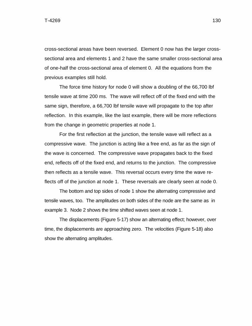
T-4269 130
cross-sectional areas have been reversed. Element 0 now has the larger cross-
sectional area and elements 1 and 2 have the same smaller cross-sectional area
of one-half the cross-sectional area of element 0. All the equations from the
previous examples still hold.
The force time history for node 0 will show a doubling of the 66,700 lbf
tensile wave at time 200 ms. The wave will reflect off of the fixed end with the
same sign, therefore, a 66,700 lbf tensile wave will propagate to the top after
reflection. In this example, like the last example, there will be more reflections
from the change in geometric properties at node 1.
For the first reflection at the junction, the tensile wave will reflect as a
compressive wave. The junction is acting like a free end, as far as the sign of
the wave is concerned. The compressive wave propagates back to the fixed
end, reflects off of the fixed end, and returns to the junction. The compressive
then reflects as a tensile wave. This reversal occurs every time the wave re-
flects off of the junction at node 1. These reversals are clearly seen at node 0.
The bottom and top sides of node 1 show the alternating compressive and
tensile waves, too. The amplitudes on both sides of the node are the same as in
example 3. Node 2 shows the time shifted waves seen at node 1.
The displacements (Figure 5-17) show an alternating effect; however, over
time, the displacements are approaching zero. The velocities (Figure 5-18) also
show the alternating amplitudes.
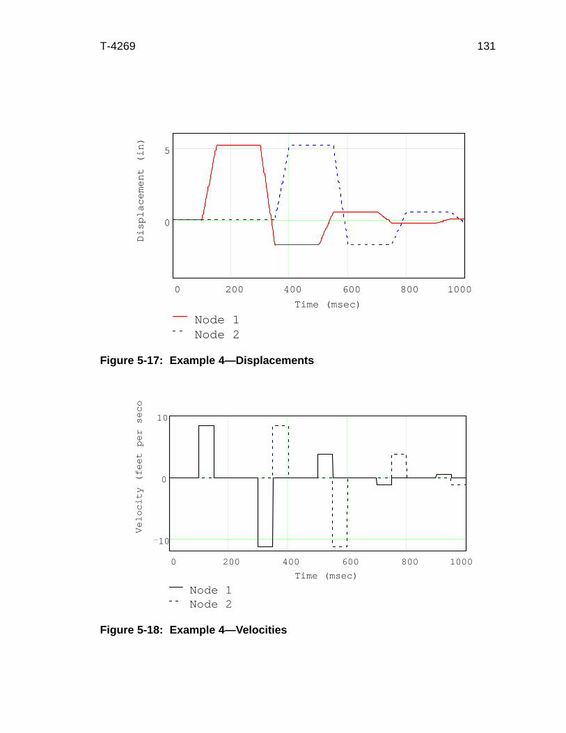
T-4269 131
Figure 5-17: Example 4—Displacements
0 200 400 600 800 1000
0
5
Node 1Node 2
Time (msec)
Dis
pla
cem
ent (in)
Figure 5-18: Example 4—Velocities
0 200 400 600 800 1000
10
0
10
Node 1Node 2
Time (msec)
Ve
loci
ty (
fee
t p
er
seco
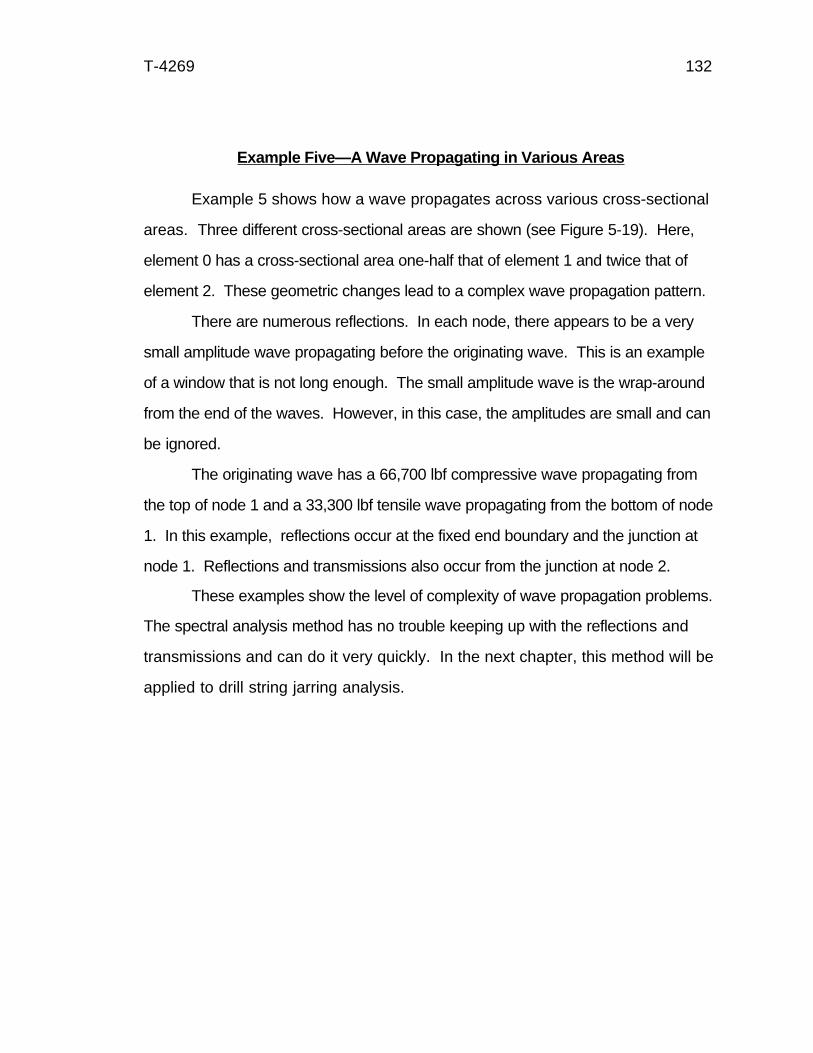
T-4269 132
Example Five—A Wave Propagating in Various Areas
Example 5 shows how a wave propagates across various cross-sectional
areas. Three different cross-sectional areas are shown (see Figure 5-19). Here,
element 0 has a cross-sectional area one-half that of element 1 and twice that of
element 2. These geometric changes lead to a complex wave propagation pattern.
There are numerous reflections. In each node, there appears to be a very
small amplitude wave propagating before the originating wave. This is an example
of a window that is not long enough. The small amplitude wave is the wrap-around
from the end of the waves. However, in this case, the amplitudes are small and can
be ignored.
The originating wave has a 66,700 lbf compressive wave propagating from
the top of node 1 and a 33,300 lbf tensile wave propagating from the bottom of node
1. In this example, reflections occur at the fixed end boundary and the junction at
node 1. Reflections and transmissions also occur from the junction at node 2.
These examples show the level of complexity of wave propagation problems.
The spectral analysis method has no trouble keeping up with the reflections and
transmissions and can do it very quickly. In the next chapter, this method will be
applied to drill string jarring analysis.
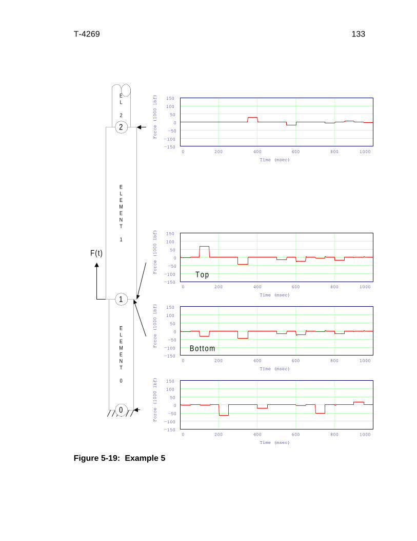
T-4269 133
0 200 400 600 800 1000150
100
50
0
50
100
150
Time (msec)
Fo
rce
(1
00
0 lb
f)
0 200 400 600 800 1000150
100
50
0
50
100
150
Time (msec)
Fo
rce
(1
00
0 lb
f)
0 200 400 600 800 1000150
100
50
0
50
100
150
Time (msec)
Fo
rce
(1
00
0 lb
f)0 200 400 600 800 1000
150
100
50
0
50
100
150
Time (msec)F
orc
e (
10
00
lbf)
Top
Bot tom
F(t)
ELEMENT
0
ELEMENT
1
EL
2
1
2
0
Figure 5-19: Example 5
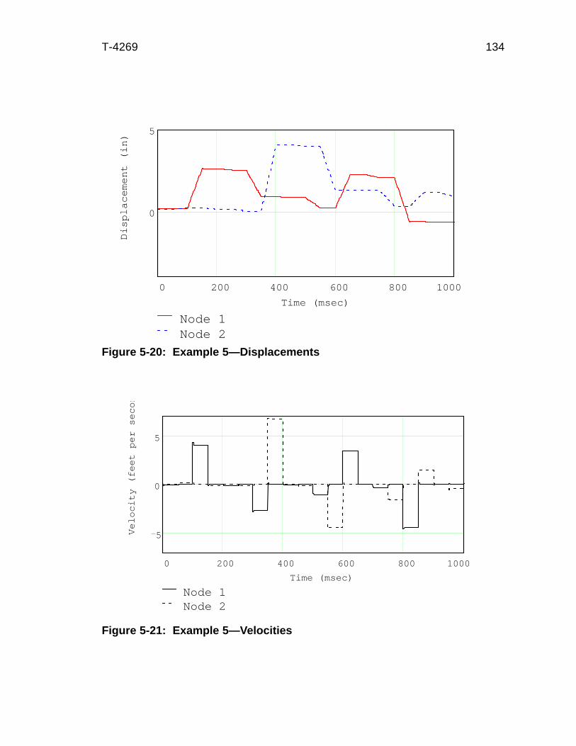
T-4269 134
Figure 5-21: Example 5—Velocities
0 200 400 600 800 1000
5
0
5
Node 1Node 2
Time (msec)
Ve
loci
ty (
fee
t p
er
seco
n
Figure 5-20: Example 5—Displacements
0 200 400 600 800 1000
0
5
Node 1Node 2
Time (msec)
Dis
pla
cem
ent (in)
T-4269 135
CHAPTER 6
THE NEW JARRING MODEL
This chapter presents the spectral analysis-based model of jarring. A
generic drill string model is described and each phase of the jarring process is
presented. Spectral analysis remedies the lack of accuracy and the need for
inordinate computational resources and time that are inherent in current jarring
models.
With the spectral analysis-based jarring model, a generic drill string can
be customized to include various sections of pipe and equipment as conditions
dictate. For example, a stuck section of pipe, drill collars, heavy weight drill
pipe, drill pipe, and an accelerator can be input into the model.
The Spectral Analysis Jarring Model
A generic jarring model using the spectral analysis method is shown in
Figure 6-1. The nodes define the various elements of the model. In each ele-
ment, friction forces and the geometric and material properties of the string can
be varied.
Starting from the bottom up, the nodes consist of
Node 8 - the ground
Node 7 - the bottom of the stuck pipe
Node 6 - the top of the stuck pipe

T-4269 136
Figure 6-1: Typical Drill String
Stuck along side of drill string
4
1
2
5
7
10,0
00 ft
300
ft90
ft10
ft18
0 ft
450
ft
6.5 in Jar Stroke
150
ft
Stuck Point
Drill Collars; 7.25 in by 2.812 in
Jar: F(t)
Drill Pipe; 4.5 in by 3.73 in
6
Node 3
Node 4
Node 2
Node 5
Node 6
Node 7
Node 8
Node 1
Node 0
Connection for stability
Not to Scale
0
Drill Collars; 7.25 in by 2.812 in
Drill Collars; 7.25 in by 2.812 in
Heavy Weight Drill Pipe; 4.5 in by 2.75 in
Accelerator (K = 13,300 lbf/in)
Rig
3
Anvil
Hammer

T-4269 137
Node 5 - the jar
Node 4 - the bottom of an accelerator (if present)
Node 3 - the top of an accelerator (if present)
Node 2 - the bottom of heavy weight drill pipe
Node 1 - the bottom of drill pipe
Node 0 - the top of the drill pipe (the rig)
The elements represent the areas from which mathematical modeling
equations are formulated. The elements are
Element 7 - the connection of the model to the Earth
(This may be a very light spring or simply more of the
string.)
Element 6 - the section of the string that is stuck.
(The friction factors in this section can be set to
various values depending upon the manner of sticking.
In differential sticking, high values would be used; in
mechanical sticking, ultra high values. By setting the
cross-sectional area of either element 6 or 7 to a very
large number, the user can simulate a fixed end at
either node 6 or node 7, respectively.)
Element 5 - the free part of the drill string below the jars.
Element 4 - the drill collars above the jar
Element 3 - an accelerator
Element 2 - drill collar above the accelerator
Element 1 - heavy weight drill pipe or drill pipe
Element 0 - drill pipe
T-4269 138
Any section of this model can be built into any part of the drill string. The
geometric properties (with units) that can be varied include
Outside diameter (OD - length)
Inside diameter (ID - length)
Length (L - length)
The material properties (with units) that can be varied include
Modulus of elasticity (E - force/length2)
Density ( ρ - mass/length3)
Viscous Damping (γ - mass/time length)
The Jarring Process
The jarring process can be broken into four phases. They are the pre-
stretch, free contraction, impact, and post-impact. This is shown in Figure 6-2.
Pre-Stretch
Pre-stretch is defined as the activities that take place prior to the jar
triggering. This includes the pulling (or pushing) on the jar in order to trigger the
jar. The forces are applied slowly; therefore, they are defined as static. Usually,
the rig cannot move within the defined time frame for dynamic conditions (at
least not intentionally). It is assumed that the drill string is in static equilibrium
just prior to triggering. That implies that the stresses from the static conditions
do not change over the time frame of the jarring action. These stresses can be
simply added to the drill string dynamic stresses.
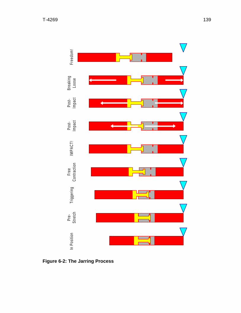
T-4269 139
Free
dom
!In
Pos
ition
Pre-
Stre
tch
Trig
gerin
gFr
eeCo
ntra
ctio
nIM
PAC
T!Po
st-
Impa
ctBr
eaki
ngLo
ose
Post
-Im
pact
Figure 6-2: The Jarring Process
T-4269 140
The values of the static stresses are derived using free body diagrams
(Mitchell 1995). In addition, it is assumed that the stresses will be from the
overpull load at the jar trigger mechanism. That is, the force at the jar trigger
mechanism is known and is the overpull necessary for the jar to trigger. All other
loads are derived from this condition.
The real axial stress loads are determined with a free body diagram
showing the weight of the drill string below the point of interest and the loads
from the stuck point and the overpull force. The effective axial stress takes into
account the fluid pressure area loads.
Bending loads from curved bore holes and doglegs are not addressed in
this particular model.
Free Contraction
After the jar triggers, the jar converts the strain energy from the static
loading in the drill string to kinetic energy. The bottom part of the jar, called the
hammer, disconnects from the top of the jar, called the anvil. The hammer
travels up with the top of the drill string. The anvil travels down with the bottom
of the drill string. Both parts freely contract until the combined distance the anvil
and hammer travels is equal to the stroke length. The hammer traveling upward
strikes the anvil traveling downwards. The stroke length is adjustable in most
jars (at the surface only).
Before the jar triggers, there is a force on the hammer and anvil equal to
the overpull force. After the jar triggers, the force on the hammer and anvil drops

T-4269 141
to zero. In effect, a negative force wave has been formed (Aarrestad and
Kyllingstad 1994). This negative wave will continue until the hammer and anvil
impact.
The important variables to determine are the velocities of the hammer and
anvil and the distance traveled by both. The velocities are used to determine the
impact force. The distance traveled by both and the wave reflection characteris-
tics determine how fast the hammer and anvil are traveling at impact.
The velocities of the hammer and anvil are dependent upon the overpull
force and the number of wave reflections from the various parts of the drill string.
For every reflection from below the jar, the anvil increases or decreases in veloc-
ity, depending upon the type of reflection. The wave reflected can either be a
compressive or tension wave. A compressive wave will increase the velocity of
the anvil; a tension wave will slow the anvil and can even reverse the direction of
the anvil.
The same conditions occur in the drill string above the jar. The hammer
velocity will increase or decrease. In most cases, however, the drill string de-
creases in cross-sectional area as one follows the drill string to the surface.
Therefore, the wave reflections continually increase the velocity of the hammer.
An accelerator will act as a free end, reflecting most of a wave back to the
jar. The jar will accelerate with each reflection of the wave from the accelerator
(hence the tool name). The faster the hammer is traveling at impact, the more
force is generated. However, since the waves have a shorter round trip time, the
duration of the impact pulse will be shorter.
T-4269 142
The spring constant (K) of an accelerator determines the effect of the
accelerator. A spring constant can be thought of as a cross-sectional area.
Assuming a length (L) and modulus of elasticity (E), one can derive a cross-
sectional area (A)
AKLE
= (6.1)
A small spring constant is equivalent to a small cross-sectional area. The
smaller the cross-sectional area, the more the propagating wave will reflect back
to the jar. An accelerator acts very much like a free boundary. Very little of the
wave will get through the accelerator. This causes the wave reflections to return
to the hammer. This will cause the hammer to accelerate to a faster velocity. If
an accelerator is not used, then the properties can be set to drill collar values
making this section a drill collar.
The time until impact is an unknown. This means that the length of the
negative force wave is an unknown. This can be remedied by insuring that the
negative wave lasts longer than the time to impact, but is not so excessively long
that it propagates into neighboring windows.
The hammer and anvil free contraction are modeled by disconnecting the
model at the jar (node 5), creating, in effect, two sub-models.
After the combined distances which the hammer and anvil traveled are
equal to the stroke length, this phase of the jarring process is finished. The
velocities of the hammer and anvil are then determined. These two values are
used to determine the impact force.
T-4269 143
Impact
After the hammer and anvil finally impact, the kinetic energy of the ham-
mer and anvil is converted back to strain energy. An impact force is generated.
The impact force in this model is determined using the standard Hopkinson bar
approach, the same method used in all other jarring papers to determine the
impact force.
The Hopkinson bar experiment consisted of two bars. One bar is static
and the other is in motion. The bar in motion is constrained to impact the static
bar at a known velocity. The force generated is directly related to the velocity of
the bar in motion. The force is calculated using conservation of momentum.
The length of the impact pulse is determined by the time required from
initial impact for the stress wave to propagate back and forth across the shortest
bar. It is assumed that there is no loss in transmission from damping and that
the bars are both made of the same material. Therefore, the wave “cancels”
itself out upon returning to the impact point. The time duration of the wave is the
round trip length in the shortest bar divided by the speed of sound in the bar.
tLc
= 2 (6.2)
where
L = length of shortest bar
c = wave propagation speed in bar
t = time of travel
The velocity of the impact face will be the same as the particle velocity. It
is the average of the hammer and anvil velocities at impact.
T-4269 144
The shape of the impact pulse is assumed to be rectangular. Actual tests
have shown that the impact wave has a quick, but not instantaneous, rise time
and oscillations along the maximum value of stress. This is explained by the fact
that the assumed impact case is for a one dimensional model. Reality is three
dimensional. Poisson effects and wave interaction with the side boundaries of
the bar will cause the observed fluctuations (Meyers 1994). However, for sim-
plicity, other jarring papers assume the ideal case. That is assumed in this
dissertation, too.
Another implicit assumption is that a “perfect” impact occurs. This is an
impact in that the hammer and anvil impact with perfectly flat faces that are
perpendicular to the direction of travel. Damping and refraction are not consid-
ered.
Post-Impact
The impact force is applied as two waves propagating outward from the
jar (at node 5) up and down the drill string. After impact, there is a very brief
finite time in which the hammer and anvil are in contact. After that time, the
hammer and anvil are assumed to disconnect. In effect, they “bounce” off of
each other. This is the rationale for creating separate sub-models for the ham-
mer and anvil. (See “Free Contraction” in this section.)
In reality, after the first impact, the hammer and anvil may or may not
come back into contact. If the hammer and anvil come back into contact, the
impact junction becomes a nonlinear element. If the junction is closed, a wave
can propagate across the junction or this wave can cause the junction to open,
thus preventing the wave from crossing the junction. Also, if the junction opens,
T-4269 145
the junction becomes two free ends. Depending upon the wave form and ampli-
tude, the wave may alternately open or close the junction allowing the wave to
propagate through it. This can occur repeatedly, resulting in chatter. The junc-
tion may stay open or closed for the duration of the period of interest, or the
junction may open and close intermittently. As pointed out in Chapter 4, the
spectral analysis method, at this time, is not amenable to the inclusion of nonlin-
ear elements. This means that the junction either needs to stay open or stay
closed for the duration of interest. Technology in this area is deficient at the
time of the writing of this dissertation and is an area for future work.
In deriving the spectral element, the assumption was made that the sum
of the forces at a node were in equilibrium. This means that if a force is applied
at a node, an equal and opposite force is generated on the other side of the
node. This is clearly shown in the examples in Chapter 5. However, in an im-
pact junction, the forces are not necessarily in equilibrium. In the case of a
hammer and anvil in a jar, two tension waves are generated at the junction. In
this model, a tension wave can be input on one side of a node. This tension
wave is offset by an equal compression wave (assuming equal cross-sectional
areas) on the other side of the node because of equilibrium conditions. As an
equal tension wave is impressed on the other side of the node, as it occurs in a
jar, the compression wave from the previous tension wave cancels this tension
wave. In addition, the other tension wave is offset by another compression wave
on the side of the first tension wave. It too is canceled, leaving no waves to be
propagated. This does not model reality.
As for the open junction condition, this is easily modeled by using two
separate sub-models (in fact the same sub-models as in the free contraction
T-4269 146
phase) for the hammer and anvil sides of the drill string. The primary impact
force is applied as tension waves at the jar node on each sub-model, just as in
the free contraction model. This wave propagates up and down the drill string
on the side it was applied. The hammer or anvil acts as a free end.
This model is accurate during the time of the primary impact regardless of
what happens to the junction. After the primary impact, the model may or may
not reflect reality. If the hammer and anvil bounce off of each other, resulting in
a open junction, the model will continue to reflect reality. In other cases, if the
hammer and anvil stay closed or chatter, there may be reflections of waves that
get through the junction and have a minor effect on the forces at the stuck point.
Although these reflections may appear in reality, research in this area suggests
that they are not significant to the “unsticking” of the drill string and can be
ignored. It appears that the primary impact force is the largest force and deter-
mines the outcome of the jarring process.
Example Calculations
The spectral analysis model is broken into the same four phases as the
jarring process: pre-stretch, free contraction, impact, and post-impact. In every
phase, the outside diameters, inside diameters, lengths, modulus of elasticity,
density, and damping coefficients of each necessary element are required. The
outside, inside, and cross-sectional areas are calculated. In addition, the wave
propagation speed and weight per unit length are calculated.
T-4269 147
Pre-Stretch
In addition to the above input values, the trigger force and inside and
outside mud weights are needed. The pipe is assumed to be stuck at the top of
element 6. Therefore, no pressure-area forces and loads from below this point
are transmitted to the sections above node 6. A requirement is that the load at
node 5, the jar, is equal to the trigger force.
The pressure-area forces are determined at each node. These forces are
added or subtracted (depending on the direction of the force) at the bottom of
each element. The weight of the element below each node is added at the top of
each element. The equation for the bottom of an element is
F F P PB TP O I= + + (6.3)
and for the top of an element
F F W LT B N N= + (6.4)
where
FTP = force at top of element below current element
PO = pressure-area force on outside of drill string
PI= pressure-area force on inside of drill string
FB = force at the bottom of the element
N = element number
WN = weight of element N per unit length
LN = length of element N
FT = force at the top of the element

T-4269 148
The exceptions to this are at and below the jar. The force at the jar is
equal to the trigger force. Below the jar, the forces are calculated at the top of
the stuck point by taking the trigger force and subtracting the weight of the ele-
ment below the jar and above the top of the stuck point.
Free Contraction
In the free contraction phase, in addition to all of the previous data, the jar
stroke is input. The next step is to take the free contraction wave and convert it
to the frequency domain.
The wave time is chosen long enough to insure the displacements of the
hammer and anvil are greater than the stroke length. In addition, the time of
investigation must be long enough to minimize wave migration from side win-
dows. This time length is dependent upon the geometry and damping coeffi-
cients and is set by the number of samples and the sampling rate.
Once the wave is converted to the frequency domain, the wave numbers
are calculated. The equation is
kc
i
A Em jm
j
m j
j j, = −ω ω γ2
2 (6.5)
where
ωm = circular frequency (radians/time)
cj = the jth element wave propagation speed (length/time)
i = imaginary
γj = the jth element damping coefficient (mass/length time)
Aj = the jth element cross-sectional area (length2)
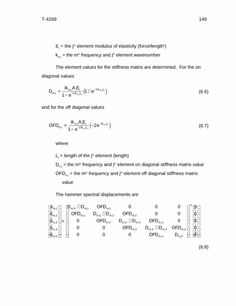
T-4269 149
Ej = the jth element modulus of elasticity (force/length2)
km,j = the mth frequency and jth element wavenumber
The element values for the stiffness matrix are determined. For the on
diagonal values
Dik A E
eem j
m j j jik L
ik L
m j j
m j j
,,
,
,=−
+−−
112
2d i (6.6)
and for the off diagonal values
OFDik A E
eem j
m j j jik L
ik L
m j j
m j j
,,
,
,=−
−−−
122 d i (6.7)
where
Lj = length of the jth element (length)
Dm,j = the mth frequency and jth element on diagonal stiffness matrix value
OFDm,j = the mth frequency and jth element off diagonal stiffness matrix
value
The hammer spectral displacements are
$
$
$
$
$ $
,
,
,
,
,
, , ,
, , , ,
, , , ,
, , , ,
, ,
u
u
u
u
u
D D OFD
OFD D D OFD
OFD D D OFD
OFD D D OFD
OFD D F
m
m
m
m
m
m m m
m m m m
m m m m
m m m m
m m
1
2
3
4
5
0 1 1
1 1 2 2
2 2 3 3
3 3 4 4
4 5
10 0 0
0 0
0 0
0 0
0 0 0
0
0
0
0
=
++
++
−
(6.8)
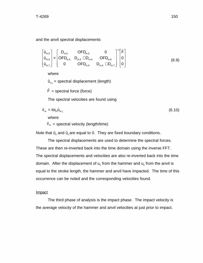
T-4269 150
and the anvil spectral displacements
$
$
$
$,
,
,
, ,
, , , ,
, , ,
u
u
u
D OFD
OFD D D OFD
OFD D D
Fm
m
m
m m
m m m m
m m m
5
6
7
5 5
5 5 6 6
6 6 7
10
0
0
0
L
N
MMM
O
Q
PPP
= ++
L
N
MMM
O
Q
PPP
L
N
MMM
O
Q
PPP
−
(6.9)
where
ûm,j = spectral displacement (length)
The spectral velocities are found using
$ $,v i um m m j= ω (6.10)
where
Note that û8 and û0 are equal to 0. They are fixed boundary conditions.
The spectral displacements are used to determine the spectral forces.
These are then re-inverted back into the time domain using the inverse FFT.
The spectral displacements and velocities are also re-inverted back into the time
domain. After the displacement of u5 from the hammer and u5 from the anvil is
equal to the stroke length, the hammer and anvil have impacted. The time of this
occurrence can be noted and the corresponding velocities found.
Impact
The third phase of analysis is the impact phase. The impact velocity is
the average velocity of the hammer and anvil velocities at just prior to impact.
$F = spectral force (force)
$vm = spectral velocity (length/time)
T-4269 151
The velocities of the hammer and anvil must be equal during the impact or other-
wise, there would not be any contact at the impact junction. The velocity after
the impact is calculated using an equation from Donnell in 1930
VV V
IHB AB=
+2
(6.11)
V V VHA HB I= − (6.12)
V V VAA I AB= − (6.13)
where
VHB = hammer velocity prior to impact (length/time)
VAB = anvil velocity prior to impact (length/time)
VI = impact velocity (length/time)
VHA = hammer velocity after impact (length/time)
VAA = anvil velocity after impact (length/time)
The force, according to the same source (Donnell, 1930) is
F VA EI I H H H= ρ (6.14)
where
AH = hammer cross-sectional area (length2)
ρH = hammer density (mass/length3)
EH = hammer modulus of elasticity (force/length2)
FI = impact force (force)
An implicit assumption with the use of equation 6.14 is that the anvil has
identical geometric and material properties.
T-4269 152
The duration of time that the force is in effect is assumed to be the time it
takes a wave to make a round trip through the element on either side of the jar.
The duration of the impact and the impact wave will be determined by which of
the two waves returns to the junction first. After the wave returns to the impact
junction, the force will drop to the pre-stretch conditions.
The wave for the final phase will be a square wave with an amplitude of
the impact force.
Post-Impact
The post-impact phase also uses the spectral analysis procedure. It is
almost identical to the free contraction phase. The inputs are the same except
impact force and its duration replaces trigger force and its duration. The re-
inverting of the forces, displacements, and velocities are the same as in the free
contraction phase.
T-4269 153
CHAPTER 7
JARRING ANALYSIS CASES
This chapter presents cases of jarring under various conditions. Cases
include the use of drill collars and drill pipe with and without heavy weight drill
pipe and with and without an accelerator. Finally, a comparison of the fre-
quency-domain model with a time-domain finite element model demonstrates the
superior results of the spectral analysis method derived in this dissertation.
Mathcad
The jarring models shown in this chapter were constructed using Mathcad
6.0 Plus. This is a powerful mathematical programming tool. The program
allows the user to input equations in typical handwritten mathematical style.
Using the equations input by the user, calculations are made. The results can
then be plotted. One example of the Mathcad documents used for this analysis
can be found in Appendix A.
The procedure has been split into two different Mathcad documents. The
first phase of the jarring procedure, pre-stretch, has its own document. Since in
every case in this chapter, this section is practically the same, this was done to
simplify this part of the jarring calculations. The next three phases, free contrac-
tion, impact, and post-impact, are included in a single document. Future imple-
T-4269 154
mentations of these procedures will combine the documents into one stand-
alone program.
Jarring Examples
For the purpose of demonstrating the capability of this jarring model, five
typical jarring cases are presented. The drill string used in these models is
similar to the drill string used in the paper, Transient Dynamic Analysis of the
Drillstring Under Jarring Operations by the FEM (Kalsi, Wang, and Chandra
1987). The first case is a drill string consisting only of drill collars and drill pipe.
The second case adds an accelerator to the first case. The third case is a drill
string consisting of drill collars, heavy weight drill pipe, and drill pipe. The fourth
case adds an accelerator to the third case. The fifth case is the same as the
fourth case except the drill string is “fixed” at the top of the stuck element during
the free contraction phase. This corresponds to the conditions shown in the
Kalsi paper and will allow for a direct comparison.
In each case, the top of the stuck point is 150 feet below the jar with 450
feet of stuck drill collars below that point. There is a 10 foot connecting element
at the bottom of the drill string.
The sticking is accomplished by setting a very high damping coefficient
over the stuck drill collar element (between node 6 and 7). The sticking type, as
defined in Chapter 1, has a strong bearing upon the nature of the stuck element.
For example, in the first four cases, the element is stuck over a long distance,
modeling pressure differential sticking. The fifth case shows the string stuck at a
point, thus modeling mechanical sticking.
T-4269 155
In all cases, the damping factors are 100 lbm per foot per second over
every element except in the stuck section and the connecting element. In the
stuck section (element 6), the damping factor is increased by a factor of fifty to
5,000 lbm per foot per second. The connecting element (7) has zero damping.
This model can be segmented into elements that correspond to different
parts of the hole (i.e., deviated sections and doglegs), rather than the typical
correspondence to changes in the drill string. Varying damping factors can then
input for the varying elements that correspond to the hole changes. This can
model the effects of deviated hole conditions.
The material properties are based solely on steel and are identical in
every element. The modulus of elasticity is 30,000,000 psi. The density is 490
lbm per cubic foot.
The jar stroke is 6.5 inches. The triggering force is set to 165,000 lbf.
The trigger is set to start 10 ms from the start of the jar analysis simulation. This
insures that the wave is self-windowing.
Case One: Drill Collars and Drill Pipe
In Case One, a drill string made up of only drill collars and drill pipe is
used. A diagram of this string is shown in Figure 7-1.
The first step is to calculate the static forces from the pre-stretch phase.
The is accomplished in the Mathcad document set forth in “Appendix A, Mathcad
Examples” under the heading “Pre-Stretch Phase.” The results, which are prac-
tically the same for every case (and therefore will not be shown for the next four
cases), are shown in Figure 7-2. The figure shows the static forces in pounds
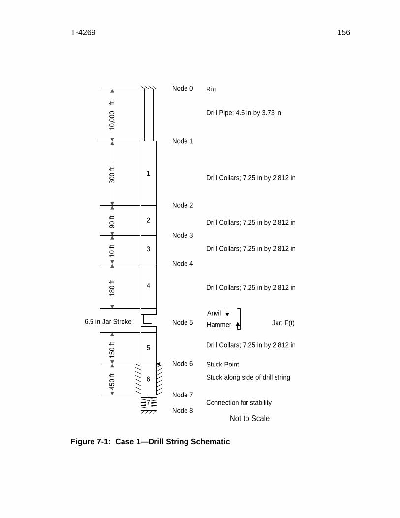
T-4269 156
Stuck along side of drill string
4
1
2
5
7
10,0
00 ft
300
ft90
ft10
ft18
0 ft
450
ft
6.5 in Jar Stroke
150
ft
Stuck Point
Drill Collars; 7.25 in by 2.812 in
Jar: F(t)
Drill Pipe; 4.5 in by 3.73 in
6
Node 3
Node 4
Node 2
Node 5
Node 6
Node 7
Node 8
Node 1
Node 0
Connection for stability
Not to Scale
0
Drill Collars; 7.25 in by 2.812 in
Drill Collars; 7.25 in by 2.812 in
Drill Collars; 7.25 in by 2.812 in
3 Drill Collars; 7.25 in by 2.812 in
Rig
Anvil
Hammer
Figure 7-1: Case 1—Drill String Schematic
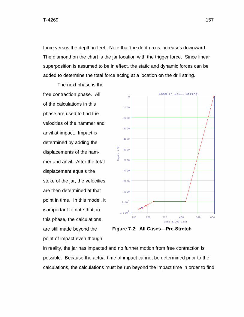
T-4269 157
force versus the depth in feet. Note that the depth axis increases downward.
The diamond on the chart is the jar location with the trigger force. Since linear
superposition is assumed to be in effect, the static and dynamic forces can be
added to determine the total force acting at a location on the drill string.
The next phase is the
free contraction phase. All
of the calculations in this
phase are used to find the
velocities of the hammer and
anvil at impact. Impact is
determined by adding the
displacements of the ham-
mer and anvil. After the total
displacement equals the
stoke of the jar, the velocities
are then determined at that
point in time. In this model, it
is important to note that, in
this phase, the calculations
are still made beyond the
point of impact even though,
in reality, the jar has impacted and no further motion from free contraction is
possible. Because the actual time of impact cannot be determined prior to the
calculations, the calculations must be run beyond the impact time in order to find
Figure 7-2: All Cases—Pre-Stretch
100 200 300 400 500 600
1.1 104
1 104
9000
8000
7000
6000
5000
4000
3000
2000
1000
0Load in Drill String
Load (1000 lbf)
De
pth
(ft)
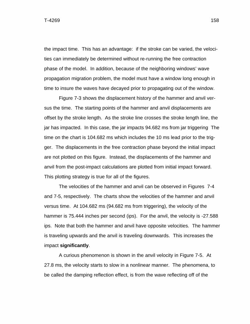
T-4269 158
the impact time. This has an advantage: if the stroke can be varied, the veloci-
ties can immediately be determined without re-running the free contraction
phase of the model. In addition, because of the neighboring windows’ wave
propagation migration problem, the model must have a window long enough in
time to insure the waves have decayed prior to propagating out of the window.
Figure 7-3 shows the displacement history of the hammer and anvil ver-
sus the time. The starting points of the hammer and anvil displacements are
offset by the stroke length. As the stroke line crosses the stroke length line, the
jar has impacted. In this case, the jar impacts 94.682 ms from jar triggering The
time on the chart is 104.682 ms which includes the 10 ms lead prior to the trig-
ger. The displacements in the free contraction phase beyond the initial impact
are not plotted on this figure. Instead, the displacements of the hammer and
anvil from the post-impact calculations are plotted from initial impact forward.
This plotting strategy is true for all of the figures.
The velocities of the hammer and anvil can be observed in Figures 7-4
and 7-5, respectively. The charts show the velocities of the hammer and anvil
versus time. At 104.682 ms (94.682 ms from triggering), the velocity of the
hammer is 75.444 inches per second (ips). For the anvil, the velocity is -27.588
ips. Note that both the hammer and anvil have opposite velocities. The hammer
is traveling upwards and the anvil is traveling downwards. This increases the
impact significantly .
A curious phenomenon is shown in the anvil velocity in Figure 7-5. At
27.8 ms, the velocity starts to slow in a nonlinear manner. The phenomena, to
be called the damping reflection effect, is from the wave reflecting off of the
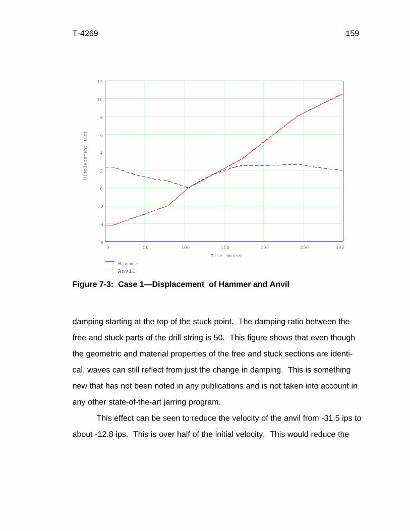
T-4269 159
damping starting at the top of the stuck point. The damping ratio between the
free and stuck parts of the drill string is 50. This figure shows that even though
the geometric and material properties of the free and stuck sections are identi-
cal, waves can still reflect from just the change in damping. This is something
new that has not been noted in any publications and is not taken into account in
any other state-of-the-art jarring program.
This effect can be seen to reduce the velocity of the anvil from -31.5 ips to
about -12.8 ips. This is over half of the initial velocity. This would reduce the
Figure 7-3: Case 1—Displacement of Hammer and Anvil
0 50 100 150 200 250 3006
4
2
0
2
4
6
8
10
12
HammerAnvil
Time (msec)
Dis
pla
cem
en
t (in
)
T-4269 160
0 50 100 150 200 250 30010
0
10
20
30
40
50
60
70
80
90
Hammer
Time (msec)
Ve
loci
ty (
inch
es
pe
r se
con
d)
Figure 7-4: Case 1—Hammer Velocity
Figure 7-5: Case 1—Anvil Velocity
0 50 100 150 200 250 30040
30
20
10
0
10
20
30
40
50
60
Anvil
Time (msec)
Velo
city
(in
ches
per
seco
nd)

T-4269 161
impact by about 38,497 lbf if impact occurred assuming the same hammer veloc-
ity. However, at 81.25 ms, a reflection of the initial free contraction wave off of
the connection element hits the anvil causing it to accelerate prior to impact.
In Figure 7-3, it can be seen from the displacement values that the anvil
oscillates. If the stroke or trigger force were such that the anvil was traveling
upwards at impact, the impact force would be far less. Assuming the same
velocity for the anvil to be upwards, the impact force would be 289,574 lbf (which
includes the static trigger force), a decrease of 143,627 lbf.
The next phase is the impact phase. The calculation of the impact force
is made. The impact force in this case is 433,201 lbf. A tension wave of this
impact force propagates outward through the hammer and anvil. This is shown
in Figure 7-6. Initially, the trigger force is applied. Then the jar is triggered,
freeing both the jar and anvil. Because the hammer and anvil are free ends, the
force should be zero. At impact, a 433,201 lbf square tension wave in the anvil
is generated. This is the force that will propagate to the stuck point. As noted in
Chapter 4, the spectral analysis procedure cannot generate the original wave. In
these cases, a wave shape and duration is assumed. This is shown in the figure
by the symmetric square waves about trigger force. The waves in the hammer
and anvil propagate outwards from the jar.
In this case, the displacements of the hammer and anvil, as shown in
Figure 7-3, show that the hammer and anvil travel together for the duration of the
impact. After that, the displacements indicate that the hammer continues to
travel upwards and the anvil continues to travel downwards. However, in reality,
the hammer and anvil are prevented from traveling past each other by the design
T-4269 162
of the jar. Because of this, the model is indicating a condition that cannot physi-
cally occur. The calculation values shown beyond the end of the impact at the
jar are suspect. Because of the finite wave propagation velocities, the calcula-
tions for the drill string (such as at the stuck point) remain valid up to the time
that a reflected wave could have propagated from the jar.
0 50 100 150 200 250 300200
100
0
100
200
300
400
500
HammerAnvil
Time (msec)
Fo
rce
(1
00
0 lb
f)
Figure 7-6: Case 1—Forces at the Jar
T-4269 163
The duration of the impact force is the time for the wave to make a round
trip from the nearest interface. For this case, it is the time it takes for the wave
to propagate up to the drill pipe/drill collar interface and reflect back to the im-
pact junction. This is the quickest round trip time. This time is 68.875 ms.
The final phase is the post-impact phase. This is another spectral analy-
sis procedure. Figure 7-7 shows the force at the top of the stuck point. Initially,
the top of the stuck point has a force on it equal to the trigger force minus the
weight of the drill string above it to the jar. The jar triggers at 10 ms. The wave
from the free contraction of the anvil hits the top of the stuck point 8.9 ms later.
Figure 7-7: Case 1—Forces at the Top of the Stuck Point
0 50 100 150 200 250 300100
0
100
200
300
400
500
Stuck Point
Time (msec)
Fo
rce
(1
00
0 lb
f)
T-4269 164
This force also shows the damping reflection effect noted in the anvil displace-
ment curve. At 72.3 ms, the reflection of the free contraction wave off of the
bottom of the drill string is seen. It is much smaller because of the significant
damping encountered in the stuck section. At 113.588 ms, the primary impact
wave is felt at the top of the stuck point. It hits a peak of 456,000 lbf at 131 ms
and ends at 182.457 ms. A reflection of the leading edge of this wave from
bouncing off of the bottom of the drill string is seen at 167.037 ms. The primary
impact wave is still traveling downwards, thus there is some wave interference
until 182.457 ms. After that point, the waves are false reflections from the free
anvil end. As noted earlier, in this case, since the hammer and anvil are locked
together, the waves should not have reflected but instead have traveled on
through the jar. Still, the primary impact wave is accurate.
Case Two: Drill Collars and Drill Pipe with an Accelerator
In Case Two, the same drill string as in the first case is used with the
addition of an accelerator 180 feet above the jar. As noted in Chapter 1, an
accelerator is used to intensify the impact forces. This is accomplished by
causing more reflections to reflect to the hammer during the free contraction
phase. A diagram of this string is shown in Figure 7-8.
The accelerator has a equivalent spring constant of 13,300 lbf per inch.
This is the equivalent of having a cross-sectional area, for a 10 foot length, of
0.0532 in2. This is in contrast to the cross-sectional area of the drill collars of
35.072 in2. Using equations 5.1 and 5.2 and setting the input force to 1 shows
that 0.3 percent of the force transmits through the accelerator and 99.7 percent
reflects off of the accelerator. It is doubtful that the wave would be felt at the
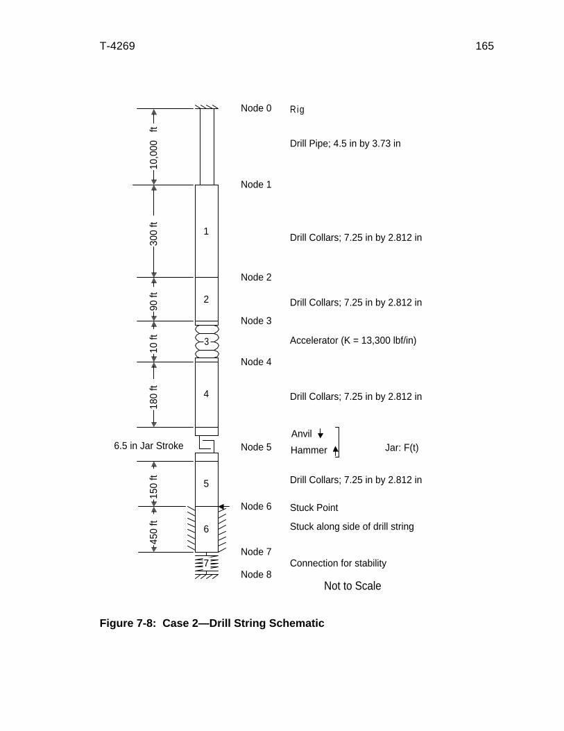
T-4269 165
Stuck along side of drill string
4
1
2
5
7
10,0
00 ft
300
ft90
ft10
ft18
0 ft
450
ft
6.5 in Jar Stroke
150
ft
Stuck Point
Drill Collars; 7.25 in by 2.812 in
Jar: F(t)
Drill Pipe; 4.5 in by 3.73 in
6
Node 3
Node 4
Node 2
Node 5
Node 6
Node 7
Node 8
Node 1
Node 0
Connection for stability
Not to Scale
0
Drill Collars; 7.25 in by 2.812 in
Drill Collars; 7.25 in by 2.812 in
Drill Collars; 7.25 in by 2.812 in
Accelerator (K = 13,300 lbf/in)
Rig
3
Anvil
Hammer
Figure 7-8: Case 2—Drill String Schematic
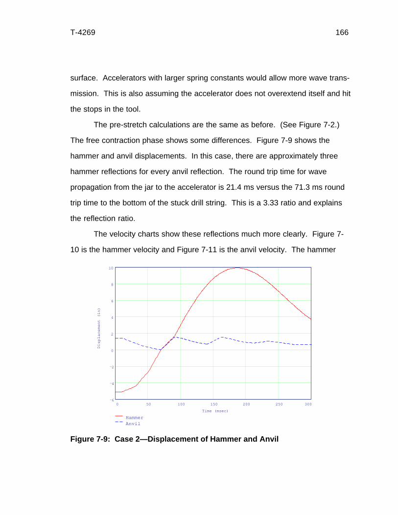
T-4269 166
surface. Accelerators with larger spring constants would allow more wave trans-
mission. This is also assuming the accelerator does not overextend itself and hit
the stops in the tool.
The pre-stretch calculations are the same as before. (See Figure 7-2.)
The free contraction phase shows some differences. Figure 7-9 shows the
hammer and anvil displacements. In this case, there are approximately three
hammer reflections for every anvil reflection. The round trip time for wave
propagation from the jar to the accelerator is 21.4 ms versus the 71.3 ms round
trip time to the bottom of the stuck drill string. This is a 3.33 ratio and explains
the reflection ratio.
The velocity charts show these reflections much more clearly. Figure 7-
10 is the hammer velocity and Figure 7-11 is the anvil velocity. The hammer
Figure 7-9: Case 2—Displacement of Hammer and Anvil
0 50 100 150 200 250 3006
4
2
0
2
4
6
8
10
HammerAnvil
Time (msec)
Dis
pla
cem
en
t (i
n)
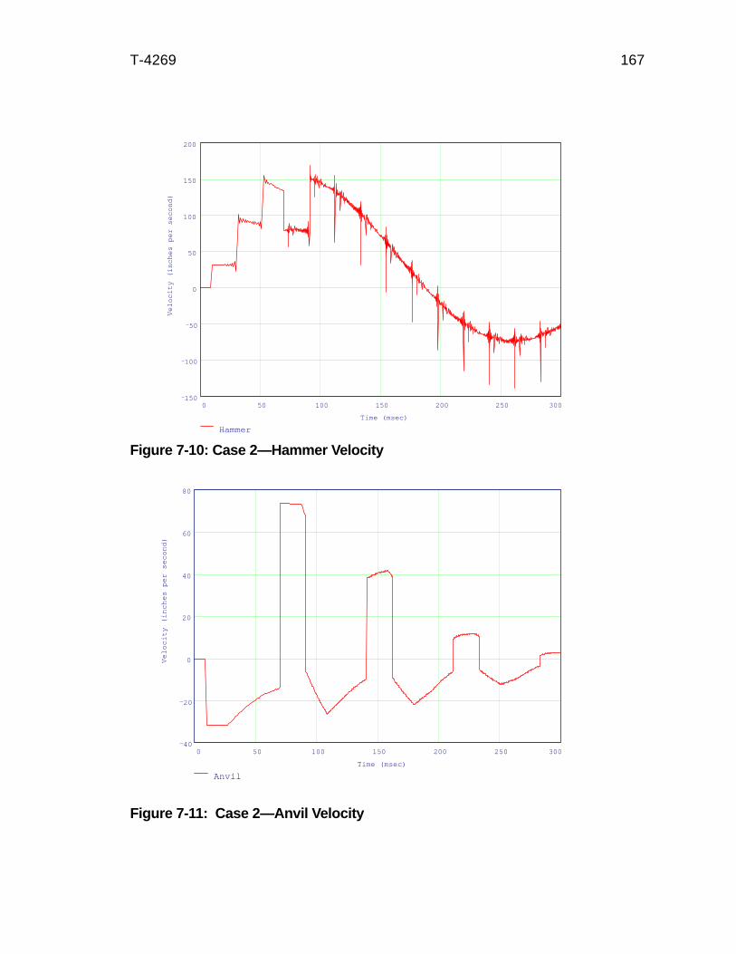
T-4269 167
Figure 7-11: Case 2—Anvil Velocity
0 50 100 150 200 250 30040
20
0
20
40
60
80
Anvil
Time (msec)
Ve
loci
ty (
inch
es
pe
r se
con
d)
Figure 7-10: Case 2—Hammer Velocity
0 50 100 150 200 250 300150
100
50
0
50
100
150
200
Hammer
Time (msec)
Ve
loci
ty (
inch
es
pe
r se
con
d)

T-4269 168
velocity shows the reflections from the accelerator rapidly increased the velocity
of the hammer prior to impact. The hammer impact velocity is 133.333 ips.
For the anvil, the time for a reflection off of the bottom of the drill string is
longer than the time until impact. Consequently, the anvil does not receive any
reflections prior to impact; therefore, the free contraction velocity of the anvil
does not increase over the initial value. The anvil velocity is -14.059 ips. The
free contraction velocity of the anvil is -31.6 ips. The damping reflection effect
has reduced the velocity of the anvil prior to impact by 17.541 ips. This is over
half of the free contraction speed. This effect has reduced the impact force by
45,659 lbf.
Since the hammer is moving faster, the impact time is sooner, occurring at
59.538 ms from trigger . (Actual time is 69.538 ms.) In Case One, impact oc-
curred at 94.682 ms, 35.144 ms later than this case. The jar also has a higher
impact force of 548,664 lbf as compared to the 433,201 lbf impact in the first
case. This is an increase in force over the first case by 27 percent.
The duration of the impact is much less, however. Because of the proxim-
ity of the accelerator, the primary impact wave bounces off of it and returns to
the jar first. Therefore, the wave is 21.375 ms long.
Examination of the displacement chart (Figure 7-9) shows that the ham-
mer “passes” by the anvil. Since this is physically impossible, the same caveats
concerning the forces beyond the primary impact apply to this case. The jar
forces are shown in Figure 7-12.
The primary impact force is 548,664 lbf and occurs at 69.538 ms and lasts
until 90.913 ms. However, as shown in Figure 7-13, the force at the top of the

T-4269 169
0 50 100 150 200 250 300300
200
100
0
100
200
300
400
500
600
HammerAnvil
Time (msec)
Fo
rce
(1
00
0 lb
f)
0 50 100 150 200 250 300100
0
100
200
300
400
500
600
700
Stuck Point
Time (msec)
Forc
e (
1000 lb
f)
Figure 7-12: Case 2—Forces at the Jar
Figure 7-13: Case 2—Forces at the Top of the Stuck Point

T-4269 170
stuck point increase to a value of 591,000 lbf. This is also the damping reflec-
tion effect. Some of the wave is reflecting back a little at a time, adding its small
value to the overall force. Although it is not as prevalent in this figure as it was
in Figure 7-7, the primary impact force shows a decrease after 17.8 ms. This is
the round trip time from the top of the stuck point to the jar. The waves from the
damping reflection effect are reflecting off of the jar thus decreasing the primary
impact force. The ramp from 99.819 ms to 117.632 ms is caused by waves from
the damping reflection effect continuing beyond the primary impact. The other
waves are the reflections of the primary wave between the anvil and the bottom
of the drill string.
Case Three: Drill Collars, Heavy Weight Drill Pipe, and Drill Pipe
In Case Three, 300 feet of heavy weight drill pipe is added between the
drill pipe and drill collars cited in Case One. The heavy weight drill pipe re-
places 300 feet of the drill collars. A diagram of this string is shown in Figure 7-
14.
In this case, instead of an accelerator, the heavy weight drill pipe acts to
partially accelerate the hammer. The heavy weight drill pipe is further away from the
jar, therefore the round trip time is longer; and, the heavy weight drill pipe has a
much larger cross-sectional area than the equivalent cross-sectional area of the
accelerator. More of the wave passes through the drill collar/heavy weight drill pipe
interface than did the wave through the accelerator.
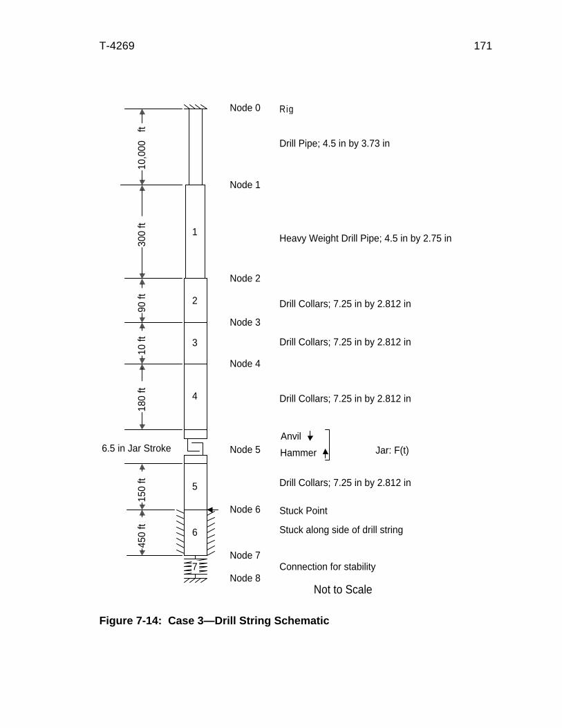
T-4269 171
Figure 7-14: Case 3—Drill String Schematic
Stuck along side of drill string
4
1
2
5
7
10,0
00 ft
300
ft90
ft10
ft18
0 ft
450
ft
6.5 in Jar Stroke
150
ft
Stuck Point
Drill Collars; 7.25 in by 2.812 in
Jar: F(t)
Drill Pipe; 4.5 in by 3.73 in
6
Node 3
Node 4
Node 2
Node 5
Node 6
Node 7
Node 8
Node 1
Node 0
Connection for stability
Not to Scale
0
Drill Collars; 7.25 in by 2.812 in
Drill Collars; 7.25 in by 2.812 in
Heavy Weight Drill Pipe; 4.5 in by 2.75 in
3 Drill Collars; 7.25 in by 2.812 in
Rig
Anvil
Hammer

T-4269 172
Using equations 5.1 and 5.2, about 44.3 percent of the incident wave is
transmitted and 55.7 percent of the wave is reflected. Consequently, some of the
wave bounces off of the heavy weight drill pipe/drill pipe interface. About 66.6
percent of the remaining wave is transmitted and 33.4 percent of the remaining wave
is reflected. This reflected wave encounters the drill collar/heavy weight drill pipe
and undergoes a transmission ratio of 155.7 percent (because the wave is going
from a smaller to a larger cross-sectional area). Multiplying all of the wave transmis-
sion percentages gives a value of 23 percent of the primary incident wave. This is a
significant value and will cause some additional acceleration of the hammer. These
extra wave reflections are modeled in this program; they have not been modelled in
other state-of-the-art jarring programs.
The hammer and anvil displacements are shown in Figure 7-15. Once again,
as in all these cases, the hammer is shown traveling past the anvil.
The hammer velocity is shown in Figure 7-16. There are four reflections prior
to impact. The first two are at 31.694 ips and 67.032 ips. The third reflection barely
appears. It is the small mark at 86.732 ips on the side of the fourth reflection. The
first three reflections are from the drill collar/heavy weight drill pipe interface. The
fourth reflection is from the heavy weight drill pipe/drill pipe nterface and is 97.715
ips. This additional reflection adds 10.983 ips. This increases the impact force by
23,665 lbf.
The anvil velocity is shown in Figure 7-17. It shows the same damping
reflection effect (decrease in the velocity) as in the first and second cases.
The impact force is 496,676 lbf. The duration of the impact is the round
trip time from the drill collar/heavy weight drill pipe interface. This is 33.25 ms.
Figure 7-18 shows the forces at the jar.
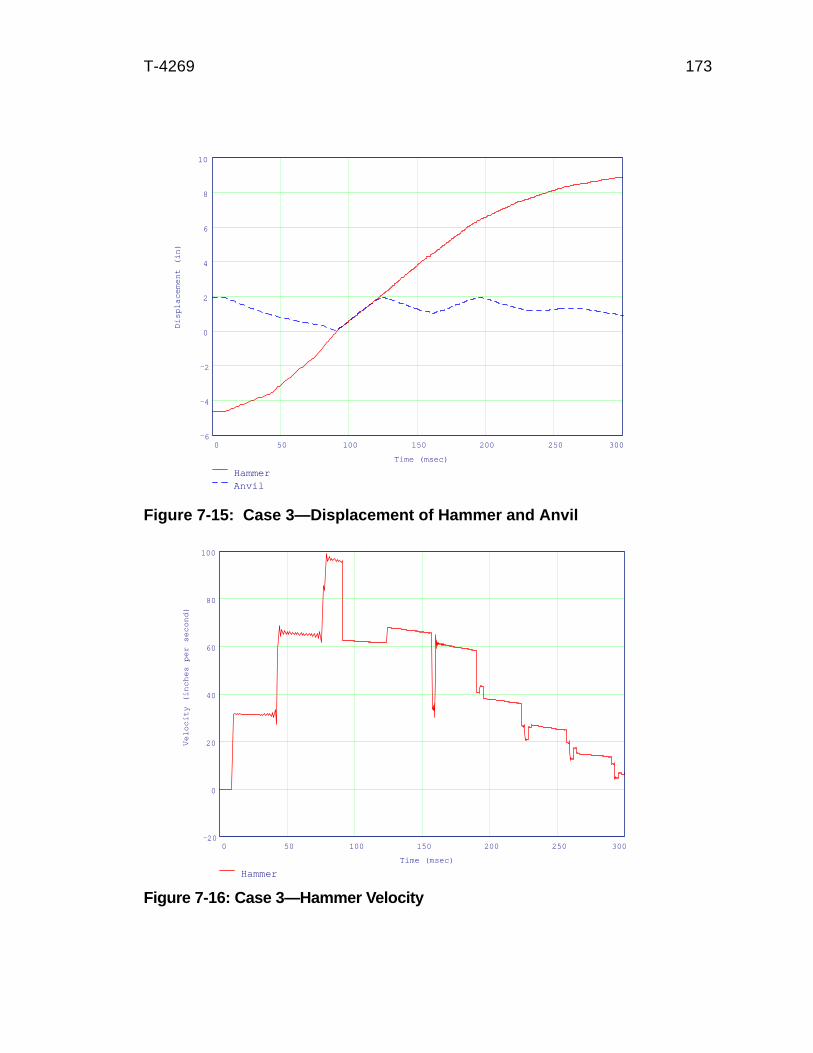
T-4269 173
Figure 7-16: Case 3—Hammer Velocity
0 50 100 150 200 250 30020
0
20
40
60
80
100
Hammer
Time (msec)
Ve
loci
ty (
inch
es
pe
r se
con
d)
0 50 100 150 200 250 3006
4
2
0
2
4
6
8
10
HammerAnvil
Time (msec)
Dis
pla
cem
ent (in)
Figure 7-15: Case 3—Displacement of Hammer and Anvil

T-4269 174
The force at the top of the stuck point is shown in Figure 7-19. The force
is 496,676 lbf at 100.51 ms. It climbs to 528,000 lbf by 118.32 ms because of
the damping reflection effect. The force starts falling after this because of reflec-
tions off of the anvil. The primary impact wave is complete at 133.76 ms.
Case Four: Drill Collars, Heavy Weight Drill Pipe, Drill Pipe, and an Accelerator
Case Four is the same as Case Three except that an accelerator is added
180 feet above the jar. The drill string schematic is shown in Figure 7-20.
Case Four is also similar to the second case. Because of the closeness
of the accelerator to the jar, the waves bounce off the accelerator first. Also,
since only 0.3 percent of the wave transmits through the accelerator, any reflec-
0 50 100 150 200 250 30040
20
0
20
40
60
80
Anvil
Time (msec)
Velo
city
(in
ches
per
seco
nd)
Figure 7-17: Case 3—Anvil Velocity
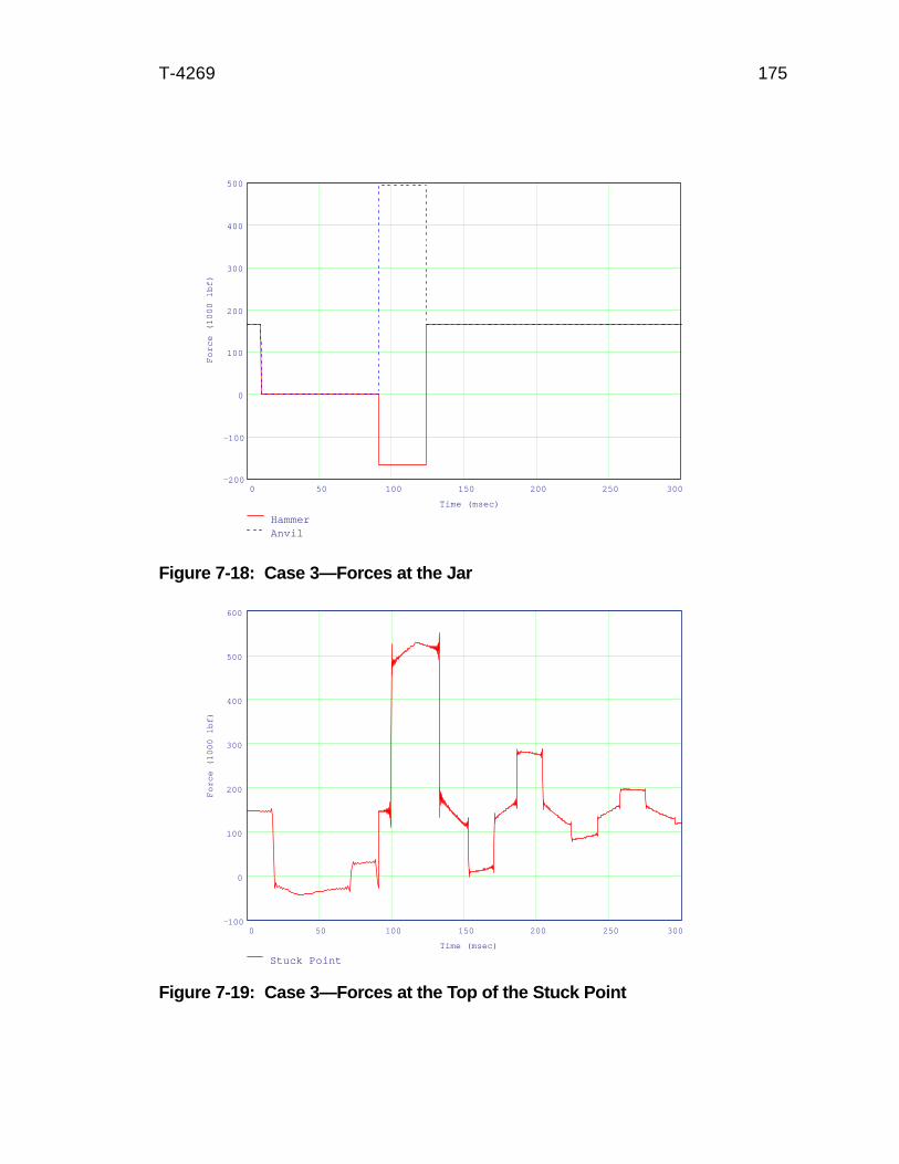
T-4269 175
Figure 7-18: Case 3—Forces at the Jar
Figure 7-19: Case 3—Forces at the Top of the Stuck Point
0 50 100 150 200 250 300100
0
100
200
300
400
500
600
Stuck Point
Time (msec)
Fo
rce
(1
00
0 lb
f)
0 50 100 150 200 250 300200
100
0
100
200
300
400
500
HammerAnvil
Time (msec)
Fo
rce
(1
00
0 lb
f)
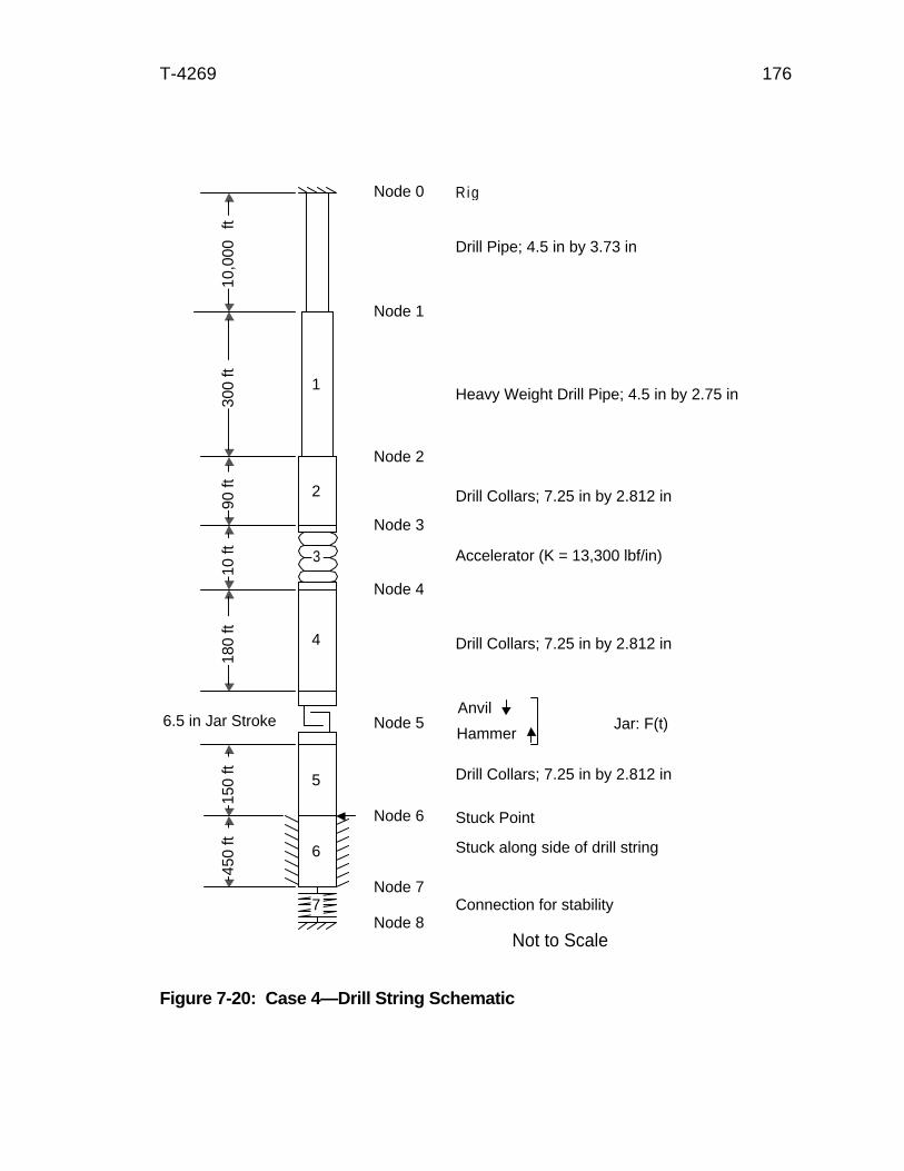
T-4269 176
Stuck along side of drill string
4
1
2
5
7
10,0
00 ft
300
ft90
ft10
ft18
0 ft
450
ft
6.5 in Jar Stroke
150
ft
Stuck Point
Drill Collars; 7.25 in by 2.812 in
Jar: F(t)
Drill Pipe; 4.5 in by 3.73 in
6
Node 3
Node 4
Node 2
Node 5
Node 6
Node 7
Node 8
Node 1
Node 0
Connection for stability
Not to Scale
0
Drill Collars; 7.25 in by 2.812 in
Drill Collars; 7.25 in by 2.812 in
Heavy Weight Drill Pipe; 4.5 in by 2.75 in
Accelerator (K = 13,300 lbf/in)
Rig
3
Anvil
Hammer
Figure 7-20: Case 4—Drill String Schematic
T-4269 177
tions from the drill collar/heavy weight drill pipe or heavy weight drill pipe/drill
pipe interface are minuscule. The accelerator dominates the wave propagation
characteristics.
This can be seen by comparing the displacements of the hammer and
anvil in the second case (Figure 7-9) to the displacements of the hammer and
anvil in this case (Figure 7-21). The two charts can practically be overlain.
This is true for the hammer velocities (Figure 7-22) and the anvil veloci-
ties (Figure 7-23). As seen in Figure 7-24, the jar forces are also equal (since
the velocities are equal). In addition, because the anvil side of the drill string
was not changed in any manner, the top of the stuck point forces are identical as
seen in Figure 7-25.
This case shows that even though the drill strings are different, one can
get the same wave propagation response with the proper tools. An accelerator
“disconnects” whatever is above it from whatever is below it (as long as it does
not hit the stops). It does not matter what is above the accelerator, whether it be
multiple drill string geometries, a dogleg, or another jar. The accelerator isolates
the drill string below it.
Case Five: Drill Collars, Heavy Weight Drill Pipe, Drill Pipe, and an Accelerator
with a Rigid Stuck Point
Case Five is a direct comparison to the drill string response as seen in
the Transient Dynamic Analysis of the Drillstring Under Jarring Operations by the
FEM paper (Kalsi, Wang, and Chandra 1987). This paper shows the analysis of
a jarring wave propagation problem using a time based finite element program.
See Chapter 2 for a discussion of this paper.

T-4269 178
Figure 7-21: Case 4—Displacement of Hammer and Anvil
Figure 7-22: Case 4—Hammer Velocity
0 50 100 150 200 250 3006
4
2
0
2
4
6
8
10
HammerAnvil
Time (msec)
Dis
pla
cem
en
t (in
)
0 50 100 150 200 250 300150
100
50
0
50
100
150
200
Hammer
Time (msec)
Ve
loci
ty (
inch
es
pe
r se
con
d)
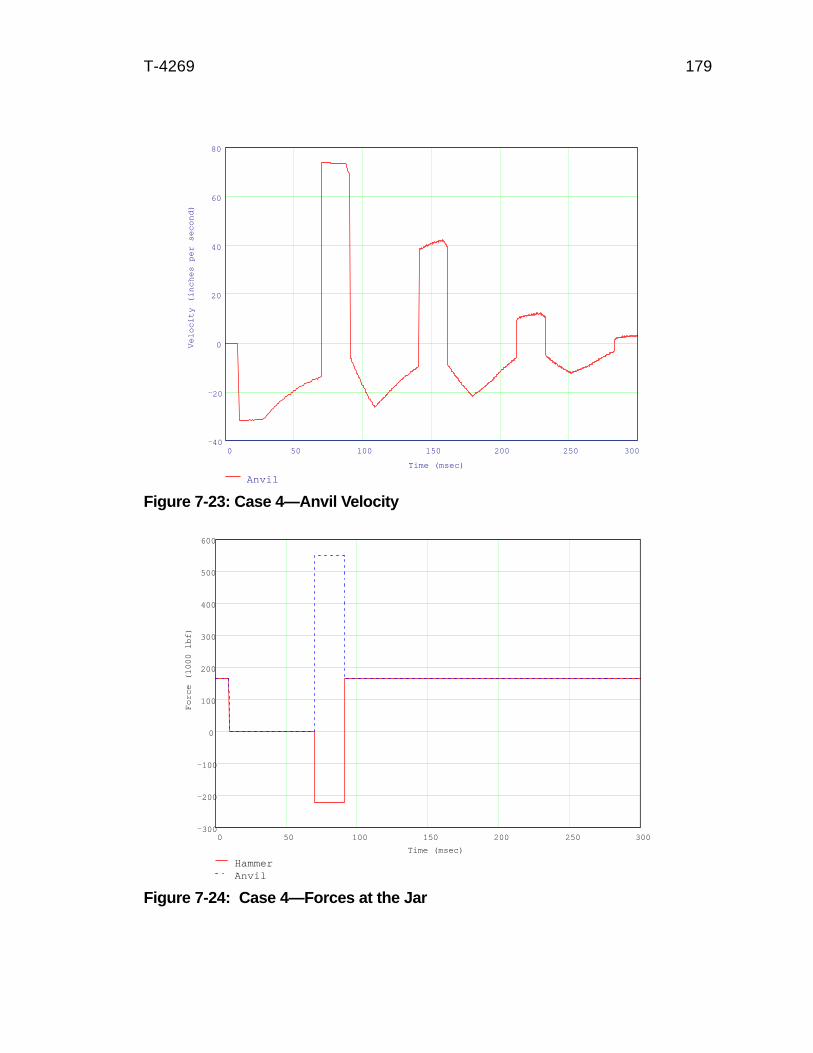
T-4269 179
0 50 100 150 200 250 30040
20
0
20
40
60
80
Anvil
Time (msec)
Ve
loci
ty (
inch
es
pe
r se
con
d)
Figure 7-23: Case 4—Anvil Velocity
Figure 7-24: Case 4—Forces at the Jar
0 50 100 150 200 250 300300
200
100
0
100
200
300
400
500
600
HammerAnvil
Time (msec)
Forc
e (
1000 lb
f)
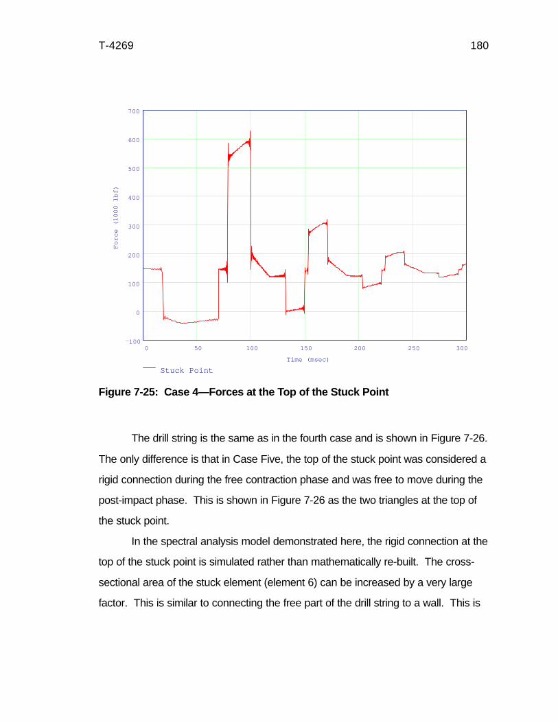
T-4269 180
The drill string is the same as in the fourth case and is shown in Figure 7-26.
The only difference is that in Case Five, the top of the stuck point was considered a
rigid connection during the free contraction phase and was free to move during the
post-impact phase. This is shown in Figure 7-26 as the two triangles at the top of
the stuck point.
In the spectral analysis model demonstrated here, the rigid connection at the
top of the stuck point is simulated rather than mathematically re-built. The cross-
sectional area of the stuck element (element 6) can be increased by a very large
factor. This is similar to connecting the free part of the drill string to a wall. This is
0 50 100 150 200 250 300100
0
100
200
300
400
500
600
700
Stuck Point
Time (msec)
Fo
rce
(1
00
0 lb
f)
Figure 7-25: Case 4—Forces at the Top of the Stuck Point

T-4269 181
Stuck at top of element 6 during freecontraction phaseStuck along side during post-impact phase
4
1
2
5
7
10,0
00 ft
300
ft90
ft10
ft18
0 ft
450
ft
6.5 in Jar Stroke
150
ft
Stuck Point
Drill Collars; 7.25 in by 2.812 in
Jar: F(t)
Drill Pipe; 4.5 in by 3.73 in
6
Node 3
Node 4
Node 2
Node 5
Node 6
Node 7
Node 8
Node 1
Node 0
Anvil
Hammer
Connection for stability
Not to Scale
0
Drill Collars; 7.25 in by 2.812 in
Drill Collars; 7.25 in by 2.812 in
Heavy Weight Drill Pipe; 4.5 in by 2.75 in
Accelerator (K = 13,300 lbf/in)
Rig
3
Figure 7-26: Case 5—Drill String Schematic
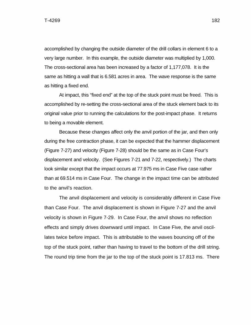
T-4269 182
accomplished by changing the outside diameter of the drill collars in element 6 to a
very large number. In this example, the outside diameter was multiplied by 1,000.
The cross-sectional area has been increased by a factor of 1,177,078. It is the
same as hitting a wall that is 6.581 acres in area. The wave response is the same
as hitting a fixed end.
At impact, this “fixed end” at the top of the stuck point must be freed. This is
accomplished by re-setting the cross-sectional area of the stuck element back to its
original value prior to running the calculations for the post-impact phase. It returns
to being a movable element.
Because these changes affect only the anvil portion of the jar, and then only
during the free contraction phase, it can be expected that the hammer displacement
(Figure 7-27) and velocity (Figure 7-28) should be the same as in Case Four’s
displacement and velocity. (See Figures 7-21 and 7-22, respectively.) The charts
look similar except that the impact occurs at 77.975 ms in Case Five case rather
than at 69.514 ms in Case Four. The change in the impact time can be attributed
to the anvil’s reaction.
The anvil displacement and velocity is considerably different in Case Five
than Case Four. The anvil displacement is shown in Figure 7-27 and the anvil
velocity is shown in Figure 7-29. In Case Four, the anvil shows no reflection
effects and simply drives downward until impact. In Case Five, the anvil oscil-
lates twice before impact. This is attributable to the waves bouncing off of the
top of the stuck point, rather than having to travel to the bottom of the drill string.
The round trip time from the jar to the top of the stuck point is 17.813 ms. There

T-4269 183
0 50 100 150 200 250 300100
50
0
50
100
150
200
250
Hammer
Time (msec)
Ve
loci
ty (
inch
es
pe
r se
con
d)
Figure 7-28: Case 5—Hammer Velocity
Figure 7-27: Case 5—Displacement of Hammer and Anvil
0 50 100 150 200 250 3008
6
4
2
0
2
4
6
8
10
12
HammerAnvil
Time (msec)
Dis
pla
cem
ent (in)
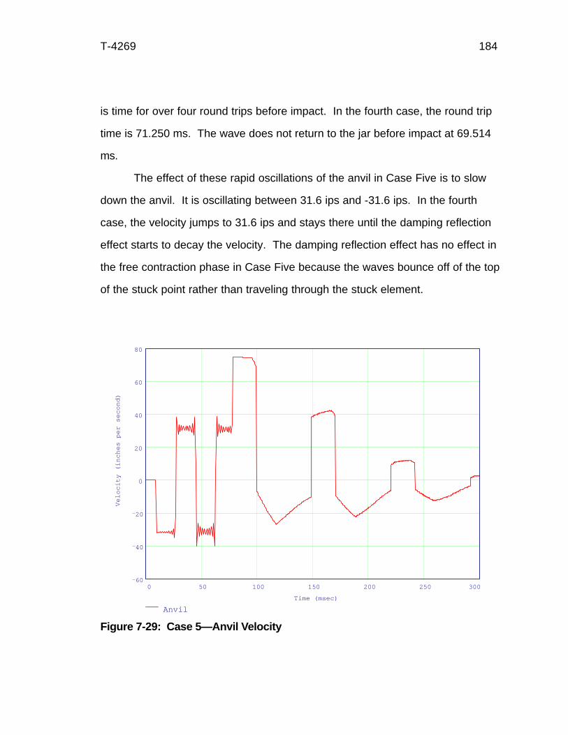
T-4269 184
is time for over four round trips before impact. In the fourth case, the round trip
time is 71.250 ms. The wave does not return to the jar before impact at 69.514
ms.
The effect of these rapid oscillations of the anvil in Case Five is to slow
down the anvil. It is oscillating between 31.6 ips and -31.6 ips. In the fourth
case, the velocity jumps to 31.6 ips and stays there until the damping reflection
effect starts to decay the velocity. The damping reflection effect has no effect in
the free contraction phase in Case Five because the waves bounce off of the top
of the stuck point rather than traveling through the stuck element.
0 50 100 150 200 250 30060
40
20
0
20
40
60
80
Anvil
Time (msec)
Ve
loci
ty (
inch
es
pe
r se
con
d)
Figure 7-29: Case 5—Anvil Velocity

T-4269 185
This oscillation can mean that the anvil is “caught” traveling upwards at
impact. That occurs in this case. The anvil velocity is 33.529 ips upwards as
opposed to -14.073 ips downwards in the fourth case, a difference of 47.602 ips.
However, because the impact required a longer free contraction time, the ham-
mer had time to accelerate to a higher velocity. Its velocity at impact is 183.176
ips as opposed to 133.763 ips in the fourth case, a difference of 49.413 ips.
Since the impact force is related to the difference in velocities, the anvil’s lost
velocity is made up by the hammer’s gain in velocity. This is a coincidence! It
does not always happen this way.
The impact force is 554,531 lbf in Case Five versus 549,820 lbf in Case
Four. This is not a significant difference. In fact, from the impact time onwards,
there is no difference in the primary impact waves in the jar as shown in Figure
7-30 or at the top of the stuck point as shown in Figure 7-31 except for the 4,711
lbf difference and the different impact time. The duration of the impact pulse is
still determined by the round trip time from the jar to the accelerator and is
21.375 ms. If the top of the stuck point was still regarded as a fixed end, then it
would determine the impact pulse duration as it is closer to the jar. Because it
was changed back to a regular drill collar, the round trip time would be the time
for the wave to travel from the jar to the bottom of the drill string.
The charts of the displacements, velocities and forces shown in the Kalsi
paper compare favorably to the spectral analysis method figures of the sam
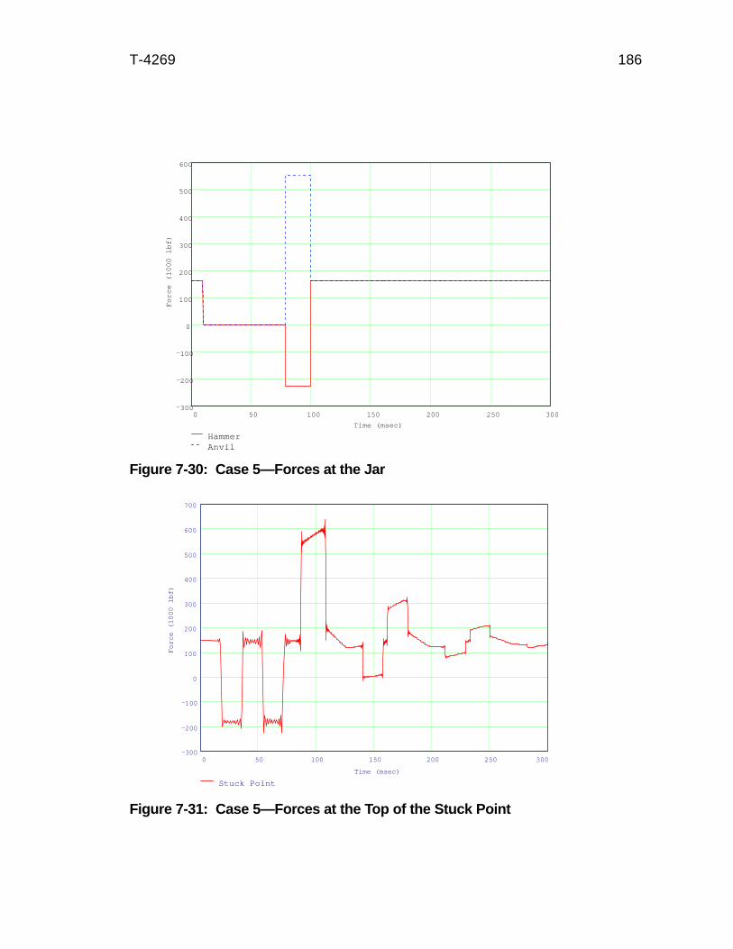
T-4269 186
0 50 100 150 200 250 300300
200
100
0
100
200
300
400
500
600
700
Stuck Point
Time (msec)
Forc
e (
1000 lb
f)
Figure 7-31: Case 5—Forces at the Top of the Stuck Point
Figure 7-30: Case 5—Forces at the Jar
0 50 100 150 200 250 300300
200
100
0
100
200
300
400
500
600
HammerAnvil
Time (msec)
Fo
rce
(1
00
0 lb
f)
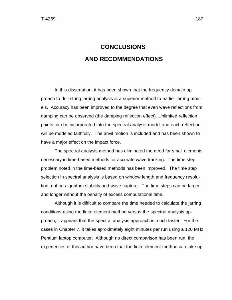
T-4269 187
CONCLUSIONS
AND RECOMMENDATIONS
In this dissertation, it has been shown that the frequency domain ap-
proach to drill string jarring analysis is a superior method to earlier jarring mod-
els. Accuracy has been improved to the degree that even wave reflections from
damping can be observed (the damping reflection effect). Unlimited reflection
points can be incorporated into the spectral analysis model and each reflection
will be modeled faithfully. The anvil motion is included and has been shown to
have a major effect on the impact force.
The spectral analysis method has eliminated the need for small elements
necessary in time-based methods for accurate wave tracking. The time step
problem noted in the time-based methods has been improved. The time step
selection in spectral analysis is based on window length and frequency resolu-
tion, not on algorithm stability and wave capture. The time steps can be larger
and longer without the penalty of excess computational time.
Although it is difficult to compare the time needed to calculate the jarring
conditions using the finite element method versus the spectral analysis ap-
proach, it appears that the spectral analysis approach is much faster. For the
cases in Chapter 7, it takes aproximately eight minutes per run using a 120 MHz
Pentium laptop computer. Although no direct comparison has been run, the
experiences of this author have been that the finite element method can take up

T-4269 188
to half an hour or more. Some of the papers reviewed in Chapter 2 allude to the
time of FEM analysis, too. These Mathcad documents are by no means opti-
mized for speed. A future stand-alone program optimized for speed and accu-
racy could improve the time requirements of spectral analysis significantly.
The spectral analysis method is easier to use than the finite element
method. The ANSYS finite element program, while a very powerful engineering
application, can be intimidating. The spectral analysis method also can be
adapted for a driller to use in the field.
This model is not a panacea for all the jarring analysis problems. For
example, waves cannot be generated; they can only be propagated, transmitted,
and reflected. Other methods are needed to generate the actual impact wave.
However, one advantage of the spectral analysis method is that any wave form
can be used. If actual wave forms from jarring operations can be recorded,
these wave forms can be used as the input. This adds a higher level of realism
to this model not found in any other model.
Currently, nonlinear effects such as Coulomb damping cannot be incorpo-
rated. This is the subject of future research.
Other Areas of Research
The spectral analysis procedure is not limited to jarring problems. Any
transient vibration problem can be analyzed using this technique. Problems
such as bit catching (called slip-stick) and bit bounce can be analyzed. Shock
T-4269 189
loading from hitting ledges or dropping tools can be determined. Even thermal
shocks can be modeled, albeit with thermal spectral equations rather than the
motion equations used in this dissertation.
Vibration Analysis
Using the stiffness matrix, the resonant frequencies of a system can be
determined. For example, in the API standards (RP 7-G), a very simplistic ap-
proach was taken for the determination of the critical rotary speeds, where rough
drilling occurs because of resonance. Basically, the API threw up their hands
and said this is too complex to calculate. However, the spectral analysis proce-
dure can be applied to find the critical rotary speeds for very complex drill
strings. The model can be built and then run through a series of frequencies
with a unit amplitude. The frequencies with the largest amplitude response are
the resonant frequencies. The relative amplitudes give an indication of the
severity of the vibration.
Impact Study
The spectral analysis procedure can be used for reverse transient wave
propagation problems. For example, the Baker Hughes Inteq ADAMS system
measures vibrations at the kelly on a drilling rig. It is theoretically possible to
take the vibrations measured at that point and back propagate the waves to
determine their origin. It might also be possible, given full knowledge of the drill
string and bit vibration behavior, to determine the lithology of the formations
being drilled by back propagating the vibrations measured at the surface.

T-4269 190
More Work to Do
There is considerable research that can be done based upon the work
presented in this dissertation. The areas that need the most research are jarring
impact and damping. Today’s knowledge is not strong in these areas. The
output of this model is sensitive to the impact magnitude and duration and to the
amount of damping. The model is excellent for determining the impact forces
anywhere on the string; but, its accuracy is only as good as the data input. A
better understanding of impact and damping areas is the first area of continued
research.
Jarring Impact
The reverse transient wave propagation technique would be very valuable
for jar impact analysis in a laboratory. Currently, the jar impact wave is assumed
to be similar to the Hopkinson bar experiments. But jars have a considerably
more complex internal arrangement than a simple bar. How does an off-center,
nonparallel hammer and anvil impact? What bending and torsional waves arise
from such an event? How much of an impact wave actually damps out before
leaving the jar?
These are questions that can be answered using the reverse transient
wave propagation techniques. A jar could be instrumented with strain gages and
accelerometers. Then the jar could be triggered and impacted. Using a spectral
analysis structure of the jar mechanisms, the waves measured by the instru-
ments could be back propagated to the source, the hammer and anvil faces.
This could help find energy losses within the jar. It would also help improve the
T-4269 191
efficiency of the jar for getting energy out to the drill string. Finally, it would give
real data to input into the model in this dissertation rather than the assumed
rectangular shape impact pulse.
Coulomb Damping
In Chapter 4, the nature of Coulomb damping was discussed. One of the
problems of the spectral analysis method is its inability to incorporate nonlinear
effects. Once in the frequency domain, it is difficult to determine the occurrence
of time-based events that are determined by the condition of the model. For
example, there was no method available to “turn off the jarring model” after the
stroke length was reached. Since this is unknown prior to running the model, it
is unknown where to stop the model until after the model has completely run its
course. It cannot be stopped in the middle of a run.
This limitation might be mitigated by using what this author calls a flying
FFT approach. While analyzing vibrations using a spectrum analyzer, such as
the ADAMS system, the instrument collects data in packets. It then runs an FFT
on the data it just gathered. If the FFT computational time is less than the time
used to collect the data, then the system can continue to show the frequency
spectrum in real time. It is taking an FFT of the data “on the fly”.
The flying FFT approach could possibly be used in reverse. The proce-
dure would be to analyze a time domain situation in the frequency domain and
determine the FFT response. Then, back in the time domain, that FFT response
would be used to modify the conditions for the next block of time in the next FFT
analysis. This technique would run repeatedly at a very high speed, maybe at
100,000 Hertz, using small time jumps. This would have the advantage of an

T-4269 192
unlimited time span with the ease of structure assembly found in spectral analy-
sis. It would allow for the incorporation of vibrations and transient analysis in the
same model. The difficulty will be overcoming the wave migration problem.
Some of the other frequency analysis problems could limit this technique as well.
But this author believes this is worth pursuing.
Torsional Waves
Using the torsional equations of motion for waves, torsional waves can be
added to the stiffness matrix. This would allow for the study of the bit slip-stick
phenomenon and its effect on a drill string.
Lateral Waves
Although far more complex, the bending equations of motion also can be
incorporated into the stiffness matrix. The effect of bending waves can be in-
cluded by incorporating the same techniques used to derive the stiffness matrix
for axial motion in this dissertation. Adding the bending wave to the axial and
torsional wave stiffness matrix will make this a full three-dimensional model. In
addition, based on discussions with others in this field, there may be a connec-
tion between lateral frequencies and buckling.
Tool Joints
Tool joints in the drill pipe and heavy weight drill pipe have an effect on
the wave propagation characteristics. Most of the time, this effect is thought to
be small; however, given the right frequency, the joints occasionally become
T-4269 193
excited through resonance. The taper of the tool joints can also change the
transmission and reflection characteristics of wave propagation through a tool
joint. This can be modeled with a tapered spectral element.
Stabilizers
Stabilizers and other bottom hole assembly tools do not have the same
geometries and material properties as drill collars. This will have some effect on
the wave propagation characteristics of the drill string. The magnitude of this
effect is unknown.
A stabilizer could be assembled into a spectral analysis sub-structure. A
sub-structure is a complicated structure that uses simpler models as building
blocks. These building blocks are assembled into a single stiffness matrix
model. This single stiffness matrix model, the sub-structure, can then be incor-
porated into an even more complex structure wherever needed.
Curved Boreholes
In the model presented in this dissertation, only straight holes were con-
sidered. Curved boreholes are important in today’s drilling. However, in wave
propagation, curved drill strings lead to coupled axial and bending waves. An
axial wave can cause a bending wave to self-generate; a bending wave can
cause an axial wave to self-generate. These effects are very complex. How-
ever, the frequency domain approach may make the solution to these problems
more easily accomplished. A curved borehole element could be assembled and
added to the existing straight hole elements’ library and used wherever needed.

T-4269 194
REFERENCES CITED
Aarrestad, Thor V., and Åge Kyllingstad. 1994. Loads on drillpipe during jarring
operations. SPE Drilling and Completion (December): 271-275. Origi-
nally presented at 1992 European Petroleum Conference at Cannes,
France.
Achenbach, J.D. 1993. Wave propagation in elastic solids. 7th ed. Amsterdam,
The Netherlands: Elsevier Science Publishers B.V.
Anderson, L.B., and P. Lembourn. 1994. Analysis of interruption and lost rig
time due to equipment failure in offshore drilling operations. IADC/SPE
27511 paper presented at 1994 IADC/SPE Drilling Conference, 15-18
February, at Dallas, Texas.
ANSYS, Inc. 1992. ANSYS theoretical reference manual. Houston, Pennsylva-
nia: ANSYS, Inc.
Askew, W.E. 1986. Computerized drilling jar placement. IADC/SPE 14746 pa-
per presented at 1986 IADC/SPE Drilling Conference, 10-12 February, at
Dallas, Texas.
Clough, Ray W., and Joseph Penzien. 1975. Dynamics of structures. New York,
New York: McGraw-Hill, Inc.
Cooley, J.W., and J.S. Tukey. 1965. An algorithm for the machine calculation of
complex Fourier series. Math. Comput. 19: 297-301.
T-4269 195
Dareing, D[on], and B. Livesay. 1968. Longitudinal and angular drillstring vibra-
tions with damping. Journal of Engineering for Industry, Trans. ASME,
(November): 671-679.
Doyle, James F. 1989. Wave propagation in structures: an FFT-based spectral
analysis methodology. New York, New York: Springer-Verlag New York,
Inc.
Doyle, James F. 1991. Static and dynamic analysis of structures with an em-
phasis on mechanics and computer matrix methods. AA Dordrecht, The
Netherlands: Kluwer Academic Publishers.
Fershter, A., B. Bleikh, and S. Sheinbaum. 1972. Vybor optimal’ nykh uslovi
raboty yasa, Neft Khoz 2 (February), 17-19,
Harris, Cyril M., ed. 1988. Shock vibration handbook. 3rd ed. New York, New
York: McGraw Hill Book Company.
Jacobsen, Lydik S. 1930. Steady forced vibration as influenced by damping.
APM-52-15 paper presented at Semi-Annual Meeting of The American So-
ciety of Mechanical Engineers, 9-12 June, at Detroit, Michigan.
Kadaster, Ali G., C. Wilton Townsend, and E. Kurt Albaugh. 1993. Drilling time
analysis—a TQM tool for drilling in the 90s. Petroleum Engineer Interna-
tional (February): 31-38.
Kalsi, M.S., J.K. Wang, and U. Chandra. 1987. Transient dynamic analysis of the
drillstring under jarring operations by the FEM. SPE Drilling Engineering,
(March): 47-55. Originally SPE paper 13466 presented at 1985 SPE/
IADC Drilling Conference, 6-8 March, at New Orleans, Louisiana.

T-4269 196
Kolsky, H. 1963. Stress waves in solids. New York, New York: Dover Publica-
tions, Inc. Originally published in 1953: Oxford, United Kingdom:
Clarendon Press.
Kemp, Gore. 1990. Oilwell fishing operations: tools and techniques. 2d ed. Hous-
ton, Texas: Gulf Publishing.
Lerma, M.K. 1985. A study of how heavy-weight drillpipe affects jarring opera-
tions. SPE 14326 paper presented at 60th Annual Technical Conference
and Exhibition of the SPE, 22-25 September, at Las Vegas, Nevada.
Meyers, Marc A. 1994. Dynamic behavior of materials. New York, New York:
John Wiley & Sons, Inc.
Mitchell, Bill. 1995. Advanced oil well drilling engineering handbook & computer
programs. 10th ed. Golden, Colorado: Mitchell Engineering.
NL McCullough. 1978. Pipe recovery manual. Houston, Texas: NL McCullough.
Reddy, J.N. 1984. An introduction to the finite element method. New York, New
York: McGraw-Hill, Inc.
Skeem, Marcus R., Morton B. Friedman and Bruce H. Walker. 1979. Drill string
dynamics during jar operation. JPT (November): 1381-1386. Originally
SPE 7521 paper presented at 53rd Annual Fall Technical Conference and
Exhibition of the SPE of AIME, 1-3 October, at Houston, Texas.
Tri-State Oil Tool Industries, Inc. n.d. Basics of fishing. Bossier City, Louisiana:
Oil Industries, Inc.

T-4269 197
Wang, Jaw-Kuang, Manmohan S. Kalsi, René A. Chapelle, and Thomas R.
Beasley. 1990. A practical approach to jarring analysis. SPE Drilling Engi-
neering (March): 86-92. Originally SPE paper 16155 presented at the
1987 IADC/SPE Conference, 15-18 March, at New Orleans, Louisiana.
Watson, Bruce, and Randy Smith. 1994. Training reduces stuck pipe costs and
incidents. Oil & Gas Journal (September 19): 44-47.
Zienkiewicz, O.C., and R.L. Taylor. 1989. The finite element method. 4th ed.
Vol 1. London, United Kingdom: McGraw-Hill Book Company Europe.

T-4269 198
SELECTED BIBLIOGRAPHY
Aadnoy, Brent S. 1986. Transversal vibrations in stabilized drilling assemblies.
Energy Sources 8, no. 4: 305-329.
Aarrestad, T[hor] V., and Å[ge] Kyllingstad. 1986. An experimental and theoreti-
cal study of coupled boundary conditions for vibrations in drillstrings.
SPE 15563 paper presented at 61st Annual Technical Conference and
Exhibition of the SPE, 5-8 October, at New Orleans, Louisiana.
Aarrestad, T[hor] V., and Å[ge] Kyllingstad. 1989. Measurements and theoreti-
cal models on rig suspension and the effect on drillstring vibrations. SPE
19553 paper presented at 64th Annual Technical Conference and Exhibi-
tion of the SPE, 8-11 October, at San Antonio, Texas.
Aarrestad, T[hor] V., and Åge Kyllingstad. 1993. Rig suspension measurements
and theoretical models and the effect on drillstring vibrations. SPE Drilling
& Completion (September): 201-206.
Aarrestad, T[hor] V., H.A. Tonnesen, and Å[ge] Kyllingstad. 1986. Drillstring
vibrations: comparison between theory and experiments on a full-scale
research drilling rig. IADC/SPE 14760 paper presented at 1986 IADC/
SPE Drilling Conference, 10-12 February, at Dallas, Texas.
Aarrestad, Thor V., and Åge Kyllingstad. 1988. An experimental and theoretical
study of a coupling mechanism between longitudinal and torsional
drillstring vibrations at the bit. SPE Drilling Engineering (March): 12-18.

T-4269 199
Adelung, Denny, Warren Askew, Jaime Bernardini, A.T. (Buck) Campbell, Mike
Chaffin, Guy Congras, Rodney Hensley, Bill Kirson, Randy Reese, and
Don Sparling. 1991. Stuck pipe: techniques for breaking free.
Schlumberger Oilfield Review 3, no. 4 (October) 27-35.
Adelung, Denny, Warren Askew, Jaime Bernardini, A.T. Campbell, Jr., Mike
Chaffin, Rodney Hensley, Bill Kirton, Randy Reese, and Don Sparling.
1991. Jars, jarring and jar placement. Schlumberger Oilfield Review
(October): 52-61.
Aldred, W.D., and M.C. Sheppard. 1992. Drillstring vibrations: a new genera-
tion mechanism and control strategies. SPE 24582 paper presented at
67th Annual Technical Conference and Exhibition of the SPE, 4-7 Octo-
ber, at Washington, D.C.
Allemang, R.J., and D.L. Brown. 1986. Multiple-input experimental modal analy-
sis—a survey. IJMA (January): 37-44.
Anstey, N.A. 1982. Simple seismics. Boston, Massachusettes: International
Human Resources Development Corporation.
Apostal, M.C., G.A. Haduch, and J.B. Williams. 1990. A study to determine the
effect of damping on finite-element-based, forced-frequency-response
models for bottomhole assembly vibration analysis. SPE 20458 paper
presented at 65th Annual Technical Conference and Exhibition of the
SPE, 23-26 September, at New Orleans, Louisiana.
Bailey, J.J., and I. Finnie. 1960. An analytical study of drill-string vibration.
Journal of Engineering for Industry, Trans. ASME (May): 122-128.

T-4269 200
Bailey, Louis, Tim Jones, Jim Belaskie, Jacques Orban, Mike Sheppard, Otto
Houwen, Stuart Jardine, and Dominic McCann. 1991. Stuck pipe:
causes, detection and prevention. Schlumberger Oilfield Review 3, no. 4
(October) 13-26.
Baker Hughes INTEQ. 1993. Vibration signature of roller cone and PDC bits.
Baker Hughes INTEQ Drilling Dynamics Technical Note DDTN 9305-001
(May).
Barez, F., W. Goldsmith, and J.L. Sackman. 1980. Longitudinal wave propaga-
tion in axisymmetric structures with material and/or aereal discontinuity.
Experimental Mechanics (October): 325-333.
Baruh, H., and J.B. Boka. 1993. Modeling and identification of boundary condi-
tions in flexible structures. Modal Analysis: the International Journal of
Analytical and Experimental Modal Analysis 8, no. 2 (April): 107-117.
Beer, Ferdinand P., and E. Russell Johnston, Jr. 1962. Mechanics for engi-
neers: statics. 2d ed. New York, New York: McGraw-Hill, Inc.
Beer, Ferdinand P., and E. Russell Johnston, Jr. 1976. Mechanics for engi-
neers: dynamics. 3rd ed. New York, New York: McGraw-Hill, Inc.
Behr, S[uzanne] M., T.M. Warren, L.A. Sinor, and J.F. Brett. 1991. Three-
dimensional modeling of PDC bits. SPE/IADC paper 21928 presented at
SPC/IADC Drilling Conference, 11-14 March, at Amsterdam, The Nether-
lands.
Bergeron, L. 1961. Water hammer in hydraulics and wave surges in electricity.
Paris, France: Dunod. Authorized translation by The American Society of
Mechanical Engineers.
T-4269 201
Besaisow, A.A., and M.L. Payne. 1986. A study of excitation mechanisms and
resonances inducing BHA vibrations. SPE 15560 paper presented at 61st
Annual Technical Conference and Exhibition of the SPE, 5-8 October, at
New Orleans, Louisiana.
Booer, A.K., and R.J. Meehan. 1993. Drillstring imaging—an interpretation of
surface drilling vibrations. SPE Drilling & Completion (June): 93-98.
Boresi, Arthur P., and Omar M. Sidebottom. 1985. Advanced mechanics of
materials. 4th ed. New York, New York: John Wiley & Sons.
Bradbury Jr., R.E., and J.C. Wilhoit, Jr. 1963. Effect of tool joints on passages
of plane longitudinal and torsional waves along a drill pipe. Journal of
Engineering for Industry, Trans. ASME. (May): 156-162. Originally paper
62 presented at the Petroleum Mechanical Engineering Conference, 23-
26 September 1962, at Dallas, Texas.
Bradley, William, B. 1991. The human factor in the stuck pipe equation.
Schlumberger Oilfield Review 3, no. 4 (October) 1.
Brett, [J.] Ford, Thomas M. Warren, and Suzanne M. Behr. 1990. Bit whirl—a
new theory of PDC bit failure. SPE Drilling Engineering (December): 275-
281.
Brett, J. Ford. 1992. The genesis of torsional drillstring vibrations. SPE Drilling
Engineering (September): 168-174.
Brillouin, L. 1953. Wave propagation in periodic structures; electric filters and
crystal lattices. 2d ed. New York, New York: Dover Publications, Inc.
Broch, Jens Trampe. 1984. Mechanical vibration and shock measurements. 2d
ed. Nærum, Denmark: Brüel & Kjær.

T-4269 202
Brüel & Kjær. 1982. Measuring vibration. Nærum, Denmark: Brüel & Kjær.
Chin, Wilson C. 1994. Wave propagation in petroleum engineering. Houston,
Texas: Gulf Publishing Company.
Clayer, F., Elf Aquitaine, J.K. Vandiver, and H.Y. Lee. 1990. The effect of
surface and downhole boundary conditions on the vibration of drillstrings.
SPE 20447 paper presented at 65th Annual Technical Conference and
Exhibition of the SPE, 23-26 September, at New Orleans, Louisiana.
Clegg, J.M. 1992. An analysis of the field performance of antiwhirl PDC bits.
IADC/SPE paper 23868 presented at IADC/SPE Drilling Conference, 18-
21 February, at New Orleans, Louisiana.
Cline, Marc, Gene Granger, Jean, Michel Hache, and Jack Lands. 1991. Stuck
pipe: backoff basics. Schlumberger Oilfield Review 3, no. 4 (October):
48-51.
Cochin, Ira. 1980. Modeling of lumped elements. Chapter 2 in Analysis and
design of dynamic systems. New York, New York: Harper & Row.
Conway, H.D., and M. Jakubowski. 1969. Axial impact of short cylindrical bars.
Journal of Applied Mechanics (December): 809-813.
Cook, Robert D., David S. Malkus, and Michael E. Plesha. 1990. Concepts and
applications of finite element analysis, 3rd ed. New York, New York: John
Wiley & Sons.
Cooley, C.H., P.E. Pastusek, and L.A. Sinor. 1992. The design and testing of
anti-whirl bits. SPE paper 24586 presented at 67th Annual Technical
Conference and Exhibition of the SPE, 4-7 October, at Washington, DC.
T-4269 203
Cornelius, C.S., and W.K. Kubitza. 1970. Experimental investigation of longitu-
dinal wave propogation in an elastic rod with coulomb friction. Experi-
mental Mechanics (April): 137-144.
Cunningham, R.A. 1968. Analysis of downhole measurements of drill string
forces and motions. Journal of Engineering for Industry, Trans. ASME
(May): 208-216.
Dailey Petroleum Services Corp. 1991. Hydraulic drilling jar. Conroe, Texas:
Dailey Petroleum Services Corp.
Dailey Petroleum Services Corp. n.d. Dailey fishing jar. Conroe, Texas: Dailey
Petroleum Services Corp.
Dale, B.A. 1988. An experimental investigation of fatigue-crack growth in
drillstring tubulars. SPE Drilling Engineering (December): 356-362.
Dally, James W. 1989. Statistical analysis of experimental data. Chapter 2 of
Manual on experimental stress analysis. 5th ed. Edited by James F.
Doyle and James W. Phillips. Bethel, Connecticut: Society for Experi-
mental Mechanics.
Dareing, Don W. 1984. Drill collar length is a major factor in vibration control.
JPT (April): reprint. Originally SPE paper 11228 presented at 57th
(1982) SPE Annual Technical Conference and Exhibition of the SPE, 26-
29 September, at New Orleans, Louisiana.
Dareing, Don W. 1984. Vibrations increase power at bit. Oil & Gas Journal
(March 5): 91-98.
DeGrande G., and G. De Roeck. 1992. A spectral element method for two-
dimensional wave propagation in horizontally layered saturated porous
T-4269 204
media. Computers and Structures 44, no. 4: 717-728.
Deily, F.H., D[on] W. Dareing, G.H. Paff, J.E. Ortloff, and R.D. Lynn. 1968.
Downhole measurements of drill string forces and motions. Journal of
Engineering for Industry, Trans. ASME (May): 217-225.
Den Hartog, J.P., 1961. Mechanics. New York, New York: Dover Publications,
Inc.
Den Hartog, J.P., 1985, Mechanical vibrations. New York, New York: Dover
Publications, Inc.
Donnell, L.H. 1930. Longitudinal wave transmission and impact. APM-52-14
paper presented at Semi-Annual Meeting of The ASME, 9-12 June, at
Detroit, Michigan.
Doyle, J[ames] F., and S. Kamie. 1985. An experimental study of the reflection
and transmission of flexural waves at discontinuities. Journal of Applied
Mechanics 52 (September): 669-673.
Doyle, J[ames] F., and S. Kamie. 1987. An experimental study of the reflection
and transmission of flexural waves at an arbitrary T-joint. Transactions of
the ASME 54 (March): 136-140.
Doyle, J[ames] F., and T.N. Farris. 1990. A spectrally formulated finite element
for flexural wave propogation in beams. The International Journal of
Analytical and Experimental Mode Analysis 5, no. 2 (April): 99-107.
Doyle, J[ames]. F., and T.N. Farris. 1990. A spectrally formulated element for
wave propagation in 3-D frame structures. The International Journal of
Analytical and Experimental Modal Analysis 5, no. 4 (October): 223-237.

T-4269 205
Doyle, James F. 1984. An experimental method for determining the dynamic
contact law. Experimental Mechanics (March): 10-16.
Doyle, James F. 1984. Further developments in determining the dynamic con-
tact law. Experimental Mechanics (December): 265-270.
Doyle, James F. 1986. Application of the fast-fourier transform (FFT) to wave-
propagation problems. IJMA (October): 18-25.
Doyle, James F. 1987. An experimental method for determining the location
and time of initiation of an unknown dispersing pulse. Experimental
Mechanics (September): 229-233.
Doyle, James F. 1988. A spectrally formulated finite element for longitudinal
wave propagation. The International Journal of Analytical and Experimen-
tal Modal Analysis 3, no. 1 (January): 1-5.
Doyle, James F. 1993. Force identification from dynamic responses of a
bimaterial beam. Experimental Mechanics (March): 64-69.
Dubinsky, V[ladimir] S.H., H[enry] P. Henneuse, Elf Aquitaine, and M[atthew] A.
Kirkman. 1982. Surface monitoring of downhole vibrations: Russian,
European, and American approaches. SPE 24969 paper presented at
European Petroleum Conference, 16-18 November, at Cannes, France.
Dunayevsky, V.A., A[rnis] Judzis, and W.H. Mills. 1984. Onset of drillstring
precession in a directional borehole. SPE 13027 paper presented at 59th
Annual Technical Conference and Exhibition of the SPE, 16-19 Septem-
ber, at Houston, Texas.
Dunayevsky, V.A., A[rnis] Judzis, W.H. Mills, and G. Griffin. 1985. Dynamic
stability of drillstrings under fluctuating weights-on-bit. SPE 14329 paper

T-4269 206
presented at 60th Annual Technical Conference and Exhbition of the
SPE, 22-25 September, at Las Vegas, Nevada.
Dunayevsky, V.A., Fereldoun Abbassian, and Arnis Judzis. 1993. Dynamic
stability of drillstrings under fluctuating weight on bit. SPE Drilling &
Completion (June): 84-92.
Dutta, P.K. 1968. The determination of stress waveforms produced by percus-
sive drill pistons of various geometrical designs. Rock Mech. Min. Sci. 5:
501-518.
Elmore, William C. and Mark A. Heald. 1985. Physics of waves. New York,
New York: Dover Publications, Inc.
Erickson, J.L. 1965. On the propagation of waves in isotropic incompressible
perfectly elastic materials. Reprint. In Vol. 8, Part 3 of International
Science Review Series. New York, New York: Gordon and Breach Sci-
ence Publishers, Inc. Originally published in Journal of Rational Mechan-
ics and Analysis 2, no. 2 (April 1953).
Evans, R.W., and T.R. Beasley. 1990. Improved drilling jar combines hydraulic
time delay with mechanical triggering. Paper presented at Offshore and
Arctic Operations Symposium, Book No. G00510, vol. 29. Reprinted by
American SPE.
Exlog, Inc. (a Baker Hughes Company). 1991. Drilling Dynamics. Exlog, Inc.
Marketing Bulletin Number 1.
Exlog, Inc. (a Baker Hughes Company). 1992. DynaByteSM. Exlog, Inc. Market-
ing Bulletin Number 2.
T-4269 207
Farris, T.N., and J[ames] F. Doyle. 1989. Wave propagation in a split
timoshenko beam. Journal of Sound and Vibration 130, no. 1: 137-147.
Fay, Hubert. 1993. Practical evaluation of rock-bit wear during drilling. SPE
Drilling & Completion (June): 99-104.
Fertis, Demeter G. 1993. Nonlinear mechanics. Boca Raton, Florida: CRC
Press, Inc.
Finnie, I., and J.J. Bailey. 1960. An experimental study of drill-string vibration.
Journal of Engineering for Industry, Trans. ASME (May): 129-135.
Fontenot, E.P. 1986. Drilling a 26-in. diameter hole to 12,550 ft: a case history.
SPE paper 15365 presented at 61st Annual Technical Conference and
Exhibition of the SPE, 5-8 October, at New Orleans, Louisiana.
Fox, Chris, ed. 1991. Stuck pipe: oil company perspectives: Schlumberger
Oilfied Review 3, no. 4 (October) 36-47. Excerpted from a roundtable at
Offshore Technology Conference, 7 May, at Houston, Texas.
French, A. n.d. Horizontal coring using air as the circulating fluid: some proto-
type studies conducted in G tunnel at the Nevada Test Site for the Yucca
Mountain Project. Las Vegas, Nevada: Reynolds Electrical and Engi-
neering Company.
Gade, S[vend], N. Thrane, H. Konstantin-Hansen, and J. Wismer. n.d. Time
windows. Brüel & Kjær Application Note BO 0436-11.
Gade, Svend, and Henrik Herlufsen. 1994. Digital filter tehniques vs. FFT tech-
niques for damping measurements. Brüel & Kjær Technical Review No. 1:
1-35.
T-4269 208
Gade, Svend, and Henrik Herlufsen. 1994. The use of impulse response func-
tion for modal parameter estimation. Brüel & Kjær Technical Review No.
2: 1-44.
Gatzwiller, Kevin, and Henrik Herlufsen. n.d. Mobility measurements. . Brüel &
Kjær Application Notes BO 0419-11.
Gaught, T.M., and B.J. Dobson. 1986. The transient analysis of a structure
using a modal model. IJMA (January): 11-17.
Gopalakrishnan, S., and J[ames] F. Doyle. 1995. Spectral super-elements for
wave propagation in structures with local non-uniformities. Computer
Methods in Applied Mechanics and Engineering 121: 77-90.
Gopalakrishnan, S., M. Martin, and J[ames] F. Doyle. 1992. A matrix methodol-
ogy for spectral analysis of wave propagation in multiple connected
timoshenko beams. Journal of Sound and Vibration 188, no. 1: 11-24.
Graff, Karl F. 1975. Wave motion in elastic solids. New York, New York: Dover
Publications, Inc. Originally published: London, United Kingdom: Oxford
University Press.
Gupta, R.B. 1979. Propagation of elastic waves in rods with variable cross
section. Journal of Applied Mechanics 46 (December): 951.
Halsey, G.W., Å[ge] Kyllingstad, T[hor] V. Aarrestad, and D. Lysne. 1986.
Drillstring torsional vibrations: comparison between theory and experi-
ment on a full-scale research drilling rig. SPE 15564 paper presented at
61st Annual Technical Conference and Exhibition of the SPE, 5-8 Octo-
ber, at New Orleans, Louisiana.

T-4269 209
Henneuse, Henry. 1992. Surface detection of vibrations and drilling optimiza-
tion: field experience. IADC/SPE 23888 paper presented at 1992 IADC/
SPE Drilling Conference, 18-21 February, at New Orleans, Louisiana.
Holden, Arun V. 1986. Chaos. Princeton, New Jersey: Princeton University
Press.
Hood, James, Edward Robnett, Michael Taylor, and Ercill Hunt. 1992. Lithology
and formation fracture identification from measurement of drillstring vibra-
tion. Paper presented at the AAPG International Conference and Exhibi-
tion, 2-5 August, at Sydney, Australia.
Huang, F., and S. Gu. 1993. A new approach for frequency response function
estimation by bispectrum. Modal Analysis: the International Journal of
Analytical and Experimental Modal Analysis 8, no. 4 (October): 301-312.
Huang, Tseng, and D[on] W. Dareing. 1968. Buckling and lateral vibration of
drill pipe. Journal of Engineering for Industry, Trans. ASME (November):
613-619.
Jacobsen, Lydik S., and Robert S. Ayre. 1958. Vibratory systems influenced by
friction. In Engineering Vibrations with Applications to Structures and
Machinery. New York: McGraw-Hill.
Jansen, J[an] D. 1992. Whirl and chaotic motion of stabilized drill collars. SPE
Drilling Engineering (June): 107-114.
Jones, Alfred T. 1970. Vibration of beams immersed in a liquid. Experimental
Mechanics (February): 84-88.
Jordan, R.W., and G.S. Whitson. 1984. Remote impact analysis by use of
propagated acceleration signals, II: comparison between theory and
T-4269 210
experiment. Journal of Sound and Vibration 97, no. 1: 53-63.
Journal of Sound and Vibration. 1981. Letter to the Editor, 75, no. 3: 453-457.
The determination of propagation path lengths of dispersive flexural
waves through structures.
Karl, John H. 1989. An introduction to digital signal processing. San Diego,
California: Academic Press, Inc.
Kaul, R.K., and J.J. McCoy. 1964. Propagation of axisymmetric waves in a
circular semiinfinite elastic rod. The Journal of the Acoustical Society of
America 36, no. 4 (April): 653-660.
Kawata, K., and S. Hashimoto. 1967. On some differences between dynamic-
and static-stress distributions. Experimental Mechanics, (February): 91-
96.
Kennedy, L.W., and O. E. Jones. 1969. Longitudinal wave propogation in a
circular bar loaded suddenly by a radially distributed end stress. Journal
of Applied Mechanics, ( September): 470-479.
Kenner, Vernal H. 1982. Discussion: Elastic-pulse propagation in thin hollow
cones. Experimental Mechanics (May): 192-193.
Kraniauskas, Peter. 1992. Transforms in signals and systems. Workingham,
England: Addison-Wesley Publishing Company.
Kreisle, Leonardt F., and John M. Vance. 1970. Mathematical analysis of the
effect of a shock sub on the longitudinal vibrations of an oilwell drill string.
SPE Journal (December): 349-356).
Lai, Michael W., David Rubin, and Erhard Krempl. 1978. Continuum mechan-
ics. Elmsford, New York: Pergamon Press Inc.

T-4269 211
Langeveld, C.J. 1992. PDC bit dynamics. IADC/SPE paper 23867 presented at
IADC/SPE Drilling Conference, 18-21 February, at New Orleans, Louisi-
ana.
Lifschitz, J.M., and G. Mor. 1982. Elastic-pulse propagation in thin hollow
cones. Experimental Mechanics (May): 166-170.
Love, A.E.H. 1944. A treatise on the mathematical theory of elasticity. 4th ed.
New York, New York: Dover Publications. Originally published in 1927:
London, United Kingdom: Cambridge University Press.
Lubinski, Arthur. 1988. Dynamic loading of drillpipe during tripping. JPT (Au-
gust): Originally SPE paper 17211 presented at 1988 IADC/SPE Drilling
Conference, 28 February - 2 March, at Dallas, Texas.
Mace, B.R. 1984. Wave reflection and transmission in beams. Journal of
Sound and Vibration 97, no. 2: 237-246.
Mal, Ajit K., and Jit Sarva Singh. 1991. Deformation of elastic solids.
Englewood Cliffs, New Jersey: Prentice-Hall Inc.
Martin, George H. 1969. Kinematics and dynamics of machines. New York,
New York: McGraw-Hill, Inc.
Martin, M., S. Gopalakrishnan, and J[ames] F. Doyle. 1994. Wave propagation
in multiply connected deep waveguides. Journal of Sound and Vibration
174, no. 4: 521-538.
McQuillin, R., M. Bacon, M., and W. Barclay. 1984. An introduction to seismic
interpretation: reflection seismics in petroleum exploration. Houston,
Texas: Gulf Publishing Company.

T-4269 212
Mead, D.J. 1986. A new method of analyzing wave propagation in periodic
structures; application to periodic timoshenko beams and stiffened plates.
Journal of Sound and Vibration 104, no. 1: 9-27.
Meirovitch, Leonard. 1986. Elements of Vibration Analysis. 2d ed. New York,
New York: McGraw-Hill Book Company.
Miklowitz, Julius. n.d. Traveling compressional waves in an elastic rod accord-
ing to the more exact one-dimensional theory. Paper presented to Office
of Naval Research.
Mindlin, R.D., and G. Herrmann. 1952. A one-dimensional theory of compres-
sional waves in an elastic rod. Transactions of the American Society of
Mechanical Engineers (June) 187-191. Paper originally presented in
1951 to the Office of Naval Research.
Mitchell, Bill J., Alfred W. Eustes III, Mark G. Miller and Michael S. Stoner. 1993.
Vibratory core rod simulator, version 2.2. Manual produced for Yucca
Mountain Project and presented to Science Applications International
Corporation, Las Vegas, Nevada.
Mitchell, Bill J., Alfred W. Eustes III, Mark G. Miller and Michael S. Stoner. 1993.
ResonantSonic Drilling SimulatorSM, version 1.0. Manual produced for
Westinghouse Hanford, Richmond, Washington.
Mitchell, Larry D. 1986. Signal processing and the fast-fourier-transform (FFT)
analyzer—a survey. IJMA (January): 24-36.
Moon, Francis C. 1987. Chaotic vibrations: an introduction for applied scientists
and engineers. New York, New York: John Wiley & Sons, Inc.

T-4269 213
Mortimer, R.W., J.L. Rose, and P.C. Chou. 1972. Longitudinal impact of cylin-
drical shells. Experimental Mechanics (January): 25-31.
Naganawa, Shigemi, Shoichi Tanaka and Naoki Sugaya. 1995. Experimental
and theoretical analysis of roller cone bit vibrations. Paper presented at
ASME/ETCE Energy & Environmental Expo 94, Drilling Symposium, 29
January - 1 February, at Houston, Texas.
Olsen, Gerner A. 1974. Elements of mechanics of materials. 3rd ed.
Englewood Cliffs, New Jersey: Prentice-Hall, Inc.
Oppenheim, Alan V., and Alan S. Willsky. 1983. Signals and systems.
Englewood Cliffs, New Jersey: Prentice-Hall, Inc.
Paslay, P[aul] R., Yih-Min Jan, J[ohn] E.E. Kingman, and J[ohn] D. Macpherson.
1992. Detection of BHA lateral resonances while drilling with surface
longitudinal and torsional sensors. SPE 24583 paper presented at 67th
Annual Technical Conference and Exhibition of the SPE, 4-7 October, at
Washington, D.C.
Pastusek, P.E., C.H. Cooley, L.A. Sinor, and Mark Anderson. 1992. Directional
and stability characteristics of anti-whirl bits with non-axisymmetric load-
ing. SPE Paper 24614 presented at 67th Annual Technical Conference
and Exhibition of the SPE, 4-7 October, at Washington, D.C.
Pestel, Eduard C., and Frederick A. Leckie. 1963. Matrix methods in elasto
mechanics. New York, New York: McGraw-Hill Book Company.
Plunkett, Robert. 1992. Damping analysis: an historical perspective. In M3D:
Mechanics and Mechanisms of Material Damping, ASTM STP 1169.
Philadelphia: American Society for Testing and Materials.

T-4269 214
Rader, D., and M. Mao. 1972. Amplification of longitudinal stress pulses in
elastic bars with an intermediate tapered region. Experimental Mechanics
(February): 90-94.
Ramirez, Robert W. 1985. The FFT: fundamentals and concepts. Englewood
Cliffs, New Jersey: Prentice-Hall, Inc.
Randall, R.B., and B.Tech. 1987. Frequency analysis. 3rd ed. Nærum, Den-
mark: Brüel & Kjær.
Rappold, Keith. 1993. Drilling optimized with surface measurement of downhole
vibrations. Oil & Gas Journal (February 15): 58-62.
Rappold, Keith. 1993. Drillstring vibration measurements detect bit stick-slip.
Oil & Gas Journal (March 1): 66-70.
Ripperger, E.A., and L.M. Yeakley. 1963. Measurement of particle velocities
associated with waves propagating in bars. Experimental Mechanics,
(February): 47-56.
Rizzi, S.A., and J[ames] F. Doyle. 1992. A spectral element approach to wave
motion in layered solids. Journal of Vibration and Accoustics 114 (Octo-
ber): 569-577.
Rizzi, S.A., and J[ames] F. Doyle. 1992. Spectral analysis of wave motion in
plane solids with boundaries. Journal of Vibration and Accoustics 114
(April): 133-140.
Rizzo, Anthony R. 1991. FEA gap elements: choosing the right stiffness. Me-
chanical Engineering (June): 57-59.
T-4269 215
Rose, J.L., R.W. Mortimer, and A. Blum. 1973. Elastic-wave propagation in a
joined cylindrical-conical-cylindrical shell. Experimental Mechanics
(April): 150-156.
Rowley, John. 1991. Recent polycrystalline diamond cutter developments . . .
potential for geothermal drilling? Geothermal Resources Council Bulletin,
20, no. 8: 221-227.
Roy, A.K., and R. Plunkett. 1985. Dispersive bending waves in uniform bars.
Experimental Mechanics (September): 308-311.
Salvini, P., and Sestieri, A. 1993. Predicting the frequency response function of
a structure when adding constraints. Modal Analysis: the International
Journal of Analytical and Experimental Modal Analysis 8, no. 1 (January):
55-62.
Schwieger, Horst. 1970. Central deflection of a transversely stuck beam. Ex-
perimental Mechanics (April): 166-169.
Scipio, L[ouis] Albert. 1967. Principles of continua with applications. New York,
New York: John Wiley & Sons, Inc.
Seto, William W. 1964. Schaum’s outline series: theory and problems of me-
chanical vibrations. New York, New York: McGraw-Hill Book Company.
Shabana, A.A. 1991. Theory of vibration. 2 vols. New York, New York:
Springer-Verlag.
Sheppard, M.C., C. Wick, and T. Burgess. 1986. Designing well paths to re-
duce drag and torque. Paper presented at 61st Annual Technical Confer-
ence and Exhibition of the SPE, 5-8 October, at New Orleans, Louisiana.

T-4269 216
Shigley, Joseph E. 1977. Mechanical engineering design. 3rd ed. New York,
New York: McGraw-Hill, Inc.
Sinor, L.A., S[uzanne] M. Behr, and M.R. Wells. 1992. Development of an anti-
whirl core bit. SPE 24587 paper presented at 67th Annual Technical
Conference and Exhibition of the SPE, 4-7 October, at Washington, DC.
Skaugen, E. and Å[ge] Kyllingstad. 1986. Performance testing of shock absorb-
ers. SPE 15561 paper presented at 61st Annual Technical Conference
and Exhibition of the SPE, 5-8 October, at New Orleans, Louisiana.
Skudrzyk, Eugene. 1968. Simple and complex vibratory systems. University
Park, Pennsylvania: The Pennsylvania State University Press.
Snowdon, J.C. 1968. Longitudinal vibration of internally damped rods. Chapter
6 in Vibration and shock in damped mechanical systems. New York, New
York: John Wiley & Sons, Inc.
Snyder, Virgil W. 1986. Structural modification and modal analysis—a survey.
IJMA (January): 45-52.
Sperry-Sun Drilling Services, Inc. 1994. The sledgehammerTM HMD hydrome-
chanical drilling jar. Houston, Texas: Sperry-Sun Drilling Services, Inc.
Strang, Gilbert. 1986. Introduction to applied mathematics. Wellesley, Massa-
chusetts: Wellesley-Cambridge Press.
Thompson, William T. 1965. Vibration theory and applications. Englewood
Cliffs, New Jersey: Prentice-Hall, Inc.
Thompson, William T. 1968. Theory of vibration with applications. 3rd ed.
Englewood Cliffs, New Jersey: Prentice-Hall, Inc.
T-4269 217
Vandiver, J. Kim, James W. Nicholson, and Rong-Juin Shyu. 1990. Case stud-
ies of the bending vibration and whirling motion of drill collars. SPE
Drilling Engineering (December): 282-290.
Velichkovich, S.V. 1989. Calculation for the elastic element of the vibration
damper of drilling columns. Chemical and Petroleum Engineering 25, nos.
3-4 (March-April): 111-115.
Walter, Patrick L. 1981. Deconvolution as a technique to improve measure-
ment-system data integrity. Experimental Mechanics (August): 309-314.
White, R.M. 1958. Elastic wave scattering at a cylindrical discontinuity in a
solid. The Journal of the Acoustical Society of America 30, no. 8 (August):
771-785.
Whitson, G.S. 1984. Remote impact analysis by use of propagated acceleration
signals, I: theoretical methods. Journal of Sound and Vibration 97, no. 1:
35-51.
Williams, F. W., and D. Kennedy. 1994. Letters to the editor: A general method
for analyzing wave propagation along longitudinally periodic structures.
Journal of Sound and Vibration 177, no. 2: 277-281.
Wismer, N. Johan. n.d. Time domain averaging combined with order tracking.
Brüel & Kjær Application Note BO 0420-11.
Wohlever, J.C., and R.J. Bernhard. 1992. Mechanical energy flow models of
rods and beams. Journal of Sound and Vibration 153, no. 1: 1-19.
Wu, Jiang, and Hans C. Juvkam-Wold. 1990. Discussion of tubing and casing
buckling in horizontal wells. JPT (August): 1062-1063.

T-4269 218
Yang, J.C.S., and R.J. Hassett. 1972. Transient stresses in axisymmetric bod-
ies of varying area. Experimental Mechanics (July): 304-309.

T-4269 219
APPENDIX A
MATHCAD EXAMPLE
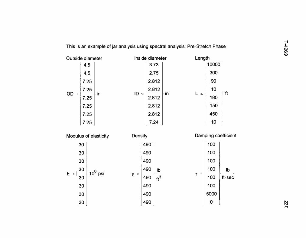
This is an example of jar analysis using spectral analysis: Pre-Stretch Phase
Outside diameter 4.5 4.5 7.25 7.25
OD = I -in7.25 7.25 7.25 7.25
Modulus of elasticity
30 30 30 30
· 106· psiE = I 30 30 30 30
Inside diameter 3.73 2.75 2.812 2.812
ID 2.812 2.812 2.812 7.24
Density
490 490 490 490 lb
p =·-
490 ft3 490 490 490
·in
Length 10000
300 90 10
L I· ft180 150 450 10
Damping coefficient
'Y =
100 100 100 100
I lb
100 ft· sec 100 5000
0 I
�.h.N 0)
N
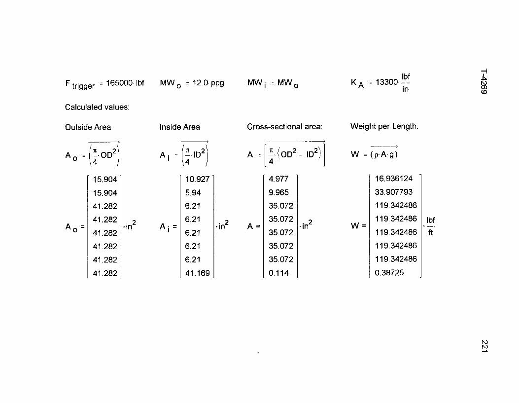
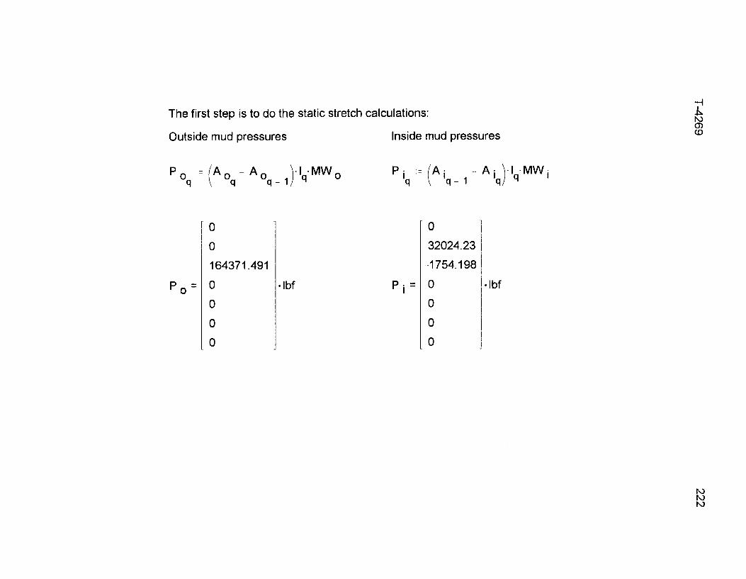
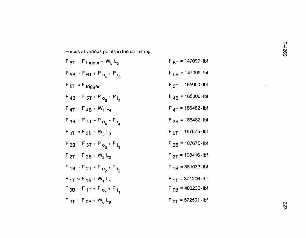
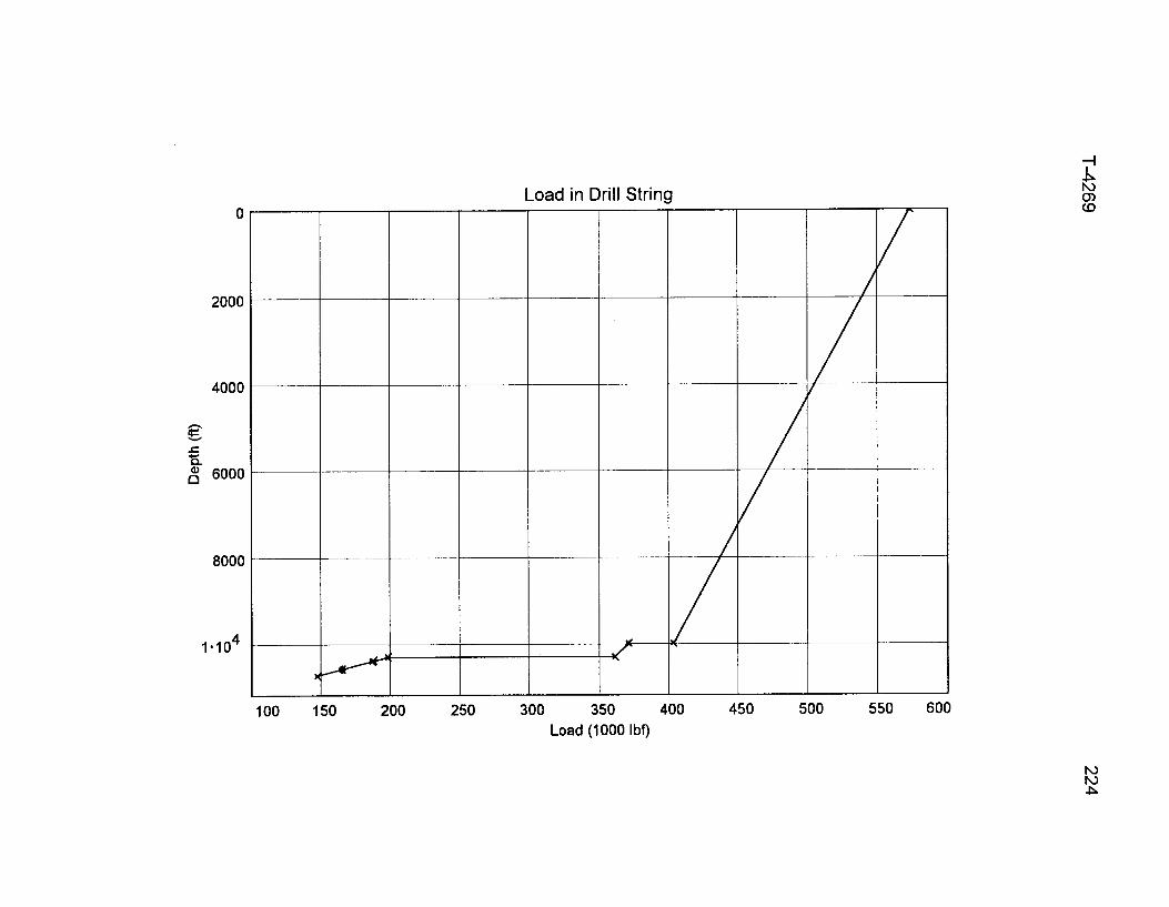
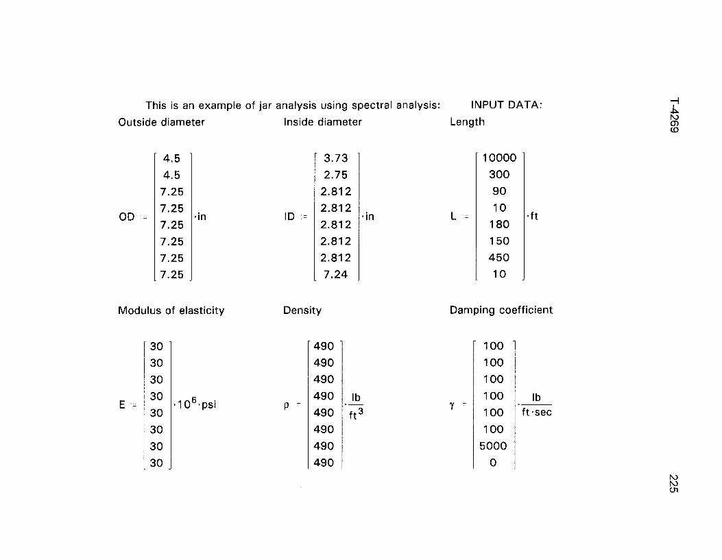
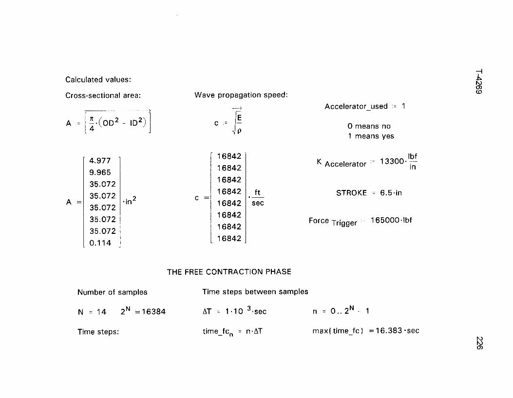


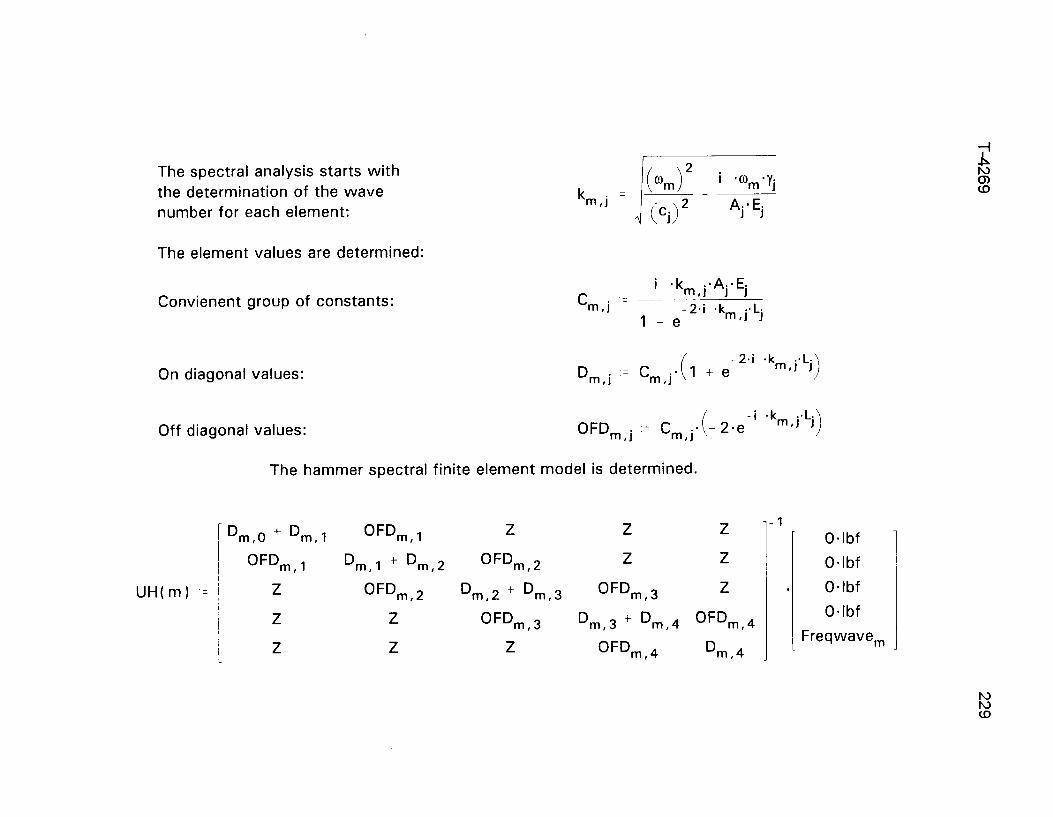
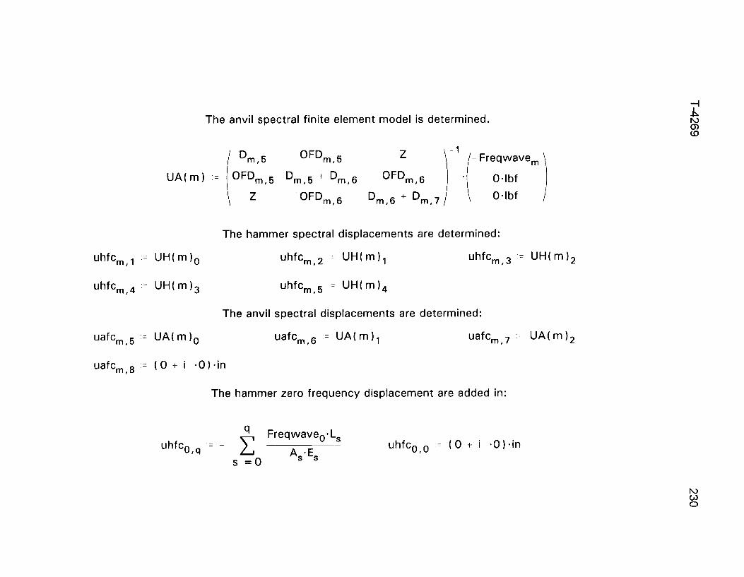
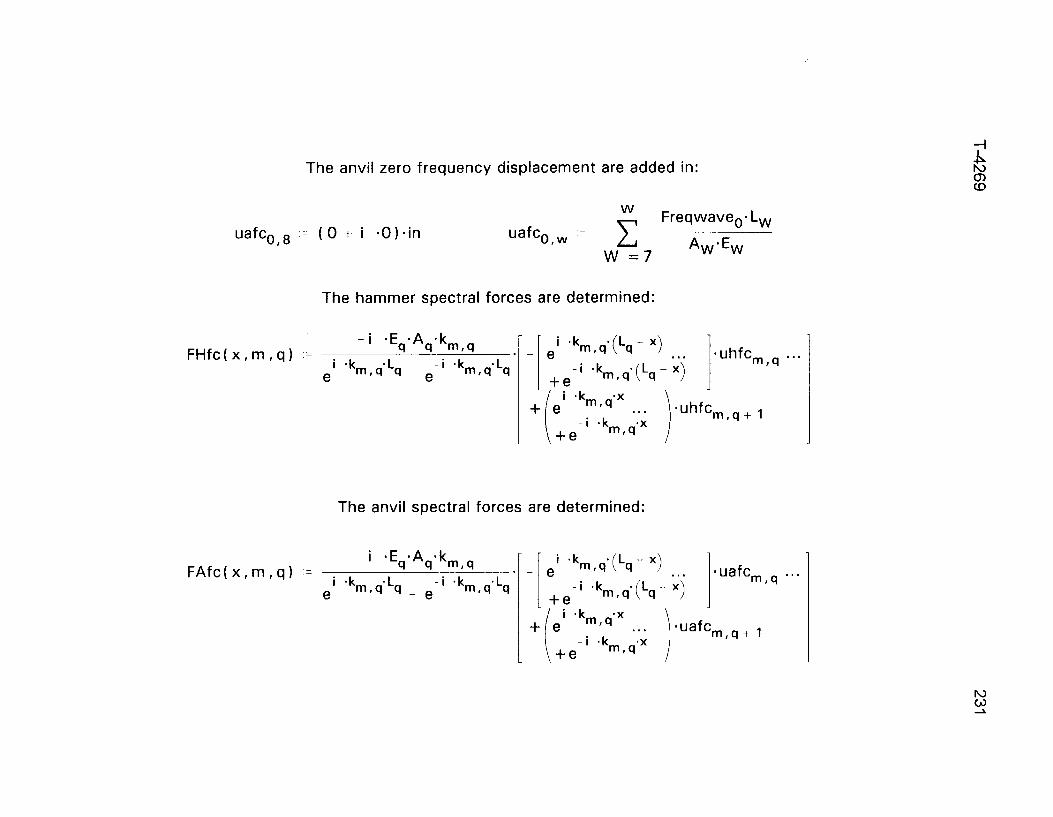
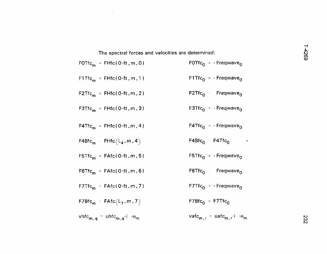


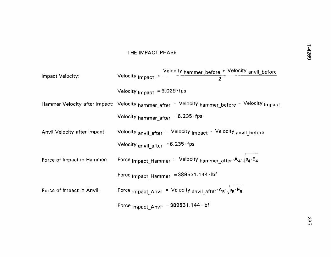
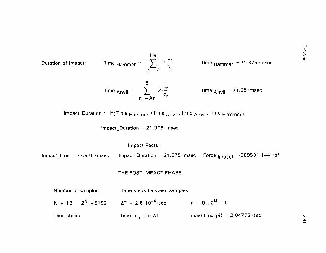
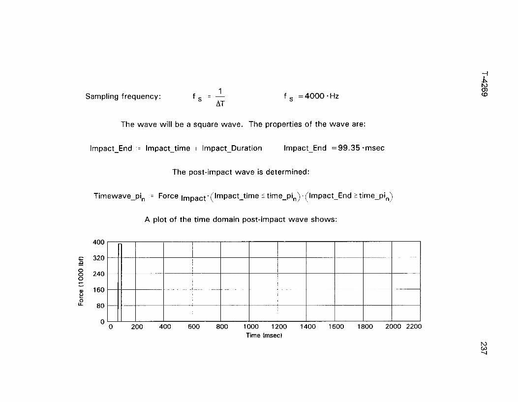
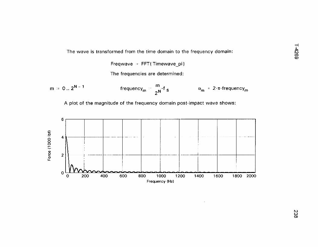

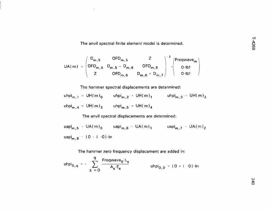
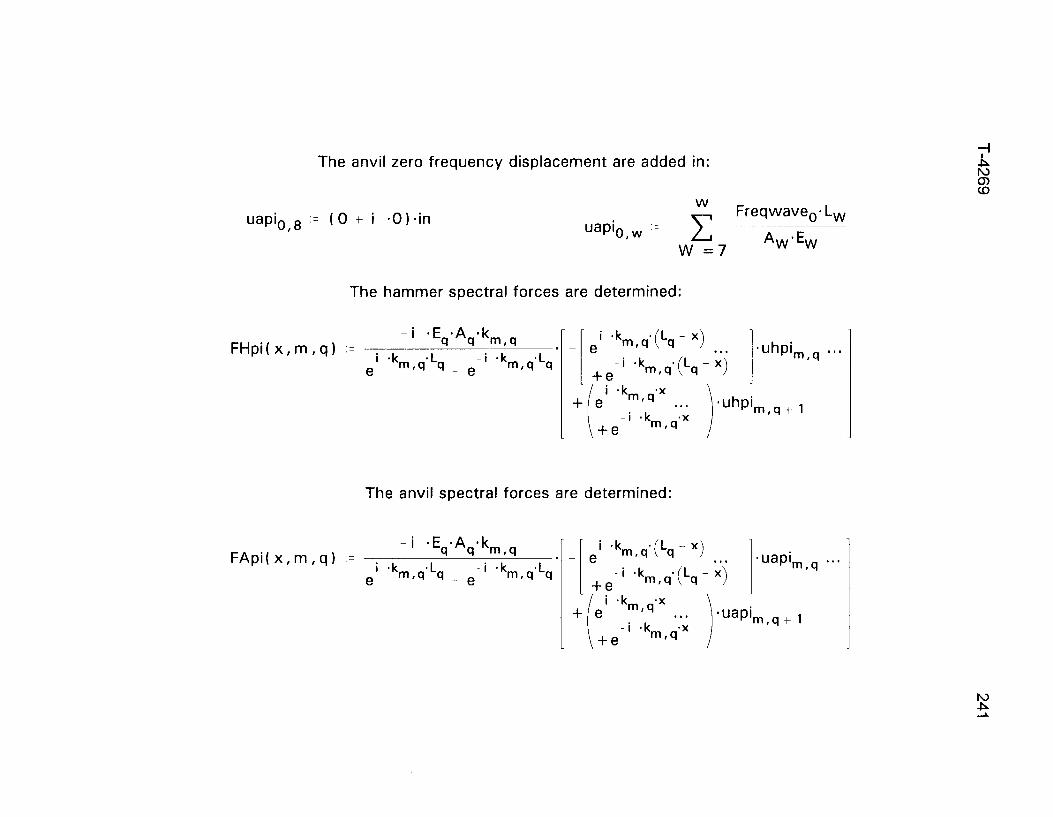
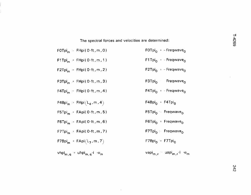
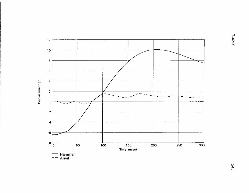
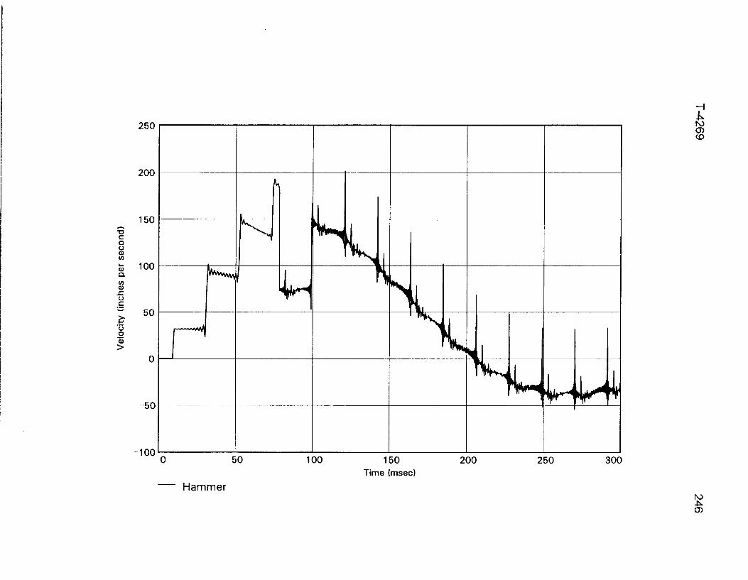
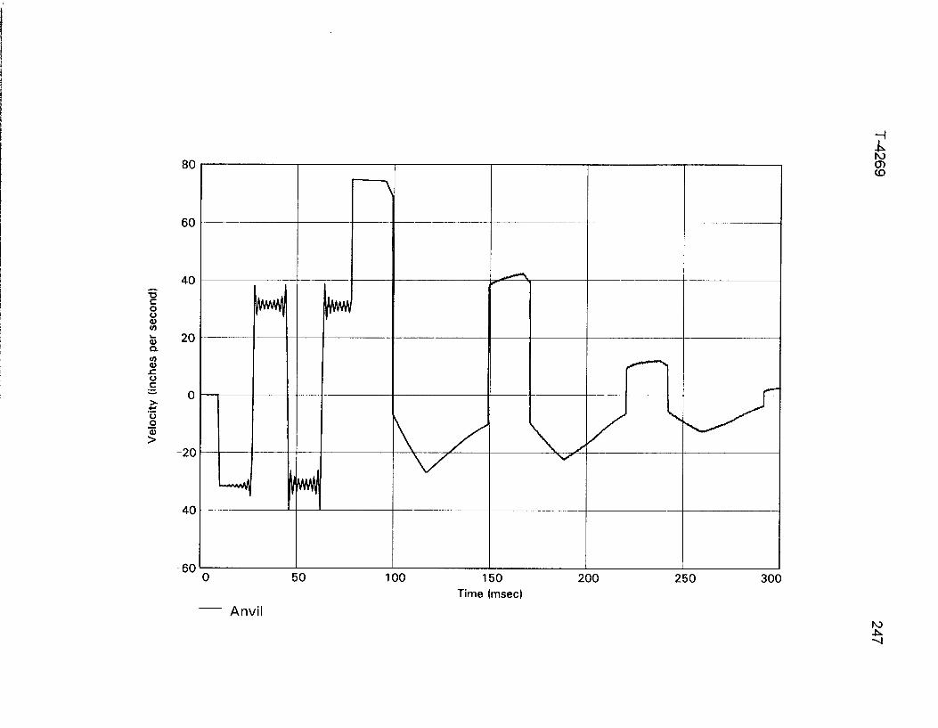
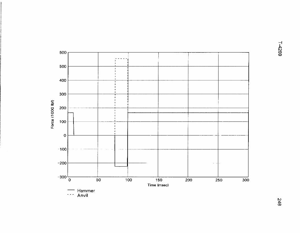

Copyright © 2022 FDOKUMEN