NASA-TP-1817 19810016604

NASA Technical Paper 1817 i

Time and Frequency Domain Analysis

of Sampled Data Controllers via

Mixed Operation Equations

Harold P. Frisch

JUNE 1981

fil/LSA

NASA Technical Paper 1817

Time and Frequency Domain Analysis

of Sampled Data Controllers via

Mixed Operation Equations

Harold P. Frisch

Goddard Space Flight Center

Greenbelt, Maryland

NI ANational Aeronautics

and Space Administration

Scientific and Technical

Information Branch

1981

All measurement values are expressed in the International System of Units (SI) in accordancewith NASA Policy Directive 2220.4, paragraph 4.

ii

ABSTRACT

Specification of the mathematical equations required to define the dynamic response of a linear con-tinuous plant, subject to sampled data control, is complicated by the fact that the digital componentsof the control system cannot be modeled via linear ordinary differential equations. This complicationcan be overcome by introducing two new mathematical operations; namely, the operation of zeroorder hold and digital delay. It is shown herein that by direct utilization of these operations, a set oflinear mixed operation equations can be written and used to define the dynamic response character-istics of the controlled system. It also is shown how these linear mixed operation equations lead, in anautomatable manner, directly to a set of finite difference equations which are in a format compatiblewith follow-on time and frequency domain analysis methods.

iii

CONTENTS

Page

ABSTRACT .............................................................. iii

INTRODUCTION .......................................................... 1

MIXED OPERATION EQUATIONS ............................................ 2

GENERALIZED FORMULATION ASSUMPTIONS AND LIMITATIONS ............... 5

MIXED MATHEMATICAL OPERATIONS ....................................... 7

SOLUTION OF MIXED OPERATION EQUATIONS ............................... 10

DIGITAL COMPUTATIONAL REQUIREMENTS ................................. 13

FREQUENCY DOMAIN ANALYSIS ........................................... 14

TIME DOMAIN ANALYSIS .................................................. 16

CONCLUSION ............................................................ 17

PROGRAM ACRONYM/AVAILABILITY LIST ................................... 18

REFERENCES ............................................................ 19

TIME AND FREQUENCY DOMAIN ANALYSIS OF SAMPLED DATA CONTROLLERSVIA MIXED OPERATION EQUATIONS

Harold P. Frisch

Goddard Space Flight CenterGreenbelt, Maryland

INTRODUCTION

The large space systems technology (LSST) program of the National Aeronautics and Space Adminis-tration (NASA) is attempting to develop an interactive integrated analysis capability (IAC). Its objec-tive is to provide engineers with an interdisciplinary (structures-thermal-controls) analysis capability

supportive of static, time and frequency domain design and performance evaluation methods. To dothis, the IAC program intends to provide a time-wise efficient and user-friendly means for accessing asequence of analysis tools and for respectively obtaining the necessary input data via a series of estab-lished interdisciplinary data flow paths. The immediate goal is to provide a coupled structures-thermal-controls analysis capability compatible with the inherent assumptions and limitations associated withcurrent widely used state-of-the-art general purpose analysis programs such as NASTRAN, DISCOS,SINDA and TRASYS.*

This stated goal implies that data must be derived and stored in computer memory in such a mannerthat it can flow between analysis modules which view intrinsically identical items of data differently.Today, the prime impediment to this interdisciplinary flow of data is the infinite number of ways thatrequested data can be generated and provided to the requestor. In a working environment, this prob-lem is usually compounded by the inability of data requestors to cross interdisciplinary semanticsbarriers and to define precisely what is being requested. The problem is particularly acute when datamust be obtained from sources outside of one's immediate working environment. The net effect of

these data flow barriers is a drop in analyst productivity while assumptions and limitations associatedwith data delivered in an unfamiliar data format are investigated.

One technique which can be used to overcome this real world problem is to define neutral formats fordata. Conceptually, once data is in a neutral format it can, with the aid of a processor, flow anywhere.Since both the neutral format and the desired format are known a priori, the development of the pro-cessor which creates the linkage becomes a routine task. In order to minimize the number of proces-sors required, the choice of a neutral format converges on the answer to the question: What is themost commonly used, readily obtainable format for requested data? For example, in the structural

analysis discipline NASTRAN is probably the most widely used general purpose analysis program.Its bulk data deck would be a good choice as the neutral format for structures data.

The choice of a neutral format for thermal analysis is complicated by the fact that there are twocompeting methods of analysis. Thermal engineers having a strong structures background usually leantoward the finite element approach and use either the NASTRAN or SPAR thermal analyzers. Thermal

*See Program Acronym/Availability List, page 18.

engineers having limited or no structures background usually lean toward the finite difference ap-proach and use the programs SINDA and TRASYS. Consequently, a bilevel neutral format will mostprobably be required for this discipline. Level one would contain the finite element neutral formatwhile level two would contain the finite difference neutral format. If NASTRAN and SINDA bulk

data decks are selected as neutral formats, then it is possible to generate an automated procedurewhich will read level 1 NASTRAN bulk data and generate from it level 2 SINDA bulk data. The reverseprobably never will be possible.

The choice of a single or multilevel neutral format for controls data is not at all straightforward. If theassumption could be made, which it cannot, that controllers are continuous system devices, then theinput data for any of the continuous system modeling programs such as ASCL, CSMP, CSSL, DARE,MODEL, etc., would be candidates for a neutral format for controls data. Since most present-dayspacecraft controllers are sampled data rather than continuous devices, new modeling programs mustbe developed or old ones extended. This is required to adequately account for, in a simultaneousmanner, the continuous time response characteristics of the plant and the digital response character-istics of controller components.

The objective of this paper is to present a framework for a neutral format which can be used for spec-ification of a full range of sampled data controllers. It is conceptually simple in that it parallels theblock diagram approach conventionally used for control system documentation. Furthermore it canbe computationally automated in such a manner that a clear distinction is made between state vari-

ables which may be labeled as continuous time or analog signals and those which may be labeled asdigital signals. This clear distinction allows for the development of integration algorithms which utilizethe discontinuous nature of digital signal state variables to improve run-time performance. When thesystem is linear, this framework also leads directly to linear constant coefficient finite differenceequations compatible with stability and frequency domain analysis methods.

MIXED OPERATION EQUATIONS

The concepts presented here stem largely from ideas derived from the work of Kalman and Bertram,1959 (Reference 4), Zadeh and Desoer, 1963 (Reference 11), and National Aeronautics and SpaceAdministration/Goddard Space Flight Center (NASA/GSFC) Solar Maximum Mission (SMM) pro-ject support activities, Donohue et al, 1978 (Reference 2).

Consider the problem of developing a simulation model for a linear continuous plant controlled by alinear sampled data control system. If this is done on an analog computer with digital components,then the plant equations are implemented by a set of summers, amplifiers and integrators, while thecontroller equations are implemented by a set of zero order holds, digital delays and some moresummers, amplifiers and integrators. If this is to be done on a digital computer, the problem is not

as straiglltforward due to the fact that zero order holds and digital delayors cannot be characterized bylinear ordinary differential equations. Furthermore, if one blindly proceeds with conventional numer-

ical integration methods, the net outcome is frequently a computationally costly solution.

To arrive at a mathematical formulation compatible with digital simulation methods, we first lookthrough the eyes of a mathematician at the bag of hardware required for the analog simulation.Summers and amplifiers are memoryless objects, while integrators, zero order holds and delayors are

finite memory objects. Carrying this a step further, we can view the integrator as a piece of b,ard-ware which implements the mathematical rules of integration; similarly, it is just as valid to view thepiece of hardware called a zero order hold as the implementation of the mathematical rules of zeroorder hold and to view the piece of hardware called a digital delayor as the implementation of the

mathematical rules of digital delay.

At this point, drop the notion of hardware and recognize that new mathematical operations havebeen defined, i.e., the mathematical operations of zero order hold and that of digital delay. Thesereadily lend themselves to block diagram representation and can be pictorially represented as

;!f x

° Iy zoH y

z Delay z

where (.) dot calls for the mathematical operation of integration, (r-l) box calls for zero order holdand (A) triangle calls for digital delay.

If several zero order holds having different sampling rates and digital delayors having different delaytimes are required, the notation immediately is expandable by introducing new symbols such as(O) circle, (O) hexagon, etc., or more simply by a numbering sequence within the symbols.

How this ties in with an ability to define sampled data controllers in terms of mixed operation equa-tions may not yet be completely obvious. Consider, therefore, the following problem: Define the

3

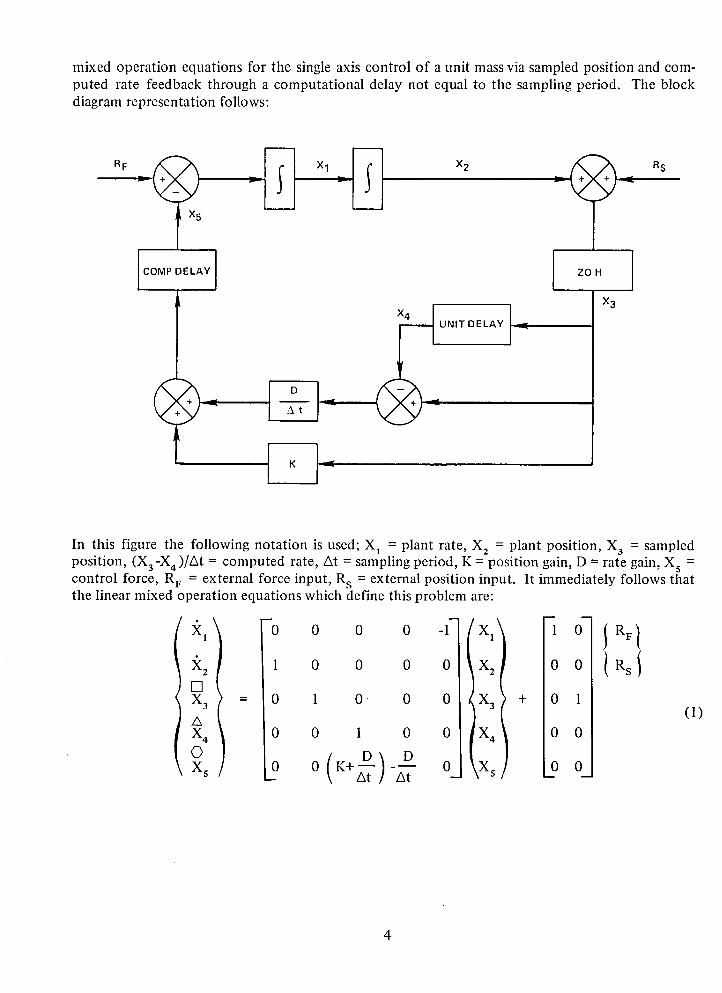
mixed operation equations for the single axis control of a unit mass via sampled position and com-puted rate feedback through a computational delay not equal to the sampling period. The blockdiagram representation follows:

COMP DELAY [ ZO H ]

X 3

X _ UNIT DELAY I _

In this figure the following notation is used; X, = plant rate, X2 = plant position, X 3 = sampledposition, (X 3-X 4)/At = computed rate, At = sampling period, K = position gain, D = rate gain, X s =control force, R v = external force input, R s = external position input. It immediately follows thatthe linear mixed operation equations which define this problem are:

O 0 0 0 "l--X 1 1 0 t RF,

1 0 0 0 0 X2 0 0 i tRs

EX = 0 1 0 0 0 X3 + 0 1(1)

0 0 I 0 0 X4 0 0

o o_ 2 o

4

The important point to note in this example is the ease with which the linear constant coefficient

mixed operation equations have been defined directly from the block diagram. The constant coeffi-

cient matrix, along with the rules associated with the mathematical operations used, completely de-fines the problem and can be readily implemented in a format compatible with digital computation.

The objective now is to define the steps required to go fromlinear mixed operation equations to linearfinite difference equations. Once these are in hand, follow-on frequency domain studies can be car-ried out. If linear time domain response is required, the finite difference equations can be coded andtime response obtained without recourse to conventional numerical integration methods. If nonlineartime domain response is required, a framework for developing special purpose integration algorithmswhich account for the digital signal characteristics of certain state variables is provided. In application,these numerical algorithms must often be developed to achieve timewise efficient simulation pro-grams.

In the next section, the concept of mixed operation equations is presented in a more generalizedframework and certain limitations imposed by the demand that the end product be computationallyefficient are discussed.

GENERALIZED FORMULATION, ASSUMPTIONS AND LIMITATIONS

Kalman and Bertram (Reference 4) define several different types of sampling systems, e.g., synchro-nous, nonsynchronous, multirate, random, etc. There is no intention here to cover all possible cases.This formulation assumes that a single clock, contained within the system, controls all sampling.The clock is assumed to provide a never-ending sequence of synchronous clock pulses, the periodbetween each clock pulse being exactly At. All sampling is carried out by the hardware items hereto-fore referred to as zero order holds. Each zero order hold is assumed to be synchronous and to haveits sampling period defined as an integer multiple of the clock pulse period At. Zero order holds inany simulation may have different sampling periods; however, if frequency domain analysis is thegoal, there must be a periodic pattern to the sampling. If not, frequency domain analysis has nomeaning.

In application, the penalty on generality paid for by restricting the sampling periods to be integermultiples of At is minimal. This is adequate for most linear and quasi-linear system design and per-formance evaluation studies, and it leads to mathematical requirements that can be implemented soas to yield timewise efficient simulation models.

The need to incorporate the effects of one or more delays in a reasonably general format presentsproblems, if one demands that the end product be useful for general application. Delays can be placed

into three general categories: 1) digital delay with time constant equal to an integer multiple ofAt, 2) digital delay with time constant not equal to an integer multiple of At, and 3) analog ortransport delays.

Analog delays are not considered here for the simple reason that the author has not been able tofind a method which he deems to be computationally practical for timewise efficient simulations.

Digital delays are considered and are implemented by the use of what will be referred to here as unitdelayors and fractional delayors subject to the following assumptions and limitations: 1) a unitdelayor delays a digital signal, which is constant during the clock pulse period At, by the amount

At, and 2) a fractional delayor delays a digital signal, which is constant during the clock pulse periodAt, by the amount "rAt where 0 < 3' < 1. These limitations are incorporated to prohibit the modelingof a delayed analog signal by a series connection of several fractional delayors, and to set up a frame-work which will lead to tractable computational requirements.

Consider a general multivariable sampled data control system subject to the above assumptions andlimitations, and let:

W - column matrix containing state variables associated with all integrators

X - column matrix containing state variables associated with all zero order holds

Y - column matrix containing state variables associated with all unit delayors

Z" - column matrix containing state variables associated with all fractional delayors

• - symbol for integration

[] - symbol for zero order hold; subpartitioned into [] , [] ,... etc., if many different zeroorder holds are used

A -- symbol for unit delay

O - symbol for fractional delay, subpartitioned into @ , Q ,... etc., if many differentfractional delays are used

Based upon the above comments and notation, the general form for a system of linear mixed opera-tion equations is

A1 i A12 Aa 3 AI 4 W B 1 R

AZl A22 Aza Az4 X B2

= + (2)

0 Aa z Aa a A34 Y 0

0 A4 2 A4 3 0 Z 0

where

A,B - partitions with nonzero elements

0 - partitions with all zero elements

R - column matrix of reference inputs assumed to be continuous functions of time; thesecannot feed directly into a delayor.

It is also possible to define systems of nonlinear mixed operation equations. These, in general, willnot painlessly lead to finite difference equations. However, at times they do lead to special-purposeintegration algorithms which are superior to those specifically developed for systems of first ordernonlinear ordinary differential equations. The user is cautioned that relative superiority must bejudged on a problem-by-problem basis and is strongly dependent upon the talents of the analyst/programmer.

MIXED MATHEMATICAL OPERATIONS

The system of linear mixed operation equations as presented is relatively easy to obtain directlyfrom a block diagram definition of a controller. However, in order for these to be useful for follow-on analysis, they must lead to a set of either linear ordinary differential or linear finite difference

equations in an automatable manner. The objective of this section is to outline the methodology tobe used to automate the procedure by which system state at clock time (k+l)At can be expressedas a linear function of system state and input at clock time kAt, k = 0,1,2,.... This is the desiredset of first order linear finite difference equations which, via use of the z-transform, will lead directlyinto follow-on frequency domain analysis methods.

Let W(k), X(k), Y(k), Z(k) define system state and let R(k) define system input at clock time kAt.

To define system state at time (k+l)At, it is necessary to know the time dependency of all systemstate variables and inputs during the At time interval

kAt _<t _<(k+l) At

This is known via the modeling restrictions imposed, and from the mathematical rules associatedwith the mixed operation equations given below as:

• Integration: The matrix equation which defines all integrator state variables takes on thegeneral form

_/(t) = A1l W(t) + U(t) (3)

where U(t) is everything in row 1 of equation 2 not explicitly stated herein. Let W(k) define a fullset of initial conditions for equation 3. It follows from the mathematical rules associated with theoperation of integration that the state of all integrator state variables at any time t in the time interval

kat < t _<(k+ 1)At

is given by

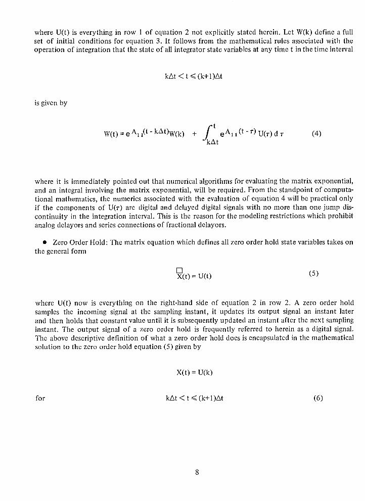
fkA (t - r) dW(t) ; eAl _(t - kAt)w(k) + eA_ 1 U(r) (4)7"

t

where it is immediately pointed out that numerical algorithms for evaluating the matrix exponential,and an integral involving the matrix exponential, will be required. From the standpoint of computa-tional mathematics, the numerics associated with the evaluation of equation 4 will be practical onlyif the components of U(r) are digital and delayed digital signals with no more than one jump dis-continuity in the integration interval. This is the reason for the modeling restrictions which prohibitanalog delayors and series connections of fractional delayors.

• Zero Order Hold: The matrix equation which defines all zero order hold state variables takes onthe general form

DX(t)= U(t) (5)

where U(t) now is everything on the right-hand side of equation 2 in row 2. A zero order holdsamples the incoming signal at the sampling instant, it updates its output signal an instant laterand then holds that constant value until it is subsequently updated an instant after the next sampling

instant. The output signal of a zero order hold is frequently referred to herein as a digital signal.The above descriptive definition of what a zero order hold does is encapsulated in the mathematicalsolution to the zero order hold equation (5) given by

X(t) = U(k)

for kat < t _< (k+l)at (6)

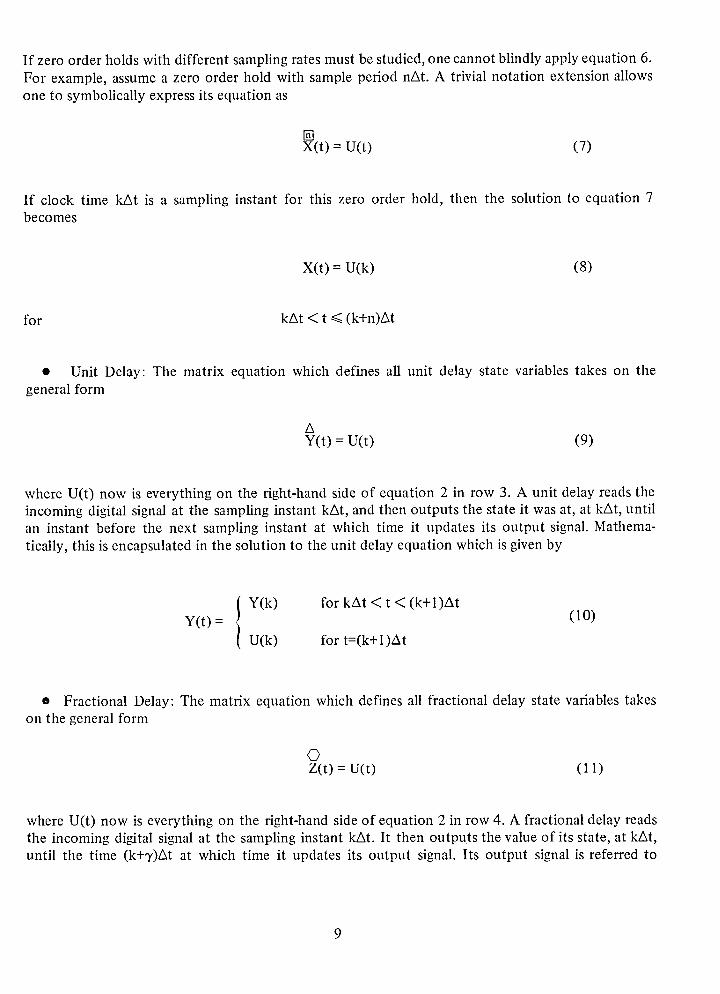
If zero order holds with different sampling rates must be studied, one cannot blindly apply equation 6.

For example, assume a zero order hold with sample period nat. A trivial notation extension allows

one to symbolically express its equation as

[]X(t) = U(t) (7)

If clock time kat is a sampling instant for this zero order hold, then the solution to equation 7becomes

X(t) = U(k) (8)

for kat < t _<(k+n)kt

• Unit Delay: The matrix equation which defines all unit delay state variables takes on thegeneral form

aY(t) = U(t) (9)

where U(t) now is everything on the right-hand side of equation 2 in row 3. A unit delay reads theincoming digital signal at the sampling instant kat, and then outputs the state it was at, at kat, untilan instant before the next sampling instant at which time it updates its output signal. Mathema-

tically, this is encapsulated in the solution to the unit delay equation which is given by

I Y(k) forkAt<t<(k+l)At

Y(t) = (10)

U(k) for t=(k+ l)At

• Fractional Delay: The matrix equation which defines all fractional delay state variables takeson the general form

©Z(t) = U(t) (11)

where U(t) now is everything on the right-hand side of equation 2 in row 4. A fractional delay readsthe incoming digital signal at the sampling instant kat. It then outputs the value of its state, at kat,until the time (k+_,)at at which time it updates its output signal. Its output signal is referred to

herein as a delayed digital signal. Mathematically, this is encapsulated in the solution to the fractionaldelay equation, i.e.,

Z(k) kAt < t _< (k+'r)At

Z(t) = (12)

U(k) (k+'r)At < t _<(k+l)At

where 0 < "r < 1. If fractional delayors with different delay times are required for simulation, sub-scripts would be required on the 'r's and in the symbol O in a manner similar to that used in thezero order hold discussion.

SOLUTION OF MIXED OPERATION EQUATIONS

The most general form for linear mixed operation equations considered in the context of this paperis presented in equation 2. This can be expressed as a set of first order finite difference equations bydirect application of the closed-form solutions for each operation considered in the previous para-graphs. In keeping with the author's intent to communicate to the reader, the solution presentedherein assumes that all zero order holds have sampling period At and all fractional delays have delaytime 'rAt. The solution for the multizero order hold, multifractional delay situation requires addi-tional notation which on the bottom line is more confusing than illuminating; it will therefore notbe presented here.

The row 1 equation of equation 2 defines the integrator state variables and is given by

W(t)= All W(t)+A_2 X(t)+A13 Y(t)+A14 Z(t)+B 1 R(t) (13)

In order to concisely define the solution to this equation let

A AtF(At)= e 11 (14)

At

f Al 1(At-r)H(ZXt)= e dr (15)

O

At

f A (At-r)H[(1-7)At] = e _ dr (16)

"rAt

10

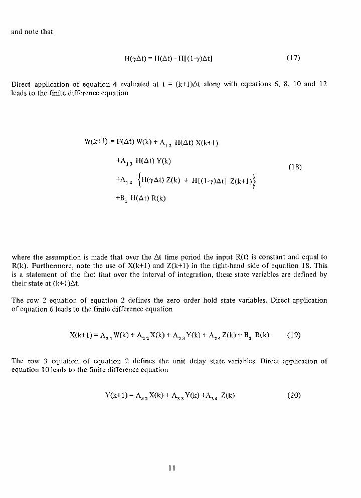
and note that

H(TAt) = H(At) - H[(1-')')Atl (17)

Direct application of equation 4 evaluated at t = (k+l)At along with equations 6, 8, 10 and 12leads to the finite difference equation

W(k+l) = F(At) W(k) + A 1 2 H(At) X(k+l)

+AI 3 H(At) Y(k) (18)

+A14 {H(TAt)Z(k) + H[(1-v)At] Z(k+l)}

+B a H(At) R(k)

where the assumption is made that over the At time period the input R(t) is constant and equal toR(k). Furthermore, note the use of X(k+l) and Z(k+l) in the right-hand side of equation 18. Thisis a statement of the fact that over the interval of integration, these state variables are defined bytheir state at (k+ 1)At.

The row 2 equation of equation 2 defines the zero order hold state variables. Direct applicationof equation 6 leads to the finite difference equation

X(k+ 1) = A a 1W(k) + A z 2X(k) + A z 3Y(k) + A 24 Z(k) + B 2 R(k) (19)

The row 3 equation of equation 2 defines the unit delay state variables. Direct application ofequation 10 leads to the finite difference equation

Y(k+ 1) = A32 X(k) + A33Y(k) +A 34 Z(k) (20)

11

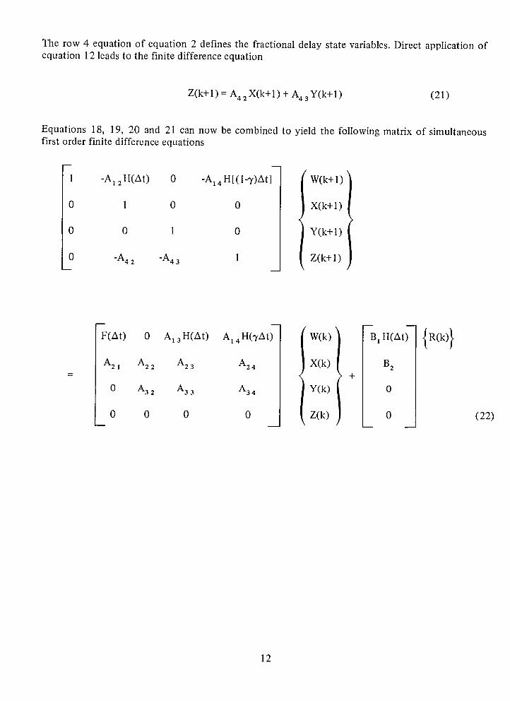
The row 4 equation of equation 2 defines the fractional delay state variables. Direct application ofequation 12 leads to the finite difference equation

Z(k+l) = A42 X(k+l ) + A43Y(k+l ) (21)

Equations 18, 19, 20 and 21 can now be combined to yield the following matrix of simultaneousfirst order finite difference equations

k m

1 -A_ 2H(At) 0 -Aa 4H[(1-3')At] (W(k+l)

0 I 0 0 I X(k+ 1)<

0 0 1 0 Y(k+ 1)

0 "A4 2 "A43 1 [ Z(k+l)

m -- B m

_t_A2,A_°_A13._t_A23AI.H_t_A_4tw_k_X_k_Bx"_t_.2tR_k'l0 A3 2 A3 3 A3 4 Y(k) 0

0 0 0 0 Z(k) 0 (22)

12

Direct use of the inverse of the coefficient matrix on the left-hand side of the equation, which is

1 {A, 2H(At) {A14H[(1-'y)At]A43} {A,4H[(1-3')At] }+AI4H[(I_)At] A42 }

0 1 0 0(23)

0 0 1 0

0 A42 A43 1

yields the final set of finite difference equations which are in a format compatible with follow-on analysis methods, i.e.,

.... { 1W(k+l) DI 1 D12 D13 Dl 4 W(k) E 1 R(k)

X(k+l) D2x D22 D23 D24 X(k) E2= + (24)

Y(k+l) D31 D32 D33 D34 Y(k) E 3

Z(k+l) D41 D42 D43 D44 Z(k) E4 [

DIGITAL COMPUTATIONAL REQUIREMENTS

Wilkinson (Reference 10) reminds us that "attractive mathematics does not protect one from therigors of digital computation." It is therefore important to determine whether or not the foregoingpresentation has led to a computationally practical methodology for the particular case workedout and for the multizero order hold, multifractional delay case mentioned.

The following sequence of steps is required to go from problem definition to the desired set of finite

difference equations to be used for either time or frequency domain follow-on analysis.

13

Step 1. Set up the linear mixed operation equations in the partitioned matrix format of equation

2. This is straightforward and can be done by hand or problem-unique computer code.

Step 2. Determine the elements in the coefficient matrices on the right- and left-hand side ofequation 22. The major numerical problem here is in the evaluation of the matrix exponentialF(at) and the integrals involving the matrix exponential, namely, H(at) and H(3'At). These matricescan be efficiently and accurately evaluated by use of subroutine PADE developed by Van Loan anddiscussed in Reference 8, discussed and published in Reference 9.

Step 3. Determine the elements in the coefficient matrices of equation 24. These are obtainableby a simple matrix multiply, since the required matrix inverse is definable in closed form.

FREQUENCY DOMAIN ANALYSIS

If frequency domain analysis is the objective, a periodic pattern to the sampling must exist. If thereexists a periodic pattern to the sampling, then it is possible via successive matrix multiplications toarrive at an equation of the form

,V k+N +,, +,3+,4 W k, tX(k+N) _2 1 _/2 2 l]/2 3 1_/24 X(k) u2

= +

Y(k+N) ff3 1 @32 1]/33 _'34 Y(k) u3 (25)

Z(k+N) ___4 1 1_/42 1I/4 3 1I/44__ Z(k) E4

where NAt is the sampling pattern period and the elements of the coefficient matrix are constantand independent of both k and N. Kalman and Bertram (Reference 4) discuss this and refer to thismatrix as a stationary transition matrix. It should be noted that in equation 25 the standard stabilityanalysis assumption that input R(k) is constant over the pattern period Nat has been made; if notmade, the resultant stationary finite difference equation is unmanageable for follow-on frequencydomain analysis.

14

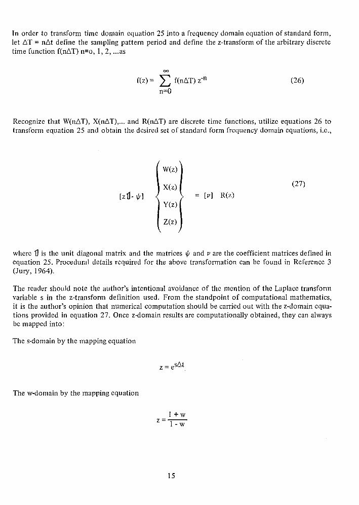
In order to transform time domain equation 25 into a frequency domain equation of standard form,let AT = nat define the sampling pattern period and define the z-transform of the arbitrary discretetime function f(nAT) n=o, 1, 2, ...as

oo

f(z) = E f(nAT) z"n (26)n=O

Recognize that W(nAT), X(nAT),... and R(nAT) are discrete time functions, utilize equations 26 to

transform equation 25 and obtain the desired set of standard form frequency domain equations, i.e.,

W(z)

X(z) (27)[zl]- _1 = [v] R(z)

Y(z)

Z(z)

where 1] is the unit diagonal matrix and the matrices _ and v are the coefficient matrices defined inequation 25. Procedural details required for the above transformation can be found in Reference 3(Jury, 1964).

The reader should note the author's intentional avoidance of the mention of the Laplace transformvariable s in the z-transform definition used. From the standpoint of computational mathematics,

it is the author's opinion that numerical computation should be carried out with the z-domain equa-tions provided in equation 27. Once z-domain results are computationally obtained, they can alwaysbe mapped into:

The s-domain by the mapping equation

z -- esAt

The w-domain by the mapping equation

l+w

z= 1-w

15

or the _-domain by the mapping equation

z-1

At

This final mapping step should be viewed as a necessity since results must be presented in a formatcompatible with the desires of control design engineers. This computational approach avoids truncatedseries approximations, and the resultant numerical computation pitfalls which can be encountered,when computation is done with s-domain equations.

Determination of closed loop system stability can be made directly from the eigenvalues of thecoefficient matrix in equation 25; these may be computed via application of the EISPACK libraryof matrix eigensystem routines published in Reference 7 (Smith, et al., 1976). If all eigenvalues are

contained within the unit circle in the complex z-domain, then the system is stable. If any eigenvalueis outside of the unit circle, the system is unstable.

Determination of margins of stability is usually accomplished with opened, partially opened andclosed loop z-domain transfer functions. A methodology for generating any of these type transferfunctions which is based upon a state variable formulation of system response is presented in Refer-ence 1 (Bodley, et al., 1978) and implemented in the DISCOS program defined therein. Even thoughthe DISCOS method is specifically for continuous time systems, and hence s-domain transfer func-tions, slight modifications can be introduced which make it applicable for z-domain transfer functions.

The DISCOS method opens control feedback loops by selectively setting elements to zero in thecoefficient matrix of the set of first order ordinary differential equations used to define systemresponse. This resultant coefficient matrix is the coefficient matrix for an opened loop system, andresultant closed loop transfer functions are in actuality the sought-after open loop transfer functionsof the original unabridged system. To apply the method to a sampled data system, it is important torecognize that feedback loops must be opened by setting to zero elements in the coefficient matrixof the mixed operation equations. One then proceeds directly as defined herein to obtain the coeffi-cient matrix for the finite difference equations, which define open loop system response, and then onto z-domain transfer function analysis.

TIME DOMAIN ANALYSIS

If time domain analysis is the objective, the concept of mixed operation equations, at times, can leadto tailor-made integration methods which, in particular applications, can reduce computation runtime by orders of magnitude.

For example, if the matrix All in equation 2 is constant and input R is constant over each Atsampling interval, classic numerical integration methods for the differential equations can be com-pletely avoided. One needs only pass through the matrix exponentiation routine PADE once, savethe results, and then compute time domain response directly from the finite difference equations

provided by equation 24. If the matrix A_ _ is slowly varying relative to At, it often will be foundto be more efficient to call up the matrix exponentiation routine periodically to update data forequation 24, rather than blindly use classical numerical integration methods.

16

The reader should recognize that numerical integration methods for differential equations are thesubject of active research; however, most of the current work being done is concentrated on what in

the literature is referred to as stiff ordinary differential equations (Shampine, et al., 1976 and 1979,References 5 and 6, and Gear, 1981, Reference 12). Methods for integrating equations of the typeencountered in the sampled data control of oscillatory plants, as defined herein, is an area of research

not being addressed in the open literature today. Hopefully, the ideas presented in this paper willstimulate research into the field of numerical integration of mixed operation equations. This is animportant class of equations for which timewise efficient methods for numerical solution are nowdeveloped on a problem-by-problem basis.

CONCLUSION

The methodology presented here is a generalization of methods successfully used at NASA/GSFCduring a control system stability and performance analysis of several modes of operation for the

SMM spacecraft. In that application equation 24 was transformed by use of the z-transform, so thatstability margins could be determined in the frequency domain. As a benchmark;in that application,20 different modes of spacecraft operation were analyzed, each requiring the regeneration of thecoefficient matrix in equation 24. Seventeen state variables were required to define the plant andcontroller, and all four mathematical operations discussed herein were utilized. Upper and lowergain margins were obtained in a straightforward iterative manner by incrementing feedback gainand checking for the gain values which put system roots (eigenvalues) on the threshold of instability,i.e., out of the z-domain unit circle. Once debugged, the entire job was run in 1.6 minutes CPU on the

IBM 360-91. Results were compared with those obtained by Donohue, et al., 1978, (Reference 2),using more conventional s-domain methods. Agreement in all cases was near perfect.

Donohue, Hager, McGlew and Zimmerman also carried out time domain performance studies for the

SMM spacecraft. The tailor-made integration method used in their study contributed significantlyto the ideas used and presented here in a generalized context. Their experience conclusively demon-strated that for certain real application problems, dramatic (orders of magnitude) improvements incomputer run-time could be obtained if one avoided the blind application of conventional numericalintegration methods for sampled data control equations.

17

PROGRAM ACRONYM/AVAILABILITY LIST

ACSL Advanced Continuous Simulation Language; Mitchell & Gauthier Associates, Inc.,Concord, Massachusetts

CSMP System/360 Continuous System Modelling Program, IBM Program Number 360A-CX- 16X

CSSL Continuous System Simulation Language; Simulation Services, Division of NilsenAssociates, Inc., Chatsworth, California

DARE Differential Analyzer Replacement; University of Arizona

DISCOS Digital Computer Program for the Dynamic Interaction Simulation of Controls andStructure, COSMIC Program Number GSC-12422

MODEL Multi-Optimal Differential Equation Language; NASA/GSFC, Guidance & ControlBranch Program

NASTRAN NASA Structural Analysis; MacNeil Schwendler Corp., Los Angeles, California,and/or COSMIC, University of Georgia, Athens, Georgia, Program NumberHQN- 10952

SINDA Systems Improved Numerical Differencing Analyzer, COSMIC Program NumberMSC-13805

SPAR A System of Computer Programs for Structural Analysis, COSMIC Program NumberLAR-12213; also under title EAL from Engineering Information Systems, Inc.,San Jose, California.

TRASYS Thermal Radiation Analysis System, Martin-Marietta and/or NASA/JSC ComputerProgram Library

18

REFERENCES

1) Bodley, C.S., Devers, A.D., Park A.C. and Frisch, H.P., "A Digital Computer Program for the

Dynamic Interaction Simulation of Controls and Structure (DISCOS)," NASA Technical Paper1219, Vols. 1 and 2, May 1978.

2) Donohue, J.H., Hager, F.W., McGlew, D.E. and Zimmerman, B.G., NASA/GSFC Guidance andControl Branch Internal Memoranda, 1978.

3) Jury, E.I., Theory and Application of the Z-Transform Method, Ch. l, John Wiley and Sons,1964.

4) Kalman, R.E. and Bertram, J.E., "A Unified Approach to the Theory of Sampling Systems,"Journal of the Frankl#z Institute, Vol. 267, pp. 405-436, May 1959.

5) Shampine, L.F. and Gear, G.W., "A User's View of Solving Stiff Ordinary Differential Equa-tions," SIAM Review, Vol. 21, No. 1, pp. 1-17, January 1979.

6) Shampine, L.F., Watts, H.A., Davenport, S.M., "Solving Nonstiff Ordinary Differential Equa-tions - The State of the Art," SIAM Review, Vol. 18, No. 3, pp. 376-411, July 1976.

7) Smith, B.T., Boyle, J.M., Dongarra, J.J., Garbow, B.S., Ikebe, Y., Klema, V.C. and Moler,C.B., "Matrix Eigensystem Routines - EISPACK Guide," Lecture Notes in Computer Science6, Springer-Verlag, 1976.

8) Van Loan, C.F., "Computing Integrals Involving the Matrix Exponential," IEEE Trans. Auto-matie Control, Vol. AC-23, No. 3, June 1978 (no subroutine source code).

9) Van Loan, C.F., "Computing Integrals Involving the Matrix Exponential," Dept. of ComputerScience, Cornell University, Ithaca, New York, TR76-298 (with subroutine source code).

10) Wilkinson, J.H., "Modern Error Analysis," SIAM Review, Vol. 13, No. 4, pp. 548-568,October 1971.

11) Zadeh, L.A. and Desoer, C.A., Lbzear System Theory, The State Space Approach, McGraw-Hill, 1963.

12) Gear, C.W.,"Numerical Solution of Ordinary Differential Equations: Is there anything left todo?" SIAM Review, Vol. 23, No. 1, pp. 10-24, January 1981.

19

1. ReportNo. 2. GovernmentAccessionNo. 3. Recipient'sCatalogNo.NASA TP-1817

4. Title andSubtitle 5. ReportDate

Time and Frequency Domain Analysis June 1981of Sampled Data Controllers via Mixed 6. Performing Organization CodeOperation Equations 712

7. Author(s) 8. Performing Organization Report No.Harold P. Frisch 81 F0042

9. Performing Organization Nameand Address 10. Work Unit No.

Goddard Space Flight CenterGreenbelt, Maryland 20771 11. Contract or Grant No.

13. Type of Report and Period Covered12. SponsoringAgencyNameandAddress

Technical PaperNational Aeronautics and Space AdministrationWashington, D.C. 20546

14. SponsoringAgencyCode

15. SupplementaryNotes

16. Abstract

Specification of the mathematical equations required to define the dynamic response of alinear continuous plant, subject to sampled data control, is complicated by the fact that thedigital components of the control system cannot be modeled via linear ordinary differentialequations. This complication can be overcome by introducing two new mathematical opera-tions; namely, the operation of zero order hold and digital delay. It is shown herein that bydirect utilization of these operations, a set of linear mixed operation equations can be writtenand used to define the dynamic response characteristics of the controlled system. It also isshown how these linear mixed operation equations lead, in an automatable manner, directly toa set of finite difference equations wliich are in a format compatible with follow-on time andfrequency domain analysis methods.

17. KeyWords(Selectedby Author(s)) 18. Distribution StatementAnalytical and Numerical Methods, Unclassified-UnlimitedGuidance and Control, SpacecraftSimulation

Subject Category 18

19. SecurityClassif.(of this report) 20. SecurityClassif.(of this page) 21. No.of Pages[ 22. Price*

Unclassified Unclassified 25 [ A02"For sale by the National Technical Information Service, Springfield, Virginia 22161.

NASA-Langley, 1981

National Aeronautics and THIRD-CLASS BULK RATE Postageand Fees PaidNational Aeronautics and

Space Administration Space AdministrationNASA-451

Washington, D.C.20546

Official Business

Penalty for Private Use, $300

N_I_ A POSTMASTER: If Undeliverable (Section 158Postal Manual) Do Not Return