Confined axisymmetric laminar jets with large expansion ratios

J. Fluid Mech. (2002), vol. 456, pp. 319–352. c© 2002 Cambridge University Press

DOI: 10.1017/S0022112001007601 Printed in the United Kingdom

319

Confined axisymmetric laminar jets with largeexpansion ratios

By A. R E V U E L T A1, A. L. S A N C H E Z1 AND A. L I N A N2

1Area de Mecanica de Fluidos, Departamento de Ingenierıa Mecanica,Universidad Carlos III de Madrid, 28911 Leganes, Spain

2Departamento de Motopropulsion y Termofluidodinamica, E. T. S. I. Aeronauticos,Universidad Politecnica de Madrid, 28040 Madrid, Spain

(Received 26 September 2000 and in revised form 17 October 2001)

This paper investigates the steady round laminar jet discharging into a coaxial ductwhen the jet Reynolds number, Rej , is large and the ratio of the jet radius to theduct radius, ε, is small. The analysis considers the distinguished double limit in whichthe Reynolds number Rea = Rejε for the final downstream flow is of order unity,when four different regions can be identified in the flow field. Near the entrance, theouter confinement exerts a negligible influence on the incoming jet, which developsas a slender unconfined jet with constant momentum flux. The jet entrains outerfluid, inducing a slow backflow motion of the surrounding fluid near the backstep.Further downstream, the jet grows to fill the duct, exchanging momentum with thesurrounding recirculating flow in a slender region where the Reynolds number isstill of the order of Rej . The streamsurface bounding the toroidal vortex eventuallyintersects the outer wall, in a non-slender transition zone to the final downstreamregion of parallel streamlines. In the region of jet development, and also in themain region of recirculating flow, the boundary-layer approximation can be used todescribe the flow, while the full Navier–Stokes equations are needed to describe theouter region surrounding the jet and the final transition region, with Rea = Rejεentering as the relevant parameter to characterize the resulting non-slender flows.

1. IntroductionConfined jet flows are of both fundamental and practical importance. They are

present in numerous applications including ejector systems and gas-turbine combus-tors. A prototypical example of such flows arises in axisymmetric ducted flows withsudden expansions; the flow separates as it encounters the expansion, comprisinga jet stream surrounded by recirculating flow. In this geometrically simple configu-ration, which is sketched in figure 1, the flow depends mainly on two parameters:the Reynolds number of the incoming jet, Rej , and the expansion ratio, 1/ε, with εrepresenting the ratio of the inner to the outer radii; the laminar jet remains stablefor values of the Reynolds number below a certain critical value. The purpose ofthe present paper is to describe the resulting steady axisymmetric solutions in thedouble limit of large Reynolds numbers (Rej � 1) and large expansion ratios (ε� 1).The analysis considers in particular the distinguished limit Rejε ∼ 1, for which theReynolds number Rea = Rejε of the asymptotic flow emerging downstream fromthe recirculating region is of order unity. In the computations, both uniform andPoiseuille profiles will be considered for the inlet velocity profile. Also, the boundary

320 A. Revuelta, A. L. Sanchez and A. Linan

ui(r) 2εa

O

M

T

a

J

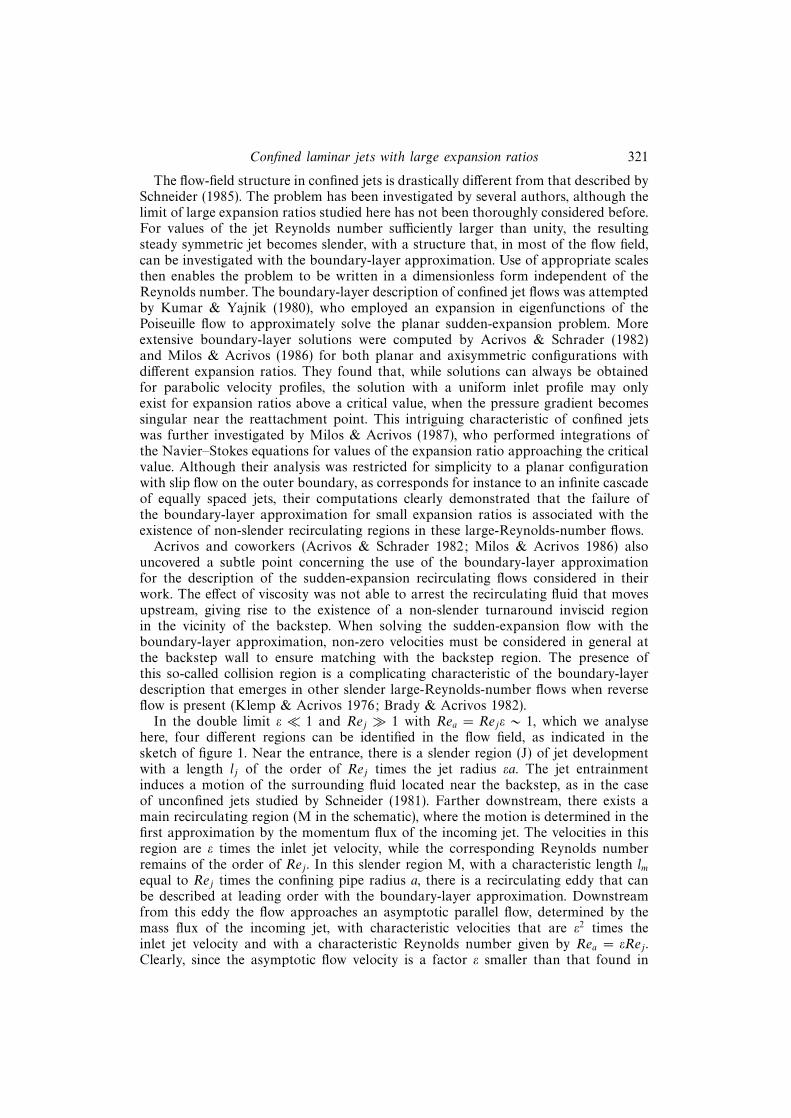
Figure 1. A schematic of the confined jet flow.

conditions on the outer wall will include both non-slip and slip flow, the latter beingan appropriate symmetry condition to represent approximately the collective effect ofthe other jets in array configurations of multiple jets. Before focusing on the problemof interest, we review below some relevant results concerning the solution for roundlaminar jets. Although stability is not the subject of the present paper, a brief accountof our current understanding of the stability of confined jets is also provided.

The flow field in unconfined jets (ε = 0) emerging normal to a wall depends onlyon the value of Rej . A uniformly valid exact solution of the resulting flow is notavailable. If Rej ∼ 1, one needs to integrate the full Navier–Stokes equations todescribe the flow field near the mouth of the pipe, i.e. at distances from the orificeof the order of its radius. The flow field has been described in jets with Rej � 1.In this case, there exists a slender jet region aligned with the pipe where the velocityis of the order of the inlet velocity, and where the momentum flux is constantin the first approximation, because the velocity outside is much smaller. This jetdevelops downstream as it entrains outer fluid. The boundary-layer approximationis applicable to describe the jet flow, whereas the full Navier–Stokes equations arenecessary to study the motion outside. At distances from the entrance much largerthan Rej times the pipe radius, the flows in the jet and in the outer region becomeself-similar. In the jet region, the solution approaches that postulated by Schlichting(1933), corresponding to a point source of momentum. The jet is seen to entrain outerfluid with a radial volume flux per unit length equal to 8πν, with ν denoting here thekinematic viscosity of the fluid. This constant entrainment rate, independent of thejet Reynolds number, is associated with a Reynolds-number-independent self-similarsolution in the outer Navier–Stokes region, a result due to Schneider (1981), wholater used a multiple-scale technique to account for the slow momentum decay thatoccurs in the jet in the presence of the outer flow (Schneider 1985). At large distancesfrom the inlet the jet has lost a significant fraction of its initial momentum, but isstill slender, and continues to entrain outer fluid with the same constant rate 8πν,at distances from the inlet smaller than Rej exp(Re2

j /15.28) times the pipe radius. Atthese distances, the jet merges with the outer flow, giving rise to a large recirculatingtoroidal eddy whose description necessitates numerical integration of the full Navier–Stokes equations. The associated parameter-free problem has not been investigated,although an approximate description, obtained by extending the near-field asymptoticexpansion outside its range of applicability, is given in Schneider (1985), with resultsin agreement with experimental observations (Zauner 1985).

Confined laminar jets with large expansion ratios 321

The flow-field structure in confined jets is drastically different from that described bySchneider (1985). The problem has been investigated by several authors, although thelimit of large expansion ratios studied here has not been thoroughly considered before.For values of the jet Reynolds number sufficiently larger than unity, the resultingsteady symmetric jet becomes slender, with a structure that, in most of the flow field,can be investigated with the boundary-layer approximation. Use of appropriate scalesthen enables the problem to be written in a dimensionless form independent of theReynolds number. The boundary-layer description of confined jet flows was attemptedby Kumar & Yajnik (1980), who employed an expansion in eigenfunctions of thePoiseuille flow to approximately solve the planar sudden-expansion problem. Moreextensive boundary-layer solutions were computed by Acrivos & Schrader (1982)and Milos & Acrivos (1986) for both planar and axisymmetric configurations withdifferent expansion ratios. They found that, while solutions can always be obtainedfor parabolic velocity profiles, the solution with a uniform inlet profile may onlyexist for expansion ratios above a critical value, when the pressure gradient becomessingular near the reattachment point. This intriguing characteristic of confined jetswas further investigated by Milos & Acrivos (1987), who performed integrations ofthe Navier–Stokes equations for values of the expansion ratio approaching the criticalvalue. Although their analysis was restricted for simplicity to a planar configurationwith slip flow on the outer boundary, as corresponds for instance to an infinite cascadeof equally spaced jets, their computations clearly demonstrated that the failure ofthe boundary-layer approximation for small expansion ratios is associated with theexistence of non-slender recirculating regions in these large-Reynolds-number flows.

Acrivos and coworkers (Acrivos & Schrader 1982; Milos & Acrivos 1986) alsouncovered a subtle point concerning the use of the boundary-layer approximationfor the description of the sudden-expansion recirculating flows considered in theirwork. The effect of viscosity was not able to arrest the recirculating fluid that movesupstream, giving rise to the existence of a non-slender turnaround inviscid regionin the vicinity of the backstep. When solving the sudden-expansion flow with theboundary-layer approximation, non-zero velocities must be considered in general atthe backstep wall to ensure matching with the backstep region. The presence ofthis so-called collision region is a complicating characteristic of the boundary-layerdescription that emerges in other slender large-Reynolds-number flows when reverseflow is present (Klemp & Acrivos 1976; Brady & Acrivos 1982).

In the double limit ε � 1 and Rej � 1 with Rea = Rejε ∼ 1, which we analysehere, four different regions can be identified in the flow field, as indicated in thesketch of figure 1. Near the entrance, there is a slender region (J) of jet developmentwith a length lj of the order of Rej times the jet radius εa. The jet entrainmentinduces a motion of the surrounding fluid located near the backstep, as in the caseof unconfined jets studied by Schneider (1981). Farther downstream, there exists amain recirculating region (M in the schematic), where the motion is determined in thefirst approximation by the momentum flux of the incoming jet. The velocities in thisregion are ε times the inlet jet velocity, while the corresponding Reynolds numberremains of the order of Rej . In this slender region M, with a characteristic length lmequal to Rej times the confining pipe radius a, there is a recirculating eddy that canbe described at leading order with the boundary-layer approximation. Downstreamfrom this eddy the flow approaches an asymptotic parallel flow, determined by themass flux of the incoming jet, with characteristic velocities that are ε2 times theinlet jet velocity and with a characteristic Reynolds number given by Rea = εRej .Clearly, since the asymptotic flow velocity is a factor ε smaller than that found in


M, the description of the recirculating eddy in the limit ε → 0 must show at leadingorder a stagnant solution downstream from the eddy end, with non-zero velocities ofrelative order ε appearing downstream only at the following order in the asymptoticdevelopment.

The streamlines of the slender recirculating eddy of length lm = Reja are alignedwith the axis, except in non-slender boundary regions of characteristic length a locatedat both ends (O and T in the schematic). In the outer region O surrounding theincoming jet, the streamlines deflect towards the axis forced by the jet entrainment. IfRea is of order unity, which corresponds to the distinguished limit εRej ∼ 1 consideredhere, then the length of jet development lj = Reaa and the length of the non-slenderregion O are comparable; this is the case represented in the schematic of figure 1. Theleading-order solution in this outer region O, and also in the final transition region T,will be described for various values of Rea ∼ 1, with the extreme cases Rea � 1 andRea � 1 also being considered. The downstream asymptotic forms of the solutionsfor the regions O and J provide in particular the velocity profile for the integrationof the boundary-layer equations in the main recirculating region; no turnaround, orcollision, region is found at the backstep in the analysis of sudden expansions withε� 1.

The stability analysis of confined jets should provide, in particular, the maximumvalue of Rej for which the steady laminar solution remains valid. Much of the stabilityresearch on confined jets has been devoted to the case of plane sudden expansions.For instance, Durst, Melling & Whitelaw (1974) and Cherdron, Durst & Whitelaw(1978) studied this problem experimentally, and found that symmetric solutions canonly exist for values of the Reynolds number below a certain critical value. For largervalues of the Reynolds number, steady asymmetric solutions appear, a result that wasconfirmed in the numerical works of Durst, Pereira & Tropea (1993) and Allerborn etal. (1997). Recent contributions regarding the symmetry-breaking bifurcation includethat of Rusak & Hawa (1999), who carried out a weakly nonlinear analysis of thebifurcation, and that of Hawa & Rusak (2000), who studied the effect of a slightasymmetry of the channel geometry on the flow behaviour.

The symmetry-breaking bifurcation was also encountered in the numerical andexperimental work of Fearn, Mullin & Cliffe (1990), who investigated a plane suddenexpansion with expansion ratio 1 : 3. They obtained a critical Reynolds number(based on the jet width) equal to 82, a result later verified by the linear stabilityanalysis of Shapira, Degani & Weihs (1990). For even larger values of the Reynoldsnumber, the experimental evidence indicates that the flow becomes time-dependent,a behaviour that Fearn et al. (1990) and Durst et al. (1993) found to be associatedwith three-dimensional effects. The dependence of the critical Reynolds number ofthe symmetry-breaking bifurcation on the expansion ratio was studied in the morerecent numerical works of Battaglia et al. (1997) and Drikakis (1997). It was foundthat reducing the expansion ratio tends to improve the stability of the symmetricsolution; the critical Reynolds number decreases with increasing expansion ratios.The interplay of viscous dissipation and convection of perturbations for increasing jetReynolds number is discussed in detail by Hawa & Rusak (2001), who combined abifurcation analysis and a linear stability study of the sudden expansion with carefuldirect numerical simulations of the problem.

The stability of axisymmetric free jets was addressed in the early experimental workof Reynolds (1962). Steady solutions were found for Reynolds numbers (based onthe jet diameter) below about 300. Confinement does not greatly affect this criticalvalue; in a free round jet the local Reynolds number remains constant with axial


distance (Schlichting 1933), causing jet stability in sudden expansions to remainroughly independent of the expansion ratio. For instance, in the experimental andnumerical work of Macagno & Hung (1967), for an expansion ratio 1 : 2 steadysolutions were found for jet Reynolds numbers at least as large as 200.

Although the stability analysis of unconfined round jets was undertaken early byBatchelor & Gill (1962) and by Mollendorf & Gebhart (1973), much remains tobe learnt about the stability of confined round jets. The stability behaviour can beexpected to be different from that described above for plane jets. The experimentalresults for turbulent jets in sudden expansions of Nathan, Hill & Luxton (1998) suggestthat, while the steady axisymmetric solution in planar jets undergoes a symmetry-breaking bifurcation to another steady solution, round jets may bifurcate to unsteadyasymmetric solutions, in which the jet precesses about the axis in a swirl-like motion.Although this type of behaviour is anticipated by Battaglia et al. (1998), carefulevaluations of the critical Reynolds numbers associated to this bifurcating mode arestill not available. Another aspect of the problem in need of further research concernsthe relationship between the stability characteristics of confined and unconfined jets.

2. Characteristic scales and problem formulationWe consider here the confined laminar jet formed when an incompressible fluid

of density ρ and kinematic viscosity ν flows through a pipe of radius εa into amuch larger coaxial pipe of radius a, a configuration sketched in figure 1. Themomentum and mass fluxes of the incoming jet are, respectively, J =

∫ εa0

2πρru2i dr

and G =∫ εa

02πρrui dr , where r is the radial distance to the axis and ui is the incoming

velocity distribution. In our analysis, we shall assume that the jet Reynolds numberRej = (J/ρ)1/2/ν is much larger than unity. Furthermore, attention is restricted tocases with large expansion ratios (ε � 1), for which different distinguished regionscan be identified in the flow field sketched in figure 1. In the following discussionof characteristic scales, the variable x denotes the axial distance measured from theentrance, u and v are the axial and radial velocity components and p denotes thepressure, all variables being expressed in dimensional form.

Close to the entrance, the outer confinement exerts a negligible influence on thejet, which thereby behaves as an unconfined free jet, with a momentum flux thatremains constant in the first approximation. In this jet development region, denotedby J in figure 1, the velocity is of order uj = (J/ρ)1/2/(εa) and the jet radius is oforder εa. An order-of-magnitude balance between the viscous terms, νuj/(εa)

2, andthe convective terms, u2

j /lj , in the jet momentum equation yields lj = Rejεa for thecharacteristic length of this initial region of jet development. Clearly, the conditionthat the jet Reynolds number Rej be large ensures that the resulting jet is slender,and can consequently be described in the boundary-layer approximation. Furtherdownstream, the solution in the jet approaches the Schlichting solution (Schlichting1933), with characteristic values for the local jet radius εax/lj and axial velocity ujlj/xthat follow from the condition of constant momentum flux and from the balancebetween viscous forces and convective terms in the momentum equation. The jetvolume flux increases with distance due to the entrainment of outer fluid, with aradial volume flux per unit length 2πrv of order ν that decreases towards the constantvalue 8πν in the self-similar Schlichting region.

The jet therefore acts as a volumetric line sink that induces the motion of thesurrounding fluid located near the backstep wall between the jet and r = a (O in thefigure), with axial and radial velocities of order uo ∼ ε2uj and vo ∼ ν/a at distances


x ∼ lj . In the distinguished limit Rea = Rejε ∼ 1, the outer region O is non-slender, i.e.lj ∼ a and uo ∼ vo. The description of the associated velocity field requires integrationof the full Navier–Stokes equations, with Rea entering as a parameter in the formu-lation. On the other hand, if Rea � 1, then the streamlines remain almost parallel tothe axis in O for x ∼ lj ∼ Reaa, where the flow can be described with the boundary-layer approximation, except in the small non-slender region of streamline deflectioncorresponding to x ∼ a. In the opposite limit Rea � 1, the length of jet developmentsatisfies lj � a, so that to study the fluid motion in O at distances x ∼ a one can usethe constant jet entrainment at the axis 8πν corresponding to Schlichting solution.

Farther downstream from the entrance there exists a much larger region (M in theschematic) characterized by a momentum exchange between the jet and the outer re-circulating fluid. Correspondingly, the characteristic axial velocity in this main region,um = (J/ρ)1/2/a = εuj , follows from the condition J ∼ ρu2

ma2. Note that this condition

of momentum exchange also implies that the characteristic Reynolds number in Mis of the order of the jet Reynolds number, i.e. uma/ν = Rej . On the other hand,the balance between the viscous term νum/a

2 and the convective term u2m/lm in the

momentum balance equation yields lm = Reja for the characteristic length of therecirculating region, whereas the continuity balance um/lm ∼ vm/a leads to a charac-teristic radial velocity in this region vm = ν/a ∼ um/Rej . These characteristic valuesum, vm and lm, together with the radius a and the characteristic pressure variation ρu2

m,are used below as scales in writing the conservation equations in dimensionless form.As shown below, in the limiting case Rej � 1 considered here, these equations reduce,with errors of order Re−2

j , to the well-known boundary-layer equations. Note that, inthe case of unconfined jets investigated by Schneider (1985), one needs a jet length oforder εaRej exp(Re2

j /15.28)� lm for the momentum to decay to negligible values.At the rear end of the recirculating region the dividing streamsurface opens up and

eventually intersects the outer wall. The flow downstream rapidly approaches eitherPoiseuille flow (if a non-slip condition is employed at r = a) or a uniform flow (if slipflow is considered). Mass conservation requires that the characteristic axial velocityin this asymptotic downstream region be of order G/(ρa2) ∼ ε2uj ∼ εum, and thatthe corresponding asymptotic Reynolds number be Rea = Rejε. Transition betweenthe recirculating flow and the final downstream parallel flow takes place in a shortregion (denoted by T in figure 1) of characteristic length Reaa where the velocityis already of order ε2uj , and where the local Reynolds number is Rea. As in regionO, the description of the flow field in T requires integration of the Navier–Stokesequations, with Rea entering as a parameter.

The scaling analysis can be extended to estimate the pressure variations taking placein the different regions. Thus, in the boundary regions O and T the pressure variationsare of order ρε4u2

j , much smaller than the axial pressure differences found along themain region M, of order ρε2u2

j . On the other hand, since the initial momentum perunit volume in the jet is of order ρu2

j , the pressure differences in O are much toosmall to affect the development of the jet at leading order. Therefore, in region Jthe velocity field can be computed using the boundary-layer approximation with thepressure gradient neglected when writing the axial momentum equation. The radialpressure differences across the jet, of order ρu2

j /Re2j , can be determined in region J by

integrating the radial component of the momentum equation once the velocity fieldhas been computed with the boundary-layer approximation.

The existence of four distinguished regions is a direct consequence of the largeexpansion ratio considered here; the boundary regions J, O and T merge with themain recirculating region M in configurations with ε of order unity. In the jet region,


and also in the main recirculating region, the condition Rej � 1 assumed here sufficesto guarantee that the flow field is slender, and that it is amenable to a boundary-layerdescription. On the other hand, the solution in the non-slender regions O and Trequires integration of the full Navier–Stokes equations, with Rea = εRej entering asa parameter in the formulation. The following four sections deal with the leading-order solution corresponding to regions J, O, M and T, respectively. The analysis ofthe main region will be extended to account for the first-order corrections, and theresults will be compared with integrations of the full Navier–Stokes equations, whichare written in non-dimensional form below.

Using as scales for the different flow variables those corresponding to the mainrecirculating region, the governing equations take the dimensionless form

∂u

∂x+

1

r

∂(rv)

∂r= 0, (2.1)

u∂u

∂x+ v

∂u

∂r= −∂p

∂x+

1

r

∂

∂r

(r∂u

∂r

)+

1

Re2j

∂2u

∂x2, (2.2)

1

Re2j

(u∂v

∂x+ v

∂v

∂r

)= −∂p

∂r+

1

Re2j

∂

∂r

(1

r

∂(rv)

∂r

)+

1

Re4j

∂2v

∂x2, (2.3)

where r = r/a, x = x/(Reja), u = u/um, v = v/vm, and p = p/(ρu2m). The boundary

conditions at x = 0 are

0 6 r 6 ε: u = ε−1Ui, v = 0 (2.4)

and

ε < r 6 1: u = v = 0. (2.5)

According to the scaling employed here, the jet velocity at the entrance, u = ε−1Ui, isof order 1/ε. The function ui/uj = Ui(r), of order unity, gives the normalized shapeof the inlet velocity profile, with limiting cases of practical interest being the uniformvelocity distributionUi = π−1/2 and the fully developed profileUi = (3/π)1/2[1−(r/ε)2].Note that the boundary condition (2.4) is only appropriate for the cases Rej � 1considered here. In general, perturbations to the flow in the pipe upstream from theexit orifice should be accounted for, but these perturbations become negligible whenthe Reynolds number in the pipe is sufficiently large.

For x > 0 the solution must satisfy the symmmetry condition at the axis

r = 0: ∂u/∂r = v = 0. (2.6)

Additional boundary conditions are, for x > 0,

r = 1: u = v = 0 (2.7)

if non-slip flow is assumed at the outer wall and

r = 1: ∂u/∂r = v = 0 (2.8)

for slip flow. As an additional boundary condition, far downstream the flow mustapproach either the Poiseuille profile for non-slip flow or a uniform flow with slip:

x� 1:

{u = (2go/π)(1− r2)ε, v = 0 (for non-slip flow)u = (go/π)ε, v = 0 (for slip flow)

(2.9)

with go being a constant of order unity that depends on the shape function Ui.


Relevant values corresponding to uniform flow and to Poiseuille flow are, respectively,go = π1/2 and go = (3π)1/2/2. In terms of the variables defined here, the momentumflux of the inlet velocity profile (2.4) is seen to satisfy

∫ ε0

2πrε−2U2i dr = 1, whereas its

associated mass flow rate, G, gives

G

ρ1/2J1/2a=

∫ ε

0

2πrε−1Ui dr = goε. (2.10)

Aside from the shape function Ui, the solution depends only on the expansion ratioε and on the jet Reynolds number Rej .

It is worth pointing out that the present analysis is only applicable to configurationsin which the outer duct is longer than the resulting recirculating region, yielding flowfields like that sketched in figure 1. Since in this case the pressure at the exit section isequal to the ambient pressure, the duct length enters in the problem by determiningthe pressure level, but it is otherwise irrelevant. The description given below is nolonger valid when the computed recirculating region is shorter than the duct. Then,fluid enters the duct from outside, giving a complicated non-slender flow pattern inthe duct, whose description is outside the scope of the present paper.

3. The jet regionThe scalings previously identified for the region of jet development, namely, r ∼ εa,

x ∼ lj , u ∼ uj and v ∼ ν/(εa), yield X = x/ε, R = r/ε, Uj = εu, and Vj = εvas appropriate rescaled variables to analyse the jet region J. Introduction of thesevariables allows (2.1) and (2.2) to be written, with small relative errors of order Re−2

j ,in the form

∂Uj

∂X+

1

R

∂(RVj)

∂R= 0, (3.1)

Uj

∂Uj

∂X+ Vj

∂Uj

∂R=

1

R

∂

∂R

(R∂Uj

∂R

), (3.2)

while the radial momentum balance, which is written below in (3.11) in terms ofthe jet variables, determines the small pressure changes that occur across the jet.Appropriate boundary conditions for this boundary-layer problem are

X = 0

{0 6 R 6 1: Uj = Ui(R)

R > 1: Uj = 0,(3.3)

X > 0

{R = 0: ∂Uj/∂R = Vj = 0R →∞: Uj = 0.

(3.4)

As previously discussed, the pressure differences that appear in the surrounding regionO are too small to affect the jet motion in the first approximation, so that the axialpressure gradient is absent in (3.2).

The numerical integration of this problem for a given initial velocity profile Ui(R)gives the evolution of the jet, which spreads downstream as it entrains outer fluid.The integration determines in particular the radial entrainment velocity by the jet,(RVj)R=∞ = −Φ(X), so that 2πΦ(X) corresponds to the radial volume flux entrained bythe jet per unit length. Correspondingly, the jet volume flux

∫ ∞0

2πRUj dR continuosly

increases, from its initial value∫ 1

02πRUi dR = go, according to the entrainment law

d

dX

(∫ ∞0

2πRUj dR

)= 2πΦ(X), (3.5)


obtained by radial integration of (3.1). Similarly, from the above system of equationsit is easy to show that the momentum flux∫ ∞

0

2πRU2j dR = 1 (3.6)

remains constant.

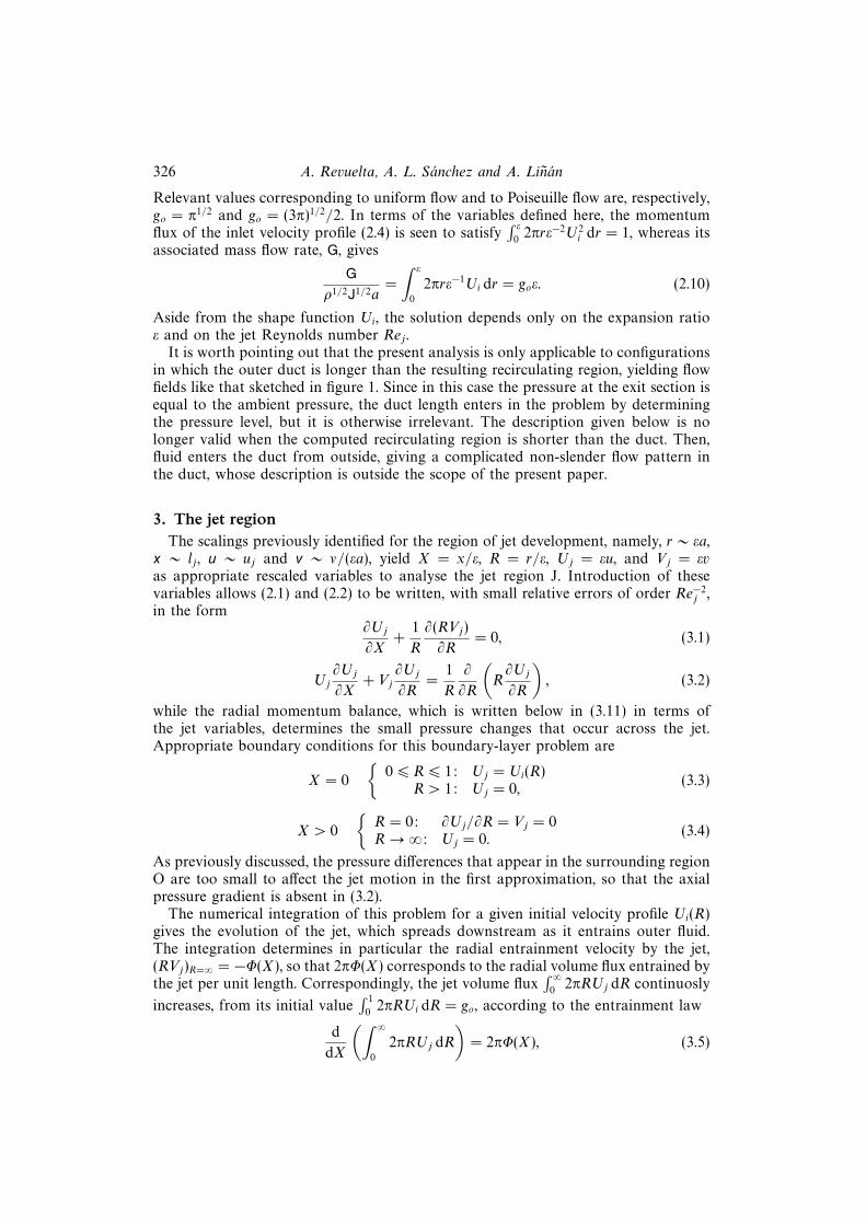
The rate of entrainment Φ(X) corresponding to an initially uniform velocity profileUi = π−1/2 and that of a fully developed parabolic profile Ui = (3/π)1/2[1 − R2]are shown in figure 2. As expected, both curves asymptotically approach the valueΦ(X) = 4 as the jet evolves to the self-similar Schlichting solution for increasingvalues of X, a transition that occurs at moderately small values of X, of order 0.1.On the other hand, for X � 1 the entrainment rate is determined by the locallyplanar mixing layer that forms at R = 1 between the jet and the outer stagnant fluid.In general, the initial entrainment rate depends on the wall value of the velocitygradient A = −dUi/dR of the jet. This gradient is A = 2(3/π)1/2 for the parabolicprofile and becomes larger for decreasing values of the boundary-layer thickness.The initial, Goldstein region of the mixing layer can be described by introducing asimilarity variable y = (R − 1)/(X/A)1/3 together with a normalized stream functionG(y) defined such that Uj = A2/3X1/3Gy and Vj = A1/3X−1/3(yGy/3 − 2G/3). Theproblem reduces to that of integrating Gyyy + 2GGyy/3 − G2

y/3 = 0 subject to the

boundary conditions Gy(y →∞) = 0 and G+ y2/2→ 0 as y → −∞ (Goldstein 1930).The boundary condition as y → −∞ comes from imposing that there are no changesin jet velocity in the first approximation, so that the mixing layer entrains fluid onlyfrom the stagnant side. The entrainment rate Φ = (2/3)G∞A1/3X−1/3 is dictated by thevalue G∞ ' 1.258 of the streamfunction at y = ∞; it grows with the cube root of thevelocity gradient at the base of the boundary layer of the incoming jet. The analysismust however be modified when a uniform velocity profile Ui = π−1/2 is considered.The appropriate similarity coordinate in that case is y = (R − 1)/(X/Ui)

1/2 andthe normalized streamfunction G(y) must be defined to give Uj = UiGy and Vj =

U1/2i X−1/2(yGy/2−G/2). The resulting equation, Gyyy+GGyy/2 = 0, must be integrated

with boundary conditions Gy(y → ∞) = 0 and G − y → 0 as y → −∞, a problemsolved by Chapman (1949) and Lessen (1950). The corresponding entrainment rate

becomes Φ = (1/2)G∞U1/2i X−1/2, where G∞ ' 1.238 is computed from the above

problem. In summary, the entrainment rate for X � 1 varies in general according toΦ = CX−α, where C ' 1.049 and α = 1/3 for a Poiseuille jet profile and C ' 0.465and α = 1/2 for a uniform profile. These asymptotic forms of the entrainment ratefor X � 1 are included for completeness in the plots shown in figure 2.

For X � 1 the solution to (3.1)–(3.4) approaches a self-similar solution in whichthe jet acts in the first approximation as a point source of momentum (Schlichting1933). The condition of constant momentum flux, together with simple order-of-magnitude estimates in (3.1) and (3.2), indicate that the radius of the jet increaseslinearly with distance, while the velocity components decrease according to Uj ∝ X−1

and Vj ∝ X−1. These scalings motivate the introduction of a similarity coordinateη = R/X, together with expansions in decreasing powers of X of the form Uj =X−1U1

j (η) +X−2U2j (η) + · · · and Vj = X−1V 1

j (η) +X−2V 2j (η) + · · · . Introducing these

new variables into (3.1) and (3.2) gives a sequence of ordinary differential equationsto be integrated with boundary conditions dUk

j /dη = Vkj = 0 at η = 0 and Uk

j = 0as η → ∞. As explained by Revuelta, Sanchez & Linan (2001), the solution for thefirst two terms in the expansion can be expressed jointly by introducing an apparent


10

8

6

4

2

0 0.2 0.4

Φ

(a)30

20

10

0 0.2 0.4

(b)

δPj

10

8

6

4

2

0 0.2 0.4

Φ

30

20

10

0 0.2 0.4

δPj

(a)

(b)

X X

Figure 2. The function Φ(X) (left-hand plots) and the pressure jump δPj(X) (right-hand plots) fora fully developed parabolic profile (a) and for a initially uniform velocity profile (b); dashed linesrepresent the asymptotic behaviors for X � 1 and X � 1.

origin XO in the axial coordinate, a development that yields

Uj =1

X +XO

512π/3

(64π/3 + η2)2, Vj =

1

X +XO

4η(64π/3− η2)

(64π/3 + η2)2, (3.7)

where the modified similarity coordinate η = R/(X+XO) also incorporates a dilatationassociated with the apparent origin. The solution satisfies the boundary conditionsgiven in (3.4) together with the additional integral constraint (3.6).

The value of the apparent origin can be calculated from continuity considerations.Thus, integrating (3.5) gives the increasing jet volume flux∫ ∞

0

2πRUj dR = go + 8π

(X +

∫ X

0

(Φ/4− 1) dX

), (3.8)

which can be evaluated at X � 1, using (3.7), to yield

8π(X +XO) = go + 8π

(X +

∫ ∞0

(Φ/4− 1) dX

), (3.9)

and then

XO =

∫ ∞0

(Φ/4− 1) dX +go

8π. (3.10)

The value of XO is seen to depend on the shape of the initial velocity distributionthrough the value of the initial volume flux go and also through the distribution ofentrainment rate Φ(X). Sample values of XO are 0.130 for the uniform jet and 0.095for the parabolic velocity profile.

The boundary-layer approximation presented here could be extended to higher


orders by accounting for smaller terms to determine, for instance, the variations ofpressure that occur across the jet. These can be computed by integrating the radialcomponent of the momentum equation

∂Pj

∂R= −Uj

∂Vj

∂X− Vj ∂Vj

∂R+

∂

∂R

(1

R

∂(RVj)

∂R

), (3.11)

in which pressure differences Pj are scaled with its characteristic value ρu2j /Re

2j . The

total pressure jump across the jet, δPj(X) = Pj(R = 0, X) − Pj(R = ∞, X), wascomputed for uniform and Poiseuille inlet velocity profiles. The resulting distributionsare shown in figure 2, along with their associated values for X � 1 and for X � 1.In the Schlichting region corresponding to X � 1, the presure increment simplifies toδPj = [3/(8π)](X +XO)−2, as can be obtained by integrating (3.11) with use made ofthe asymptotic velocity profiles (3.7). On the other hand, the solution for the mixinglayers at X � 1 yields δPj = (G2∞Ui/4)X−1 for the uniform velocity profile Ui = π−1/2

and δPj = (8/27)G2∞A2/3X−2/3 for the Goldstein mixing layer that forms otherwise,where the velocity gradient A takes the value A = 2(3/π)1/2 for the Poiseuille velocityprofile.

The problem of finding the pressure distribution in the jet is in principle coupledto the solution in the outer region O, which determines the boundary value for Pj asR →∞. When Re2

j ε4 � 1 the analysis is simpler, in that the pressure variations in O,

of order ρε4u2j , are smaller than those occurring across the jet, of order ρu2

j /Re2j , and

can be consequently neglected when integrating (3.11). Differentiating the resultingvalue of δPj determines the axial pressure gradient along the axis, which takes forinstance the value

∂Pj

∂X= − 3/(4π)

(X +XO)3(3.12)

for X � 1, a result to be used later.The value of δPj calculated above increases as the inlet is approached, so that at

distances from the jet exit of the order of the pipe radius εa, the pressure jump acrossthe mixing layer becomes of order ρu2

j /Rej for the initially uniform velocity profile

and of order ρu2j /Re

4/3j for a non-uniform velocity profile. These pressure increments

will also be found at distances of order εa upstream from the jet exit, inducing smallchanges in the axial velocity of order uj/Rej for the uniform velocity profile and

smaller changes of order uj/Re4/3j otherwise. The calculation of these perturbations

at the mouth of the pipe requires the solution of an elliptic problem, which we do notcarry out in this paper because these perturbations are small, and do not influencethe flow at the pipe exit at the leading order considered here. Similarly, the pressuredifferences found in regions O, M and T are also much smaller than ρu2

j . Therefore,in confined jets with ε � 1 the initial velocity profile ui at the pipe exit, which isassumed to be a known boundary condition in our analysis, can be calculated withoutaccounting for pressure changes in the recirculating flow by analysing the flow in thepipe with the pressure at its exit assumed to be equal to the pressure at the ductoutlet when this is downstream, and not too far, from region T.

4. Fluid motion outside the jetAs previously anticipated, the fluid motion in region O, in the vicinity of the

backstep, is induced by the jet entrainment, and it depends on the effective Reynoldsnumber Rea = Rejε. Adequate variables of order unity to describe the flow field


at distances of order lj = Reaa from the backstep, where u ∼ ε2uj , v ∼ ν/a, andp ∼ ρε4u2

j , are X = x/ε, Uo = u/ε, Vo = v and P = p/ε2. Introducing these variablesinto (2.1)–(2.3) gives

∂Uo

∂X+

1

r

∂(rVo)

∂r= 0, (4.1)

Uo

∂Uo

∂X+ Vo

∂Uo

∂r= − ∂P

∂X+

1

r

∂

∂r

(r∂Uo

∂r

)+

1

Re2a

∂2Uo

∂X2, (4.2)

1

Re2a

(Uo

∂Vo

∂X+ Vo

∂Vo

∂r

)= −∂P

∂r+

1

Re2a

∂

∂r

(1

r

∂(rVo)

∂r

)+

1

Re4a

∂2Vo

∂X2. (4.3)

Appropriate boundary conditions for X > 0 are

r = 1:

{Uo = Vo = 0 (non-slip flow)∂Uo/∂r = Vo = 0 (slip flow).

(4.4)

Also, the velocity near the axis must match with that in the jet for R � 1,

r → 0: rVo = −Φ(X), r∂Uo

∂r= − 1

Re2a

dΦ

dX. (4.5)

At the backstep wall (0 < r 6 1), the solution must satisfy the non-slip condition

X = 0: Uo = Vo = 0. (4.6)

To write the remaining boundary conditions one needs to study the solution to (4.1)–(4.3) as X → ∞, where the entrainment rate reaches the constant value Φ(X) = 4,and where the solution in O matches with that of the main region M.

4.1. Asymptotic solution for X � 1

At distances X � 1 where Φ(X) = 4, equations (4.1)–(4.5) have an exact self-similarsolution, with the radial velocity independent of X, while the axial velocity and thepressure gradient both increase linearly with distance. Introducing the self-similarvariables

X � 1: Uo = [X +XO − go/(8π)]U(r), Vo = V (r), (4.7)

and dP/dX = [X +XO − go/(8π)]Λ into (4.1) and (4.2) gives

U + (1/r)(rV )r = 0 (4.8)

Urr +Ur(−V + (1/r))−U2 = Λ, (4.9)

to be integrated with boundary conditions rV = −4 at r = 0. For the non-slip solution,the boundary conditions at r = 1 reduce to U = V = 0, while Ur = V = 0 must beused for slip flow. In the notation, the subindex r denotes a derivative in the radialdirection. The boundary conditions at r = 1 correspond to those given in (2.7) and(2.8), while the boundary condition at r = 0 follows from matching the entrainmentrate (4.5) evaluated at X � 1. The translation XO − go/(8π) =

∫ ∞0

(Φ/4 − 1) dXemployed in the expansions for Uo and dP/dX guarantees that the total volume fluxacross the pipe equals εgo in agreeement with (2.10), as can be seen by adding (3.8)

to the outer volume flux∫ 1

02πrUo dr = −8π(X +XO) + go.

For slip flow, the above problem can be integrated exactly to give

U = −8, V = −4(1− r2)/r, Λ = −64. (4.10)

On the other hand, the solution for non-slip flow is facilitated by writing the problem


1.0

0.8

0.6

0.4

0.2

0 1 2 3 4

r

–rV(r)

1.0

0.8

0.6

0.4

0.2

–20 –15 –10 –5 0

r

U(r)

0

Figure 3. The radial variation of the functions U(r) and F = −rV .

in terms of the stream function ψ(r, X) = [X+XO−go/(8π)]F(r). Substituing U = Fr/rand V = −F/r in (4.9) yields

Frrr + Frr(F − 1)/r + Fr(1− rFr − F)/r2 = Λr, (4.11)

to be integrated with boundary conditions

F(1) = Fr(1) = 0, F(0) = 4. (4.12)

Integration of the above problem by a shooting method determines the function Fas well as the unknown constant Λ = 12.258. Profiles of F = −rV and U = Fr/r aredisplayed in figure 3. The integrations were initiated at r � 1, where the function Fdepends on three unknown constants according to F = 4+Λr4/48+A1r

2 +A2 +A3r−2.

The two constants A2 = A3 = 0 must be chosen to satisfy the boundary conditionF(0) = 4, yielding F = 4 + Λr4/48 + A1r

2 as the starting solution at 0 < r � 1. Anembedded Runge–Kutta–Fehlberg method of fourth and fifth order was employed inthe numerical integrations, with the shooting constants A1 and Λ being corrected tosatisfy the two conditions F = Fr = 0 at r = 1 via a Newton–Raphson formula. Avalue A1 = −9.695 was found for the solution with Λ = 12.258 shown in figure 3.

It is worth mentioning that the solution to (4.11) is not unique; a second solution,corresponding to Λ = −387.438 and A1 = −33.976, also exists. Unlike the solutionin figure 3, for which the velocity U is negative everywhere, the axial velocity of thesecond solution vanishes at an intermediate radial location and becomes positive nearthe wall. Multiple solutions also appear in the solution with slip flow: integrationof (4.11) with Frr = Fr (Ur = 0) replacing the non-slip condition Fr = 0 at r = 1gives, in addition to the uniform velocity profile U = −8 previously discussed, asecond solution for Λ = −194.690 and A1 = −25.244 with positive U near the wall.To test the validity of these additional solutions as intermediate asymptotic profiles


corresponding to X � 1 and x� 1, their associated velocity profiles were employedin the boundary condition for integration of the flow in region M. The resultingintegration showed profiles that evolved rapidly to recover those corresponding tofigure 3 for non-slip flow and those given in (4.10) for slip flow, only two or threegrid points away from the boundary. This outcome indicates that these additionalsolutions of (4.11) are irrelevant; although they are similarity solutions of the flow inO for X � 1, they do not satisfy the matching condition with the solution in M, andcan be therefore discarded in the following development.

4.2. Leading-order solution in O

The Navier–Stokes equations (4.1)–(4.3) were integrated with boundary conditions(4.4)–(4.7) for different values of the parameter Rea and with entrainment-rate lawsΦ(X) corresponding to both uniform and Poiseuille inlet velocity profiles. The resultsshown in figures 4 and 5 correspond to a uniform inlet profile with non-slip flow atr = 1. The equations were solved with the simple algorithm introduced by Patankar& Spalding (1972) and Patankar (1980). The problem was formulated as unsteady byincluding false time derivatives in the two components of the momentum equation,and was integrated in time until the steady state was reached. A three-level fullyimplicit scheme in time and second-order centred schemes for the spatial derivativeswere used for the discretization of the momentum equations. These were solved inevery time step with an alternating direction implicit (ADI) procedure. The singularbehaviour of the scaled radial velocity Vo near the axis was avoided in this problemby replacing the variable Vo with (rVo). The graphs shown correspond to a minimumradius of the integration equal to 0.01. No significant differences were observed in theresults obtained with other values (e.g. 0.02, 0.005). Also, the numerical integrationswere performed with the boundary condition as X → ∞ evaluated at differentlocations X � 1 to guarantee that the results are independent of this selection. Inparticular, for the integrations shown here the profiles (4.7) were evaluated at X = 5.

Figure 4(a, b) exhibits streamlines corresponding to Rea = 1.0 and 2.5. As expected,the jet entrainment causes the resulting streamlines to deflect towards the axis, exceptnear the corner, where a recirculating eddy emerges. With the streamfunction Ψdefined in the usual manner with Ψ = 0 at the wall, the streamlines ending at theaxis correspond to equal increments δΨ = 0.25 from this value, while for the slowrecirculating flow the spacing of the streamlines is δΨ = 10−4. According to Moffatt(1964), the non-slender recirculating eddy must be followed by an infinite series ofStokes corner eddies of decaying size and strength, but this local detail of the flowpattern could not be resolved in our computation.

Figure 5 represents the evolution with distance of the scaled pressure gradient∂P/∂X along the wall. The pressure gradient, which increases linearly with distancefor X � 1, becomes negative at an intermediate location, then reaches a minimumvalue and eventually becomes positive again as the corner is approached. The com-parison of figures 4 and 5 reveals that the location of minimum pressure gradientcoincides approximately with the reattachment point of the streamline bounding therecirculating eddy.

Note that the structure of the flow field near the corner does not change significantlywith Rea, although this outcome is not apparent in figure 4 because of the scaleused for the coordinate X. To compare the different non-slender eddies, it is moreappropriate to use the radius a to scale both the radial and axial coordinate, as isdone in figure 6 to be discussed below.

Note also that the results obtained with an entrainment rate Φ(X) corresponding to


1.0

0.8

0.6

0.4

0.2

0 0.1 0.2 0.3 0.4 0.5 0.6 0.7 0.8 0.9 1.0

(a)

r

1.0

0.8

0.6

0.4

0.2

0 0.1 0.2 0.3 0.4 0.5 0.6 0.7 0.8 0.9 1.0

(b)

r

1.0

0.8

0.6

0.4

0.2

0 0.1 0.2 0.3 0.4 0.5 0.6 0.7 0.8 0.9 1.0

(c)

r

1.0

0.8

0.6

0.4

0.2

0

(d)

r

–3.0

X

Figure 4. Solution in the outer region O with non-slip flow at r = 1 and uniform inlet velocityprofile for (a) Rea = 1.0, (b) Rea = 2.5, and (c) Rea = ∞ (BL). Streamlines ending at the axiscorrespond to increments δΨ = 0.25 from the Ψ = 0 value at the wall, while streamlines ofrecirculating fluid correspond to decrements δΨ = −10−4 from this same value. (d ) Velocity profilesfor the boundary-layer results are given at X = (0.025, 0.1, 0.25, 0.5, 0.75) with the velocity scaleindicated at X = 0.5 and with the asymptotic profile Uo = [X+XO − go/(8π)]U at X = 0.1 (dashedline) being included for comparison.


20

10

0

–10

–20

–30

–400 0.2 0.4 0.6 0.8 1.0

0 0.2 0.4

8

6

4

2

0

BL

BL

Rea = 2.5

Rea = 1.0

∂P∂X

X

Figure 5. The evolution of the axial pressure gradient ∂P/∂X at the wall obtained in region O withnon-slip flow at r = 1 and uniform inlet velocity profile for Rea = 1.0, Rea = 2.5, and Rea = ∞. Theinset shows a magnification of the pressure gradient for Rea = ∞, with the dashed line representingits asymptotic behaviour at X � 1.

a Poiseuille profile change only marginally from those exhibited above for the uniforminlet profile. In particular, the streamlines of the recirculating eddy and the pressurefield found at the corner are very similar in both cases. For instance, the pressuregradient along the wall for Rea = 2.5, which reaches a minimum ∂P/∂X ' −16.53at X ' 0.066 in figure 5, with Poiseuille entrainment exhibits a minimum value∂P/∂X ' −14.79 at X ' 0.061. Significant quantitative changes are only found nearthe origin, where differences in the entrainment rate are more strongly felt, therebymodifying the velocity field in agreement with (4.5). For the case of slip flow at thewall, the differences with the results in figures 4 and 5 are more pronounced, andaffect in particular the flow pattern near the corner, where there is no recirculatingeddy.

4.2.1. The limit of large Reynolds numbers, Rea � 1

In this limiting case, the boundary-layer approximation can be used to describe theflow in O at distances from the backstep of order lj = Reaa, as can be seen by takingthe limit Rea →∞ in (4.1)–(4.3). The corresponding equations, obtained by replacing(4.3) with ∂P/∂r = 0 and by neglecting the last term in (4.2), can be integrated withboundary conditions (4.4) and (4.5) and with an initial velocity profile at X � 1 givenin (4.7). Since the function U(r) shown in figure 3 is negative everywhere, the flowis directed towards the backstep in this outer region for X � 1, and the resultingproblem becomes parabolic in decreasing values of X. Integration can be performed


by marching from X � 1 towards the backstep, provided Uo remains negative acrossthe pipe, a result that was verified in the computations.

When slip flow is considered at r = 1, the boundary-layer problem can be integratedexactly to give

Uo = −2

∫ X

0

Φ dX, Vo = −Φ(1− r2)/r,dP

dX= −4Φ

∫ X

0

Φ dX. (4.13)

Numerical integration is required to solve the problem however when non-slip bound-ary conditions at r = 1 are employed. The procedure was implemented with an implicitnumerical scheme. Although the presence of a singularity in Φ at X = 0 complicatesthe computation of the solution in the inmediate vicinity of the backstep, the integra-tion could be extended to values of X as small as X = 2 × 10−3. Entrainment ratesΦ(X) corresponding to both uniform and parabolic jets were considered. Since onlybackflow (negative values of Uo) was found in the computations, the parabolicity ofthe problem and the validity of the results obtained up to the smallest value of Xcomputed is guaranteed.

Results corresponding to a uniform inlet velocity profile are shown in figures 4 and5. Figure 4 represents streamlines, with the plot (d ) exhibiting the associated velocityprofiles Uo at different axial locations. Following the transition of the entrainmentrate to the Schlichting solution observed in figure 2, the axial velocity profiles areseen to evolve rapidly towards the asymptotic solution Uo = [X + XO − go/(8π)]U,as shown in the figure by comparing at X = 0.1 the asymptotic velocity profilewith that obtained numerically. On the other hand, figure 5 represents the evolutionwith distance of the normalized pressure gradient dP/dX, along with its asymptoticbehaviour dP/dX = [X + XO − go/(8π)]Λ corresponding to X � 1. Although thecomputation reveals a negative pressure gradient at X � 1, the associated decelerationwas not enough to reverse the backflow in the domain computed.

Note that the boundary-layer approximation can be expected to fail at distancesx ∼ a from the backstep (X ∼ Re−1

a ), in a region where u ∼ v ∼ Reαaν/a. Forthe analysis of this inviscid region of strong streamline deflection, not given here,the rescaled variables ReaX, Re1−α

a Uo, Re−αa Vo and Re2(1−α)

a P should be introduced.Boundary conditions for the associated Euler equations must consider the largeentrainment rate Φ = CX−α at the axis as well as the velocity profiles found at theend of the boundary-layer region.

4.2.2. The limit of small Reynolds numbers, Rea � 1

In the opposite limit Rea � 1, the region of streamline deflection x ∼ a, wherethe characteristic velocity components are u ∼ v ∼ ν/a, is much larger than theregion of jet development. To describe the outer motion, it is therefore convenientto use a and ν/a as scales for lengths and velocities. They lead to the rescaled axial

coordinate X = x/a = ReaX and modified variables Uo = u/(ν/a) = ReaUo and

P = p/(ρν2/a2) = Re2aP , to be used to write the conservation equations (4.1)–(4.3)

in a form independent of Rea. The resulting parameter-free Navier–Stokes equationsmust be integrated with boundary conditions, obtained by neglecting small terms oforder Rea in (4.4)–(4.7), given by

X > 0:

r = 0: rVo = −4

r = 1:

{Uo = Vo = 0 (non-slip flow)

∂Uo/∂r = Vo = 0 (slip flow)

(4.14)


and

0 < r 6 1:

{X = 0: Uo = Vo = 0

X = ∞: Uo = XU(r), Vo = V (r).(4.15)

The resulting flow field is similar to those given above for finite values of Rea.Specifically, in an r–X plot the resulting streamline pattern is practically identical tothat shown in the r–X plot of figure 4 for Rea = 1. In this limiting case Rea � 1,the flow near the origin approaches the similarity Navier–Stokes solution proposedby Schneider (1981). This region of self-similar flow corresponds to distances fromthe jet entrance much smaller than a and yet much larger than lj = Reaa, so that theentrainment rate at the axis becomes constant.

As previously noted, the flow-field structure at the corner is weakly dependenton the value of Rea, an outcome that is investigated in figure 6(a), where thestreamlines corresponding to values of the rescaled streamfunction Ψ = ReaΨ =(0,−10−4,−2 × 10−4) are plotted for the three rescaled Reynolds numbers Rea =(0, 1.0, 2.5). The agreement obtained is seen to be excellent for the values of Reaconsidered. For the axial pressure field at the wall, the results in figure 5 suggest thatthe difference between the axial pressure gradient and its asymptotic value at X � 1,∂P/∂X = [X+XO−go/(8π)]Λ, scales with Re−1

a . To further elucidate this issue, we alsorepresent in figure 6(b) the variation of ReaδP = Rea{∂P/∂X− [X+XO−go/(8π)]Λ}along the wall for Rea = (1.0, 2.5) and also for Rea = 0 (ReaδP = ∂P /∂X − ΛX).Again, the agreement found further confirms that the flow pattern at the corner isweakly dependent on Rea, so that the solution for Rea = 0 remains accurate even formoderately large values of Rea.

5. The main recirculating regionThe conservation equations in M are those given above in (2.1)–(2.3), which reduce,

with small relative errors of order Re−2j , to the boundary-layer equations

∂u

∂x+

1

r

∂(rv)

∂r= 0, (5.1)

u∂u

∂x+ v

∂u

∂r= −dp

dx+

1

r

∂

∂r

(r∂u

∂r

). (5.2)

These equations are to be integrated with an initial velocity profile determined bymatching the solution in M with the solution in regions J and O. Thus, combiningthe outer solution for X � 1 given in (4.7) with the Schlichting solution given in (3.7)yields, with relative errors of order ε2,

u =[x+ ε

(XO − go

8π

)]U(r) +

512π

3(x+ εXO)

(64π

3+

r2

(x+ εXO)2

)−2

(5.3)

for the velocity profile at x = 0. To proceed with the asymptotic analysis, expansions inpowers of ε (or, alternatively, in powers of Re−1

j , since both procedures are equivalentin the distinguished limit Rejε ∼ 1 used here) should be introduced for the differentflow variables. Solving the resulting problem arising at each order then produces therequired solution in a sequential manner. Since the boundary-layer equations (5.1)–(5.2) and the associated initial velocity profile (5.3) have relative errors of order Re−2

j

and ε2, respectively, they can be used to calculate the first two terms in the asymptotic


1.00

0.96

0.92

0.88

0.84

0.800 0.04 0.08 0.12 0.16 0.20

(a)

r

0

–10

–20

–30

–40

–500 0.1 0.2 0.3 0.4 0.5 0.6

XRea

ReaδP

(b)

Figure 6. (a) Equally spaced streamlines near the corner with δΨ = 10−4 for Rea = 0 (solidlines), Rea = 1.0 (dot-dashed lines) and Rea = 2.5 (dashed lines); (b) the corresponding incrementalpressure gradient ReaδP along the wall.

expansion presented below. Details of the finite-volume scheme used to integrate theboundary-layer equations are given in an appendix.

5.1. Leading-order description

At leading order, the problem reduces to that of integrating (5.1) and (5.2) withboundary conditions at the axis and on the wall given in (2.6)–(2.8), and with an


1.0

0.8

0.6

0.4

0.2

0 0.02 0.04 0.06 0.08 0.10 0.12

(a)

x

r

1.0

0.8

0.6

0.4

0.2

0

r

(b)

–1.0 1.0

Figure 7. The leading-order solution for the confined jet with non-slip flow at r = 1: (a) streamlines(the stream function for outermost streamline is ψ = 5 × 10−6 and the remaining streamlinescorrespond to increasing values of ψ from ψ = 5 × 10−3 in equal increments δψ = 5 × 10−3) and(b) axial velocity profiles at x = (0.02, 0.04, 0.06, 0.08, 0.10), with the velocity scale indicated for theprofile at x = 0.04.

initial velocity profile

u = xU(r) +512π

3x

(64π

3+r2

x2

)−2

(5.4)

obtained from (5.3) with ε = 0. In this leading-order description, the jet acts as apoint source of momentum with negligible mass flow rate, yielding a parameter-freeproblem independent of the shape of the inlet velocity profile. The mass flux and theshape of the inlet velocity profile will enter at the following order, in agreement with(2.10).

Figures 7 and 8 show the streamlines of the resulting flow field with non-slipand slip flow, respectively, along with characteristic axial velocity profiles at differentdownstream locations. As a result of the zero mass flux associated with the leading-order description, the axial velocity vanishes at a finite location xs and the flowremains stagnant downstream. For non-slip flow, the eddy extends to xs ' 0.106,while due to the absence of viscous forces at r = 1 the eddy length increases toxs ' 0.131 for slip flow. With the stream function ψ defined in the usual manner withψ = 0 along the axis, the maximum value obtained at the eddy centre was seen to beψ = 0.0816 for non-slip flow and ψ = 0.1057 for slip flow. The outermost streamlinedepicted in both plots corresponds to ψ = 5 × 10−6, whereas values of the streamfunction for the remaining streamlines increase from ψ = 5×10−3 in equal incrementsδψ = 5× 10−3 (for non-slip flow) and δψ = 10−2 (for slip flow).

Note that the eddy length xs ' 0.106 calculated here differs significantly from thatobtained in the numerical integrations of axysimmetric sudden expansions reportedin Acrivos & Schrader (1982). Their prediction for the eddy length when ε → 0 can


1.0

0.8

0.6

0.4

0.2

0 0.02 0.04 0.06 0.08 0.10 0.12

(a)

x

r

1.0

0.8

0.6

0.4

0.2

0

r

(b)

–1.0 1.0

Figure 8. The leading-order solution for the confined jet with slip flow at r = 1: (a) streamlines (thestream function for outermost streamline is ψ = 5× 10−6 and the remaining streamlines correspondto increasing values of ψ from ψ = 5× 10−3 in equal increments δψ = 10−2) and (b) axial velocityprofiles at x = (0.02, 0.04, 0.06, 0.08, 0.10, 0.12), with the velocity scale indicated for the profile atx = 0.04.

be written as xs ' 0.119 in terms of the axial coordinate used here. This discrepancymay be explained by recalling that Acrivos & Schrader (1982) treated the case ε� 1only marginally; they were in fact interested in expansion ratios of order unity orsmaller. Perhaps their numerical integrations were not extended to cover sufficientlysmall values of ε, or their numerical scheme was not adapted well to describe thesingular behaviour associated with the jet in the limit ε→ 0.

Figure 9(a) shows the pressure gradient, which is compared with the asymptoticprediction dp/dx = xΛ associated with (5.4). The pressure gradient with non-slipflow increases from a zero initial value at the entrance to reach a maximum valuedp/dx ' 10.49 at x = 0.061. For x > 0.061, dp/dx continuously decreases, vanishingas the eddy rear end is approached. With slip flow at r = 1, the pressure gradientis initially negative, although it eventually becomes positive, reaching a maximumvalue dp/dx ' 6.077 at x = 0.080. The different behaviour can be easily explainedin physical terms. With slip flow at r = 1 the initial pressure gradient is negative asrequired to inviscidly decelerate the outer flow that approaches the backstep, whereasin the case of non-slip flow the pressure gradient is initially positive to overcome theviscous force exerted by the confining wall.

Integration of the pressure gradient provides the pressure variations from the cornervalue, which are also shown in the figure. The final value (p ' 0.593 for non-slipflow and p ' 0.318 for slip flow) gives the total pressure increment associated withthe sudden expansion. Note that the value obtained numerically with slip flow agreeswell with the exact value p = 1/π, determined in this case using the integral form ofthe momentum equation for the fluid volume occupied by the eddy.

For completeness, figure 9(b) also shows the evolution with x of the axial velocity


12

8

6

0 0.04 0.08 0.12

0.1

0.2

0.3

0.4

0.5

0.6

0

NS

(a)

p

103

102

101

100

10–1

10–20 0.04 0.08 0.12

NS

S

S6

4

2

0

–2

0.3

0.2

0.1

0

–0.10 0.04 0.08 0.12

0.0

–0.1

–0.2

–0.3

–0.4

–0.50 0.04 0.08 0.12

x x

dpdx

dpdx

p

u(r

= 0

, x)

u(r

= 1

, x)

(b)

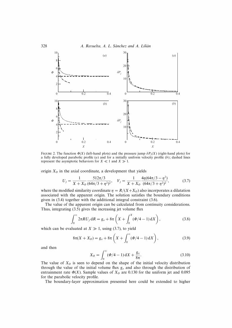
Figure 9. (a) The pressure gradients (solid lines) and associated leading-order pressure distributions(dot-dashed lines) corresponding to the confined jet with both non-slip flow (NS) and slip flow (S),and (b) the corresponding distributions of axial velocity at the axis (upper plot) and at the wall(lower plot); dashed lines represent the asymptotic predictions for x� 1 and for (xs − x)� 1.

u along the axis (for both non-slip and slip flow) and also at the wall (for slip flow).The results are compared with the boundary solutions u = 3/(8πx) at r = 0 andu = −8x at r = 1 obtained from (5.4) for x� 1. The velocity along the axis is seen toevolve from the large jet value to the vanishing values found as the stagnation plane,x = xs, is approached, showing a disparity of scales that is exhibited in the plot byusing a logarithmic scale for u. The negative velocity at the slip wall is seen to reacha minimum value u = −0.433 at a location x = 0.0582 upstream from the point ofmaximum pressure gradient.

5.2. First-order corrections

The solution described above represents at leading order the flow field in region M.The first-order correction, of order ε, must satisfy the linearized form of the boundary-layer equations (5.1) and (5.2) subject to an initial condition determined by linearizing(5.3) about the leading-order solution. Combining the leading-order results with thecorrection in a two-term expansion would then provide a description for the flow field


in the main region M with small relative errors of order ε2. This expansion fails atx = xs, where the correction for the axial velocity is seen to develop a logarithmicsingularity proportional to ln(xs − x) as the leading-order solution vanishes. As seenbelow in (6.7), the description of the transition region towards the final downstreamsolution must account for the presence of this singularity.

Instead of following this standard procedure, we choose here to integrate (5.1)and (5.2) with the initial velocity profile given in (5.3). This alternative methodyields the solution in M with relative errors of order ε2, just like the two-termexpansion previously discussed. The main advantage is that the resulting solutiondoes not become singular at x = xs, and reproduces the asymptotic flow founddownstream, thereby providing results that can be easily compared with integrationsof the full Navier–Stokes problem (2.1)–(2.9). Nevertheless, the procedure proposedis not expected to describe accurately the solution in the boundary region T , whichis considered separately below.

The results obtained with the initial velocity profile (5.3) are similar to the leading-order results previously described. The main differences stem from the non-zero massflow rate (2.10), which causes the flow downstream to approach either the Poiseuillesolution with a negative constant value of the pressure gradient (if non-slip flow isconsidered) or a uniform velocity profile with zero pressure gradient (for slip flow).Streamlines corresponding to the case ε = 0.05 obtained for a Poiseuille inlet profilewith non-slip outer wall are given in figure 10(e). The results of the integration,notably the resulting eddy length, were seen to be quite independent of the initiallocation used to evaluate (5.3) provided 1 � x & 0.1ε (x = 0.005 for the integrationshown in the figure). As can be seen, the toroidal vortex is very similar to that shownin figure 7 for the case ε = 0. In particular, the streamline separating the recirculatingflow intersects the wall at a location xf that differs by a small amount (xf−xs)/xs ∼ εfrom the eddy length xs of figure 7.

The results of the boundary-layer analysis were compared with numerical integra-tions of the full Navier–Stokes problem formulated in (2.1)–(2.9). As in the integrationof the problem (4.1)–(4.6), the simple algorithm was used. In the computations, (2.9)was replaced with an outflow boundary condition. Streamlines corresponding to val-ues of the Reynolds number ranging from Rej = 20 to Rej = 500 are plotted infigure 10(a–d ). As can be seen, the streamline pattern is very similar for all casesconsidered. The eddy length predicted by the boundary-layer approximation matchesthe results of the Navier–Stokes integrations, although larger discrepancies occur asRej decreases. Note that the corner eddy encountered above in region O also appearsin the Navier–Stokes integrations for the two smaller Rej considered.

Further comparisons between the boundary-layer results and those of the fullintegrations are given in figure 11. Figure 11(c) shows the evolution of the flowvelocity along the axis as obtained with the boundary-layer approximation and withthe Navier–Stokes equations for Rej = 50 and 200. The agreement is very good inboth cases, with the curve for Rej = 200 being practically indistinguishable from thatof the boundary-layer results over the range of x considered.

Comparisons of axial pressure gradients obtained for Rej = 50 and 200 with thatobtained from the boundary-layer approach are given in figure 11(a, b); plot (b) showsthe evolution of ∂p/∂x at the wall. The boundary-layer approximation reproducesaccurately the results for Rej = 200, whereas somewhat larger discrepancies are seenfor the case Rej = 50. Notice also that as the backstep is approached the pressuregradient at the wall reproduces the behaviour predicted in the outer region O, i.e. itexhibits a minimum value that is more pronounced for smaller values of Rea = Rejε.


0.8

0.4

0 0.02 0.04 0.06 0.08 0.10 0.12

(a)

r

0.8

0.4

0 0.02 0.04 0.06 0.08 0.10 0.12

(b)

r

0.8

0.4

0 0.02 0.04 0.06 0.08 0.10 0.12

(c)

r

0.8

0.4

0 0.02 0.04 0.06 0.08 0.10 0.12

(d )

r

0.8

0.4

0 0.02 0.04 0.06 0.08 0.10 0.12

(e )

r

x

Figure 10. Streamlines of the confined jet for ε = 0.05 with non-slip flow at r = 1 and Poiseuille inletvelocity profile as obtained by integrating the boundary-layer equations (5.1) and (5.2) (e) and byintegrating the full Navier–Stokes problem (2.1)–(2.9) for different values of the Reynolds numberRej: (a) Rej = 20, (b) Rej = 50, (c) Rej = 200, (d ) Rej = 500. The recirculating streamlines (solidlines) correspond to increments δψ = goε/(2π) from the ψ = 0 value of the dividing streamline,while streamlines of escaping fluid (dashed lines) correspond to decrements δψ = −goε/(10π) fromthis same value.


12

8

4

0

–4

–8

–12

(a)

0 0.04 0.08 0.12

Rej = 200

Rej = 50

∂p∂p

12

8

4

0

(b)

0 0.04 0.08 0.12

Rej = 200

Rej = 50∂p∂p

x

102

101

100

10–1

10–2

0 0.04 0.08 0.12x

Rej = 200

Rej = 50

(c)

u(r

= 0

, x)

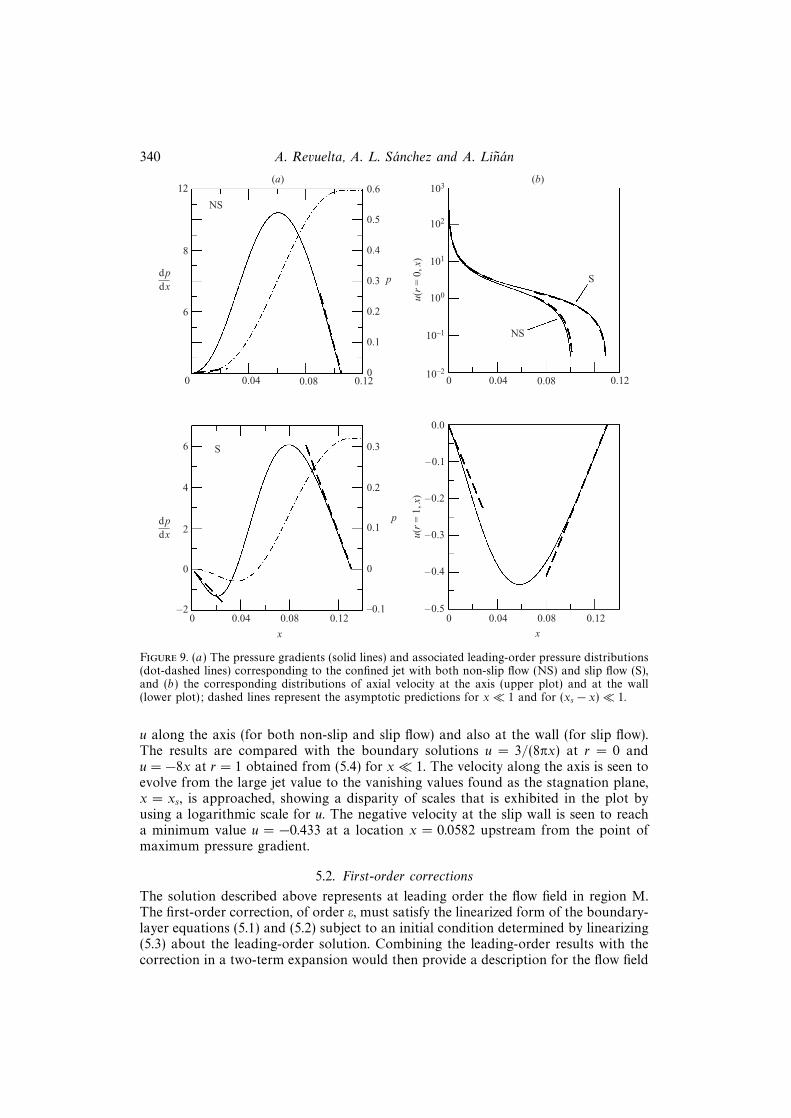
Figure 11. The pressure gradients at the wall (b) and at the axis (a), along with the axial velocitydistribution along the axis (c) as obtained from the boundary-layer results (dashed lines) and fromthe full Navier–Stokes problem (solid lines) for ε = 0.05 with non-slip flow at r = 1 and Poiseuilleprofile at the inlet.

The pressure gradient along the axis is shown in figure 11(a). To account for thepresence of the jet, the pressure gradient of the asymptotic analysis is constructed inthis case by adding the contribution of Schlichting solution ∂p/∂x = −(3/4π)Re−2

j (x+

εXO)−3, calculated above in (3.12), to the distribution obtained in region M from (5.1)and (5.2). The resulting composite expansion for the pressure gradient is seen todescribe well the Navier–Stokes results for the two values of Rej considered.

6. The transition regionAs previously anticipated, the dividing streamline eventually opens up at the rear

end of the recirculating region, leading to a downstream region of parallel flowthrough a short transition region, denoted by T in the sketch of figure 1, whereu is of order ε. If a non-slip wall is considered, as in the calculation of figure 10,then the pressure gradient, which was positive in the recirculating region, becomesnegative somewhere in this transition region, and reaches the Poiseuille value shortlydownstream. A uniform stream with zero pressure gradient replaces the Poiseuillesolution downstream from the transition region if slip flow is considered at r = 1.

The description of the flow structure in region T employes a stretched axialcoordinate X = (x− xe)/ε, where xe is a given location within this region. The choiceof xe is in principle arbitrary; one could for instance use xe = xs or define xe as the


location where the pressure reaches its peak value (in non-slip flow configurations).This arbitrariness will be removed when defining the boundary conditions at X = −∞.Introducing the coordinate X together with the variables Ut = u/ε, Vt = v andP = p/ε2, reduces (2.1)–(2.3) to

∂Ut

∂X+

1

r

∂(rVt)

∂r= 0, (6.1)

Ut

∂Ut

∂X+ Vt

∂Ut

∂r= − ∂P

∂X+

1

r

∂

∂r

(r∂Ut

∂r

)+

1

Re2a

∂2Ut

∂X2, (6.2)

1

Re2a

(Ut

∂Vt

∂X+ Vt

∂Vt

∂r

)= −∂P

∂r+

1

Re2a

∂

∂r

(1

r

∂(rVt)

∂r

)+

1

Re4a

∂2Vt

∂X2, (6.3)

to be integrated with boundary conditions

r = 0: ∂Ut/∂r = Vt = 0 (6.4)

and

r = 1:

{Ut = Vt = 0 (non-slip flow)∂Ut/∂r = Vt = 0 (slip flow).

(6.5)

The boundary conditions far downstream,

X � 1:

{Ut = (2go/π)(1− r2), Vt = 0 (non-slip flow)Ut = go/π, Vt = 0 (slip flow)

(6.6)

follow from rewriting (2.9) for the present variables. For the Poiseuille profile, theassociated pressure gradient becomes dP /dX = −8go/π, while the pressure gradientwith slip flow vanishes as X → ∞. To write the remaining boundary conditionsone needs to study the solution to (6.1)–(6.3) as X → −∞, which matches with theasymptotic results in M as x→ xs.

6.1. Solution for X → −∞For X → −∞ the flow approaches a self-similar solution of the equations, of the typefound downstream from region O. In particular, the radial velocity becomes indepen-dent of X, and the axial velocity and the axial pressure gradient increase linearly withdistance. Appropriate similarity expansions for the different flow variables are

Ut = −U(X + Bgo ln |X|) + BgoU + · · · ,Vt = V (1 + Bgo/X) + · · · ,dP

dX= Λ(X + Bgo ln |X|) + · · · .

(6.7)

Note that the first terms in the expansions above match with the leading-ordersolution in M, whereas the remaining terms would enter when matching with thefirst-order correction, of order ε, which includes a logarithmic singularity as explainedabove.

Introducing these similarity variables into (6.1) and (6.2) yields at leading order

−U + (1/r)(rV )r = 0, (6.8)

Urr + ((1/r)− V )Ur + U2 = −Λ, (6.9)

to be integrated with boundary conditions given in (6.4) and (6.5):

Ur(0) = V (0) = U(1) = V (1) = 0 (6.10)


for non-slip flow and

Ur(0) = V (0) = Ur(1) = V (1) = 0 (6.11)

for slip flow. Use of the similarity stream function XF(r), such that U = −Fr/r andV = −F/r, reduces the problem to that of integrating

Frrr + Frr(F − 1)/r + Fr(1− rFr − F)/r2 = Λr, (6.12)

with boundary conditions

(Fr/r)r = F = 0 (6.13)

at r = 0 and

Fr = F = 0 (non-slip flow)(Fr/r)r = F = 0 (slip flow)

}(6.14)

at r = 1. The equation for F is identical to that previously written in (4.11) for thestream function F downstream from region O.

Apart from the solution F = 0 and Λ = 0, the problem admits a non-trivialsolution for Λ = −348.59 (non-slip flow) and Λ = −162.27 (slip flow), and theassociated velocity profiles U = −Fr/r and V = −F/r are shown in figure 12. Ashooting method was used, as before, to integrate (4.11). Shooting was initiatedat r � 1, where the solution of the above equation is in general of the formF = Λr4/16 + B1r

2 + B2 + B3r2 ln(r). The boundary conditions at r = 0 require

that B2 = B3 = 0, leaving B1 and Λ as shooting parameters to be varied until thetwo boundary conditions at r = 1 were satisfied. The values B1 = −17.698 andB1 = −12.424 were obtained for non-slip and slip flow, respectively.

As previously mentioned, the first terms in the expansions (6.7) match with theleading-order solution in M, which near the stagnation plane admits the simplifiedrepresentation u = (xs − x)U(r), v = V (r), and dp/dx = Λ(x − xs). This result canbe used to further test the accuracy of the boundary-layer solutions obtained byintegrating (5.1) and (5.2). The degree of agreement obtained is illustrated in figures 9and 12. The linear decrease with distance of the pressure gradient and of the axialvelocity seen in figure 9 closely agrees with the asymptotic predictions. Also, theradial velocity distribution near x = xs adjusts to the asymptotic prediction v = V (r),a result that is illustrated in figure 12.

The expansions (6.7) incorporate a higher-order correction U(r) to the axial velocity,which is included to accommodate the non-zero mass flux go, along with appropriateswitchback terms (the second terms in the parentheses), which are necessary to providesolvability for U(r). The correction is determined by the linear problem

Urr +

(1

r− V

)Ur + UU = U2 − V Ur, (6.15)

Ur(0) = U(1) = 0 (non-slip flow)Ur(0) = Ur(1) = 0 (slip flow).

}(6.16)

The resulting profile U(r) is shown in figure 13. The constant B appearing in (6.7) is

given by B =(∫ 1

02πrU dr

)−1

, yielding B = 0.01981 for non-slip flow and B = 0.01953

for slip flow.

6.2. Leading-order solution

The expressions given in (6.7) for the velocity components complete the boundaryconditions needed to integrate (6.1)–(6.3), which are invariant under translations in X.


1.0

0.8

0.6

0.4

0.2

0 1 2 3 4 5

S

NS

r

V(r)

1.0

0.8

0.6

0.4

0.2

0–10 0 10 20 30 40

S

NS

U(r)

r

Figure 12. The radial variation of the functions U(r) and V (r) with non-slip boundary conditions(NS) and with slip boundary conditions (S); the dashed line represents the radial velocity profile ofthe overall solution for ε = 0 evaluated at x = 0.102 (NS) and at x = 0.129 (S).

One could arbitrarily choose the origin of X incorporating a translation of magnitudeXT in the boundary condition, by using Ut = −U(X+XT +Bgo ln |X|)+BgoU insteadof the corresponding expansion shown in (6.7). In the results presented below, thisarbitrariness was removed by choosing XT = 0.

The numerical procedure employed is identical to that developed for integrating(4.1)–(4.3). Streamlines of the resulting flow field with non-slip flow at r = 1 and aPoiseuille inlet velocity profile are exhibited in figure 14(a, b) for Rea = 1.0 and 2.5. Thedividing streamline is here assigned the value Ψ = εψ = 0. Solid lines correspond topositive values of Ψ (recirculating fluid) equally spaced in increments δΨ = go/(2π),whereas the spacing used for the negative values of Ψ equals δΨ = go/(10π). Ascan be seen, a result of our selection for XT is that the dividing streamline intersectsthe wall at an axial location X 6= 0 which varies with Rea. The transition towardsthe final Poiseuille solution occurs downstream from this location, in a region thatbecomes shorter as the Reynolds number increases, a behaviour also observed in thenumerical computations of the overall problem shown in figure 10.

Results corresponding to Rea → ∞ are also included in figure 14(c). In that case,(6.1)–(6.3) reduce to the boundary-layer equations, with ∂P /∂r = 0 replacing (6.3)and with the last term neglected in (6.2). The axial velocity profile given in (6.7) isemployed as the initial condition in the integration. As can be seen, the streamlinesare similar to those obtained with Rea = 2.5, indicating that the boundary-layer limitapproximates well the structure of the transition region even for values of Rea only


1.0

0.8

0.6

0.4

0.2

0 20 40 60

(a)

r

1.0

0.8

0.6

0.4

0.2

0 20 40 60

(b)

r

U

Figure 13. The radial variation of the function U(r) with (a) non-slip boundary conditions and(b) with slip boundary conditions.

moderately large. For completeness, the plot includes axial velocity profiles obtainedwith the boundary-layer approximation at different downstream locations.

The dependence of the solution on Rea is further illustrated in figure 15, wherethe axial pressure gradient at the axis (plot a), at the wall (plot b), and the velocitydistribution along the axis (plot c) are shown for the three cases of figure 14. Theplot reproduces the trends observed previously: the transition to the final Poiseuillesolution is more abrupt for larger values of Rea, and the quantitative agreementbetween the boundary-layer results and those of the Navier–Stokes integrations isalready apparent for Rea = 2.5.

Small modifications should be incorporated in the problem formulation to describethe region of streamline deflection in the limit Rea � 1, a development that parallelsthe analysis of region O in this same limit. The characteristic axial length of streamlinedeflection, x − xe ∼ a, and the characteristic axial velocity, u ∼ ν/a, must be used indefining appropriate rescaled variables X = ReaX, Ut = ReaUt and P = Re2

aP . Useof these variables enables the parameter Rea to be scaled out of the Navier–Stokesequations (6.1)–(6.3). Apart from (6.4) and (6.5), the rescaled velocity must satisfy Ut =−UX and Vt = V at X = −∞ and Ut = Vt = 0 at X = ∞, the leading-order boundaryconditions obtained by neglecting in (6.6) and (6.7) terms that vanish when Rea → 0.With a zero mass flux, the leading-order solution must show for X → ∞ a velocitythat decays with X at an exponential rate, eventually giving rise to the Stokes toroidalvortices described by Wakiya (1976). This leading-order description can be expected


1.0

0.8

0.6

0.4

0.2

0–1.0 –0.8 –0.6 –0.4 –0.2 0 0.2 0.4 0.6 0.8 1.0

(a)

r

1.0

0.8

0.6

0.4

0.2

0–1.0 –0.8 –0.6 –0.4 –0.2 0 0.2 0.4 0.6 0.8 1.0

(b)

r

1.0

0.8

0.6

0.4

0.2

0–1.0 –0.8 –0.6 –0.4 –0.2 0 0.2 0.4 0.6 0.8 1.0

(c)

r

1.0

0.8

0.6

0.4

0.2

0

r

–3 3

X

(d)

Figure 14. Solution in the transition region with non-slip flow at r = 1 and Poiseuille velocity profileat the inlet for (a) Rea = 1.0, (b) Rea = 2.5, (c) Rea = ∞. Recirculating streamlines (solid lines) corre-spond to increments δΨ = go/(2π) from theΨ = 0 value of the dividing streamline, while streamlinesof escaping fluid (dashed lines) correspond to decrements δΨ = −go/(10π) from this same value.(d ) Velocity profiles for the boundary-layer results are given at X = (−0.6,−0.3, 0.0, 0.3, 0.6), withthe velocity scale indicated in the plot at X = −0.3.


400

300

200

100

0

–2 –1 0 1 2

Rea = 1.0

(a)

Rea = 2.5

∂P∂X

400

300

200

100

0

–2 –1 0 1 2

Rea = 1.0

(b)

Rea = 2.5∂P∂X

40

30

20

10

0–2 –1 0 1 2

Rea = 2.5

Rea = 1.0

(c)

Ut(

r =

0, X

)

X X

Figure 15. The pressure gradients at the wall (b) and at the axis (a), along with the axial velocitydistribution along the axis (c) as obtained from the boundary-layer results (dashed lines) and fromthe full Navier–Stokes problem (solid lines) for the transition region of figure 14.

to fail as Ut decays to values of order Rea, where the mass flux should be taken intoaccount, eventually leading to either the Poiseuille profile or a uniform velocity profile.

7. ConclusionsRound laminar jets with coaxial confinement are investigated when the jet Reynolds

number and the expansion ratio are both large quantities. The long recirculatingregion that forms in this case is seen to be bounded at both ends by relatively shortboundary regions. All regions have been described separately for relevant values ofthe parameters involved, including the distinguished limit Rejε ∼ 1 for the analysisof the slow fluid motion in the boundary regions. The asymptotic analysis providesin particular quantitative results of practical interest, including the length of therecirculating eddy (0.106

√J/ρa/ν for non-slip flow and 0.131

√J/ρa/ν for slip flow)

and its associated pressure increment (0.593J/a2 for non-slip flow and 0.318J/a2 forslip flow). The asymptotic description has been validated through comparisons withresults of integrations of the Navier–Stokes equations for moderately large values ofRej and 1/ε.

The analysis presented herein has attempted to address in as much generality aspossible the description of confined laminar jets with large expansion ratios. Never-theless, our work has deliberately ignored some limiting cases that are left for futurework, including the analysis of confined and unconfined jets with Reynolds numbersof order unity and smaller. Confined jets with Rej � 1 and with exponentially large


expansion ratios such that ε ∼ exp(−Re2j /15.28), when momentum decay in the jet

region becomes important, is another limiting case that deserves further attention,since it provides the transition from the confined jets analysed here to the unconfinedjets of Schneider (1985).

The type of asymptotic treatment presented here can also be useful to addressstability, which should be treated in future work. Also of interest is the extensionof the present work to combustion applications, when a compound jet, formed forexample by a fuel jet and a coaxial air jet, discharges in the chamber. While a numberof papers have been recently published on flame stabilization in axisymmetric freejet flows (see, e.g., Lee & Chung 1997 and Chen & Bilger 2000), the effect ofconfinement on the stabilization mechanism remains unclear. It can be expected thatthe composition of the recirculating gases plays an important role in the stability ofthe combustion process, an issue to be clarified in future work.

The extension of the analysis to cover turbulent flows also deserves investigation.The solution of laminar and turbulent free jets is known to be alike, in that, byreplacing ν by an appropriate eddy viscosity, Schlichting analysis is seen to reproducewell the results of turbulent jets. It can therefore be expected that a similar simpleanalysis with slip flow considered at the outer wall applies in confined turbulent jets.Matching the recirculating length obtained with the boundary-layer approximationwith that found in turbulent flows seems to be an appropriate criterion for theselection of the eddy viscosity in that case.

The authors are indebted to Professor F. Higuera and to Mr J. D. Mellado forenlightening discussions on the subject. The work of A. R. and A. L. S. was supportedby the Spanish DGESIC under project number PB98-0142-C04-02, while that of A. L.was supported by the Spanish CICYT under contract no PB94-0400.

Appendix. Boundary-layer numerical schemeA pseudo-transient finite-volume scheme was used to integrate the boundary-layer

equations in the main region. The conservation equations, written in conservative form,and with a time derivative artificially added to the momentum balance equation, wereintegrated until convergence to a steady solution was achieved. The time scheme wasa generalized implicit Crank–Nicholson scheme in the radial coordinate and explicitin the axial coordinate. Second-order centred schemes were used for the spatialderivatives. This treatment involves the solution of a tridiagonal system of the linearequations for every axial position and time step.

The method employed to solve the problem is equivalent to that of Brady & Acrivos(1982) . The pressure gradient is obtained as part of the solution, to conserve mass.For the n + 1 time step dp/dxn+1 = dp/dxn + δ(dp/dx) and un+1 = u? + δu, and thetime-discretization of the momentum equation is set as

r(u? − un)∆t

= (1− β)

[∂

∂r

(r∂u?

∂r

)− ∂(rvnu?)

∂r

]+β

[∂

∂r

(r∂un

∂r

)− ∂(rvnun)

∂r

]− ∂(runun)

∂x− r dp

dx

n

(A 1)

and δu = −∆t × δ(dp/dx), where the correction of the axial velocity δu = εgo/π −∫ 1

02ru? dr is computed from the mass-conservation condition (2.10). Finally the values

of the radial velocity vn+1 are calculated with the continuity equation from the valuesof the axial velocity.


The value of the β-parameter used for the Crank–Nicholson scheme was β = 0.25,a compromise between β = 0.5, which tends to produce nonlinear instabilities,and β = 0, corresponding to the full implicit scheme, which yields less accurateresults. The axial convective term determines the time step selected according to∆t = CFL × ∆xmin/|Umax|, with a CFL = 1 being utilized in the computations. Theresults presented below correspond to a grid that is uniformly distributed in the axialdirection with spacing δx = 1.0× 10−3. The radial node distribution is non-uniform,with minimum spacing δr = 1.03 × 10−3 near the axis and also near the wall. Theconvergence criterion selected was that the variation of the pressure gradient alongthe axis at each time step was much smaller than the corresponding integration timestep, i.e.

∑ |dp/dxn+1 − dp/dxn| � ∆t.The numerical method was tested extensively. For instance, the accuracy of the final

numerical solutions was checked by evaluating the integral form of the momentumequation applied to the recirculating fluid, yielding an error of less than 0.6% forthe calculations shown below. Different modifications were introduced to furthervalidate the numerical scheme proposed. It was seen that streching of the axialcoordinate does not provide significant improvement. Alternative discretizations thatwere tested include a three-level implicit scheme in time for the radial coordinate, andhigh-order upwind schemes (Drikais & Tsangaris 1993) for the x-convective term.These alternative discretizations enable larger time steps in the computation, but nosignificant differences were observed in the accuracy of the final results.

To analyse the grid-dependence of the results, the leading-order problem of figure 7,which was calculated with a grid of NX×NR = 120× 75 nodes, was also computedwith a coarser grid of 60×50 nodes (δx = 2.0×10−3 and minimum δr = 1.65×10−3)and with a finer grid of 180× 100 nodes (δx = 6.67× 10−4 and minimum δr = 7.45×10−4), yielding an error in the momentum integral balance equal to 1% and 0.4%,respectively. The values of the maximum pressure gradient (= 10.419, 10.492, 10.515)and eddy length (= 0.108, 0.1062, 0.1056) were seen to vary only by a small amountwith grid refinement for the three grids employed, with differences between the twofinest grids being smaller than 0.6%. To study the influence of the time step on thefinal results and the stability of the numerical method, different values of the CFLranging from 0.5 to 3 were used. Negligible differences in the final results were foundfor the same grid.

REFERENCES

Acrivos A. & Schrader, M. L. 1982 Steady flow in a sudden expansion at high Reynolds numbers.Phys. Fluids 25, 923–930.

Allerborn, N., Nandakumar, K., Raszillier, H. & Durst, F. 1997 Further contributions on thetwo-dimensional flow in a sudden expansion. J. Fluid Mech. 330, 169–188.

Batchelor, G. K. & Gill, A. E. 1962 Analysis of the stability of axisymmetric jets. J. Fluid Mech.14, 529–551.

Battaglia, F., Kulkarni, A. K., Feng, J., & Merkle, C. L. 1998 Simulations of planar flappingjets in confined channels. AIAA J. 36, 1425–1431.

Battaglia, F., Tavener, S. J., Kulkarni, A. K. & Merkle, C. L. 1997 Bifurcation of low Reynoldsnumber flows in symmetric channels. AIAA J. 35, 99–105.

Brady, J. F. & Acrivos, A. 1982 Closed-cavity laminar flows at moderate Reynolds numbers.J. Fluid Mech. 115, 427–442.

Chapman, D. R. 1949 Laminar mixing of a compressible fluid. NACA-TN 1800.

Chen, Y. C. & Bilger, R. W. 2000 Stabilization mechanisms of lifted laminar flames in axisymmetricjet flows. Combust. Flame 123, 23–45.


Cherdron, W., Durst, F. & Whitelaw, J. H. 1978 Asymmetric flows and instabilities in symmetricducts with sudden expansions. J. Fluid Mech. 84, 13–31.

Drikakis, D. 1997 Bifurcation phenomena in incompressible sudden expansion flows. Phys. Fluids9, 76–87.

Drikakis, D. & Tsangaris, S. 1993 On the solution of the compressible Navier–Stokes equationsusing improved flux vector splitting. Appl. Math. Modelling 17, 282–297.

Durst, F., Melling, A. & Whitelaw, J. H. 1974 Low Reynolds number flow over a planesymmetrical sudden expansion. J. Fluid Mech. 64, 111–128.

Durst, F., Pereira, J. C. F. & Tropea C. 1993 The plane symmetric sudden-expansion flow at lowReynolds numbers. J. Fluid Mech. 248, 567–581.

Fearn, R. M., Mullin, T. & Cliffe, K. A. 1990 Nonlinear flow phenomenon in a symmetric suddenexpansion. J. Fluid Mech. 211, 595–608.

Goldstein, S. 1930 Concerning some solutions of the boundary-layer equations in hydrodynamics.Proc. Camb. Phil. Soc. 26, 1–30.

Hawa, T. & Rusak, Z. 2000 Viscous flow in a slight asymmetric channel with a sudden expansion.Phys. Fluids 12, 2257–2267.

Hawa, T. & Rusak, Z. 2001 The dynamics of a laminar flow in a symmetric channel with a suddenexpansion. J. Fluid Mech. 436, 283–320.

Klemp, J. B. & Acrivos, A. 1976 A moving-wall boundary layer with reverse flow. J. Fluid Mech.76, 363–381.

Kumar, A. & Yajnik, K. S. 1980 Internal separated flows at large Reynolds numbers. J. FluidMech. 97, 27–51.

Lee, B. J. & Chung, S. H. 1997 Stabilization of lifted tribrachial flames in a laminar nonpremixedjet. Combust. Flame 109, 163–172.

Lessen, M. 1950 On the stability of the laminar free boundary between parallel streams. NACA-R979.

Macagno, E. O. & Hung, T-K. 1967 Computational and experimental study of a captive annulareddy. J. Fluid Mech. 28, 43–64.

Milos, F. S. & Acrivos, A. 1986 Steady flow past sudden expansions at large Reynolds numbers.Part I: Boundary layer solutions. Phys. Fluids 29, 1353–1359.

Milos, F. S. & Acrivos, A. 1987 Steady flow past sudden expansions at large Reynolds numbers.Part II: Navier–Stokes solutions for the cascade expansion. Phys. Fluids 30, 7–18.

Moffatt, H. K. 1964 Viscous and resistive eddies near a sharp corner. J. Fluid Mech. 18, 1–18.

Mollendorf, J. C. & Gebhart, B. 1973 An experimental and numerical study of the viscousstability of a round laminar vertical jet with and without thermal buoyancy for symmetric andasymmetric disturbances. J. Fluid Mech. 61, 367–399.

Nathan, G. J., Hill, S. J. & Luxton, R. E. 1998 An axisymmetric fluidic nozzle to generate jetprecession. J. Fluid Mech. 370, 347–380.

Patankar, S. V. 1980 Numerical Heat Transfer and Fluid Flow. Hemisphere.

Patankar S. V. & Spalding, D. B. 1972 A calculation procedure for heat, mass and momenttransfer in three-dimensional parabolic flows. Intl J. Heat Mass Transfer 15, 1787–1806.

Revuelta, A., Sanchez, A. L. & Linan, A. 2002 Laminar mixing in diluted and undiluted fuel jetsupstream from lifted flames. Combust. Flame, In Press.

Reynolds, A. J. 1962 Observations of a liquid-into-liquid jet. J. Fluid Mech. 14, 552–556.

Rusak, Z. & Hawa, T. 1999 A weakly nonlinear analysis of the dynamics of a viscous flow in asymmetric channel with a sudden expansion. Phys. Fluids 11, 3629–3636.

Schlichting, H. 1933 Laminare strahlausbreitung. Z. Angew. Math. Mech. 13, 260–263.

Schneider, W. 1981 Flow induced by jets and plumes. J. Fluid Mech. 108, 55–65.

Schneider, W. 1985 Decay of momentum flux in submerged jets. J. Fluid Mech. 154, 91–110.

Shapira, M., Degani, D. & Weihs, D. 1990 Stability and existence of multiple solutions for viscousflow in suddenly enlarged channel. Comput. Fluids 18, 239–258.

Wakiya, S. 1976 Axysimmetric flow of a viscous fluid near the vertex of a body. J. Fluid Mech. 78,737–747.

Zauner, E. 1985 Visualization of the viscous flow induced by a round jet. J. Fluid Mech. 154,111–119.

Confined axisymmetric laminar jets with large expansion ratios

Documents

Transcript of Confined axisymmetric laminar jets with large expansion ratios