Investigations on Key Principles of PTP1B Selectivity - Refubium
193
Investigations on Key Principles of PTP1B Selectivity Dissertation zur Erlangung des akademischen Grades des Doktors der Naturwissenschaften (Dr. rer. nat.) eingereicht im Fachbereich Biologie, Chemie, Pharmazie der Freien Universität Berlin vorgelegt von Alexandra Vanessa Olympia Naß Berlin 2018
-
Upload
khangminh22 -
Category
Documents
-
view
1 -
download
0
Transcript of Investigations on Key Principles of PTP1B Selectivity - Refubium
Investigations on Key Principles
of
PTP1B Selectivity
Dissertation zur Erlangung des akademischen Grades
des Doktors der Naturwissenschaften (Dr. rer. nat.)
eingereicht im Fachbereich Biologie, Chemie, Pharmazie
der Freien Universität Berlin
vorgelegt von
Alexandra Vanessa Olympia Naß
Berlin
2018


Die vorliegende Arbeit wurde von Oktober 2013 bis April 2018 unter der
Leitung von Prof. Dr. Gerhard Wolber am Institut für Pharmazie der
Freien Universität Berlin angefertig.
1. Gutachter: Prof. Dr. Gerhard Wolber
2. Gutachter: Prof. Dr. Peter Kolb
Disputation am 08. Juni 2018


Acknowledgements
First of all I want to express sincere gratitute to my supervisor Prof. Dr. Gerhard Wolber.
Without his relentless scientific advice this thesis would not have been possible.
I am especially grateful for the freedom I enjoyed in his group and the happy and open-
minded working athmosphere.
This pleasant environment relies heavily on all people involved. I therefore would also
like to thank all my former and present co-workers in the AGWolber, especially Robert
Schulz for being a smart-ass and David Schaller for an awesome Moonlight Session at
the GCC.
I would also like to thank Prof. Dr. Peter Kolb for agreeing to co-examine this thesis.
Further I would like to thank the supervisors of the EUROPIN PhD program for their
critical discussions on my work. Here I want to mention Prof. Dr. Wolfgang Sippl and
Prof. Dr. Gerhard Ecker who enabled my first steps in Computational Drug Design.
I am grateful to Prof. Dr. Rosanna Maccari for the fruitful collaboration on PTP1B in-
hibitors and other topics.
Thanks also goes to Dr. Annette Kietzmann for her kind support during teaching.
Gratefully acknowledged is the computing cluster Soroban of the FU Berlin and the
help of their support team.
Finally, I want to thank my family for their uncompromising continuous support.


Man sollte sich immer zu Ende wundern.
unbekannt

Contents
1. Introduction 1
1.1. Phosphatases . . . . . . . . . . . . . . . . . . . . . . . . . . . . . . . . . . . . . . . . . . . . 1
1.2. Inhibition of Protein Tyrosine Phosphatase 1B . . . . . . . . . . . . . . . . . . . . 2
2. Aim and Objectives 7
3. Computational Methods 9
3.1. Structural Data . . . . . . . . . . . . . . . . . . . . . . . . . . . . . . . . . . . . . . . . . . . 9
3.1.1. Ligand Databases . . . . . . . . . . . . . . . . . . . . . . . . . . . . . . . . . . . . 9
3.1.2. Crystal Structures and Homology Modeling . . . . . . . . . . . . . . . . . 10
3.2. Conformation Generation . . . . . . . . . . . . . . . . . . . . . . . . . . . . . . . . . . . 11
3.2.1. Protein-Ligand Docking . . . . . . . . . . . . . . . . . . . . . . . . . . . . . . . 11
3.2.2. Molecular Dynamics Simulations . . . . . . . . . . . . . . . . . . . . . . . . 13
3.3. Ligand-Target Complementarity . . . . . . . . . . . . . . . . . . . . . . . . . . . . . . 14
3.3.1. Molecular Interaction Fields . . . . . . . . . . . . . . . . . . . . . . . . . . . . 15
3.3.2. 3D Pharmacophores and Dynophores . . . . . . . . . . . . . . . . . . . . . 15
3.3.3. Shape Complementarity . . . . . . . . . . . . . . . . . . . . . . . . . . . . . . . 16
3.4. Binding Site Shape Clustering . . . . . . . . . . . . . . . . . . . . . . . . . . . . . . . . 17
4. Results 21
4.1. Part I: Protein-Ligand Interaction Analysis . . . . . . . . . . . . . . . . . . . . . . . 21
4.1.1. Sequence Comparison of PTP1B and TC-PTP . . . . . . . . . . . . . . . 21
4.1.2. PTP1B Crystal Structure Analysis . . . . . . . . . . . . . . . . . . . . . . . . 23
4.1.3. TC-PTP Crystal Structure Analysis and Homology Modeling . . . . . 24
4.1.4. Molecular Dynamics Simulations . . . . . . . . . . . . . . . . . . . . . . . . 25
4.1.5. Dynophore Analysis . . . . . . . . . . . . . . . . . . . . . . . . . . . . . . . . . . 29
4.1.6. Shape Complementarity Analysis . . . . . . . . . . . . . . . . . . . . . . . . 38

4.2. Part II: Binding Site Shape Clustering and Screening . . . . . . . . . . . . . . . . 56
4.2.1. Generation of Input Data . . . . . . . . . . . . . . . . . . . . . . . . . . . . . . 56
4.2.2. Bootstrapping and Clustering . . . . . . . . . . . . . . . . . . . . . . . . . . . 57
4.2.3. Selectivity and Interaction Patterns . . . . . . . . . . . . . . . . . . . . . . . 62
4.2.4. Virtual Screening . . . . . . . . . . . . . . . . . . . . . . . . . . . . . . . . . . . . 64
5. Discussion 75
5.1. Part I: Protein-Ligand Interaction Analysis . . . . . . . . . . . . . . . . . . . . . . . 75
5.2. Part II: Binding Site Shape Clustering and Screening . . . . . . . . . . . . . . . . 78
6. Conclusion and Outlook 83
7. Experimental Section 85
7.1. Part I: Protein-Ligand Interaction Analysis . . . . . . . . . . . . . . . . . . . . . . . 85
7.1.1. Sequence Comparison of PTP1B and TC-PTP . . . . . . . . . . . . . . . 85
7.1.2. PTP1B Crystal Structure Analysis . . . . . . . . . . . . . . . . . . . . . . . . 85
7.1.3. TC-PTP Crystal Structure Analysis and Homology Modeling . . . . . 86
7.1.4. Molecular Dynamics Simulations . . . . . . . . . . . . . . . . . . . . . . . . 86
7.1.5. Dynophore Analysis . . . . . . . . . . . . . . . . . . . . . . . . . . . . . . . . . . 86
7.1.6. Shape Complementarity Analysis . . . . . . . . . . . . . . . . . . . . . . . . 87
7.2. Part II: Binding Site Shape Clustering and Screening . . . . . . . . . . . . . . . . 87
7.2.1. Generation of Input Data . . . . . . . . . . . . . . . . . . . . . . . . . . . . . . 87
7.2.2. Selectivity and Interaction Patterns . . . . . . . . . . . . . . . . . . . . . . . 88
7.2.3. Virtual Screening . . . . . . . . . . . . . . . . . . . . . . . . . . . . . . . . . . . . 88
8. Summary 89
9. Zusammenfassung 91
A. Appendix 107
A.1. Modified Version of the POVME2 Tool . . . . . . . . . . . . . . . . . . . . . . . . . . 107
A.2. Shape Complementarity R Script . . . . . . . . . . . . . . . . . . . . . . . . . . . . . . 154
A.3. Cluster Step Selection R Script . . . . . . . . . . . . . . . . . . . . . . . . . . . . . . . . 162
A.4. Pose Consistency R Script . . . . . . . . . . . . . . . . . . . . . . . . . . . . . . . . . . . 175
B. Publications 181

1. Introduction
1.1. Phosphatases
With about 30% of proteins being able to get phosphorylated, reversible phosphoryla-
tion is one of the major posttranslational modification mechanisms [1]. The phospho-
rylation state of a protein is determined by protein kinases, attaching phosphate groups
to proteins, and protein phosphatases, catalyzing the reverse reaction [2]. While the im-
portant role of kinases has been established long ago, phosphatases were erroneously
considered second row enzymes for maintaining a kinase dependent equilibrium until
recently, but are now known to play critical and highly specific roles in many signaling
processes such as growth, proliferation and metabolism [3, 4]. Furthermore have they
been shown to act as positive as well as negative modulators in signaling [5]. Recent
literature suggests that kinases are involved in controlling the amplitude of a signaling
response, whereas phosphatases are controlling rate and duration of a response [6].
Originally, phosphatases were classified into Ser/Thr-specific, Tyr-specific and dual-
specific phosphatases based on their substrate specificity [7]. However, newer studies
do not support this differentiation based on substrate specificity, because many phos-
phatases show a broader range of accepted substrates than expected. Therefore Sacco
et al. suggested a classification based on amino acid sequence similarity of the cat-
alytic sites with Ser/Thr-specific and Tyr-specific phosphatases being further divided
into different subgroups and dual-specific phosphatases classified in one family to-
gether with Tyr-specific phosphatases [7, 8].
Later investigations of phosphatase substrate selectivity interestingly revealed that
they often do not show significant selectivity in vitro, but clear preference to phos-
phorylate certain substrates in vivo. Whereas one part of this in vivo selectivity can
be related to non-catalytic phosphatase domains, regulating their activity or enrich-
ing substrate concentration in the environment of the phosphatase by targeting it to a
certain compartment of the cell, there is still a considerable part of the selectivity that
1
seems to be related to the catalytic domains of the phosphatases. This indicates that
active site directed selective inhibition should be possible, but might be dependend on
assay conditions [8].
Although protein-tyrosine phosphorylation only constitutes less than 1% of protein
phosphorylation activity [1], protein tyrosine phosphatases are encoded by the largest
family of phosphatase genes [9], which depicts their importance in phosphorylation
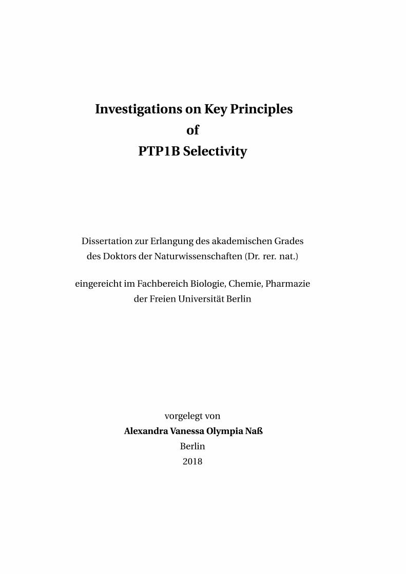
mediated signaling. Protein tyrosine phosphatases share a so-called signature motif,
which is the conserved sequence (H/V)C(X)5R(S/T) in the active site [6]. This motif
includes the cysteine working as the nucleophile of the catalytic substrate reaction as
published by Pannifer et al. (Figure 1.1) [6, 10].
Figure 1.1.: Mechanism of protein-tyrosine phosphorylation. A: Formation ofcysteinyl-phosphate, B: regeneration by hydrolysis. Adapted from Pannifer et al. [10].
1.2. Inhibition of Protein Tyrosine Phosphatase 1B
The most prominent member of the PTP superfamily, PTP1B, was purified over 25 years
ago from human placenta [11]. It consists of 435 amino acids with residues 30-278 sum-
marized as the catalytic domain and 35 C-terminal residues responsible for targeting
the enzyme to the cytosolic face of the endoplasmic reticulum [12]. During many years
of intense studies PTP1B has been validated as a drug target for diabetes and obesity
as well as a promising target for different types of cancer [13, 14, 4]. PTP1B negatively
modulates insulin and leptin signaling [5] and is overexpressed in the mentioned dis-
eases [4]. Figure 1.2 depicts cellular pathways with PTP1B interference.
2
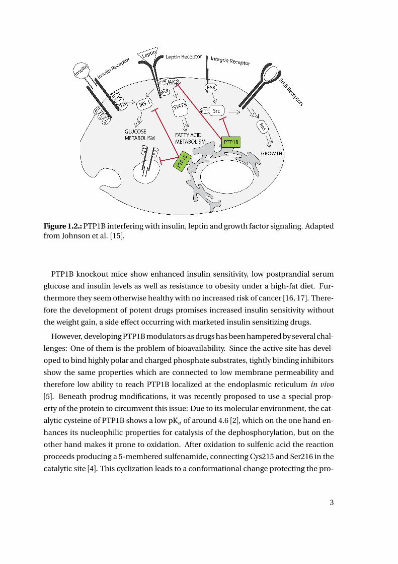
Figure 1.2.: PTP1B interfering with insulin, leptin and growth factor signaling. Adaptedfrom Johnson et al. [15].
PTP1B knockout mice show enhanced insulin sensitivity, low postprandial serum
glucose and insulin levels as well as resistance to obesity under a high-fat diet. Fur-
thermore they seem otherwise healthy with no increased risk of cancer [16, 17]. There-
fore the development of potent drugs promises increased insulin sensitivity without
the weight gain, a side effect occurring with marketed insulin sensitizing drugs.
However, developing PTP1B modulators as drugs has been hampered by several chal-
lenges: One of them is the problem of bioavailability. Since the active site has devel-
oped to bind highly polar and charged phosphate substrates, tightly binding inhibitors
show the same properties which are connected to low membrane permeability and
therefore low ability to reach PTP1B localized at the endoplasmic reticulum in vivo
[5]. Beneath prodrug modifications, it was recently proposed to use a special prop-
erty of the protein to circumvent this issue: Due to its molecular environment, the cat-
alytic cysteine of PTP1B shows a low pKa of around 4.6 [2], which on the one hand en-
hances its nucleophilic properties for catalysis of the dephosphorylation, but on the
other hand makes it prone to oxidation. After oxidation to sulfenic acid the reaction
proceeds producing a 5-membered sulfenamide, connecting Cys215 and Ser216 in the
catalytic site [4]. This cyclization leads to a conformational change protecting the pro-
3
tein from irreversible oxidation and facilitating reactivation by reduction. The resulting
protein cavity, however, is less polar than the reduced version, but more open, and was
suggested as a promising target structure for less polar inhibitors [3].
Unfortunately, the circumstances and the amount of oxidation in vivo are not thor-
oughly discovered. Therefore it remains unclear how relevant targeting this state of
the protein might be for the treatment of the abovementioned diseases. Noteworthily,
this susceptibility to oxidation has caused problems in high-throughput screening, of-
ten including oxidizing or peroxide releasing compounds, which is another obstacle in
inhibitor design for PTP1B [4].
The most challenging part in the development of PTP1B targeting drugs, however,
is related to the high degree of structural conservation throughout the active sites of
PTPs [5]: An especially close relative of PTP1B –TC-PTP –shows an overall identity of
74% in the catalytic domain shared by both proteins and 100% sequence identity of
catalytic site residues (T177-P185, H214-R221, Q266; PTP1B naming). A study by You-
Ten et al.[18] led to the result that TC-PTP knockout mice die within 5 weeks after birth
showing severe defects in T-Cell and B-Cell function. This is supported by the genetic
association of the TC-PTP gene with inflammation and autoimmunity [19]. Therefore
selectivity of PTP1B inhibitors against the highly similar TC-PTP seems strongly ad-
vised to prevent severe side effects in humans. While selectivity was discovered to be
achievable over other PTPs, only few PTP1B inhibitors could be developed to at most
moderate selectivity over TC-PTP [6].
Moreover, complicating structure-based drug design approaches, the flexible WPD
(Trp, Pro, Asp) loop closes upon substrate binding, enabling catalytic activity of the
enzyme. Furthermore, stronger inhibitors seem to bind to the closed conformation of
the active site [15]. While for PTP1B both conformations were resolved in several crystal
structures, there is only one crystal structure publicly available for TC-PTP [20]. This
structure, however, depicts the open WPD loop conformation and therefore the less
relevant structure for inhibitor design. Additionally, this structure is of low quality as
discussed in Section 4.1.3 which restricts its use in detailed structure comparisons.
Despite the mentioned challenges, some progress has been made in the develop-
ment of PTP1B inhibitors which is summarized in several reviews [15, 21, 12]. Major
breakthroughs include: A) Discovery of the difluoromethylene phosphonate group as
phosphotyrosine mimetic, which converted peptidic substrates to inhibitors [22], B)
Identification of a second phosphotyrosine binding site (B-site) close to the catalytic
site with slight differences in amino acid composition in TC-PTP compared to PTP1B
4

[23], C) Identification of early bi-pTYR-mimetic peptides not binding to the second
phosphotyrosine binding site in crystal structures, but showing interactions with Arg47
(C-site), surprisingly still leading to moderate selectivity - about tenfold - against TC-
PTP [24].
Later efforts concentrated on reducing the peptidic character of the inhibitors and
reducing the charge, keeping the bidentate approach to increase selectivity [25, 26, 27,
28, 29]. This lead to carboxylic acid based inhibitors and finally the highly active thia-
diazolidinone and isothiazolidinone derivatives which are stabilized in the active site
by a hydrogen bonding network similar to that of pTYR residues [30, 31, 32, 12]. Figure
1.3 shows the binding site interactions of an thiadiazolidinone-derivative in compari-
son to the interactions of a phenylphosphate ligand. The thiadiazolidinone-derivative
is able to effectively replace almost all hydrogen bonding interactions observed for the
phenylphosphate moiety even replacing the active site water molecule and its medi-
ated interactions. Newer studies state higher selectivity with selectivity ratios up to
45 against TC-PTP, however they lack detailed biological data like inhibition curves or
data from kinetic analyses as well as structural proof of binding mode in form of crystal
structures [33].
Figure 1.3.: Left: Phenylphosphate ligand and water molecule in the active site cavityof PTP1B (derived from PDB structure 1PTY); Right: Isothiadiazolidinone-derivative inthe active site cavity of PTP1B (PDB structure 2GBE); light blue dashed lines representhydrogen bonds.
5

2. Aim and Objectives
This study focuses on structure based design of small, active site, reversible selective in-
hibitors of PTP1B. The moderate selectivity of known substrates and inhibitors lead us
to assume that selectivity can be achieved and increased through targeted interactions
within the active site. Furthermore, we hypothesize that the overall sequence differ-
ences lead to a specific flexible behavior of PTP1B compared to TC-PTP and that those
differences could lead to differing preferred conformations, which can be exploited
to design selective inhibitors. Additionally, the concept of dynamically mapping con-
formational differences to achieve selectivity could be applied to other projects were
specificly targeting one of two or more closely related proteins is crucial.
Based on the abovementioned assumptions two approaches are chosen to increase
selectivity of PTP1B inhibitors:
I) To detect the key factors of selectivity in and around the active site of PTP1B,
crystal structures of the protein in complex with some of the most selective com-
pounds known so far will be investigated thoroughly, starting with
i) analysis of three-dimensional protein structures with special regard to lig-
and interactions with sites of amino acid sequence differences to TC-PTP,
followed by
ii) investigations of the flexible behavior of those complexes using molecu-
lar dynamics simulations and their comparison to the respective TC-PTP-
ligand complexes obtained by homology modeling based on each investi-
gated PTP1B complex structure.
For the investigations of the protein-ligand complexes established modeling meth-
ods like 3D pharmacophores, surface depictions and molecular interaction fields
are employed. The investigations of flexible behavior, however, require more
elaborate methods. For that, dynamic three-dimensional pharmacophores called
7

dynophores [34, 35, 36] as recently established by our group seem suitable. Addi-
tionally, due to the high similarity of the two proteins, it seems reasonable to com-
plement this method concentrating on pharmacophoric features by developing
a method to assess the quality of steric complementarity of protein and ligand
over time. Since this aspect is still neglected in available interaction monitoring
tools, such a tool bears the potential for broader application.
II) The second part explores the flexibility of both proteins without a known selec-
tive inhibitor with respect to possible differences in conformational preferences:
starting with molecular dynamics simulations of both proteins a method will be
developed to classify the occuring conformations into clusters of different bind-
ing site shapes and identify clusters or conformations preferred by PTP1B, but
highly improbable for TC-PTP.
Consequently, the key features of selectivity derived from both approaches will be
integrated into an adapted virtual screening workflow to find commercially available
compounds with high potential to be PTP1B selective inhibitors.
8
3. Computational Methods
This work mainly deals with computational methods which can be subsumed under
the term Computer Aided Drug Design. Since computational power is developing fast
and becoming more affordable, computational methods have become an important
part in drug design, saving money and time by limiting the number of compounds sub-
mitted to more expensive biological tests [37, 38, 39]. Often different methods are com-
bined to reduce the number of false positive predictions [37]. Depending on the avail-
able or utilized data those methods can be divided into ligand- and structure-based
methodologies: ligand-based methods are based on 2D structures of known ligands
and their activities ranging from quantitative structure-activity relationships, as first
developed by Hansch in the 1960s, to three-dimensional pharmacophore generation
[40, 41]. Their interpretability is often limited, since predictions are based on two-
dimensional ligand structures, elaborated guesses of three-dimensional bound con-
formations or calculated descriptors based on those structures. Therefore, if available,
inclusion of structural information of the protein into the process is preferred.
This chapter briefly describes structure-based methods employed in this study divid-
ing them into the sections ”Structural Data”, ”Conformation Generation” and ”Ligand-
Target Complementarity” followed by a section ”Binding Site Shape Clustering” ex-
plaining the method to find differences in binding site conformational preferences de-
veloped specifically for this project and the underlying principle of conformational se-
lection theory.
3.1. Structural Data
3.1.1. Ligand Databases
Small molecules in commercial databases usually contain information of the molecule
together with a two-dimensional representation of the ligand or a string-like encod-
9
ing of the ligand in SMILES format, where the same chemical moiety can be repre-
sented in several ways. Different tools implemented in most modeling software suites
as Schrödinger’s Maestro [42]or CCG’s MOE [43] can be used to convert those structures
into a three-dimensional format as required for most modeling tasks. Furthermore, the
careful assignment of stereochemistry, tautomeric forms and ionization states is nec-
essary [37, 44].
For preparation of the vendor databases used for screening the Chemaxon Standard-
izer toolbox [45] was used, since it allows user-defined conversion rules in addition to
common preset rules for standardization of the molecular input structures and per-
forms well even on huge databases.
3.1.2. Crystal Structures and Homology Modeling
X-ray scattering and NMR spectroscopy allow the determination of three-dimensional
protein structures at almost atomic resolution. However, in common resolution ranges,
which are much lower than 1A, hydrogen atoms cannot be unambiguously assigned
based on the experimental data. Therefore, hydrogen atoms are usually assigned based
on force-field calculations or common protonation rules. Unfortunately, those meth-
ods are not capable to correctly assign unusual protonation states due to surrounding
amino acids as the negative charge of the catalytic cysteine in PTP1B, which therefore
require manual intervention.
Many of the experimentally derived three-dimensional protein structures are de-
posited in the publicly available Protein Data Bank [46] together with information about
their origin and quality. The selection of crystal structure complexes for PTP1B was
driven by the selectivity factor of the complexed ligand and additionally influenced by
the resolution of the structures as a simple quality criterion as well as the occurrence
of mutations in or close to the binding site that could disturb the investigation of inter-
actions.
If no crystal structure is available, homology modeling can be used to build a three-
dimensional structural model from the protein sequence and an experimentally deter-
mined three-dimensional structure of a closely related protein. This technique is based
on the observation that in protein families, structure is usually better conserved than
sequence [47]. The homology modeling process usually starts with the search for a re-
lated protein with known 3D structure, followed by the alignment of both sequences,
the assignment of the respective coordinates from the template to the target and fi-
nally a model refinement step with subsequent evaluation of the model [37]. Homol-
10

ogy modeling has been shown to yield useful models for structure based drug design,
if the pairwise alignment of target and template exceeds 50% [48]. Common protein
structure modeling tools like Modeller [49], PHYRE2 [50] and SWISS-MODEL [51] of-
fer special features like multi-template modelling in addition to automatic template
search [52].
For the single template modeling of the known closely related structure of TC-PTP
based on PTP1B structures (sequence identity 57%), the modeling tool integrated into
the software package MOE [43] was chosen, since it offers detailed control over the
modeling process and additionally allows to take into account a ligand bound to the
template structure in the modeling process.
3.2. Conformation Generation
3.2.1. Protein-Ligand Docking
In structure based drug design, conformation generation of a ligand often is performed
in the form of protein-ligand docking to only obtain ligand conformations that fit the
binding pocket of the protein. Available programs address this problem with different
methodologies. Differences mainly lie in the way they handle ligand flexibility which
can roughly be divided into systematic and random or stochastic approaches [53]. Sys-
tematic methods can further be divided into conformational search based, fragmen-
tation based and database based methods [53]. The most thorough, but also com-
putationally most expensive variant of the different systematic approaches is confor-
mational search, where all rotatable ligand bonds are systematically rotated in small
steps to evaluate all possible combinations [53]. Fragmentation methods try to cir-
cumvent the combinatorial explosion implicated by using conformational search for
ligands with a high number of rotatable bonds by docking one or several parts of the
ligand and then joining or incrementally growing the solution to a docking pose of
the whole ligand [53]. Database based methods seperate the problem of conformation
generation from the binding site fitting step, by precalculating a number of conforma-
tions per ligand and then rigidly docking those precalculated conformations [53]. The
second group of methods to explore ligand conformatinal space employs random or
stochastic methods: here Monte Carlo methods and genetic algorithms are the most
popular subgroups [53]. Monte Carlo methods select poses based on a probability
function, while genetic algorithms start with a population of ligands and by sequen-
11
tially changing and combining parameters of the population members using a fitness
function converge towards a final pose [53, 54]. A prominent program employing a ge-
netic algorithm is the software Gold [54].
The programs also differ in the type of simulation methods they use which can apply
principles of molecular dynamics or energy minimization [55]. Possible conformations
of the ligand are assessed with scoring functions, which can be theory derived or empir-
ical [56]. Often a simpler function is used for prescoring during the conformation gen-
eration process, whereas a more elaborated function is used afterwards to yield more
reliable results for affinity prediction [55]. Currently available scoring functions have
their limitations, for example are most scoring functions focusing on energetic rather
than entropic contributions to binding, which might lead to high ranking errors, if the
binding of a concerned ligand is predominantly entropy driven [55]. Therefore, dock-
ing programs are able to explore the conformational space of ligands sufficiently well
to find binding poses very similar to that found in a crystal structure protein-ligand
complex, but in many cases they are not able to correctly place that pose at the top of
their ranking [57]. Inclusion of target specific information into the ranking process has
been shown to increase prediction quality [57].
A few programs additionally offer the introduction of some degree of conformational
flexibility to the target. This can be achieved by either using different input target con-
formations, known as ensemble docking, or sampling of sidechain conformations, ran-
domly or based on rotamer libraries [55]. However, those artificial changes of a protein
need to be handled with care, since introducing protein flexibility to docking can come
with the cost of increased false positive rates due to less restrictive binding sites, espe-
cially if the cost of the protein movements to these conformations from a low energy
conformation is not accounted for [58].
Common docking programs [56] are AutoDock [59, 60], DOCK [61], FlexX [62], Glide
[63] and GOLD [54]. For this study, GOLD was chosen, since in a comparative study of
docking programs including PTP1B as a target, GOLD performed especially well to re-
cover a high amount of actives with top ranked scores, which seemed not only related
to the high negative charges of the known actives for this target [64]. Subsequent en-
ergy minimization of the resulting poses together with surrounding amino acids was
performed. Careful attention was paid to the fact that energy minimization can intro-
duce hardly recognizable strain in order to optimize directed interactions and therefore
create the illusion of good binding [65].
12
3.2.2. Molecular Dynamics Simulations
A more elaborate way than rotamer changes to sample protein flexibility are molecular
dynamics simulations [66]. Those are simulations of the motions of a macromolecule
in atomic detail with the aim of assessing its accessible conformational space. This can
be done by numerical solution of the classical equations of motion, which is therefore
restricted in accuracy by the available computational power as well as the quality of
available force-fields and includes the following components [67, 68]:
I: System Set-Up. The input structure is inspected and errors are corrected, the
ionization state of the macromolecule is calculated, counter ions and solvent are
included.
II: Force Fields. Forces are calculated for every atom with the help of force-field
equations. Those equations contain parameters for bond stretching, bending
and rotations as well as for non-bonded interatomic interactions like van der
Waals contacts and electrostatic potentials.
III: Laws of Motion Using the previously calculated forces accelerations and ve-
locities are computed using Newton’s law of motion. Initial velocities are usually
assigned randomly based on the overall energy of the system and therefore repli-
cas of the simulation using different initial velocities help to sample the effects of
different starting points.
IV: Trajectory Simulation. With the obtained velocities atom coordinates can
be updated. However, since the calculations include numerical integration, this
needs to be done for a time step of shorter than the fastest movements in the
molecule and is usually preset between 1 and 2 fs. With the repetition of steps II
to IV snapshots of atom coordinates can be saved over a period of time to form
the trajectory.
Common software for molecular dynamics simulations includes AMBER [69], GRO-
MACS [70], Desmond [71] and NAMD [72] and OpenMM [73]. Simulations by those pro-
grams are to a great extent depending on the applied force-field and the model chosen
to represent the solvating water. However, no force-field could be shown to be consis-
tently more feasible for drug design approaches than the others and simulations on one
starting structure with different force-fields often show consistent results [74]. For this
study the freely available Desmond software with OPLS-AA force-field was chosen due
13
to its user-friendliness being integrated into the Maestro software suite and its ability
to assign ligand parameters [71].
Initial analysis steps usually involve calculation of root mean square deviation (RMSD)
and root mean square fluctuation (RMSF). The RMSD is calculated as follows
R M S D =
√
√
√1
n
n∑
i=1
d 2i
with n: number of atoms compared and di : distance of one atom i in one frame com-
pared to a reference frame.
RMDS calculation requires a preceding alignment step of each frame to a reference
structure - usually the starting structure of the simulation - in order to eliminate the
effects of translational and rotational movements of the whole protein during simula-
tion. Plotting of the RMSD of the Cα atoms of a protein over the time of a molecular
dynamics simulation allows conclusions about the stability of a protein structure.
The RMSF describes the atom-wise deviation to a reference structure - usually a mean
structural state of the protein over the simulation or the starting structure of the simu-
lation - averaged over the simulation steps. This allows to identify and compare stable
and unstable regions of a protein over a simulation.
3.3. Ligand-Target Complementarity
Affinity of a ligand to a target is heavily affected by its favorable and repelling interac-
tions. Therefore, investigating these interactions can lead to important insights for the
design of new ligands. The main principles found in almost all high-affinity protein
ligand complexes are high steric complementarity, high complementarity of surface
properties like polarity or hydrophobicity and an energetically favorable ligand con-
formation [75]. However, some of those criteria are easier to assess then others. For
example the entropy contribution to binding free energy is usually not observable in
static structures [76]. Furthermore, a protein-ligand pair can display more than one
stable bound conformation [76]. Additionally, flexible protein parts tend to prefer more
flexible ligand moieties, another aspect hard to observe in static structures [65].
Several concepts have been applied to visualize favorable protein-ligand interactions
or promising interaction sites at a protein surface. The ones that play an in important
role in this study, namely (1) molecular interaction fields, (2) 3D pharmacophores and
14
dynophores as well as (3) shape complementarity calculations will be described below.
3.3.1. Molecular Interaction Fields
Molecular interaction fields (MIFs) depict the spatial distribution of the interaction po-
tential between a target structure and a probe [77, 44]. That means for a given probe,
like a secondary amine nitrogen, this probe is placed at every point of a regular grid
in and around the target structure where its energy of interactions is calculated taking
into account for example the hydrogen bonding energy, van der Waals forces as well
as charge interaction energies. This data can then be depicted in form of an interac-
tion map at a chosen interaction energy threshold for a specified probe. Which terms
of interaction energy and which parameters of the probe are included into the calcu-
lations depends on the implementation of this method, of which the most elaborate
one is found in the software GRID [78, 79]. Since this method was only used to support
the screening model developed based on the binding site shape clustering explained
below, the readily available implementation of the MOE software was considered of
sufficient accuracy.
The application of molecular interaction fields was selected to support screening in
this work, since the developed shape pattern alone would not have been restrictive
enough for virtual screening. Additionally, the shape pattern was designed to introduce
selectivity, which cannot be achieved without activity. Consequently, it was aimed to
introduce activity based on the information on favorable protein-probe interactions.
To combine both the selectivity and the activity model, the format of a 3D pharmaco-
phore (described in the following section) was chosen, since 3D pharmacophores are
particularly efficient for virtual screening [80, 81]. This, however, requires the transla-
tion of molecular interaction field potentials into pharmacophoric features, which was
achieved by calculating the local minima of the computed interaction fields for differ-
ent probes reflecting hydrogen bond donor, hydrogen bond acceptor and hydrophobic
behavior.
3.3.2. 3D Pharmacophores and Dynophores
3D pharmacophores are abstractions of interactions into different types like hydrogen
bonding interactions, hydrophobic contacts and aromatic interactions together with
their spatial arrangement. In a stricter sense like specified in the IUPAC definition,
the term 3D pharmacophore only describes those kinds of three-dimensional interac-
15

tion patterns for which their containing features are ”necessary to ensure the optimal
supramolecular interactions with a specific biological target structure and to trigger
(or to block) its biological response” [82]. In order to ensure that an interaction pat-
tern corresponds to that definition, validation of the model is performed by assuring a
good compromise of retrieval rates of known active and potentially inactive molecules
[75, 83]. Nevertheless, a pharmacophoric feature found with all known ligands does not
mean it is necessary to achieve high affinity binding as well as good pharmacophoric
fit can still lead to low affinity due to e.g. steric clashes [75]. Due to their high level of
abstraction, pharmacophores are especially feasible for scaffold hopping [84].
Common programs for 3D pharmacophore generation and virtual screening are CAT-
ALYST [85], Phase [86], MOE [43], LIGANDSCOUT [80] and FLAP [87]. They show subtle
distinctions in feature definition and placement, as well as more significant differences
in the matching algorithm used for screening, which affects accuracy of the results as
well as screening velocity [88, 84]. In this study the MIF-based interaction patterns were
encoded into LigandScout pharmacophore format, since it is easily interpretable and
manipulatable and allows fast and accurate screening.
Recently, the concept of 3D pharmacophores derived from a protein structure and
a bound ligand was transferred to molecular dynamics simulations of protein-ligand
complexes [34, 35, 36]. This allows the analysis of protein-ligand binding for many dif-
ferent conformations and therefore a more detailed inspection of the stability and qual-
ity of interactions together with the variability of interaction partners on the protein
site. For this purpose, the Dynophore application was used for analysis of molecular
dynamics simulations of higher selective ligands in PTP1B in comparison to simula-
tions of the same ligands in homology models of TC-PTP.
3.3.3. Shape Complementarity
The abovementioned tools for analyzing ligand-target complementarity only cover one
of the three principles of high affinity binding, the high complementarity of surface
properties. Unfortunately, steric complementarity is not sufficiently accounted for in
established methods for monitoring protein-ligand interactions. 3D pharmacophores,
however, often allow specification of excluded volumes, which enable the user to add
spacial restrictions to the interaction pattern and can introduce steric complementar-
ity of the hits to the target [84]. But especially for shape complementarity, assessment
on a single snapshot seems of limited use, due to for example the previously mentioned
tendency of flexible protein parts to prefer more flexible ligand moieties. Therefore
16

a tool was created and implemented in R that can quantify shape complementarity
throughout a whole molecular dynamics trajectory, trace back the complementarity to
certain parts of the ligand and allows the statistical analysis of differences for one ligand
in different protein surroundings [89]. Nevertheless, a particularly good shape fit can
be less energetically favorable, if the ligand is forced into this conformation due to the
lack of better alternatives. In order to detect especially unfavorable ligand conforma-
tions, the ligand strain energy was calculated in addition to the shape fit and they were
assessed together. Strain energy is an estimate of the difference between the energy of
the ligand in the bound state compared to that in the nearest local energy minimum
conformation. The strain energy can be calculated as a MOE 3D descriptor. However,
due to the many simplifications and assumptions integrated in this calculation, the
generated values need to be handled with caution. They are therefore not accurate
enough to be integrated in calculations of ligand binding energy, but still can give im-
portant hints on the twist or strain of a ligand.
3.4. Binding Site Shape Clustering
The method of binding site shape clustering developed in this study to exploit differ-
ences in conformational flexibility of two closely related proteins is based on the con-
cept of conformational selection theory. It is assumed that conformational changes
in the target happen before association with a ligand and that the ligand chooses an
appropriate conformation for binding out of the available ensemble of target confor-
mations. Protein-ligand binding therefore gets likelier with increased presence of suit-
able protein conformations in the ensemble of target conformations as well as with
increased presence of suitable ligand conformations in the ligand conformational en-
semble. This is in line with the abovementioned increased probability to find energet-
ically favorable ligand conformations in high-affinity protein-ligand complexes. Con-
formational selection theory therefore stands in contrast to the concept of induced fit
assuming initial ligand binding to a suboptimal protein conformation followed by an
adaption of the protein to the bound ligand. Recent studies describe increasing evi-
dence for the existence of ligand binding conformations without ligand presence and
assume a dominant role of conformational selection, although the coexistence of both
mechanism cannot be ruled out [90, 91].
The screening process implemented in this study additionally considers ligand rigid-
ity as favorable. Chang et al. state that a ligand binding to a protein loses conforma-
17

tional flexibility resulting in an entropy loss opposing binding [92]. Some sources there-
fore assume that binding of an inflexible ligand is less entropically unfavorable, since
rotational freedom of the ligand was already restricted before binding [93]. However,
experimental evidence for this assumption is scarce, which may be due to the lack ap-
propriate methods for determination of entropic contributions to binding in such de-
tail. Chang et al. additionally stress the downside of rigid ligands: they require an exact
fit of the protein to the ligand and therefore high resolution structures and accurate
predictions in the modelling process, since the ligand’s ability to adapt to the binding
site is limited [92].
Based on those assumptions, the method of binding site shape clustering was de-
veloped: To compare protein conformations with focus on the catalytic binding site
surroundings, the open source tool POVME2 [94, 95], originally created to measure
and compare pocket volumes, is used to depict the shape of the binding site for every
molecular dynamics frame based on equidistant points. Since the tool is used to com-
pare the shapes of the resulting point maps, a preceding alignment step of the molecu-
lar dynamics frames is required. This alignment influences the shape point maps, since
the placement of the initial map points in space stays the same for every frame, only
those points of a bigger map that are very close to or inside the protein are deleted.
The resulting shape point maps are then translated into bit strings encoding pres-
ence or absence of each point of the starting point map in the binding site shape point
map for each molecular dynamics frame respectively using the software R. If molecular
dynamics trajectories of two similar proteins are aligned and binding site shape point
maps are calculated with the same starting point map, the bit strings of both proteins
can be compared. To identify the most prominent conformational states of the binding
sites throughout the molecular dynamics simulations, cluster analysis of the bit string
data was performed. Clustering methods have become a popular means to deal with
the high amount of data from molecular dynamics simulations in different contexts
[96, 97, 98].
Cluster analysis seeks to create homogeneous groups of objects with low inter-cluster
homogeneity in a set of data based on the states or values of their attributes. Cluster-
ing therefore is a valuable tool to structure data, although it has to be considered that
the resulting clusters do not necessarily have a useful interpretation for the analyzed
aspects of the data. Additionally, very different groups can be found for the same set of
data using different clustering algorithms [99]. Since the final cluster size or number of
clusters to obtain was unclear, a hierarchical clustering algorithm was chosen [99]. The
18

term hierarchical clustering covers methods that divide data into a hierarchy of groups
with levels of subgroups and therefore allows for the decision of cluster size to be post-
poned until after clustering. Hierarchical clustering methods can further be divided
into agglomerative methods, starting with singletons and merging clusters until all data
is combined in one cluster, and divisive methods, starting with the whole dataset and
subsequently dividing this set into smaller groups [99]. The chosen clustering method
falls within the category of hierarchical agglomerative clustering methods, because it
starts with each entry being its own cluster and consequently merges clusters in a way
that the increase in dissimilarity sum stays minimal [100].
As clustering algorithm, the function ward.D from the package hclust was used as
implemented in R which is a generalization of Ward’s clustering algorithm [100]. The
Ward algorithm was developed for data that allows calculation of Euclidean distances
and then depicts minimization of the variance of the data in a cluster. Finch showed
that calculating appropriate distance measures for dichotomous data and submitting
the calculated distance matrices to Ward’s clustering can lead to good results repre-
senting the natural groups of the data. However, it has to be considered that the origi-
nal interpretation of minimizing variance is lost, if other than Euclidean distances are
used as input [101]. For calculating the similarity/dissimilarity of two objects the sim-
ple matching coefficient was used here, which is defined as the number of matching
attributes divided by the number of total attributes [102]. This differs for example from
the Russel-Rao Index where only the simultaneous presence, of a state is considered
as matching, but not the simultaneous absence. It was reasoned here that absence of
a point in the map should be weighted the same as its presence, since the total map
size stays the same during the calculations and considering both simultaneous ap-
pearances as matching is therefore not resulting in different weighting of "off" or back-
ground attributes for different frames as had to be considered if the starting map would
have been small in some cases and big in others. Nonetheless, the absence of a point
which is never "on" and therefore never considered part of the binding site is rated as a
similarity with this measure. This was considered negligible since this number should
be small due to the restricted binding site definition.
After clustering, the cluster stage (total number of clusters) useful for analysis is cho-
sen with a variation of the elbow method [103]. The clusters of the selected stage are
further processed: In order to differentiate between conformations possible for both
proteins and those only possible for one of them, an affiliation ratio representing the
number of frames from PTP1B divided by the total number of frames in that cluster
19

was assigned to each of them. Additionally, occupancies are calculated for each point
of the starting point map throughout all frames, representing how often a specific point
is marked as present (1) in the binding site divided by the total number of frames in that
cluster.
Differences of the clusters are then computed to find the PTP1B affiliated cluster that
is most different to all TC-PTP affiliated clusters. After selection of this cluster poten-
tially representing a PTP1B exclusive conformation, the points with significant differ-
ences in occupancy in this cluster compared to all TC-PTP clusters are extracted and
analyzed. They are further used to extract a diverse selection of frames matching this
selectivity map, which can then be used for virtual screening as described in the previ-
ous sections.
All steps processing the POVME2 output were collected in R scripts to ensure easy
adaption and repeating of the steps on different samples.
20

4. Results
4.1. Part I: Protein-Ligand Interaction Analysis
4.1.1. Sequence Comparison of PTP1B and TC-PTP
Sequence alignment with Clustal Omega [104] calculates a total sequence identity of
about 57%. The binding sites of both protein tyrosine phosphatases, however, are highly
conserved: 55 residues were considered as binding site residues and compared. Ac-
cording to Li et al. they were grouped into different subsites named site A (catalytic
site) to site D [105]. The catalytic site shows a sequence identity between both proteins
of over 95%, while all subsites together still show a sequence identity of 80%. Table 4.1
highlights differences in amino acid sequence for the binding site subsites of PTP1B
compared to TC-PTP.
Subsite Residues Sequence PTP1B Sequence TC-PTP
Site AT177-P185 TTWPDFGVP TTWPDFGVPH214-R221 HCSAGIGR HCSAGIGRT263-Q266 TADQ TPDQ
Site B
R254-Q262 RKFRMGLIQ RKYRMGLIQR24-C32 RHEASDFPC RNESHDYPH
Y20 Y YF52 F Y
Site CR47-P51 YRDVSP YRDVSP
K41 K E
Site DK116-C121 KGSLKC KESVKC
R45-Y46 RY RY
Table 4.1.: Sequence comparison of active site surrounding residues (PTP1B number-ing). Differences are highlighted in red.
21
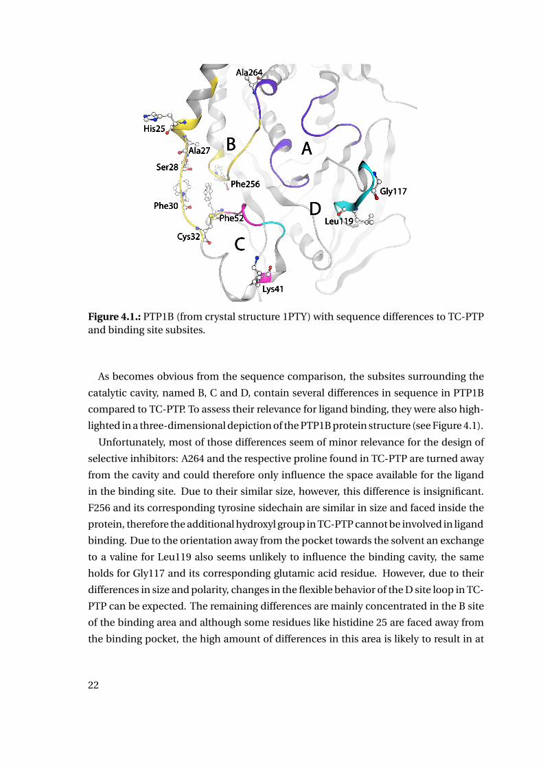
Figure 4.1.: PTP1B (from crystal structure 1PTY) with sequence differences to TC-PTPand binding site subsites.
As becomes obvious from the sequence comparison, the subsites surrounding the
catalytic cavity, named B, C and D, contain several differences in sequence in PTP1B
compared to TC-PTP. To assess their relevance for ligand binding, they were also high-
lighted in a three-dimensional depiction of the PTP1B protein structure (see Figure 4.1).
Unfortunately, most of those differences seem of minor relevance for the design of
selective inhibitors: A264 and the respective proline found in TC-PTP are turned away
from the cavity and could therefore only influence the space available for the ligand
in the binding site. Due to their similar size, however, this difference is insignificant.
F256 and its corresponding tyrosine sidechain are similar in size and faced inside the
protein, therefore the additional hydroxyl group in TC-PTP cannot be involved in ligand
binding. Due to the orientation away from the pocket towards the solvent an exchange
to a valine for Leu119 also seems unlikely to influence the binding cavity, the same
holds for Gly117 and its corresponding glutamic acid residue. However, due to their
differences in size and polarity, changes in the flexible behavior of the D site loop in TC-
PTP can be expected. The remaining differences are mainly concentrated in the B site
of the binding area and although some residues like histidine 25 are faced away from
the binding pocket, the high amount of differences in this area is likely to result in at
22
least subtle differences of the pocket’s shape and electrostatic properties. Furthermore,
Lys41 in the C site could lead to a different conformation of the adjacent C site (YRD)
loop through charge interactions not possible for the corresponding valine in TC-PTP.
4.1.2. PTP1B Crystal Structure Analysis
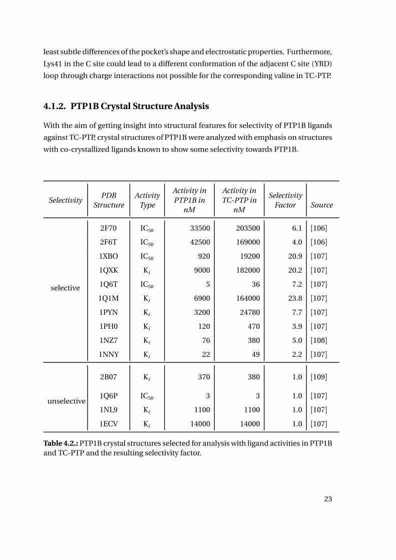
With the aim of getting insight into structural features for selectivity of PTP1B ligands
against TC-PTP, crystal structures of PTP1B were analyzed with emphasis on structures
with co-crystallized ligands known to show some selectivity towards PTP1B.
SelectivityPDB
Structure
Activity
Type
Activity in
PTP1B in
nM
Activity in
TC-PTP in
nM
Selectivity
Factor Source
selective
2F70 IC50 33500 203500 6.1 [106]
2F6T IC50 42500 169000 4.0 [106]
1XBO IC50 920 19200 20.9 [107]
1QXK Ki 9000 182000 20.2 [107]
1Q6T IC50 5 36 7.2 [107]
1Q1M Ki 6900 164000 23.8 [107]
1PYN Ki 3200 24780 7.7 [107]
1PH0 Ki 120 470 3.9 [107]
1NZ7 Ki 76 380 5.0 [108]
1NNY Ki 22 49 2.2 [107]
unselective
2B07 Ki 370 380 1.0 [109]
1Q6P IC50 3 3 1.0 [107]
1NL9 Ki 1100 1100 1.0 [107]
1ECV Ki 14000 14000 1.0 [107]
Table 4.2.: PTP1B crystal structures selected for analysis with ligand activities in PTP1Band TC-PTP and the resulting selectivity factor.
23
Systematic investigation of PTP1B crystal structures was started with 145 crystal struc-
tures of human PTP1B listed in the Uniprot database for human PTP1B (P18031) at the
time of this study (last checked March 2018), 7 of which were excluded from analysis
due to low resolution (>2.70 Å) [110, 46]. Additional 59 structures were excluded due
to covalent modifications in or close to the active site. From the remaining 79 crystal
structure complexes 14 complexes were chosen, for which activity data of the ligands
towards both PTP1B and TC-PTP were available and where the ligands showed either
selective behavior against TC-PTP (selectivity factor > 2) - true for 10 of the structures
- or unselective behavior (selectivity factor between 0.95 and 1.05). Table 4.2 lists the
selected structures with their ligand activities in PTP1B and TC-PTP and the resulting
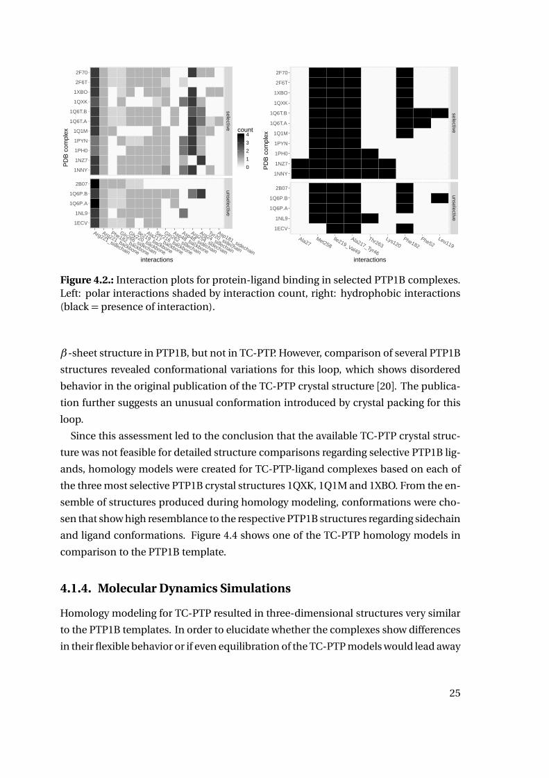
activity factor. Interaction counts for polar interactions, counting hydrogen bonds as
well as ionic interactions as 1 and water mediated hydrogen bonds as 0.5, are depicted
as heat map in Figure 4.2(left). On the one hand, unselective ligands show a tendency
for fewer B site interactions to Gln262, Arg24 and Arg254. On the other hand, polar
interactions to the sidechain of Asp48 and Asp181 seem favorable to introduce selec-
tivity. In the investigated complexes selective ligands additionally show a tendency to-
wards fewer interactions to the backbone of Phe182. For complexes 1Q6T and 1Q6P
crystal packing seems to influence the interactions of the ligand to the protein. Con-
clusions from interaction counts for those structures therefore show a higher level of
uncertainty.
The counts of hydrophobic parts of the ligand interacting with hydrophobic areas on
the protein surface depicted in Figure 4.2(right) show no clear tendency of the interac-
tions to increase or decrease selectivity of the ligands. However, during the investiga-
tion of the crystal structures the missing ability of this method to distinguish between
bigger and smaller lipophilic areas of interaction was noticed.
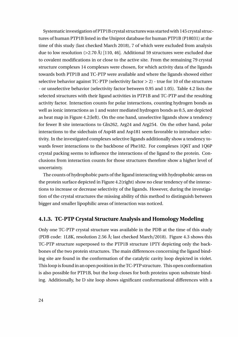
4.1.3. TC-PTP Crystal Structure Analysis and Homology Modeling
Only one TC-PTP crystal structure was available in the PDB at the time of this study
(PDB code: 1L8K, resolution 2.56 Å; last checked March/2018). Figure 4.3 shows this
TC-PTP structure superposed to the PTP1B structure 1PTY depicting only the back-
bones of the two protein structures. The main differences concerning the ligand bind-
ing site are found in the conformation of the catalytic cavity loop depicted in violet.
This loop is found in an open position in the TC-PTP structure. This open conformation
is also possible for PTP1B, but the loop closes for both proteins upon substrate bind-
ing. Additionally, he D site loop shows significant conformational differences with a
24
1NNY
1NZ7
1PH0
1PYN
1Q1M
1Q6T.A
1Q6T.B
1QXK
1XBO
2F6T
2F70
1ECV
1NL9
1Q6P.A
1Q6P.B
2B07
selectiveunselective
Arg221_sidechain
Arg221_backbone
Phe182_backbone
Gln266_sidechain
Gly220_backbone
Ile219_backbone
Ala217_backbone
Ser216_backbone
Gln262_sidechain
Asp48_backbone
Asp48_sidechain
Arg254_sidechain
Arg24_sidechain
Tyr20_sidechain
Asp181_sidechain
interactions
PD
B c
ompl
ex
0
1
2
3
4count
1NNY
1NZ7
1PH0
1PYN
1Q1M
1Q6T.A
1Q6T.B
1QXK
1XBO
2F6T
2F70
1ECV
1NL9
1Q6P.A
1Q6P.B
2B07
selectiveunselective
Ala27Met258
Ile219_Val49
Ala217_Tyr46
Thr263Lys120
Phe182
Phe52Leu119
interactionsP
DB
com
plex
Figure 4.2.: Interaction plots for protein-ligand binding in selected PTP1B complexes.Left: polar interactions shaded by interaction count, right: hydrophobic interactions(black = presence of interaction).
β -sheet structure in PTP1B, but not in TC-PTP. However, comparison of several PTP1B
structures revealed conformational variations for this loop, which shows disordered
behavior in the original publication of the TC-PTP crystal structure [20]. The publica-
tion further suggests an unusual conformation introduced by crystal packing for this
loop.
Since this assessment led to the conclusion that the available TC-PTP crystal struc-
ture was not feasible for detailed structure comparisons regarding selective PTP1B lig-
ands, homology models were created for TC-PTP-ligand complexes based on each of
the three most selective PTP1B crystal structures 1QXK, 1Q1M and 1XBO. From the en-
semble of structures produced during homology modeling, conformations were cho-
sen that show high resemblance to the respective PTP1B structures regarding sidechain
and ligand conformations. Figure 4.4 shows one of the TC-PTP homology models in
comparison to the PTP1B template.
4.1.4. Molecular Dynamics Simulations
Homology modeling for TC-PTP resulted in three-dimensional structures very similar
to the PTP1B templates. In order to elucidate whether the complexes show differences
in their flexible behavior or if even equilibration of the TC-PTP models would lead away
25

Figure 4.3.: PTP1B (PDB code 1PTY) in light grey superposed to TC-PTP (PDB code1L8K) in dark grey. Major conformational differences highlighted in violet and cyan.
from the PTP1B equivalent ligand binding conformation, molecular dynamics simula-
tions were performed and analyzed. For each of the three most selective PTP1B com-
plexes and the respective homology models three simulations with varying seeds were
performed to be able to distinguish effects due to the initially assigned velocities from
system typical behavior during analysis.
For the 1XBO complex and the respective TC-PTP homology model complex, anal-
ysis of the Cα-RMSD plots after backbone alignment (Figure 4.5) showed stable sys-
tem behavior with similarly fast equilibration of the PTP1B and TC-PTP systems after
less than 5 ns and only minor deviations up to 2.1 Å from the starting conformation.
Simulation 1 of the homology model shows a slight RMSD drift towards the end of the
simulation time. Overall, the RMSD plots show a tendency of the homology models for
slightly higher RMSD values, which is in good agreement with the expectations consid-
ering that TC-PTP was forced into a PTP1B conformation during homology modeling.
Similar behavior is found for the 1Q1M complex and the respective TC-PTP homology
model complex (Figure 4.6). However, the differences between PTP1B and TC-PTP are
smaller, suggesting that the homology model based on 1Q1M is slightly closer to a na-
tive TC-PTP structure.
26
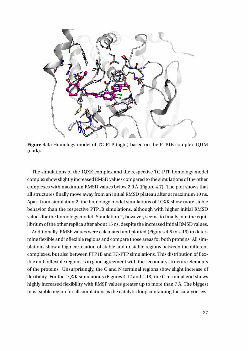
Figure 4.4.: Homology model of TC-PTP (light) based on the PTP1B complex 1Q1M(dark).
The simulations of the 1QXK complex and the respective TC-PTP homology model
complex show slightly increased RMSD values compared to the simulations of the other
complexes with maximum RMSD values below 2.0 Å (Figure 4.7). The plot shows that
all structures finally move away from an initial RMSD plateau after at maximum 10 ns.
Apart from simulation 2, the homology model simulations of 1QXK show more stable
behavior than the respective PTP1B simulations, although with higher initial RMSD
values for the homology model. Simulation 2, however, seems to finally join the equi-
librium of the other replica after about 15 ns, despite the increased initial RMSD values.
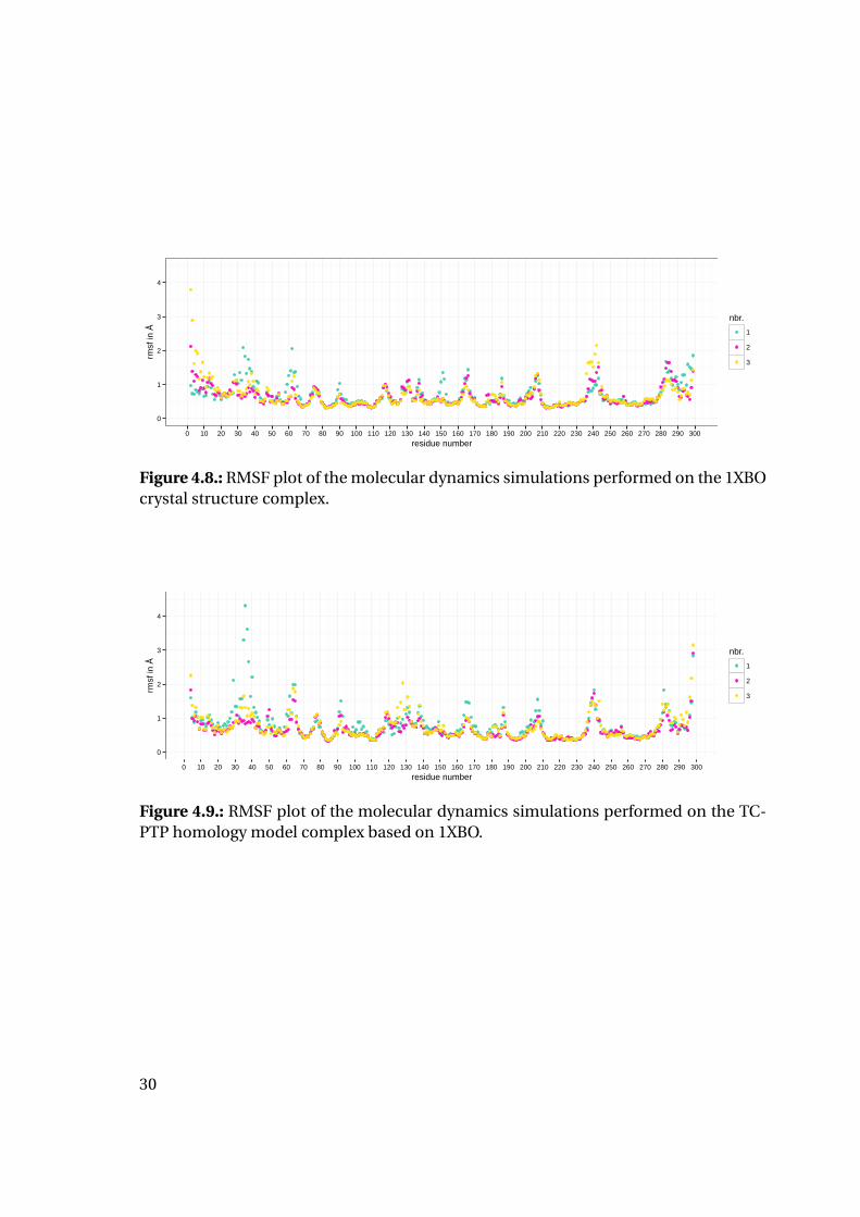
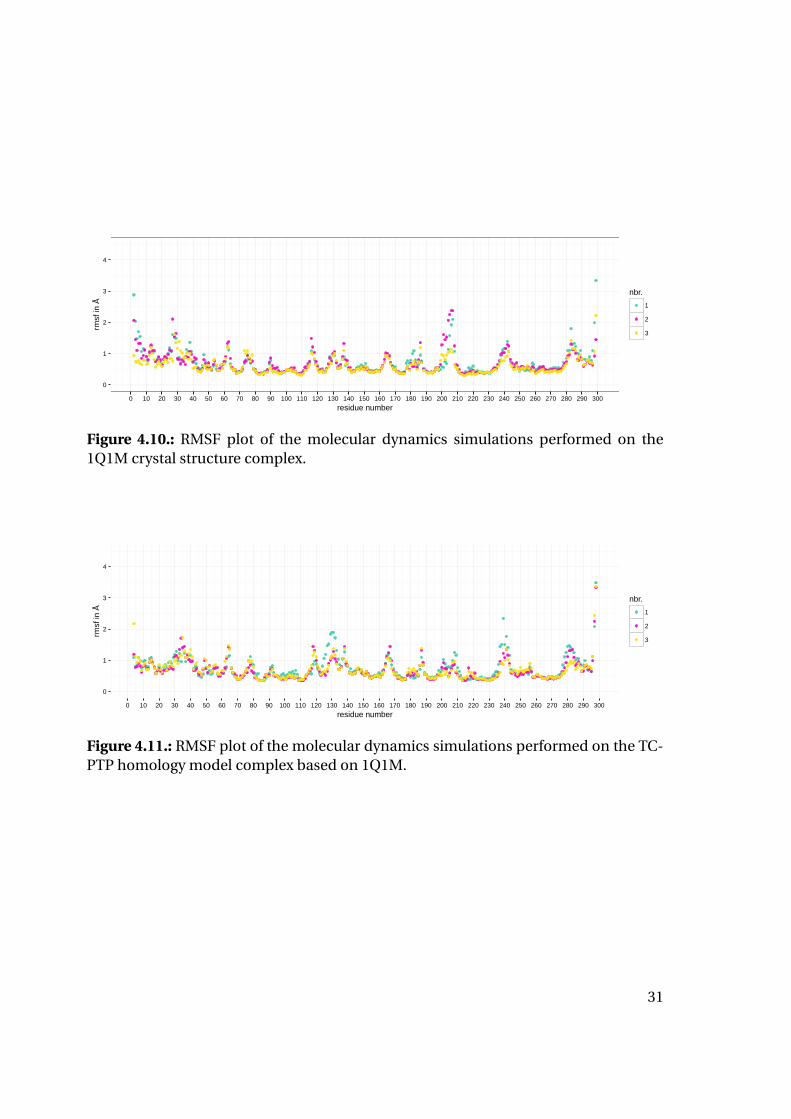
Additionally, RMSF values were calculated and plotted (Figures 4.8 to 4.13) to deter-
mine flexible and inflexible regions and compare those areas for both proteins: All sim-
ulations show a high correlation of stable and unstable regions between the different
complexes, but also between PTP1B and TC-PTP simulations. This distribution of flex-
ible and inflexible regions is in good agreement with the secondary structure elements
of the proteins. Unsurprisingly, the C and N terminal regions show slight increase of
flexibility. For the 1QXK simulations (Figures 4.12 and 4.13) the C terminal end shows
highly increased flexibility with RMSF values greater up to more than 7 Å. The biggest
most stable region for all simulations is the catalytic loop containing the catalytic cys-
27

0.0
0.5
1.0
1.5
2.0
0 5 10 15 20 25simulation time in ns
rmsd
in Å nbr.
123
0.0
0.5
1.0
1.5
2.0
0 5 10 15 20 25simulation time in ns
rmsd
in Å
Figure 4.5.: RMSD plots of the molecular dynamics simulations performed on the1XBO crystal structure complex (left) and the respective TC-PTP homology model com-plex (right).
0.0
0.5
1.0
1.5
2.0
0 5 10 15 20 25simulation time in ns
rmsd
in Å nbr.
123
0.0
0.5
1.0
1.5
2.0
0 5 10 15 20 25simulation time in ns
rmsd
in Å
Figure 4.6.: RMSD plots of the molecular dynamics simulations performed on the1Q1M crystal structure complex (left) and the respective TC-PTP homology modelcomplex (right).
0.0
0.5
1.0
1.5
2.0
0 5 10 15 20 25simulation time in ns
rmsd
in Å nbr.
123
0.0
0.5
1.0
1.5
2.0
0 5 10 15 20 25simulation time in ns
rmsd
in Å
Figure 4.7.: RMSD plots of the molecular dynamics simulations performed on the1QXK crystal structure complex (left) and the respective TC-PTP homology model com-plex (right).
28

teine and the α helix connected to this loop. Interestingly, the WPD loop, known for
its high flexibility during the ligand binding process, shows only limited flexibility be-
low 2 Å for all simulations. The B site residues from 254 to 262 as well as the YRD loop
(47-51) show slightly increased flexibility compared to the catalytic loop for all simu-
lations. Additional to those similarities, some cases of behavior specific for PTP1B or
TC-PTP can be observed from the RMSF plots: The 1XBO and 1QXK simulations are
showing higher flexibility for the TC-PTP simulations regarding the D site (116-121)
and the neighboring region (122-140). Additionally, for all complexes, the TC-PTP sim-
ulations show higher flexibility in the residues 30-40, a loop like structure lying directly
behind the YRD loop viewed from the catalytic cavity.
4.1.5. Dynophore Analysis
In addition to the abovementioned parameters, dynamic pharmacophores were cal-
culated and analyzed to gain insight into protein-ligand interactions to further char-
acterize the selective complexes and their stability over time. For this analysis, frame
1000 was considered as starting point of the dynophore analysis, since all systems were
considered equilibrated based on the RMSD analysis after this point (about 5 ns).
Figure 4.14 shows the three-dimensional depiction of the first simulation based on
the 1XBO complex. The three-dimensional depiction of a dynophore is influenced by
the alignment of the single frames, in this case the Cα-atoms of the stable active site
loop amino acids Cys215-Arg221 were chosen. Since no differences are obvious be-
tween PTP1B and TC-PTP on visual inspection of the dynophores, the underlying in-
teractions were statistically analyzed: To elucidate the differences between PTP1B and
TC-PTP ligand binding features, two-dimensional plots of the ligands together with the
detected hydrogen bond acceptors (HBA), hydrogen bond donors (HBD), hydrophobic
(HYD), aromatic (AR) and negative ionizable (NI) features were created. For each fea-
ture mean occurrences over three molecular dynamics simulations together with the
95% confidence intervals were plotted as bar charts juxtaposing PTP1B and TC-PTP.
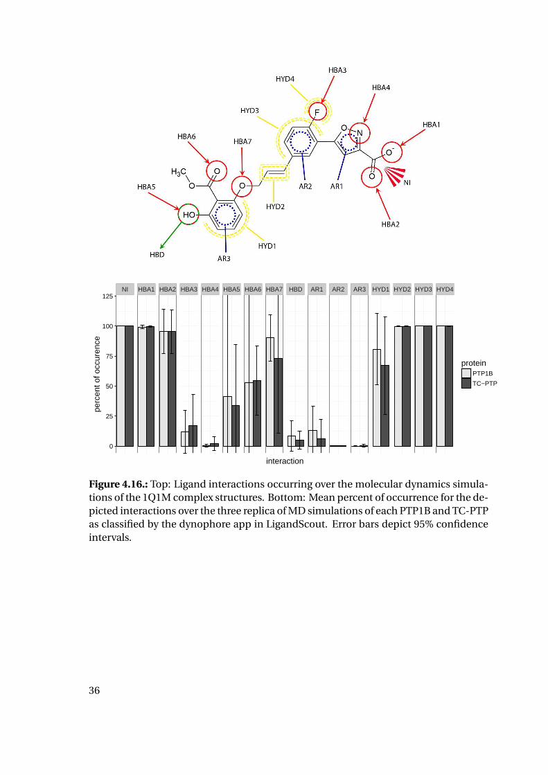
For all three selective complexes, differences between PTP1B and TC-PTP are small
compared to the confidence intervals. However, for all simulations, mean occurence
values of the B site hydrogen bond acceptors (HBA5, HBA6 and HBA7) tend to be higher
in PTP1B simulations compared to the mean values of the corresponding TC-PTP sim-
ulations. This tendency is even more distinctive for the hydrophobic B site interaction
(HYD1).
29
0
1
2
3
4
0 10 20 30 40 50 60 70 80 90 100 110 120 130 140 150 160 170 180 190 200 210 220 230 240 250 260 270 280 290 300
residue number
rmsf
in Å
nbr.
1
2
3
Figure 4.8.: RMSF plot of the molecular dynamics simulations performed on the 1XBOcrystal structure complex.
0
1
2
3
4
0 10 20 30 40 50 60 70 80 90 100 110 120 130 140 150 160 170 180 190 200 210 220 230 240 250 260 270 280 290 300
residue number
rmsf
in Å
nbr.
1
2
3
Figure 4.9.: RMSF plot of the molecular dynamics simulations performed on the TC-PTP homology model complex based on 1XBO.
30
0
1
2
3
4
0 10 20 30 40 50 60 70 80 90 100 110 120 130 140 150 160 170 180 190 200 210 220 230 240 250 260 270 280 290 300
residue number
rmsf
in Å
nbr.
1
2
3
Figure 4.10.: RMSF plot of the molecular dynamics simulations performed on the1Q1M crystal structure complex.
0
1
2
3
4
0 10 20 30 40 50 60 70 80 90 100 110 120 130 140 150 160 170 180 190 200 210 220 230 240 250 260 270 280 290 300
residue number
rmsf
in Å
nbr.
1
2
3
Figure 4.11.: RMSF plot of the molecular dynamics simulations performed on the TC-PTP homology model complex based on 1Q1M.
31

0
2
4
6
0 10 20 30 40 50 60 70 80 90 100 110 120 130 140 150 160 170 180 190 200 210 220 230 240 250 260 270 280 290
residue number
rmsf
in Å
nbr.
1
2
3
Figure 4.12.: RMSF plot of the molecular dynamics simulations performed on the 1QXKcrystal structure complex.
0
2
4
6
0 10 20 30 40 50 60 70 80 90 100 110 120 130 140 150 160 170 180 190 200 210 220 230 240 250 260 270 280 290
residue number
rmsf
in Å
nbr.
1
2
3
Figure 4.13.: RMSF plot of the molecular dynamics simulations performed on the TC-PTP homology model complex based on 1QXK.
32

Figure 4.14.: Three-dimenional depiction of the dynophore created based on one ofthe performed molecular dynamics simulations of the 1XBO complex. Dots representpharmacophoric features of interactions detected for a molecular dynamics frame.Red: hydrogen bond acceptor or negative ionizable interaction, green: hydrogen bonddonor, blue: aromatic interaction, yellow: hydrophobic interaction.
Interestingly, there is one interaction in the catalytic cavity - HBA3 - which shows com-
parably high occurrence in PTP1B compared to TC-PTP for the simulations of 1XBO
and 1Q1M.
Apart from those similarities, the dynophore interactions also reveal binding inter-
actions characteristic for each single protein: The simulations based on the 1XBO com-
plex show the fewest, but most stable interactions. The dominant interaction partner
in the only occasionally occurring HBD2 interaction are different water molecules sug-
gesting minor importance for the protein ligand interaction energy. Closer analysis of
the interaction partners on protein side for all interactions reveals a tendency of the
PTP1B interaction HYD1 to interact not only with Met258, but also Ile219, whereas the
latter interaction is not found for the TC-PTP simulations. Instead, in the TC-PTP sim-
ulations the Met interaction is extended to the HYD2 feature. The high occurrence of
the HBA4 interaction was found to be caused by a trapped water molecule transferred
from the crystal structure. The 1Q1M simulations show more interactions, some of
33
them, especially the aromatic interactions, are of very low occurrence. As for the 1XBO
simulations, the A site interactions (NI, HBA1 and HBA2) as well as the hydrophobic
features are of high occurrence, suggesting very stable hydrogen bonds with active site
amino acids and good placement of the ligand in the channel, connecting A and B site
of the binding pocket with increased flexibility for all simulations in the B site (HYD1).
Apart from lower occurrence of the hydrophobic features on the slightly longer chain in
the center of the ligand, 1QXK simulations show similar behaviour as described for the
1Q1M complex. However the 1QXK ligand is the only one of the three analyzed ligands
showing C site interactions. Interestingly, the C site interactions HBD3 and HBD4 of
this ligand are among the interactions with highest preference for PTP1B. Additionally,
the 1QXK ligand shows several interactions (HBA2, HBA3, HBA4, HBD1 and AR1), all
located in the active site binding part of the ligand, where mean occurences in TC-PTP
exceed those in PTP1B.
34

NI HBA1 HBA2 HBA3 HBA4 HBA5 HBA6 HBA7 HBD1 HBD2 AR HYD1 HYD2 HYD3
0
25
50
75
100
125
interaction
perc
ent o
f occ
uren
ce
proteinPTP1B
TC−PTP
Figure 4.15.: Top: Ligand interactions occurring over the molecular dynamics simula-tions of the 1XBO complex structures. Bottom: Mean percent of occurrence for the de-picted interactions over the three replica of MD simulations of each PTP1B and TC-PTPas classified by the dynophore app in LigandScout. Error bars depict 95% confidenceintervals.
35
NI HBA1 HBA2 HBA3 HBA4 HBA5 HBA6 HBA7 HBD AR1 AR2 AR3 HYD1 HYD2 HYD3 HYD4
0
25
50
75
100
125
interaction
perc
ent o
f occ
uren
ce
proteinPTP1B
TC−PTP
Figure 4.16.: Top: Ligand interactions occurring over the molecular dynamics simula-tions of the 1Q1M complex structures. Bottom: Mean percent of occurrence for the de-picted interactions over the three replica of MD simulations of each PTP1B and TC-PTPas classified by the dynophore app in LigandScout. Error bars depict 95% confidenceintervals.
36
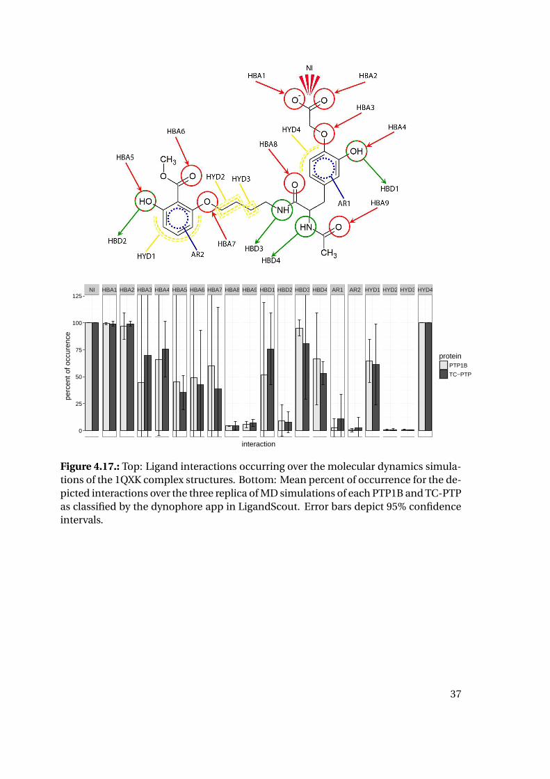
NI HBA1 HBA2 HBA3 HBA4 HBA5 HBA6 HBA7 HBA8 HBA9 HBD1 HBD2 HBD3 HBD4 AR1 AR2 HYD1 HYD2 HYD3 HYD4
0
25
50
75
100
125
interaction
perc
ent o
f occ
uren
ce
proteinPTP1B
TC−PTP
Figure 4.17.: Top: Ligand interactions occurring over the molecular dynamics simula-tions of the 1QXK complex structures. Bottom: Mean percent of occurrence for the de-picted interactions over the three replica of MD simulations of each PTP1B and TC-PTPas classified by the dynophore app in LigandScout. Error bars depict 95% confidenceintervals.
37
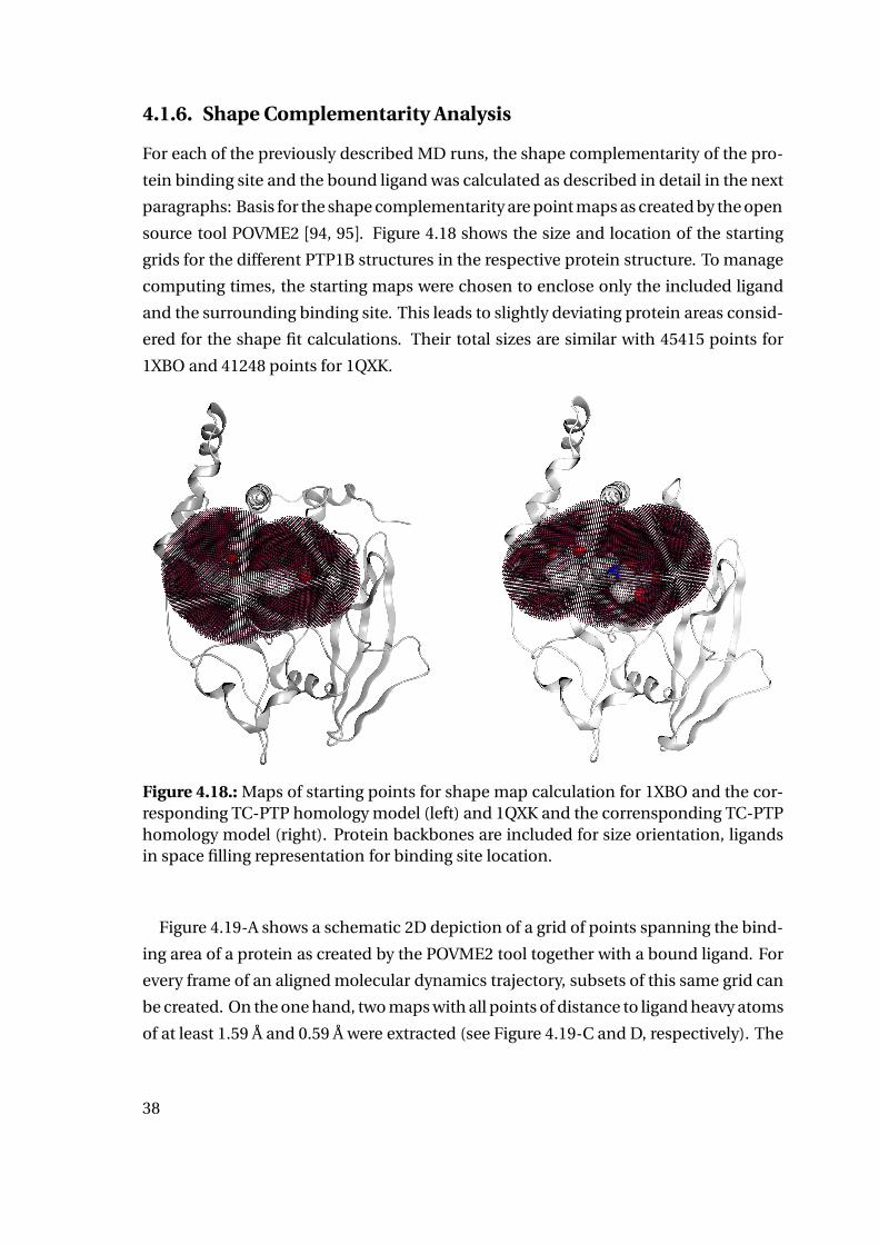
4.1.6. Shape Complementarity Analysis
For each of the previously described MD runs, the shape complementarity of the pro-
tein binding site and the bound ligand was calculated as described in detail in the next
paragraphs: Basis for the shape complementarity are point maps as created by the open
source tool POVME2 [94, 95]. Figure 4.18 shows the size and location of the starting
grids for the different PTP1B structures in the respective protein structure. To manage
computing times, the starting maps were chosen to enclose only the included ligand
and the surrounding binding site. This leads to slightly deviating protein areas consid-
ered for the shape fit calculations. Their total sizes are similar with 45415 points for
1XBO and 41248 points for 1QXK.
Figure 4.18.: Maps of starting points for shape map calculation for 1XBO and the cor-responding TC-PTP homology model (left) and 1QXK and the corrensponding TC-PTPhomology model (right). Protein backbones are included for size orientation, ligandsin space filling representation for binding site location.
Figure 4.19-A shows a schematic 2D depiction of a grid of points spanning the bind-
ing area of a protein as created by the POVME2 tool together with a bound ligand. For
every frame of an aligned molecular dynamics trajectory, subsets of this same grid can
be created. On the one hand, two maps with all points of distance to ligand heavy atoms
of at least 1.59 Å and 0.59 Å were extracted (see Figure 4.19-C and D, respectively). The
38
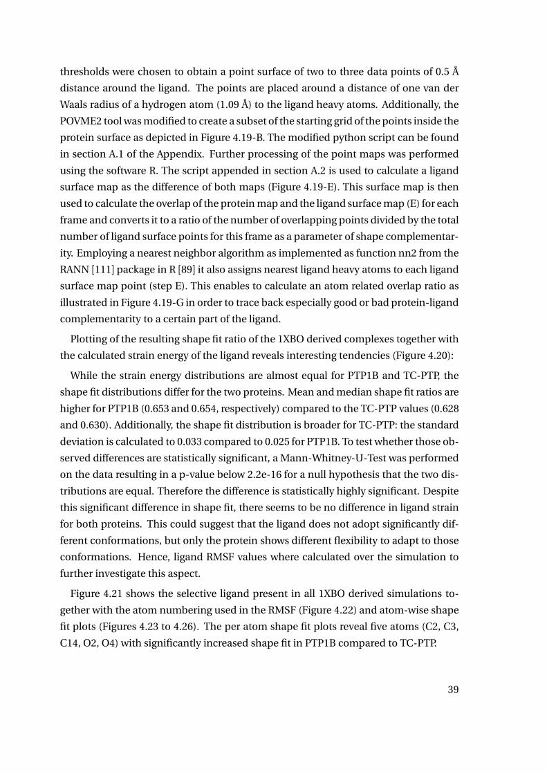
thresholds were chosen to obtain a point surface of two to three data points of 0.5 Å
distance around the ligand. The points are placed around a distance of one van der
Waals radius of a hydrogen atom (1.09 Å) to the ligand heavy atoms. Additionally, the
POVME2 tool was modified to create a subset of the starting grid of the points inside the
protein surface as depicted in Figure 4.19-B. The modified python script can be found
in section A.1 of the Appendix. Further processing of the point maps was performed
using the software R. The script appended in section A.2 is used to calculate a ligand
surface map as the difference of both maps (Figure 4.19-E). This surface map is then
used to calculate the overlap of the protein map and the ligand surface map (E) for each
frame and converts it to a ratio of the number of overlapping points divided by the total
number of ligand surface points for this frame as a parameter of shape complementar-
ity. Employing a nearest neighbor algorithm as implemented as function nn2 from the
RANN [111] package in R [89] it also assigns nearest ligand heavy atoms to each ligand
surface map point (step E). This enables to calculate an atom related overlap ratio as
illustrated in Figure 4.19-G in order to trace back especially good or bad protein-ligand
complementarity to a certain part of the ligand.
Plotting of the resulting shape fit ratio of the 1XBO derived complexes together with
the calculated strain energy of the ligand reveals interesting tendencies (Figure 4.20):
While the strain energy distributions are almost equal for PTP1B and TC-PTP, the
shape fit distributions differ for the two proteins. Mean and median shape fit ratios are
higher for PTP1B (0.653 and 0.654, respectively) compared to the TC-PTP values (0.628
and 0.630). Additionally, the shape fit distribution is broader for TC-PTP: the standard
deviation is calculated to 0.033 compared to 0.025 for PTP1B. To test whether those ob-
served differences are statistically significant, a Mann-Whitney-U-Test was performed
on the data resulting in a p-value below 2.2e-16 for a null hypothesis that the two dis-
tributions are equal. Therefore the difference is statistically highly significant. Despite
this significant difference in shape fit, there seems to be no difference in ligand strain
for both proteins. This could suggest that the ligand does not adopt significantly dif-
ferent conformations, but only the protein shows different flexibility to adapt to those
conformations. Hence, ligand RMSF values where calculated over the simulation to
further investigate this aspect.
Figure 4.21 shows the selective ligand present in all 1XBO derived simulations to-
gether with the atom numbering used in the RMSF (Figure 4.22) and atom-wise shape
fit plots (Figures 4.23 to 4.26). The per atom shape fit plots reveal five atoms (C2, C3,
C14, O2, O4) with significantly increased shape fit in PTP1B compared to TC-PTP.
39

{{
A
B
C D
E
F
G
starting point map: regular grid span-ning binding area
protein surfaceligand + close and more distant surr-ounding surface
Figure 4.19.: Schematic representation of the shape complementarity workflow.
40

Further, four atoms (C15, C16, C35, O1) show a slightly better shape fit for the lig-
and in PTP1B. It is noteworthy that all of the identified atoms except for C35 are lo-
cated in the catalytic pocket of the protein during simulation and not in the B site as
expected. The differences in total ligand shapefit therefore mainly seem related to the
catalytic cavity (A site), which is almost identical in amino acid sequence for both pro-
teins. Interestingly, the ligand RMSF plot shows very similar RMSF values of the B site
atoms (C32-39 and O11, O13, O14) for both proteins, whereas some atoms (C14-16 and
O2) although buried in the active site cavity during simulation for both proteins, show
the biggest differences with higher stability in PTP1B. Shape complementarity and lig-
and RMSF together therefore suggest increased protein-ligand shape fit with resulting
higher ligand stability in the active site cavity for PTP1B.
Shapefit calculations were also performed for the PTP1B an TC-PTP complexes based
on crystal structure 1QXK (see Figure 4.27). The shape fit distributions reveal the same
tendency as for the 1XBO derived complexes: Mean and median shape fit ratios are
higher for PTP1B (0.528 and 0.526, respectively) compared to the TC-PTP values (0.506
and 0.502) and the distribution is broader for TC-PTP with standard deviation of 0.033
for PTP1B and 0.046 for TC-PTP. Equivalent to the 1XBO simulations the Mann-Whitney-
U-Test was performed and resulted in a p-value below 2.2e-16 for a null hypothesis that
the two distributions are equal. The difference in mean of the two distributions is there-
fore statistically highly significant. Different to the 1XBO simulations, the 1QXK simu-
lations additionally show a difference in the calculated ligand strain distributions. For
3521 of the 12633 frames of PTP1B the ligand strain is below 53, while only 181 frames
of TC-PTP show such a low ligand strain. Interestingly, the 2D plot reveals that the low
ligand strain values of the PTP1B frames do not correlate with especially low shape fit
ratios.
Analogously to the calculations on 1XBO derived simulations, ligand RMSF and atom-
wise shape fit were calculated for the 1QXK based simulations to further investigate the
relationship between ligand flexibility and shape fit. Figure 4.28 shows the selective lig-
and present in all 1QXK derived simulations together with the atom numbering used in
the RMSF (Figure 4.29) and atom-wise shape fit plots (Figures 4.30 to 4.34). Unexpect-
edly, the atoms C2, C3, C24, O5, O6 and O7 show a tendency for increased shape fit in
TC-PTP despite the overall observation of better shape fit of the ligand to PTP1B. These
atoms all belong to the part of the ligand which is bound to the catalytic cavity. The
opposite tendency is found for atoms C15, C23, C38, C39, N1, N2, O1, O11 and O12.
Five of those atoms (C38, C39, O1, O11 and O12) belong to the ligand part bound to the
41
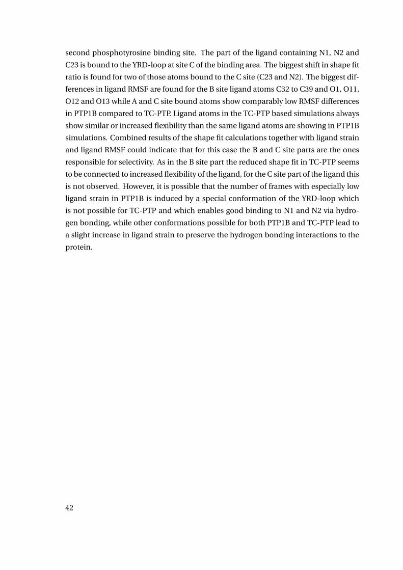
second phosphotyrosine binding site. The part of the ligand containing N1, N2 and
C23 is bound to the YRD-loop at site C of the binding area. The biggest shift in shape fit
ratio is found for two of those atoms bound to the C site (C23 and N2). The biggest dif-
ferences in ligand RMSF are found for the B site ligand atoms C32 to C39 and O1, O11,
O12 and O13 while A and C site bound atoms show comparably low RMSF differences
in PTP1B compared to TC-PTP. Ligand atoms in the TC-PTP based simulations always
show similar or increased flexibility than the same ligand atoms are showing in PTP1B
simulations. Combined results of the shape fit calculations together with ligand strain
and ligand RMSF could indicate that for this case the B and C site parts are the ones
responsible for selectivity. As in the B site part the reduced shape fit in TC-PTP seems
to be connected to increased flexibility of the ligand, for the C site part of the ligand this
is not observed. However, it is possible that the number of frames with especially low
ligand strain in PTP1B is induced by a special conformation of the YRD-loop which
is not possible for TC-PTP and which enables good binding to N1 and N2 via hydro-
gen bonding, while other conformations possible for both PTP1B and TC-PTP lead to
a slight increase in ligand strain to preserve the hydrogen bonding interactions to the
protein.
42
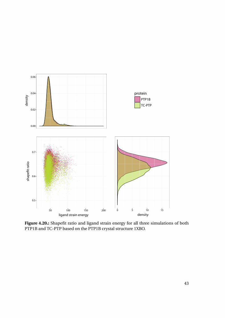
0.00
0.02
0.04
0.06
den
sity
protein
PTP1B
TC-PTP
0.5
0.6
0.7
50 100 150 200
ligand strain energy
shap
e!t r
atio
0 5 10 15
density
Figure 4.20.: Shapefit ratio and ligand strain energy for all three simulations of bothPTP1B and TC-PTP based on the PTP1B crystal structure 1XBO.
43
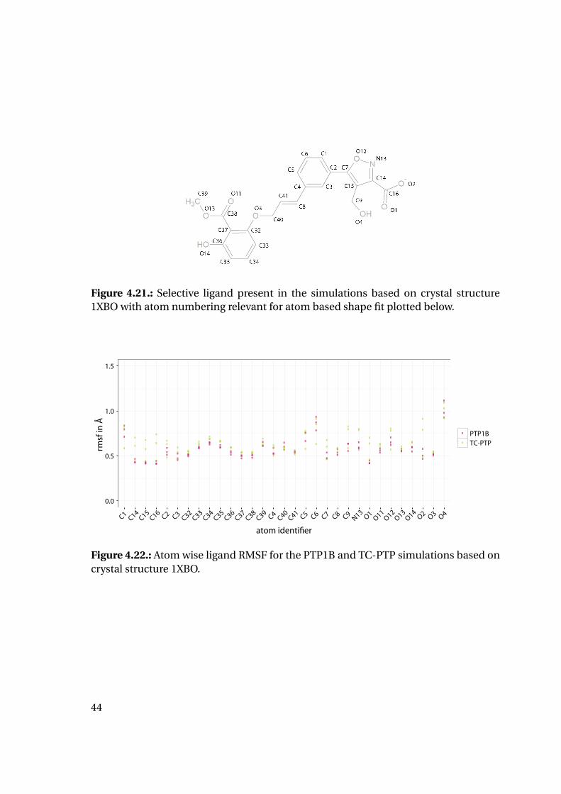
Figure 4.21.: Selective ligand present in the simulations based on crystal structure1XBO with atom numbering relevant for atom based shape fit plotted below.
�
�
�
�
�
�
�
�
�
��
�
�
�
�
�
�
��
�
��
� �
�
�
�
�� �
�
�
�
�
�
�
�
�
�
�
� � �
�
�
��
�
��
�
� �
� �
��
�
�
�
�
�
�
�
�
�
�
�
�
�
�
� ��
�
�
��
�
�
�
�
� �
��
�
�
�
�
�
�
�
�
�
�
�
�
�
�
��
�
�
�
�
�
�
�
�
��
�
� �
��
�
�
�
�
�
�
�
�
� ��
�
�
�
��
� � �
��
��
�
�
�
�
� �
��
��
��
�
�
�
�
�
��
�
�
�
��
��
�
�
�
�
�
�
��
�
� �
�
�
��
��
�
�
�
0.0
0.5
1.0
1.5
C1C14
C15C16
C2 C3C32
C33C34
C35C36
C37C38
C39C4
C40C41
C5 C6 C7 C8 C9N13
O1O11
O12O13
O14O2 O3 O4
atom identi!er
rmsf
in Å
�
� TC-PTPPTP1B
Figure 4.22.: Atom wise ligand RMSF for the PTP1B and TC-PTP simulations based oncrystal structure 1XBO.
44
Figure 4.23.: Density plots for atom-wise shape fit ratio in PDB complex 1XBO; pink:PTP1B, green: TC-PTP.
45
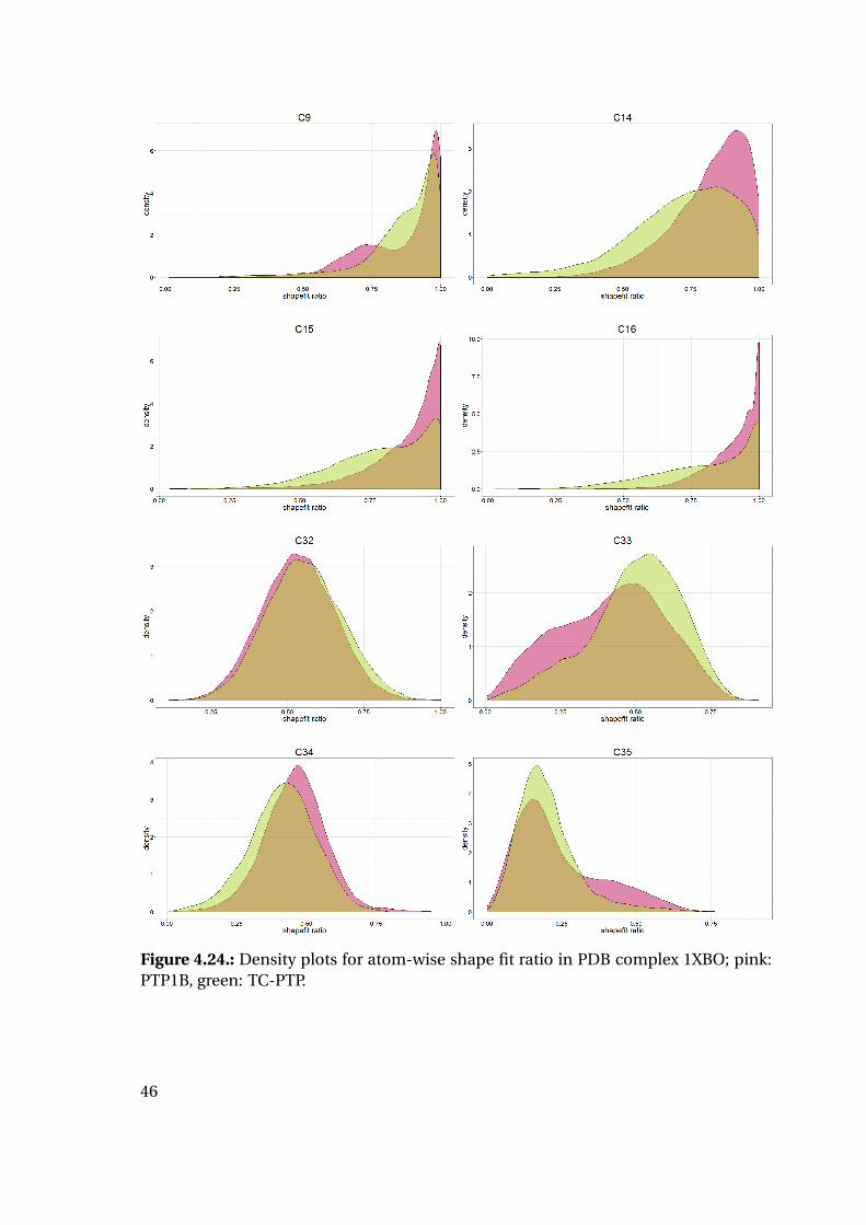
Figure 4.24.: Density plots for atom-wise shape fit ratio in PDB complex 1XBO; pink:PTP1B, green: TC-PTP.
46

Figure 4.25.: Density plots for atom-wise shape fit ratio in PDB complex 1XBO; pink:PTP1B, green: TC-PTP.
47
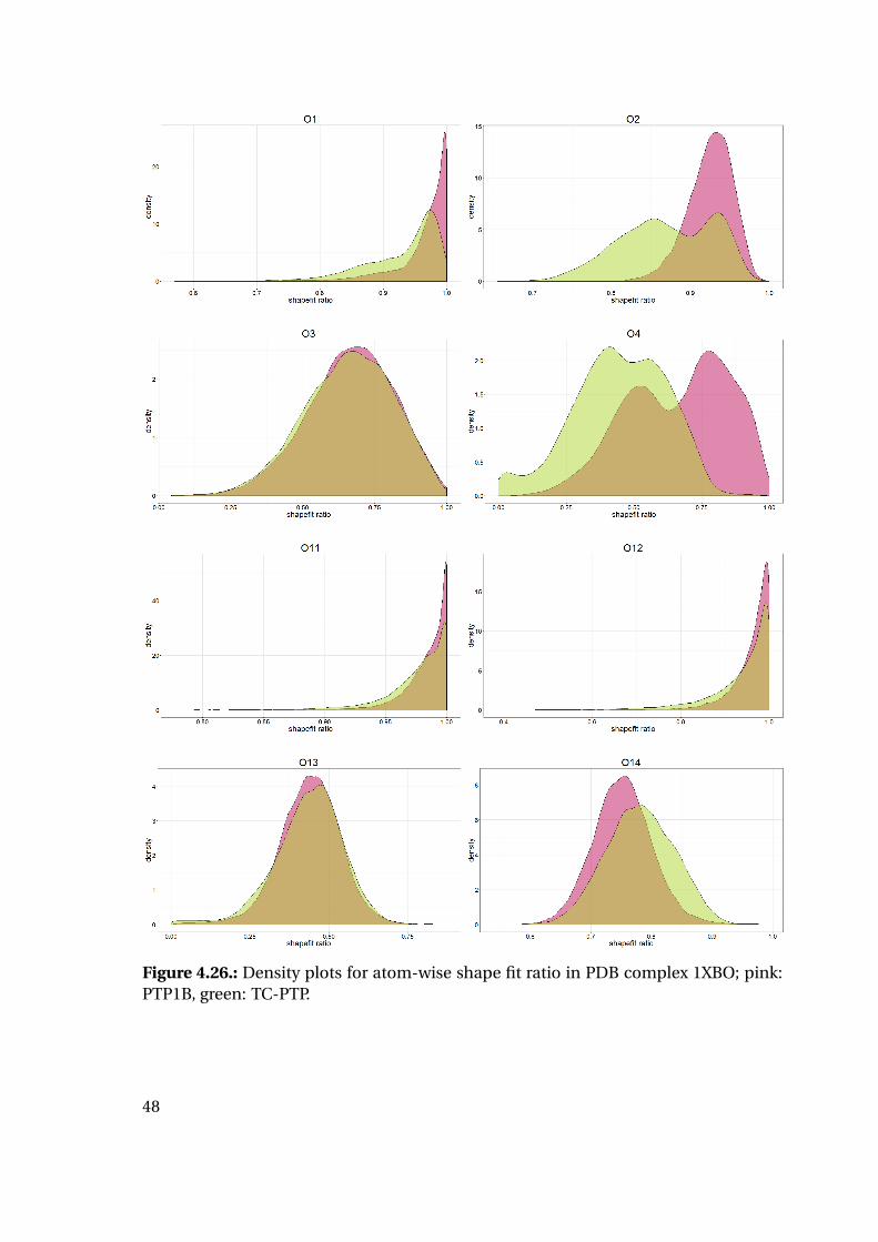
Figure 4.26.: Density plots for atom-wise shape fit ratio in PDB complex 1XBO; pink:PTP1B, green: TC-PTP.
48
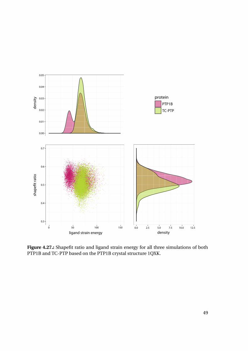
0.00
0.01
0.02
0.03
0.04
0.05
0.3
0.4
0.5
0.6
0.7
0 50 100 150 0.0 2.5 5.0 7.5 10.0 12.5
protein
PTP1B
TC-PTP
den
sity
ligand strain energy
shap
e!t r
atio
density
Figure 4.27.: Shapefit ratio and ligand strain energy for all three simulations of bothPTP1B and TC-PTP based on the PTP1B crystal structure 1QXK.
49
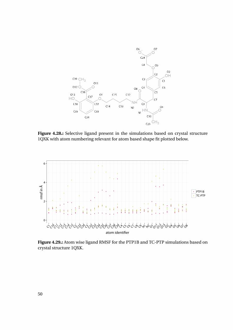
Figure 4.28.: Selective ligand present in the simulations based on crystal structure1QXK with atom numbering relevant for atom based shape fit plotted below.
�
�� �
�
� �
� �
�
���
��� �
�
�
���
� �
�
��
� ��
� �� �
� �
�
� �� �
����
�
�
��
� ��
� �
��
� ���
�
�
�
�
��
�
� �
�
�
�
�
�
� �� � �� �
��
��
�
��
���
�
�
�
�
��
��
�
�
�
�
�
�
�
� �
�
�
���
��
��
�
�
�
�
�
�
�
�
�
�
�
�
�
�
��
�
� �
�
�
� �
�
��
�
�
�
�
��� � � �
� �� �
�
��
� ��� �
�
�
�
�
��
�
�
�
�
��
�
� �
�
�
� �
�
�� � � �
���
�
�
� ��
� �� �
��
�
��
�� ��
�
�
��
� �
�
�
�
�
�
0
2
4
6
C1C10
C11C12
C13C14
C15C2
C23C24
C3C32
C33C34
C35C36
C37C38
C39C4 C5 C6 C7 C8 C9 N1 N2 O1
O11O12
O13O2 O4 O5 O6 O7 O8
atom identi!er
rmsf
in Å
�
� TC-PTPPTP1B
Figure 4.29.: Atom wise ligand RMSF for the PTP1B and TC-PTP simulations based oncrystal structure 1QXK.
50
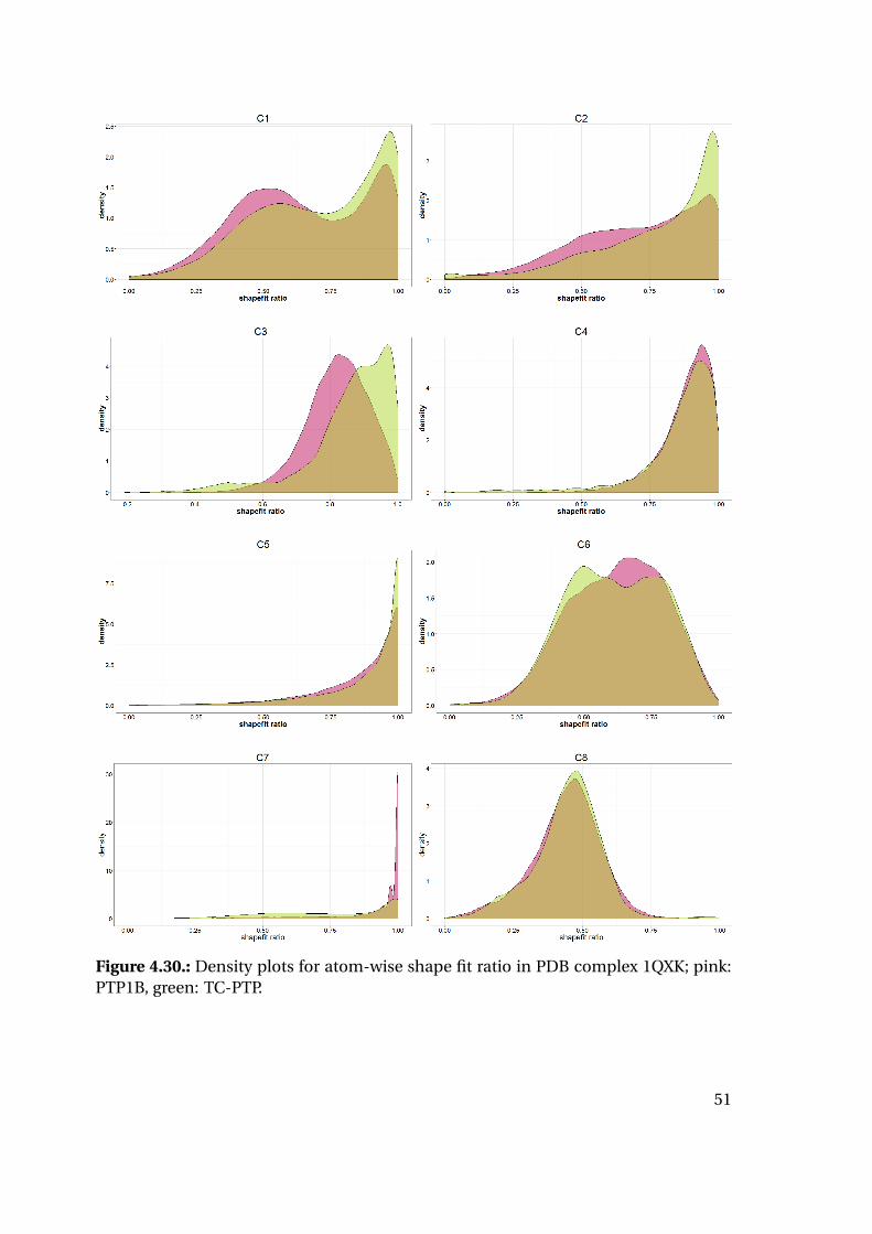
Figure 4.30.: Density plots for atom-wise shape fit ratio in PDB complex 1QXK; pink:PTP1B, green: TC-PTP.
51
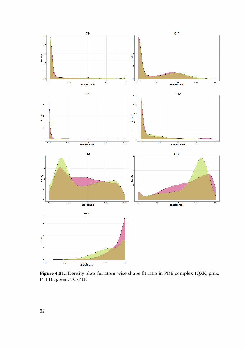
Figure 4.31.: Density plots for atom-wise shape fit ratio in PDB complex 1QXK; pink:PTP1B, green: TC-PTP.
52
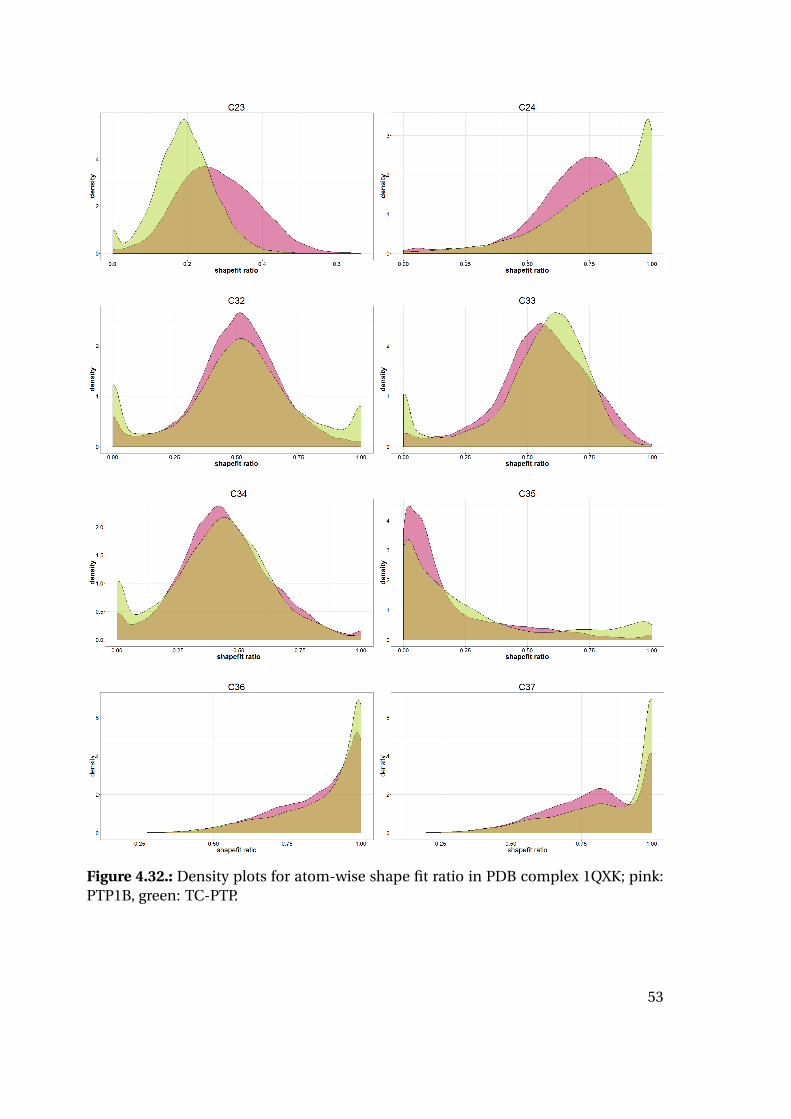
Figure 4.32.: Density plots for atom-wise shape fit ratio in PDB complex 1QXK; pink:PTP1B, green: TC-PTP.
53

Figure 4.33.: Density plots for atom-wise shape fit ratio in PDB complex 1QXK; pink:PTP1B, green: TC-PTP.
54
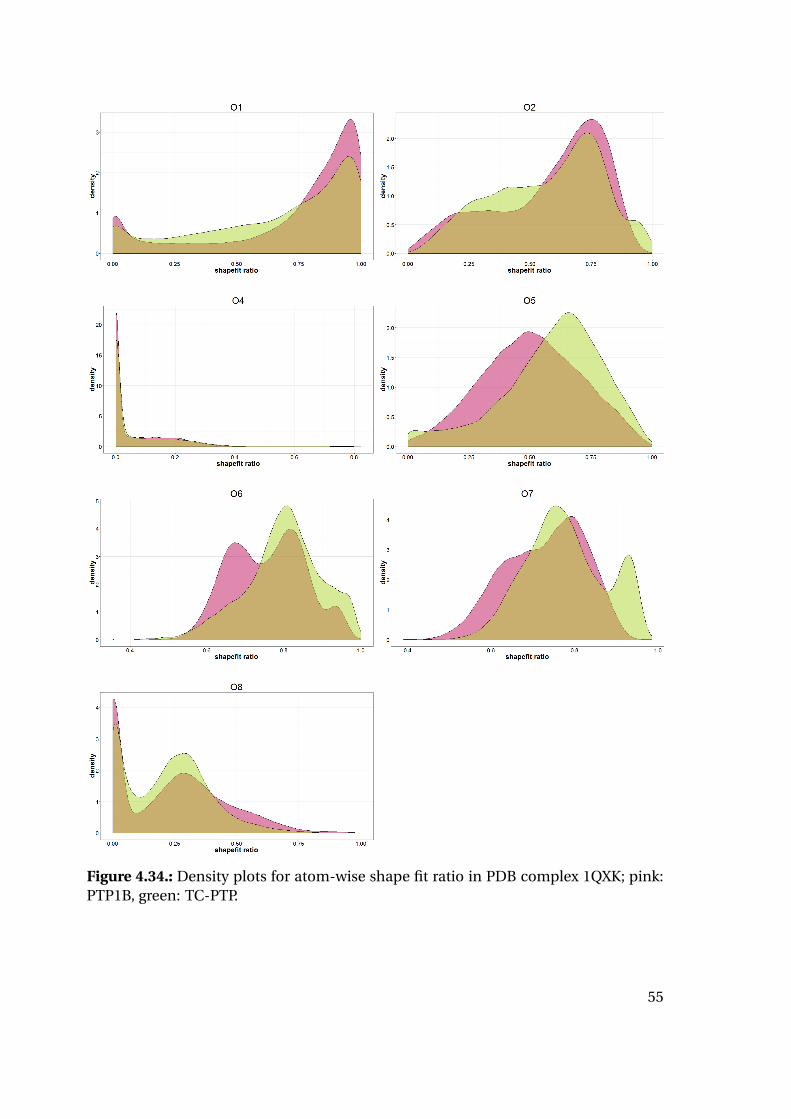
Figure 4.34.: Density plots for atom-wise shape fit ratio in PDB complex 1QXK; pink:PTP1B, green: TC-PTP.
55
4.2. Part II: Binding Site Shape Clustering and Screening
4.2.1. Generation of Input Data
Due to the observation that stronger inhibitors of PTP1B are found to preferably bind
to the closed conformation of the active site cavity this approach strives to discover
PTP1B selective compounds targeting the closed active site conformation. In order
to prevent the occurrence of loop opening events during the simulations and poten-
tially connected conformational changes in other parts of the protein, the protein was
guided to keep the closed conformation with a phosphotyrosine residue bound to the
catalytic cavity. As starting system for PTP1B, PDB structure 1PTY was chosen, which
contains phosphotyrosine residues in the catalytic cavity and the second phosphoty-
rosine binding site. The second phosphotyrosine was removed prior to the molecular
dynamics simulations, with the aim not to unnecessarily bias the rest of the binding
cavity. Since a closed cavity complex was not available for TC-PTP, a homology model
was build based on the PTP1B complex 1PTY. To yield a structure equivalent to the
PTP1B structure for simulation, the coordinates of the catalytic phosphotyrosine and
the adjacent catalytic water molecule were transposed to the TC-PTP homology model.
Molecular dynamics simulations were performed on both complexes in triplicates over
50 ns each. Analogously as for the previously described molecular dynamics simula-
tions Cα-RMSD and RMSF plots were created and analyzed.
Similar to the previously described complexes, the simulations of the 1PTY derived
complexes show stable system behavior with RMSD values below 2.4 Å. RMSD plots in
Figure 4.35 show that the PTP1B simulations reach equilibrium after about 5 ns, while
the TC-PTP structures still seem not to have finished the rearrangement after 10 to 15
ns. Further they show a slightly higher overall RMSD than the PTP1B simulations. Both
observations are in good agreement with our expectations due to the fact that ligand
coordinates were transposed from the PTP1B structure without energy minimization.
The time point of 15 ns was therefore considered as starting point of the simulations
for further analysis.
Starting from the determined point of equilibration, point maps depicting the bind-
ing site shape were generated for each frame with the tool POVME2 [94, 95]. Again
the Cα-atoms of the stable active site loop amino acids Cys215-Arg221 were chosen
for alignment of all frames. The TC-PTP trajectories were aligned on the first frame of
the PTP1B trajectories to enable direct comparison of the resulting data due to use of
the same starting point map for the POVME2 calculations. The starting point map to-
56

0.0
0.5
1.0
1.5
2.0
2.5
0 10 20 30 40 50simulation time in ns
rmsd
in Å nbr.
123
0.0
0.5
1.0
1.5
2.0
2.5
0 10 20 30 40 50simulation time in ns
rmsd
in Å nbr.
123
Figure 4.35.: RMSD plots of the molecular dynamics simulations performed on the1PTY crystal structure with a cropped phosphotyrosine in the catalytic pocket (top)and the corresponding TC-PTP homology model complex (bottom).
gether with the protein surface of the starting frame is depicted in Figure 4.37(left). The
starting point map spans the whole binding area of PTP1B with all subsites (compare
Figure 4.1). However, the outside of the lid closing the catalytic pocket is only partially
covered. Considerations on the influence of this fact regarding the outcome of the clus-
tering workflow are included in the following chapter.
4.2.2. Bootstrapping and Clustering
Since the amount of storage capacity required for clustering the whole dataset exceeded
the available resources, bootstrapping was used to create three smaller samples of 14598
(one third of the considered frames) frames each [112]. Calculations were then per-
formed on all three samples. Clustering results for each sample were further processed
with an R script, which can be found in section A.3 to guide the selection of the appro-
priate clustering level for further analysis. The approach developed here is similar to
the elbow method to find the optimal number of clusters for a dataset [103]. Like the
elbow method, it strives to assess how intra-cluster variance changes for each step and
especially after which step it does not increase significantly anymore. Due to the nature
of clustering algorithms, clusters will get more uniform the smaller they get, but too
57
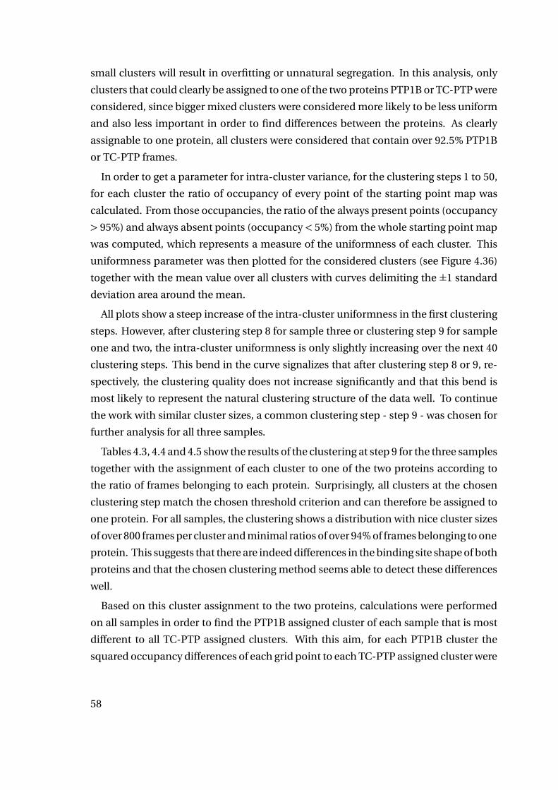
small clusters will result in overfitting or unnatural segregation. In this analysis, only
clusters that could clearly be assigned to one of the two proteins PTP1B or TC-PTP were
considered, since bigger mixed clusters were considered more likely to be less uniform
and also less important in order to find differences between the proteins. As clearly
assignable to one protein, all clusters were considered that contain over 92.5% PTP1B
or TC-PTP frames.
In order to get a parameter for intra-cluster variance, for the clustering steps 1 to 50,
for each cluster the ratio of occupancy of every point of the starting point map was
calculated. From those occupancies, the ratio of the always present points (occupancy
> 95%) and always absent points (occupancy< 5%) from the whole starting point map
was computed, which represents a measure of the uniformness of each cluster. This
uniformness parameter was then plotted for the considered clusters (see Figure 4.36)
together with the mean value over all clusters with curves delimiting the ±1 standard
deviation area around the mean.
All plots show a steep increase of the intra-cluster uniformness in the first clustering
steps. However, after clustering step 8 for sample three or clustering step 9 for sample
one and two, the intra-cluster uniformness is only slightly increasing over the next 40
clustering steps. This bend in the curve signalizes that after clustering step 8 or 9, re-
spectively, the clustering quality does not increase significantly and that this bend is
most likely to represent the natural clustering structure of the data well. To continue
the work with similar cluster sizes, a common clustering step - step 9 - was chosen for
further analysis for all three samples.
Tables 4.3, 4.4 and 4.5 show the results of the clustering at step 9 for the three samples
together with the assignment of each cluster to one of the two proteins according to
the ratio of frames belonging to each protein. Surprisingly, all clusters at the chosen
clustering step match the chosen threshold criterion and can therefore be assigned to
one protein. For all samples, the clustering shows a distribution with nice cluster sizes
of over 800 frames per cluster and minimal ratios of over 94% of frames belonging to one
protein. This suggests that there are indeed differences in the binding site shape of both
proteins and that the chosen clustering method seems able to detect these differences
well.
Based on this cluster assignment to the two proteins, calculations were performed
on all samples in order to find the PTP1B assigned cluster of each sample that is most
different to all TC-PTP assigned clusters. With this aim, for each PTP1B cluster the
squared occupancy differences of each grid point to each TC-PTP assigned cluster were
58
0.70
0.75
0.80
0.85
2 4 6 8 10 12 14 16 18 20 22 24 26 28 30 32 34 36 38 40 42 44 46 48 50
clustering step
intr
a-c
luste
r uniform
ness
0.70
0.75
0.80
0.85
2 4 6 8 10 12 14 16 18 20 22 24 26 28 30 32 34 36 38 40 42 44 46 48 50
clustering step
intr
a-c
luste
r uniform
ness
0.70
0.75
0.80
0.85
2 4 6 8 10 12 14 16 18 20 22 24 26 28 30 32 34 36 38 40 42 44 46 48 50
clustering step
intr
a-c
luste
r uniform
ness
Figure 4.36.: Intra-cluster uniformness over clustering step number for all three sam-ples. Mean value over all clusters per step as pink line; pink area represents±1 standarddeviation area around the mean.
59
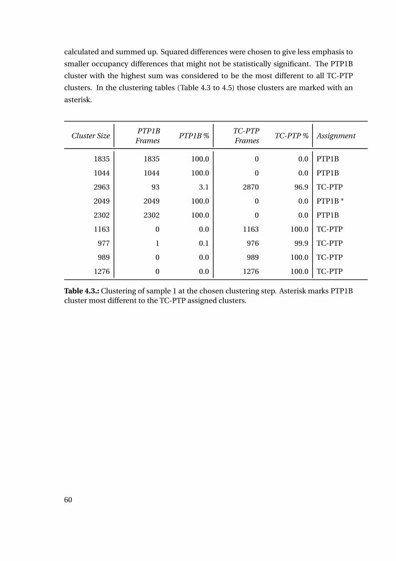
calculated and summed up. Squared differences were chosen to give less emphasis to
smaller occupancy differences that might not be statistically significant. The PTP1B
cluster with the highest sum was considered to be the most different to all TC-PTP
clusters. In the clustering tables (Table 4.3 to 4.5) those clusters are marked with an
asterisk.
Cluster SizePTP1B
FramesPTP1B %
TC-PTP
FramesTC-PTP % Assignment
1835 1835 100.0 0 0.0 PTP1B
1044 1044 100.0 0 0.0 PTP1B
2963 93 3.1 2870 96.9 TC-PTP
2049 2049 100.0 0 0.0 PTP1B *
2302 2302 100.0 0 0.0 PTP1B
1163 0 0.0 1163 100.0 TC-PTP
977 1 0.1 976 99.9 TC-PTP
989 0 0.0 989 100.0 TC-PTP
1276 0 0.0 1276 100.0 TC-PTP
Table 4.3.: Clustering of sample 1 at the chosen clustering step. Asterisk marks PTP1Bcluster most different to the TC-PTP assigned clusters.
60
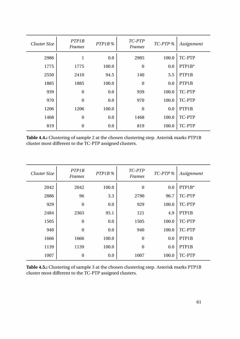
Cluster SizePTP1B
FramesPTP1B %
TC-PTP
FramesTC-PTP % Assignment
2986 1 0.0 2985 100.0 TC-PTP
1775 1775 100.0 0 0.0 PTP1B*
2550 2410 94.5 140 5.5 PTP1B
1885 1885 100.0 0 0.0 PTP1B
939 0 0.0 939 100.0 TC-PTP
970 0 0.0 970 100.0 TC-PTP
1206 1206 100.0 0 0.0 PTP1B
1468 0 0.0 1468 100.0 TC-PTP
819 0 0.0 819 100.0 TC-PTP
Table 4.4.: Clustering of sample 2 at the chosen clustering step. Asterisk marks PTP1Bcluster most different to the TC-PTP assigned clusters.
Cluster SizePTP1B
FramesPTP1B %
TC-PTP
FramesTC-PTP % Assignment
2042 2042 100.0 0 0.0 PTP1B*
2886 96 3.3 2790 96.7 TC-PTP
929 0 0.0 929 100.0 TC-PTP
2484 2363 95.1 121 4.9 PTP1B
1505 0 0.0 1505 100.0 TC-PTP
940 0 0.0 940 100.0 TC-PTP
1666 1666 100.0 0 0.0 PTP1B
1139 1139 100.0 0 0.0 PTP1B
1007 0 0.0 1007 100.0 TC-PTP
Table 4.5.: Clustering of sample 3 at the chosen clustering step. Asterisk marks PTP1Bcluster most different to the TC-PTP assigned clusters.
61
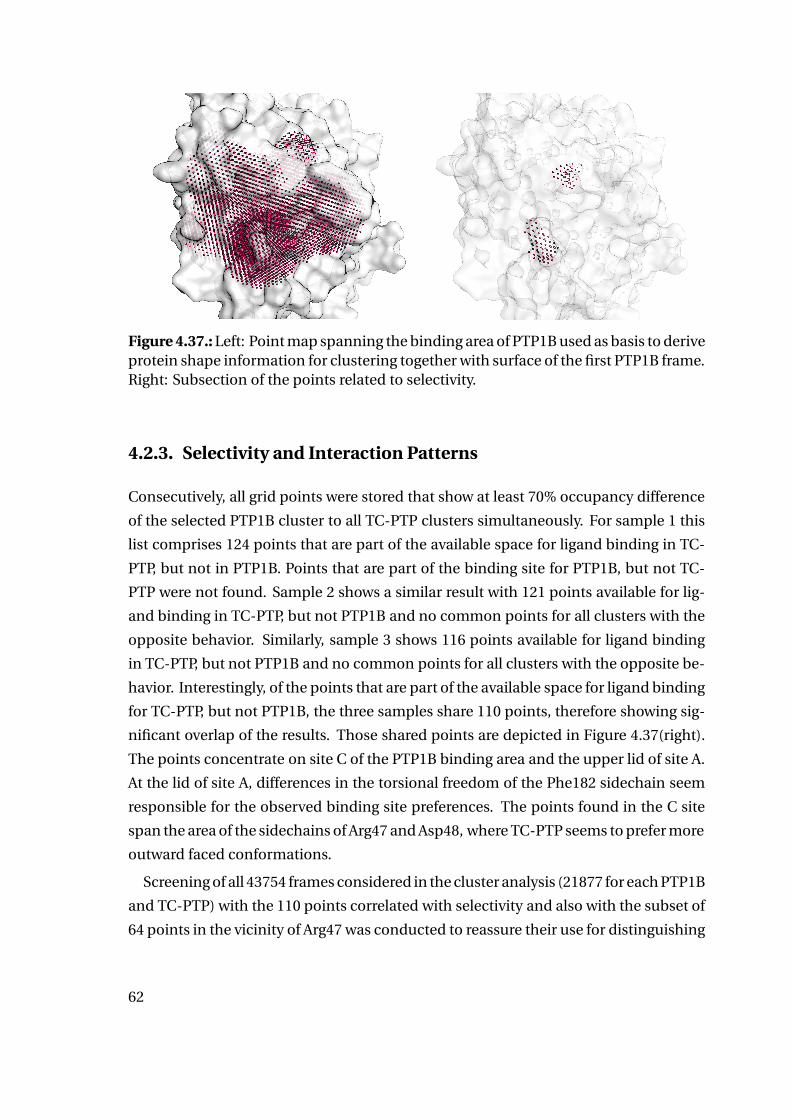
Figure 4.37.: Left: Point map spanning the binding area of PTP1B used as basis to deriveprotein shape information for clustering together with surface of the first PTP1B frame.Right: Subsection of the points related to selectivity.
4.2.3. Selectivity and Interaction Patterns
Consecutively, all grid points were stored that show at least 70% occupancy difference
of the selected PTP1B cluster to all TC-PTP clusters simultaneously. For sample 1 this
list comprises 124 points that are part of the available space for ligand binding in TC-
PTP, but not in PTP1B. Points that are part of the binding site for PTP1B, but not TC-
PTP were not found. Sample 2 shows a similar result with 121 points available for lig-
and binding in TC-PTP, but not PTP1B and no common points for all clusters with the
opposite behavior. Similarly, sample 3 shows 116 points available for ligand binding
in TC-PTP, but not PTP1B and no common points for all clusters with the opposite be-
havior. Interestingly, of the points that are part of the available space for ligand binding
for TC-PTP, but not PTP1B, the three samples share 110 points, therefore showing sig-
nificant overlap of the results. Those shared points are depicted in Figure 4.37(right).
The points concentrate on site C of the PTP1B binding area and the upper lid of site A.
At the lid of site A, differences in the torsional freedom of the Phe182 sidechain seem
responsible for the observed binding site preferences. The points found in the C site
span the area of the sidechains of Arg47 and Asp48, where TC-PTP seems to prefer more
outward faced conformations.
Screening of all 43754 frames considered in the cluster analysis (21877 for each PTP1B
and TC-PTP) with the 110 points correlated with selectivity and also with the subset of
64 points in the vicinity of Arg47 was conducted to reassure their use for distinguishing
62
0
25
50
75
100
0255075100percent of selectivity points matched
perc
ent o
f fra
mes
dis
cove
red
PTP1B
TCPTP
0
25
50
75
100
0255075100percent of selectivity points matched
perc
ent o
f fra
mes
dis
cove
red
Figure 4.38.: Ratio of frames matching at least x percent of the selectivity map. Left:For the subset of 64 points around Arg47. Right: For the whole map of 110 points.
between PTP1B and TC-PTP frames, but also to select PTP1B frames for the consequent
virtual screening workflow. The results are plotted in Figure 4.38. The selectivity map
containing all 110 points is fulfilled by 905 PTP1B frames, but no TC-PTP frame. The
best fitting frame of all TC-PTP frames matches 73 of the 110 points. The subset of the
selectivity map containing the 64 points around Arg47 is fulfilled by 1491 PTP1B frames,
but no TC-PTP frame. The best fitting frame of all TC-PTP frames matches 59 of those
64 points. However, many of the TC-PTP frames - 13542 - match none of the 64 points.
Further it can be deduced from Figure 4.38 that the TC-PTP frames matching higher
numbers of the selectivity map points are rare for both the full map and the subset of
64 points.
From the 905 PTP1B frames matching all of the 110 points of the selectivity map, five
diverse frames were extracted for the virtual screening workflow:
• "1PTYorigFrame3290"
• "1PTYrep2Frame5561"
• "1PTYorigFrame5079"
• "1PTYorigFrame7139"
• "1PTYrep2Frame7181"
63
4.2.4. Virtual Screening
With the aim to find ligands showing selective inhibition of PTP1B, a virtual screen-
ing workflow was developed using the previously described selectivity map. In order to
add a filtering step to the screening process to increase the likelihood of activity against
PTP1B an approach based on molecular interaction fields was chosen to deduce phar-
macophoric features from the chosen protein frames, since a purely shape-based ap-
proach would lead to many false positive hits with no suitable distribution of pharma-
cophoric features. A schematic representation of the workflow is depicted in Figure
4.39.
In a first step (Fig. 4.39-A), molecular interaction fields were generated with MOE us-
ing probes for hydrogen bond donor, hydrogen bond acceptor and hydrophobic inter-
actions. To translate the interaction energy maxima to pharmacophore feature points,
the generated molecular interaction fields were saved in .cns format and further pro-
cessed using an R script created for this purpose. The script reads the interaction fields
and finds interaction energy maxima by comparing the energy at each grid point with
all neighboring points. A binding site center is defined and all points more than 15 Å
away from this center are excluded. Exclusion volumes are added on those points of
the 110 points correlated with selectivity, which are close to the binding site of the con-
sidered frame and not inside the protein surrounded by other exclusion volumes (Fig.
4.39-C). This limitation of the exclusion volumes to the necessary ones saves time dur-
ing screening. Both feature points as well as exclusion volume spheres of each frame
are written to a LigandScout pharmacophore format for visual inspection. Upon visual
inspection features with high overlap were merged and features distant from the cat-
alytic site were removed. Additionally, less restrictive exclusion volumes were added
manually at protein atom positions in binding site regions not covered by the selectiv-
ity map derived exclusion volumes (Fig. 4.39-D).
The final models are named by their molecular dynamics frame of origin. Mod_3290
is depicted in Figure 4.39-E. It comprises one hydrogen bond donor feature and four
hydrogen bond acceptor features of which one shows high overlap with the hydrogen
bond donor feature. The other three hydrogen bond acceptor features are arranged
with low overlap in the catalytic cavity. Further the model contains one hydropho-
bic feature of increased size between the triple of hydrogen bond acceptors and the
overlapping hydrogen bond donor / hydrogen bond acceptor feature. It also contains
over 50 exclusion volumes of different size in total. The other models show a similar
number and arrangement of exclusion volumes and similar feature arrangements as
64
depicted in Figure 4.40: Mod_5079 shows a triple of hydrogen bond acceptor features
separated from a fourth hydrogen bond acceptor feature by two hydrophobic features.
In mod_5561 a quadruple of hydrogen bond acceptors is separated from a fifth hydro-
gen bond acceptor by only one hydrophobic feature. Mod_7139 only shows a triple of
hydrogen bond acceptor features and two hydrophobic features. In mod_7181 a triple
of hydrogen bond acceptor features is joined by a hydrogen bond donor and a hydro-
gen bond acceptor feature of high overlap and separated from another hydrogen bond
acceptor feature by a hydrophobic feature.
All pharmacophore models show high similarity of the feature types and their distri-
bution compared to a PTP1B bound phosphotyrosine residue: They all show at least
three overlapping hydrogen bond acceptor features in the catalytic pocket together
with a hydrophobic feature in a distance of 4 to 5 Å to the nested hydrogen bond ac-
ceptor features, which are also found for phosphotyrosine and other PTP1B ligands.
However, they all show additional features close to the YRD loop to ensure interactions
with residues of the C site in a selective binding site conformation.
65

Figure 4.39.: Schematic representation of the pharmacophore generation workflow onthe example of frame "1PTYorigFrame3290"; A: Molecular interaction field, B: phar-macophore translation of selected interaction energy maxima, C: automatically gen-erated exclusion volumes based on selectivity pattern, D: manually added exclusionvolumes, E: final interaction pattern; color code: green - hydrogen bond donor, MIFthreshold -3.4; red - hydrogen bond acceptor, MIF threshold -3.4; yellow - hydropho-bic, MIF threshold -1.7.
66

Figure 4.40.: Molecular interaction fields and final interaction patterns based on theselected frames "1PTYorigFrame5079", "1PTYrep2Frame5561", "1PTYorigFrame7139"and "1PTYrep2Frame7181"; color code: green - hydrogen bond donor, MIF thresh-old -3.4; red - hydrogen bond acceptor, MIF threshold -3.4; yellow - hydrophobic, MIFthreshold -1.7.
67

In the next step, four databases of commercially available compounds were prepared
as described in the Experimental Section and screened with the optimized selectivity
and interaction patterns. The numbers of hits for each pharmacophore are summa-
rized in Table 4.6.
Database mod_3290 mod_5079 mod_7139 mod_5561 mod_7181
ChemBridge 3368 610 7356 1759 8
ChemDiv 2834 1107 12859 2352 7
keyorganics 599 197 1821 399 5
VitasM 4203 941 16176 2633 84
Table 4.6.: Virtual screening results (number of hits) of four vendor databases with theoptimized interaction patterns.
Database mod_3290 mod_5079 mod_7139 mod_5561 mod_7181
ChemBridge 326 58 403 108 0
ChemDiv 162 151 541 137 0
keyorganics 67 52 308 26 0
VitasM 359 113 1157 167 1
Table 4.7.: Results (number of hits) of the pharmacophore rescreening of the represen-tative poses extracted from docking grouped by the four vendor databases.
All hits of the pharmacophore screening were submitted to protein-ligand docking
into the corresponding frame to assess their most likely binding modes and in order to
reassure in the next step the pharmacophore fit of the ligand in a protein bound con-
formation. 25 docking poses per ligand were generated and checked for consistency
utilizing an R script created for that purpose (see Section A.4). The script performs
a density-based clustering of the poses for each ligand and based on the number of
68

clusters with sufficient size chooses up to three representatives. Figure 4.41 shows an
example for the result of the density-based clustering for 25 docking poses of a small
molecule in PTP1B. Two clusters are found beneath two single poses. For the identified
clusters representative structures are selected. The results of the automatic processing
nicely agree with intuitively chosen poses.
Hit numbers of the consequent pharmacophore rescreening of the representatives
can be found in Table 4.7.
Figure 4.41.: Results of the density-based clustering in R for 25 docking poses of an ex-emplary small molecule in the PTP1B binding site; yellow and orange poses are chosenfor further analysis, translucent poses are discarded.
The results show that the selection of consistent poses together with the pharma-
cophore rescreening leads to a significant reduction of hits. The number of hits was
further reduced by reassuring that the selected binding poses additionally fit the se-
lected protein frames well: Since the protein could show adaption to the bound lig-
and and move away from the conformational pattern correlated with selectivity, energy
minimization of the poses selected via pharmacophore rescreening together with the
surrounding amino acids was performed. This step was then followed by visual inspec-
tion of the energy minimized conformations with the previously described selectivity
map. Only poses with protein conformations matching at least 100 of the 110 points
69
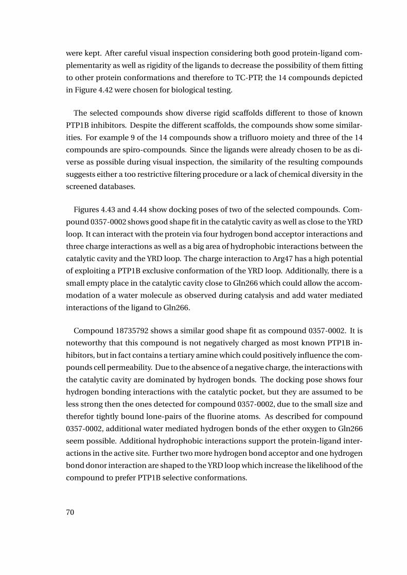
were kept. After careful visual inspection considering both good protein-ligand com-
plementarity as well as rigidity of the ligands to decrease the possibility of them fitting
to other protein conformations and therefore to TC-PTP, the 14 compounds depicted
in Figure 4.42 were chosen for biological testing.
The selected compounds show diverse rigid scaffolds different to those of known
PTP1B inhibitors. Despite the different scaffolds, the compounds show some similar-
ities. For example 9 of the 14 compounds show a trifluoro moiety and three of the 14
compounds are spiro-compounds. Since the ligands were already chosen to be as di-
verse as possible during visual inspection, the similarity of the resulting compounds
suggests either a too restrictive filtering procedure or a lack of chemical diversity in the
screened databases.
Figures 4.43 and 4.44 show docking poses of two of the selected compounds. Com-
pound 0357-0002 shows good shape fit in the catalytic cavity as well as close to the YRD
loop. It can interact with the protein via four hydrogen bond acceptor interactions and
three charge interactions as well as a big area of hydrophobic interactions between the
catalytic cavity and the YRD loop. The charge interaction to Arg47 has a high potential
of exploiting a PTP1B exclusive conformation of the YRD loop. Additionally, there is a
small empty place in the catalytic cavity close to Gln266 which could allow the accom-
modation of a water molecule as observed during catalysis and add water mediated
interactions of the ligand to Gln266.
Compound 18735792 shows a similar good shape fit as compound 0357-0002. It is
noteworthy that this compound is not negatively charged as most known PTP1B in-
hibitors, but in fact contains a tertiary amine which could positively influence the com-
pounds cell permeability. Due to the absence of a negative charge, the interactions with
the catalytic cavity are dominated by hydrogen bonds. The docking pose shows four
hydrogen bonding interactions with the catalytic pocket, but they are assumed to be
less strong then the ones detected for compound 0357-0002, due to the small size and
therefor tightly bound lone-pairs of the fluorine atoms. As described for compound
0357-0002, additional water mediated hydrogen bonds of the ether oxygen to Gln266
seem possible. Additional hydrophobic interactions support the protein-ligand inter-
actions in the active site. Further two more hydrogen bond acceptor and one hydrogen
bond donor interaction are shaped to the YRD loop which increase the likelihood of the
compound to prefer PTP1B selective conformations.
70
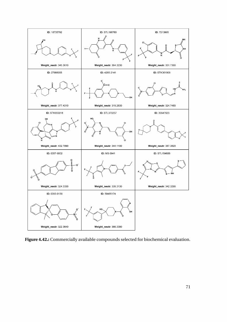
Figure 4.42.: Commercially available compounds selected for biochemical evaluation.
71
Figure 4.43.: Docking pose of compound 0357-0002 in the active site of PTP1B; Top: 3dimensional depiction of protein binding site and ligand shape; Bottom: 2 dimensionalligand depiction with pharmacophoric interactions to the protein; red circles and lines:hydrogen bond acceptor, red star: negative ionizable, green: hydrogen bond donor,yellow: hydrophobic interactions.
72
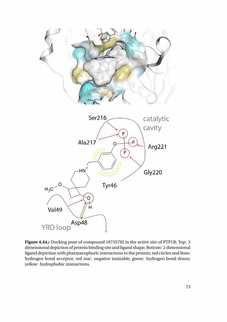
Figure 4.44.: Docking pose of compound 18735792 in the active site of PTP1B; Top: 3dimensional depiction of protein binding site and ligand shape; Bottom: 2 dimensionalligand depiction with pharmacophoric interactions to the protein; red circles and lines:hydrogen bond acceptor, red star: negative ionizable, green: hydrogen bond donor,yellow: hydrophobic interactions.
73

5. Discussion
5.1. Part I: Protein-Ligand Interaction Analysis
The overall aim of this study was the detection of key features in the surrounding of
the active site of PTP1B that could drive selectivity of PTP1B ligands. It was therefore
assumed that despite the disappointing research experiences found in literature, the
active site of PTP1B contains unique features that can be exploited to achieve selectivity
of small molecule binders against TC-PTP.
The first section of the corresponding analysis deals with comparison of the protein
sequences and of three-dimensional information from crystal structures. The high se-
quence similarity found in the active site area is not a new finding, still this detailed
analysis lays important groundwork for further parts of this study. Additionally, the
consideration of sequence differences together with the three-dimensional structure of
PTP1B can explain, why the observed sequence differences in the active site are hard
to target with ligand features. It is worth mentioning that the overall sequence iden-
tity of the two proteins is only 57% and therefore low in comparison to the active site
similarity. This part of the study therefore supports the idea that differences in the over-
all protein structure could influence ligand binding and enable ligand selectivity. This
idea was brought up many years before this study, however, so far no definite proof or
reasonable mechanism was found for this hypothesis. Consequently, binding poses of
co-crystallized selective PTP1B inhibitors were analyzed with different methods. Con-
ventional methods like the comparison of protein-ligand interactions of selective and
unselective PTP1B inhibitors show only subtle tendencies, but no solid explanation
for the observed selectivities. Additional, the results suggest C site interactions, espe-
cially with Asp48, to influence selectivity against TC-PTP. The analysis of interaction
counts also reveals the drawbacks of this method: Two crystal structures (1Q6T and
1Q6P) show crystal packing artifacts, which could introduce structural changes that
distort the result. Further, while counting polar interactions like hydrogen bonds is
75
rather intuitive, the quantification of hydrophobic interactions and the corresponding
effects on entropy is challenging. Additionally, ligand binding affinities for different
high affinity complexes have been related to shape complementarity or buried surface,
a factor that is not accounted for by counting protein-ligand interactions. The question
of PTP1B selectivity therefore seems unsolvable taking into account only conventional
methods of analysis on static protein structures. Still conventional methods like ana-
lyzing protein-ligand interactions in static structures have been proven useful in many
cases, therefore the absence of explanations in the case of PTP1B selectivity is an im-
portant result.
Since static protein structures did not reveal promising results, the flexible behavior
of selective inhibitors in both proteins was then analyzed using molecular dynamics
simulations. Contemplating the results of this part, however, it needs to be taken into
account that the molecular dynamics simulations for TC-PTP were run on homology
models using PTP1B template structures. Therefore it may simply not be possible for
the TC-PTP structures to escape the possibly artificial local energy minimum created
by homology modeling.
RMSD and RMSF plots of the conducted simulations did not reveal meaningful dif-
ferences in protein flexibility between the two proteins. However, they all support that
the region of the pTYR loop and the connected α-helix is the most stable part of the
protein. Therefore, for further analyses the molecular dynamics frames were aligned
on this stable region to get a picture about flexibility of the surroundings given a ligand
anchored in the catalytic cavity. Remarkably, the WPD loop known for its high flexibil-
ity shows very low flexibility over the time of the simulations, probably due to fixation
in the closed state by the complexed ligands.
To investigate protein-ligand interactions over the molecular dynamics simulations,
dynophores were used. Similar to the static interaction analysis the variation of the re-
sults was high and allowed no clear deductions regarding differences of both proteins.
However, according to the dynophore analyses, B site interactions seem more stable
for PTP1B which is in agreement with their relevance for selectivity deduced form the
static interaction counts and also found in literature. Unfortunately, for those inter-
actions the variations between simulations of one protein are especially high, which
makes this result highly unreliable. However, this analysis also suggests parts of the A
site and the C site as possible interaction sites to introduce selectivity. In the simula-
tions of PTP1B-complex 1XBO and the corresponding homology model a slight shift
of the ligand between A and B site in TC-PTP compared to PTP1B could be observed
76

which seems to be connected to different hydrophobic interactions in the region con-
necting both sites. Unfortunately, the dynophore results share the drawback of static
interaction counts that hydrophobic interactions are hard to quantify and shape com-
plementarity is not sufficiently accounted for.
Consequently, we developed a new method to assess protein-ligand shape comple-
mentarity on frames of a molecular dynamics trajectory. Surprisingly, the results on the
test case 1XBO indicate that flexible shape complementarity might be the previously
undiscovered key feature of PTP1B selectivity. Interestingly, this method suggests the
A site interactions to play a main role in the selectivity of the 1XBO ligand, which agrees
with the result of the dynophore analysis that suggests HBA3 to be selectivity relevant.
Additionally, the detected difference in HYD1 interactions from the dynophore analysis
matches the only detected atom outside the A site, C35. Further, the strain energy plot
did not indicate significant differences in ligand conformations. It stands out that the
atoms with highest differences in ligand RMSF values match the atoms with shape fit
differences. The increased activity of the ligand in PTP1B could therefore be explained
by tighter binding due to better shape complementarity of the protein to the ligand in
the catalytic cavity. Also for the second test case, 1QXK, the new method indicated that
shape fit and here additionally ligand strain could be responsible for the observed se-
lectivity of the ligand. Surprisingly, for the 1QXK ligand, despite an overall better shape
fit to PTP1B, the active site part of the ligand shows increased shape fit to TC-PTP, which
fits the tendency observed in the dynophore statistics where HBA3, HBA4 and HBD1
show higher mean occurences in TC-PTP. Here, B and C site interactions seem respon-
sible for the selectivity and connected to especially good shape fit. As for the B site,
this good shape fit is correlated with reduced flexibility of the ligand in this area like
observed for 1XBO. For the C site, however, the increased shape fit does not correlate
with a difference in ligand flexibility. One possible explanation for that could be the as-
sociation of good shape fit in this area with the high number of frames with low ligand
strain in PTP1B: a PTP1B exclusive protein conformation of the YRD-loop could enable
ligand relaxation compared to other protein conformations which possibly introduce
ligand strain in order to enable hydrogen bonding at N1(HBD4) and N2(HBD3). This
hypothesis is supported by the result of the dynophore analysis indicating higher oc-
curences of the relevant hydrogen bonds in PTP1B as well as the results of Binding Site
Shape Clustering section.
Since the novel method of protein-ligand shape complementarity yielded interest-
ing results for the PTP1B/TC-PTP testcases in this study, investigations on additional
77
testcases would be highly interesting to discover the applicability of the protein-ligand
shape complementarity method for other other projects and proteins. Unfortunately,
since this method is in the current implementation highly time and resources con-
suming, we had to refrain from investigating further test cases. In order to assess its
relevance on further test cases reimplementation therefore might be a rational step.
Additionally, supplementary studies on the impact of results on input settings of the
method like the size and shape of the starting point map and the spacing of the grid
points would be desirable to optimize the method for general use. Overall, this method
represents a novel opportunity to look at protein-ligand interactions from a different
viewpoint and could help to explain ligand activity differences in so far undisclosed
cases.
5.2. Part II: Binding Site Shape Clustering and Screening
The second part of this study deals with the question if the differences discovered in
protein-ligand complementarity can be targeted to find or create inhibitors of increased
selectivity. Hence, it is assumed that the differences in shape complementarity origi-
nate in differing conformational preferences of the two proteins.
Consequently, molecular dynamics simulations of protein structures for both PTP1B
and TC-PTP with only a ligand anchor to keep the WPD loop closed were performed
and analyzed. Keeping the WPD loop closed was considered appropiate due to most
higher active inhibitor binding poses showing a closed WPD loop. Furthermore, this
approach aims to separate the movements connected to the WPD loop opening and
closure from movements relevant for selectivity of active site inhibitors. However, there
is no guarantee that this restraint on the WPD loop is not suppressing relevant move-
ments or introducing unnatural behavior, especially in TC-PTP, into which the anchor
ligand was just placed instead of using protein-ligand docking. Additionally, the se-
lection of the starting structure of PTP1B and the created homology model for TC-PTP
could impact the outcome of the analysis, as could parameters like size and position
of the starting point map as well as grid spacing or the choice of the clustering algo-
rithm. Especially, due to the insufficient placement of grid points on the WPD loop,
loop movements could not be properly detected in this analysis. However, due to the
anchor ligand they were assumed to be negligible. Again, investigation of all influenc-
ing factors was out of the scope of this thesis and leaves room for further investigations
of this novel method.
78
Overall, the method yields interesting results with rationally guided selection of input
parameters, showing differing conformational preferences for the two proteins:
Firstly, clustering of the three bootstrapping samples leads to a good agreement of
the single results regarding number and size of the detected clusters with nice sepa-
ration between PTP1B and TC-PTP clusters. Secondly, the grid points selected to be
selectivity relevant by the method show a high amount of overlap between the results
of the bootstrapping samples.
Translation of this information into a selectivity point map allows visualization of the
result and exploitation for filtering of molecular dynamics frames. This way it could be
verified that filtering with the map selects PTP1B frames (905 frames selected), but not
a single TC-PTP frame. Additionally, PTP1B frames matching the selectivity map could
be chosen as representative frames for the consequent virtual screening workflow.
Interestingly, the points detected as relevant for selectivity concentrate around only
two protein sites: the first site is located around the side chain of Phe182. The detected
differences here seem to correlate only with rotations of the phenyl ring of this amino
acid. A detection of an area in the A site with this method corroborates the results
of the first part of this study, which indicates this site as selectivity relevant for some
of the analyzed ligands. However, these differences could be induced by the artificial
placement of the phenylphosphate moiety in the active site for loop closure during ho-
mology modeling. The second part of the selectivity map is located around Arg47 and
Asp48 in the C site of the binding area. Here the YRD loop seems more flexible in PTP1B
and therefore able to adapt a conformation more bent towards the catalytic cavity. As-
tonishingly, also the static protein-ligand interaction analysis as well as the dynophore
analysis of ligand 1QXK pointed to this site to be relevant for selectivity. Surprisingly, no
points in the B site were detected to be relevant for selectivity. This could correlate with
the high intra-protein variance discovered in the dynophore analysis. Additionally, the
alignment on stable A site atoms could lead to higher variation in more distant points.
Both factors could disturb a pattern of occupancy differences and render it undiscov-
erable by the clustering method.
The final part of this study aims at exploiting conformational differences of PTP1B
and TC-PTP to find selective PTP1B inhibitors. Of the 905 frames matching the selectiv-
ity map, 5 were chosen for the virtual screening workflow. The number was limited by
the available computing time for screening, therefore diverse frames were picked from
the set. Possibly more elaborate picking methods like choosing frames with many close
neighbors could increase the chance to find relevant protein conformations.
79

In the attempt to not only include spatial, but also pharmacophoric information to
the screening to increase the likelihood of activity at the protein, molecular interaction
fields were used to create interaction patterns screenable with LigandScout. Different
to classical 3D pharmacophores, these interaction patterns are not based on one or
more ligands. This has advantages and disadvantages: On the one hand, purely pro-
tein structure based interaction patterns allow inclusion of interactions with high like-
lihood of positive impact on activity independent on whether or not they are already
present in known ligands. On the other hand, a good interaction energy score at a cer-
tain grid point does not necessarily imply relevance of this interaction for activity. In
fact, the good score might be related to the energy function or the interaction point
could be too small or restricted in its angle to be met by a real ligand. However, this
protein structure based selection of interaction points is a common approach, which
was implemented in a similar fashion in Discovery Studio/Catalyst and the most recent
LigandScout version [113, 80, 81].
The results of this method are corroborated by the high resemblance of the interac-
tion patterns to 3D pharmacophores of known PTP1B ligands with at least three nested
hydrogen bond acceptor features in the catalytic cavity and a close-by hydrophobic
feature below the WPD loop. Due to the additional C site interactions optimized to
fit only selective PTP1B conformations, there is no appropriate data set for validation
of the interaction patterns. Validating the interaction patterns on PTP1B inhibitors by
omitting their C site features would also be of limited relevance, since the remaining in-
teraction patterns would only contain a few number of features and most likely be very
unspecific. Their high similarity to pharmacophores of known ligands in the active site
therefore depicts the only validation method.
The applied combination of screening with the chosen interaction patterns, protein-
ligand docking, pose-consistency filtering and interaction pattern rescreening was cho-
sen to reduce false positives among the screening hits. As mentioned in the "Compu-
tational Methods" section combinations of filtering and or screening methods are not
uncommon to decrease false positive rates is virtual screening. However, most stud-
ies rely on docking scores rather than pose-consistency filtering. Pose-consistency fil-
tering was developed and used in this study, since docking scores were found to be
unreliable in many cases, especially if they were not adapted and validated on the rele-
vant target. Although pose-consistency is depending on the created docking poses and
therefore also on the scoring function, it gives a more qualitative decision criterion for
pose selection which is not dependent on the total score and factors like ligand size.
80

The combination of conformational rigidity, good shape fit of the ligand to the selec-
tive protein frame and matching of the interaction patterns depicts a very restrictive
filter for small molecules. Therefore it seems reasonable that the resulting compounds
from vendor databases show a lack of diversity and partially unsatisfactory agreement
with the requirements like the trifluoro-group as triple hydrogen bond acceptor fea-
tures. Since all of the mentioned aspects ensure integral properties of the desired lig-
ands, the only option to find more customized ligands would be de novo synthesis.
However, this was out of the scope of this study, but would be a desirable step after an
initial biochemical validation of the workflow. Further, fluorinated motifs have been
discovered to adopt diverse protein binding features and could therefore be an inter-
esting alternative to known phosphotyrosine mimetics [114].
In total the second part supports the hypothesis discovered in the first part of the
study, suggesting that differences in conformational flexibility of both proteins exist. In
fact, the results even suggest a possibility to exploit those differences by small catalytic
site binding compounds.
81

6. Conclusion and Outlook
Despite decades of research, the key principles of PTP1B selectivity against TC-PTP are
still unknown and highly selective PTP1B inhibitors have not been published. Since
selective inhibition of PTP1B could be a valuable contribution in the fight against de-
seases like Type 2 diabetes and obesity, this study strived to detect and exploit key fea-
tures of PTP1B selectivity. This aim was persued in two different approaches: a detailed
analysis of partially selective PTP1B inhibitors in their protein bound conformations in
Part I and a consequent predictive method based on clustering of binding site shapes
derived from molecular dynamics simulations in Part II.
Since classical interaction analysis approaches did not lead to concise results regard-
ing influencing factors of PTP1B selectivity, a novel method to measure flexible protein-
ligand shape complementarity was developed and implemented. Validation on two
partially selective ligands led to interesting findings, indicating protein-ligand shape
complementarity and resulting increased ligand stability in different areas of the bind-
ing site to be responsible for the selectivity of the investigated ligands. Additionally, for
one of the ligands the results point towards an increased possibility of PTP1B to adapt
to the ligand with the YRD loop.
Those conclusions were corroborated by the second part of the study: The novel
method of binding site shape clustering developed here also implicated a part of the
catalytic cavity as an area of differing protein flexibility in PTP1B and TC-PTP and there-
fore relevant for selectivity. However, due to the limited space in the catalytic cavity
and the highly similar interaction feature patterns in both proteins, the optimization
of ligands towards a PTP1B preferred conformation at this site would be extremely dif-
ficult. Interestingly, this method further strongly suggested the C-site of the protein
binding site to show different conformational preferences in both proteins. Opposed
to the differences in the catalytic cavity, these differences show increased potential for
exploitation with small ligands. Consequently, the method was extended to exploit the
detected selectivity shape features for virtual screening. With this approach, commer-
83
cially available compounds with high potential to be selective PTP1B inhibitors could
be identified.
Beneath the interesting results on the test case of PTP1B, the two novel methods
developed in this study represent valuable new tools that could be of use for differ-
ent applications: The shape complementarity tool complements the shortcomings of
classical protein-ligand interaction analysis tools by focusing on ligand conformational
preferences and shape fit, which have been shown to be integral parts of ligand affinity
and could therefore help to explain and exploit activity differences especially in simi-
lar protein-ligand complexes. The binding site shape clustering tool addresses the is-
sue of different conformational preferences of similar proteins for exploitation in drug
development projects. It could therefore guide development of selective ligands even
in cases where interaction patterns of the proteins are highly similar. However, both
methods are only valuable in combination with interaction feature based methods like
pharmacophores or molecular interaction fields to ensure an overall sufficient com-
plementarity of a ligand to the target.
Overall, the results of both parts of this study concur nicely in indicating shape com-
plementarity as an important feature to increase PTP1B selectivity. Additionally, the
novel Binding Site Shape Clustering method developed in this study made it possible
to exploit this discovery for virtual screening and both aspects together could positively
impact future drug design projects, where selectivity plays an important role.
84

7. Experimental Section
Since this thesis focuses on computational methods, this part primarily contains de-
tails and settings of the conducted computational steps that would disturb the expla-
nations in the "Computational Methods" section.
7.1. Part I: Protein-Ligand Interaction Analysis
7.1.1. Sequence Comparison of PTP1B and TC-PTP
Protein sequences for PTP1B (P18031) and Isoform 1 of TC-PTP (P17706-1) were ex-
tracted from Uniprot [110] and aligned with default settings for proteins using Clustal
Omega [115]. PDB [46] complex 1PTY [116]was chosen as representative for analysis of
binding site residues.
7.1.2. PTP1B Crystal Structure Analysis
The Uniprot referenced PDB structures for PTP1B were sorted by resolution and com-
plexes with worse or equal resolution than 2.70 Å were excluded. Structures with co-
valent active site or nearby (Cα in 15 Å sphere around GLN262-CD) modifications like
mutations, intermediates or missing loops were excluded, since they could disrupt the
natural protein conformation and due to the high similarity of the two proteins sub-
tle changes could distort features of selectivity. Also excluded were structures with
residue modifications connected to modified activity (see e.g. [117] or [118]) and struc-
tures with no ligand or only allosteric ligand. For the selected structures, the Chembl
database [107] and, if not available there, the original publication were checked for lig-
and activities of the co-crystallized ligand against PTP1B and TC-PTP. If available, activ-
ities of the ligand against both proteins from the same group and assay and under com-
parable conditions were preferred. Selectivity factors were calculated and the 10 most
selective structures were chosen additionally to 4 non-selective complexes. Analysis
85

of the selected complexes was performed using MOE(2015.10) [43] and LigandScout(4)
[80, 81]. Interaction frequencies were plotted with R [89].
7.1.3. TC-PTP Crystal Structure Analysis and Homology Modeling
Backbone alignment for visual inspection of PTP1B structure 1PTY and TC-PTP struc-
ture 1L8K was performed in MOE(2015.10) [43]. Homology modeling was also per-
formed using MOE(2015.10) [43]: The TC-PTP sequence was aligned to the sequence
of the PTP1B template being one of the crystal structure complexes 1QXK [119], 1Q1M
[120] and 1XBO [121]. C- and N-terminal outgap modeling was disabled, automatic
disulfide bond detection was enabled and atoms of the co-crystallized ligand were se-
lected as environment for induced fit. The basic modeling step was chosen to create 25
main chain models with 10 side chain samples each at 300 K. Amber99 was chosen as
forcefield . Model refinement was performed in mode "Fine" with RMS Gradient set to
1.0. The resulting 250 models were analyzed regarding their protein and ligand RMSD
to the modeling template.
7.1.4. Molecular Dynamics Simulations
Basic protein preparation was performed in MOE(2015.10)[43]: sidechain protonation
was performed with the Protonate 3D tool at pH=7. The cysteine residue in the cat-
alytic center was deprotonated manually. All molecular dynamics simulations were
performed with the software Desmond 3.1 [71]. Systems were set up in an orthorhom-
bic box with SPC water and neutralized with Na+ ions. NaCl was added to a concentra-
tion of 0.15 M. Simulations were performed with NPT ensemble at 300 K and 1.01325
bar under periodic boundary conditions. A short relaxation time was followed by a 25
ns production run. For relaxation the Desmond standard NPT relaxation protocol was
used. Energies were recorded every 1.2 ps and the trajectory was saved every 4.8 ps. As
forcefield OPLS2005 was chosen. Calculations were run in triplicates on 24 CPUs each
on the Soroban computing cluster of FU Berlin. Trajectories were analyzed using VMD
[122] and the R package "bio3d" [89, 123].
7.1.5. Dynophore Analysis
The dynophore analysis is based on the dynophore tool for statistical analysis of Lig-
andScout 3D pharmacophores, which was recently developed in our group by Gerhard
86
Wolber and Dominique Sydow [34, 35, 80, 81]. Additional statistical analyses of the re-
sults were carried out in R [89].
The dynophore application creates a 3D pharmacophore for each frame of a molec-
ular dynamics trajectory. Pharmacophore features with the same feature type and in-
teracting atoms on the ligand are binned into superfeatures. Superfeatures are then
statistically analyzed for example regarding its occurrence over the molecular dynam-
ics simulation and the distances of the interacting atoms on protein and ligand side.
7.1.6. Shape Complementarity Analysis
The modification of the POVME tool [94, 95], which was used in this study can be found
in section A.1 of the Appendix. For generation of the POVME point maps grid spacing
of 0.5 Å was used. The distance cutoff for ligand heavy atoms to points of the created
maps was set to 0.59 Å for the inner map and 1.59 Å for the outer map. The distance
cutoff for protein heavy atoms to the created point maps was kept at 0.59 Å.
7.2. Part II: Binding Site Shape Clustering and Screening
7.2.1. Generation of Input Data
Homology modeling was performed using MOE(2015.10) [43]: The TC-PTP sequence
was aligned to the sequence of the PTP1B template 1PTY [116]. The ligand was reduced
to its phenylphosphate moiety and not used for adaptive homology modeling. The
basic modeling step was chosen to create 25 main chain models with 10 side chain
samples each at 300 K. As forcefield Amber99 was chosen. Model refinement was per-
formed in mode "Fine" with RMS Gradient set to 1.0. The resulting 250 models were
analyzed and filtered regarding the similarity to the PTP1B template in the binding area.
After selection of the final model, the phenylphosphate moiety and the adjacent cat-
alytic water molecule were transposed to the TC-PTP homology model.
Molecular dynamics simulations were prepared and conducted as described in the
subsection Molecular Dynamics in Part I of the methods section. Simulations were run
in triplicates over 50 ns each after a short relaxation run.
For the creation of point maps using the modified POVME script (section A.1 of the
Appendix) a starting point map of 10427 points spanning the whole binding area was
created. Grid spacing was set to 1.0 Å and the distance cutoff of protein atoms to points
87

of the created maps was fixed to 1.09 Å. A contiguous pocket seed sphere was placed in
the center of the catalytic cavity.
7.2.2. Selectivity and Interaction Patterns
Molecular interaction fields were created using MOE2015.10 [43]. Three probes were
selected for interaction field generation: "N1" (amide NH group) for hydrogen bond
donor interactions, "N:" (nitrogen atom with lone pair) for hydrogen bond acceptor
interactions, "DRY" for hydrophobic interactions.
7.2.3. Virtual Screening
For virtual screening databases of the vendors ChemBridge, ChemDiv, VitasM and key-
Organics were chosen. Vendor databases were downloaded in the version of July 2016.
The databases were prepared removing salt and solvent molecules from compound en-
tries. Then standardization of the structures was performed using the group protocol
for the ChemAxon Standardizer software [45]: amidine and guanidine structures were
harmonized, different acidic structures were deprotonated and basic structures were
protonated. 25 conformations per ligand were generated with LigandScout 4 [80, 81].
After the preparation the databases contained the following numbers of molecules:
ChemBridge - 1,141,083; ChemDiv - 1,455,331; VitasM - 1,384,271; keyOrganics - 79,617.
Screening of the databases and rescreening of selected docking poses with the molec-
ular interaction field derived interaction patterns was conducted with LigandScout 4
[80, 81]. Protein-ligand docking of the resulting hits into the corresponding molecular
dynamics frames was performed with GOLD version 5.2.2 [54]. The phenylphosphate
moiety and all solvent molecules were removed prior to docking. The binding site was
restricted to a sphere of 12 Å radius around the sulfur atom of CYS215. 25 poses per
ligand were generated. Scoring of the docking poses was performed using the scoring
function PLP with rescoring using Goldscore.
Density based clustering on the RMSD matrix of each molecule’s 25 docking poses
was performed using the package "dbscan" in R with the options eps = 1.5 and minPts
= 8 [89].
88

8. Summary
Protein Tyrosine Phosphatase 1B (PTP1B) is a validated drug target for the treatment of
diabetes type 2 and obesity. Until now, development of suitable modulators has been
hampered by the polarity of the binding site and related bioavailability issues of the
molecules. The design of selective inhibitors of PTP1B against the closely related T-Cell
protein tyrosine phosphatase (TC-PTP), which was associated to severe side effects in
animal studies, proved even more challenging. Over the years progress was made, but
known PTP1B inhibitors only achieved at maximum moderate selectivity over TC-PTP.
This study aims to break the traditional boundaries of PTP1B selectivity by deliber-
ately exploiting structural differences of both proteins. Due to their high similarity this
requires thorough analysis of their static structures as well as their flexible behavior.
The goal was therefore pursued with two different approaches:
In Part I of the study a detailed analysis of protein complexes with selective ligands
was performed including their flexible behavior as determined from molecular dynam-
ics simulations. Since common analysis methods were not able to explain the selectiv-
ity of the investigated ligands, a new method was developed which is able to assess pa-
rameters of ligand affinity that are not covered by currently available methods: steric
complementarity of the ligand to the protein together with ligand strain. The devel-
oped tool allows to assess those properties on high numbers of molecular dynamics
frames to calculate ligand shape fit in a flexible context. It further enables to trace back
the ligand atoms or parts responsible for good or bad shape fit.
In Part II of this study the flexible behavior of the apoproteins was studied. Since sur-
face properties are highly similar in both proteins, the analysis focused on binding site
shapes. For this, a novel approach was chosen that translates binding site shapes from
molecular dynamics simulations into point maps and subsequently uses clustering
and difference calculations to find a PTP1B conformation most unlike to all discovered
TC-PTP conformations. The workflow includes calculation of a selectivity map consist-
ing of points in the binding site where highest and most relevant differences in PTP1B
89
and TC-PTP conformations occur. This map can be visualized and used for screening
of selective PTP1B frames, which can then be used for protein structure based virtual
screening for potentially selective PTP1B inhibitors.
Results of Part I indicate shape fit as the previously undiscovered reason for selec-
tivity of some known PTP1B inhibitors. They further suggest that selectivity can be
achieved by interactions in the catalytic cavity as well as in previously suggested ar-
eas (the B and C site) of the binding site. Additionally, the discovered reduced lig-
and strain in PTP1B for one of the analyzed ligands, while almost maintaining same
occurences of protein-ligand interaction features, lead to the assumption that PTP1B
possesses a higher ability to conformationally adapt to the ligand than TC-PTP. This as-
sumption is corroborated by the results of Part II: The selectivity map indicates the cat-
alytic cavity and the YRD-loop (C site) as areas of different flexible behavior. Especially
the YRD-loop shows increased flexibility in PTP1B compared to TC-PTP. Additionally,
ligands that have a high likelihood of exploiting the discovered conformational differ-
ences while still showing sufficient activity in PTP1B could be found in databases of
commercially available molecules.
Overall, the two innovative approaches to discover key factors of PTP1B selectivity
did not only lead to interesting findings, but could also be adapted to promote other
drug design projects where selectivity is crucial but hard to achieve.
90
9. Zusammenfassung
Das Enzym Protein Tyrosin Phosphatase 1B (PTP1B) ist ein validiertes Wirkstoffziel
für die Behandlung von Diabetes Typ 2 und Übergewicht. Die Entwicklung passender
Modulatoren wurde immer wieder durch die Polarität der Bindetasche und damit ver-
bundene Bioverfügbarkeitsprobleme der Moleküle zurückgeworfen. Noch schwieriger
ist es aber, die Moleküle so zu modifizieren, dass sie Selektivität gegenüber dem nahe
verwandten Enzym T-Zell Protein Tyrosin Phosphatase (TC-PTP) erhalten, was auf-
grund der mit diesem Protein assoziierten starken unerwünschten Wirkungen notwen-
dig erscheint. Trotz einiger Fortschritte in den letzten Jahren erreichen bekannte PTP1B-
Inhibitoren bis jetzt maximal moderate Selektivität gegenüber TC-PTP.
Diese Arbeit hat es sich zum Ziel gemacht die durch bisherige Forschung gesetzten
Grenzen der PTP1B-Selektivität zu durchbrechen, indem systematisch strukturelle Un-
terschiede der beiden Proteine ausgenutzt werden. Aufgrund ihrer sehr großen Ähn-
lichkeit erfordert dies eine genaue Analyse der statischen Proteinstrukturen sowie ihres
dynamischen Verhaltens. Um dieses Ziel zu erreichen, wurden zwei Ansätze gewählt:
In Teil I der Arbeit wurde eine detaillierte Analyse von Protein-Komplexen mit se-
lektiven Liganden und deren dynamischen Verhaltens mithilfe von Moleküldynamik-
simulationen durchgeführt. Da verfügbare Analysemethoden nicht in der Lage waren
die beobachtete Selektivität zu erklären, wurde eine neue Methode entwickelt, welche
es ermöglicht zusätzliche Faktoren für Ligandenaffinität zu erfassen: sterische Kom-
plementarität und konformationelle Energie des Liganden. Die entwickelte Methode
ermöglicht es diese Faktoren an einer großen Anzahl von Moleküldynamik-Schritten
zu erfassen, um Verteilungen für die sterische Komplementarität am flexiblen Protein-
Liganden-Komplex zu erhalten. Zusätzlich können die Anteile eines jeden Ligandena-
toms an der Gesamtkomplementarität berechnet und dargestellt werden.
In Teil II der Arbeit wurde das flexible Verhalten der Apoproteine näher untersucht.
Da die Oberflächeneigenschaften beider Proteine kaum Unterschiede zeigen, konzen-
trierte sich diese Analyse auf die Form der Bindetaschen. Dafür wurde ein neuartiger
91
Ansatz gewählt, der die Form der Bindetasche aus Moleküldynamiksimulationen ex-
trahiert und in Punktwolken übersetzt. Diese werden anschließend geclustert, worauf-
hin mithilfe von Distanzberechnungen PTP1B-Konformationen ermittelt werden, die
den größtmöglichen Unterschied zu allen ermittelten TC-PTP-Konformationen auf-
weisen. Der dafür verwendete Workflow berechnet zusätzlich einen Selektivitätsfilter
bestehend aus denjenigen Punkten der Punktwolke, die die größten beziehungsweise
relevantesten Unterschiede in den PTP1B- und TC-PTP-Konformationen zeigen. Dieser
Filter dient einerseits dazu die Selektivitätsrelevanten Bindetaschenareale zu visuali-
sieren, kann aber auch zum Filtern nach selektiven PTP1B-Konformationen aus Mole-
küldynamiksimulationen dienen, welche anschließend zum strukturbasierten virtuel-
len Screening nach potentiell selektiven PTP1B-Inhibitoren genutzt werden können.
Die Ergebnisse von Teil I deuten darauf hin, dass die sterische Komplementarität den
bisher unbekannten Grund für die Selektivität einiger bekannter PTP1B-Inhibitoren
darstellen könnte. Außerdem geht aus den Analysen hervor, dass Selektivität womög-
lich auch durch Interaktionen mit der katalytischen Tasche hervorgerufen werden kann,
neben Interaktionen mit schon in früheren Studien vorgeschlagenen Arealen der Binde-
tasche (B- und C-Seite). Zusätzlich zeigt einer der selektiven Liganden eine teilweise re-
duzierte konformationelle innere Enenergie, obwohl kaum Unterschiede im Vorkom-
men der Häufigkeiten der Protein-Liganden-Bindungen zu erkennen sind. Hier kann
die Vermutung aufgestellt werden, dass dies durch eine erhöhte Fähigkeit von PTP1B
im Vergleich zu TC-PTP verursacht wird seine Konformation an den Liganden anzu-
passen. Diese Vermutung wird durch die Ergebnisse aus Teil II der Arbeit gestützt: Der
Selektivitätsfilter weist einerseits auf die katalytische Bindetasche, andererseits auf den
YRD-loop (C-Seite) als Areale unterschiedlicher Flexibilität hin. Insbesondere der YRD-
loop zeigt erhöhte Flexibilität in PTP1B im Vergleich zu TC-PTP. Zusätzlich konnten in
diesem Teil der Arbeit Liganden in Datenbanken käuflich erwerbbarer Moleküle ge-
funden werden, welche nach unserem Modell eine große Wahrscheinlichkeit haben
die ermittelten konformationellen Unterschiede bei zusätzlich guter Aktivität in PTP1B
gezielt auszunutzen.
Insgesamt führten die zwei innovativen Ansätze zur Ermittlung von Schlüsselfak-
toren der PTP1B-Selektivität nicht nur zu äußerst interessanten Ergebnissen, sondern
könnten auch angepasst werden um Wirkstoffdesignprojekte voranzutreiben, bei de-
nen Selektivität von großer Wichtigkeit, aber schwer zu erreichen ist.
92
Bibliography
[1] Z. Y. Zhang. Protein tyrosine phosphatases: structure and function, substrate
specificity, and inhibitor development. Annu Rev Pharmacol Toxicol, 42:209–34,
2002.
[2] D. Barford, A. K. Das, and M. P. Egloff. The structure and mechanism of protein
phosphatases: insights into catalysis and regulation. Annu Rev Biophys Biomol
Struct, 27:133–64, 1998.
[3] N. K. Tonks. Protein tyrosine phosphatases - from housekeeping enzymes to
master regulators of signal transduction. FEBS J, 280(2):346–78, 2013.
[4] N. K. Tonks. PTP1B: from the sidelines to the front lines! FEBS Lett, 546(1):140–8,
2003.
[5] S. Zhang and Z. Y. Zhang. PTP1B as a drug target: recent developments in PTP1B
inhibitor discovery. Drug Discov Today, 12(9-10):373–81, 2007.
[6] S. Koren and I. G. Fantus. Inhibition of the protein tyrosine phosphatase PTP1B:
potential therapy for obesity, insulin resistance and type-2 diabetes mellitus. Best
Pract Res Clin Endocrinol Metab, 21(4):621–40, 2007.
[7] G. Moorhead (Ed.). Protein Phosphatase Protocols. Methods in Molecular Biology.
Totowa, 2007.
[8] F. Sacco, L. Perfetto, L. Castagnoli, and G. Cesareni. The human phosphatase
interactome: An intricate family portrait. FEBS Lett, 586(17):2732–9, 2012.
[9] N. K. Tonks. Protein tyrosine phosphatases: from genes, to function, to disease.
Nat Rev Mol Cell Biol, 7(11):833–46, 2006.
93
[10] A. D. Pannifer, A. J. Flint, N. K. Tonks, and D. Barford. Visualization of the
cysteinyl-phosphate intermediate of a protein-tyrosine phosphatase by x-ray
crystallography. J Biol Chem, 273(17):10454–62, 1998.
[11] N. K. Tonks, C. D. Diltz, and E. H. Fischer. Purification of the major protein-
tyrosine-phosphatases of human placenta. J Biol Chem, 263(14):6722–30, 1988.
[12] A. P. Combs. Recent advances in the discovery of competitive protein tyrosine
phosphatase 1B inhibitors for the treatment of diabetes, obesity, and cancer. J
Med Chem, 53(6):2333–44, 2010.
[13] J. C. Byon, A. B. Kusari, and J. Kusari. Protein-tyrosine phosphatase-1B acts as
a negative regulator of insulin signal transduction. Mol Cell Biochem, 182(1-2):
101–8, 1998.
[14] N. Dube and M. L. Tremblay. Involvement of the small protein tyrosine phos-
phatases TC-PTP and PTP1B in signal transduction and diseases: from diabetes,
obesity to cell cycle, and cancer. Biochim Biophys Acta, 1754(1-2):108–17, 2005.
[15] T. O. Johnson, J. Ermolieff, and M. R. Jirousek. Protein tyrosine phosphatase 1B
inhibitors for diabetes. Nat Rev Drug Discov, 1(9):696–709, 2002.
[16] M. Elchebly, P. Payette, E. Michaliszyn, W. Cromlish, S. Collins, A. L. Loy, D. Nor-
mandin, A. Cheng, J. Himms-Hagen, C. C. Chan, C. Ramachandran, M. J. Gresser,
M. L. Tremblay, and B. P. Kennedy. Increased insulin sensitivity and obesity re-
sistance in mice lacking the protein tyrosine phosphatase-1B gene. Science, 283
(5407):1544–8, 1999.
[17] L. D. Klaman, O. Boss, O. D. Peroni, J. K. Kim, J. L. Martino, J. M. Zabolotny,
N. Moghal, M. Lubkin, Y. B. Kim, A. H. Sharpe, A. Stricker-Krongrad, G. I. Shul-
man, B. G. Neel, and B. B. Kahn. Increased energy expenditure, decreased adi-
posity, and tissue-specific insulin sensitivity in protein-tyrosine phosphatase 1B-
deficient mice. Mol Cell Biol, 20(15):5479–89, 2000.
[18] K. E. You-Ten, E. S. Muise, A. Itie, E. Michaliszyn, J. Wagner, S. Jothy, W. S. Lapp,
and M. L. Tremblay. Impaired bone marrow microenvironment and immune
function in t cell protein tyrosine phosphatase-deficient mice. J Exp Med, 186
(5):683–93, 1997.
94
[19] D. A. Chistiakov and E. I. Chistiakova. T-cell protein tyrosine phosphatase: A role
in inflammation and autoimmunity. International Journal of Diabetes Mellitus,
(2):114–118, 2010.
[20] L. F. Iversen, K. B. Moller, A. K. Pedersen, G. H. Peters, A. S. Petersen, H. S. Ander-
sen, S. Branner, S. B. Mortensen, and N. P. Moller. Structure determination of T
cell protein-tyrosine phosphatase. J Biol Chem, 277(22):19982–90, 2002.
[21] L. Bialy and H. Waldmann. Inhibitors of protein tyrosine phosphatases: next-
generation drugs? Angew Chem Int Ed Engl, 44(25):3814–39, 2005.
[22] Jr. Burke, T. R., B. Ye, X. Yan, S. Wang, Z. Jia, L. Chen, Z. Y. Zhang, and D. Barford.
Small molecule interactions with protein-tyrosine phosphatase PTP1B and their
use in inhibitor design. Biochemistry, 35(50):15989–96, 1996.
[23] Y. A. Puius, Y. Zhao, M. Sullivan, D. S. Lawrence, S. C. Almo, and Z. Y. Zhang.
Identification of a second aryl phosphate-binding site in protein-tyrosine phos-
phatase 1B: a paradigm for inhibitor design. Proc Natl Acad Sci U S A, 94(25):
13420–5, 1997.
[24] J. P. Sun, A. A. Fedorov, S. Y. Lee, X. L. Guo, K. Shen, D. S. Lawrence, S. C. Almo,
and Z. Y. Zhang. Crystal structure of PTP1B complexed with a potent and selective
bidentate inhibitor. J Biol Chem, 278(14):12406–14, 2003.
[25] L. F. Iversen, H. S. Andersen, S. Branner, S. B. Mortensen, G. H. Peters, K. Norris,
O. H. Olsen, C. B. Jeppesen, B. F. Lundt, W. Ripka, K. B. Moller, and N. P. Moller.
Structure-based design of a low molecular weight, nonphosphorus, nonpeptide,
and highly selective inhibitor of protein-tyrosine phosphatase 1B. J Biol Chem,
275(14):10300–7, 2000.
[26] G. Liu, Z. Xin, H. Liang, C. Abad-Zapatero, P. J. Hajduk, D. A. Janowick, B. G.
Szczepankiewicz, Z. Pei, C. W. Hutchins, S. J. Ballaron, M. A. Stashko, T. H.
Lubben, C. E. Berg, C. M. Rondinone, J. M. Trevillyan, and M. R. Jirousek. Selective
protein tyrosine phosphatase 1B inhibitors: targeting the second phosphotyro-
sine binding site with non-carboxylic acid-containing ligands. J Med Chem, 46
(16):3437–40, 2003.
[27] B. G. Szczepankiewicz, G. Liu, P. J. Hajduk, C. Abad-Zapatero, Z. Pei, Z. Xin, T. H.
Lubben, J. M. Trevillyan, M. A. Stashko, S. J. Ballaron, H. Liang, F. Huang, C. W.
95

Hutchins, S. W. Fesik, and M. R. Jirousek. Discovery of a potent, selective protein
tyrosine phosphatase 1B inhibitor using a linked-fragment strategy. J Am Chem
Soc, 125(14):4087–96, 2003.
[28] C. K. Lau, C. I. Bayly, J. Y. Gauthier, C. S. Li, M. Therien, E. Asante-Appiah,
W. Cromlish, Y. Boie, F. Forghani, S. Desmarais, Q. Wang, K. Skorey, D. Waddle-
ton, P. Payette, C. Ramachandran, B. P. Kennedy, and G. Scapin. Structure based
design of a series of potent and selective non peptidic PTP-1B inhibitors. Bioorg
Med Chem Lett, 14(4):1043–8, 2004.
[29] X. Chen, Q. Gan, C. Feng, X. Liu, and Q. Zhang. Virtual screening of novel and se-
lective inhibitors of protein tyrosine phosphatase 1B over t-cell protein tyrosine
phosphatase using a bidentate inhibition strategy. J Chem Inf Model, 2018.
[30] E. Black, J. Breed, A. L. Breeze, K. Embrey, R. Garcia, T. W. Gero, L. Godfrey, P. W.
Kenny, A. D. Morley, C. A. Minshull, A. D. Pannifer, J. Read, A. Rees, D. J. Russell,
D. Toader, and J. Tucker. Structure-based design of protein tyrosine phosphatase-
1B inhibitors. Bioorg Med Chem Lett, 15(10):2503–7, 2005.
[31] A. P. Combs, E. W. Yue, M. Bower, P. J. Ala, B. Wayland, B. Douty, A. Takvorian, P. Po-
lam, Z. Wasserman, W. Zhu, M. L. Crawley, J. Pruitt, R. Sparks, B. Glass, D. Modi,
E. McLaughlin, L. Bostrom, M. Li, L. Galya, K. Blom, M. Hillman, L. Gonneville,
B. G. Reid, M. Wei, M. Becker-Pasha, R. Klabe, R. Huber, Y. Li, G. Hollis, T. C. Burn,
R. Wynn, P. Liu, and B. Metcalf. Structure-based design and discovery of pro-
tein tyrosine phosphatase inhibitors incorporating novel isothiazolidinone het-
erocyclic phosphotyrosine mimetics. J Med Chem, 48(21):6544–8, 2005.
[32] E. W. Yue, B. Wayland, B. Douty, M. L. Crawley, E. McLaughlin, A. Takvorian,
Z. Wasserman, M. J. Bower, M. Wei, Y. Li, P. J. Ala, L. Gonneville, R. Wynn, T. C.
Burn, P. C. Liu, and A. P. Combs. Isothiazolidinone heterocycles as inhibitors of
protein tyrosine phosphatases: synthesis and structure-activity relationships of
a peptide scaffold. Bioorg Med Chem, 14(17):5833–49, 2006.
[33] Y. Du, Y. Zhang, H. Ling, Q. Li, and J. Shen. Discovery of novel high potent and
cellular active ADC type PTP1B inhibitors with selectivity over TC-PTP via mod-
ification interacting with C site. Eur J Med Chem, 144:692–700, 2018.
[34] D. Sydow. Dynophores: Novel Dynamic Pharmacophores. Humboldt-Universität
zu Berlin, Lebenswissenschaftliche Fakultät, 2015.
96

[35] A. Bock, M. Bermudez, F. Krebs, C. Matera, B. Chirinda, D. Sydow, C. Dallanoce,
U. Holzgrabe, M. De Amici, M. J. Lohse, G. Wolber, and K. Mohr. Ligand binding
ensembles determine graded agonist efficacies at a G protein-coupled receptor.
J Biol Chem, 291(31):16375–89, 2016.
[36] J. Mortier, J. R. C. Prevost, D. Sydow, S. Teuchert, C. Omieczynski, M. Bermudez,
R. Frederick, and G. Wolber. Arginase structure and inhibition: Catalytic site plas-
ticity reveals new modulation possibilities. Sci Rep, 7(1):13616, 2017.
[37] G. Sliwoski, S. Kothiwale, J. Meiler, and Jr. Lowe, E. W. Computational methods
in drug discovery. Pharmacol Rev, 66(1):334–95, 2014.
[38] I. Muegge, A. Bergner, and J. M. Kriegl. Computer-aided drug design at
Boehringer Ingelheim. J Comput Aided Mol Des, 31(3):275–285, 2017.
[39] F. K. Brown, E. C. Sherer, S. A. Johnson, M. K. Holloway, and B. S. Sherborne. The
evolution of drug design at Merck Research Laboratories. J Comput Aided Mol
Des, 31(3):255–266, 2017.
[40] C. Hansch and T. Fujita. p-s-p analysis. a method for the correlation of biological
activity and chemical structure. Journal of the American Chemical Society, 86(8):
1616–1626, 1964.
[41] D. E. Clark. What has computer-aided molecular design ever done for drug dis-
covery? Expert Opin Drug Discov, 1(2):103–10, 2006.
[42] Maestro. Schrödinger LLC, 2018.
[43] Molecular Operating Environment (MOE). Chemical Computing Group ULC,
1010 Sherbooke St. West, Suite #910, Montreal, QC, Canada, H3A 2R7, 2018.
[44] S. Cross and G. Cruciani. Molecular fields in drug discovery: getting old or reach-
ing maturity? Drug Discov Today, 15(1-2):23–32, 2010.
[45] Standardizer. ChemAxon, 2018.
[46] H. M. Berman, J. Westbrook, Z. Feng, G. Gilliland, T. N. Bhat, H. Weissig, I. N.
Shindyalov, and P. E. Bourne. The Protein Data Bank. Nucleic Acids Res, 28(1):
235–42, 2000.
97
[47] Ardell D.H. Illergård, K. and A. Elofsson. Structure is three to ten times more con-
served than sequence –a study of structural response in protein cores. Proteins,
(77):499–508, 2009.
[48] A. Hillisch, L. F. Pineda, and R. Hilgenfeld. Utility of homology models in the drug
discovery process. Drug Discov Today, 9(15):659–69, 2004.
[49] N. Eswar, B. Webb, M. A. Marti-Renom, M.S. Madhusudhan, D. Eramian, M. Shen,
U. Pieper, and A. Sali. Comparative protein structure modeling using Modeller.
Current Protocols in Bioinformatics, 28(5.6.1-5.6.32), 2014.
[50] Lawrence A. Kelley, Stefans Mezulis, Christopher M. Yates, Mark N. Wass, and
Michael J. E. Sternberg. The Phyre2 web portal for protein modeling, prediction
and analysis. Nature Protocols, 10:845, 2015.
[51] M. Biasini, S. Bienert, A. Waterhouse, K. Arnold, G. Studer, T. Schmidt, F. Kiefer,
T. G. Cassarino, M. Bertoni, L. Bordoli, and T. Schwede. SWISS-MODEL: mod-
elling protein tertiary and quaternary structure using evolutionary information.
Nucleic Acids Research, 42(Web Server issue):W252–W258, 2014.
[52] T. Schwede. Protein modeling: what happened to the "protein structure gap"?
Structure, 21(9):1531–40, 2013.
[53] P. A. Sousa, S. F.and Fernandes and M. J. Ramos. Protein-ligand docking: Current
status and future challenges. Proteins: Structure, Function, and Bioinformatics,
65(1):15–26, 2006.
[54] G. Jones, P. Willett, R. C. Glen, A. R. Leach, and R. Taylor. Development and vali-
dation of a genetic algorithm for flexible docking. J Mol Biol, 267(3):727–48, 1997.
[55] D. B. Kitchen, H. Decornez, J. R. Furr, and J. Bajorath. Docking and scoring in
virtual screening for drug discovery: methods and applications. Nat Rev Drug
Discov, 3(11):935–49, 2004.
[56] R. T. Kroemer. Structure-based drug design: docking and scoring. Curr Protein
Pept Sci, 8(4):312–28, 2007.
[57] G. L. Warren, C. W. Andrews, A. M. Capelli, B. Clarke, J. LaLonde, M. H. Lambert,
M. Lindvall, N. Nevins, S. F. Semus, S. Senger, G. Tedesco, I. D. Wall, J. M. Woolven,
C. E. Peishoff, and M. S. Head. A critical assessment of docking programs and
scoring functions. J Med Chem, 49(20):5912–31, 2006.
98
[58] B. Q. Wei, L. H. Weaver, A. M. Ferrari, B. W. Matthews, and B. K. Shoichet. Testing
a flexible-receptor docking algorithm in a model binding site. J Mol Biol, 337(5):
1161–82, 2004.
[59] G. M. Morris, W. Huey, R.and Lindstrom, M. F. Sanner, R. K. Belew, D. S. Goodsell,
and A. J. Olson. AutoDock4 and AutoDockTools4: Automated docking with se-
lective receptor flexibility. Journal of computational chemistry, 30(16):2785–2791,
2009.
[60] S. Forli, M. E. Huey, R.and Pique, M. Sanner, D. S. Goodsell, and A. J. Olson. Com-
putational protein-ligand docking and virtual drug screening with the AutoDock
suite. Nature protocols, 11(5):905–919, 2016.
[61] R. G. Coleman, M. Carchia, T. Sterling, J. J. Irwin, and B. K. Shoichet. Ligand pose
and orientational sampling in molecular docking. PLOS ONE, 8(10):e75992,2013.
[62] M. Rarey, T. Kramer, B.and Lengauer, and G. Klebe. A fast flexible docking method
using an incremental construction algorithm. Journal of Molecular Biology, 261
(3):470–489, 1996.
[63] R. A. Friesner, R. B. Murphy, M. P. Repasky, L. L. Frye, J. R. Greenwood, T. A. Hal-
gren, P. C. Sanschagrin, and D. T. Mainz. Extra precision Glide: Docking and
scoring incorporating a model of hydrophobic enclosure for protein-ligand com-
plexes. Journal of Medicinal Chemistry, 49(21):6177–6196, 2006.
[64] M. D. Cummings, R. L. DesJarlais, A. C. Gibbs, V. Mohan, and E. P. Jaeger. Com-
parison of automated docking programs as virtual screening tools. J Med Chem,
48(4):962–76, 2005.
[65] C. Bissantz, B. Kuhn, and M. Stahl. A medicinal chemist’s guide to molecular
interactions. J Med Chem, 53(14):5061–84, 2010.
[66] A. Ganesan, M. L. Coote, and K. Barakat. Molecular dynamics-driven drug discov-
ery: leaping forward with confidence. Drug Discov Today, 22(2):249–269, 2017.
[67] A. Hospital, J. R. Goni, M. Orozco, and J. L. Gelpi. Molecular dynamics simula-
tions: advances and applications. Adv Appl Bioinform Chem, 8:37–47, 2015.
[68] M. P. Allen. Introduction to molecular dynamics simulation. volume 23 of NIC
Series. John von Neumann Institute for Computing, 2004.
99

[69] R. Salomon-Ferrer, D.A. Case, and R. C. Walker. An overview of the Amber
biomolecular simulation package. Wiley Interdisciplinary Reviews: Computa-
tional Molecular Science, 3(2):198–210, 2013.
[70] S. Pronk, S. Páll, R. Schulz, P. Larsson, P. Bjelkmar, R. Apostolov, M. R. Shirts, J. C.
Smith, P. M. Kasson, D. van der Spoel, B. Hess, and E. Lindahl. GROMACS 4.5: a
high-throughput and highly parallel open source molecular simulation toolkit.
Bioinformatics, 29(7):845–854, 2013.
[71] K. J. Bowers, D. E. Chow, H. Xu, R. O. Dror, M. P. Eastwood, B. A. Gregersen, J. L.
Klepeis, I. Kolossvary, M. A. Moraes, F. D. Sacerdoti, J. K. Salmon, Y. Shan, and D. E.
Shaw. Scalable algorithms for molecular dynamics simulations on commodity
clusters. In SC 2006 Conference, Proceedings of the ACM/IEEE, pages 43–43, 2006.
[72] J.C. Phillips, W. Braun, R.and Wang, J. Gumbart, E. Tajkhorshid, E. Villa, C. Chipot,
R. D. Skeel, L. Kalé, and K. Schulten. Scalable molecular dynamics with NAMD.
Journal of computational chemistry, 26(16):1781–1802, 2005.
[73] P. Eastman, M. S. Friedrichs, J. D. Chodera, R. J. Radmer, C. M. Bruns, J.P. Ku, K. A.
Beauchamp, T. J. Lane, D. Wang, L.-P.and Shukla, T. Tye, M. Houston, T. Stich,
C. Klein, M. R. Shirts, and V. S. Pande. OpenMM 4: A reusable, extensible, hard-
ware independent library for high performance molecular simulation. Journal of
Chemical Theory and Computation, 9(1):461–469, 2013.
[74] F. R. Salsbury. Molecular dynamics simulations of protein dynamics and their
relevance to drug discovery. Current opinion in pharmacology, 10(6):738–744,
2010.
[75] H.-J. Böhm and G. Schneider. Protein-Ligand Interactions: From Molecular
Recognition to Drug Design. WILEY-VCH, Weinheim, 2003.
[76] D. L. Mobley and K. A. Dill. Binding of small-molecule ligands to proteins: "what
you see" is not always "what you get". Structure, 17(4):489–98, 2009.
[77] A. Artese, S. Alcaro, F. Moraca, R. Reina, M. Ventura, G. Costantino, A. R. Bec-
cari, and F. Ortuso. State-of-the-art and dissemination of computational tools
for drug-design purposes: a survey among italian academics and industrial in-
stitutions. Future Med Chem, 5(8):907–27, 2013.
100
[78] E. Carosati and G. Sciabola, S.and Cruciani. Hydrogen bonding interactions of
covalently bonded fluorine atoms: From crystallographic data to a new angular
function in the grid force field. Journal of Medicinal Chemistry, 47(21):5114–5125,
2004.
[79] P. Goodford. The basic principles of GRID. In Molecular Interaction Fields, pages
1–25. Wiley-VCH Verlag GmbH & Co. KGaA, 2005.
[80] G. Wolber and T. Langer. LigandScout: 3-D pharmacophores derived from
protein-bound ligands and their use as virtual screening filters. Journal of Chem-
ical Information and Modeling, 45(1):160–169, 2005.
[81] G. Wolber, A. A. Dornhofer, and T. Langer. Efficient overlay of small organic
molecules using 3D pharmacophores. J Comput Aided Mol Des, 20(12):773–788,
2006.
[82] C. G. Wermuth, C. R. Ganellin, P. Lindberg, and L. A. Mitscher. Glossary of terms
used in medicinal chemistry. Pure & Appl. Chem., 70(5):15, 1998.
[83] U. Perricone, M. Wieder, T. Seidel, T. Langer, A. Padova, A. M. Almerico, and
M. Tutone. A molecular dynamics-shared pharmacophore approach to boost
early-enrichment virtual screening: A case study on peroxisome proliferator-
activated receptor alpha. ChemMedChem, 12(16):1399–1407, 2017.
[84] T. Seidel, G. Ibis, F. Bendix, and G. Wolber. Strategies for 3D pharmacophore-
based virtual screening. Drug Discovery Today: Technologies, 7(4):e221–e228,
2010.
[85] CATALYST, Discovery Studio Modeling Environment. Dassault Systèmes BIOVIA,
2016.
[86] S. L. Dixon, A. M. Smondyrev, E. H. Knoll, S. N. Rao, D. E. Shaw, and R. A. Friesner.
PHASE: a new engine for pharmacophore perception, 3D QSAR model develop-
ment, and 3D database screening: 1. methodology and preliminary results. J
Comput Aided Mol Des, 20(10-11):647–671, 2006.
[87] S. Cross, M. Baroni, L. Goracci, and G. Cruciani. GRID-based three-dimensional
pharmacophores I: FLAPpharm, a novel approach for pharmacophore elucida-
tion. Journal of Chemical Information and Modeling, 52(10):2587–2598, 2012.
101
[88] M. P. A. Sanders, R. McGuire, L. Roumen, I. J. P. de Esch, J. P. G. de Vlieg,
J.and Klomp, and C. de Graaf. From the protein’s perspective: the benefits and
challenges of protein structure-based pharmacophore modeling. MedChem-
Comm, 3(1):28–38, 2012.
[89] R Core Team. R: A Language and Environment for Statistical Computing. R Foun-
dation for Statistical Computing, 2018.
[90] J. P. Changeux and S. Edelstein. Conformational selection or induced fit? 50 years
of debate resolved. F1000 Biol Rep, 3:19, 2011.
[91] A. D. Vogt and E. Di Cera. Conformational selection is a dominant mechanism of
ligand binding. Biochemistry, 52(34):5723–9, 2013.
[92] C. E. Chang, W. Chen, and M. K. Gilson. Ligand configurational entropy and pro-
tein binding. Proc Natl Acad Sci U S A, 104(5):1534–9, 2007.
[93] G. Klebe. Wirkstoffdesign - Entwurf und Wirkung von Arzneistoffen. Springer
Spektrum, 2009.
[94] J. D. Durrant, C. A. de Oliveira, and J. A. McCammon. POVME: an algorithm for
measuring binding-pocket volumes. J Mol Graph Model, 29(5):773–6, 2011.
[95] J. D. Durrant, L. Votapka, J. Sorensen, and R. E. Amaro. POVME 2.0: An enhanced
tool for determining pocket shape and volume characteristics. J Chem Theory
Comput, 10(11):5047–5056, 2014.
[96] F. Paul, C. Wehmeyer, E. T. Abualrous, H. Wu, M. D. Crabtree, J. Schöneberg,
J. Clarke, C. Freund, T. R. Weikl, and F. Noé. Protein-peptide association kinet-
ics beyond the seconds timescale from atomistic simulations. Nat Commun, 8
(1):1095, 2017.
[97] A. P. Montgomery, D. Skropeta, and H. Yu. Transition state-based ST6Gal I in-
hibitors: Mimicking the phosphodiester linkage with a triazole or carbamate
through an enthalpy-entropy compensation. Sci Rep, 7(1):14428, 2017.
[98] J. Shao, S. W. Tanner, N. Thompson, and T. E. Cheatham. Clustering molecular
dynamics trajectories: 1. characterizing the performance of different clustering
algorithms. J Chem Theory Comput, 3(6):2312–34, 2007.
102

[99] L. Kaufman and P. J. Rousseeuw. Introduction. In Finding Groups in Data, pages
1–67. John Wiley & Sons, Inc., 1990.
[100] F. Murtagh and P. Legendre. Ward’s hierarchical agglomerative clustering
method: Which algorithms implement Ward’s criterion? Journal of Classifica-
tion, 31(3):274–295, 2014.
[101] F. Holmes. Comparison of distance measures in cluster analysis with dichoto-
mous data. Journal of Data Science, 3(1):85–100, 2005.
[102] V. Consonni and R. Todeschini. New similarity coefficients for binary data.
MATCH Communications in Mathematical and in Computer Chemistry, 68(2):
581–592, 2012.
[103] R. Tibshirani, G. Walther, and T. Hastie. Estimating the number of clusters in
a data set via the gap statistic. Journal of the Royal Statistical Society: Series B
(Statistical Methodology), 63(2):411–423, 2001.
[104] F. Sievers, D. Wilm, A.and Dineen, T. J. Gibson, K. Karplus, W. Li, R. Lopez,
H. McWilliam, J. Remmert, M.and Söding, J. D. Thompson, and D. G. Higgins.
Fast, scalable generation of high-quality protein multiple sequence alignments
using Clustal Omega. Molecular Systems Biology, 7(1), 2011.
[105] X. Li, L. Wang, and D. Shi. The design strategy of selective PTP1B inhibitors over
TCPTP. Bioorg Med Chem, 24(16):3343–52, 2016.
[106] S. R. Klopfenstein, A. G. Evdokimov, N. T. Colson, A.-O.and Fairweather, J. J.
Neuman, M.B. Maier, J. L. Gray, G. S. Gerwe, G. E. Stake, B. W. Howard, J. A.
Farmer, M. E. Pokross, T. R. Downs, B. Kasibhatla, and K. G. Peters. 1,2,3,4-
tetrahydroisoquinolinyl sulfamic acids as phosphatase PTP1B inhibitors. Bioor-
ganic & Medicinal Chemistry Letters, 16(6):1574–1578, 2006.
[107] A. P. Bento, A. Gaulton, A. Hersey, L. J. Bellis, J. Chambers, M. Davies, F. A. Kruger,
Y. Light, L. Mak, S. McGlinchey, M. Nowotka, G. Papadatos, R. Santos, and J. P.
Overington. The ChEMBL bioactivity database: an update. Nucleic Acids Res, 42
(Database issue):D1083–90, 2014.
[108] Z. Xin, T. K. Oost, C. Abad-Zapatero, P. J. Hajduk, Z. Pei, B. G. Szczepankiewicz,
C. W. Hutchins, S. J. Ballaron, M. A. Stashko, T. Lubben, J. M. Trevillyan, M. R.
103
Jirousek, and G. Liu. Potent, selective inhibitors of protein tyrosine phosphatase
1B. Bioorg Med Chem Lett, 13(11):1887–90, 2003.
[109] A. F. Moretto, S. J. Kirincich, W. X. Xu, M. J. Smith, Z. K. Wan, D. P. Wilson, B. C.
Follows, E. Binnun, D. Joseph-McCarthy, K. Foreman, D. V. Erbe, Y. L. Zhang, S. K.
Tam, S. Y. Tam, and J. Lee. Bicyclic and tricyclic thiophenes as protein tyrosine
phosphatase 1B inhibitors. Bioorg Med Chem, 14(7):2162–77, 2006.
[110] The UniProt Consortium. UniProt: the universal protein knowledgebase. Nucleic
Acids Res, 45(D1):D158–D169, 2017.
[111] S. Arya, D. M. Mount, N. S. Netanyahu, R. Silverman, and A. Y. Wu. An optimal
algorithm for approximate nearest neighbor searching fixed dimensions. J. ACM,
45(6):891–923, 1998.
[112] L. Pace (Ed.). The "new" statistics: Resampling and bootstrapping. In Beginning
R: An Introduction to Statistical Programming, pages 257–268. Apress, Berkeley,
CA, 2012.
[113] C. Barillari, G. Marcou, and D. Rognan. Hot-spots-guided receptor-based
pharmacophores (HS-Pharm): A knowledge-based approach to identify ligand-
anchoring atoms in protein cavities and prioritize structure-based pharma-
cophores. Journal of Chemical Information and Modeling, 48(7):1396–1410, 2008.
[114] N. A. Meanwell. Fluorine and fluorinated motifs in the design and application of
bioisosteres for drug design. J Med Chem, 2018.
[115] F. Sievers, A. Wilm, D. Dineen, T. J. Gibson, K. Karplus, W. Li, R. Lopez,
H. McWilliam, M. Remmert, J. Soding, J. D. Thompson, and D. G. Higgins. Fast,
scalable generation of high-quality protein multiple sequence alignments using
clustal omega. Mol Syst Biol, 7:539, 2011.
[116] Y. A. Puius, Y. Zhao, M. Sullivan, D. S. Lawrence, S. C. Almo, and Z. Y. Zhang.
Identification of a second aryl phosphate-binding site in protein-tyrosine phos-
phatase 1B: a paradigm for inhibitor design. Proc Natl Acad Sci USA, 94(25):
13420–5, 1997.
[117] J. Montalibet, K. Skorey, D. McKay, G. Scapin, E. Asante-Appiah, and B. P.
Kennedy. Residues distant from the active site influence protein-tyrosine phos-
phatase 1B inhibitor binding. J Biol Chem, 281(8):5258–66, 2006.
104
[118] M. S. Choy, Y. Li, Lesf Machado, M. B. A. Kunze, C. R. Connors, X. Wei, K. Lindorff-
Larsen, R. Page, and W. Peti. Conformational rigidity and protein dynamics at
distinct timescales regulate PTP1B activity and allostery. Mol Cell, 65(4):644–658
e5, 2017.
[119] Z. Xin, G. Liu, C. Abad-Zapatero, Z. Pei, B. G. Szczepankiewicz, X. Li, T. Zhang,
C. W. Hutchins, P. J. Hajduk, S. J. Ballaron, M. A. Stashko, T. H. Lubben, J. M. Tre-
villyan, and M. R. Jirousek. Identification of a monoacid-based, cell permeable,
selective inhibitor of protein tyrosine phosphatase 1B. Bioorg Med Chem Lett, 13
(22):3947–50, 2003.
[120] G. Liu, Z. Xin, Z. Pei, P. J. Hajduk, C. Abad-Zapatero, C. W. Hutchins, H. Zhao, T. H.
Lubben, S. J. Ballaron, D. L. Haasch, W. Kaszubska, C. M. Rondinone, J. M. Tre-
villyan, and M. R. Jirousek. Fragment screening and assembly: a highly efficient
approach to a selective and cell active protein tyrosine phosphatase 1B inhibitor.
J Med Chem, 46(20):4232–5, 2003.
[121] H. Zhao, G. Liu, Z. Xin, M. D. Serby, Z. Pei, B. G. Szczepankiewicz, P. J. Hajduk,
C. Abad-Zapatero, C. W. Hutchins, T. H. Lubben, S. J. Ballaron, D. L. Haasch,
W. Kaszubska, C. M. Rondinone, J. M. Trevillyan, and M. R. Jirousek. Isoxazole
carboxylic acids as protein tyrosine phosphatase 1B (PTP1B) inhibitors. Bioor-
ganic & Medicinal Chemistry Letters, 14(22):5543–5546, 2004.
[122] W. Humphrey, A. Dalke, and K. Schulten. VMD: visual molecular dynamics. J Mol
Graph, 14(1):33–38, 1996.
[123] B. J. Grant, A. P. Rodrigues, K. M. ElSawy, J. A. McCammon, and L. S. Caves. Bio3d:
an R package for the comparative analysis of protein structures. Bioinformatics,
22(21):2695–6, 2006.
105

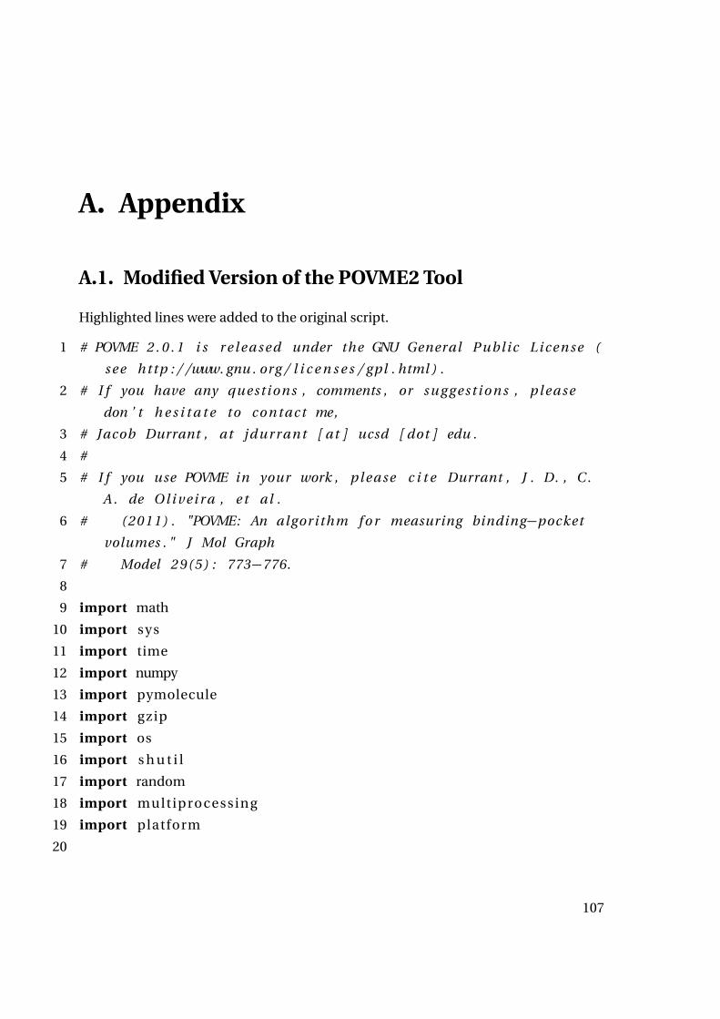
A. Appendix
A.1. Modified Version of the POVME2 Tool
Highlighted lines were added to the original script.
1 # POVME 2 . 0 . 1 i s r e l e a s e d under the GNU General Public L i c e n s e (
s e e http : / /www. gnu . org / l i c e n s e s / gpl . html ) .
2 # I f you have any quest ions , comments , or s u g g e s t i o n s , p l e a s e
don ’ t h e s i t a t e to c o n t a c t me,
3 # Jacob Durrant , at jdurrant [ at ] ucsd [ dot ] edu .
4 #
5 # I f you use POVME in your work , p l e a s e c i t e Durrant , J . D. , C .
A . de O l i v e i r a , e t al .
6 # (2011) . "POVME: An algorithm f o r measuring binding−pocket
volumes . " J Mol Graph
7 # Model 2 9 ( 5 ) : 773−776.
8
9 import math
10 import sys
11 import time
12 import numpy
13 import pymolecule
14 import gzip
15 import os
16 import s h u t i l
17 import random
18 import multiprocessing
19 import platform
20
107
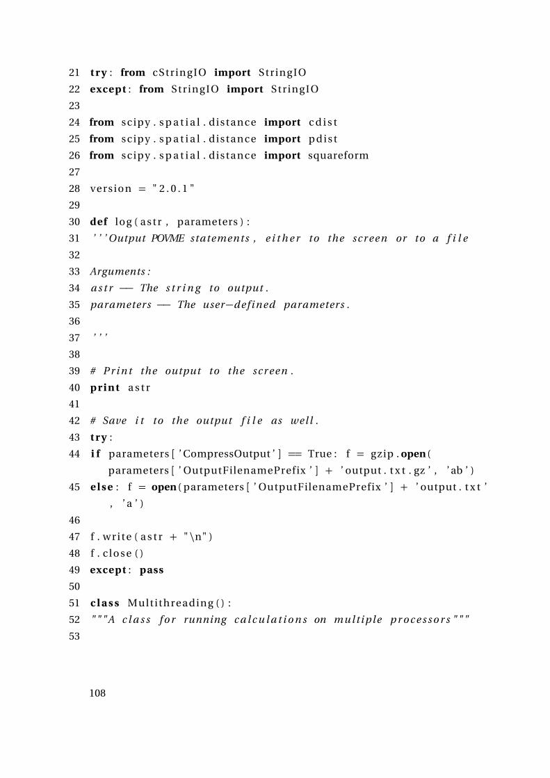
21 t r y : from cStringIO import StringIO
22 except : from StringIO import StringIO
23
24 from scipy . s p a t i a l . distance import c d i s t
25 from scipy . s p a t i a l . distance import p d i s t
26 from scipy . s p a t i a l . distance import squareform
27
28 version = " 2 . 0 . 1 "
29
30 def log ( a s t r , parameters ) :
31 ’ ’ ’ Output POVME statements , e i t h e r to the s c r e e n or to a f i l e
32
33 Arguments :
34 a s t r −− The s t r i n g to output .
35 parameters −− The user−defined parameters .
36
37 ’ ’ ’
38
39 # P r i n t the output to the s c r e e n .
40 p ri n t a s t r
41
42 # Save i t to the output f i l e as wel l .
43 t r y :
44 i f parameters [ ’ CompressOutput ’ ] == True : f = gzip . open (
parameters [ ’ OutputFilenamePrefix ’ ] + ’ output . t x t . gz ’ , ’ ab ’ )
45 e l s e : f = open ( parameters [ ’ OutputFilenamePrefix ’ ] + ’ output . t x t ’
, ’ a ’ )
46
47 f . w r i t e ( a s t r + "\n" )
48 f . c l o s e ( )
49 except : pass
50
51 c l a s s Multithreading ( ) :
52 " " " A c l a s s f o r running c a l c u l a t i o n s on multiple p r o c e s s o r s " " "
53
108
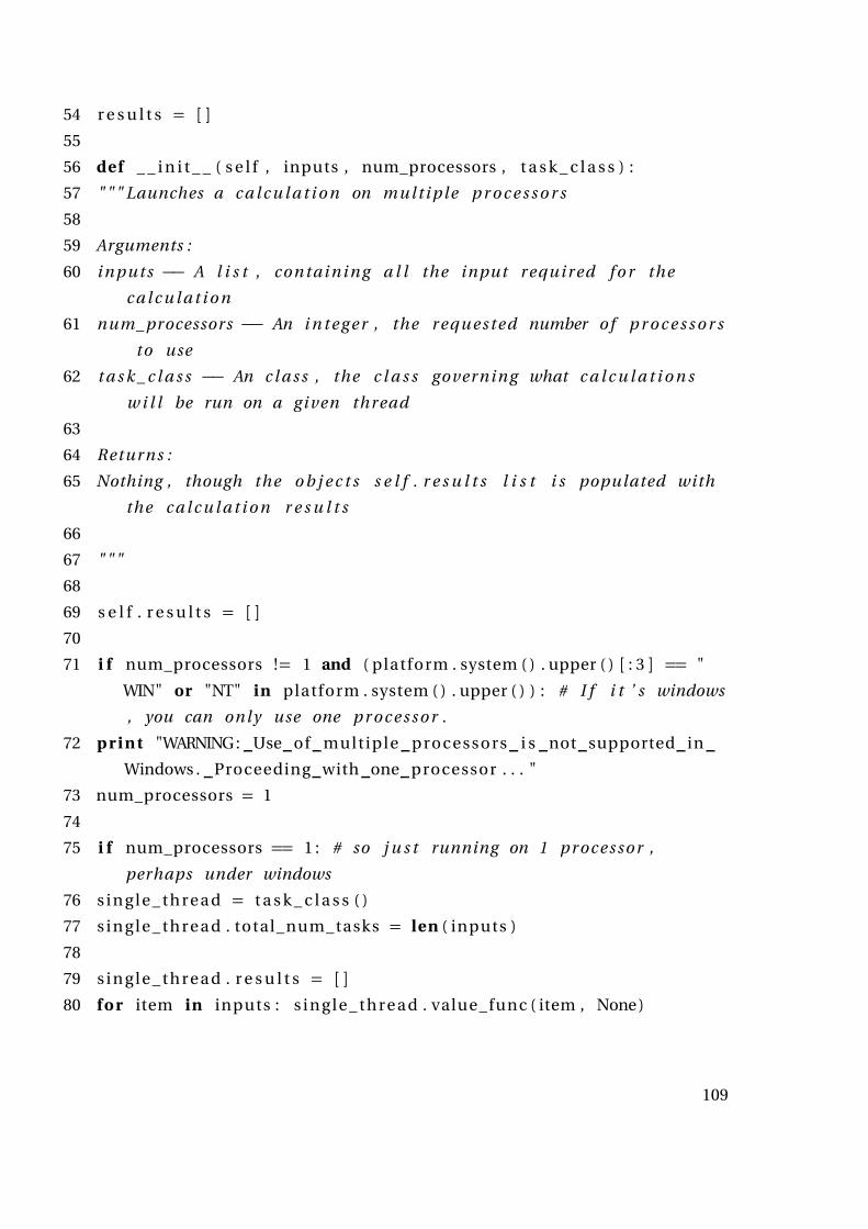
54 r e s u l t s = [ ]
55
56 def _ _ i n i t _ _ ( s e l f , inputs , num_processors , t a s k _ c l a s s ) :
57 " " " Launches a c a l c u l a t i o n on multiple p r o c e s s o r s
58
59 Arguments :
60 inputs −− A l i s t , containing a l l the input required f o r the
c a l c u l a t i o n
61 num_processors −− An i n t e g e r , the r e q u e s t e d number o f p r o c e s s o r s
to use
62 t a s k _ c l a s s −− An c l a s s , the c l a s s governing what c a l c u l a t i o n s
w i l l be run on a given thread
63
64 Returns :
65 Nothing , though the o b j e c t s s e l f . r e s u l t s l i s t i s populated with
the c a l c u l a t i o n r e s u l t s
66
67 " " "
68
69 s e l f . r e s u l t s = [ ]
70
71 i f num_processors != 1 and ( platform . system ( ) . upper ( ) [ : 3 ] == "
WIN" or "NT" in platform . system ( ) . upper ( ) ) : # I f i t ’ s windows
, you can only use one p r o c e s s o r .
72 p ri n t "WARNING: Use of mult iple processors i s not supported in
Windows . Proceeding with one processor . . . "
73 num_processors = 1
74
75 i f num_processors == 1 : # so j u s t running on 1 p r o c e s s o r ,
perhaps under windows
76 s i n g l e _ t h r e a d = t a s k _ c l a s s ( )
77 s i n g l e _ t h r e a d . total_num_tasks = len ( inputs )
78
79 s i n g l e _ t h r e a d . r e s u l t s = [ ]
80 f o r item in inputs : s i n g l e _ t h r e a d . value_func ( item , None )
109
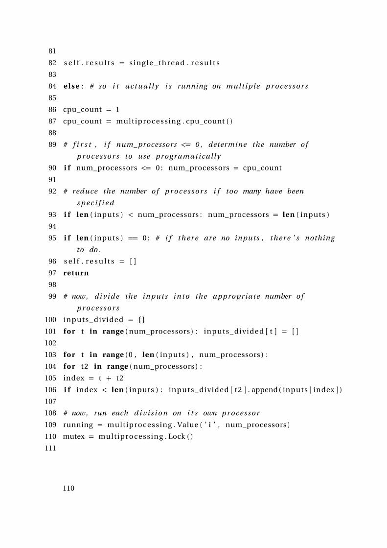
81
82 s e l f . r e s u l t s = s i n g l e _ t h r e a d . r e s u l t s
83
84 e l s e : # so i t a c t u a l l y i s running on multiple p r o c e s s o r s
85
86 cpu_count = 1
87 cpu_count = multiprocessing . cpu_count ( )
88
89 # f i r s t , i f num_processors <= 0 , determine the number o f
p r o c e s s o r s to use p r o g r a m a t i c al ly
90 i f num_processors <= 0 : num_processors = cpu_count
91
92 # reduce the number o f p r o c e s s o r s i f too many have been
s p e c i f i e d
93 i f len ( inputs ) < num_processors : num_processors = len ( inputs )
94
95 i f len ( inputs ) == 0 : # i f t h e r e are no inputs , t h e r e ’ s nothing
to do .
96 s e l f . r e s u l t s = [ ]
97 return
98
99 # now , d i v i d e the inputs i n t o the appropriate number o f
p r o c e s s o r s
100 inputs_divided = {}
101 f o r t in range ( num_processors ) : inputs_divided [ t ] = [ ]
102
103 f o r t in range ( 0 , len ( inputs ) , num_processors ) :
104 f o r t2 in range ( num_processors ) :
105 index = t + t2
106 i f index < len ( inputs ) : inputs_divided [ t2 ] . append ( inputs [ index ] )
107
108 # now , run each d i v i s i o n on i t s own p r o c e s s o r
109 running = multiprocessing . Value ( ’ i ’ , num_processors )
110 mutex = multiprocessing . Lock ( )
111
110
112 a r r a y s = [ ]
113 threads = [ ]
114 f o r i in range ( num_processors ) :
115 athread = t a s k _ c l a s s ( )
116 athread . total_num_tasks = len ( inputs )
117
118 threads . append ( athread )
119 a r r a y s . append ( mult iprocessing . Array ( ’ i ’ , [0 , 1 ] ) )
120
121 results_queue = multiprocessing . Queue ( ) # to keep t r a c k o f the
r e s u l t s
122
123 processes = [ ]
124 f o r i in range ( num_processors ) :
125 p = multiprocessing . Process ( t a r g e t=threads [ i ] . runit , args=(
running , mutex , results_queue , inputs_divided [ i ] ) )
126 p . s t a r t ( )
127 processes . append ( p )
128
129 while running . value > 0 : is_running = 0 # wait f o r e v e r y t h i n g to
f i n i s h
130
131 # compile a l l r e s u l t s i n t o one l i s t
132 f o r thread in threads :
133 chunk = results_queue . get ( )
134 s e l f . r e s u l t s . extend ( chunk )
135
136 c l a s s MultithreadingTaskGeneral :
137 " " " A parent c l a s s o f o t h e r s that governs what c a l c u l a t i o n s are
run on each thread " " "
138
139 r e s u l t s = [ ]
140
141 def r u n i t ( s e l f , running , mutex , results_queue , items ) :
142 " " " Launches the c a l c u l a t i o n s on t h i s thread
111
143
144 Arguments :
145 running −− A m u l t i p r o c e s s i n g . Value o b j e c t
146 mutex −− A m u l t i p r o c e s s i n g . Lock o b j e c t
147 r e s u l t s _ q u e u e −− A m u l t i p r o c e s s i n g . Queue ( ) o b j e c t f o r s t o r i n g
the c a l c u l a t i o n output
148 i tems −− A l i s t , the input data required f o r the c a l c u l a t i o n
149
150 " " "
151
152 f o r item in items : s e l f . value_func ( item , results_queue )
153
154 mutex . acquire ( )
155 running . value −= 1
156 mutex . r e l e a s e ( )
157 results_queue . put ( s e l f . r e s u l t s )
158
159 def value_func ( s e l f , item , results_queue ) : # so o v e r w r i t i n g t h i s
function
160 " " " The d e f i n i t i o n that a c t u a l l y does the work .
161
162 Arguments :
163 item −− A l i s t or tuple , the input data required f o r the
c a l c u l a t i o n
164 r e s u l t s _ q u e u e −− A m u l t i p r o c e s s i n g . Queue ( ) o b j e c t f o r s t o r i n g
the c a l c u l a t i o n output
165
166 " " "
167
168 # input1 = item [ 0 ]
169 # input2 = item [ 1 ]
170 # input3 = item [ 2 ]
171 # input4 = item [ 3 ]
172 # input5 = item [ 4 ]
173 # input6 = item [ 5 ]
112
174
175 # use inputs to come up with a r e s u l t , some_result
176
177 # s e l f . r e s u l t s . append ( some_result )
178
179 pass
180
181 c l a s s ConvexHull ( ) :
182 " " " A c l a s s to handle convex−h u l l c a l c u l a t i o n s " " "
183
184 def get_seg_dict_num ( s e l f , seg_dict , seg_index ) :
185 " " " s e g _ d i c t i s a d i c t i o n a r y o b j e c t that contains information
about segments within the convex h u l l . The keys are 2x3
t u p l e s , which r e p r e s e n t two ends o f a segment in space . The
values o f s e g _ d i c t are the number o f times a segment has been
part o f a t r i a n g l e , e i t h e r 1 or 2 . ( Zero times would mean
that the segment doesn ’ t e x i s t in the d i c t i o n a r y y e t ) . This
function l o o k s up and r e t u r n s the value o f a seg_index from
s e g _ d i c t
186
187 Arguments :
188 s e g _ d i c t −− the d i c t i o n a r y o f segment 2x3 t u p l e s as keys ,
i n t e g e r s as values
189 seg_index −− the key o f the d i c t i o n a r y member we are going to
r e t r i e v e
190
191 Returns :
192 i f seg_index e x i s t s in the keys o f s e g _ d i c t , return the value .
Otherwise , return 0
193
194 " " "
195
196 i f seg_index [ 0 ] [ 0 ] > seg_index [ 1 ] [ 0 ] : # we want the index with
the g r e a t e r x−value , so we don ’ t g e t i d e n t i c a l segments in
the d i c t i o n a r y more than once
113
197 index = seg_index
198 e l s e :
199 index = seg_index [ : : − 1 ]
200
201 i f index in s e g _ d i c t :
202 return s e g _ d i c t [ index ]
203 e l s e :
204 return 0
205
206 def increment_seg_dict ( s e l f , seg_dict , seg_index ) :
207 " " " s e g _ d i c t i s a d i c t i o n a r y o b j e c t that contains information
about segments within the convex h u l l . The keys are 2x3
t u p l e s , which r e p r e s e n t two ends o f a segment in space . The
values o f s e g _ d i c t are the number o f times a segment has been
part o f a t r i a n g l e , e i t h e r 1 or 2 . ( Zero times would mean
that the segment doesn ’ t e x i s t in the d i c t i o n a r y y e t ) . This
function increments the values within s e g _ d i c t , or i n i t i a t e s
them i f they dont e x i s t y e t .
208
209 Arguments :
210 s e g _ d i c t −− the d i c t i o n a r y o f segment 2x3 t u p l e s as keys ,
i n t e g e r s as values
211 seg_index −− the key o f the d i c t i o n a r y member we are going to
increment
212
213 Returns :
214 None : the values o f s e g _ d i c t are r e c e i v e d and modified by
r e f e r e n c e
215 " " "
216
217 i f seg_index [ 0 ] [ 0 ] > seg_index [ 1 ] [ 0 ] : # we want the index with
the g r e a t e r x−value , so we don ’ t g e t i d e n t i c a l segments in
the d i c t i o n a r y more than once
218 index = seg_index
219 e l s e :
114

220 index = seg_index [ : : − 1 ]
221
222 # " putt ing index : " , index , " i n t o s e g _ d i c t because " , index [ 0 ] [ 0 ] ,
">" , index [ 1 ] [ 0 ]
223
224 i f index in s e g _ d i c t : # i f the e n t r y already e x i s t s in s e g _ d i c t
225 s e g _ d i c t [ index ] += 1 # increment
226 e l s e :
227 s e g _ d i c t [ index ] = 1 # i n i t i a t e with a value o f 1 because i t now
e x i s t s on a t r i a n g l e
228 return
229
230 def gift_wrapping_3d ( s e l f , raw_points ) :
231 " " " G i f t wrapping f o r 3d convex h u l l
232
233 Arguments :
234 raw_points −− A nx3 array o f points , where each row corresponds
to an x , y , z point coordinate
235
236 Returns :
237 A convex h u l l r e p r e s e n t e d by a l i s t o f t r i a n g l e s . Each t r i a n g l e
i s a 3x3 array , where each row i s an x , y , z coordinate in
space . The 3 rows d e s c r i b e the l o c a t i o n o f the 3 c o r n e r s o f
the t r i a n g l e . Each o f the 3 p o i n t s are arranged so that a
c r o s s product w i l l point outwards from the h u l l
238
239
240 " " "
241
242 n = numpy . shape ( raw_points ) [ 0 ] # number o f p o i n t s
243 point1 = raw_points [ 0 ] # take the f i r s t point
244 x a x i s = numpy . array ( [ 1 , 0 , 0 ] ) # c r e a t e a r e f v e c t o r pointing
along x a x i s
245 maxx = raw_points [ 0 ] [ 0 ] # i n i t i a t e h i g h e s t x value
246 points = [ ] # a l i s t o f t u p l e s f o r easy d i c t i o n a r y lookup
115
247 s e g _ d i c t = {} # a d i c t i o n a r y that contains the number o f
t r i a n g l e s a s e g i s in
248
249 begintime = time . time ( )
250 f o r i in range (n ) : # f i n d the n with the l a r g e s t x value
251 point = tuple ( raw_points [ i ] )
252 points . append ( point )
253 i f point [ 0 ] > maxx :
254 maxx = point [ 0 ]
255 point1 = raw_points [ i ]
256 # p r i n t " f i n d max x : " , time . time ( ) − begintime
257
258 best_dot = −1.0 # i n i t i a t e dot r e l a t i v e to x−a x i s
259 point2 = numpy . array ( raw_points [ 1 ] ) # i n i t i a t e b e s t segment
260
261 # f i n d f i r s t / b e s t segment
262 begintime = time . time ( )
263 f o r i in range (n ) :
264 p o i n t i = raw_points [ i ]
265 i f numpy . array_equal ( pointi , point1 ) : continue
266 d i f f _ v e c = p o i n t i − point1
267 d i f f _ l e n = numpy . l i n a l g . norm( d i f f _ v e c )
268
269 t e s t _ d o t = numpy . dot ( d i f f _ v e c / d i f f _ l e n , x a x i s )
270 i f t e s t _ d o t > best_dot :
271 best_dot = t e s t _ d o t
272 point2 = p o i n t i
273
274 # p r i n t " f i n d f i r s t segment : " , time . time ( ) − begintime
275 point1 = tuple ( point1 )
276 point2 = tuple ( point2 )
277 r e f _ v e c = x a x i s
278
279 # now fi n d the b e s t t r i a n g l e
280 t r i a n g l e s = [ ]
116

281
282 s e g _ l i s t = s e t ( [ ( point1 , point2 ) , ] )
283 norm_dict = { ( point1 , point2 ) : x a x i s }
284 s e l f . increment_seg_dict ( seg_dict , ( point1 , point2 ) )
285
286 counter = 0
287 f i r s t _ t i m e = True
288
289 begintime = time . time ( )
290 section1 = 0 . 0
291 section2 = 0 . 0
292 section3 = 0 . 0
293 while s e g _ l i s t : # as long as t h e r e are unexplored edges o f
t r i a n g l e s in the h u l l . . .
294
295 counter += 1
296 seg = s e g _ l i s t . pop ( ) # take a segment out o f the s e g _ l i s t
297 tuple1 = seg [ 0 ] # the two ends o f the segment
298 tuple2 = seg [ 1 ]
299 point1 = numpy . array ( seg [ 0 ] )
300 point2 = numpy . array ( seg [ 1 ] )
301 r e s u l t = s e l f . get_seg_dict_num ( seg_dict , ( seg [ 0 ] , seg [ 1 ] ) )
302
303 i f r e s u l t >= 2 : # then we already have 2 t r i a n g l e s on t h i s
segment
304 continue # f o r g e t about drawing a t r i a n g l e f o r t h i s s e g
305
306 r e f _ v e c = norm_dict [ ( seg [ 0 ] , seg [ 1 ] ) ] # g e t the norm f o r a
t r i a n g l e that the segment i s part o f
307
308 best_dot_cross = −1.0
309 best_point = None
310
311 f o r i in range (n ) : # look at each point
312
117
313 p o i n t i = raw_points [ i ]
314 # i f numpy . array_equal ( pointi , point1 ) or numpy . array_equal (
pointi , point2 ) : continue # i f we are t r y i n g one o f the
p o i n t s that are point1 or point2
315 d i f f _ v e c 1 = point2 − point1
316 # d i f f _ l e n 1 = numpy . l i n a l g . norm( d i f f _ v e c 1 )
317 d i f f _ v e c 2 = p o i n t i − point2
318 # d i f f _ l e n 2 = numpy . l i n a l g . norm( d i f f _ v e c 2 )
319
320 # t e s t _ c r o s s = numpy . c r o s s ( d i f f _ v e c 1 / d i f f _ l e n 1 , d i f f _ v e c 2 /
d i f f _ l e n 2 )
321 # t e s t _ c r o s s = numpy . c r o s s ( d i f f _ v e c 1 , d i f f _ v e c 2 )
322 t e s t _ c r o s s = numpy . array ( [ d i f f _ v e c 1 [ 1 ] ∗ d i f f _ v e c 2 [2 ]− d i f f _ v e c 1
[ 2 ] ∗ d i f f _ v e c 2 [ 1 ] , d i f f _ v e c 1 [ 2 ] ∗ d i f f _ v e c 2 [0 ]− d i f f _ v e c 1 [ 0 ] ∗
d i f f _ v e c 2 [ 2 ] , d i f f _ v e c 1 [ 0 ] ∗ d i f f _ v e c 2 [1 ]− d i f f _ v e c 1 [ 1 ] ∗
d i f f _ v e c 2 [ 0 ] ] ) # c r o s s product
323
324 t e s t _ c r o s s _ l e n = numpy . s q r t ( t e s t _ c r o s s [ 0 ] ∗ t e s t _ c r o s s [ 0 ] +
t e s t _ c r o s s [ 1 ] ∗ t e s t _ c r o s s [ 1 ] + t e s t _ c r o s s [ 2 ] ∗ t e s t _ c r o s s [ 2 ] ) #
numpy . l i n a l g . norm( t e s t _ c r o s s ) # g e t the norm o f the c r o s s
product
325
326 i f t e s t _ c r o s s _ l e n <= 0 . 0 : continue
327 # t e s t _ c r o s s _ l e n _ i n v = 1 / t e s t _ c r o s s _ l e n
328 t e s t _ c r o s s = t e s t _ c r o s s / t e s t _ c r o s s _ l e n
329 dot_cross = numpy . dot ( t e s t _ c r o s s , r e f _ v e c )
330 # d o t _ c r o s s = t e s t _ c r o s s [ 0 ] ∗ r e f _ v e c [ 0 ] + t e s t _ c r o s s [ 1 ] ∗ r e f _ v e c [ 1 ]
+ t e s t _ c r o s s [ 2 ] ∗ r e f _ v e c [ 2 ]
331 i f dot_cross > best_dot_cross :
332 b e s t _ c r o s s = t e s t _ c r o s s
333 best_dot_cross = dot_cross
334 best_point = p o i n t i
335 tuple3 = points [ i ]
336
337
118

338 point3 = best_point
339
340 i f s e l f . get_seg_dict_num ( seg_dict , ( tuple2 , tuple1 ) ) > 2 :
continue
341 i f s e l f . get_seg_dict_num ( seg_dict , ( tuple3 , tuple2 ) ) > 2 :
continue
342 i f s e l f . get_seg_dict_num ( seg_dict , ( tuple1 , tuple3 ) ) > 2 :
continue
343
344 # now we have a t r i a n g l e from point1 −> point2 −> point3
345 # must t e s t each edge
346 i f f i r s t _ t i m e :
347 s e l f . increment_seg_dict ( seg_dict , ( tuple2 , tuple1 ) )
348 s e g _ l i s t . add ( ( tuple2 , tuple1 ) )
349 norm_dict [ ( tuple2 , tuple1 ) ] = b e s t _ c r o s s
350
351 s e l f . increment_seg_dict ( seg_dict , ( tuple3 , tuple2 ) )
352 s e g _ l i s t . add ( ( tuple3 , tuple2 ) )
353 norm_dict [ ( tuple3 , tuple2 ) ] = b e s t _ c r o s s
354
355 s e l f . increment_seg_dict ( seg_dict , ( tuple1 , tuple3 ) )
356 s e g _ l i s t . add ( ( tuple1 , tuple3 ) )
357 norm_dict [ ( tuple1 , tuple3 ) ] = b e s t _ c r o s s
358
359 t r i a n g l e s . append ( ( numpy . array ( tuple1 ) ,numpy . array ( tuple2 ) ,numpy .
array ( tuple3 ) ) )
360
361 f i r s t _ t i m e = False
362
363 # p r i n t " f i n d a l l t r i a n g l e s : " , time . time ( ) − begintime
364
365 # p r i n t " s e c t i o n 1 : " , s e c t i o n 1
366 # p r i n t " s e c t i o n 2 : " , s e c t i o n 2
367 # p r i n t " s e c t i o n 3 : " , s e c t i o n 3
368 return t r i a n g l e s
119
369
370 def a k l _ t o u s s a i n t ( s e l f , points ) :
371 " " " The Akl−Toussaint H e u r i s t i c . Given a s e t o f points , t h i s
d e f i n i t i o n w i l l c r e a t e an octahedron whose c o r n e r s are the
extremes in x , y , and z d i r e c t i o n s . Every point within t h i s
octahedron w i l l be removed because they are not part o f the
convex h u l l . This causes any expected running time f o r a
convex h u l l algorithm to be reduced to l i n e a r time .
372
373 Arguments :
374 p o i n t s −− An nx3 array o f x , y , z c o o r d i n a t e s
375
376 Returns :
377 A l l members o f o r i g i n a l s e t o f p o i n t s that f a l l o u t s i d e the Akl−
Toussaint octahedron
378
379 " " "
380
381 x_high = (−1e99 , 0 , 0 ) ; x_low = (1 e99 , 0 , 0 ) ; y_high = (0 ,−1e99 , 0 ) ;
y_low = ( 0 , 1 e99 , 0 ) ; z_high = (0 ,0 ,−1 e99 ) ; z_low = ( 0 , 0 , 1 e99 )
382
383
384 f o r point in points : # f i n d the c o r n e r s o f the octahedron
385 i f point [ 0 ] > x_high [ 0 ] : x_high = point
386 i f point [ 0 ] < x_low [ 0 ] : x_low = point
387 i f point [ 1 ] > y_high [ 1 ] : y_high = point
388 i f point [ 1 ] < y_low [ 1 ] : y_low = point
389 i f point [ 2 ] > z_high [ 2 ] : z_high = point
390 i f point [ 2 ] < z_low [ 2 ] : z_low = point
391
392 octahedron = [ # d e f i n e the t r i a n g l e s o f the s u r f a c e s o f the
octahedron
393 numpy . array ( ( x_high , y_high , z_high ) ) ,
394 numpy . array ( ( x_high , z_low , y_high ) ) ,
395 numpy . array ( ( x_high , y_low , z_low ) ) ,
120
396 numpy . array ( ( x_high , z_high , y_low ) ) ,
397 numpy . array ( ( x_low , y_low , z_high ) ) ,
398 numpy . array ( ( x_low , z_low , y_low ) ) ,
399 numpy . array ( ( x_low , y_high , z_low ) ) ,
400 numpy . array ( ( x_low , z_high , y_high ) ) ,
401 ]
402 new_points = [ ] # e v e r y t h i n g o u t s i d e o f the octahedron
403 f o r point in points : # now check to s e e i f a point i s i n s i d e or
o u t s i d e the octahedron
404 outside = s e l f . o u t s i d e _ h u l l ( point , octahedron , epsi lon=−1.0e−5)
405 i f outside :
406 new_points . append ( point )
407
408 return numpy . array ( new_points ) # c o n v e r t back to an array
409
410 def o u t s i d e _ h u l l ( s e l f , our_point , t r i a n g l e s , epsi lon=1.0e−5) :
411 " " " Given the h u l l as defined by a l i s t o f t r i a n g l e s , t h i s
d e f i n i t i o n w i l l return whether a point i s within t h e s e or not
.
412
413 Arguments :
414 our_point −− an x , y , z array that i s being t e s t e d to s e e whether
i t e x i s t s i n s i d e the h u l l or not
415 t r i a n g l e s −− a l i s t o f t r i a n g l e s that d e f i n e the h u l l
416 e p s i l o n −− needed f o r i m p r e c i s i o n s in the f l o a t i n g −point
o p e r a t i o n s .
417
418 Returns :
419 True i f our_point e x i s t s o u t s i d e o f the hull , Fa l s e otherwise
420
421 " " "
422
423 our_point = numpy . array ( our_point ) # c o n v e r t i t to an numpy .
array
424 f o r t r i a n g l e in t r i a n g l e s :
121
425 r e l _ p o i n t = our_point − t r i a n g l e [ 0 ] # v e c t o r from t r i a n g l e
corner 0 to point
426 vec1 = t r i a n g l e [ 1 ] − t r i a n g l e [ 0 ] # v e c t o r from t r i a n g l e corner 0
to corner 1
427 vec2 = t r i a n g l e [ 2 ] − t r i a n g l e [ 1 ] # v e c t o r from t r i a n g l e corner 1
to corner 2
428 our_cross = numpy . cross ( vec1 , vec2 ) # c r o s s product between vec1
and vec2
429 our_dot = numpy . dot ( r e l _ p o i n t , our_cross ) # dot product to
determine whether c r o s s i s point inward or outward
430 i f numpy . dot ( r e l _ p o i n t , our_cross ) > epsi lon : # i f the dot i s
g r e a t e r than 0 , then i t s o u t s i d e
431 return True
432
433 return False
434
435 def unique_rows ( a ) :
436 " " " I d e n t i f i e s unique p o i n t s ( rows ) in an array o f p o i n t s .
437
438 Arguments :
439 a −− A nx3 numpy . array r e p r e s e n t i n g 3D p o i n t s .
440
441 Returns :
442 A nx2 numpy . array containing the 3D p o i n t s that are unique .
443
444 " " "
445
446 a [ a == −0.0 ] = 0 . 0
447 b = numpy . ascontiguousarray ( a ) . view (numpy . dtype ( ( numpy . void , a .
dtype . i temsize ∗ a . shape [ 1 ] ) ) )
448 unique_a = numpy . unique ( b ) . view ( a . dtype ) . reshape (−1 , a . shape [ 1 ] )
449
450 return unique_a
451
452 def create_pdb_l ine ( numpy_array , index , resname , l e t t e r ) :
122

453 " " " Create a s t r i n g formatted according to the PDB standard .
454
455 Arguments :
456 numpy_array −− A 1x3 numpy . array r e p r e s e n t i n g a 3D point .
457 l e t t e r −− A s t r i n g , the atom name/ chain/ e t c to use f o r the
output .
458
459 Returns :
460 A s t r i n g , formatted according to the PDB standard .
461
462 " " "
463
464 i f len ( numpy_array ) == 2 : numpy_array = numpy . array ( [ numpy_array
[ 0 ] , numpy_array [ 1 ] , 0 . 0 ] )
465 i f numpy_array . shape == ( 1 , 3) : numpy_array = numpy_array [ 0 ]
466
467 output = "ATOM "
468 output = output + s t r ( index % 999999) . r j u s t ( 6 ) + l e t t e r . r j u s t ( 5 )
+ resname . r j u s t ( 4 ) + l e t t e r . r j u s t ( 2 ) + s t r ( index % 9999) .
r j u s t ( 4 )
469 output = output + ( "%.3 f " % numpy_array [ 0 ] ) . r j u s t ( 1 2 )
470 output = output + ( "%.3 f " % numpy_array [ 1 ] ) . r j u s t ( 8 )
471 output = output + ( "%.3 f " % numpy_array [ 2 ] ) . r j u s t ( 8 )
472 output = output + l e t t e r . r j u s t ( 2 4 )
473
474 return output
475
476 def numpy_to_pdb( narray , l e t t e r , resname=" " ) :
477 " " " Create a s t r i n g formatted according to the PDB standard .
478
479 Arguments :
480 narray −− A nx3 numpy . array r e p r e s e n t i n g a 3D point .
481 l e t t e r −− A s t r i n g , the atom name/ chain/ e t c to use f o r the
output .
482
123
483 Returns :
484 ( Optional ly ) A s t r i n g , formatted according to the PDB standard .
485
486 " " "
487
488 i f len ( narray . f l a t t e n ( ) ) == 3 :
489 return create_pdb_l ine ( narray , 1 , "AAA" , l e t t e r ) + "\n"
490 e l s e :
491 i f resname == " " :
492 l e t t e r s = [ "A" , "B" , "C" , "D" , "E" , "F" , "G" , "H" , " I " , " J " , "K"
, "L" , "M" , "N" , "O" , "P" , "Q" , "R" , "S" , "T" , "U" , "V" , "W" ,
"X" , "Y" , "Z" ]
493 resnames = [ ]
494 f o r l 1 in l e t t e r s :
495 f o r l 2 in l e t t e r s :
496 f o r l 3 in l e t t e r s :
497 resnames . append ( l 1+l 2+ l 3 )
498 resnames . remove ( "XXX" ) # because t h i s i s r e s e r v e d f o r empty
atoms
499 e l s e :
500 resnames = [ resname ]
501
502 t = " "
503 f o r i , item in enumerate( narray ) : t = t + create_pdb_l ine ( item ,
i +1 , resnames [ i % len ( resnames ) ] , l e t t e r ) + "\n"
504 return t
505
506 def dx_freq ( freq_mat , parameters ) :
507 ’ ’ ’
508 Generates a DX f i l e that r e c o r d s the frequency that a volume
element i s open
509
510 Arguments :
511 freq_mat −− a Nx4 matrix , where the f i r s t 3 columns are the x , y ,
z coords o f the point , and the 4 th column i s the frequency o f
124
emptiness f o r that point in space
512
513 ’ ’ ’
514
515 header_template = " " " # Data from POVME 2 . 0 . 1
516 #
517 # FREQUENCY ( u n i t l e s s )
518 #
519 o b j e c t 1 c l a s s g r i d p o s i t i o n s counts %d %d %d
520 o r i g i n %8.6e %8.6e %8.6e
521 d e l t a %8.6e 0.000000e+00 0.000000e+00
522 d e l t a 0.000000e+00 %8.6e 0.000000e+00
523 d e l t a 0.000000e+00 0.000000e+00 %8.6e
524 o b j e c t 2 c l a s s g r i d c o n n e c t i o n s counts %d %d %d
525 o b j e c t 3 c l a s s array type double rank 0 items %d data f o l l o w s
526 " " "
527
528 footer_template = " " "
529 a t t r i b u t e " dep " s t r i n g " p o s i t i o n s "
530 o b j e c t " r e g u l a r p o s i t i o n s r e g u l a r connections " c l a s s f i e l d
531 component " p o s i t i o n s " value 1
532 component " connections " value 2
533 component " data " value 3 " " "
534
535 # 1 . S o r t the p o i n t s i n t o the proper order f o r a dx f i l e
536
537 # already s o r t e d c o r r e c t l y
538
539 # 2 . Obtain key information about the g r i d
540 N = freq_mat . shape [ 0 ] # number o f data p o i n t s
541
542 minx = min( freq_mat [ : , 0 ] )
543 miny = min( freq_mat [ : , 1 ] )
544 minz = min( freq_mat [ : , 2 ] ) # f i n d the upper and lower c o r n e r s o f
the g r i d
125
545 maxx = max( freq_mat [ : , 0 ] )
546 maxy = max( freq_mat [ : , 1 ] )
547 maxz = max( freq_mat [ : , 2 ] )
548
549 widthx = maxx − minx # f i n d the widths o f the g r i d
550 widthy = maxy − miny
551 widthz = maxz − minz
552
553 xs = numpy . unique ( freq_mat [ : , 0 ] )
554 ys = numpy . unique ( freq_mat [ : , 1 ] )
555 zs = numpy . unique ( freq_mat [ : , 2 ] )
556
557 r e s x = xs [1 ]− xs [ 0 ]
558 resy = ys [1 ]− ys [ 0 ]
559 r e s z = zs [1 ]− zs [ 0 ]
560
561 # r e s x = freq_mat [ ( widthz+1) ∗ ( widthy+1) , 0 ] − freq_mat [0 , 0 ]
562 # r e s y = freq_mat [widthz+1 ,1 ] − freq_mat [0 , 1 ] # f i n d the
r e s o l u t i o n o f the g r i d
563 # r e s z = freq_mat [1 , 2 ] − freq_mat [0 , 2 ]
564
565 nx = ( widthx ) / r e s x + 1 # number o f g r i d p o i n t s in each
dimension
566 ny = ( widthy ) / resy + 1 # need to add one because the
s u b t r a c t i o n l e a v e s out an e n t i r e row
567 nz = ( widthz ) / r e s z + 1
568
569 # t e s t to make sure a l l i s wel l with the s i z e o f the g r i d and
i t s dimensions
570 a s s e r t ( nx ∗ ny ∗ nz ) == N, " Something i s wrong with the
freq_mat array : i t i s not a prismatic shape "
571
572 # 3 . w r i t e the header and f o o t e r
573 i f parameters [ ’ SaveVolumetricDensityMap ’ ] == True :
126

574 i f parameters [ ’ CompressOutput ’ ] == True : d x _ f i l e = gzip . open (
parameters [ ’ OutputFilenamePrefix ’ ] + " volumetric_density . dx .
gz " , ’wb ’ )
575 e l s e : d x _ f i l e = open ( parameters [ ’ OutputFilenamePrefix ’ ] + "
volumetric_density . dx" , ’w ’ )
576
577 header = header_template % ( nx , ny , nz , minx , miny , minz , resx ,
resy , resz , nx , ny , nz , N) # format the header
578 f o o t e r = footer_template # the f o o t e r needs no formatting
579 d x _ f i l e . w r i t e ( header )
580 newline_counter = 1
581 f o r i in range (N) : # w r i t e the data to the DX f i l e
582 d x _ f i l e . w r i t e ( " %8.6e " % freq_mat [ i , 3 ] )
583 i f newline_counter == 3 :
584 newline_counter = 0
585 d x _ f i l e . w r i t e ( "\n" )
586 e l s e :
587 d x _ f i l e . w r i t e ( " " )
588 newline_counter += 1
589 d x _ f i l e . w r i t e ( f o o t e r )
590 d x _ f i l e . c l o s e
591 return
592
593 c l a s s MultithreadingCalcVolumeTask ( MultithreadingTaskGeneral ) :
594 ’ ’ ’ A c l a s s f o r c a l c u l a t i n g the volume . ’ ’ ’
595
596 def value_func ( s e l f , item , results_queue ) :
597 " " " C a l c u l a t e the volume .
598
599 Arguments :
600 item −− A l i s t or tuple , the input data required f o r the
c a l c u l a t i o n
601 r e s u l t s _ q u e u e −− A m u l t i p r o c e s s i n g . Queue ( ) o b j e c t f o r s t o r i n g
the c a l c u l a t i o n output
602
127
603 " " "
604
605 frame_indx = item [ 0 ]
606 pdb = item [ 1 ]
607 parameters = item [ 2 ]
608 # p t s = parameters [ ’ p t s _ o r i g ’ ] . copy ( ) # t h i s works
609 pts = parameters [ ’ p t s _ o r i g ’ ] # a l s o works , so keep because
f a s t e r
610
611 # i f the user wants to save empty p o i n t s ( p o i n t s that are
removed ) , then we need a copy o f the o r i g i n a l
612 i f parameters [ ’ OutputEqualNumPointsPerFrame ’ ] == True :
613 p t s _ d e l e t e d = pts . copy ( )
614
615 # you may need to load i t from d i s k i f the user so s p e c i f i e d
616 i f parameters [ ’ UseDiskNotMemory ’ ] == True : # so you need to load
i t from d i s k
617 pym_filename = pdb
618 pdb = pymolecule . Molecule ( )
619 pdb . f i l e i o . load_pym_into ( pym_filename )
620
621 # remove the p o i n t s that are f a r from the p o i n t s region anyway
622 min_pts = numpy . min( pts , 0 ) − parameters [ ’ DistanceCutoff ’ ] − 1
623 max_pts = numpy .max( pts , 0 ) + parameters [ ’ DistanceCutoff ’ ] + 1
624
625 # i d e n t i f y atoms that are so f a r away from p o i n t s that they can
be ignored
626 index_to_keep1 = numpy . nonzero ( ( pdb . information . coordinates [ : , 0 ]
> min_pts [ 0 ] ) ) [ 0 ] # x ’ s too small
627 index_to_keep2 = numpy . nonzero ( ( pdb . information . coordinates [ : , 0 ]
< max_pts [ 0 ] ) ) [ 0 ] # x ’ s too l a r g e
628 index_to_keep3 = numpy . nonzero ( ( pdb . information . coordinates [ : , 1 ]
> min_pts [ 1 ] ) ) [ 0 ] # y ’ s too small
629 index_to_keep4 = numpy . nonzero ( ( pdb . information . coordinates [ : , 1 ]
< max_pts [ 1 ] ) ) [ 0 ] # y ’ s too l a r g e
128
630 index_to_keep5 = numpy . nonzero ( ( pdb . information . coordinates [ : , 2 ]
> min_pts [ 2 ] ) ) [ 0 ] # z ’ s too small
631 index_to_keep6 = numpy . nonzero ( ( pdb . information . coordinates [ : , 2 ]
< max_pts [ 2 ] ) ) [ 0 ] # z ’ s too l a r g e
632
633 index_to_keep = numpy . i n t e r s e c t 1 d ( index_to_keep1 , index_to_keep2
, assume_unique=True )
634 index_to_keep = numpy . i n t e r s e c t 1 d ( index_to_keep , index_to_keep3 ,
assume_unique=True )
635 index_to_keep = numpy . i n t e r s e c t 1 d ( index_to_keep , index_to_keep4 ,
assume_unique=True )
636 index_to_keep = numpy . i n t e r s e c t 1 d ( index_to_keep , index_to_keep5 ,
assume_unique=True )
637 index_to_keep = numpy . i n t e r s e c t 1 d ( index_to_keep , index_to_keep6 ,
assume_unique=True )
638
639 # keep only r e l e v a n t atoms
640 i f len ( index_to_keep ) > 0 : pdb = pdb . s e l e c t i o n s .
create_molecule_from_selection ( index_to_keep )
641
642 # g e t the vdw r a d i i o f each p r o t e i n atom
643 vdw = numpy . ones ( len ( pdb . information . coordinates ) ) # so the
d e f a u l t vdw i s 1 . 0
644
645 # g e t vdw . . . you might want to f i l l t h i s out with a d d i t i o n a l vdw
values
646 vdw [numpy . nonzero ( pdb . information . atom_information [ ’
element_stripped ’ ] == "H" ) [ 0 ] ] = 1 . 2
647 vdw [numpy . nonzero ( pdb . information . atom_information [ ’
element_stripped ’ ] == "C" ) [ 0 ] ] = 1 . 7
648 vdw [numpy . nonzero ( pdb . information . atom_information [ ’
element_stripped ’ ] == "N" ) [ 0 ] ] = 1.55
649 vdw [numpy . nonzero ( pdb . information . atom_information [ ’
element_stripped ’ ] == "O" ) [ 0 ] ] = 1.52
129
650 vdw [numpy . nonzero ( pdb . information . atom_information [ ’
element_stripped ’ ] == "F" ) [ 0 ] ] = 1.47
651 vdw [numpy . nonzero ( pdb . information . atom_information [ ’
element_stripped ’ ] == "P" ) [ 0 ] ] = 1 . 8
652 vdw [numpy . nonzero ( pdb . information . atom_information [ ’
element_stripped ’ ] == "S" ) [ 0 ] ] = 1 . 8
653 vdw = numpy . repeat (numpy . array ( [ vdw ] ) . T , len ( pts ) , a x i s=1)
654
655 # now i d e n t i f y the p o i n t s that are c l o s e to the p r o t e i n atoms
656 d i s t s = c d i s t ( pdb . information . coordinates , pts )
657 close_pt_index = numpy . nonzero ( ( d i s t s < (vdw + parameters [ ’
DistanceCutoff ’ ] ) ) ) [ 1 ]
658
659 # save p o i n t s i n s i d e p r o t e i n or l igand
660 rememberedall = pts
661
662 # now keep the appropriate p o i n t s
663 pts = numpy . d e l e t e ( pts , close_pt_index , a x i s=0)
664
665 # exclude p o i n t s o u t s i d e convex h u l l
666 i f parameters [ ’ ConvexHullExclusion ’ ] == True :
667 convex_hull_3d = ConvexHull ( )
668
669 # g e t the c o o r d i n a t e s o f the non−hydrogen atoms ( f a s t e r to
d i s c a r d hydrogens )
670 hydros = pdb . s e l e c t i o n s . select_atoms ( { ’ element_stripped ’ : [ ’H ’ ] } )
671 not_hydros = pdb . s e l e c t i o n s . i n v e r t _ s e l e c t i o n ( hydros )
672 not_hydros_coors = pdb . information . coordinates [ not_hydros ]
673
674 # not_hydros = pdb . s e l e c t i o n s . s e l e c t _ a t o m s ( { ’ name_stripped ’ : [ ’ CA
’ ] } )
675 # not_hydros_coors = pdb . information . c o o r d i n a t e s [ not_hydros ]
676
677 # modify p t s here .
130
678 # note that the atoms o f the pdb frame are in pdb . information .
c o o r d i n a t e s
679 # begintime = time . time ( ) # measure execution time
680 a k l _ t o u s s a i n t _ p t s = convex_hull_3d . a k l _ t o u s s a i n t (
not_hydros_coors ) # q u i c k l y reduces input s i z e
681 # p r i n t " akl Toussaint : " , time . time ( ) − begintime
682 begintime = time . time ( ) # measure execution time
683 h u l l = convex_hull_3d . gift_wrapping_3d ( a k l _ t o u s s a i n t _ p t s ) #
c a l c u l a t e convex h u l l using g i f t wrapping algorithm
684 # p r i n t " gi ft_wrapping : " , time . time ( ) − begintime
685
686 old_pts = pts # we w i l l need to r e g e n e r a t e the p t s l i s t ,
d i s r e g a r d i n g t h o s e o u t s i d e the h u l l
687 pts = [ ]
688 f o r pt in old_pts :
689 pt_outside = convex_hull_3d . o u t s i d e _ h u l l ( pt , h u l l ) # check i f pt
i s o u t s i d e h u l l
690 i f not pt_outside :
691 pts . append ( pt ) # i f i t s not o u t s i d e the hull , then include i t in
the volume measurement
692 pts = numpy . array ( pts )
693
694 # Now, e n fo r c e c o n t i g u i t y i f needed
695 i f len ( parameters [ ’ ContiguousPocketSeedRegions ’ ] ) > 0 and len (
pts ) > 0 :
696 # f i r s t , f o r each point , determine how many neighbors i t has
697 c u t o f f _ d i s t = parameters [ ’ GridSpacing ’ ] ∗ 1.01 ∗ math . s q r t ( 3 ) #
to count kiddy−corner p o i n t s too
698 p t s _ d i s t s = squareform ( p d i s t ( pts ) )
699 neighbor_counts = numpy . sum( p t s _ d i s t s < c u t o f f _ d i s t , a x i s=0) − 1
# minus 1 because an atom shouldn ’ t be considered i t s own
neighor
700
701 # remove a l l the p o i n t s that don ’ t have enough neighbors
131
702 pts = pts [numpy . nonzero ( neighbor_counts >= parameters [ ’
C o n t i g u o u s P o i n t s C r i t e r i a ’ ] ) [ 0 ] ]
703
704 # g e t a l l the p o i n t s in the defined parameters [ ’ ContiguousPocket
’ ] seed r e g i o n s
705 c o n t i g _ p t s = parameters [ ’ ContiguousPocketSeedRegions ’ ] [ 0 ] .
p o i n t s _ s e t ( parameters [ ’ GridSpacing ’ ] )
706 f o r Contig in parameters [ ’ ContiguousPocketSeedRegions ’ ] [ 1 : ] :
c o n t i g _ p t s = numpy . vstack ( ( contig_pts , Contig . p o i n t s _ s e t (
parameters [ ’ GridSpacing ’ ] ) ) )
707 c o n t i g _ p t s = unique_rows ( c o n t i g _ p t s )
708
709 t r y : # e r r o r here i f t h e r e are no p o i n t s o f contiguous seed
region o u t s i d e o f p r o t e i n volume .
710 # now j u s t g e t the ones that are not near the p r o t e i n
711 c o n t i g _ p t s = pts [numpy . nonzero ( c d i s t ( contig_pts , pts ) < 1e−7)
[ 1 ] ]
712
713 l a s t _ s i z e _ o f _ c o n t i g _ p t s = 0
714 while l a s t _ s i z e _ o f _ c o n t i g _ p t s != len ( c o n t i g _ p t s ) :
715 l a s t _ s i z e _ o f _ c o n t i g _ p t s = len ( c o n t i g _ p t s )
716
717 # now g e t the i n d e c i e s o f a l l p o i n t s that are c l o s e to the
c o n t i g _ p t s
718 a l l _ p t s _ c l o s e _ t o _ c o n t i g _ p t s _ b o o l e a n = ( c d i s t ( pts , c o n t i g _ p t s ) <
c u t o f f _ d i s t )
719 i n d e x _ a l l _ p t s _ c l o s e _ t o _ c o n t i g _ p t s = numpy . unique (numpy . nonzero (
a l l _ p t s _ c l o s e _ t o _ c o n t i g _ p t s _ b o o l e a n ) [ 0 ] )
720 c o n t i g _ p t s = pts [ i n d e x _ a l l _ p t s _ c l o s e _ t o _ c o n t i g _ p t s ]
721
722 pts = c o n t i g _ p t s
723
724 except :
725 log ( "\ tFrame " + s t r ( frame_indx ) + " : None of the points in the
contiguous−pocket seed region \n\ t \ t a r e outside the volume of
132
the protein ! Assuming a pocket \n\ t \ tvolume of 0 . 0 A . " ,
parameters )
726 pts = numpy . array ( [ ] )
727
728 #make l i s t s from whole s e t and f i n a l p t s s e t
729 p ri n t ( rememberedall )
730 rememberedal l_ l is t = rememberedall . t o l i s t ( )
731 p ri n t ( rememberedal l_ l is t )
732
733 p ri n t ( pts )
734 p t s _ l i s t = pts . t o l i s t ( )
735 p ri n t ( p t s _ l i s t )
736
737 # f i n d not−shared p o i n t s o f both l i s t s
738 r e s t = tuple ( x f o r x in rememberedal l_ l is t i f x not in p t s _ l i s t )
739 p ri n t ( r e s t )
740 r e s t a r r a y = numpy . a s a r r a y ( r e s t )
741
742 # w r i t e the remembered p o i n t s ( i n s i d e p r o t e i n ) to . pdb
743 i f parameters [ ’ SaveIndividualPocketVolumes ’ ] == True :
744 remem_text = " "
745 remem_text = remem_text + "REMARK Frame " + s t r ( frame_indx ) + "
\n"
746 remem_text = remem_text + numpy_to_pdb( r e s t a r r a y , ’X ’ )
747 remem_text = remem_text + "END\n"
748
749 f l = open ( parameters [ ’ OutputFilenamePrefix ’ ] + "
inLigOrProt_frame_ " + s t r ( frame_indx ) + " . pdb" , ’w ’ )
750 f l . w r i t e ( remem_text )
751 f l . c l o s e
752
753 # now w r i t e the pdb and c a l c u l a t e the volume
754 volume = len ( pts ) ∗ math . pow( parameters [ ’ GridSpacing ’ ] , 3 )
755
133
756 log ( "\ tFrame " + s t r ( frame_indx ) + " : " + repr ( volume ) + " A^3" ,
parameters )
757 i f parameters [ ’ SaveIndividualPocketVolumes ’ ] == True :
758 frame_text = " "
759 frame_text = f rame_text + "REMARK Frame " + s t r ( frame_indx ) + "\
n"
760 frame_text = f rame_text + "REMARK Volume = " + repr ( volume ) + "
Cubic Angtroms\n"
761 frame_text = f rame_text + numpy_to_pdb( pts , ’X ’ )
762
763 i f parameters [ ’ OutputEqualNumPointsPerFrame ’ ] == True :
764 # you need to f i n d the p o i n t s that are in p t s _ d e l e t e d but not in
p t s
765 tmp = reduce ( lambda x , y : x | numpy . a l l ( p t s _ d e l e t e d == y , a x i s
=−1) , pts , numpy . zeros ( p t s _ d e l e t e d . shape [ : 1 ] , dtype=numpy .
bool ) )
766 i n d i c e s = numpy . where (tmp ) [ 0 ]
767 p t s _ d e l e t e d = numpy . d e l e t e ( pts_deleted , indices , a x i s=0)
768
769 p t s _ d e l e t e d = numpy . zeros ( p t s _ d e l e t e d . shape ) # So e x t r a p o i n t s
w i l l always be at the o r i g i n . These can be e a s i l y hidden with
your v i s u a l i z a t i o n s o ft w a r e .
770 frame_text = f rame_text + numpy_to_pdb( pts_deleted , ’X ’ , "XXX" )
771
772 frame_text = f rame_text + "END\n"
773
774 i f parameters [ ’ CompressOutput ’ ] == True : f l = gzip . open (
parameters [ ’ OutputFilenamePrefix ’ ] + " frame_ " + s t r (
frame_indx ) + " . pdb . gz " , ’wb ’ )
775 e l s e : f l = open ( parameters [ ’ OutputFilenamePrefix ’ ] + " frame_ " +
s t r ( frame_indx ) + " . pdb" , ’w ’ )
776 f l . w r i t e ( frame_text )
777 f l . c l o s e ( )
778
779 extra_data_to_add = {}
134
780 i f parameters [ ’ SaveVolumetricDensityMap ’ ] == True :
extra_data_to_add [ ’ SaveVolumetricDensityMap ’ ] = pts
781
782 s e l f . r e s u l t s . append ( ( frame_indx , volume , extra_data_to_add ) )
783
784 # i f len ( extra_data_to_add . keys ( ) ) != 0 :
785 # e l s e : s e l f . r e s u l t s . append ( ( frame_indx , volume ) )
786
787 c l a s s MultithreadingStringToMoleculeTask (
MultithreadingTaskGeneral ) :
788 ’ ’ ’ A c l a s s f o r loading PDB frames ( as s t r i n g s ) i n t o pymolecule .
Molecule o b j e c t s . ’ ’ ’
789
790 def value_func ( s e l f , item , results_queue ) :
791 " " " Convert a PDB s t r i n g i n t o a pymolecule . Molecule o b j e c t
792
793 Arguments :
794 item −− A l i s t or tuple , the input data required f o r the
c a l c u l a t i o n
795 r e s u l t s _ q u e u e −− A m u l t i p r o c e s s i n g . Queue ( ) o b j e c t f o r s t o r i n g
the c a l c u l a t i o n output
796
797 " " "
798
799 pdb_string = item [ 0 ]
800 index = item [ 1 ]
801 parameters = item [ 2 ]
802
803 # make the pdb o b j e c t
804 s t r _ o b j = StringIO ( pdb_string )
805 tmp = pymolecule . Molecule ( )
806 tmp . f i l e i o . l o a d _ p d b _ i n t o _ u s i n g _ f i l e _ o b j e c t ( s t r _ o b j , False , False
, False )
807
808 log ( "\ t F u r t h e r processing frame " + s t r ( index ) , parameters )
135

809
810 i f parameters [ ’ UseDiskNotMemory ’ ] == False : # so load the whole
t r a j e c t o r y i n t o memory
811 s e l f . r e s u l t s . append ( ( index , tmp ) )
812 e l s e : # save to disk , record filename
813 pym_filename = " . " + os . sep + " . povme_tmp" + os . sep + " frame_ " +
s t r ( index ) + " .pym"
814 tmp . f i l e i o . save_pym ( pym_filename , False , False , False , False ,
False )
815 s e l f . r e s u l t s . append ( ( index , pym_filename ) )
816
817 c l a s s Region :
818 ’ ’ ’ A c l a s s f o r d e f i n i n g r e g i o n s that w i l l be f i l l e d with p o i n t s .
’ ’ ’
819
820 def _ _ i n i t _ _ ( s e l f ) :
821 ’ ’ ’ I n i t i a l i z e some v a r i a b l e s . ’ ’ ’
822
823 s e l f . center = numpy . array ( [9 9 9 9 . 9 , 9 9 9 9 . 9 , 9 9 9 9 . 9 ] )
824 s e l f . radius = 9999.9 # in case the region i s a sphere
825 s e l f . box_dimen = numpy . array ( [9 9 9 9 . 9 , 9 9 9 9 . 9 , 9 9 9 9 . 9 ] ) # in case
the region i s a box
826
827 s e l f . region_type = "SPHERE" # could a l s o be BOX
828
829 def _ _ s t r _ _ ( s e l f ) :
830 ’ ’ ’ Returns a s t r i n g r e p r e s e n t a t i o n o f the region . ’ ’ ’
831
832 i f s e l f . region_type == "SPHERE" : return " sphere at ( " + s t r ( s e l f
. center [ 0 ] ) + " , " + s t r ( s e l f . center [ 1 ] ) + " , " + s t r ( s e l f .
center [ 2 ] ) + " ) , radius = " + s t r ( s e l f . radius )
833 i f s e l f . region_type == "BOX" : return "box centered at ( " + s t r (
s e l f . center [ 0 ] ) + " , " + s t r ( s e l f . center [ 1 ] ) + " , " + s t r (
s e l f . center [ 2 ] ) + " ) with x , y , z dimensions of ( " + s t r ( s e l f .
box_dimen [ 0 ] ) + " , " + s t r ( s e l f . box_dimen [ 1 ] ) + " , " + s t r (
136

s e l f . box_dimen [ 2 ] ) + " ) "
834 return ’ ’
835
836 def __snap ( s e l f , pts , reso ) :
837 " " " Snaps a s e t o f p o i n t s to a f i x e d g r i d .
838
839 Arguments :
840 p t s −− A nx3 numpy . array r e p r e s e n t i n g 3D p o i n t s .
841 r e s o −− A f l o a t , the r e s o l u t i o n o f the g r i d .
842
843 Returns :
844 A nx3 numpy . array with the 3D p o i n t s snapped to the n e a r e s t g r i d
point .
845
846 " " "
847
848 # unfortunately , numpy . around rounds evenly , so 0 . 5 rounds to
0 . 0 and 1 . 5 rounds to 2 . 0 .
849 # v e r y annoying , I ’ l l j u s t add a t i n y amount to 0 . 5 => 0.500001
850 # t h i s should work , s i n c e user i s u n l i k e l y to s e l e c t region
c e n t e r or radius with such
851 # p r e c i s i o n
852
853 pts = pts + 1e−10
854 return numpy . around ( pts / reso ) ∗ reso
855
856 def p o i n t s _ s e t ( s e l f , reso ) :
857 " " " Generates a point f i e l d by f i l l i n g the region with e q u a l l y
spaced p o i n t s .
858
859 Arguments :
860 r e s o −− A f l o a t , the r e s o l u t i o n o f the g r i d on which the p o i n t s
w i l l be placed .
861
862 Returns :
137

863 A nx3 numpy . array with the 3D p o i n t s f i l l i n g the region .
864
865 " " "
866
867 t o t a l _ p t s = None
868
869 i f s e l f . region_type == "BOX" :
870 xs = numpy . arange ( s e l f . center [ 0 ] − s e l f . box_dimen [ 0 ] / 2 , s e l f .
center [ 0 ] + s e l f . box_dimen [ 0 ] / 2 , reso )
871 ys = numpy . arange ( s e l f . center [ 1 ] − s e l f . box_dimen [ 1 ] / 2 , s e l f .
center [ 1 ] + s e l f . box_dimen [ 1 ] / 2 , reso )
872 zs = numpy . arange ( s e l f . center [ 2 ] − s e l f . box_dimen [ 2 ] / 2 , s e l f .
center [ 2 ] + s e l f . box_dimen [ 2 ] / 2 , reso )
873
874 t o t a l _ p t s = numpy . empty ( ( len ( xs ) ∗ len ( ys ) ∗ len ( zs ) , 3) )
875
876 i = 0
877 f o r x in xs :
878 f o r y in ys :
879 f o r z in zs :
880 t o t a l _ p t s [ i ] [ 0 ] = x
881 t o t a l _ p t s [ i ] [ 1 ] = y
882 t o t a l _ p t s [ i ] [ 2 ] = z
883
884 i = i + 1
885
886 t o t a l _ p t s = s e l f . __snap ( t o t a l _ p t s , reso )
887
888 e l i f s e l f . region_type == "SPHERE" :
889 xs = numpy . arange ( s e l f . center [ 0 ] − s e l f . radius , s e l f . center [ 0 ] +
s e l f . radius , reso )
890 ys = numpy . arange ( s e l f . center [ 1 ] − s e l f . radius , s e l f . center [ 1 ] +
s e l f . radius , reso )
891 zs = numpy . arange ( s e l f . center [ 2 ] − s e l f . radius , s e l f . center [ 2 ] +
s e l f . radius , reso )
138
892
893 t o t a l _ p t s = numpy . empty ( ( len ( xs ) ∗ len ( ys ) ∗ len ( zs ) , 3) )
894
895 i = 0
896 f o r x in xs :
897 f o r y in ys :
898 f o r z in zs :
899 t o t a l _ p t s [ i ] [ 0 ] = x
900 t o t a l _ p t s [ i ] [ 1 ] = y
901 t o t a l _ p t s [ i ] [ 2 ] = z
902
903 i = i + 1
904
905 t o t a l _ p t s = s e l f . __snap ( t o t a l _ p t s , reso )
906
907 # now remove a l l the p o i n t s o u t s i d e o f t h i s sphere
908 index_inside_sphere = numpy . nonzero ( c d i s t ( t o t a l _ p t s , numpy . array
( [ s e l f . center ] ) ) < s e l f . radius ) [ 0 ]
909 t o t a l _ p t s = t o t a l _ p t s [ index_inside_sphere ]
910
911 return t o t a l _ p t s
912
913 c l a s s C o n f i g F i l e :
914 ’ ’ ’ A c l a s s f o r p r o c e s s i n g the user−provided c o n fi g u r a t i o n f i l e .
’ ’ ’
915
916 e n t i t i e s = [ ]
917
918 def _ _ i n i t _ _ ( s e l f , FileName ) :
919 " " " Generates a point f i e l d by f i l l i n g the region with e q u a l l y
spaced p o i n t s .
920
921 Arguments :
922 FileName −− A s t r i n g , the fi lename o f the c o n fi g u r a t i o n f i l e .
923
139
924 " " "
925
926 f = open ( FileName , ’ r ’ )
927 l i n e s = f . r e a d l i n e s ( )
928 f . c l o s e ( )
929
930 f o r l i n e in l i n e s :
931 # remove comments
932 l i n e = l i n e . s p l i t ( "#" , 1 ) [ 0 ]
933 # l i n e = l i n e . s p l i t ( " / / " , 1 ) [ 0 ] # We can ’ t have t h e s e kinds o f
comments any more because o f Windows fi lenames .
934
935 l i n e = l i n e . s t r i p ( )
936
937 i f l i n e != " " :
938
939 # r e p l a c e ; and , and : with space
940 # l i n e = l i n e . r e p l a c e ( ’ , ’ , ’ ’ )
941 # l i n e = l i n e . r e p l a c e ( ’ ; ’ , ’ ’ )
942 # l i n e = l i n e . r e p l a c e ( ’ : ’ , ’ ’ ) # t h i s messes up Windows
fi lenames
943 l i n e = l i n e . replace ( "\ t " , ’ ’ )
944
945 # now s t r i p s t r i n g
946 l i n e = l i n e . s t r i p ( )
947
948 # now , r e p l a c e double spaces with one space
949 while ’ ’ in l i n e : l i n e = l i n e . replace ( ’ ’ , ’ ’ )
950
951 # Now s p l i t the thing
952 l i n e = l i n e . s p l i t ( ’ ’ , 1 )
953
954 # now , make i t upper case
955 l i n e [ 0 ] = l i n e [ 0 ] . upper ( )
956
140

957 # I f t h e r e ’ s QUIT , EXIT , or STOP , then don ’ t continue .
958 i f l i n e [ 0 ] in [ ’QUIT ’ , ’ EXIT ’ , ’STOP ’ ] : break
959
960 s e l f . e n t i t i e s . append ( l i n e )
961
962 c l a s s r u n i t ( ) :
963 ’ ’ ’ The main c l a s s to run POVME. ’ ’ ’
964
965 def r e f e r e n c e ( s e l f , parameters , before=" " ) :
966 ’ ’ ’ P r i n t out a message regarding terms o f use . ’ ’ ’
967
968 log ( " " , parameters )
969 log ( before + " I f you use POVME in your research , please c i t e the
f o l l o w i n g r e f e r e n c e : " , parameters )
970 log ( before + " Durrant , J . D. , C . A . de O l i v e i r a , e t a l . (2011)
. \"POVME: An algorithm " , parameters )
971 log ( before + " f o r measuring binding−pocket volumes . \ " J Mol
Graph Model 2 9 ( 5 ) : 773−776. " , parameters )
972
973 def load_multi_frame_pdb ( s e l f , filename , parameters ) :
974 " " " Load a multi−frame PDB i n t o memory or i n t o s e p a r a t e f i l e s (
depending on user s p e c i f i c a t i o n s ) .
975
976 Arguments :
977 fi lename −− A s t r i n g , the fi lename o f the multi−frame PDB
978 parameters −− A python d i c t i o n a r y , where the keys are the user−
defined parameter names and the values are the corresponding
parameter values .
979
980 Returns :
981 I f the user has r e q u e s t e d that the d i s k be used to save memory ,
t h i s function r e t u r n s a l i s t o f t u p l e s , where the f i r s t item
in each t u p l e i s the frame index , and the second i s a
filename containing the i n d i v i d u a l frame .
141

982 I f memory i s to be used i n s t e a d o f the disk , t h i s function
r e t u r n s a l i s t o f t u p l e s , where the f i r s t item in each t u p l e
i s the frame index , and the second i s a pymolecule . Molecule
o b j e c t r e p r e s e n t i n g the frame .
983
984 " " "
985
986 pdb_strings = [ ]
987 growing_string = ’ ’
988
989 log ( " " , parameters )
990 log ( " Reading frames from " + filename , parameters )
991
992 f = open ( filename , ’ rb ’ )
993 while True :
994
995 i f parameters [ ’NumFrames ’ ] != −1:
996 i f len ( pdb_strings ) >= parameters [ ’NumFrames ’ ] : break
997
998 l i n e = f . r e a d l i n e ( )
999
1000 i f len ( l i n e ) == 0 :
1001 pdb_strings . append ( growing_string )
1002 break
1003 i f l i n e [ : 3 ] == "END" :
1004 pdb_strings . append ( growing_string )
1005 growing_string = ’ ’
1006 e l s e :
1007 growing_string = growing_string + l i n e
1008
1009 f . c l o s e ( )
1010
1011 while ’ ’ in pdb_strings : pdb_strings . remove ( ’ ’ )
1012
1013 # now c o n v e r t each pdb s t r i n g i n t o a pymolecule . Molecule o b j e c t
142
1014 molecules = Multithreading ( [ ( pdb_strings [ idx ] , idx + 1 ,
parameters ) f o r idx in range ( len ( pdb_strings ) ) ] , parameters [ ’
NumProcessors ’ ] , MultithreadingStringToMoleculeTask )
1015 molecules = molecules . r e s u l t s
1016
1017 return molecules
1018
1019 def _ _ i n i t _ _ ( s e l f , argv ) :
1020 ’ ’ ’ S t a r t POVME
1021
1022 Arguments :
1023 argv −− A l i s t o f the command− l i n e arguments .
1024
1025 ’ ’ ’
1026
1027 s t a r t _ t i m e = time . time ( )
1028
1029 # Load the c o n fi g u r a t i o n f i l e
1030 i f len ( argv ) == 1 :
1031 p ri n t "\nPOVME " + version
1032 p ri n t "\nPlease s p e c i f y the input f i l e from the command l i n e ! \n\
nExample : python POVME. py i n p u t _ f i l e . i n i "
1033 s e l f . r e f e r e n c e ( { } )
1034 p ri n t
1035 sys . e x i t ( )
1036
1037 config = C o n f i g F i l e ( argv [ 1 ] )
1038
1039 # P r o c e s s the c o n f i g f i l e
1040 parameters = {}
1041
1042 parameters [ ’ GridSpacing ’ ] = 1 . 0 # d e f a u l t
1043 parameters [ ’ PointsIncludeRegions ’ ] = [ ]
1044 parameters [ ’ PointsExcludeRegions ’ ] = [ ]
1045 parameters [ ’ SavePoints ’ ] = False # d e f a u l t
143

1046 parameters [ ’ LoadPointsFilename ’ ] = ’ ’ # d e f a u l t
1047 parameters [ ’ PDBFileName ’ ] = " " # d e f a u l t
1048 parameters [ ’ DistanceCutoff ’ ] = 1.09 # d e f a u l t i s VDW radius o f
hydrogen
1049 parameters [ ’ ConvexHullExclusion ’ ] = True
1050 parameters [ ’ ContiguousPocketSeedRegions ’ ] = [ ]
1051 parameters [ ’ C o n t i g u o u s P o i n t s C r i t e r i a ’ ] = 4
1052 parameters [ ’ NumProcessors ’ ] = 4
1053 parameters [ ’ UseDiskNotMemory ’ ] = False
1054 parameters [ ’ OutputFilenamePrefix ’ ] = "POVME_output . " + time .
s t r f t i m e ( "%m−%d−%y " ) + " . " + time . s t r f t i m e ( "%H−%M−%S" ) + os .
sep
1055 parameters [ ’ SaveIndividualPocketVolumes ’ ] = False
1056 parameters [ ’ SavePocketVolumesTrajectory ’ ] = False
1057 parameters [ ’ OutputEqualNumPointsPerFrame ’ ] = False
1058 parameters [ ’ SaveTabbedVolumeFile ’ ] = False
1059 parameters [ ’ SaveVolumetricDensityMap ’ ] = False
1060 parameters [ ’ CompressOutput ’ ] = False
1061 parameters [ ’NumFrames ’ ] = −1 # This i s a parameter f o r debugging
purposes only .
1062
1063 f loat_paramete r s = [ " GridSpacing " , " DistanceCutoff " ]
1064 boolean_parameters = [ " SavePoints " , " ConvexHullExclusion" , "
CompressOutput" , "UseDiskNotMemory" , "
SaveVolumetricDensityMap " , " OutputEqualNumPointsPerFrame " , "
SaveIndividualPocketVolumes " , " SaveTabbedVolumeFile" , "
SavePocketVolumesTrajectory " ]
1065 int_parameters = [ "NumFrames" , " C o n t i g u o u s P o i n t s C r i t e r i a " , "
NumProcessors " ]
1066 string_parameters = [ " OutputFilenamePrefix " , "PDBFileName " , "
LoadPointsFilename " ]
1067
1068 p ri n t config . e n t i t i e s
1069
1070 f o r e n t i t y in config . e n t i t i e s :
144
1071 t r y :
1072 index = [p . upper ( ) f o r p in f loat_paramet e rs ] . index ( e n t i t y [ 0 ] )
1073 parameters [ f loat_paramet er s [ index ] ] = f l o a t ( e n t i t y [ 1 ] )
1074 except : pass
1075
1076 t r y :
1077 index = [p . upper ( ) f o r p in boolean_parameters ] . index ( e n t i t y [ 0 ] )
1078 i f e n t i t y [ 1 ] . upper ( ) in [ "YES" , "TRUE" ] : parameters [
boolean_parameters [ index ] ] = True
1079 e l s e : parameters [ boolean_parameters [ index ] ] = False
1080 except : pass
1081
1082 t r y :
1083 index = [p . upper ( ) f o r p in int_parameters ] . index ( e n t i t y [ 0 ] )
1084 parameters [ int_parameters [ index ] ] = i n t ( e n t i t y [ 1 ] )
1085 except : pass
1086
1087 t r y :
1088 index = [p . upper ( ) f o r p in str ing_parameters ] . index ( e n t i t y [ 0 ] )
1089 parameters [ str ing_parameters [ index ] ] = e n t i t y [ 1 ] . s t r i p ( )
1090 except : pass
1091
1092 # Regions are handled s e p a r a t e l y f o r each parameter . . .
1093 i f e n t i t y [ 0 ] == "POINTSINCLUSIONSPHERE" :
1094 Include = Region ( )
1095 items = e n t i t y [ 1 ] . s p l i t ( ’ ’ )
1096 Include . center [ 0 ] = f l o a t ( items [ 0 ] )
1097 Include . center [ 1 ] = f l o a t ( items [ 1 ] )
1098 Include . center [ 2 ] = f l o a t ( items [ 2 ] )
1099 Include . radius = f l o a t ( items [ 3 ] )
1100 Include . region_type = "SPHERE"
1101 parameters [ ’ PointsIncludeRegions ’ ] . append ( Include )
1102 e l i f e n t i t y [ 0 ] == "POINTSINCLUSIONBOX" :
1103 Include = Region ( )
1104 items = e n t i t y [ 1 ] . s p l i t ( ’ ’ )
145
1105 Include . center [ 0 ] = f l o a t ( items [ 0 ] )
1106 Include . center [ 1 ] = f l o a t ( items [ 1 ] )
1107 Include . center [ 2 ] = f l o a t ( items [ 2 ] )
1108 Include . box_dimen [ 0 ] = f l o a t ( items [ 3 ] )
1109 Include . box_dimen [ 1 ] = f l o a t ( items [ 4 ] )
1110 Include . box_dimen [ 2 ] = f l o a t ( items [ 5 ] )
1111 Include . region_type = "BOX"
1112 parameters [ ’ PointsIncludeRegions ’ ] . append ( Include )
1113 i f e n t i t y [ 0 ] == "CONTIGUOUSPOCKETSEEDSPHERE" :
1114 Contig = Region ( )
1115 items = e n t i t y [ 1 ] . s p l i t ( ’ ’ )
1116 Contig . center [ 0 ] = f l o a t ( items [ 0 ] )
1117 Contig . center [ 1 ] = f l o a t ( items [ 1 ] )
1118 Contig . center [ 2 ] = f l o a t ( items [ 2 ] )
1119 Contig . radius = f l o a t ( items [ 3 ] )
1120 Contig . region_type = "SPHERE"
1121 parameters [ ’ ContiguousPocketSeedRegions ’ ] . append ( Contig )
1122 e l i f e n t i t y [ 0 ] == "CONTIGUOUSPOCKETSEEDBOX" :
1123 Contig = Region ( )
1124 items = e n t i t y [ 1 ] . s p l i t ( ’ ’ )
1125 Contig . center [ 0 ] = f l o a t ( items [ 0 ] )
1126 Contig . center [ 1 ] = f l o a t ( items [ 1 ] )
1127 Contig . center [ 2 ] = f l o a t ( items [ 2 ] )
1128 Contig . box_dimen [ 0 ] = f l o a t ( items [ 3 ] )
1129 Contig . box_dimen [ 1 ] = f l o a t ( items [ 4 ] )
1130 Contig . box_dimen [ 2 ] = f l o a t ( items [ 5 ] )
1131 Contig . region_type = "BOX"
1132 parameters [ ’ ContiguousPocketSeedRegions ’ ] . append ( Contig )
1133 e l i f e n t i t y [ 0 ] == "POINTSEXCLUSIONSPHERE" :
1134 Exclude = Region ( )
1135 items = e n t i t y [ 1 ] . s p l i t ( ’ ’ )
1136 Exclude . center [ 0 ] = f l o a t ( items [ 0 ] )
1137 Exclude . center [ 1 ] = f l o a t ( items [ 1 ] )
1138 Exclude . center [ 2 ] = f l o a t ( items [ 2 ] )
1139 Exclude . radius = f l o a t ( items [ 3 ] )
146
1140 Exclude . region_type = "SPHERE"
1141 parameters [ ’ PointsExcludeRegions ’ ] . append ( Exclude )
1142 e l i f e n t i t y [ 0 ] == "POINTSEXCLUSIONBOX" :
1143 Exclude = Region ( )
1144 items = e n t i t y [ 1 ] . s p l i t ( ’ ’ )
1145 Exclude . center [ 0 ] = f l o a t ( items [ 0 ] )
1146 Exclude . center [ 1 ] = f l o a t ( items [ 1 ] )
1147 Exclude . center [ 2 ] = f l o a t ( items [ 2 ] )
1148 Exclude . box_dimen [ 0 ] = f l o a t ( items [ 3 ] )
1149 Exclude . box_dimen [ 1 ] = f l o a t ( items [ 4 ] )
1150 Exclude . box_dimen [ 2 ] = f l o a t ( items [ 5 ] )
1151 Exclude . region_type = "BOX"
1152 parameters [ ’ PointsExcludeRegions ’ ] . append ( Exclude )
1153
1154 # I f the output p r e f i x i n c l u d e s a d i r e c t o r y , c r e a t e that
d i r e c t o r y i f n e c e s s a r y
1155 i f os . sep in parameters [ ’ OutputFilenamePrefix ’ ] :
1156 output_dirname = os . path . dirname ( parameters [ ’
OutputFilenamePrefix ’ ] )
1157 # i f os . path . e x i s t s ( output_dirname ) : s h u t i l . rmtree ( output_dirname
) # So d e l e t e the d i r e c t o r y i f i t already e x i s t s .
1158 t r y : os . mkdir ( output_dirname )
1159 except : pass
1160
1161 # p r i n t out the header
1162 s e l f . r e f e r e n c e ( parameters , " " )
1163 log ( ’ ’ , parameters )
1164
1165 # c r e a t e temp swap d i r e c t o r y i f needed
1166 i f parameters [ ’ UseDiskNotMemory ’ ] == True :
1167 i f os . path . e x i s t s ( ’ . ’ + os . sep + ’ . povme_tmp ’ ) : s h u t i l . rmtree ( ’ .
’ + os . sep + ’ . povme_tmp ’ )
1168 os . mkdir ( ’ . ’ + os . sep + ’ . povme_tmp ’ )
1169
1170 # p r i n t out parameters
147

1171 log ( " Parameters : " , parameters )
1172 f o r i in parameters . keys ( ) :
1173
1174 i f i == ’NumFrames ’ and parameters [ ’NumFrames ’ ] == −1: continue
# So only show t h i s parameter i f i t ’ s value i s not the
d e f a u l t .
1175
1176 i f type ( parameters [ i ] ) i s l i s t :
1177 f o r i 2 in parameters [ i ] :
1178 i f i 2 != " " : log ( "\ t " + s t r ( i ) + " : " + s t r ( i 2 ) , parameters )
1179 e l s e :
1180 i f parameters [ i ] != " " : log ( "\ t " + s t r ( i ) + " : " + s t r (
parameters [ i ] ) , parameters )
1181
1182 pts = None
1183 i f len ( parameters [ ’ PointsIncludeRegions ’ ] ) > 0 : # so c r e a t e the
point f i l e
1184
1185 log ( "\nGenerating the pocket−encompassing point f i e l d " ,
parameters )
1186
1187 # g e t a l l the p o i n t s o f the i n c l u s i o n r e g i o n s
1188 pts = parameters [ ’ PointsIncludeRegions ’ ] [ 0 ] . p o i n t s _ s e t (
parameters [ ’ GridSpacing ’ ] )
1189 f o r Included in parameters [ ’ PointsIncludeRegions ’ ] [ 1 : ] : pts =
numpy . vstack ( ( pts , Included . p o i n t s _ s e t ( parameters [ ’
GridSpacing ’ ] ) ) )
1190 pts = unique_rows ( pts )
1191
1192 # g e t a l l the p o i n t s o f the e x c l u s i o n r e g i o n s
1193 i f len ( parameters [ ’ PointsExcludeRegions ’ ] ) > 0 :
1194 p t s _ e x c l u s i o n = parameters [ ’ PointsExcludeRegions ’ ] [ 0 ] . p o i n t s _ s e t
( parameters [ ’ GridSpacing ’ ] )
1195 f o r Excluded in parameters [ ’ PointsExcludeRegions ’ ] [ 1 : ] :
p t s _ e x c l u s i o n = numpy . vstack ( ( pts_exclusion , Excluded .
148

p o i n t s _ s e t ( parameters [ ’ GridSpacing ’ ] ) ) )
1196 p t s _ e x c l u s i o n = unique_rows ( p t s _ e x c l u s i o n )
1197
1198 # remove the e x c l u s i o n p o i n t s from the i n c l u s i o n p o i n t s
1199 # I think t h e r e ought to be a s e t−based way o f doing t h i s ,
1200 # but I ’m going to go f o r the pairwise comparison .
1201 # c o n s i d e r r e w r i t i n g l a t e r
1202 index_to_remove = numpy . nonzero ( c d i s t ( pts , p t s _ e x c l u s i o n ) < 1e
−7) [ 0 ]
1203 pts = numpy . d e l e t e ( pts , index_to_remove , a x i s=0)
1204
1205 # save the p o i n t s as PDB
1206 i f parameters [ ’ SavePoints ’ ] == True :
1207
1208 # F i r s t , save the point f i e l d i t s e l f
1209
1210 log ( "\nSaving the point f i e l d as a PDB and NPY f i l e " , parameters
)
1211
1212 points_f i lename = parameters [ ’ OutputFilenamePrefix ’ ] + "
p o i n t _ f i e l d . pdb"
1213
1214 i f parameters [ ’ CompressOutput ’ ] == True : a f i l e = gzip . open (
points_f i lename + " . gz " , ’wb ’ )
1215 e l s e : a f i l e = open ( points_fi lename , ’w ’ )
1216
1217 a f i l e . w r i t e ( numpy_to_pdb( pts , "X" ) )
1218 a f i l e . c l o s e ( )
1219
1220 # save the p o i n t s as npy
1221 numpy . save ( points_f i lename + " . npy" , pts )
1222
1223 log ( "\ t P o i n t f i e l d saved to " + points_f i lename + " to permit
v i s u a l i z a t i o n " , parameters )
149

1224 log ( "\ t P o i n t f i e l d saved to " + points_f i lename + " . npy to
o p t i o n a l l y load f o r the volume c a l c u l a t i o n " , parameters )
1225 log ( " " , parameters )
1226
1227 # Now, save the contiguous seed p o i n t s as well , i f s p e c i f i e d .
1228 i f len ( parameters [ ’ ContiguousPocketSeedRegions ’ ] ) > 0 :
1229 # g e t a l l the contiguous p o i n t s
1230 c o n t i g _ p t s = parameters [ ’ ContiguousPocketSeedRegions ’ ] [ 0 ] .
p o i n t s _ s e t ( parameters [ ’ GridSpacing ’ ] )
1231 f o r Contig in parameters [ ’ ContiguousPocketSeedRegions ’ ] [ 1 : ] :
c o n t i g _ p t s = numpy . vstack ( ( contig_pts , Contig . p o i n t s _ s e t (
parameters [ ’ GridSpacing ’ ] ) ) )
1232 c o n t i g _ p t s = unique_rows ( c o n t i g _ p t s )
1233
1234 log ( "\nSaving the contiguous−pocket seed points as a PDB f i l e " ,
parameters )
1235
1236 points_f i lename = parameters [ ’ OutputFilenamePrefix ’ ] + "
contiguous_pocket_seed_points . pdb"
1237
1238 i f parameters [ ’ CompressOutput ’ ] == True : a f i l e = gzip . open (
points_f i lename + " . gz " , ’wb ’ )
1239 e l s e : a f i l e = open ( points_fi lename , ’w ’ )
1240
1241 a f i l e . w r i t e ( numpy_to_pdb( contig_pts , "X" ) )
1242 a f i l e . c l o s e ( )
1243
1244 log ( "\ tContiguous−pocket seed points saved to " +
points_f i lename + " to permit v i s u a l i z a t i o n " , parameters )
1245 log ( " " , parameters )
1246
1247 i f parameters [ ’ PDBFileName ’ ] != ’ ’ : # so t h e r e ’ s a PDB point
s p e c i f i e d f o r c a l c u l a t i n g the volume .
1248
1249 # load the p o i n t s in they aren ’ t already p r e s e n t
150
1250 i f pts i s None :
1251 log ( "\nLoading the point− f i e l d NPY f i l e . . . " , parameters )
1252 parameters [ ’ p t s _ o r i g ’ ] = numpy . load ( parameters [ ’
LoadPointsFilename ’ ] )
1253 e l s e : parameters [ ’ p t s _ o r i g ’ ] = pts
1254
1255 # load the PDB frames
1256 index_and_pdbs = s e l f . load_multi_frame_pdb ( parameters [ ’
PDBFileName ’ ] , parameters )
1257
1258 # c a l c u l a t e a l l the volumes
1259 log ( " " , parameters )
1260 log ( " C a l c u l a t i n g the pocket volume of each frame " , parameters )
1261 tmp = Multithreading ( [ ( index , pdb_object , parameters ) f o r index ,
pdb_object in index_and_pdbs ] , parameters [ ’ NumProcessors ’ ] ,
MultithreadingCalcVolumeTask )
1262
1263 # d e l e t e the temp swap d i r e c t o r y i f n e c e s s a r y
1264 i f parameters [ ’ UseDiskNotMemory ’ ] == True :
1265 i f os . path . e x i s t s ( ’ . ’ + os . sep + ’ . povme_tmp ’ ) : s h u t i l . rmtree ( ’ .
’ + os . sep + ’ . povme_tmp ’ )
1266
1267 # d i s p l a y the r e s u l t s
1268 r e s u l t s _ d i c = {}
1269 f o r r e s u l t in tmp . r e s u l t s : r e s u l t s _ d i c [ r e s u l t [ 0 ] ] = r e s u l t [ 1 ]
1270 log ( " " , parameters )
1271 log ( "FRAME | VOLUME (A^3) " , parameters )
1272 log ( "−−−−−−−−−−−−−+−−−−−−−−−−−−−" , parameters )
1273 f o r i in sorted ( r e s u l t s _ d i c . keys ( ) ) : log ( s t r ( i ) . l j u s t ( 1 3 ) + " | "
+ s t r ( r e s u l t s _ d i c [ i ] ) , parameters )
1274
1275 log ( " " , parameters )
1276 log ( " Execution time = " + s t r ( time . time ( )−s t a r t _ t i m e ) + " sec " ,
parameters )
1277 log ( " " , parameters )
151
1278
1279 # i f the user r e q u e s t e d a s e p a r a t e volume f i l e , save that as
wel l
1280 i f parameters [ ’ SaveTabbedVolumeFile ’ ] == True :
1281 i f parameters [ ’ CompressOutput ’ ] == True : f = gzip . open (
parameters [ ’ OutputFilenamePrefix ’ ] + " volumes . tabbed . t x t . gz " ,
’wb ’ )
1282 e l s e : f = open ( parameters [ ’ OutputFilenamePrefix ’ ] + "volumes .
tabbed . t x t " , ’w ’ )
1283
1284 f o r i in sorted ( r e s u l t s _ d i c . keys ( ) ) : f . w r i t e ( s t r ( i ) + "\ t " + s t r
( r e s u l t s _ d i c [ i ] ) + "\n" )
1285 f . c l o s e ( )
1286
1287 # i f the user wanted a s i n g l e t r a j e c t o r y containing a l l the
volumes , g e n e r a t e that here .
1288 i f parameters [ ’ SavePocketVolumesTrajectory ’ ] == True :
1289 i f parameters [ ’ CompressOutput ’ ] == True : t r a j _ f i l e = gzip . open (
parameters [ ’ OutputFilenamePrefix ’ ] + " volume_trajectory . pdb .
gz " , ’wb ’ )
1290 e l s e : t r a j _ f i l e = open ( parameters [ ’ OutputFilenamePrefix ’ ] + "
volume_trajectory . pdb" , ’w ’ )
1291
1292 f o r frame_index in range ( 1 , len ( r e s u l t s _ d i c . keys ( ) )+1) :
1293 i f parameters [ ’ CompressOutput ’ ] == True : f r a m e _ f i l e = gzip . open (
parameters [ ’ OutputFilenamePrefix ’ ] + " frame_ " + s t r (
frame_index ) + " . pdb . gz " , ’ rb ’ )
1294 e l s e : f r a m e _ f i l e = open ( parameters [ ’ OutputFilenamePrefix ’ ] + "
frame_ " + s t r ( frame_index ) + " . pdb" , ’ r ’ )
1295
1296 t r a j _ f i l e . w r i t e ( f r a m e _ f i l e . read ( ) )
1297 f r a m e _ f i l e . c l o s e ( )
1298
1299 t r a j _ f i l e . c l o s e ( )
1300
152

1301 # i f the user r e q u e s t e d a volumetric d e n s i t y map, then g e n e r a t e
i t here
1302 i f parameters [ ’ SaveVolumetricDensityMap ’ ] == True :
1303 unique_points = {}
1304
1305 overall_min = numpy . ones ( 3 ) ∗ 1e100
1306 overall_max = numpy . ones ( 3 ) ∗ −1e100
1307
1308 f o r r e s u l t in tmp . r e s u l t s :
1309 pts = r e s u l t [ 2 ] [ ’ SaveVolumetricDensityMap ’ ]
1310
1311 i f len ( pts ) > 0 :
1312 amin = numpy . min( pts , a x i s=0)
1313 amax = numpy . max( pts , a x i s=0)
1314
1315 overall_min = numpy . min(numpy . vstack ( ( overall_min , amin ) ) , a x i s
=0)
1316 overall_max = numpy .max(numpy . vstack ( ( overall_max , amax) ) , a x i s
=0)
1317
1318 f o r pt in pts :
1319 pt_key = s t r ( pt [ 0 ] ) + " ; " + s t r ( pt [ 1 ] ) + " ; " + s t r ( pt [ 2 ] )
1320 t r y : unique_points [ pt_key ] = unique_points [ pt_key ] + 1
1321 except : unique_points [ pt_key ] = 1
1322 i f overall_min [ 0 ] == 1e100 :
1323 log ( "ERROR ! Cannont save volumetric density f i l e because no
volumes present in any frame . " , parameters )
1324 e l s e :
1325 xpts = numpy . arange ( overall_min [ 0 ] , overall_max [ 0 ] + parameters [
’ GridSpacing ’ ] , parameters [ ’ GridSpacing ’ ] )
1326 ypts = numpy . arange ( overall_min [ 1 ] , overall_max [ 1 ] + parameters [
’ GridSpacing ’ ] , parameters [ ’ GridSpacing ’ ] )
1327 zpts = numpy . arange ( overall_min [ 2 ] , overall_max [ 2 ] + parameters [
’ GridSpacing ’ ] , parameters [ ’ GridSpacing ’ ] )
1328
153

1329 a l l _ p t s = numpy . zeros ( ( len ( xpts ) ∗ len ( ypts ) ∗ len ( zpts ) , 4) )
1330
1331 i = 0
1332 f o r x in xpts :
1333 f o r y in ypts :
1334 f o r z in zpts :
1335 key = s t r ( x ) + " ; " + s t r ( y ) + " ; " + s t r ( z )
1336 a l l _ p t s [ i ] [ 0 ] = x
1337 a l l _ p t s [ i ] [ 1 ] = y
1338 a l l _ p t s [ i ] [ 2 ] = z
1339
1340 t r y : a l l _ p t s [ i ] [ 3 ] = unique_points [ key ]
1341 except : pass
1342
1343 i = i + 1
1344
1345 # c o n v e r t the counts in the fourth column i n t o f r e q u e n c i e s
1346 a l l _ p t s [ : , 3 ] = a l l _ p t s [ : , 3 ] / len ( tmp . r e s u l t s )
1347 dx_freq ( a l l _ p t s , parameters ) # save the dx f i l e
1348
1349 # p r i n t "To turn i n t o a DX f i l e : "
1350 # p r i n t a l l _ p t s
1351 #import c P i c k l e as p i c k l e
1352 # p i c k l e .dump( a l l _ p t s , open ( ’ d i l l . p i c k l e ’ , ’w ’ ) )
1353
1354 i f __name__ == " __main__" : dorun = r u n i t ( sys . argv )
A.2. Shape Complementarity R Script
1 ###whole t r a j e c t o r y al igned on f i r s t frame , l igand and p r o t e i n
c o o r d i n a t e s e x t r a c t e d s e p e r a t e l y
2 ###POVME maps c r e a t e d as d e s c r i b e d in the Experimental S e c t i o n
3 ### f o r l a t e r pair ing with other frame parameters , make sure
ordering o f the input data according to the MD t i m e l i n e i s
154
maintained
4
5
6 workingDirectory <− " /some/working / d i r e c t o r y "
7 setwd ( workingDirectory )
8
9 ### s p e c i f i c a t i o n o f input f i l e s
10
11 ligandPDB <− " p d b f i l e _ of _ l igandconfs /over _MD/without _ headline .
pdb"
12 s t a r t i n g P o i n t s <− " f i l e _ of _ s t a r t i n g _ point _map/ as _ created _by_
POVME. pdb"
13 povmeOutputDir <− " d i r e c t o r y /of /povme/output _ f i l e s / "
14 f i l e P a t t e r n P r o t e i n <− " pattern / according / to /povmeoutput" #
something l i k e " t r j p r o t e i n p a r t .+ inLigOrProt .+\\ . pdb " to
s p e c i f i y the POVME output f i l e s o f the p o i n t s i n s i d e the
p r o t e i n
15 f i l e P a t t e r n L i g i n n e r <− #something l i k e " t r j l i g a n d p a r t [0−9 ] [0−9 ]
inner059frame\\_ [0−9 ]+\\ .pdb " to s p e c i f i y the POVME output
f i l e s o f the p o i n t s surrounding the l igand with d i s t a n c e to
heavy atoms o f at l e a s t 0 .59 Angstrom
16 f i l e P a t t e r n L i g o u t e r <− #something l i k e " t r j l i g a n d p a r t
[0−9 ] [0−9 ] innerframe \\_ [0−9 ]+\\ .pdb " to s p e c i f i y the POVME
output f i l e s o f the p o i n t s surrounding the l igand with
d i s t a n c e to heavy atoms o f at l e a s t 1 .59 Angstrom
17
18 ### load required packages
19
20 l i b r a r y (doSNOW)
21 l i b r a r y (R . u t i l s )
22 l i b r a r y ( gdata )
23 l i b r a r y (RANN)
24
25
26 ### load the ordering o f atoms f o r the l igand
155
27
28 l i g a t o m f i l e l e n g t h <− countLines ( ligandPDB )
29 l igatomlength <− ( grep ( "END" , readLines ( ligandPDB ) ) [ [1 ] ] −1 )
30 numberofframes <− ( l i g a t o m f i l e l e n g t h ) / ( l igatomlength+1)
31 l i g a t o m l i s t <− l i s t ( )
32 f o r ( i in 1 : numberofframes ) { l i g a t o m l i s t [ [ i ] ] <− read . fwf (
ligandPDB , widths = c (−8 ,3 ,5 ,−14 ,8 ,8 ,8 ,−23 ,1) , skip =(( i −1)∗ (
l igatomlength+1) ) , nrow = l igatomlength ) }
33 saveRDS ( l i g a t o m l i s t , " l i g a t o m l i s t . rds " )
34
35 ### load s t a r t i n g point map
36
37 f i l e l e n g t h <− countLines ( s t a r t i n g P o i n t s )
38 pointMaplist <− read . fwf ( s t a r t i n g P o i n t s , widths = c
(−30 ,8 ,8 ,8 ,−24) , nrow = f i l e l e n g t h )
39 pointMapmatrix <− do . c a l l ( cbind , pointMaplist )
40 saveRDS ( pointMapmatrix , " pointMapmatrix . rds " )
41
42 ### load point maps o f the p r o t e i n in the binding area
43
44 f i l e l i s t P r o t <− l i s t . f i l e s ( path = povmeOutputDir , pattern =
f i l e P a t t e r n P r o t e i n )
45 f i l e p a t h l i s t P r o t <− paste ( povmeOutputDir , f i l e l i s t P r o t , sep=" " )
46
47 d a t a l i s t P r o t <− l i s t ( )
48 s i z e P r o t <− l i s t ( )
49 f o r ( i in 1 : length ( f i l e p a t h l i s t P r o t ) ) { s i z e P r o t [ [ i ] ] <−
countLines ( f i l e p a t h l i s t P r o t [ [ i ] ] ) }
50
51 c l u s t e r <− makeCluster ( 3 )
52 registerDoSNOW ( c l u s t e r )
53
54 d a t a l i s t P r o t <− foreach ( x=1: length ( f i l e p a t h l i s t P r o t ) , .
errorhandling="remove " ) %dopar% read . fwf ( f i l e p a t h l i s t P r o t [ [ x
] ] , skip=1 , widths=c (−30 ,8 ,8 ,8 ,−24) , nrow=s i z e P r o t [ [ x ] ] −2 )
156
55
56 s t o p C l u s t e r ( c l u s t e r )
57
58 saveRDS ( d a t a l i s t P r o t , " d a t a l i s t P r o t . rds " )
59
60 d a t a l i s t n o t 0 P r o t <− l i s t ( )
61 f o r ( i in 1 : length ( d a t a l i s t P r o t ) ) { d a t a l i s t n o t 0 P r o t [ [ i ] ] <−
d a t a l i s t P r o t [ [ i ] ] [ apply ( d a t a l i s t P r o t [ [ i ] ] , MARGIN=1 , function (
x ) ! a l l ( x==0) ) , ] }
62 saveRDS ( d a t a l i s t n o t 0 P r o t , " d a t a l i s t n o t 0 P r o t . rds " )
63
64
65 ### load ligand surrounding point maps with at l e a s t 1 .59
Angstrom d i s t a n c e to the l igand
66
67 f i l e l i s t I n v l i g <− l i s t . f i l e s ( path = povmeOutputDir , pattern =
f i l e P a t t e r n L i g o u t e r )
68 f i l e p a t h l i s t I n v l i g <− paste ( povmeOutputDir , f i l e l i s t I n v l i g , sep=
" " )
69
70 d a t a l i s t I n v l i g <− l i s t ( )
71 s i z e I n v l i g <− l i s t ( )
72 f o r ( i in 1 : length ( f i l e p a t h l i s t I n v l i g ) ) { s i z e I n v l i g [ [ i ] ] <−
countLines ( f i l e p a t h l i s t I n v l i g [ [ i ] ] ) }
73
74 c l u s t e r <− makeCluster ( 3 )
75 registerDoSNOW ( c l u s t e r )
76
77 d a t a l i s t I n v l i g <− foreach ( x=1: length ( f i l e p a t h l i s t I n v l i g ) , .
errorhandling="remove " ) %dopar% read . fwf ( f i l e p a t h l i s t I n v l i g [ [
x ] ] , skip=2 , widths=c (−30 ,8 ,8 ,8 ,−24) , nrow=s i z e I n v l i g [ [ x ] ] −3 )
78
79 s t o p C l u s t e r ( c l u s t e r )
80
81 saveRDS ( d a t a l i s t I n v l i g , " d a t a l i s t I n v l i g . rds " )
157
82
83 d a t a l i s t n o t 0 I n v l i g <− l i s t ( )
84 f o r ( i in 1 : length ( d a t a l i s t I n v l i g ) ) { d a t a l i s t n o t 0 I n v l i g [ [ i ] ] <−
d a t a l i s t I n v l i g [ [ i ] ] [ apply ( d a t a l i s t I n v l i g [ [ i ] ] , MARGIN=1 ,
function ( x ) ! a l l ( x==0) ) , ] }
85 saveRDS ( d a t a l i s t n o t 0 I n v l i g , " d a t a l i s t n o t 0 I n v l i g . rds " )
86
87
88 ### load ligand surrounding point maps with at l e a s t 0 .59
Angstrom d i s t a n c e to the l igand
89
90 f i l e l i s t I n v l i g i n n e r <− l i s t . f i l e s ( path = povmeOutputDir , pattern
= f i l e P a t t e r n L i g i n n e r )
91 f i l e p a t h l i s t I n v l i g i n n e r <− paste ( povmeOutputDir ,
f i l e l i s t I n v l i g i n n e r , sep=" " )
92
93 d a t a l i s t I n v l i g i n n e r <− l i s t ( )
94 s i z e I n v l i g i n n e r <− l i s t ( )
95 f o r ( i in 1 : length ( f i l e p a t h l i s t I n v l i g i n n e r ) ) { s i z e I n v l i g i n n e r [ [ i
] ] <− countLines ( f i l e p a t h l i s t I n v l i g i n n e r [ [ i ] ] ) }
96
97 c l u s t e r <− makeCluster ( 3 )
98 registerDoSNOW ( c l u s t e r )
99
100 d a t a l i s t I n v l i g i n n e r <− foreach ( x=1: length (
f i l e p a t h l i s t I n v l i g i n n e r ) , . errorhandling="remove " ) %dopar%
read . fwf ( f i l e p a t h l i s t I n v l i g i n n e r [ [ x ] ] , skip=2 , widths=c
(−30 ,8 ,8 ,8 ,−24) , nrow=s i z e I n v l i g i n n e r [ [ x ] ] −3 )
101
102 s t o p C l u s t e r ( c l u s t e r )
103
104 saveRDS ( d a t a l i s t I n v l i g i n n e r , " d a t a l i s t I n v l i g i n n e r . rds " )
105
106 d a t a l i s t n o t 0 I n v l i g i n n e r <− l i s t ( )
158
107 f o r ( i in 1 : length ( d a t a l i s t I n v l i g i n n e r ) ) {
d a t a l i s t n o t 0 I n v l i g i n n e r [ [ i ] ] <− d a t a l i s t I n v l i g i n n e r [ [ i ] ] [
apply ( d a t a l i s t I n v l i g i n n e r [ [ i ] ] , MARGIN=1 , function ( x ) ! a l l ( x
==0) ) , ] }
108 saveRDS ( d a t a l i s t n o t 0 I n v l i g i n n e r , " d a t a l i s t n o t 0 I n v l i g i n n e r . rds " )
109
110 ###from both ligand surrounding maps c a l c u l a t e the l igand
surrounding s u r f a c e map p o i n t s ( overlap )
111
112 notduplicatedPoints <− l i s t ( )
113 d a t a l i s t L i g I D s <− l i s t ( )
114 d a t a l i s t L i g <− l i s t ( )
115 f o r ( t in 1 : length ( d a t a l i s t n o t 0 I n v l i g i n n e r ) ) { notduplicatedPoints
[ [ t ] ] <− ! duplicated ( rbind ( d a t a l i s t n o t 0 I n v l i g [ [ t ] ] ,
d a t a l i s t n o t 0 I n v l i g i n n e r [ [ t ] ] ) )
116 mapStart <− dim ( d a t a l i s t n o t 0 I n v l i g [ [ t ] ] )
[1 ]+1
117 mapEnd <− dim( rbind ( d a t a l i s t n o t 0 I n v l i g [ [ t
] ] , d a t a l i s t n o t 0 I n v l i g i n n e r [ [ t ] ] ) ) [ 1 ]
118 d a t a l i s t L i g I D s [ [ t ] ] <− notduplicatedPoints
[ [ t ] ] [ mapStart : mapEnd ]
119 d a t a l i s t L i g [ [ t ] ] <− d a t a l i s t n o t 0 I n v l i g i n n e r
[ [ t ] ] [ d a t a l i s t L i g I D s [ [ t ] ] , ] }
120
121
122 saveRDS ( d a t a l i s t L i g , " d a t a l i s t L i g . rds " )
123
124 ### a s s i g n l igand atoms to near p a r t s o f the l igand surrounding
point map
125
126 l igatomlistnoHs <− l i s t ( )
127
128 f o r ( l in 1 : length ( l i g a t o m l i s t ) ) { l igatomlistnoHs [ [ l ] ] <−
l i g a t o m l i s t [ [ l ] ] [ ! ( l i g a t o m l i s t [ [ l ] ] [ "V6" ]=="H" ) , ] }
129
159

130
131 nnresult<− l i s t ( )
132
133 f o r ( l in 1 : length ( l i g a t o m l i s t ) ) {
134 nnresult [ [ l ] ] <− nn2 ( l igatomlistnoHs [ [ l ] ] [ , 3 : 5 ] ,
d a t a l i s t L i g [ [ l ] ] [ , 1 : 3 ] , k=1 , t r e e t y p e="kd" )
135 }
136
137 r e s u l t l i s t <− l i s t ( )
138
139 f o r ( l in 1 : length ( l i g a t o m l i s t ) ) {
140 r e s u l t s <− l i s t ( )
141 f o r ( n in 1 : length ( nnresult [ [ l ] ] [ [ 1 ] ] ) ) {
142 r e s u l t s [ [ n ] ] <− l igatomlistnoHs [ [ 1 ] ] [ nnresult [ [ l
] ] [ [ 1 ] ] [ n ] , 2 ]
143 }
144 r e s u l t l i s t [ [ l ] ] <− u n l i s t ( r e s u l t s )
145 }
146
147 f o r ( l in 1 : length ( l i g a t o m l i s t ) ) {
148 d a t a l i s t L i g [ [ l ] ] [ "atom" ] <− r e s u l t l i s t [ [ l ] ]
149 }
150
151 saveRDS ( d a t a l i s t L i g , " d a t a l i s t L i g At o m . rds " )
152
153 ### f i n d overlap o f l igand surrounding and p r o t e i n surrounding
maps
154
155 duplicatedPoint s <− l i s t ( )
156 overlapMapIDs <− l i s t ( )
157 overlapMap <− l i s t ( )
158 f o r ( t in 1 : length ( d a t a l i s t n o t 0 P r o t ) ) { duplicatedPoints [ [ t ] ] <−
duplicated ( rbind ( d a t a l i s t n o t 0 P r o t [ [ t ] ] , d a t a l i s t L i g [ [ t
] ] [ 1 : 3 ] ) )
160
159 mapStart <− dim ( d a t a l i s t n o t 0 P r o t [ [ t ] ] )
[ [ 1 ] ] + 1
160 mapEnd <− length ( duplicatedPoints [ [ t ] ] )
161 overlapMapIDs [ [ t ] ] <− duplicatedPoints [ [ t
] ] [ mapStart : mapEnd ]
162 overlapMap [ [ t ] ] <− d a t a l i s t L i g [ [ t ] ] [
overlapMapIDs [ [ t ] ] , ] }
163
164
165 saveRDS ( overlapMap , " overlapMap . rds " )
166
167 overlapLength <− l i s t ( )
168 f o r ( i in 1 : length ( overlapMap ) ) { overlapLength [ [ i ] ] <− ( dim (
overlapMap [ [ i ] ] ) [ [ 1 ] ] ) }
169 saveRDS ( overlapLength , " overlapLength . rds " )
170
171 write . fwf ( ( as . data . frame ( u n l i s t ( overlapLength ) ) ) , f i l e="
overlapLength . dat " ,rownames=FALSE , colnames=FALSE , quote=
FALSE , j u s t i f y=" r i g h t " , width=10)
172
173 overlapRatio <− l i s t ( )
174 f o r ( i in 1 : length ( overlapLength ) ) { overlapRatio [ [ i ] ] <− (
overlapLength [ [ i ] ] / ( dim( d a t a l i s t L i g [ [ i ] ] ) [ 1 ] ) ) }
175 saveRDS ( overlapRatio , " overlapRatio . rds " )
176
177 write . fwf ( ( as . data . frame ( u n l i s t ( overlapRatio ) ) ) , f i l e="
overlapRatio . dat " ,rownames=FALSE , colnames=FALSE , quote=FALSE
, j u s t i f y=" r i g h t " , width=12)
178
179 ratiobyatom <− l i s t ( )
180 f o r ( l in 1 : length ( l i g a t o m l i s t ) ) {
181 ratiobyatom [ [ l ] ] <− t a b l e ( overlapMap [ [ l ] ] $atom ) / t a b l e (
d a t a l i s t L i g [ [ l ] ] $atom )
182 }
183 saveRDS ( ratiobyatom , " overlapRatiobyatom . rds " )
161
184
185
186 df <− lapply ( ratiobyatom , as . data . frame )
187 t d f <− lapply ( df , t )
188 t d f 2 <− l i s t ( )
189 f o r ( l in 1 : length ( t d f ) ) {
190 t d f 2 [ [ l ] ] <− as . numeric( t d f [ [ l ] ] [ 2 , ] ) }
191 exp <− do . c a l l ( rbind , t d f 2 )
192 saveRDS ( exp , " plotdata . rds " )
193 names <− u n l i s t ( df [ [ 1 ] ] [ 1 ] )
194
195 write . fwf ( exp , f i l e=" overlapRatiobyatom . dat " ,rownames=FALSE ,
colnames=FALSE , quote=FALSE , j u s t i f y=" r i g h t " , width=12)
196 write . fwf ( t ( df [ [ 1 ] ] [ 1 ] ) , f i l e=" colnamesOverlapRatiobyatom . dat " ,
rownames=FALSE , colnames=FALSE , quote=FALSE , j u s t i f y=" r i g h t " ,
width=12)
A.3. Cluster Step Selection R Script
1 ###whole t r a j e c t o r y al igned on f i r s t frame , only p r o t e i n
c o o r d i n a t e s e x t r a c t e d
2 ###POVME maps c r e a t e d as d e s c r i b e d in the Experimental S e c t i o n
3 ### f o r l a t e r pair ing with other frame parameters , make sure
ordering o f the input data according to the MD t i m e l i n e i s
maintained
4 ### input i s a datamatrix containing f o r each frame binary data
on whether a g r i d point i s p r e s e n t ( part o f the binding s i t e )
or not
5
6 workingDirectory <− " /some/working / d i r e c t o r y "
7 setwd ( workingDirectory )
8
9 ### packages
10
11 l i b r a r y ( ade4 )
162

12 l i b r a r y ( gdata )
13
14 ### input data
15
16 matrix _ bothprots _ a l l _names <− readRDS ( " matrix _ bothprots_ a l l _
names . rds " )
17
18 ###data from e q u i l i b r a t i o n and bootstrapping
19
20 matrix _ allfromeq <− matrix _ bothprots _ a l l _names[−c ( 1 : 3 1 2 5 ,
10420:13545 , 20838:23963 , 31256:34381 , 41675:44800 ,
52093:55218) , ]
21
22 saveRDS ( matrix _ allfromeq , " matrix _ allfromeq . rds " )
23
24 rm( matrix _ bothprots _ a l l _names)
25
26 s e t . seed ( 1 9 )
27 sampledata<−matrix _ allfromeq [ sample ( nrow ( matrix _ allfromeq ) ,
14598) , ]
28 saveRDS ( sampledata , " sampledata _ 1 9 . rds " )
29 rm( matrix _ allfromeq )
30
31 ### d i s t a n c e matrix simple matching
32
33 matchingdist<−d i s t . binary ( sampledata , method=2 , diag=FALSE ,
upper=FALSE )
34
35 rm( sampledata )
36 ###ward ’ s c l u s t e r i n g
37
38 w a r d s r e s u l t s<−h c l u s t ( matchingdist , method="ward .D" , )
39 saveRDS ( wardsresults , " w a r d s r e s u l t s _sample19fromeq . rds " )
40
41 ### a n a l y s i s o f l e v e l s 1 :50 o f c l u s t e r i n g r e s u l t s
163

42 ### g e t c l u s t e r s
43
44 t r e e s<−cutree ( wardsresults , k=1:50)
45
46 t r e e l i s t<− l i s t ( )
47 f o r ( i in 1 : 5 0 )
48 {
49 t r e e l i s t [ [ i ] ]<−s o rt ( t r e e s [ , i ] )
50 }
51
52 c l u s t e r l i s t<− l i s t ( l i s t ( ) )
53 f o r ( i in 1 : 5 0 )
54 {
55 c l u s t e r<− l i s t ( )
56 f o r ( n in 1 : i )
57 {
58 c l u s t e r [ [ n ] ]<−rownames ( subset ( as . data . frame (
t r e e l i s t [ [ i ] ] ) , as . data . frame ( t r e e l i s t [ [ i ] ] )
[ ,1 ]==n ) )
59 }
60 c l u s t e r l i s t [ [ i ] ]<−c l u s t e r
61 }
62
63 saveRDS ( c l u s t e r l i s t , " WardsClusters . rds " )
64
65 c l u s t e r r a t i o l i s t<− l i s t ( l i s t ( ) )
66 c l u s t e r r a t i o o n l y l i s t<− l i s t ( l i s t ( ) )
67
68 ### f i n d out how many frames are in each c l u s t e r and which r a t i o
o f i t belongs to PTP1B (named "1PTY . . . . " ) frames
69
70 f o r ( i in 1 : 5 0 )
71 {
72 c l u s t e r r a t i o<− l i s t ( )
73 c l u s t e r r a t i o o n l y<− l i s t ( )
164
74 f o r ( n in 1 : length ( c l u s t e r l i s t [ [ i ] ] ) )
75 {
76
77 count<−0
78 f o r ( y in 1 : length ( c l u s t e r l i s t [ [ i ] ] [ [ n ] ] ) )
79 {
80 i f ( g r e p l ( "1P" , c l u s t e r l i s t [ [ i ] ] [ [ n ] ] [ [ y ] ] )==TRUE
)
81 {count<−count+1} e l s e {count<−count }
82 }
83 c l u s t e r r a t i o [ [ n ] ]<−paste ( count/ length (
c l u s t e r l i s t [ [ i ] ] [ [ n ] ] ) , length ( c l u s t e r l i s t [ [ i
] ] [ [ n ] ] ) , sep="−" )
84 c l u s t e r r a t i o o n l y [ [ n ] ]<− count/ length ( c l u s t e r l i s t
[ [ i ] ] [ [ n ] ] )
85 }
86 c l u s t e r r a t i o l i s t [ [ i ] ]<−c l u s t e r r a t i o
87 c l u s t e r r a t i o o n l y l i s t [ [ i ] ]<−c l u s t e r r a t i o o n l y
88 i<− i+1
89 }
90 saveRDS ( c l u s t e r r a t i o l i s t , " WardsClusterRatios . rds " )
91 saveRDS ( c l u s t e r r a t i o o n l y l i s t , " WardsClusterRatiosOnly . rds " )
92
93 ### determine f o r each c l u s t e r i n g s t e p which c l u s t e r s belong to 1
B and which to TC ( contain more than 92.5% or l e s s than 7.5%
PTP1B frames )
94
95 n b r o f c l u s t e r s t e p s<−length ( c l u s t e r r a t i o o n l y l i s t )
96
97 n b r s 1 B l i s t<− l i s t ( )
98 n b r s T C l i s t<− l i s t ( )
99 f o r ( step in 2 : n b r o f c l u s t e r s t e p s )
100 {
101 n b r s 1 B l i s t [ [ step ] ]<−which ( c l u s t e r r a t i o o n l y l i s t [ [ step
] ] >0 . 9 2 5 )
165
102 n b r s T C l i s t [ [ step ] ]<−which ( c l u s t e r r a t i o o n l y l i s t [ [ step
] ] <0 . 0 7 5 )
103 }
104
105 ### g e t names o f frames f o r both the 1B and TC l i s t s
106
107 names1Blist<− l i s t ( l i s t ( ) )
108 f o r ( step in 3 : n b r o f c l u s t e r s t e p s )
109 {
110 names1B<− l i s t ( )
111 f o r ( l in 1 : length ( n b r s 1 B l i s t [ [ step ] ] ) )
112 {
113 names1B [ [ l ] ]<− c l u s t e r l i s t [ [ step ] ] [ [ n b r s 1 B l i s t [ [
step ] ] [ l ] ] ]
114 }
115
116 names1Blist [ [ step ] ]<−names1B
117 }
118
119 namesTClist<− l i s t ( l i s t ( ) )
120 f o r ( step in 3 : n b r o f c l u s t e r s t e p s )
121 {
122 namesTC<− l i s t ( )
123 f o r ( l in 1 : length ( n b r s T C l i s t [ [ step ] ] ) )
124 {
125 namesTC [ [ l ] ]<− c l u s t e r l i s t [ [ step ] ] [ [ n b r s T C l i s t [ [
step ] ] [ l ] ] ]
126 }
127
128 namesTClist [ [ step ] ]<−namesTC
129 }
130
131
132 ### clean up
133
166
134 rm( c l u s t e r r a t i o o n l y l i s t )
135 rm( c l u s t e r l i s t )
136 rm( n b r s 1 B l i s t )
137 rm( n b r s T C l i s t )
138
139 ### g e t point map data corresponding to the framenames from
o r i g i n a l matrix
140
141 matrix _ bothprots<−readRDS ( " . . /matrix _ allfromeq . rds " )
142
143
144 f o r ( step in 3 : n b r o f c l u s t e r s t e p s )
145 {
146 data1B<− l i s t ( )
147 f o r ( z in 1 : length ( names1Blist [ [ step ] ] ) )
148 {
149 data1B [ [ z ] ]<−matrix _ bothprots [ names1Blist [ [ step
] ] [ [ z ] ] , ]
150 }
151 filename<−paste ( " data1B_ step " , step , " . rds " , sep=" " )
152 saveRDS ( data1B , fi lename )
153 }
154
155 f o r ( step in 3 : n b r o f c l u s t e r s t e p s )
156 {
157 dataTC<− l i s t ( )
158 f o r ( z in 1 : length ( namesTClist [ [ step ] ] ) )
159 {
160 dataTC [ [ z ] ]<−matrix _ bothprots [ namesTClist [ [ step
] ] [ [ z ] ] , ]
161 }
162 filename<−paste ( "dataTC_ step " , step , " . rds " , sep=" " )
163 saveRDS ( dataTC , fi lename )
164 }
165
167
166
167 ### c a l c u l a t e occupancy f o r each TC or 1B assigned c l u s t e r (how
o ft e n i s a point o f the s t a r t i n g map part o f the binding s i t e
throughout t h i s c l u s t e r ) f o r l e v e l s 3 :50 ( not much
c l u s t e r i n g has happened in l e v e l 1 and 2 t h e r e f o r e omitted )
168
169 f o r ( step in 3 : 5 0 )
170 {
171 filename<−paste ( "dataTC_ step " , step , " . rds " , sep=" " )
172 dataTC<−readRDS ( filename )
173 rm( f i lename )
174
175 f o r ( subcl in 1 : length ( dataTC ) )
176 {
177 name <− paste ( "MDSumsCl_ " , step , " _TCSubcl _ " ,
subcl , sep=" " )
178 s u b c l u s t e r<−assign (name , dataTC [ [ subcl ] ] )
179 MDSums<− colSums ( s u b c l u s t e r )
180 c a l c u l a t e r a t i o<−function (MDSums, s i z e=s i z e<−dim (
s u b c l u s t e r ) [ 1 ] )
181 { r a t i o<− ( (MDSums/ s i z e ) ∗100)
182 return ( r a t i o ) }
183 occupancy<−lapply (MDSums, c a l c u l a t e r a t i o )
184 occupancyround<−lapply ( occupancy , round , d i g i t s
=2)
185 occ<−u n l i s t ( occupancyround )
186 filename<−paste ( " /home/ a l e x /Desktop/
Rworkspacewards_ allfromeq / seed19fromeq/
Occupancy_ Cl _ " , step , " _TCSubcl _ " , subcl , " .
dat " , sep=" " )
187 write . fwf ( ( as . data . frame ( occ ) ) , f i l e=filename ,
rownames=FALSE , colnames=FALSE , quote=FALSE ,
j u s t i f y=" r i g h t " , width=6)
188 rdsname<−paste ( "Occupancy_ Cl _ " , step , " _TCSubcl _
" , subcl , " . rds " , sep=" " )
168

189 saveRDS ( occ , rdsname )
190
191 rm(name)
192 rm( s u b c l u s t e r )
193 rm(MDSums)
194 rm( c a l c u l a t e r a t i o )
195 rm( occupancy )
196 rm( occupancyround )
197 rm( occ )
198 rm( f i lename )
199 rm( rdsname )
200 }
201
202 rm( dataTC )
203
204 }
205
206 f o r ( step in 3 : 5 0 )
207 {
208
209 filename<−paste ( " data1B_ step " , step , " . rds " , sep=" " )
210 data1B<−readRDS ( filename )
211 rm( f i lename )
212
213 f o r ( subcl in 1 : length ( data1B ) )
214 {
215 name <− paste ( "MDSumsCl_ " , step , " _1BSubcl_ " ,
subcl , sep=" " )
216 s u b c l u s t e r<−assign (name , data1B [ [ subcl ] ] )
217 MDSums<− colSums ( s u b c l u s t e r )
218 c a l c u l a t e r a t i o<−function (MDSums, s i z e=s i z e<−dim (
s u b c l u s t e r ) [ 1 ] )
219 { r a t i o<− ( (MDSums/ s i z e ) ∗100)
220 return ( r a t i o ) }
221 occupancy<−lapply (MDSums, c a l c u l a t e r a t i o )
169
222 occupancyround<−lapply ( occupancy , round , d i g i t s
=2)
223 occ<−u n l i s t ( occupancyround )
224 filename<−paste ( " /home/ a l e x /Desktop/
Rworkspacewards_ allfromeq / seed19fromeq/
Occupancy_ Cl _ " , step , " _1BSubcl_ " , subcl , " .
dat " , sep=" " )
225 write . fwf ( ( as . data . frame ( occ ) ) , f i l e=filename ,
rownames=FALSE , colnames=FALSE , quote=FALSE ,
j u s t i f y=" r i g h t " , width=6)
226 rdsname<−paste ( "Occupancy_ Cl _ " , step , " _1BSubcl_
" , subcl , " . rds " , sep=" " )
227 saveRDS ( occ , rdsname )
228
229 rm(name)
230 rm( s u b c l u s t e r )
231 rm(MDSums)
232 rm( c a l c u l a t e r a t i o )
233 rm( occupancy )
234 rm( occupancyround )
235 rm( occ )
236 rm( f i lename )
237 rm( rdsname )
238 }
239
240 rm( data1B )
241 }
242
243 occupancyvar1Blist<− l i s t ( )
244
245 ### f o r the same l e v e l s i n v e s t i g a t e a l l 1B and TC assigned
c l u s t e r s : count how many p o i n t s are p r e s e n t in more than 95%
or l e s s than 5% o f the contained frames
246
247 f o r ( step in 3 : 5 0 )
170
248 {
249 cat ( " step " , step )
250 occupancyvars1B<− l i s t ( )
251 filename<−paste ( " /home/ a l e x /Desktop/Rworkspacewards_ allfromeq /
seed19fromeq/data1B_ step " , step , " . rds " , sep=" " )
252 data1B<−readRDS ( filename )
253 subcl _ length<−length ( data1B )
254 rm( data1B )
255
256 f o r ( subcl in 1 : subcl _ length )
257 {
258 cat ( " subcl " , subcl )
259 rdsname<−paste ( " /home/ a l e x /Desktop/Rworkspacewards_
allfromeq /seed19fromeq/Occupancy_ Cl _ " , step , " _1
BSubcl_ " , subcl , " . rds " , sep=" " )
260 occupancy<−readRDS ( rdsname )
261
262 l<−1
263 nbr<−0
264 while ( l < ( length ( occupancy )+1) )
265 {
266 cat ( " step " , step , " subcl " , subcl , " l " , l )
267 i f ( occupancy [ [ l ] ] >95 | | occupancy [ [ l ] ] <5 ) {nbr<−
nbr+1
268 cat ( " nbr " , nbr ) }
269 l<− l+1
270 }
271
272 occupancyvars1B [ [ subcl ] ]<−nbr
273 }
274
275 occupancyvar1Blist [ [ step ] ]<−occupancyvars1B
276 savename<−paste ( "OccVar1B _ Cl _ " , step , " . rds " , sep=" " )
277 saveRDS ( occupancyvars1B , savename )
278 }
171

279
280 saveRDS ( occupancyvar1Blist , " occupancyvar1Blist . rds " )
281
282 rm( l i s t= l s ( a l l=TRUE) )
283
284 occupancyvarTClist<− l i s t ( )
285
286 f o r ( step in 3 : 5 0 )
287 {
288
289 occupancyvarsTC<− l i s t ( )
290 filename<−paste ( " /home/ a l e x /Desktop/Rworkspacewards_ allfromeq /
seed19fromeq/dataTC_ step " , step , " . rds " , sep=" " )
291 dataTC<−readRDS ( filename )
292 subcl _ length<−length ( dataTC )
293 rm( dataTC )
294
295 f o r ( subcl in 1 : subcl _ length )
296 {
297 rdsname<−paste ( "Occupancy_ Cl _ " , step , " _TCSubcl _ " , subcl
, " . rds " , sep=" " )
298 occupancy<−readRDS ( rdsname )
299
300 l<−1
301 nbr<−0
302 while ( l < ( length ( occupancy )+1) )
303 {
304 i f ( occupancy [ [ l ] ] >95 | | occupancy [ [ l
] ] <5 ) {nbr<−nbr+1}
305 l<− l+1
306 }
307
308 occupancyvarsTC [ [ subcl ] ]<−nbr
309 }
310
172

311 occupancyvarTClist [ [ step ] ]<−occupancyvarsTC
312 savename<−paste ( "OccVarTC_ Cl _ " , step , " . rds " , sep=" " )
313 saveRDS ( occupancyvarsTC , savename )
314 }
315
316 saveRDS ( occupancyvarTClist , " occupancyvarTClist . rds " )
317
318
319
320 x<−c ( )
321 y<−c ( )
322
323 f o r ( step in 3 : length ( occupancyvar1Blist ) )
324 {
325 f o r ( s c l in 1 : length ( occupancyvar1Blist [ [ step ] ] ) )
326 {
327 x<−append ( x , step )
328 y<−append ( y , ( occupancyvar1Blist [ [ step ] ] [ [ s c l ] ] /10427) )
329 }
330 }
331
332
333
334 f o r ( step in 3 : length ( occupancyvarTClist ) )
335 {
336 f o r ( s c l in 1 : length ( occupancyvarTClist [ [ step ] ] ) )
337 {
338 x<−append ( x , step )
339 y<−append ( y , ( occupancyvarTClist [ [ step ] ] [ [ s c l ] ] /10427) )
340 }
341 }
342
343 saveRDS ( x , " c l u s t e r d e c i s i o n _x_n . rds " )
344 saveRDS ( y , " c l u s t e r d e c i s i o n _y_n . rds " )
345
173
346
347
348 t a b l e<−cbind ( x , y )
349 s o r t e d t a b l e<−t a b l e [ order ( x ) , ]
350 d_ f<−as . data . frame ( s o r t e d t a b l e )
351
352 ymean<−c ( )
353 xstep<−c ( )
354 ysd<−c ( )
355
356 f o r ( step in 3 : 5 0 )
357 {
358 ymean_n<−mean( d_ f [which ( d_ f $x==step ) , ] $y )
359 ymean<−append ( ymean , ymean_n )
360 ysd _n<−sd ( d_ f [which ( d_ f $x==step ) , ] $y )
361 ysd<−append ( ysd , ysd _n )
362 xstep<−append ( xstep , step )
363 }
364
365 d_ f _mean<−data . frame ( xstep , ymean)
366
367 l i b r a r y ( ggplot2 )
368 step _ p l o t<−ggplot ( ) + theme_bw( ) + geom_ point ( aes ( y = y , x = x ) ,
data = d_ f , s t a t=" i d e n t i t y " , s i z e =0.1) +geom_ l i n e ( aes ( y=ymean
, x=xstep ) , data = d_ f _mean, s t a t=" i d e n t i t y " , colour = "#
fc0cc1 " , s i z e=1) + geom_ ribbon ( aes ( ymin = ymean − ysd [ xstep
−2 ] , ymax = ymean + ysd [ xstep −2 ] , x=xstep ) , data = d_ f _mean,
f i l l = "# fc0cc1 " , alpha=0.2) + l a b s ( x=" c l u s t e r i n g step " , y="
i n t r a−c l u s t e r uniformness " )+ theme ( t e x t = element_ t e x t ( s i z e =
12) )+ ylim ( 0 . 7 , 0 . 8 7 )+ xlim ( 0 , 50) + s c a l e _x_ continuous (
breaks=seq ( 0 , 5 0 , 2 ) )
369
370 p o s t s c r i p t ( " step _ plot19 . eps " , width=10 , height=4.5)
371 p ri n t ( step _ p l o t )
372 dev . o f f ( )
174
373 pdf ( " step _ plot19 . pdf " , width=10 , height=4.5)
374 p ri n t ( step _ p l o t )
375 dev . o f f ( )
A.4. Pose Consistency R Script
1 #
#####################################################################
2 # s c r i p t f o r c a l c u l a t i n g and e x t r a c t i n g c o n s i s t e n t pose
r e p r e s e n t a t i v e s
3 #from protein−l igand docking output
4 #
#####################################################################
5 # t h i s v e r s i o n works on a s p l i t t e d input f i l e with a l l docking
poses f o r a l igand
6 # in one f i l e ( f o r example with " c s p l i t " ; output f i l e p r e f i x "
part " )
7 #
#####################################################################
8 #working d i r e c t r y and number o f poses per l igand have to be
s p e c i f i e d below ( s e e −−>)
9 #
#####################################################################
10
11
12 #−−>s p e c i f y f o l d e r were input f i l e s l i e
13 setwd ( " / . . . / . . . / . . . " )
14
15 # load packages
16 l i b r a r y ( readr )
17 l i b r a r y ( bio3d )
175
18 l i b r a r y ( dbscan )
19 l i b r a r y ( gdata )
20
21 #−−>s p e c i f y number o f poses per l igand ( has to be constant )
22 p o s e s p e r l i g<−25
23
24 # c o l l e c t input f i l e s
25 f i l e l i s t <− l i s t . f i l e s ( pattern=" part " )
26 moleculenumber<−length ( f i l e l i s t ) / p o s e s p e r l i g
27
28 tokeep<−c ( )
29
30 f o r (m in 1 : moleculenumber )
31 {
32 #read input f i l e s
33 s t a r t<− ( (m−1)∗p o s e s p e r l i g )+1
34 end<−m∗25
35 filename<− f i l e l i s t [ [ s t a r t ] ]
36 con<− f i l e ( filename , open=" r " )
37 l i n e<−readLines ( con )
38 atomnumber<−as . numeric ( substr ( l i n e [ [ 4 ] ] , 0 , 3 ) )
39 cl o s e ( con )
40 rm( l i n e )
41
42 d a t a l i s t<− l i s t ( )
43 count<−1
44 f o r ( f in s t a r t : end )
45 {
46 d a t a l i s t [ [ count ] ]<−read _ fwf ( f i l e l i s t [ [ f ] ] , fwf _
widths ( c ( 1 0 , 1 0 , 1 0 , 3 , 1 ) ) , skip=4 , n_max =
atomnumber )
47 count<−count+1
48 }
49
50 # c o n v e r t heavy atom c o o r d i n a t e s i n t o matrix
176
51 coordinate _ l i s t<− l i s t ( )
52 coordinates<− l i s t ( )
53 f o r ( s in 1 : p o s e s p e r l i g )
54
55 {
56 withoutHs<−d a t a l i s t [ [ s ] ] [ ! ( d a t a l i s t [ [ s ] ] [ "X4" ]
== "H" ) , ]
57 coordinate _ l i s t [ [ s ] ]<−withoutHs [ c ( "X1" , "X2" , "X3"
) ]
58 coordinates [ [ s ] ]<−c ( do . c a l l ( rbind , coordinate _
l i s t [ [ s ] ] ) )
59
60 }
61
62 matrix<−do . c a l l ( rbind , coordinates )
63
64 # c r e a t e rmsd matrix from a l l pose c o o r d i n a t e s o f each
ligand
65 rmsdmatrix<−rmsd ( matrix , ncore=3)
66 rmsddistmatrix<−as . d i s t ( rmsdmatrix )
67
68
69
70 # parameters f o r c l u s t e r i n g can be changed here
71 r e s u l t s<−dbscan ( rmsddistmatrix , 1 . 5 , minPts=8)
72
73 index<−seq ( 1 : 2 5 )
74 t a b l e<−as . data . frame ( cbind ( index , r e s u l t s $ c l u s t e r ) )
75
76 # a s s i g n value 9 to a l l values in the l i n e s ( poses ) that
do not belong to a c l u s t e r ( f o r each c l u s t e r number
s e p e r a t e l y )
77 reducedmatrix<− l i s t ( )
78 i f (max( r e s u l t s $ c l u s t e r ) >0)
79 {
177
80 f o r ( r in 1 :max( r e s u l t s $ c l u s t e r ) )
81 {
82 reducedmatrix [ [ r ] ]<−rmsdmatrix
83 reducedmatrix [ [ r ] ] [ ! ( r e s u l t s $ c l u s t e r==r )
, ]<−9
84
85 }
86 }
87
88
89
90 # f o r each row o f a reduced matrix c a l c u l a t e the pose ,
which i s the one with the l o w e s t rmsd sum ( s i m i l a r to
medioid pose )
91 repres<− l i s t ( )
92 i f (max( r e s u l t s $ c l u s t e r )>0)
93 { f o r ( r in 1 : length ( reducedmatrix ) )
94 {
95 repres [ [ r ] ]<−which ( apply ( reducedmatrix [ [ r ] ] , 1 , sum)==
min( apply ( reducedmatrix [ [ r ] ] , 1 , sum) ) )
96 }
97 }
98
99 zeros<−rep ( 0 , p o s e s p e r l i g )
100
101 i f (max( r e s u l t s $ c l u s t e r )>0)
102 {
103 repres<−u n l i s t ( repres )
104 zeros [ repres ]<−1
105 }
106
107 tokeep<−c ( tokeep , zeros )
108
109 }
110
178

111 # save a l l c o n s i s t e n t pose r e p r e s e n t a t i v e s to f i l e ( can be merged
with . s d f o f docking poses f o r exmaple with MOE)
112 saveRDS ( tokeep , " tokeep . rds " )
113
114 index<−seq ( 1 : length ( tokeep ) )
115 t a b l e<−as . data . frame ( cbind ( index , tokeep ) )
116
117 write . fwf ( table , f i l e=" tokeeptable . t x t " , rownames=FALSE ,
colnames=FALSE , quote=FALSE , j u s t i f y=" r i g h t " , width=c ( 1 0 , 5 ) )
179

B. Publications
Peer-reviewed Articles
[1] Maccari, R., Ettari, R., Adornato, I., Naß, A., Wolber, G., Bitto, A., Mannino, F.,
Aliquò, F., Bruno, G., Nicolò, F., Previti, S., Grasso, S., Zappalà, M., Ottanà, R. Iden-
tification of 2-thioxoimidazolidin-4-one derivatives as novel noncovalent protea-
some and immunoproteasome inhibitors, Bioorganic & Medicinal Chemistry Let-
ters, 28(3), 278-283, 2018.
https://doi.org/10.1016/j.bmcl.2017.12.053
[2] Liu, J., Chen, L., Joseph, J.F., Naß, A., Stoll, A., de la Torre, X., Botrè, F., Wolber, G.,
Parr, M.K., Bureik, M. Combined chemical and biotechnological production of
20βOH-NorDHCMT, a long-term metabolite of Oral-Turinabol (DHCMT), Jour-
nal of Inorganic Biochemistry, Epub ahead of print, 2018.
https://doi.org/10.1016/j.jinorgbio.2018.02.020
[3] Ottanà, R., Paoli, P., Naß, A., Lori, G., Cardile, V., Adornato, I., Rotondo, A., Graziano,
A.C.E., Wolber, G., Maccari, R. Discovery of 4-[(5-arylidene-4-oxothiazolidin-3-
yl)-methyl]benzoic acid derivatives active as novel potent allosteric inhibitors of
protein tyrosine phosphatase 1B: In silico studies and in vitro evaluation as and
anti-inflammatory agents, European Journal of Medicinal Chemistry, 127, 840-
858, 2017.
https://doi.org/10.1016/j.ejmech.2016.10.063
[4] Schaller, D., Hagenow, S., Alpert, G., Naß, A., Schulz, R., Bermudez, M., Stark,
H., Wolber, G. Systematic Data Mining Reveals Synergistic H3R/MCHR1 Ligands,
ACS Medicinal Chemistry Letters, 8(6), 648-653, 2017.
https://doi.org/10.1021/acsmedchemlett.7b00118
181
[5] Parr, M.K., Botrè, F., Naß, A., Hengevoss, J., Diel, P., Wolber, G. Ecdysteroids: A
novel class of anabolic agents? Biology of Sport, 32(2), 169–173, 2015.
https://doi.org/10.5604/20831862.1144420
Conferences
[1] Naß, A., & Wolber, G. Interaction Pattern Analysis – What are we Missing? Talk
at the 11th International Conference on Chemical Structures, Mai 27-31, 2018,
Noordwijkerhout, the Netherlands.
[2] Naß, A., & Wolber, G. Chemoinformatic Approaches towards Selective PTP1B In-
hibitors. Talk at the 20. Frühjahrssymposium des GDCh Jungchemikerforums,
March 21-24, 2018, Konstanz, Germany.
[3] Naß, A., & Wolber, G. New Methods to Assess Flexible Aspects of Protein-Ligand
Shape Complementarity and their Application to Increase Selectivity of PTP1B
Inhibitors. Poster presentation at the 13th German Conference on Chemoinfor-
matics, November 5-7, 2017, Fulda, Germany.
[4] Naß, A., & Wolber, G. PTP1B Selectivity – Exploring the world of protein ligand
interactions beyond hydrogen bond counts in static structures. Talk at the EU-
ROPIN Summer School on Drug Design/EUROPIN Retreat 2017, September 17-22,
2017, Vienna, Austria.
[5] Naß, A., & Wolber, G. Binding Site Shape Clustering and Shape Complementarity
to Increase Selectivity of PTP1B Inhibitors. Talk at the 12th German Conference
on Chemoinformatics, November 6-8, 2016, Fulda, Germany.
[6] Naß, A., & Wolber, G. Binding Site Shape Clustering to Modulate Selectivity Pro-
files of Protein Tyrosine Phosphatase Inhibitors. Talk at the Young Scientists in
Cancer Research Symposium, May 26, 2016, Berlin, Germany.
[7] Naß, A., & Wolber, G. A New Method for Binding Site Shape Clustering to Increase
Selectivity of PTP1B Ligands. Poster presentation at the 11th German Conference
on Chemoinformatics, November 8-10, 2015, Fulda, Germany.
182

[8] Naß, A., & Wolber, G. Protein Tyrosine Phaosphatase 1B - Combining Inhibitory
Activity with Selectivity. Talk at the Vienna Summer School Drug Design/EUROPIN
Retreat 2015, September 20-25, 2015, Vienna, Austria.
[9] Naß, A., & Wolber, G. Fragment-Based Discovery of Key Parameters for PTP1B
Selectivity. Poster presentation at the Fragments 2015: 5th RSC-BMCS Fragment-
based Drug Discovery, March 22-24, 2015, Cambridge, United Kingdom.
[10] Naß, A., & Wolber, G. Protein Tyrosine Phaosphatase 1B - Combining Inhibitory
Activity with Selectivity. Talk at the EUROPIN Retreat Gdansk 2014, September
26, 2014, Gdansk, Poland.
[11] Naß, A., & Wolber, G. Active and Selective: Fragment Based Design for PTP1B
Inhibitors. Talk at Der wissenschaftliche Nachwuchs stellt sich vor, July 4, 2014,
Berlin, Germany.
[12] Naß, A., & Wolber, G. PTP1B – Combining Inhibitory Activity with Selectivity. Poster
presentation at the 10th International Conference on Chemical Structures, June 1-
5, 2014, Noordwijkerhout, the Netherlands.
183